The MIT Press Journals - CLU-IN

The MIT Press Journals http://mitpress.mit.edu/journals

This article is provided courtesy of The MIT Press. To join an e-mail alert list and receive the latest news on our publications, please visit: http://mitpress.mit.edu/e-mail

http://mitpress.mit.edu/journals

http://mitpress.mit.edu/e-mail

F O R U M

http://mitpress.mit.edu/jie Journal of Industrial Ecology 49

� Copyright 2003 by theMassachusetts Institute of Technologyand Yale University

Volume 6, Number 3–4

TRACIThe Tool for the Reduction and Assessmentof Chemical and Other EnvironmentalImpacts

Jane C. Bare, Gregory A. Norris, David W. Pennington,and Thomas McKone

Keywords

environmental impact modelinglife-cycle assessment (LCA)life-cycle impact assessment (LCIA)midpointsite-dependent impact assessmentsoftware

e-supplement available on the JIEWeb site

Address correspondence to:Jane C. BareU.S. EPA (MS-466)26 W. MLK Dr.Cincinnati, OH [email protected]

Summary

The tool for the reduction and assessment of chemical andother environmental impacts (TRACI) is described along withits history, the research and methodologies it incorporates, andthe insights it provides within individual impact categories.

TRACI, a stand-alone computer program developed by theU.S. Environmental Protection Agency, facilitates the charac-terization of environmental stressors that have potential ef-fects, including ozone depletion, global warming, acidification,eutrophication, tropospheric ozone (smog) formation, eco-toxicity, human health criteria–related effects, human healthcancer effects, human health noncancer effects, fossil fuel de-pletion, and land-use effects. TRACI was originally designed foruse with life-cycle assessment (LCA), but it is expected to findwider application in the future.

To develop TRACI, impact categories were selected, avail-able methodologies were reviewed, and categories were pri-oritized for further research. Impact categories were charac-terized at the midpoint level for reasons including a higher levelof societal consensus concerning the certainties of modeling atthis point in the cause-effect chain. Research in the impactcategories of acidification, smog formation, eutrophication,land use, human cancer, human noncancer, and human criteriapollutants was conducted to construct methodologies for rep-resenting potential effects in the United States. Probabilisticanalyses allowed the determination of an appropriate levelof sophistication and spatial resolution necessary for impactmodeling for each category, yet the tool was designed toaccommodate current variation in practice (e.g., site-specificinformation is often not available). The methodologies under-lying TRACI reflect state-of-the-art developments and best-available practice for life-cycle impact assessment (LCIA) in theUnited States and are the focus of this article. TRACI’s use andthe impact of regionalization are illustrated with the exampleof concrete production in the northeastern United States.

F O R U M

50 Journal of Industrial Ecology

Introduction

Life-cycle assessment (LCA), a method forthe systematic environmental assessment of fa-cility, process, service, and product choices fromraw material extraction through manufacturingand use to end-of-life management, has grownconsiderably in prominence and sophisticationover the last decade. As interest in LCA has in-creased, there has been increasing discussion ofthe sophistication, accuracy, and complexity inlife-cycle impact assessment (LCIA), includingthe consideration of temporal and spatial dimen-sions of potential impacts (ISO 14042) (Udo deHaes et al. 2002; Bare et al. 1999, 2000; Udo deHaes et al. 1999a, 1999b; Owens 1997). An idealLCA without budget or time constraints woulduse the highest quality data to incorporate alldisaggregated impact categories, all stressors, andall life-cycle stages. Unfortunately, completingcomprehensive assessments for all potential ef-fects at a high level of simulation sophisticationand disaggregation would require impossiblylarge amounts of time, data, knowledge, and re-sources. It therefore follows that every study mustbe limited in some aspect of sophistication and/or comprehensiveness.

LCIA methods must be usable with existingand foreseeable life-cycle inventory (LCI) data.LCIs contain information about the materials ex-tracted from and released to the environmentover entire product life cycles, including manu-facturing supply chains, the use phase, and end-of-life processes. These inventories often lackspatial information. LCIA methods that can ac-commodate the absence of data from some of themany hundreds or even thousands of sites con-tributing to the LCI totals are required to gen-erate results that are as meaningful as possible.At the same time, where the use of additionalsource information could significantly reduce theuncertainty of LCIA results, the LCIA methodsshould be able to make use of (and thus encour-age future tracking of) such information.

Researchers have been discussing the mostappropriate number and representation of impactcategories, as well as the best available method-ologies, in various public and literature forums(Udo de Haes et al. 1999; Bare et al. 1999, 2000).Hofstetter (1999) pointed out that many of theearly impact categories appeared to emerge from

existing environmental regulations, perhaps re-lying on the assumption that the most significantenvironmental problems would have a corre-sponding regulation. Later methodologies in-cluded stressors and impact categories that werenot included within environmental regulationsbut were assumed to be of interest to society. Atthis point in time, there is no single worldwideconsensus on either the list of impact categoriesfor inclusion or the associated methodologies foruse in LCIA; instead, many methodologies forLCIA exist. The evaluation of the appropriatelevel of method sophistication and comprehen-siveness in individual studies depends upon theapplication, goal, and scope of the study and isultimately the responsibility of the person or or-ganization sponsoring the study and those thatconduct it.

TRACI Development

In 1995, while conducting several LCA casestudies, the U.S. Environmental ProtectionAgency (U.S. EPA) sought to find the best im-pact assessment tool for LCIA, pollution preven-tion, and sustainability metrics for the UnitedStates. A literature survey was conducted to as-certain the applicability, sophistication, andcomprehensiveness of all existing methodologies.One of the most popular methodologies beingused in the United States was developed by theDutch for stressors released in Europe (Heijungset al. 1992). When the development of a soft-ware tool began, nearly all U.S. practitionersused these chemical potencies when conductingLCIAs for U.S. conditions simply because similarsimulations had not been conducted within theUnited States. Because it was apparent that notool existed that would allow the sophistication,comprehensiveness, and applicability to theUnited States that was desired, the U.S. EPA de-cided to begin development of software to con-duct impact assessment with the best applicablemethodologies within each category. The resultwas the tool for the reduction and assessment ofchemical and other environmental impacts(TRACI).

Because the U.S. EPA decided to makeTRACI widely available,1 it was important thatit be simple and small enough to run on a per-sonal computer (PC). This provided some con-

F O R U M

Bare et al., TRACI 51

straints because advanced features such as geo-graphical information system spatial linking andthe inclusion of uncertainty modeling, such asMonte Carlo analysis for propagation of errors,could have exceeded the memory of many PCsand may have significantly complicated the useof TRACI. Although future versions of TRACImay allow for the inclusion of such features, thisversion is designed for simplicity and thereforedoes not facilitate a quantification of propagateduncertainty.

The first step in developing this tool was toselect the impact categories for analysis andmethodology development. An updated litera-ture search revealed several researchers that havediscussed this issue, including Heijungs and col-leagues (1992), Udo de Haes (1996), and Guineeand colleagues (1996). Impact categories aregenerally of two types: (1) the depletion cate-gories, which include abiotic resource depletion,biotic resource depletion, land use, and wateruse, and (2) the pollution categories, which in-clude ozone depletion, global warming, humantoxicology, eco-toxicology, smog formation, acid-ification, eutrophication, odor, noise, radiation,and waste heat. The applicability of many ofthese impact categories in such a broad-reachingtool as LCA has been discussed widely (e.g., ap-plying generic methodologies to unknown loca-tions for impact categories such as odor and noisecan be difficult). Indeed, it was recognized by theU.S. EPA that the selection of these impact cate-gories is a normative decision depending on whatis valued; it is also apparent that these impactcategories can be taken to further points alongthe cause-effect chain or can be subdivided oraggregated. Additional efforts to develop a globallisting comprising all impact categories and ac-ceptable methodologies continue (UNEP-SETAC 2000). In the absence of such a globalconsensus, the selection of the impact categoriesis left as one part of the goal and scope of eachindividual case study or is left to the discretionof the tool designer.

For the development of TRACI, each of theabove impact categories was considered and itscurrent state of development and perceived so-cietal value were assessed. The traditional pol-lution categories of ozone depletion, globalwarming, human toxicology, eco-toxicology,smog formation, acidification, and eutrophica-

tion were included within TRACI because vari-ous programs and regulations within the U.S.EPA recognize the value of minimizing effectsfrom these categories. The category of humanhealth was further subdivided into cancer, non-cancer, and criteria pollutants2 (with an initialfocus on particulates) to better reflect the focusof U.S. EPA regulations and to allow method-ology development consistent with U.S. regula-tions, handbooks, and guidelines (e.g., the EPARisk Assessment Guidance for Superfund, U.S. EPA1989b and the Exposure Factors Handbook, U.S.EPA 1989a). Smog-formation effects were keptindependent and not further aggregated withother human health impacts because environ-mental effects related to smog formation wouldhave become masked and/or lost in the processof aggregation. Criteria pollutants were main-tained as a separate human health impact cate-gory, allowing a modeling approach that can takeadvantage of the extensive epidemiological dataassociated with these well-studied impacts.

The categories of odor, noise, radiation, wasteheat, and accidents are outside of the U.S. EPA’spurview and are usually not included within casestudies in the United States for various reasons,including, perhaps, because the perceived threatfrom these categories is often considered mini-mal, local, or difficult to predict. The resourcedepletion categories are recognized as being ofsignificance in the United States, especially forfossil fuel, land, and water use. Therefore, thecategories selected at this time include the fol-lowing:

• Ozone depletion• Global warming• Smog formation• Acidification• Eutrophication• Human health cancer• Human health noncancer• Human health criteria pollutants• Eco-toxicity• Fossil fuel depletion• Land use• Water use

It should be noted, however, that the impactcategories selected for inclusion within TRACIare considered a minimal set that may be ex-panded in future versions.

F O R U M


The TRACI Framework

TRACI is a stand-alone application that canrun on computers with Windows 95, Windows98, or Windows NT. Because TRACI uses a run-time version of Microsoft Access, it runs on com-puters whether or not they include a version ofAccess.

As shown in figure 1, the TRACI softwareutility allows the storage of inventory data, clas-sification of stressors, and characterization for thelisted impact categories. Inventory data arestored as either inputs or outputs on specific pro-cess levels within the various life-cycle stages.Studies can be conducted on products or pro-cesses and compared to alternatives.

TRACI’s Modular Design

TRACI is a modular set of LCIA methodsintended to provide the most up-to-date possibletreatment of impact categories for the NorthAmerican context. The methods have beenmade operational within a public-domain soft-ware tool available from the U.S. EPA. The soft-ware reads inventory data and applies theTRACI methods to provide results. These meth-ods can also be used within other LCA tools,such as LCA modeling and decision support soft-ware. TRACI’s modular design allows the com-pilation of the most sophisticated impact assess-ment methodologies that can be utilized insoftware developed for PCs. Where sophisticatedand applicable methodologies did not exist, sim-ulations were conducted to determine the mostappropriate characterization factors for the vari-ous conditions within the United States. As theresearch, modeling, and databases for LCIAmethods continue to improve, each module ofTRACI can be improved and updated. A frame-work and software utility for quantitative uncer-tainty analysis in conjunction with the TRACImethodologies is under development. Future re-search is expected to advance methodologies forresource-related impact categories.

A framework incorporating normalizationand valuation processes allows decision makersto determine their values for one situation andto maintain the use of these values for consis-tency in other environmental situations requir-ing similar trade-offs between impact categories.

At the time of writing, the current best practicefor normalization and valuation is still very muchunder debate (Hofstetter 1998; Finnveden et al.1997; Volkwein and Klopffer 1996; Volkwein etal. 1996; Grahl and Schmincke 1996). Examplesexist demonstrating the use of normalization inEuropean situations with European normaliza-tion databases, whereas a comparable U.S. nor-malization database is not yet available. Thevaluation process was (and is) also in need ofadvancement. Participants in an internationalworkshop on midpoints versus endpoints held inBrighton, England, in May 2000 (Bare et al.2000) could not point out any examples of suc-cessful, unbiased panel procedures that couldguide future valuation processes. Because of theseissues, and because of possible misinterpretationand misuse, it was determined that the state ofthe art for the normalization and valuation pro-cesses did not yet support inclusion in TRACI.

TRACI Impact AssessmentMethodology Development

A workshop was held in Brussels, Belgium, in1998 to discuss, among experts worldwide, thedegree of sophistication in LCIA in the conductof case studies, research, and tool development,as well as in the development of ISO 14042 (Bareet al. 1999). Most researchers agreed that themost sophisticated methodologies should beused, as long as they did not require significantadditional work in compiling the inventory anddid not require significant additional modelingassumptions that were not already incorporatedinto regulations or societal standards. They rec-ognized that this level of sophistication wouldvary across impact categories, with some of thecategories (e.g., human toxicity) having hadyears of research and standardization, whereasother categories (e.g., land use) were still verymuch in their infancy, even in determining whatis to be valued. The U.S. EPA decided to incor-porate the most sophisticated methodology foreach impact category in TRACI, minimizingnew modeling assumptions. A modular approachwas chosen to facilitate updates as new impactassessment research becomes available.

As an example, prior to the development ofTRACI, many researchers used simple measuresof toxicity (Heijungs et al. 1992) or scoring pro-

F O R U M


Figure 1 TRACI’s framework, using carcinogenicity due to chemical emissions as an example.

cedures based on persistence, bioaccumulation,and toxicity (Swanson and Socha 1997) to pro-vide indicators for human toxicity. These meth-ods yielded proxy indicators that did not fullyquantify the potential for effects, but simply pro-vided a measure of a related parameter. By in-corporating a sophisticated multimedia modelfollowed by human exposure modeling, the cur-rent methodology within TRACI provides amore sophisticated output that is related to thepotential impacts being quantified.

In addition to model sophistication, factorsinvolved in methodology development includedportability and ease of use, consistency with ex-isting U.S. EPA regulatory guidance, and last, butimportantly, minimization of assumptions andvalue choices. Significant emphasis was given toapplicability to the United States.

Applicability to the United States is impor-tant for many of the categories that havelocation-specific input parameters. In those cate-gories (e.g., human health cancer and noncan-cer) where sophisticated models allowed it, thelocation-related input parameters (e.g., meteor-ology and geology) were varied according to asensitivity analysis structure. Within the humanhealth cancer and noncancer categories, researchsuggested that uncertainties not related to loca-

tion—for example, uncertainties in toxicity orcancer potency—exceeded regional sensitivitiesfor the impact factors by several orders of mag-nitude. For this reason, U.S. average impact fac-tors were developed for the human cancer andnoncancer categories. For categories such asacidification and smog formation, detailed U.S.empirical models, such as those developed by theU.S. National Acid Precipitation AssessmentProgram (Shannon 1992) and the California AirResources Board (Carter 2000), allowed the in-clusion of more sophisticated location-specificapproaches and characterization factors. In allimpact categories, values are available for theUnited States where location (e.g., state orcounty level) information about the inventorydata is otherwise lacking.

Consistency with previous modeling assump-tions (especially those of the U.S. EPA) was im-portant for every category. The human healthcancer and noncancer categories were heavilybased on the assumptions made for the U.S.EPA’s Risk Assessment Guidance for Superfund(U.S. EPA 1989b). The U.S. EPA’s Exposure Fac-tors Handbook (U.S. EPA 1989a) was utilized tomake decisions related to the various input pa-rameters for both of these categories as well. An-other example of consistency with U.S. EPA

F O R U M


Figure 2 Ozone depletion midpoint/endpoint modeling. The rectangle indicates the midpoint and theoval indicates the endpoints.

modeling assumptions includes the use of the100-year time frame reference for global warmingpotentials.

When there was no U.S. EPA precedent, as-sumptions and value choices were minimized insome cases by the use of midpoints. Althoughother modelers have extrapolated to endpointsin published LCIA methodologies (e.g., Goed-koop and Spriensma 1999), the U.S. EPA de-cided that TRACI should not conduct these cal-culations because several assumptions and valuechoices are necessary to extrapolate to the end-points. Other advantages to the use of midpoints(such as comprehensiveness) are discussed in thenext section.

TRACI’s Midpoint Choices

Many of the impact assessment methodolo-gies within TRACI are based on “midpoint”characterization approaches (Bare et al. 2000).The impact assessment models reflect the rela-tive potency of the stressors at a common mid-point within the cause-effect chain; see the ex-ample in figure 2 for ozone depletion. Thisdiagram shows that characterization could takeplace at the level of midpoints, such as ozone

depletion potential, or endpoints, such as skincancer, crop damage, immune-system suppres-sion, damage to materials such as plastics,marine-life damage, and cataracts. Analysis at amidpoint minimizes the amount of forecastingand effect modeling incorporated into the LCIA,thereby reducing the complexity of the modelingand often simplifying communication. Anotherfactor supporting the use of midpoint modelingis the incompleteness of model coverage for end-point estimation. For example, as shown in figure2, models and data may exist to allow a predic-tion of potential endpoint effects such as skincancer and cataracts, but the inclusion of effectssuch as crop damage, immune-system suppres-sion, damage to materials, and marine-life dam-age is less well supported. These associated end-points and their expected effects remainimportant but are not often captured in certainendpoint analyses.

Within this article, under the individual dis-cussions of impact categories, simple cause-effectchains are drawn showing the point at whicheach impact category is characterized. The indi-cators and associated level of site specificityadopted in the current version of TRACI aresummarized in table 1.

F O R U M


Table 1 Cause-effect chain selection

Impact category Midpoint level selectedLevel of site

specificity selected Possible endpoints

Ozonedepletion

Potential to destroy ozonebased on chemical’s reactivityand lifetime

Global Skin cancer, cataracts,material damage, immune-system suppression, cropdamage, other plant andanimal effects

Globalwarming

Potential global warmingbased on chemical’s radiativeforcing and lifetime

Global Malaria, coastal area damage,agricultural effects, forestdamage, plant and animaleffects

Acidification Potential to cause wet or dryacid deposition

U.S., east or westof the MississippiRiver, U.S. censusregions, states

Plant, animal, and ecosystemeffects, damage to buildings

Eutrophication Potential to causeeutrophication


Plant, animal and ecosystemeffects, odors andrecreational effects, humanhealth impacts

Photochemicalsmog

Potential to causephotochemical smog

U.S., east or westof the MississippiRiver, U.S. censusregions, state

Human mortality, asthmaeffects, plant effects

Ecotoxicity Potential of a chemicalreleased into an evaluativeenvironment to causeecological harm

U.S Plant, animal, and ecosystemeffects

Human health:criteria airpollutants

Exposure to elevatedparticulate matter less than2.5lm


Disability-adjusted life-years(DALYs), toxicologicalhuman health effects

Human health:cancer

Potential of a chemicalreleased into an evaluativeenvironment to cause humancancer effects

U.S. Variety of specific humancancer effects

Human health:noncancer

Potential of a chemicalreleased into an evaluativeenvironment to cause humannoncancer effects

U.S. Variety of specific humantoxicological noncancereffects

Fossil fuel Potential to lead to thereduction of the availabilityof low cost/energy fossil fuelsupplies

Global Fossil fuel shortages leadingto use of other energysources, which may lead toother environmental oreconomic effects

Land use Proxy indicator expressingpotential damage tothreatened and endangeredspecies

U.S., east or westof the MississippiRiver, U.S. censusregions, state,county

Effects on threatened andendangered species (asdefined by proxy indicator)

Water use Not characterized at this time Water shortages leading toagricultural, human, plant,and animal effects

F O R U M


Individual Impact AssessmentMethodologies

Stratospheric Ozone Depletion

Stratospheric ozone depletion is the reductionof the protective ozone within the stratospherecaused by emissions of ozone-depleting sub-stances. Recent anthropogenic emissions of chlo-rofluorocarbons (CFCs), halons, and otherozone-depleting substances are believed to becausing an acceleration of destructive chemicalreactions, resulting in lower ozone levels andozone “holes” in certain locations. These reduc-tions in the level of ozone in the stratospherelead to increasing ultraviolet-B (UVB) radiationreaching the earth. As shown in figure 2, increas-ing UVB radiation can cause additional cases ofskin cancer and cataracts. UVB radiation canalso have deleterious effects on crops, materials,and marine life.

International consensus exists on the use ofozone depletion potentials, a metric proposed bythe World Meteorological Organization for cal-culating the relative importance of CFCs, hy-drochlorofluorocarbons (HFCs), and halons ex-pected to contribute significantly to thebreakdown of the ozone layer. The ozone deple-tion potentials have been published in the Hand-book for the International Treaties for the Protectionof the Ozone Layer (UNEP-SETAC 2000), wherechemicals are characterized relative to CFC-11.The final sum, known as the ozone depletion in-dex, indicates the potential contribution toozone depletion:

Ozone Depletion Index � R e � ODP (1)i i i

where ei is the emission (in kilograms) of sub-stance i and ODPi is the ozone depletion poten-tial of substance i.

Climate Change

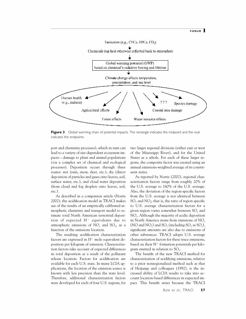
The impact category of global climate changerefers to the potential change in the earth’s cli-mate caused by the buildup of chemicals (i.e.,“greenhouse gases”) that trap heat from the re-flected sunlight that would have otherwise passedout of the earth’s atmosphere (see figure 3 for theglobal warming chain of potential impacts).

Since preindustrial times, atmospheric concen-trations of carbon dioxide (CO2), methane(CH4), and nitrous oxide (N2O) have climbedby over 30%, 145%, and 15%, respectively. Al-though “sinks” exist for greenhouse gases (e.g.,oceans and land vegetation absorb carbon diox-ide), the rate of emissions in the industrial agehas been exceeding the rate of absorption. Sim-ulations are currently being conducted by globalwarming researchers to try to quantify the poten-tial endpoint effects of these exceedences, in-cluding increased droughts, floods, loss of polarice caps, sea-level rise, soil moisture loss, forestloss, change in wind and ocean patterns, changesin agricultural production, decreased biodiver-sity, and increasing occurrences of extremeweather events.

TRACI uses global warming potentials, amidpoint metric proposed by the InternationalPanel on Climate Change (IPCC), for the cal-culation of the potency of greenhouse gases rela-tive to CO2 (IPCC 1996). The 100-year timehorizons recommended by the IPCC and used bythe United States for policy making and report-ing (U.S. EPA 2001) are adopted within TRACI.The final sum, known as the global warming in-dex, indicates the potential contribution toglobal warming:

Global Warming Index � R e � GWP (2)i i i

where ei is the emission (in kilograms) of sub-stance i and GWPi is the global warming poten-tial of substance i.

Acidification

Acidification comprises processes that in-crease the acidity (hydrogen ion concentration,[H�]) of water and soil systems. Acid rain gen-erally reduces the alkalinity of lakes. Changes inthe alkalinity of lakes, related to their acid-neutralizing capacity, are used as a diagnostic forfreshwater systems analogous to the use of H�

budgets in terrestrial watersheds (Schlesinger1997). Acid deposition also has deleterious (cor-rosive) effects on buildings, monuments, and his-torical artifacts.

The stressor-effects diagram for acidificationhas three stages (figure 4). Emissions lead to de-position (via a complex set of atmospheric trans-

F O R U M


Figure 3 Global warming chain of potential impacts. The rectangle indicates the midpoint and the ovalindicates the endpoints.

port and chemistry processes), which in turn canlead to a variety of site-dependent ecosystem im-pacts—damage to plant and animal populations(via a complex set of chemical and ecologicalprocesses). Deposition occurs through threeroutes: wet (rain, snow, sleet, etc.), dry (directdeposition of particles and gases onto leaves, soil,surface water, etc.), and cloud water deposition(from cloud and fog droplets onto leaves, soil,etc.).

As described in a companion article (Norris2002), the acidification model in TRACI makesuse of the results of an empirically calibrated at-mospheric chemistry and transport model to es-timate total North American terrestrial deposi-tion of expected H� equivalents due toatmospheric emissions of NOx and SO2, as afunction of the emissions location.

The resulting acidification characterizationfactors are expressed in H� mole equivalent de-position per kilogram of emission. Characteriza-tion factors take account of expected differencesin total deposition as a result of the pollutantrelease location. Factors for acidification areavailable for each U.S. state. In many LCIA ap-plications, the location of the emission source isknown with less precision than the state level.Therefore, additional characterization factorswere developed for each of four U.S. regions, for

two larger regional divisions (either east or westof the Mississippi River), and for the UnitedStates as a whole. For each of these larger re-gions, the composite factor was created using anannual emissions-weighted average of its constit-uent states.

As reported by Norris (2002), regional char-acterization factors range from roughly 20% ofthe U.S. average to 160% of the U.S. average.Also, the deviation of the region-specific factorsfrom the U.S. average is not identical betweenSO2 and NOx; that is, the ratio of region specificto U.S. average characterization factors for agiven region varies somewhat between SO2 andNOx. Although the majority of acidic depositionin North America stems from emissions of NOx

(NO and NO2) and SO2 (including SO2 as SOx),significant amounts are also due to emissions ofother substances. TRACI adopts U.S. averagecharacterization factors for these trace emissions,based on their H� formation potentials per kilo-gram emitted in relation to SO2.

The benefit of the new TRACI method forcharacterization of acidifying emissions, relativeto a prior nonregionalized method such as thatof Heijungs and colleagues (1992), is the in-creased ability of LCIA results to take into ac-count location-based differences in expected im-pact. This benefit arises because the TRACI

F O R U M


Figure 4 Acidification chain of potential impacts. The rectangle indicates the midpoint and the ovalindicates the endpoints.

acidification factors pertain to a focused mid-point within the impact chain (total terrestrialdeposition) for which there is considerable, wellunderstood, and quantifiable variability amongsource regions.

In at least two ways, the regional variabilityin deposition potential can impact the acidifi-cation potential. In the event that the alterna-tives being studied in the LCA have their pro-cesses (and thus their emissions) clustered indifferent regions, the overall deposition poten-tials for both SO2 and NOx can vary by as muchas a factor of 5 or more (Norris 2002). Anotherpossibility is that the alternatives have their pro-cesses predominantly clustered in the same re-gions. If this is the case, then the relative depo-sition potentials of a kilogram of NOx versus

SO2 emissions can vary by nearly a factor of 2from one region to another. In this instance, us-ing the region-appropriate characterization fac-tors may be important to the overall study out-come.

The modeling stops at the midpoint in thecause-effect chain (deposition) because in theUnited States there is no regional database ofreceiving environment sensitivities (as is avail-able in Europe3). Thus, the source-region-basedvariability in total terrestrial deposition hasbeen captured, but not the receiving-region-based variability in sensitivity or ultimate dam-age. Future advances of the TRACI acidifica-tion method may address regionalized transportand deposition of ammonia emissions and in-vestigate the potential of accounting for re-

F O R U M


gional differentiation of receiving environmentsensitivities.

Eutrophication

Eutrophication is the fertilization of surfacewaters by nutrients that were previously scarce.When a previously scarce (limiting) nutrient isadded, it leads to the proliferation of aquatic pho-tosynthetic plant life. This may lead to a chain offurther consequences, including foul odor ortaste, death or poisoning of fish or shellfish re-duced biodiversity, or production of chemicalcompounds toxic to humans, marine mammals,or livestock (figure 5). The limiting-nutrient is-sue is key to characterization analysis of phos-phorus (P) and nitrogen (N) releases withinLCIA. If equal quantities of N and P are releasedto a freshwater system that is strictly P limited,then the characterization factors for these twonutrients should account for this fact (e.g., thecharacterization factor for N should approachzero in this instance).

The most common impairment of surfacewaters in the U.S. is eutrophicationcaused by excessive inputs of P and N.Impaired waters are defined as those thatare not suitable for designated uses suchas drinking, irrigation, by industry, recre-

ation, or fishing. Eutrophication is re-sponsible for about half of the impairedlake area, 60% of the impaired riverreaches in the U.S., and is also the mostwidespread pollution problem of U.S. es-tuaries. (Carpenter et al. 1998, 560)

Prior to utilization of TRACI, it is importantto determine the actual nutrient emissions thatare transported into water. As an example, fer-tilizers are applied to provide nutrition to thevegetation that covers the soil; therefore, onlythe runoff of fertilizer makes it into the water-ways. The overapplication rate is highly variableand may depend on soil type, vegetation, topog-raphy, and even the timing of the applicationrelative to weather events.

The TRACI characterization factors for eu-trophication are the product of a nutrient factorand a transport factor. The nutrient factor cap-tures the relative strength of influence on algaegrowth in the photic zone of aquatic ecosystemsof 1 kg of N versus 1 kg of P, when each is thelimiting nutrient. The location or context-basedtransport factors vary between 1 and 0 and takeinto account the probability that the release ar-rives in an aquatic environment (either initiallyor via air or water transport) in which it is alimiting nutrient (figure 6). The TRACI char-acterization method for eutrophication is de-scribed in more detail in the companion article(Norris 2002).

Figure 5 Chain of potential impacts of eutrophication. The rectangle indicates the midpoint and the ovalindicates the endpoints.

F O R U M


Figure 6 Pathways for nutrient transport to fresh and coastal waters. The rectangles indicate thereceiving environment.

The characterization factors estimate the eu-trophication potential of a release of chemicalscontaining N or P to air or water, per kilogramof chemical released, relative to 1 kg N dis-charged directly to surface freshwater. The re-gional variability in the resulting eutrophicationfactors shows that the location of the source in-fluences not only the relative strength of influ-ence for a unit emission of a given pollutant, butit also influences the relative strength of influ-ence among pollutants. The benefit of the newTRACI method for characterizing eutrophyingemissions, relative to a prior nonregionalizedmethod such as that of Heijungs and colleagues(1992), is the increased ability of LCIA resultsto take into account the expected influence oflocation on both atmospheric and hydrologic nu-trient transport and thus the expected influenceof release location upon expected nutrient im-pact. The combined influence of atmospherictransport and deposition along with hydrologictransport can lead to total transport factors dif-fering by a factor of 100 or more (Norris 2002).

As with both acidification and photochemicaloxidant formation (below), TRACI providescharacterization factors for nine different groupsof U.S. states, known as census regions,4 for east-ern and western regions and for the UnitedStates as a whole, for use when the location ofthe release is not more precisely known. For each

of these larger regions, the composite factor wascreated using an average of those for its constit-uent states.

Photochemical Oxidant Formation

Ozone (O3) is a reactive oxidant gas producednaturally in trace amounts in the earth’s atmo-sphere. Ozone in the troposphere leads to detri-mental impacts on human health and ecosystems(figure 7). The characterization point associatedwith photochemical oxidant formation is the for-mation of ozone molecules in the troposphere.Rates of ozone formation in the troposphere aregoverned by complex chemical reactions, whichare influenced by ambient concentrations of ni-trogen oxides (NOx) and volatile organic com-pounds (VOCs), as well as the particular mix ofVOCs, temperature, sunlight, and convectiveflows. In addition, recent research in theSouthern Oxidants Study (e.g., Chameides andCowling 1995) indicates that carbon monoxide(CO) and methane (CH4) can also play a role inozone formation.

More than 100 different types of VOCs areemitted to the atmosphere, and they can differby more than an order of magnitude in terms oftheir estimated influence on photochemical ox-idant formation (e.g., Carter 1994). Further com-plicating the issue is the fact that in most regions

F O R U M


Figure 7 Cause-effect linkages for tropospheric ozone. The rectangle indicates the midpoint and the ovalindicates the endpoints.

of the United States, ambient VOC concentra-tions are due largely to biological sources (trees).For example, in urban and suburban regions ofthe United States at midday, biogenic VOCs canaccount for a significant fraction (10% to 40%)of the total ambient VOC reactivity (NRC1991). In rural areas of the eastern United States,biogenic VOCs contribute more than 90% of thetotal ambient VOC reactivity in near-surface air.

Conventional smog characterization factorsfor LCIA have been based on European model-ing of the relative reactivities among VOCs andhave neglected NOx entirely. This neglect ofNOx is a highly significant omission. Throughoutthe past decade, numerous U.S. studies havefound spatial and temporal observations of near-surface ozone concentrations to be strongly cor-related with ambient NOx concentrations andmore weakly correlated with anthropogenic

VOC emissions (see, for example, NRC 1991;Cardelino and Chameides 1995). Another omis-sion in all existing smog characterization factorshas been the potential influence of emission lo-cation.

The approach to smog characterization anal-ysis for VOCs and NOx in TRACI incorporatesthe following components: (1) relative influenceof individual VOCs on smog formation, (2) rela-tive influence of NOx concentrations versus av-erage VOC mixture on smog formation, (3) im-pact of emissions (by release location) uponconcentration by state, and (4) methods for ag-gregation of effects among receiving states byarea.

To characterize the relative influence on O3

formation among the individual VOCs, Carter’slatest maximum incremental reactivity calcula-tions are used (Carter 2000). These reflect the

F O R U M


estimated relative influence on conditions underwhich NOx availability is moderately high andVOCs have their strongest influence upon O3

formation. For the relative influence of NOx

emissions in comparison to the base reactive or-ganic gas mixture, a midrange factor of 2 is used,which is in agreement with empirical studies onregional impacts for the eastern United States(e.g., Cardelino and Chameides 1995) and is atthe middle of a range of model-based studies(Rabl and Eyre 1997; Seppala 1997).

The influence of NOx emissions on regionalambient levels has been modeled using source/receptor matrices that relate the quantity of sea-sonal NOx emissions in a given source region tochanges in ambient NOx concentrations in eachreceiving region across North America. Thesesource/receptor matrices were obtained from sim-ulations of the Advanced Statistical TrajectoryRegional Air Pollution model (Shannon 1991,1992, 1996). Source and receptor regions are thecontiguous U.S. states and Washington, D.C.,plus the ten Canadian provinces and northernMexico. Recent empirical research (e.g., St. Johnet al. 1998; Kasibhatla et al. 1998) shows thataverage O3 concentrations exhibit strong andstable correlations with regional ambient NOx

concentrations.The assumption was made that VOC emis-

sion impacts on regional O3 concentrations havethe same spatial distribution as the ambient NOx

concentration impacts (i.e., similar regionaltransport for VOCs and NOx). Finally, the out-come of the source/transport modeling is propor-tional to estimated O3 concentration impacts(grams per square meter) per state, given an as-sumed linear relationship between the changesin NOx and O3 concentrations (with VOC con-centrations converted to NOx equivalents).

Human Health Criteria Pollutants

Ambient concentrations of particulate matter(PM) are strongly associated with changes inbackground rates of chronic and acute respiratorysymptoms, as well as mortality rates. Ambientparticulate concentrations are elevated by emis-sions of primary particulates, measured variouslyas total suspended particulates, PM less than 10

lm in diameter (PM10), PM less than 2.5 lm indiameter (PM2.5), and by emissions of SO2 andNOx, which lead to the formation of the so-calledsecondary particulates sulfate and nitrate.

A three-stage method for LCIA of the humanhealth impacts of these emissions has been de-veloped for use in TRACI. The first stage of themodel uses the output of atmospheric transportmodels to estimate the expected change in ex-posure to PM2.5 due to emissions; this modelingincorporates atmospheric reactions and trans-port, as well as regional variability in populationdensities. The second stage in the model relieson epidemiological studies to provideconcentration-response (C-R) functions that areused to relate changes in exposure to changes inmortality rates and a variety of morbidity effects.The third stage in the model translates the dif-ferent mortality and morbidity effects into a sin-gle summary measure of disability-adjusted life-years (DALYs). Uncertainties at each stage of themodel are estimated and modeled quantitatively.The second and third optional stages of themodel provide a means to increase the relevanceto final decision making.

This methodology has been adopted for thisparticular impact category as a way of aggregatingthe different human health effects that are cor-related with exposures to ambient particulates.The epidemiological data that are used enableestimation of the incidence of a variety of humanhealth endpoints that differ in severity. This con-trasts with the human health cancer and non-cancer effects categories that include manychemicals that may have multiple effects of dif-ferent severities at various levels—many ofwhich may be unknown as a result of inadequatetoxicity testing data. Also, the potential effectsof criteria pollutants are well matched with theDALY methodology; that is, DALYs exist for res-piratory effects and mortality effects, which con-trasts with some of the human health effects forthe other categories. For example, DALYs can-not currently be used to quantify the potentialvalue of certain reproductive or teratogenic ef-fects.

To determine the relationship between emis-sions and exposure by setting (model stage 1),the approach described by Nishioka and col-leagues (2000) is used and the state-level “intake

F O R U M


fractions” are derived in the study. The intakefraction is the fraction of a pollutant emitted thatis actually inhaled; in fact, it represents more pre-cisely the probability that an emitted moleculeof emission will be inhaled. Nishioka and col-leagues (2002) used the regression models re-ported by Levy and colleagues (2000) to estimatestate-level point and area intake fractions. Thefinal predictive equations for the intake fractionof primary PM2.5, secondary sulfates, and second-ary nitrates were able to predict these intake frac-tions quite well (R2 between 0.5 and 0.9) basedon a limited number of simple parameters (e.g.,total population within 500 km, annual averagetemperature at the source). Levy and colleagues(2000) selected these parameters both for theirpredictive power and because they could be eas-ily collected for point and area sources.

To determine the health benefits associatedwith the estimated reductions in PM2.5 exposure(model stage 2), a survey of the relevant epide-miological literature was used. Premature mor-tality is the principal focus, because it has con-tributed a large portion of the total impacts (aftervaluation) in past studies (U.S. EPA 1999). Inaddition, to help communicate the range ofhealth effects, C-R functions are applied forchronic bronchitis, cardiovascular hospital ad-missions, and restricted activity days. A numberof studies report associations between variousmorbidity categories and PM. Morbidity catego-ries with a nonnegligible contribution to totalimpacts were selected (e.g., based on U.S. EPA1999); studies were included for which reason-able scientific and epidemiological evidence wereavailable. For this analysis, the study used theconsiderable evidence for a linear C-R functionthroughout the range of ambient concentrationsin the United States, with any potential effectsthreshold being below the lowest ambient con-centration. The evidence of the linear relation-ship between particulate air pollution at the cur-rent level and daily mortality without a thresholdis supported by Daniels (2000) in a study inwhich daily time-series data for the 20 largestU.S. cities for 1987–1994 was analyzed using aspline model. This also greatly simplifies the im-pact assessment; because ambient PM2.5 concen-trations vary across the United States, any non-linearities would imply that different slopes

should be applied in different locations. For sim-plicity, background disease prevalence and mor-tality rates are assumed constant across theUnited States. The potential effects of regionalvariation in background rates are explored sep-arately (Nishioka et al. 2002).

Stage 3 of the model entails aggregation of themortality and morbidity outcomes. When an in-dividual dies of exposure to PM, the number ofyears lost is calculated based on age- and gender-specific life expectancy tables. Estimates of thetotal life-years lost by a population exposed toPM depend on several factors, including the agedistribution and the size of the exposed popula-tion, the magnitude of the PM change, the rela-tive risk assumed to be associated with thechange in PM, and the length of exposure (U.S.EPA 1999).

The “burden of disease” measure developed byMurray and Lopez (1996) can be used to estimatethe health loss associated with air pollution. Sev-eral hundred severity weights are reported intheir study (Murray and Lopez 1996). Also, dis-ability weights have been derived for the Neth-erlands, addressing 56 diagnostic groups separat-ing more than 100 different disease stages(Stouthard et al. 2000). Environmental disease-related disability weights have been provided byDe Hollander and colleagues (1999) based onthe work of Stouthard and colleagues (2000). DeHollander and colleagues (1999) used both theGlobal Burden of Disease project and the DutchBurden of Disease project to attribute weight toenvironmental health impacts.

The DALYs measure combined years of lifelost and years lived with disability that are stan-dardized by means of severity weights. Thus, theannual number of DALYs lost can be calculatedas follows:

DALY � N � D � S (3)

where N is the number of cases, D is the averageduration of the response, including loss of lifeexpectancy as a consequence of premature mor-tality, and S is the discount weights to the un-favorable health conditions.

For premature mortality due to long-term ex-posure to particulate air pollution, De Hollanderand colleagues (1999) reported a severity score5

of 1 and the years of life lost to be 10.9 yr per

F O R U M


case. Thus, the DALY value of 10.9 per mortalitycase is used.

Human Cancer and Noncancer Effects

Reliable ranking and relative comparisons ofa large number of chemicals in terms of their po-tential to cause toxicological impacts are moreimportant than trying to characterize absoluterisk. Indeed, a number of researchers believe thatthere is not currently sufficient data to make re-liable estimates of low-dose risk on an absolutebasis, and a large number of methodologies havebeen proposed in the literature to help comparechemical emissions in this context (Penningtonand Bare 2002; Pennington and Yue 2000; Swan-son and Socha 1997). As local and worker healthimpacts are controlled largely through site-specific initiatives, comparisons are performed inLCA in the context of long-term exposures at amacro scale (regional and global). Such ap-proaches require considering the long-term fateof a chemical, human exposure, and the effectson human health.

Quantitative characterization factors are usu-ally predicted in LCIA in the context of toxi-cological impacts using integrated multimediafate, exposure, and effect models (e.g., Guinee etal. 1996; Hertwich et al. 2001; Huijbregts1999a). Generic models are usually adopted, par-ticularly in the absence of site-specific emissionsinventory and chemical property data. The rela-tive toxicological concern of an emission in thecontext of human health is currently calculatedin TRACI based on human toxicity potentials(HTPs) (Hertwich et al. 2001). These best-estimate HTPs (usually between the mean andthe median of the HTP distributions given pa-rameter uncertainty and variability) were derivedusing a closed-system, steady-state version ofCalTOX (Version 2.2) (McKone 1993), a mul-timedia fate and multiple-exposure pathwaymodel with fixed generic parameters for theUnited States. The closed system is used to pro-vide a scenario in which a chemical can only beremoved from the environment, or modeled unitworld, by transformation and not by relocationto other regions.

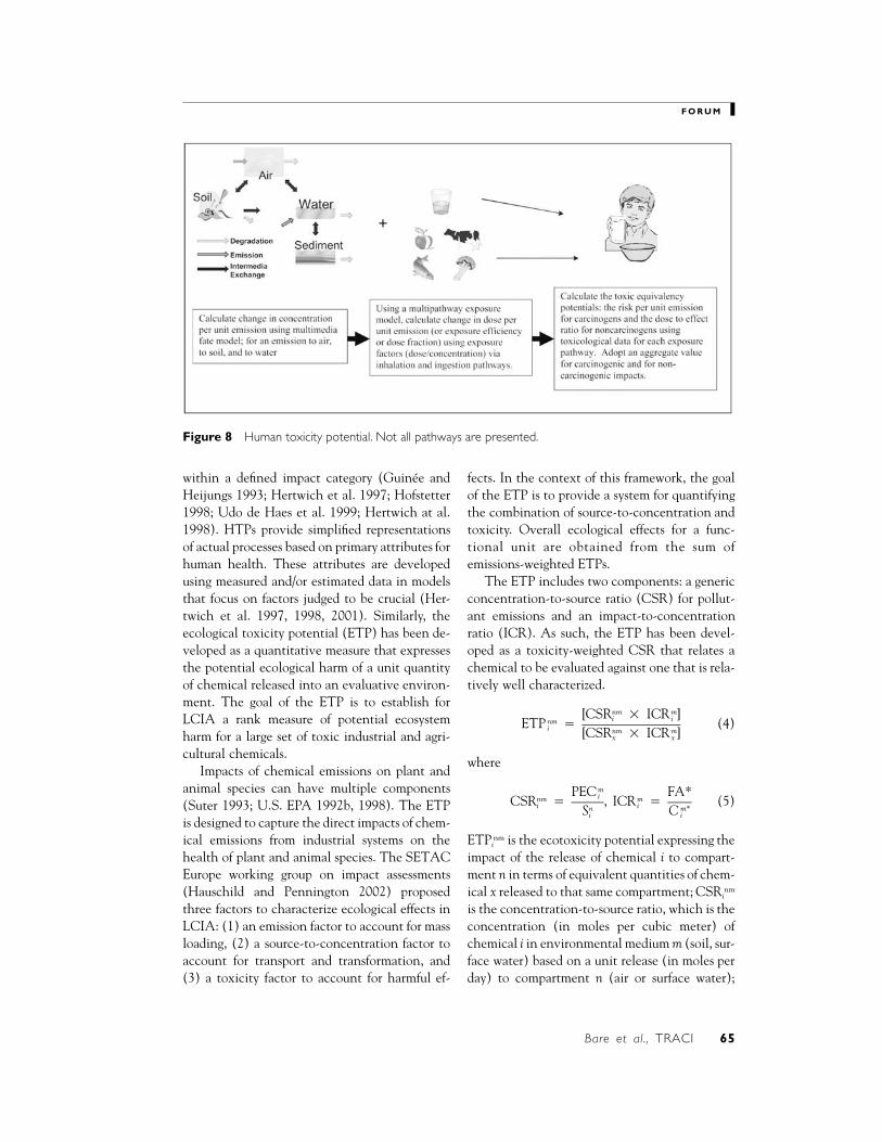
The modified model used to calculate theHTPs for LCIA, CalTOX (McKone 1993), con-sists of a regional multimedia fate model coupledwith human exposure correlations for 23 path-ways (U.S. EPA 1989a, 1992a; CalEPA 1996;Yang and Nelson 1986) to estimate exposuredoses. These doses are then compared with effectpotency data, as illustrated in figure 8. Exposurevia dermal contact with soils, ingestion (of waterand contaminated food), and inhalation aretaken into account.

Using CalTOX, the dose per unit release rate(in kilograms per hour) of a chemical is esti-mated. As in risk assessment, each dose/unit re-lease rate is divided by an acceptable daily intakefor noncarcinogens or multiplied by a carcino-genic risk potency factor (q1

*) to help derive theHTPs. The acceptable daily intakes used in theHTP calculations are currently based on refer-ence doses for ingestion and reference concen-trations for inhalation. Separate HTPs are cal-culated for each exposure pathway, releasemedium (currently emissions to air and to water),and type of effect (carcinogenic or noncarcino-genic). Aggregate values of the calculated non-cancer and cancer HTPs are reported for eachrelease medium. The HTPs for each chemical arethen compared to baseline values using benzenefor carcinogens and toluene for noncarcinogens,hence chemical emissions are comparable interms of toxicological equivalencies.

Using CalTOX, a variation analysis was con-ducted to determine the effect of the various lev-els of uncertainty in chemical input parametersrelative to the variability introduced in exposurefactors and landscape parameters.

The largest sources of uncertainty in themodel were the result of the chemical input pa-rameters, especially half-life data. For somechemicals, exposure factor uncertainty was sig-nificant, but landscape parameters were consid-ered to be of minor significance in general (Her-twich et al. 1999).

Eco-toxicity

For ecological impacts, as well as for humanhealth, LCIA currently uses measures of hazardto compare the relative importance of pollutants

F O R U M


Figure 8 Human toxicity potential. Not all pathways are presented.

within a defined impact category (Guinee andHeijungs 1993; Hertwich et al. 1997; Hofstetter1998; Udo de Haes et al. 1999; Hertwich at al.1998). HTPs provide simplified representationsof actual processes based on primary attributes forhuman health. These attributes are developedusing measured and/or estimated data in modelsthat focus on factors judged to be crucial (Her-twich et al. 1997, 1998, 2001). Similarly, theecological toxicity potential (ETP) has been de-veloped as a quantitative measure that expressesthe potential ecological harm of a unit quantityof chemical released into an evaluative environ-ment. The goal of the ETP is to establish forLCIA a rank measure of potential ecosystemharm for a large set of toxic industrial and agri-cultural chemicals.

Impacts of chemical emissions on plant andanimal species can have multiple components(Suter 1993; U.S. EPA 1992b, 1998). The ETPis designed to capture the direct impacts of chem-ical emissions from industrial systems on thehealth of plant and animal species. The SETACEurope working group on impact assessments(Hauschild and Pennington 2002) proposedthree factors to characterize ecological effects inLCIA: (1) an emission factor to account for massloading, (2) a source-to-concentration factor toaccount for transport and transformation, and(3) a toxicity factor to account for harmful ef-

fects. In the context of this framework, the goalof the ETP is to provide a system for quantifyingthe combination of source-to-concentration andtoxicity. Overall ecological effects for a func-tional unit are obtained from the sum ofemissions-weighted ETPs.

The ETP includes two components: a genericconcentration-to-source ratio (CSR) for pollut-ant emissions and an impact-to-concentrationratio (ICR). As such, the ETP has been devel-oped as a toxicity-weighted CSR that relates achemical to be evaluated against one that is rela-tively well characterized.

nm m[CSR � ICR ]i inmETP � (4)i nm m[CSR � ICR ]x x

where

mPEC FA*inm mCSR � , ICR � (5)i in m*S Ci i

ETPinm is the ecotoxicity potential expressing the

impact of the release of chemical i to compart-ment n in terms of equivalent quantities of chem-ical x released to that same compartment; CSRi

nm

is the concentration-to-source ratio, which is theconcentration (in moles per cubic meter) ofchemical i in environmental medium m (soil, sur-face water) based on a unit release (in moles perday) to compartment n (air or surface water);

F O R U M


ICRim is the impact-to-concentration ratio for

chemical i in environmental medium m, that isthe measure of potential impact (i.e., species af-fected) associated with a marginal increase ofconcentration (in moles per cubic meter) in me-dium m (soil, water); PECi

m is the predicted en-vironmental concentration (in moles per cubicmeter) of chemical i in environmental mediumm from a continuous release Si

n (in moles per day)to compartment n; FA* is a standardized measureof harm, such as the fraction of species adverselyaffected, that is used as a consistent measure ofpotential harm among a large set of chemicalsubstances; and Ci

m* is a benchmark concentra-tion (in moles per cubic meter) for chemical iand is the concentration on the exposure-response curve at which there is a point of de-parture where the likelihood of effect and not theseverity of effect increases with increasing ex-posure.

Emissions to air and surface water (sw) areconsidered separately (ETPi

air,m and ETPisw,m). In

addition, for each emission type (air and sw), anETP is calculated based on potential terrestrialecosystem impacts and potential aquatic ecosys-tems impact so that there are four ETP values,ETPi

air,soil, ETPiair,sw, ETPi

sw,soil, and ETPisw,sw. This

is reduced to a set of two ETP values based on asimple combination of the water ETP and soilETP impact for a release to either air or water.As a result, the overall ETP for each release sce-nario is calculated as follows:

air air,soilETP (overall) � 0.5 � ETPi i (6)air,sw� 0.5 � ETP i

sw sw,soilETP (overall) � 0.5 � ETPi i (7)sw,sw� 0.5 � ETP i

Calculating the ETPThe CSR expresses the concentration (in

moles per cubic meter) of chemical i in environ-mental medium m (soil or surface water) basedon a continuous unit release (in moles per day)to compartment n (air or surface water). For thecurrent set of ETP estimates, the same modifiedversion of CalTOX and the chemical and land-scape data sets employed by Hertwich and col-leagues (2001) for HTP calculations are used.

The soil and surface water CSRs are obtainedfrom the steady-state solution of the CalTOXmultimedia mass-balance model with continuousair and surface water emissions.

The ICR is based on the ecosystem predictedno-effects concentration (PNEC), which is themeasure of ecosystem impact that has been mostfrequently used in life-cycle impact and for com-parative risk assessment (see, for example, Gui-nee and Heijungs 1993; Guinee et al. 1996;Hauschild et al. 1998; Huijbregts 1999a; Huij-bregts et al. 2000; Jolliet and Crettaz 1997; Wen-zel et al. 1997). For ecosystem health, the PNECis defined as the environmental concentrationexpected to cause no effects, acute or chronic, onthe structure or function of ecosystems (Euro-pean Commission 1996; U.S. EPA 2000).

As has been done by others, notably Huij-bregts and colleagues (2000), the potential frac-tion of species affected is selected as an appro-priate measure of harm for ecosystems to estimatePNECs. The potential fraction of species affectedis obtained from the species sensitivity distribu-tion of no observable effect concentration(SSDNOEC) values (Klepper et al. 1998; U.S.EPA 2000). Typically, one adopts the lowerbound, such as the fifth percentile, of theSSDNOEC to obtain a PNEC (Klepper et al.1998; Suter 1998; Huijbregts 1999b; Huijbregtset al. 2000; van Beelen et al. 2001).

The current ETP set includes 161 chemicals.For emissions to air and surface water, an ETP iscalculated based on potential terrestrial ecosys-tem impacts (related to soil concentration) andpotential aquatic ecosystems impact. 2,4-Dichlo-rophenoxyacetic acid (2,4-D, CAS ID 94-75-7)is used as a reference substance.

Resource Depletion

Land, fossil fuel, and water use are includedas resource depletion categories. Other resourcedepletion issues (e.g., minerals) could be in-cluded, but these three are currently more oftenincluded in LCA studies than others.

The methodologies that support the resourcedepletion categories have the least consensus. Todate, much more focus has been on chemicalemissions and the assessment of the potential ef-fects from these categories. In the resource de-

F O R U M


pletion categories, there is still no consensus onthe “value” of the resource (e.g., what factors areinvolved in valuing land). The methodologiesprovided for these categories should not be con-sidered as robust, given current insights, but arethe most likely to change with additional re-search.

Land UseHow to best characterize and aggregate indi-

vidual land-use modifications is a topic of wide-spread controversy and research. Recent publi-cations discuss a variety of techniques (Heijungset al. 1997; Lindeijer et al. 1998; Swan 1998;Goedkoop and Spriensma 1999). Among thevarious existing techniques are economic ap-praisals, species area relationships, and land-conversion and land-occupation assessments.Some of these techniques require knowledge ofthe land’s historical condition, as well as its al-tered condition and expected time for restorationto its original state. Most land-use valuationtechniques recognize that the locality of the landis important because it often affects the eco-nomic value of the land, but also because it isintegrally linked to the climate, topography, andresident plant and animal species, making it aunique location in many respects.

TRACI recognizes that location has a verylarge role in determining the environmental im-portance of land. Rather than trying to charac-terize various different land uses and inhabitantspecies, TRACI uses the density of threatenedand endangered (T&E) species in a specific area(e.g., county) as a proxy for environmental im-portance. This allows users to characterize landthat is to be developed or modified at a specificlocation and then to tie into a T&E species da-tabase to calculate the potential T&E displace-ment of the proposed altered land. The T&E spe-cies proxy approach operates under theassumption that land that has a higher numberof T&E species is inherently more valuable in sofar as species might completely disappear in theUnited States if additional land is developed.Land within a county may be expected to besimilar in climate, soil type, typography, andmany other aspects that may be valuable to theseT&E species. The T&E database is providedwithin TRACI, so that the user does not need

to know the T&E species count within the rele-vant county. In the absence of knowledge of thespecific county, a more generalized T&E densityvalue (e.g., state T&E density) may be used;however, the user should be cautioned that theremay be significant differences in T&E densityvalue within a particular state, and therefore thevalue of the model is significantly reduced whenthe state- or national-level T&E density value isused.

All land modifications are not created equal,so some decisions need to be made about whichland modifications are considered significantenough to result in potential habitat effects. Mi-nor land modifications (e.g., land that is simplybeing converted from one agricultural use to an-other agricultural use) should not be counted,but significant alterations (e.g., land that is beingdeforested and converted into a shopping mall)should be counted. Significance can be measuredbased upon (1) previous use (history) versus pro-posed use, (2) extent of modifications, (3) oc-cupation time, and (4) recovery time. Althoughit is recognized that this guidance is currentlyvague, it is anticipated that this impact categorywill continue to receive much research attention.The equation for land use is as follows:

Land Use Index � R A � (T&E )/CA (8)i i i i

where Ai is the human activity area per func-tional unit of product, T&Ei is the T&E speciescount for the county, and CAi is the area of thecounty.

Fossil Fuel UseSeveral ways of analyzing fossil fuel and en-

ergy consumption exist. Many of these tech-niques acknowledge a preference for renewableenergy sources as opposed to nonrenewable en-ergy sources. Although a useful measure, totalnonrenewable energy consumption does not fullyaddress potential depletion issues associated withthese flows. For example, solid and liquid fuelsare not perfect substitutes (i.e., solid fuels are notcurrently practical in personal transportation ap-plications). For this reason, depletion of petro-leum has different implications than depletion ofcoal, and so forth.

An existing technique described in Eco-Indicator’99 was selected for incorporation into

F O R U M


TRACI (Goedkoop and Spriensma 1999). Thistechnique takes into account the fact that con-tinued extraction and production of fossil fuelstends to consume the most economically recov-erable reserves first, so that (assuming fixed tech-nology) continued extraction will become moreenergy intensive in the future. This is especiallytrue once economically recoverable reserves ofconventional petroleum and natural gas are con-sumed, leading to the need to use nonconven-tional sources, such as oil shale. For each presentfuel, experts generated scenarios for replacementfuels at a point in the future when total cumu-lative consumption equals 5 times the presentcumulative consumption. The current energy in-tensity (energy per unit of fuel delivered) forthese future fuel extraction and production sce-narios was specified. The increase in unit energyrequirements per unit of consumption for eachfuel provides an estimate of the incremental en-ergy input “cost” per unit of consumption. Thesefactors then provide a basis for weighting theconsumption of different fossil fuel energy re-sources.

Fossil Fuel Index � R N � F (9)i i i

where Ni is the increase in energy input require-ments per unit of consumption of fuel i and Fi isthe consumption of fuel i per unit of product.

Water UseWater use has generally been tracked in sim-

ple mass or volume terms in LCI, without sub-sequent characterization analysis that wouldweight different usage flows to take into accountimportant differences among source types and us-age locations (Owens 2001). Rather than tryingto capture the addition of water pollutants intothe environment, this impact category is struc-tured to capture the significant use of water inareas of low availability. As it is a relatively newconsideration in LCIA, an impact assessmentmethodology for water use is not incorporatedwithin TRACI.

Application Example

A simplified case study was conducted forvarious reasons: (1) to demonstrate the use ofTRACI, (2) to determine the effects of site-

specific LCIA on deterministic results, and (3)to analyze the uncertainty reductions by the useof site-specific LCIA.

The case study is based on LCI models forconcrete manufacturing developed for theAthena Sustainable Materials Institute byGeorge Venta (ASMI 1993, 2001). Because thepurpose of the case study was to demonstrate andillustrate the three conditions above and not tosupport or inform a specific decision, the casestudy was simplified to include only the LCI datafor the criteria pollutants and CO2.

The process tree for the manufacture of ce-ment is shown in figure 9. In this example, as-sumptions are made about process locationsbased on concrete manufacturing taking place inMassachusetts in the northeastern United States.Process location assumptions are shown follow-ing the process name in figure 9. The quarryingof coarse and fine aggregates takes place in Mas-sachusetts, as does fuel combustion in the finalconcrete manufacturing stage. Electricity inputto the concrete plant is generated somewhere inthe northeast United States, but cannot be re-gionally resolved more precisely than that, giventhe extent of regional power wheeling. The man-ufacture and transport of “secondary cementa-tious materials” into concrete manufacturingcould occur anywhere in the United States, asthis is not a massive material input.

As processes further up the supply chain(which are processes appearing toward the bot-tom of figure 9) are considered, their locationbecomes less precisely known. Thus, productionof cement, clinker, gypsum, and raw meal (thefine powder that results from dry grinding ofthese raw materials) takes place in New England,with electricity generation and most inputs toraw meal production coming from the north-eastern United States. Iron ore production is as-sumed to come from an unspecified location inthe United States.

In this example, the LCIA results withTRACI change when process (and thus emis-sion) location information is used, as comparedwith an alternative scenario that occurs any-where in the United States. Because TRACI hasdeveloped regionalized factors for the impactcategories of acidification, eutrophication, andsmog, these impact categories are the focus of

F O R U M


Figure 9 Process tree with location indications for concrete manufacturing.

this case study. The actual LCI data contain 107different inventory flows, for releases to air, wa-ter, and land, and are available on the journal’sWeb site (http://mitpress.mit.edu/JIE). LCIAdata processing and results presentation are sim-plified for this example by focusing strictly on thereleases of five pollutants to air, most of whichare relevant to the three impact categories ad-dressed here. These condensed LCI data are pre-sented in table 2. The bulk of the emissions ofeach pollutant tends to come from half a dozenor so of the downstream processes, including ag-gregates quarrying and transport, clinker produc-tion, fuel combustion at the concrete plant, sec-ondary cementatious materials manufacture andtransport, and electricity inputs to cement manu-facturing.

TRACI contains U.S. average LCIA factorsfor all of the impact categories for use in appli-cations when the process location is not known.By using these regionalized characterization fac-tors in place of U.S. average factors, the impacts

on deterministic results as well as uncertainty re-ductions were analyzed and determined to be sig-nificant.

The uncertainty inherent in national andmacroregional characterization factors relative tostate-specific characterization factors is quanti-fied as follows. For each process in figure 9 andtable 1, if location information is not specified,then the process could in principle be locatedanywhere in the United States (assuming an en-tirely domestic supply chain, which is reasonablefor the processes in this example). To reflect thisindeterminacy, the characterization factor foreach process is expressed as a discrete probabilitydistribution, whose possible values are the state-level characterization factors, each with givennonzero probability. Two plausible sets of prob-abilities are tested: one where each release lo-cation (e.g., each U.S. state) is consideredequally likely, and another where the likelihoodof each release location being the source of a pro-cess release is given by the share of U.S. emis-

F O R U M


Table 2 Condensed life-cycle inventory data for the case example in figure 9

Unit process CO2 NOx PM SOx VOCs

Concrete 0 0 120 0 0Coarse aggregate 3781 52 53.47 9.82 12.1Fine aggregate 5001 59.7 54.6 14.9 14.6SCM 717 5.88 0.889 1.97 2.29Cement 0 0 0 0 0Electricity: concrete 355 1 0 2 0Fuel: concrete 5401 66.2 4.57 41.15 19.8Clinker 843 2 0.4 0.1 0.001Electricity: cement 5 0.02 0.01 0.03 0.001Gypsum 0 0 0 0 0Transport: clinker 10.92 0.10 0.01 0.03 0.04Fuel: clinker 7.92 0.05 0.24 0.43 0.14Raw meal 0 0 0 0 0Fuel: gypsum 7.72 0.06 0.003 0.09 0.03Electricity: gypsum 3.76 0.01 0.00 0.02 0.0005Limestone 1.94 0.04 0.47 0.0043 0.01Sand 0.03 0.0005 0.01 0.0001 0.0001Clay 0.08 0.0015 0.02 0.0002 0.0003Iron ore 0.05 0.0010 0.01 0.00 0.0002Transport: raw meal inputs 4.56 0.05 0.004 0.01 0.02Fuel: raw meal 5.54 0.02 0.001 0.08 0.02Electricity: raw meal 3.80 0.01 0.005 0.02 0.0005

sions for the pollutant that is emitted withineach U.S. state. Thus, the probabilistic charac-terization factors (CFs) for each region in theexample, for a given pollutant and impact cate-gory, are given by the following:

CF � v p (10a)USA � i ii�USA

CF � v p (10b)NorthEast � j jj�NorthEast

CF � v p (10c)NewEngland � k kk�NewEngland

CF � v (10d)Massachusetts Massachusetts

where vk indicates the characterization factorvalue for state k and pk is the probability of theemission occurring in that state.

Characterization results for two cases arecompared. In the first case, the locations of theprocesses are known (as summarized in figure 9),in which case the region-appropriate character-ization factors as given by equations (10a–d) areapplied. In the second case, the locations of theprocesses are known only to be somewhere in the

United States, so that the U.S. characterizationfactor given by equation (10a) is used for eachprocess.

Figure 10 summarizes the expected results forthe regionalized versus nonregionalized (U.S.)approaches to LCIA for the case study LCI datafor the impact categories of acidification, eutro-phication, and smog. The results are normalizedrelative to the U.S. results. The emissions-weighted probability assumption is applied to thestates in each multistate region (U.S., Northeast,and New England). Using this equal-probabilityassumption introduces less than a 5% change inthe expected results for this case study. The re-sults in figure 10 clearly show that the expectedresult for each impact category is significantly in-fluenced by the process location information to-gether with the regionalized TRACI character-ization factors, cutting the total characterizationvalue by more than half for two of the three im-pact categories.

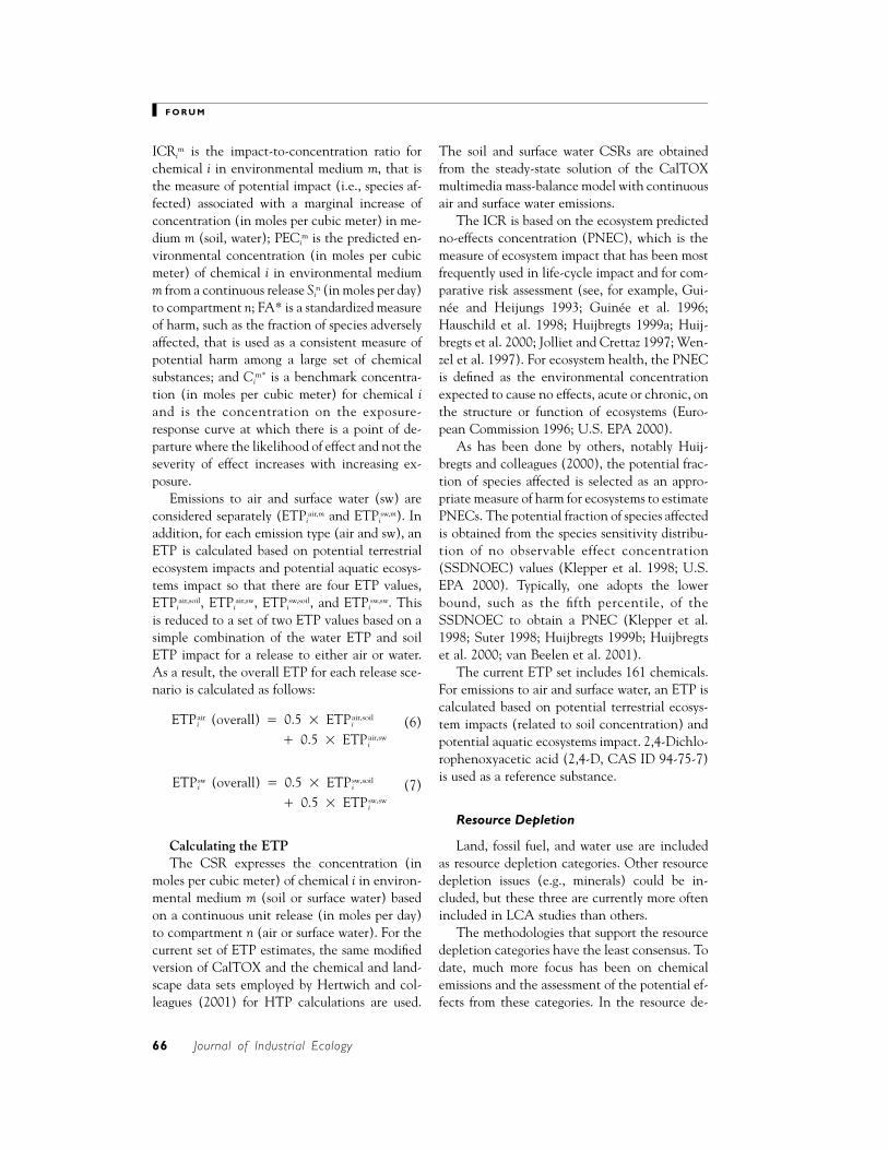
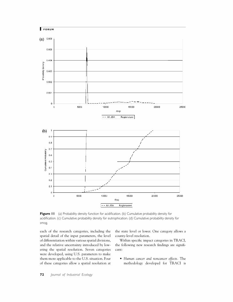
The results of regionalization are even morestriking with respect to their uncertainty reduc-tion. Figure 11a is a comparison of the probabil-ity density functions for acidification. The cu-

F O R U M


Figure 10 Results for regionalized versus nonregionalized LCIA for the concrete case study.

mulative probability distribution is the integralof the probability density function. Figures 11b,11c, and 11d compare regionalized and nonre-gionalized cumulative probability distributionsfor each of the three impact categories for theemissions-weighted probability assumption. Ineach case, the uncertainty (as measured by thespread of possible values) is reduced by orders ofmagnitude. Further, in this case study, the plau-sible range for the regionalized results falls at thevery tail end of the distribution of possible valuesfor the nonregionalized results. This latter effectis primarily because the case study region is thenortheastern United States, for which a signifi-cant share of the emissions are carried out to searather than across populated areas of the NorthAmerican continent. Still, the differences in un-certainties (magnitudes of plausible ranges of val-ues) would be expected even if the case studyregion were changed.

Figure 12 demonstrates that the probabilitybasis has very little influence upon the results.Selecting emissions-weighted probabilities of thestates within a region has the effect of slightlynarrowing the plausible range of values for thetotal characterized result.

These results demonstrate the powerful influ-ence of TRACI’s regionalization for LCIA resultsfor acidification, eutrophication, and smog. Re-gionalization changes the expected values andhelps to reduce uncertainties. Many other

sources of uncertainty in LCIA results exist be-sides those introduced by regional variability inexpected impact per unit emission. OngoingTRACI research is developing a generalizedframework for probabilistic uncertainty analysisthat integrates the various sources of inventoryand impact assessment uncertainty, as well as theappropriate display and communication of thesophistication of probabilistic results. This ca-pability should enable users to assess the poten-tial information (that is, uncertainty reduction)benefits of using more sophisticated LCIA mod-els, such as region-specific characterization fac-tors.

Conclusions

This article presents the research behind theselection and development of impact assessmentmethodologies within TRACI. Cause-effectchain mechanisms are discussed for each impactcategory along with the research and methodol-ogies that were constructed to best represent thecharacterizations for the United States. When-ever possible, existing U.S. EPA guidelines,handbooks, and databases were used to ensureconsistency with regulations and policy. Impactcategories were often characterized at the mid-point level to minimize assumptions and valuechoices and to reflect a higher level of societalconsensus. Spatial resolution is considered for

F O R U M


Figure 11 (a) Probability density function for acidification. (b) Cumulative probability density foracidification. (c) Cumulative probability density for eutrophication. (d) Cumulative probability density forsmog.

each of the research categories, including thespatial detail of the input parameters, the levelof differentiation within various spatial divisions,and the relative uncertainty introduced by low-ering the spatial resolution. Seven categorieswere developed, using U.S. parameters to makethem more applicable to the U.S. situation. Fourof these categories allow a spatial resolution at

the state level or lower. One category allows acounty-level resolution.

Within specific impact categories in TRACI,the following new research findings are signifi-cant:

• Human cancer and noncancer effects. Themethodology developed for TRACI is

F O R U M


based on a multimedia fate, multipathwayhuman exposure and toxicological potencyapproach using CalTOX. Twenty-three ex-posure pathways were taken into accountwithin the analysis, including inhalation,ingestion of water and various plants andanimals, and dermal contact with the soiland water. Toxicity is based on cancer po-tencies for carcinogens and reference dosesor concentrations for noncarcinogens.HTPs were calculated for 330 chemicals,including chemicals representing 80% ofthe total weight of toxics release inventory

releases in 1997. Probabilistic analysis ofuncertainty using the proposed model in-dicates that uncertainty associated withhalf-life and toxicity represents a large por-tion of the total uncertainty in calculatingHTPs. As landscape information was con-sidered here to be fairly insignificant incontributing to uncertainty, and becausean analysis of the U.S. states did not reveala reordering of HTP values relative toother chemicals, one U.S. value was se-lected for each chemical to represent re-leases anywhere within the United States.

F O R U M


Figure 12 The influence of state probability basis on nonregionalized case study results for acidification.

• Acidification, eutrophication, and smog. Themethods developed for TRACI for each ofthese impact categories have taken region-specific differential influence on fate, trans-port, and expected effects into account,with U.S.-specific modeling. We foundthat source location can influence acidifi-cation impact factors by up to a factor of 4and eutrophication impact factors by morethan a factor of 100. The TRACI methodsshow, for example, that differentiatingsource location can be even more impor-tant than differentiating the actual chem-ical species for some of these impact cate-gories. These methods have taken amidpoint rather than an endpoint ap-proach to characterization in each cate-gory, stopping at points in the cause-effectimpact chain where there is a uniquemechanism taking place as a result of eachchemical and from which there is consis-tency of expected impacts among chemi-cals later in the impact chain.

Finally, a case study of cement manufacture wasconducted, and the impacts of site-specific anal-ysis were shown to have significant effects inboth the deterministic results and the uncer-tainty reductions.

Acknowledgments

We gratefully acknowledge the contributionsof Edgar Hertwich (currently of the InternationalInstitute for Applied Systems Analysis in Lax-enburg, Austria) for the development of the hu-man health toxicity potentials (HTPs) and Pat-rick Hofstetter (U.S. EPA–ORISE) for providingcomments. The work on factors for acidification,eutrophication, and smog benefited from expertinput at an EPA-sponsored workshop in 1998and from contributions by colleagues includingJyri Seppala, Jose Potting, Mark Goedkoop, Pat-rick Hofstetter, and Jeroen Guinee.

Disclaimer

Use of TRACI, including but not limited toimpact assessment modeling, does not create reg-ulatory or scientific approval by the U.S. EPA onany issues to which it is applied, nor does it re-lease any users from any potential liability, eitheradministratively or judicially, for any damage tohuman health or the environment. The U.S.EPA does not make any warranty concerning thecorrectness of the database, any actions taken bythird parties as a result of using the model, or themerchantability or fitness for a particular purposeof the model. The U.S. EPA does not endorseany products or services.

F O R U M


Notes

1. TRACI is available on the Internet at no cost at�http://epa.gov/ORD/NRMRL/std/sab/iam_traci.htm�.

2. “Criteria pollutants” is a term used in U.S. en-vironmental regulation to describe those regu-lated air pollutants for which the U.S. EPA useshealth-based criteria to set permissible levels.The criteria pollutants are ozone, carbon mon-oxide, total suspended particulates, sulfur diox-ide, lead, and nitrogen oxides.

3. Editor’s note: For a discussion of a regional da-tabase for receiving environment sensitivities inEurope, see the article by Potting et al., Journalof Industrial Ecology 2(2): 63–87.

4. U. S. census regions are available at �http://www.eia.doe.gov/emeu/reps/maps/us_census.html�.

5. The severity weight in DALY calculations is 1 fordeath and 0 for perfect health.

References

ASMI (Athena Sustainable Materials Institute). 1993.Cement and structural concrete products: Raw ma-terials balances, energy profiles, and environmentalunit factor estimates. Ottawa, Canada: ASMI.

ASMI. 2001. Cement and structural concrete products.Update: Raw materials balances, energy profiles, andenvironmental unit factor estimates. Ottawa, Can-ada: ASMI.

Bare, J. C., D. W. Pennington, and H. A. Udo de Haes.1999. Life cycle impact assessment sophistica-tion: International workshop. International Jour-nal of Life Cycle Assessment 4: 299–306.

Bare, J. C., P. Hofstetter, D. W. Pennington, and H. A.Udo de Haes. 2000. Life cycle impact assessmentmidpoints vs. endpoints: The sacrifices and thebenefits. International Journal of Life Cycle Assess-ment 5: 319–326.

CalEPA (California Environmental ProtectionAgency). 1996. Risk assessment guidelines, Part 4:Technical support document: Exposure assessmentand stochastic analysis. Sacramento, CA: State ofCalifornia Office of Environmental Health Haz-ard Assessment.

Cardelino, C. A. and W. L. Chameides. 1995. Anobservation-based model for analyzing ozone pre-cursor relationships in the urban atmosphere.Journal of the Air and Waste Management Associ-ation 45: 161–180.

Carpenter, S., N. Caraco, D. Correll, R. Howarth, A.Sharpley, and V. Smith. 1998. Nonpoint pollu-

tion of surface waters with phosphorus and nitro-gen. Ecological Applications 8(3): 559–568.

Carter, W. 1994. Development of ozone reactivityscales for volatile organic compounds. Journal ofthe Air and Waste Management Association 44:881–899.

Carter, W. 2000. Updated maximum incremental reactiv-ity scale for regulatory applications. Sacramento,CA: California Air Resources Board.

Chameides, W. L. and E. B. Cowling, eds. 1995. Thestate of the southern oxidants study: Policy-relevant findings in ozone pollution research1988 to 1994. Raleigh, NC: North Carolina StateUniversity.

Daniels, M. J., F. Dominici, J. M. Samet, and S. L.Zeger. 2000. Estimating particulate matter-mortality dose-response curves and threshold lev-els: An analysis of daily time series for the 20largest U.S. cities. American Journal of Epidemi-ology 152: 407–412.

De Hollander, A. E. M., J. M. Melse, E. Lebret, andP. G. N. Kramers. 1999. An aggregate publichealth indicator to represent the impact of mul-tiple environmental exposures. Epidemiology 10:606–617.

European Commission. 1996. Technical guidance docu-ments in support of Directive 93/67/EEC on risk as-sessment of new notified substances and Regulation(EC) No. 1488/94 on risk assessment of existingsubstances (Parts I, II, III, and IV). EC catalognumbers CR-48-96-001, 002, 003, and 004-EN-C. Luxembourg: Office for Official Publicationsof the European Community.

Finnveden, G. 1997. Valuation methods within LCA:Where are the values? International Journal of LifeCycle Assessment 2: 163–169.

Goedkoop, M. and R. Spriensma. 1999. The Eco-Indicator 99: A damage orientated method for lifecycle impact assessment. The Hague, The Neth-erlands: VROM, Ministry of Housing, SpatialPlanning, and the Environment.

Grahl, B. and E. Schmincke. 1996. Evaluation anddecision-making processes in life cycle assess-ment. International Journal of Life Cycle Assess-ment 1: 32–35.

Guinee, J. B. and R. Heijungs. 1993. A proposal forthe classification of toxic substances within theframework of life cycle assessment of products.Chemosphere 26: 1925–1944.

Guinee, J., R. Heijungs, L. van Oers, D. van de Meent,T. Vermeire, and M. Rikken. 1996. LCA impactassessment of toxic releases: Generic modelling offate, exposure, and effect for ecosystems and humanbeings with data for about 100 chemicals. No. 1996/

F O R U M


21. The Hague, The Netherlands: VROM, Min-istry of Housing, Spatial Planning, and the En-vironment.

Hauschild, M. and D. W. Pennington. 2002. Methodsof effect assessment for ecotoxicity. In Towardsbest available practice in life cycle impact assessment,edited by Udo de Haes et al. Brussels: SETACEurope Press.

Hauschild, M., H. Wenzel, A. Damborg, and J. Tørs-løv. 1998. Ecotoxocity as a criterion in the en-vironmental assessment of products. In Environ-mental Assessment of Products. Vol. 2, Scientificbackground, edited by M. Hauschild and H. Wen-zel. London: Chapman and Hall.

Heijungs, R., J. Guinee, G. Huppes, R. Lankreijer, H.Udo de Haes, A. Wegener Sleeswijk, A. Ansems,P. Eggels, R. van Duin, and H. de Goede. 1992.Environmental life cycle assessment of products. Vol.1, Guide and Vol. 2, Backgrounds. Leiden, TheNetherlands: Centre of Environmental Science,Leiden University.

Heijungs, R., J. Guinee, and G. Huppes. 1997. Impactcategories for natural resources and land use. CMLreport 138, Section: Substances and products.Leiden, The Netherlands: Centre of Environ-mental Science, Leiden University.

Hertwich, E. G., W. S. Pease, and C. P. Koshland.1997. Evaluating the environmental impact ofproducts and production processes: A comparisonof six methods. The Science of the Total Environ-ment 196: 13–29.

Hertwich, E. G., W. S. Pease, and T. E. McKone. 1998.Evaluating toxic impact assessment methods:What works best? Environmental Science and Tech-nology 32: A138–A144.

Hertwich, E., T. McKone, and W. Pease. 1999. Param-eter uncertainty and variability in evaluative fateand exposure models. Risk Analysis 19: 1193–1204.

Hertwich, E. G., S. F. Mateles, W. S. Pease, and T. E.McKone. 2001. Human toxicity potentials for lifecycle analysis and toxics release inventory riskscreening. Environmental Toxicology and Chemistry20: 928–939.

Hofstetter, P. 1998. Perspectives in life cycle impact as-sessment: A structured approach to combine modelsof the technosphere, ecosphere, and valuesphere. Bos-ton: Kluwer.

Hofstetter, P. 1999. Top-down arguments for a goal-oriented assessment structure. Global LCA Village.�www.ecomed.de/journals/lca/village/WIA2_99/TopDown.htm�. Accessed October 2002.

Huijbregts, M. A. J. 1999a. Priority assessment of toxicsubstances in the frame of LCA: Development and

application of the multi-media fate, exposure, and ef-fect model USES-LCA. Amsterdam: InterfacultyDepartment of Environmental Science, Facultyof Environmental Sciences, University of Amster-dam. �www.leidenuniv.nl/interfac/cml/lca2�. Ac-cessed June 2002.

Huijbregts, M. A. J. 1999b. Ecotoxicological effect factorsfor the terrestrial environment in the frame of LCA.Amsterdam: Interfaculty Department of Environ-mental Science, Faculty of Environmental Sci-ences, University of Amsterdam. �www.leidenuniv.nl/interfac/cml/lca2/TerrestrialLCA.pdf�.Accessed October 2002.

Huijbregts, M. A. J., U. Thissen, J. B. Guinee, T. Jager,D. van de Meent, A. M. J. Ragas, A. WegenerSleeswijk, and L. Reijnders. 2000. Priority assess-ment of toxic substances in life cycle assessment,Part 1: Calculation of toxicity potentials for 181substances with the nested multi-media fate, ex-posure, and effects model USES-LCA. Chemo-sphere 41: 541–573.

IPCC (Intergovernmental Panel on Climate Change).1996. Climate change 1995: The science of climatechange. Edited by Intergovernmental Panel onClimate Change: J. T. Houghton, L. G. MeiraFilho, B. A. Callander, N. Harris, A. Kattenberg,and K. Maskell. Cambridge, UK: Cambridge Uni-versity Press.

Jolliet, O. and P. Crettaz. 1997. Critical surface-time 95:A life cycle impact assessment methodology includingfate and exposure. Lausanne, Switzerland: EcolePolytechnique Federale de Lausanne.

Kasibhatala, P., W. L. Chameides, R. D. Saylor, and D.Olerud. 1998. Relationships between regionalozone pollution and emissions of nitrogen oxidesin the eastern United States. Journal of Geophys-ical Research 103(D17): 22663–22669.

Klepper, O., J. Bakker, T. P. Traas, and D. van deMeent. 1998. Mapping the potentially affectedfraction (PAF) of species as a basis for comparisonof ecotoxicological risks between substances andregions. Journal of Hazardous Materials 61: 337–344.

Levy, J. I., S. Wolff, and J. S. Evans. 2002. Aregression-based approach for estimating primaryand secondary particulate matter exposure effi-ciency. Risk Analysis. 22(5): 895–904.

Lindeijer, E., M. Kampen, and P. Fraanje. 1998. Bio-diversity and life support indicators for land use im-pacts in LCA. Report no. W-DWW-98–059. Am-sterdam: IVAM and IBN/DLO.

McKone, T. E. 1993. CalTOX: A multimedia total ex-posure model for hazardous-waste sites. UCRL-CR-111456PtI-IV. Livermore, CA: Lawrence Liver-more National Laboratory.

F O R U M


Murray, C. J. L. and A. D. Lopez, eds. 1996. The globalburden of disease. The global burden of disease andinjury, Vol. 1. Cambridge, MA: Harvard Univer-sity Press.

Nishioka, Y., J. I. Levy, G. A. Norris, A. Wilson, P.Hofstetter, and J. D. Spengler. 2002. Estimatingthe public health benefits of increased residentialinsulation for new housing. Risk Analysis 22(5):1003–1017.

Nishioka, Y., G. A. Norris, and J. Levy. 2003. TheTRACI midpoint- and endpoint-based methodfor life cycle impact assessment of primary andsecondary particulates. In preparation.

Norris, G. 2002. Impact characterization in the toolfor the reduction and assessment of chemical andother environmental impacts: Methods for acid-ification, eutrophication, and ozone formation.Journal of Industrial Ecology 6(3/4): 83–105.

NRC (National Research Council). 1991. Rethinkingthe ozone problem in urban and regional air pollution.Washington, DC: National Academy Press.

Owens, J. W. 1997. Life-cycle assessment: Constraintson moving from inventory to impact assessment.Journal of Industrial Ecology 1(1): 37–49.

Owens, J. W. 2001. Water resources in life-cycle im-pact assessment: Considerations in choosing cate-gory indicators. Journal of Industrial Ecology 5(2):37–54.

Pennington, D. W. and J. C. Bare. 2002. Comparisonof human health screening and ranking ap-proaches: The waste minimization prioritizationtool (WMPT) and toxic equivalency potentials(TEPs). Risk Analysis 21: 897–913.

Pennington, D. W. and P. L. Yue. 2000. Options forcomparison of process design alternatives in termsof regional environmental impacts. Journal ofCleaner Production 8: 1–9.

Rabl, A. and N. Eyre. 1997. An estimate of regional andglobal O3 damage from precursor NOx and VOCemissions. Unpublished manuscript. Paris: Ecoledes Mines.

Schlesinger, W. 1997. Biogeochemistry: An analysis ofglobal change. Boston: Academic Press.

Seppala, J. 1997. Decision analysis as a tool for life cycleimpact assessment. Helsinki: Finnish EnvironmentInstitute.

Shannon, J. D. 1991. Modeled sulfur deposition trendssince 1900 in North America. In Air pollutionmodeling and its application, Vol. 8, edited by H.van Dop and G. Kallos. New York: Plenum.

Shannon, J. D. 1992. Regional analysis of S emission-deposition trends in North America from 1979through 1988. In Air pollution modeling and its ap-plication, Vol. 9, edited by H. van Dop and G.Kallos. New York: Plenum.

Shannon, J. D. 1996. Atmospheric pathways module.In Tracking and analysis framework (TAF) modeldocumentation and user’s guide: An interactive modelfor integrated assessment of Title IV of the Clean AirAct Amendments. ANL/DIS/TM-36. Argonne,IL: Argonne National Laboratory.

St. John, J. C., W. Chameides, and R. Saylor. 1998. Therole of anthropogenic NOx and VOC as ozone pre-cursors: A case study from the SOS Nashville/Mid-dle Tennessee ozone study. Journal of GeophysicalResearch 103(D17): 22415–22423.

Stouthard, M. E. A., M.-L. Essink-Bot, and J. G. Bonsel.2000. Disability weights for diseases: A modifiedprotocol and results for a Western European re-gion. European Journal of Public Health 10: 24–30.

Suter, G. W., II. 1993. Ecological risk assessment. BocaRaton, FL: Lewis Publishers.

Suter, G. W., II. 1998. Ecotoxicological effects extrap-olation models. In Risk assessment: Logic and mea-surement, edited by C. L. Strojan and M. C. New-man. Ann Arbor, MI: Ann Arbor Press.

Swan, G. 1998. Evaluation of land use in life cycle as-sessment. Report 1998:2. Goteborg, Sweden:Chalmers University of Technology, Center forEnvironmental Assessment of Product and Ma-terial Systems.

Swanson, M. B. and A. C. Socha, eds. 1997. Chemicalranking and scoring: Guidelines for relative as-sessments of chemicals. In Proceedings of the Pells-ton Workshop on Chemical Ranking and Scoring.Pensacola, FL: SETAC Press.

Udo de Haes, H. A., ed. 1996. Towards a methodologyfor life cycle impact assessment. Brussels: SETACEurope.

Udo de Haes, H. A., G. Finnveden, M. Goedkoop, M.Hauschild, E. G. Hertwich, P. Hofstetter, O. Jol-liet, W. Klopffer, W. Krewitt, E. W. Lindeijer, R.Mueller-Wenk, S. I. Olson, D. W. Pennington, J.Potting, and B. Steen. 2002. Life cycle impact as-sessment: Striving towards best practice. Brussels:SETAC-Europe.

Udo de Haes, H. A., O. Jolliet, G. Finnveden, M.Hauschild, W. Krewitt, and R. Mueller-Wenk.1999a. Best available practice regarding impactcategories and category indicators in life cycle im-pact assessment, Part 1. International Journal ofLife Cycle Assessment 4(2): 66–74.

Udo de Haes, H. A., O. Jolliet, G. Finnveden, M.Hauschild, W. Krewitt, and R. Mueller-Wenk.1999b. Best available practice regarding impactcategories and category indicators in life cycle im-pact assessment, Part 2. International Journal ofLife Cycle Assessment 4(3): 167–174.

UNEP-SETAC (United Nations Environmental Pro-gramme–Society of Environmental Toxicology

F O R U M


and Chemistry). 2000. Letter of intent: Best avail-able practice of life cycle assessment with genericapplication dependency. Signed by the Interna-tional Council of SETAC, and UNEP, DivisionTechnology, Industry, and Economics. �www.uneptie.org/pc/sustain/lca/letter-of-intent.htm�.Accessed October 2002.

U.S. EPA (Environmental Protection Agency). 1989a.Exposure factors handbook. EPA/600/8–89/043.Washington, DC: Office of Health and Environ-mental Assessment.

U.S. EPA. 1989b. Risk assessment guidance for Super-fund. Vol. 1, Human health evaluation manual(Part A). EPA/540/1-89/002. Washington, DC:Office of Emergency and Remedial Response.

U.S. EPA. 1992a. Dermal exposure assessment: Principlesand applications. EPA/600/8-91/011B. Washing-ton, DC: Office of Health and Environmental As-sessment.

U.S. EPA. 1992b. Framework for ecological risk assess-ment. EPA/630/R-92/001. Washington, DC:Government Printing Office.

U.S. EPA. 1998. Guidelines for ecological risk assessment.EPA/630/R-95/002F. Washington, DC: Govern-ment Printing Office.

U.S. EPA. 1999. The benefits and costs of the Clean AirAct: 1990 to 2010. EPA-410-R99-001. Washing-ton, DC: EPA Office of Air and Radiation.

U.S. EPA. 2000. Ecological soil screening level guidance.Washington, DC: Office of Emergency andRemedial Response. �www.epa.gov/superfund/programs/risk/ecorisk/frdraft.pdf�. Accessed Oc-tober 2002.

U.S. EPA. 2001. National emissions: Global warming po-tentials. �http:// yosemite.epa.gov / oar / globalwarming.nsf / content / EmissionsNationalGlobalWarmingPotentials.html�. Accessed Oct. 21, 2002.

van Beelen, P., A. K. Fleuren-Kemila, and T. Alden-berg. 2001. The relation between extrapolatedrisk, expressed as potentially affected fraction,

and community effects, expressed as pollution-induced community tolerance. EnvironmentalToxicology and Chemistry 20: 1133–1140.

Volkwein, S. and W. Klopffer. 1996. The valuation stepwithin LCA, Part 1: General principles. Interna-tional Journal of Life Cycle Assessment 1(1): 36–39.

Volkwein, S., R. Gihr, and W. Klopffer. 1996. Thevaluation step within LCA, Part 2: A formalizedmethod of prioritization by expert panels. Inter-national Journal of Life Cycle Assessment 1(4):182–192.

Wenzel, H., M. Z. Hauschild, and L. Alting. 1997. En-vironmental assessment of products. Vol. 1, Meth-odology, tools and case studies in product devel-opment. London: Chapman and Hall.

Yang, Y. Y. and C. B. Nelson. 1986. An estimation ofdaily food usage factors for assessing radionuclideintakes in the US population. Health Physics 50:245–257.

About the Authors

Jane C. Bare is a chemical engineer in the systemsanalysis branch of the sustainable technology divisionat the National Risk Management Research Labora-tory of the U.S. Environmental Protection Agency,Cincinnati, Ohio, USA. Gregory A. Norris is a vis-iting scientist at the Harvard School of Public Health,adjunct professor at the University of New Hampshire,and president of Sylvatica in North Berwick, Maine,USA. David W. Pennington is now a temporary agentwith the Soil and Water Unit of the Institute for En-vironment and Sustainability, a unit of the DirectorateGeneral Joint Research Center of the European Unionin Ispra, Italy. Thomas McKone is senior staff scientistat the Lawrence Berkeley National Laboratory and ad-junct professor of public health at the University ofCalifornia, Berkeley, California, USA.

The MIT Press Journals - CLU-IN

Documents