The Mexican Peso Crisis: Sudden Death or Death Foretold?

> JOWNld lNFH@FA~lllNAL ECOllgMlCS

- ELSEVIER Journal of International Economics 41 (1996) 265-283

The Mexican peso crisis: Sudden death or death foretold?

Jeffrey Sachsasb, Aar6n Tornell”3b, And& VelascobXc’*

“Department of Economics, Harvard University, Cambridge, MA 02138, USA bNafional Bureau of Economic Research, Cambridge, MA 02138, USA,

‘Department of Economics, New York Universily, 269 Mercer Street, New York, NY looO3, USA

Received 4 December 1996

Abstract

We argue that allowing for the possibility of a self-fulfilling panic helps to understand several features of the recent Mexican crisis. Self-fulfilling expectations became decisive in generating a panic only after the government ran down gross reserves and ran up short-term dollar debt. We present a simple model to explain how and why multiple equilibria can occur for some levels of reserves or debt, but not for others. Lastly, we argue that the imperfect credibility of Mexican exchange rate policy made it advisable to follow more contractionary fiscal and monetary policies in 1994. Our model formalizes the reasons why this is so.

Key words: Fixed exchange rates; Capital movements; Currency crises

JEL classification: E52; E58; F31; F32; 023; 054

1. Introduction

Two hypotheses have been put forward to explain the Mexican currency crisis of December 1994 and the financial turmoil that followed. The first - which we term the real disequilibria hypothesis - claims that because of an overvalued exchange rate and an unsustainable current account deficit, Mexico was inevitably headed for disaster; the crisis that followed was nothing but the consequence of these misaligned fundamentals, coupled with the external shocks that hit Mexico

*Corresponding author. Tel. 212-998-8958; fax 212-995-3932; e-mail [email protected]

Published by Elsevier Science B.V PII SOO22-1996(96)01437-7

266 .I. Sachs et al. I Journal of Intematiod Economics 41 (19%) 265-283

in 1994. The second view - which we term the speculative attack hypothesis - is that Mexico suffered a run-of-the- mill balance-of-payments crisis, which can be best described in terms of the standard speculative attack model: excessive money growth caused reserves to decline until speculators predictably mounted an attack on the currency and caused the collapse of the peg. What both views have in common is that they describe Mexico’s crisis as a “death foretold”: once a combination of shocks and inadequate policies set the economy on an unsustainable course, it was simply a matter of time until a crisis hit.’

In this paper we argue that neither of these views is completely correct. While real disequilibria set the stage for what was to come, it is by no means clear that Mexico was on an unsustainable course: fiscal policy was quite conservative, and debt ratios were low by world standards. The speculative attack crisis hypothesis is also less than satisfactory, for the behavior of interest rates does not fit the dynamics predicted by the relevant literature (Krugman, 1979; Flood and Garber, 1984) - in particular, the crisis seems not to have been expected by agents, who did not demand higher interest rate premia in the run-up to the currency collapse. A sudden shift to a panic equilibrium took place in December 1994 after the announcement of a 15% devaluation. Thus, Mexico’s was a “sudden death”, not a “death foretold”.

The second point we stress throughout the paper is that self-fulfilling expectations became decisive in generating a panic only after the government ran down gross reserves and ran up short-term dollar debt. By contrast, this situation was much less likely to have happened early in 1994. We present a simple model to explain how and why multiple equilibria can occur at some levels of a relevant state variable (reserves, say, or debt) but not at others. In situations with indeterminacy, rumors become all-important and events can become focal points for drastic shifts in expectations. The December devaluation was one such event, which gave rise to a run on the peso and a panic in the market for Mexican government securities whose intensity and depth surprised even the most skeptical observers.

Given this diagnosis, we evaluate alternative policy options faced by the Mexican authorities during 1994. The March assassination of presidential candi- date Colosio dried up a significant part of the capital inflows which were financing the current account deficit of nearly 8% of GDP. As argued in some detail in Sachs et al., 1995, the policy stance subsequently adopted - in which monetary policy was loose, the exchange rate was allowed to depreciate to the top of the band but no further, and fiscal policy was not tightened - made the eventual exhaustion of reserves likely. An alternative policy stance would have involved devaluing the currency further (by lifting the ceiling of the band) and following tighter monetary

‘The phrase “death foretold” is from the paper by Calvo and Mendoza in this volume, although they also recognize the importance of self-fulfilling expectations in the Mexican story. The best known paper advocating the real disequilibria hypothesis is by Dombusch and Werner, 1994.

J. Sachs et al. I Journal of International Economics 41 (1996) 265-28.3 261

and fiscal policies. We argue that such an alternative policy mix could (with high probability) have avoided the December crisis. To illustrate this point we present a model in which an increase in net government debt can place the economy in a region of multiple equilibria, so that a shift in expectations can throw the economy into the “bad” equilibrium. Thus, not devaluing in response to a negative shock might have the unintended effect of increasing the likelihood of a future devaluation because it leads to lower reserves and higher government debt.

The paper is organized as follows. In Section 2 we present a brief diagnostic and a simple one-period model* that shows how multiplicities can occur for some levels of government debt, but not for others. In Section 3 we analyze the policy options open to the Mexican authorities, and we develop an extended two-period model which (we hope) is helpful in thinking analytically about these policy options. Section 4 concludes.

2. The economics of self-fulfilling panics

It has become fashionable to argue that in early 1994 Mexico was on an unsustainable course, and the need for correction was urgent: the current account deficit would inevitably grow as a result of currency overvaluation, and the resulting gap could not possibly be financed from abroad. How correct is this view? Mexico indeed required adjustment by late 1993. Two factors signalled disequilibrium: (i) peso overvaluation, and (ii) a very large current account deficit.

Yet the problem was more subtle than it has been described ex post. By early 1994 the real exchange rate was appreciated by 20%-25% by most estimates, but Mexican inflation had declined sufficiently so that the extent of overvaluation had stabilized. Moreover, in March 1994 the nominal exchange rate depreciated by lo%, and the U.S. dollar itself was depreciating in real terms against the European currencies and the Japanese yen. Concerning the current account, it had indeed reached the 6.8% of GDP in 1993 and it was to deteriorate further to 7.9% in 1994. But Mexican public debt levels were low - at 30% of GDP in 1993, less than half of the OECD average. A scenario in which Mexico continued in 1994 to borrow internationally to the same extent as in 1993 (i.e. about 8% of GDP) seemed plausible if one assumed (as Mexican policy-makers reportedly did) that NAFTA approval and implementation would lead to a consolidation of foreign investment flows into Mexico.

The simple speculative attack hypothesis is not fully convincing either. As argued in greater detail by Sachs et al., 1995, loose monetary policies in 1994 helped run down gross reserves from a post-NAFTA high of 29 billion in February

‘The formulation of the decision to devalue as a public finance problem is sim$ar to that in Calvo

and Guidotti, 1990, among others. The reasons for multiplicity are closest to those found in Obstfeld, 1994.

268 .I. Sachs et al. I Journal of International Economics 41 (19%) 265-283

1994 to around 6 billion in December 1994. But there are two features of the process that led to the December panic which do not fit the predictions of the standard speculative attack literature. The first comes from the behavior of interest rates on Mexican peso-denominated Cetes and dollar-denominated Tesobonos. The interest rate differential between Cetes and Tesobonos is an indicator of expected devaluation; the spread between Tesobonos and and the U.S. T-bill is a proxy for Mexico’s risk premium. Both spreads rose after the assassination in March 1994, fell after Zedillo’s electoral success in August and remained basically constant until November. The big jump did not take place until after the December devaluation. This is not the pattern of behavior that standard theory would predict. Regarding nominal rates, in a speculative attack model the rate differential should increase as reserves fall and the likelihood of depreciation increases.3 Moreover, after the devaluation took place in December the interest rate differential shot up (both in nominal and real terms), whereas in a speculative attack model the nominal differential may increase after the attack (since the exchange rate is then floating) but the real differential should fall.

The second piece of evidence comes from international press coverage, which strongly suggest that agents were not expecting a peso collapse in December, nor that they were concerned about the possibility that Mexico might default. Before December 1994, only one article in which Tesobonos was an issue (in the New York Times, in July) appeared in the Financial Times, the New York Times, or the Wall Street Journal. The number of such articles jumped to six in December and to 46 in January, and then fell to 29 in February and eight in March. Moreover, during 1994 articles on Mexico were very optimistic about Mexico’s future and about its investment opportunities.

In short, our diagnostic is that the December crisis was the result of a shift to a panic equilibrium. Net reserve erosion set the stage, but the timing and, especially, the magnitude of the attack were not pinned down. In fact, the decline in interest rate differentials in the period before the devaluation strongly suggests that the shift to the “bad” equilibrium was largely unanticipated by agents.

2.1. A one-period model of selj+lJlling panics

Consider an economy populated by a government and a private sector composed of many atomistic agents. The resource constraint is

‘In a model with uncertainty (for instance, Flood and Garber, 1984), the nominal rate should clearly

rise as time passes and the probability of devaluation rises. In a model without uncertainty of the

Krugman, 1979 type, yields on instant maturity bonds remain constant until an instant before the crash, and then jump up; but yields on longer maturity bonds also begin to rise long before the crash. The

interest rates cited in the text are for three-month paper. We conclude that, regardless of the exact model in the back of one’s mind, these rates should have started rising prior to the devaluation. Rose and Svensson, 1994 and Eichengreen et al., 1995 note a similar pattern of interest rate behavior in the run-up to the EMS crisis.

J. Sachs et al. I Journal of International Economics 41 (19%) 265-283 269

Rb, + t?(n; - n;) = x,, 8 > 0 (1)

where rr is the actual rate of devaluation, 7rTTe is the expected rate, and R is the world gross real rate of interest (assumed exogenous to the small open economy as a result of perfect capital mobility). Constraint 1 sets the stage for the public finance problem of the government: b is the inherited real stock of net commitments of the consolidated government (including the Central Bank), and x is the (policy-determined) flow of government tax revenue. Assume purchasing power parity, so that the rate of inflation and nominal devaluation are the same. Then, the term B(r, - n-p) can be interpreted as inflation tax revenue, which falls with anticipated inflation (demand for money and therefore the tax base goes down) and increases with actual inflation (the tax rate goes up)P Alternatively, if we allow for non-indexed government debt (and with only minor violence to the algebra involved), the term 0(7r, - n:) can be interpreted as the gain to the government associated with having unexpected devaluation deflate the real value of outstanding government debt.5

The authorities’ objective is to minimize

0 ;C cm;? + xf), cl! > 0 (2)

Objective function 2 indicates that the policymaker dislikes both devaluation and taxes. She sets ?T and x to minimize Eq. (2) subject to Eq. (l), the structure of costs, and the public’s expectations of devaluation.

The policy maker acting with discretion sets n; and X, optimally, taking rrp as given. The solution to this problem is

where A = ~ ff + I9

< 1. Using Eq. (3) the loss for the policymaker is

‘?he fact that fully anticipated inflation yields no revenue can be thought of as a normalization. Little would change if it were otherwise.

5An alternative interpretation of this budget constraint emphasizes the role of real wages and the real exchange rate in the determination of the current account, and may appeal to readers with more

Keynesian propensities. Under this interpretation b is the national net foreign liability position (including both government and private sector debts, and assumed always non-negative in what

follows) and x denotes an index of domestic aggregate demand (defined so that raising x reduces the current account deficit, thereby curtailing the accumulation of foreign liabilities). The term e(rr: - rr,)

implies that nominal wage contracts are pre-set, so that whenever actual devaluation exceeds expected devaluation the real wage falls and the current account improves. In what follows we will use the language of the public finance interpretation, but the reader should keep in mind that the alternative

interpretation is also plausible.

270 J. Sachs et al. I Journal of International Economics 41 (1996) 265-283

where the superscript d stands for “devaluing”. If, in addition, we impose the perfect foresight condition that 7r: = T,, then we have from Eq. (3) that

Rb,

Consider what happens, on the other hand, if the policy-maker has precommited not to devalue, so that nc = 0. Solvency dictates that

X, = Rb, + 6%; (6)

and the corresponding loss is

L’(b,) =($)(Rb, + t%;)*

where the superscript f stands for “fixing”. Next assume that the policy-maker faces a fixed private cost of engineering a

surprise devaluation: governments that commit to a peg and then renege on the promise typically face costs - loss of pride, voter disapproval, maybe even removal from office - that need not be proportional to the size of the devaluation or to any other macroeconomic variableP If devaluation expectations are P;, the government finds it optimal to devalue if Ld(b,,ry) + c < Lf(b,,n-y), where c>O is the cost that the policy-maker pays. Using Eqs. (4,7) this implies

Rb,+th;>k (8)

where k=(l -A)-“* (2~)“~ > 0 .’ Hence, a devaluation will occur in equilibrium whenever inherited debt or expectations of devaluation are sufficiently high.

Expectations of devaluation are determined rationally by agents that understand the temptation summarized by Eq. (8). We want to answer the following questions:

1. When will the government not devalue regardless of TL? 2. When will the government devalue regardless of $? 3. When will the government not devalue if T: = 0, but devalue if T: is

sufficiently high?

Assume first that agents expect that 7~: = 0. When will this be a rational

‘In this we follow Obstfeld, 1991; Cukierman et al., 1994; Ozkan and Sutherland, 1994, 1995,

among many others. ‘Notice that we have not automatically set T: = 0 because even if the government announces no

devaluation, this promise may enjoy little or no credibility.

J. Sachs et al. I Journal of International Economics 41 (1996) 265-283 271

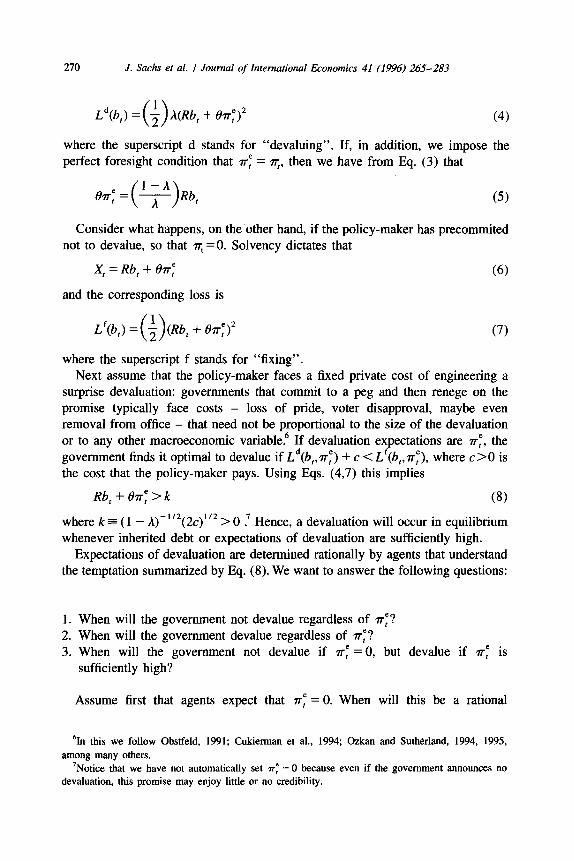
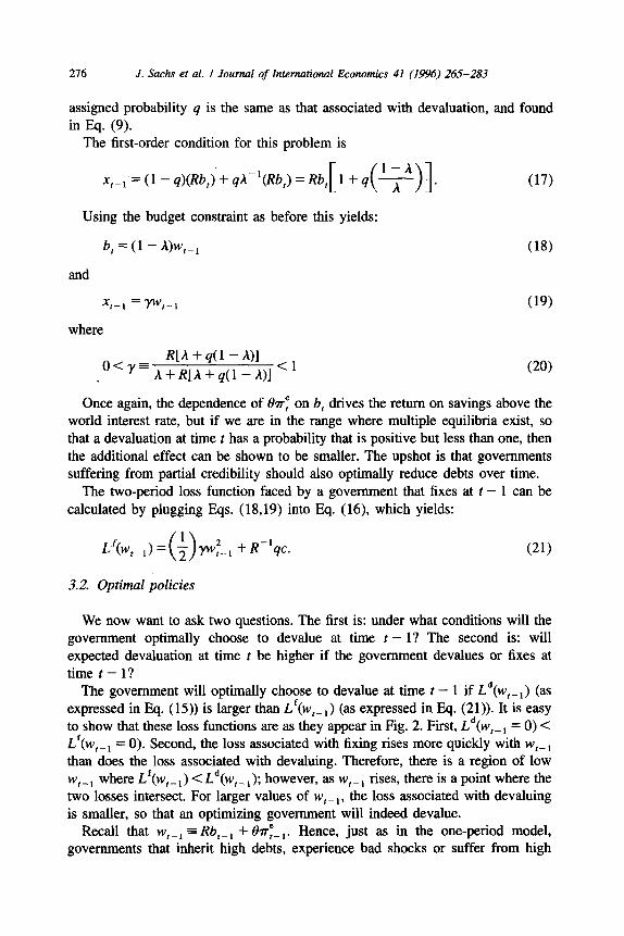
Full Crcdiiity Partial Credibility No Credibility

I I I

b

2.k k Rb

Fig. 1. Debt levels and multiple equilibria.

expectations equilibrium? Devaluation condition 2.8 shows that it is rational to set VT = 0 if the accumulated stock of debt is sufficiently low: Rb, I k. Suppose now that agents expect that the government will devalue by the discretionary amount indicated in Eq. (5). Using this expression in Eq. (8) yields the result that such expectations will be fulfilled if Rb, > Ak. These two conditions give rise to the following partition of the state space, depicted in Fig. 1. For levels of debt Rb, no larger than Ak, only one equilibrium (with no expected devaluation) is possible: attaching a positive probability to devaluation cannot be rational, for no devaluation will take place regardless of what agents expected. In this range the fixed exchange rate enjoys full credibility. For levels of debt larger than Ak, but no larger than k, there are two possible equilibria: if agents expect a devaluation of size 0~: = (( 1 - A)IA)Rb,, then such expectations will be validated by the government; if agents expect no devaluation, on the other hand, then no devaluation will take place ex post. Hence the credibility of the fixed exchange rate is partial, and depends on animal spirits. Finally, for levels of debt larger than k a devaluation will inevitably take place. The fixed rate regime has no credibility.

Notice also that if an equilibrium with devaluation does materialize, then the corresponding loss for policymakers is

Rb, - 7 A-‘(Rb,)‘+ c. )-(‘) (9)

By contrast, if an equilibrium with no devaluation materializes, then the loss is

Lf(b,,&r; = 0) = + 0 (Rb,)‘. (10)

2.2. When do multiple equilibria occur?

This simple model can readily yield multiple equilibria, and for reasons similar to the seminal models by Obstfeld, 1986, 1991, 1994 and Calvo, 1988.’ Such multiplicity arises from two features of the economic environment. First, optimizing governments lack access to a precommitment technology, so ex post (after expectations have been set) they may not deliver the policies they promised ex

‘See also de Kock and Grilli, 1993; Ozkan and Sutherland, 1994, 1995; Bensaid and Jeanne, 1994a,b; Velasco, 1995.


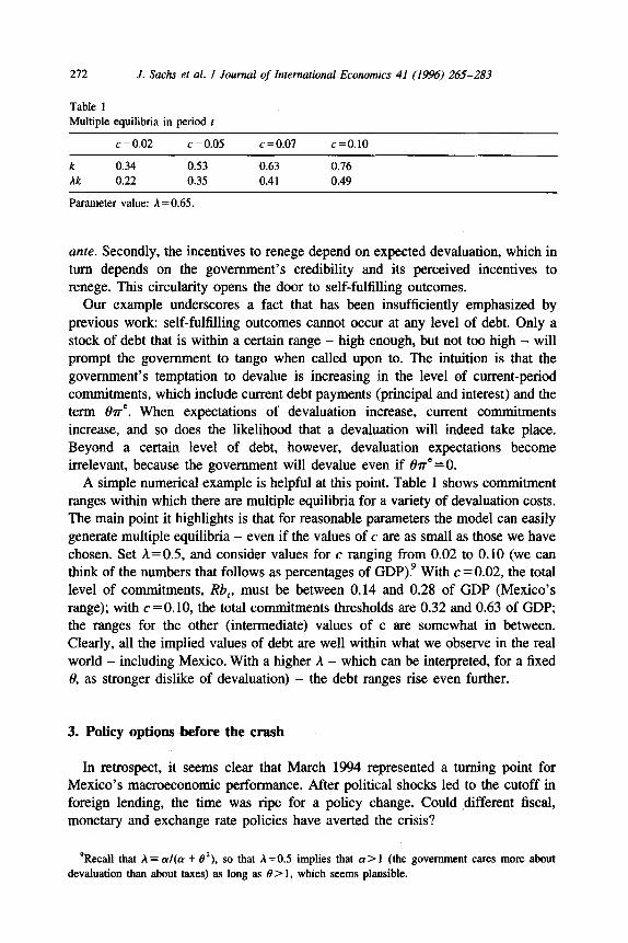
Table 1 Multiple equilibria in period t

c=o.o2 c = 0.05 c = 0.07 c=O.lO

k 0.34 0.53 0.63 0.76 Ak 0.22 0.35 0.41 0.49

Parameter value: A = 0.65.

ante. Secondly, the incentives to renege depend on expected devaluation, which in turn depends on the government’s credibility and its perceived incentives to renege. This circularity opens the door to self-fulfilling outcomes.

Our example underscores a fact that has been insufficiently emphasized by previous work: self-fulfilling outcomes cannot occur at any level of debt. Only a stock of debt that is within a certain range - high enough, but not too high - will prompt the government to tango when called upon to. The intuition is that the government’s temptation to devalue is increasing in the level of current-period commitments, which include current debt payments (principal and interest) and the term 0~“. When expectations of devaluation increase, current commitments increase, and so does the likelihood that a devaluation will indeed take place. Beyond a certain level of debt, however, devaluation expectations become irrelevant, because the government will devalue even if 8~” =O.

A simple numerical example is helpful at this point. Table 1 shows commitment ranges within which there are multiple equilibria for a variety of devaluation costs. The main point it highlights is that for reasonable parameters the model can easily generate multiple equilibria - even if the values of c are as small as those we have chosen. Set A=0.5, and consider values for c ranging from 0.02 to 0.10 (we can think of the numbers that follows as percentages of GDP)P With c = 0.02, the total level of commitments, Rb,, must be between 0.14 and 0.28 of GDP (Mexico’s range); with c =O.lO, the total commitments thresholds are 0.32 and 0.63 of GDP; the ranges for the other (intermediate) values of c are somewhat in between. Clearly, all the implied values of debt are well within what we observe in the real world - including Mexico. With a higher h - which can be interpreted, for a fixed 0, as stronger dislike of devaluation) - the debt ranges rise even further.

3. Policy options before the crash

In retrospect, it seems clear that March 1994 represented a turning point for Mexico’s macroeconomic performance. After political shocks led to the cutoff in foreign lending, the time was ripe for a policy change. Could different fiscal, monetary and exchange rate policies have averted the crisis?

‘Recall that A = a/(cr + 0’). so that A=OS implies that a> 1 (the government cares more about devaluation than about taxes) as long as 0 > 1, which seems plausible.

J. Sachs et al. I Journal of International Economics 41 (19%) 265-283 213

We have documented at some length in Section 2 that Mexican monetary policy was not as contractionary as might have been necessary to maintain the exchange rate peg. Fiscal policy was not used either to carry out an adjustment. A more contractionary fiscal policy could have been helpful in correcting real exchange rate misalignment (had a reduction of public expenditure on non-traded goods taken place) and in reducing the total outstanding stock of public debt (in particular, domestic debt). But fiscal policy, if anything, was more expansionary in 1994 than in previous years: the operational fiscal surplus fell from 2.1% of GDP in 1993 (and 2.9% in 1992) to 0.5% of GDP in 1994.

If monetary and fiscal policies were not used actively to effect the required adjustment, what about the exchange rate? Following the Colosio assassination the nominal rate rose all the way to the top of the band (in what constituted a nominal devaluation of about 10%) and spent the rest of the year at or very near the ceiling. The upshot is that between April and December Mexico operated an essentially pegged exchange rate. Opponents of moving the band ceiling and attaining a greater devaluation stressed credibility costs: the whole reform effort depended on adhering to the pre-announced exchange rate rule, even in the face of a large exogenous shock. By contrast, a surprise devaluation, however small, would simply destroy the hard-won credibility capital and convince the public of the policy-makers’ taste for discretionary policy.

This argument is correct - but also woefully incomplete. The public’s confidence that a fixed exchange rate will be maintained depends not only on the government’s perceived desire not to devalue, but also (and crucially) on the government’s ability not to devalue given external circumstances. By letting reserves dwindle, the government of Mexico may have convinced the public of its desire not to devalue, but also made it increasingly likely that the desire could not be sustained. By not devaluing in March, the government may have increased rather than decreased the expected rate of devaluation.

3.1. A two-period model

To evaluate the options faced by the government in the aftermath of the assassination, we extend the previous formalization by considering two periods. We economize by using the model of the previous section as the second period of the more general setup. Hence, the budget constraint (Eq. (1)) must be sup- plemented by

(11)

where b,-, is simply given. In addition, the objective function (Eq. (2)) must be replaced by lo

“Note that we have set the discount rate equal to the world interest rate, so that no anticipated debt accumulation or decumulation should take place, except for strategic reasons.

214 J. Sachs et al. I Journal of International Economics 41 (19%) 265-283

0 ; & ff7rz + Xf)R+‘+‘), a! > 0. s--1 1

(12)

Lastly, we must specify more carefully the impact of actions taken by the policy-maker at time t - 1 on expectations at time t. First, assume that the cost c is paid by the policy-maker only the first time she devalues; in particular, if there is a devaluation at time t - 1, she does not pay the cost again no matter what she does to the exchange rate at time t. This assumption is designed to capture the fact that fixed costs accrue to politicians when they first renege on promises, not when they engage in repeated devaluations. Secondly, we introduce reputational considera- tions by assuming that a politician that cheats is never believed by the public again. This assumption is of course a special case of the trigger strategies first employed in a similar context by Barro and Gordon, 1983.

Next we analyze the two courses of action available to the policy-maker in period t - 1. Suppose she sets rr-, > 0 (we will determine the optimal size of this devaluation below). Then, at time t agents will expect a devaluation with probability one, which corresponds to Eq. (5), and the associated loss will be as given by Eq. (9). Hence, a policy-maker who decides to devalue at t - 1 must solve the following problem:

~~(b,- I ) = Max (13)

subject to Eq. (11) and taking rrrel as given, where the next-period value is obtained from Eq. (9).

Fist order conditions are

Rb x,-, andx,-, = A 0 <.

Note that since h < 1, the “return” associated with government savings is higher than the world rate of interest. This is because if the government accumulates assets between periods 1 and 2, then it not only obtains the interest earned on the additional assets, but it also lowers devaluation expectations for the following period. Because a higher 0~: requires higher taxes or devaluation that period, lowering 8~: is equivalent to relaxing the resource constraint at 2 - and hence is equivalent to having a larger return on savings. Using Eqs. (11,14) we

A’ have b, = w,-r

(A*+Rj’ where w,- r = Rb,- , + OF- 1 is the total amount of

commitments the government faces at time t - 1 (of course, t?rF-, is endogenous, but that does not matter for what follows). Hence, the extra “kick” obtained from savings means that a government that expects to have no credibility next period should optimally reduce its expected commitments beyond what the standard

1. Sachs et al. I Journal of International Economics 41 (1996) 265-283 275

Barre, 1979 smoothing rule would suggest.” Using Eq. (13) we can write the corresponding minimized two-period loss function as

Ld(W,-,) =(;)A(%) + c. (15)

This completes the description of the choices faced by a government that devalues at time t - 1.

What about a government that does not devalue at time t - l? Fixing during the first period means that promises of continued fixing at time t may be given some credibility by agents. How much credibility will depend on the inherited stock of commitments.

AssuT;-t$ following: in period t, the outcome involving no credibility

(en-; = - h Rb,) and an associated devaluation materializes with probability q, and the outcome involving full credibility (0,: = 0) and continued fixing materializes with probability 1 - q, where clearly 0 5 q I 1. That is to say, “sunspots” determine which outcome prevails. A government that upholds its promise to fix at time t - 1 and leaves b, behind expects a loss the next period that is the weighted average of both possible outcomes.‘*

Then, the relevant problem for the government at time t - 1 is

Lf(w,_,) = max +R-‘q[ 0

; K’(Rw,p, -Rx-,)* + c]

+R-‘(1 -4) ; (Rw,_, -Rr,m,)” 0 (16)

where the losses in period t under devaluation and no devaluation are taken from Eq. (9) and Eq. (lo), respectively. Two things are worth noting in Eq. (16). First, that only the setting for x,-~ is to be decided at time t - 1; it must be the case that “r-1 = 0, for otherwise an outcome with no credibility and expectations &rF = (l-4 ARb, would certainly materialize at time t. Secondly, that “pessimistic” expectations materialize in period t and credibility goes to naught, then the loss for that period is exactly the same (for a given inherited level of debt) than it would have been if the government had devalued at time t - 1. That is why the loss

“Obstfeld, 1991 was the first to derive such a result. See also Calvo and Guidotti, 1990.

‘*Note that (strictly speaking) this formulation makes sense if, for some O<q< 1, the b, that results from the government’s optimal choice is such that Ak<Rb,Sk, so that multiplicities are indeed

possible in period t. However, the first-order conditions that follow encompass all possible situations at time t given the following procedure. Set q=O; then if the resulting b, is such that Rb,dk, then assigning probability 0 to a devaluation at time r is indeed a rational expectation. Alternatively, set

q = 1; if the resulting b, is such that Rb, > k, then assigning -probability 1 to a devaluation at time t is indeed a rational expectation.


assigned probability q is the same as that associated with devaluation, and found in Fq. (9).

The first-order condition for this problem is

xI-l=(l-q)(Rb,)+qA-L(Rb,)=Rb, l+q [ WI* (17)

Using the budget constraint as before this yields:

b, = (1 - A)w,-,

and

(18)

X,-l = wt.-1 (19)

where

R[A + qu - A)] .“<Y=A+RIA+q(l-A),<l (20)

Once again, the dependence of err: on b, drives the return on savings above the world interest rate, but if we are in the range where multiple equilibria exist, so that a devaluation at time t has a probability that is positive but less than one, then the additional effect can be shown to be smaller. The upshot is that governments suffering from partial credibility should also optimally reduce debts over time.

The two-period loss function faced by a government that fixes at t - 1 can be calculated by plugging Eqs. (18,19) into Eq. (16), which yields:

Lf(w,-J = ; yv:-, + K’qc. 0

3.2. Optimal policies

We now want to ask two questions. The first is: under what conditions will the government optimally choose to devalue at time t - l? The second is: will expected devaluation at time t be higher if the government devalues or fixes at time t-l?

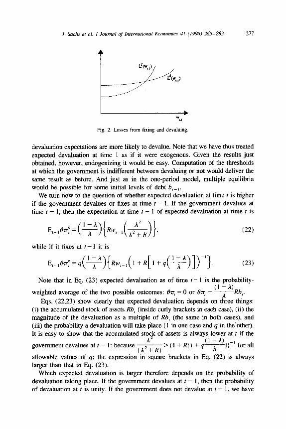
The government will optimally choose to devalue at time t - 1 if Ld(w,-,) (as expressed in Eq. (15)) is larger than L’(w,-,) (as expressed in Eq. (21)). It is easy to show that these loss functions are as they appear in Fig. 2. First, Ld(w,- 1 = 0) < Lf(w,-, = 0). Second, the loss associated with fixing rises more quickly with w,-i than does the loss associated with devaluing. Therefore, there is a region of low w,- I where Lf(w,- ,) C Ld(w,- ,); however, as w,- I rises, there is a point where the two losses intersect. For larger values of w,- , , the loss associated with devaluing is smaller, so that an optimizing government will indeed devalue.

Recall that w,-~ = Rb,-, + &rF-i. Hence, just as in the one-period model, governments that inherit high debts, experience bad shocks or suffer from high

J. Sachs et al. I Journal of International Economics 41 (1996) 265-283 211

Fig. 2. Losses from fixing and devaluing.

devaluation expectations are more likely to devalue. Note that we have thus treated expected devaluation at time 1 as if it were exogenous. Given the results just obtained, however, endogenizing it would be easy. Computation of the thresholds at which the government is indifferent between devaluing or not would deliver the same result as before. And just as in the one-period model, multiple equilibria would be possible for some initial levels of debt b,-, .

We turn now to the question of whether expected devaluation at time t is higher if the government devalues or fixes at time t - 1. If the government devalues at time t - 1, then the expectation at time t - 1 of expected devaluation at time t is

E,-,th; =(q){Rwt-,(A)}3 while if it fixes at t - 1 it is

(22)

(23)

Note that in Eq. (23) expected devaluation as of time t - 1 is the probability- Cl- NRb

weighted average of the two possible outcomes: &r, = 0 or 8~~ = ~ Eqs. (22,23) show clearly that expected devaluation depends on thhree things:

(i) the accumulated stock of assets Rb, (inside curly brackets in each case), (ii) the magnitude of the devaluation as a multiple of Rb, (the same in both cases), and (iii) the probability a devaluation will take place (1 in one case and q in the’other). It is easy to show that the accumulated stock of assets is always lower at t if the

A2 government devalues at t - 1: because

(A2 + R) >(l +R[l +qA (’ - *)1)-l for all

allowable values of q; the expression in square brackets in Eq. (22) is always larger than that in F!q. (23).

Which expected devaluation is larger therefore depends on the probability of devaluation taking place. If the government devalues at t - 1, then the probability of devaluation at t is unity. If the government does not devalue at t - 1, we have

278 .I. Sachs et al. I Journal of International Economics 41 (1996) 265-283

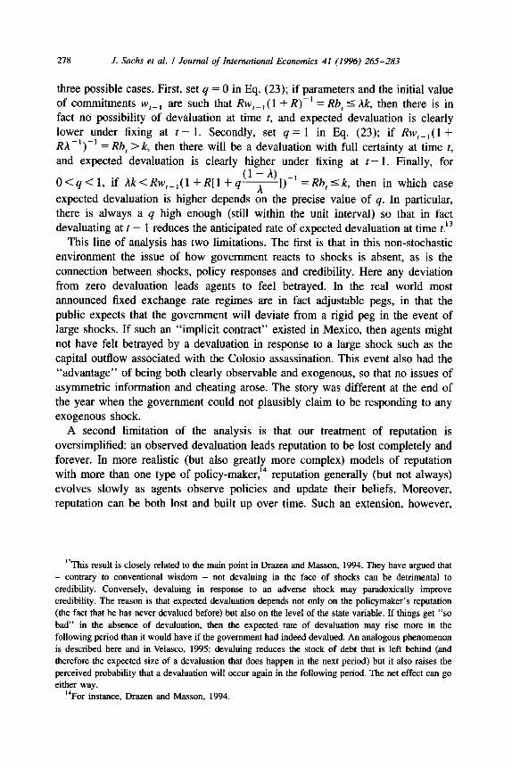
three possible cases. First, set q = 0 in Eq. (23); if parameters and the initial value of commitments wt-, are such that Rw,-,( 1 + R)-’ = Rb, 5 hk, then there is in fact no possibility of devaluation at time t, and expected devaluation is clearly lower under fixing at t - 1. Secondly, set q = 1 in Eq. (23); if Rw,-,( 1 + RX’)-’ = Rb, > k, then there will be a devaluation with full certainty at time t, and expected devaluation is clearly higher under fixing at t - 1. Finally, for

(1-N -, O<q<l, if Ak<Rw,-,(l+R[l+q- h 1) = Rb, 5 k, then in which case expected devaluation is higher depends on the precise value of q. In particular, there is always a q high enough (still within the unit interval) so that in fact devaluating at t - 1 reduces the anticipated rate of expected devaluation at time t.13

This line of analysis has two limitations. The first is that in this non-stochastic environment the issue of how government reacts to shocks is absent, as is the connection between shocks, policy responses and credibility. Here any deviation from zero devaluation leads agents to feel betrayed. In the real world most announced fixed exchange rate regimes are in fact adjustable pegs, in that the public expects that the government will deviate from a rigid peg in the event of large shocks. If such an “implicit contract” existed in Mexico, then agents might not have felt betrayed by a devaluation in response to a large shock such as the capital outflow associated with the Colosio assassination. This event also had the “advantage” of being both clearly observable and exogenous, so that no issues of asymmetric information and cheating arose. The story was different at the end of the year when the government could not plausibly claim to be responding to any exogenous shock.

A second limitation of the analysis is that our treatment of reputation is oversimplified: an observed devaluation leads reputation to be lost completely and forever. In more realistic (but also greatly more complex) models of reputation with more than one type of policy-maker,‘4 reputation generally (but not always) evolves slowly as agents observe policies and update their beliefs. Moreover, reputation can be both lost and built up over time. Such an extension, however,

13This result is closely related to the main point in Drazen and Masson, 1994. They have argued that - contrary to conventional wisdom - not devaluing in the face of shocks can be detrimental to

credibility. Conversely, devaluing in response to an adverse shock may paradoxically improve credibility. The reason is that expected devaluation depends not only on the policymaker’s reputation (the fact that he has never devalued before) but also on the level of the state variable. If things get “so

bad” in the absence of devaluation, then the expected rate of devaluation may rise more in the following period than it would have if the government had indeed devalued. An analogous phenomenon is described here and in Velasco, 1995: devaluing reduces the stock of debt that is left behind (and

therefore the expected size of a devaluation that does happen in the next period) but it also raises the

perceived probability that a devaluation will occur again in the following period. The net effect can go either way.

14For instance, Drazen and Masson, 1994.

.I. Sachs et al. I Journal of International Economics 41 (1996) 265-283 279

would only strengthen the point we are trying to make. If in the extreme in which reputation is completely lost, unexpected devaluation can lower devaluation expectations, the same could more easily be true in a situation in which reputation is only partially lost as a result of a surprise devaluation.

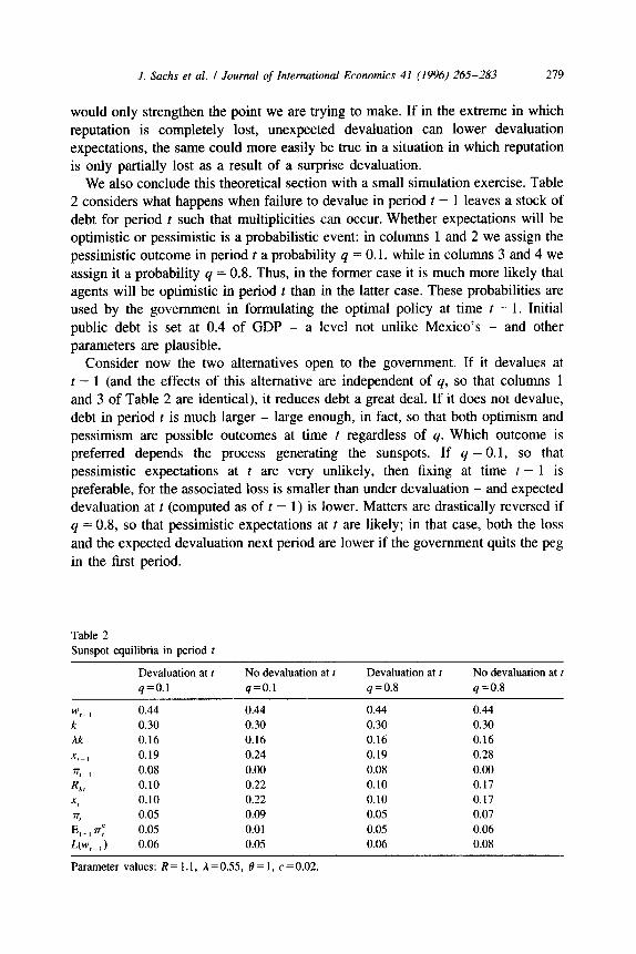
We also conclude this theoretical section with a small simulation exercise. Table 2 considers what happens when failure to devalue in period t - 1 leaves a stock of debt for period t such that multiplicities can occur. Whether expectations will be optimistic or pessimistic is a probabilistic event: in columns 1 and 2 we assign the pessimistic outcome in period t a probability q = 0. I, while in columns 3 and 4 we assign it a probability q = 0.8. Thus, in the former case it is much more likely that agents will be optimistic in period t than in the latter case. These probabilities are used by the government in formulating the optimal policy at time t - 1. Initial public debt is set at 0.4 of GDP - a level not unlike Mexico’s - and other parameters are plausible.

Consider now the two alternatives open to the government. If it devalues at t - 1 (and the effects of this alternative are independent of q, so that columns 1 and 3 of Table 2 are identical), it reduces debt a great deal. If it does not devalue, debt in period t is much larger - large enough, in fact, so that both optimism and pessimism are possible outcomes at time t regardless of q. Which outcome is preferred depends the process generating the sunspots. If q = 0. I, so that pessimistic expectations at t are very unlikely, then fixing at time t - 1 is preferable, for the associated loss is smaller than under devaluation - and expected devaluation at t (computed as of t - 1) is lower. Matters are drastically reversed if q = 0.8, so that pessimistic expectations at t are likely; in that case, both the loss and the expected devaluation next period are lower if the government quits the peg in the first period.

Table 2

Sunspot equilibria in period t

w,-I k

Ak x 1-I “,-I 4,

x, “,

Et-, n-: uw.-,)

Devaluation at t No devaluation at t Devaluation at t No devaluation at t q=O.l q=O.l q=O.8 q=O.8

0.44 0.44 0.44 0.44 0.30 0.30 0.30 0.30 0.16 0.16 0.16 0.16 0.19 0.24 0.19 0.28 0.08 0.00 0.08 0.00 0.10 0.22 0.10 0.17 0.10 0.22 0.10 0.17 0.05 0.09 0.05 0.07

0.05 0.01 0.05 0.06 0.06 0.05 0.06 0.08

Parameter values: R=l.l, A=0.55, 0= 1, c=O.O2.


4. Conclusions

In this concluding section we attempt to summarize our interpretation of the Mexican experience in terms of our simple theoretical framework. Two aspects of that episode are relevant. The first is the question of whether an element of self-fulfilling expectations helped to determine the timing and magnitude of the attack. The behavior of interest rates seems to suggest that multiplicities did play a role: the peso problem that standard speculative attack models15 would predict did not materialize. A sudden shift in expectations - probably prompted by the devaluation - was the trigger for the crisis. Why was the Mexican Central Bank vulnerable to a self-fulfilling attack in late 1994, but was not in the previous six years during which it had sustained a fixed (or quasi-fixed) exchange rate? As Mendoza and Calvo, 1996 stress, by late 1994 Mexico’s ratio of reserves to short-term liabilities was well below one. Our model and its associated interpretation highlight the fact that attacks are self-fulfilling at high levels of debt (low levels of reserves), but not otherwise.

The second interesting policy issue is whether Mexican authorities should have acted differently in the course of 1994. Dornbusch and Werner, 1994, in a much-discussed contribution, argued for an early devaluation; Sachs et al., 1995 stress that an insufficiently restrictive monetary policy in 1994 contributed to the erosion of reserves; others have blamed fiscal policy for the same phenomenon. What is the proper theoretical framework within which to evaluate such claims? The model presented here offers two relevant suggestions. The first is that governments suffering from imperfect credibility in their exchange rate policy have an additional reason to engage in fiscal and monetary tightening, for expected devaluation is, ceteris paribus, an increasing function of the level of debt (and a decreasing function of the level of reserves). Along the same lines, a government that allows a bad shock to increase the level of debt may move the economy from a region where one equilibrium was possible to a region where two equilibria (a good one and a bad one) are possible. This suggests that Mexican authorities may indeed have been insufficiently restrictive in the course of 1994. In particular, by allowing reserves to dwindle, they may have put the economy in a situation where multiplicities existed and where a self-fulfilling attack was feasible.

A related question is whether Mexico should have devalued in response to the shocks of 1994. The model in this assumes that a surprise devaluation does indeed destroy all hard-won credibility (the probability of a discretionary devaluation is thereafter one), but also recognizes that expected devaluation is the product of two terms: the probability of a devaluation taking place times the size of the relevant discretionary devaluation. Because optimal discretionary devaluation is an increasing function of debt, and because a surprise devaluation reduces debt, the second term in the product falls just as the first one rises; the net outcome can be in either

“In particular, Flood and Garber, 1984.

J. Sachs et al. I Journal of International Economics 41 (1996) 245283 281

direction. In terms of the Mexican experience, by sticking to the exchange rate rule Mexican authorities may have convinced the public of their desire not to devalue. But the spectacle of dwindling reserves and rising debt ensured that, if a devaluation did occur, it would be large.

The lesson: acting “tough” on the exchange rate does not necessarily enhance credibility, just as a devaluation is not the end of the world, even in countries where the finance minister has ritually pledged that no depreciation will ever occur. Recall, for example, the aftermath of the devaluation crisis of the EMS in 1992. The devaluing countries experienced a fall in interest rates and an acceleration of growth.

What else have we learned from this episode? That exchange rate pegs are more fragile, and the harm associated with their collapse greater, than the economics profession has realized until recently.16 Fixed exchange rates require that the money supply be mainly determined by the balance of payments. But this adjustment process was not allowed to operate in Mexico - neither in the upswing (when capital flowed in) nor in the downswing (when capital flowed out).17 That the automatic correction mechanism was systematically aborted says something not only about policy-making in Mexico, but about the difficulties inherent in adjustment under fixed rates. It is hard to find cases where governments have let the process run its course. In Chile in the early 198Os, not even all-powerful General Pinochet could push nominal wages far enough down to avoid a devaluation. In Europe in the early 199Os, country after country abandoned the ERM once the employment or domestic financial consequences of a high-interest- rate policy undermined their ability to sustain pegged exchange rates.

In the case of Mexico matters were made particularly tricky by three factors. The first was the political cycle, with elections in mid-1994. The second was the vulnerability of the financial sector, whose assets were quickly deteriorating. The third was uncertainty about the future course of capital flows: after the elections and witnessing a modest recovery of capital inflows, Mexican policy-makers could conjecture (rather riskily) that the worst was over, and that new inflows would make more drastic adjustments unnecessary. All three factors helped to justify the loose credit stance adopted through much of 1994, a policy stance which in the end depleted reserves and caused the currency to crash. But clearly, elections, weak banks and uncertainty are not uniquely Mexican phenomena. Analogous complications bedevil almost everyone attempting adjustment through fixed rates.

We conclude there is now enough experience to suggest that pegged exchange rates can render countries extremely vulnerable, even with seemingly virtuous monetary and fiscal policies. Pegging seems to be extremely important in the early

‘6Forhmately, the conventional wisdom that viewed fixing as a fairly straightforward and easily achieved matter seems to be changing. See Svensson, 1993; Obstfeld and Rogoff, 1995 for two influential (and increasingly skeptical) views.

“See Sachs et al., 1995.

282 J. Sachs et al. I Journal of International Economics 41 (19%) 265-283

stages of a stabilization program, when anchoring expectations and permitting remonetization are priorities. But just as important is to get out of the fixed exchange rate system in time. In the aftermath of stabilization, flexible crawling pegs complemented by a wide band - such as those used successfully by Israel and Chile - seem safer.

Acknowledgments

We thank the Center for International Affairs at Harvard University and the C.V. Starr Center for Applied Economics at NYU for financial support, and Gerard0 Esquivel for excellent research assistance. All errors are our own.

References

Barm, R., 1979, On the determination of the public debt, Journal of Political Economy, Vol. 87. Barro, R. and D. Gordon, 1983, A positive theory of monetary policy in a natural rate model, Journal of

Political Economy. Bensaid and Jeanne, 1994a. The instability of fixed exchange rate systems when raising the nominal

interest rate is costly, LSE financial markets group Discussion Paper No. 190, July. Bensaid and Jeanne, 1994b. The instability of monetary policy rules, mimeo, CERAS-ENPC,

November. Calvo, G., 1988, Servicing the pubhc debt: the role of expectations, American Economic Review, 78

(September). Calvo, G., and P. Guidotti, 1990, ‘Credibility and nominal debt: exploring the role of maturity in

managing inflation, JMF Staff Papers, 37 (3) (September). Cukierman, A., M. Kiguel and L. Leiderman, 1994, Choosing the width of exchange rate bands:

credibility vs. flexibility, CEPR Discussion Paper No. 809, January. de Kock, G. and V. Grilli, 1993, Fiscal policies and the choice of exchange rate regime, The Economic

Journal, 103 (March). Dombusch, R. and A. Werner, 1994, Mexico: stabilization, reform and no growth, Brookings Papers in

Economic Activity, 1. Drazen, A. and P Masson, 1994, Credibility of policies versus credibility of policymakers, Quarterly

Journal of Economics. Eichengreen, B., A. Rose and C. Wyplosz, 1995, Exchange market mayhem: the antecedents and

aftermaths of speculative attacks, Economic Policy, 21. Flood, R.P. and R. Garber, 1984, Collapsing exchange rate regimes: some linear examples, Journal of

International Economics, 17, 1-13. Krugman, P, 1979, A model of balance of payments crises, Journal of Money, Credit and Banking. Mendoza, E. and G. Calvo, 1995 Reflections on Mexico’s balance of payments crisis: chronicle of a

death foretold, Journal of International Economics 41, 235-264. Obstfeld, M., 1986, Rational and self-fulfilling balance of payments crises, American Economic

Review. Obstfeld, M., 1991, Destabilizing effects of exchange rate escape clauses, NBER Working Paper No.

3603. Obstfeld, M., 1994, The logic of currency crises, Cahiers Economiques et Monetaires, 43. Obstfeld, M. and K. Rogoff, The mirage of fixed exchange rates, NBER Working Paper No. 5191, July.

.I. Sachs et al. I Journal of International Economics 41 (1996) 265-283 283

Ozkan, F.G. and A. Sutherland, 1994, A currency crisis model with an optimizing policymaker, mimeo.

University of York, December. Ozkan, F.G. and A. Sutherland, 1995, Policy measures to avoid a currency crisis, The Economic

Journal, 105 (March). Rose, A. and L. Svensson, 1994, European exchange rate credibility before the fall, European

Economic Review, 38.

Sachs, J., A. Tome11 and A. Velasco, 1995, The collapse of the Mexican peso: what have we learned? NBER Working Paper 5142, July. Forthcoming in Economic Policy.

Svensson, 1993, Fixed exchange rates as a means to price stability: What have we learned?, NBER

Working Paper No. 4504, October.

Velasco, A., 1995, When are fixed exchange rates really fixed? Paper presented to the 8th NBER Interamerican Seminar, Bogota, Colombia, November.

The Mexican Peso Crisis: Sudden Death or Death Foretold?

Documents