The MERLIN-Expo Potato model · the merlin-expo potato model. v1.3. author: ... initialization of mass balance in media 22 ... 5.2.4 parameters related to the chemical degradation

1

The MERLIN-Expo Potato model V1.3

Author: Lucie Pastor1, Taku Tanaka1 1EDF R&D, 6 quai Watier, 78400 Chatou, France [email protected], [email protected]

Reviewers: Philippe Ciffroy1

mailto:[email protected]

2

Content

LEVEL 1 DOCUMENTATION (BASIC KNOWLEDGE ON MODEL PURPOSE, APPLICABILITY AND COMPONENTS) 4

1. MODEL PURPOSE 4

1.1. GOAL 4 1.2. POTENTIAL DECISION AND REGULATORY FRAMEWORK(S) 4

2. MODEL APPLICABILITY 4

2.1. SPATIAL SCALE AND RESOLUTION 4 2.2. TEMPORAL SCALE AND RESOLUTION 4 2.3. CHEMICAL CONSIDERED 4 2.4. STEADY-STATE VS DYNAMIC PROCESSES 4

3. MODEL COMPONENTS 5

3.1. MEDIA CONSIDERED 5 3.2. LOADINGS, LOSSES, AND EXCHANGES BETWEEN DIFFERENT MEDIA 5 3.3. COUPLING WITH OTHER MODELS 6 3.4. FORCING VARIABLES 7 3.5. PARAMETERS 8 3.6. INTERMEDIATE STATE VARIABLES 10 3.7. REGULATORY STATE VARIABLES 17

LEVEL 2 DOCUMENTATION (BACKGROUND SCIENCE) 19

4. PROCESSES AND ASSUMPTIONS 19

4.1. PROCESS N°1: PARTITION BETWEEN PHASES 19 4.2. PROCESS N°2: TRANSFER BY DIFFUSION 20 4.3. PROCESS N°3: DEGRADATION IN THE POTATO COMPARTMENT 20 4.4. PROCESS N°4: UPTAKE OF METALS 20

LEVEL 3 DOCUMENTATION (NUMERICAL INFORMATION) 22

5. NUMERICAL DEFAULT VALUES (DETERMINISTIC AND/OR PROBABILISTIC) 22

5.1. INITIALIZATION OF MASS BALANCE IN MEDIA 22 5.2. DEFAULT PARAMETER VALUES 22 5.2.1 SITE-SPECIFIC AND PLANT PARAMETERS 22 5.2.2 PARAMETERS RELATED TO THE PARTITION BETWEEN PHASES 25

3

5.2.3 PARAMETERS RELATED TO THE TRANSFER BY DIFFUSION 42 5.2.4 PARAMETERS RELATED TO THE CHEMICAL DEGRADATION 44 5.2.5 PARAMETERS RELATED TO THE TRANSFER FROM SOIL TO POTATO GOVERNED BY THE EQUILIBRIUM TRANSFER FACTOR 45

LEVEL 4 DOCUMENTATION (MATHEMATICAL INFORMATION) 48

6. MASS BALANCE EQUATION 48

7. CALCULATION OF STATE VARIABLES 48

7.1. UPTAKE THROUGH DIFFUSION (UPTAKE_DIFFUSION) AND LOSS BY DEPURATION (K_DEPURATION_POTATO) 48 7.1.1 MASS OF POTATO PER UNIT AREA OF SOIL (M_POTATO) 49 7.1.2 DISTRIBUTION COEFFICIENT OF THE POLLUTANT BETWEEN SOIL AND WATER (KD_SOIL) 49 7.1.3 UPTAKE RATE BY POTATO THROUGH DIFFUSION (K_UPTAKE_POTATO) 50 7.1.4 PARTITION COEFFICIENT BETWEEN POTATO AND WATER (K_POTATO_WATER) 50 7.1.5 DEPURATION RATE FROM POTATO THROUGH DIFFUSION (K_DEPURATION_POTATO) 51 7.1.6 DIFFUSION COEFFICIENT IN POTATO (D_POTATO) 51 7.1.7 DIFFUSION COEFFICIENT IN WATER/GAS PORES OF POTATO (D_W_POTATO, D_GAS_POTATO) 52 7.1.8 EFFECTIVE DIFFUSION COEFFICIENT IN PURE WATER/PURE AIR (D_WATER, D_GAS) 52 7.1.9 TORTUOSITY IN WATER/AIR PORES OF THE POTATO (T_W_POTATO, T_G_POTATO) 53 7.1.10 FRACTION OF THE POLLUTANT DISSOLVED IN THE POTATO WATER/IN AIR OF THE POTATO (F_W_POTATO, F_G_POTATO) 54 7.1.11 PARTITION COEFFICIENT BETWEEN AIR AND WATER (K_AIR_WATER) 54 7.2. LOSS BY DEGRADATION IN POTATO (LOSS_DEG_POTATO) 55 7.3. UPTAKE OF METALS (UPTAKE_METALS) 55 7.4. CONCENTRATION IN POTATO AT HARVEST (C_POTATO) 56

REFERENCE 57

4

Level 1 documentation (basic knowledge on model purpose, applicability and components)

1. Model purpose

1.1. Goal The Potato model is used to estimate the time-dependent accumulation (in mass and concentration bases) of organic/metals in potato.

1.2. Potential decision and regulatory framework(s) Coupled with the information about the ingestion rate of potato crops (Kg fresh weight d-1), the Potato model can estimate the human exposure dose to organic substances/metals through the ingestion of potato crops. This output can be used for evaluating the risk to exceed regulatory thresholds for human health or used as an input for PBPK models.

2. Model applicability

2.1. Spatial scale and resolution The Potato model consists of one below-ground compartment. This compartment is fixed in space and is treated as being homogeneous, i.e. well-mixed in chemical composition, that is, the Potato model considers no spatial variation in chemical concentration. When model users need to consider, in their own scenarios, several regions with different levels of contamination in soil, they can set up multiple Potato models and make the models correspond to different levels of contamination in soil to cover several regions in their scenarios.

2.2. Temporal scale and resolution All the transfer processes considered in the Potato model are expressed on a daily basis, and thus the model should be run by the daily simulation setting.

2.3. Chemical considered The Potato model can be applicable for a variety of chemicals including many types of organic substances (such as PAHs, PCBs, Dioxins, VOCs) and also metals for which soil-to-plant transfer factors were found in the literature (i.e. Al, As, Cd, Cr, Cu, Fe, Mn, Pb, Zn). However, it should be noted that the model used for organic chemicals is limited to neutral compounds; it is not really applicable to ionic or dissociating compounds. For example, practically all herbicides and all ‘systemic’ pesticides are weak bases (Trapp, 2004). Also many of pharmaceuticals are weak bases or acids. These electrolytes undergo more complicated processes inside plants than neutral compounds.

2.4. Steady-state vs dynamic processes As for organic substances, the Potato model considers the diffusion from soil into spherical potatoes and the degradation. The uptake of chemicals by diffusion is assumed to be a dynamic process considering an uptake rate and a depuration rate. Following equilibrium partition coefficients are used to estimate those diffusion rates; (i) the partition coefficient between potato and water (K_potato_water), (ii) the partition coefficient between air and water (Kaw), and (iii) the partition coefficient between soil particles and soil pore-water (Kd_soil).

5

As for metals, the Potato model calculates the uptake by equilibrium transfer factors. The transfer factor expressed by the ratio of the concentration in root to the concentration in soil.

3. Model components

3.1. Media considered Definition: A ‘Medium’ is defined as an environmental or human compartment assumed to contain a given quantity of the chemical. The quantity of the chemical in the media is governed by loadings/losses (see 3.2 and 3.3) from/to other media and by transformation processes (e.g. degradation). The Potato model includes the following media (compartment):

• ‘Potato’. In this media, a time-dependent chemical mass (mg) in potatoes is calculated from the mass balance equation.

3.2. Loadings, losses, and exchanges between different media In the Potato model, the transfer processes for organic substances are assumed to be different from those for metals. In the Potato model, it is assumed that all the transfer processes take place only during the growing period of potato, that is, only between the germination time and harvest time. Out of the period, no chemical accumulation arises in the Potato model. At harvest time, the chemical mass accumulated in the potato compartments gets completely erased (set to zero), which is expressed in the model by the process of ‘Loss by harvest’ (see Table 1). After the harvest time, the transfer processes restart from the germination time in the next growing season. Each process is presented in the following table for each type of target substances (organic or metal) as follows:

Table 1 Loading and loss processes in the Potato model

For organic substances For metals

Input from soil to potato by diffusion Input from soil to potato governed by the equilibrium transfer factor

Loss by depuration (through diffusion)

Loss by chemical degradation

Loss by harvest Loss by harvest

Figure 1 and 2 present all the input/loss processes for organic substances and metals, respectively.

Definition: • A ‘Loading’ is defined as the rate of release/input of the chemical of interest to the receiving

system, here the potato media; • A ‘Loss’ is defined as the rate of output of the chemical of interest from the receiving system; • An ‘Exchange’ is defined as the transfer of the chemical of interest between two media of the

system.

6

Figure 1 Input and loss processes in the Potato model (for organic substances)

Figure 2 Input and loss processes in the Potato model (for metals)

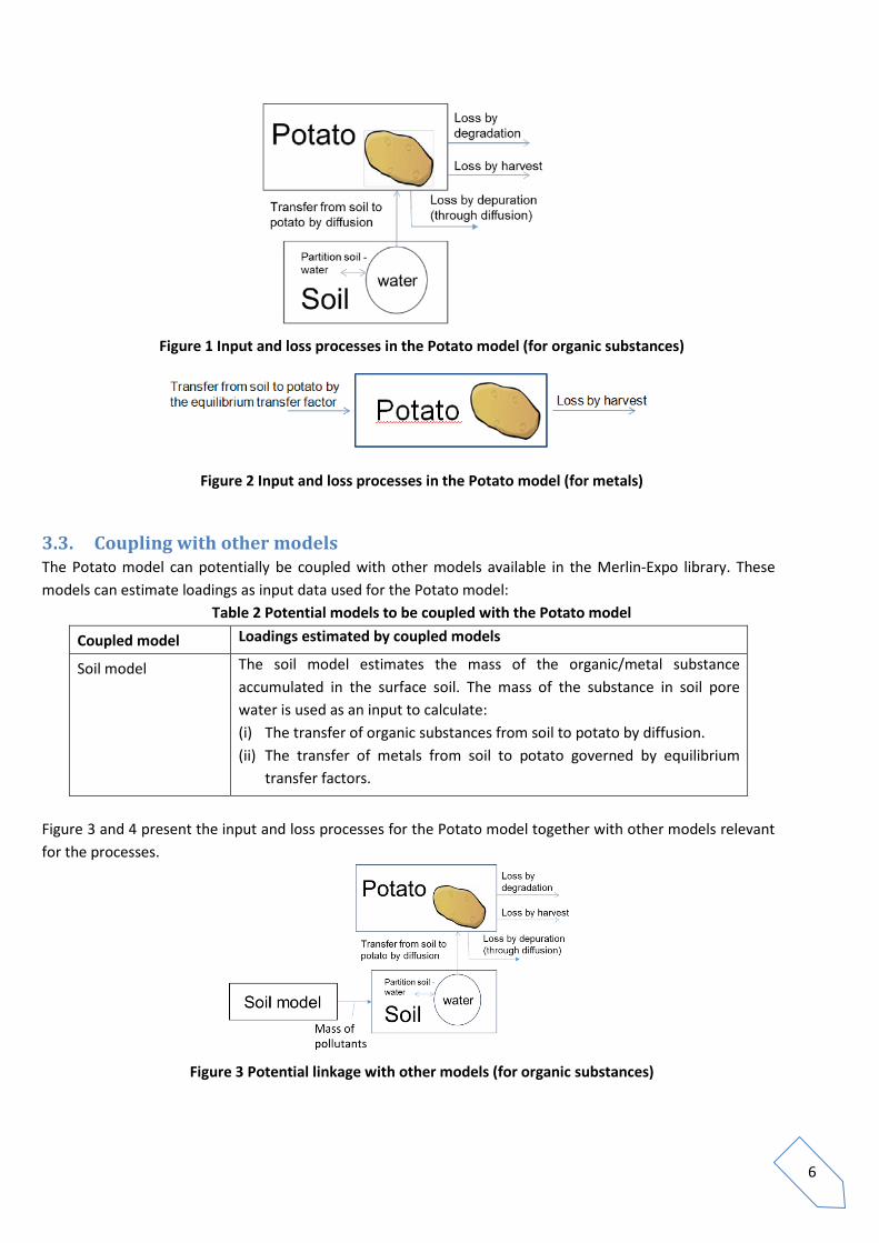
3.3. Coupling with other models The Potato model can potentially be coupled with other models available in the Merlin-Expo library. These models can estimate loadings as input data used for the Potato model:

Table 2 Potential models to be coupled with the Potato model

Coupled model Loadings estimated by coupled models

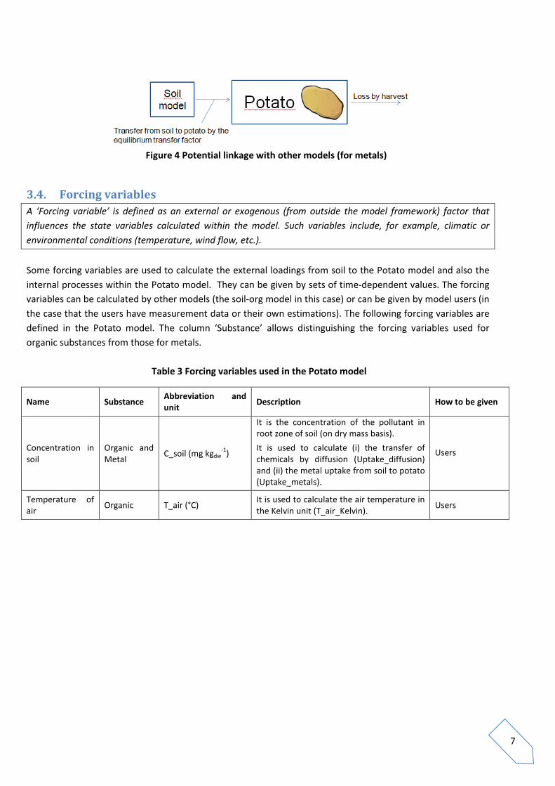
Soil model

The soil model estimates the mass of the organic/metal substance accumulated in the surface soil. The mass of the substance in soil pore water is used as an input to calculate: (i) The transfer of organic substances from soil to potato by diffusion. (ii) The transfer of metals from soil to potato governed by equilibrium

transfer factors.

Figure 3 and 4 present the input and loss processes for the Potato model together with other models relevant for the processes.

Figure 3 Potential linkage with other models (for organic substances)

7

Figure 4 Potential linkage with other models (for metals)

3.4. Forcing variables A ‘Forcing variable’ is defined as an external or exogenous (from outside the model framework) factor that influences the state variables calculated within the model. Such variables include, for example, climatic or environmental conditions (temperature, wind flow, etc.). Some forcing variables are used to calculate the external loadings from soil to the Potato model and also the internal processes within the Potato model. They can be given by sets of time-dependent values. The forcing variables can be calculated by other models (the soil-org model in this case) or can be given by model users (in the case that the users have measurement data or their own estimations). The following forcing variables are defined in the Potato model. The column ‘Substance’ allows distinguishing the forcing variables used for organic substances from those for metals.

Table 3 Forcing variables used in the Potato model

Name Substance Abbreviation and unit Description How to be given

Concentration in soil

Organic and Metal C_soil (mg kgdw

-1)

It is the concentration of the pollutant in root zone of soil (on dry mass basis). It is used to calculate (i) the transfer of chemicals by diffusion (Uptake_diffusion) and (ii) the metal uptake from soil to potato (Uptake_metals).

Users

Temperature of air Organic T_air (°C) It is used to calculate the air temperature in

the Kelvin unit (T_air_Kelvin). Users

3.5. Parameters A ‘Parameter’ is defined as a term in the model that is fixed during a model run or simulation but can be changed in different runs as a method for conducting sensitivity analysis or to achieve calibration goals. The parameters used in the Potato model are listed in the following tables. Table 4 presents all the parameters alphabetically by their abbreviations. The column ‘Substance’ allows distinguishing the parameters used for organic substances from those for metals.

Table 4 Parameters used in the Potato model Name Abbrebiation Description Unit Substance Carbohydrate content in potato CH_potato The content of carbohydrate contained in

potato per fresh weight of potato L kgfw-1 Organic

Diffusion coefficient of water in air D_H2O_air Diffusion coefficient of water vapour in air m2 d-1 Organic

Diffusion coefficient of oxygen in water D_O2_water - m2 d-1 Organic

Correction for density difference between water and n-octanol

delta_density_OW Factor correcting difference between densities of water and of n-octanol

L kg-1 Organic

Empirical correction factor for differences between solubility in octanol and sorption to tuber lipids

delta_solubility_lipids_potato Empirical factor correcting differences between solubility in octanol and sorption to potato lipids

unitless Organic

Fraction of organic matter in soil f_OM_soil - g g-1 Organic

Air content in potato G_potato Air volume contained in potato per fresh weight of potato L kgfw

-1 Organic

Henry's law constant H

Ratio of a chemical’s abundance in gas phase (vapour pressure) to that in aqueous phase (solubility) at equilibrium at a given temperature

Pa m3 mol-1 Organic

Carbohydrate-water partition coefficient K_CH_water Ratio of the equilibrium concentration of a

chemical in carbohydrate to that in water unitless Organic

Lipid content of potato L_potato Lipid quantity contained in fresh weight of potato kg kgfw

-1 Organic

Degradation rate in potato Lambda_deg_potato First order decay rate of pollutants in potato d-1 Organic

Water-organic carbon partition coefficient (in log10)

Log10_K_oc Ratio of the equilibrium concentration of a chemical in water to that in soil organic carbon

unitless (L kg-1 in normal scale) Organic

Octanol-water partition coefficient (in log 10) Log10_K_ow Ratio of the equilibrium concentration of a

chemical in octanol to that in water unitless (m3 m-3 in normal scale) Organic

Molar mass of the pollutant M_molar - g mol-1 Organic

Molar mass of water M_H2O - g mol-1 Organic Molar mass of dioxygen M_O2 - g mol-1 Organic Mass of potato per unit area of soil at harvest m_potato_harvest The maximal potato mass per unit ground

surface area (m2) at harvest time kgfw m-2 Organic and Metal

Universal gas constant R 8.314 Pa m3 mol-1 K-1 Organic Potato radius at harvest R_potato m Organic and Metal

Surface area of field S_field Surface area of cultivated field for the plant of interest m2 Organic and Metal

Date of germination of potato crops t_germ_potato Difference between the germination date

and the harvest date represents the growth period of potato crops

d Organic and Metal

Date of harvest of potato crops t_harv_potato d Organic and Metal

Transfer factor from soil to potato TF_soil_potato

The substance-specific equilibrium factor. The factor is defined as the concentration in potato divided by the concentration in soil and thus is empirically derived.

kgdw kgdw-1 Metal

Water content of potato Theta_potato Water volume contained in potato per fresh weight of potato L kgfw

-1 Organic and Metal

3.6. Intermediate State variables An ‘Intermediate State variable’ is defined as a dependent variable calculated within the model. Some State variables are fixed during a model run or simulation because they are calculated only from parameters. Some others are time-dependent because they are calculated not only from parameters but also from time-dependent forcing variables. We distinguish ‘Intermediate State variables’ and ‘Regulatory State variables’. The first ones are generally not used by decision-makers for regulatory purposes but can be used as performance indicators of the model that change over the simulation. The second ones can be used by decision-makers for regulatory purposes. All the state variables for which no forcing variables are required are constant all over the calculation time, while the state variables for which forcing variables are required are time-dependent. They are grouped by the following three categories.

1. Parameters related to partition between phases (relevant only for organic substances); 2. ‘Transfer by diffusion’: Transfer from soil water to potato through diffusion (relevant only for organic substances);

3. ‘Uptake of metals’: Transfer from soil to potato governed by the equilibrium transfer factor (relevant only for metals). The intermediate state variables used in the Potato model are listed in the following tables. In the tables, the calculation processes of the intermediate state variables are depicted by the following three symbols:

It should be noted that some state variables such as T_air_Kelvin, K_air_water, and m_potato (in abbreviation) are commonly used over different transfer processes.

Table 5 Partition between phases State variable n°

Name Abbreviation and unit

Description Process followed for calculating the state variable

1

Distribution coefficient of the pollutant between soil and water

Kd_soil (m3 kg-1)

Kd_soil is the equilibrium partitioning between concentrations in soil pore water (mg m-3) and in soil solids (mg kg-1).

2 Temperature of air (in Kelvin)

T_air_Kelvin (K) T_air_Kelvin is an expression of temperature of air in Kelvin unit.

3

Partition coefficient between air and water

K_air_water (m3 m-3)

K_air_water is the equilibrium partitioning between concentrations in air and in water. It is an expression of Henry’s law constant in terms of a dimensionless ratio concentration.

4

Partition coefficient between potato and water

K_potato_water (L kgfw

-1)

K_potato_water is the equilibrium partitioning between concentrations in potato (mg kgfw

-1) and in water (mg L-1). K_potato_water considers the sorption to potato lipids (estimated by L_potato, delta_density_OW, log10_K_ow, and delta_solubility_lipids_potato), carbohydrates (estimated by CH_grain and K_CH_water), the dissolution into the aqueous solution of potato cells (given by Theta_potato), and the partition to the gas phase of potato (estimated by G_potato and K_air_water).

Table 6 Transfer from soil to potato through diffusion (‘Transfer by diffusion’)

State variable n°



5 Mass of potato per unit area of soil

M_potato (kgfw m-2) The mass of potato is assumed to grow linearly over the growing period.

6

Fraction of the pollutant dissolved in the potato water

f_w_potato (unitless)

f_w_potato is assumed to be the ratio of the concentration of the pollutant in water (of potato tissue) to the total concentration in potato.

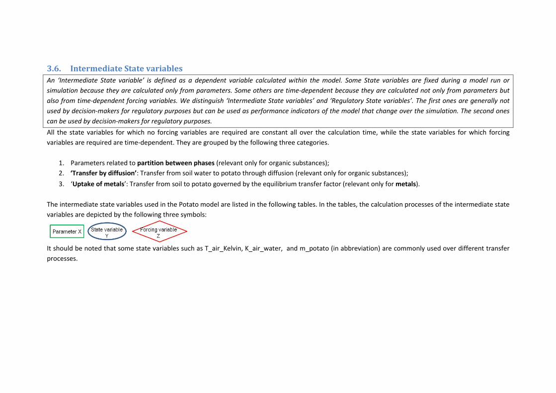
7 Tortuosity in water pores of the potato

Tau_w_potato (unitless)

In porous solids such as plant tissue, diffusion is hampered by a “labyrinth factor”, named tortuosity. Tau_w_potato is the tortuosity for diffusion in water pores of the potato.

8

Fraction of the pollutant dissolved in air of the potato

f_g_potato (unitless) f_g_potato is assumed to be the ratio of the concentration of the pollutant in air (of potato tissue) to the total concentration in potato.

9 Tortuosity in air pores of the potato

Tau_g_potato (unitless)

In porous solids such as plant tissue, diffusion is hampered by a “labyrinth factor”, named tortuosity. Tau_g_potato is the tortuosity for diffusion in gas pores of the potato.

10 Effective diffusion coefficient in pure water

D_water (m2 d-1)

D_water is the effective diffusion coefficient of the pollutant in pure water. It can be related to the ratio between the square root of the pollutant molar mass and that of dioxygen.

11 Effective diffusion coefficient in pure air

D_gas (m2 d-1)

D_gas is the effective diffusion coefficient of the pollutant in pure air. It can be related to the ratio between the square root of the pollutant molar mass and that of H2O.

12

Diffusion coefficient in water pores of potato

D_w_potato (m2 d-1) D_w_potato is the diffusion coefficient of the pollutant in water pores of potato.

13 Diffusion coefficient in gas pores of potato

D_gas_potato (m2 d-

1) D_gas_potato is the diffusion coefficient of the pollutant in gas pores of potato.

14 Diffusion coefficient in potato

D_potato (m2 d-1)

D_potato is the diffusion coefficient of the pollutant in potato tissue, which is assumed to be the sum of the diffusion of the pollutant in water pores of potato (D_w_potato) and that in gas pores of potato (D_gas_potato).

15 Depuration rate from potato through diffusion

K_depuration_potato (d-1)

K_depuration_potato is the depuration rate of the pollutant from potato through diffusion. It is deduced from a radial diffusion model.

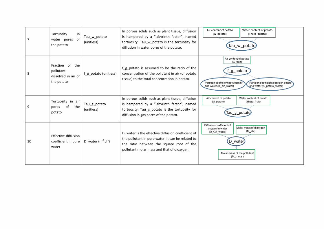
16 Uptake rate by potato through diffusion

K_uptake_potato (m3 kgfw

-1 d-1)

K_uptake_potato is the uptake rate of pollutant the by potato through diffusion. It is calculated from the depuration rate and the phase equilibriums.

17 Uptake through diffusion

Uptake_diffusion (mg d-1)

Uptake_diffusion is the uptake of the pollutant by potato through diffusion. It is estimated from K_uptake_potato, m_potato, C_soil, Kd_soil, and the surface area of field (S_field).

Table 7 Transfer from soil to potato governed by the equilibrium transfer factor (‘Uptake of metals’)

State variable n°



18 Mass of potato per unit area of soil

m_potato (kgfw m-2) Described in table 7 Described in table 7

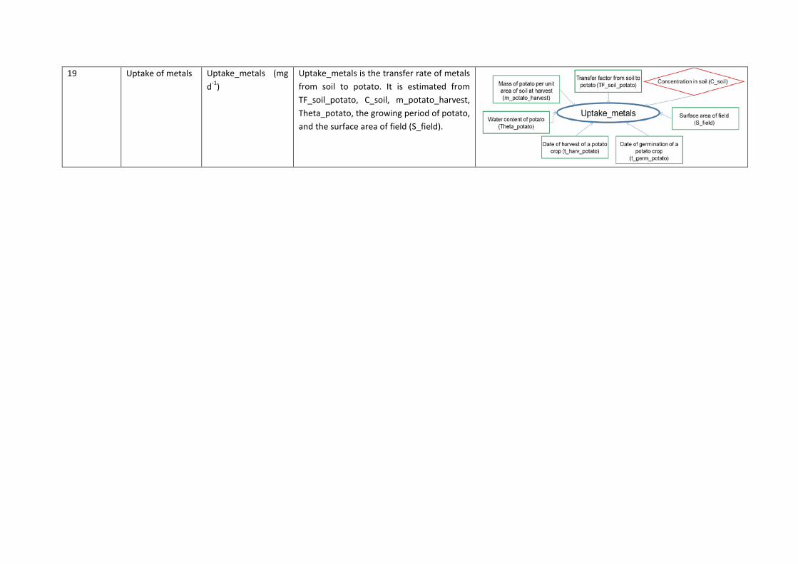
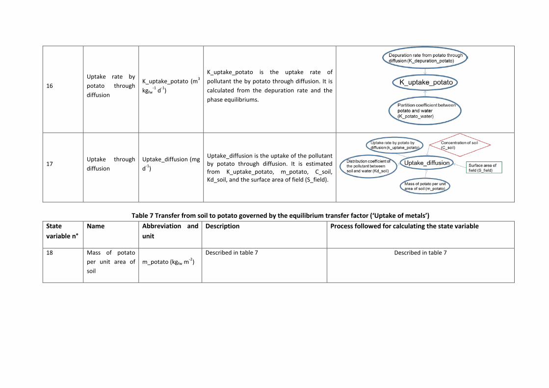
19 Uptake of metals Uptake_metals (mg d-1)

Uptake_metals is the transfer rate of metals from soil to potato. It is estimated from TF_soil_potato, C_soil, m_potato_harvest, Theta_potato, the growing period of potato, and the surface area of field (S_field).

17

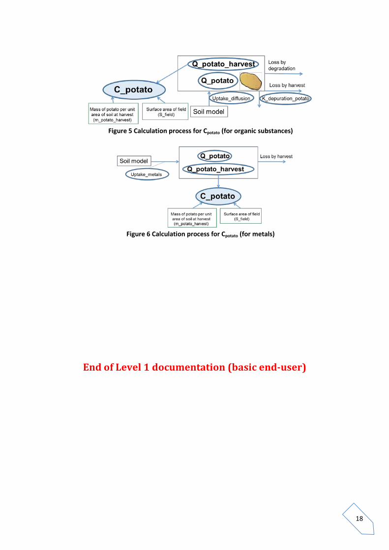
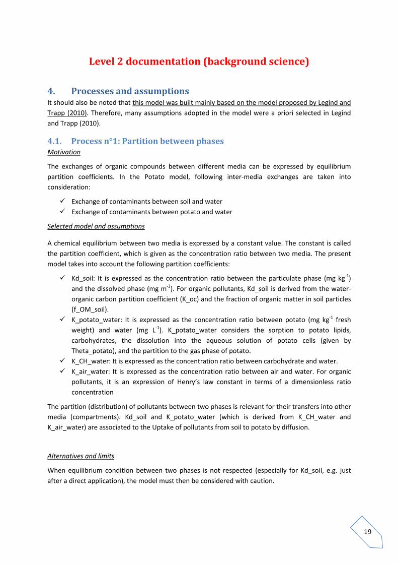
3.7. Regulatory State variables A ‘Regulatory State variable’ is defined as a dependent variable calculated within the model. It is generally time-dependent because it is calculated from parameters, but also from time-dependent forcing variables and loadings. We distinguish ‘Intermediate State variables’ and ‘Regulatory State variables’. The first ones are generally not used by decision-makers for regulatory purposes but can be used as performance indicators of the model that change over the simulation. The second ones can be used by decision-makers for regulatory purposes. The concentration of a target pollutant in the potato compartment at harvest time (C_potato) is defined as a regulatory state variable. The regulatory state variable is presented in the following table together with other state variables used to calculate it. Figure 5 and Figure 6 summarize the calculation processes for organic substances and metals.

Table 8 Regulatory variable for the Potato model State variable n°


Description

20 Quantity in potato Q_potato (mg) Total quantity of the pollutant in potato.

21 Quantity in potato at harvest

Q_potato_harvest (mg)

Q_potato_harvest is the total quantity of the pollutant in potato at harvest time.

22 Concentration in potato at harvest

C_potato (mg kgfw-1) C_potato is the concentration of the

pollutant in potato at harvest time. It is calculated from the total quantity of the pollutant in potato at harvest time (Q_potato_harvest), the mass of potato at harvest (m_potato_harvest), and the surface area of field (S_field).

18

Figure 5 Calculation process for Cpotato (for organic substances)

Figure 6 Calculation process for Cpotato (for metals)

End of Level 1 documentation (basic end-user)

19

Level 2 documentation (background science)

4. Processes and assumptions It should also be noted that this model was built mainly based on the model proposed by Legind and Trapp (2010). Therefore, many assumptions adopted in the model were a priori selected in Legind and Trapp (2010).

4.1. Process n°1: Partition between phases Motivation

The exchanges of organic compounds between different media can be expressed by equilibrium partition coefficients. In the Potato model, following inter-media exchanges are taken into consideration:

Exchange of contaminants between soil and water Exchange of contaminants between potato and water

Selected model and assumptions

A chemical equilibrium between two media is expressed by a constant value. The constant is called the partition coefficient, which is given as the concentration ratio between two media. The present model takes into account the following partition coefficients:

Kd_soil: It is expressed as the concentration ratio between the particulate phase (mg kg-1) and the dissolved phase (mg m-3). For organic pollutants, Kd_soil is derived from the water-organic carbon partition coefficient (K_oc) and the fraction of organic matter in soil particles (f_OM_soil).

K_potato_water: It is expressed as the concentration ratio between potato (mg kg-1 fresh weight) and water (mg L-1). K_potato_water considers the sorption to potato lipids, carbohydrates, the dissolution into the aqueous solution of potato cells (given by Theta_potato), and the partition to the gas phase of potato.

K_CH_water: It is expressed as the concentration ratio between carbohydrate and water. K_air_water: It is expressed as the concentration ratio between air and water. For organic

pollutants, it is an expression of Henry’s law constant in terms of a dimensionless ratio concentration

The partition (distribution) of pollutants between two phases is relevant for their transfers into other media (compartments). Kd_soil and K_potato_water (which is derived from K_CH_water and K_air_water) are associated to the Uptake of pollutants from soil to potato by diffusion.

Alternatives and limits

When equilibrium condition between two phases is not respected (especially for Kd_soil, e.g. just after a direct application), the model must then be considered with caution.

20

4.2. Process n°2: Transfer by diffusion Motivation

Diffusive mass transfer of chemicals from soil into potatoes can be considered as a main process contributing to the accumulation of hydrophobic compounds in potato. Description and selected assumptions

Botanically, potato is a tuber and is seen as a part of stem. It can be assumed that the potato has no connection with the root system and the transpiration stream. The accumulation of pollutants in potato may occur via translocation downward via phloem. However, for hydrophobic organic compounds, the translocation via phloem is negligible (Kleier, 1988). The uptake of hydrophobic organic pollutants into potato is, therefore, most likely to take place from soil by diffusion through the peel of potato (we consider the potato to be a sphere). According to Trapp et al (2007), the accumulation of pollutants in potatoes can be estimated using the diffusion coefficients which are, in the present model, the uptake rate and depuration rate (See equations (6) and (8) in the section 7.1).


In the present assumption, the translocation of chemicals via phloem was excluded as it may occur only for weak acids and polar neutral compounds.

4.3. Process n°3: Degradation in the potato compartment Motivation

Dilution by growth and degradation are loss terms in potatoes.

Description and selected assumptions Loss by degradation is governed by a degradation rate. The first order degradation rate represents both biotic and abiotic processes. An example of an abiotic process is photodegradation of dioxins in aboveground plant parts. Biotic processes are metabolism in plants, which for most chemicals is unknown, so the degradation rate constant is an optional input. The individual processes that are responsible for degradation (e.g. biodegradation, photolysis) are not distinguished here but they are added into an aggregated loss rate. Degradation is assumed to follow linear first-order kinetics.

4.4. Process n°4: Uptake of metals Motivation The bioaccumulation concepts developed for neutral hydrophobic substances (based in particular on diffusion across the lipid biomembranes) are not relevant for metals. For these latter compounds, other processes can significantly influence the accumulation of trace elements by plants like sequestration, detoxification, storage, regulation, etc. The accumulation of metals by plants is generally described by soil-to-plant transfer factors at equilibrium.

Description and selected assumptions

21

The soil-potato transfer is governed by a substance-specific equilibrium transfer factor (TF_soil_potato). The factor is defined as the concentration in potato (mg kgdw

-1) divided by the total concentration in soil (mg kgdw

-1) and thus is empirically derived.


CLEA model (Jeffries and Martin, 2008) estimates the concentration of metals in plant tissue (potato, shoot, or fruit). The model assumes that the concentration in the root is directly proportional to the concentration in the soil solution. The concentration in edible plant parts are found by multiplication with the fraction of metal in the roots that reaches the root store, potato, shoot or fruit by xylem or phloem flow.

Since the transfers to potato via atmospheric depositions and diffusion are not relevant for the present model, the equilibrium transfer factor (TF_soil_potato) will be a dominant parameter to determine the metal level in potato. As the parameter in general entails the large variability, a deterministic calculation using a best estimate of the parameter can be insufficient in terms of risk evaluations of metals.

End of Level 2 documentation (end-user with expertise in process)

22

Level 3 documentation (numerical information)

5. Numerical default values (deterministic and/or probabilistic)

5.1. Initialization of mass balance in Media The initial mass in the target media, i.e. the total quantity of potatoes (Qpotato (mg)) must be a priori set in the model. By default, no contaminant accumulation (Qpotato = 0) is assumed at the beginning of the simulation.

5.2. Default parameter values This section proposes default parameter values. Parameters are grouped by five categories almost as defined in the section 1.1 but the first category “Site-specific and plant parameters” includes not only the site-specific parameters but also the parameters about physiological characteristics of plant (e.g. G_potato, Theta_potato, m_potato_harvest in abbreviation) and plant growth (e.g. t_germ_potato, t_harv_potato, m_potato_harvest in abbreviation). Those parameters grouped in the first category are commonly used over different transfer processes. At the end of each part, a recommended best estimate and a PDF are proposed.

In the following tables, PDFs are presented by their types and statistical values as follows:

• Normal distribution: N(Mean, Sd(standard deviation));

• Log-normal distribution: LN(GM(geometric mean), GSD(geometric standard deviation)) or LN(5%, 95%);

• Uniform distribution: U(Min(minimum), Max(maximum));

• Triangular distribution: T(Min(minimum), Max(maximum), Mode).

5.2.1 Site-specific and plant parameters

5.2.1.1 Surface area of field (S_field)

Physical/chemical/biological/empirical meaning The Surface of the field under investigation (S_field) represents the dimensions of the region under evaluation. The relevant spatial scale is governed by the homogeneity of the soil and agronomic system under investigation (e.g. homogeneity in contamination levels, agricultural practices, and meteorological conditions). It is advised to define a field surface that show low variations in its land use and contamination level.

Parameter default value and PDF As this parameter is purely site-specific, neither default best estimate nor PDF is provided here. Therefore it should be defined by model users.

5.2.1.2 Air/water/lipid/carbohydrate contents of potato (G_potato, Theta_potato, L_potato, CH_potato)

Physical/chemical/biological/empirical meaning

23

Air/water/lipid/carbohydrates contents of potato represent respectively the air volume, the water volume, the lipid quantity and the carbohydrate quantity contained in potato per fresh weight of potato.

Description of data source

A literature survey was conducted to collect the data of the parameters. The following table presents the parameter values collected from the literature survey and their sources.

Table 9: Values of G_potato, CH_potato, L_potato and Theta_potato collected from the literature survey

Abbreviation of parameter

Unit Values found in Source

Remark Original Source

G_potato L kgfw-1 0,04

Trapp et al (2007) - supporting information

CH_potato L kgfw-1

0,086

Trapp (2003) presents 0,172 kg.kg-1 of carbohydrate fraction in potato and assumes a density of 2 kg.L-1 for carbohydrate. The parameter with unit of L.kg-1 was then calculated by dividing 0,172 kg.kg-1 by 2 kg.L-1.

Trapp (2003)

0.092

The database of “DTU Food National Food Institute” presents 0,183 kg.kg-1 of total carbohydrate fraction in potato. The parameter with unit of L.kg-1 was then calculated by dividing 0,183 kg.kg-1 by 2 kg.L-1.

National Food Institute (2009)

L_potato Kg kgfw-1 0.001

Trapp et al (2007) cite Elmadfa et al (1991) for the value.

Trapp et al (2007), Elmadfa et al (1991)

Theta_potato L kgfw-1

0.778 Trapp et al (2007) cite Elmadfa et al (1991) for the value.

Trapp et al (2007), Elmadfa et al (1991)

GM = 0.75. GM = 1.1, Min = 0.62, Max = 0.82 (n = 10)

IAEA (2010) reports values of the water content for tubers. These values apply to the edible part of the plant as harvested.

IAEA (2010)

Parameter default value and PDF

The following table lists, for each parameter, a recommended value selected from the previous table and also presents a probability density function (PDF).

24

Table 10: Default values of G_potato, CH_potato, L_potato and Theta_potato Abbreviation of parameter

Unit Best estimate PDF Comment

G_potato L kgfw-1 0.04

CH_potato L kgfw-1 0.092

A value from DTU Food National Food Institute was selected because it is originated from the most recent survey.

L_potato Kg kgfw-1 0.001

Theta_potato L kgfw-1 0.75

U(min = 0.62, max = 0.82)

Values from IAEA (2010) were selected because they were derived from a number of samples, and thus they can be regarded as generic (representative) values for whole potato plants.

5.2.1.3 Dates of germination/harvest of a potato crop (t_germ_potato, t_harv_potato)


The dates of germination/harvest of a potato crop represent the growing period of the potato of interest. In the Potato model, all the transfer processes take place only during the growing period.


The growing periods of crops of interest can vary significantly depending on the types of crops and on the regions. Therefore the dates of germination/harvest of potato crops are regarded as site-specific and they should be chosen by model users.

5.2.1.4 Mass of potato per unit area of soil at harvest (m_potato_harvest)


Mass of potato per unit area of soil at harvest represents the maximal potato mass per unit ground surface area (m2) at harvest time.

Description of data source and default value

The following table presents the parameter values collected from the FAOStat freely available on internet (http://faostat.fao.org). The geometric means and ranges (min – max) shown in Table 11 were obtained based on the statistics for France and years 1993 to 2012.

Table 11: Default values of m_potato_harvest for potatoes (from FAOStat) Fruit species GM of m_potato_harvest (Kgfw

m-2) over the period from 1993 to 2012 in France

Range of m_potato_harvest (Kgfw m-2) over the period from 1993 to 2012 in France

Potatoes 4.0 3.3-4.7

5.2.1.5 Potato radius at harvest (R_potato)


25

Potato radius at harvest represents the length of a potato radius under investigation at harvest time (m)

Description of data source and default value

As this parameter is purely site-specific and its data can be highly available, for example, from local food markets, neither default best estimate nor PDF is provided here. Therefore it should be defined by model users. As a generic value, however, Trapp et al (2007) proposes 0.04 (m) for potato.

5.2.2 Parameters related to the partition between phases

5.2.2.1 Fraction of organic matter in soil (f_OM_soil)

Physical/chemical/biological/empirical meaning Organic carbon is considered the main sorbing phase in soil for neutral organic compounds. As for non-neutral organics, which typically have a log(Kow) greater than 4, their affinity to organic matter tends to be much stronger than to mineral surfaces and the sorption to these latter can be neglected. Organic carbon content can be divided between amorphous, soft or new and condensed, old or black carbon. Even if this division in types of sedimentary organic matter can be relevant for non-ionic organics, we considered in the model organic carbon as a unique sorbing phase.

The exchanges of organic contaminants between soil pore water and solid soil are assumed to be at equilibrium and represented by partition coefficients at equilibrium (Kdsoil). Interaction of chemicals with solid soil is assumed to be governed by lipophilic sorption onto organic matter. In the present model, the fraction of organic carbon in soil (fOC_soil), together with the water-organic carbon partition coefficient (Koc), is used to calculate the partition coefficient at equilibrium Kdsoil.

Factors influencing parameter value Organic Matter content in soils depends on natural backgrounds as well as on anthropogenic activities (land use coverage, wet zones management, etc).

Description of data source Panagos et al (2013) collected data of soil organic carbon and soil erosion in Europe using the European Environment Information and Observation Network for soil (EIONET-SOIL). Panagos et al (2013) presents a best estimate for each European country. Each participating country provided monitoring data on the basis of a grid of 1 km×1 km cells and for 30 cm soil depth. For data at a regional scale, specific national monitoring programs can be used. For example, data were collected in the frame of a French program aiming at mapping soil properties at local scales. These data are freely available and can be found in the website www.gissol.fr. Mean and extreme values can thus be calculated for each French region.

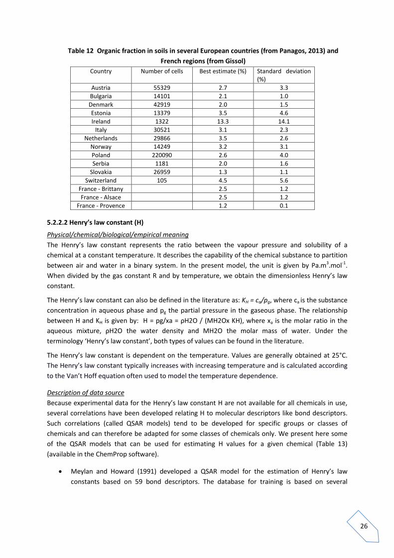
Parameter default value and PDF Table 12 presents the best estimate value and the standard deviation for each country, based on the proposition made by Panagos et al (2013). The data are assumed to follow normal distributions, which must be truncated at zero to avoid negative values. Three examples of default values extracted from the French program Gissol are provided as well in Table 12.

26

Table 12 Organic fraction in soils in several European countries (from Panagos, 2013) and French regions (from Gissol)

Country Number of cells Best estimate (%) Standard deviation (%)

Austria 55329 2.7 3.3 Bulgaria 14101 2.1 1.0 Denmark 42919 2.0 1.5 Estonia 13379 3.5 4.6 Ireland 1322 13.3 14.1

Italy 30521 3.1 2.3 Netherlands 29866 3.5 2.6

Norway 14249 3.2 3.1 Poland 220090 2.6 4.0 Serbia 1181 2.0 1.6

Slovakia 26959 1.3 1.1 Switzerland 105 4.5 5.6

France - Brittany 2.5 1.2 France - Alsace 2.5 1.2

France - Provence 1.2 0.1

5.2.2.2 Henry’s law constant (H)

Physical/chemical/biological/empirical meaning The Henry’s law constant represents the ratio between the vapour pressure and solubility of a chemical at a constant temperature. It describes the capability of the chemical substance to partition between air and water in a binary system. In the present model, the unit is given by Pa.m3.mol-1. When divided by the gas constant R and by temperature, we obtain the dimensionless Henry’s law constant.

The Henry’s law constant can also be defined in the literature as: KH = ca/pg, where ca is the substance concentration in aqueous phase and pg the partial pressure in the gaseous phase. The relationship between H and KH is given by: H = pg/xa = ρH2O / (MH2Ox KH), where xa is the molar ratio in the aqueous mixture, ρH2O the water density and MH2O the molar mass of water. Under the terminology ‘Henry’s law constant’, both types of values can be found in the literature.

The Henry’s law constant is dependent on the temperature. Values are generally obtained at 25°C. The Henry’s law constant typically increases with increasing temperature and is calculated according to the Van’t Hoff equation often used to model the temperature dependence.

Description of data source Because experimental data for the Henry’s law constant H are not available for all chemicals in use, several correlations have been developed relating H to molecular descriptors like bond descriptors. Such correlations (called QSAR models) tend to be developed for specific groups or classes of chemicals and can therefore be adapted for some classes of chemicals only. We present here some of the QSAR models that can be used for estimating H values for a given chemical (Table 13) (available in the ChemProp software).

• Meylan and Howard (1991) developed a QSAR model for the estimation of Henry’s law constants based on 59 bond descriptors. The database for training is based on several

27

chemical classes1. The model was fitted on 345 chemicals and validated on a independent dataset of 74 substances. The 345-chemical data set contains a subset of 120 compounds that have both an experimentally measured Henry’s law constants and measured vapor pressures and water solubilities. The standard deviation of the regression model is 0.46 log units.

• Viswanadhan at al (1999) developed a QSAR model based on solvation free energy to estimate Henry’s law constants. Their method (ALOGS) used an extensive atom classification scheme and was fitted on a database containing 265 molecules with experimentally determined solvation free energies. The model was then tested on 27 molecules not present in the training set. The standard deviation of the regression model is 0.86 log units.

• Abraham et al (1994) developed a model based on 5 molecular descriptors, i.e. the excess molar refraction, the dipolarity/polarizability, the effective hydrogen-bond acidity and basicity, and the McGowan characteristic volume. It was fitted on 408 gaseous compounds and the standard deviation of the regression model is 0.15 log units.

• A model was developed by Kühne et al (2005) to estimate the temperature dependency of Henry's law constant in water for organic compounds from the 2D structure. Air/water partition enthalpies of 456 chemicals from various compound classes were fitted to 46 substructure fragments. Application of the model together with experimental 25°C data to a set of 462 compounds with 2119 experimental Henry's law constants at temperatures below 20°C yields a standard error of 0.21 logarithmic units. The prediction capability is further evaluated using cross validation and permutation.

• A read-across approach was developed by UFZ (personal communication; method is not published yet; details will not be disclosed before publication). The read-across set covers 2354 compounds. Three models are proposed: (i) a Default model (n. of data=1409; rms=0.66); (ii) a High similarity model (n. of data=1127; rms=0.54); (iii) a Low similarity model (n. of data=2352; rms=1.23). Structurally similar compounds in a reference set are looked up via comparison of atom-centered fragments (ACF). The experimental values of the similar compounds are weighted by their similarity. The final result is a weighted average of different runs.

Other models based on the estimation of both water solubility and vapor pressure are also available. The QSAR models that are indicated above are based on linear regressions fitted by ordinary least squares. Assuming identical, independent and normally distributed errors, the in a QSAR prediction

Log H can be defined as the predictive distribution by the predictive mean LogH and standard error

of predictions )(LogHSE :

)(. LogHSEtLogHLogH 1kn −−+~

2Chemical classes in the Meylan’s database with indication of the number of chemicals: Alkanes 16 ; Alkenes 20 ; Alkynes 7 ; Acids, aliphatic 6; Alcohols 18; Aldehydes 17; Esters 27; Ethers 16; Epoxides 2; Ketones 9; Halomethanes 22; Haloethanes 20; Halopropanes 11; Halobutanes 9; Other haloalkanes 4; Haloalcohols 5; Haloalkenes 12; Aliphatic amines 13; Nitriles 5; Other aliphatic nitrogen compounds 11; Aliphatic sulfur compounds 8; Five-member aromatic rings 3; P yridines 12; Benzene and alkylated; benzenes 13; Halogenated benzenes 12; Anilines 3; Phenols 8; Biphenyls 3; Polyaromatics 13; Other aromatics 14; Pesticides 6

28

Where 1knt −− is the student t-distribution with n-k-1 degrees of freedom, n is the number of data in

the training set, k is the number of descriptors in the model (and k+1 is the intercept plus the number of descriptors). The QSAR models that are indicated above generally provide an estimation of the standard error of

predictions )(LogHSE by the Mean Squared error MSE. Since MSE is an expectation value, it is subject to estimation error that could be taken into account. The uncertainty on MSE can be calculated from a Bayesian point of view, assuming that the uncertainty of MSE has a scaled inverse Chi distribution. A re-analysis of raw data used in the training set would however be necessary to calculate this posterior distribution. Therefore, in the present model, the MSE uncertainty is not included and the

standard error of predictions )(LogHSE is assumed to be equal to the MSE value provided in each

QSAR model description.

Table 13 QSAR and read-across models available for calculating Henry’s law constant H Source Descriptors N. of data in

the training set MSE )(. LogHSEt 1kn −−

- 5th-95th percentile

Meylan and Howard, 1991

59 chemical bonds 345 (and 74 compounds used in the

prediction set)

0.46 ± 0.76

Viswanadhan et al, 1999

No information 265 (and 26 compounds used in the

prediction set)

0.86 ±

Abraham et al, 1994

5 descriptors (excess molar refraction,dipolarity/polarizability, effective hydrogen-bond acidity and basicity, McGowan characteristic volume)

408 0.15 ± 0.25

Kühne et al, 2005

46 substructure fragments. 456 0.21 ± 0.34

UFZ, personal communication

Read-across 2354

Parameter default value and PDF According to the approach described above, the default best estimates and PDFs of the parameter are given on a log scaled basis for several key substances in Table 14. All the calculations were computed on the ChemProp software that is freely available on request (http://www.ufz.de/index.php?en=6738). The ChemProp returns a result for each compound separately, by applying the methods in the order listed below. The first valid result is accepted. Default order: 1 - Meylan and Howard, 1991; 2 - Viswanadhan et al, 1999; 3 - Abraham et al, 1994. By comparison, the result obtained according to Kühne et al, 2005 and to UFZ (personal communication) is also given. The Meylan method is those that is proposed by default in the Merlin-Expo tool. However, end-users are encouraged to run the ChemProp software with alternative methods (that are not reported comprehensively here) to check the concordance between several approaches and to evaluate the plausibility of estimations (see for example some discrepancies for pesticides in Table 14).

29

Table 14 Henry’s law constant of selected substances Chemical class Substance Model Best

estimate – log10H

5th-95th percentile - log10H

5th-95th percentile – H (Pa.m3.mol-1)

PAH Anthracene Meylan 0.71 -4.6.10-2 ; 1.47 0.9;29.8 UFZ-Read-across 0.46 Benzo(a)pyrene Meylan -1.09 -1.85 ; -3.2.10-1 1.4.10-2 ; 4.7.10-1 UFZ-Read-across -0.87 Benzo(b)fluoranthene Meylan -1.09 -1.85 ; -3.2.10-1 1.4.10-2 ; 4.7.10-1 UFZ-Read-across -1.2 Benzo(k)fluoranthene Meylan -1.09 -1.85 ; -3.2.10-1 1.4.10-2 ; 4.7.10-1 UFZ-Read-across -1.2 Fluoranthene Meylan -7.6.10-2 -8.4.10-1 ; 6.8.10-

1 0.15 ; 4.8

UFZ-Read-across 4.4.10-2 Naphtalene Meylan 1.1 3.4.10-1 ; 1.9 2.2 ; 73.1 UFZ-Read-across 1.27 PCB PCB28 Meylan 1.23 4.7.10-1 ; 2 3 ; 98.7 UFZ-Read-across 1.32 PCB 52 Meylan 1.1 3.4.10-1 ; 1.9 2.2 ; 73.2 UFZ-Read-across 1.27 PCB101 Meylan 0.97 2.1.10-1 ; 1.7 1.6 ; 54.2 UFZ-Read-across 1.15 PCB118 Meylan 0.97 2.1.10-1 ; 1.7 1.6 ; 54.2 UFZ-Read-across 1.15 PCB138 Meylan 0.84 8.4.10-2 ; 1.6 1.2 ; 40.2 UFZ-Read-across 0.8 PCB153 Meylan 0.84 8.4.10-2 ; 1.6 1.2 ; 40.2 UFZ-Read-across 0.8 PCB180 Meylan 0.71 -4.6.10-1 ; 1.5 0.9 ; 29.8 UFZ-Read-across 0.7 Pesticides Alachlor Meylan -2.65 -3.4 ; -1.9 3.9.10-4 ; 1.3.10-2 UFZ-Read-across -2.08 Atrazine Meylan -3.35 -4.1 ; -2.6 7.8.10-5 ; 2.6.10-3 UFZ-Read-across -3.15 Chlordane Meylan 0.85 9.4.10-2 ; 1.6 1.2 ; 41.1 UFZ-Read-across 0.9 Chlorpyrifos Meylan -0.6 -1.4 ; 1.6.10-1 4.4.10-2 ; 1.46 UFZ-Read-across -0.38 DDT Meylan 0.19 -5.7.10-1 ; 9.5.10-

1 0.27 ; 9

UFZ-Read-across -7.6.10-2 Dieldrin Meylan -1.27 -2 ; -5.1.10-1 9.4.10-3 ; 0.31 UFZ-Read-across -0.13 Diuron Meylan -4.27 -5 ; -3.5 9.4.10-6 ; 3.1.10-4 UFZ-Read-across -4.74 Endosulfan Meylan -2.04 -2.8 ; -1.3 1.6.10-3 ; 5.3.10-2 UFZ-Read-across -0.79 Hexachlorocyclohexane

(lindane) Meylan 1.41 6.5.10-1 ; 2.2 4.5 ; 149.4

UFZ-Read-across -0.65 Isopruturon Meylan -3.7 -4.5 ; -3 3.3.10-5 ; 1.1.10-3 UFZ-Read-across -4.62 Malathion Meylan -4.07 -4.8 ; -3.3 1.5.10-5 ; 4.9.10-4 UFZ-Read-across -2.22 Parathion Meylan -1.52 2.3 ; -0.77 5.2.10-3 ; 0.17 UFZ-Read-across -1.51 Pentachlorophenol Meylan -1.9 -2.7 ; -1.1 2.2.10-3 ; 7.3.10-2 UFZ-Read-across -0.42 Brominated Pentabromo Meylan -0.93 -1.7 ; -1.6.10-1 2.1.10-2 ; 0.68

30

flame retardants

diphenylether

UFZ-Read-across -1.6.10-2 Hexabromobiphenyl Meylan -7.8.10-1 -1.5 ; -1.6.10-2 2.9.10-2 ; 0.96 UFZ-Read-across n.a. VOCs Benzene Meylan 2.73 2 ; 3.5 94.3 ; 3121.3 UFZ-Read-across 2.75 1,2-Dichloroethane Meylan 3.09 2.3 ; 3.9 215.9 ; 7150.6 UFZ-Read-across 2.00 Dichloromethane Meylan 2.96 2.2 ; 3.7 160.1 ; 5300.8 UFZ-Read-across 2.41 Hexachlorobenzene

(HCB) Meylan 1.95 1.2 ; 2.7 15.6 ; 518

UFZ-Read-across 1.37 Hexachlorobutadiene Meylan 3.03 2.3 ; 3.8 188.1 ; 6227.8 UFZ-Read-across 2.63 Pentachlorobenzene Meylan 2.08 1.3 ; 2.8 21.1 ; 698.8 UFZ-Read-across 1.77 Trichlorobenzene Meylan 2.34 1.58 ; 3.1 UFZ-Read-across 2.18 Trichloromethane

(chloroform) Meylan 2.51 1.75 ; 3.3 56.8 ; 1880.8

UFZ-Read-across 2.58 Phthalate Dibutylphthalate (DBP) Meylan -0.9 -1.67 ; -0.15 2.2.10-2 ; 0.72 UFZ-Read-across -0.71 Di(2-

ethylhexyl)phthalate (DEHP)

Meylan 7.4.10-2 -0.69 ; 0.83 0.2 ; 6.8

UFZ-Read-across -0.31 Dioxins 2,3,7,8-TCDD Meylan -0.44 -1.21 ; 0.31 6.2.10-2 ; 2.06 UFZ-Read-across 0.1 1,2,3,7,8-PeCDD Meylan -0.58 -1.34 ; 0.18 4.6.10-2 ; 1.53 UFZ-Read-across 0.18 1,2,3,7,8-HxCDD Meylan -0.7 -1.47 ; 5.4.10-2 3.4.10-2 ; 1.13 UFZ-Read-across -0.37 Phenols - Alkylphenols

2,4,6-tri-tert-butylphenol

Meylan -5.7.10-3 -0.77 ; 0.75 0.17 ; 5.68

UFZ-Read-across n.a. Nonylphenol Meylan -0.22 -0.98 ; 0.54 0.11 ; 3.5

UFZ-Read-across -0.41

2-Octylphenol Meylan -0.35 -1.11 ; 0.41 7.8.10-2 ; 2.6

UFZ-Read-across 1.31

5.2.2.3 Octanol-water partition coefficient in log 10 (log10_K_ow)


The partition coefficient of a substance between water and a lipophilic solvent (n-octanol) characterizes the equilibrium distribution of the chemical between the two phases. The partition coefficient between water and n-octanol (Kow) is defined as the ratio of the equilibrium concentrations of a chemical in octanol saturated with water and water saturated with octanol. The parameter characterizes the equilibrium distribution of the chemical between the two phases and hence represents the degree to which a chemical prefers organic material to water.

31

In accordance with Nernst’s law Kow is independent from compound absolute concentration in n-octanol and water. Kow is usually weakly dependent on temperature, and experiments to measure Kow values are set to standard conditions i.e. 25°C and 1 atm (OECD protocol). Large organic compounds or highly nonpolar compounds exhibit a high degree of hydrophobicity. Such hydrophobic substances tend to partition to octanol rather than to water and hence have large values of Kow. In contrast, smaller or polar substances are less hydrophobic and have smaller values of Kow. The range of Kow is many orders of magnitude for variety of organic compounds.

Literature value with log Kow > 6 may contain significant error and thus should be carefully checked.

Kow is not an accurate determinant of lipophilicity for ionizable compounds because it only correctly describes the partition coefficient of neutral (uncharged) molecules. For example, the parameter is not a good predictor of drug behaviours in the changing pH environments of the body because the majority of them are ionizable. The partition coefficients between fruit/root and water (K_root_water and K_fruit_water) are governed by the lipid content of the plant organs. For calculating these partition coefficients, empirical relationships are generally proposed, using the Octanol-water partition coefficient as a surrogate for Lipid-water partition.

Kow is not an accurate determinant of lipophilicity for ionizable compounds because it only correctly describes the partition coefficient of neutral (uncharged) molecules. For example, the parameter is not a good predictor of drug behaviors in the changing pH environments of the body because the majority of them are ionizable.


Experimental protocols to measure Kow are well established and standardised, for example, in OECD guidelines (OECD, 2006; OECD, 2004; OECD 1995). When the parameter is measured following such well-established experimental protocols, it can be assumed that the obtained values of Kow are not likely to be very variable. The measurement values of Kow are available for many of well-recognized toxic substances. Therefore, in this document, measurement data were selected in preference for the determination of default Kow values.

The measurement data were obtained from OECD (2004) and from the software called EPI-Suite developed by US-EPA (http://www.epa.gov/opptintr/exposure/pubs/episuite.htm). The measurement data in EPI-Suite were initially entered by junior and senior scientists using many sources for which the data had already been carefully evaluated, and then were checked by senior scientists. The QSAR approach used in the EPI-Suite (i.e. “KOWWIN”) was applied to estimate Kow in the case where no measurement was available. The approach uses a "fragment constant" methodology to predict Kow. In the "fragment constant" method, a structure is divided into fragments (atom or larger functional groups) and coefficient values of each fragment or group are summed together to yield the log Kow estimate. KOWWIN’s methodology is known as an Atom/Fragment Contribution (AFC) method. Coefficients for individual fragments and groups were derived by multiple regression. Meylan and Howard (1995) presents a more complete description of KOWWIN’s methodology. Analysis of applicability domain of KOWWIN model (Nikolova and Jaworska, 2005) was based on training set of 2434 compounds (r2 = 0,981 and RMSE (root mean squared error) = 0,22) revealed 186 different fragments and 322 different correction factors, resulting in a 508-dimensional descriptor space. The validation set consisted of 10 910 substances, in which the log Kow values vary between -4.99 and 11.71.

32

Assuming identical, independent and normally distributed errors, the uncertainty in a QSAR prediction log Kow can be defined as the predictive distribution by the predictive mean log Kow and standard error of predictions K_ow��: log K_owp~log K_owp�� + tn−k−1. SE (log K_ow��p) Where 1−−knt is the student t-distribution with n-k-1 degrees of freedom, n is the number of data in

the training set, k is the number of descriptors in the model (and k+1 is the intercept plus the number of descriptors).

The QSAR model used here provides an estimation of the standard error of predictions SE (log K_ow��p) by the Mean Squared error (MSE). Parameter default value and PDF

Table 15 presents the values of Kow for well-recognized toxic substances with experimental data (when available), simulated data generated by KOWWIN and uncertainty derived from the approach presented above. Experimental references sited by EPI-Suite are all documented in the software (freely downloadable from the link shown above).

Table 15 Kow of selected substances Chemical class Substance Log Kow experimental

estimate (ref in appendix 1)

Log Kow KOWWIN estimate

5th-95th percentile (KOWWIN)

PAH Anthracene 4.45 4.35 3.99 - 4.71

Benzo(a)pyrene 6.13 6.11 5.75 - 6.47

Benzo(b)fluoranthene 5.78 6.11 5.75 - 6.47

Benzo(k)fluoranthene 6.11 6.11 5.75 - 6.47

Fluoranthene 5.16 4.93 4.57 - 5.29

Naphthalene 3.30 3.17 2.81 - 3.53

PCB PCB28 5.62 5.69 5.33 - 6.05

PCB 52 6.09 6.34 5.98 - 6.70

PCB101 6.80 6.98 6.62 - 7.34

PCB118 7.12 6.98 6.62 - 7.34

PCB138 7.44 7.62 7.26 - 7.98

PCB153 7.75 7.62 7.26 - 7.98

PCB180 - 8.27 7,91 – 8,63

Pesticides Alachlor 3.37 3.52 3.01 - 3.73

33

Atrazine 2.61 2.82 2.46 - 3.18

Chlordane 6.16 6.26 5.90 - 6.62

Chlorpyrifos 4.96 4.66 4.30 - 5.02

DDT 6.91 6.79 6.43 - 7.15

Dieldrin 5.40 5.45 5.09 - 5.81

Diuron 2.68 2.67 2.31 - 3.03

Endosulfan 3.83 3.50 3.14 - 3.86

Hexachlorocyclohexane (lindane)

3.72 4.26 3.90 - 4.62

Isoproturon 2.87 2.84 2.48 - 3.20

Malathion 2.36 2.29 1.93 - 2.65

Parathion 3.83 3.73 3.37 - 4.09

Pentachlorophenol 5.12 4.74 4.38 - 5.10

Brominated flame retardants

Pentabromo diphenylether

- 7.66 7,30 – 8,02

Hexabromobiphenyl - 9.10 8,74 – 9,46

VOCs Benzene 2.13 1.99 1.63 - 2.35

1,2-Dichloroethane 1.48 1.83 1.47 - 2.19

Dichloromethane 1.25 1.34 0.98 - 1.70

Hexachlorobenzene (HCB) 5.73 5.86 5.50 -6.22

Hexachlorobutadiene 4.78 4.72 4.36 - 5.08

Pentachlorobenzene 5.17 5.22 4.86 - 5.58

Trichlorobenzene 4.05 3.93 3.57 - 4.29

Trichloromethane (chloroform)

1.97 1.52 1.16 - 1.88

Phthalate Dibutylphthalate (DBP) 5.53 4.61 4.25 - 4.97

Di(2-ethylhexyl)phthalate (DEHP)

7.60 8.39 8.03 - 8.75

Dioxins 2,3,7,8-TCDD 6.80 6.92 6.56 - 7.28

1,2,3,7,8-PeCDD 6.64 7.56 7.20 - 7.92

34

1,2,3,6,8-HxCDD 7.80 8.21 7.85 - 8.57

Phenols - Alkylphenols

2,4,6-tri-tert-butylphenol 6.06 6.39 6.03 - 6.75

Nonylphenol 5.76 5.99 5.63 - 6.35

2-Octylphenol - 5.50 5,14 – 5,86

5.2.2.4 Water-organic carbon partition coefficient in log10 (log10_K_oc)


Organic carbon is assumed to be the main particulate media interacting with hydrophobic chemicals potentially present in soil. The Water-Organic Carbon partition coefficient represents the ratio at equilibrium of the chemical associated to particulate organic matter and present in water respectively.

The exchanges of contaminants between Pore Water and Soil particles are assumed to be at equilibrium and represented by a Partition coefficient at equilibrium Kd_soil_organic. Interaction of chemicals with particles are assumed to be governed by lipophilic sorption onto organic matter. The Koc parameter, together with the organic fraction in soil, allows calculating the partition coefficient at equilibrium Kd_soil.

The main limitation of the approach described above is that the variability in the soil composition is only described by the content of organic carbon. The validity of this assumption can be disputable especially for ionizable compounds (Ter Laak et al, 2006). In particular, the organic carbon content alone as the descriptor of soil composition is not sufficient to predict the soil–water distribution of chemicals that do not exclusively adsorb to organic matter. Furthermore, the composition of organic carbon itself can vary substantially and influence sorption. Complexation is another process neglected by the model, although it may have significant impact for some compounds.


Because experimental Koc data are not available for all chemicals in use, numerous correlations have been developed relating Koc to molecular descriptors like the Octanol-Water partition coefficient Kow. Such correlations (called QSAR models) tend to be developed for specific groups or classes of chemicals and can therefore be adapted for some classes of chemicals only. We present here some of the QSAR models that can be used for estimating Koc values for a given chemical (Table 16).

• A classical hydrophobic approach based on Kow and on a decision tree was proposed by Sablić et al (1995, 1996). Log Koc is estimated by a hierarchical decision tree, offering 20 different equations in total. The first equation applies the topological index 1χ2, while the other 19 equations correlate log Koc to log Kow. For non-polar compounds, the more precise but also restricted model is the one with 1χ, if it cannot be applied, a more general, less precise equation is used.

2 The topological index was introduced by Kier et Hall (1990, 1999) following the suggestions of Randic (1975). nχ is a n-order topological index where n represents the number of atoms (except H) linked to each atom (except H) belonging to the molecule.

35

• Schüürmann et al (2006) developed another model for non-ionic organic compounds. Literature data of logKoc for 571 organic chemicals (subdivided in 457 for training set and 114 for predictive set) were fitted to 29 parameters. The general form of the model is:

dIcFbPaLogKk

kki j

jjiioc +++= ∑∑ ∑

with 3 variable Pi (molecular weight, bond connectivity, molecular E-state), 21 fragment correction factors Fj, 4 structural indicator variables Ik. The data set compounds are neutral organics (except for partial ionization of acids and bases at soil pH) that include the following atom types: C, H, N, O, P, S, F, Cl, and Br. Because the training set contained no organoiodine compounds, I is not included, but it is likely that a simple extension (see below) will provide reasonable estimates for compounds with iodine attached to aliphatic or aromatic carbon. The range confidence is checked for the molecular correction factors by comparing the frequency of these substructures in the molecule to the training set. The compound will be checked versus the original training set compounds by means of second order ACFs (Atom Centered Fragments). The applicability domain is then classified as: (i) In: All ACFs are matching including the number of occurrences; (ii) Borderline in: Either the frequency of at least one substructure of the compound exceeds the range of occurrences in the training set, or one substructure is not in the training set at all; (iii) Borderline out: More than one substructure is not in the training set at all, but all 1st order ACFs are matching; (iv) Out: There is mismatch even with 1st order ACFs.

• Tao et al (1999) developed another model based on logKoc data for 592 organic chemicals (subdivided in 430 for training set and 162 for predictive set) and on 98 parameters (74 fragment constants and 24 structural factors).

• Huuskonen (2003) developed a model based on atom-type electrotopological state indices, involving 12 parameters (connectivity index 1χ, 11 atom-type E-state indices). It was tested on logKoc data for 201 organic pesticides (subdivided in 143 for training set and 58 for predictive set). The general form of the model is:

6220Sa3500LogKi

ii1

oc .. ++= ∑c

where Si are the atom-type E-state values..

• Poole and Poole (1999) developed a solvatation-based model to predict logKoc. After removal of the outliers, the model is under the form:

)(..... OB272A310E740V092210LogKoc −−++=

where V is the McGowan’s characteristic volume, E is the excess molar refraction, A and B(O) are the solute’s effective hydrogen-bond acidity and hydrogen-bond basicity.

• Franco et al (2008, 2009) developed a QSAR model for ionizable compounds (monovalent organic acids and bases). The classical Kow model is applied here, but the Kow value accounts for the distribution of the chemical between neutral and ionic forms. The neutral and ionic fractions are calculated from the substance pKa and the surrounding pH, according to the Henderson-Hasselbalch relationship:

36

pKapHneutral 1011

−+=φ for acids;

phpKaneutral 1011

−+=φ for bases.

Thus, supplying of a valid pKa and a pH is required for running the model. The models do not work for neutral compounds without specification of pKa.

The QSAR models that are indicated above are based on linear regressions fitted by ordinary least squares. Assuming identical, independent and normally distributed errors, the uncertainty in a QSAR

prediction Log Koc,p can be defined as the predictive distribution by the predictive mean pLogKoc,

and standard error of predictions ),( pLogKocSE :

)(. ,,, poc1knpocpoc LogKSEtLogKLogK −−+~

Where 1knt −− is the student t-distribution with n-k-1 degrees of freedom, n is the number of data in

the training set, k is the number of descriptors in the model (and k+1 is the intercept plus the number of descriptors).

The QSAR models that are indicated above generally provide an estimation of the standard error of

predictions ),( pLogKocSE by the Mean Squared error MSE. Since MSE is an expectation value, it is

subject to estimation error that could be taken into account. The uncertainty on MSE can be calculated from a Bayesian point of view, assuming that the uncertainty of MSE has a scaled inverse Chi distribution. A re-analysis of raw data used in the training set would however be necessary to calculate this posterior distribution. Therefore, in the present model, the MSE uncertainty is not

included and the standard error of predictions ),( pLogKocSE is assumed to be equal to the MSE value

provided in each QSAR model description.

Table 16 QSAR available for calculating logKoc Source Descriptors N. of data

in the training set

MSE Applicability domain )(. , poc1kn LogKSEt −−

- 5th-95th percentile

Sablić et al (1995, 1996)

1: topological index 1χ

81 0.264 Predominantly hydrophobics3 - 3 to 22 atoms of carbon or halogenes with 1<logKoc<6,5

± 0.44

1: octanol-water partition coefficient Kow

81 0.451 Predominantly hydrophobics

± 0.75

390 0.557 Nonhydrophobics 4 with -2<logKow<8

± 0.92

54 0.401 Phenols, Anilines, Benzonitriles, Nitrobenzenes with 1<logKow<5

± 0.67

216 0.425 Acetanilides, Carbamates, ± 0.70 3 Defined as molecules containing only C, H and halogen (F, Cl, Br, I) 4 Defined as all the molecules that contains other atoms than C, H and halogen (F, Cl, Br, I). Does not imply anything about their lipophilicity.

37

Esters, Phenylureas, Phosphates, Triazines, Triazoles, Uracils with -1<logKow<8

36 0.388 Alcohols, Organic acids with -1<logKow<5

± 0.66

21 0.339 Acetanilides ± 0.59 13 0.397 Alcohols ± 0.71 28 0.491 Amides ± 0.84

20 0.341 Anilines ± 0.59 43 0.408 Carbamates ± 0.69 20 0.242 Dinitroanilines ± 0.42 25 0.463 Esters ± 0.79 10 0.583 Nitrobenzenes ± 1.08 23 0.336 Organic acids ± 0.58 24 0.373 Phenols, Benzonitriles ± 0.64 52 0.335 Phenylureas ± 0.56 41 0.452 Phosphates ± 0.76 16 0.379 Triazines ± 0.67 15 0.482 Triazoles ± 0.85 Schüürmann et al, 2006

29 descriptors : molecular weight, bond connectivity, molecular E-state, 24 fragment corrections representing polar groups, one indicator for nonpolar and weakly polar compounds

457 (and 114

compounds used in the prediction

set)

0.467 Neutral organics (except for partial ionization of acids and bases at soil pH) with atom types C, H, N, O, P, S, F, Cl, Br

± 0.77

Tao et al, 1999

98 descriptors (74 fragment constants and 24 structural factors)

430 (and 162


set)

0.366 Organics with K_oc over 7.65 log-units

± 0.60

Huuskonen, 2003

12 structural parameters (connectivity index 1χ, 11 atom-type E-state indices)

143 (and 58


set)

0.40 Organic pesticides (with logKoc ranging from 0.42 to 5.31)

± 0.66

Poole et al, 1999

4 descriptors 131 0.248 ± 0.41

38

Franco et al, 2008, 2009

3 descriptors or conditions (octanol-water partition coefficient Kow, pKa, pH)

44 (10 acids, 12

bases, different

pH)

0.32 Ionizable monovalent organic acids and bases

± 0.54


According to the approach described above, the default best estimates and PDFs for the Log scaled Koc parameter are given for several key substances in Table 17. All the calculations were computed on the ChemProp software that is freely available on request (http://www.ufz.de/index.php?en=6738). When the Schüürmann’s approach indicates ‘In’ for the applicability domain, it was the preferred approach because it explicitly checks the validity domain. Instead, the Sablic approach was considered. For pesticides, the Huuskonen’s approach was considered because it was specifically developed for this class of chemicals. The grey lines indicate the methods that are proposed by default in the MERLIN-Expo tool. However, end-users are encouraged to run the ChemProp software with alternative methods (that are not reported comprehensively here) to check the concordance between several approaches and to evaluate the plausibility of estimations.

Table 17 Log10 Koc of selected substances Chemical class Substance Model Applicability domain Best

estimate 5th-95th percentile

PAH Anthracene Sablić – Equ. 1 4.3 3.86-4.74 Schüürmann In 4.08 3,31-4,85 Benzo(a)pyrene Sablić – Equ. 1 5.86 5,42-6,3 Schüürmann In 5.7 4,93-6,47 Benzo(b)fluoranthene Sablić – Equ. 1 5.86 5,42-6,3 Schüürmann In 5.18 4,41-5,95 Benzo(k)fluoranthene Sablić – Equ. 1 5.86 5,42-6,3 Schüürmann In 5.18 4,41-5,95 Fluoranthene Sablić – Equ. 1 4.83 4,39-5,27 Schüürmann In 4.23 3,46-5 Naphtalene Sablić – Equ. 1 3.28 2,84-3,72 Schüürmann In 3.12 2,35-3,89 PCB PCB28 Sablić – Equ. 1 4.43 3,99-4,87 Schüürmann In 4.26 3,49-5,03 PCB 52 Sablić – Equ. 1 4.64 4,2-5,08 Schüürmann In 4.63 3,86-5,4 PCB101 Sablić – Equ. 1 4.85 4,41-5,29 Schüürmann In 5.00 4,23-5,77 PCB118 Sablić – Equ. 1 4.85 4,41-5,29 Tao 6.12 5,52-6,72 Poole 5.61 5,2-6,02 PCB138 Sablić – Equ. 1 5.08 4,64-5,52 Schüürmann In 5.36 4,59-6,13 PCB153 Sablić – Equ. 1 5.07 4,63-5,51 Schüürmann Border In 5.37 4,6-6,14 Tao 6.63 6,03-7,23 Poole 5.88 5,47-6,29 PCB180 Sablić – Equ. 1 5.29 4,85-5,73 Schüürmann Border In 5.73 4,96-6,5 Tao 7.14 6,54-7,74 Poole 6.26 5,85-6,67 Pesticides Alachlor Huuskonen 2.83 2,17-3,49 Atrazine 2.44 1,78-3,1 Chlordane 5.15 4,49-5,81

39

Chlorpyrifos 3.6 2,94-4,26 DDT 4.72 4,06-5,38 Dieldrin 4.49 3,83-5,15 Diuron 2.29 1,63-2,95 Endosulfan 4.04 3,38-4,7 Hexachlorocyclohexane

(lindane) 3.7 3,04-4,36

Isopruturon 2.05 1,39-2,71 Malathion 2.4 1,74-3,06 Parathion 2.82 2,16-3,48 Pentachlorophenol 3.46 2,8-4,12 Brominated flame retardants

Pentabromo diphenylether Sablić – Equ. 3 4.74 3.82-5,66

Schüürmann Border Out 5.34 4,57-6,11 Hexabromobiphenyl

Sablić – Equ. 1 5.08 4,64-5,52

Schüürmann Border Out 6.32 5,55-7,09 VOCs Benzene Sablić – Equ. 1 2.26 1,82-2,7 Schüürmann In 2.18 1,41-2,95 1,2-Dichloroethane Sablić – Equ. 1 1.70 1,26-2,14 Schüürmann In 1.85 1,08-2,62 Dichloromethane Sablić – Equ. 1 1.44 1-1,88 Hexachlorobenzene (HCB) Sablić – Equ. 1 3.54 3,1-3,98 Schüürmann Border In 4.37 3,6-5,14 Hexachlorobutadiene Sablić – Equ. 1 3.02 2,58-3,46 Pentachlorobenzene Sablić – Equ. 1 3.32 2,88-3,76 Schüürmann In 4.01 3,24-4,78 Trichlorobenzene Sablić – Equ. 1 2.89 2,45-3,33 Schüürmann In 3.28 2,51-4,05 Trichloromethane

(chloroform) Sablić – Equ. 1 1.6 1,16-2,04

Phthalate Dibutylphthalate (DBP) Sablić – Equ. 1 Chemical domain mismatch : at least one substructure not represented

3.03 2,59-3,47

Di(2-ethylhexyl)phthalate (DEHP)

Sablić – Equ. 1 4.54 4,1-4,98

Schüürmann In 4.15 3,38-4,92

Dioxins 2,3,7,8-TCDD Sablić – Equ. 1 3.91 3,47-4,35 Schüürmann In 4.62 3,85-5,39 1,2,3,7,8-PeCDD Sablić – Equ. 1 4.26 3,82-4,7 Schüürmann Border Out 4.98 4,21-5,75 1,2,3,6,8-HxCDD Sablić – Equ. 3 4.62 3,7-5,54 Phenols - Alkylphenols


Sablić – Equ. 3 Chemical domain borderline approached : at least one substructure occurrence outside thresholds

4.35 3,43-5,27

Nonylphenol Sablić – Equ. 3 3.82 2,9-4,74

Schüürmann Border Out 3.62 2,85-4,39

2-Octylphenol Sablić – Equ. 3 3.58 2,66-4,5

Schüürmann Border Out 3.46 2,69-4,23

40

5.2.2.5 Carbohydrate – water partition coefficient (K_CH_water)


The partition coefficient of a substance between carbohydrate and water characterizes the equilibrium distribution of the chemical between the two phases. According to Chiou et al (2001), the values of the coefficient are expected to be small due to the high polarity of carbohydrates.

Description of data source and Parameter default value

Measurements of the carbohydrate-water partition coefficients are not available whereas those of the cellulose-water partition coefficient are. Based on the fact that the cellulose is similar in composition to the carbohydrates, Chiou et al (2001) approximated the K_CH_water values using the observed information of the cellulose-water partition coefficients, where the coefficients are associated with logKow.

Table 18 K_CH_water correlated with different levels of lipophilicity represented by Kow K_CH_water Log Kow 0.1 < 0 0.2 0.1 – 0.9 0.5 1.0 – 1.9 1 2.0 – 2.9 2 3.0 – 3.9 3 ≥ 4

Default values of K_CH_water were then given to selected substances referring to their log Kow values present in Table 19.

Table 19 K_CH_water of selected substances Chemical class Substance K_CH_water Log Kow KOWWIN estimate

PAH Anthracene 3 4.35

Benzo(a)pyrene 3 6.11

Benzo(b)fluoranthene 3 6.11

Benzo(k)fluoranthene 3 6.11

Fluoranthene 3 4.93

Naphthalene 2 3.17

PCB PCB28 3 5.69

PCB 52 3 6.34

PCB101 3 6.98

PCB118 3 6.98

41

PCB138 3 7.62

PCB153 3 7.62

PCB180 3 8.27

Pesticides Alachlor 2 3.52

Atrazine 1 2.82

Chlordane 3 6.26

Chlorpyrifos 3 4.66

DDT 3 6.79

Dieldrin 3 5.45

Diuron 1 2.67

Endosulfan 2 3.50

Hexachlorocyclohexane (lindane) 3 4.26

Isoproturon 1 2.84

Malathion 1 2.29

Parathion 2 3.73

Pentachlorophenol 3 4.74

Brominated flame retardants Pentabromo diphenylether 3 7.66

Hexabromobiphenyl 3 9.10

VOCs Benzene 0.5 1.99

1,2-Dichloroethane 0.5 1.83

Dichloromethane 0.5 1.34

Hexachlorobenzene (HCB) 3 5.86

Hexachlorobutadiene 3 4.72

Pentachlorobenzene 3 5.22

Trichlorobenzene 2 3.93

Trichloromethane (chloroform) 0.5 1.52

Phthalate Dibutylphthalate (DBP) 3 4.61

Di(2-ethylhexyl)phthalate (DEHP) 3 8.39

42

Dioxins 2,3,7,8-TCDD 3 6.92

1,2,3,7,8-PeCDD 3 7.56

1,2,3,6,8-HxCDD 3 8.21

Phenols - Alkylphenols 2,4,6-tri-tert-butylphenol 3 6.39

Nonylphenol 3 5.99

2-Octylphenol 3 5.50

5.2.2.6 Empirical correction factors


A couple of empirical correction factors are used in the Potato model to correct differences between:

• solubility in octanol and sorption to tuber lipids (delta_solubility_lipids_potato) • densities of water and of octanol (delta_density_OW)

Description of data source and Parameter default value

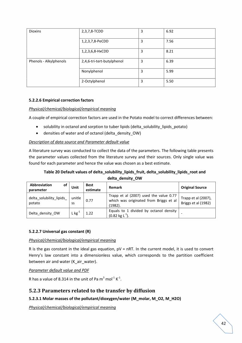
A literature survey was conducted to collect the data of the parameters. The following table presents the parameter values collected from the literature survey and their sources. Only single value was found for each parameter and hence the value was chosen as a best estimate.

Table 20 Default values of delta_solubility_lipids_fruit, delta_solubility_lipids_root and delta_density_OW

Abbreviation of parameter Unit Best

estimate Remark Original Source

delta_solubility_lipids_potato

unitless 0.77

Trapp et al (2007) used the value 0.77 which was originated from Briggs et al (1982).

Trapp et al (2007), Briggs et al (1982)

Delta_density_OW L kg-1 1.22 Equals to 1 divided by octanol density (0.82 kg L-1). -

5.2.2.7 Universal gas constant (R)


R is the gas constant in the ideal gas equation, pV = nRT. In the current model, it is used to convert Henry’s law constant into a dimensionless value, which corresponds to the partition coefficient between air and water (K_air_water).


R has a value of 8.314 in the unit of Pa m3 mol-1 K-1.

5.2.3 Parameters related to the transfer by diffusion 5.2.3.1 Molar masses of the pollutant/dioxygen/water (M_molar, M_O2, M_H2O)


43

The molar masses of each contaminant, oxygen and water are determined by the molecular formula.


The molar masses of several key substances is presented in Table 21. The molar masses of di-oxygen and water are 32 g mol-1 and 18 g mol-1, respectively.

Table 21 Molar mass of selected substances Chemical class Substance Molar mass (g mol-1) PAH Anthracene 178 Benzo(a)pyrene 252 Benzo(b)fluoranthene 252 Benzo(k)fluoranthene 252 Fluoranthene 202 Naphtalene 128 PCB PCB28 257.5 PCB 52 292 PCB101 326.5 PCB118 326.5 PCB138 361 PCB153 361 PCB180 503.5 Pesticides Alachlor 269.5 Atrazine 215.5 Chlordane 410 Chlorpyrifos 350.6 DDT 354.5 Dieldrin 358.5 Diuron 233 Endosulfan 407.1 Hexachlorocyclohexane 291 Isopruturon 206 Malathion 447.2 Parathion 291.1 Pentachlorophenol 266.5 Brominated flame retardants

Pentabromo diphenylether 564.5

Hexabromobiphenyl 627.4

VOCs Benzene 78 1,2-Dichloroethane 99 Dichloromethane 85 Hexachlorobenzene (HCB) 285 Hexachlorobutadiene 261 Pentachlorobenzene 250.5 Trichlorobenzene 181.5 Trichloromethane (chloroform) 119.5 Phthalate Dibutylphthalate (DBP) 276 Di(2-ethylhexyl)phthalate (DEHP) 390 Dioxins 2,3,7,8-TCDD 322 1,2,3,7,8-PeCDD 356.5 1,2,3,7,8-HxCDD 391 Phenols - Alkylphenols


262

Nonylphenol 220

2-Octylphenol 206

44

5.2.3.2 Diffusion coefficient of water in air and of oxygen in water (D_H2O_air, D_O2_water)


The diffusion coefficients of water in air and of oxygen in water depend on temperature.



Table 22 Values of D_H2O_air and D_O2_water collected from the literature survey Abbreviation of parameter Unit Value Remark Original Source

D_H2O_air m2 d-1 2.22 No indication about temperature. Trapp and

Matthies (1998) 2.25 At 25°C. E.L. Cussler (2009)

D_O2_water m2 d-1

1.73E-04 No indication about temperature. Trapp and Matthies (1998)

1.70E-04

At 20°C, calculated based on the formula developed by Wilke and Chang (1955) and the unit was converted from cm2.S-1 into m2.d-1.

Richard (1996), Wilke and Chang (1955)


The following table lists, for each parameter, a recommended value selected from the previous table and also presents a probability density function (PDF).

Table 23 Default values of D_H2O_air and D_O2_water Abbreviation of parameter Unit Best estimate PDF Comment

D_H2O_air m2 d-1 2.25 - E.L. Cussler (2009) indicates the temperature relevant for the value, but the other does not.

D_O2_water m2 d-1 1.70E-04 -

The value from Richard (1996), Wilke and Chang (1955) was selected because the value from Trapp and Matthies (1998) is not presented with temperature.

5.2.4 Parameters related to the chemical degradation

5.2.4.1 Degradation rate in potato (lambda_deg_potato)


It represents first order decay rate of pollutants in potato. The value varies depends on chemicals of interest.



45

Table 24 Values of lambda_deg_potato collected from the literature survey Abbreviation of parameter Unit Value Remark Original Source

lambda_deg_potato

d-1

0

No data were found. We assume that the degradation rate in fruit is negligible as indicated for other plant types in Rein et al (2011).

Rein et al (2011)

5.2.5 Parameters related to the transfer from soil to potato governed by the equilibrium transfer factor

5.2.5.1 Transfer factor from soil to potato (TF_soil_potato)


The transfer factor from soil to plant is the equilibrium ratio of the metal concentration in potatoes to the metal concentration in soil. This parameter is then calculated by:

𝑇𝑇𝑇𝑇𝑠𝑠𝑠𝑠𝑠𝑠𝑠𝑠_𝑝𝑝𝑠𝑠𝑜𝑜𝑜𝑜𝑜𝑜𝑠𝑠 =𝐶𝐶𝑝𝑝𝑠𝑠𝑜𝑜𝑜𝑜𝑜𝑜𝑠𝑠𝐶𝐶𝑠𝑠𝑠𝑠𝑠𝑠𝑠𝑠

where Cpotato denotes the concentration of metal in the edible part of a fruit crop (mg kgdw-1) and Csoil

denotes the total concentration of metal in soil (mg kgdw-1).

When Cpotato is obtrained on a basis of fresh weight, it is necessary to convert the unit from fresh into dry weight by using the data of dry matter fraction in a potato.

TF_soil_potato may depend on many factors such as soil texture, pH in soil, type of plants, and the experimental conditions. Precise estimation of TF_soil_potato based on these factors remains uncertain, due to the high variability observed in experimental data.


A literature survey was conducted to collect the data of TF_soil_potato. In addition of the literature survey, the database called BAPPET (Base de données sur les teneurs en Eléments Traces métalliques de Plantes Potagères, http://www.developpementdurable. gouv.fr/BAPPET-BAse-de-donnees-sur-les.html) was used to obtain the values. The BAPPET stores many experimental data of metal concentration in plants and in soil and those concentrations allows the calculation of TF_soil_potato by the equation above. The concentration of metal in a plant is given in the database in function of the metal considered, of factors associated with the plant/soil (e.g. type of plant/soil), of environmental context (e.g. industrial, rural, urban, and artificial), and of experimental conditions (e.g. mode of extraction of metal: total extraction, semi-total extraction, and partial). The BAPPET compiles the data together with the information about such differing factors.


Most of values of TF_soil_potato were calculated. The data of Cpotato and Csoil, which are used to calculate the parameter, were obtained from individual scientific article and the BAPPET. Some of the parameter values originated from the BAPPET were a priori filtered out considering the following factors:

46

Environmental contexts: The environment where measurements were carried out. The database categorizes the contexts into ‘industrial’ (industrial zone, zone neighboring factories..), rural (zone away from industrial or urban zones), ‘urban’, ‘artificial’ (zone where experiments are conducted with metals in chemical form), and ‘agricultural’.

- The data obtained in the context of ‘industrial’ were excluded to filter out the studies made in the regions receiving air deposits originated from industrial emissions.

Mode of metal extraction: The mode of metal extraction in soil. The database categorizes the mode into ‘total’, ‘semi-total’ extractions (using strong acids) and ‘partial’ extraction (using weak solvants).

- The data associated with ‘partial’ were removed because the equation above considers the total concentration in soil.

Organ: Part of plant analysed. The database categorizes the organ into ‘consumable (edible) part’ and ‘whole part’.

- The data associated with ‘whole part’ were removed because the equation above considers the total concentration in soil.

These three factors were in the same way taken into account for individual articles.

The generated parameter values were all transformed into log-scaled values (natural logarithm). Assuming that the transformed values follow the normality, a standard deviation (SD) method was applied to detect outliers according to Seo (2006). In the method, the values greater than X + 2SD or the values smaller than X – 2SD were regarded as outliers (X : mean, SD : standard deviation).

After removing the outliers, the Goodness-of-fit test was used with significant level 5% to evaluate the adjustment of distributions on the parameter values. Log-normal distribution was a priori chosen as the form of PDF. When the log-normality was found to be invalid, the Gamma and Weibull distributions were tested. Table 25 presents a best estimate and a PDF of TF_soil_potato for each selected metal.

Table 25 Default values of TF_soil_potato for selected metals Metal Best estimate PDF Number of

data Al 4.41E-04 LN(4.41E-04, 1.45)* 13 As 1.29E-03 LN(1.29E-03, 3.76) 12 Cd 1.38E-01 LN(1.38E-01, 2.99) 63 Cr 4.61E-03 LN(4.61E-03, 4.89) 21 Cu 2.78E-01 LN(2.78E-01, 2.22) 49 Fe 7.96E-04 LN(7.96E-04, 1.97) 10 Mn 1.20E-02 LN(1.20E-02, 2.34) 15 Pb 4.36E-03 LN(4.36E-03, 4.19) 68 Zn 1.47E-01 LN(1.47E-01, 2.31) 72

* LN signifies log-normal distribution. The first and second values in bracket following the symbol represent geometric mean and geometric standard deviation, respectively.

47

End of Level 3 documentation (end-user with expertise in parameterization)

48

Level 4 documentation (mathematical information)

6. Mass balance equation The Potato model developed consists of a potato compartment. A mass balance, which accounts for loading, loss, and accumulation of the pollutant, is taken into account. Following equations express mass balances in compartment in potato. It should be noted that the loss by harvest is not included in the mass balance equations because the loss process is considered only at the end of the plant growing period during which pollutants are accumulated in plant:

• Mass balance equations used for organic substances

(1) potatolossQpotatodepurationKQdiffusionUptake

Qpotatopotato

potato deg_____dt

d×−×−=

• Mass balance equations used for metals

(2) metalsUptake

Qpotato _dt

d=

Where Qpotato (mg) : Total quantity of the pollutant in potato Uptake_diffusion (mg d-1) : Uptake through diffusion K_depuration_potato (d-1) : Depuration rate from potato through diffusion loss_deg_potato (d-1) : Loss by degradation in potato Uptake_metals (mg d-1) : Transfer from soil to potato by the equilibrium transfer factor

7. Calculation of state variables This chapter presents the equations to calculate the state variables used in the Potato model. Those equations are grouped by differing transfer processes shown in the equation (1) and (2). Together with the equations, state variables are depicted by the following three symbols:

7.1. Uptake through diffusion (Uptake_diffusion) and loss by depuration (K_depuration_potato)

(3) soil

soilfieldpotatoatouptake_pot Kd

CSmkdiffusionUptake ×××=_

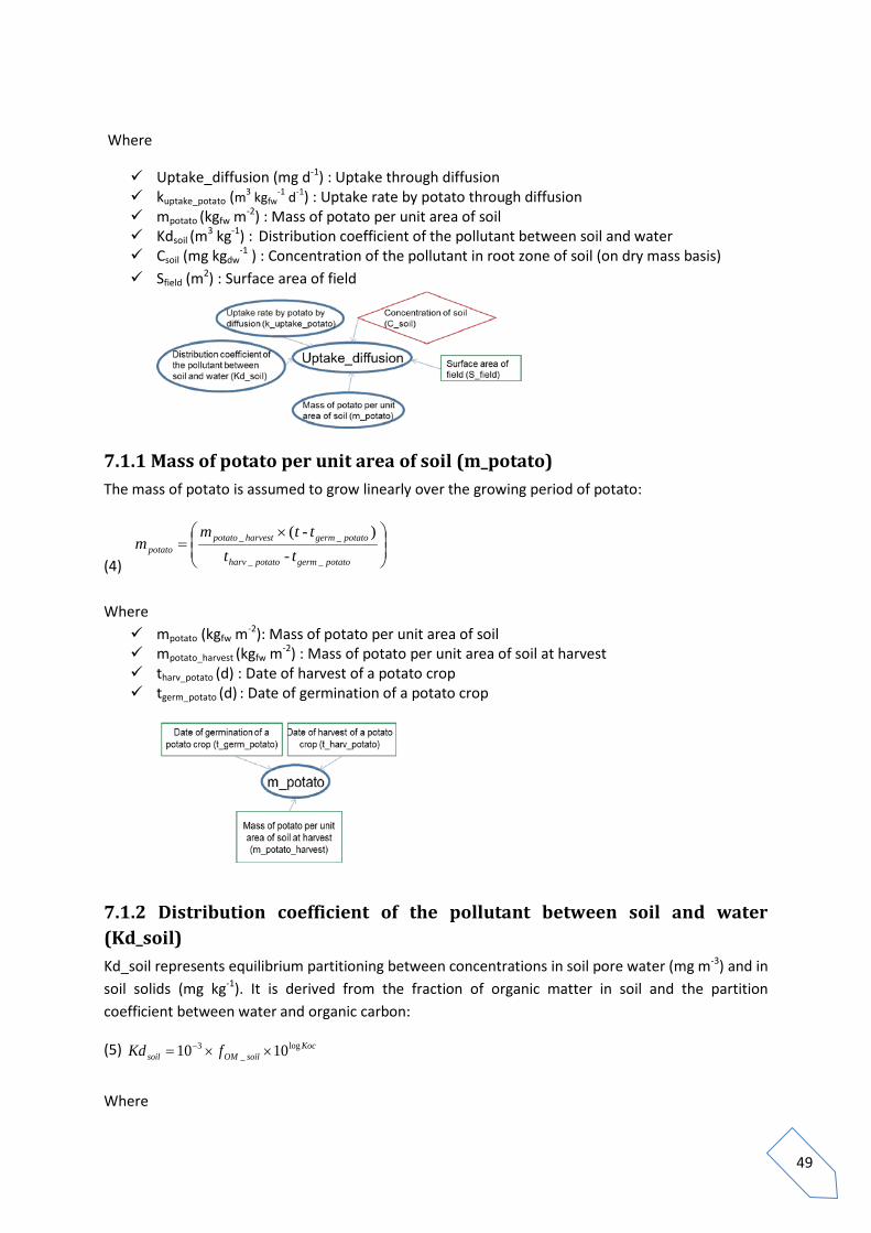
49

Where

Uptake_diffusion (mg d-1) : Uptake through diffusion kuptake_potato (m3 kgfw

-1 d-1) : Uptake rate by potato through diffusion mpotato (kgfw m-2) : Mass of potato per unit area of soil Kdsoil (m3 kg-1) : Distribution coefficient of the pollutant between soil and water Csoil (mg kgdw

-1 ) : Concentration of the pollutant in root zone of soil (on dry mass basis) Sfield (m2) : Surface area of field

7.1.1 Mass of potato per unit area of soil (m_potato) The mass of potato is assumed to grow linearly over the growing period of potato:

(4)

×=

potatogermpotatoharv

potatogermharvestpotatopotato tt

ttmm

__

__

-)-(

Where mpotato (kgfw m-2): Mass of potato per unit area of soil mpotato_harvest (kgfw m-2) : Mass of potato per unit area of soil at harvest tharv_potato (d) : Date of harvest of a potato crop tgerm_potato (d) : Date of germination of a potato crop

7.1.2 Distribution coefficient of the pollutant between soil and water (Kd_soil) Kd_soil represents equilibrium partitioning between concentrations in soil pore water (mg m-3) and in soil solids (mg kg-1). It is derived from the fraction of organic matter in soil and the partition coefficient between water and organic carbon:

(5) KocsoilOMsoil fKd log

_3 1010 ××= −

Where

50

Kdsoil (m3 kg-1) : Distribution coefficient of the pollutant between soil and water fOM_soil (g g-1) : Fraction of organic matter in soil logKoc (unitless) : Water-organic carbon partition coefficient (in log10) 10-3 is the unit correction factor with the unit of m3 L-1 ocKlog10 has the unit of L kg-1

7.1.3 Uptake rate by potato through diffusion (K_uptake_potato)

The uptake rate kuptake_potato is calculated from phase equilibrium:

(6) erpotato_wat_potatodepurationatouptake_pot Kkk ××= 001.0

Where kuptake_potato (m3 kgfw

-1 d-1) : Uptake rate by potato through diffusion kdepuration_potato (d-1) : Depuration rate from potato through diffusion Kpotato_water (L kgfw

-1) : Partition coefficient between potato and water 0.001 is the unit correction factor with the unit of m3 L-1

7.1.4 Partition coefficient between potato and water (K_potato_water) Potato is composed of water, carbohydrate, traces of lipids, and gas phase. The partition coefficient between potato and water is defined as the ratio of the concentration in all the phases of potato (water phase, lipids, carbohydrate and gas phase), Cpotato_total (mg kg fw-1), to the concentration in the water phase of potato, Cpotato_water (mg L-1). Kpotato-water can alternatively be estimated from:

(7)

Where Kpotato_water (L kgfw

-1) : Partition coefficient between potato and water Θpotato (L kgfw

-1) : Water content of potato CHpotato (L kgfw

-1) : Carbohydrate content in potato KCH,water (unitless) : Partition coefficient between carbohydrate and water Lpotato (kg kgfw

-1) : Lipid content of potato δdensity_OW (L kg-1) : Correction for density difference between water and n-octanol

waterairpotatotato_lipids_posolubilityKow

density_OWpotatoCH_waterpotatopotatoerpotato_wat KGLKCHK _10log )10( ×+××+×+= δδθ

51

logKow (m3 m-3) : Octanol-water partition coefficient (in log 10) δsolubility_lipids_potato (unitless) : Empirical correction factor for differences between solubility in

octanol and sorption to tuber lipids Gpotato (L kgfw

-1) : Air content in potato Kair_water (m3 m-3) : Partition coefficient between air and water

7.1.5 Depuration rate from potato through diffusion (K_depuration_potato) The depuration rate is deduced from a radial diffusion model:

(8) 2potato

Potato_potatodepuration R

Dk)(

23×=

Where kdepuration_potato (d-1) : Depuration rate from potato through diffusion Dpotato (m2 d-1) : Diffusion coefficient in potato Rpotato (m) : Potato radius at harvest

7.1.6 Diffusion coefficient in potato (D_potato) The diffusion coefficient in potato tissue is calculated from the diffusion in the water and air phases of the potato:

(9) gas_potatopotatowpotato DDD += _

Where Dpotato (m2 d-1) : Diffusion coefficient in potato Dw_potato (m2 d-1) : Diffusion coefficient in water pores of potato Dgas_potato (m2 d-1) : Diffusion coefficient in gas pores of potato

52

7.1.7 Diffusion coefficient in water/gas pores of potato (D_w_potato, D_gas_potato) Diffusion coefficient in water/gas pores is calculated as follows:

(10) waterpotatowpotatoww_potato DfTD ××= __ (11) gaspotatogpotatoggas_potato DfTD ××= __ Where

Dw_potato (m2 d-1) : Diffusion coefficient in water pores of potato Dgas_potato (m2 d-1) : Diffusion coefficient in gas pores of potato Tau_w_potato (unitless) : Tortuosity in water pores of the potato Tau_g_potato (unitless) : Tortuosity in air pores of the potato fw_potato (unitless) : Fraction of the pollutant dissolved in the potato water fg_potato (unitless) : Fraction of the pollutant dissolved in air of the potato Dwater (m2 d-1) : Effective diffusion coefficient in water Dgas (m2 d-1) : Effective diffusion coefficient in pure air

7.1.8 Effective diffusion coefficient in pure water/pure air (D_water, D_gas) For organic substances, the effective diffusion coefficient in water is related to the square root of the molar mass and also related to the diffusion coefficient of oxygen in water whereas the diffusion coefficient in air is related to the square root of the molar mass and also related to the diffusion coefficient of water in air:

(12) molar

OwaterOwater M

MDD 2,2

×=

(13) molar

OHairOHgas M

MDD 2_2 ×=

53

Where Dwater (m2 d-1) : Effective diffusion coefficient in pure water Dgas (m2 d-1) : Diffusion coefficient in pure air DO2_water (m2 d-1) : Diffusion coefficient of oxygen in water DH2O_air (m2 d-1) : Diffusion coefficient of water in air MO2 (g mol-1) : Molar mass of dioxygen MH2O (g mol-1) : Molar mass of water Mmolar (g mol-1) : Molar mass of the pollutant

7.1.9 Tortuosity in water/air pores of the potato (T_w_potato, T_g_potato) In porous solids such as plant tissue, the diffusion is hampered by a “labyrinth factor”, named the tortuosity. This is estimated by the method of Millington and Quirk (cited in Jury et al (1983)). The equations are not unit true:

(14) 2

3/10

)( potatopotato

potatow_potato G

T+

=θ

θ

(15)

2

3/10

)( potatopotato

potatog_potato G

GT

+=θ

Where Tw_potato (unitless) : Tortuosity in water pores of the potato Tg_potato (unitless) : Tortuosity in air pores of the potato ϴpotato (L kgfw

-1) : Water content of potato Gpotato (L kgfw

-1) : Air content of potato

54

7.1.10 Fraction of the pollutant dissolved in the potato water/in air of the potato (f_w_potato, f_g_potato) The fractions of chemicals dissolved in the water and air of the fruit are equal to the ratios of concentration in water and air phase, respectively, of the plant tissue to total concentration in the potato:

(16) erpotato_wat

potatow_potato K

fθ

=

(17) waterairerpotato_wat

potatog_potato K

KG

f _×=

Where fw_fruit (unitless) : Fraction of the pollutant dissolved in the potato water fg_potato (unitless) : Fraction of the pollutant dissolved in air of the potato ϴpotato (L kgfw

-1) : Water content of potato Gpotato (L kgfw

-1) : Air content of potato Kpotato_water (L kgfw

-1) : Partition coefficient between potato and water Kair_water (m3 m-3) : Partition coefficient between air and water

7.1.11 Partition coefficient between air and water (K_air_water) K_air_water is the equilibrium partitioning between concentrations in air and in water. It is an expression of Henry’s law constant in terms of a dimensionless ratio concentration:

(18) air_Kelvin

air_water TRHK

×=

Where Kair_water (m3 m-3) : Partition coefficient between air and water H (Pa m3 mol-1) : Henry’s law constant R (Pa m3 mol-1 K-1) : Universal gas constant Tair_Kelvin (K) : Temperature of air (in Kelvin)

55

(19) airair_Kelvin TT += 0.273

Where Tair_Kelvin (K) : Temperature of air (in Kelvin) Tair (°C) : Temperature of air (in Celsius)

7.2. Loss by degradation in potato (Loss_deg_potato) The degradation of the pollutant in potato is expressed by the first order decay rate (d-1):

λdeg_potato (d-1) : Degradation rate in potato (See equation (1))

7.3. Uptake of metals (Uptake_metals) The uptake of metals from soil into potatoes is governed by a substance-specific equilibrium transfer factor:

(20) fieldsoilharvestpotatopotatogermpotatoharv

potatopotatosoilmetals SCm

ttTFUptake ×××

−

−×= _

___ )(

)1( θ

Where Uptakemetals (mg d-1) : Uptake of metals TFsoil_potato (kgdw kgdw

-1) : Transfer factor from soil to potato ϴpotato (L kgfw

-1) : Water content of potato tharv_potato (d) : Date of harvest of a potato crop tgerm_potato (d) : Date of germination of a potato crop mpotato_harvest (kgfw m-2) : Mass of potato per unit area of soil at harvest Qsoil (mg) : Total quantity of the pollutant in the root zone Csoil (mg kgdw

-1 ) : Concentration in soil (on dry mass basis) Sfield (m2) : Surface area of field

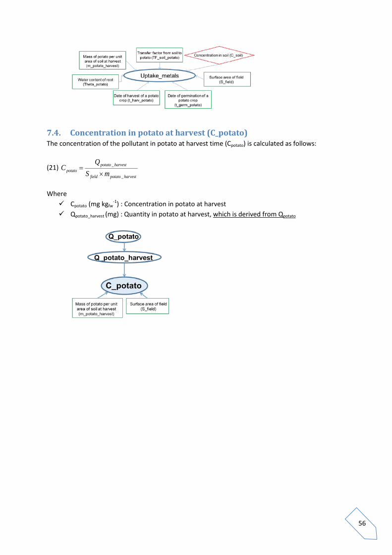
56

7.4. Concentration in potato at harvest (C_potato) The concentration of the pollutant in potato at harvest time (Cpotato) is calculated as follows:

(21) harvestpotatofield

harvestpotatopotato mS

QC

_

_

×=

Where Cpotato (mg kgfw

-1) : Concentration in potato at harvest Qpotato_harvest (mg) : Quantity in potato at harvest, which is derived from Qpotato

57

Reference

Abraham MH, Andonian-Haftvan J, Whiting GS, Leo A, Taft RS (1994) Hydrogen bonding. Part 34. The factors that influence the solubility of gases and vapors in water at 298 K, and a new method for its determination. J. Chem. Soc. Perkin Trans. 2: 1777-1791

Briggs GG, Bromilow RH, Evans AA (1982) Relationships between lipophilicity and root uptake and translocation of non-ionised chemicals by barleya. Pestic. Sci. 13: 495-504.

Chiou CT, Sheng G, Manes M (2001) A partition-limited model for the plant uptake of organic contaminants from soil to water. Environ. Sci. Technol. 35: 1437-1444.

EL Cussler (2009) Diffusion: Mass Transfer in Fluid Systems. Third edition, Cambridge University Press, UK.

Elmadfa I, Aign W, Muskat E, Fritsche H, Cremer D (1991) Die grosse GU Nährwert Tabelle, Gräfe und Unzer: Giessen.

Franco A, Fu W, Trapp S (2009) Influence of soil pH on the sorption of ionizable chemicals: Modeling advances. Environ. Toxicol. Chem. 28: 458-464.

Franco A, Trapp S (2008) Estimation of the soil-water partition coefficient normalized to organic carbon for ionizable organic chemicals. Environ. Toxicol. Chem. 27: 1995-2004.

Huuskonen J (2003) Prediction of soil sorption coefficient of organic pesticides from the atom-type electrotopological state indices. Environ. Toxicol. Chem. 22: 816-820.

IAEA (2010) Handbook of parameter values for the prediction of radionuclide transfer in terrestrial and freshwater environments. Technical Reports Series No.472.

Jeffries J, Martin I (2008) Updated technical background to the CLEA model. SC050021/SR3. Bristol, UK, Environment Agency. Science Report.

Jury WA, Spencer WF, Farmer W J (1983) Behavior assessment model for trace organics in soil 1. Model description. J.Environ.Qual. 12(4): 558-564.

Kleier DA (1988) Phloem mobility of xenobiotics I. Mathematical model unifying the weak acid and intermediate permeability theories. Plant Physiol. 86: 803-810.

Kühne R, Ebert R-U, Schüürmann G (2005) Prediction of the temperature dependency of Henry's Law constant from chemical structure. Environ. Sci. Technol. 39: 6705-6711.

Legind CN, Trapp S (2010) Review of features, events and processes incorporated in existing models for chemical uptake into plants and animals – Proposal of the conceptual and mathematical 2-FUN model for assessing transfer of chemicals to plants and animals. Written as Deliverable 2.4 in the framework of the 2-FUN project (FP6 Project-2005-Global-4 Integrated Project - Contract n°: 036976).

58

Meylan WM, Howard PH (1991) Bond contrlbution method for estimating Henry’s law constants. Environmental Toxicology and Chemistry 10: 283-1293.

Meylan WM, Howard PH (1995) Atom/fragment contribution method for estimating octanol-water partition coefficients. J. Pharm. Sci. 84: 83-92.

OECD (1995) OECD guidelines for the testing of chemicals - Partition Coefficient (n-Octanol/Water): Shake Flask Method.

OECD (2004) OECD guidelines for the testing of chemicals - Partition Coefficient (n-Octanol/Water): High Performance Liquid Chromatography (HPLC) Method.

OECD (2006) OECD guidelines for the testing of chemicals - Partition Coefficient (1-Octanol/Water): Slow-Stirring Method.

Panagos P, Hiederer R, Van Liedekerke M, Bampa F (2013) Estimating soil organic carbon in Europe based on data collected through an European network. Ecological Indicators 24: 439–450.

Poole SK, Poole CF (1999) Chromatographic models for the sorption of neutral organic compounds by soil from air and water. J. Chromatogr. A. 845: 381-400.

Rein A, Legind CN, Trapp S (2011) New concepts for dynamic plant uptake models. SAR and QSAR in Environmental Research 22: 191-215.

Richard T (1996) Calculating the oxygen diffusion coefficient in water. http://compost.css.cornell.edu/oxygen/oxygen.diff.water.html, checked in 01/03/2014.

Sablic A, Güsten H, Verhaar H, Hermens J (1995) QSAR modelling of soil sorption. Improvements and systematics of log KOC vs. log KOW correlations. Chemosphere 31: 4489- 4514, Corrigendum: Vol. 33 (1996): p2577.

Schüürmann G, Ebert R-U, Kühne R (2006) Prediction of the sorption of organic compounds into soil organic matter from molecular structure. Environ. Sci. Technol. 40: 7005-7011.

Seo S (2006) A Review and Comparison of Methods for Detecting Outliers in Univariate Data Sets. University of Pittsburgh, United States.

Tao S, Piao H, Dawson R, Lu X, Hu H (1999) Estimation of organic carbon normalized sorption coefficient (Koc) for soils using the fragment constant method. Environ. Sci. Technol. 33: 2719-2725.

Trapp S (2003) Modellering af optagelse aforganiske stoffer i grøntsager ogfrugt, Teknologiudviklingsprogrammet for jord- og grundvandsforurening. Miljøprojekt Nr. 765.

Trapp S, Matthies M (1998) Chemodynamics and Environmental Modeling. An Introduction. Springer, berlin, Germany.

Trapp S, Cammarano A, Capri E, Reichenberg F, Mayer P (2007) Diffusion of PAH in potato and carrot slices and application for a potato model. Environ Sci Technol 41, 3103-3108, supporting imformation.

59

Viswanadhan VN, Ghose AK, Singh UC, Wendoloski JJ (1999) Prediction of solvation free energies of small organic molecules. Additive-constitutive models based on molecular fingerprints and atomic constants. J. Chem. Inform. Comput. Sci. 39: 405-412.

Wilke CR and Chang P (1955) A.E.CH.E. Journal 1: 264-270.

The MERLIN-Expo Potato model · the merlin-expo potato model. v1.3. author: ... initialization of mass balance in media 22 ... 5.2.4 parameters related to the chemical degradation

Documents