The M/EEG inverse problem and solutions Gareth R. Barnes.

The M/EEG inverse problem and solutions

Gareth R. Barnes

Format

• The inverse problem• Choice of prior knowledge in some popular

algorithms• Why the solution is important.

Volume currents

Magnetic field

Electrical potential difference (EEG)

5-10nAmAggregate post-synaptic potentials

of ~10,000 pyrammidal neurons

cortex

skull

scalp

MEG pick-up coil

Inverse problem

1s

Active Passive

Local field potential (LFP)

MEG measurement

1nAm

1pT

pick-up coils

What we’ve got

What we want

Forward problem

Useful priors cinema audiences

• Things further from the camera appear smaller

• People are about the same size• Planes are much bigger than people

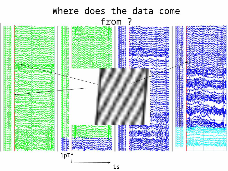
Where does the data come from ?

1pT

1s

Useful priors for MEG analysis

• At any given time only a small number of sources are active. (dipole fitting)

• All sources are active but overall their energy is minimized. (Minimum norm)

• As above but there are also no correlations between distant sources (Beamformers)

The source covariance matrix

1 2 3 4 5 6 7 8 9 10

1

2

3

4

5

6

7

8

9

10

1 2 3 4 5 6 7 8 9 10

1

2

3

4

5

6

7

8

9

10

1 2 3 4 5 6 7 8 9 10

1

2

3

4

5

6

7

8

9

10

1 2 3 4 5 6 7 8 9 10

1

2

3

4

5

6

7

8

9

10

1 2 3 4 5 6 7 8 9 10

1

2

3

4

5

6

7

8

9

10

Source number

Sou

rce

num

ber

1 2 3 4 5 6 7 8 9 10

1

2

3

4

5

6

7

8

9

10

1 2 3 4 5 6 7 8 9 10

1

2

3

4

5

6

7

8

9

10

1 2 3 4 5 6 7 8 9 10

1

2

3

4

5

6

7

8

9

10

-6-4-20246x 10

-13

-6

-4

-2

0

2

4

6x 10

-13

-6

-4

-2

0

2

4

6x 10

-13

Estimated dataEstimated position

Measured data

Dipole Fitting

?

-6-4-20246x 10

-13

-6

-4

-2

0

2

4

6x 10

-13

-6

-4

-2

0

2

4

6x 10

-13

Estimated data/Channel covariance matrixMeasured data/

Channel covariance

Dipole fitting

1 2 3 4 5 6 7 8 9 10

1

2

3

4

5

6

7

8

9

10

1 2 3 4 5 6 7 8 9 10

1

2

3

4

5

6

7

8

9

10

1 2 3 4 5 6 7 8 9 10

1

2

3

4

5

6

7

8

9

10

True source covariance

Prior source covariance

Fisher et al. 2004

Dipole fitting

Effective at modelling short (<200ms) latency evoked responses

Clinically very useful: Pre-surgical mapping of sensory /motor cortex ( Ganslandt et al 1999)

Need to specify number of dipoles, non-linear minimization becomes unstable for more sources.

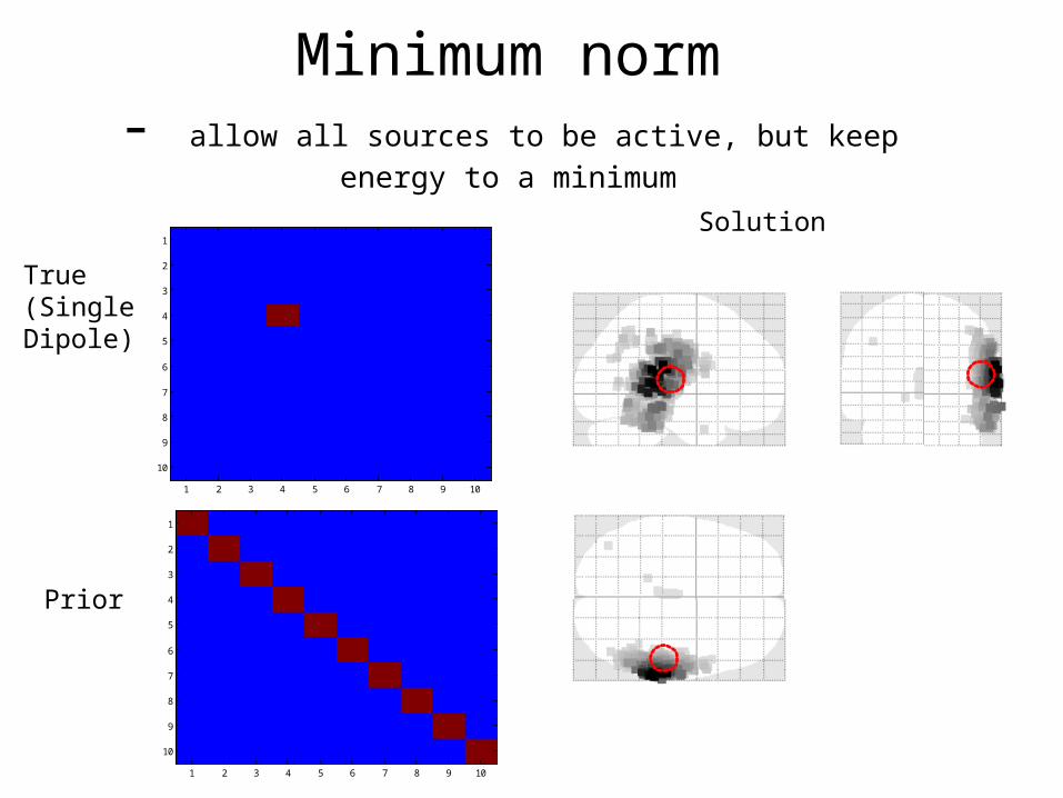
Minimum norm- allow all sources to be active, but keep energy to a minimum

1 2 3 4 5 6 7 8 9 10

1

2

3

4

5

6

7

8

9

10

Solution

0 100 200 300 400 500 600 700-10

-8

-6

-4

-2

0

2

4

6

8

10

estimated response - condition 1at 52, -31, 11 mm

time ms

PPM at 379 ms (79 percent confidence)512 dipoles

Percent variance explained 99.91 (93.65)log-evidence = 21694116.2

0 100 200 300 400 500 600 700-10

-8

-6

-4

-2

0

2

4

6

8

10

estimated response - condition 1at 52, -31, 11 mm

time ms

PPM at 379 ms (79 percent confidence)512 dipoles

Percent variance explained 99.91 (93.65)log-evidence = 21694116.2

Prior

1 2 3 4 5 6 7 8 9 10

1

2

3

4

5

6

7

8

9

10

1 2 3 4 5 6 7 8 9 10

1

2

3

4

5

6

7

8

9

10

1 2 3 4 5 6 7 8 9 10

1

2

3

4

5

6

7

8

9

10

True(Single Dipole)

Problem is that superficial elements have much larger lead fields

MEG sensitivity

Basic Minimum norm solutions

Solutions are diffuse and have superficial bias (where source power can be smallest).

But unlike dipole fit, no need to specify the number of sources in advance.

Can we extend the assumption set ?

Coh

eren

ce

Distance

0 12 24 30mm

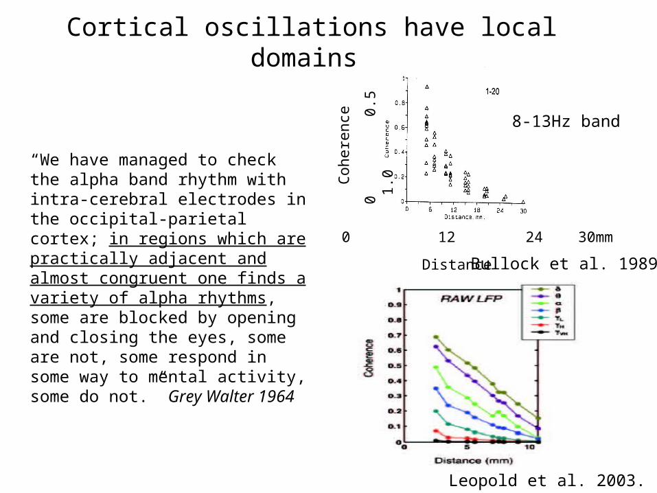
8-13Hz band

0

0

.5

1

.0

Cortical oscillations have local domains

Bullock et al. 1989

“We have managed to check the alpha band rhythm with intra-cerebral electrodes in the occipital-parietal cortex; in regions which are practically adjacent and almost congruent one finds a variety of alpha rhythms, some are blocked by opening and closing the eyes, some are not, some respond in some way to mental activity, some do not.” Grey Walter 1964

Leopold et al. 2003.

Beamformer: if you assume no correlations between sources, can calculate a prior covariance matrix from the

data

1 2 3 4 5 6 7 8 9 10

1

2

3

4

5

6

7

8

9

10

True

0 100 200 300 400 500 600 700-10

-8

-6

-4

-2

0

2

4

6

8

10

estimated response - condition 1at 52, -31, 11 mm

time ms

PPM at 379 ms (79 percent confidence)512 dipoles

Percent variance explained 99.91 (93.65)log-evidence = 21694116.2

Prior,Estimated From data

1 2 3 4 5 6 7 8 9 10

1

2

3

4

5

6

7

8

9

10

1 2 3 4 5 6 7 8 9 10

1

2

3

4

5

6

7

8

9

10

1 2 3 4 5 6 7 8 9 10

1

2

3

4

5

6

7

8

9

10

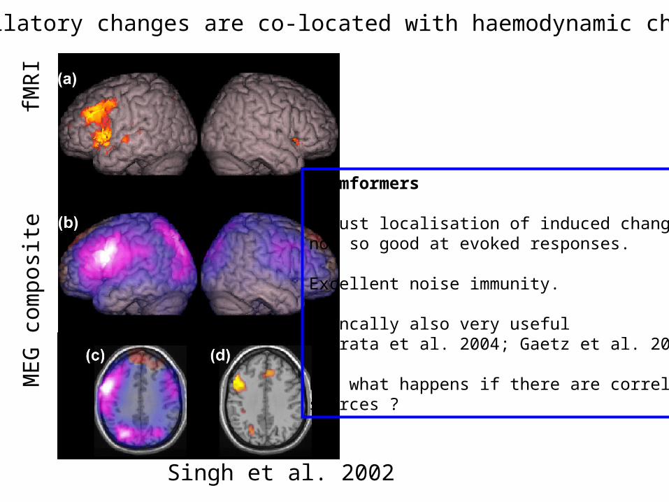
Singh et al. 2002

ME

G c

ompo

site

fMR

IOscillatory changes are co-located with haemodynamic changes

Beamformers

Robust localisation of induced changes, not so good at evoked responses.

Excellent noise immunity.

Clincally also very useful (Hirata et al. 2004; Gaetz et al. 2007)

But what happens if there are correlatedsources ?

Beamformer for correlated sources

1 2 3 4 5 6 7 8 9 10

1

2

3

4

5

6

7

8

9

10

0 100 200 300 400 500 600 700-1.5

-1

-0.5

0

0.5

1

1.5

estimated response - condition 1at -2, -21, 5 mm

time ms

PPM at 229 ms (99 percent confidence)512 dipoles

Percent variance explained 99.81 (65.46)log-evidence = 8249519.0

Prior(estimated from data)

True Sources

12345678910

1

2

3

4

5

6

7

8

9

10

12345678910

1

2

3

4

5

6

7

8

9

10

12345678910

1

2

3

4

5

6

7

8

9

10

-6-4-20246x 10

-13

-6

-4

-2

0

2

4

6x 10

-13

-6

-4

-2

0

2

4

6x 10

-13

Estimated data/Channel covariance matrixMeasured data/

Channel covariance

Dipole fitting

1 2 3 4 5 6 7 8 9 10

1

2

3

4

5

6

7

8

9

10

1 2 3 4 5 6 7 8 9 10

1

2

3

4

5

6

7

8

9

10

1 2 3 4 5 6 7 8 9 10

1

2

3

4

5

6

7

8

9

10

True source covariance

Prior source covariance

?

Muliple Sparse Priors (MSP)

1 2 3 4 5 6 7 8 9 10

1

2

3

4

5

6

7

8

9

10

1 2 3 4 5 6 7 8 9 10

1

2

3

4

5

6

7

8

9

10

12345678910

1

2

3

4

5

6

7

8

9

10

1 2 3 4 5 6 7 8 9 10

1

2

3

4

5

6

7

8

9

10

1 2 3 4 5 6 7 8 9 10

1

2

3

4

5

6

7

8

9

10

1 2 3 4 5 6 7 8 9 10

1

2

3

4

5

6

7

8

9

10

1 2 3 4 5 6 7 8 9 10

1

2

3

4

5

6

7

8

9

10

n

Estimated (based on data)

TrueP

12345678910

1

2

3

4

5

6

7

8

9

10

Priors

(Covariance estimates are made in channel space)

= sensitivity (lead field matrix)

0 100 200 300 400 500 600 700-8

-6

-4

-2

0

2

4

6

8

estimated response - condition 1at 36, -18, -23 mm

time ms

PPM at 229 ms (100 percent confidence)512 dipoles

Percent variance explained 99.15 (65.03)log-evidence = 8157380.8

0 100 200 300 400 500 600 700-2

-1.5

-1

-0.5

0

0.5

1

1.5

2

estimated response - condition 1at 46, -31, 4 mm

time ms

PPM at 229 ms (100 percent confidence)512 dipoles

Percent variance explained 99.93 (65.54)log-evidence = 8361406.1

0 100 200 300 400 500 600 700-2

-1.5

-1

-0.5

0

0.5

1

1.5

2

estimated response - condition 1at 46, -31, 4 mm

time ms

PPM at 229 ms (100 percent confidence)512 dipoles

Percent variance explained 99.87 (65.51)log-evidence = 8388254.2

0 50 100 15010

2

104

106

108

Iteration

Free energyAccuracyComplexity

0 100 200 300 400 500 600 700-2

-1.5

-1

-0.5

0

0.5

1

1.5

2

estimated response - condition 1at 46, -31, 4 mm

time ms

PPM at 229 ms (100 percent confidence)512 dipoles

Percent variance explained 99.90 (65.53)log-evidence = 8389771.6

AccuracyFree EnergyCompexity

0 100 200 300 400 500 600 700-1.5

-1

-0.5

0

0.5

1

1.5

estimated response - condition 1at -2, -21, 5 mm

time ms

PPM at 229 ms (99 percent confidence)512 dipoles

Percent variance explained 99.81 (65.46)log-evidence = 8249519.0

0 100 200 300 400 500 600 700-2

-1.5

-1

-0.5

0

0.5

1

1.5

2

estimated response - condition 1at 46, -31, 4 mm

time ms

PPM at 229 ms (100 percent confidence)512 dipoles

Percent variance explained 99.90 (65.53)log-evidence = 8389771.6Can use model evidence to choose between solutions

So it is possible,but why bother ?

Rols et al. 2001

Stimulus(1º)

Gamma oscillations in monkey

evoked

Inducedgammapower

Time-frequencypower

Time-frequencypower changefrom baseline

20

40

60

80

0Stimulus(3cpd,1.5º)

Evoked(0-70Hz)

-3nAm

GammaPower

Adjamian et al. 2004 ,Hall et al. 2005, Adjamian et al. 2008

100%

0%

0.8

0.4

nAm

^2/H

z

030 40 50 60Hz

30

60

0.3 2s

Hz

Hadjipapas et al. 2009,Kawabata Duncan et al. 2009,

Different spectra, different underlying neuronal populations

?

p<0.05

Power spectrum

Rank spectrum

Where does the data come from ?

1pT

1s

Conclusion

• MEG inverse problem can be solved.. If you have some prior knowledge.

• All prior knowledge encapsulated in a source covariance matrix

• Can test between priors in a Bayesian framework.

• Exciting part is the millisecond temporal resolution we can now exploit.