Journal of Public Economics 3 (1974) 303-328. 0 North-Holland Publishing Company THE MEASUREMENT OF URBAN TRAVEL DEMAND Daniel MCFADDEN* Department of Economics, University of California, Berkeley, U.S.A. Transport projects involve sinking money in expensive capital investments, which have a long life and wide repercussions. There is no escape from the attempt both to estimate the demand for their services over twenty or thirty years and to assess their repercussions on the economy as a whole. Denys Munby, Transport, 1968 1. Introduction It is a truism that the transportation system is a critical component of every urban economy, and that transportation policy decisions can have a profound effect on the development of the urban system. Public transportation projects are often massive and mutually exclusive, with irreversible cumulative effects over long periods. If major social losses are to be avoided, careful planning based on a conceptually sound and empirically accurate benefit-cost calculus is essential. Accurate forecasts of travel demand under alternative transport policies are required for precise calculations of benefits. To be fully satisfactory, these fore- casts must be sufficiently sensitive to reflect the impact of the changing urban environment over the lifetime of proposed transport projects. Travel demand forecasting has long been the province of transportation engineers, who have built up over the years considerable empirical wisdom and a repertory of largely ad hoc models which have proved successful in various applications. The contribution of psychologists and economists to forecasting methodology has been limited; despite a surge of recent interest, there still does not exist a solid foundation in behavioral theory for demand forecasting *This research was supported by National Science Foundation Grants GS-27226 and GS- 35890X and by the Department of Transportation, whose views are not necessarily represented by the contents of this paper. I am indebted to T. Domencich and M.K. Richter for useful comments at various stages of this research, and to M. Johnson, F. Reid, H. Varian, H. Wills and G. Duguay who have made major contributions to the empirical analysis of this paper; and I gratefully acknowledge the valuable comments of discussants R. Cooter, F.X. de Donnea, and E. Sheshinski. I claim sole responsibility for errors.

Welcome message from author
This document is posted to help you gain knowledge. Please leave a comment to let me know what you think about it! Share it to your friends and learn new things together.
Transcript
Journal of Public Economics 3 (1974) 303-328. 0 North-Holland Publishing Company
THE MEASUREMENT OF URBAN TRAVEL DEMAND
Daniel MCFADDEN*
Department of Economics, University of California, Berkeley, U.S.A.
Transport projects involve sinking money in expensive capital investments, which have a long life and wide repercussions. There is no escape from the attempt both to estimate the demand for their services over twenty or thirty years and to assess their repercussions on the economy as a whole.
Denys Munby, Transport, 1968
1. Introduction
It is a truism that the transportation system is a critical component of every urban economy, and that transportation policy decisions can have a profound effect on the development of the urban system. Public transportation projects are often massive and mutually exclusive, with irreversible cumulative effects over long periods. If major social losses are to be avoided, careful planning based on a conceptually sound and empirically accurate benefit-cost calculus is essential. Accurate forecasts of travel demand under alternative transport policies are required for precise calculations of benefits. To be fully satisfactory, these fore- casts must be sufficiently sensitive to reflect the impact of the changing urban environment over the lifetime of proposed transport projects.
Travel demand forecasting has long been the province of transportation engineers, who have built up over the years considerable empirical wisdom and a repertory of largely ad hoc models which have proved successful in various applications. The contribution of psychologists and economists to forecasting methodology has been limited; despite a surge of recent interest, there still does not exist a solid foundation in behavioral theory for demand forecasting
*This research was supported by National Science Foundation Grants GS-27226 and GS- 35890X and by the Department of Transportation, whose views are not necessarily represented by the contents of this paper. I am indebted to T. Domencich and M.K. Richter for useful comments at various stages of this research, and to M. Johnson, F. Reid, H. Varian, H. Wills and G. Duguay who have made major contributions to the empirical analysis of this paper; and I gratefully acknowledge the valuable comments of discussants R. Cooter, F.X. de Donnea, and E. Sheshinski. I claim sole responsibility for errors.
304 D. McFadden, Measurement of urban travel demand
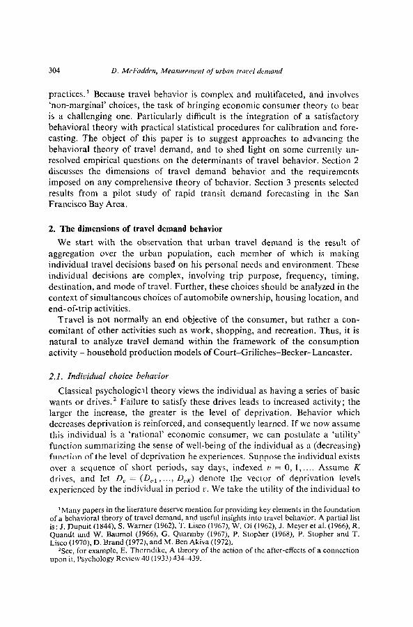
practices.’ Because travel behavior is complex and multifaceted, and involves ‘non-marginal’ choices, the task of bringing economic consumer theory to bear is a challenging one. Particularly difficult is the integration of a satisfactory behavioral theory with practical statistical procedures for calibration and fore- casting. The object of this paper is to suggest approaches to advancing the behavioral theory of travel demand, and to shed light on some currently un- resolved empirical questions on the determinants of travel behavior. Section 2 discusses the dimensions of travel demand behavior and the requirements imposed on any comprehensive theory of behavior. Section 3 presents selected results from a pilot study of rapid transit demand forecasting in the San Francisco Bay Area.
2. The dimensions of travel demand behavior
We start with the observation that urban travel demand is the result of aggregation over the urban population, each member of which is making individual travel decisions based on his personal needs and environment. These individual decisions are complex, involving trip purpose, frequency, timing, destination, and mode of travel. Further, these choices should be analyzed in the context of simultaneous choices of automobile ownership, housing location, and end-of-trip activities.
Travel is not normally an end objective of the consumer, but rather a con- comitant of other activities such as work, shopping, and recreation. Thus, it is natural to analyze travel demand within the framework of the consumption activity - household production models of Court-Griliches-Becker-Lancaster.
2.1. Individual choice behavior
Classical psychologic, theory views the individual as having a series of basic wants or drives.* Failure to satisfy these drives leads to increased activity; the larger the increase, the greater is the level of deprivation. Behavior which decreases deprivation is reinforced, and consequently learned. If we now assume this individual is a ‘rational’ economic consumer, we can postulate a ‘utility’ function summarizing the sense of well-being of the individual as a (decreasing) function of the level of deprivation he experiences. Suppose the individual exists over a sequence of short periods, say days, indexed v = 0, 1,. . . . Assume K drives, and let D, = (DOI, . . . . DvK) denote the vector of deprivation levels
experienced by the individual in period v. We take the utility of the individual to
‘Many papers in the lilerature deserve mention for providing key elements in the foundation of a behavioral theory of travel demand, and useful insights into travel behavior. A partial list is: J. Dupuit (1844), S. Warner (1962), T. Lisco (1967), W. Oi (1962), J. Meyer et al. (1966), R. Quandt and W. Baumol (1966), G. Quarmby (1967), P. Stopher (1968), P. Stopher and T. Lisco (1970), D. Brand (1972), and M. Ben Akiva (1972).
%ee, for example, E. Thorndike, A :heory of the action of the after-effects of a connection upon it, Psychology Review 40 (1933) 434439.
D. McFadden, Measurement of urban travel demand 305
be a discounted sum of ‘per day’ utilities, writing
u = “ZO SW~“) 3 (1)
where 6 is a discount factor and the individual’s horizon is taken to be infinite to simplify later calculation. 3
Over his lifetime, the individual has available a set B of mutually exclusive alternative choices. Each member x E B is a vector x = (x0, x1, . . .), with x, a sub-vector of attributes associated with the decision made in period v. A simple example would be an individual whose only decision in life is a binary commute mode choice; i.e., his work type and location, residential location,.auto owner- ship, and non-work behavior are all completely determined. Let x0, xb denote the vectors of attributes such as travel time, cost, and comfort, associated with the two modes in period 0, and suppose these attributes do not change over time. Then, letting A = (x’, sb>, the set B is the Cartesian product B = A x A x . . . . More generally, the individual will face both long-run (residential location, auto ownership) decisions and short-run (timing of trips, mode choice) decisions, with the former decisions restricting the range of latter opportunities.
The set of period v decisions x, associated with x E B will not be a simple ‘budget set’ of the type ordinarily encountered in consumer theory because of the qualitative transport choices involved and the ‘fixed charge’ nature of transport in facilitating consumer activities. To simplify analysis, we shall assume that the set of options at each u is finite; there is no particular technical difficulty in extending our analysis to the non-finite case.
The relation between the consumer’s decision x E B and the evolution of deprivation levels over time is determined by the definition of drives and the nature of the household production technology; we assume this has the general form4
D u+l =f(Dv,x,). (2)
The rational economic consumer will choose x E B to maximize utility (1) subject to his initial deprivation level D, and the constraints (2).
To push the analysis beyond this very genera1 statement of the mechanism for determining behavior, we shall now make very specific and concrete assumptions on the functional forms of utility and the determination of drives; namely, utility linear in deprivation levels,
u(D,) = -/?'D,,
and deprivation levels evolving in a linear first-order difference equation,
sThe linear additive form is justified only by convenience. 4The assumptions that the evolution of deprivation levels follows a first-order process and
that the alternative sets are independent over time are made for notational convenience. They can be relaxed explicitly, or implicitly by broadening the definitions of deprivation levels and choice attributes to include historical information.
306 D. McFadden, Measurement of urban traoel demand
D “+I = rD,+g(x,).
To avoid boundary problems, we assume all real levels of deprivation, positive or negative, are defined. In these formulae, j3 is a vector of non-negative para- meters and r is a Kx K matrix. In what follows, we shall assume the roots of r all lie in the interior of the unit circle; i.e., there are no self-sustaining rises in deprivation levels over time.5 It should be noted that while the functional forms (3) and (4) are concrete, they are not as specialized as might at first appear. First, since any sufliciently smooth utility function can be approximated on a specific set by a linear combination of appropriately chosen numerical functions, one can shape (3) by taking a sufficiently broad definition of the list of ‘drives’. Second, by including historical information in the deprivation-level vector and choosing the form of the functiong, a broad range of functional relations between the attribute vectors X, and per-day utility levels can be attained.
We next use the forms (3) and (4) to simplify the statement of the utility maximization problem. Pre-multiply (4) by 6”+ ’ and sum over U:
Assuming that the last term in this sum exists, we have
f 6"D, = (Z-W)- l v--o
Do + “to cY+‘g(x,)) ,
5An earlier draft of this paper allowed for the possibility that some roots of I- could be unstable. This could correspond, for example, to the presence of drives such as ‘boredom’ which may have intrinsicJly unstable deprivation levels requiring continual monitoring and positive control, and could provide a theoretical explanation for cyclic variations in individual choice in the presence of static alternative sets. To make this possibility compatible with the earl& simplification assumption of an infinite horizon, I had previously assumed the matrix 6r to be stable. Discussant Robert C‘ooter has pointed out that this leads to the implausible conclusion that unstable deprivation levels will be divergent in the optimal solution, with the individual accepting extreme values of these variables in the discounted future in exchange for the short-run benefits of ‘steady-state’ behavior. While the unboundedness of deprivation levels might be dismissed as a consequence of our linearization of the consumer’s problem, the abscncc of cyclic behavior is contrary to the initial objectives of the construction. A much better approach to incorporating the possibility of cyclic behavior is to assume a finite horizon H in the utility function (1) anti impose no conditions on the roots of SK Then, the analogue of eq. (7) is
N--L z/ = -B’n,,o,-/? c /lr,-a-16~+‘g(X,),
“ZO
with ,/f, = c” ii”T”, or [I- 6r]nS = I- (Jr)“+ ’ . “CO
It should be clear that the analysis we carry out for the case of stable rcould readily be adapted to this more general model. On the other hand, the assumption of a stable f seems more appro- priate for application to steady-state Icork trip commute behavior.
D. McFadden, Measurement of urban travel demand 307
and hence
u = -p’(z-6r)-‘D0-~‘(z--6r)- I”$ a”+ ‘g(x,).
The first term in this expression is constant; hence, the utility maximization problem reduces to
MaxU= -Min X=(XO,XI,. . .)EB
fi’(Z- U) - l “ZO P+ l&X”).
Further simplification of the problem occurs when B is a Cartesian product B = A x A x . . , as in the mode choice example cited above :6
MaxU= -Min xo~A
2.2. Population choice behavior
Before giving concrete examples showing how problems (8) or (9) can be used to obtain implications for individual behavior, it is useful to explore the link between behavioral models of the individual and the data obtained from sampling an urban population. Our theory of individual behavior is not ‘singled- valued’; we cannot exclude the possibility that within our framework of economic rationality and postulated structure of utility maximization there will be un- observed characteristics, such as tastes and unmeasured attributes of alternatives, which vary over population and obscure the implications of the individual behavior model. However, it is possible to deduce from the individual choice model properties of population choice behavior which have empirical content. The following rather extensive digression on this subject may clarify the con- ceptual issues involved.
Consider the textbook model of economic consumer behavior. The individual has a utility function u = U(x; p), representing tastes, which is maximized subject to a budget constraint x E B at a system of demands
x = h(B; p), (10)
where p is a specification of the individual’s tastes [e.g., p may be the individual’s binary preference relation (for which U is a representation), or a parameter vector specifying the utility function within a class of functional forms; factors influencing tastes and included in p are observed demographic variables such as sex, age, and education, and unobserved variables such as intelligence, experience, and childhood training; textbook models usually suppress the p argument]. The
6The reader will note that we have ended up with utility expressed as a function of attributes of the chosen alternatives. The conceptual apparatus of drives and household production has mattered only in the specification of the coefficient vector, and from a formal point of view could be dispensed with altogether. However, in drawing out the empirical implications of taste and production effects, the more elaborate structure is useful.

econometrician typically has data on the behavior of a cross-section of consumers drawn from a population with common observed demographic characteristics: budgets B, and demands X, for individuals t = 1, . . . . T. He wishes to test hypotheses about the behavioral model (10) which may range from specific structural features of parametric demand functions (e.g., price and income elasticities) to the general revealed preference hypothesis that the observed data are generated by utility-maximizing consumers. The observed data will fail to fit eq. (10) exactly because of measurement errors in x,, consumer optimization errors, and unobserved variations in the population. The procedure of most empirical demand studies is to ignore the possibility of taste variations in the sample and make the plausible and convenient, but untested, assumption that the cross-section of consumers has observed demands which ‘are distributed randomly about the exact values .Y for some common or representative tastes /?; i.e.,
x, = MB,; P)fE,, (11)
where E, is an unobserved random term distributed independently of B,.
The relation of observed aggregated demand to individual demand under this speGfication is straightforward. In a population of consumers who are homo- geneous with respect to budgets faced, aggregate demand will equal individual demand ‘writ large’, and all systematic variations in aggregate demand are inter- preted as generated by a common variation at the intensive margin of the identical individual demands. In the absence of unobserved variations in tastes or budgets, there is no extensive margin affecting aggregate demand.
Conventional statistical techniques can be applied to eq. (11) under the specification above to test hypotheses on the structure of h. In the conventional demand study, where quantities demanded vary continuously, it is reasonable to expect marginal optimization errors and measurement errors to be important, and perhaps dominate the effect of taste variations. Then the specification (11) is fairly realistic.7
We now re-examine the conventional demand specification in the case that the set of alternative choices is finite. A utility maximum exists under standard conditions, and generates the demand equation (10). This equation predicts a single chosen x when tastes and unobserved attributes of alternatives are
‘Under scme conditions, the conclusion above on estimation of continuously varying demands will continue to hold even in the presence of some types of taste variation. Suppose one can postulate that consumers are homogeneous in tastes up to a vector of parameters that appear linearly in the demand function. (An example would be individuals with log-linear functions who face conventional budget constraints, with variation in the parameters of the utility function across individuals.) Then the demand functions can be estimated using random coefficients econometric models; what is important is that except for refinements in estimation of the error structure and the variances of estimators, this approach will lead to the same models and estimates as were obtained under the ‘identical consumers’ assumption. We shall next show that when consumer choice involves discrete alternatives rather than continuous choice, this ‘robustness’ property of the conventional model is lost.
D. McFadden, Measurement of urban travel demand 309
assumed uniform across the population. The conventional statistical specifica- tion in (11) would then imply that all observed variation X, in demand over the finite set of alternatives is the result of errors in measurement and optimization. The argument that measurement error is an important factor is clearly im- plausible. Consumer optimization errors may be important, but then we must question the relevance of this behavioral model in which a substantial proportion of the observed variation in choice is attributed to aspects of behavior described only by the ad hoc error specification.
Aggregate demand can usually be treated as a continuous variable, as the effect of the discreteness of individuals’ alternatives is negligible. As a result, aggregate demand may superficially resemble the demand for a pppulation of identical individuals for a divisible commodity. However, systematic variations in the aggregate demand for the lumpy commodity are all due to shifts at the extensive margin where individuals are switching from one alternative to another, and not at the intensive margin as in the divisible commodity, identical individual case. Thus, it is fallacious to apply the latter model to obtain speci- fications of aggregate demand for discrete alternatives. What is required is a formulation of the demand model in which the effects of individual differences in tastes and optimization behavior on the error structure in eq. (11) are made explicit. The implications of this specification for choice among discrete alterna- tives differ substantially from the conventional specification, as several examples will show. For notational simplicity, the utility function given in (7) is written in these examples as a general function of the attributes of alternative decisions,
U(x).
Example A. Suppose each member of the population has the utility function
U(x,,x,) = x,+alogx,, and the budget constraint y = plx, +p2x2, with y 2 pr and x1 = 0 or 1. The taste parameter LX varies in the population with a cumulative distribution function G(a) and mean Cr. Then, utility is maximized by purchasing a unit of good 1 when U( 1, (y-p JpJ > U(0, y/p2), or LX < - l/log (1 -p,/y). Hence, Prob (xIt = 1) = G( - l/log (1 -P~~/Y,)). Suppose an observed cross-section sample, has T income-price levels, indexed (Y~,P~~,P~,), R, individuals at income-price level t, and S, observed purchases of a unit of the first commodity among the individuals at level t. Then, the observed relative frequency f, = S,/R, is an estimate of the probability P, = G(- l/log (1 -pit/ y,)), and a statistical technique such as maximum likelihood or minimum chi- square can be used to estimate the unknown parameters of G. Suppose, for example, c( has the reciprocal exponential distribution G(a) = e(-e1’a)+e2* (0 < LX 6 0,/0,>, where 0, and Q2 are positive parameters. Then log P, = e1 log (1 -pl,/vJ + (!I2 and a consistent (as all R, + + co) estimator of (0,) 0,) can be obtained by applying ordinary least squares to the equation logf, = 8, log (1 -p 1 Jy,) + O2 + qt. (A weighted regression yields an asymptotically efficient estimator.)
D. McFadden, Measurement of urban travel demand
Example B. Each member of the population has a utility function U(x, , x2) = x1 su log x2 and budget constraint y = plxl +pzx,, where x1, x2 vary con- tinuously. The demand functions are x1 = Max (0, y/p1 -E) and x2 = Min (y/p2, c(pI/p2). If c1 varies in the population with a cumulative distribution function G(E), then the probability of observing an individual with zero demand for commodity 1 is Prob (x1 = 0) = 1 -G(y/p,). One then has a limited dependent variable which assumes its limiting value with positive probability. This problem can be handled statistically by maximum likelihood methods. For a log normal this model is a version of Tobit analysis.
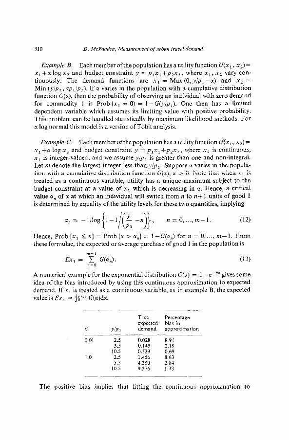
Example C. Each member of the population has a utility function U(x i, x2) = x1 +cc log x2 and budget constraint y = plx, +p2x2, where x2 is continuous, x1 is integer-valued, and we assume y/p, is greater than one and non-integral. Let m denote the largest integer less than y/p,. Suppose CI varies in the popula- tion with a cumulative distribution function G(a), a > 0. Note that when x1 is treated as a continuous variable, utility has a unique maximum subject to the budget constraint at a value of x1 which is decreasing in TV. Hence, a critical value ~1, of cc at which an individual will switch from n to n+ 1 units of good 1 is determined by equality of the utility levels for these two quantities, implying
c(” = -l,log{l-I& +)}, n = 0 )...) nz-1. (12)
Hence, Prob [xi 5 n] = Prob [Z > cc,] = l-G(cc,) for n = O,..., m-l. From ihese formulae, the expected or average purchase of good 1 in the population is
m-l
Ex, = y G(q). “50
(13)
A numerical example for the exponential distribution G(U) = 1 -e-” gives some idea of the bias introduced by using this continuous approximation to expected demand. If x1 is treated as a continuous variable, as in example B, the expected value is Ex, = j$‘P’ G(cr)dcr.
True Percentage expected bias in
0 Y/PI demand approximation
0.01 2.5 0.028 8.94 5.5 0.145 2.1s
10.5 0.529 0.69 1.0 2.5 1.456 5.63
5.5 4.350 2.84 10.5 9.376 1.33
The positive bias implies that fitting the continuous approximation to
D. McFadden, Measurement of urban travel demand 311
data generated by the model will lead to underestimates of the para- meter 8, which in turn will give spuriously high forecasts of the response of
aggregate demand for good 1 to changes in price and income.
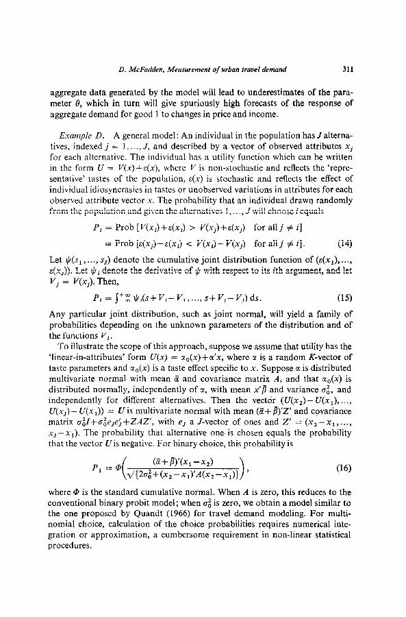
Example D. A general model : An individual in the population has J alterna- tives, indexed j = 1,. . ., J, and described by a vector of observed attributes Xi for each alternative. The individual has a utility function which can be written in the form U = V(X) + F(X), where V is non-stochastic and reflects the ‘repre- sentative’ tastes of the population, E(X) is stochastic and reflects the effect of individual idiosyncrasies in tastes or unobserved variations in attributes for each observed attribute vector x. The probability that an individual drawq randomly from the population and given the alternatives 1, . . ., J will choose i equals
Pi = Prob [V(xi)+&(Xi) > v(xj)+&(Xj) for all j # i]
= Prob [&(xj)-E(x~) < V(XJ- V(xj) for allj # i]. (14)
Let I/+~, . . . . sJ) denote the cumulative joint distribution function of (&(x1), . . . . E(x~)). Let $ i denote the derivative of $ with respect to its ith argument, and let Vi = V(Xj). Then,
Pi = j”z $i(~+Vi-V,,...y s+Vi-VJ)ds. (1%
Any particular joint distribution, such as joint normal, will yield a family of probabilities depending on the unknown parameters of the distribution and of the functions Vi.
To illustrate the scope of this approach, suppose we assume that utility has the ‘linear-in-attributes’ form U(x) = CI~(X)+U’X, where c1 is a random K-vector of taste parameters and a,,(x) is a taste effect specific to x. Suppose a is distributed multivariate normal with mean Or and covariance matrix A, and that aO(x) is distributed normally, independently of CC, with mean x’p and variance ai, and independently for different alternatives. Then the vectdr (U(x,) - U(x,), . . ., U(x,) - U(x,)) = U is multivariate normal with mean (E+ fl)‘Z’ and covariance matrix a$l+oge,e;+ZAZ’, with e, a J-vector of ones and Z’ = (x2-x1, ..,, xJ-x1). The probability that alternative one, is chosen equals the probability that the vector U is negative. For binary choice, this probability is
p1 = cp ( (~+iv(xi-xz> 2/{20~+(X2-X&4(X~-X1)} > ’
(16)
where @ is the standard cumulative normal. When A is zero, this reduces to the conventional binary probit model; when 0; is zero, we obtain a model similar to the one proposed by Quandt (1966) for travel demand modeling. For multi- nomial choice, calculation of the choice probabilities requires numerical inte- gration or approximation, a cumbersome requirement in non-linear statistical procedures.
312 D. McFadden, Mecwrctnent of urban iravcl demand
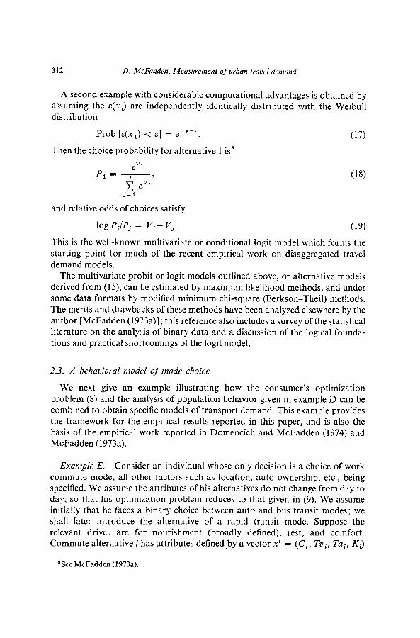
A second example with considerable computational advantages is obtaintd by assuming the E(.Y~) are independently identically distributed with the Wetbull distribution
Prob [E(x~) < c] = eee-‘.
Then the choice probability for alternative 1 is8
(17)
P, = ey ’
7’ C evI
j=l
and relative odds of choices satisfy
log Pi/Pj = vi- vi.
(18)
This is the well-known multivariate or conditional logit model which forms the starting point for much of the recent empirical work on disaggregated travel demand models.
The multivariate probit or logit models outlined above, or alternative models derived from (15), can be estimated by maxim:lm likelihood methods, and under some data formats by modified minimum chi-square (Berkson-Theil) methods. The merits and drawbacks of these methods have been analyzed elsewhere by the author [McFadden (1973a)]; this reference also includes a survey of the statistical literature on the analysis of binary data and a discussion of the logical founda- tions and practical shortcomings of the logit model.
2.3. A behaktal model of mode choice
We next give an example illustrating how the consumer’s optimization problem (8) and the analysis of population behavior given in example D can be combined to obtain specific models of transport demand. This example provides the framework for the empirical results reported in this paper, and is also the basis of the empirical work reported in Domencich and McFadden (1974) and McFadden (1973a).
Example E. Consider an individual whose only decision is a choice of work commute mode, all other factors such as location, auto ownership, etc., being specified. We assume the attributes of his alternatives do not change from day to day, so that his optimization problem reduces to that given in (9). We assume initially that he faces a binary choice between auto and bus transit modes; we shall later introduce the alternative of a rapid transit mode. Suppose the relevant drive, are for nourishment (broadly defined), rest, and comfort. Commute alternative i has attributes defined by a vector xi = (Ci, Tvi, Ta,, Ki)
*See McFadden (1973a).
D. McFadden, Measurement of urban travel demand 313
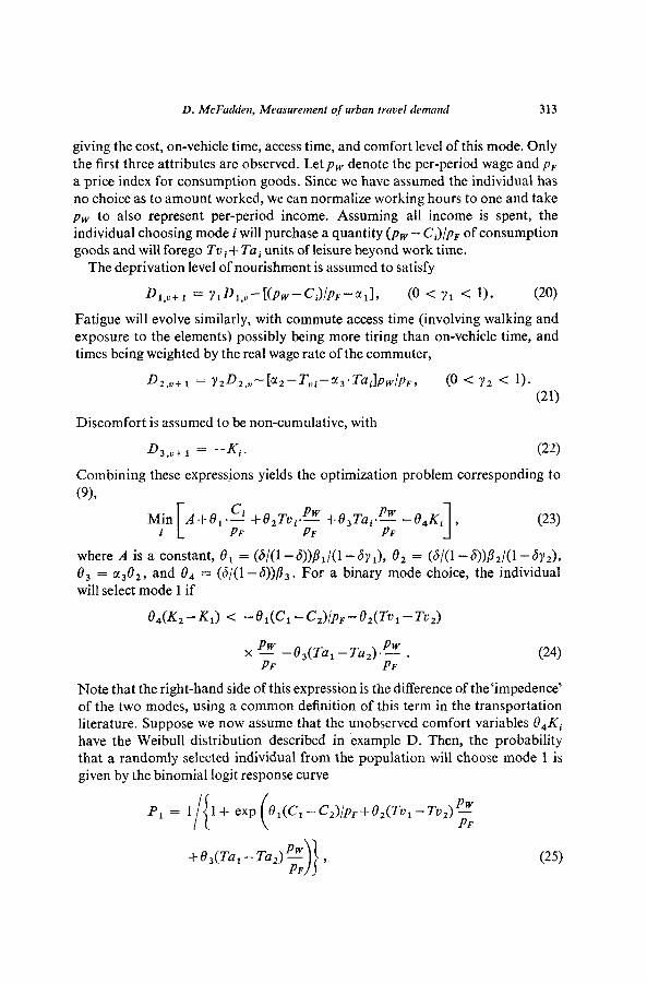
giving the cost, on-vehicle time, access time, and comfort level of this mode. Only the first three attributes are observed. Letp, denote the per-period wage and pr a price index for consumption goods. Since we have assumed the individual has no choice as to amount worked, we can normalize working hours to one and take pw to also represent per-period income. Assuming all income is spent, the individual choosing mode i will purchase a quantity (pw - Ci)/pF of consumption goods and will forego TV i+ Ta i units of leisure beyond work time.
The deprivation level of nourishment is assumed to satisfy
D 1&J+ 1 = Y~D,,“-[(Pw-Ci)/P~-~~l, (0 < Yl < 1). (20)
Fatigue will evolve similarly, with commute access time (involving walking and exposure to the elements) possibly being more tiring than on-vehicle time, and times being weighted by the real wage rate of the commuter,
D 2,v+ 1 = YzD2,“-I~2_T”i_cr,.Tail~w/PF, (0 < Y2 < 1).
(21)
Discomfort is assumed to be non-cumulative, with
D 3,v+1 = --Ki. (22)
Combining these expressions yields the optimization problem corresponding to
(9),
A+O,.s +02Tt,,.e +B,Tai.p~ -OaKi 1 , (23) PF PF
where A is a constant, 0r = (S/(1 -S))p,/(l-6y,), tY2 = (S/(1 -S))j3,/(1-6y,), 0, = Q2, and e4 = (S/(1 -S))p,. F or a binary mode choice, the individual
will select mode 1 if
x pFT -O,(Ta,-Ta,).if . (24)
Mote that the right-hand side of this expression is the difference of the‘impedence’ of the two modes, using a common definition of this term in the transportation literature. Suppose we now assume that the unobserved comfort variables e4Ki have the Weibull distribution described in .example D. Then, the probability that a randomly selected individual from the population will choose mode 1 is given by the binomial logit response curve
P, = 1 l+ exp 1-I (
O,(C,-C,)/p~+e~(TvI_Ttz)p~
+O,(Ta,-Ta,)e PF
(25)
314 D. McFadden, Measurement of urban travel demand
obtained from eq. (18) in the case J = 2 and
This response curve appears frequently in the transportation literature. What is interesting here is not the fact that we are able to derive conventional response curves by a (non-unique) choice of functional forms in a behavioral model, but rather that arguments of the type we have outlined could be used to generate functional forms for practical response curves from detailed analysis of individual behavior.
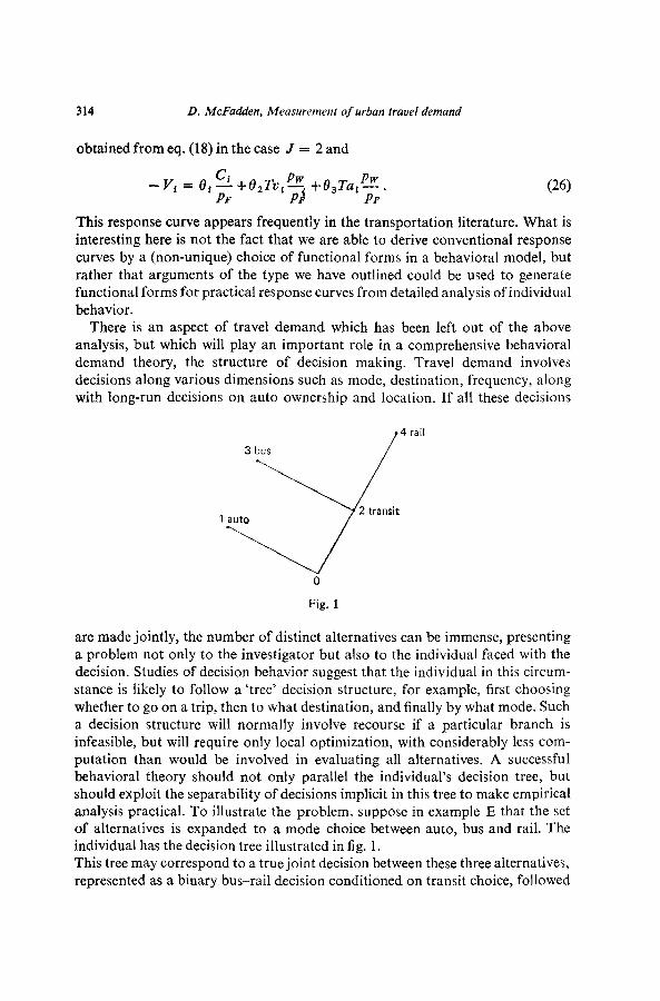
There is an aspect of travel demand which has been left out of the above analysis, but which will play an important role in a comprehensive behavioral demand theory, the structure of decision making. Travel demand involves decisions along various dimensions such as mode, destination, frequency, along with long-run decisions on auto ownership and location. If all these decisions
3 bus
4 rail
1 auto
Fig. 1
are made jointly, the number of distinct alternatives can be immense, presenting a problem not only to the investigator but also to the individual faced with the decision. Studies of decision behavior suggest that the individual in this circum- stance is likely to follow a ‘tree’ decision structure, for example, first choosing whether to go on a trip, then to what destination, and finally by what mode. Such a decision structure will normally involve recourse if a particular branch is infeasible, but will require only local optimization, with considerably less com- putation than would be involved in evaluating all alternatives. A successful behavioral theory should not only parallel the individual’s decision tree, but should exploit the separability of decisions implicit in this tree to make empirical analysis practical. To illustrate the problem, suppose in example E that the set of alternatives is expanded to a mode choice between auto, bus and rail. The individual has the decision tree illustrated in fig. 1. This tree may correspond to a true joint decision between these three alternatives, represented as a binary bus-rail decision conditioned on transit choice, followed
D. McFadden, Measurement of urban travel demand 315
by an auto-transit decision based on the ‘weighted’ attributes of transit. Alterna-
tively, it may represent a true recursive structure in which the auto-transit decision is made based on some ‘average’ perceptionoftransit attributes,followed in the case that the transit leg is chosen by a decision among transit modes. In the first case, decisions can be viewed as being made moving down the tree; in the second case, moving up. Assuming the unobserved term in the rail alterna- tive has a Weibull distribution as in example E, eq. (18) provides the multiple choice probabilities in the case of a joint choice among the final alternatives. Letting Vi, V, , V, denote the ‘representative’ utility of these three alternatives, we have
PI = evl evl
e" + ey3 + ev4 r=-,
e"' + ev2 (27)
where V, is defined to satisfy evZ = ev3 +ev4 and represents the ‘weighted’ utility
of the transit alternative. The probability of bus conditioned on transit is
(28)
On the other hand, an individual moving up the decision tree will use (28) to choose between 3 and 4 once decision point 2 is reached, but may use a different ‘weighting’ for V, in the formula
(29)
For example, the ‘averaging’ rule might be
or V, = Max(V,, V,), (30)
v, = v,p,,,,+ VP4,34. (31)
Both these rules will weigh the transit alternative less positively than the pure conditional logit weighting. The multiple choice models based on (30) and (31) are termed the ‘maximum’ and ‘cascade’ models, respectively. Although these models are plausible empirical alternatives to the conditional logit model, it should be noted that they are not derived from the utility maximization frame- work of example D.9
3. Empirical results10
We report here on the initial results obtained from a three-phase investigation
9The consistency ofdecision tree models under separability assumptions on utility is discussed in detail in Domencich and McFadden (1974).
reThe empirical equations of this paper are revised upon the suggestion of discussants F.X. de Donnea and E. Sheshinski to incorporate the effects of income and after-tax wage (opportunity cost of travel time). A more extensive empirical analysis, including material contained in the previous version of this paper, is given in McFadden (1974).
316 D. McFadden, Measurement of urban travel demand
of patronage forecasting models for rail rapid transit, using data collected in the San Francisco Bay Area before and after the introduction of Bay Area Rapid Transit (BART). The BART system is one of the first totally new fixed rail transit systems built in the United States since the beginning of the century, and is unique in that it combines the advantages of subway-like operation in down- town areas with extensive service corridors in suburban areas. It is fully auto- mated to achieve low running times and headways, and is designed to be com- petitive with the automobile in comfort. It is the prototype of a series of rapid transit projects under consideration in major American cities. Thus, there is potentially a great social return to refining patronage forecasting methods for such systems, and thereby enhancing the accuracy of the cost-benefit analyses on which design and construction decisions are made.
The results below are based on a sample of 213 households living and working in BART ‘accession areas’; a detailed description of the sample is given in McFadden (1973b, ch. II), which is also the source of the following summary:
The Work Travel Study was undertaken to examine factors in the choice of travel mode to work among Bay Area residents prior to the opening of the new Bay Area Rapid Transit System. Since resources did not permit the inter- viewing of more than about 200 respondents, the study did not attempt a full geographic coverage of the Bay Area or a coverage of all types of commuting patterns. Rather, it focused on three considerations.
First, interviewing was confined to household residents of a Y-shaped area of Alameda and Contra Costa Counties, centering on the major industrial cities of Oakland and Berkeley and on the small city of Emeryville lying between them. It also encompassed surrounding suburban areas lying suffi,ciently close to the radiating BART lines to make commuting by BART into the central area a realistic possibility.
Second, interviewing was restricted to employed persons whose usual places of work were within the cities of Oakland, Berkeley, or Emeryville or across the bay in San Francisco or Daly City. This restriction was imposed in the belief that subsequent work travel on BART initiating within the study area would consist primarily of movements (a) within and between the core cities of Oakland, Berkeley and Emeryville; (b) into these core areas from surround- ing suburban areas; and (c) from these areas to San Francisco or to the endpoint of the San Francisco BART line in Daly City.
Third, since persons living closest to BART stations seemed most likely to use the new system, the sample was disproportionately drawn from persons residing in census tracts containing BART stations or immediately adjacent to them (hereafter, these shall be called BART contiguous tracts). The remainder of the area was more lightly sampled. As a rough goal, the sample was to consist of approximately equal numbers of commuters residing in (a) BART contiguous tracts of the core cities, (b) other tracts of the core cities,
D. MrFaddcn, Measurement of urban travel demand 317
(c) BART contiguous tracts of surrounding suburban areas, and (d) other tracts of the surrounding suburban areas.
While controlling approximate numbers in these four cells, the sample also was to be drawn in such a way as to permit the preparation of unbiased estimates of the characteristics of all household residents of the study area commuting to the designated cities. Thus, respondents could not be chosen simply to meet a predesignated quota; rather, they had to be part of a care- fully controlled probability sample.
This was accomplished by dividing the study area into a number of carefully defined geographic strata and then by sampling each stratum by multistage area probability sampling methods. After the strata were designated, one or more census tracts were chosen from each stratum, with probability pro- portionate to the stratum’s number of housing units. One city block was then chosen from each sampled tract by the same method, a list was prepared of all housing units on each sampled block, and approximately equal numbers of housing units were then chosen from each block by systematic random sampling from the list. Thus, in each stratum all housing units had the same probability of selection. Although sampling ratios varied from stratum to stratum - that is, a larger proportion of households were chosen in some strata than in others to provide the desired numbers of commuters of each type called for by ;!re design-estimates for the full study area could be prepared by appropriately weighting the stratum results.
The task of designing a sample to meet these goals was greatly complicated by the need to screen comparatively large numbers of households to locate persons commuting to work in the designated cities. Many suburban residents, of course, are employed in their own communities rather than in the central cities. In addition, many households - especially in the central cities - contain no employed persons but only those who are retired, unemployed, or supported by Welfare. Data from a previous survey and from the 1970 Census were employed to estimate the total sample necessary to yield the desired number of cases of each type, but these provided only approximate guides, and during the course of the fieldwork it proved necessary to augment the original sample in order to obtain the desired numbers. A total of 710 occupied households was ultimately contacted to achieve a final sample of 213 interviews.
A reinterview of this sample, combined with a retrospective interview of a larger sample, will be carried out in 1975 to extend and validate the models considered in the current analysis.
The survey data was augmented with careful calculations of travel time, costs, congestion, and related variables for existing auto and bus modes, and for projected BART service. The auto data was collected by F. Reid; the pro- cedures are described in McFadden (1973b, ch. III). The bus data was collected by M. Johnson; as described in McFadden (1973b, ch. IV).
B
318 D. McFadden, Measurement of urban travel demand
In order to limit the size of the investigation and to concentrate on the simplest and best understood travel behavior where the advantages and dis- advantages of alternative models could be most easily detected, attention was confined to work trip behavior, specifically mode choice and timing of the commute trip. We report here only on the mode choice decision.
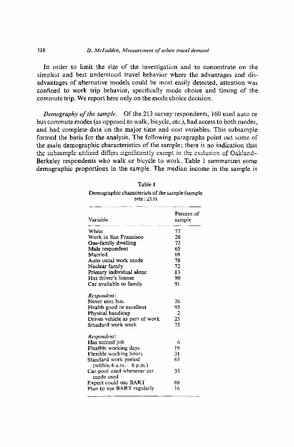
Demography of the sample. Of the 213 survey respondents, 160 used auto or bus commute modes (as opposed to walk, bicycle, etc.), had access to both modes, and had complete data on the major time and cost variables. This subsample formed the basis for the analysis. The following paragraphs point out some of the main demographic characteristics of the sample; there is no indication that the subsample utilized differs significantly except in the exclusion of Oakland- Berkeley respondents who walk or bicycle to work. Table 1 summarizes some demographic proportions in the sample. The median income in the sample is
Table 1
Demographic characterists of the sample (sample size : 213).
Variable Percent of sample
White 17 Work in San Francisco 26 One-family dwelling 72 Male respondent 65 Married 69 Auto usual work mode 78 Nuclear family Primary individual alone Has driver’s license Car available to family
Respondenr : Never uses bus Health good or excellent Physical handicap Drives vehicle as part of work Standard work week
Respondent: Has second job Flexible working days Flexible working hours Standard work period
(within 6 a.m. - 6 p.m.) Car pool used whenever car
mode used
72 13 90 91
26 95
2 25 75
6 19 31 65
33
Expect could use BART 69 Plan to use BART regularly 16
D. McFadden, Measurement of urban travel demand 319
$12,500, the average number of adults over sixteen is 2.23, the average age of the respondent is forty-one, the average number of household members employed is 1.6, and the average number of cars per worker is 1.29. These figures are generally comparable to census statistics for families with employed members.
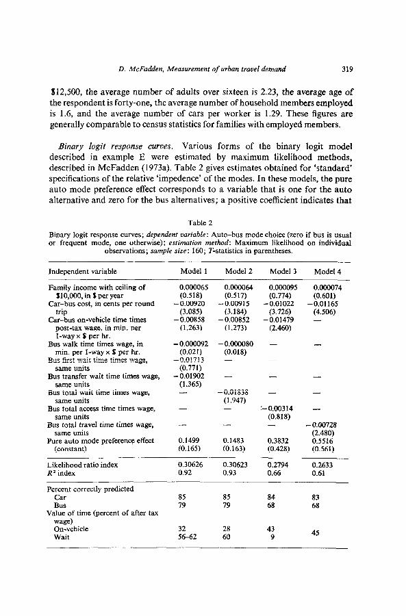
Binary logit response curves. Various forms of the binary logit model described in example E were estimated by maximum likelihood methods, described in McFadden (1973a). Table 2 gives estimates obtained for ‘standard’ specifications of the relative ‘impedence’ of the modes. In these models, the pure auto mode preference effect corresponds to a variable that is one for the auto alternative and zero for the bus alternatives; a positive coefficient indicates that
Table 2
Binary logit response curves; dependent variable: Auto-bus mode choice (zero if bus is usual or frequent mode, one otherwise); estimation method: Maximum likelihood on individual
observations; sample size: 160; T-statistics in parentheses.
Independent variable Model 1 Model 2 Model 3 Model 4
Family income with ceiling of $10,000, in IE per year
Car-bus cost, in cents per round trip
Car-bus on-vehicle time times post-tax wage, in mm. per l-way x 0 per hr.
Bus walk time times wage, in min. per l-way x S per hr.
Bus first wait time times wage, same units
Bus transfer wait time times wage, same units
Bus total wait time times wage, same units
Bus total access time times wage, same units
Bus total travel time times wage, same units
Pure auto mode preference effect (constant)
0.000065 0.000064 o.oooo95 (0.518) (0.517) (0.774)
- 0.00920 -0.00915 -0.01022 (3.085) (3.184) (3.726)
-0.00858 -0.00852 - 0.01479 (1.263) (1.273) (2.460)
- 0.000092 (0.021)
-0.01713 (0.771)
- 0.01902 (1.365) -
- 0.000080 (0.018) - -
- -
-0.01838 (1.947) -
-
0.1499 0.1483 0.3832 (0.165) (0.163) (0.428)
:--0.00314 (0.818) -
0.000074 (0.601)
-0.01165 (4.506) -
-
-
-
- 0.00728 (2.480) 0.5516 (0.561)
Likelihood ratio index 0.30626 0.30623 0.2794 0.2633 R2 index 0.92 0.93 0.66 0.61
Percent correctly predicted Car Bus
Value of time (percent of after tax wage) On-vehicle Wait
85 85 84 83 79 79 68 68
32 28 43 56-62 60 9 45
320 D. McFadden, Measurement of urban travel demand
when the remaining variables are zero, more than half the population will choose auto. Bus transfer wait time is calculated directly from transit schedules. Initial wait time is taken to be one-half the average headway on the initial carrier for the home to work and the work to home trips, with a ceiling of a fifteen-minute wait; this measure will be biased upward when commuters can follow transit schedules. Bus walk time is computed from the number of blocks walked at the origin and destination, assuming a walking time of two minutes per block. Models l-4 ignore the possibility of auto access to transit even though twenty- two percent of the bus riders use auto access to bus. Thus, walk time may be a substantial overestimate of actual bus access time, particularly for suburban commuters where the ‘park-ride’ option is most common. This shortcoming of the empirical analysis may explain the unexpected insignificance of the coefficient of bus walk time in these models. l1
The likelihood ratio index and R2 index reported in table 2 are measures of goodness of fit discussed in McFadden (1973a). The R2 index is similar to the multiple correlation coefficient in ordinary least squares; the likelihood ratio index is a more stable and statistically satisfactory measure for the estimation method used. The models of table 2 all give coefficients of expected sign. With the exception of bus walk time, the implied valuations of time agree with previous estimates [Quarmby (1967), Thomas (1971)]; at the sample mean after- tax wage of $3.87 per hour, the value of on-vehicle time is $1.23 per hour and the value of wait time is $2.32 per hour. However, because of the low precision of the estimates of the travel time coefficients, we cannot reject at the ten percent level the hypothesis that all components of travel time are weighed equally.
Weighting of time and cost components. The specification of the models in table 2 can be tested against alternative hypotheses that different travel time and cost variables and other factors have distinguishable effects on behavior. Of particular interest are the questions of whether mode attributes can be measured generically using conventional time and cost variables, and whether components of time and cost are weighted equally. We summarize the conclusions; the estimates on which they are based are given in McFadden (1974).
(a) We accept at the ten percent level the hypothesis that auto and bus on-vehicle times are weighed the same. The power of the test is low, and the point estimates imply an average premium of $0.88 per hour in the weight attached to bus travel. This premium could reflect the reduced comfort and privacy of bus transit which are not measured directly.
(b) We accept at the ten percent level the hypotheses that no weight is given to schedule delay (defined as the average of the waiting times at the workplace before the job begins and after the job ends which are required to fit bus
* ‘A conditional logit analysis treating bus with walk and ride access as distinct alternatives is reported in McFadden (1974).

D. McFadden, Measurement of urban travel demand 321
schedules), number of transfers, or auto time spent in driving on freeways at less than twenty miles per hour. The power of the tests is again low. The estimates provide speculative, but plausible, values of $3.33 per hour for schedule delay, 15.5 cents per transfer, and a prentiunt of $2.13 per hour on auto time spent driving under congested conditions.
(c) We accept at the ten percent level the hypothesis that the value of travel time is linear homogeneous in the after-tax wage rate. The estimates suggest, however, that value of time may be an increasing function of the wage rate. This conclusion, if substantiated, would be consistent with hours-worked decisions more closely approximating the neoclassical labor-leisure margin at higher wage levels, or with imperfect correlation of measured and effective wages in labor markets segmented by wage rate.i2
(d) We accept at the ten percent level the hypotheses of equal weighting of total auto costs and total bus costs, and of auto mileage, tolls, parking, and maintenance costs. The estimates suggest that mileage and maintenance costs may not be weighed as heavily as tolls and parking costs; however, the precision of these estimates is quite low.
Because of the small sample size, none of the tests above are conclusive, and should be taken only as suggestions for further research.
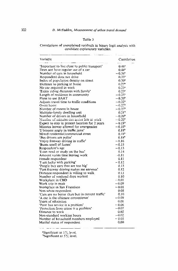
Inventory of possible explanatory variables. In order to make an inventory of the large number of additional variables which might influence mode choice, we posed the question of whether the ‘unexplained residual’ from the binary logit model was correlated with these variables. This was done by calculating trans- formed residuals from the logit estimating equation, and correlating these residuals with the list of candidate explanatory variables. This method was devised for the binary logit case by Cox (1970); an essentially equivalent multi- nomial transformation described in McFadden (1973a) was used in the present analysis. The residuals are derived from Model 1. They are distributed with zero mean and unit variance if Model 1 is correct, and in this analysis are positive when bus is chosen, negative otherwise. (Hence, a positive correlation indicates high values of the explanatory variable are associated with increased bus use.) Table 3 is a selected list of variables correlated with the residuals; those signi- ficant at the five percent level are candidates for inclusion in further estimation. It should be noted that some of the significant correlations are with variables which we would expect to be jointly determined with mode choice rather than predetermined at the point the mode choice decision is made. The behavioral model should be expanded to include a theory of this simultaneous choice.
A number of correlations in table 3 deserve comment. First, there are variables,
“This conclusion is based on unpublished research by Luke Chan, University of California, Berkeley.
322 D. McFadden, Measurement of urban travel demand
Table 3
Correlations of unexplained residuals in binary logit analysis with candidate explanatory variables.
Variable ~.______ _
‘Important to live close to public transport’ Does not have regular use of a car Number of cars in household Respondent does not drive Index of population density on street Distance to parking at home No car required in work ‘Enjoy riding distances with family’ Length of residence in community Plans to use BART Adjusts travel time to traffic conditions Owns home Number of rooms in house Multiple-family dwelling unit Number of drivers in household Number of minutes can arrive late at work Expect to stay in present location for 2 years Minutes leeway allowed for emergencies ‘I become angry in traffic jams’ Mixed residential/commercial street ‘Bus drivers are polite’ ‘Enjoy freeway driving in traffic’ ‘Buses smell of fumes’ Respondent’s age ‘I can read or study on the bus’ Amount varies time leaving work Female respondent ‘I am lucky with parking’ ‘People buy cars that are too big’ ‘Fast freeway driving makes me nervous’ Distance respondent is willing to walk Number of weekend days worked Workplace in CBD Work trip in peak Workplace in San Francisco Non-white respondent ‘Cars are no better than bus in current traffic’ ‘A car is the ultimate convenience’ Years of education ‘Poor bus service is a problem’ ‘Protection from crime is a problem’ Distance to work Non-standard working hours Number of household members employed Marital status of respondent
“Significant at 1 % level. %ignificant at 5 o/o level.
Correlation
0.48” 0.44”
- 0.34” 0.33” 0.30” 0.27” 0.23” 0.23”
-0.23; -0.20b -0.22b -0.22b - 0.22”
0.21 b - 0.20b - 0.20b -0.19b -0.18b
O.lgb O.lgb O.lgb
-0.16 -0.15 -0.13
0.14 -0.11
0.11 -0.12
0.13 0.12 0.13 0.10
- 0.01 -0.09 -0.01
0.08 0.10
-0.09 0.01
-0.06 - 0.07
0.02 -0.02 - 0.05
0.00
-
D. McFadden, Measurement of urban travel demand 323
such as (the respondent does not drive), which indicate whether the respondent has access to the auto mode. The model should clearly either screen out in- dividuals with these atypical choice sets or include explanatory variables identi- fying these cases. There is the danger that some variables of this type are simul- taneously determined by mode choice; to avoid the statistical problems associated
with simultaneity, instrumental variables methods may be required. Second, variables such as (number of cars in household) tend to be correlated
due to the joint determination of auto ownership and mode choice. We report elsewhere on estimation of the simultaneous auto ownership and mode choice decisions using instrumental variables methods within the binary logit frame-
work [McFadden (1974)]. Third, variables such as (distance to parking at home) and (no car required in
work) represent legitimate explanatory factors that appear to reflect attributes of modes not captured in the summary time and cost measures.
Fourth, variables such as (length of residence in community) and (owns home) reflect socioeconomic factors which appear to influence the distribution of tastes.
Fifth, variables such as (index of population density on street), (‘important to live close to public transit’), and to some extent (number of rooms in house), (owns home), etc. are all related to the location decision, which in turn may be made jointly with the mode choice. These correlations suggest that there is a significant relationship between these decisions. If individuals with pro-bus tastes or relatively low valuations of time locate where bus impedence is relatively low, and vice versa, and Model 1 is estimated without taking this effect into account, then the steepness of the estimated response curve is exaggerated, and one may forecast too high an incremental response to a policy change.
Sixth, a few attitude variables are significant: (‘enjoy riding distances with family’), (‘I become angry in traffic jams’), and (‘bus drivers are polite’). These may reflect a causal effect of attitudes on tastes and behavior, or alternatively may themselves be jointly determined with’mode choice by more basic explana- tory factors. The interest in attitude variables from the standpoint of transport policy analysis lies in the question of whether planners can influence behavior by campaigns to modify attitudes. A demand model with explanatory attitude variables is not useful in answering this question unless the mechanism for the action of public relations programs on these attitudes can be discovered. In the latter case, one may well be able to bypass the measurement of attitudes entirely, and concentrate directly on the relation between publicity campaigns and mode choice behavior. Alternatively, one may wish to develop models of the simul- taneous processes of attitude formation and modification of travel behavior. Neither of these alternatives suggests that it is particularly useful to estimate travel demand models treating attitudes as pure explanatory variables. The current inventory of attitude items indicates that with the exception of (‘bus drivers are polite’), there is little relation between behavior and the attitudes that might be influenced by a campaign publicizing the attributes of transit.
324 D. McFadderr, Mcasuretnent of urbarr rraoel demand
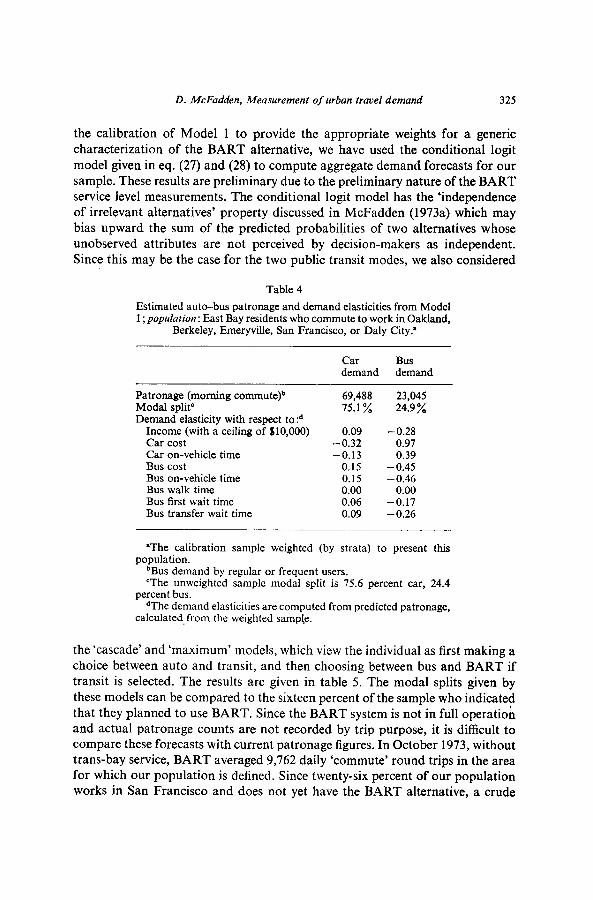
Travel demandforecasts. The binary logit response curves estimated in table 1 provide a basis for predicting or forecasting individual mode choice, both for the existing auto-bus alternatives and for the auto-bus-rail alternatives available after BART is fully operational. Further, by inference from the sample to the population from which it is drawn, one can forecast aggregate modal split.
Suppose we have a sample that is representative of the population and a logit model such as Model 1 estimated either from the sample or from external sources. Then, the predicted probability for any individual in the sample is a best estimate of the distribution of responses in the population by those individuals facing the same environments. Since the sample represents a (weighted) random selection of the environments faced by the population as a whole, the (inversely weighted) average of the predicted probabilities over the sample is a best estimate of aggregate demand. ’ 3 The influence of transport policy on aggregate demand can then be assessed by computing its effect on the sample average. It should be noted that this procedure provides a more accurate measure of demand elasticities than can be obtained by the conventional method of computing the elasticity of the respo;lse curve at the mean of the independent variables : Aggregate demand is the average of the response curve weighted by the distribution of the indepen- dent variable. If a substantial proportion of the population faces relative impedences which are sufficiently extreme to elicit almost certain mode choices in one direction or the other, then a small change in the impedence of one of the modes will still leave the relative impedence for this proportion of the population sufficiently extreme to almost certainly determine mode choice. As a result, the response of aggregate demand to this impedence change will be low, and will bear no systematic relation to the elasticity of the response curve at the data mean.
Table 4 presents computations of the aggregate modal split (observed weighted sample frequency) for the auto-bus choice, and the elasticity of these aggregate demands with respect to changes in the explanatory variables. The elasticity values are relatively low, as is normally expected for short-run travel demand. They suggest that the most effective way to increase bus patronage is to increase auto costs, say, by introducing parking or gasoline taxes. A ten percent reduction in bus fares or in running times would each yield a patronage increase of approxi-
mately five percent. We next turn to the question of forecasting demand for a new mode, BART.
Using engineering forecasts of BART service levels made in July 1972, and taking
13An alternative method of computing aggregate demands is to specify a distribution of the indepqndcnt variables in the population a,ld compute anniytical!y or numerically the expecta- tion of the response curve with respect to :his distribution. This can be done particularly con- veniently in the case of binary probit analysis: If the independent variables x are normally distribuied with mean 1 and covariance matrix A, and the probit response curve is P = @g(@x), then aggregate demand is given by D = @{O’~/,l(l+t)‘AO)). This demand again has the proper;; that the more disperse the distribution ok ihe independent variables, the lower the demand elasticities.
D. McFadden, Measurement of urban travel demand 325
the calibration of Model 1 to provide the appropriate weights for a generic characterization of the BART alternative, we have used the conditional logit
model given in eq. (27) and (28) to compute aggregate demand forecasts for our sample. These results are preliminary due to the preliminary nature of the BART service level measurements. The conditional logit model has the ‘independence of irrelevant alternatives’ property discussed in McFadden (1973a) which may bias upward the sum of the predicted probabiiities of two alternatives whose unobserved attributes are not perceived by decision-makers as independent. Since this may be the case for the two public transit modes, we also considered
Table 4
Estimated auto-bus patronage and demand elasticities from Model 1 ;population: East Bay residents who commute to work in Oakland,
Berkeley, Emeryville, San Francisco, or Daly City.a
Car Bus demand demand
Patronage (morning commute)b Modal spW Demand elasticity with respect to !
Income (with a ceiling of $10,000) Car cost Car on-vehicle time Bus cost Bus on-vehicle time Bus walk time Bus first wait time Bus transfer wait time
69,488 23,045 75.1% 24.9 %
0.09 - 0.28 -0.32 0.97 -0.13 0.39
0.15 - 0.45 0.15 -0.46 0.00 0.00 0.06 -0.17 0.09 -0.26
“The calibration sample weighted (by strata) to present this population.
bB~s demand by regular or frequent users. ‘The unweighted sample modal split is 75.6 percent car, 24.4
percent bus. “The demand elasticities are computed from predicted patronage,
calculated,from the weighted sample.
the ‘cascade’ and ‘maximum’ models, which view the individual as first making a choice between auto and transit, and then choosing between bus and BART if transit is selected. The results are given in table 5. The modal splits given by these models can be compared to the sixteen percent of the sample who indicated that they planned to use BART. Since the BART system is not in full operatioh and actual patronage counts are not recorded by trip purpose, it is difficult to compare these forecasts with current patronage figures. In October 1973, without trans-bay service, BART averaged 9,762 daily ‘commute’ round trips in the area for which our population is defined. Since twenty-six percent of our population works in San Francisco and does not yet have the BART alternative, a crude
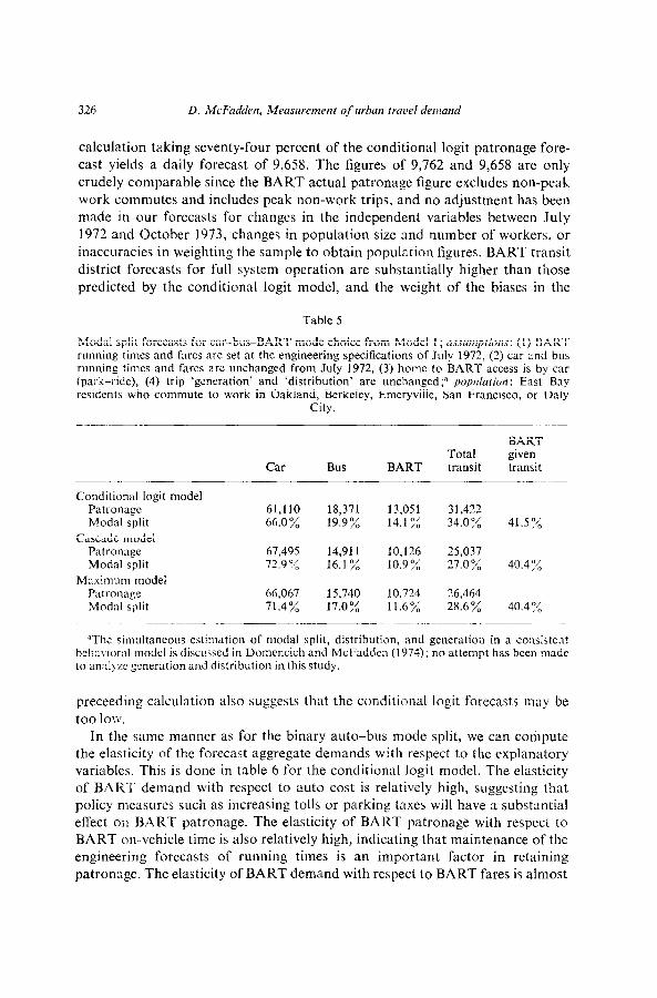
326 D. McFadden, Measurement of urban travel demand
calculation taking seventy-four percent of the conditional logit patronage fore- cast yields a daily forecast of 9,658. The figures of 9,762 and 9,658 are only crudely comparable since the BART actual patronage figure excludes non-peak work commutes and includes peak non-work trips, and no adjustment has been made in our forecasts for changes in the independent variables between July 1972 and October 1973, changes in population size and number of workers, or inaccuracies in weighting the sample to obtain population figures. BART transit district forecasts for full system operation are substantially higher than those predicted by the conditional logit model, and the weight of the biases in the
Table 5
Modal split forecasts for car-bus-BART mode choice from Model I ; assunptiorts: (1) SART running times and fares are set at the engineering specifications of July 1972, (2) car and bus running times and fares arc unchanged from July 1972, (3) home to BART access is by car (park-ride), (4) trip ‘generation’ and ‘distribution’ are unchanged;” population: East Bay residents who commute to work in Oakland, Berkeley, Emeryvillc, San Francisco, or Daly
City.
Car BUS BART Total transit
BART given transit
Conditional logit model Patronage Modal split
Cascade model Patronage Modal split
Maximum model Patronage Modal split
61,110 18,371 13,051 3 1,422 66.0% 19.9% 14.1% 34.0% 41.5%
67,495 14,911 10,126 25,037 72.9 ;,; 16.1% 10.9% 27.0% 40.4 ;,‘,
66,067 15,740 10,724 26,464 71.4% 17.0% 11.6% 28.6% 40.4 :/,
“The simultaneous estimation of modal split, distribution, and generation in a consistent behavioral model is discussed in Domencich and McFadden (1974); no attempt has been made to an:~1yzc generation and distribution in this study.
preceeding calculation also suggests that the conditional logit forecasts may be
too low. In the same manner as for the binary auto-bus mode split, we can corilpute
the elasticity of the forecast aggregate demands with respect to the explanatory variables. This is done in table 6 for the conditional logit model. The elasticity of BART demand with respect to auto cost is relatively high, suggesting that policy measures such as increasing tolls or parking taxes will have a substantial effect on BART patronage. The elasticity of BART patronage with respect to BART on-vehicle time is also relatively high, indicating that mairrtenance of the engineering forecasts of running times is an important factor in retaining patronage. The elasticity of BART demand with respect to BART fares is almost
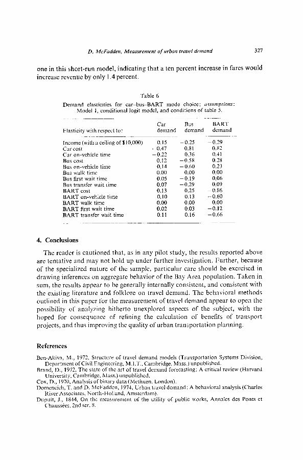
D. A4cFadden, Measurement of urban trove1 demand 327
one in this short-run model, indicating that a ten percent increase in fares would increase revenue by only 1.4 percent.
Table 6
Demand elasticities for car-bus-BART mode choice; asmn~pfions: Model 1, conditional logit model, and conditions of table 5.
Elasticity with respect to: Car Bus BART demand demand demand
Income (with a ceiling of 810,000) 0.15 -0.25 -0.29 Car cost -0.47 0.81 0.82 Car on-vehicle time -0.22 0.36 0.41 Bus cost 0.12 -0.58 0.28 Bus on-vehicle time 0.14 -0.60 0.23 Bus walk time 0.00 0.00 0.00 Bus first wait time 0.05 -0.19 0.06 Bus transfer wait lime 0.07 -0.29 0.09 BART cost 0.13 0.25 -0.S6 BART on-vei-.;cle time 0.10 0.13 -0.60 BART walk time 0.00 0.00 0.00 BART first wait time 0.02 0.03 -0.12 BART transfer Wait time 0.11 0.16 -0.66
4. Conclusions
The reader is cautioned that, as in any pilot study, the results reported above are tentative and may not hold up under further investigation. Further, because of the specialized nature of the sample, particular care should be exercised in drawing inferences on aggregate behavior of the Bay Area population. Taken in sum, the results appear to be generally internally consistent, and consistent with the existing literature and folklore on travel demand. The behavioral methods outlined in this paper for the measurement of travel demand appear to open the possibility of analyzing hitherto unexplored aspects of the subject, with the hoped for consequence of refining the calculation of benefits of transport projects, and thus improving the quality of urban transportation planning.
References
Ben-Akiva, Ij4., 1972, Structure of travel demand models (Transportation Systems Division, Department ofCivil Engineering, M.I.T., Cambridge, Mass.) unpublished.
Brand, D., 1972, The slate of the art of travel demand forecasting: A critical review (Harvard University, Cambridge, Mass.) unpublished.
Cox, D., 1970, Analysis of binary data (Methuen, London). Domencich, T. and D. h?cFadden, 1974, Urban travel demand: A behavioral analysis (Charles
River Associates, North-Holland, Amsterdam). Dupuit, J., 1844, On the measurement of the utility of public works, Annales des Ponts et
Chaussees, 2nd ser. 8.
328 D. McFadden, Measurement of urban travel demand
Lisco, T., 1967, The value of commuters’ travel time -A study in urban transportation, dissertation (University of Chicago, Chicago, Ill.).
McFadden, D., 1968, The revealed preferences of a government bureaucracy (Department of Economics, University of California, Berkeley, Calif.) unpublished.
McFadden, D., 1973a, Conditional logit analysis ofqualitative choice behavior, in: P. Zarembka, ed., Frontiers in econometrics (Academic Press, New York).
McFadden, D., 1973b, Travel demand forecasting study, BART Impact Study Final Report Series (Institute of Urban and Regional Development, University of California, Berkeley, Calif.) unpublished.
McFadden, D., 1974, The measurement of urban travel demand, II (Department of Economics, University of California, Berkeley, Calif.) unpublished.
McFadden, D. and F. Reid, 1974, Aggregate travel demand forecasting from disaggregated behavioral models (Department of Economics, University of California, Berkeley, Calif.) unpublished.
Meyer, J., J. Kain and M. Wohl, 1966, The urban transportation problem (Harvard University Press, Cambridge, Mass.).
Oi, W. and P. Shuldiner, 1962, An analysis of urban travel demands (Northwestern University Press, Evanston, Ill.).
Quandt, R. and W. Baumol, 1966, The demand for abstract transport modes: Theory and measurement, Journal of Regional Science 6,13-26.
Quarmby, G., 1967, Choice of travel mode for the journey to work: Some tindings, Journal of Transport Economics and Policy 1.
Stopher, P. and T. Lisco, 1970, Modelling travel demand: A disaggregate behavioral approach - Issues and applications, Transportation Research Forum Proc., 195-214.
Thomas, T. and G. Thompson, 1971, Value of time saved by trip purpose, Highway Research Record369,104-113.
Warner, S., 1962, Stochastic choice of mode in urban travel: A study in binary choice (North- western University Press, Evanston, Ill.).
Related Documents