The Markowitz Model Selecting an Efficient Investment Portfolioramanujan.math.trinity.edu/tumath/research/studpapers/s21.pdf · The Markowitz Model Selecting an Efficient Investment

The Markowitz Model Selecting an Efficient Investment Portfolio

Allison Beste Dennis Leventhal Jared Williams

Dr. Qin Lu

Lafayette College Mathematics REU Program 2002

Introduction: Consider a portfolio P consisting of n securities, In this portfolio, each security is weighted on a percentage basis by such that the sum of these weights equals one. Note that these weights can be negative, indicating a short sale. (A short sale in where an investor borrows a share of stock from a broker and sells it hoping the price will decrease so that the investor can buy it back later at a lower price.) Additionally, let

.,,1 nSS K

nxx ,,1 K

iµ be the expected return on investment on a percentage basis of the security. Thenthi pµ , the expected return of a portfolio, is the weighted sum of each security’s expected return, given by the following equation:

.1∑=

µ=µn

iiip x (1)

One measure of the risk associated with the i security is the variance of its return,σ . The variance of a portfolio is

th 2i

∑∑∑= <=

+σ=σn

i ijji

n

iii xxx

11

222 j)Cov(i, (2)

where Cov(i,j), a measure of correlation, is the covariance between the i and securities,. We assume that the random return of a security is normally distributed, so the random vector of returns is drawn from a multivariate normal distribution. As a result, the expected return and variance of any security is finite.

th thj

The financial model of mean-variance analysis, developed by Harry Markowitz in 1952, assumes that investors prefer greater return and less risk. The model treats any portfolio as a single point in the σ plane. Markowitz claimed that the set of all portfolios form a hyperbola in the σ plane[1].

µ−µ−

The model originally incorporated iso-mean and iso-variance surfaces for proving portfolio optimization. An iso-variance surface is the set of all portfolios in the 121 −−−− nxxx K space that have the same variance. Similarly, an iso-mean surface is the set of all portfolios in that space that have the same expected return. Note that iso-mean surfaces always take the shape of (n-2)-dimensional planes while iso-variance surfaces are always ellipsoids. In a three-security model, they take the shape of lines and ellipses, respectively. However, the geometric visualization required with this method makes it difficult to see the generalization past the three-security case.

The point of tangency between iso-mean and iso-variance curves is indeed a frontier portfolio. Additionally, the set of these frontier portfolios form a hyperbola in the plane. µ−σ

New methods have been developed that generalize more easily to higher-dimensional instances while maintaining the basic concept of mean-variance analysis. The basic setup of the model, as noted in Huang’s book[2], is as follows:

1

E(P) :Such that

Var(P)21

21 Minimize

=

==

=

1x

µx

Vxx

T

T

T

pµ , (3)

where:

[ ][ ]

[ ]portfolio. for thereturn expected of level desired theis and

1,,1,1

returns ofmatrix covariance theis returns expected of vector the,,,

securityeach for weightsportfolio oftor column vec a ,,,,

1

21

p

n

nxxx

µ=

µµ=

=

T

T

T

1

Vµ

x

K

K

K

We also assume that V is invertible and that no two securities can have the same expected return Note that this is typically the case when using real data. j).i, ( ∀µ≠µ ji

Any that is a solution to this system for a given xpµ is called a frontier portfolio. By this method, the set of

all frontier portfolios still form a hyperbola in the µ−σ plane, matching Markowitz’s original method.

0.35 0.45 0.5 0.55

0.05

0.1

0.15

0.2

0.25

0.3

Figure 1

Markowitz hyperbola with Some example portfolios

This hyperbola is also referred to as the Markowitz frontier and is defined by the following equation:

1)(1

2

22

=−µ

−σ

CD

CA

C (4)

where:

.2

1

1

11

ABCDCBA

−=

=

=

==

−

−

−−

1V1eVe

1VeeV1

T

T

TT

(5)

Recall that covariance matrices are by definition non-negative definite[3]. However, since we assume the invertibility of V, we can infer that V is positive definite. As a result of this,

for any vector . Therefore, is also positive definite, so Now we’ll claim that D > 0. Consider the identity

0>VxxT 0x ≠ 1−V .0 and 0 >> CB

).()()( 21 ABCBBABA −=−− − 1eV1e T (6) Note that − BA is implied by a previous assumption that (01e ≠ j).i, ∀µ≠µ ji

)( 2 >− ABCB

Since

is positive definite, the left-hand side is always positive. Therefore, But, since B > 0, must be positive. Therefore, D > 0.

1−V .02A−BC

This hyperbola has a vertex at ).,1(),CA

C=µσ( The upper half of the hyperbola is

called the efficient frontier while the bottom half is referred to as the inefficient frontier. Note that for any portfolio on the inefficient frontier, you could hold your level of risk (standard deviation) constant and increase your expected return by moving up to the efficient frontier; therefore, the optimal portfolios occur on the upper half of the hyperbola (insert small graph here?).

Given this hyperbola of the frontier portfolios, the minimal level of risk, , can be deduced for a desired level of expected return from equation (4). Furthermore, according to Huang[2], unique portfolio weights can be determined for securities that lie on the hyperbola as a linear function of expected return as follows:

σ

pp µ+= hgx (7) where

)]()([1 11 eV1Vg −− −= ABD

. (7a)

)]()([1 11 1VeVh −− −= ACD

(7b)

Section 1: In [2], Huang showed that the portfolio weights on the Markowitz hyperbola are unique.

However, he did not address the question of whether the ),( µσ points inside the hyperbola have unique weights associated with them.

Theorem 1: Non-uniqueness of portfolio weights inside the hyperbola Consider the sets of all iso-variance ellipsoids and all iso-mean planes. Specifically,

consider the set of all points of tangency between iso-mean and iso-variance surfaces. These points will lie on a line, called the critical line, in 121 −−−− nxxx K

),space. Markowitz proved that

the critical line is the set of all portfolio weights whose ( µσ combination lie on the hyperbola[5]. Now return to the question of whether points inside the hyperbola have unique portfolios associated with them. Let the point be inside the hyperbola. Consider the iso-

variance ellipsoid with variance σ and the iso-expected return plane with value µ . Since

is inside the hyperbola, we know that the iso-mean and iso-variance curves do intersect, but since this point is not on the frontier, the intersection(s) is/are not a point of tangency. In the three security case, we have a planar ellipse for our iso-variance ellipsoid and a line for our iso-expected return plane. Thus, we conclude that there exists two intersections between the iso-variance ellipse with variance σ

), *µ( *σ*

*

*

),( ** µσ

2 and the iso-expected return line with expected return , because a line and ellipse that intersect non-tangentially must intersect at exactly two points in two-dimensional space. Therefore, for the three security case, every point inside the frontier has exactly two portfolios associated with it.

*µ

For the four security case, we get the set of non-tangential intersections between an ellipsoid and a plane in 3-space. Thus, there exist infinitely many portfolios for any point inside

the frontier for this case. The conclusion that there exist infinitely many portfolios for any point inside the frontier also holds for any n security case where n>3. QED

-7.5 -5 -2.5 0 2.5 5 7.5 10

-7.5

-5

-2.5

0

2.5

5

7.5

10

Figure 2

Iso-mean lines and iso-variance ellipses

Another question we could ask is how the addition of another security would affect the frontier. We shall examine the necessary and sufficient conditions for a security to improve the Markowitz hyperbola, and in particular, if Markowitz’s assumption that investors should only consider securities with relatively high expected returns and relatively low risks is reasonable.

Let P = { be a set of n securities among which we may choose for our portfolio. Additionally, let Q = P \ { = { . Additionally, let

},,, 21 nSSS K

}iS },,,,, 1121 nii SSSSS KK +− pℑ and be the Markowitz hyperbolas for the security sets P and Q respectively. Recall qℑ µ+= hx g .

Theorem 2:

(a) If g , then . 0== ii h qp ℑ=ℑ

Proof: Assume . Then 0== ii hg 0=µ+= iii hgx for allµ . Hence, the ith security has a zero weight for every point on , and so it may be disregarded from portfolio consideration (as it does not improve the hyperbola). But upon removing the i

pℑth security from P, we are left

with Q. In other words, the set of securities that optimize pℑ equals the set of securities that optimize ℑ . Therefore, . QED q qℑp =ℑ (b) If h , then 0 and 0 ≠= ii g qp ℑ≠ℑ and any point on pℑ has a non-zero fixed weight of the ith security. Proof: Clearly, if 0 and 0 ≠= ii gh , the expression µ+ ii hg equals and µ allfor igthus, any point on ℑ has a fixed non-zero weight of the ip

th security. Recalling that points on have unique portfolios associated with them (and that each point pℑ

on has a non-zero weight of the ith security), we conclude that pℑ qp ℑ≠ℑ . QED (c) If h , then , so 0≠i qp ℑ≠ℑ pℑ and qℑ are tangent at exactly one point. Proof: Clearly, the linear function bax + will have exactly one root if a ≠ 0. )/at ( abx −=Thus, if , µ will be the only 0≠ih ii hg /* −= µ such that 0* =µ+= iii hgx ; i.e., *µ will be the only value of µ at which the Markowitz hyperbolas pℑ and qℑ intersect. This is because at , ii hg /−* =µ .0=µih+ig Therefore, 0=ix , so the Ith security is not involved. Additionally, and cannot cross each other so it is easy to see p qℑℑ qℑ is inside or on pℑ . Therefore, the intersection of the two Markowitz hyperbolas must be a tangent point. Also, since and only intersect at one point, it is clear that pℑ qℑ qp ℑ≠ℑ . QED

Corollary 2.1: if and only if 0== ii hg qp ℑ=ℑ

Proof: ( ) See Theorem 1(a) ( ) Assume does not hold. See Theorems 1(b) and 1(c). QED 0== ii hg

Theorem 3: if and only if ( . 0== ii hg 0)() 11 == −−

ii eV1V

Proof: ( ) Assume . 0== ii hg Then = A and (8) iB )( 11V −

i)( 1eV −

C ( = A ( (9) i)1eV −i)11V −

Remember that B and C are always positive. Therefore, from (8), we have = (A/B) ( , and substituting into (9), we obtain:

i)( 11V −

i)1eV −

C ( = (Ai)1eV − 2/B) . i)( 1eV −

If ( , then we conclude C=(A0)1 ≠−ieV 2/B), which implies BC=A2, and that D =

BC-A2 = 0, which is impossible. So ( =0. i)1eV −

Thus, the right side of (8) equals zero, and so B ( must equal zero as well. i)11V −

But B>0, so we conclude that =0 as well, so = ( =0. QED i)( 11V −i)( 11V −

i)1eV −

( ) Assume = ( = 0. i)( 1eV −

i)11V −

Then clearly (1/D)(B –A ) = 0, so i)( 11V −i)( 1eV − 0=ig .

Also, (1/D)(C – A ) = 0, so i)( 1eV −i)( 11V − 0=ih . Thus, 0== ii hg . QED

Corollary 3.1: ( = ( = 0 if and only if i)1eV −

i)11V −qp ℑ=ℑ .

Proof: Apply Theorem 3 and Corollary 2.1. Remark: Corollary 3.1 provides a necessary and sufficient condition for some security, , to improve a Markowitz hyperbola. This will be so provided the addition of the to the existing security set is such that the new covariance matrix V*, which includes , is invertible and the

condition ( ( = 0 does not hold. This necessary and sufficient condition can be met even if has a lower expected return and a higher risk than every other security under consideration. Hence, even stocks with high risk and low expected return can improve a Markowitz hyperbola and Markowitz’s assumption that

1+nS

1+nS

1+nS

11* ) +

−

neV =

1+nS1

1* ) +

−

n1V

21 µ<µ implies that σ is not necessary.

2σ1 <

Section 2: Theorem 4:

A portfolio consisting of the kth security lies on the frontier if and only if 0)Cov()()1Cov()()Cov()( 11 =µ−µ+µ−µ+µ−µ −− k,nk,n-k,m nmmnnn .21: −≤≤∀ nmm

It has been shown that every portfolio on the frontier is a point of tangency between an iso-

variance surface and an iso-mean surface in the nxxx −−− K21 space. Since , we

can plug this into the iso-variance and iso-mean equations and get equations in n-1 variables

∑−

=

−=1

11

n

iin xx

),Cov()1(2)Cov(2)1(1

1

1

11

21

1

1

1

222 nixxi,jxxxxn

i

n

iii

n

i ijjin

n

ii

n

iii ∑ ∑∑∑∑∑

−

=

−

== <

−

=

−

=

−++σ−+σ=σ (10)

and . (11) µ=µ−+µ ∑∑−

=

−

=n

n

ii

n

iii xx )1(

1

1

1

1

Looking at equation (10), we can consider it such that is an implicit function of Now we can differentiate equation (10) with respect to each such that

Doing so and simplifying, we get

1−nx.,,, 221 −nxxx K

.21 −≤≤ nmmx

11n−

)Cov()x-(1),Cov()1(1)nCov(i,)Cov(-n

1ii

11

1

1

1

1

1m,nni

xx

xxx

xi,mxm

nn

ii

n

i m

ni

ii ∑∑∑∑

=

−−

=

−

=

−

=

+∂∂

−−+−∂∂

+

0)1)(1()1Cov()1( 211

1

1

1

1 =σ∂∂

−−−+−−∂∂

+ −−

=

−

=

− ∑∑ nm

nn

ii

n

ii

m

n

xx

x,nnxxx

. (12)

See Appendix 1 for a more thorough examination of this step. The kth security is on the frontier if and only if the tangency between iso-mean and iso-

variance curves occurs at the point [ ]0,0,1,0,0 KK=x with 1=kx . Plugging this in results in

0)Cov()1()1Cov()Cov( 11 =∂∂

−−+∂∂

+ −− k,nxx

k,n-xx

k,mm

n

m

n . (13)

Solving equation (11) for and taking the derivative with respect to results in 1−nx mx

.1

1

nn

mn

m

n

xx

µ−µµ−µ

=∂∂

−

− (14)

At the tangential point, the direction vector for the iso-mean surface is equal to that of the iso-variance surface. Therefore, putting this into equation (13) and simplifying gives us 0)Cov()()1Cov()()Cov()( 11 =µ−µ+µ−µ+µ−µ −− k,nk,n-k,m nmmnnn . (15) Section 3: Algorithm 1:

The following algorithm can be used to cut the Markowitz hyperbola into segments based on the number of positive and negative weights of investments in the portfolio.

Additionally, we use concrete data to illustrate our algorithm. The data used in the following example comes from Lindsay Carifi’s honor thesis on the Markowitz model from Lafayette College. The expected return and variance for ten securities were calculated for the period September 28, 2001 to December 31, 2001. The securities used are the stocks of General Motors, Disney, Coca-Cola, General Mills, Home Depot, Microsoft, Kellogg, Sears, Hewlett-Packard and Wal-Mart.

1. Calculate the column vectors g and h using the formulas given above. 2. Check to see if any hi is equal to 0. If no hi is equal to 0, proceed to step 3. If any hi

is equal to 0, look at gi. Case 1: If gi > 0, the weight of security i will be positive for all points on the

hyperbola. Case 2: If gi < 0, the weight of security i will be negative for all points on the

hyperbola. Case 3: If gi = 0, security i will have a weight of zero for all points on the

hyperbola, i.e. security i is not involved in the Markowitz hyperbola. For hi not equal to zero, consider the following steps.

3. Now that no hi is equal to 0, calculate a new column vector, Q, whose entries are

i

ii h

gq

−= .

4. Once you have Q, create another column vector, Q*, whose entries are the same as in Q, except listed from smallest to largest. (See Figure 3.)

5. Now create a column vector, P, whose entries denote where the values in Q* were originally located in vector Q. For example, the first entry in Q* in Figure 1, -2.37156, was originally in the second entry of Q. Therefore, the first entry of P should be 2.

6. Next create a column labeled Sign. The entries in this column correspond to the sign of the ith entry of h where i is given by column P. In Figure 3, the first entry in Sign is + (positive). It comes from the sign of h2, + (positive). The reason that it relates to h2 is because the first entry of P is 2.

Figure 3: g h Q Q* P Sign Count 1 0.101024 -0.136736 0.738825 -2.37156 2 + 52 0.113218 0.0477399 -2.37156 -0.5162 4 + 63 0.315612 -0.375619 0.840245 -0.24363 9 + 74 0.266859 0.51697 -0.5162 0.06773 6 + 8

-0.141972 0.0833772 1.702768 0.267925 8 + 96 -0.01537 0.226929 0.06773 0.450638 10 - 87 0.222148 -0.259333 0.856613 0.738825 1 - 78 -0.0971831 0.362725 0.267925 0.840245 3 - 69 0.00899899 0.0369365 -0.24363 0.856613 7 - 5

10 0.226666 -0.502989 0.450638 1.702768 5 + 6

7. In fact, the entries of Q* represent various values of µ where the hyperbola can be cut into segments. To see this more clearly, place the values in Q* along a number line and mark each cutting point with its corresponding sign. (See Figure 4.) The sign we mean here is the corresponding entry in the column Sign. For example, -2.37156 has the sign +.

Figure 4:

µ -2.37156 -0.5162 -0.24363 0.06773 0.267925 0.450638 0.738825 0.840245 0.856613 1.702768

8

9

+ + + + + - - - - +

. Create a final column labeled Count. To find the entries in this column, begin with the ith number on the number line above and count all the – (negative) signs after the ith number and all the + (positive) signs before the ith number. If the sign corresponding to the ith number is + (positive), add one to the total. Otherwise, do not add one to the total. This total will be the ith entry in the column Count. For example, in Figure 2, starting with the 5th number on the number line, 0.267925, there are four – signs after that number and four + signs before the number. Since the sign in the 5th number is +, add one to the total, which brings the total to 4 + 4 + 1 = 9. Therefore, 9 will be the 5th entry of Count.

. The entries of Count designate the number of securities in a portfolio that have positive weights for expected return levels within the intervals on the above number

line. For instance, for portfolios with µ values in the interval (–2.37156, -0.5162) there are five securities that have positive weights. The particular securities in the interval which have positive weights are the ones which contributed in the column Count. In the interval (–2.37156, -0.5162) in Figure 4, the securities with positive weights are Securities 10, 1, 3, 7, and 2. For all points along the Markowitz hyperbola within a single interval of µ, the sign of the weight of a particular security will never change.

Proof: We will use the above data to illustrate the proof for the algorithm. Consider the number line in Figure 2 again.

2

2

hg−

4

4

hg−

9

9

hg−

6

6

hg−

8

8

hg−

10

10

hg−

1

1

hg−

3

3

hg−

7

7

hg−

5

5

hg−

µ

+ + + + + - - - - +

-2.37156 -0.5162 -0.24363 0.06773 0.267925 0.450638 0.738825 0.840245 0.856613 1.702768

Consider 1

1

hg−

= 0.738825, where g1 = 0.101024 and h1 = -0.136736. If µ < 1

1

hg−

, then

µ(-h1) < gi since h1 < 0. Thus, g1 + h1µ > 0. Recall that x1 = g1 + h1µ. We then have x1 > 0. If

µ > 1

1

hg−

, for the same reason we have x1 < 0. Therefore, if µ < 1

1

hg−

, then x1 > 0 and if

µ > 1

1

hg−

, then x1 < 0.

Now consider 2

2

hg−

= -2.371546, where g2 = 0.113218 and h2 = 0.0477399. Noting that

h2 > 0 and using the same formulation as above, we find that if µ < 2

2

hg−

, then x2 < 0, and if

µ > 2

2

hg−

, then x2 > 0.

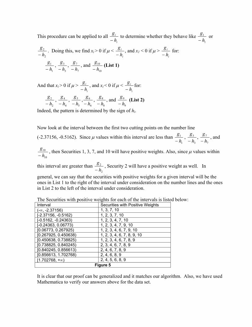
This procedure can be applied to all i

i

hg−

to determine whether they behave like 1

1

hg−

or

2

2

hg−

. Doing this, we find xi > 0 if µ < i

i

hg−

, and x1 < 0 if µ > i

i

hg−

for:

1

1

hg−

, 3

3

hg−

, 7

7

hg−

, and 10

10

hg−

(List 1)

And that xi > 0 if µ > i

i

hg−

, and xi < 0 if µ < i

i

hg−

for:

2

2

hg−

, 4

4

hg−

, 5

5

hg−

,6

6

hg−

, 8

8

hg−

, and 9

9

hg−

(List 2)

Indeed, the pattern is determined by the sign of hi. Now look at the interval between the first two cutting points on the number line

(-2.37156, -0.5162). Since µ values within this interval are less than 1

1

hg−

, 3

3

hg−

, 7

7

hg−

, and

10

10

hg−

, then Securities 1, 3, 7, and 10 will have positive weights. Also, since µ values within

this interval are greater than 2

2

hg−

, Security 2 will have a positive weight as well. In

general, we can say that the securities with positive weights for a given interval will be the ones in List 1 to the right of the interval under consideration on the number lines and the ones in List 2 to the left of the interval under consideration. The Securities with positive weights for each of the intervals is listed below: Interval Securities with Positive Weights (-∞, -2.37156) 1, 3, 7, 10 [-2.37156, -0.5162) 1, 2, 3, 7, 10 [-0.5162, -0.24363) 1, 2, 3, 4, 7, 10 [-0.24363, 0.06773) 1, 2, 3, 4, 7, 9, 10 [0.06773, 0.267925) 1, 2, 3, 4, 6, 7, 9, 10 [0.267925, 0.450638) 1, 2, 3, 4, 6, 7, 8, 9, 10 [0.450638, 0.738825) 1, 2, 3, 4, 6, 7, 8, 9 [0.738825, 0.840245) 2, 3, 4, 6, 7, 8, 9 [0.840245, 0.856613) 2, 4, 6, 7, 8, 9 [0.856613, 1.702768) 2, 4, 6, 8, 9 [1.702768, +∞) 2, 4, 5, 6, 8, 9

Figure 5 It is clear that our proof can be generalized and it matches our algorithm. Also, we have used Mathematica to verify our answers above for the data set.

Appendix 1: )(⇐ A step-by-step of Theorem 1

The derivative of the iso-variance equation is broken into four terms, each enclosed in brackets. A F A A B

+++σ∂

−−−+σ∂

+σ= ∑∑∑−<<<

−−

=−

−−

1

211

1

21

11

2 )Cov(),Cov([2])1)(1[(2][20nim

imj

jnm

nn

iin

m

nnmm i,mxmjx

xx

xxx

xx

B A B B

])1,Cov())(,1Cov(1)-nCov(j,1

111

1 ∑∑−<<

−−−

−

<

−∂

+∂

+−+∂

njm m

nj

m

nmn

m

n

mjj nj

xx

xxx

xxmnxx

x

D C E C

)1Cov())1()1((),Cov()]1()1[(2 11

1

1

111

1,nn-

xx

xxxx

nmxx

xxm

nn

n

ii

m

n

m

nm

n

ii ∂

∂−−+−

∂∂

+∂∂

−−+−+ −−

−

=

−−−

=∑∑

C

∑−≠

−

∂∂

−−+1,

1 ))]Cov()1(nmi m

ni i,n

xx

x . (16)

To make handling the third term easier, here is a small chart of the derivatives that need to be taken: i \ j <m m m<j<n-1 n-1 <m 0 X X X m 1 X X X m<i<n-1 0 2 0 X n-1 3 4 5 X Since the second summation involved all jx j i<such that , terms in the table with an X do not exist. Those entries in the table that are 0 imply that the derivatives are 0. Therefore, there are only five situations that matter. Inside the third set of brackets, the five terms correspond sequentially to A, B, C, D, and E. In the fourth term, the three cases sequentially listed are i=m, i=n-1, and i=else. Above each term, there is a bold letter. Combining the terms with the same letter gives you a new term in equation (12). A B C D

)Cov()x-(1),Cov()1(1)nCov(i,)Cov(1-n

1ii

11

1

1

1

11

1m,nni

xx

xxx

xi,mxm

nn

ii

n

i m

ni

n

ii ∑∑∑∑

=

−−

=

−

=

−−

=

+∂∂

−−+−∂∂

+

E F

0)1)(1()1Cov()1( 211

1

1

1

1 =σ∂∂

−−−+−−∂∂

+ −−

=

−

=

− ∑∑ nm

nn

ii

n

ii

m

n

xx

x,nnxxx

Works Cited 1. Arnold, Steven F. The Theory of Linear Models and Multivariate Analysis,

Wiley, 1981. 2. Huang, Chi-Fu. Foundations for Financial Economics, Elsevier Science

Publishing Co., 1988. 3. Markowitz, Harry M. Portfolio Selection: Efficient Diversification of Investments,

Wiley, 1959 4. Markowitz, Harry M. “Portfolio Selection,” Journal of Finance. March 1952. 5. Chapter 5, finding the efficient set