INTERNATIONAL ACCOUNTING AND BUSINESS CONFERENCE 2011 PROCEEDINGS IABC2011 Page 1 THE MARKET VALUATION OF R&D: EMPIRICAL EVIDENCE FROM MALAYSIAN FIRMS SUNARTI BINTI HALID AMIZAHANUM BINTI ADAM NUR ADURA BINTI AHMAD NORUDDIN MASETAH BINTI AHMAD TARMIZI Faculty of Accountancy Universiti Teknologi MARA Seri Iskandar Campus 32610 Bandar Baru Seri Iskandar Perak Malaysia [email protected] Abstract Purpose - The major objective of this study is to understand and recognize the value relevance of research and development (R&D) in market valuation. The firms selected for this study is from Malaysia from the period 2000-2007. This study have examined whether the market perceived R&D information as an important variable in determining the value of a company. Specifically, this study empirically investigated the association between R&D information in determining and explaining the market value. The study also described a relationship between R&D with all other assets. Furthermore, we examined the relationship between the R&D and the sign of earnings items. Design/methodology/approach - An equity valuation model based on the modified balance sheet identity was used to permit R&D and other assets to have separate empirical coefficient values. Findings - This study found weak empirical support at best for the value relevance of R&D at the firm level. However, market was taken into consideration BVNA in determining the firm‟s equity value as compared to R&D. Also, the results showed that the market‟s valuation of R&D is not priced differently from other assets. In addition, our results provided evidence that there is no significant relationship between R&D information and the sign of earnings items. Originality/value - This study employs an approach using the equity valuation model to measure the value relevance of R&D in market valuation. Keywords - Research and Development, Market Valuation, Equity Valuation Model Paper type - Research Paper

Welcome message from author
This document is posted to help you gain knowledge. Please leave a comment to let me know what you think about it! Share it to your friends and learn new things together.
Transcript

INTERNATIONAL ACCOUNTING AND BUSINESS CONFERENCE
2011
PROCEEDINGS IABC2011 Page 1
THE MARKET VALUATION OF R&D:
EMPIRICAL EVIDENCE FROM MALAYSIAN FIRMS
SUNARTI BINTI HALID
AMIZAHANUM BINTI ADAM
NUR ADURA BINTI AHMAD NORUDDIN
MASETAH BINTI AHMAD TARMIZI
Faculty of Accountancy
Universiti Teknologi MARA
Seri Iskandar Campus
32610 Bandar Baru Seri Iskandar
Perak Malaysia
Abstract
Purpose - The major objective of this study is to understand and recognize the value relevance
of research and development (R&D) in market valuation. The firms selected for this study is
from Malaysia from the period 2000-2007. This study have examined whether the market
perceived R&D information as an important variable in determining the value of a company.
Specifically, this study empirically investigated the association between R&D information in
determining and explaining the market value. The study also described a relationship between
R&D with all other assets. Furthermore, we examined the relationship between the R&D and the
sign of earnings items.
Design/methodology/approach - An equity valuation model based on the modified balance
sheet identity was used to permit R&D and other assets to have separate empirical coefficient
values.
Findings - This study found weak empirical support at best for the value relevance of R&D at
the firm level. However, market was taken into consideration BVNA in determining the firm‟s
equity value as compared to R&D. Also, the results showed that the market‟s valuation of R&D
is not priced differently from other assets. In addition, our results provided evidence that there is
no significant relationship between R&D information and the sign of earnings items.
Originality/value - This study employs an approach using the equity valuation model to
measure the value relevance of R&D in market valuation.
Keywords - Research and Development, Market Valuation, Equity Valuation Model
Paper type - Research Paper
INTERNATIONAL ACCOUNTING AND BUSINESS CONFERENCE
2011
PROCEEDINGS IABC2011 Page 2
Introduction
Research and development (R&D) is perceived part of the innovation process which involve the
translation of knowledge into tangible output. However, according to Dato‟ Shaziman bin Abu
Mansor, Minister of Works, in Construction Industry Research Achievement International
Conference (2009), „‟the translating R&D into something tangible in the market is challenge”.
He added it is normal to expect less than five percent R&D results to reach the market in
Malaysia.
To promote the R&D in Malaysia, Multimedia Super Corridor (MSC) Malaysia had allocated
RM85 million for the MSC Malaysia Research and Development Grant Scheme (MGS) which
help the company to develop its ICT/Multimedia products to its full commercial potential. Other
than that, Malaysian Industrial Development Authority (MIDA) had introduced various
incentives for R&D, which among others include give pioneer status with income tax exemption
of 100% of the statutory income for five years and Investment Tax Allowance (ITA) of 100% on
the qualifying capital expenditure incurred within 10 years; to a contract R&D company i.e. a
company that provides R&D services in Malaysia to a company other than its related company.
R&D is an expensive activity where it requires an investment of certain amount of capital with
the belief that they would result in some increased benefits in the future periods. The evidence
from previous study seems to indicate that the company that will received benefit from the R&D
activities basically those in the high-technology industries. Chamberlain‟s (1999) study on share
price reaction to R&D spending announcements for a sample of Canadian companies revealed
that investors react differently to R&D announcements by high and low technology firms and
that the market's assessment of R&D spending plans may be influenced by other factors, such as
insider trading activity. It is collaborate with findings discovered by Chan et al. (1990) which
found that investors reacted positively to the announcement of R&D expenditures especially
firms in the high-technology sector.
In Malaysia, with various governments‟ incentives, the R&D activity was still considered
relatively low. European Commission in Comparative Analysis of R&D Developments in
Malaysia (1992) reported that the R&D activities in Malaysia mainly in high technology by
foreign multinational companies (MNCs) but were conducted outside Malaysia and often in their
home countries. While, manufacturing by local enterprise were mainly in the low technology
sector which requires minimal R&D activities. Alfan (2003) reported that the amount spend on
R&D was very much less compared to other countries such as the United States, Japan and
Germany. Alfan found that from a survey by the Malaysia Science and Technology Information
Centre (MASTIC) revealed that the major factors contribute to the lack of R&D activities was
due to the lack of R&D strategy and shortage of expert R&D personnel.

INTERNATIONAL ACCOUNTING AND BUSINESS CONFERENCE
2011
PROCEEDINGS IABC2011 Page 3
Most current studies produce results that accounting number of R&D has value-relevance or in
other words has future economic benefit. Many researchers have conjectured that benefits from
the research and development are plausible. According to Nobelius (2004), R&D has been
studied for a long time within different contexts, economies and environmental demands
throughout the years. Nevertheless, whether information on intangible assets reported under
current financial reporting requirements conveys information that is value relevant to market
participants‟ valuation of firms‟ equity has long been a question of interest to accounting
policymakers and researchers.
Basically, the primary purpose for conducting the tests of value relevance is to extend our
knowledge regarding the relevance and reliability of accounting numbers as reflected in equity
values. The value relevance research assesses how well accounting numbers reflect information
used by equity investors. Besides, the findings of this research should be important for those
involved in the setting and monitoring of standards, as relevance and reliability are the two
primary criteria in accounting conceptual framework.
However, one could pose the question as to whether the controversy surrounding R&D is really
important or whether it is just making „noise‟ in the security market. Apart from that, one of the
possibilities is to examine whether the market perceives the amount of R&D as an important
variable in the determination of the value of a company. As a complement, the empirical aims of
this study are to investigate the relationship between R&D disclosures in accounts and market
values and the relationship between R&D with other assets. Apart from that, this paper uses an
equity market value as the valuation benchmark for a sample firms from Malaysian over a period
of seven years from 2000 to 2007. Further, we examined the relationship between R&D and the
sign of earnings items. Earnings items are used as a proxy throughout the study period.
Literature Review
Value Relevance of Accounting Numbers
Accounting information is considered as the most important mechanism for the investors to
evaluate the performance of the company. It is an important way for companies to communicate
with the market participants. Meanwhile, value relevance is the ability of accounting numbers to
confine information relevant to equity valuation. In other words, accounting numbers is defined
as value relevant if it has a predicted association with equity market values. Basically, value
relevance most commonly measured by the r-squared in a regression of market price on
accounting information. The greater the variables of the explanatory power of specific financial
statement, the greater would be the value relevance.
Many of the researches have shown that financial statements and other accounting information
play a vital role in the capital markets since they provide essential information about the value of

INTERNATIONAL ACCOUNTING AND BUSINESS CONFERENCE
2011
PROCEEDINGS IABC2011 Page 4
firms. The distribution of value-relevant accounting information helps to reduce the information
asymmetry among the investors. Furthermore, Jenkins (2002) stated that value relevance in the
accounting literature refers to the strength of the relationship between accounting information
and stock market valuation. Besides, value relevance means measuring the degree to which
markets responds to reported accounting information or, in other words, the degree to which
accounting information is able to drive equity prices.
Francis and Schipper (1999) operationalize value relevance in two ways. The first measure of
relevance focuses on the market-adjusted returns, which could be earned, based on
foreknowledge of financial statement information. Meanwhile, second measure is based on the
explanatory power of accounting information for measurers of market value. The first relation
investigates the ability of earnings to explain annual market-adjusted returns (earnings relation);
the second examines the ability of assets and liabilities to explain market value of equity
(balance sheet relation); and the third examines the ability of book values and earnings to explain
market equity values (book value and earnings relation).
As mentioned by Barth et al. (2001), value relevance studies use various valuation models to
tests of specific null and alternative hypotheses regarding relevance and reliability. Moreover,
numerous papers use equity market value as the valuation benchmark to assess how well
particular accounting numbers reflect information used by investors. The tests often focus on the
coefficient on the accounting numbers in the estimation equation. Holthausen and Watts (2001)
classify the value relevance study into three categories. According to them, the first category is
the relative association studies that compare the association between stock market values and
alternative bottom lines measurers. The accounting number with the greater r-squared is
described as being more value relevant. Meanwhile, the second category is the incremental
association studies that determine whether the accounting number of interest is helpful in
explaining value given other specified variables. Thus, the accounting number is typically
deemed to be value relevant if its estimated regression coefficient is significantly different from
zero. Holthausen and Watts also noted the third category is marginal information content studies
that investigate whether a particular accounting number adds to the information set available to
investors. This type of research typically uses event studies to determine if the release of an
accounting number is associated with value changes. Price reactions are considered evidence of
value relevance.
A study done by Landsman (1986), which shows the relationship between market values and
accounting numbers, is to look at empirical evidence of the relationship between pension funds
assets and liabilities and the market value of shareholder equity. The data used in his study was
taken from United States companies over three annual accounting periods, from 1979 to 1981.
Landsman employed an equity valuation model based on the balance sheet identity, which
permitted pension and non-pension assets and liabilities to have separate empirical coefficient
values. His model was based on the fundamental accounting identity, which holds that
shareholders‟ equity is the residual of corporate assets less corporate liabilities. By using this
INTERNATIONAL ACCOUNTING AND BUSINESS CONFERENCE
2011
PROCEEDINGS IABC2011 Page 5
equation, Landsman was able to compare the coefficient values of non-pension assets and
liabilities to their pension counterparts. The empirical findings of this study show the market
prices the assets and liabilities of pension funds as part of the corporate assets and liabilities.
Landsman (1986) lists four econometric problems associated with estimation of the model. One
of the major econometric problems when estimating the cross-sectional valuation model is the
problem of heteroscedasticity disturbance. This problem arises from the fact that large or small
firms tend to produce large or small disturbance. The independent variable that was used in
Landsman‟s study is the total sales value of the firm. Landsman (1986) also discusses the
problem of multicollinearity due to the existence of a linear relationship among the explanatory
variables of regression model. The presence of a severe multicollinearity problem could result in
misleading inferences being drawn from sample t-statistics. In particular, in a case where the
sample t-statistics are unbiased, if there are no other econometric problems, it is difficult to
determine whether the sampling variances are large because of multicollinearity, or whether the
variance of the true population is large. In order to reduce this problem, Landsman estimated his
model using the net asset form; using net non-pension assets and net pension assets.
Besides, Gopalakrishnan and Sugrue (1993) extended the work of Landsman (1986) in pension
fund property rights. The main findings of their study indicated that investors perceive pension
assets and liabilities as part of corporate assets and liabilities. Furthermore, it shows that pension
assets and liabilities have significant information content beyond what is conveyed by non-
pension assets and liabilities. On the other side, Dhaliwal (1986) examined empirically whether
capital market participants view unfunded vested pension obligations as debt liabilities in
assessing the market risk of the firm. A test was conducted in their study in order to examine the
effect of the inclusion of unfunded vested pension obligations in the measurement of financial
leverage on the explanatory power of the model. Dhaliwal reported that the market views these
pension liabilities as a form of a debt and the market is capable of using the footnote disclosure
regarding unfounded vested liabilities in its assessment of market risk. Therefore, there is no
reason to incorporate this information into the balance sheet.
Kane and Unal (1990) reported on their empirical investigation of structural and temporal
variation in the market‟s valuation of banking firms. The authors developed a model to capture
the hidden reserves in United States banking firms. According to them, hidden capital exists
whenever the accounting measure of a firm‟s net worth diverges from its economic value. Such
unbooked capital has on-balance-sheet and off-balance-sheet sources. Kane and Unal developed
a model to estimate both forms of hidden capital and to test hypotheses about their determinants.
Therefore, the model makes direct use of accounting information on the bookable position of a
firm and separate bookable from unbookable sources of value. Kane and Unal (1990) used
regression analysis to partition the market value of a firm‟s stock into two components. The two
components namely recorded capital reserves and unrecorded (or hidden) net worth. In their
study, hidden capital is, in turn, allocated between values that are either unbooked or bookable
through asset turnover or write-downs on a historical-cost balance sheet under General Accepted

INTERNATIONAL ACCOUNTING AND BUSINESS CONFERENCE
2011
PROCEEDINGS IABC2011 Page 6
Accounting Practices (GAAP) or values, which GAAP currently designated as an unbookable off
balance-sheet item.
Francis and Schipper (1999) argued that financial statements have lost a significant portion of
their relevance to investors, specifically over the period of 1952 until 1994. This finding and its
implications raise concerns among financial accountants, standard-setters, educators and
auditors, and have given rise to a number of research and policy initiatives whose common goal
is to improve financial reporting by altering the current financial reporting model. The
interpretation of value relevance as given by Francis and Schipper is based on value relevance as
indicated by a statistical association between financial information and prices or returns. The
statistical association measures whether investors actually use the information in question in
setting prices, hence, value relevance would be measured by the ability of information in
financial statements to change the total mix of information in the marketplace. Moreover, they
noted a decline in the value relevance of earnings and an increase in the value relevance of book
value over time for the United States firms. These studies also found no evidence that the value
relevance of the combined earnings and book values has declined over time.
Francis and Schipper (1999) also compared the value relevance of accounting information
between high and low technology firms. The results indicated that high technology firms have
not experienced a greater decline in the value relevance of accounting information (earnings and
book value) compared to low technology firms. Meanwhile, according to Barth et al. (2001), a
primary focus of financial statements is equity investment. As well, the primary purpose for
conducting tests of value relevance is to extent our knowledge regarding the relevance and
reliability of accounting amounts as reflected in equity values. It is supported by Ball and Brown
(1968), where the financial information is relevant if it summarizes or captures the factors that
affect security prices. Furthermore, value relevance in the accounting literature refers to the
strength of the relationship between accounting information and stock market valuation (Jenkins,
2002). Indeed, value relevance is measuring the degree to which the market responds to reported
accounting information in the financial statement. Similarly, another study by Chen et al. (2001)
reported that accounting information is value-relevant in the Chinese market according to both
the pooled cross-section and time series regressions or the year-by-year regression.
Arce and Mora (2002) studied the differences in the value relevance of earnings and book value
across eight European countries that represent the most important capital markets in Europe.
Their findings revealed a significant difference in the value relevance of earnings and book value
in all countries under study except Belgium and Italy. Earnings are more value relevant than
book value in the United Kingdom, the Netherlands and France. Meanwhile, book value is more
relevant than earnings in Germany, Switzerland and Spain. Apart from that, Black and White
INTERNATIONAL ACCOUNTING AND BUSINESS CONFERENCE
2011
PROCEEDINGS IABC2011 Page 7
(2003) has examined the effect of earnings sign, firm size and macroeconomics events on the
value relevance of earnings and book value in three countries. The samples of countries selected
for their study were Germany, Japan and the United States. In their study, they compared the
value relevance of earnings relative to book value of equity. Their study hypothesizes that book
values are more value relevant than earnings in Germany and Japan while earnings are more
value relevant in the United States, because capital providers in Germany and Japan are more
concerned with balance sheet measurers such as liquidity. The results show that Germany are
robust, as book value is more value relevant for both positive and negative earnings, in all years
with sufficient sample sizes, and for all size quartiles. However, their findings suggested that
earning sign, firm size and macroeconomic events affect the value relevance of earnings and
book value in Japan and the United States.
Value Relevance of Intangibles
There is an extensive body of literature review providing empirical evidence on the relevance of
intangibles for equity valuation and, therefore, pointing out the need to take intangibles into
account in investment, credit and management decision-making. McCarthy and Schneider (1995)
analyzed the market perception of goodwill as an asset in the determination of a firm‟s valuation
in the United States market. They also examined how the market perceives goodwill in relation
to all other assets. Their findings show that investors perceive goodwill as an asset when valuing
a firm and suggest that the market include goodwill when valuing a company. Besides, another
finding is that, relative to book value, goodwill is valued by the market at least as much as other
assets.
Jennings et al. (1996) also studied the relationship between purchased goodwill and market
value. The authors examined the relation between equity values and accounting goodwill
numbers in the United States during the period 1982-1988. The study indicates a strong cross-
sectional relation between equity values and accounting assets and liabilities. Besides, the
estimated coefficients for recorded net goodwill are positive and highly significant in each of the
seven years. Furthermore, the results also suggest that investors may view purchased goodwill as
an economic resource that does not decline in value for some firms.
Meanwhile, in the second part of their study, Jennings et al. (1996) examined whether purchased
goodwill was reflected in equity values as a wasting resources. Actually, their motivation was
the fact that all United States firms are required to amortize goodwill over periods not exceeding
40 years. Besides, this requirement is based on the argument that purchased goodwill declines in
value over time because the underlying stream of cash flows is likely to be of limited duration.
The authors estimated a cross-sectional regression based on income statement issues that involve
regressing equity values on components of expected future earnings, including expected
goodwill amortization.
Their results indicate a strong positive cross-sectional association between equity values and
recorded goodwill assets amounts after controlling for other components of net assets. In
addition, Jennings at al. (1996) finds evidence of a negative association between equity values
and goodwill amortization after controlling for other components‟ expected earnings. In the

INTERNATIONAL ACCOUNTING AND BUSINESS CONFERENCE
2011
PROCEEDINGS IABC2011 Page 8
meantime, Ibrahim et al. (2001) conducted a study concerning accounting for goodwill in
Malaysian context. Their study attempts to investigate the association between purchased
goodwill and market value and to describe the relationship between purchased goodwill and
other assets. Ibrahim et al. findings stated that the market incorporates the information on
purchased goodwill in the valuation of a firm and the results also show that the market seems to
perceive purchased goodwill to have at least a value equal to other asset.
As mentioned by Barth et al. (2001), the fair value accounting value relevance literature also
addresses questions relating to non-financial intangible assets costs related to goodwill. The
findings show that available estimates of intangible asset values reliably reflect the values of the
assets as assessed by investors. Besides, the estimates have a significantly positive relation with
share price. In fact, there was a review of the literature indicates the diverse paradigms that have
encompassed R&D. The transition from early days‟ booming markets and economic growth in
the 1950s to today‟s highly competitive and global marketplace is reflected in the way R&D has
been managed (Nobelius, 2004).
Moreover, in an efficient capital market, relevant information about firms will be reflected in
security prices regardless of whether the information is reported on the balance sheet or in the
footnotes (Dyckman & Morse, 1986). Besides, Nobelius (2004) noted that early success stories
such as the industrial research laboratories Bell Labs, Xerox Parc and Lockheed Martin
Skunkwords have been replaced by companies like the more market-focused 3M, the rapid
introductions of new product ranges from Japanese manufacturers like Toyota and Sony, and
R&D collaborations like Ericsson‟s network of companies around the “Bluetooth” technology
and standard.
In addition, R&D constitutes a fundamental factor for the successful introduction of new, more
efficient and clean supply and end-use technologies and the achievement of economic, safety,
environmental and other goals (Barreto and Kypreos, 2004). Hence, do investors really look at
R&D information in determining company‟s market value or value of companies? These
questions raise another issue taken up by this study, which is to examine whether the commotion
surrounding the subject of R&D is really important to the investors due to corporate growth, or is
just to create „noise‟ in the security market. Thus, the study will try to uncover if R&D reported
in the financial statement is being taken into consideration by investors when valuing a company.
Therefore, prior research had been conducted to examine the value relevance of R&D. Other
than that, numerous articles that consist of various models and framework also had been
developed.
Many studies have tested whether stock prices or returns of firms that invest in R&D increase
according to the level of R&D intangibles. Chan et al. (1990) acknowledged a positive effect on
stock prices for two days surrounding R&D announcements. Meanwhile, there is evidence that
previous level of firm‟s involvement in R&D affect the firm‟s market value. Other prior research

INTERNATIONAL ACCOUNTING AND BUSINESS CONFERENCE
2011
PROCEEDINGS IABC2011 Page 9
that related was Shevlin (1991). Shevlin investigated whether capital market investors, in
assessing the market values of R&D firms‟ equity, view R&D Limited Partnership (LP) as
increasing both the assets and liabilities of the R&D firms. The results are consistent with market
participants capitalizing in-house R&D expenditures, viewing the call option feature of the
limited partnership as relevant information in assessing the market value of the R&D firm.
Shevlin (1991) also estimated the LP variables from information provided in footnote disclosure
items by R&D firms.
Several implications arise from Shevlin‟s study. The empirical results are consistent with the
argument that footnote disclosures allow investors to make some estimate of the value of the LP
to the firm. The results also indicate that in addition to the reported assets and debt on the face of
the balance sheet, investors use information in the footnotes to help assess the market value of
firms. Finally, Shevlin‟s results add further support to the empirical usefulness of the balance
sheet identity approach as used by Landsman (1986) to develop a cross-sectional valuation
model to address off-balance sheet issues.
Past research has generally attested to the information advantage of a general accounting rule
that would capitalize R&D (e.g. Lev and Sougiannis, 1996). Lev and Sougiannis (1996) address
the issues of reliability, objectivity, and value-relevance of R&D capitalization. For this reason,
Lev and Sougiannis documented a significant inter-temporal association between firms‟ R&D
capital and subsequent stock returns, suggesting a systematic mispricing of the shares of R&D
intensive companies, or a compensation for an extra market risk factor associated with R&D.
They attempt to establish an empirical connection between R&D spending and subsequent
earnings. Indeed, they examined this issue empirically for the United States in a cross-sectional
framework and estimate R&D amortization rates based on the relation between earnings and
lagged R&D expenditures. Finally, the findings suggest that R&D capitalization yields
statistically reliable and economically relevant information to investors. In other words, they find
that the capitalized R&D amount is value relevant.
Even though, Aboody and Lev (1998) examined the value-relevance of information on the
capitalization of software development costs, which was promulgated in 1985 by Financial
Accounting Standards Board No. 86 (SFAS 86), they concluded that capitalized software
development costs are impounded in prices and that large distortions in the firm‟s financial
position arise from expensing rather than capitalizing R&D spending. They identify four
variables that are significantly associated with the capitalization decision using data from 163
software companies over 1987-1995.1 Based on the results, the authors argue that the coefficient
of the software asset is only slightly lower than the coefficient of equity, indicating that
investor‟s value, on average, the capitalized software asset slightly less than a firm‟s tangible
assets. The results find no evidence that somewhat subjective software capitalization values are
irrelevant to investors‟ decisions. Nevertheless, Lev and Sougiannis (1996) found the asset to be
1 Aboody and Lev’s results are based on regression of the annual capitalized development cost (as a percent of
market value of equity) on market value of equity, profitability, development intensity, leverage and systematic risk.

INTERNATIONAL ACCOUNTING AND BUSINESS CONFERENCE
2011
PROCEEDINGS IABC2011 Page 10
value-relevant using a synthesized R&D asset and research on value-relevance shows that the
market is capable of valuing intangible assets, especially R&D. They estimate the R&D capital
of a large sample of public companies using Almon lag technology. In addition, Lev and
Sougiannis (1996) found that the stock price as well as stock returns reflects the market‟s view
on intangibles.
Choi et al. (2000) reported empirical evidence on the relationship between the reported value of
intangible asset, the associated amortization expense, and firms‟ equity market values. According
to them, there is a positive relation between the book value of intangible assets and the market
value of common equity. Moreover, consistent with the uncertainty hypothesis, the market‟s
valuation of a dollar of intangible assets is lower than its valuation of other reported balance
sheet items (Choi et al., 2000). With regards to the income statement hypotheses, the regression
analyses show that amortization expense is not significantly related to annual stock returns. Choi
et al. (2000) suggest that either the market does not view intangible assets as wasting assets or
that recorded amortization expense reflects the decline in value of the intangible asset with
considerable error.
Furthermore, a study done by Boone and Raman (2001), represent that off-balance sheet
(unrecorded) R&D benefits could generate ex ante inequity in the capital markets in the form of
an information gap (asymmetry) between informed investors and other investors. Here, the
results suggest that the market makers adverse selection costs are higher for R&D-intensive
firms rather than non-R&D-intensive firms. For R&D-intensive firms, there is a negative
association between market liquidity and the magnitude of off-balance sheet R&D assets. In
other words, these studies suggest that market liquidity will improve if there is more disclosure
about these firms‟ R&D projects. Meanwhile, Chan et al. (2001) summarized that R&D activity
represents a significant and growing portion of firm resources. They found that high R&D plays
a distinctive role arises from stocks with high R&D relative to the market value of equity.
Besides, their evidence does not support a direct link between R&D spending and future stock
returns. In other words, the association between R&D intensity measured relative to sales and
future returns is not strong for firms engaged in R&D.
Xu and Zhang (2004) examined the role of R&D in explaining the cross-section of stock returns
in Japanese market for the period from 1985 to 2000. R&D activities are characterized by
potential high reward and great uncertainty in future cash flows. According to them, Japan also
had the second largest stock market in the world in terms of market capitalization. Xu and Zhang
(2004) concluded that the average stock return is positively related to R&D expenditure in that
period. Besides, Han and Manry (2004) examined the value relevance of R&D disclosures and
advertising expenditures reported by firms listed on the Korean Stock Exchange from 1988 to
1998, using a regression model based on the Ohlson equity-valuation framework. From that
research, R&D expenditures are positively associated with stock price, suggesting that
capitalizing R&D expenditures is appropriate. However, these findings suggest that investors
believe the economic benefits of advertising expenditures expire in the current period, similar to
other expenses.

INTERNATIONAL ACCOUNTING AND BUSINESS CONFERENCE
2011
PROCEEDINGS IABC2011 Page 11
Zainol et al. (2008) in the study using the PROBIT model, conclude that R&D activities initiated
by a firm are an important signal for a firm‟s potential future value-creation. According to this
study which was conducted based on 230 public- listed companies from the main board of Bursa
Malaysia, companies in the consumer sector have a higher probability of reporting R&D as
intangible assets than the companies in industrial sector. By treating R&D as intangible assets,
the consumer sector companies manage to increase the possible inflow of foreign direct
investment and enhance the market value of the firm. The study also finds that companies with
high total assets tend to have a greater probability of reporting R&D cost as intangible assets.
The study also reveals companies which report the R&D as intangible assets are eligible for tax
credit, tax deduction and special depreciation allowance including tax exemption under
Malaysian Income Tax Act, 1967. According to Mani (2002), in South Korea, companies are
permitted to apply for 50 percent tax credit for the expenditure over and above the average
expenditure in the past two years. The tax credits in South Korea include the cost of R&D
personnel, patents registration, maintenance fees and the cost of leasing of fixed and current
assets for companies undertaking R&D activities. Wang and Tsai (1998) discover that small and
medium sized enterprises in Taiwan are motivated to spend for R&D when tax credits are
provided to them. However, due to uncertain nature of outcomes of R&D, many companies
report R&D as an expense and immediately write-off from the balance sheet. Even though this
practice is found to be common in many corporations, nevertheless this has under-estimate the
accumulation of intellectual capital and does not accurately capture a company‟s equity strength
(Zainol et al. (2008).
R&D cost is believed to create value for science and technology development even though the
cost for R&D is usually high. According to Tishler (2008), the cost of executing R&D program
is a function of the expected outcomes of the R&D program. Based to his study, when the
expected outcomes of the R&D programs are identical, the expected profit maximizing firm
should always choose the highest-risk R&D program as on average, when the high-risk R&D
programs are successful, the markets will expand overtime. In relation to this issue, Ella
Syafputri report in Science and Development Network (dated 24 September 2007), Malaysia has
allocated RM12 billion in its 2008 budget to R&D and commercialization of science and
technology in universities. The four universities which received at least RM400 million for their
research programmes include Universiti Sains Malaysia, Universiti Kebangsaan Malaysia,
Universiti Malaya and Universiti Putra Malaysia (research university status are granted for these
four universities). The money allocation may help to improve infrastructure and develop a better
system for commercialization.
One of the possible reasons which may contribute to the increase in the allocation of R&D cost is
due to the increase number of research scientists and engineers in year 1998. Other than that, the
RM12 billion allocation may be said to improve weak and non-existent linkages between the
private sector and institute of higher learning and government research institution that results
much of Malaysia‟s R&D activities at institutional level have not been able to pass through the

INTERNATIONAL ACCOUNTING AND BUSINESS CONFERENCE
2011
PROCEEDINGS IABC2011 Page 12
commercial stage of development (White Paper - Comparative Analysis of R&D Developments
in Malaysia, 2002). Callen and Morel (2005) in their study incorporating the Ohlson model agree
that cross-sectional and panel data studies of R&D investments consistently show that R&D
expenditures are value relevant and impounded in security prices. However, results of their
studies reported that a very weak empirical support exists for the value-relevance of R&D
expenditures (only 25 percent R&D investment significantly affects firm‟s valuation).
For pragmatic reasons, most research on intangibles focuses on those intangibles generated by
R&D expenditures. Meanwhile, data on R&D spending are widely available because R&D
expenditures must be disclosed separately under SFAS No.2, Accounting for Research and
Development Costs. Overall, research suggests that investors use disclosures on intangibles
expenditures and those intangibles expenditures have future benefits, but that these benefits are
more uncertain than those associated with conventionally recognised assets (Maines et al., 2003).
In addition, a study by Laincz (2005), presents the partial equilibrium for a single industry
demonstrating how growth-promoting R&D subsidies alter the endogenously determined market
structure. The results indicated about optimal R&D policies in existing endogenous growth
models rely on strong assumptions regarding market structure.
Development of the Theoretical Framework
Theoretical Model
The accounting identity model, also called the balance sheet model is based on the theory that
the market value of the firm‟s equity is the market value of its assets minus the market value of
its liabilities where investors assign values to the firm by taking the difference between the
market value of total assets and the market value of total liabilities. Balance sheet model has
been widely used by many researchers in their study.
The balance sheet model includes only the balance sheet variables in the regression equation, as
in Landsman (1986). In his study, Landsman empirically examined whether pension fund assets
and liabilities associated with corporate-sponsored defined benefit pension plans are valued by
the securities market as corporate assets and liabilities, a recent study which used an equity
valuation based on balance sheet model. This model permits pension and nonpension assets and
liabilities to have separate empirical coefficient values. Essentially, the model was actually based
on basis accounting equation, which holds that shareholders equity is the residual of corporate
assets less corporate liabilities. Therefore, the shareholders‟ equity can be written as:
Shareholders‟ equity (Net assets) = Total assets - Total liabilities
The use of this equation enables Landsman to compare coefficient values of assets and liabilities
to their counterparts. By removing earning, which is one of the explanatory variables; there is no
longer a weighted average between the income variable and the balance sheet variable. The
model is as follows: -

INTERNATIONAL ACCOUNTING AND BUSINESS CONFERENCE
2011
PROCEEDINGS IABC2011 Page 13
MVEjt = a0 + a1BVNAjt + a2R/Djt + ejt…(Model 3.1)
Where
MVEjt = Market value of shareholders‟ equity of firm j in year t
BVNAjt = Book value of the net assets minus R&D of firm j in
year t
R/Djt = Research and development of firm j in year t
ejt = Error term
Meanwhile, Barth et al. (2001) noted that value relevance studies use various valuation models to
tests for specific null and alternative hypotheses regarding relevance and reliability. Numerous
papers use equity market value as the valuation benchmark to assess how well particular
accounting numbers reflect information used by investors. Besides, the tests often focus on the
coefficient of the accounting numbers in the estimation equation. Similar to Barth et al. (2001),
we examine whether the estimated coefficient on the accounting numbers is significantly
different from zero with the predicted sign. Rejecting the null of no significance or unpredicted
sign is interpreted as evidence that the accounting amount is relevant and not totally unreliable.
This study also examines how the market perceives the accounting numbers in relation to all
other amounts recognized in financial statements. Thus, rejecting the null that the coefficients are
the same is interpreted as evidence that the accounting numbers being studied have relevance and
reliability that differ from recognized amounts. Therefore, the multiple regression analysis is
used to test the model and analyzed the relationship. The market valuation model is estimated for
each of the years from 2000 to 2007. Thus, the model tested in this study is as follows: -
MVEjt = a0 + a1BVNAjt + a2EARNjt + a3R/Djt + ejt…(Model 3.2)
Where
MVEjt = Market value of shareholders‟ equity of firm j in year t
BVNAjt = Book value of the net assets minus R&D of firm j in
year t
EARNjt = Net profit of firm j in year t
R/Djt = Research and development of firm j in year t
ejt = Error term
We estimated yearly cross-sectional regressions over a seven-year period from 2000 to 2007 and
use r-squared as one of the method to measure value-relevance. Apart from that, there is another
extension model that can be tested empirically to discover the relationship between R&D
information and the sign of earnings items throughout the study period. Besides, a new variable
was added to the original model used in this study. The basic model had been extended to

INTERNATIONAL ACCOUNTING AND BUSINESS CONFERENCE
2011
PROCEEDINGS IABC2011 Page 14
include a dummy variable. This dummy variable stood for the direction of earnings items, which
were divided into positive (profit) and negative (loss). If the reported earnings items were
positive, the value for this dummy variable was 1. On the other hand, if the reported earnings
items were negative, the value for this dummy variable was 0. The new extended model is
established as follows: -
R/Djt = a0 + a1MVEjt + a2 BVNAjt + a3EARNjt + a4DEARNjt +
ejt… (Model 3.3)
Where
R/Djt = Research and development of firm j in year t
MVEjt = Market value of shareholders‟ equity of firm j in year t
BVNAjt = Book value of the net assets minus R&D of firm j in
year t
EARNjt = Net profit of firm j in year t
DEARNjt = Dummy variable taking the value of 1 for positive
earnings and 0 otherwise
ejt = Error term
From the above models discussed, error terms are independent, identically normally distributed
with mean 0 and a constant variance, σ2.
Research Hypotheses
Three hypotheses have been developed and will be tested in this study. In fact, the analysis that
is going to be performed will be based on these three hypotheses. The first hypothesis to be
addressed in this study is whether R&D should be considered as an important element when
determining a firm‟s market value. In order to achieve this objective, a3 is the coefficient of main
interest (as in Model 3.2). If the market places value on R&D of a firm, then R&D should be
significant and positively correlated with the firm‟s market value. In order to check for this
relationship the following null hypothesis is tested based on the Model 3.2:
H1: a3 = 0
If the R&D information is significant variable, then further examination should test how the
market perceives R&D in relation to all other assets. In other words, is it priced differently from
other assets? In order to check for this relationship, the following null hypothesis is established
based on the Model 3.2:
H2: a1 = a3
Meanwhile, the third hypothesis examine whether there is any relationship between R&D and the
sign of earnings items throughout the study period. In order to check for this relationship, the
following null hypothesis is tested based on the Model 3.3:

INTERNATIONAL ACCOUNTING AND BUSINESS CONFERENCE
2011
PROCEEDINGS IABC2011 Page 15
H3: There is no relationship between R&D information and the sign of earnings items.
Description of Data Collection
As stated earlier, the main objectives of the study is to investigate empirically the association
between R&D information in determining and explaining the market value and to establish a
relationship between R&D information with all other assets specifically over the period of 2000
until 2007 based on Malaysian firms. Literally, assets are rights accruing to the entity meanwhile
equities represent sources of the assets and consists of liabilities and the stockholders equity.
Thus, income earned is the property of the entity until it is distributed as dividends to the
shareholders. Hence, the firm‟s book value of net assets (excluding R&D), earning and R&D
will be the independent variables in the framework. Consequently, the theoretical model is
presents in Figure 3.1.
Figure 3.1: The Framework for the Relationship between Independent and Dependent
Variables
Sample Selection
It is now possible to see how both sampling design and sample size are important to establish the
representativeness of the sample for generalizability (Sekaran, 2000). According to the Sekaran,
if the appropriate sampling design is not used, a large sample size will not, in itself, allow the
Independent Variables
Book Value of Net Assets (Excluding R&D)
R&D
Earnings
Dependent Variable
Market Value of Equity
(Share price x ordinary
shares outstanding)

INTERNATIONAL ACCOUNTING AND BUSINESS CONFERENCE
2011
PROCEEDINGS IABC2011 Page 16
findings to be generalized to the population. Similarly, unless the sample size is adequate for the
desired level of precision and confidence, no sampling design, however sophisticated, can be
useful to the researcher in meeting the objectives of the study (Sekaran, 2000). Thus, sampling
decisions should consider both the sampling design and the sample size.
Black and White (2003) have listed several criteria in choosing sample for their research. These
criteria, as set by Black and White, are used in selecting sample for this research. Thus, the study
population consists of Malaysian firms. The coverage of the study is seven years, starting with
year 2000 until 2007 fiscal year from the listing datastream. Indeed, the data of this study are
extracted from the Balance Sheet and Profit and Loss Statement of the respective firms. Data for
this study were collected from the Thompson One Banker over seven-year period from 2000 to
2007.
A firm-year is included as observation if all such variables (market value of shareholders‟ equity,
book value of net assets, earnings and R&D) are presented for a given fiscal year. Firm-year
from the selected companies with any missing variables is excluded. As a result, the final
sample consists of various sample sizes during the period under study. Table 3.1 summarizes the
sample selection and size used for the study. After excluding the missing observations of
variables market value of equity, book value of net assets, earning and R&D, the final sample for
this study is 387 firm-year observations.
Table 3.1: Sample Selection and Size
Sample Selection
Firm-years
Thompson One Banker 2000-2007
9872
Missing observations of market value of equity
(MVE), book value of net assets (BVNA),
earnings (EARN) and capitalized R&D (R/D)
(9485)
Sample Size
387
Table 3.2: Sample Classified by Years
Year Original
Datastream
Clean Data
(Record R&D)
Non-record
R&D
2000 1234 19 1215
2001 1234 31 1203

INTERNATIONAL ACCOUNTING AND BUSINESS CONFERENCE
2011
PROCEEDINGS IABC2011 Page 17
2002 1234 35 1199
2003 1234 46 1188
2004 1234 53 1181
2005 1234 63 1171
2006 1234 69 1165
2007 1234 71 1163
Variable Definitions
The accounting variables included in the regression model are market value of equity, book
value of net assets, earnings and research and development. A summary of the variables of
interest is presented in Table 3.3. The market value of shareholders‟ equity (MVE) is defined as
the share price multiplied by the number of shares outstanding at the end of the accounting year.
The book value of total assets, research and development (R&D), total liabilities and the earning
figure (EARN) are also taken directly from the Thompson One Banker without any modification,
but with variables combined in some cases as shown. However, the book value of net assets
(BVNA) is derived by deducting the total assets (excluding R&D) with total liabilities.
Table 3.3: Variables Required for Regression from Thompson One Banker
Name variables required for
regression Variables Symbol
Market value of equity
Ordinary share outstanding x share price
MVE
Book value of total assets
Total assets
Book value of total liabilities
Total liabilities
Total sales
Turnover
Earnings
Profit attributable to Shareholders
EARN

INTERNATIONAL ACCOUNTING AND BUSINESS CONFERENCE
2011
PROCEEDINGS IABC2011 Page 18
Name variables required for
regression Variables Symbol
Net assets
Book value of total assets - Book value of total
liabilities - Research and development
BVNA
Research and Development
R&D to sales
R&D
Measurement
Measurement procedures
For purposes of empirical analysis, this study uses descriptive statistics and regressions analysis
as the underlying statistical tests. A descriptive statistics of the data obtained will be conducted
to obtain sample characteristics. In other words, descriptive statistics are used to describe and
summarize the dependent and independent variables. Apart from that, correlation is a statistical
method used to answer questions about relations between variables.
The correlation coefficient is a number that measurers the strength of the relation variables.
Values of the correlation coefficient can range from +1.00 for perfectly positively correlated
variables to -1.00 for perfectly negatively correlated variables. A correlation coefficient of -1.00
and +1.00 indicates perfect correlation. If there is absolutely no relationship between the two
variables, the correlation coefficient will be zero. A coefficient correlation that is close to zero
shows that the relationship is quite weak.
Past studies have used Ordinary Least Square (OLS) regression of market values on accounting
measurers to examine value relevance. Thus, OLS regression test is performed on the dependent
variable (MVE), to check the relationship between the R&D accounting numbers for the firms
operating in selected countries. OLS is based on a number of assumptions about the variables
and the error term that must be satisfied in order to ensure the interpretations of the regression
estimates are valid. According to Gujarati (1995), under these assumptions, the OLS estimators
of the regression coefficients are the best linear unbiased estimator.
Basically, r-squared measures the movement or changes in a variable that can be explained by
movements in another variable.2 A variable with greater r-squared indicates explanatory power
of that variable in explaining market value of equity. If the r-squared is lower, then the
explanatory variable is less relevant. A 5% significance level was used in this study. This test is
performed using the MICROFIT 4.0 software package. Besides, the analysis of the data is based
on cross-sectional regression. This study also discusses two major statistical problems associated
with the estimation of the models. The two major problems are heteroscedasticity disturbances
2 Literally, r-squared is the proportion of the variance of Y that has been explained by X. For technical reasons (the
total squared error can be decomposed into two squared components: explained and unexplained), the variance (the squared standard deviation) has traditionally been used.

INTERNATIONAL ACCOUNTING AND BUSINESS CONFERENCE
2011
PROCEEDINGS IABC2011 Page 19
and multicollinearity. Heteroscedasticity is the most common statistical problem to be
encountered when estimating a cross-sectional valuation model.
According to Ibrahim et al. (2003a), one of the major econometric problems when estimating
cross-sectional valuation models is heteroscedastic disturbances that appear from the fact that
large (small) firms tend to produce large (small) disturbances. If heteroscedasticity is present,
then the usual OLS estimators, although unbiased, no longer exhibit minimum variance among
all linear unbiased estimators (Gujarati, 1995). In short, they are no longer the best linear
unbiased estimator. Meanwhile, in the case of the two-variable linear model, one common
deflation technique involves transforming the variables by deflating the independent variable
(Landsman, 1986). This procedure implies that the true error variance is proportional to the
square of the independent. Landsman (1986) addressed the heteroscedasticity problem by
estimating the model in deflated form. In this respect, all variables are deflated by total sales.
Besides, the multicollinearity problem will be discussed in depth in Chapter 4.
Finally, the Wald Test is computed in Model 3.2 to measure whether the information provided
by one variable is significantly different from that provided by another. The Wald Test is
performed using the MICROFIT 4.0 software package. In this study, the Wald Test is computed
in order to check how the market perceives R&D in relation to all other assets.
Deflation Technique
Potential statistical problems associated with the estimation of the model were also noted in the
models that are relevant to the present study; as in the examples in Landsman (1986). The major
problem is heteroscedasticity disturbances. In addressing this issue, entire variables are
transformed by deflating them with the independent variable, which in this study is earnings/total
sales, to produce a constant (but still unknown) variance. Through this „deflation technique‟ the
heteroscedasticity problems can be minimized. The „deflation technique‟ has been widely used
by previous researchers, for example Landsman (1986), Shevlin (1991), McCarthy and
Schneider (1995) and Jennings et al. (1996). In these studies, (except for Shevlin, 1991) all data
in the basic models are deflated by total sales in order to reduce the heteroscedasticity problems
as well as to increase efficiency.
Findings & Conclusion
Descriptive Statistics
Estimates of Correlation on the Independent and Dependent Variables
A summary of the estimates of correlation between independent and dependent variables is
reported in Table 4.1. Table 4.1 presents the correlation of market value of equity (MVE) and
independent variables which include the book value of net assets (BVNA), earnings of the firm
(EARN) and research and development (R&D) in Malaysian firms during the period 2000-2007.
From the table, we can see that the correlation between MVE and R&D are considerably

INTERNATIONAL ACCOUNTING AND BUSINESS CONFERENCE
2011
PROCEEDINGS IABC2011 Page 20
moderate (Year 2000 = 0.379; Year 2001 = 0.438; Year 2002 = 0.544; and Year 2003 = 0.198;
Year 2004 = 0.057; Year 2005 = 0.122; Year 2006 = 0.118; and Year 2007 = 0.240) and a
significant positive. In other words, higher correlation between independent and dependent
variables can predict the regression of market value. Apart from that, based on the estimated
coefficients of correlation between other assets in valuing the market shareholder‟s equity in
Malaysian firms for 2000 until 2007 shows a significant positive correlation. Besides, the value
for correlation between BVNA and MVE is somewhat higher than the correlation between R&D
with MVE.
Table 4.1: Estimated Correlation Matrix of Variables for Malaysian Firms
Variables
BVNA
EARN
RD
2000
MVE
BVNA
EARN
0.654
-0.110
-0.600
0.379
0.018
0.133
2001
MVE
BVNA
EARN
0.670
-0.323
-0.460
0.438
0.111
-0.191
2002
MVE
BVNA
EARN
0.483
0.388
-0.033
0.544
0.255
0.254
2003
MVE
BVNA
EARN
0.359
0.342
0.285
0.198
0.405
-0.017
2004
MVE
BVNA
EARN
0.329
0.190
0.419
0.057
0.580
0.033
2005
MVE
BVNA
EARN
0.362
0.581
0.539
0.122
0.300
0.077
2006
MVE
BVNA
EARN
0.552
0.543
0.574
0.118
0.192
0.118
2007
MVE
BVNA
EARN
0.626
0.304
0.233
0.240
0.399
-0.292
Descriptive Statistics on the Independent and Dependent Variables
In general, descriptive statistics summarizes and describes the observation of the data used in this
study. As mentioned in the Chapter 3, one potential econometric problem when estimating cross-
sectional valuation models is the problem of heteroscedastic disturbances, which arise from the
fact that large or small companies tend to produce large or small disturbances. Thus, to address
this issue, the whole variables are transformed by deflating all variables with the total

INTERNATIONAL ACCOUNTING AND BUSINESS CONFERENCE
2011
PROCEEDINGS IABC2011 Page 21
sales/earnings in order to produce a constant variance but still unknown. Besides, this „deflation
technique‟ is hoped to eliminate the heteroscedasticity problem. A summary of the overall
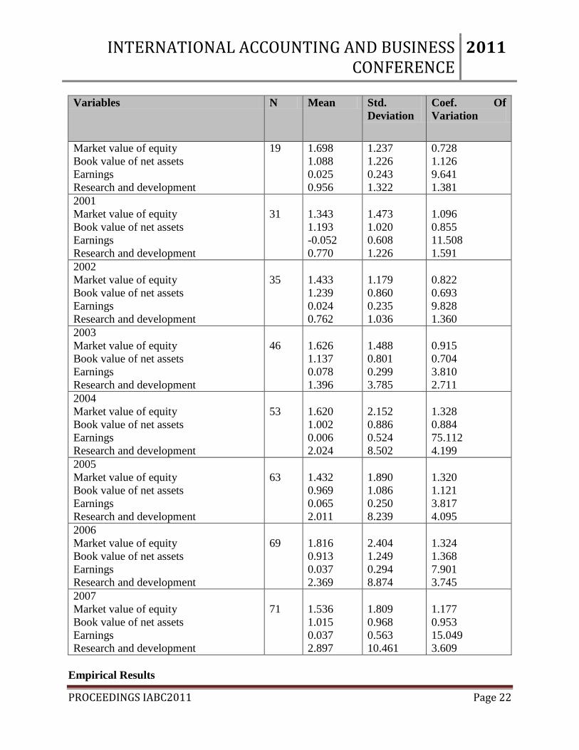
descriptive statistics obtained from the sample size is presented in Table 4.2. The table provides
the mean, standard deviation and coefficient of variation for selected variables: market value of
equity, book value of net assets, earnings and R&D, during the period 2000-2007.
Table 4.2 presents the mean, standard deviation and coefficient of variation for selected variables
in Malaysian firms during the period 2000-2007. Besides, all the variables were deflated by the
total sales. From the table, the results show that the values vary significantly throughout the
study period. The mean values of R&D in Malaysian companies are considerably moderate
throughout the study period (Year 2000 = 0.956; Year 2001 = 0.770; Year 2002 = 0.762; Year
2003 = 1.396; Year 2004 = 2.024; Year 2005; 2.011; Year 2006 = 2.369; and Year 2007 =
2.897). It concludes that R&D is a significant activity from the sample of Malaysian firms.
Apart from that, the mean values of variable MVE in Malaysian companies are also considerably
moderate (Year 2000 = 1.698; Year 2001 = 1.343; Year 2002 = 1.433; Year 2003 = 1.626; Year
2004 = 1.620; Year 2005 = 1.432 ;Year 2006 = 1.816; and Year 2007 = 1.536). Meanwhile, in
2001, the mean value of earnings was negative, which constitute of -0.052 (as reported in Table
4.2). The negative value shows that a few firms in Malaysia are suffering from losses in Year
2001. Standard deviation is a measure of the spread of data in relation to the mean. The standard
deviation is the traditional choice and is the most widely used. It summarizes how far an
observation typically is from the average. It is the most common measure of the variability of a
set of data. If the standard deviation is smaller, it means the probability of distribution is tighter.
From Table 4.2 it can be seen that standard deviation values for R&D is somewhat higher than
other selected variables during the period 2000-2007 (Year 2000 = 1.322; Year 2001 = 1.226;
Year 2002 = 1.036; Year 2003 = 3.785; Year 2004 = 8.502; Year 2005 = 8.239; Year 2006 =
8.874; and Year 2007 = 10.461). Meanwhile, the coefficient of variation is defined as the
standard deviation divided by the average and is a relative measure of variability as a percentage
or proportion of the average. The result also shows that the coefficient of variation for earnings
(Year 2000 = 9.641; Year 2001 = 11.508; Year 2002 = 9.828; Year 2003 = 3.810; Year 2004 =
75.112; Year 2005 = 3.817; Year 2006 = 7.901 and Year 2007 = 15.049) is higher than
coefficient of variation for R&D (Year 2000 = 1.381; Year 2001 = 1.591; Year 2002 = 1.360;
Year 2003 = 2.711; Year 2004 = 4.199; Year 2005 = 4.095; Year 2006 = 3.745 and Year 2007 =
3.609). This measure (coefficient of variation values for earnings) which is the ratio of standard
deviation of earnings to mean earnings capture the volatility for earnings for a given mean dollar
amount of earnings. In other words the earnings are more volatile than R&D in Malaysian firms
throughout the study period.
Table 4.2: Descriptive Statistics for Malaysian Firms (Deflated Form - Total Sales as
Deflator)
Variables N Mean Std.
Deviation
Coef. Of
Variation
2000
INTERNATIONAL ACCOUNTING AND BUSINESS CONFERENCE
2011
PROCEEDINGS IABC2011 Page 22
Variables N Mean Std.
Deviation
Coef. Of
Variation
Market value of equity
Book value of net assets
Earnings
Research and development
19 1.698
1.088
0.025
0.956
1.237
1.226
0.243
1.322
0.728
1.126
9.641
1.381
2001
Market value of equity
Book value of net assets
Earnings
Research and development
31
1.343
1.193
-0.052
0.770
1.473
1.020
0.608
1.226
1.096
0.855
11.508
1.591
2002
Market value of equity
Book value of net assets
Earnings
Research and development
35
1.433
1.239
0.024
0.762
1.179
0.860
0.235
1.036
0.822
0.693
9.828
1.360
2003
Market value of equity
Book value of net assets
Earnings
Research and development
46
1.626
1.137
0.078
1.396
1.488
0.801
0.299
3.785
0.915
0.704
3.810
2.711
2004
Market value of equity
Book value of net assets
Earnings
Research and development
53
1.620
1.002
0.006
2.024
2.152
0.886
0.524
8.502
1.328
0.884
75.112
4.199
2005
Market value of equity
Book value of net assets
Earnings
Research and development
63
1.432
0.969
0.065
2.011
1.890
1.086
0.250
8.239
1.320
1.121
3.817
4.095
2006
Market value of equity
Book value of net assets
Earnings
Research and development
69
1.816
0.913
0.037
2.369
2.404
1.249
0.294
8.874
1.324
1.368
7.901
3.745
2007
Market value of equity
Book value of net assets
Earnings
Research and development
71
1.536
1.015
0.037
2.897
1.809
0.968
0.563
10.461
1.177
0.953
15.049
3.609
Empirical Results
INTERNATIONAL ACCOUNTING AND BUSINESS CONFERENCE
2011
PROCEEDINGS IABC2011 Page 23
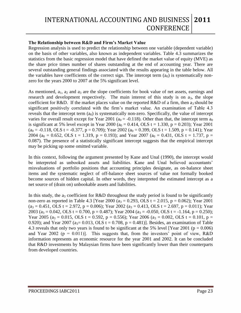
The Relationship between R&D and Firm’s Market Value
Regression analysis is used to predict the relationship between one variable (dependent variable)
on the basis of other variables, also known as independent variables. Table 4.3 summarizes the
statistics from the basic regression model that have defined the market value of equity (MVE) as
the share price times number of shares outstanding at the end of accounting year. There are
several outstanding general findings associated with the results appearing in the table below. All
the variables have coefficients of the correct sign. The intercept term (a0) is systematically non-
zero for the years 2000 to 2007 at the 5% significant level.
As mentioned, a1, a2 and a3 are the slope coefficients for book value of net assets, earnings and
research and development respectively. The main interest of this study is on a3, the slope
coefficient for R&D. If the market places value on the reported R&D of a firm, then a3 should be
significant positively correlated with the firm‟s market value. An examination of Table 4.3
reveals that the intercept term (a0) is systematically non-zero. Specifically, the value of intercept
varies for overall result except for Year 2001 (a0 = -0.118). Other than that, the intercept term a0
is significant at 5% level except in Year 2000 (a0 = 0.414, OLS t = 1.330, p = 0.203); Year 2001
(a0 = -0.118, OLS t = -0.377, p = 0.709); Year 2002 (a0 = 0.399, OLS t = 1.509, p = 0.141); Year
2004 (a0 = 0.652, OLS t = 1.319, p = 0.193); and Year 2007 (a0 = 0.431, OLS t = 1.737, p =
0.087). The presence of a statistically significant intercept suggests that the empirical intercept
may be picking up some omitted variable.
In this context, following the argument presented by Kane and Unal (1990), the intercept would
be interpreted as unbooked assets and liabilities. Kane and Unal believed accountants‟
misvaluations of portfolio positions that accounting principles designate, as on-balance sheet
items and the systematic neglect of off-balance sheet sources of value not formally booked
become sources of hidden capital. In other words, they interpreted the estimated intercept as a
net source of (drain on) unbookable assets and liabilities.
In this study, the a3 coefficient for R&D throughout the study period is found to be significantly
non-zero as reported in Table 4.3 [Year 2000 (a3 = 0.293, OLS t = 2.015, p = 0.062); Year 2001
(a3 = 0.451, OLS t = 2.972, p = 0.006); Year 2002 (a3 = 0.413, OLS t = 2.697, p = 0.011); Year
2003 (a3 = 0.042, OLS t = 0.700, p = 0.487); Year 2004 (a3 = -0.050, OLS t = -1.164, p = 0.250);
Year 2005 (a3 = 0.015, OLS t = 0.592, p = 0.556); Year 2006 (a3 = 0.002, OLS t = 0.101, p =
0.920); and Year 2007 (a3= 0.013, OLS t = 0.708, p = 0.481)]. Besides, an examination of Table
4.3 reveals that only two years is found to be significant at the 5% level [Year 2001 (p = 0.006)
and Year 2002 (p = 0.011)]. This suggests that, from the investors‟ point of view, R&D
information represents an economic resource for the year 2001 and 2002. It can be concluded
that R&D investments by Malaysian firms have been significantly lower than their counterparts
from developed countries.

INTERNATIONAL ACCOUNTING AND BUSINESS CONFERENCE
2011
PROCEEDINGS IABC2011 Page 24
Apart from that, Malaysia‟s R&D intensity still indicates that it is still below that of other
developing countries such as South Africa, Pakistan, India, China, Brazil and Venezuela. A
major reason for Malaysia‟s low R&D intensity is that many Malaysian enterprises are oriented
towards the domestic market and thereafter remain less pressure to be innovative, through R&D,
to be competitive in the international markets (White Paper - Comparative Analysis of R&D
Developments in Malaysia, 2002). In fact, annual surveys carried out by the United Kingdom
Department of Trade & Industry, none of Malaysian companies ranked in the top 500
international companies that undertook R&D investment in the year 2000 and 2001. This shows
that firms in Malaysia do not spent as much on R&D as compared to other firms in developed
countries. Apart from that, R&D activities among firms in Malaysia were very limited.
Compared to firms in other countries such as the United States, Japan and Germany, the amount
spent on R&D by Malaysian firms was very much less (Alfan, 2003).
Apart from that, investors more perceive on BVNA in market valuation. The result (as reported
in Table 4.3) is as follows: [Year 2000 (a1 = 0.878, OLS t = 4.512, p = 0.000); Year 2001 (a1 =
0.938, OLS t = 4.654, p = 0.000); Year 2002 (a1 = 0.549, OLS t = 3.074, p = 0.004); Year 2003
(a1 = 0.440, OLS t = 1.488, p = 0.144); Year 2004 (a1 = 1.066, OLS t = 2.346, p = 0.023); Year
2005 (a1 = 0.077, OLS t = 0.337, p = 0.737); Year 2006 (a1 = 0.685, OLS t = 2.952, p = 0.004);
and Year 2007 (a1= 1.025, OLS t = 4.972, p = 0.000)]. Consequently, these findings confirm the
belief that the market was taking into consideration BVNA in determining the firm‟s equity
value as compared to R&D.
As explained in Chapter 3, r-squared measures the movement or changes in a variable that can be
explained by movements in another variable. A variable with greater r-squared indicates
explanatory power of that variable in explaining market value of equity. In general, the higher
the r-squared value, the better the model fits the data. However, if r-squared is lower, then the
explanatory variable is less relevant. Table 4.3 reports the result of r-squared value for Malaysian
companies across the year 2000-2007 (Year 2000 = 0.648; Year 2001 = 0.585; Year 2002 =
0.512; Year 2003 = 0.200; Year 2004 = 0.136; Year 2005 = 0.345; Year 2006 = 0.381; and Year
2007 = 0.423). On top, we can conclude that the Model 3.2 has its explanatory power due to a
higher value of r-squared for year 2000, 2001, 2002 and 2007. Therefore, there is an evidence to
infer that a linear relationship exists between the dependent and independent variables for whole
year of study.

INTERNATIONAL ACCOUNTING AND BUSINESS CONFERENCE
2011
PROCEEDINGS IABC2011 Page 25
Table 4.3: Market Value Predictions for Malaysian Firms (Basic Model)
Predicted Sign
a0
?
a1
+
a2
+
a3
+
R2 N
2000
coefficient
OLS-t
p-value
0.414
1.330
0.203
0.878
4.512
0.000*
1.880
1.901
0.077
0.293
2.015
0.062
0.648
19
2001
coefficient
OLS-t
p-value
-0.118
-0.377
0.709
0.938
4.654
0.000*
0.116
0.338
0.737
0.451
2.972
0.006*
0.585
31
2002
coefficient
OLS-t
p-value
0.399
1.509
0.141
0.549
3.074
0.004*
1.548
2.376
0.024*
0.413
2.697
0.011*
0.512
35
2003
coefficient
OLS-t
p-value
0.958
2.660
0.011*
0.440
1.488
0.144
1.374
1.895
0.065
0.042
0.700
0.487
0.200
46
2004
coefficient
OLS-t
p-value
0.652
1.319
0.193
1.066
2.346
0.023*
0.053
0.085
0.932
-0.050
-1.164
0.250
0.136
53
2005
coefficient
OLS-t
p-value
1.053
3.889
0.000*
0.077
0.337
0.737
4.167
4.396
0.000*
0.015
0.592
0.556
0.345
63
2006
coefficient
OLS-t
p-value
1.081
3.569
0.001*
0.685
2.952
0.004*
2.759
2.832
0.006*
0.002
0.101
0.920
0.381
69
2007
coefficient
OLS-t
p-value
0.431
1.737
0.087
1.025
4.972
0.000*
0.641
1.889
0.063
0.013
0.708
0.481
0.423
71
Note: The table indicates significance at 5% (*).
Model (Basic): MVEjt = a0 + a1BVNAjt + a2EARNjt + a3R/Djt + ejt…(Model 3.2)

INTERNATIONAL ACCOUNTING AND BUSINESS CONFERENCE
2011
PROCEEDINGS IABC2011 Page 26
The Relationship Between R&D and Firm’s Market Value after taking into Consideration
Heteroscedasticity Problem
The first common econometric problem to be encountered when estimating cross-sectional
valuation models is heteroscedasticity. This problem arises due to the fact that small companies
tend to produce small disturbance whereas large firms produce large disturbance. If
heteroscedasticity is present, then the standard errors are understated, resulting in overstated t-
statistics. In order to address these issues, the entire variables are transformed by deflating them
with the independent variable, which in this case is earnings/total sales, to produce a constant
(but still unknown) variance. As discussed in Chapter Three, „deflation technique‟ hopefully
eliminates the heteroscedasticity problems. This technique has already been employed by
previous researchers such as Landsman (1986), Gopalakrishnan and Sugrue (1993), Shevlin
(1991), McCarthy and Schneider (1995), Jennings et al. (1996) and Ibrahim et al. (1999).
According to Gujarati (1995), if heteroscedasticity is present, then the usual OLS estimators,
although unbiased, no longer exhibit minimum variance among all linear unbiased estimators. In
short, they are no longer the best linear unbiased estimator. As a result, all elements of data for
the basic model reported in the previous chapter are deflated by total sales at the end of the year
to reduce heteroscedasticity problems as well as to increase efficiency. As heteroscedasticity was
one of the major problems, the heteroscedasticity test statistics available with the MICROFIT
software package are analyzed.
The null hypothesis that the variance of the residuals of the model is constant throughout the
whole sample is rejected at the 5% level of significance for all cases. White‟s heteroscedasticity-
corrected standards errors are available with the MICROFIT software package as a standard
output so it is possible to compare the results from the regular OLS (as reported in Table 4.4)
with the adjusted one. Table 4.4 demonstrates the summary statistics from the basic regression
models that are based on White‟s heteroscedasticity adjusted standards errors by Malaysian firms
during 2000-2007. Specifically, the values of a0 are non-zero and higher than one for overall
result except (as reported in Table 4.4) in year 2001 (a0 = -0.118, White‟s t = -0.316). Other than
that, the intercept term a0 significant at 5% level except (as reported in Table 4.4) in Year 2000
(a0 = 0.414, White‟s t = 1.827, p = 0.088), Year 2001 (a0 = -0.118, White‟s t = -0.316, p =
0.754); Year 2002 (a0 = 0.399, White‟s t = 1.662, p = 0.107); Year 2004 (a0 = 0.652, White‟s t =
1.850, p = 0.070) and Year 2007 (a0 = 0.431, White‟s t = 1.415, p = 0.162).
With comparing these two results, obviously White‟s heteroscedasticity-corrected standard errors
are considerably larger than the OLS standard errors and therefore the estimated t values are
much smaller than those obtained by OLS. Although most of the t values are smaller, the overall
results are consistent with the results reported in the previous sub-section. Several studies have
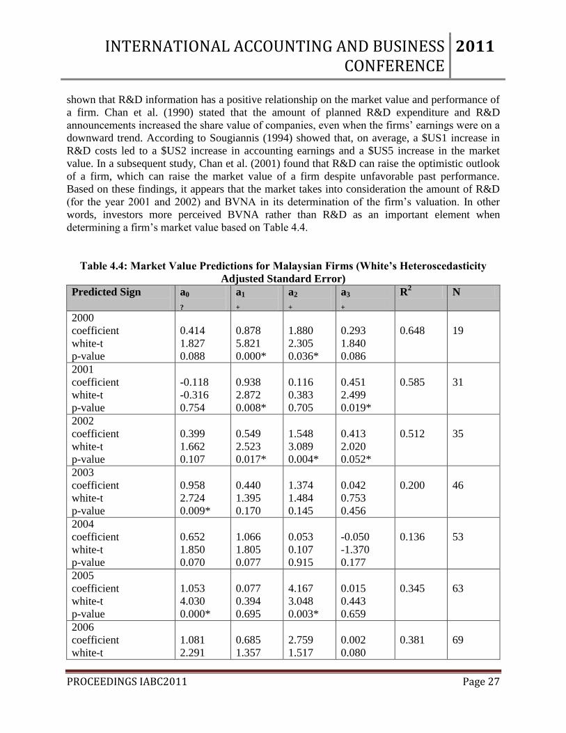
INTERNATIONAL ACCOUNTING AND BUSINESS CONFERENCE
2011
PROCEEDINGS IABC2011 Page 27
shown that R&D information has a positive relationship on the market value and performance of
a firm. Chan et al. (1990) stated that the amount of planned R&D expenditure and R&D
announcements increased the share value of companies, even when the firms‟ earnings were on a
downward trend. According to Sougiannis (1994) showed that, on average, a $US1 increase in
R&D costs led to a $US2 increase in accounting earnings and a $US5 increase in the market
value. In a subsequent study, Chan et al. (2001) found that R&D can raise the optimistic outlook
of a firm, which can raise the market value of a firm despite unfavorable past performance.
Based on these findings, it appears that the market takes into consideration the amount of R&D
(for the year 2001 and 2002) and BVNA in its determination of the firm‟s valuation. In other
words, investors more perceived BVNA rather than R&D as an important element when
determining a firm‟s market value based on Table 4.4.
Table 4.4: Market Value Predictions for Malaysian Firms (White’s Heteroscedasticity
Adjusted Standard Error)
Predicted Sign
a0
?
a1
+
a2
+
a3
+
R2 N
2000
coefficient
white-t
p-value
0.414
1.827
0.088
0.878
5.821
0.000*
1.880
2.305
0.036*
0.293
1.840
0.086
0.648
19
2001
coefficient
white-t
p-value
-0.118
-0.316
0.754
0.938
2.872
0.008*
0.116
0.383
0.705
0.451
2.499
0.019*
0.585
31
2002
coefficient
white-t
p-value
0.399
1.662
0.107
0.549
2.523
0.017*
1.548
3.089
0.004*
0.413
2.020
0.052*
0.512
35
2003
coefficient
white-t
p-value
0.958
2.724
0.009*
0.440
1.395
0.170
1.374
1.484
0.145
0.042
0.753
0.456
0.200
46
2004
coefficient
white-t
p-value
0.652
1.850
0.070
1.066
1.805
0.077
0.053
0.107
0.915
-0.050
-1.370
0.177
0.136
53
2005
coefficient
white-t
p-value
1.053
4.030
0.000*
0.077
0.394
0.695
4.167
3.048
0.003*
0.015
0.443
0.659
0.345
63
2006
coefficient
white-t
1.081
2.291
0.685
1.357
2.759
1.517
0.002
0.080
0.381
69

INTERNATIONAL ACCOUNTING AND BUSINESS CONFERENCE
2011
PROCEEDINGS IABC2011 Page 28
Predicted Sign
a0
?
a1
+
a2
+
a3
+
R2 N
p-value 0.025* 0.179 0.134 0.936
2007
coefficient
white-t
p-value
0.431
1.415
0.162
1.025
2.779
0.007*
0.641
1.929
0.058
0.013
0.410
0.683
0.423
71
Note: The table indicates significance at 5% (*).
Model (Basic): MVEjt = a0 + a1BVNAjt + a2EARNjt + a3R/Djt + ejt…(Model 3.2)
The Relationship between R&D Information and Firm’s Market Value after taking into
Consideration Multicollinearity Problem
The second potential problem in the classical linear regression model is multicollinearity.
Multicollinearity is a condition that exists when the independent variables are correlated with
one another.3 The adverse effect of multicollinearity is that the estimated regression coefficients
of the independent variables that are correlated tend to have large sampling errors. This is based
on the assumption that there is no multicollinearity among the regressors included in the
regression model.
According to Gujarati (1995), the term multicollinearity is used where the variables (regressors)
are intercorrelated (perfect or non-perfect). If multicollinearity is perfect the regression
coefficients of the variables are indeterminate and their standard errors are infinite. If
multicollinearity is less than perfect, the regression coefficient, although determinate, possess
large standard errors (in relation to the coefficients themselves), which means the coefficients
cannot be estimated with great precision or accuracy. The problem is due to the existence of a
linear relationship among the explanatory variables of a regression model. Therefore, the
presence of a severe multicollinearity problem could result in drawing misleading inferences
from sample t-statistics (Gujarati, 1995). Multicollinearity is a question of degree and not of
kind. The meaningful distinction is not between the presence and the absence of multicollinearity
but between its various degrees. Since multicollinearity refers to the condition of the explanatory
variables that are assumed to be non stochastic, it is a feature of the sample and not of the
population. Therefore, we do not „test for multicollinearity‟ but can, if we wish, measure its
degree in any particular sample.4
As mentioned earlier, the presence of a severe multicollinearity problem could result in drawing
misleading inferences from t-statistics. One possible way of increasing the precision of the
estimates of the coefficients in basic models is to estimate the model in net assets; i.e., to use
BVNA or NAV (Book value of Net Assets or Net Assets Value) as explanatory variables. In
principle, book value of assets and book value of liabilities are jointly determined variables,
affected by many of the same unknown exogenous variables. Treating book value of assets and
3 Multicollinearity refers to the existence of more than one exact linear relationship.
4 Jan Kmenta, Elements of Econometrics, 2
nd ed. Macmillan, New York, 1986, p 431.

INTERNATIONAL ACCOUNTING AND BUSINESS CONFERENCE
2011
PROCEEDINGS IABC2011 Page 29
book value of liabilities as separate exogenous regressors could introduce interpretative problems
(Kane and Unal, 1990).
When some of explanatory variables are similar to one another, it may have a multicollinearity
problem because it is difficult for multiple regressions to distinguish between the effect of one
variable and the effect of another. Therefore, in solving the multicollinearity problem, the book
value of asset and book value of liabilities are jointly determined as one variable in a net asset
model in order to increase the accuracy of the estimates of the coefficients in the basic models. It
means BVNA is used as an explanatory variable.
Thus, BVNA will be used as an explanatory variable that are truly independent of one another
and can helps to reduce multicollinearity. According to Landsman (1986), one possible way to
increase the precision of the estimate model is to estimate it in net asset form. Similar with
Ibrahim et al. (1999), Ibrahim et al. (2001) and Ibrahim et al. (2002), we used BVNA as an
explanatory variable in order to reduce the multicollinearity problem in this study. In general,
the net assets model improves the basic model. The most likely cause of the increase in
robustness is the reduction in the collinearity of the two regressors, book value of assets and
book value of liabilities.
Market Valuation of Research and Development versus Other Assets
Given that research and development appears to be a significant factor in valuing a company, the
second hypothesis examines how the market perceives R&D in relation to all other assets. In
other words, is it priced differently from other assets? This hypothesis (H2) is tested by
comparing the coefficients of R&D and BVNA. If the two coefficients were not significantly
different, then this would suggest that the market treats research and development like any other
assets.
However, if the coefficients are significantly different, then the market perceives reported
research and development differently from the other assets. By answering this question, it would
provide insight into the relative importance of reported R&D in valuing a firm compared to other
assets, and then such results would provide additional evidence for the recognition of R&D in the
balance sheet. After comparing the coefficients of R&D and BVNA, the Wald Test is computed
in order to check on how the market perceives the amount of R&D in relation to all other assets.
The absolute value of BVNA and R&D coefficients from the basic model presented in Table 4.5
is discussed. The result shows (as reported in Table 4.5) is as follows: Year 2000 a1 0.878 > a3 =
0.153; Year 2001 a1 = 0.873 > a3 = 0.188; Year 2002 a1 = 0.915 > a3 = 0.114; and Year 2003 a1 =
0.717 > a3 = 0.085. It is obvious that the absolute values of BVNA coefficients are not so much
higher than R&D for all cases. It indicates that the investors treat R&D like any other assets.
After considering the absolute values of both coefficients, the hypothesis to examine the
magnitude of the market perception of R&D in relation to other assets is tested. The result of this

INTERNATIONAL ACCOUNTING AND BUSINESS CONFERENCE
2011
PROCEEDINGS IABC2011 Page 30
test is presented in Table 4.5 and we have enough statistical evidence not to reject the null
hypothesis of equal coefficients. Therefore, it can be concluded that the R&D is not priced
differently from other assets.
Table 4.5: Wald Test Restriction Imposed on Parameter of Market Value Predictions for
Malaysian Firms
Year Coefficient
a1 a3
Chi-Square p-Value
2000
0.878
0.293
1.616
0.204
2001
0.938
0.451
0.189
0.664
2002
0.549
0.413
2.622
0.105
2003
0.440
0.042
0.288
0.591
2004
1.066
-0.050
0.913
0.339
2005
0.077
0.015
11.120
0.001
2006
0.685
0.002
3.213
0.073
2007
1.025
0.013
0.304
0.581
Model (Basic): MVEjt = a0 + a1BVNAjt + a2EARNjt + a3R/Djt + ejt…(Model 3.2)
Restriction: a1 - a3 = 0
The Relationship between R&D and Earnings Sign
Positive and Negative Earnings
Since earnings items have both positive and negative values, which refer to profit and loss
respectively, a new variable was added to the original model used in this study. A new variable
that was used in this study was the dummy variable designed for the earnings items in order to
differentiate positive earnings from negative earnings towards the volume of R&D. If the
reported earnings items were positive, the value for this dummy variable was 1. On the other
INTERNATIONAL ACCOUNTING AND BUSINESS CONFERENCE
2011
PROCEEDINGS IABC2011 Page 31
hand, if the reported earnings items were negative, the value for this dummy variable was 0. In
other words, for Model 3.3, in measuring positive (+) or negative (-) earnings, we measure it as
profit (+) or loss (-) similar with Chen et al. (2001).
Chen et al. empirically investigated the value relevance of accounting information in the
emerging Chinese stock market. The sample selection starts with all listed companies in both the
Shanghai and Shenzhen Stock Exchanges from 1991 to 1998. First, they documented that
accounting information is value relevant in the Chinese market according to both the pooled
cross-section and time-series regressions or the year-by-year regressions. Second, they examined
whether value relevance in China changes in a predictable manner with respect to four factors
including positive versus negative earnings, firm size, earnings persistence and liquidity of stock.
Chen et al. divided their sample into two groups based on each of the four factors reveal above.
Then, they employed a dummy variable to denote a firm‟s membership in each group and test the
significance of the dummy-accounting variable interaction to assess the impact of each factor on
value relevance. As well, in measuring positive (+) or negative (-) earnings, Chen at al. (2001)
differentiated it as profit (+) or loss (-). They found that investors in China differentiate positive
earnings from negative earnings. The results provide evidence consistent with the notion that
accounting information is value relevant to investors in the Chinese market according to year-by-
year regressions despite the young age of the market and the perception of inadequate accounting
and financial reporting in China (Chen et al., 2001).
The regression was conducted separately for each year under this study. Since earnings items
have both positive (+) and negative (-) values, which refer to profit (+) and loss (-) respectively,
another regression equation was developed to test whether a different sign or direction of
earnings had a relationship on the R&D. As mentioned above, a new variable was added to the
original basic model used in this study, which was the dummy variable for the direction of
earnings items. If the coefficient of the dummy variable, a4 is significant, this implies that the
direction of earnings items had some effects on the R&D. On the other hand, if the coefficient
value is not significant, this would indicate that there is no relationship between R&D and the
direction of earnings items. In other words, it (refer to R&D) did not matter whether the
earnings items were gains or losses.
Moreover, the one common econometric problem that often arises when conducting a cross-
sectional analysis is heteroscedasticity. As mentioned, if heteroscedasticity is present, then the
usual OLS estimators, although unbiased, no longer exhibit minimum variance among all linear
unbiased estimators (Gujarati, 1995). If the variance is not constant across observations, the
regression is said to be heteroscedastic. Failure to control for heteroscedasticity can result in
biased standard error estimates and estimation inefficiency. In other words, they are no longer
the best linear unbiased estimator. After taking into consideration of heteroscedasticity problem,
Table 4.6 reports the summary statistics from the extended model (Model 3.3) that are based on
White‟s heteroscedasticity adjusted standard errors. Those tables show different t-values,
compared to the OLS results reported earlier. The result in Table 4.6 shows that the coefficients

INTERNATIONAL ACCOUNTING AND BUSINESS CONFERENCE
2011
PROCEEDINGS IABC2011 Page 32
a4 are not significant at the 5% level. This implied that there is no relationship between the
amount of R&D and the sign of earnings items for Malaysian firms throughout the study period.
Earnings Item
Table 4.6 reports that the coefficient a3 are not significant at the 5% level during the period 2000
to 2007. Nevertheless, it is significant at the 5% level only in Year 2007 (a3 = -7.612, White‟s t =
-2.247, p = 0.028) but with incorrect sign. Therefore, we have enough statistical evidence not to
reject the null hypothesis. As a result, we can conclude that there is no significant relationship
exists between the amount of R&D and earnings items. The coefficients also showed that the
value of R&D has negative relation with earnings items (as reported in Table 4.6) except in Year
2000 (a3 = 6.452) and Year 2002 (a3 = 0.937).
Table 4.6: Market Value Predictions for Malaysian Firms - Dummy Variable Included
(White’s Heteroscedasticity Adjusted Standard Error)
Predicted
Sign
a0
?
a1
+
a2
+
a3
+
a4
?
R2
N
2000
coefficient
white-t
p-value
4.549
2.049
0.060
0.397
1.583
0.136
-0.045
-0.101
0.921
6.452
1.242
0.234
-4.896
-1.735
0.105
0.466
19
2001
coefficient
white-t
p-value
0.862
1.389
0.177
0.532
2.399
0.024*
-0.463
-2.061
0.049*
-0.221
-1.024
0.315
-0.343
-0.652
0.520
0.285
31
2002
coefficient
white-t
p-value
0.555
1.271
0.213
0.405
2.023
0.052*
0.035
0.121
0.904
0.937
0.935
0.357
-0.531
-1.285
0.208
0.316
35
2003
coefficient
white-t
p-value
-0.556
-0.519
0.606
0.280
0.979
0.333
1.849
1.804
0.079
-1.720
-1.410
0.166
-0.659
-0.450
0.655
0.198
46
2004
coefficient
white-t
p-value
-3.728
-0.811
0.421
-0.531
-0.973
0.335
7.002
1.563
0.125
-3.854
-1.479
0.145
-0.448
-0.139
0.890
0.407
53
2005
coefficient
white-t
p-value
-1.963
-0.621
0.537
0.455
0.999
0.322
2.770
0.830
0.410
-7.271
-1.006
0.318
1.377
0.656
0.514
0.108
63
INTERNATIONAL ACCOUNTING AND BUSINESS CONFERENCE
2011
PROCEEDINGS IABC2011 Page 33
Predicted
Sign
a0
?
a1
+
a2
+
a3
+
a4
?
R2
N
2006
coefficient
white-t
p-value
0.538
0.506
0.614
0.076
0.117
0.907
1.267
0.747
0.457
-0.430
-0.362
0.718
0.666
0.574
0.568
0.037
69
2007
coefficient
white-t
p-value
-1.864
-1.112
0.270
0.537
0.497
0.621
4.757
1.644
0.105
-7.612
-2.247
0.028*
-0.746
-0.435
0.665
0.322
71
Note: The table indicates significance at 5% level.
Limitation and Recommendation of the Study
There is one limitation encountered in this study. The data set were obtained from the listing
datastream without any classification by sector. Therefore, overall results can be generalized
only for those companies from the listing datastream throughout the study period.
The results and limitation in the current study raise several issues, which can be better explained
through future research. Future research could extend this study to include the classification of
sector. This is to ensure that the model can be generalized to determine the market value for
different sector. By regrouping of companies by sector may produce better results in determining
whether R&D information can affect its market value.
In addition, interviews session or questionnaires can be conducted with Managing Director/Chief
Executive Officer of companies and examine how they view the role of R&D towards market
valuation, companies performance and well being. Apart from that, interviews session can also
be conducted with investors and examine how they perceives fundamental R&D information as
an important variable in the determination of the value of a company. Further efforts are needed
in order to understand the behaviour of investors with respect to intangibles information
especially for R&D. This approach would provide supporting information to the empirical results
for the findings of the study.
References
Aboody, D. and Lev, B. (1998). The Value-Relevance of Intangibles: The Case of Software
Capitalization, Journal of Accounting Research, 36, pp 161-191.

INTERNATIONAL ACCOUNTING AND BUSINESS CONFERENCE
2011
PROCEEDINGS IABC2011 Page 34
Alfan, E. (2003). Low spending R&D - Is the accounting treatment at fault?, Berita CPA, 1(13)
Arce, M. and Mora, A. (2002). Empirical Evidence of the Effect of European Accounting
Differences on the Stock Market Valuation of Earnings and Book Value, The European
Accounting Review, 11, 573-599.
A world of strangers: International Accounting Standards Explained. (2000). First Edition, John
Wiley & Sons. Ltd, New York.
Ball, R. and Brown, P. (1968). An Empirical Evaluation of Accounting Income Numbers,
Journal of Accounting Research, 6, pp 159-178.
Barreto, L. and Kypreos, S. (2004). Endogenizing R&D and Market Experience in the Bottom-
Up Energy-Systems ERIS Model, Technovation, 24, pp 615-629.
Barth, M.E., Beaver, W.H. and Landsman, W.R. (2001). The Relevance of the Value Relevance
Literature for Financial Accounting Standard Setting: Another View, Journal of Accounting
and Economics, 31, pp 77-104.
Belkaoui, A.R. (1992). Accounting Theory, Academic Press, London.
Biddle, G., Seow, G. and Siegel, A.F. (1995). Relative Versus Incremental Information Content,
Contemporary Accounting Research, 12, pp 1-23.
Black, E.L. and White, J.J. (2003). An International Comparison of Income Statement and
Balance Sheet Information: Germany, Japan and the US, European Accounting Review, 12,
pp 29-46.
Blake, J. and Lunt, H. (2001). Accounting Standard, Seven Edition, Prentice Hall, England.
Bloom, N. and Griffith, R. (2001). The Internationalisation of UK R&D, Fiscal Studies, 22, 3, pp
337-355.
Boone, J.P. and Raman, K.K. (2001). Off-Balance Sheet R&D Assets and Market Liquidity,
Journal of Accounting and Public Policy, 20, pp 97-128.
Callen J. L., Morel M. (2005). The Value Relevance of R&D Expenditures: Time Series
Evidence, International Review of Financial Analysis, 14, pp 304-325.
Chamberlain, W. (1999). Share Price Reaction to Research and Development Spending:
Canadian Evidence, International Advances in Economic Research
Chan, L.K.C., Lakonishok, J. and Sougiannis, T. (2001). The Stock Market Valuation of
Research and Development Expenditures, The Journal of Finance, LVI, 6, pp 2431-2456.

INTERNATIONAL ACCOUNTING AND BUSINESS CONFERENCE
2011
PROCEEDINGS IABC2011 Page 35
Chan, S.H., Martin, J.D. and Kensigner, J.W. (1990). Corporate Research and Development
Expenditures and Share Value, Journal of Financial Economics, 26, pp 255-276.
Chen, C.J.P., Chen, S. and Su, X. (2001). Is Accounting Information Value-Relevant in the
Emerging Chinese Stock Market? Journal of International Accounting, Auditing and
Taxation, 10, pp 1-22.
Choi, W.W., Kwon, S.S. and Lobo, G.L (2000). Market Valuation of Intangible Assets, Journal
of Business Research, 49, pp 35-45.
Collins, D.W., Maydew, E.L. and Weiss, I.S. (1997). Changes in the Value-Relevance of
Earnings and Book Values Over The Past Forty Years, Journal of Accounting and
Economics, 24, pp 39-67.
Dato‟ Shaziman bin Abu Mansor. (2009). Opening Sppech,Construction Industry Research
Achievement International Conference.
Dhaliwal, D.S. (1986). Measurement of Financial Leverage in the Presence of Unfunded Pension
Obligations, The Accounting Review, 61, pp. 651-661.
Dyckman, T.R. and Morse, D. (1986). Efficient Capital Markets and Accounting: A Critical
Analysis, Prentice Hall, New Jersey.
Ella Syafputri, Science and Development Network, dated 24 September 2007 (www.scidev.net)
Epstein, B.J and Mirza, A.A. (2003). Interpretation and Application of International Accounting
Standards, John Wiley & Sons. Inc, England.
Fang, S.F., Lin, J.L., Hsiao, L.Y.C., Huang, C.M. and Fang, S.R. (2002). The Relationship of
Foreign R&D Units in Taiwan and the Taiwanese Knowledge-Flow System, Technovation,
22, pp 371-383.
Financial Reporting Standards 138, Intangible Assets
Francis, J. and Schipper, K. (1999). Have Financial Statements Lost Their Relevance? Journal of
Accounting Research, 37, 2, pp 319-351.
Gopalkrishnan, V. and Sugrue, T.F. (1993). An Empirical Investigation of Stock Market
Valuation of Corporate Projected Pension Liabilities, Journal of Business Finance &
Accounting, pp 711-724.
Goulder, L.H. and Mathai, K. (2000). Optimal CO2 Abatement in the Presence of Induced
Technological Change, Journal of Environmental Economics and Management, 39, pp 1-38.
INTERNATIONAL ACCOUNTING AND BUSINESS CONFERENCE
2011
PROCEEDINGS IABC2011 Page 36
Gujarati, D.N. (1995). Basis Econometrics, Third Edition, McGraw-Hill Inc, New York.
Han, B.H and Manry, D. (2004). The Value-Relevance of R&D and Advertising Expenditures:
Evidence from Korea, The International Journal of Accounting, 39, pp 155-173.
Hicks, G.L. and Redding, S.G. (1983). The story of the East Asian economic miracle. Euro-
Asian Business Review 3 and 4.
Holthausen, R.W. and Watts, R.L. (2001). The Relevance of the Value-Relevance Literature for
Financial Accounting Standard Setting, Journal of Accounting & Economics, 31, pp 3-75.
Ibrahim, M.K., Danila, R., Yusoff, H. and Yatim, N. (2002). Market Value and Balance Sheet
Numbers: Evidence from Malaysia, Asian Accounting Review.
Ibrahim, M.K., McLeay, S. and Neal, D. (1999). Market Value, Book Value and Goodwill,
National British Accounting Association Conference, Glasgow University, United Kingdom.
Ibrahim, M.K., Mohd Said, M., Abd Latif, R. and Abdul Shukur, Z. (2001). Value Relevance of
accounting numbers: An empirical investigation of purchased goodwill, Conference on
Business, University of Hawaii, United States.
Isa, S. (2002). MASB 4 Research and Development Costs - An Analysis, Akauntan Nasional, 15,
8, pp. 24-27.
Jenkins, D.S. (2002). Profitability, Firm Survival and the Value Relevance of Negative Earnings.
PhD Thesis, University of Maryland, U.S.
Jennings, R., Robinson, J., Thompson II, R.B. and Duvall, L. (1996). The Relation Between
Accounting Goodwill Numbers and Equity Values, Journal of Business Finance and
Accounting, 23, 4, pp 513-533.
Kahal, S.E. (2001). Business in Asia Pacific Text and Cases, First Edition, Oxford University
Press, New York.
Kane, E.J. and Unal, H. (1990). Modelling Structural and Temporal Variation in the Market‟s
Valuation of Banking Firms, Journal of Finance, XLV, 1, pp 113-136.
Laincz, C.A. (2005). Market Structure and Endogenous Productivity Growth: How do R&D
Subsidies Affect Market Structure? Journal of Economic Dynamics & Control, 29, pp 187-
223.
Landry, S. and Callimaci, A. (2004). Market Valuation of Research and Development Spending
under Canadian GAAP, Canadian Accounting Perspectives, 3, 1, pp 33-53.
INTERNATIONAL ACCOUNTING AND BUSINESS CONFERENCE
2011
PROCEEDINGS IABC2011 Page 37
Landry, S. and Callimaci, A. (2003). The Effect of Management Incentives and Cross-Listing
Status on the Accounting Treatment of R&D Spending, Journal of International
Accounting, Auditing and Taxation, 12, pp 131-152.
Landsman, W. (1986). An Empirical Investigation of Pension Fund Property Rights, The
Accounting Review, 61, 4, pp 662-691.
Lev, B. and Sougiannis, T. (1996). The Capitalization, Amortization, and Value-Relevance of
R&D, Journal of Accounting and Economics, 21, pp 107-138.
Liu, D.N. and Ku, Y.H. (2003). A Case Study of the Success and Failure of Multinational Firms‟
Investment in Taiwan, Chung-Hua Institution for Economic Research, Taipei.
Maines, L.A., Bartov, E., Fairfield, P.M. and Hirst, D.E. (2003). Implications of Accounting
Research for the FASB‟s Initiatives on Disclosure of Information about Intangible Assets,
Accounting Horizons, 17, 2, pp 175-185.
Mani S. (2002). Government, Innovation and Technology Policy: An International Comparative
Analysis, Edward Elgar, Cheltenham.
Mathews, J.A. (2002). The Origins and Dynamics of Taiwan‟s R&D Consortia, Research Policy,
31, pp 633-651.
McCarthy, M.G. and Schneider, D.K. (1995). Market Perception of Goodwill: Some Empirical
Evidence, Accounting and Business Research, pp 69-81.
Neelankavil, J.P. and Alaganar, V.T. (2003). Strategic Resource Commitment of High-
Technology Firms An International Comparison, Journal of Business Research, 56, pp
493-502.
Nobelius, D. (2004). Towards the Sixth Generation of R&D Management, International Journal
of Project Management, 22, pp 369-375.
Radebaugh, L.H. and Gray, S.J. (2002). International Accounting and Multinational Enterprises,
Fifth Edition, John Wiley & Sons, Inc, New York.
Sekaran, (2000). Research Methods for Business A Skill-Building Approach, Third Edition, John
Wiley & Sons, Inc, New York.
Shefer, D. and Frenkel, A. (2005). R&D, Firm Size and Innovation: An Empirical Analysis,
Technovation, 25, pp 25-32.
Shevlin, T. (1991). The Valuation of R&D Firms with R&D Limited Partnerships, The
Accounting Review, 66, 1, pp 1-21.
INTERNATIONAL ACCOUNTING AND BUSINESS CONFERENCE
2011
PROCEEDINGS IABC2011 Page 38
Kamarun Nisham, T.M., Rohaida, A.L., Wan Nordin, W.H. & Ku Nor Izah, K.I. (2006) The
Value-Relevance of R&D Expenditure: Experience from Malaysia, IIUM Journal of
Economics and Management 14, No 2,
Tishler A. (2008). How Risky Should R&D program Be? Economics Letters 99, pp 268-271
Wakelin, K. (2001). Productivity Growth and R&D Expenditure in UK Manufacturing Firms,
Research Policy, 30, pp 1079-1090.
Wang, J.C., Tsai K.H. (2003). The Impact of Research and Development Promotion Schemes in
Taiwanese Electronic Components Industry, R&D Management, 28(2), pp 119-124.
White Paper (November 2002): Comparative Analysis of R&D Developments in Malaysia, A.
(2002).
Wyatt, A. (2002). Towards a Financial Reporting Framework for Intangibles Insights from the
Australian Experience, Journal of Intellectual Capital, 3, 1, pp 71-86.
Xu, M. and Zhang, C. (2004). The Explanatory Power of R&D for the Cross- Section of Stock
Returns: Japan 1985-2000, Pacific-Basin Finance Journal, 12, pp 245-269.
Zainol A., Nair M., Kasipillai J (2008). R&D Reporting Practice: Case of A Developing
Economy, Journal of Intellectual Capital, Vol 9, No. 1, pp 122-132.
Zedtwitz, M.V. and Gassmann, O. (2002). Market Versus Technology Drive in R&D
Internationalization: Four Different Patterns of Managing Research and Development,
Research Policy, 31, pp 569-588.
Related Documents


