The Marginal Voter™s Curse

The Marginal Voter’s Curse∗

Helios Herrera Aniol Llorente-Saguer Joseph C. McMurray

University of Warwick Queen Mary University Brigham Young University

and CEPR of London and CEPR

This Version: November 20, 2018First Version: October 1, 2014.

Abstract

The swing voter’s curse is useful for explaining patterns of voter participa-

tion, but arises because voters restrict attention to the rare event of a pivotal

vote. Recent empirical evidence suggests that electoral margins influence pol-

icy outcomes, even away from the 50% threshold. If so, voters should also pay

attention to the marginal impact of a vote. Adopting this assumption, we find

that a marginal voter’s curse gives voters a new reason to abstain, to avoid

diluting the pool of information. The two curses have similar origins and ex-

hibit similar patterns, but the marginal voter’s curse is both stronger and more

robust. In fact, the swing voter’s curse turns out to be knife-edge: in large

elections, a model with both pivotal and marginal considerations and a model

with marginal considerations alone generate identical equilibrium behavior.

JEL classification: C72, D70

Keywords: Turnout, Information aggregation, Underdog effect

∗We thank participants at the Political Economy Workshops at Alghero, Bath, Lancaster Uni-versity, Mont Tremblant and at the Wallis Institute. We also thank seminar participants at BrighamYoung University, Caltech, Carlos III, CERGE-EI, European University Institute, NYU Abu Dhabi,Queen Mary University of London, Simon Frazer University, UC Berkeley, UCL, UC San Diego, Uni-versità di Bologna, Université de Montréal, University of British Columbia, University of Hawaii,University of Mannheim, University of Portsmouth, University of Queensland, University of Surrey,University of Tokyo, University of Toronto, University of Warwick, University of Western Ontario.We particularly thank Dan Bernhardt, Chris Bidner, Laurent Bouton, Alessandra Casella, Mi-cael Castanheira, Jon Eguia, Tim Feddersen, Faruk Gul, Wei Li, Claudio Mezzetti, David Myatt,Santiago Oliveros, Louis Philippos, Carlo Prato, and Francesco Trebbi for helpful comments andsuggestions. We would also like to thank Bruno Nogueira Lanzer for excellent assistance.

brought to you by COREView metadata, citation and similar papers at core.ac.uk

provided by Queen Mary Research Online

1 Introduction

Standard models of elections restrict attention to the mechanical impact of a

vote, which is that it can be pivotal in changing the identity of an election winner,

by making or breaking a tie. Empirically, however, it seems that votes may also

exert a marginal influence on policy outcomes, by adjusting the balance between

political parties in power. Claiming a “mandate” from voters, for example, U.S.

presidents who win by larger margins pursue more major policy changes (Conley,

2001). When members of Congress win reelection by larger margins, they have more

partisan voting records (Faravelli, Man, and Walsh, 2015).1 With legislative rules

such as Proportional Representation, larger electoral margins shift the balance of

power mechanically, by altering the composition of a legislature. Slight increases in

a party’s power can be important, even when that party has more than 50% of the

power: in the most recent legislative session, the U.S. Republican party lacked the

political strength for desired health and immigration legislation in spite of control-

ling both houses of Congress and the presidency, but presumably would have been

successful with a larger majority. For any of these reasons, the relationship between

electoral margins and policy outcomes may be as Figure 1 illustrates, where crossing

the 50% threshold shifts the policy outcome discontinuously, but policies respond

to electoral margins even away from this threshold. If so, then every vote has a

small but direct impact on the policy outcome, since every vote slightly increases or

decreases the winning party’s margin of victory.

In a seminal paper, Feddersen and Pesendorfer (1996) derive an important implica-

tion of the standard pivotal voting calculus, which is that voters who lack information

about available policy alternatives have a strategic incentive to abstain from voting,

effectively delegating their decision to voters with superior information.2 This is use-

ful for explaining why voters often deliberately abstain, even in settings where voting

1Fowler (2005) shows that parties that win by large margins also nominate more extreme candi-dates in subsequent elections. Bernhard et al. (2008) find that senators who win by larger marginsmoderate less in the two years before the subsequent election. Fowler (2006) also shows that bondmarket investors expect larger policy changes after landslide election outcomes.

2This relates to pivotal voting because, when a voter expects others to make an informed decision,his own vote will change the election outcome precisely when he has mistakenly voted for the inferiorpolicy alternative.

1

0.2

.4.6

.81

Policy

Outcome

0 .2 .4 .6 .8 1

Vote share

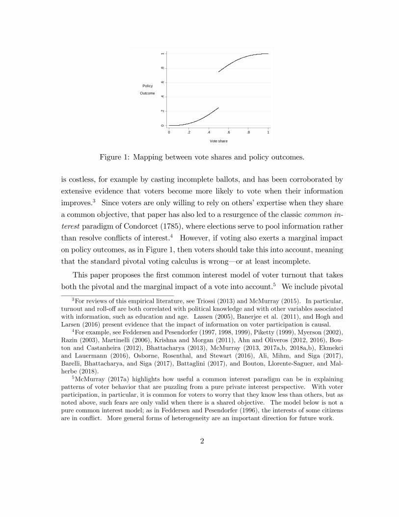
Figure 1: Mapping between vote shares and policy outcomes.

is costless, for example by casting incomplete ballots, and has been corroborated by

extensive evidence that voters become more likely to vote when their information

improves.3 Since voters are only willing to rely on others’expertise when they share

a common objective, that paper has also led to a resurgence of the classic common in-

terest paradigm of Condorcet (1785), where elections serve to pool information rather

than resolve conflicts of interest.4 However, if voting also exerts a marginal impact

on policy outcomes, as in Figure 1, then voters should take this into account, meaning

that the standard pivotal voting calculus is wrong– or at least incomplete.

This paper proposes the first common interest model of voter turnout that takes

both the pivotal and the marginal impact of a vote into account.5 We include pivotal

3For reviews of this empirical literature, see Triossi (2013) and McMurray (2015). In particular,turnout and roll-off are both correlated with political knowledge and with other variables associatedwith information, such as education and age. Lassen (2005), Banerjee et al. (2011), and Hogh andLarsen (2016) present evidence that the impact of information on voter participation is causal.

4For example, see Feddersen and Pesendorfer (1997, 1998, 1999), Piketty (1999), Myerson (2002),Razin (2003), Martinelli (2006), Krishna and Morgan (2011), Ahn and Oliveros (2012, 2016), Bou-ton and Castanheira (2012), Bhattacharya (2013), McMurray (2013, 2017a,b, 2018a,b), Ekmekciand Lauermann (2016), Osborne, Rosenthal, and Stewart (2016), Ali, Mihm, and Siga (2017),Barelli, Bhattacharya, and Siga (2017), Battaglini (2017), and Bouton, Llorente-Saguer, and Mal-herbe (2018).

5McMurray (2017a) highlights how useful a common interest paradigm can be in explainingpatterns of voter behavior that are puzzling from a pure private interest perspective. With voterparticipation, in particular, it is common for voters to worry that they know less than others, but asnoted above, such fears are only valid when there is a shared objective. The model below is not apure common interest model; as in Feddersen and Pesendorfer (1996), the interests of some citizensare in conflict. More general forms of heterogeneity are an important direction for future work.

2

voting incentives by allowing the policy outcome to jump discontinuously when one

party’s vote share crosses the 50% threshold, but importantly, we also allow votes to

have a marginal impact on the policy outcome away from this threshold, as depicted

in Figure 1. For a broad class of policy mappings, the main result is that citizens

with low (though still positive) levels of information abstain, even when voting is

costless. As long as a pivot remains at the 50% threshold, this is not surprising;

however, abstention also occurs even when this pivot is removed entirely. In that

case, voters abstain to avoid what we call the marginal voter’s curse of nudging the

policy in the wrong direction.

The marginal voter’s curse arises because the impact of an individual’s vote is

diluted by the votes of like-minded citizens. The impact of a vote for the party that

is already leading is diluted more than the impact of a vote for the trailing party.

In a common interest environment, the superior party tends to be leading, which

means that voting for the correct alternative/party tends to have a smaller impact

on the policy outcome than voting for the inferior alternative/party has. With no

information about which party is superior, therefore, the benefit of voting for either

party is negative, so a voter abstains in equilibrium, even if voting is costless. Unlike

the swing voter’s curse, which results from low-probability, high-impact events, the

marginal voter’s curse is generated by high-probability, low-impact events. In spite

of this contrast, however, both curses result from the same general underdog property,

whereby an additional vote for the leading party has smaller impact than an additional

vote for the losing party. The two curses thus exhibit similar comparative statics

with regard to the underlying distributions of voter preferences and information.

Intuitively, it might seem that comparing nudges in one direction or the other

would have less impact on voter beliefs than conditioning on an event with major

impact as a pivotal vote. However, the marginal voter’s curse turns out to be stronger

than the swing voter’s curse, in the sense that abstention is higher in a pure marginal

voting model than in a pure pivotal voting model.6 In a general model that includes

6This abstention with costless voting result is the opposite of that obtained in a costly votingprivate value setting of Herrera, Morelli, and Palfrey (2014), where abstention is higher in a purepivotal voting model than in a pure marginal voting model, as long as support for the two partiesis not precisely balanced.

3

both pivotal and marginal considerations, of course, both curses operate. As the

number of votes grows large, however, the importance of pivotal voting considerations

also shrinks compared to marginal voting considerations. In the limit, then, even

though the marginal impact of a vote is minimal, voter participation converges to

the same level that would prevail if there were no discontinuity at all at the 50%

threshold. In other words, a model that includes both pivotal and marginal voting

considerations makes the same predictions for large elections as a model with marginal

voting considerations alone. In that sense, ignoring marginal voting incentives not

only fails to capture an aspect of elections that is relevant empirically; it also generates

predictions that turn out to be knife-edge in a more general setting.

While this paper focuses on pure common interest voters in addition to private

interest voters, a number of existing papers analyze voter participation in light of the

marginal impact of voting, but in a purely private interest setting.7 Others study

participation in common interest elections, but focus only on pivotal voting.8 In a

common interest setting, Razin (2003) considers a model where political parties share

voters’interests, and voluntarily adjust their policy positions to utilize information

revealed by electoral margins. Introducing abstention into that model, McMurray

(2017b) shows that relatively uninformed citizens abstain to avoid the “signaling

voter’s curse”of conveying misleading information. In contrast, the marginal voter’s

curse arises with a mapping from vote shares to policy outcomes that is purely me-

chanical. As explained below, this could reflect adjustments in the balance of power

between parties that do not share voters’interests, or hold overconfident policy be-

liefs. Together, the swing voter’s curse, signaling voter’s curse, and marginal voter’s

curse make clear that common interest and heterogeneous expertise generate strategic

abstention for a variety of institutional details.

The organization of this paper is simple. Section 2 introduces the formal model,

and Section 3 analyzes equilibrium incentives for voter participation, first for elections

of arbitrary size and then in the limit as the electorate grows large. For simplicity, this

7For example, see Castanheira (2003), Shotts (2006), Meirowitz and Shotts (2009), Herrera,Morelli, and Palfrey (2014), Faravelli, Man, and Walsh (2015), Faravelli and Sanchez-Pages (2015),Herrera, Morelli, and Nunnari (2015) and Kartal (2015).

8For example, see Feddersen and Pesendorfer (1996, 1999), Krishna and Morgan (2011, 2012),and McMurray (2013).

4

analysis assumes that policies (aside from the discontinuity at 50%) depend linearly

on the vote share. Section 3.3 then shows that the same results hold for a broad class

of general policy functions, as well, such as the one pictured in Figure 1. Section 4

concludes, and proofs of theoretical results are presented in the Appendix.

2 The Model

An electorate consists of N citizens where N is finite but unknown, and follows a

Poisson distribution with mean n.9 Together, these citizens must choose a policy from

an interval. There are two political parties, each with policy positions in the interval.

At the beginning of the game, and with equal probability, Nature designates one of

these policy positions as better for society than the other. Let A denote the party

with the superior position and B denote the party with the inferior position. Letting

0 denote the inferior policy position and 1 denote the superior position, x ∈ [0, 1]

can denote any policy between the two parties’positions and also the social welfare

u (x) = x that will be attained if that policy is implemented.

Citizens are each independently designated as one of two types. With probability

2p, a citizen is a partisan, and has a vested interest in promoting one party or the

other (each with probability p), regardless of which policy position Nature designated

as superior. With remaining probability I = 1 − 2p, a citizen is independent or

non-partisan. Independents prefer to do whatever is socially optimal, evaluating

policy x according to the welfare function u (x) given above. From an independent’s

perspective, each of his fellow citizens has probability p of being a partisan supporter

of the superior party A and probability p of being a partisan supporter of the inferior

party B. Let a and b denote the numbers of votes cast for either party and λ+ = aa+b

and λ− = ba+b

denote the parties’vote shares (where λ+ = λ− = 12if a = b = 0).

The most standard assumption is that the policy outcome x is simply given by

9This follows Myerson (1998). A known population size is unrealistic, and generates pathologicalequilibria, where voters play weakly dominated strategies, knowing that their votes will not bepivotal. If N is odd, the swing voter’s curse also needs not arise, as a tie conveys no informationabout the state variable. Poisson uncertainty substantially simplifies the analysis, especially inderiving the limiting probabilities of pivotal events.

5

the policy position xw ∈ {xA, xB} of the party w who wins the election (i.e. 0 if b > a

and 1 if a > b, breaking a tie if necessary by a fair coin toss). Alternatively, the

ultimate policy outcome might be a product of bargaining between the two parties.10

If a party’s bargaining power is determined by its vote share, for example, the policy

outcome might be given by the weighted average 0 (λ−) + 1 (λ+) = λ+.11 We refer to

these cases as pure pivotal voting and pure marginal voting, respectively, and assume

more generally that the policy outcome (and welfare) are given by the weighted

average

x = θλ+ + (1− θ)xw (1)

of these two extremes. As in Figure 1, policy then shifts discontinuously when one

party’s vote share crosses the 50% threshold, but even away from this threshold,

changes in one party’s vote share push the policy outcome marginally in that party’s

direction.12

The optimal policy cannot be observed directly, but independent voters observe

private signals si that are informative of Nature’s choice.13 These signals are of

heterogeneous quality, reflecting the fact that citizens differ in their expertise on

the issue at hand. Specifically, each citizen is endowed with information quality

qi ∈ Q = [0, 1], drawn independently according to a common distribution F which,

for simplicity, is continuous and has full support. Conditional on qi = q, a citizen’s

signal correctly identifies the party whose policy position is truly superior with the

10McMurray (2017b) assumes parties to be like independent voters, favoring policies as close aspossible to the state variable. With no need to bargain, the winning side voluntarily calibratesits policy position to account for the strength of evidence for and against its side. Here, partiesare better thought of as partisan voters, favoring extreme policies but for lack of bargaining power.Alternatively, the same specification applies if parties share independent voters’interests but holdoverconfident beliefs, as in McMurray (2018a).

11This is the welfare outcome if independent voters are risk neutral, and parties implement theirpreferred policies 0 and 1 with probabilities λ− and λ+. It could also result from a bargainingmodel with alternating offers, where vote shares determine the probability of being able to offer thenext proposal. Alternatively, it could result from probabilistic voting across independent legislativedistricts, as in Levy and Razin (2015).

12The specification in (1) constrains the policy function to be linear in the vote share (with slopeθ). Section 3.3 extends this to more general functional forms, such as that illustrated in Figure 1.

13Partisans could receive signals as well, of course, but would ignore them in equilibrium.

6

following probability.

Pr (si = A|q) =1

2(1 + q) (2)

With complementary probability, a citizen mistakes the inferior party for the superior

party.

Pr (si = B|q) =1

2(1− q) (3)

With this specification, qi can be interpreted as the correlation coeffi cient between

a voter’s private opinion and the truth. That is, a signal with qi = 1 perfectly

reveals Nature’s choice while a signal with qi = 0 is completely uninformative. An

independent can vote (at no cost) for the party that he perceives to be superior, or

can abstain.14 Let σ : Q → [0, 1] denote a (mixed) participation strategy, where

σ (q) denotes the probability of voting for an individual with expertise q ∈ Q, andlet Σ denote the set of such strategies. If he votes for his signal, a voter’s posterior

belief that he has correctly voted for the superior party or mistakenly voted for the

inferior party are given simply by the right-hand sides of (2) and (3), respectively, by

Bayes’rule.

As an example of political decisions that might fit the structure outlined here,

consider any division of funding between two programs with a common objective, such

as using education money either to increase teacher salaries or to reduce class sizes–

or, at higher levels, using tax revenue to strengthen either the military or the social

safety net. At either level, some voters simply have a vested interest in one program or

the other, and vote accordingly, but others support whichever policy they believe will

be truly best for the group. Interior policies represent various possible compromises

that partially fund both programs, and can result from bargaining between parties

with different levels of power, but if truth were known, independent voters would

prefer to fully fund whichever program is more productive over any such compromise,

and may vote with an eye toward increasing the bargaining power of the party whose

policy proposal seems superior.

Given a participation strategy, the probabilities with which a citizen votes for

14A strategy of voting against one’s signal could be allowed but would not be used in equilibrium.

7

party A and party B, respectively, are given by the following.

v+ = p+ I

∫ 1

0

σ (q)1

2(1 + q) dF (q) (4)

v− = p+ I

∫ 1

0

σ (q)1

2(1− q) dF (q) (5)

These include the probability p of favoring either party for partisan reasons, as well as

the probabilities of voting as an independent with any level of expertise. Together,

(4) and (5) also determine the level v = v+ + v− of voter turnout.

If every citizen follows the same participation strategy, (4) and (5) can be inter-

preted as the expected vote shares of the superior and inferior parties, respectively.

By the decomposition property of Poisson random variables (Myerson 1998), the

numbers a and b of votes for the superior and inferior parties, respectively, are inde-

pendent Poisson random variables with means n+ = nv+ and n− = nv−. Thus, the

probability of exactly a votes for the superior party and b votes for the inferior party

is the product

Pr (a, b) =e−n+na+a!

e−n−nb−b!

(6)

of Poisson probabilities. Similarly, the expected total number of votes can be written

as nv.

By the environmental equivalence property of Poisson games (Myerson 1998), an

individual from within the game reinterprets a and b as the numbers of correct and

incorrect votes cast by his peers; by voting himself, he might add one to either total.

When there are a votes for the superior party and b votes for the inferior party, the

change in utility ∆+x (a, b) from contributing one additional vote for the superior

party and the change in utility ∆−x (a, b) from adding one vote for the inferior party

are given by the following.

∆+x (a, b) = x (a+ 1, b)− x (a, b) (7)

∆−x (a, b) = x (a, b+ 1)− x (a, b) (8)

The magnitudes of these utility changes depend on the numbers of votes cast for either

8

side by a citizen’s peers; averaging over all possible voting outcomes, the expected

benefit of voting is given by

∆Eu (q) = Ea,b

[1

2(1 + q) ∆+x (a, b) +

1

2(1− q) ∆−x (a, b)

](9)

which depends on a citizen’s expertise q. Implicitly, the expectation in (9) depends on

the voting strategy adopted by a citizen’s peers. If his peers all follow the strategy

σ ∈ Σ, a citizen’s best response is to vote if his q is such that (9) is positive and

to abstain otherwise. A strategy σ∗ that is its own best response constitutes a

(symmetric) Bayesian Nash equilibrium of the game. Section 3 now analyzes the

properties of such equilibria, first generically and then for large electorates, and then

extends the model to more general relationships between vote totals and the policy

outcome.

3 Equilibrium Analysis

3.1 Finite elections

The potential benefit of voting lies in a voter’s ability to bring the policy outcome

closer to the policy that is truly optimal. The potential damage of voting lies in the

possibility that the voter will accidentally push the policy outcome away from what

is optimal. Whether the net expected benefit of voting (9) is positive or negative

therefore depends on how confident a voter is that his vote will push the policy

outcome in the right direction, and this confidence increases with a voter’s expertise

q. Accordingly, best response voting follows a quality threshold strategy, defined in

Definition 1, meaning simply that suffi ciently expert voters vote, while those who

lack expertise abstain. As Proposition 1 now states, this characterizes equilibrium,

as well, and a standard fixed point argument on the interval of possible thresholds

guarantees equilibrium existence.

Definition 1 στ ∈ Σ is a quality threshold strategy (with quality threshold τ) if

στ (q) = 1q≥τ .

9

Proposition 1 If σ∗ ∈ Σ is a Bayesian Nash equilibrium then it is a quality threshold

strategy, with quality threshold τ ∗ > 0. Moreover, such an equilibrium exists.

Definition 1 allows the possibility that τ = 0, meaning that all citizens vote. In

equilibrium, however, Proposition 1 states that τ ∗ > 0, meaning that the fraction

F (τ ∗) of independent voters who abstain is positive. For the case of θ = 0, the logic

for this is the swing voter’s curse, familiar from Feddersen and Pesendorfer (1996) and

McMurray (2013): the party whose policy position is truly superior is more likely to

win by one vote than to lose by one vote, so one additional vote for this party is less

likely to be pivotal than one additional vote for the opposing party. Since a mistake

is more likely to have impact than a correct vote, a voter who has no information

strictly prefers to abstain. By continuity, voters with near-zero expertise prefer to

abstain, as well.

For the case of θ = 1, the impact of a vote is entirely marginal, so pivotal events

no longer matter. In that case, the swing voter’s curse does not arise. Nevertheless,

Proposition 1 states that τ ∗ > 0 in that case as well, implying that a positive fraction

of the electorate still abstain. They do so to avoid the marginal voter’s curse of

pushing the policy outcome in the wrong direction. For intermediate values of θ,

both curses operate.

Like the swing voter’s curse, the marginal voter’s curse arises because the damage

a voter will inflict if he is in error exceeds the benefit his vote will generate if his private

opinion is correct, so an uninformed voter– and, by continuity, a poorly informed

voter– prefers to abstain. The key observation is that the impact of a vote gets

diluted when others vote the same way. This means that one additional vote for the

losing side has greater impact on the margin of victory than one additional vote for

the winning side has. If one alternative receives three out of five votes, for example,

or a 60% vote share, then an additional vote for the winning party increases this vote

share by seven percentage points (i.e. to 67%, or four out of six) but an additional vote

for the losing party decreases the winning party’s vote share by ten percentage points

(i.e. to 50%, or three out of six). As before, this matters because the party whose

policy position is truly superior is more likely to be ahead than behind. Thus, one

additional vote for the inferior party should have greater impact than an additional

10

vote for the superior party.

The result that independent voters each receive informative private signals but

not all report their signals in equilibrium implies that valuable information is lost.

Intuitively, this may seem to justify efforts to increase voter participation, for example

by punishing non-voters with stigma or fines. However, McLennan (1998) shows that,

in common interest environments such as this, whatever is socially optimal is also

individually optimal, implying that equilibrium abstention in this setting actually

improves welfare. To see how it can be welfare improving to throw away signals,

note that citizens actually have not one but two pieces of private information: their

signal realization si and their expertise qi. In an ideal electoral system, all signal

realizations would be utilized, but would be weighted according to their underlying

expertise. Here, however, votes that are cast are all weighted equally. Whether

the impact of a vote is pivotal or marginal, abstention provides a crude mechanism

whereby citizens can transfer weight from the lowest quality signals to those that

reflect better expertise.

3.2 Large elections

The analysis above applies for elections of arbitrary size. In most elections,

however, n is quite large. Accordingly, Proposition 2, below, characterizes behavior

of voters in the limit as n→∞. Not surprisingly, the quality threshold structure ofvoting persists. Moreover, the limiting threshold τ ∗∞ is unique. This means that,

if multiple equilibria exist in finite elections (a possibility which Proposition 1 does

not exclude), they all converge when n is large.15 A unique quality threshold also

translates into a unique level of turnout 1 − F (τ ∗∞). Parts 1 and 2 of Proposition

2 state further that the unique limiting threshold lies strictly between 0 and 1 (for

all but one parameter combination, as explained below), implying that the fractions

of independent voters who vote and abstain both remain substantial, no matter how

large the electorate grows.

15For pure pivotal voting, uniqueness in the limit requires that the density of expertise be suf-ficiently spread out, as McMurray (2013) explains. A suffi cient condition for this is that f islog-concave, meaning that ln (f) is concave. This condition is unnecessary for the cases of θ > 0.

11

A unique limit facilitates meaningful comparative static comparisons for changes

in model parameters. Part 3 of Proposition 2 states that adding partisans to the

electorate reduces the limiting participation threshold for independents. This in-

creases participation among independents and, since partisans always vote, increases

participation overall. Part 4 considers an overall improvement in voter information,

in terms of the monotone likelihood ratio property (MLRP), as defined in Defini-

tion 2, and states that such an improvement raises the limiting equilibrium quality

threshold. By themselves, lifting voters above the limiting quality threshold would

increase turnout, but raising the threshold would lower turnout; when both occur,

the net affect is ambiguous.16

Definition 2 Let F denote the set of distribution functions on [0, 1]. If F ∈ F andG ∈ F have densities f and g then F <MLRP G if g(x)

f(x)increases in x. A function

h : F → R is increasing if F <MLRP G implies that h (F ) < h (G).

Proposition 2 If f is log-concave then there exists a unique quality threshold τ ∗∞such that limn→∞ τ

∗n = τ ∗∞ for any sequence (τ ∗n) of equilibrium quality thresholds.

Moreover, τ ∗∞ satisfies the following (for all (p, θ, F ), unless otherwise specified).

(1) τ ∗∞ > 0

(2) τ ∗∞ < 1 if and only if (p, θ) 6= (0, 1)

(3) τ ∗∞ decreases with p

(4) τ ∗∞ increases with F

The logic behind Proposition 2 is that, for any quality threshold τ , the proof

of Proposition 1 defines another quality threshold τ brn (τ) that characterizes its best

response. As n grows large, realized vote shares converge to their expectations, and

τ brn (τ) converges to a unique limit, τ br∞ (τ). Given the continuity of utility, a sequence

of equilibrium thresholds τ ∗n must converge to a fixed point of τbr∞. For the case of

pure pivotal voting, the proof that τ br∞ has exactly one fixed point follows McMurray

16All of the parts of this proposition are also proven by Feddersen and Pesendorfer (1996) andMcMurray (2013), but only for the case of θ = 0. Extending to θ > 0 is useful because it showsthat the empirical applications of those papers remain valid even if the full impact of a vote is notlimited to pivotal events. The proof below is also more intuitive.

12

(2013). For pure marginal voting, the proof of Proposition 2 rewrites the fixed point

condition τ br∞ (τ) = τ as equation (??), which is equivalent to the following.

λ+ (τ) =v+ (τ)

v+ (τ) + v− (τ)=

1

2(1 + τ) (10)

A key observation is that equation (10) is also the first-order condition for maximizing

λ+ (τ). Once the left- and right-hand sides of (10) cross, therefore, the former

decreases and the latter increases in τ , preventing additional intersections. Figure 2

illustrates this for a particular levels of partisanship, and for a uniform distribution

of expertise.

The result that equating the left- and right-hand sides of (10) also maximizes

λ+ is intuitive in light of McLennan’s (1998) observation that, in a common interest

setting such as this, whatever is socially optimal is also individually optimal, and can

therefore prevail in equilibrium. After all, when voters follow the quality threshold

strategy στ , λ+ (τ) can be interpreted as the fraction of voters who correctly vote

for the superior party. The right-hand side of (10) gives the posterior belief of a

voter with expertise q = τ exactly at the threshold, which is also the probability

that this voter will vote correctly for the superior party. When τ is so low that the

marginal voter has a lower probability of voting correctly than the average voter has,

the marginal voter prefers to abstain in response. When τ is so high that the marginal

voter is more likely to vote correctly than an average voter, he strictly prefers to vote.

In equilibrium, of course, the marginal voter must be indifferent between voting and

abstaining.17

With pure pivotal voting, the proof of Proposition 2 rewrites the fixed point

condition τ br∞ (τ) = τ as equation (??), which is equivalent to the following.√v+ (τ)√

v+ (τ) +√v− (τ)

=1

2(1 + τ) (11)

Like (10), the right-hand side of (11) gives the posterior belief of the marginal voter–

17This logic for why equating average and marginal probabilities maximizes the average is thesame reasoning behind the familiar result in industrial organization, that average costs are minimizedwhen they equal marginal costs.

13

Figure 2: Left- and righ-hand side of equation (10) for different levels of partisanship.

that is, the strength of evidence of his own private information. FromMyerson (2000),

the left-hand side of (11) can be interpreted as the limit of the probability Pr (P−|P)

that a vote for the inferior party is pivotal (event P−), given that either a vote forthe inferior party or a vote for the superior party is pivotal (event P). Since his

peers are more likely to elect the superior party by one vote than the inferior party

by one vote, a mistaken vote is more likely to be pivotal than a correct vote, and the

left-hand side of (11) can be interpreted as the strength of evidence that a voter is

mistaken, conditional on his vote being pivotal in one direction or the other. If the

probability of a mistake, conditional on being pivotal, is greater than the probability

of a voter’s own signal being correct (i.e., if the left-hand side of (11) exceeds the

right-hand side) then a voter should abstain; otherwise (i.e., if the right-hand side

exceeds the left-hand side), he should vote with his signal.18

18Equation (11) can be written equivalently as follows.

1

2(1− τ)

√v+ (τ)√

v+ (τ) +√v− (τ)

|−1| = 1

2(1 + τ)

√v− (τ)√

v+ (τ) +√v− (τ)

|1|

The left-hand side of this expression is the cost of voting in a large election: the marginal probability12 (1 + τ) of a mistaken opinion, times the limiting probability

√v+(τ)√

v+(τ)+√v−(τ)

of being pivotal in the

wrong direction (conditional on being pivotal at all), times the magnitude |−1| of the utility impact

14

The result that equilibrium behavior under pure marginal voting asymptotically

maximizes the marginal voting objective raises the question of whether equilibrium

behavior under pure pivotal voting also asymptotically maximizes the pure pivotal

objective. Indeed, this turns out to be the case, which existing literature on com-

mon interest elections seems not to have noted: for large n, Myerson (2002) shows

that the probability with which the superior party wins a majority election is of or-

der e−n(√v+−√v−)

2

, and the first-order condition for maximizing this quantity is none

other than (11). Thus, equilibrium behavior under marginal voting serves to maxi-

mize the superior party’s margin of victory, and equilibrium behavior under pivotal

voting serves to maximize the superior party’s probability of winning. Whether the

impact of a vote is pivotal or marginal or some hybrid of the two, the location of

the equilibrium quality threshold trades off the quality and the quantity of private

information reported by voters: a high threshold aggregates the signals that are best

informed, while a low threshold aggregates a larger number of signals. The logic be-

hind Part 3 of Proposition 2 is simply that, as the electorate becomes more partisan,

there is a greater need for a large quantity of independent votes, to make sure that

the electoral decision is made by independents, not partisans.

With pure pivotal voting, the quantity of information still matters when there

are no partisans, as McMurray (2013) explains, because the expected outcome is a

vote share higher than 50% for the superior party, and additional votes reduce the

variance around this expectation, ensuring that a vote share below 50% doesn’t occur

by mistake. With marginal voting, it is still valuable to ensure that the realized vote

of changing the policy outcome from good to bad. The right-hand side is the benefit of voting: the

marginal probability 12 (1− τ) of a mistaken opinion, times the limiting probability

√v−(τ)√

v+(τ)+√v−(τ)

of being pivotal in the right direction (conditional on being pivotal at all), times the magnitude |1| ofthe utility impact of changing the policy outcome from bad to good. Thus, the limiting equilibriumcondition can be seen simply as equating the cost and benefit for the marginal voter. Equation (10)can be similarly rewritten as equating costs and benefits for the marginal voter.

1

2(1− τ) (1) v+ (τ)

v+ (τ) + v− (τ)=1

2(1 + τ) (1)

v− (τ)

v+ (τ) + v− (τ)

With marginal voting, however, the probability of influencing the electoral outcome is (1), andthe (relative) utility impact of a correct vote and a mistaken vote are given by v−(τ)

v+(τ)+v−(τ)and

v+(τ)v+(τ)+v−(τ)

, respectively.

15

share is not too far below its expectation, but shrinking the variance also ensures that

the realized vote share is not too far above its expectation, either, and this is unde-

sirable. With linear utility, these positive and negative outcomes exactly cancel out.

Thus, quantity is not particularly of value. In very small elections, poorly informed

voters participate just to ensure that somebody votes, as n grows large, a voter who

was previously right at the participation threshold now abstains, to avoid casting the

noisiest vote. As voters become increasingly selective on quality, voter exit prompts

more voter exit, and an unraveling occurs. In the limit, Part 2 of Proposition 2

states that the equilibrium participation threshold approaches the upper bound of

the distribution of expertise, so that everyone abstains except a vanishing fraction of

the most elite voters, who are most nearly infallible.19 In this way, voters ensure

that the superior party will not only win, but win with as large a margin as possible,

which is what matters when the policy outcome responds to the marginal impact of

a vote. These results are illustrated in Figure 3, which displays participation rates

for independent voters under different parameter configurations, assuming a uniform

distribution of expertise. Part 4 of Proposition 2 follows from similar reasoning:

as others’information improves, an individual becomes more inclined to abstain, in

deference to those who know more.20

Intuitively, it might seem that conditioning on the event a pivotal vote should have

a much greater impact on behavior than conditioning on the marginal impact of a

nudge in one direction or the other– especially in large elections, where a pivotal vote

is such a special event, and where the magnitude of the nudge is vanishingly small. If

so, abstention should be much higher– and turnout much lower– under pure pivotal

voting than under pure marginal voting, and in large elections, the swing voter’s

curse should dominate voters’ participation decisions. To the contrary, however,

Proposition 3 now states that it is the marginal voter’s curse that is stronger, in the

sense that abstention is higher for θ = 1 than for θ = 0, for any level of partisanship.21

19Log-concavity is not required for that result.20Since improved information lifts some non-voters above the participation threshold but leads

some voters to abstain in deference to now-more reliable peers, the net effect on voter turnout isambiguous.

21If f is not log-concave then a solution to (11) need not be unique, but Proposition 3 holds forany limit point τ∗∞ (p, 0, F ) of a sequence of equilibrium thresholds.

16

Figure 3: Turnout among independent voters as a function of the partisan share (2p)when the distribution F of expertise is uniform.

Moreover, intermediate values of θ generate equilibrium behavior that converges in

large elections to be identical to the case of pure marginal voting. In that sense,

both curses operate in equilibrium, but as the electorate grows large, participation

and abstention are determined entirely by the marginal voter’s curse. The swing

voter’s curse can then be seen as a knife-edge result, in that any non-zero weight on

the marginal impact of a vote snaps the equilibrium abruptly away from the case of

θ = 0.

Proposition 3 τ ∗∞ (p, 0, F ) < τ ∗∞ (p, θ, F ) = τ ∗∞ (p, 1, F ) for any (p, θ, F ) with θ > 0.

Mathematically, Proposition 3 follows because, for any τ , the left-hand side of (10)

exceeds the left-hand side of (11), so equation (10) yields a higher fixed point. In-

tuitively, the reason that abstention is higher for pure marginal voting than for pure

pivotal voting is that mistakes are more costly, because of the dilution problem de-

scribed above, and the need to vote as unanimously as possible. With pure pivotal

voting, a single mistake can be remedied by a single correct vote for the party with

the superior policy position. The same is not true when margins matter, because

vote shares become diluted, so a vote for the majority party has a lower impact on

policy than a vote for the minority. As a simple illustration of this, suppose that the

17

superior party received three out of five votes, or a 60% vote share. One additional

vote for the opposite party reduces this vote share to 50% (three out of six), and an

additional vote of support brings it back up, but only to 57% (four out of seven).

Thus, it takes more than one vote to compensate for one mistaken vote. In that

sense, mistakes are more permanent when a vote has a marginal impact on policy

than when it doesn’t, and voters work harder to avoid them. The marginal impact

of a vote decays linearly as the number of voters grows large, but the probability of

casting a pivotal vote decays exponentially, so in large elections, marginal considera-

tions dominate. This is why intermediate values of θ generate equilibrium behavior

that is identical in the limit to the case of pure marginal voting, θ = 1.

Propositions 2 and 3 analyze how changes in model parameters impact the equilib-

rium threshold and voter participation. Proposition 4 now analyzes how such changes

impact welfare, which can be measured by a single independent voter’s utility, since

partisan interests are zero-sum and are balanced by assumption. Pure pivotal voting

in large elections perfectly implements the superior policy, and this does not depend

on the distribution of expertise or the size of partisan shares. With pure marginal

voting– or intermediate values of θ, which are asymptotically equivalent– welfare is

lower, unless there are no partisans.22 In general, welfare improves as voter informa-

tion improves, and decreases with the expected partisan share p.

Proposition 4 Let u∗∞ = limn→∞E [u (x∗n)]. If θ = 0 then u∗∞ = 1. If θ > 0 then

u∗∞ increases in F and decreases in p , with u∗∞ =

{1 if p = 012if p = 1

2

.

That improving voter information improves welfare is intuitive. That partisans

have a negative impact under pure marginal voting but no impact at all under pure

pivotal voting relates again to the dilution principle described above. With pivotal

voting, an additional A partisan and an additional B partisan simply nullify each

other’s votes, leaving independents to wield the same influence as before. With mar-

ginal voting, however, adding equal numbers of partisan votes on either side dilutes

22Even with no partisans, the result that u∗∞ = 1 for θ > 0 relies on the assumption that q has fullsupport; more generally, asymptotic welfare equals the posterior 1

2 (1 + qmax) of the best informedmembers of the electorate.

18

the impact of non-partisan votes. When three out of five independents make the

right decision and there are no partisans, for example, the superior party receives

60% of the votes. With one partisan on each side, this drops to 57% (or four out of

seven); with two partisans on each side, it drops to 56% (or five out of nine). The

more partisans there are, the more diffi cult it becomes for the electorate to be united

in the direction of truth.

3.3 General Policy Functions

Using the parameter θ, the policy function described in Section 2 can be written

as a single function x = ψ (a, b) of vote totals a and b,

x = ψ (a, b) =

aa+b

θ + 0 (1− θ) if a < baa+b

θ + 12

(1− θ) if a = baa+b

θ + 1 (1− θ) if a > b

(12)

which includes pure pivotal voting, pure marginal voting, and mixtures as special

cases. This particular policy specification is special, however, in that the marginal

voting component is simply linear in the vote share λ+ = aa+b. The purpose of this

section is to show that the results above hold for much more general functional forms,

as well, such as that pictured in Figure 1. Specifically, Proposition 5 below states a

suffi cient condition for a positive fraction of the electorate to abstain in equilibrium,

which is that the policy function ψ satisfies Conditions 1 through 3.

Condition 1 (Monotonicity) ψ (a, b) increases in a and decreases in b.

Condition 2 (Symmetry) For any a, b ∈ Z+, ψ (b, a) = 1− ψ (a, b).

Condition 3 (Underdog property) |ψ (a, b+ 1)− ψ (a, b)| −|ψ (a+ 1, b)− ψ (a, b)| has the same sign as a− b.

Monotonicity merely states that A and B votes push the policy outcome toward 1

and 0 and therefore increase and decrease utility, respectively. Symmetry implies that

reversing the numbers of votes that each party receives exactly reverses the parties’

19

power, for example implying that ψ (a, b) = 12when a = b. The underdog property

states that the impact of one additional vote for the party that has fewer votes is

greater than the impact of one additional vote for the party with a majority. This

property is satisfied by (12), including for the extreme cases of pure pivotal or pure

marginal voting, but also holds for a much broader class of policy functions. If ψ

is any monotonic and symmetric function of the vote share λ+ = aa+b, for example,

then Condition 3 holds if ψ is S-shaped– that is, convex for vote shares in[0, 1

2

]and concave for vote shares in

[12, 1]–meaning that the vote share has a diminishing

marginal impact on the majority party’s power. “Contest”functions of the form

ψ (a, b) =az

az + bz=

[1 +

(1

λ+− 1

)z]−1satisfy Condition 3, as well, and are S-shaped for z > 1 but an inverted S-shape (i.e.

concave and then convex) for z < 1.

Proposition 5 If ψ : Z2+ → [0, 1] satisfies Conditions 1 through 3 then σ∗ ∈ Σ is a

Bayesian Nash equilibrium only if it is a quality threshold strategy στ∗ with τ ∗ > 0.

Moreover, such an equilibrium exists.

Fundamentally, the logic of Proposition 5 is the same as the logic of Proposition 1:

a voter with no private information is equally likely to make the policy outcome better

or worse, but the underdog property implies that an additional vote for the trailing

party will have greater impact than an additional vote for the leader, and when others

vote informatively, the trailing party is likely to be inferior.

The substantive assumption reflected in the underdog property is crowding out.

That is, the impact of an individual’s vote is smaller, the more people there are voting

with him. To see this, rewrite the case of pure marginal voting as follows,

ψ (a, b) =1

2+

1

2

a− ba+ b

(13)

thereby making clear that deviations from 12are proportional to the electoral margin,

which is proportional to the vote differential but inversely proportional to the total

20

number of votes. Next, consider an alternative policy function,

ψ (a, b) =1

2+

1

2

a− ba+ b

a+ b

N=

1

2+

1

2

a− bN

(14)

where deviations from 12are in proportion to the electoral margin a−b

a+b, but also to

the turnout rate a+bN.23 The product of these is proportional to the vote differential

but inversely proportional to the total number N of voters and non-voters combined,

which remains constant no matter how many votes are cast. Equations (13) and

(14) thus have similar structure, but the latter does not satisfy Condition 3. With a

constant marginal impact, voters no longer have any reason to abstain. Which type

of function more closely matches a particular electoral setting is an open question.

De jure, we are not aware of any electoral rules that are explicit functions of turnout;

de facto, however, it may well be that mandates are stronger when turnout is higher.24

In discussing the shape of ψ, this section has maintained the assumption

of linear utility. With more exotic utility functions, Condition 3 would have

to be augmented to require that the difference |u [ψ (a, b+ 1)]− u [ψ (a, b)]| −|u [ψ (a+ 1, b)]− u [ψ (a, b)]| in utility have the same sign as a− b. In that sense, theunderdog condition is as much a restriction on preferences as it is on the mapping

from vote shares to policy outcomes. In contrast, the swing voter’s curse does not

impose any restriction on utility, except that policy 1 is preferred to policy 0, because

when voting is purely pivotal, only these two policy outcomes are possible, so the

shape of u over intermediate policy outcomes is irrelevant.

4 Conclusion

That voters should focus on the rare event of a pivotal vote is often viewed as the

central hallmark of rationality in models of elections. In common interest settings,

23We thank an anonymous referee for this example.24McMurray (2017b) models mandates as a Bayesian reaction by candidates to voter information.

In that setting, electoral margins indeed imply stronger mandates when turnout is higher, becauseadding signals in the same proportion as existing signals strengthens a candidate’s beliefs, leadingher to put less weight on her prior. Abstention then still occurs, however, because of the signalingvoter’s curse, as voters try to manipulate the message that is being sent.

21

this has been shown to have dramatic consequences for voting behavior, including

the swing voter’s curse, which has been useful for explaining patterns of voter partic-

ipation. Embracing the common interest paradigm but assuming, in light of recent

evidence, that margins of victory matter even away from the 50% threshold, this

paper has discovered a new strategic incentive for abstention, the marginal voter’s

curse. The two curses exhibit similar patterns, and both are manifestations of the

same underdog property, whereby votes from like-minded voters crowd out an indi-

vidual’s influence on the election outcome. In large elections, however, the marginal

voter’s curse is more severe, in that abstention is higher with pure marginal voting

than with pure pivotal voting. It is also more robust, in that marginal and pivotal

considerations together generate the same behavior as marginal considerations alone.

These predictions are confirmed empirically in the laboratory experiments of Herrera,

Llorente-Saguer, and McMurray (2018).

In legislative elections, Proportional Representation is a common alternative to

majority rule. With PR, changes to a party’s vote share can matter even away from

the 50% threshold, as Section 1 notes, so that the standard pivotal voting calculus,

and therefore the swing voter’s curse, do not directly apply. Existing literature often

models PR as above, equating the policy outcome to a party’s vote share. This does

not perfectly match the institutional details of PR, where number of legislative seats

is finite, but does capture the ideal that the composition of the legislature should

match the electorate as closely as possible. To the extent that the model of Section

2 accurately approximates PR, therefore, the marginal voter’s curse predicts that

strategic abstention should occur under PR, just as it does under majority rule. This

is useful because, empirically, Sobbrio and Navarra (2010) find that poorly informed

voters in either system are more likely to abstain.25 Partial ballots seem just as

prevalent under PR as they are in majority rule. In the 2011 Peruvian national

elections, for example, 12% of those who went to the polls failed to cast valid votes

in the Presidential election (the first round of a runoff system), but larger fractions,

namely 23% and 39% respectively, failed to vote in the PR elections for Congress and

for the Andean Parliament.26 Just as in majoritarian settings, a lack of information

25See also Riambau (2018).26See the webpage of the Oficina Nacional de Procesos Electorales (http://www.web.onpe.gob.pe).

22

seems an intuitive rationale for such selective abstention.

Section 2 assumes that voters are equally likely to be A partisan or B partisan,

that the two parties are ex-ante equally likely to be superior, that private signals are

equally informative in either case, and that utility in the two states is symmetric.

Such symmetry keeps the analysis tractable, but asymmetries are relevant to many

applications, and so should be explored in future work. The model above also as-

sumes that truth is binary: the two parties’policy positions are the best policy and

worst policy available. Given that assumption, it is not surprising that pivotal vot-

ing is superior to marginal voting, as it guarantees one of these extremes. In many

applications, however, the optimal policy may not be either extreme, but rather a

compromise between the two.27 In such situations, the welfare ranking in Propo-

sition 4 may well be reversed. To explore this possibility, future work should seek

extend the present model to additional truth states.28 In addition to these direc-

tions, future work should study richer forms of preference heterogeneity. The present

model mixes private and common values, but independents are perfectly unified, and

partisans do not care at all about the true state of the world; more generally, all

voters might have objectives that put some weight on their own interests, and some

weight on the common good.29

References

[1] Ahn, David S., and Santiago Oliveros. 2012. “Combinatorial voting.”Economet-rica, 80(1): 89-141.

Peru’s experience is more informative than that of many other countries that use PR, becauseelsewhere, elections at different levels of government are often held at different times or have differentrules for elligibility.

27In the examples of Section 2, a mix of defense and domestic spending may be more useful thanfully funding one priority or the other.

28This substantially complicates the analysis, because, before voting himself, a voter who believesthat policy needs to move in a particular direction has to first forecast whether the votes of his peersmight push it so far in the desired direction that he actually now wants to pull it back.

29As McMurray (2017a) discusses, voters might also be subject to informational impediments,not modeled here, that lead them to persist in beliefs that they know to be unpopular.

23

[2] Ahn, David S., and Santiago Oliveros. 2016. “Approval voting and scoring ruleswith common values.”Journal of Economic Theory, 166: 304-310.

[3] Ali, S. Nageeb, Maximilian Mihm, and Lucas Siga. 2017. “The Perverse Politicsof Polarization.” Working paper, Pennsylvania State University.

[4] Bagnoli, Mark, and Ted Bergstrom. 2005. “Log-Concave Probability and ItsApplications.”Economic Theory, 26(2): 445—469.

[5] Banerjee, Abhijit V., Selvan Kumar, Rohini Pande, and Felix Su. 2011. “DoInformed Voters Make Better Choices? Experimental Evidence from UrbanIndia.” Working paper, Harvard University.

[6] Barelli, Paulo, Sourav Bhattacharya, and Lucas Siga. 2017. “On the possibilityof information aggregation in large elections.” Working paper, University ofRochester, Royal Holloway University of London.

[7] Battaglini, Marco. 2017. “Public protests and policy making.”Quarterly Journalof Economics, 132 (1): 485-549.

[8] Bernhard, William, Timothy P. Nokken and Brian R. Sala. 2008. “StrategicShifting: Reelection Seeking and Ideological Adjustment in the U.S. Senate,1952-98.”Working paper.

[9] Bhattacharya, Sourav. 2013. “Preference monotonicity and information aggrega-tion in elections.”Econometrica, 81(3): 1229-1247.

[10] Bouton, Laurent, and Micael Castanheira. 2012. “One person, many votes: Di-vided majority and information aggregation.”Econometrica, 80(1): 43-87.

[11] Bouton, Laurent, Aniol Llorente-Saguer, and Frédéric Malherbe. 2018. “Get ridof unanimity: The superiority of majority rule with veto power.” Journal ofPolitical Economy, 126: 107—149.

[12] Castanheira, Micael. 2003. “Victory margins and the paradox of voting.”Euro-pean Journal of Political Economy, 19(4): 817—841.

[13] Condorcet, Marquis de. 1785. Essay on the Application of Analysis to the Prob-ability of Majority Decisions. Paris: De l’imprimerie royale. Trans. Iain McLeanand Fiona Hewitt. 1994.

[14] Conley, Patricia Heidotting. 2001. Presidential Mandates: How Elections Shapethe National Agenda, Chicago: University of Chicago Press.

24

[15] Ekmekci, Mehmet, and Stephan Lauermann. 2015. “Manipulated electorates andinformation aggregation.”Manuscript, University of Bonn.

[16] Faravelli, Marco, Priscilla Man, and Randall Walsh. 2015. “Mandate and Pater-nalism: A Theory of Large Elections.” Games and Economic Behavior, 93:1—23.

[17] Faravelli, Marco and Santiago Sanchez-Pages. 2015. “(Don’t) Make My VoteCount.”Journal of Theoretical Politics, 27(4): 544-569.

[18] Feddersen, Timothy J. and Wolfgang Pesendorfer. 1996. “The Swing Voter’sCurse.”The American Economic Review, 86(3): 408—424.

[19] Feddersen, Timothy, and Wolfgang Pesendorfer. 1997. “Voting behavior andinformation aggregation in elections with private information.” Econometrica,65(5): 1029-1058.

[20] Feddersen, Timothy J. and Wolfgang Pesendorfer. 1998. “Convicting the Inno-cent: The Inferiority of Unanimous Jury Verdicts under Strategic Voting.”TheAmerican Political Science Review, 92(1): 23-35.

[21] Feddersen, Timothy J. andWolfgang Pesendorfer. 1999. “Abstention in Electionswith Asymmetric Information and Diverse Preferences.”The American PoliticalScience Review, 93(2): 381—398.

[22] Fowler, James H. 2005. “Dynamic responsiveness in the US Senate.”AmericanJournal of Political Science, 49(2): 299—312.

[23] Fowler, James H. 2006. “Elections and markets: The effect of partisan orien-tation, policy risk, and mandates on the economy.” Journal of Politics, 68(1):89—103.

[24] Fowler, James H. and Oleg Smirnov. 2007. Mandates, Parties, and Voters: HowElections Shape the Future. Philadelphia, PA: Temple University Press.

[25] Herrera, Helios, Aniol Llorente-Saguer, and Joseph C. McMurray. 2016. “Infor-mation Aggregation and Turnout in Proportional Representation: A LaboratoryExperiment.” Working paper.

[26] Herrera, Helios, Massimo Morelli, and Salvatore Nunnari. 2015. “Turnout acrossDemocracies.”The American Journal of Political Science, forthcoming.

[27] Herrera, Helios, Massimo Morelli, and Thomas Palfrey. 2014. “Turnout andPower Sharing.” The Economic Journal, 124: F131—F162.

25

[28] Hogh, Esben and Martin Vinæs Larsen. 2016. “Can Information IncreaseTurnout in European Parliament Elections? Evidence from a Quasi-experimentin Denmark.” Journal of Common Market Studies, forthcoming.

[29] Kartal, Melis. 2015. “A Comparative Welfare Analysis of Electoral Systems withEndogenous Turnout,”The Economic Journal, 125: 1369—1392.

[30] Krishna, Vijay and John Morgan. 2011.“Overcoming Ideological Bias in Elec-tions.”Journal of Political Economy, 119(2): 183—211.

[31] Krishna, Vijay and John Morgan. 2012. “Voluntary Voting: Costs and Benefits.”Journal of Economic Theory, 147(6): 2083—2123.

[32] Lassen, David. 2005. “The Effect of Information on Voter Turnout: Evidencefrom a Natural Experiment.”American Journal of Political Science, 49(1): 103—118.

[33] Levy, Gilat and Ronny Razin. 2015. “Does Polarisation of Opinions Lead toPolarisation of Platforms? The Case of Correlation Neglect.” Quarterly Journalof Political Science, 10: 321-355.

[34] Martinelli, César. 2006. “Would rational voters acquire costly information?.”Journal of Economic Theory, 129(1): 225-251.

[35] McLennan, Andrew. 1998. “Consequences of the Condorcet Jury theorem forBeneficial Information Aggregation by Rational Agents.”American Political Sci-ence Review, 92(2): 413—418.

[36] McMurray, Joseph C. 2013. “Aggregating Information by Voting: The Wisdomof the Experts versus the Wisdom of the Masses.” The Review of EconomicStudies, 80(1): 277-312.

[37] McMurray, Joseph C. 2015. “The Paradox of Information and Voter Turnout.”Public Choice 165 (1-2): 13-23.

[38] McMurray, Joseph C. 2017a. “Ideology as Opinion: A Spatial Model ofCommon-value Elections.” American Economic Journal: Microeconomics, forth-coming.

[39] McMurray, Joseph C. 2017b. “Voting as Communicating: Mandates, MinorParties, and the Signaling Voter’s Curse.” Games and Economic Behavior, 102:199-223.

26

[40] McMurray, Joseph C. 2018a. “Polarization and Pandering in a Spatial Modelof Common-value Elections.” Manuscript, Brigham Young University.

[41] McMurray, Joseph C. 2018b. “Why the Political World is Flat: An Endoge-nous Left-Right Spectrum in Multidimensional Political Conflict.” Manuscript,Brigham Young University.

[42] Meirowitz, Adam and Kenneth W. Shotts. 2009. “Pivots Versus Signals inElections.” Journal of Economic Theory, 144: 744-771.

[43] Myatt, David P. 2012. “On the Rational Choice Theory of Voter Turnout.”Manuscript, Oxford University.

[44] Myerson, Roger. 1998. “Population Uncertainty and Poisson Games.”Interna-tional Journal of Game Theory, 27(3): 375—392.

[45] Myerson, Roger. 2000. “Large Poisson Games.”Journal of Economic Theory, 94:7-45.

[46] Myerson, Roger. 2002. “Comparison of Scoring Rules in Poisson Voting Games.”Journal of Economic Theory, 103: 219-251.

[47] Osborne, Martin J., Jeffrey S. Rosenthal, and Colin Stewart. 2016. “Informationaggregation with costly reporting.”Manuscript, University of Toronto.

[48] Piketty, Thomas. 1999. “The Information-aggregation Approach to PoliticalInstitutions.” European Economic Review, 43: 791-800.

[49] Razin, Ronny. 2003. “Signaling and Election Motivations in a Voting Model withCommon Values and Responsive Candidates.”Econometrica, 71(4): 1083—1119.

[50] Riambau, Guillem. 2018. “Strategic Abstention in Proportional RepresentationSystems (Evidence from Multiple Countries).”Working paper, Yale-NUS.

[51] Shotts, Kenneth W. 2006. “A Signaling Model of Repeated Elections.” SocialChoice and Welfare, 27: 251-261.

[52] Sobbrio, Francesco and Pietro Navarra. 2010. “Electoral Participation andCommunicative Voting in Europe.” European Journal of Political Economy,26(2): 185—207.

[53] Triossi, Matteo. 2013. “Costly Information Acquisition. Is it better to Toss aCoin?”Games and Economic Behavior, 82: 169-191.

27

Online Appendix

Online Appendix to the paper: “The Marginal Voter’s Curse”by H. Herrera, A.Llorente-Saguer, and J. McMurray, published at the Economic Journal. This version:November 2018. This file contains the proofs of the lemmas and propositions in thepaper.

Proof of Proposition 1. We establish this proposition first for the case of puremarginal voting, θ = 1, then for the case of pure pivotal voting, θ = 0, and finally forthe general case of θ ∈ (0, 1). In all three cases, the first step is to show that the bestresponse σbr to any voting strategy is a quality threshold strategy. If θ = 1 then thepolicy outcome x = λ+ is simply the vote share of the party with the superior policyposition. Changes in utility (7) and (8) from an additional vote for the superior partyand from an additional vote for the inferior party can then be written as follows,

∆+x (a, b) =a+ 1

a+ b+ 1− a

a+ b= ∆λ+ (15)

∆−x (a, b) =a

a+ b+ 1− a

a+ b= −∆λ− (16)

in terms of the increases ∆λ+ = a+1a+b+1

− aa+b

and ∆λ− = b+1a+b+1

− ba+b

in thesevote shares that an additional correct vote or an additional incorrect vote cause,respectively.

Since ∆λ+ and ∆λ− are both positive, (9) is increasing in q, and is positive forall q above the following threshold.

τ br =Ea,b (∆λ−)− Ea,b (∆λ+)

Ea,b (∆λ−) + Ea,b (∆λ+)(17)

In other words, the best response to σ is a quality threshold strategy, with qualitythreshold given by (17): a voter votes if his expertise exceeds τ br, and abstains oth-erwise. In particular, if his peers follow a quality threshold strategy with arbitraryquality threshold τ then a voter’s best response is another quality threshold strategy,with quality threshold τ br. Accordingly, (17) can be reinterpreted as an implicit func-tion from the compact interval [0, 1] of possible thresholds into itself. The continuityof (4) through (9) and ∆λ+ and ∆λ− imply that τ br (τ) is continuous in τ , so a fixedpoint τ ∗ = τ br (τ ∗) exists by Brouwer’s theorem, and characterizes a quality thresholdstrategy σ∗ = στ∗ that is its own best response, thus constituting a Bayesian Nashequilibrium.

1

The denominator of (17) is positive, and the numerator can be rewritten as follows.

Ea,b (∆λ−)− Ea,b (∆λ+) = Ea,b

(b− a

a+ b+ 1− b− aa+ b

)=

∞∑b=0

∞∑a=b

(b− a

a+ b+ 1− b− aa+ b

)[Pr (a, b)− Pr (b, a)]

The term in parentheses is positive, and from (6), the difference in brackets can bewritten as follows.

e−n+na+a!

e−n−nb−b!

−e−n+nb+b!

e−n−na−a!

=e−nvna+b

a!b!

(va+v

b− − vb+va−

)=

e−nvna+b

a!b!vb+v

b−(va−b+ − va−b−

)For any strategy in which a positive fraction of the electorate votes, (4) and (5) makeclear that v+ > v−, implying that this expression and therefore the numerator of (17)are strictly positive, as well. That τ br > 0 for any best response implies that τ ∗ > 0in equilibrium, as well, as claimed.

For the case of θ = 0, or pure pivotal voting, the policy outcome is a randomvariable xw that equals 0 if a < b, 1 if a > b, and 0 or 1 with equal probability ifa = b. A single vote for the superior party therefore increases that party’s probabilityof winning by the following amount,

Pr (P+) =1

2Pr (a = b) +

1

2Pr (a = b+ 1) (18)

which is the standard probability of being pivotal (event P+). Similarly, the prob-ability with which a vote for the inferior party is pivotal (event P−) is given by thefollowing.

Pr (P−) =1

2Pr (a = b) +

1

2Pr (b = a+ 1) (19)

A pivotal vote for the party with the superior policy position increases utility fromzero to one (a change of 1) and a pivotal vote for the inferior party decreases utilityfrom one to zero (a change of −1). Outside of these pivotal events, a vote does notchange the policy outcome, and so does not impact utility; accordingly, the expectedbenefit (9) of voting reduces to the following.

∆Eu (q) =1

2(1 + q) Pr (P+)− 1

2(1− q) Pr (P−) (20)

2

Since pivot probabilities are positive, (20) increases in q, and is positive if andonly if q exceeds the following threshold.

τ br =Pr (P−)− Pr (P+)

Pr (P−) + Pr (P+)(21)

In other words, the best response to σ is a quality threshold strategy, with qualitythreshold given by (21): a voter votes if his expertise exceeds τ br, and abstains oth-erwise. In particular, if his peers follow a quality threshold strategy with arbitraryquality threshold τ then a voter’s best response is another quality threshold strategy,with quality threshold τ br. Accordingly, (17) can be reinterpreted as an implicitfunction from the compact interval [0, 1] of possible thresholds into itself. The con-tinuity of (4) through (9) and (18) through (20) imply that τ br (τ) is continuous inτ , so a fixed point τ ∗ = τ br (τ ∗) exists by Brouwer’s theorem, and characterizes aquality threshold strategy σ∗ = στ∗ that is its own best response, thus constituting aBayesian Nash equilibrium.

The denominator of (21) is positive, and from (18) and (19), the numerator isproportional to the following.

Pr (a = b+ 1)− Pr (b = a+ 1) =∞∑k=0

[Pr (k + 1, k)− Pr (k, k + 1)]

From (6), the bracketed expression can be rewritten as follows.

e−n+nk+1+

(k + 1)!

e−n−nk−k!

−e−n+nk+k!

e−n−nk+1−(k + 1)!

=e−n+−n−nk+n

k−

k! (k + 1)!(n+ − n−)

=e−n+−n−nk+n

k−

k! (k + 1)!n (v+ − v−)

As noted above, v+ > v− for any strategy in which a positive fraction of the electoratevotes, so the final difference in parentheses is positive, implying that the entire ex-pression is positive, as is the numerator of (21). That τ br > 0 for any best responseimplies that τ ∗ > 0 in equilibrium, as well, as claimed.

If θ is strictly between 0 and 1 then the electoral rule is a hybrid of marginalvoting and pivotal voting then the expected benefit of voting is merely the weightedaverage of the expected benefits above.

∆Eu (q) =1

2(1 + q) [θ (∆λ+) + (1− θ) Pr (P+)]−1

2(1− q) [θ (∆λ−) + (1− θ) Pr (P−)]

As in the cases of θ = 0 and θ = 1, this difference increases in q, and is positive if

3

and only if q exceeds the following threshold.

τ br =θ (∆λ− −∆λ+) + (1− θ) [Pr (P−)− Pr (P+)]

θ (∆λ+ + ∆λ−) + (1− θ) [Pr (P+) + Pr (P−)](22)

In other words, the best response to σ is again a quality threshold strategy, this timewith quality threshold given by (22). In particular, the best response to a qual-ity threshold strategy with arbitrary quality threshold τ is another quality thresholdstrategy, with quality threshold τ br, so (17) can be reinterpreted as an implicit func-tion from the compact interval [0, 1] of possible thresholds into itself. The continuityof (4) through (20) (and of ∆λ+ and ∆λ−) imply that τ br (τ) is continuous in τ , soa fixed point τ ∗ = τ br (τ ∗) exists by Brouwer’s theorem, and characterizes a qualitythreshold strategy σ∗ = στ∗ that is its own best response, thus constituting a BayesianNash equilibrium. Clearly, (22) lies between (17) and (21), which are both positivefor any τ . This implies that τ br (τ) is positive, and therefore that the fixed point τ ∗

is positive, as well.

Lemma 1 If voting follows a quality threshold strategy στ with quality threshold τ < 1then the following hold for any n.

Ea,b (∆λ+) =v−nv2

+n(v2+ − v2−

)− 2v−

2nv2e−nv (23)

Ea,b (∆λ−) =v+nv2

+n(v2− − v2+

)− 2v+

2nv2e−nv (24)

Proof of Lemma 1. The expected vote share of the superior party can be writtenas follows,

Ea,b [λ+ (a, b)] =∞∑a=0

∞∑b=0

e−nvna+a!

nb−b!λ+ (a, b)

=1

2e−nv + e−nv

∞∑a=1

∞∑b=0

na+a!

nb−b!

(a

a+ b

)

=1

2e−nv + e−nv

∞∑a=1

[1

(a− 1)!

na+na−

∞∑b=0

na+b−b! (a+ b)

]

4

where the second equality follows because λ+ (0, 0) = 12. Differentiating and inte-

grating the inner summand as follows,

∞∑b=0

na+b−b! (a+ b)

=∞∑b=0

∫ n−

0

d

dt

(ta+b

b!

1

a+ b

)dt

=

∫ n−

0

∞∑b=0

(ta+b−1

b!

)dt

=

∫ n−

0

ta−1etdt

this reduces further to the following.

Ea,b [λ+ (a, b)] =1

2e−nv + e−nv

n+n−

∫ n−

0

∞∑a=1

(n+n−t)a−1

(a− 1)!etdt

=1

2e−nv + e−nv

v+v−

∫ n−

0

e

(v+v−

t)etdt

=1

2e−nv + e−nv

v+v−

∫ n−

0

evv−

tdt

=1

2e−nv + e−nv

v+v

(env − 1)

=v+v

+v− − v+

2ve−nv (25)

If a citizen votes for the party with the superior platform, this increases theexpected vote share to the following.

Ea,b [λ+ (a+ 1, b)] =∞∑a=0

∞∑b=0

e−nv(na+a!

)(nb−b!

)a+ 1

a+ b+ 1

= e−nv∞∑a=0

[a+ 1

a!

na+na+1−

∞∑b=0

na+b+1−b! (a+ b+ 1)

]

5

Differentiating and integrating as before, this reduces further as follows.

= e−nv∞∑a=0

a+ 1

a!

na+na+1−

∫ n−

0

taetdt

= e−nv∫ n−

0

∞∑a=0

(a

a!

na+na+1−

ta +1

a!

na+na+1−

ta)etdt.

= e−nv∫ n−

0

n+n2−

t∞∑a=1

(n+n−t)a−1

(a− 1)!+

1

n−

∞∑a=0

(n+n−t)a

a!

etdt= e−nv

∫ n−

0

[n+n2−

te

(n+n−

t)

+1

n−e

(n+n−

t)]etdt

=n+n2−

e−nv∫ n−

0

tevv−

tdt+

1

n−e−nv

∫ n−

0

evv−

tdt

Integrating by parts, this reduces to the following.

n+n2−

e−nv(v−venv − 0− v−

v

∫ n−

0

evv−

t)

+1

nve−nv (env − 1)

=v+nv2−

e−nv[nv2−e

nv

v−v2−v2

(env − 1)

]+

1

nv

(1− e−nv

)=

(v+v− v+nv2

+1

nv

)+

(v+nv2− 1

nv

)e−nv

=nvv+ + v−

nv2− v−nv2

e−nv (26)

The difference Ea,b (∆λ+) between (25) and (26) is then given by (23). A symmetricderivation shows Ea,b (∆λ−) to be equal to (24).

6

Proof of Proposition 2. For a quality threshold strategy with arbitrary qualitythreshold τ ∈ [0, 1], (4) and (5) reduces so that expected vote shares v+ and v− andturnout rate v can be written as follows,

v+ (τ) = p+ I

∫ 1

τ

1

2(1 + q) dF (q)

= p+1

2I [1− F (τ)] [1 +m (τ)] (27)

v− (τ) = p+ I

∫ 1

τ

1

2(1− q) dF (q)

= p+1

2I [1− F (τ)] [1−m (τ)] (28)

v (τ) = 2p+ I [1− F (τ)]

where m (τ) = E (q|q > τ) denotes the average expertise among citizens who actuallyvote. Using these, the likelihood ratio ρ (τ) of a correct vote to an incorrect vote canthen be written as follows,

ρ (τ) =v+ (τ)

v− (τ)=K + [1− F (τ)] [1 +m (τ)]

K + [1− F (τ)] [1−m (τ)](29)

in terms of the ratio K = 2pIof partisan to independent voters.

Given these preliminaries, we establish the proposition as in Proposition 1, firstfor the case of pure marginal voting, θ = 1, then for the case of pure pivotal voting,θ = 0, and finally for the intermediate cases θ ∈ (0, 1). For θ = 1, the proofof Proposition 1 shows that the best response to a quality threshold strategy withquality threshold τ is another quality threshold strategy, with quality threshold givenby (17). Equivalently, τ br solves the following,

1 + τ

1− τ =Ea,b (∆λ−)

Ea,b (∆λ+)=

2v+ +[n(v2+ − v2−

)− 2v−

]e−nv

2v− + [n (v2− − v2+)− 2v+] e−nv(30)

where the arguments of v+, v−, and v are supressed for brevity, and where the secondequality follows from technical Lemma 1.30 As n grows large, the right-hand sideof this expression converges simply to (29). Since (30) is continuous both in τ andin n, the limit τ ∗∞ of any sequence (τ ∗n) of solutions to (30) must therefore solve the

30Lemma 1 only applies if τ < 1; if τ = 1 then Ea,b (∆λ+) = λ+ (0, 0) = 12 and Ea,b (∆λ−) =

λ− (0, 0) = 12 , so

Ea,b(∆λ−)Ea,b(∆λ+) = 1 and τ br (τ) = 0 for any n.

7

following, simpler equation.

ρ (τ) =1 + τ

1− τ (31)

From (29) it is clear that the left-hand side of (31) exceeds the right-hand side atτ = 0, implying that τ ∗∞ > 0 as claimed in (1).

As τ increases from zero to one, the right-hand side of (31) increases from one toinfinity. For any p, differentiating (27) and (28) with respect to τ yields

v′+ = −I2

(1 + τ) f (τ)

v′− = −I2

(1− τ) f (τ)

and differentiating (29) therefore yields

ρ′ (τ) =v′+ (τ) v− (τ)− v+ (τ) v′− (τ)

v− (τ)2=I

2f (τ)

− (1 + τ) v− (τ) + (1− τ) v+ (τ)

v− (τ)2

which is positive if and only if the left-hand side of (31) exceeds the right-handside. In other words, any solution to (31) uniquely maximizes ρ (τ) (and thereforeρ(τ)1+ρ(τ)

= v+(τ)v+(τ)+v−(τ)

= λ+ (τ)). There is exactly one such solution. If p = K = 0

then (29) reduces to ρ (τ) = 1+m(τ)1−m(τ) and the solution to (31) requires m (τ) = τ , which

is uniquely satisfied for τ ∗∞ = 1. If p > 0 then (29) exceeds the right-hand side of(31) for τ = 0 but not for τ = 1, so the solution τ ∗∞ is strictly between 0 and 1. Thisestablishes claim (2). (29) also decreases in K (and therefore in p) for all τ , implyingthat the solution τ ∗∞ to (31) strictly decreases in K (and therefore in p), as claimedin (3).

Claim (4) follows because ρ (τ) increases with F , as shown below. Since theright-hand side of (31) increases in τ , an increase in the left-hand side for all τ yieldsa higher solution τ ∗∞ than before. In other words, τ ∗∞ increases in F . To see thatρ (τ) increases with F , first rewrite (29) as follows,

ρ (τ) =K +

∫ 1τ

(1 + q) f (q) dq

K +∫ 1τ

(1− q) f (q) dq=

∫ 10

Γ+τ (q) f (q) dq∫ 10

Γ−τ (q) f (q) dq(32)

in terms of Γ+τ (q) = K + 1q≥τ (1 + q) and Γ−τ (q) = K + 1q≥τ (1− q), where 1q≥τ isthe indicator function that equals one if q ≥ τ and zero otherwise. For any K, Γ+τ (q)and Γ−τ (q) are non-negative and respectively increasing and decreasing functions ofq. Written this way, it can be shown that ρ increases in F . To see this, write (32)for distribution functions F <MLRP G as ρF and ρG. The difference ρG − ρF can

8

then be written as follows,∫ 10

Γ+τ (q) g (q) dq∫ 10

Γ−τ (q) g (q) dq>

∫ 10

Γ+τ (q) f (q) dq∫ 10

Γ−τ (q) f (q) dq

which is proportional to the following,∫ 1

0

∫ 1

0

Γ+τ (q) Γ−τ (q′) f (q′) g (q) dqdq′ −∫ 1

0

∫ 1

0

Γ+τ (q) Γ−τ (q′) f (q) g (q′) dqdq′

=

∫ 1

0

∫ 1

0

Γ+τ (q) Γ−τ (q′) [f (q) g (q′)− f (q′) g (q)] dqdq′

=

∫ ∫q>τ

Γ+τ (q) Γ−τ (q̃) [f (q̃) g (q)− f (q) g (q̃)] dqdq̃

+

∫ ∫τ>q

Γ+τ (q) Γ−τ (q̃) [f (q̃) g (q)− f (q) g (q̃)] dqdq̃

=

∫ ∫q>τ

[Γ+τ (q) Γ−τ (q̃)− Γ+τ (q̃) Γ−τ (q)

][f (q̃) g (q)− f (q) g (q̃)] dqdq̃

=

∫ ∫q>τ

Γ−τ (q) Γ−τ (q̃)

[Γ+τ (q)

Γ−τ (q)− Γ+τ (q̃)

Γ−τ (q̃)

]f (q) f (q̃)

[g (q)

f (q)− g (q̃)

f (q̃)

]dqdq̃

where the third equality follows from reversing the labels of q and q̃ in the seconddouble integral. Since Γ+τ and

g(q)f(q)

both increase in q and since Γ−τ decreases in q,this expression is positive, implying that ρG > ρF , as claimed.

Having established claims (1) through (4) for the case of θ = 1, we turn now to thecase of θ = 0, following the arguments of Theorem 4 of McMurray (2013), generalizedto accommodate p > 0. Myerson (2000) provides a useful preliminary result, whichis that pivot probabilities can be written as follows (again suppressing the argumentof v+ of v−), where h1 (n) and h2 (n) both approach one as n grows large.

Pr (P+) =e−n(

√v+−√v−)

2

4√nπ√v+v−

√v+ +

√v−√

v+h1 (n) (33)

Pr (P−) =e−n(

√v+−√v−)

2

4√nπ√v+v−

√v+ +

√v−√

v−h2 (n) (34)

9

Using these formulas (and since v+ (τ) 6= v− (τ) for any quality threshold strategy),the best-response condition (21) converges to the following as n grows large.

τ =

√v+ (τ)−

√v− (τ)√

v+ (τ) +√v− (τ)

Like (17), this can be written in terms of the likelihood ratio ρ (τ), as follows.

ρ (τ) =v+ (τ)

v− (τ)=

(1 + τ

1− τ

)2(35)

The limit τ ∗∞ of any sequence τ∗n of equilibrium thresholds must be a solution to this

equation.

As before, the limiting equilibrium condition (35) can be rewritten using (29), andsolved for K, as follows.

1− F (τ)

τ

[(1 + τ 2)

2m (τ)− τ

]= K (36)

As we show below, the left-hand side of (36) starts at +∞ for τ = 0 and decreaseswith τ until it reaches its minimum at some negative level for a unique minimizerτ ∈ (0, 1), then increases again to zero for τ = 1. That the left-hand side is strictlydecreasing when positive implies that (36) has a unique solution τ ∗∞ for any K ≥ 0,which is hence decreasing in K and therefore in p. Moreover, for p = 0 = K itsatisfies 0 < τ ∗∞ < τ < 1. This establishes claims (1) through (3). Claim (4) followsjust as in the case of pure marginal voting: the right-hand side of (35) increases withτ , and an increase in F raises the left-hand side, thereby increasing the solution τ ∗∞.

To see that the left-hand side of (36) decreases on [0, τ ] for some τ < 1, differentiateit to yield the following.

1− τ 22

[1− F (τ)]

(f (τ)

1− F (τ)− m (τ)

τ 2

)(37)

To obtain the above we differentiated m (τ) = 11−F (τ)

∫ 1τqf (q) dq using the Leibnitz

formula, as follows.

m′ (τ) =− [1− F (τ)] τf (τ) + f (τ)

∫ 1τqf (q) dq

[1− F (τ)]2=

f (τ)

1− F (τ)[m (τ)− τ ]

It is clear from the definition of m (τ) = E (q|q ≥ τ) that it always exceeds τ . Sincef (τ) is log-concave, Bagnoli and Bergstrom (2005) show further that m′ (τ) < 1

10

and that f(τ)1−F (τ) increases in τ . This former implies that m(τ)

τdecreases in τ , the

latter implies that the difference in parentheses in (37) increases in τ , and is thereforenegative and positive to the left and the right of some unique minimizer τ ∈ (0, 1),respectively.

Proposition 3 states below that τ ∗∞ is the same for any θ ∈ (0, 1]. Thus, theproofs of claims (1) through (4) for the case of θ = 1 apply to intermediate casesθ ∈ (0, 1), as well.

Proof of Proposition 3. Equation (22) gives the equilibrium condition for a generalmodel with arbitrary θ ∈ [0, 1] and finite n. According to Lemma 1, the marginalchanges ∆λ+ and ∆λ− in policy associated with additional votes for the superiorand inferior parties, respectively, can be rewritten as (23) and (24). According toMyerson (2000), pivot probabilities Pr (P+) and Pr (P−) can be written as (33) and(34). (22) can thus be written as follows (once again suppressing the argument ofv+ of v−).

1 + τ

1− τ =

θ

[v+nv2

+n(v2−−v2+)−2v+

2nv2e−nv

]+ (1− θ)

[e−n(

√v+−

√v−)

2

4√nπ√v+v−

√v++√v−√

v−h1 (n)

]θ

[v−nv2

+n(v2+−v2−)−2v−

2nv2e−nv

]+ (1− θ)

[e−n(

√v+−

√v−)

2

4√nπ√v+v−

√v++√v−√

v+h2 (n)

] (38)

For any θ > 0, exponential terms vanish more quickly than other terms, so thisexpression converges simply to (31) in the limit as n grows large. This establishesthe equality in the proposition.

For θ = 0, equation (38) instead converges to (35), which is equivalent to (11),while (31) is equivalent to (10). As the proof Proposition 2 shows, the latter hasa unique solution τ ∗∞ (p, 1, F ), which also maximizes its left-hand side. If f is notlog-concave, Equation (11) may have multiple solutions. However, the right-handsides of (10) and (11) are the same, and the left-hand side of (11) is no greater thanthe left-hand side of (10). For any τ > τ ∗∞ (p, 1, F ), therefore, the left-hand side of(11) is smaller than the left-hand side of (10), which is smaller than the right-handside of either equation, and is therefore not a solution to (11).

Proof of Proposition 4. Section 2 equates utility u (x) = x with the policyoutcome, which for generic θ is given in (1). Expected utility can therefore bewritten as follows, in terms of the numbers a and b of votes for the superior andinferior party.

E [u (x)] = θa

a+ b+ (1− θ)

[Pr (a > b) +

1

2Pr (a = b)

](39)

11

For any θ, Proposition 1 characterizes equilibrium in finite elections as a qualitythreshold strategy, with expected vote shares given by (27) and (28). The realizednumbers a and b of votes for the superior and inferior parties are independent Poissonrandom variables, with respective means nv+ (τ) and nv− (τ).

For any n, Proposition 1 characterizes equilibrium voting as a quality thresholdstrategy, with quality threshold τ ∗n. If θ = 0 then any limit point τ ∗∞ of {τ ∗n} mustsolve Equation (11). As n grows large, the ratio a

bof actual votes for either party

approaches in probability the ratio v+(τ∗∞)v−(τ∗∞)

= ρ (τ ∗∞) of expected vote shares. Sinceρ (τ) > 1 for any τ , the probability that a

b> 1 approaches one, implying that welfare

approaches u∗∞ = 1. If θ > 0 then {τ ∗n} has a unique limit point, which must solveEquation (10). In that case, a

a+bconverges in probability to u∗∞ = ρ(τ∗∞)

1+ρ(τ∗∞), which

increases with ρ (τ ∗∞). The proof of Proposition 2 shows that ρ (τ ∗∞) increases withF and decreases with p, implying that u∗∞ increases with F and decreases with p,as well. If p = K = 0 then (29) reduces to ρ (τ) = 1+m(τ)

1−m(τ) , so a solution to (31)requires m (τ) = τ , which is true if and only if τ ∗∞ = 1. If p = 1

2(so that I = 0)

then (27) and (28) reduce to v+ (τ) = v− (τ) = p for any τ , so (29) reduces toρ (τ) = 1 and the unique solution to (31) is τ ∗∞ = 0, implying that welfare approachesu∗∞ = ρ(τ∗∞)

1+ρ(τ∗∞)= 1

2, as claimed.

Proof of Proposition 5. With a generalized policy function, the expected benefitof voting (9) can be rewritten as follows for the case of θ = 1,

∆Eu (q) = Ea,b

[1

2(1 + q) ∆+ψ (a, b) +

1

2(1− q) ∆−ψ (a, b)

]in terms of the difference in policy ∆+ψ (a, b) = ψ (a+ 1, b) − ψ (a, b) induced byone additional vote for the superior party A and the policy difference ∆−ψ (a, b) =ψ (a, b+ 1) − ψ (a, b) induced by one additional vote for party B. By monotonic-ity, these differences are positive and negative, respectively. Given the symmetrycondition, the latter difference can also be written as follows,

∆−ψ (a, b) = [1− ψ (b+ 1, a)]− [1− ψ (b, a)]

= ψ (b, a)− ψ (b+ 1, a)

= −∆+ψ (b, a)

in terms of the positive impact of a correct vote when there are b votes for party Aand a votes for party B.

12

Since∆+ψ (a, b) and∆+ψ (b, a) are both positive (by monotonicity), (9) is positiveif and only if q exceeds the following threshold,

τ br =Ea,b [∆+ψ (b, a)]− Ea,b [∆+ψ (a, b)]

Ea,b [∆+ψ (a, b)] + Ea,b [∆+ψ (b, a)](40)

which generalizes (17). In particular, the best response to a quality threshold strategywith quality threshold τ is another quality threshold strategy, with quality thresholdτ br. Since Pr (a, b) is continuous in τ , so is ∆Eu (q), and therefore τ br (τ), even ifψ (a, b) is not continuous in a and b. A fixed point τ ∗ = τ br (τ ∗) therefore exists byBrouwer’s theorem, which defines a quality threshold strategy that is its own bestresponse. This establishes equilibrium existence.

The denominator of (40) is positive, and the numerator reduces as follows.

∑a,b

[∆+ψ (b, a)−∆+ψ (a, b)]e−n(v+−v−)na+bva+v

b−

a!b!

=∑a>b

[∆+ψ (b, a)−∆+ψ (a, b)]e−n(v+−v−)na+bva+v

b−

a!b!

+∑a<b

[∆+ψ (b, a)−∆+ψ (a, b)]e−n(v+−v−)na+bva+v

b−

a!b!

Relabeling variables in the second summation yields the following.

∑a>b

[∆+ψ (b, a)−∆+ψ (a, b)]e−n(v+−v−)na+bva+v

b−

a!b!

+∑b<a

[∆+ψ (a, b)−∆+ψ (b, a)]e−n(v+−v−)na+bvb+v

a−

a!b!

=∑a>b

[∆+ψ (b, a)−∆+ψ (a, b)]e−n(v+−v−)na+bvb+v

b−

a!b!

(va−b+ − va−b−

)Monotonicity and the underdog property together imply that ∆+ψ (a, b) < ∆+ψ (b, a)if and only if a > b. This, together with the fact that n+ = nv+ > nv− = n−, impliesthat the above expression is strictly positive, and therefore that τ br is positive. Thatthe best-response threshold is strictly positive implies that any equilibrium thresholdis positive as well, and a positive fraction of the electorate therefore prefer to abstainin equilibrium.

13