The Marginal Voter™s Curse - University of Rochester

The Marginal Voter’s Curse∗

Helios Herrera Aniol Llorente-Saguer Joseph C. McMurrayHEC Montréal Queen Mary Brigham Young University

University of London

This Version: September 4, 2015.First Version: October 1, 2014.

AbstractAn intuitive explanation for voter abstention is that a voter is uncertain

which policy or candidate to vote for, and so defers to the rest of the electorateto make the decision. In majoritarian elections this has been formally modelledas a strategic response to the swing voter’s curse, which arises because therare event of a pivotal vote conveys substantial information. In electoralsystems other than majority rule, however, the standard pivotal voting calculusmay not apply. This paper analyzes one such system, namely proportionalrepresentation, where additional votes continue to push the policy outcome inone direction or the other. A new strategic incentive for abstention arises inthat case, to avoid the “marginal voter’s curse”of pushing the policy outcomein the wrong direction. Intuitively, conditioning on the rare event of a pivotalvote might seem to have a greater impact on behavior, but the marginal voter’scurse actually presents a larger disincentive for voting than the swing voter’scurse. This and other predictions of the model are confirmed empirically bya series of laboratory experiments.

JEL classification: C92, D70Keywords: Turnout, Information aggregation, Majority Rule, Propor-

tional Representation, Experiment

∗We thank participants at the Political Economy Workshops at Alghero, Lancaster Universityand Mont Tremblant. We also thank seminar participants at Università di Bologna and Universitéde Montréal. We particularly thank Laurent Bouton, Micael Castanheira, Claudio Mezzetti, andLouis Philippos for helpful comments and suggestions.

1

1 Introduction

In majoritarian elections, it is well known that a vote only changes the election out-come if it is pivotal, making or breaking a tie. In common-value settings, Feddersenand Pesendorfer (1996) demonstrate an important consequence of this, namely theswing voter’s curse: when a citizen’s peers vote informatively, his own vote will bemore likely to be pivotal when he mistakenly votes for the inferior of two alterna-tives. To avoid this, poorly informed citizens should abstain from voting. Thisresult offers an explanation for extensive empirical evidence that information makesa citizen more likely to vote.1 Much of that evidence can alternatively be explainedby costly voting, but voting costs cannot explain the phenomenon of roll off , wherebycitizens cast incomplete ballots, voting in some races but abstaining in others, whichWattenberg, McAllister and Salvanto (2000) show is most common among voterswho lack information.Intuitively, the logic of delegating one’s decision to those who know better seems

not to depend strongly on the institutional details of the electoral system. However,the swing voter’s curse stems from the particular voting calculus induced by majorityrule. This begs the question of whether other electoral institutions give similarrise to strategic abstention, or not. This paper analyzes the case of ProportionalRepresentation (PR), which is increasingly prevalent in legislative elections aroundthe globe, including much of Europe and Latin America.2

Emprically, patterns of abstention and roll-off for PR elections do not seem so dif-ferent from those in majoritarian regimes. Consider, for example, the 2011 Peruviannational elections, where a single ballot asked citizens to vote in the first round of apresidential run-off election, a PR election for the Peruvian Congress, and anotherPR election for the Andean Parliament.3 17.7 of the 19.9 million registered votersturned out that day, and 87.7% of these cast valid votes in the presidential election,but only 76.9% and 60.7% cast valid votes in the PR elections for Congress and theAndean Parliament, respectively.4 Using survey data for residents of countries thatuse PR, Sobbrio and Navarra (2010) also find that individuals who are uninformedabout politics are less likely to participate at all in national elections, consistent with

1For a review of this evidence, see McMurray (2015).2According to the ACE Electoral Knowledge Network, Proportional Representation is now

used in the national legislative elections of 53.3% of countries. See http://aceproject.org/epic-en/CDTable?question=ES005&set_language=en (accessed 9/1/2015).

3Peru’s experience is more informative than that of many other countries that use PR, becauseelsewhere, elections at different levels of government are often held at different times or have differentrules for elligibility.

4 [Cite source. Maybe also note invalid votes.]

2

similar findings for majoritarian regimes.In an ideal PR system, a party that receives 37% of the votes receives 37% of

the seats in the legislature. Since every vote slightly shifts the vote shares thatparties receive, every vote slightly adjusts the composition of the legislature. Ifthe policy outcome ultimately results from bargaining within the legislature thenshifting the composition of the legislature translates into shifting the location of thefinal policy outcome. In that sense, every vote is pivotal, and no voting outcomecan be ignored.5 Theoretically, therefore, PR elections may seem to leave no reasonfor abstention. Contrary to this intuition, however, the central result of this paperis that PR gives citizens a new reason to abstain, thus explaining why empiricalparticipation patterns do not seem to differ substantially across electoral systems.The model below adopts the basic common-value setup of Feddersen and Pe-

sendorfer (1996): there are two policy extremes, 0 and 1, associated with parties Aand B, respectively. Nature designates one of these as superior, and independentvoters prefer policies that are as close as possible to this optimum. There mayalso be partisan voters who prefer one of the two extremes regardless of Nature’schoice. As an illustrative example, consider the allocation of public money, eitherto education or to national defense. Many voters will wish to allocate public fundsto whatever program will truly make the greatest contribution to social welfare, butthis depends on many unknown variables, such as the true labor market returns toschooling and the true threat of foreign attack. Thus, voters with different opin-ions on these more primitive questions may favor different spending allocations, eventhough they ultimately share the same objective. Other voters may prefer one orthe other type of spending, regardless of the consequences for social welfare.Under majority rule, the policy outcome x is at whichever extreme is favored

by the party who receives more votes: x = 0 if a > b and x = 1 if a < b, wherea and b are the numbers of votes for parties A and B, respectively. Expectedutility is then determined simply by the relative probabilities of x = 0 and x = 1 inthe two states of the world, and the benefit of voting is simply proportional to theprobability of improving this outcome. Under PR, the policy outcome is instead aconvex combination x = a

a+b(0) + b

a+b(1) = b

a+bof the two extremes, with weights

determined by the two parties’vote shares. Continuing the example above, x = 23

5As a practical matter, of course, legislatures have limited numbers of seats, so PR systemscannot match the vote shares precisely. It is not therefore the case that every vote is pivotal, perse, but it is still the case that there are many pivotal events (i.e. as many as there are seats inthe legislature), in contrast with majoritarian systems. The “ideal”PR system considered belowcan be viewed as an approximation of this, where the additional smoothness serves to simplify theanalysis.

3

could be interpreted as devoting two thirds of available funding to military endeavorsand one third of the funding to education. For expected utility, what matters thenis the magnitude of the policy change xa,b+1 − xa,b = b+1

a+b+1− b

a+b, say from voting

B, averaged over all possible realizations of a and b.The key observation of this paper is that the magnitude b+1

a+b+1− b

a+bof the impact

of one additional B vote is largest when the existing vote share for B is smallest.When voting is informative, a small vote share for B is most likely when the optimalpolicy is 0, but in that case, an additional B vote will push the policy outcome inthe wrong direction. Thus, whereas majority rule produces a swing voter’s cursebecause a mistaken vote is more likely to be pivotal than a vote for the side thatis truly superior, PR generates a marginal voter’s curse because a mistaken vote islikely to have a larger policy impact than a vote for the superior side. Ultimately,then, voters have similar strategic incentives in either system.That abstention occurs under either electoral regime begs the question of which

curse is more severe? This may seem inherently ambiguous: a mistaken vote undermajority rule can be catastrophic if it is pivotal, but this is extremely unlikely;under PR, every mistake nudges the policy outcome in the wrong direction, but themarginal utility loss is small in that case. In large elections, it might seem thatconditioning on the event of a pivotal vote should have a much greater impact onbehavior than conditioning on the marginal impact of a nudge, because a pivotalvote increasingly differs from the expected electoral outcome, while the magnitudeof a nudge becomes vanishingly small. In fact, however, the opposite is true: forany level of partisanship, turnout in large elections is unambiguously higher undermajority rule than under PR. In other words, the marginal voter’s curse is actuallystronger than the swing voter’s curse.The essential intuition for this comparative result is that, under majority rule,

the damage caused by a mistaken vote can be corrected by a single vote for theoptimal policy. Under PR, by contrast, each vote dilutes the impact of subsequentvotes, so that multiple correct votes are required for undoing the mal-effects of asingle mistake. As a simple illustration of this, suppose that the better of twoalternatives received three out of five votes, or a 60% vote share. One additionalvote for the opposite party would reduce this vote share to 50% (three out of six),and an additional vote of support would bring it back up, but only to 57% (four outof seven). In other words, it is not suffi cient to give lots of votes to the superior side;the electorate must also give as few votes as possible to the inferior side, so that thebetter side not only wins, but wins by a large margin. If there are no partisans, infact, turnout under PR is negligible in large elections, because everyone defers to theminiscule fraction of the electorate who are most nearly infallible. This is in contrast

4

with majority rule, where McMurray (2013) shows that moderately informed citizenscontinue voting even in the limit, willingly trading off some average quality to havea higher quantity of votes.In either electoral system, turnout is highest when the electorate is most partisan,

because citizens who lack expertise worry less about canceling the votes of better-informed independents when the share of independents is small. For a given level ofpartisanship, the precise level of voter participation depends on the distribution ofexpertise. In general, however, improving voter expertise has an ambiguous effecton voter participation, because a citizen’s incentive to vote is increasing in his owninformation but decreasing in the information of his peers. For any combinationof parameters and in either electoral system, the logic of McLennan (1998) ensuresthat socially optimal behavior can occur in equilibrium. Welfare is higher undermajority rule, where in large elections, the policy outcome converges almost surelyto whichever side is truly optimal for society. This is not the case under PR: if 20%of the electorate is partisan (i.e., 10% on each side), for example, then even by votingunanimously, independents can achieve only a 90% vote share.We test our theoretical results in the laboratory. We implement a 2x3 between-

subjects design and vary both the voting rule and the share of partisans in theelectorate. Behavior is not close to the point predictions of equilibrium analysis, butmost comparative statics are in line with the model. First, poorly informed subjectsabstain significantly more than well informed subjects, with the latter almost neverabstaining. Second, abstention by poorly informed subjects decreases with the shareof partisans in both voting systems. Third, abstention rates among poorly informedsubjects are weakly higher in PR treatments.Razin (2003) proposes a model of majority rule in which candidates respond

to mandates from voters, conveyed by the margin of victory. Like proportionalrepresentation, this shifts a voter’s attention from the standard pivotal event tohis marginal impact on vote totals. That paper does not address voter participa-tion, but McMurray (2014) introduces abstention into that majoritarian setting andshows that uninformed citizens indeed abstain to avoid a “signaling voter’s curse”ofpushing candidates’beliefs in the wrong direction. Both of those papers rely on acommonality between voters and candidates, so that a voter can trust candidates torespond to the votes of his peers in a way that is optimal from his own perspective.The model below differs in that policy outcomes are linked to voting in a mechan-ical way, via the voting rule. Together, the swing voter’s curse, signaling voter’scurse, and marginal voter’s curse suggest that the incentive to abstain is a robustconsequence of common values and heterogeneous expertise, not an artifact of theparticular institution of majority rule.

5

Proportional representation is of interest in its own right, because of its grow-ing prevalence in legislative settings. The comparison of turnout across electoralsystems, and PR in particular, has been a subject of growing interest in recent lit-erature, including both theoretical studies (e.g. Herrera, Morelli and Nunnari, 2015;Herrera, Morelli and Palfrey, 2014; Kartal, 2014a; Faravelli and Sanchez-Pages, 2014;Matakos, Troumpounis and Xefteris, 2014; and Faravelli, Man and Walsch, 2015)and laboratory experiments (e.g. Herrera, Morelli, and Palfrey, 2014; and Kartal,2014b). This literature focuses on private values and costly voting, however, whereasthe emphasis of the present paper is strategic abstention for informational reasons.Literature on strategic abstention also includes both theoretical studies (e.g. Fed-dersen and Pesendorfer, 1996; Krishna and Morgan, 2011, 2012; McMurray, 2013)and laboratory experiments (e.g. Battaglini, Morton and Palfrey, 2008, 2010; andMorton and Tyran, 2011), but these focus exclusively on majority rule. To ourknowledge, the present paper is the first to analyze strategic abstention under pro-portional representation or to compare majority rule and PR in a common-valueenvironment.

2 The Model

2.1 Model Description

An electorate consists of N citizens where, following Myerson (1998), N is finite butunknown, and follows a Poisson distribution with mean n. Together, these citizensmust choose a policy x from the interval [0, 1]. Parties A and B are associated withthe policy positions 0 and 1 on the left and right, respectively, and each citizenchooses an action in {A,B, 0}, which can be interpreted respectively as a vote forparty A, a vote or for party B, or abstention from voting. Let a and b denotethe numbers of A and B votes. In a Proportional Representation (PR) electoralsystem, the final policy outcome x is a convex combination of the two parties’policypositions, with weights given by the parties’vote shares λA = a

a+band λB = b

a+b.

This reduces simply to

x (a, b) = 0λA + 1λB = λB =b

a+ b. (1)

Section 3.2 contrasts this with the case of majority rule, in which x is simply thepolicy position associated with the party that receives the largest number of votes(i.e. 0 or 1), breaking ties if necessary by a coin toss.

6

Some citizens are A or B partisans, and prefer policies as close as possible tothe positions of the two parties: uA (x) = 1 − x and uB (x) = x. The rest of theelectorate are non-partisan, or independent, and have preferences that depend on anunknown state of the world ω = {α, β} with uniform prior Pr (α) = Pr (β) = 1

2. For

these citizens, policy 0 is optimal if ω = α but policy 1 is optimal if ω = β, and theutility of other policies merely depends on the distance from the optimum:

u (x|α) = 1− x u (x|β) = x. (2)

At the beginning of the game, each citizen is independently designated as an Apartisan with probability p, as a B partisan with probability p, and as an independentwith probability I = 1− 2p.The optimal policy cannot be observed directly, but non-partisans observe private

signals si ∈ {sα, sβ} that are informative of the true state of the world.6 These signalsare of heterogeneous quality, reflecting the fact that citizens differ in their expertiseon the issue at hand. Specifically, each citizens is endowed with information qualityqi ∈ [0, 1], drawn independently from a common distribution F which, for simplicity,is continuous and has full support. Conditional on ω and on qi = q, signals are thendrawn independently from the following distribution,

Pr (sα|α, q) = Pr (sβ|β, q) =1

2(1 + q) .

With this specification, q specifies the correlation coeffi cient between s and ω. Inparticular, citizens with q = 0 are totally uninformed and citizens with q = 1 areperfectly informed about the state of the world. More generally, by Bayes’ rule,posterior beliefs are given by

φα (q, s) = Pr (α|s, q) =

{12

(1 + q) if s = sα12

(1− q) if s = sβ(3)

and φβ (q, s) = 1− φα (q, s).Partisan citizens have a dominant strategy to vote for the party they favor, so the

only strategic choice is that of independents, who must choose an action for everyrealization of qi and si. Let σ : [0, 1] × {sα, sβ} → ∆ {A,B, 0} denote the mixedstrategy of such a citizen, and let Σ denote the set of strategies. Abusing notationslightly, denote a pure strategy simply as σ (q, s) = j for any j ∈ {A,B, 0}. Theultimate policy outcome depends on the realizations of N and ω and the partisantype of each voter, together with the voting strategy and the realization of private

6Partisans could receive signals as well, of course, but would ignore them.

7

information (qi, si) for each independent. The equilibrium concept used is BayesianNash equilibrium. With the assumption of Poisson population uncertainty, suchequilibria are necessarily symmetric, meaning that citizens with the same type andsame private information take the same action, and are thus fully characterized bya single voting strategy σ∗ ∈ Σ for independents.7

2.2 Definitions

Depending on the voting strategy, parties may receive votes from non-partisan citi-zens with particular realizations of private information, in addition to partisan sup-port. Integrating over the space of signals, therefore, the total probability vj (ω) withwhich a citizen votes for party j ∈ {A,B} in state ω ∈ {α, β} can be written as

vj (ω) = p+ I

∫ 1

0

∑s=sα,sβ

σ (j|q, s) Pr (s|ω, q)

dF (q) . (4)

This expression can also be interpreted as the expected vote share of party j. By thedecomposition property of Poisson random variables (Myerson 1998), the numbersNA and NB of A and B votes are independent Poisson random variables with meansRω ≡ nvA (ω) and Sω ≡ nvB (ω). Thus, the probability of a particular electoraloutcome NA = a and NB = b is given by

Pr (a, b|ω) =

(e−RωRa

ω

a!

)(e−SωSbωb!

). (5)

By the environmental equivalence property of Poisson games (Myerson 1998), anindividual from within the game reinterprets NA and NB as the numbers of A andB votes cast by his peers; by voting himself, he can add one to either total. Ifhe abstains, the policy outcome will be chosen by his peers, and the individual willreceive expected utility

Eu (0|q, s) =∑ω=α,β

∞∑a=0

∞∑b=0

u [x (a, b) |ω] Pr (a, b|ω)φω, (6)

7In games of Poisson population uncertainty, the finite set of citizens who actually play the gamecan be viewed as a random draw from an infinite set of potential citizens, for whom strategies couldbe defined (see Myerson 1998). The distribution of opponent behavior is therefore the same forany two individuals within the game (unlike a game between a finite set of players), implying thata best response for one citizen is a best response for all.

8

where x (a, b) depends on the electoral system. Note that this expectation dependson private information only through the posteriors φω. Similarly, an individual canobtain either of the following by voting for A or B, respectively.

Eu (A|q, s) =∑ω=α,β

∞∑a=0

∞∑b=0

u [x (a+ 1, b) |ω] Pr (a, b|ω)φω (7)

Eu (B|q, s) =∑ω=α,β

∞∑a=0

∞∑b=0

u [x (a, b+ 1) |ω] Pr (a, b|ω)φω (8)

and also that these expectations depend implicitly (through Pr (a, b|ω)) on the strat-egy σ adopted by a citizen’s peers. The individual’s best response σbr (σ) is totake the pure action j ∈ {A,B, 0} that maximizes Eu (j|q, s), and a Bayesian Nashequilibrium σ∗ ∈ Σ is a fixed point of σ : Σ→ Σ.Both for PR and for majority rule, the analysis below emphasizes the impor-

tance of a posterior threshold strategy σφ̄αφ̄β ∈ Σ, which is characterized by posteriorthresholds φ̄α + φ̄β ∈ [1, 2] such that

σφ̄αφ̄β (q, s) =

A if φα ≥ φ̄αB if φβ ≥ φ̄β0 else

.

When following a posterior threshold strategy, a citizen votes A if he is suffi cientlyconfident that ω = α and votes B if he is suffi ciently confident that ω = β, abstainingwith some probability if φ̄α + φ̄β > 1. Also of interest is a quality threshold strategyσq̄ ∈ Σ, defined such that

σq̄ (q, s) =

A if q ≥ q̄ and s = sαB if q ≥ q̄ and s = sβ

0 else.

That is, a citizen votes if his expertise exceeds q̄ and abstains otherwise, and condi-tional on voting, he simply votes for the party whose position seems superior, on thebasis of his private signal s.8

Under a quality threshold strategy σq̄, (4) reduces to the following, so that theprobabilities v+ ≡ vA (α) = vB (β) and v− ≡ vA (β) = vB (α) of voting for the right

8Given the formulation in (3), a quality threshold strategy can also be interpreted as a posteriorthreshold strategy for which the posterior thresholds φ̄α = φ̄β = φ̄ coincide. In that case, q̄ =

2(φ̄− 1

2

).

9

or wrong alternative, respectively, are independent of the state.

v+ (q̄) = p+ I

∫ 1

q

1

2(1 + q) dF (q) = p+

1

2I [1− F (q)] [1 +m (q̄)] (9)

v− (q̄) = p+ I

∫ 1

q

1

2(1− q) dF (q) = p+

1

2I [1− F (q)] [1−m (q̄)] , (10)

where m (q̄) = E (q|q > q) is the average expertise among citizens who actually vote.From these, we can three write expressions useful later on, namely: expected turnoutT ≡ v+ + v−, the expected winning margin W ≡ v+ − v−, and the likelihood ratioL ≡ v+

v−of right votes to wrong votes:

T (q̄) = 2p+ I [1− F (q̄)] (11)

W (q̄) = I [1− F (q̄)]m (q̄)

L (q̄) =K + [1− F (q̄)] [1 +m (q̄)]

K + [1− F (q̄)] [1−m (q̄)]

where K ≡ 2pIis the ratio of partisans to non-partisans in the population.

As q̄ increases, voting is limited to an increasingly elite group of the most ex-pert citizens. F (q̄) and m (q̄) therefore increase and, accordingly, T (q̄) and W (q̄)decrease.

3 Equilibrium Analysis

3.1 Proportional Representation

Under proportional representation, x (a, b) = λB = ba+b

as defined as in (1), so utilityreduces to

u (x|α) = 1− x = λA =a

a+ b

u (x|β) = x = λB =b

a+ b,

and expected utility reduces from (6) through (8) to the following.

E [u (0|q, s)] = φαEa,b(

aa+b|α)

+ φβEa,b(

ba+b|β)

E [u (A|q, s)] = φαEa,b(

a+1a+b+1

|α)

+ φβEa,b(

ba+b+1

|β)

E [u (B|q, s)] = φαEa,b(

aa+b+1

|α)

+ φβEa,b(

b+1a+b+1

|β).

10

Relative to abstaining, the expected benefit∆0jE [u (x) |q, s] = E [u (j|q, s)]−E [u (0|q, s)]of voting for candidate j ∈ {A,B} depends merely on the expected changesE (∆0jλA|ω)and E (∆0jλB|ω) that this induces in the vote shares of each party, as follows.

∆0AE [u (x) |q, s] = φαEa,b(

a+1a+b+1

− aa+b|α)

+ φβEa,b(

ba+b+1

− ba+b|β)

(12)

= φαE (∆0AλA|α) + φβE (∆0AλB|β)

∆0BE [u (x) |q, s] = φαEa,b(

aa+b+1

− aa+b|α)

+ φβEa,b(

b+1a+b+1

− ba+b|β)

(13)

= φα∆0BE (λA|α) + φβ∆0BE (λB|β) .

The first term in (12) is positive, and reflects the benefit of increasing A’s vote sharewhen ω = α. The second term is negative, reflecting the disutility of decreasing B’svote share when ω = β. Accordingly, the benefit of voting A is increasing in φα anddecreasing in φβ. Symmetrically, (13) is increasing in φβ and decreasing in φα. Theconsequence of this is that a citizen who is suffi ciently confident that ω = α wishes tovote A, while a citizen who is suffi ciently confident that ω = β wishes to vote B. Inother words, as Proposition 1 now states, the best response to any voting strategy canbe characterized as a posterior threshold strategy. In particular, the best responseto a posterior threshold strategy is another posterior threshold strategy, so standardfixed point arguments on the pair of posterior thresholds guarantee the existence ofan equilibrium. In fact, the symmetry of the model is such that these equilibriumthresholds can be symmetric, in which case equilibrium voting reduces simply to aquality threshold strategy σq̄∗.

Proposition 1 If σbr ∈ Σ is a best response to σ ∈ Σ then σbr is a posterior thresholdstrategy. Moreover, there exists a quality threshold q̄∗ ∈ [0, 1] such that the qualitythreshold strategy σq̄∗ is a Bayesian Nash equilibrium.

As noted in Section 2.2, a consequence of a quality threshold strategy is thatvA (α) = vB (β) and vA (β) = vB (α), so that NA has the same distribution instate α that NB has in state β, and vice versa. This implies that Pr (a, b|ω) =Pr (b, a|ω̃), where ω̃ is the opposite state from ω, and therefore that E (∆0AλA|ω) =E (∆0BλB|ω) and E (∆0AλB|ω) = E (∆0BλA|ω̃). Since φα (q, sα) = φβ (q, sβ) =12

(1 + q) and φα (q, sβ) = φβ (q, sα) = 12

(1− q), this further implies that the benefit∆0AE [u (x) |q, sα] of voting A in response to a signal sα is the same as the bene-fit ∆0BE [u (x) |q, sβ] of voting B in response to a signal sβ. In particular, sinceE (∆0jλA|ω) + E (∆0jλB|ω) = 0 for any j ∈ {A,B}, (12) and (13) reduce to

∆0AE [u (x) |q, sα] = ∆0BE [u (x) |q, sβ] =1 + q

2E (∆0AλA|α) +

1− q2

E (∆0AλB|β) ,

(14)

11

which is positive if and only if q exceeds the threshold q̄br, defined as follows:

q̄br =E (∆0AλA|β)− E (∆0AλA|α)

E (∆0AλA|α) + E (∆0AλA|β). (15)

If q̄ = 0 then everyone votes. Intuitively, this may seem likely to be the casein equilibrium, because voting is costless, and because every citizen has a privatesignal that is informative regarding the optimal policy. The standard pivotal votingcalculus could generate a swing voter’s curse, as in Feddersen and Pesendorfer (1996),but that calculus is irrelevant here, because A positive fraction of the electorateabstain , but that is because of the pivotal voting calculus, which is irrelevant here,where every vote influences the policy outcome. As Theorem 1 now states, however,a strictly positive fraction of the electorate necessarily abstain in equilibrium.

Theorem 1 (Marginal Voter’s Curse) If a quality threshold strategy σq∗ is aBayesian Nash equilibrium then q∗ > 0.

The logic of Theorem 1 is simple. First, note that the impact a+1a+b+1

− aa+b

ofone additional A vote on the vote share of party A is largest when a is small andb is large. When his peers are voting informatively, however, this is most likely tooccur when ω = β, in which case the additional A vote reduces utility. Similarly,one additional B vote likely has the greatest impact when ω = α. In other words, avote for the inferior party is likely to exert greater influence on the policy outcomethan a vote for the superior party. By voting, then, a totally uninformed citizenwould suffer from a marginal voter’s curse. To avoid this, such a citizen abstains inequilibrium, and the only citizens who vote are those who are suffi ciently confidentthat they have correctly identified the true state of the world.

3.2 Majority Rule

An interesting question is how turnout in a PR system compares, theoretically, withturnout under majority rule. Accordingly, this section derives the latter.9 Theassumptions of this model are the same as those made above, except that the policyoutcome x is now 0 whenever A votes outnumber B votes, and 1 otherwise (breakinga tie, if necessary, by a fair coin toss). For non-partisans, therefore, expected utilitycan be written as

Eu (x|α) = 1× Pr (x = 0|α) + 0× Pr (x = 1|α) = Pr (x = 0|α)

Eu (x|β) = 0× Pr (x = 0|β) + 1× Pr (x = 1|β) = Pr (x = 1|β) ,

9This generalizes the derivation in McMurray (2013) to include partisan voters.

12

where the right-hand-side probabilities depend on a citizen’s own voting decision.In particular, if a citizen abstains then

Pr (x = 0|ω) = Pr (a > b|ω) +1

2Pr (a = b|ω) .

By voting for A, he can change this to

Pr (x = 0|ω) = Pr (a > b+ 1|ω) +1

2Pr (a = b+ 1|ω) .

The difference between these two expressions is the probability with which a singleadditional A vote is pivotal (event pivA), reversing the outcome of the election:

∆0A Pr (x = 0|ω) =1

2Pr (a = b|ω) +

1

2Pr (a = b+ 1|ω) ≡ Pr (pivA|ω) .

In terms of this pivot probability, the expected benefit ∆0AEu (x|q, s) to a citizenwith qi = q and si = s (and therefore posteriors φα and φβ) of voting A instead ofabstaining is simply

∆0AE [u (x) |q, s] = φα∆0A Pr (x = 0|α)− φβ∆0A Pr (x = 1|β)

= φα Pr (pivA|α)− φβ Pr (pivA|β) , (16)

which is positive if and only if φα exceeds

φ̄brα =

Pr (pivA|β)

Pr (pivA|α) + Pr (pivA|β).

Similarly, a vote for B is pivotal with probability

∆0B Pr (x = 1|ω) =1

2Pr (a = b|ω) +

1

2Pr (a+ 1 = b|ω) ≡ Pr (pivB|ω)

and thus provides expected benefit

∆0BE [u (x) |q, s] = −φα Pr (pivB|α) + φβ Pr (pivB|β) (17)

which is positive if and only if φβ exceeds

φ̄brβ =

Pr (pivB|α)

Pr (pivB|α) + Pr (pivB|β).

By logic identical to Proposition 1, Proposition 2 characterizes the best responseto any voting strategy as a posterior threshold strategy, and states that an equilib-rium strategy exists. Given the symmetry of the model, the posterior thresholdsmay coincide, thus reducing to a quality threshold strategy. The proof is quitesimilar to those above, and is thus omitted.

13

Proposition 2 If σbr ∈ Σ is a best response to σ ∈ Σ then σbr is a posterior thresholdstrategy. Moreover, there exists a quality threshold q̄∗ ∈ [0, 1] such that the qualitythreshold strategy σq̄∗ is a Bayesian Nash equilibrium.

When voting follows a quality threshold strategy, it is symmetric with respectto ω, as in Section 3.1. Since posteriors φα (q, sα) = φβ (q, sβ) = 1

2(1 + q) and

φα (q, sβ) = φβ (q, sα) = 12

(1− q) are symmetric as well, (16) and (17) reduce to

∆0AE [u (x) |q, sα] = ∆0BE [u (x) |q, sβ] =1 + q

2Pr (pivA|α)− 1− q

2Pr (pivA|β) ,

which is positive if and only if q exceeds the threshold q̄, defined by

q̄ =Pr (pivA|β)− Pr (pivA|α)

Pr (pivA|α) + Pr (pivA|β). (18)

If citizens follow a quality threshold strategy then, when ω = α, they are morelikely to vote for candidate A than candidate B. Accordingly, candidate A is morelikely to be ahead by one vote than behind by one vote. This implies, however, thatan additional vote for candidate B is more likely to be pivotal than an additionalvote for candidate A. Similarly, when ω = β, a vote for B is less likely to be pivotalthan a vote for A. These observations, together with the symmetry of qualitythreshold strategies, imply that (18) is positive, as Proposition 2 now states. Thus,as in Feddersen and Pesendorfer (1996), relatively uninformed citizens abstain inequilibrium, to avoid the swing voter’s curse of overturning an informed electoraldecision.

Theorem 2 (Swing Voter’s Curse) If a quality threshold strategy σq̄∗ is a BayesianNash equilibrium then q̄∗ > 0.

3.3 Welfare

Drawing on the equilibrium analysis above, this section analyzes voter welfare. Exante, the probabilities of being an A partisan and a B partisan are the same, andbetween these groups, the election outcome is zero-sum. It is therefore uncontrover-sial to interpret the expected utility of an independent citizen as an ex-ante measureof social welfare. Since every citizen receives an informative private signal but onlysome report their signals in equilibrium, valuable information is lost. Intuitively,this may seem to justify efforts to increase voter participation, say by punishingnon-voters with stigma or fines. To the contrary, however, Proposition 3 states thatequilibrium abstention actually improves welfare.

14

Proposition 3 Whether the electoral system is majority rule or PR, if σ∗∗ is thesocially optimal voting strategy then σ∗∗ also constitutes a Bayesian Nash equilibrium,and specifies that a positive fraction v∗∗0 > 0 of the electorate abstain.

The proof of Proposition 3 relies on the logic of McLennan (1998), that in acommon-value environment such as this, whatever is socially optimal is also individ-ually optimal. The necessity of abstention then follows from Theorem 1 for PR andfrom Proposition 2 for majority rule. To see how it can be welfare improving tothrow away signals, note that citizens actually have not one but two pieces of privateinformation: their signal realizing si and their expertise qi. In an ideal electoralsystem, all signals would be utilized, but would be weighted according to their un-derlying expertise. In a standard electoral system (whether majority rule or PR),votes are instead weighted equally. Abstention gives citizens a crude mechanismfor transferring weight from the lowest quality signals to those that reflect betterexpertise.

4 Asymptotic Results

The results above apply for a population of any finite size n. Sections 4.1 and 4.2 nowderive the limit of equilibrium behavior as n grows large, for PR and majoritarianelections, respectively. This is relevant because electorates do tend to be large,and also simplifies the analysis to facilitate a direct comparison of the two electoralsystems, which is the topic of Section 4.3.

4.1 Proportional Representation

For PR, asymptotic results are made possible by Lemma 1, which offers an algebraicsimplification of the formulas obtained previously, in terms of the expected numbersRω and Sω of votes for A and B in state ω.

Lemma 1 For any n and for any quality threshold strategy σ, the following identityholds:

E (∆0AλA|ω) = −E (∆0AλB|ω) = E (∆0BλB|ω̃) = −E (∆0BλA|ω̃)

=Sω + Rω2−Sω2−Sω

2e−(Rω+Sω)

(Rω + Sω)2 . (19)

15

As noted above, an equilibrium quality threshold q̄∗n for a particular n mustsolve ∆0AE [u (x) |q, sα] = ∆0BE [u (x) |q, sβ] = 0. Combining (14) and (19), this isequivalent to the following.

0 =1 + q

2

(Sα + R2α−S2α−Sα

2e−(Rα+Sα)

(Rα + Sα)2

)− 1− q

2

Sβ − R2β−S2β−Sβ2

e−(Rβ+Sβ)

(Rβ + Sβ)2

=

1+q

n(v++v−)2

(v− +

n(v2+−v2−)−v−2

e−n(v++v−)

)− 1−qn(v++v−)2

(v+ −

n(v2+−v2−)−v−2

e−n(v++v−)

)

or, more compactly,1 + q

1− q =v+ − nTW−v−

2e−nT

v− + nTW−v−2

e−nT. (20)

Equation (20) must be satisfied for a given population size parameter n, but as ngrows large, the right-hand side converges simply to the ratio v+

v−= L (q̄).10 Thus,

the limit qP = limn→∞ q̄∗n of any sequence of equilibrium quality threshold must solve

the simpler equation,

L (q̄) =1 + q

1− q . (21)

Proposition 4 shows that such a solution to (20) exists, and is unique. Unique-ness in the limit does not imply a unique equilibrium in any game with finite sizeparameter n, but if there are multiple equilibrium participation thresholds then theimplication of Proposition 4 is that these all converge to each other in the limit, ata level that is determined entirely by the level p of partisans and the distributionF of expertise. Note that expected turnout (11) strictly decreases in q̄, so that aunique limiting quality threshold qP implies a unique level of turnout, as well. Theexpected margin of victory v+

(qP)− v−

(qP)is uniquely determined by qP as well.

In large elections, of course, actual turnout and actual victory margins converge totheir expectations.Proposition 4 also derives the comparative static implications of (21). Intuitively,

it might seem that the marginal voter’s curse should attenuate as n grows large,because the damage caused by one mistaken vote shrinks, so citizens should be lessworried about making mistakes. If this intuition were accurate then abstentionwould decline as the electorate grows large, and turnout would tend toward 100% in

10This convergence is not trivial, but is demonstrated formally in the proof of Proposition 4.

16

the limit. Contrary to this intuition, however, the first part of Proposition 4 statesthat qP is strictly positive, meaning that a positive fraction of the electorate alwaysabstains. In fact, if there are no partisans then qP equals one, meaning that turnoutactually tends to 0% in the limit. This is because the policy outcome is a weightedaverage of the two extremes, with weights corresponding to vote shares. Citizenswish to vote as unanimously as possible in favor of the superior side, and this isaccomplished by limiting participation to those who are the least likely to err.

Proposition 4 In the PR system, there exists a unique solution qP to (21), whichexhibits the following properties:(i) qP > 0 for any partisan share p. If p = 0 then qP = 1.(ii) qP decreases strictly with p.(iii) qP increases with increases in the distribution F of expertise that satisfy

the monotone likelihood ratio property.

The result that equilibrium outcomes depend uniquely on the distribution ofexpertise can be illustrated by solving the limiting equilibrium condition (21) forK = 2p

1−2p, which is simply a monotonic transformation of the partisan share. That

is, qP must solve1− F (q̄)

q̄[m (q̄)− q̄] = K, (22)

so for any distribution F of expertise and participation threshold qP , it is simple todetermine the fraction of partisans for which qP is the limiting equilibrium participa-tion threshold. For a uniform distribution, for instance, F (q̄) = q̄ and m (q̄) = 1+q̄

2,

so (22) reduces toqP = (K + 1)−

√K (K + 2). (23)

Using the uniform distribution, Figure 1 plots the left- and right-hand sides of(21) for various levels p of partisanship. Evidently, the left-hand side of (21) ismaximized precisely at the intersection of the two. Indeed, this must always bethe case: it is straightforward to show that (21) coincides exactly with the first-order condition for maximizing L (q̄). The intuition for Proposition 4 is related tothe intuition for this phenomenon. To see this, first note that the left-hand sideof (21) represents the likelihood ratio of a correct vote to an incorrect vote, for anaverage voter, chosen at random. The objective of independent voters is preciselyto make this ratio as large as possible, so that the policy outcome will be as close aspossible to whatever is truly optimal. Similarly, the right-hand side of (21) is theratio of the likelihood ratio of a correct vote to an incorrect vote for the marginalindependent voter, whose expertise is right at the participation threshold. Equating

17

1

2

3

4

5

6

7

8

0 .2 .4 .6 .8 1

q

(1+q)/(1­q)L(p=0.05)L(p=0.1)L(p=0.2)

Figure 1: Left and right-hand side of equation (21) when the distribution F ofexpertise is uniform for various levels of partisans.

the average and marginal likelihood ratios serves to maximize the average, just asequating the average and marginal costs of a firm’s production serves to minimizethe average: if the marginal voter’s likelihood ratio is not as good as the averagevoter’s then increasing the participation threshold removes votes of below-averagequality, thus improving the average; if the marginal voter’s likelihood ratio is betterthan the average voter’s then raising the participation threshold removes votes ofabove-average quality, thus making things worse.The second part of Proposition 4 states that the marginal voter’s curse is most

severe when there are fewer partisans. Since partisans always vote, this impliesthat turnout is lower with fewer partisans, as well. With no partisans at all, averagequality always exceeds marginal quality, because the marginal voter is precisely theone with the lowest expertise– except at the very top of the domain of expertise; thus,the equilibrium quality threshold rises all the way to qP = 1. From an independent’sperspective, however, adding partisans adds noise to the electoral process. For anyparticipation threshold q̄, therefore, a higher level of partisanship reduces the averageaccuracy of a vote, as Figure 1 makes clear. The accuracy of the marginal voter isunchanged, however, and strictly improves with q̄, implying that the solution qP to(21) is lower, as stated in the second part of Proposition 4. Since partisans alwaysvote, this has the clear effect of raising turnout.The last part of Proposition 4 states that improving the distribution of expertise

has the effect of raising the limiting participation threshold qP . The intuition for thismerely complements that of increasing partisanship: improving expertise improvesthe correct-to-incorrect vote ratio for any participation threshold q̄, so the solution

18

to (21) is higher than before. In the case of partisanship, lowering qP unambiguouslyraises voter participation. For changes in the distribution of expertise, however, theimpact on voter participation is ambiguous: on one hand, raising citizens above theparticipation threshold increases turnout by transforming non-voters into voters, buton the other hand, raising the participation threshold lowers turnout, by transformingvoters into non-voters.Proposition 5 delineates situations in which a first-order stochastic dominance

shift in F (which is weaker than a shift that satisfies MLRP) has an unambiguousimpact on turnout: (1) improving nonvoters’information has no effect on turnout, ifit does not lift them above the participation threshold; (2) improving the expertise ofvoters who are already above the participation threshold raises the margin of victoryof the superior alternative, thereby strengthening the marginal voter’s curse so thatthe participation threshold rises, and turnout falls; (3) moderate improvements innonvoter’s information increase turnout twice, first by pushing these non-voters abovethe participation threshold and then, since this lowers the margin of victory andweakens the marginal voter’s curse, the participation threshold rises further, so thatturnout increases still further.

Proposition 5 If F and G both have log-concave densities f and g and G first-orderstochastically dominates F then(i) If G (q) = F (q) for all q ≥ qPF then q

PG = qPF .

(ii) If G (q) = F (q) for all q ≤ qPF then qPG > qPF .

(iii) If G (q) = F (q) for all q ≥ mF

(qPF)and G

(qPF)< F

(qPF)then qPG < qPF .

4.2 Majority Rule

Like Section 4.1, this section considers how the equilibrium threshold changes as ngrows large. Here, however, the focus is on majority rule. Myerson (2000) providesa useful preliminary result, which is that pivot probabilities in large elections can beclosely approximated as follows.

Pr (pivA|α) ≈ e−n[√v+−√v−]

2

4n√π√v+v−

√v+ +

√v−√

v+

Pr (pivA|β) ≈ e−n[√v+−√v−]

2

4n√π√v+v−

√v+ +

√v−√

v−,

19

implying that the limit qM = limn→∞ q̄∗n of any sequence of equilibrium quality

thresholds must solve the following approximation of (18).11

q̄ =

√v+ −

√v−√

v+ +√v−

or, equivalently,

L =v+

v−=

(1 + q

1− q

)2

. (24)

Proposition 6 now states that a solution to (24) exists. If the distribution F ofexpertise is well-behaved, this solution is unique.12 As in PR, uniqueness in the limitimplies that if multiple equilibria exist then they all converge to the same behavior,and uniquely determine expected voter turnout and the expected margin of error,as well, where actual turnout and margins of error converge to their expectations.Uniqueness also facilitates the derivation of comparative statics, which according toProposition 6 match those of PR: a higher partisan share leads to a lower qM , and abetter-informed electorate leads to a higher qM .

Proposition 6 In majority rule, there exists a solution qM to (24), which lies strictlybetween 0 and 1. Moreover, if F has a log-concave density then qM is unique, andsatisfies the following additional properties:(i) qM strictly decreases in p(ii) qM increases with increases in the distribution F of expertise that satisfy

the monotone likelihood ratio property.

As above, the result that equilibrium outcomes depend uniquely on the distribu-tion of expertise can be illustrated by solving the limiting equilibrium condition (24)for K.

1− F (q̄)

q̄

(1 + (q̄)2

2m (q̄)− q̄

)= K. (25)

11This approximation actually requires that the number of votes tend to infinity, not just thenumber of citizens, but this is guaranteed by the result below that qM < 1 no matter what fractionof the electorate is partisan.12Bagnoli and Bergstrom (2005) show that log-concavity is satisfied by many of the most standard

density functions, but log-concavity is actually stronger than necessary for uniqueness: one caneasily construct examples that exhibit unique equilibria but are not log-concave. The importantthing, as the proof the proposition indicates, is that raising the participation threshold q̄ shouldnot increase the average expertise m (q̄) of citizens above the threshold too quickly. This could beviolated, for example, if the distribution of expertise included atoms, or “spikes”of probability.

20

For a given distribution F of expertise, it is then straightforward for any q̄ to find thelevel of K (and therefore the level of p) such that qM = q̄ is the limiting equilibriumquality threshold.In stating that qM is strictly positive, the first part of Proposition 6 implies that,

for any level of partisanship, a positive fraction of the electorate abstain from voting,no matter how large the electorate grows. This was also true of PR, as stated inProposition 4. Under PR, a positive fraction of the electorate also continues voting,no matter how large the electorate grows, except in the case of p = 0, for whichqP = 1. In contrast, Proposition 6 states that qM is strictly less than one for any p(including zero), a difference emphasized further in Section 4.3.The logic for the result that qM decreases in p is analogous to the corresponding

result for qP : when the fraction of partisans is low, an uninformed independentworries that he will cancel the vote of a better-informed independent, but whenthe fraction of partisans is high, it is more likely that he is canceling the vote of apartisan; in the former case he wishes to abstain, but in the latter case he wishesto vote. Mathematically, an increase in p lowers the average vote quality for anyparticipation threshold, and therefore the correct-to-incorrect vote ratio, which isthe left-hand side of (24). Since L (q̄) increases in q̄, this implies a solution that islower than before. Similar logic underlies the last part of Proposition 6, becauseimproving the distribution of expertise raises L (q̄) for any q̄, and the solution to (24)is higher than before. As in PR, however, Proposition 7 states that changes in thedistribution of information have ambiguous consequences for voter turnout: (1) ifthe information of non-voters improves, but not by enough to push them above theparticipation threshold, then participation does not change; (2) if the informationof voters improves then the marginal voter’s curse becomes stronger, and turnoutdeclines; (3) if non-voters are lifted only slightly above the participation thresholdthen turnout increases, both because non-voters now vote and because the marginalvoter’s curse is not as strong. The proof is essentially identical to that of Proposition5, and is thus omitted.13

Proposition 7 If F and G both have log-concave densities f and g and G first-orderstochastically dominates F then(i) If G (q) = F (q) for all q ≥ qMF then qMG = qMF .(ii) If G (q) = F (q) for all q ≤ qMF then qMG > qMF .(iii) If G (q) = F (q) for all q ≥ mF

(qMF)and G

(qMF)< F

(qMF)then qMG < qMF .

13This generalizes Proposition 3 of McMurray (2013), which treats only the case of p = 0.

21

4.3 Comparison

Sections 4.1 and 4.2 emphasize the similarities between the comparative static im-plications of the marginal voter’s curse for PR and the swing voter’s curse for ma-joritarian electoral systems. Maintaining a focus on large electorates, this sectionnow compares the levels of equilibrium voter participation under the two regimes(assuming a log-concave density of expertise, so that equilibrium behavior under ei-ther electoral system is unique). Such a comparison is surprisingly unambiguous,because of the strong similarity between the limiting equilibrium conditions (21) and(24) for PR and majority rule.Intuitively, it might seem that conditioning on the event a pivotal vote should

have a much greater impact on behavior than conditioning on the marginal impactof a nudge in one direction or the other– especially in large elections, where a pivotalvote is so extremely rare, and where the magnitude of the nudge is vanishingly small.If so, abstention should be much higher– and turnout much lower– under majorityrule than under PR. As Theorem 3 now states, however, the opposite is true: qP

exceeds qM , meaning that voter participation is lower.

Theorem 3 If f is log-concave then qP > qM > 0.

In stating that qP > qM , Theorem 3 leaves open the possibility that the twothresholds are quite close to one another, so that the difference is negligible. Forspecific distributions, this is straightforward to investigate. Suppose, for example,that F is uniform and that partisans comprise one third of the electorate (i.e. p = 1

6,

and therefore K = 12). From (23), this implies that qP ≈ 0.38, implying approxi-

mately 75% turnout in large PR elections (i.e. 62% turnout among independents and100% turnout among partisans). From (25), qM ≈ 0.19, implying approximately87% turnout in large majoritarian elections (i.e. 81% turnout among independentsand 100% turnout among partisans). Similar computations can be made for anylevel of partisanship, and corresponding turnout levels are displayed in Figure 2.Evidently, there is a substantial gap between qP and qM for all but the highest levelsof partisanship.The gap between turnout under majority rule and PR is most notable when there

are no partisans. In that case, as Section 4.1 explains, turnout under PR tendstoward 0%, because of strategic unraveling: citizens with below-average expertiseabstain, so as to not bring down the average vote quality, but then the averageamong those who are still voting is higher, and citizens below this average abstain,and so on. Since the marginal citizen is always below average, this unravelingcontinues until only the infinitessimal fraction of the most expert citizens remain.

22

0

.2

.4

.6

.8

1

Turn

out r

ate

0 .1 .2 .3 .4 .5 .6 .7 .8 .9 1

Partisan share (2p)

PRMajority Rule

Figure 2: Turnout among independent voters as a function of the partisan share (2p)and the voting rule.

Intuitively, it might seem that turnout should unravel under majority rule, justas it does under PR, because regardless of the electoral system, the marginal citizenalways has less expertise than the average citizen, and so should eventually abstain,to get out of the way. To the contrary, however, Proposition 6 states that a substan-tial fraction of the electorate continue to vote, no matter how large the electorategrows. As McMurray (2013) explains, this reflects a trade-off between the quantityof information and the quality of information: holding the number of voters fixed,electoral outcomes are better when the expertise behind those votes is higher. Hold-ing expertise fixed, however, increasing the number of votes also improves electionaccuracy, just as in the classic “jury theorem”of Condorcet (1785). For a citizenwith below-average expertise, voting has the opposite effects of decreasing the av-erage quality of information while increasing the quantity of information. Thesebalance in the limit so that turnout remains substantial. In PR, by contrast, thequality of information matters but the quantity of information does not: fixing thedistribution of expertise, there is no advantage to having more votes. Winning anelection by 50 to 40 is the same as winning by 500 to 400, for example, because thepolicy outcomes 50

90= 500

900are the same. Thus, quality considerations dominate, and

turnout unravels in that case.An alternative intuition for the discrepancy between turnout levels under majority

rule and PR makes use of the optimality arguments above. As Section 4.1 notes,the limiting equilibrium condition (21) coincides with the first-order condition formaximizing L (q̄) = v+

v−– or equivalently, for maximizing v+

v++v−. The latter is simply

23

1

2

3

4

5

6

7

8

0 .2 .4 .6 .8 1

q

(1+q)/(1­q)((1+q)/(1­q))2

L(p=0.05)L(p=0.1)L(p=0.2)

Figure 3: Left and right-hand sides of equations (21) and (24) with a uniform distri-bution F of expertise, for various levels of partisanship.

a formula for expected utility in large elections (i.e. where actual vote shares haveconverged to expectations), as can be seen from (1) and (2). In other words, L (q̄)can be viewed as a monotonic transformation of voters’objective function (in largeelections), and the quality threshold adjusts to the level qP that maximizes this

objective. The condition (24) for majority rule equates L (q̄) to(

1+q̄1−q̄

)2

instead of

to 1+q̄1−q̄ . Since the latter maximizes L (q̄), the former does not, as Figure 3 illustrates

for a uniform distribution. The figure also illustrates how(

1+q̄1−q̄

)2

> 1+q̄1−q̄ guarantees

that qM < qP , which is the crux of the proof of Theorem 3.That qP maximizes the objective function for PR in large elections begs the

question of whether qM maximizes the objective function for majoritarian elections.Indeed, this turns out to be the case– a feature that seems not to have been noted inexisting literature on majority rule. Under majority rule, expected utility is givenby the probability that N+ > N− (plus half the probability of a tie, which becomesvanishingly small in large elections), where N+ is the number of votes that matchthe state of the world and N− is the number of votes that do not. Since each voteris more likely to cast a correct vote than an incorrect vote, the expected number nv+

of good votes exceeds the expected number nv− of mistakes. As Figure 4 illustrates,large deviations from this expectation are less likely than small deviations; if N−does exceed N+, the most likely margin of victory is a single vote.As Myerson (2000) discusses, deviations from the expected election outcome be-

come exponentially less likely as n grows large. The magnitude of a set of events

24

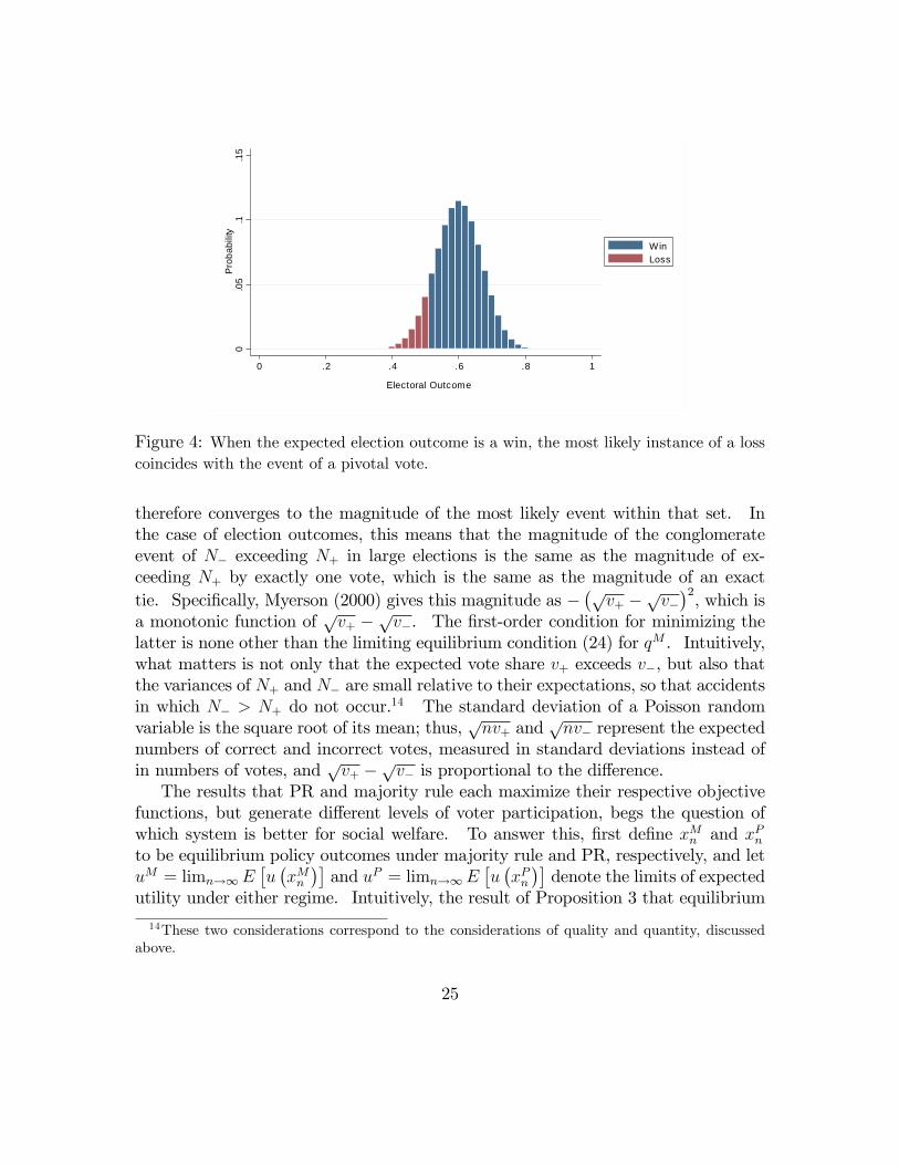
0.0

5.1

.15

Pro

babi

lity

0 .2 .4 .6 .8 1

Electoral Outcome

WinLoss

Figure 4: When the expected election outcome is a win, the most likely instance of a losscoincides with the event of a pivotal vote.

therefore converges to the magnitude of the most likely event within that set. Inthe case of election outcomes, this means that the magnitude of the conglomerateevent of N− exceeding N+ in large elections is the same as the magnitude of ex-ceeding N+ by exactly one vote, which is the same as the magnitude of an exacttie. Specifically, Myerson (2000) gives this magnitude as −

(√v+ −

√v−)2, which is

a monotonic function of√v+ −

√v−. The first-order condition for minimizing the

latter is none other than the limiting equilibrium condition (24) for qM . Intuitively,what matters is not only that the expected vote share v+ exceeds v−, but also thatthe variances of N+ and N− are small relative to their expectations, so that accidentsin which N− > N+ do not occur.14 The standard deviation of a Poisson randomvariable is the square root of its mean; thus,

√nv+ and

√nv− represent the expected

numbers of correct and incorrect votes, measured in standard deviations instead ofin numbers of votes, and

√v+ −

√v− is proportional to the difference.

The results that PR and majority rule each maximize their respective objectivefunctions, but generate different levels of voter participation, begs the question ofwhich system is better for social welfare. To answer this, first define xMn and xPnto be equilibrium policy outcomes under majority rule and PR, respectively, and letuM = limn→∞E

[u(xMn)]and uP = limn→∞E

[u(xPn)]denote the limits of expected

utility under either regime. Intuitively, the result of Proposition 3 that equilibrium

14These two considerations correspond to the considerations of quality and quantity, discussedabove.

25

abstention improves welfare, together with the result of Theorem 3 that participationin large elections is higher under a majoritarian regime than under PR, might seem tosuggest that welfare should be higher under PR than under majority rule. However,the opposite actually turns out to be true, as Proposition 8 now states: in largeelections, welfare is higher under majority rule than under PR, especially for highlevels of partisanship.

Proposition 8 uM = 1 for all p < 1. uP decreases in p, from 1 for p = 0 to 12for

p = 1.

The comparison here of welfare has little to do with the comparison of turnoutfrom Theorem 3. What drives the result is that, under majority rule, A partisansand B partisans negate one another’s influence, so that the majority decision isdetermined entirely by the behavior of independent voters, no matter how small thisgroup is. In a large election, a majority of these almost surely identify the true stateof the world. If there are no partisans, then PR delivers the same outcome in thelimit, as abstention is limited to an increasingly elite fraction of voters, the electionoutcome tends toward unanimity, and the policy outcome converges to the desiredextreme. A positive mass of partisan votes for either side, however, bounds thepolicy outcome away from 0 and 1, implying some utility loss, which is increasing inp. Actually, even with no partisans, PR would be inferior to majority voting if thedomain of the distribution of expertise were bounded below one, so that even themost elite citizens were incapable of agreeing unanimously on the state of the world.

5 Experiment

The model presented above is diffi cult to test with observational data, due to theendogeneity problems inherent in much of the empirical literature on turnout. Toavoid this problem, we generate new data through a series of laboratory experiments.Implementation in the laboratory poses a number of challenges. First, financialand space constraints limit the number of participants, making it diffi cult to testasymptotic results for large elections. Second, technical features of the model such asthe Poisson population uncertainty and the continuum of possible types, while elegantand convenient for theoretical derivations, are diffi cult to explain to experimentalsubjects. To circumvent these challenges we implement a simplified version of themodel above, and derive equilibrium predictions computationally. As explainedbelow, the simple version of the game features the main comparative statics of themodel above.

26

5.1 Experimental Design and Procedures

Subjects interacted for 40 periods. The instructions in each period were identical.In each period, subjects interacted in groups of six. At the beginning of eachround, the color of a triangle was chosen randomly to be either blue or red withequal probability. Subjects were not told the color of the triangle, but were toldthat their goal would be work together as a group to guess the color of the triangle.Independently, each would observe one ball (a signal) drawn randomly from an urnwith 20 blue and red balls. With 40% probability, a participant would be designatedas a high type (H), and 19 of the 20 balls in the urn would be the same color as thetriangle. With 60% probability, a participant would be designated as a low type(L), in which case only 13 of the 20 balls would be the same color as the triangle.Individual were told their own types, but did not know the types of the other fivemembers of their group.After observing their signals, each subject had to take one of three actions: vote

Blue, vote Red, or abstain from voting. Regardless of which action they chose,however, they were told that their action choice might be replaced at random, bythe choice of a computer: with 10% probability, their vote choice was changed toAbstain.15 With probability p the voting choice was replaced with a Blue vote, andwith probability p it was replaced with a Red vote. Replacements of votes weredetermined independently across subjects. The partisanship parameter p was oneof the treatment variables of the experiment. We considered three different values:p = 0%, p = 12.5% and p = 25%. The second treatment variable, the voting rule,determined subjects’payoff as a function of the group votes. In the Majority Rule(M) treatments, subjects each received payoffs of 100 points if the number of votes forthe color of the triangle exceeded the number of votes for the other color, 50 pointsin case of a tie and 0 points otherwise. In the case of Proportional Representation(P) treatments, subjects each received as payoff in points the percentage of non-abstention votes that had the same color as the triangle– or, if everyone abstained,a payoff equal to 50 points.For each of the two voting rules and each of the three levels of partisanship,

Table 1 lists the equilibrium abstention rates σ∗0,H and σ∗0,L for high- and low-type

individuals. If they vote at all, both types of citizens should vote in accordance withtheir private signals. High-type individuals should always vote, but the equilibrium

15This form of population uncertainty follows Feddersen and Pesendorfer (1996). With a knownnumber of voters, the swing voter’s would depend heavily on whether that number is even or odd.If it is odd, for example, there is always an equilibrium with full participation, because a vote is thenpivotal only if the rest of the electorate is evenly split. In that case, a citizen infers no informationbeyond his or her own signal, and therefore has a strict incentive to vote.

27

Treatment Voting Rule % Partisans σ∗0,H σ∗0,LM0 Majority Rule 0 0% 100%M25 Majority Rule 25 0% 0%M50 Majority Rule 50 0% 0%P0 Proportional Representation 0 0% 100%P25 Proportional Representation 25 0% 100%P50 Proportional Representation 50 0% 0%

Table 1: Equilibrium abstention rates for high and low types, for all treatments.

strategy of low-type voters varies by treatment. Under majority rule, they shouldabstain when p = 0 but vote whenever p is positive. Under Proportional Represen-tation, low-type individuals should abstain unless p is at its highest level, so thata vote is 50% likely to be replaced by a partisan computer. We summarize thesepredictions in the following hypotheses:

Hypothesis 1 High types should vote (weakly) more than low types

Hypothesis 2 The frequency of abstention of high types should not change with thenumber of partisans or with the voting rule.

Hypothesis 3 Under either voting rule, the frequency of abstention of low typesdecreases with the number of partisans.

Hypothesis 4 The frequency of abstention of low types voters is weakly lower undermajority rule than under PR.

Experiments were conducted at the Experimental Economics Laboratory at theUniversity of Valencia (LINEEX) in November 2014. We ran one session for eachtreatment, with 60 subjects each. No subject participated in more than one ses-sion. Students interacted through computer terminals, and the experiment wasprogrammed and conducted with the software z-Tree (Fischbacher 2007). All exper-imental sessions were organized along the same procedure: subjects received detailedwritten instructions (see Appendix A3), which an instructor read aloud. Before start-ing the experiment, students were asked to answer a questionnaire to check their fullunderstanding of the experimental design. Right after that, subjects played one ofthe treatments for 40 periods and random matching. Matching occurred withinmatching groups of 12 subjects, which generated 5 independent groups in each ses-sion. At the end of each round, each subject was given the information about the

28

color of the triangle, their original and their final vote, and the total numbers of Bluevotes, Red votes, and abstentions in their group (though they could not tell whetherthese were the intended votes of the other participants, or computer overrides). In Ptreatments, they also observed the percentage of votes that matched the color of thetriangle; in M treatments, they instead were told whether the color of the Trianglereceived more, equal, or fewer votes than the other color. To determine payment atthe end of the experiment, the computer randomly selected five periods and partici-pants earned the total of the amount earned in these periods. Points were convertedto euros at the rate of 0.025€. In total, subjects earned an average of 14.21€, in-cluding a show-up fee of 4 Euros. Each experimental session lasted approximatelyan hour.

5.2 Experimental Results

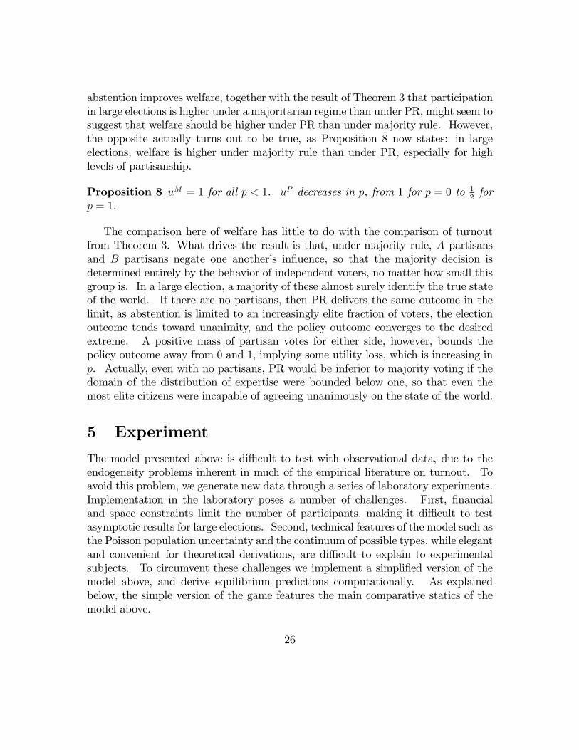
Figure 5 displays empirical abstention rates for all treatments, for voters of high andlow types. The figure shows several interesting patterns that we formalize and testwith the regression presented in Table 2. Table 2 displays the results of a randomeffects GLS regression of the frequency of abstention on dummies for each possiblecombination of voter type, level of partisanship, and voting rule (except for thecombination of high types and 0% partisanship under majority rule, which is thereference category).16

Let’s focus first on the behavior of high types. According to the theoreticalpredictions, these voters should never abstain. Empirically, abstention is indeedextremely low in all treatments, ranging from 0.3% only to 3.2%. Overall, we cannotreject the null hypothesis that the frequency of abstention across high-type voters isconstant across all treatments (χ2

4 = 3.28, p = 0.512), in line with Hypothesis 2.Figure 5 indicates a stark contrast in behavior across voter types: while the

frequency of abstention of high-type voters is 1.73%, this frequency is 33.53% acrosslow types. We find indeed a significant difference at under every single treatment.17

This finding is line with Hypothesis 1: better informed voters tend to participatemore in elections. See, however, that in contrast with the theoretical predictions,we find a strict significance in all treatments. In treatments where the percentage ofpartisans is 50%, for instance, all types of voters should always vote and therefore we

16The regressions lacks temporal variables and therefore ignores potential evolution in behaviorthroughout the experiment in order to ease interpretation of the coeffi cients. The results are robustto introducing temporal variables.17χ21 = 45.77, p < 0.001 in M0, χ21 = 82.46, p < 0.001 in M25, χ21 = 32.90, p < 0.001 in M50,

χ21 = 15.17, p < 0.001 in M0, χ21 = 90.53, p < 0.001 in M25, and χ21 = 18.36, p < 0.001 in M50.

29

010

2030

4050

0 25 50 0 25 50

High Ty pes Low Ty pes

Majority  Rule PR

Abst

entio

n R

ate

Partisans Share

Figure 5: Observed abstention for each treatment, by voter type.

shouldn’t such strict difference. This brings us to study behavior of low-type votersmore closely.Recall from Table 1 that we have corner solutions in all treatments. That is, low

types should either all abstain or all vote. Figure 5 indicates that average frequen-cies are more moderate. However, this is not surprising as the model abstracts fromcertain aspects that do influence behavior. A perhaps more insightful question iswhether the theory captures the comparative statics with respect to the voting mech-anisms and to the level of partisans in the electorate. Let’s attack these questionsin turn. Figure 5 suggests that, in line with the predictions, the level of abstentiondecreases with the percentage of partisans in the electorate. Indeed, the percentagesof abstention are 42.6%, 29.7% and 28.5% in treatments M0, M25, and M50, respec-tively, and 37.0%, 36.2% and 27.5% in treatments P0, P25, and P50. Moreover, thebiggest drop coincides with this one predicted by theory. In the case of M treat-ments we can indeed reject the null hypothesis that the level of abstention is notconstant across different levels of partisans in line with Hypothesis 3 (χ2

2 = 58.75,p < 0.001). Instead, we can’t reject the null hypothesis in the case of P treatments(χ2

1 = 2.17, p = 0.338).Do we observe significant differences across voting mechanisms? According to

theory we should only observe significant differences the level of partisans is 25%,and in this case we should observe that abstention is substantially higher under PR.Although the magnitude of the difference is off, this is exactly what we find in the

30

Variable Coef. Std. Err. z P>z 95% C.I.

High×M25 0.021 0.012 1.81 0.071 [−0.002, 0.045]High×M50 0.019 0.006 3.26 0.001 [0.008, 0.031]High× P0 0.008 0.006 1.47 0.142 [−0.003, 0.020]High× P25 0.011 0.011 1.04 0.298 [−0.010, 0.032]High× P50 0.032 0.022 1.45 0.147 [−0.011, 0.075]Low ×M0 0.420 0.062 6.77 0.000 [0.299, 0.542]Low ×M25 0.293 0.038 7.63 0.000 [0.218, 0.368]Low ×M50 0.284 0.050 5.69 0.000 [0.186, 0.382]Low × P0 0.361 0.093 3.89 0.000 [0.179, 0.543]Low × P25 0.359 0.040 9.08 0.000 [0.281, 0.436]Low × P50 0.272 0.061 4.5 0.000 [0.154, 0.391]Constant 0.003 0.006 0.54 0.588 [−0.009, 0.015]

Observations 14,400 σu .209 ρ .313Subjects 360 σe .309

Table 2: Random effects GLS regression of the probability of abstention on a constantand a number of dummies indicating the interaction between voter type, voting rule, andlevel of partisanship.

5060

7080

9010

0

50 60 70 80 90 100 50 60 70 80 90 100

M P

No Partisans 25% Partisans 50% Partisans

Rea

lized

 Pay

off

Equilibrium Payoff

Figure 6: Realized payoff vs equilibrium payoff in each independent group.

31

data: we find no significant differences when the level of partisans is 0% or 50%(χ2

1 = 0.43, p = 0.514 and χ21 = 0.04, p = 0.844 respectively), but a statistically

significant difference in favor of PR when the level of partisans is 25% (χ21 = 16.76,

p < 0.001).So far we have been focusing solely on abstention. According to theory, if they

didn’t abstain they should always vote their signal. This is not what we alwaysobserve. Overall, they deviate from voting their signal 11.6% of the time: 4.5%across high-type voters and 16.5% across low-type voters.18 Additionally, thesefrequencies seems to increase with the level of partisans. This is consistent withmodels of quantal response equilibrium, where mistakes are less prevalent when thepayoff difference across actions is smaller.19

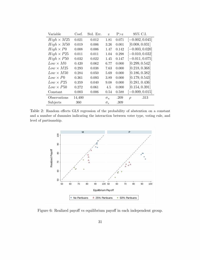
Finally, let’s turn to welfare. Figure 6 displays the realized average payoff in eachindependent group vis-à-vis the prediction for the realized draws. Actual payoffsare lower than would have been obtained by following the equilibrium strategy, butnot by much: on average, realized payoffs were 91.7% as those that would havebeen obtained by following the equilibrium strategies. In other words, deviationsfrom equilibrium reduced payoffs by only 8.3%. There is some heterogeneity acrossvoting rules: realized payoffs under majority rule were 93.7% as high as equilibriumpayoffs would have been, while payoffs under PR were 89.7% as high as equilibriumpayoffs. A clear outlier among all the treatments is P0, where overparticipationof low types reduced payoff substantially, to 84.3% of the equilibrium levels. Thisis not too surprising given the mechanical effect of the partisans, however; realizedpayoffs clearly decrease with the level of partisanship. A similar regression to theone in Table 2 where the independent variable is payoff and the random effect ison each group shows that payoffs were higher in P0 than P25, higher in P25 thanP50, higher in M0 than M25, and higher in M25 than M50, by amounts that arestatistically significant at the 1% level in all cases.

6 Conclusion

The electoral system of Proportional Representation has become increasingly pop-ular in recent decades, but its properties remain less well understood than those ofmajority rule. In particular, the swing voter’s curse identified by Feddersen and

18This anomaly has been found systematically in experimental studies on information aggregation.See, for instance, Bouton et al. (2014) or Bouton et al. (2015).19See Guarnaschelli, McKelvey and Palfrey (2000) and Holt and Goeree (2005) for applications

of QRE to voting.

32

Pesendorfer (1996) has been extremely influential in understanding voter participa-tion in majoritarian systems, but existing literature has not provided an analogousresult for PR. This paper fills that gap by demonstrating a marginal voter’s curse,which gives citizens a strategic incentive to abstain in PR systems, just as undermajority rule. This suggests that the incentive to abstain in deference to thosewith better information is not highly sensitive to the electoral system, but resultsmore intrinsically from the common-values assumption, together with the inevitableheterogeneity of expertise.While it is not obvious, ex ante, which electoral system should provide greater

incentive for voter turnout, the analysis above finds that equilibrium turnout isunambiguously higher under majority rule. This is in contrast with Herrera, Morelli,and Palfrey (2014), who analyze a private-value model with costly voting, and findthat turnout can be higher in either system. To observers who view high levels ofvoter participation as intrinsically desirable, this may make PR unattractive. Thewelfare analysis above does not place value on participation, per se, and in factdemonstrates that some abstention is desirable, in the sense that the resulting policyoutcome better matches the unknown state of the world than it would if everyonewere to have voted. Nevertheless, the mechanism that leads to lower turnout underPR is shown to lower welfare directly: namely, proportional representation makes theinfluence of partisan voters more diffi cult to negate.Several aspects of the analysis above would benefit from future extension. For

example, the superiority of majority rule results at least partly from the assumptionthat the state of the world is binary, so that the optimal policy ultimately lies at oneof the two extremes; in situations where the optimal policy is likely to lie betweenthe two extremes, proportional rule may be advantageous. Another useful exten-sion would be to consider an imbalance between partisan groups. Feddersen andPesendorfer (1996) show that, when partisan groups are imbalanced, uninformed in-dependents no longer abstain, instead voting to neutralize the partisan bias. Turnoutis likely to increase under PR for a similar reason, but by even more, as negatingthe influence of one partisan requires more than one independent vote. Lastly, ofcourse, is the issue of voting costs, which may have differential effects under the twoelectoral systems.

7 Appendix

Proof of Proposition 1. In response to σ, a citizen prefers to vote A if∆0AE [u (x) |q, s] exceeds the maximum of zero and ∆0BE [u (x) |q, s]. Since (12)is increasing in φα and (13) is decreasing in φα, these inequalities are satisfied for

33

any φα above some threshold φ̄brα . By symmetric reasoning, a citizen prefers to

vote B if φβ exceeds a threshold φ̄brβ . Accordingly, these thresholds characterize a

posterior threshold strategy that is the unique best response to σ.If σq̄ is a quality threshold strategy with quality threshold q̄ then, as noted in

Section 2.2, vA (α) = vB (β) and vA (β) = vB (α). This implies that symmetricelectoral outcomes are equally probable. That is, NA has the same distribution instate α that NB has in state β, and vice versa, so that Pr (a, b|α) = Pr (b, a|β). Inthat case, it is straightforward to show that ∆0AE [u (x) |q, sα] = ∆0BE [u (x) |q, sβ]

and ∆0AE [u (x) |q, sβ] = ∆0BE [u (x) |q, sα], implying that φ̄brα = φ̄brβ . Thus, the best

response to σq̄ is another quality threshold strategy σq̄br . In this way, q̄br (q̄) can beinterpreted as a continuous function from the compact set [0, 1] of quality thresholdsinto itself. A fixed point q̄∗exists by Brouwer’s theorem, and the correspondingquality threshold strategy σq̄∗ constitutes its own best response.

Proof of Theorem 1. The logic of this proof is to show that the best responseto the quality threshold strategy σ0 with full participation is a quality thresholdstrategy σq̄br(0) with a best-response quality threshold q̄br (0) > 0, implying less-than-full participation. To see this, first note that if citizens follow σ0 then (4)reduces so that vA (α) = vB (β) > vA (β) = vB (α). Therefore, the distribution ofNA when ω = α first-order stochastically dominates the distribution of NA whenω = β, and the distribution of NB when ω = β first-order stochastically dominatesthe distribution ofNA when ω = α. The difference∆0AλA = a+1

a+b+1− aa+b

is decreasingin a and increasing in b, however, which implies that the distribution of ∆0AλA whenω = β first-order stochastically dominates the distribution of ∆0AλA when ω = α.Thus, E (∆0AλA|β) > E (∆0AλA|α), implying that (15) is strictly positive.

Proof of Proposition 2. When voters follow a quality threshold strategy,

Pr (pivA|β)− Pr (pivA|α) =1

2[Pr (a+ 1 = b|β)− Pr (a+ 1 = b|α)]

=1

2[Pr (a = b+ 1|α)− Pr (a+ 1 = b|α)]

=1

2

∞∑k=0

e−nvA(α)−nvB(α)n2k+1

k! (k + 1)!

[vk+1A (α) vkB (α)− vkA (α) vk+1

B (α)]

> 0,

where the second equality follows from the symmetry of the strategy and the inequal-ity follows because vA (α) > vB (α). Thus, the best-response quality threshold (18)

34

is strictly positive, implying that an equilibrium quality threshold must be positiveas well.

Proof of Proposition 3. McLennan (1998) points out that, in a common interestgame such as this, any strategy σ∗∗ is socially optimal is also individually rational,and thus constitutes an equilibrium. This logic applies whether the electoral systemis PR or Majority Rule. That a positive fraction v∗∗0 > 0 of the electorate necessarilyabstain in equilibrium follows from Theorem 1 for PR and from Proposition 2.

Proof of Lemma 1. From (5) we have

E

(a+ 1

a+ b+ 1|ω)

= e−Rω−Sω∞∑a=0

∞∑b=0

(Raω

a!

)(Sbωb!

)(a+ 1

a+ b+ 1

)E

(a

a+ b|ω)

= e−Rω−Sω∞∑a=0

∞∑b=0

(Raω

a!

)(Sbωb!

)(a

a+ b

).

Omitting the ω subscripts, this can be reduced as follows.

∞∑b=0

Sb

b!

a

a+ b=

a

Sa

∞∑b=0

∫ S

0

d

dr

(1

b!

ra+b

a+ b

)dr =

=a

Sa

∫ S

0

∞∑b=0

(1

b!ra+b−1

)dr =

aSa

∫ S0ra−1erdr for a ≥ 1

1/2 for a = 0

and∞∑b=0

Sb

b!

a+ 1

a+ b+ 1=a+ 1

Sa+1

∫ S

0

raerdr.

By inverting the series and integral operators again in the series over a, we have

35

equal to

E

(a+ 1

a+ b+ 1|ω)− E

(a

a+ b|ω)

= e−R−S

( ∞∑a=0

Ra

a!

(a+ 1

Sa+1

∫ S

0

raerdr

)−( ∞∑a=1

Ra

a!

(a

Sa

∫ S

0

ra−1erdr

)+

1

2

))

= e−R−S

(∫ S

0

1

S

( ∞∑a=0

(RSr)a

a!+

∞∑a=1

(RSr)a

(a− 1)!

)erdr −

(∫ S

0

R

S

∞∑a=1

(RSr)a−1

(a− 1)!erdr +

1

2

))

= e−R−S(∫ S

0

1

S

(eRSr +

R

Sre

RSr

)erdr −

(∫ S

0

R

SeRSrerdr +

1

2

))= e−R−S

1

S2

∫ S

0

e(1+RS )r (S +Rr) dr −

(R

1− e−(R+S)

R + S+e−(R+S)

2

)=

S

(R + S)2 +e−(R+S)

(R + S)2

R2 − S2 − S2

In sum,

E (∆0AλA|ω) =Sω + Rω2−Sω2−Sω

2e−(Rω+Sω)

(Rω + Sω)2 .

That E (∆0BλB|ω̃) = E (∆0AλA|ω) follows from the symmetry of a quality thresholdstrategy, and since λA + λB = 1, ∆0jλA + ∆0jλB = 0 for j ∈ {A,B}.

Proof of Proposition 4. The equilibrium condition (20) is continuous in n (andin v+, v−, T , and W , which also vary continuously with n) so a sequence q̄∗n ofsolutions to (20) must converge to a solution of the limit of (20). That is, lettingl ≡ limn→∞

nTW−v−2

e−nT , qP must solve

1 + q

1− q =v+ − lv− + l

or, equivalently,

q̄ =v+ − v− − 2l

v+ + v−.

Suppose we have l > 0, then qP satisfies

q̄ <v+ − v−v+ + v−

≤ 1,

36

implying a positive turnout rate T > 0, and therefore that nT → +∞. In that case,l = limn→∞

nTW−v−2

e−nT = 0, yielding a contradiction.Studying the sign of the derivative of

L (q̄) =K + [1− F (q̄)] [1 +m (q̄)]

K + [1− F (q̄)] [1−m (q̄)]

we obtain for any K the condition:

L′ (q̄) ≷ 0 ⇐⇒ L (q̄) ≷ 1 + q

1− q

For any K > 0 we have L (0) > 1 and L (1) = 1, moreover the function 1+q1−q is

increasing from 1 to infinity. Thus, qP must be positive, and by the condition aboveL (q̄) is increasing initially, must eventually cross 1+q

1−q and is decreasing from there

after. Hence L (q̄) has a unique maximum which solves L (q̄) = 1+q1−q which therefore

coincides with the unique solution qP . Moreover, qP decreases in K as the functionL (q̄) decreases in K for all q̄.If K = 0 then L (q̄) = 1+m(q̄)

1−m(q̄)which is always increasing, hence we must have

L (q̄) > 1+q1−q for all q̄ ∈ [0, 1), hence: qP = 1 solves L (q̄) = 1+q

1−q = +∞.As for stochastic dominance, we first want to show that any MLR shift of the

distribution increases L (q̄)for any K ≥ 0 and any q ∈ [0, 1). By 9 and 10 we canwrite:

L (q̄) =K +

∫ 1

q(1 + q) f (q) dq

K +∫ 1

q(1− q) f (q) dq

=

∫ 1

0α (q) f (q) dq∫ 1

0β (q) f (q) dq

α (q) := K + Iq (1 + q) , β (q) := K + Iq (1− q)where Iq is the indicator function of the interval [q̄, 1] and therefore α (q) and β (q)are both non-negative and respectively non-decreasing and non-increasing functionsof q for all K.We need to show that for any distribution g such that g(q)

f(q)is increasing, we have:∫ 1

0α (q) f (q) dq∫ 1

0β (q) f (q) dq

<

∫ 1

0α (q) g (q) dq∫ 1

0β (q) g (q) dq

We can write the above inequality as:∫ 1

0

∫ 1

0

α (q) β (q′) f (q) g (q′) dqdq′ <

∫ 1

0

∫ 1

0

α (q) β (q′) f (q′) g (q) dqdq′

37

hence we need to show that the following function Γ is negative, namely:

Γ :=

∫ 1

0

∫ 1

0

α (q) β (q′) [f (q) g (q′)− f (q′) g (q)] dqdq′ < 0

Splitting the domain of integration in two symmetric parts we have:

Γ =

∫ ∫q>q′

α (q) β (q′) [f (q) g (q′)− f (q′) g (q)] dqdq′+

∫ ∫q′>q

α (q) β (q′) [f (q) g (q′)− f (q′) g (q)] dqdq′

Renaming the variables (q as q′) in the second double integral, and collecting similarterms, we have:

Γ =

∫ ∫q>q′

[α (q) β (q′)− α (q′) β (q)] [f (q) g (q′)− f (q′) g (q)] dqdq′

=

∫ ∫q>q′

β (q) β (q′)

[α (q)

β (q)− α (q′)

β (q′)

]f (q) f (q′)

[g (q′)

f (q′)− g (q)

f (q)

]dqdq′

For any q > q′ and the properties listed above the first square brackets is positivewhile the second is negative.In sum, for any K ≥ 0 and any q ∈ [0, 1) a strict MLR shift increases L (q̄).

Hence if qP solves

qP : L (q̄) =1 + q

1− qgiven that the RHS is increasing in q and unchanged after a MLR shift of F, the newsolution after such a shift must be larger than qP .

Proof of Proposition 5. As a preliminary step, note that the following expres-sion is equivalent to the conditional mean m (q̄) = E (q|q ≥ q̄), as can be seen byintegrating by parts.

m (q̄) = q̄ +

∫ 1

q̄

1− F (q)

1− F (q̄)dq. (26)

38

As a second preliminary step, rewrite the limiting equilibrium conditions (21) and(24) in terms of G as follows:

1−G (q̄)

q[mG (q)− q] = K (27)

1−G (q̄)

q

(1 + q2

2mG (q)− q

)= K. (28)

1. If G (q) = F (q) for all q ≥ qPF then from (26) it is clear that mG

(qPF)

=mF

(qPF). If qPF solves (21), therefore, then it solves (27) as well.

2. If G (q) = F (q) for all q ≤ qPF but G first-order stochastically dominates Fthen from (26) it is clear that mG

(qPF)> mF

(qPF). Therefore,

1−G(qPF)

qPF

[mG

(qPF)− qPF

]>

1− F(qPF)

qPF

[mF

(qPF)− qPF

]= K. (29)

By the log-concavity of g, the left-hand side of (27) is decreasing in q̄ (as shown inthe proof of Proposition 4), so the unique solution qPG must exceed q

PF .

3. If G (q) = F (q) for all q ≥ mF

(qPF)and G

(qPF)< F

(qPF)then∫ 1

qPF

qg (q) dq =

∫ 1

qPF

qf (q) dq +

∫ mF (qPF )

qPF

q [g (q)− f (q)] dq

<

∫ 1

qPF

qf (q) dq +

∫ mF (qPF )

qPF

mF

(qPF)

[g (q)− f (q)] dq

= mF

(qPF){∫ 1

qPF

f (q) dq +

∫ mF (qPF )

qPF

[g (q)− f (q)] dq

}= mF

(qPF) [

1−G(qPF)],

so mG

(qPF)

=

∫ 1qPFqg(q)dq

1−G(qPF )< mF

(qPF). Thus, the inequality in (29) is reversed. By

the log-concavity of g, the left-hand side of (27) is decreasing in q̄ (as shown in theproof of Proposition 4), so the unique solution qPG must be less than q

PF .

Proof of Proposition 6. In the expression (24) we can isolate K, yielding:

1− F (q̄)

q

(1 + q2

2m (q)− q

)= K. (30)

39

To prove existence, first note that the left-hand side of (30) approaches zero as q̄approaches 1. Thus, qM = 1 solves (30) if and only if K = 0. Moreover, iflimq→1

f ′(q)f(q)

< ∞ then 0 < qM < 1. In that case, however, the condition that

limq→1f ′(q)f(q)

< ∞ implies that no sequence of equilibrium quality thresholds canconverge to one, by Theorem 3 of McMurray (2013).20 As q̄ tends to zero, theleft-hand side of (30) tends to infinity. Thus, for any K, there exists a solution0 < qM < 1 by the Intermediate Value Theorem and continuity of the left-hand sideof (30).As for uniqueness, for K = 0, Theorem 4 of McMurray (2013) states that the

solution to (30) is unique on the open interval (0, 1).21 For q̄ below that solution,therefore, the left-hand side of (30) is positive (tending to infinity as q̄ tends to zero),while for q̄ above that solution, it is negative. When it is positive, inspection of (30)reveals that we must have

m (q̄) >2q

1 + q2 . (31)

In that case, the left-hand side of (30)is also decreasing in q̄. To see this, differentiatethe left-hand side of (30) to obtain

−f (q̄)

(1 + q2

2

m (q)

q− 1

)+

1− F (q̄)

2

(−1 + q2

q2m (q) +

1 + q2

qm′ (q)

).

By (31), the first term in this expression is negative. The second term is negative ifand only if

m′ (q̄) <m (q̄)

q̄,

which is a condition equivalent to a decreasingm (q̄)−q̄ = E (q − q̄|q ≥ q̄), sometimescalled themean residual lifetime of a machine: a machine “ages”with time if its meanresidual lifetime decreases. According to Lemma 2 of Bagnoli and Bergstrom (2005),a necessary and suffi cient condition for the latter is that f is log-concave. Thus,under log-concavity the left-hand side of (30) is decreasing whenever it is positive,implying a unique solution for any K > 0.The latter also implies that, ifK increases, then qM decreases under log-concavity.The argument for MLR shifts is analogous to the one obtained for the PR system.

20As that paper notes, this condition merely rules out electorates that are arbitrarily close tobeing perfectly informed, and is suffi cient for the result but not necessary.21 q̄ = 1 constitutes another solution but cannot be the limit of a sequence of equilibrium thresh-

olds.

40

Proof of Theorem 3. From the characterization results, we know that qM ∈ (0, 1)is the (possibly not unique) solution to:

qM : L (q̄) =

(1 + q

1− q

)2

while qP ∈ (0, 1] is the unique solution to:

qP : L (q̄) =

(1 + q

1− q

)Thus, we have

q = qP ∈ (0, 1] =⇒ L (q̄) =

(1 + q

1− q

)<

(1 + q

1− q

)2

q = 0 =⇒ L (q) > 1 =

(1 + q

1− q

)2

Hence the continuous functions L (q) and(

1+q1−q

)2

must cross at some value qM ∈(0, qP ).

Proof of Proposition 8. As n grows large, equilibrium strategies converge point-wise to σqM under majority rule and to σqP under PR. In either regime, actual voteshares converge in probability to expected vote shares. That is, N+

N→p

nv+n

= v+

and N−N→p

nv−n

= v−.For q̄ = qM , v+ exceeds v−, implying that Pr (N+ > N−) converges almost

surely to one, and utility converges almost surely uM = limn→∞ Pr (N+ > N−) +12

limn→∞ Pr (N+ = N−) = 1 + 0. This logic is valid for any p < 1. (For p = 1,Pr (N+ > N−) = Pr (N+ < N−) for any n, implying that uM = 1

2+ 0).

With Proportional Representation, utility is given by N+N++N−

, which converges in

probability to uP = v+v++v−

=L(qP )L(qP )+1

. This decreases in p since it increases in L,which decreases in p. As explained in Section 4.1, limq̄→qP L (q̄) = ∞ for p = 0,implying that uP = 1. From (9) and (10) it is also clear that L (q̄) = 1

2when p = 1

for any q̄, implying that uP = 12in that case.

References

[1] Bagnoli, Mark, and Ted Bergstrom. 2005. “Log-Concave Probability and ItsApplications.”Economic Theory, 26(2): 445-469.

41

[2] Battaglini, Marco, Rebecca B. Morton, and Thomas R. Palfrey. 2010. “TheSwing Voter’s Curse in the Laboratory.”Review of Economic Studies, 77(1):61-89.

[3] Battaglini, Marco, Rebecca B. Morton, and Thomas R. Palfrey. 2008. “Infor-mation aggregation and strategic abstention in large laboratory elections.”TheAmerican Economic Review P&P, 98(2): 194—200.

[4] Bouton, Laurent, Micael Castanheira and Aniol Llorente-Saguer. 2014. “DividedMajority and Information Aggregation: Theory and Experiment.”Manuscript,Max Planck Institute for Collective Goods.

[5] Bouton, Laurent, Aniol Llorente-Saguer and Frédéric Malherbe. 2015. “Veto,Abstention and Framing: An Experiment on Majority with Veto Power.”Man-uscript, Queen Mary Unviersity of London.

[6] Condorcet, Marquis de. 1785. Essai sur l’application de l’analyse a la proba-bilite’ des decisions rendues a la pluralite’ des voix [Essay on the Applicationof Analysis to the Probability of Majority Decisions]. Paris: De l’imprimerieroyale. Trans. Iain McLean and Fiona Hewitt. 1994.

[7] Faravelli, Marco, Priscilla Man, and Randall Walsh. 2015. “Mandate andPaternalism: A Theory of Large Elections.” Games and Economic Behavior,93:1-23.

[8] Faravelli, Marco and Santiago Sanchez-Pages. 2014. “(Don’t) Make My VoteCount.”Journal of Theoretical Politics, forthcoming.

[9] Feddersen, Timothy J. and Wolfgang Pesendorfer. 1996. “The Swing Voter’sCurse.”The American Economic Review, 86(3): 408-424.

[10] Fischbacher, Urs. 2007. “z-Tree - Zurich Toolbox for Readymade Economic Ex-periments.”Experimental Economics, 10(2): 171-178.

[11] Goeree, Jacob and Charles Holt. 2005. “An Explanation of Anomalous Behaviorin Models of Political Participation.”American Political Science Review, 99(2):201-213.

[12] Guarnaschelli, Serena, Richard McKelvey and Thomas R. Palfrey. 2000. “AnExperimental Study of Jury Decision Rules”American Political Science Review,94(2): 407-423.

42

[13] Herrera, Helios, Massimo Morelli, and Salvatore Nunnari. 2015. “Turnoutacross Democracies.”The American Journal of Political Science, forthcoming.

[14] Herrera, Helios, Massimo Morelli, and Thomas Palfrey. 2014. “Turnout andPower Sharing.” The Economic Journal, forthcoming.

[15] Kartal, Melis. 2014a. “A Comparative Welfare Analysis of Electoral Systemswith Endogenous Turnout,”The Economic Journal, forthcoming.

[16] Kartal, Melis. 2014b. “Laboratory elections with endogenous turnout: propor-tional representation versus majoritarian rule.”Experimental Economics, forth-coming.

[17] Krishna, Vijay and John Morgan. 2011.“Overcoming Ideological Bias in Elec-tions.”Journal of Political Economy, 119(2): 183-211.

[18] Krishna, Vijay and John Morgan. 2012. “Voluntary Voting: Costs and Benefits.”Journal of Economic Theory, 147(6): 2083—2123.

[19] Matakos, Konstantinos, Orestis Troumpounis and Dimitrios Xefteris. 2014.“Turnout and polarization under alternative electoral systems.” Manuscript,Lancaster University.

[20] McLennan, Andrew. 1998. “Consequences of the Condorcet Jury theorem forBeneficial Information Aggregation by Rational Agents.” American PoliticalScience Review, 92(2): 413-418.

[21] McMurray, Joseph C. 2013. “Aggregating Information by Voting: The Wisdomof the Experts versus the Wisdom of the Masses.” The Review of EconomicStudies, 80(1): 277-312.

[22] McMurray, Joseph C. 2014. “Mandates, Multiple Candidates, and the SignalingVoter’s Curse.”Manuscript, Brigham Young University.

[23] McMurray, Joseph C. 2015. “The Paradox of Information and Voter Turnout.”Forthcoming, Public Choice.

[24] Morton, Rebecca B., and Jean-Robert Tyran. 2011. “Let the experts decide?Asymmetric information, abstention, and coordination in standing committees.”Games and Economic Behavior, 72(2): 485-509.

[25] Myerson, Roger. 1998. “Population Uncertainty and Poisson Games.”Interna-tional Journal of Game Theory, 27(3): 375-392.

43

[26] Sobbrio, Francesco and Pietro Navarra. 2010. “Electoral Participation andCommunicative Voting in Europe.” European Journal of Political Economy,26(2): 185-207.

[27] Razin, Ronny. 2003. “Signaling and Election Motivations in a Voting Model withCommon Values and Responsive Candidates.”Econometrica, 71(4): 1083-1119.

[28] Wattenberg, Martin, Ian McAllister, and Anthony Salvanto. 2000. “How Votingis Like Taking an SAT Test: An Analysis of American Voter Rolloff.” AmericanPolitics Research, 28: 234-250.

44