The Marginal Edge of Learning Progressions and Modeling ...

The Marginal Edge of Learning Progressions and Modeling: Investigating Diagnostic Inferences

from Learning Progressions Assessment

by

Ruhan Circi Kizil

B.S., Bogazici University, 2005

M.S., Bogazici University, 2010

A Dissertation

Submitted in Partial Fulfillment of the Requirements for the

Doctor of Philosophy

Research and Evaluation Methodology Program

in the Graduate School of Education

University of Colorado at Boulder

2015

This dissertation entitled:


from Learning Progressions Assessment written by Ruhan Circi Kizil

has been approved for the School of Education

Department of Research and Evaluation Methodology

___________________________________________________

Dr. Derek C. Briggs

___________________________________________________

Dr. Lorrie A. Shepard

___________________________________________________

Dr. Andrew Maul

___________________________________________________

Dr. Erin M. Furtak

___________________________________________________

Dr. Michael Stallings

Date_____________

The final copy of this dissertation has been examined by the signatories, and we find that both

the content and the form meet acceptable presentation standards of scholarly work in the above

mentioned discipline.

iii

Circi Kizil, Ruhan (Ph.D., Research and Evaluation Methodology)


from Learning Progressions Assessment

Dissertation directed by Dr. Derek Briggs

Abstract

Learning Progressions (LPs) are hypothesized pathways describing the development of

students’ understanding. Although they show promise for informing decisions about student

learning, and helping develop standards and curricula, attempts to validate LPs empirically have

been virtually nonexistent.

The purpose of this dissertation is twofold: 1) to validate an LP by applying psychometric

models and 2) to examine and compare these models and their results in terms of their

applicability to that LP. I examine the information produced by Item Response Theory (IRT)

models and Diagnostic Classification Models (DCMs) when applied to item responses from an

assessment—composed of Ordered Multiple Choice (OMC) items—designed to measure an LP

of Force and Motion. I apply the Partial Credit Model (PCM; Embretson & Reise, 2000),

Attribute Hierarchy Model (AHM; Gierl, Leighton, & Hunka, 2006), and Generalized Diagnostic

Model (GDM; von Davier, 2005) to the assessment data.

All three models in this study yield evidence that student item responses do not follow

progressions given in the LP. Hence, the hypothesized LP, as well as the OMC items used to

measure student understanding of that LP, should be reexamined. In particular, the assessment

tasks and associated OMC items exhibit ceiling and floor effects that impair the models’ abilities

to associate student responses LP levels.

iv

Each model had unique limitations in terms of its applicability to the LP. The PCM

model’s assumptions and its resulting item statistics were inappropriate, and could not be used to

classify students into LP levels. In contrast, both the AHM and GDM models did classify

students into latent classes, but they were still limited. The AHM’s estimation procedure, which

relies on an artificial neural network approach, introduced problems, as did the overall fit of the

model. The GDM is so complex that it is conceptually hard to understand and utilize, even

though it did produce both item level statistics (unlike AHM) and student classifications.

Overall, this study provides insights into how to use psychometric modeling to inform an

LP and LP assessment, as well as the viability of three models from two different frameworks in

the context of an LP.

Dedication

To real family and Turkish tea.

vi

Acknowledgments

I have received more support during the writing of this dissertation than can be

acknowledge here. Despite this limitation, I would be remiss if I did not acknowledge the

support I have received from my family, friends and mentors.

First, I wish to thank Dr. Derek Briggs for his generosity and his support at every

moment of my graduate study. Without his contagious enthusiasm for psychometrics, his

patience, and encouragement, I would not be able to forward in my career.

Second, I would like to acknowledge the endless support I have received from my family

and husband. Without them this work would not be possible.

Third, I would also thank you my friends whose support and perspective have been

invaluable. I am lucky to have encountered fellow students at the School of Education who view

me a colleague, friend and a sister. These current and past students include: Nathan Dadey, Ben

Domingue, Kate Allison, Jessica Alzen, and Jon Weeks. My friends who live oversea and

outside the academia also gave me encouragement in my completion of this work, particularly

Elif Altuntas.

Fourth, I would like to thank my committee members for their insight and dedication to

make this work the best it could be.

vii

Contents

Chapter

1. Introduction ................................................................................................................................. 1

1.1 Introduction and Problem Statement ..................................................................................... 1

1.2 Research Problem ................................................................................................................ 10

1.3 Research Questions ............................................................................................................. 13

1.4 Chapter Summary ................................................................................................................ 14

2. Literature Review: Learning Progressions and Modeling ........................................................ 17

2.1 Assessment for Diagnostic Purposes................................................................................... 17

2.2 Learning Progressions ......................................................................................................... 25

2.2.1 Defining, Assessing and Using Strands ........................................................................ 25

2.2.2 Learning Progressions in the Large Scale Context ....................................................... 30

2.2.3 Validity Argument for Learning Progressions ............................................................. 31

2.2.4 Modeling Strand ........................................................................................................... 36

3. Methodology ............................................................................................................................. 42

3.1 The FM Learning Progression............................................................................................. 43

3.1.1 Ordered Multiple-Choice Items .................................................................................... 44

3.1.2 Basics of Data Set Analyzed in Current Study ............................................................. 47

3.2 Modal (Simplistic) Approach .............................................................................................. 48

3.3 Psychometric Models for Diagnostic Feedback .................................................................. 49

3.4 IRT Modeling ...................................................................................................................... 52

3.4.1 Partial Credit Model ..................................................................................................... 57

3.5 Diagnostic Classification Models (DCM) ........................................................................... 63

3.5.1 Probabilistic Models (DINA Example) ........................................................................ 65

3.5.2 General Diagnostic Model ............................................................................................ 68

3.5.3 Pattern Recognition Models (AHM Example) ............................................................. 75

3.6 Chapter Summary ................................................................................................................ 86

4. Results ....................................................................................................................................... 87

4.1 Examination of Data............................................................................................................ 88

4.1.2 Modal Classification Results ........................................................................................ 90

4.2 Unidimensional Partial Credit Item Response Theory Model ............................................ 91

viii

4.2.1 Examination of Empirical Dimensionality ................................................................... 92

4.2.2 Item Parameter Estimation ........................................................................................... 97

4.2.3 Model Fit .................................................................................................................... 102

4.2.4 Item-Person Map ........................................................................................................ 105

4.2.5 PCM-based Classification into LP Levels .................................................................. 106

4.3 Attribute Hierarchy Model Results ................................................................................... 108

4.3.1 Linear Hierarchy ......................................................................................................... 108

4.3.2 Model Fit Results........................................................................................................ 110

4.3.3 Attribute Probability Estimation Results .................................................................... 112

4.3.4 Attribute Relationships ............................................................................................... 113

4.3.5 Distribution of Attribute Mastery with Different Cutoff Values ................................ 114

4.3.6 The Prediction Variance of Attribute Probabilities from ANNs ................................ 115

4.4 Generalized Diagnostic Model Results ............................................................................. 118

4.4.1 GDM ........................................................................................................................... 118

4.4.2 Parameter estimates .................................................................................................... 120

4.4.3 Model Fit .................................................................................................................... 123

4.4.4 Parameter Invariance .................................................................................................. 125

4.4.4 Relationship between Attributes ................................................................................. 126

4.4.5 Classifications into Latent Classes ............................................................................. 127

4.5 Comparison of Models ...................................................................................................... 131

4.5.1 Comparison between AHM and Modal Classification ............................................... 131

4.5.2 Comparison between GDM and Modal Classifications, AHM .................................. 133

4.5.3 Comparison of Person Parameter Estimates across Models ....................................... 134

5. Discussion ............................................................................................................................... 138

5.1 Model Evaluations in the Context of FM LP Assessment ................................................ 141

5.2 Inferences across Models .................................................................................................. 145

5.3 Limitations ........................................................................................................................ 149

5.4 Implications and Future Research ..................................................................................... 151

5.5 Conclusion ......................................................................................................................... 154

References ................................................................................................................................... 156

Appendix

ix

A: Force and Motion Learning Progression ................................................................................ 170

B: 16 Force and Motion Items .................................................................................................... 173

C: Earth and Solar System Learning Progression Levels and Descriptions ............................... 179

D: Summary of Results from Well-behaved Subset of Items ..................................................... 180

x

List of Tables

3.1. Descriptive Statistics for Each FM OMC Items .................................................................... 46

3.2. Descriptives and Reliability for OMC Items. ........................................................................ 48

3.4. Excerpt of the Qr Matrix Associated with FM LP Attribute Hierarchy. ................................ 81

3.5. Expected Response Patterns for Two OMC Items: Option Level. ........................................ 82

3.6. The Concept of Misfit with OMC Items. ............................................................................... 84

4.1. Mean Level Values of FM LP Assessment............................................................................ 88

4.2. Mean Total Score for Students Selecting Same LP Level Option in an Item........................ 90

4.3. Basic FM LP Level Placement Results. ................................................................................. 91

4.4. Factor Loadings from Oblique Exploratory Factor Analyses for 1-Factor Structure. ........... 95

4.5. Factor Loadings from Oblique Exploratory Factor Analyses for 4-Factor Structure. ........... 96

4.6. Category Boundary Parameter Estimates of 16 Items. .......................................................... 99

4.7. Descriptives of Correlations for Parameter Invariance across 100 Sampled Groups. ......... 104

4.8. The Category Difficulty Parameters for 11 Items................................................................ 107

4.9. Descriptive Statistics for RCI Index. ................................................................................... 111

4.10. Example of Attribute Probabilities for Perfectly Fitting Response Patterns ..................... 113

4.11. Descriptive Statistics of Attribute Probabilities for Real Students. ................................... 113

4.12. Correlations between Attributes. ....................................................................................... 114

4.13. The Distribution of Levels with Different Cutoff Values. ................................................. 114

4.14. The Summary of Standard Deviations in Estimates across 100 ANN Trials. ................... 116

4.15. Correlations between Attributes across 100 ANN Trials. ................................................. 117

4.16. Example of AHM Derived LP Levels. ............................................................................. 118

4.17. Category Easiness Parameters for FM LP Items. .............................................................. 121

4.18. Slope Parameters for Each FM LP Item. ........................................................................... 122

xi

4.19. Item Fit Results for GDM. ................................................................................................. 124

4.20. Comparison of Model Fit of 4 skills GDM and PCM. ...................................................... 124

4.21. Descriptives of Item Parameter Correlations for GDM across 100 Pairs of Groups. ........ 125

4.22. Relationship between Attributes (GDM). .......................................................................... 126

4.23. Percent of Students across 16 Possible Latent Classes. ..................................................... 128

4.24. Summary of Attribute Mastery Probabilities. .................................................................... 130

4.25. LP Level Placements with AHM. ..................................................................................... 132

4.26. Cross Examination of LP Level Classification (Modal and AHM). .................................. 132

4.27. Cross Examination of LP Level Classification (cont.) ...................................................... 133

4.28. Cross Examination of LP Level Classification (Modal and GDM). .................................. 133

4.29. Cross Examination of LP Level Classification (AHM and GDM). ................................... 134

4.30. Correlations of Person Estimates across Models. .............................................................. 136

5.1. Information Provided by Three Models. .............................................................................. 141

D1.1. Category Boundary Parameter Estimates for 10 Items ..................................................... 180

D2.1. The Summary of Standard Deviations in Estimates across 100 ANN Trials for 10 Items.

..................................................................................................................................................... 181

D2.2. LP Level Placements with AHM Based on 10 Items. ....................................................... 182

D2.3. Cross Examination of LP Level Classification Using 10 Items (Modal and AHM). ....... 182

D3.1. Category Easiness Parameters for 10 Items. ..................................................................... 183

D3.2. Slope Parameters for 10 Items. ......................................................................................... 183

D3.3. Percent of Students across 16 Possible Latent Classes for 10 Items. ............................... 184

xii

List of Figures

1.1. A Short Version of FM Learning Progression ......................................................................... 5

1.2. Sample OMC Item from FM Learning Progression. ............................................................... 7

2.1. Relationship between the NCR (2001) Assessment Triangle and Four Strands of ............... 22

Learning Progressions (Alonzo, 2012, p.243). ...................................................................... 22

3.1. Example OMC Item from FM Learning Progression. ........................................................... 45

3.3. An Example of a Wright Map for the Rasch Model. ............................................................. 56

3.4. A Simple 3-Attribute Hierarchy............................................................................................. 75

3.5. Mechanism of Artificial Neural Network. ............................................................................. 77

4.1. Parallel Analysis Approach Scree Plot. ................................................................................. 93

4.2. FM LP Item 1. ...................................................................................................................... 100

4.3. Category Response Functions with Ordered Category Boundaries for Item 1 .................... 100

4.4. FM LP Item 15 ..................................................................................................................... 101

4.5. Category Response Functions with Reversed Category Boundaries for Item 15. ............... 101

4.6. Distribution of Correlations between Validation Samples across 100 Trials. ..................... 105

4.7. Item-person Map for FM LP Items (regrouped items). ....................................................... 106

4.8. FM Learning Progression .................................................................................................... 109

4.9. Observed Distribution of the RCI for 16 FM OMC Items................................................... 111

4.10. Overlap of RCI Values between Randomly Generated Data and FM LP Data. ................ 112

4.11. Distribution of Marginal Attribute Probabilities. ............................................................... 130

4.12. Relationship between Total Score and PCM Ability Estimates. ....................................... 134

4.13. Relationship between Total Score and AHM Attribute Estimates in Logits. .................... 135

4.14. Relationship between Total Score and GDM Attribute Estimates in Logits. .................... 135

4.15. Relationship between GDM and AHM Attribute Estimates in Logits. ............................. 137

1

Chapter 1

Introduction

1.1 Introduction and Problem Statement

In response to the desire for students to build their knowledge and develop complex

inquiry reasoning over the past two decades, the education community has developed new

frameworks to better understand student learning and respond accordingly. Over the same period

of time, in the field of psychometrics, models have been developed to extract detailed

information about students’ strengths and weaknesses in a content domain. There can be a

tension in the relationship between theories that posit complex sets of interrelated skills and

psychometric models that necessarily make simplifying assumptions about these skills. That is,

complicated statistical models used with assessments developed with restricted cognitive tasks

are impractical, and similarly assessments which are developed under the guidance of learning

theories with a detailed understanding of student learning but analyzed with models that are

unable to provide detailed interpretation of the data are specious.

Learning progressions (LPs)1 have captured the attention of the education community in

the past decade, especially among science and mathematics educators (e.g., Duschl, Maeng &

Sezen, 2011; Learning Progressions in Science Conference (LeaPS), 2009; Foundations for

Success: Report of the National Mathematics Advisory Panel, 2008), as helpful theoretical and

hypothetical frames that show how student learning progresses across predefined developmental

1 The term ‘learning trajectory’ is used commonly in mathematics education literature while ‘learning

progression’ is preferred in science education literature (Mosher, 2011).

2

levels (Corcoran, Mosher & Rogat, 2009). In theory at least, LPs can be used to provide insights

into the evolution of a student’s learning process. These progressions provide a tool that can be

used to track the advancement of the student’s understanding of a topic, from virtually no

understanding (a novice) to a complex and sophisticated understanding (an expert). Learning

progression level descriptors can be used to indicate the degree of sophistication of a student’s

understanding.

To provide information about student understanding of a given concept, the instrument(s)

used to observe and elicit information about student learning play a central role. These

instruments need to facilitate the extraction of diagnostic feedback so that users understand the

students’ current learning level and needs in order to progress to the next step. Thoughtfully

designed assessments could serve this purpose (Steedle, 2008). These assessments are likewise

important for collecting validity evidence on hypothesized learning progressions. However, the

potential utility of LPs is balanced against the difficulties inherent in developing and modeling

them. Particular methods are selected in this dissertation to investigate the latter by

systematically examining and comparing the viability of two approaches; a) Item Response

Theory (IRT) modeling, and b) diagnostic classification modeling (DCM). In the context of a

previously established LPs in science, I examine whether the hypothesized levels of each LP

align with students’ actual answers, and collect information on the quality of assessment items

through the lens of different information provided by each psychometric model. I likewise

examine the extent to which choices of different model specifications can lead to substantially

different inferences about students’ skills. To provide an overview and motivation for this

dissertation, I first provide an example of a learning progression with an overview of two

3

common modeling approaches. I conclude this chapter with the research questions that are the

focus of this study.

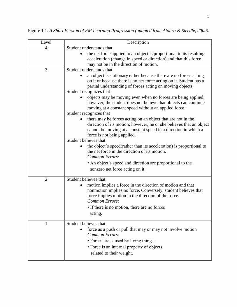
Figure 1.1 illustrates a learning progression crafted around the content area: “Force and

Motion” learning progression. The FM learning progression is the learning progression that I will

examine in my dissertation. In their research, Alonzo and Steedle (2009) posited this learning

progression by analyzing the science education research literature and relevant content

benchmarks (i.e. eighth-grade students of Force and Motion content for top level of the learning

progression and research literature reporting students’ ideas about force and motion as well as

expert judgements for the lower levels). The learning progression is revised in an iterative

process via cognitive interviews and analyses of student responses to preliminary versions of

ordered multiple-choice and open-ended assessment items.

In the FM learning progression, the levels are defined with respect to the combination of

four phenomena in the FM domain, a) Force: Situations in which a force is acting, and students

are asked about the resulting motion, b) No Force: Situations in which there is no net force

acting, and students are asked about the resulting motion, c) Motion: Situations in which an

object is moving, and students are asked about the force(s) acting on the object, and d) No

Motion: Situations in which an object is at rest, and students are asked about the force(s) acting

on the object. In other words, the LP focuses on understanding of the reciprocal relationships

between force and motion in a one-directional space (i.e., students are expected to consider only

one-dimensional motion. In this case, force acting in the opposite direction is also required in the

4

items). FM LP has four levels2 and descriptions of students’ understanding of concepts at each

level.

2 Alonzo and Steedle (2009) described additional two sublevels (2A and 3A) where students at a given

level (e.g., Level 2 or Level 3) and students at the corresponding sublevel A (e.g., Level 2A or 3A) share the same

underlying idea about the relationship between force and motion. Students at Levels 2 and 3 are described to have a

more conventional understanding of “force” while students at sublevels present an “impetus view” of force. For the

purpose of this study, I did not differentiate across levels and sublevels.

5

Figure 1.1. A Short Version of FM Learning Progression (adapted from Alonzo & Steedle, 2009).

Level Description

4 Student understands that

the net force applied to an object is proportional to its resulting

acceleration (change in speed or direction) and that this force

may not be in the direction of motion.


an object is stationary either because there are no forces acting

on it or because there is no net force acting on it. Student has a

partial understanding of forces acting on moving objects.

Student recognizes that

objects may be moving even when no forces are being applied;

however, the student does not believe that objects can continue

moving at a constant speed without an applied force.


there may be forces acting on an object that are not in the

direction of its motion; however, he or she believes that an object

cannot be moving at a constant speed in a direction in which a

force is not being applied.

Student believes that

the object’s speed(rather than its acceleration) is proportional to

the net force in the direction of its motion.

Common Errors:

• An object’s speed and direction are proportional to the

nonzero net force acting on it.

2 Student believes that

motion implies a force in the direction of motion and that

nonmotion implies no force. Conversely, student believes that

force implies motion in the direction of the force.

Common Errors:

• If there is no motion, there are no forces

acting.


force as a push or pull that may or may not involve motion

Common Errors:

• Forces are caused by living things.

• Force is an internal property of objects

related to their weight.

6

This learning progression maps a hypothesis about increasingly sophisticated

understanding as a student learns about these key phenomena. Researchers specify student

thinking, typical at each level, and include partial understanding and ‘common errors’ related to

each level. This approach not only explains how new knowledge is incorporated into a student’s

mental model, but also provides information about limitations in students’ understanding. It is

hypothesized that when students transition to the next level, they are likely to have resolved these

common errors.

Following Gotwals and Alonzo (2012), I describe any learning progression as having

four interdependent strands; a) a well-defined construct and the conceptualization of student

progress, b) assessments developed in relation to the learning progression, c) modeling and

interpreting student performance on the assessments, and d) the use of the learning progression

to support teaching and learning. Figure 1.1 exemplifies the first feature by defining the construct

and providing a continuum with the levels for students’ progress in the FM domain. The next

strand requires developing assessments that elicit students’ understanding in connection to the

learning progression. This step provides tools to extract richer information on student learning as

well as to place students into the levels of progression validly and reliably. Therefore, using

different types of assessments and items becomes particularly important in the context of

learning progressions. When the items in the assessments of learning progressions are

constructed so that they are linked to the levels of a learning progression, patterns of student

responses then provide information about what students know and can do relative to the learning

progression (e.g., Briggs, Alonzo, Schwab & Wilson, 2006; Wilson & Sloane, 2000). Ordered

multiple choice (OMC) items are distinctive tasks particularly well aligned with LP assessments.

OMCs contain item options which reflect the different levels of a learning progression.

7

Returning to the FM example, Figure 1.2 illustrates an OMC item showing the correspondence

between response options and FM LP levels.

Figure 1.2. Sample OMC Item from FM Learning Progression.

Learning progressions are hypotheses about the nature of student learning, and as such,

they are iterative. Following the development of a learning progression and corresponding

assessment items, we need to answer the critical question of “how to model the data?” and “how

to do it more efficiently?” The modeling strand has the potential to provide compelling

information that can help to confirm or disconfirm the initial hypotheses used to develop the LP.

Psychometric modeling is important for learning progressions for two reasons: a) it

allows us to make probabilistic inferences about unobserved – latent – states of student

understanding, and b) it offers a systematic way to validate the learning progression with the help

of a specified model and evaluation of its fit to data (Briggs & Alonzo, 2012). Determining a

student’s position on an LP can help educators as well as the student to decide what skills they

have mastered, and it also may provide some ideas for next steps that can be taken to progress to

8

the upper level. Collecting evidence to validate the learning progressions can help to better

understand the hypothesized progression and the degree to which assessment tasks are able to

provide evidence about student learning. This crucial modeling step is the focus of this study.

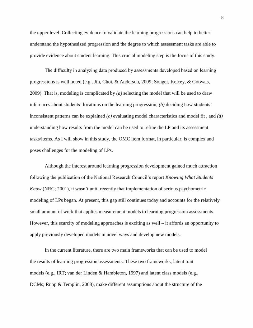
The difficulty in analyzing data produced by assessments developed based on learning

progressions is well noted (e.g., Jin, Choi, & Anderson, 2009; Songer, Kelcey, & Gotwals,

2009). That is, modeling is complicated by (a) selecting the model that will be used to draw

inferences about students’ locations on the learning progression, (b) deciding how students’

inconsistent patterns can be explained (c) evaluating model characteristics and model fit , and (d)

understanding how results from the model can be used to refine the LP and its assessment

tasks/items. As I will show in this study, the OMC item format, in particular, is complex and

poses challenges for the modeling of LPs.

Although the interest around learning progression development gained much attraction

following the publication of the National Research Council’s report Knowing What Students

Know (NRC; 2001), it wasn’t until recently that implementation of serious psychometric

modeling of LPs began. At present, this gap still continues today and accounts for the relatively

small amount of work that applies measurement models to learning progression assessments.

However, this scarcity of modeling approaches is exciting as well – it affords an opportunity to

apply previously developed models in novel ways and develop new models.

In the current literature, there are two main frameworks that can be used to model

the results of learning progression assessments. These two frameworks, latent trait

models (e.g., IRT; van der Linden & Hambleton, 1997) and latent class models (e.g.,

DCMs; Rupp & Templin, 2008), make different assumptions about the structure of the

9

underlying latent ability or abilities that indicate where students are on the LP.

Specifically, IRT assumes that the latent ability is a continuum, whereas DCM assumes

that the latent ability is made up of separate discrete classes.

Nonetheless, both IRT and DCM models are essentially a similar set of statistical tools

(Rupp & Templin, 2008) that can provide information about the performance of the students on

an assessment. The main purpose of using diagnostic classification models is to classify students

into levels of finely defined attributes directly, while the main purpose of IRT analysis is to

specify the location of a student on a continuum with a criterion-referenced classification

possibly following in a second step. Both models can be used to place the students into levels of

learning progressions.

The approach taken in skill diagnosis using IRT models is similar to that used in standard

setting procedures for large-scale assessments (Roussos, Templin, & Henson, 2007) in that the

end result is a series of cut scores on unidimensional scales (Rupp, Templin & Henson, 2010).

These cut-scores are established with the help of experts and statistical information about items

and respondents. Then, students are classified into the categories based on their placement in

relation to the cut scores (e.g., de la Torre & Karelitz, 2009).

Over the last decade, there has been an explosion of psychometric models that fall within

a cognitive diagnostic framework (Rupp et al., 2010). The supposed promise of diagnostic

models is that they are capable of communicating item response data in a more diagnostic way

which highlights students’ weaknesses and strengths on the relevant latent discrete variables.

With such a claim, it is natural to think that such models would be especially relevant in the

context of assessment items created for a learning progression. Currently, there are only a few

10

unique attempts to model the learning progression data by the different diagnostic classification

models (e.g., Briggs & Alonzo, 2012; West et al., 2012).

Neither IRT nor latent class models are a panacea, however. Diagnostic Classification

Models (DCMs) have become increasingly popular but, they are frequently criticized for their

complexity in estimation and interpretation (Wilhelm & Robitzsch, 2009). Because we model

discrete latent traits, an increase in the number of distinct traits specified in any analysis can lead

to a dramatic increase in computational burden. Additionally, some of the characteristics such as

global model fit indices have not been developed thoroughly for DCMs. IRT models, particularly

those from the Rasch family, can be used for diagnostic purposes (Wilson, 2005), but critics of

use of IRT models in the learning progression context point out the poor alignment between the

nature of the latent variable underlying progression (i.e., discrete nature) and the continuous

latent variable assumption in IRT models (Briggs & Alonzo, 2012).

DCMs and IRT models differ in several ways and have their own pros and cons. There

are few (see de la Torre, 2009, for an example) examples of studies comparing the results

coming from both IRT and DCM frameworks with the same data, and in most cases these studies

rely on simulated data. Hence, the issue of the usefulness of the multidimensional profiles

estimated in the DCM over and above traditional scores has remained mostly unanswered. This

dissertation is unique in this sense because it is premised on empirical data from assessment

items developed together with a learning progression.

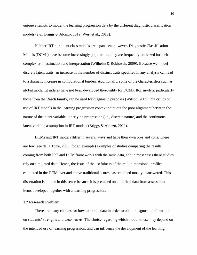
1.2 Research Problem

There are many choices for how to model data in order to obtain diagnostic information

on students’ strengths and weaknesses. The choice regarding which model to use may depend on

the intended use of learning progression, and can influence the development of the learning

11

progression. That is, the theory of LP and task design provides the framework for modeling the

observations of student understanding and in turn, measurement models formalize the

characteristic of underlying latent constructs. In this study, I use the Force & Motion (FM;

Alonzo & Steedle, 2009) learning progression in which items are designed to map differences in

the LP levels into the response options, OMC items.

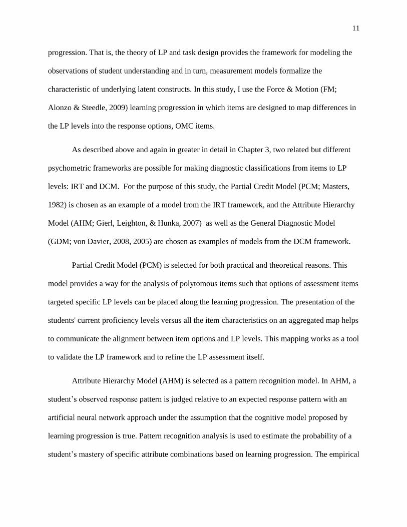
As described above and again in greater in detail in Chapter 3, two related but different

psychometric frameworks are possible for making diagnostic classifications from items to LP

levels: IRT and DCM. For the purpose of this study, the Partial Credit Model (PCM; Masters,

1982) is chosen as an example of a model from the IRT framework, and the Attribute Hierarchy

Model (AHM; Gierl, Leighton, & Hunka, 2007) as well as the General Diagnostic Model

(GDM; von Davier, 2008, 2005) are chosen as examples of models from the DCM framework.

Partial Credit Model (PCM) is selected for both practical and theoretical reasons. This

model provides a way for the analysis of polytomous items such that options of assessment items

targeted specific LP levels can be placed along the learning progression. The presentation of the

students' current proficiency levels versus all the item characteristics on an aggregated map helps

to communicate the alignment between item options and LP levels. This mapping works as a tool

to validate the LP framework and to refine the LP assessment itself.

Attribute Hierarchy Model (AHM) is selected as a pattern recognition model. In AHM, a

student’s observed response pattern is judged relative to an expected response pattern with an

artificial neural network approach under the assumption that the cognitive model proposed by

learning progression is true. Pattern recognition analysis is used to estimate the probability of a

student’s mastery of specific attribute combinations based on learning progression. The empirical

12

relationships between each of the attributes are examined for their alignment with the theoretical

expectations in learning progression.

General Diagnostic Model (GDM) is selected due to its power to connect item level

probability for polytomous items with discrete latent variables. It produces item level

information as well as the strength of relationships between discrete latent variables

corresponding to the skills in learning progressions. It also places students into the latent classes

composed of a variation of the skills. Because it does not require any hierarchy across the latent

variables, it provides evidence of non-hierarchical groups of latent classes in which students may

reason with different combinations of skills across problem contexts.

These three models are the mathematical representations of the learning progression

assessment data. Hence, it is important to have a systematic examination on the pertinence of the

models. The methodical approach used in this dissertation is based on evaluation of

appropriateness of the models based on the available tools before attempting the classification of

students into the LP levels. While the final classification and its interpretation is an important

product of psychometric analysis, when a model is assumed there are a number of psychometric

assumptions and characteristics that need to be evaluated and addressed. Therefore, to examine

the appropriateness of the models in the context of OMC based learning progression

assessments, I repeated the specific steps used at each model.

a. Examination of the dimensionality

b. Examination of item parameter invariance

c. Model fit

d. Item parameter estimation

e. Attribute/skill mastery status estimation

13

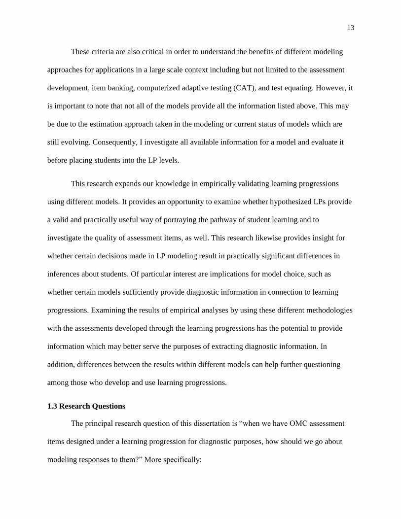
These criteria are also critical in order to understand the benefits of different modeling

approaches for applications in a large scale context including but not limited to the assessment

development, item banking, computerized adaptive testing (CAT), and test equating. However, it

is important to note that not all of the models provide all the information listed above. This may

be due to the estimation approach taken in the modeling or current status of models which are

still evolving. Consequently, I investigate all available information for a model and evaluate it

before placing students into the LP levels.

This research expands our knowledge in empirically validating learning progressions

using different models. It provides an opportunity to examine whether hypothesized LPs provide

a valid and practically useful way of portraying the pathway of student learning and to

investigate the quality of assessment items, as well. This research likewise provides insight for

whether certain decisions made in LP modeling result in practically significant differences in

inferences about students. Of particular interest are implications for model choice, such as

whether certain models sufficiently provide diagnostic information in connection to learning

progressions. Examining the results of empirical analyses by using these different methodologies

with the assessments developed through the learning progressions has the potential to provide

information which may better serve the purposes of extracting diagnostic information. In

addition, differences between the results within different models can help further questioning

among those who develop and use learning progressions.

1.3 Research Questions

The principal research question of this dissertation is “when we have OMC assessment

items designed under a learning progression for diagnostic purposes, how should we go about

modeling responses to them?” More specifically:

14

1. What information does each model provide to the researcher about the quality of learning

progression hypothesis and assessment items?

a. What information is provided by the PCM model within the IRT framework about

the quality of the LP and its assessment items?

b. What information is provided by the AHM and GDM within a DCM framework

about the quality of the learning progressions and assessment items?

2. What are the qualitative differences (student classification) across different models?

a. How similar are the results of analyses for classification of students produced by

AHM and GDM from diagnostic framework and PCM from IRT framework?

The theoretical framework provided by Briggs and Alonzo (2012) is promising for the

analyses of learning progressions with ordered multiple choices, but it has yet to be extensively

examined. In addition, at present there is not a comprehensive study to explore the comparability

of models from the IRT and DCM frameworks for analyzing data from a small cluster of

diagnostic LP assessment items. In sum, this dissertation study is poised to contribute to the

expanding diagnostic assessment and modeling work by examining inferences from different

frameworks and thereby informing the decision making process by developers and users of these

assessments.

1.4 Chapter Summary

This dissertation is divided into four chapters, in addition to this introduction. Chapter 2

provides and overview of learning progression assessments as tools for diagnostic purposes and

various applications and related concerns to the analysis of data from learning progression

assessments. The chapter begins with changing use of assessments from providing normative

information (Scott, 2004) to deliver feedback to teachers and students to modify instruction and

15

enhance learning (NCR, 2001; Black & Wiliam, 1998). This is followed by a presentation of four

strands of learning progressions to categorize and describe the work done so far in science

education. The chapter concludes with a separate review of modeling in learning progressions, as

the focus of this dissertation, pointing to modeling as the critical, and least investigated, strand in

the learning progression literature.

Chapter 3 provides an overview of the data used in this dissertation. It also presents two

major modeling frameworks that can be used to extract diagnostic information tied to specific

learning progressions – Item Response Theory (IRT) and Diagnostic Classification Models

(DCMs) frameworks. It focuses on models which can be used for diagnostic purposes and

presents the details of three models that I use in the current study. It starts with the description of

unidimensional IRT models and their properties as well as underlying assumptions, then

transitions to the IRT modeling practices in the context of learning progressions with a focus on

PCM (Masters, 1982; Embretson & Reise, 2000). This is followed by description of DCMs as

models specifically developed for multivariate classifications of respondents on the basis of

hypothesized sets of discrete latent skills. The properties of two DMCs used in this dissertation

are presented- GDM (von Davier, 2005) and AHM (Briggs & Alonzo, 2012; Gierl, Cui, &

Hunka, 2007) with an extension to the polytomous items.

Chapter 4 begins with the exploratory analysis of the data via descriptive statistics and an

examination of the classification of students into LP levels from a modal analysis. This is

followed by analysis results to examine my first research question. I started with PCM analysis

results. At the beginning of PCM section, special focus is given on the investigation of the

dimensional structure underlying the Force and Motion (FM) learning progression assessment. I

conducted parallel analysis and explanatory factor analysis to examine whether there is support

16

for selected models with different underlying assumptions. Note that the results from

dimensionality analysis inform all models selected for the current study.

I continued with the PCM model fit and parameter invariance results. Then, I presented

the parameter estimation results by highlighting the challenges and opportunities on how to place

students into the LP levels in the context of OMC items of learning progression assessments. For

AHM, I provide the description of the linear structure specified across attributes, and introduce a

new person model fit which is adapted from original consistency index. I likewise investigate the

relationship between attributes and provide results on classification of students into mastery

status for each attribute. For GDM, I present item parameters estimates together with item fit

statistics. I likewise present the results on the skill mastery probabilities. This is followed by the

comparison of skill mastery probabilities from GDM with overall ability estimates from PCM

and comparison of model fit across two models.

Chapter 5 presents a summary of findings from Chapter 4 and discusses the implications

of these findings a) in the context of validation of learning progressions, b) in the context of

policy determinations (i.e., using learning progressions at classroom level and/or at large-scale),

and c) from a methodological perspective (i.e., the potential advantages and challenges of

different modeling frameworks to analyze LP data). The chapter concludes with a discussion of

future research directions and limitations of the study.

17

Chapter 2

Literature Review: Learning Progressions and Modeling

The use of learning progression assessments requires embracing alternative approaches to

statistical modeling that can help to provide key stakeholders with the type of information that

they need to improve learning and teaching. The premise of this dissertation is to address

empirical questions that have yet to be answered. The study examines the viability of models

from two different frameworks within a novel data context to draw conclusions regarding

modeling learning progressions (LP) while also highlighting the opportunities and challenges

emerging in the wake of such an examination. This chapter provides the background relevant to

these questions. The first part of the chapter covers the notion of using assessments for

diagnostic purposes. The second part describes operational concepts and research relevant to

learning progressions. This chapter concludes with the modeling concerns for analyzing data

from learning progression assessments in connection to both small scale and large scale

assessments.

2.1 Assessment for Diagnostic Purposes

The incorporation of testing into education in the United States has a long history going

back to at least the mid-nineteenth century (e.g., Gallagher, 2003; McArthur, 1983). It has been

seen as a powerful tool for change in student learning, instruction, schools and systems (Herman,

Dreyfus, & Golan, 1990). It has had two main functions which sometimes have overlapped:

18

sorting and selecting students through comparisons to one another, and improving the quality of

education (Haertel & Herman, 2005).

Historically, large-scale assessments have been used to provide normative information

about student academic achievement. Using normed-referenced standardized tests became a

common practice starting in the 1920s and steadily increased over time (Scott, 2004). Tests have

frequently been designed to rank order test takers along a bell curve (Zucker, 2003). That is, to

compare students’ scores against a norm group (e.g., a nationally representative group) where

one can only say student A is better than student B or, or that student A has scored higher than x

percent of students who took the test (Ingram, 1985). One well-known example of these tests is

the Iowa Test of Basic Skills, which was first administered in 1935 (Salkind, 2007) and used by

most states until the No Child Left Behind Act was passed in 2001 (NCLB, 2001). Other

commercial and internationally normed-referenced tests continue to be used nationally, such as

the California Achievement Test, Comprehensive Test of Basic Skills, Metropolitan

Achievement Test, and Scholastic Aptitude Test. The prevailing approach of testing practices

remained normed-referenced until the 1970s. Two main limitations have been noted on the use

of normed-referenced tests: potential deflection in instruction due to limiting curriculum to the

expected content of the test, otherwise known as teaching to the test (Popham, 1999) and the

impossibility of all students to place at the higher end of the distribution (Burley, 2002).

The desire to obtain richer data at the individual student level and give teachers more

feedback on their students’ learning outcomes is rooted in “Bloom’s Taxonomy” (Bloom,

Englehart, Furst, Hill, & Krathwohl, 1956). The idea of designing a test to show what students

know without referring to a norm group led to substantial progress in the development and the

use of criterion-referenced tests (Dziuban & Vickery, 1973). These tests allowed making

19

interpretations about student performance in terms of specific standards that are defined by a

domain of tasks within a specific content area that should be performed by the individual (Glaser

& Nitko, 1971). Standards have been used both in classrooms to guide day-to-day classroom

instruction and as broader large scale assessments for other purposes, including program

evaluation (e.g., Haertel & Herman, 2005). In the last decade, this shift in large scale testing,

especially to measure student mastery of specific curricular objectives, is partially due to the

NCLB law which pushed for criterion- referenced assessments. There has been a radical increase

in the number of tests used at the state level since NCLB was implemented in 2001 (NCES,

2005). This illustrated that large scale testing has likewise desired not just to determine how a

student score relates to others, but also what this student knows and can do. This shift in the

landscape of testing also headed to the more frequent assessment of students on more local

levels. A well-known example of criterion-referenced tests is National Assessment of

Educational Progress (NAEP). Even before NCLB, NAEP adapted the use of achievement levels

describing what a student in an achievement level knows and can do. Currently, there are three

cumulative achievement levels: Basic, Proficient, and Advanced, spanning all grades and

subjects (NAEP, 2012). Other examples of widely used international-comparison tests include

the Programme for International Student Assessment, the Progress in International Reading

Literacy Study, and the Trends in International Mathematics and Science Study (Giacomo,

Fishbein, & Buckley, 2012). Mostly, these tests are designed to enable comparisons between

larger units such as schools, states, and countries rather than examining skill profiles of

individual students. However, the results of these assessments have captured the interest of

politicians, educators, and researchers and have contributed to the development of tests to

provide feedback at the student level. Most recently, in order to support the implementation of

20

Common Core State Standards (CCSS), the Partnership for Assessment of Readiness for College

and Careers (PARCC) has announced it will create assessments providing detailed information

about what students know in Grades 2-8 (PARCC, 2013). That is, criterion referencing itself has

constituted a part of a continuum towards more diagnostically-oriented assessments.

While the large scale attempts to provide more information on student learning via

criterion-referenced tests and the diagnostic value of large-scale assessments created enthusiasm

within the education community, they are challenged to provide little insight with respect to

strengths and weaknesses of students. That is, because they are distal to teaching and learning

(e.g., broad content coverage, less focus on determining specific reasons for student

misunderstanding), an angle towards classroom assessment received more attention. Although

the notion of classroom assessment traditionally grew out of the behaviorist view of learning and

testing practices, more recently, it has been reconceptualized as a part of the learning process and

teaching under the principles of cognitive and constructivist theories (Shepard, 2000). Recently,

there has been increased discussion on how to link assessment with student learning and the use

of assessment to provide feedback to teachers and students to modify instruction and enhance

learning. In their highly influential study, Black and Wiliam (1998) concluded that there was a

vast body of evidence on formative assessment leading to increased student learning. That is,

they highlight that high quality formative assessment has a powerful impact on student learning

and is one of the most important interventions for promoting high student performance.

Following Sadler (1989), they focus on the significant role of feedback from assessment to

compare the actual level of students’ performance to the desired level, and to engage in effective

actions to reduce this gap (Wiliam, 2007; Wiliam, 2006). Current common understanding on

formative assessment focuses on attending to student thinking, eliciting what they understand,

21

and using assessment tools to collect evidence which can be used to improve the current learning

of students (e.g., Shepard, 2000; CCSSO, 2008). This understanding underlines the need of

detailed and timely feedback for both students and teachers and use of a variety of assessment

tools that are not necessarily tests.

Another document that has had a significant influence on current practices and research is

the NRC report “Knowing What Students Know” (KWSK; NCR, 2001). The report argued for

assessments that coordinated task design, psychometric modeling, assessment delivery, and

psychological research, and also provided guidelines for the development and evaluation of such

assessments. It introduced an assessment model which emphasized the need to incorporate

cognitive theories into the development of assessments and to use evidence to support

interpretations from observed performance. Also, it called for a “balanced assessment system”

(p.221) of large scale and classroom assessments by highlighting new development in cognitive

science, educational measurement, and technology.

Two examples of frameworks that coordinate various aspects of task design,

psychometric modeling, assessment delivery, and psychological research are, “evidence-centered

design” by Mislevy and his colleagues (2003) and the “BEAR assessment system” by Wilson

(2005). Both have developed a conceptual approach to, and methodology for, test design. The

first approach directly links test design to both evidentiary reasoning and general design science.

The latter makes use of construct maps for the development of assessments and provides a

guideline to analyze the observed scores as assessments outputs.

The call for assessments that incorporate cognitive theory has received considerable

attention, especially in science and mathematics education. Assessments that are based on a

model of cognitive development, of which learning progressions are an example, are grounded in

22

research on how students’ learning actually develops, rather than in traditional curriculum

sequences or logical analysis of how learning components may fit together (Heritage, 2008).

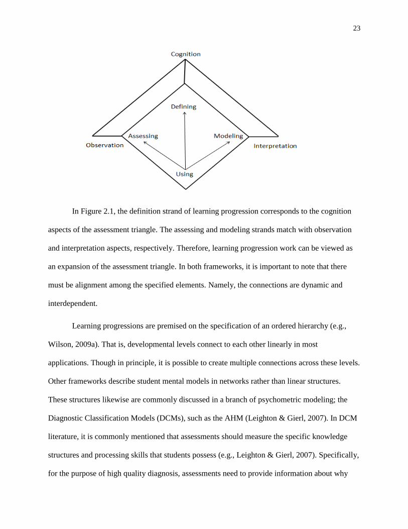
The close alignment between learning progressions and the KWSK assessment model is

evident in the ‘assessment triangle’ defined in KWSK (NCR, 2001). The assessment triangle

shows three elements needed for an effective assessment system: cognition (cognitive processes

defined as part of achievement to be assessed), observations (assessment activities to observe

student learning), and interpretation (analyses and interpretation of student work). These three

elements are connected to each other and have reciprocal relationships. Exploration and

elaboration of the relationships among these three elements lead to a diversity of work on

learning progressions, developing assessments, and interpreting the results of students’

understanding of a particular phenomenon (e.g., Alonzo & Gotwals, 2012; Duschl, Maeng, &

Sezen, 2011). Currently in LP work, four strands are defined: defining, assessing, modeling and

using. As Alonzo (2012) shows, these strands can be coordinated with the KWSK assessment

triangle as presented in Figure 2.1.

Figure 2.1. Relationship between the NCR (2001) Assessment Triangle and Four Strands of

Learning Progressions (Alonzo, 2012, p.243).

23

In Figure 2.1, the definition strand of learning progression corresponds to the cognition

aspects of the assessment triangle. The assessing and modeling strands match with observation

and interpretation aspects, respectively. Therefore, learning progression work can be viewed as

an expansion of the assessment triangle. In both frameworks, it is important to note that there

must be alignment among the specified elements. Namely, the connections are dynamic and

interdependent.

Learning progressions are premised on the specification of an ordered hierarchy (e.g.,

Wilson, 2009a). That is, developmental levels connect to each other linearly in most

applications. Though in principle, it is possible to create multiple connections across these levels.

Other frameworks describe student mental models in networks rather than linear structures.

These structures likewise are commonly discussed in a branch of psychometric modeling; the

Diagnostic Classification Models (DCMs), such as the AHM (Leighton & Gierl, 2007). In DCM

literature, it is commonly mentioned that assessments should measure the specific knowledge

structures and processing skills that students possess (e.g., Leighton & Gierl, 2007). Specifically,

for the purpose of high quality diagnosis, assessments need to provide information about why

24

students respond in the ways they do, provide feedback at the level of the individual, and

distinguish between skills mastered and those yet to be learned (Gorin, 2007). In order to give

valid feedback to students, tasks should be designed from an explicit model of how students

learn and allow respondents to show their potential weaknesses and strengths in a specific

content domain. So far, methodological developments of DCMs have been illustrated by

preexisting data sets rather than assessments designed with respect to cognitive or learning

theories. Therefore, learning progressions are good candidates to examine the use of different

models, including DCMs, to extract more detailed information on student learning. Learning

progressions can also provide an opportunity to examine the capability of the models in the

context of an assessment built from the ground up to diagnose student understanding in a

targeted content.

Learning progressions are also appealing for assessments that will be used for

accountability purposes (Wilson, 2009b). Current education policies demand that the

assessments should be grounded in frameworks of how understanding develops in a given

subject domain. The request from policy makers has increased the need for research on both

assessments and the models to extract inferences from these assessments to provide feedback on

student learning.

In sum, testing practices have evolved such that there is an increasing desire for

assessments that can be used for diagnostic purposes. A substantial amount of work has been

done in the last decade, leading to new developments in both assessment and modeling of

learning progressions. However, these attempts to develop assessment and modeling raise many

new questions. In what follows, I will review some of these attempts by focusing on learning

progressions in current literature of the field.

25

2.2 Learning Progressions

As the idea of providing detailed feedback on student learning grows in both importance

and popularity, it becomes important to examine the consequences of implementations in

different strands. Because the learning progressions used in this dissertation are in the science

domain, I focus mainly on the LP framework in science education. The field is dynamic, so one

sees diversity among relevant research that addresses both potentials and challenges that

researchers encountered in four different strands of learning progressions: defining, assessing,

modeling, and using. These four strands help categorize and describe the work done so far on

learning progressions in science, and also identify the gaps in the field central to my dissertation

research.

The focus of my work is on the LP modeling. However, as I mentioned earlier, all aspects

of LP work depend on each other. In the following sections, I describe literature about defining,

assessing, and using strands related with my work, and then I present the modeling strand in a

separate sub-section. I likewise provide a set of arguments for the validity of learning

progressions, and for justifying my choice of models.

2.2.1 Defining, Assessing and Using Strands

As Mohan and Plummer (2012) note, the definition of learning progression has become

more precise in the last few years. The commonly cited definition for a learning progression is

“hypothesized descriptions of the successively more sophisticated ways student thinking about

an important domain of knowledge or practice develops…over an appropriate time span”

(Corcoran et al., 2009, p.37). This definition emphasizes commonly agreed upon characteristics

of a learning progression as students develop sophisticated ways of thinking (a change of

understanding that begins with simple concepts and increases in complexity) and growth of

26

student knowledge over time rather than moving through an ordered set of ideas or curriculum

pieces. When analyzing their linear structure, Steedle (2008) notes learning progressions assume

that students systematically use a specified set of ideas and these ideas can be ordered in relation

to the expert-level understanding. These features of learning progressions necessitate carefully

designed instruction in order to move students’ learning forward. At the classroom level,

learning progressions are promising tools for teachers, helping them construct stronger classroom

assessment practices (e.g., Furtak & Heredia, 2014). The information obtained through the

learning progressions on student progress regarding the mastery of key concepts specified in

learning progression levels can help teachers in several ways: teachers can better understand how

core concepts are related and then use inferences from these assessments to tailor their

instruction. This same information can also help researchers gain a better understanding of the

teaching and learning process.

Decisions regarding what to assess and how to assess lead to differences in the structure

of learning progressions and related assessments. Examples of decisions to be made here include

domain specifications (coarse domain topics vs fine-grained domain topics) and the use of single

vs. multiple progress structures in a learning progression or item design used in assessments.

The defining strand requires the author of a learning progression to make several

decisions. First, content domain and important topics (or big ideas in the domain) are decided.

The development of learning progressions was guided and received a boost when two model

learning progressions are developed at the request of the NCR (2005) committee–atomic

molecular theory of matter (Smith, Wiser, Anderson, & Krajcik, 2006) and theory of evolution–

were released to the public (Catley, Lehrer, & Reiser, 2005).

27

Up to now, researchers have developed hypothetical LPs on big ideas for various science

disciplines, including biology, chemistry, physics, and environmental science. One example of a

heavily studied topic in the LP literature is the structure of matter (e.g., Seviana & Talanquerb,

2014; Wilson, Black, & Morell, 2013; Stevens, Delgado, & Krajcik, 2010; Park & Light, 2009;

Smith et al., 2006). Another example is ecological systems (e.g., Guncke1, Covitt, Salinas, &

Anderson, 2012; Jin, & Anderson, 2012; Gunckel, Covitt, & Anderson, 2009; Mohan, Chen &

Anderson, 2008). LPs have also been developed for scientific modeling (Schwarz et al., 2009),

scientific argumentation (Berland & McNeill, 2010), and quantitative reasoning (Mayes,

Peterson, & Bonilla, 2013).

In the next step of the definition strand, LP levels are defined, and student learning in

each LP level is described. When constructing hypothetical LP and LP levels, sources including

standards, literature, and classroom research are used together in most studies. In connection to

this step, decisions on grain size–which range in relation to the description of learning

progression topic – are made. Some LPs have narrowly-focused domain topics such as a celestial

motion (Plummer & Maynard, 2014; Plummer & Krajcik, 2010), formation of a solar system

(Plummer, Flarend, Palma, Rubin, & Botzer, 2013), complex reasoning about biodiversity

(Songer, Kelcey, & Gotwals, 2009), and the molecular basis of heredity (Roseman, Caldwell,

Gogos, & Kurth, 2006). Other LPs have a broader focus, like atomic-molecular theory (e.g.,

Smith et al., 2006) and energy (e.g., Neumann, Viering, Boone, & Fischer, 2013). In addition to

defining student understanding at each level of the progression, the notion of common errors can

be embedded into the levels (e.g., Alonzo, 2012). These student misconceptions can also help to

clarify the difference between levels, such that the misconceptions at a lower level are resolved

in the next level (e.g., Alonzo & Steedle, 2009; Roseman, Caldwell, Gogos, & Kurth, 2006;

28

Briggs, Alonzo, Schwab, & Wilson, 2006). Besides, single or multiple constructs can be used in

a single learning progression. For example, the Earth and Solar System LP (Briggs et al., 2006)

is a single construct, including one progression, while the Natural Selection LP (Furtak, 2012) is

a multiple construct made up of multiple progressions (these include biotic potential, random

mutations, and differential survival with each having its own progression levels).

The assessing strand is focused on eliciting the evidence on student learning in

connection to the constructed LP, with the development of assessments playing a central role

(e.g., Corcoran et al., 2009). The focus on content or practices, and the grain size of the construct

all affect the development of assessment tasks. When the learning progression is a single

construct and fine-grained size, assessment tasks need to elicit student understanding on one

phenomenon while allowing us to obtain more specific information on student learning.

A review of the literature shows that different types of assessment tasks have developed

in connection to hypothetical LPs. These range from interviews (e.g., Mohan, Chen, &

Anderson, 2008; Plummer & Krajcik, 2010) to multiple choice item assessments (e.g., Swarat,

Light, Park, & Drane, 2011). In addition, different item types are used in LP assessments. Some

of them use novel item types, such as scaffolded items (e.g., Gotwals & Songer, 2013) and

ordered multiple choice items (e.g., Briggs et al., 2006). Some others use classical items types,

such as constructed response items (e.g., Seviana & Talanquerb, 2014; Gunckel et al., 2012;

Songer et al., 2009), and multiple choice items (e.g., Plummer & Maynard, 2014; Neumann et

al., 2013). In the modeling strand, measurement models used to analyze assessment data help

inform revisions of both the LP, and the aforementioned items (e.g., via model fit examination;

Alonzo, 2012).

29

The use strand relates to the notion of validity by focusing on how and for what purposes

it will be used. LPs provide a framework that can inform curriculum development (Corrigan,

Loper, Barber, Brown, & Kulikowich, 2009; Stevens et al., 2007), professional development

(Hestness et al., 2014; Gunckel, Covitt & Salinas, 2014; Furtak, 2009; Plummer & Slagle, 2009),

classroom assessment (e.g., Cooper, Underwood, Hilley, & Klymkowsky, 2012; Gunckel et al.,

2012; Furtak, 2009), standard construction, and large-scale assessment. Learning progressions of

the appropriate breadth and granularity are important for the intended use. For example, to

inform classroom instruction, smaller granularity-rather than broad content- can be preferable

with the fine-grained shifts across LP levels. However, a very small grain size would be

unmanageable with too much information. If the purpose of using assessment is summative, it

becomes more important to classify students (i.e. location of students at LP levels) as reliably as

possible. In contrast, if the purpose is mainly to inform teachers for tailoring their instruction,

reliability may be less important (e.g., Gotwals, 2012).

The Force and Motion (FM) learning progression I use in my research is developed

primarily for classroom instruction (it is also possible to consider it nested in LPs with broader

foci). FM LP is in line with a single construct (there is only one construct per LP), specified

domain topic (Force and Motion), and aligned with standards documents. The assessment is

connected to the hypothesized learning progression, which include naïve (or alternative)

conceptions students bring to school at the lower level of learning progression and describe

progress on accurate scientific knowledge. As a distinctive item design, Ordered Multiple-

Choice (OMC) items (Briggs et. al, 2006) is used in the assessment of learning progression.

30

2.2.2 Learning Progressions in the Large Scale Context

Although most of the current LPs are developed for small scale purposes, the interest of

educators and policy makers on LPs has raised when NRC (2005) recommended science learning

progressions to align instruction, curriculum and assessment around big core ideas and inclusion

of LPs in the science framework of NAEP 2009. The consideration of LPs for large scale

assessments has gained even more attention in the context of Common Core Standards and Next

Generation Science Standards that build on the establishing standards and assessments to prepare

students for success in college and workforce (e.g., Kobrin, Larson, Cromwell, & Garza, 2015).

LPs as tools which provide a context for increasing sophistication of student thinking across LP

levels in a specific domain seem to have potential to align current research on how student learns

and large scale assessments.

Several researchers (Alonzo, Neidorf, &Anderson, 2012; Shepard, Daro, & Stancavage,

2013) provided cautions in implementing or integrating LPs into the large scale context. They

pointed out different psychometric challenges in item development, item analysis, scoring, and

reporting that need to be addressed to ensure the defensibility of integrating this type of

assessment into a large-scale system.

As noted by Shepard et al. (2013), a significant challenge for using LPs for a large scale

program is the scarcity of the full research cycle on learning progressions (e.g., revised and

validated LPs). Another challenge is the close connection required for LPs between assessment

tasks and instruction while in the large scale assessments target is to make assessment curriculum

or instruction neutral. Specifically, Alonzo et al. (2012) referred to the dynamic nature of LPs

where LP assessments are subject to revision based on the further evidence such as field testing

of items and development of coherent set of items. They note that the typical item analysis

31

followed in large scale assessments may not be appropriate for the LP assessments. For example,

item difficulty is measured as the mean score (or as the amount of the latent trait needed to have

a .5 probability of correctly answering an item) and represents the correctness (or difficulty).

Therefore, in large scale assessments, more items in the middle range are preferred. Large scale

assessments such as NAEP use the IRT methodology to produce scores which are well-examined

across decades to produce reliable individual scores. However, the interpretation is totally

different in LP items. The mean score of an LP item can be interpreted as the sophistication level

of student thinking in connection to LP levels. For instance, because students in different grades

are exposed to various degrees of the instruction related with Force and Motion, one could

expect different mean scores such that elicit evidence about student thinking at or above LP level

expected for a particular grade. The traditional analyses may not be adequate for evaluating LP

assessments and the alternative ways are dearth in current research.

In sum, while the use of LPs in the large scale context requires more research, the

evaluation of current psychometric practices and possible alternatives for validation and

reporting of LP specific scales provide an opportunity for further developments. It highlights

barriers ahead and potential areas both for classroom use and large scale consideration of the LPs

and LPs assessments. It also aligns well with the objective of LPs as providing information

regarding the state of a student with respect to the level of understanding of a given domain.

2.2.3 Validity Argument for Learning Progressions

One aspect of this is study is to validate an LP by applying psychometric models. The

term ‘validate’ can have different meanings in different contexts. In this study, it refers to

establishing evidence based on the relationship between students’ understanding—observed by

LP assessment—and the proposed progression. As mentioned before, validating a learning

32

progression is not independent of its intended use. Hence, this section helps to contextualize

how, in principle, the information provided by the different psychometric models is relevant to

the proposed uses of the test.

A learning progression has the potential to be a helpful tool for different uses such as

guiding curriculum development, helping teachers with formative assessment or professional

development, and constructing a bridge between large scale summative assessment and

formative assessment. Learning progressions, if valid, can be used to report student

understanding and fulfill other intended uses. Hence, the validation of the learning progression

(LP) is critical for every use (Kobrin et al., 2015). Yet, the intended validity evidence for each

use may not be the same. As Anderson (2008) underlined, the conceptual coherence and

development from a strong research base are critical as a first step for the validation of the LPs.

Yet, the LP gains both power and validity from empirical examination (Anderson, 2008). Hence,

the evidence for validating learning progressions includes:

a. A strong research that presents a well-developed exposition of progressively more

sophisticated understandings about the content domain. In the development of FM

LP, the learning progression and levels are sourced from research, science education

standards documents, and curriculum materials as well as the research literature on

students’ alternative conceptions.

b. LP levels describe the kinds of performances that students at different levels of the

learning progression are likely to exhibit. The inclusion of the misconceptions at each

level makes the LP stronger to cover alternative conceptions of the students.

33

c. The assessment tasks are connected to the big ideas in the learning progressions (e.g.,

the nature of force, motion implying the force, force associated with speed, and force

associated with acceleration).

d. An observation of the quality of the student’s work is extracted in a specified format.

The assessment items, OMC in the FM LP, become a part of a larger investigation to

validate the learning progression.

The empirical evidence for supporting the validation process is extracted from the data

obtained from administering assessment tasks to students. Similar to evidence collected from

cognitive interviews and other methods, the data can inform not only item revision, but also

consideration of the learning progression itself. Student thinking, as revealed by their responses

to the assessment tasks, may lead to different connections between ideas in the learning

progression or a reorganization of the ideas it contains. The focus on the use of different

psychometric models to support the validation efforts of LPs may differ for proposed uses of the

assessment. For example, FM LP is developed primarily for classroom instruction. But, it can

also be considered as a part of large scale assessment.

At the classroom level, learning progressions help teachers understand the pathways

along which students are expected to progress with their learning. When teachers have an

understanding of how learning develops in a particular domain, they can locate students’ current

learning status and they can take action to help students move forward. Hence, they support

instructional planning, and act as a touchstone for formative assessment. As Heritage (2008)

notes, “many teachers are unclear about how learning progresses in specific domains…. [this]

affects teachers’ ability to engage in formative assessment” (p.2). While the teachers may not be

interested in the precise LP-level placement of students, the empirical verification on the learning

34

progressions via psychometric models in the background provides support for informing the

progress of learning. Likewise, they can use LP assessments to determine a student’s level

relative to an LP in order to make decisions about appropriate instructional interventions (e.g.,

Furtak, 2012). Hence, the well-developed assessments and items add more value to the

classroom instruction.

However, Alonzo and Elby (2015) note that teachers are most interested in observing the

students’ responses to the individual items for their formative assessment rather than getting

information at the LP level. The evaluation and refinement of the LP assessment, as one of the

formative assessment tools, can lead to high quality items and support teachers’ inferences about

their students’ understanding of specific topics. Overall, the LPs and assessments refined with

the help of psychometric analysis better guide what learning activities may be appropriate for

further learning in a classroom.

For large-scale purposes, the focus is on the quality of the items and assessment as a

whole, as well as precisely locating students on scales defined in terms of learning progressions.

The former include the examination of the items’ locations along the learning progression. For

OMC items, an item option is classified as being “at the level” if it supported an interpretation

that students reaching that LP level would be able to pick that option whereas students at lower

levels would not be able to pick it. The latter information can be used in turn to draw inferences

about the skills a student has. We may infer that the student is most likely in one of the classes

composed of different skills. Both student-level and aggregate results are useful in understanding

and improving student outcomes at different levels.

To summarize, in order to achieve its potential, it is beneficial to utilize the statistical

tools to link the student performance to the learning progressions. As of now, the modeling

35

attempts to validate the developed LPs and provide detailed probabilistic feedback on the student

learning have remained elusive. At the same time, while there is a large pool of psychometric

models that can align with the theory underlying the learning progressions, there are few

attempts detailing the challenges of applying different models in the context of learning

progressions. By selecting three psychometric models from different modeling approaches, I

show how the information from these models can be used for practical purposes.

The modeling challenge in LPs using psychometric models arises from how to relate the

LP assessment data back into the LP. In the context of FM LP, this is how the information from

OMC items can inform us about FM LP and the LP assessment tasks/items with the help of

different psychometric modeling approaches. Each OMC item on the LP assessment is linked at

one level of one LP. Hence, this makes it possible to extract evidence about the targeted level of

LP by means of item features as long as the selected model allows analysis at the item level. The

examination of item features, such as difficulty, guides us in the way that tasks may incorporate

ideas or student understanding outside the targeted LP levels. This may suggest insights that

require skills either not yet studied or interacting with the targeted skills in novel ways. This can

help to redefine the LP and to create the assessment items and options to target the skills at each

LP level. Examining items on the LP assessment may show how two seemingly similar items

actually assess different levels of a learning progression. OMC item options are matched with an

LP level that refers to the different skills defined at each level. However, this intention is affected

by the choice made in the task (e.g., this intention can be curbed by requirements from undefined

or unrelated skills).

Initial analysis provides insight into the nature of the items and their relationships to LP

levels. For instance, classical difficulty values can be calculated in order to identify items that

36

might not be appropriate for further analysis. Factor analytic methods can give an idea about the

relationship between items as they measure one common skill or clustered under separate skills.

The probabilistic models allow for the representation of the skills defined by the LP and use

probability theory to characterize and examine the strength of those relationships. Therefore,

they provide more information about items, relationships between multiple skills, and placement

of the students into LP levels.

2.2.4 Modeling Strand

As it is apparent in the previous sections, in comparison to the large number of

hypothetical LPs developed in the field, only a small portion of them have been tested and

validated. The focus of this dissertation is on the first validation criterion of Anderson (2008),

namely the modeling strand of LPs. By providing the link between student responses to LP

assessments and the learning progression levels, the modeling strand helps in the process of

validating learning progressions: evidence is gathered to test the robustness of the hypothesized

learning progression and the hypothesis that the use of a suggested progression sequence is

effective at producing the desired outcomes.

There are various methods used to validate the learning progressions. These different

empirical pieces examine students’ conceptions on selected topics against LP levels through

interviews (e.g., Seviana & Talanquerb, 2014; Plummer et al., 2013; Jin & Anderson, 2012;

Swarat et al., 2011; Mohan et al., 2008), student demonstrations, explanations or interventions

(e.g., Neumann, Viering, Boone, & Fischer, 2013; Gunckel et al., 2012; Plummer & Krajcik,

2010).

Unlike the methods listed above, my focus in this dissertation is the use of the

psychometric models in the validation of LPs, which is a relatively new practice in the field, but

37

has already been established as critical (Wilson, 2009). In particular, this requires use of

psychometric models for the evaluation of the extent to which the LP assessment captures

student thinking as hypothesized in the LP and the extent to which the LP framework reflect the

student thinking. From the modeling side, it is a reasonable to question why we need

psychometric models for analyzing data from LPs which are intended to be used for formative

assessment purposes (e.g., at classroom level). For example, Brookhart (2003) states that

classroom assessments don’t need to be “as reliable” as large scale assessment because

judgement in one day may change in next day (p.11). There are two main reasons why

psychometric modeling is important for learning progressions: a) it allows us to make

probabilistic inferences about unobserved – latent–states of student understanding, and b) it

offers a systematic way to validate the learning progression with the help of a specified model

and evaluation of its fit to data (Briggs & Alonzo, 2012). The two reasons are equally important

such that we may not extract this kind of information with other empirical methods.

Additionally, the attempts to incorporate the LP assessments to large-scale context may be

benefitted from the comparison of different methods that some of them are used in current

scoring of large-scale assessments and others are alternative methods. It helps both researchers

and policy makers to see the adaptability of LPs into the large scale by highlighting opportunities

and challenges introduced by different methods.

There are two main frameworks used to model the relationship between latent attribute(s)

and student responses: latent trait models and latent class models. These two frameworks differ

from each other in the way they treat the latent variable(s). The former assumes latent attributes

are measured on a continuum (e.g., Wilson, 2005), while the latter assumes discrete categories

(e.g., Briggs & Alonzo, 2009). Models from both these frameworks can be used for extracting

38

diagnostic information from learning progressions. The framework developed by Mark Wilson

and colleagues, known as the BEAR Assessment System (Wilson, 2005; Wilson & Sloane,

2000), has had a strong influence on LP modeling practices (e.g., Lehrer, Kim, Ayers, & Wilson,

2014; Plummer & Maynard, 2014; Neumann et al., 2013; Lehrer, Wilson, Ayers, & Kim, 2011;

Liu, Waight, Gregorius, Smith, & Park, 2012; Mohan, et al., 2008). In fact, this influence is so

noticeable that it appears to underlie most of the studies cited above.

There are few other methods used (and theorized) in the validation of learning

progressions. Briggs and Alonzo (2009) relied on Attribute Hierarchy Method (AHM) based on

the assumption that there are discrete attributes across the levels of LPs. Steedle and Shavelson

(2009) implemented latent class analysis and West et al. (2012) introduced the use of the

Bayesian network approach to check the validity of diagnosing levels of learning progressions.

These are all novel attempts and more investigation is needed to show their potential in modeling

learning progressions.

2.2.3.1 Dimensionality. Selecting a modeling approach is challenging. It requires

understanding the relationship between the granularity of the hypothesis in the design of

assessment items and the granularity of the latent variable underlying the psychometric model.

The assumption about the nature of the underlying construct can lead to different ways of

connecting observed student responses into the qualitative descriptions provided in learning

progressions. However, assumptions made about the nature of the latent variable in a learning

progression can be difficult to evaluate.

Unidimensionality is one end of a (nature of a latent variable) continuum and constitutes

a key assumption in IRT modeling. Multidimensionality is on the other end of this continuum

39

and, accordingly, forms an assumption for the latent class based models3. The unidimensionality

assumption refers to the case that student responses are mainly a function of a single continuous

latent variable (de Ayala, 2009). Technically, it can be defined that item responses are

independent when a single latent variable is controlled for. For example, on a science test to meet

this assumption, it is assumed that there is a single latent science proficiency variable that

underlies the student performance. There are factors such as content variety, construct

complexity, and varying item formats that can lead to multidimensionality (e.g., Li, Jiao, &

Lissitz, 2012; Traub, 1993). If the data measure multiple dimensions, but are modeled

unidimensionally, the estimated item parameters are likely to be biased which lead to distortions

in the scale. In practice, it is difficult to find tests measuring only one single construct. Hence, it

is usually the goal to find a dominant factor rather than only one factor.

While dimensionality is mostly examined via fit statistics, dimensionality is often

assumed to be theoretical rather than empirically tested. Thus, in parallel to what Smith (1996)

argues, it is important to ask whether dimensionality threatens the interpretation of the item and

person parameters estimates. While the examination of dimensionality is a critical question by

itself, it is not the main focus of my dissertation. Rather, I investigate the question of whether

validating a learning progression with models that make two different assumptions about the

nature of dimensionality lead to significantly different inferences about student learning. That is,

I wonder whether the discrete version can be considered as a coarsely divided representation of

the continuous latent trait and if there are any practical advantages of one assumption over other.

However, due to the severe effect of violating the dimensionality assumption on the scale, it is

3 Note that there are IRT models handling the multidimensionality. However, latent trait is still supposed to

be continuous. To put a caution, as mentioned by Heinen (1996), the difference between latent trait and latent class

models is not clear. That is, continuous latent variable can be approximated by a discrete distribution.

40

critical to examine the dimensional structure supported by data. Hence, instead of attempting to

assume unidimensionality or multidimensionality for data and fitting the selected models from

each modeling framework, there is an added value in examining the assessment data to find

support in favor of either assumption. This leads to an exploratory approach where the goal is to

empirically identify the underlying set of dimensions.

One of the common ways to evaluate the dimensionality of the assessment data is the use

of Principle Component Analysis (PCA) together with eigenvalue plots and Factor Analysis (FA)

(e.g., Hattie, 1985). While two methods are similar in their overall approach, they differ in the

underlying assumptions (Stevens, 2002). The main difference between the two approaches is the

way that the communalities4 are used. In principal component analysis, it is assumed that the

communalities are initially 1. In other words, principal component analysis assumes that the total

variance of the variables can be accounted for by means of its components (or factors), and

hence that there is no error variance. On the other hand, factor analysis does assume error

variance. Unidimensionality, in either FA or PCA, can be examined by searching for the

existence of a single dominant component that explains the covariation among the items. One of

the criticisms related with the eigenvalue plots of PCA is the lack of the statistical index guiding

to decide the number of dimensions. Various criteria have been proposed to solve the problem.

For example, Carmines and Zeller (1979) proposed that at least 40% of the variability should be

attributed to the measure dimension when unidimensionality is present. Kaiser (1970) suggested

omitting the components with eigenvalues less than 1.00. Lord (1980) suggested checking the

ratio of the first component’s residual to the second and compare this with the ratio of the second

4 The communalities for the a variable is computed by taking the sum of the squared loadings for that

variable across extracted factors.

41

to any of the next eigenvalue. As noted by Hambleton, Swaminathan, and Rogers (1991) the

parallel analysis with baseline plots are very helpful in interpreting the dimensionality as

researchers have started to use it commonly in the last decade. In the parallel analysis, the

eigenvalue plot of actual data is compared with the baseline plot from an inter-item correlation

matrix of the random data, which are generated from uncorrelated variables. If the test data are

unidimensional, the eigenvalue plot and the baseline plot should look similar except that the first

eigenvalue of the real data is much bigger than the first eigenvalue of the random data. The

remaining eigenvalues should be close since they are expected from random errors. It has been

suggested that exploratory factor analysis with parallel analysis may be used prior to the

application of IRT models in order to give early indications of any dimensionality issues

(Budescu, Cohen, & Ben-Simon, 1997; Weng & Cheng, 2005).

To sum up, as the demand on providing diagnostic information for student learning

increases, it would be helpful to examine the empirical basis for using different psychometric

models in the context of learning progressions. Previous research on the learning progressions

shows that there has been a focus on the defining and assessing strands while modeling attempts

are relatively small. Examining the new models can provide a new platform to validate learning

progressions and obtain probabilistic inferences about unobserved states of student

understanding. For this purpose, I examine the viability of three models: Partial Credit Model

(Masters, 1982; Embretson & Reise, 2000) from the IRT framework and both the Attribute

Hierarchy Model (as modified by Briggs and Alonzo, 2009) and the General Diagnostic Model

(von Davier, 2005, 2008) from latent class framework. I review the place of these three models

among the ones used to extract diagnostic feedback on student learning in the next chapter.

42

Chapter 3

Methodology

In the previous chapter, I showed that validating LPs is highly critical that any evaluation

of LP assessments necessarily includes concurrent evaluation of the hypothesized LP itself.

Hence, it is important to examine the opportunities provided by psychometric modeling

frameworks that they link the theory embodied in a LP, tasks that provide evidence about a

student’s level on that LP, and mathematical models that can characterize the relationship

between student performance and levels of the learning progression. I likewise pointed out that

for all the potential benefits of learning progression assessments, there are substantial conceptual

and measurement challenges in modeling them. There has been little psychometric modeling of

learning progressions, mostly focused on the use of a set of IRT models. There has been an

explosion of psychometric models in the cognitive diagnostic framework in the last decade (e.g.,

Rupp et al., 2010). But, the number of practical applications of these new models has remained

relatively small with simulation studies (e.g., de la Torre & Douglas, 2004) or use of a few pre-

existing data sets (e.g., von Davier, 2005; Birenbaum, Tatsuoka, & Yamada, 2004). This

provides an opportunity that there are numerous psychometric models that could be extended to

the learning progression context, although these models introduce their own set of challenges.

The first part of this chapter describes the data source: dataset based on administration of

Ordered-Multiple Choice (OMC) items written to assess student understanding relative to the

Force and Motion learning progressions.

43

The primary goal for the second part is to describe the two major modeling frameworks

that can be used to extract diagnostic information tied to specific learning progressions – IRT

and DCM frameworks. This section begins with an overview of how the models from these

frameworks are used (or can be used) to extract diagnostic information from LP assessments.

This is followed by the details of the methods I employ in my dissertation; a) the Partial Credit

Model (PCM; Masters, 1982; Embretson & Reise, 2000) from the IRT literature, b) the Attribute

Hierarchy Method (as modified by Briggs &Alonzo, 2012) adapted for OMC items, and c) the

General Diagnostic Model (von Davier, 2005, 2008). The second part likewise details how I

address the two research questions by using three models. Additionally, it underscores the

potential challenges that the use of OMC items can create for the diagnostic modeling.

3.1 The FM Learning Progression

This study uses empirical data from a learning progression (see Appendix A for actual

FM LP). The LP focuses on the concept of Forces and Motion (FM). A total of 16 items were

developed (Alonzo & Steedle, 2009) to assess students’ understanding of one-dimensional forces

(e.g., downward gravitational force represented on – y axis in Cartesian coordinate system) and

resulting motion (see Appendix B for assessment items). This LP describes the growth of

students’ understanding across five levels from no evidence on student understanding of

concepts, to an “expert” level of understanding the relationship between force and acceleration

(i.e., change in speed or direction). Each LP level includes the descriptions of student thinking

about the objects’ behaviors in the cases of force/no force and motion/no motion (Alonzo &

Steedle, 2009). FM LP is developed using the science standards defined for understanding of

force and motion expected of eighth-grade students and related research on student

conceptions/misconceptions.

44

The LP assessment was administered within one test including 28 items to a sample of

1008 high school students at six schools in rural and suburban Iowa during the 2008-09 school

year. The schools and teachers that agreed to administer the assessment were a convenience

sample. As noted by Briggs and Alonzo (2012), the reason for choosing high school students for

the study was to minimize guessing based on the claim that most high school students should

have been exposed to the ideas in the two learning progressions (which had been based on

concepts typically associated with science curricula from grades 3 through 8) and therefore

would not need to guess at answers. As a consequence, such students are less likely to

consistently choose responses consistent with lower levels of functioning on the LP.

According to Briggs and Alonzo (2009), the average participation rate across all classes

was fairly high at 83%. Almost half of the sample (48%) was female students. Students were also

asked whether content of assessment questions was covered in any science class they have taken.

For FM LP, 73% of students responded “yes,” another 8.0% answered “no”, 17% answered “I

am not sure”, and 2% did not respond at all. Later, for the purpose of this study, I examine the

sensitivity of my results to restricting the sample to only those students who did not responded

“no.”

3.1.1 Ordered Multiple-Choice Items

The LP assessment used in this dissertation consisted of Ordered-Multiple Choice (OMC)

items. This item type is suggested especially to assess student learning with respect to ordered

descriptions of understanding such as in LPs (Briggs et al., 2006).

OMC items look like traditional multiple choice items; however, they contain item

options that have been written to reflect different levels of the learning progression. That means

that although one of the options is the most correct response, based on the fact that it is linked to

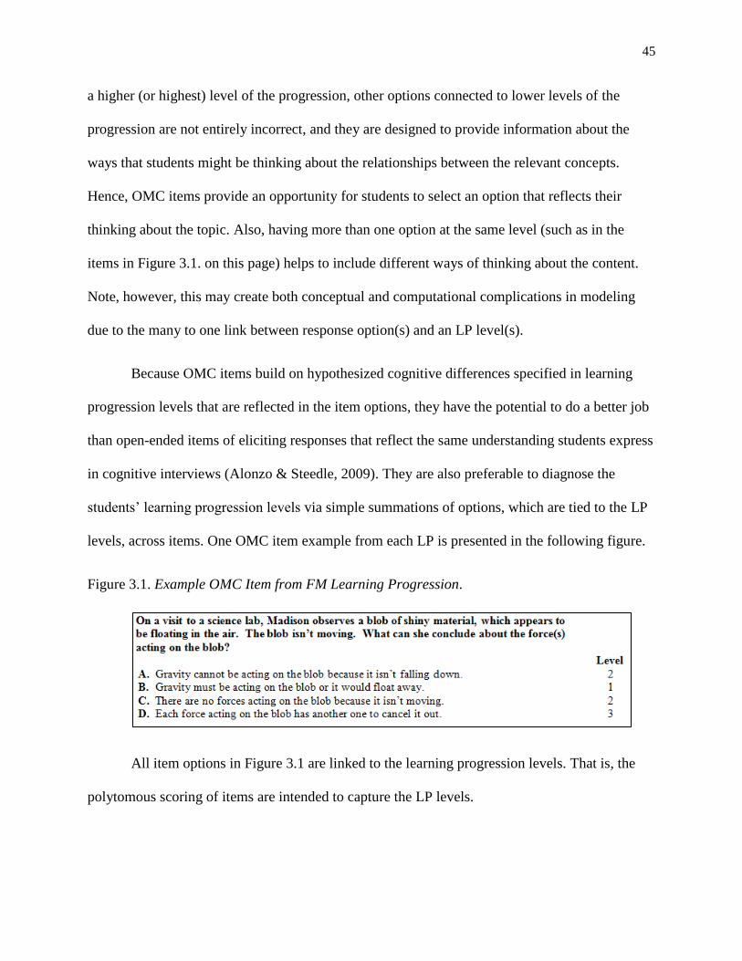
45

a higher (or highest) level of the progression, other options connected to lower levels of the

progression are not entirely incorrect, and they are designed to provide information about the

ways that students might be thinking about the relationships between the relevant concepts.

Hence, OMC items provide an opportunity for students to select an option that reflects their

thinking about the topic. Also, having more than one option at the same level (such as in the

items in Figure 3.1. on this page) helps to include different ways of thinking about the content.

Note, however, this may create both conceptual and computational complications in modeling

due to the many to one link between response option(s) and an LP level(s).

Because OMC items build on hypothesized cognitive differences specified in learning

progression levels that are reflected in the item options, they have the potential to do a better job

than open-ended items of eliciting responses that reflect the same understanding students express

in cognitive interviews (Alonzo & Steedle, 2009). They are also preferable to diagnose the

students’ learning progression levels via simple summations of options, which are tied to the LP

levels, across items. One OMC item example from each LP is presented in the following figure.

Figure 3.1. Example OMC Item from FM Learning Progression.

All item options in Figure 3.1 are linked to the learning progression levels. That is, the

polytomous scoring of items are intended to capture the LP levels.

46

Table 3.1 shows the distribution of student OMC item responses mapped to the levels of

the FM learning progressions, respectively. The values in each cell give an indication of the

easiness of OMC item options where, “easiness” is defined as the proportion of students (as

percentages) selecting a given response option. The colored coding is used to make clear some

characteristics of data. The grey cells represent the absence of the related LP level for specific

items. Yellow cells show the options that are connected into two LP levels. The orange colored

cells represent the most difficult items, and green colored cell shows the easiest item. Point-

biserial coefficients associated with the highest level response options for each OMC item are

presented at the bottom of the tables. These values can be used to evaluate item quality. For

example, for Item 11, most of students selected options in the highest level of the FM

progression but point-biserial was 0.405. That is, students choosing this option were not

necessarily those who performed the best on the remaining items.

Table 3.1. Descriptive Statistics for Each FM OMC Items (% responding at each level).

Notes:

1Columns sum to 100%.

In this table, the items are arranged from easiest to hardest. Notice that this

conceptualization is sample dependent. That is, a different sample might yield a different

ordering. For example, 57% of students selected the highest possible response option for item 11

(“On a visit to a science lab, Madison observes a blob of shiny material, which appears to be

5 As in all correlations, point-biserial values range from -1.00 to +1.00.

47

floating in the air. The blob isn’t moving. What can she conclude about the force(s) acting on

the blob?”). Thus, item 11 is the easiest item. However, only 5% of students selected the option

connected to the highest level possible for item 12 (Ignoring air resistance, what force(s) are

acting on the stone when it is moving up through point A?). Hence, item 12 is the hardest item.

Table 3.1 highlights a challenge inherent in modeling OMC items. Not only will there be,

upon occasion, multiple response options linked to the same LP level, but OMC items may have

floor effects or ceiling effects. A floor effect occurs any time the response options to an OMC

item are all higher than the lowest level on an LP (e.g., as in Item 14 for FM LP). A ceiling effect

occurs any time the response options to an OMC item do not include a response at the highest

level(s) of the LP (e.g., as in Item 11 for FM LP).

3.1.2 Basics of Data Set Analyzed in Current Study

Recall that the data used for this study originally included 16 Forces and Motion (FM)

OMC items with a sample of 1,088 high school students. However, for the FM data set, 8.0 % of

the students answered “no” to the question of “Was the content of [these] questions covered in a

science class you’ve taken?” These students were excluded from further analyses, leaving us

with 1,006 cases. Further, I cleaned the data for students who did not answer any of the FM

questions. Likewise, one of the students chose an unavailable option for item 14, so this student

is also excluded from the analyses. The LP levels range between Level 1 and Level 4 (i.e., score

1 to 4). Because all of the items do not have the range from 1 to 4, the minimum possible score

for the FM items is 24 and the maximum possible score is 60. Also, category response

frequencies ranged from a minimum of 13 to a maximum of 815. The further analyses for FM LP

include 931 cases.

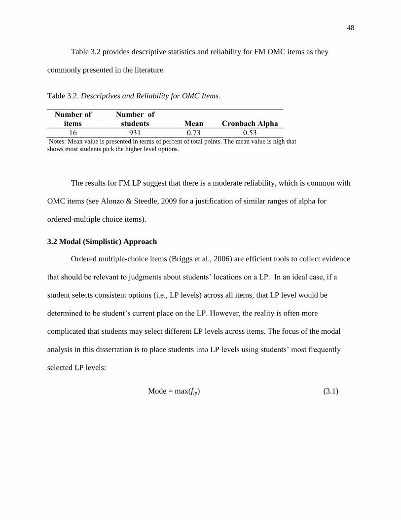
48

Table 3.2 provides descriptive statistics and reliability for FM OMC items as they

commonly presented in the literature.

Table 3.2. Descriptives and Reliability for OMC Items.

Number of

items

Number of

students Mean Cronbach Alpha

16 931 0.73 0.53 Notes: Mean value is presented in terms of percent of total points. The mean value is high that

shows most students pick the higher level options.

The results for FM LP suggest that there is a moderate reliability, which is common with

OMC items (see Alonzo & Steedle, 2009 for a justification of similar ranges of alpha for

ordered-multiple choice items).

3.2 Modal (Simplistic) Approach

Ordered multiple-choice items (Briggs et al., 2006) are efficient tools to collect evidence

that should be relevant to judgments about students’ locations on a LP. In an ideal case, if a

student selects consistent options (i.e., LP levels) across all items, that LP level would be

determined to be student’s current place on the LP. However, the reality is often more

complicated that students may select different LP levels across items. The focus of the modal

analysis in this dissertation is to place students into LP levels using students’ most frequently

selected LP levels:

Mode = max(flp) (3.1)

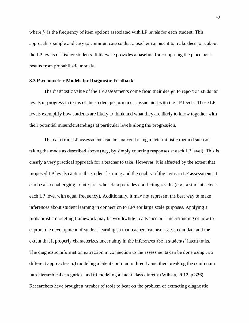
49

where flp is the frequency of item options associated with LP levels for each student. This

approach is simple and easy to communicate so that a teacher can use it to make decisions about

the LP levels of his/her students. It likewise provides a baseline for comparing the placement

results from probabilistic models.

3.3 Psychometric Models for Diagnostic Feedback

The diagnostic value of the LP assessments come from their design to report on students’

levels of progress in terms of the student performances associated with the LP levels. These LP

levels exemplify how students are likely to think and what they are likely to know together with

their potential misunderstandings at particular levels along the progression.

The data from LP assessments can be analyzed using a deterministic method such as

taking the mode as described above (e.g., by simply counting responses at each LP level). This is

clearly a very practical approach for a teacher to take. However, it is affected by the extent that

proposed LP levels capture the student learning and the quality of the items in LP assessment. It

can be also challenging to interpret when data provides conflicting results (e.g., a student selects

each LP level with equal frequency). Additionally, it may not represent the best way to make

inferences about student learning in connection to LPs for large scale purposes. Applying a

probabilistic modeling framework may be worthwhile to advance our understanding of how to

capture the development of student learning so that teachers can use assessment data and the

extent that it properly characterizes uncertainty in the inferences about students’ latent traits.

The diagnostic information extraction in connection to the assessments can be done using two

different approaches: a) modeling a latent continuum directly and then breaking the continuum

into hierarchical categories, and b) modeling a latent class directly (Wilson, 2012, p.326).

Researchers have brought a number of tools to bear on the problem of extracting diagnostic

50

information and diagnostic classification of respondents. In Figure 3.2, I provide a basic schema

of the measurement models that can be used for these purposes from the two frameworks.

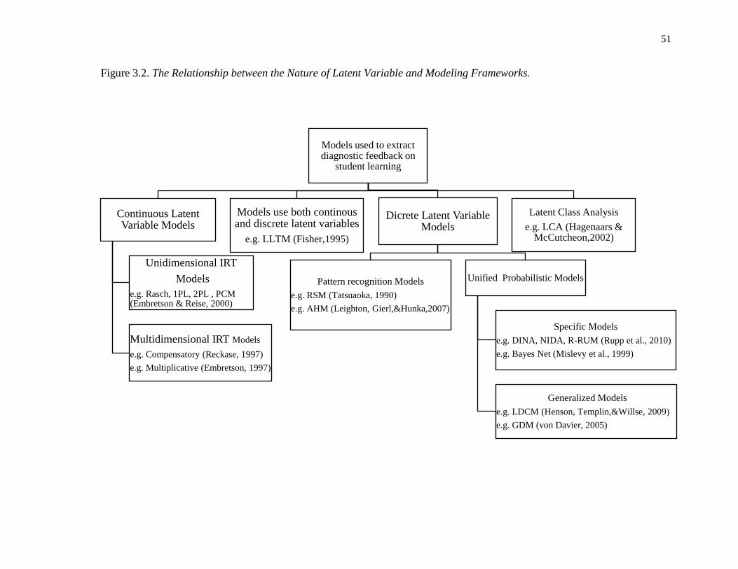
51

Figure 3.2. The Relationship between the Nature of Latent Variable and Modeling Frameworks.

Models used to extract diagnostic feedback on

student learning

Continuous Latent Variable Models

Unidimensional IRT

Models

e.g. Rasch, 1PL, 2PL , PCM (Embretson & Reise, 2000)

Multidimensional IRT Models

e.g. Compensatory (Reckase, 1997)

e.g. Multiplicative (Embretson, 1997)

Models use both continous and discrete latent variables

e.g. LLTM (Fisher,1995)

Dicrete Latent Variable Models

Pattern recognition Models

e.g. RSM (Tatsuaoka, 1990)

e.g. AHM (Leighton, Gierl,&Hunka,2007)

Unified Probabilistic Models

Specific Models

e.g. DINA, NIDA, R-RUM (Rupp et al., 2010)

e.g. Bayes Net (Mislevy et al., 1999)

Generalized Models

e.g. LDCM (Henson, Templin,&Willse, 2009)

e.g. GDM (von Davier, 2005)

Latent Class Analysis

e.g. LCA (Hagenaars & McCutcheon,2002)

52

It is clear from Figure 3.2 that there are a number of tools for summarizing evidence

about student understanding. Notice that Figure 3.2 does not show all models used to extract

information for diagnostic purposes, however it helps to understand the range of the models that

can be used and the place of the models I use in my dissertation work among these models. As

noted by some authors (e.g., Xu & von Davier, 2008; Heinen, 1996), the difference between the

models blurs when the distribution of theta (i.e., person ability) is approximated by a discrete

distribution (e.g., marginal maximum likelihood using the quadrature points). That is, the

estimation of the latent variable is always discrete in practice.

As it is presented in the previous chapter, current attempts of modeling learning

progressions mostly depend on the IRT models (latent trait/continuum models) although there

are several novel attempts to use latent class approach related models. I use three particular

models in this dissertation, one latent continuum and two latent class-based models, to

investigate the relation that links student performance on LP assessment tasks/items to their

levels on the LPs. Unlike other LPs, assessment tasks used in my work are based on OMC

items, which introduce inherent challenges in relationship to these models.

In the next section, I present IRT modeling and its use in context of the learning

progressions. Then, I cover diagnostic classification models and how they can relate to the

learning progression work.

3.4 IRT Modeling

When modeling LP assessment data with IRT, there are general assumptions and

characteristics of IRT models that violating them affects the interpretation of the student

classification into the LP categories. In order to critically examine the information from IRT

53

modeling in the context of LPs it is important to have a review of these assumptions and

characteristics.

In item response theory, the probability of an item response is characterized as a

nonlinear function of person ability and item characteristics (difficulty, discrimination, and

guessing). The probability can be modeled for items that are scored dichotomously or

polytomously. Differences between IRT models are based on the nature of the items used to

generate student responses (dichotomous vs. polytomous), number of dimensions they use to

describe the item and student characteristics (unidimensional vs. multidimensional), and the

number and type of item characteristics involved in relation to each dimension (Yen &

Fitzpatrick, 2006). Consider the Rasch model (Rasch, 1980). Given a test consisting of

dichotomously scored items, the probability of a correct response to an item i, is expressed as

𝑝𝑖 (𝜃) =1

1 + 𝑒−(𝜃−𝑏𝑖 )

(3.2)

where 𝑝𝑖 (𝜃) indicates probability that a student of ability 𝜃 responds correctly to item i, which is

modeled by one item characteristic. Although 𝜃 is theoretically unbounded, it usually ranges

from -3.0 to 3.0 for a population whose ability distribution is scaled to mean of zero and standard

deviation of 1. This item parameter, b, refers to item difficulty or location. As a distinct feature

of the Rasch model, the difference between a student’s ability and an item’s difficulty determines

the probability of a correct response. The Rasch model makes it possible to present the

distribution of items’ difficulty and students’ ability along the same unidimensional logit scale.

Hence, it provides a theoretical basis for “item-mapping,” in which item difficulty and student

ability are expressed relative to each other on a linear scale.

54

The use of IRT in general is grounded in two strong, related, assumptions: local

independence and unidimensionality. Unidimensionality requires a test to measure only one

construct. The assumption of local independence implies that the correlation between items

should only be through the construct measured by the test (Lord & Novick, 1968). In order for

this to hold, all of the items are required to measure a single dimension. When local item

independence is not present, we expect inaccurate estimation of item parameters, test statistics,

and student ability because of model misspecification (e.g., Hambleton, Swaminathan, & Rogers,

1991).

Two critical properties of IRT are scale indeterminancy and parameter invariance. The

former implies that the probability of a correct response (e.g., Equation 3.2 on previous page) as

a function of person and item parameters is invariant to any linear transformation of either set of

parameters. The latter denotes that if assumptions are met and the model fits, item and person

parameters should be the same, regardless of the group of persons and items used to estimate

them (e.g., Hambleton, Swaminathan, & Rogers, 1991). Given these properties, IRT is attractive,

especially for large scale assessments, because it makes it relatively easy to build item banks to

create tailored tests.

The IRT modeling is likewise used for diagnostic purposes. In the modeling practices of

learning progressions, the BEAR Assessment System (BAS; Wilson, 2005; Wilson & Sloane,

2000) is predominant and it uses IRT models, particularly those from the Rasch family. The BAS

is organized around four “building blocks”: the construct map, the item design, item scoring and

item response modeling.

55

A construct map constitutes one of the main building blocks of the BAS and represents a

description of ordering of qualitatively different levels of student performance focusing on one

characteristic (or construct). In many applications, the terms construct map and learning

progression are used interchangeably. Sometimes, the learning progression includes only one

construct, which is equivalent to a construct map (e.g., Plummer & Maynard, 2014). Or, a set of

construct maps can comprise the learning progression (e.g., Draney, 2009).

The second building block is the item design, where assessment tasks are written to elicit

evidence of a student’s location on the construct map. The third building block is item scoring

(i.e., the outcome space) in which a rule is set up to connect a respondent’s answer to assessment

tasks back to the levels of the construct map. The last building block is the measurement model,

which defines how we can make inferences about student understandings from their observed

scores. Ability measures and item difficulty measures are developed using the same scale which

facilitates the interpretation of student ability measures on the construct. The IRT models used

for the analyses in the context of learning progressions differ from binary models such as Rasch

modeling (e.g., Liu, Waight, Gregorius, Smith, & Park, 2007) to Rasch-based polytomous

models such as the Partial Credit Model (e.g., Lehrer, Wilson, Ayers, & Kim, 2011; Liu et al.,

2012), and to multidimensional IRT models (e.g., Lehrer, Kim, Ayers, & Wilson, 2014; Walker,

Wilson, Schwartz, & Irribarra, 2009).

A “Wright Map” serves as a visual and empirical representation of a construct map. It

provides an advantage of easy communication of the results via the graphical placement of

student ability and item difficulty on a common scale. Students with lower 𝜃 estimates and items

with lower difficulty appear at the bottom of the scale, while higher difficulty items and higher

proficiency persons are at the top. Using the information coming from the Wright map, the

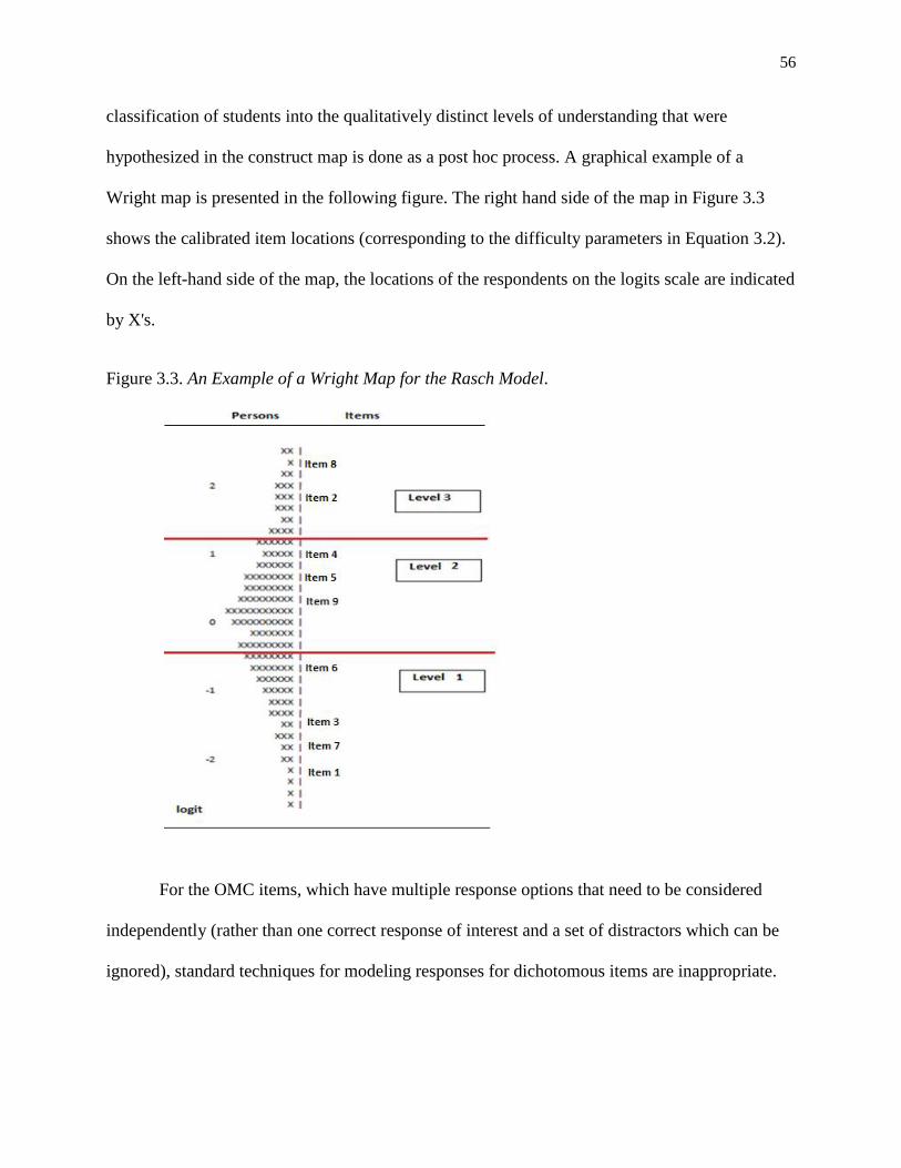
56

classification of students into the qualitatively distinct levels of understanding that were

hypothesized in the construct map is done as a post hoc process. A graphical example of a

Wright map is presented in the following figure. The right hand side of the map in Figure 3.3

shows the calibrated item locations (corresponding to the difficulty parameters in Equation 3.2).

On the left-hand side of the map, the locations of the respondents on the logits scale are indicated

by X's.

Figure 3.3. An Example of a Wright Map for the Rasch Model.

For the OMC items, which have multiple response options that need to be considered

independently (rather than one correct response of interest and a set of distractors which can be

ignored), standard techniques for modeling responses for dichotomous items are inappropriate.

57

Several models are available for modeling ordinal polytomous data. My strategy is to use the

Partial Credit Model (PCM; Masters, 1982).

3.4.1 Partial Credit Model

The goal of IRT modeling for polytomously scored items is to define the probability that

a student responds in a particular category. The PCM parameterizes the interaction between

student responses and items which have various response categories. This model is a divide-by-

sum model where the probability of a response in each category is defined as an exponential

divided by sum of exponentials. Let Xij represent a random variable, the response of any given

examinee to category j in item i. Given a test consisting of polytomously scored items, an

observed response Xij = x is coded in terms of a sequence of numeric scores from 0 to m, where

m represents the highest score. The total number of categories for any given item (indexed by i)

is therefore Ki=1+mi. For example, when an item has Xij = 0 for a lowest level item response,

and Xij = 3 for a highest level response, the item would have 4 categories in total. The probability

of observing a response in category j for an ability level of θ is

𝑃𝑖(𝑥 = 𝑗|theta) = exp[∑ (𝜃 − 𝛿𝑖𝑗)𝑥

𝑗=0 ]

∑ [exp ∑ (𝜃 − 𝛿𝑖𝑗)𝑟𝑗=0 ]

𝑚𝑖𝑟=0

(3.3)

where ∑ (𝜃 − 0𝑗=0 𝛿𝑖𝑗) ≡ 0

The 𝛿𝑖𝑗 (j=1, … , mi) parameters are the item category boundaries (also called category

intersections) associated with a level score of j on item i. In the numerator of the formula, x is the

count of the boundary locations up to the category under consideration. The argument r in the

denominator goes from 0 to mi (note that mi allows a different category number for each item). It

provides the sum of all m+1 possible numerators and so it assures the sum of the probabilities for

58

a person corresponding to each category is 1. Hence, the calculation of probability of a

respondent of given θ level in a particular category is obtained directly. The “where…” statement

in the equation introduces a constraint in estimating the parameters that the sum of ability level

minus the category boundary parameter for the first step should be zero. That is, the value of

𝛿𝑖0has no impact on the model.

When the response Xij is coded using a set of responses starting from 1 instead of zero,

then, m = 1,…,mi where mi is equal to the total number of categories. The response probabilities

can be modeled using the following formula,

𝑃𝑖(𝑥 = 𝑚|theta) = exp[∑ (𝜃 − 𝛿𝑖𝑗)𝑚

𝑗=1 ]

∑ [exp ∑ (𝜃 − 𝛿𝑖𝑗)𝑟𝑗=1 ]

𝑚𝑖𝑟=1

(3.4)

The ratio of probabilities takes the form

𝑃𝑖(𝑥=𝑗|theta)

𝑃𝑖(𝑥=(𝑗−1)|theta)= 𝑒𝑥𝑝 (𝜃 − 𝛿𝑖𝑗) and

𝑃𝑖(𝑥=𝑗|𝜃)

𝑃𝑖(𝑥=(𝑗−1)|𝜃)+ 𝑃𝑖(𝑥=𝑗|𝜃) =

exp(𝜃−𝛿𝑖𝑗)

1+ exp(𝜃−𝛿𝑖𝑗)

(3.5)

Equation 3.5 is read as the probability of responding in category m over category m-1 is

the function of the difference between latent ability,, and the item category boundary parameter,

δij. It also shows that the probability at adjacent categories has the form of the simple Rasch

model for dichotomously scored items. That is, the item parameters estimated in the PCM are

simply item difficulty parameters and they have the same interpretation as in dichotomous

models.

59

The PCM compares the adjacent response categories. That makes a student’s probability

of scoring m rather than m-1 independent of all other outcomes and each category boundary

parameter relates to adjacent response categories only. Because of this independence there is not

a constraint to ensure that the sequence of item category boundaries within a single item is

ordered as categories increase. It is also important to note that estimated item parameters do not

model the responses in independent pairs of categories (Nering & Ostini, 2010). For example, if

any of the item parameters change, the response probability in other categories also changes.

My examination of the PCM in the context of the learning progression assessment

composed of OMC items starts with investigation of dimensionality. Applying unidimensional

IRT methods investigate the claims that LP levels can be placed on a continuum and aligns with

student ability. According to the claim, the LP lies on a continuum along which students can be

ordered and distances along this are meaningful and there should be a single dimension defined

by the LP levels that accounts for a significant portion of the variance in student performance.

Investigating dimensionality can provide insight whether the unidimensional claim is reasonable.

It provides information on whether students use a single dominant ability or different abilities to

answer the items.

Note that when we model a multidimensional assessment unidimensionally,

interpretations of model parameter estimates as well as the placement of students into LP levels

are likely to be distorted. As such, there may be a greater value in using DCMs to allow for

examinations of mastery on different dimensions. DCM models assume that the data are

multidimensional, and multidimensionality is expressed in the Q-matrix, which shows the match

between items and specified attributes. That is, each test item is constructed to measure one or

60

more of the attributes. Because an item can measure more than one attribute, multidimensionality

can exist within (i.e., complex structure) as well as between items (i.e., simple structure).

While there is not a consensus regarding which one works better to investigate the

dimensionality of data, there are a number of approaches that can be classified as parametric

(e.g., principal component analysis), and nonparametric (e.g., DIMTEST as test of local

independence assumption). Two commonly used methods in practice are principal component

analysis (PCA) and exploratory factor analyses. PCA together with eigenvalue plots is a

commonly used method to assess test dimensionality and has been used for a long time (e.g.,

Hattie, 1985). The percentage of total variance explained by the first principle component is

examined in a way that the higher percentage of total variance the first principle component

accounts for, the closer the test is to unidimensionality. Several criteria have been proposed to

decide the number of dimensions. For example, Kaiser (1970) recommended keeping the

components with eigenvalues larger than 1.0, and Lord (1980) suggested checking the ratio of

the first to the second eigenvalue, and compare that with the ratio of the second to any of the

other eigenvalues. However, it is well noted in the literature regarding dimensionality that these

approaches may not identify the correct number of dimensions (e.g., Zeng, 2010). As noted by

Hambleton, Swaminathan, & Rogers (1991), the parallel analysis (Horn, 1965) with baseline

plots has been very helpful in interpreting test dimensionality and the analysis has been used

more recently.

Parallel analysis (Drasgow & Lissak, 1983) identifies the number of orthogonal

components that are distinguishable from random noise. In parallel analyses, the value of one is

replaced with the mean eigenvalues created by independent normal variates. The main idea is

that even if all population eigenvalues of a correlation matrix are all one, any finite sample can

61

produce eigenvalues more than one because of the sampling variability. Note that we have 16

manifest ordered category items; however, they have a different number of categories (i.e., not

all of the items K levels), and this introduces a complication into the interpretation. That is

because the analysis depends on decomposing a correlation matrix across items.

Next, I examine the results of the category boundary estimates. Recall that in some

studies using IRT methods in an LP context (e.g., Liu et al., 2012; Lehrer et al., 2011; Liu et al.,

2007) there is a tendency to use cumulative item category difficulty parameters, also called

thresholds. In this case, each threshold divides the response categories into two, up to and

including m-1 and m and above. The use of cumulative item difficulty parameters ensures the

increasing difficulty across scoring categories (which is same with LP levels). However, this

approach masks the potential problems that ordered categories are working as intended.

Examining category boundary parameters across items provide better information about the

ordering of category difficulties. When category difficulties are not increasing monotonically,

the interpretation that the selecting of a higher category aligns with higher trait level is not held

anymore (e.g., Andrich, 2015). Therefore, an investigation is needed in the ordering of the

category boundaries within items to check the alignment with the LP levels. But, note that it is

challenging to apply the PCM to OMC data. OMC items are different from regular polytomous

items. As mentioned previously, not all levels are available for each OMC item (floor and ceiling

effects), and for some of the items, multiple response options map to the same level. Because of

these features, the item category parameters will have different substantive interpretations from

item to item.

Next, I examine the parameter invariance where parameter refers to the population

quantities of the set of item parameters and the set of examinee parameters which are linked to a

62

specific model. Parameter invariance is critical for inferences to be equally valid for different

populations of students or across different conditions (Rupp & Zumbo, 2006). Therefore, in

order to check parameter invariance, we need at least two populations or two conditions for

parameters. Because I have only one set of data, I randomly split the data into two samples and

run PCM analyses for each subsample. Then, I repeat the process 100 times, and I summarize the

resulting distribution of all possible pairwise correlation coefficients together with the standard

deviation. A distribution with high average correlations and a low standard deviation provides

evidence of invariance across samples.

Then, I examine the results from model fit which signals how accurately or predictably

data fit the model. Fit investigation helps examine the question of whether there is evidence to

reject the LP hypothesis or whether there is evidence to highlight some of the items for further

check. Lack of model fit illustrates either there is a problem with the confirmatory LP hypothesis

or there is a need to use another model. In the literature, the justification of model fit is usually

done by monitoring the parameter-level fit statistics along with the global fit statistics (Wilson,

2005). Especially for polytomous data, there has been a considerable debate around the issue of

what is the most appropriate fit statistic to use, what range of fit statistics should be employed

when evaluating fit, and how fit statistics should be interpreted. Mean square fit statistics are

commonly used in the literature related to Rasch Models (Smith, 2004). Both fit statistics are

based on residuals (the differences between the observations and their expected values according

to the Rasch-based model). They can be transformed into standardized form (Linacre, 2002)

where fit statistics have an almost standard normal distribution (i.e., ~N(0,1)) with an acceptable

range of -2 to 2. Wu and Adams (2013) showed that the commonly used interval of 0.77 to 1.33

relates to a sample size of around 100 for outfit statistics. Hence, there is a need for adjustment

63

on an acceptable range based on the sample size we currently have. I follow their guideline and

examine the item statistics for appropriate fit range. However, several problems are noted

regarding the use of chi-squared based item fit statistics (Sinharay, 2006). The critics are based

on properties of the chi-squared distribution when estimates of parameters from the original

observations are used.

Based on the evaluation of model assumptions and model fit together with the close

examination of the item parameter estimates, I examine the possibility of deciding cut off points

on the latent continuum as a means of classifying students into LP levels based on a post-hoc

analysis. All PCM analysis is conducted using the package called “eRm” in free R software.

3.5 Diagnostic Classification Models (DCM)

In this subsection, I provide the reader with a framework to understand the different types

of models developed specifically for multivariate classifications of respondents on the basis of

hypothesized sets of discrete latent skills. A more comprehensive depiction of the models and

their relationship can be found in Rupp et al. (2010), Rupp and Templin (2008), and DiBello,

Roussos, and Stout (2007).

The definition of DCMs I use in this work is given by Rupp and Templin (2008). They

point out the key characteristic of these models is that they are confirmatory in nature, consist of

discrete latent variables, and have complex loading structures (i.e. skills intended to be measured

in the assessment) and even interactions between latent variables. In what follows, I refer to

discrete latent variables as “attributes.”

DCMs are confirmatory in nature because the multiple attributes measured by the

assessment are defined prior to the analyses. Each test item is written to measure one or more of

64

the attributes which allows a complex loading structure. The mapping of items to attributes is

captured by a matrix, called a Q-matrix, in which rows represent items, and columns represent

attributes. An entry of 1 in a cell of the matrix indicates that a given item measures a

hypothesized attribute and an entry of 0 indicates that it does not. When single items are written

to measure more than one construct, how the defined skills are assumed to interact with each

other is specified in advance (Rupp et al., 2010). That is, it is hypothesized whether having a

high level attribute can compensate a low level attribute or not. For example, say that attributes

1, 2, and 3 are deemed necessary to solve an item; in this case a student needs to hold all of the

skills to have a high probability to answer the item correctly (or choose a specific option).

The comparison between two frameworks, IRT and DCM, can illuminate the differences

between the models used. For example, we express science ability, θ, as a continuum in IRT

modeling, but in DCMs we reconceptualize θ as a set of attributes (e.g. force, motion,

acceleration and gravity). In unidimensional IRT models, all items are assumed to measure the

same latent variable, while in DCMs items don’t have to measure the same attributes and the

relationship between attributes and items are designated via the Q-matrix. In IRT, we finely

locate each respondent along a continuum of latent variable, in DCMs we coarsely classify each

respondent with respect to each attribute (e.g., as masters or non-masters of the attribute).

DCMs estimate the probability of respondents’ mastery states (e.g., mastery or

nonmastery) on the attributes of interests based on respondents’ observed response patterns.

There are two distinct families of models distinguished by parameter estimation method - pattern

recognition models or probabilistic models (DiBello et al., 2007). Pattern recognition models use

classification/pattern recognition algorithms (e.g., Rule Space Methodology by Tatsuoka, 1983)

as an approach for classifying respondents. The purpose of the analysis is to estimate the

65

probability that a respondent possess specific attribute combinations based on their observed

item response patterns (Gierl, Cui, & Hunka, 2007). In such models there is not a link between

individual latent variables and the probability of an observed response; that is to say we don’t

model item responses in terms of specified skills and item parameters and then use this to

estimate the parameters via a likelihood function. Probabilistic models are unified statistical

models that are defined in a fully probabilistic framework. Probabilistic DCMs model the

relationship between response probability in a latent class (e.g. latent class where none of the

attributes are mastered) connected to item parameters and attributes measured in this item.

3.5.1 Probabilistic Models (DINA Example)

A probabilistic diagnostic classification model has a mathematical function specifying the

probability of a particular item response in terms of the respondents’ skills and item

characteristics (Dibello et al., 2007). There are a number of well-known models that have been

developed: the DINA and NIDA (Junker & Sijtsma, 2001), DINO (Templin & Henson, 2006),

NIDO (Rupp et al., 2010), Fusion model (Roussos et al., 2007), RUM (Hartz, 2002). In this

section, I present one of the simplest and most commonly referenced models, the DINA model,

as an example. The DINA model is a parsimonious model and it is nested within GDM that is

used in the current study.

The Deterministic Input, Noisy “And” Gate (DINA) model assumes that all attributes

required by an item must be mastered in order for an examinee to answer correctly on that item.

In other words, missing any of the required attributes is equivalent to missing all of the required

attributes, leading to an incorrect response. In technical terms, each item on a test which

measures K attributes partitions 2K

attribute vectors into two latent classes (one group requires

all specified attributes and other group lacks at least one of the attributes). For example, imagine

66

that item 1 requires two attributes to be answered correctly (A1 and A2). It follows that for this

item we will have 4 different attribute vectors to consider ([00], [01], [10], and [11]). In the

DINA model, we classify these vectors deterministically into two groups. The first group takes

the vector including all required attributes and second group involves all three vectors which lack

at least one of the attributes. The DINA assumes that vectors in the same group have the same

correct response probability. Because of this, the model produces the same probability values for

the attribute vectors of [00], [01], and [10] and a noticeably higher probability for the attribute

vector [11].

There are three main elements in the DINA model. The deterministic input is the latent

variable 𝜉𝑖𝑐 which is viewed as either having (𝜉𝑖𝑐 = 1) or not having (𝜉𝑖𝑐 = 0) a particular

attribute for item i in a certain latent class c6. That is, whether a respondent within a specific

latent class possesses all the attributes required for item i. The Q-matrix (item-attribute

mapping) serves as the link between the model and examinee’s responses to the items and allows

inferences to be drawn about which skills have or have not been mastered by the examinees.

The probabilistic part of the DINA is modeled by slipping (si) and guessing (gi)

parameters at the item level. Slipping refers to the amount of incorrect application of the attribute

even it is mastered. Similarly, guessing amounts to the correct application of the attribute

although it is not mastered. Therefore, the latent response variable (correct response of a

respondent in a latent class) is defined at the item level and only one slipping and guessing

parameter is estimated for each item. The related formula is

6 c represents latent class rather than individual respondent this is because we can think the respondents are

changeable in each latent class and diagnostic models group large number of individuals into small number of latent

classes (Rupp & Templin, 2008)

67

𝜋𝑖𝑐 = 𝑃(𝑋𝑖𝑐 = 1|𝜉𝑖𝑐) = (1 − 𝑠𝑖)𝜉𝑖𝑐 𝑔𝑖

(1−𝜉𝑖𝑐) where 𝜉𝑖𝑐 = ∑ 𝛼𝑐𝑎𝑞𝑖𝑎𝐴

𝑎=1 (3.6)

In 3.6, 𝜋𝑖𝑐 represents the probability of a correct response for item i by a respondent in

latent class c. This probability depends on the values of si and gi and whether a respondent in a

latent class c possesses all the attributes required for item i, namely 𝜉𝑖𝑐. The 𝑞𝑖𝑎 shows whether

attribute a measured by item i and 𝛼𝑐𝑎 represents whether respondents in class c mastered the

attribute a. Note that since the gi and si denote item parameters, there are two parameters per item

in the DINA model.

As an end product, respondents are located into latent classes showing the combinations

of attributes that the students in that class mastered (e.g., if we had only 3 attributes measured in

the test we would have 8 latent classes such as [000],[100],[010], [001], [110],[101],[011] and

[111], where [000] represents a student that has not mastered any of the skills).

As in all psychometrics models, a well-fitting model is critical in DCMs for the

interpretation of parameter estimates. The model checking process focuses on the assessment of

the degree of fit between the estimated model and observed data. There are several fit statistics

used for this purpose such as mean absolute difference (Roussos et al, 2006) and model fit via

Bayes-net (Sinharay, 2006). Another standard global fit statistic used with probabilistic models is

the log-likelihood statistic, especially to compare the nested models (e.g., von Davier, 2005).

General models that are much more flexible than the DINA (e.g., log-linear cognitive

diagnostic model (LDCM; Henson, Templin, & Wilse, 2009; General Diagnostic model (GDM;

von Davier, 2005) have also been introduced in recent years. A general model means that with an

appropriate link function and restrictions it is possible to derive other commonly used models. I

use the General Diagnostic Model (GDM) proposed by von Davier (2005, 2008) as the

68

probabilistic diagnostic classification model in my dissertation. GDM formulates the response

probability in connection to item parameters. Hence, provides opportunities for comparisons

across item parameters and model fit with PCM. While the PCM can be seen as a restricted

version of the discrete skills GDM model and this relationship can be shown algebraically, doing

so is beyond the scope of this work. Next, I present the details of the GDM model.

3.5.2 General Diagnostic Model

The GDM allows for polytomously scored items as opposed to other basic diagnostic

classification models which only permit modeling of dichotomous data (though see de la Torre,

2009 as an exception). Data from several large-scale tests such as NAEP and TOEFL have been

analyzed with this model (von Davier, 2005; Xu & von Davier, 2008) but the model has not yet

been applied with an assessment developed for diagnostic purposes.

Before addressing the specifics of the GDM, it is important to be clear about how we can

connect IRT modeling with latent class analysis in the context of GDM. The diagnostic use of

GDM is based on the idea that theta (θ) can be modeled as discrete rather than continuous

(Heinen, 1996). Recall that in IRT modeling, we typically assume a unidimensional continuous

person variable (θ) as in the case of PCM. However, when we estimate the item parameters via

the marginal maximum likelihood/ expectation maximization (MML/EM) algorithm we

approximate this continuous person variable discretely. This approach requires certain

assumptions with respect to the distribution of latent variable θ. For example, if we assume that θ

has an underlying normal distribution, we can use Gauss-Hermite quadrature nodes (equally

spaced θ values) and weights to approximate the normal distribution. This helps us to estimate

the item parameters without jointly estimating the ability parameters by integrating out the

unknown person parameters. Once the item parameters have been estimated, person parameters

69

can be estimated by treating item parameters as known and maximizing the log-likelihood with

respect to the latent trait or, alternatively, using the expected value or the maximum value of the

corresponding posterior distribution. Building on this, an IRT model can be made to approximate

a latent class model if during estimation we specify the latent trait as discrete (e.g., 0/1 or

1,2,3,…m as the restricted version of -3.0, -2.5, …, 2.5, 3.0 of Gauss-Hermite quadrature points).

We conceptualize the latent trait composed of an ordered set of a limited number of latent groups

which have a fixed latent ability level attached to them. In this case, we use a fixed number of

node points on the latent axis and assign particular values to these nodes, and the weights (i.e.,

latent class portions belonging to the fixed latent node points) are no longer fixed and need to be

estimated from the data. Instead of node points chosen along the continuous θ interval (e.g., -3 to

+3) and assumed to be equally spaced on this interval, we specify two nodes, and the two values

of -1 and +1 are selected. Additionally, note that the form of the latent distribution is fixed in a

way that it can be approximated by a discrete distribution with a specific number of nodes.

With multiple random variables associated with the selection of a category in an item, we

can use random vectors (e.g., θ1, θ2, θ3…, θz where z indexes a dimension or attribute) with

discrete distributions. We can allow for different parameterizations for the conditional

distribution of the response variables given the latent traits - such as in the Partial Credit Model -

depending on the constraints imposed on the item parameters (e.g., slope parameters are

restricted to be 1 in PCM). In summary, the GDM makes it possible to specify what amounts to a

multidimensional item response model(s) with discrete latent variables for polytomous item

responses. Because the model is based on the extension of IRT models with the latent class

models (LCA), it allows tools such as model fit and item parameters estimates (which do not

exist with the AHM approach described below).

70

I fit the GDM to polytomous items with dichotomous skill mastery (i.e., mastered vs.

non-mastered with two nodes on each discrete θz that we will represent with ak to show different

attributes). Let’s assume N students with observations on I ordinal response variables 𝑥𝑛 =

(𝑥𝑛1, 𝑥𝑛2, , … . , 𝑥𝑛𝐼) each with outcomes 𝑥𝑛𝑖 ∈ {0,1, … . , 𝑚𝑖} , and a set of K discrete attribute

variables 𝑎𝑛 = (𝑎𝑛1, 𝑎𝑛2, , … . , 𝑎𝑛𝐾) with skill categories 𝑎𝑛𝑘 ∈ {𝑠𝑘(0), 𝑠𝑘(1), … . , 𝑠𝑘(𝑙𝑘)} .

Notice that 𝑥𝑛 is observed and 𝑎𝑛 is multidimensional and unobserved for all students (n = 1, 2,

…, N).

If the assumption of local independence holds, then the conditional probability of the

response pattern 𝑥𝑛 given the attribute vector a can be written as

𝑝(𝑥𝑛1, 𝑥𝑛2, , … . , 𝑥𝑛𝐼|𝒂) = ∏ 𝑝𝑖 (𝑥𝑛𝑖|𝒂),𝐼

𝑖=1

(3.7)

showing that the conditional probability of students’ response pattern can be written as the

product of the conditional probabilities of each response.

The Q matrix is defined as Q = (𝒒𝒊𝒌)𝒊=𝟏,……,𝑰;𝒌=𝟏,…..,𝑲 where Q is a IxK matrix with I

items and K attributes with real-valued 𝒒𝒊𝒌. While the structure of the Q matrix is the same in all

diagnostic classification models, its use differs. That is in contrast with the AHM (described

below), where the Q-matrix is used primarily as a tool to get the ideal patterns of observed

response patterns, the probabilistic GDM uses the Q matrix for specifying the conditional

probability of an observed response vector given the latent variable vector. The formula for the

GDM is

𝑃𝑖 (𝑥|𝒂) = 𝑃 (𝑥|𝛽𝑖, 𝒒𝒊, 𝛾𝑖, a) = exp [𝛽𝑥𝑖 + 𝛾𝑥𝑖.

𝑇 𝒉(𝒒𝒊, 𝒂)]

1 + ∑ exp [𝛽𝑦𝑖 + 𝛾𝑦𝑖.𝑇 𝒉(𝒒𝒊, 𝒂)]

𝑚𝑖𝑦=1

, (3.8)

71

where 𝛽𝑥𝑖 is the difficulty parameter and 𝛾𝑥𝑖. is k-dimensional slope parameter7 (𝛾𝑥𝑖. =

𝛾𝑥𝑖1, 𝛾𝑥𝑖2, … , 𝛾𝑥𝑖𝐾) for 𝑥 ∈ {0,1, … . , 𝑚𝑖}. In the formula, the conditional probability of response

is expressed in two terms; a global difficulty parameter 𝛽𝑥𝑖 (as category boundary parameters in

the case of polytomous items) and a combination of 𝑎𝑘 and a Q matrix specified as ℎ(𝑞𝑖. , 𝑎 ) =

(ℎ1(𝑞𝑖. , 𝑎), … . . , ℎ𝑘(𝑞𝑖. , 𝑎 )). When the Q matrix has a non-zero entry the slope parameters

convey the contribution of the associated attributes (𝑎 = (𝑎1, 𝑎2, … . , 𝑎𝐾)) to the response

probability of item i.

The h() function in the formula helps to determine how the Q-matrix entries 𝑞𝑖𝑘 and the

skills 𝑎𝐾 interact. That is, the function establishes how Q-matrix entries determine the effect of a

particular skill on conditional response probabilities, which is 𝑃𝑖 (𝑥|𝒂) = 𝑃 (𝑥|𝛽𝑖, 𝒒𝒊, 𝛾𝑖, a) for

item i. If the skill levels are 0/1, the commonly used general function is ℎ(𝑞, 𝑎) = 𝑞𝑎.

In our case of polytomous items ( 𝑥 𝜖 {0, 1, 2, . . . , 𝑚𝑖 } ) with dichotomous attributes (i.e.,

Q-matrix entries are 0/1), Von Davier and Yamamoto (2004) assume a simpler form that extends

well-known IRT models to diagnostic applications with multivariate latent skills. They put an

additional restriction on γ where 𝛾𝑥𝑖𝑘 = 𝑥𝛾𝑖𝑘 𝑎𝑛𝑑 ℎ (𝑞𝑖𝑘 , 𝑎𝑘) = 𝑞𝑖𝑘 𝑎𝑘. The former allows the

polytomous scores to have an effect on the item slopes per attribute. The parameter 𝛾𝑖𝑘 is a k-

dimensional slope parameter (𝛾𝑖𝑘 = 𝛾𝑖1, 𝛾𝑖2, … , 𝛾𝑖𝐾) for each item i. The latter means that when

𝑞𝑖𝑘= 0, the student's mastery position on the attribute does not influence the probability of the

7 Note that in this notation 𝛾𝑥𝑖.

𝑇 𝒉(𝒒𝒊, 𝒂) term represents∑ 𝛾𝑥𝑖𝑘ℎ(𝑞𝑖𝑘 , 𝑎𝑘)𝐾𝑘=1 .

72

particular response. If qik =1, the response is influenced by the attribute8. The formula of

conditional response is given as

𝑃𝑖 (𝑥|𝒂) = 𝑃 (𝑥|𝛽𝑖, 𝒒𝒊, 𝛾𝑖, a) = exp [𝛽𝑥𝑖 + ∑ 𝑥𝛾𝑖𝑘𝑞𝑖𝑘𝑎𝑘)𝐾

𝑘=1 ]

1 + ∑ exp [𝛽𝑦𝑖 + ∑ 𝑦𝛾𝑖𝑘𝑞𝑖𝑘𝑎𝑘)𝐾𝑘=1 ]

𝑚𝑖𝑦=1

(3.9)

Skill levels for 𝑎𝑘 discrete skill levels are determined before estimation by assigning real

numbers to the skill levels. For current purposes I selected a0 = −1 and a1 = 1 for my

dichotomous skills (i.e., mastered vs non-mastered). I put the constraints of mean 1 for slope

parameters and mean 0 for intercept parameters for the identification of the model. The

intercepts 𝛽𝑥𝑖 can be viewed as item category difficulty parameters, for item i. Note that

Equation 3.6 has an exponent with the inside expression of 𝛽𝑥𝑖 + ∑ 𝑥𝛾𝑖𝑘𝑞𝑖𝑘𝑎𝑘𝐾𝑘=1 showing that

the intercept parameters should be interpreted such that larger values represent item categories

that are “easier” to select rather than more “difficult.” Slope parameters in the places where the

Q-matrix does not have a zero entry can be viewed as the discrimination parameter for each item

on each skill dimension. They have an interpretation that is analogous to factor loadings. The Q-

matrix for FM LP data that is analyzed in this study is presented in the following table.

8 This member of the GDMs can be seen as a multivariate, discrete Generalized Partial Credit Model (von

Davier, DiBello, & Yamamoto, 2006).

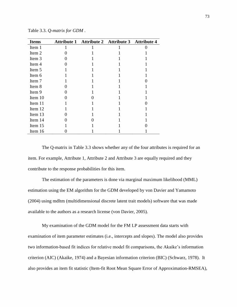
73

Table 3.3. Q-matrix for GDM .

Items Attribute 1 Attribute 2 Attribute 3 Attribute 4

Item 1 1 1 1 0

Item 2 0 1 1 1

Item 3 0 1 1 1

Item 4 0 1 1 1

Item 5 1 1 1 1

Item 6 1 1 1 1

Item 7 1 1 1 0

Item 8 0 1 1 1

Item 9 0 1 1 1

Item 10 0 0 1 1

Item 11 1 1 1 0

Item 12 1 1 1 1

Item 13 0 1 1 1

Item 14 0 0 1 1

Item 15 1 1 1 0

Item 16 0 1 1 1

The Q-matrix in Table 3.3 shows whether any of the four attributes is required for an

item. For example, Attribute 1, Attribute 2 and Attribute 3 are equally required and they

contribute to the response probabilities for this item.

The estimation of the parameters is done via marginal maximum likelihood (MML)

estimation using the EM algorithm for the GDM developed by von Davier and Yamamoto

(2004) using mdltm (multidimensional discrete latent trait models) software that was made

available to the authors as a research license (von Davier, 2005).

My examination of the GDM model for the FM LP assessment data starts with

examination of item parameter estimates (i.e., intercepts and slopes). The model also provides

two information-based fit indices for relative model fit comparisons, the Akaike’s information

criterion (AIC) (Akaike, 1974) and a Bayesian information criterion (BIC) (Schwarz, 1978). It

also provides an item fit statistic (Item-fit Root Mean Square Error of Approximation-RMSEA),

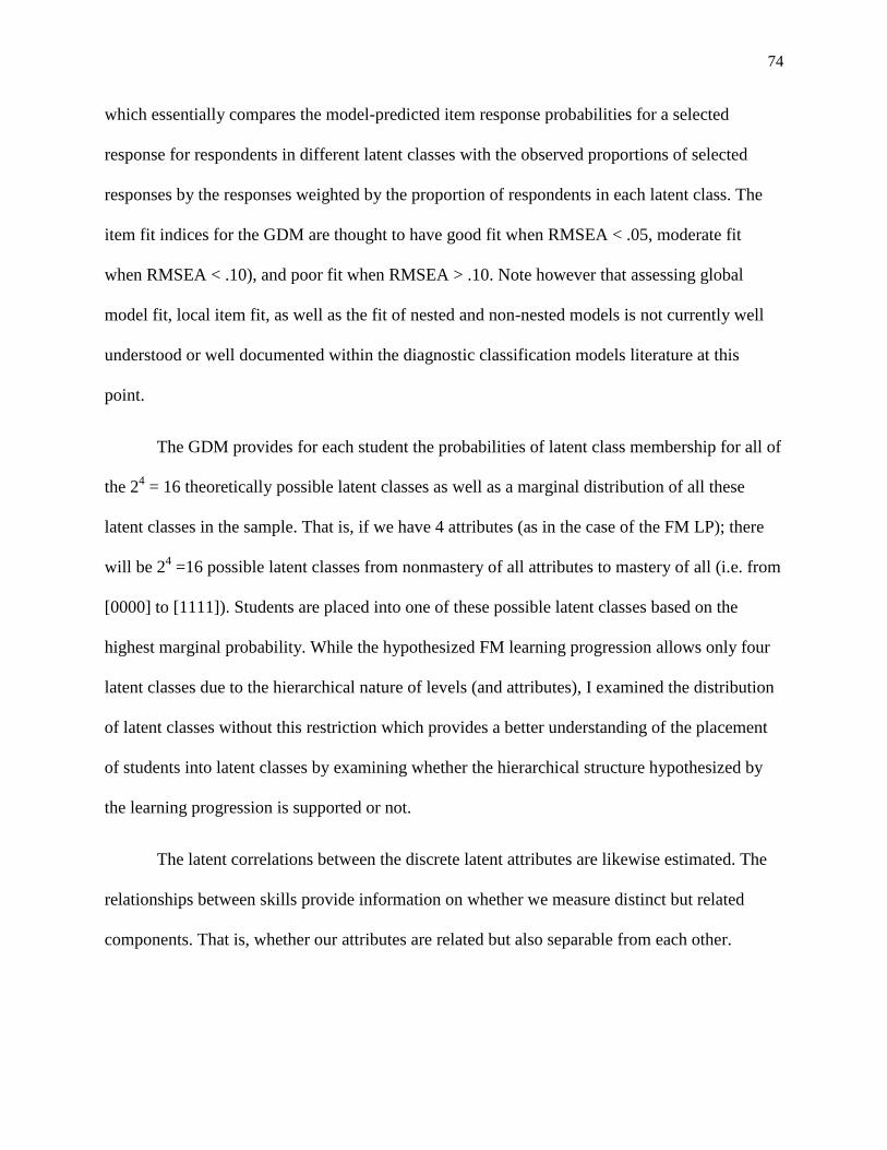
74

which essentially compares the model-predicted item response probabilities for a selected

response for respondents in different latent classes with the observed proportions of selected

responses by the responses weighted by the proportion of respondents in each latent class. The

item fit indices for the GDM are thought to have good fit when RMSEA < .05, moderate fit

when RMSEA < .10), and poor fit when RMSEA > .10. Note however that assessing global

model fit, local item fit, as well as the fit of nested and non-nested models is not currently well

understood or well documented within the diagnostic classification models literature at this

point.

The GDM provides for each student the probabilities of latent class membership for all of

the 24 = 16 theoretically possible latent classes as well as a marginal distribution of all these

latent classes in the sample. That is, if we have 4 attributes (as in the case of the FM LP); there

will be 24 =16 possible latent classes from nonmastery of all attributes to mastery of all (i.e. from

[0000] to [1111]). Students are placed into one of these possible latent classes based on the

highest marginal probability. While the hypothesized FM learning progression allows only four

latent classes due to the hierarchical nature of levels (and attributes), I examined the distribution

of latent classes without this restriction which provides a better understanding of the placement

of students into latent classes by examining whether the hierarchical structure hypothesized by

the learning progression is supported or not.

The latent correlations between the discrete latent attributes are likewise estimated. The

relationships between skills provide information on whether we measure distinct but related

components. That is, whether our attributes are related but also separable from each other.

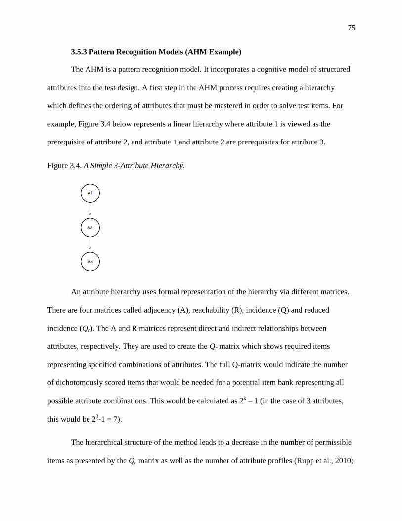
75

3.5.3 Pattern Recognition Models (AHM Example)

The AHM is a pattern recognition model. It incorporates a cognitive model of structured

attributes into the test design. A first step in the AHM process requires creating a hierarchy

which defines the ordering of attributes that must be mastered in order to solve test items. For

example, Figure 3.4 below represents a linear hierarchy where attribute 1 is viewed as the

prerequisite of attribute 2, and attribute 1 and attribute 2 are prerequisites for attribute 3.

Figure 3.4. A Simple 3-Attribute Hierarchy.

An attribute hierarchy uses formal representation of the hierarchy via different matrices.

There are four matrices called adjacency (A), reachability (R), incidence (Q) and reduced

incidence (Qr). The A and R matrices represent direct and indirect relationships between

attributes, respectively. They are used to create the Qr matrix which shows required items

representing specified combinations of attributes. The full Q-matrix would indicate the number

of dichotomously scored items that would be needed for a potential item bank representing all

possible attribute combinations. This would be calculated as 2k – 1 (in the case of 3 attributes,

this would be 23-1 = 7).

The hierarchical structure of the method leads to a decrease in the number of permissible

items as presented by the Qr matrix as well as the number of attribute profiles (Rupp et al., 2010;

76

Gierl et al., 2007; Leighton, Gierl, & Hunka, 2004). Similar to a Q-matrix, the attributes are

indicated by columns and items by rows. The Qr matrix for the attribute hierarchy shown in

Figure 3.4 would be

𝑄𝑟 = [1 1 10 1 10 0 1

]

The Qr matrix shows that at least three unique types of items are required. One item

should measure first attribute, the next one requires both attribute 1 and 2 together, and the last

one requires all three attributes.

Given the attribute hierarchy, expected response patterns representing the response

patterns of students who don’t make slips with respect to attribute hierarchy are determined. For

the attribute hierarchy shown in Figure 3.4., there will be three expected response patterns (i.e.,

response vectors of [100], [110], and [111] where [111] vector shows all items are answered

correctly). Also, examinee attribute vectors presenting the possible latent classes (e.g., [100])

represent students in a class that only mastered the first attribute) are generated. In recent

research, Artificial Neural Networks (ANNs) are used to estimate the latent class membership of

students (Cui, Gierl, & Leighton, 2009). ANNs typically consist of three groups: one input layer,

one hidden layer, and an output layer. Each layer consists of “neurons”, which have different

interpretations depending upon the layer. For dichotomously scored test items, the number of

neurons is equivalent to the total number of items on a test.

The neurons in the output layer are fixed to correspond to the different attributes

hypothesized to comprise an attribute hierarchy. A hidden layer in a neural network makes it

possible to examine the impact of input neurons interactions on output neurons. Figure 3.5 shows

the mechanism within a neural network.

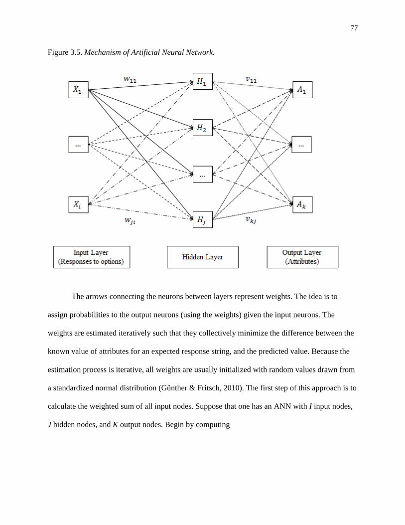
77

Figure 3.5. Mechanism of Artificial Neural Network.

The arrows connecting the neurons between layers represent weights. The idea is to

assign probabilities to the output neurons (using the weights) given the input neurons. The

weights are estimated iteratively such that they collectively minimize the difference between the

known value of attributes for an expected response string, and the predicted value. Because the

estimation process is iterative, all weights are usually initialized with random values drawn from

a standardized normal distribution (Günther & Fritsch, 2010). The first step of this approach is to

calculate the weighted sum of all input nodes. Suppose that one has an ANN with I input nodes,

J hidden nodes, and K output nodes. Begin by computing

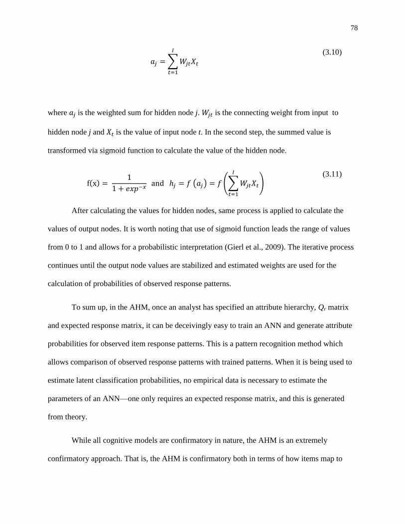
78

𝑎𝑗 = ∑ 𝑊𝑗𝑡𝑋𝑡

𝐼

𝑡=1

(3.10)

where 𝑎𝑗 is the weighted sum for hidden node j. 𝑊𝑗𝑡 is the connecting weight from input to

hidden node j and 𝑋𝑡 is the value of input node t. In the second step, the summed value is

transformed via sigmoid function to calculate the value of the hidden node.

f(x) = 1

1 + 𝑒𝑥𝑝−𝑥 and ℎ𝑗 = 𝑓 (𝑎𝑗) = 𝑓 (∑ 𝑊𝑗𝑡𝑋𝑡

𝐼

𝑡=1

) (3.11)

After calculating the values for hidden nodes, same process is applied to calculate the

values of output nodes. It is worth noting that use of sigmoid function leads the range of values

from 0 to 1 and allows for a probabilistic interpretation (Gierl et al., 2009). The iterative process

continues until the output node values are stabilized and estimated weights are used for the

calculation of probabilities of observed response patterns.

To sum up, in the AHM, once an analyst has specified an attribute hierarchy, Qr matrix

and expected response matrix, it can be deceivingly easy to train an ANN and generate attribute

probabilities for observed item response patterns. This is a pattern recognition method which

allows comparison of observed response patterns with trained patterns. When it is being used to

estimate latent classification probabilities, no empirical data is necessary to estimate the

parameters of an ANN—one only requires an expected response matrix, and this is generated

from theory.

While all cognitive models are confirmatory in nature, the AHM is an extremely

confirmatory approach. That is, the AHM is confirmatory both in terms of how items map to

79

attributes (here it is similar in nature to the DINA, described above), and also in terms of how

attributes relate to each other in the hierarchy. Its utility rests upon the correctness of the attribute

hierarchy that has been stipulated as well as the attributes specified in the Q-matrix.

The model uses a person-fit statistic called the hierarchy consistency index (HCI) (see

Cui & Leighton, 2009) to evaluate the degree to which the response patterns of students are

consistent with the ones constructed based on the attribute hierarchy representing the processes

students used to solve the items. The underlying logic of the HCI index is that student who

answered an item correctly needs to first answer its prerequisite items right. The values of the

index range between -1 and 1, and it is suggested not to use a cognitive model in the case of

really low values for inferences about students. Usually, the median value of the HCIs across all

students is used to determine the overall model fit. Currently, in contrast to IRT models, this

approach has not obtained item parameter estimates. Additionally, the estimated attribute

probabilities for each student are not group invariant.

The AHM related research has grown in recent years with a number of applications (

Gierl, Leighton, Wang, Zhou, Gokiert, & Tan, 2009; Broaddus, 2012; Wang & Gierl, 2011). The

AHM does not parameterize item characteristics. Instead, as described above, it uses a pattern

recognition approach to produce the expected response patterns specified by the hypothesized

hierarchy.

The AHM framework is selected because the application of the AHM in the context of

learning progressions has been previously suggested and illustrated by Briggs and Alonzo

(2012). The authors presented potential challenges to modeling the OMC item responses to

support diagnostic inferences with conventional IRT models and posited the use of the AHM

80

approach as an alternative. I follow their proposed method in my dissertation. The AHM

approach modified for OMC items is presented in the following section.

3.5.3.1AHM model: Extension to the ordered multiple choice items. As described

above, the first step in the AHM requires creating a hierarchy which defines the ordering of

attributes that must be mastered in order to solve test items. This is identical in structure to the

hierarchy being conceptualized for the learning progressions. Briggs and Alonzo (2012)

converted the qualitative descriptions of levels in the Earth and Solar System (ESS) learning

progression (see Appendix C) into the attributes required in AHM (p. 305).

A1: Student recognizes that objects in the sky move systematically.

A2: Student knows that the Earth orbits the Sun, the Moon orbits the Earth,

and the Earth rotates on its axis.

A3: Student can coordinate apparent and actual motions of objects in sky.

A4: Student can incorporate the motions of the Earth and Moon into a

complete description of motion in the Solar System that explains the

day/night cycle, phases of the Moon, and the seasons.

They specify a linear hierarchy among these four attributes which reflects the original

hierarchies implied in the learning progression (A1 A2 A3 A4). Because there is a linear

hierarchy the conjunctive nature of attributes is straightforward. That means a student must

possess an attribute lower in the hierarchy (e.g., A1 and A2) in order to possess a higher attribute

(e.g., A3). They specify the connection between LP levels and attributes as follow:

Level 1 = No attributes

Level 2 = A1

Level 3 = A1 & A2

Level 4 = A1 & A2 & A3

Level 5 = A1 & A2 & A3 & A4

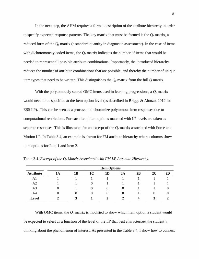
81

In the next step, the AHM requires a formal description of the attribute hierarchy in order

to specify expected response patterns. The key matrix that must be formed is the Qr matrix, a

reduced form of the Qr matrix (a standard quantity in diagnostic assessment). In the case of items

with dichotomously coded items, the Qr matrix indicates the number of items that would be

needed to represent all possible attribute combinations. Importantly, the introduced hierarchy

reduces the number of attribute combinations that are possible, and thereby the number of unique

item types that need to be written. This distinguishes the Qr matrix from the full Q matrix.

With the polytomously scored OMC items used in learning progressions, a Qr matrix

would need to be specified at the item option level (as described in Briggs & Alonzo, 2012 for

ESS LP). This can be seen as a process to dichotomize polytomous item responses due to

computational restrictions. For each item, item options matched with LP levels are taken as

separate responses. This is illustrated for an excerpt of the Qr matrix associated with Force and

Motion LP. In Table 3.4, an example is shown for FM attribute hierarchy where columns show

item options for Item 1 and Item 2.

Table 3.4. Excerpt of the Qr Matrix Associated with FM LP Attribute Hierarchy.

Item Options

Attribute 1A 1B 1C 1D 2A 2B 2C 2D

A1 1 1 1 1 1 1 1 1

A2 1 1 0 1 1 1 1 1

A3 0 1 0 0 0 1 1 0

A4 0 0 0 0 0 1 0 0

Level 2 3 1 2 2 4 3 2

With OMC items, the Qr matrix is modified to show which item option a student would

be expected to select as a function of the level of the LP that best characterizes the student’s

thinking about the phenomenon of interest. As presented in the Table 3.4, I show how to connect

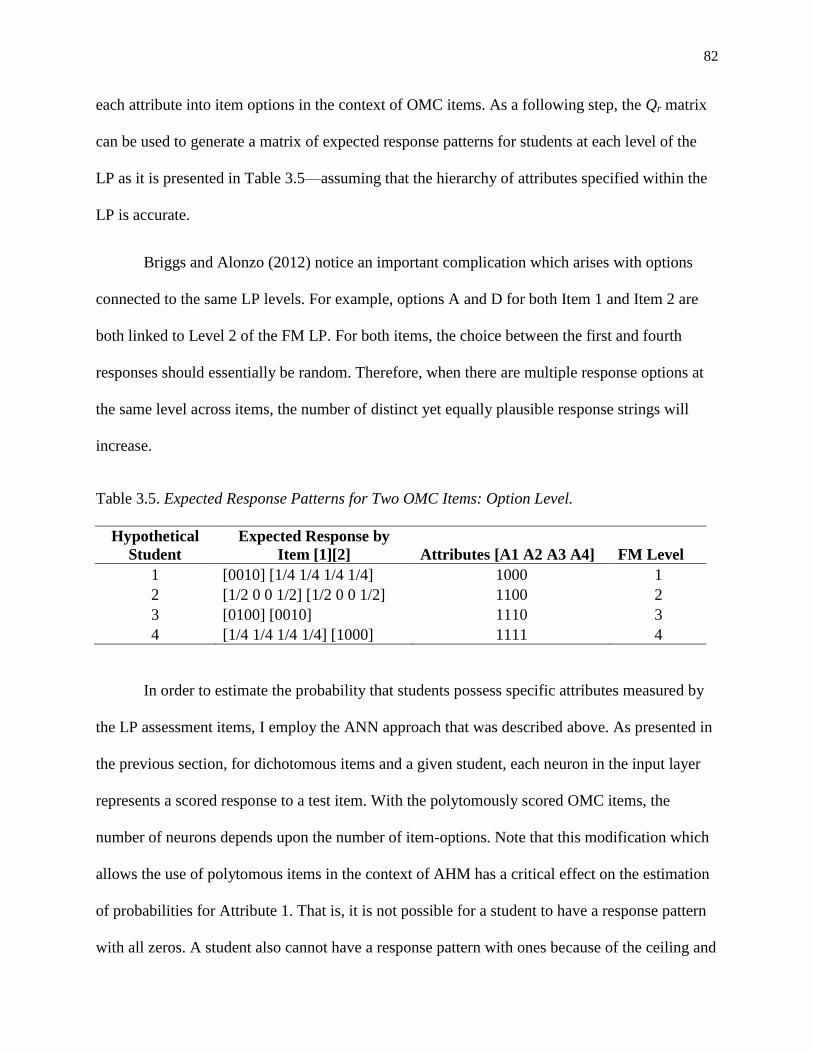
82

each attribute into item options in the context of OMC items. As a following step, the Qr matrix

can be used to generate a matrix of expected response patterns for students at each level of the

LP as it is presented in Table 3.5—assuming that the hierarchy of attributes specified within the

LP is accurate.

Briggs and Alonzo (2012) notice an important complication which arises with options

connected to the same LP levels. For example, options A and D for both Item 1 and Item 2 are

both linked to Level 2 of the FM LP. For both items, the choice between the first and fourth

responses should essentially be random. Therefore, when there are multiple response options at

the same level across items, the number of distinct yet equally plausible response strings will

increase.

Table 3.5. Expected Response Patterns for Two OMC Items: Option Level.

Hypothetical

Student

Expected Response by

Item [1][2] Attributes [A1 A2 A3 A4] FM Level

1 [0010] [1/4 1/4 1/4 1/4] 1000 1

2 [1/2 0 0 1/2] [1/2 0 0 1/2] 1100 2

3 [0100] [0010] 1110 3

4 [1/4 1/4 1/4 1/4] [1000] 1111 4

In order to estimate the probability that students possess specific attributes measured by

the LP assessment items, I employ the ANN approach that was described above. As presented in

the previous section, for dichotomous items and a given student, each neuron in the input layer

represents a scored response to a test item. With the polytomously scored OMC items, the

number of neurons depends upon the number of item-options. Note that this modification which

allows the use of polytomous items in the context of AHM has a critical effect on the estimation

of probabilities for Attribute 1. That is, it is not possible for a student to have a response pattern

with all zeros. A student also cannot have a response pattern with ones because of the ceiling and

83

floor effects in OMC items. We always observe a response pattern with a mixture of ones and

twos, in a worst case scenario. Hence, even we train the ANN with an expected response pattern

of all zeros or all ones; every student will be classified as mastered for the Attribute 1.

In order to examine AHM in the context of learning progression assessments, I again start

with an examination of model fit. Again, this approach does not provide item parameter

estimates based on observed student responses. Hence, it is not possible to examine item fit

statistics. Instead, I adapt the notion of a person-fit statistic for dichotomously scored items (Cui,

Leighton, Gierl, & Hunka, 2006). In the cases of LPs with OMC items, the index needs revision

with adjustments that take into account the unique nature of OMC items. With OMC items,

students ideally are expected to demonstrate consistent performance (i.e., provide responses at

the same level(s) of a LP framework) across different items. OMC items specify an attribute

hierarchy within an item (between item response options) rather than between items. For a given

student, when student selects an item option corresponding to an attribute combination at the

high end of the FM learning progression, the student has mastered all these attributes and s/he is

expected to select the similar (higher level) option in another item. Hence, the conception of fit

requires consistency among the student selection of options with same/similar attributes.

The simplest formula for a “Response Consistency Index” can be

RCIi = 1 − # of misfits

# 𝑜𝑓 𝑐𝑜𝑚𝑝𝑎𝑟𝑖𝑠𝑜𝑛𝑠 . (3.12)

However this calculation would only be appropriate when applied to the response

patterns for the OMC items for which there are no floor or ceiling effects. For my analysis, I use

the idea of consistently selecting similar options with the formula;

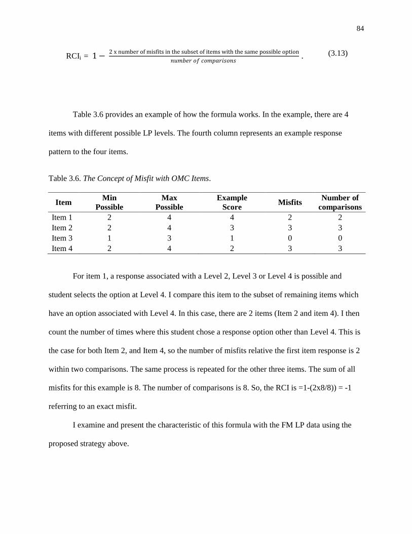
84

RCIi = 1 − 2 x number of misfits in the subset of items with the same possible option

𝑛𝑢𝑚𝑏𝑒𝑟 𝑜𝑓 𝑐𝑜𝑚𝑝𝑎𝑟𝑖𝑠𝑜𝑛𝑠 . (3.13)

Table 3.6 provides an example of how the formula works. In the example, there are 4

items with different possible LP levels. The fourth column represents an example response

pattern to the four items.

Table 3.6. The Concept of Misfit with OMC Items.

Item Min

Possible

Max

Possible

Example

Score Misfits

Number of

comparisons

Item 1 2 4 4 2 2

Item 2 2 4 3 3 3

Item 3 1 3 1 0 0

Item 4 2 4 2 3 3

For item 1, a response associated with a Level 2, Level 3 or Level 4 is possible and

student selects the option at Level 4. I compare this item to the subset of remaining items which

have an option associated with Level 4. In this case, there are 2 items (Item 2 and item 4). I then

count the number of times where this student chose a response option other than Level 4. This is

the case for both Item 2, and Item 4, so the number of misfits relative the first item response is 2

within two comparisons. The same process is repeated for the other three items. The sum of all

misfits for this example is 8. The number of comparisons is 8. So, the RCI is =1-(2x8/8)) = -1

referring to an exact misfit.

I examine and present the characteristic of this formula with the FM LP data using the

proposed strategy above.

85

Recall that there are not item parameters estimated in AHM. Hence, the examination of

parameter item parameter invariance is not possible. The parameters estimated in AHM are the

weights in ANN (see Figure 3.5) and they have an effect on the attribute probabilities of

students. With the cautions put on the ANN approach, it is important to examine the consistency

of the student attribute estimates across multiple trainings.

Later, I estimate attribute probabilities for the student sample responding to the Force and

Motion OMC items on the basis of a neural net specification with one hidden layer, four hidden

neurons, backpropagation algorithm and a learning rate of 0.01. The initial weights are selected

randomly from a normal distribution. However, these random initial weights are noted to have

potential problems of both local minima and slow convergence (c.f., Li, Alnuweiri, & Wu,

1993).

After computing attribute probabilities for each student by using their observed response

patterns in neural network, one typically examines the mean and SD for each attribute

probability estimate with the expectation that the mean values decrease with higher level

attributes showing relative difficulty of mastering each attribute. That is, with linear FM LP

hierarchy it should decrease from A1 (easiest) to A4 (most difficult). I also examine the

correlation between attribute pairs at this stage where adjacent attributes are expected to have a

higher correlation.

Finally, for placing a student into a mastery category for each attribute, I examine the

mastery status of students for three thresholds; 0.5 (which is common in the literature), 0.65, and

0.75. Note that a high threshold means a more conservative approach to place students into

higher level LP levels. For example, a lower threshold (such as 0.50) leads more students being

86

placed in the mastery category of attributes. After deciding mastery status of the students, I will

place them into LP levels based on their mastery sequence.

In the context of diagnostic models, the comparison of DCMs with IRT model results is

common. The comparisons mostly focus on the model fit (e.g., von Davier, 2008), but they do

not come to the end point of how these models differ in terms of the inferences that are actually

communicated to teachers or students. My second research question focuses on the comparison

of the models on the inferences on student classifications into LP levels. For that purpose, I

examine the differences and similarities in the student placements across different modeling

approaches.

3.6 Chapter Summary

This chapter focused on the basics of the empirical data used in this dissertation and the

modeling approaches that I will be applying for extracting diagnostic information about the

students’ understanding of force and motion concept. It likewise presented the details of three

models that I use in my dissertation together with the adjustments I need for analyses of LP

assessments composed of OMC items. It presented the IRT framework, which is predominant in

current psychometric modeling of learning progressions. It likewise presented the diagnostic

classification models as promising, but which remain largely unexamined with small diagnostic

assessments, and as tools to model the data from LP assessments composed of OMC items.

With the methods and methodological refinements that are required in mind, I provide the

analysis results of the data for each model in the following chapter.

87

Chapter 4

Results

The primary goal of this chapter is to examine the FM LP data and present the results

from different frameworks. In section 4.1, I start with a “naïve” non-probabilistic approach. I

provide the results from the exploratory analysis of data and categorization of students into LP

levels. For this first part, my examination of data aims to understand the data better for the later

analyses and results. This is followed by an examination of the classification of students into LP

levels from a modal analysis. A fundamental argument in favor of taking a probabilistic

approach to classifying students for diagnostic purposes is that such an approach offers more

nuanced insights into a student’s strengths and weaknesses than taking a more ad hoc or modal

approach, such as simply classifying a student as a function of his or her modal response. Thus,

the results from the modal approach aim to provide a basis for comparisons from the

probabilistic models that I use in this dissertation to examine whether there are practical reasons

to use more complicated models. Next, I continue with the results from three probabilistic

models; PCM, AHM and GDM, respectively. The presentation of the results for each of the

models includes the investigation of the model assumptions, item parameter estimates, attribute

probabilities (person estimates), and the classification of students into the LP levels. This chapter

ends with the comparisons across models to examine the differences produced in terms of

classification of students into LP levels.

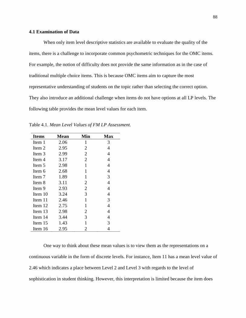
88

4.1 Examination of Data

When only item level descriptive statistics are available to evaluate the quality of the

items, there is a challenge to incorporate common psychometric techniques for the OMC items.

For example, the notion of difficulty does not provide the same information as in the case of

traditional multiple choice items. This is because OMC items aim to capture the most

representative understanding of students on the topic rather than selecting the correct option.

They also introduce an additional challenge when items do not have options at all LP levels. The

following table provides the mean level values for each item.

Table 4.1. Mean Level Values of FM LP Assessment.

Items Mean Min Max

Item 1 2.06 1 3

Item 2 2.95 2 4

Item 3 2.99 2 4

Item 4 3.17 2 4

Item 5 2.98 1 4

Item 6 2.68 1 4

Item 7 1.89 1 3

Item 8 3.11 2 4

Item 9 2.93 2 4

Item 10 3.24 3 4

Item 11 2.46 1 3

Item 12 2.75 1 4

Item 13 2.98 2 4

Item 14 3.44 3 4

Item 15 1.43 1 3

Item 16 2.95 2 4

One way to think about these mean values is to view them as the representations on a

continuous variable in the form of discrete levels. For instance, Item 11 has a mean level value of

2.46 which indicates a place between Level 2 and Level 3 with regards to the level of

sophistication in student thinking. However, this interpretation is limited because the item does

89

not have an option at Level 4 which makes representation of students’ understanding at this level

unclear.

Next, in order to evaluate the match between LP levels assigned by the assessment

developers and observed data for each item, I examine both the point-biserial correlations at the

option level, and the cross tabulation of items options where any unexpected order of response

frequency is flagged as a mismatch. Since all items are written as (at least) ordinal categories, the

point-biserial correlations are expected to increase monotonically on each level. This is the

correlation between a response category coded as a dummy variable (a score of 1 for students

that responded with the current LP level and a score of 0 for students in other response

categories) and the total score. After applying this strategy, none of FM LP items satisfy the

monotonic increase with increasing LP levels. The potential reasons for distorted point-biserials

are the relatively small number of students at lower levels, also a result of a small number of

lowest level options available.

Another important consideration is the extent to which the frequency of students

responses align with expected frequency across different LP levels. I examine consistency across

item options using the mean scores of each student group who selected the same option in an

item. The results for each item are presented in Table 4.2. First four columns in the table

illustrate the mean scores at specific level (e.g., mean total score is 41.07 for students who picked

Level 1 option for Item 1). Multiple options column shows whether the item has multiple options

linked to the same LP level (e.g., Item 1 has 2 options linked to the Level 2). Final column on

Table 4.2 shows if there is an unexpected pattern across LP levels (e.g., for Item 7, mean total

score of students selecting Level 1 option is higher than the mean total score of students who

selected a Level 2 option and the item is flagged as ‘Yes’).

90

Overall, there is an increasing trend across levels for 7 out of 16 items but variability in

mean total scores is small.

Table 4.2. Mean Total Score for Students Selecting Same LP Level Option in an Item.

Item Level 1 Level 2 Level 3 Level 4

Multiple

options

(in any)

Flag

Item 1 41.07 41.18 43.62 . L2 No

Item 2 . 40.95 40.01 41.91 L2 Yes

Item 3 . 39.76 41.41 41.07 L3 Yes

Item 4 . 39.58 40.14 42.26 L2 No

Item 5 38.73 38.67 41.19 41.26 N/A Yes

Item 6 39.23 39.94 42.18 42.83 L2 No

Item 7 41.56 40.92 43.54 . L1 Yes

Item 8 . 38.98 40.81 42.06 L3 No

Item 9 . 40.13 40.16 42.58 L2 No

Item 10 .

40.68 41.06 N/A No

Item 11 40.07 40.56 42.39 . L2 No

Item 12 38.61 39.43 41.98 42.37 N/A No

Item 13 . 39.66 41.50 41.19 L2 Yes

Item 14 . . 40.12 44.15 N/A No

Item 15 42.62 41.63 42.54 . L1 Yes

Item 16 . 41.69 40.45 41.45 L3 Yes

Margin Mean 40.39 40.35 41.60 42.30

Notes: 1Mean performance across all level is 43.42. The mean values are calculated after item removed.

I will use the same strategy in the following sections with mean IRT theta estimates and

DCM attribute probabilities, again, to check the alignment between LP levels and estimated

student ability and student mastery.

4.1.2 Modal Classification Results

Of the 931 students in our sample, 858 (92%) could be classified into a level of the

Forces and Motion LP on the basis of the OMC response option associated with the LP level

selected most frequently. Some students (74) chose two levels at equal frequency. The

distribution of students into the FM LP levels is given in Table 4.3.

91

Table 4.3. Basic FM LP Level Placement Results.

Level Frequency

Level 1 1

Level 2 84

Level 3 733

Level 4 39

Level 2 - Level 3 47

Level 2 - Level 4 4

Level 3 - Level 4 23

Looking at Table 4.3, the modal approach placed most of the students into the Level 3.

From simplistic perspective, this shows that there is limited variability in this sample. There is

only 1 student who selected Level 1 options the most frequently, which may be expected due to

the fact that a Level 1 response option was not even possible for 9 out of 16 items. Almost 8% of

the students could not be placed into a specific level because they selected an equal number of

options at two levels.

The results from this “modal” approach will serve as a baseline contrast relative to the

classifications made from the three models I use in this dissertation (i.e., PCM, AHM and GDM).

4.2 Unidimensional Partial Credit Item Response Theory Model

In this section, I start with examination of the dimensionality of the FM assessment items.

Recall that models from the DCM and IRT framework have different assumptions of the

underlying latent trait (continuous vs. discrete). That is IRT models assume that there is one

underlying trait or a common composite of traits that explains students’ performance on the

assessment items. However, DCMs conceptualize the latent trait(s) as an ordered set of a limited

number of latent groups. They identify a mathematical model that can represent the connection

between the probability of a response to an item and the location of a person in a multi-skill

92

discrete space9. The examination of dimensionality helps us to provide support for the underlying

latent trait assumptions for selected models. Then, I continue with the investigation of PCM item

parameter estimation results. In the next subsection, I investigate model fit results where item

statistics are considered as a gauge of the suitability of the model. Relatedly, item parameter

invariance is examined across random samples. Finally, I present results from examination of a

person-item map to show the challenges introduced by OMC items for the alignment of

categories across items. The results did not support for putting meaningful cutoffs along the

ability distribution to classify students into levels of the underlying LP.

4.2.1 Examination of Empirical Dimensionality

The use of the PCM depends on two assumptions: unidimensionality and local

independence. The local independence assumption requires that when we condition on the latent

ability of a respondent (i.e., for fixed values of theta) the responses to items are statistically

independent. Unidimensionality is a prerequisite for this to hold. When these assumptions hold

and the model fits the data, the property of parameter invariance should hold, meaning that item

and person parameters are independent from each other. The issue of multidimensionality is

related to the model misfit, where if we model multidimensional data unidimensionally, the

parameter estimates are likely to be distorted. In contrast, DCMs assume a complex structure

where the multidimensionality can exist within as well as between items. Using DCMs are

recommended only if the model approximates data better than more parsimonious and

computationally less demanding models (Sinharay & Haberman, 2009).

9 Multidimensional IRT models likewise assume a set of traits underlying the students’ responses and

identify a mathematical model to place a student in a multidimensional space. However, they assume latent traits to

be continuous in each dimension (Reckase, 2009).

93

For current purposes, I follow an exploratory approach where my goal is to investigate

the underlying set of dimension(s). In order to examine the dimensional structure of the data, I

will follow the steps;

(a) compute polychoric correlations based on the polytomous item responses,

(b) run a parallel analysis (PA) to examine the number of dimensions supported by the

data,

(c) run an explanatory factor analysis (EFA) to examine and identify the items with

strong loadings on specified number of factors.

The parallel analysis results for FM LP assessment are presented in the Figure 110

.

Parallel analysis identified 6 factors in FM LP assessment using polychoric correlation. That is,

six simulated eigenvalues fall behind the corresponding, real eigenvalues.

Figure 4.1. Parallel Analysis Approach Scree Plot.

While the results from the exploratory analysis suggest that there may be multiple

dimensions that underlie the FM LP assessment, the results need to be interpreted with caution.

10

I also ran the analysis by excluding Item 10 and Item 14 which only have categories 3 and 4. The result

changed very little and the conclusion was same.

94

Note that, in practice, it is unlikely any empirical data will be purely unidimensional. That is,

data may be considered basically as unidimensional when there is a “dominant” factor

underlying the responses (e.g., Lord, 1980) where any other factors can be thought as nuisance

dimensions. In FM LP assessment data, it is hard to say that there is one dominant factor. The

eigenvalue for the first factor in Figure 4.1 is just 1.87, which is pretty small in comparison to

values we observe in most testing situations (e.g., values between 6-20 for the first eigenvalue

are highly likely in large scale administrations as for NAEP). However, there is a rule of thumb

that is described by Lord (1980) and expanded by Divgi (1980) with the minimum value of 3 to

defer the unidimensionality and commonly used in the large scale assessments (e.g., the 2008

technical report for the Illinois state). I find that the ratio of the difference of the first and second

eigenvalues (1.87-0.57 = 1.3) over the difference of the second and third eigenvalues (0.57 –

0.49 =0.06) is to be 21.7. This approach supports the LP assessment to be calibrated with a

unidimensional model.

A reasonable next step to examine the dimensional structure of FM LP assessment is to

investigate the distribution of items across factors. For that purpose, I fit the data into a 1-factor

solution first and examined the loadings. As I discussed above, from statistical view, PA analysis

suggests 6 separate factors. However, when we consider practical significance, adding to the

cumulative variation by an additional factor, we can conclude that a 4-factor structure is

supportable in comparison to other higher number factor structure. Additionally, the eigenvalue

of the fifth factor is close to the eigenvalue produced by resampled data and simulated data. In

the next subsection, I will examine the loadings of 16 items on the 4-factor model.

95

4.2.1.1 EFA Analyses Results. In this section, I first ran a FA with 1-factor and then with 4-

factor structure. I examine the loadings of items for the former and the number of items placed at

each factor11

for the latter. Table 4.4 presents the loadings of each item on one factor.

Table 4.4. Factor Loadings from Oblique Exploratory Factor Analyses for 1-Factor Structure.

Items Factor 1

Item 12 0.52

Item 6 0.51

Item 9 0.48

Item 1 0.46

Item 4 0.46

Item 11 0.46

Item 7 0.43

Item 8 0.30

Item 14 0.24

Item 13 0.22

Item 5 0.19

Item 3 0.18

Item 2 0.15

Item 10 0.07

Item 15 0.01

Item 16 -0.04

Half of the items are found to have little relevance in the 1-factor model (i.e., uniqueness

close to 1 and low factor loadings)12

. This suggests that our data does not support

unidimensionality where each item of the assessment relates to only one unique latent dimension.

Between-item multidimensionality where groups of items load on different latent dimensions or

within-item multidimensionality where each item of the assessment relates to more than one

latent dimension can be the case. For multi-factor structures, the hypothesized relationship

11

It can be considered that examining loading of options which are coded as 0-1 can be a better strategy;

but the matrix is not convertible in this case which is common in practice (e.g., Flora & Curran, 2004). 12

Recall that in factor analysis, the greater ‘uniqueness’ the lower the relevance of the variable in the factor

model. Also, factor loadings can be interpreted like standardized regression coefficients. Hence, the coefficients

represent the relationship of observed variables with factors.

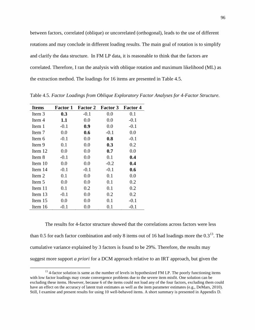
96

between factors, correlated (oblique) or uncorrelated (orthogonal), leads to the use of different

rotations and may conclude in different loading results. The main goal of rotation is to simplify

and clarify the data structure. In FM LP data, it is reasonable to think that the factors are

correlated. Therefore, I ran the analysis with oblique rotation and maximum likelihood (ML) as

the extraction method. The loadings for 16 items are presented in Table 4.5.

Table 4.5. Factor Loadings from Oblique Exploratory Factor Analyses for 4-Factor Structure.

Items Factor 1 Factor 2 Factor 3 Factor 4

Item 3 0.3 -0.1 0.0 0.1

Item 4 1.1 0.0 0.0 -0.1

Item 1 -0.1 0.9 0.0 -0.1

Item 7 0.0 0.6 -0.1 0.0

Item 6 -0.1 0.0 0.8 -0.1

Item 9 0.1 0.0 0.3 0.2

Item 12 0.0 0.0 0.7 0.0

Item 8 -0.1 0.0 0.1 0.4

Item 10 0.0 0.0 -0.2 0.4

Item 14 -0.1 -0.1 -0.1 0.6

Item 2 0.1 0.0 0.1 0.0

Item 5 0.0 0.0 0.1 0.2

Item 11 0.1 0.2 0.1 0.2

Item 13 -0.1 0.0 0.2 0.2

Item 15 0.0 0.0 0.1 -0.1

Item 16 -0.1 0.0 0.1 -0.1

The results for 4-factor structure showed that the correlations across factors were less

than 0.5 for each factor combination and only 8 items out of 16 had loadings more the 0.313

. The

cumulative variance explained by 3 factors is found to be 29%. Therefore, the results may

suggest more support a priori for a DCM approach relative to an IRT approach, but given the

13

4-factor solution is same as the number of levels in hypothesized FM LP. The poorly functioning items

with low factor loadings may create convergence problems due to the severe item misfit. One solution can be

excluding these items. However, because 6 of the items could not load any of the four factors, excluding them could

have an effect on the accuracy of latent trait estimates as well as the item parameter estimates (e.g., DeMars, 2010).

Still, I examine and present results for using 10 well-behaved items. A short summary is presented in Appendix D.

97

fact that items do not load on multiple factors and factors explain a small portion of the overall

variability, there is not a clear-cut solution suggested by the explanatory methods. Hence,

although the question of dimensionality is quite important, it turns out to be highly challenging to

make a decision using current methods.

4.2.2 Item Parameter Estimation

In the PCM case, by incorporating a location parameter for each category boundary and

each item (δ𝑖𝑗) we obtain a flexible model where the number and structure of categories can vary

across items in an assessment. However, the model requires polytomous items to be coded

without missing categories. One design criterion of learning progression-based items is that,

ideally, students at the same ability level will get the same level across all items. In the context of

PCM, this means that the item category boundaries (δ𝑖1,δ𝑖2,δ𝑖3) should be similar across items.

In the case of OMCs, we have natural missing categories (ceiling and floor effects) and also have

multiple categories connected to the same LP levels. For example, when an item has all possible

categories, an item that was supposed to be scored from 1 to 4 can be used to estimate category

boundary parameters (δ𝑖1, δ𝑖2, and δ𝑖3). However, a challenge arises when an OMC item has

only some of the possible categories. So, for example, instead of having a response that can be

linked to levels 1, 2, 3, and 4, it may only be possible for respondents to select response options

linked to levels 2, 3, and 4. In this latter case, the response vector needs to be recoded to become

1, 2, and 3 and category parameters of δ𝑖1and δ𝑖2 are produced. Therefore, there appears a need

to follow a strategy in how to compare the item parameters estimated across items which have

different structures. For my current purposes, I reorganized the item parameter estimates with

regard to their original categories. That is, if an item has options of 2, 3, and 4, I categorized the

item parameter estimates as δ𝑖2and δ𝑖3 rather than δ𝑖1and δ𝑖2. It is critical to note that I made a

98

strong assumption here. I expect the item category parameter estimates (δ𝑖𝑗) to be similar across

items when they have the same options. For example, both Item 12 and Item 13 ask about the

forces acting on a stone. Item 12 has options associated with levels of 1, 2, 3 and 4 and Item 13

has options 2, 3 and 4. If we examine the options associated with level 2 (“Only the force that

Derek put on the stone is acting on it.” and “There is no more force left from Derek’s throw.”)

and level 3 (“Both gravity and the force that Derek put on the stone are acting on it.” and “The

force of gravity is now equal to the force from Derek's throw.”), it can be argued that the similar

options are measuring the same concepts and we may expect the category boundary parameters

to be similar (δ12,2, δ13,1).

Table 4.6 contains the one to three 𝛿𝑖𝑗 values for each item categorized as explained

above. The estimates vary between -2.68 and 4.09, covering a wide range of ability distribution.

In addition, the estimation results within each category boundary demonstrate a wide variation.

The variation in the results suggests potential problems in using these results to classify students

into LP levels.

99

Table 4.6. Category Boundary Parameter Estimates of 16 Items.

Items Level 1-Level 2(𝜹𝒊𝟏) Level 2-Level 3(𝜹𝒊𝟐) Level 3-Level 4(𝜹𝒊𝟑)

Item 10 . . 1.63

Item 14 . . 0.71

Item 1 -0.03 0.72 .

Item 7 1.27 -0.05 .

Item 11 -0.59 -0.18 .

Item 15 4.09 -1.7 .

Item 2 . 0.96 0.11

Item 3 . -0.78 1.74

Item 4 . -0.19 0.48

Item 8 . -2.12 2.01

Item 9 . 1.47 -0.38

Item 13 . -0.61 1.65

Item 16 . -0.05 1.16

Item 5 -0.81 -2.55 3.19

Item 6 -2.36 0.11 2.25

Item 12 -2.68 -0.48 3.14 Note:

1Bold italics values indicate the items with disordered categories.

It is also seen that the boundary orders vary (bold and italicized in Table 4.6). In Table

4.6, category difficulty estimates are reversed in 5 out of the 16 FM LP items. Consider now two

FM items- Item 1 and Item 15- and their score structure more carefully. These two LP items

selected as examples have a similar structure in terms of the task demand that they have options

associated with LP levels of 1, 2 and 3. For Item 1, the boundaries are sequentially ordered,

indicating an item functioning as expected; therefore, all three scores have some part of the latent

trait distribution that a response in the score category is more probable than the other score

categories. Figure 4.2 shows actual Item 1 which asks about a non-moving object on a table. This

item has two options linked to LP level 2. Figure 4.3 illustrates item category response curves for

Item 1 that shows the probability of the response of a student at any location on the latent ability.

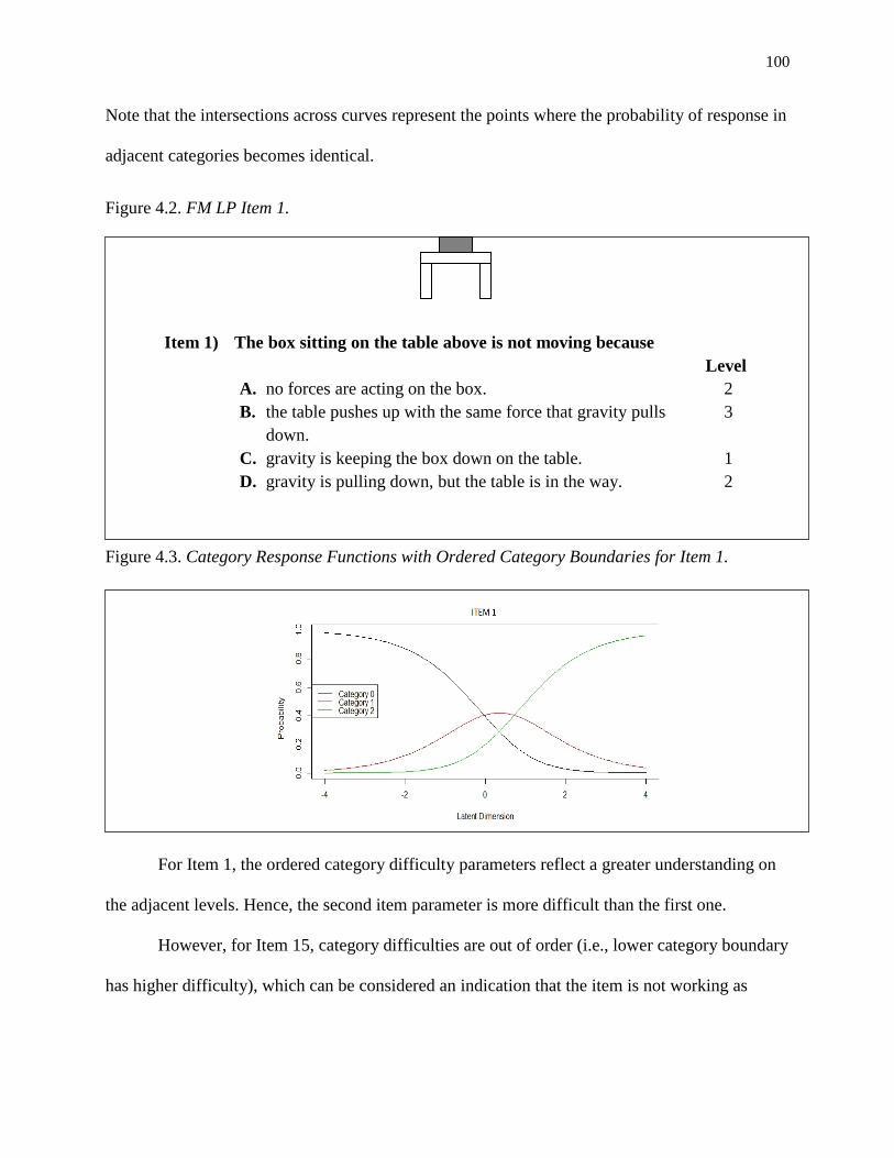
100

Note that the intersections across curves represent the points where the probability of response in

adjacent categories becomes identical.

Figure 4.2. FM LP Item 1.

Item 1) The box sitting on the table above is not moving because

Level

A. no forces are acting on the box. 2

B. the table pushes up with the same force that gravity pulls

down.

3

C. gravity is keeping the box down on the table. 1

D. gravity is pulling down, but the table is in the way. 2

Figure 4.3. Category Response Functions with Ordered Category Boundaries for Item 1.

For Item 1, the ordered category difficulty parameters reflect a greater understanding on

the adjacent levels. Hence, the second item parameter is more difficult than the first one.

However, for Item 15, category difficulties are out of order (i.e., lower category boundary

has higher difficulty), which can be considered an indication that the item is not working as

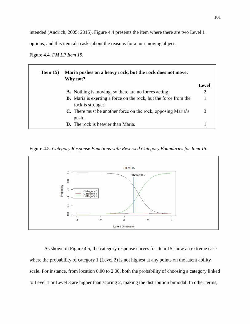
101

intended (Andrich, 2005; 2015). Figure 4.4 presents the item where there are two Level 1

options, and this item also asks about the reasons for a non-moving object.

Figure 4.4. FM LP Item 15.

Item 15) Maria pushes on a heavy rock, but the rock does not move.

Why not?

Level

A. Nothing is moving, so there are no forces acting. 2

B. Maria is exerting a force on the rock, but the force from the

rock is stronger.

1

C. There must be another force on the rock, opposing Maria’s

push.

3

D. The rock is heavier than Maria. 1

Figure 4.5. Category Response Functions with Reversed Category Boundaries for Item 15.

As shown in Figure 4.5, the category response curves for Item 15 show an extreme case

where the probability of category 1 (Level 2) is not highest at any points on the latent ability

scale. For instance, from location 0.00 to 2.00, both the probability of choosing a category linked

to Level 1 or Level 3 are higher than scoring 2, making the distribution bimodal. In other terms,

Theta= 0.7

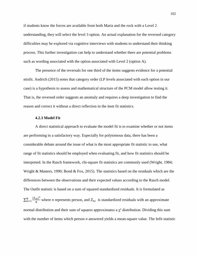
102

if students know the forces are available from both Maria and the rock with a Level 2

understanding, they will select the level 3 option. An actual explanation for the reversed category

difficulties may be explored via cognitive interviews with students to understand their thinking

process. This further investigation can help to understand whether there are potential problems

such as wording associated with the option associated with Level 2 (option A).

The presence of the reversals for one third of the items suggests evidence for a potential

misfit. Andrich (2015) notes that category order (LP levels associated with each option in our

case) is a hypothesis to assess and mathematical structure of the PCM model allow testing it.

That is, the reversed order suggests an anomaly and requires a deep investigation to find the

reason and correct it without a direct reflection in the item fit statistics.

4.2.3 Model Fit

A direct statistical approach to evaluate the model fit is to examine whether or not items

are performing in a satisfactory way. Especially for polytomous data, there has been a

considerable debate around the issue of what is the most appropriate fit statistic to use, what

range of fit statistics should be employed when evaluating fit, and how fit statistics should be

interpreted. In the Rasch framework, chi-square fit statistics are commonly used (Wright, 1984;

Wright & Masters, 1990; Bond & Fox, 2015). The statistics based on the residuals which are the

differences between the observations and their expected values according to the Rasch model.

The Outfit statistic is based on a sum of squared standardized residuals. It is formulated as

∑(𝑍𝑛𝑖)2

𝑁𝑁𝑛=1 where n represents person, and 𝑍𝑛𝑖 is standardized residuals with an approximate

normal distribution and their sum of squares approximates a χ² distribution. Dividing this sum

with the number of items which person n answered yields a mean-square value. The Infit statistic

103

is an information-weighted form of outfit with the formula of ∑ (𝑍𝑛𝑖)2 𝑊𝑛𝑖

𝑁𝑛=1

∑ 𝑊𝑛𝑖𝑁𝑛=1

where 𝑊𝑛𝑖

respresents the individual residual variance. These statistics have an expected value of 1 and can

range from 0 to infinity. Fit statistics greater than 1 are interpreted as more variation between the

model and the observed scores (e.g., 1.30 for an item illustrates 30 % more variation) and

illustrates an underfit. Similarly, statistics lower than 1 show less variation (e.g., a fit statistic of

0.70 for an item would indicate 30% less variation than predicted) and show an overfit. Items

demonstrating more variation than predicted by the model can be considered as not conforming

to the unidimensionality requirement of the Rasch model. In addition, the mean square statistics

can be transformed into standardized form (Linacre, 2002) where fit statistics have almost

standard normal distribution (i.e., ~N(0,1)) with an acceptable range of -2 to 2.

First, I considered the infit statistics (Wright & Masters, 1990) for the item parameter

estimates (also known as the “weighted mean square” fit statistic). The weighted mean square fit

statistics for the FM LP assessment show that none of 16 items had a weighted mean square fit

statistic that was outside the range of the 95% confidence interval. However, this approach does

not take the sample size into account. Wu and Adams (2013) showed that the commonly used

interval of 0.77 to 1.33 relates to a sample size of around 100 for outfit statistics. The outfit

statistics are based on conventional sum of squared standardized residuals (i.e., not weighted by

individual variances). Wu and Adams (2013) emphasize the fact that misfit shows a relative fit

(e.g., how an item differs from others) rather than an absolute fit to the theoretical ICC. They

concluded that for larger samples the smaller the appropriate confidence interval and for large

data sets examining effect size of fit mean square statistic is better. Following their guidelines

(Wu & Adams, 2013, p.29), I examined the item outfit statistics with the confidence interval ~ 1

(+/-) 0.07. Note that we expect to see the misfit as a part of our relative support on the

104

multidimensional structure of the data. Supporting this expectation, I found that 10 out of 16

items show signs of misfit.

An indirect approach to evaluate model fit is examining the parameter invariance

property of the IRT model (Green, Camilli, & Elmore, 2006). This model feature of IRT is

never observed in the strictest sense in practice. Parameter invariance is specifically important

for large scale testing applications. It refers to the inferences to be equally valid for different

populations of students or across different conditions (Rupp & Zumbo, 2006). Therefore, in

order to check parameter invariance, we need at least two populations or two conditions for

parameters. Because I have only one data set, I randomly split the data into two samples and ran

PCM analyses for each subsample. Then, I repeat the process 100 times, and I provide

correlation coefficients together with standard deviation where high correlation and low standard

deviation shows the invariance across samples. I provide correlation coefficients together with

standard deviation in Table 4.7.

Table 4.7. Descriptives of Correlations for Parameter Invariance across 100 Sampled Groups.

Category boundary Min Max Mean SD

Category boundary 1 0.96 1.00 0.99 0.008



The results in Table 4.7 show that there is a high correlation between difficulty estimates

across 100 trials of the sampled groups, except category boundary 3. In particular, the correlation

of 0.89 shows that the estimates of category boundary 3 for three items are slightly fluctuating

across samples. The distribution of correlations across 100 trials of estimates is presented in the

following figure.

105

Figure 4.6. Distribution of Correlations between Validation Samples across 100 Trials.

The lack of invariance for the category boundary is a cause for concern and again

indicates failure to meet the assumptions of IRT. In the literature, the reasons for the lack of

parameter invariance are attributed to different contextual effects, sample, and test characteristic

(e.g., Chan, Drasgow, & Sawin, 1999).

4.2.4 Item-Person Map

The person ability estimates and the item category boundary estimates from the PCM

analysis can be summarized graphically using an item-person map (i.e., Wright Map). By

representing both the person abilities and category parameters (and the LP levels that they relate

to) on the same scale, the results of the partial credit analysis can be related visually to the

proposed theory of development presented by the LP. To be able to examine appropriate cut

points on the ability distribution in order to align with LP levels, I also put the standard errors

around the item category parameter estimates.

Because not all items have responses that map to the same number of LP levels, first I

regrouped the items in a way that we can see the results for items with the same LP levels.

106

Figure 4.7. Item-person Map for FM LP Items (regrouped items).

Figure 4.7 presents the results for ordering of item category difficulties (on y axis) for

each item across LP levels (on x axis).

The presentation of the items groups in Figure 4.7 gives us the opportunity to examine

how the items with same LP levels work within these groups. Particularly, consider Item 10 and

Item 14 that both have options connected to LP levels 3 and 4 and have one category difficulty

parameter estimated. The difficulty parameters (δi1) are 1.62 and 0.92 respectively. That is, they

are not as close as we might have hypothesized. Similarly, in other item groups, we see that the

same category thresholds do not align with each other. The results suggest that the levels of

understanding are not similar across the items in the same clusters.

4.2.5 PCM-based Classification into LP Levels

The results from our examination of model assumptions as wells as item characteristics

raise some questions about the appropriateness of the PCM to model the LP assessments

composed of OMC items (as also noted by Briggs and Alonzo, 2009). Even we ignore concerns

about dimensionality, item parameter invariance, and model fit, the variation among the category

107

boundary estimates across items together with the reversals do not provide a clear solution for

setting cut scores on the latent continuum. This makes the next step, to classify students into the

qualitatively distinct levels of understanding that were hypothesized in the LP, extremely

difficult.

To show the potential challenges with classification, I precede the steps to classify the

students into LP categories. First, we need to decide the cut points. Because of the potential

average out effect, I exclude the items with disordered category boundary parameters; thus, I use

item parameters from 11 items (after excluding 5 with reversals) to decide cut points for placing

students into LP levels as it is presented in Table 4.8.

Table 4.8. The Category Difficulty Parameters for 11 Items.

Items Level 1-Level 2

(𝜹𝒊𝟏)

Level 2-Level 3

(𝜹𝒊𝟐)

Level 3-Level 4

(𝜹𝒊𝟑)

Item 10 . . 1.63

Item 14 . . 0.71

Item 1 -0.03 0.72 .

Item 11 -0.59 -0.18 .

Item 3 . -0.78 1.74

Item 4 . -0.19 0.48

Item 8 . -2.12 2.01

Item 13 . -0.61 1.65

Item 16 . -0.05 1.16

Item 6 -2.36 0.11 2.25

Item 12 -2.68 -0.48 3.14

Mean -1.41 -0.40 1.64

Mean

(Item 6 & 12) -2.52 -0.19 2.70

The mean values at the bottom of the Table 4.8 show the average values of the category

difficulty parameters across items as they linked to the hypothetical LP levels. However,

someone could easily argue that there are two items (Item 6 and Item 12) that we can estimate all

108

item category parameters and it is reasonable to use the average of these two items. The last row

on Table 4.8 shows the means of item category parameters just for these two items. The

demarcations of continuum look acceptable in both choices. If we classify students into the LP

levels based on the cut-off scores determined in the ways described, the distribution of students

into the FM LP levels would be highly different. As a result, I decided that results from applying

the PCM cannot be used to reasonably or defensibly classify students into LP levels.

4.3 Attribute Hierarchy Model Results

This section presents the linear structure, model fit, and estimation results from the data

analysis of the AHM. I likewise examine the relationship between attributes in order to check the

hypothesized linear structure across attributes. This section ends with classification of students

into mastery status for each attribute. Recall that AHM does not provide any item parameter

estimation, hence the examination of item fit statistics or item parameter invariance is not

available for this model.

4.3.1 Linear Hierarchy

The first step of AHM is the creation of the cognitive model14

. This step includes the

formation of attribute hierarchy. For my current study, I will model the LP as involving 4 levels

represented by 4 attributes15

which are defined as

A1 = what the force is

A2 = motion implies force

A3 = net force associated with speed

14

The original FM LP levels are modified in different studies (see Alonzo & Steedle, 2009 for detailed

descriptions) The final version has not fitted with linearity requirement of AHM (e.g., one of the attributes is

appeared in all levels). Therefore, the hierarchy is modified for the purpose of this dissertation. 15

The level 1 is added in the current hierarchy while it is agreed that A1 (what a force) not in a conjunctive

relationship with the rest of the attributes (personal communication Alonzo, 2013). The reason is that, the nature

OMC items require the selection of an option, meaning that everyone has high probability to hold the first attribute.

109

A4 = net force associated with acceleration.

The descriptions of each level for this simplified LP are presented in Figure 4.8.

Figure 4.8. FM Learning Progression from Alonzo & Steedle (2009).

Level Description


the net force applied to an object is proportional to its resulting

acceleration (change in speed or direction) and that this force

may not be in the direction of motion.


an object is stationary either because there are no forces acting

on it or because there is no net force acting on it. Student has a

partial understanding of forces acting on moving objects.


objects may be moving even when no forces are being applied;

however, the student does not believe that objects can continue

moving at a constant speed without an applied force.


there may be forces acting on an object that are not in the

direction of its motion; however, he or she believes that an object

cannot be moving at a constant speed in a direction in which a

force is not being applied.

Student believes that

the object’s speed (rather than its acceleration) is proportional to

the net force in the direction of its motion.


motion implies a force in the direction of motion and that

nonmotion implies no force. Conversely, student believes that

force implies motion in the direction of the force.


force as a push or pull that may or may not involve motion

Therefore, the attribute level relationships from hierarchy are as follows:

Level 1 = A1

Level 2 = A1 & A2

Level 3 = A1 & A2 & A3

Level 4 = A1 & A2 & A3 & A4

This implies a simple linear conjunctive model such that A1 A2 A3 A4. It

follows that a student at level 1 of the learning progression thinks the force is not necessarily

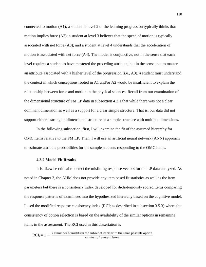
110

connected to motion (A1); a student at level 2 of the learning progression typically thinks that

motion implies force (A2); a student at level 3 believes that the speed of motion is typically

associated with net force (A3); and a student at level 4 understands that the acceleration of

motion is associated with net force (A4). The model is conjunctive, not in the sense that each

level requires a student to have mastered the preceding attribute, but in the sense that to master

an attribute associated with a higher level of the progression (i.e., A3), a student must understand

the context in which conceptions rooted in A1 and/or A2 would be insufficient to explain the

relationship between force and motion in the physical sciences. Recall from our examination of

the dimensional structure of FM LP data in subsection 4.2.1 that while there was not a clear

dominant dimension as well as a support for a clear simple structure. That is, our data did not

support either a strong unidimensional structure or a simple structure with multiple dimensions.

In the following subsection, first, I will examine the fit of the assumed hierarchy for

OMC items relative to the FM LP. Then, I will use an artificial neural network (ANN) approach

to estimate attribute probabilities for the sample students responding to the OMC items.

4.3.2 Model Fit Results

It is likewise critical to detect the misfitting response vectors for the LP data analyzed. As

noted in Chapter 3, the AHM does not provide any item based fit statistics as well as the item

parameters but there is a consistency index developed for dichotomously scored items comparing

the response patterns of examinees into the hypothesized hierarchy based on the cognitive model.

I used the modified response consistency index (RCI; as described in subsection 3.5.3) where the

consistency of option selection is based on the availability of the similar options in remaining

items in the assessment. The RCI used in this dissertation is

RCIi = 1 − 2 x number of misfits in the subset of items with the same possible option

𝑛𝑢𝑚𝑏𝑒𝑟 𝑜𝑓 𝑐𝑜𝑚𝑝𝑎𝑟𝑖𝑠𝑜𝑛𝑠

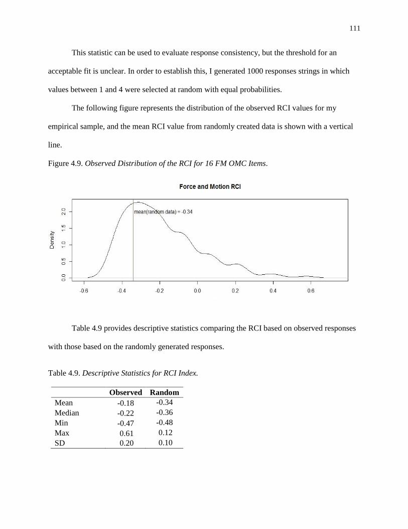
111

This statistic can be used to evaluate response consistency, but the threshold for an

acceptable fit is unclear. In order to establish this, I generated 1000 responses strings in which

values between 1 and 4 were selected at random with equal probabilities.

The following figure represents the distribution of the observed RCI values for my

empirical sample, and the mean RCI value from randomly created data is shown with a vertical

line.

Figure 4.9. Observed Distribution of the RCI for 16 FM OMC Items.

Table 4.9 provides descriptive statistics comparing the RCI based on observed responses

with those based on the randomly generated responses.

Table 4.9. Descriptive Statistics for RCI Index.

Observed Random

Mean -0.18 -0.34

Median -0.22 -0.36

Min -0.47 -0.48

Max 0.61 0.12

SD 0.20 0.10

112

Figure 4.10 also presents the density distributions of RCI value where red colored density

distribution belongs to randomly generated data. There is considerable overlap in the observed

and randomly generated RCI values which indicates that this sample of students did not respond

to these OMC items as consistently as would have been expected by the hypothesized learning

progression.

Figure 4.10. Overlap of RCI Values between Randomly Generated Data and FM LP Data.

Results indicated that student response patterns rarely reflected the expected response

patterns of the AHM. As it turns out, the lack of fit may complicate our ability to estimate

attribute probabilities and classify students meaningfully along the FM LP.

4.3.3 Attribute Probability Estimation Results

Expected response patterns under the assumption that the FM attribute hierarchy is

correct were created, replicated 20 times, and then used to train an ANN with a single hidden

layer and four hidden units. Weights were estimated in R with neuralnet using a backpropagation

algorithm and a conservative learning rate of 0.01. The sum of squared errors upon convergence

after 12,272 steps was 0.052. Table 4.10 shows that the attribute probabilities estimated by the

ANN for each of our expected response patterns indicated an almost exact match.

113

Table 4.10. Example of Attribute Probabilities for Perfectly Fitting Response Patterns.

Levels

Attribute

combination A1 A2 A3 A4

Level 1 1000 0.999 0.002 0.004 0.000

Level 2 1100 1.000 0.993 0.001 0.000

Level 3 1110 0.999 0.988 0.993 0.008

Level 4 1111 0.999 1.000 0.998 0.997

An advantage of the ANN approach is to learn the mapping between inputs and outputs

and to generalize this learning to the unseen cases. Hence the next step is to enter the actual

response patterns of 931 students and calculate the probabilities on each attribute. The resulting

estimates, summarized in Table 4.11, all suggest a process that has worked the way it was

intended. All of the students mastered Attribute 1 as expected, and within other attributes, there

is a variation.

Table 4.11. Descriptive Statistics of Attribute Probabilities for Real Students.

Attribute 1 Attribute 2 Attribute 3 Attribute 4

Min. 0.996 0.003 0.000 0.000

1st Qu. 0.999 0.815 0.146 0.004

Median 0.999 0.981 0.750 0.013

Mean 0.999 0.794 0.584 0.119

3rd Qu. 0.999 0.990 0.972 0.025

Max. 1.000 1.000 1.000 0.997

SD 0.001 0.343 0.398 0.276

4.3.4 Attribute Relationships

The examination of the attribute relationships provide evidence about the assessment and

hypothesized hierarchy. That is, in the case of a linear hierarchy, we expect attributes to be more

strongly correlated with the adjacent attribute and less strongly correlated to the attributes at a

114

distance in the hierarchy. The correlations across four attributes to see whether there is evidence

that supports the linear hierarchy (i.e., A1 A2 A3 A4) are presented in Table 4.12.

Table 4.12. Correlations between Attributes.


Attribute 1 1.00 . . .

Attribute 2 0.83 1.00 . .

Attribute 3 0.44 0.64 1.00

Attribute 4 0.28 0.13 0.32 1.00

Table 4.12 shows that the correlations across attributes support the linearity assumption

in the hierarchy for the associations between A1-A2, A1-A3, A1-A4, A2-A3, and A2-A4 while

the relation between Attribute 3 and Attribute 4 is not as high as expected.

4.3.5 Distribution of Attribute Mastery with Different Cutoff Values

In order to place students into the LP levels, we need to decide the mastery status of each

student on each attribute. At that point, the choice of the cutoff values used for mastery status

decision is critical because they affect the classification results. Hence, examination of the LP

level distributions with different cutoff values helps us to understand this effect. Specifically, I

will examine three selected cutoff values; 0.5 (as most common value in AHM literature), 0.65,

and 0.75 (as the most conservative for the purpose of highest accuracy). The classification results

into LP levels based on these three cutoff values are presented in Table 4.13.

Table 4.13. The Distribution of Levels with Different Cutoff Values.


Cutoff Freq % Freq % Freq % Freq %

0.50 931 100 753 80.88 541 58.11 99 10.63

0.65 931 100 731 78.52 496 53.27 90 9.67

0.75 931 100 709 76.16 465 49.95 81 8.70 Notes:

1Freq stands for frequency.

115

As expected, Table 4.13 shows that as the mastery cutoff thresholds increase, the number

of the students categorized as having mastered each attribute decrease.

4.3.6 The Prediction Variance of Attribute Probabilities from ANNs

After specifying attribute hierarchy and producing the expected response matrix, it is an

easy process to train an ANN and generate attribute probabilities for observed item response

patterns. However, it is critical to underline that we do not need empirical data to estimate the

parameters of an ANN. The training of an ANN is based on the data generated from theory. The

estimation of latent classification probabilities are done in a second step. This is the reason that

the creation of attribute hierarchy is critical for the rest of the process, but there is not a direct

empirical way to check the appropriateness of the hierarchy.

There is no doubt that the most desirable property of a network is its ability to generalize

to new cases. However, as noted in the literature (e.g., Panchal, Ganatra, Shah, & Panchal, 2011;

Intrator & Intrator, 2001), there are important reasons to be cautious about the results from

applying an ANN. These can be applied under two sections: a) structure of the network and b)

algorithm used to train the ANN. The former includes decisions on the configuration of the ANN

structure, such as number of hidden layers and hidden neurons and use of random initial values

versus fixed initial values. The potential problems in relation to these concerns are estimated

ANN weights ending in the local minima solution, and potential fluctuations in the estimation of

unseen data. The latter is also related to the algorithm chosen for ANN to ‘learn’ the mapping

between inputs and outputs. Specialized learning algorithms are used for adaptation of the weight

values connecting inputs to outputs; there are a number of algorithms used in the literature where

the backpropagation algorithm is one of the most popular in the domain (e.g., Zurada, 1992).

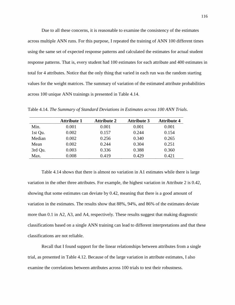
116

Due to all these concerns, it is reasonable to examine the consistency of the estimates

across multiple ANN runs. For this purpose, I repeated the training of ANN 100 different times

using the same set of expected response patterns and calculated the estimates for actual student

response patterns. That is, every student had 100 estimates for each attribute and 400 estimates in

total for 4 attributes. Notice that the only thing that varied in each run was the random starting

values for the weight matrices. The summary of variation of the estimated attribute probabilities

across 100 unique ANN trainings is presented in Table 4.14.

Table 4.14. The Summary of Standard Deviations in Estimates across 100 ANN Trials.


Min. 0.001 0.001 0.001 0.001

1st Qu. 0.002 0.157 0.244 0.154

Median 0.002 0.256 0.340 0.265

Mean 0.002 0.244 0.304 0.251

3rd Qu. 0.003 0.336 0.388 0.360

Max. 0.008 0.419 0.429 0.421

Table 4.14 shows that there is almost no variation in A1 estimates while there is large

variation in the other three attributes. For example, the highest variation in Attribute 2 is 0.42,

showing that some estimates can deviate by 0.42, meaning that there is a good amount of

variation in the estimates. The results show that 88%, 94%, and 86% of the estimates deviate

more than 0.1 in A2, A3, and A4, respectively. These results suggest that making diagnostic

classifications based on a single ANN training can lead to different interpretations and that these

classifications are not reliable.

Recall that I found support for the linear relationships between attributes from a single

trial, as presented in Table 4.12. Because of the large variation in attribute estimates, I also

examine the correlations between attributes across 100 trials to test their robustness.

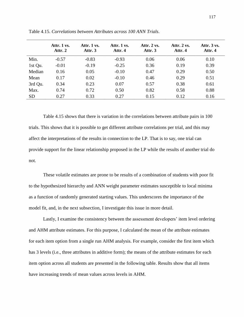
117

Table 4.15. Correlations between Attributes across 100 ANN Trials.

Attr. 1 vs.

Attr. 2

Attr. 1 vs.

Attr. 3

Attr. 1 vs.

Attr. 4

Attr. 2 vs.

Attr. 3

Attr. 2 vs.

Attr. 4

Attr. 3 vs.

Attr. 4

Min. -0.57 -0.83 -0.93 0.06 0.06 0.10

1st Qu. -0.01 -0.19 -0.25 0.36 0.19 0.39

Median 0.16 0.05 -0.10 0.47 0.29 0.50

Mean 0.17 0.02 -0.10 0.46 0.29 0.51

3rd Qu. 0.34 0.23 0.07 0.57 0.38 0.61

Max. 0.74 0.72 0.50 0.82 0.58 0.88

SD 0.27 0.33 0.27 0.15 0.12 0.16

Table 4.15 shows that there is variation in the correlations between attribute pairs in 100

trials. This shows that it is possible to get different attribute correlations per trial, and this may

affect the interpretations of the results in connection to the LP. That is to say, one trial can

provide support for the linear relationship proposed in the LP while the results of another trial do

not.

These volatile estimates are prone to be results of a combination of students with poor fit

to the hypothesized hierarchy and ANN weight parameter estimates susceptible to local minima

as a function of randomly generated starting values. This underscores the importance of the

model fit, and, in the next subsection, I investigate this issue in more detail.

Lastly, I examine the consistency between the assessment developers’ item level ordering

and AHM attribute estimates. For this purpose, I calculated the mean of the attribute estimates

for each item option from a single run AHM analysis. For example, consider the first item which

has 3 levels (i.e., three attributes in additive form); the means of the attribute estimates for each

item option across all students are presented in the following table. Results show that all items

have increasing trends of mean values across levels in AHM.

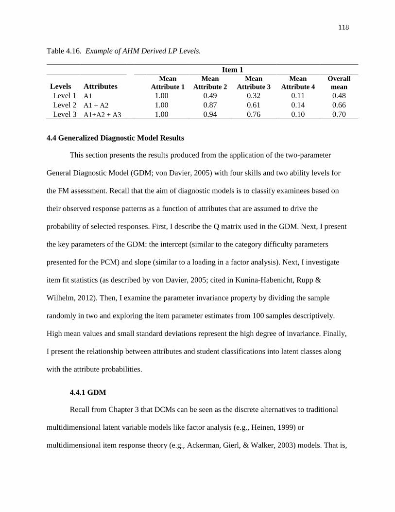
118

Table 4.16. Example of AHM Derived LP Levels.

Item 1

Levels Attributes Mean

Attribute 1

Mean

Attribute 2

Mean

Attribute 3

Mean

Attribute 4

Overall

mean

Level 1 A1 1.00 0.49 0.32 0.11 0.48

Level 2 A1 + A2 1.00 0.87 0.61 0.14 0.66

Level 3 A1+A2 + A3 1.00 0.94 0.76 0.10 0.70

4.4 Generalized Diagnostic Model Results

This section presents the results produced from the application of the two-parameter

General Diagnostic Model (GDM; von Davier, 2005) with four skills and two ability levels for

the FM assessment. Recall that the aim of diagnostic models is to classify examinees based on

their observed response patterns as a function of attributes that are assumed to drive the

probability of selected responses. First, I describe the Q matrix used in the GDM. Next, I present

the key parameters of the GDM: the intercept (similar to the category difficulty parameters

presented for the PCM) and slope (similar to a loading in a factor analysis). Next, I investigate

item fit statistics (as described by von Davier, 2005; cited in Kunina-Habenicht, Rupp &

Wilhelm, 2012). Then, I examine the parameter invariance property by dividing the sample

randomly in two and exploring the item parameter estimates from 100 samples descriptively.

High mean values and small standard deviations represent the high degree of invariance. Finally,

I present the relationship between attributes and student classifications into latent classes along

with the attribute probabilities.

4.4.1 GDM

Recall from Chapter 3 that DCMs can be seen as the discrete alternatives to traditional

multidimensional latent variable models like factor analysis (e.g., Heinen, 1999) or

multidimensional item response theory (e.g., Ackerman, Gierl, & Walker, 2003) models. That is,

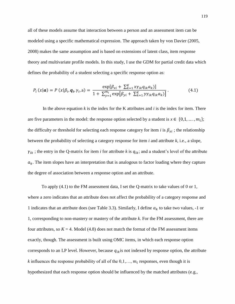
119

all of these models assume that interaction between a person and an assessment item can be

modeled using a specific mathematical expression. The approach taken by von Davier (2005,

2008) makes the same assumption and is based on extensions of latent class, item response

theory and multivariate profile models. In this study, I use the GDM for partial credit data which

defines the probability of a student selecting a specific response option as:

𝑃𝑖 (𝑥|𝒂) = 𝑃 (𝑥|𝛽𝑖, 𝒒𝒊, 𝛾𝑖, a) = exp [𝛽𝑥𝑖 + ∑ 𝑥𝛾𝑖𝑘𝑞𝑖𝑘𝑎𝑘)𝐾

𝑘=1 ]

1 + ∑ exp [𝛽𝑦𝑖 + ∑ 𝑦𝛾𝑖𝑘𝑞𝑖𝑘𝑎𝑘)𝐾𝑘=1 ]

𝑚𝑖𝑦=1

. (4.1)

In the above equation k is the index for the K attributes and i is the index for item. There

are five parameters in the model: the response option selected by a student is x ∈ {0,1, … . , 𝑚𝑖};

the difficulty or threshold for selecting each response category for item i is 𝛽𝑥𝑖 ; the relationship

between the probability of selecting a category response for item i and attribute k, i.e., a slope,

𝛾𝑖𝑘 ; the entry in the Q-matrix for item i for attribute k is 𝑞𝑖𝑘; and a student’s level of the attribute

𝑎𝑘. The item slopes have an interpretation that is analogous to factor loading where they capture

the degree of association between a response option and an attribute.

To apply (4.1) to the FM assessment data, I set the Q-matrix to take values of 0 or 1,

where a zero indicates that an attribute does not affect the probability of a category response and

1 indicates that an attribute does (see Table 3.3). Similarly, I define 𝑎𝑘 to take two values, -1 or

1, corresponding to non-mastery or mastery of the attribute k. For the FM assessment, there are

four attributes, so K = 4. Model (4.8) does not match the format of the FM assessment items

exactly, though. The assessment is built using OMC items, in which each response option

corresponds to an LP level. However, because 𝑞𝑖𝑘is not indexed by response option, the attribute

k influences the response probability of all of the 0,1,…, 𝑚𝑖 responses, even though it is

hypothesized that each response option should be influenced by the matched attributes (e.g.,

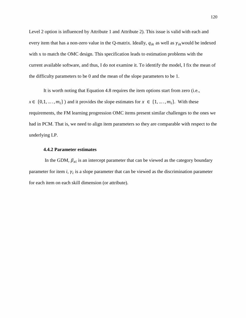
120

Level 2 option is influenced by Attribute 1 and Attribute 2). This issue is valid with each and

every item that has a non-zero value in the Q-matrix. Ideally, 𝑞𝑖𝑘 as well as 𝛾𝑖𝑘would be indexed

with x to match the OMC design. This specification leads to estimation problems with the

current available software, and thus, I do not examine it. To identify the model, I fix the mean of

the difficulty parameters to be 0 and the mean of the slope parameters to be 1.

It is worth noting that Equation 4.8 requires the item options start from zero (i.e.,

x ∈ {0,1, … . , 𝑚𝑖} ) and it provides the slope estimates for 𝑥 ∈ {1, … . , 𝑚𝑖}. With these

requirements, the FM learning progression OMC items present similar challenges to the ones we

had in PCM. That is, we need to align item parameters so they are comparable with respect to the

underlying LP.

4.4.2 Parameter estimates

In the GDM, 𝛽𝑥𝑖 is an intercept parameter that can be viewed as the category boundary

parameter for item i, 𝛾𝑖 is a slope parameter that can be viewed as the discrimination parameter

for each item on each skill dimension (or attribute).

121

Table 4.17. Category Easiness Parameters for FM LP Items.


(𝜷𝟏𝒊)

Level 2-Level 3

(𝜷𝟐𝒊)

Level 3-Level 4

(𝜷𝟑𝒊)

Item 10 . . -1.20

Item 14 . . -0.28

Item 1 0.43 -0.92 .

Item 7 -0.87 -0.12 .

Item 11 1.26 0.61 .

Item 15 -4.97 0.63 .

Item 2 . -0.55 0.32

Item 3 . 1.21 -1.24

Item 4 . 0.81 -0.38

Item 8 . 2.61 -1.63

Item 9 . -0.94 0.83

Item 13 . 1.04 -1.16

Item 16 . 0.41 -0.74

Item 5 2.94 4.02 1.72

Item 6 3.69 3.35 0.49

Item 12 5.08 2.09 1.68

The examination of average item difficulty parameters produced similar results to those

from the PCM analysis with one exception. In GDM analysis, Item 2 does not have item

categories with a reversal in difficulty. There is a wide range of difficulty estimates for each item

category parameter. Item 12 and 5 have the most extreme item category parameters of the set.

Item 12 is the least difficult (δ1,12,δ2,12,δ3,12 are 5.08, 2.09, and 1.68, respectively). Only 5 out

of 16 items have parameters disordered in difficulty across categories. However, it is worth

noting that in a similar case with a continuous θ within the multidimensional IRT models for

polytomous items (Reckase, 2009), the interpretation of the item category parameters is not well

examined and may not be exactly feasible with a discrete GDM approach. Hence, interpretation

of the intercepts to order items with respect to difficulty (which load on the same attribute) can

be more meaningful. Table 4.18 shows the slope parameter estimates of the FM LP items.

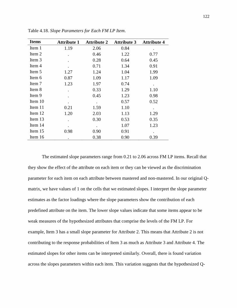
122

Table 4.18. Slope Parameters for Each FM LP Item.


Item 1 1.19 2.06 0.84 .

Item 2 . 0.46 1.22 0.77

Item 3 . 0.28 0.64 0.45

Item 4 . 0.71 1.34 0.91

Item 5 1.27 1.24 1.04 1.99

Item 6 0.87 1.09 1.17 1.09

Item 7 1.23 1.97 0.74 .

Item 8 . 0.33 1.29 1.10

Item 9 . 0.45 1.23 0.98

Item 10 . . 0.57 0.52

Item 11 0.21 1.59 1.10 .

Item 12 1.20 2.03 1.13 1.29

Item 13 . 0.30 0.53 0.35

Item 14 . . 1.07 1.23

Item 15 0.98 0.90 0.91 .

Item 16 . 0.38 0.90 0.39

The estimated slope parameters range from 0.21 to 2.06 across FM LP items. Recall that

they show the effect of the attribute on each item or they can be viewed as the discrimination

parameter for each item on each attribute between mastered and non-mastered. In our original Q-

matrix, we have values of 1 on the cells that we estimated slopes. I interpret the slope parameter

estimates as the factor loadings where the slope parameters show the contribution of each

predefined attribute on the item. The lower slope values indicate that some items appear to be

weak measures of the hypothesized attributes that comprise the levels of the FM LP. For

example, Item 3 has a small slope parameter for Attribute 2. This means that Attribute 2 is not

contributing to the response probabilities of Item 3 as much as Attribute 3 and Attribute 4. The

estimated slopes for other items can be interpreted similarly. Overall, there is found variation

across the slopes parameters within each item. This variation suggests that the hypothesized Q-

123

matrix is not fully recovered. Therefore, there may be a possible mismatch between the Q-matrix

and underlying LP progress levels.

4.4.3 Model Fit

As noted by Jurich and Bradshaw (2013), global model fit indices have not been

developed thoroughly for DCMs. GDM item fit statistics are predicted as a chi squared based

measure in the model. The item fit indices for the GDM showed that 12 of the items showed

good fit (RMSEA < .05), 4 of the items showed moderate fit (RMSEA < .10), and none of the

items showed poor fit (RMSEA > .10). Note that the impact of such item misfit on subsequent

inferences about respondents and items has not been established in detail for the GDM at this

point. The simplest interpretation of these results is that the items with moderate fit require more

examination (e.g., Item 13) and it is not advisable to use the model for high-stakes purposes in

the learning progression context.

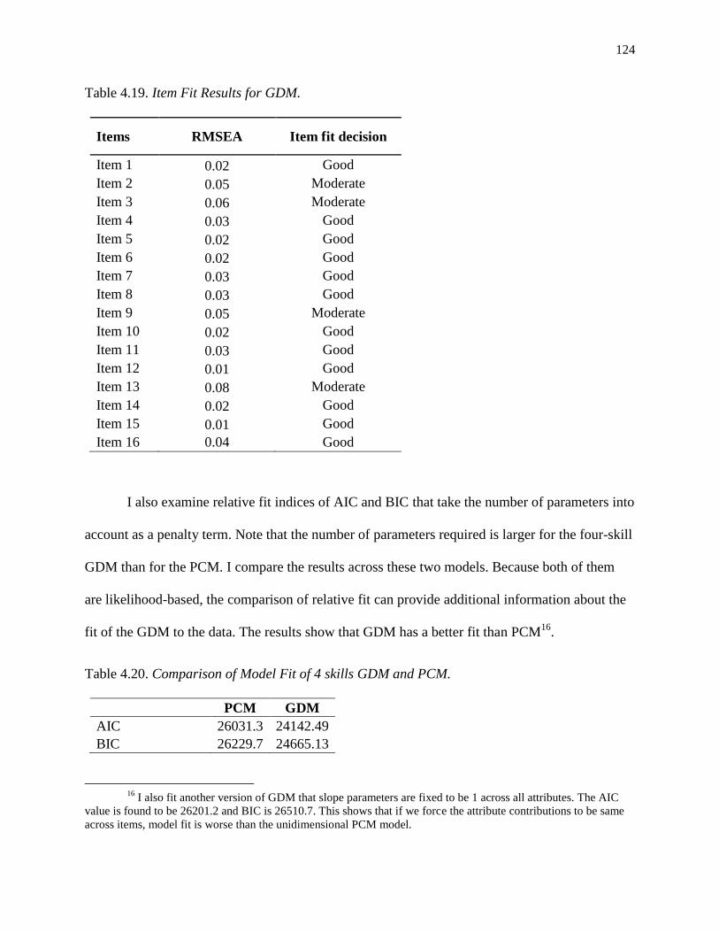
124

Table 4.19. Item Fit Results for GDM.

Items RMSEA Item fit decision

Item 1 0.02 Good

Item 2 0.05 Moderate


Item 4 0.03 Good

Item 5 0.02 Good

Item 6 0.02 Good

Item 7 0.03 Good

Item 8 0.03 Good


Item 10 0.02 Good

Item 11 0.03 Good

Item 12 0.01 Good


Item 14 0.02 Good

Item 15 0.01 Good

Item 16 0.04 Good

I also examine relative fit indices of AIC and BIC that take the number of parameters into

account as a penalty term. Note that the number of parameters required is larger for the four-skill

GDM than for the PCM. I compare the results across these two models. Because both of them

are likelihood-based, the comparison of relative fit can provide additional information about the

fit of the GDM to the data. The results show that GDM has a better fit than PCM16

.

Table 4.20. Comparison of Model Fit of 4 skills GDM and PCM.

PCM GDM

AIC 26031.3 24142.49

BIC 26229.7 24665.13

16

I also fit another version of GDM that slope parameters are fixed to be 1 across all attributes. The AIC

value is found to be 26201.2 and BIC is 26510.7. This shows that if we force the attribute contributions to be same

across items, model fit is worse than the unidimensional PCM model.

125

4.4.4 Parameter Invariance

Currently, there is very little research about invariance testing in DCMs. In a similar

manner to the IRT modeling, a few studies focus on the differential item functioning (e.g.,

Bozard, 2010). De la Torre and Lee (2010) examined the item parameter invariance of the

deterministic inputs, noisy “and” gate (DINA) model using the simulated data and concluded that

the DINA model parameters are invariant when the model perfectly fits the data. For the

purposes of the current study, I examined the invariance property of the FM LP item parameters

across 100 randomly divided groups via correlations. Table 4.21 presents the descriptive

statistics across 100 trials.

Table 4.21. Descriptives of Item Parameter Correlations for GDM across 100 Pairs of Groups.

Parameters Min Max Mean SD

Slope (𝛾𝑖1.) 0.93 0.90 0.91 0.01

Slope (𝛾𝑖2.) 0.92 0.91 0.91 0.01

Slope (𝛾𝑖3.) 0.93 0.92 0.91 0.01

Slope (𝛾𝑖4.) 0.95 0.82 0.95 0.04

Intercept (𝛽𝑖1) 0.92 0.96 0.94 0.02

Intercept (𝛽𝑖2) 0.93 0.95 0.92 0.02

Intercept (𝛽𝑖3) 0.93 0.98 0.95 0.02

Intercept (𝛽𝑖4) 0.93 0.96 0.95 0.01

The results for item parameter estimates in GDM are consistent with de la Torre and

Lee’s (2009) findings for the DINA model. There have been found high correlations across all

item parameters. It is important to note this property of the model is advantageous for large-scale

purposes, but the exact interpretation of the parameter invariance (i.e., across parameters

representing the same parameters) is challenging due to the complexity model.

126

4.4.4 Relationship between Attributes

The latent correlations between the discrete latent skill variables are also estimated and

shown in Table 4.22. The correlation pattern of the discrete individual skill estimates for the

GDM was found to be highly different from AHM results while both models use discrete latent

variables as opposed to continuous trait assumption in PCM. The absolute magnitude of these

correlations is higher in the GDM than in the AHM model, which is likely a result of the fact that

the latter forces a hierarchy using expected response patterns while the former does not put any

constraints on the relationship between attributes.

Table 4.22. Relationship between Attributes (GDM).


Attribute 1 1.00

Attribute 2 -0.47 1.00

Attribute 3 0.61 -0.82 1.00

Attribute 4 -0.40 0.81 -0.84 1.00

The correlation between attributes ranged from -0.84 to 0.81. Commonly, in the DCM

literature moderate to high correlations across attributes have been found that support several

distinct, yet related, attributes in different subdomains (e.g., Bradshaw, Izhak, Templin, &

Jacobson, 2014). The analysis of the FM LP assessment results suggests that the specified

attributes do not have a patterned relationship such as a linear hierarchy, as in the case of AHM,

nor do they strongly coexist together, which may support a unidimensional modeling approach.

In contrast, either they suggest that it is not plausible for several attribute pairs to exist together

or some attributes can compensate for the lack of other in pairs. For example, between Attribute

3 and Attribute 4, there is a strong negative correlation. That is, students who have high

probabilities of mastering Attribute 4 (the net force applied to an object is proportional to its

127

resulting acceleration and this force may not be in the direction of motion) show low

probabilities for mastering Attribute 3 (that objects are either at rest or moving with constant

speed when forces are balanced). One way to think about this is that a student who passes a

threshold for mastering more complex understanding does not need to master the lower-level

understanding (e.g., negative correlations between the pairs of A1-A2, A2-A3, A3-A4). But this

interpretation is challenged by the fact that there are high correlations across attribute pairs of 2-

4 and 1-3. These two findings together can be interpreted as the distinct existence of the attribute

pairs rather than increasing complexity of student understanding with each mastered attribute.

For example, students require having the factual knowledge of what a force is (Attribute 1), in

order to express Attribute 3: that an object moving with constant speed requires a net force in the

direction of motion. In such a case, Attribute 2 can be skipped. This kind of interpretation leads

to the fact that students can make different connections to master attributes, rather than following

a systematic application of attributes in order. That is, students can have pieces of loosely related

knowledge of force and motion, which leads to non-linear combinations of attributes for

particular contextual representations of force and motion tasks as in FM LP assessment.

However, it is worth reiterating that we have already had great challenges when modeling FM

data composed of OMC items with GDM. These challenges further complicated our attempt to

interpret the results on the relationship between attributes and classification of the students into

the latent classes in the next section.

4.4.5 Classifications into Latent Classes

Even though there are a total of 24 = 16 latent classes that can be theoretically

distinguished without postulating any conditional relationships among the latent skill variables,

fewer latent classes could be empirically distinguished for the FM LP data. The examination of

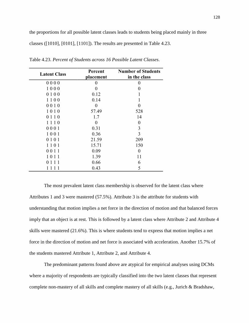
128

the proportions for all possible latent classes leads to students being placed mainly in three

classes ([1010], [0101], [1101]). The results are presented in Table 4.23.

Table 4.23. Percent of Students across 16 Possible Latent Classes.

Latent Class Percent

placement

Number of Students

in the class

0 0 0 0 0 0

1 0 0 0 0 0

0 1 0 0 0.12 1

1 1 0 0 0.14 1

0 0 1 0 0 0

1 0 1 0 57.49 528

0 1 1 0 1.7 14

1 1 1 0 0 0

0 0 0 1 0.31 3

1 0 0 1 0.36 3

0 1 0 1 21.59 209

1 1 0 1 15.71 150

0 0 1 1 0.09 0

1 0 1 1 1.39 11

0 1 1 1 0.66 6

1 1 1 1 0.43 5

The most prevalent latent class membership is observed for the latent class where

Attributes 1 and 3 were mastered (57.5%). Attribute 3 is the attribute for students with

understanding that motion implies a net force in the direction of motion and that balanced forces

imply that an object is at rest. This is followed by a latent class where Attribute 2 and Attribute 4

skills were mastered (21.6%). This is where students tend to express that motion implies a net

force in the direction of motion and net force is associated with acceleration. Another 15.7% of

the students mastered Attribute 1, Attribute 2, and Attribute 4.

The predominant patterns found above are atypical for empirical analyses using DCMs

where a majority of respondents are typically classified into the two latent classes that represent

complete non-mastery of all skills and complete mastery of all skills (e.g., Jurich & Bradshaw,

129

2014). Yet, most of these studies have used dichotomous data. Hence, the variation in latent

classes can be a result of using polytomous items, which are more informative when we place

students into latent classes. For FM LP assessment data, the most populated classes do not

support the alignment with the proposed LPs. For example, no students are placed into the latent

classes of [1,0,0,0] representing the mastery of only Attribute 1 or [1,1,1,0] representing mastery

of the first three attributes. These results suggest that there may be several problems with the

proposed learning progression. It seems that the proposed learning progression can have levels

where different attribute combinations are possible to be mastered. These results may also

suggest that students carry some of the misconceptions across levels, and therefore the

definitions of the levels are not supported by the student responses. Another potential reason can

be that attributes do not generalize across different problem contexts (e.g., Steedle & Shavelson,

2009). Direct interpretation of the levels may lead to a conclusion that LP levels are not properly

ordered with additive structure of attributes. However, as I mentioned before, the challenges

introduced by OMC items may prevent us from making clear conclusions with regard to the FM

LP.

GDM produces the posterior latent class probabilities for 24 possible classes. To get the

individual skill/attribute probabilities I calculated the expected value for each across all latent

classes. That is, I summed the probabilities of a latent class membership across all latent classes

for which a specific attribute is mastered. I did this by following the formula:

P (Attribute 1 | latent class membership) = ∑ 𝐴𝑡𝑡1. 𝑃𝑜𝑠𝑡𝑒𝑟𝑖𝑜𝑟 𝑙𝑎𝑡𝑒𝑛𝑡 𝑐𝑙𝑎𝑠𝑠16𝑙𝑎𝑡𝑒𝑛𝑡 𝑐𝑙𝑎𝑠𝑠=1 (4.2)

The summary of the marginal skill probabilities is presented in the following table.

130

Table 4.24. Summary of Attribute Mastery Probabilities.

Attribute1 Attribute2 Attribute3 Attribute4

Min. 0.02 0.00 0.00 0.00

1st Qu. 0.52 0.00 0.18 0.00

Median 0.94 0.22 0.80 0.24

Mean 0.76 0.40 0.62 0.41

3rd Qu. 1.00 0.86 1.00 0.86

Max. 1.00 1.00 1.00 1.00

As it is reflected in the posterior latent class probabilities, there is variation across

marginal probabilities of all attributes. This diversity is well represented in the following plots.

Figure 4.11. Distribution of Marginal Attribute Probabilities.

Note that the latent class placement results from GDM do not allow us to place students

into LP levels as the LP levels are defined in the additive form of the attributes. That is, GDM

produces the latent class memberships for the majority of the students in different mastery

combinations of the attributes such as [1010] where Attribute 1 and Attribute 3 are mastered.

131

4.5 Comparison of Models

The ultimate aim of LPs is to provide information about the level of sophistication in

student thinking as described in the LP levels. Therefore, in order to examine whether

probabilistic models added value over the descriptive methods, I compare the results of student

classifications into LP levels from all three probabilistic models with the simpler modal

approach. Recall that I concluded not to use PCM for placing students into LP levels in

subsection 4.2.4 and GDM placed only six students into the latent classes which are consistent

with the LP levels (one student in latent class [1100] and 5 students in latent class [1111]). At

that point, we could examine the similarity of student placements into the LP levels between only

the modal approach and AHM. Hence, this section starts with the placement comparisons

between modal approach and AHM. Then, I provide results of agreement between classifications

across these two approaches, with a simple percent agreement. While it is not possible to

examine the consistency between the modal approach - GDM and GDM - AHM, it is interesting

to examine the latent class distributions in GDM for those students classified into LP levels by

AHM and modal approach. Thus, I present the distribution of GDM latent classes in comparison

to AHM and the modal approach, respectively. Finally, I present the results on the comparison of

total raw scores with ability estimates from PCM and skill probabilities from both DCMs17

.

4.5.1 Comparison between AHM and Modal Classification

Before proceeding to the comparison, I provide the classification results of students into

the LP categories using a cutoff of 0.75. I found that 17 of the students were not placed into any

of the LP levels because of the inconsistent probability estimates with the proposed hierarchy.

17

It is unclear if those parameters on the same continuum exactly. However, we can still examine their

associations.

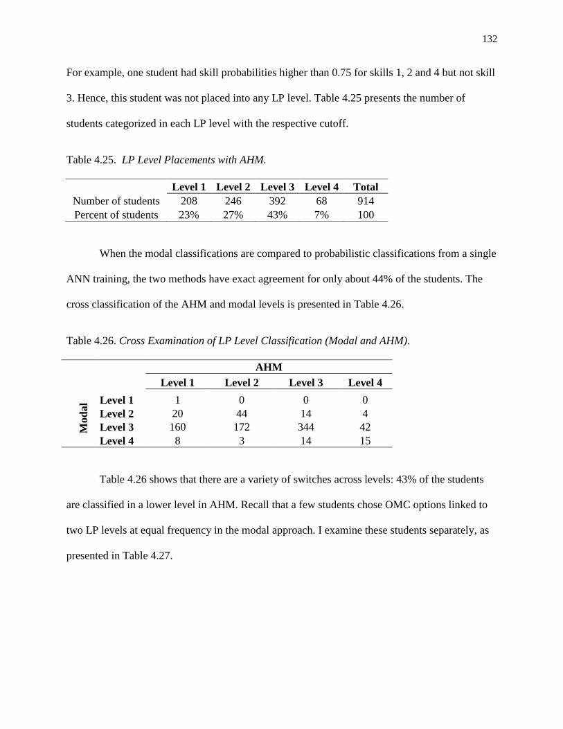
132

For example, one student had skill probabilities higher than 0.75 for skills 1, 2 and 4 but not skill

3. Hence, this student was not placed into any LP level. Table 4.25 presents the number of

students categorized in each LP level with the respective cutoff.

Table 4.25. LP Level Placements with AHM.

Level 1 Level 2 Level 3 Level 4 Total

Number of students 208 246 392 68 914

Percent of students 23% 27% 43% 7% 100

When the modal classifications are compared to probabilistic classifications from a single

ANN training, the two methods have exact agreement for only about 44% of the students. The

cross classification of the AHM and modal levels is presented in Table 4.26.

Table 4.26. Cross Examination of LP Level Classification (Modal and AHM).

AHM

Level 1 Level 2 Level 3 Level 4

Mod

al

Level 1 1 0 0 0

Level 2 20 44 14 4

Level 3 160 172 344 42

Level 4 8 3 14 15

Table 4.26 shows that there are a variety of switches across levels: 43% of the students

are classified in a lower level in AHM. Recall that a few students chose OMC options linked to

two LP levels at equal frequency in the modal approach. I examine these students separately, as

presented in Table 4.27.

133

Table 4.27. Cross Examination of LP Level Classification (cont.)

AHM


Mo

da

l Level 2- Level 3 14 23 7 2 47

Level 2- Level 4 1 0 3 0 4

Level 3- Level 4 4 4 10 5 23

4.5.2 Comparison between GDM and Modal Classifications, AHM

The distribution of the GDM latent classes in comparison to the level classifications done

via the modal approach is presented in Table 4.28.

Table 4.28. Cross Examination of LP Level Classification (Modal and GDM).

Table 4.28 shows that GDM placed most of the students into the [0101] class and

students who classified into Level 3 in the modal approach are distributed across different latent

classes in GDM.

Similarly, the distribution of GDM latent classes are examined for the students who were

placed into LP levels by the AHM model. As expected, most of the students who are classified in

different LP levels using AHM are placed into the latent class [1010]. The results are presented

in Table 4.29.

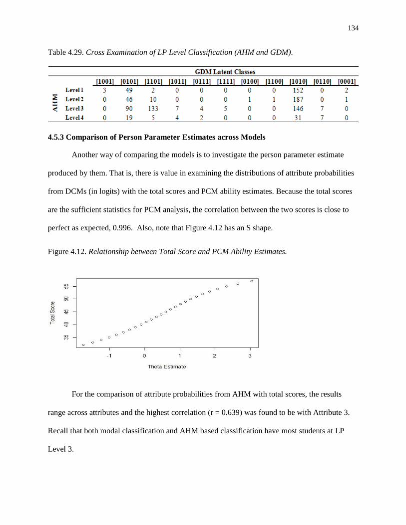
134

Table 4.29. Cross Examination of LP Level Classification (AHM and GDM).

4.5.3 Comparison of Person Parameter Estimates across Models

Another way of comparing the models is to investigate the person parameter estimate

produced by them. That is, there is value in examining the distributions of attribute probabilities

from DCMs (in logits) with the total scores and PCM ability estimates. Because the total scores

are the sufficient statistics for PCM analysis, the correlation between the two scores is close to

perfect as expected, 0.996. Also, note that Figure 4.12 has an S shape.

Figure 4.12. Relationship between Total Score and PCM Ability Estimates.

For the comparison of attribute probabilities from AHM with total scores, the results

range across attributes and the highest correlation (r = 0.639) was found to be with Attribute 3.

Recall that both modal classification and AHM based classification have most students at LP

Level 3.

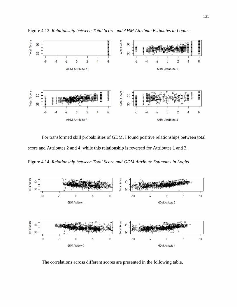
135

Figure 4.13. Relationship between Total Score and AHM Attribute Estimates in Logits.

For transformed skill probabilities of GDM, I found positive relationships between total

score and Attributes 2 and 4, while this relationship is reversed for Attributes 1 and 3.

Figure 4.14. Relationship between Total Score and GDM Attribute Estimates in Logits.

The correlations across different scores are presented in the following table.

136

Table 4.30. Correlations of Person Estimates across Models.

Pearson

Correlation (r)

Total Score - Theta Estimates 0.996

Total Score - AHM Attribute 1 NA

Total Score - AHM Attribute 2 0.386



Total Score - GDM Attribute 1 -0.300

Total Score - GDM Attribute 2 0.584

Total Score - GDM Attribute 3 -0.408

Total Score - GDM Attribute 4 0.524 Note:

1Because all cases for Attribute 1 in AHM are almost 1, SD is 0.

For AHM, there are positive correlations between students’ total scores and attributes.

This shows that AHM results have relatively similar trends with total scores but also provide

different information than the total score of students. For GDM, the results are mixed: there are

positive correlations with attribute probabilities of 2 and 4 while the associations are negative

with attribute probabilities of 1 and 3. That is, for less able students on Attribute 1 or Attribute 3,

their total score tended to be higher, whereas for more able students, the total score is higher.

These results are difficult to interpret in the sense that a high total score requires students to pick

item options more at Level 3 and Level 4. Similarly, we could examine the relationship between

PCM theta estimates and probabilities for each attribute from AHM and GDM. However,

because PCM ability estimates have almost perfect correlation with total scores, the results and

interpretations would stay the same. Hence, I continue with the comparisons of the attribute

probabilities from AHM and GDM.

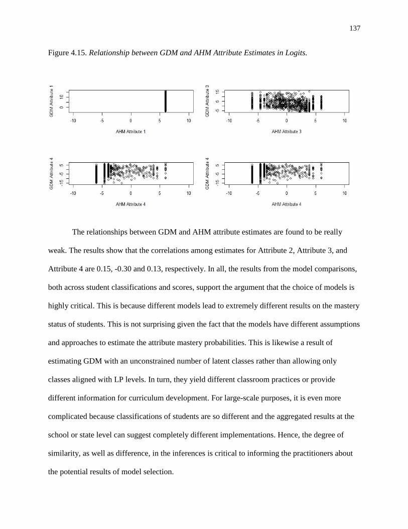
137

Figure 4.15. Relationship between GDM and AHM Attribute Estimates in Logits.

The relationships between GDM and AHM attribute estimates are found to be really

weak. The results show that the correlations among estimates for Attribute 2, Attribute 3, and

Attribute 4 are 0.15, -0.30 and 0.13, respectively. In all, the results from the model comparisons,

both across student classifications and scores, support the argument that the choice of models is

highly critical. This is because different models lead to extremely different results on the mastery

status of students. This is not surprising given the fact that the models have different assumptions

and approaches to estimate the attribute mastery probabilities. This is likewise a result of

estimating GDM with an unconstrained number of latent classes rather than allowing only

classes aligned with LP levels. In turn, they yield different classroom practices or provide

different information for curriculum development. For large-scale purposes, it is even more

complicated because classifications of students are so different and the aggregated results at the

school or state level can suggest completely different implementations. Hence, the degree of

similarity, as well as difference, in the inferences is critical to informing the practitioners about

the potential results of model selection.

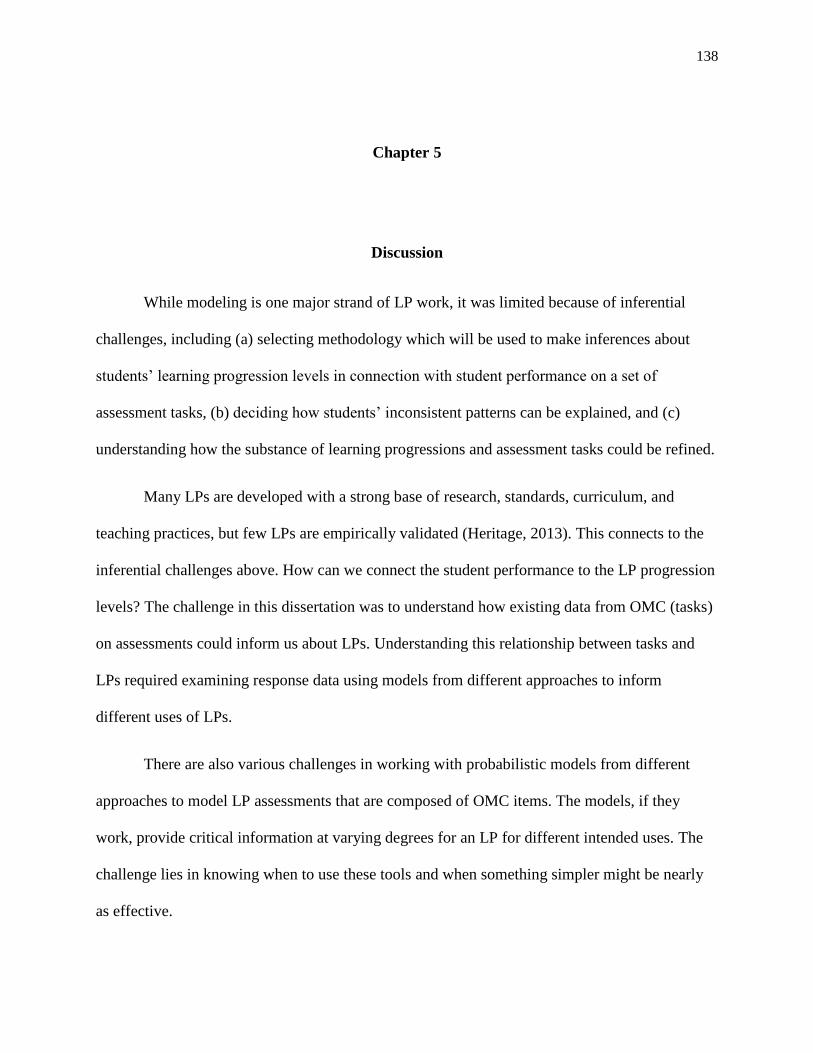
138

Chapter 5

Discussion

While modeling is one major strand of LP work, it was limited because of inferential

challenges, including (a) selecting methodology which will be used to make inferences about

students’ learning progression levels in connection with student performance on a set of

assessment tasks, (b) deciding how students’ inconsistent patterns can be explained, and (c)

understanding how the substance of learning progressions and assessment tasks could be refined.

Many LPs are developed with a strong base of research, standards, curriculum, and

teaching practices, but few LPs are empirically validated (Heritage, 2013). This connects to the

inferential challenges above. How can we connect the student performance to the LP progression

levels? The challenge in this dissertation was to understand how existing data from OMC (tasks)

on assessments could inform us about LPs. Understanding this relationship between tasks and

LPs required examining response data using models from different approaches to inform

different uses of LPs.

There are also various challenges in working with probabilistic models from different

approaches to model LP assessments that are composed of OMC items. The models, if they

work, provide critical information at varying degrees for an LP for different intended uses. The

challenge lies in knowing when to use these tools and when something simpler might be nearly

as effective.

139

This dissertation is an attempt to better understand the use of models from different

modeling frameworks by showing their potential benefits and challenges when investigating the

relationship between student responses and LP levels. This examination demonstrated how and

to what extent the assessment data can be used to validate a learning progression via different

statistical modeling approaches. The quality of assessment items were examined within each

approach and it was demonstrated how students could be classified into LP levels based on their

assessment results.

My first research question is: “What information does each model provide to the

researcher about the quality of the learning progression hypothesis and assessment items?” This

question refers to the information each model provides about the quality of learning progression

hypotheses and assessment items. Through the course of this study, it was discovered that

responding effectively to this research question requires evaluating results regarding model

characteristics for all of the models, so these conclusions are discussed in section 5.1. My second

research question is: “What are the qualitative differences in student classification across

different models?” This research question focuses on the classification of students into LP levels

across different models and the results are discussed in section 5.2.

Recall that as the first step, I used a modal approach to examine the learning progression

data, which is conceptually easy to understand, communicate, and utilize in the classroom. With

the presence of OMC items, it is clear that useful interpretations of learning progression level

diagnoses are possible, when students select consistent responses reflecting a single learning

progression level. However, in FM LP data, if students select options inconsistently, this makes

the interpretation of student understanding difficult for both teachers and researchers.

140

Given the intended use of the LPs in the classroom, the use of the simplistic approach can be

the best option. At the classroom level, LPs provide a guideline on how learning progresses.

Teachers can use LP assessments to determine a student’s level relative to an LP and use this

information to tailor their instruction planning and to enrich their formative assessment practices.

They can also use individual items to attend to their students’ thinking. However, the utility of

simplistic approach is balanced against appropriateness of the progression in the LP and the quality

of the items. Therefore, the use of the psychometric models for assessing LPs and LP assessments

remains important, but less urgent for classroom applications. For large scale purposes, the use of

modal approach is less appropriate because the approach is not robust (e.g., for item parameters, and

classification of students into LP levels). Hence, examination of different models in order to get

probabilistic inferences about students’ understanding is valuable as they are in the current study.

It is worth reiterating that the models selected for this study differ in their conceptual

standpoints because one of them is an IRT model (PCM), another is an IRT-based diagnostic

classification model (GDM), and the last one is a non-IRT based diagnostic classification model

(AHM). However, it is important to examine different models from different approaches that can

be adapted to model the LP assessment data. The information provided by models can be

connected with the intended use of LPs. Therefore, in order to understand the ways these models

are working similarly and differently, I summarize the factors that I will discuss in the following

table across all three models. Note that columns 2 to 5 are used to examine the first research

question and the final column is used to examine the second research question. When there are

notable differences in the classification of students into the LP levels made on the basis of each

model, it is highly possible that the results are combined effects of these factors.

141

Table 5.1. Information Provided by Three Models.

Latent

variable

hypothesis

Item

parameter

estimates

Model fit Parameter

invariance

Attribute

relationships

Student

classification

PCM Continuous

(simple)

Available Examined

item fit

Examined Not available Not

conducted

GDM Discrete

(complex)

Available Examined

item fit

Examined Examined Conducted

AHM Discrete

hierarchical

(complex)

Not

available

Examined

person fit

Not

available

Examined Conducted

5.1 Model Evaluations in the Context of FM LP Assessment

As it turns out, some of the interesting results from this study arose from my analysis of

the dimensionality of the OMC assessment items. The results from exploratory analysis suggest

that there may be more than one factor that underlies the FM LP assessment with a simple

structure (i.e., item groups loaded on different factors). These results did not clearly favor either

unidimensional modeling or diagnostic modeling where DCMs are promising when items are

measured by multiple attributes (i.e., complex structure). Therefore, this issue is critical when

considering modeling options for the learning progression assessments. That is because the

underlying dimensional structure of the data has an effect on the usefulness of the models such

that use of DMCs is more beneficial when the data supports a complex multidimensional

structure.

Both PCM and GDM provide item-level statistics that help to investigate the quality of

the items to the extent that they were appropriate for the students and they measured students’

142

latent trait. The AHM does not parameterize item characteristics. This is a limitation, especially

for the large-scale applications such as assessment development, item banking, and test equating.

PCM and GDM produced item category estimates. The comparison of parameters

showed that they produce similar information with regard to OMC items in FM LP assessments.

The correlation among the item category parameters of the two models was found to be high: r =

-0.71 (recall that GDMs produce item easiness parameters)18

. This relationship suggests that the

PCM is a restricted version of the four skills two-parameter GDM model. While it is likely that

this relationship can be shown algebraically, doing so is beyond the scope of this work.

Additionally, GDM produces slope parameters for each item representing the effect of

each attribute on the probability of student response (as indicated by non-zero entries in the Q-

matrix). The results from GDM slope parameters provide unique information with regard to the

items and the Q-matrix. The low values of the slopes within items suggested a need to revisit the

relationship between items and hypothesized attributes.

Next, the model fitting results are critical to understand the relative viability of the

probabilistic models where viability refers to a criterion reflecting substantively meaningful

inferences about the placement of the students into the LP levels. I examined the item fit in both

PCM and GDM, and person fit for the AHM. The results from the item fit examination showed

that there were no poorly fitting items in PCM using a conventional range, but that 10 out of 16

items were out of range when the interval was adjusted for the sample size. For GDM, the

examination of the RMSEA values suggested no poorly fitting items. For AHM, I created a

modified version of the originally proposed hierarchy consistency index to examine the extent of

18

When I fit GDM model with slope parameters set to 1 across all items, the correlation between PCM and

GDM item parameters are found to be -0.75.

143

consistency across student answers with the options they selected. The simulation designed to

analyze the statistical properties of the modified consistency index suggested that students did

not respond to the OMC items as consistently as expected. However, it is unclear whether this

lack of fit is due to the actual inconsistencies present in the observed data or the proposed index.

This is because the number of expected response patterns is enormously high when we model the

options rather than the items themselves, and the proposed RCI index does not take this into

account. Additionally, the linear structure proposed is noted as a potential cause for the poor fit.

That is, a branching hierarchy, with a more complex cognitive representation, is usually observed

to yield better model fit than purely linear hierarchies (Roberts, 2014, personal communication).

In addition, examination of the relative fit between GDM and PCM favored the GDM.

Examination of the fit results from three models provides evidence that the PCM model has

worse fit than the GDM model, while the results of the AHM model are not clear.

As an indirect approach to the model fit examination, I likewise conducted the

examination of parameter invariance in both PCM and GDM models. The results from the

parameter invariance investigation provided high correlations across 100 randomly divided

samples for both models. This evidence suggested that the item parameter estimates for PCM

and GDM were invariant. This finding is somewhat surprising for PCM given that several

misfitting items were found. This examination overall suggests that the GDM model can be a

better choice than the PCM model in the context of LP assessments composed of OMC items.

Investigating the extent of the relationship between attributes in diagnostic classification

models helps to inform the LP and LP levels. In the context of AHM, the results from the

examination of the attribute relationships from one trial suggest that there is a possible linear

hierarchy between proposed attributes. This is supported by the high correlations between

144

adjacent attributes and low correlations between distant attributes. However, the examination of

the results across 100 trials has shown varying results and has made the inferences about the

proposed LP structure unclear. The results for GDM provided mixed results for correlations

across attributes. An inspection of the correlation patterns illustrated that there exist high

correlations between attribute pairs of 1 and 3, and 2 and 4. These results suggest that the

specified attributes are clustered rather than forming a linear hierarchy or becoming highly

connected or distinct. Put simply, with the current form of the FM LP assessment, two pairs of

latent attributes contribute unique information over and above the other pair. The results suggest

that core concepts are related in a different way than hypothesized in the FM LP. Given the

definition of attributes, it is interesting to have a high correlation between Attribute 1 (“what the

force is”) and Attribute 3 (“ the net force associated with speed”), without mastering Attribute 2

(“motion implies force”). A reasonable explanation for this kind of clustering can be the context

of FM LP tasks such that a student can connect the notion of force, specifically in one direction,

with the speed of the objects, rather than recognizing that motion implies force. However, as

noted before, these results are affected by the restrictions I put in the GDM model (e.g.,

estimation of one slope parameter per attribute per item) and the way that model estimates the

response probability.

Overall, the results of the three models regarding the Force and Motion learning

progression hypotheses indicate that students may not follow the hypothesized progression. That

is, the relationships across the four skills may not maintain a strict hierarchy as specified in the

FM LP or there can be other attributes interfering with students’ response processes. Hence, a

revision in LP is suggested with the information at hand. The PCM provides mixed item fit

results across 16 items while the GDM, which uses separate attributes as input, shows acceptable

145

fits for all items. In both models, I found large variation in item category estimates within each

category and several item category parameters are disordered. These results suggest a detailed

examination of the item stems and options in the assessment. Hence, a practitioner may want to

be cautious about using the LP and LP assessment results for both classroom and high stakes

situations. On the other hand, one can interpret the results as, given the data, none of the models

used in current study could recover underlying progress levels. That is, there can be other models

that would do better to support hypothesized progression levels.

5.2 Inferences across Models

All told, the second research question points out the differences across models with

respect to the inferences on student learning. Recall that the value of the learning progression

assessment is to place students into LP levels. After that, the descriptions in the levels can be

used to provide a detailed explanation of student understanding reflecting a set of coherent ideas.

Placement of students into LP levels across models shows that there was considerable variation

across the modal approach, AHM and GDM. Remember that I decided not to place students into

LP levels with PCM.

The conclusions from the modal classifications show that most of the students express

Level 3 understanding. The underrepresentation of Level 1 classifications is partially due to the

lack of options at this level in 9 out of 16 items. Additionally, for a small portion of students, it is

difficult to place them into any unique LP level. It is true that this would not introduce a

challenge for the use of LP assessments at the classroom level, where teachers can make

decisions about students’ understanding on the topic even using a single high quality item. The

modal approach provides a practical way to scan student understanding and place them into LP

levels for classroom purposes. However, again, this practicality of the modal approach is

146

challenged with the need for a valid LP and high quality LP assessment. The use of psychometric

models fulfills this purpose by providing a systematic way to collect evidence on LPs and LP

assessments. Also, the possibility of incorporating or using LP assessments for large-scale

purposes motivates the exploration of the probabilistic models.

The examination of the PCM model characteristics together with the item parameter

estimates led me to conclude that there is not enough supporting evidence for deciding cutoff

points on the continuous latent trait and, in turn, for the meaningful placement of students into

discrete LP levels. My conclusion regarding the PCM analysis in the context of OMC items is a

result of evaluating different model properties. The conclusion regarding the potential flaws in

the use of PCM model-to-model OMC items is consistent with that suggested by Briggs and

Alonzo (2009).

The AHM approach provides probability estimates for each attribute. For 17 students, it

did not produce monotonically decreasing probabilities for each attribute (e.g., 0.9, 0.1, 0.4, and

0.7). When I examine the response patterns of these students, I did not find any similarity

between response patterns. That is, it is not clear what the reason is for these attribute

probabilities. Next, the classification of students into LP levels requires choosing the cutoff

values in order to decide the students’ mastery status for each attribute. Students are placed into

LP levels using different cutoff values. As expected, when the value cutoff increases, the number

of students categorized as “mastered” within higher-level attributes decreases. These results

suggest that there may be a need to examine the most appropriate cutoff points in relation to the

selected topic because AHM does not provide any item parameters that allow for item

evaluation. The agreement between AHM (using a cutoff of 0.75) and modal classification is

found to be moderate (44%) when AHM placed almost half of the students into a lower level.

147

Based on the results in Chapter 4, there are strong reasons to suspect that the placement

of students into LP levels may not be consistent, in particular due to the fluctuating results of

attribute mastery estimates. However, this is particularly important given that much of the

current research on AHM as well as learning progressions does not utilize a detailed examination

similar to the one I conducted in this study. For both classroom and large-scale applications of

this model, there is a need for more research on the use of the Artificial Neural Network (ANN)

approach and specifications of the guidelines (e.g., use of random initial values versus fixed

values). Hence, practitioners who want to use the AHM approach in the context of LP work

should be careful with all of the points discussed in this study.

In GDM, I allowed the model to produce probabilities for all possible latent classes (i.e.,

16 classes). The results were used to check the alignment of the proposed LP with the latent

classes. The attribute combinations representing the LP levels with near-zero latent class

proportions (i.e., [1,0,0,0], [1,1,0,0], and [1,1,1,0]) suggest a potential misalignment across levels

in LP. For example, there was no group of students who systematically applied the notion that

motion implies force. Therefore, LP Level 2 (i.e., [1100]) was not among the latent classes that

could be distinguishable for FM LP assessment data. Similarly, LP Level 3 [1110] did have a

zero latent class proportion because no students systematically applied the notion that an object

is not moving either because there are no forces acting on it or because there is no net force

acting on it. Finally, FM LP Level 1 was not estimated because none of the students showed the

notion of force as a push or pull that may or may not involve motion alone.

In GDM, as a consequence of having LP levels with zero latent class proportions, large

heterogeneous groups of students get bunched into different latent classes with the mastery of

different attribute combinations. This results in further misalignments between the fitted model

148

and the proposed FM LP. That is, one could conclude that these results suggest a misalignment

for the proposed LP. However, note that due to practical reasons I restricted the item category

slope parameters to be the same within each item in the GDM model. Therefore, I could not

examine the effect of the attributes on the item categories but I did investigate their contributions

to items. Some challenges due to the ceiling and floor effects of OMC items also intervene with

the interpretation of results. The use of GDM with discrete skills seems advantageous especially

for large scale purposes. It provides item parameters with which difficulty and slopes of items

can be examined. However, the interpretation of these parameters is not straightforward and

further research is needed to understand the use of this model with a small number of items.

In sum, all three probabilistic models are differently formulated attempts to model the

learning progression assessment data. Yet they have varying issues that make their application

and interpretation of results challenging. The results from the FM LP data analysis via three

probabilistic models show that one source of challenges is the use of low quality items. That is,

items that are not working well may be decided and eliminated from further analyses.

Descriptive statistics and explanatory factor analysis can help for this purpose. I found slightly

improved results using high quality items but all of the methodology related challenges remained

(see Appendix D). Another source of challenges is the ceiling and floor effects in the OMC items

in the context of FM LP assessment. In all models, the interpretation of the estimated parameters,

both item and person, have become more challenging due to a lack of options associated with the

lowest LP levels. While OMC options have the potential to provide much more diagnostic

information about student understanding in LP assessments, their potential is restricted when

writing options linked to each LP level is not possible. When there are OMC options associated

with a restricted range of learning progression levels, they have the potential to under or over

149

predict students’ real learning progression levels, but quantifying this effect is not possible with

the current data at hand. So, the effect of the use of OMC items regarding the effectiveness of the

models stayed unclear in the current study. The development of items with options representing

the lowest level of the LP or the inclusion of misconceptions at the lowest level (and scoring

them as the lowest level across all items) can help make better use of the probabilistic

approaches. However, it is well-known that one of the obstacles with regard to OMC items is to

write options at the lowest and highest achievement levels without using specific genres

(Anderson, Alonzo, Smith, & Wilson, 2009). The use of more coarse topics can help solve this

problem, but at the expense of detailed feedback.

5.3 Limitations

This study is only a beginning of investigations into applying different models to LPs and

examining the information provided by different modeling approaches. There are at least four

important limitations to this work, 1) choice of learning progression, 2) interpretation of model

parameters, 3) generalizability, and 4) retrofitting.

First, the results of this study are limited by the choice of data. There are two related

issues. First, originally items in the FM LP assessment had options with the intermediate levels

of 2A and 3A. For the purpose of this study, I recoded them as Level 2 and Level 3 to decrease

the computational burden and make the interpretation of results more distinct. For example,

students at Level 2 and at the corresponding sublevel 2A have the same understanding about the

relationship between force and motion. However, students at Level 2A have a more “impetus

view” of the notion of force (i.e., the effect of initial force to start the motion, Alonzo and

Steedle, 2009). Second, the context of the items in this LP assessment limits the use of OMC

items in a way that not all of the items have options connected to each LP level. It could very

150

well be the case that the interpretations would differ if all of the items had similar options

available.

Next, as it is presented in Chapter 4, relative interpretations of the item parameters across

items for the PCM and GDM models could be misleading. Because OMC items do not have

similar options associated with the LP levels and some of them have multiple options linked to

the same LP levels, it requires strong assumptions to compare estimated item parameters. A

different limitation is introduced by the very nature of AHM. This approach did not provide item

parameter estimates to inform the quality of assessment tasks and the item model fit. Hence, all

models are concluded to pose practical challenges to inform the LP refinement. While the use of

well-behaved subset of items are slightly improved the comparison results across models, most

of the challenges regarding each model stayed the same (see Appendix D).

An additional limitation from the modeling side is the examination of the dimensional

structure using an exploratory approach. IRT and DCM models assume different underlying

structures with respect to the latent variable. My examination of the dimensional structure stayed

limited to the exploratory approaches selected, and results did not provide clear guidance in

favor of any of the modeling approaches. The question of whether exploratory or confirmatory

approaches should be used remains unanswered. A further limitation related to the models is the

lack of criteria with which to compare all models used. That is, while IRT and GDM allow for

comparison based on relative model fit indices, there is no way to compare these models with

AHM.

Generalizability is another limitation of this study because only data from a convenient

sample for one learning progression were analyzed. It is possible that with another set of items,

models would yield different latent classes. Also, with another learning progression (e.g., with

151

different content or different item types), it is clear that our conclusions about the viability of the

models could be different.

Fourth, one common limitation in the application of the diagnostic classification models

is the use of a post-hoc or retrofitting type approach. As discussed earlier, while the LP

assessments are developed for diagnostic purposes, they are not developed with a specific

modeling framework in mind. Hence, in this dissertation, I retrofitted the DCM models to pre-

existing LP assessment forms. While this is common practice in diagnostic assessment

(Tatsuaoka, 1983), it brings several limitations (Gierl et al., 2009). From a technical viewpoint,

Rupp and Templin (2008) state that retrofitting can lead to convergence problems and poor item,

person or model fit. Hence, it is subject to many threats to its validity (e.g., Borsboom &

Mellenberg, 2007) that the intended use of assessment results may not be appropriate. However,

examining the new models to feed the learning progressions with different types of information

helps both practitioners and researchers in terms of the development, evaluation, and use of LP

assessments.

5.4 Implications and Future Research

The results of this dissertation have implications for both the use of learning progressions

in science education and diagnostic classification models. A practitioner who is using LP and LP

assessment for measuring student understanding may want to understand how different modeling

options provide information. At the classroom level, the use of LPs is mostly formative

assessment oriented where teachers try to attend to student understanding. This can happen if the

progression in the LP is validated and the items in the LP assessment are well-aligned with the

LP levels. For large-scale use of LPs, a practitioner may want to determine if the selected model

can be used for consistent classification of students into LP levels as well as checking the item

152

quality and evaluating the appropriateness of the progression in the LP. For both of the intended

uses, the examination and comparison of different models are useful. But, none of the models

used in this dissertation is a panacea to model the LP assessment composed of OMC items. It is

not exactly clear from my findings that the results are due to the structural problems with the

learning progression or the construction of OMC items in a Force and Motion context. For the

former, all models provide some evidence that students’ performance paths differ from what is

hypothesized in the LP. For the latter, usefulness of the probabilistic models may be affected by

the OMC items when they do not have options at all levels, especially at the lowest LP level.

Because options for the OMC items are a result of the item context selected for the LP

assessment, decisions about the item selection may need to be reconsidered together with the

modeling approach. Moreover, selection of the models is critical and different models lead to

different LP level placement results. The results of this study suggest a number of areas that

warrant further exploration.

Because of both theoretical and practical reasons, I selected PCM from the IRT

framework. However, the use of OMC items, especially with multiple options linked to the same

LP level, introduces extra challenges in the interpretation of item parameters and the

determination of cutoff points on the continuous scale. Examination of models that do not

assume an order of all response categories, such as the ordered partition model (Wilson, 1992),

may provide better fit and additional information about the relative difficulty of the levels.

For AHM, I suggested a workable approach as an extended version of model fit for

polytomous OMC items. Yet further examination of the model fit is required in order to test the

effect of test length, number of attributes models, and number of items per attribute. The

modified version of AHM used in this study can be seen as an approach based on the

153

dichotomization of items. Recall that use of the dichotomized items led to a significantly

increased number of expected response patterns, which may complicate the training of ANN.

Further modifications of AHM for polytomous items would be beneficial to researchers

extracting richer information about student learning.

There is relatively less research on the use of the GDM model in comparison to PCM and

AHM. Current research focuses on the use of large-scale data with a large number of items.

Further examination of the model with small numbers of items and comparisons with regard to

interpretation of item parameter estimation, evaluation of the violation of model assumptions,

and model fit, can specifically help practitioners make model selection decisions.

The challenges of this study are further complicated by the items connected to common

stems. The OMC items in LPs are not completely independent items. None of the models

selected for this dissertation handle this nested nature of items. Therefore, by examining the

robustness of different models with respect to local dependency, it may be possible to more

clearly articulate the dimensional structure of LP assessments and interpret the item level

parameter estimates.

In general, more studies should be conducted to apply diagnostic classification models

such as the AHM and GDM to different assessment situations. Given that there is an increasing

interest in the use of different assessment types such as performance assessments (e.g., Davey,

Ferrara, Holland, Shavelson, Webb & Wise, 2015), researchers and assessment developers

should continue to investigate the application of assessments and measurement models that

effectively provide feedback on student learning. While the focus of this study was on the use of

OMC items, similar studies would benefit from using different types of items.

154

Although most of the models have been investigated with well-known data sets

composed of traditional item types, there is an increasing need to respond to new assessment

types such as the ones consisting of OMC items. That is, more studies are needed to explore how

currently available psychometric models can be used to evaluate the quality of assessments.

Moreover, additional studies should investigate topics in different fields (e.g., mathematics or

social sciences) to compare results with this study.

5.5 Conclusion

It is quite challenging to develop and use learning progression assessments. It requires a

considerable amount of work with a number of decisions to be made at each step. Modeling LP

assessment data via probabilistic approaches raises the question: “is it worth it?” That is, can the

use of raw data provide the same information for student learning and quality of the LP and

assessment items, or does using statistically burdensome models make a difference? For

classroom use, a simple approach (e.g., counting the most frequently selected options by each

student) can be easier for a teacher to understand and use. However, the use of LPs in the

classroom will be more efficient with validated LPs. Additionally, given the current interest in

learning progressions as learning environments align curriculum, instruction and assessment, and

attempts to implement LPs in large-scale contexts, examination of psychometric modeling

options can help the revision of LPs and assessment items and provide information on how to

extract more detailed feedback on student understanding. Investigating the use of probabilistic

models in the context of a learning progression also helps highlight the caveats in the

psychometric models intended to model LP assessment data.

This study makes contributions to a broad spectrum of research areas. These

contributions include examining the available models with more than two latent classes and

155

polytomous item responses, exploring the latent structure of diagnostic science assessment data,

identifying particularly challenging areas in the use of different models from two modeling

approaches, and informing decisions regarding the development of new assessments. I hope that

these contributions help advance efforts to align the use of diagnostic assessments with the

development of psychometric models.

156

References

Ackerman, T. A., Gierl, M. J., & Walker, C. M. (2003). Using multidimensional item response

theory to evaluate educational and psychological tests. Educational Measurement: Issues

and Practice, 22(3), 37-53.

Akaike, H. (1974). A new look at the statistical model identification. IEEE Transactions on

Automatic Control, 19, 716-723.

Alonzo, A. C. (2012). Eliciting student responses relative to a learning progression. In A.

Alonzo & A. Gotwals (Eds.), Learning Progressions in science (pp. 241-254). Sense

Publishers.

Alonzo, A. C. & Elby, A. (2015, April). Physics teachers’ use of learning-progression-based

assessment information to reason about student ideas and instructional responses. Paper

presented at the annual meeting of the National Association for Research in Science

Teaching, Chicago, IL.

Alonzo, A. C., Neidorf, T. & Anderson, C.W. (2012). Using learning progressions to inform

large-scale assessment. In A.C. Alonzo & A. W. Gotwals (Eds.), Learning progressions

in science: Current challenges and future directions (pp. 211-241). Rotterdam, The

Netherlands: Sense Publishers.

Alonzo, A. C., & Steedle, J. T. (2009). Developing and assessing a force and motion learning

progression. Science Education, 93(3), 389-421.

Anderson, C. W. (2008). Conceptual and empirical validation of learning progressions.

Retrieved March 5, 2015 from

http://www.cpre.org/ccii/images/stories/ccii_pdfs/learning%20progressions%20anderson.

pdf

Andrich, D. (2005). The Rasch model explained. In Sivakumar Alagumalai, David D Durtis, and

Njora Hungi (Eds.) Applied Rasch Measurement: A book of exemplars. Springer-Kluwer,

pp. 308-328.

Andrich, D. (2015). The Problem with the step metaphor for polytomous models for ordinal

Assessments, Educational Measurement: Issues and Practice, (34), 8–14. doi:

10.1111/emip.12074

Berland, L. K., & McNeill, K. L. (2010). A learning progression for scientific argumentation:

Understanding student work and designing supportive instructional contexts. Science

Education, 94(5), 765-793.

Birenbaum, M., Tatsuoka, C., & Yamada, Y. (2004). Diagnostic assessment in TIMMS-R:

Between countries and within country comparisons of eight graders' mathematics

performance. Studies in Educational Evaluation, 30, 151-173.

Black, P., & Wiliam, D. (1998). Assessment and classroom learning. Assessment in Education,

157

5(1), 7–74.

Bloom, B. S., Englehart, M. B., Furst, E. J., Hill, W. H., & Krathwohl, D. R. (1956). Taxonomy

of educational objectives, the classification of educational goals – Handbook I: Cognitive

domain. New York: McKay.

Bond, D., Fox, C. M. (2015). Applying the Rasch Model.; Fundemental Measurement in the

human sciences. Taylor & Francis, Newyork.

Bozard, J. L. (2010). Invariance testing in diagnostic classification models. Unpublished

masters’ thesis. The University of Georgia, Athens, GA.

Bradshaw, L., Izsák, A., Templin, J., & Jacobson, E. (2014). Diagnosing teachers’

understandings of rational numbers: Building a multidimensional test within the

diagnostic classification framework. Educational Measurement: Issues and Practice, 33,

2–14. doi: 10.1111/emip.12020

Briggs, D. C., & Alonzo, A. C. (2012). The psychometric modeling of ordered multiple-choice

item responses for diagnostic assessment with a learning progression. In A. Alonzo & A.

Gotwals (Eds.), Learning progressions in science (pp. 345-355). Sense Publishers.

Briggs, D. C. & Alonzo, A. C. (2009, June). The psychometric modeling of ordered multiple-

choice item responses for diagnostic assessment with a learning progression. Paper

presented at the Learning Progressions in Science (LeaPS) Conference, Iowa City, IA.

Briggs, D. C., Alonzo, A. C., Schwab, S., & Wilson, M. (2006). Diagnostic assessment with

ordered multiple-choice items. Educational Assessment, 11, 33-63.

Broaddus, A. (2012). Modeling student understanding of foundational concepts related to

slope: an application of the Attribute Hierarchy Method. Retrieved October, 2014 from

https://cete.ku.edu/sites/cete.drupal.ku.edu/files/docs/Presentations/2012_04_Broaddus%

20Modeling%20Student%20Understanding.pdf

Brookhart, S.M. (2003). Developing measurement theory for classroom assessment purposes

and uses. Educational Measurement: Issues and Practice, 22(4), 5-12.

Budescu, D. V., Cohen, Y., & Ben-Simon, A. (1997). A revised modified parallel analysis for

the construction of unidimensional item pools. Applied Psychological Measurement, 21,

233-252.

Burley, H. (2002, February). A measure of knowledge. The American School Board

Journal, 23-27.

Carmines, E. G., & Zeller, R. A. (1979). Reliability and Validity Assessment. Newbury Park,

CA: Sage Publications.

Catley, K., Lehrer, R., & Reiser, B. (2005). Tracing a proposed learning progression for

developing understanding of evolution. Paper commissioned for the Committee on Test

Design for K-12 Science Achievement. Center for Education, National Research Council.

158

CCSSO (2008). Formative assessment: Examples of practice. A work product initiated

and led by Caroline Wylie, ETS, for the Formative Assessment for Students

and Teachers (FAST) Collaborative. Council of Chief State School Officers:

Washington, DC.

Chan, K-Y., Drasgow, F., & Sawin, L. L. (1999). What is the shelf life of a test? The

effect of time on psychometrics of a cognitive ability test battery. Journal of Applied

Psychology, 84, 610-619.

Cooper M., Underwood S., Hilley C., & Klymkowsky M. (2012). Development and assessment

of a molecular structure and properties learning progression. Journal of Chemical

Education, 89(11), 1351-1357.

Corcoran, T., Mosher, F.A., & Rogat, A. (2009). Learning progressions in science: An

evidencebased approach to reform. Consortium for Policy Research in Education

Report #RR-63. Philadelphia, PA: Consortium for Policy Research in Education.

Corrigan, S., Loper, S., Barber, J., Brown, N., & Kulikowich, J. (2009, June). The juncture of

supply and demand for information: How and when can learning progressions meet the

information demands of curriculum developers? Paper presented at the Learning

Progressions in Science (LeaPS) Conference, Iowa City, IA.

Cui, Y., & Leighton, J. P. (2009). The hierarchy consistency index: Evaluating person-fit for

cognitive diagnostic assessment. Journal of Educational Measurement, 46, 429–449.

Cui, Y., Leighton, J. P., Gierl, M. J., & Hunka, S. M. (2006, April). The Hierarchical

Consistency Index: A person-fit statistic for the Attribute Hierarchy Method. Paper

presented at the annual meeting of the National Council on Measurement in Education,

San Francisco, CA.

Cui, Y., Gierl, M. J., & Leighton, J. (2009). Estimating the Attribute Hierarchy

Method with Mathematica. Retrieved October 15, 2013 from

http://www.crame.ualberta.ca/files/Estimating%20the%20Attribute%20Hierarchy%20Me

thod%20With%20Mathematica.pdf

Davey, T.,Ferrara, S.,Holland,P. W.,Shavelson, R. Webb,N.M.,& Wise, L.L. (2015).

Psychometric considerations for the next generation of performance assessment.

Princeton, NJ: K-12 Center at ETS.

De Ayala, R. J. (2009). The theory and practice of item response theory. New York: Guilford

Press.

de la Torre, J. (2009). A cognitive diagnosis model for cognitively-based multiple-choice

options. Applied Psychological Measurement, 33, 163-183.

de la Torre, J., & Douglas, J. (2004). Higher-order latent trait models for cognitive diagnosis.

Psychometrika, 69, 333-353.

de la Torre J., & Karelitz T. M. (2009). Impact of diagnosticity on the adequacy of models for

159

cognitive diagnosis under a linear attribute structure: A simulation study. Journal of

Educational Measurement, 46, 450-469.

de la Torre, J. & Lee, Y. S. (2010) A note on the invariance of the DINA model parameters.

Journal of Educational Measurement, 47, 115-127.

DeMars, C. (2010). Item Response Theory. Oxford: Oxford University Press.

DiBello, L., Roussos, L., & Stout, W. (2007). Review of cognitively diagnostic assessment and a

summary of psychometric models. In C.R Rao & S. Sinharay (Eds.) Handbook of

Statistics, 26, (pp. 979-1030). Amsterdam: Elsevier.

Divgi, D. R. (1980,Boston). Dimensionality of Binary Items: Use of a Mixed Model. Paper

presented at the annual meeting of the National Council on Measurement in Education,

MA.

Draney, K. (2009, June). Designing learning progressions with the BEAR assessment system.

Paper presented at the Learning Progressions in Science (LeaPS) Conference, Lowa City,

IA, USA.

Drasgow, F. & Lissak, R.I. (1983). MOdificed parallel analysis: A procedure for examining the

latent dimensionality of dichotomously scored item responses. Journal of Applied

Psychology, 68, 363-373.

Duschl, R., Maeng, S., Sezen, A. (2011). Learning progressions and teaching sequences: A

review and analysis. Studies in Science Education, 47(2), 123-182.

Dziuban, C. D., & Vickery, K. V. (1973). Criterion-referenced measurements: some recent

Developments. Educational Leadership, 483- 486.

Embretson, S. E. (1997). Multicomponent response models. In W. J. van der Linden &R. K.

Hambleton (Eds.), Handbook of modern item response theory. New York: Springer-

Verlag.

Embretson, S. E., & Reise, S. (2000). Item response theory for psychologists. Mahwah, NJ:

Erlbaum Publishers.

Fisher, G. H. (1995). The linear logistic test model. IN G.H. Fisher and I.W. Molenaar (Eds.),

Rasch Models, Foundations, Recent Developments, and Applications (pp. 131-155).

Newyork:Springer-Verlag.

Flora, D. B., Curran, P. J. (2004). An empirical evaluation of alternative methods of estimation

for confirmatory factor analysis with ordinal data. Psychological Methods. 9, 466–491.

Furtak, E. M., & Heredia, S. C. (2014). Exploring the influence of learning progressions in two

teacher communities. Journal of Research in Science Teaching, 51, 982–1020. doi:

10.1002/tea.21156

Furtak, E. M. (2012). Linking a learning progression for natural selection to teachers’

enactment of formative assessment. Journal of Research in Science Teaching, 49(9),

160

1181-1210.

Furtak, E.M. (2009, June). Toward learning progressions as teacher development tools. Paper

presented at the Learning Progressions in Science (LeaPS) Conference, Iowa City, IA.

Gallagher, C. J. (2003). Reconciling a tradition of testing with a new learning paradigm.

Educational Psychology Review, 15(1), 83-99.

Giacomo,T. F., Fishbein, B.G., & Buckley, W.V. (2012). International comparative

assessments: broadening the interpretability, application and relevance to the united

states (Research In Review 2012-5). New York: College Board.

Gierl, M. J., Leighton, J. P., Wang, C., Zhou, J., Gokiert, R., & Tan, A. (2009). Developing and

validating cognitive models of algebra performance on the SAT© (Research Report No.

2009-03). New York: The College Board.

Gierl, M. J., Leighton, J. P., & Hunka, S. (2007). Using the attribute hierarchy method to make

diagnostic inferences about examinees’ cognitive skills. In J. P. Leighton & M. J. Gierl

(Eds.), Cognitive diagnostic assessment for education: Theory and practices. Cambridge

University Press.

Gierl, M.J., Cui, Y., & Hunka, S. (2007, April). Using connectionist models to evaluate

examinees’ response patterns on tests. Paper presented at the annual meeting of the

National Council on Measurement in Education, Chicago, IL.

Glaser, R., & Nitko, A. J. (1971). Measurement in learning and instruction. In R. L. Thorndike

(Ed.), Educational Measurement (pp. 625 – 670). Washington: American Council in

Education.

Gorin, J. S. (2007). Test construction and diagnostic testing. In J. P. Leighton & M. J. Gierl

(Eds.) Cognitive diagnostic assessment for education: Theory and practices (pp.173-

205). Cambridge University Press.

Gotwals, A. W. & Alonzo, A. C., & (2012). Leaping into learning progressions in science. In

A. Alonzo & A. Gotwals (Eds.), Learning Progressions in science (pp. 3-12). Sense

Publishers.

Gotwals, A. W., & Songer, N. B. (2013). Validity evidence for learning progression-based

assessment items that fuse core disciplinary ideas and science practices. Journal of

Research in Science Teaching, 50(5), 97–626.

Gotwals, A. W. (2012). Learning progressions for multiple purposes. In A. Alonzo & A.

Gotwals (Eds.), Learning progressions in science (pp. 461-472). Sense Publishers.

Green, J. L., Camilli, G. G., Elmore, P. P. (2006). Handbook of complementary methods in

education research. Washington DC: American Educational Research Association.

Gunckel, K. L., Covitt, B.A., Salinas, I. (2014, April). Teachers' uses of learning progression-

161

based tools for reasoning in teaching about water in environmental systems. Paper

presented at the 2014 Annual International Conference of the National Association for

Research in Science Teaching. Pittsburgh, PA.

Gunckel, K. L., Covitt, B. A., Salinas, I., & Anderson, C. W. (2012). A learning progression for

water in socio-ecological systems. Journal of Research in Science Teaching, 49(7), 843-

868.

Günther, F., & Fritsch, S (2010). Neuralnet:training of neural networks. Retrieved October,

2012, http://journal.r-project.org/archive/2010-1/RJournal_2010-

1_Guenther+Fritsch.pdf

Haertel, E. H., & Herman, J. L. (2005). A historical perspective on validity arguments for

accountability testing. In. J. L. Herman & E. H. Haertel (Eds.), Uses and misuses of

data for educational accountability and improvement. The 104th Yearbook of the

National Society for the Study of Education (part 2, pp. 1-34). Malden, MA:

Blackwell.

Hambleton, R. K., Swaminathan, H., & Rogers, H. J. (1991). Fundamentals of item response

theory. Newbury Park, CA: Sage.

Hagenaars, J.A., & McCutcheon, A. L. (2002). Applied latent class analysis. Cambridge,

Cambridge University Press.

Hartz, S. (2002). A Bayesian framework for the Unified Model for assessing cognitive

abilities: Blending theory with practicality (Doctoral dissertation). University of

Illinois, Urbana-Champaign.

Hattie, J. (1985). Methodology review: assessing unidimensionality of tests and items. Applied

Psychological Measurement, 9, 139–164.

Heinen, T. (1996). Latent class and discrete latent trait models: Similarities and differences.

Thousands Oaks, CA: Sage.

Henson, R., Templin, J., & Willse, J. (2009). Defining a family of cognitive diagnosis models

using log-linear models with latent variables. Psychometrika, 74(2), 191-210.

Heritage, M. (2008). Learning progressions: Supporting instruction and formative assessment.

Washington, DC: Council of Chief State School Officers.

Heritage, M. (2013). Formative Assessment in Practice: A Process of Inquiry and

Action.Cambridge, MA: Harvard University Press.

Herman, J., Dreyfus, J., & Golan, S. (1990). The effects of testing on teaching and learning.

Los Angeles, CA: National Center for Research on Evaluation, Standards and Student

Testing. (ERIC Document Reproduction Service No. ED 352382).

Hestness, J. E., McGinnis, R., Breslyn, W., McDonald, R. C., Mouza, C., Shea, N., &

162

Wellington, K. (2014, April). Investigating science educators’ conceptions of climate

science and learning progressions in a professional development academy on climate

change education. Paper presented at the National Association of Research in Science

Teaching (NARST).

Horn, J. L. (1965). A rationale and test for the number of factors in factor analysis.

Psychometrika, 30, 179-85.

Illinois Standards Achievement Test: Writing 2008 Technical Manual. Retrieved March 13,

2014, from http://www.isbe.net/assessment/pdfs/isat_tech_2008_writing.pdf

Ingram, D. E. (1985). Assessing proficiency: An overview of some aspects of testing. In K.

Hyltenstam, & M. Pienemann (Eds.), Modelling and assessing second language

acquisition (pp. 215-276). San Diego, CA.

Intrator, O., & Intrator, N. (2001). Interpreting neural-network results: a simulation study.

Computational Statistics and Data Analysis, 37, 373-393.

Jin, H., & Anderson, C. W. (2012). A learning progression for energy in socio‐ ecological

systems. Journal of Research in Science Teaching, 49(9), 1149-1180.

Jin, H., Choi, J., & Anderson, C.W. (2009). Development and validation of assessments for a

learning progression on carbon cycling in socio-ecological system. Paper presented at the

Learning Progressions in Science (LeaPS) Conference, Iowa City, IA.

Junker, B., & Sijtsma, K. (2001). Cognitive assessment models with few assumptions, and

connections with nonparametric item response theory. Applied Psychological

Measurement, 25(3), 258-272.

Jurich,D.P., & Bradshaw, L. P. (2013). An illustration of diagnostic classification modeling in

student learning outcomes assessment. International Journal of Testing, 14(1), 49-72.

Kaiser, H.F. (1970). A second generation Little Jiffy. Psychometrika, 35, 401-405.

Kobrin, J. L., Larson, S. ,Cromwell, A., & Garza, P. (2015). A framework for evaluating

learning progressions on features related to their intended uses. Journal of Educational

Research and Practice, 5(1), 58-73.

Kunina-Habenicht, O., Rupp, A.A. & Wilhelm, O. (2012). The impact of model misspecification

on parameter estimation and Item-fit assessment in Log-Linear diagnostic classification

models. Journal of Educational Measurement, 49(1), 59-81.

LeaPS. (2009). Proceedings of the learning progressions in science conference. June 24-26,

Iowa City, IA. Retrieved March 28, 2014, from

http://education.msu.edu/projects/leaps/proceedings/Default.html

Lehrer, R., Kim, M-J., Ayers, E., &Wilson, R. (To appear). Toward establishing a learning

163

progression to support the development of statistical reasoning. In J. Confrey & A.

Maloney (Eds.), Learning over time: Learning trajectories in mathematics education.

Charlotte, NC: Information Age Publishers.

Lehrer, R., Wilson, R., Ayers, E., & Kim, M-J., (2011). Assessing data modeling and statistical

reasoning. Paper presented at The Society for Research on Educational Effectiveness

Conference, Washington D.C.

Leighton, J. P., & Gierl, M. J. (Eds.) (2007). Cognitive diagnostic assessment for education:

Theory and practices. Cambridge University Press.

Leighton, J. P., Gierl, M. J., & Hunka, S. M. (2004). The attribute hierarchy method for

cognitive assessment: A variation on Tatsuoka's rule-space approach. Journal of

Educational Measurement, 41(3), 205–237.

Li, G., Alnuweiri, H., Wu, Y. (1993). Acceleration of backpropagations through initial weight

pre-training with delta rule. Proceedings of the IEEE International Conference on Neural

Networks. IEEE

Li, Y., Jiao, H., & Lissitz, R. W. (2012) . Applying multidimensional item response theory

models in validating test dimensionality: An example of K–12 large-scale science

assessment, Journal of Applied Testing Technology, 2012, (13), 2, p.44-59.

Linacre, J.M. (2002). Optimizing Rating Scale Category Effectiveness. Journal of Applied

Measurement, 3, 85-106.

Liu, X., Waight, N., Gregorius, R., Smith, E. & Park, M. (2012). Developing computer

model-based assessment of chemical reasoning: A feasibility study. Journal of

Computers in Mathematics and Science Teaching, 31(3), 259-281.

Liu, X., Waight, N., Gregorius, R., Smith, E. & Park, M. (2007). Developing computer model-

based assessment of learning progression. Retrieved November, 2014 from

http://wings.buffalo.edu/faculty/research/ConnectedChemistry/LIU.pdf

Lord, F. M. (1980). Applications of item response theory to practical testing problems. Hillsdale,

NJ: Lawrence Erlbaum.

Lord, F. M., & Novick, M. R. (1968). Statistical Theories of Mental Test Scores. Reading ,

MA: Addison-Wesley.

Masters, G. N. (1982). A Rasch model for partial credit scoring. Psychometrika, 47, 149-174.

Mayes, R. L., Forrester, J. H., Christus, J. S., Peterson, F. I., Bonilla, R., & Yestness, N. (2014).

Quantitative Reasoning in Environmental Science: A learning progression. International

Journal of Science Education, 36(4), 635-658.

McArthur, D. L. (1983). Educational testing and measurement: A brief history (CSE Report No.

216). University of California, Los Angeles.

Mislevy, R. J., Almond, R. G., Yan, D., & Steinberg, L. S. (1999). Bayes nets in educational

164

assessment: Where do the numbers come from? In K .B. Laskey & H. Prade (Eds.),

Proceedings of the Fifteenth Conference on Uncertainty in Artificial Intelligence (pp.

437-446). San Francisco: Morgan Kaufmann.

Mislevy, R. J., Steinberg, L. S., & Almond, R. G. (2003). On the structure of educational

assessments. Measurement: Interdisciplinary Research and Perspectives, 1, 3-67.

Mohan, L., & Plummer J. (2012). Exploring challenges to defining learning progressions. In

Alonzo A. C, Gotwals A. W. (Eds.) Learning progressions in science,(pp. 139-147).

Sense Publishers.

Mohan, L., Chen, J., & Anderson, C.W. (2008). Developing a K-12 learning progression for

carbon cycling in socio-ecological systems. Center for Curriculum Materials in Science

Research Report, Michigan State University (Downloaded from http:/

/edr1.educ.msu.edu/EnvironmentalLit/publicsite/html/ carbon.html).

Mosher, F. (2011). The Role of Learning Progressions in Standards-Based Education

Reform. CPRE Policy Briefs. Retrieved from

http://repository.upenn.edu/cpre_policybriefs/40

National Center for Education Statistics (NCES). (2005). The condition of education 2005,

NCES 2005-094,Washington, DC: U.S. Government Printing Office. Retrieved October,

2014 from http://nces.ed.gov/pubs2005/2005094.pdf

National Research Council. (2005). How students learn: Mathematics in the classroom.

Committee on How People Learn, A Targeted Report for Teachers, M. S

Donovan & J. D. Bransford, (Eds.). Division of Behavioral and Social Sciences

and Education. Washington, DC: The National Academies Press.

National Research Council. (2001). Knowing what students know: The science and design of

educational assessment. (J.W. Pellegrino, N. Chudowsky, & R. Glaser, Eds.).

Washington: National Academy Press.

National Assessment of Educational Progress (NAEP). (2012). NAEP achievement levels.

Retrieved November, 2014 from http://nces.ed.gov/nationsreportcard/achievement.aspx

National Mathematics Advisory Panel. (2008). Foundations for success: The final report of the

National Mathematics Advisory Panel. Washington, DC: U.S. Department of Education.

Nering, M. L., & Ostini, R. (2010). Handbook of polytomous item response theory models. New

York: Routledge.

Neumann, K., Viering, T., Boone, W. J., & Fischer, H. E. (2013). Towards a learning

progression of energy. Journal of Research in Science Teaching, 50, 162–188. doi:

10.1002/tea.21061

No Child Left Behind Act of 2001, Pub. L. No. 107-110. [On-line]Available:

http://thomas.loc.gov/

165

Panchal, G., Ganatra, A., Shah, P., & Panchal, D. (2011). Determination of over-learning and

over-fitting problem in back propagation neural network. International Journal on Soft

Computing, 2(2), 40-51.

Park, E. J., & Light, G. (2009). Identifying atomic structure as a threshold concept: student

mental models and troublesomeness. International Journal of Science Education, 31(2),

233-258.

Partnership for the Assessment of College and Career Readiness – First Edition (2013). PARCC

Accessibility features and accommodations manual 2013 – 2014. Achieve, Inc.

Washington, DC: PARCC Assessment Consortia.

Plummer, J. D., & Maynard, L. (2014), Building a learning progression for celestial motion: An

exploration of students' reasoning about the seasons. Journal of Research in Science

Teaching, 51, 902–929. doi: 10.1002/tea.21151

Plummer, J., Flarend, A., Palma, C., Rubin, K., & Botzer, B. (2013, April). Development of a

learning progression for formation of the Solar System. Poster presented at the annual

meeting of the National Association for Research on Science Teaching (NARST), Rio

Grande, PR.

Plummer, J. D., & Krajcik, J. S. (2010). Building a learning progression for celestial motion:

Elementary levels from an Earth-based perspective. Journal of Research in Science

Teaching, 47, 768–787.

Plummer, J., & Slagle, C. (2009, April). Children explaining celestial motion: Development of a

learning progression. Paper presented at the National Association for Research in

Science Teaching Conference, Garden Gove, CA.

Popham, W. J. (1999). Where large scale assessment is heading and why it shouldn't.

Educational Measurement: Issues and Practice, 18(3), 13–17.

Rasch, G. (1980). Probabilistic models for some intelligence and attainment tests. Chicago,

IL: MESA Press.

Reckase, M. D. (1997). The past and future of multidimensional item response theory. Applied

Psychological Measurement, 27, 25-36.

Roseman, J. E., Caldwell, A., Gogos, A., & Kurth, L. (2006). Mapping a coherent

learning progression for the molecular basis of heredity. Paper presented at the annual

meeting of the National Association for Research in Science Teaching, San

Francisco, CA.

Roussos, L., Templin, J., & Henson, R. (2007). Skills diagnosis using IRT-based latent class

models. Journal of Educational Measurement, 44, 293-311.

Rupp, A., Templin, J., & Henson, R. (2010). Diagnostic measurement: theory, methods, and

applications. New York: Guilford.

166

Rupp, A. A., & Templin, J. L. (2008). Unique characteristics of diagnostic classification

models: a comprehensive review of the current state-of-the-art, Measurement:

Interdisciplinary Research and Perspectives, 6(4), 219-262.

Rupp, A. A., & Zumbo, B. D. (2006). Understanding parameter invariance in unidimensional

IRT models. Educational and Psychological Measurement, 66, 63-84.

Sadler, D. R. (1989). Formative assessment and the design of instructional systems,

Instructional Science, 18, 119-144.

Salkind, N. J. (Eds.). (2007). Encyclopedia of measurement and statistics. California, CA: Sage

Publications.

Schwarz, C.V., Reiser, B.J., Davis, E.A., Kenyon, L., Achér, A., Fortus, D.,. . . Krajcik, J.

(2009). Developing a learning progression for scientific modeling: Making scientific

modeling accessible and meaningful for learners. Journal of Research in Science

Teaching, 46, 632–654.

Schwarz, G. E. (1978). Estimating the dimension of a model. Annals of Statistics, 6(2), 461–464.

doi:10.1214/aos/1176344136.

Scott, T. (2004). Teaching the ideology of assessment. Radical Teacher, 71(4), 30-37.

Seviana, H., & Talanquerb, V. (2014). Rethinking chemistry: a learning progression on

chemical thinking. Chemistry Education Research Practice, 15,10.

Shepard, L.A., Daro, P., & Stancavage, F. B. (2013). The relevance of learning

progressions for NAEP. Retrieved June 20, 2015 from

http://files.eric.ed.gov/fulltext/ED545240.pdf

Shepard, L. A. (2000). The role of assessment in a learning culture, Educational

Researcher, 29(7), 4-14.

Sinharay, S. (2006). Model diagnostics for Bayesian networks. Journal of Educational and

Behavioral Statistics, 31(1), 1-34.

Smith, C., Wiser, M., Anderson, C.W, & Krajcik, J. (2006). Implications of research on

children’s learning for standards and assessment: A proposed learning progression for

matter and the atomic molecular theory. Measurement: Interdisciplinary Research and

Perspectives, 14(1&2), 1-98.

Smith, R. M. (2004). Fit analysis in latent trait measurement models. In Smith, E.V & Smith,

R. M. (eds.) Introduction to Rasch measurement (pp.73-92). Maple Grove, Minnesota.

Smith, R. M. (1996). A comparison of methods for determining dimensionality in rasch

measurement. Structural Equation Modeling - A Multidisciplinary Journal, 3(1), 25-40.

Songer, N. B., Kelcey, B., & Gotwals, A. W. (2009). How and when does complex reasoning

occur? Empirically driven development of a learning progression focused on complex

reasoning about biodiversity. Journal of Research in Science Teaching, 46(6), 610-633.

167

Steedle, J. T., & Shavelson, R. (2009). Supporting valid interpretations of learning progression

level diagnoses. Journal of Research in Science Teaching, 46(6), 699-715.

Steedle, J. T. (2008). Latent class analysis of diagnostic science assessment data using Bayesian

networks. Doctoral dissertation, Stanford University, Stanford.

Stevens, J. (2002). Applied multivariate statistics for the social sciences (4th Ed.). Mahwah, NJ:

Lawrence Erlbaum.

Stevens, S., Delgado, C., & Krajcik, J. (2010). Developing a hypothetical multi-dimensional

learning progression for the nature of matter. Journal of Research in Science Teaching,

47(6), 687-715.

Stevens, S., Shin, N., Delgado, C., Krajcik, J., & Pellegrino, J. (2007, April). Using

learning progressions to inform curriculum, instruction and assessment design.

Paper presented at the National Association for Research in Science Teaching,

New Orleans, LA.

Swarat, S., Light, G., Park, E. J., & Drane, D. (2011). A typology of undergraduate

students’ conceptions of size and scale: Identifying and characterizing conceptual

variation. Journal of Research in Science Teaching, 48(5), 512–53.

Tatsuoka, K. K. (1983). Rule-space: An approach for dealing with misconceptions based on item

response theory. Journal of Educational Measurement, 20, 34-38.

Templin, J., & Henson, R. (2006). Measurement of psychological disorders using cognitive

diagnosis models. Psychological Methods, 11, 287-305.

Traub, R. E. (1993). On the equivalence of traits assessed by multiple-choice and constructed-

response test In R. E. Bennett & W. C. Ward (Eds.), Construction versus choice in

cognitive measurement (pp. 29-44). Hillsdale, NJ: Lawrence Erlbaum.

van der Linden, W.J., & Hambleton,R.K. (1997). Handbook of modern item response theory.

Springer, New York.

von Davier, M. (2008). The mixture general diagnostic model. In Hancock. G. R. &

Samuelson, K. M. (Eds.) advances in latent variable mixture models. Information Age

Publishing.

von Davier, M. (2005). A general diagnostic model applied to language testing data (Research

Report No. RR-05-16). Princeton, NJ: Educational Testing Service.

von Davier, M., Dibello, L., & Yamamoto, K. Y. (2006). Reporting test outcomes with models

for cognitive diagnosis (ETS Research Rep. NO. RR-06-28). Princeton, NJ: Education

Testing Service.

von Davier, M., & Yamamoto, K. Y. (2004). Partially observed mixtures of IRT models: An

extension of the generalized partial credit model. Applied Psychological Measurement,

28, 389-406.

168

Walker, L., Wilson, M., Schwartz, R. & Irribarra, D.T. (2009, June). Coordinated progress in

conceptual understanding and representational competence. Paper presented at the

Learning Progressions in Science (LeaPS) Conference, Iowa City, IA

Wang, C., & Gierl, M. J. (2011). Using the attribute hierarchy method to make diagnostic

inferences about examinees' cognitive skills in critical reading. Journal of Educational

Measurement, 48, 1-24.

Weng, L-J. & Cheng, C-P. (2005). Parallel analysis with unidimensional binary data.

Educational and Psychological Measurement, 65, 697-716.

West, P., Rutstein, D. W., Mislevy, R. J., Liu, J., Levy, R., Dicerbo, K. E., … Behrens, J. T.

(2012). A bayesian network approach to modeling learning progressions. In A. Alonzo &

A. Gotwals (Eds.), Learning progressions in science (pp 257-292). Sense Publishers.

Wilhelm, O., & Robitzsch, A. (2009). Have cognitive diagnostic models delivered their goods?

Some substantial and methodological concerns. Measurement, 7, 53-57

Wiliam, D. (2007). Keeping learning on track. In F. K. Lester (Ed.), Second handbook of

research on mathematics teaching and learning (pp. 1053–1098). Charlotte, NC:

Information Age.

Wiliam, D. (2006). Formative assessment: Getting the focus right. Educational Assessment,

11(3-4), 283–289. doi:10.1207/s15326977ea1103&4_7

Wilson, M., Black, P., & Morell, L. (2013). A learning progression approach to understanding

students’ conceptions of the structure of matter. Paper presented at the annual meeting of

the American Educational Research Association, San Francisco.

Wilson, M. (2012). Responding to a challenge that learning progressions pose to measurement

practice. In A. Alonzo & A. Gotwals (Eds.), Learning progressions in science (pp. 317-

343). Sense Publishers.

Wilson, M. (2009a). Measuring progressions: Assessment structures underlying a learning

progression. Journal of Research in Science Teaching, 46(6), 716-730.

Wilson, M. (2009b). Assessment for learning and for accountability. Retrieved September, 2014

from http://www.k12center.org/rsc/pdf/WilsonPolicyBrief.pdf

Wilson, M. (2005). Constructing measures: An item response modeling approach. Mahwah, NJ:

Lawrence Erlbaum Associates.

Wilson, M., & Sloane, K. (2000). From principles to practice: An embedded assessment system.

Applied Measurement in Education, 13(2), 181–208.

Wilson, M. (1992). The ordered partition model: An extension of the partial credit model.

Applied Psychological Measurement, 16, 309-325.

Wright, B. D. (1984). Despair and hope for educational measurement. Contemporary Education

Review, 3(1), 281-288.

169

Wright, B. D. & Mastes, G.N. (1990). Computation of Outfit and Infit statistics. Rasch

Measurement Transactions, 3(4), 84-85.

Wu, M., & Adams, R. J. (2013). Properties of Rasch residual fit statistics. Journal of Applied

Measurement, 14(4), 339 -355.

Xu, X. & von Davier, M. (2008). Linking with the General Diagnostic Model.

Research Report, RR-08-08. ETS: Princeton, NJ.

Yen, W., & Fitzpatrick, A. R. (2006). Item response theory. In R. L. Brennan (Ed.),

Educational measurement (4th ed., pp. 111-153). Westport, CT: Praeger Publishers.

Zeng, J. (2010). Development of a hybrid method for dimensionality identification incorporating

an angle-based approach. Unpublished doctoral dissertation, Michigan State

University, East Lansing, MI.

Zucker, S. (2003). Fundamentals of standardized testing. San Antonio, TX: Harcourt

Assessment.

Zurada, J. M. (1992). Introduction to Artificial Neural Systems. California: West Publishing

Company.

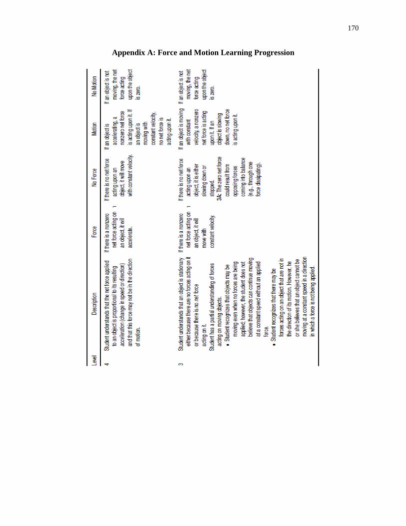
170

Appendix A: Force and Motion Learning Progression

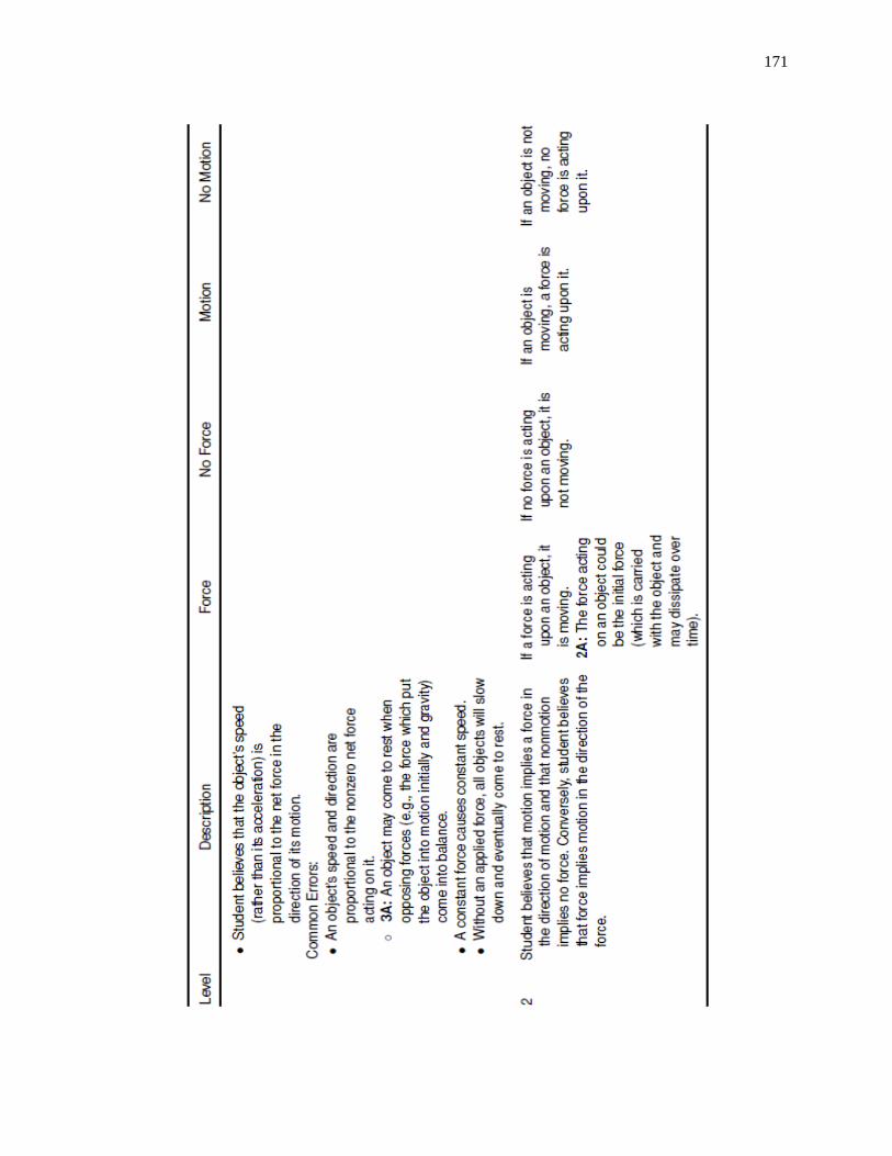
171

172

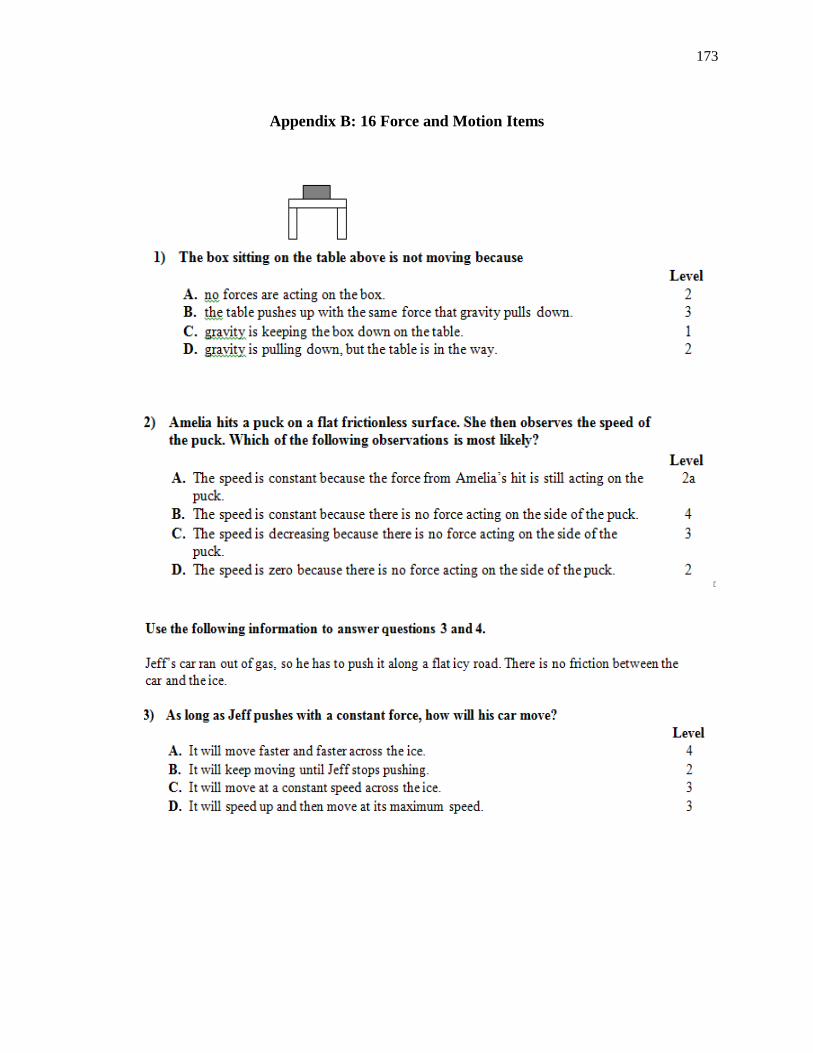
173

Appendix B: 16 Force and Motion Items

174

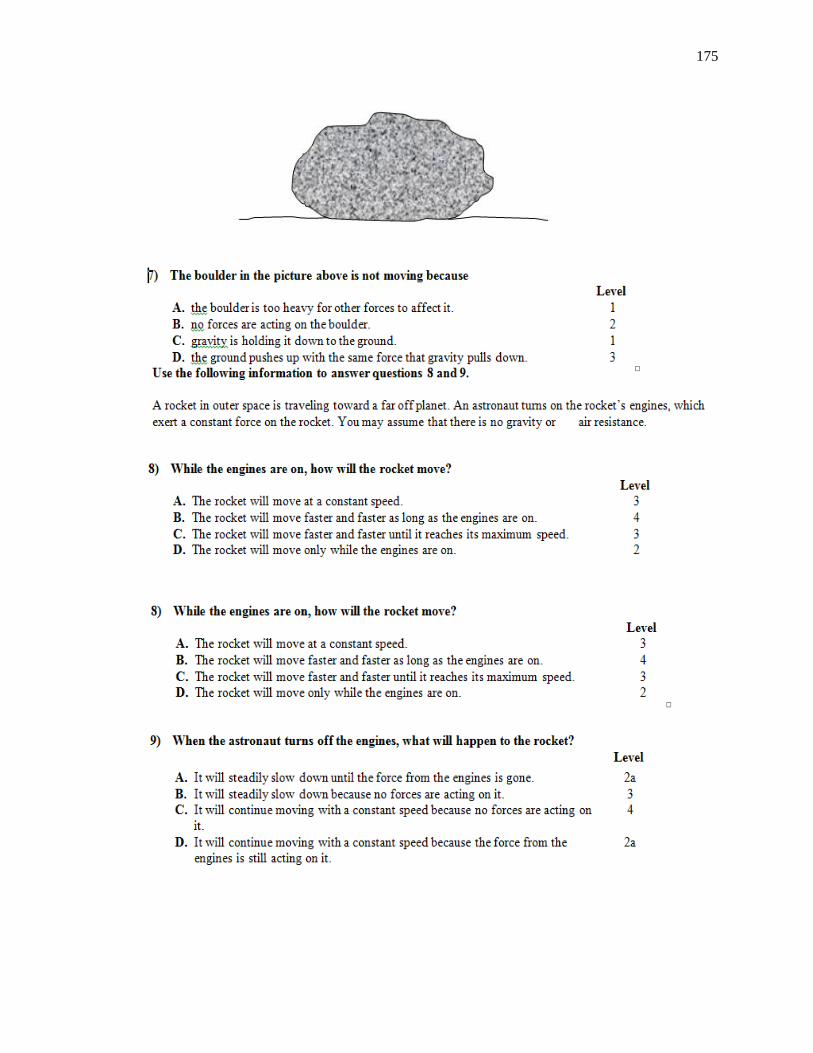
175

176

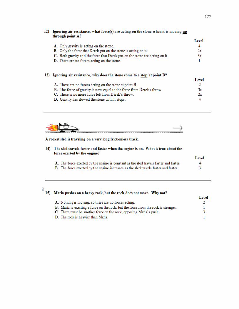
177

178

179

Appendix C: Earth and Solar System Learning Progression Levels and Descriptions

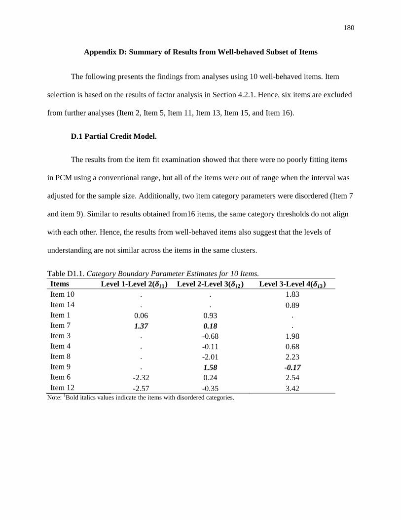
180

Appendix D: Summary of Results from Well-behaved Subset of Items

The following presents the findings from analyses using 10 well-behaved items. Item

selection is based on the results of factor analysis in Section 4.2.1. Hence, six items are excluded

from further analyses (Item 2, Item 5, Item 11, Item 13, Item 15, and Item 16).

D.1 Partial Credit Model.

The results from the item fit examination showed that there were no poorly fitting items

in PCM using a conventional range, but all of the items were out of range when the interval was

adjusted for the sample size. Additionally, two item category parameters were disordered (Item 7

and item 9). Similar to results obtained from16 items, the same category thresholds do not align

with each other. Hence, the results from well-behaved items also suggest that the levels of

understanding are not similar across the items in the same clusters.

Table D1.1. Category Boundary Parameter Estimates for 10 Items.

Items Level 1-Level 2(𝜹𝒊𝟏) Level 2-Level 3(𝜹𝒊𝟐) Level 3-Level 4(𝜹𝒊𝟑)

Item 10 . . 1.83

Item 14 . . 0.89

Item 1 0.06 0.93 .

Item 7 1.37 0.18 .

Item 3 . -0.68 1.98

Item 4 . -0.11 0.68

Item 8 . -2.01 2.23

Item 9 . 1.58 -0.17

Item 6 -2.32 0.24 2.54

Item 12 -2.57 -0.35 3.42 Note:

1Bold italics values indicate the items with disordered categories.

181

The overall results also suggest that there is not enough supporting evidence for deciding

cutoff points on the continuous latent trait and, in turn, for the meaningful placement of students

into discrete LP levels using 10 well-behaved items.

D.2 Attribute Hierarchy Model.

The results from person fit examination (via RCI calculations) that students did not

respond to the OMC items as consistently as expected. While the attribute probabilities estimated

by the ANN for each of our expected response patterns indicated an almost exact match, there is

found variation in the attribute estimates with the actual student response data across different

trials.

Table D2.1. The Summary of Standard Deviations in Estimates across 100 ANN Trials for 10

Items.


Min. 0.001 0.001 0.001 0.001

1st Qu. 0.002 0.031 0.109 0.047

Median 0.003 0.092 0.247 0.189

Mean 0.003 0.128 0.220 0.186

3rd Qu. 0.003 0.213 0.341 0.318

Max. 0.008 0.396 0.401 0.397

Table D2.1 shows that there is almost no variation in A1 estimates while there is large

variation in the other three attributes. The magnitude of the variation in attribute estimates across

100 trials using 10 well-behaved items are smaller than that of the variation found using 16 FM

LP assessment items (see Table 4.14). However, these results still suggest that making diagnostic

classifications based on a single ANN training can lead to different interpretations and that these

classifications are not reliable.

182

Table D2.2. LP Level Placements with AHM Based on 10 Items.


Number of students 197 296 310 127 930

Percent of students 21% 31% 33% 13.6% 100

LP level placement results between AHM and the modal approach are similar with results

obtained from 16 items. The agreement between AHM and modal classification using 10 items is

found to be moderate (48.4%).

Table D2.3. Cross Examination of LP Level Classification Using 10 Items (Modal and AHM).

AHM

Level 1 Level 2 Level 3 Level 4

Mod

al

Level 1 1 0 0 0

Level 2 20 76 8 4

Level 3 146 171 275 56

Level 4 4 5 9 46

D.3 Generalized Diagnostic Model.

The examination of the RMSEA values for item fit suggests 9 good fitting items and 1

moderately fitting item. Item parameter examinations of well-behaved items show similar results

to 16-item results. There is found a wide range of difficulty estimates for each item category

parameter.

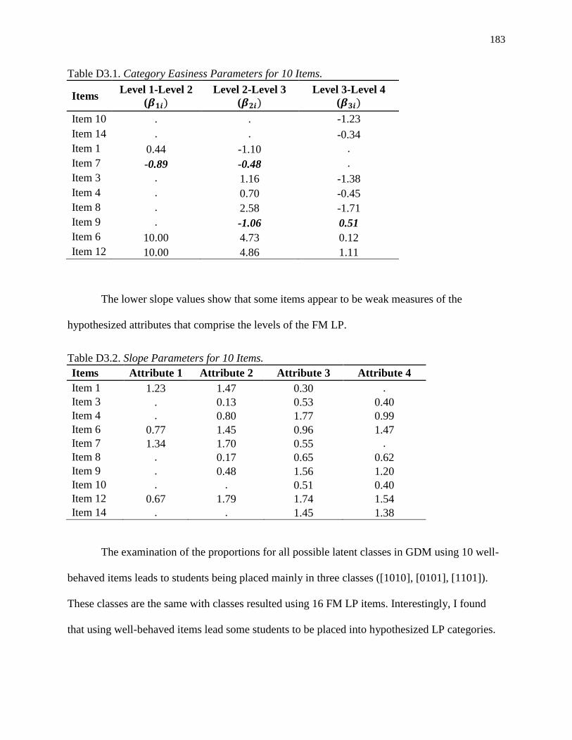
183

Table D3.1. Category Easiness Parameters for 10 Items.


(𝜷𝟏𝒊)

Level 2-Level 3

(𝜷𝟐𝒊)

Level 3-Level 4

(𝜷𝟑𝒊)

Item 10 . . -1.23

Item 14 . . -0.34

Item 1 0.44 -1.10 .

Item 7 -0.89 -0.48 .

Item 3 . 1.16 -1.38

Item 4 . 0.70 -0.45

Item 8 . 2.58 -1.71

Item 9 . -1.06 0.51

Item 6 10.00 4.73 0.12

Item 12 10.00 4.86 1.11

The lower slope values show that some items appear to be weak measures of the

hypothesized attributes that comprise the levels of the FM LP.

Table D3.2. Slope Parameters for 10 Items.


Item 1 1.23 1.47 0.30 .

Item 3 . 0.13 0.53 0.40

Item 4 . 0.80 1.77 0.99

Item 6 0.77 1.45 0.96 1.47

Item 7 1.34 1.70 0.55 .

Item 8 . 0.17 0.65 0.62

Item 9 . 0.48 1.56 1.20

Item 10 . . 0.51 0.40

Item 12 0.67 1.79 1.74 1.54

Item 14 . . 1.45 1.38

The examination of the proportions for all possible latent classes in GDM using 10 well-

behaved items leads to students being placed mainly in three classes ([1010], [0101], [1101]).

These classes are the same with classes resulted using 16 FM LP items. Interestingly, I found

that using well-behaved items lead some students to be placed into hypothesized LP categories.

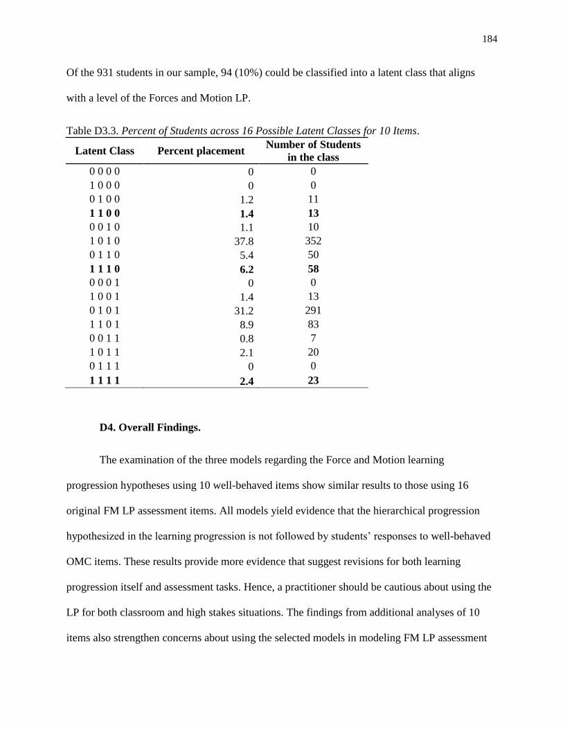
184

Of the 931 students in our sample, 94 (10%) could be classified into a latent class that aligns

with a level of the Forces and Motion LP.

Table D3.3. Percent of Students across 16 Possible Latent Classes for 10 Items.

Latent Class Percent placement Number of Students

in the class

0 0 0 0 0 0

1 0 0 0 0 0

0 1 0 0 1.2 11

1 1 0 0 1.4 13

0 0 1 0 1.1 10

1 0 1 0 37.8 352

0 1 1 0 5.4 50

1 1 1 0 6.2 58

0 0 0 1 0 0

1 0 0 1 1.4 13

0 1 0 1 31.2 291

1 1 0 1 8.9 83

0 0 1 1 0.8 7

1 0 1 1 2.1 20

0 1 1 1 0 0

1 1 1 1 2.4 23

D4. Overall Findings.

The examination of the three models regarding the Force and Motion learning

progression hypotheses using 10 well-behaved items show similar results to those using 16

original FM LP assessment items. All models yield evidence that the hierarchical progression

hypothesized in the learning progression is not followed by students’ responses to well-behaved

OMC items. These results provide more evidence that suggest revisions for both learning

progression itself and assessment tasks. Hence, a practitioner should be cautious about using the

LP for both classroom and high stakes situations. The findings from additional analyses of 10

items also strengthen concerns about using the selected models in modeling FM LP assessment

185

data composed of OMC items. The PCM model was found to be inappropriate for the

classification of students into the LP levels. AHM produced instable attribute estimates across

different trials and the interpretation of the parameters in GDM remained obscure. The results

from all three models indicated that the promise of the OMC items to reflect student

understanding associated with the LP levels is clouded by the ceiling and floor effects inherent in

the context of Force and Motion tasks. Hence, there is a need to examine the effect of structure

of OMC items in a separate study. Overall, results of this dissertation suggest some rethinking on

the progression and granularity of the LP for the effective use of psychometric models.

The Marginal Edge of Learning Progressions and Modeling ...

Documents