The Macrotheme Reviewmacrotheme.com/yahoo_site_admin/assets/docs/8nusMR... · Irina Khvostova, Alexander Larin, Anna Novak, and Andrei Shulgin, The Macrotheme Review 2(7), Winter

Irina Khvostova, Alexander Larin, Anna Novak, and Andrei Shulgin, The Macrotheme Review 2(7), Winter 2013

82

The Macrotheme Review A multidisciplinary journal of global macro trends

The Balance of Payments Dynamics in the Period of Crisis

Irina Khvostova, Alexander Larin, Anna Novak*, and Andrei Shulgin National Research University Higher School of Economics, Russia

[email protected]*

Abstract

The paper analyses the key factors of balance of payments dynamics for countries with

different exchange rate regimes. We consider the differences in approaches to the

analysis of balance of payments effects, and provide an overview of recent studies on

current account and capital account dynamics. We present an estimates based on

quarterly data on 40 countries with floating exchange rate regime and 38 countries with

intermediate exchange rate regimes from 2006 to 2010. In the period of crisis, the

response of trade balance is opposite depending on exchange rate regime. Data also

support the hypothesis of reversal effect of BOP. The hypothesis about interest rate to be

a policy instrument in crisis period is not supported.

Keywords: balance of payments, current account, capital account, exchange rate regime

1. Introduction

Monetary policy is closely connected with the dynamics of balance of payments (BOP). If a

country chooses a floating exchange rate regime, the BOP determines the dynamics of the

national currency exchange rate, which, in turn, influence the macroeconomic performance of the

country. In this case the dynamics of BOP is an important indicator of monetary policy.

In case of intermediate exchange rate regimes the situation is more complicated. On the one hand,

monetary authorities prevent significant exchange rate volatility, that is, it becomes possible to

have short-term payment imbalance. On the other hand, the monetary authorities have to think

about the future monetary stability, for which they need to adjust monetary policy to reduce the

imbalance (Summers, 1996; Taylor, 2002). In this case, BOP is not only an indicator, but also the

target of monetary policy. The described effect was observed in developing countries during the

global financial crisis in 2008-2009. For example, several CIS countries (Ukraine, Belarus,

Tajikistan, Kyrgyzstan, and others) were forced to devalue their currencies only to reduce the

emerging negative payment imbalances.

Under floating exchange rate regime, the shocks of current and capital accounts are linked with

fluctuations in the equilibrium exchange rate. On the contrary, under intermediate exchange rate

regime, Central Bank stabilizes both BOP and exchange rate. As a result, the exogenous shocks

of current and capital accounts are more closely connected with the exchange rate dynamics, than

in intermediate regime (Kharel and Martin, 2010). Consequently, in countries with floating and

mailto:[email protected]*


83

intermediate exchange rate regimes under the same environmental conditions in the short term,

the joint dynamics of current account and real exchange rate may have a different direction due to

the correction of the monetary authorities.

Capital account of BOP plays an important role in periods of problems with liquidity and

insolvency (Calvo, 1996; Chang and Turnovsky, 2009). In countries with floating exchange

regime, BOP imbalances activate the market mechanism, which leads to changes in the level of

interest rates. If monetary authorities prefer to interfere in the establishment of BOP equilibrium,

the negative shock of capital outflows can be compensated by adjusting interest rates. High

interest rates in this case are working in two directions: a) increase the demand for liquid assets in

the domestic country; b) increase the cost of servicing the national debt. Therefore, in countries

with intermediate exchange rate regime this effect is uncertain during the crisis period.

The aim of the paper is twofold. Firstly, the purpose is to discuss theoretical aspects of the BOP

effects on the monetary policy. The paper examines the differences in approaches to the analysis

of the BOP effects; provides an overview of theoretical and empirical researches devoted to the

analysis of BOP dynamics. The great attention is paid to the peculiarities of using the monetary

instruments to stabilize BOP, depending on exchange rate regime. Secondly, the aim is to

investigate the monetary dynamics of countries with different exchange rate regimes in the crisis

period of 2008–2009 and to reveal differences in the stabilization behavior of monetary

authorities.

The rest of the paper has the following structure. In Section 2 we describe theoretical aspects of

BOP dynamics. Firstly, we consider trade balance as an element of the monetary transmission

mechanism. We summarize studies that consider the response of the current account of BOP to

the price level and the nominal exchange rate. We discuss here the existence of the J-curve effect

of the Marshall-Lerner condition.

Then, we consider BOP as an intermediate target of monetary policy. Studies on this problem are

based on the assumption of the existence of the sustainable level of current account balance and

on the idea of reversal dynamic of trade balance. Depending on exchange rate regime this process

may differ significantly.

Finally, we shift our focus to the role of capital account in the analysis of the balance of

payments. We consider studies that estimate monetary policy reaction to capital account shocks

and conclude that capital account is an intermediate goal of monetary policy in the period of

problems with liquidity and solvency.

In Section 3 we provide the results of econometric testing of the BOP effects in crisis period

2008-2009 for countries with floating and intermediate exchange rate regimes. We show the

differences in the stabilization policy of these two groups of countries. Firstly, we describe the

data used and the procedure of choosing the crisis period that are based on Bai-Perron test. To

analyze the relation between exchange rate and current account, we estimate simple linear models

using weighted ordinary least squares. We estimate the coefficient at exchange rate to find how it

affects trade balance for different group of countries for crisis and non-crisis periods. We also test

the hypothesis of reversal effect of BOP for both groups of countries. To reveal the relation

between interest rate and capital account, we estimate linear regression as well. We estimate,

whether interest rate is considered as policy instrument in crisis and non-crisis period or not. We

also present a series of tests to reveal the role of the difference in average values of shocks. We

conclude in Section 4.


84

2. Factors of BOP dynamics

Exchange rate regime is a way for monetary authorities to establish exchange rate relations

between national currency and foreign currencies. There are fixed, floating and various types of

intermediate exchange rate regimes1. A key feature for countries with intermediate and fixed

exchange rate is the additional component in BOP — the change in international reserves. This

component makes it possible to smooth fluctuations or completely fix the exchange rate in case

of BOP imbalance.

Among many papers that analyze the dynamics of BOP, there are several areas of research. The

first group of papers is devoted to the study of reaction of trade balance to changes in exchange

rate. The second group pays attention to the study of BOP reversal effect. The third one studies

the dynamics of capital account, depending on a variety of financial factors.

2.1. Trade balance as an element of monetary transmission mechanism

In an open economy, monetary transmission mechanism largely depends on the terms of trade of

the country, that is, the current account of BOP (Gali and Monaselli, 2008; Svensson, 2001,

2003). Trade flows are changing under influence of the relative changes in the prices of tradable

goods and the dynamics of capital flows.

The traditional approach to modeling the dynamics of BOP in reduced form is (Rose, 1991; Lee

and Chinn, 1998; Boyd at al., 2001; Gomez and Paz, 2005):

ttttttttt emxppsmxb )( *

, (1)

where b — trade balance, p — price level in the country, p* — foreign price level, m —volume

of imports, s — nominal exchange rate, x — exports, e — real effective exchange rate. All the

variables are log transformed.

Devaluation is usually associated with the improvement of trade balance. However, there is no

consensus on how the effects of exports and imports are distributed over time. Orkutt (1950)

argued that the trade flow responds differently to small, temporary shocks and large, permanent

changes (e.g. devaluation). This means that the adjustment of trade balance to large-scale changes

in price level or to changes of nominal exchange rate is faster than the adjustment to small

changes. That is why the response of current account of BOP in crisis period (which implies a

substantial devaluation) may differ from its reaction in non crisis period.

Later this effect has been studied for countries with different exchange rate regimes. Wilson and

Takacs (1979), Janz and Rhomberg (1973) have studied the difference in responses to changes in

rates for countries with fixed exchange rate regime. Wilson and Takacs have shown the same

response of trade balance to nominal exchange rate and price level changes. Janz and Rhomberg

subjected these results to the criticism and demonstrated that the reaction time to changes in

nominal exchange rate is smaller than the response time to change in price levels. This idea was

further developed by Bahmani-Osco (1986), Bahmani-Osco and Kara (2003), Hacker and Hatami

(2004), Boyd at al.(2001), Gomez and Paz (2005).

In addition, these studies also observe the J-curve effect. This phenomenon describes the fact that

the initial impact of devaluation is negative for trade balance (reduction of import exceeds export

1 IMF De Facto Classification of Exchange Rate Regimes April 31, 2008


85

growth), but over time exports increases due to competitive prices and, ultimately, trade balance

is growing significantly. Janz and Rhomberg explain the J-curve effect by different lags,

including time lag, decision-making lag, delivery lag and product replacement lag.

The results of Wilson and Takacs also have been expanded. In 1991 Tegene, using vector

autoregression approach, came to the conclusion that export and import functions are equally

responsive to relative price changes and changes in nominal exchange rate.

The next area of BOP researches is devoted to the devaluation impact on BOP dynamics. The

devaluation of national currency is usually associated with the improvement of trade balance, but

is accompanied by an adjustment to changes in real exchange rate with a certain time lag. The

size of the lag is determined by individual characteristics of each country. It may even be zero for

some countries. The study of this effect has also been associated with the problem of the

Marshall-Lerner condition: devaluation is accompanied by the growth of trade balance if price

elasticity of export and import is greater than one. Empirical studies of trade balance reaction to

exchange rate fluctuations have found that the condition is not satisfied in the short term (see, for

example, Gomez and Paz, 2005). However, the reaction may depend on the exchange rate

regime, the size of the fluctuations, and may be different for the cases of real and nominal

devaluation.

The other line of researches links BOP and exchange rate by analyzing how BOP imbalance

affects foreign exchange rate over time. Most theoretical works use dynamic approach to the

analysis of international payments according to the joint dynamic behavior of the various

components of BOP.

The paper of Muller-Plantenberg (2010) summarizes the results of theoretical studies of

dynamics of exchange rate and provides models that explain fundamental differences between

interaction of exchange rate and international payments depending on imposed restrictions on

capital flows and exchange rate regime of the country. Muller-Plantenberg paper is a synthesis of

theoretical models of previous studies.

Theoretical models of Muller-Plantenberg have an empirical support. Bussiere and Mulder

(1999), Eichengreen (2003), Pontines and Siregar (2008) have shown that variables such as the

current account, export growth, international reserves and short-term international debt are good

indicators to predict currency crises.

2.2. The balance of payments as an intermediate target of monetary policy

BOP is an intermediate target of monetary policy when the stability of exchange rate regime is

under the threat. Studies on this problem, based on the assertion of existence of sustainable level

of current account balance – the level at which the country is able to meet all its obligations to

foreign loans due to the current and future savings. In the light of this assumption, it is considered

that trade deficit is a problem for monetary authorities, threatening the stability of monetary

sphere, when the level exceeds sustainable limit. Thus, for the U.S. it is about 5% of GDP (Mann,

2002, Freund, 2000,2005) for New Zealand, Portugal, Singapore - 10% (Summers, 1996),

France, Italy, Spain - 3 % (Taylor, 2002).

Change in the direction of BOP dynamics is called the "reversal". Most of the papers devoted to

the reversal of BOP, suggest the effect of market adjustment mechanisms in the case of floating

exchange rate regimes (Obstfeld and Rogoff , 2005; Freund, 2000; Mann, 2002). In the case of

countries with intermediate exchange rate regimes reversal is controlled by monetary authorities,


86

who are trying to correct the effect of market factors. The effect of reversal then arises in the

form of: (a) delayed reaction of components of BOP to the ongoing correction of exchange rate,

(b) smoothed response of the Central Bank to payments imbalance.

The imbalance is threatens exchange rate regime in the country, while the reversal is

accompanied by depreciation of national currency. The overall effect of devaluation of developed

countries was estimated to be 20% (Freund, 2005). Using the definition of currency crisis

proposed by Frankel and Rose (1996), the devaluation of the national currency by 25% or more

in nominal terms is considered to be a currency crisis, respectively, we can say that the

imbalances in BOP can lead to currency crisis (Edwards, 2001). The threat of crisis stimulates

monetary authorities of intermediate exchange rate regimes to intervene in the process of

reversal.

There are studies for developing countries, showing that the effect of reversal does not

necessarily entail a currency crisis. In Milesi-Ferretti and Razin (1998) less than a third of cases

in a sample of 105 countries systematically accompanied by a currency crisis.

This effect shows that under the same environmental conditions in the countries in transition

mode and floating exchange rate devaluation will occur at different times and at different speeds.

Moreover, in the short term, the joint dynamics of current account and real exchange rate may

have a different direction due to corrections of monetary authorities.

2.3. The role of capital account in the analysis of the BOP

Capital account of BOP comes to the fore during the problems with liquidity and insolvency. If

monetary authorities prefer to influence the establishment of BOP, negative shock of capital

outflows is associated with two alternatives: a) the reduction of production in response to decline

in investment and b) the use of international reserves to mitigate the impact on domestic demand

(Ranciere and Jeanne, 2006). Using, for example, interest rate in order to regulate capital flows

can lead to negative consequences (Lahiri, Vegh, 2003; Pak-Hung, 2009) and only tighten the

problems in the financial sector.

High interest rates in this case, first, increase the demand for interest-bearing liquid assets in the

country, and secondly, increase the cost of servicing the public debt. Thus, the effect is uncertain

during the crisis, and is characteristic of countries with intermediate exchange rate regimes.

The relationship between financial variables looks ambiguous. For example, relatively small

negative shock (interest rate change) may lead to radical changes in the dynamics of the capital

account and have serious consequences for the social sphere (Calvo, 1996; Chang, 2009). With

the example of the financial crisis in Mexico in 1994 Calvo showed that in a world where

international relations are well developed, the reaction of investors to financial shocks can be

disproportionately high, at least in the initial response. The reason for this may be financial

vulnerability of the country or expectations of investors.

Financial factors in crisis and non-crisis period may have a completely different impact on capital

account of BOP. This conclusion is most typical for countries protecting their exchange rate

regime.


87

3. Empirical analysis of the BOP effects on monetary policy

3.1. The data

In this paper we investigate the joint dynamics of BOP and exchange rate of 78 countries which

produce more than 93% of the World Gross Domestic Product. We divide the entire sample into

two groups. The first group includes countries that manage the exchange rate of the national

currency, and the second group involves countries that do not control the exchange rate. Groups

were formed on the basis of the International Monetary Fund (IMF) classification (Table 1).

The first group includes 40 countries with a floating exchange rate regime and two countries with

currency board exchange rates regime. We add these two countries because in case of Currency

Board the national currency is pegged to free floating currencies that makes differences between

these two regimes irrelevant in this particular study. We also treat countries of Euroarea as one

observation. The second group consists of 38 countries with intermediate exchange rate regimes

(managed floating, crawling peg and currency band).

Data for each country cover the period from the third quarter of 2006 (2006Q3) to the first

quarter of 2010 (2010Q1). Econometric testing is carried out on quarterly data forming the panel

dimension in 78 countries and 15 quarters. The analysis is based on the dynamics of BOP,

balance of trade, interest rates, real effective exchange rates.


88

Table 1. Classification of the sample countries according to the exchange rate regime

Group I (40) Group II (38)

Free floating

(38)

Currency

Board

(2)

Conventional

fixed peg

(17)

Crawling

peg

(3)

Currency

band

(1)

Managed

floating

(17)

Australia

Brazil

Canada

Chile

Czech

Republic

Euroarea

Hungary

Iceland

Israel

Mexico

New Zealand

Norway

Philippines

Poland

South Africa

South Korea

Sweden

Switzerland

Turkey

United

Kingdom

USA

Japan

Bulgaria

Hong Kong

Argentina

Belarus

Belize

Croatia

Denmark

Fiji

Kazakhstan

Latvia

Lesotho

Macedonia

Morocco

Russian

Federation

Samoa

Solomon Islands

Trinidad and

Tobago

Tunisia

Venezuela

Bolivia

China

Nicaragua

Costa Rica

Armenia

Colombia

Georgia

India

Indonesia

Kyrgyzstan

Malaysia

Moldova

Pakistan

Paraguay

Peru

Romania

Singapore

Thailand

Uganda

Ukraine

Uruguay

Note: The number of countries included in each group is in parentheses.

BOP statistics

We use the IMF quarterly statistics on capital, financial and current account. It is important to

note that the methodology of compiling BOP have significant differences among countries we

consider. For example, some countries do not separate financial account into a particular group.

Therefore, we consider the sum of capital and financial accounts to avoid problems with the

comparability of methodologies.

Trade Balance

Quarterly trade balance data are also taken from the IMF statistics. To fill the gap in case when

there were no data on trade balance, we use the following calculations:


89

ti

titi

tier

IMEXTB

,

,,

,

, (1)

where tiTB , — quarterly trade balance of country i in period t (millions US dollars), tiEX ,

tiIM , — quarterly export (import) of country i in national currency, tier , — average exchange

rate for the quarter.

Interest rate

Proxy for the interest rate is the annual discount rate at the end of the quarter. In the absence of

discount rate for any particular country, we use refinancing rate (percent per annum); in the

absence of refinancing rate, we use repo rate (percent per annum).

Real effective exchange rate

For countries where this indicator was not availiable in the IMF database, we calculate the rate on

the basis of country’s import structure. For calculations we use the structure of import into the

country in 2009. We consider this structure to be constant during the period under consideration.

We calculate the real exchange rate of domestic currency and the currencies of countries-

importers:

t

t

tt P

P

NEERREER

*

, (2)

where tREER — real effective exchange rate (domestic currency against the unit of foreign

currency),

N

jtjt

jeNEER1

,

*— nominal effective exchange rate, tt CPIP — price

level in the domestic country,

N

jtjt

jCPIP1

,*

*— average price level of importers;

N

jj

j

j

1

*

— share of the importer j based on the import structure; tje , — nominal exchange

rate (domestic currency against the unit of foreign currency).

Econometric test requires stationarity of the considered series. Dickey-Fuller test indicate the

presence of a unit root in all of the series, which demonstrates that they are not stationary. In

addition, the graphs of the dynamics of indices also show signs of the presence of a unit root -

there is no return to the average level. That is the reason why we use first differences of the data

(quarterly changes).

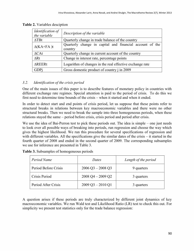
Description and symbols of all the variables which we use in the econometric analysis are

described in Table 2.


90

Table 2. Variables desciption

Identification of

the variable Description of the variable

∆TBt Quarterly change in trade balance of the country

∆(KA+FA )t Quarterly change in capital and financial account of the

country

∆CAt Quarterly change in current account of the country

∆Rt Change in interest rate, percentage points

∆REERt Logarithm of changes in the real effective exchange rate

GDPj Gross domestic product of country j in 2009

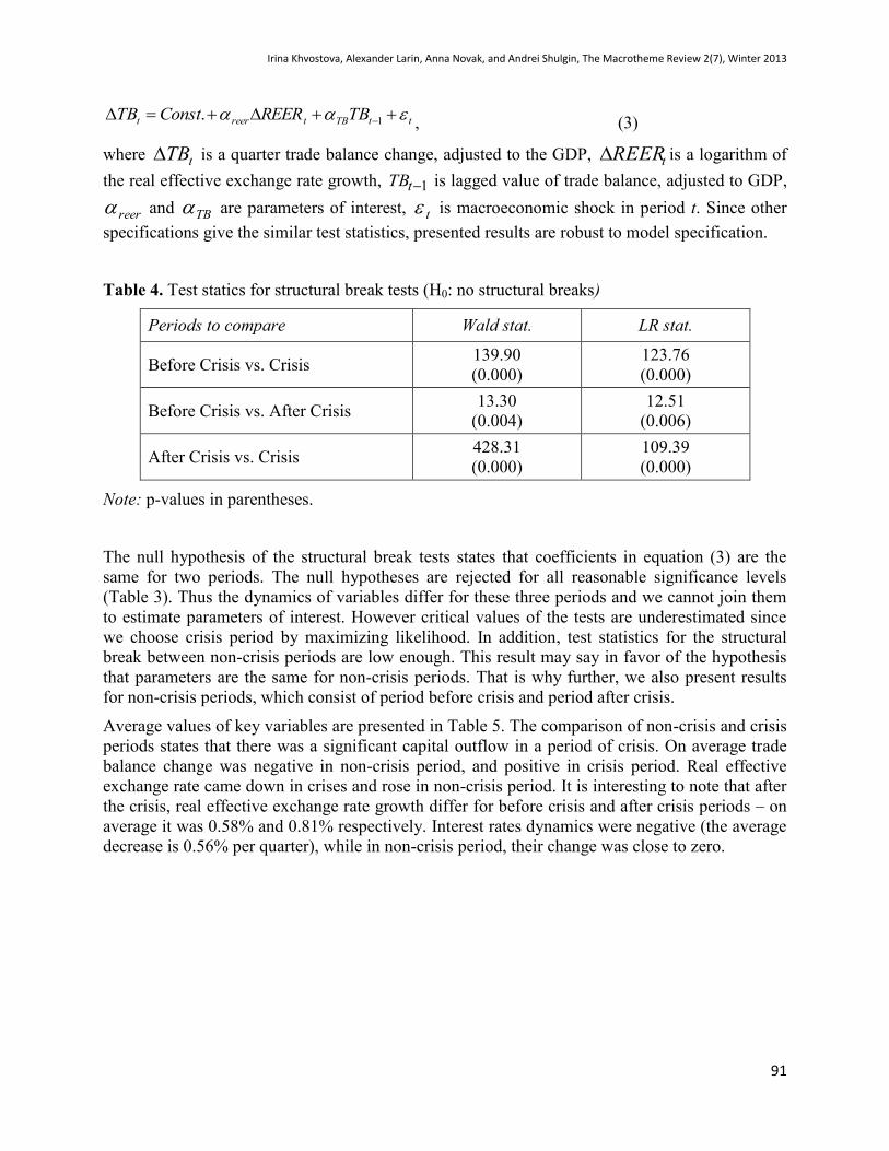
3.2. Identification of the crisis period

One of the main issues of this paper is to describe features of monetary policy in countries with

different exchange rate regimes. Special attention is paid to the period of crisis. To do this we

first need to determine time bounds of the crisis – when it started and when it ended.

In order to detect start and end points of crisis period, let us suppose that these points refer to

structural breaks in relations between key macroeconomic variables and there were no other

structural breaks. Then we need to break the sample into three homogeneous periods, when these

relations stayed the same – period before crisis, crisis period and period after crisis.

We use the idea of Bai-Perron test to pick these periods out. The idea is simple – one just needs

to look over all possible ways of breaking into periods, run regression and choose the way which

gives the highest likelihood. We run this procedure for several specifications of regression and

with different variables. All the specifications give the similar dates of the crisis – it started in the

fourth quarter of 2008 and ended in the second quarter of 2009. The corresponding subsamples

we use for inference are presented in Table 3.

Table 3. Subsamples of homogeneous periods

Period Name Dates Length of the period

Period Before Crisis 2006 Q3 – 2008 Q3 9 quarters

Crisis Period 2008 Q4 – 2009 Q2 3 quarters

Period After Crisis 2009 Q3 – 2010 Q1 3 quarters

A question arises if these periods are truly characterized by different joint dynamics of key

macroeconomic variables. We run Wald test and Likelihood Ratio (LR) test to check this out. For

simplicity we present test statistics only for the trade balance regression:


91

ttTBtreert TBREERConstTB 1., (3)

where tTB is a quarter trade balance change, adjusted to the GDP, tREER is a logarithm of

the real effective exchange rate growth, 1tTB is lagged value of trade balance, adjusted to GDP,

reer and TB are parameters of interest, t is macroeconomic shock in period t. Since other

specifications give the similar test statistics, presented results are robust to model specification.

Table 4. Test statics for structural break tests (Н0: no structural breaks)

Periods to compare Wald stat. LR stat.

Before Crisis vs. Crisis 139.90

(0.000)

123.76

(0.000)

Before Crisis vs. After Crisis 13.30

(0.004)

12.51

(0.006)

After Crisis vs. Crisis 428.31

(0.000)

109.39

(0.000)

Note: p-values in parentheses.

The null hypothesis of the structural break tests states that coefficients in equation (3) are the

same for two periods. The null hypotheses are rejected for all reasonable significance levels

(Table 3). Thus the dynamics of variables differ for these three periods and we cannot join them

to estimate parameters of interest. However critical values of the tests are underestimated since

we choose crisis period by maximizing likelihood. In addition, test statistics for the structural

break between non-crisis periods are low enough. This result may say in favor of the hypothesis

that parameters are the same for non-crisis periods. That is why further, we also present results

for non-crisis periods, which consist of period before crisis and period after crisis.

Average values of key variables are presented in Table 5. The comparison of non-crisis and crisis

periods states that there was a significant capital outflow in a period of crisis. On average trade

balance change was negative in non-crisis period, and positive in crisis period. Real effective

exchange rate came down in crises and rose in non-crisis period. It is interesting to note that after

the crisis, real effective exchange rate growth differ for before crisis and after crisis periods – on

average it was 0.58% and 0.81% respectively. Interest rates dynamics were negative (the average

decrease is 0.56% per quarter), while in non-crisis period, their change was close to zero.


92

Table 5. Average values of variables (all countries)

Variable Before

Crisis

After Crisis Non-Crisis

Period

Crisis

Period

All Periods

∆TB -5.04 -1.81 -4.19 11.44 -0.81

∆KA+∆FA 4.85 2.18 4.17 -11.53 0.73

∆CA -4.06 -4.92 -4.27 11.34 -0.86

∆R (%) 0.14 -0.41 -0.01 -0.56 -0.13

∆REER (%) 0.81 0.58 0.75 -1.00 0.37

Average values of variables for two groups of countries – with floating exchange rate regime and

with intermediate exchange rate regime – are presented in Tables 6 and 7 respectively. The

average dynamics of trade balance, as well as the dynamics of current account, are almost the

same for these two groups, irrespectively of the period we consider.

The distinguishing feature of most countries with one of intermediate exchange rate regimes is its

high dependence on export. Tables 6 and 7 indicate high capital outflow in crisis period and

especially for countries with floating exchange rate regime. This fact says in favor of hypothesis

that reaction to shocks is higher for countries with floating regime, than for countries with

intermediate regime.

The dynamics of real effective exchange rate for these two groups of countries are different as

well. In pre-crisis period, countries with intermediate regime demonstrate higher growth of the

exchange rate – 0.99% – while for countries with floating regime average growth were 0.51%. In

crisis, exchange rate growth fell down to -0.43% and -1.91% for intermediate and floating

regimes respectively. In post-crisis period, exchange rate dynamics were restored for countries

with floating regime – its growth came to 1.66%. At the same time, in countries with intermediate

regime, exchange rate continued to fall down by 0.09% per quarter.

Table 6. Average values of variables (countries with floating exchange rate regime)

Variable Before

Crisis


Period

Crisis

Period

All Periods

∆TB -1.95 -0.21 -1.48 10.92 1.18

∆KA+∆FA 8.68 -3.33 5.57 -16.81 0.70

∆CA -3.20 1.12 -2.11 13.06 1.21

∆R (%) 0.08 -0.24 -0.01 -1.06 -0.24

∆REER (%) 0.51 1.66 0.82 -1.91 0.24


93

Table 7. Average values of variables (countries with intermediate exchange rate regime)

Variable Before

Crisis


Period

Crisis

Period

All Periods

∆TB -7.03 -2.88 -5.93 11.77 -2.08

∆KA+∆FA 2.29 6.03 3.23 -8.01 0.76

∆CA -4.62 -8.98 -5.72 10.18 -2.24

∆R (%) 0.19 -0.52 -0.01 -0.25 -0.06

∆REER (%) 0.99 -0.09 0.7 -0.43 0.46

Analyzing the dynamics of interest rates, one may point out the tendency to decrease for both

groups of countries. However, in crisis, the decrease of interest rate came to 1.06% per quarter

for countries with floating regime. This decrease is four times as high as the average by all

periods we consider. For countries with intermediate regime, the decrease of interest rates is not

so dramatic. This may be explained by the fact that the sample consists of developing countries

whose goal is to attract capital. That is why they try to avoid interest rates decrease, which may

negatively affect investment image of the country.

3.3. Testing the BOP Effects

To detect differences in macroeconomic relations in crisis and non-crisis periods, we use simple

linear models of trade balance and estimate them with OLS. Estimation results help to explain

trade balance reaction to shocks of export, import and capital account.

We concentrate our attention to two interrelations. First, we estimate how exchange rate affects

the dynamics of current account. And second, we estimate how interest rate affects the dynamics

of capital account. Dependent variables in two corresponding regressions are trade balance

change (∆TB) and a sum of capital and financial accounts changes ∆(KA+FA) respectively. We

include logarithm of real effective exchange rate growth (∆REER) as an explanatory variable in

the first regression and interest rate change (∆R) – in the second regression.

It is obvious that economies of the countries in sample differ in scale. As a consequence, shocks

both of capital and current account also differ in scale, or in other words have different variance.

When estimating equations with OLS, this leads to the problem of heteroskedasticity.

The problem of heteroskedasticity is caused by differences in scales of economies and/or

countries foreign trading activity. That is why to solve the problem and to obtain more effective

estimates, we use weighted ordinary least squares. We use two ways of weighting – on GDP and

on sum of export and import. But in the second case standard errors become higher (estimates are

less precise). That is why we present estimates, obtained by weighting all observations on inverse

to nominal GDP of 2009.

Trade balance and Exchange Rate

To reveal the influence of exchange rate on trade balance, we estimate the following linear

model:

ttTBtreert TBREERConstTB 1.. (5)


94

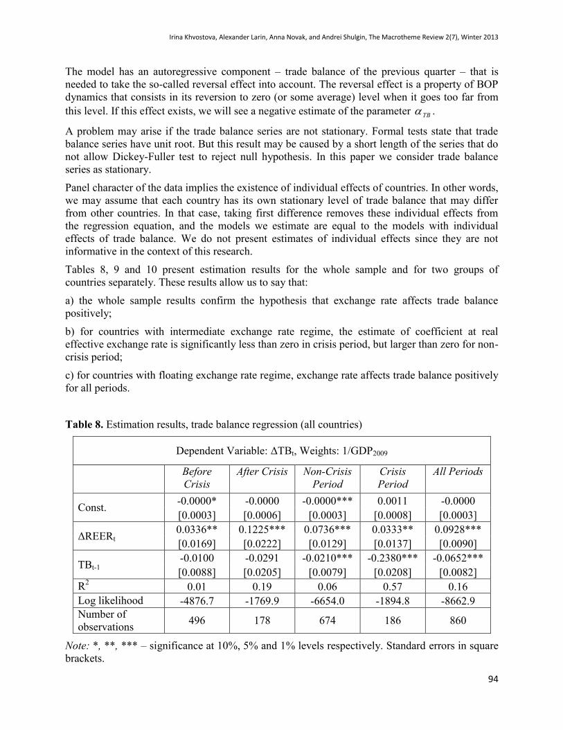
The model has an autoregressive component – trade balance of the previous quarter – that is

needed to take the so-called reversal effect into account. The reversal effect is a property of BOP

dynamics that consists in its reversion to zero (or some average) level when it goes too far from

this level. If this effect exists, we will see a negative estimate of the parameter TB .

A problem may arise if the trade balance series are not stationary. Formal tests state that trade

balance series have unit root. But this result may be caused by a short length of the series that do

not allow Dickey-Fuller test to reject null hypothesis. In this paper we consider trade balance

series as stationary.

Panel character of the data implies the existence of individual effects of countries. In other words,

we may assume that each country has its own stationary level of trade balance that may differ

from other countries. In that case, taking first difference removes these individual effects from

the regression equation, and the models we estimate are equal to the models with individual

effects of trade balance. We do not present estimates of individual effects since they are not

informative in the context of this research.

Tables 8, 9 and 10 present estimation results for the whole sample and for two groups of

countries separately. These results allow us to say that:

a) the whole sample results confirm the hypothesis that exchange rate affects trade balance

positively;

b) for countries with intermediate exchange rate regime, the estimate of coefficient at real

effective exchange rate is significantly less than zero in crisis period, but larger than zero for non-

crisis period;

c) for countries with floating exchange rate regime, exchange rate affects trade balance positively

for all periods.

Table 8. Estimation results, trade balance regression (all countries)

Dependent Variable: ΔTBt, Weights: 1/GDP2009

Before

Crisis


Period

Crisis

Period

All Periods

Const. -0.0000* -0.0000 -0.0000*** 0.0011 -0.0000

[0.0003] [0.0006] [0.0003] [0.0008] [0.0003]

ΔREERt 0.0336** 0.1225*** 0.0736*** 0.0333** 0.0928***

[0.0169] [0.0222] [0.0129] [0.0137] [0.0090]

TBt-1 -0.0100 -0.0291 -0.0210*** -0.2380*** -0.0652***

[0.0088] [0.0205] [0.0079] [0.0208] [0.0082]

R2 0.01 0.19 0.06 0.57 0.16

Log likelihood -4876.7 -1769.9 -6654.0 -1894.8 -8662.9

Number of

observations 496 178 674 186 860

Note: *, **, *** – significance at 10%, 5% and 1% levels respectively. Standard errors in square

brackets.


95

The estimates allow us to conclude that for countries with intermediate regime, changes in trade

balance may push Central Bank to correct exchange rate.

It is worth noting that data support the hypothesis of reversal effect of BOP — estimates of the

coefficient at lagged trade balance is significantly negative in both crisis and non-crisis periods.

Thus, if trade balance goes too far from its average level, we may expect its reversal dynamics.

And the more this deviation is, the more likely reversal will happen. The fact that the estimates

are insignificant for some subsamples and some periods (pre-crisis and post-crisis) may be caused

by small number of observations that leads to high standard errors.

Table 9. Estimation results, trade balance regression (countries with intermediate regime)


Before

Crisis


Period

Crisis

Period

All Periods

Const. 0.0033* -0.003 0.0024 0.0064* 0.0047***

[0.0017] [0.0029] [0.0015] [0.0037] [0.0015]

ΔREERt 0.0844 -0.455*** -0.079* 0.4109*** 0.1727***

[0.0627] [0.0782] [0.0446] [0.0511] [0.0359]

TBt-1 -0.035 -0.087 -0.012 -0.385*** -0.172***

[0.0299] [0.0614] [0.0286] [0.0492] [0.0266]

R2 0.04 0.27 0.01 0.57 0.1

Log likelihood -2924.9 -1053.6 -4010.1 -1129.4 -5197.9

Number of

observations 304 107 411 114 525


brackets.


96

Table 10. Estimation results, trade balance regression (countries with floating regime)


Before

Crisis


Period

Crisis

Period

All Periods

Const. -0.0010*** 0.0000 -0.001*** 0.0013 0.0000

[0.0005] [0.0005] [0.0004] [0.0011] [0.0004]

ΔREERt 0.0293 0.1637*** 0.0836*** 0.019 0.0891***

[0.0211] [0.0174] [0.0150] [0.0159] [0.0110]

TBt-1 -0.025** -0.022 -0.033*** -0.236*** -0.061***

[0.0124] [0.0186] [0.0103] [0.0330] [0.0118]

R2 0.03 0.59 0.14 0.68 0.23

Log likelihood -1924.9 -685.3 -2626.6 -739.1 -3432.5

Number of

observations 192 71 263 72 335


brackets.

When analyzing these results, one may suggest a hypothesis that different reaction of trade

balance to exchange rate may be caused by different shocks (positive or negative), which came to

these two groups of countries. In other words, if countries with intermediate exchange rate

regime suffered from large positive shocks of trade balance and countries with floating exchange

rate – from large negative shocks, we would expect the results, obtained above. In that case the

negative impact of exchange rate is not necessary.

In order to verify this hypothesis, we include dummy variable for exchange rate regime – floating

or intermediate – and estimate the equation on the whole sample. If the reaction to exchange rate

in these two groups of countries is the same and differences are just a result of dissimilar shocks,

then we may expect the significance of dummy variable. In this regression the coefficient at

exchange rate regime denotes the difference in average values of shocks between countries with

floating regime and with intermediate regime. Zero value of this coefficient is consistent with the

hypothesis that average shocks are the same and monetary policy were truly different for these

two groups of countries. In other words Central Banks react differently to the same shocks,

depending on exchange rate regime.

The equation we estimate is:

tfltreert floaterREERConstTB ., (6)

where floater is a dummy variable that takes zero value for countries with intermediate regime

and unity for countries with floating regime.

In the period of crisis, exchange rate regime is insignificant. Thus the hypothesis about difference

in average values of shocks is rejected and shocks are not the reason why reaction to exchange

rate is different (Table 11).


97

Table 11. Estimation results, trade balance regression with dummy for exchange rate regime


Before

Crisis


Period

Crisis

Period

All Periods

Const. 0.0027** -0.002 0.0006 -0.013*** -0.002**

[0.0012] [0.0021] [0.0010] [0.0033] [0.0011]

ΔREERt 0.0152 0.1208*** 0.0610*** 0.0734*** 0.0907***

[0.0156] [0.0222] [0.0125] [0.0159] [0.0093]

Floater -0.003*** 0.0024 -0.001 0.0202*** 0.0036***

[0.0012] [0.0022] [0.0011] [0.0034] [0.0012]

R2 0.02 0.18 0.05 0.38 0.11

Log likelihood -4873.8 -1770.3 -6656.9 -1929.5 -8689.6

Number of

observations 496 178 674 186 860


brackets.

Capital Account and Interest Rate

To analyze the relation between interest rate and capital/financial account, we estimate following

equation:

tttt FAKARConstFAKA 1)(.)( . (7)

Estimates, obtained on the whole sample, support the hypothesis that Central Banks use interest

rate as policy instrument in both crisis and non-crisis periods. Moreover in the period of crisis,

the estimate of the coefficient at interest rate is twice as high as in non-crisis period – it equals

0.074 and 0.033 respectively (Table 12). When considering countries by exchange rate regime,

estimates says about positive relation for countries with intermediate regime (Table 13), but do

not reveal any dependence for countries with floating regime (Table 14).


98

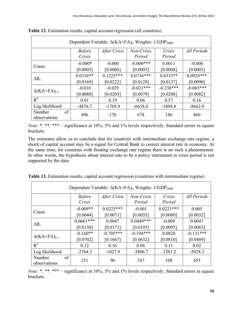
Table 12. Estimation results, capital account regression (all countries)

Dependent Variable: Δ(KA+FA)t, Weights: 1/GDP2009

Before

Crisis


Period

Crisis

Period

All Periods

Const. -0.000* -0.000 -0.000*** 0.0011 -0.000

[0.0003] [0.0006] [0.0003] [0.0008] [0.0003]

ΔRt 0.0336** 0.1225*** 0.0736*** 0.0333** 0.0928***

[0.0169] [0.0222] [0.0129] [0.0137] [0.0090]

Δ(KA+FA)t-1 -0.010 -0.029 -0.021*** -0.238*** -0.065***

[0.0088] [0.0205] [0.0079] [0.0208] [0.0082]

R2

0.01 0.19 0.06 0.57 0.16

Log likelihood -4876.7 -1769.9 -6654.0 -1894.8 -8662.9

Number of

observations 496 178 674 186 860


brackets.

The estimates allow us to conclude that for countries with intermediate exchange rate regime, a

shock of capital account may be a signal for Central Bank to correct interest rate in economy. At

the same time, for countries with floating exchange rate regime there is no such a phenomenon.

In other words, the hypothesis about interest rate to be a policy instrument in crisis period is not

supported by the data.

Table 13. Estimation results, capital account regression (countries with intermediate regime)


Before

Crisis


Period

Crisis

Period

All Periods

Const. -0.009** 0.0225*** -0.001 0.0221*** 0.005

[0.0044] [0.0071] [0.0035] [0.0080] [0.0032]

ΔRt

0.0661*** 0.0047 0.0449*** -0.009 0.0047

[0.0130] [0.0171] [0.0105] [0.0095] [0.0063]

Δ(KA+FA)t-1 -0.160** -0.705*** -0.194*** 0.0828 -0.131***

[0.0702] [0.1667] [0.0632] [0.0810] [0.0489]

R2

0.12 0.16 0.08 0.11 0.02

Log likelihood -2764.3 -1027.9 -3806.7 -1201.2 -5028.2

Number of

observations 251 96 347 108 455


brackets.


99

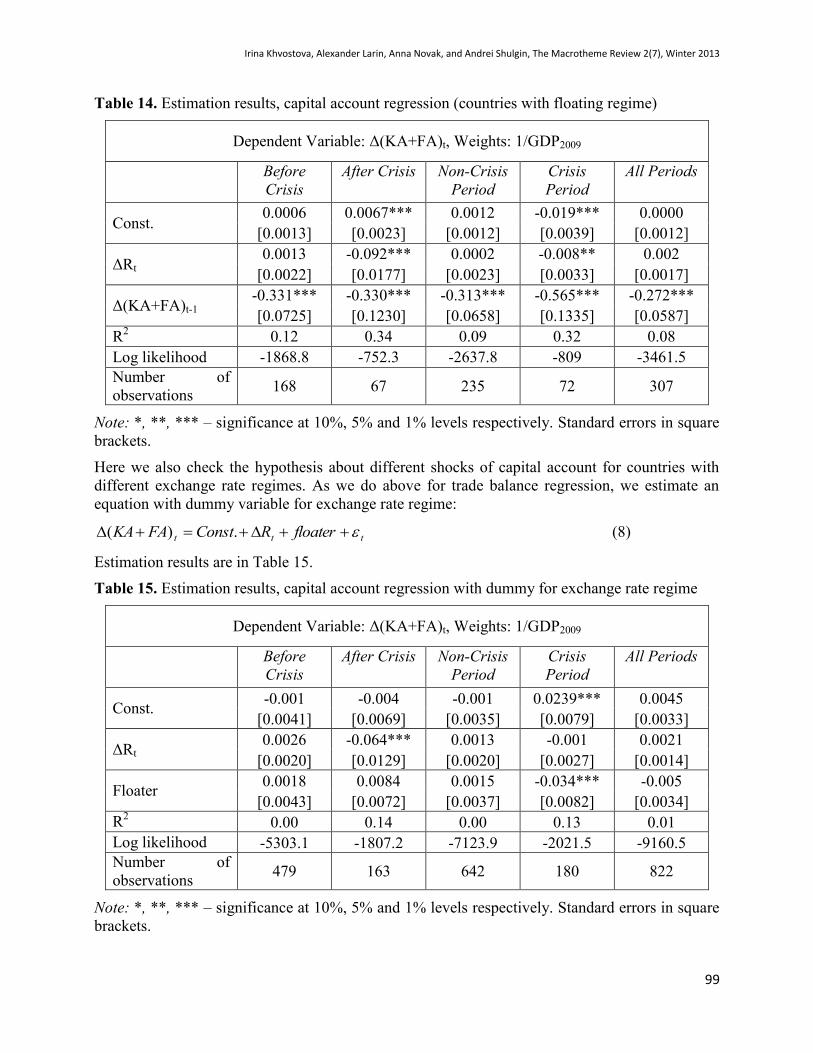
Table 14. Estimation results, capital account regression (countries with floating regime)


Before

Crisis


Period

Crisis

Period

All Periods

Const. 0.0006 0.0067*** 0.0012 -0.019*** 0.0000

[0.0013] [0.0023] [0.0012] [0.0039] [0.0012]

ΔRt

0.0013 -0.092*** 0.0002 -0.008** 0.002

[0.0022] [0.0177] [0.0023] [0.0033] [0.0017]

Δ(KA+FA)t-1 -0.331*** -0.330*** -0.313*** -0.565*** -0.272***

[0.0725] [0.1230] [0.0658] [0.1335] [0.0587]

R2

0.12 0.34 0.09 0.32 0.08

Log likelihood -1868.8 -752.3 -2637.8 -809 -3461.5

Number of

observations 168 67 235 72 307


brackets.

Here we also check the hypothesis about different shocks of capital account for countries with

different exchange rate regimes. As we do above for trade balance regression, we estimate an

equation with dummy variable for exchange rate regime:

ttt floaterRConstFAKA .)( (8)

Estimation results are in Table 15.

Table 15. Estimation results, capital account regression with dummy for exchange rate regime


Before

Crisis


Period

Crisis

Period

All Periods

Const. -0.001 -0.004 -0.001 0.0239*** 0.0045

[0.0041] [0.0069] [0.0035] [0.0079] [0.0033]

ΔRt 0.0026 -0.064*** 0.0013 -0.001 0.0021

[0.0020] [0.0129] [0.0020] [0.0027] [0.0014]

Floater 0.0018 0.0084 0.0015 -0.034*** -0.005

[0.0043] [0.0072] [0.0037] [0.0082] [0.0034]

R2 0.00 0.14 0.00 0.13 0.01

Log likelihood -5303.1 -1807.2 -7123.9 -2021.5 -9160.5

Number of

observations 479 163 642 180 822


brackets.


100

In crisis period, dummy for exchange rate regime is insignificant. Thus, different shocks are not a

reason why reaction to interest rate was different. It supports the opinion that Central Bank

reaction to incoming shocks was different and stabilization policy was different depending on

exchange rate regime.

4. Concluding Remarks

This paper investigates BOP effects in the period of crisis of 2008-2009. Inference is based on

two subsamples. First subsample consists of 40 countries with floating exchange rate regime.

Second subsample consists of 38 countries with intermediate exchange rate regimes. The period

of crisis – from IV quarter 2008 to II quarter of 2009 – is chosen as period with unusual dynamics

of investigated variables.

Estimation results allow us to tell about differences in Central Bank policy for countries with

different exchange rate regimes. For countries with one of intermediate regimes, data support the

hypothesis about negative relation between trade balance and real effective exchange rate in the

period of crisis. After crisis, this negative relation became even clearer. At the same time, for

countries with floating exchange rate, this relation stayed positive.

The hypothesis of reversal effect is supported for both groups of countries – if trade balance goes

too far from its average level, we may expect its reversal dynamics.

The results for capital and financial account confirm the main conclusion – Central Bank policy

is highly influenced by exchange rate regime of the country. In crisis, statistically significant

relation between capital account and interest rate is observed only for countries with intermediate

exchange rate regime.

References

Bahmani-Oskooee, M. (1986) Determinants of International Trade Flows: the Case of Developing

Countries // Journal of Development Economics, 20, 107–123.

Bahmani-Oskooee, M., Kara, O. (2003) Relative Responsiveness of Trade Flows to a Change in Prices

and Exchange Rate // International Review of Applied Economics, 17(3), 293–308.

Bussiere, M., & Mulder, C. (1999) External Vulnerability in Emerging Market Economies: How High

Liquidity Can Offset Weak Fundamentals and the Effects of Contagion // IMF Working Paper 88.

Boyd, D., Caporale, G.M., Smith, R. (2001) Real Exchange Rate Effects on the Balance of Trade:

Cointegration and the Marshall–Lerner Condition // International Journal of Finance and Economics, 6,

187–200.

Calvo, G. A. (1996) Capital Flows and Macroeconomic Management: Tequila Lessons // International

Journal of Finance Economics, 1, 207–223

Chung K., Turnovsky S. (2009.) Foreign Debt Supply in an Imperfect International Capital Market:

Theory and Evidence. // Journal of International Money and Finance, 29, 201–223

Edwards S. (2001) Does the Current Account Matter? // National Bureau of Economic Research, Inc. WP

8275

Eichengreen, B. (2003). Capital Flows and Crises // Cambridge, Massachusetts: The MIT Press.

Frankel J., Rose A. (1996) Currency Crashes in Emerging Markets: An Empirical Treatment // Journal of

International Economics, 41(3–4), 351–366.

http://ideas.repec.org/h/nbr/nberch/10633.html

http://ideas.repec.org/s/eee/inecon.html



101

Freund, C.L. (2005) Current Account Adjustments in Industrialized Countries // Journal of International

Money and Finance, 24 (8), 1278–1298.

Galí J., Monacelli T. (2008) Optimal Monetary and Fiscal Policy in a Currency Union // Journal of

International Economics, 76(1), 116-132.

Gomes F., Paz L. (2005) Can Real Exchange Rate Devaluation Improve the Trade Balance? The 1990–

1998 Brazilian case // Applied Economics Letters, 12, 525–528.

Hacker, R., Hatemi-J, A. (2004) The Effect of Exchange Rate Changes on Trade Balances in the Short and

Long Run: Evidence from German Trade with Transitional Central European Economies. // Economics of

Transition, 12(4), 777–799.

Junz, H., Rhomberg R. R. (1973) Price Competitiveness in Export Trade Among Industrial Countries //

American Economic Review, Papers and Proceedings, 63, 412–418.

Kharel R., Martin C., Milas C. (2010) The Complex Response of Monetary Policy to the Exchange Rate //

Scottish Journal of Political Economy, 57, 103–117.

Lahiri A., Vegh C. (2003) Delaying the Inevitable: Interest Rate Defense and BOP Crises // Journal of

Political Economy, 111(2), 404-424.

Lee, J., Chinn, M. D. (1998) The Current account and the Real Exchange Rate: a Structural VAR Analysis

of Major Currencies // National Bureau of Economic Research, Inc. WP6495.

Mann, C.L. (2002) Perspectives on the US Current Account Deficit and Sustainability // Journal of

Economic Perspectives, 16 (3), 131–152.

Milesi-Ferretti, G.M., Razin A. (1998) Current Account Reversals and Currency Crises: Empirical

Regularities // IMF Working Papers 98/89.

Muller-Plantenberg N. (2010) BOP Accounting and Exchange Rate Dynamics // International Review of

Economics and Finance, 19, 46–63.

Obstfeld, M., Rogoff, K. (2005) The Unsustainable US Current Account Position Revisited // University

of California Berkeley, Mimeo, WP10869.

Orcutt, G. H. (1950) Measurement of Price Elasticities in International Trade // Review of Economics and

Statistics, May, 117–132.

Pontines, V., Siregar, R. (2008) Fundamental Pitfalls of Exchange Market Pressure-based Approaches to

Identification of Currency Crises // International Review of Economics and Finance, 17(3), 345−365.

Pak-Hung, M. (2009) Impossible Trinity, Capital Flow Market and Financial Stability // Kyklos,

Blackwell Publishing, 62(4), 611–618.

Ranciere R., Jeanne O. (2006) The Optimal Level of International Reserves for Emerging Market

Countries: Formulas and Applications // IMF Working Papers 06/229.

Rose, A. K. (1991) The Role of Exchange Rates in a Popular Model of International Trade: Does the

‘Marshall–Lerner’s Condition Hold? // Journal of International Economics, 30, 301–316.

Summers, L. C. (1996) Volatile Capital Flows: Taming Their Impact on Latin America // Inter-American

Development Bank and Johns Hopkins University Press, Baltimore, 53–57.

Svensson, L.E.O. (2001) Transparency and Credibility: Monetary Policy with Unobservable Goals. //

International Economic Review, 42 (2), 369–397.

Svensson, L.E.O. (2003) Comment on: The Future of Monetary Aggregates in Monetary Policy Analysis

// Journal of Monetary Economics, 50/5, 1061–1070.

http://ideas.repec.org/p/upf/upfgen/909.html



http://www3.interscience.wiley.com/journal/118796306/abstract



http://onlinelibrary.wiley.com/doi/10.1111/sjpe.2010.57.issue-1/issuetoc

http://ideas.repec.org/s/imf/imfwpa.html

http://ideas.repec.org/a/bla/kyklos/v62y2009i4p611-618.html

http://ideas.repec.org/s/bla/kyklos.html

http://ideas.repec.org/p/imf/imfwpa/06-229.html

http://ideas.repec.org/p/imf/imfwpa/06-229.html

http://ideas.repec.org/s/imf/imfwpa.html

http://82.179.249.32:2076/record/display.url?eid=2-s2.0-0009903373&origin=reflist&sort=plf-f&src=s&st1=svensson&nlo=&nlr=&nls=&sid=nXd1oIt4lJKcYMUPp3M7-50%3a340&sot=b&sdt=cl&cluster=scosubjabbr%2c%22ECON%22%2ct%2c%22MULT%22%2ct%2bscoexactsrctitle%2c%22Journal+of+Monetary+Economics%22%2ct%2c%22Journal+of+International+Economics%22%2ct%2c%22European+Economic+Review%22%2ct%2bscopubyr%2c%222003%22%2ct%2c%222002%22%2ct%2c%222000%22%2ct&sl=21&s=AUTHOR-NAME%28svensson%29

http://82.179.249.32:2076/authid/detail.url?authorId=7201590382

http://82.179.249.32:2076/source/sourceInfo.url?sourceId=17555&origin=recordpage


102

Taylor, A.M. (2002) A Century of Current Account Dynamics // Journal of International Money and

Finance, 21 (6), 725–748.

Tegene, A. (1991) Trade Flows, Relative Prices, and Effective Exchange Rates: a VAR on Ethiopian Data

// Applied Economics, 23, 1369–1375.

Wilson, J.F., Takacs, W.E. (1979) Differential Responses to Price and Exchange Rate Influences in the

Foreign Trade of Selected Industrial Countries // Review of Economics and Statistics, 61(2), 267–279.

The Macrotheme Reviewmacrotheme.com/yahoo_site_admin/assets/docs/8nusMR... · Irina Khvostova, Alexander Larin, Anna Novak, and Andrei Shulgin, The Macrotheme Review 2(7), Winter

Documents