The Low-z Intergalactic Medium. II. LyB, OVI, and CIII Forest

arX

iv:a

stro

-ph/

0508

656v

2 1

Dec

200

5Draft version February 5, 2008Preprint typeset using LATEX style emulateapj v. 6/22/04

THE LOW-z INTERGALACTIC MEDIUM. II. Lyβ, OVI, AND C III FOREST

Charles W. Danforth, J. Michael Shull, Jessica L. Rosenberg1, & John T. StockeCenter for Astrophysics and Space Astronomy, Dept. of Astrophysial & Planetary Sciences, University of Colorado, Boulder, CO 80309;

[email protected], [email protected], [email protected] version February 5, 2008

ABSTRACT

We present the results of a large survey of H I, O VI, and C III absorption lines in the low-redshift(z < 0.3) intergalactic medium (IGM). We begin with 171 strong Lyα absorption lines (Wλ ≥ 80 mA)in 31 AGN sight lines studied with the Hubble Space Telescope and measure corresponding absorptionfrom higher-order Lyman lines with FUSE. Higher-order Lyman lines are used to determine NHI andbHI accurately through a curve-of-growth (COG) analysis. We find that the number of H I absorbers

per column density bin is a power-law distribution, dN/dNHI ∝ N−βHI , with βHI = 1.68 ± 0.11. We

made 40 detections of O VI λλ1032,1038 and 30 detections of C III λ977 out of 129 and 148 potentialabsorbers, respectively. The column density distribution of C III absorbers has βCIII = 1.68 ± 0.04,similar to βHI but not as steep as βOVI = 2.1± 0.1. From the absorption-line frequency, dNCIII/dz =12+3

−2 for Wλ(CIII) > 30 mA, we calculate a typical IGM absorber size r0 ∼ 400 kpc, similar to scales

derived by other means. The COG-derived b-values show that H I samples material with T < 105 K,incompatible with a hot IGM phase. By calculating a grid of CLOUDY models of IGM absorbers witha range of collisional and photoionization parameters, we find it difficult to simultaneously account forthe O VI and C III observations with a single phase. Instead, the observations require a multiphaseIGM in which H I and C III arise in photoionized regions, while O VI is produced primarily throughshocks. From the multiphase ratio NHI/NCIII, we infer the IGM metallicity to be ZC = 0.12 Z⊙,similar to our previous estimate of ZO = 0.09 Z⊙ from O VI.

Subject headings: cosmological parameters—cosmology: observations—intergalactic medium—quasars: absorption lines

1. INTRODUCTION

The study of the intergalactic medium (IGM) is cru-cial for understanding the structure and evolution ofgalaxies. Much has been learned from the distribu-tion of visible galaxies in large-scale structure, but alarge fraction of the baryonic mass of the universe stillresides in the IGM (Cen & Ostriker 1999a; Cen et al.2001; Dave et al. 1999, 2001), even at low redshift(Stocke, Shull, & Penton 2005). These intergalactic ab-sorbers are likely composed of primordial material leftover from the big bang and processed material ejectedfrom galaxies. The identification of these absorbers andtheir origins will help to constrain both the evolution ofprimordial gas in the universe as well as galactic outflowsand metal processing. By comparing local, low-redshiftIGM absorbers with those in the high-redshift universe,we can watch the evolution of these processes throughcosmic time.

The IGM is best probed with absorption-line stud-ies using distant continuum sources such as quasars andAGN. H I is best detected through Lyman line absorp-tion in the rest-frame far ultraviolet (FUV; 912–1216 A),particularly Lyα at 1216 A. Ironically, much analysis hasbeen done of the Lyα forest and metal lines in the dis-tant universe (2 < z < 5), but comparatively little existsfor the local universe (z < 1). To fill this gap in ourknowledge, we must examine the IGM in the FUV.

The Lyα line is arguably the most important diagnos-

1 NSF Astronomy and Astrophysics Postdoctoral Fellow, cur-rently at Harvard-Smithsonian Center for Astrophysics;[email protected]

tic of the IGM, but it has inherent limitations. Stronglines exhibit saturation and blending from weaker, un-resolved components. Profile fits to the Lyα line tendto underestimate H I column density and overestimatethe Doppler width (Shull et al. 2000). For more accurateanalysis, weaker Lyman lines such as Lyβ are required inconjunction with Lyα. The trade-off is that weaker linesare more difficult to detect and, at low redshift, lie ina wavelength range complicated with H2 and ionic linesfrom the local interstellar medium (ISM).

The Hubble Space Telescope (HST) has housed a pairof ultraviolet instruments, the Goddard High Resolu-tion Spectrograph (GHRS) and the Space Telescope Imag-ing Spectrograph (STIS), which have brought UV spec-troscopy into a golden age with high-resolution spectro-graphic capabilities down to ∼1150 A. The Far Ultra-violet Spectroscopic Explorer (FUSE) complements thecapabilities of HST, providing coverage of the 905–1187A band with the higher Lyman lines missed by HST atz < 0.12 as well as the important diagnostic lines ofO VI λλ1032, 1038 and C III λ977 out to modest red-shifts (Moos et al. 2000).

These spectrographs have compiled a sizeable catalogof IGM absorbers along extragalactic sight lines. Absorp-tion systems in the IGM can be identified using strongLyα lines in the relatively uncomplicated spectral regionof GHRS and STIS data. Once located, the higher Ly-man lines and metal diagnostics covered by FUSE give amuch more complete picture of the system.

In this study, we use published catalogs of Lyα ab-sorbers in extragalactic sight lines and search for coun-

2

terpart absorption in the higher Lyman lines (Lyβ, Lyγ,Lyδ, etc) to more accurately determine the column den-sity NHI and Doppler line width bHI for neutral hydro-gen in the IGM. Furthermore, we look for counterpartabsorption in probes of the crucial warm-hot ionizedmedium (WHIM), O VI λλ1031.926, 1037.617 and pos-sibly C III λ977.020. O VI is present in gas at 105−6

K and is thought to arise from shock ionization perhapswith some contribution from hard, ionizing external ra-diation in low density gas. The H I absorption can beseen in the FUSE band at 0.003 < z < 0.3, while O VI

and C III can be measured between 0 < z < 0.15 and0 < z < 0.21, respectively. We use these lines to gainbetter understanding of how gas becomes ionized in thelow-redshift universe.

We gave an overview of the project and some of themore important cosmological results in Danforth & Shull(2005; henceforth Paper I). In this paper, we describe incomplete detail our catalog of 171 Lyα absorbers in sightlines toward 31 AGN, including several dozen new Lyαabsorbers. We also describe our survey of Lyβ and C III

absorbers. We present our criteria for selection of sightlines and absorber in § 2 along with a list of previouslyunpublished Lyα absorbers. Our analysis methods andresults are presented in § 3. In § 4 we discuss the im-portance of multiple Lyman lines to accurate H I mea-surements, analyze the distribution of C III detections,discuss new evidence for a multiphase IGM, and inves-tigate the metallicity of the IGM. We summarize ourconclusions in § 5.

2. SIGHT LINES AND ABSORBERS

The catalog of FUSE observations of extragalacticsight lines is large enough that a statistical study ofO VI in the low-redshift IGM is feasible. We searchedthe catalog of observations for sight lines with previousquasar absorption-line studies. The majority of our tar-get list was obtained from the Colorado surveys basedon GHRS and STIS grating observations of 30 AGN(Penton, Stocke, & Shull 2000; Penton, Shull, & Stocke2000; Penton, Stocke, & Shull 2003, 2004). Six of thesetargets lack FUSE data of sufficient quality to be in-cluded in our survey. The target list was augmentedby additional studies of these sight lines from the litera-ture, using all available moderate and high-resolution UVdata. We analyzed archival STIS/E140M echelle data forsix additional sight lines as described below. Our finalsample consists of 31 sight lines with reasonable qual-ity FUSE data and a known set of Lyα absorbers (or aknown lack of Lyα absorbers) over at least part of theirpath length (Table 1). The total pathlength surveyed forLyα absorbers is noted in column 7 of Table 1.

One of our goals was to rigorously determine the H I

column density for the IGM absorbers via curves ofgrowth. Different authors use different techniques to de-termine column densities and b-values, resulting in a het-erogenous sample of absorber information. For this rea-son, the primary information we take from the Lyα sur-veys is absorber redshift zabs and Lyα equivalent widthWLyα, both of which are measured directly from the dataand are not subject to analytical interpretation.

In six cases, we used archival STIS/E140M data andperformed our own Lyα absorber search. The datawere smoothed by three pixels to better match the in-

strumental resolution. For four targets (PKS 0405−123,PG0953+415, PG1259+593, and PKS1302−102), ouranalysis was carried out as follows: (1) the major ab-sorption and emission line regions were marked by handfor exclusion; (2) the excluded regions of the spectrumwere then replaced with a linear interpolation over tenpixels on either side of the excluded region; (3) a roughsmoothing over 100 pixels was applied to the resultingcontinuum;, finally (4) a cubic-spline linear interpolationwas derived from all of the continuum data points thatwere less than 2σ from the smoothed continuum value.This linear interpolation over points deviating by lessthan 2σ from the smoothed value for the continuum wasthe fit used in the processing of the data. The one ex-ception was for lines that fell on the damping wings ofGalactic Lyα; in these cases a local fit to the continuumwas performed.

The measurement of the absorption lines in the E140Mdata was performed using the program VPFIT2 whichperforms Voigt profile fitting for each of the lines. Theline fitting was performed interactively for each of thelines. In general, we were conservative about addingmultiple components to the fit since the fit can almostalways be improved by adding these components even ifit is not justified by an F-test. We did, however, addmultiple components to the Lyα fits in cases where thehigher Lyman lines or metal lines for the same absorberindicated a multi-component structure. In some of thesecases, we use the information derived from the high-orderlines to fix the positions and/or the b-values for the Lyαline fits.

In two other cases, HE 0226−4110 and PHL1811, weanalyzed the STIS/E140M data using an IDL code ina manner procedurally similar to that described above.Strong absorption lines at λ > 1216 A were flagged aspossible intervening Lyα lines. Candidate Lyα lines wereconfirmed by checking for counterpart Lyβ and Lyγ ab-sorption before being accepted. Equivalent widths weremeasured interactively from the normalized Lyα pro-files. As above, multiple components were not used un-less there was compelling evidence for their existence inweaker Lyman lines. The STIS/G140M data for Mrk 876were analyzed similarly. In all, our analysis yielded con-sistent results with published data in terms of velocitiesand equivalent widths.

The distribution of H I absorbers as a functionof column density is a power law with a negativeslope as discussed below (Penton, Shull, & Stocke 2000;Penton, Stocke, & Shull 2004). Thus, the absorber listfeatures many weak absorbers and relatively few strongsystems. The ratio of equivalent widths for unsaturatedH I absorbers is equal to the ratio of fλ2 between thelines, a factor of 6.24 for Lyα and Lyβ. Since the 3σlimiting equivalent width of good FUSE data is typi-cally 10-20 mA, we set an equivalent width threshold ofWLyα > 80 mA to have any realistic chance of detectingweaker Lyman series or ionic lines. Profile fits to weakLyα lines typically give more accurate column densitiesthan strong lines (in the absense of a sufficiently opticallythin higher order line), so curve-of-growth (COG) fitting

2 VPFIT was written by R. F. Carswell, J. K. Webb, M. J.Irwin, & A. J. Cooke. More information is available athttp://www.ast.cam.ac.uk/∼rfc/vpfit.html

3

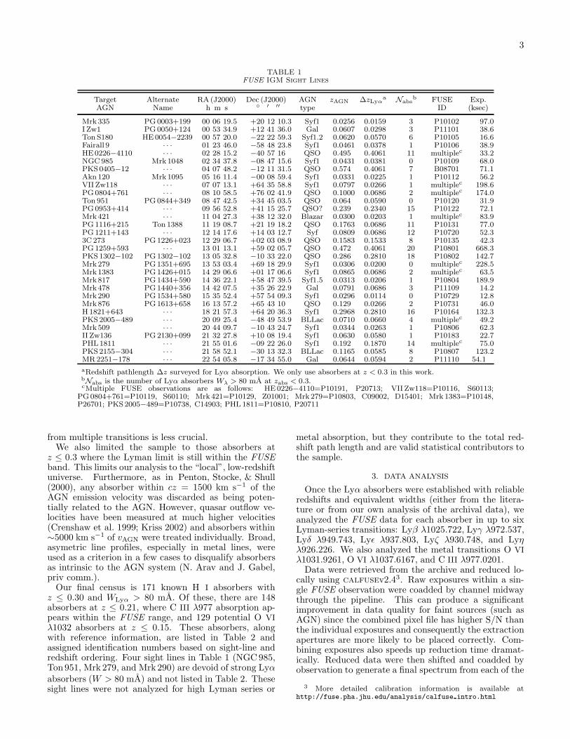
TABLE 1FUSE IGM Sight Lines

Target Alternate RA(J2000) Dec (J2000) AGN zAGN ∆zLyαa Nabs

b FUSE Exp.AGN Name h m s ◦ ′ ′′ type ID (ksec)

Mrk335 PG0003+199 00 06 19.5 +20 12 10.3 Syf1 0.0256 0.0159 3 P10102 97.0I Zw1 PG0050+124 00 53 34.9 +12 41 36.0 Gal 0.0607 0.0298 3 P11101 38.6Ton S180 HE 0054−2239 00 57 20.0 −22 22 59.3 Syf1.2 0.0620 0.0570 6 P10105 16.6Fairall 9 · · · 01 23 46.0 −58 48 23.8 Syf1 0.0461 0.0378 1 P10106 38.9HE0226−4110 · · · 02 28 15.2 −40 57 16 QSO 0.495 0.4061 11 multiplec 33.2NGC 985 Mrk1048 02 34 37.8 −08 47 15.6 Syf1 0.0431 0.0381 0 P10109 68.0PKS0405−12 · · · 04 07 48.2 −12 11 31.5 QSO 0.574 0.4061 7 B08701 71.1Akn 120 Mrk1095 05 16 11.4 −00 08 59.4 Syf1 0.0331 0.0225 1 P10112 56.2VII Zw118 · · · 07 07 13.1 +64 35 58.8 Syf1 0.0797 0.0266 1 multiplec 198.6PG0804+761 · · · 08 10 58.5 +76 02 41.9 QSO 0.1000 0.0686 2 multiplec 174.0Ton 951 PG0844+349 08 47 42.5 +34 45 03.5 QSO 0.064 0.0590 0 P10120 31.9PG0953+414 · · · 09 56 52.8 +41 15 25.7 QSO? 0.239 0.2340 15 P10122 72.1Mrk421 · · · 11 04 27.3 +38 12 32.0 Blazar 0.0300 0.0203 1 multiplec 83.9PG1116+215 Ton 1388 11 19 08.7 +21 19 18.2 QSO 0.1763 0.0686 11 P10131 77.0PG1211+143 · · · 12 14 17.6 +14 03 12.7 Syf 0.0809 0.0686 12 P10720 52.33C 273 PG1226+023 12 29 06.7 +02 03 08.9 QSO 0.1583 0.1533 8 P10135 42.3PG1259+593 · · · 13 01 13.1 +59 02 05.7 QSO 0.472 0.4061 20 P10801 668.3PKS1302−102 PG1302−102 13 05 32.8 −10 33 22.0 QSO 0.286 0.2810 18 P10802 142.7Mrk279 PG1351+695 13 53 03.4 +69 18 29.9 Syf1 0.0306 0.0200 0 multiplec 228.5Mrk1383 PG1426+015 14 29 06.6 +01 17 06.6 Syf1 0.0865 0.0686 2 multiplec 63.5Mrk817 PG1434+590 14 36 22.1 +58 47 39.5 Syf1.5 0.0313 0.0206 1 P10804 189.9Mrk478 PG1440+356 14 42 07.5 +35 26 22.9 Gal 0.0791 0.0686 3 P11109 14.2Mrk290 PG1534+580 15 35 52.4 +57 54 09.3 Syf1 0.0296 0.0114 0 P10729 12.8Mrk876 PG1613+658 16 13 57.2 +65 43 10 QSO 0.129 0.0266 2 P10731 46.0H1821+643 · · · 18 21 57.3 +64 20 36.3 Syf1 0.2968 0.2810 16 P10164 132.3PKS2005−489 · · · 20 09 25.4 −48 49 53.9 BLLac 0.0710 0.0660 4 multiplec 49.2Mrk509 · · · 20 44 09.7 −10 43 24.7 Syf1 0.0344 0.0263 1 P10806 62.3II Zw136 PG2130+099 21 32 27.8 +10 08 19.4 Syf1 0.0630 0.0580 1 P10183 22.7PHL1811 · · · 21 55 01.6 −09 22 26.0 Syf1 0.192 0.1870 14 multiplec 75.0PKS2155−304 · · · 21 58 52.1 −30 13 32.3 BLLac 0.1165 0.0585 8 P10807 123.2MR2251−178 · · · 22 54 05.8 −17 34 55.0 Gal 0.0644 0.0594 2 P11110 54.1

aRedshift pathlength ∆z surveyed for Lyα absorption. We only use absorbers at z < 0.3 in this work.bNabs is the number of Lyα absorbers Wλ > 80 mA at zabs < 0.3.cMultiple FUSE observations are as follows: HE 0226−4110=P10191, P20713; VII Zw118=P10116, S60113;

PG0804+761=P10119, S60110; Mrk421=P10129, Z01001; Mrk279=P10803, C09002, D15401; Mrk 1383=P10148,P26701; PKS2005−489=P10738, C14903; PHL 1811=P10810, P20711

from multiple transitions is less crucial.We also limited the sample to those absorbers at

z ≤ 0.3 where the Lyman limit is still within the FUSEband. This limits our analysis to the “local”, low-redshiftuniverse. Furthermore, as in Penton, Stocke, & Shull(2000), any absorber within cz = 1500 km s−1 of theAGN emission velocity was discarded as being poten-tially related to the AGN. However, quasar outflow ve-locities have been measured at much higher velocities(Crenshaw et al. 1999; Kriss 2002) and absorbers within∼5000 km s−1 of vAGN were treated individually. Broad,asymetric line profiles, especially in metal lines, wereused as a criterion in a few cases to disqualify absorbersas intrinsic to the AGN system (N. Arav and J. Gabel,priv comm.).

Our final census is 171 known H I absorbers withz ≤ 0.30 and WLyα > 80 mA. Of these, there are 148absorbers at z ≤ 0.21, where C III λ977 absorption ap-pears within the FUSE range, and 129 potential O VI

λ1032 absorbers at z ≤ 0.15. These absorbers, alongwith reference information, are listed in Table 2 andassigned identification numbers based on sight-line andredshift ordering. Four sight lines in Table 1 (NGC 985,Ton951, Mrk 279, and Mrk 290) are devoid of strong Lyαabsorbers (W > 80 mA) and not listed in Table 2. Thesesight lines were not analyzed for high Lyman series or

metal absorption, but they contribute to the total red-shift path length and are valid statistical contributors tothe sample.

3. DATA ANALYSIS

Once the Lyα absorbers were established with reliableredshifts and equivalent widths (either from the litera-ture or from our own analysis of the archival data), weanalyzed the FUSE data for each absorber in up to sixLyman-series transitions: Lyβ λ1025.722, Lyγ λ972.537,Lyδ λ949.743, Lyǫ λ937.803, Lyζ λ930.748, and Lyηλ926.226. We also analyzed the metal transitions O VI

λ1031.9261, O VI λ1037.6167, and C III λ977.0201.Data were retrieved from the archive and reduced lo-

cally using calfusev2.43. Raw exposures within a sin-gle FUSE observation were coadded by channel midwaythrough the pipeline. This can produce a significantimprovement in data quality for faint sources (such asAGN) since the combined pixel file has higher S/N thanthe individual exposures and consequently the extractionapertures are more likely to be placed correctly. Com-bining exposures also speeds up reduction time dramat-ically. Reduced data were then shifted and coadded byobservation to generate a final spectrum from each of the

3 More detailed calibration information is available athttp://fuse.pha.jhu.edu/analysis/calfuse intro.html

4

eight data channels. The data were binned by three pix-els; FUSE resolution is typically 8-10 pixels or roughly 3bins.

The data were normalized in 10 A segments centeredon the location of each IGM absorber as follows: the lo-cations of prominent Galactic ISM lines, IGM lines, andintrinsic absorption lines from the AGN were markedautomatically. Line-free regions were then selected in-teractively and fitted using Legendre polynomials of or-der less than six. The signal to noise per binned pixel(S/N)pix was established locally as the 1σ deviationfrom the mean in the line-free continuum regions within5 A of the IGM line. Given that a FUSE resolutionelement is typically 8–10 raw pixels (∼3 binned pix-els) or ∆V ≈ 20 km s−1, we adopt the relationship

(S/N)res =√

3 (S/N)pix throughout this study. Abso-lute velocity calibration in FUSE data is not determinedto much better than a resolution element. We calibratedeach segment by setting Galactic H2 lines to vlsr = 0. IfH2 lines were unavailable, low-ionization ISM lines (Ar I,Si II, Fe II, P II) in the area were used or, if necessary,other IGM lines. This process was carried out for eachtransition of each absorber in each of up to four detectorchannels covering the wavelength region.

Once a collection of normalized spectral segments wasgenerated, the quantitative analysis began. Each tran-sition was examined and measured interactively in twoways. A multi-component Voigt profile fit was performedon the IGM absorber as well as on any other nearby lineswith free parameters, v, b, and Nfit. From b and Nfit, theequivalent width Wfit was determined. We used as fewabsorption components as possible in our fits since arbi-trary additional components always improve the fit visu-ally. Second, an apparent column density Na, line width,Wa, and velocity centroid were determined via techniquesdescribed in Savage & Sembach (1991). Roughly half ofthe lines in our survey were fit using both apparent col-umn and Voigt fitting techniques and the resulting col-umn densities, velocity centroids, b-values, and equiva-lent widths are within the uncertainties in most cases forlow or moderate-saturation lines. Voigt fitting tends togive more reliable results for saturated lines and lineswhere blending and multiple components are present.The apparent column method is superior in noisy dataor in weak absorbers where a profile fit will be heavilyinfluenced by noise. All equivalent widths were shiftedto the rest frame: Wr = Wobs(1 + z)−1.

A 3σ upper limit on equivalent width was also deter-mined for each absorber based on the spectrograph reso-lution R = λ/∆λ and local signal-to-noise per resolutionelement (S/N)res,

Wmin =3 λ

R (S/N)res, (1)

where R = λ/∆λ ≈ 15, 000. In cases where no absorp-tion was detected or when a detection was below a 3σlevel, the upper limit equivalent width was substituted.In cases where a line was strongly blended, the total,blended equivalent width was used as an upper limit.

Roughly half the sight lines featured moderate tostrong absorption by Galactic H2 at λ < 1120 A outof rotational levels J ≤ 4. We modeled and removedthese lines when possible using a database of H2 columnmeasurements compiled by Gillmon et al. (2005). How-

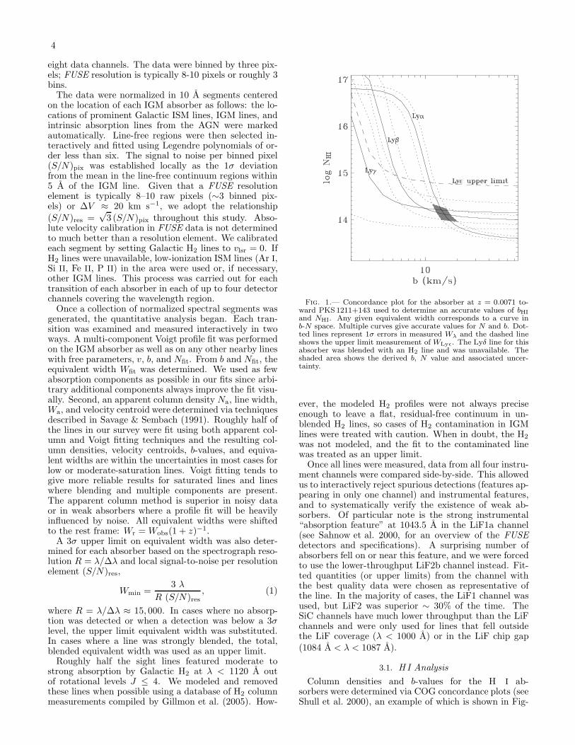
Fig. 1.— Concordance plot for the absorber at z = 0.0071 to-ward PKS 1211+143 used to determine an accurate values of bHI

and NHI. Any given equivalent width corresponds to a curve inb-N space. Multiple curves give accurate values for N and b. Dot-ted lines represent 1σ errors in measured Wλ and the dashed lineshows the upper limit measurement of WLyǫ. The Lyδ line for thisabsorber was blended with an H2 line and was unavailable. Theshaded area shows the derived b, N value and associated uncer-tainty.

ever, the modeled H2 profiles were not always preciseenough to leave a flat, residual-free continuum in un-blended H2 lines, so cases of H2 contamination in IGMlines were treated with caution. When in doubt, the H2

was not modeled, and the fit to the contaminated linewas treated as an upper limit.

Once all lines were measured, data from all four instru-ment channels were compared side-by-side. This allowedus to interactively reject spurious detections (features ap-pearing in only one channel) and instrumental features,and to systematically verify the existence of weak ab-sorbers. Of particular note is the strong instrumental“absorption feature” at 1043.5 A in the LiF1a channel(see Sahnow et al. 2000, for an overview of the FUSEdetectors and specifications). A surprising number ofabsorbers fell on or near this feature, and we were forcedto use the lower-throughput LiF2b channel instead. Fit-ted quantities (or upper limits) from the channel withthe best quality data were chosen as representative ofthe line. In the majority of cases, the LiF1 channel wasused, but LiF2 was superior ∼ 30% of the time. TheSiC channels have much lower throughput than the LiFchannels and were only used for lines that fell outsidethe LiF coverage (λ < 1000 A) or in the LiF chip gap(1084 A < λ < 1087 A).

3.1. H I Analysis

Column densities and b-values for the H I ab-sorbers were determined via COG concordance plots (seeShull et al. 2000), an example of which is shown in Fig-

5

ure 1. Each value of equivalent width for a particular setof atomic parameters traces out a curve in b, N space.By plotting curves from several transitions with a highcontrast in fλ, we can determine the accurate columndensity Ncog and b-value. This method is equivalent to atraditional curve of growth fit, but it gives a better ideaof the degree of uncertainty involved in both parame-ters. In several cases, anomalously strong absorption inone Lyman line or another was caught and corrected bythis technique.

Several Lyα absorbers in our sample show clear ev-idence of multiple components, and many others un-doubtedly feature unresolved structure. Since our studyfocusses primarily on O VI absorption, we have combinedresolved H I components into single absorbers in caseswhere only one, broad O VI absorber is seen; for exam-ple, the pair of H I absorbers at z = 0.0948 and 0.0950toward PKS1302-102 show a single, broad O VI line andthus have been combined into one absorber. Other cases,where both Lyα and O VI show clear multiple structure,have been treated as separate absorbers.

To test our concordance plot method of determin-ing N and b, we simulated multi-component absorberswith a grid of ∼ 100 models varying the column den-sity ratio (N1/N2 = 1 − 10) and velocity separation(∆v = 0 − 75 km s−1). We measured the equivalentwidth of the blended pair of simulated absorbers andtreated them as a single absorber without any a prioriknowledge of their structure. For a pair of simulatedH I absorbers with column densities N1 and N2 and linewidths b1 and b2 separated by ∆v, a COG analysis ofthe blended system yields a combined column densityno more than 20% greater than N1 + N2 and usuallysubstantially better. The derived line width is affectedby unresolved structure as component separation mimicsa larger b value. Nevertheless, we find empirically thatb2COG ≤ b2

max +0.45 (∆v)2 where bmax is the larger of thetwo component linewidths. Multiple components, for in-stance multiple absorbers within the same galaxy clus-ter, may mimic a broader single absorber, but the effectis small for line separations of FUSE instrumental reso-lution or less. Total column density is essentially insen-sitive to blended sub-components via our methods. Thisresult is consistent with that found by Jenkins (1986).

Our COG-derived N and b values for the H I absorbers,along with 1σ limits, are listed in Table 3. In somecases, particularly for weak absorbers, concordance plotsyielded no useful information and we adopt N and b fromother sources. In most of these cases, we adopt mea-surements from Lyα-only fits or apparent column mea-surements quoted in the literature or measured by theColorado group. In a few cases, we assume b = 20 ± 10km s−1 and derive N based on the observed Lyα equiv-alent width. These cases are noted in Table 3.

As a further check on the validity of our methods, wechecked our bHI and NHI values against published values.There are surprisingly few COG-qualified H I measure-ments in the literature and we were only able to find 30H I absorbers for our comparison. Our NHI values areconsistent within ±1σ with published values in 20 out of30 cases (67%), within ±2σ in 24 cases (80%), and within±3σ in all cases. Doppler width is consistent within ±1σin 18 out of 28 cases (64%, two absorbers were disquali-fied from consideration because they were interpretted as

multiple absorbers in the litterature but as a single ab-sorber in this study) and within ±2σ in 26 cases (93%).We have noted > 2σ deviations from published values inTable 3. The median absolute deviance in the sample is∼ 0.6σ for both bHI and NHI. The two-sided deviancedistribution in each case is symetric and consistent withno systematic over- or under-prediction.

3.2. OVI and C III Analysis

The O VI doublet does not have enough contrast in fλto use concordance plots to determine accurate columns,nor are both lines detected for many absorbers. Appar-ent and/or profile-fit column densities and b-values wereadopted for these transitions. The equivalent width ofabsorption lines on the linear part of the curve of growthfollows the relation

Wλ =

(

πe2

mec

)

Nfλ2

c(2)

while line-center optical depth goes as

τ0 =

(

πe2

mec

)

Nfλ√π b

. (3)

Thus an absorbsion line saturates (reaches τ0 = 1) atequivalent width Wλ(sat) = (b/c)

√πλ = (153 mA) b25

where b25 is the Doppler parameter in units of 25 km s−1.This corresponds to NHI = (1013.62 cm−2) b25 for Lyα.For O VI, saturation occurs at a column density NOVI

∼ (1014.09 cm−2) b25 and most of our O VI detections areat or below this level (see Figure 1a of Paper I). Similarly,C III saturates at NCIII ∼ (1013.35 cm−2) b25 which iswithin the range of our measurements. Any saturation inionic absorbers is mild at worst, and Voigt profile fits andapparent column measurements are probably indicativeof the true values. For upper limit cases, the S/N-based3σ minimum equivalent width was converted to columndensity via a curve of growth assuming b = 25 km s−1.

Our measured line widths and equivalent widths forthe O VI doublet absorbers are listed in Table 4. Incases where both lines of the O VI doublet were de-tected, an error-weighted mean of the columns was takenas the canonical value. Quoted errors are 1σ uncertain-ties based on line fits. In some cases, absorption is seenat velocities different from the expected value. Part ofthe difference is due to the variable FUSE wavelengthsolution and uncertainty in the fiducial Lyα absorber ve-locity, but ∆v > 30 km s−1 probably represents a realkinematic difference. High-∆v cases are noted in Table 4.

C III has only one resonance transition at 977.02 A inthe FUSE band, which makes detection more challeng-ing than for the O VI doublet lines. Furthermore, low-redshift C III absorbers must be measured at λ < 1000 Awhere the H2 line density is high and FUSE S/N is low.On the other hand, the short rest wavelength of C III

allows absorbers to be measured out to a higher red-shift (z ≤ 0.21) in FUSE data. Column densities andb-values for C III were determined in the same way asO VI and are listed in Table 5. In several cases, mul-tiple C III components were seen in an evidently singleH I absorber. These were measured separately, and thequantities listed in Table 5 represent the total equivalentwidth and column for the system.

As a final step in our analysis, we carefully inspectedeach candidate O VI and C III absorber by hand to verify

6

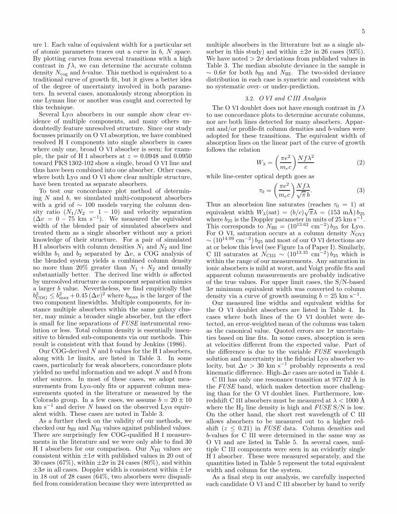
Fig. 2.— (Left) Comparison of line width measured from Lyα lines alone versus curve-of-growth b from our concordance plots. (Right)b value predictive accuracy as a function of NHI. There is little correlation between the b measured from concordance plots (bCOG) andfrom the Lyα line alone (bLyα), but bLyα tends to overpredict bCOG values. The ratio bLyα/bCOG has a faint dependence on columndensity, with the widths of stronger absorbers being more accurately predicted by Lyα-only measurements in comparison to lower NHI

lines. Median uncertainties are shown in the lower right of each panel.

its existence. Consequently, some detections were down-graded to upper limits because of blending or suspectdata features such as flat-fielding issues. In total, we de-tect 30 C III absorbers and 88 upper limits. O VI is de-tected in one or both lines of the doublet in 40 absorberswith 84 upper limits.

4. DISCUSSION

4.1. The Importance of Lyβ

The majority of the literature on IGM absorption lines,particularly at high redshift, is based on analysis of Lyαlines. A few words of caution regarding this are in order.Our curve-of-growth measurements of NHI and bHI us-ing multiple Lyman lines for each absorber should bemore accurate than measurements based on Lyα de-tections alone; Lyα lines saturate at logNHI ∼ 13.5(WLyα ∼ 180 b25 mA). We expect Lyα-only measure-ments to accurately describe the column and width ofweak absorbers where saturation is minimal, but theLyα-only measurements should grow increasingly inac-curate as saturation and unresolved subcomponents be-come more substantial. The median WLyα in our sample

is greater than 200 mA, so Lyα saturation is a definiteconcern.

Figure 2a shows no correlation between COG-determined Doppler width, bCOG, and line-width basedon the Lyα absorbers alone, bLyα. In general, bLyα

overpredicts the multi-line bCOG by a factor of two ormore as seen in Shull et al. (2000), but there is no othercorrelation. Using high-resolution data, Sembach et al.(2001) found multiple narrow velocity components withinthe Lyα absorption complex at z = 0.0053. TheirCOG analysis of this system using Lyα-Lyθ lines showsb = 16.1 ± 1.1 km s−1 and logNHI = 15.85+0.10

−0.08 while

Lyα-only measurements give b = 34.2 ± 3.3 km s−1 andlogNHI = 14.22± 0.07, a factor of two in line width and

43 in column density. Figure 2b shows bLyα/bCOG as afunction of NHI; the stronger absorbers show less line-width overprediction than the weaker absorbers. How-ever, given the heterogenous nature of the methods usedto measure Lyα line widths and column densities, we arehesitant to spend too much effort analyzing their differ-ences.

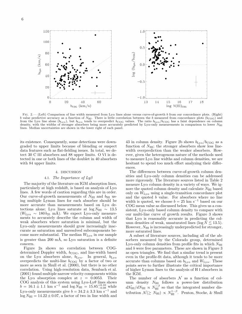
The differences between curve-of-growth column den-sities and Lyα-only column densities can be addressedmore rigorously. The literature sources listed in Table 2measure Lyα column density in a variety of ways. We ig-nore the quoted column density and calculate NHI basedonly on WLyα using a single-transition concordance plotand the quoted b value. For absorbers where no linewidth is quoted, we choose b = 25 km s−1 based on ourCOG mean value as discussed below. This gives us a con-sistent, Lyα-only based column density to compare withour multi-line curve of growth results. Figure 3 showsthat Lyα is reasonably accurate in predicting the col-umn densities of weak, unsaturated lines (logN . 13.5).However, NHI is increasingly underpredicted for stronger,more saturated lines.

A subset of literature sources, including all of the ab-sorbers measured by the Colorado group, determinedLyα-only column densities from profile fits in which NHI

and b were free parameters. These are shown in Figure 3as open triangles. We find that a similar trend is presenteven in the profile-fit data, although it tends to be moreaccurate than columns based on bLyα and WLyα. Thesepoints serve to further illustrate the critical importanceof higher Lyman lines to the analysis of H I absorbers inthe IGM.

The number of absorbers N as a function of col-umn density NHI follows a power-law distribution

dNHI/dNHI ∝ N−βHI so that the integrated number dis-

tribution N (≥ NHI) ∝ N1−βHI . Penton, Stocke, & Shull

7

Fig. 3.— A comparison of column density determined from Lyαlines alone vs curve-of-growth column density. NHI determinedfrom WLyα and Lyα line width (circles) is less than that deter-mined from a COG using multiple Lyman lines. The underpredic-tion generally becomes worse for more saturated Lyα absorbers. Avalue b = 25 km s−1 is assumed for any absorbers with no listedLyα linewidth (open circles). Fitting Lyα lines with Voigt pro-files (triangles) generally gives a better match, but still tends tounderpredict NHI from a COG.

(2004) obtained values of β = 1.65±0.07 over the columndensity range 12.3 ≤ log NHI ≤ 14.5 and β = 1.33± 0.30for 14.5 ≤ log NHI ≤ 17.5, based on a similar set of ab-sorbers and an assumed b = 25 km s−1. Williger et al.(2006) find β = 2.06±0.14 for logNHI≥ 13.3 based on 60H I absorbers. Our sample is limited to WLyα > 80 mA,so much of the lower range in column density is missingwhen compared to the Penton sample, but we recreatethe power-law fits to the distribution using b and NHI

values from curves of growth. We find β = 1.85 ± 0.39for the weak absorbers (13.8 ≤ log NHI ≤ 14.5) andβ = 1.50 ± 0.23 for the stronger absorbers (14.5 ≤log NHI ≤ 17.5) but note that the individual sub-samplesare small and may be of reduced statistical significance.This slight steepening of the distribution between Lyα-only and full COG analyses is contrary to what we wouldexpect. Given that Lyα-only measurements tend to un-derpredict column density relative to full COG analysesas shown in Figure 3, we would expect a flatter distribu-tion, especially for stronger absorbers.

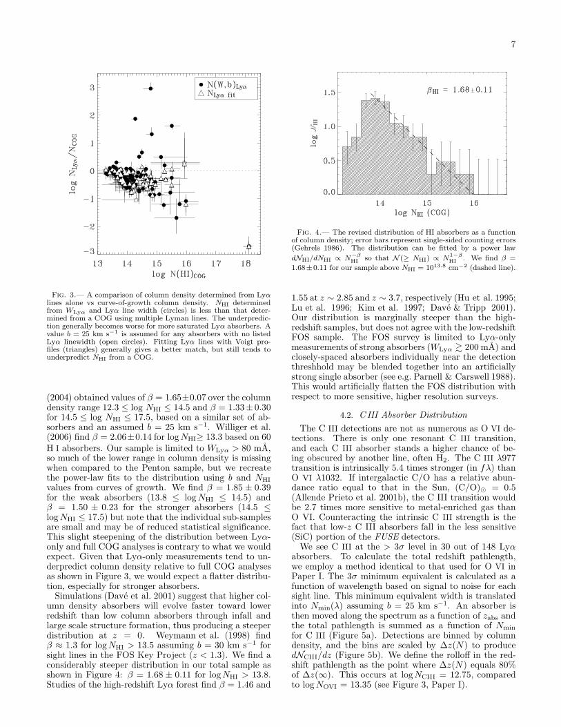
Simulations (Dave et al. 2001) suggest that higher col-umn density absorbers will evolve faster toward lowerredshift than low column absorbers through infall andlarge scale structure formation, thus producing a steeperdistribution at z = 0. Weymann et al. (1998) findβ ≈ 1.3 for logNHI > 13.5 assuming b = 30 km s−1 forsight lines in the FOS Key Project (z < 1.3). We find aconsiderably steeper distribution in our total sample asshown in Figure 4: β = 1.68 ± 0.11 for logNHI > 13.8.Studies of the high-redshift Lyα forest find β = 1.46 and

Fig. 4.— The revised distribution of HI absorbers as a functionof column density; error bars represent single-sided counting errors(Gehrels 1986). The distribution can be fitted by a power law

dNHI/dNHI ∝ N−β

HIso that N (≥ NHI) ∝ N1−β

HI. We find β =

1.68±0.11 for our sample above NHI = 1013.8 cm−2 (dashed line).

1.55 at z ∼ 2.85 and z ∼ 3.7, respectively (Hu et al. 1995;Lu et al. 1996; Kim et al. 1997; Dave & Tripp 2001).Our distribution is marginally steeper than the high-redshift samples, but does not agree with the low-redshiftFOS sample. The FOS survey is limited to Lyα-onlymeasurements of strong absorbers (WLyα & 200 mA) andclosely-spaced absorbers individually near the detectionthreshhold may be blended together into an artificiallystrong single absorber (see e.g. Parnell & Carswell 1988).This would artificially flatten the FOS distribution withrespect to more sensitive, higher resolution surveys.

4.2. CIII Absorber Distribution

The C III detections are not as numerous as O VI de-tections. There is only one resonant C III transition,and each C III absorber stands a higher chance of be-ing obscured by another line, often H2. The C III λ977transition is intrinsically 5.4 times stronger (in fλ) thanO VI λ1032. If intergalactic C/O has a relative abun-dance ratio equal to that in the Sun, (C/O)⊙ = 0.5(Allende Prieto et al. 2001b), the C III transition wouldbe 2.7 times more sensitive to metal-enriched gas thanO VI. Counteracting the intrinsic C III strength is thefact that low-z C III absorbers fall in the less sensitive(SiC) portion of the FUSE detectors.

We see C III at the > 3σ level in 30 out of 148 Lyαabsorbers. To calculate the total redshift pathlength,we employ a method identical to that used for O VI inPaper I. The 3σ minimum equivalent is calculated as afunction of wavelength based on signal to noise for eachsight line. This minimum equivalent width is translatedinto Nmin(λ) assuming b = 25 km s−1. An absorber isthen moved along the spectrum as a function of zabs andthe total pathlength is summed as a function of Nmin

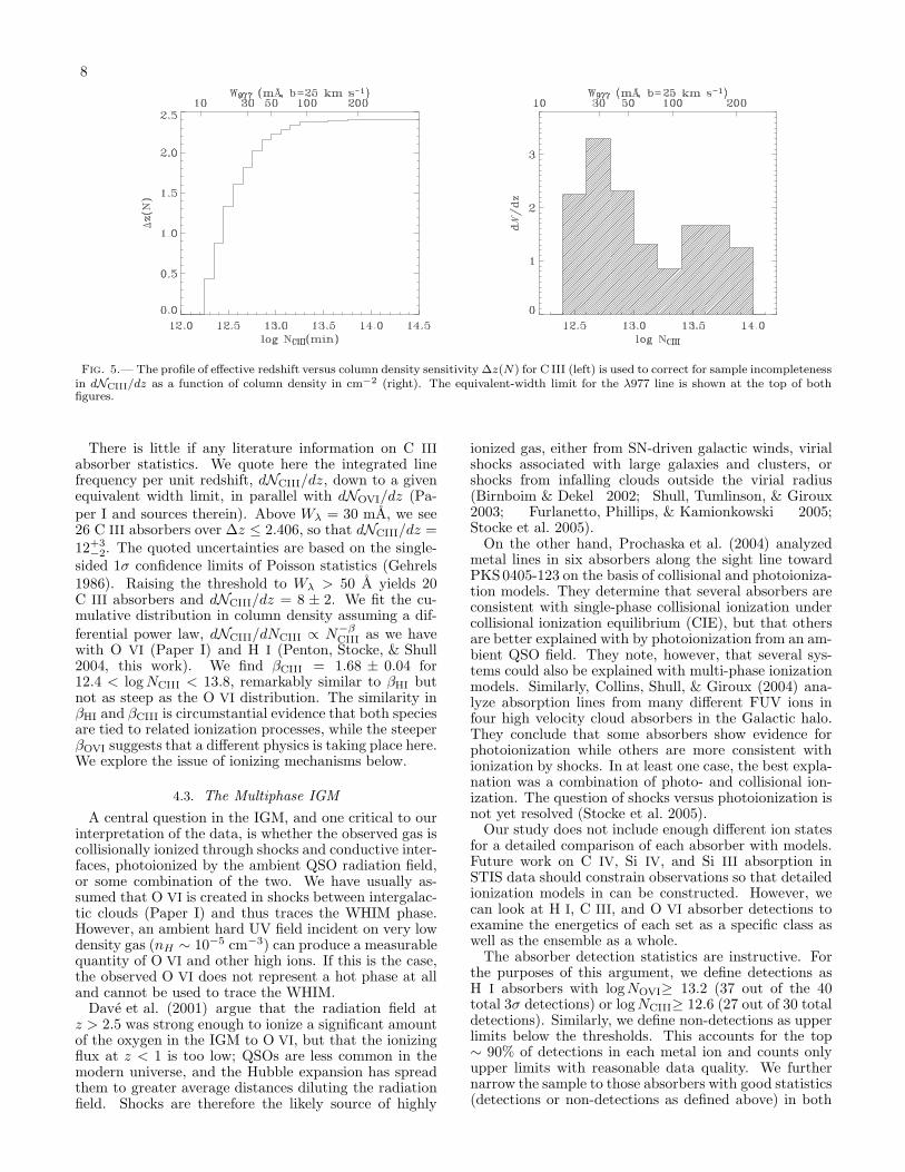
for C III (Figure 5a). Detections are binned by columndensity, and the bins are scaled by ∆z(N) to producedNCIII/dz (Figure 5b). We define the rolloff in the red-shift pathlength as the point where ∆z(N) equals 80%of ∆z(∞). This occurs at logNCIII = 12.75, comparedto logNOVI = 13.35 (see Figure 3, Paper I).

8

Fig. 5.— The profile of effective redshift versus column density sensitivity ∆z(N) for C III (left) is used to correct for sample incompletenessin dNCIII/dz as a function of column density in cm−2 (right). The equivalent-width limit for the λ977 line is shown at the top of bothfigures.

There is little if any literature information on C III

absorber statistics. We quote here the integrated linefrequency per unit redshift, dNCIII/dz, down to a givenequivalent width limit, in parallel with dNOVI/dz (Pa-per I and sources therein). Above Wλ = 30 mA, we see26 C III absorbers over ∆z ≤ 2.406, so that dNCIII/dz =12+3

−2. The quoted uncertainties are based on the single-sided 1σ confidence limits of Poisson statistics (Gehrels1986). Raising the threshold to Wλ > 50 A yields 20C III absorbers and dNCIII/dz = 8 ± 2. We fit the cu-mulative distribution in column density assuming a dif-

ferential power law, dNCIII/dNCIII ∝ N−βCIII as we have

with O VI (Paper I) and H I (Penton, Stocke, & Shull2004, this work). We find βCIII = 1.68 ± 0.04 for12.4 < log NCIII < 13.8, remarkably similar to βHI butnot as steep as the O VI distribution. The similarity inβHI and βCIII is circumstantial evidence that both speciesare tied to related ionization processes, while the steeperβOVI suggests that a different physics is taking place here.We explore the issue of ionizing mechanisms below.

4.3. The Multiphase IGM

A central question in the IGM, and one critical to ourinterpretation of the data, is whether the observed gas iscollisionally ionized through shocks and conductive inter-faces, photoionized by the ambient QSO radiation field,or some combination of the two. We have usually as-sumed that O VI is created in shocks between intergalac-tic clouds (Paper I) and thus traces the WHIM phase.However, an ambient hard UV field incident on very lowdensity gas (nH ∼ 10−5 cm−3) can produce a measurablequantity of O VI and other high ions. If this is the case,the observed O VI does not represent a hot phase at alland cannot be used to trace the WHIM.

Dave et al. (2001) argue that the radiation field atz > 2.5 was strong enough to ionize a significant amountof the oxygen in the IGM to O VI, but that the ionizingflux at z < 1 is too low; QSOs are less common in themodern universe, and the Hubble expansion has spreadthem to greater average distances diluting the radiationfield. Shocks are therefore the likely source of highly

ionized gas, either from SN-driven galactic winds, virialshocks associated with large galaxies and clusters, orshocks from infalling clouds outside the virial radius(Birnboim & Dekel 2002; Shull, Tumlinson, & Giroux2003; Furlanetto, Phillips, & Kamionkowski 2005;Stocke et al. 2005).

On the other hand, Prochaska et al. (2004) analyzedmetal lines in six absorbers along the sight line towardPKS0405-123 on the basis of collisional and photoioniza-tion models. They determine that several absorbers areconsistent with single-phase collisional ionization undercollisional ionization equilibrium (CIE), but that othersare better explained with by photoionization from an am-bient QSO field. They note, however, that several sys-tems could also be explained with multi-phase ionizationmodels. Similarly, Collins, Shull, & Giroux (2004) ana-lyze absorption lines from many different FUV ions infour high velocity cloud absorbers in the Galactic halo.They conclude that some absorbers show evidence forphotoionization while others are more consistent withionization by shocks. In at least one case, the best expla-nation was a combination of photo- and collisional ion-ization. The question of shocks versus photoionization isnot yet resolved (Stocke et al. 2005).

Our study does not include enough different ion statesfor a detailed comparison of each absorber with models.Future work on C IV, Si IV, and Si III absorption inSTIS data should constrain observations so that detailedionization models in can be constructed. However, wecan look at H I, C III, and O VI absorber detections toexamine the energetics of each set as a specific class aswell as the ensemble as a whole.

The absorber detection statistics are instructive. Forthe purposes of this argument, we define detections asH I absorbers with logNOVI≥ 13.2 (37 out of the 40total 3σ detections) or logNCIII≥ 12.6 (27 out of 30 totaldetections). Similarly, we define non-detections as upperlimits below the thresholds. This accounts for the top∼ 90% of detections in each metal ion and counts onlyupper limits with reasonable data quality. We furthernarrow the sample to those absorbers with good statistics(detections or non-detections as defined above) in both

9

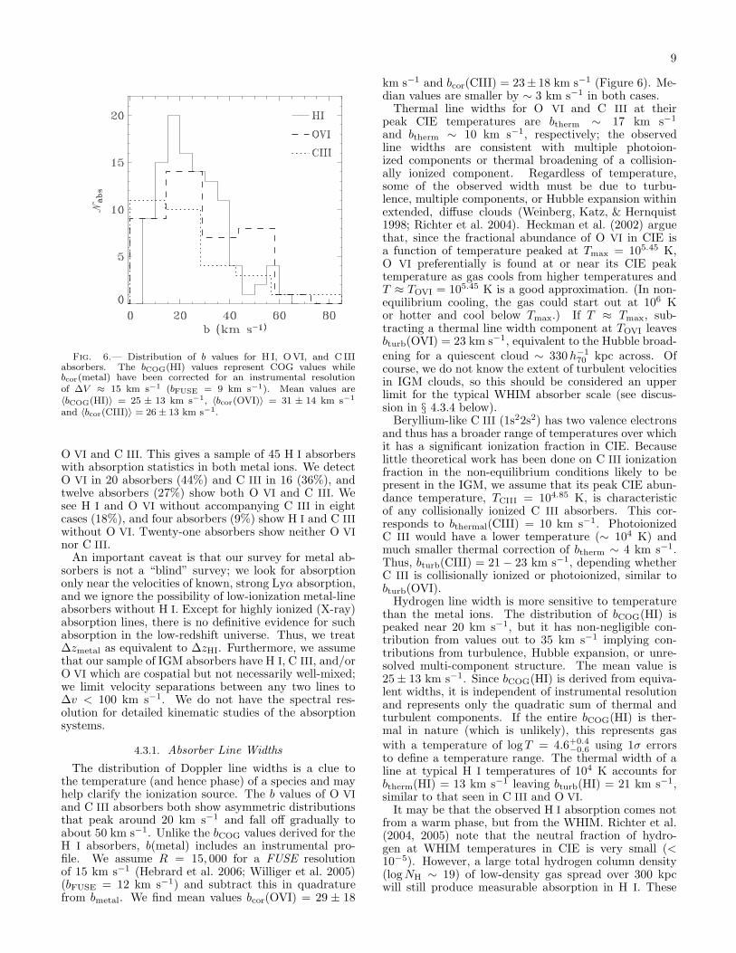
Fig. 6.— Distribution of b values for H I, O VI, and C IIIabsorbers. The bCOG(HI) values represent COG values whilebcor(metal) have been corrected for an instrumental resolutionof ∆V ≈ 15 km s−1 (bFUSE = 9 km s−1). Mean values are〈bCOG(HI)〉 = 25 ± 13 km s−1, 〈bcor(OVI)〉 = 31 ± 14 km s−1

and 〈bcor(CIII)〉 = 26 ± 13 km s−1.

O VI and C III. This gives a sample of 45 H I absorberswith absorption statistics in both metal ions. We detectO VI in 20 absorbers (44%) and C III in 16 (36%), andtwelve absorbers (27%) show both O VI and C III. Wesee H I and O VI without accompanying C III in eightcases (18%), and four absorbers (9%) show H I and C III

without O VI. Twenty-one absorbers show neither O VI

nor C III.An important caveat is that our survey for metal ab-

sorbers is not a “blind” survey; we look for absorptiononly near the velocities of known, strong Lyα absorption,and we ignore the possibility of low-ionization metal-lineabsorbers without H I. Except for highly ionized (X-ray)absorption lines, there is no definitive evidence for suchabsorption in the low-redshift universe. Thus, we treat∆zmetal as equivalent to ∆zHI. Furthermore, we assumethat our sample of IGM absorbers have H I, C III, and/orO VI which are cospatial but not necessarily well-mixed;we limit velocity separations between any two lines to∆v < 100 km s−1. We do not have the spectral res-olution for detailed kinematic studies of the absorptionsystems.

4.3.1. Absorber Line Widths

The distribution of Doppler line widths is a clue tothe temperature (and hence phase) of a species and mayhelp clarify the ionization source. The b values of O VI

and C III absorbers both show asymmetric distributionsthat peak around 20 km s−1 and fall off gradually toabout 50 km s−1. Unlike the bCOG values derived for theH I absorbers, b(metal) includes an instrumental pro-file. We assume R = 15, 000 for a FUSE resolutionof 15 km s−1 (Hebrard et al. 2006; Williger et al. 2005)(bFUSE = 12 km s−1) and subtract this in quadraturefrom bmetal. We find mean values bcor(OVI) = 29 ± 18

km s−1 and bcor(CIII) = 23± 18 km s−1 (Figure 6). Me-dian values are smaller by ∼ 3 km s−1 in both cases.

Thermal line widths for O VI and C III at theirpeak CIE temperatures are btherm ∼ 17 km s−1

and btherm ∼ 10 km s−1, respectively; the observedline widths are consistent with multiple photoion-ized components or thermal broadening of a collision-ally ionized component. Regardless of temperature,some of the observed width must be due to turbu-lence, multiple components, or Hubble expansion withinextended, diffuse clouds (Weinberg, Katz, & Hernquist1998; Richter et al. 2004). Heckman et al. (2002) arguethat, since the fractional abundance of O VI in CIE isa function of temperature peaked at Tmax = 105.45 K,O VI preferentially is found at or near its CIE peaktemperature as gas cools from higher temperatures andT ≈ TOVI = 105.45 K is a good approximation. (In non-equilibrium cooling, the gas could start out at 106 Kor hotter and cool below Tmax.) If T ≈ Tmax, sub-tracting a thermal line width component at TOVI leavesbturb(OVI) = 23 km s−1, equivalent to the Hubble broad-ening for a quiescent cloud ∼ 330 h−1

70 kpc across. Ofcourse, we do not know the extent of turbulent velocitiesin IGM clouds, so this should be considered an upperlimit for the typical WHIM absorber scale (see discus-sion in § 4.3.4 below).

Beryllium-like C III (1s22s2) has two valence electronsand thus has a broader range of temperatures over whichit has a significant ionization fraction in CIE. Becauselittle theoretical work has been done on C III ionizationfraction in the non-equilibrium conditions likely to bepresent in the IGM, we assume that its peak CIE abun-dance temperature, TCIII = 104.85 K, is characteristicof any collisionally ionized C III absorbers. This cor-responds to bthermal(CIII) = 10 km s−1. PhotoionizedC III would have a lower temperature (∼ 104 K) andmuch smaller thermal correction of btherm ∼ 4 km s−1.Thus, bturb(CIII) = 21 − 23 km s−1, depending whetherC III is collisionally ionized or photoionized, similar tobturb(OVI).

Hydrogen line width is more sensitive to temperaturethan the metal ions. The distribution of bCOG(HI) ispeaked near 20 km s−1, but it has non-negligible con-tribution from values out to 35 km s−1 implying con-tributions from turbulence, Hubble expansion, or unre-solved multi-component structure. The mean value is25 ± 13 km s−1. Since bCOG(HI) is derived from equiva-lent widths, it is independent of instrumental resolutionand represents only the quadratic sum of thermal andturbulent components. If the entire bCOG(HI) is ther-mal in nature (which is unlikely), this represents gaswith a temperature of logT = 4.6+0.4

−0.6 using 1σ errorsto define a temperature range. The thermal width of aline at typical H I temperatures of 104 K accounts forbtherm(HI) = 13 km s−1 leaving bturb(HI) = 21 km s−1,similar to that seen in C III and O VI.

It may be that the observed H I absorption comes notfrom a warm phase, but from the WHIM. Richter et al.(2004, 2005) note that the neutral fraction of hydro-gen at WHIM temperatures in CIE is very small (<10−5). However, a large total hydrogen column density(logNH ∼ 19) of low-density gas spread over 300 kpcwill still produce measurable absorption in H I. These

10

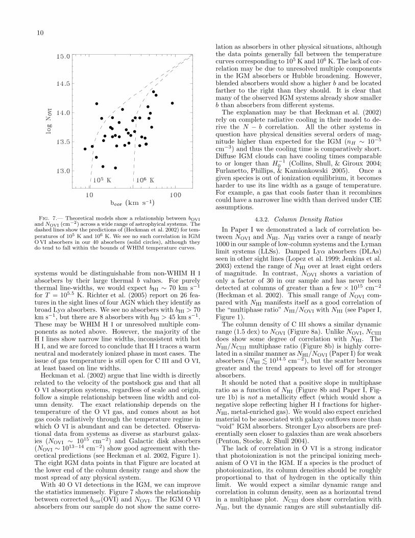
Fig. 7.— Theoretical models show a relationship between bOVI

and NOVI (cm−2) across a wide range of astrophyical systems. Thedashed lines show the predictions of (Heckman et al. 2002) for tem-peratures of 105 K and 106 K. We see no such correlation in IGMOVI absorbers in our 40 absorbers (solid circles), although theydo tend to fall within the bounds of WHIM temperature curves.

systems would be distinguishable from non-WHIM H I

absorbers by their large thermal b values. For purelythermal line-widths, we would expect bHI ∼ 70 km s−1

for T = 105.5 K. Richter et al. (2005) report on 26 fea-tures in the sight lines of four AGN which they identify asbroad Lyα absorbers. We see no absorbers with bHI > 70km s−1, but there are 8 absorbers with bHI > 45 km s−1.These may be WHIM H I or unresolved multiple com-ponents as noted above. However, the majority of theH I lines show narrow line widths, inconsistent with hotH I, and we are forced to conclude that H I traces a warmneutral and moderately ionized phase in most cases. Theissue of gas temperature is still open for C III and O VI,at least based on line widths.

Heckman et al. (2002) argue that line width is directlyrelated to the velocity of the postshock gas and that allO VI absorption systems, regardless of scale and origin,follow a simple relationship between line width and col-umn density. The exact relationship depends on thetemperature of the O VI gas, and comes about as hotgas cools radiatively through the temperature regime inwhich O VI is abundant and can be detected. Observa-tional data from systems as diverse as starburst galax-ies (NOVI ∼ 1015 cm−2) and Galactic disk absorbers(NOVI ∼ 1013−14 cm−2) show good agreement with the-oretical predictions (see Heckman et al. 2002, Figure 1).The eight IGM data points in that Figure are located atthe lower end of the column density range and show themost spread of any physical system.

With 40 O VI detections in the IGM, we can improvethe statistics immensely. Figure 7 shows the relationshipbetween corrected bcor(OVI) and NOVI. The IGM O VI

absorbers from our sample do not show the same corre-

lation as absorbers in other physical situations, althoughthe data points generally fall between the temperaturecurves corresponding to 105 K and 106 K. The lack of cor-relation may be due to unresolved multiple componentsin the IGM absorbers or Hubble broadening. However,blended absorbers would show a higher b and be locatedfarther to the right than they should. It is clear thatmany of the observed IGM systems already show smallerb than absorbers from different systems.

The explanation may be that Heckman et al. (2002)rely on complete radiative cooling in their model to de-rive the N − b correlation. All the other systems inquestion have physical densities several orders of mag-nitude higher than expected for the IGM (nH ∼ 10−5

cm−3) and thus the cooling time is comparatively short.Diffuse IGM clouds can have cooling times comparableto or longer than H−1

0 (Collins, Shull, & Giroux 2004;Furlanetto, Phillips, & Kamionkowski 2005). Once agiven species is out of ionization equilibrium, it becomesharder to use its line width as a gauge of temperature.For example, a gas that cools faster than it recombinescould have a narrower line width than derived under CIEassumptions.

4.3.2. Column Density Ratios

In Paper I we demonstrated a lack of correlation be-tween NOVI and NHI. NHI varies over a range of nearly1000 in our sample of low-column systems and the Lymanlimit systems (LLSs). Damped Lyα absorbers (DLAs)seen in other sight lines (Lopez et al. 1999; Jenkins et al.2003) extend the range of NHI over at least eight ordersof magnitude. In contrast, NOVI shows a variation ofonly a factor of 30 in our sample and has never beendetected at columns of greater than a few × 1015 cm−2

(Heckman et al. 2002). This small range of NOVI com-pared with NHI manifests itself as a good correlation ofthe “multiphase ratio” NHI/NOVI with NHI (see Paper I,Figure 1).

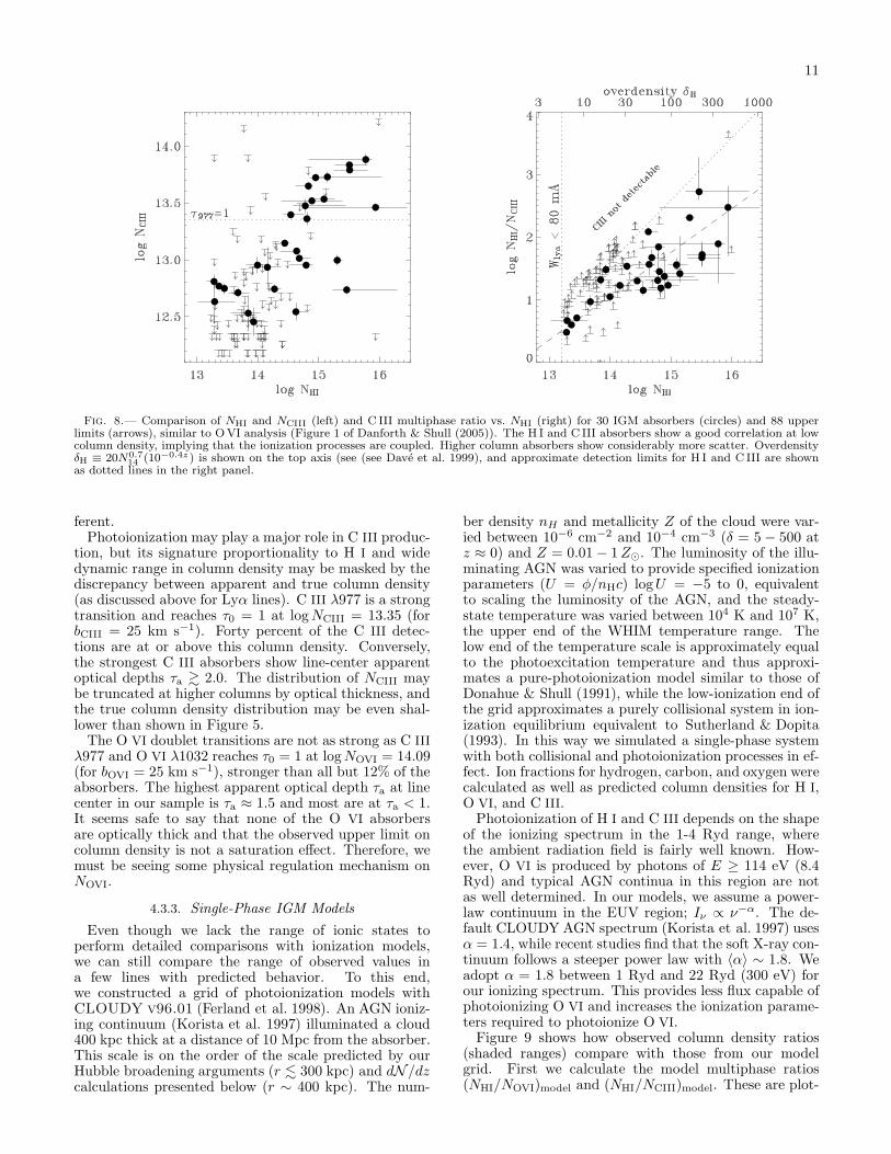
The column density of C III shows a similar dynamicrange (1.5 dex) to NOVI (Figure 8a). Unlike NOVI, NCIII

does show some degree of correlation with NHI. TheNHI/NCIII multiphase ratio (Figure 8b) is highly corre-lated in a similar manner as NHI/NOVI (Paper I) for weakabsorbers (NHI . 1014.5 cm−2), but the scatter becomesgreater and the trend appears to level off for strongerabsorbers.

It should be noted that a positive slope in multiphaseratio as a function of NHI (Figure 8b and Paper I, Fig-ure 1b) is not a metallicity effect (which would show anegative slope reflecting higher H I fractions for higher-NHI, metal-enriched gas). We would also expect enrichedmaterial to be associated with galaxy outflows more than“void” IGM absorbers. Stronger Lyα absorbers are pref-erentially seen closer to galaxies than are weak absorbers(Penton, Stocke, & Shull 2004).

The lack of correlation in O VI is a strong indicatorthat photoionization is not the principal ionizing mech-anism of O VI in the IGM. If a species is the product ofphotoionization, its column densities should be roughlyproportional to that of hydrogen in the optically thinlimit. We would expect a similar dynamic range andcorrelation in column density, seen as a horizontal trendin a multiphase plot. NCIII does show correlation withNHI, but the dynamic ranges are still substantially dif-

11

Fig. 8.— Comparison of NHI and NCIII (left) and C III multiphase ratio vs. NHI (right) for 30 IGM absorbers (circles) and 88 upperlimits (arrows), similar to O VI analysis (Figure 1 of Danforth & Shull (2005)). The H I and C III absorbers show a good correlation at lowcolumn density, implying that the ionization processes are coupled. Higher column absorbers show considerably more scatter. OverdensityδH ≡ 20N0.7

14 (10−0.4z ) is shown on the top axis (see (see Dave et al. 1999), and approximate detection limits for H I and C III are shownas dotted lines in the right panel.

ferent.Photoionization may play a major role in C III produc-

tion, but its signature proportionality to H I and widedynamic range in column density may be masked by thediscrepancy between apparent and true column density(as discussed above for Lyα lines). C III λ977 is a strongtransition and reaches τ0 = 1 at logNCIII = 13.35 (forbCIII = 25 km s−1). Forty percent of the C III detec-tions are at or above this column density. Conversely,the strongest C III absorbers show line-center apparentoptical depths τa & 2.0. The distribution of NCIII maybe truncated at higher columns by optical thickness, andthe true column density distribution may be even shal-lower than shown in Figure 5.

The O VI doublet transitions are not as strong as C III

λ977 and O VI λ1032 reaches τ0 = 1 at logNOVI = 14.09(for bOVI = 25 km s−1), stronger than all but 12% of theabsorbers. The highest apparent optical depth τa at linecenter in our sample is τa ≈ 1.5 and most are at τa < 1.It seems safe to say that none of the O VI absorbersare optically thick and that the observed upper limit oncolumn density is not a saturation effect. Therefore, wemust be seeing some physical regulation mechanism onNOVI.

4.3.3. Single-Phase IGM Models

Even though we lack the range of ionic states toperform detailed comparisons with ionization models,we can still compare the range of observed values ina few lines with predicted behavior. To this end,we constructed a grid of photoionization models withCLOUDY v96.01 (Ferland et al. 1998). An AGN ioniz-ing continuum (Korista et al. 1997) illuminated a cloud400 kpc thick at a distance of 10 Mpc from the absorber.This scale is on the order of the scale predicted by ourHubble broadening arguments (r . 300 kpc) and dN/dzcalculations presented below (r ∼ 400 kpc). The num-

ber density nH and metallicity Z of the cloud were var-ied between 10−6 cm−2 and 10−4 cm−3 (δ = 5 − 500 atz ≈ 0) and Z = 0.01 − 1 Z⊙. The luminosity of the illu-minating AGN was varied to provide specified ionizationparameters (U = φ/nHc) logU = −5 to 0, equivalentto scaling the luminosity of the AGN, and the steady-state temperature was varied between 104 K and 107 K,the upper end of the WHIM temperature range. Thelow end of the temperature scale is approximately equalto the photoexcitation temperature and thus approxi-mates a pure-photoionization model similar to those ofDonahue & Shull (1991), while the low-ionization end ofthe grid approximates a purely collisional system in ion-ization equilibrium equivalent to Sutherland & Dopita(1993). In this way we simulated a single-phase systemwith both collisional and photoionization processes in ef-fect. Ion fractions for hydrogen, carbon, and oxygen werecalculated as well as predicted column densities for H I,O VI, and C III.

Photoionization of H I and C III depends on the shapeof the ionizing spectrum in the 1-4 Ryd range, wherethe ambient radiation field is fairly well known. How-ever, O VI is produced by photons of E ≥ 114 eV (8.4Ryd) and typical AGN continua in this region are notas well determined. In our models, we assume a power-law continuum in the EUV region; Iν ∝ ν−α. The de-fault CLOUDY AGN spectrum (Korista et al. 1997) usesα = 1.4, while recent studies find that the soft X-ray con-tinuum follows a steeper power law with 〈α〉 ∼ 1.8. Weadopt α = 1.8 between 1 Ryd and 22 Ryd (300 eV) forour ionizing spectrum. This provides less flux capable ofphotoionizing O VI and increases the ionization parame-ters required to photoionize O VI.

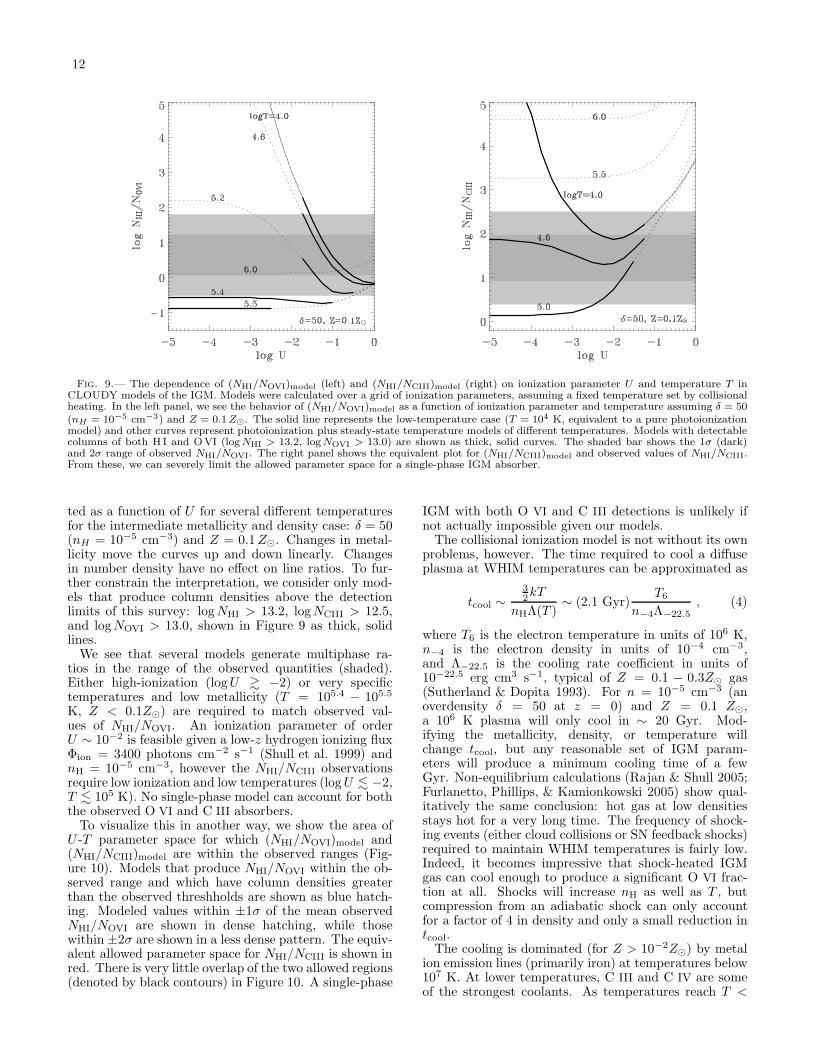
Figure 9 shows how observed column density ratios(shaded ranges) compare with those from our modelgrid. First we calculate the model multiphase ratios(NHI/NOVI)model and (NHI/NCIII)model. These are plot-

12

Fig. 9.— The dependence of (NHI/NOVI)model (left) and (NHI/NCIII)model (right) on ionization parameter U and temperature T inCLOUDY models of the IGM. Models were calculated over a grid of ionization parameters, assuming a fixed temperature set by collisionalheating. In the left panel, we see the behavior of (NHI/NOVI)model as a function of ionization parameter and temperature assuming δ = 50(nH = 10−5 cm−3) and Z = 0.1 Z⊙. The solid line represents the low-temperature case (T = 104 K, equivalent to a pure photoionizationmodel) and other curves represent photoionization plus steady-state temperature models of different temperatures. Models with detectablecolumns of both H I and OVI (log NHI > 13.2, log NOVI > 13.0) are shown as thick, solid curves. The shaded bar shows the 1σ (dark)and 2σ range of observed NHI/NOVI. The right panel shows the equivalent plot for (NHI/NCIII)model and observed values of NHI/NCIII.From these, we can severely limit the allowed parameter space for a single-phase IGM absorber.

ted as a function of U for several different temperaturesfor the intermediate metallicity and density case: δ = 50(nH = 10−5 cm−3) and Z = 0.1 Z⊙. Changes in metal-licity move the curves up and down linearly. Changesin number density have no effect on line ratios. To fur-ther constrain the interpretation, we consider only mod-els that produce column densities above the detectionlimits of this survey: logNHI > 13.2, logNCIII > 12.5,and logNOVI > 13.0, shown in Figure 9 as thick, solidlines.

We see that several models generate multiphase ra-tios in the range of the observed quantities (shaded).Either high-ionization (logU & −2) or very specifictemperatures and low metallicity (T = 105.4 − 105.5

K, Z < 0.1Z⊙) are required to match observed val-ues of NHI/NOVI. An ionization parameter of orderU ∼ 10−2 is feasible given a low-z hydrogen ionizing fluxΦion = 3400 photons cm−2 s−1 (Shull et al. 1999) andnH = 10−5 cm−3, however the NHI/NCIII observationsrequire low ionization and low temperatures (log U . −2,T . 105 K). No single-phase model can account for boththe observed O VI and C III absorbers.

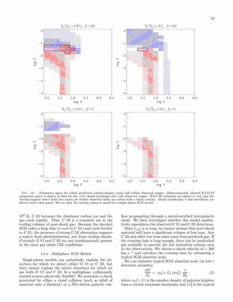
To visualize this in another way, we show the area ofU -T parameter space for which (NHI/NOVI)model and(NHI/NCIII)model are within the observed ranges (Fig-ure 10). Models that produce NHI/NOVI within the ob-served range and which have column densities greaterthan the observed threshholds are shown as blue hatch-ing. Modeled values within ±1σ of the mean observedNHI/NOVI are shown in dense hatching, while thosewithin ±2σ are shown in a less dense pattern. The equiv-alent allowed parameter space for NHI/NCIII is shown inred. There is very little overlap of the two allowed regions(denoted by black contours) in Figure 10. A single-phase

IGM with both O VI and C III detections is unlikely ifnot actually impossible given our models.

The collisional ionization model is not without its ownproblems, however. The time required to cool a diffuseplasma at WHIM temperatures can be approximated as

tcool ∼32kT

nHΛ(T )∼ (2.1 Gyr)

T6

n−4Λ−22.5, (4)

where T6 is the electron temperature in units of 106 K,n−4 is the electron density in units of 10−4 cm−3,and Λ−22.5 is the cooling rate coefficient in units of10−22.5 erg cm3 s−1, typical of Z = 0.1 − 0.3Z⊙ gas(Sutherland & Dopita 1993). For n = 10−5 cm−3 (anoverdensity δ = 50 at z = 0) and Z = 0.1 Z⊙,a 106 K plasma will only cool in ∼ 20 Gyr. Mod-ifying the metallicity, density, or temperature willchange tcool, but any reasonable set of IGM param-eters will produce a minimum cooling time of a fewGyr. Non-equilibrium calculations (Rajan & Shull 2005;Furlanetto, Phillips, & Kamionkowski 2005) show qual-itatively the same conclusion: hot gas at low densitiesstays hot for a very long time. The frequency of shock-ing events (either cloud collisions or SN feedback shocks)required to maintain WHIM temperatures is fairly low.Indeed, it becomes impressive that shock-heated IGMgas can cool enough to produce a significant O VI frac-tion at all. Shocks will increase nH as well as T , butcompression from an adiabatic shock can only accountfor a factor of 4 in density and only a small reduction intcool.

The cooling is dominated (for Z > 10−2Z⊙) by metalion emission lines (primarily iron) at temperatures below107 K. At lower temperatures, C III and C IV are someof the strongest coolants. As temperatures reach T <

13

Fig. 10.— Parameter space for which predicted column-density ratios fall within observed ranges. Observationally allowed H I/O VIparameter space is shown in blue for the ±1σ (dense hatching) and ±2σ observed ranges. H I/C III solutions are shown in red, and theoverlap regions where both line ratios are within observed limits are noted with a black contour. Model overdensity δ and metallicity areshown above each panel. We see that the overlap region is small for a single-phase IGM model.

105 K, C III becomes the dominant carbon ion and thegas cools rapidly. Thus, C III is a transient ion in thecooling column of post-shock gas. Because the shockedIGM takes a long time to cool to C III (and cools furtherto C II), the presence of strong C III absorption suggestsa source from photoionization, not from cooling shocks.Certainly O VI and C III are not simultaneously presentin the same gas under CIE conditions.

4.3.4. Multiphase IGM Models

Single-phase models can potentially explain the ab-sorbers for which we detect either O VI or C III, butthey cannot explain the twelve absorbers for which wesee both O VI and C III. Is a multiphase, collisionallyionized system physically feasible? We postulate a shockgenerated by either a cloud collision (such as infall ofmaterial onto a filament) or a SNe-driven galactic out-

flow propagating through a metal-enriched intergalacticcloud. We then investigate whether this model qualita-tively reproduces the observed O VI and C III detections.

Since tcool is so long, we cannot assume that post-shockmaterial will have a significant column of low ions. AnyC III and other low-ions must come from preshock gas. Ifthe crossing time is long enough, there can be unshockedgas available to provide the low ionization column seenin the observations. We choose a shock velocity of ∼ 200km s−1 and calculate the crossing time by estimating atypical IGM absorber scale.

We can estimate typical IGM absorber scale via low-zdetection statistics;

dNdz

= n0(> L) (πr20)

c

H0, (5)

where n0(> L) is the number density of galaxies brighterthan a certain minimum luminosity and πr2

0 is the typical

14

absorber cross section. We use a Schechter luminosityfunction

φ(L)dL = φ∗(L/L∗)−α e−L/L∗

(dL/L∗) , (6)

and integrate down to luminosity L. In the special case ofα = 1, typical of the faint-end slope, the integral becomesthe first exponential integral E1;

n0(> L)=φ∗

∫ ∞

L

(L/L∗)−1 e−L/L∗ dL

L∗

=φ∗ E1(L/L∗). (7)

Recent results from the Sloan Digital Sky Survey (SDSSBlanton et al. 2003) give φ∗ = 0.0149 h3 Mpc−3 orφ∗ = 5.11×10−3 h3

70 Mpc−3. We use dNOVI/dz = 17±3for Wλ > 30 mA (Danforth & Shull 2005) and find thatr0 = (1060±100) h−1

70 kpc for L∗ galaxies. However, it islikely that the IGM is enriched preferentially by smallergalaxies (Stocke et al. 2005). If we integrate down to L =0.1L∗, we find r0 = (370±30) h−1

70 kpc, a size scale in rea-sonable agreement with inferred distances of metal dis-tributions from nearest-neighbor galaxies (Stocke et al.2005). Adjusting φ∗ downward by 1/3, to account forellipticals that may not have outflows, we find that r0

increases by ∼ 20%. This analysis assumes a uniformdistribution of galaxies. Tumlinson & Fang (2005) findsimilar scales with r0 = 750 kpc and r0 = 300 kpc forL∗ and 0.1L∗ limits based on actual galaxy distributionsfrom SDSS.

A typical IGM absorber scale of ∼ 400 h−170 kpc also

agrees with Lyα forest cloud sizes inferred from pho-toionization modeling (Shull et al. 1998; Schaye 2001;Tumlinson et al. 2005) and with our rough upper limiton cloud scale based on Hubble broadening of H I ab-sorption lines. Observations of quasar pairs give resultsnot inconsistent with our derived value. The quasar pairLBQS1343+264A/B shows characteristic r0 ∼ 300 h−1

70at z ∼ 2 (Bechtold et al. 1994; Dinshaw et al. 1994). Atlower redshift, Young, Impey, & Foltz (2001) find that acoherence length between Lyα absorbers of 500–1000 kpcat 0.4 < z < 0.9 in a rare triple QSO system.

The crossing time for a 400 kpc cloud by a 200 km s−1

shock is 2 Gyr, which is of the same order as the WHIMcooling time. Assuming that IGM absorbers are as-sociated with dwarf galaxies and that shocking eventsare infrequent, it is perfectly feasible that unshocked,photoionized material would exist to provide the ob-served C III column density along AGN sight lines, whileshocked material could provide the observed O VI.

We can now revisit the different samples of absorbersintroduced in § 4.3. The 12 absorbers with both O VI

and C III detections can most plausibly be understood asmultiphase absorbers. Column densities and line widthsshow no correlation and are not easily explained witha single-phase photoionized-plus-collisional system. Oursight lines pass through both quiescent photoionized andshocked regions, and we are unable to kinematically dif-ferentiate the two phases in the spectra. The two metalions occupy different temperature and ionization param-eter regimes and are found in physically distinct parts ofthe absorber. Likely the H I absorption is associated withthe cooler, photoionized phase, since bHI . 40 km s−1 inmost cases.

There are eight absorbers with H I and O VI detectionsand good C III non-detections. These systems may be

large, diffuse, photoionized clouds with a high ionizationparameter (logU > −2), sufficient to produce O VI byphotoionization, and high enough that carbon would beionized to C IV. The small fraction of neutral hydrogenat this high ionization parameter would show the nar-row thermal profiles observed in our H I sample. Equiv-alently, these systems can be interpreted as two-phasesystems with a shocked, WHIM phase (probed by O VI)and an unshocked, photoionized phase observed in H I.The small range of NOVI compared to NHI and the lackof correlation between the two species in column den-sity and β suggests the latter, multiphase interpretation.A broad, WHIM component in H I may be masked bystronger narrow components or be below the detectionthreshhold of our data.

The four systems with H I and C III detections andO VI non-detections are likely photoionized. CIE coolingis extremely fast at T < 105 K, and we do not expect that∼ 10% of the total metal absorbers would be observedduring the relatively brief period during which C III iscollisionally ionized. The photoionization interpretationprovides us with an upper limit to the ionization param-eter (U . 10−2) and we must therefore posit that, forthis population of absorbers at least, nH ≫ 10−5 cm−3

or that the metagalactic ionizing radiation field is weakerthan expected from models.

The 21 absorbers with neither O VI nor C III are likelycollisionally ionized to T > 106 K or metal-poor sys-tems (Z < 10−2Z⊙). The lack of broad H I absorp-tion makes the high-temperature interpretation implau-sible, and purely photoionized clouds with even modestenrichment should show measurable C III. Stocke et al.(2005) investigate our detection statistics more thor-oughly and catalog nearest-neighbor galaxies for each ab-sorber. They find that the Lyα detections with no metallines tend to show larger nearest-neighbor distances thanthose with metal line detections. Williger et al. (2006)find stronger clustering between Lyα systems and galax-ies for higher NHI systems over larger velocity scales.These results suggest that the metal-enrichment expla-nation is the most likely.

4.4. Metallicity of the IGM

In Paper I, we found good agreement between our ob-served distribution of dNOVI/dz and the cosmic evolutionmodels of Chen et al. (2003) at ∼ 10% metallicity. Wealso derived ZO ≈ 0.09 Z⊙ (fOVI/0.2)−1 based on theNHI/NOVI multiphase plot, where (fOVI/0.2) is a nor-malized ionization fraction of O VI in units of the CIEpeak value of 20%. Our value of 9% is consistent withthe canonical 10% value assumed in many sources (e.g.,Savage et al. 2002; Tripp, Savage, & Jenkins 2000).

We determine (C/H)IGM via the H I/C III multiphasedata using the same formalism as Paper I,

⟨

NC

NH

⟩

=

⟨

NCIII

NHI

⟩

×(

fHI

fCIII

)

, (8)

where fHI and fCIII are the ionization fractions of thosetwo species. We fit the C III multiphase plot (Figure 8b)as a power law

⟨

NHI

NCIII

⟩

= C14 Nα14 , (9)

15

where N14 is the H I column density in units of 1014

cm−2 and C14 is a scaling constant. The best-fit param-eters are similar, whether we use the low-NHI half of theC III absorber sample or the entire range of NHI: forlogNHI < 14.5, α = 0.73 ± 0.08, C14 = 1.06 ± 0.04; forthe entire sample, α = 0.70±0.03, C14 = 1.05±0.02. Weadopt the first set of values here, but note that it makeslittle difference. The mean absorber redshift in our C III

sample is 〈zabs〉 ≈ 0.1.We also make use of an empirical relationship from

Dave et al. (1999) relating the baryon overdensity, δH,to H I column density

δH ≡ nH

(1.90 × 10−7 cm−3) (1 + z)3(10)

≈20 N0.714 10−0.4 z . (11)

Combining Eqs. (9) and (11) and substituting the appro-priate constants from the fit, we find

⟨

NHI

NCIII

⟩

= 26.6 δ1.04 . (12)

The neutral hydrogen fraction fHI in Eq. 8 can be de-rived from case-A photoionization equilibrium in a lowdensity gas:

fHI =neα

(A)H

ΓH= 4.74 nH T−0.726

4 Γ−1−13

=9.01 × 10−7 δH (1 + z)3 T−0.7264 Γ−1

−13 , (13)

where T4 is the temperature in units of 104 K and Γ−13

is the H I photoionization rate in units of 10−13 s−1. TheC III ionization fraction is harder to handle analytically.We take fCIII ≈ 0.8 since this is roughly its maximumvalue under both CIE and the photoionization modelingof Donahue & Shull (1991). Substituting Eqs. (12) and(13) into Eq (8), we get

⟨

NC

NH

⟩

=(2.89 × 10−5)

(

fCIII

0.8

)−1

δ−0.04H T−0.726

4 Γ−1−13

ZC =(0.12 Z⊙)

(

fCIII

0.8

)−1

, (14)

using (C/H)⊙ = 2.45 × 10−4 (Allende Prieto et al.2001a). Our value ZC = 12% is reassuringly close tothe value ZO = 9% from Paper I, considering that bothvalues are probably uncertain by at least a factor of two.

The leading contender for IGM enrichment is outflowsfrom starbursting dwarf galaxies (Heckman et al. 2001;Keeney et al. 2006). These starburst winds would bedominated by the products of the most massive stars,which show an elevated abundance of oxygen in rela-tion to carbon as a result of α-process nucleosynthesis(Garnett et al. 1995; Sneden 2004). Within the large un-certainties, the observed (C/O)IGM ≈ (C/O)⊙ impliesthat the IGM is enriched by a more mature gas mixturefrom a broader range of stellar masses.

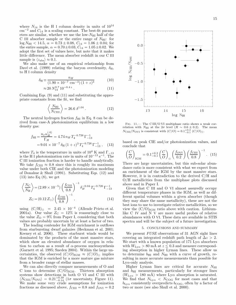
We can also directly compare measurements of O andC ions to determine (C/O)IGM. Thirteen absorptionsystems show detections in both O VI and C III with〈NCIII/NOVI〉 = 0.21+0.39

−0.14 (1σ uncertainty, Figure 11).We make some very crude assumptions for ionizationfractions as discussed above, fCIII = 0.8 and fOVI = 0.2

Fig. 11.— The C III/O VI multiphase ratio shows a weak cor-relation with NHI at the 2σ level (R ∼ 0.6 ± 0.2). The mean

NCIII/NOVI is consistent with (C/O) = 0.1+0.2−0.1 (C/O)⊙.

based on peak CIE and/or photoionization values, andconclude that

(

C

O

)

IGM

= 0.1+0.2−0.1

(

C

O

)

⊙

(

fOVI

0.2

)(

fCIII

0.8

)−1

. (15)

There are large uncertainties, but this sub-solar abun-dance ratio is more consistent with what we expect froman enrichment of the IGM by the most massive stars.However, it is in contradiction to the derived C/H andO/H metallicities from the multiphase plots discussedabove and in Paper I.

Given that C III and O VI almost assuredly occupydifferent temperature phases in the IGM, as well as dif-ferent spatial volumes within a given absorber (thoughthey may share the same metallicity), these are not thebest ions to use to investigate relative metallicities, so weview the (C/O)IGM ratio above with caution. Lithium-like C IV and N V are more useful probes of relativeabundances with O VI. These data are available in STISspectra and will be the subject of a future investigation.

5. CONCLUSIONS AND SUMMARY

We present FUSE observations of 31 AGN sight linescovering an integrated redshift path length of ∆z > 2.We start with a known population of 171 Lyα absorberswith WLyα > 80 mA at z ≤ 0.3 and measure correspond-ing absorption in higher Lyman lines. These allow usto determine bHI and NHI with a curve of growth, re-sulting in more accurate measurements than possible forLyα-only analysis.

Higher Lyman lines are critical for accurate NHI

and bHI measurements, particularly for stronger lines(WLyα > 180 mA) where Lyα absorption is saturated.We find that NLyα < NCOG for most cases and thatbLyα consistently overpredicts bCOG, often by a factor oftwo or more (see also Shull et al. 2000).

16

We measure corresponding metal-line absorption inO VI (for z ≤ 0.15) and C III (z < 0.21). In all, O VI

is detected in 40 out of 129 possible absorbers, and C III

is detected in 30 out of 148 absorbers. C III detectionstatistics give dNCIII/dz = 12+3

−2. We calculate a typ-ical size for IGM absorbers from detection statistics inO VI and find r0 ∼ 400 kpc if absorbers are associatedwith 0.1L∗ galaxies. This size is similar to the resultsof Tumlinson & Fang (2005) and consistent with con-straints placed on r0 from Hubble broadening and ob-served b-values.

Our observations strongly suggest that H I and C III

probe photionized regions of the IGM, while O VI isprimarily a product of collisional (shock) ionization andtherefore a valid probe of the WHIM. Line width anal-ysis sets an upper limit on absorber temperature. Allthree species have similar distributions of b-values, withmedian values ∼ 25 km s−1. The O VI is consis-tent with WHIM-phase, collisionally ionized WHIM, but〈b(HI)〉 = 25± 13 km s−1 requires that the observed H I

absorption arise in a medium with T < 105 K. Single-phase CLOUDY models featuring both photoionizationand collisional ionization limit which areas of parameterspace are allowed for O VI and C III absorbers. Ob-served NOVI values require logU & −2, while observedNCIII requires logU . −2, regardless of temperature.

We calculate the column density distribution of H I ab-sorbers and find that it follows a power law distribution

N (NHI) ∝ N−βHI with β = 1.68±0.11, similar to the result

found by Penton, Stocke, & Shull (2000, 2004). We findthat C III absorbers also follow a power-law distributionwith slope βCIII = 1.68± 0.04, similar to βHI, but not assteep as βOVI = 2.2 ± 0.1 found in Paper I. This simi-larity in N distribution slope is circumstantial evidencethat H I and C III arise through similar mechanisms.

Our absorber sample includes 45 H I absorbers withgood statistics in both O VI and C III lines. We interpret12 absorbers with H I, O VI, and C III as multi-phasesystems with shock-heated WHIM (probed by O VI) anda photoionized component seen in C III and H I. Thefour H I+C III systems are interpreted as unshocked,photoionized gas at 104 K. The eight systems with H I

and O VI but no C III are probably multi-phase ab-sorbers with photoionized H I and WHIM O VI. The 21absorbers with neither O VI nor C III are most likelylow-metallicity, unshocked systems. Stocke et al. (2005)find that these systems have larger nearest-neighbor dis-tances than the population of metal absorbers.

Finally, the metallicity of IGM absorbers appears closeto the canonical 10% solar value. The NHI/NCIII mul-tiphase relationship implies an IGM carbon metallicityZC = 0.12 Z⊙ (fCIII/0.8)−1, remarkably consistent withthe result ZO = 0.09 Z⊙ (fOVI/0.2)−1 from Paper I. Thisimplies a near-solar abundance ratio of C/O in the IGM,higher than what we expect from stellar nucleosynthesismodels which say that the IGM is preferentially enrichedby O-rich massive stars.

Future work with other highly ionized species (e.g.C IV, Si III, and Si IV) will help constrain ionizationand temperature and cast more light on the metallicitytrends in the low-redshift universe. Deeper FUV obser-vations will allow us to seach for lower column densityabsorbers, and additional sight lines from future observa-tions will contribute redshift pathlength to the statistics.

It is our pleasure to acknowledge useful discussionswith Nahum Arav, Jack Gabel, and Van Dixon. StevePenton reduced the STIS/E140M data for six sight lines.We made extensive use of CLOUDY v.96.01 and aregrateful to Gary Ferland and Peter van Hoof for tech-nical assistance with the code. We would also like tothank Gerry Williger for a thorough job refereeing ourmanuscript. This work contains data obtained for theGuaranteed Time Team by the NASA-CNES-CSA FUSEmission operated by the Johns Hopkins University, aswell as data from the Hubble Space Telescope. J.L.R. hasreceived financial support from NSF grant AST-0302049.Financial support to the University of Colorado has beenprovided by NASA/FUSE contract NAS5-32985 andgrant NAG5-13004, by our HST Lyα survey (GO Pro-gram 6593), and by theoretical grants from NASA/LTSA(NAG5-7262)and NSF (AST02-06042).

REFERENCES

Allende Prieto, C., Lambert, D. L., & Asplund, M. 2001, ApJ, 556,L63

Allende Prieto, C., Lambert, D. L., & Asplund, M. 2001, ApJ, 573,L137

Bechtold, J. B., Crotts, A. P. S., Duncan, R. C., & Fang, Y. 1994,ApJ, 437, L83

Bechtold, J. B., et al. 2002, ApJS, 140, 143Blanton, M. R., et al. 2003, ApJ, 592, 819Birnboim, Y. & Dekel, A. 2002, MNRAS, 345, 349Cen, R., & Ostriker, J. P. 1999a, ApJ, 519, L109Cen, R., & Ostriker, J. P. 1999b, ApJ, 514, 1Cen, R., Tripp, T. M., Ostriker, J. P., & Jenkins, E. 2001, ApJ,

559, L5Chen, X., Weinberg, D. H., Katz, N., & Dave, R. 2003, ApJ, 594,

42Collins, J. A., Shull, J. M., & Giroux, M. L. 2004, ApJ, 605, 216Crenshaw, D. M., Kraemer, S. B., Boggess, A., Maran, S. P.,

Mushotzky, R. F., & Wu, C. 1999, ApJ, 516, 750Danforth, C. W. & Shull, J. M. 2005, ApJ, 624, 555 (Paper I)Dave, R., et al. 1999, ApJ, 511, 521Dave, R., et al. 2001, ApJ, 552, 473Dave, R., & Tripp, T. M. 2001, ApJ, 553, 528Dinshaw, N., Weymann, R. J., Impey, C. D., Foltz, C. B., Morris,

S. L., & Ake, T. 1997, ApJ, 437, L87

Donahue, M. & Shull, J. M. 1991, ApJ, 383, 511Ferland, G. J., et al. 1998, PASP, 110, 761Furlanetto, S. R., Phillips, L. A., & Kamionkowski, M. 2005,

MNRAS, 359, 295Garnett, D. R., et al. 1995, ApJ, 443, 64Gehrels, N. 1986, ApJ, 303, 336Gillmon, K., Shull, J. M., Tumlinson, J., & Danforth, C. W. 2005,

ApJ, submitted (astro-ph/0507581)Hartigan, P., Raymond, J., & Hartmann, L. 1987, ApJ, 316, 323Hebrard, G., et al. 2006, ApJ, accepted (astro-ph/0508611)Heckman, T. M., et al. 2001, ApJ, 554, 1021Heckman, T. M., Norman, C. A., Strickland, D. K., & Sembach,

K. R. 2002, ApJ, 577, 691Hu, E. M., Kim, T.-S., Cowie, L. L., Songaila, A., & Rauch, M.

1995, AJ, 110, 1526Jenkins, E. B. 1986, ApJ, 304, 739Jenkins, E. B., et al. 2003, AJ, 125, 2824Keeney, B., Danforth, C. W., Stocke, J. T., Penton, S. V., & Shull,

J. M. 2006, in prepKim, T.-S., Hu, E. M., Cowie, L. L., & Songaila, A. 1997, AJ, 114,

1Kriss, G. A. 2002, in “Mass Outflow in Active Galactic Nuclei: New

Perspectives”, ASP Conf. Ser. 255, 69Korista, K., et al. 1997, ApJS, 108, 401

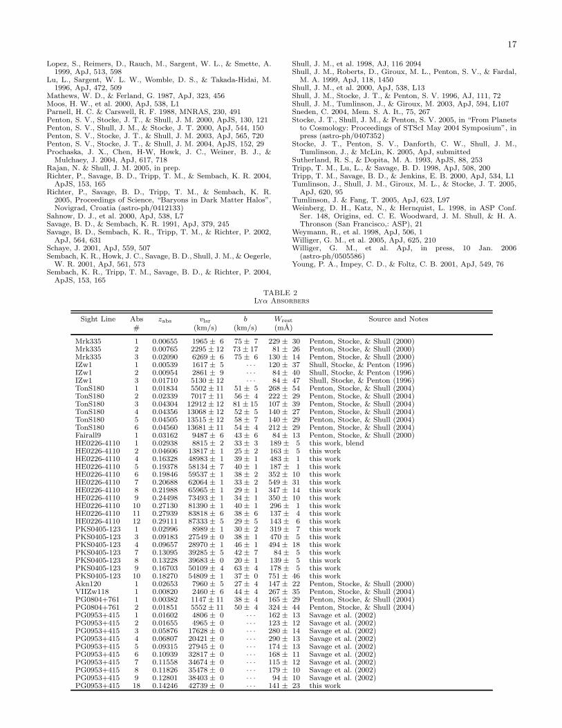
17

Lopez, S., Reimers, D., Rauch, M., Sargent, W. L., & Smette, A.1999, ApJ, 513, 598

Lu, L., Sargent, W. L. W., Womble, D. S., & Takada-Hidai, M.1996, ApJ, 472, 509

Mathews, W. D., & Ferland, G. 1987, ApJ, 323, 456Moos, H. W., et al. 2000, ApJ, 538, L1Parnell, H. C. & Carswell, R. F. 1988, MNRAS, 230, 491Penton, S. V., Stocke, J. T., & Shull, J. M. 2000, ApJS, 130, 121Penton, S. V., Shull, J. M., & Stocke, J. T. 2000, ApJ, 544, 150Penton, S. V., Stocke, J. T., & Shull, J. M. 2003, ApJ, 565, 720Penton, S. V., Stocke, J. T., & Shull, J. M. 2004, ApJS, 152, 29Prochaska, J. X., Chen, H-W, Howk, J. C., Weiner, B. J., &

Mulchaey, J. 2004, ApJ, 617, 718Rajan, N. & Shull, J. M. 2005, in prep.Richter, P., Savage, B. D., Tripp, T. M., & Sembach, K. R. 2004,

ApJS, 153, 165Richter, P., Savage, B. D., Tripp, T. M., & Sembach, K. R.

2005, Proceedings of Science, “Baryons in Dark Matter Halos”,Novigrad, Croatia (astro-ph/0412133)

Sahnow, D. J., et al. 2000, ApJ, 538, L7Savage, B. D., & Sembach, K. R. 1991, ApJ, 379, 245Savage, B. D., Sembach, K. R., Tripp, T. M., & Richter, P. 2002,

ApJ, 564, 631Schaye, J. 2001, ApJ, 559, 507Sembach, K. R., Howk, J. C., Savage, B. D., Shull, J. M., & Oegerle,

W. R. 2001, ApJ, 561, 573Sembach, K. R., Tripp, T. M., Savage, B. D., & Richter, P. 2004,

ApJS, 153, 165

Shull, J. M., et al. 1998, AJ, 116 2094Shull, J. M., Roberts, D., Giroux, M. L., Penton, S. V., & Fardal,

M. A. 1999, ApJ, 118, 1450Shull, J. M., et al. 2000, ApJ, 538, L13Shull, J. M., Stocke, J. T., & Penton, S. V. 1996, AJ, 111, 72Shull, J. M., Tumlinson, J., & Giroux, M. 2003, ApJ, 594, L107Sneden, C. 2004, Mem. S. A. It., 75, 267Stocke, J. T., Shull, J. M., & Penton, S. V. 2005, in “From Planets

to Cosmology: Proceedings of STScI May 2004 Symposium”, inpress (astro-ph/0407352)

Stocke, J. T., Penton, S. V., Danforth, C. W., Shull, J. M.,Tumlinson, J., & McLin, K. 2005, ApJ, submitted

Sutherland, R. S., & Dopita, M. A. 1993, ApJS, 88, 253Tripp, T. M., Lu, L., & Savage, B. D. 1998, ApJ, 508, 200Tripp, T. M., Savage, B. D., & Jenkins, E. B. 2000, ApJ, 534, L1Tumlinson, J., Shull, J. M., Giroux, M. L., & Stocke, J. T. 2005,

ApJ, 620, 95Tumlinson, J. & Fang, T. 2005, ApJ, 623, L97Weinberg, D. H., Katz, N., & Hernquist, L. 1998, in ASP Conf.

Ser. 148, Origins, ed. C. E. Woodward, J. M. Shull, & H. A.Thronson (San Francisco,: ASP), 21

Weymann, R., et al. 1998, ApJ, 506, 1Williger, G. M., et al. 2005, ApJ, 625, 210Williger, G. M., et al. ApJ, in press, 10 Jan. 2006

(astro-ph/0505586)Young, P. A., Impey, C. D., & Foltz, C. B. 2001, ApJ, 549, 76

TABLE 2Lyα Absorbers

Sight Line Abs zabs vlsr b Wrest Source and Notes# (km/s) (km/s) (mA)

Mrk335 1 0.00655 1965 ± 6 75 ± 7 229 ± 30 Penton, Stocke, & Shull (2000)Mrk335 2 0.00765 2295 ± 12 73 ± 17 81 ± 26 Penton, Stocke, & Shull (2000)Mrk335 3 0.02090 6269 ± 6 75 ± 6 130 ± 14 Penton, Stocke, & Shull (2000)IZw1 1 0.00539 1617 ± 5 · · · 120 ± 37 Shull, Stocke, & Penton (1996)IZw1 2 0.00954 2861 ± 9 · · · 84 ± 40 Shull, Stocke, & Penton (1996)IZw1 3 0.01710 5130 ± 12 · · · 84 ± 47 Shull, Stocke, & Penton (1996)TonS180 1 0.01834 5502 ± 11 51 ± 5 268 ± 54 Penton, Stocke, & Shull (2004)TonS180 2 0.02339 7017 ± 11 56 ± 4 222 ± 29 Penton, Stocke, & Shull (2004)TonS180 3 0.04304 12912 ± 12 81 ± 15 107 ± 39 Penton, Stocke, & Shull (2004)TonS180 4 0.04356 13068 ± 12 52 ± 5 140 ± 27 Penton, Stocke, & Shull (2004)TonS180 5 0.04505 13515 ± 12 58 ± 7 140 ± 29 Penton, Stocke, & Shull (2004)TonS180 6 0.04560 13681 ± 11 54 ± 4 212 ± 29 Penton, Stocke, & Shull (2004)Fairall9 1 0.03162 9487 ± 6 43 ± 6 84 ± 13 Penton, Stocke, & Shull (2000)HE0226-4110 1 0.02938 8815 ± 2 33 ± 3 189 ± 5 this work, blendHE0226-4110 2 0.04606 13817 ± 1 25 ± 2 163 ± 5 this workHE0226-4110 4 0.16328 48983 ± 1 39 ± 1 483 ± 1 this workHE0226-4110 5 0.19378 58134 ± 7 40 ± 1 187 ± 1 this workHE0226-4110 6 0.19846 59537 ± 1 38 ± 2 352 ± 10 this workHE0226-4110 7 0.20688 62064 ± 1 33 ± 2 549 ± 31 this workHE0226-4110 8 0.21988 65965 ± 1 29 ± 1 347 ± 14 this workHE0226-4110 9 0.24498 73493 ± 1 34 ± 1 350 ± 10 this workHE0226-4110 10 0.27130 81390 ± 1 40 ± 1 296 ± 1 this workHE0226-4110 11 0.27939 83818 ± 6 38 ± 6 137 ± 4 this workHE0226-4110 12 0.29111 87333 ± 5 29 ± 5 143 ± 6 this workPKS0405-123 1 0.02996 8989 ± 1 30 ± 2 319 ± 7 this workPKS0405-123 3 0.09183 27549 ± 0 38 ± 1 470 ± 5 this workPKS0405-123 4 0.09657 28970 ± 1 46 ± 1 494 ± 18 this workPKS0405-123 7 0.13095 39285 ± 5 42 ± 7 84 ± 5 this workPKS0405-123 8 0.13228 39683 ± 0 20 ± 1 139 ± 5 this workPKS0405-123 9 0.16703 50109 ± 4 63 ± 4 178 ± 5 this workPKS0405-123 10 0.18270 54809 ± 1 37 ± 0 751 ± 46 this workAkn120 1 0.02653 7960 ± 5 27 ± 4 147 ± 22 Penton, Stocke, & Shull (2000)VIIZw118 1 0.00820 2460 ± 6 44 ± 4 267 ± 35 Penton, Stocke, & Shull (2004)PG0804+761 1 0.00382 1147 ± 11 38 ± 4 165 ± 29 Penton, Stocke, & Shull (2004)PG0804+761 2 0.01851 5552 ± 11 50 ± 4 324 ± 44 Penton, Stocke, & Shull (2004)PG0953+415 1 0.01602 4806 ± 0 · · · 162 ± 13 Savage et al. (2002)PG0953+415 2 0.01655 4965 ± 0 · · · 123 ± 12 Savage et al. (2002)PG0953+415 3 0.05876 17628 ± 0 · · · 280 ± 14 Savage et al. (2002)PG0953+415 4 0.06807 20421 ± 0 · · · 290 ± 13 Savage et al. (2002)PG0953+415 5 0.09315 27945 ± 0 · · · 174 ± 13 Savage et al. (2002)PG0953+415 6 0.10939 32817 ± 0 · · · 168 ± 11 Savage et al. (2002)PG0953+415 7 0.11558 34674 ± 0 · · · 115 ± 12 Savage et al. (2002)PG0953+415 8 0.11826 35478 ± 0 · · · 179 ± 10 Savage et al. (2002)PG0953+415 9 0.12801 38403 ± 0 · · · 94 ± 10 Savage et al. (2002)PG0953+415 18 0.14246 42739 ± 0 · · · 141 ± 23 this work

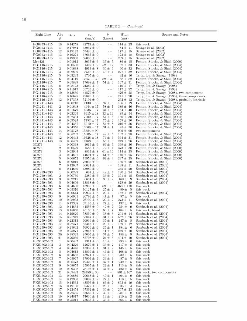
18

TABLE 2 — Continued

Sight Line Abs zabs vlsr b Wrest Source and Notes# (km/s) (km/s) (mA)

PG0953+415 19 0.14258 42774 ± 0 · · · 114 ± 23 this workPG0953+415 11 0.17984 53952 ± 0 · · · 84 ± 11 Savage et al. (2002)PG0953+415 12 0.19142 57426 ± 0 · · · 177 ± 15 Savage et al. (2002)PG0953+415 13 0.19221 57663 ± 0 · · · 122 ± 18 Savage et al. (2002)PG0953+415 14 0.19360 58080 ± 0 · · · 269 ± 15 Savage et al. (2002)Mrk421 1 0.01012 3035 ± 6 35 ± 5 86 ± 15 Penton, Stocke, & Shull (2000)PG1116+215 1 0.00500 1499 ± 9 52 ± 12 82 ± 33 Penton, Stocke, & Shull (2004)PG1116+215 2 0.01638 4913 ± 8 30 ± 9 90 ± 32 Penton, Stocke, & Shull (2004)PG1116+215 4 0.02839 8518 ± 8 45 ± 4 227 ± 32 Penton, Stocke, & Shull (2004)PG1116+215 5 0.03235 9705 ± 0 · · · 92 ± 16 Tripp, Lu, & Savage (1998)PG1116+215 6 0.04119 12357 ± 30 89 ± 39 88 ± 82 Penton, Stocke, & Shull (2004)PG1116+215 7 0.05899 17698 ± 7 51 ± 6 167 ± 31 Penton, Stocke, & Shull (2004)PG1116+215 8 0.08123 24369 ± 0 · · · 110 ± 17 Tripp, Lu, & Savage (1998)PG1116+215 9 0.11912 35735 ± 0 · · · 117 ± 22 Tripp, Lu, & Savage (1998)PG1116+215 10 0.13860 41579 ± 0 · · · 476 ± 28 Tripp, Lu, & Savage (1998), two componentsPG1116+215 11 0.16625 49876 ± 0 · · · 741 ± 20 Tripp, Lu, & Savage (1998), three componentsPG1116+215 12 0.17368 52104 ± 0 · · · 262 ± 12 Tripp, Lu, & Savage (1998), probably intrinsicPG1211+143 1 0.00710 2130 ± 18 97 ± 3 186 ± 19 Penton, Stocke, & Shull (2004)PG1211+143 2 0.01648 4944 ± 17 58 ± 7 189 ± 46 Penton, Stocke, & Shull (2004)PG1211+143 3 0.01679 5036 ± 17 34 ± 6 154 ± 40 Penton, Stocke, & Shull (2004)PG1211+143 4 0.02205 6615 ± 18 32 ± 13 89 ± 54 Penton, Stocke, & Shull (2004)PG1211+143 5 0.02334 7002 ± 17 54 ± 6 150 ± 30 Penton, Stocke, & Shull (2004)PG1211+143 6 0.02584 7752 ± 17 75 ± 6 159 ± 26 Penton, Stocke, & Shull (2004)PG1211+143 7 0.04337 13010 ± 17 54 ± 8 216 ± 56 Penton, Stocke, & Shull (2004)PG1211+143 8 0.04356 13068 ± 17 31 ± 7 95 ± 30 Penton, Stocke, & Shull (2004)PG1211+143 14 0.05128 15384 ± 90 · · · 999 ± 60 two componentsPG1211+143 11 0.05202 15605 ± 17 42 ± 5 132 ± 28 Penton, Stocke, & Shull (2004)PG1211+143 12 0.06443 19328 ± 18 74 ± 3 564 ± 31 Penton, Stocke, & Shull (2004)PG1211+143 13 0.06489 19468 ± 18 56 ± 3 249 ± 26 Penton, Stocke, & Shull (2004)3C273 1 0.00338 1015 ± 6 69 ± 5 369 ± 36 Penton, Stocke, & Shull (2000)3C273 2 0.00529 1586 ± 6 72 ± 4 373 ± 30 Penton, Stocke, & Shull (2000)3C273 3 0.02944 8832 ± 8 61 ± 10 114 ± 25 Penton, Stocke, & Shull (2000)3C273 4 0.04897 14691 ± 7 61 ± 8 140 ± 25 Penton, Stocke, & Shull (2000)3C273 5 0.06652 19956 ± 6 62 ± 4 297 ± 25 Penton, Stocke, & Shull (2000)3C273 6 0.09012 27036 ± 0 · · · 160 ± 20 Sembach et al. (2001)3C273 7 0.12007 36021 ± 0 · · · 138 ± 11 Sembach et al. (2001)3C273 8 0.14660 43980 ± 0 · · · 355 ± 20 Sembach et al. (2001)PG1259+593 1 0.00229 687 ± 9 42 ± 4 190 ± 24 Sembach et al. (2004)PG1259+593 2 0.00760 2280 ± 6 35 ± 2 301 ± 15 Sembach et al. (2004)PG1259+593 3 0.02217 6651 ± 6 30 ± 2 160 ± 9 Sembach et al. (2004)PG1259+593 5 0.04606 13818 ± 9 · · · 878 ± 29 Sembach et al. (2004)PG1259+593 6 0.04650 13950 ± 0 89 ± 15 463 ± 118 this workPG1259+593 7 0.05376 16127 ± 1 25 ± 2 99 ± 5 this workPG1259+593 8 0.06644 19932 ± 6 29 ± 3 162 ± 12 Sembach et al. (2004)PG1259+593 9 0.06931 20793 ± 5 47 ± 7 97 ± 5 this workPG1259+593 10 0.08933 26799 ± 6 29 ± 2 273 ± 11 Sembach et al. (2004)PG1259+593 11 0.12388 37165 ± 2 27 ± 3 132 ± 8 this workPG1259+593 12 0.14852 44556 ± 9 42 ± 2 254 ± 9 Sembach et al. (2004)PG1259+593 13 0.15050 45150 ± 5 60 ± 7 184 ± 5 this work, blendPG1259+593 14 0.19620 58860 ± 9 33 ± 3 201 ± 14 Sembach et al. (2004)PG1259+593 15 0.21949 65847 ± 9 31 ± 4 552 ± 26 Sembach et al. (2004)PG1259+593 16 0.22313 66939 ± 6 35 ± 1 247 ± 8 Sembach et al. (2004)PG1259+593 17 0.22471 67413 ± 9 29 ± 2 169 ± 12 Sembach et al. (2004)PG1259+593 18 0.25642 76926 ± 6 25 ± 1 184 ± 6 Sembach et al. (2004)PG1259+593 19 0.25971 77913 ± 9 41 ± 5 249 ± 10 Sembach et al. (2004)PG1259+593 20 0.28335 85005 ± 9 37 ± 5 158 ± 9 Sembach et al. (2004)PG1259+593 21 0.29236 87708 ± 9 24 ± 3 404 ± 19 Sembach et al. (2004)PKS1302-102 1 0.00437 1311 ± 0 16 ± 0 293 ± 0 this workPKS1302-102 3 0.04226 12679 ± 1 36 ± 2 417 ± 8 this workPKS1302-102 4 0.04446 13339 ± 1 31 ± 2 145 ± 5 this workPKS1302-102 5 0.04613 13839 ± 4 46 ± 6 108 ± 5 this workPKS1302-102 6 0.04658 13974 ± 2 48 ± 3 232 ± 5 this workPKS1302-102 7 0.05967 17902 ± 2 24 ± 3 87 ± 5 this workPKS1302-102 8 0.06473 19420 ± 1 37 ± 1 249 ± 5 this workPKS1302-102 9 0.08655 25965 ± 1 22 ± 1 113 ± 5 this workPKS1302-102 10 0.09398 28193 ± 1 34 ± 2 422 ± 5 this workPKS1302-102 21 0.09483 28450 ± 30 · · · 881 ± 167 this work, two componentsPKS1302-102 13 0.09889 29668 ± 2 49 ± 1 504 ± 9 this workPKS1302-102 14 0.12336 37009 ± 2 27 ± 3 110 ± 5 this workPKS1302-102 15 0.14532 43596 ± 1 65 ± 2 893 ± 19 this workPKS1302-102 16 0.19160 57479 ± 0 23 ± 0 335 ± 4 this workPKS1302-102 17 0.22454 67362 ± 2 30 ± 0 267 ± 23 this workPKS1302-102 18 0.22555 67665 ± 2 39 ± 0 281 ± 8 this workPKS1302-102 19 0.24877 74630 ± 1 19 ± 0 210 ± 2 this workPKS1302-102 20 0.25211 75633 ± 2 33 ± 0 365 ± 5 this work

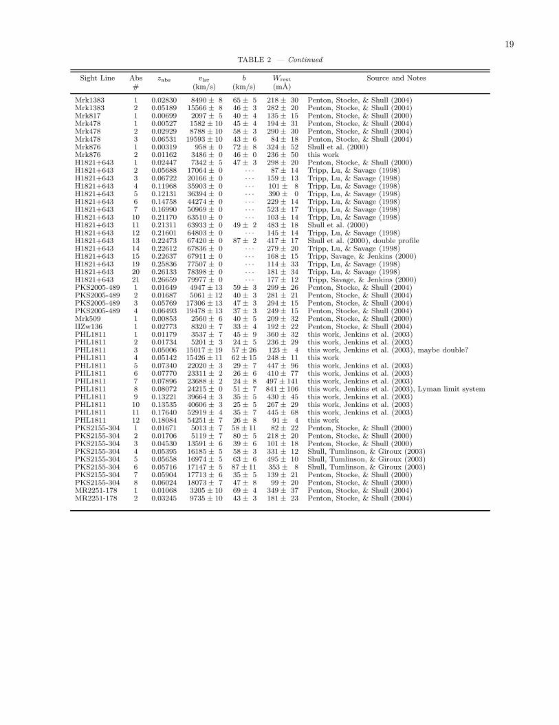
19

TABLE 2 — Continued

Sight Line Abs zabs vlsr b Wrest Source and Notes# (km/s) (km/s) (mA)

Mrk1383 1 0.02830 8490 ± 8 65 ± 5 218 ± 30 Penton, Stocke, & Shull (2004)Mrk1383 2 0.05189 15566 ± 8 46 ± 3 282 ± 20 Penton, Stocke, & Shull (2004)Mrk817 1 0.00699 2097 ± 5 40 ± 4 135 ± 15 Penton, Stocke, & Shull (2000)Mrk478 1 0.00527 1582 ± 10 45 ± 4 194 ± 31 Penton, Stocke, & Shull (2004)Mrk478 2 0.02929 8788 ± 10 58 ± 3 290 ± 30 Penton, Stocke, & Shull (2004)Mrk478 3 0.06531 19593 ± 10 43 ± 6 84 ± 18 Penton, Stocke, & Shull (2004)Mrk876 1 0.00319 958 ± 0 72 ± 8 324 ± 52 Shull et al. (2000)Mrk876 2 0.01162 3486 ± 0 46 ± 0 236 ± 50 this workH1821+643 1 0.02447 7342 ± 5 47 ± 3 298 ± 20 Penton, Stocke, & Shull (2000)H1821+643 2 0.05688 17064 ± 0 · · · 87 ± 14 Tripp, Lu, & Savage (1998)H1821+643 3 0.06722 20166 ± 0 · · · 159 ± 13 Tripp, Lu, & Savage (1998)H1821+643 4 0.11968 35903 ± 0 · · · 101 ± 8 Tripp, Lu, & Savage (1998)H1821+643 5 0.12131 36394 ± 0 · · · 390 ± 0 Tripp, Lu, & Savage (1998)H1821+643 6 0.14758 44274 ± 0 · · · 229 ± 14 Tripp, Lu, & Savage (1998)H1821+643 7 0.16990 50969 ± 0 · · · 523 ± 17 Tripp, Lu, & Savage (1998)H1821+643 10 0.21170 63510 ± 0 · · · 103 ± 14 Tripp, Lu, & Savage (1998)H1821+643 11 0.21311 63933 ± 0 49 ± 2 483 ± 18 Shull et al. (2000)H1821+643 12 0.21601 64803 ± 0 · · · 145 ± 14 Tripp, Lu, & Savage (1998)H1821+643 13 0.22473 67420 ± 0 87 ± 2 417 ± 17 Shull et al. (2000), double profileH1821+643 14 0.22612 67836 ± 0 · · · 279 ± 20 Tripp, Lu, & Savage (1998)H1821+643 15 0.22637 67911 ± 0 · · · 168 ± 15 Tripp, Savage, & Jenkins (2000)H1821+643 19 0.25836 77507 ± 0 · · · 114 ± 33 Tripp, Lu, & Savage (1998)H1821+643 20 0.26133 78398 ± 0 · · · 181 ± 34 Tripp, Lu, & Savage (1998)H1821+643 21 0.26659 79977 ± 0 · · · 177 ± 12 Tripp, Savage, & Jenkins (2000)PKS2005-489 1 0.01649 4947 ± 13 59 ± 3 299 ± 26 Penton, Stocke, & Shull (2004)PKS2005-489 2 0.01687 5061 ± 12 40 ± 3 281 ± 21 Penton, Stocke, & Shull (2004)PKS2005-489 3 0.05769 17306 ± 13 47 ± 3 294 ± 15 Penton, Stocke, & Shull (2004)PKS2005-489 4 0.06493 19478 ± 13 37 ± 3 249 ± 15 Penton, Stocke, & Shull (2004)Mrk509 1 0.00853 2560 ± 6 40 ± 5 209 ± 32 Penton, Stocke, & Shull (2000)IIZw136 1 0.02773 8320 ± 7 33 ± 4 192 ± 22 Penton, Stocke, & Shull (2004)PHL1811 1 0.01179 3537 ± 7 45 ± 9 360 ± 32 this work, Jenkins et al. (2003)PHL1811 2 0.01734 5201 ± 3 24 ± 5 236 ± 29 this work, Jenkins et al. (2003)PHL1811 3 0.05006 15017 ± 19 57 ± 26 123 ± 4 this work, Jenkins et al. (2003), maybe double?PHL1811 4 0.05142 15426 ± 11 62 ± 15 248 ± 11 this workPHL1811 5 0.07340 22020 ± 3 29 ± 7 447 ± 96 this work, Jenkins et al. (2003)PHL1811 6 0.07770 23311 ± 2 26 ± 6 410 ± 77 this work, Jenkins et al. (2003)PHL1811 7 0.07896 23688 ± 2 24 ± 8 497 ± 141 this work, Jenkins et al. (2003)PHL1811 8 0.08072 24215 ± 0 51 ± 7 841 ± 106 this work, Jenkins et al. (2003), Lyman limit systemPHL1811 9 0.13221 39664 ± 3 35 ± 5 430 ± 45 this work, Jenkins et al. (2003)PHL1811 10 0.13535 40606 ± 3 25 ± 5 267 ± 29 this work, Jenkins et al. (2003)PHL1811 11 0.17640 52919 ± 4 35 ± 7 445 ± 68 this work, Jenkins et al. (2003)PHL1811 12 0.18084 54251 ± 7 26 ± 8 91 ± 4 this workPKS2155-304 1 0.01671 5013 ± 7 58 ± 11 82 ± 22 Penton, Stocke, & Shull (2000)PKS2155-304 2 0.01706 5119 ± 7 80 ± 5 218 ± 20 Penton, Stocke, & Shull (2000)PKS2155-304 3 0.04530 13591 ± 6 39 ± 6 101 ± 18 Penton, Stocke, & Shull (2000)PKS2155-304 4 0.05395 16185 ± 5 58 ± 3 331 ± 12 Shull, Tumlinson, & Giroux (2003)PKS2155-304 5 0.05658 16974 ± 5 63 ± 6 495 ± 10 Shull, Tumlinson, & Giroux (2003)PKS2155-304 6 0.05716 17147 ± 5 87 ± 11 353 ± 8 Shull, Tumlinson, & Giroux (2003)PKS2155-304 7 0.05904 17713 ± 6 35 ± 5 139 ± 21 Penton, Stocke, & Shull (2000)PKS2155-304 8 0.06024 18073 ± 7 47 ± 8 99 ± 20 Penton, Stocke, & Shull (2000)MR2251-178 1 0.01068 3205 ± 10 69 ± 4 349 ± 37 Penton, Stocke, & Shull (2004)MR2251-178 2 0.03245 9735 ± 10 43 ± 3 181 ± 23 Penton, Stocke, & Shull (2004)

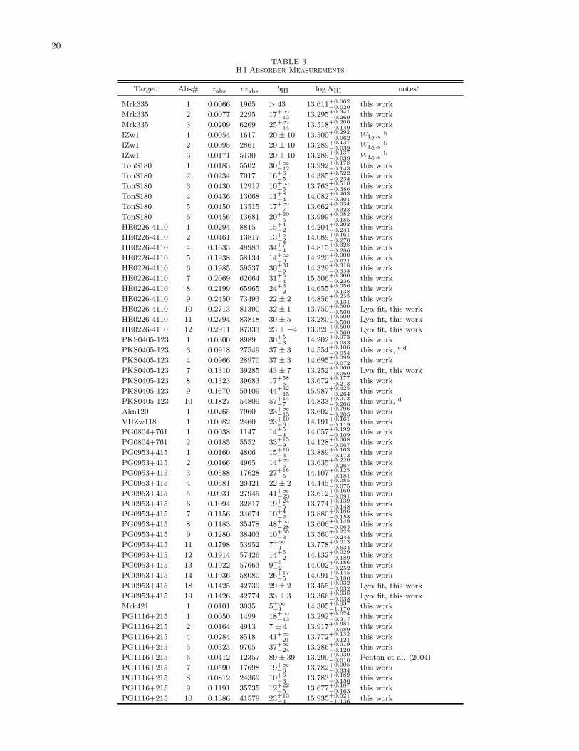
20

TABLE 3H I Absorber Measurements

Target Abs# zabs czabs bHI log NHI notesa

Mrk335 1 0.0066 1965 > 43 13.611+0.062−0.020 this work

Mrk335 2 0.0077 2295 17+∞

−13 13.295+0.341−0.269 this work

Mrk335 3 0.0209 6269 25+∞

−14 13.518+0.200−0.149 this work

IZw1 1 0.0054 1617 20 ± 10 13.500+0.292−0.062 WLyα

b

IZw1 2 0.0095 2861 20 ± 10 13.289+0.137−0.039 WLyα

b

IZw1 3 0.0171 5130 20 ± 10 13.289+0.137−0.039 WLyα

b

TonS180 1 0.0183 5502 30+∞

−12 13.992+0.178−0.143 this work

TonS180 2 0.0234 7017 16+6−5 14.385+0.522

−0.234 this work

TonS180 3 0.0430 12912 10+∞

−5 13.763+0.510−0.386 this work

TonS180 4 0.0436 13068 11+8−4 14.082+0.463

−0.301 this work

TonS180 5 0.0450 13515 17+∞

−7 13.662+0.034−0.323 this work

TonS180 6 0.0456 13681 20+20−5 13.999+0.082

−0.185 this work

HE0226-4110 1 0.0294 8815 15+4−2 14.204+0.202

−0.241 this work

HE0226-4110 2 0.0461 13817 13+5−2 14.089+0.161

−0.270 this work

HE0226-4110 4 0.1633 48983 34+7−4 14.815+0.328

−0.286 this work

HE0226-4110 5 0.1938 58134 14+∞

−0 14.220+0.000−0.621 this work

HE0226-4110 6 0.1985 59537 30+31−6 14.329+0.318

−0.338 this work

HE0226-4110 7 0.2069 62064 31+5−4 15.506+0.300

−0.236 this work

HE0226-4110 8 0.2199 65965 24+3−2 14.655+0.056

−0.138 this work

HE0226-4110 9 0.2450 73493 22 ± 2 14.856+0.235−0.131 this work

HE0226-4110 10 0.2713 81390 32 ± 1 13.750+0.500−0.500 Lyα fit, this work

HE0226-4110 11 0.2794 83818 30 ± 5 13.280+0.500−0.500 Lyα fit, this work

HE0226-4110 12 0.2911 87333 23 ±−4 13.320+0.500−0.500 Lyα fit, this work

PKS0405-123 1 0.0300 8989 30+5−3 14.202+0.073

−0.083 this work

PKS0405-123 3 0.0918 27549 37 ± 3 14.554+0.106−0.054 this work, c,d

PKS0405-123 4 0.0966 28970 37 ± 3 14.695+0.099−0.072 this work

PKS0405-123 7 0.1310 39285 43 ± 7 13.252+0.060−0.060 Lyα fit, this work

PKS0405-123 8 0.1323 39683 17+58−5 13.672+0.177

−0.213 this work

PKS0405-123 9 0.1670 50109 44+32−15 15.987+0.425

−0.264 this work

PKS0405-123 10 0.1827 54809 57+14−7 14.833+0.073

−0.206 this work, d

Akn120 1 0.0265 7960 23+∞

−15 13.602+0.796−0.205 this work

VIIZw118 1 0.0082 2460 23+10−6 14.191+0.161

−0.119 this work

PG0804+761 1 0.0038 1147 14+5−4 14.057+0.199

−0.109 this work

PG0804+761 2 0.0185 5552 33+15−9 14.128+0.068

−0.067 this work

PG0953+415 1 0.0160 4806 15+10−3 13.889+0.163

−0.173 this work

PG0953+415 2 0.0166 4965 14+∞

−5 13.635+0.220−0.267 this work

PG0953+415 3 0.0588 17628 27+16−5 14.107+0.125

−0.181 this work

PG0953+415 4 0.0681 20421 22 ± 2 14.445+0.085−0.075 this work

PG0953+415 5 0.0931 27945 41+∞

−23 13.612+0.160−0.091 this work

PG0953+415 6 0.1094 32817 19+24−5 13.774+0.139

−0.148 this work

PG0953+415 7 0.1156 34674 10+4−2 13.880+0.186

−0.158 this work

PG0953+415 8 0.1183 35478 48+∞

−28 13.606+0.149−0.063 this work

PG0953+415 9 0.1280 38403 10+55−3 13.560+0.222

−0.244 this work

PG0953+415 11 0.1798 53952 7+∞

−1 13.778+0.013−0.634 this work

PG0953+415 12 0.1914 57426 14+5−2 14.132+0.029

−0.189 this work

PG0953+415 13 0.1922 57663 9+5−2 14.002+0.186

−0.252 this work

PG0953+415 14 0.1936 58080 26+17−5 14.091+0.145

−0.180 this work

PG0953+415 18 0.1425 42739 29 ± 2 13.455+0.032−0.032 Lyα fit, this work

PG0953+415 19 0.1426 42774 33 ± 3 13.366+0.038−0.038 Lyα fit, this work

Mrk421 1 0.0101 3035 5+∞

−1 14.305+0.037−1.170 this work

PG1116+215 1 0.0050 1499 18+∞

−13 13.292+0.074−0.317 this work

PG1116+215 2 0.0164 4913 7 ± 4 13.917+0.681−0.089 this work

PG1116+215 4 0.0284 8518 41+∞

−21 13.772+0.132−0.121 this work

PG1116+215 5 0.0323 9705 37+∞

−24 13.286+0.019−0.120 this work

PG1116+215 6 0.0412 12357 89 ± 39 13.290+0.030−0.010 Penton et al. (2004)

PG1116+215 7 0.0590 17698 19+∞

−6 13.782+0.005−0.334 this work

PG1116+215 8 0.0812 24369 10+6−3 13.783+0.189

−0.150 this work

PG1116+215 9 0.1191 35735 12+22−5 13.677+0.187

−0.163 this work

PG1116+215 10 0.1386 41579 23+13−4 15.935+0.521

−1.136 this work

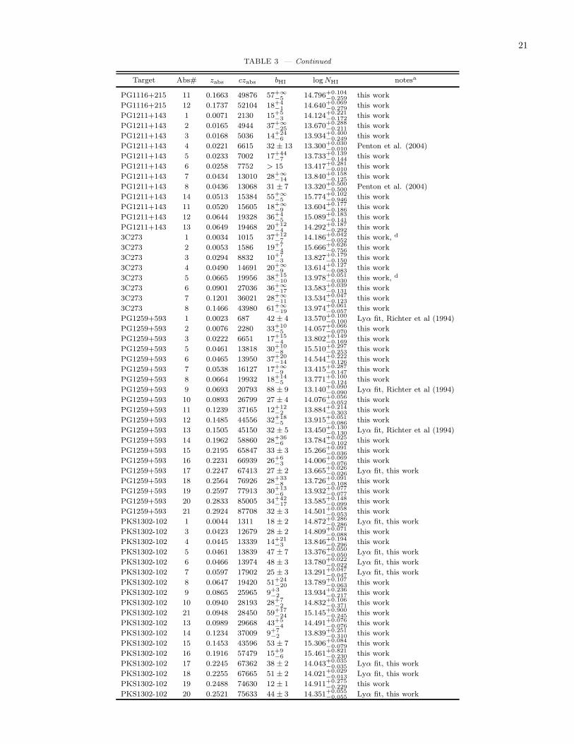
21

TABLE 3 — Continued

Target Abs# zabs czabs bHI log NHI notesa

PG1116+215 11 0.1663 49876 57+∞

−5 14.796+0.104−0.259 this work

PG1116+215 12 0.1737 52104 18+4−1 14.640+0.069

−0.279 this work

PG1211+143 1 0.0071 2130 15+5−3 14.124+0.221

−0.172 this work

PG1211+143 2 0.0165 4944 37+∞

−25 13.670+0.288−0.211 this work

PG1211+143 3 0.0168 5036 14+24−6 13.934+0.400

−0.249 this work

PG1211+143 4 0.0221 6615 32 ± 13 13.300+0.030−0.010 Penton et al. (2004)

PG1211+143 5 0.0233 7002 17+44−7 13.733+0.139

−0.144 this work

PG1211+143 6 0.0258 7752 > 15 13.417+0.281−0.010 this work

PG1211+143 7 0.0434 13010 28+∞

−14 13.840+0.158−0.125 this work

PG1211+143 8 0.0436 13068 31 ± 7 13.320+0.500−0.500 Penton et al. (2004)

PG1211+143 14 0.0513 15384 55+∞

−5 15.774+0.102−0.946 this work

PG1211+143 11 0.0520 15605 18+∞

−9 13.604+0.177−0.186 this work

PG1211+143 12 0.0644 19328 36+4−5 15.089+0.183

−0.141 this work

PG1211+143 13 0.0649 19468 20+12−4 14.292+0.187

−0.292 this work

3C273 1 0.0034 1015 37+12−7 14.186+0.042

−0.052 this work, d

3C273 2 0.0053 1586 19+7−4 15.666+0.626

−0.756 this work

3C273 3 0.0294 8832 10+7−3 13.827+0.179

−0.150 this work

3C273 4 0.0490 14691 20+∞

−9 13.614+0.127−0.083 this work

3C273 5 0.0665 19956 38+15−10 13.978+0.051

−0.030 this work, d

3C273 6 0.0901 27036 36+∞

−17 13.583+0.039−0.131 this work

3C273 7 0.1201 36021 28+∞

−11 13.534+0.047−0.123 this work

3C273 8 0.1466 43980 61+∞

−19 13.974+0.061−0.057 this work

PG1259+593 1 0.0023 687 42 ± 4 13.570+0.100−0.100 Lyα fit, Richter et al (1994)

PG1259+593 2 0.0076 2280 33+10−5 14.057+0.066

−0.070 this work

PG1259+593 3 0.0222 6651 17+15−4 13.802+0.149

−0.169 this work

PG1259+593 5 0.0461 13818 30+10−8 15.510+0.297

−0.253 this work

PG1259+593 6 0.0465 13950 37+20−14 14.544+0.222

−0.126 this work

PG1259+593 7 0.0538 16127 17+∞

−9 13.415+0.287−0.147 this work

PG1259+593 8 0.0664 19932 18+14−5 13.771+0.100

−0.124 this work

PG1259+593 9 0.0693 20793 88 ± 9 13.140+0.090−0.090 Lyα fit, Richter et al (1994)

PG1259+593 10 0.0893 26799 27 ± 4 14.076+0.056−0.052 this work

PG1259+593 11 0.1239 37165 12+12−2 13.884+0.214

−0.303 this work

PG1259+593 12 0.1485 44556 32+18−5 13.915+0.051

−0.086 this work

PG1259+593 13 0.1505 45150 32 ± 5 13.450+0.130−0.130 Lyα fit, Richter et al (1994)

PG1259+593 14 0.1962 58860 28+36−6 13.784+0.025

−0.102 this work

PG1259+593 15 0.2195 65847 33 ± 3 15.266+0.091−0.036 this work

PG1259+593 16 0.2231 66939 26+6−3 14.006+0.069

−0.076 this work

PG1259+593 17 0.2247 67413 27 ± 2 13.665+0.026−0.026 Lyα fit, this work

PG1259+593 18 0.2564 76926 28+33−8 13.726+0.091

−0.108 this work

PG1259+593 19 0.2597 77913 30+13−6 13.932+0.077

−0.077 this work

PG1259+593 20 0.2833 85005 34+42−17 13.585+0.148

−0.099 this work

PG1259+593 21 0.2924 87708 32 ± 3 14.501+0.058−0.053 this work

PKS1302-102 1 0.0044 1311 18 ± 2 14.872+0.286−0.286 Lyα fit, this work

PKS1302-102 3 0.0423 12679 28 ± 2 14.809+0.071−0.088 this work

PKS1302-102 4 0.0445 13339 14+21−3 13.846+0.194

−0.296 this work

PKS1302-102 5 0.0461 13839 47 ± 7 13.376+0.050−0.050 Lyα fit, this work

PKS1302-102 6 0.0466 13974 48 ± 3 13.780+0.022−0.022 Lyα fit, this work

PKS1302-102 7 0.0597 17902 25 ± 3 13.291+0.047−0.047 Lyα fit, this work

PKS1302-102 8 0.0647 19420 51+24−20 13.789+0.107

−0.063 this work

PKS1302-102 9 0.0865 25965 9+3−2 13.934+0.236

−0.217 this work

PKS1302-102 10 0.0940 28193 28+7−2 14.832+0.106

−0.371 this work

PKS1302-102 21 0.0948 28450 59+17−24 15.145+0.900

−0.245 this work

PKS1302-102 13 0.0989 29668 43+5−4 14.491+0.076

−0.076 this work

PKS1302-102 14 0.1234 37009 9+7−2 13.839+0.251

−0.310 this work

PKS1302-102 15 0.1453 43596 53 ± 7 15.306+0.084−0.079 this work

PKS1302-102 16 0.1916 57479 15+9−6 15.461+0.821

−0.230 this work

PKS1302-102 17 0.2245 67362 38 ± 2 14.043+0.035−0.035 Lyα fit, this work

PKS1302-102 18 0.2255 67665 51 ± 2 14.021+0.029−0.013 Lyα fit, this work

PKS1302-102 19 0.2488 74630 12 ± 1 14.911+0.275−0.229 this work

PKS1302-102 20 0.2521 75633 44 ± 3 14.351+0.055−0.055 Lyα fit, this work

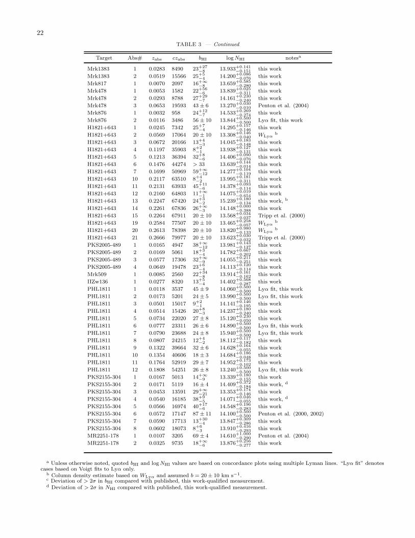
22

TABLE 3 — Continued

Target Abs# zabs czabs bHI log NHI notesa

Mrk1383 1 0.0283 8490 23+27−8 13.933+0.141

−0.151 this work

Mrk1383 2 0.0519 15566 25+5−4 14.200+0.086

−0.076 this work

Mrk817 1 0.0070 2097 16+∞

−8 13.659+0.585−0.280 this work

Mrk478 1 0.0053 1582 22+56−6 13.839+0.025

−0.311 this work

Mrk478 2 0.0293 8788 27+29−7 14.161+0.230

−0.240 this work

Mrk478 3 0.0653 19593 43 ± 6 13.270+0.030−0.010 Penton et al. (2004)

Mrk876 1 0.0032 958 24+12−7 14.533+0.269

−0.274 this work

Mrk876 2 0.0116 3486 56 ± 10 13.844+0.500−0.500 Lyα fit, this work

H1821+643 1 0.0245 7342 25+7−4 14.295+0.157

−0.146 this work

H1821+643 2 0.0569 17064 20 ± 10 13.308+0.146−0.040 WLyα

b

H1821+643 3 0.0672 20166 13+4−3 14.045+0.183

−0.148 this work

H1821+643 4 0.1197 35903 8+2−1 13.938+0.127

−0.131 this work

H1821+643 5 0.1213 36394 32+8−6 14.406+0.090

−0.076 this work

H1821+643 6 0.1476 44274 > 33 13.639+0.144−0.014 this work

H1821+643 7 0.1699 50969 59+∞

−12 14.277+0.104−0.119 this work

H1821+643 10 0.2117 63510 8+4−2 13.995+0.181

−0.311 this work

H1821+643 11 0.2131 63933 45+11−6 14.378+0.093

−0.114 this work

H1821+643 12 0.2160 64803 11+∞

−1 14.075+0.019−0.654 this work

H1821+643 13 0.2247 67420 24+3−2 15.239+0.180

−0.134 this work, b

H1821+643 14 0.2261 67836 26+∞

−3 14.148+0.000−0.388 this work

H1821+643 15 0.2264 67911 20 ± 10 13.568+0.034−0.037 Tripp et al. (2000)

H1821+643 19 0.2584 77507 20 ± 10 13.465+0.258−0.057 WLyα

b

H1821+643 20 0.2613 78398 20 ± 10 13.820+0.980−0.133 WLyα

b

H1821+643 21 0.2666 79977 20 ± 10 13.623+0.030−0.032 Tripp et al. (2000)

PKS2005-489 1 0.0165 4947 38+∞

−12 13.981+0.143−0.127 this work

PKS2005-489 2 0.0169 5061 18+3−4 14.782+0.667

−0.202 this work

PKS2005-489 3 0.0577 17306 32+∞

−9 14.055+0.211−0.251 this work

PKS2005-489 4 0.0649 19478 23+6−4 14.113+0.120

−0.114 this work

Mrk509 1 0.0085 2560 22+34−8 13.914+0.161

−0.162 this work

IIZw136 1 0.0277 8320 13+5−4 14.402+0.568

−0.287 this work

PHL1811 1 0.0118 3537 45 ± 9 14.060+0.500−0.500 Lyα fit, this work

PHL1811 2 0.0173 5201 24 ± 5 13.990+0.500−0.500 Lyα fit, this work

PHL1811 3 0.0501 15017 9+2−1 14.141+0.146

−0.195 this work

PHL1811 4 0.0514 15426 20+8−3 14.237+0.180

−0.240 this work

PHL1811 5 0.0734 22020 27 ± 8 15.120+0.230−0.050 this work

PHL1811 6 0.0777 23311 26 ± 6 14.890+0.500−0.500 Lyα fit, this work

PHL1811 7 0.0790 23688 24 ± 8 15.940+0.500−0.500 Lyα fit, this work

PHL1811 8 0.0807 24215 12+4−2 18.112+0.117

−0.182 this work

PHL1811 9 0.1322 39664 32 ± 6 14.628+0.164−0.055 this work

PHL1811 10 0.1354 40606 18 ± 3 14.684+0.186−0.048 this work

PHL1811 11 0.1764 52919 29 ± 7 14.952+0.173−0.102 this work

PHL1811 12 0.1808 54251 26 ± 8 13.240+0.500−0.500 Lyα fit, this work

PKS2155-304 1 0.0167 5013 14+∞

−9 13.339+0.180−0.155 this work

PKS2155-304 2 0.0171 5119 16 ± 4 14.409+0.372−0.184 this work, d

PKS2155-304 3 0.0453 13591 29+∞

−21 13.353+0.174−0.146 this work

PKS2155-304 4 0.0540 16185 38+9−5 14.071+0.046

−0.055 this work, d

PKS2155-304 5 0.0566 16974 40+17−6 14.548+0.196

−0.283 this work

PKS2155-304 6 0.0572 17147 87 ± 11 14.100+0.500−0.500 Penton et al. (2000, 2002)

PKS2155-304 7 0.0590 17713 13+30−4 13.847+0.309

−0.286 this work

PKS2155-304 8 0.0602 18073 8+6−3 13.910+0.416

−0.293 this work

MR2251-178 1 0.0107 3205 69 ± 4 14.610+1.000−0.290 Penton et al. (2004)

MR2251-178 2 0.0325 9735 18+∞

−6 13.876+0.256−0.277 this work

a Unless otherwise noted, quoted bHI and log NHI values are based on concordance plots using multiple Lyman lines. “Lyα fit” denotescases based on Voigt fits to Lyα only.

b Column density estimate based on WLyα and assumed b = 20 ± 10 km s−1.c Deviation of > 2σ in bHI compared with published, this work-qualified measurement.d Deviation of > 2σ in NHI compared with published, this work-qualified measurement.

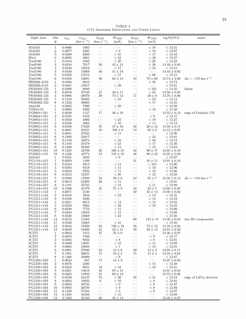
23

TABLE 4O VI Absorber Detections and Upper Limits

Sight Line Abs zabs czabs b1032 W1032 b1032 W1038 logN(OVI) notes# (km s−1) (km s−1) (mA) (km s−1) (mA)

Mrk335 1 0.0066 1965 · · · · · · · · · < 10 < 13.21Mrk335 2 0.0077 2295 · · · < 9 · · · < 10 < 12.87Mrk335 3 0.0209 6269 · · · < 31 · · · < 17 < 13.42IZw1 2 0.0095 2861 · · · < 42 · · · < 39 < 13.57TonS180 1 0.0183 5502 · · · < 20 · · · < 20 < 13.22TonS180 2 0.0234 7017 30 43 ± 15 · · · < 20 13.48 ± 0.05TonS180 3 0.0430 12912 · · · < 17 · · · < 18 < 13.15TonS180 4 0.0436 13068 40 31 ± 18 · · · · · · 13.43 ± 0.02TonS180 5 0.0450 13515 · · · < 17 · · · < 66 < 13.15TonS180 6 0.0456 13681 20 62 ± 14 34 78 ± 60 13.74 ± 0.06 ∆v ∼ +70 km s−1

HE0226-4110 1 0.0294 8815 · · · · · · · · · < 32 < 13.74HE0226-4110 2 0.0461 13817 · · · < 39 · · · · · · < 13.81PKS0405-123 1 0.0300 8989 · · · · · · · · · < 105 < 14.35 blendPKS0405-123 3 0.0918 27549 21 49 ± 11 · · · < 24 13.58 ± 0.05PKS0405-123 4 0.0966 28970 39 73 ± 12 17 28 ± 9 13.70 ± 0.06PKS0405-123 7 0.1310 39285 · · · < 16 · · · < 24 < 13.12PKS0405-123 8 0.1323 39683 · · · · · · · · · < 17 < 13.45Akn120 1 0.0265 7960 · · · < 28 · · · · · · < 13.38VIIZw118 1 0.0082 2460 · · · · · · · · · < 18 < 13.48PG0804+761 1 0.0038 1147 17 36 ± 10 · · · · · · 13.52 ± 0.12 edge of Galactic CIIPG0804+761 2 0.0185 5552 · · · · · · · · · < 9 < 13.17PG0953+415 1 0.0160 4806 · · · < 23 · · · < 19 < 13.27PG0953+415 2 0.0166 4965 · · · < 16 · · · < 14 < 13.12PG0953+415 3 0.0588 17628 35 47 ± 10 48 29 ± 12 13.58 ± 0.11PG0953+415 4 0.0681 20421 16 108 ± 8 14 82 ± 8 14.15 ± 0.07PG0953+415 5 0.0931 27945 · · · < 11 · · · · · · < 12.96PG0953+415 6 0.1094 32817 · · · · · · · · · < 23 < 13.61PG0953+415 7 0.1156 34674 · · · < 16 · · · < 30 < 13.12PG0953+415 8 0.1183 35478 · · · < 23 · · · < 17 < 13.30PG0953+415 9 0.1280 38403 · · · < 13 · · · < 13 < 13.03PG0953+415 18 0.1425 42739 20 100 ± 10 32 96 ± 17 14.05 ± 0.10PG0953+415 19 0.1426 42774 53 133 ± 18 46 98 ± 23 14.22 ± 0.06Mrk421 1 0.0101 3035 · · · < 9 · · · · · · < 12.87PG1116+215 1 0.0050 1499 · · · · · · 21 45 ± 11 13.91 ± 0.10PG1116+215 2 0.0164 4913 · · · < 14 · · · < 184 < 13.06PG1116+215 4 0.0284 8518 · · · < 11 · · · < 10 < 12.96PG1116+215 5 0.0323 9705 · · · < 11 · · · < 10 < 12.96PG1116+215 6 0.0412 12357 · · · < 26 · · · < 12 < 13.29PG1116+215 7 0.0590 17698 24 38 ± 6 24 35 ± 7 13.58 ± 0.13 ∆v ∼ +50 km s−1

PG1116+215 8 0.0812 24369 26 < 11 · · · · · · < 13.01PG1116+215 9 0.1191 35735 · · · < 12 · · · < 11 < 12.99PG1116+215 10 0.1386 41579 25 57 ± 9 10 23 ± 7 13.60 ± 0.05PG1211+143 1 0.0071 2130 · · · · · · 50 45 ± 14 13.90 ± 0.02PG1211+143 2 0.0165 4944 · · · < 23 · · · < 13 < 13.31PG1211+143 3 0.0168 5036 · · · · · · · · · < 13 < 13.33PG1211+143 4 0.0221 6615 · · · < 13 · · · < 14 < 13.03PG1211+143 5 0.0233 7002 · · · < 28 · · · < 19 < 13.35PG1211+143 6 0.0258 7752 · · · < 15 · · · · · · < 13.09PG1211+143 7 0.0434 13010 · · · < 15 · · · · · · < 13.09PG1211+143 8 0.0436 13068 · · · < 22 · · · · · · < 13.30PG1211+143 14 0.0513 15384 · · · · · · 60 122 ± 13 14.30 ± 0.02 two HI componentsPG1211+143 11 0.0520 15605 · · · < 41 · · · · · · < 13.56PG1211+143 12 0.0644 19328 40 126 ± 16 58 73 ± 12 14.10 ± 0.04PG1211+143 13 0.0649 19468 21 43 ± 11 49 49 ± 12 13.91 ± 0.203C273 1 0.0034 1015 47 35 ± 6 · · · · · · 13.46 ± 0.073C273 2 0.0053 1586 · · · · · · · · · < 9 < 13.173C273 3 0.0294 8832 · · · < 8 · · · < 9 < 12.813C273 4 0.0490 14691 · · · < 15 · · · < 11 < 13.093C273 5 0.0665 19956 · · · < 7 · · · < 13 < 12.813C273 6 0.0901 27036 24 13 ± 6 20 13 ± 3 13.05 ± 0.113C273 7 0.1201 36021 15 24 ± 3 15 15 ± 4 13.23 ± 0.043C273 8 0.1466 43980 · · · < 9 · · · · · · < 12.87PG1259+593 1 0.0023 687 17 14 ± 9 · · · · · · 13.07 ± 0.09PG1259+593 2 0.0076 2280 · · · · · · · · · < 15 < 13.39PG1259+593 3 0.0222 6651 16 < 34 · · · < 10 < 13.21PG1259+593 5 0.0461 13818 40 95 ± 15 · · · · · · 13.91 ± 0.04PG1259+593 6 0.0465 13950 21 60 ± 12 · · · · · · 13.72 ± 0.06PG1259+593 7 0.0538 16127 72 < 40 58 < 21 < 13.54 edge of LiF1a detectorPG1259+593 8 0.0664 19932 6 < 10 · · · < 8 < 12.91PG1259+593 9 0.0693 20793 · · · < 9 · · · < 8 < 12.87PG1259+593 10 0.0893 26799 · · · < 9 · · · < 9 < 12.89PG1259+593 11 0.1239 37165 · · · < 9 · · · < 9 < 12.87PG1259+593 12 0.1485 44556 · · · < 15 · · · · · · < 13.09PG1259+593 13 0.1505 45150 46 45 ± 14 · · · · · · 13.46 ± 0.07

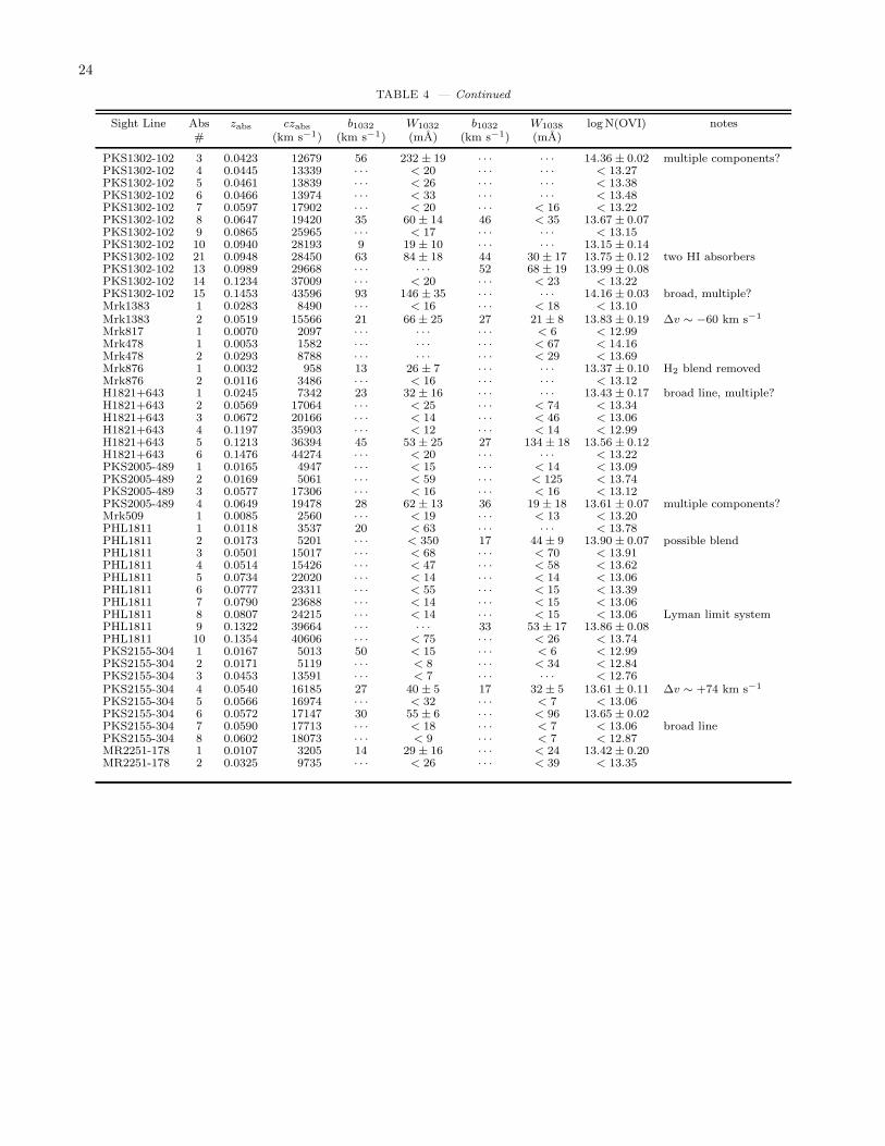
24

TABLE 4 — Continued

Sight Line Abs zabs czabs b1032 W1032 b1032 W1038 logN(OVI) notes# (km s−1) (km s−1) (mA) (km s−1) (mA)

PKS1302-102 3 0.0423 12679 56 232 ± 19 · · · · · · 14.36 ± 0.02 multiple components?PKS1302-102 4 0.0445 13339 · · · < 20 · · · · · · < 13.27PKS1302-102 5 0.0461 13839 · · · < 26 · · · · · · < 13.38PKS1302-102 6 0.0466 13974 · · · < 33 · · · · · · < 13.48PKS1302-102 7 0.0597 17902 · · · < 20 · · · < 16 < 13.22PKS1302-102 8 0.0647 19420 35 60 ± 14 46 < 35 13.67 ± 0.07PKS1302-102 9 0.0865 25965 · · · < 17 · · · · · · < 13.15PKS1302-102 10 0.0940 28193 9 19 ± 10 · · · · · · 13.15 ± 0.14PKS1302-102 21 0.0948 28450 63 84 ± 18 44 30 ± 17 13.75 ± 0.12 two HI absorbersPKS1302-102 13 0.0989 29668 · · · · · · 52 68 ± 19 13.99 ± 0.08PKS1302-102 14 0.1234 37009 · · · < 20 · · · < 23 < 13.22PKS1302-102 15 0.1453 43596 93 146 ± 35 · · · · · · 14.16 ± 0.03 broad, multiple?Mrk1383 1 0.0283 8490 · · · < 16 · · · < 18 < 13.10Mrk1383 2 0.0519 15566 21 66 ± 25 27 21 ± 8 13.83 ± 0.19 ∆v ∼ −60 km s−1

Mrk817 1 0.0070 2097 · · · · · · · · · < 6 < 12.99Mrk478 1 0.0053 1582 · · · · · · · · · < 67 < 14.16Mrk478 2 0.0293 8788 · · · · · · · · · < 29 < 13.69Mrk876 1 0.0032 958 13 26 ± 7 · · · · · · 13.37 ± 0.10 H2 blend removedMrk876 2 0.0116 3486 · · · < 16 · · · · · · < 13.12H1821+643 1 0.0245 7342 23 32 ± 16 · · · · · · 13.43 ± 0.17 broad line, multiple?H1821+643 2 0.0569 17064 · · · < 25 · · · < 74 < 13.34H1821+643 3 0.0672 20166 · · · < 14 · · · < 46 < 13.06H1821+643 4 0.1197 35903 · · · < 12 · · · < 14 < 12.99H1821+643 5 0.1213 36394 45 53 ± 25 27 134 ± 18 13.56 ± 0.12H1821+643 6 0.1476 44274 · · · < 20 · · · · · · < 13.22PKS2005-489 1 0.0165 4947 · · · < 15 · · · < 14 < 13.09PKS2005-489 2 0.0169 5061 · · · < 59 · · · < 125 < 13.74PKS2005-489 3 0.0577 17306 · · · < 16 · · · < 16 < 13.12PKS2005-489 4 0.0649 19478 28 62 ± 13 36 19 ± 18 13.61 ± 0.07 multiple components?Mrk509 1 0.0085 2560 · · · < 19 · · · < 13 < 13.20PHL1811 1 0.0118 3537 20 < 63 · · · · · · < 13.78PHL1811 2 0.0173 5201 · · · < 350 17 44 ± 9 13.90 ± 0.07 possible blendPHL1811 3 0.0501 15017 · · · < 68 · · · < 70 < 13.91PHL1811 4 0.0514 15426 · · · < 47 · · · < 58 < 13.62PHL1811 5 0.0734 22020 · · · < 14 · · · < 14 < 13.06PHL1811 6 0.0777 23311 · · · < 55 · · · < 15 < 13.39PHL1811 7 0.0790 23688 · · · < 14 · · · < 15 < 13.06PHL1811 8 0.0807 24215 · · · < 14 · · · < 15 < 13.06 Lyman limit systemPHL1811 9 0.1322 39664 · · · · · · 33 53 ± 17 13.86 ± 0.08PHL1811 10 0.1354 40606 · · · < 75 · · · < 26 < 13.74PKS2155-304 1 0.0167 5013 50 < 15 · · · < 6 < 12.99PKS2155-304 2 0.0171 5119 · · · < 8 · · · < 34 < 12.84PKS2155-304 3 0.0453 13591 · · · < 7 · · · · · · < 12.76PKS2155-304 4 0.0540 16185 27 40 ± 5 17 32 ± 5 13.61 ± 0.11 ∆v ∼ +74 km s−1

PKS2155-304 5 0.0566 16974 · · · < 32 · · · < 7 < 13.06PKS2155-304 6 0.0572 17147 30 55 ± 6 · · · < 96 13.65 ± 0.02PKS2155-304 7 0.0590 17713 · · · < 18 · · · < 7 < 13.06 broad linePKS2155-304 8 0.0602 18073 · · · < 9 · · · < 7 < 12.87MR2251-178 1 0.0107 3205 14 29 ± 16 · · · < 24 13.42 ± 0.20MR2251-178 2 0.0325 9735 · · · < 26 · · · < 39 < 13.35

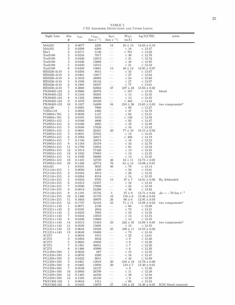
25

TABLE 5C III Absorber Detections and Upper Limits

Sight Line Abs zabs czabs b977 W977 logN(CIII) notes# (km s−1) (km s−1) (mA)

Mrk335 2 0.0077 2295 13 25 ± 13 12.63 ± 0.19Mrk335 3 0.0209 6269 · · · < 18 < 12.47IZw1 3 0.0171 5130 · · · < 701 < 13.92TonS180 2 0.0234 7017 · · · < 30 < 12.70TonS180 3 0.0430 12912 · · · < 21 < 12.52TonS180 4 0.0436 13068 · · · < 48 < 12.95TonS180 5 0.0450 13515 · · · < 21 < 12.52TonS180 6 0.0456 13681 13 48 ± 12 12.95 ± 0.07HE0226-4110 1 0.0294 8815 · · · < 45 < 13.07HE0226-4110 2 0.0461 13817 · · · < 27 < 12.64HE0226-4110 4 0.1633 48983 · · · < 24 < 12.60HE0226-4110 5 0.1938 58134 · · · < 27 < 12.67HE0226-4110 6 0.1985 59537 · · · < 77 < 13.01HE0226-4110 7 0.2069 62064 27 237 ± 38 13.83 ± 0.02PKS0405-123 4 0.0966 28970 · · · < 167 < 13.50 blendPKS0405-123 7 0.1310 39285 · · · < 14 < 12.35PKS0405-123 8 0.1323 39683 · · · < 14 < 12.35PKS0405-123 9 0.1670 50109 · · · < 363 < 14.24PKS0405-123 10 0.1827 54809 34 210 ± 26 13.65 ± 0.03 two componentsa

Akn120 1 0.0265 7960 · · · < 80 < 13.27VIIZw118 1 0.0082 2460 · · · < 37 < 12.79PG0804+761 1 0.0038 1147 · · · < 82 < 13.21PG0804+761 2 0.0185 5552 · · · < 148 < 13.59PG0953+415 1 0.0160 4806 · · · < 92 < 13.47PG0953+415 2 0.0166 4965 · · · < 32 < 12.89PG0953+415 3 0.0588 17628 · · · < 16 < 12.42PG0953+415 4 0.0681 20421 20 77 ± 10 13.15 ± 0.02PG0953+415 5 0.0931 27945 · · · < 13 < 12.35PG0953+415 6 0.1094 32817 · · · < 486 < 14.19PG0953+415 7 0.1156 34674 · · · < 18 < 12.52PG0953+415 8 0.1183 35478 · · · < 43 < 12.76PG0953+415 11 0.1798 53952 · · · < 65 < 12.92PG0953+415 12 0.1914 57426 · · · < 13 < 12.35PG0953+415 13 0.1922 57663 · · · < 13 < 12.35PG0953+415 14 0.1936 58080 · · · < 13 < 12.35PG0953+415 18 0.1425 42739 46 44 ± 11 12.75 ± 0.05PG0953+415 19 0.1426 42774 76 61 ± 14 13.08 ± 0.01Mrk421 1 0.0101 3035 36 < 79 < 13.14PG1116+215 1 0.0050 1499 · · · < 56 < 13.01PG1116+215 2 0.0164 4913 · · · < 20 < 12.52PG1116+215 4 0.0284 8518 · · · < 14 < 12.35PG1116+215 5 0.0323 9705 15 37 ± 7 12.81 ± 0.06 H2 deblendedPG1116+215 6 0.0412 12357 · · · < 16 < 12.42PG1116+215 7 0.0590 17698 · · · < 22 < 12.59PG1116+215 8 0.0812 24369 · · · < 46 < 12.82PG1116+215 9 0.1191 35735 5 27 ± 9 12.71 ± 0.04 ∆v ∼ −70 km s−1

PG1116+215 10 0.1386 41579 16 116 ± 6 13.46 ± 0.03PG1116+215 11 0.1663 49876 26 66 ± 6 12.95 ± 0.03PG1116+215 12 0.1737 52104 43 71 ± 11 13.08 ± 0.02 two componentsa

PG1211+143 1 0.0071 2130 · · · < 66 < 13.09PG1211+143 2 0.0165 4944 · · · < 73 < 13.21PG1211+143 5 0.0233 7002 · · · < 22 < 12.56PG1211+143 7 0.0434 13010 · · · < 14 < 12.35PG1211+143 8 0.0436 13068 · · · < 14 < 12.35PG1211+143 14 0.0513 15384 23 222 ± 35 13.88 ± 0.05 two componentsa

PG1211+143 11 0.0520 15605 · · · < 13 < 12.35PG1211+143 12 0.0644 19328 35 169 ± 11 13.53 ± 0.03PG1211+143 13 0.0649 19468 · · · < 73 < 13.163C273 1 0.0034 1015 · · · < 22 < 12.613C273 3 0.0294 8832 · · · < 8 < 12.203C273 5 0.0665 19956 · · · < 9 < 12.203C273 7 0.1201 36021 · · · < 7 < 12.203C273 8 0.1466 43980 · · · < 6 < 12.20PG1259+593 1 0.0023 687 · · · < 15 < 12.35PG1259+593 2 0.0076 2280 · · · < 18 < 12.47PG1259+593 3 0.0222 6651 · · · < 42 < 12.89PG1259+593 5 0.0461 13818 30 216 ± 10 13.79 ± 0.00PG1259+593 6 0.0465 13950 20 110 ± 7 13.40 ± 0.01PG1259+593 7 0.0538 16127 · · · < 9 < 12.20PG1259+593 10 0.0893 26799 · · · < 11 < 12.29PG1259+593 12 0.1485 44556 · · · < 49 < 12.94PG1259+593 13 0.1505 45150 · · · < 9 < 12.20PKS1302-102 1 0.0044 1311 · · · < 66 < 13.24PKS1302-102 3 0.0423 12679 27 116 ± 22 13.36 ± 0.05 IGM blend removed

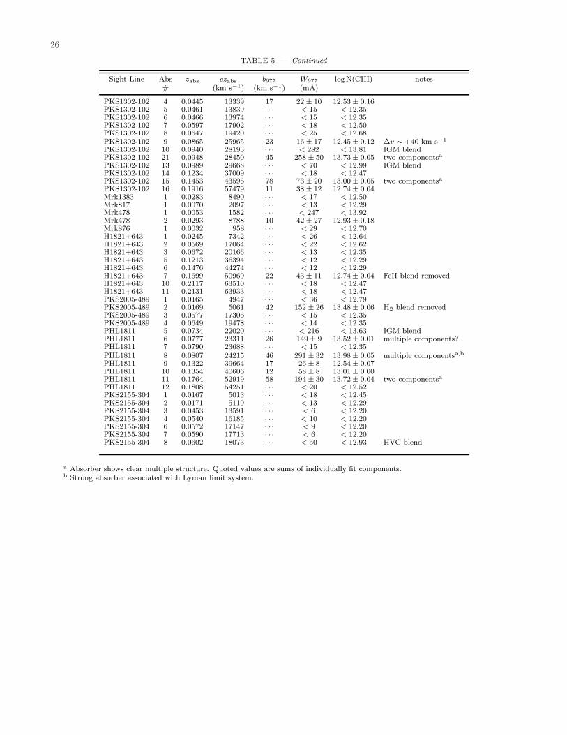
26

TABLE 5 — Continued

Sight Line Abs zabs czabs b977 W977 logN(CIII) notes# (km s−1) (km s−1) (mA)

PKS1302-102 4 0.0445 13339 17 22 ± 10 12.53 ± 0.16PKS1302-102 5 0.0461 13839 · · · < 15 < 12.35PKS1302-102 6 0.0466 13974 · · · < 15 < 12.35PKS1302-102 7 0.0597 17902 · · · < 18 < 12.50PKS1302-102 8 0.0647 19420 · · · < 25 < 12.68PKS1302-102 9 0.0865 25965 23 16 ± 17 12.45 ± 0.12 ∆v ∼ +40 km s−1

PKS1302-102 10 0.0940 28193 · · · < 282 < 13.81 IGM blendPKS1302-102 21 0.0948 28450 45 258 ± 50 13.73 ± 0.05 two componentsa

PKS1302-102 13 0.0989 29668 · · · < 70 < 12.99 IGM blendPKS1302-102 14 0.1234 37009 · · · < 18 < 12.47PKS1302-102 15 0.1453 43596 78 73 ± 20 13.00 ± 0.05 two componentsa

PKS1302-102 16 0.1916 57479 11 38 ± 12 12.74 ± 0.04Mrk1383 1 0.0283 8490 · · · < 17 < 12.50Mrk817 1 0.0070 2097 · · · < 13 < 12.29Mrk478 1 0.0053 1582 · · · < 247 < 13.92Mrk478 2 0.0293 8788 10 42 ± 27 12.93 ± 0.18Mrk876 1 0.0032 958 · · · < 29 < 12.70H1821+643 1 0.0245 7342 · · · < 26 < 12.64H1821+643 2 0.0569 17064 · · · < 22 < 12.62H1821+643 3 0.0672 20166 · · · < 13 < 12.35H1821+643 5 0.1213 36394 · · · < 12 < 12.29H1821+643 6 0.1476 44274 · · · < 12 < 12.29H1821+643 7 0.1699 50969 22 43 ± 11 12.74 ± 0.04 FeII blend removedH1821+643 10 0.2117 63510 · · · < 18 < 12.47H1821+643 11 0.2131 63933 · · · < 18 < 12.47PKS2005-489 1 0.0165 4947 · · · < 36 < 12.79PKS2005-489 2 0.0169 5061 42 152 ± 26 13.48 ± 0.06 H2 blend removedPKS2005-489 3 0.0577 17306 · · · < 15 < 12.35PKS2005-489 4 0.0649 19478 · · · < 14 < 12.35PHL1811 5 0.0734 22020 · · · < 216 < 13.63 IGM blendPHL1811 6 0.0777 23311 26 149 ± 9 13.52 ± 0.01 multiple components?PHL1811 7 0.0790 23688 · · · < 15 < 12.35PHL1811 8 0.0807 24215 46 291 ± 32 13.98 ± 0.05 multiple componentsa,b

PHL1811 9 0.1322 39664 17 26 ± 8 12.54 ± 0.07PHL1811 10 0.1354 40606 12 58 ± 8 13.01 ± 0.00PHL1811 11 0.1764 52919 58 194 ± 30 13.72 ± 0.04 two componentsa

PHL1811 12 0.1808 54251 · · · < 20 < 12.52PKS2155-304 1 0.0167 5013 · · · < 18 < 12.45PKS2155-304 2 0.0171 5119 · · · < 13 < 12.29PKS2155-304 3 0.0453 13591 · · · < 6 < 12.20PKS2155-304 4 0.0540 16185 · · · < 10 < 12.20PKS2155-304 6 0.0572 17147 · · · < 9 < 12.20PKS2155-304 7 0.0590 17713 · · · < 6 < 12.20PKS2155-304 8 0.0602 18073 · · · < 50 < 12.93 HVC blend

a Absorber shows clear multiple structure. Quoted values are sums of individually fit components.b Strong absorber associated with Lyman limit system.