The Long-Run Phillips Curve is ... a Curve

The Long-Run Phillips Curve is ... a Curve∗

Guido Ascari †

De Nederlandsche Bank

University of Pavia

Paolo Bonomolo‡

De Nederlandsche Bank

Qazi Haque §

The University of Adelaide

Centre for Applied Macroeconomic Analysis

March 13, 2022

Abstract

In U.S. data, inflation and output are negatively related in the long run. A BayesianVAR with stochastic trends generalized to be piecewise linear provides robust reduced-formevidence in favor of a threshold level of trend inflation below which potential output isindependent of trend inflation, and above which, instead, potential output is negativelyaffected by trend inflation. The threshold level of inflation is slightly lower than 4%, abovewhich every percentage point increase in inflation is related to about 1% decrease in potentialoutput per year. A New Keynesian model generalized to admit time-varying trend inflationand estimated via particle filtering provides theoretical foundations to this reduced-formevidence. The structural long-run Phillips Curve implied by the estimated New Keynesianmodel is not statistically different from the one implied by the reduced-form piecewise linearBVAR model.

JEL Classification Numbers: C32, C51, E30, E31, E52Keywords: Long-Run Phillips Curve, Inflation, Bayesian VAR, DSGE; Particle Filter.

∗We thank Greg Ganics, Valentina Gavazza, Massimiliano Marcellino, Elmar Mertens, conference participantsat the Ventotene Workshop in Macroeconomics 2021, the ECB and Cleveland Fed Inflation Conference 2021,and seminar participants at Bundesbank, University of Pavia, University of Milano Bicocca and FriendlyFacesMeetings. The views expressed are those of the authors and do not necessarily reflect official positions of DeNederlandsche Bank.†Email: [email protected]‡Email: [email protected]§Email: [email protected]

1 Introduction

Inflation is on the rise. An uplift in inflationary pressures has been increasingly evident in

recent months and quarters in most advanced economies around the world. Measurements of

underlying inflation (which largely exclude pandemic related effects and volatile items) have

also picked up while inflation risks have increased as evident from survey measures of long-

term inflation expectations. U.S. with inflation is at at 40-year highs, sparkling a debate about

whether high inflation is on the way back after years of playing dead. If inflationary pressures

turn out to be more permanent, this may lead to higher underlying trend inflation. What would

be the impact of higher trend inflation on real economic activity in the long-run?

Answering this question requires understanding the long-run relationship between inflation

and economic activity, dubbed the long-run Phillips curve (LRPC), which plays a cornerstone

role in monetary economics. On the one hand, a vertical LRPC implies that the inflation rate is

unrelated to the natural level of output (or the unemployment rate) and the central bank should

therefore simply aim at keeping inflation low and stable because there is no long-run trade-off

between the two variables. On the other hand, a positive relationship between inflation and

output (or equivalently a negative relationship between inflation and the unemployment rate)

in the long-run would open up the possibility of trading off a permanent increase in inflation for

a permanent increase in output (or a permanent reduction in output). Is there such a tradeoff

between inflation and output in the long run?

The answer is no, according to macroeconomics textbooks. These textbooks explain that

while there is a short-run tradeoff between inflation and output (or the unemployment rate), this

tradeoff disappears in the long run, so that the long-run Phillips curve is vertical at the natural

level of output (or the natural rate of unemployment). The LRPC can shift if real forces shift

this natural level, but inflation and monetary factors do not affect the LRPC, so that inflation

and real economic activity are unrelated in the long-run. From the seminal works of Friedman

(1968) and Phelps (1967) onwards, the idea that “inflation is a monetary phenomenon” is a

central tenet of macroeconomic theory and of the inflation targeting monetary policy strategy

of most western central banks.

The relationship between inflation and economic activity is therefore of paramount impor-

tance for monetary policymaking as most central banks, including the Federal Reserve and the

European Central Bank, perceive price stability as the basis for long-term economic growth.

While considerable effort has been devoted in the economics literature to investigate this rela-

tionship in the short-run, it might be very surprising to realize that (see discussion below): (i)

little econometric work has been devoted to estimating the LRPC, and (ii) the New Keynesian

framework, which has become a workhorse in both academia and central banks, might or might

not imply a vertical LRPC, depending on the way nominal rigidities are modelled. This paper

1

tackles both issues by investigating the nature of the long-run relationship between inflation

and economic activity using both reduced-form and structural macroeconomic models.

Regarding (i), a first contribution of the paper is to develop a new empirical framework

to investigate the existence of a potential non-linear relationship between inflation and output

in the long-run. The framework generalizes the Bayesian VAR with stochastic trends (see

Del Negro et al., 2017; Johannsen and Mertens, 2021) to a piecewise linear case. From a

methodological point of view, the functional form of the piecewise linear model depends on

the latent processes (in our case trend inflation). Our theoretical contribution is to show that

both the likelihood function and the posterior distribution of the latent states can be derived

analytically. Therefore, in terms of efficiency our estimator is comparable to the case of linear

models. More importantly, the piecewise linear framework allows us to test the idea that

the long-run relationship between inflation and output can change nature depending on the

level of trend inflation. The main result is the evidence in favor of a threshold level of trend

inflation below which potential output is independent of trend inflation, and above which,

instead, potential output is negatively affected by trend inflation. The threshold level of inflation

is slightly below 4%, above which every percentage point increase in inflation is related to about

1% decrease in potential output per year. We can therefore define a new concept of output gap:

“the long-run output gap” that is the deviation of potential output under positive trend inflation

from its counterfactual level under zero trend inflation. We then show that the long-run output

gap has been on average about negative 2% per year during the Great Inflation. Related to

this point, we also discuss the implications of a negatively-sloped LRPC for the measurement

of business cycles. Specifically, we show that neglecting the long-run relationship between

inflation and output leads to more negative short-run output gap estimates in periods of high

inflation, particularly the Great Inflation, thereby overstating the cyclical component of output

fluctuations.

Regarding (ii), we look for a possible theoretical interpretation of this empirical reduced-form

result. It is natural to start by asking whether the most standard workhorse New Keynesian

(NK) framework can quantitatively reproduce the LRPC estimates of the BVAR. The canonical

NK model does imply a non-linear LRPC (see Ascari and Sbordone, 2014) because positive

trend inflation creates inefficient price dispersion due to nominal rigidities and hence reduces

the natural level of output.1 The relevance of this non-linearity and the magnitude of the

negative effect depend on the parameters of the model. Then, the question becomes empirical.

Moreover, to verify the extent to which the New Keynesian model can reproduce the main

features of the long-run relationship between inflation and output found in the BVAR analysis,

we need to extend the model by allowing for time variation in steady state inflation. Allowing

1We use the terms ‘natural level of output’, ‘potential output’, ‘steady state output’ as indicating the sameobject: the long-run level of output. Furthermore, we will use as synonymous the terms ‘trend inflation’, ‘inflationtarget’ and ‘steady state inflation’.

2

trend inflation to vary every period is a non-trivial modification of the baseline model, both

because the steady state of the model becomes time-varying, and because the dynamics of the

model is affected non-linearly by the level of trend inflation. This paper, thus, generalizes to

a full NK model the work in Cogley and Sbordone (2008), who estimate the New Keynesian

Phillips Curve (NKPC) allowing for time variation in trend inflation, and thus in the NKPC

coefficients.2 A second contribution of the paper, thus, is to estimate the structural NK model

generalized by adding time-varying trend inflation and stochastic volatility. We develop an

econometric strategy suited for this problem, allowing us to jointly estimate the short-run

dynamics and the long-run relationship implied by the model. The model parameters and

the latent states are estimated using a Bayesian approach based on Sequential Monte Carlo

methods. In particular, we use the econometric strategy for parameter learning that combines

the approach of Carvalho et al. (2010), and the particle filter of Liu and West (2001), as in

Ascari et al. (2019).3

The estimated Generalized New Keynesian (GNK) model reproduces very well the evidence

of the reduced-form BVAR model of a negative long-run relationship between inflation and

output. The LRPC is not vertical but negatively sloped and non-linear. In particular, it is

vertical for very low levels of inflation and then it exhibits an increasingly negative slope as

the long-run inflation rate increases above 3-4%. In terms of output losses, going from 2% to

4% inflation target causes an output loss of roughly about 0.65% per year. The effect is highly

non-linear such that a 5% and a 6% inflation target would imply an output loss (relative to 2%

target) of roughly 1.2% and 2% per year, respectively. The estimates are quite precise and they

are not statistically different from the one implied by the reduced-form piecewise linear BVAR

model, i.e. the estimated structural LRPC is within the credibility bands of the estimated

long-run relation between trend inflation and potential output from the BVAR. In addition,

the long-run output gap estimate from the structural model is quantitatively similar to the one

from the BVAR, with output cost estimates of about 1−3% per year during the Great Inflation.

From a medium to long-run perspective, these numbers are not negligible, even for low levels

of trend inflation if one looks at the cumulative losses over the years.4

2Cogley and Sbordone (2008) structurally decompose inflation dynamics into a time-varying long-run com-ponent (i.e., trend inflation) and a short-run one (i.e., the inflation gap given by the difference between inflationand trend inflation). Their main finding is that time-varying trend inflation captures the low frequency variationin the dynamics of inflation, while the short-run inflation gap fits well a purely forward-looking NKPC withoutthe need of any ad hoc intrinsic inertia.

3Fernandez-Villaverde and Rubio-Ramırez (2007) present pioneering work on the estimation of non-linear ornon-Gaussian DSGE models, based on particle filtering within a Markov chain Monte Carlo scheme. The useof Sequential Monte Carlo methods is less common in the literature. Exceptions are Creal (2007), Chen et al.(2010) and Herbst and Schorfheide (2014).

4This point is also made by Coibion et al. (2012) where they compare the large costs of ZLB episodes, whichare rare, to the small costs of a higher target, which are paid every period.

3

Related Literature. The famous correlation unveiled by Phillips (1958) was initially thought

to imply a long-run negative tradeoff between (wage) inflation and unemployment (Phillips,

1958; Samuelson and Solow, 1960). As is well-known, the idea of a long-run tradeoff disappeared

with the seminal papers by Friedman (1968) and Phelps (1967) that introduce the keystone

concept of a natural rate of unemployment and a vertical LRPC. Early tests of the natural rate

hypothesis (NRH) (e.g., Sargan, 1964; Solow, 1969; Gordon, 1970) were based on estimating

a Phillips Curve using some distributed lags of inflation to capture expectations and then

look at whether the sum on the inflation coefficients would add up to one.5 After these early

times, the literature on testing the natural rate hypothesis is surprisingly slim, given its pivotal

role in macroeconomics. King and Watson’s (1994) influential paper find the inflation and

unemployment series to be I(1) but no evidence of cointegration between them. Karanassou

et al. (2005) is one of the first papers to cast doubt about the NRH.6 Beyer and Farmer (2007)

cannot reject the assumption of I(1) for inflation and unemployment, but, unlike King and

Watson (1994), they find that the low frequency comovements are stable and cointegrated

across the whole sample. They interpret their finding as evidence against the NRH. Even more

surprisingly, they find that the cointegrating vector in their VECM model implies a positive

long-run relationship between inflation and unemployment, contrary to the famous Phillips

(1958) negative correlation. Berentsen et al. (2011) reports a positive correlation between the

low frequency (filtered) component of inflation and unemployment. Haug and King (2014)

corroborate this suggestive evidence using more advanced time-series methods for filtering.

A recent paper by Ait Lahcen et al. (2021) uses cross-country panel data from the OECD

countries to document that the positive correlation between long-run anticipated inflation and

unemployment is state-dependent, i.e., it is higher when unemployment is higher. This is

consistent with our findings. Benati (2015) conducts SVAR analysis on U.S. data and concludes

that there is no evidence in favour of a non-vertical LRPC. However, the uncertainty surrounding

the estimates is so large that is not possible to reject an alternative view, where he meant a

negative relationship.

We add to this literature in many dimensions. First, we employ a different methodology

based on the BVAR analysis with stochastic trends, thereby providing a multivariate trend-cycle

decomposition. Second, we provide a methodological contribution as we generalize this approach

to a non-linear setting. While the non-linear approach is necessary to identify a threshold value

of trend inflation that tilts the long-run relationship between inflation and output, it is also

justified by the difficulties in estimating this relationship, as flagged by Beyer and Farmer

5See King and Watson (1994) and King (2008) for a comprehensive survey of the history of the debate overthe nature of the Phillips curve in macroeconomic history in the ‘70s and‘80s. See Karanassou and Sala (2010)and Svensson (2015) for a very recent investigation using a similar approach.

6Karanassou and Sala have a series of papers investigating the NRH for various countries and using differentmethods - GMM, VAR and chain-reaction theory (CRT) - see Karanassou and Sala (2010) and Karanassou et al.(2010) for a survey of these works.

4

(2007) and Benati (2015). Beyer and Farmer (2007) estimate the model over two different sub-

samples because of parameter shifts. Benati (2015) discusses the difficulties in identifying this

long-run relationship because of changing inflation dynamics due to different monetary policy

regimes (Benati, 2008). The possibility of identifying the LRPC depends on the inflation process

displaying permanent variations, i.e., a unit root. However, inflation persistence changed quite

dramatically during the post-WWII sample in the U.S. data, and the Great Inflation might be

the only period that allows identification of the LRPC. Finally, we also estimate a structural

model providing theoretical underpinnings to the empirical analysis.

Regarding theory, first, it is well-known that the GNK model delivers a negative relationship

between steady state inflation and output (Ascari, 2004; Ascari and Sbordone, 2014). Hence, it

is natural to work with the workhorse NK model which is at the core of the modern analysis of

business cycle and monetary policy.7 Second, given the complexity of the estimation procedure,

we estimate a relatively small-scale version of this model with flexible wages and no role for

capital. Third, the cost of steady state inflation is higher in the standard Calvo model compared

to alternative sticky price models, because it leads to a large level of inefficient price dispersion in

steady state. In particular, Nakamura et al. (2018) criticize the welfare costs of inflation implied

by the standard NK model. If price dispersion increases rapidly with inflation, then the absolute

size of price changes should also increase with inflation. However, they find no evidence of larger

absolute price changes in a dataset on pricing behavior during the Great Inflation period. The

frequency of price changes, instead, substantially increased, suggesting that state-dependent

sticky price models might be a more plausible mechanism to describe pricing frictions. Nakamura

et al. (2018) further show that the positive relationship between inflation and price dispersion is

very weak in their state-dependent pricing model, thus reducing the costs of inflation, as showed

in Burstein and Hellwig (2008). This is an important point and few comments are in order.

First, estimating a LRPC in a DSGE model with state-dependent prices and time varying trend

inflation is computationally challenging, if not infeasible. Second, while Nakamura et al. (2018)

focus on the comovement between actual inflation and price dispersion and on the short-run

welfare costs of inflation, we are concerned with long-run relationships. The estimated level of

trend inflation does not go as high as actual inflation in the sample, so the difference between

the welfare cost in a Calvo model and in a menu cost model is less dramatic than with a 2 digit

inflation rate. Moreover, the flat relationship between price dispersion and inflation in menu

costs model heavily depends on the fact that the model needs large idiosyncratic shocks to fit

the microdata. Third, recent works (e.g., Nakamura and Steinsson, 2010; Alvarez et al., 2016)

introduce a random opportunity of price change, hence a Calvo component, in the menu cost

7Berentsen et al. (2011) uses an alternative approach based on search-and-matching frictions both in the goodand labor market to explain the positive correlation between long-run anticipated inflation and unemployment.Ait Lahcen et al. (2021) builds on this model to explain the non-linearity in this relationship they find in theOECD data. None of these papers is estimating the model.

5

model so the model could explain a mass of small price changes in the microdata. In such an

augmented menu cost model, the difference with the Calvo model is bound to be smaller. Fourth,

Sheremirov (2020) shows that microdata exhibit a positive comovement between inflation and

the dispersion of regular prices - that is, excluding temporary sales - and that the Calvo model

overstates this comovement, while the standard fixed menu cost model understates it. Moreover,

Sheremirov (2020) suggests that a Calvo model with sales is the only one able to replicate the

relation between inflation and price dispersion in the microdata. Importantly for us, he shows

that: (i) the inflation cost of business cycles is 40% higher in his favourite model compared to

the standard Calvo model, leading to a lower optimal inflation rate; (ii) the shape of the output

response to monetary policy shock in the Calvo model with sales is similar to the standard one

without sales, suggesting that the implied short-run dynamics of the Calvo model is a good

approximation for aggregate variables. Moreover, a recent paper by Abbritti et al. (2021) insert

in a standard Calvo-type a New Keynesian (NK) framework endogenous growth, a frictional

labor market and downward wage rigidity. The model yields a long-run trade-off between

output growth and inflation and consumption equivalent welfare losses of deviation from the

optimal inflation target that are a multiple of those associated with traditional models, because

endogenous growth magnifies the trade-off between price distortions and output hysteresis.

Finally, and most importantly, we show that our estimated GNK model is able to reproduce

the LRPC estimated with the reduced-form BVAR analysis. Therefore, it is able to capture the

long-run tradeoff between inflation and output in the aggregate data, despite not capturing the

richness of the microdata behaviour, while a menu cost model might have more hard time in

matching the reduced form empirical evidence in aggregate data. The Calvo model thus seems

to be a good approximation not only for capturing aggregate short-run dynamics (see Kehoe

and Midrigan, 2015; Sheremirov, 2020), but also aggregate key long-run relationships.

The paper proceeds as follows. The next section presents the reduced form BVAR method-

ology along with the estimated long-run Phillips curve. The section introduces the notion of

the long-run output gap and shows its estimates from the BVAR and also discusses the impli-

cations for business cycle measurement arising from a non-linear LRPC. Section 3 presents the

structural GNK model, the estimation methodology and the estimation results. The section

documents that a canonical NK model with time-varying trend inflation implies an estimated

LRPC that is both qualitatively and quantitatively in line with the BVAR analysis. Finally,

Section 4 concludes.

2 A time series approach

We propose a time series model that is tailored to the purpose of estimating the long-run Phillips

curve. As in Del Negro et al. (2017) and Johannsen and Mertens (2021), we express a VAR

6

in deviations from time varying trends that we interpret as the long-run components of the

respective variables.8 The methodology is a generalization of the steady state VAR by Villani

(2009) and is a trend-cycle decomposition in which the dynamics of the cyclical components

are described by an unrestricted VAR, but the long-run trends have a structure inspired by

economic theory.

More formally, indicate with Xt a n × 1 vector of observed variables at time t. We define

Xt as the long-run component of Xt. This interpretation follows from the assumption that the

deviations (Xt − Xt) have stable dynamics and unconditional expectations equal to zero. In

particular these deviations are described by the following stable VAR:

A (L)(Xt − Xt

)= εt (1)

where A (L) is a polynomial in the lag operator L and εt ∼ N (0,Σε,t). We assume that the

reduce form shocks εt have stochastic volatility:

Σε,t = B−1St(B−1St)

′ (2)

with St is diagonal and B is lower triangular. Collecting the elements in the main diagonal of St

in the vector st, we follow the well-established literature (see for example Cogley and Sargent,

2005; Primiceri, 2005) by modeling the time variation in the volatilities as:

log st = log st−1 + νt νt ∼ N (0,Σν) (3)

and we restrict Σν to be diagonal.

The focus of our analysis is the long-run component Xt which is assumed to depend on a

(q × 1) vector of latent variables θt: Xt = h (θt)

θt = f (θt−1, ηt)

(4)

where h(θt) and f (θt−1, ηt) are generic (potentially non-linear) functions, and ηt is a vector of

exogenous Gaussian shocks. In this way we can specify the dynamics of the long-run component

in a sufficiently general way, and in particular we are going to use equation (4) to define a long-

run Phillips curve.

8This approach has been recently used by Maffei-Faccioli (2020) and Ascari and Fosso (2021).

7

2.1 The model

We build a model for the GDP per capita yt, the inflation rate πt and the nominal interest rate

it. We use a bar over each respective variable to indicate its time-varying long-run component,

e.g., πt is the long-run component of inflation (trend inflation) at time t.

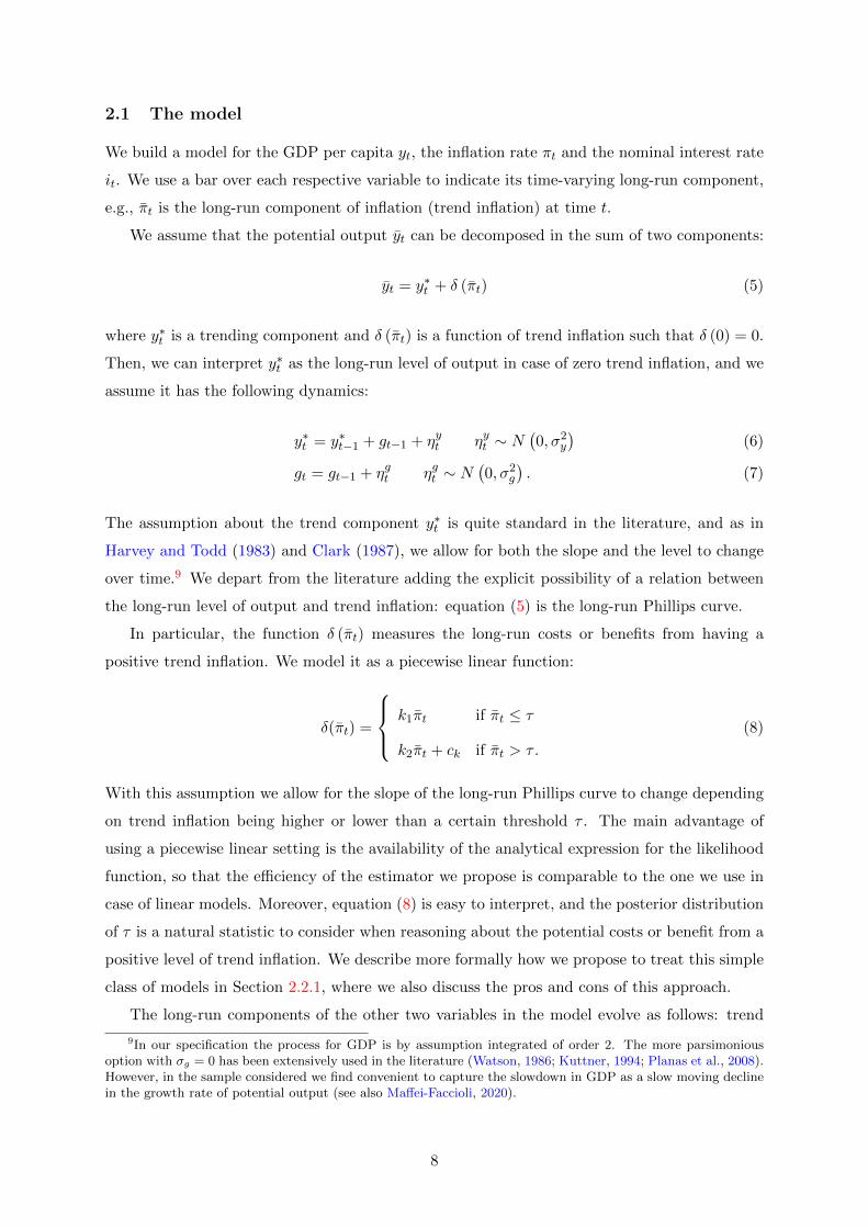
We assume that the potential output yt can be decomposed in the sum of two components:

yt = y∗t + δ (πt) (5)

where y∗t is a trending component and δ (πt) is a function of trend inflation such that δ (0) = 0.

Then, we can interpret y∗t as the long-run level of output in case of zero trend inflation, and we

assume it has the following dynamics:

y∗t = y∗t−1 + gt−1 + ηyt ηyt ∼ N(0, σ2

y

)(6)

gt = gt−1 + ηgt ηgt ∼ N(0, σ2

g

). (7)

The assumption about the trend component y∗t is quite standard in the literature, and as in

Harvey and Todd (1983) and Clark (1987), we allow for both the slope and the level to change

over time.9 We depart from the literature adding the explicit possibility of a relation between

the long-run level of output and trend inflation: equation (5) is the long-run Phillips curve.

In particular, the function δ (πt) measures the long-run costs or benefits from having a

positive trend inflation. We model it as a piecewise linear function:

δ(πt) =

k1πt if πt ≤ τ

k2πt + ck if πt > τ .

(8)

With this assumption we allow for the slope of the long-run Phillips curve to change depending

on trend inflation being higher or lower than a certain threshold τ . The main advantage of

using a piecewise linear setting is the availability of the analytical expression for the likelihood

function, so that the efficiency of the estimator we propose is comparable to the one we use in

case of linear models. Moreover, equation (8) is easy to interpret, and the posterior distribution

of τ is a natural statistic to consider when reasoning about the potential costs or benefit from a

positive level of trend inflation. We describe more formally how we propose to treat this simple

class of models in Section 2.2.1, where we also discuss the pros and cons of this approach.

The long-run components of the other two variables in the model evolve as follows: trend

9In our specification the process for GDP is by assumption integrated of order 2. The more parsimoniousoption with σg = 0 has been extensively used in the literature (Watson, 1986; Kuttner, 1994; Planas et al., 2008).However, in the sample considered we find convenient to capture the slowdown in GDP as a slow moving declinein the growth rate of potential output (see also Maffei-Faccioli, 2020).

8

inflation dynamics are described by a random walk:10

πt = πt−1 + ηπt ηπt ∼ N(0, σ2

π

), (9)

and the nominal interest rate obeys the long-run Fisher equation:

it = πt + cgt + zt. (10)

As in Laubach and Williams (2003), we assume that the long-run real interest rate is a function

of the growth rate of potential output gt and of a component zt that captures all the slow

moving trends that might affect the natural rate of interest, but are not directly included in the

model. In particular we assume that zt also evolves as a random walk:

zt = zt−1 + ηzt ηzt ∼ N(0, σ2

z

). (11)

The model described above belongs to a general class of piecewise linear specifications in

which equation (4) is written as: Xt = Dt +Htθt

θt = Mt + Gtθt−1 + Ptηt

(12)

with ηt ∼ N (0,Ση,t) and Dt, Ht, Mt, Gt, Pt are matrices of appropriate dimensions that are

functions of the latent vector θt. In particular, at each time t we have a finite number N of

possibilities depending on the region to which θt belongs:

(Dt, Ht, Mt, Gt, Pt

)=

(D1,t, H1,t, M1,t, G1,t, P1,t

)if θt ∈ Θ1(

D2,t, H2,t, M2,t, G2,t, P2,t

)if θt ∈ Θ2

...(DN ,t, HN ,t, MN ,t, GN ,t, PN ,t

)if θt ∈ ΘN

(13)

where Θ1,Θ2, ...,ΘN ⊆ Θ is a partition of the support of θt. The time subscript on the right-

hand side of (13) indicates that the groups of matrices do not have to be the same at each time

t: the important assumption is that we always have a finite number of options so that the model

is piecewise linear.

In our case the variable Xt contains the long-run components of GDP per capita, inflation

rate and the nominal interest rate. Moreover, Dt = 0 ∀t and Ht = H is a constant matrix.

10A large part of the literature also assumes stochastic volatility for the shock to trend inflation (see Stockand Watson, 2007, 2016; Mertens, 2016; Mertens and Nason, 2020). We make this assumption for the structuralmodel of Section 3.

9

Finally, the latent vector θt contains trend inflation πt, potential output yt, the growth rate

of long-run output gt and the residual component of the long-run real interest rate zt (see the

Appendix for a detailed description).

2.2 Empirical strategy

We use a Bayesian approach to estimate the joint posterior distribution of the unknown param-

eters and latent processes:

p (θt, st, A(L),ΨB,ΨX ,Ψθ, τ,Σν ,Ση|X1:T ) (14)

where ΨB is the set of parameters of the matrix B in equation (2), and ΨX ,Ψθ, are the set of

parameters of the matrices in the respective equations of system (12). In terms of notation, a

subscript s : t indicates the collection of values from time s to time t, and T is the sample size

such that X1:T denotes the complete data set available for the analysis.

The posterior distribution (14) is approximated through particle filtering: we combine the

particle learning approach by Carvalho et al. (2010) with the methodology by Liu and West

(2001). Particle filtering is a convenient choice to estimate both linear and non-linear models,

and recent applications include Ascari et al. (2019) and Mertens and Nason (2020). Note that

the model described above is non-linear due to the dependency of the matrices in (12) the latent

processes, i.e., θt, and the presence of stochastic volatility, i.e., st. It is important to distinguish

these two sources of non linearity: conditional on the volatility processes, the model is piecewise

linear and below we describe a convenient way to treat this class of models.

2.2.1 The posterior distribution of piecewise linear models

Similar to the case of linear models, we are able to derive the full conditional posterior distribu-

tion of the latent vector θt (considering all the parameters and the stochastic volatility processes

as given). However, we still have one caveat: the posterior distribution at time t is equal to the

weighted sum of 2t distributions. Although all the addenda can be computed analytically, the

number quickly becomes too big, thus making the overall computation subject to the curse of

dimensionality. The following simple example clarifies this point.

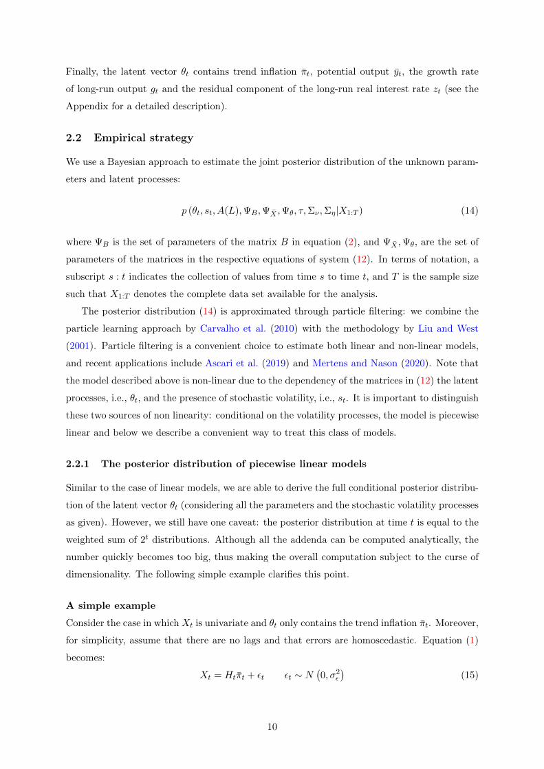
A simple example

Consider the case in which Xt is univariate and θt only contains the trend inflation πt. Moreover,

for simplicity, assume that there are no lags and that errors are homoscedastic. Equation (1)

becomes:

Xt = Htπt + εt εt ∼ N(0, σ2

ε

)(15)

10

where Ht is now a scalar such that:

Ht =

H1 if πt ≤ τ

H2 if πt > τ.

(16)

Assume that before observing any data, trend inflation at time zero is distributed as a Normal:

π0 ∼ N (m0, C0) , so the predictive density is:

π1 ∼ N (a1, R1) , a1 = m0, R1 = C0 + σ2π. (17)

When the first data X1 arrives, we can compute the posterior distribution of π1, which is given

by the sum of two addends:

p (π1|X1) =p (π1|π1 ≤ τ,X1) Pr (π1 ≤ τ |X1) +

p (π1|π1 > τ,X1) Pr (π1 > τ |X1) . (18)

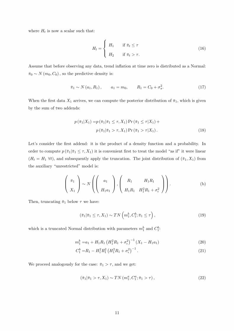
Let’s consider the first addend: it is the product of a density function and a probability. In

order to compute p (π1|π1 ≤ τ,X1) it is convenient first to treat the model “as if” it were linear

(Ht = H1 ∀t), and subsequently apply the truncation. The joint distribution of (π1, X1) from

the auxiliary “unrestricted” model is: π1

X1

∼ N a1

H1a1

,

R1 H1R1

H1R1 H21R1 + σ2

ε

. (b)

Then, truncating π1 below τ we have:

(π1|π1 ≤ τ,X1) ∼ TN(mb

1, Cb1; π1 ≤ τ

), (19)

which is a truncated Normal distribution with parameters mb1 and Cb1:

mb1 =a1 +H1R1

(H2

1R1 + σ2ε

)−1(X1 −H1a1) (20)

Cb1 =R1 −H21R

21

(H2

1R1 + σ2ε

)−1. (21)

We proceed analogously for the case: π1 > τ , and we get:

(π1|π1 > τ,X1) ∼ TN (ma1, C

a1 ; π1 > τ) , (22)

11

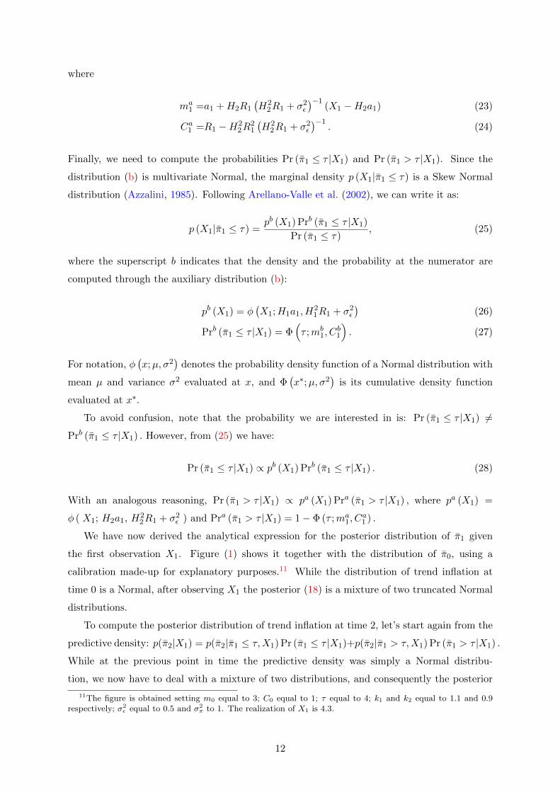
where

ma1 =a1 +H2R1

(H2

2R1 + σ2ε

)−1(X1 −H2a1) (23)

Ca1 =R1 −H22R

21

(H2

2R1 + σ2ε

)−1. (24)

Finally, we need to compute the probabilities Pr (π1 ≤ τ |X1) and Pr (π1 > τ |X1). Since the

distribution (b) is multivariate Normal, the marginal density p (X1|π1 ≤ τ) is a Skew Normal

distribution (Azzalini, 1985). Following Arellano-Valle et al. (2002), we can write it as:

p (X1|π1 ≤ τ) =pb (X1) Prb (π1 ≤ τ |X1)

Pr (π1 ≤ τ), (25)

where the superscript b indicates that the density and the probability at the numerator are

computed through the auxiliary distribution (b):

pb (X1) = φ(X1;H1a1, H

21R1 + σ2

ε

)(26)

Prb (π1 ≤ τ |X1) = Φ(τ ;mb

1, Cb1

). (27)

For notation, φ(x;µ, σ2

)denotes the probability density function of a Normal distribution with

mean µ and variance σ2 evaluated at x, and Φ(x∗;µ, σ2

)is its cumulative density function

evaluated at x∗.

To avoid confusion, note that the probability we are interested in is: Pr (π1 ≤ τ |X1) 6=

Prb (π1 ≤ τ |X1) . However, from (25) we have:

Pr (π1 ≤ τ |X1) ∝ pb (X1) Prb (π1 ≤ τ |X1) . (28)

With an analogous reasoning, Pr (π1 > τ |X1) ∝ pa (X1) Pra (π1 > τ |X1) , where pa (X1) =

φ ( X1; H2a1, H22R1 + σ2

ε ) and Pra (π1 > τ |X1) = 1− Φ (τ ;ma1, C

a1 ) .

We have now derived the analytical expression for the posterior distribution of π1 given

the first observation X1. Figure (1) shows it together with the distribution of π0, using a

calibration made-up for explanatory purposes.11 While the distribution of trend inflation at

time 0 is a Normal, after observing X1 the posterior (18) is a mixture of two truncated Normal

distributions.

To compute the posterior distribution of trend inflation at time 2, let’s start again from the

predictive density: p(π2|X1) = p(π2|π1 ≤ τ,X1) Pr (π1 ≤ τ |X1)+p(π2|π1 > τ,X1) Pr (π1 > τ |X1) .

While at the previous point in time the predictive density was simply a Normal distribu-

tion, we now have to deal with a mixture of two distributions, and consequently the posterior

11The figure is obtained setting m0 equal to 3; C0 equal to 1; τ equal to 4; k1 and k2 equal to 1.1 and 0.9respectively; σ2

ε equal to 0.5 and σ2π to 1. The realization of X1 is 4.3.

12

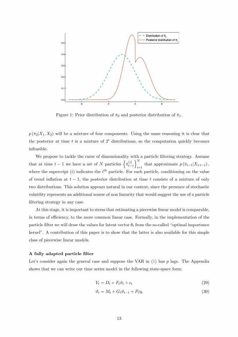
Figure 1: Prior distribution of π0 and posterior distribution of π1.

p (π2|X1, X2) will be a mixture of four components. Using the same reasoning it is clear that

the posterior at time t is a mixture of 2t distributions, so the computation quickly becomes

infeasible.

We propose to tackle the curse of dimensionality with a particle filtering strategy. Assume

that at time t − 1 we have a set of N particlesπ

(i)t−1

Ni=1

that approximate p (πt−1|X1:t−1) ,

where the supercript (i) indicates the ith particle. For each particle, conditioning on the value

of trend inflation at t − 1, the posterior distribution at time t consists of a mixture of only

two distributions. This solution appears natural in our context, since the presence of stochastic

volatility represents an additional sourse of non linearity that would suggest the use of a particle

filtering strategy in any case.

At this stage, it is important to stress that estimating a piecewise linear model is comparable,

in terms of efficiency, to the more common linear case. Formally, in the implementation of the

particle filter we will draw the values for latent vector θt from the so-called “optimal importance

kernel”. A contribution of this paper is to show that the latter is also available for this simple

class of piecewise linear models.

A fully adapted particle filter

Let’s consider again the general case and suppose the VAR in (1) has p lags. The Appendix

shows that we can write our time series model in the following state-space form:

Yt = Dt + Ftϑt + εt (29)

ϑt = Mt +Gtϑt−1 + Ptηt (30)

13

where Yt is an observed vector of dimension n×1 and the latent vector ϑt =(θ′t θ′t−1 · · · θ′t−p

)′.

The matrices of the state-space (29) and (30) are functions of ϑt since they are constructed using

the matrices in (13), so they can belong to different groups depending on the region to which ϑt

belongs. In other words, the state-space model is piecewise linear and for now we are considering

the case in which both the parameters and the volatility processes are known.

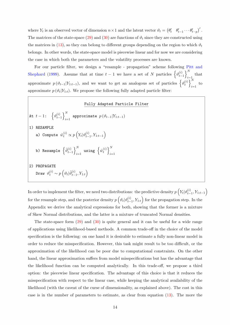
For our particle filter, we design a “resample - propagation” scheme following Pitt and

Shephard (1999). Assume that at time t − 1 we have a set of N particlesϑ

(i)t−1

Ni=1

that

approximate p (ϑt−1|Y1:t−1), and we want to get an analogous set of particlesϑ

(i)t

Ni=1

to

approximate p (ϑt|Y1:t). We propose the following fully adapted particle filter:

Fully Adapted Particle Filter

At t− 1:ϑ

(i)t−1

Ni=1

approximate p (ϑt−1|Y1:t−1)

1) RESAMPLE

a) Compute w(i)t ∝ p

(Yt|ϑ(i)

t−1, Y1:t−1

)

b) Resampleϑ

(i)t−1

Ni=1

usingw

(i)t

Ni=1

2) PROPAGATE

Draw ϑ(i)t ∼ p

(ϑt|ϑ(i)

t−1, Y1:t

)

In order to implement the filter, we need two distributions: the predictive density p(Yt|ϑ(i)

t−1, Y1:t−1

)for the resample step, and the posterior density p

(ϑt|ϑ(i)

t−1, Y1:t

)for the propagation step. In the

Appendix we derive the analytical expressions for both, showing that the former is a mixture

of Skew Normal distributions, and the latter is a mixture of truncated Normal densities.

The state-space form (29) and (30) is quite general and it can be useful for a wide range

of applications using likelihood-based methods. A common trade-off in the choice of the model

specification is the following: on one hand it is desirable to estimate a fully non-linear model in

order to reduce the misspecification. However, this task might result to be too difficult, or the

approximation of the likelihood can be poor due to computational constraints. On the other

hand, the linear approximation suffers from model misspecifications but has the advantage that

the likelihood function can be computed analytically. In this trade-off, we propose a third

option: the piecewise linear specification. The advantage of this choice is that it reduces the

misspecification with respect to the linear case, while keeping the analytical availability of the

likelihood (with the caveat of the curse of dimensionality, as explained above). The cost in this

case is in the number of parameters to estimate, as clear from equation (13). The more the

14

number of intervals, the better the approximation, but the more the number of parameters to

estimate. We lack of a formal criterion to choose an appropriate number of intervals. While

we think this is an interesting question for future research, in this paper we opt for the simple

choice of a single break.

2.2.2 A particle filtering approach for state and parameter learning

For the estimation of non-linear macroeconomic models there is a strong tradition that makes

use of particle filters to get an approximation of the likelihood function in the context of Markov

chain Monte Carlo methods, as pioneered by Fernandez-Villaverde and Rubio-Ramırez (2007).

In this paper, instead, the use of a particle filtering strategy directly aims at approximating the

joint posterior distribution of the latent processes and the parameters, as expressed in (14).

We now describe the main features of our particle filter while having a more detailed expla-

nation in the Appendix. The presence of stochastic volatility introduces another non-linearity

in our model. However, as discussed above, conditional on the stochastic volatility processes,

the model is piecewise linear and both the predictive density and the posterior distribution are

available analytically. In other terms, we implement a marginalized particle filter to increase

the efficiency of the estimator through the Rao-Blackwell theorem. In order to get draws of

the stochastic volatility we simply use a “blind” distribution based on the dynamics of the

stochastic volatilities in equation (A5).

To estimate the parameters we primarily use the particle learning approach by Carvalho

et al. (2010). The methodology consists of augmenting the vector of latent processes with suffi-

cient statistics for the full conditional distributions of the different parameters. This idea uses

the same “Rao-Blackwellization” principle to increase the efficiency of the estimator. Unfortu-

nately, we are not able to use it for all the parameters: in particular sufficient statistics are not

available for the posterior distribution of τ . To estimate the latter, we use a mixture of Normal

distributions, following Liu and West (2001).

The use of particle filters, and in general sequential Monte Carlo methods, to estimate

the parameters of macroeconomic models is becoming more common. With respect to the

more traditional approaches based on Monte Carlo Markov Chain (MCMC), sequential Monte

Carlo (SMC) methods do not have the problems related to the convergence of the chain (which

can be severe in case of non-linear models), and are much better at approximating multi-

modal posterior distributions. Moreover, it is easy to exploit computational advantages from

parallelization, especially in the era of multi-core processors.12

12See the discussion in Herbst and Schorfheide (2014).

15

2.3 Estimation

We estimate the model using three U.S. quarterly time series: per capita real GDP, (annualized)

quarterly growth rate of the GDP deflator, and the Federal Funds rate, over the period 1960Q1−

2008Q2.13 As discussed by Benati (2015), while the Great inflation period is crucial for the

estimation of the long-run Phillips curve, more recent decades contain less relevant information.

Hence, we choose to exclude post-2008 data from our sample to avoid all the technical issues

related to the lower bound on the nominal interest rate.

2.3.1 Priors

The prior distribution of the parameters in the model for the long-run component X are reported

in Table 1. According to our prior information the long-run Phillips curve is vertical: this is

summarized by the choice of a Normal distribution with mean equal to 0 and standard deviation

equal to 0.75 for both k1 and k2. The prior for the threshold τ is centered at 4, which is close

to the average of inflation in our sample. This prior is quite informative because we want to

avoid wasting effort in exploring unrealistic region of the support, especially considering the

range of trend inflation estimates in the literature (see for example Cogley and Sbordone, 2008;

Cogley et al., 2010a; Stock and Watson, 2016; Mertens, 2016; Mertens and Nason, 2020). The

parameter c governs the relation between the growth rate of potential output and the natural

interest rate. While the empirical evidence in favor of this link has been debated (Hamilton

et al., 2016), this relation can be derived from the Euler equation in a micro-founded structural

model, and we make our prior consistent with logarithmic utility (the nominal interest rate

is expressed in annual terms). The priors for the variances of the shocks to the long-run

components are assumed to follow standard Inverse-Gamma distributions whose parameters

are shown in Table 1. The short-run dynamics are described by the VAR in equation (1) for

which we choose 4 lags. For the 36 parameters in A(L), we use a standard Minnesota prior

with the hyperparameter governing the overall tightness equal to 0.2, and the ones for the cross-

variable tightness and lag length decay equal to 1. The prior for the matrices in equation (2)

that decompose the covariance matrix Σε,t is centered at the OLS estimates of the corresponding

VAR with constant volatility. In particular, we assume an Inverse-Wishart distribution with 5

degrees of freedom and we consider the implied distributions for each coefficient. Finally, the

variances of the shocks to the stochastic volatilities have an Inverse-Gamma prior with mean

0.022 and 5 degrees of freedom.

13Data are from the FRED database available at: https://fred.stlouisfed.org .

16

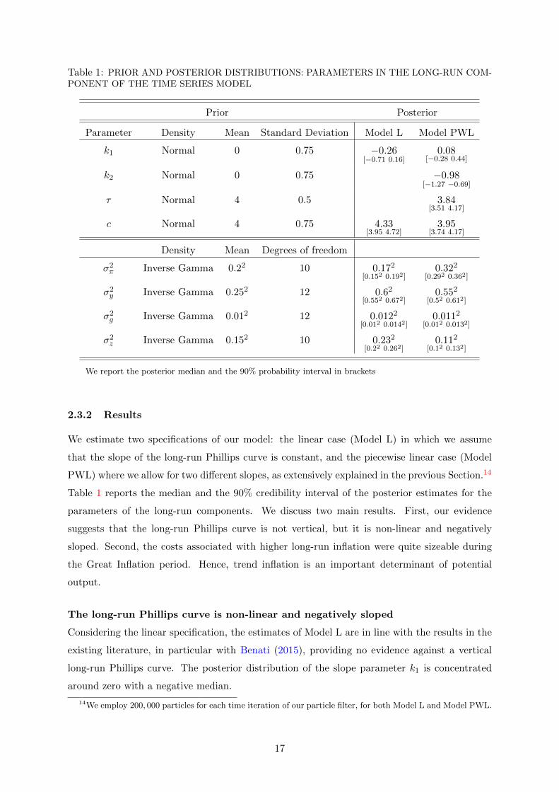
Table 1: PRIOR AND POSTERIOR DISTRIBUTIONS: PARAMETERS IN THE LONG-RUN COM-PONENT OF THE TIME SERIES MODEL

Prior Posterior

Parameter Density Mean Standard Deviation Model L Model PWL

k1 Normal 0 0.75 −0.26[−0.71 0.16]

0.08[−0.28 0.44]

k2 Normal 0 0.75 −0.98[−1.27 −0.69]

τ Normal 4 0.5 3.84[3.51 4.17]

c Normal 4 0.75 4.33[3.95 4.72]

3.95[3.74 4.17]

Density Mean Degrees of freedom

σ2π Inverse Gamma 0.22 10 0.172

[0.152 0.192]0.322

[0.292 0.362]

σ2y Inverse Gamma 0.252 12 0.62

[0.552 0.672]0.552

[0.52 0.612]

σ2g Inverse Gamma 0.012 12 0.0122

[0.012 0.0142]0.0112

[0.012 0.0132]

σ2z Inverse Gamma 0.152 10 0.232

[0.22 0.262]0.112

[0.12 0.132]

We report the posterior median and the 90% probability interval in brackets

2.3.2 Results

We estimate two specifications of our model: the linear case (Model L) in which we assume

that the slope of the long-run Phillips curve is constant, and the piecewise linear case (Model

PWL) where we allow for two different slopes, as extensively explained in the previous Section.14

Table 1 reports the median and the 90% credibility interval of the posterior estimates for the

parameters of the long-run components. We discuss two main results. First, our evidence

suggests that the long-run Phillips curve is not vertical, but it is non-linear and negatively

sloped. Second, the costs associated with higher long-run inflation were quite sizeable during

the Great Inflation period. Hence, trend inflation is an important determinant of potential

output.

The long-run Phillips curve is non-linear and negatively sloped

Considering the linear specification, the estimates of Model L are in line with the results in the

existing literature, in particular with Benati (2015), providing no evidence against a vertical

long-run Phillips curve. The posterior distribution of the slope parameter k1 is concentrated

around zero with a negative median.

14We employ 200, 000 particles for each time iteration of our particle filter, for both Model L and Model PWL.

17

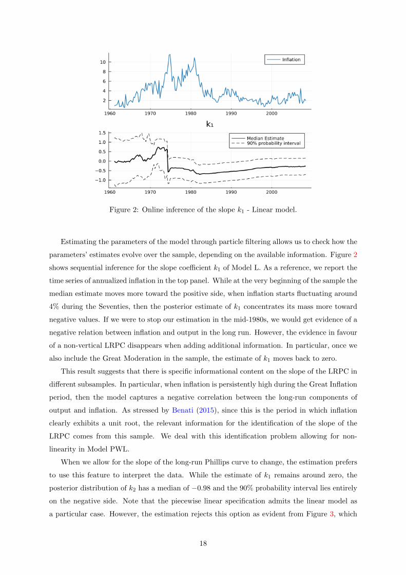
Figure 2: Online inference of the slope k1 - Linear model.

Estimating the parameters of the model through particle filtering allows us to check how the

parameters’ estimates evolve over the sample, depending on the available information. Figure 2

shows sequential inference for the slope coefficient k1 of Model L. As a reference, we report the

time series of annualized inflation in the top panel. While at the very beginning of the sample the

median estimate moves more toward the positive side, when inflation starts fluctuating around

4% during the Seventies, then the posterior estimate of k1 concentrates its mass more toward

negative values. If we were to stop our estimation in the mid-1980s, we would get evidence of a

negative relation between inflation and output in the long run. However, the evidence in favour

of a non-vertical LRPC disappears when adding additional information. In particular, once we

also include the Great Moderation in the sample, the estimate of k1 moves back to zero.

This result suggests that there is specific informational content on the slope of the LRPC in

different subsamples. In particular, when inflation is persistently high during the Great Inflation

period, then the model captures a negative correlation between the long-run components of

output and inflation. As stressed by Benati (2015), since this is the period in which inflation

clearly exhibits a unit root, the relevant information for the identification of the slope of the

LRPC comes from this sample. We deal with this identification problem allowing for non-

linearity in Model PWL.

When we allow for the slope of the long-run Phillips curve to change, the estimation prefers

to use this feature to interpret the data. While the estimate of k1 remains around zero, the

posterior distribution of k2 has a median of −0.98 and the 90% probability interval lies entirely

on the negative side. Note that the piecewise linear specification admits the linear model as

a particular case. However, the estimation rejects this option as evident from Figure 3, which

18

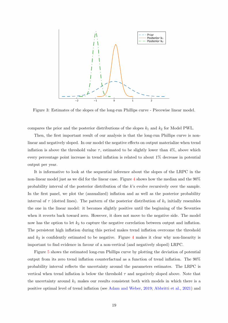
Figure 3: Estimates of the slopes of the long-run Phillips curve - Piecewise linear model.

compares the prior and the posterior distributions of the slopes k1 and k2 for Model PWL.

Then, the first important result of our analysis is that the long-run Phillips curve is non-

linear and negatively sloped. In our model the negative effects on output materialize when trend

inflation is above the threshold value τ , estimated to be slightly lower than 4%, above which

every percentage point increase in trend inflation is related to about 1% decrease in potential

output per year.

It is informative to look at the sequential inference about the slopes of the LRPC in the

non-linear model just as we did for the linear case. Figure 4 shows how the median and the 90%

probability interval of the posterior distribution of the k’s evolve recursively over the sample.

In the first panel, we plot the (annualized) inflation and as well as the posterior probability

interval of τ (dotted lines). The pattern of the posterior distribution of k1 initially resembles

the one in the linear model: it becomes slightly positive until the beginning of the Seventies

when it reverts back toward zero. However, it does not move to the negative side. The model

now has the option to let k2 to capture the negative correlation between output and inflation.

The persistent high inflation during this period makes trend inflation overcome the threshold

and k2 is confidently estimated to be negative. Figure 4 makes it clear why non-linearity is

important to find evidence in favour of a non-vertical (and negatively sloped) LRPC.

Figure 5 shows the estimated long-run Phillips curve by plotting the deviation of potential

output from its zero trend inflation counterfactual as a function of trend inflation. The 90%

probability interval reflects the uncertainty around the parameters estimates. The LRPC is

vertical when trend inflation is below the threshold τ and negatively sloped above. Note that

the uncertainty around k1 makes our results consistent both with models in which there is a

positive optimal level of trend inflation (see Adam and Weber, 2019; Abbritti et al., 2021) and

19

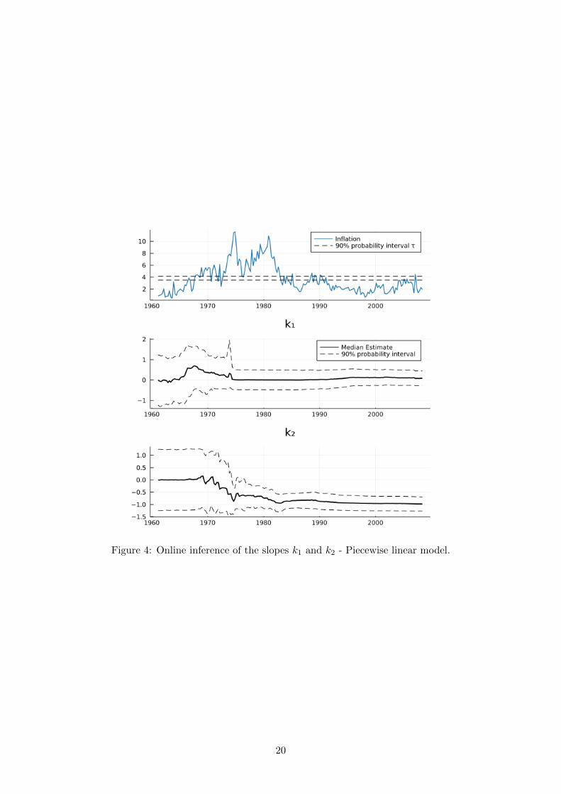
Figure 4: Online inference of the slopes k1 and k2 - Piecewise linear model.

20

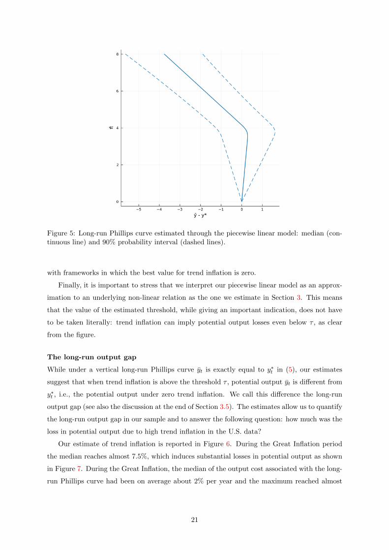
Figure 5: Long-run Phillips curve estimated through the piecewise linear model: median (con-tinuous line) and 90% probability interval (dashed lines).

with frameworks in which the best value for trend inflation is zero.

Finally, it is important to stress that we interpret our piecewise linear model as an approx-

imation to an underlying non-linear relation as the one we estimate in Section 3. This means

that the value of the estimated threshold, while giving an important indication, does not have

to be taken literally: trend inflation can imply potential output losses even below τ , as clear

from the figure.

The long-run output gap

While under a vertical long-run Phillips curve yt is exactly equal to y∗t in (5), our estimates

suggest that when trend inflation is above the threshold τ , potential output yt is different from

y∗t , i.e., the potential output under zero trend inflation. We call this difference the long-run

output gap (see also the discussion at the end of Section 3.5). The estimates allow us to quantify

the long-run output gap in our sample and to answer the following question: how much was the

loss in potential output due to high trend inflation in the U.S. data?

Our estimate of trend inflation is reported in Figure 6. During the Great Inflation period

the median reaches almost 7.5%, which induces substantial losses in potential output as shown

in Figure 7. During the Great Inflation, the median of the output cost associated with the long-

run Phillips curve had been on average about 2% per year and the maximum reached almost

21

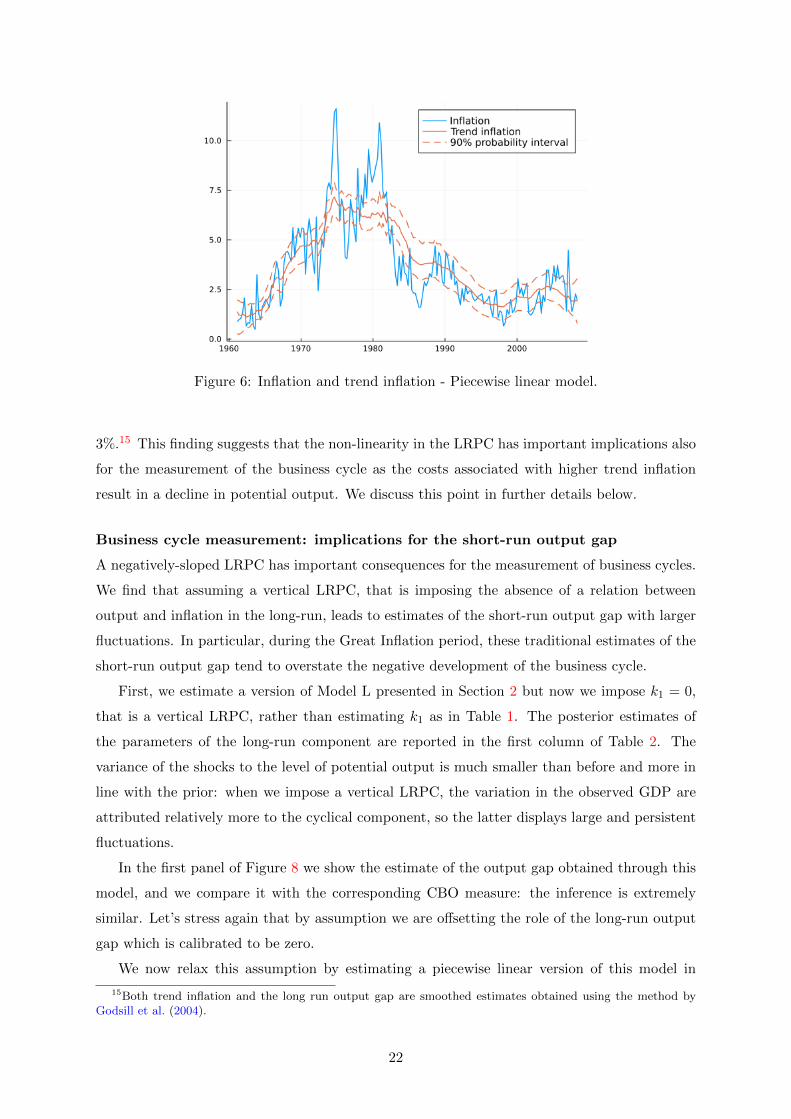
Figure 6: Inflation and trend inflation - Piecewise linear model.

3%.15 This finding suggests that the non-linearity in the LRPC has important implications also

for the measurement of the business cycle as the costs associated with higher trend inflation

result in a decline in potential output. We discuss this point in further details below.

Business cycle measurement: implications for the short-run output gap

A negatively-sloped LRPC has important consequences for the measurement of business cycles.

We find that assuming a vertical LRPC, that is imposing the absence of a relation between

output and inflation in the long-run, leads to estimates of the short-run output gap with larger

fluctuations. In particular, during the Great Inflation period, these traditional estimates of the

short-run output gap tend to overstate the negative development of the business cycle.

First, we estimate a version of Model L presented in Section 2 but now we impose k1 = 0,

that is a vertical LRPC, rather than estimating k1 as in Table 1. The posterior estimates of

the parameters of the long-run component are reported in the first column of Table 2. The

variance of the shocks to the level of potential output is much smaller than before and more in

line with the prior: when we impose a vertical LRPC, the variation in the observed GDP are

attributed relatively more to the cyclical component, so the latter displays large and persistent

fluctuations.

In the first panel of Figure 8 we show the estimate of the output gap obtained through this

model, and we compare it with the corresponding CBO measure: the inference is extremely

similar. Let’s stress again that by assumption we are offsetting the role of the long-run output

gap which is calibrated to be zero.

We now relax this assumption by estimating a piecewise linear version of this model in

15Both trend inflation and the long run output gap are smoothed estimates obtained using the method byGodsill et al. (2004).

22

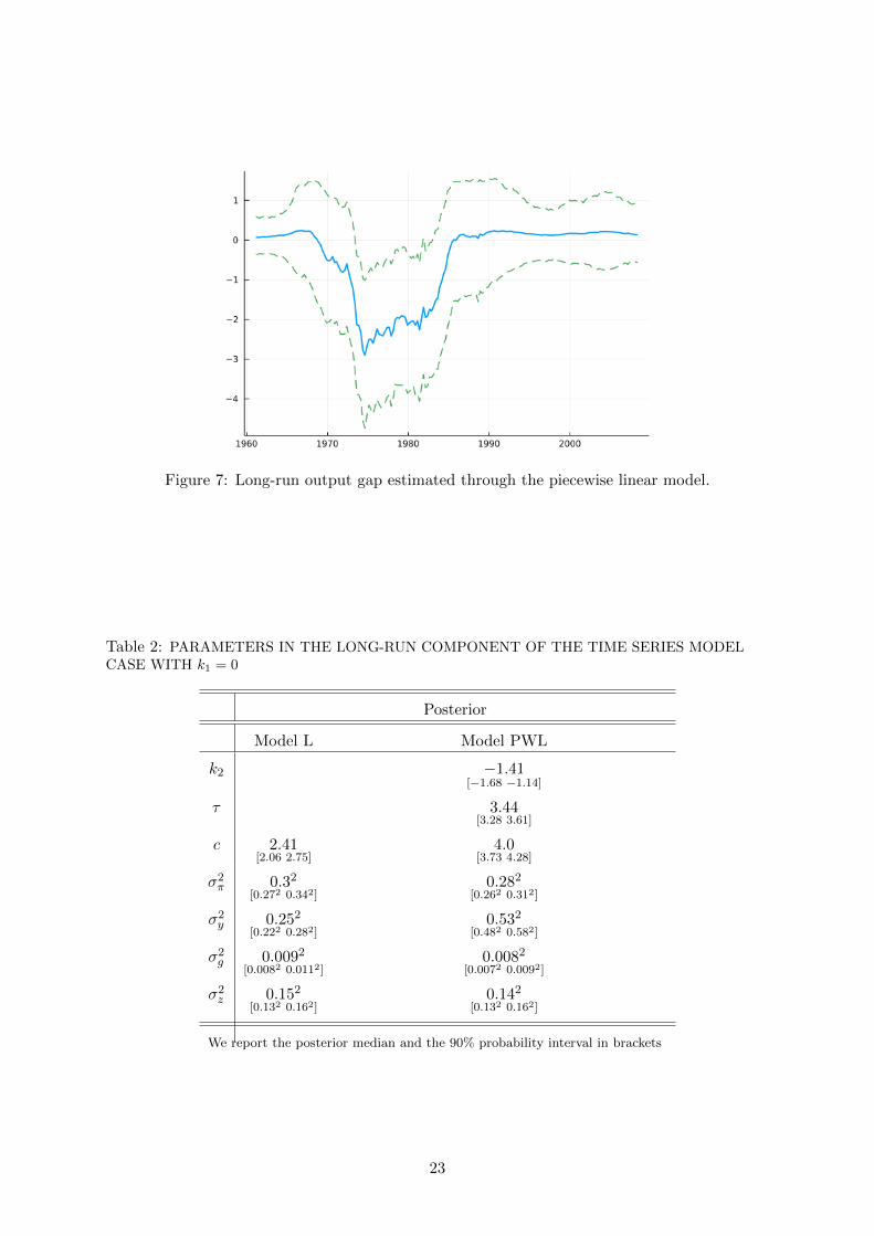
Figure 7: Long-run output gap estimated through the piecewise linear model.

Table 2: PARAMETERS IN THE LONG-RUN COMPONENT OF THE TIME SERIES MODELCASE WITH k1 = 0

Posterior

Model L Model PWL

k2 −1.41[−1.68 −1.14]

τ 3.44[3.28 3.61]

c 2.41[2.06 2.75]

4.0[3.73 4.28]

σ2π 0.32

[0.272 0.342]0.282

[0.262 0.312]

σ2y 0.252

[0.222 0.282]0.532

[0.482 0.582]

σ2g 0.0092

[0.0082 0.0112]0.0082

[0.0072 0.0092]

σ2z 0.152

[0.132 0.162]0.142

[0.132 0.162]

We report the posterior median and the 90% probability interval in brackets

23

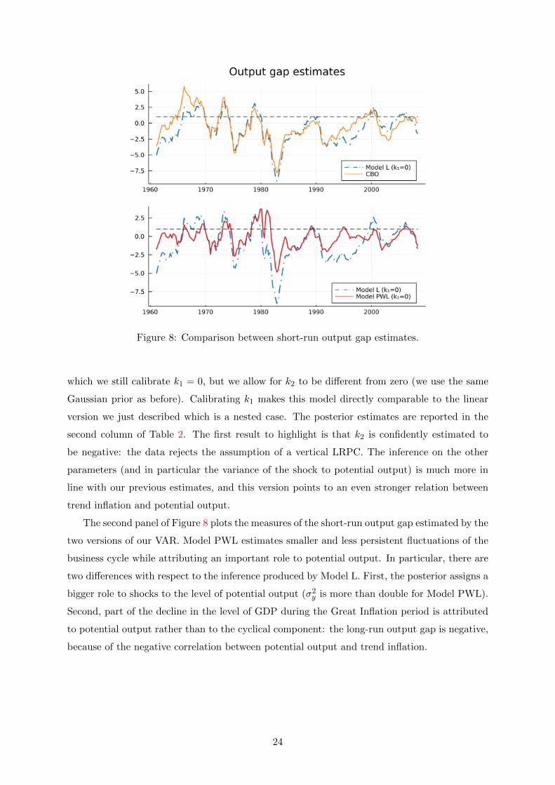
Figure 8: Comparison between short-run output gap estimates.

which we still calibrate k1 = 0, but we allow for k2 to be different from zero (we use the same

Gaussian prior as before). Calibrating k1 makes this model directly comparable to the linear

version we just described which is a nested case. The posterior estimates are reported in the

second column of Table 2. The first result to highlight is that k2 is confidently estimated to

be negative: the data rejects the assumption of a vertical LRPC. The inference on the other

parameters (and in particular the variance of the shock to potential output) is much more in

line with our previous estimates, and this version points to an even stronger relation between

trend inflation and potential output.

The second panel of Figure 8 plots the measures of the short-run output gap estimated by the

two versions of our VAR. Model PWL estimates smaller and less persistent fluctuations of the

business cycle while attributing an important role to potential output. In particular, there are

two differences with respect to the inference produced by Model L. First, the posterior assigns a

bigger role to shocks to the level of potential output (σ2y is more than double for Model PWL).

Second, part of the decline in the level of GDP during the Great Inflation period is attributed

to potential output rather than to the cyclical component: the long-run output gap is negative,

because of the negative correlation between potential output and trend inflation.

24

3 A structural approach

We work with a GNK model with time-varying trend inflation. As in the reduced-form model,

the variables are decomposed into short-run and long-run components, and we estimate the

two components together with the parameters of the model. The aim is to get a model-based

measure of trend inflation, of potential output, and a LRPC. We estimate the model using

a particle filtering (and SMC) strategy analogous to the one used to estimate the time VAR

described in the previous section.

3.1 The model

The artificial economy is a variant of the Generalized New Keynesian (GNK) model in Ascari

and Sbordone (2014). The model consists of a representative household, a representative final-

good firm, a continuum of intermediate-good firms, and a central bank. The model is very

standard, so here we describe the main features, while Appendix B contains the details. The

novelty comes from the assumption of a time-varying trend inflation. Hence, we need to take

particular care of how we log-linearize the model around a time-varying steady state.

The representative agent maximises the following expected utility function where preferences

are additively separable in individual consumption of final goods, Ct, and labor, Nt :

E0

∞∑t=0

βtdt

[ln(Ct − hCt−1

)− dn

N1+ϕt

1 + ϕ

]0 < β < 1, dn > 0, ϕ ≥ 0, 0 ≤ h ≤ 1, (31)

where, Ct is aggregate consumption, E0 represents the expectations operator, the term ϕ is the

inverse of the Frisch labor supply elasticity, dn governs the steady state disutility of work, and

h is the degree of (external) habit persistence in consumption. The term dt stands for a shock

to the discount factor, β, which follows the stationary autoregressive process:

ln dt = (1− ρd) d+ ρd ln dt−1 + σd,tεd,t, (32)

where εd,t is i.i.d N(0, 1) and σd,t denotes time-varying standard deviation of the preference

shock. The period budget constraint is given by:

PtCt +R−1t Bt = WtNt − Tt +Dt +Bt−1, (33)

where Pt is the price level, Rt is the gross nominal interest rate on bonds, Bt is one-period bond

holdings, Wt is the nominal wage rate, Tt is lump sum taxes, and Dt is the profit income.

Firms come in two forms. Final-good firms produce output for consumption. This output is

made from the range of differentiated goods that are supplied by intermediate-good firms who

have market power. Each intermediate-good firm i produces a differentiated good Yi,t under

25

monopolistic competition using the production function Yi,t = AtN1−αi,t . Here At denotes the

level of aggregate technology that is non-stationary and its growth rate gt ≡ At/At−1 follows

the process:

ln gt = ln g + σg,tεg,t, (34)

where g is the steady-state gross rate of technological progress which is also equal to the steady-

state balanced growth rate, εg,t is a i.i.d. N(0, 1) and σg,t is the time-varying standard deviation

of the technology shock. Intermediate-good producers are subject to nominal rigidities in the

form of Calvo (1983) with partial indexation. Hence, they face a constant probability, 0 <

(1 − θ) < 1, of being able to adjust their price and the price of a firm that cannot change the

price is automatically indexed to past-inflation with a degree χ.

The central bank monetary policy follows a Taylor rule featuring inertia and responding to

the inflation gap, the output gap and output growth. The inflation gap is the deviation of the

inflation rate from time-varying trend inflation, i.e., πt, which represents the central’s banks

(time-varying) inflation target and follows a unit root process:

lnπt = lnπt−1 + σπ,tεπ,t, (35)

where επ,t is i.i.d. N(0, 1) and σπ,t denotes time-varying standard deviation of the inflation

target shock. The output gap is the deviation of the level of output from the natural level of

output, i.e., the flexible prices output level. We assume a monetary policy shock εr,t is an i.i.d.

N(0, 1) monetary policy shock with time-varying standard deviation σr,t.

Following Justiniano and Primiceri (2008), we allow for stochastic volatility by assuming

that each element of σt evolves independently according to the following stochastic process:

lnσi,t = lnσi,t−1 + νi,t νi,t ∼ N(0, δ2

i

). (36)

3.2 The state-space form

Note that the steady state of the system is stochastically changing because it is characterized by

time-varying trend inflation, πt, and also because of stochastic (unit-root) technology process.

As a result, we first de-trend the real variables of the model to remove the trend in technology

and then log-linearize the resulting non-linear model around a drifting steady state.16 Here,

we describe heuristically the state-space form for the estimation, composed of the following

elements.

16The Technical Appendix B presents the non-linear equations of the model, its steady state and details onthe log-linearization around the time-varying steady state. As in Cogley and Sbordone (2008), the steady stateof the model is time-varying because of drifts in trend inflation. As such, care must be taken when log-linearizingthe model. As in Cogley and Sbordone (2008) - see footnote 5 therein - we assume ‘anticipated utility’ followingKreps (1998).

26

1. A set of equations that define the detrended variables (vector Zt) as deviations from steady

state Zt = ZtZt/Zt = ZtZt. In logs: lnZt = lnZt + Zt, where Zt ≡ ln Zt.

2. A law of motion for πt: πt = πt−1 exp(σπ,tεπ,t).

3. A set of equations that define the steady state of the variables as a function of πt: Zt =

F (πt, πt−1).

We can then write the usual system for the dynamics of log-linearized variables in canonical

form, but now the system will have time-varying parameters as they are functions of πt:

Γ0(πt)Zt = Γ1(πt)Zt−1 + Ψ(πt)εt + Π(πt)ηt, (37)

where εt is a vector of exogenous disturbances and ηt is a vector of one-step ahead forecast

errors. Hence for any given value of πt (and for a given realization of stochastic volatility),

the system (37) is conditionally linear and can be solved with standard methods (see Appendix

B.4).

At each time t, we observe a vector of data denoted by yt. Then, the solution of model (37)

has the following state-space representation:

yt = c1 + FZt (38)

Zt = c2,t +Mz,tZt−1 +Mε,tεt εt ∼ N(0,Σε,t)

where Σε,t is a diagonal matrix with σi,t of time-varying standard deviations on the main

diagonal. Note that the terms that appear in the state equations, c2,t, Mz,t, Mε,t, depend on t

due to time-varying trend inflation.

3.3 Econometric strategy

We follow a Bayesian approach to make inference regarding the parameters and the latent

processes of the DSGE model. The presence of time-varying trend inflation as well as stochastic

volatility leads to a non-Gaussian and analytically intractable likelihood function. We use the

same particle filtering strategy as for the time-series model to directly approximate the joint

posterior distribution of both the parameters and the latent state variables. In the context of

DSGE models this approach has been use by Chen et al. (2010) and Ascari et al. (2019).

Recently, sequential Monte Carlo (SMC) methods are becoming more popular. The main

idea is to get an approximation of a complicated posterior through the sequential approximation

of simpler distributions. Two approaches have been proposed for DSGE models: (i) a likelihood

tempering scheme (Herbst and Schorfheide, 2014) in which the simpler sequential distributions

are obtained by tempering the likelihood function; (ii) a filtering scheme in which the intermedi-

27

ate distributions are obtained by sequentially adding observations to the likelihood function.17

In this paper we opt for the second approach.

As in Ascari et al. (2019) we can get higher efficiency through Rao-Blackwellization: con-

ditional on πt and the realization of stochastic volatility σi,t, the state space (38) is linear and

Gaussian. This implies that, given a set of particles for πt and σi,t, both the predictive like-

lihood and the full conditional distribution of the other latent states are analytically available

through the standard Kalman filter recursion.

The parameters are divided into two sets: one with the variances of the disturbance to

the stochastic volatility processes, and one with all the other structural parameters. For the

former, we assume Inverse-Gamma priors, allowing us to characterize the posterior distribution

analytically using sufficient statistics computed as functions of the data and the latent processes

of the model. We make inference on these parameters using the particle learning approach

(Carvalho et al., 2010). We approximate the posterior distribution of all the other parameters

through mixtures of Normal distributions, following Liu and West (2001).18

3.4 Data, calibration and prior distributions

We estimate the model using the same U.S. data as in the time-series analysis: per capita real

GDP growth rate, (annualized) quarterly growth rate of the GDP deflator and the Federal

Funds rate, over the period 1960Q1− 2008Q2.

As customary when taking DSGE models to the data, we calibrate a small number of

parameters. In particular, we set the discount factor β to 0.997, the steady state markup to 10

per cent (i.e. ε = 11), the inverse of the labor supply elasticity ϕ to 1, the quarterly net steady

state output growth rate g to 0.5, and the degree of decreasing returns to scale α to 0.3. In light

of the result of Cogley and Sbordone (2008) regarding the lack of support for intrinsic inertia

in the GNK Phillips curve, the model is estimated without backward-looking price indexation,

i.e. χ = 0. The remaining parametes are estimated. Table 3 summarizes the specification of

the prior distributions. The prior for the inflation coefficient ψπ follows a Gamma distribution

centered at 1.50 with a standard deviation of 0.50 while the response coefficient to the output

gap and output growth are centered at 0.125 with standard deviation 0.10. We employ a Beta

distributions with mean 0.70 for the interest rate smoothing parameter ρ and the persistence of

the discount factor shock ρd, while the Calvo probability θ, and habit persistence in consumption

h are centered around 0.50. The steady state real interest rate follows a Gamma distribution

centered at 2. For the variances of the shocks to the volatilities δ2i , we assume an Inverse Gamma

distribution with mean equal to 0.02 and 5 degrees of freedom. Our estimation assumes a unique

17See also Creal (2007) and Herbst and Schorfheide (2016).18For a more detailed description of the SMC algorithm, we refer to the online appendix of Ascari et al. (2019).

28

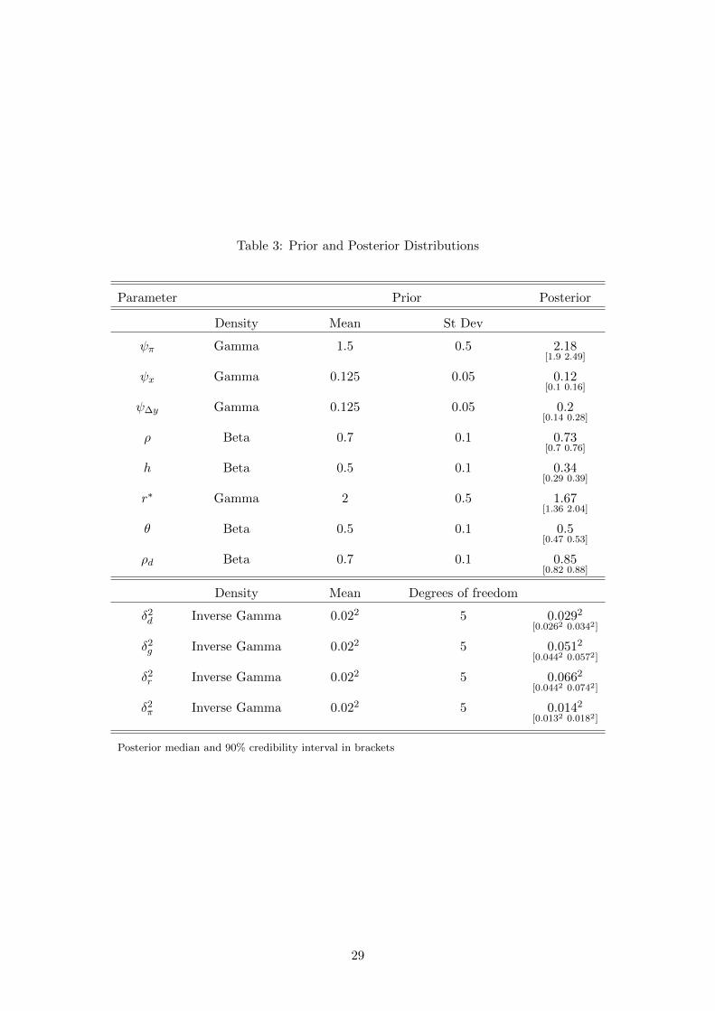
Table 3: Prior and Posterior Distributions

Parameter Prior Posterior

Density Mean St Dev

ψπ Gamma 1.5 0.5 2.18[1.9 2.49]

ψx Gamma 0.125 0.05 0.12[0.1 0.16]

ψ∆y Gamma 0.125 0.05 0.2[0.14 0.28]

ρ Beta 0.7 0.1 0.73[0.7 0.76]

h Beta 0.5 0.1 0.34[0.29 0.39]

r∗ Gamma 2 0.5 1.67[1.36 2.04]

θ Beta 0.5 0.1 0.5[0.47 0.53]

ρd Beta 0.7 0.1 0.85[0.82 0.88]

Density Mean Degrees of freedom

δ2d Inverse Gamma 0.022 5 0.0292

[0.0262 0.0342]

δ2g Inverse Gamma 0.022 5 0.0512

[0.0442 0.0572]

δ2r Inverse Gamma 0.022 5 0.0662

[0.0442 0.0742]

δ2π Inverse Gamma 0.022 5 0.0142

[0.0132 0.0182]

Posterior median and 90% credibility interval in brackets

29

rational expectations equilibrium, i.e. we do not allow for indeterminacy.19

3.5 Estimation results

Table 3 reports the posterior medians and the 90% posterior density intervals based on one

million particles from the final stage in the SMC algorithm. The Taylor rule’s response to the

inflation gap is strongly active as the estimated response lies mostly above 2. We also find a

moderate response to the output gap and a strong response to output growth along with high

degree of interest rate smoothing. The degree of habit formation is somewhat low and close to

0.3. The posterior mean for the degree of price stickiness θ turns out to be around 0.5, which is

smaller than the estimates reported in Smets and Wouters (2007) and Justiniano et al. (2010)

and implies an expected price duration of six months.

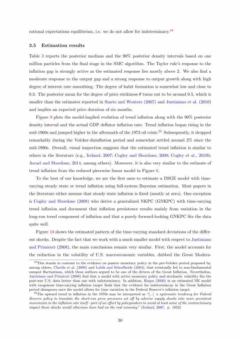
Figure 9 plots the model-implied evolution of trend inflation along with the 90% posterior

density interval and the actual GDP deflator inflation rate. Trend inflation began rising in the

mid-1960s and jumped higher in the aftermath of the 1973 oil crisis.20 Subsequently, it dropped

remarkably during the Volcker-disinflation period and somewhat settled around 2% since the

mid-1990s. Overall, visual inspection suggests that the estimated trend inflation is similar to

others in the literature (e.g., Ireland, 2007; Cogley and Sbordone, 2008; Cogley et al., 2010b;

Ascari and Sbordone, 2014, among others). Moreover, it is also very similar to the estimate of

trend inflation from the reduced piecewise linear model in Figure 6.

To the best of our knowledge, we are the first ones to estimate a DSGE model with time-

varying steady state or trend inflation using full-system Bayesian estimation. Most papers in

the literature either assume that steady state inflation is fixed (mostly at zero). One exception

is Cogley and Sbordone (2008) who derive a generalized NKPC (GNKPC) with time-varying

trend inflation and document that inflation persistence results mainly from variation in the

long-run trend component of inflation and that a purely forward-looking GNKPC fits the data

quite well.

Figure 10 shows the estimated pattern of the time-varying standard deviations of the differ-

ent shocks. Despite the fact that we work with a much smaller model with respect to Justiniano

and Primiceri (2008), the main conclusions remain very similar. First, the model accounts for

the reduction in the volatility of U.S. macroeconomic variables, dubbed the Great Modera-

19This stands in contrast to the evidence on passive monetary policy in the pre-Volcker period proposed by,among others, Clarida et al. (2000) and Lubik and Schorfheide (2004), that eventually led to non-fundamentalsunspot fluctuations, which these authors argued to be one of the drivers of the Great Inflation. Nevertheless,Justiniano and Primiceri (2008) find that a model with active monetary policy and stochastic volatility fits thepost-war U.S. data better than one with indeterminacy. In addition, Haque (2020) in an estimated NK modelwith exogenous time-varying inflation target finds that the evidence for indetermincay in the Great Inflationperiod dissapears once the model allows for time variation in the Federal Reserve’s inflation target.

20The upward trend in inflation in the 1970s may be interpreted as “[...] a systematic tendency for FederalReserve policy to translate the short-run price pressures set off by adverse supply shocks into more persistentmovements in the inflation rate itself - part of an effort by policymakers to avoid at least some of the contractionaryimpact those shocks would otherwise have had on the real economy.” (Ireland, 2007, p. 1853)

30

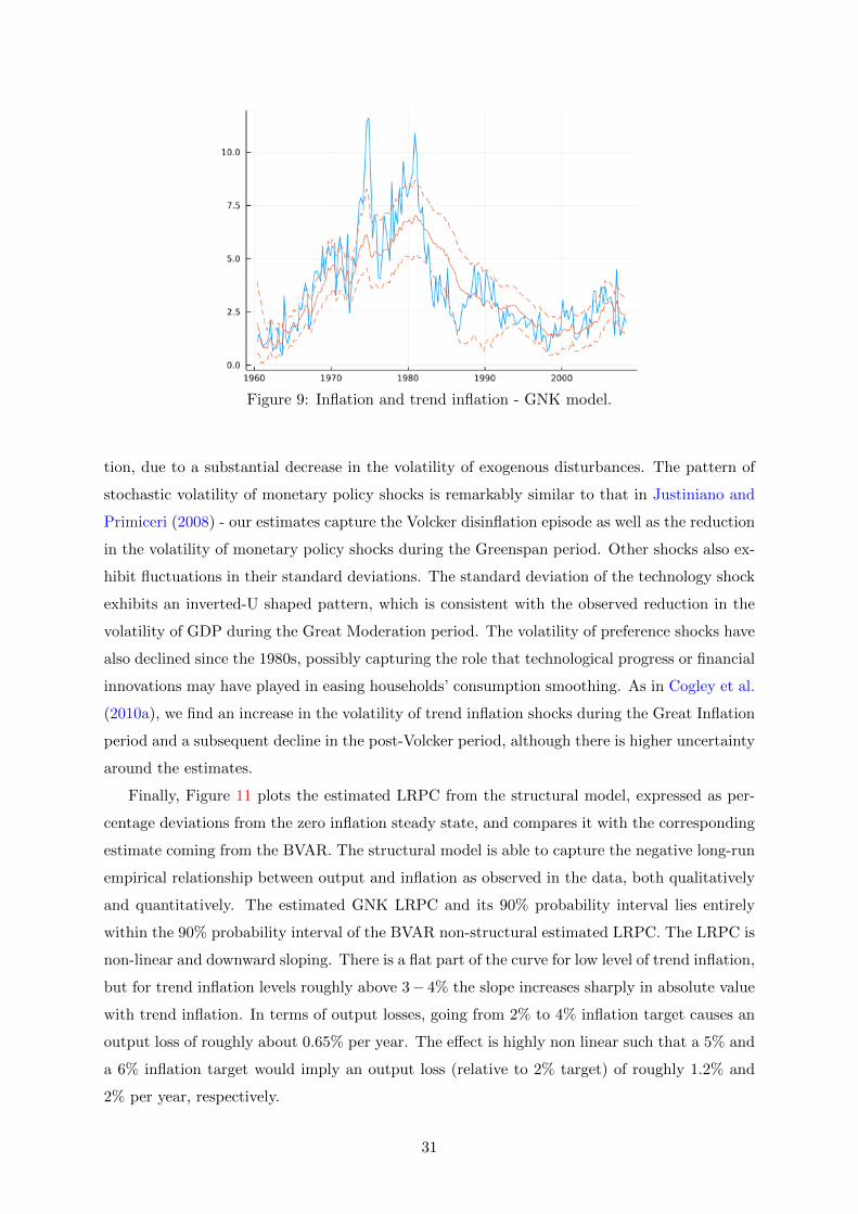
Figure 9: Inflation and trend inflation - GNK model.

tion, due to a substantial decrease in the volatility of exogenous disturbances. The pattern of

stochastic volatility of monetary policy shocks is remarkably similar to that in Justiniano and

Primiceri (2008) - our estimates capture the Volcker disinflation episode as well as the reduction

in the volatility of monetary policy shocks during the Greenspan period. Other shocks also ex-

hibit fluctuations in their standard deviations. The standard deviation of the technology shock

exhibits an inverted-U shaped pattern, which is consistent with the observed reduction in the

volatility of GDP during the Great Moderation period. The volatility of preference shocks have

also declined since the 1980s, possibly capturing the role that technological progress or financial

innovations may have played in easing households’ consumption smoothing. As in Cogley et al.

(2010a), we find an increase in the volatility of trend inflation shocks during the Great Inflation

period and a subsequent decline in the post-Volcker period, although there is higher uncertainty

around the estimates.

Finally, Figure 11 plots the estimated LRPC from the structural model, expressed as per-

centage deviations from the zero inflation steady state, and compares it with the corresponding

estimate coming from the BVAR. The structural model is able to capture the negative long-run

empirical relationship between output and inflation as observed in the data, both qualitatively

and quantitatively. The estimated GNK LRPC and its 90% probability interval lies entirely

within the 90% probability interval of the BVAR non-structural estimated LRPC. The LRPC is

non-linear and downward sloping. There is a flat part of the curve for low level of trend inflation,

but for trend inflation levels roughly above 3− 4% the slope increases sharply in absolute value

with trend inflation. In terms of output losses, going from 2% to 4% inflation target causes an

output loss of roughly about 0.65% per year. The effect is highly non linear such that a 5% and

a 6% inflation target would imply an output loss (relative to 2% target) of roughly 1.2% and

2% per year, respectively.

31

Figure 10: Stochastic volatility of the structural shocks

As well-known in the literature, the negative steady state relationship between inflation and

output in the GNK model is due to the negative effect of higher price dispersion on aggregate

output. Higher trend inflation increases price dispersion by causing a greater difference between

the price set by the resetting firms and the average price level. Higher price dispersion works

like a negative aggregate productivity shock, as it increases the amount of input required to

produce a given level of output, which in turn translates into an output loss. Therefore, long-run

superneutrality breaks down and a negative long run relationship emerges between inflation and

output (see Ascari, 2004; Yun, 2005), in both the estimated BVAR and the structural DSGE

model.

As for the BVAR, a time-varying trend inflation generates a long-run wedge alongside the

usual short-run wedge for the variables in the model. In the standard NK model the output

gap (i.e., short-run wedge) is usually defined as deviation of output from its flexible price

counterpart:

Yt =YtY nt

in logs→ yt = yt − ynt (39)

Normally, the steady states of the sticky prices NK model and the one of its flexible price

counterpart are the same because of the assumption of a vertical LRPC, obtained by assuming

either zero inflation in steady state or full indexation of reset prices to some combination of

32

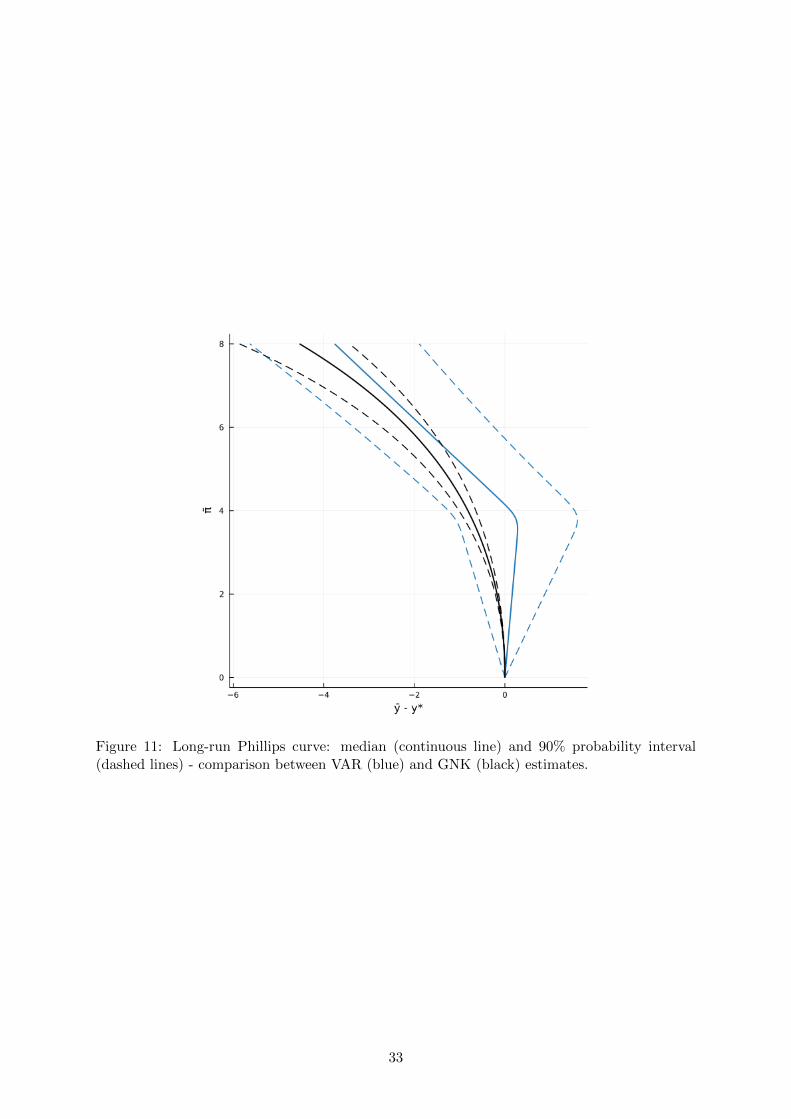
Figure 11: Long-run Phillips curve: median (continuous line) and 90% probability interval(dashed lines) - comparison between VAR (blue) and GNK (black) estimates.

33

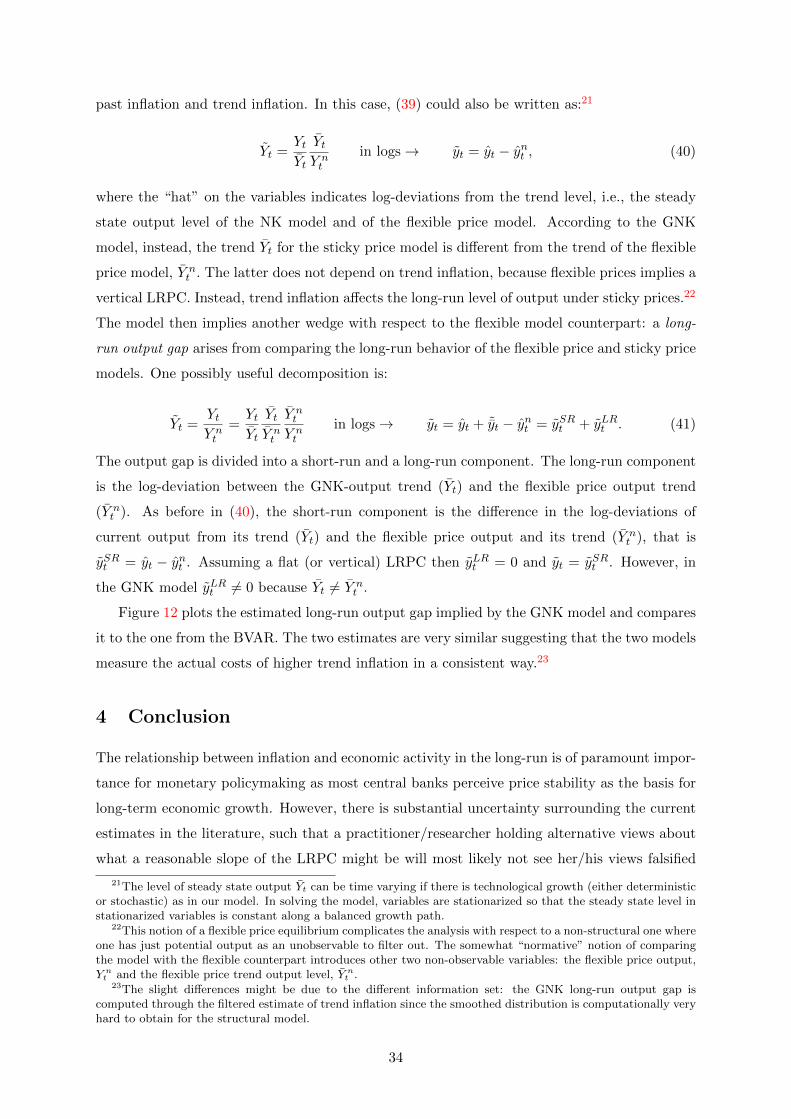
past inflation and trend inflation. In this case, (39) could also be written as:21

Yt =YtYt

YtY nt

in logs→ yt = yt − ynt , (40)

where the “hat” on the variables indicates log-deviations from the trend level, i.e., the steady

state output level of the NK model and of the flexible price model. According to the GNK

model, instead, the trend Yt for the sticky price model is different from the trend of the flexible

price model, Y nt . The latter does not depend on trend inflation, because flexible prices implies a

vertical LRPC. Instead, trend inflation affects the long-run level of output under sticky prices.22

The model then implies another wedge with respect to the flexible model counterpart: a long-

run output gap arises from comparing the long-run behavior of the flexible price and sticky price

models. One possibly useful decomposition is:

Yt =YtY nt

=YtYt

YtY nt

Y nt

Y nt

in logs→ yt = yt + ˜yt − ynt = ySRt + yLRt . (41)

The output gap is divided into a short-run and a long-run component. The long-run component

is the log-deviation between the GNK-output trend (Yt) and the flexible price output trend

(Y nt ). As before in (40), the short-run component is the difference in the log-deviations of

current output from its trend (Yt) and the flexible price output and its trend (Y nt ), that is

ySRt = yt − ynt . Assuming a flat (or vertical) LRPC then yLRt = 0 and yt = ySRt . However, in

the GNK model yLRt 6= 0 because Yt 6= Y nt .

Figure 12 plots the estimated long-run output gap implied by the GNK model and compares

it to the one from the BVAR. The two estimates are very similar suggesting that the two models

measure the actual costs of higher trend inflation in a consistent way.23

4 Conclusion

The relationship between inflation and economic activity in the long-run is of paramount impor-

tance for monetary policymaking as most central banks perceive price stability as the basis for

long-term economic growth. However, there is substantial uncertainty surrounding the current

estimates in the literature, such that a practitioner/researcher holding alternative views about

what a reasonable slope of the LRPC might be will most likely not see her/his views falsified

21The level of steady state output Yt can be time varying if there is technological growth (either deterministicor stochastic) as in our model. In solving the model, variables are stationarized so that the steady state level instationarized variables is constant along a balanced growth path.

22This notion of a flexible price equilibrium complicates the analysis with respect to a non-structural one whereone has just potential output as an unobservable to filter out. The somewhat “normative” notion of comparingthe model with the flexible counterpart introduces other two non-observable variables: the flexible price output,Y nt and the flexible price trend output level, Y nt .

23The slight differences might be due to the different information set: the GNK long-run output gap iscomputed through the filtered estimate of trend inflation since the smoothed distribution is computationally veryhard to obtain for the structural model.

34

Figure 12: Comparison between long-run output gap estimates: VAR (blue) and GNK (black).

(see Benati, 2015). This paper aims to develop an empirical methodology which is tailored to

the purpose of providing more precise estimates of the LRPC.

We develop a vector autoregression (VAR) framework with stochastic trends, and provide

a sophisticated trend-cycle decomposition of the data. A key methodological contribution is to

generalize this VAR-based trend-cycle decomposition to a piecewise linear model and show that

both the likelihood function and the posterior distribution of the latent state variables can be

derived analytically. While the non-linear approach is necessary to identify a threshold value

of trend inflation that tilts the long-run relationship, it also captures changes in the nature of

inflation persistence over the post-war period, which is important for the identification of the

LRPC. Another important advantage of the framework, relative to existing studies, is that it

allows for simultaneous estimation of both the short-run business cycle and the long-run trend

components, such that the estimated LRPC is also consistent with the cyclical properties of the

data.

Our results show that inflation and output in the U.S. are negatively related in the long-

run. The threshold level of inflation is slightly lower than 4%, above which every percentage

point increase in trend inflation is related to about 1% decrease in potential output per year.

Using our estimated model, we document that the long-run output gap, which captures the

deviation of potential output under positive trend inflation from its counterfactual level under

zero trend inflation, has been on average about negative 2% per year during the Great Inflation.

We further show that neglecting this long-run relationship between inflation and output leads

to more negative short-run output gap estimates in periods of high inflation, particularly the

Great Inflation, thereby overstating the cyclical component of output fluctuations. Finally,

a New Keynesian model generalized to admit time-varying trend inflation and estimated via

35

particle filtering provides theoretical foundations to this reduced-form evidence coming from

the BVAR. We show that the structural long-run Phillips Curve implied by the estimated New

Keynesian model is not statistically different from the one implied by the reduced-form piecewise

linear BVAR model.

36

References

Abbritti, M., A. Consolo, and S. Weber (2021, December). Endogenous growth, downward wage

rigidity and optimal inflation. Working Paper Series 2635, European Central Bank.

Adam, K. and H. Weber (2019, February). Optimal trend inflation. American Economic

Review 109 (2), 702–37.

Ait Lahcen, M., G. Baughman, S. Rabinovich, and H. van Buggenum (2021). Nonlinear unem-

ployment effects of the inflation tax. Technical Report mimeo.

Alvarez, F., H. L. Bihan, and F. Lippi (2016). The Real Effects of Monetary Shocks in Sticky

Price Models: A Sufficient Statistic Approach. American Economic Review 106 (10), 2817–

2851.

Arellano-Valle, R., G. del Pino, and E. San Martin (2002). Definition and probabilistic properties

of skew-distribution. Statistics & Probability Letters 58, 111–121.

Arellano-Valle, R. B. and A. Azzalini (2006). On the unification of families of skew-normal

distributions. Scandinavian Journal of Statistics 33 (3), 561–574.

Ascari, G. (2004). Staggered prices and trend inflation: Some nuisances. Review of Economic

Dynamics 7, 642–667.

Ascari, G., P. Bonomolo, and H. F. Lopes (2019). Walk on the wild side: Temporarily unstable

paths and multiplicative sunspots. American Economic Review 109 (5), 1805–42.

Ascari, G. and L. Fosso (2021, April). The Inflation Rate Disconnect Puzzle: On The Inter-

national Component of Trend Inflation and The Flattening of The Phillips Curve. Technical

report, Working paper.

Ascari, G. and A. M. Sbordone (2014). The macroeconomics of trend inflation. Journal of

Economic Literature 52 (3), 679–739.

Azzalini, A. (1985). A class of distributions which includes the normal ones. Scandinavian

Journal of Statistics 12 (2), 171–178.

Benati, L. (2008). Investigating Inflation Persistence Across Monetary Regimes. The Quarterly

Journal of Economics 123 (3), 1005–1060.

Benati, L. (2015). The long-run Phillips curve: A structural VAR investigation. Journal of

Monetary Economics 76 (C), 15–28.

Berentsen, A., G. Menzio, and R. Wright (2011). Inflation and unemployment in the long run.

American Economic Review 101 (1), 371–98.

37

Beyer, A. and R. E. Farmer (2007). Natural rate doubts. Journal of Economic Dynamics and

Control 31 (3), 797–825.

Bils, M. and P. J. Klenow (2004). Some evidence on the importance of sticky prices. Journal

of Political Economy 112(5), 947–985.

Burstein, A. and C. Hellwig (2008). Welfare Costs of Inflation in a Menu Cost Model. American

Economic Review 98 (2), 438–443.

Calvo, G. (1983). Staggered prices in a utility-maximizing framework. Journal of Monetary

Economics 12, 383–398.

Carvalho, C. M., M. S. Johannes, H. F. Lopes, and N. G. Polson (2010, 02). Particle learning

and smoothing. Statistical Science 25 (1), 88–106.

Chen, H., F. Petralia, and H. F. Lopes (2010, June). Sequential Monte Carlo Estimation of

DSGE Models. Working papers.

Clarida, R., J. Galı, and M. Gertler (2000). Monetary policy rules and macroeconomic stability:

Evidence and some theory. Quarterly Journal of Economics 115, 147–180.

Clark, P. K. (1987). The cyclical component of u. s. economic activity. The Quarterly Journal

of Economics 102 (4), 797–814.

Cogley, T., G. E. Primiceri, and T. Sargent (2010a). Inflation-gap persistence in the u.s.

American Economic Journal: Macroeconomics 2(1), 43–69.

Cogley, T. and T. J. Sargent (2005). Drifts and volatilities: Monetary policies and outcomes in

the post WWII U.S. Review of Economic Dynamics 8 (2), 262–302.

Cogley, T. and A. M. Sbordone (2008). Trend inflation, indexation and inflation persistence in

the New Keynesian Phillips Curve. American Economic Review 98 (5), 2101–2126.

Cogley, T. W., G. Primiceri, and T. J. Sargent (2010b). Inflation-gap persistence in the U.S.

American Economic Journal: Macroeconomics 2 (1), 43–69.

Coibion, O., Y. Gorodnichenko, and J. F. Wieland (2012). The optimal inflation rate in new

keynesian models: Should central banks raise their inflation targets in light of the zlb? Review

of Economic Studies 79, 1371–1406.

Creal, D. (2007). Sequential Monte Carlo samplers for Bayesian DSGE models. Working papers,

Vrije Universitiet Amsterdam.

Del Negro, M., D. Giannone, M. P. Giannoni, and A. Tambalotti (2017). Safety, Liquidity, and

the Natural Rate of Interest. Brookings Papers on Economic Activity 48 (1 (Spring), 235–316.

38

Fernandez-Villaverde, J. and J. Rubio-Ramırez (2007). Estimating macroeconomic models: A

likelihood approach. Review of Economic Studies 74, 1059–1087.

Friedman, M. (1968). The role of monetary policy. The American Economic Review 58 (1),

1–17.

Godsill, S. J., A. Doucet, and M. West (2004). Monte carlo smoothing for nonlinear time series.

Journal of the American Statistical Association 99 (465), 156–168.

Gordon, R. J. (1970). The Recent Acceleration of Inflation and Its Lessons for the Future.

Brookings Papers on Economic Activity 1 (1), 8–47.

Hamilton, J. D., E. S. Harris, J. Hatzius, and K. D. West (2016). The Equilibrium Real Funds

Rate: Past, Present, and Future. IMF Economic Review 64 (4), 660–707.

Haque, Q. (2020). Monetary Policy, Inflation Target and the Great Moderation: An Empirical

Investigation. mimeo, The University of Western Australia, Centre for Applied Macroeco-

nomic Analysis.

Harvey, A. C. and P. H. J. Todd (1983). Forecasting economic time series with structural and

box-jenkins models: A case study. Journal of Business & Economic Statistics 1 (4), 299–307.

Haug, A. A. and I. King (2014). In the long run, US unemployment follows inflation like a

faithful dog. Journal of Macroeconomics 41 (C), 42–52.

Herbst, E. and F. Schorfheide (2014). Sequential Monte Carlo Sampling For Dsge Models.

Journal of Applied Econometrics 29 (7), 1073–1098.

Herbst, E. P. and F. Schorfheide (2016). Bayesian Estimation of DSGE Models. Number 10612

in Economics Books. Princeton University Press.

Ireland, P. (2007). Changes in Federal Reserve’s inflation target: Causes and consequences.

Journal of Money, Credit and Banking 39(8), 1851–1882.

Johannsen, B. K. and E. Mertens (2021). A time-series model of interest rates with the effective

lower bound. Journal of Money, Credit and Banking 53 (5), 1005–1046.

Justiniano, A. and G. E. Primiceri (2008). The Time-Varying Volatility of Macroeconomic

Fluctuations. American Economic Review 98(3), 604–641.

Justiniano, A., G. E. Primiceri, and A. Tambalotti (2010). Investment Shocks and Business

Cycles. Journal of Monetary Economics 57(2), 132–145.

Karanassou, M. and H. Sala (2010). The US inflation-unemployment trade-off revisited: New

evidence for policy-making. Journal of Policy Modeling 32 (6), 758–777.

39

Karanassou, M., H. Sala, and D. Snower (2005). A reappraisal of the inflation-unemployment

tradeoff. European Journal of Political Economy 21, 1–32.

Karanassou, M., H. Sala, and D. J. Snower (2010). Phillips Curves And Unemployment Dy-

namics: A Critique And A Holistic Perspective. Journal of Economic Surveys 24 (1), 1–51.

Kehoe, P. and V. Midrigan (2015). Prices are sticky after all. Journal of Monetary Eco-

nomics 75 (C), 35–53.

King, R. G. (2008). The Phillips curve and U.S. macroeconomic policy : snapshots, 1958-1996.

Economic Quarterly 94 (Fall), 311–359.

King, R. G. and M. W. Watson (1994). The post-war u.s. phillips curve: a revisionist econo-

metric history. Carnegie-Rochester Conference Series on Public Policy 41, 157–219.

Kreps, D. M. (1998). Anticipated Utility and Dynamic Choice (1997), pp. 242–274. Econometric

Society Monographs. Cambridge University Press.

Kuttner, K. (1994). Estimating potential output as a latent variable. Journal of Business &

Economic Statistics 12 (3), 361–68.

Laubach, T. and J. C. Williams (2003). Measuring the Natural Rate of Interest. The Review

of Economics and Statistics 85 (4), 1063–1070.

Liu, J. and M. West (2001). Combined parameters and state estimation in simulation-based

filtering. In Springer (Ed.), Sequential Monte Carlo Methods in Practice, Chapter 10, pp.

197–223. New York: Arnaud Doucet and Nando de Freitas and Neil Gordon.

Lubik, T. and F. Schorfheide (2004). Testing for Indeterminacy: An Application to U.S. Mon-

etary Policy. American Economic Review 94(1), 190–217.

Maffei-Faccioli, N. (2020, October). Identifying the Sources of the Slowdown in Growth: De-

mand vs. Supply. 2020 Papers pma2978, Job Market Papers.

Mertens, E. (2016). Measuring the Level and Uncertainty of Trend Inflation. The Review of

Economics and Statistics 98 (5), 950–967.

Mertens, E. and J. M. Nason (2020). Inflation and professional forecast dynamics: An evaluation

of stickiness, persistence, and volatility. Quantitative Economics 11 (4), 1485–1520.

Nakamura, E. and J. Steinsson (2008). Five facts about prices: A reevaluation of menu cost

models. Quarterly Journal of Economics 123(4), 1415–1464.

Nakamura, E. and J. Steinsson (2010). Monetary non-neutrality in a multisector menu cost

model. The Quarterly Journal of Economics 125 (3), 961–1013.

40

Nakamura, E., J. Steinsson, P. Sun, and D. Villar (2018). The Elusive Costs of Inflation: Price

Dispersion during the U.S. Great Inflation*. The Quarterly Journal of Economics 133 (4),

1933–1980.

Phelps, E. S. (1967). Phillips curves, expectations of inflation and optimal unemployment over

time. Economica 34 (135), 254–281.

Phillips, A. W. (1958). The relation between unemployment and the rate of change of money

wage rates in the united kingdom, 1861-1957. Economica 25 (100), 283–299.

Pitt, M. K. and N. Shephard (1999). Filtering via simulation: Auxiliary particle filters. Journal

of the American Statistical Association 94 (446), 590–599.

Planas, C., A. Rossi, and G. Fiorentini (2008, January). Bayesian Analysis of the Output Gap.

Journal of Business & Economic Statistics 26, 18–32.

Primiceri, G. E. (2005). Time-varying structural vector autoregressions and monetary policy.

Review of Economic Studies 72, 821–852.

Samuelson, P. A. and R. M. Solow (1960). Analytical aspects of anti-inflation policy. The

American Economic Review 50 (2), 177–194.

Sargan, J. D. (1964). Wages and prices in the united kingdom: a study in econometric method-

ology. Econometric analysis for national economic planning 16, 25–54.

Sheremirov, V. (2020). Price dispersion and inflation: New facts and theoretical implications.

Journal of Monetary Economics 114 (C), 59–70.

Smets, F. and R. Wouters (2007). Shocks and frictions in US business cycles: A bayesian DSGE

approach. American Economic Review 97 (3), 586–606.

Solow, R. M. (1969). Price Expectations and the Behavior of the Price Level. Manchester, UK,

Manchester University Press.

Stock, J. H. and M. W. Watson (2007). Why has U.S. inflation become harder to forecast?

Journal of Money, Credit and Banking 39, 3–33.

Stock, J. H. and M. W. Watson (2016). Core Inflation and Trend Inflation. The Review of

Economics and Statistics 98 (4), 770–784.

Svensson, L. E. O. (2015). The Possible Unemployment Cost of Average Inflation below a

Credible Target. American Economic Journal: Macroeconomics 7 (1), 258–296.

Villani, M. (2009). Steady-state priors for vector autoregressions. Journal of Applied Econo-

metrics 24 (4), 630–650.

41

Watson, M. (1986). Univariate detrending methods with stochastic trends. Journal of Monetary

Economics 18 (1), 49–75.

Yun, T. (2005). Optimal monetary policy with relative price distortions. American Economic

Review 95, 89–108.

42

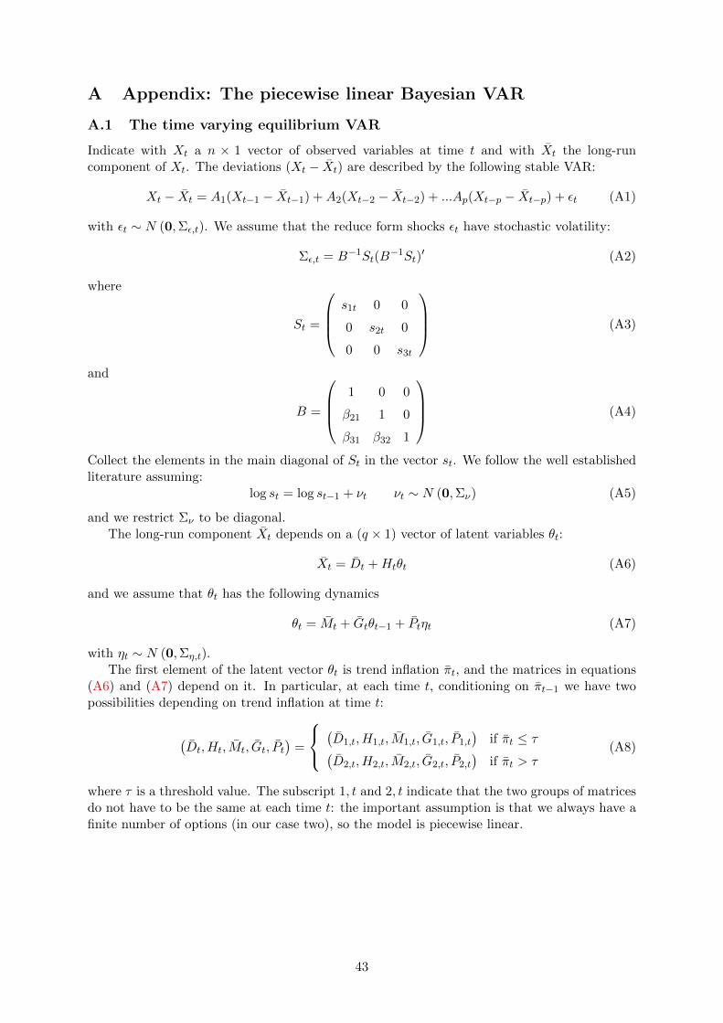
A Appendix: The piecewise linear Bayesian VAR

A.1 The time varying equilibrium VAR

Indicate with Xt a n × 1 vector of observed variables at time t and with Xt the long-runcomponent of Xt. The deviations (Xt − Xt) are described by the following stable VAR:

Xt − Xt = A1(Xt−1 − Xt−1) +A2(Xt−2 − Xt−2) + ...Ap(Xt−p − Xt−p) + εt (A1)

with εt ∼ N (0,Σε,t). We assume that the reduce form shocks εt have stochastic volatility:

Σε,t = B−1St(B−1St)

′ (A2)

where

St =

s1t 0 0

0 s2t 0

0 0 s3t

(A3)

and

B =

1 0 0

β21 1 0

β31 β32 1

(A4)

Collect the elements in the main diagonal of St in the vector st. We follow the well establishedliterature assuming:

log st = log st−1 + νt νt ∼ N (0,Σν) (A5)

and we restrict Σν to be diagonal.The long-run component Xt depends on a (q × 1) vector of latent variables θt:

Xt = Dt +Htθt (A6)

and we assume that θt has the following dynamics

θt = Mt + Gtθt−1 + Ptηt (A7)

with ηt ∼ N (0,Ση,t).The first element of the latent vector θt is trend inflation πt, and the matrices in equations

(A6) and (A7) depend on it. In particular, at each time t, conditioning on πt−1 we have twopossibilities depending on trend inflation at time t:

(Dt, Ht, Mt, Gt, Pt

)=

(D1,t, H1,t, M1,t, G1,t, P1,t

)if πt ≤ τ(

D2,t, H2,t, M2,t, G2,t, P2,t

)if πt > τ

(A8)

where τ is a threshold value. The subscript 1, t and 2, t indicate that the two groups of matricesdo not have to be the same at each time t: the important assumption is that we always have afinite number of options (in our case two), so the model is piecewise linear.

43

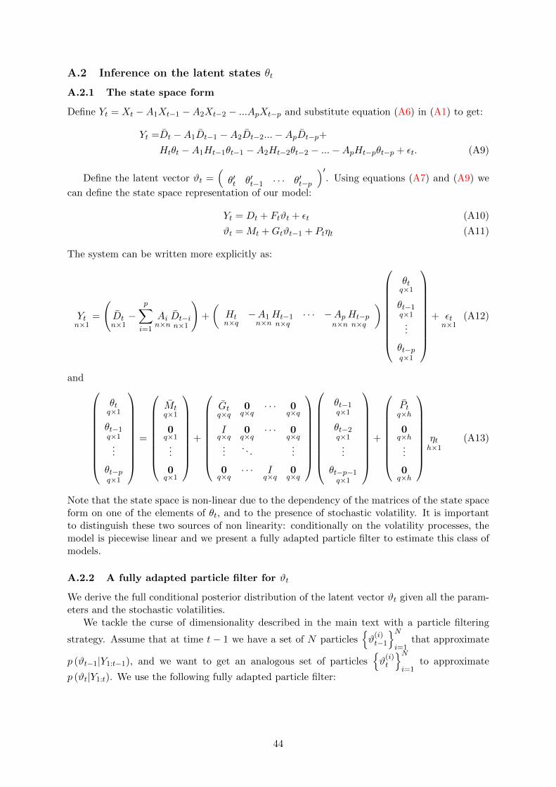
A.2 Inference on the latent states θt

A.2.1 The state space form

Define Yt = Xt −A1Xt−1 −A2Xt−2 − ...ApXt−p and substitute equation (A6) in (A1) to get:

Yt =Dt −A1Dt−1 −A2Dt−2...−ApDt−p+

Htθt −A1Ht−1θt−1 −A2Ht−2θt−2 − ...−ApHt−pθt−p + εt. (A9)

Define the latent vector ϑt =(θ′t θ′t−1 · · · θ′t−p

)′. Using equations (A7) and (A9) we

can define the state space representation of our model:

Yt = Dt + Ftϑt + εt (A10)

ϑt = Mt +Gtϑt−1 + Ptηt (A11)

The system can be written more explicitly as:

Ytn×1

=

(Dtn×1−

p∑i=1

Ain×n

Dt−in×1

)+

(Htn×q

−A1n×n

Ht−1n×q

· · · −Apn×n

Ht−pn×q

)

θtq×1

θt−1q×1...

θt−pq×1

+ εtn×1

(A12)

and

θtq×1

θt−1q×1...

θt−pq×1

=

Mtq×1

0q×1...

0q×1

+

Gtq×q

0q×q

· · · 0q×q

Iq×q

0q×q

· · · 0q×q

.... . .

...

0q×q

· · · Iq×q

0q×q

θt−1q×1

θt−2q×1...

θt−p−1q×1

+

Ptq×h

0q×h

...

0q×h

ηth×1

(A13)

Note that the state space is non-linear due to the dependency of the matrices of the state spaceform on one of the elements of θt, and to the presence of stochastic volatility. It is importantto distinguish these two sources of non linearity: conditionally on the volatility processes, themodel is piecewise linear and we present a fully adapted particle filter to estimate this class ofmodels.

A.2.2 A fully adapted particle filter for ϑt

We derive the full conditional posterior distribution of the latent vector ϑt given all the param-eters and the stochastic volatilities.

We tackle the curse of dimensionality described in the main text with a particle filtering

strategy. Assume that at time t − 1 we have a set of N particlesϑ

(i)t−1

Ni=1

that approximate

p (ϑt−1|Y1:t−1), and we want to get an analogous set of particlesϑ

(i)t

Ni=1

to approximate

p (ϑt|Y1:t). We use the following fully adapted particle filter:

44

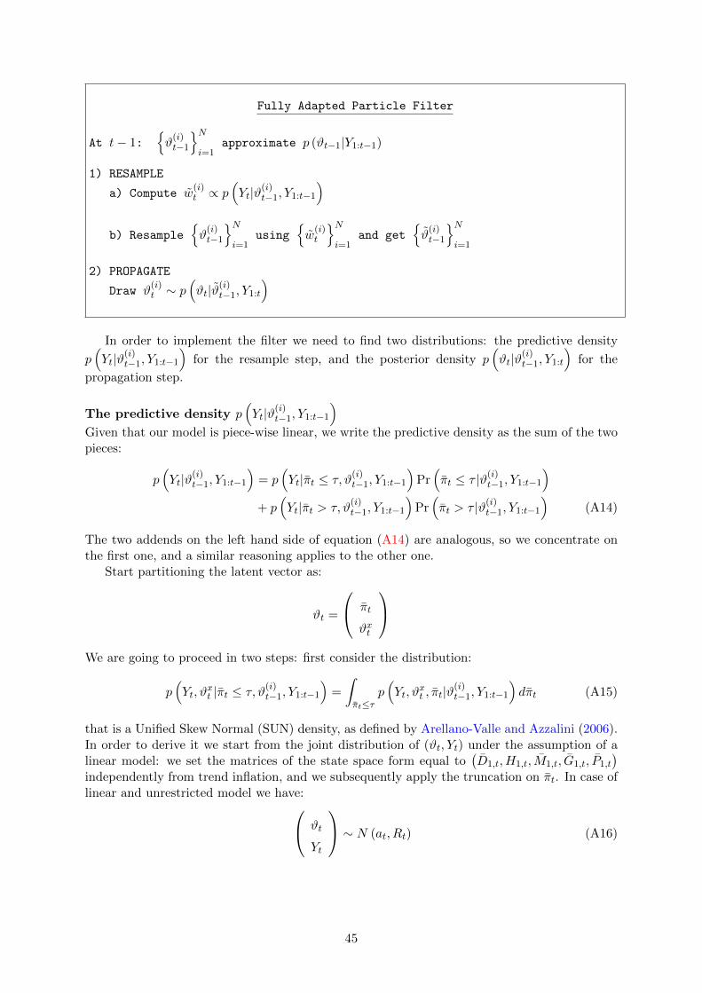
Fully Adapted Particle Filter

At t− 1:ϑ

(i)t−1

Ni=1

approximate p (ϑt−1|Y1:t−1)

1) RESAMPLE

a) Compute w(i)t ∝ p

(Yt|ϑ(i)

t−1, Y1:t−1

)b) Resample

ϑ

(i)t−1

Ni=1

usingw

(i)t

Ni=1

and getϑ

(i)t−1

Ni=1

2) PROPAGATE

Draw ϑ(i)t ∼ p

(ϑt|ϑ(i)

t−1, Y1:t

)

In order to implement the filter we need to find two distributions: the predictive density

p(Yt|ϑ(i)

t−1, Y1:t−1

)for the resample step, and the posterior density p

(ϑt|ϑ(i)

t−1, Y1:t

)for the

propagation step.

The predictive density p(Yt|ϑ(i)

t−1, Y1:t−1

)Given that our model is piece-wise linear, we write the predictive density as the sum of the twopieces:

p(Yt|ϑ(i)

t−1, Y1:t−1

)= p

(Yt|πt ≤ τ, ϑ(i)

t−1, Y1:t−1

)Pr(πt ≤ τ |ϑ(i)

t−1, Y1:t−1

)+ p

(Yt|πt > τ, ϑ

(i)t−1, Y1:t−1

)Pr(πt > τ |ϑ(i)

t−1, Y1:t−1

)(A14)

The two addends on the left hand side of equation (A14) are analogous, so we concentrate onthe first one, and a similar reasoning applies to the other one.

Start partitioning the latent vector as:

ϑt =

πt

ϑxt

We are going to proceed in two steps: first consider the distribution:

p(Yt, ϑ

xt |πt ≤ τ, ϑ

(i)t−1, Y1:t−1

)=

∫πt≤τ

p(Yt, ϑ

xt , πt|ϑ

(i)t−1, Y1:t−1

)dπt (A15)

that is a Unified Skew Normal (SUN) density, as defined by Arellano-Valle and Azzalini (2006).In order to derive it we start from the joint distribution of (ϑt, Yt) under the assumption of alinear model: we set the matrices of the state space form equal to

(D1,t, H1,t, M1,t, G1,t, P1,t

)independently from trend inflation, and we subsequently apply the truncation on πt. In case oflinear and unrestricted model we have: ϑt

Yt

∼ N (at, Rt) (A16)

45

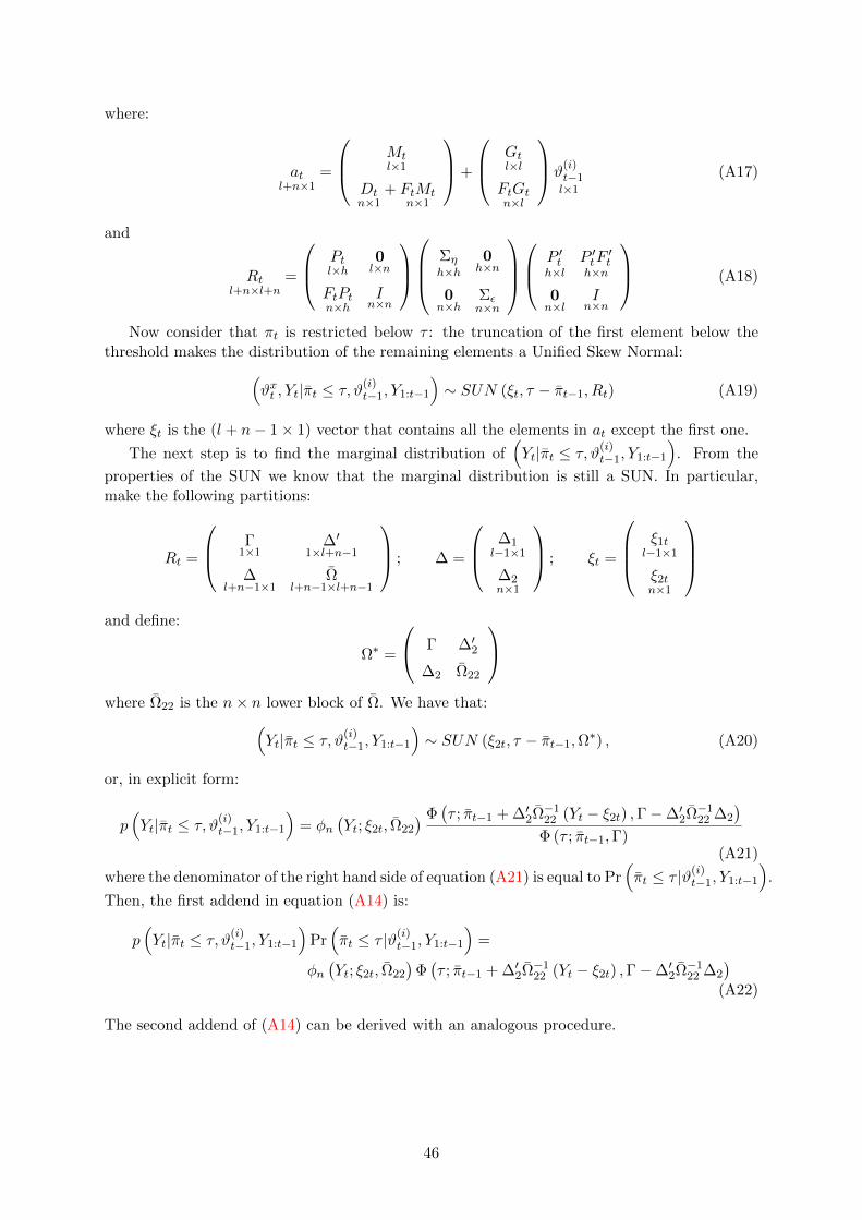
where:

atl+n×1

=

Mtl×1

Dtn×1

+ FtMtn×1

+

Gtl×l

FtGtn×l

ϑ(i)t−1l×1

(A17)

and

Rtl+n×l+n

=

Ptl×h

0l×n

FtPtn×h

In×n

Ση

h×h0h×n

0n×h

Σεn×n

P ′t

h×lP ′tF

′t

h×n

0n×l

In×n

(A18)

Now consider that πt is restricted below τ : the truncation of the first element below thethreshold makes the distribution of the remaining elements a Unified Skew Normal:(

ϑxt , Yt|πt ≤ τ, ϑ(i)t−1, Y1:t−1

)∼ SUN (ξt, τ − πt−1, Rt) (A19)

where ξt is the (l + n− 1× 1) vector that contains all the elements in at except the first one.

The next step is to find the marginal distribution of(Yt|πt ≤ τ, ϑ(i)

t−1, Y1:t−1

). From the

properties of the SUN we know that the marginal distribution is still a SUN. In particular,make the following partitions:

Rt =

Γ1×1

∆′1×l+n−1

∆l+n−1×1

Ωl+n−1×l+n−1

; ∆ =

∆1l−1×1

∆2n×1

; ξt =

ξ1tl−1×1

ξ2tn×1

and define:

Ω∗ =

Γ ∆′2

∆2 Ω22

where Ω22 is the n× n lower block of Ω. We have that:(

Yt|πt ≤ τ, ϑ(i)t−1, Y1:t−1

)∼ SUN (ξ2t, τ − πt−1,Ω

∗) , (A20)

or, in explicit form:

p(Yt|πt ≤ τ, ϑ(i)

t−1, Y1:t−1

)= φn

(Yt; ξ2t, Ω22

) Φ(τ ; πt−1 + ∆′2Ω−1

22 (Yt − ξ2t) ,Γ−∆′2Ω−122 ∆2

)Φ (τ ; πt−1,Γ)

(A21)

where the denominator of the right hand side of equation (A21) is equal to Pr(πt ≤ τ |ϑ(i)

t−1, Y1:t−1

).

Then, the first addend in equation (A14) is:

p(Yt|πt ≤ τ, ϑ(i)

t−1, Y1:t−1

)Pr(πt ≤ τ |ϑ(i)

t−1, Y1:t−1

)=

φn(Yt; ξ2t, Ω22

)Φ(τ ; πt−1 + ∆′2Ω−1

22 (Yt − ξ2t) ,Γ−∆′2Ω−122 ∆2

)(A22)

The second addend of (A14) can be derived with an analogous procedure.

46

The posterior distribution p(ϑt|ϑ(i)

t−1, Y1:t

)Also the posterior distribution can be written as the sum of two pieces:

p(ϑt|ϑ(i)

t−1, Y1:t

)= p

(ϑt|πt ≤ τ, ϑ(i)

t−1, Y1:t

)Pr(πt ≤ τ |ϑ(i)

t−1, Y1:t

)+ p

(ϑt|πt > τ, ϑ

(i)t−1, Y1:t

)Pr(πt > τ |ϑ(i)

t−1, Y1:t

)(A23)

As we did for the predictive density, we concentrate on the first row of (A23) (an analogousreasoning will apply to the second row).

Operate the following partitions:

at =

a1tl×1

a2tn×1

; Rt =

R11l×l

R12l×n

R21n×l

R22n×n

.

The posterior distribution of ϑt, conditioning on trend inflation below the threshold is a multi-variate truncated normal:(

ϑt|πt ≤ τ, ϑ(i)t−1, Y1:t

)∼ TN (mt, Ct; πt ≤ τ) (A24)

where:

mt = a1t +R12R−122 (Yt − a2t) (A25)

Ct = R11 −R12R−122 R21 (A26)

Finally, we need to compute the second term in the first line of equation (A23):

Pr(πt ≤ τ |ϑ(i)

t−1, Y1:t

)∝ p

(Yt|πt ≤ τ, ϑ(i)

t−1, Y1:t−1

)Pr(πt ≤ τ |ϑ(i)

t−1, Y1:t−1

)= φn

(Yt; ξ2t, Ω

)Φ(τ ; πt−1 + ∆′2Ω−1

22 (Yt − ξ2t) ,Γ−∆′2Ω−122 ∆2

)(A27)

that is exactly equation (A22).

A.3 Stochastic volatility

We now augment our algorithm to estimate the time varying standard deviations of the shocks in

(A1). As in the Section above, given a set of particlesϑ

(i)t−1, log s

(i)t−1

Ni=1

that approximate the

joint distribution of (ϑt−1, log st−1), we want to get a new setϑ

(i)t , log s

(i)t

Ni=1

to approximate

p(ϑt, log st|ϑ(i)

t−1, log s(i)t−1, Y1:t

)where we omitted the dependencies on all the parameters to simplify the notation. Since in theprevious Section we derived the posterior distribution of ϑt conditional on log st, it is convenientto write the posterior at time t as:

p (ϑt, log st|ϑt−1, log st−1Y1:t) = p (ϑt| log st, ϑt−1, log st−1, Y1:t)︸ ︷︷ ︸Full conditional posterior

p (log st|ϑt−1, log st−1, Y1:t)︸ ︷︷ ︸Blind proposal

.

(A28)We can get draws using an importance distribution that operates in two steps: we first useequation (A5) to get particles of log st: this is called a ”blind” proposal because it is notconditioned on observed data. Then, we can condition on these draws and get values for ϑt

47

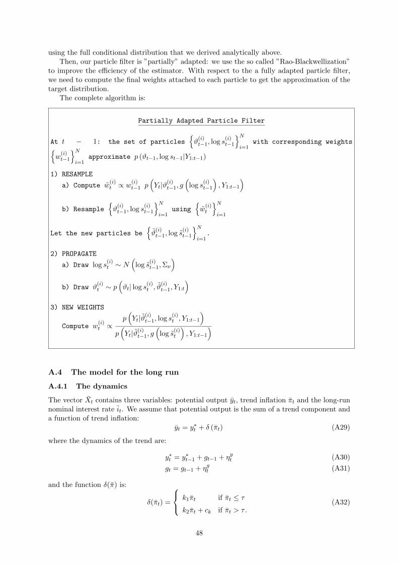
using the full conditional distribution that we derived analytically above.Then, our particle filter is ”partially” adapted: we use the so called ”Rao-Blackwellization”

to improve the efficiency of the estimator. With respect to the a fully adapted particle filter,we need to compute the final weights attached to each particle to get the approximation of thetarget distribution.

The complete algorithm is:

Partially Adapted Particle Filter

At t − 1: the set of particlesϑ

(i)t−1, log s

(i)t−1

Ni=1

with corresponding weightsw

(i)t−1

Ni=1

approximate p (ϑt−1, log st−1|Y1:t−1)

1) RESAMPLE

a) Compute w(i)t ∝ w

(i)t−1 p

(Yt|ϑ(i)

t−1, g(

log s(i)t−1

), Y1:t−1

)b) Resample

ϑ

(i)t−1, log s

(i)t−1

Ni=1

usingw

(i)t

Ni=1

Let the new particles beϑ

(i)t−1, log s

(i)t−1

Ni=1

.

2) PROPAGATE

a) Draw log s(i)t ∼ N

(log s

(i)t−1,Σν

)b) Draw ϑ

(i)t ∼ p

(ϑt| log s

(i)t , ϑ

(i)t−1, Y1:t

)3) NEW WEIGHTS

Compute w(i)t ∝

p(Yt|ϑ(i)

t−1, log s(i)t , Y1:t−1

)p(Yt|ϑ(i)

t−1, g(

log s(i)t

), Y1:t−1

)

A.4 The model for the long run

A.4.1 The dynamics

The vector Xt contains three variables: potential output yt, trend inflation πt and the long-runnominal interest rate it. We assume that potential output is the sum of a trend component anda function of trend inflation:

yt = y∗t + δ (πt) (A29)

where the dynamics of the trend are:

y∗t = y∗t−1 + gt−1 + ηyt (A30)

gt = gt−1 + ηgt (A31)

and the function δ(π) is:

δ(πt) =

k1πt if πt ≤ τk2πt + ck if πt > τ .

(A32)

48

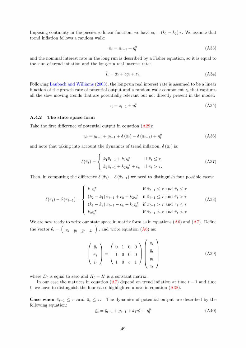
Imposing continuity in the piecewise linear function, we have ck = (k1 − k2) τ . We assume thattrend inflation follows a random walk:

πt = πt−1 + ηπt (A33)

and the nominal interest rate in the long run is described by a Fisher equation, so it is equal tothe sum of trend inflation and the long-run real interest rate:

it = πt + cgt + zt. (A34)

Following Laubach and Williams (2003), the long-run real interest rate is assumed to be a linearfunction of the growth rate of potential output and a random walk component zt that capturesall the slow moving trends that are potentially relevant but not directly present in the model:

zt = zt−1 + ηzt (A35)

A.4.2 The state space form

Take the first difference of potential output in equation (A29):

yt = yt−1 + gt−1 + δ (πt)− δ (πt−1) + ηyt (A36)

and note that taking into account the dynamics of trend inflation, δ (πt) is:

δ(πt) =

k1πt−1 + k1ηπt if πt ≤ τ

k2πt−1 + k2ηπt + ck if πt > τ .

(A37)

Then, in computing the difference δ (πt)− δ (πt−1) we need to distinguish four possible cases:

δ(πt)− δ (πt−1) =

k1η

πt if πt−1 ≤ τ and πt ≤ τ

(k2 − k1)πt−1 + ck + k2ηπt if πt−1 ≤ τ and πt > τ

(k1 − k2)πt−1 − ck + k1ηπt if πt−1 > τ and πt ≤ τ

k2ηπt if πt−1 > τ and πt > τ

(A38)

We are now ready to write our state space in matrix form as in equations (A6) and (A7). Define

the vector θt =(πt yt gt zt

)′, and write equation (A6) as:

yt

πt

it

=

0 1 0 0

1 0 0 0

1 0 c 1

πt

yt

gt

zt

(A39)

where Dt is equal to zero and Ht = H is a constant matrix.In our case the matrices in equation (A7) depend on trend inflation at time t− 1 and time

t: we have to distinguish the four cases highlighted above in equation (A38).

Case when πt−1 ≤ τ and πt ≤ τ . The dynamics of potential output are described by thefollowing equation:

yt = yt−1 + gt−1 + k1ηπt + ηyt (A40)

49

so the system in matrix form is:πt

yt

gt

zt

=

0

0

0

0

+

1 0 0 0

0 1 1 0

0 0 1 0

0 0 0 1

πt−1

yt−1

gt−1

zt−1

+

1 0 0 0

k1 1 0 0

0 0 1 0

0 0 0 1

ηπt

ηyt

ηgt

ηzt

. (A41)

Case when πt−1 ≤ τ and πt > τ . Potential output in this case follows:

yt = yt−1 + gt−1 + (k2 − k1)πt−1 + ck + k2ηπt + ηyt (A42)

and equation (A7) becomes:πt

yt

gt

zt

=

0

ck

0

0

+

1 0 0 0

(k2 − k1) 1 1 0

0 0 1 0

0 0 0 1

πt−1

yt−1

gt−1

zt−1

+

1 0 0 0

k2 1 0 0

0 0 1 0

0 0 0 1

ηπt

ηyt

ηgt

ηzt

.

(A43)

Case when πt−1 > τ and πt ≤ τ . The equation for the dynamics of potential output is:

yt = yt−1 + gt−1 + (k1 − k2)πt−1 − ck + k1ηπt + ηyt (A44)

and the system becomes:πt

yt

gt

zt

=

0

−ck0

0

+

1 0 0 0

(k1 − k2) 1 1 0

0 0 1 0

0 0 0 1

πt−1

yt−1

gt−1

zt−1

+

1 0 0 0

k1 1 0 0

0 0 1 0

0 0 0 1

ηπt

ηyt

ηgt

ηzt

.

(A45)

Case when πt−1 > τ and πt > τ . For this last case the dynamics of potential output follow:

yt = yt−1 + gt−1 + k2ηπt + ηyt (A46)

and the system is:πt

yt

gt

zt

=

0

0

0

0

+

1 0 0 0

0 1 1 0

0 0 1 0

0 0 0 1

πt−1

yt−1

gt−1

zt−1

+

1 0 0 0

k2 1 0 0

0 0 1 0

0 0 0 1

ηπt

ηyt

ηgt

ηzt

. (A47)

A.5 Inference on the parameters

In our particle filtering strategy we estimate the parameters combining two approaches: theposterior distribution of τ is approximated through a mixture of Normal densities as in Liu andWest (2001); for all the other parameters we use the Particle Learning scheme by Carvalho et al.(2010), which is based on the analytical availability of sufficient statistics that characterize the

50

posterior distributions. For most of the parameters the derivation of these sufficient statisticsis standard. Then, we only describe the inference on the parameters in the model for the longrun, except for the variances of the shocks which are standard conjugate Inverse Gamma.

A.5.1 The posterior distribution of parameters in the matrix H

In our case Dt is equal to zero and the matrix H is constant. Then, equation (A6) is:

Xt = Hθt. (A48)

Rearranging equation (A1) and substituting the definition of X we have:

Yt = Hθt −A1Hθt−1 −A2Hθt−2 − ...ApHθt−p + εt. (A49)

where Yt has been defined in Section A.2.1.Then, indicating with ~H the vectorized matrix H we obtain the regression:

Yt = XHt~H + εt (A50)

whereXHt =

[θ′t ⊗ In − θ′t−1 ⊗A1 − θ′t−2 ⊗A2 − ...θ′t−p ⊗Ap

]. (A51)

Note that usually ~H contains some known coefficients and some unknown coefficients thatwe want to estimate. In our specific case we only have c as unknown: the other coefficients areall ones or zeros. As general practice, collect all the known coefficients in ~HK and the unknowncoefficients in ~HU . With a similar notation indicate with XH

t,K and XHt,U the corresponding

columns of XHt . We can write:

Yt −XHt,K

~HK = XHt,U

~HU + εt (A52)

Y Ht = XH

t,U~HU + εt (A53)

Equation (A53) is our regression: using Gaussian priors for the coefficients in ~HU , the inferenceis obtained as in standard Bayesian regression models.

A.5.2 The posterior distribution of slopes k1 and k2

First, define Y Gt = yt − yt−1 − gt−1 and ~k =

(k1 k2

)′. Then, we define the vector XG

t

distinguishing the usual four possible cases:

XGt =

(πt − πt−1 0

)if πt−1 ≤ τ and πt ≤ τ(

τ − πt−1 πt − τ)

if πt−1 ≤ τ and πt > τ(πt − τ τ − πt−1

)if πt−1 > τ and πt ≤ τ(

0 πt − πt−1

)if πt−1 > τ and πt > τ

(A54)

Finally, we can write the dynamics of potential output as:

Y Gt = XG

t~k + ηyt . (A55)

The equation above is a regression with coefficients ~k: using a Gaussian prior for ~k we easilyobtain a conjugate posterior distribution.

51

B Appendix: The DSGE model

Households. The first-order conditions with respect to consumption, labor supply and bondholdings are:

λt =dt

Ct − hCt−1, (B56)

Wt

Pt=dndtN

ϕt

λt,

1 = Etβλt+1

λt

Rtπt+1

, (B57)

where λt is the marginal utility of consumption, and πt = PtPt−1

is the gross inflation rate.Firms. In each period t, a final good, Yt, is produced by a perfectly competitive represen-

tative final-good firm, by combining a continuum of intermediate inputs, Yi,t, i ∈ [0, 1], via thetechnology

Yt =

[∫ 1

0Y

ε−1ε

i,t di

] εε−1

, (B58)

where ε > 1 is the elasticity of substitution among intermediate inputs. The first-order conditionfor profit maximization yields the final-good firm’s demand for intermediate good i

Yi,t =

(Pi,tPt

)−εYt. (B59)

The final-good market clearing condition is given by Yt = Ct.We assume that the price of a firm that cannot change the price is automatically in-

dexed to past-inflation with a degree χ, that is Pi,t = Pi,t−1

(Pt−1

Pt−2

)χ= Pi,t−1 (πt−1)χ , where

hence πt ≡ PtPt−1

. Hence if a firm fix P ∗i,t today and will not be able to change it in the

future then the price evolves accordingly to Pi,t+1 = P ∗i,t (πt)χ , Pi,t+2 = P ∗i,t (πt)

χ (πt+1)χ ,Pi,t+j = P ∗i,t (πt)

χ (πt+1)χ ... (πt+j−1)χ = P ∗i,tπt|t−1+j , where

πt|t+j−1 =PtPt−1

× Pt+1

Pt× ...× Pt+j−1

Pt+j−2for j > 1 and πt|t =

PtPt−1

= πt

= 1 for j = 0. (B60)

The intermediate goods producers face a constant probability, 0 < (1 − θ) < 1, of being ableto adjust prices to a new optimal one, P ∗i,t. Thus, to maximize expected discounted profit theysolve the following problem

Et

∞∑j=0

θjβjλt+jλt

[P ∗i,tπ

χt|t+j−1

Pt+jYi,t+j −

Wt+j

Pt+j

[Yi,t+jAt+j

] 11−α]

s.t. Yi,t+j =

[P ∗i,tπ

χt|t+j−1

Pt+j

]−εYt+j ,

Defining “average” marginal cost as MCt =A

11−αt

1−αWtPtY

α1−αt , first order condition for the opti-

52

mized relative price xt(=P ∗i,tPt

) can be written as

(xt)1+ εα

1−α =ε

ε− 1

Et∑∞

j=0(θβ)jλt+jYt+j

[πχt|t+j−1

πt+1|t+j

]− ε1−α

MCt+j

Et∑∞

j=0(θβ)jλt+jYt+j

[πχt|t+j−1

πt+1|t+j

]1−ε . (B61)

The aggregate price level, Pt =[∫ 1

0 Pi,t1−εdi

] 11−ε

, evolves according to

xt =

[1− θπ(1−ε)χ

t−1 πε−1t

1− θ

] 11−ε

. (B62)

Lastly, define price dispersion st ≡∫ 1

0 (Pi,tPt

)−εdi. Under the Calvo price mechanism, theabove expression can be written recursively as

st = (1− θ)x−εt + θπ−εχt−1 πεt st−1. (B63)

Recursive formulation of the optimal price-setting equation. The joint dynamicsof the optimal reset price and inflation can be compactly described by rewriting the first-ordercondition for the optimal price in a recursive formulation as follows:

x1+ εα

1−αt =

ε

(ε− 1)

ψtφt, (B64)

where ψt and φt are auxiliary variables that allow one to rewrite the infinite sums that appearin the numerator and denominator of the above equation in recursive formulation:

ψt = MCtYtλt + θβπ− εχ

1−αt Et

[π

ε1−αt+1 ψt+1

], (B65)

and

φt = Ytλt + θβπχ(1−ε)t Et

[πε−1t+1φt+1

]. (B66)

Note that in defining these two auxiliary variables, we used the definition λt = dtCt−hCt−1

=dt

Yt−hYt−1.

Monetary Policy. The central bank’s policy is described by the following Taylor rule

lnRt = ρ lnRt−1+(1− ρ) ln Rt+(1− ρ)ψπ ln

(πtπt

)+(1− ρ)ψx lnXn

t +(1− ρ)ψ∆y ln

(gytgy

)+σr,tεr,t,

(B67)where Xn

t = YtY nt

is the output gap, Y nt is the natural level of output, gyt is the growth rate of

output, gy = g is the steady state growth rate of output, and εr,t is an i.i.d. N(0, 1) monetarypolicy shock with time-varying standard deviation σr,t. The parameters ψπ, ψx and ψ∆y governthe central bank’s responses to the inflation gap, output gap and output growth, respectively.Here πt denotes trend inflation, which is the central’s banks (time-varying) inflation target andfollows a unit root process

lnπt = lnπt−1 + σπ,tεπ,t, (B68)

where επ,t is i.i.d. N(0, 1) and σπ,t denotes time-varying standard deviation of the inflationtarget shock.

By considering flexible prices, the law of motion for Y nt is given by

53

(Y nt

At

) 1+ϕ1−α

=(ε− 1) (1− α)

εdn+ h

(Y nt

At

)ϕ+α1−α Y n

t−1

At. (B69)

B.1 Final equations of the non-linear system

The real variables inherit unit roots from the process for technology. First, we detrend the

real variables to get the non-linear system in terms of transformed variables:^Yt = Yt/At,

^Y nt =

Y nt /At,

^wt = wt/At,

^λt = λtAt and gt = At/At−1. The non-linear model is described by the

following equations:

^λ t =

dt^Y t − h

^Y t−1g

−1t

(1m)

^λ t^wt = dndtN

ϕt (2m)

^λ t = βEt

[Rtπt+1

]^λ t+1g

−1t+1

(3m)

1 = θπχ(1−ε)t−1 πε−1

t + (1− θ)x1−εt (4m)

x1+ εα

1−αt =

ε

(ε− 1)

ψtφt

(5m)

ψt = MCt^Y t

^λ t + θβπ

− εχ1−α

t Et

[π

ε1−αt+1 ψt+1

](6m)

φt =^Y t

^λ t + θβπ

χ(1−ε)t Et

[πε−1t+1φt+1

](7m)

Nt = st^Y

11−αt (8m)

st = (1− θ)x− ε

1−αt + θπ

− εχ1−α

t−1 πε

1−αt st−1 (9m)

MCt =1

1− α^wt

^Y

α1−αt (10m)

lnRt = ρ lnRt−1+(1− ρ) ln Rt+(1− ρ)ψπ ln

(πtπt

)+(1− ρ)ψx lnXn

t +(1− ρ)ψ∆y ln

(gytgy

)+εr,t,

(11m)

gyt =

^Y tgt^Y t−1

(12m)

lnπt = lnπt−1 + επ,t (13m)

ln gt = (1− ρg) ln g + ρg ln gt−1 + εg,t (14m)

ln dt = (1− ρd) ln d+ ρd ln dt−1 + εd,t (15m)

54

^

Y nt

1+ϕ1−α

=(ε− 1) (1− α)

εdn+ h

^

Y nt

ϕ+α1−α ^

Y nt−1g

−1t . (16m)

Xnt =

Yt

Y nt

(17m)

B.2 Stochastic Steady State

Next, we evaluate the stochastic steady state of the system characterized by time-varying trendinflation equal to πt:

λt =d

Yt(1− hg−1

) (1ss)

wt =dndN

ϕt

λt(2ss)

rt = r =g

β24 =

Rtπt

=> Rt = Rt = rπt =g

βπt (3ss)

xt =

[1− θπ(1−χ)(ε−1)

t

1− θ

] 11−ε

(4ss)

x1+ εα

1−αt =

ε

(ε− 1)

ψtφt

(5ss)

ψt =MCtY tλt

1− θβπε(1−χ)1−α

t

(6ss)

φt =Y tλt

1− θβπ(ε−1)(1−χ)t

(7ss)

N t = stY1

1−αt (8ss)

st =

1− θ

1− θπε(1−χ)1−α

t

x− ε1−α

t (9ss)

MCt =1

1− αwtY

α1−αt (10ss)

The steady state is solved in the following sequence:

r =g

β(rss)

xt =

[1− θπ(1−χ)(ε−1)

t

1− θ

] 11−ε

(xss)

st =

1− θ

1− θπε(1−χ)1−α

t

x− ε1−α

t (sss)

24rt = Rtπt

is the transformed nominal interest rate.

55

Putting together (xss) and (sss) yields:

st =

1− θ

1− θπε(1−χ)1−α

t

[1− θπ(1−χ)(ε−1)t

1− θ

]− ε(1−ε)(1−α)

Then:

ψtφt

=

MCtY tλt

1−θβπε(1−χ)1−α

t

Y tλt

1−θβπ(ε−1)(1−χ)t

=

1− θβπ(ε−1)(1−χ)t

1− θβπε(1−χ)1−α

t

MCt

Thus from (5ss):

x1+ εα

1−αt =

ε

(ε− 1)

ψtφt

x1+ εα

1−αt =

ε

(ε− 1)

1− θβπ(ε−1)(1−χ)t

1− θβπε(1−χ)1−α

t

MCt

Plugging (10ss):

x1+ εα

1−αt =

ε

(ε− 1) (1− α)

1− θβπ(ε−1)(1−χ)t

1− θβπε(1−χ)1−α

t

wtY α1−αt

Plugging (2ss):

x1+ εα

1−αt =

ε

(ε− 1) (1− α)

1− θβπ(ε−1)(1−χ)t

1− θβπε(1−χ)1−α

t

dndNϕt

λtY

α1−αt

Plugging (8ss):

x1+ εα

1−αt =

ε

(ε− 1) (1− α)

1− θβπ(ε−1)(1−χ)t

1− θβπε(1−χ)1−α

t

dnd[stY

11−αt

]ϕλt

Yα

1−αt

Rearranging:

Y t = x1−α+εα

1+ϕ

t s−ϕ(1−α)

1+ϕ

t

(ε− 1) (1− α) g

dnε (g − h)

1− θβπε(1−χ)1−α

t

1− θβπ(ε−1)(1−χ)t

1−α1+ϕ

(yss)

Then,

N t = stY1

1−αt (Nss)

λt =dg

Yt (g − h)(λss)

wt =dndN

ϕt

λt(wss)

56

MCt =1

1− αwtY

α1−αt (MCss)

ψt =MCtY tλt

1− θβπε(1−χ)1−α

t

(ψss)

φt =Y tλt

1− θβπ(ε−1)(1−χ)t

(φss)

Y n =

[(ε− 1) (1− α)

εdn (1− hg−1)

] 1−α1+ϕ

(YnSS)

B.3 The Log-linearized GNK Model

We log-linearize the equilibrium conditions of the model around a shifting steady state associatedwith a time-varying trend inflation πt. In what follows, we define the stationary variables

πt = πt/πt, gπt = πt/πt−1, rt = Rt/πt, λt = λt/λt, Yt =

^Y t/Y t, wt =

^wt/wt, Nt = Nt/N t,

xt = xt/xt, ψt = ψt/ψt, φt = φt/φt, MCt = MCt/MCt, st = st/st.From (1m):

^λ t =

dtgt

gt^Y t − h

^Y t−1

^λ tgt

^Y t − h

^λ t

^Y t−1 = dtgt

We transform the above equation to express in terms of the stationary variables defined above:

λtλtgtYtY t − hλtλtYt−1Y t−1 = dtgt,

λtλtgtYtY t − hλtλtYt−1

(gYt

)−1Y t = dtgt,

where gYt = Y t/Y t−1. In steady state, λt = Yt = gYt = 1, and the above equation boils down

to λt = dYt(1−hg−1)

, i.e. (1ss). Defining hat variables λt ≡ ln λt, Yt ≡ ln Yt, gYt = ln

(Y t/Y t−1

),

gt = ln (gt/g) , and dt = ln(dt/d

), the log-linear approximation of the above equation around

its steady state is:

λt = −(

h

g − h

)gt −

(g

g − h

)Yt +

(h

g − h

)Yt−1 −

(h

g − h

)gYt + dt (1L)

From (2m):

^λ t^wt = dndtN

ϕt

Transform the above equation to express in terms of the stationary variables:

λtλtwtwt = dndtNϕt N

ϕt

In steady state, λt = wt = Nt = 1. Defining hat variables wt ≡ ln wt, Nt ≡ ln Nt, the log-linearapproximation is:

wt = dt + ϕNt − λt (2L)

57

where we have suppressed the terms in expectations of gπt+1, gλt+1 and gt+1 which are zeroin expectations since these are innovation processes (see footnote 24, p. 2121 in Cogley andSbordone AER Appendix).

From (3m):

^λ t = βEt

Rtπt+1

^λ t+1g

−1t+1

,

λtλt = βEt

RtRt

πt+1πt+1λt+1λt+1g

−1t+1

,

λtλt = βEt

RtRtπt+1πt

(gπt+1

)−1λt+1g

λt+1λtg

−1t+1

,

where gλt = λt/λt−1. In steady state, λt = πt+1 = Rt = gπt+1 = gλt+1 = 1. Defining hat variables

Rt ≡ ln Rt, πt ≡ ln πt, gπt = ln (πt/πt−1) , gλt = ln

(λt/λt−1

), the log-linear approximation of the

above equation around its steady state is:[λt]λt =

[βRtλt (gπt)

−1]Rt +

[−βRtλt (gπt)

−1]Etπt+1 +

[βRtλt (gπt)

−1]Etλt+1

Note that in SS Rt = rπt = gβπt, hence

λt = Rt − Etπt+1 + Etλt+1, (3L)

where we have suppressed the terms in expectations of gπt+1, gλt+1 and gt+1 which are zeroin expectations since these are innovation processes (see footnote 24, p. 2121 in Cogley andSbordone AER Appendix).

From (4m):

1 = θπχ(1−ε)t−1 πε−1

t + (1− θ)x1−εt

1 = θπ(1−χ)(ε−1)t

(gπt)−χ(1−ε)

πχ(1−ε)t−1 πε−1

t + (1− θ)x1−εt x1−ε

t

In steady state, xt = πt = gπt = 1. Defining hat variables xt ≡ ln xt, the log-linear approximationof the above equation around its steady state is:

0 =[1− θπ(1−χ)(ε−1)

t

]xt − θπ(1−χ)(ε−1)

t

[πt − χπt−1 + χgπt

](4L)

From (5m):

x1+ εα

1−αt =

ε

(ε− 1)

ψtφt

x1+ εα

1−αt x

1+ εα1−α

t =ε

(ε− 1)

ψtψt

φtφt

In steady state, xt = ψt = φt = 1. Defining hat variables ψt ≡ ln ψt and φt ≡ ln φt, the log-linearapproximation of the above equation around its steady state is:(

1 +εα

1− α

)xt = ψt − φt (5L)

58

From (6m):

ψt = MCt^Y t

^λ t + θβπ

− εχ1−α

t Et

[π

ε1−αt+1 ψt+1

]ψtψt = MCtMCtYtY tλtλt + θβπ

ε(1−χ)1−α

t Et

[(gπt+1

) ε1−α π

− εχ1−α

t πε

1−αt+1 ψt+1g

ψt+1ψt

]where gψt = ψt/ψt−1. In steady state, ψt = MCt = Yt = λt = πt = πt+1 = gπt+1 = gψt+1 = 1.

Defining hat variables mct ≡ ln MCt, the log-linear approximation of the above equation aroundits steady state is:

ψt =

[1− θβπ

ε(1−χ)1−α

t

](mct + Yt + λt

)+ θβπ

ε(1−χ)1−α

t Et

(ψt+1 +

ε

1− απt+1 −

εχ

1− απt

)(6L)

where we have suppressed the terms in expectations of gπt+1 and gψt+1 which are zero in expec-tations.

From (7m):

φt =^Y t

^λ t + θβπ

χ(1−ε)t Et

[πε−1t+1φt+1

]φtφt = YtY tλtλt + θβπ

(1−χ)(ε−1)t Et

((gπt+1

)(ε−1)πχ(1−ε)t πε−1

t+1 φt+1gφt+1φt

)where gφt = φt/φt−1. In steady state, φt = Yt = λt = πt = πt+1 = gπt+1 = gφt+1 = 1. Thelog-linear approximation of the above equation around its steady state is:

φt =[1− θβπ(1−χ)(ε−1)

] (Yt + λt

)+θβπ(1−χ)(ε−1)Et

(φt+1 + (ε− 1) πt+1 + χ (1− ε) πt

)(7L)

where we have suppressed the terms in expectations of gπt+1 and gφt+1 which are zero in expec-tations.

From (8m):

Nt = st^Y

11−αt

NtN t = ststY1

1−αt Y

11−αt

In steady state, Nt = st = Yt = 1. Defining hat variables st ≡ ln st, the log-linear approxi-mation of the above equation around its steady state is:

Nt = st +

(1

1− α

)Yt (8L)

From (9m):

st = (1− θ)x− ε

1−αt + θπ

− εχ1−α

t−1 πε

1−αt st−1

stst = (1− θ)x− ε

1−αt x

− ε1−α

t + θπε(1−χ)1−α

(gπt) εχ

1−α π− εχ

1−αt−1 π

ε1−αt st−1

(gst)−1

st

where gst = st/st−1. In steady state, st = xt = πt = πt−1 = gπt = gst = 1. Defining gst =ln (st/st−1) , the log-linear approximation of the above equation around its steady state is:

59

st =

[− ε

1− α

(1− θπ

ε(1−χ)1−α

t

)]xt + θπ

ε(1−χ)1−α

t

[ε

1− απt −

εχ

1− απt−1 + st−1 +

εχ

1− αgπt − gst

](9L)

From (10m):

MCt =1

1− α^wt

^Y

α1−αt

MCtMCt =1

1− αwtwtY

α1−αt Y

α1−αt

In steady state, MCt = wt = Yt = 1. The log-linear approximation of the above equationaround its steady state is:

mct = wt +

(α

1− α

)Yt (10L)

From (11m):

lnRt = ρ lnRt−1+(1− ρ) ln Rt+(1− ρ)ψπ ln

(πtπt

)+(1− ρ)ψx lnXn

t +(1− ρ)ψ∆y ln

(gytgy

)+εr,t,

ln(RtRt

)= ρ ln

(Rt−1

(gRt

)−1Rt

)+ (1− ρ) ln Rt + (1− ρ)ψπ ln

(πtπt

)+ (1− ρ)ψx lnXn

t

+ (1− ρ)ψ∆y ln

(gytgy

)+ εr,t

Log-linearize around ln Rt and ln Rt = ln gRt = 0

ln(RtRt

)= ρ ln

(Rt−1

(gRt

)−1Rt

)+ (1− ρ) ln Rt + (1− ρ)ψπ ln

(πtπt

)+ (1− ρ)ψx lnXn

t

+ (1− ρ)ψ∆y ln

(gytgy

)+ εr,t

Note that gπt = gRt . Infact, Rt = rπt => RtRt−1

= πtπt−1

Rt = ρRt−1 − ρgπt + (1− ρ)ψππt + (1− ρ)ψxxnt + (1− ρ)ψ∆y g

yt + εr,t (11L)

From (12m):

gyt =

^Y tgt^Y t−1

gyt^Y t−1 =

^Y tgt

gyt Yt−1Y t−1 = YtY tgt

gyt Yt−1

(gYt

)−1= Ytgt

60

In steady state, Yt = gYt = 1 and gyt = g. The log-linear approximation of the above equationaround its steady state is

gyt = Yt − Yt−1 + gt + gYt (12L)

Moreover we need to add 2 more equations: the dynamics and the definition of the naturalrate of output. Define Xn

t = Xnt /X

nt then (17m) becomes

Xnt =

Xnt

Xnt

=

YtY ntYtY n

=

YtYt

Y ntY n

=Yt

Y nt

(17m)

taking logsxnt = Yt − Y n

t (17L)

where xnt = ln Xnt .

Then (16m)^

Y nt

1+ϕ1−α

=(ε− 1) (1− α)

εdn+ h

^

Y nt

ϕ+α1−α ^

Y nt−1g

−1t (16m)

Note that the natural level of output does not depend on trend inflation, is stationary and isconstant in steady state. Hence, it can be log-linearized in the standard way

(Yn) 1+ϕ

1−α exp

[(1 + ϕ

1− α

)Y nt

]=

(ε− 1) (1− α)

εdn+

h(Yn)ϕ+α1−α exp

[(ϕ+ α

1− α

)Y nt

]Y n exp

[Y nt−1

]g−1 exp [−gt]

which simplifies to [g (1 + ϕ)− h (ϕ+ α)

h (1− α)

]Y nt = Y n

t−1 − gt (16L)

B.3.1 Final equations of the log-linearized GNK model

λt = −(

h

g − h

)gt −

(g

g − h

)Yt +

(h

g − h

)Yt−1 −

(h

g − h

)gYt + dt (1L)

wt = dt + ϕNt − λt (2L)

λt = Rt − Etπt+1 + Etλt+1, (3L)

0 =[1− θπ(1−χ)(ε−1)

t

]xt − θπ(1−χ)(ε−1)

t

[πt − χπt−1 + χgπt

](4L)

(1 +

εα

1− α

)xt = ψt − φt (5L)

ψt =

[1− θβπ

ε(1−χ)1−α

t

](mct + Yt + λt

)+ θβπ

ε(1−χ)1−α

t Et

(ψt+1 +

ε

1− απt+1 −

εχ

1− απt

)(6L)

φt =[1− θβπ(1−χ)(ε−1)

t

] (Yt + λt

)+θβπ

(1−χ)(ε−1)t Et

(φt+1 + (ε− 1) πt+1 + χ (1− ε) πt

)(7L)

61

Nt = st +

(1

1− α

)Yt (8L)

st =

[− ε

1− α

(1− θπ

ε(1−χ)1−α

t

)]xt + θπ

ε(1−χ)1−α

t

[ε

1− απt −

εχ

1− απt−1 + st−1 +

εχ

1− αgπt − gst

](9L)

mct = wt +

(α

1− α

)Yt (10L)

Rt = ρRt−1 − ρgπt + (1− ρ)ψππt + (1− ρ)ψxxnt + (1− ρ)ψ∆y g

yt + εr,t (11L)

gyt = Yt − Yt−1 + gt + gYt (12L)

gt = ρg gt−1 + εg,t (13L)

dt = ρddt−1 + εd,t (14L)[g (1 + ϕ)− h (ϕ+ α)

h (1− α)

]Y nt = Y n

t−1 − gt (15L)

xnt = Yt − Y nt (16L)

B.3.2 The constant terms

Givenπt = πt−1 exp(επ,t) (B70)

gπt = πt/πt−1 => gπt = (πt/πt−1 − 1) ≈ ln (πt/πt−1) = επ,t

then one can solve for the new steady state levels of the variables following Section B.2. Thisis anyway needed to recover the original level of the variables from lnZt = lnZt + Zt.

However, note that only few steady state variables are needed here to solve for the Zt becausein the log-linearized system the coefficients depend only on πt , and the only constant termsthat are needed relate to the backward-looking variables: gst and gYt . So to solve for the Zt usingGensys we just need those.

gst = st/st−1 => gst = (st/st−1 − 1) =

[1−θ

1−θπε(1−χ)1−α

t

] [1−θπ(1−χ)(ε−1)

t1−θ

]− ε(1−ε)(1−α)

1−θ

1−θπε(1−χ)1−α

t−1

[1−θπ(1−χ)(ε−1)t−1

1−θ

]− ε(1−ε)(1−α)

− 1

≈ ln (st/st−1) = ln

[1−θ

1−θπε(1−χ)1−α

t

] [1−θπ(1−χ)(ε−1)

t1−θ

]− ε(1−ε)(1−α)

1−θ

1−θπε(1−χ)1−α

t−1

[1−θπ(1−χ)(ε−1)t−1

1−θ

]− ε(1−ε)(1−α)

62

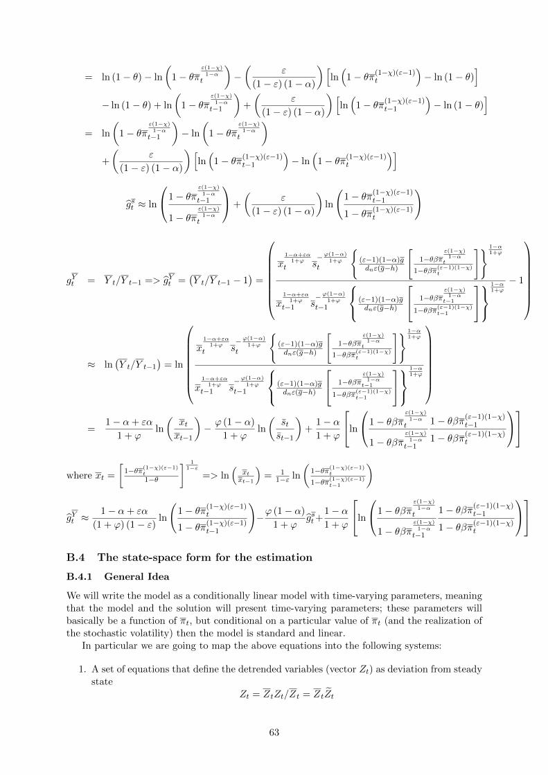
= ln (1− θ)− ln

(1− θπ

ε(1−χ)1−α

t

)−(

ε

(1− ε) (1− α)

)[ln(

1− θπ(1−χ)(ε−1)t

)− ln (1− θ)

]− ln (1− θ) + ln

(1− θπ

ε(1−χ)1−α

t−1

)+

(ε

(1− ε) (1− α)

)[ln(

1− θπ(1−χ)(ε−1)t−1

)− ln (1− θ)

]= ln

(1− θπ

ε(1−χ)1−α

t−1

)− ln

(1− θπ

ε(1−χ)1−α

t

)+

(ε

(1− ε) (1− α)

)[ln(

1− θπ(1−χ)(ε−1)t−1

)− ln

(1− θπ(1−χ)(ε−1)

t

)]

gst ≈ ln

1− θπε(1−χ)1−α

t−1

1− θπε(1−χ)1−α

t

+

(ε

(1− ε) (1− α)

)ln

(1− θπ(1−χ)(ε−1)

t−1

1− θπ(1−χ)(ε−1)t

)

gYt = Y t/Y t−1 => gYt =(Y t/Y t−1 − 1

)=

x

1−α+εα1+ϕ

t s−ϕ(1−α)

1+ϕ

t

(ε−1)(1−α)gdnε(g−h)

[1−θβπ

ε(1−χ)1−α

t

1−θβπ(ε−1)(1−χ)t

] 1−α1+ϕ

x1−α+εα

1+ϕ

t−1 s−ϕ(1−α)

1+ϕ

t−1

(ε−1)(1−α)gdnε(g−h)

1−θβπε(1−χ)1−α

t−1

1−θβπ(ε−1)(1−χ)t−1

1−α1+ϕ

− 1

≈ ln(Y t/Y t−1

)= ln

x

1−α+εα1+ϕ

t s−ϕ(1−α)

1+ϕ

t

(ε−1)(1−α)gdnε(g−h)

[1−θβπ

ε(1−χ)1−α

t

1−θβπ(ε−1)(1−χ)t

] 1−α1+ϕ

x1−α+εα

1+ϕ

t−1 s−ϕ(1−α)

1+ϕ

t−1

(ε−1)(1−α)gdnε(g−h)

1−θβπε(1−χ)1−α

t−1

1−θβπ(ε−1)(1−χ)t−1

1−α1+ϕ

=

1− α+ εα

1 + ϕln

(xtxt−1

)− ϕ (1− α)

1 + ϕln

(stst−1

)+

1− α1 + ϕ

ln

1− θβπε(1−χ)1−α

t

1− θβπε(1−χ)1−α

t−1

1− θβπ(ε−1)(1−χ)t−1

1− θβπ(ε−1)(1−χ)t

where xt =

[1−θπ(1−χ)(ε−1)

t1−θ

] 11−ε

=> ln(

xtxt−1

)= 1

1−ε ln

(1−θπ(1−χ)(ε−1)

t

1−θπ(1−χ)(ε−1)t−1

)

gYt ≈1− α+ εα

(1 + ϕ) (1− ε)ln

(1− θπ(1−χ)(ε−1)

t

1− θπ(1−χ)(ε−1)t−1

)−ϕ (1− α)

1 + ϕgst+

1− α1 + ϕ

ln

1− θβπε(1−χ)1−α

t

1− θβπε(1−χ)1−α

t−1

1− θβπ(ε−1)(1−χ)t−1

1− θβπ(ε−1)(1−χ)t

B.4 The state-space form for the estimation

B.4.1 General Idea

We will write the model as a conditionally linear model with time-varying parameters, meaningthat the model and the solution will present time-varying parameters; these parameters willbasically be a function of πt, but conditional on a particular value of πt (and the realization ofthe stochastic volatility) then the model is standard and linear.

In particular we are going to map the above equations into the following systems:

1. A set of equations that define the detrended variables (vector Zt) as deviation from steadystate

Zt = ZtZt/Zt = ZtZt

63

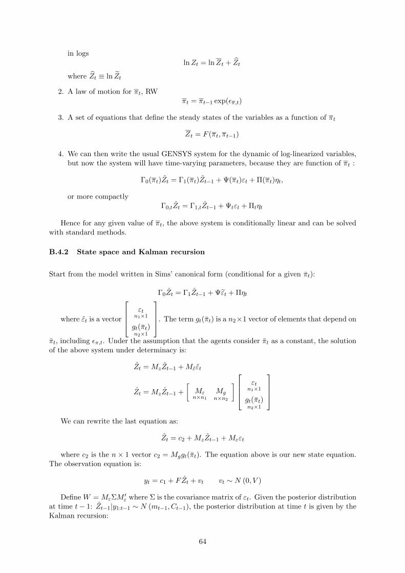
in logslnZt = lnZt + Zt

where Zt ≡ ln Zt

2. A law of motion for πt, RWπt = πt−1 exp(επ,t)

3. A set of equations that define the steady states of the variables as a function of πt

Zt = F (πt, πt−1)

4. We can then write the usual GENSYS system for the dynamic of log-linearized variables,but now the system will have time-varying parameters, because they are function of πt :

Γ0(πt)Zt = Γ1(πt)Zt−1 + Ψ(πt)εt + Π(πt)ηt,

or more compactlyΓ0,tZt = Γ1,tZt−1 + Ψtεt + Πtηt

Hence for any given value of πt, the above system is conditionally linear and can be solvedwith standard methods.

B.4.2 State space and Kalman recursion

Start from the model written in Sims’ canonical form (conditional for a given πt):

Γ0Zt = Γ1Zt−1 + Ψεt + Πηt

where εt is a vector

εtn1×1

gt(πt)n2×1

. The term gt(πt) is a n2×1 vector of elements that depend on

πt, including επ,t. Under the assumption that the agents consider πt as a constant, the solutionof the above system under determinacy is:

Zt = MzZt−1 +Mεεt

Zt = MzZt−1 +

[Mεn×n1

Mgn×n2

] εtn1×1

gt(πt)n2×1

We can rewrite the last equation as:

Zt = c2 +MzZt−1 +Mεεt

where c2 is the n× 1 vector c2 = Mggt(πt). The equation above is our new state equation.The observation equation is:

yt = c1 + FZt + vt vt ∼ N (0, V )

Define W = MεΣM′ε where Σ is the covariance matrix of εt. Given the posterior distribution

at time t− 1: Zt−1|y1:t−1 ∼ N (mt−1, Ct−1), the posterior distribution at time t is given by theKalman recursion:

64

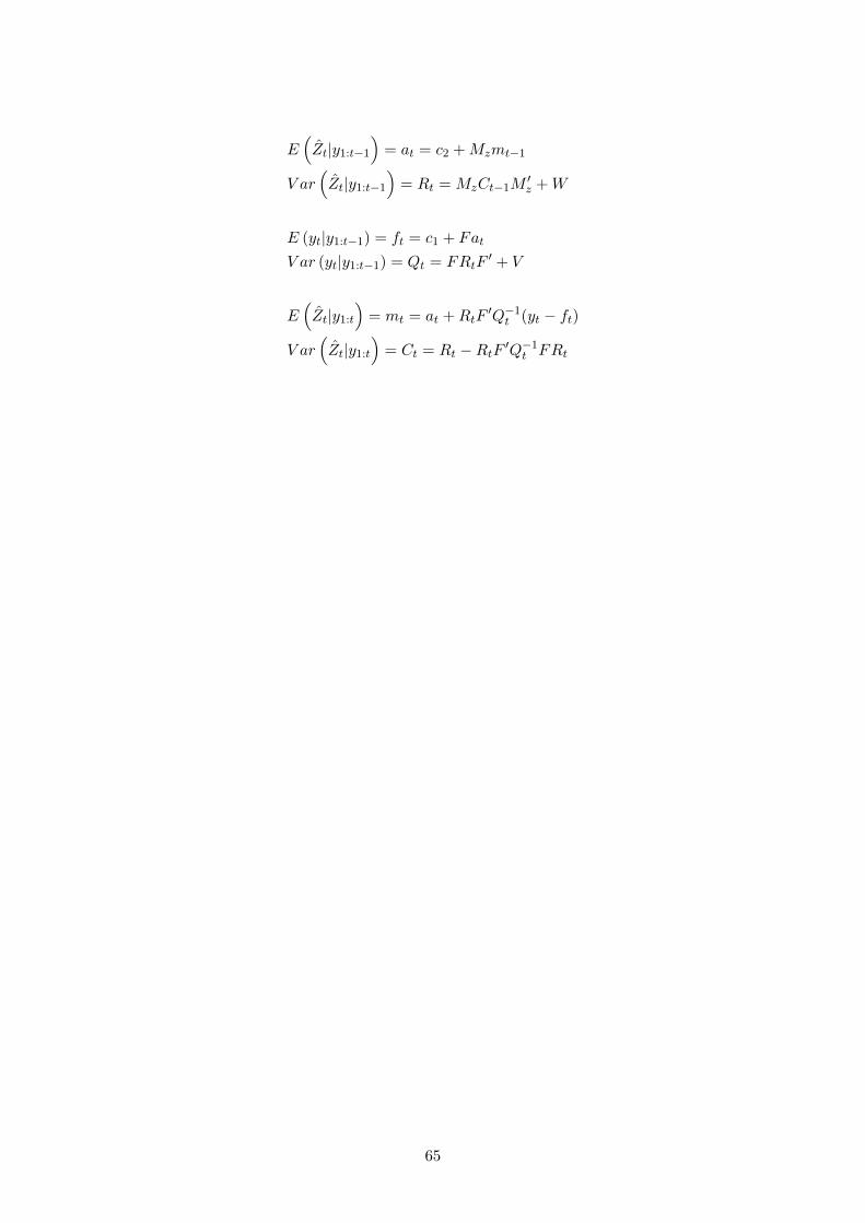
E(Zt|y1:t−1

)= at = c2 +Mzmt−1

V ar(Zt|y1:t−1

)= Rt = MzCt−1M

′z +W

E (yt|y1:t−1) = ft = c1 + Fat

V ar (yt|y1:t−1) = Qt = FRtF′ + V

E(Zt|y1:t

)= mt = at +RtF

′Q−1t (yt − ft)

V ar(Zt|y1:t

)= Ct = Rt −RtF ′Q−1

t FRt

65