The long-run impact of nuclear waste shipments on the property market: Evidence from a quasi-experiment $ Kishore Gawande a,n , Hank Jenkins-Smith b , May Yuan c a Bush School of Government and Public Service, Texas A&M University, College Station, TX 77843-4220, United States b Department of Political Science, University of Oklahoma, United States c College of Atmospheric and Geographic Sciences, University of Oklahoma, United States article info Article history: Received 14 April 2010 Available online 20 July 2012 Keywords: Spent nuclear fuel Average treatment effect Difference-in-differences Pooled cross-section Panel abstract We use evidence from a quasi-experiment – the shipping of radioactive spent nuclear fuel by train through South Carolina – to assess whether many years of incident-free transport of nuclear waste no longer negatively affects market valuation of properties along the route. Using Charleston County (SC) property sales data over 13 years we find, to the contrary, that the negative impact of the nuclear waste shipments on property values continues to be felt over the long run. The perception of risk from nuclear waste transport appears to be resilient. We contribute methodologically by comparing well- defined treatment and control groups of properties to estimate the average treatment effect of the nuclear waste shipment program. The results are affirmed in both a pooled cross-section sample, as well as a panel data sample of repeated property sales. & 2012 Elsevier Inc. All rights reserved. 1. Introduction Handling highly radioactive waste has proved to be one of the most difficult parts of hazardous materials management. As the United States debates large-scale transport of spent nuclear fuel (SNF) from the 73 storage sites scattered across 33 states to more centralized interim storage sites and permanent deep-geologic repositories versus maintaining the status quo of continued on-site storage at or near reactors, 1 concerns have focused on safety and efficiency of the transport [5], National Research Council, [45]). The Obama administration’s decision to withdraw the license application to construct the 77,000-ton capacity Yucca Mountain repository site, reversing the policy of former President Bush, remains controversial. The stalemate leaves in limbo the long-run solution to the current US inventory of 70,000 ton of SNF in existing sites, plus the annual output of more than 2000 ton of SNF annually produced by the country’s reactors. Subsequent to its withdrawal of the license application for Yucca Mountain, the Obama administration appointed a blue-ribbon commission to advise the government on a new strategy for managing nuclear waste. In January of 2012 the commission concluded that the US Contents lists available at SciVerse ScienceDirect journal homepage: www.elsevier.com/locate/jeem Journal of Environmental Economics and Management 0095-0696/$ - see front matter & 2012 Elsevier Inc. All rights reserved. http://dx.doi.org/10.1016/j.jeem.2012.07.003 $ Funding from National Science Foundation Award (# 0452874) is acknowledged. We thank Carol Silva and Amy Goodin for their thoughtful and insightful participation in this research. Joanna Lahey, Lori Taylor and Ren Mu provided helpful comments in the initial stages. Insightful comments made by anonymous referees have improved the paper considerably. We appreciate their careful reading of the paper. Responsibility for any remaining errors is ours. n Corresponding author. Fax: þ1 979 845 4155. E-mail address: [email protected] (K. Gawande). 1 Most commercial used nuclear fuel is stored at or near operating reactors. However nine of the 73 storage sites are at shutdown reactors, often referred to as ‘‘orphan’’ storage sites. Journal of Environmental Economics and Management 65 (2013) 56–73

Welcome message from author
This document is posted to help you gain knowledge. Please leave a comment to let me know what you think about it! Share it to your friends and learn new things together.
Transcript

Contents lists available at SciVerse ScienceDirect
Journal ofEnvironmental Economics and Management
Journal of Environmental Economics and Management 65 (2013) 56–73
0095-06
http://d
$ Fun
insightf
by anon
is ours.n Corr
E-m1 M
referred
journal homepage: www.elsevier.com/locate/jeem
The long-run impact of nuclear waste shipments on theproperty market: Evidence from a quasi-experiment$
Kishore Gawande a,n, Hank Jenkins-Smith b, May Yuan c
a Bush School of Government and Public Service, Texas A&M University, College Station, TX 77843-4220, United Statesb Department of Political Science, University of Oklahoma, United Statesc College of Atmospheric and Geographic Sciences, University of Oklahoma, United States
a r t i c l e i n f o
Article history:
Received 14 April 2010Available online 20 July 2012
Keywords:
Spent nuclear fuel
Average treatment effect
Difference-in-differences
Pooled cross-section
Panel
96/$ - see front matter & 2012 Elsevier Inc. A
x.doi.org/10.1016/j.jeem.2012.07.003
ding from National Science Foundation Awa
ul participation in this research. Joanna Lahey
ymous referees have improved the paper con
esponding author. Fax: þ1 979 845 4155.
ail address: [email protected] (K. Gawand
ost commercial used nuclear fuel is stored a
to as ‘‘orphan’’ storage sites.
a b s t r a c t
We use evidence from a quasi-experiment – the shipping of radioactive spent nuclear
fuel by train through South Carolina – to assess whether many years of incident-free
transport of nuclear waste no longer negatively affects market valuation of properties
along the route. Using Charleston County (SC) property sales data over 13 years we find,
to the contrary, that the negative impact of the nuclear waste shipments on property
values continues to be felt over the long run. The perception of risk from nuclear waste
transport appears to be resilient. We contribute methodologically by comparing well-
defined treatment and control groups of properties to estimate the average treatment
effect of the nuclear waste shipment program. The results are affirmed in both a pooled
cross-section sample, as well as a panel data sample of repeated property sales.
& 2012 Elsevier Inc. All rights reserved.
1. Introduction
Handling highly radioactive waste has proved to be one of the most difficult parts of hazardous materials management.As the United States debates large-scale transport of spent nuclear fuel (SNF) from the 73 storage sites scattered across 33states to more centralized interim storage sites and permanent deep-geologic repositories versus maintaining the statusquo of continued on-site storage at or near reactors,1 concerns have focused on safety and efficiency of the transport [5],National Research Council, [45]). The Obama administration’s decision to withdraw the license application to construct the77,000-ton capacity Yucca Mountain repository site, reversing the policy of former President Bush, remains controversial.The stalemate leaves in limbo the long-run solution to the current US inventory of 70,000 ton of SNF in existing sites, plusthe annual output of more than 2000 ton of SNF annually produced by the country’s reactors. Subsequent to its withdrawalof the license application for Yucca Mountain, the Obama administration appointed a blue-ribbon commission to advisethe government on a new strategy for managing nuclear waste. In January of 2012 the commission concluded that the US
ll rights reserved.
rd (# 0452874) is acknowledged. We thank Carol Silva and Amy Goodin for their thoughtful and
, Lori Taylor and Ren Mu provided helpful comments in the initial stages. Insightful comments made
siderably. We appreciate their careful reading of the paper. Responsibility for any remaining errors
e).
t or near operating reactors. However nine of the 73 storage sites are at shutdown reactors, often
K. Gawande et al. / Journal of Environmental Economics and Management 65 (2013) 56–73 57
will require interim storage sites and one or more permanent, centralized geologic repositories, and recommended earlypreparation for transport of used nuclear fuel and high-level radioactive wastes [5].
Of interest in this paper are the economic effects that transporting spent fuel may activate, possibly resulting frombeliefs about the risks posed by such transport. Experience with hazards, ranging from chemical wastes at Superfund sitesto deposition of lead from smelting plants has demonstrated that property values can be sensitive to proximity to suchhazards.2 But does proximity to the route by which radioactive materials are shipped in highly resilient transport casksalso affect property values? If so, by what amount do values diminish, and over what geographic scope? Finally, and mostimportantly, are these effects permanent or transitory?
This paper supplies answers to these questions using new methods. It is motivated by Gawande and Jenkins-Smith’s [17],henceforth GJS, study of shipments of spent fuel through South Carolina in the early years after the shipments began in 1994. Atthat time, the shipments were beset by enormous controversy and the wide press coverage that followed was rarely positive.Into the first two years of the shipments, GJS found that in populous Charleston County, a home five miles from the shipmentroute was worth 3% more than a similar home located on the route. This result has been used on both sides of a fierce policydebate over Yucca Mountain.3
The shipments continue to this day. There has not been a single negative incident over the fifteen years, andnewspaper reports of the shipments are almost negligible. This suggests that individuals’ perceptions about the risk ofSNF shipments may have been updated over time due to the lack of media coverage and absence of incidents. A largeliterature on environmental clean-ups argues that clean-ups restore property values in the long run.4 This literature, whilerelated, is distinct from risk revision. Cleanups entail the removal of a risk, whereas the risk may continue to be inherent inthe current context, though individuals may have updated their beliefs about the risk. The time is not only apt for re-investigating the finding using long-term data, but it has critical implications for both research and policy.5
This paper uses the same South Carolina SNF shipment setting as Gawande and Jenkins-Smith, and improves on it inthree respects. First, we appropriately view the SNF shipment as a natural experiment and use average treatment effectestimators. We use a difference-in-differences strategy to identify and estimate the average treatment effect in the treatedpopulation of properties in Charleston, South Carolina. Gawande and Jenkins-Smith [17] suffers methodologically from thesame issues that Greenstone and Gallagher [21] critique in earlier studies of the impact of NPL clean-ups, namely that themethods do not control for untreated properties. We remedy this deficiency. Second, the data include propertytransactions over a much longer duration. We obtained records of all residential property sales in Charleston Countybetween 1992 and 2005 (the GJS paper stopped at 1996). The transactions data permit us to estimate the effects of thespent fuel shipment program on property values over a decade of shipments without incident. Third, we are able to weighin with panel data, while much of the literature has used pooled cross-sections. Existing studies of the effects of theenvironment on land and property values has largely used cross-sectional data combined with a heavy reliance on hedonicvariables to control for heterogeneity. Even with the controls, doubts may remain about unobserved heterogeneity in thecross-section. Therefore, in addition to the pooled cross-section, we use repeat sales information to create panel data on anumber of properties.
The paper proceeds as follows. In Section 2 we describe the foreign spent nuclear fuel shipments that began in 1996.Section 3 describes the difference-in-differences methodology using both pooled cross-section data and panel data. Section4 explains in detail the construction of our data set. The data are unique in many respects, and add new dimensions to theenvironmental impact evaluation enterprise. Section 5 presents and analyzes the findings. The main finding is that theprices of properties in the most urban and populous County (Charleston) continue to be influenced negatively by SNFshipments despite the absence of any incidents that might heighten risk perceptions about the shipments. Section 6provides our discussion and conclusions.
2 The idea that property values will be affected by the presence of hazardous materials – including incinerators, electricity transmission lines,
landfills, and nuclear power plants – has been studied, for example, by Kiel and McClain [33], Kiel [32], McClelland et al. [38], Kohlhase [34], Michaels and
Smith [41], and Gamble et al. [16]. These studies use the hedonic pricing logic, viewing proximity to the environment as a characteristic of the property.
The earliest efforts involved inference about the marginal value of clean air from housing prices [23,39].3 Board of County Commissioners Lincoln County NV [4], Clark County Department of Comprehensive Planning, Nuclear Waste Division [11], Hom
et al. [25], Nuclear and Radiation Studies Board [45], O’Connor [46], State of Nevada [52,51], and US Nuclear Regulatory Commission [58].4 In a properly functioning market if a disamenity is transitory, it should not have permanent effects on housing prices. Stock [53], Kohlhase [34], and
Ketkar [31] find this to be true about properties near cleaned-up hazardous waste sites as do Carroll et al. [7] and Dale et al. [13] in the context of
chemical clean-ups. Studies by Nelson [43], Gamble and Downing [15] and Gamble et al. [16] examining incidents near nuclear power plants, specifically
the Three Mile Island (TMI) accident, found no decrease in housing prices due to proximity to the TMI plant. However, since nuclear power plants
produce jobs and tax revenues, they may offset the possible disamenity effects. Studies of waste sites such as the Frenald plant in Ohio (Feiertag, [60])
and Rocky Flats in Colorado (Hunsperger, [27]) indicate the effects on property values to be similar to those of Superfund sites.5 In a white paper, Department of Energy analysts Holm et al. [25, p. 12] write: ‘‘The numerous and complex socioeconomic analyses that attempt to
quantify stigma damages for various transportation scenarios are based on a single, limited, preliminary study whose authors themselves argue that the
issue requires further study. Apart from the GJS study, there appears to be no defensible empirical evidence whatsoever that stigma from transportation
even exists. Their finding that there may be a statistically significant effect may be supported by further research, or it may not. What is certain is that
repeated and sustained citations to this single isolated study in secondary sources and reports do not validate the findings themselves.’’
‘‘Much of the research conducted to date has used polling methodologies, as opposed to empirical or real-time data. The GJS study, by contrast, used
real estate sales data along with the results of systematic surveys to reach its conclusions. DOE’s Appendix I of the FEIS on Yucca Mountain suggests that
additional research is needed. If such analysis is undertaken y(t)he research should use actual real estate transaction data for a significant period of
timey.’’
0
10
20
30
40
50
60
1994 1996 1998 2000 2002 2004 2006Year
Frequency
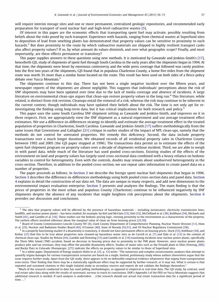
Fig. 1. Monthly reporting on nuclear issues in South Carolina.
Source: Post and Courier.
K. Gawande et al. / Journal of Environmental Economics and Management 65 (2013) 56–7358
2. Theory
2.1. Background
The United States program to reclaim spent nuclear fuel from overseas reactors seeks to remove from commercepotential access to weapons-grade nuclear materials – both highly enriched uranium and the plutonium byproduct offission in the reactor. The fuel, originally provided to many nations as part of the Atoms for Peace program, has beenowned by the United States.6 In the 1990s, a campaign to ship accumulated stocks of spent fuel back to the United Stateswas initiated. Initial plans to return the fuel through ports in North Carolina and Contra Costa County, CA, resulted insubstantial opposition. The Governor of South Carolina, the state where much of the spent fuel was to be stored, soughtunsuccessfully to block the shipments in the courts. South Carolina newspapers and television news provided amplecoverage of the dispute, highlighting the route and communicating the dire concerns of some state officials, anti-nuclearactivists, and citizens. After a delay of nearly two years following the initial shipment in 1994, foreign spent nuclear fuel(SNF) has been transported at least once a year from the Port of Charleston to the Department of Energy’s Savannah Riverfacility in Aiken County, SC. Appendix A (available from the authors) lists the dates of each of the rail shipments between1996 and 2003.
In contrast to the substantial initial public outcry over the shipments, there has been little negative press oversubsequent years. No accidents or incidents have occurred that resulted in release of radiation. Indeed, our review of newsarticles in the Charleston Post and Courier newspaper, summarized in Fig. 1, found no articles claiming that such events hadoccurred. Did the lack of SNF transport incidents together with declining attention in the news lower the perceived risksfrom SNF shipments? Specific to nuclear waste, surveys by Slovic et al. [50], and Kunreuther and Easterling [35] havedemonstrated that nuclear images of a place lower stated preferences for vacationing and residing there, suggesting long-term stigmatization of properties may occur near nuclear waste storage facilities.
2.2. Theory
A simple model of how risk perception affects property prices is developed by Gayer et al. [18]. Individuals maximizeexpected utility over two states of the world, U1 when harm comes to them from exposure to radiation from spent nuclearfuel, and U2 when they are unexposed and healthy. U24U1 for any given income, and marginal utility of income is greaterwhen healthy. The consumer has income y which is spent on buying a home and a composite good a. Utility in each state isa function of characteristics of the home X, perceived risk of harm from exposure to the spent nuclear fuel p, and distanceto the SNF route D (which measures the visual disamenity from the SNF shipment). The price of a home P is a function ofcharacteristics X, risk perception p, and distance to the SNF route D. The consumer chooses the arguments in P and a tomaximize expected utility subject to the budget constraint:
Max EU¼ pU1ða,X,DÞþð1�pÞU2ða,X,DÞ
s.t.
y¼ aþPðp,X,DÞ:
6 The objective of the Atoms for Peace program was to provide non-nuclear nations with peaceful means to employ nuclear technologies (usually in
the form of research reactors and the reactor fuel) in return for the recipient countries’ willingness to forego development of their own nuclear weapons
program.
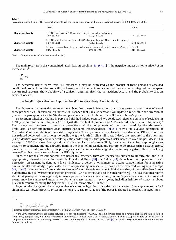
Table 1Perceived probabilities of FSNF transport accidents and consequences as measured in cross-sectional surveys in 1994, 1995 and 2005.
1994 1995 2005
Charleston County 1. FSNF train accident? (0¼never happen; 10¼certain to happen)
4.68, sd¼0.17 4.77, sd¼0.13 5.65, sd¼0.13
2. FSNG canister rupture (if accident)? (0¼never happen; 10¼certain to happen)
Charleston County 5.07, sd¼0.18 4.66, sd¼0.15 5.74, sd¼0.14
3. Expectation of harm to area residents (if accident and canister rupture)? (percent ‘‘yes’’)
Charleston County 84%, sd¼0.03 80%, sd¼0.02 91%, sd¼0.01
Notes: 1. Sample means and standard deviations (sd).
K. Gawande et al. / Journal of Environmental Economics and Management 65 (2013) 56–73 59
The main result from this constrained maximization problem [18, p. 441] is the negative impact on home price P of anincrease in p7:
@P
@po0:
The perceived risk of harm from SNF exposure p may be expressed as the product of three personally assessedconditional probabilities: the probability of harm given that an accident occurs and the canister carrying radioactive spentnuclear fuel ruptures, the probability of a canister rupturing given that an accident occurs, and the probability that anaccident occurs:
p¼ ProbðHarm9Accident and RuptureÞ � ProbðRupture9AccidentÞ � ProbðAccidentÞ:
The change in risk perception Dp may come about due to new information that changes personal assessments of any ofthese probabilities. For example, an increase in Prob(Accident), all else constant, will update risk beliefs in the direction ofgreater risk perception ðDp40Þ. Via the comparative static result above, this will lower a home’s price.
To ascertain whether a change in perceived risk had indeed occurred, we conducted telephone surveys of residents in1994 (just prior to the first shipment), 1995 (just after the first shipment), and 2005 (a decade after the first shipments).8
The survey was designed to measure perceptions of the components of the risks posed by the shipments:ProbðHarm9Accident and RuptureÞ,ProbðRupture9AccidentÞ, Prob(Accident). Table 1 shows the average perception ofCharleston County residents of these risk components. The experience with a decade of accident-free SNF transport hasnot reduced perceived risks among the public along the South Carolina rail route. Indeed, the responses to the questions(using identical wording and very similar question order) suggest that perceived risks increased over the past decade. Onaverage, in 2005 Charleston County residents believe accidents to be more likely, the chance of a canister rupture given anaccident to be higher, and the expected harm in the event of an accident and rupture to be greater than a decade before.Since perceived risks are a factor in property values, the survey data suggest a continuing negative effect from being‘‘treated’’ with exposure to risk from the SNF shipments.
Since the probability components are personally assessed, they are themselves subject to uncertainty, and p isappropriately viewed as a random variable. Riddel and Shaw [48] and Riddel [47] show how the imprecision in riskperception assessment p, denoted s2
p, can influence a person’s willingness to accept compensation for a negativeenvironmental externality. In particular, a median-preserving increase in s2
p increases the expected willingness to accept[48, p. 346]. Using evidence from a primary survey of South Nevada residents Riddel shows that, of the welfare loss from ahypothetical nuclear waste transportation program, 12.4% is attributable to the uncertainty s2
p. The idea that uncertaintyabout risk perceptions can negatively influence property prices applies naturally in our Bayesian framework. A number ofevents may have increased uncertainty about risk assessment in recent years, including heightened concerns aboutnuclear terrorism following the September 11, 2001, terror attacks in the US.
Together, the theory and the survey evidence lead to the hypothesis that the treatment effect from exposure to the SNFshipments will lower property prices in the long run. The remainder of the paper is devoted to testing this hypothesis.
7
@P
@p ¼U1�U2
p@U1=@aþð1�pÞ@U2=@ao0:
If distance directly influences risk perception, y¼ aþPðpðDÞ,XÞ, with p0ðDÞo0, then @P=@D40.
8 The 2005 interviews were conducted between October 7 and December 4, 2005. The samples were based on a random digit-dialing frame obtained
from Survey Sampling Inc., of Fairfield Connecticut. The surveys lasted an average of 17 minutes, and resulted in a cooperation rate of 57% in 2005, in
comparison to cooperation rates (using AAPOR’s ‘‘COOP2’’ formula) of 88% in 1994 and 61% 1995 [1]. All three surveys included over 250 Charleston
County respondents.
propertiesspent shipment routeother railroads
12 km buffer zonearound the shipment route
counties in South Carolina
Charleston county urban area
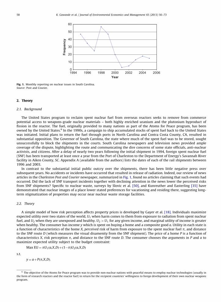
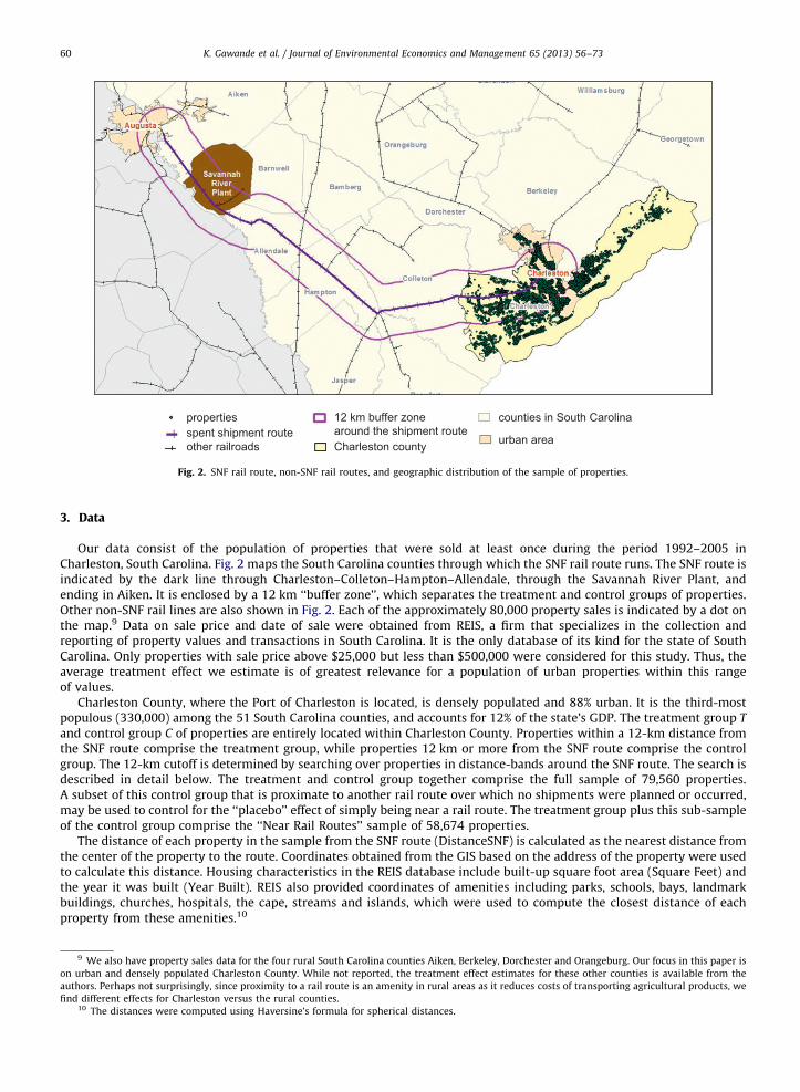
Fig. 2. SNF rail route, non-SNF rail routes, and geographic distribution of the sample of properties.
K. Gawande et al. / Journal of Environmental Economics and Management 65 (2013) 56–7360
3. Data
Our data consist of the population of properties that were sold at least once during the period 1992–2005 inCharleston, South Carolina. Fig. 2 maps the South Carolina counties through which the SNF rail route runs. The SNF route isindicated by the dark line through Charleston–Colleton–Hampton–Allendale, through the Savannah River Plant, andending in Aiken. It is enclosed by a 12 km ‘‘buffer zone’’, which separates the treatment and control groups of properties.Other non-SNF rail lines are also shown in Fig. 2. Each of the approximately 80,000 property sales is indicated by a dot onthe map.9 Data on sale price and date of sale were obtained from REIS, a firm that specializes in the collection andreporting of property values and transactions in South Carolina. It is the only database of its kind for the state of SouthCarolina. Only properties with sale price above $25,000 but less than $500,000 were considered for this study. Thus, theaverage treatment effect we estimate is of greatest relevance for a population of urban properties within this rangeof values.
Charleston County, where the Port of Charleston is located, is densely populated and 88% urban. It is the third-mostpopulous (330,000) among the 51 South Carolina counties, and accounts for 12% of the state’s GDP. The treatment group T
and control group C of properties are entirely located within Charleston County. Properties within a 12-km distance fromthe SNF route comprise the treatment group, while properties 12 km or more from the SNF route comprise the controlgroup. The 12-km cutoff is determined by searching over properties in distance-bands around the SNF route. The search isdescribed in detail below. The treatment and control group together comprise the full sample of 79,560 properties.A subset of this control group that is proximate to another rail route over which no shipments were planned or occurred,may be used to control for the ‘‘placebo’’ effect of simply being near a rail route. The treatment group plus this sub-sampleof the control group comprise the ‘‘Near Rail Routes’’ sample of 58,674 properties.
The distance of each property in the sample from the SNF route (DistanceSNF) is calculated as the nearest distance fromthe center of the property to the route. Coordinates obtained from the GIS based on the address of the property were usedto calculate this distance. Housing characteristics in the REIS database include built-up square foot area (Square Feet) andthe year it was built (Year Built). REIS also provided coordinates of amenities including parks, schools, bays, landmarkbuildings, churches, hospitals, the cape, streams and islands, which were used to compute the closest distance of eachproperty from these amenities.10
9 We also have property sales data for the four rural South Carolina counties Aiken, Berkeley, Dorchester and Orangeburg. Our focus in this paper is
on urban and densely populated Charleston County. While not reported, the treatment effect estimates for these other counties is available from the
authors. Perhaps not surprisingly, since proximity to a rail route is an amenity in rural areas as it reduces costs of transporting agricultural products, we
find different effects for Charleston versus the rural counties.10 The distances were computed using Haversine’s formula for spherical distances.

K. Gawande et al. / Journal of Environmental Economics and Management 65 (2013) 56–73 61
Census-block demographic and income data obtained from the 1990 United States Census were mapped to eachproperty based on its address and zip code. These variables include the percent of the population in the census block whoare White (% White), Black (% Black), and Hispanic (% Hispanic), and the median household income in the census block(HH Income). In sum, we have as complete a data set as possible on sale price, property characteristics, external amenities,and census block characteristics with which to investigate the effect of SNF shipments on property sale prices.
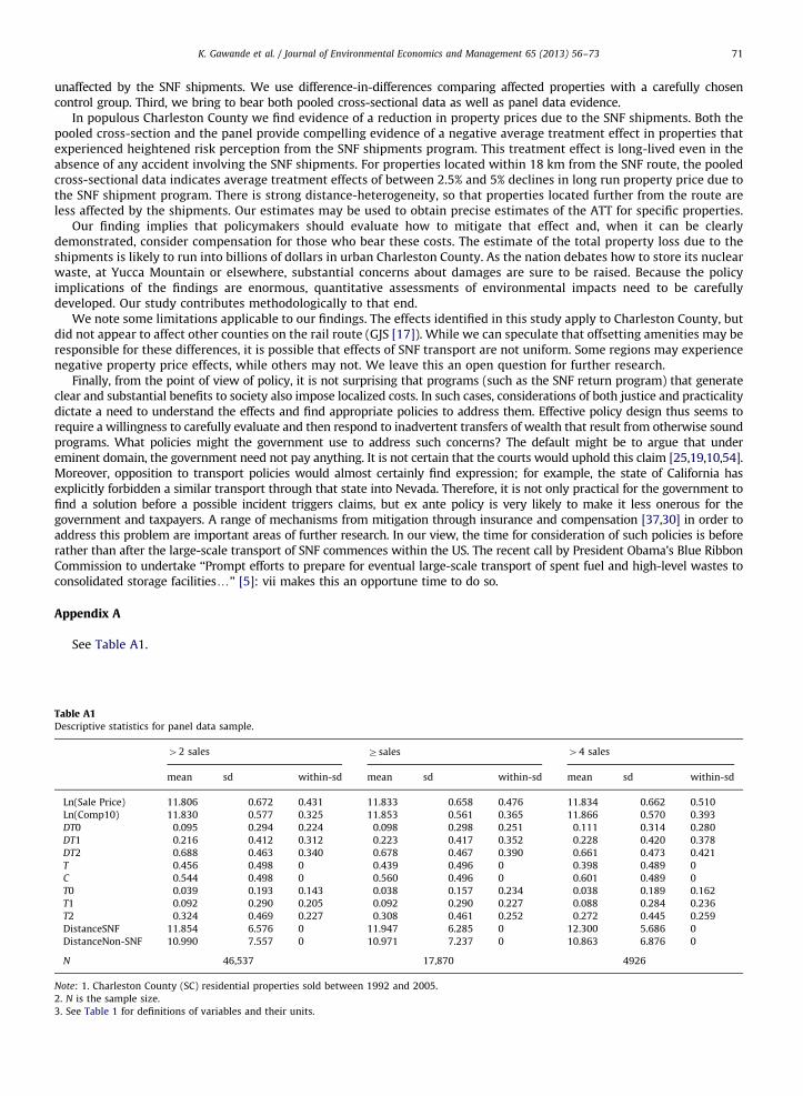
Table 2 provides descriptive statistics for the Charleston County pooled cross-section. Of the 79,650 residentialproperties in the full sample, 48% belong to the treatment group and 52% to the control group. 10% of the transactions inthe sample preceded the shipments (DT0) and 90% were recorded in the shipments regime. We will distinguish theprogram’s short-term impact (8/1994–12/1997) from its long-term impact (1/1998–2005). 21% of the sample is from theshort-term regime (DT1) while 71% is from the long-term regime (DT2). The average building in the sample was 1893square feet and was built in 1971. The distance of properties from the SNF route had a mean of 11.63 km and standarddeviation equal to 6.79 km. The average distance of treated properties from the SNF route was 6.052 km.
Our panel data are constructed as three separate data sets, one comprising 46,537 properties that were sold at leasttwice, another comprising 17,870 properties that were sold at least thrice, and a third comprising 4926 properties thatwere sold at least four times during the 1990–2005 period. Appendix Table A1 provides descriptive statistics for thepanels. The statistics indicate considerable within-variation in the price data.
4. Methodology
4.1. Pooled cross-section
The SNF shipment program provides a natural experiment for assessing the impact of nuclear waste shipments onresidential property prices. Residential properties in Charleston, South Carolina potentially impacted by the shipments, or‘‘treated’’ to the risk of exposure, are the units of analysis. We use difference-in-differences (DID) to identify and estimatethe average treatment effect on this population of treated properties (ATT).11
The difference in differences compares the effect of SNF shipments on properties perceived to be exposed to the risk ofcontamination (the treated group) versus properties that were not perceived to be exposed to the risk (the control group).Specifically, the pre-shipment to post-shipment change in the selling price of properties for the treated group is comparedto the pre-shipment to post-shipment change in the selling price of properties for the control group. The post-shipmentphase is broken down into a two periods to enable us to contrast the short-term versus the long-term impact of theshipments. Specifically, using a pooled cross-section of property prices, we estimate parameters of the econometric model
lnðPitÞ ¼ gTiþtSðDT1t � TiÞþtLðDT2t � TiÞþb0Xiþyear fixed effectsþeit , ð1Þ
where Pit is the selling price of property i at in year t. The assignment to treatment group indicator Ti ¼ 1 if property i iswithin 12 km of the SNF route, that is, perceived to be exposed to risk from the SNF shipments. Properties beyond 12 km ofthe shipment route are assigned to the control group. The property bands model described below is used to determine the12 km cutoff. DT1t and DT2t are short run and long run indicators: DT1t ¼ 1 if the observation records a sale after the firstSNF shipment in 8/94–12/97; DT2t ¼ 1 if the observation records a sale during 1/98–12/05.12 The coefficient g measuresthe average time-invariant difference between properties perceived to be exposed to risk versus properties that were notso perceived. The difference-in-differences estimators are the coefficients on the interaction terms: tS measures the short-run average treatment effect of the shipments in the 3-year period following the inception of shipments. tL measures thelong-run average treatment effect of the SNF shipments.
4.1.1. Assumptions
Three assumptions are needed for the error term eit to be independent of assignment to treatment Ti, so that the DIDestimators tS and tL are identified.
4.1.1.1. Functional form. The first assumption concerns stability of functional form across treated and control units.Hedonic variables Xi described in the data section measure property-specific attributes, census block characteristics andproximity to amenities, all of which have been emphasized in the literature (e.g. [9]). The use of hedonic models in whichthe parameters b measure the marginal valuations of each characteristic (linearly) is standard in the large literature onproperty valuation. This is relevant for our estimation strategy, since DID relies on strong assumptions about stability offunctional form. Specifically, the large literature on hedonics supports our assumption that b is the same for treated and
11 Rubin’s [49] potential outcomes framework motivates this analytical framework (see [28]). If the property-specific treatment effect is constant
across every property, then DID estimates the Charleston county population average treatment effect (ATE). However, if the treatment effect is
heterogeneous then DID estimates the average treatment effect on the treated properties (ATT). The treatment effect is heterogeneous in a specific and
measurable way, as we show below.12 Their own effects are absorbed into the year fixed effects.

K. Gawande et al. / Journal of Environmental Economics and Management 65 (2013) 56–7362
untreated properties, and is not a source of bias.13 The log-linear specification solves the problem of skewness in thehousing price, which would otherwise make the errors non-normal.14
4.1.1.2. Common trends. The second assumption is that in the absence of the SNF shipments, properties in both thetreatment and control groups would have common trends. This assumption would be violated if, for example, theshipment route was chosen endogenously, deliberately on the basis of trends that distinguished the treatment propertiesfrom the control properties. We believe the assignment of properties to treatment from the SNF program was doneindependently of their value. Two reasons for this view are, first, the choice of the South Carolina SNF rail route was highlyconstrained by requirements associated with distance, track quality, and traffic density (DOE [57]) and second, onlyexisting routes were utilized. No new routes were constructed. If interest groups representing high-values homes, forexample, had been able to use their influence to move the route away from their homes, then assignment to treatmentwould not be exogenous. Or if a new route were built at a safe distance from the city of Charleston by policymakers inresponse to strong public opinion, the assignment to treatment of homes built around this new route would beendogenous. Neither of these occurred. The transportation corridor was chosen from routes that had existed for decades,imposing a random shock on properties along the chosen route. Quite simply, properties near the SNF route becameexposed to risk, while properties located outside its range of influence were much less exposed or unexposed. In theempirical section we attempt to falsify this assumption by testing the equality of trends using pre-shipment data.
4.1.1.3. SUTVA. The third assumption needed for the error term eit to be independent of assignment to treatment is thestable unit treatment value assumption (SUTVA) that the treatment has no externalities. That is, treatment of a propertyhas no repercussions on the values of other properties. This assumption is likely to be violated because of strong spatialcorrelation inherent in neighboring property values. In a neighborhood, the market prices similar properties similarly.Realtors often advise sellers to set the price according to the best ‘‘comp’’ or comparable house in the neighborhood.
We consider two options. The first option is to ignore the externality and use (1) to estimate the treatment effect. If theprice of a treated home is depressed because the comps are all selling for less, but the comps sold for less due to thetreatment, then one should not control for the price of comps in the analysis. Since we are interested in the total derivativeof the SNF treatment on home value, this eliminates ‘‘intermediate outcomes’’ such as the effect on comps. Netting out theeffect on the comps underestimates the treatment effect on a home, since, in this view, the effect on the comps should beattributed to the home.
The second option is to control for the neighborhood externality directly by including a spatially lagged regressor. Wedo so by including the variable COMP10, constructed as
COMP10i ¼X10
j ¼ 1
1dijP10
j ¼ 11dij
24
35Pj,
where Pj’s are prices of homes closest to home i, each dij kilometers from it. To avoid endogeneity, the Pj’s are taken fromproperty sales that occurred between six and twelve months prior to the sale date of property i. COMP10 limits the compsto 10 previously sold properties neighboring property i. Adding COMP10 to (1) results in the model
lnðPitÞ ¼ gTiþtSðDT1t � TiÞþtLðDT2t � TiÞþf lnðCOMP10itÞþb0Xiþyear fixed effectsþeit : ð2Þ
A reason for including COMP10 is econometric. Ignoring comps induces spatial correlations in the errors, leadingto inefficient estimates of the DID and other parameters [2]. We find that including COMP10 greatly reduces spatialcorrelation in the errors.
Another reason for including COMP10 is that it may ameliorate the impact of the SUTVA violation. There is a possiblepositive externality on the price of control units, due to their lack of treatment and consequent greater demand. Thus, DIDis an upper bound on the cost to homeowners in the treated units, but does reflect the total effect on the relative price oftreated versus control units. COMP10 then captures some of the effect of the treatment on the decrease in price of thetreated units and increase in price of control units. COMP10 also captures unobserved neighborhood attributes ofindividual units that may be correlated with treatment status. Even though COMP10 may not fully internalize theexternality, including COMP10 may nevertheless alleviate the problem. We find a substantial difference between DIDsfrom the model without comps versus the model with comps, and report both, leaving the choice for the reader to make.15
13 For example, X may change in response to the treatment if only smaller properties were built in the region along the route exposed to risk from the
SNF shipments. Results available from the author show that there was no statistical difference in property characteristics between the treatment and
control groups.14 Estimating the same models with a Box–Cox transformation yields results that are close to those reported here.15 If it is possible to satisfy no externalities across clusters defined by comps, then a neighborhood-level SUTVA, or NL-SUTVA assumption is valid
[59]. However, spillovers do traverse comps-levels and even across the treatment and control groups since diminished demand for homes in the
treatment group may increase demand in the control group. Still, it is worth considering the following possibility in future research. NL-SUTVA requires
that there be no treatment externalities between homes in different comp groups, that is, the effect of the SNF shipments in one comp cluster does not
affect the outcome in another comp cluster. Suppose any externality from the treatment, reflected in values of the comps, is confined to the treated
group, and there are no cross-group spillovers (this may be tested). Then, since NL-SUTVA is satisfied, Eq. (2) may be used in a manner similar to

K. Gawande et al. / Journal of Environmental Economics and Management 65 (2013) 56–73 63
4.1.2. Heterogeneity
A key source of heterogeneity in the treatment effect, recognized in the theory section, and also in the GJS study, is thatperceived risk from exposure decreases as distance from the SNF route increases. Two extensions of (2) are used to takethis into account. In the first extension, we assign properties within three parallel 4 km distance bands, each bandsuccessively further from the SNF route:
lnðPitÞ ¼ gTiþX3
j ¼ 1
tSj ðDT1t � TijÞþ
X3
j ¼ 1
tLj ðDT2t � TijÞþf lnðCOMP10itÞþb
0Xiþyear fixed effectsþeit : ð3Þ
where assignment of each property i to a band is indicated by the three dummy variables Tij, j¼ 1, . . . ,3. We expect theDIDs to follow the order t14t24t3 (for both SR and LR treatment effects) since properties located further from theshipment route become less exposed to perceived risk. We use this model to search for a credible distance cutoff fordefining the unexposed control group of properties. To start the search we define the treatment group indicator Ti ¼ 1 ifproperty i is within 18 km of the SNF route.16
In the second extension, rather than estimating constant DIDs within different bands we estimate it as a continuousfunction of distance from the SNF route:
lnðPitÞ ¼ gTiþtSðDT1t � TiÞþtLðDT2t � TiÞþtSDðDistanceSNFi � DT1t � TiÞþtL
DðDistanceSNFi � DT2t � TiÞ
þf lnðCOMP10itÞþb0Xiþyear fixed effectsþeit : ð4Þ
The DID for property i is computed as tþðtD � DistanceSNFiÞ, where the constant treatment effect t is adjusted for theameliorating effect of distance from the SNF route. From a modeling perspective, (4) captures distance from the shipmentroute as an essential source of heterogeneity. Since the property-specific treatment effect is not constant across everyproperty, the DID estimates the average treatment effect on treated properties (ATT) in the Charleston county population.Specifically, the DID estimates the additional change over time in property values for the treated relative to the controls.From a policy perspective, the distance effect is critical in assessing damage valuations for individual properties.
4.2. Panel data
The availability of repeat sales data is uncommon because several years of data must be available before we can obtaina mix of properties that have been sold two, three, four, or more times. We have that luxury, and are able to estimate panelmodels with property-fixed effects. The panel DID model of short- and long-run ATTs is specified as
lnðPitÞ ¼ tSðDT1t � TiÞþtLðDT2t � TiÞþtSDðDistanceSNFi � DT1t � TiÞþtL
DðDistanceSNFi � DT2t � TiÞ
þf lnðCOMP10itÞþyear fixed effectsþuiþEit : ð5Þ
In (5) ui are property fixed effects. Time-invariant regressors like property attributes, distance to amenities, andneighborhood characteristics are absorbed into the property fixed effects.17 COMP10 is time-varying and controls forspatial errors. Bertrand et al. [3] caution about underreporting standard errors, since in panels with long durations oftreatment, autocorrelation of treatment with the outcome is likely. We note that since individual properties sell at randompoints during the period of the sample, the autocorrelation problem in our case is not severe. Regardless, we follow theirsuggestion of using White’s robust standard errors, which accounts for clustering on fixed effects, for computing t-values[3, fn 29].
5. Results
5.1. Pooled cross-section
5.1.1. Distance bands of properties
OLS estimates from the pooled cross-section of parameters in the distance bands model (3) are reported in Table 3. Theeffect of the spatial control variable COMP10 is measured extremely precisely. As expected, it is a good predictor of thechange in sale prices. In the first model, for example, a 10% increase in the price of the closest 10 properties sold isassociated with a 4.62% increase in the value of a home in that neighborhood. The spatial variable accomplishes its othertask, namely reducing spatial correlation. While it is not possible to compute spatial statistics such as Moran’s I and Getty’s
(footnote continued)
VanderWeele’s [59] two-level model for estimating neighborhood effects. In the two-level model properties are treated in clusters of comps (i.e.
‘‘neighborhood’’), enabling estimation of comps-level ATTs.16 The plausibility of 18 km as a cutoff choice is based on these considerations. If a ‘‘safe’’ distance such as 25 km is chosen as a cutoff to determine
the boundary between treated and control properties, then 99% of the Charleston properties fall in the treated group. On the other hand, a shorter cutoff,
say at 5 km, may include a sizable set of properties the control group that are actually perceived to be exposed to risk from the SNF. The DID coefficient twould then understate the actual treatment effect.
17 In theory, improvements to properties may change their characteristics, and building new amenities can introduce time-variation. However, in our
sample too few properties expanded or contracted in terms of square footage, and the stock of amenities remained constant.
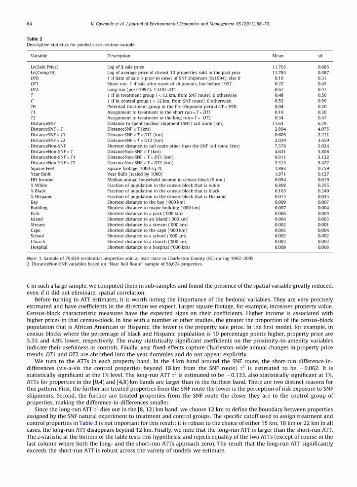
Table 2Descriptive statistics for pooled cross-section sample.
Variable Description Mean sd
Ln(Sale Price) Log of $ sale price 11.765 0.685
Ln(Comp10) Log of average price of closest 10 properties sold in the past year 11.783 0.587
DT0 1 if date of sale is prior to onset of SNF shipment (8/1994), else 0 0.10 0.31
DT1 Short run: 1 if sale after onset of shipments, but before 1997. 0.22 0.42
DT2 Long run (post-1997): 1-DT0–DT1 0.67 0.47
T 1 if in treatment group (o12 km. from SNF route), 0 otherwise 0.48 0.50
C 1 if in control group (Z12 km. from SNF route), 0 otherwise 0.52 0.50
T0 Potential treatment group in the Pre-Shipment period¼T�DT0 0.04 0.20
T1 Assignment to treatment in the short run¼T�DT1 0.10 0.30
T2 Assignment to treatment in the long run¼T� DT2 0.34 0.47
DistanceSNF Distance to spent nuclear shipment (SNF) rail route (km) 11.63 6.79
DistanceSNF� T DistanceSNF� T (km) 2.894 4.075
DistanceSNF� T1 DistanceSNF� T�DT1 (km) 0.605 2.211
DistanceSNF� T2 DistanceSNF� T�DT2 (km) 2.029 3.659
DistanceNon-SNF Shortest distance to rail route other than the SNF rail route (km) 7.578 5.024
DistanceNon-SNF� T DistanceNon-SNF� T (km) 4.621 5.858
DistanceNon-SNF� T1 DistanceNon-SNF� T�DT1 (km) 0.911 3.122
DistanceNon-SNF� T2 DistanceNon-SNF� T�DT2 (km) 3.313 5.427
Square Feet Square footage, 1000 sq. ft. 1.893 0.759
Year Built Year Built (scaled by 1000) 1.971 0.127
HH Income Median annual household income in census block ($ mn.) 0.054 0.019
% White Fraction of population in the census block that is white 0.808 0.255
% Black Fraction of population in the census block that is black 0.165 0.249
% Hispanic Fraction of population in the census block that is Hispanic 0.015 0.035
Bay Shortest distance to the bay (‘000 km) 0.009 0.007
Building Shortest distance to major building (‘000 km) 0.007 0.004
Park Shortest distance to a park (‘000 km) 0.006 0.004
Island Shortest distance to an island (‘000 km) 0.004 0.003
Stream Shortest distance to a stream (‘000 km) 0.002 0.001
Cape Shortest distance to the cape (‘000 km) 0.005 0.004
School Shortest distance to a school (‘000 km) 0.002 0.002
Church Shortest distance to a church (‘000 km) 0.002 0.002
Hospital Shortest distance to a hospital (‘000 km) 0.009 0.008
Note: 1. Sample of 79,650 residential properties sold at least once in Charleston County (SC) during 1992–2005.
2. DistanceNon-SNF variables based on ‘‘Near Rail Route’’ sample of 58,674 properties.
K. Gawande et al. / Journal of Environmental Economics and Management 65 (2013) 56–7364
C in such a large sample, we computed them in sub-samples and found the presence of the spatial variable greatly reduced,even if it did not eliminate, spatial correlation.
Before turning to ATT estimates, it is worth noting the importance of the hedonic variables. They are very preciselyestimated and have coefficients in the direction we expect. Larger square footage, for example, increases property value.Census-block characteristic measures have the expected signs on their coefficients. Higher income is associated withhigher prices in that census-block. In line with a number of other studies, the greater the proportion of the census-blockpopulation that is African American or Hispanic, the lower is the property sale price. In the first model, for example, incensus blocks where the percentage of black and Hispanic population is 10 percentage points higher, property price are5.5% and 4.9% lower, respectively. The many statistically significant coefficients on the proximity-to-amenity variablesindicate their usefulness as controls. Finally, year fixed-effects capture Charleston-wide annual changes in property pricetrends. DT1 and DT2 are absorbed into the year dummies and do not appear explicitly.
We turn to the ATTs in each property band. In the 4 km band around the SNF route, the short-run difference-in-differences (vis-a-vis the control properties beyond 18 km from the SNF route) tS is estimated to be �0.062. It isstatistically significant at the 1% level. The long-run ATT tL is estimated to be �0.133, also statistically significant at 1%.ATTs for properties in the [0,4) and [4,8) km bands are larger than in the furthest band. There are two distinct reasons forthis pattern. First, the further are treated properties from the SNF route the lower is the perception of risk exposure to SNFshipments. Second, the further are treated properties from the SNF route the closer they are to the control group ofproperties, making the difference-in-differences smaller.
Since the long-run ATT tL dies out in the [8, 12) km band, we choose 12 km to define the boundary between propertiesassigned by the SNF natural experiment to treatment and control groups. The specific cutoff used to assign treatment andcontrol properties in Table 3 is not important for this result: it is robust to the choice of either 15 km, 18 km or 22 km In allcases, the long-run ATT disappears beyond 12 km. Finally, we note that the long-run ATT is larger than the short-run ATT.The z-statistic at the bottom of the table tests this hypothesis, and rejects equality of the two ATTs (except of course in thelast column where both the long- and the short-run ATTs approach zero). The result that the long-run ATT significantlyexceeds the short-run ATT is robust across the variety of models we estimate.
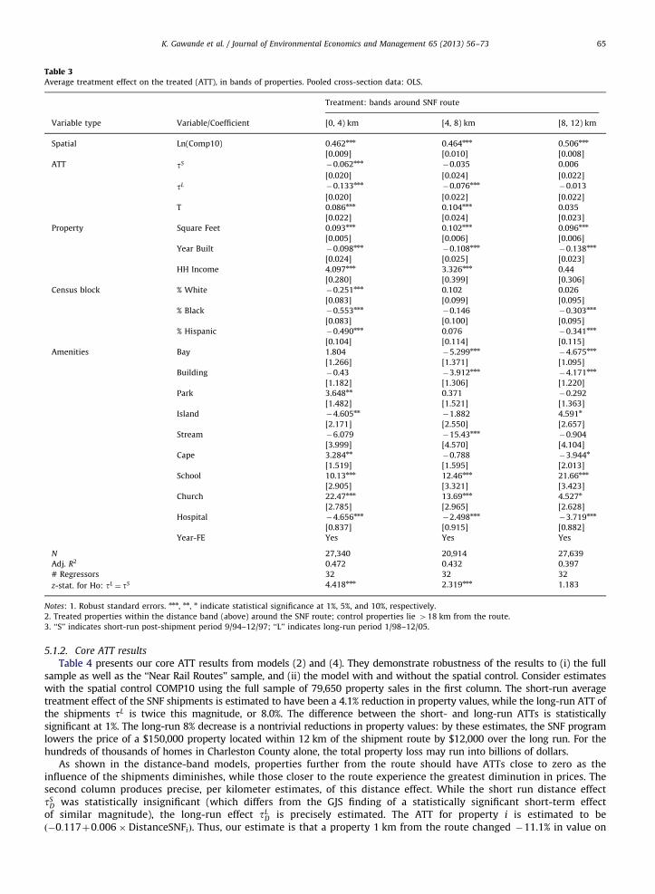
Table 3Average treatment effect on the treated (ATT), in bands of properties. Pooled cross-section data: OLS.
Treatment: bands around SNF route
Variable type Variable/Coefficient [0, 4) km [4, 8) km [8, 12) km
Spatial Ln(Comp10) 0.462nnn 0.464nnn 0.506nnn
[0.009] [0.010] [0.008]
ATT tS �0.062nnn�0.035 0.006
[0.020] [0.024] [0.022]
tL �0.133nnn�0.076nnn
�0.013
[0.020] [0.022] [0.022]
T 0.086nnn 0.104nnn 0.035
[0.022] [0.024] [0.023]
Property Square Feet 0.093nnn 0.102nnn 0.096nnn
[0.005] [0.006] [0.006]
Year Built �0.098nnn�0.108nnn
�0.138nnn
[0.024] [0.025] [0.023]
HH Income 4.097nnn 3.326nnn 0.44
[0.280] [0.399] [0.306]
Census block % White �0.251nnn 0.102 0.026
[0.083] [0.099] [0.095]
% Black �0.553nnn�0.146 �0.303nnn
[0.083] [0.100] [0.095]
% Hispanic �0.490nnn 0.076 �0.341nnn
[0.104] [0.114] [0.115]
Amenities Bay 1.804 �5.299nnn�4.675nnn
[1.266] [1.371] [1.095]
Building �0.43 �3.912nnn�4.171nnn
[1.182] [1.306] [1.220]
Park 3.648nn 0.371 �0.292
[1.482] [1.521] [1.363]
Island �4.605nn�1.882 4.591n
[2.171] [2.550] [2.657]
Stream �6.079 �15.43nnn�0.904
[3.999] [4.570] [4.104]
Cape 3.284nn�0.788 �3.944n
[1.519] [1.595] [2.013]
School 10.13nnn 12.46nnn 21.66nnn
[2.905] [3.321] [3.423]
Church 22.47nnn 13.69nnn 4.527n
[2.785] [2.965] [2.628]
Hospital �4.656nnn�2.498nnn
�3.719nnn
[0.837] [0.915] [0.882]
Year-FE Yes Yes Yes
N 27,340 20,914 27,639
Adj. R2 0.472 0.432 0.397
# Regressors 32 32 32
z-stat. for Ho: tL ¼ tS 4.418nnn 2.319nnn 1.183
Notes: 1. Robust standard errors. nnn, nn, n indicate statistical significance at 1%, 5%, and 10%, respectively.
2. Treated properties within the distance band (above) around the SNF route; control properties lie 418 km from the route.
3. ‘‘S’’ indicates short-run post-shipment period 9/94–12/97; ‘‘L’’ indicates long-run period 1/98–12/05.
K. Gawande et al. / Journal of Environmental Economics and Management 65 (2013) 56–73 65
5.1.2. Core ATT results
Table 4 presents our core ATT results from models (2) and (4). They demonstrate robustness of the results to (i) the fullsample as well as the ‘‘Near Rail Routes’’ sample, and (ii) the model with and without the spatial control. Consider estimateswith the spatial control COMP10 using the full sample of 79,650 property sales in the first column. The short-run averagetreatment effect of the SNF shipments is estimated to have been a 4.1% reduction in property values, while the long-run ATT ofthe shipments tL is twice this magnitude, or 8.0%. The difference between the short- and long-run ATTs is statisticallysignificant at 1%. The long-run 8% decrease is a nontrivial reductions in property values: by these estimates, the SNF programlowers the price of a $150,000 property located within 12 km of the shipment route by $12,000 over the long run. For thehundreds of thousands of homes in Charleston County alone, the total property loss may run into billions of dollars.
As shown in the distance-band models, properties further from the route should have ATTs close to zero as theinfluence of the shipments diminishes, while those closer to the route experience the greatest diminution in prices. Thesecond column produces precise, per kilometer estimates, of this distance effect. While the short run distance effecttS
D was statistically insignificant (which differs from the GJS finding of a statistically significant short-term effectof similar magnitude), the long-run effect tL
D is precisely estimated. The ATT for property i is estimated to beð�0:117þ0:006� DistanceSNFiÞ. Thus, our estimate is that a property 1 km from the route changed �11.1% in value on

Table 4Core results: ATT w and w/o distance effects dependent variable: Ln(Sale Price).
With spatial control Without spatial control
Full sample Near Rail Routes Full sample Near Rail Routes
Ln(Comp10) 0.512nnn 0.506nnn 0.479nnn 0 477nnn
[0.006] [0.006] [0.007] [0.007]
tS �0.041nnn�0.055nnn
�0.027 �0.040n�0.092nnn
�0.132nnn�0.056nnn
�0.093nnn
[0.012] [0.018] [0.018] [0.022] [0.013] [0.019] [0.019] [0.022]
tL �0.080nnn�0.117nnn
�0.071nnn�0.109nnn
�0.213nnn�0.270nnn
�0.179nnn�0.241nnn
[0.012] [0.017] [0.017] [0.020] [0.012] [0.017] [0.017] [0.020]
T 0.066nnn 0.040nn�0.044nn
�0.041n 0.196nnn 0.099nnn�0.028 �0.040n
[0.0116] [0.017] [0.018] [0.022] [0.012] [0.017] [0.019] [0.022]
tSD
0.003 0.002 0.007nnn 0.006nn
[0.003] [0.002] [0.003] [0.003]
tLD
0.006nnn 0.006nnn 0.010nnn 0.010nnn
[0.002] [0.002] [0.002] [0.002]
T�D 0.003 0.0002 0.012nnn 0.003
[0.002] [0.002] [0.002] [0.002]
tSD (non-SNF route) �0.003 �0.003 �0.004n
�0.003
[0.002] [0.002] [0.002] [0.002]
tLD (non-SNF route) �0.002 �0.002 0.001 0.002
[0.002] [0.002] [0.002] [0.002]
T�D (non-SNFroute) 0.015nnn 0.012nnn 0.031nnn 0.024nnn
[0.002] [0.002] [0.002] [0.002]
N 79,650 79,650 58,674 58,674 79,698 79,698 58,706 58,706
Adj. R2 0.445 0.445 0.486 0.486 0.359 0.363 0.418 0.419
# Regressors 32 35 35 38 31 34 34 37
ATTLR�ATTSR �0.039nnn
�0.039nnn�0.044nnn
�0.045nnn�0.121nnn
�0.117nnn�0.123nnn
�0.122nnn
Non-SNF (tLD�tS
DÞ0.001 0.001 0.005nnn 0.005nnn
Notes: 1. See Notes to Table 3.
2. Models include but do not report property, census block, and amenity characteristicsþyear FE.
3. ATTSR and ATTLRare the short- and long-run ATTs, respectively. In models w/o SNF route distance effects, they are simply tS and tL , respectively. In the
distance effect models, they are evaluated at the mean distance of treated properties from the SNF route.
K. Gawande et al. / Journal of Environmental Economics and Management 65 (2013) 56–7366
account of the SNF program, while a property 10 km from the route diminished �5.7%. At the mean distance for treatedproperties of 6.052 km, the diminution in property value is the same as the ATT in the first model, or �8.0%. The(homogeneous) ATT is therefore interpreted as the treatment effect on a property located at the ‘‘average’’ distance fromthe route among treated properties.
The ‘‘Near Rail Routes’’ sample has the same treatment group as the full sample, but includes only the subset of controlgroup properties that are less than 12 km away from a non-SNF rail route. The control group therefore also picks up thedisamenity (the negative placebo effect) of being near a rail route per se. The third column indicates that the ATT continuesto be both statistically and economically significant: the long-run ATT of the SNF program is �7.1%. Thus, the program’slong-run impact is robust to placebo control. The fourth column shows that this sample produces almost the samedistance-from-the-SNF-route effect and the impact of the program on each property that was found using the full sample.This sample also informs us whether the distance effects observed with respect to the SNF route are also observed for thenon-SNF route. The estimates on the non-SNF route tS
D and tLD are both statistically no different from zero. Unlike the post-
shipment distance effect from the SNF route, the distance effect from the non-SNF route remained unchanged from thatwhich existed before the shipments started.
The models with COMP10 included do not suffer from spatial correlation in the data, and provide our preferredestimates for the ATTs. However, as we have mentioned, controlling for COMP10 may absorb some of the ‘‘true’’ treatmenteffect. Owners may argue that their home price is depressed because the comps are all selling for less, and that the compssold for less due to the treatment. The correct ATT then requires dropping the price of comps in the analysis. The last fourcolumns mirror the first four columns, but without the spatial control COMP10. The magnitudes of the ATT estimateswithout the comps are sharply higher than the ATTs with the spatial control. The long run ATT of the SNF program isestimated to be �21.3% in the full sample and �17.9% in the ‘‘Near Rail Routes’’ sample, depressing prices by two to threetimes as much as the diminution estimated by the comps models. On the other hand, omitting COMP10 produces spatialcorrelation in the error term. Perhaps the real value of reporting the (possibly biased) estimates without the comps is toindicate that the true ATT is probably higher than in the model with the comps, but lower than without.
In sum, the pooled cross-section evidence overwhelmingly rejects the null hypothesis of no treatment effect from theSNF shipments over the long run. The negative quantitative impact of the SNF shipments is striking, especially for
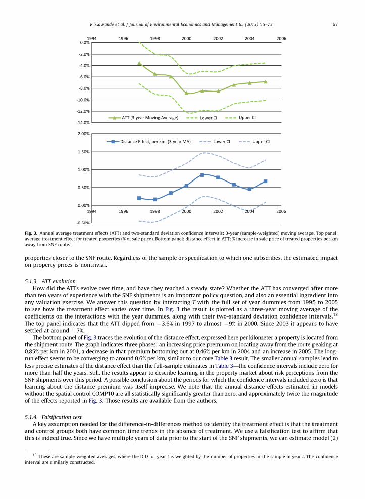
Fig. 3. Annual average treatment effects (ATT) and two-standard deviation confidence intervals: 3-year (sample-weighted) moving average. Top panel:
average treatment effect for treated properties (% of sale price). Bottom panel: distance effect in ATT: % increase in sale price of treated properties per km
away from SNF route.
K. Gawande et al. / Journal of Environmental Economics and Management 65 (2013) 56–73 67
properties closer to the SNF route. Regardless of the sample or specification to which one subscribes, the estimated impacton property prices is nontrivial.
5.1.3. ATT evolution
How did the ATTs evolve over time, and have they reached a steady state? Whether the ATT has converged after morethan ten years of experience with the SNF shipments is an important policy question, and also an essential ingredient intoany valuation exercise. We answer this question by interacting T with the full set of year dummies from 1995 to 2005to see how the treatment effect varies over time. In Fig. 3 the result is plotted as a three-year moving average of thecoefficients on the interactions with the year dummies, along with their two-standard deviation confidence intervals.18
The top panel indicates that the ATT dipped from �3.6% in 1997 to almost �9% in 2000. Since 2003 it appears to havesettled at around �7%.
The bottom panel of Fig. 3 traces the evolution of the distance effect, expressed here per kilometer a property is located fromthe shipment route. The graph indicates three phases: an increasing price premium on locating away from the route peaking at0.85% per km in 2001, a decrease in that premium bottoming out at 0.46% per km in 2004 and an increase in 2005. The long-run effect seems to be converging to around 0.6% per km, similar to our core Table 3 result. The smaller annual samples lead toless precise estimates of the distance effect than the full-sample estimates in Table 3—the confidence intervals include zero formore than half the years. Still, the results appear to describe learning in the property market about risk perceptions from theSNF shipments over this period. A possible conclusion about the periods for which the confidence intervals included zero is thatlearning about the distance premium was itself imprecise. We note that the annual distance effects estimated in modelswithout the spatial control COMP10 are all statistically significantly greater than zero, and approximately twice the magnitudeof the effects reported in Fig. 3. Those results are available from the authors.
5.1.4. Falsification test
A key assumption needed for the difference-in-differences method to identify the treatment effect is that the treatmentand control groups both have common time trends in the absence of treatment. We use a falsification test to affirm thatthis is indeed true. Since we have multiple years of data prior to the start of the SNF shipments, we can estimate model (2)
18 These are sample-weighted averages, where the DID for year t is weighted by the number of properties in the sample in year t. The confidence
interval are similarly constructed.

Table 5Identification: falsification test with pre-shipment data dependent variable: Ln(Sale Price).
W/spatial W/o spatial
Ln(Comp10) 0.422nnn
[0.0173]
d‘‘PRE’’�0.033 �0.041
[0.040] [0.040]
T �0.059 0.097nnn
[0.038] [0.037]
d‘‘POST’’� T 0.137nnn 0.034
[0.036] [0.035]
Square Feet 0.171nnn 0.216nnn
[0.011] [0.011]
Year Built �0.877nn�0.863n
[0.445] [0.479]
HH Income 2.048nnn 5.046nnn
[0.528] [0.541]
% White 0.227 0.277n
[0.159] [0.161]
% Black �0.128 �0.222
[0.162] [0.164]
% Hispanic �0.206 �0.149
[0.168] [0.178]
Amenities Yes Yes
Year-FE Yes Yes
N 7867 7915
Adj. R2 0.293 0.225
# regressors 21 20
Note: 1. OLS, robust errors. See Notes 1 and 2 to Table 3.
2. Pre-shipment sample: from 1992 through 8/1994. d‘‘POST’’¼1 if property sold after 1/1993.
3. Treated properties (T¼1) within 12 km, of the SNF route; 41% ‘‘treated’’ and 59% ‘‘control’’.
K. Gawande et al. / Journal of Environmental Economics and Management 65 (2013) 56–7368
using only data before the start of the shipments (8/1994), with 1/1993 as a ‘‘placebo’’ treatment cutoff. If the assumptionabout common trends is valid, there should be no significant treatment effect using only this data (see e.g. [36]).
Table 5 reports results from the falsification test. In the model without spatial controls the ATT is statistically notsignificant, suggesting no important differences in the time trends of control and to-be-treated properties prior toknowledge of the SNF shipments. The model with comps shows a statistically significant ATT but in the opposite directionto our core ATT results. If there were differences in the time trends of control and to-be-treated properties prior to theshipments, then the shipments reversed these trends. It is possible that the difference in the ATT estimates in the modelswith and without comps is due to this difference in pre-treatment trends. Subsequent reporting of our results are from themodel with comps. We note that in every case the models without comps produce the same contrast as we have seen inTables 4 and 5.
5.1.5. ATTs for quantiles
Are ATTs different for properties in different price ranges? We investigate this source of ATT heterogeneity usingquantile regressions, and report the results in Table 6. For brevity, results with the shorter sample are omitted here andavailable from the authors. The short run ATTs are statistically insignificant except for properties priced in the thirdquartile. The long-run ATTs are statistically significant, and large. At the mean distance of treated properties, the ATT of theSNF program is an expected loss of 10.2% over the long run for properties at the 25th quartile, of 5.0% for properties at themedian, and of 3.1% for properties at the third quartile. Higher-priced properties appear to be a bit more resilient, but notby much. A 3.1% price decline for properties priced above $300,000 is a significant reduction in value.
5.2. Panel data
Data on repeated sales of properties are not easy to find. Even in the rare instance that they are available, the absence ofidentifying information about the property such as address or cross-streets-plus-zip-codes makes them less useful. Hencethe tradition in the literature assessing the impact of environmental disamenities is to use a (pooled, if possible) cross-section of properties and available hedonic variables as controls, as we do above. However, even an extended list ofcontrols cannot fully account for the heterogeneity in the cross-section. A feature that distinguishes this from other studiesis that we have available detailed identifying information on the properties. We use that to construct three panel data sets:one consisting of properties that were sold at least twice during the 1992–2005 period (sample size¼46,632 with 19,940distinct units); another consisting of properties that were sold at least thrice (N¼17,877 with 5523 units); and a thirdconsisting of properties that were sold at least four times during this period (N¼4926 with 1191 units). The panels
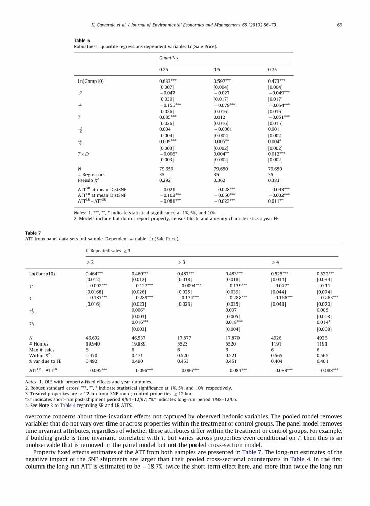
Table 6Robustness: quantile regressions dependent variable: Ln(Sale Price).
Quantiles
0.25 0.5 0.75
Ln(Comp10) 0.633nnn 0.597nnn 0.473nnn
[0.007] [0.004] [0.004]
tS �0.047 �0.027 �0.049nnn
[0.030] [0.017] [0.017]
tL �0.155nnn�0.079nnn
�0.054nnn
[0.026] [0.016] [0.016]
T 0.085nnn 0.012 �0.051nnn
[0.026] [0.016] [0.015]
tSD
0.004 �0.0001 0.001
[0.004] [0.002] [0.002]
tLD
0.009nnn 0.005nn 0.004n
[0.003] [0.002] [0.002]
T�D �0.006n 0.004nn 0.012nnn
[0.003] [0.002] [0.002]
N 79,650 79,650 79,650
# Regressors 35 35 35
Pseudo R2 0.292 0.362 0.383
ATTSR at mean DistSNF �0.021 �0.028nnn�0.043nnn
ATTLR at mean DistSNF �0.102nnn�0.050nnn
�0.032nnn
ATTLR�ATTSR
�0.081nnn�0.022nnn 0.011nn
Notes: 1. nnn, nn, n indicate statistical significance at 1%, 5%, and 10%.
2. Models include but do not report property, census block, and amenity characteristicsþyear FE.
Table 7ATT from panel data sets full sample. Dependent variable: Ln(Sale Price).
# Repeated sales Z3
Z2 Z3 Z4
Ln(Comp10) 0.464nnn 0.460nnn 0.487nnn 0.483nnn 0.525nnn 0.522nnn
[0.012] [0.012] [0.018] [0.018] [0.034] [0.034]
tS �0.092nnn�0.127nnn
�0.0094nnn�0.139nnn
�0.077n�0.11
[0.0168] [0.026] [0.025] [0.039] [0.044] [0.074]
tL �0.187nnn�0.289nnn
�0.174nnn�0.288nnn
�0.166nnn�0.263nnn
[0.016] [0.023] [0.023] [0.035] [0.043] [0.070]
tSD
0.006n 0.007 0.005
[0.003] [0.005] [0.008]
tLD
0.016nnn 0.018nnn 0.014n
[0.003] [0.004] [0.008]
N 46,632 46,537 17,877 17,870 4926 4926
# Homes 19,940 19,889 5523 5520 1191 1191
Max # sales 6 6 6 6 6 6
Within R2 0.470 0.471 0.520 0.521 0.565 0.565
% var due to FE 0.492 0.490 0.453 0.451 0.404 0.401
ATTLR�ATTSR
�0.095nnn�0.096nnn
�0.086nnn�0.081nnn
�0.089nnn�0.088nnn
Notes: 1. OLS with property-fixed effects and year dummies.
2. Robust standard errors. nnn, nn, n indicate statistical significance at 1%, 5%, and 10%, respectively.
3. Treated properties are o12 km from SNF route; control properties Z12 km.
‘‘S’’ indicates short-run post-shipment period 9/94–12/97; ‘‘L’’ indicates long-run period 1/98–12/05.
4. See Note 3 to Table 4 regarding SR and LR ATTS.
K. Gawande et al. / Journal of Environmental Economics and Management 65 (2013) 56–73 69
overcome concerns about time-invariant effects not captured by observed hedonic variables. The pooled model removesvariables that do not vary over time or across properties within the treatment or control groups. The panel model removestime invariant attributes, regardless of whether these attributes differ within the treatment or control groups. For example,if building grade is time invariant, correlated with T, but varies across properties even conditional on T, then this is anunobservable that is removed in the panel model but not the pooled cross-section model.
Property fixed effects estimates of the ATT from both samples are presented in Table 7. The long-run estimates of thenegative impact of the SNF shipments are larger than their pooled cross-sectional counterparts in Table 4. In the firstcolumn the long-run ATT is estimated to be �18.7%, twice the short-term effect here, and more than twice the long-run
K. Gawande et al. / Journal of Environmental Economics and Management 65 (2013) 56–7370
ATT (of �8%) from the pooled data. The distance effect tLD is also more than double that from the pooled data, indicating a
stronger influence of the shipments on homes proximate to the route. The total effect on home i is estimated to beð�0:289þ0:016� DistanceSNFiÞ. A home located at the mean treatment distance (of 6.233 km) from the route has a long-term treatment effect equal to that in the first column, or �18.7%.
A possible reason for why the panel ATTs differ markedly from the pooled ATTs is omitted variables bias in the pooleddata. Property-fixed effects in the panel data control for all variables that are time-invariant, while the set of hedonicvariables in the pooled cross-section only capture time-invariant influences that are measurable. In particular, in (2) if anomitted time-invariant regressor has a theoretically positive (negative) coefficient, and is positively (negatively) correlated withthe assignment to long-run treatment variable DT2t � Ti, then the absolute size of the coefficient tL is diminished. Examples ofomitted property-specific variables include number of bedrooms or bathrooms, swimming pool, condition of the building, andbuilding grade. If building grade, for example, is time invariant, correlated with T, but varies across properties even conditionalon T, then this is an unobservable that is removed in the panel model but not the pooled cross-section model. Specifically,suppose treated properties are of higher grade than control properties. Since this omitted variable is positively correlated withT, the absolute value of the OLS estimate of tL is attenuated in the pooled cross-section.
A second reason is that the panel data includes only those properties that have been sold more than once. If thepropensity to re-sell increased after the inception of the SNF shipments, then it provides a new explanation for how theshipments negatively influenced prices for the treated properties. Suppose the distribution of risk aversion among ownersis heterogeneous, but the distributions are the same in the treatment and control groups. Exposure to the risk from the SNFshipments induces especially risk-averse owners of treated properties to sell at whatever price they can get, even if thismeans taking a loss on the property in order to move to a safer location. Owners in the pre-shipment era or owners ofcontrol properties in the post-shipment era, on the other hand, do not perceive the same risk and do not need to sell theirproperty on unfavorable terms. Since the onset of the SNF shipments makes this channel of influence salient, the causalmechanism is clearly identified. Perceived risk from the shipment reduces the bargaining power of sellers assigned totreatment but leaves unaltered the bargaining power of other potential sellers. Therefore, the sample consisting of repeatsales produces a larger negative average treatment effect than a sample in which a predominance of single-sale homesmutes this mechanism. The predominance of single-sale properties in the pooled cross-section is evident in the muchsmaller samples in Table 7 in which they are dropped, as compared with Table 4.
This finds support in Riddel and Shaw’s [48] survey of Southern Nevada residents about their perceived mortality riskand willingness to accept the risks related to nuclear waste transportation. Riddel [47] reports that willingness to acceptrisk varied significantly across population characteristics. Women perceived more risk than men, higher education wascorrelated with lower risk perception, and older persons perceived greater risk. The pooled cross-section does not includeinformation about the gender and age of the homeowner, and their relation to risk perception. To the extent thesecharacteristics are time-invariant, the DIDs from the panel reflect the disparate attitudes.
The results from the three panel samples produce remarkably similar inferences about the magnitudes of the short- andlong-run ATTs. The long-run ATTs are greater by about 8–10 percentage points. As a further robustness check we estimatethe models using the ‘‘near Rail Routes’’ panel samples. They produces ATTs similar in magnitude to those reported inTable 7, showing the results are driven by the proximity to the shipment route, not a non-shipment rail route. Finally, thepanel allow us to take account of autocorrelation in repeat-sale prices. An AR(1) model of (5) produces estimates of theAR(1) coefficient of over 0.55, which indicate that dynamics may be important.19 The long-run ATTs from the AR(1) modelsare estimated to be between �6% and �15.8%.
6. Conclusion
Modern industrial societies produce and manage many types of hazardous materials that may impose risks on thosewho live near their storage sites and transport routes. While the benefits from industrial and commercial activities thatgenerate hazardous materials may be of sufficient social value to justify those perceived risks, important equity concernsare raised when those perceived risks are involuntary and the potential losses are geographically concentrated. In suchcases, fixed values in property may come to reflect lower market valuation attributable to proximity to the hazardousmaterials. From a property rights perspective, if the imposition of such a cost was verified, then it could be perceived as a‘‘taking’’ by those who experience the reduced property values. The policy implications of studies that weigh in on thisissue are of major consequence.
This paper quantifies the cost of transporting radioactive spent nuclear fuel (SNF), based on property sales data fromCharleston, South Carolina over the 1992–2005 period. The SNF shipments began in 1994 and are ongoing. The impact onhousing values in the early years of these shipments was studied by Gawande and Jenkins-Smith [17], GJS. We reconsider theevidence in that study. First, the GJS study estimates only the distance gradient – the effect of the distance from the SNF routeon the price of a property – but not the absolute effect of the shipment program on the property price, or the treatment effect.We are able to estimate the average treatment effect of the SNF shipment program using appropriate program evaluationmethods [22]. Second, the treatment effect measured by GJS ignored trends in prices of comparable properties that were
19 Due to the differencing, properties that sold twice are dropped, reducing the effective sample considerably.
K. Gawande et al. / Journal of Environmental Economics and Management 65 (2013) 56–73 71
unaffected by the SNF shipments. We use difference-in-differences comparing affected properties with a carefully chosencontrol group. Third, we bring to bear both pooled cross-sectional data as well as panel data evidence.
In populous Charleston County we find evidence of a reduction in property prices due to the SNF shipments. Both thepooled cross-section and the panel provide compelling evidence of a negative average treatment effect in properties thatexperienced heightened risk perception from the SNF shipments program. This treatment effect is long-lived even in theabsence of any accident involving the SNF shipments. For properties located within 18 km from the SNF route, the pooledcross-sectional data indicates average treatment effects of between 2.5% and 5% declines in long run property price due tothe SNF shipment program. There is strong distance-heterogeneity, so that properties located further from the route areless affected by the shipments. Our estimates may be used to obtain precise estimates of the ATT for specific properties.
Our finding implies that policymakers should evaluate how to mitigate that effect and, when it can be clearlydemonstrated, consider compensation for those who bear these costs. The estimate of the total property loss due to theshipments is likely to run into billions of dollars in urban Charleston County. As the nation debates how to store its nuclearwaste, at Yucca Mountain or elsewhere, substantial concerns about damages are sure to be raised. Because the policyimplications of the findings are enormous, quantitative assessments of environmental impacts need to be carefullydeveloped. Our study contributes methodologically to that end.
We note some limitations applicable to our findings. The effects identified in this study apply to Charleston County, butdid not appear to affect other counties on the rail route (GJS [17]). While we can speculate that offsetting amenities may beresponsible for these differences, it is possible that effects of SNF transport are not uniform. Some regions may experiencenegative property price effects, while others may not. We leave this an open question for further research.
Finally, from the point of view of policy, it is not surprising that programs (such as the SNF return program) that generateclear and substantial benefits to society also impose localized costs. In such cases, considerations of both justice and practicalitydictate a need to understand the effects and find appropriate policies to address them. Effective policy design thus seems torequire a willingness to carefully evaluate and then respond to inadvertent transfers of wealth that result from otherwise soundprograms. What policies might the government use to address such concerns? The default might be to argue that undereminent domain, the government need not pay anything. It is not certain that the courts would uphold this claim [25,19,10,54].Moreover, opposition to transport policies would almost certainly find expression; for example, the state of California hasexplicitly forbidden a similar transport through that state into Nevada. Therefore, it is not only practical for the government tofind a solution before a possible incident triggers claims, but ex ante policy is very likely to make it less onerous for thegovernment and taxpayers. A range of mechanisms from mitigation through insurance and compensation [37,30] in order toaddress this problem are important areas of further research. In our view, the time for consideration of such policies is beforerather than after the large-scale transport of SNF commences within the US. The recent call by President Obama’s Blue RibbonCommission to undertake ‘‘Prompt efforts to prepare for eventual large-scale transport of spent fuel and high-level wastes toconsolidated storage facilitiesy’’ [5]: vii makes this an opportune time to do so.
Appendix A
See Table A1.
Table A1Descriptive statistics for panel data sample.
42 sales Zsales 44 sales
mean sd within-sd mean sd within-sd mean sd within-sd
Ln(Sale Price) 11.806 0.672 0.431 11.833 0.658 0.476 11.834 0.662 0.510
Ln(Comp10) 11.830 0.577 0.325 11.853 0.561 0.365 11.866 0.570 0.393
DT0 0.095 0.294 0.224 0.098 0.298 0.251 0.111 0.314 0.280
DT1 0.216 0.412 0.312 0.223 0.417 0.352 0.228 0.420 0.378
DT2 0.688 0.463 0.340 0.678 0.467 0.390 0.661 0.473 0.421
T 0.456 0.498 0 0.439 0.496 0 0.398 0.489 0
C 0.544 0.498 0 0.560 0.496 0 0.601 0.489 0
T0 0.039 0.193 0.143 0.038 0.157 0.234 0.038 0.189 0.162
T1 0.092 0.290 0.205 0.092 0.290 0.227 0.088 0.284 0.236
T2 0.324 0.469 0.227 0.308 0.461 0.252 0.272 0.445 0.259
DistanceSNF 11.854 6.576 0 11.947 6.285 0 12.300 5.686 0
DistanceNon-SNF 10.990 7.557 0 10.971 7.237 0 10.863 6.876 0
N 46,537 17,870 4926
Note: 1. Charleston County (SC) residential properties sold between 1992 and 2005.
2. N is the sample size.
3. See Table 1 for definitions of variables and their units.
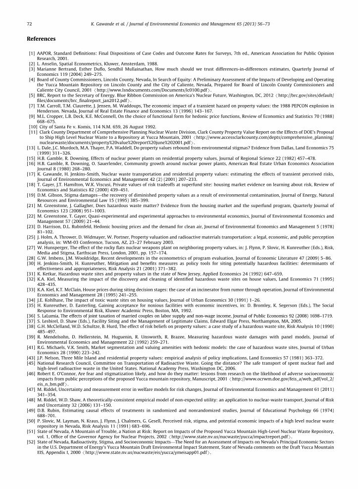
K. Gawande et al. / Journal of Environmental Economics and Management 65 (2013) 56–7372
References
[1] AAPOR, Standard Definitions: Final Dispositions of Case Codes and Outcome Rates for Surveys, 7th ed., American Association for Public OpinionResearch, 2001.
[2] L. Anselin, Spatial Econometrics, Kluwer, Amsterdam, 1988.[3] Marianne Bertrand, Esther Duflo, Sendhil Mullainathan, How much should we trust differences-in-differences estimates, Quarterly Journal of
Economics 119 (2004) 249–275.[4] Board of County Commissioners, Lincoln County, Nevada, In Search of Equity: A Preliminary Assessment of the Impacts of Developing and Operating
the Yucca Mountain Repository on Lincoln County and the City of Caliente, Nevada, Prepared for Board of Lincoln County Commissioners andCaliente City Council, 2001 /http://www.lsndocuments.com/Documents/lc0100.pdfS.
[5] BRC, Report to the Secretary of Energy. Blue Ribbon Commission on America’s Nuclear Future, Washington, DC, 2012 /http://brc.gov/sites/default/files/documents/brc_finalreport_jan2012.pdfS.
[7] T.M. Carroll, T.M. Claurette, J. Jensen, M. Waddoups, The economic impact of a transient hazard on property values: the 1988 PEPCON explosion inHenderson. Nevada, Journal of Real Estate Finance and Economics 13 (1996) 143–167.
[9] M.L. Cropper, L.B. Deck, K.E. McConnell, On the choice of functional form for hedonic price functions, Review of Economics and Statistics 70 (1988)668–675.
[10] City of Santa Fe v. Komis, 114 N.M. 659, 26 August 1992.[11] Clark County Department of Comprehensive Planning Nuclear Waste Division, Clark County Property Value Report on the Effects of DOE’s Proposal
to Ship High Level Nuclear Waste to a Repository at Yucca Mountain, 2001 /http://www.accessclarkcounty.com/depts/comprehensive_planning/nuclearwaste/documents/property%20value%20report%20june%202001.pdfS.
[13] L. Dale, J.C. Murdoch, M.A. Thayer, P.A. Waddell, Do property values rebound from environmental stigmas? Evidence from Dallas, Land Economics 75(1999) 311–326.
[15] H.B. Gamble, R. Downing, Effects of nuclear power plants on residential property values, Journal of Regional Science 22 (1982) 457–478.[16] H.B. Gamble, R. Downing, O. Sauerlender, Community growth around nuclear power plants, American Real Estate Urban Economics Association
Journal 8 (1980) 268–280.[17] K. Gawande, H. Jenkins-Smith, Nuclear waste transportation and residential property values: estimating the effects of transient perceived risks,
Journal of Environmental Economics and Management 42 (2) (2001) 207–233.[18] T. Gayer, J.T. Hamilton, W.K. Viscusi, Private values of risk tradeoffs at superfund site: housing market evidence on learning about risk, Review of
Economics and Statistics 82 (2000) 439–451.[19] D.M. Gibson, Stigma damages—the recovery of diminished property values as a result of environmental contamination, Journal of Energy, Natural
Resources and Environmental Law 15 (1995) 385–399.[21] M. Greenstone, J. Gallagher, Does hazardous waste matter? Evidence from the housing market and the superfund program, Quarterly Journal of
Economics 123 (2008) 951–1003.[22] M. Greenstone, T. Gayer, Quasi-experimental and experimental approaches to environmental economics, Journal of Environmental Economics and
Management 57 (2009) 21–44.[23] D. Harrison, D.L. Rubinfeld, Hedonic housing prices and the demand for clean air, Journal of Environmental Economics and Management 5 (1978)
81–102.[25] J. Holm, A. Thrower, D. Widmayer, W. Portner, Property valuation and radioactive materials transportation: a legal, economic, and public perception
analysis, in: WM-03 Conference, Tucson, AZ, 23–27 February 2003.[27] W. Hunsperger, The effect of the rocky flats nuclear weapons plant on neighboring property values, in: J. Flynn, P. Slovic, H. Kunreuther (Eds.), Risk,
Media and Stigma, Earthscan Press, London, 2001, pp. 157–174.[28] G.W. Imbens, J.M. Wooldridge, Recent developments in the econometrics of program evaluation, Journal of Economic Literature 47 (2009) 5–86.[30] H. Jenkins-Smith, H. Kunreuther, Mitigation and benefits measures as policy tools for siting potentially hazardous facilities: determinants of
effectiveness and appropriateness, Risk Analysis 21 (2001) 371–382.[31] K. Ketkar, Hazardous waste sites and property values in the state of New Jersey, Applied Economics 24 (1992) 647–659.[32] K.A. Kiel, Measuring the impact of the discovery and cleaning of identified hazardous waste sites on house values, Land Economics 71 (1995)
428–435.[33] K.A. Kiel, K.T. McClain, House prices during siting decision stages: the case of an incinerator from rumor through operation, Journal of Environmental
Economics and Management 28 (1995) 241–255.[34] J.E. Kohlhase, The impact of toxic waste sites on housing values, Journal of Urban Economics 30 (1991) 1–26.[35] H. Kunreuther, D. Easterling, Gaining acceptance for noxious facilities with economic incentives, in: D. Bromley, K. Segerson (Eds.), The Social
Response to Environmental Risk, Kluwer Academic Press, Boston, MA, 1992.[36] S. LaLumia, The effects of joint taxation of married couples on labor supply and non-wage income, Journal of Public Economics 92 (2008) 1698–1719.[37] S. Lesbirel, D. Shaw (Eds.), Facility Siting and the Management of Legitimate Claims, Edward Elgar Press, Northampton, MA, 2005.[38] G.H. McClelland, W.D. Schultze, B. Hurd, The effect of risk beliefs on property values: a case study of a hazardous waste site, Risk Analysis 10 (1990)
485–497.[39] R. Mendelsohn, D. Hellerstein, M. Huguenin, R. Unsworth, R. Brazee, Measuring hazardous waste damages with panel models, Journal of
Environmental Economics and Management 22 (1992) 259–271.[41] R.G. Michaels, V.K. Smith, Market segmentation and valuing amenities with hedonic models: the case of hazardous waste sites, Journal of Urban
Economics 28 (1990) 223–242.[43] J.P. Nelson, Three Mile Island and residential property values: empirical analysis of policy implications, Land Economics 57 (1981) 363–372.[45] National Research Council, Committee on Transportation of Radioactive Waste. Going the distance? The safe transport of spent nuclear fuel and
high-level radioactive waste in the United States. National Academy Press, Washington DC, 2006.[46] Robert E. O’Connor, Are fear and stigmatization likely, and how do they matter: lessons from research on the likelihood of adverse socioeconomic
impacts from public perceptions of the proposed Yucca mountain repository, Manuscript, 2001 /http://www.ocrwm.doe.gov/feis_a/web_pdf/vol_2/eis_n_bm.pdfS.
[47] M. Riddel, Uncertainty and measurement error in welfare models for risk changes, Journal of Environmental Economics and Management 61 (2011)341–354.
[48] M. Riddel, W.D. Shaw, A theoretically-consistent empirical model of non-expected utility: an application to nuclear-waste transport, Journal of Riskand Uncertainty 32 (2006) 131–150.
[49] D.B. Rubin, Estimating causal effects of treatments in randomized and nonrandomized studies, Journal of Educational Psychology 66 (1974)688–701.
[50] P. Slovic, M. Layman, N. Kraus, J. Flynn, J. Chalmers, G. Gesell, Perceived risk, stigma, and potential economic impacts of a high level nuclear wasterepository in Nevada, Risk Analysis 11 (1991) 683–696.
[51] State of Nevada, A Mountain of Trouble, a Nation at Risk: Report on Impacts of the Proposed Yucca Mountain High-Level Nuclear Waste Repository,vol. 1, Office of the Governor Agency for Nuclear Projects, 2002 /http://www.state.nv.us/nucwaste/yucca/impactreport.pdfS.
[52] State of Nevada, Radioactivity, Stigma, and Socioeconomic Impacts—The Need for an Assessment of Impacts on Nevada’s Principal Economic Sectorsin the U.S. Department of Energy’s Yucca Mountain Draft Environmental Impact Statement, State of Nevada comments on the Draft Yucca MountainEIS, Appendix I, 2000 /http://www.state.nv.us/nucwaste/eis/yucca/ymeisapp01.pdfS.

K. Gawande et al. / Journal of Environmental Economics and Management 65 (2013) 56–73 73
[53] J.H. Stock, Nonparametric policy analysis: an application to estimating hazardous waste cleanup benefits, in: W.A. Barnett, J. Powell, G. Tauchen(Eds.), Nonparametric and Semiparametric Methods in Econometrics and Statistics, Cambridge University Press, 1988.
[54] J. Tauberman, Statutory reform for ‘Toxic Torts’: relieving the legal scientific and economic burdens of the chemical victim, Harvard EnvironmentLaw Review 7 (1983) 177–296.
[57] U.S. Department of Energy, Savannah River Operations Office, U.S. Department of Energy Foreign Research Reactor Nuclear Spent Fuel ShipmentsTransportation Plan for Rail or Motor Transport, Charleston, SC to Savannah River Site, Revision 0, February 1998.
[58] United States Nuclear Regulatory Commission (before the Atomic Safety and Licensing Board), In the Matter of: Clark County, Nevada’s Request forHearing, Petition to Intervene and Filing of contentions, U.S. Department of Energy (High Level Waste Repository), Docket No. 63-001, 2008 /http://www.accessclarkcounty.com/depts/comprehensive_planning/nuclearwaste/Documents/PetitiontoInterveneDec2008.pdf S.
[59] Tyler J. VanderWeele, Ignorability and stability assumptions in neighborhood effects research, Statistics in Medicine 27 (2008) 1934–1943.[60] J. Feiertag, Frenald not too neighborly for home values, Journal News, March 27 (1992).
Related Documents