The Logic of Reversible Computing

U N I V E R S I T Y O F C O P E N H A G E NF A C U L T Y O F S C I E N C E

PhD thesisRobin Kaarsgaard

TheLogicofReversibleComputingTheory and Practice

Academic advisors: Robert Glück (principal), Holger Bock Axelsen, Andrzej Filinski

Submitted: December 22, 2017

The Logic of Reversible ComputingTheory and Practice

Robin KaarsgaardDIKU, Department of Computer Science,

University of Copenhagen

December 22, 2017

This thesis has been submitted to the PhD Schoolof the Faculty of Science at the University of Copenhagen.

To Sophie

iv

Abstract

Reversible computing is the study of models of computation that exhibit both forward andbackward determinism. While reversible computing initially gained interest through itspotential to reduce the energy consumption of computing machinery, via a result fromphysics now known as Landauer’s principle, a number of other applications in computerscience have since been proposed, from syntax descriptions to model-based testing, debug-ging, and even robotics.

In spite of its numerous current (and potential future) applications, the establishedfoundations for computation and programming, such as Turing machines, λ-calculi, andvarious categorical models, are largely ill equipped to handle reversible computing, as theseoften tacitly rely on irreversible operations to function. To set reversible computing ona foundation as solid as the one for conventional computing requires both a significantadaptation of existing techniques and the development of new ones.

In this thesis, we investigate reversible computing from a perspective of logic, broadlyconstrued. To complement the operational point of view from which reversible computingis often studied, we offer a denotational account of reversibility in computation based onrecent work in category theory. We propose two new techniques, founded in formal logic,for reasoning about reversible logic circuits. Further, we account for the behaviour of fixedpoints in certain proposed categorical models of reversible computing, and connect theseresults to the behaviour of recursive functions and data types in established reversible pro-gramming languages. In an application and extension of some of these results, we proposea uniform categorical foundation for a large class of reversible imperative programminglanguages known as structured reversible flowchart languages. We investigate the role of re-versible effects in reversible functional programming, and show that a wide palette of thesemay be modelled as arrows (in the sense of Hughes) satisfying certain additional equations.Finally, we propose a brief vision for the future of the reversible functional programminglanguage Rfun.

v

vi

Dansk resumé

Reversibel beregning er studiet af beregningsmodeller der er både fremad- og baguddeter-ministiske. På trods af at reversibel beregning oprindeligt fik interesse igennem dets poten-tialle til at reducere beregningsmaskiners energiforbrug, via et resultat fra fysikken der nukendes som Landauer’s princip, har det senere fundet et antal andre anvendelser i datalo-gien, fra syntaksbeskrivelser til model-baseret testning, fejlfinding i programmel, og enddarobotteknologi.

På trods af disse talrige nuværende (og potentielle fremtidige) anvendelser er mangegrundlæggende modeller for beregning og programmerinbg, såsom Turingmaskiner, λ-kalkyler og visse kategoriske modeller, i høj grad dårligt rustede til at håndtere reversibelberegning, da disse ofte implicit afhænger af irreversible operationer for at virke. At kunneplacere reversibel beregning på et lige så solidt grundlag som det for konventionel beregningkræver både betydelige tilpasninger af eksisterende teknikker, og udviklingen af nye.

I denne afhandling undersøger vi reversibel beregning fra et (i bred forstand) logisk per-spektiv. Som supplement til det operationelle udgangspunkt der ofte benyttes til at studerereversible beregning giver vi en denotationel redegørelse af reversibilitet i beregning, baseretpå nylige resultater fra kategoriteori. Vi fremsætter to nye teknikker, grundlagt i teknikkerfra formel logik, til at ræsonnere om reversible logiske kredsløb. Endvidere redegør vifor fikspunkters opførsel i visse foreslåede kategoriske modeller for reversibel beregning, ogforbinder denne redegørelse til rekursive funktioner og datatypers opførsel i etablerede re-versible programmeringssprog. Ved brug og udvidelse af nogle af disse resultater foreslår viet ensartet kategorisk grundlag for en betydelig mængde af imperative reversible program-meringssprog, de såkaldte strukturerede reversible flowchartsprog. Vi undersøger reversibleeffekters rolle i reversibel funktionsprogrammering, og viser, at en bred palet af disse kanmodelleres som pile (i Hughes’ fortolkning) der opfylder visse yderligere ligheder. Endeligfremsætter vi en kortfattet vision for fremtiden for det reversible funktionsprogrammer-ingssprog Rfun.

vii

viii

Contents

Abstract iv

Dansk resumé vi

Preface xi

1 Introduction 11.1 Reversibility and invertibility: A semantic perspective . . . . . . . . . . . 11.2 Unifying operational and denotational reversibility . . . . . . . . . . . . 61.3 Reversible computing as physical computing . . . . . . . . . . . . . . . . 81.4 Reversibility and invertibility in programming languages . . . . . . . . . . 101.5 Contributions . . . . . . . . . . . . . . . . . . . . . . . . . . . . . . . 12

References 17

A Reversible circuit logic 25A.1 Ricercar: A language for describing and rewriting reversible circuits . . . . 27A.2 A classical propositional logic for reasoning about reversible logic circuits . 45

B Foundations of reversible recursion 63B.1 Join inverse categories and reversible recursion . . . . . . . . . . . . . . . 65B.2 Inversion, fixed points, and the art of dual wielding . . . . . . . . . . . . 85

C Semantics of reversible programming languages 103C.1 A categorical foundation for structured reversible flowchart languages: Sound-

ness and adequacy . . . . . . . . . . . . . . . . . . . . . . . . . . . . . 105C.2 Reversible effects as inverse arrows . . . . . . . . . . . . . . . . . . . . . 139C.3 RFun revisited . . . . . . . . . . . . . . . . . . . . . . . . . . . . . . . 159

ix

x

Preface

This manuscript constitutes the author’s PhD thesis, an endeavour that could not havebeen completed without the support and encouragement from a tremendous number ofpeople. First of all, I would like to thank my academic advisors Holger Bock Axelsen,Andrzej Filinski, and Robert Glück for their encouragement and sage advice, always readyto discuss a particularly puzzling topic (of which there are many) or to point me in theright direction. I would also like to thank my (current and previous) office mates and otherfellow PhD students, with whom I’ve shared many discussions (academic and otherwise),thoughts, and beers. In no particular order: Ulrik Terp Rasmussen, Bjørn “Nillerbjørn”Bugge Grathwohl, Vivek Shah, Oleksandr Shturmov, Danil Annenkov, Abraham Wolk,Martin Dybdal. I’d also like to thank Fritz Henglein for many interesting discussions, foragreeing to chair my thesis committee, and for entrusting me early on with teaching dutiesin one of my favourite courses here at DIKU, Logic in Computer Science. I would also liketo thank Hanna van Lee, who quickly became my partner in crime in teaching this course.

I would also like to thank those who have helped me broaden my horizons, and whohave showed in interest in my work: Apart from those already mentioned, I’d like to thankTorben Mogensen, Marcos vaz Salles and the rest of the APL group here at DIKU; andRasmus Møgelberg (who first introduced me to category theory) and Marco Paviotti forgreat discussions and great coffee. I also owe thanks to Bart Jacobs and the rest of theNijmegen Quantum Logic Group at Radboud University for hosting me in the spring of2016: Aleks Kissinger, Fabio Zanasi, Mathys Rennela, Bas Westerbaan, Bram Westerbaan,Kenta Chō, and Sander Uijlen. I would also like to thank Dexter Kozen, Michael Johnson,Robin Cockett, and Tarmo Uustalu for interesting discussions, and for showing interestin my work; and, the latter two, for agreeing to serve on my thesis committee. A specialthanks goes to my (non-advisor) collaborators: Chris Heunen, Martti Karvonen, MathiasSoeken, Michael Kirkedal Thomsen. I am also grateful for the support offered by COSTAction IC1405: Reversible computing – extending horizons of computing.

Finally, I would like to thank my friends and family for their support during the pastthree years; and Sophie, for everything.

Robin Kaarsgaard

Full name: Robin Kaarsgaard Jensen

xi

“Sometimes I wish I knew how to go crazy. I forget how.”“It’s a lost art,” Hank said. “Maybe there’s an instruction manual on it.”

Philip K. Dick, A Scanner Darkly

1Introduction

A famous parable from the Rigveda, familiar to many category theorists due to the trulyawesome work of Peter Johnstone [74], is that of the blind men examining an elephant:One man, holding the trunk, says it is like a snake; another man, touching one of theelephant’s legs, says it is like a pillar; a third man, holding the tail, says it is like a rope, etc.Similar sound but incomplete statements can be made of reversible computing: It is aboutcomputations that can be undone; it is about computers as physical machines; it is aboutcomputation free of information effects [72]; and so on.

In this chapter we will give an introduction to central concepts in reversible computingas they will be used later in the thesis. To set the stage for some of these developments,we will also present a new denotational view of reversible computing that highlights com-positionality as a central principle of reversibility, clarify some concepts that are often leftunderspecified, and connect this to existing views on reversible computing presented in theliterature during the past semicentury.

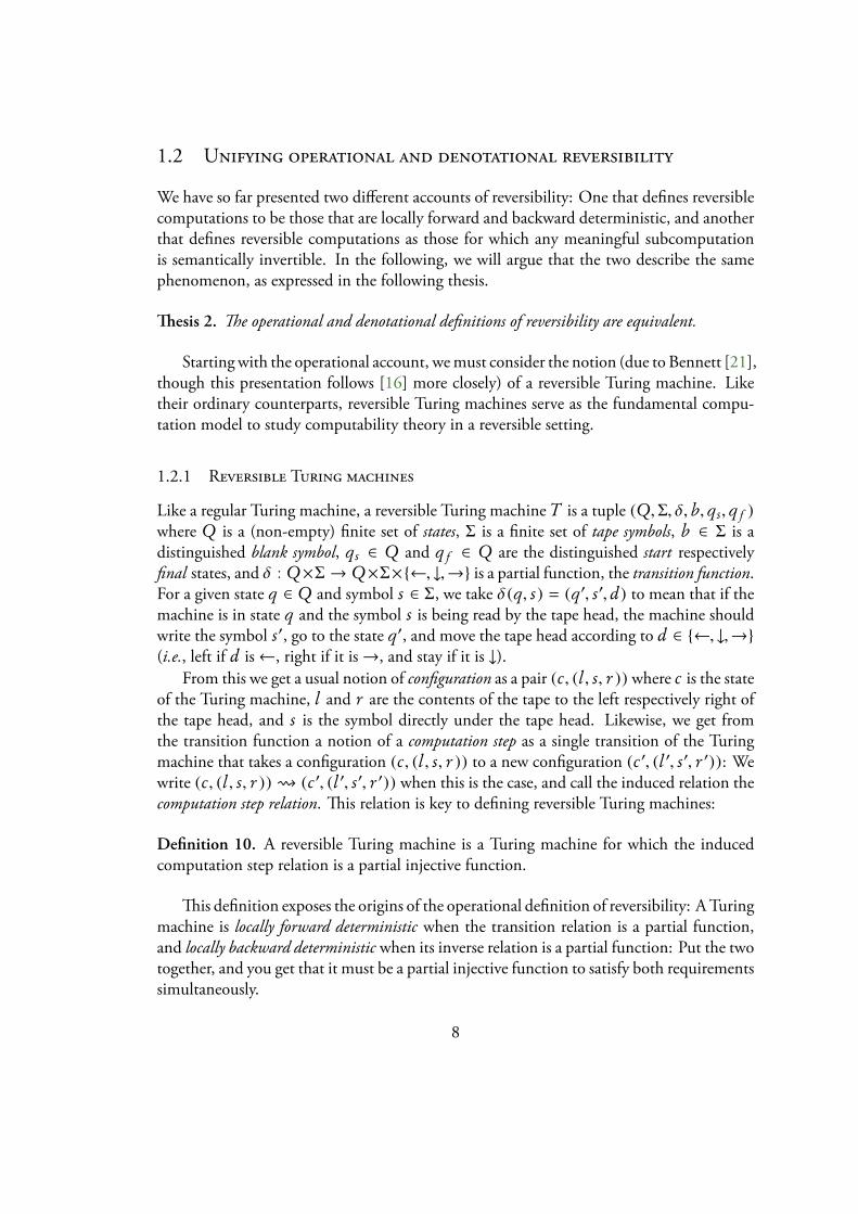
1.1 Reversibility and invertibility: A semantic perspective

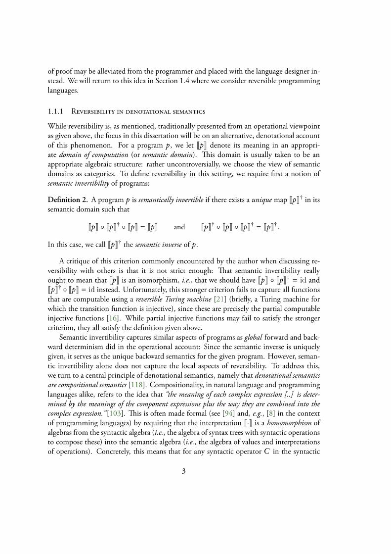
Reversibility in computational processes is often presented as an operational property basedon forward and backward determinism. We illustrate these concepts by means of Figure 1.1.A program is locally forward deterministic (or simply deterministic) if every computationstate in the program has a unique next computation state. For example, programs writtenin programming languages such as Java or Haskell are all forward deterministic. Moreexotic is the notion of local backward determinism, requiring that every computation state

1

has a unique previous state. This is typically not guaranteed by common programminglanguages: For example, in an imperative language, a program performing a destructiveassignment such as

x := 2

is not backward deterministic, since there is generally no way of recovering the state of xbefore it was assigned to have the value 2. Likewise, in functional programming languages,branching expressions (such as conditionals or case-expressions) are common sources ofbackward nondeterminism, as two or more branches may produce identical outputs ondistinct inputs.

X X

Previous Current Next

Figure 1.1: Forward and backward deter-minism.

The locality of forward and backward determin-ism is a crucial part of what is sometimes humorouslycalled the Copenhagen interpretation of reversibility, andis often presented by the slogan that reversibility is a lo-cal phenomenon. Concretely, it requires not only thatthe entire program behaves in a way that is forwardand backward deterministic (i.e., inputs uniquely de-termine outputs and vice versa), but that any compu-tation step along the way (no matter if it is a simpleinstruction or a complicated loop structure) behavesin this way as well. Put in another way, reversibility is a property of the program ratherthan the function it computes (i.e., it is an intensional property). Without the empha-sis on locality, it is not clear that one would be able to separate reversible programs fromthose merely computing injective functions (which is a distinction we wish to make). Wesummarise this view on reversibility in the following definition.

Definition 1. A program is reversible if it is locally forward deterministic and locally back-ward deterministic.

A consequence of this view is that reversible programs can be uniquely assigned bothforward and backward semantics, if they can be assigned semantics at all. As an example,consider a an operational semantics for an imperative language, i.e., with a judgment formof σ ⊢ p ↓ σ′ taken to mean that evaluating any command p in the state σ yields the stateσ′. Forward determinism states that for all states σ and commands p, there is at most onestate σ′ such that σ ⊢ p ↓ σ′. Symmetrically, backward determinism states that for allstates σ′ and commands p, there is at most one state σ such that σ ⊢ p ↓ σ′.

Since reversibility is an intensional property, it requires very careful program construc-tion, and just as careful argumentation, to establish for a program. Even worse, it is dif-ficult even to heuristically check for reversibility by means of testing, as traditional testingtechniques are designed to test extensional properties (e.g., I/O behaviour) rather than in-tensional ones. For this reason, the problem of guaranteeing reversibility for programs isone best solved through cautious design of programming languages, such that the burden

2

of proof may be alleviated from the programmer and placed with the language designer in-stead. We will return to this idea in Section 1.4 where we consider reversible programminglanguages.

1.1.1 Reversibility in denotational semantics

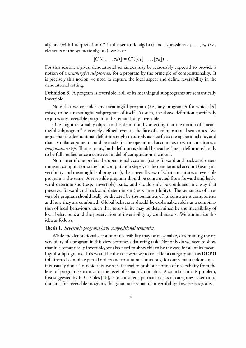
While reversibility is, as mentioned, traditionally presented from an operational viewpointas given above, the focus in this dissertation will be on an alternative, denotational accountof this phenomenon. For a program p, we let JpK denote its meaning in an appropri-ate domain of computation (or semantic domain). This domain is usually taken to be anappropriate algebraic structure: rather uncontroversially, we choose the view of semanticdomains as categories. To define reversibility in this setting, we require first a notion ofsemantic invertibility of programs:

Definition 2. A program p is semantically invertible if there exists a unique map JpK† in itssemantic domain such that

JpK ◦ JpK† ◦ JpK = JpK and JpK† ◦ JpK ◦ JpK† = JpK†.In this case, we call JpK† the semantic inverse of p.

A critique of this criterion commonly encountered by the author when discussing re-versibility with others is that it is not strict enough: That semantic invertibility reallyought to mean that JpK is an isomorphism, i.e., that we should have JpK ◦ JpK† = id andJpK† ◦ JpK = id instead. Unfortunately, this stronger criterion fails to capture all functionsthat are computable using a reversible Turing machine [21] (briefly, a Turing machine forwhich the transition function is injective), since these are precisely the partial computableinjective functions [16]. While partial injective functions may fail to satisfy the strongercriterion, they all satisfy the definition given above.

Semantic invertibility captures similar aspects of programs as global forward and back-ward determinism did in the operational account: Since the semantic inverse is uniquelygiven, it serves as the unique backward semantics for the given program. However, seman-tic invertibility alone does not capture the local aspects of reversibility. To address this,we turn to a central principle of denotational semantics, namely that denotational semanticsare compositional semantics [118]. Compositionality, in natural language and programminglanguages alike, refers to the idea that “the meaning of each complex expression [..] is deter-mined by the meanings of the component expressions plus the way they are combined into thecomplex expression.” [103]. This is often made formal (see [94] and, e.g., [8] in the contextof programming languages) by requiring that the interpretation J·K is a homomorphism ofalgebras from the syntactic algebra (i.e., the algebra of syntax trees with syntactic operationsto compose these) into the semantic algebra (i.e., the algebra of values and interpretationsof operations). Concretely, this means that for any syntactic operator C in the syntactic

3

algebra (with interpretation C ′ in the semantic algebra) and expressions e1, . . . , en (i.e.,elements of the syntactic algebra), we haveJC (e1, . . . en)K = C ′(Je1K, . . . , JenK) .

For this reason, a given denotational semantics may be reasonably expected to provide anotion of a meaningful subprogram for a program by the principle of compositionality. Itis precisely this notion we need to capture the local aspect and define reversibility in thedenotational setting.Definition 3. A program is reversible if all of its meaningful subprograms are semanticallyinvertible.

Note that we consider any meaningful program (i.e., any program p for which JpKexists) to be a meaningful subprogram of itself. As such, the above definition specificallyrequires any reversible program to be semantically invertible.

One might reasonably object to this definition by asserting that the notion of “mean-ingful subprogram” is vaguely defined, even in the face of a compositional semantics. Weargue that the denotational definition ought to be only as specific as the operational one, andthat a similar argument could be made for the operational account as to what constitutes acomputation step. That is to say, both definitions should be read as “meta-definitions”, onlyto be fully reified once a concrete model of computation is chosen.

No matter if one prefers the operational account (using forward and backward deter-minism, computation states and computation steps), or the denotational account (using in-vertibility and meaningful subprograms), their overall view of what constitutes a reversibleprogram is the same: A reversible program should be constructed from forward and back-ward deterministic (resp. invertible) parts, and should only be combined in a way thatpreserves forward and backward determinism (resp. invertibility). The semantics of a re-versible program should really be dictated by the semantics of its constituent componentsand how they are combined: Global behaviour should be explainable solely as a combina-tion of local behaviours, such that reversibility may be determined by the invertibility oflocal behaviours and the preservation of invertibility by combinators. We summarise thisidea as follows.Thesis 1. Reversible programs have compositional semantics.

While the denotational account of reversibility may be reasonable, determining the re-versibility of a program in this view becomes a daunting task: Not only do we need to showthat it is semantically invertible, we also need to show this to be the case for all of its mean-ingful subprograms. This would be the case were we to consider a category such as DCPO(of directed-complete partial orders and continuous functions) for our semantic domain, asit is usually done. To avoid this, we seek instead to push our notion of reversibility from thelevel of program semantics to the level of semantic domains. A solution to this problem,first suggested by B. G. Giles [46], is to consider a particular class of categories as semanticdomains for reversible programs that guarantee semantic invertibility: Inverse categories.

4

1.1.2 Inverse categories

Inverse categories are categories that internalise a notion of partial invertibility, as inversesemigroups do for semigroups. These are defined as follows (see [79]).

Definition 4. A category C is said to be an inverse category if for every morphism f : X →Y of C, there exists a unique morphism g : Y → X , called the partial inverse of f , suchthat f ◦ g ◦ f = f .

As is the case for inverse semigroups, it can be shown that requiring partial inverses tobe unique is equivalent to requiring all idempotents to commute. Further, it follows thatpartial inverses are symmetrically assigned, i.e., if f is partial inverse to g then g is partialinverse to f . Before we move further, we consider a few important examples of inversecategories.

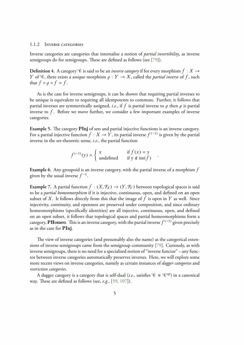
Example 5. The category PInj of sets and partial injective functions is an inverse category.For a partial injective function f : X → Y , its partial inverse f (−1) is given by the partialinverse in the set-theoretic sense, i.e., the partial function

f (−1) (y) ={

x if f (x ) = yundefined if y < im( f ) .

Example 6. Any groupoid is an inverse category, with the partial inverse of a morphism fgiven by the usual inverse f −1.

Example 7. A partial function f : (X ,TX ) → (Y ,TY ) between topological spaces is saidto be a partial homeomorphism if it is injective, continuous, open, and defined on an opensubset of X . It follows directly from this that the image of f is open in Y as well. Sinceinjectivity, continuity, and openness are preserved under composition, and since ordinaryhomeomorphisms (specifically identities) are all injective, continuous, open, and definedon an open subset, it follows that topological spaces and partial homeomorphisms form acategory, PHomeo. This is an inverse category, with the partial inverse f (−1) given preciselyas in the case for PInj.

The view of inverse categories (and presumably also the name) as the categorical exten-sions of inverse semigroups came from the semigroup community [79]. Curiously, as withinverse semigroups, there is no need for a specialised notion of “inverse functor” – any func-tor between inverse categories automatically preserves inverses. Here, we will explore somemore recent views on inverse categories, namely as certain instances of dagger categories andrestriction categories.

A dagger category is a category that is self-dual (i.e., satisfies C � Cop) in a canonicalway. These are defined as follows (see, e.g., [59, 107]).

5

Definition 8. A category C is said to be a dagger category if it is equipped with a contravari-ant, involutive, identity-on-objects endofunctor, i.e., a functor (−)† : Cop → C satisfyingid†X = idX , f †† = f , and (g ◦ f )† = f † ◦ g† for all objects X and composable morphismsf , g of C.

Note that a dagger is a structure on a category, and as such, a given category may be adagger category in several different ways. As such, when specifying a dagger category, wereally ought to specify which dagger structure on the category we are referring to, thoughthis is often left implicit. A functor F : C → D between dagger categories is a daggerfunctor if it preserves the dagger structure, i.e., if F ( f †) = F ( f )† for all f . Examples ofdagger categories include Rel of sets and relations (with f † given by the relational conversef −1 of f ), PInj of sets and partial injective functions (with f † given by the partial inversef (−1) of f ), and FHilb of finite dimensional Hilbert spaces and linear maps (with f † givenby the Hermitian conjugate of f , which is typically also denoted f †).

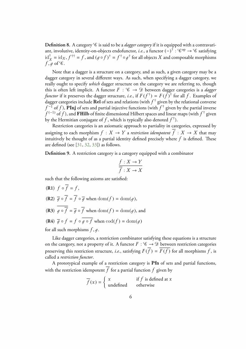
Restriction categories is an axiomatic approach to partiality in categories, expressed byassigning to each morphism f : X → Y a restriction idempotent f : X → X that mayintuitively be thought of as a partial identity defined precisely where f is defined. Theseare defined (see [31, 32, 33]) as follows.

Definition 9. A restriction category is a category equipped with a combinator

f : X → Y

f : X → X

such that the following axioms are satisfied:

(R1) f ◦ f = f ,

(R2) g ◦ f = f ◦ g when dom( f ) = dom(g ),

(R3) g ◦ f = g ◦ f when dom( f ) = dom(g ), and

(R4) g ◦ f = f ◦ g ◦ f when cod( f ) = dom(g )

for all such morphisms f , g .

Like dagger categories, a restriction combinator satisfying these equations is a structureon the category, not a property of it. A functor F : C→ D between restriction categoriespreserving this restriction structure, i.e., satisfying F ( f ) = F ( f ) for all morphisms f , iscalled a restriction functor.

A prototypical example of a restriction category is Pfn of sets and partial functions,with the restriction idempotent f for a partial function f given by

f (x) ={

x if f is defined at xundefined otherwise

6

Another example, with a similar restriction structure, is PTop of topological spaces and par-tial continuous functions defined on open sets. The Kleisli category of the (·) + 1 monadover any distributive category (i.e., a category with products and coproducts such that prod-ucts distribute over coproducts) can also be outfitted with a restriction structure [31] bydefining f for a morphism f : X → Y as the composition

X⟨id,id⟩−−−−−→ X × X

id× f−−−−→ X × (Y + 1)

δ−→ (X ×Y ) + (X × 1)π1+π2−−−−−→ X + 1

For our purposes, a particularly interesting class of morphisms in restriction categories isthe class of partial isomorphisms (or restricted isomorphisms). A partial isomorphism in arestriction category is a morphism f : X → Y for which there exists a g : Y → X suchthat g ◦ f = f and f ◦ g = g . As the name suggests, this notion generalises ordinary iso-morphisms in that any isomorphism is a partial isomorphism. For some concrete examples,partial isomorphisms in Pfn are precisely the partial injective functions (i.e., the morphismsof PInj), while the partial isomorphisms of PTop are partial homeomorphisms (that is,morphisms of PHomeo). Indeed, just like any ordinary category C induces a groupoidCore( C) as a subcategory consisting only of its isomorphisms, any restriction category Cinduces a subcategory of partial isomorphisms, Inv( C), which is an inverse category by thefollowing characterisation.

Proposition 1. Let C be a category. The following are equivalent:

(i) C is an inverse category.

(ii) C is a restriction category and each morphism of C is a partial isomorphism.

(iii) C is a dagger category and for each morphism f of C, f † is the unique morphism suchthat f ◦ f † ◦ f = f .

Proof. See [31], Theorem 2.20. □

Given that inverse categories internalise the notion of partial invertibility, they are aparticularly good fit for reversible computation when seen through the denotational lens.Consider any program p that can be assigned a compositional semantics JpK as a morphismin an inverse category C. Since C is an inverse category, JpK is partially invertible, i.e., p issemantically invertible. However, since p has been assigned compositional semantics in C,any meaningful subprogram p′ of p must also have an interpretation as a morphism Jp′K ofC; which, since C is inverse, must also be partially invertible, such that p′ is semanticallyinvertible. But since this argument could be applied to any meaningful subprogram of p,p must be reversible by the denotational defintion. This can be summarised in the sloganthat inverse categories are semantic domains for reversible programs.

7

1.2 Unifying operational and denotational reversibility

We have so far presented two different accounts of reversibility: One that defines reversiblecomputations to be those that are locally forward and backward deterministic, and anotherthat defines reversible computations as those for which any meaningful subcomputationis semantically invertible. In the following, we will argue that the two describe the samephenomenon, as expressed in the following thesis.

Thesis 2. The operational and denotational definitions of reversibility are equivalent.

Starting with the operational account, we must consider the notion (due to Bennett [21],though this presentation follows [16] more closely) of a reversible Turing machine. Liketheir ordinary counterparts, reversible Turing machines serve as the fundamental compu-tation model to study computability theory in a reversible setting.

1.2.1 Reversible Turing machines

Like a regular Turing machine, a reversible Turing machine T is a tuple (Q,Σ, δ, b, qs, q f )where Q is a (non-empty) finite set of states, Σ is a finite set of tape symbols, b ∈ Σ is adistinguished blank symbol, qs ∈ Q and q f ∈ Q are the distinguished start respectivelyfinal states, and δ : Q×Σ → Q×Σ×{←,↓,→} is a partial function, the transition function.For a given state q ∈ Q and symbol s ∈ Σ, we take δ (q, s) = (q′, s′, d ) to mean that if themachine is in state q and the symbol s is being read by the tape head, the machine shouldwrite the symbol s′, go to the state q′, and move the tape head according to d ∈ {←,↓,→}(i.e., left if d is←, right if it is→, and stay if it is ↓).

From this we get a usual notion of configuration as a pair (c, (l , s, r )) where c is the stateof the Turing machine, l and r are the contents of the tape to the left respectively right ofthe tape head, and s is the symbol directly under the tape head. Likewise, we get fromthe transition function a notion of a computation step as a single transition of the Turingmachine that takes a configuration (c, (l , s, r )) to a new configuration (c ′, (l ′, s′, r ′)): Wewrite (c, (l , s, r ))⇝ (c ′, (l ′, s′, r ′)) when this is the case, and call the induced relation thecomputation step relation. This relation is key to defining reversible Turing machines:

Definition 10. A reversible Turing machine is a Turing machine for which the inducedcomputation step relation is a partial injective function.

This definition exposes the origins of the operational definition of reversibility: A Turingmachine is locally forward deterministic when the transition relation is a partial function,and locally backward deterministic when its inverse relation is a partial function: Put the twotogether, and you get that it must be a partial injective function to satisfy both requirementssimultaneously.

8

As for ordinary Turing machines, reversible Turing machines are associated with a func-tion it computes. It can be shown (see [16]) that reversible Turing machines are in a one-to-one correspondence with the computable partial injective functions: Every reversible Turingmachine computes a (necessarily computable) partial injective function, and for every par-tial injective function computable on a regular Turing machine, there exists a reversible onethat computes it as well. Curiously, no real computational power is lost when consideringonly reversible Turing machines: Bennett showed [21] that it is always possible to “re-versibilise” any ordinary Turing machine (call it T , and call the function it computes T f ),by fashioning a reversible Turing machine that computes the function x 7→ (x,T f (x)).

Since the identity function on any given countable set is computable, and the compo-sition of computable functions is again computable, sets and computable partial injectivefunctions form a category, CPInj. Further, since a partial injective function is computableif and only if its partial inverse is (see, e.g., [16]), this is an inverse category.

To see that this model lives up to the denotational definition of reversibility, we mustconsider what “meaningful subprogram” means in terms of reversible Turing machines. Itseems clear that any meaningful subprogram of a reversible Turing machine T must onlydo a part of what T does. In other words, a meaningful subprogram of a reversible Turingmachine T must be another Turing machine T ′ for which the transition relation of T ′,·⇝T ′ · is a subset of that of T , ·⇝T ·. But since ·⇝T · is a partial injective function, somust ·⇝T ′ · be, so T ′ must also be reversible. But then T ′ must compute a computablepartial injective function, which again is a morphism of CPInj. In this way, the standardmodel of reversible Turing machines, from which the operational definition was extracted,satisfies the denotational definition of reversibility.

1.2.2 Support categories and deterministic maps

An argument for the proposition that the denotational account respects the operational onecomes from the theory of support categories. A support category (see [30]) is a category thatis almost a restriction category, save for the fact that it only satisfies a weaker form of axiom(R4) of restriction categories:

Definition 11. A support category is a category equipped with a combinator

f : X → Y

f : X → X

such that the following axioms are satisfied:

(R1) f ◦ f = f ,

(R2) g ◦ f = f ◦ g when dom( f ) = dom(g ),

9

(R3) g ◦ f = g ◦ f when dom( f ) = dom(g ), and

(wR4) g ◦ f = g ◦ f when cod( f ) = dom(g )

for all such morphisms f , g .

The reason for this related concept of support categories is that restriction categoriesoften fail to capture partiality in categories that are somehow nondeterministic. For exam-ple, the category Rel of sets and relations, with the support R : X → X of a relationR : X → Y given by (x, x ) ∈ R iff there exists y ∈ Y such that (x, y) ∈ R, givesa support structure on Rel, but not a restriction structure as it fails to satisfy (R4). Forthis reason, the axiom (R4) is sometimes called the axiom of determinism. It can be shownthat the axiom (wR4) is weaker than (R4) in the presence of the remaining axioms, as it issatisfied in any restriction category. As such, any restriction category is a support categoryas well.

Following this terminology from [30], a morphism f in a support category is said tobe deterministic if it satisfies (R4) for all other morphisms g ; i.e., if for all g with cod( f ) =dom(g ), g ◦ f = f ◦ g ◦ f . It can be shown [30] that the deterministic morphisms of asupport category C form a subcategory of C, and that the support structure inherited fromC is a full restriction structure in this subcategory. For example, the deterministic maps inRel are precisely the partial functions, and so the subcategory of deterministic maps of Relis the category Pfn of sets and partial functions. As such, any morphism in a restrictioncategory can be said to be deterministic in this sense.

If we accept that the definition of determinism in a support category corresponds ina reasonable manner to determinism as we usually consider it, inverse categories – thatis, semantic domains for reversible programs – are precisely categories in which both theforward semantics Jp′K and backward semantics Jp′K† of any meaningful subprogram p′ ofany program p′ is deterministic.

1.3 Reversible computing as physical computing

While reversible computing has many applications in areas such as debugging, parser con-struction, fast discrete event simulation, and even robotics (see, e.g., [29, 101, 104, 105,106]), and may even be considered as more fundamental than classical (irreversible) com-puting [72, 111], one of the earliest motivations for studying reversible computing camefrom physics.

In his seminal 1961 paper [84], physicist Rolf Landauer established a connection be-tween information and thermodynamics in what has since been dubbed Landauer’s princi-ple: The erasure of a single bit of information is associated with the dissipation of kT ln(2)joules of energy as heat (where k is Boltzmann’s constant, and T is the temperature of thesystem in Kelvins). Since information in computing machinery must necessarily have a

10

(a)

•

(b)

••

(c)

• •• • •

•(d)

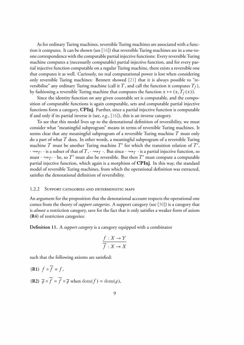
Figure 1.2: The not gate (a), cnot gate (b), toffoli gate (c), and a reversible circuit composed of not,cnot, and toffoli gates (d).

physical realisation, logical irreversibility of a computing process (such as resetting a bit tohave a particular value), Landauer argues, inexorably leads to physical irreversibility. Sincethis physical irreversibility is associated with a decrease in entropy, which cannot occur ina closed system by the laws of thermodynamics, Landauer goes on to argue that this localdecrease in entropy must be expressed as an increase in entropy in the environment, in theform of heat dissipation [84, p. 265]:

“Consider a statistical ensemble of bits in thermal equilibrium. If these are all resetto one, the number of states covered in the ensemble therefore has been reduced byk ln(2) = 0,6931k per bit. The entropy of a closed system, e.g., a computer withits own batteries, cannot decrease; hence this entropy must appear elsewhere as aheating effect, supplying 0,6931kT per restored bit to the surroundings.”

On the other hand, logically reversible computations can have physically reversible realisa-tions, which are, in turn, not associated with this heat dissipation in the ideal case.

As a physical principle, Landauer’s principle has been a subject of much debate, notablyin the Norton-Ladyman controversy [82, 83, 97] (see also [6]). Since then, the principlehas seen redemption in the form of experimental validation [23, 98, 65] and even formalverification [6]. Aside from Landauer’s principle, reversibility is also a key component inquantum computing: The quantum circuit model [40] relies on gates that are all unitary,i.e., linear isomorphisms of Hilbert spaces that preserve the inner product.

1.3.1 Reversible gates and reversible circuits

While Landauer demonstrated the possibility for low-power computing via reversibility,it would take another twenty years before his ideas were fully formalised by Toffoli intoa universal gate set for designing actual reversible computers. Though other gate sets havesince appeared (notably the Fredkin gate set [44]), we focus here on the Toffoli gate set [114](which we will use extensively in Chapter A).

The Toffoli gate set consist of three gates, depicted in Figure 1.2: The not gate, thecnot (or feynman) gate, and the toffoli gate. The not gate works precisely as it does inirreversible computing, mapping 0 to 1 and vice versa. The cnot gate (short for “controllednot”) takes two inputs – one, marked with • is called the control line, while the other,marked with ⊕, is called the target line – and produces two outputs. The output of the

11

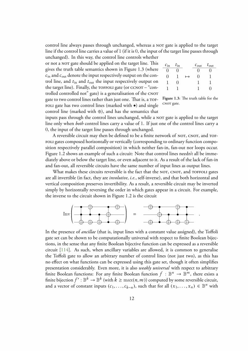
control line always passes through unchanged, whereas a not gate is applied to the targetline if the control line carries a value of 1 (if it is 0, the input of the target line passes through

cin tin cout tout0 0 0 00 1 7→ 0 11 0 1 11 1 1 0

Figure 1.3: The truth table for thecnot gate.

unchanged). In this way, the control line controls whetheror not a not gate should be applied on the target line. Thisgives the truth table semantics shown in Figure 1.3 (wherecin and cout denote the input respectively output on the con-trol line, and tin and tout the input respectively output onthe target line). Finally, the toffoli gate (or ccnot – “con-trolled controlled not” gate) is a generalisation of the cnotgate to two control lines rather than just one. That is, a tof-foli gate has two control lines (marked with •) and singlecontrol line (marked with ⊕), and has the semantics thatinputs pass through the control lines unchanged, while a not gate is applied to the targetline only when both control lines carry a value of 1. If just one of the control lines carry a0, the input of the target line passes through unchanged.

A reversible circuit may then be defined to be a finite network of not, cnot, and tof-foli gates composed horizontally or vertically (corresponding to ordinary function compo-sition respectively parallel composition) in which neither fan-in, fan-out nor loops occur.Figure 1.2 shows an example of such a circuit: Note that control lines needn’t all be imme-diately above or below the target line, or even adjacent to it. As a result of the lack of fan-inand fan-out, all reversible circuits have the same number of input lines as output lines.

What makes these circuits reversible is the fact that the not, cnot, and toffoli gatesare all invertible (in fact, they are involutive, i.e., self-inverse), and that both horizontal andvertical composition preserves invertibility. As a result, a reversible circuit may be invertedsimply by horizontally reversing the order in which gates appear in a circuit. For example,the inverse to the circuit shown in Figure 1.2 is the circuit

Inv*..,• •• • •

•

+//- =

• •• • •

•.

In the presence of ancillae (that is, input lines with a constant value assigned), the Toffoligate set can be shown to be computationally universal with respect to finite Boolean bijec-tions, in the sense that any finite Boolean bijective function can be expressed as a reversiblecircuit [114]. As such, when ancillary variables are allowed, it is common to generalisethe Toffoli gate to allow an arbitrary number of control lines (not just two), as this hasno effect on what functions can be expressed using this gate set, though it often simplifiespresentation considerably. Even more, it is also weakly universal with respect to arbitraryfinite Boolean functions: For any finite Boolean function f : Bn → Bm , there exists afinite bijection f ′ : Bk → Bk (with k ≥ max(n,m)) computed by some reversible circuit,and a vector of constant inputs (c1, . . . , ck−n), such that for all (x1, . . . , xn) ∈ Bn with

12

f (x1, . . . , xn) = (y1, . . . , ym ),

f ′(c1, . . . , ck−n, x1, . . . , xn) = (g1, . . . , gk−m, y1, . . . , ym ) .

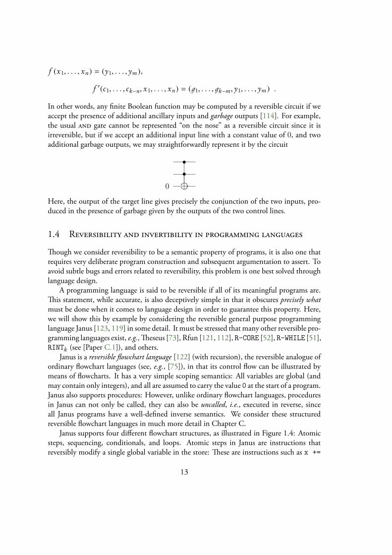
In other words, any finite Boolean function may be computed by a reversible circuit if weaccept the presence of additional ancillary inputs and garbage outputs [114]. For example,the usual and gate cannot be represented “on the nose” as a reversible circuit since it isirreversible, but if we accept an additional input line with a constant value of 0, and twoadditional garbage outputs, we may straightforwardly represent it by the circuit

••

0

Here, the output of the target line gives precisely the conjunction of the two inputs, pro-duced in the presence of garbage given by the outputs of the two control lines.

1.4 Reversibility and invertibility in programming languages

Though we consider reversibility to be a semantic property of programs, it is also one thatrequires very deliberate program construction and subsequent argumentation to assert. Toavoid subtle bugs and errors related to reversibility, this problem is one best solved throughlanguage design.

A programming language is said to be reversible if all of its meaningful programs are.This statement, while accurate, is also deceptively simple in that it obscures precisely whatmust be done when it comes to language design in order to guarantee this property. Here,we will show this by example by considering the reversible general purpose programminglanguage Janus [123, 119] in some detail. It must be stressed that many other reversible pro-gramming languages exist, e.g., Theseus [73], Rfun [121, 112], R-CORE [52], R-WHILE [51],RINTk (see [Paper C.1]), and others.

Janus is a reversible flowchart language [122] (with recursion), the reversible analogue ofordinary flowchart languages (see, e.g., [75]), in that its control flow can be illustrated bymeans of flowcharts. It has a very simple scoping semantics: All variables are global (andmay contain only integers), and all are assumed to carry the value 0 at the start of a program.Janus also supports procedures: However, unlike ordinary flowchart languages, proceduresin Janus can not only be called, they can also be uncalled, i.e., executed in reverse, sinceall Janus programs have a well-defined inverse semantics. We consider these structuredreversible flowchart languages in much more detail in Chapter C.

Janus supports four different flowchart structures, as illustrated in Figure 1.4: Atomicsteps, sequencing, conditionals, and loops. Atomic steps in Janus are instructions thatreversibly modify a single global variable in the store: These are instructions such as x +=

13

- a - - B1 - B2 - -��@@��

@@pt

f

- B1?�

���q

t

f

-

- B2 6

-��

��pt

f

- B1?

��@@��

@@q t

f�B26

-

Figure 1.4: The reversible flowchart structures in Janus: Atomic steps, sequences, conditionals, and loops.Squares denote flowcharts, diamonds are tests, and circles are assertions. Figures adapted from [122].

y (add the contents of y to the contents of x), x <=> y (swap the contents of x and y),and so on. Sequences are simply that: Sequences of statements separated by carriage return.Conditionals, on the other hand, are a little more tricky: Unlike ordinary conditionalswhich has a single predicate that decides which branch to take, a Janus conditional takesthe form if p then B1 else B2 fi q , where p and q are predicates, and B1 and B2 arestatements. Here, the trailing predicate q must be fashioned in such a way as to be truewhenever the then-branch is chosen by p, and false when the else-branch is chosen. Thisextra predicate is necessary to guarantee reversibility of the entire conditional, as it mightnot otherwise be possible to deduce which branch to choose in the backward direction.

procedure fiby += 1from x = 0 do

skiploop

x += yx <=> yn -= 1

until n = 0

Figure 1.5: The Fibonaccipair procedure in Janus.

Like conditionals, loops in Janus require an additional predi-cate in order to be reversible. That is, loops in Janus take the formfrom p do B1 loop B2 until q , where p is a predicate that mustbe true before any iterations of the loop, and false after one or moreiterations. The semantics of such loops are the following: Afterchecking the assertion p, the statement B1 is executed, and the testq is executed: If it is true, the loop is exited; otherwise, the state-ment B2 is executed and the program counter returns to the entryassertion to start anew. An example of a Janus program using loopsis shown in Figure 1.5. Assuming that x and y are both zero clearedand that n contains some positive integer, after calling the fib pro-cedure the pair of variables (x, y) will contain ( fn, fn+1), where fiis the i th Fibonacci number. This procedure also an example of aninjectivisation of a problem: The function mapping n 7→ fn is notinjective since the first and second Fibonacci numbers are both 1, but it can be made in-jective by changing its semantics slightly to compute Fibonacci pairs instead. Such smallsemantic changes to problems are common in practical reversible programming, as prob-lems are often formulated in a non-injective way.

Though Janus is a rather simple language compared to mainstream programming lan-guages such as Java or Haskell, when augmented with a dynamic data structure such as astack [119], it is as expressive as it can be reversibly, in the sense that it is r-Turing com-

14

plete [16, 119]: In other words, it is as computationally powerful as reversible Turing ma-chines, which serve as the gold standard for reversible computability.

1.4.1 Program inversion and inverse interpretation

A feature of Janus (and other reversible languages) that is often highlighted is the fact thatit comes equipped with a sound and complete program inverter. A program inverter is aprogram transformer Inv (that is, a program that takes program texts as inputs and producesthem as outputs) satisfying for all program texts p that JInv(p)K = JpK†. Though programinversion was first considered for general (irreversible) programming languages [36] (byhand, even), it has found a home in reversible programming, as program inverters are bothvery meaningful to have, and often straightforward to produce, for reversible languages.

Similar to program inverters are inverse interpreter. An inverse interpreter is a programInvInt satisfying for all program texts p and inputs x that JInvIntK(p, x ) = JpK†(x ). In-verse interpretation goes back even further than program inversion (and was likewise origi-nally considered for irreversible languages), as it was first studied when McCarthy developedhis generate-and-test method in 1958. In Janus, such an inverse interpreter was constructedby remarkable means in [123]: Instead of implementing one directly, the authors insteadimplemented a self-interpreter for Janus (i.e., a Janus interpreter written in Janus), and thenshowed that inverse interpretation could be achieved by using the uncall-functionality ofJanus to uncall the self-interpreter.

Though this was not realised until much later [50] (see also [49]), inverse interpretationand program inversion are connected via the Futamura projections [45]. Given a programspecialiser, a program inverter can be produced by specialising the specialiser with respectto the inverse interpreter. Note, however, that the language in which the inverse programproduced by this program inverter is expressed is the target language of the specialiser. Thisis a subtle point regarding program inversion in reversible languages: While a determin-istic inverse interpreter can always be fashioned for a reversible programming language L(though it may have to be written in another language), the language L may not be ex-pressive enough to express its own inverse programs. We illustrate this by the followingexample.

Consider the following programming language, an imperative language with stores con-sisting of a single memory cell containing an integer, which we shall refer to as Zinc (“Zwith incrementation”): The syntax is given by finite (possibly empty) lists of the symbol+, i.e., ϵ , '+', '++', '+++', and so on. Its semantics is given by the reduction relationn ⊢ p ↓ n′ (where p is a program, and n and n′ are integers corresponding to the contentsof the store before and after execution) defined as follows:

n ⊢ ϵ ↓ nn ⊢ c1 ↓ n′ n′ ⊢ c2 ↓ n′′

n ⊢ c1c2 ↓ n′′ n ⊢ '+' ↓ n + 1

15

For example, executing the program '+++' in a store containing the integer n results in astore containing the integer n + 3. This is a reversible language: For any Zinc commandc , given any integer n there exists at most one n′ such that n ⊢ c ↓ n′, and given anyinteger m there exists at most one m′ such that m′ ⊢ c ↓ m. However, since Zinccannot express decrementation, inverse programs of Zinc programs are not expressiblein Zinc: We say that Zinc (unlike Janus) is not closed under program inversion. Closureunder program inversion should be considered a constructive property: Even if a reversibleprogramming language is r-Turing complete (and, as such, strong enough to express its owninverse programs by the Church-Turing thesis, as a partial injective function is computableif and only if its inverse is), it should not be considered closed under program inversionuntil a (sound and complete) program inverter is produced.

1.5 Contributions

In this chapter, we have introduced the prevalent operational account of reversibility whichgoes back to the seminal work of Bennett [21], as well as a novel denotational account,which links up with pioneering work on inverse categories as models of reversible com-puting [46], that stresses the importance of compositional semantics for reversible programs.Further, using concepts from the literature on reversible computing and inverse categorytheory, we have argued why these two accounts should be seen as complimentary ratherthan competing. We have introduced Landauer’s principle as the physical motivation for re-versible computing, and Toffoli’s gate set as a foundations for a practical realisation of theseconcepts. Finally, we have discussed reversibility as it applies to programming languages,and the role of program inversion and inverse interpretation in reversible programming.

The remaining part of this thesis is given as an appendix of manuscripts produced bythe author (and others) during the course of the past three years. The appendix consists ofseven papers split into three topical chapters, covering the areas of reversible circuit logic,foundations of reversible recursion, and the semantics of reversible programming languages.We outline below the main contributions of these papers.

1.5.1 Reversible circuit logic

The reversible circuit model, based on the Toffoli gate set (see Figure 1.2 on page 9), providesthe mathematical foundation for the construction of real world reversible computers. Muchlike programs in high level languages, reversible circuits are not all created equal: Some arebetter than others at performing the same job, in that they require fewer gates or ancillarylines, or produce fewer garbage outputs.

Chapter A concerns itself with two approaches to the equivalence problem for reversiblecircuits: Given two reversible circuits C and D, which thus compute finite bijective func-tions fC, fD : Bk → Bk , we wish to determine whether these two circuits are equivalent,i.e., whether it is the case that fC (x) = fD (x) for all x ∈ Bk . Unfortunately, as for the

16

circuit equivalence problem for the conventional (irreversible) circuit model, this is a com-putationally intractable problem shown to be coNP-complete [76]. For this reason, theequivalence problem is one best solved by providing tools that aid humans in solving it forconcrete instances.

One such tool is the hardware description language Ricercar presented in [Paper A.1],which comes equipped with an equational theory based on previous work by two of the au-thors [110]. The equational theory exploits the compositional nature of reversible circuits(cf. Thesis 1), and is similar to the template-based approach to reversible circuit optimisa-tion that has become popular in recent years (see, e.g., [12]).

Ricercar regards reversible circuits as constructed using only the identity and notgates as primitives: Circuits may be formed through the sequential composition of smallercircuits, or by letting their execution be controlled by an arbitrary Boolean formula. Thisview of control by a Boolean formula as an operation on circuits leads to a much widerapplicability of the equational theory. Ricercar also introduces a notion of scoped ancillaryvariables as input variables which are guaranteed to be unchanged across the execution ofthe circuit, and also provides a set of equational rewriting rules for reasoning about circuitswith scoped ancillae. Since ancillary lines are often used to temporarily store partial resultsfrom computations, assigning and maintaining scopes to ancillae facilitates reuse of ancillarylines, which may help in bringing down the overall circuit size. Unfortunately, though theRicercar semantics and equational theory is sound with respect to the reversible circuitmodel, and though good results can often be obtained in practice, it is demonstrated to beincomplete (in that there exist two equivalent circuits that cannot be shown to be equivalentby means of the equational theory of Ricercar).

Where Ricercar adopts a view of circuits vaguely similar to that of propositional dynamiclogics (see, e.g., [42]), an approach to the equivalence problem much more reminiscentof classical propositional logic is chosen in [Paper A.2], through the development of thelogic LRS⊛. In this view, reversible circuits (much like ordinary, irreversible circuits inclassical propositional logic) are expressible as propositions, and propositional equivalenceof circuit representations correspond to the equivalence of represented circuits. The result isa two-level proof calculus that is sound and complete with respect to a semantics based onso-called Toffoli lattices, which, in turn, is shown to be equationally complete with respect toreversible logic circuits. This, finally, leads to a sound and complete equational theory forpropositional representations of reversible circuits. However, this approach comes at thecost that propositions are not guaranteed to correspond to reversible circuits: Reversiblecircuits merely embed in the logic as propositions in an equivalence-preserving way.

1.5.2 Foundations of reversible recursion

Out of all language features, the ability to express (primitively or generally) recursive pro-cedures is often what separates simple, toy-like languages from fully fledged programminglanguages capable of expressing sophisticated computations. In Chapter B of this thesis, we

17

investigate the role of recursion in reversible programming languages and how to model itin a categorical setting.

In existing reversible programming languages, recursion presents itself in several differ-ent forms: Rfun [121, 112] allows generally recursive functions1, while Theseus [72, 73]allows only tail recursive functions to be expressed by means of iteration labels (a syntac-tic sugarcoating of a sufficiently well-behaved trace operator [77, 73, 108]). Even more,Janus [123, 119] (see also Section 1.4) supports both general recursion and tail recursionin the form of recursive procedures respectively reversible while-loops.

In the irreversible case, recursion (be it recursively defined procedures or data types)is often studied through the lens of domain theory (see, e.g., [7]), i.e., by means of cate-gories enriched in the category DCPO of directed complete partial orders and continuousmaps. Following the mantra that inverse categories are models of reversible computing (asdiscussed in Section 1.1), we give a domain theoretic account of inverse categories outfit-ted with joins (in the sense of [53], but see also [115]) in [Paper B.1] (an extended ver-sion of a previously published conference paper and workshop abstract). In particular,it is shown that having at least countable joins leads to a DCPO-enrichment for whichthe canonical dagger is locally continuous. This gives a family of fixed point operatorsfix : ( C(X ,Y ) → C(X ,Y )) → C(X ,Y ) in the join inverse category C for modellinggenerally recursive first-order functions, and (crucially, as far as reversibility is concerned)it is shown that each continuous map φ : C(X ,Y ) → C(X ,Y ) has a fixed point adjointφ‡ : C(Y ,X ) → C(Y ,X ) such that (fix φ)† = fix φ‡.

Essentially, this result states that inversion of recursive maps can be solved by localmeans alone, a result which is consistent with established procedures for inversion of recur-sively defined reversible programs (e.g., in Rfun [121]). Using a representation theorem forjoin restriction categories from [53], it is further shown that each join inverse category canbe embedded in one that is algebraically ω-compact for locally continuous (in particular,join-preserving) functors, which may be used to model recursively defined data types. Fi-nally, it is shown that when outfitted with a disjointness tensor [46] that preserves joins, thejoin inverse category may be canonically regarded as a unique decomposition category [55],equipping it with a trace operator that is shown to be preserve the canonical dagger – inother words, modelling reversible tail recursion in the style of Theseus.

In [Paper B.2], we seek to generalise key results from [Paper B.1] by asking what fea-tures of a join inverse category are necessary for fixed point adjoints to exist, and if theycan be made canonical in some way. For this reason, we study the more general daggercategories enriched in DCPO. Unlike inverse categories, these categories also model com-putations that are not reversible under the Copenhagen interpretation (see page 2), but stillhave adjoints2: Examples include relational, doubly-stochastic, and even certain quantum

1Which, to the initial astonishment of the author, works precisely as it does in the irreversible case: Usinga call stack, no changes required.

2By an adjoint to some f : X → Y we simply mean a “partner” f † : Y → X , with no additionalrequirements.

18

computations. It is shown that for a dagger category enriched in DCPO to have fixedpoint adjoints (as in [Paper B.1]), it is sufficient that the dagger is locally monotone, aresult that even extends to parametrised fixed points (see, e.g., [38]). The requirement oflocal monotony of the dagger can be seen as an instance of the way of the dagger [62], atenet of dagger category theory stating that all structure in sight must cooperate with thedagger. We show that an induced category of functionals over such a DCPO-enricheddagger category is canonically an involutive monoidal category [70], a view enables us toexplain seemingly unrelated notions such as fixed point adjoints (in the sense of [PaperB.1]), dagger-preserving natural transformations, and the ambidexterity of dagger adjunc-tions in terms of conjugation of functionals. In particular, there is a world beyond the strictCopenhagen interpretation of reversibility where reversible recursion is still well-behaved.

1.5.3 Semantics of reversible programming languages

In the final chapter of the thesis, Chapter C, we consider the applications of inverse categorytheory in giving semantics to (aspects of ) reversible programming languages.

In [Paper C.1] (an extended version of a previously published conference paper), wedevelop categorical semantics for structured reversible flowchart languages (of which Januswithout recursion is an example), i.e., imperative reversible programming languages witha control flow that can be illustrated purely by means of flowchart structures (Figure 1.4on page 10 shows the flowchart structures available in Janus without recursion). Sincemany of these flowchart structures involve tests (and assertions), this hinges on a reversiblerepresentation of these as predicates (and their inverses), which we provide in the form ofdecisions (inspired by the analogous notion in restriction category theory, see [33]). Usingthese decisions, we give semantics to a universal class of reversible flowchart structures incertain join inverse categories, using some of the machinery developed in [Paper A.1] togive semantics to reversible while-loops via the dagger trace operator. We likewise providean operational semantics for the reversible flowchart structures and tests, and show that ourcategorical semantics are both sound and adequate with respect to the operational ones.We additionally provide a sufficient condition for full abstraction (see, e.g., [8, 99]), anddemonstrate how a program inverter can be extracted from the semantics. We also showhow the developed techniques can be used to straightforwardly give semantics to a classof structured reversible flowchart languages called RINTk (a family of structured reversibleflowchart languages inspired by reversible counter machines [95, 78]) in the category PInjof sets and partial injective functions.

In [Paper C.2], we give an account of reversible effects in reversible programming. Mon-ads are the typically the weapon of choice for modelling effects in the irreversible case (see,e.g., [93, 116]), and though these have an analogue in dagger categories as Frobenius mon-ads [62], we were only able to produce trivial or otherwise contrived examples of Frobeniusmonads in inverse categories. For this reason, we develop instead reversible versions of ar-rows [67, 71] (which generalise monads) as dagger arrows and inverse arrows. These arrows

19

correspond to arrows between dagger (respectively inverse) categories that preserve inver-sion. We extend the arrow laws with laws for dagger and inverse arrows, and demonstratetheir applicability by a number of examples, notably stateful reversible computations and areversible variant of the Writer monad which we call the Rewriter arrow as inverse arrows,and the CPM construction [107] used to lift pure quantum computations to mixed onesas a dagger arrow. Following the idea that arrows, like monads, are monoids [61] (here inthe category of profunctors), we show that dagger arrows correspond precisely to involutivemonoids, and inverse arrows to dagger arrows satisfying additional equations.

Finally, in the brief [Paper C.3], we present a vision for the future of the reversiblefunctional programming language Rfun [121]. New features include support for ancillaryvariables, which can be seen as a slight generalisation of the parametrised maps found inTheseus [73], and the abolishment of the duplication/equality operator3 in favor of a com-bined relevant (see, e.g., [37]) and unrestricted type system (see also [100]) that allows forreversible duplication and deduplication of first-order data.

3A source of confusion for students and reviewers alike.

20

References

[1] S. M. Abramov and R. Glück. The universal resolving algorithm: inverse compu-tation in a functional language. In R. Backhouse and J. N. Oliveira, editors, Pro-ceedings of the 5th International Conference on Mathematics of Program Construction(MPC 2000), volume 1837 of Lecture Notes in Computer Science, pages 187–212.Springer-Verlag, 2000.

[2] S. M. Abramov and R. Glück. Principles of inverse computation and the universalresolving algorithm. In T. Æ. Mogensen, D. A. Schmidt, and I. H. Sudborough,editors, The Essence of Computation: Complexity, Analysis, Transformation, volume2566 of Lecture Notes in Computer Science, pages 269–295. Springer-Verlag, 2002.

[3] S. Abramsky. Retracing some paths in process algebra. In U. Montanari and V. Sas-sone, editors, CONCUR ’96, pages 1–17. Springer, 1996.

[4] S. Abramsky. A structural approach to reversible computation. Theoretical ComputerScience, 347(3):441–464, 2005.

[5] S. Abramsky, E. Haghverdi, and P. Scott. Geometry of interaction and linear combi-natory algebras. Mathematical Structures in Computer Science, 12(5):625–665, 2002.

[6] S. Abramsky and D. Horsman. DEMONIC programming: a computational lan-guage for single-particle equilibrium thermodynamics, and its formal semantics. InC. Heunen, P. Selinger, and J. Vicary, editors, Proceedings of the 12th InternationalWorkshop on Quantum Physics and Logic (QPL 2015), volume 195 of Electronic Pro-ceedings in Theoretical Computer Science, pages 1–16. Open Publishing Association,2015.

[7] S. Abramsky and A. Jung. Domain Theory. In S. Abramsky, D. M. Gabbay, andT. S. E. Maibaum, editors, Handbook of Logic in Computer Science, volume 3, pages1–168. Oxford University Press, 1994.

[8] S. Abramsky and C.-H. L. Ong. Full abstraction in the lazy lambda calculus. Infor-mation and Computation, 105(2):159–267, 1993.

21

[9] J. Adámek. Recursive data types in algebraically ω-complete categories. Informationand Computation, 118:181–190, 1995.

[10] J. Adámek and V. Koubek. Least fixed point of a functor. Journal of Computer andSystem Sciences, 19(2):163–178, 1979.

[11] T. Altenkirch, J. Chapman, and T. Uustalu. Monads need not be endofunctors.Logical Methods in Computer Science, 11(1), 2015.

[12] M. Arabzadeh, M. Saeedi, and M. S. Zamani. Rule-based optimization of reversiblecircuits. In Proceedings of the 15th Asia and South-Pacific Design Automation Confer-ence (ASP-DAC 2010), pages 849–854, 2010.

[13] S. Awodey. Category theory, volume 52 of Oxford Logic Guides. Oxford UniversityPress, second edition, 2010.

[14] H. B. Axelsen and R. Glück. A simple and efficient universal reversible turing ma-chine. In A.-H. Dediu, S. Inenaga, and C. Martín-Vide, editors, Proceedings ofthe 5th International Conference on Language and Automata Theory and Applications(LATA 2011), pages 117–128. Springer-Verlag, 2011.

[15] H. B. Axelsen and R. Glück. What do reversible programs compute? In M. Hof-mann, editor, Foundations of Software Science and Computation Structures (FoSSaCS),volume 6604 of Lecture Notes in Computer Science, pages 42–56. Springer-Verlag,2011.

[16] H. B. Axelsen and R. Glück. On reversible turing machines and their functionuniversality. Acta Informatica, 53(5):509–543, 2016.

[17] H. B. Axelsen, R. Glück, and T. Yokoyama. Reversible machine code and its abstractprocessor architecture. In V. Diekert, M. V. Volkov, and A. Voronkov, editors, Pro-ceedings of the Second International Symposium on Computer Science in Russia (CSR2007), volume 4649 of Lecture Notes in Computer Science, pages 56–69. Springer-Verlag, 2007.

[18] E. S. Bainbridge, P. J. Freyd, A. Scedrov, and P. J. Scott. Functorial polymorphism.Theoretical Computer Science, 70(1):35–64, 1990.

[19] M. Barr. Algebraically compact functors. Journal of Pure and Applied Algebra,82(3):211–231, 1992.

[20] E. J. Beggs and S. Majid. Bar categories and star operations. Algebras and Represen-tation Theory, 12(2):103–152, 2009.

22

[21] C. H. Bennett. Logical reversibility of computation. IBM Journal of Research andDevelopment, 17(6):525–532, 1973.

[22] N. Benton and M. Hyland. Traced premonoidal categories. Theoretical Informaticsand Applications, 37(4):273–299, 2003.

[23] A. Bérut, A. Arakelyan, A. Petrosyan, S. Ciliberto, R. Dillenschneider, and E. Lutz.Experimental verification of Landauer’s principle linking information and thermo-dynamics. Nature, 483(7388):187–189, 2012.

[24] F. Borceux. Handbook of categorical algebra. Cambridge University Press, 1994.

[25] W. J. Bowman, R. P. James, and A. Sabry. Dagger traced symmetric monoidalcategories and reversible programming. In A. De Vos and R. Wille, editors, Pre-proceedings of the 3rd International Workshop on Reversible Computation (RC 2011),pages 51–56. Ghent University, 2011.

[26] A. Carboni, S. Lack, and R. F. C. Walters. Introduction to extensive and distributivecategories. Journal of Pure and Applied Algebra, 84(2):145 – 158, 1993.

[27] J. Carette and A. Sabry. Computing with semirings and weak rig groupoids. InP. Thiemann, editor, Proceedings of the 25th European Symposium on Programming(ESOP 2016), volume 9632 of Lecture Notes in Computer Science, pages 123–148.Springer-Verlag, 2016.

[28] C. D. Carothers, K. S. Perumalla, and R. M. Fujimoto. Efficient optimistic parallelsimulations using reverse computation. ACM Transactions on Modeling and Com-puter Simulation, 9(3):224–253, 1999.

[29] S.-K. Chen, W. K. Fuchs, and J.-Y. Chung. Reversible debugging using programinstrumentation. IEEE Transactions on Software Engineering, 27(8):715–727, 2001.

[30] J. R. B. Cockett, X. Guo, and P. Hofstra. Range categories i: General theory. Theoryand Applications of Categories, 26(17):412–452, 2012.

[31] J. R. B. Cockett and S. Lack. Restriction categories I: Categories of partial maps.Theoretical Computer Science, 270(1–2):223–259, 2002.

[32] J. R. B. Cockett and S. Lack. Restriction categories II: Partial map classification.Theoretical Computer Science, 294(1–2):61–102, 2003.

[33] J. R. B. Cockett and S. Lack. Restriction categories III: Colimits, partial limits andextensivity. Mathematical Structures in Computer Science, 17(4):775–817, 2007.

23

[34] R. Cockett and R. Garner. Restriction categories as enriched categories. TheoreticalComputer Science, 523:37–55, 2014.

[35] I. Cristescu, J. Krivine, and D. Varacca. A compositional semantics for the reversibleπ-calculus. In Proceedings of the 28th Annual IEEE/ACM Symposium on Logic inComputer Science (LICS 2013), pages 388–397. IEEE Computer Society, 2013.

[36] E. W. Dijkstra. Program inversion. In F. L. Bauer and M. Broy, editors, ProgramConstruction, International Summer School, pages 54–57. Springer-Verlag, 1979.

[37] J. M. Dunn and G. Restall. Relevance logic. In D. M. Gabbay and F. Guenther,editors, Handbook of Philosophical Logic, volume 6, pages 1–136. Kluwer AcademicPublishers, 2002.

[38] Z. Ésik. Fixed point theory. In M. Droste, W. Kuich, and H. Vogler, editors,Handbook of Weighted Automata, pages 29–65. Springer-Verlag, 2009.

[39] Z. Ésik. Equational properties of fixed point operations in cartesian categories: Anoverview. In G. Italiano, G. Pighizzini, and D. Sannella, editors, Proceedings ofthe 40th International Symposium on Mathematical Foundations of Computer Science(MFCS 2015), Part I, pages 18–37. Springer-Verlag, 2015.

[40] R. P. Feynman. Quantum mechanical computers. Optics News, 11(2):11–20, 1985.

[41] M. P. Fiore. Axiomatic Domain Theory in Categories of Partial Maps. PhD thesis,University of Edinburgh, 1994.

[42] M. J. Fischer and R. E. Ladner. Propositional dynamic logic of regular programs.Journal of Computer and System Sciences, 18(2):194–211, 1979.

[43] M. P. Frank. Reversibility for efficient computing. PhD thesis, Massachusetts Instituteof Technology, 1999.

[44] E. Fredkin and T. Toffoli. Conservative logic. International Journal of TheoreticalPhysics, 21(3-4):219–253, 1982.

[45] Y. Futamura. Partial computation of programs. In E. Goto, K. Furukawa, R. Naka-jima, I. Nakata, and A. Yonezawa, editors, RIMS Symposia on Software Science andEngineering, Proceedings, pages 1–35. Springer-Verlag, 1983.

[46] B. G. Giles. An Investigation of some Theoretical Aspects of Reversible Computing. PhDthesis, University of Calgary, 2014.

24

[47] R. Glück and M. Kawabe. A program inverter for a functional language with equalityand constructors. In A. Ohori, editor, Proceedings of the First Asian Symposium onProgramming Languages and Systems (APLAS 2003), volume 2895 of Lecture Notesin Computer Science, pages 246–264. Springer-Verlag, 2003.

[48] R. Glück and M. Kawabe. Derivation of deterministic inverse programs based on LRparsing. In Y. Kameyama and P. J. Stuckey, editors, Proceedings of the 7th InternationalSymposium on Functional and Logic Programming (FLOPS 2004), volume 2998 ofLecture Notes in Computer Science, pages 291–306. Springer-Verlag, 2004.

[49] R. Glück, Y. Kawada, and T. Hashimoto. Transforming interpreters into inverseinterpreters by partial evaluation. In M. Leuschel, editor, Proceedings of the 2003ACM SIGPLAN Workshop on Partial Evaluation and Semantics-based Program Ma-nipulation (PEPM ’03), pages 10–19. ACM Press, 2003.

[50] R. Glück and M. H. Sørensen. A roadmap to metacomputation by supercompila-tion. In O. Danvy, R. Glück, and P. Thiemann, editors, Partial Evaluation: Inter-national Seminar, Selected Papers, pages 137–160. Springer-Verlag, 1996.

[51] R. Glück and T. Yokoyama. A linear-time self-interpreter of a reversible imperativelanguage. Computer Software, 33(3):108–128, 2016.

[52] R. Glück and T. Yokoyama. A minimalist’s reversible while language. IEICE Trans-actions on Information and Systems, E100-D(5):1026–1034, 2017.

[53] X. Guo. Products, Joins, Meets, and Ranges in Restriction Categories. PhD thesis,University of Calgary, 2012.

[54] E. Haghverdi. A Categorical Approach to Linear Logic, Geometry of Proofs and FullCompleteness. PhD thesis, Carlton University and University of Ottawa, 2000.

[55] E. Haghverdi. Unique decomposition categories, Geometry of Interaction and com-binatory logic. Mathematical Structures in Computer Science, 10(2):205–230, 2000.

[56] M. Hasegawa. Decomposing typed lambda calculus into a couple of categoricalprogramming languages. In D. Pitt, D. E. Rydeheard, and P. Johnstone, editors,Proceedings of the 6th International Conference on Category Theory and Computer Sci-ence (CTCS ’95), volume 953 of Lecture Notes in Computer Science, pages 200–219.Springer-Verlag, 1995.

[57] M. Hasegawa. Models of Sharing Graphs. PhD thesis, University of Edinburgh, 1997.

[58] M. Hasegawa. Recursion from cyclic sharing: Traced monoidal categories and mod-els of cyclic lambda calculi. In P. de Groote and J. R. Hindley, editors, Proceedings of

25

the Third International Conference on Typed Lambda Calculi and Applications (TLCA’97), volume 1210 of Lecture Notes in Computer Science, pages 196–213. Springer-Verlag, 1997.

[59] C. Heunen. Categorical quantum models and logics. PhD thesis, Radboud UniversityNijmegen, 2009.

[60] C. Heunen. On the functor `2. In Computation, Logic, Games, and QuantumFoundations - The Many Facets of Samson Abramsky, volume 7860 of Lecture Notes inComputer Science, pages 107–121. Springer-Verlag, 2013.

[61] C. Heunen and B. Jacobs. Arrows, like monads, are monoids. In S. D. Brookes andM. W. Mislove, editors, Proceedings of the 22nd Annual Conference on MathematicalFoundations of Programming Semantics (MFPS XXII), volume 158 of Electronic Notesin Theoretical Computer Science, pages 219–236, 2006.

[62] C. Heunen and M. Karvonen. Monads on dagger categories. Theory and Applicationsof Categories, 31(35):1016–1043, 2016.

[63] P. M. Hines. The Algebra of Self-Similarity and its Applications. PhD thesis, Universityof Wales, Bangor, 1998.

[64] P. M. Hines and S. Braunstein. The structure of partial isometries. In S. Gay andI. Mackie, editors, Semantic Techniques in Quantum Computation, pages 361–388.Cambridge University Press, 2009.

[65] J. Hong, B. Lambson, S. Dhuey, and J. Bokor. Experimental test of Landauer’sprinciple in single-bit operations on nanomagnetic memory bits. Science Advances,2(3), 2016.

[66] N. Hoshino. A representation theorem for unique decomposition categories. InU. Berger and M. Mislove, editors, Proceedings of the 28th Conference on the Mathe-matical Foundations of Programming Semantics (MFPS XXVIII), volume 286 of Elec-tronic Notes in Theoretical Computer Science, pages 213–227. Elsevier, 2012.

[67] J. Hughes. Generalising monads to arrows. Science of Computer Programming,37:67–111, 2000.

[68] M. Hyland. Abstract and concrete models for recursion. In O. Grumberg, T. Nip-kow, and C. Pfaller, editors, Proceedings of the NATO Advanced Study Institute on For-mal Logical Methods for System Security and Correctness, pages 175–198. IOS Press,2008.

[69] B. Jacobs. Semantics of weakening and contraction. Annals of Pure and AppliedLogic, 69:73–106, 1994.

26

[70] B. Jacobs. Involutive categories and monoids, with a GNS-correspondence. Foun-dations of Physics, 42(7):874–895, 2012.

[71] B. Jacobs, C. Heunen, and I. Hasuo. Categorical semantics for arrows. Journal ofFunctional Programming, 19(3-4):403–438, 2009.

[72] R. P. James and A. Sabry. Information effects. In Proceedings of the 39th AnnualACM SIGPLAN-SIGACT Symposium on Principles of Programming Languages, pages73–84. ACM, 2012.

[73] R. P. James and A. Sabry. Theseus: A high level language for reversible comput-ing. Work-in-progress report presented at RC 2014, available at https://www.cs.indiana.edu/~sabry/papers/theseus.pdf., 2014.

[74] P. T. Johnstone. Sketches of an elephant: A topos theory compendium, volume 1. OxfordUniversity Press, 2002.

[75] N. D. Jones, C. K. Gomard, and P. Sestoft. Partial Evaluation and Automatic ProgramGeneration. Prentice Hall International, 1993.

[76] S. P. Jordan. Strong equivalence of reversible circuits is coNP-complete. QuantumInformation and Computation, 14(15-16):1302–1307, 2014.

[77] A. Joyal, R. Street, and D. Verity. Traced monoidal categories. Mathematical Pro-ceedings of the Cambridge Philosophical Society, 119(3):447–468, 1996.

[78] J. Kari and N. Ollinger. Periodicity and immortality in reversible computing. InE. Ochmański and J. Tyszkiewicz, editors, Proceedings of the 33rd International Sym-posium on Mathematical Foundations of Computer Science (MFCS 2008), pages 419–430. Springer-Verlag, 2008.

[79] J. Kastl. Inverse categories. In H.-J. Hoehnke, editor, Algebraische Modelle, Kate-gorien und Gruppoide, volume 7 of Studien zur Algebra und ihre Anwendungen, pages51–60. Akademie Verlag, 1979.

[80] M. Kawabe and R. Glück. The program inverter lrinv and its structure. In M. V.Hermenegildo and D. Cabeza, editors, Proceedings of the 7th International Conferenceon Practical Aspects of Declarative Languages (PADL ’05), volume 3350 of LectureNotes in Computer Science, pages 219–234. Springer-Verlag, 2005.

[81] G. M. Kelly. Basic Concepts of Enriched Category Theory, volume 64 of London Math-ematical Society Lecture Note Series. Cambridge University Press, 1982.

27

[82] J. Ladyman, S. Presnell, A. J. Short, and B. Groisman. The connection betweenlogical and thermodynamic irreversibility. Studies in History and Philosophy of SciencePart B: Studies in History and Philosophy of Modern Physics, 38(1):58–79, 2007.

[83] J. Ladyman and K. Robertson. Landauer defended: Reply to norton. Studies inHistory and Philosophy of Science Part B: Studies in History and Philosophy of ModernPhysics, 44(3):263–271, 2013.

[84] R. Landauer. Irreversibility and heat generation in the computing process. IBMJournal of Research and Development, 5(3):183–191, 1961.

[85] M. L. Laplaza. Coherence for distributivity. In G. M. Kelly, M. L. Laplaza, G. Lewis,and S. Mac Lane, editors, Coherence in Categories, volume 281 of Lecture Notes inMathematics, pages 29–65. Springer-Verlag, 1972.

[86] M. V. Lawson. Inverse Semigroups: The Theory of Partial Symmetries. World Scientific,1998.

[87] S. Mac Lane. Categories for the Working Mathematician, volume 5 of Graduate Textsin Mathematics. Springer-Verlag, second edition, 1998.

[88] E. G. Manes and M. A. Arbib. Algebraic approaches to program semantics. Springer-Verlag, 1986.

[89] E. G. Manes and D. B. Benson. The inverse semigroup of a sum-ordered semiring.Semigroup Forum, 31(1):129–152, 1985.

[90] M. L. Minsky. Computation: Finite and Infinite Machines. Prentice-Hall, Inc., 1967.

[91] T. Æ. Mogensen. Partial evaluation of the reversible language Janus. In Proceedings ofthe 20th ACM SIGPLAN workshop on Partial Evaluation and Program Manipulation(PEPM ’11), pages 23–32. ACM Press, 2011.

[92] T. Æ. Mogensen. Garbage collection for reversible functional languages. In J. Krivineand J.-B. Stefani, editors, Proceedings of the 7th International Conference on ReversibleComputation (RC 2015), volume 9138 of Lecture Notes in Computer Science, pages79–94. Springer-Verlag, 2015.

[93] E. Moggi. Notions of computation and monads. Information and Computation,93(1):55–92, 1991.

[94] R. Montague. Universal grammar. Theoria, 36(3):373–398, 1970.

[95] K. Morita. Universality of a reversible two-counter machine. Theoretical ComputerScience, 168(2):303–320, 1996.

28

[96] K. Nakata and T. Uustalu. Trace-based coinductive operational semantics for while.In S. Berghofer, T. Nipkow, C. Urban, and M. Wenzel, editors, Proceedings of the22nd International Conference on Theorem Proving in Higher Order Logics (TPHOLs2009), volume 5674 of Lecture Notes in Computer Science, pages 375–390. Springer-Verlag, 2009.

[97] J. D. Norton. Waiting for Landauer. Studies in History and Philosophy of Science PartB: Studies in History and Philosophy of Modern Physics, 42(3):184–198, 2011.

[98] A. O. Orlov, C. S. Lent, C. C. Thorpe, G. P. Boechler, and G. L. Snider. Experi-mental test of Landauer’s principle at the sub-kbt level. Japanese Journal of AppliedPhysics, 51(6S):06FE10, 2012.

[99] G. Plotkin. Full abstraction, totality and pcf. Mathematical. Structures in Comp. Sci.,9(1):1–20, 1999.

[100] J. Polakow. Ordered linear logic and applications. PhD thesis, Carnegie Mellon Uni-versity, 2001.

[101] T. Rendel and K. Ostermann. Invertible syntax descriptions: Unifying parsing andpretty printing. SIGPLAN Notices, 45(11):1–12, 2010.

[102] E. Robinson and G. Rosolini. Categories of partial maps. Information and Compu-tation, 79:95–130, 1988.

[103] G. Sandu and J. Hintikka. Aspects of compositionality. Journal of Logic, Languageand Information, 10(1):49–61, 2001.

[104] M. Schordan, D. Jefferson, P. Barnes, T. Oppelstrup, and D. Quinlan. Reverse codegeneration for parallel discrete event simulation. In J. Krivine and J.-B. Stefani,editors, Proceedings of the 7th International Conference on Reversible Computation (RC2015), volume 9138 of Lecture Notes in Computer Science, pages 95–110. Springer-Verlag, 2015.

[105] U. P. Schultz, M. Bordignon, and K. Støy. Robust and reversible execution of self-reconfiguration sequences. Robotica, 29(1):35–57, 2011.

[106] U. P. Schultz, J. S. Laursen, L.-P. Ellekilde, and H. B. Axelsen. Towards a domain-specific language for reversible assembly sequences. In J. Krivine and J.-B. Stefani,editors, Proceedings of the 7th International Conference on Reversible Computation (RC2015), volume 9138 of Lecture Notes in Computer Science, pages 111–126. Springer-Verlag, 2015.

29

[107] P. Selinger. Dagger compact closed categories and completely positive maps. InProceedings of the 3rd International Workshop on Quantum Programming Languages(QPL 2005), volume 170 of Electronic Notes in Theoretical Computer Science, pages139–163. Elsevier, 2007.

[108] P. Selinger. A survey of graphical languages for monoidal categories. In B. Coecke,editor, New Structures for Physics, volume 813 of Lecture Notes in Physics, pages 289–355. Springer-Verlag, 2011.

[109] M. B. Smyth and G. D. Plotkin. The category-theoretic solution of recursive domainequations. SIAM Journal on Computing, 11(4):761–783, 1982.

[110] M. Soeken and M. K. Thomsen. White dots do matter: Rewriting reversible logiccircuits. In G. W. Dueck and D. M. Miller, editors, Proceedings of the 5th Inter-national Conference on Reversible Computation (RC 2013), volume 7948 of LectureNotes in Computer Science, pages 196–208, 2013.

[111] Z. Sparks and A. Sabry. Superstructural reversible logic. Presented at the 3rd In-ternational Workshop on Linearity, available at https://www.cs.indiana.edu/~sabry/papers/superstructural.pdf, 2014.

[112] M. K. Thomsen and H. B. Axelsen. Interpretation and programming of the reversiblefunctional language rfun. In R. Lämmel, editor, Proceedings of the 27th Symposium onthe Implementation and Application of Functional Programming Languages (IFL ’15),pages 8:1–8:13. ACM Press, 2015.

[113] M. K. Thomsen, H. B. Axelsen, and R. Glück. A reversible processor architectureand its reversible logic design. In A. De Vos and R. Wille, editors, Proceedings of the3rd International Workshop on Reversible Computation (RC 2011), volume 7165 ofLecture Notes in Computer Science, pages 30–42. Springer-Verlag, 2012.

[114] T. Toffoli. Reversible computing. In J. W. de Bakker and J. van Leeuwen, editors,Proceedings of the 7th International Colloquium on Automata, Languages and Program-ming (ICALP 1980), pages 632–644. Springer-Verlag, 1980.

[115] T. Uustalu and N. Veltri. The delay monad and restriction categories. In D. V.Hung and D. Kapur, editors, Proceedings of the 14th International Colloquium onTheoretical Aspects of Computing (ICTAC 2017), volume 10580 of Lecture Notes inComputer Science, pages 32–50. Springer-Verlag, 2017.

[116] P. Wadler. Monads for functional programming. In J. Jeuring and E. Meijer, editors,First International Spring School on Advanced Functional Programming Techniques,Tutorial Text, pages 24–52. Springer-Verlag, 1995.

30

[117] M. Wand. Fixed point constructions in order-enriched categories. Theoretical Com-puter Science, 8(1):13–30, 1979.

[118] G. Winskel. The Formal Semantics of Programming Languages: An Introduction. MITPress, 1993.

[119] T. Yokoyama, H. B. Axelsen, and R. Glück. Principles of a reversible programminglanguage. In A. Ramírez, G. Bilardi, and M. Gschwind, editors, Proceedings of the5th Conference on Computing Frontiers (CF ’08), pages 43–54. ACM Press, 2008.

[120] T. Yokoyama, H. B. Axelsen, and R. Glück. Reversible flowchart languages and thestructured reversible program theorem. In L. Aceto, I. Damgård, L. A. Goldberg,M. M. Halldórsson, A. Ingólfsdóttir, and I. Walukiewicz, editors, Proceedings of the35th International Colloquium on Automata, Languages and Programming (ICALP2008), volume 5126 of Lecture Notes in Computer Science, pages 258–270. Springer-Verlag, 2008.

[121] T. Yokoyama, H. B. Axelsen, and R. Glück. Towards a reversible functional language.In A. De Vos and R. Wille, editors, Proceedings of the 3rd Workshop on ReversibleComputation (RC 2011), volume 7165 of Lecture Notes in Computer Science, pages14–29. Springer-Verlag, 2012.

[122] T. Yokoyama, H. B. Axelsen, and R. Glück. Fundamentals of reversible flowchartlanguages. Theoretical Computer Science, 611:87–115, 2016.

[123] T. Yokoyama and R. Glück. A reversible programming language and its invertibleself-interpreter. In G. Ramalingam and E. Visser, editors, PEPM ’07: Proceedings ofthe 2007 ACM SIGPLAN Workshop on Partial evaluation and semantics-based programmanipulation, pages 144–153. ACM Press, 2007.

31

32

I have seen myself backward.Philip K. Dick, A Scanner Darkly

AReversible circuit logic

This chapter contains two papers related to reversible circuit logic.

(A1) M. K. Thomsen, R. Kaarsgaard, and M. Soeken. Ricercar: A Language for Describ-ing and Rewriting Reversible Circuits with Ancillae and its Permutation Semantics.In J. Krivine and J.-B. Stefani, editors, Reversible Computation, Lecture Notes inComputer Science volume 9138, pages 200–215, Springer Verlag, 2015.

(A2) H. B. Axelsen, R. Glück, and R. Kaarsgaard. A Classical Propositional Logic forReasoning about Reversible Logic Circuits. In J. Väänänen, Å. Hirvonen, and R. deQueiroz, editors, Logic, Language, Information, and Computation (WoLLIC), LectureNotes in Computer Science volume 9803, pages 52–67, Springer Verlag, 2016.

33

34

Ricercar: A Language for Describingand Rewriting Reversible Circuits with Ancillae

and Its Permutation Semantics

Michael Kirkedal Thomsen1(B), Robin Kaarsgaard2, and Mathias Soeken1

1 Group of Computer Architecture, University of Bremen, Bremen, Germany{kirkedal,msoeken}@informatik.uni-bremen.de

2 DIKU, Department of Computer Science,University of Copenhagen, Copenhagen, Denmark

[email protected]

Abstract. Previously, Soeken and Thomsen presented six basicsemantics-preserving rules for rewriting reversible logic circuits, definedusing the well-known diagrammatic notation of Feynman. While thisnotation is both useful and intuitive for describing reversible circuits, itsshortcomings in generality complicates the specification of more sophis-ticated and abstract rewriting rules.

In this paper, we introduce Ricercar, a general textual description lan-guage for reversible logic circuits designed explicitly to support rewriting.Taking the not gate and the identity gate as primitives, this languageallows circuits to be constructed using control gates, sequential compo-sition, and ancillae, through a notion of ancilla scope. We show how theabove-mentioned rewriting rules are defined in this language, and extendthe rewriting system with five additional rules to introduce and modifyancilla scope. This treatment of ancillae addresses the limitations of theoriginal rewriting system in rewriting circuits with ancillae in the generalcase.

To set Ricercar on a theoretical foundation, we also define a permuta-tion semantics over symmetric groups and show how the operations overpermutations as transposition relate to the semantics of the language.

Keywords: Reversible logic · Term rewriting · Ancillae ·Circuit equivalence · Permutation

1 Introduction

In [14] two of the authors presented six elementary rules for rewriting reversiblecircuits using mixed-polarity multiple-control Toffoli gates. Building on this,

M.K. Thomsen—This work was partly funded by the European Commission underthe 7th Framework Programme.M.K. Thomsen—A preliminary version of Ricercar was presented as work-in-progressat 6th Conference on Reversible Computation, 2014.

c© Springer International Publishing Switzerland 2015J. Krivine and J.-B. Stefani (Eds.): RC 2015, LNCS 9138, pp. 200–215, 2015.DOI: 10.1007/978-3-319-20860-2 13

35

Ricercar: A Language for Describing and Rewriting Reversible Circuits 201

more complex rules, such as moving and deletion rules, can be derived. Rewritingusing such rules can be used not just to reduce the size and cost of reversible cir-cuits, but also to analyse and explain other optimisation approaches for reversiblecircuits. As one example, the templates presented in [12] are all derivable fromthese rewriting rules.

The rewriting rules in [14] are based on the diagrammatic notation first intro-duced by Feynman. This notation gives a very intuitive description of reversiblecircuits and the presented rewriting rules inherit this benefit. However, one goalwith rewriting is to provide computer aid to the design of reversible circuits, andjust as intuitive as diagrammatic notation is to understand for humans, just ashard it is to model for computers. In particular, representing the more generalrules poses a problem.

In this paper we introduce Ricercar, a description language for reversible logiccircuits (Sect. 3.) inspired by work on a reversible combinator language [18] andthe logic of reversible structures [11]. Its only basic atoms are the not gate and theidentity gate (both with named wires) from which other circuits are constructedusing control gates and sequential composition. After describing the syntax andsemantics of the language, we show how to define the graphical rewriting rulesof [14] as textual rewriting rules for Ricercar descriptions (Sect. 4.) To give atheoretical foundation for Ricercar, we also define a permutation semantics oversymmetric groups (Sect. 2) and show how the operations over permutations astransposition relate to the semantics of the language (Sect. 3.3).

A notable feature of the language is that it directly supports ancillae. Sincereversible circuit logic does not support arbitrary fan-out, ancillae are often usedto store partial results from computations by means of reversible duplication.The concept of ancillae have, however, been used in many different ways, butin this work we take the most strict possible definition. By ancillae we mean avariable (or a line) that are, for all possible assignments of other defined variables,guaranteed to be unchanged over the execution of a circuit.

This definition is much more strict than what is normally characterisedby temporary storage, but it is needed if one wants to ensure that informa-tion is leaked and, thus, the backwards semantics of the circuits can be useddirectly. It is, however, still very useful in both high-level programs as well asreversible circuit constructs. As an example, an n-bit binary adder of lineardepth can be implemented without ancillae, but it requires the use of reversiblegates that have n inputs. However, using just one ancilla line the linear depthV-shaped adder [5,20] is implemented using only gates with a constant numberof inputs. Furthermore, all current designs for implementing sub-linear depthadders require a larger number of ancilla lines that is dependent on the inputsize [7,17,19]. Using a similar definition, the restore model [4] has been investi-gated with respect to is computational complexity limits.

In Sect. 5 we discuss the ancilla scope construct of Ricercar and show fivebasic rewriting rules for inserting and modifying ancilla wires (Sect. 5.1). Thisis interesting given that deciding if a wire is indeed an ancilla wire is difficult;it can generally be done using equivalence checking, which for reversible circuits

36

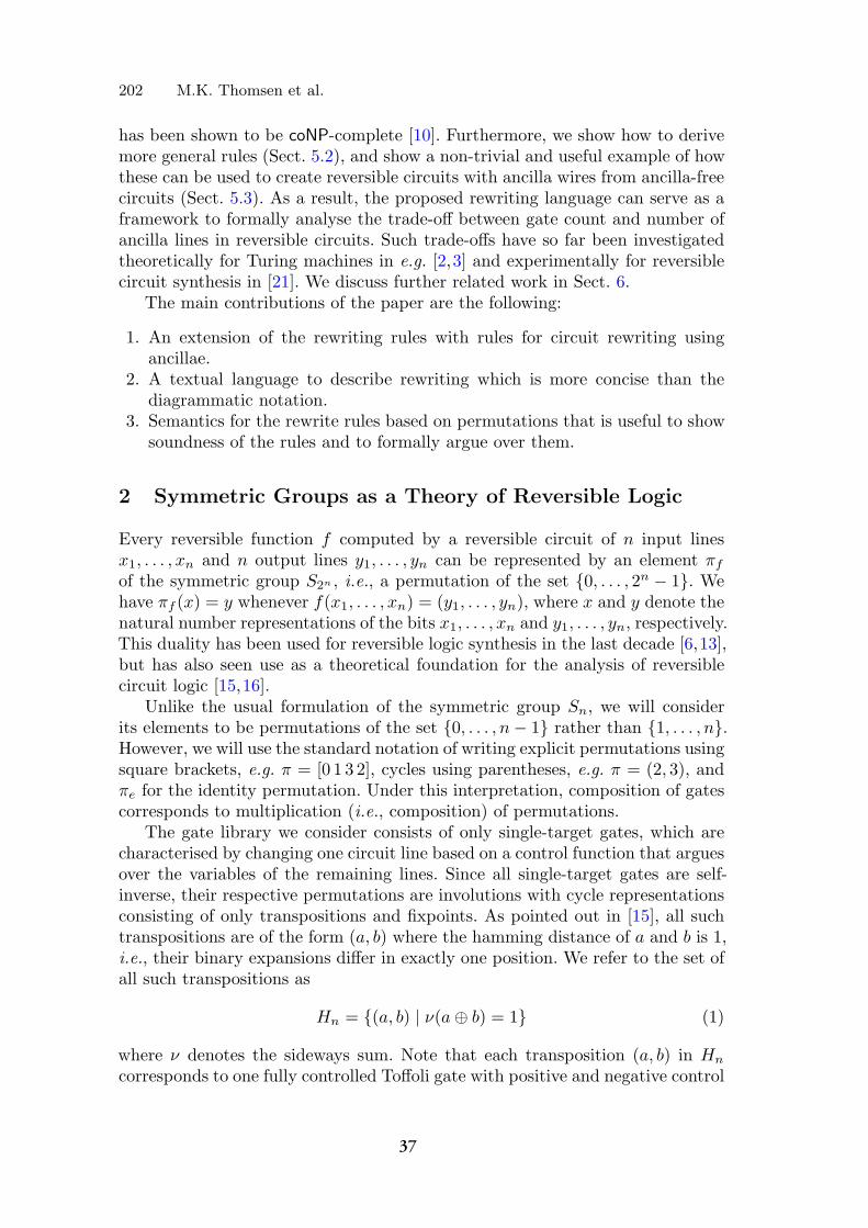
202 M.K. Thomsen et al.

has been shown to be coNP-complete [10]. Furthermore, we show how to derivemore general rules (Sect. 5.2), and show a non-trivial and useful example of howthese can be used to create reversible circuits with ancilla wires from ancilla-freecircuits (Sect. 5.3). As a result, the proposed rewriting language can serve as aframework to formally analyse the trade-off between gate count and number ofancilla lines in reversible circuits. Such trade-offs have so far been investigatedtheoretically for Turing machines in e.g. [2,3] and experimentally for reversiblecircuit synthesis in [21]. We discuss further related work in Sect. 6.

The main contributions of the paper are the following:

1. An extension of the rewriting rules with rules for circuit rewriting usingancillae.

2. A textual language to describe rewriting which is more concise than thediagrammatic notation.

3. Semantics for the rewrite rules based on permutations that is useful to showsoundness of the rules and to formally argue over them.

2 Symmetric Groups as a Theory of Reversible Logic

Every reversible function f computed by a reversible circuit of n input linesx1, . . . , xn and n output lines y1, . . . , yn can be represented by an element πf

of the symmetric group S2n , i.e., a permutation of the set {0, . . . , 2n − 1}. Wehave πf (x) = y whenever f(x1, . . . , xn) = (y1, . . . , yn), where x and y denote thenatural number representations of the bits x1, . . . , xn and y1, . . . , yn, respectively.This duality has been used for reversible logic synthesis in the last decade [6,13],but has also seen use as a theoretical foundation for the analysis of reversiblecircuit logic [15,16].

Unlike the usual formulation of the symmetric group Sn, we will considerits elements to be permutations of the set {0, . . . , n − 1} rather than {1, . . . , n}.However, we will use the standard notation of writing explicit permutations usingsquare brackets, e.g. π = [0 1 3 2], cycles using parentheses, e.g. π = (2, 3), andπe for the identity permutation. Under this interpretation, composition of gatescorresponds to multiplication (i.e., composition) of permutations.

The gate library we consider consists of only single-target gates, which arecharacterised by changing one circuit line based on a control function that arguesover the variables of the remaining lines. Since all single-target gates are self-inverse, their respective permutations are involutions with cycle representationsconsisting of only transpositions and fixpoints. As pointed out in [15], all suchtranspositions are of the form (a, b) where the hamming distance of a and b is 1,i.e., their binary expansions differ in exactly one position. We refer to the set ofall such transpositions as

Hn = {(a, b) | ν(a ⊕ b) = 1} (1)

where ν denotes the sideways sum. Note that each transposition (a, b) in Hn

corresponds to one fully controlled Toffoli gate with positive and negative control

37

Ricercar: A Language for Describing and Rewriting Reversible Circuits 203

lines, acting on line i, where i is the single index for which ai �= bi. The polarityof the controls is chosen according to the other bits. Based on this observation,we partition the set Hn into n sets Hn,1,Hn,2, . . . , Hn,n such that

Hn,i = {(a, b) ∈ Hn | a ⊕ b = 2i−1} (2)

contains all transpositions in which the components differ in their i-th bit. Single-target gates that act on the target line i are all permutations that consist of asubset of transpositions in Hn,i.

We call gn(f) ∈ S2n a transposition generation function which takes as argu-ment an injective function f : {0, . . . , 2n − 1} ↪→ {0, . . . , 2n − 1} and returns thepermutation

(0, f(0))(1, f(1)) · · · (2n − 1, f(2n − 1)). (3)

3 Ricercar: A Description Language for Reversible Logic

In this section, we will explain the description language, Ricercar, that is usedto formulate the rewriting rules. We will first explain the syntax (Fig. 1) andthen show two ways to describe the semantics.

3.1 Syntax

Circuit wires (denoted by lower case Latin letters in the end of the alphabet:. . . , x, y, z) are defined over a set of names Σ that includes both input/outputwires and ancilla wires currently in scope. (For wires without specific names, wewill use lower case Latin letters starting from a.) We define a circuit (denotedby upper case Latin letters) to be one of the following five forms:

– The identity gate on a wire x, written Id(x), where x ∈ Σ.– The not gate applied to a wire x, written Not(x), where x ∈ Σ.– Sequential composition of two circuits, written using the operator “ ; ”.

A, B, C ::= Id(x) | Not(x) Identity and not gate

| A ; B Sequence of circuits

| φ� A Controlled circuit

| αx.A Scope of ancilla variable α; α is part of the syntax

φ, ψ, π ::= x | ¬φ | φ ∧ φ Boolean formulas

| � | ⊥ | φ ∨ φ | φ ⊕ φ Derivable Boolean operators

Fig. 1. Syntax of Ricercar. Note that this grammar does not guarantee reversibility initself. By x we mean that variables occurring in Boolean formulas must be elementsfrom a predefined set of input/output wires or ancilla wires in scope.

38

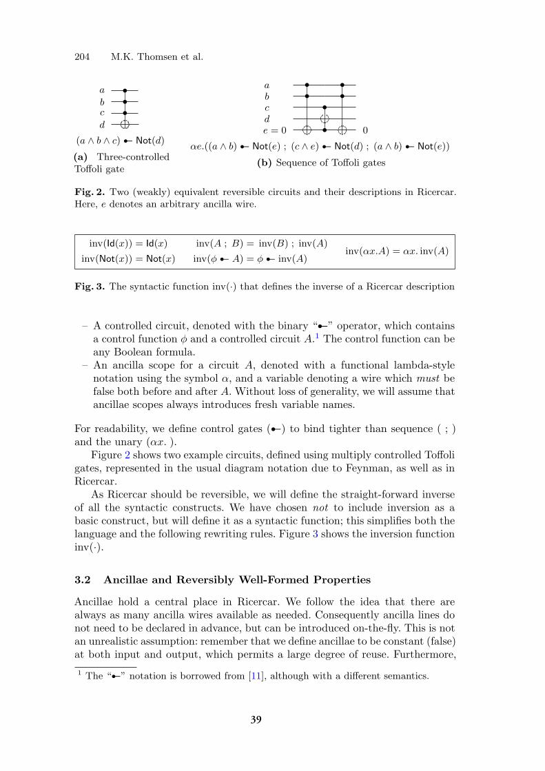
204 M.K. Thomsen et al.

a •b •c •d

(a ∧ b ∧ c)� Not(d)

(a) Three-controlledToffoli gate

a • •b • •c •de = 0 • 0

αe.((a ∧ b)� Not(e) ; (c ∧ e)� Not(d) ; (a ∧ b)� Not(e))

(b) Sequence of Toffoli gates

Fig. 2. Two (weakly) equivalent reversible circuits and their descriptions in Ricercar.Here, e denotes an arbitrary ancilla wire.

inv(Id(x)) = Id(x)

inv(Not(x)) = Not(x)

inv(A ; B) = inv(B) ; inv(A)

inv(φ� A) = φ� inv(A)inv(αx.A) = αx. inv(A)

Fig. 3. The syntactic function inv(·) that defines the inverse of a Ricercar description

– A controlled circuit, denoted with the binary “�” operator, which containsa control function φ and a controlled circuit A.1 The control function can beany Boolean formula.

– An ancilla scope for a circuit A, denoted with a functional lambda-stylenotation using the symbol α, and a variable denoting a wire which must befalse both before and after A. Without loss of generality, we will assume thatancillae scopes always introduces fresh variable names.

For readability, we define control gates (�) to bind tighter than sequence ( ; )and the unary (αx. ).

Figure 2 shows two example circuits, defined using multiply controlled Toffoligates, represented in the usual diagram notation due to Feynman, as well as inRicercar.

As Ricercar should be reversible, we will define the straight-forward inverseof all the syntactic constructs. We have chosen not to include inversion as abasic construct, but will define it as a syntactic function; this simplifies both thelanguage and the following rewriting rules. Figure 3 shows the inversion functioninv(·).

3.2 Ancillae and Reversibly Well-Formed Properties

Ancillae hold a central place in Ricercar. We follow the idea that there arealways as many ancilla wires available as needed. Consequently ancilla lines donot need to be declared in advance, but can be introduced on-the-fly. This is notan unrealistic assumption: remember that we define ancillae to be constant (false)at both input and output, which permits a large degree of reuse. Furthermore,

1 The “�” notation is borrowed from [11], although with a different semantics.

39

Ricercar: A Language for Describing and Rewriting Reversible Circuits 205

rwf(Id(x)) = {x}rwf(Not(x)) = {x}

rwf(A ; B) = rwf(A) ∪ rwf(B)

rwf(φ� A) = dom(φ) � rwf(A)rwf(αx.A) = rwf(A)\{x}

Fig. 4. A reversible circuit, A, is reversibly well-formed iff rwf(A) evaluates to a set.Here, � is the disjoint union and dom(φ) is the domain of the Boolean function φ. Weassume that the disjoint union is undefined whenever the operands are not disjoint.

the actual number of ancilla lines used is limited by the depth of the circuit, andcannot grow unboundedly. As an example, given that we know the upper boundof the depth to implement a reversible circuit without ancillae (cf. [1]), this alsogives an upper bound on the number of (useful) ancilla any circuit with smallerdepth can have.

The syntax presented in Fig. 1 does not guarantee reversibility by itself. Oneproblem comes from the control gate, where we must enforce that the wires ofthe control function are disjoint from wires of the circuit being controlled. This issimilar to the concept used in the reversible updates in Janus [22]. Figure 4 showsa function rwf(·) that implements this check; we say that the circuit is reversiblywell-formed if it upholds this restriction. Given a circuit description A, it returnsthe set of all used variable names if and only if A is reversibly well-formed. If acircuit A is not reversibly well-formed, the disjoint union operation will fail onthe control gate operator, and the result of rwf(A) will thus be undefined.

However, even a reversibly well-formed circuit is not necessarily reversible.2

To ensure that an ancilla variable within an ancilla scope does indeed have ancillabehaviour (guaranteed false at both input and output), we need a additionalsemantic check. However, a circuit without ancillae is reversibly well-formed ifand only if it is reversible. In Sect. 5, we will show how this can be exploited tointroduce ancillae in a way that guarentees reversibility.

3.3 Operational Semantics

The straightforward semantics of Ricercar is shown in Fig. 5; they follow, but alsoextend, the logic by Fredkin and Toffoli, and describe the mapping from a circuitdescription to a reversible circuit using the well-known gates. More concretely,this semantics can be used to show that Ricercar is actually reversible.

Theorem 1 (Reversibility). For all mappings σ and circuits A there exists amapping σ′ and a circuit B such that

σ � A → σ′ ⇐⇒ σ′ � B → σ.

This theorem and the following two lemmas are easily proven by structural induc-tion over the circuit A and reference to the operational semantics of Ricercar(Fig. 5).

2 The other direction holds: all reversible circuits are reversibly well-formed.

40

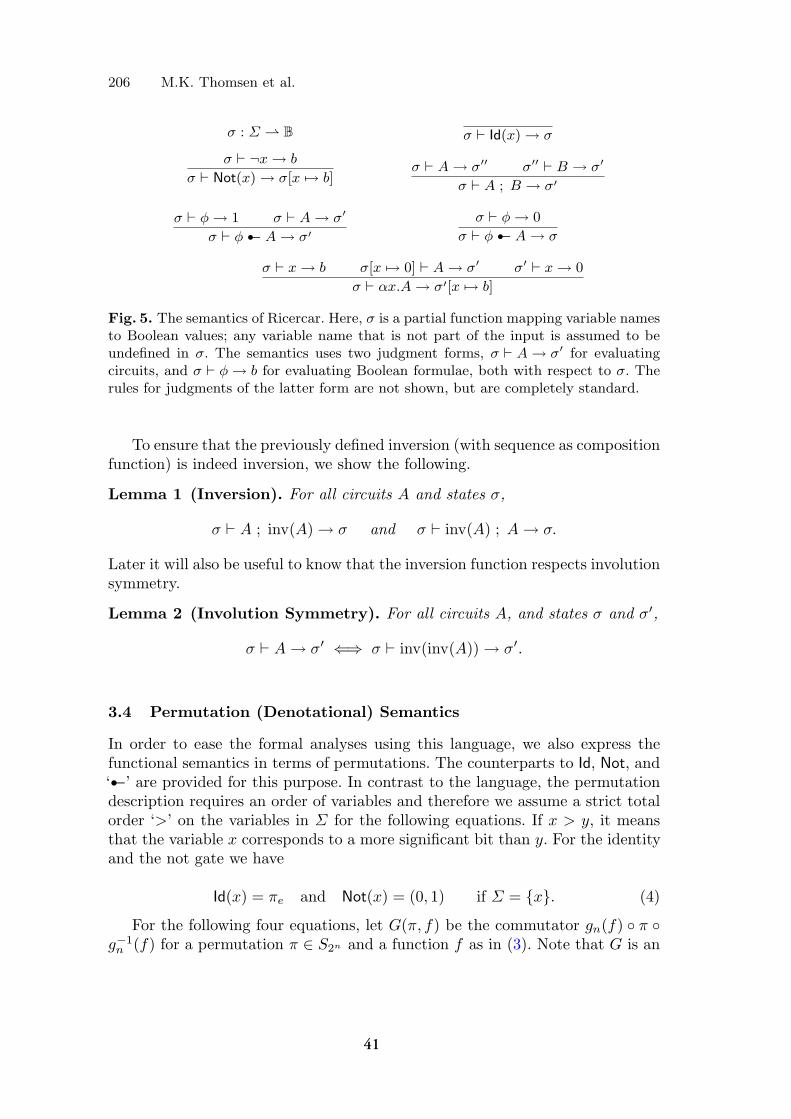
206 M.K. Thomsen et al.

σ : Σ ⇀ B σ � Id(x) → σ

σ � ¬x → b

σ � Not(x) → σ[x → b]σ � A → σ′′ σ′′ � B → σ′

σ � A ; B → σ′

σ � φ → 1 σ � A → σ′

σ � φ� A → σ′σ � φ → 0

σ � φ� A → σ

σ � x → b σ[x → 0] � A → σ′ σ′ � x → 0

σ � αx.A → σ′[x → b]

Fig. 5. The semantics of Ricercar. Here, σ is a partial function mapping variable namesto Boolean values; any variable name that is not part of the input is assumed to beundefined in σ. The semantics uses two judgment forms, σ � A → σ′ for evaluatingcircuits, and σ � φ → b for evaluating Boolean formulae, both with respect to σ. Therules for judgments of the latter form are not shown, but are completely standard.

To ensure that the previously defined inversion (with sequence as compositionfunction) is indeed inversion, we show the following.

Lemma 1 (Inversion). For all circuits A and states σ,

σ � A ; inv(A) → σ and σ � inv(A) ; A → σ.

Later it will also be useful to know that the inversion function respects involutionsymmetry.

Lemma 2 (Involution Symmetry). For all circuits A, and states σ and σ′,

σ � A → σ′ ⇐⇒ σ � inv(inv(A)) → σ′.

3.4 Permutation (Denotational) Semantics

In order to ease the formal analyses using this language, we also express thefunctional semantics in terms of permutations. The counterparts to Id, Not, and‘�’ are provided for this purpose. In contrast to the language, the permutationdescription requires an order of variables and therefore we assume a strict totalorder ‘>’ on the variables in Σ for the following equations. If x > y, it meansthat the variable x corresponds to a more significant bit than y. For the identityand the not gate we have

Id(x) = πe and Not(x) = (0, 1) if Σ = {x}. (4)

For the following four equations, let G(π, f) be the commutator gn(f) ◦ π ◦g−1n (f) for a permutation π ∈ S2n and a function f as in (3). Note that G is an

41

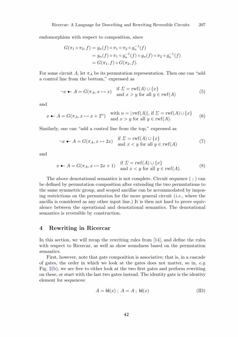
Ricercar: A Language for Describing and Rewriting Reversible Circuits 207

endomorphism with respect to composition, since

G(π1 ◦ π2, f) = gn(f) ◦ π1 ◦ π2 ◦ g−1n (f)

= gn(f) ◦ π1 ◦ g−1n (f) ◦ gn(f) ◦ π2 ◦ g−1

n (f)= G(π1, f) ◦ G(π2, f).

For some circuit A, let πA be its permutation representation. Then one can “adda control line from the bottom,” expressed as

¬x� A = G(πA, x → x) if Σ = rwf(A) ∪ {x}and x > y for all y ∈ rwf(A) (5)

and

x� A = G(πA, x → x + 2n) with n = | rwf(A)|, if Σ = rwf(A)∪{x}and x > y for all y ∈ rwf(A). (6)

Similarly, one can “add a control line from the top,” expressed as

¬x� A = G(πA, x → 2x) if Σ = rwf(A) ∪ {x}and x < y for all y ∈ rwf(A) (7)

and

x� A = G(πA, x → 2x + 1) if Σ = rwf(A) ∪ {x}and x < y for all y ∈ rwf(A). (8)

The above denotational semantics is not complete. Circuit sequence ( ; ) canbe defined by permutation composition after extending the two permutations tothe same symmetric group, and scoped ancillae can be accommodated by impos-ing restrictions on the permutation for the more general circuit (i.e., where theancilla is considered as any other input line.) It is then not hard to prove equiv-alence between the operational and denotational semantics. The denotationalsemantics is reversible by construction.

4 Rewriting in Ricercar

In this section, we will recap the rewriting rules from [14], and define the ruleswith respect to Ricercar, as well as show soundness based on the permutationsemantics.

First, however, note that gate composition is associative; that is, in a cascadeof gates, the order in which we look at the gates does not matter, so in, e.g.Fig. 2(b), we are free to either look at the two first gates and perform rewritingon these, or start with the last two gates instead. The identity gate is the identityelement for sequences:

A = Id(x) ; A = A ; Id(x) (ID)

42

208 M.K. Thomsen et al.

Furthermore, note that we can always rewrite the controlling Boolean func-tions and, e.g. use identities from AND-EXOR decomposition:

φ� ψ � A = (φ ∧ ψ)� A andφ� A ; ψ � A = (φ ⊕ ψ)� A if A = inv(A).

Finally, implicit to rules is that the circuits must always be reversibly well-formed both before and after a rewriting, and that in any given circuit we canrewrite any sub-circuit we like.

The first rule presented in [14] is for introducing and eliminating not gates,and states that we can always rewrite the identity function to two not gates.

x = Id(x) = Not(x) ; Not(x) (R1)Soundness trivially follows from πe = (0, 1) ◦ (0, 1).

The second rule states that we can “move” a not gate over a control if wenegate the control line.

x •=

y

x� Not(y) ; Not(x) =Not(x) ; ¬x� Not(y) (R2)

Similar to [14], we notice that its dual rule with negative control can bederived using this rule in combination with Rule R1:

¬x� Not(y) ; Not(x)(R1)= Not(x) ; Not(x) ; ¬x� Not(y) ; Not(x)

(R2)= Not(x) ; x� Not(y) ; Not(x) ; Not(x)

(R1)= Not(x) ; x� Not(y). (R2’)

Soundness follows from Eqs. (5)–(8) and the identity (a, b)(b, c) = (a, c)(a, b) =(a, c)(b, c).

Third, we can extend a gate by copying it and adding once a positive andonce a negative control line to it.

x •=

y

Id(x) ; Not(y) =x� Not(y) ; ¬x� Not(y) (R3)

Soundness follows from Eqs. (7) and (8). In fact, in permutation notation, bothcontrolled not gates are represented by a single transposition, and combiningthem results in the (permutation corresponding to the) not gate. Also, combiningthe equation of adding a negative and positive control yields an equation foradding an empty line.

Next, two arbitrary adjacent gates can be interchanged whenever they havea common control line with different polarities. Notice how Ricercar capturesthe fact that two controlled circuits can have any circuit structure; somethingthat is not well captured by the diagrammatic notation in [14].

43

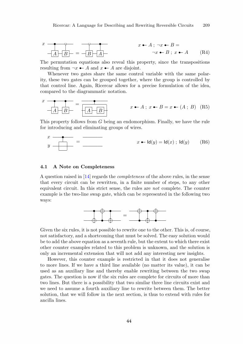
Ricercar: A Language for Describing and Rewriting Reversible Circuits 209

x • •A B = B A

x� A ; ¬x� B =¬x� B ; x� A (R4)

The permutation equations also reveal this property, since the transpositionsresulting from ¬x� A and x� A are disjoint.

Whenever two gates share the same control variable with the same polar-ity, these two gates can be grouped together, where the group is controlled bythat control line. Again, Ricercar allows for a precise formulation of the idea,compared to the diagrammatic notation.

x • •=

A B

•A B

x� A ; x� B = x� (A ; B) (R5)

This property follows from G being an endomorphism. Finally, we have the rulefor introducing and eliminating groups of wires.

x •=

yx� Id(y) = Id(x) ; Id(y) (R6)

4.1 A Note on Completeness

A question raised in [14] regards the completeness of the above rules, in the sensethat every circuit can be rewritten, in a finite number of steps, to any otherequivalent circuit. In this strict sense, the rules are not complete. The counterexample is the two-line swap gate, which can be represented in the following twoways:

• • •=

• • •Given the six rules, it is not possible to rewrite one to the other. This is, of course,not satisfactory, and a shortcoming that must be solved. The easy solution wouldbe to add the above equation as a seventh rule, but the extent to which there existother counter examples related to this problem is unknown, and the solution isonly an incremental extension that will not add any interesting new insights.

However, this counter example is restricted in that it does not generaliseto more lines. If we have a third line available (no matter its value), it can beused as an auxiliary line and thereby enable rewriting between the two swapgates. The question is now if the six rules are complete for circuits of more thantwo lines. But there is a possibility that two similar three line circuits exist andwe need to assume a fourth auxiliary line to rewrite between them. The bettersolution, that we will follow in the next section, is thus to extend with rules forancilla lines.

44

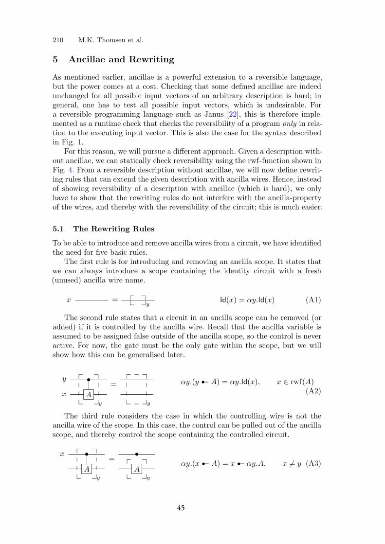
210 M.K. Thomsen et al.

5 Ancillae and Rewriting

As mentioned earlier, ancillae is a powerful extension to a reversible language,but the power comes at a cost. Checking that some defined ancillae are indeedunchanged for all possible input vectors of an arbitrary description is hard; ingeneral, one has to test all possible input vectors, which is undesirable. Fora reversible programming language such as Janus [22], this is therefore imple-mented as a runtime check that checks the reversibility of a program only in rela-tion to the executing input vector. This is also the case for the syntax describedin Fig. 1.

For this reason, we will pursue a different approach. Given a description with-out ancillae, we can statically check reversibility using the rwf-function shown inFig. 4. From a reversible description without ancillae, we will now define rewrit-ing rules that can extend the given description with ancilla wires. Hence, insteadof showing reversibility of a description with ancillae (which is hard), we onlyhave to show that the rewriting rules do not interfere with the ancilla-propertyof the wires, and thereby with the reversibility of the circuit; this is much easier.

5.1 The Rewriting Rules

To be able to introduce and remove ancilla wires from a circuit, we have identifiedthe need for five basic rules.

The first rule is for introducing and removing an ancilla scope. It states thatwe can always introduce a scope containing the identity circuit with a fresh(unused) ancilla wire name.

x =y

� ���

��� � Id(x) = αy.Id(x) (A1)

The second rule states that a circuit in an ancilla scope can be removed (oradded) if it is controlled by the ancilla wire. Recall that the ancilla variable isassumed to be assigned false outside of the ancilla scope, so the control is neveractive. For now, the gate must be the only gate within the scope, but we willshow how this can be generalised later.

y •=

x Ay y

� �����

����

� �

� � �����

����

� � �

αy.(y � A) = αy.Id(x), x ∈ rwf(A)(A2)

The third rule considers the case in which the controlling wire is not theancilla wire of the scope. In this case, the control can be pulled out of the ancillascope, and thereby control the scope containing the controlled circuit.

x • •=

A Ay y

� ��

�

�

�� �

� �����

����

� �

αy.(x� A) = x� αy.A, x �= y (A3)

45

Ricercar: A Language for Describing and Rewriting Reversible Circuits 211

The fourth rules states that a not gate on a non-ancilla wire that is positionedto the immediate left of a circuit it shares a scope with can be pulled out of theancilla scope.

xA A=

y y

� � � �����

����� � � �

� � �����

����� � �

αy.(Not(x) ; A) =Not(x) ; αy.A, x �= y (A4)

In the case where the not gate is on the right, a similar rule can be derivedfrom the Involution Symmetry Lemma with Rule A4.

xA A=

y y

� � � �����

����� � � �

� � �����

����� � �

αy.(A ; Not(x)) =(αy.A) ; Not(x), x �= y (A4’)

The fifth and final rule states that if (and only if) an ancilla scope containsa sequence of two circuits where the first is positively controlled, and the secondis negatively controlled by the same wire, then this scope can be divided intotwo; or, in the other direction, merged. Note that x can be equal to y. This ruleis likely the most powerful of the five, and it shows up in the proofs that extendand generalise the previous rules.

x • •=A B A B

y y y

� � � � �����

����

� � � � �

� �����

����

� �

� � �����

����

� � �

αy.(x� A ; ¬x� B) =(αy.x� A) ; (αy.¬x� B) (A5)

That the first four rules (A1 to A4) do not interfere with the ancilla-propertyof a wire is clear, but the last rule (A5) requires an argument. Only either A orB (but not both) is performed as the control on x is exclusive. Thus assumingthat x �= y, any usage of y in A must have uncomputed y to zero again; similarlyany usage of y in B must have assumed it to be zero. Therefore, we can dividethe ancilla scope of y. If x = y then y will always be unchanged (zero) as y isnot used in B.

5.2 Generalisation of Ancilla Rules

Rule A2 has a twin-rule for the case where the gate is negatively controlled bythe ancilla wire. We can derive that this is equal to the controlled gate in thefollowing way:

αy.(¬y � A)(ID)= Id(x) ; (αy.¬y � A)

(A1)= (αy.Id(x)) ; (αy.¬y � A)

(A2)= (αy.y � A) ; (αy.¬y � A)

(A5)= αy.(y � A ; ¬y � A)

(R3)= αy.A. (A2’)

46

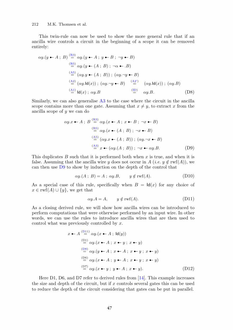
212 M.K. Thomsen et al.

This twin-rule can now be used to show the more general rule that if anancilla wire controls a circuit in the beginning of a scope it can be removedentirely:

αy.(y � A ; B)(R3)= αy.(y � A ; y � B ; ¬y � B)

(R5)= αy.(y � (A ; B) ; ¬α� .B)

(A5)= (αy.y � (A ; B)) ; (αy.¬y � B)

(A2)= (αy.Id(x)) ; (αy.¬y � B)

(A2’)= (αy.Id(x)) ; (αy.B)

(A1)= Id(x) ; αy.B

(ID)= αy.B. (D8)

Similarly, we can also generalise A3 to the case where the circuit in the ancillascope contains more than one gate. Assuming that x �= y, to extract x from theancilla scope of y we can do

αy.x� A ; B(R3)= αy.(x� A ; x� B ; ¬x� B)

(R5)= αy.(x� (A ; B) ; ¬x� B)

(A5)= (αy.x� (A ; B)) ; (αy.¬x� B)

(A3)= x� (αy.(A ; B)) ; ¬x� αy.B. (D9)

This duplicates B such that it is performed both when x is true, and when it isfalse. Assuming that the ancilla wire y does not occur in A (i.e. y /∈ rwf(A)), wecan then use D9 to show by induction on the depth of the control that

αy.(A ; B) = A ; αy.B, y /∈ rwf(A). (D10)

As a special case of this rule, specifically when B = Id(x) for any choice ofx ∈ rwf(A) ∪ {y}, we get that

αy.A = A, y /∈ rwf(A). (D11)

As a closing derived rule, we will show how ancilla wires can be introduced toperform computations that were otherwise performed by an input wire. In otherwords, we can use the rules to introduce ancilla wires that are then used tocontrol what was previously controlled by x.

x� A(D11)= αy.(x� A ; Id(y))

(D1)= αy.(x� A ; x� y ; x� y)

(D8)= αy.(y � A ; x� A ; x� y ; x� y)

(D6)= αy.(x� A ; y � A ; x� y ; x� y)

(D7)= αy.(x� y ; y � A ; x� y). (D12)

Here D1, D6, and D7 refer to derived rules from [14]. This example increasesthe size and depth of the circuit, but if x controls several gates this can be usedto reduce the depth of the circuit considering that gates can be put in parallel.

47

Ricercar: A Language for Describing and Rewriting Reversible Circuits 213

5.3 Practical Example of Application of Ricercar

As a final example we show how to derive the circuit depicted in Fig. 2(b) fromthe one in Fig. 2(a) using the rewriting rules. Again D1 and D7 refer to derivedrules from [14].

(a ∧ b ∧ c)� Not(d)

(D11)= αe.((a ∧ b ∧ c)� Not(d))

(D8)= αe.((c ∧ β)� Not(d) ; (a ∧ b ∧ c)� Not(d))

(D1)= αe.((a ∧ b)� Not(e) ; (a ∧ b)� Not(e) ; (c ∧ e)� Not(d) ;

(a ∧ b ∧ c)� Not(d))

(D7)= αe.((a ∧ b)� Not(e) ; (c ∧ e)� Not(d) ; (a ∧ b)� Not(e) ;

(a ∧ b ∧ c)� Not(d) ; (a ∧ b ∧ c)� Not(d))

(D1)= αe.((a ∧ b)� Not(e) ; (c ∧ e)� Not(d) ; (a ∧ b)� Not(e)).

6 Related Work

This is not the first language that has been designed to describe the concepts ofreversible logic; there exist description languages for both reversible and quan-tum circuits.

The closest related work is the Reversible Combinator Language (RCL) [18]that was also made to describe reversible logic; though it is more general thanour work, there are still some common ideas. Taking inspiration from RCL, weuse a similar sequence operator, and the conditional in RCL is (in its semantics)comparable to our control operator. However, being a combinator language, RCLdoes not have variables, but rather a type system in which circuits of arbitrarysize with a given structure can be defined. Also it has more general combinators,such as a ripple circuit and parallel composition, as basic constructs. RCL alsoadmits a number of rewriting rules, but compared to Ricercar, RCL’s type systemand larger set of atomic gates makes rewriting more cumbersome.

Although aiming to describe quantum circuits, it is worth mentioning Quip-per [8,9]. Though Quipper also supports ancilla scopes, in order to upholdthe ancilla-property, the Quipper synthesis results in a symmetric compute-use-uncompute “Bennett-style” structure of the ancilla wires. In contrast, the ancillascopes in Ricercar are more general, but have to be built from the bottom upwith rewriting to uphold the property. The interested reader can find furtherreferences for quantum description languages in the works above.

7 Conclusion

In this paper we have presented Ricercar, a language designed to describereversible circuits. A main focus during the design process of the language has

48

214 M.K. Thomsen et al.

been rewriting, specifically that rewriting rules should be easy to both define andapply in the language. The previous approach to rewriting of reversible circuitswas shown for the standard diagrammatic notation, but this notation neithercaptures the full intent of all of the six original rules, nor does it provide anoptimal setting for a future computer aided system. Ricercar, with its simplesymbolic description, both captures the complete intent of the original rules,and has a syntax that is directly implementable.

In addition, Ricercar has support for ancillae as a basic circuit construct inthe form of a scope. Using this construct, we have extended the six original ruleswith five basic rules that applies when rewriting ancillae. We have shown howit is possible to use these rules to derive more general ones that also apply toancillae, and as a final example, how to derive a rule that moves the control ofa gate from an input wire to an ancilla wire.

Determining reversibility of a circuit that contains ancillae is generally hard,but with the presented rewriting rules, it is possible to take an ancillae-freecircuit (for which it is easy to show reversibility) and rewrite it into a circuitthat contains ancillae, and is guaranteed to be reversible. The key here is thatthe basic rules (and all of the derived rules) cannot break the ancilla-propertyof a wire and, thus, the reversibility of the circuit.

We hope that this approach can further help in the understanding of thetrade-off between ancillae on the one hand, and the size and depth of a reversiblecircuit on the other.

Acknowledgments. The authors thank the anonymous reviewers from RC’14 fortheir useful comments on a preliminary version of this paper, presented as work-in-progress at 6th Conference on Reversible Computation, 2014 and the anonymousreviewers from RC’15 on the current version. Finally, we thank Holger Bock Axelsenfor several discussion on work in this paper.

References

1. Abdessaied, N., Soeken, M., Thomsen, M.K., Drechsler, R.: Upper bounds forreversible circuits based on Young subgroups. Information Processing Letters114(6), 282–286 (2014)

2. Bennett, C.H.: Time/Space Trade-Offs for reversible computation. SIAM Journalon Computing 18(4), 766–776 (1989)

3. Buhrman, H., Tromp, J., Vitanyi, P.: Time and space bounds for reversible simu-lation. Journal of Physics A: Mathematical and General 34(35), 6821–6830 (2001)

4. Chan, T., Munro, J.I., Raman, V.: Selection and sorting in the “restore” model.In: Proceedings of the Twenty-Fifth Annual ACM-SIAM Symposium on DiscreteAlgorithms, pp. 995–1004 (2014)

5. Cuccaro, S.A., Draper, T.G., Kutin, S.A., Moulton, D.P.: A new quantum ripple-carry addition circuit. arXiv:quant-ph/0410184v1 (2005)

6. De Vos, A., Rentergem, Y.V.: Reversible computing: from mathematical grouptheory to electronical circuit experiment. In: Proceedings of the Second Conferenceon Computing Frontiers, 2005, Ischia, Italy, May 4–6, 2005, pp. 35–44 (2005)

49

Ricercar: A Language for Describing and Rewriting Reversible Circuits 215

7. Draper, T.G., Kutin, S.A., Rains, E.M., Svore, K.M.: A logarithmic-depth quantumcarry-lookahead adder. arXiv:quant-ph/0406142 (2008)

8. Green, A.S., Lumsdaine, P.L.F., Ross, N.J., Selinger, P., Valiron, B.: An introduc-tion to quantum programming in quipper. In: Dueck, G.W., Miller, D.M. (eds.)RC 2013. LNCS, vol. 7948, pp. 110–124. Springer, Heidelberg (2013)

9. Green, A.S., Lumsdaine, P.L., Ross, N.J., Selinger, P., Valiron, B.: Quipper: a scal-able quantum programming language. In: Conference on Programming LanguageDesign and Implementation, PLDI 2013, pp. 333–342. ACM (2013)

10. Jordan, S.P.: Strong equivalence of reversible circuits is coNP-complete. QuantumInformation & Computation 14(15–16), 1302–1307 (2014)

11. Kaarsgaard, R.: Towards a propositional logic for reversible logic circuits. In: deHaan, R. (ed.) Proceedings of the ESSLLI 2014 Student Session, pp. 33–41 (2014).http://www.kr.tuwien.ac.at/drm/dehaan/stus2014/proceedings.pdf

12. Miller, D.M., Maslov, D., Dueck, G.W.: A transformation based algorithm forreversible logic synthesis. In: Design Automation Conference, DAC, pp. 318–323(2003)

13. Shende, V.V., Prasad, A.K., Markov, I.L., Hayes, J.P.: Synthesis of reversible logiccircuits. IEEE Trans. on CAD of Integrated Circuits and Systems 22(6), 710–722(2003)

14. Soeken, M., Thomsen, M.K.: White dots do matter: rewriting reversible logic cir-cuits. In: Dueck, G.W., Miller, D.M. (eds.) RC 2013. LNCS, vol. 7948, pp. 196–208.Springer, Heidelberg (2013)

15. Soeken, M., Thomsen, M.K., Dueck, G.W., Miller, D.M.: Self-inverse functions andpalindromic circuits. arXiv 1502.05825 (2015)

16. Storme, L., De Vos, A., Jacobs, G.: Group theoretical aspects of reversible logicgates. J. UCS 5(5), 307–321 (1999)

17. Takahashi, Y., Kunihiro, N.: A fast quantum circuit for addition with few qubits.Quantum Info. Comput. 8(6), 636–649 (2008)

18. Thomsen, M.K.: Describing and optimising reversible logic using a functional lan-guage. In: Gill, A., Hage, J. (eds.) IFL 2011. LNCS, vol. 7257, pp. 148–163. Springer,Heidelberg (2012)

19. Thomsen, M.K., Axelsen, H.B.: Parallelization of reversible ripple-carry adders.Parallel Processing Letters 19(1), 205–222 (2009)

20. Vedral, V., Barenco, A., Ekert, A.: Quantum networks for elementary arithmeticoperations. Physical Review A 54(1), 147–153 (1996)

21. Wille, R., Soeken, M., Miller, D.M., Drechsler, R.: Trading off circuit lines andgate costs in the synthesis of reversible logic. Integration, the VLSI Journal 47(2),284–294 (2014)

22. Yokoyama, T., Axelsen, H.B., Gluck, R.: Principles of a reversible programminglanguage. In: Conference on Computing Frontiers, CF, pp. 43–54. ACM Press(2008)

50

51

52

A Classical Propositional Logic for ReasoningAbout Reversible Logic Circuits

Holger Bock Axelsen, Robert Gluck, and Robin Kaarsgaard(B)

DIKU, Department of Computer Science,University of Copenhagen, Copenhagen, Denmark

{funkstar,glueck,robin}@di.ku.dk

Abstract. We propose a syntactic representation of reversible logic cir-cuits in their entirety, based on Feynman’s control interpretation of Tof-foli’s reversible gate set. A pair of interacting proof calculi for reasoningabout these circuits is presented, based on classical propositional logicand monoidal structure, and a natural order-theoretic structure is devel-oped, demonstrated equivalent to Boolean algebras, and extended cat-egorically to form a sound and complete semantics for this system. Weshow that all strong equivalences of reversible logic circuits are prov-able in the system, derive an equivalent equational theory, and describeits main applications in the verification of both reversible circuits andtemplate-based reversible circuit rewriting systems.

1 Introduction

Reversible computing–the study of computing models deterministic in both theforward and backward directions–is primarily motivated by a potential to reducethe power consumption of computing processes, but has also seen applicationsin topics such as static average-case program analysis [17], unified descriptionsof parsers and pretty-printers [16], and quantum computing [6]. The potentialenergy reduction was first theorized by Rolf Landauer in the early 1960s [12], andhas more recently seen experimental verification [2,14]. Reaping these potentialbenefits in energy consumption, however, requires the use of a specialized gateset guaranteeing reversibility, when applied at the level of logic circuits.

Boolean logic circuits correspond immediately to propositions in classicalpropositional logic (CPL): This is done by identifying input lines with proposi-tional atoms, and logic gates with propositional connectives, reducing the prob-lem of reasoning about circuits to that of reasoning about arbitrary propositionsin a classical setting. However, although Toffoli’s gate set for reversible circuitlogic is equivalent to the Boolean one in terms of what can be computed [22],it falls short of this immediate and pleasant correspondence. This article seeks

The authors acknowledge support from the Danish Council for IndependentResearch | Natural Sciences under the Foundations of Reversible Computing project,and partial support from COST Action IC1405 Reversible Computation.Colors in electronic version.

c© Springer-Verlag Berlin Heidelberg 2016J. Vaananen et al. (Eds.): WoLLIC 2016, LNCS 9803, pp. 52–67, 2016.DOI: 10.1007/978-3-662-52921-8 4

53

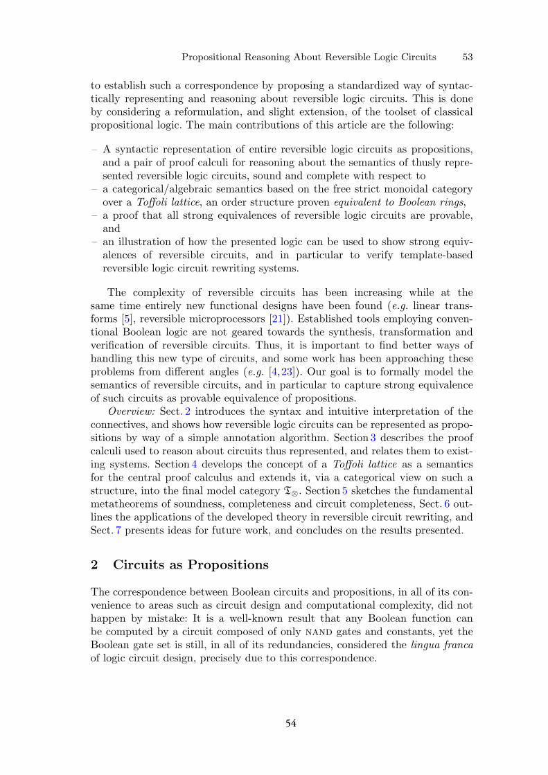
Propositional Reasoning About Reversible Logic Circuits 53

to establish such a correspondence by proposing a standardized way of syntac-tically representing and reasoning about reversible logic circuits. This is doneby considering a reformulation, and slight extension, of the toolset of classicalpropositional logic. The main contributions of this article are the following:

– A syntactic representation of entire reversible logic circuits as propositions,and a pair of proof calculi for reasoning about the semantics of thusly repre-sented reversible logic circuits, sound and complete with respect to

– a categorical/algebraic semantics based on the free strict monoidal categoryover a Toffoli lattice, an order structure proven equivalent to Boolean rings,

– a proof that all strong equivalences of reversible logic circuits are provable,and

– an illustration of how the presented logic can be used to show strong equiv-alences of reversible circuits, and in particular to verify template-basedreversible logic circuit rewriting systems.

The complexity of reversible circuits has been increasing while at thesame time entirely new functional designs have been found (e.g. linear trans-forms [5], reversible microprocessors [21]). Established tools employing conven-tional Boolean logic are not geared towards the synthesis, transformation andverification of reversible circuits. Thus, it is important to find better ways ofhandling this new type of circuits, and some work has been approaching theseproblems from different angles (e.g. [4,23]). Our goal is to formally model thesemantics of reversible circuits, and in particular to capture strong equivalenceof such circuits as provable equivalence of propositions.

Overview: Sect. 2 introduces the syntax and intuitive interpretation of theconnectives, and shows how reversible logic circuits can be represented as propo-sitions by way of a simple annotation algorithm. Section 3 describes the proofcalculi used to reason about circuits thus represented, and relates them to exist-ing systems. Section 4 develops the concept of a Toffoli lattice as a semanticsfor the central proof calculus and extends it, via a categorical view on such astructure, into the final model category T⊗. Section 5 sketches the fundamentalmetatheorems of soundness, completeness and circuit completeness, Sect. 6 out-lines the applications of the developed theory in reversible circuit rewriting, andSect. 7 presents ideas for future work, and concludes on the results presented.

2 Circuits as Propositions

The correspondence between Boolean circuits and propositions, in all of its con-venience to areas such as circuit design and computational complexity, did nothappen by mistake: It is a well-known result that any Boolean function canbe computed by a circuit composed of only nand gates and constants, yet theBoolean gate set is still, in all of its redundancies, considered the lingua francaof logic circuit design, precisely due to this correspondence.

54

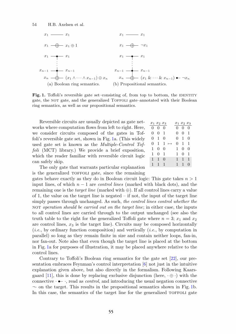
54 H.B. Axelsen et al.

Fig. 1. Toffoli’s reversible gate set–consisting of, from top to bottom, the identitygate, the not gate, and the generalized Toffoli gate–annotated with their Booleanring semantics, as well as our propositional semantics.

x1 x2 x3 x1 x2 x3

0 0 0 0 0 00 0 1 0 0 10 1 0 0 1 00 1 1 �→ 0 1 11 0 0 1 0 01 0 1 1 0 11 1 0 1 1 11 1 1 1 1 0

Reversible circuits are usually depicted as gate net-works where computation flows from left to right. Here,we consider circuits composed of the gates in Tof-foli’s reversible gate set, shown in Fig. 1a. (This widelyused gate set is known as the Multiple-Control Tof-foli (MCT) library.) We provide a brief exposition,which the reader familiar with reversible circuit logiccan safely skip.

The only gate that warrants particular explanationis the generalized toffoli gate, since the remaininggates behave exactly as they do in Boolean circuit logic: This gate takes n > 1input lines, of which n − 1 are control lines (marked with black dots), and theremaining one is the target line (marked with ⊕). If all control lines carry a valueof 1, the value on the target line is negated – if not, the input of the target linesimply passes through unchanged. As such, the control lines control whether thenot operation should be carried out on the target line; in either case, the inputsto all control lines are carried through to the output unchanged (see also thetruth table to the right for the generalized Toffoli gate where n = 3; x1 and x2

are control lines, x3 is the target line). Circuits may be composed horizontally(i.e., by ordinary function composition) and vertically (i.e., by computation inparallel) so long as they remain finite in size and contain neither loops, fan-in,nor fan-out. Note also that even though the target line is placed at the bottomin Fig. 1a for purposes of illustration, it may be placed anywhere relative to thecontrol lines.

Contrary to Toffoli’s Boolean ring semantics for the gate set [22], our pre-sentation embraces Feynman’s control interpretation [6] not just in the intuitiveexplanation given above, but also directly in the formalism. Following Kaars-gaard [11], this is done by replacing exclusive disjunction (here, · ⊕ ·) with theconnective · •− ·, read as control, and introducing the usual negation connective¬· on the target. This results in the propositional semantics shown in Fig. 1b.In this case, the semantics of the target line for the generalized toffoli gate

55

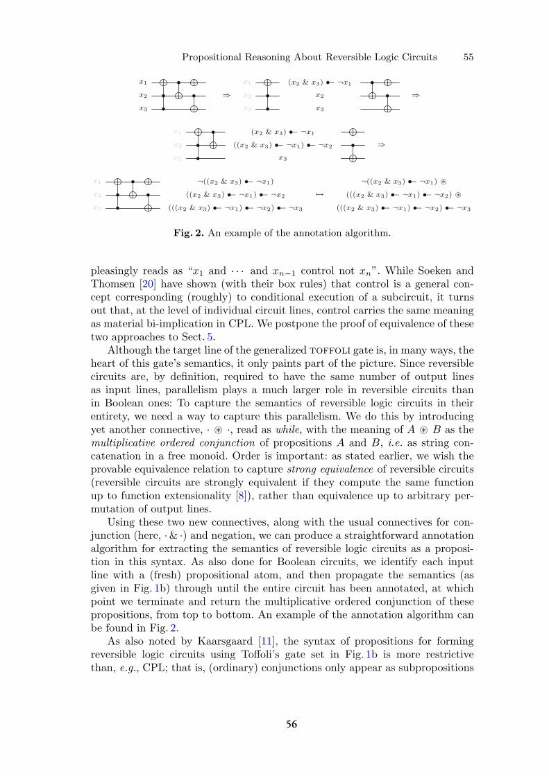
Propositional Reasoning About Reversible Logic Circuits 55

Fig. 2. An example of the annotation algorithm.

pleasingly reads as “x1 and · · · and xn−1 control not xn”. While Soeken andThomsen [20] have shown (with their box rules) that control is a general con-cept corresponding (roughly) to conditional execution of a subcircuit, it turnsout that, at the level of individual circuit lines, control carries the same meaningas material bi-implication in CPL. We postpone the proof of equivalence of thesetwo approaches to Sect. 5.

Although the target line of the generalized toffoli gate is, in many ways, theheart of this gate’s semantics, it only paints part of the picture. Since reversiblecircuits are, by definition, required to have the same number of output linesas input lines, parallelism plays a much larger role in reversible circuits thanin Boolean ones: To capture the semantics of reversible logic circuits in theirentirety, we need a way to capture this parallelism. We do this by introducingyet another connective, · � ·, read as while, with the meaning of A � B as themultiplicative ordered conjunction of propositions A and B, i.e. as string con-catenation in a free monoid. Order is important: as stated earlier, we wish theprovable equivalence relation to capture strong equivalence of reversible circuits(reversible circuits are strongly equivalent if they compute the same functionup to function extensionality [8]), rather than equivalence up to arbitrary per-mutation of output lines.

Using these two new connectives, along with the usual connectives for con-junction (here, ·& ·) and negation, we can produce a straightforward annotationalgorithm for extracting the semantics of reversible logic circuits as a proposi-tion in this syntax. As also done for Boolean circuits, we identify each inputline with a (fresh) propositional atom, and then propagate the semantics (asgiven in Fig. 1b) through until the entire circuit has been annotated, at whichpoint we terminate and return the multiplicative ordered conjunction of thesepropositions, from top to bottom. An example of the annotation algorithm canbe found in Fig. 2.

As also noted by Kaarsgaard [11], the syntax of propositions for formingreversible logic circuits using Toffoli’s gate set in Fig. 1b is more restrictivethan, e.g., CPL; that is, (ordinary) conjunctions only appear as subpropositions

56

56 H.B. Axelsen et al.

of controls. Further, linear ordered conjunctions only appear as a way of “glue-ing” the propositions of individual circuit lines together (see, e.g., the final stepin Fig. 2).

This structure suggests a syntactic hierarchy, which we will illustrate bymeans of color: Blue propositions will be those that correspond to the semanticsof a single circuit line (perhaps of many in a circuit), red propositions correspondto the semantics of entire circuits (or subcircuits), and yellow (or recolorable)propositions will be those that can be either of these two. Formally, we definesuch propositions to be those produced by the grammars

AB , BB , CB := AY | ¬AB | AB & BB (Blue propositions)AY , BY , CY := a | 0 | 1 | ¬AY | AB •− BY | AY •− BB (Yellow propositions)AR, BR, CR := AY | AR � BR | e (Red propositions)

where a denotes any propositional atom; we will assume that there is a denu-merable set P of these. For readability, we adopt the convention that ¬· bindstighter than · & ·, which binds tighter than · •− ·, which finally binds tighterthan ·� ·. Further, we will omit subscripts when the syntactic class is clear fromthe context.

Starting with blue and recolorable propositions, 0 and 1 represent the falserespectively true proposition (corresponding to ancillae, lines of constant value,in circuit terms), ¬AY the usual negation of a proposition, AB •− BY and AY •−BB as “A control B”, and finally AB & BB as the usual (additive) conjunction.Red propositions are interpreted as circuit structures, with AR�BR representingthe ordered (parallel) structure made up of AR and BR, and e representing theempty structure (i.e., the empty circuit). Further, we will denote the set of allsuch well-formed blue respectively red propositions by ΦB respectively ΦR.

In the same manner, well-formed blue and red contexts (a notion of a recol-orable context is unnecessary) are those produced by the grammars

ΓB ,ΔB ,ΠB := · | ΓB, AB (Blue contexts)ΓR,ΔR,ΠR := · | ΓR, AR (Red contexts)

The distinction between the empty blue context and the empty red one is impor-tant, since the two types of contexts will be interpreted in two different ways;blue contexts are interpreted as an additive (blue) conjunction with 1 as unit,while red contexts are interpreted as an ordered multiplicative (red) conjunc-tion with e as unit. As we did for propositions, we will denote the set of allwell-formed blue respectively red contexts by Φ∗

B respectively Φ∗R.

3 Proof Calculi

As the syntax presented in the previous section perhaps already alludes to,we will use not one but two proof calculi to reason about propositions thusformed. Figures 3 and 4 show the two proof calculi–the blue and the red fragment,respectively–that make up the logic which we shall call LRS�.

57

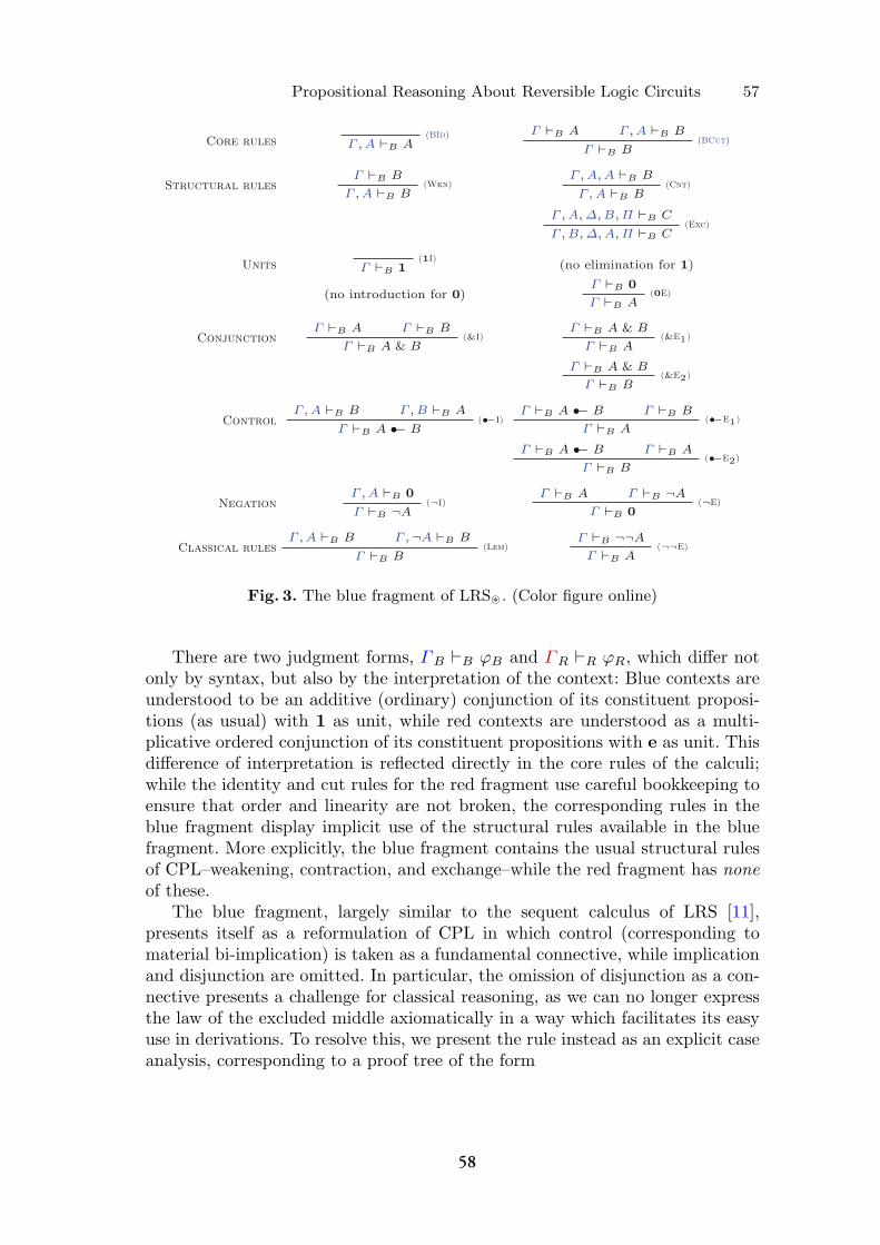
Propositional Reasoning About Reversible Logic Circuits 57

Fig. 3. The blue fragment of LRS� . (Color figure online)

There are two judgment forms, ΓB �B ϕB and ΓR �R ϕR, which differ notonly by syntax, but also by the interpretation of the context: Blue contexts areunderstood to be an additive (ordinary) conjunction of its constituent proposi-tions (as usual) with 1 as unit, while red contexts are understood as a multi-plicative ordered conjunction of its constituent propositions with e as unit. Thisdifference of interpretation is reflected directly in the core rules of the calculi;while the identity and cut rules for the red fragment use careful bookkeeping toensure that order and linearity are not broken, the corresponding rules in theblue fragment display implicit use of the structural rules available in the bluefragment. More explicitly, the blue fragment contains the usual structural rulesof CPL–weakening, contraction, and exchange–while the red fragment has noneof these.

The blue fragment, largely similar to the sequent calculus of LRS [11],presents itself as a reformulation of CPL in which control (corresponding tomaterial bi-implication) is taken as a fundamental connective, while implicationand disjunction are omitted. In particular, the omission of disjunction as a con-nective presents a challenge for classical reasoning, as we can no longer expressthe law of the excluded middle axiomatically in a way which facilitates its easyuse in derivations. To resolve this, we present the rule instead as an explicit caseanalysis, corresponding to a proof tree of the form

58

58 H.B. Axelsen et al.

Fig. 4. The red fragment of LRS� . (Color figure online)

(Lem)

Γ � A ∨ ¬A

...

Γ, A � B

...

Γ, ¬A � B(∨E)

Γ � B

in CPL, which not only presents the common use case of the law of the excludedmiddle, but is also strong enough to derive the double negation elimination rulein the straightforward way. (Proof theoretically inclined buyers beware: Thoughthis rule is sufficiently powerful, it threatens the subformula property [3] evenin the face of cut-elimination.) Note that as we are not aiming for minimality,both rules are included in the blue fragment.

The red fragment offers little in terms of rules, since the only structure weare interested in is the parallel structure of circuit lines, captured by the rules forordered multiplicative conjunction – essentially corresponding to concatenation ofstrings (though our formulation follows the conjunctive fragment of Polakow’s pre-sentation [15] of the Lambek calculus), with e corresponding to the empty string.

In our setting, by far the most interesting rule of the red fragment is therecoloring rule, which states that any logical deduction from a single recolorableproposition can be inserted into a structure of unit length, as long as the succe-dent is likewise recolorable. Recall that the recolorable propositions are preciselythose that are well-formed as both blue and red propositions, so this (purely syn-tactic) side condition is entirely reasonable. Figure 5 gives a larger example ofan LRS� derivation, showing ¬x1 � x1 •− ¬x2 �R ¬x1 � ¬¬x1 •− ¬x2.

Finally, it is worth noting that the syntax of red propositions is not strongenough to ensure that only reversible circuits can be represented. For example,the red proposition x1 � x1 & x2 •− ¬x3 is perfectly well-formed, but does notcorrespond directly to a reversible circuit. On the other hand, every reversible cir-cuit can adequately, and with minimal work, be represented as a red proposition,as we saw in Sect. 2. This turned out to result in an interesting tradeoff in theproof calculi: Naturally, it would be desirable if we could guarantee that every redproposition corresponded precisely to a reversible circuit–however, by not guar-anteeing this property, we may consider the semantics of a single line or group oflines in isolation, without having to take the overall structure of the circuit intoaccount at every step of a derivation, making for simpler overall logic.

59

Propositional Reasoning About Reversible Logic Circuits 59

4 Semantics

Given the obvious similarities between CPL and the blue fragment of LRS�,it would seem highly natural to adopt truth-functional semantics here as well.While this approach certainly works when considering the blue fragment in iso-lation, extending this approach to the red fragment runs into the problem ofdefining a single truth value–and for good reason, since truth should be inter-preted relative to a circuit structure, taking order and resource use (i.e., viewingcircuit lines as ordered resources) into consideration.

For this reason, we will instead take the algebraic approach to semanticsby considering what we call a Toffoli lattice, an order structure with obvioussimilarities to the blue fragment of LRS�. This approach has the immediatebenefit that order structures can very easily be interpreted as categories, givingus a whole suite of tools to extend the semantics to the red fragment. We defineToffoli lattices, and their corresponding homomorphisms, as follows:

Definition 1. A Toffoli lattice A = (A,≤,�,⊥,∧,�, · ) consists of a partiallyordered set (A,≤) furnished with the following operations and conditions:

(i) There is a greatest element � such that x ≤ � for any element x.(ii) There is a least element ⊥ such that ⊥ ≤ x for any element x.(iii) Given elements a, b there is an element a ∧ b such that x ≤ a ∧ b iff x ≤ a

and x ≤ b.(iv) Given elements a, b there is an element a � b, the relative equivalence of

a and b, such that x ≤ a � b iff x ∧ a ≤ b and x ∧ b ≤ a.(v) Given an element a, there is an element a satisfying x ≤ a iff x ∧ a ≤ ⊥,

a ∧ a ≤ ⊥, and if x ∧ a ≤ b and x ∧ a ≤ b then x ≤ b.

As is often done, we will use |A| to denote the carrier set A.

Definition 2. Let A and B be Toffoli lattices. A Toffoli lattice homomorphismis a function h : |A| → |B| that preserves all lattice operations and constants,i.e., h(�) = �, h(⊥) = ⊥, h(a ∧ b) = h(a) ∧ h(b), h(a � b) = h(a) � h(b), andh(a) = h(a) for all a, b ∈ |A|.

From this definition, the truth-functional semantics appear by consideringthe set {0, 1}:

Example 1. The set {0, 1} equipped with the usual partial order is a Toffolilattice: Assigning the usual truth table semantics to �, ⊥, ∧, and complement,and defining

0 � 0 = 1 0 � 1 = 0 1 � 0 = 0 1 � 1 = 1

it is straightforward to verify that this yields a Toffoli lattice.

Though no explicit join operation is given, joins may be defined using meetsand complements–i.e., analogously to Boolean algebras, one can show that x ∧ yis the least upper bound of x and y.

60

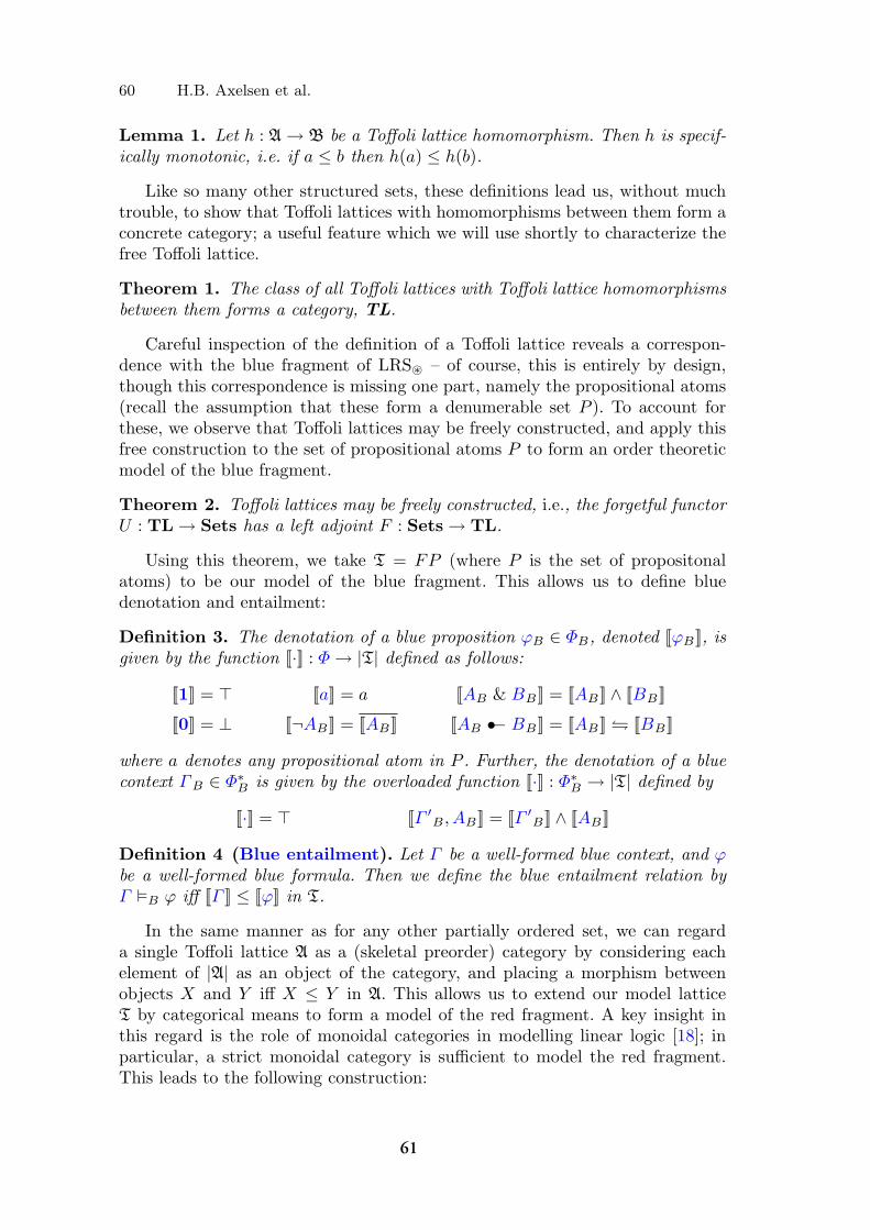
60 H.B. Axelsen et al.

Lemma 1. Let h : A → B be a Toffoli lattice homomorphism. Then h is specif-ically monotonic, i.e. if a ≤ b then h(a) ≤ h(b).

Like so many other structured sets, these definitions lead us, without muchtrouble, to show that Toffoli lattices with homomorphisms between them form aconcrete category; a useful feature which we will use shortly to characterize thefree Toffoli lattice.

Theorem 1. The class of all Toffoli lattices with Toffoli lattice homomorphismsbetween them forms a category, TL.

Careful inspection of the definition of a Toffoli lattice reveals a correspon-dence with the blue fragment of LRS� – of course, this is entirely by design,though this correspondence is missing one part, namely the propositional atoms(recall the assumption that these form a denumerable set P ). To account forthese, we observe that Toffoli lattices may be freely constructed, and apply thisfree construction to the set of propositional atoms P to form an order theoreticmodel of the blue fragment.

Theorem 2. Toffoli lattices may be freely constructed, i.e., the forgetful functorU : TL → Sets has a left adjoint F : Sets → TL.

Using this theorem, we take T = FP (where P is the set of propositonalatoms) to be our model of the blue fragment. This allows us to define bluedenotation and entailment:

Definition 3. The denotation of a blue proposition ϕB ∈ ΦB, denoted [[ϕB ]], isgiven by the function [[·]] : Φ → |T| defined as follows:

[[1]] = � [[a]] = a [[AB & BB ]] = [[AB ]] ∧ [[BB ]]

[[0]] = ⊥ [[¬AB ]] = [[AB ]] [[AB •− BB ]] = [[AB ]] � [[BB ]]

where a denotes any propositional atom in P . Further, the denotation of a bluecontext ΓB ∈ Φ∗

B is given by the overloaded function [[·]] : Φ∗B → |T| defined by

[[·]] = � [[Γ ′B , AB ]] = [[Γ ′

B ]] ∧ [[AB ]]

Definition 4 (Blue entailment). Let Γ be a well-formed blue context, and ϕbe a well-formed blue formula. Then we define the blue entailment relation byΓ �B ϕ iff [[Γ ]] ≤ [[ϕ]] in T.

In the same manner as for any other partially ordered set, we can regarda single Toffoli lattice A as a (skeletal preorder) category by considering eachelement of |A| as an object of the category, and placing a morphism betweenobjects X and Y iff X ≤ Y in A. This allows us to extend our model latticeT by categorical means to form a model of the red fragment. A key insight inthis regard is the role of monoidal categories in modelling linear logic [18]; inparticular, a strict monoidal category is sufficient to model the red fragment.This leads to the following construction:

61

Propositional Reasoning About Reversible Logic Circuits 61

Definition 5. Let T⊗ denote the free strict monoidal category over T. That is,T⊗ has as objects all strings X1X2 . . . Xn where all Xi are objects of T, and asmorphisms all strings of morphisms f1f2 . . . fn : X1X2 . . . Xn → Y1Y2 . . . Yn formorphisms fi : Xi → Yi of T. It has a monoidal tensor − ⊗ − : T⊗ × T⊗ → T⊗defined by concatenation; thus it is strictly associative and has a strict unit i,denoting the empty string.

See, e.g., Joyal and Street [9,10] for the construction of the free strictmonoidal category (or, in their nomenclature, free strict tensor category) over agiven category C; it simply amounts to be the coproduct of all functor categoriesof the form Cn, where n is the discrete category of n objects. This allows us tocharacterize T⊗ by means of a (Grothendieck) fibration (see, e.g., Jacobs [7])into the discrete category ΔN which has, as objects, all natural numbers1:

Theorem 3. The functor Ψ : T⊗ → ΔN defined by mapping objects totheir lengths as strings, and morphisms to the corresponding identities is aGrothendieck fibration and a monoidal functor. Specifically, each inverse imageΨ−1(k) for k in (ΔN)0 is a full subcategory of T⊗.

Proof. (Proof sketch). Since ΔN is discrete, for any object X1X2 . . . Xn of T⊗,the only possible morphism in ΔN of the form u : K → Ψ(X1X2 . . . Xn) isthe identity 1Ψ(X1X2...Xn), which the identity morphism 1X1X2...Xn

is triviallycartesian over.

To see that Ψ is a strict monoidal functor, we note the obvious tensor productin ΔN given by addition, i.e., by mapping objects A⊗B to their sum (as naturalnumbers) A+B, and likewise morphisms 1A ⊗1B to 1A+B . From this, it followsdirectly that Ψ(A ⊗ B) = Ψ(A) ⊗ Ψ(B). ��

This approach is closely related to the theory of PROs, PROPs, and operads(see, e.g., Leinster [13])–indeed, T⊗ is a PRO–but we will avoid relying on thistheory for the sake of a more coherent presentation.

In order to define denotation and entailment in the red propositions, weneed one last lemma, stating the obvious isomorphism between Ψ−1(1) (thesubcategory of strings of objects of T of length precisely 1) and T:

Lemma 2. There exist functors I : T → Ψ−1(1) and J : Ψ−1(1) → T witnessingΨ−1(1) ∼= T.

Definition 6. The denotation of a red proposition ϕR ∈ ΦR, denoted [[ϕR]], isgiven by the function [[·]] : ΦR → (T⊗)0 defined as follows:

[[e]] = i [[AR � BR]] = [[AR]] ⊗ [[BR]] [[AR]] = I([[AB ]]) if ARis a recolorable.

As we did for blue propositions, we overload the denotation function to apply to(in this case, red) contexts as well, by defining the function [[·]] : Φ∗

R → (T⊗)0 as

[[·]] = i [[ΓR, AR]] = [[ΓR]] ⊗ [[AR]]

1 We use the notation ΔN for the discrete category specifically to avoid confusion withthe ordinal category ω, which some authors denote N.

62

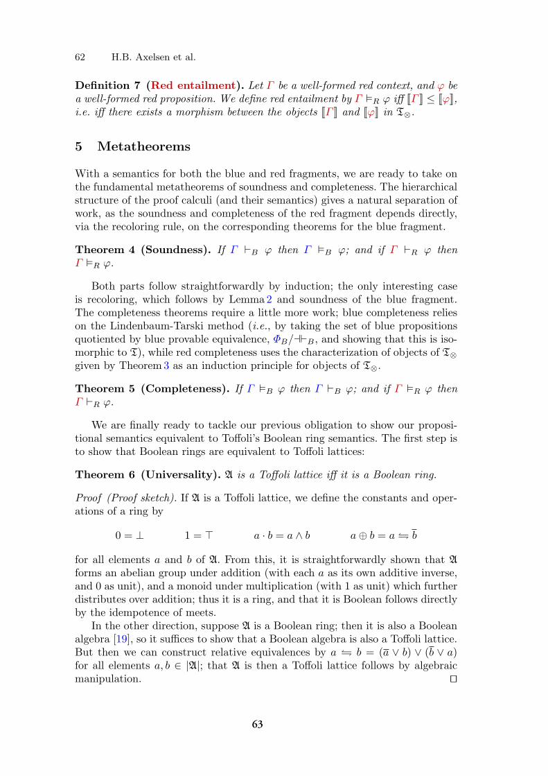
62 H.B. Axelsen et al.

Definition 7 (Red entailment). Let Γ be a well-formed red context, and ϕ bea well-formed red proposition. We define red entailment by Γ �R ϕ iff [[Γ ]] ≤ [[ϕ]],i.e. iff there exists a morphism between the objects [[Γ ]] and [[ϕ]] in T⊗.

5 Metatheorems

With a semantics for both the blue and red fragments, we are ready to take onthe fundamental metatheorems of soundness and completeness. The hierarchicalstructure of the proof calculi (and their semantics) gives a natural separation ofwork, as the soundness and completeness of the red fragment depends directly,via the recoloring rule, on the corresponding theorems for the blue fragment.

Theorem 4 (Soundness). If Γ �B ϕ then Γ �B ϕ; and if Γ �R ϕ thenΓ �R ϕ.

Both parts follow straightforwardly by induction; the only interesting caseis recoloring, which follows by Lemma 2 and soundness of the blue fragment.The completeness theorems require a little more work; blue completeness relieson the Lindenbaum-Tarski method (i.e., by taking the set of blue propositionsquotiented by blue provable equivalence, ΦB/��B , and showing that this is iso-morphic to T), while red completeness uses the characterization of objects of T⊗given by Theorem3 as an induction principle for objects of T⊗.

Theorem 5 (Completeness). If Γ �B ϕ then Γ �B ϕ; and if Γ �R ϕ thenΓ �R ϕ.

We are finally ready to tackle our previous obligation to show our proposi-tional semantics equivalent to Toffoli’s Boolean ring semantics. The first step isto show that Boolean rings are equivalent to Toffoli lattices:

Theorem 6 (Universality). A is a Toffoli lattice iff it is a Boolean ring.

Proof (Proof sketch). If A is a Toffoli lattice, we define the constants and oper-ations of a ring by

0 = ⊥ 1 = � a · b = a ∧ b a ⊕ b = a � b

for all elements a and b of A. From this, it is straightforwardly shown that Aforms an abelian group under addition (with each a as its own additive inverse,and 0 as unit), and a monoid under multiplication (with 1 as unit) which furtherdistributes over addition; thus it is a ring, and that it is Boolean follows directlyby the idempotence of meets.

In the other direction, suppose A is a Boolean ring; then it is also a Booleanalgebra [19], so it suffices to show that a Boolean algebra is also a Toffoli lattice.But then we can construct relative equivalences by a � b = (a ∨ b) ∨ (b ∨ a)for all elements a, b ∈ |A|; that A is then a Toffoli lattice follows by algebraicmanipulation. ��

63

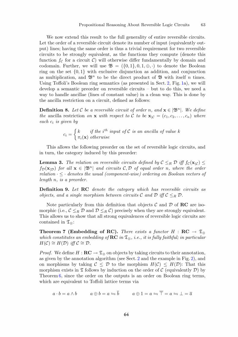
Propositional Reasoning About Reversible Logic Circuits 63

We now extend this result to the full generality of entire reversible circuits.Let the order of a reversible circuit denote its number of input (equivalently out-put) lines; having the same order is thus a trivial requirement for two reversiblecircuits to be strongly equivalent, as the functions they compute (denote thisfunction fC for a circuit C) will otherwise differ fundamentally by domain andcodomain. Further, we will use B = ({0, 1}, 0, 1,⊕, ·) to denote the Booleanring on the set {0, 1} with exclusive disjunction as addition, and conjunctionas multiplication, and Bn to be the direct product of B with itself n times.Using Toffoli’s Boolean ring semantics (as presented in Sect. 2, Fig. 1a), we willdevelop a semantic preorder on reversible circuits – but to do this, we need away to handle ancillae (lines of constant value) in a clean way. This is done bythe ancilla restriction on a circuit, defined as follows:

Definition 8. Let C be a reversible circuit of order n, and x ∈ |Bn|. We definethe ancilla restriction on x with respect to C to be x|C = (c1, c2, . . . , cn) whereeach ci is given by

ci ={

k if the ith input of C is an ancilla of value kπi(x) otherwise

This allows the following preorder on the set of reversible logic circuits, andin turn, the category induced by this preorder:

Lemma 3. The relation on reversible circuits defined by C ≤R D iff fC(x|C) ≤fD(x|D) for all x ∈ |Bn| and circuits C,D of equal order n, where the orderrelation · ≤ · denotes the usual (component-wise) ordering on Boolean vectors oflength n, is a preorder.

Definition 9. Let RC denote the category which has reversible circuits asobjects, and a single morphism between circuits C and D iff C ≤R D.

Note particularly from this definition that objects C and D of RC are iso-morphic (i.e., C ≤R D and D ≤R C) precisely when they are strongly equivalent.This allows us to show that all strong equivalences of reversible logic circuits arecontained in T⊗:

Theorem 7 (Embedding of RC). There exists a functor H : RC → T⊗which constitutes an embedding of RC in T⊗, i.e., it is fully faithful; in particularH(C) ∼= H(D) iff C ∼= D.

Proof. We define H : RC → T⊗ on objects by taking circuits to their annotation,as given by the annotation algorithm (see Sect. 2 and the example in Fig. 2), andon morphisms by taking C ≤ D to the morphism H(C) ≤ H(D): That thismorphism exists in T follows by induction on the order of C (equivalently D) byTheorem 6, since the order on the outputs is an order on Boolean ring terms,which are equivalent to Toffoli lattice terms via

a · b = a ∧ b a ⊕ b = a � b a ⊕ 1 = a � � = a � ⊥ = a

64

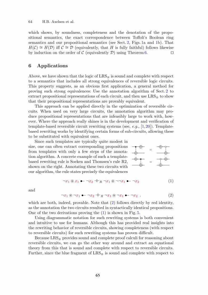
64 H.B. Axelsen et al.

which shows, by soundness, completeness and the denotation of the propo-sitional semantics, the exact correspondence between Toffoli’s Boolean ringsemantics and our propositional semantics (see Sect. 2, Figs. 1a and 1b). ThatH(C) ∼= H(D) iff C ∼= D (equivalently, that H is fully faithful) follows likewiseby induction on the order of C (equivalently D) using Theorem 6. ��

6 Applications

Above, we have shown that the logic of LRS� is sound and complete with respectto a semantics that includes all strong equivalences of reversible logic circuits.This property suggests, as an obvious first application, a general method forproving such strong equivalences: Use the annotation algorithm of Sect. 2 toextract propositional representations of each circuit, and then use LRS� to showthat their propositional representations are provably equivalent.

This approach can be applied directly in the optimization of reversible cir-cuits. When used on very large circuits, the annotation algorithm may pro-duce propositional representations that are infeasibly large to work with, how-ever. Where the approach really shines is in the development and verification oftemplate-based reversible circuit rewriting systems (see, e.g., [1,20]). Template-based rewriting works by identifying certain forms of sub-circuits, allowing theseto be substituted with equivalent ones.

•

•

Since such templates are typically quite modest insize, one can often extract corresponding propositionsfrom templates with only a few steps of the annota-tion algorithm. A concrete example of such a template-based rewriting rule is Soeken and Thomsen’s rule R2,shown on the right. Annotating these two circuits withour algorithm, the rule states precisely the equivalences

¬x1 � x1 •− ¬x2 ��R ¬x1 � ¬¬x1 •− ¬x2 (1)

and¬x1 � ¬x1 •− ¬x2 ��R ¬x1 � ¬x1 •− ¬x2 . (2)

which are both, indeed, provable. Note that (2) follows directly by red identity,as the annotation the two circuits resulted in syntactically identical propositions.One of the two derivations proving the (1) is shown in Fig. 5.

Using diagrammatic notation for such rewriting systems is both convenientand intuitive to use for humans. Although this has provided real insights intothe rewriting behavior of reversible circuits, showing completeness (with respectto reversible circuits) for such rewriting systems has proven difficult.

Because LRS� provides sound and complete proof calculi for reasoning aboutreversible circuits, we can go the other way around and extract an equationaltheory from this that is sound and complete with respect to reversible circuits.Further, since the blue fragment of LRS� is sound and complete with respect to

65

Propositional Reasoning About Reversible Logic Circuits 65

Fig. 5. Derivation in LRS� for verifying the first direction of Soeken and Thomsen’srule R2.

Toffoli lattices, we can instead extract an equational theory for the blue fragmentfrom the definition of a Toffoli lattice, using the following lemma:

Lemma 4. In any Toffoli lattice, a ≤ b iff a ∧ b = ⊥.

This lemma allows us to straightforwardly recast the definition of a Toffolilattice in purely equational terms (although the result is not exactly elegant).What this does give us, is a set of equations that must hold for all Toffoli lattices,and which any other complete equational theory must therefore be equivalent to,and the means to show such an equivalence by converting equalities to statementsabout the underlying order structure and vice versa.

Figure 6 shows a more pleasing equational theory for the blue fragment, pre-sented in the syntax of LRS� (the intrinsic properties of equality, i.e., reflexivity,symmetry, transitivity, and congruences are not shown,) proven equivalent (andtherefore sound and complete) exactly in the way outlined above (by the powerof boring algebra). Deriving an equational theory for the red fragment is simpler,as it is sound and complete with respect to the free monoidal part of T⊗, whichis already expressed in equational terms. As such, the equational theory for thered fragment shown in Fig. 6 is sound and complete by definition, though congru-ences applied in the red fragment are syntactically restricted by recolorability;that is, we can only replace recolorable propositions by recolorable propositions.

The usefulness of such an equational theory is evident in that we can, e.g.,now prove the soundness of the R2 rules directly by applying equation (B9)in Fig. 6. Such equational theories can themselves also be used to develop newrewriting systems for reversible circuits, in particular to suggest new templates.

66

66 H.B. Axelsen et al.

Fig. 6. Sound and complete equational theories for the two calculi. (Color figure online)

7 Conclusion and Future Work

In this article, we have presented a syntactic representation of reversible logiccircuits centered around the control interpretation of Toffoli’s reversible gateset, and shown, via two proof calculi of natural deduction, that a variant ofclassical propositional logic extended with ordered multiplicative conjunction issufficient to reason about these. We have developed an algebraic and categoricalsemantics, shown that the proof calculi are sound and complete with respect tothese, and that this model subsumes the established notion of strong equivalenceof reversible logic circuits. Finally, we have shown how our work can be used toprove strong equivalences of reversible logic circuits, to verify existing systemsof reversible logic circuit rewriting, and to develop new such rewriting systems.

The approach has been successful in enabling reasoning about reversible logiccircuits, but it is not quite on even footing with the template-based approachesto reversible circuit rewriting, as these use a graphical circuit notation which,by definition, asserts circuit reversibility on every rewriting step. Although ourapproach faithfully models circuit semantics, it is not currently clear when look-ing at an arbitrary proposition whether it corresponds to a reversible circuitor not. On the other hand, by decoupling the propositions from the graphicalrepresentations, the current logic may allow for much shorter rewritings than ifeach step must yield representations which directly translate to circuits in thisway.

References

1. Arabzadeh, M., Saeedi, M., Zamani, M.S.: Rule-based optimization of reversiblecircuits. In: Proceedings of the ASP-DAC 2010, pp. 849–854. IEEE (2010)

2. Berut, A., Arakelyan, A., Petrosyan, A., Ciliberto, S., Dillenschneider, R., Lutz,E.: Experimental verification of Landauer’s principle linking information and ther-modynamics. Nature 483(7388), 187–189 (2012)

3. Buss, S.R.: Handbook of Proof Theory. Elsevier, Amsterdam (1998)4. De Vos, A.: Reversible Computing. Wiley-VCH, Weinheim (2010)

67

Propositional Reasoning About Reversible Logic Circuits 67

5. De Vos, A., Burignat, S., Gluck, R., Mogensen, T.Æ., Axelsen, H.B., Thomsen,M.K., Rotenberg, E., Yokoyama, T.: Designing garbage-free reversible implementa-tions of the integer cosine transform. ACM J. Emerg. Tech. Com. 11(2), 11:1–11:15(2014)

6. Feynman, R.P.: Quantum mechanical computers. Found. Phys. 16(6), 507–531(1986)

7. Jacobs, B.: Categorical Logic and Type Theory. Elsevier, Amsterdam (1999)8. Jordan, S.P.: Strong equivalence of reversible circuits is coNP-complete. Quantum

Inf. Comput. 14(15–16), 1302–1307 (2014)9. Joyal, A., Street, R.: The geometry of tensor calculus I. Adv. Math. 88(1), 55–112

(1991)10. Joyal, A., Street, R.: Braided tensor categories. Adv. Math. 102(1), 20–78 (1993)11. Kaarsgaard, R.: Towards a propositional logic for reversible logic circuits. In: Pro-

ceedings of the ESSLLI 2014 Student Session, pp. 33–41 (2014). http://www.kr.tuwien.ac.at/drm/dehaan/stus2014/proceedings.pdf

12. Landauer, R.: Irreversibility and heat generation in the computing process. IBMJ. Res. Dev. 5(3), 261–269 (1961)

13. Leinster, T.: Higher Operads, Higher Categories. London Mathematical SocietyLecture Note Series, vol. 298. Cambridge University Press, Cambridge (2004)

14. Orlov, A.O., Lent, C.S., Thorpe, C.C., Boechler, G.P., Snider, G.L.: Experimentaltest of Landauer’s principle at the sub-kbt level. Japan. J. Appl. Phys. 51, 06FE10(2012)

15. Polakow, J.: Ordered linear logic and applications. Ph.D. thesis, CMU (2001)16. Rendel, T., Ostermann, K.: Invertible syntax descriptions: unifying parsing and

pretty printing. ACM SIGPLAN Notices, vol. 45, No. 11, pp. 1–12 (2010)17. Schellekens, M.P.: MOQA: unlocking the potential of compositional static average-

case analysis. J. Log. Algebr. Program. 79(1), 61–83 (2010)18. Seely, R.A.G.: Linear logic, *-autonomous categories and cofree coalgebras. Con-

temp. Math. 92, 371–382 (1989)19. Sikorski, R.: Boolean Algebras. Springer, Heidelberg (1969)20. Soeken, M., Thomsen, M.K.: White dots do matter: rewriting reversible logic cir-

cuits. In: Dueck, G.W., Miller, D.M. (eds.) RC 2013. LNCS, vol. 7948, pp. 196–208.Springer, Heidelberg (2013)

21. Thomsen, M.K., Gluck, R., Axelsen, H.B.: Reversible arithmetic logic unit forquantum arithmetic. J. Phys. A Math. Theor. 43(38), 382002 (2010)

22. Toffoli, T.: Reversible computing. In: de Bakker, J., van Leeuwen, J. (eds.)Automata, Languages and Programming. LNCS, vol. 85, pp. 632–644. Springer,Heidelberg (1980)

23. Wille, R., Drechsler, R.: Towards a Design Flow for Reversible Logic. Springer,Heidelberg (2010)

68

69

70

A psychologist said, “They used to talk about seeing only ‘reflections’ of reality.Not reality itself. The main thing wrong with a reflection is not that it isn’treal, but that it’s reversed.”

Philip K. Dick, A Scanner Darkly

BFoundations of reversible recursion

This chapter contains two papers related to the categorical foundations of reversible recur-sion.

(B1) R. Kaarsgaard, H. B. Axelsen, and R. Glück. Join Inverse Categories and ReversibleRecursion. Journal of Logical and Algebraic Methods in Programming, volume 87,pages 33–50, February 2017.

(B2) R. Kaarsgaard. Inversion, Fixed Points, and the Art of Dual-Wielding. In S. Alvesand R. Wassermann, editors, Proceedings of the 12th Workshop on Logical and Seman-tic Frameworks with Applications (LSFA 2017), pages 94–109, available at http://lsfa2017.cic.unb.br/LSFA2017.pdf, 2017.

Paper (B1) is the extended version of a conference paper, which, in turn, was extended froman abstract presented at a workshop:

• H. B. Axelsen and R. Kaarsgaard. Join inverse categories as models of reversible recur-sion. In B. Jacobs and C. Löding, editors, Foundations of Software Science and Com-putation Structures (FoSSaCS), Lecture Notes in Computer Science volume 9634,pages 73–90, Springer Verlag, 2016.

• R. Kaarsgaard. Join inverse categories and reversible recursion. In L. Aceto, I. Fábre-gas, Á. García-Perez, A. Ingolfsdottir, editors, Proceedings of the 27th Nordic Workshopon Programming Theory, Technical Report RUTR-SCS16001, pages 69–71, Reyk-javík University, 2015.

71

72

Journal of Logical and Algebraic Methods in Programming 87 (2017) 33–50

Contents lists available at ScienceDirect

Journal of Logical and Algebraic Methods in

Programmingwww.elsevier.com/locate/jlamp

Join inverse categories and reversible recursion ✩

Robin Kaarsgaard ∗, Holger Bock Axelsen, Robert GlückDIKU, Department of Computer Science, University of Copenhagen, Denmark

a r t i c l e i n f o a b s t r a c t

Article history:Received 31 January 2016Received in revised form 14 August 2016Accepted 16 August 2016Available online 24 August 2016

Keywords:Reversible computingRecursionCategorical semanticsEnriched category theory

Recently, a number of reversible functional programming languages have been proposed. Common to several of these is the assumption of totality, a property that is not necessarily desirable, and certainly not required in order to guarantee reversibility. In a categorical setting, however, faithfully capturing partiality requires handling it as additional structure. Recently, Giles studied inverse categories as a model of partial reversible (functional) programming. In this paper, we show how additionally assuming the existence of countable joins on such inverse categories leads to a number of properties that are desirable when modeling reversible functional programming, notably morphism schemes for reversible recursion, a †-trace, and algebraic ω-compactness. This gives a categorical account of reversible recursion, and, for the latter, provides an answer to the problem posed by Giles regarding the formulation of recursive data types at the inverse category level.

© 2016 Elsevier Inc. All rights reserved.

1. Introduction

Reversible computing, that is, the study of computations that exhibit both forward and backward determinism, origi-nally grew out of the thermodynamics of computation. Landauer’s principle states that computations performed by some physical system (thermodynamically) dissipate heat when information is erased, but that no dissipation is entailed by information-preserving computations [3]. This has motivated a long study of diverse reversible computation models, such as logic circuits [4], Turing machines [5,6], and many forms of restricted automata models [7,8]. Reversibility concepts are im-portant in quantum computing, but are increasingly seen to be of interest in other areas as well, including high-performance computing [9], process calculi [10], and even robotics [11,12].

In this paper we concern ourselves with the categorical underpinnings of reversible functional programming languages. At the programming language level, reversible languages exhibit interesting program properties, such as easy program in-version [13]. Now, most reversible languages are stateful, giving them a fairly straightforward semantic interpretation [14]. While functional programs are usually easier to reason about at the meta-level, they do not have the concept of state that imperative languages do, making their semantics interesting objects of study.

Further, many reversible functional programming languages (such as Theseus [15] and the "-family of combinator cal-culi [16]) come equipped with a tacit assumption of totality, a property that is neither required [6] nor necessarily desirable as far as guaranteeing reversibility is concerned. Shedding ourselves of the “tyranny of totality,” however, requires us to handle partiality explicitly as additional categorical structure.

✩ This is an extended version of an abstract presented at NWPT 2015 [1] and a paper presented at FoSSaCS 2016 [2], elaborated with full proofs, additional examples, and more comprehensive background.

* Corresponding author.E-mail addresses: [email protected] (R. Kaarsgaard), [email protected] (H.B. Axelsen), [email protected] (R. Glück).

http://dx.doi.org/10.1016/j.jlamp.2016.08.0032352-2208/© 2016 Elsevier Inc. All rights reserved.

73

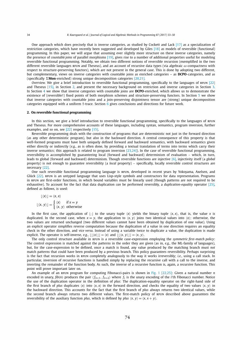
34 R. Kaarsgaard et al. / Journal of Logical and Algebraic Methods in Programming 87 (2017) 33–50

One approach which does precisely that is inverse categories, as studied by Cockett and Lack [17] as a specialization of restriction categories, which have recently been suggested and developed by Giles [18] as models of reversible (functional) programming. In this paper, we will argue that assuming ever slightly more structure on these inverse categories, namely the presence of countable joins of parallel morphisms [19], gives rise to a number of additional properties useful for modelingreversible functional programming. Notably, we obtain two different notions of reversible recursion (exemplified in the two different reversible languages rfun and Theseus), and an account of recursive data types (via algebraic ω-compactness with respect to structure-preserving functors), which are not present in the general case. This is done by adopting two different, but complementary, views on inverse categories with countable joins as enriched categories – as DCPO-categories, and as (specifically #Mon-enriched) strong unique decomposition categories [20,21].

Overview. We give a brief introduction to reversible functional programming, specifically to the languages of rfun [22]and Theseus [15], in Section 2, and present the necessary background on restriction and inverse categories in Section 3. In Section 4 we show that inverse categories with countable joins are DCPO-enriched, which allows us to demonstrate the existence of (reversible!) fixed points of both morphism schemes and structure-preserving functors. In Section 5 we show that inverse categories with countable joins and a join-preserving disjointness tensor are (strong) unique decomposition categories equipped with a uniform †-trace. Section 6 gives conclusions and directions for future work.

2. On reversible functional programming

In this section, we give a brief introduction to reversible functional programming, specifically to the languages of rfunand Theseus. For more comprehensive accounts of these languages, including syntax, semantics, program inversion, further examples, and so on, see [22] respectively [15].

Reversible programming deals with the construction of programs that are deterministic not just in the forward direction (as any other deterministic program), but also in the backward direction. A central consequence of this property is that well-formed programs must have both uniquely defined forward and backward semantics, with backward semantics given either directly or indirectly (e.g., as is often done, by providing a textual translation of terms into terms which carry their inverse semantics; this approach is related to program inversion [23,24]). In the case of reversible functional programming, reversibility is accomplished by guaranteeing local (forward and backward) determinism of evaluation – which, in turn, leads to global (forward and backward) determinism. Though reversible functions are injective [6], injectivity itself (a globalproperty) is not enough to guarantee reversibility (a local property) – specifically, locally reversible control structures are necessary [22].

One such reversible functional programming language is rfun, developed in recent years by Yokoyama, Axelsen, and Glück [22]. rfun is an untyped language that uses Lisp-style symbols and constructors for data representation. Programs in rfun are first-order functions, in which bound variables must be linearly used (though patterns are not required to be exhaustive). To account for the fact that data duplication can be performed reversibly, a duplication-equality operator [25], defined as follows, is used:

⌊⟨x⟩⌋ = ⟨x, x⟩

⌊⟨x, y⟩⌋ ={

⟨x⟩ if x = y⟨x, y⟩ otherwise

In the first case, the application of ⌊·⌋ to the unary tuple ⟨x⟩ yields the binary tuple ⟨x, x⟩, that is, the value x is duplicated. In the second case, when x = y, the application to ⟨x, y⟩ joins two identical values into ⟨x⟩; otherwise, the two values are returned unchanged (two different values cannot have been obtained by duplication of one value). Using an explicit operator simplifies reverse computation because the duplication of a value in one direction requires an equality check in the other direction, and vice versa. Instead of using a variable twice to duplicate a value, the duplication is made explicit. The operator is self-inverse, e.g., ⌊⌊⟨x⟩⌋⌋ = ⟨x⟩ and ⌊⌊⟨x, y⟩⌋⌋ = ⟨x, y⟩.

The only control structure available in rfun is a reversible case-expression employing the symmetric first-match policy: The control expression is matched against the patterns in the order they are given (as in, e.g., the ML-family of languages), but, for the case-expression to be defined, once a match is found, any value produced by the matching branch must notmatch patterns that could have been produced by a previous branch. This policy guarantees reversibility. Perhaps surprising is the fact that recursion works in rfun completely analogously to the way it works irreversibly; i.e., using a call stack. In particular, inversion of recursive functions is handled simply by replacing the recursive call with a call to the inverse, and inverting the remainder of the function body. As such, the inverse of a recursive function is, again, a recursive function. This point will prove important later on.

An example of an rfun program for computing Fibonacci-pairs is shown in Fig. 1 [22,25]: Given a natural number nencoded in unary, fib(n) produces the pair ⟨ fn+1, fn+2⟩ where f i is the unary encoding of the i’th Fibonacci number. Notice the use of the duplication operator in the definition of plus: The duplication-equality operator on the right-hand side of the first branch of plus duplicates ⟨x⟩ into ⟨x, x⟩ in the forward direction, and checks the equality of two values ⟨x, y⟩ in the backward direction. This accounts for the fact that the first branch of plus always returns two identical values, while the second branch always returns two different values. The first-match policy of rfun described above guarantees the reversibility of the auxiliary function plus, which is defined by plus ⟨x, y⟩ = ⟨x, x + y⟩.

74

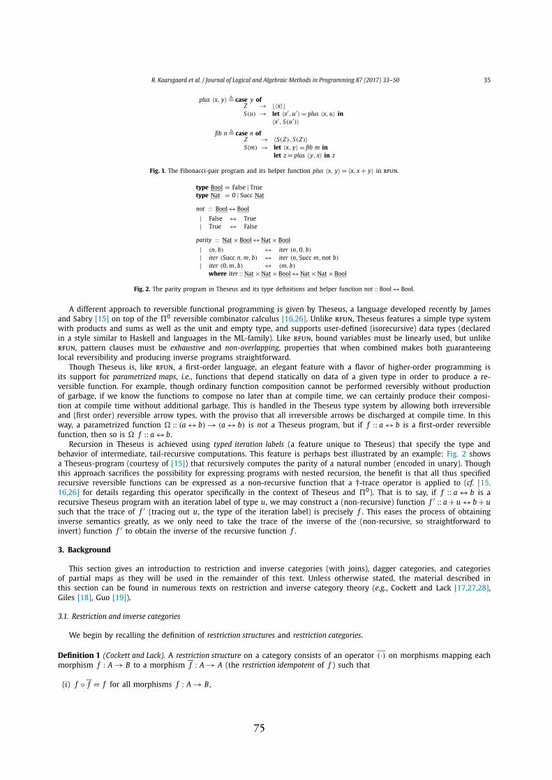
R. Kaarsgaard et al. / Journal of Logical and Algebraic Methods in Programming 87 (2017) 33–50 35

plus ⟨x, y⟩! case y ofZ → ⌊⟨x⟩⌋S(u) → let ⟨x′, u′⟩ = plus ⟨x, u⟩ in

⟨x′, S(u′)⟩fib n ! case n of

Z → ⟨S(Z), S(Z)⟩S(m) → let ⟨x, y⟩ = fib m in

let z = plus ⟨y, x⟩ in z

Fig. 1. The Fibonacci-pair program and its helper function plus ⟨x, y⟩ = ⟨x, x + y⟩ in rfun.

type Bool = False | Truetype Nat = 0 | Succ Nat

not :: Bool ↔ Bool

| False ↔ True| True ↔ False

parity :: Nat × Bool ↔ Nat × Bool

| (n,b) ↔ iter (n,0,b)

| iter (Succ n,m,b) ↔ iter (n,Succ m,not b)

| iter (0,m,b) ↔ (m,b)

where iter :: Nat × Nat × Bool ↔ Nat × Nat × Bool

Fig. 2. The parity program in Theseus and its type definitions and helper function not :: Bool ↔ Bool.

A different approach to reversible functional programming is given by Theseus, a language developed recently by James and Sabry [15] on top of the "0 reversible combinator calculus [16,26]. Unlike rfun, Theseus features a simple type system with products and sums as well as the unit and empty type, and supports user-defined (isorecursive) data types (declared in a style similar to Haskell and languages in the ML-family). Like rfun, bound variables must be linearly used, but unlikerfun, pattern clauses must be exhaustive and non-overlapping, properties that when combined makes both guaranteeing local reversibility and producing inverse programs straightforward.

Though Theseus is, like rfun, a first-order language, an elegant feature with a flavor of higher-order programming is its support for parametrized maps, i.e., functions that depend statically on data of a given type in order to produce a re-versible function. For example, though ordinary function composition cannot be performed reversibly without production of garbage, if we know the functions to compose no later than at compile time, we can certainly produce their composi-tion at compile time without additional garbage. This is handled in the Theseus type system by allowing both irreversible and (first order) reversible arrow types, with the proviso that all irreversible arrows be discharged at compile time. In this way, a parametrized function $ :: (a ↔ b) → (a ↔ b) is not a Theseus program, but if f :: a ↔ b is a first-order reversible function, then so is $ f :: a ↔ b.

Recursion in Theseus is achieved using typed iteration labels (a feature unique to Theseus) that specify the type and behavior of intermediate, tail-recursive computations. This feature is perhaps best illustrated by an example: Fig. 2 shows a Theseus-program (courtesy of [15]) that recursively computes the parity of a natural number (encoded in unary). Though this approach sacrifices the possibility for expressing programs with nested recursion, the benefit is that all thus specified recursive reversible functions can be expressed as a non-recursive function that a †-trace operator is applied to (cf. [15,16,26] for details regarding this operator specifically in the context of Theseus and "0). That is to say, if f :: a ↔ b is a recursive Theseus program with an iteration label of type u, we may construct a (non-recursive) function f ′ :: a + u ↔ b + usuch that the trace of f ′ (tracing out u, the type of the iteration label) is precisely f . This eases the process of obtaining inverse semantics greatly, as we only need to take the trace of the inverse of the (non-recursive, so straightforward to invert) function f ′ to obtain the inverse of the recursive function f .

3. Background

This section gives an introduction to restriction and inverse categories (with joins), dagger categories, and categories of partial maps as they will be used in the remainder of this text. Unless otherwise stated, the material described in this section can be found in numerous texts on restriction and inverse category theory (e.g., Cockett and Lack [17,27,28], Giles [18], Guo [19]).

3.1. Restriction and inverse categories

We begin by recalling the definition of restriction structures and restriction categories.

Definition 1 (Cockett and Lack). A restriction structure on a category consists of an operator (·) on morphisms mapping each morphism f : A → B to a morphism f : A → A (the restriction idempotent of f ) such that

(i) f ◦ f = f for all morphisms f : A → B ,

75

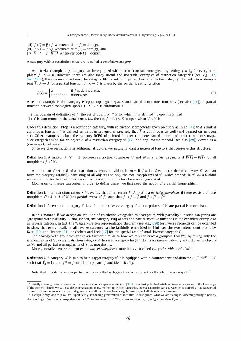
36 R. Kaarsgaard et al. / Journal of Logical and Algebraic Methods in Programming 87 (2017) 33–50

(ii) f ◦ g = g ◦ f whenever dom( f ) = dom(g),(iii) f ◦ g = f ◦ g whenever dom( f ) = dom(g), and(iv) h ◦ f = f ◦ h ◦ f whenever cod( f ) = dom(h).

A category with a restriction structure is called a restriction category.

As a trivial example, any category can be equipped with a restriction structure given by setting f = 1A for every mor-phism f : A → B . However, there are also many useful and nontrivial examples of restriction categories (see, e.g., [17, Sec. 2.1.3]), the canonical one being the category Pfn of sets and partial functions. In this category, the restriction idempo-tent f : A → A for a partial function f : A → B is given by the partial identity function

f (x) ={

x if f is defined at x,undefined otherwise. (1)

A related example is the category PTop of topological spaces and partial continuous functions (see also [18]). A partial function between topological spaces f : X → Y is continuous if

(i) the domain of definition of f (the set of points X ′ ⊆ X for which f is defined) is open in X , and(ii) f is continuous in the usual sense, i.e., the set f −1(V ) ⊆ X is open when V ⊆ Y is.

Under this definition, PTop is a restriction category, with restriction idempotents given precisely as in Eq. (1); that a partial continuous function f is defined on an open set ensures precisely that f is continuous as well (and defined on an open set). Other examples include the category DCPO of pointed directed-complete partial orders and strict continuous maps, slice categories C /A for an object A of a restriction category C [17], and any inverse monoid (see also [29]) viewed as a (one-object) category.

Since we take restrictions as additional structure, we naturally want a notion of functors that preserve this structure.

Definition 2. A functor F : C → D between restriction categories C and D is a restriction functor if F ( f ) = F ( f ) for all morphisms f of C .

A morphism f : A → B of a restriction category is said to be total if f = 1A . Given a restriction category C , we can form the category Total(C ), consisting of all objects and only the total morphisms of C , which embeds in C via a faithful restriction functor. Restriction categories with restriction functors form a category, rCat.

Moving on to inverse categories, in order to define these1 we first need the notion of a partial isomorphism:

Definition 3. In a restriction category C , we say that a morphism f : A → B is a partial isomorphism if there exists a unique morphism f ◦ : B → A of C (the partial inverse of f ) such that f ◦ ◦ f = f and f ◦ f ◦ = f ◦ .

Definition 4. A restriction category C is said to be an inverse category if all morphisms of C are partial isomorphisms.

In this manner, if we accept an intuition of restriction categories as “categories with partiality,” inverse categories are “groupoids with partiality” – and, indeed, the category PInj of sets and partial injective functions is the canonical example of an inverse category. In fact, the Wagner–Preston representation theorem (see, e.g., [29]) for inverse monoids can be extended to show that every locally small inverse category can be faithfully embedded in PInj (see the two independent proofs by Kastl [30] and Heunen [31], or Cockett and Lack [17] for the special case of small inverse categories).

The analogy with groupoids goes even further; similar to how we can construct a groupoid Core(C ) by taking only the isomorphisms of C , every restriction category C has a subcategory Inv(C ) that is an inverse category with the same objects as C , and all partial isomorphisms of C as morphisms.

More generally, inverse categories are dagger categories (sometimes also called categories with involution):

Definition 5. A category C is said to be a dagger category if it is equipped with a contravariant endofunctor (−)† : C op → Csuch that 1†

A = 1A and f †† = f for all morphisms f and identities 1A .

Note that this definition in particular implies that a dagger functor must act as the identity on objects.2

1 Strictly speaking, inverse categories predate restriction categories – see Kastl [30] for the first published article on inverse categories to the knowledge of the authors. Though we will use the axiomatization following from restriction categories, inverse categories can equivalently be defined as the categorical extension of inverse monoids, i.e., as categories where all morphisms have a regular inverse, and all idempotents commute.

2 Though it may look as if we are superfluously demanding preservation of identities at first glance, what we are stating is something stronger, namely that the dagger functor must map identities in C op to themselves in C . That is, we are requiring 1†

A = 1A rather than 1†A = 1A† .

76

R. Kaarsgaard et al. / Journal of Logical and Algebraic Methods in Programming 87 (2017) 33–50 37

Proposition 1. Every inverse category C is a dagger category with the dagger functor given by A† = A on objects, and f † = f ◦ on morphisms.

As is conventional, we will call f † the adjoint of f , and say that f is self-adjoint (or hermitian) if f = f †, and unitaryif f † = f −1. In inverse categories, unitary morphisms thus correspond precisely to (total) isomorphisms. For the remainder of this text, we will use this induced dagger-structure when referring to the partial inverse of a morphism (and write, e.g., f † rather than f ◦).

A useful feature of this definition of inverse categories is that we do not need an additional notion of an “inverse functor” as a functor that preserves partial inverses; restriction functors suffice.

Proposition 2. Every restriction functor F : C → D between inverse categories preserves the canonical dagger structure of C , i.e., F ( f )† = F ( f †) for all morphisms f of C .

A simple argument for this proposition is the fact that partial isomorphisms are defined purely in terms of composition and restriction idempotents, both of which are preserved by restriction functors. Inverse categories with restriction functors form a category, invCat.

3.2. Split restriction categories and categories of partial maps

When working in a category with a distinguished class of idempotents, it is often desirable that they split.3 In restriction categories, such a distinguished class is given by the class of restriction idempotents, leading us to the straightforward definition of a split restriction category:

Definition 6. A restriction category in which every restriction idempotent splits is called a split restriction category.

For example, when equipped with the usual restriction structure, Pfn and PTop are both split restriction categories, though it straightforward to come up with subcategories of either that are not. It follows, by way of the Karoubi envelope, that every restriction category C can be embedded in a split restriction category Split(C ) via a fully faithful restriction functor (though this requires us to show that Split(C ) inherits the restriction structure from C , and that the fully faithful functor into this category preserves restrictions; see Prop. 2.26 of [17] for details). Prime examples of split restriction categories are categories of partial maps.

Categories of partial maps provide a synthetic approach to partiality in a categorical setting [32]. To form a category of partial maps, we consider a stable system of monics: In a category C , a collection M of monics of C is said to be a stable system of monics if it contains all isomorphisms of C and is closed under composition and pullbacks (in the sense that the pullback m′ of an m : X → B in M along any f : A → B exists and m′ ∈ M). Given such a stable system of monics M in a category C , we can form the category of partial maps as follows:

Proposition 3. Given a category C and a stable system of monics M of C , we form the category of partial maps Par(C , M) by choosing the objects to be the objects of C , and placing a morphism (m, f ) : A → B for every pair (m, f ) where m : A′ → A ∈ M and f : A′ → B is a morphism of C , as in

A′

A B

m f

factored out by the equivalence relation · ∼ · in which (m, f ) ∼ (m′, f ′) if there exists an isomorphism α : A′ → A′′ such that m′ ◦α = m and f ′ ◦ α = f . Composition of morphisms (m, f ) : A → B and (m′, g) : B → C is given by (m ◦ m′′, g ◦ f ′) : A → C where m′′ and f ′ arise from the pullback

A′

A′′

A B

B ′

C

mm′

m′′

f

g

f ′

where m′′ ◦ m ∈ M precisely by M closed under composition and pullbacks.

3 Recall that a splitting of an idempotent e : A → A consists of an object A′ and morphisms m : A → A′ and r : A′ → A such that r ◦m = e and m ◦r = idA′ .

77

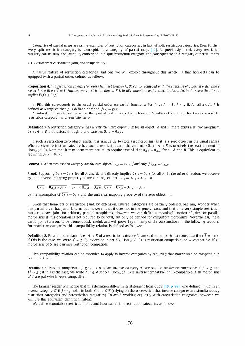
38 R. Kaarsgaard et al. / Journal of Logical and Algebraic Methods in Programming 87 (2017) 33–50

Categories of partial maps are prime examples of restriction categories; in fact, of split restriction categories. Even further, every split restriction category is isomorphic to a category of partial maps [17]. As previously noted, every restriction category can be fully and faithfully embedded in a split restriction category, and consequently, in a category of partial maps.

3.3. Partial order enrichment, joins, and compatibility

A useful feature of restriction categories, and one we will exploit throughout this article, is that hom-sets can be equipped with a partial order, defined as follows:

Proposition 4. In a restriction category C , every hom-set HomC (A, B) can be equipped with the structure of a partial order where we let f ≤ g iff g ◦ f = f . Further, every restriction functor F is locally monotone with respect to this order, in the sense that f ≤ gimplies F ( f ) ≤ F (g).

In Pfn, this corresponds to the usual partial order on partial functions: For f , g : A → B , f ≤ g if, for all x ∈ A, f is defined at x implies that g is defined at x and f (x) = g(x).

A natural question to ask is when this partial order has a least element: A sufficient condition for this is when the restriction category has a restriction zero.

Definition 7. A restriction category C has a restriction zero object 0 iff for all objects A and B , there exists a unique morphism 0A,B : A → B that factors through 0 and satisfies 0A,A = 0A,A .

If such a restriction zero object exists, it is unique up to (total) isomorphism (as it is a zero object in the usual sense). When a given restriction category has such a restriction zero, the zero map 0A,B : A → B is precisely the least element of HomC (A, B). Note that it may seem more natural to require instead that 0A,B = 0A,A for all A and B . This is equivalent to requiring 0A,A = 0A,A :

Lemma 1. When a restriction category has the zero object, 0A,A = 0A,A if and only if 0A,B = 0A,A .

Proof. Supposing 0A,B = 0A,A for all A and B , this directly implies 0A,A = 0A,A for all A. In the other direction, we observe by the universal mapping property of the zero object that 0A,B = 0A,B ◦ 0A,A , so

0A,B = 0A,B ◦ 0A,A = 0A,B ◦ 0A,A = 0A,B ◦ 0A,A = 0A,B ◦ 0A,A = 0A,A

by the assumption of 0A,A = 0A,A and the universal mapping property of the zero object. ✷

Given that hom-sets of restriction (and, by extension, inverse) categories are partially ordered, one may wonder when this partial order has joins. It turns out, however, that it does not in the general case, and that only very simple restriction categories have joins for arbitrary parallel morphisms. However, we can define a meaningful notion of joins for parallel morphisms if this operation is not required to be total, but only be defined for compatible morphisms. Nevertheless, these partial joins turn out to be tremendously useful, and will prove key in many of the constructions in the following sections. For restriction categories, this compatibility relation is defined as follows:

Definition 8. Parallel morphisms f , g : A → B of a restriction category C are said to be restriction compatible if g ◦ f = f ◦ g; if this is the case, we write f ⌣ g . By extension, a set S ⊆ HomC (A, B) is restriction compatible, or ⌣-compatible, if all morphisms of S are pairwise restriction compatible.

This compatibility relation can be extended to apply to inverse categories by requiring that morphisms be compatible in both directions:

Definition 9. Parallel morphisms f , g : A → B of an inverse category C are said to be inverse compatible if f ⌣ g and f † ⌣ g†; if this is the case, we write f ≍ g . A set S ⊆ HomC (A, B) is inverse compatible, or ≍-compatible, if all morphisms of S are pairwise inverse compatible.

The familiar reader will notice that this definition differs in its statement from Guo’s [19, p. 98], who defined f ≍ g in an inverse category C if f ⌣ g holds in both C and C op (relying on the observation that inverse categories are simultaneously restriction categories and corestriction categories). To avoid working explicitly with corestriction categories, however, we will use this equivalent definition instead.

We define (countable) restriction joins and (countable) join restriction categories as follows:

78

R. Kaarsgaard et al. / Journal of Logical and Algebraic Methods in Programming 87 (2017) 33–50 39

Definition 10 (Guo). Say that a restriction category C is outfitted with (countable) ∼-joins if for all (countable) ∼-compatible subsets S of all hom sets HomC (A, B) (for a compatibility relation · ∼ ·), there exists a morphism

∨s∈S s such that

(i) s ≤ ∨s∈S s for all s ∈ S , and s ≤ t for all s ∈ S implies

∨s∈S s ≤ t;

(ii)∨

s∈S s = ∨s∈S s;

(iii) f ◦(∨

s∈S s)= ∨

s∈S ( f ◦ s) for all f : B → X ; and(iv)

(∨s∈S s

)◦ g = ∨

s∈S (s ◦ g) for all g : Y → A.

Definition 11. A restriction category is said to be a (countable) join restriction category if it has (countable) ⌣-joins.

In addition, we say that a restriction functor that preserves all thus constructed joins is a join restriction functor. Notice that the join of the empty set (which is vacuously compatible for any compatibility relation), which we will tellingly denote 0A,B : A → B , is always the least element with respect to the partial order on hom-sets. When a join restriction category has a restriction zero object, empty joins and zero maps coincide.

As a concrete example, Pfn has joins of all restriction compatible sets; here, f ⌣ g iff whenever f and g are both defined at some point x, f (x) = g(x), and the join of a set of restriction compatible partial functions F is given by

⎛

⎝∨

f ∈F

f

⎞

⎠ (x) ={

f ′(x) if there exists an f ′ ∈ F such that f ′ is defined at x,undefined otherwise.

Notice that the compatibility relation ensures precisely that the result is a partial function. This construction extends to the category PTop of topological spaces and partial continuous functions defined on open sets: That the resulting function is defined on an open set follows by the fact that arbitrary unions are open, and that it is continuous follows by openness and the gluing (or pasting) lemma. As such, PTop has all joins as well.

This, finally, allows us to define join inverse categories by narrowing the definition above to only require the existence of joins of inverse compatible (sets of) morphisms:

Definition 12. An inverse category is said to be a (countable) join inverse category if has (countable) ≍-joins.

Analogously to Pfn, the category PInj is a join inverse category with joins given precisely as in Pfn, since the additional requirement that f † ⌣ g† ensures that the resulting partial function is injective.

4. As DCPO-categories

In the present section, we will show that inverse categories with countable joins are intrinsically DCPO-enriched. This observation leads to two properties that are highly useful for modeling reversible functional programming, namely the existence of fixed points for both morphism schemes for recursion (that is, continuous endomorphisms on hom-objects) and for locally continuous functors. The former can be applied to model reversible recursive functions, and the latter to model recursive data types [33]. Further, we will show that the partial inverse of the fixed point of a morphism scheme for recursion can be computed as the fixed point of an adjoint morphism scheme, giving a style of recursion similar to rfun as discussed in Section 2.

Recall that a category is DCPO-enriched (or simply a DCPO-category) if all hom-sets are pointed directed complete partial orders (i.e., they have a least element and satisfy that each directed subset has a supremum), and composition is continuous and strict (recall that continuous functions are monotone by definition). For full generality, though the countable case will suffice for our applications,4 for some cardinal κ we let DCPOκ denote the category of pointed directed κ-complete partial orders (i.e., partially ordered sets with a least element satisfying that every directed subset of cardinality at most κ has a supremum) with strict and continuous maps. To begin, we will need the lemma below:

Lemma 2. In any inverse category, partial inversion is monotone with respect to the natural partial order in the sense that f ≤ gimplies f † ≤ g† .

Proof. Suppose f ≤ g , i.e., g ◦ f = f by definition. Then

g† ◦ f † = g† ◦ f ◦ f † = g† ◦ g ◦ f ◦ f † = g ◦ f ◦ f † = g ◦ f ◦ f †

= f ◦ f † = f † ◦ f ◦ f † = f † ◦ f † = f †

so f † ≤ g† as well, as desired. ✷

4 Strictly speaking, enrichment in ω-CPOs is sufficient to show all results that follow from Theorem 4, i.e., Corollary 5, Theorem 7, and Theorem 14. Notably, only countable joins (rather than arbitrary joins) are needed to obtain these results.

79

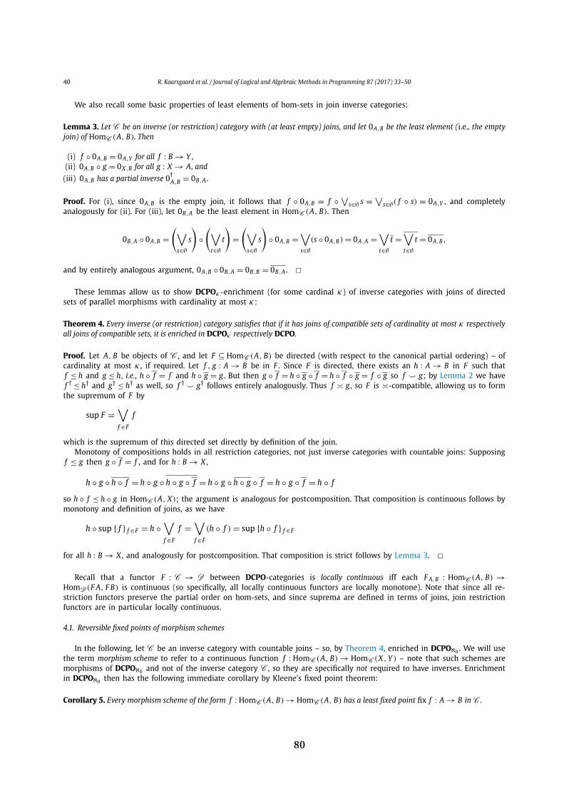
40 R. Kaarsgaard et al. / Journal of Logical and Algebraic Methods in Programming 87 (2017) 33–50

We also recall some basic properties of least elements of hom-sets in join inverse categories:

Lemma 3. Let C be an inverse (or restriction) category with (at least empty) joins, and let 0A,B be the least element (i.e., the empty join) of HomC (A, B). Then

(i) f ◦ 0A,B = 0A,Y for all f : B → Y ,(ii) 0A,B ◦ g = 0X,B for all g : X → A, and

(iii) 0A,B has a partial inverse 0†A,B = 0B,A .

Proof. For (i), since 0A,B is the empty join, it follows that f ◦ 0A,B = f ◦ ∨s∈∅ s = ∨

s∈∅( f ◦ s) = 0A,Y , and completely analogously for (ii). For (iii), let 0B,A be the least element in HomC (A, B). Then

0B,A ◦ 0A,B =(

∨

s∈∅s

)

◦(

∨

t∈∅t

)

=(

∨

s∈∅s

)

◦ 0A,B =∨

s∈∅(s ◦ 0A,B) = 0A,A =

∨

t∈∅t =

∨

t∈∅t = 0A,B ,

and by entirely analogous argument, 0A,B ◦ 0B,A = 0B,B = 0B,A . ✷

These lemmas allow us to show DCPOκ -enrichment (for some cardinal κ ) of inverse categories with joins of directed sets of parallel morphisms with cardinality at most κ :

Theorem 4. Every inverse (or restriction) category satisfies that if it has joins of compatible sets of cardinality at most κ respectively all joins of compatible sets, it is enriched in DCPOκ respectively DCPO.

Proof. Let A, B be objects of C , and let F ⊆ HomC (A, B) be directed (with respect to the canonical partial ordering) – of cardinality at most κ , if required. Let f , g : A → B be in F . Since F is directed, there exists an h : A → B in F such that f ≤ h and g ≤ h, i.e., h ◦ f = f and h ◦ g = g . But then g ◦ f = h ◦ g ◦ f = h ◦ f ◦ g = f ◦ g so f ⌣ g; by Lemma 2 we have f † ≤ h† and g† ≤ h† as well, so f † ⌣ g† follows entirely analogously. Thus f ≍ g , so F is ≍-compatible, allowing us to form the supremum of F by

sup F =∨

f ∈F

f

which is the supremum of this directed set directly by definition of the join.Monotony of compositions holds in all restriction categories, not just inverse categories with countable joins: Supposing

f ≤ g then g ◦ f = f , and for h : B → X ,

h ◦ g ◦ h ◦ f = h ◦ g ◦ h ◦ g ◦ f = h ◦ g ◦ h ◦ g ◦ f = h ◦ g ◦ f = h ◦ f

so h ◦ f ≤ h ◦ g in HomC (A, X); the argument is analogous for postcomposition. That composition is continuous follows by monotony and definition of joins, as we have

h ◦ sup { f } f ∈F = h ◦∨

f ∈F

f =∨

f ∈F

(h ◦ f ) = sup {h ◦ f } f ∈F

for all h : B → X , and analogously for postcomposition. That composition is strict follows by Lemma 3. ✷

Recall that a functor F : C → D between DCPO-categories is locally continuous iff each F A,B : HomC (A, B) →HomD (F A, F B) is continuous (so specifically, all locally continuous functors are locally monotone). Note that since all re-striction functors preserve the partial order on hom-sets, and since suprema are defined in terms of joins, join restriction functors are in particular locally continuous.

4.1. Reversible fixed points of morphism schemes

In the following, let C be an inverse category with countable joins – so, by Theorem 4, enriched in DCPOℵ0 . We will use the term morphism scheme to refer to a continuous function f : HomC (A, B) → HomC (X, Y ) – note that such schemes are morphisms of DCPOℵ0 and not of the inverse category C , so they are specifically not required to have inverses. Enrichment in DCPOℵ0 then has the following immediate corollary by Kleene’s fixed point theorem:

Corollary 5. Every morphism scheme of the form f : HomC (A, B) → HomC (A, B) has a least fixed point fix f : A → B in C .

80

R. Kaarsgaard et al. / Journal of Logical and Algebraic Methods in Programming 87 (2017) 33–50 41

Proof. Define fix f = sup { f n(0A,B)}n∈ω; this is an ω-chain, so specifically a directed set of cardinality at most ℵ0. That this is the least fixed point follows by Kleene’s fixed point theorem, as 0A,B is the least element in HomC (A, B). ✷

Morphism schemes on their own are useful for modeling parametrized reversible functions, as discussed in relation to Theseus in Section 2. Under this interpretation, recursive reversible functions can be seen as the least fixed points of self-parametrized reversible functions.

Given that we can thus model reversible recursive functions via least fixed points of morphism schemes, a prudent question to ask is if the inverse of a least fixed point can be computed as the least fixed point of another morphism scheme. We will answer this in the affirmative, but to do this, we need to show that the induced dagger functor is locally continuous.

Lemma 6. The canonical dagger functor † : C op → C is locally continuous.

Proof. Let F ⊆ HomC (A, B) be directed with respect to the canonical partial order. As local monotony was already shown in Lemma 2, it suffices to show that suprema are preserved. Since f ≤ ∨

f ∈F f for each f ∈ F by Definition 12, we have

f † ≤(∨

f ∈F f)†

for all f ∈ F by monotony of †, and so

sup { f †} f ∈F =∨

f ∈F

f † ≤

⎛

⎝∨

f ∈F

f

⎞

⎠†

= sup { f }†f ∈F

by Definition 12. In the other direction, we have f † ≤ ∨f ∈F f † for all f ∈ F by Definition 12, so by monotony of †, f =

f †† ≤(∨

f ∈F f †)†

for all f ∈ F . But then ∨

f ∈F f ≤(∨

f ∈F f †)†

by Definition 12, and so by monotony of †, we finally get

sup { f }†f ∈F =

⎛

⎝∨

f ∈F

f

⎞

⎠†

≤

⎛

⎝∨

f ∈F

f †

⎞

⎠††

=∨

f ∈F

f † = sup { f †} f ∈F

as desired. ✷

With this lemma, we are able to show that the inverse of a least fixed point of a morphism scheme can be computed as the least fixed point of an adjoint morphism scheme:

Theorem 7. Every morphism scheme of the form f : HomC (A, B) → HomC (A, B) has an adjoint morphism scheme f‡ :HomC (B, A) → HomC (B, A) such that (fix f )† = fix f‡ .

Proof. Let ιA,B : HomC (A, B) → HomC (B, A) denote the family of functions defined by ιA,B ( f ) = f †; each of these are continuous by Lemma 6, and an isomorphism (with inverse ιB,A ) by f †† = f . Given a morphism scheme f : HomC (A, B) →HomC (A, B), we define f‡ = ιA,B ◦ f ◦ιB,A – this is continuous since it is a (continuous) composition of continuous functions. But since

f n‡ = (ιA,B ◦ f ◦ ιB,A)n = ιA,B ◦ f n ◦ ιB,A

by ιB,A an isomorphism with inverse ιA,B , and since 0†A,B = 0B,A by Lemma 3, we get

fix f‡ = sup { f n‡ (0B,A)}n∈ω = sup {(ιA,B ◦ f n ◦ ιB,A)(0B,A)}n∈ω = sup { f n(0†

B,A)†}n∈ω

= sup { f n(0A,B)†}n∈ω = sup { f n(0A,B)}†n∈ω = (fix f )†

as desired. ✷

In modeling recursion in reversible functional programming, this theorem states precisely that the partial inverse of a recursive reversible function is, itself, a recursive reversible function, and that it can be obtained by inverting the function body and replacing recursive calls with recursive calls to the thus constructed inverse: This is precisely the inverse semantics of recursive reversible functions in rfun, as discussed in Section 2.

81

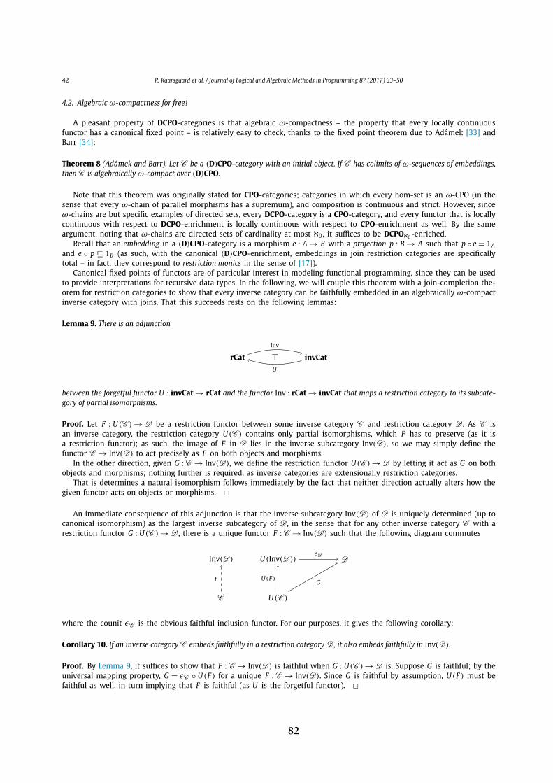
42 R. Kaarsgaard et al. / Journal of Logical and Algebraic Methods in Programming 87 (2017) 33–50

4.2. Algebraic ω-compactness for free!

A pleasant property of DCPO-categories is that algebraic ω-compactness – the property that every locally continuous functor has a canonical fixed point – is relatively easy to check, thanks to the fixed point theorem due to Adámek [33] and Barr [34]:

Theorem 8 (Adámek and Barr). Let C be a (D)CPO-category with an initial object. If C has colimits of ω-sequences of embeddings, then C is algebraically ω-compact over (D)CPO.

Note that this theorem was originally stated for CPO-categories; categories in which every hom-set is an ω-CPO (in the sense that every ω-chain of parallel morphisms has a supremum), and composition is continuous and strict. However, since ω-chains are but specific examples of directed sets, every DCPO-category is a CPO-category, and every functor that is locally continuous with respect to DCPO-enrichment is locally continuous with respect to CPO-enrichment as well. By the same argument, noting that ω-chains are directed sets of cardinality at most ℵ0, it suffices to be DCPOℵ0 -enriched.

Recall that an embedding in a (D)CPO-category is a morphism e : A → B with a projection p : B → A such that p ◦ e = 1Aand e ◦ p ⊑ 1B (as such, with the canonical (D)CPO-enrichment, embeddings in join restriction categories are specifically total – in fact, they correspond to restriction monics in the sense of [17]).

Canonical fixed points of functors are of particular interest in modeling functional programming, since they can be used to provide interpretations for recursive data types. In the following, we will couple this theorem with a join-completion the-orem for restriction categories to show that every inverse category can be faithfully embedded in an algebraically ω-compact inverse category with joins. That this succeeds rests on the following lemmas:

Lemma 9. There is an adjunction

rCat ⊤ invCat

Inv

U

between the forgetful functor U : invCat → rCat and the functor Inv : rCat → invCat that maps a restriction category to its subcate-gory of partial isomorphisms.

Proof. Let F : U (C ) → D be a restriction functor between some inverse category C and restriction category D . As C is an inverse category, the restriction category U (C ) contains only partial isomorphisms, which F has to preserve (as it is a restriction functor); as such, the image of F in D lies in the inverse subcategory Inv(D), so we may simply define the functor C → Inv(D) to act precisely as F on both objects and morphisms.

In the other direction, given G : C → Inv(D), we define the restriction functor U (C ) → D by letting it act as G on both objects and morphisms; nothing further is required, as inverse categories are extensionally restriction categories.

That is determines a natural isomorphism follows immediately by the fact that neither direction actually alters how the given functor acts on objects or morphisms. ✷

An immediate consequence of this adjunction is that the inverse subcategory Inv(D) of D is uniquely determined (up to canonical isomorphism) as the largest inverse subcategory of D , in the sense that for any other inverse category C with a restriction functor G : U (C ) → D , there is a unique functor F : C → Inv(D) such that the following diagram commutes

C

Inv(D) U (Inv(D))

U (C )

D

F U (F )G

ϵD

where the counit ϵC is the obvious faithful inclusion functor. For our purposes, it gives the following corollary:

Corollary 10. If an inverse category C embeds faithfully in a restriction category D , it also embeds faithfully in Inv(D).

Proof. By Lemma 9, it suffices to show that F : C → Inv(D) is faithful when G : U (C ) → D is. Suppose G is faithful; by the universal mapping property, G = ϵC ◦ U (F ) for a unique F : C → Inv(D). Since G is faithful by assumption, U (F ) must be faithful as well, in turn implying that F is faithful (as U is the forgetful functor). ✷

82

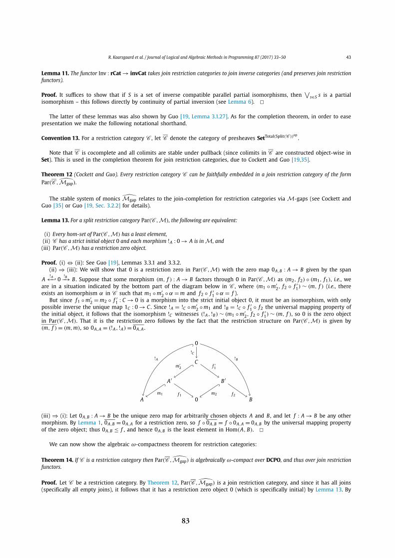
R. Kaarsgaard et al. / Journal of Logical and Algebraic Methods in Programming 87 (2017) 33–50 43

Lemma 11. The functor Inv : rCat → invCat takes join restriction categories to join inverse categories (and preserves join restriction functors).

Proof. It suffices to show that if S is a set of inverse compatible parallel partial isomorphisms, then ∨

s∈S s is a partial isomorphism – this follows directly by continuity of partial inversion (see Lemma 6). ✷

The latter of these lemmas was also shown by Guo [19, Lemma 3.1.27]. As for the completion theorem, in order to ease presentation we make the following notational shorthand.

Convention 13. For a restriction category C , let C denote the category of presheaves SetTotal(Split(C ))op.

Note that C is cocomplete and all colimits are stable under pullback (since colimits in C are constructed object-wise in Set). This is used in the completion theorem for join restriction categories, due to Cockett and Guo [19,35].

Theorem 12 (Cockett and Guo). Every restriction category C can be faithfully embedded in a join restriction category of the form Par(C , !Mgap).

The stable system of monics !Mgap relates to the join-completion for restriction categories via M-gaps (see Cockett and Guo [35] or Guo [19, Sec. 3.2.2] for details).

Lemma 13. For a split restriction category Par(C , M), the following are equivalent:

(i) Every hom-set of Par(C , M) has a least element,(ii) C has a strict initial object 0 and each morphism !A : 0 → A is in M, and

(iii) Par(C , M) has a restriction zero object.

Proof. (i) ⇔ (ii): See Guo [19], Lemmas 3.3.1 and 3.3.2.(ii) ⇒ (iii): We will show that 0 is a restriction zero in Par(C , M) with the zero map 0A,B : A → B given by the span

A !A←−↩ 0 !B−→ B . Suppose that some morphism (m, f ) : A → B factors through 0 in Par(C , M) as (m2, f2) ◦ (m1, f1), i.e., we are in a situation indicated by the bottom part of the diagram below in C , where (m1 ◦ m′

2, f2 ◦ f ′1) ∼ (m, f ) (i.e., there

exists an isomorphism α in C such that m1 ◦ m′2 ◦ α = m and f2 ◦ f ′

1 ◦ α = f ).But since f1 ◦ m′

2 = m2 ◦ f ′1 : C → 0 is a morphism into the strict initial object 0, it must be an isomorphism, with only

possible inverse the unique map 1C : 0 → C . Since !A = !C ◦ m′2 ◦ m1 and !B = !C ◦ f ′

1 ◦ f2 the universal mapping property of the initial object, it follows that the isomorphism !C witnesses (!A, !B) ∼ (m1 ◦ m′

2, f2 ◦ f ′1) ∼ (m, f ), so 0 is the zero object

in Par(C , M). That it is the restriction zero follows by the fact that the restriction structure on Par(C , M) is given by (m, f ) = (m, m), so 0A,A = (!A, !A) = 0A,A .

A′

A 0

B ′

B

C

0

m1 f1 m2 f2

m′2 f ′

1

!A !B

!C

(iii) ⇒ (i): Let 0A,B : A → B be the unique zero map for arbitrarily chosen objects A and B , and let f : A → B be any other morphism. By Lemma 1, 0A,B = 0A,A for a restriction zero, so f ◦ 0A,B = f ◦ 0A,A = 0A,B by the universal mapping property of the zero object; thus 0A,B ≤ f , and hence 0A,B is the least element in Hom(A, B). ✷

We can now show the algebraic ω-compactness theorem for restriction categories:

Theorem 14. If C is a restriction category then Par(C , !Mgap) is algebraically ω-compact over DCPO, and thus over join restriction functors.

Proof. Let C be a restriction category. By Theorem 12, Par(C , !Mgap) is a join restriction category, and since it has all joins (specifically all empty joins), it follows that it has a restriction zero object 0 (which is specifically initial) by Lemma 13. By

83

44 R. Kaarsgaard et al. / Journal of Logical and Algebraic Methods in Programming 87 (2017) 33–50

Adámek and Barr’s fixed point theorem and the fact that restriction categories with arbitrary joins are DCPO-enriched (by Theorem 4), it suffices to show that Par(C , !Mgap) has colimits of ω-diagrams of embeddings. Let D : ω → Par(C , !Mgap) be such a diagram of embeddings. This corresponds to the diagram

A

D(0) D(1)

B

D(2) . . .

m0 f0 m1 f1

in C . Since C is cocomplete, this diagram has a colimiting cocone α : D ⇒ colim D such that the diagram below com-mutes. Further, since colimits in C are constructed object-wise in Set, this colimit is stable under pullbacks, so the pullbacks in C used for composition in Par(C , !Mgap) commutes with this colimit. Since embeddings are total, each miis an isomorphism, and since isomorphisms are stable under pullback, any m′

i arising from a pullback (corresponding

to composition) is an isomorphism as well. As such, any mi ◦ m′i+1 is an isomorphism, and so the isomorphism m′ (−1)

i+1witnesses (mi ◦ m′

i+1, αD(i+2) ◦ f i+1 ◦ f ′i ) ∼ (mi, αD(i+1) ◦ f i); iterating this argument for arbitrary finite k, we see that

everything commutes, as desired. Thus, the family of morphisms {(mi, αD(i+1) ◦ f i)}i∈ω is a colimiting cocone for D in Par(C , !Mgap).

✷

Finally, using this machinery, we can show how this theorem extends to inverse categories.

Corollary 15. Every inverse category can be faithfully embedded in a join inverse category that is algebraically ω-compact over join restriction functors.

Proof. Let C be an inverse category. Since U (C ) is the exact same category viewed as a restriction category, U (C ) embeds faithfully in Par(C , !Mgap), which is a join restriction category by Theorem 12, and algebraically ω-compact by Theorem 14. But then it follows by Corollary 10 that C embeds faithfully in Inv(Par(C , !Mgap)), which is a join inverse category by Lemma 11, and is algebraically ω-compact for join restriction functors (which are specifically locally continuous) since fixed points of functors are (total) isomorphisms, so preserved in Inv(Par(C , !Mgap)). ✷

4.3. Applications in models of reversible functional programming

This final corollary shows directly that join inverse categories are consistent with algebraic ω-compactness over join restriction functors, which can thus be used to model recursive data types in the style of Theseus as well as rfun terms, given the existence of suitable join-preserving monoidal functors as follows: Suppose we are given an inverse product (⊗, 1)and a disjointness tensor (⊕, 0), both join-preserving (see [18] for details on both; the definition of latter can also found in Definition 17 in the following section) such that there are (total) natural isomorphisms

A ⊗ (B ⊕ C)δA,B,C∼= (A ⊗ B) ⊕ (A ⊗ C) A ⊗ 0

νA∼= 0

giving the category the structure of a bimonoidal category (or rig category; see also [36,37]). Using the compactness theorem from before, this enables us to model all (isorecursive) data types expressible in Theseus by modeling product types using the inverse product, sum types using the disjointness tensor, the unit type as 1, the empty type as 0, and recursive types using the canonical fixed point. For example, the two types from the Theseus example in Fig. 2, defined as

type Bool = False | True

type Nat = 0 | Succ Nat

84

R. Kaarsgaard et al. / Journal of Logical and Algebraic Methods in Programming 87 (2017) 33–50 45

can both be given very familiar denotations as 1 ⊕ 1 respectively µX .1 ⊕ X (i.e., the least – in this case, unique – fixed point of the functor defined by F (X) = 1 ⊕ X).

Though rfun is untyped, with terms formed using Lisp-style symbols and constructors, this bimonoidal structure is also helpful in constructing a denotation of the universal type of rfun terms. Formally, rfun terms are constructed inductively as follows: Given a denumerable set S of symbols, a term t is either a symbol (i.e., t ∈ S) or of the form c(t1, t2, . . . , tk) for some finite k, where c ∈ S and each ti is a term. Supposing that S is the Kleene star closure of the latin alphabet, examples of terms include a, s(s(z)), and f (o, o(bar, baz)).

Since the symbols S is denumerable, we can identify symbols one-to-one with natural numbers – and so with the object µX .1 ⊕ X using algebraic compactness. Further, in the familiar way, we can define the functor mapping an object A to lists of A by A :→ µX .1 ⊕ (A ⊗ X). This, finally, means that we can define a functor mapping an object A to terms over A by A :→ µX .A ⊗ L(X).

Moreover, we saw how this view of join restriction categories as DCPO-categories also enabled the style of reversible recursion found in rfun, exemplified in the Fibonacci-pair program in Fig. 1. More specifically, to give the denotation of a recursive function in rfun, instead of trying to interpret it directly as an endomorphism on the term object T → T , we instead interpret it as a morphism scheme Hom(T , T ) [[ f ′]]−−−→ Hom(T , T ) in which the recursive call is replaced by a call to the morphism given as argument, and then take the least fixed point of this morphism scheme fix [ [ f ′] ] as the denotation of the recursive function f . Further details on this construction, and the other constructions sketched in this section, will appear in a forthcoming paper.

5. As unique decomposition categories

Complementary to the view on inverse categories with countable joins as DCPO-categories, we will show that these can also be viewed as unique decomposition categories, a kind of category introduced by Haghverdi [20] equipped with a partial sum operation on hom-sets via enrichment in the category of #-monoids (shown to be symmetric monoidal by Hoshino [21]). Unique decomposition categories (including Hoshino’s strong unique decomposition categories [21] which we will employ here) are specifically traced monoidal categories [38] if they satisfy certain conditions. This is desirable when modeling functional programming, as traces can be used to model notions of feedback [39] and recursion [40–42].

Here, we will show that inverse categories with countable joins and a join-preserving disjointness tensor (due to Giles [18]) are strong unique decomposition categories, and satisfy the conditions required to be equipped with a trace. We extend this result further to show that the trace is a †-trace [43], and thus has pleasant inversion properties (the trace in PInj is well studied, cf. [44,20,45]). This is particularly interesting given that the reversible programming language Theseus [15] and the combinator calculus "0 [16] both rely on a †-trace for reversible recursion.

We begin with the definition of a #-monoid [20] (see also Manes and Benson [46] where these first appeared as positive partial monoids):

Definition 14. A #-monoid (M, #) consists of a nonempty set M and a partial operator # defined on countable families in M (say that a family {xi}i∈I is summable if

∑i∈I xi is defined) such that

(i) if {xi}i∈I is a countable family in M and {I j} j∈ J is a countable partitioning of I , then {xi}i∈I is summable iff all {xi}i∈I j

and ∑

i∈I jxi are summable for all j ∈ J , and in this case

∑

j∈ J

∑

i∈I j

xi =∑

i∈I

xi ,

(ii) any family {xi}i∈I in M where I is singleton is summable with ∑

i∈I xi = x j if I = { j}.

The class of #-monoids with homomorphisms preserving partial sums forms a category, #Mon. As such, a category Cis enriched in #Mon if all hom-sets of C are #-monoids, and composition distributes over partial addition.

Lemma 16. Every inverse category with countable joins is #Mon-enriched.

Proof. Let C be an inverse category with countable joins. Let {si}i∈I be a countable family of morphisms taken from HomC (A, B) for some objects A, B of C and countable index set I . We define

∑

i∈I

si =∨

s∈{si |i∈I}s

so, by definition, summability coincides with join compatibility.To see that axiom (i) of Definition 14 is satisfied, let {I j} j∈ J be a partitioning of I and suppose that {si}i∈I is summable,

i.e., inverse compatible. By definition of inverse compatibility, this means that all morphisms of {si}i∈I are pairwise inverse

85

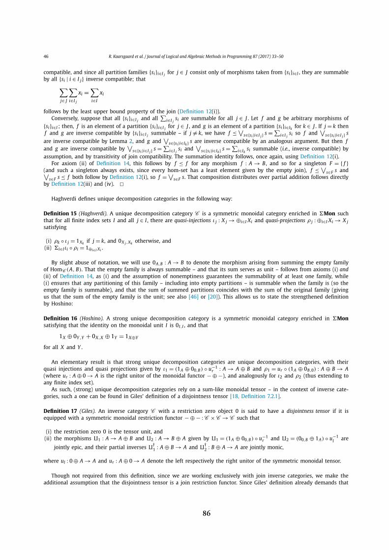
46 R. Kaarsgaard et al. / Journal of Logical and Algebraic Methods in Programming 87 (2017) 33–50

compatible, and since all partition families {si}i∈I j for j ∈ J consist only of morphisms taken from {si}i∈I , they are summable by all {si | i ∈ I j} inverse compatible; that

∑

j∈ J

∑

i∈I j

xi =∑

i∈I

xi

follows by the least upper bound property of the join (Definition 12(i)).Conversely, suppose that all {si}i∈I j and all

∑i∈I j

si are summable for all j ∈ J . Let f and g be arbitrary morphisms of {si}i∈I ; then, f is an element of a partition {si}i∈I j for j ∈ J , and g is an element of a partition {si}i∈Ik for k ∈ J . If j = k then f and g are inverse compatible by {si}i∈I j summable – if j = k, we have f ≤ ∨

s∈{si |i∈I j} s = ∑i∈I j

si so f and ∨

s∈{si |i∈I j} sare inverse compatible by Lemma 2, and g and

∨s∈{si |i∈Ik} s are inverse compatible by an analogous argument. But then f

and g are inverse compatible by ∨

s∈{si |i∈I j} s = ∑i∈I j

si and ∨

s∈{si |i∈Ik} s = ∑i∈Ik

si summable (i.e., inverse compatible) by assumption, and by transitivity of join compatibility. The summation identity follows, once again, using Definition 12(i).

For axiom (ii) of Definition 14, this follows by f ≤ f for any morphism f : A → B , and so for a singleton F = { f }(and such a singleton always exists, since every hom-set has a least element given by the empty join), f ≤ ∨

s∈F s and ∨s∈F s ≤ f both follow by Definition 12(i), so f = ∨

s∈F s. That composition distributes over partial addition follows directly by Definition 12(iii) and (iv). ✷

Haghverdi defines unique decomposition categories in the following way:

Definition 15 (Haghverdi). A unique decomposition category C is a symmetric monoidal category enriched in #Mon such that for all finite index sets I and all j ∈ I , there are quasi-injections ι j : X j → ⊕i∈I Xi and quasi-projections ρ j : ⊕i∈I Xi → X jsatisfying

(i) ρk ◦ ι j = 1Xk if j = k, and 0X j ,Xk otherwise, and(ii) #i∈I ιi ◦ ρi = 1⊕i∈I Xi .

By slight abuse of notation, we will use 0A,B : A → B to denote the morphism arising from summing the empty family of HomC (A, B). That the empty family is always summable – and that its sum serves as unit – follows from axioms (i) and(ii) of Definition 14, as (i) and the assumption of nonemptiness guarantees the summability of at least one family, while (i) ensures that any partitioning of this family – including into empty partitions – is summable when the family is (so the empty family is summable), and that the sum of summed partitions coincides with the sum of the original family (giving us that the sum of the empty family is the unit; see also [46] or [20]). This allows us to state the strengthened definition by Hoshino:

Definition 16 (Hoshino). A strong unique decomposition category is a symmetric monoidal category enriched in #Monsatisfying that the identity on the monoidal unit I is 0I,I , and that

1X ⊕ 0Y ,Y + 0X,X ⊕ 1Y = 1X⊕Y

for all X and Y .

An elementary result is that strong unique decomposition categories are unique decomposition categories, with their quasi injections and quasi projections given by ι1 = (1A ⊕ 00,B) ◦ u−1

r : A → A ⊕ B and ρ1 = ur ◦ (1A ⊕ 0B,0) : A ⊕ B → A(where ur : A ⊕ 0 → A is the right unitor of the monoidal functor − ⊕ −), and analogously for ι2 and ρ2 (thus extending to any finite index set).

As such, (strong) unique decomposition categories rely on a sum-like monoidal tensor – in the context of inverse cate-gories, such a one can be found in Giles’ definition of a disjointness tensor [18, Definition 7.2.1].

Definition 17 (Giles). An inverse category C with a restriction zero object 0 is said to have a disjointness tensor if it is equipped with a symmetric monoidal restriction functor − ⊕ − : C × C → C such that

(i) the restriction zero 0 is the tensor unit, and(ii) the morphisms ⨿1 : A → A ⊕ B and ⨿2 : A → B ⊕ A given by ⨿1 = (1A ⊕ 00,B) ◦ u−1

r and ⨿2 = (00,B ⊕ 1A) ◦ u−1l are

jointly epic, and their partial inverses ⨿†1 : A ⊕ B → A and ⨿†

2 : B ⊕ A → A are jointly monic,

where ul : 0 ⊕ A → A and ur : A ⊕ 0 → A denote the left respectively the right unitor of the symmetric monoidal tensor.

Though not required from this definition, since we are working exclusively with join inverse categories, we make the additional assumption that the disjointness tensor is a join restriction functor. Since Giles’ definition already demands that

86

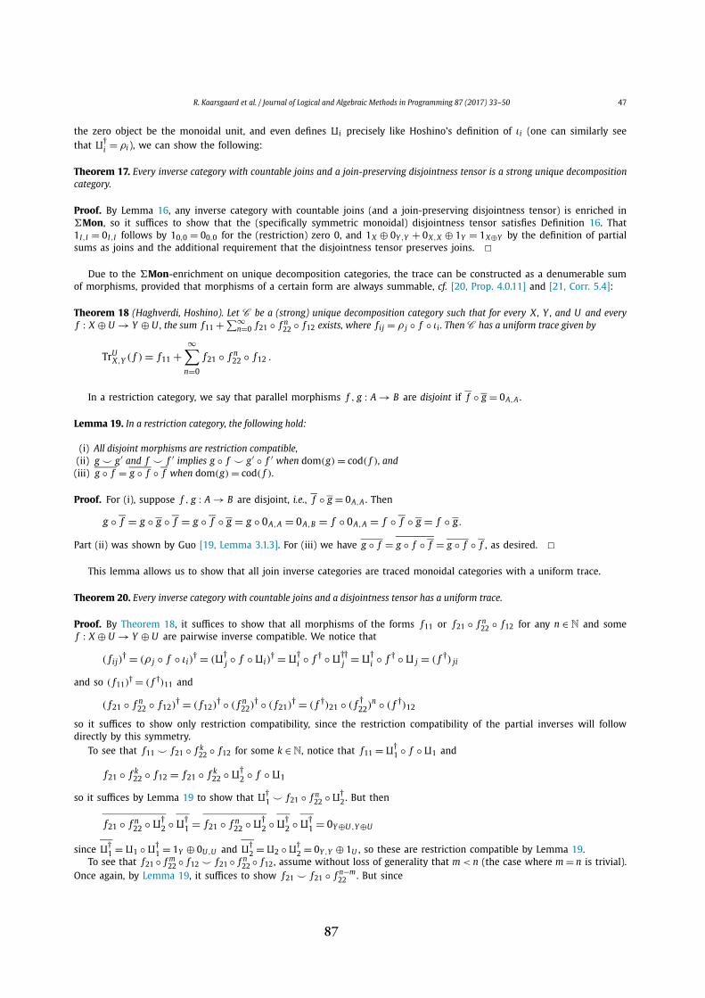
R. Kaarsgaard et al. / Journal of Logical and Algebraic Methods in Programming 87 (2017) 33–50 47

the zero object be the monoidal unit, and even defines ⨿i precisely like Hoshino’s definition of ιi (one can similarly see that ⨿†

i = ρi ), we can show the following:

Theorem 17. Every inverse category with countable joins and a join-preserving disjointness tensor is a strong unique decomposition category.

Proof. By Lemma 16, any inverse category with countable joins (and a join-preserving disjointness tensor) is enriched in #Mon, so it suffices to show that the (specifically symmetric monoidal) disjointness tensor satisfies Definition 16. That 1I,I = 0I,I follows by 10,0 = 00,0 for the (restriction) zero 0, and 1X ⊕ 0Y ,Y + 0X,X ⊕ 1Y = 1X⊕Y by the definition of partial sums as joins and the additional requirement that the disjointness tensor preserves joins. ✷

Due to the #Mon-enrichment on unique decomposition categories, the trace can be constructed as a denumerable sum of morphisms, provided that morphisms of a certain form are always summable, cf. [20, Prop. 4.0.11] and [21, Corr. 5.4]:

Theorem 18 (Haghverdi, Hoshino). Let C be a (strong) unique decomposition category such that for every X, Y , and U and every f : X ⊕ U → Y ⊕ U , the sum f11 + ∑∞

n=0 f21 ◦ f n22 ◦ f12 exists, where f i j = ρ j ◦ f ◦ ιi . Then C has a uniform trace given by

TrUX,Y ( f ) = f11 +

∞∑

n=0

f21 ◦ f n22 ◦ f12 .

In a restriction category, we say that parallel morphisms f , g : A → B are disjoint if f ◦ g = 0A,A .

Lemma 19. In a restriction category, the following hold:

(i) All disjoint morphisms are restriction compatible,(ii) g ⌣ g′ and f ⌣ f ′ implies g ◦ f ⌣ g′ ◦ f ′ when dom(g) = cod( f ), and

(iii) g ◦ f = g ◦ f ◦ f when dom(g) = cod( f ).

Proof. For (i), suppose f , g : A → B are disjoint, i.e., f ◦ g = 0A,A . Then

g ◦ f = g ◦ g ◦ f = g ◦ f ◦ g = g ◦ 0A,A = 0A,B = f ◦ 0A,A = f ◦ f ◦ g = f ◦ g.

Part (ii) was shown by Guo [19, Lemma 3.1.3]. For (iii) we have g ◦ f = g ◦ f ◦ f = g ◦ f ◦ f , as desired. ✷

This lemma allows us to show that all join inverse categories are traced monoidal categories with a uniform trace.

Theorem 20. Every inverse category with countable joins and a disjointness tensor has a uniform trace.

Proof. By Theorem 18, it suffices to show that all morphisms of the forms f11 or f21 ◦ f n22 ◦ f12 for any n ∈ N and some

f : X ⊕ U → Y ⊕ U are pairwise inverse compatible. We notice that

( f i j)† = (ρ j ◦ f ◦ ιi)

† = (⨿†j ◦ f ◦ ⨿i)

† = ⨿†i ◦ f † ◦ ⨿††

j = ⨿†i ◦ f † ◦ ⨿ j = ( f †) ji

and so ( f11)† = ( f †)11 and

( f21 ◦ f n22 ◦ f12)

† = ( f12)† ◦ ( f n

22)† ◦ ( f21)

† = ( f †)21 ◦ ( f †22)

n ◦ ( f †)12

so it suffices to show only restriction compatibility, since the restriction compatibility of the partial inverses will follow directly by this symmetry.

To see that f11 ⌣ f21 ◦ f k22 ◦ f12 for some k ∈ N, notice that f11 = ⨿†

1 ◦ f ◦ ⨿1 and

f21 ◦ f k22 ◦ f12 = f21 ◦ f k

22 ◦ ⨿†2 ◦ f ◦ ⨿1

so it suffices by Lemma 19 to show that ⨿†1 ⌣ f21 ◦ f n

22 ◦ ⨿†2. But then

f21 ◦ f n22 ◦ ⨿†

2 ◦ ⨿†1 = f21 ◦ f n

22 ◦ ⨿†2 ◦ ⨿†

2 ◦ ⨿†1 = 0Y ⊕U ,Y ⊕U

since ⨿†1 = ⨿1 ◦ ⨿†

1 = 1Y ⊕ 0U ,U and ⨿†2 = ⨿2 ◦ ⨿†

2 = 0Y ,Y ⊕ 1U , so these are restriction compatible by Lemma 19.To see that f21 ◦ f m

22 ◦ f12 ⌣ f21 ◦ f n22 ◦ f12, assume without loss of generality that m < n (the case where m = n is trivial).

Once again, by Lemma 19, it suffices to show f21 ⌣ f21 ◦ f n−m22 . But since

87

48 R. Kaarsgaard et al. / Journal of Logical and Algebraic Methods in Programming 87 (2017) 33–50

f21 = ⨿†1 ◦ f ◦ ⨿2

and

f21 ◦ f n−m22 = f21 ◦ (⨿†

2 ◦ f ◦ ⨿2)(n−m)−1 ◦ ⨿†

2 ◦ f ◦ ⨿2

restriction compatibility follows by analogous argument to the previous case. ✷

Recall that a †-category with a trace is said to have a †-trace (see, e.g., [43]) if TrUX,Y ( f )† = TrU

Y ,X ( f †) for every morphism f : X ⊕ U → Y ⊕ U .

Theorem 21. The canonical trace in an inverse category with countable joins and a disjointness tensor is a †-trace.

Proof. To see that the trace induced by Theorems 18 and 20 is a †-trace, let f : X ⊕ U → Y ⊕ U be a morphism of C .In the proof of Theorem 20, we noticed that ( f i j)

† = ( f †) ji and ( f21 ◦ f n22 ◦ f12)

† = ( f †)21 ◦ ( f †22)

n ◦ ( f †)12. Expanding this in the definition of the canonical trace given by Theorem 18, we get

TrUX,Y ( f )† =

(

f11 +∑

n∈ω

f21 ◦ f n22 ◦ f12

)†

=(

f11 ∨∨

n∈ω

f21 ◦ f n22 ◦ f12

)†

= ( f11)† ∨

(∨

n∈ω

f21 ◦ f n22 ◦ f12

)†

= ( f11)† ∨

∨

n∈ω

( f12)† ◦ ( f n

22)† ◦ ( f21)

†

= ( f †)11 ∨∨

n∈ω

( f †)21 ◦ ( f †)n22 ◦ ( f †)12 = TrU

Y ,X ( f †)

by definition of the partial sum as join (Lemma 16), and by (∨

f ∈F f )† = ∨f ∈F f † by Lemma 6. ✷

5.1. Applications in models of reversible functional programming

This final theorem is highly relevant to modeling Theseus in join inverse categories, as the iteration label-approach to reversible tail recursion (exemplified in the parity program in Fig. 2) is equivalent to the existence of a †-trace operator. This can be observed from the fact that we are not only able to provide a forward and backward semantics to functions with iteration labels via a †-trace [15] (see also the discussion in Section 2), but that it is also possible to express a †-trace operator as a parametrized function (which, in turn, can be naturally regarded categorically as a morphism scheme) in Theseus [15].

To give a concrete example, consider the recursive parity function in Theseus from Fig. 2. To give semantics to its recursive behavior using a †-trace, we systematically transform from a function of type Nat × Bool ↔ Nat × Bool with an internal iteration label of type Nat×Nat×Bool ↔ Nat×Nat×Bool into a function of type (Nat×Bool) +(Nat×Nat×Bool) ↔(Nat × Bool) + (Nat × Nat × Bool) by prefacing patterns for the outer (parity) function by Left, replacing patterns for the inner (iteration label) function by Right-patterns, replacing calls to the inner function by Right-expressions, and prefacing return values by Left-expressions, as in the following:

parity :: Nat × Bool ↔ Nat × Bool| (n,b) ↔ iter (n,0,b)

| iter (Succ n,m,b) ↔ iter (n,Succ m,not b)

| iter (0,m,b) ↔ (m,b)

where iter :: Nat × Nat × Bool ↔Nat × Nat × Bool

⇒

parity′ :: (Nat × Bool) + (Nat × Nat × Bool) ↔(Nat × Bool) + (Nat × Nat × Bool)

| Left (n,b) ↔ Right (n,0,b)

| Right (Succ n,m,b) ↔ Right (n,Succ m,not b)

| Right (0,m,b) ↔ Left (m,b)

Notice that this transformation preserves non-overlapping and exhaustive patterns, as are required of Theseus functions. In this way, we can obtain the denotation of the original parity function by taking the †-trace of the denotation of the transformed parity′ function.

6. Conclusion

We have shown that inverse categories with countable joins carry with them a few key properties that are highly useful for modeling partial reversible functional programming. Notably, we have shown that any inverse category with countable joins is DCPO-enriched – from this view, we gathered that morphism schemes have fixed points, and that the partial inverses of such fixed points can be computed as fixed points of adjoint morphism schemes. This gave us a model of recursion à la rfun.

Further, we were able to show that any inverse category can be embedded in an inverse category with joins, in which all join restriction functors have canonical fixed points. Finally, we showed that the presence of a join-preserving disjointness

88

R. Kaarsgaard et al. / Journal of Logical and Algebraic Methods in Programming 87 (2017) 33–50 49

tensor on an inverse category with countable joins gives us a strong unique decomposition category, and in turn, a uniform †-trace: a model of recursion à la Theseus and "0.

Restriction categories have recently been considered as enriched categories by Cockett and Garner [47], though their approach relied on enrichments based on weak double categories rather than monoidal categories, as it is otherwise usually done (including in this paper). Further, fixed points in categories with a notion of partiality have previously been considered, notably by Fiore [48] who also relied on order-enrichment, though his work was in categories of partial maps directly. Finally, Giles [18] has shown the construction of a trace in inverse categories recently, relying instead on the presence of countable disjoint sums rather than joins (whether or not this approach leads to a †-trace is unspecified). It should also be noted that the trace in the canonical inverse category PInj has been studied independently of unique decomposition and restriction categories, notably by Hines [44] and Abramsky, Haghverdi, and Scott [45].

As regards future work, since an inverse category with countable joins and a disjointness tensor is †-traced, it can be embedded in a †-compact closed category via the Int-construction [38,49]. It may be of interest to consider †-compact closed categories generated in this manner, as we suspect these will be inverse categories as well (notably, Int(PInj) is [44]) – and could provide, e.g., an alternative treatment of projectors as restriction idempotents, and isometries as restriction monics (see also [50]).

Additionally, while our focus in this article has been on inverse categories, we conjecture that many of these results can be generalized to restriction categories.

Acknowledgements

The authors wish to thank the anonymous reviewers for their thoughtful and detailed comments, and the anonymous reviewers of FoSSaCS 2016 as well as the participants of NWPT 2015 for their useful comments on earlier versions of the paper. The research was partly funded by the Danish Council for Independent Research under the Foundations of Reversible Computing project. We also acknowledge the support given by COST Action IC1405 Reversible Computation: Extending Horizons of Computing.

References

[1] R. Kaarsgaard, Join inverse categories and reversible recursion, 2015, abstract presented at the 27th Nordic Workshop on Programming Theory.[2] H.B. Axelsen, R. Kaarsgaard, Join inverse categories as models of reversible recursion, in: B. Jacobs, C. Löding (Eds.), Foundations of Software Science

and Computation Structures, 19th International Conference, FoSSaCS 2016, Proceedings, in: Lecture Notes in Computer Science, vol. 9634, Springer, 2016, pp. 73–90.

[3] R. Landauer, Irreversibility and heat generation in the computing process, IBM J. Res. Dev. 5 (3) (1961) 183–191.[4] E. Fredkin, T. Toffoli, Conservative logic, Int. J. Theor. Phys. 21 (3–4) (1982) 219–253.[5] C.H. Bennett, Logical reversibility of computation, IBM J. Res. Dev. 17 (6) (1973) 525–532.[6] H.B. Axelsen, R. Glück, What do reversible programs compute?, in: M. Hofmann (Ed.), Foundations of Software Science and Computational Structures,

14th International Conference, FOSSACS 2011, Proceedings, in: Lecture Notes in Computer Science, vol. 6604, Springer, 2011, pp. 42–56.[7] M. Kutrib, M. Wendlandt, Reversible limited automata, in: J. Durand-Lose, B. Nagy (Eds.), Machines, Computations, and Universality, 7th International

Conference, MCU 2015, Proceedings, in: Lecture Notes in Computer Science, vol. 9288, Springer, 2015, pp. 113–128.[8] K. Morita, Two-way reversible multihead automata, Fundam. Inform. 110 (1–4) (2011) 241–254.[9] M. Schordan, D. Jefferson, P. Barnes, T. Oppelstrup, D. Quinlan, Reverse code generation for parallel discrete event simulation, in: J. Krivine, J.-B. Stefani

(Eds.), Reversible Computation, 7th International Conference, RC 2015, Proceedings, in: Lecture Notes in Computer Science, vol. 9138, Springer, 2015, pp. 95–110.

[10] I. Cristescu, J. Krivine, D. Varacca, A compositional semantics for the reversible π -calculus, in: LICS 2013, IEEE Computer Society, 2013, pp. 388–397.[11] U.P. Schultz, M. Bordignon, K. Støy, Robust and reversible execution of self-reconfiguration sequences, Robotica 29 (1) (2011) 35–57.[12] U.P. Schultz, J.S. Laursen, L. Ellekilde, H.B. Axelsen, Towards a domain-specific language for reversible assembly sequences, in: J. Krivine, J.-B. Stefani

(Eds.), Reversible Computation, 7th International Conference, RC 2015, Proceedings, in: Lecture Notes in Computer Science, vol. 9138, Springer, 2015, pp. 111–126.

[13] T. Yokoyama, R. Glück, A reversible programming language and its invertible self-interpreter, in: Partial Evaluation and Program Manipulation. Proceed-ings, ACM, 2007, pp. 144–153.

[14] T. Yokoyama, H.B. Axelsen, R. Glück, Fundamentals of reversible flowchart languages, Theor. Comput. Sci. 611 (2016) 87–115.[15] R.P. James, A. Sabry, Theseus: A high level language for reversible computing, work-in-progress report at RC, 2014, available at https://www.cs.

indiana.edu/~sabry/papers/theseus.pdf, 2014.[16] W.J. Bowman, R.P. James, A. Sabry, Dagger traced symmetric monoidal categories and reversible programming, in: A. De Vos, R. Wille (Eds.), Reversible

Computation 2011, Proceedings, Ghent University, 2011, pp. 51–56.[17] J.R.B. Cockett, S. Lack, Restriction categories I: categories of partial maps, Theor. Comput. Sci. 270 (1–2) (2002) 223–259.[18] B.G. Giles, An investigation of some theoretical aspects of reversible computing, Ph.D. thesis, University of Calgary, 2014.[19] X. Guo, Products, joins, meets, and ranges in restriction categories, Ph.D. thesis, University of Calgary, 2012.[20] E. Haghverdi, A categorical approach to linear logic, geometry of proofs and full completeness, Ph.D. thesis, Carlton University and University of Ottawa,

2000.[21] N. Hoshino, A representation theorem for unique decomposition categories, in: U. Berger, M. Mislove (Eds.), MFPS XXVIII, in: Electronic Notes in

Theoretical Computer Science, vol. 286, Elsevier, 2012, pp. 213–227.[22] T. Yokoyama, H.B. Axelsen, R. Glück, Towards a reversible functional language, in: A. De Vos, R. Wille (Eds.), Reversible Computation, Third International

Workshop, RC 2011, Revised papers, in: Lecture Notes in Computer Science, vol. 7165, Springer, 2012, pp. 14–29.[23] S.M. Abramov, R. Glück, Principles of inverse computation and the universal resolving algorithm, in: T. Æ. Mogensen, D.A. Schmidt, I.H. Sudbor-

ough (Eds.), The Essence of Computation: Complexity, Analysis, Transformation, in: Lecture Notes in Computer Science, vol. 2566, Springer, 2002, pp. 269–295.

[24] R. Glück, M. Kawabe, Derivation of deterministic inverse programs based on LR parsing, in: Y. Kameyama, P.J. Stuckey (Eds.), Functional and Logic Programming, 7th International Symposium, FLOPS 2004, Proceedings, in: Lecture Notes in Computer Science, vol. 2998, Springer, 2004, pp. 291–306.

89

50 R. Kaarsgaard et al. / Journal of Logical and Algebraic Methods in Programming 87 (2017) 33–50

[25] R. Glück, M. Kawabe, A program inverter for a functional language with equality and constructors, in: A. Ohori (Ed.), Programming Languages and Systems, First Asian Symposium, APLAS 2003, Proceedings, in: Lecture Notes in Computer Science, vol. 2895, Springer, 2003, pp. 246–264.

[26] R.P. James, A. Sabry, Information effects, in: Proceedings of the 39th Annual ACM SIGPLAN-SIGACT Symposium on Principles of Programming Languages, POPL ’12, ACM, 2012, pp. 73–84.

[27] J.R.B. Cockett, S. Lack, Restriction categories II: partial map classification, Theor. Comput. Sci. 294 (1–2) (2003) 61–102.[28] J.R.B. Cockett, S. Lack, Restriction categories III: colimits, partial limits and extensivity, Math. Struct. Comput. Sci. 17 (4) (2007) 775–817.[29] M.V. Lawson, Inverse Semigroups: The Theory of Partial Symmetries, World Scientific, 1998.[30] J. Kastl, Inverse categories, in: H.-J. Hoehnke (Ed.), Algebraische Modelle, Kategorien und Gruppoide, in: Studien zur Algebra und Ihre Anwendungen,

vol. 7, Akademie-Verlag, 1979, pp. 51–60.[31] C. Heunen, On the functor ℓ2, in: Computation, Logic, Games, and Quantum Foundations – The Many Facets of Samson Abramsky, in: Lecture Notes in

Computer Science, vol. 7860, Springer, 2013, pp. 107–121.[32] E. Robinson, G. Rosolini, Categories of partial maps, Inf. Comput. 79 (1988) 95–130.[33] J. Adámek, Recursive data types in algebraically ω-complete categories, Inf. Comput. 118 (1995) 181–190.[34] M. Barr, Algebraically compact functors, J. Pure Appl. Algebra 82 (3) (1992) 211–231.[35] J.R.B. Cockett, X. Guo, Join restriction categories and the importance of being adhesive, presentation at Category Theory (2007), 2007.[36] M.L. Laplaza, Coherence for distributivity, in: G.M. Kelly, M.L. Laplaza, G. Lewis, S. Mac Lane (Eds.), Coherence in Categories, in: Lecture Notes in

Mathematics, vol. 281, Springer, 1972, pp. 29–65.[37] J. Carette, A. Sabry, Computing with semirings and weak rig groupoids, in: P. Thiemann (Ed.), Programming Languages and Systems, 25th European

Symposium on Programming, Proceedings, in: Lecture Notes in Computer Science, vol. 9632, Springer, 2016, pp. 123–148.[38] A. Joyal, R. Street, D. Verity, Traced monoidal categories, Math. Proc. Camb. Philos. Soc. 119 (3) (1996) 447–468.[39] S. Abramsky, Retracing some paths in process algebra, in: U. Montanari, V. Sassone (Eds.), CONCUR ’96: Concurrency Theory, 7th International Confer-

ence, Proceedings, in: Lecture Notes in Computer Science, vol. 1119, Springer, 1996, pp. 1–17.[40] M. Hasegawa, Recursion from cyclic sharing: traced monoidal categories and models of cyclic lambda calculi, in: P. de Groote, J.R. Hindley (Eds.), Typed

Lambda Calculi and Applications, Third International Conference on Typed Lambda Calculi and Applications, TLCA ’97, Proceedings, in: Lecture Notes in Computer Science, vol. 1210, Springer, 1997, pp. 196–213.

[41] M. Hasegawa, Models of sharing graphs, Ph.D. thesis, University of Edinburgh, 1997.[42] M. Hyland, Abstract and concrete models for recursion, in: O. Grumberg, T. Nipkow, C. Pfaller (Eds.), Proceedings of the NATO Advanced Study Institute

on Formal Logical Methods for System Security and Correctness, IOS Press, 2008, pp. 175–198.[43] P. Selinger, A survey of graphical languages for monoidal categories, in: B. Coecke (Ed.), New Structures for Physics, in: Lecture Notes in Physics,

vol. 813, Springer, 2011, pp. 289–355.[44] P.M. Hines, The algebra of self-similarity and its applications, Ph.D. thesis, University of Wales, Bangor, 1998.[45] S. Abramsky, E. Haghverdi, P. Scott, Geometry of Interaction and linear combinatory algebras, Math. Struct. Comput. Sci. 12 (05) (2002) 625–665.[46] E.G. Manes, D.B. Benson, The inverse semigroup of a sum-ordered semiring, Semigroup Forum 31 (1) (1985) 129–152.[47] R. Cockett, R. Garner, Restriction categories as enriched categories, Theor. Comput. Sci. 523 (2014) 37–55.[48] M.P. Fiore, Axiomatic domain theory in categories of partial maps, Ph.D. thesis, University of Edinburgh, 1994.[49] P. Selinger, Finite dimensional Hilbert spaces are complete for dagger compact closed categories, Log. Methods Comput. Sci. 8 (3) (2012) 1–12.[50] P. Selinger, Idempotents in dagger categories, in: P. Selinger (Ed.), QPL 2006, in: Electronic Notes in Theoretical Computer Science, vol. 210, Elsevier,

2008, pp. 107–122.

90

91

92

Replace this file with prentcsmacro.sty for your meeting,or with entcsmacro.sty for your meeting. Both can befound at the ENTCS Macro Home Page.

Inversion, Fixed Points, and theArt of Dual Wielding

Robin Kaarsgaard1,2

DIKU, Department of Computer Science, University of Copenhagen

Abstract

In category theory, the symbol † (“dagger”) is used to denote (at least) two very different operations onmorphisms: Taking their adjoint (in the context of dagger categories) and finding their least fixed point (inthe context of domain theory and categories enriched in domains). In the present paper, we wield both ofthese daggers at once and consider dagger categories enriched in domains. Exploiting the view of daggercategories as enriched in involutive monoidal categories, we develop a notion of a monotone dagger structureas a dagger structure that is well behaved with respect to the enrichment, and show that such a structureleads to pleasant inversion properties of the fixed points that arise as a result of this enrichment. Notably,such a structure guarantees the existence of fixed point adjoints, which we show are intimately related to theconjugates arising from the canonical involutive monoidal structure in the enrichment. Finally, we relate theresults to applications in the design and semantics of reversible programming languages.

Keywords: reversible computing, dagger categories, domain theory, enriched category theory

1 Introduction

Dagger categories are categories that are canonically self-dual, assigning to each

morphism an adjoint morphism in a contravariantly functorial way. In recent

years, dagger categories have been used to capture central aspects of both re-

versible [28,29,31] and quantum [2,35,13] computing. Likewise, domain theory and

categories enriched in domains (see, e.g., [3,15,16,4,7,38]) have been successful since

their inception in modelling both recursive functions and data types in programming.

In the present paper, we develop the art of dual wielding the two daggers that

arise from respectively dagger category theory and domain theory (where the very

same †-symbol is occasionally used to denote fixed points, cf. [15,16]). Concretely,

we ask how these structures must interact in order to guarantee that fixed points

are well-behaved with respect to the dagger, in the sense that each functional has

a fixed point adjoint [31]. Previously, the author and others showed that certain

1 Email: [email protected] The author would like to thank Martti Karvonen, Mathys Rennela, and Robert Gluck for their usefulcomments, corrections, and suggestions; and to acknowledge the support given by COST Action IC1405Reversible computation: Extending horizons of computing.

c©2017 Published by Elsevier Science B. V.

93

Kaarsgaard

domain enriched dagger categories, join inverse categories, had such well-behaved

fixed points [31]. Here, we identify a sufficient condition for fixed points to be

well-behaved in the presence of a dagger, allowing us not only to generalize previous

results, but also to show new ones about parametrized fixed points.

A slogan of domain theory could be that well-behaved functions are continuous –

and as a corollary, that well-behaved functors are locally continuous. When augmented

with a dagger, the proper addendum to this slogan turns out to be that well-behaved

inversion is monotone, captured in the definition of a monotone dagger structure.

Given a domain enriched category C with a monotone dagger structure, we

develop an induced involutive monoidal category of domains enriching C , which we

think of as the category of continuous functionals on C . This canonically constructed

involutive structure at the level of functionals proves fruitful in unifying seemingly

disparate concepts from the literature under the banner of conjugation of functionals.

Notably, we show that the conjugate functionals arising from this involutive structure

coincide with fixed point adjoints [5,31], and that they occur naturally both in proving

the ambidexterity of dagger adjunctions [23] and in natural transformations that

preserve the dagger (which include dagger traces [36]).

While these results could be applied to model a reversible functional programming

language with general recursion and parametrized functions (such as an extended ver-

sion of Theseus [29]), they are general enough to account for even certain probabilistic

and nondeterministic models of computation.

Overview: A brief introduction to the relevant background material on dag-

ger categories, (DCPO-)enriched categories, iteration categories, and involutive

monoidal categories is given in Section 2. In Section 3 the concept of a monotone

dagger structure on a DCPO-category is introduced, and it is demonstrated that

such a structure leads to the existence of fixed point adjoints for (ordinary and

externally parametrized) fixed points, given by their conjugates. We also explore

natural transformations in this setting, and develop a notion of self-conjugate nat-

ural transformations, of which †-trace operators are examples. Finally, we discuss

potential applications and avenues for future research in Section 4, and end with a

few concluding remarks in Section 5.

2 Background

Though familiarity with basic category theory, including monoidal categories, is

assumed, we recall here some basic concepts relating to dagger categories, (DCPO)-

enriched categories, iteration categories, and involutive monoidal categories [26,8].

The material is only covered here briefly, but can be found in much more detail in

the numerous texts on dagger category theory (see, e.g., [35,2,21]), enriched category

theory (for which [33] is the standard text), and domain theory and iteration

categories (see, e.g., [3,16]).

2.1 Dagger categories

A dagger category (or †-category) is a category equipped with a suitable method for

flipping the direction of morphisms, by assigning to each morphism an adjoint in a

2

94

Kaarsgaard

manner consistent with composition. They are formally defined as follows.

Definition 2.1 A dagger category is a category C equipped with an functor (−)† :

C op → C satisfying that id†X = idX and f †† = f for all identities XidX−−→ X and

morphisms Xf−→ Y .

Dagger categories, dagger functors (i.e., functors F satisfying F (f †) = F (f)†),

and natural transformations form a 2-category, DagCat.

A given category may have several different daggers which need not agree. An

example of this is the groupoid of finite-dimensional Hilbert spaces and linear

isomorphisms, which has (at least!) two daggers: One maps linear isomorphisms to

their linear inverse, the other maps linear isomorphisms to their hermitian conjugate.

The two only agree on the unitaries, i.e., the linear isomorphisms which additionally

preserve the inner product. For this reason, one would in principle need to specify

which dagger one is talking about on a given category, though this is often left

implicit (as will also be done here).

Let us recall the definition of the some interesting properties of morphisms in a

dagger category: By theft of terminology from linear algebra, say that a morphism

Xf−→ Y in a dagger category is hermitian or self-adjoint if f = f †, and unitary if it is

an isomorphism and f−1 = f †. Whereas objects are usually considered equivalent if

they are isomorphic, the “way of the dagger” [23] dictates that all structure in sight

must cooperate with the dagger; as such, objects ought to be considered equivalent

in dagger categories only if they are isomorphic via a unitary map.

We end with a few examples of dagger categories. As discussed above, FHilb is

an example (the motivating one, even [35]) of dagger categories, with the dagger

given by hermitian conjugation. The category PInj of sets and partial injective

functions is a dagger category (indeed, it is an inverse category [32,12]) with f †

given by the partial inverse of f . Similarly, the category Rel of sets and relations

has a dagger given by R† = R◦, i.e., the relational converse of R. Noting that a

dagger subcategory is given by the existence of a faithful dagger functor, it can be

shown that PInj is a dagger subcategory of Rel with the given dagger structures.

2.2 DCPO-categories and other enriched categories

Enriched categories (see, e.g., [33]) capture the idea that homsets on certain categories

can (indeed, ought to) be understood as something other than sets – or in other

words, as objects of a another category than Set. A category C is enriched in

a monoidal category V if all homsets C (X,Y ) of C are objects of V , and for all

objects X,Y, Z of C , V has families of morphisms C (Y, Z)⊗ C (X,Y )→ C (X,Z)

and I → C (X,X) corresponding to composition and identities in C , subject to

commutativity of diagrams corresponding to the usual requirements of associativity

of composition, and of left and right identity. As is common, we will often use the

shorthand “C is a V -category” to mean that C is enriched in the category V .

We focus here on categories enriched in the category of domains (see, e.g., [3]),

i.e., the category DCPO of pointed directed complete partial orders and continuous

maps. A partially ordered (X,v) is said to be directed complete if every directed

set (i.e., a non-empty A ⊆ X satisfying that any pair of elements of A has a

3

95

Kaarsgaard

supremum in A) has a supremum in X. A function f between directed complete

partial orders is monotone if x v y implies f(x) v f(y) for all x, y, and continuous

if f(supA) = supa∈A{f(a)} for each directed set A (note that continuity implies

monotony). A directed complete partial order is pointed if it has a least element

⊥ (or, in other words, if also the empty set has a supremum), and a function f

between such is called strict if f(⊥) = ⊥ (i.e., if also the supremum of the empty

set is preserved 3 ). Pointed directed complete partial orders and continuous maps

form a category, DCPO.

As such, a category enriched in DCPO is a category C in which homsets C (X,Y )

are directed complete partial orders, and composition is continuous. Additionally,

we will require that composition is strict (meaning that ⊥ ◦ f = ⊥ and g ◦ ⊥ = ⊥for all suitable morphisms f and g), so that the category is actually enriched in the

category DCPO! of directed complete partial orders and strict continuous functions,

though we will not otherwise require functions to be strict.

Enrichment in DCPO provides a method for constructing morphisms in the

enriched category as least fixed points of continuous functions between homsets:

This is commonly used to model recursion. Given a continuous function C (X,Y )ϕ−→

C (X,Y ), by Kleene’s fixed point theorem there exists a least fixed point Xfixϕ−−→ Y

given by supn∈ω{ϕn(⊥)}, where ϕn is the n-fold composition of ϕ with itself.

2.3 Parametrized fixed points and iteration categories

Related to the fixed point operator is the parametrized fixed point operator, an

operator pfix assigning morphisms of the form X×Y ψ−→ X to a morphism Ypfixψ−−−→ X

satisfying equations such as the parametrized fixed point identity

pfixψ = ψ ◦ 〈pfixψ, idY 〉

and others (see, e.g., [25,15]). Parametrized fixed points are used to solve domain

equations of the form x = ψ(x, p) for some given parameter p ∈ Y . Indeed, if

for a continuous function X × Y ψ−→ X we define ψ0(x, p) = x and ψn+1(x, p) =

ψ(ψn(x, p), p), we can construct its parametrized fixed point in DCPO in a way

reminiscent of the usual fixed point by

(pfixψ)(p) = supn∈ω{ψn(⊥X , p)} .

In fact, a parametrized fixed point operator may be derived from an ordinary fixed

point operator by (pfixψ)(p) = fixψ(−, p). Similarly, we may derive an ordinary

fixed point operator from a parametrized one by considering a morphism Xϕ−→ X

to be parametrized by the terminal object 1, so that the fixed point of Xϕ−→ X is

given by the parametrized fixed point of X × 1π1−→ X

ϕ−→ X.

The parametrized fixed point operation is sometimes also called a dagger oper-

ation [15], and denoted by f † rather than pfix f . Though this is indeed the other

3 This is not the case in general, as continuous functions are only required to preserve least upper boundsof directed sets, which, by definition, does not include the empty set.

4

96

Kaarsgaard

dagger that we are wielding, we will use the phrase “parametrized fixed point” and

notation “pfix” to avoid unnecessary confusion.

An iteration category [16] is a cartesian category with a parametrized fixed point

operator that behaves in a canonical way. The definition of an iteration category

came out of the observation that the parametrized fixed point operator in a host of

concrete categories (notably DCPO) satisfy the same identities. This lead to an

elegant semantic characterization of iteration categories, due to [16].

Definition 2.2 An iteration category is a cartesian category with a parametrized

fixed point operator satisfying all identities (of the parametrized fixed point operator)

that hold in DCPO.

Note that the original definition defined iteration categories in relation to the

category CPOm of ω-complete partial orders and monotone functions, rather than

to DCPO. However, the motivating theorem [16, Theorem 1] shows that the

parametrized fixed point operator in CPOm satisfies the same identities as the one

found in CPO (i.e., with continuous rather than monotone functions). Since the

parametrized fixed point operator of DCPO is constructed precisely as it is in CPO

(noting that ω-chains are directed sets), this definition is equivalent to the original.

2.4 Involutive monoidal categories

An involutive category [26] is a category in which every object X can be assigned a

conjugate object X in a functorial way such that X ∼= X. A novel idea by Egger [14]

is to consider dagger categories as categories enriched in an involutive monoidal

category. We will return to this idea in Section 3.1, and recall the relevant definitions

in the meantime (due to [26], compare also with bar categories [8]).

Definition 2.3 A category V is involutive if it is equipped with a functor V(−)−−→ V

(the involution) and a natural isomorphism idι

=⇒ (−) satisfying ιX = ιX .

Borrowing terminology from linear algebra, we call X (respectively f) the

conjugate of an object X (respectively a morphism f), and say that an object

X is self-conjugate if X ∼= X. Note that since conjugation is covariant, any category

C can be made involutive by assigning X = X, f = f , and letting idι

=⇒ (−) be

the identity in each component; as such, an involution is a structure rather than

a property. Non-trivial examples of involutive categories include the category of

complex vector spaces VectC, with the involution given by the usual conjugation

of complex vector spaces; and the category Poset of partially ordered sets and

monotone functions, with the involution given by order reversal.

When a category is both involutive and (symmetric) monoidal, we say that it is

an involutive (symmetric) monoidal category when these two structures play well

together, as in the following definition [26].

Definition 2.4 An involutive (symmetric) monoidal category is a (symmetric)

monoidal category V which is also involutive, such that the involution is a monoidal

functor, and id⇒ (−) is a monoidal natural isomorphism.

5

97

Kaarsgaard

This specifically gives us a natural family of isomorphisms X ⊗ Y ∼= X ⊗ Y , and

when the monoidal product is symmetric, this extends to a natural isomorphism

X ⊗ Y ∼= Y ⊗ X. This fact will turn out to be useful later on when we consider

dagger categories as enriched in certain involutive symmetric monoidal categories.

3 Domain enriched dagger categories

Given a dagger category that also happens to be enriched in domains, we ask how

these two structures ought to interact with one another. Since domain theory dictates

that the well-behaved functions are precisely the continuous ones, a natural first

answer would be to that the dagger should be locally continuous; however, it turns

out that we can make do with less.

Definition 3.1 Say that a dagger structure on DCPO-category is monotone if the

dagger is locally monotone, i.e., if f v g implies f † v g† for all f and g.

In the following, we will use the terms “DCPO-category with a monotone dagger

structure” and “DCPO-†-category” interchangably. That this is sufficient to get

what we want – in particular to obtain local continuity of the dagger – is shown in

the following lemma.

Lemma 3.2 In any DCPO-†-category, the dagger is an order isomorphism on

morphisms; in particular it is continuous and strict.

Proof. For C a dagger category, C ∼= C op so C (X,Y ) ∼= C op(X,Y ) = C (Y,X) for

all objects X,Y ; that this isomorphism of hom-objects is an order isomorphism

follows directly by local monotony. 2

Let us consider a few examples of DCPO-†-categories.

Example 3.3 The category Rel of sets and relations is a dagger category, with the

dagger given by R† = R◦, the relational converse of R (i.e., defined by (y, x) ∈ R◦ iff

(x, y) ∈ R) for each such relation. It is also enriched in DCPO by the usual subset

ordering: Since a relation X → Y is nothing more than a subset of X ×Y , equipped

with the subset order − ⊆ − we have that sup(∆) =⋃R∈∆R for any directed set

∆ ⊆ Rel(X ,Y). It is also pointed, with the least element of each homset given by

the empty relation.

To see that this is a monotone dagger structure, let X R,S−−→ Y be relations and

suppose that R ⊆ S. Let (y, x) ∈ R◦.Since (y, x) ∈ R◦ we have (x, y) ∈ R by

definition of the relational converse, and by the assumption that R ⊆ S we also

have (x, y) ∈ S. But then (y, x) ∈ S◦ by definition of the relational converse, so

R† = R◦ ⊆ S◦ = S† follows by extensionality.

Example 3.4 We noted earlier that the category PInj of sets and partial injective

functions is a dagger subcategory of Rel, with f † given by the partial inverse (a

special case of the relational converse) of a partial injection f . Further, it is also a

DCPO-subcategory of Rel; in PInj, this becomes the relation that for Xf,g−−→ Y ,

f v g iff for all x ∈ X, if f is defined at x and f(x) = y, then g is also defined at x

and g(x) = y. Like Rel, it is pointed with the nowhere defined partial function as

6

98

Kaarsgaard

the least element of each homset. That sup(∆) for some directed ∆ ⊆ PInj(X,Y )

is a partial injection follows straightforwardly, and that this dagger structure is

monotone follows by an argument analogous to the one for Rel.

Example 3.5 More generally, any join inverse category (see [17]), of which PInj

is one, is a DCPO-†-category. Inverse categories are canonically dagger categories

enriched in partial orders. That this extends to DCPO-enrichment in the presence

of joins is shown in [5,31]; that the canonical dagger is monotonous with respect to

the partial order is an elementary result (see, e.g., [5, Lemma 2]).

Example 3.6 The category DStoch≤1 of finite sets and doubly substochastic maps

is an example of a probabilistic DCPO-†-category. A doubly substochastic map

Xf−→ Y , where |X| = |Y | = n, is given by an n × n matrix A = [aij ] with non-

negative real entries such that∑n

i=1 aij ≤ 1 and∑n

j=1 aij ≤ 1. Composition is given

by the usual multiplication of matrices.

This is a dagger category with the dagger given by matrix transposition. It is

also enriched in DCPO by ordering doubly substochastic maps entry-wise (i.e.,

A ≤ B if aij ≤ bij for all i, j), with the everywhere-zero matrix as the least element

in each homset, and with suprema of directed sets given by computing suprema

entry-wise. That this dagger structure is monotone follows by the fact that if A ≤ B,

so aij ≤ bij for all i, j, then also aji ≤ bji for all j, i, which is precisely to say that

A† = AT ≤ BT = B†.

As such, in terms of computational content, these are examples of deterministic,

nondeterministic, and probabilistic DCPO-†-categories. We will also discuss the

related category CP∗(FHilb), used to model quantum phenomena, in Section 4.

3.1 The category of continuous functionals

We illustrate here the idea of dagger categories as categories enriched in an involutive

monoidal category by an example that will be used throughout the remainder of

this article: Enrichment in a suitable subcategory of DCPO. It is worth stressing,

however, that the construction is not limited to dagger categories enriched in DCPO;

any dagger category will do. As we will see later, however, this canonical involution

turns out to be very useful when DCPO-†-categories are considered.

Let C be a DCPO-†-category. We define an induced (full monoidal) subcategory

of DCPO, call it DcpoOp(C ), which enriches C (by its definition) as follows:

Definition 3.7 For a DCPO-†-category C , define DcpoOp(C ) to have as objects

all objects Θ,Λ of DCPO of the form C (X,Y ), C op(X,Y ) (for all objects X,Y of

C ), 1, and Θ×Λ (with 1 initial object of DCPO, and −×− the cartesian product),

and as morphisms all continuous functions between these.

In other words, DcpoOp(C ) is the (full) cartesian subcategory of DCPO

generated by objects used in the enrichment of C , with all continuous maps between

these. That the dagger on C induces an involution on DcpoOp(C ) is shown in the

following theorem.

Theorem 3.8 DcpoOp(C ) is an involutive symmetric monoidal category.

7

99

Kaarsgaard

Proof. On objects, define an involution (−) with respect to the cartesian (specif-

ically symmetric monoidal) product of DCPO as follows, for all objects Θ,Λ,Σ

of DcpoOp(C ): C (X,Y ) = C op(X,Y ), C op(X,Y ) = C (X,Y ), 1 = 1, and

Θ× Λ = Θ×Λ. To see that this is well-defined, recall that C ∼= C op for any dagger

category C , so in particular there is an isomorphism witnessing C (X,Y ) ∼= C op(X,Y )

given by the mapping f 7→ f †. But then C op(X,Y ) = {f † | f ∈ C (X,Y )}, so if

C (X,Y ) = C (X ′, Y ′) then C (X,Y ) = C op(X,Y ) = {f † | f ∈ C (X,Y )} = {f † | f ∈C (X ′, Y ′)} = C op(X ′, Y ′) = C (X ′, Y ′). That C op(X,Y ) = C (X,Y ) is well-defined

follows by analogous argument.

On morphisms, we define a family ξ of isomorphisms by ξI = idI , ξC (X,Y ) = (−)†,

ξC op(X,Y ) = (−)†, and ξΘ×Λ = ξΘ × ξΛ, and then define

Θϕ−→ Λ = Θ

ξ−1Θ−−→ Θ

ϕ−→ ΛξΛ−→ Λ.

This is functorial as idΘ = ξΘ ◦ idΘ ◦ξ−1Θ = ξΘ ◦ ξ−1

Θ = idΘ, and for Θϕ−→ Λ

ψ−→ Σ,

ψ ◦ ϕ = ξΣ ◦ ψ ◦ ϕ ◦ ξ−1Θ = ξΣ ◦ ψ ◦ ξ−1

Λ ◦ ξΛ ◦ ϕ ◦ ξ−1Θ = ψ ◦ ϕ.

Finally, since the involution is straightforwardly a monoidal functor, and since the

natural transformation id⇒ (−) can be chosen to be the identity since all objects of

DcpoOp(C ) satisfy Θ = Θ by definition, this is an involutive symmetric monoidal

category. 2

The resulting category DcpoOp(C ) can very naturally be thought of as the

induced category of (continuous) functionals (or second-order functions) of C .

Notice that this is a special case of a more general construction on dagger

categories: For a dagger category C enriched in some category V (which could

simply be Set in the unenriched case), one can construct the category V Op(C ),

given on objects by the image of the hom-functor C (−,−) closed under monoidal

products, and on morphisms by all morphisms of V between objects of this form.

Defining the involution as above, V Op(C ) can be shown to be involutive monoidal.

Example 3.9 One may question how natural (in a non-technical sense) the choice

of involution on DcpoOp(C ) is. One instance where it turns out to be useful is in

the context of dagger adjunctions (see [23] for details), that is, adjunctions between

dagger categories where both functors are dagger functors.

Dagger adjunctions have no specified left and right adjoint, as all such adjunctions

can be shown to be ambidextrous in the following way: Given F a G between

endofunctors on C , there is a natural isomorphism C (FX, Y )αX,Y−−−→ C (X,GY ).

Since C is a dagger category, we can define a natural isomorphism C (X,FY )βX,Y−−−→

C (GX,Y ) by f 7→ αY,X(f †)†, i.e., by the composition

C (X,FY )ξ−→ C (FY,X)

αY,X−−−→ C (Y,GX)ξ−→ C (GX,Y )

which then witnesses G a F (as it is a composition of natural isomorphisms). But

then βX,Y is defined precisely to be αY,X when F and G are endofunctors.

8

100

Kaarsgaard

3.2 Daggers and fixed points

In this section we consider the morphisms of DcpoOp(C ) in some detail, for a

DCPO-†-category C . Since least fixed points of morphisms are such a prominent

and useful feature of DCPO-enriched categories, we ask how these behave with

respect to the dagger. To answer this question, we transplant the notion of a fixed

point adjoint from [5,31] to DCPO-†-categories, where an answer to this question

in relation to the more specific join inverse categories was given:

Definition 3.10 A functional C (Y,X)ϕ‡−→ C (Y,X) is fixed point adjoint to a

functional C (X,Y )ϕ−→ C (X,Y ) iff (fixϕ)† = fixϕ‡.

Note that this is symmetric: If ϕ‡ is fixed point adjoint to ϕ then fix(ϕ‡)† =

(fixϕ)†† = fixϕ, so ϕ is also fixed point adjoint to ϕ‡. As shown in the following

theorem, it turns out that the conjugate ϕ of a functional ϕ is precisely fixed point

adjoint to it. This is a generalization of a theorem from [31], where a more ad-hoc

formulation was shown for join inverse categories, which constitute a non-trivial

subclass of DCPO-†-categories.

Theorem 3.11 Every functional is fixed point adjoint to its conjugate.

Proof. The proof applies the exact same construction as in [31], since being a

DCPO-†-category suffices, and the constructed fixed point adjoint turns out to be the

exact same. Let C (X,Y )ϕ−→ C (X,Y ) be a functional. Since ϕ = ξC (X,Y )◦ϕ◦ξ−1

C (X,Y ),

ϕn =(ξC (X,Y ) ◦ ϕ ◦ ξ−1

C (X,Y )

)n= ξC (X,Y ) ◦ ϕn ◦ ξ−1

C (X,Y )

and so

fixϕ = sup{ϕn(⊥Y,X)}n∈ω = sup{ϕn(⊥†Y,X)†} = sup{ϕn(⊥X,Y )†}= sup{ϕn(⊥X,Y )}† = (fixϕ)†

as desired. 2

This theorem is somewhat surprising, as the conjugate came out of the involutive

monoidal structure on DcpoOp(C ), which is not specifically related to the presence

of fixed points. As previously noted, had C been enriched in another category V ,

we would still be able to construct a category V Op(C ) of V -functionals with the

exact same involutive structure.

As regards recursion, this theorem underlines the slogan that reversibility is a

local phenomenon: To construct the inverse to a recursively defined morphism fixϕ,

it suffices to invert the local morphism ϕ at each step (which is essentially what is

done by the conjugate ϕ) in order to construct the global inverse (fixϕ)†.

Parametrized functionals and their external fixed points are also interesting

to consider in this setting, as some examples of DCPO-†-categories (e.g., PInj)

fail to have an internal hom. For example, in a dagger category with objects

L(X) corresponding to “lists of X” (usually constructed as the fixed point of a

suitable functor), one could very reasonably construe the usual map-function not

9

101

Kaarsgaard

as a higher-order function, but as a family of morphisms LXmap〈f〉−−−−→ LY indexed

by Xf−→ Y – or, in other words, as a functional C (X,Y )

map−−→ C (LX,LY ). Indeed,

this is how certain higher-order behaviours are mimicked in the reversible functional

programming language Theseus (see also Section 4).

To achieve such parametrized fixed points of functionals, we naturally need

a parametrized fixed point operator on DcpoOp(C ) satisfying the appropriate

equations – or, in other words, we need DcpoOp(C ) to be an iteration category.

That DcpoOp(C ) is such an iteration category follows immediately by its definition

(i.e., since DcpoOp(C ) is a full subcategory of DCPO, we can define a parametrized

fixed point operator in DcpoOp(C ) to be precisely the one in DCPO), noting that

parametrized fixed points preserve continuity.

Lemma 3.12 DcpoOp(C ) is an iteration category.

For functionals of the form C (X,Y ) × C (P,Q)ψ−→ C (X,Y ), we can make a

similar definition of a parametrized fixed point adjoint :

Definition 3.13 A functional C (X,Y ) × C (P,Q)ψ‡−→ C (X,Y ) is parametrized

fixed point adjoint to a functional C (X,Y )× C (P,Q)ψ−→ C (X,Y ) iff (pfixψ)(p)† =

(pfixψ‡)(p†).

We can now show a similar theorem for parametrized fixed points of functionals

and their conjugates:

Theorem 3.14 Every functional is parametrized fixed point adjoint to its conjugate.

Proof. Let C (X,Y )× C (P,Q)ψ−→ C (X,Y ) be a functional. We start by showing

that ψn(f, p) = ψn(f †, p†)† for all Yf−→ X, Q

p−→ P , and n ∈ N, by induction on n.

For n = 0 we have

ψ0(f, p) = f = f †† = (f †)† = ψ0(f †, p†)†.

Assuming now the induction hypothesis for some n, we have

ψn+1(f, p) = ψ(ψn(f, p), p) = ψ(ψn(f †, p†)†, p) = ψ(ψn(f †, p†)††, p†)†

= ψ(ψn(f †, p†), p†)† = ψn+1(f †, p†)†

Using this fact, we now get

(pfixψ)(p†) = supn∈ω{ψn(⊥Y,X , p†)} = sup

n∈ω{ψn(⊥†Y,X , p

††)†}

= supn∈ω{ψn(⊥X,Y , p)}† = (pfixψ)(p)†

which was what we wanted. 2

Again, this theorem highlights the local nature of reversibility, here in the presence

of additional parameters. We observe further the following highly useful property of

parametrized fixed points in DcpoOp(C ):

10

102

Kaarsgaard

Lemma 3.15 Parametrized fixed points in DcpoOp(C ) preserve conjugation.

Proof. Let C (X,Y ) × C (P,Q)ψ−→ C (X,Y ) be continuous, and P

p−→ Q. Then

pfixψ(p) = (ξ ◦ (pfixψ) ◦ ξ−1)(p) = (pfixψ)(p†)† = (pfixψ)(p)†† = (pfixψ)(p), so

pfixψ = pfixψ. 2

Note that a lemma of this form only makes sense for parametrized fixed points,

as the usual fixed point of a functional C (X,Y )ϕ−→ C (X,Y ) results in a morphism

Xfixϕ−−→ Y in C , not a functional in DcpoOp(C ).

3.3 Naturality and self-conjugacy

We now consider the behaviour of functionals and their parametrized fixed points

when they are natural. For example, given a natural family of functionals

C (FX,FY )αX,Y−−−→ C (GX,GY ) natural in X and Y (for dagger endofunctors F

and G on C ), what does it mean for such a family to be well-behaved with respect to

the dagger on C ? We would certainly want that such a family preserves the dagger,

in the sense that αX,Y (f)† = αY,X(f †) in each component X,Y . It turns out that

this, too, can be expressed in terms of conjugation of functionals.

Lemma 3.16 Let C (FX,FY )αX,Y−−−→ C (GX,GY ) be a family of functionals natural

in X and Y . Then αX,Y (f)† = αY,X(f †) for all Xf−→ Y iff αX,Y = αY,X .

Proof. Suppose αX,Y (f)† = αY,X(f †). Then αX,Y (f) = αX,Y (f)†† = αY,X(f †)† =

αY,X(f), so αX,Y = αY,X . Conversely, assuming αX,Y = αY,X we then have for all

Xf−→ Y that αX,Y (f) = αY,X(f †)†, so αX,Y (f)† = αY,X(f †)†† = αY,X(f †). 2

If a natural transformation α satisfies αX,Y = αY,X in all components X,Y ,

we say that it is self-conjugate. An important example of a self-conjugate natural

transformation is the dagger trace operator, as detailed in the following example.

Example 3.17 A trace operator [30] on a braided monoidal category D is family

of functionals

D(X ⊗ U, Y ⊗ U)TrUX,Y−−−−→ D(X,Y )

subject to equations such as naturality in X and Y , dinaturality in U , and others.

Traces have been used to model features from traces in tensorial vector spaces [20]

to tail recursion in programming languages [1,9,19], and occur naturally in compact

closed (or, more generally, tortile monoidal) categories [30] and unique decomposition

categories [18,24].

A dagger trace operator on a dagger category (see, e.g., [36]) is precisely a

trace operator on a dagger monoidal category (i.e., a monoidal category where the

monoidal functor is a dagger functor) that satisfies TrUX,Y (f)† = TrUY,X(f †) in all

components X,Y . Such traces have been used to model reversible tail recursion in

reversible programming languages [28,29,31], and also occur in the dagger compact

closed categories (see, e.g., [37]) used to model quantum computation. In light

of Lemma 3.16, dagger traces are important examples of self-conjugate natural

transformations on dagger categories.

11

103

Kaarsgaard

Given the connections between (di)naturality and parametric polymorphism [39,6],

one would wish that parametrized fixed points preserve naturality. Luckily, this does

turn out to be the case, as shown in the proof of the following theorem.

Theorem 3.18 If C (FX,FY ) × C (GX,GY )αX,Y−−−→ C (FX,FY ) is natural in X

and Y , so is its parametrized fixed point.

Proof. Suppose that α is natural in X and Y , i.e., the following diagram commutes

for all X,Y .

C (FX,FY )× C (GX,GY ) C (FX,FY )

C (FX ′, FY ′)× C (GX ′, GY ′) C (FX ′, FY ′)

αX,Y

Ff ×Gf ◦ − ◦ Fg ×Gg Ff ◦ − ◦ Fg

αX′,Y ′

Under this assumption, we start by showing naturality of αn for all n ∈ N, i.e., for

all GXp−→ GY

αnX′,Y ′(⊥X′,Y ′ , Gf ◦ p ◦Gg) = Ff ◦ αnX,Y (⊥X,Y , p) ◦ Fg

by induction on n. For n = 0 we have

α0X′,Y ′(⊥X,Y , Gf ◦ p ◦Gg) = ⊥X′,Y ′

= Ff ◦ ⊥X,Y ◦ Fg= Ff ◦ α0

X,Y (⊥X,Y , p) ◦ Fg.

where Ff ◦⊥X,Y ◦Fg = ⊥X′,Y ′ by strictness of composition. Assuming the induction

hypothesis now for some n, we have

αn+1X′,Y ′(⊥X′,Y ′ , Gf ◦ p ◦Gg) = αX′,Y ′(α

nX′,Y ′(⊥X′,Y ′ , Gf ◦ p ◦Gg), Gf ◦ p ◦Gg)

= αX′,Y ′(Ff ◦ αnX,Y (⊥X,Y , p) ◦ Fg,Gf ◦ p ◦Gg)

= Ff ◦ αX,Y (αnX,Y (⊥X,Y , p), p) ◦ Fg= Ff ◦ αn+1

X,Y (⊥X,Y , p) ◦ Fg

so αn is, indeed, natural for any choice of n ∈ N. But then

(pfixαX′,Y ′)(Gf ◦ p ◦Gg) = supn∈ω

{αnX′,Y ′(⊥X′,Y ′ , Gf ◦ p ◦Gg)

}= sup

n∈ω

{αnX′,Y ′(Ff ◦ ⊥X,Y ◦ Fg,Gf ◦ p ◦Gg)

}= sup

n∈ω

{Ff ◦ αnX,Y (⊥X,Y , p) ◦ Fg

}= Ff ◦ sup

n∈ω

{αnX,Y (⊥X,Y , p)

}◦ Fg

= Ff ◦ (pfixαX,Y )(p) ◦ Fg

so pfixαX,Y is natural as well. 2

This theorem can be read as stating that, just like reversibility, a recursive

polymorphic map can be obtained from one that is only locally polymorphic. Com-

12

104

Kaarsgaard

bining this result with Lemma 3.16 regarding self-conjugacy, we obtain the following

corollary.

Corollary 3.19 If C (FX,FY )×C (GX,GY )αX,Y−−−→ C (FX,FY ) is a self-conjugate

natural transformation, so is pfixαX,Y .

Proof. If αX,Y = αY,X for all X,Y then also pfixαX,Y = pfixαY,X , which is further

natural in X and Y by Theorem 3.18. But then pfixαX,Y = pfixαX,Y = pfixαY,X ,

as parametrized fixed points preserve conjugation. 2

4 Applications and future work

Reversible programming languages

Theseus [29] is a typed reversible functional programming language similar in

syntax and spirit to Haskell. It has support for recursive data types, as well as

reversible tail recursion using so-called typed iteration labels as syntactic sugar for a

dagger trace operator. Theseus is based on the Π-family of reversible combinator

calculi [28], which bases itself on dagger traced symmetric monoidal categories

augmented with a certain class of algebraically ω-compact functors.

Theseus also supports parametrized functions, that is, families of reversible

functions indexed by reversible functions of a given type, with the proviso that

parameters must be passed to parametrized maps statically. For example, (if one

extended Theseus with polymorphism) the reversible map function would have the

signature map :: (a ↔ b) → ([a] ↔ [b]), and so map is not in itself a reversible

function, though map 〈f〉 is (for some suitable function f passed statically). This

gives many of the benefits of higher-order programming, but without the headaches

of higher-order reversible programming.

The presented results show very directly that we can extend Theseus with a fixed

point operator for general recursion while maintaining desirable inversion properties,

rather than making do with the simpler tail recursion. Additionally, the focus on

the continuous functionals of C given by the category DcpoOp(C ) also highlights

the feature of parametrized functions in Theseus, and our results go further to show

that even parametrized functions that use general recursion not only have desirable

inversion properties, but also preserve naturality, the latter of which is useful for

extending Theseus with parametric polymorphism.

Quantum programming languages

An interesting possibility as regards quantum programming languages is the

category CP∗(FHilb) (see [13] for details on the CP∗-construction), which is dagger

compact closed and equivalent to the category of finite-dimensional C∗-algebras and

completely positive maps [13]. Since finite-dimensional C∗-algebras are specifically

von Neumann algebras, it follows (see [10,34]) that this category is enriched in

the category of bounded directed complete partial orders; and since it inherits the

dagger from FHilb (and is locally ordered by the pointwise extension of the Lowner

order restricted to positive operators), the dagger structure is monotone, too. As

such, the presented results ought to apply in this case as well – modulo concerns of

boundedness – though this warrants more careful study.

13

105

Kaarsgaard

Dagger traces in DCPO-†-categories

Given a suitable monoidal tensor (e.g., one with the zero object as tensor unit)

and a partial additive structure on morphisms, giving the category the structure

of a unique decomposition category [18,24], a trace operator can be constructed by

means of the so-called trace formula

TrUX,Y (f) = f11 +∑n∈ω

f21 ◦ fn22 ◦ f12

where fmn = ρm ◦ f ◦ ιn, with Xnιn−→⊕

i∈I Xi and⊕

i∈I Xiρm−−→ Xm are families of

canonical quasi-injections respectively quasi-projections of the monoidal tensor. In

previous work [5,31], the author (among others) demonstrated that a certain class

of DCPO-†-categories, namely join inverse categories, had a dagger trace under

suitably mild assumptions. It is conjectured that this theorem may be generalized to

other DCPO-†-categories that are not necessarily inverse categories, again provided

that certain assumptions are satisfied.

Involutive iteration categories

As it turned out that the category DcpoOp(C ) of continuous functionals on

C was both involutive and an iteration category, an immediate question to ask is

how the involution functor ought to interact with parametrized fixed points in the

general case. A remarkable fact of iteration categories is that they are defined to be

cartesian categories that satisfy all equations of parametrized fixed points that hold

in the category CPOm of ω-complete partial orders and monotone functions, yet

also have a complete (though infinite) equational axiomatization [16].

We have provided an example of an interaction between parametrized fixed points

and the involution functor here, namely that DcpoOp(C ) satisfies pfixψ = pfixψ.

It could be interesting to search for examples of involutive iteration categories in the

wild (as candidates for a semantic definition), and to see if Esik’s axiomatization

could be extended to accomodate for the involution functor in the semantic category.

Algebraic compactness of dagger functors

Another useful feature of categories enriched in domains, as shown independently

by Adamek [4] and Barr [7], is the algebraic compactness of locally continuous

functors, provided that certain (co)completeness requirements are met. Since the

way of the dagger dictates that fixed points of (dagger) functors ought to be unique

up to unitaries (rather than up to any old isomorphism), the entire machinery

of DCPO-categories developed for this purpose needs readjustment in order to

accomodate for this requirement of uniqueness up to unitary maps. This is the topic

of another paper by the author.

5 Conclusion and related work

We have developed a notion of DCPO-categories with a monotone dagger structure

(of which PInj, Rel, and DStoch≤1 are examples, and CP∗(FHilb) is closely

related), and shown that these categories can be taken to be enriched in an induced

14

106

Kaarsgaard

involutive monoidal category of continuous functionals. With this, we were able

to account for (ordinary and parametrized) fixed point adjoints as arising from

conjugation of the functional in the induced involutive monoidal category, to show

that parametrized fixed points preserve conjugation and naturality, and that natural

transformations that preserve the dagger are precisely those that are self-conjugate.

We also described a number of potential applications in connection with reversible

and quantum computing.

A great deal of work has been carried out in recent years on the domain theory of

quantum computing, with noteworthy results in categories of von Neumann algebras

(see, e.g., [34,10,27,11]). Though the interaction between dagger structure and the

domain structure on homsets was not the object of study, Heunen considers the

similarities and differences of FHilb and PInj, also in relation to domain structure

on homsets, in [22], though he also notes that FHilb fails to enrich in domains

as composition is not even monotone (this is not to say that domain theory and

quantum computing do not mix; only that FHilb is the wrong category to consider

for this purpose). Finally, dagger traced symmetric monoidal categories, with the

dagger trace serving as an operator for reversible tail recursion, have been studied in

connection with reversible combinator calculi [28] and functional programming [29].

References

[1] Abramsky, S., Retracing some paths in process algebra, in: U. Montanari and V. Sassone, editors,CONCUR ’96, Springer, 1996 pp. 1–17.

[2] Abramsky, S. and B. Coecke, A categorical semantics of quantum protocol, in: Logic in ComputerScience, 2004, Proceedings, IEEE, 2004, pp. 415–425.

[3] Abramsky, S. and A. Jung, Domain theory, in: S. Abramsky, D. Gabbay and T. Maibaum, editors,Handbook of Logic in Computer Science, 3, Clarendon Press, 1994 pp. 1–168.

[4] Adamek, J., Recursive data types in algebraically ω-complete categories, Information and Computation118 (1995), pp. 181–190.

[5] Axelsen, H. B. and R. Kaarsgaard, Join inverse categories as models of reversible recursion, in: B. Jacobsand C. Loding, editors, FOSSACS 2016, Proceedings (2016), pp. 73–90.

[6] Bainbridge, E. S., P. J. Freyd, A. Scedrov and P. J. Scott, Functorial polymorphism, TheoreticalComputer Science 70 (1990), pp. 35–64.

[7] Barr, M., Algebraically compact functors, Journal of Pure and Applied Algebra 82 (1992), pp. 211–231.

[8] Beggs, E. J. and S. Majid, Bar categories and star operations, Algebras and Representation Theory 12(2009), pp. 103–152.

[9] Benton, N. and M. Hyland, Traced premonoidal categories, Theoretical Informatics and Applications 37(2003), pp. 273–299.

[10] Cho, K., “Semantics for a Quantum Programming Language by Operator Algebras,” Master’s thesis,University of Tokyo (2014).

[11] Cho, K., B. Jacobs, B. Westerbaan and A. Westerbaan, An Introduction to Effectus Theory (2015),arXiv:1512.05813 [cs.LO].

[12] Cockett, J. R. B. and S. Lack, Restriction categories I: Categories of partial maps, Theoretical ComputerScience 270 (2002), pp. 223–259.

[13] Coecke, B., C. Heunen and A. Kissinger, Categories of quantum and classical channels, QuantumInformation Processing 15 (2016), pp. 5179–5209.

[14] Egger, J., Involutive monoidal categories and enriched dagger categories (2008), seminar talk, Universityof Oxford, available at https://www.youtube.com/watch?v=75dTIkppk8Q (fetched Mar. 31., 2017).

15

107

Kaarsgaard

[15] Esik, Z., Fixed point theory, in: M. Droste, W. Kuich and H. Vogler, editors, Handbook of WeightedAutomata, Springer, 2009 pp. 29–65.

[16] Esik, Z., Equational properties of fixed point operations in cartesian categories: An overview, in:G. Italiano, G. Pighizzini and D. Sannella, editors, MFCS 2015, Proceedings, Part I, Springer, 2015 pp.18–37.

[17] Guo, X., “Products, Joins, Meets, and Ranges in Restriction Categories,” Ph.D. thesis, University ofCalgary (2012).

[18] Haghverdi, E., Unique decomposition categories, Geometry of Interaction and combinatory logic,Mathematical Structures in Computer Science 10 (2000), pp. 205–230.

[19] Hasegawa, M., Recursion from cyclic sharing: Traced monoidal categories and models of cyclic lambdacalculi, in: P. de Groote and J. R. Hindley, editors, TLCA ’97, Lecture Notes in Computer Science 1210,Springer, 1997 pp. 196–213.

[20] Hasegawa, M., M. Hofmann and G. Plotkin, Finite dimensional vector spaces are complete for tracedsymmetric monoidal categories, in: A. Avron, N. Dershowitz and A. Rabinovich, editors, Pillars ofComputer Science: Essays Dedicated to Boris (Boaz) Trakhtenbrot on the Occasion of His 85th Birthday(2008), pp. 367–385.

[21] Heunen, C., “Categorical quantum models and logics,” Ph.D. thesis, Radboud University Nijmegen(2009).

[22] Heunen, C., On the functor `2, in: Computation, Logic, Games, and Quantum Foundations – The ManyFacets of Samson Abramsky, Springer, 2013 pp. 107–121.

[23] Heunen, C. and M. Karvonen, Monads on dagger categories, Theory and Applications of Categories 31(2016), pp. 1016–1043.

[24] Hoshino, N., A representation theorem for unique decomposition categories, Electronic Notes inTheoretical Computer Science 286 (2012), pp. 213–227.

[25] Hyland, M., Abstract and concrete models for recursion, in: O. Grumberg, T. Nipkow and C. Pfaller,editors, Proceedings of the NATO Advanced Study Institute on Formal Logical Methods for SystemSecurity and Correctness (2008), pp. 175–198.

[26] Jacobs, B., Involutive categories and monoids, with a GNS-correspondence, Foundations of Physics 42(2012), pp. 874–895.

[27] Jacobs, B., New directions in categorical logic, for classical, probabilistic and quantum logic, LogicalMethods in Computer Science 11 (2015), pp. 1–76.

[28] James, R. P. and A. Sabry, Information effects, in: POPL 2012, Proceedings (2012), pp. 73–84.

[29] James, R. P. and A. Sabry, Theseus: A high level language for reversible computing (2014), work-in-progress report at RC 2014, available at https://www.cs.indiana.edu/~sabry/papers/theseus.pdf.

[30] Joyal, A., R. Street and D. Verity, Traced monoidal categories, Mathematical Proceedings of theCambridge Philosophical Society 119 (1996), pp. 447–468.

[31] Kaarsgaard, R., H. B. Axelsen and R. Gluck, Join inverse categories and reversible recursion, Journalof Logical and Algebraic Methods in Programming 87 (2017), pp. 33–50.

[32] Kastl, J., Inverse categories, in: H.-J. Hoehnke, editor, Algebraische Modelle, Kategorien und Gruppoide,Studien zur Algebra und ihre Anwendungen 7, Akademie-Verlag, 1979 pp. 51–60.

[33] Kelly, G. M., “Basic Concepts of Enriched Category Theory,” London Mathematical Society LectureNote Series 64, Cambridge University Press, 1982.

[34] Rennela, M., Towards a quantum domain theory: Order-enrichment and fixpoints in W*-algebras,Electronic Notes in Theoretical Computer Science 308 (2014), pp. 289–307.

[35] Selinger, P., Dagger compact closed categories and completely positive maps, Electronic Notes inTheoretical Computer Science 170 (2007), pp. 139–163.

[36] Selinger, P., A survey of graphical languages for monoidal categories, in: B. Coecke, editor, NewStructures for Physics, Springer, 2011 pp. 289–355.

[37] Selinger, P., Finite dimensional Hilbert spaces are complete for dagger compact closed categories, LogicalMethods in Computer Science 8 (2012), pp. 1–12.

[38] Smyth, M. B. and G. D. Plotkin, The category-theoretic solution of recursive domain equations, SIAMJournal on Computing 11 (1982), pp. 761–783.

[39] Wadler, P., Theorems for free!, in: Proceedings of the Fourth International Conference on FunctionalProgramming Languages and Computer Architecture, FPCA ’89 (1989), pp. 347–359.

16

108

109

110

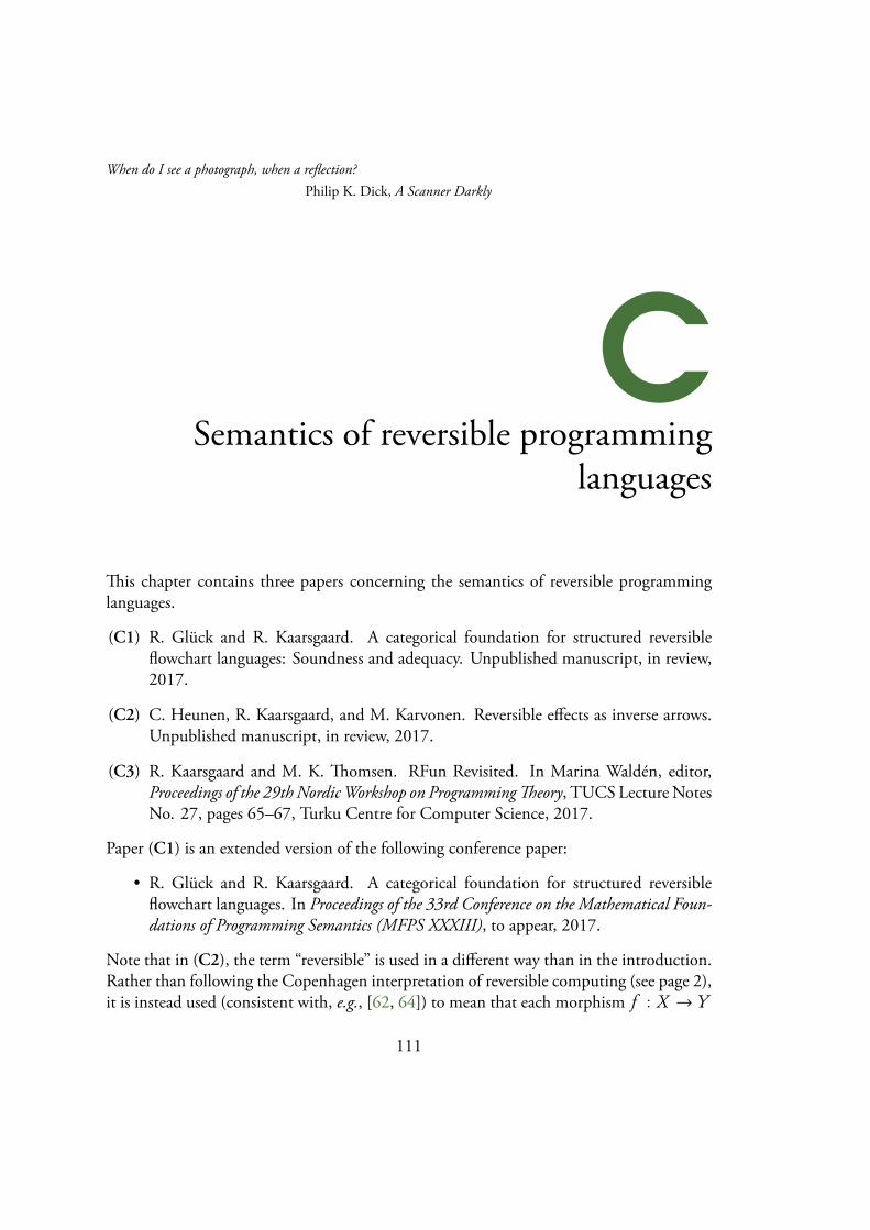
When do I see a photograph, when a reflection?Philip K. Dick, A Scanner Darkly

CSemantics of reversible programming

languages

This chapter contains three papers concerning the semantics of reversible programminglanguages.

(C1) R. Glück and R. Kaarsgaard. A categorical foundation for structured reversibleflowchart languages: Soundness and adequacy. Unpublished manuscript, in review,2017.

(C2) C. Heunen, R. Kaarsgaard, and M. Karvonen. Reversible effects as inverse arrows.Unpublished manuscript, in review, 2017.

(C3) R. Kaarsgaard and M. K. Thomsen. RFun Revisited. In Marina Waldén, editor,Proceedings of the 29th Nordic Workshop on Programming Theory, TUCS Lecture NotesNo. 27, pages 65–67, Turku Centre for Computer Science, 2017.

Paper (C1) is an extended version of the following conference paper:

• R. Glück and R. Kaarsgaard. A categorical foundation for structured reversibleflowchart languages. In Proceedings of the 33rd Conference on the Mathematical Foun-dations of Programming Semantics (MFPS XXXIII), to appear, 2017.

Note that in (C2), the term “reversible” is used in a different way than in the introduction.Rather than following the Copenhagen interpretation of reversible computing (see page 2),it is instead used (consistent with, e.g., [62, 64]) to mean that each morphism f : X → Y

111

has an adjoint f † : Y → X such that this gives the category a dagger structure (seeDefinition 8 on page 4).

112

A CATEGORICAL FOUNDATION FOR STRUCTURED REVERSIBLE

FLOWCHART LANGUAGES: SOUNDNESS AND ADEQUACY

ROBERT GLUCK AND ROBIN KAARSGAARD

DIKU, Department of Computer Science, University of Copenhagen, Denmarke-mail address: [email protected]

DIKU, Department of Computer Science, University of Copenhagen, Denmarke-mail address: [email protected]

Abstract. Structured reversible flowchart languages is a class of imperative reversibleprogramming languages allowing for a simple diagrammatic representation of control flowbuilt from a limited set of control flow structures. This class includes the reversibleprogramming language Janus (without recursion), as well as more recently developedreversible programming languages such as R-CORE and R-WHILE.

In the present paper, we develop a categorical foundation for this class of languagesbased on inverse categories with joins. We generalize the notion of extensivity of restrictioncategories to one that may be accommodated by inverse categories, and use the resultingdecision maps to give a reversible representation of predicates and assertions. This leadsto a categorical semantics for structured reversible flowcharts, which we show to be bothsound, adequate, and fully abstract with respect to the operational semantics under certainconditions.

1. Introduction

Reversible computing is an emerging paradigm that adopts a physical principle of realityinto a computation model without information erasure. Reversible computing extends thestandard forward-only mode of computation with the ability to execute in reverse as easilyas forward. Reversible computing is a necessity in the context of quantum computing andsome bio-inspired computation models. Regardless of the physical motivation, bidirectionaldeterminism is interesting in its own right. The potential benefits include the designof innovative reversible architectures (e.g., [28, 27, 30]), new programming models andtechniques (e.g., [32, 15, 23]), and the enhancement of software with reversibility (e.g., [6]).

1998 ACM Subject Classification: D.3.1, F.3.2.Key words and phrases: Reversible computing, flowchart languages, structured programming, categorical

semantics, category theory.This is the extended version of an article presented at MFPS XXXIII [14], extended with proofs that

previously appeared in the appendix, as well as new sections on soundness, adequacy, and full abstraction.The authors acknowledge the support given by COST Action IC1405 Reversible computation: Extending

horizons of computing. We also thank the anonymous reviewers of MFPS XXXIII for their thoughtful anddetailed comments on a previous version of this paper.

LOGICAL METHODSIN COMPUTER SCIENCE DOI:10.2168/LMCS-???

c© Gluck and KaarsgaardCreative Commons

1

113

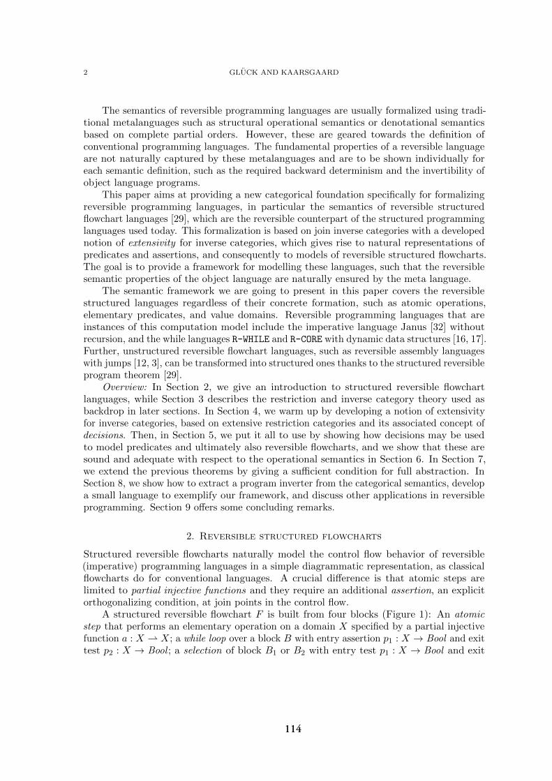
2 GLUCK AND KAARSGAARD

The semantics of reversible programming languages are usually formalized using tradi-tional metalanguages such as structural operational semantics or denotational semanticsbased on complete partial orders. However, these are geared towards the definition ofconventional programming languages. The fundamental properties of a reversible languageare not naturally captured by these metalanguages and are to be shown individually foreach semantic definition, such as the required backward determinism and the invertibility ofobject language programs.

This paper aims at providing a new categorical foundation specifically for formalizingreversible programming languages, in particular the semantics of reversible structuredflowchart languages [29], which are the reversible counterpart of the structured programminglanguages used today. This formalization is based on join inverse categories with a developednotion of extensivity for inverse categories, which gives rise to natural representations ofpredicates and assertions, and consequently to models of reversible structured flowcharts.The goal is to provide a framework for modelling these languages, such that the reversiblesemantic properties of the object language are naturally ensured by the meta language.

The semantic framework we are going to present in this paper covers the reversiblestructured languages regardless of their concrete formation, such as atomic operations,elementary predicates, and value domains. Reversible programming languages that areinstances of this computation model include the imperative language Janus [32] withoutrecursion, and the while languages R-WHILE and R-CORE with dynamic data structures [16, 17].Further, unstructured reversible flowchart languages, such as reversible assembly languageswith jumps [12, 3], can be transformed into structured ones thanks to the structured reversibleprogram theorem [29].

Overview: In Section 2, we give an introduction to structured reversible flowchartlanguages, while Section 3 describes the restriction and inverse category theory used asbackdrop in later sections. In Section 4, we warm up by developing a notion of extensivityfor inverse categories, based on extensive restriction categories and its associated concept ofdecisions. Then, in Section 5, we put it all to use by showing how decisions may be usedto model predicates and ultimately also reversible flowcharts, and we show that these aresound and adequate with respect to the operational semantics in Section 6. In Section 7,we extend the previous theorems by giving a sufficient condition for full abstraction. InSection 8, we show how to extract a program inverter from the categorical semantics, developa small language to exemplify our framework, and discuss other applications in reversibleprogramming. Section 9 offers some concluding remarks.

2. Reversible structured flowcharts

Structured reversible flowcharts naturally model the control flow behavior of reversible(imperative) programming languages in a simple diagrammatic representation, as classicalflowcharts do for conventional languages. A crucial difference is that atomic steps arelimited to partial injective functions and they require an additional assertion, an explicitorthogonalizing condition, at join points in the control flow.

A structured reversible flowchart F is built from four blocks (Figure 1): An atomicstep that performs an elementary operation on a domain X specified by a partial injectivefunction a : X ⇀ X; a while loop over a block B with entry assertion p1 : X → Bool and exittest p2 : X → Bool ; a selection of block B1 or B2 with entry test p1 : X → Bool and exit

114

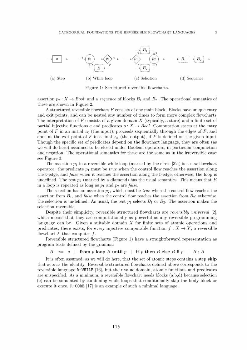
CATEGORICAL FOUNDATIONS FOR REVERSIBLE FLOWCHART LANGUAGES 3

- a - -��

��p1t

f

-��@@��@@p2 t

f�B6

- -��@@��@@p1

t

f

- B1?�

���p2

t

f

-

- B26

- B1- B2

-

(a) Step (b) While loop (c) Selection (d) Sequence

Figure 1: Structured reversible flowcharts.

assertion p2 : X → Bool ; and a sequence of blocks B1 and B2. The operational semantics ofthese are shown in Figure 2.

A structured reversible flowchart F consists of one main block. Blocks have unique entryand exit points, and can be nested any number of times to form more complex flowcharts.The interpretation of F consists of a given domain X (typically, a store) and a finite set ofpartial injective functions a and predicates p : X → Bool . Computation starts at the entrypoint of F in an initial x0 (the input), proceeds sequentially through the edges of F , andends at the exit point of F in a final xn (the output), if F is defined on the given input.Though the specific set of predicates depend on the flowchart language, they are often (aswe will do here) assumed to be closed under Boolean operators, in particular conjunctionand negation. The operational semantics for these are the same as in the irreversible case;see Figure 3.

The assertion p1 in a reversible while loop (marked by the circle [32]) is a new flowchartoperator: the predicate p1 must be true when the control flow reaches the assertion alongthe t-edge, and false when it reaches the assertion along the f -edge; otherwise, the loop isundefined. The test p2 (marked by a diamond) has the usual semantics. This means that Bin a loop is repeated as long as p1 and p2 are false.

The selection has an assertion p2, which must be true when the control flow reaches theassertion from B1, and false when the control flow reaches the assertion from B2; otherwise,the selection is undefined. As usual, the test p1 selects B1 or B2. The assertion makes theselection reversible.

Despite their simplicity, reversible structured flowcharts are reversibly universal [2],which means that they are computationally as powerful as any reversible programminglanguage can be. Given a suitable domain X for finite sets of atomic operations andpredicates, there exists, for every injective computable function f : X → Y , a reversibleflowchart F that computes f .

Reversible structured flowcharts (Figure 1) have a straightforward representation asprogram texts defined by the grammar

B ::= a | from p loop B until p | if p then B else B fi p | B ; B

It is often assumed, as we will do here, that the set of atomic steps contains a step skipthat acts as the identity. Reversible structured flowcharts defined above corresponds to thereversible language R-WHILE [16], but their value domain, atomic functions and predicatesare unspecified. As a minimum, a reversible flowchart needs blocks (a,b,d) because selection(c) can be simulated by combining while loops that conditionally skip the body block orexecute it once. R-CORE [17] is an example of such a minimal language.

115

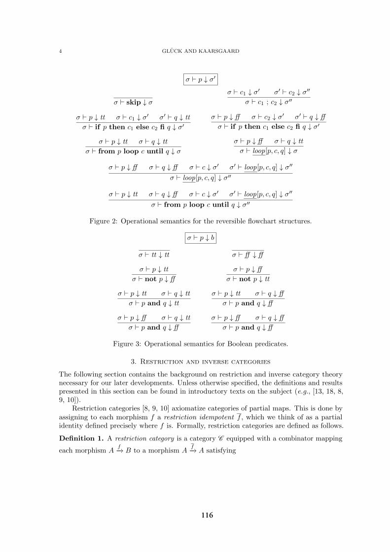
4 GLUCK AND KAARSGAARD

σ ` p ↓ σ′

σ ` skip ↓ σ

σ ` p ↓ tt σ ` c1 ↓ σ′ σ′ ` q ↓ tt

σ ` if p then c1 else c2 fi q ↓ σ′

σ ` p ↓ tt σ ` q ↓ tt

σ ` from p loop c until q ↓ σ

σ ` c1 ↓ σ′ σ′ ` c2 ↓ σ′′

σ ` c1 ; c2 ↓ σ′′

σ ` p ↓ ff σ ` c2 ↓ σ′ σ′ ` q ↓ ff

σ ` if p then c1 else c2 fi q ↓ σ′

σ ` p ↓ ff σ ` q ↓ tt

σ ` loop[p, c, q] ↓ σ

σ ` p ↓ ff σ ` q ↓ ff σ ` c ↓ σ′ σ′ ` loop[p, c, q] ↓ σ′′

σ ` loop[p, c, q] ↓ σ′′

σ ` p ↓ tt σ ` q ↓ ff σ ` c ↓ σ′ σ′ ` loop[p, c, q] ↓ σ′′

σ ` from p loop c until q ↓ σ′′

Figure 2: Operational semantics for the reversible flowchart structures.

σ ` p ↓ b

σ ` tt ↓ tt

σ ` p ↓ tt

σ ` not p ↓ ff

σ ` p ↓ tt σ ` q ↓ tt

σ ` p and q ↓ tt

σ ` p ↓ ff σ ` q ↓ tt

σ ` p and q ↓ ff

σ ` ff ↓ ff

σ ` p ↓ ff

σ ` not p ↓ tt

σ ` p ↓ tt σ ` q ↓ ff

σ ` p and q ↓ ff

σ ` p ↓ ff σ ` q ↓ ff

σ ` p and q ↓ ff

Figure 3: Operational semantics for Boolean predicates.

3. Restriction and inverse categories

The following section contains the background on restriction and inverse category theorynecessary for our later developments. Unless otherwise specified, the definitions and resultspresented in this section can be found in introductory texts on the subject (e.g., [13, 18, 8,9, 10]).

Restriction categories [8, 9, 10] axiomatize categories of partial maps. This is done byassigning to each morphism f a restriction idempotent f , which we think of as a partialidentity defined precisely where f is. Formally, restriction categories are defined as follows.

Definition 1. A restriction category is a category C equipped with a combinator mapping

each morphism Af−→ B to a morphism A

f−→ A satisfying

116

CATEGORICAL FOUNDATIONS FOR REVERSIBLE FLOWCHART LANGUAGES 5

(i) ff = f ,(ii) gf = fg,

(iii) fg = fg, and(iv) gf = fgf

for all suitable g.

As an example, the category Pfn of sets and partial functions is a restriction category,with f(x) = x if f is defined at x, and undefined otherwise. Note that being a restrictioncategory is a structure, not a property; a category may be a restriction category in severaldifferent ways (e.g., assigning f = id for each morphism f gives a trivial restriction structureto any category).

In restriction categories, we say that a morphism Af−→ B is total if f = idA, and a

partial isomorphism if there exists a (necessarily unique) partial inverse Bf†−→ A such that

f †f = f and ff † = f †. Isomorphisms are then simply the total partial isomorphisms withtotal partial inverses. An inverse category can then be defined as a special kind of restrictioncategory1.

Definition 2. An inverse category is a restriction category where each morphism is a partialisomorphism.

Every restriction category C gives rise to an inverse category Inv(C ), which has asobjects all objects of C , and as morphisms all of the partial isomorphisms of C . As such,since partial isomorphisms in Pfn are partial injective functions, a canonical example of aninverse category is the category Inv(Pfn) ∼= PInj of sets and partial injective functions.

Since each morphism in an inverse category has a unique partial inverse, as also suggestedby our notation this makes inverse categories canonically dagger categories [25], in the sensethat they come equipped with a contravariant endofunctor (−)† satisfying f = f †† and

id†A = idA for each morphism f and object A.Given two restriction categories C and D , the well-behaved functors between them are

restriction functors, i.e., functors F satisfying F (f) = F (f). Analogous to how regularsemigroup homomorphisms preserve partial inverses in inverse semigroups, when C and Dare inverse categories, all functors between them are restriction functors; specifically theypreserve the canonical dagger, i.e., F (f †) = F (f)†.

3.1. Partial order enrichment and joins. A consequence of how restriction (and inverse)categories are defined is that hom sets C (A,B) may be equipped with a partial order givenby f ≤ g iff gf = f (this extends to an enrichment in the category of partial orders andmonotone functions). Intuitively, this states that f is below g iff g behaves exactly like fwhen restricted to the points where f is defined. A sufficient condition for each C (A,B)to have a least element is that C has a restriction zero; a zero object 0 in the usual sense

which additionally satisfies A0A,A−−−→ A = A

0A,A−−−→ A for each endo-zero map 0A,A.One may now wonder when C (A,B) has joins as a partial order. Unfortunately, C (A,B)

has joins of all morphisms only in very degenerate cases. However, if instead of consideringarbitrary joins we consider joins of maps that are somehow compatible, this becomes muchmore viable.

1This is a rather modern definition due to [8]. Originally, inverse categories were defined as the categoricalextensions of inverse semigroups; see [22].

117

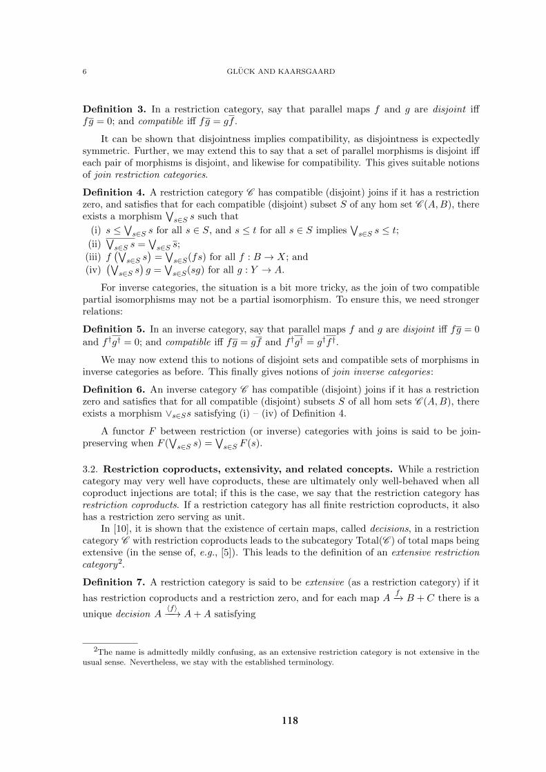
6 GLUCK AND KAARSGAARD

Definition 3. In a restriction category, say that parallel maps f and g are disjoint ifffg = 0; and compatible iff fg = gf .

It can be shown that disjointness implies compatibility, as disjointness is expectedlysymmetric. Further, we may extend this to say that a set of parallel morphisms is disjoint iffeach pair of morphisms is disjoint, and likewise for compatibility. This gives suitable notionsof join restriction categories.

Definition 4. A restriction category C has compatible (disjoint) joins if it has a restrictionzero, and satisfies that for each compatible (disjoint) subset S of any hom set C (A,B), thereexists a morphism

∨s∈S s such that

(i) s ≤∨s∈S s for all s ∈ S, and s ≤ t for all s ∈ S implies

∨s∈S s ≤ t;

(ii)∨s∈S s =

∨s∈S s;

(iii) f(∨

s∈S s)

=∨s∈S(fs) for all f : B → X; and

(iv)(∨

s∈S s)g =

∨s∈S(sg) for all g : Y → A.

For inverse categories, the situation is a bit more tricky, as the join of two compatiblepartial isomorphisms may not be a partial isomorphism. To ensure this, we need strongerrelations:

Definition 5. In an inverse category, say that parallel maps f and g are disjoint iff fg = 0

and f †g† = 0; and compatible iff fg = gf and f †g† = g†f †.

We may now extend this to notions of disjoint sets and compatible sets of morphisms ininverse categories as before. This finally gives notions of join inverse categories:

Definition 6. An inverse category C has compatible (disjoint) joins if it has a restrictionzero and satisfies that for all compatible (disjoint) subsets S of all hom sets C (A,B), thereexists a morphism ∨s∈Ss satisfying (i) – (iv) of Definition 4.

A functor F between restriction (or inverse) categories with joins is said to be join-preserving when F (

∨s∈S s) =

∨s∈S F (s).

3.2. Restriction coproducts, extensivity, and related concepts. While a restrictioncategory may very well have coproducts, these are ultimately only well-behaved when allcoproduct injections are total; if this is the case, we say that the restriction category hasrestriction coproducts. If a restriction category has all finite restriction coproducts, it alsohas a restriction zero serving as unit.

In [10], it is shown that the existence of certain maps, called decisions, in a restrictioncategory C with restriction coproducts leads to the subcategory Total(C ) of total maps beingextensive (in the sense of, e.g., [5]). This leads to the definition of an extensive restrictioncategory2.

Definition 7. A restriction category is said to be extensive (as a restriction category) if it

has restriction coproducts and a restriction zero, and for each map Af−→ B + C there is a

unique decision A〈f〉−−→ A+A satisfying

2The name is admittedly mildly confusing, as an extensive restriction category is not extensive in theusual sense. Nevertheless, we stay with the established terminology.

118

CATEGORICAL FOUNDATIONS FOR REVERSIBLE FLOWCHART LANGUAGES 7

(D.1): ∇〈f〉 = f and (D.2): (f + f)〈f〉 = (κ1 + κ2)f .

In the above, ∇ denotes the codiagonal [id, id]. A consequence of these axioms is thateach decision is a partial isomorphism; one can show that 〈f〉 must be partial inverse to

[κ†1f, κ†2f ] (see [10]). Further, when a restriction category with restriction coproducts has

finite joins, it is also extensive with 〈f〉 = κ1κ†1f ∨ κ2κ

†2f . As an example, Pfn is extensive

with A〈f〉−−→ A+A for A

f−→ B + C given by

〈f〉(x) =

κ1(x) if f(x) = κ1(y) for some y ∈ Bκ2(x) if f(x) = κ2(z) for some z ∈ Cundefined if f(x) is undefined

.

While inverse categories only have coproducts (much less restriction coproducts) in verydegenerate cases (see [13]), they may very well be equipped with a more general sum-likesymmetric monoidal tensor, a disjointness tensor.

Definition 8. A disjointness tensor on a restriction category is a symmetric monoidalrestriction functor −⊕− satisfying that its unit is the restriction zero, and that the canonicalmaps

q1 = Aρ−1

−−→ A⊕ 0id⊕0−−−→ A⊕B q2 = B

λ−1

−−→ 0⊕B 0⊕id−−−→ A⊕Bare jointly epic, where ρ respectively λ is the left respectively right unitor of the monoidalfunctor −⊕−.

It can be straightforwardly shown that any restriction coproduct gives rise to a disjoint-ness tensor. A useful interaction between compatible joins and a join-preserving disjointnesstensor in inverse categories was shown in [4, 21], namely that it leads to a †-trace (in thesense of [20, 26]):

Proposition 1. Let C be an inverse category with (at least countable) compatible joins anda join-preserving disjointness tensor. Then C has a trace operator given by

TrUA,B(f) = f11 ∨∨n∈ω

f21f22f12

satisfying TrUA,B(f)† = TrUA,B(f †), where fij = q†jfqi.

4. Extensivity of inverse categories

As discussed earlier, extensivity of restriction categories hinges on the existence of certainpartial isomorphisms – decisions – yet their axiomatization relies on the presence of a mapthat is not a partial isomorphism, the codiagonal.

In this section, we tweak the axiomatization of extensivity of restriction categories toone that is equivalent, but additionally transports more easily to inverse categories. We thengive a definition of extensitivity for inverse categories, from which it follows that Inv(C ) isan extensive inverse category when C is an extensive restriction category.

Recall that decisions satisfy the following two axioms:

119

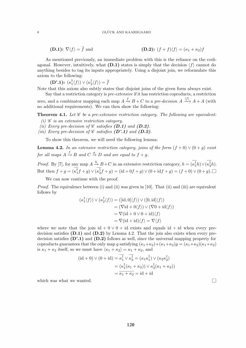
8 GLUCK AND KAARSGAARD

(D.1): ∇〈f〉 = f and (D.2): (f + f)〈f〉 = (κ1 + κ2)f

As mentioned previously, an immediate problem with this is the reliance on the codi-agonal. However, intuitively, what (D.1) states is simply that the decision 〈f〉 cannot doanything besides to tag its inputs appropriately. Using a disjoint join, we reformulate thisaxiom to the following:

(D’.1): (κ†1〈f〉) ∨ (κ†2〈f〉) = f

Note that this axiom also subtly states that disjoint joins of the given form always exist.Say that a restriction category is pre-extensive if it has restriction coproducts, a restriction

zero, and a combinator mapping each map Af−→ B +C to a pre-decision A

〈f〉−−→ A+A (withno additional requirements). We can then show the following:

Theorem 4.1. Let C be a pre-extensive restriction category. The following are equivalent:

(i) C is an extensive restriction category.(ii) Every pre-decision of C satisfies (D.1) and (D.2).

(iii) Every pre-decision of C satisfies (D’.1) and (D.2).

To show this theorem, we will need the following lemma:

Lemma 4.2. In an extensive restriction category, joins of the form (f + 0) ∨ (0 + g) exist

for all maps Af−→ B and C

g−→ D and are equal to f + g.

Proof. By [7], for any map Ah−→ B+C in an extensive restriction category, h = (κ†1h)∨(κ†2h).

But then f + g = (κ†1f + g)∨ (κ†2f + g) = (id + 0f + g)∨ (0 + idf + g) = (f + 0)∨ (0 + g).

We can now continue with the proof.

Proof. The equivalence between (i) and (ii) was given in [10]. That (ii) and (iii) are equivalentfollows by

(κ†1〈f〉) ∨ (κ†2〈f〉) = ([id, 0]〈f〉) ∨ ([0, id]〈f〉)= (∇id + 0〈f〉) ∨ (∇0 + id〈f〉)= ∇(id + 0 ∨ 0 + id)〈f〉= ∇(id + id)〈f〉 = ∇〈f〉

where we note that the join id + 0 ∨ 0 + id exists and equals id + id when every pre-decision satisfies (D.1) and (D.2) by Lemma 4.2. That the join also exists when every pre-decision satisfies (D’.1) and (D.2) follows as well, since the universal mapping property forcoproducts guarantees that the only map g satisfying (κ1+κ2)+(κ1+κ2)g = (κ1+κ2)(κ1+κ2)is κ1 + κ2 itself, so we must have 〈κ1 + κ2〉 = κ1 + κ2, and

(id + 0) ∨ (0 + id) = κ†1 ∨ κ†2 = (κ1κ

†1) ∨ (κ2κ

†2)

= (κ†1(κ1 + κ2)) ∨ κ†2(κ1 + κ2))

= κ1 + κ2 = id + id

which was what we wanted.

120

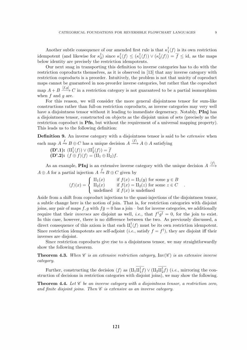
CATEGORICAL FOUNDATIONS FOR REVERSIBLE FLOWCHART LANGUAGES 9

Another subtle consequence of our amended first rule is that κ†1〈f〉 is its own restriction

idempotent (and likewise for κ†2) since κ†1〈f〉 ≤ (κ†1〈f〉) ∨ (κ†2〈f〉) = f ≤ id, as the mapsbelow identity are precisely the restriction idempotents.

Our next snag in transporting this definition to inverse categories has to do with therestriction coproducts themselves, as it is observed in [13] that any inverse category withrestriction coproducts is a preorder. Intuitively, the problem is not that unicity of coproductmaps cannot be guaranteed in non-preorder inverse categories, but rather that the coproduct

map A+B[f,g]−−→ C in a restriction category is not guaranteed to be a partial isomorphism

when f and g are.For this reason, we will consider the more general disjointness tensor for sum-like

constructions rather than full-on restriction coproducts, as inverse categories may very wellhave a disjointness tensor without it leading to immediate degeneracy. Notably, PInj hasa disjointness tensor, constructed on objects as the disjoint union of sets (precisely as therestriction coproduct in Pfn, but without the requirement of a universal mapping property).This leads us to the following definition:

Definition 9. An inverse category with a disjointness tensor is said to be extensive when

each map Af−→ B ⊕ C has a unique decision A

〈f〉−−→ A⊕A satisfying

(D’.1): (q†1〈f〉) ∨ (q†2〈f〉) = f(D’.2): (f ⊕ f)〈f〉 = (q1 ⊕q2)f .

As an example, PInj is an extensive inverse category with the unique decision A〈f〉−−→

A⊕A for a partial injection Af−→ B ⊕ C given by

〈f〉(x) =

q1(x) if f(x) = q1(y) for some y ∈ Bq2(x) if f(x) = q2(z) for some z ∈ Cundefined if f(x) is undefined

.

Aside from a shift from coproduct injections to the quasi-injections of the disjointness tensor,a subtle change here is the notion of join. That is, for restriction categories with disjointjoins, any pair of maps f, g with fg = 0 has a join – but for inverse categories, we additionally

require that their inverses are disjoint as well, i.e., that f †g† = 0, for the join to exist.In this case, however, there is no difference between the two. As previously discussed, a

direct consequence of this axiom is that each q†i 〈f〉 must be its own restriction idempotent.

Since restriction idempotents are self-adjoint (i.e., satisfy f = f †), they are disjoint iff theirinverses are disjoint.

Since restriction coproducts give rise to a disjointness tensor, we may straightforwardlyshow the following theorem.

Theorem 4.3. When C is an extensive restriction category, Inv(C ) is an extensive inversecategory.

Further, constructing the decision 〈f〉 as (q1q†1f) ∨ (q2q†2f) (i.e., mirroring the con-struction of decisions in restriction categories with disjoint joins), we may show the following.

Theorem 4.4. Let C be an inverse category with a disjointness tensor, a restriction zero,and finite disjoint joins. Then C is extensive as an inverse category.

121

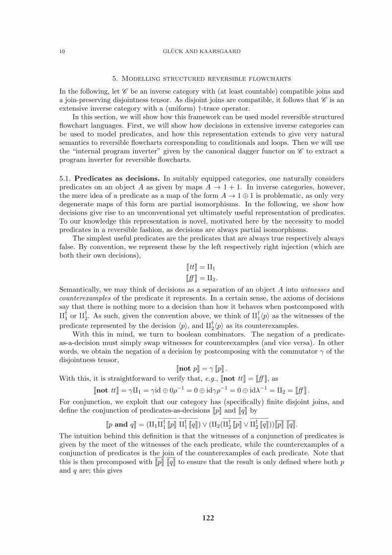
10 GLUCK AND KAARSGAARD

5. Modelling structured reversible flowcharts

In the following, let C be an inverse category with (at least countable) compatible joins anda join-preserving disjointness tensor. As disjoint joins are compatible, it follows that C is anextensive inverse category with a (uniform) †-trace operator.

In this section, we will show how this framework can be used model reversible structuredflowchart languages. First, we will show how decisions in extensive inverse categories canbe used to model predicates, and how this representation extends to give very naturalsemantics to reversible flowcharts corresponding to conditionals and loops. Then we will usethe “internal program inverter” given by the canonical dagger functor on C to extract aprogram inverter for reversible flowcharts.

5.1. Predicates as decisions. In suitably equipped categories, one naturally considerspredicates on an object A as given by maps A → 1 + 1. In inverse categories, however,the mere idea of a predicate as a map of the form A→ 1⊕ 1 is problematic, as only verydegenerate maps of this form are partial isomorphisms. In the following, we show howdecisions give rise to an unconventional yet ultimately useful representation of predicates.To our knowledge this representation is novel, motivated here by the necessity to modelpredicates in a reversible fashion, as decisions are always partial isomorphisms.

The simplest useful predicates are the predicates that are always true respectively alwaysfalse. By convention, we represent these by the left respectively right injection (which areboth their own decisions),

JttK = q1

Jff K = q2.

Semantically, we may think of decisions as a separation of an object A into witnesses andcounterexamples of the predicate it represents. In a certain sense, the axioms of decisionssay that there is nothing more to a decision than how it behaves when postcomposed with

q†1 or q†2. As such, given the convention above, we think of q†1〈p〉 as the witnesses of the

predicate represented by the decision 〈p〉, and q†2〈p〉 as its counterexamples.With this in mind, we turn to boolean combinators. The negation of a predicate-

as-a-decision must simply swap witnesses for counterexamples (and vice versa). In otherwords, we obtain the negation of a decision by postcomposing with the commutator γ of thedisjointness tensor,

Jnot pK = γ JpK .With this, it is straightforward to verify that, e.g., Jnot ttK = Jff K, as

Jnot ttK = γq1 = γid⊕ 0ρ−1 = 0⊕ idγρ−1 = 0⊕ idλ−1 = q2 = Jff K .

For conjunction, we exploit that our category has (specifically) finite disjoint joins, anddefine the conjunction of predicates-as-decisions JpK and JqK by

Jp and qK = (q1q†1 JpK q†1 JqK) ∨ (q2(q†2 JpK ∨ q†2 JqK))JpK JqK.

The intuition behind this definition is that the witnesses of a conjunction of predicates isgiven by the meet of the witnesses of the each predicate, while the counterexamples of aconjunction of predicates is the join of the counterexamples of each predicate. Note thatthis is then precomposed with JpK JqK to ensure that the result is only defined where both pand q are; this gives

122

CATEGORICAL FOUNDATIONS FOR REVERSIBLE FLOWCHART LANGUAGES 11

Noting that the meet of two restriction idempotents is given by their composition, thisis precisely what this definition states. Similarly we define the disjunction of JpK and JqK by

Jp or qK = (q1(q†1 JpK ∨ q†1 JqK)) ∨ (q2(q†2 JpK q†2 JqK))JpK JqK,

as Jp or qK then has as witnesses the join of the witnesses of JpK and JqK, and as counterex-amples the meet of the counterexamples of JpK and JqK. With these definitions, it can beshown that, e.g., the De Morgan laws are satisfied. However, since we can thus constructthis from conjunctions and negations, we will leave disjunctions as syntactic sugar.

That all of these are indeed decisions can be shown straightforwardly, as summarized inthe following closure theorem.

Theorem 5.1. Decisions in C are closed under Boolean negation, conjunction, and dis-junction.

5.2. Reversible structured flowcharts, categorically. To give a categorical account ofstructured reversible flowchart languages, we assume the existence of a suitable distinguishedobject Σ of stores, which we think of as the domain of computation, such that we may givedenotations to structured reversible flowcharts as morphisms Σ→ Σ.

Since atomic steps (corresponding to elementary operations, e.g., store updates) mayvary from language to language, we assume that each such atomic step in our language hasa denotation as a morphism Σ → Σ. In the realm of reversible flowcharts, these atomicsteps are required to be partial injective functions; here, we abstract this to require thattheir denotation is a partial isomorphism (though this is a trivial requirement in inversecategories).

Likewise, elementary predicates (e.g., comparison of values in a store) may vary fromlanguage to language, so we assume that such elementary predicates have denotations aswell as decisions Σ→ Σ⊕ Σ. If necessary (as is the case for Janus [32]), we may then closethese elementary predicates under boolean combinations as discussed in the previous section.

To start, we note how sequencing of flowcharts may be modelled trivially by means ofcomposition, i.e.,

Jc1 ; c2K = Jc2K Jc1Kor, using the diagrammatic notation of flowcharts and the string diagrams for monoidalcategories in the style of [26] (read left-to-right and bottom-to-top),

q- c1 - c2 -

y= Jc1K Jc2K .

To extend this elementary model to one that additionally models reversible conditionals,we observe that the partial inverse to a decision is precisely its corresponding assertion.Intuitively, a decision separates an object into witnesses (in the first component) andcounterexamples (in the second). As such, the partial inverse to a decision must be definedonly on witnesses in the first component, and only on counterexamples in the second.

With this in mind, we achieve a denotation of reversible conditionals as

Jif p then c1 else c2 fi qK = JqK† Jc1K⊕ Jc2K JpK

123

12 GLUCK AND KAARSGAARD

or, as diagramsu

wwwwv-��@@��@@p

t

f

- c1?�

���q

t

f

-

- c2 6

}

����~

= JpKJc2K

Jc1KJqK† .

For reversible loops, we use the †-trace operator to obtain the denotation

Jfrom p loop c until qK = TrΣΣ,Σ(idΣ ⊕ JcK JqK JpK†)

or diagrammatically

u

wv-��

��qt

f

-��@@��@@p t

f�c6

-

}

�~ = JqK† JpK

JcK.

That this has the desired operational behavior follows from the fact that the †-trace operatoris canonically constructed in join inverse categories as

TrUX,Y (f) = f11 ∨∨n∈ω

f21fn22f12 .

Recall that fij = q†jfqi. As such, for our loop construct defined above, the f11-cases

correpond to cases where a given state bypasses the loop entirely; f21f12 (that is, for n = 0)to cases where exactly one iteration is performed by a given state before exiting the loop;f21f22f12 to cases where two iterations are performed before exiting; and so on. In this way,the given trace semantics contain all successive loop unrollings, as desired. We will makethis more formal in the following section, where we show soundness and adequacy for thesewith respect to the operational semantics.

In order to be able to provide a correspondence between categorical and operationalsemantics, we also need an interpretation of the meta-command loop. While it may not beso clear at the present, it turns out that the appropriate one is

qloop[p, c, q]

y=∨n∈ω

β[p, c, q]21β[p, c, q]n22

where β[p, c, q] = idΣ⊕ JcK JqK JpK†, i.e., the inner part of the interpretation of the from-loop.While it may seem like a small point, the mere existence of a categorical semantics in

inverse categories for a reversible programming language has some immediate benefits. Inparticular, that a programming language is reversible can be rather complicated to showby means of operational semantics (see, e.g., [32, Sec. 2.3]), yet it follows directly in ourcategorical semantics, as all morphisms in inverse categories have a unique partial inverse.

6. Soundness and adequacy

Soundness and adequacy (see, e.g., [11]) are the two fundamental properties of operationalsemantics with respect to their denotational counterparts, as soundness and completenessare for proof systems with respect to their semantics. In brief, soundness and adequacy statethat the respective notions of convergence of the operational and denotational semantics arein agreement.

124

CATEGORICAL FOUNDATIONS FOR REVERSIBLE FLOWCHART LANGUAGES 13

In the operational semantics, the notion of convergence seems straightforward: aprogram p converges in a state σ if there exists another state σ′ such that σ ` p ↓ σ′. Onthe denotational side, it seems less obvious what a proper notion of convergence is.

An idea (used by, e.g., Fiore [11]) is to let values (in this case, states) be interpreted astotal morphisms from some sufficiently simple object I into an appropriate object V (here,we will use our object Σ of states). In this context, the notion of convergence for a programp in a state σ is then that the resulting value (state) JpK JσK is again, a state – i.e., it is total.Naturally, this approach requires machinery to separate total maps from partial ones. Asluck would have it, inverse categories fit the bill perfectly, as they can be regarded as specialinstances of restriction categories.

To make this idea more clear in the current context, and to allow us to use the establishedformulations of soundness and adequacy, we define a model of a structured reversible flowchartlanguage to be the following:

Definition 10. A model of a structured reversible flowchart language L consists of a joininverse category C with a disjointness tensor, further equipped with distinguished objects Iand Σ satisfying

(i) the identity and zero maps on I are distinct, i.e., idI 6= 0I,I ,

(ii) if Ie−→ I is a restriction idempotent then e = idI or e = 0I,I , and

(iii) each L-state σ is interpreted as a total morphism IJσK−−→ Σ.

Here, we think of I as the indexing object, and Σ as the object of states. In irreversibleprogramming languages, the first two conditions in the definition above are often left out,as the indexing object is typically chosen to be the terminal object 1. However, terminalobjects are degenerate in inverse categories, as they always coincide with the initial objectwhen they exist – that is, they are zero objects. For this reason, we require instead theexistence of a sufficiently simple indexing object, as described by these two properties. Forexample, in PInj, any one-element set will satisfy these conditions.

Even further, the third condition is typically proven rather than assumed. We includeit here as an assumption since structured reversible flowchart languages may take manydifferent forms, and we have no way of knowing how the concrete states are formed. Assuch, rather than limiting ourselves to languages where states take a certain form in orderto show totality of interpretation, we instead assume it to be able to show properties aboutmore programming languages.

This also leads us to another important point: We are only able to show soundness andadequacy for the operational semantics as they are stated, i.e., we are not able to take intoaccount the specific atomic steps (besides skip) or elementary predicates of the language.

As such, soundness and adequacy (and what may follow from that) should be understoodconditionally : If a structured reversible flowchart language has a model of the form aboveand it is sound and adequate with respect to its atomic steps and elementary predicates,then the entire interpretation is sound and adequate as well.

We begin by recalling the definition of the denotation of predicates and commands in amodel of a structured reversible flowchart language from Section 5.

Definition 11. Recall the interpretation of predicates in L as decisions in C :

(i) JttK = q1,(ii) Jff K = q2,

(iii) Jnot pK = γ JpK,

125

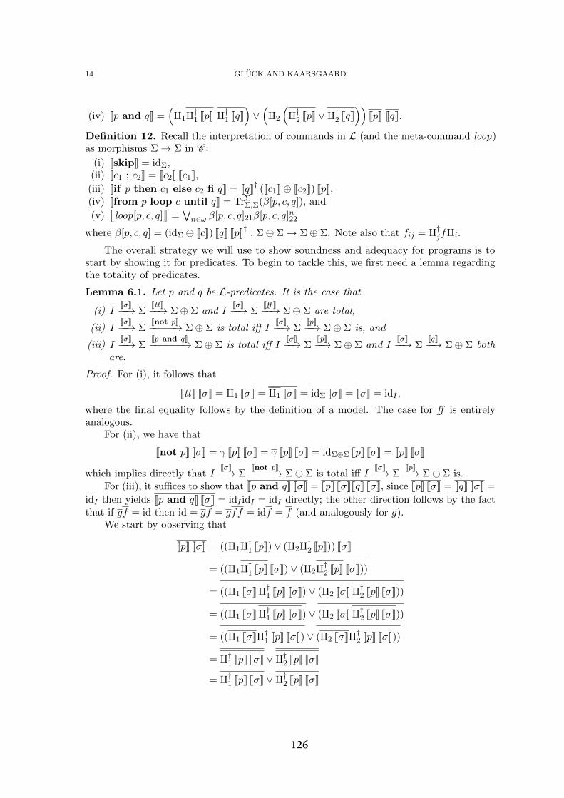
14 GLUCK AND KAARSGAARD

(iv) Jp and qK =(q1q†1 JpK q†1 JqK

)∨(q2

(q†2 JpK ∨ q†2 JqK

))JpK JqK.

Definition 12. Recall the interpretation of commands in L (and the meta-command loop)as morphisms Σ→ Σ in C :

(i) JskipK = idΣ,(ii) Jc1 ; c2K = Jc2K Jc1K,

(iii) Jif p then c1 else c2 fi qK = JqK† (Jc1K⊕ Jc2K) JpK,(iv) Jfrom p loop c until qK = TrΣ

Σ,Σ(β[p, c, q]), and

(v)q

loop[p, c, q]y

=∨n∈ω β[p, c, q]21β[p, c, q]n22

where β[p, c, q] = (idΣ ⊕ JcK) JqK JpK† : Σ⊕ Σ→ Σ⊕ Σ. Note also that fij = q†jfqi.The overall strategy we will use to show soundness and adequacy for programs is to

start by showing it for predicates. To begin to tackle this, we first need a lemma regardingthe totality of predicates.

Lemma 6.1. Let p and q be L-predicates. It is the case that

(i) IJσK−−→ Σ

JttK−−→ Σ⊕ Σ and IJσK−−→ Σ

Jff K−−→ Σ⊕ Σ are total,

(ii) IJσK−−→ Σ

Jnot pK−−−−−→ Σ⊕ Σ is total iff IJσK−−→ Σ

JpK−−→ Σ⊕ Σ is, and

(iii) IJσK−−→ Σ

Jp and qK−−−−−−→ Σ⊕ Σ is total iff IJσK−−→ Σ

JpK−−→ Σ⊕ Σ and IJσK−−→ Σ

JqK−−→ Σ⊕ Σ bothare.

Proof. For (i), it follows that

JttK JσK = q1 JσK = q1 JσK = idΣ JσK = JσK = idI ,

where the final equality follows by the definition of a model. The case for ff is entirelyanalogous.

For (ii), we have that

Jnot pK JσK = γ JpK JσK = γ JpK JσK = idΣ⊕Σ JpK JσK = JpK JσK

which implies directly that IJσK−−→ Σ

Jnot pK−−−−−→ Σ⊕ Σ is total iff IJσK−−→ Σ

JpK−−→ Σ⊕ Σ is.For (iii), it suffices to show that Jp and qK JσK = JpK JσKJqK JσK, since JpK JσK = JqK JσK =

idI then yields Jp and qK JσK = idI idI = idI directly; the other direction follows by the factthat if gf = id then id = gf = gff = idf = f (and analogously for g).

We start by observing that

JpK JσK = ((q1q†1 JpK) ∨ (q2q†2 JpK)) JσK

= ((q1q†1 JpK JσK) ∨ (q2q†2 JpK JσK))

= ((q1 JσKq†1 JpK JσK) ∨ (q2 JσKq†2 JpK JσK))

= ((q1 JσKq†1 JpK JσK) ∨ (q2 JσKq†2 JpK JσK))

= ((q1 JσKq†1 JpK JσK) ∨ (q2 JσKq†2 JpK JσK))

= q†1 JpK JσK ∨ q†2 JpK JσK

= q†1 JpK JσK ∨ q†2 JpK JσK

126

CATEGORICAL FOUNDATIONS FOR REVERSIBLE FLOWCHART LANGUAGES 15

where q1 JσK = q2 JσK = idI follows by (i), and q†1 JpK = q†1 JpK and q†2 JpK = q†2 JpK followby JpK a decision. We may establish by analogous argument that

JqK JσK = q†1 JqK JσK ∨ q†2 JqK JσK

as well. In the following, let σp = JpK JσK and σq = JqK JσK. We have

Jp and qK JσK =((q†1 JpK JσK q†1 JqK JσK

)∨(q†2 JpK JσK ∨ q†2 JqK JσK

))JpK JσK JqK JσK

=((q†1σp q

†1σq

)∨(q†2σp ∨ q

†2σq

))σp σq

=((q†1σp q

†1σq

)∨ q†2σp ∨ q

†2σq

)σp σq

=(q†1σp q

†1σq σp σq

)∨(q†2σp σp σq

)∨(q†2σq σp σq

)=(q†1σp σp q

†1σq σq

)∨(q†2σp σp σq

)∨(q†2σq σq σp

)=(q†1σp q

†1σq

)∨(q†2σp σq

)∨(q†2σq σp

)=(q†1σp q

†1σq

)∨(q†2σp

(q†1σq ∨ q

†2σq

))∨(q†2σq

(q†1σp ∨ q

†2σp

))=(q†1σp q

†1σq

)∨(q†2σp q

†1σq

)∨(q†2σp q

†2σq

)∨(q†2σq q

†1σp

)∨(q†2σq q

†2σp

)=(q†1σp q

†1σq

)∨(q†1σp q

†2σq

)∨(q†2σp q

†1σq

)∨(q†2σp q

†2σq

)=(q†1σp ∨ q

†2σp

)(q†1σq ∨ q

†2σq

)= σp σq

which was what we wanted.

A common way to show soundness (see, e.g., [11]) is to show a kind of preservationproperty; that interpretations are, in a sense, preserved across evaluation in the operationalsemantics. This is shown in the following lemma:

Lemma 6.2. If σ ` p ↓ b then JpK JσK = JbK JσK.

Proof. By induction on the structure of the derivation D of σ ` p ↓ b.• Case D =

σ ` tt ↓ tt. We trivially have JttK JσK = JttK JσK.

• Case D =σ ` ff ↓ ff

. Again, we trivially have Jff K JσK = Jff K JσK.

• Case D =σ ` p ↓ tt

σ ` not p ↓ ff.

By induction we have that JpK JσK = JttK JσK = q1 JσK. But then Jnot pK JσK =γ JpK JσK = γ q1 JσK = q2 JσK = Jff K JσK.

• Case D =σ ` p ↓ ff

σ ` not p ↓ tt.

By induction we have that JpK JσK = Jff K JσK = q2 JσK. Thus Jnot pK JσK =γ JpK JσK = γ q2 JσK = q1 JσK = JttK JσK.

• Case D =σ ` p ↓ tt σ ` q ↓ tt

σ ` p and q ↓ tt.

127

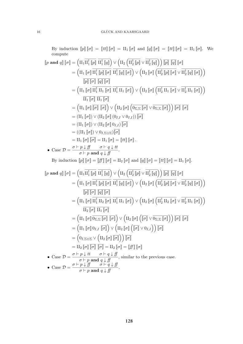
16 GLUCK AND KAARSGAARD

By induction JpK JσK = JttK JσK = q1 JσK and JqK JσK = JttK JσK = q1 JσK. Wecompute

Jp and qK JσK =(q1q†1 JpK q†1 JqK

)∨(q2

(q†2 JpK ∨ q†2 JqK

))JpK JqK JσK

=(q1 JσKq†1 JpK JσK q†1 JqK JσK

)∨(q2 JσK

(q†2 JpK JσK ∨ q†2 JqK JσK

))JpK JσK JqK JσK

=(q1 JσKq†1 q1 JσK q†1 q1 JσK

)∨(q2 JσK

(q†2 q1 JσK ∨ q†2 q1 JσK

))q1 JσK q1 JσK

=(q1 JσK JσK JσK

)∨(q2 JσK

(0Σ,Σ JσK ∨ 0Σ,Σ JσK

))JσK JσK

= (q1 JσK) ∨ (q2 JσK (0I,I ∨ 0I,I)) JσK

= (q1 JσK) ∨ (q2 JσK 0I,I) JσK

= ((q1 JσK) ∨ 0I,Σ⊕Σ)JσK

= q1 JσK JσK = q1 JσK = JttK JσK .

• Case D =σ ` p ↓ ff σ ` q ↓ tt

σ ` p and q ↓ ff.

By induction JpK JσK = Jff K JσK = q2 JσK and JqK JσK = JttK JσK = q1 JσK.

Jp and qK JσK =(q1q†1 JpK q†1 JqK

)∨(q2

(q†2 JpK ∨ q†2 JqK

))JpK JqK JσK

=(q1 JσKq†1 JpK JσK q†1 JqK JσK

)∨(q2 JσK

(q†2 JpK JσK ∨ q†2 JqK JσK

))JpK JσK JqK JσK

=(q1 JσKq†1 q2 JσK q†1 q1 JσK

)∨(q2 JσK

(q†2 q2 JσK ∨ q†2 q1 JσK

))q2 JσK q1 JσK

=(q1 JσK 0Σ,Σ JσK JσK

)∨(q2 JσK

(JσK ∨ 0Σ,Σ JσK

))JσK JσK

=(q1 JσK 0I,I JσK

)∨(q2 JσK

(JσK ∨ 0I,I

))JσK

=(

0I,Σ⊕Σ ∨(q2 JσK JσK

))JσK

= q2 JσK JσK JσK = q2 JσK = Jff K JσK

• Case D =σ ` p ↓ tt σ ` q ↓ ff

σ ` p and q ↓ ff, similar to the previous case.

• Case D =σ ` p ↓ ff σ ` q ↓ ff

σ ` p and q ↓ ff.

128

CATEGORICAL FOUNDATIONS FOR REVERSIBLE FLOWCHART LANGUAGES 17

By induction JpK JσK = Jff K JσK = q2 JσK and JqK JσK = Jff K JσK = q2 JσK.

Jp and qK JσK =(q1q†1 JpK q†1 JqK

)∨(q2

(q†2 JpK ∨ q†2 JqK

))JpK JqK JσK

=(q1 JσKq†1 JpK JσK q†1 JqK JσK

)∨(q2 JσK

(q†2 JpK JσK ∨ q†2 JqK JσK

))JpK JσK JqK JσK

=(q1 JσKq†1 q2 JσK q†1 q2 JσK

)∨(q2 JσK

(q†2 q2 JσK ∨ q†2 q2 JσK

))q2 JσK q2 JσK

=(q1 JσK 0Σ,Σ JσK 0Σ,Σ JσK

)∨(q2 JσK

(JσK ∨ JσK

))JσK JσK

= (q1 JσK 0I,I) ∨(q2 JσK JσK

)JσK

=(

0I,Σ⊕Σ ∨(q2 JσK JσK

))JσK

= q2 JσK JσK JσK = q2 JσK = Jff K JσK .

With this done, the soundness lemma for predicates follows readily.

Lemma 6.3. If there exists b such that σ ` p ↓ b then JpK JσK is total.

Proof. Suppose there exists b such that σ ` p ↓ b by some derivation. It follows bythe operational semantics that b must be either tt or ff , and in either case it follows byLemma 6.1 (i) that JbK JσK is total, i.e., JbK JσK = idI . Applying the derivation of σ ` p ↓ b to

Lemma 6.2 yields that JpK JσK = JbK JσK, so specifically JpK JσK = JbK JσK = idI , as desired.

Adequacy for predicates can then be shown by induction on the structure of the predicate,and by letting Lemma 6.1 (regarding the totality of predicates) do much of the heavy lifting.

Lemma 6.4. If JpK JσK is total then there exists b such that σ ` p ↓ b.

Proof. By induction on the structure of p.

• Case p = tt . Then σ ` tt ↓ tt byσ ` tt ↓ tt

.

• Case p = ff . Then σ ` ff ↓ ff byσ ` ff ↓ ff

.

• Case p = not p′. Since Jnot p′K JσK is total, it follows by Lemma 6.1 that Jp′K JσK istotal as well, so by induction, there exists b such that σ ` p′ ↓ b by some derivationD. We have two cases to consider: If b = tt , D is a derivation of σ ` p′ ↓ tt , and sowe may derive σ ` not p′ ↓ ff by

Dσ ` p′ ↓ tt

σ ` not p′ ↓ ff

If on the other hand b = ff , D is a derivation of σ ` p′ ↓ ff , and we may use theother not-rule with D to derive

Dσ ` p′ ↓ ff

σ ` not p′ ↓ tt.

129

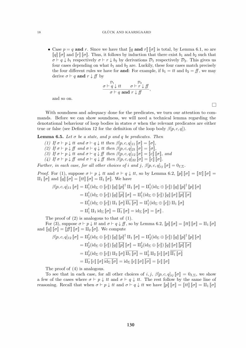
18 GLUCK AND KAARSGAARD

• Case p = q and r. Since we have that Jq and rK JσK is total, by Lemma 6.1, so areJqK JσK and JrK JσK. Thus, it follows by induction that there exist b1 and b2 such thatσ ` q ↓ b1 respectively σ ` r ↓ b2 by derivations D1 respectively D2. This gives usfour cases depending on what b1 and b2 are. Luckily, these four cases match preciselythe four different rules we have for and: For example, if b1 = tt and b2 = ff , we mayderive σ ` q and r ↓ ff by

D1

σ ` q ↓ ttD2

σ ` r ↓ ff

σ ` q and r ↓ ff,

and so on.

With soundness and adequacy done for the predicates, we turn our attention to com-mands. Before we can show soundness, we will need a technical lemma regarding thedenotational behaviour of loop bodies in states σ when the relevant predicates are eithertrue or false (see Definition 12 for the definition of the loop body β[p, c, q]).

Lemma 6.5. Let σ be a state, and p and q be predicates. Then

(1) If σ ` p ↓ tt and σ ` q ↓ tt then β[p, c, q]11 JσK = JσK,(2) If σ ` p ↓ ff and σ ` q ↓ tt then β[p, c, q]21 JσK = JσK,(3) If σ ` p ↓ tt and σ ` q ↓ ff then β[p, c, q]12 JσK = JcK JσK, and(4) If σ ` p ↓ ff and σ ` q ↓ ff then β[p, c, q]22 JσK = JcK JσK.

Further, in each case, for all other choices of i and j, β[p, c, q]ij JσK = 0I,Σ.

Proof. For (1), suppose σ ` p ↓ tt and σ ` q ↓ tt , so by Lemma 6.2, JpK JσK = JttK JσK =q1 JσK and JqK JσK = JttK JσK = q1 JσK. We have

β[p, c, q]11 JσK = q†1(idΣ ⊕ JcK) JqK JpK† q1 JσK = q†1(idΣ ⊕ JcK) JqK JpK† JpK JσK

= q†1(idΣ ⊕ JcK) JqK JpK JσK = q†1(idΣ ⊕ JcK) JqK JσK JpK JσK

= q†1(idΣ ⊕ JcK)q1 JσKq1 JσK = q†1(idΣ ⊕ JcK)q1 JσK

= q†1 q1 idΣ JσK = q1 JσK = idΣ JσK = JσK .

The proof of (2) is analogous to that of (1).For (3), suppose σ ` p ↓ tt and σ ` q ↓ ff , so by Lemma 6.2, JpK JσK = JttK JσK = q1 JσK

and JqK JσK = Jff K JσK = q2 JσK. We compute

β[p, c, q]12 JσK = q†2(idΣ ⊕ JcK) JqK JpK† q1 JσK = q†2(idΣ ⊕ JcK) JqK JpK† JpK JσK

= q†2(idΣ ⊕ JcK) JqK JpK JσK = q†2(idΣ ⊕ JcK) JqK JσK JpK JσK

= q†2(idΣ ⊕ JcK)q2 JσKq1 JσK = q†2 q2 JcK JσKq1 JσK

= q2 JcK JσK idΣ JσK = idΣ JcK JσK JσK = JcK JσK

The proof of (4) is analogous.To see that in each case, for all other choices of i, j, β[p, c, q]ij JσK = 0I,Σ, we show

a few of the cases where σ ` p ↓ tt and σ ` q ↓ tt . The rest follow by the same line ofreasoning. Recall that when σ ` p ↓ tt and σ ` q ↓ tt we have JpK JσK = JttK JσK = q1 JσK

130

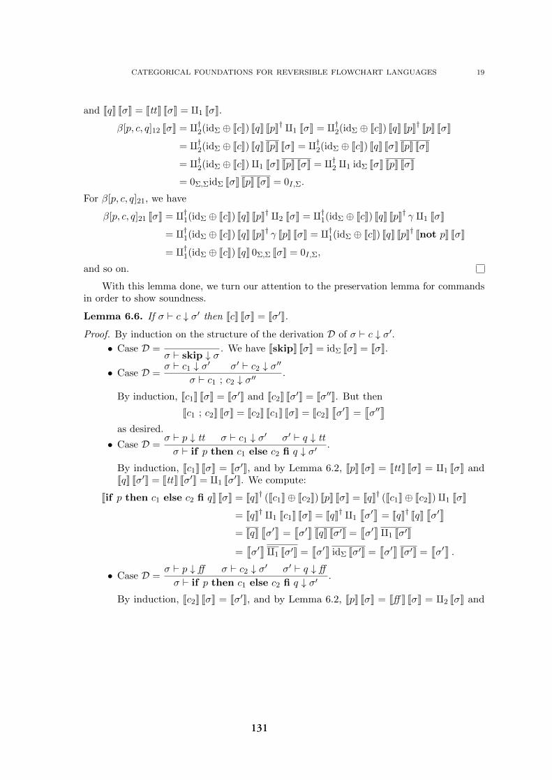
CATEGORICAL FOUNDATIONS FOR REVERSIBLE FLOWCHART LANGUAGES 19

and JqK JσK = JttK JσK = q1 JσK.

β[p, c, q]12 JσK = q†2(idΣ ⊕ JcK) JqK JpK† q1 JσK = q†2(idΣ ⊕ JcK) JqK JpK† JpK JσK

= q†2(idΣ ⊕ JcK) JqK JpK JσK = q†2(idΣ ⊕ JcK) JqK JσK JpK JσK

= q†2(idΣ ⊕ JcK)q1 JσK JpK JσK = q†2 q1 idΣ JσK JpK JσK

= 0Σ,ΣidΣ JσK JpK JσK = 0I,Σ.

For β[p, c, q]21, we have

β[p, c, q]21 JσK = q†1(idΣ ⊕ JcK) JqK JpK† q2 JσK = q†1(idΣ ⊕ JcK) JqK JpK† γ q1 JσK

= q†1(idΣ ⊕ JcK) JqK JpK† γ JpK JσK = q†1(idΣ ⊕ JcK) JqK JpK† Jnot pK JσK

= q†1(idΣ ⊕ JcK) JqK 0Σ,Σ JσK = 0I,Σ,

and so on.

With this lemma done, we turn our attention to the preservation lemma for commandsin order to show soundness.

Lemma 6.6. If σ ` c ↓ σ′ then JcK JσK = Jσ′K.

Proof. By induction on the structure of the derivation D of σ ` c ↓ σ′.• Case D =

σ ` skip ↓ σ. We have JskipK JσK = idΣ JσK = JσK.

• Case D =σ ` c1 ↓ σ′ σ′ ` c2 ↓ σ′′

σ ` c1 ; c2 ↓ σ′′.

By induction, Jc1K JσK = Jσ′K and Jc2K Jσ′K = Jσ′′K. But then

Jc1 ; c2K JσK = Jc2K Jc1K JσK = Jc2Kqσ′

y=

qσ′′

y

as desired.

• Case D =σ ` p ↓ tt σ ` c1 ↓ σ′ σ′ ` q ↓ tt

σ ` if p then c1 else c2 fi q ↓ σ′.

By induction, Jc1K JσK = Jσ′K, and by Lemma 6.2, JpK JσK = JttK JσK = q1 JσK andJqK Jσ′K = JttK Jσ′K = q1 Jσ′K. We compute:

Jif p then c1 else c2 fi qK JσK = JqK† (Jc1K⊕ Jc2K) JpK JσK = JqK† (Jc1K⊕ Jc2K)q1 JσK

= JqK† q1 Jc1K JσK = JqK† q1

qσ′

y= JqK† JqK

qσ′

y

= JqKqσ′

y=

qσ′

yJqK Jσ′K =

qσ′

yq1 Jσ′K

=qσ′

yq1 Jσ′K =

qσ′

yidΣ Jσ′K =

qσ′

yJσ′K =

qσ′

y.

• Case D =σ ` p ↓ ff σ ` c2 ↓ σ′ σ′ ` q ↓ ff

σ ` if p then c1 else c2 fi q ↓ σ′.

By induction, Jc2K JσK = Jσ′K, and by Lemma 6.2, JpK JσK = Jff K JσK = q2 JσK and

131

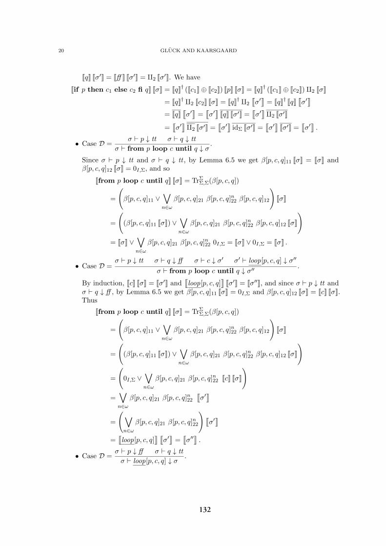
20 GLUCK AND KAARSGAARD

JqK Jσ′K = Jff K Jσ′K = q2 Jσ′K. We have

Jif p then c1 else c2 fi qK JσK = JqK† (Jc1K⊕ Jc2K) JpK JσK = JqK† (Jc1K⊕ Jc2K)q2 JσK

= JqK† q2 Jc2K JσK = JqK† q2

qσ′

y= JqK† JqK

qσ′

y

= JqKqσ′

y=

qσ′

yJqK Jσ′K =

qσ′

yq2 Jσ′K

=qσ′

yq2 Jσ′K =

qσ′

yidΣ Jσ′K =

qσ′

yJσ′K =

qσ′

y.

• Case D =σ ` p ↓ tt σ ` q ↓ tt

σ ` from p loop c until q ↓ σ.

Since σ ` p ↓ tt and σ ` q ↓ tt , by Lemma 6.5 we get β[p, c, q]11 JσK = JσK andβ[p, c, q]12 JσK = 0I,Σ, and so

Jfrom p loop c until qK JσK = TrΣΣ,Σ(β[p, c, q])

=

(β[p, c, q]11 ∨

∨n∈ω

β[p, c, q]21 β[p, c, q]n22 β[p, c, q]12

)JσK

=

((β[p, c, q]11 JσK) ∨

∨n∈ω

β[p, c, q]21 β[p, c, q]n22 β[p, c, q]12 JσK

)= JσK ∨

∨n∈ω

β[p, c, q]21 β[p, c, q]n22 0I,Σ = JσK ∨ 0I,Σ = JσK .

• Case D =σ ` p ↓ tt σ ` q ↓ ff σ ` c ↓ σ′ σ′ ` loop[p, c, q] ↓ σ′′

σ ` from p loop c until q ↓ σ′′.

By induction, JcK JσK = Jσ′K andq

loop[p, c, q]y

Jσ′K = Jσ′′K, and since σ ` p ↓ tt andσ ` q ↓ ff , by Lemma 6.5 we get β[p, c, q]11 JσK = 0I,Σ and β[p, c, q]12 JσK = JcK JσK.Thus

Jfrom p loop c until qK JσK = TrΣΣ,Σ(β[p, c, q])

=

(β[p, c, q]11 ∨

∨n∈ω

β[p, c, q]21 β[p, c, q]n22 β[p, c, q]12

)JσK

=

((β[p, c, q]11 JσK) ∨

∨n∈ω

β[p, c, q]21 β[p, c, q]n22 β[p, c, q]12 JσK

)

=

(0I,Σ ∨

∨n∈ω

β[p, c, q]21 β[p, c, q]n22 JcK JσK

)=∨n∈ω

β[p, c, q]21 β[p, c, q]n22

qσ′

y

=

(∨n∈ω

β[p, c, q]21 β[p, c, q]n22

)qσ′

y

=q

loop[p, c, q]y qσ′

y=

qσ′′

y.

• Case D =σ ` p ↓ ff σ ` q ↓ tt

σ ` loop[p, c, q] ↓ σ.

132

CATEGORICAL FOUNDATIONS FOR REVERSIBLE FLOWCHART LANGUAGES 21

Since σ ` p ↓ ff and σ ` q ↓ tt , by Lemma 6.5 we get β[p, c, q]22 JσK = 0I,Σ andβ[p, c, q]21 JσK = JσK. This gives us

qloop[p, c, q]

yJσK =

(∨n∈ω

β[p, c, q]21β[p, c, q]n22

)JσK

=

(β[p, c, q]21 ∨

∨n∈ω

β[p, c, q]21β[p, c, q]n+122

)JσK

=

((β[p, c, q]21 JσK) ∨

∨n∈ω

β[p, c, q]21β[p, c, q]n+122 JσK

)

=

(JσK ∨

∨n∈ω

β[p, c, q]21β[p, c, q]n22β[p, c, q]22 JσK

)

=

(JσK ∨

∨n∈ω

β[p, c, q]21β[p, c, q]n220I,Σ

)= JσK ∨ 0I,Σ = JσK

• Case D =σ ` p ↓ ff σ ` q ↓ ff σ ` c ↓ σ′ σ′ ` loop[p, c, q] ↓ σ′′

σ ` loop[p, c, q] ↓ σ′′.

By induction, JcK JσK = Jσ′K andq

loop[p, c, q]y

Jσ′K = Jσ′′K, and since σ ` p ↓ ff andσ ` q ↓ ff , it follows by Lemma 6.5 that β[p, c, q]22 JσK = JcK JσK and β[p, c, q]21 JσK =0I,Σ. We then have

qloop[p, c, q]

yJσK =

(∨n∈ω

β[p, c, q]21β[p, c, q]n22

)JσK

=

(β[p, c, q]21 ∨

∨n∈ω

β[p, c, q]21β[p, c, q]n+122

)JσK

=

((β[p, c, q]21 JσK) ∨

∨n∈ω

β[p, c, q]21β[p, c, q]n+122 JσK

)= 0I,Σ ∨

∨n∈ω

β[p, c, q]21β[p, c, q]n+122 JσK

=∨n∈ω

β[p, c, q]21β[p, c, q]n22β[p, c, q]22 JσK

=∨n∈ω

β[p, c, q]21β[p, c, q]n22 JcK JσK

=∨n∈ω

β[p, c, q]21β[p, c, q]n22

qσ′

y

=

(∨n∈ω

β[p, c, q]21β[p, c, q]n22

)qσ′

y

=q

loop[p, c, q]y qσ′

y=

qσ′′

y

133

22 GLUCK AND KAARSGAARD

which was what we wanted.

This finally allows us to show the soundness theorem for commands – and so, forprograms – in a straightforward manner.

Theorem 6.7 (Soundness). If there exists σ′ such that σ ` c ↓ σ′ then JcK JσK is total.

Proof. Suppose there exists σ′ such that σ ` c ↓ σ′. By Lemma 6.6, JcK JσK = Jσ′K, and since

the interpretation of any state is assumed to be total, it follows that JcK JσK = Jσ′K = idI ,which was what we wanted.

With soundness done, we only have adequacy left to prove. Adequacy is much simplerthan usual in our case, as we have no higher order data to deal with, and as such, it canbe shown by plain structural induction rather than by the assistance of logical relations.Nevertheless, we require two technical lemmas in order to succeed.

Lemma 6.8. If gf is total, so is f .

Proof. Let f : A→ B and g : B → C be morphisms such that gf = idA. Then f = idAf =

gf f = gff = gf = idA, so f is total as well.

Lemma 6.9. Let f : A⊕ U → B ⊕ U and s : I → A be morphisms. If TrUA,B(f)s is total,

either TrUA,B(f)s = f11s, or there exists n ∈ ω such that TrUA,B(f)s = f21fn22f12s.

Proof. Since the trace is canonically constructed, it takes the form

TrUA,B(f) = f11 ∨∨n∈ω

f21fn22f12.

Further, in the proof of Theorem 20 in [21], it is shown that this join not only exists but isa disjoint join, i.e., for any choice of n ∈ ω,

f11f21fn22f12 = (f21fn22f12) f11 = 0A,B

and for all n,m ∈ ω with n 6= m,

f21fn22f12f21fm22f12 = f21fm22f12f21f

n22f12 = 0A,B.

But then,

TrUA,B(f)s =

(f11 ∨

∨n∈ω

f21fn22f12

)s

= (f11s) ∨∨n∈ω

(f21fn22f12s)

= f11s ∨∨n∈ω

f21fn22f12s.

Since all of the morphisms f11s and f21fn22f12s for any n ∈ ω are restriction idempotentsI → I, it follows for each of them that they are either equal to idI or to 0I,I . Supposethat none of these are equal to the identity idI . Then they must all be 0I,I , and so

TrUA,B(f)s = 0I,I 6= idI , contradicting totality. On the other hand, suppose that there existsan identity among these. Then, it follows by the disjointness property above that the restmust be 0I,I .

134

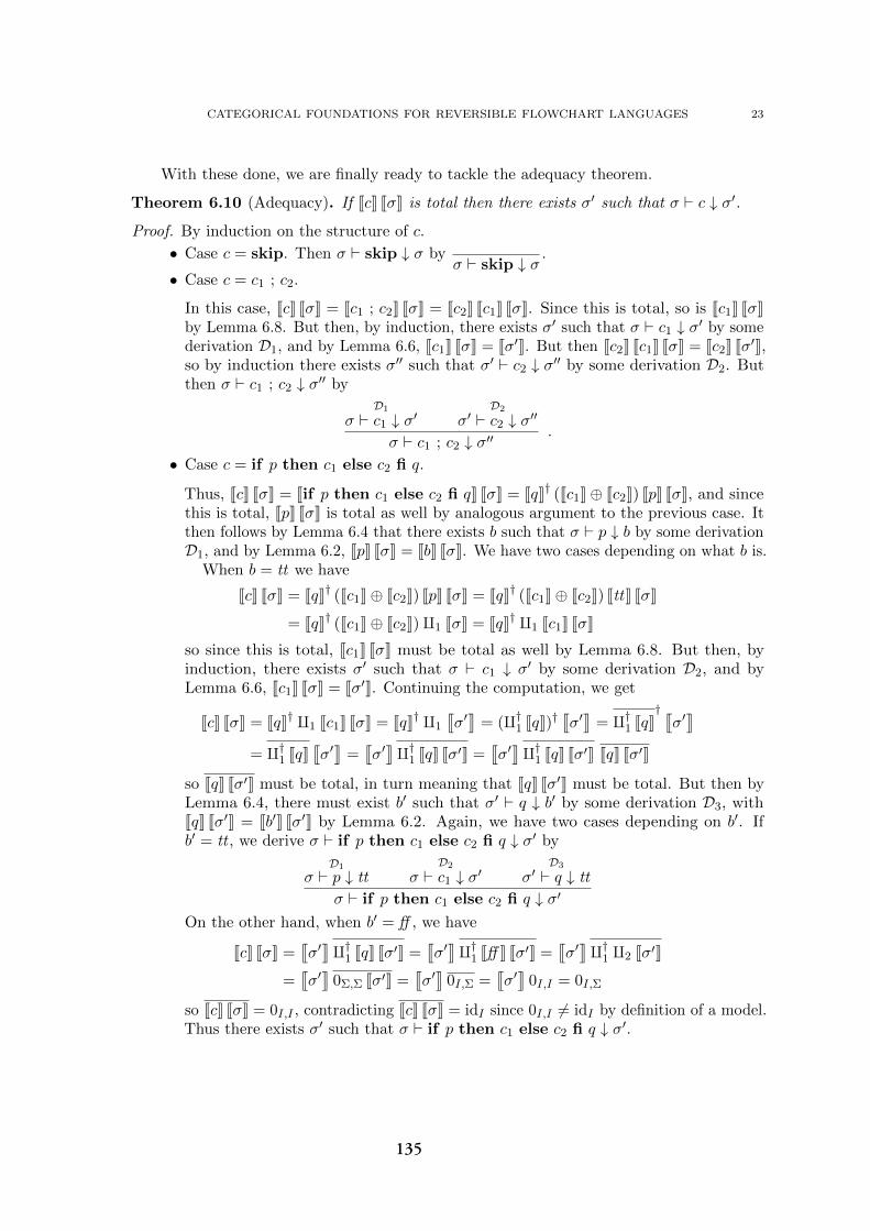
CATEGORICAL FOUNDATIONS FOR REVERSIBLE FLOWCHART LANGUAGES 23

With these done, we are finally ready to tackle the adequacy theorem.

Theorem 6.10 (Adequacy). If JcK JσK is total then there exists σ′ such that σ ` c ↓ σ′.

Proof. By induction on the structure of c.

• Case c = skip. Then σ ` skip ↓ σ byσ ` skip ↓ σ

.

• Case c = c1 ; c2.

In this case, JcK JσK = Jc1 ; c2K JσK = Jc2K Jc1K JσK. Since this is total, so is Jc1K JσKby Lemma 6.8. But then, by induction, there exists σ′ such that σ ` c1 ↓ σ′ by somederivation D1, and by Lemma 6.6, Jc1K JσK = Jσ′K. But then Jc2K Jc1K JσK = Jc2K Jσ′K,so by induction there exists σ′′ such that σ′ ` c2 ↓ σ′′ by some derivation D2. Butthen σ ` c1 ; c2 ↓ σ′′ by

D1

σ ` c1 ↓ σ′D2

σ′ ` c2 ↓ σ′′

σ ` c1 ; c2 ↓ σ′′.

• Case c = if p then c1 else c2 fi q.

Thus, JcK JσK = Jif p then c1 else c2 fi qK JσK = JqK† (Jc1K⊕ Jc2K) JpK JσK, and sincethis is total, JpK JσK is total as well by analogous argument to the previous case. Itthen follows by Lemma 6.4 that there exists b such that σ ` p ↓ b by some derivationD1, and by Lemma 6.2, JpK JσK = JbK JσK. We have two cases depending on what b is.

When b = tt we have

JcK JσK = JqK† (Jc1K⊕ Jc2K) JpK JσK = JqK† (Jc1K⊕ Jc2K) JttK JσK

= JqK† (Jc1K⊕ Jc2K)q1 JσK = JqK† q1 Jc1K JσK

so since this is total, Jc1K JσK must be total as well by Lemma 6.8. But then, byinduction, there exists σ′ such that σ ` c1 ↓ σ′ by some derivation D2, and byLemma 6.6, Jc1K JσK = Jσ′K. Continuing the computation, we get

JcK JσK = JqK† q1 Jc1K JσK = JqK† q1

qσ′

y= (q†1 JqK)†

qσ′

y= q†1 JqK

† qσ′

y

= q†1 JqKqσ′

y=

qσ′

yq†1 JqK Jσ′K =

qσ′

yq†1 JqK Jσ′K JqK Jσ′K

so JqK Jσ′K must be total, in turn meaning that JqK Jσ′K must be total. But then byLemma 6.4, there must exist b′ such that σ′ ` q ↓ b′ by some derivation D3, withJqK Jσ′K = Jb′K Jσ′K by Lemma 6.2. Again, we have two cases depending on b′. Ifb′ = tt , we derive σ ` if p then c1 else c2 fi q ↓ σ′ by

D1

σ ` p ↓ ttD2

σ ` c1 ↓ σ′D3

σ′ ` q ↓ tt

σ ` if p then c1 else c2 fi q ↓ σ′

On the other hand, when b′ = ff , we have

JcK JσK =qσ′

yq†1 JqK Jσ′K =

qσ′

yq†1 Jff K Jσ′K =

qσ′

yq†1 q2 Jσ′K

=qσ′

y0Σ,Σ Jσ′K =

qσ′

y0I,Σ =

qσ′

y0I,I = 0I,Σ

so JcK JσK = 0I,I , contradicting JcK JσK = idI since 0I,I 6= idI by definition of a model.Thus there exists σ′ such that σ ` if p then c1 else c2 fi q ↓ σ′.

135

24 GLUCK AND KAARSGAARD

To show the case when b = ff , we proceed as before. We then have

JcK JσK = JqK† (Jc1K⊕ Jc2K) JpK JσK = JqK† (Jc1K⊕ Jc2K) Jff K JσK

= JqK† (Jc1K⊕ Jc2K)q2 JσK = JqK† q2 Jc2K JσK

So Jc2K JσK must be total by Lemma 6.8, which means that by induction there existsσ′ such that σ ` c2 ↓ σ′ by a derivation D2, and by Lemma 6.6, Jc2K JσK = Jσ′K.Continuing as before, we obtain now that

JcK JσK = JqK† q2 Jc2K JσK = JqK† q2

qσ′

y= (q†2 JqK)†

qσ′

y= q†2 JqK

† qσ′

y

= q†2 JqKqσ′

y=

qσ′

yq†2 JqK Jσ′K =

qσ′

yq†2 JqK Jσ′K JqK Jσ′K

and so JqK Jσ′K must be total in this case as well, so by Lemma 6.4 there must existb′ such that σ′ ` q ↓ b′ by some derivation D3, and JqK Jσ′K = Jb′K Jσ′K by Lemma 6.2.Again, we do a case analysis depending on the value of b′.

If b′ = tt , we have

JcK JσK =qσ′

yq†2 JqK Jσ′K =

qσ′

yq†2 JttK Jσ′K =

qσ′

yq†2 q1 Jσ′K

=qσ′

y0Σ,Σ Jσ′K =

qσ′

y0I,Σ =

qσ′

y0I,I = 0I,Σ

which contradicts the totality of JcK JσK by JcK JσK = 0I,Σ = 0I,I 6= idI , and we getby contradiction that there exists σ′ such that σ ` if p then c1 else c2 fi q ↓ σ′.

If b′ = ff , we derive σ ` if p then c1 else c2 fi q ↓ σ′ by

D1

σ ` p ↓ ffD2

σ ` c2 ↓ σ′D3

σ′ ` q ↓ ff

σ ` if p then c1 else c2 fi q ↓ σ′.

• Case c = from p loop c1 until q.

In this case, JcK JσK = Jfrom p loop c1 until qK JσK = TrΣΣ,Σ(β[p, c1, q]) JσK. Since

this is total and JσK : I → Σ, it follows by Lemma 6.9 that either

Jfrom p loop c1 until qK JσK = β[p, c1, q]11 JσK

or there exists n ∈ ω such that

Jfrom p loop c1 until qK JσK = β[p, c1, q]21β[p, c1, q]n22β[p, c1, q]12 JσK .

If Jfrom p loop c1 until qK JσK = β[p, c1, q]11 JσK, we have

Jfrom p loop c1 until qK JσK = β[p, c1, q]11 JσK = q†1(idΣ ⊕ Jc1K) JqK JpK† q1 JσK

= q†1(idΣ ⊕ Jc1K) JqKq†1 JpK JσK

= q†1(idΣ ⊕ Jc1K) JqK JσKq†1 JpK JσK

= q†1(idΣ ⊕ Jc1K) JqK JσKq†1 JpK JσK JqK JσK JpK JσK

so it follows by totality of JcK JσK that JpK JσK and JqK JσK must be total, so JpK JσKand JqK JσK must be total as well. It then follows by Lemma 6.4 that there existb1 and b2 such that σ ` p ↓ b1 and σ ` q ↓ b2 by derivations D1 respectivelyD2. But then it follows by Lemma 6.5 that b1 = b2 = tt , as we would otherwise

136

CATEGORICAL FOUNDATIONS FOR REVERSIBLE FLOWCHART LANGUAGES 25

have JcK JσK = β[p, c1, q]11 JσK = 0I,Σ, contradicting totality. Thus we may deriveσ ` from p loop c1 until q ↓ σ by

D1

σ ` p ↓ ttD2

σ ` q ↓ tt

σ ` from p loop c1 until q ↓ σ.

On the other hand, suppose that there exists n ∈ ω such that

JcK JσK = Jfrom p loop c1 until qK JσK = β[p, c1, q]21β[p, c1, q]n22β[p, c1, q]12 JσK .

Since this is total, by Lemma 6.8 β[p, c1, q]12 JσK is total as well, and

β[p, c1, q]12 JσK = q†2(idΣ ⊕ Jc1K) JqK JpK† q1 JσK = q†2(idΣ ⊕ Jc1K) JqKq†1 JpK JσK

= q†2(idΣ ⊕ Jc1K) JqK JσKq†1 JpK JσK

= q†2(idΣ ⊕ Jc1K) JqK JσKq†1 JpK JσKJpK JσK JqK JσK

But then JpK JσK and JqK JσK must be total as well, so by Lemma 6.4 there exist b1and b2 such that σ ` p ↓ b1 and σ ` q ↓ b2 by derivations D1 respectively D2. Sinceβ[p, c1, q]12 JσK is total, it further follows by Lemma 6.5 that b1 = tt and b2 = ff , aswe would otherwise have β[p, c1, q]12 JσK = 0I,Σ. Further, β[p, c1, q]12 JσK = Jc1K JσK,and since this is total, by induction there exists σ′ such that σ ` c1 ↓ σ′ by somederivation D3, with Jc1K JσK = Jσ′K by Lemma 6.6.

To summarize, we have now that

Jfrom p loop c1 until qK JσK = β[p, c1, q]21β[p, c1, q]n22β[p, c1, q]12 JσK

= β[p, c1, q]21β[p, c1, q]n22 Jc1K JσK

= β[p, c1, q]21β[p, c1, q]n22

qσ′

y

is total, and we have derivations D1 of σ ` p ↓ tt , D2 of σ ` q ↓ ff , and D3 of σ ` c1 ↓σ′. To finish the proof, we show by induction on n that if β[p, c1, q]21β[p, c1, q]

n22 Jσ′K

is total for any state σ′, there exists a state σ′′ such that σ′ ` loop[p, c1, q] ↓ σ′′ bysome derivation D4.

– In the base case n = 0, so β[p, c1, q]21β[p, c1, q]n22 Jσ′K = β[p, c1, q]21 Jσ′K. By

proof analogous to previous cases, we have that JpK Jσ′K and JqK Jσ′K must betotal, so by Lemma 6.4 there exist b′1 and b′2 such that σ′ ` p ↓ b′1 and σ′ ` q ↓ b′1by derivations D′1 respectively D′2. Further, by totality, it follows by Lemma 6.5that we must have b′1 = ff , b′2 = tt . Thus we may produce our derivation D4 ofσ′ ` loop[p, c1, q] ↓ σ′ by

D′1σ′ ` p ↓ ff

D′2σ′ ` q ↓ tt

σ′ ` loop[p, c, q] ↓ σ′

– In the inductive case, we have that

β[p, c1, q]21β[p, c1, q]n+122

qσ′

y= β[p, c1, q]21β[p, c1, q]

n22β[p, c1, q]22

qσ′

y

and since this is assumed to be total, it follows by Lemma 6.8 that β[p, c1, q]22 Jσ′Kis total as well. Again, by argument analogous to previous cases, this impliesthat JpK Jσ′K and JqK Jσ′K are both total, so by Lemma 6.4 there exist b′1 and b′2such that σ′ ` p ↓ b′1 and σ′ ` q ↓ b′2 by derivations D′1 respectively D′2. Likewise,

137

26 GLUCK AND KAARSGAARD

it then follows by Lemma 6.5 that since this is total, we must have b′1 = b′2 = ff ,and so β[p, c1, q]22 Jσ′K = Jc1K Jσ′K, again by Lemma 6.5. Since Jc1K Jσ′K is total,by the outer induction hypothesis there exists a derivation D′3 of σ′ ` c1 ↓ σ′′for some σ′′, and so Jc1K Jσ′K = Jσ′′K by Lemma 6.6. But then

β[p, c1, q]21β[p, c1, q]n+122

qσ′

y= β[p, c1, q]21β[p, c1, q]

n22β[p, c1, q]22

qσ′

y

= β[p, c1, q]21β[p, c1, q]n22 Jc1K

qσ′

y

= β[p, c1, q]21β[p, c1, q]n22

qσ′′

y

since this is total, by (inner) induction there exists a derivation D′4 of σ′′ `loop[p, c1, q] ↓ σ′′′. Thus, we may produce our derivation D4 as

D′1σ′ ` p ↓ ff

D′2σ′ ` q ↓ ff

D′3σ′ ` c1 ↓ σ′′

D′4σ′′ ` loop[p, c, q] ↓ σ′′′

σ′ ` loop[p, c1, q] ↓ σ′′′

concluding the internal lemma.

Since this is the case, we may finally show σ ` from p loop q until c ↓ σ′ by

D1

σ ` p ↓ ttD2

σ ` q ↓ ffD3

σ ` c ↓ σ′D4

σ′ ` loop[p, c, q] ↓ σ′′

σ ` from p loop c until q ↓ σ′′,

which concludes the proof.

7. Full abstraction

Where soundness and adequacy state an agreement in the notions of convergence betweenthe operational and denotational semantics, full abstraction deals with their respectivenotions of equivalence (see, e.g., [24]). Unlike the case for soundness and adequacy, wheredefining a proper notion of convergence required more work on the categorical side, thetables have turned when it comes to program equivalence. In the categorical semantics,program equivalence is clear – equality of interpretations. Operationally, however, there isnothing immediately corresponding to equality of behaviour at runtime.

To produce this, we consider how two programs may behave when executed from thesame start state. If they always produce the same result, we say that they are observationallyequivalent. Formally, we define this as follows:

Definition 13. Say that programs p1 and p2 are observationally equivalent, denoted p1 ≈ p2,if for all states σ, σ ` p1 ↓ σ′ if and only if σ ` p2 ↓ σ′.

A model is said to be fully abstract if these two notions of program equivalence are inagreement. In the present section, we will show a sufficient condition for full abstraction ofmodels of structured reversible flowchart languages. This condition will be that the givenmodel additionally has the properties of being I-well pointed and bijective on states.

Definition 14. Say that a model of a structured reversible flowchart language is I-wellpointed if, for all parallel morphisms f, g : A → B, f = g precisely when fp = gp for allp : I → A.

138

CATEGORICAL FOUNDATIONS FOR REVERSIBLE FLOWCHART LANGUAGES 27

Definition 15. Say that a model C of a structured reversible flowchart language L isbijective on states if there is a bijective correspondence between states of L and totalmorphisms I → Σ of C .

If a sound and adequate model of a structured reversible flowchart language is bijectiveon states, we can show a stronger version of Lemma 6.6.

Lemma 7.1. If C be a sound and adequate model of a structured reversible flowchartlanguage which is bijective on states. Then σ ` c ↓ σ′ iff JcK JσK = Jσ′K and this is total.

Proof. By Lemma 6.6 and Theorem 6.7, we only need to show that JcK JσK = Jσ′K impliesσ ` c ↓ σ′. Assume that JcK JσK = Jσ′K and that this is total. By Theorem 6.10, there existsσ′′ such that σ ` c ↓ σ′′, so by Lemma 6.6, JcK JσK = Jσ′′K. Thus Jσ′K = JcK JσK = Jσ′′K, soσ′ = σ′′ by bijectivity on states.

With this, we can show full abstraction.

Theorem 7.2 (Full abstraction). Let C be a sound and adequate model of a structuredreversible flowchart language that is furthermore I-well pointed and bijective on states. ThenC is fully abstract, i.e., p1 ≈ p2 if and only if Jp1K = Jp2K.

Proof. Suppose p1 ≈ p2, i.e., for all σ, σ ` p1 ↓ σ′ if and only if σ ` p2 ↓ σ′. Let s : I → Σbe a morphism. Since C is a model of a structured reversible flowchart language, it followsthat either s = idI or s = 0I,I where idI 6= 0I,I .

If s = 0I,I , we have Jp1K s = Jp2K s = 0I,Σ by unicity of the zero map.On the other hand, if s = idI , by bijectivity on states there exists σ0 such that s = Jσ0K.

Consider now Jp1K s = Jp1K Jσ0K. If this is total, by Theorem 6.10 there exists σ′0 such thatσ0 ` p1 ↓ σ′0, and by p1 ≈ p2, σ0 ` p2 ↓ σ′0 as well. But then, applying Lemma 6.6 on bothyields that

Jp1K s = Jp1K Jσ0K =qσ′0

y= Jp2K Jσ0K = Jp2K s .

If, on the other hand, Jp1K s is not total, by the contrapositive to Theorem 6.7, there existsno σ′0 such that σ0 ` p1 ↓ σ′0, so by p1 ≈ p2 there exists no σ′′0 such that σ0 ` p1 ↓ σ′′0 . Butthen, by the contrapositive of Theorem 6.10 and the fact that restriction idempotents on Iare either idI or 0I,I , it follows that

Jp1K s = Jp1K Jσ0K = 0I,Σ = Jp2K Jσ0K = Jp1K s.

Since s was chosen arbitrarily and Jp1K s = Jp2K s in all cases, it follows by I-well pointednessthat Jp1K = Jp2K.

In the other direction, suppose Jp1K = Jp2K, let σ0 be a state, and suppose that thereexists σ′0 such that σ0 ` p1 ↓ σ′0. By Lemma 6.6, Jp1K Jσ0K = Jσ′0K, and by Theorem 6.7 this istotal. But then, by Jp1K = Jp2K, Jp2K Jσ0K = Jp1K Jσ0K = Jσ′0K, so by Lemma 7.1, σ0 ` p2 ↓ σ′0.The other direction follows similarly.

8. Applications

In this section, we briefly cover some applications of the developed theory: We show how aprogram inverter can be derived from the semantics; introduce a small reversible flowchartlanguage, and use the results from the previous sections to give it semantics; and discusshow decisions may be used as a programming technique to naturally represent predicates ina reversible functional language.

139

28 GLUCK AND KAARSGAARD

8.1. Extracting a program inverter. A desirable syntactic property for reversible pro-gramming languages is to be closed under program inversion, in the sense that for each

program p, there is another program I[p] such that JI[p]K = JpK†. Janus, R-WHILE, andR-CORE [32, 16, 17] are all examples of reversible programming languages with this property.This is typically witnessed by a program inverter [1], that is, a procedure mapping theprogram text of a program to the program text of its inverse program3.

Suppose that we are given a language where elementary operations are closed underprogram inversion (i.e., where each elementary operation b has an inverse I[b] such that

JI[b]K = JbK†). We can extend this to a program inverter for skip, sequencing, reversibleconditionals and loops as follows, by structural induction with the hypothesis that JI[c]K =

JcK†. For skip, we have

JskipK† = id†Σ = idΣ = JskipKgiving us the usual inversion rule of I[skip] = skip. Likewise for sequences,

Jc1 ; c2K† = (Jc2K Jc1K)† = Jc1K† Jc2K† = JI[c1]K JI[c2]K = JI[c2] ; I[c1]K

giving us the inversion ruleI[c1 ; c2] = I[c2] ; I[c1] .

Our approach becomes more interesting when we come to conditionals. Given someconditional statement if p then c1 else c2 fi q, we notice that

Jif p then c1 else c2 fi qK† = (JqK† Jc1K⊕ Jc2K JpK)†

= JpK† Jc1K† ⊕ Jc2K† JqK††

= JpK† Jc1K† ⊕ Jc2K† JqK

= JpK† JI[c1]K⊕ JI[c2]K JqK= Jif q then I[c1] else I[c2] fi pK

which yields the inversion rule

I[if p then c1 else c2 fi q] = if q then I[c1] else I[c2] fi p].

Fortunately, this is precisely the usual inversion rule for reversible conditionals (see, e.g.,[16, 17]). For reversible loops, we have

Jfrom p loop c until qK† = TrΣΣ,Σ(idΣ ⊕ JcK JqK JpK†)†

= TrΣΣ,Σ((idΣ ⊕ JcK JqK JpK†)†)

= TrΣΣ,Σ(JpK JqK† idΣ ⊕ JcK†)

= TrΣΣ,Σ(idΣ ⊕ JcK† JpK JqK†)

= TrΣΣ,Σ(idΣ ⊕ JI[c]K JpK JqK†)

= Jfrom q loop I[c] until pK

3While semantic inverses are unique, their program texts generally are not. As such, a programminglanguage may have many different sound and complete program inverters, though they will all be equivalentup to program semantics.

140

CATEGORICAL FOUNDATIONS FOR REVERSIBLE FLOWCHART LANGUAGES 29

where the fact that it is a †-trace allows us to move the dagger inside the trace, and

dinaturality of the trace in the second component allows us to move idΣ⊕ JcK† from the veryright to the very left. This gives us the inversion rule

I[from p loop c until q] = from q loop I[c] until p

which matches the usual inversion rule for reversible loops [17]. We summarize this in thefollowing theorem:

Theorem 8.1. If a reversible structured flowchart language is syntactically closed underinversion of elementary operations, it is also closed under inversion of reversible conditionalsand loops.

8.2. Example: A reversible flowchart language. Consider the following family of (nei-ther particularly useful nor particularly useless) reversible flowchart languages for reversiblecomputing with integer data, RINTk. RINTk has precisely k variables available for storage,denoted x1 through xk (of which x1 is designated by convention as the input/output variable),and its only atomic operations are addition and subtraction of variables, as well as additionwith a constant. Variables are used as elementary predicates, with zero designating truthand non-zero values all designating falsehood. For control structures we have reversibleconditionals and loops, and sequencing as usual. This gives the syntax:

p ::= tt | ff | xi | p and p | not p (Tests)

c ::= c ; c | xi += xj | xi −= xj | xi += n

| if p then c else c fi p

| from p loop c until p (Commands)

Here, n is the syntactic representation of an integer n. In the cases for addition andsubtraction, we impose the additional syntactic constraints that 1 ≤ i ≤ k, 1 ≤ j ≤ k, andi 6= j, the latter to guarantee reversibility. Subtraction by a constant is not included as itmay be derived straightforwardly from addition with a constant. A program in RINTk isthen simply a command.

We may now give semantics to this language in our framework. For a concrete model,we select the category PInj of sets and partial injections, which is a join inverse categorywith a join-preserving disjointness tensor (given on objects by the disjoint union of sets), soit is extensive in the sense of Definition 9 by Theorem 4.4. By our developments previouslyin this section, to give a full semantics to RINTk in PInj, it suffices to provide an object(i.e., a set) of stores Σ, denotations of our three classes of elementary operations (additionby a variable, addition by a constant, and subtraction by a variable) as morphisms (i.e.,partial injective functions) Σ→ Σ, and denotations of our class of elementary predicates(here, testing whether a variable is zero or not) as decisions Σ→ Σ⊕Σ. These are all shownin Figure 4. It is uncomplicated to show that all of these are partial injective functions, andthat the denotation of each predicate JxiK is a decision, so that this is, in fact, a model ofRINTk in PInj.

We can now reap the benefits in the form of a reversibility theorem for free:

Theorem 8.2 (Reversibility). Every RINTk program p is semantically reversible in the sensethat JpK is a partial isomorphism.

141

30 GLUCK AND KAARSGAARD

Σ = Zk

JxiK (a1, . . . , ak) =

{q1(a1, . . . , ak) if ai = 0q2(a1, . . . , ak) otherwise

qxi += xj

y(a1, . . . , ak) = (a1, . . . , ai−1, ai + aj , . . . , ak)

Jxi += nK (a1, . . . , ak) = (a1, . . . , ai−1, ai + n, . . . , ak)qxi −= xj

y(a1, . . . , ak) = (a1, . . . , ai−1, ai − aj , . . . , ak)

Figure 4: The object of stores and semantics of elementary operations and predicates ofRINTk in PInj.

Further, since we can straightforwardly show thatqxi += xj

y†=

qxi −= xj

yand

Jxi += nK† = Jxi += −n K, we can use the technique from Sec. 8.1 to obtain a sound andcomplete program inverter.

Theorem 8.3 (Program inversion). RINTk has a (sound and complete) program inverter.

In particular, for every RINTk program p there exists a program I[p] such that JI[p]K = JpK†.

8.3. Decisions as a programming technique. Decisions offer a solution to the awk-wardness in representing predicates reversibly. On the programming side, the reversibleduplication/equality operator [15] (see also [31]) can be seen as a distant ancestor to predicates-as-decisions, in that it provides an ad-hoc solution to the problem of checking whether twovalues are equal in a reversible manner.

Decisions offer a more systematic approach: They suggest that one ought to defineBoolean values in reversible functional programming not in the usual way, but rather bymeans of the polymorphic datatype

data PBool α = True α | False α

storing not only the result, but also what was tested to begin with. With this definition,negation on these polymorphic Booleans (pnot) may be defined straightforwardly as shownin Figure 5. In turn, this allows for more complex predicates to be expressed in a largelyfamiliar way. For example, the decision for testing whether a natural number is even (peven)is also shown in Figure 5, with fmap given in the straightforward way on polymorphicBooleans. For comparison, the corresponding irreversible predicate is typically defined asfollows, with not the usual negation of Booleans

even :: Nat → Booleven 0 = Trueeven (n + 1) = not (even n) .

As such, the reversible implementation as a decision is nearly identical, the only differencebeing the use of fmap in the definition of peven to recover the input value once the branchhas been decided.

142

CATEGORICAL FOUNDATIONS FOR REVERSIBLE FLOWCHART LANGUAGES 31

pnot :: PBool α ↔ PBool αpnot (True x ) = False xpnot (False x ) = True x

peven :: Nat ↔ PBool Natpeven 0 = True 0peven (n + 1) = fmap (+1) (pnot (peven n))

Figure 5: The definition of the even-predicate as a decision on natural numbers.

9. Concluding remarks

In the present paper, we have built on the work on extensive restriction categories toderive a related concept of extensivity for inverse categories. We have used this concept togive a novel reversible representation of predicates and their corresponding assertions in(specifically extensive) join inverse categories with a disjointness tensor, and in turn usedthese to model the fundamental control structures of reversible loops and conditionals instructured reversible flowchart languages. We have shown that these categorical semanticsare sound and adequate with respect to the operational semantics, and given a sufficientcondition for full abstraction.

Further, this approach also allowed us to derive a program inversion theorem forstructured reversible flowchart languages, and we illustrated our approach by developinga family of structured reversible flowchart languages and using our framework to give itdenotational semantics, with theorems regarding reversibility and program inversion for free.

The idea to represent predicates by decisions was partially inspired by the instrumentsassociated with predicates in Effectus theory [19]. Given that side effect free instruments ιsatisfy a similar rule, ∇ι = id, and that Boolean effecti are extensive, it could be interestingto explore the connections between extensive restriction categories and Boolean effecti,especially as regards their internal logic.

Finally, on the programming language side, it could be interesting to further explorehow decisions can be used in reversible programming, e.g., to do the heavy lifting involvedin pattern matching and branch joining. As our focus has been on the representation ofpredicates, our approach may be easily adapted to other reversible flowchart structures, e.g.,Janus-style loops [32].

References

[1] Abramov, S. M. and R. Gluck, The universal resolving algorithm: inverse computation in a functionallanguage, in: R. Backhouse and J. N. Oliveira, editors, Mathematics of Program Construction. Proceedings,LNCS 1837 (2000), pp. 187–212.

[2] Axelsen, H. B. and R. Gluck, What do reversible programs compute?, in: M. Hofmann, editor, Foundationsof Software Science and Computation Structures. Proceedings, Lecture Notes in Computer Science 6604(2011), pp. 42–56.

[3] Axelsen, H. B., R. Gluck and T. Yokoyama, Reversible machine code and its abstract processor architecture,in: V. Diekert, M. V. Volkov and A. Voronkov, editors, Computer Science – Theory and Applications.Proceedings, Lecture Notes in Computer Science 4649 (2007), pp. 56–69.

[4] Axelsen, H. B. and R. Kaarsgaard, Join inverse categories as models of reversible recursion, in: B. Jacobsand C. Loding, editors, FOSSACS 2016, Proceedings, number 9634 in LNCS (2016), pp. 73–90.

[5] Carboni, A., S. Lack and R. F. C. Walters, Introduction to extensive and distributive categories, Journalof Pure and Applied Algebra 84 (1993), pp. 145 – 158.

[6] Carothers, C. D., K. S. Perumalla and R. M. Fujimoto, Efficient optimistic parallel simulations usingreverse computation, ACM Trans. Model. Comput. Simul. 9 (1999), pp. 224–253.

[7] Cockett, J. R. B., Itegories & PCAs (2007), slides from talk at FMCS 2007.

143

32 GLUCK AND KAARSGAARD

[8] Cockett, J. R. B. and S. Lack, Restriction categories I: Categories of partial maps, Theoretical ComputerScience 270 (2002), pp. 223–259.

[9] Cockett, J. R. B. and S. Lack, Restriction categories II: Partial map classification, Theoretical ComputerScience 294 (2003), pp. 61–102.

[10] Cockett, R. and S. Lack, Restriction categories III: Colimits, partial limits and extensivity, MathematicalStructures in Computer Science 17 (2007), pp. 775–817.

[11] Fiore, M. P., “Axiomatic Domain Theory in Categories of Partial Maps,” Ph.D. thesis, University ofEdinburgh (1994).

[12] Frank, M. P., “Reversibility for efficient computing,” Ph.D. thesis, EECS Dept., Massachusetts Instituteof Technology (1999).

[13] Giles, B. G., “An Investigation of some Theoretical Aspects of Reversible Computing,” Ph.D. thesis,University of Calgary (2014).

[14] Gluck, R. and R. Kaarsgaard, A categorical foundation for structured reversible flowchart languages, in:Proceedings of the 33rd Conference on the Mathematical Foundations of Programming Semantics (MFPSXXXIII), 2017, to appear.

[15] Gluck, R. and M. Kawabe, A program inverter for a functional language with equality and constructors,in: A. Ohori, editor, Programming Languages and Systems. Proceedings, Lecture Notes in ComputerScience 2895 (2003), pp. 246–264.

[16] Gluck, R. and T. Yokoyama, A linear-time self-interpreter of a reversible imperative language, ComputerSoftware 33 (2016), pp. 108–128.

[17] Gluck, R. and T. Yokoyama, A minimalist’s reversible while language, IEICE Transactions on Informationand Systems E100-D (2017), pp. 1026–1034.

[18] Guo, X., “Products, Joins, Meets, and Ranges in Restriction Categories,” Ph.D. thesis, University ofCalgary (2012).

[19] Jacobs, B., New directions in categorical logic, for classical, probabilistic and quantum logic, LogicalMethods in Computer Science 11 (2015), pp. 1–76.

[20] Joyal, A., R. Street and D. Verity, Traced monoidal categories, Mathematical Proceedings of theCambridge Philosophical Society 119 (1996), pp. 447–468.

[21] Kaarsgaard, R., H. B. Axelsen and R. Gluck, Join inverse categories and reversible recursion, Journal ofLogical and Algebraic Methods in Programming 87 (2017), pp. 33–50.

[22] Kastl, J., Inverse categories, in: H.-J. Hoehnke, editor, Algebraische Modelle, Kategorien und Gruppoide,Studien zur Algebra und ihre Anwendungen 7, Akademie-Verlag, 1979 pp. 51–60.

[23] Mogensen, T. Æ., Partial evaluation of the reversible language Janus, in: Partial Evaluation and ProgramManipulation. Proceedings (2011), pp. 23–32.

[24] Plotkin, G., Full abstraction, totality and PCF, Mathematical Structures in Computer Science 9 (1999),pp. 1–20.

[25] Selinger, P., Dagger compact closed categories and completely positive maps, Electronic Notes in Theo-retical Computer Science 170 (2007), pp. 139–163.

[26] Selinger, P., A survey of graphical languages for monoidal categories, in: B. Coecke, editor, NewStructures for Physics, number 813 in Lecture Notes in Physics (2011), pp. 289–355.

[27] Thomsen, M. K., H. B. Axelsen and R. Gluck, A reversible processor architecture and its reversiblelogic design, in: A. De Vos and R. Wille, editors, Reversible Computation. Proceedings, Lecture Notes inComputer Science 7165 (2012), pp. 30–42.

[28] Thomsen, M. K., R. Gluck and H. B. Axelsen, Reversible arithmetic logic unit for quantum arithmetic,Journal of Physics A: Mathematical and Theoretical 43 (2010), p. 382002.

[29] Yokoyama, T., H. B. Axelsen and R. Gluck, Reversible flowchart languages and the structured reversibleprogram theorem, in: L. Aceto, I. Damgard, L. A. Goldberg, M. M. Halldorsson, A. Ingolfsdottirand I. Walukiewicz, editors, International Colloquium on Automata, Languages and Programming.Proceedings, Lecture Notes in Computer Science 5126 (2008), pp. 258–270.

[30] Yokoyama, T., H. B. Axelsen and R. Gluck, Optimizing clean reversible simulation of injective functions,Journal of Multiple-Valued Logic and Soft Computing 18 (2012), pp. 5–24.

[31] Yokoyama, T., H. B. Axelsen and R. Gluck, Towards a reversible functional language, in: A. De Vos andR. Wille, editors, RC 2011, LNCS 7165 (2012), pp. 14–29.

[32] Yokoyama, T. and R. Gluck, A reversible programming language and its invertible self-interpreter, in:Partial Evaluation and Semantics-Based Program Manipulation. Proceedings (2007), pp. 144–153.

144

145

146

Reversible effects as inverse arrows

Chris Heunen1, Robin Kaarsgaard2, and Martti Karvonen3

1 University of Edinburgh, [email protected] University of Copenhagen, [email protected]

3 University of Edinburgh, [email protected]

Abstract. Reversible computing models settings in which all processescan be reversed. Applications include low-power computing, quantumcomputing, and robotics. It is unclear how to represent side-effects inthis setting, because conventional methods need not respect reversibility.We model reversible effects by adapting Hughes’ arrows to dagger arrowsand inverse arrows. This captures several fundamental reversible effects,including concurrency and mutable store computations. Whereas arrowsare monoids in the category of profunctors, dagger arrows are involutivemonoids in the category of profunctors, and inverse arrows satisfy certainadditional properties. These semantics inform the design of functionalreversible programs supporting side-effects.

Keywords: Reversible Effect; Arrow; Inverse Category; Involutive Monoid

1 Introduction

Reversible computing studies settings in which all processes can be reversed:programs can be run backwards as well as forwards. Its history goes back at leastas far as 1961, when Landauer formulated his physical principle that logicallyirreversible manipulation of information costs work. This sparked the interest indeveloping reversible models of computation as a means to making them moreenergy efficient. Reversible computing has since also found applications in high-performance computing [29], process calculi [8], probabilistic computing [32],quantum computing [31], and robotics [30].

There are various theoretical models of reversible computations. The mostwell-known ones are perhaps Bennett’s reversible Turing machines [4] and Tof-foli’s reversible circuit model [33]. There are also various other models of re-versible automata [26, 24] and combinator calculi [1, 20].

We are interested in models of reversibility suited to functional programminglanguages. Functional languages are interesting in a reversible setting for tworeasons. First, they are easier to reason and prove properties about, which is aboon if we want to understand the logic behind reversible programming. Second,they are not stateful by definition, which makes it easier to reverse programs. Itis fair to say that existing reversible functional programming languages [21, 34]still lack various desirable constructs familiar from the irreversible setting.

Irreversible functional programming languages like Haskell naturally take se-mantics in categories. The objects interpret types, and the morphisms interpret

147

functions. Functional languages are by definition not stateful, and their cate-gorical semantics only models pure functions. However, sometimes it is usefulto have non-functional side-effects, such as exceptions, input/output, or indeedeven state. Irreversible functional languages can handle this elegantly using mon-ads [25] or more generally arrows [18].

A word on terminology. We call computation a : X → Y is reversible whenit comes with a specified partner computation a† : Y → X in the opposite direc-tion. This implies nothing about possible side-effects. Saying that a computationis partially invertible is stronger, and requires a ◦ a† ◦ a = a. Saying that it isinvertible is even stronger, and requires a ◦ a† and a† ◦ a to be identities. Wecall this partner of a reversible effect its dagger. In other words, reversible com-puting for us concerns dagger arrows on dagger categories, and is modeled usinginvolutions [16]. Unfortunately, categories of partially invertible maps are calledinverse categories [6], and categories of invertible maps are called groupoids [11].Thus, inverse arrows on inverse categories concern partially invertible maps.

We develop dagger arrows and inverse arrows, which are useful in two ways:

– We illustrate the reach of these notions by exhibiting many fundamental re-versible computational side-effects that are captured (in Section 3), includ-ing: pure reversible functions, information effects, reversible state, concur-rency, dagger Frobenius monads [15, 16], recursion [22], and superoperators.Because there is not enough space for much detail, we treat each example in-formally from the perspective of programming languages, but formally fromthe perspective of category theory.

– We prove that these notions behave well mathematically (in Section 4):whereas arrows are monoids in a category of profunctors [19], dagger ar-rows and inverse arrows are involutive monoids.

This paper aims to inform design principles of sound reversible programminglanguages. The main contribution is to match desirable programming concepts toprecise category theoretic constructions. As such, it is written from a theoreticalbackground, and does not adopt syntax from one specific language.

We begin with preliminaries on reversible base categories (in Section 2).

2 Dagger categories and inverse categories

This section introduces the categories we work with to model pure computations:dagger categories and inverse categories. Each has a clear notion of reversingmorphisms. Regard morphisms in these base categories as pure, ineffectful maps.

Definition 1. A dagger category is a category equipped with a dagger: a con-travariant endofunctor C→ C satisfying f†† = f for morphisms f and X† = Xfor objects X. A morphism f in a dagger category is:

– positive if f = g† ◦ g for some morphism g;– a partial isometry if f = f ◦ f† ◦ f ;– unitary if f ◦ f† = id and f† ◦ f = id.

148

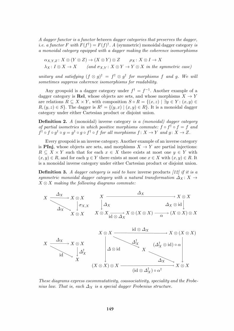
A dagger functor is a functor between dagger categories that preserves the dagger,i.e. a functor F with F (f†) = F (f)†. A (symmetric) monoidal dagger category isa monoidal category equipped with a dagger making the coherence isomorphisms

αX,Y,Z : X ⊗ (Y ⊗ Z)→ (X ⊗ Y )⊗ Z ρX : X ⊗ I → X

λX : I ⊗X → X (and σX,Y : X ⊗ Y → Y ⊗X in the symmetric case)

unitary and satisfying (f ⊗ g)† = f† ⊗ g† for morphisms f and g. We willsometimes suppress coherence isomorphisms for readability.

Any groupoid is a dagger category under f† = f−1. Another example of adagger category is Rel, whose objects are sets, and whose morphisms X → Yare relations R ⊆ X × Y , with composition S ◦ R = {(x, z) | ∃y ∈ Y : (x, y) ∈R, (y, z) ∈ S}. The dagger is R† = {(y, x) | (x, y) ∈ R}. It is a monoidal daggercategory under either Cartesian product or disjoint union.

Definition 2. A (monoidal) inverse category is a (monoidal) dagger categoryof partial isometries in which positive morphisms commute: f ◦ f† ◦ f = f andf† ◦ f ◦ g† ◦ g = g† ◦ g ◦ f† ◦ f for all morphisms f : X → Y and g : X → Z.

Every groupoid is an inverse category. Another example of an inverse categoryis PInj, whose objects are sets, and morphisms X → Y are partial injections:R ⊆ X × Y such that for each x ∈ X there exists at most one y ∈ Y with(x, y) ∈ R, and for each y ∈ Y there exists at most one x ∈ X with (x, y) ∈ R. Itis a monoidal inverse category under either Cartesian product or disjoint union.

Definition 3. A dagger category is said to have inverse products [12] if it is asymmetric monoidal dagger category with a natural transformation ∆X : X →X ⊗X making the following diagrams commute:

X X ⊗X

X ⊗X∆X

∆X

σX,X

X X ⊗X

X ⊗X X ⊗ (X ⊗X) (X ⊗X)⊗X

∆X

∆X

id ⊗∆Xα

∆X ⊗ id

X X ⊗X

Xid

∆X

ƠX

X ⊗X X ⊗ (X ⊗X)

X

(X ⊗X)⊗X X ⊗X

∆⊗ id

id ⊗∆X

ƠX

∆X

(id ⊗∆†X) ◦ α†

(∆†X ⊗ id) ◦ α

These diagrams express cocommutativity, coassociativity, speciality and the Frobe-nius law. That is, each ∆X is a special dagger Frobenius structure.

149

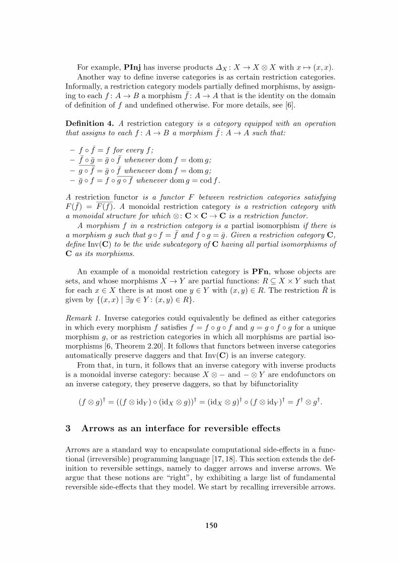
For example, PInj has inverse products ∆X : X → X ⊗X with x 7→ (x, x).

Another way to define inverse categories is as certain restriction categories.Informally, a restriction category models partially defined morphisms, by assign-ing to each f : A→ B a morphism f : A→ A that is the identity on the domainof definition of f and undefined otherwise. For more details, see [6].

Definition 4. A restriction category is a category equipped with an operationthat assigns to each f : A→ B a morphism f : A→ A such that:

– f ◦ f = f for every f ;

– f ◦ g = g ◦ f whenever dom f = dom g;

– g ◦ f = g ◦ f whenever dom f = dom g;

– g ◦ f = f ◦ g ◦ f whenever dom g = cod f .

A restriction functor is a functor F between restriction categories satisfyingF (f) = F (f). A monoidal restriction category is a restriction category witha monoidal structure for which ⊗ : C×C→ C is a restriction functor.

A morphism f in a restriction category is a partial isomorphism if there isa morphism g such that g ◦ f = f and f ◦ g = g. Given a restriction category C,define Inv(C) to be the wide subcategory of C having all partial isomorphisms ofC as its morphisms.

An example of a monoidal restriction category is PFn, whose objects aresets, and whose morphisms X → Y are partial functions: R ⊆ X × Y such thatfor each x ∈ X there is at most one y ∈ Y with (x, y) ∈ R. The restriction R isgiven by {(x, x) | ∃y ∈ Y : (x, y) ∈ R}.

Remark 1. Inverse categories could equivalently be defined as either categoriesin which every morphism f satisfies f = f ◦ g ◦ f and g = g ◦ f ◦ g for a uniquemorphism g, or as restriction categories in which all morphisms are partial iso-morphisms [6, Theorem 2.20]. It follows that functors between inverse categoriesautomatically preserve daggers and that Inv(C) is an inverse category.

From that, in turn, it follows that an inverse category with inverse productsis a monoidal inverse category: because X ⊗ − and − ⊗ Y are endofunctors onan inverse category, they preserve daggers, so that by bifunctoriality

(f ⊗ g)† = ((f ⊗ idY ) ◦ (idX ⊗ g))† = (idX ⊗ g)† ◦ (f ⊗ idY )† = f† ⊗ g†.

3 Arrows as an interface for reversible effects

Arrows are a standard way to encapsulate computational side-effects in a func-tional (irreversible) programming language [17, 18]. This section extends the def-inition to reversible settings, namely to dagger arrows and inverse arrows. Weargue that these notions are “right”, by exhibiting a large list of fundamentalreversible side-effects that they model. We start by recalling irreversible arrows.

150

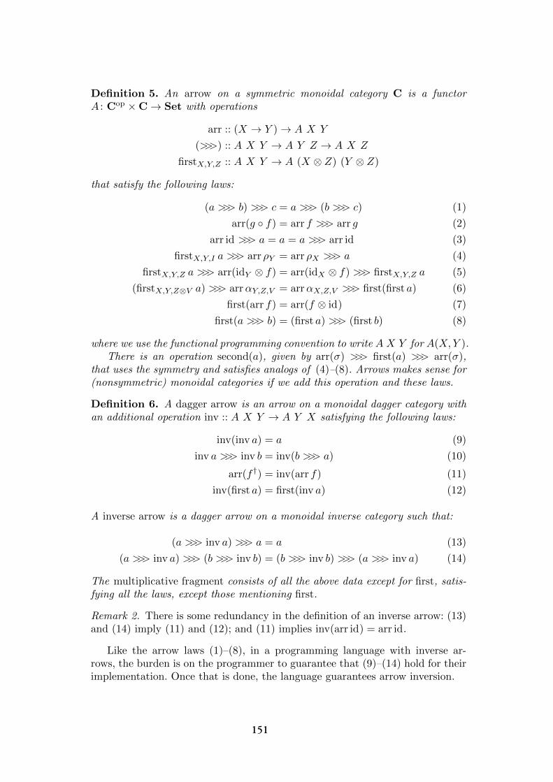
Definition 5. An arrow on a symmetric monoidal category C is a functorA : Cop ×C→ Set with operations

arr :: (X → Y )→ A X Y

(>>>) :: A X Y → A Y Z → A X Z

firstX,Y,Z :: A X Y → A (X ⊗ Z) (Y ⊗ Z)

that satisfy the following laws:

(a >>> b) >>> c = a >>> (b >>> c) (1)

arr(g ◦ f) = arr f >>> arr g (2)

arr id >>> a = a = a >>> arr id (3)

firstX,Y,I a >>> arr ρY = arr ρX >>> a (4)

firstX,Y,Z a >>> arr(idY ⊗ f) = arr(idX ⊗ f) >>> firstX,Y,Z a (5)

(firstX,Y,Z⊗V a) >>> arrαY,Z,V = arrαX,Z,V >>> first(first a) (6)

first(arr f) = arr(f ⊗ id) (7)

first(a >>> b) = (first a) >>> (first b) (8)

where we use the functional programming convention to write A X Y for A(X,Y ).There is an operation second(a), given by arr(σ) >>> first(a) >>> arr(σ),

that uses the symmetry and satisfies analogs of (4)–(8). Arrows makes sense for(nonsymmetric) monoidal categories if we add this operation and these laws.

Definition 6. A dagger arrow is an arrow on a monoidal dagger category withan additional operation inv :: A X Y → A Y X satisfying the following laws:

inv(inv a) = a (9)

inv a >>> inv b = inv(b >>> a) (10)

arr(f†) = inv(arr f) (11)

inv(first a) = first(inv a) (12)

A inverse arrow is a dagger arrow on a monoidal inverse category such that:

(a >>> inv a) >>> a = a (13)

(a >>> inv a) >>> (b >>> inv b) = (b >>> inv b) >>> (a >>> inv a) (14)

The multiplicative fragment consists of all the above data except for first, satis-fying all the laws, except those mentioning first.

Remark 2. There is some redundancy in the definition of an inverse arrow: (13)and (14) imply (11) and (12); and (11) implies inv(arr id) = arr id.

Like the arrow laws (1)–(8), in a programming language with inverse ar-rows, the burden is on the programmer to guarantee that (9)–(14) hold for theirimplementation. Once that is done, the language guarantees arrow inversion.

151

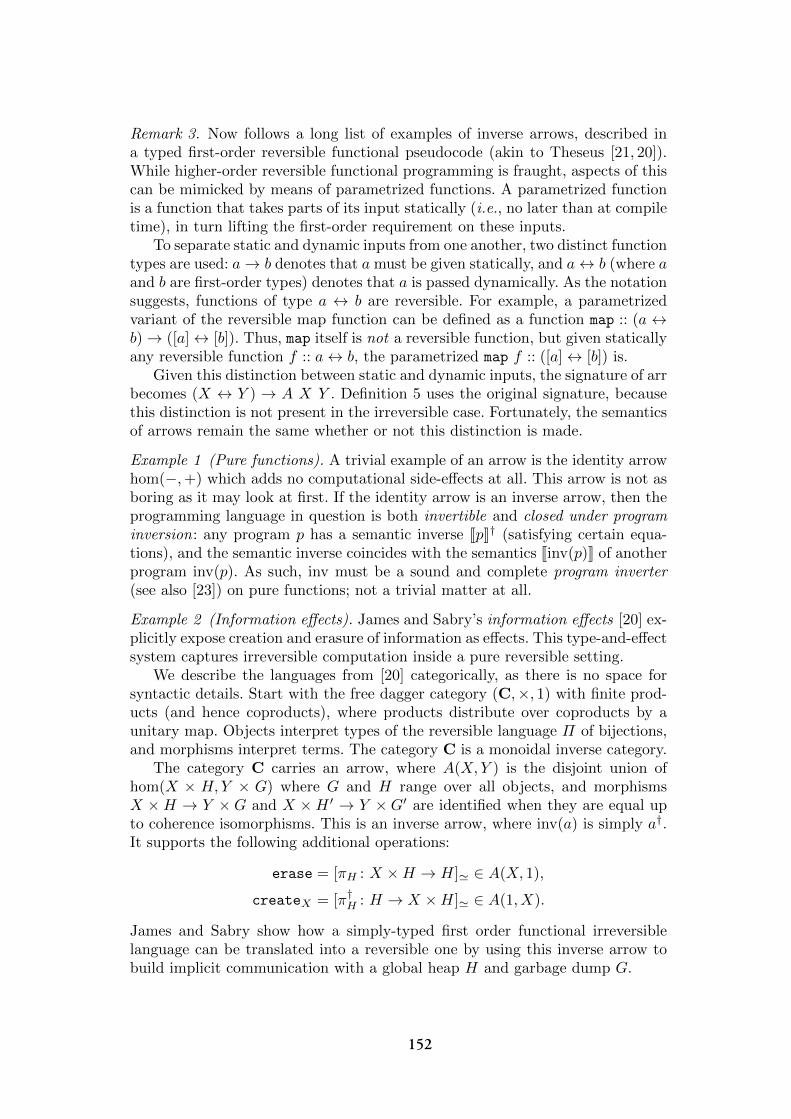
Remark 3. Now follows a long list of examples of inverse arrows, described ina typed first-order reversible functional pseudocode (akin to Theseus [21, 20]).While higher-order reversible functional programming is fraught, aspects of thiscan be mimicked by means of parametrized functions. A parametrized functionis a function that takes parts of its input statically (i.e., no later than at compiletime), in turn lifting the first-order requirement on these inputs.

To separate static and dynamic inputs from one another, two distinct functiontypes are used: a→ b denotes that a must be given statically, and a↔ b (where aand b are first-order types) denotes that a is passed dynamically. As the notationsuggests, functions of type a ↔ b are reversible. For example, a parametrizedvariant of the reversible map function can be defined as a function map :: (a ↔b)→ ([a]↔ [b]). Thus, map itself is not a reversible function, but given staticallyany reversible function f :: a↔ b, the parametrized map f :: ([a]↔ [b]) is.

Given this distinction between static and dynamic inputs, the signature of arrbecomes (X ↔ Y ) → A X Y . Definition 5 uses the original signature, becausethis distinction is not present in the irreversible case. Fortunately, the semanticsof arrows remain the same whether or not this distinction is made.

Example 1 (Pure functions). A trivial example of an arrow is the identity arrowhom(−,+) which adds no computational side-effects at all. This arrow is not asboring as it may look at first. If the identity arrow is an inverse arrow, then theprogramming language in question is both invertible and closed under programinversion: any program p has a semantic inverse JpK† (satisfying certain equa-tions), and the semantic inverse coincides with the semantics Jinv(p)K of anotherprogram inv(p). As such, inv must be a sound and complete program inverter(see also [23]) on pure functions; not a trivial matter at all.

Example 2 (Information effects). James and Sabry’s information effects [20] ex-plicitly expose creation and erasure of information as effects. This type-and-effectsystem captures irreversible computation inside a pure reversible setting.

We describe the languages from [20] categorically, as there is no space forsyntactic details. Start with the free dagger category (C,×, 1) with finite prod-ucts (and hence coproducts), where products distribute over coproducts by aunitary map. Objects interpret types of the reversible language Π of bijections,and morphisms interpret terms. The category C is a monoidal inverse category.

The category C carries an arrow, where A(X,Y ) is the disjoint union ofhom(X × H,Y × G) where G and H range over all objects, and morphismsX ×H → Y ×G and X ×H ′ → Y ×G′ are identified when they are equal upto coherence isomorphisms. This is an inverse arrow, where inv(a) is simply a†.It supports the following additional operations:

erase = [πH : X ×H → H]' ∈ A(X, 1),

createX = [π†H : H → X ×H]' ∈ A(1, X).

James and Sabry show how a simply-typed first order functional irreversiblelanguage can be translated into a reversible one by using this inverse arrow tobuild implicit communication with a global heap H and garbage dump G.

152

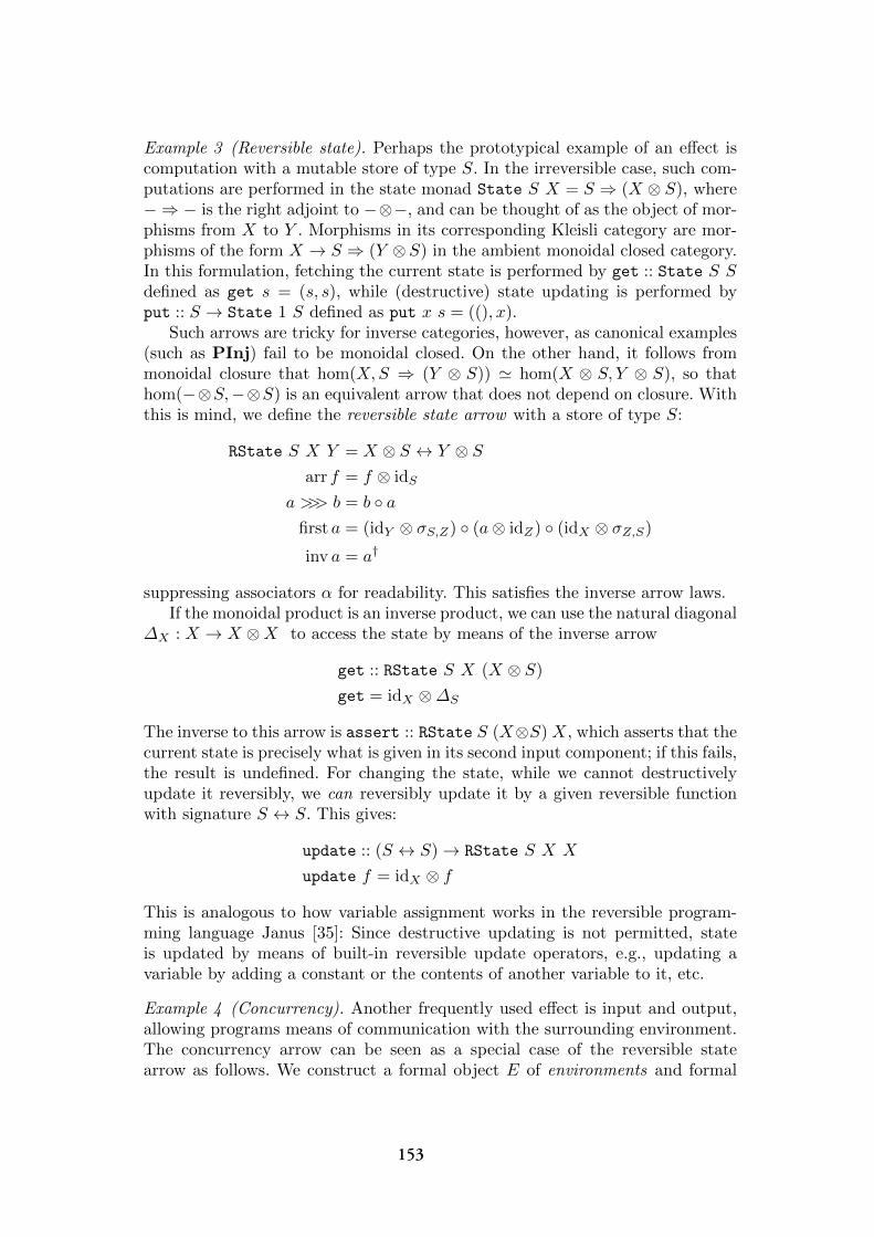
Example 3 (Reversible state). Perhaps the prototypical example of an effect iscomputation with a mutable store of type S. In the irreversible case, such com-putations are performed in the state monad State S X = S ⇒ (X ⊗ S), where− ⇒ − is the right adjoint to −⊗−, and can be thought of as the object of mor-phisms from X to Y . Morphisms in its corresponding Kleisli category are mor-phisms of the form X → S ⇒ (Y ⊗ S) in the ambient monoidal closed category.In this formulation, fetching the current state is performed by get :: State S Sdefined as get s = (s, s), while (destructive) state updating is performed byput :: S → State 1 S defined as put x s = ((), x).

Such arrows are tricky for inverse categories, however, as canonical examples(such as PInj) fail to be monoidal closed. On the other hand, it follows frommonoidal closure that hom(X,S ⇒ (Y ⊗ S)) ' hom(X ⊗ S, Y ⊗ S), so thathom(−⊗S,−⊗S) is an equivalent arrow that does not depend on closure. Withthis is mind, we define the reversible state arrow with a store of type S:

RState S X Y = X ⊗ S ↔ Y ⊗ Sarr f = f ⊗ idS

a >>> b = b ◦ afirst a = (idY ⊗ σS,Z) ◦ (a⊗ idZ) ◦ (idX ⊗ σZ,S)

inv a = a†

suppressing associators α for readability. This satisfies the inverse arrow laws.If the monoidal product is an inverse product, we can use the natural diagonal

∆X : X → X ⊗X to access the state by means of the inverse arrow

get :: RState S X (X ⊗ S)

get = idX ⊗∆S

The inverse to this arrow is assert :: RState S (X⊗S) X, which asserts that thecurrent state is precisely what is given in its second input component; if this fails,the result is undefined. For changing the state, while we cannot destructivelyupdate it reversibly, we can reversibly update it by a given reversible functionwith signature S ↔ S. This gives:

update :: (S ↔ S)→ RState S X X

update f = idX ⊗ f

This is analogous to how variable assignment works in the reversible program-ming language Janus [35]: Since destructive updating is not permitted, stateis updated by means of built-in reversible update operators, e.g., updating avariable by adding a constant or the contents of another variable to it, etc.

Example 4 (Concurrency). Another frequently used effect is input and output,allowing programs means of communication with the surrounding environment.The concurrency arrow can be seen as a special case of the reversible statearrow as follows. We construct a formal object E of environments and formal

153

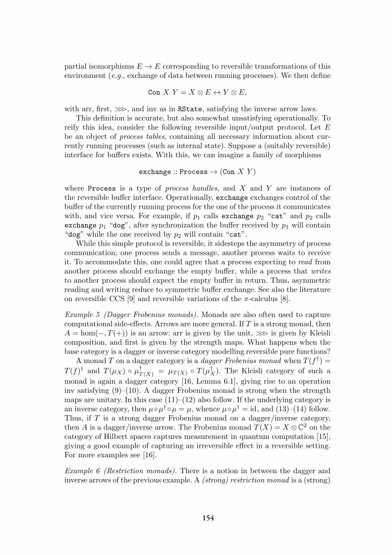
partial isomorphisms E → E corresponding to reversible transformations of thisenvironment (e.g., exchange of data between running processes). We then define

Con X Y = X ⊗ E ↔ Y ⊗ E,

with arr, first, >>>, and inv as in RState, satisfying the inverse arrow laws.This definition is accurate, but also somewhat unsatisfying operationally. To

reify this idea, consider the following reversible input/output protocol. Let Ebe an object of process tables, containing all necessary information about cur-rently running processes (such as internal state). Suppose a (suitably reversible)interface for buffers exists. With this, we can imagine a family of morphisms

exchange :: Process→ (Con X Y )

where Process is a type of process handles, and X and Y are instances ofthe reversible buffer interface. Operationally, exchange exchanges control of thebuffer of the currently running process for the one of the process it communicateswith, and vice versa. For example, if p1 calls exchange p2 “cat” and p2 callsexchange p1 “dog”, after synchronization the buffer received by p1 will contain“dog” while the one received by p2 will contain “cat”.

While this simple protocol is reversible, it sidesteps the asymmetry of processcommunication; one process sends a message, another process waits to receiveit. To accommodate this, one could agree that a process expecting to read fromanother process should exchange the empty buffer, while a process that writesto another process should expect the empty buffer in return. Thus, asymmetricreading and writing reduce to symmetric buffer exchange. See also the literatureon reversible CCS [9] and reversible variations of the π-calculus [8].

Example 5 (Dagger Frobenius monads). Monads are also often used to capturecomputational side-effects. Arrows are more general. If T is a strong monad, thenA = hom(−, T (+)) is an arrow: arr is given by the unit, >>> is given by Kleislicomposition, and first is given by the strength maps. What happens when thebase category is a dagger or inverse category modelling reversible pure functions?

A monad T on a dagger category is a dagger Frobenius monad when T (f†) =

T (f)† and T (µX) ◦ µ†T (X) = µT (X) ◦ T (µ†X). The Kleisli category of such a

monad is again a dagger category [16, Lemma 6.1], giving rise to an operationinv satisfying (9)–(10). A dagger Frobenius monad is strong when the strengthmaps are unitary. In this case (11)–(12) also follow. If the underlying category isan inverse category, then µ◦µ† ◦µ = µ, whence µ◦µ† = id, and (13)–(14) follow.Thus, if T is a strong dagger Frobenius monad on a dagger/inverse category,then A is a dagger/inverse arrow. The Frobenius monad T (X) = X ⊗C2 on thecategory of Hilbert spaces captures measurement in quantum computation [15],giving a good example of capturing an irreversible effect in a reversible setting.For more examples see [16].

Example 6 (Restriction monads). There is a notion in between the dagger andinverse arrows of the previous example. A (strong) restriction monad is a (strong)

154

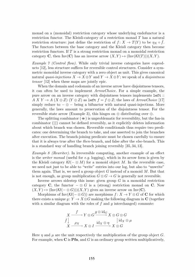
monad on a (monoidal) restriction category whose underlying endofunctor is arestriction functor. The Kleisli-category of a restriction monad T has a naturalrestriction structure: just define the restriction of f : X → T (Y ) to be ηX ◦ f .The functors between the base category and the Kleisli category then becomerestriction functors. If T is a strong restriction monad on a monoidal restrictioncategory C, then Inv(C) has an inverse arrow (X,Y ) 7→ (Inv(K (T )))(X,Y ).

Example 7 (Control flow). While only trivial inverse categories have coprod-ucts [12], less structure suffices for reversible control structures. Consider a sym-metric monoidal inverse category with a zero object as unit. This gives canonicalnatural quasi-injections X → X⊕Y and Y → X⊕Y ; we speak of a disjointnesstensor [12] when these maps are jointly epic.

When the domain and codomain of an inverse arrow have disjointness tensors,it can often be used to implement ArrowChoice. For a simple example, thepure arrow on an inverse category with disjointness tensors implements left ::A X Y → A (X ⊕Z) (Y ⊕Z) as left f = f ⊕Z; the laws of ArrowChoice [17]simply reduce to − ⊕ − being a bifunctor with natural quasi-injections. Moregenerally, the laws amount to preservation of the disjointness tensor. For thereversible state arrow (Example 3), this hinges on ⊗ distributing over ⊕.

The splitting combinator (+++) is unproblematic for reversiblity, but the fan-incombinator (|||) cannot be defined reversibly, as it explicitly deletes informationabout which branch was chosen. Reversible conditionals thus require two predi-cates: one determining the branch to take, and one asserted to join the branchesafter execution. The branch-joining predicate must be chosen carefully to ensurethat it is always true after the then-branch, and false after the else-branch. Thisis a standard way of handling branch joining reversibly [35, 34, 13].

Example 8 (Rewriter). In irreversible computing, another example of an effectis the writer monad (useful for e.g. logging), which in its arrow form is given bythe Kleisli category K (− ⊗M) for a monoid object M . In the reversible case,we need not just to be able to “write” entries into our log, but also to “unwrite”them again. That is, we need a group object G instead of a monoid M . But thatis not enough, as group multiplication G⊗G→ G is generally not reversible.

Inverse arrows sidestep this issue: given group G in a monoidal restrictioncategory C, the functor − ⊗ G is a (strong) restriction monad on C. Now(X,Y ) 7→ (Inv(K (−⊗G)))(X,Y ) gives an inverse arrow on Inv(C).

Morphisms of Inv(K (−⊗G)) are morphisms f : X → Y ⊗G of C for whichthere exists a unique g : Y → X⊗G making the following diagram in C (togetherwith a similar diagram with the roles of f and g interchanged) commute:

X

X

Y ⊗G

X ⊗ I

X ⊗G⊗G

X ⊗G

f g ⊗ idG

idX ⊗ µfρX idX ⊗ η

Here η and µ are the unit respectively the multiplication of the group object G.For example, when C is Pfn, and G is an ordinary group written multiplicatively,

155

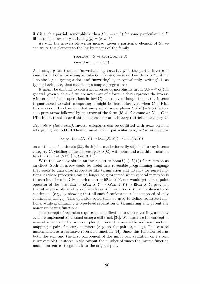
if f is such a partial isomorphism, then f(x) = (y, h) for some particular x ∈ Xiff its unique inverse g satisfies g(y) = (x, h−1).

As with the irreversible writer monad, given a particular element of G, wecan write this element to the log by means of the family

rewrite :: G→ Rewriter X X

rewrite g x = (x, g) .

A message g can then be “unwritten” by rewrite g−1, the partial inverse ofrewrite g. For a toy example, take G = (Z,+); we may then think of ‘writing’1 to the log as typing a dot, and ‘unwriting’ 1, or equivalently ‘writing’ -1, astyping backspace, thus modelling a simple progress bar.

It might be difficult to construct inverses of morphisms in Inv(K (−⊗G)) ingeneral: given such an f , we are not aware of a formula that expresses the inverseg in terms of f and operations in Inv(C). Thus, even though the partial inverseis guaranteed to exist, computing it might be hard. However, when C is Pfn,this works out by observing that any partial isomorphism f of K (−⊗G) factorsas a pure arrow followed by an arrow of the form 〈id, h〉 for some h : X → G inPfn, but it is not clear if this is the case for an arbitrary restriction category C.

Example 9 (Recursion). Inverse categories can be outfitted with joins on homsets, giving rise to DCPO-enrichment, and in particular to a fixed point operator

fixX,Y : (hom(X,Y )→ hom(X,Y ))→ hom(X,Y )

on continuous functionals [22]. Such joins can be formally adjoined to any inversecategory C, yielding an inverse category J(C) with joins and a faithful inclusionfunctor I : C→ J(C) [14, Sec. 3.1.3].

With this we may obtain an inverse arrow hom(I(−), I(+)) for recursion asan effect. Such an arrow could be useful in a reversible programming languagethat seeks to guarantee properties like termination and totality for pure func-tions, as these properties can no longer be guaranteed when general recursion isthrown into the mix. Given such an arrow RFix X Y , one would get a fixed pointoperator of the form fix :: (RFix X Y → RFix X Y ) → RFix X Y, providedthat all expressible functions of type RFix X Y → RFix X Y can be shown to becontinuous (e.g., by showing that all such functions must be composed of onlycontinuous things). This operator could then be used to define recursive func-tions, while maintaining a type-level separation of terminating and potentiallynon-terminating functions.

The concept of recursion requires no modification to work reversibly, and mayeven be implemented as usual using a call stack [34]. We illustrate the concept ofreversible recursion by two examples: Consider the reversible addition function,mapping a pair of natural numbers (x, y) to the pair (x, x + y). This can beimplemented as a recursive reversible function [34]. Since this function returnsboth the sum and the first component of the input pair (addition on its ownis irreversible), it stores in the output the number of times the inverse functionmust “unrecurse” to get back to the original pair.

156

Another example is the reversible Fibonacci function, mapping a naturalnumber n to the pair (xn, xn+1) where each xi is the i’th number in the Fibonacciseries. This may also be implemented as a reversible recursive function. Here,however, the number of times that the inverse function must “unrecurse” isgiven only implicitly in the output: The inverse iteratively computes (xi, xi+1) 7→(xi+1 − xi, xi) until the result becomes (0, 1) – the first Fibonacci pair – andthen returns the number of iterations it had to perform. If the inverse is given apair of natural numbers that is not a Fibonacci pair, the result is undefined (i.e.,the inverse function may never terminate, or may produce a garbage output).

Example 10 (Superoperators). Quantum information theory has to deal withenvironments. The basic category FHilb is that of finite-dimensional Hilbertspaces and linear maps. But because a system may be entangled with its en-vironment, the only morphisms that preserve states are the so-called superop-erators, or completely positive maps [31, 7]: they are not just positive, but staypositive when tensored with an arbitrary ancillary object. In a sense, informa-tion about the system may be stored in the environment without breaking the(reversible) laws of nature. This leads to the so-called CPM construction. It isinfamously known not to be a monad. But it is a dagger arrow on FHilb, whereA X Y is the set of completely positive maps X∗⊗X → Y ∗⊗Y , arr f = f∗⊗f ,a >>> b = b ◦ a, firstX,Y,Z a = a⊗ idZ∗⊗Z , and inv a = a†.

4 Inverse arrows, categorically

This section explicates the categorical structure of inverse arrows. Arrows onC can be modelled categorically as monoids in the functor category [Cop ×C,Set] [19]. They also correspond to certain identity-on-objects functors J : C→D. The category D for an arrow A is built by D(X,Y ) = A X Y , and arr pro-vides the functor J .

We will only consider the multiplicative fragment. The operation first canbe incorporated in a standard way using strength [19, 3], and poses no addeddifficulty in the reversible setting.

Clearly, dagger arrows correspond to D being a dagger category and J adagger functor, whereas inverse arrows correspond to both C and D being in-verse categories and J a (dagger) functor. This section takes the first point ofview: which monoids correspond to dagger arrows and inverse arrows? In thedagger case, the answer is quite simple: the dagger makes [Cop×C,Set] into aninvolutive monoidal category, and then dagger arrows correspond to involutivemonoids. Inverse arrows furthermore require certain diagrams to commute.

Definition 7. An involutive monoidal category is a monoidal category C equipped

with an involution: a functor ( ) : C → C satisfying f = f for all morphismsf , together with a natural isomorphism χX,Y : X ⊗ Y → Y ⊗X that makes the

157

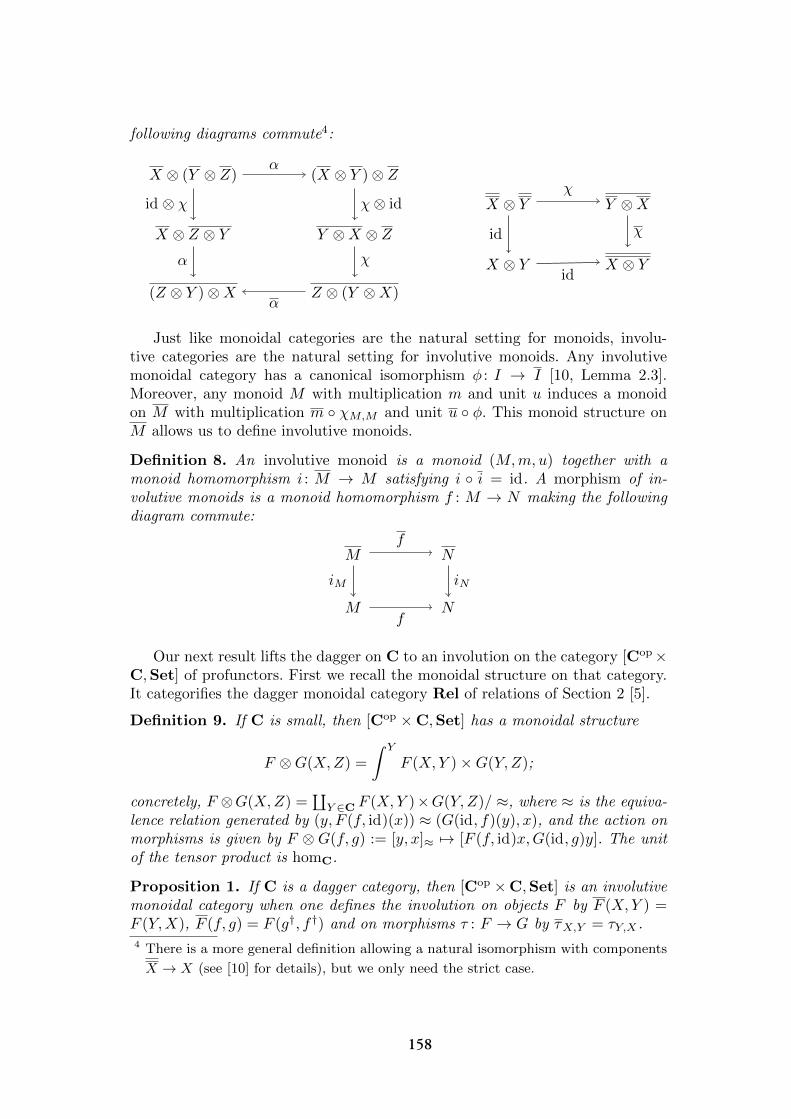
following diagrams commute4:

X ⊗ (Y ⊗ Z) (X ⊗ Y )⊗ Z

X ⊗ Z ⊗ Y Y ⊗X ⊗ Z

(Z ⊗ Y )⊗X Z ⊗ (Y ⊗X)

id ⊗ χ

α

χ⊗ id

χ

α

α

X ⊗ Y Y ⊗X

X ⊗ Y X ⊗ Y

id

χ

χ

id

Just like monoidal categories are the natural setting for monoids, involu-tive categories are the natural setting for involutive monoids. Any involutivemonoidal category has a canonical isomorphism φ : I → I [10, Lemma 2.3].Moreover, any monoid M with multiplication m and unit u induces a monoidon M with multiplication m ◦ χM,M and unit u ◦ φ. This monoid structure onM allows us to define involutive monoids.

Definition 8. An involutive monoid is a monoid (M,m, u) together with amonoid homomorphism i : M → M satisfying i ◦ i = id. A morphism of in-volutive monoids is a monoid homomorphism f : M → N making the followingdiagram commute:

M N

M N

iM

f

iN

f

Our next result lifts the dagger on C to an involution on the category [Cop×C,Set] of profunctors. First we recall the monoidal structure on that category.It categorifies the dagger monoidal category Rel of relations of Section 2 [5].

Definition 9. If C is small, then [Cop ×C,Set] has a monoidal structure

F ⊗G(X,Z) =

∫ Y

F (X,Y )×G(Y,Z);

concretely, F ⊗G(X,Z) =∐

Y ∈C F (X,Y )×G(Y,Z)/ ≈, where ≈ is the equiva-lence relation generated by (y, F (f, id)(x)) ≈ (G(id, f)(y), x), and the action onmorphisms is given by F ⊗G(f, g) := [y, x]≈ 7→ [F (f, id)x,G(id, g)y]. The unitof the tensor product is homC.

Proposition 1. If C is a dagger category, then [Cop ×C,Set] is an involutivemonoidal category when one defines the involution on objects F by F (X,Y ) =F (Y,X), F (f, g) = F (g†, f†) and on morphisms τ : F → G by τX,Y = τY,X .4 There is a more general definition allowing a natural isomorphism with components

X → X (see [10] for details), but we only need the strict case.

158

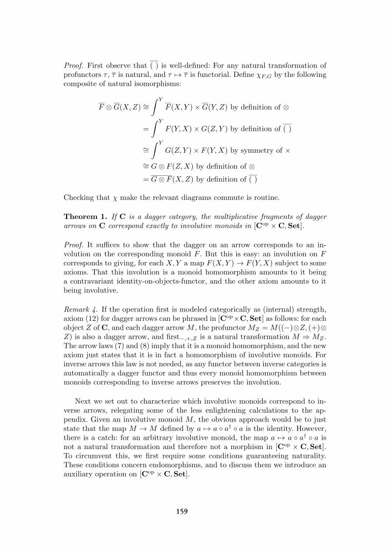
Proof. First observe that ( ) is well-defined: For any natural transformation ofprofunctors τ , τ is natural, and τ 7→ τ is functorial. Define χF,G by the followingcomposite of natural isomorphisms:

F ⊗G(X,Z) ∼=∫ Y

F (X,Y )×G(Y,Z) by definition of ⊗

=

∫ Y

F (Y,X)×G(Z, Y ) by definition of ( )

∼=∫ Y

G(Z, Y )× F (Y,X) by symmetry of ×

∼= G⊗ F (Z,X) by definition of ⊗

= G⊗ F (X,Z) by definition of ( )

Checking that χ make the relevant diagrams commute is routine.

Theorem 1. If C is a dagger category, the multiplicative fragments of daggerarrows on C correspond exactly to involutive monoids in [Cop ×C,Set].

Proof. It suffices to show that the dagger on an arrow corresponds to an in-volution on the corresponding monoid F . But this is easy: an involution on Fcorresponds to giving, for each X,Y a map F (X,Y )→ F (Y,X) subject to someaxioms. That this involution is a monoid homomorphism amounts to it beinga contravariant identity-on-objects-functor, and the other axiom amounts to itbeing involutive.

Remark 4. If the operation first is modeled categorically as (internal) strength,axiom (12) for dagger arrows can be phrased in [Cop×C,Set] as follows: for eachobject Z of C, and each dagger arrow M , the profunctor MZ = M((−)⊗Z, (+)⊗Z) is also a dagger arrow, and first−,+,Z is a natural transformation M ⇒MZ .The arrow laws (7) and (8) imply that it is a monoid homomorphism, and the newaxiom just states that it is in fact a homomorphism of involutive monoids. Forinverse arrows this law is not needed, as any functor between inverse categories isautomatically a dagger functor and thus every monoid homomorphism betweenmonoids corresponding to inverse arrows preserves the involution.

Next we set out to characterize which involutive monoids correspond to in-verse arrows, relegating some of the less enlightening calculations to the ap-pendix. Given an involutive monoid M , the obvious approach would be to juststate that the map M → M defined by a 7→ a ◦ a† ◦ a is the identity. However,there is a catch: for an arbitrary involutive monoid, the map a 7→ a ◦ a† ◦ a isnot a natural transformation and therefore not a morphism in [Cop × C,Set].To circumvent this, we first require some conditions guaranteeing naturality.These conditions concern endomorphisms, and to discuss them we introduce anauxiliary operation on [Cop ×C,Set].

159

Definition 10. Let C be a dagger category. Given a profunctor M : Cop×C→Set, define LM : Cop ×C→ Set by

LM(X,Y ) = M(X,X),

LM(f, g) = f† ◦ (−) ◦ f .

If M is an involutive monoid in [Cop ×C,Set], define a subprofunctor of LM :

L+M(X,Y ) = {a† ◦ a ∈M(X,X) | a ∈M(X,Z) for some Z}.

Remark 5. The construction L is a functor [Cop × C,Set] → [Cop × C,Set].There is an analogous construction RM(X,Y ) = M(Y, Y ) and R+M , and fur-thermore RM = LM . For any monoid M in [Cop × C,Set], LM is a rightM -module (and RM a left M -module). Compare Example 10.

For the rest of this section, assume the base category C to be an inversecategory. This lets us multiply positive arrows by positive pure morphisms. If Mis an involutive monoid in [Cop×C,Set], then the map LM×L+(homC)→ LMdefined by (a, g† ◦ g) 7→ a ◦ g† ◦ g is natural, as shown in the appendix.

Similarly there is a map L+(hom) × LM → LM defined by (g† ◦ g, a) 7→g†◦g◦a. Now the category corresponding to M satisfies a†◦a◦g†◦g = g†◦g◦a†◦afor all a and pure g if and only if the following diagram commutes:

L+M × L+(hom) LM × L+(hom)

L+(hom)× L+M L+(hom)× LM LM

(15)If this is satisfied for an involutive monoid M in [Cop × C,Set], then positivearrows multiply. In other words, the map L+M × L+M → LM defined by(a† ◦ a, b† ◦ b) 7→ a† ◦ a ◦ b† ◦ b is natural, as shown in the appendix. Thismultiplication is commutative iff the following diagram commutes:

L+M × L+M L+M × L+M

LM

σ

(16)

Finally, let DM ↪→M ×M ×M be the diagonal

DM (X,Y ) = {(a, a†, a) | a ∈M(X,Y }.

If M satisfies (15), then a calculation included in the appendix shows thatthe map DM →M defined by (a, a†, a) 7→ a ◦ a† ◦ a is natural.

160

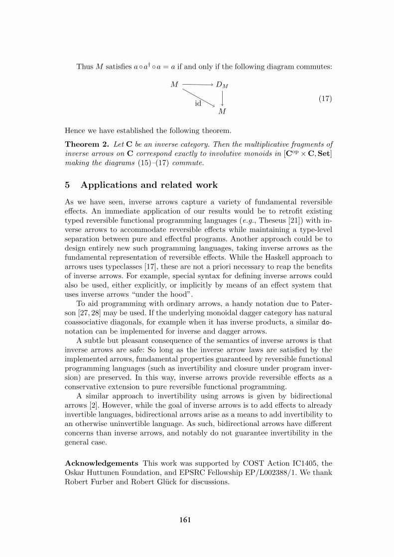
Thus M satisfies a◦a† ◦a = a if and only if the following diagram commutes:

M DM

Mid

(17)

Hence we have established the following theorem.

Theorem 2. Let C be an inverse category. Then the multiplicative fragments ofinverse arrows on C correspond exactly to involutive monoids in [Cop ×C,Set]making the diagrams (15)–(17) commute.

5 Applications and related work

As we have seen, inverse arrows capture a variety of fundamental reversibleeffects. An immediate application of our results would be to retrofit existingtyped reversible functional programming languages (e.g., Theseus [21]) with in-verse arrows to accommodate reversible effects while maintaining a type-levelseparation between pure and effectful programs. Another approach could be todesign entirely new such programming languages, taking inverse arrows as thefundamental representation of reversible effects. While the Haskell approach toarrows uses typeclasses [17], these are not a priori necessary to reap the benefitsof inverse arrows. For example, special syntax for defining inverse arrows couldalso be used, either explicitly, or implicitly by means of an effect system thatuses inverse arrows “under the hood”.

To aid programming with ordinary arrows, a handy notation due to Pater-son [27, 28] may be used. If the underlying monoidal dagger category has naturalcoassociative diagonals, for example when it has inverse products, a similar do-notation can be implemented for inverse and dagger arrows.

A subtle but pleasant consequence of the semantics of inverse arrows is thatinverse arrows are safe: So long as the inverse arrow laws are satisfied by theimplemented arrows, fundamental properties guaranteed by reversible functionalprogramming languages (such as invertibility and closure under program inver-sion) are preserved. In this way, inverse arrows provide reversible effects as aconservative extension to pure reversible functional programming.

A similar approach to invertibility using arrows is given by bidirectionalarrows [2]. However, while the goal of inverse arrows is to add effects to alreadyinvertible languages, bidirectional arrows arise as a means to add invertibility toan otherwise uninvertible language. As such, bidirectional arrows have differentconcerns than inverse arrows, and notably do not guarantee invertibility in thegeneral case.

Acknowledgements This work was supported by COST Action IC1405, theOskar Huttunen Foundation, and EPSRC Fellowship EP/L002388/1. We thankRobert Furber and Robert Gluck for discussions.

161

References

1. S. Abramsky. A structural approach to reversible computation. Theoretical Com-puter Science, 347(3):441–464, 2005.

2. A. Alimarine, S. Smetsers, A. van Weelden, M. van Eekelen, and R. Plasmeijer.There and back again: Arrows for invertible programming. In Proceedings of the2005 ACM SIGPLAN workshop on Haskell, pages 86–97, 2005.

3. K. Asada. Arrows are strong monads. In Proceedings of the third ACM SIG-PLAN workshop on Mathematically Structured Functional Programming, pages33–42. ACM, 2010.

4. C. H. Bennett. Logical reversibility of computation. IBM Journal of Research andDevelopment, 17(6):525–532, 1973.

5. F. Borceux. Handbook of categorical algebra. Cambridge University Press, 1994.6. J. R. B. Cockett and S. Lack. Restriction categories I: categories of partial maps.

Theoretical Computer Science, 270:223–259, 2002.7. B. Coecke and C. Heunen. Pictures of complete positivity in arbitrary dimension.

Information and Computation, 250:50–58, 2016.8. I. Cristescu, J. Krivine, and D. Varacca. A compositional semantics for the re-

versible π-calculus. In Logic in Computer Science, pages 388–397. IEEE ComputerSociety, 2013.

9. V. Danos and J. Krivine. Reversible communicating systems. In InternationalConference on Concurrency Theory, volume 3170 of LNCS, pages 292–307, 2004.

10. J. M. Egger. On involutive monoidal categories. Theory and Applications of Cat-egories, 25(14):368–393, 2011.

11. M. J. Gabbay and P. H. Kropholler. Imaginary groups: lazy monoids and reversiblecomputation. Mathematical Structures in Computer Science, 23(5):1002–10031,2013.

12. B. G. Giles. An investigation of some theoretical aspects of reversible computing.PhD thesis, University of Calgary, 2014.

13. R. Gluck and R. Kaarsgaard. A categorical foundations for structured reversibleflowchart languages. In Mathematical Foundations of Program Semantics XXXIII,Proceedings, 2017. to appear.

14. X. Guo. Products, Joins, Meets, and Ranges in Restriction Categories. PhD thesis,University of Calgary, 2012.

15. C. Heunen and M. Karvonen. Reversible monadic computing. In MathematicalFoundations of Programming Semantics (MFPS), volume 319 of Electronic Notesin Theoretical Computer Science, pages 217–237, 2015.

16. C. Heunen and M. Karvonen. Monads on dagger categories. Theory and Applica-tions of Categories, 31(35):1016–1043, 2016.

17. J. Hughes. Generalising monads to arrows. Science of Computer Programming,37:67–111, 2000.

18. J. Hughes. Advanced Functional Programming, volume 3622 of Lecture Notes inComputer Science, chapter Programming with Arrows, pages 73–129. Springer,2005.

19. B. Jacobs, C. Heunen, and I. Hasuo. Categorical semantics for arrows. Journal ofFunctional Programming, 19(3-4):403–438, 2009.

20. R. P. James and A. Sabry. Information effects. In Principles of ProgrammingLanguages, pages 73–84. ACM, 2012.

21. R. P. James and A. Sabry. Theseus: A high level language for re-versible computing, 2014. Work-in-progress report at RC 2014, available athttps://www.cs.indiana.edu/ sabry/papers/theseus.pdf.

162

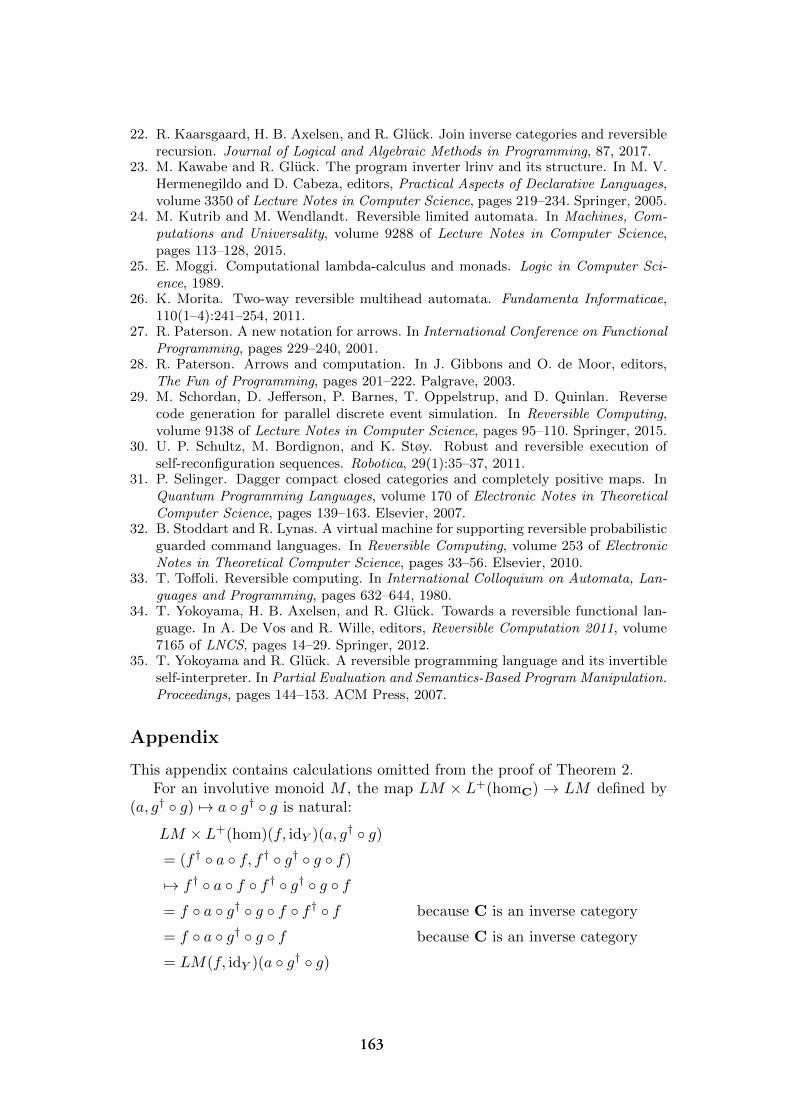
22. R. Kaarsgaard, H. B. Axelsen, and R. Gluck. Join inverse categories and reversiblerecursion. Journal of Logical and Algebraic Methods in Programming, 87, 2017.

23. M. Kawabe and R. Gluck. The program inverter lrinv and its structure. In M. V.Hermenegildo and D. Cabeza, editors, Practical Aspects of Declarative Languages,volume 3350 of Lecture Notes in Computer Science, pages 219–234. Springer, 2005.

24. M. Kutrib and M. Wendlandt. Reversible limited automata. In Machines, Com-putations and Universality, volume 9288 of Lecture Notes in Computer Science,pages 113–128, 2015.

25. E. Moggi. Computational lambda-calculus and monads. Logic in Computer Sci-ence, 1989.

26. K. Morita. Two-way reversible multihead automata. Fundamenta Informaticae,110(1–4):241–254, 2011.

27. R. Paterson. A new notation for arrows. In International Conference on FunctionalProgramming, pages 229–240, 2001.

28. R. Paterson. Arrows and computation. In J. Gibbons and O. de Moor, editors,The Fun of Programming, pages 201–222. Palgrave, 2003.

29. M. Schordan, D. Jefferson, P. Barnes, T. Oppelstrup, and D. Quinlan. Reversecode generation for parallel discrete event simulation. In Reversible Computing,volume 9138 of Lecture Notes in Computer Science, pages 95–110. Springer, 2015.

30. U. P. Schultz, M. Bordignon, and K. Støy. Robust and reversible execution ofself-reconfiguration sequences. Robotica, 29(1):35–37, 2011.

31. P. Selinger. Dagger compact closed categories and completely positive maps. InQuantum Programming Languages, volume 170 of Electronic Notes in TheoreticalComputer Science, pages 139–163. Elsevier, 2007.

32. B. Stoddart and R. Lynas. A virtual machine for supporting reversible probabilisticguarded command languages. In Reversible Computing, volume 253 of ElectronicNotes in Theoretical Computer Science, pages 33–56. Elsevier, 2010.

33. T. Toffoli. Reversible computing. In International Colloquium on Automata, Lan-guages and Programming, pages 632–644, 1980.

34. T. Yokoyama, H. B. Axelsen, and R. Gluck. Towards a reversible functional lan-guage. In A. De Vos and R. Wille, editors, Reversible Computation 2011, volume7165 of LNCS, pages 14–29. Springer, 2012.

35. T. Yokoyama and R. Gluck. A reversible programming language and its invertibleself-interpreter. In Partial Evaluation and Semantics-Based Program Manipulation.Proceedings, pages 144–153. ACM Press, 2007.

Appendix

This appendix contains calculations omitted from the proof of Theorem 2.For an involutive monoid M , the map LM × L+(homC) → LM defined by

(a, g† ◦ g) 7→ a ◦ g† ◦ g is natural:

LM × L+(hom)(f, idY )(a, g† ◦ g)

= (f† ◦ a ◦ f, f† ◦ g† ◦ g ◦ f)

7→ f† ◦ a ◦ f ◦ f† ◦ g† ◦ g ◦ f= f ◦ a ◦ g† ◦ g ◦ f ◦ f† ◦ f because C is an inverse category

= f ◦ a ◦ g† ◦ g ◦ f because C is an inverse category

= LM(f, idY )(a ◦ g† ◦ g)

163

If an involutive monoid M satisfies (15), then the map L+M×L+M → LMdefined by (a† ◦ a, b† ◦ b) 7→ a† ◦ a ◦ b† ◦ b is natural:

L+M × L+M(f, id)(a† ◦ a, b† ◦ b)= (f† ◦ a† ◦ a ◦ f, f† ◦ b† ◦ b ◦ f)

7→ f† ◦ a† ◦ a ◦ f ◦ f† ◦ b† ◦ b ◦ f= f ◦ a† ◦ a ◦ b† ◦ b ◦ f ◦ f† ◦ f by (15)

= f ◦ a† ◦ a ◦ b† ◦ b ◦ f because C is an inverse category

= L+M(f, id)(a† ◦ a ◦ b† ◦ b)

If an involutive monoid M satisfies (15), then the map DM → M definedby (a, a†, a) 7→ a ◦ a† ◦ a is natural:

DM (f, g)(a, a†, a)

= (g ◦ a ◦ f, f† ◦ a† ◦ g†, g ◦ a ◦ f)

7→ g ◦ a ◦ f ◦ f† ◦ a† ◦ g† ◦ g ◦ a ◦ f= g ◦ a ◦ a† ◦ g† ◦ g ◦ a ◦ f ◦ f† ◦ f by (15)

= g ◦ a ◦ a† ◦ g† ◦ g ◦ a ◦ f because C is an inverse category

= g ◦ g† ◦ g ◦ a ◦ a† ◦ a ◦ f by (15)

= g ◦ a ◦ a† ◦ a ◦ f because C is an inverse category

= M(f, g)(a ◦ a† ◦ a)

164

165

166

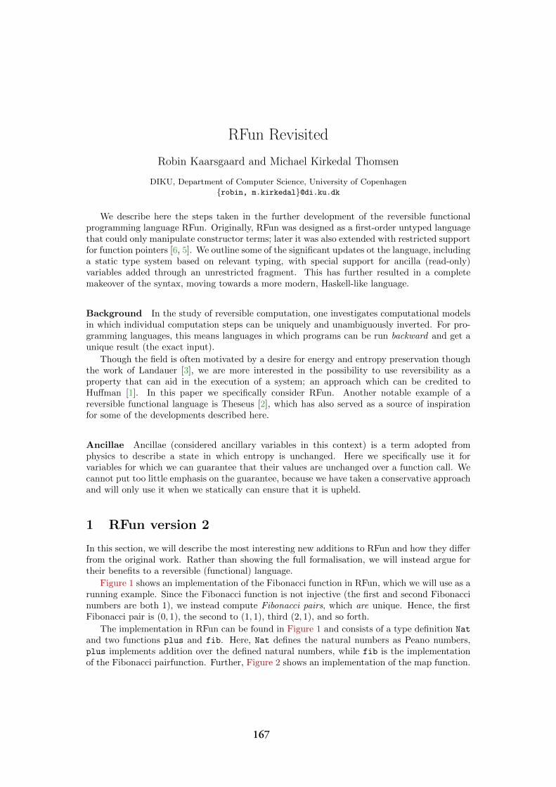
RFun Revisited

Robin Kaarsgaard and Michael Kirkedal Thomsen

DIKU, Department of Computer Science, University of Copenhagen{robin, m.kirkedal}@di.ku.dk

We describe here the steps taken in the further development of the reversible functionalprogramming language RFun. Originally, RFun was designed as a first-order untyped languagethat could only manipulate constructor terms; later it was also extended with restricted supportfor function pointers [6, 5]. We outline some of the significant updates ot the language, includinga static type system based on relevant typing, with special support for ancilla (read-only)variables added through an unrestricted fragment. This has further resulted in a completemakeover of the syntax, moving towards a more modern, Haskell-like language.

Background In the study of reversible computation, one investigates computational modelsin which individual computation steps can be uniquely and unambiguously inverted. For pro-gramming languages, this means languages in which programs can be run backward and get aunique result (the exact input).

Though the field is often motivated by a desire for energy and entropy preservation thoughthe work of Landauer [3], we are more interested in the possibility to use reversibility as aproperty that can aid in the execution of a system; an approach which can be credited toHuffman [1]. In this paper we specifically consider RFun. Another notable example of areversible functional language is Theseus [2], which has also served as a source of inspirationfor some of the developments described here.

Ancillae Ancillae (considered ancillary variables in this context) is a term adopted fromphysics to describe a state in which entropy is unchanged. Here we specifically use it forvariables for which we can guarantee that their values are unchanged over a function call. Wecannot put too little emphasis on the guarantee, because we have taken a conservative approachand will only use it when we statically can ensure that it is upheld.

1 RFun version 2

In this section, we will describe the most interesting new additions to RFun and how they differfrom the original work. Rather than showing the full formalisation, we will instead argue fortheir benefits to a reversible (functional) language.

Figure 1 shows an implementation of the Fibonacci function in RFun, which we will use as arunning example. Since the Fibonacci function is not injective (the first and second Fibonaccinumbers are both 1), we instead compute Fibonacci pairs, which are unique. Hence, the firstFibonacci pair is (0, 1), the second to (1, 1), third (2, 1), and so forth.

The implementation in RFun can be found in Figure 1 and consists of a type definition Nat

and two functions plus and fib. Here, Nat defines the natural numbers as Peano numbers,plus implements addition over the defined natural numbers, while fib is the implementationof the Fibonacci pairfunction. Further, Figure 2 shows an implementation of the map function.

167

RFun Revisited Kaarsgaard and Thomsen

data Nat = Z | S Nat

plus :: Nat → Nat ↔ Nat

plus Z x = x

plus (S y) x =let x’ = plus y x

in (S x’)

fib :: Nat ↔ (Nat, Nat)fib Z = ((S Z), Z)fib (S m) =let (x, y) = fib m

y’ = plus x y

in (y’, x)

Figure 1: RFun program computing Fibonacci pairs.

map :: (a ↔ b) → [a] ↔ [b]map fun [ ] = [ ]map fun (l:ls) =let l’ = fun l

ls’ = map fun ls

in (l’: ls’)

Figure 2: Map function in RFun.

1.1 Type system

With Milner’s motto that “well-typed programs cannot go wrong,” type systems have provenimmensely successful in guaranteeing fundamental well-behavedness properties of programs. Inreversible functional programming, linear type systems (see, e.g., [2]) have played an importantrole in ensuring reversibility.

Fundamentally, a reversible computation can be considered as an injective transformationof a state into an updated state. In this view, it seems obvious to let the type system guaranteelinearity, i.e., that each available resource (in this case, variable) is used exactly once. Thoughlinearity is not enough to guarantee reversibility, it enables the type system to statically rejectcertain irreversible operations (e.g., projections). However, linearity is also more restrictive thanneeded: if we accept that functions may be partial (a necessity for r-Turing completeness), first-order data can be duplicated reversibly. For this reason, we may relax the linearity constraintto relevance, i.e., that all available variables must be used at least once. This guarantees thatvalues are never lost, while also enabling implicit duplication of values.

A useful concept in reversible programming is access to ancillae, i.e., values that remainunchanged across function calls. Such values are often used as a means to guarantee reversibilityin a straightforward manner. For example, in Figure 1, the first input variable of the plus

function is ancillary; it’s value is tacitly returned automatically as part of the output.

To support such ancillary variables at the type level, a type system inspired by Polakow’scombined reasoning system of ordered, linear, and unrestricted intuitionistic logic [4] is used.The type system splits the typing contexts into two parts: a static one (containing ancillaryvariables and other static parts of the environment), and a dynamic one (containing variablesnot considered ancillary). This gives a typing judgment of Σ; Γ ` e : τ , where Σ is the staticcontext, and Γ the dynamic one.

Whereas we must ensure that variables in the dynamic context Γ are used in a relevantmanner to guarantee reversibility, there are no restrictions on the use of variables in the staticcontext – these can used as many or as few times (including not at all) as desired. To distinguishbetween ancillary and dynamic variables at the type level, two different arrow types are used:t1 → t2 denotes that the input variable is ancillary, whereas t1 ↔ t2 denotes that it is dynamic.As such, the type of plus in Figure 1 signifies that the first input variable is ancillary, and thesecond is dynamic.

A neat use of ancillae is to provide limited support for behaviour similar to higher-orderfunctions. For example, the usual map function is not reversible, as not every function oftype [ a] ↔ [b] arises as a functorial application of some function of type a ↔ b. However, ifwe consider the input function f :: a ↔ b to be ancillary, one can straightforwardly define areversible map function (see Figure 2) as one of type (a ↔ b) → ([a] ↔ [b]). In this way, ancillaecan be considered as a slight generalization of the parametrized maps found in Theseus [2].

2

168

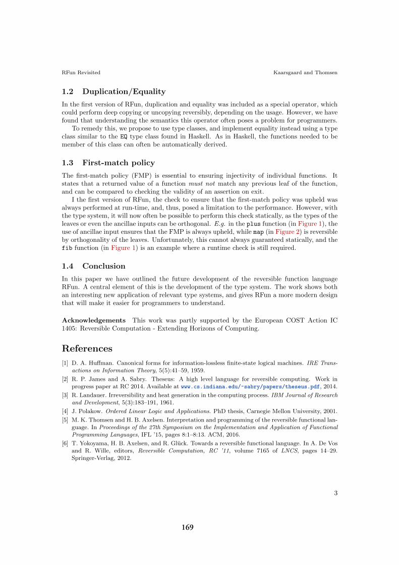
RFun Revisited Kaarsgaard and Thomsen

1.2 Duplication/Equality

In the first version of RFun, duplication and equality was included as a special operator, whichcould perform deep copying or uncopying reversibly, depending on the usage. However, we havefound that understanding the semantics this operator often poses a problem for programmers.

To remedy this, we propose to use type classes, and implement equality instead using a typeclass similar to the EQ type class found in Haskell. As in Haskell, the functions needed to bemember of this class can often be automatically derived.

1.3 First-match policy

The first-match policy (FMP) is essential to ensuring injectivity of individual functions. Itstates that a returned value of a function must not match any previous leaf of the function,and can be compared to checking the validity of an assertion on exit.

I the first version of RFun, the check to ensure that the first-match policy was upheld wasalways performed at run-time, and, thus, posed a limitation to the performance. However, withthe type system, it will now often be possible to perform this check statically, as the types of theleaves or even the ancillae inputs can be orthogonal. E.g. in the plus function (in Figure 1), theuse of ancillae input ensures that the FMP is always upheld, while map (in Figure 2) is reversibleby orthogonality of the leaves. Unfortunately, this cannot always guaranteed statically, and thefib function (in Figure 1) is an example where a runtime check is still required.

1.4 Conclusion

In this paper we have outlined the future development of the reversible function languageRFun. A central element of this is the development of the type system. The work shows bothan interesting new application of relevant type systems, and gives RFun a more modern designthat will make it easier for programmers to understand.

Acknowledgements This work was partly supported by the European COST Action IC1405: Reversible Computation - Extending Horizons of Computing.

References

[1] D. A. Huffman. Canonical forms for information-lossless finite-state logical machines. IRE Trans-actions on Information Theory, 5(5):41–59, 1959.

[2] R. P. James and A. Sabry. Theseus: A high level language for reversible computing. Work inprogress paper at RC 2014. Available at www.cs.indiana.edu/~sabry/papers/theseus.pdf, 2014.

[3] R. Landauer. Irreversibility and heat generation in the computing process. IBM Journal of Researchand Development, 5(3):183–191, 1961.

[4] J. Polakow. Ordered Linear Logic and Applications. PhD thesis, Carnegie Mellon University, 2001.

[5] M. K. Thomsen and H. B. Axelsen. Interpretation and programming of the reversible functional lan-guage. In Proceedings of the 27th Symposium on the Implementation and Application of FunctionalProgramming Languages, IFL ’15, pages 8:1–8:13. ACM, 2016.

[6] T. Yokoyama, H. B. Axelsen, and R. Gluck. Towards a reversible functional language. In A. De Vosand R. Wille, editors, Reversible Computation, RC ’11, volume 7165 of LNCS, pages 14–29.Springer-Verlag, 2012.

3

169