The local discontinuous Galerkin method for three-dimensional shallow water flow

www.elsevier.com/locate/cma

Comput. Methods Appl. Mech. Engrg. 196 (2007) 734–746

The local discontinuous Galerkin method for three-dimensionalshallow water flow q

Vadym Aizinger, Clint Dawson *

Center for Subsurface Modeling – C0200, Institute for Computational Engineering and Sciences (ICES),

The University of Texas at Austin, Austin, TX 78712, United States

Received 13 December 2005; accepted 6 April 2006

Abstract

We formulate and present a stability analysis for the local discontinuous Galerkin method applied to a model of three-dimensionalshallow water flow. This model is described by the Navier–Stokes equations, assuming hydrostatic pressure. The resulting system ofequations is given by momentum equations for the x and y components of velocity, the continuity equation, which is used to solvefor the vertical component of velocity, and an equation describing the motion of the free surface. Our analysis includes the full nonlin-earities in the model with no simplifying assumptions and accounts for the movement of the mesh due to the free surface. To our knowl-edge this is the first analysis of any numerical scheme for this complex system of equations. Numerical results are presented whichdemonstrate the accuracy of the method for a problem with a known analytical solution.� 2006 Elsevier B.V. All rights reserved.

Keywords: Shallow water equations; Local discontinuous Galerkin method; Free surface; Stability analysis

1. Introduction

The shallow water equations (SWE), derived from thethree-dimensional incompressible Navier–Stokes equationsusing the hydrostatic pressure assumption and the Bous-sinesq approximation, are a standard mathematical repre-sentation valid for most types of flow encountered incoastal sea, river, and ocean modeling. They can be utilizedto predict storm surges, tsunamis, floods, and, augmentedby additional equations (e.g., transport, reaction), to modeloil slicks, contaminant plume propagation, temperatureand salinity transport, among other problems.

In many cases of practical interest, vertical variationsare small relative to the horizontal, and one can integratethe Navier–Stokes equations over the depth, applying kine-matic boundary conditions at the bottom and free surface,to obtain the two-dimensional shallow water equations.

0045-7825/$ - see front matter � 2006 Elsevier B.V. All rights reserved.

doi:10.1016/j.cma.2006.04.010

q This work was supported by NSF grant DMS-0411413.* Corresponding author. Tel.: +1 512 4758627.

E-mail address: [email protected] (C. Dawson).

When vertical effects are important, for example in baro-clinic regimes where density varies with salinity and tem-perature, the three-dimensional equations should be used.See [14,13] for a discussion of shallow water models in bothtwo and three dimensions. These models are complicatedby nonlinearities and are often applied to complex domainswith highly irregular bottom topography and land bound-aries. Viscosity effects, especially horizontal viscosity, areusually relatively small, and algorithms which are stableand accurate for smooth to highly advective flows on gen-eral geometries are of interest for the numerical solution ofthese problems.

In this paper we investigate a discontinuous Galerkin(DG) finite element method for the three-dimensional shal-low water equations. Several methods have been proposedfor the numerical solution of this system of PDEs. Onewidely used approach is to compute the free surface eleva-tion using a second-order wave equation and then apply astandard continuous finite element method to the resultingsystem; see [10,11]. Another popular method is based onemploying a staggered grid where normal components of

mailto:[email protected]

V. Aizinger, C. Dawson / Comput. Methods Appl. Mech. Engrg. 196 (2007) 734–746 735

velocity are approximated at the faces of elements and ele-vation at the element centers; see, for example, [9]. Despitethese and other modeling advances the search is still on formethods which are locally mass conservative, can handlevery general types of elements, and are stable and accurateunder highly varying flow regimes. Recently developedalgorithms such as the DG method are therefore of greatinterest within the shallow water community.

DG methods are promising because of their flexibilitywith regard to geometrically complex elements, use ofshock-capturing numerical fluxes, adaptivity in polynomialorder, ability to handle nonconforming grids, and localconservation properties; see [5] for a historical overviewof DG methods. In [2,4], we investigated DG and relatedfinite volume methods for the solution of the two-dimen-sional shallow water equations. Viscosity (second-orderderivative) terms are handled in this method through theso-called local discontinuous Galerkin (LDG) framework[7], which employs a mixed formulation. Application ofthe methodology to three-dimensional shallow water mod-els was first described in [8]. The 3D formulation is not astraightforward extension of the two-dimensional algo-rithm. In particular, it uses a special form of the continuityequation for the free surface elevation and requires post-processing the elevation solution to smooth the computa-tional domain. While the numerical results given in [8]are promising, further work is needed to ascertain the accu-racy, stability and efficiency of this methodology.

In this paper, we take steps in this direction by focusingspecifically on the stability properties of the LDG methodfor the 3D shallow water equations. We prove L2 stabilityfor the method applied to the full nonlinear model andshow numerical examples demonstrating stability and con-vergence of the method. Our stability result also takes intoaccount the moving free surface and the mesh smoothingerror – a feature not present yet in the DG literature tothe best of our knowledge.

The rest of this paper is organized as follows. In the nextsection, we introduce the notation and some of the mathe-matical tools employed in our analysis. The system of 3Dshallow water equations is presented in Section 3. In Sec-tion 4, an LDG discretization of this system is conducted.Section 5 contains a stability analysis of our semi-discreteformulation. Numerical examples demonstrating stabilityand convergence of our scheme are shown in Section 6.

2. Preliminaries

2.1. Notation and definitions

For a; b 2 Rd ; c 2 Re, we denote by ac the tensor-prod-uct of a and c and by a Æ b the dot-product of a and b.

Let X be a bounded domain in Rd . Let T ¼ fTDxðXÞ;Dx > 0g be a family of regular but not necessarily conform-ing partitions of X into elements Xe with Lipschitz bound-ary and diameter Dxe, such that

SXe2TDx

Xe ¼ X, andXe \ Xf = ; for e 5 f.

We will assume TDx is locally quasi-uniform [3], anddenote by Dx the maximum element diameter. The spaceV on TDx is defined as follows:

V ¼ L2ðXÞ \ fv : v 2 H 1ðXeÞ; 8Xe 2TDxg: ð1Þ

Let c0 : H 1ðXeÞ ! H12ðoXeÞ be the trace operator on Xe, and

let Ce,f = oXe \ oXf 5 ; for some e < f. For u 2 V, we de-fine the average and jump operators on Ce,f as follows:

½u� ¼ ðc0uÞjoXe\Ce;f� ðc0uÞjoXf \Ce;f

; ð2Þ

u ¼ 1

2ðc0uÞjoXe\Ce;f

þ ðc0uÞjoXf \Ce;f

� �: ð3Þ

In this paper, we will use standard broken norms onSobolev spaces

kukW kpðXÞ ¼

XXe2TDx

ZX

Xjaj6k

jDauðxÞjp dx

( )1p

; ð4Þ

where Dau denotes a weak derivative of u. To simplifynotation we will write kukX for the L2 norm of u on X,and (., .)X, h., .iC for the L2 inner products on domainsX � Rd and d � 1 dimensional surfaces C.

2.2. Mathematical tools

In our analysis, we will employ several standard resultsfrom functional analysis and the theory of the finite ele-ment method (see [3]).

Theorem 2.1 (Trace theorem). Suppose that Xe has a

Lipschitz boundary. Then there is a constant, Ket , such

that

kukoXe6 Ke

t kuk12Xekuk

12

H1ðXeÞ; 8u 2 H 1ðXeÞ: ð5Þ

In addition, we define the trace constant Kt ¼supDx>0ðmaxXe2TDx K

et Þ.

Theorem 2.2 (Inverse inequality). Let Pk(Xe) be the space ofcomplete polynomials defined on Xe of degree less than or

equal to k. Then there exists a constant Kei independent of

Dxe, such that

kukH1ðXeÞ 6 Kei ðDxeÞ�1kukXe

; 8u 2 P kðXeÞ: ð6Þ

Let Ki ¼ supDx>0ðmaxXe2TDxKe

i Þ. For standard meshtypes Ki can be shown to be finite.

We will also make extensive use of Young’s inequality

ab 6�

2a2 þ 1

2�b2; � > 0; a; b 2 R; ð7Þ

and well-known properties of jump terms,

½ab� ¼ a½b� þ ½a�b; ð8Þ

ab ¼ abþ 1

4½a�½b�: ð9Þ

736 V. Aizinger, C. Dawson / Comput. Methods Appl. Mech. Engrg. 196 (2007) 734–746

3. Mathematical model

3.1. Domain and mesh

A very important feature of 3D geophysical flow modelsis their natural anisotropy due to the gravity force acting inthe vertical direction. This fact is usually reflected in themathematical and numerical formulations as well as in theconstruction of computational domains and grids. The topboundary of most 3D shallow water domains is a dynami-cally changing surface whose movements correspond to timevariations in the free surface elevation, although some mod-els make ‘rigid lid’ assumption to avoid increased computa-tional costs connected with dynamically changing meshes.

Let XðtÞ � R3 be our time-dependent domain. The topboundary of the domain oXtop(t) is the only moving bound-ary. The bottom oXbot and lateral oXD(t) boundaries areassumed to be fixed (though the height of the lateralboundaries can vary with time accordingly to the move-ments of the free surface). We also require the lateralboundaries to be strictly vertical (see Fig. 1). The lastrequirement is only needed to assure that the horizontalcross-section of the domain X(t) (denoted by Xxy) doesnot change with time.

Keeping in line with the specific anisotropy of X(t) weconstruct our 3D mesh by extending a 2D triangular meshof Xxy in the vertical direction, thus producing a 3D meshof X(t) that consists of one or more layers of prismatic ele-ments. In order to better reproduce the bathymetry and thefree surface elevation of the computational domain we donot require top and bottom faces of prisms to be parallelto the xy-plane, although the lateral faces are required tobe strictly vertical.

For our analysis we introduce the following sets of ele-ment and face indices:

• Ie – set of element indices for prismatic elements in X(t);• Ie,xy – set of element indices for triangular elements in

Xxy;• If – set of face indices for prism faces;• Iint � If – set of interior face indices;

∂Ωbot

X

Z

0 Ωxy

∂Ωtop(t)

∂ΩD(t)∂ΩD(t)

Ω(t)

Fig. 1. Vertical cross-section of the computational domain X(t).

• Iext � If – set of exterior face indices;• Ilat � Iint – set of interior lateral face indices;• Ihoriz � Iint – set of interior horizontal face indices;• ID � Iext – set of exterior lateral face indices;• Itop � Iext – set of indices for exterior faces on the top

boundary;• Ibot � Iext – set of indices for exterior faces on the bot-

tom boundary.

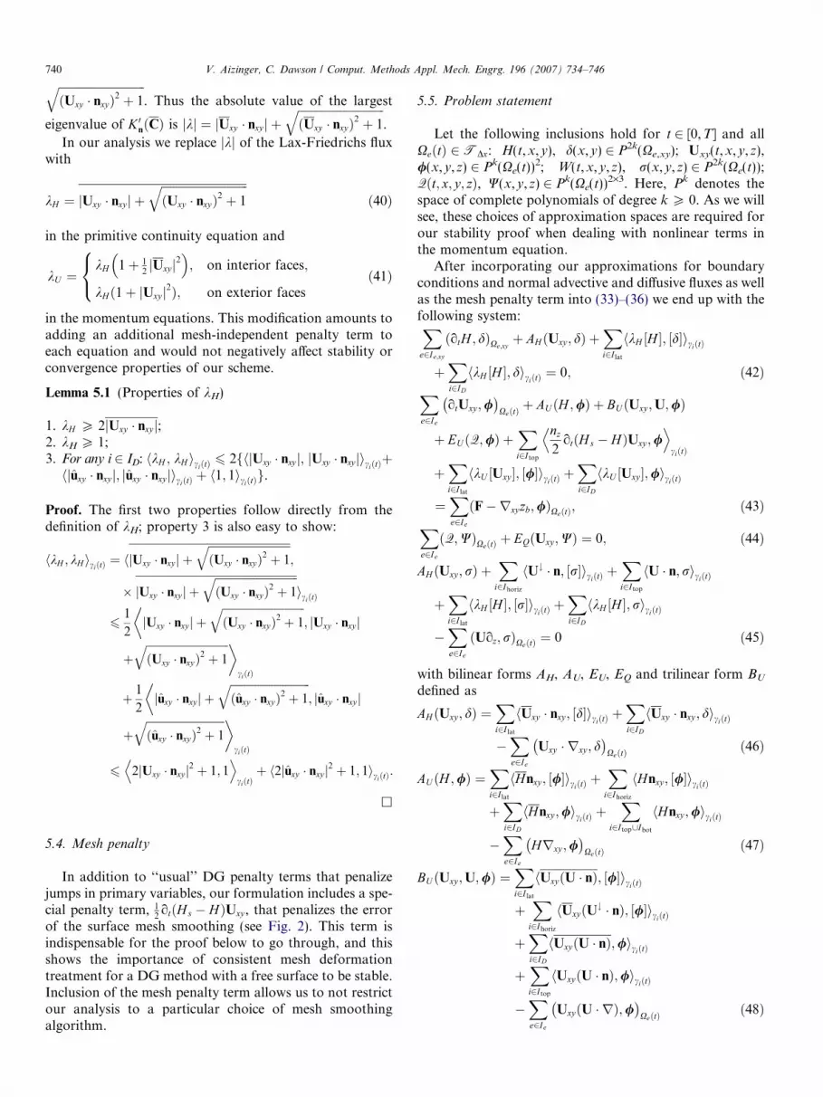
For a point (x,y) 2 Xxy we denote by zb(x,y) the value ofthe z-coordinate at the bottom of the domain and byNs(t,x,y) at the top. A key feature of our 3D LDG modelis the fact that all primary variables, including the free sur-face elevation, are discretized using discontinuous poly-nomial spaces. As a result, computed values of the freesurface elevation may have jumps across inter-elementboundaries. If our finite element grids were to followexactly the computed free surface elevation field this wouldcause the elements in the surface layer to have mismatchinglateral faces (staircase boundary). We avoid this difficultyby employing a globally continuous free surface approxi-mation that is obtained from the computed values of thefree surface elevation N with the help of a smoothingalgorithm (see Fig. 2). Thus Ns denotes the free surface ele-vation of the smoothed mesh, H = N � zb the computed,and Hs = Ns�zb the postprocessed height of the watercolumn.

It must be noted here that solely the computationalmesh is modified by the smoothing algorithm whereasthe computed (discontinuous) approximations to allunknowns, including the free surface elevation, are leftunchanged. This approach preserves the local conservationproperty of the LDG method and is essential for our algo-rithm’s stability.

3.2. System of 3D shallow water equations

The momentum equations in conservative form (assum-ing constant density) are given by [13]

otuxy þr � ðuxyu�DruxyÞ þ grxyn�0 �fc

fc 0

� �uxy ¼ F;

ð10Þwhere the wind stress, the atmospheric pressure gradient,and the tidal potential are combined into a body force termF, $xy = (ox,oy), n is the value of the z coordinate at thefree surface, u = (u,v,w) is the velocity vector, uxy = (u,v)is the vector of horizontal velocity components, fc is theCoriolis coefficient, g is acceleration due to gravity, andD is the tensor of eddy viscosity coefficients defined asfollows:

D ¼Du 0

0 Dv

� �; ð11Þ

with Du, Dv 3 · 3 symmetric positive-definite matrices, and

Druxy ¼DuruDvrv

� �.

P

HH–

(H ,U ,V ,W )

+

+ + + +P

(H ,U ,V W+ )

(H–,U–,V–,W– )

Hs

+ + +

(H–,U–,V–,W–)

,

Fig. 2. Illustration of mesh smoothing: (a) before surface mesh smoothing and (b) after surface mesh smoothing.


The continuity equation is simply

r � u ¼ 0: ð12Þ

3.3. Boundary conditions

The following boundary conditions are specified for thesystem:

• To reduce the technicalities of analysis we employDirichlet boundary conditions at the lateral boundaryoXD(t) though more realistic boundary conditions canbe analyzed and implemented on lateral boundaries [1]

uxy joXDðtÞ¼ uxy ; hjoXDðtÞ

¼ h: ð13Þ

In 3D equations, u will imply ðuxy ; 0Þ on lateralboundaries.

• At the bottom boundary oXbot, we have no normal flow

uðzbÞ � n ¼ 0 ð14Þand no slip for the horizontal velocity components

uðzbÞ ¼ vðzbÞ ¼ 0; ð15Þwhere n = (nx,ny,nz) is an exterior unit normal to theboundary.

• The free surface boundary conditions have the form

otnþ uðnÞoxnþ vðnÞoyn� wðnÞ ¼ 0; ð16ÞruðnÞ � n ¼ rvðnÞ � n ¼ 0: ð17Þ

Analytically, the free surface elevation can be computedfrom (16). However, a computationally more robustmethod [13] is obtained by integrating continuity equation(12) over the total height of the water column. Taking intoaccount boundary conditions (14)–(16) at the bottom and

top boundaries we arrive at a 2D equation for the free sur-face elevation commonly called the primitive continuityequation (PCE),

otnþ ox

Z n

zb

udzþ oy

Z n

zb

vdz ¼ 0: ð18Þ

To prevent our analysis from being obscured by nonessen-tial details we simplify the momentum equations by drop-ping the Coriolis term and rescaling the system so thatg = 1. Let h = n � zb be the total height of the water col-umn. Then the system of the 3D shallow water equationscan be written as

othþ ox

Z n

zb

udzþ oy

Z n

zb

vdz ¼ 0; ð19Þ

otuxy þr � ðuxyu�DruxyÞ þ rxyh ¼ F�rxyzb; ð20Þr � u ¼ 0: ð21Þ

Note that, unlike in the incompressible Navier–Stokes sys-tem, (21) is not a constraint used to determine pressure,rather it is the equation used to determine w.

4. LDG discretization

4.1. Weak formulation

To obtain an LDG formulation of the 3D shallow waterequations we first rewrite the second-order momentumequation (20) in mixed form. Then by introducing anauxiliary variable Q the following first-order system isobtained:

otuxy þr � ðuxyuþffiffiffiffiDp

QÞ þ rxyh ¼ F�rxyzb; ð22ÞQ ¼ �

ffiffiffiffiDpruxy : ð23Þ


To produce a weak form of the momentum equations wemultiply (22) and (23) by smooth test functions / and W,respectively, integrate them on each element XeðtÞ 2TDx,and integrate by parts, getting

ðotuxy ;/ÞXeðtÞ þ hðuxyuþffiffiffiffiDp

QÞ � ne þ hne;/ioXeðtÞ

� ððuxyuþffiffiffiffiDp

QÞ � r þ hrxy ;/ÞXeðtÞ ¼ ðF�rxyzb;/ÞXeðtÞ;

ð24ÞðQ;WÞXeðtÞ ¼ �huxyð

ffiffiffiffiDp

neÞ;WioXeðtÞ þ ðuxyðffiffiffiffiDprÞ;WÞXeðtÞ;

ð25Þ

where ne is a unit exterior normal to oXe(t). This weak for-mulation is well defined for any uxy(t,x,y,z) 2 H1(0,T;V2);/(x,y,z) 2 V2; w(t,x,y,z) 2 V; Qðt; x; y; zÞ 2 V 2�3; 8t 2½0; T �; and W(x,y,z) 2 V2 ·3 with V defined as in (1). Fixingthe direction of the unit normal n on the interior faces sothat it points to the element with a higher index, we cansum over all elements XeðtÞ 2TDx and obtain a weak formof the momentum equations:Xe2Ie

ðotuxy ;/ÞXeðtÞ þXi2I int

hðuxyuþffiffiffiffiDp

QÞ � n

þ hn; ½/�iciðtÞ þXi2Iext

hðuxyuþffiffiffiffiDp

QÞ � nþ hn;/iciðtÞ

�Xe2Ie

ððuxyuþffiffiffiffiDp

QÞ � r þ hrxy ;/ÞXeðtÞ

¼Xe2Ie

F�rxyzb;/� �

XeðtÞ; ð26Þ

Xe2Ie

ðQ;WÞXeðtÞ ¼ �Xi2I int

huxyðffiffiffiffiDp

nÞ; ½W�iciðtÞ

�Xi2Iext


nÞ;WiciðtÞ

þXe2Ie

ðuxyðffiffiffiffiDprÞ;WÞXeðtÞ: ð27Þ

Discretization of the primitive continuity equation is donein a similar way. Let P be the standard orthogonal projec-tion operator from R3 to R2 (P(x,y,z) = (x,y), 8ðx; y; zÞ 2R3), and let Xe,xy = PXe(t). Since the free surface is theonly moving boundary of X(t), and all lateral faces arestrictly vertical, 2D elements Xe,xy are not time-dependent.We multiply (19) by a smooth test function d = d(x,y),integrate it over Xe,xy, and integrate by parts. Then themass balance in the water column corresponding to Xe,xy

can be expressed as

ðoth;dÞXe;xyþ

Z n

zb

uxy dz �n;d� �

oXe;xy

�Z n

zb

uxy dz �rxy ;d

� �Xe;xy

¼ 0:

ð28Þ

We can rewrite the equation above in a special 2D/3D form

ðoth; dÞXe;xyþ

XPXeðtÞ¼Xe;xy

huxy � nxy ; dioXe;latðtÞ

�X

PXeðtÞ¼Xe;xy

ðuxy � rxy ; dÞXeðtÞ ¼ 0; ð29Þ

where nxy = (nx,ny), oXe,lat(t) denotes the lateral boundaryfaces of prism Xe(t), and the summation is over the set of3D elements in the water column corresponding to Xe,xy.Note that the expression above is well defined for anydðx; yÞ 2H ¼def L2ðXxyÞ \ fh : hjPXeðtÞ

2 H 1ðPXeðtÞÞ;8XeðtÞ 2TDxg and hðt; x; yÞ 2 H 1ð0; T ;HÞ. Summing over all ele-ments XeðtÞ 2TDx we obtain a weak form of the PCEXe2Ie;xy

ðoth; dÞXe;xyþXi2I lat

huxy � nxy ; ½d�iciðtÞ

þXi2ID

huxy � nxy ; diciðtÞ �Xe2Ie

ðuxy � rxy ; dÞXeðtÞ ¼ 0: ð30Þ

To discretize the continuity equation we multiply (21) by asmooth test function r, integrate it over Xe(t), and integrateby parts obtaining

hu � n; rioXeðtÞ � ðu � r; rÞXeðtÞ ¼ 0: ð31Þ

Summing over all XeðtÞ 2TDx we get a weak form of thecontinuity equationXi2I int

hu � n; ½r�iciðtÞ þXi2Iext

hu � n; riciðtÞ �Xe2Ie

ðu � r; rÞXeðtÞ ¼ 0:

ð32Þ
4.2. Semi-discrete formulation
Our next step is to approximate cðt; �Þ ¼ ðhðt; �Þ;uxyðt; �Þ;wðt; �Þ;Qðt; �ÞÞ, a solution to problem (26), (27),(30), (32), with a function Cðt; �Þ ¼ ðHðt; �Þ;Uxyðt; �Þ;W ðt; �Þ;Qðt; �ÞÞ 2HD � UD � W D � ZD, where HD �H,UD � V2, WD � V, and ZD � V2·3 are some finite-dimen-sional subspaces. For this purpose, we can use the weakformulation with one important modification. Since theapproximation spaces utilized in the DG methods do notguarantee continuity across the inter-element boundariesall integrands in the integrals over interior faces have tobe replaced by suitably chosen numerical fluxes that pre-serve consistency and stability of the method. Similar treat-ment may be needed at the exterior boundaries as well.Then a semi-discrete finite element solution C(t, Æ) isobtained by requiring that for any t 2 [0, T], for allXeðtÞ 2TDx, and for all ðd;/;W; dÞ 2HD�UD � W D � ZD

the following holds:Xe2Ie;xy

ðotH ; dÞXe;xyþXi2I lat

hKh;nðC�;CþÞ; ½d�iciðtÞ

þXi2ID

hKh;nðC�;CþÞ; diciðtÞ �Xe2Ie

Uxy � rxy ; d� �

XeðtÞ¼ 0;

ð33ÞXe2Ie

ðotUxy ;/ÞXeðtÞ þXi2I int

hKu;nðC�;CþÞ þffiffiffiffiDp

Q � n; ½/�iciðtÞ

þXi2Iext

hKu;nðC�;CþÞ þffiffiffiffiDp

Q � n;/iciðtÞ

�Xe2Ie

ðUxyUþffiffiffiffiDp

QÞ � r þ Hrxy ;/

XeðtÞ

¼Xe2Ie

ðF�rxyzb;/ÞXeðtÞ; ð34Þ


Xe2Ie

Q;Wð ÞXeðtÞ ¼ �Xi2I int

hUxyðffiffiffiffiDp

nÞ; ½W�iciðtÞ

�Xi2Iext


nÞ;WiciðtÞ

þXe2Ie

ðUxyðffiffiffiffiDprÞ;WÞXeðtÞ; ð35Þ

Xi2I int

hKw;nðC�;CþÞ; ½r�iciðtÞ þXi2Iext

hKw;nðC�;CþÞ; riciðtÞ

�Xe2Ie

ðU � r; rÞXeðtÞ ¼ 0; ð36Þ

where Kh;nðC�CþÞ; Ku;nðC�;CþÞ, and Kw;nðC�;CþÞ areapproximations to normal fluxes Uxy Æ nxy, UxyU Æ n +Hnxy, and U Æ n that depend on the values of state variablesC� and C+ on both sides of the discontinuity. The choice ofthis approximation on the interior faces can affect the sta-bility of a DG scheme in a crucial way. The fluxes for theprimitive continuity equation (33) and momentum equa-tion (34) should be computed by a Riemann solver (forexample, Roe, HLLC, Lax-Friedrichs, etc.). See [1,8,12]for a more detailed discussion of this issue. In this work,we treat normal advective fluxes using the Lax-FriedrichsRiemann solver (slightly modifying it in the proof of thestability estimate). Similarly, U and Q denote approxima-tions to U and Q for the normal diffusive fluxes. However,the diffusive terms in our problem being much simpler thanthe advective, U and Q can be set equal to the averagesof the corresponding quantities on both sides of thediscontinuity.

On the exterior faces, treatment of normal fluxes (forboth advection and diffusion) depends on the type ofboundary condition specified and can also strongly affectthe stability properties of a DG scheme. Components ofC+ on those faces can be taken either from boundary con-ditions or set equal to C�.

The vertical velocity component W is computed fromvalues of U and V at the new time level using the discretecontinuity equation (36). This computation is performedlayer-by-layer, starting at the bottom and utilizing thesolution from the element below (or the boundary condi-tion for W at the bottom boundary) as an initial value.For the LDG scheme above to posses the local mass con-servation property one has to choose the normal fluxeson lateral faces for the continuity equation (36), Kw;n

ðC�;CþÞ, equal to those in the primitive continuity equa-tion (33).

5. Stability analysis

5.1. Initial conditions

Let p be the L2 projection operator into the correspond-ing piecewise polynomial space. We specify the initial

conditions as H(0,x,y) = ph(0,x,y), "Xe,xy; Uxy(0, x,y,z) =puxy(0,x,y,z), "Xe(t).

5.2. Boundary conditions

• On exterior lateral faces, we compute normal advectivefluxes by solving the Riemann problem with Hþ ¼ hand Uþ ¼ u. For the diffusive terms we take U ¼ u

and Q ¼ Q�.• At the bottom boundary U = V = W = 0 and Q ¼ Q�

are assumed.• The free surface boundary conditions have the form

U = U�, V = V�, and Q ¼ 0.

5.3. Normal fluxes on interior faces

As already mentioned, the approximation of normaladvective fluxes is one of the crucial issues in our analysis(as well as in the theory and practice of DG methods fornonlinear conservation laws). For our particular applica-tion area the treatment of those terms on lateral faces ismuch more important for stability than on horizontalfaces. The reason for this is the fact that the free surfaceelevation has jumps across lateral faces but not across hor-izontal ones. This feature of our problem means that wehave to solve a coupled Riemann problem for the primitivecontinuity and momentum equations on the lateral faces,but we only need to deal with the momentum equationson horizontal faces.

Thus we set Ku;nðC�;CþÞ ¼ UxyðU# � nÞ on horizontalfaces, where U# denotes the value of U taken from theelement below the face.

To prove stability of our method we employ a slightlymodified version of the Lax-Friedrichs flux as a Riemannsolver for advective terms on lateral faces. A general formof the Lax-Friedrichs flux (see, e.g., [12]) can be written as

KnðC�;CþÞ ¼1

2ðKnðC�Þ þ KnðCþÞÞ þ jkj½C�; ð37Þ

where k is the largest (in absolute value) eigenvalue of theJacobian K 0nðCÞ of the normal flux KnðCÞ.

For system (33), (34) the normal flux Kn(C) on lateralfaces is

KnðCÞ ¼Uxy � nxy

UUxy � nxy þ Hnx

V Uxy � nxy þ Hny

0B@

1CA; ð38Þ

and its Jacobian

K 0nðCÞ ¼0 nx ny

nx 2Unx þ Vny Uny

ny Vnx Unx þ 2Vny

0B@

1CA: ð39Þ

The eigenvalues of K 0nðCÞ are k1 ¼ Uxy � nxy �ffiffiffiffiffiffiffiffiffiffiffiffiffiffiffiffiffiffiffiffiffiffiffiffiffiffiffiffiffiffiðUxy � nxyÞ2 þ 1

q, k2 = Uxy Æ nxy, and k3 ¼ Uxy � nxy þ

ffiffiffiffiffiffiffiffiffiffiffiffiffiffiffiffiffiffiffiffiffiffiffiffiffiffiffiffiffiffiðUxy � nxyÞ2 þ 1
q. Thus the absolute value of the largest

eigenvalue of K 0nðCÞ is jkj ¼ jUxy � nxy j þffiffiffiffiffiffiffiffiffiffiffiffiffiffiffiffiffiffiffiffiffiffiffiffiffiffiffiffiffiffiðUxy � nxyÞ2 þ 1

q.

In our analysis we replace jkj of the Lax-Friedrichs fluxwith

kH ¼ jUxy � nxy j þffiffiffiffiffiffiffiffiffiffiffiffiffiffiffiffiffiffiffiffiffiffiffiffiffiffiffiffiffiffiðUxy � nxyÞ2 þ 1

qð40Þ

in the primitive continuity equation and

kU ¼kH 1þ 1

2jUxy j2

; on interior faces;

kHð1þ jUxy j2Þ; on exterior faces

8<: ð41Þ

in the momentum equations. This modification amounts toadding an additional mesh-independent penalty term toeach equation and would not negatively affect stability orconvergence properties of our scheme.

Lemma 5.1 (Properties of kH)

1. kH P 2jUxy � nxy j;2. kH P 1;3. For any i 2 ID: hkH ; kH iciðtÞ 6 2fhjUxy � nxy j; jUxy � nxy jiciðtÞþhjuxy � nxy j; juxy � nxy jiciðtÞ þ h1; 1iciðtÞg.

Proof. The first two properties follow directly from thedefinition of kH; property 3 is also easy to show:

hkH ; kH iciðtÞ ¼ hjUxy � nxy j þffiffiffiffiffiffiffiffiffiffiffiffiffiffiffiffiffiffiffiffiffiffiffiffiffiffiffiffiffiffiðUxy � nxyÞ2 þ 1

q;

� jUxy � nxy j þffiffiffiffiffiffiffiffiffiffiffiffiffiffiffiffiffiffiffiffiffiffiffiffiffiffiffiffiffiffiðUxy � nxyÞ2 þ 1

qiciðtÞ

61

2jUxy � nxy j þ

ffiffiffiffiffiffiffiffiffiffiffiffiffiffiffiffiffiffiffiffiffiffiffiffiffiffiffiffiffiffiðUxy � nxyÞ2 þ 1

q; jUxy � nxy j

�

þffiffiffiffiffiffiffiffiffiffiffiffiffiffiffiffiffiffiffiffiffiffiffiffiffiffiffiffiffiffiðUxy � nxyÞ2 þ 1

q �ciðtÞ

þ 1

2juxy � nxy j þ

ffiffiffiffiffiffiffiffiffiffiffiffiffiffiffiffiffiffiffiffiffiffiffiffiffiffiffiffiffiðuxy � nxyÞ2 þ 1

q; juxy � nxy j

�

þffiffiffiffiffiffiffiffiffiffiffiffiffiffiffiffiffiffiffiffiffiffiffiffiffiffiffiffiffiðuxy � nxyÞ2 þ 1

q �ciðtÞ

6 2jUxy � nxy j2 þ 1; 1D E

ciðtÞþ h2juxy � nxy j2 þ 1; 1iciðtÞ:

h

5.4. Mesh penalty

In addition to ‘‘usual’’ DG penalty terms that penalizejumps in primary variables, our formulation includes a spe-cial penalty term, 1

2otðHs � HÞUxy , that penalizes the error

of the surface mesh smoothing (see Fig. 2). This term isindispensable for the proof below to go through, and thisshows the importance of consistent mesh deformationtreatment for a DG method with a free surface to be stable.Inclusion of the mesh penalty term allows us to not restrictour analysis to a particular choice of mesh smoothingalgorithm.

5.5. Problem statement

Let the following inclusions hold for t 2 [0,T] and allXeðtÞ 2TDx: H(t,x,y), d(x,y) 2 P2k(Xe,xy); Uxy(t,x,y,z),/(x,y,z) 2 Pk(Xe(t))

2; W(t,x,y,z), r(x,y,z) 2 P2k(Xe(t));Qðt; x; y; zÞ, W(x,y,z) 2 Pk(Xe(t))

2·3. Here, Pk denotes thespace of complete polynomials of degree k P 0. As we willsee, these choices of approximation spaces are required forour stability proof when dealing with nonlinear terms inthe momentum equation.

After incorporating our approximations for boundaryconditions and normal advective and diffusive fluxes as wellas the mesh penalty term into (33)–(36) we end up with thefollowing system:Xe2Ie;xy

ðotH ; dÞXe;xyþ AH ðUxy ; dÞ þ

Xi2I lat

hkH ½H �; ½d�iciðtÞ

þXi2ID

hkH ½H �; diciðtÞ ¼ 0; ð42ÞXe2Ie

otUxy ;/� �

XeðtÞþ AU ðH ;/Þ þ BU ðUxy ;U;/Þ

þ EU ðQ;/Þ þXi2I top

nz

2otðH s � HÞUxy ;/

D EciðtÞ

þXi2I lat

hkU ½Uxy �; ½/�iciðtÞ þXi2ID

hkU ½Uxy �;/iciðtÞ

¼Xe2Ie

ðF�rxyzb;/ÞXeðtÞ; ð43ÞXe2Ie

ðQ;WÞXeðtÞ þ EQðUxy ;WÞ ¼ 0; ð44Þ

AH ðUxy ; rÞ þX

i2Ihoriz

hU# � n; ½r�iciðtÞ þXi2I top

hU � n; riciðtÞ

þXi2I lat

hkH ½H �; ½r�iciðtÞ þXi2ID

hkH ½H �; riciðtÞ

�Xe2Ie

Uoz; rð ÞXeðtÞ ¼ 0 ð45Þ

with bilinear forms AH, AU, EU, EQ and trilinear form BU

defined as

AH ðUxy ; dÞ ¼Xi2I lat

hUxy � nxy ; ½d�iciðtÞ þXi2ID

hUxy � nxy ; diciðtÞ

�Xe2Ie

Uxy � rxy ; d� �

XeðtÞð46Þ

AU ðH ;/Þ ¼Xi2I lat

hHnxy ; ½/�iciðtÞ þX

i2Ihoriz

hHnxy ; ½/�iciðtÞ

þXi2ID

hHnxy ;/iciðtÞ þX

i2I top[Ibot

hHnxy ;/iciðtÞ

�Xe2Ie

Hrxy ;/� �

XeðtÞð47Þ

BU ðUxy ;U;/Þ ¼Xi2I lat

hUxyðU � nÞ; ½/�iciðtÞ

þX

i2Ihoriz

hUxyðU# � nÞ; ½/�iciðtÞ

þXi2ID

hUxyðU � nÞ;/iciðtÞ

þXi2I top

hUxyðU � nÞ;/iciðtÞ

�Xe2Ie

UxyðU � rÞ;/� �

XeðtÞð48Þ


EUðQ;/Þ ¼Xi2I int

hffiffiffiffiDp

Q � n; ½/�iciðtÞ

þX

i2ID[Ibot

hffiffiffiffiDp

Q � n;/iciðtÞ

�Xe2Ie

ffiffiffiffiDp

Q � r;/

XeðtÞð49Þ

EQðUxy ;WÞ ¼Xi2I int


nÞ; ½W�iciðtÞ

þXi2ID


nÞ;WiciðtÞ

þXi2I top


nÞ;WiciðtÞ

�Xe2Ie

UxyðffiffiffiffiDprÞ;W

XeðtÞ

: ð50Þ

5.6. Stability estimate

We now state our main result.

Theorem 5.2 (Discrete stability). Let l = max{(Dxe)�1 :

oXe \ [i2IDci(t) 5 ;}. Then the following stability result

holds for scheme (42)–(45):

kHðT Þk2XxyþkUxyðT Þk2

XðT Þ þZ T

0

QðtÞk k2XðtÞdt

þZ T

0

Xi2I lat

hkH ½H �; ½H �iciðtÞdtþZ T

0

Xi2I lat

hkH ½Uxy �; ½Uxy �iciðtÞdt

6K Hð0Þk k2Xxyþ Uxyð0Þ�� 2

Xð0Þ þZ T

0

FðtÞ�rxyzb

�� 2

XðtÞdt�

þZ T

0

khðtÞk2oXDðtÞdtþ

Z T

0

khðtÞk4L4ðoXDðtÞÞdt

þZ T

0

kuxyðtÞk2oXDðtÞdtþ

Z T

0

kuxyðtÞk4L4ðoXDðtÞÞdt

þZ T

0

kuxyðtÞk8L8ðoXDðtÞÞdtþ

Z T

0

lkuxyðtÞk2oXDðtÞdt

þZ T

0

k1k2oXDðtÞdt

;

where K ¼ KðKt;Ki;D; T Þ.

Proof. Let d ¼ H ;/ ¼ Uxy ;W ¼ Q. Eqs. (42)–(44) are inte-grated from 0 to T and added together to obtainZ T

0

Xe2Ie;xy

ðotH ;HÞXe;xydt þ

Z T

0

AHðUxy ;HÞdt

þZ T

0

Xi2I lat

hkH ½H �; ½H �iciðtÞ dt þZ T

0

Xi2ID

hkH ½H �;HiciðtÞ dt

þZ T

0

Xe2Ie

otUxy ;Uxy

� �XeðtÞ

dt þZ T

0

AU ðH ;UxyÞdt

þZ T

0

BU ðUxy ;U;UxyÞdt þZ T

0

EUðQ;UxyÞdt

þZ T

0

Xi2I top

nz

2otðH s � HÞUxy ;Uxy

D EciðtÞ

dt

þZ T

0

Xi2I lat

hkU ½Uxy �; ½Uxy �iciðtÞ dt

þZ T

0

Xi2ID

hkU ½Uxy �;UxyiciðtÞ dt þZ T

0

Xe2Ie

Q;Qð ÞXeðtÞ dt

þZ T

0

EQðUxy ;QÞdt ¼Z T

0

Xe2Ie

ðFðtÞ � rxyzb;UxyÞXeðtÞdt:

ð51ÞFirst, let us eliminate some terms containing H. Integratingby parts and using (8)

AH ðUxy ;HÞ þ AU ðH ;UxyÞ¼Xi2I lat

hUxy � nxy ; ½H �iciðtÞ þXi2ID

hUxy � nxy ;HiciðtÞ

�Xe2Ie

Uxy � rxy ;H� �

XeðtÞþXi2I lat

hHnxy ; ½Uxy �iciðtÞ

þX

i2Ihoriz

hHnxy ; ½Uxy �iciðtÞ þXi2ID

hHnxy ;UxyiciðtÞ

þX

i2I top[Ibot

hHnxy ;UxyiciðtÞ �Xe2Ie

Hrxy ;Uxy

� �XeðtÞ

¼ 1

2

Xi2ID

huxy � nxy ;HiciðtÞ þ1

2

Xi2ID

hhnxy ;UxyiciðtÞ: ð52Þ

Next, the advective terms from the momentum equationare handled using the discrete continuity equation (45).To do this first note that

�Xe2Ie

ðUxyðU � rÞ;UxyÞXeðtÞ ¼ �1

2

Xe2Ie

ðU;rU2xyÞXeðtÞ: ð53Þ

Setting r ¼ U2xy , recalling that the test space in (45) con-

tains products of elements from the test space of (43),and using (8) and (9) we find

BU ðUxy ;U;UxyÞ¼Xi2I lat

hUxyðU � nÞ; ½Uxy �iciðtÞ þX

i2Ihoriz

hUxyðU# � nÞ; ½Uxy �iciðtÞ

þXi2ID

hUxyðU � nÞ;UxyiciðtÞ þXi2I top

hUxyðU � nÞ;UxyiciðtÞ

� 1

2

Xi2I lat

hU � n; ½U2xy �iciðtÞ �

1

2

Xi2Ihoriz

hU# � n; ½U2xy �iciðtÞ

� 1

2

Xi2I top

hU � n;U2xyiciðtÞ �

1

2

Xi2ID

hUxy � nxy ;U2xyiciðtÞ

� 1

2

Xi2I lat

hkH ½H �; ½U2xy �iciðtÞ �

1

2

Xi2ID

hkH ½H �;U2xyiciðtÞ

¼ 1

4

Xi2I lat

h½Uxy �½U � n�; ½Uxy �iciðtÞ þ1

4

Xi2ID

hUxy ½U � n�;UxyiciðtÞ

þ 1

2

Xi2ID

huxyðuxy � nxyÞ;UxyiciðtÞ

þ 1

2

Xi2I top

hUxyðU � nÞ;UxyiciðtÞ �Xi2I lat

hkH Uxy ½H �; ½Uxy �iciðtÞ

� 1

2

Xi2ID

hkH Uxy ½H �;UxyiciðtÞ: ð54Þ


In the next step, we will use the mesh penalty term toaccount for the moving free surface in the momentumequation. For that purpose we will utilize Eqs. (42) and(45), again taking advantage of the higher order test spacesspecified for them. Noting that for any free surface bound-ary face c in our smoothed mesh

Rc nzf ðx; y; zÞds ¼R

PðcÞ f ðx; y;NsÞdxdy and applying Leibnitz’ Rule we pro-ceed as follows:Z T

0

Xe2Ie

otUxy ;Uxy

� �XeðtÞ

dt

þZ T

0

Xi2I top

nz

2otðH s � HÞUxy ;Uxy

D EciðtÞ

dt

¼ 1

2

Z T

0

Xe2Ie;xy

Z NsðtÞ

zbot

otjUxy j2 dz; 1� �

Xe;xy

dt

þ 1

2

Z T

0

Xe2Ie;xy

otNs � otH ; jUxyðNsÞj2

Xe;xy

dt

¼ 1

2

Z T

0

Xe2Ie

otkUxyk2XeðtÞ dt

� 1

2

Z T

0

Xe2Ie;xy

ðotH ; jUxyðNsÞj2ÞXe;xydt: ð55Þ

Setting d = r = jUxy(Ns)j2 in (42) and (45), respectively,and adding the results we find

1

2

Z T

0

Xe2Ie

otkUxyk2XeðtÞ dt � 1

2

Z T

0

Xe2Ie;xy

ðotH ; jUxyðNsÞj2ÞXe;xydt

¼ 1

2kUxyðT Þk2

XðT Þ �1

2kUxyð0Þtk2

Xð0Þ

� 1

2

Z T

0

Xi2I top

hU � n;U2xyiciðtÞ dt: ð56Þ

The last term in the expression above cancels a correspond-ing term in the previous estimate. For eddy viscosity termsthe divergence theorem and (8) give us

EUðQ;UxyÞ þ EQðUxy ;QÞ¼Xi2I int

hffiffiffiffiDp

Q � n; ½Uxy �iciðtÞ þX

i2ID[Ibot

hffiffiffiffiDp

Q � n;UxyiciðtÞ

�Xe2Ie

ðffiffiffiffiDp

Q � r;UxyÞXeðtÞ þXi2I int


nÞ; ½Q�iciðtÞ

þXi2ID


nÞ;QiciðtÞ þXi2I top


nÞ;QiciðtÞ

�Xe2Ie

ðUxyðffiffiffiffiDprÞ;QÞXeðtÞ

¼Xi2ID


nÞ;QiciðtÞ: ð57Þ

Noting thatZ T

0

Xe2Ie;xy

ðotH ;HÞXe;xydt ¼ 1

2kHðT Þk2

Xxy� 1

2kHð0Þk2

Xxyð58Þ

and substituting the results of the above simplifications in(51) we obtain

1

2kHðT Þk2

Xxyþ 1

2kUxyðT Þk2

XðT Þ þZ T

0

kQðtÞk2XðtÞ dt

þZ T

0

Xi2I lat

hkH ½H �; ½H �iciðtÞ dt þZ T

0

Xi2ID

hkH H ;HiciðtÞ dt

þZ T

0

Xi2I lat

hkU ½Uxy �; ½Uxy �iciðtÞ dt

þZ T

0

Xi2ID

hkU Uxy ;UxyiciðtÞ dt

þ 1

4

Z T

0

Xi2I lat

h½Uxy �½U � n�; ½Uxy �iciðtÞ dt

þ 1

4

Z T

0

Xi2ID

hUxy ½U � n�;UxyiciðtÞ dt

¼Z T

0

Xe2Ie

ðFðtÞ � rxyzb;UxyÞXeðtÞ dt þ 1

2Hð0Þk k2

Xxy

þ 1

2Uxyð0Þ�� 2

Xð0Þ �1

2

Z T

0

Xi2ID

huxy � nxy ;HiciðtÞ dt

� 1

2

Z T

0

Xi2ID

hhnxy ;UxyiciðtÞ dt þZ T

0

Xi2ID

hkH h;HiciðtÞ dt

þZ T

0

Xi2ID

hkU uxy ;UxyiciðtÞ dt

�Z T

0

Xi2ID


nÞ;QiciðtÞ dt

� 1

2

Z T

0

Xi2ID

huxyðuxy � nxyÞ;UxyiciðtÞ dt

þZ T

0

Xi2I lat

hkH Uxy ½H �; ½Uxy �iciðtÞ dt

þ 1

2

Z T

0

Xi2ID

hkH Uxy ½H �;UxyiciðtÞ dt: ð59Þ

The remainder of the proof consists of estimating theunderlined terms.

1

4

Xi2I lat

h½Uxy �½U � n�; ½Uxy �iciðtÞ 61

2

Xi2I lat

h½Uxy �jU � nj; ½Uxy �iciðtÞ;

ð60Þ

1

4

Xi2ID

hUxy ½U � n�;UxyiciðtÞ 61

2

Xi2ID

hUxy jU � nj;UxyiciðtÞ; ð61Þ

�1

2

Xi2ID

huxy � nxy ;HiciðtÞ 61

4

Xi2ID

huxy ; uxyiciðtÞ þ1

4

Xi2ID

hH ;HiciðtÞ;

ð62Þ

� 1

2

Xi2ID

hhnxy ;UxyiciðtÞ 6Xi2ID

hh; hiciðtÞ þ1

16

Xi2ID

hUxy ;UxyiciðtÞ;

ð63Þ


Xi2ID

hkH h;HiciðtÞ 6Xi2ID

hkH h; hiciðtÞ þ1

4

Xi2ID

hkH H ;HiciðtÞ

61

64

Xi2ID

hkH ; kHiciðtÞ þ 16Xi2ID

hh2; h2iciðtÞ

þ 1

4

Xi2ID

hkH H ;HiciðtÞ; ð64Þ

Xi2ID

hkU uxy ;UxyiciðtÞ61

2

Xi2ID

hkU uxy ; uxyiciðtÞ þ1

2

Xi2ID

hkU Uxy ;UxyiciðtÞ

¼ 1

2

Xi2ID

hkH ð1þjUxy j2Þuxy ; uxyiciðtÞ

þ1

2

Xi2ID


61

64

Xi2ID

hkH ;kH iciðtÞ þ4Xi2ID

hjuxy j2; juxy j2iciðtÞ

þ1

4

Xi2ID

hkH jUxy j2; jUxy j2iciðtÞ

þ1

4

Xi2ID

hkH juxy j2; juxy j2iciðtÞ

þ1

2

Xi2ID


61

32

Xi2ID

hkH ;kH iciðtÞ þ4Xi2ID


þ1

4

Xi2ID

hkH jUxy j2; jUxy j2iciðtÞ

þXi2ID


þ1

2

Xi2ID

hkU Uxy ;UxyiciðtÞ; ð65Þ

�Xi2ID


nÞ;QiciðtÞ

6KtKi

2

Xi2ID

lhuxyðffiffiffiffiDp

nÞ; uxyðffiffiffiffiDp

nÞiciðtÞ

þ 1

2KtKi

Xi2ID

l�1hQ;QiciðtÞ

6 KðKt;Ki;DÞXi2ID

lhuxy ; uxyiciðtÞ þ1

2Qk k2

XðtÞ; ð66Þ

� 1

2

Xi2ID

huxyðuxy � nxyÞ;UxyiciðtÞ

6

Xi2ID

huxyðuxy � nxyÞ2; uxyiciðtÞ þ1

16

Xi2ID

hUxy ;UxyiciðtÞ

6

Xi2ID

hjuxy j2; juxy j2iciðtÞ þ1

16

Xi2ID

hUxy ;UxyiciðtÞ; ð67Þ

Xi2I lat

hkH Uxy ½H �; ½Uxy �iciðtÞ

61

2

Xi2I lat

hkH ½H �; ½H �iciðtÞ þ1

2

Xi2I lat

hkH jUxy j2½Uxy �; ½Uxy �iciðtÞ;

ð68Þ

1

2

Xi2ID

hkH Uxy ½H �;UxyiciðtÞ

61

4

Xi2ID


4

Xi2ID

hkH jUxy j2Uxy ;UxyiciðtÞ

61

2

Xi2ID

hkH H ;HiciðtÞ þ1

2

Xi2ID

hkH h; hiciðtÞ

þ 1

4

Xi2ID

hkH jUxy j2Uxy ;UxyiciðtÞ

61

2

Xi2ID

hkH H ;HiciðtÞ þ1

64

Xi2ID

hkH ; kH iciðtÞ

þ 4Xi2ID

hh2; h2iciðtÞ þ1

4

Xi2ID

hkH jUxy j2Uxy ;UxyiciðtÞ: ð69Þ

Combining the penalty terms from (59) and applying theresults above, the definition of kU (41), and properties ofkH (Lemma 5.1), we findXi2I lat

hkH ½H �; ½H �iciðtÞ þXi2ID

hkH H ;HiciðtÞ þXi2I lat

hkU ½Uxy �; ½Uxy �iciðtÞ

þXi2ID

hkU Uxy ;UxyiciðtÞ þ1

4

Xi2I lat

h½Uxy �½U �n�; ½Uxy �iciðtÞdt

þ1

4

Xi2ID

hUxy ½U �n�;UxyiciðtÞdt�1

4

Xi2ID

hH ;HiciðtÞ

� 1

16

Xi2ID

hUxy ;UxyiciðtÞ �1

4

Xi2ID

hkH H ;HiciðtÞ

�1

4

Xi2ID

hkH jUxy j2; jUxy j2iciðtÞ �1

2

Xi2ID


� 1

16

Xi2ID


2

Xi2I lat

hkH ½H �; ½H �iciðtÞ

�1

2

Xi2I lat

hkH jUxy j2½Uxy �; ½Uxy �iciðtÞ �1

2

Xi2ID

hkH H ;HiciðtÞ

�1

4

Xi2ID

hkH jUxy j2Uxy ;UxyiciðtÞ �1

16

Xi2ID

hkH ;kH iciðtÞ

¼ 1

2

Xi2I lat


4

Xi2ID

hkH H ;HiciðtÞ

þXi2I lat

hkH ½Uxy �; ½Uxy �iciðtÞ þ1

2

Xi2ID

hkH Uxy ;UxyiciðtÞ

þ1

4

Xi2I lat

h½Uxy �½U �n�; ½Uxy �iciðtÞdt

þ1

4

Xi2ID

hUxy ½U �n�;UxyiciðtÞdt�1

4

Xi2ID

hH ;HiciðtÞ

�1

8

Xi2ID


16

Xi2ID

hkH ;kHiciðtÞ

P1

2

Xi2I lat


2

Xi2I lat

hkH ½Uxy �; ½Uxy �iciðtÞ

þ1

8

Xi2ID

hkH Uxy ;UxyiciðtÞ �1

16

Xi2ID

hkH ;kH iciðtÞ


P1

2

Xi2I lat


2

Xi2I lat

hkH ½Uxy �; ½Uxy �iciðtÞ

�1

8

Xi2ID

h1;1iciðtÞdt�1

8

Xi2ID

hjuxy �nxy j; juxy �nxy jiciðtÞdt:

Substituting the estimates above in (59) we arrive at thefollowing inequality:

1

2HðT Þk k2

Xxyþ 1

2UxyðT Þ�� 2

XðT Þ þ1

2

Z T

0

QðtÞk k2XðtÞ dt

þ 1

2

Z T

0

Xi2I lat

hkH ½H �; ½H �iciðtÞ dt

þ 1

2

Z T

0

Xi2I lat

hkH ½Uxy �; ½Uxy �iciðtÞ dt

61

2Hð0Þk k2

Xxyþ 1

2Uxyð0Þ�� 2

Xð0Þ

þZ T

0

Xe2Ie

FðtÞ � rxyzb;Uxy

� �XeðtÞ

dt

þ 1

4

Z T

0

Xi2ID

huxy ; uxyiciðtÞ dt þZ T

0

Xi2ID

hh; hiciðtÞ dt

þ 20

Z T

0

Xi2ID

hh2; h2iciðtÞdt

þ 5

Z T

0

Xi2ID

hjuxy j2; juxy j2iciðtÞ dt

þZ T

0

Xi2ID

hjuxy j4; juxy j4iciðtÞ dt

þ KðKt;Ki;DÞZ T

0

Xi2ID

lhuxy ; uxyiciðtÞ dt

þ 1

8

Z T

0

Xi2ID

h1; 1iciðtÞ dt

þ 1

8

Z T

0

Xi2ID

hjuxy � nxy j; juxy � nxy jiciðtÞ dt: ð70Þ

Finally, the remaining term on the right hand side can beestimated by

Xe2Ie

ðFðtÞ�rxyzb;UxyÞXeðtÞ61

2kFðtÞ�rxyzbk2

XðtÞ þ1

2kUxyk2

XðtÞ:

ð71Þ

The claim of our theorem follows from substitution of theestimate above into (70) and application of Gronwall’slemma. h

5.7. Stability estimate without Gronwall’s constant

The stability result can be improved upon by showingthat the large constant produced by Gronwall’s lemma is,

in fact, not necessary. A way to do it is demonstrated inthe following:

Corollary 5.3. The stability result in Theorem 5.2 also holds

for a K ¼ KðKt;Ki;D; T Þ obtained without Gronwall’s

lemma.

Proof. First, note that (70) holds for any T > 0. Let us fixsome T > 0 and introduce the following notation:

KðtÞ ¼ khðtÞk2oXDðtÞ þ 20khðtÞk4

L4ðoXDðtÞÞ

þ 3

8kuxyðtÞk2

oXDðtÞ þ 5kuxyðtÞk4L4ðoXDðtÞÞ

þ kuxyðtÞk8L8ðoXDðtÞÞ

þ KðKt;Ki;DÞlkuxyðtÞk2oXDðtÞ þ

1

8k1k2

oXDðtÞ: ð72Þ

Let ~t 2 ½0; T � be such that kUxyð~tÞkXð~tÞ ¼ maxt2½0;T �kUxy

ðtÞkXðtÞ. Theorem 5.2 guarantees that kUxyð~tÞkXð~tÞ is finite.Moreover, (70) implies that

kUxyð~tÞk2Xð~tÞ 6 kHð0Þk

2Xxyþ kUxyð0Þk2

Xð0Þ þ 2

Z T

0

KðtÞdt

þ 2

Z T

0

Xe2Ie

jðFðtÞ � rxyzb;UxyÞXeðtÞjdt: ð73Þ

The last term above can be estimated using Schwarz’ andYoung’s inequalitiesZ T

0

Xe2Ie

jðFðtÞ � rxyzb;UxyÞXeðtÞjdt

6 kUxyð~tÞkXð~tÞZ T

0

kFðtÞ � rxyzbkXðtÞ dt

61

4kUxyð~tÞk2

Xð~tÞ þZ T

0

kFðtÞ � rxyzbkXðtÞ dt� 2

61

4kUxyð~tÞk2

Xð~tÞ þ TZ T

0

kFðtÞ � rxyzbk2XðtÞ dt: ð74Þ

Substitution of the expression above into (73) produces

kUxyð~tÞk2Xð~tÞ 6 2kHð0Þk2

Xxyþ 2kUxyð0Þk2

Xð0Þ þ 4

Z T

0

KðtÞdt

þ 4TZ T

0


Then (74) yieldsZ T

0

Xe2Ie

jðFðtÞ � rxyzb;UxyÞXeðtÞjdt

61

2kHð0Þk2

Xxyþ 1

2kUxyð0Þk2

Xð0Þ þZ T

0

KðtÞdt

þ 2TZ T

0


Substituting (76) into (70) we arrive at the result ofTheorem 5.2 without using Gronwall’s lemma. h


6. Numerical results

The theoretical results above prove stability, but do notaddress the question of accuracy of the DG method formu-lated above. Obtaining an a priori error estimate for themethod has proven to be a more difficult undertaking.The main hurdle when applying arguments similar to thestability proof to derive an error estimate lies in the conti-nuity equation, which is solved as an initial value problemstarting at the bottom and going layer-by-layer to the top,accumulating in the process the discretization error. There-fore, an error estimate for the DG formulation presented inthis paper is still a subject of ongoing research.

In this section, we will demonstrate that, in fact, themethod does converge for a test problem with a manufac-tured smooth analytical solution. The same test problemwas also used in [8] and was obtained by plugging a smoothfunction that satisfies the continuity (21) and the primitivecontinuity (18) equations into our system and solving aDirichlet problem with a corresponding forcing term andboundary conditions given by the exact solution. The par-ticular DG method examined in [8] was somewhat differentfrom the one presented here in that we used a different nor-mal boundary flux approximation on the lateral faces, themesh smoothing penalty term in (43) was omitted, andequal order approximations were used for all unknowns.

The analytical solution to the test problem was

Table 1Piecewise constant approximation, forward Euler, advection only

N Ne Nl Er(n) C(n) Er(u) C(u)

1 2 1 2.54e�1 5.24e�12 8 2 2.88e�1 �0.18 8.78e�1 �0.743 32 4 1.98e�1 0.54 7.69e�1 0.094 128 8 1.38e�1 0.52 4.39e�1 0.815 512 16 8.59e�2 0.68 2.68e�1 0.71

Table 2Piecewise linear horizontal velocities, piecewise quadratic surface elevation and


1 2 1 3.00e�1 6.35e�12 8 2 1.13e�1 1.41 3.45e�1 0.883 32 4 2.74e�2 2.04 9.90e�2 1.804 128 8 6.97e�3 1.97 3.25e�2 1.615 512 16 1.75e�3 1.99 1.06e�2 1.62

Table 3Piecewise constant approximation, forward Euler, advection–diffusion


1 2 1 7.68e�1 4.00e02 8 2 9.16e�1 �0.25 3.75e0 0.093 32 4 3.04e�1 1.59 2.16e0 0.804 128 8 1.47e�1 1.05 1.23e0 0.815 512 16 5.81e�2 1.34 7.22e�1 0.77

nðt; x; yÞ ¼ eðsinðxðxþ tÞÞ þ sinðxðy þ tÞÞÞ;uðt; x; y; zÞ ¼ dðz� zbÞ sinðxðxþ tÞÞ;vðt; x; y; zÞ ¼ dðz� zbÞ sinðxðy þ tÞÞ;

wðt; x; y; zÞ ¼ dðz� zbÞozb

oxsinðxðxþ tÞÞ þ ozb

oysinðxðy þ tÞÞ

� �

� 1

2dxðz� zbÞ2ðcosðxðxþ tÞÞ þ cosðxðy þ tÞÞÞ;

where e = 0.01, d = 0.1, x = 0.01. X(t) was a [0,100] ·[0,100] square with a dynamic free surface and the bathy-metry varying linearly as zb(x,y) = 0.005(x + y)�2. Theproblem was solved for t 2 [0, T] with T = 0.001 days using64-bit floating point arithmetic. In Tables 1–4, we list theL2 norm of the error at time T for the surface elevationand velocity. We denote by Ne the number of surface trian-gles, Nl the maximum number of vertical layers, Dt thetime step in seconds, Er(Æ) the norm of the error, and C(Æ)the convergence rate.

We conducted two series of tests: pure advection andadvection–diffusion (Du = Dv = 0.1I) problems. The firstsimulation in each series was carried out using piecewiseconstant approximation for all variables, the second oneemployed piecewise linear polynomials for horizontalvelocity components and piecewise quadratic for the sur-face elevation and the vertical velocity. The time steppingwas carried out by forward Euler for the piecewise constant

Er(v) C(v) Er(w) C(w) Dt

5.24e�1 4.41e�2 88.78e�1 �0.74 6.40e�2 �0.54 47.69e�1 0.09 2.84e�2 1.17 24.39e�1 0.81 1.51e�2 0.91 12.68e�1 0.71 8.68e�3 0.80 0.4

the vertical velocity component, two-stage Runge–Kutta, advection only


6.35e�1 1.41e�2 23.45e�1 0.87 9.76e�3 0.53 19.90e�2 1.80 2.98e�3 1.71 0.53.25e�2 1.61 1.40e�3 1.09 0.251.06e�2 1.62 6.71e�4 1.06 0.1


4.00e0 4.66e�2 83.75e0 0.09 6.89e�2 �0.56 42.16e0 0.80 3.63e�2 0.92 21.23e0 0.81 2.35e�2 0.63 0.57.22e�1 0.77 1.37e�2 0.78 0.125

Table 4Piecewise linear horizontal velocities, piecewise quadratic surface elevation and the vertical velocity component, two-stage Runge–Kutta, advection–diffusion

N Ne Nl Er(n) C(n) Er(u) C(u) Er(v) C(v) Er(w) C(w) Dt

1 2 1 7.90e�1 4.78e�1 4.78e�1 1.17e�2 22 8 2 1.84e�1 2.10 2.23e�1 1.10 2.23e�1 1.10 9.29e�3 0.33 0.83 32 4 3.01e�2 2.61 5.11e�2 2.13 5.11e�2 2.13 2.84e�3 1.71 0.24 128 8 7.52e�3 2.00 1.26e�2 2.02 1.26e�2 2.02 1.37e�3 1.05 0.055 512 16 1.88e�3 2.00 3.53e�3 1.84 3.53e�2 1.84 6.17e�4 1.15 0.0125


approximation and by a second-order TVB Runge–Kuttascheme [6] for piecewise linear/quadratic case. Normaladvective fluxes were computed using standard Lax-Fried-richs solver, and the mesh smoothing was performed byaveraging of the free surface elevation values around eachsurface node. The convergence rates observed in our testswere generally in line with those of [8].

7. Concluding remarks

In this paper we have derived new stability estimates fora DG method applied to the three-dimensional shallowwater equations. The analysis applies to the full nonlinearsystem of shallow water equations, including the dynamicfree surface and domain smoothing. In addition, the pres-ence of second-order diffusion (eddy viscosity) terms isnot required for the stability proof to go through.

References

[1] V. Aizinger, A discontinuous Galerkin method for two- and three-dimensional shallow water equations, Ph.D. Thesis, University ofTexas at Austin, 2004.

[2] V. Aizinger, C. Dawson, A discontinuous Galerkin method for two-dimensional flow and transport in shallow water, Adv. Water Resour.25 (2002) 67–84.

[3] S. Brenner, L. Scott, The Mathematical Theory of Finite ElementMethods, Springer, 2002.

[4] S. Chippada, C.N. Dawson, M. Martinez, M.F. Wheeler, A Godu-nov-type finite volume method for the system of shallow water

equations, Comput. Methods Appl. Mech. Engrg. 151 (1998) 105–129.

[5] B. Cockburn, G. Karniadakis, C.-W. Shu, The development ofdiscontinuous Galerkin methods, in: B. Cockburn, G. Karniadakis,C.-W. Shu (Eds.), Discontinuous Galerkin Methods: Theory, Com-putation and Applications, Lecture Notes in Computational Scienceand Engineering, Part I: Overview, vol. 11, Springer, 2000, pp. 3–50.

[6] B. Cockburn, C.-W. Shu, The Runge–Kutta local projectionP1-discontinuous Galerkin method for scalar conservation laws,RAIRO Model. Math. Anal. Numer. 25 (1991) 337–361.

[7] B. Cockburn, C.-W. Shu, The local discontinuous Galerkin finiteelement method for convection–diffusion systems, SIAM J. Numer.Anal. 35 (1998) 2440–2463.

[8] C. Dawson, V. Aizinger, A discontinuous Galerkin method for three-dimensional shallow water equations, J. Scientific Comput. 22–23(2005) 245–267.

[9] B.H. Johnson, K.W. Kim, R.E. Heath, B.B. Hsieh, H.L. Butler,Development and verification of a three-dimensional numericalhydrodynamic, salinity and temperature model of Chesapeake Bay,Technical Report HL-91-7, US Army Engineer Waterways Experi-ment Station, Vicksburg, MS, 1991.

[10] R.A. Luettich, J.J. Westerink, N.W. Scheffner, ADCIRC: anadvanced three-dimensional circulation model for shelves, coastsand estuaries, Report 1, US Army Corps of Engineers, Washington,DC, 20314-1000, December 1991.

[11] D.R. Lynch, F.E. Werner, Three-dimensional hydrodynamics onfinite elements. Part II: Non-linear time-stepping model, Int. J.Numer. Methods Fluids 12 (1991) 507–533.

[12] E.F. Toro, Shock-Capturing Methods for Free-Surface ShallowFlows, John Wiley and Sons Ltd., Chichester, 2001.

[13] C.B. Vreugdenhil, Numerical Methods for Shallow-Water Flow,Kluwer, 1994.

[14] T. Weiyan, Shallow Water Hydrodynamics, Elsevier OceanographySeries, vol. 55, Elsevier, 1992.

The local discontinuous Galerkin method for three-dimensional shallow water flow

Documents