The light–cone gauge and the calculation of the two–loop ...

CERN-TH/98-133

ETH-TH/98-12

DFPD 98/TH 19

The light–cone gauge and the calculation

of the two–loop splitting functions

A. Bassettoa, G. Heinrichb, Z. Kunsztb, W. Vogelsangc

aDipartimento di Fisica “G. Galilei”, via Marzolo 8, I–35131 Padova, Italy,INFN, Sezione di Padova

bInstitute of Theoretical Physics, ETH Zurich, Switzerland

cTheoretical Physics Division, CERN, CH-1211 Geneva 23, Switzerland

Abstract

We present calculations of next–to–leading order QCD splitting functions, employing thelight–cone gauge method of Curci, Furmanski, and Petronzio (CFP). In contrast to the‘principal–value’ prescription used in the original CFP paper for dealing with the poles ofthe light–cone gauge gluon propagator, we adopt the Mandelstam–Leibbrandt prescriptionwhich is known to have a solid field–theoretical foundation. We find that indeed thecalculation using this prescription is conceptionally clear and avoids the somewhat dubiousmanipulations of the spurious poles required when the principal–value method is applied.We reproduce the well–known results for the flavour non–singlet splitting function and theN2C part of the gluon–to–gluon singlet splitting function, which are the most complicated

ones, and which provide an exhaustive test of the ML prescription. We also discuss insome detail the x = 1 endpoint contributions to the splitting functions.

1 Introduction

The advantages of working in axial gauges when performing perturbative QCD calcula-

tions are known since a long time [1]. Those gauges enable us to retain, in higher order

calculations, a natural ‘partonic’ interpretation for the vector field, typical to leading log

approximation.

Among axial gauges, the one which enjoys a privileged status is the light–cone axial

gauge (LCA), characterized by the condition nµAµ = 0, nµ being a light–like vector

(n2 = 0). At variance with temporal (n2 > 0) and spacelike (n2 < 0) axial gauges,

which do have problems already at the free level [2], and with the spacelike ‘planar’

gauge [1] in which the behaviour of the theory in higher loop orders is still unsettled [2],

LCA can be canonically quantized [3] and renormalized [4] at all orders in the loop

expansion following a well–established procedure. To reach this goal it is crucial to treat

the ‘spurious’ singularity occurring in the tensorial part of the vector propagator

Dµν(l) =i

l2 + iε

(− gµν +

nµlν + nν lµ

nl

)(1)

according to a prescription independently suggested by Mandelstam [5] and Leibbrandt [6]

(ML) and derived in Ref. [3] in the context of equal–time canonical quantization:

1

(nl)→

1

[nl]≡

1

nl + iεsign(n∗l)=

n∗l

n∗lnl + iε, (2)

the two expressions being equal in the sense of the theory of distributions. The vector n∗

is light-like and such that n∗n = 1. Denoting by l⊥ the transverse part of the vector lµ,

orthogonal to both nµ and n∗µ, one has

2(nl)(n∗l) = l2 + l2⊥ . (3)

The key feature of the ML prescription is that the spurious poles in the complex l0

plane are placed in the second and fourth quadrants, i.e., with the same pattern as one

encounters for usual covariant denominators like 1/(l2 + iε). One can therefore perform

a proper Wick rotation to Euclidean momenta, and a suitable power counting criterion

in the Euclidean integrals will give information on the ultraviolet (UV) divergencies of

1

the corresponding Minkowskian integrals. This is in contrast to the Cauchy principal

value (PV) prescription, which, under a Wick rotation, entails further contributions and

therefrom a violation of power counting.

A crucial property of the ML distribution is the occurrence of two contributions with

opposite signs in the absorptive part of the vector propagator [7],

disc[Dµν(l)] = 2π δ(l2)Θ(l0)

(−gµν +

2n∗l

n∗n·nµlν + nνlµ

l2⊥

)(4)

−2π δ(l2 + l2⊥)Θ(l0)2n∗l

n∗n

nµlν + nνlµl2⊥

.

Here the second, ghost–like, contribution (which is not present in the PV prescription) is

responsible for the milder infrared (IR) behaviour of the ML propagator. The presence of

this axial ghost was stressed in [8]; its properties are exhaustively discussed in [2]. Clearly,

if one has a cut diagram with, say, m final–state gluons, there is a discontinuity like (4)

for each of the gluons, i.e., the phase space will split up into 2m pieces.

One of the most interesting and non–trivial applications of the LCA is the computa-

tion of the (spin independent) splitting functions for the two–loop Altarelli–Parisi (AP)

evolution of parton densities, following a method proposed and used by Curci, Furmanski

and Petronzio (CFP) in Refs. [9, 10]. This method is based on the observation [11] that in

axial gauges the two–particle irreducible kernels of the ladder diagrams are finite, so that

the collinear singularities that give rise to parton evolution, only originate from the lines

connecting the kernels. Therefrom, using renormalization group techniques, the splitting

functions are obtained by some suitable projection of the ladder diagrams, exploiting the

factorization theorem of mass singularities [11]. We refrain from giving further details of

the CFP method, since these can be found in [9, 12]. We just mention at this point that

one projects on the quantity Γij , given by

Γij

(x, αs,

1

ε

)= Zj

[δ(1− x)δij + x PP

∫ddk

(2π)dδ

(x−

nk

pn

)UiK

1

1− PKLj

], (5)

where 2ε = (4− d) and K is a 2PI kernel, which is finite in the light–cone gauge [11, 9].

The labels i, j run over quarks and gluons; in the flavour non–singlet case one has just

{ij} = {qq}. Furthermore, in (5) PP denotes the pole part, and the projectors Ui,Li are

2

given by

Uq =1

4nk6n , Lq = 6p ,

Ug = −gµν , Lg =1

d− 2

[− gµν +

nµpν + nνpµ

pn

]. (6)

The splitting functions Pij to the desired order can be read off from the 1/ε pole of Γij:

Γij

(x, αs,

1

ε

)= δ(1− x)δij −

1

ε

(αs

2πP

(0)ij (x) +

1

2

(αs2π

)2

P(1)ij (x) + . . .

)+O

(1

ε2

). (7)

For future reference, we write down a similar expression [9] for the residue Zj (j = q, g)

of the pole of the full quark (or gluon) propagator:

Zj = 1−1

ε

(αs

2πξ

(0)j (x) +

1

2

(αs2π

)2

ξ(1)j (x) + . . .

)+O

(1

ε2

). (8)

Inspecting Eqs. (5),(7),(8), we see that Zq and Zg contribute to the endpoint (∼ δ(1−x))

parts of the splitting functions Pqq and Pgg, respectively.

In the above references [9, 10], the ‘spurious’ singularity 1/nl of the gluon propa-

gator was handled according to the PV prescription. The method of [9, 10] has been

very successful in providing the first correct result for the next–to–leading order (NLO)

gluon–to–gluon splitting function. The result previously obtained in the operator product

expansion (OPE) method [14] was not correct due to a subtle conceptual problem which

was recently clarified [15, 16]. The new Feynman gauge OPE calculations confirmed

the old CFP result. Despite of this success, the LCA calculation with PV prescription

is considered dubious because of the difficulties with power counting and Wick rotation

mentioned above. In particular it is not clear whether its ‘calculational rules’ remain valid

in higher orders. We note that the precise description of some of the new high precision

collider data call for the extension of the NLO QCD analysis to next–to–next–to–leading

order (NNLO). Therefore a deeper understanding of the formal field–theoretical basis of

the CFP method is strongly motivated. The use of PV is by no means mandatory in

the CFP method, it can also be applied when handling the 1/ln singularities with the

theoretically more sound ML prescription.

A first attempt using the ML prescription in connection with the CFP method has

been performed in Ref. [7], where the one-loop AP splitting functions [13] have been

3

correctly reproduced, both for the flavour non–singlet and for the flavour singlet case. A

new characteristic feature of this calculation is that ‘real’ and ‘virtual’ contributions are

separately well–defined in the limit x → 1, x being the longitudinal momentum fraction,

at variance with the corresponding PV result. This occurs thanks to the presence of the

‘axial’ ghost, which, standing by the usual gluon term, protects its singular behaviour

with respect to the transverse momentum. There is no need of any IR cutoff to regularize

intermediate results.

Beyond one loop, the calculation of the splitting functions according to the CFP

method in LCA with the ML prescription, has already been tackled in a recent paper [17].

We believe, however, that improvements to the calculation [17] can and should be made.

First of all, only the C2F part of the flavour non–singlet splitting function is studied

in [17]. In this paper we will also calculate the CFTf part and, in particular, the far more

complicated piece ∼ CFNC of this function, as well as the N2C part of the gluon–to–gluon

splitting function contributing to the flavour singlet sector. As we will show, this set of

functions we consider comprises all possible one–loop structures of QCD and thus enables

an exhaustive test of the ML prescription in this application. The ML calculation of the

other singlet splitting functions, like the non–diagonal quark–to–gluon (and vice versa)

one, is therefore not really required in this context: they will certainly come out correctly

if the prescription works for the far more complicated cases we study.

Secondly, the power and virtues of the ML prescription were not fully exploited in [17],

where some contributions resulting from the axial ghosts of the ML prescription were ne-

glected. These contributions are ∼ δ(1 − x) and thus only affect the endpoints of the

diagonal splitting functions. Nevertheless, their inclusion is required for a complete anal-

ysis, since only then the crucial question of the finiteness of the two–particle–irreducible

(2PI) kernels in the light–cone gauge can be fully answered. We also remind the reader in

this context that in the original CFP papers [9, 10], the endpoint contributions to the di-

agonal splitting functions were never determined by explicit calculation, but were derived

in an indirect way from fermion number and energy–momentum conservation. The fact

that we pay more attention to the point x = 1 will enable us to improve this situation

4

to a certain extent: for the first time within the CFP method, we will determine the full

part ∼ CFTfδ(1− x) of PV,(1)qq by explicit calculation.

Finally, in [17] a principal value regularization was still used at some intermediate

steps of the calculation. Even though this was only done at places where it seemed a safe

and well–defined procedure, it is more in the spirit of the ML prescription to abandon the

PV completely and to stick to one single regularization, the dimensional one. This view is

corroborated by the observation that the PV regularization as used in [17] actually turns

out to become technically too complicated when one studies the CFNC part of the flavour

non–singlet splitting function, or the N2C part of P

(1)gg .

The remainder of this paper is organized as follows: to set the framework, we will

present a brief rederivation of the leading order (LO) quark–to–quark splitting function

P(0)qq in sec. 2. Section 3 will contain the calculation of the flavour non–singlet splitting

function at two loops. More specifically, we will discuss in detail the treatment of the

various virtual–cut and real–cut contributions in subsections 3.1 and 3.2, respectively,

while sec. 3.3 presents the final results of the calculation. In 3.4, we discuss the endpoint

contributions and provide a sample calculation of a two–loop contribution to the quark

self–energy in the LCA with ML prescription. Section 4 deals with the calculation of the

N2C part of P

(1)gg . Finally, we summarize our work in sec. 5.

2 Recalculation of the LO splitting function

As a first example, we will rederive the LO result for the flavour non–singlet splitting

function, using the ML prescription. This is a rather trivial calculation that nevertheless

displays the main improvements provided by the use of ML. Furthermore, the virtual

graphs in the NLO calculation have the LO kinematics, so this section also serves to

prepare the NLO calculation. We noted before that the LO example has already been

worked out in [7] where collinear poles were regularized by taking the initial quark off–

shell, p2 < 0, rather than by using dimensional regularization. This is perfectly fine at

the LO level, but beyond LO it seems a forbidding task to keep p2 6= 0, and in fact the

5

underlying method of [9, 10] that we are employing has been set up in such a way that

it relies on the use of dimensional regularization, yielding final results that correspond to

the MS scheme. It therefore seems a useful exercise to sketch the calculation of P(0)qq in

the ML prescription if dimensional regularization is used.

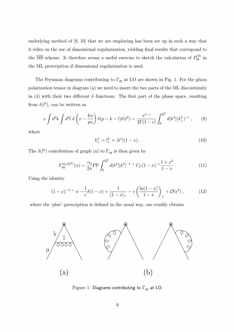
The Feynman diagrams contributing to Γqq at LO are shown in Fig. 1. For the gluon

polarization tensor in diagram (a) we need to insert the two parts of the ML discontinuity

in (4) with their two different δ–functions. The first part of the phase space, resulting

from δ(l2), can be written as

x

∫ddk

∫ddl δ

(x−

kn

pn

)δ(p− k − l)δ(l2) =

π1−ε

2Γ(1− ε)

∫ Q2

0

d|k2|(k2⊥)−ε , (9)

where

k2⊥ = l2⊥ = |k2|(1− x) . (10)

The δ(l2) contribution of graph (a) to Γqq is then given by

Γ(a),δ(l2)qq (x) =

αs2π

PP

∫ Q2

0

d|k2||k2|−1−ε CF (1− x)−ε1 + x2

1− x. (11)

Using the identity

(1− x)−1−ε ≡ −1

εδ(1− x) +

1

(1− x)+− ε

(ln(1− x)

1− x

)+

+O(ε2) , (12)

where the ‘plus’–prescription is defined in the usual way, one readily obtains

(a) (b)

p

kl

Figure 1: Diagrams contributing to Γqq at LO.

6

Γ(a),δ(l2)qq (x) =

αs2π

PP

∫ Q2

0

d|k2||k2|−1−ε CF

[−

2

εδ(1− x) +

1 + x2

(1− x)+

]. (13)

For the ghost–like part we introduce the variable κ as

k2⊥ = l2⊥ = −l2 = |k2|κ . (14)

The phase space is then given by∫ddk

∫ddl δ

(x−

kn

pn

)δ(p− k − l)δ(l2 + l2⊥)

=π1−ε

2Γ(1− ε)

∫ Q2

0

d|k2|

∫ 1

0

dκ(k2⊥

)−εδ ((1− x)(1− κ))

=π1−ε

2Γ(1− ε)δ(1− x)

∫ Q2

0

d|k2|

∫ 1

0

dκ

1− κ

(k2⊥

)−ε, (15)

where the last line follows since the root of the delta function for κ = 1 never contributes

when we insert the second term in (4) for the gluon polarization tensor into graph (a),

thanks to the factor 2n∗l/l2⊥ ∼ (1− κ)/κ accompanying the δ(l2 + l2⊥) in (4). Thus, the

ghost part contributes only at x = 1. The contribution ∼ 1/κ of 2n∗l/l2⊥ gives rise to a

1/ε–pole in the final answer:

Γ(a),δ(l2+l2⊥)qq (x) =

αs2πδ(1− x)PP

∫ Q2

0

d|k2||k2|−1−ε CF

[2

ε

]. (16)

Adding Eqs. (13) and (16), we get the full contribution of graph (a) to Γqq:

Γ(a)qq (x) =

αs2π

PP

∫ Q2

0

d|k2||k2|−1−ε CF1 + x2

(1− x)+

. (17)

An important feature of this result should be emphasized, as it will also be encountered at

NLO: the integrand in (17) is completely finite, in a distributional sense. In other words,

using the ML prescription, we have verified the finiteness of the LO 2PI kernel q → qg

in the light–cone gauge. We point out, however, that the finite 2PI kernel arises as the

sum of the two singular pieces in Eqs. (13),(16). This is again a finding that will recur

at NLO: the full discontinuity (4) of the gluon propagator in the ML prescription has a

much milder behaviour than the individual contributions to it.

It is instructive to contrast the result in (17) with the one obtained for the PV pre-

scription [9]:

Γ(a),PVqq (x) =

αs2π

PP

∫ Q2

0

d|k2||k2|−1−ε CF

[1 + x2

(1− x)++ 2I0δ(1− x)

], (18)

7

where

I0 ≡

∫ 1

0

u

u2 + δ2du ≈ − ln δ . (19)

Thus, the 2PI kernel for the PV prescription has a divergent coefficient of δ(1 − x),

resulting from the gauge denominator 1/nl and being regularized by the parameter δ.

The calculation of the LO splitting function is completed by determining the endpoint

contributions at x = 1, corresponding to Zq in (5) and given by the graphs in Fig. 1(b).

They can be straightforwardly obtained1 using the UV–singular structure of the one–loop

quark self–energy, determined for the ML prescription in [18]. One finds [7]:

Zq = 1−αs2π

1

εCF

3

2, that is, ξ(0)

q =3

2CF . (20)

Putting everything together, one eventually obtains

P (0)qq (x) = CF

[1 + x2

(1− x)+

+3

2δ(1− x)

], (21)

in agreement with [13]. We finally note that of course the same final answer is obtained

within the PV prescription: the singular integral I0 in (18) is cancelled by the contribution

from Zq, since we have [9]

ZPVq = 1−

αs2π

1

εCF

[3

2− 2I0

]. (22)

Thus, to summarize, the advantage of the ML prescription at the LO level mainly amounts

to producing truly finite results for the 2PI kernels, as required for the method of [11, 9, 10].

Furthermore, there is no need for introducing renormalization constants depending on

additional singular quantities like I0 that represent a mix–up in the treatment of UV and

IR singularities.

1Alternatively one can obtain the contributions from the requirement∫ 1

0P

(0)qq (x)dx = 0 [13, 9].

8

3 The calculation of the flavour non–singlet splitting

function at NLO

At NLO, there are two different non–singlet evolution kernels, P−,(1) and P+,(1), governing

the evolutions of the quark density combinations q − q and q + q − (q′ + q′), respectively.

The two kernels are given in terms of the (flavour–diagonal) quark–to–quark and quark–

to–antiquark splitting functions by (see, for instance, Ref. [12])

P±,(1) ≡ P V,(1)qq ± P V,(1)

qq , (23)

where the last splitting function originates from a tree graph that does not comprise

any real–gluon emission and is therefore free of any problems related to the use of the

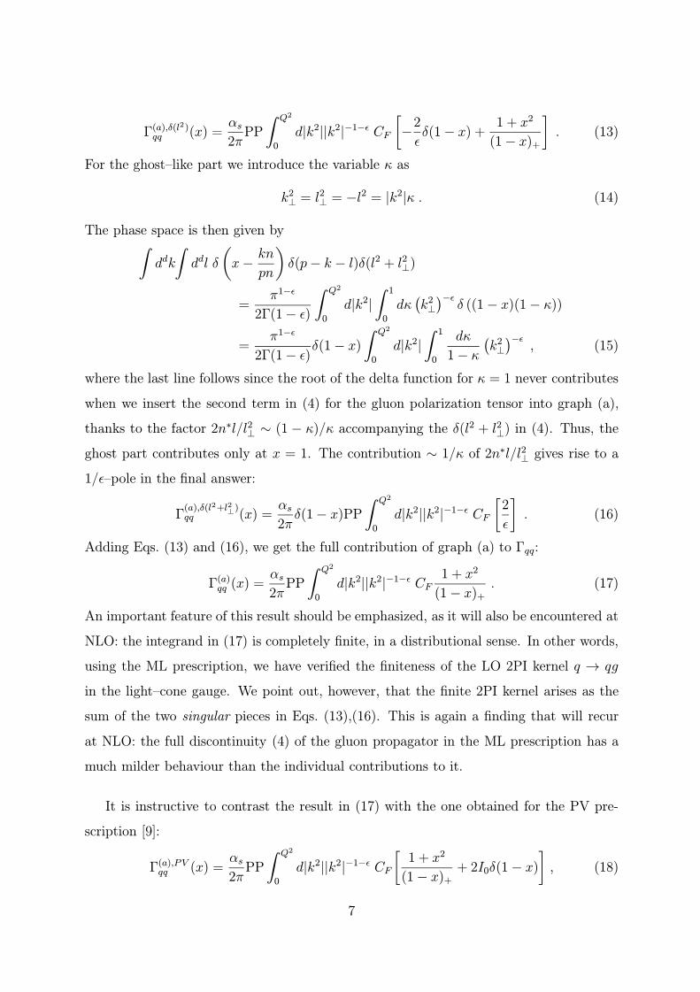
light–cone gauge. Thus, we do not need to recalculate PV,(1)qq . The Feynman diagrams

contributing to PV,(1)qq are collected in Fig. 2. We have labelled the graphs according to

the notation of [9, 12]. We also show the graphs contributing to Zq at two loops. We will

not calculate all of these, since this is not really required. Their role will be discussed in

subsection 3.4.

3.1 Virtual–cut diagrams and renormalization

Many of the diagrams in Fig. 2 have real and virtual cuts, as has been indicated by the

dashed lines. Let us start by discussing the contributions from the virtual cuts in graphs

(c),(d),(e),(f),(g). It is clear that these essentially have the LO topology in the sense

that there is always one outgoing gluon (momentum l), to be treated according to the

ML prescription as discussed in the previous section. We recall that this means that

there are two contributions for this gluon, one at l2 = 0, and the other with l2 + l2⊥ = 0,

corresponding to the gluon acting as an axial ghost2. This immediately implies that we

will have to calculate the loop integrals for these two situations. In addition, it is clear

that the ML prescription also has to be used in the calculation of the loop itself, not just

2In the next subsection we will see that for diagrams (d),(f) there are also other contributions atl2 + l2⊥ = 0, not just the one from the axial ghost going into the loop. However, the integration of thosecontributions proceeds in exactly the same way as outlined here. We postpone the discussion of all thecontributions at l2 + l2⊥ = 0 for graphs (d),(f) to the next subsection.

9

C2F

p

k

l1

l2

(h�i) (c) (b) (e)

(c) (b) (d) (f)

(g)

12CFNC

CFTf

�(1)q

Figure 2: Diagrams contributing to Γqq at NLO.

for the treatment of the external gluon. For instance, the gauge denominator 1/(r · n),

where r is the loop momentum, is subject to the prescription (1). In short, we will need

several two–point and three–point functions with and without gauge denominators like

1/(n · r), and for both l2 = 0 and l2 + l2⊥ = 0.

We point out that important qualitative differences with respect to the PV prescription

arise here: in the PV calculation one always has l2 = 0 for the outgoing gluon in the

10

virtual–cut graphs, and there is no explicit dependence on l2⊥. For instance, the way to

deal with the self–energies in graphs (f),(g) in the PV prescription is identical to their

treatment in covariant gauges: one calculates them for off–shell l2, renormalizes them, and

eventually takes the limit l2 → 0. In this way, almost all contributions of the diagrams

will vanish since all loop integrals have to be proportional to (l2)−ε (ε < 0) on dimensional

grounds. Only the contribution from the MS counterterm remains [19, 9] because this is

the only quantity not proportional to (l2)−ε. In contrast to this, in the ML prescription l2⊥

sets an extra mass scale. For graph (f), one therefore encounters terms ∼ (l2)−ε, but also

terms of the form ∼ (a l2 + b l2⊥)−ε. The latter terms yield non–vanishing contributions to

the virtual–cut result even at l2 = 0. This is still not the case for graph (g) since here the

pure quark loop of course does not contain any light–cone gauge denominator and thus

does not depend on l2⊥. Nevertheless, one gets a contribution from the quark loop in (g)

for l2 + l2⊥ = 0, i.e., when the gluon running into the loop is an axial ghost, corresponding

to the second part of the ML discontinuity in (4).

As expected, in the actual derivation of the loop integrals the property of the ML

prescription to allow a Wick rotation is of great help. Nevertheless, some of the integrals

are quite involved, since the ML prescription introduces explicit dependence of the loop

integrands on the transverse components r2⊥ due to the identity 2(nr)(n∗r) = r2 + r2

⊥.

Furthermore, since we are interested in calculating also the contributions at x = 1, we

need to calculate the loop integrals up to O(ε) rather than O(1). The reason for this

is that very often the final answer for a loop calculation with l2 = 0 will contain terms

of the form (1 − x)−1−aε (a = 1, 2), to be expanded according to Eq. (12). As a result,

a further pole factor 1/ε is introduced into the calculation, yielding finite contributions

when multiplied by the O(ε) terms in the loop integrals. A similar thing happens in the

loop part with l2 + l2⊥ = 0. Here, an extra factor 1/ε can be introduced when integrating

this part over the phase space in (15). The higher pole terms created in these ways will

cancel out eventually, but not the finite parts they have generated in intermediate steps

of the calculation. The detailed expressions for the loop integrals in the ML prescription

are given in Appendix A.

11

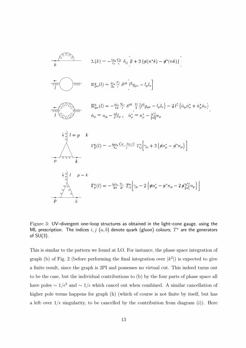
For the renormalization of the loop diagrams, one needs to subtract their UV poles,

which is achieved in the easiest way by inserting the UV–divergent one–loop structures as

calculated for the light–cone gauge in the ML prescription in [6, 18, 20, 21]. All structures

have also been compiled in [2]. The ones we need for the non–singlet calculation are

displayed in Fig. 3. One notices that, as expected, the structures are gauge–dependent

and Lorentz non–covariant. Even more, the expressions for the non–Abelian quantities

Πgµν and Γgµ in Fig. 3 are non–polynomial in the external momenta, owing to terms ∼

1/[nl]. It is an important feature of the ML prescription that these non–local terms exist,

but decouple from physical Green’s functions [4] thanks to the orthogonality of the free

propagator with respect to the gauge vector, nµDµν(l) = 0 (this has actually been an

important ingredient for the proof [4] of the renormalizability of QCD in the ML light–

cone gauge). Thus, the non–local pole parts never appear in our calculation. This is in

contrast to the PV prescription, where one has [9] contributions from the renormalization

constants to the calculation that explicitly depend on the external momentum fractions

x, 1− x.

3.2 Real–cut graphs

Let us now deal with the real cuts. One way of evaluating these is to integrate over

the phase space of the two outgoing particles with momenta l1,l2 (for the notation of

the momenta, see Fig. 2), in addition to the integration over the ‘observed’ parton with

momentum k. This is the strategy we have adopted for all diagrams contributing to the

C2F and the CFTf parts of the splitting function, i.e., graphs (b),(c),(g),(h). For graphs

(d),(f), we found it simpler to use a different method, as will be pointed out below.

If the two outgoing partons are gluons, their phase space in the ML prescription splits

up into four pieces, as we discussed in Sec. 1. It is possible to write down a phase space

that deals with all four parts. We leave the details for Appendix B.

Upon integration of the squared real–cut matrix element for a diagram, each of the four

parts of phase space gives highly divergent results, but their sum is usually less singular.

12

k�(k) = � i�s

4�CF

��ij

"6k + 2 f6n(n�k)� 6n�(nk)g

#

l�q

��(l) =i�s3�

Tf��ab

"l2g�� � l�l�

#

l

�g��(l) = � i�s

4�NC

��ab

"113

nl2g�� � l�l�

o� 2 l2

nn�n

�

� + n��n�

o #

n� � n� �nll2l� ; n�� � n�� �

n�l[nl]

n�

p k

l = p� k

�q�(l) = � ig�s

4�CF�NC=2

�T aij

" � + 2

n6nn�� � 6n

�n�

o #

p k

l = p� k

�g�(l) = � ig�s

4�NC

2�T aij

" � � 2

�6nn�� + 6n

�n� � 2 6nn�l[nl]

n�

� #

Figure 3: UV–divergent one–loop structures as obtained in the light–cone gauge, using theML prescription. The indices i, j (a, b) denote quark (gluon) colours; T a are the generatorsof SU(3).

This is similar to the pattern we found at LO. For instance, the phase space integration of

graph (b) of Fig. 2 (before performing the final integration over |k2|) is expected to give

a finite result, since the graph is 2PI and possesses no virtual cut. This indeed turns out

to be the case, but the individual contributions to (b) by the four parts of phase space all

have poles ∼ 1/ε2 and ∼ 1/ε which cancel out when combined. A similar cancellation of

higher pole terms happens for graph (h) (which of course is not finite by itself, but has

a left–over 1/ε singularity, to be cancelled by the contribution from diagram (i)). Here

13

even poles ∼ 1/ε3 occur at intermediate stages of the calculation. For those graphs that

also have virtual cuts, the situation is in general even more complicated, as cancellations

will occur only in the sum of the real and virtual cuts. An example for this case will be

given in sec. 3.3.

For graphs (d),(f), the phase space integrals become extremely complicated. This is

due to the extra denominator 1/(l1 + l2)2 present in these graphs, which causes great

complications in the axial–ghost parts of the phase space. For (f), we found it still

possible to get the correct result via the ‘phase space method’, but for (d) this seemed a

forbidding task. It turned out to be more convenient to determine the result in a different

way: if one calculates, for instance, the gluon loop in graph (f) for an arbitrary off–shell

momentum l going into the loop, the imaginary part of the loop will correspond to the

real–cut contribution we are looking for. To be more precise, the strategy goes as follows:

we calculate the loop graph for off–shell l and insert the result into the appropriate LO

phase space. The latter can be derived as in (9), omitting, however, the δ(l2) there. One

finds

x

∫ddk

∫ddl δ

(x−

kn

pn

)δ(p− k − l) =

π1−ε

2Γ(1− ε)

∫ Q2

0

d|k2|

∫ 1/(1−x)

0

dτ (k2⊥)−ε , (24)

where now

k2⊥ = l2⊥ = |k2|(1− x)τ , l2 =

|k2|(1− x)

x(1− τ) . (25)

The limits for the τ integration in (24) span the largest possible range for τ , given by the

conditions l2⊥ > 0, l2 + l2⊥ > 0. The full imaginary part arising when performing the loop

and the τ integrations has to correspond to the sum over all cuts in the diagram. One

encounters discontinuities from the following sources:

(A) from the loop integrations. Here imaginary parts arise, for instance, if for certain

values of τ and of the Feynman parameters t1, . . . , tk, one finds terms of the form(f(t1, . . . , tk, τ)

)−ε, (26)

where f is negative. Details for integrals with such properties are given in Ap-

pendix C. The imaginary part originating in this way essentially corresponds to the

cut through the loop itself, i.e., to the real–cut contribution we are looking for.

14

(B) from the propagator 1/(l2 + iε) via the identity

1

l2 + iε= PV

(1

l2

)− iπδ(l2) , (27)

where PV denotes the principal value. The imaginary part ∼ δ(l2) obviously repre-

sents the loop contribution at l2 = 0 which we have determined in the last subsection.

Therefore, we do not need to reconsider this part of the discontinuity.

(C) from terms ∼ 1/[nl], for which a relation similar to (27) holds,

1

[nl]≡

1

nl + iεsign(n∗l)= PV

(1

nl

)− iπsign(n∗l)δ(nl) . (28)

At first sight, one might think that the discontinuity ∼ δ(nl) simply corresponds

to the calculation of the gluon loop for the case when the gluon entering the loop

is an axial ghost with l2 = −l2⊥. However, the situation is more subtle: The terms

∼ 1/[nl] do not only originate from the propagators of the external gluons, but also

from splitting formulas like [2]

1

[nr][n(l − r)]=

1

[nl]

(1

[nr]+

1

[n(l − r)]

)(29)

(where r is the loop momentum), as well as from the loop integrals themselves, like

in the case of ∫ddr

(2π)d1

(r2 + iε)((l − r)2 + iε)[nr]. (30)

All these terms ∼ 1/[nl] have to be treated according to the ML prescription, i.e.,

give rise to discontinuities ∼ δ(nl) ∼ δ(1−x) via (28). The sum of all discontinuities

arising in this way actually has to correspond to the ‘pure–axial–ghost’ part of the

graph, given by (a) the virtual–cut contribution when the gluon going into the loop

is an axial ghost, plus (b) the real–cut contribution when both final–state gluons act

as axial ghosts. These two parts cannot easily be separated from each other, which

is the reason why we postponed the whole treatment of graphs (d),(f) at l2 = −l2⊥ to

this section. The integrals needed to obtain this part of the discontinuity are those

already mentioned in the last subsection and collected in the right–hand column of

Tab. 4 of Appendix A.

15

It is also worth mentioning that despite the fact that graph (f) has a squared gluon propa-

gator, there are cancellations coming from the algebra in the numerator; as a consequence,

one never encounters expressions like 1/[nl]2 or 1/(l2+iε)2 before taking the discontinuity,

and (28),(27) are all we need.

Clearly, when finally collecting all the imaginary parts from (A) and (C), the PV–parts

in (B) and (C) play a role in the calculation. While 1/nl ∼ 1/(1−x) in (28) only diverges

at the endpoint at x = 1 where it is always regularized by factors like (1 − x)−ε, the

propagator 1/l2 in (27) in general has its singularity inside the region of the τ integration:

from (25) one finds that l2 > 0 for τ < 1, but l2 < 0 for τ > 1. The principal value

prescription3 in (27) takes care of the pole at τ = 1 and leads to a cancellation of the

positive spike for τ → 1− and the negative one for τ → 1+, resulting in a perfectly

well–defined finite result.

The vertex graph (d) can be treated in a similar fashion as (f). Here one calculates

the full vertex for p2 = 0, k2 < 0, but arbitrary l2, and determines the imaginary parts

arising with respect to l2. This corresponds again to point (A) above, and calculational

details are also given in Appendix C. The imaginary part from (B) is again related to the

virtual–cut contribution at l2 = 0 that we already calculated in the last subsection. The

discontinuity from (C) needs to be taken into account, and as before it corresponds to the

full ‘pure–ghost’ contribution (virtual–cut and real–cut), residing at x = 1.

A final comment concerns graph (i). Its contribution to Γqq is essentially given by a

convolution of two LO expressions, each corresponding to Fig. 1(a), keeping however also

all finite terms in the upper part of the diagram, including the factor (1−x)−ε from phase

space (see (11),(12)):

(i) ∼1

ε

[1 + z2

(1− z)+− ε(1 + z2)

(ln(1− z)

1− z

)+

− ε(1− z)

]⊗

1

ε

[1 + z2

(1− z)+

], (31)

where (f ⊗ g

)(x) ≡

∫ 1

x

dz

zf(xz

)g(z) . (32)

3To avoid confusion, we emphasize at this point that the principal value for 1/l2 in (27) is well–defined here and not related to the principal value prescription for the light–cone denominator 1/nl thatwe heavily criticised in the introduction.

16

Note that this is in contrast to the PV prescription where the contribution from (i) does

not correspond to a genuine convolution in the mathematical sense. Since both of the

convoluted functions in (31) contain distributions, the convolution itself will also be a

distribution. The evaluation of (31) is most conveniently performed in Mellin–moment

space where convolutions become simple products. Some details of the calculation and a

few non–standard moment expressions are given in Appendix D.

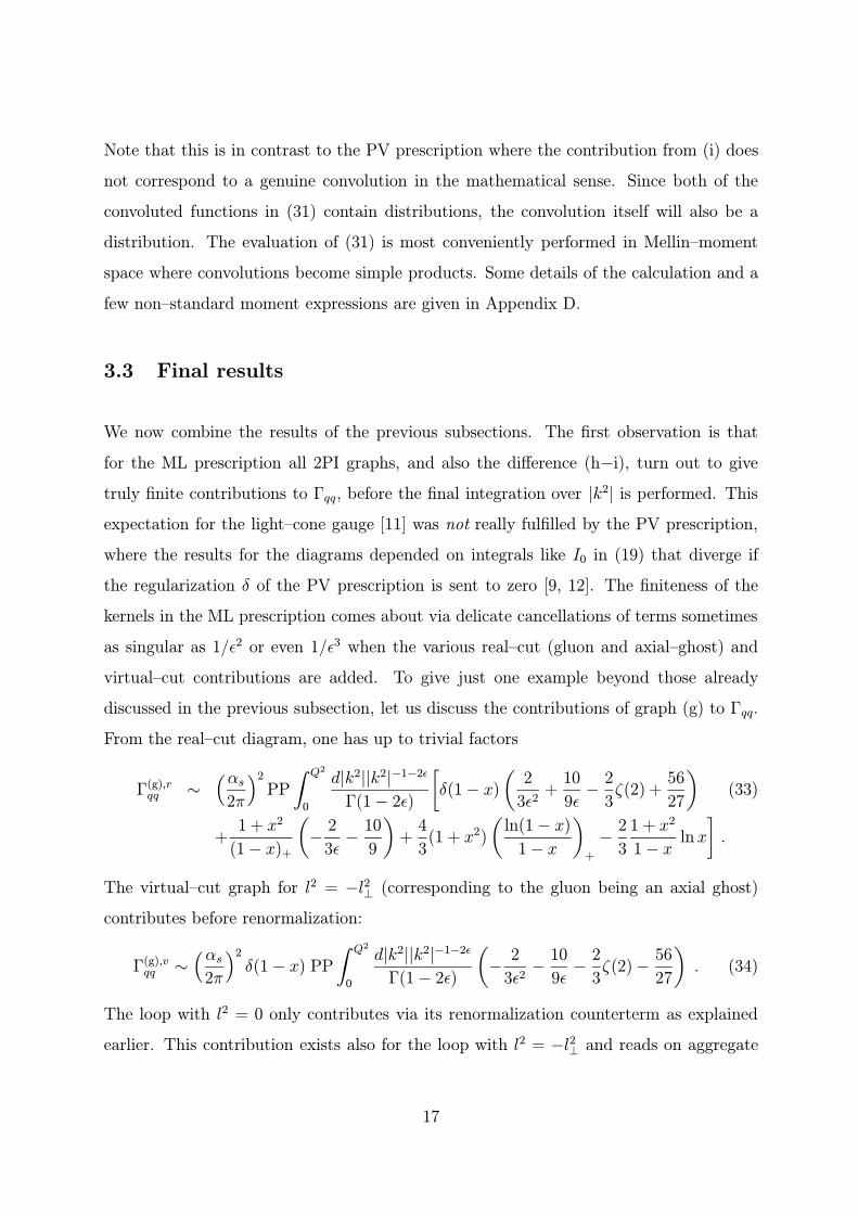
3.3 Final results

We now combine the results of the previous subsections. The first observation is that

for the ML prescription all 2PI graphs, and also the difference (h−i), turn out to give

truly finite contributions to Γqq, before the final integration over |k2| is performed. This

expectation for the light–cone gauge [11] was not really fulfilled by the PV prescription,

where the results for the diagrams depended on integrals like I0 in (19) that diverge if

the regularization δ of the PV prescription is sent to zero [9, 12]. The finiteness of the

kernels in the ML prescription comes about via delicate cancellations of terms sometimes

as singular as 1/ε2 or even 1/ε3 when the various real–cut (gluon and axial–ghost) and

virtual–cut contributions are added. To give just one example beyond those already

discussed in the previous subsection, let us discuss the contributions of graph (g) to Γqq.

From the real–cut diagram, one has up to trivial factors

Γ(g),rqq ∼

(αs2π

)2

PP

∫ Q2

0

d|k2||k2|−1−2ε

Γ(1− 2ε)

[δ(1− x)

(2

3ε2+

10

9ε−

2

3ζ(2) +

56

27

)(33)

+1 + x2

(1− x)+

(−

2

3ε−

10

9

)+

4

3(1 + x2)

(ln(1− x)

1− x

)+

−2

3

1 + x2

1− xlnx

].

The virtual–cut graph for l2 = −l2⊥ (corresponding to the gluon being an axial ghost)

contributes before renormalization:

Γ(g),vqq ∼

(αs2π

)2

δ(1− x) PP

∫ Q2

0

d|k2||k2|−1−2ε

Γ(1− 2ε)

(−

2

3ε2−

10

9ε−

2

3ζ(2)−

56

27

). (34)

The loop with l2 = 0 only contributes via its renormalization counterterm as explained

earlier. This contribution exists also for the loop with l2 = −l2⊥ and reads on aggregate

17

for both loop parts:

Γ(g),‘ren′

qq ∼(αs

2π

)2

PP

∫ Q2

0

d|k2||k2|−1−ε

Γ(1− 2ε)

2

3

[1

ε

1 + x2

(1− x)+− (1 + x2)

(ln(1− x)

1− x

)+

− 1 + x

].

(35)

When adding the integrands of Eqs. (33)–(35), all poles cancel, and as promised the

contribution to Γqq is finite before integration over |k2|.

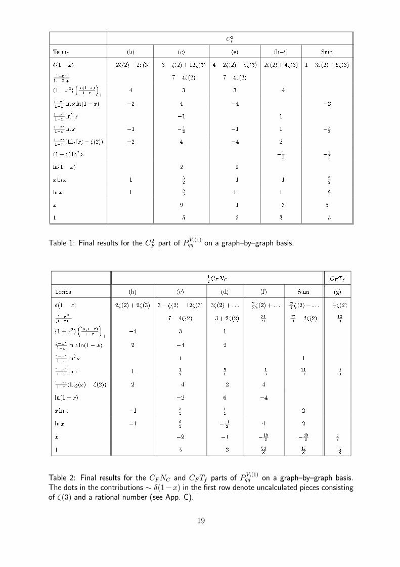
Next, we determine the contributions of the various graphs to PV,(1)qq , making use of

Eq. (7). The results are displayed in Tables 1 and 2. We see that all entries in the tables

are completely well–defined, even at x = 1, in terms of distributions, which is a property

that we already encountered at LO.

The sums of the various graph–by–graph contributions are also presented in Tables 1,2.

One realizes that many more complicated structures, like the dilogarithm Li2(x), cancel

in the sums. Considering only x < 1 for the moment, it is the most important finding of

this work that the entries in the columns ‘Sum’ in Tables 1,2 exactly reproduce the results

found in the PV calculations [9, 12] for x < 1. Since the latter are in agreement with

those obtained in the covariant–gauge OPE calculations [22], we conclude that the ML

prescription has led to the correct final result. To a certain extent, this is a check on the

prescription itself in the framework of a highly non–trivial application. Since – in contrast

to the PV recipe – the ML prescription possesses a solid field–theoretical foundation [3, 4],

our calculation has finally provided a ‘clean’ derivation of the NLO flavour non–singlet

splitting function within the CFP method, highlighting the viability of that method.

The next subsection will address the endpoint (δ(1 − x)) contributions to the NLO

flavour non–singlet splitting function.

18

C2

F

Terms (b) (c) (e) (h�i) Sum

�(1� x) �2�(2)� 2�(3) �3� �(2) + 12�(3) 4� 2�(2)� 8�(3) 2�(2) + 4�(3) 1� 3�(2) + 6�(3)

1+x2

(1�x)+�7 + 4�(2) 7� 4�(2)

(1 + x2)�ln(1�x)

1�x

�+

4 �3 3 �4

1+x2

1�xlnx ln(1� x) �2 4 �4 �2

1+x2

1�xln

2 x �1 1

1+x2

1�xlnx �1 �

12

�1 1 �

32

1+x2

1�x(Li2(x) � �(2)) �2 4 �4 2

(1 + x) ln2 x �

12

�

12

ln(1� x) 2 �2

x lnx 1 �

52

�1 �1 �

72

lnx 1 �

92

1 1 �

32

x 9 �1 �3 5

1 �5 �3 3 �5

Table 1: Final results for the C2F part of P

V,(1)qq on a graph–by–graph basis.

12CFNC CFTf

Terms (b) (c) (d) (f) Sum (g)

�(1� x) 2�(2) + 2�(3) 3 + �(2)� 12�(3) 5�(2) + : : : �

23�(2) + : : : 22

3�(2) + : : : �

43�(2)

1+x2

(1�x)+7� 4�(2) �3 + 2�(2) 31

9679� 2�(2) �

109

(1 + x2)�ln(1�x)

1�x

�+

�4 3 1

1+x2

1�xlnx ln(1� x) 2 �4 2

1+x2

1�xln

2 x 1 1

1+x2

1�xlnx 1 1

252

�

13

113

�

23

1+x2

1�x(Li2(x)� �(2)) 2 �4 �2 4

ln(1� x) �2 6 �4

x ln x �1 52

12

2

lnx �1 92

�

112

4 2

x �9 �1 �

103

�

403

43

1 5 �3 343

403

�

43

Table 2: Final results for the CFNC and CFTf parts of PV,(1)qq on a graph–by–graph basis.

The dots in the contributions ∼ δ(1−x) in the first row denote uncalculated pieces consistingof ζ(3) and a rational number (see App. C).

19

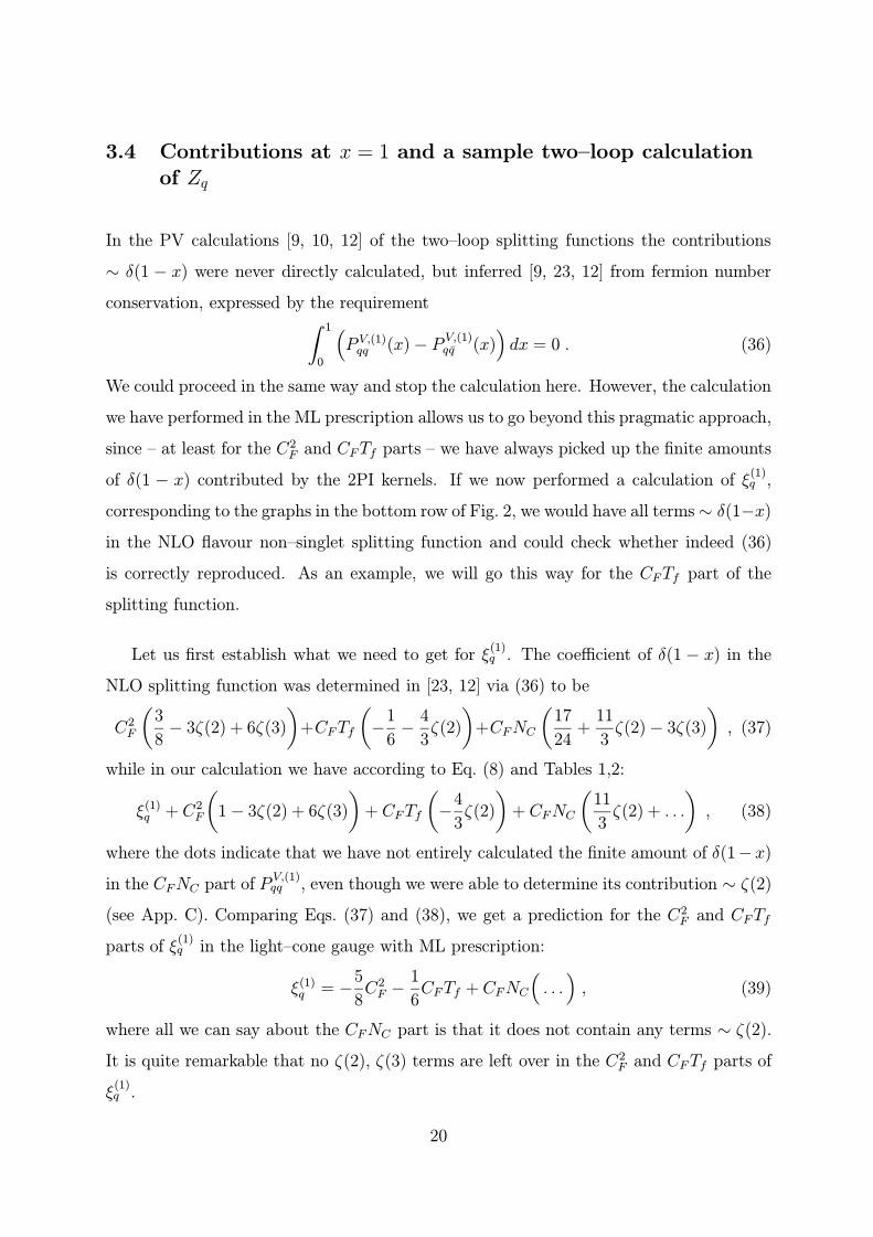
3.4 Contributions at x = 1 and a sample two–loop calculationof Zq

In the PV calculations [9, 10, 12] of the two–loop splitting functions the contributions

∼ δ(1 − x) were never directly calculated, but inferred [9, 23, 12] from fermion number

conservation, expressed by the requirement∫ 1

0

(P V,(1)qq (x)− P V,(1)

qq (x))dx = 0 . (36)

We could proceed in the same way and stop the calculation here. However, the calculation

we have performed in the ML prescription allows us to go beyond this pragmatic approach,

since – at least for the C2F and CFTf parts – we have always picked up the finite amounts

of δ(1 − x) contributed by the 2PI kernels. If we now performed a calculation of ξ(1)q ,

corresponding to the graphs in the bottom row of Fig. 2, we would have all terms∼ δ(1−x)

in the NLO flavour non–singlet splitting function and could check whether indeed (36)

is correctly reproduced. As an example, we will go this way for the CFTf part of the

splitting function.

Let us first establish what we need to get for ξ(1)q . The coefficient of δ(1 − x) in the

NLO splitting function was determined in [23, 12] via (36) to be

C2F

(3

8− 3ζ(2) + 6ζ(3)

)+CFTf

(−

1

6−

4

3ζ(2)

)+CFNC

(17

24+

11

3ζ(2)− 3ζ(3)

), (37)

while in our calculation we have according to Eq. (8) and Tables 1,2:

ξ(1)q + C2

F

(1− 3ζ(2) + 6ζ(3)

)+ CFTf

(−

4

3ζ(2)

)+ CFNC

(11

3ζ(2) + . . .

), (38)

where the dots indicate that we have not entirely calculated the finite amount of δ(1−x)

in the CFNC part of PV,(1)qq , even though we were able to determine its contribution ∼ ζ(2)

(see App. C). Comparing Eqs. (37) and (38), we get a prediction for the C2F and CFTf

parts of ξ(1)q in the light–cone gauge with ML prescription:

ξ(1)q = −

5

8C2F −

1

6CFTf + CFNC

(. . .), (39)

where all we can say about the CFNC part is that it does not contain any terms ∼ ζ(2).

It is quite remarkable that no ζ(2), ζ(3) terms are left over in the C2F and CFTf parts of

ξ(1)q .

20

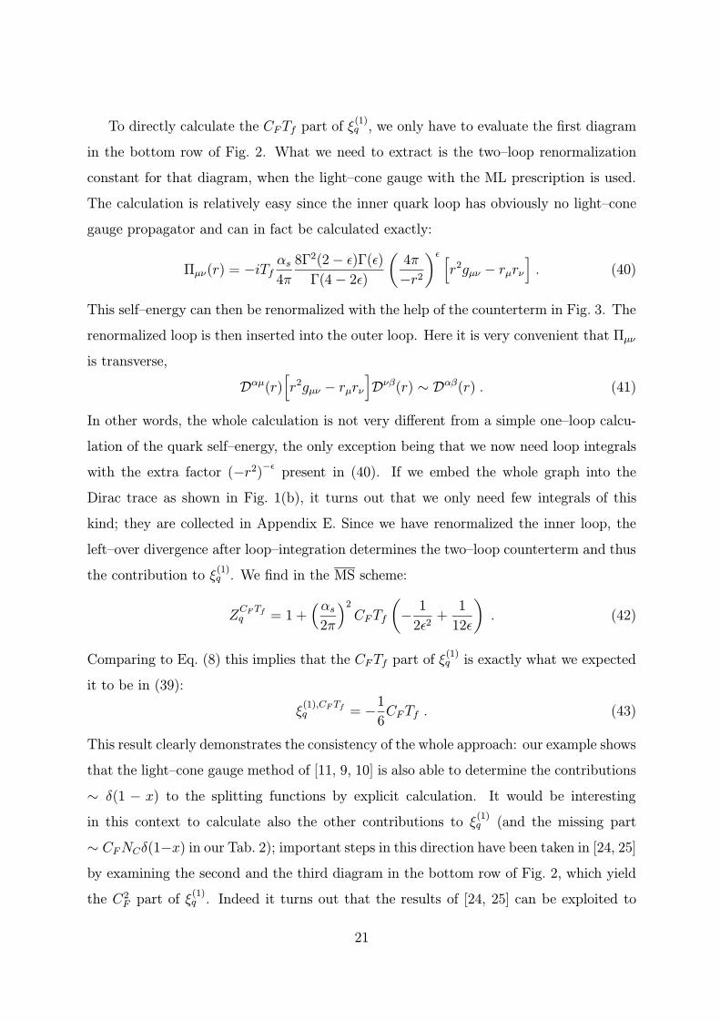
To directly calculate the CFTf part of ξ(1)q , we only have to evaluate the first diagram

in the bottom row of Fig. 2. What we need to extract is the two–loop renormalization

constant for that diagram, when the light–cone gauge with the ML prescription is used.

The calculation is relatively easy since the inner quark loop has obviously no light–cone

gauge propagator and can in fact be calculated exactly:

Πµν(r) = −iTfαs

4π

8Γ2(2− ε)Γ(ε)

Γ(4− 2ε)

(4π

−r2

)ε [r2gµν − rµrν

]. (40)

This self–energy can then be renormalized with the help of the counterterm in Fig. 3. The

renormalized loop is then inserted into the outer loop. Here it is very convenient that Πµν

is transverse,

Dαµ(r)[r2gµν − rµrν

]Dνβ(r) ∼ Dαβ(r) . (41)

In other words, the whole calculation is not very different from a simple one–loop calcu-

lation of the quark self–energy, the only exception being that we now need loop integrals

with the extra factor (−r2)−ε

present in (40). If we embed the whole graph into the

Dirac trace as shown in Fig. 1(b), it turns out that we only need few integrals of this

kind; they are collected in Appendix E. Since we have renormalized the inner loop, the

left–over divergence after loop–integration determines the two–loop counterterm and thus

the contribution to ξ(1)q . We find in the MS scheme:

ZCFTfq = 1 +

(αs2π

)2

CFTf

(−

1

2ε2+

1

12ε

). (42)

Comparing to Eq. (8) this implies that the CFTf part of ξ(1)q is exactly what we expected

it to be in (39):

ξ(1),CFTfq = −

1

6CFTf . (43)

This result clearly demonstrates the consistency of the whole approach: our example shows

that the light–cone gauge method of [11, 9, 10] is also able to determine the contributions

∼ δ(1 − x) to the splitting functions by explicit calculation. It would be interesting

in this context to calculate also the other contributions to ξ(1)q (and the missing part

∼ CFNCδ(1−x) in our Tab. 2); important steps in this direction have been taken in [24, 25]

by examining the second and the third diagram in the bottom row of Fig. 2, which yield

the C2F part of ξ

(1)q . Indeed it turns out that the results of [24, 25] can be exploited to

21

reproduce the term −5C2F/8 in our prediction (39) for ξ

(1)q , which can be regarded as a

further confirmation of our results.

We have to admit, however, at this point that the ability to obtain the correct endpoint

contributions is not restricted to the ML prescription: this is also possible for the PV

prescription. Here, the coefficient of δ(1− x) in the CFTf part of PV,(1)qq reads

ξ(1),CF Tfq,PV − CFTf

20

9I0 . (44)

Here the second term originates from the entry ‘−10/9’ in the last column of Tab. 2, when

we omit the ‘plus’–prescription there and reintroduce it using the PV identity [9]

1

1− x−→ I0δ(1− x) +

1

(1− x)+

, (45)

where I0 is as defined in (19). Furthermore, ξ(1),CF Tfq,PV denotes the CFTf part of ξ

(1)q when

the PV prescription is used. The explicit calculation gives

ZCFTfq,PV = 1 +

(αs2π

)2

CFTf

[−

1

2ε2

(1−

4

3I0

)+

1

ε

(1

12+

2

3ζ(2)−

10

9I0

)], (46)

that is

ξ(1),CFTfq,PV = CFTf

(−

1

6−

4

3ζ(2) +

20

9I0

). (47)

It is interesting to see how upon combining Eqs. (44) and (47) the I0 terms drop out,

and the CFTf part of the endpoint contributions comes out correctly as in (37) also for

the PV prescription. We note, however, that again this happens at the expense of having

renormalization constants depending on singular quantities like I0 that represent a mix–up

in the treatment of UV and IR singularities.

22

4 The calculation of the N2C part of the singlet

splitting function Pgg at NLO

Let us now turn to the calculation of P(1)gg . We restrict ourselves to its N2

C part, since

the contributions ∼ CFTf , NCTf are essentially trivial as far as the treatment of the

LCA is concerned: The CFTf part comprises no gluon emission at all, and all diagrams

contributing to the NCTf part contain a quark loop and the emission of at most one gluon.

Such diagrams with one–gluon emission have the LO kinematics and will not reveal any

new features as compared to what we have already discussed. In contrast to this, the

N2C part of P

(1)gg requires the renormalization of the non–Abelian part of the three–gluon

vertex and therefore really provides a further challenge for the ML prescription.

The diagrams contributing to the N2C part of Γgg at NLO are shown in Fig. 4. We do

not show here the graphs contributing to Zg at two loops, since we will not attempt to

calculate them.

N2C

(h�i) (d) (b) (e)

(f) (s1) (s2) (j) (k)

Figure 4: Diagrams contributing to the N2C part of Γgg at NLO.

23

The calculation of the various real–cut and virtual–cut diagrams proceeds in exactly

the same way as before. For the renormalization of the virtual–cut contributions in the

triangle graph (d) and the ‘swordfish’ ones (s1),(s2), we need the UV counter–term for

the three–gluon vertex in the light–cone gauge with ML prescription. Here we can rely

on the result presented in [26] (see also [27, 2]); the part of it that is relevant for our

calculation is recalled in Fig. 5.

Concerning the real cuts, we mention that for graphs (h),(b),(j),(k) we use the expres-

sion in (B.5) for the phase space. As for the CFNC part of PV,(1)qq , we found it easier to

determine the contributions of the real cuts of the remaining diagrams via the extraction

p2; a2 p3; a3

p1; a1 �1

�2 �3

T�1�2�3(p1; p2; p3) =ig�s4�

NC

2�fa1a2a3

"4

3A�1�2�3 + 2C�1�2�3 + : : :

#

p2; a2 p3; a3

p1; a1 �1

�2 �3+ perm.

S�1�2�3(p1; p2; p3) =ig�s4�

NC

2�fa1a2a3

"6A�1�2�3 � 6C�1�2�3 + : : :

#

��1�2�3(p1; p2; p3) = T�1�2�3(p1; p2; p3) + S�1�2�3(p1; p2; p3)

= ig�s4�

NC

�fa1a2a3

"11

3A�1�2�3 � 2C�1�2�3 + : : :

#

A�1�2�3= g�2�3(p2 � p3)�1 + g�3�1(p3 � p1)�2 + g�1�2(p1 � p2)�3

C�1�2�3= g�2�3n

�

�1(p2 � p3) � n+ g�3�1n

�

�2(p3 � p1) � n

+g�1�2n�

�3(p1 � p2) � n

sum

Figure 5: UV–divergent structures of the non–Abelian part of the three–gluon vertex asobtained in the light–cone gauge, using the ML prescription. p1,p2,p3 denote the momentaof the external gluons, a1,a2,a3 are the associated colour indices (fa1a2a3 being the structureconstants of SU(3)), and µ1,µ2,µ3 are Lorentz indices. The dots indicate structures (some ofthem non–local) which do not contribute to our calculation thanks to the orthogonality of thefree propagator to the gauge vector n.

24

of the imaginary parts of the associated virtual graphs.

We have verified that again for the ML prescription all 2PI graphs give truly finite

contributions to Γgg, before the final integration over |k2| is performed. This also applies

to the endpoint x = 1, where the result for each graph is again always well–defined in

terms of distributions and, as before, also has a coefficient of δ(1 − x) that contains no

1/ε poles. Table 3 presents the contributions of the various diagrams to P(1)gg . Here we

have defined the functions

pgg(x) ≡(1− x+ x2)

2

x(1− x)+,

lgg(x) ≡(1− x+ x2)

2

x

(ln(1− x)

1− x

)+

, (48)

S2(x) ≡

∫ 11+x

x1+x

dz

zln(1− z

z

)= −2Li2(−x)− 2 lnx ln(1 + x) +

1

2ln2 x− ζ(2) .

We mention in passing that graph (j) and the ‘swordfish’ diagram (s1) give vanishing

contributions to P(1)gg if the PV prescription is used, but are non–vanishing for the ML

prescription, where finite contributions arise from their ghost parts.

As for the case of PV,(1)qq , the full result for the N2

C part of P(1)gg , given by the column

‘Sum’, is (at x < 1) in agreement with the PV result of [10], which in turn coincides

with the OPE4 one [15]. Thus, the CFP method with ML prescription has also led to

the correct final answer in this case, which clearly constitutes a further non–trivial and

complementary check. As can be seen from Tab. 3, we have not determined the finite

amounts of contributions ∼ δ(1−x) for the graphs since, like in the case of the CFNC part

of PV,(1)qq , these are quite hard to extract in some cases. The endpoint contributions to

P(1)gg can then only be derived from the energy–momentum conservation condition [23, 12].

We emphasize however that, just as for PV,(1)qq , there is no principal problem concerning

the calculation of the endpoint contributions: had we calculated the full δ(1− x)–terms

in Tab. 3 and the two–loop quantity ξ(1)g , all endpoint contributions would be at our dis-

posal, and it would no longer be necessary to invoke the energy–momentum conservation

condition; in fact, this could serve as a further check of the calculation.

4See also our discussion in the introduction concerning the OPE calculations [15, 14] of P(1)gg .

25

N2 C

Terms

(b)

(d)

(s1+s2)

(e)

(f)

(h�

i)

(j)

(k)

Sum

pgg(x)

�

98 9

+6�(2)

1349

�

8�(2)

31 9

67 9

�

2�(2)

l gg(x)

4

�

10 3

22 3

�

8

pgg(x)lnxln(1�

x)

�

2

6

�

8

�

4

pgg(x)ln

2

x

�

1

2

1

pgg(x)lnx

�

3 2

11 6

�

3 2

�

1

�

1 3

1

3 2

pgg(x)(Li 2(x)�

�(2))

�

2

2

�

8

4

4

pgg(�x)S2(x)

2

2

(1+x)ln

2

x

4

4

x2

lnx

�

31 6

11 6

�

3 2

�

2

�

3

�

19 3

3 2

�

44 3

xlnx

�

8

�

52 3

3

4

6

16

11 3

lnx

�

17 2

26 3

�

3

�

5

�

5

3

3 2

�

25 3

1 xlnx

�

25 6

�

67 6

3 2

1

4

31 3

�

3 2

x2

ln(1�

x)

�

4

1

3

xln(1�

x)

13

�

3

�

4

�

6

ln(1�

x)

�

25 2

3 2

6

5

1 xln(1�

x)

8

�

4

�

4

x2

1369

13 3

9

1

�

20 3

�

46 3

67 9

x

�

1058

�

16 3

�

9

�

6

139

12

19 2

�

9 8

�

27 2

1

1058

59 6

�

9 2

12

�

103

12

�

19 2

9 8

27 2

1 x

�

1369

�

22 3

�

8

23 3

46 3

�

67 9

Table 3: Final results for the N2C part of P

(1)gg on a graph–by–graph basis. The table does not

include the coefficients of δ(1 − x), which we have not determined. However, as mentionedin the main text, we have proven that each graph contributes a finite amount of δ(1− x) toΓgg (before the final integration over |k2| is performed).

26

5 Conclusions

We have performed a new evaluation of the NLO flavour non–singlet splitting function

and of the N2C part of the NLO gluon–to–gluon splitting function within the light–cone

gauge method of [11, 9]. The new feature of our calculation is the use of the Mandelstam–

Leibbrandt prescription for dealing with the spurious poles generated by the gauge denom-

inator in the gluon propagator. In contrast to the principal value prescription employed

in previous calculations [9, 10, 12], the ML prescription has a solid field–theoretical foun-

dation and will therefore provide a ‘cleaner’ derivation of the result. As expected, the

final results come out correctly, i.e., are in agreement with the ones in [9, 10, 12, 22].

This finding is both a corroboration of the usefulness of the general method of [11, 9] to

calculate splitting functions, and a useful check on the ML prescription itself in a highly

non–trivial application.

We have also discussed the δ(1 − x) contributions to the NLO flavour non–singlet

splitting function, performing an explicit sample calculation of a two–loop contribution

to the renormalization constant Zq in the ML light–cone gauge. It turns out that one

indeed obtains the right amount of contributions at x = 1 as required by fermion number

conservation.

We conclude by conceding that the ML prescription is in general much more compli-

cated to handle than the simpler, but less well–founded, PV prescription. With regard to

future applications at, for instance, three–loop order, this creates a certain dilemma: the

ML prescription might be too complicated to be used in that case, while on the other hand

the ill–understood success of the PV prescription at the two–loop level is not a warranty

that it will also produce correct results beyond.

Acknowledgement

This work was supported in part by the EU Fourth Framework Programme ‘Training and

Mobility of Researchers’, Network ‘Quantum Chromodynamics and the Deep Structure

of Elementary Particles’, contract FMRX-CT98-0194 (DG 12-MIHT).

27

Appendix A: Virtual integrals

Here we list some loop integrals needed for the calculation. We do not need to recall any of

the covariant integrals, which are standard, but will only present those with a light–cone

gauge denominator, to be treated according to the ML prescription (1).

We begin by performing a sample calculation of the integral

I(n, q) ≡

∫ddr

(2π)d1

(r2 + iε)((q − r)2 + iε)[nr]

=

∫ddr

(2π)dn∗r

(r2 + iε)((q − r)2 + iε)(nr n∗r + iε). (A.1)

We recall the definitions [9]

n =pn

2P(1, 0, . . . , 0,−1) , n∗ =

P

pn(1, 0, . . . , 0, 1) ≡

1

pnp , (A.2)

where p = P (1, 0, . . . , 0, 1) is the momentum of the incoming quark, see Fig. 2. Introducing

Feynman parameters, one has

I(n, q) =4P

pn

∫ 1

0

dt

∫ 1−t

0

ds

∫ddr

(2π)dr0 − rz[

r2 + sr2⊥ − 2(q · r)t+ q2t+ iε

]3 . (A.3)

After performing a Wick rotation and straightforward integrations over r one arrives at

I(n, q) =iΓ(1 + ε)

16π2

2n∗q

q2 + iε

( 4π

−q2

)ε ∫ 1

0

dt t−ε(1−t)−1−ε

∫ 1

0

ds

(1+st

q2 + q2⊥ + iε

(q2 + iε)(1− t)

)−1−ε

.

(A.4)

For example, for the case q = k one finds

I(n, k) =iΓ(1 + ε)

16π2

( 4π

|k2|

)ε 1

[nk]

[ζ(2)− Li2

(k2⊥

|k2|

)+ 2εζ(3)

], (A.5)

where we have kept those terms that contribute to the final answer. In (A.5), ζ(n) is

Riemann’s ζ–function and Li2(x) denotes the dilogarithm, defined by [28]

Li2(z) ≡ −

∫ 1

0

ln(1− zy)

ydy . (A.6)

The result in (A.5) coincides with the one in [2] for ε = 0. Note that the ML prescription

arising for 1/[nk] is actually immaterial here since nk = x pn never vanishes.

28

Setting, on the other hand, q = l one gets for l2 = 0

I(n, l) =iΓ(1 + ε)

16π2

( 4π

−|k2|(1− x)

)ε 1

nl

1

2ε2, (A.7)

and for l2 = −l2⊥

I(n, l) =iΓ(1 + ε)

16π2

( 4π

−l2

)ε 2n∗l

l2B(−ε, 1− ε) . (A.8)

Note that the real part of (A.7) has to be taken5. Table 4 contains all the required

integrals with an ML light–cone gauge denominator. The integrals in the first column are

for l2 = 0; they depend on

x =nk

pnand x =

nl

pn= 1− x . (A.9)

Recall that terms ∼ (1 − x)−1−aε will lead to further poles, as was shown by (12). The

integrals in the second column of Tab. 4 are for the axial ghost case, l2 = −l2⊥, and

eventually need to be integrated further over the variable κ defined in Eqs. (15),(14). The

κ integration produces further poles. We have

κ =k2⊥

|k2|and κ = 1− κ . (A.10)

We note that the last integral was much easier obtained by performing the κ integration

before the ones over the Feynman parameters. Therefore we only present the final, κ–

integrated, result in this case. As can be seen, the integral was accompanied by two

different powers of κ.

5Here one obviously has to discard the overall factor i.

29

∫ddr/(2π)d l2 = 0 l2 + l2⊥ = 0

pnr2(k−r)2[nr]

1x

[ζ(2)− Li2 (x) + 2εζ(3)

]ζ(2)− Li2 (κ) + 2εζ(3)

(r2−2nk n∗r) pnr2(k−r)2[nr]

k2[

1ε

+ 2(1− lnx) + 1xLi2(x) k2κ

[1ε

+ 2(1− ln κ) + 1κLi2(κ)

− 1xζ(2) + ε (4 + ζ(2)− 2ζ(3))

]− 1κζ(2) + ε (4 + ζ(2)− 2ζ(3))

]pn

r2(l−r)2[nr]1

2ε2x−1−ε(1− ε2ζ(2) + 2ε3ζ(3)) −κ−ε 1

ε

(1− 1

κ

)(1 + ε2ζ(2))

(r2−2nl n∗r) pnr2(l−r)2[nr]

−2k2x−ε[

1ε

+ 2 + ε(4− ζ(2))]

0

pn(p−r)2(k−r)2[nr]

1x

[lnxε− 1

2ln2 x− Li2(x)

(1ε

+ 2 + 4ε+ εζ(2))

(κ−ε − 1)

−εx+ 2εζ(2) lnx]

+(1− 1

κ

)ln κ+ ε(3− ζ(2))

pn(p−r)2(l−r)2[nr]

does not occur 1ε2

(1 + ε2ζ(2)) (κ−ε − 1)

pn(k+r)2(l−r)2[nr]

(x−ε − x−ε)(

1ε2− ζ(2) + 2εζ(3)

)−κ−ε

[1ε2

+ 2ζ(2) + 2εζ(3)]

−3ζ(2)x−ε

pnr2(p−r)2(k−r)2[nr]

1k2

[1ε2

+ lnxε− 2Li2(x) 1

k2

[1ε2

(1− κ−ε)

−12

ln2 x− 2εζ(3)]

−κ−ε (Li2(κ) + ζ(2))

−2 (Li2(κ)− ζ(2) + εζ(3))]

pnr2(k+r)2(l−r)2[nr]

x−1−ε

k2

[3

2ε2+ lnx

ε− Li2(x) 1

k2κ

[1ε

ln κ+ Li2(κ)− 12

ln2 κ

−12

ln2 x− 52ζ(2)− ε (x+ 5ζ(3)) −κ−ε

(1ε2

+ 3ζ(2) + 6εζ(3)) ]

−12ε ln x(ln2 x− 2Li2(x)− lnx ln x)

]pn

r2(p−r)2(l−r)2[nr]does not occur 1

k2

[1

2ε3− ζ(2)

2ε− 3ζ(3)

](after integration

∫ 1

0dκκ−ε)

2k2

[1ε

+ 3 + ζ(2)]

(after integration∫ 1

0dκκ1−ε)

Table 4: Two– and three–point integrals with a light–cone gauge denominator forthe ML prescription, calculated up to O(ε). We have dropped the ubiquitous factori/16π2 (4π/|k2|)

εΓ(1 − ε)/Γ(1 − 2ε). x and κ have been defined in Eqs. (A.9) and (A.10),

respectively.

30

Appendix B: Three–particle phase space

As we discussed in Sec. 1, the phase space for two gluons (plus one ‘observed’ parton)

will split up into four pieces for the ML prescription:

PS1 = x

∫ddl1d

dl2 δ

(1− x−

nl1 + nl2pn

)δ(l21)δ(l22) ,

PS2 = x

∫ddl1d

dl2 δ

(1− x−

nl1 + nl2

pn

)δ(l21 + l21,⊥)δ(l22) ,

PS3 = x

∫ddl1d

dl2 δ

(1− x−

nl1 + nl2

pn

)δ(l21)δ(l22 + l22,⊥) ,

PS4 = x

∫ddl1d

dl2 δ

(1− x−

nl1 + nl2pn

)δ(l21 + l21,⊥)δ(l22 + l22,⊥) , (B.1)

where l1,l2 are the gluon momenta. The δ functions in (B.1) determine whether one (or

both) of the gluons acts as an axial ghost.

As we know from the discontinuity in (4), the tensorial structures of the non–ghost

part and the ghost part are different. However, we can rewrite (4) as

disc [Dµν(l)] = 2πΘ(l0)2n∗l

l2⊥

(δ(l2)− δ(l2 + l2⊥)

)[− gµν(nl) + nµlν + nνlµ

]. (B.2)

This is possible because of 2n∗l/l2⊥ = 1/nl for l2 = 0 and (nl)(n∗l) = 0 for l2 + l2⊥ = 0.

In this way, it is always possible to calculate just one combined matrix element, using

the tensorial structure in square brackets, and integrate it over a phase space subject to

simply the difference δ(l2)− δ(l2 + l2⊥). For our two–gluon case, this means that we have

to consider only the combination

PS1 − PS2 − PS3 + PS4 . (B.3)

We now introduce the Sudakov parametrizations

lµ1 = (1− z)pµ +l1p

pnnµ + lµ1,⊥ ,

lµ2 = z(1− y)pµ +l2p

pnnµ + lµ2,⊥ , (B.4)

where (lµi,⊥)2 = −l2i,⊥. The first δ functions in (B.1) imply y = x/z. If one wants to

integrate over an arbitrary function f of scalar products of the momenta, one writes the

31

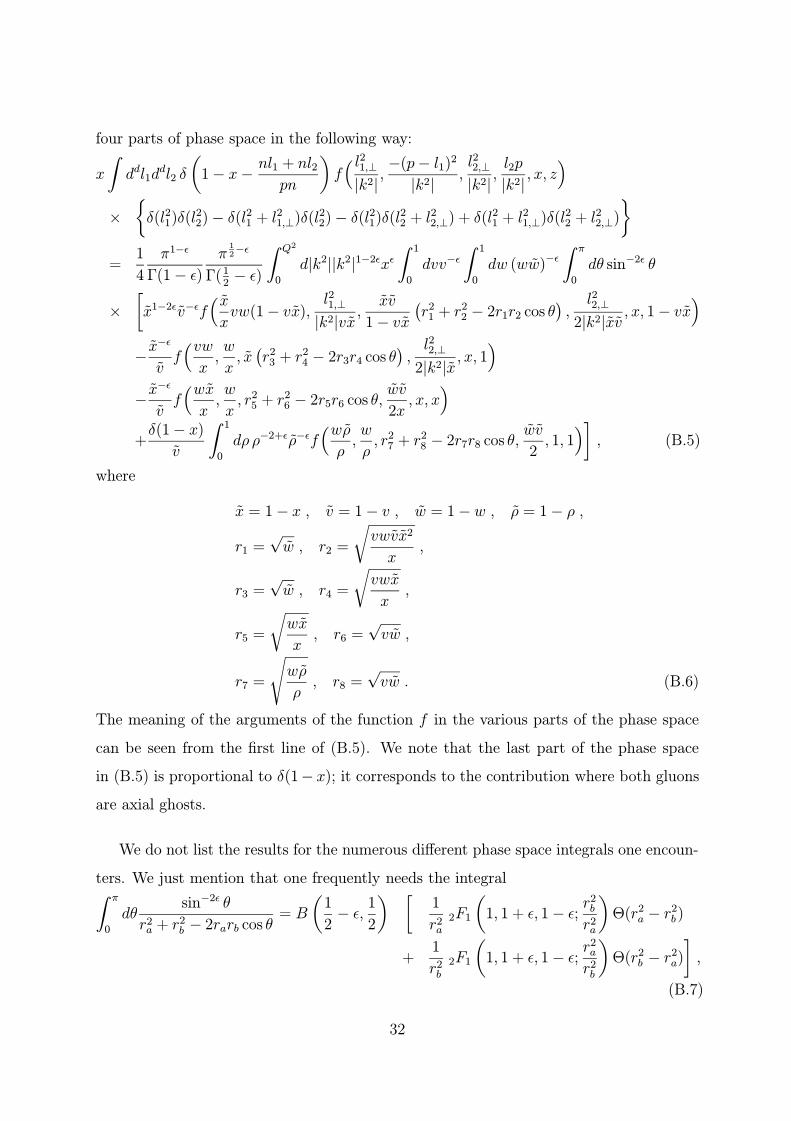
four parts of phase space in the following way:

x

∫ddl1d

dl2 δ

(1− x−

nl1 + nl2pn

)f( l21,⊥|k2|

,−(p− l1)2

|k2|,l22,⊥|k2|

,l2p

|k2|, x, z

)×

{δ(l21)δ(l22)− δ(l21 + l21,⊥)δ(l22)− δ(l21)δ(l22 + l22,⊥) + δ(l21 + l21,⊥)δ(l22 + l22,⊥)

}=

1

4

π1−ε

Γ(1− ε)

π12−ε

Γ(12− ε)

∫ Q2

0

d|k2||k2|1−2εxε∫ 1

0

dvv−ε∫ 1

0

dw (ww)−ε∫ π

0

dθ sin−2ε θ

×

[x1−2εv−εf

( xxvw(1− vx),

l21,⊥|k2|vx

,xv

1− vx

(r2

1 + r22 − 2r1r2 cos θ

),

l22,⊥2|k2|xv

, x, 1− vx)

−x−ε

vf(vwx,w

x, x(r2

3 + r24 − 2r3r4 cos θ

),l22,⊥

2|k2|x, x, 1

)−x−ε

vf(wxx,w

x, r2

5 + r26 − 2r5r6 cos θ,

wv

2x, x, x

)+δ(1− x)

v

∫ 1

0

dρ ρ−2+ερ−εf(wρρ,w

ρ, r2

7 + r28 − 2r7r8 cos θ,

wv

2, 1, 1

)], (B.5)

where

x = 1− x , v = 1− v , w = 1− w , ρ = 1− ρ ,

r1 =√w , r2 =

√vwvx2

x,

r3 =√w , r4 =

√vwx

x,

r5 =

√wx

x, r6 =

√vw ,

r7 =

√wρ

ρ, r8 =

√vw . (B.6)

The meaning of the arguments of the function f in the various parts of the phase space

can be seen from the first line of (B.5). We note that the last part of the phase space

in (B.5) is proportional to δ(1− x); it corresponds to the contribution where both gluons

are axial ghosts.

We do not list the results for the numerous different phase space integrals one encoun-

ters. We just mention that one frequently needs the integral∫ π

0

dθsin−2ε θ

r2a + r2

b − 2rarb cos θ= B

(1

2− ε,

1

2

) [1

r2a

2F1

(1, 1 + ε, 1− ε;

r2b

r2a

)Θ(r2

a − r2b )

+1

r2b

2F1

(1, 1 + ε, 1− ε;

r2a

r2b

)Θ(r2

b − r2a)

],

(B.7)

32

where 2F1(a, b, c; z) denotes the hypergeometric function [29]. To expand in ε, the relations

2F1(1, 1 + ε, 1− ε; z) = (1− z)−1−2ε2F1(−ε,−2ε, 1− ε; z) , (B.8)

2F1(aε, bε, 1− cε; z) = 1 + abε2(

Li2(z) + εcLi3(z) + ε(a+ b+ c)S1,2(z))

+O(ε2)

are useful, where [28]

Li3(z) ≡

∫ 1

0

ln y ln(1− zy)

ydy , S1,2(z) ≡

1

2

∫ 1

0

ln2(1− zy)

ydy . (B.9)

33

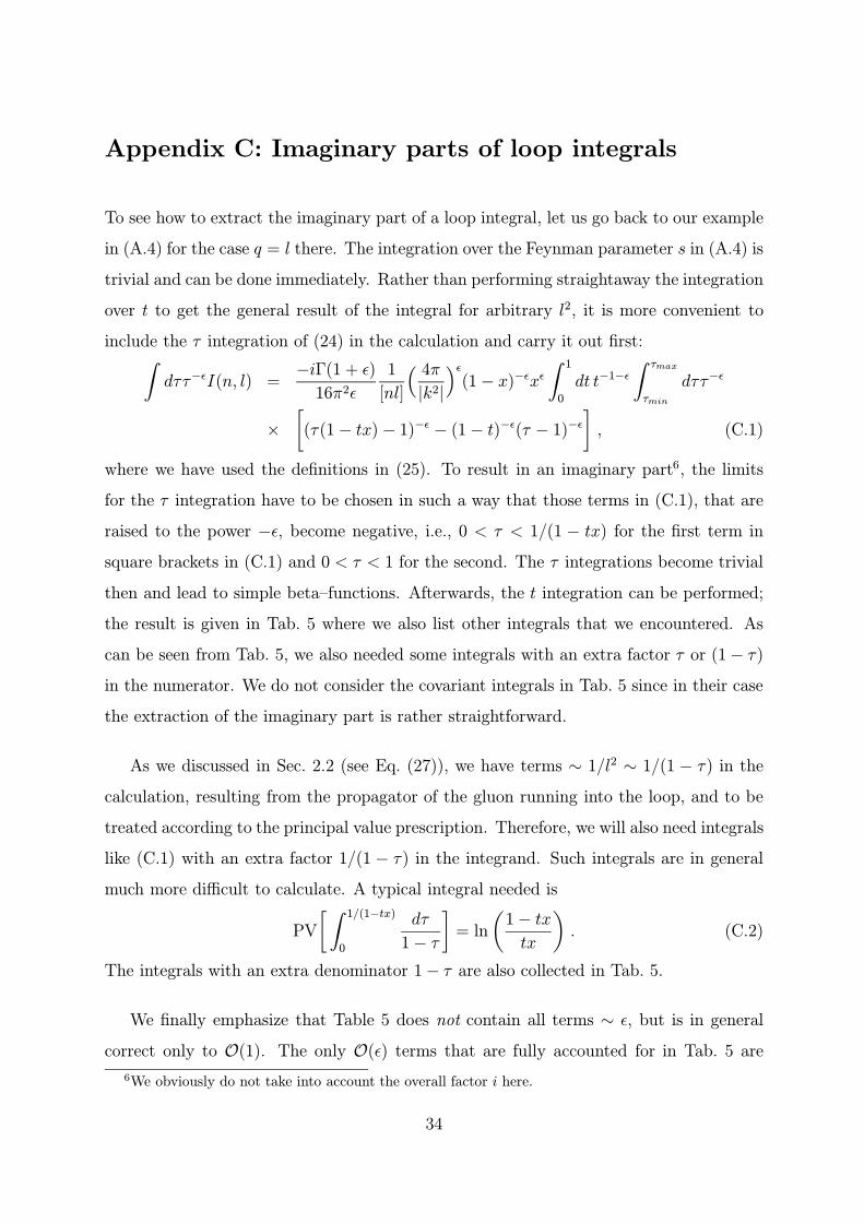
Appendix C: Imaginary parts of loop integrals

To see how to extract the imaginary part of a loop integral, let us go back to our example

in (A.4) for the case q = l there. The integration over the Feynman parameter s in (A.4) is

trivial and can be done immediately. Rather than performing straightaway the integration

over t to get the general result of the integral for arbitrary l2, it is more convenient to

include the τ integration of (24) in the calculation and carry it out first:∫dττ−εI(n, l) =

−iΓ(1 + ε)

16π2ε

1

[nl]

( 4π

|k2|

)ε(1− x)−εxε

∫ 1

0

dt t−1−ε

∫ τmax

τmin

dττ−ε

×

[(τ(1− tx)− 1)−ε − (1− t)−ε(τ − 1)−ε

], (C.1)

where we have used the definitions in (25). To result in an imaginary part6, the limits

for the τ integration have to be chosen in such a way that those terms in (C.1), that are

raised to the power −ε, become negative, i.e., 0 < τ < 1/(1 − tx) for the first term in

square brackets in (C.1) and 0 < τ < 1 for the second. The τ integrations become trivial

then and lead to simple beta–functions. Afterwards, the t integration can be performed;

the result is given in Tab. 5 where we also list other integrals that we encountered. As

can be seen from Tab. 5, we also needed some integrals with an extra factor τ or (1− τ)

in the numerator. We do not consider the covariant integrals in Tab. 5 since in their case

the extraction of the imaginary part is rather straightforward.

As we discussed in Sec. 2.2 (see Eq. (27)), we have terms ∼ 1/l2 ∼ 1/(1 − τ) in the

calculation, resulting from the propagator of the gluon running into the loop, and to be

treated according to the principal value prescription. Therefore, we will also need integrals

like (C.1) with an extra factor 1/(1 − τ) in the integrand. Such integrals are in general

much more difficult to calculate. A typical integral needed is

PV

[ ∫ 1/(1−tx)

0

dτ

1− τ

]= ln

(1− tx

tx

). (C.2)

The integrals with an extra denominator 1− τ are also collected in Tab. 5.

We finally emphasize that Table 5 does not contain all terms ∼ ε, but is in general

correct only to O(1). The only O(ε) terms that are fully accounted for in Tab. 5 are

6We obviously do not take into account the overall factor i here.

34

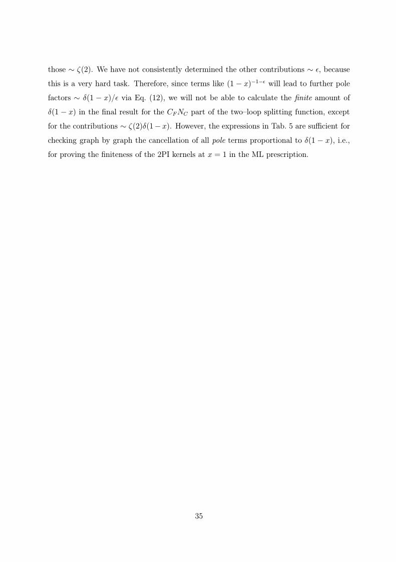
those ∼ ζ(2). We have not consistently determined the other contributions ∼ ε, because

this is a very hard task. Therefore, since terms like (1 − x)−1−ε will lead to further pole

factors ∼ δ(1 − x)/ε via Eq. (12), we will not be able to calculate the finite amount of

δ(1 − x) in the final result for the CFNC part of the two–loop splitting function, except

for the contributions ∼ ζ(2)δ(1− x). However, the expressions in Tab. 5 are sufficient for

checking graph by graph the cancellation of all pole terms proportional to δ(1 − x), i.e.,

for proving the finiteness of the 2PI kernels at x = 1 in the ML prescription.

35

−IP[

1iπ

∫ddr/(2π)d

] ∫dττ−ετα(1− τ)β

∫dτ τ

−ε

1−τ

pnr2(l−r)2[nr]

1x

[(1 + 2ε)1−x−ε

ε+ εζ(2)

]1

2ε2x−1−ε(1− ε2ζ(2))

(α = 0, β = 0) + 1x(Li2(x)− ζ(2))

(r2−2nl n∗r) pnr2(l−r)2[nr]

does not occur k2[− 1

ε− 1− 1

x+ lnx

− ln x(1− 1x)− 2x−ε

]pn

(p−r)2(k−r)2[nr]−x−1−ε lnx x−1−ε

[lnxε

+ 12

ln2 x

(α = 0, β = 0) −2Li2(x) + εxζ(2)]

pn(p−r)2(l−r)2[nr]

− 1x

(α = 0, β = 0) does not occur

pn(k+r)2(l−r)2[nr]

1x

[1ε

+ 2 + lnx]

(1− x−ε)( 1ε2− ζ(2))− lnx

ε

(α = 0, β = 0) +ζ(2)− 2Li2(x)− 12

ln2 x

pnr2(p−r)2(k−r)2[nr]

1k2 x−ε[− 1

ε+ 2x

xlnx+ εζ(2)

]1k2 x−ε[

1ε2

+ 2 lnxε

(α = 0, β = 0) −4Li2(1− x)− ζ(2)]

pnr2(k+r)2(l−r)2[nr]

1k2x

[− (1− x−ε)( 1

ε2− ζ(2)) 1

k2x

[32x−ε( 1

ε2− ζ(2))

−Li2(x)− lnx ln x]

+2(Li2(x)− ζ(2))]

(α = 0, β = 0)

xk2x2

[1ε

+ 2− 2 ln x(1− 1x) + lnx

](α = 1, β = 0)

pnr2(p−r)2(l−r)2[nr]

xk2x

[− (1− x−ε)( 1

ε2− ζ(2)) + lnx

εdoes not occur

+2Li2(x) + 12

ln2 x− 3ζ(2)]

(α = 0, β = 0)

xk2x2

[− x

ε− 2 + 3x+ 2x ln x

−(1− 3x) lnx]

(α = 0, β = 1)

Table 5: Imaginary parts ‘IP ’ of loop integrals for the ML prescription, after integrationover the variable τ of the LO phase space (24). As before we have defined x = 1 − x. Theintegrals are in general only correct to O(1); see text. Note that terms ∼ (1 − x)−ε mustnot be expanded in ε, as further pole terms can arise via Eq. (12). We have dropped theubiquitous factor 1/16π2 (4π/|k2|)ε Γ(1− ε)/Γ(1− 2ε).

36

Appendix D: Mellin moments

The Mellin–moments of a function f(x) are defined by

fn ≡

∫ 1

0

dxxn−1 f(x) . (D.1)

As a result, the moments of a convolution f ⊗ g (see Eq. (32)) become the product of the

moments of f and g:

(f ⊗ g)n = fn gn . (D.2)

The moments of (31) are easily obtained using the formulae in the appendix of [30]. To

invert the moments of the product fngn back to x–space, one needs some further moment

expressions. Everything can be derived from the relations in [30], and from∫ 1

0

dx xn−1 ln2(1− x) =1

n

(S2

1(n) + S2(n)),∫ 1

0

dx xn−1

[ln2(1− x)

1− x

]+

=1

n

(S2

1(n) + S2(n))−

1

3S3

1(n)− S1(n)S2(n)−2

3S3(n) ,∫ 1

0

dx xn−1Li2(x) =1

nζ(2)−

1

n2S1(n) ,∫ 1

0

dx xn−1 lnx ln(1− x) =1

n

(S2(n)− ζ(2)

)+

1

n2S1(n) , (D.3)∫ 1

0

dx xn−1 lnx ln(1− x)

1− x=

(S2(n)− ζ(2)

)(1

n− S1(n)

)+

1

n2S1(n)− S3(n) + ζ(3) ,

where

Sk(n) ≡n∑j=1

1

jk. (D.4)

37

Appendix E: Two–loop integrals

For the calculation of the CFTf part of the two–loop quark self–energy we need some

integrals with an extra non–integer power of −r2 in the integrand, where r is the loop

momentum. Making use of the identities

1

aαb= α

∫ 1

0

dxxα−1

[ax+ b(1− x)]α+1 ,

1

aαbc= α(α+ 1)

∫ 1

0

dx

∫ 1−x

0

dyxα−1

[ax+ by + c(1− x− y)]α+2 , (E.1)

one obtains rather easily:∫ddr

(2π)d(−r2)

−ε

(p− r)2=

i

16π2(4π)ε

(−p2

)1−2ε εΓ(2ε)

Γ(1 + ε)

Γ(1− ε)Γ(1− 2ε)

Γ(3− 3ε), (E.2)∫

ddr

(2π)d(−r2)

−ε

r2(p− r)2=

i

16π2(4π)ε

(−p2

)−2ε Γ(2ε)

Γ(1 + ε)

Γ(1− ε)Γ(1− 2ε)

Γ(2− 3ε), (E.3)∫

ddr

(2π)d(−r2)

−ε

r2(p− r)2[nr]=

(−p2

)−ε (1 + ε2ζ(2)

) ∫ ddr

(2π)d1

r2(p− r)2[nr], (E.4)

where the integral on the right–hand–side of (E.4) was determined in App. A and is

actually finite. For the ML prescription we therefore do not need the integral on the

left–hand–side of (E.4); however, we will see below that the integral is divergent for the

PV prescription. Also note that the integral in (E.2) vanishes if the factor (−r2)−ε

is not

present.

Finally, for the PV prescription one obtains for the integral in (E.4):∫ddr

(2π)d(−r2)

−ε

r2(p− r)2[nr]=

i

16π2(4π)ε

(−p2

)−2ε 1

2εpn[I0 + εζ(2)− 2εI1] +O(ε) , (E.5)

while∫ddr

(2π)d1

r2(p− r)2[nr]=

i

16π2(4π)ε

(−p2

)−ε 1

εpn[I0 + εζ(2)− εI1] +O(ε) . (E.6)

Here

I1 ≡

∫ 1

0

u lnu

u2 + δ2du . (E.7)

38

References

[1] See e.g. Yu.L. Dokshitzer, D.I. Dyakonov and S.I. Troyan, Phys. Rep. 58, 270 (1980).

[2] A. Bassetto, G. Nardelli, and R. Soldati, Yang–Mills Theories in Algebraic Non–

covariant Gauges, World Scientific, Singapore, 1991.

[3] A. Bassetto, M. Dalbosco, I. Lazzizzera, and R. Soldati, Phys. Rev. D31, 2012 (1985).

[4] A. Bassetto, M. Dalbosco, and R. Soldati, Phys. Rev. D36, 3138 (1987).

[5] S. Mandelstam, Nucl. Phys. B213, 149 (1983).

[6] G. Leibbrandt, Phys. Rev. D29, 1699 (1984).

[7] A. Bassetto in QCD and High Energy Hadronic Interaction, ed. J. Tran Than Van,

Frontieres 1993; Nucl. Phys. Proc. Suppl. 51C, 281 (1996).

[8] A. Bassetto in Proceedings of the VIII Warsaw Symposium on Elementary Particle

Physics, ed. Z. Ajduk, Warszawa 1985.

[9] G. Curci, W. Furmanski, and R. Petronzio, Nucl. Phys. B175, 27 (1980).

[10] W. Furmanski and R. Petronzio, Phys. Lett. 97B, 437 (1980).

[11] R.K. Ellis, H. Georgi, M. Machacek, H.D. Politzer, and G.G. Ross, Phys. Lett. 78B,

281 (1978); Nucl. Phys. B152, 285 (1979).

[12] R.K. Ellis and W. Vogelsang, CERN–TH/96–50, RAL-TR-96-012, hep-ph/9602356.

[13] G. Altarelli and G. Parisi, Nucl. Phys. B126, 298 (1977).

[14] E.G. Floratos, D.A. Ross, and C.T. Sachrajda, Nucl. Phys. B152, 493 (1979);

see also: A. Gonzales-Arroyo and C. Lopez, Nucl. Phys. B166, 429 (1980).

[15] R. Hamberg, W.L. van Neerven, Nucl. Phys. B379, 143 (1992);

see also: Y. Matiounine, J. Smith, and W.L. van Neerven, hep-ph/9801224, to

appear in Phys. Rev. D.

39

[16] J.C. Collins and R.J. Scalise, Phys. Rev. D50, 4117 (1994).

[17] G. Heinrich and Z. Kunszt, ETH–TH/97–18, hep-ph/9708334, to appear in Nucl.

Phys. B.

[18] G. Leibbrandt and S.L. Nyeo, Phys. Lett. 140B, 417 (1984).

[19] M.A. Nowak, M. Praszalowicz, and W. Slominski, Ann. Phys. 166, 443 (1986).

[20] M. Dalbosco, Phys. Lett. 180B, 121 (1986).

[21] G. Leibbrandt, Rev. Mod. Phys. 59, 1067 (1987).

[22] E.G. Floratos, D.A. Ross, and C.T. Sachrajda, Nucl. Phys. B129, 66 (1977); E: 139,

545 (1978);

see also: A. Gonzales-Arroyo, C. Lopez, and F.J. Yndurain, Nucl. Phys. B153, 161

(1979).

[23] R.T. Herrod and S. Wada, Phys. Lett. 96B, 195 (1980).

[24] G. Leibbrandt and J. Williams, Nucl. Phys. B440, 573 (1995).

[25] J. Williams, Ph.D. thesis, University of Guelph (1998), to appear. We are grateful

to J. Williams for communicating to us his results concerning the second and third

diagram of Fig. 2.

[26] M. Dalbosco, Phys. Lett. 163B, 181 (1985).

[27] G. Leibbrandt, Noncovariant gauges: Quantization of Yang–Mills and Chern–Simons

theory in axial type gauges, World Scientific, Singapore 1994.

[28] A. Devoto and D.W. Duke, Riv. Nuov. Cim. 7, 1 (1984).

[29] I.S. Gradshteyn and I.M. Ryzhik, Table of Integrals, Series, and Products, Academic

Press, London, 1979.

[30] G. Altarelli, R.K. Ellis, and G. Martinelli, Nucl. Phys. B157, 461 (1979).

40