The LatMix Summer Campaign: Submesoscale Stirring in the Upper Ocean

The LatMix Summer Campaign: Submesoscale Stirring in the

Upper Ocean. A part of AMS special collection “LatMix: Studies of Submesoscale Stirring and Mixing”

Andrey Y. Shcherbina, Miles A. Sundermeyer, Eric Kunze, Eric D’Asaro, Gualtiero Badin, Daniel Birch, Anne-Marie E. G. Brunner-Suzuki, Jörn Callies, Brandy T. Kuebel Cervantes, Mariona Claret, Brian Concannon, Jeffrey Early, Raffaele Ferrari, Louis Goodman, Ramsey R. Harcourt, Jody M. Klymak, Craig M. Lee, M.-Pascale Lelong, Murray D. Levine, Ren-Chieh Lien, Amala Mahadevan, James C. McWilliams, M. Jeroen Molemaker, Sonaljit Mukherjee, Jonathan D. Nash, Tamay Özgökmen, Stephen D. Pierce, Sanjiv Ramachandran, Roger M. Samelson, Thomas B. Sanford, R. Kipp Shearman, Eric D. Skyllingstad, K. Shafer Smith, Amit Tandon, John R. Taylor, Eugene A. Terray, Leif N. Thomas, James R. Ledwell Corresponding author: Andrey Shcherbina Applied Physics Laboratory, University of Washington 1013 NE 40th St., Seattle, WA 98105 Phone: (206)897-1446 e-mail: [email protected] Affiliations: Badin–University of Hamburg, Hamburg, Germany; Birch, Brunner-Suzuki, Goodman, Mukherjee, Ramachandran, Sundermeyer, Tandon–University of Massachusetts Dartmouth, North Dartmouth, Massachusetts; Callies– MIT/WHOI Joint Program in Oceanography, Cambridge/Woods Hole, Massachusetts; Claret, Ledwell, Mahadevan, Terray –Woods Hole Oceanographic Institution, Woods Hole, Massachusetts; Concannon–Naval Air Systems Command, Patuxent River, Maryland; D’Asaro, Harcourt, Lee, Lien, Sanford, Shcherbina–University of Washington, Seattle, Washington; Early, Lelong–NorthWest Research Associates, Redmond, Washington; Ferrari–Massachusetts Institute of Technology, Cambridge, Massachusetts; Klymak–University of Victoria, Victoria, Canada; Kuebel Cervantes, Levine, Nash, Pierce, Samelson, Shearman, Skyllingstad–Oregon State University, Corvallis, Oregon; Kunze–8505 16th NE, Seattle, WA 98115; McWilliams, Molemaker–University of California, Los Angeles, Los Angeles, California; Özgökmen –University of Miami, Miami, Florida; Smith–New York University, New York, New York; Taylor–University of Cambridge, Cambridge, United Kingdom; Thomas–Stanford University, Stanford, California;

Accepted for BAMS publication 11 November 2014

Capsule

LatMix combines shipboard, autonomous, and airborne field observations with modeling to improve

understanding of ocean stirring across multiple scales.

Abstract

Lateral stirring is a basic oceanographic phenomenon affecting the distribution of physical, chemical,

and biological fields. Eddy stirring at scales of order 100 km (the mesoscale) is fairly well

understood and explicitly represented in modern eddy-resolving numerical models of global ocean

circulation. The same cannot be said for smaller-scale stirring processes. Here, we describe a major

oceanographic field experiment aimed at observing and understanding the processes responsible for

stirring at scales of 0.1 to 10 km. Stirring processes of varying intensity were studied in the Sargasso

Sea eddy field approximately 250 km southeast of Cape Hatteras. Lateral variability of water-mass

properties, the distribution of microscale turbulence, and the evolution of several patches of inert dye

were studied with an array of shipboard, autonomous, and airborne instruments. Observations were

made at two sites, characterized by weak and moderate background mesoscale straining, to contrast

different regimes of lateral stirring. Analyses to date suggest that, in both cases, the lateral dispersion

of natural and deliberately released tracers was O(1 m2 s−1) as found elsewhere, which is faster than

might be expected from traditional shear dispersion by persistent mesoscale flow and linear internal

waves. These findings point to the possible importance of kilometer-scale stirring by submesoscale

eddies and nonlinear internal wave processes, or the need to modify the traditional shear-dispersion

paradigm to include higher-order effects. A unique aspect of the LatMix field experiment is the

combination of direct measurements of dye dispersion with the concurrent multi-scale hydrographic

and turbulence observations, enabling evaluation of the underlying mechanisms responsible for the

observed dispersion at a new level.

3

INTRODUCTION Dispersion of natural and anthropogenic tracers in the ocean is traditionally conceptualized as

a two-stage process: The first step, stirring, is an adiabatic rearrangement of water parcels that

does not change their potential temperature, salinity, or other tracer concentrations; it tends to

stretch tracer patches into convoluted streaks and therefore enhances overall variance of tracer

gradients. Molecular diffusion then acts to reduce small-scale gradients and effects the ultimate

mixing [Eckart, 1948; Garrett, 2006]. In practice, all small-scale processes not resolved in a

particular numerical or analytic framework (e.g., Reynolds-averaged Navier-Stokes equations)

are often lumped into mixing with the understanding that it may include unresolved stirring as

well. Within the strongly stratified ocean interior, a clear distinction can be made between

isopycnal processes, which act along surfaces of constant potential density (or more strictly,

neutral surfaces [Montgomery, 1940; McDougall, 1984]), and diapycnal processes, which act

across these surfaces [Gregg, 1987; MacKinnon et al., 2013].

Interpretation of lateral dispersion of tracers in the ocean in terms of mixing is fraught with

ambiguity. The unresolved flux JT of a tracer T ascribed to lateral mixing is commonly

parameterized with Fickian diffusion law

JT = −Kh∇T,

where Kh is the effective diffusivity and ∇T is the resolved tracer gradient. However, it has been

long recognized that Kh depends strongly on the spatial and temporal scales being considered

[Stommel, 1949; Ozmidov, 1958]. Therefore, any estimate of Kh must be accompanied with the

specification of scales, which are themselves somewhat arbitrarily defined [Okubo, 1976]. These

ambiguities can be overcome by understanding and modeling the processes responsible for

lateral stirring of tracers.

4

Stirring cascades variance from large scales, where it is produced, to O(1 cm) scales, where it

is removed by molecular diffusion [Stern, 1975]. On the mesoscale O(10–100 km), isopycnal

stirring by geostrophic eddies is well understood [e.g., Smith and Ferrari, 2009]. Likewise,

stirring by microscale (0.01–1 m) isotropic turbulence to the molecular scale has been studied for

many decades and its physics is well established. In contrast, the dynamics that control stirring

on the submesoscale (0.1–10 km), and the relative importance of various processes are not as

well known. Contributions from both geostrophically balanced motions and internal gravity

waves are expected, but their relative importance and the mechanisms by which they stir have

not been quantified. Here, we discuss a recent campaign to improve our understanding of

submesoscale stirring and mixing in the ocean interior.

Traditionally, dynamic signals at the submesoscale have been thought to be dominated by the

ubiquitous presence of energetic broadband internal gravity waves (IGW). Decades of

observations of these motions have clearly established their role in controlling diapycnal mixing

[Gregg, 1989; Polzin et al., 1995; MacKinnon et al., 2013]. Although these motions have

traditionally been modeled and conceptualized as a superposition of nearly linear IGW,

significant deviations from this paradigm have been persistently observed, promoting

speculations about the presence of coexisting vortical modes dominated by isopycnal velocities

[Lien and Müller, 1992; Sundermeyer et al., 2005; Pinkel, 2014]. IGW have long been thought to

also have an important role in isopycnal mixing through shear dispersion, in which vertical

internal-wave shear couples with diapycnal mixing [Young et al., 1982, YRG82 hereafter].

Traditional YRG82 scaling for the resulting effective isopycnal diffusivity is Kh ~

<Kv><(∂V/∂z)2>f −2, where <Kv> is the average diapycnal diffusivity and <(∂V/∂z)2> the average

variance of vertical shear dominated by finescale near-inertial waves. Dye-release studies have

5

consistently found isopycnal diffusivities O(1 m2 s−1) at 1–5 km scales, an order of magnitude

larger than could be inferred from YRG82 theory [Ledwell et al., 1998; Sundermeyer and

Ledwell, 2001]. This discrepancy may be due to (i) covariance between internal-wave strain and

shear-driven turbulence [Kunze and Sundermeyer, 2014], (ii) internal-wave Stokes drifts [Bühler

et al., 2013], (iii) subinertial vortical modes generated by breaking internal waves [Brunner-

Suzuki et al., 2014], or (iv) submesoscale processes unrelated to internal waves [Mahadevan and

Tandon, 2006; Capet et al., 2008; Thomas et al., 2008; Molemaker et al., 2010].

Recent high-resolution numerical models and targeted observations reveal intricate patterns

of three-dimensional submesoscale fronts and filaments emerging from mesoscale features

[Capet et al., 2008]. A number of dynamical processes have been proposed to explain this

mesoscale-submesoscale transition, including spontaneous instability of deep mixed layers,

ageostrophic instability, frontogenesis, and direct wind forcing at mesoscale fronts [Boccaletti et

al., 2007; Thomas et al., 2008]. Numerical simulations suggest that non-QG baroclinic mixed

layer instabilities can penetrate into the thermocline, leading to lateral stirring of tracers below

the mixed layer [Badin et al., 2011].

It appears that both internal-wave and subinertial submesoscale dynamics cascade tracer

variance and turbulent kinetic energy from larger scales, where they are generated, to dissipate at

small scales, but the relative importance of various pathways has not been resolved [McWilliams

et al., 2001; Müller et al., 2005; Molemaker et al., 2010]. Moreover, it is presently unclear which

processes participating in the cascade control downscale flux of variance [Garrett, 2006].

The “Scalable Lateral Mixing and Coherent Turbulence” (LatMix) initiative led by the Office

of Naval Research tackled the problem of submesoscale oceanic stirring spanning mesoscale to

microscale processes from observational, theoretical, and numerical perspectives. Here, we

6

present an overview of the major 2011 LatMix campaign involving three regional-class research

vessels with numerous shipboard, towed and autonomous instrument platforms, as well as

airborne and satellite remote sensing and supporting numerical simulations.

FIELD EXPERIMENT

Aims

The LatMix initiative set out to address the following primary hypotheses for what drives

isopycnal stirring and mixing at the submesoscale, while recognizing that the answer may be all

or none of these processes:

1. Internal-wave shear dispersion in which diapycnal mixing interacts with the vertical shear of

the waves;

2. Stirring associated with finescale potential vorticity anomalies (vortical modes) caused by

internal-wave breaking;

3. Progressive straining of tracer fields to smaller scales by mesoscale processes adequately

described by quasigeostrophic dynamics;

4. High-Rossby-number subinertial motions on the submesocale that are not quasigeostrophic,

such as frontogenesis and mixed-layer instabilities.

Experimental testing of these hypotheses required observations of submesoscale lateral tracer

dispersion at various levels of background mesoscale straining and atmospheric forcing. The

LatMix initiative included two major field campaigns, along with several modeling studies, to

address processes ranging in scale from 0.01 to 100 km. Here, we describe the first field

experiment of summer 2011, conducted in the Sargasso Sea in a region of low-to-moderate

straining and shallow mixed layers. The second campaign in late winter and spring 2012 (to be

7

described in forthcoming articles), was situated in the Gulf Stream front, a strongly straining

flow with strong surface fluxes and deep mixed layers.

Logistics and participants

Three regional class vessels participated in the field campaign: R/Vs Cape Hatteras,

Endeavor, and Oceanus. Each vessel carried a wide range of shipboard, towed, and autonomous

deployable instrumentation (see Table 1 and Appendix). Additionally, R/V Cape Hatteras

conducted a series of fluorescein and rhodamine dye releases that were surveyed with all three

vessels. Dye patches were also surveyed by airborne lidar on board a Navy Lockheed P3 Orion

aircraft. Broad context was established by analysis of satellite remote-sensing products and

operational numerical models.

Timely collective decision-making and coordination among the science parties on three

research vessels required near real-time integration and sharing of information. Shore support

provided automated downloading, subsetting, and packaging of satellite and operational model

sea surface height and temperature datasets. These were consolidated with telemetered

instrument data streams in a common shore-side database, which was routinely replicated on the

research vessels for local use. Positions of the vessels and all the autonomous platforms were

plotted in near real-time on situation-awareness displays on the ships’ bridges to aid navigation

and avoid collisions. Technical details about the instrumentation and data products used in this

study are given in the Appendix.

8

Oceanographic and meteorological context

The summer LatMix experiment was conducted 1–20 June 2011 in the Sargasso Sea

approximately 250 km south-southeast of Cape Hatteras, and southeast of the Gulf Stream. The

area was selected based on water clarity and relative proximity to shore, to optimize conditions

for optical remote sensing by the aircraft, and for the relative weakness of the mesoscale eddy

field required for low- and moderate-dispersion studies. Bathymetry is generally flat and

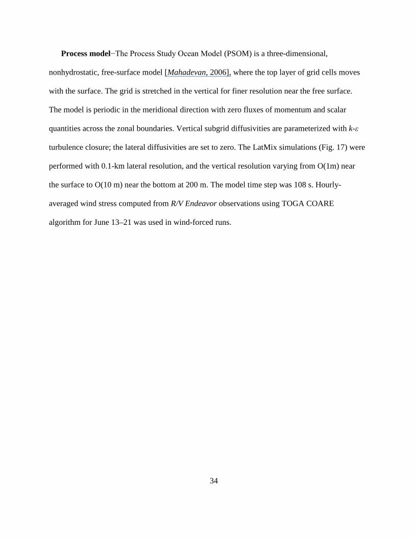
featureless, with the typical water depth of 4–5 km. Upper 500-m ocean stratification was

characteristic of the summertime interior subtropical gyre (Fig. 1). Strong surface heating

resulted in a shallow (10–20 m) and warm (25–28ºC) mixed layer. The buoyancy frequency

below the mixed layer (20–30 m) was on the order of 0.02 s−1.

Fair summertime weather prevailed during the experiment (Fig. 2). Average air temperatures

of 24.3ºC were about a degree cooler than the sea surface. Winds were typically light

(<10 m s−1). Two short storms on 12 and 18 June brought precipitation of 50 and 150 mm,

respectively, maximum wind speeds of 15 m s−1, and short-term cooling.

EXPERIMENT PROGRESS AND MAIN FINDINGS The summer 2011 LatMix field experiment consisted of weak straining1 [O(0.05f), 2–10

June] and moderate straining [O(0.1f), 11–19 June] case studies, where f=7.7×10−5 rad s−1 is the

Coriolis frequency at 32°N. Sites for the studies were selected based on satellite imagery and

coordinated reconnaissance surveys. Geographically, the sites of weak- and moderate-straining

studies overlapped; increased straining during the second case study was due to eastward

1 Characteristic magnitudes of mesoscale [O(10 km)] strain rate tensors in each case study were determined

from the maps of mean near-surface (0–50 m) velocity, objectively interpolated from shipboard ADCP observations

during the reconnaissance surveys.

9

expansion of several warm-core mesoscale eddies.

Each case study started with a coordinated 100 km × 100 km mesoscale survey carried out by

the three vessels, followed by ~100-kg rhodamine dye releases on an isopycnal surface in the

seasonal pycnocline at depths around 30 m (see Appendix for dye injection details). A

Lagrangian float was deployed within the dye patch and tracked acoustically. Drogued drifters

and profiling EM-APEX floats were deployed in an array surrounding the patch. Subsequently,

the vessels commenced nested surveys of the area centered on the dye: a 30 km × 30 km radiator

pattern covered by R/V Oceanus, a 15 km × 15 km butterfly pattern by R/V Endeavor, and an

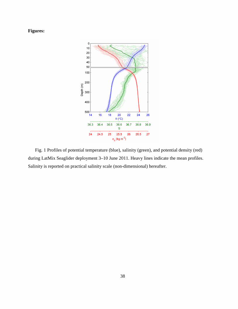
O(1-km) adaptive survey by R/V Cape Hatteras (Fig. 3). The surveys were supplemented by a

group of four Slocum gliders and one SeaGlider. The surveys were guided in real time by the

advection of the Lagrangian float and drogued drifters, as well as by the integral of the R/V Cape

Hatteras 150-kHz ADCP velocity in the depth bin occupied by the dye. Details about the

instrumentation and sampling are given in the Appendix.

A series of eight smaller (~10–27 kg) fluorescein dye releases were also performed in close

proximity in depth and location to the rhodamine experiments. These releases were tracked by

towed instruments for about a day each during continued surveys of the rhodamine patches. Four

of these fluorescein dye patches were also surveyed for the first 6 hours or so of their evolution

by airborne lidar. During the daylight hours, after most of the fluorescein deployments, a

microprobe-equipped autonomous underwater vehicle T-REMUS was deployed to conduct 1-km

box surveys around a drogued Gateway buoy (see Appendix) while Hammerhead was towyoed

in 2-km radius circles around it. Nested within surveys by Triaxus and Moving Vessel Profiler

(MVP) instrument systems, these measurements collectively spanned horizontal scales of 0.03–

30 km (Fig. 3).

10

A Google Earth interactive map of shipboard, autonomous, and airborne surveys during the

summer 2011 LatMix experiment is available online as supplemental material [link].

Weak-straining study

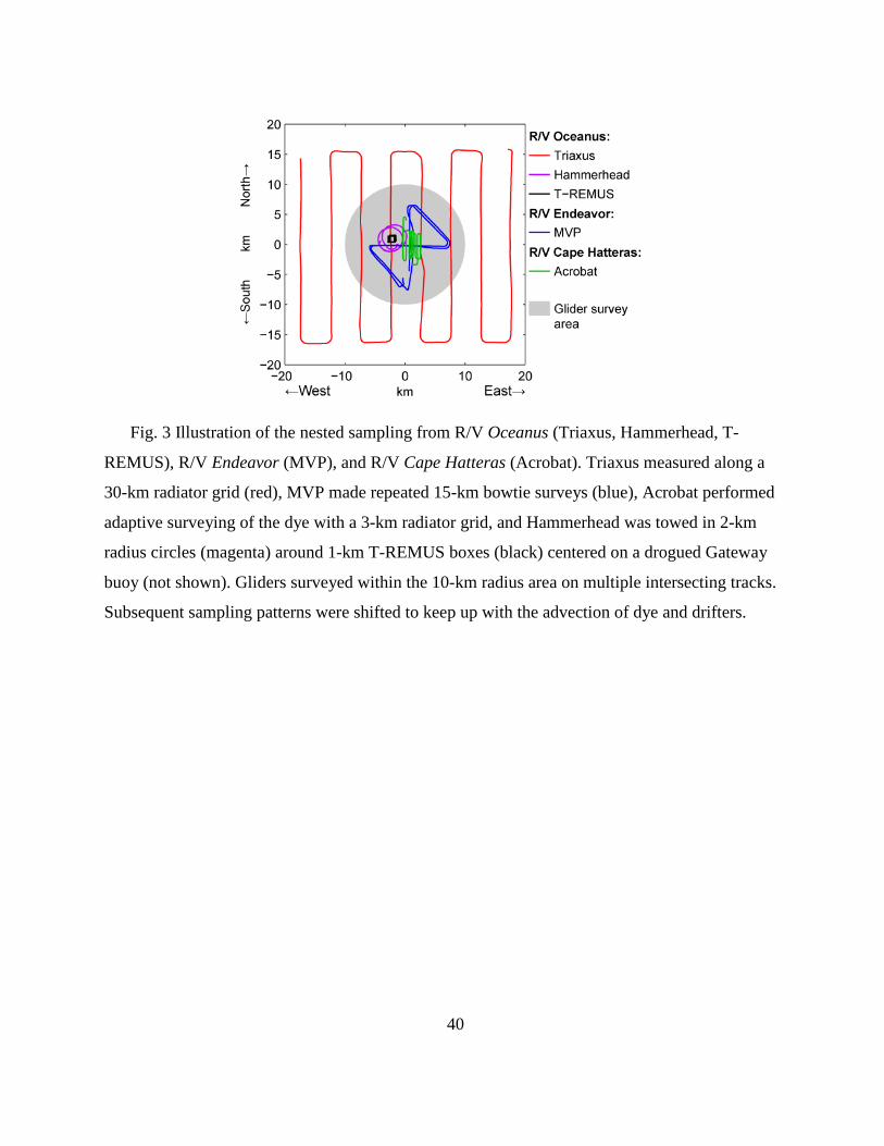
The weak-straining study started on 2 June 2011 at a quiescent site with lateral velocity

gradients of O(0.05f) estimated at 10-km scale using the mesoscale map of mean near-surface

(0–50 m) ADCP velocities (Fig. 4), and simultaneously inferred from the drifter and dye

convergence/elongation at km-scale. Lateral thermohaline variability was weak, with the

exception of a 0.02 km−1 salinity gradient in the mixed layer and a few coherent features with

O(0.1) salinity anomalies in the pycnocline (Fig. 5). The upper-ocean flow was dominated by 6–

9 cm s−1 inertial oscillations, as evident from the looping trajectories of the tracking drifters (Fig.

6). Subinertial advection was initially negligible, but increased to 15 cm s−1 southward flow by

10 June.

A 1.5-km long zonal streak of rhodamine dye was released on 4 June 2011 in the upper

seasonal pycnocline with the vertical potential density gradient −0.025 kg m−4 at potential

density 25.42 kg m−3 (RMS deviation ±0.014 kg m−3) and a mean depth of 30±1.4 m (Figs. 5 and

6). The dye release was accompanied by deployment of 9 GPS-tracked drifters drogued at 30 m,

in a cross pattern, and a Lagrangian float at the center of the streak (Fig. 6). Simultaneously, a

swarm of 18 EM-APEX floats forming three concentric circles (1-, 2-, and 3.5-km nominal

diameters) was deployed at the site of the release; on 5 and 7 June, two EM-APEX floats were

repositioned, and three additional floats were deployed.

Over the next 6 days, culminating on 10 June, the dye and surrounding drifters and floats

traveled 30 km SSE, while remaining in a relatively compact group (Fig. 6). The outer ring of

EM-APEX floats was stretched in the NW-SE direction by a factor of 2.8 and compressed by

11

about a factor of 2 in the orthogonal direction. The drifter array showed similar stretching along

the same NW-SE axis. This relatively weak deformation of the float and drifter arrays, and

relatively little rotation, confirmed that weak-straining (0.03f – 0.07f), weak-vorticity conditions

persisted throughout this case study in the upper 150 m. Over the same period, the rhodamine

dye patch was stretched and diffused laterally into a relatively coherent, though somewhat

distorted 12 km × 5 km ellipse (Fig. 6). The weak diapycnal spreading of the patch (Fig. 7)

corresponded to a diapycnal diffusivity of less than 10−5 m2 s−1.

Stretching of the dye patch in the direction of the major axis of the deformation tensor

implied an along-streak strain rate on the order of 3×10−6 s−1 (0.04f). This along-streak stretching

presumably was balanced by a confluence along the orthogonal axis, as evidenced by the

convergence of the drifters in the cross-streak direction. Assuming Fickian diffusion and a

steady-state balance between confluence and diffusion, the spread of dye in the cross-streak

direction in the face of this confluence implied an isopycnal diffusivity on the order of 1 m2 s−1 at

the 1–5 km scales of the dye patch.

Tracking the spreading of the array of drogued drifters provided an alternative measure of

lateral (but not isopycnal) dispersion. The change in mean-square separation between the nine

drogued drifters over the six-day period gave an upper bound of 0.6 m2 s−1 for the effective

lateral diffusivity. Moreover, fitting a strain-diffusive model to the second moment of the drifter

separation gave a best estimate of lateral diffusivity of 0.2 m2 s−1, while the strain rate estimate

was in agreement with that mentioned above (3×10−6 s−1 or 0.04f)2. This factor of 5 discrepancy

in the lateral diffusivity estimates may reflect the differences between dispersion of dye and of

2 Work in progress by J. Early.

12

drifters: while the dye measures true isopycnal dispersion, the drifters respond to the velocity at

the fixed depth of their drogues, which may not have a fixed potential density. Therefore, drifter

estimates of dispersion may not always accurately represent the dispersion of tracers.

Short nighttime fluorescein releases were performed on 5, 8, 9 and 10 June. These releases

were accompanied by deployment of a second Lagrangian float and three drogued drifters. The

fluorescein patches were mapped by R/V Cape Hatteras between or during continued surveys of

the rhodamine patch. The fourth fluorescein patch of this set (10 June) was the first one surveyed

by airborne lidar.

Moderate-straining study

A saddle point in the flow on the periphery of an O(100 km) mesoscale eddy was chosen as

the initial location for the moderate-straining case study during 12 – 20 June 2011 (Fig. 8). A

chain of such co-rotating cyclonic (counterclockwise) eddies appeared to be forming in

secondary instability of a larger Gulf Stream meander (Figs. 4 and 8). The saddle point occurred

at the edge of a warm, relatively fresh, anticyclonic (clockwise) filament from the eddy intruding

into a cooler and saltier northward-flowing filament.

Underneath the surface thermohaline front visible at the stagnation point (Fig. 8) was an

upper pycnocline front of the opposite sense, with saltier, denser, and somewhat cooler water to

the west (Fig. 9A I–IV). High-resolution data from the MVP surveys by R/V Endeavor found

salinity differences as high as 0.3 on isopycnal surfaces in the vicinity of this front (Fig. 10).

Consistent with the reversal of density gradients below the mixed layer, maximum northward

flow exceeding 0.4 m s−1 occurred at mid-depth (40 m). Kilometer-scale strain rates associated

with the front reached 0.5f.

The early evolution of the upper pycnocline thermohaline front prior to and immediately

13

after the dye release (12–15 June) is shown in Fig. 10 in isopycnal coordinates. Initially spanning

several kilometers, the width of the front sharpened to O(100-m) over the course of 4 days due to

confluence of order 0.1f. This sharpening was not monotonic in time because of significant near-

inertial vertical shear that tilted isohalines.

Rhodamine was released for the moderate-straining study on 13 June along a 2-km long line

oriented about 20° from true north (Fig. 11). The mean potential density at the release was

25.04±0.011 kg m−3 (vertical potential density gradient ≈−0.04 kg m−4) and mean depth

approximately 30±1.1 m, similar to those in the weak-straining case. Again, the dye patch was

marked with 9 drogued drifters in an approximate cross pattern and a Lagrangian float. As

before, a swarm of 18 EM-APEX floats in three concentric circles (1-, 2-, and 4-km nominal

diameters) was also deployed (Fig. 11).

The dye patch and drogued drifters were entrained in the northward branch of the flow,

accelerating to 0.4 m s−1 by 14 June. In contrast, northward progress of the EM-APEX floats

lagged substantially as a result of strong vertical shear experienced by the floats, since they

cycled between the surface and 150-m depth (see Appendix). By 16 June, separation between the

dye patch and the EM-APEX swarm grew to almost 55 km, straining surveying resources. At the

same time, the swarm also stretched into a narrow 20-km long line, so it could no longer provide

adequate spatial coverage for estimates of vorticity. As a consequence, on 17 June, all EM-

APEX floats were recovered and re-deployed 10 km downstream of the dye patch in a similar

but enlarged pattern of concentric circles (2.5-, 5-, and 10-km nominal diameters).

During the moderate-straining case study, a rich structure of submesoscale strands became

evident in survey transects, most noticeable in the salinity field (Fig. 9B II). To what extent these

features represented spatial variability in the front vs. temporal evolution is not known. SST

14

imagery (Fig. 12b) suggests fragmentation and warming of the cold filament at the surface.

However, the subsurface northward jet advecting the dye and drifters remained coherent and

strengthened to >0.5 m s−1 (Fig. 9B IV). The dye patch was also unaffected by this fragmentation

and remained a coherent continuous streak. By the end of the study, the along-stream extent of

the dye patch exceeded 50 km, so daily rhodamine surveys were limited to its north end.

By the end of the second study (17–20 June), the cold filament formed a mushroom-like

feature strained by a pair of counter-rotating mesoscale eddies (Fig. 12c). The subsurface jet split

into several cores and decelerated, while the vertical shear increased (Fig. 9C IV). The sharp

salinity fronts in the upper pycnocline disappeared (Fig. 9C II). A series of slanted thermohaline

interleaving features (intrusions) formed at 40–80 m (Fig. 9C I-II), possibly a signature of

submesoscale frontal instabilities that led to restratification and fragmentation of the front

[Shcherbina et al., 2010]. The drifters, Lagrangian float, and EM-APEX swarm slowed and

dispersed in response to increased vertical shear (Figs. 11 and 12c). The surveyed part of the

rhodamine dye patch broadened in the cross-stream direction while its along-stream extent

remained in excess of 55 km.

In spite of the stronger background currents characterizing the moderate-strain case,

diffusivities inferred from the dye were similar to those for the weak-straining case, namely a

diapycnal diffusivity of less than 10−5 m2 s−1 and a 1–5 km isopycnal diffusivity on the order of 1

m2 s−1 (again assuming a Fickian diffusivity and a steady-state balance between cross-streak

confluence and diffusion).

During the moderate-straining study, short nighttime fluorescein dye releases were

performed along the drift track on 15, 16 and 18 June (one to the east and two to the west of the

main rhodamine streak). The first two fluorescein patches were surveyed by R/V Cape Hatteras,

15

the T-REMUS autonomous vehicle and airborne lidar (airborne surveys of the last fluorescein

patch were prevented by a line of energetic thunderstorms that passed over the experimental site

for several hours while the aircraft stood by).

Lidar studies of kilometer-scale dye dispersion

As with laboratory dye experiments, details of dispersion processes are best studied before

different parts of the dye patch overlap with one another. Furthermore, one wants a time series of

synoptic views of the dye as it evolves – something very difficult to obtain from a research

vessel with towed instruments. Thus, the experimental program included rapid surveys with

airborne lidar (see Appendix for details). The lidar system used was tuned to the absorption and

emission bands of fluorescein. Hence, relatively short-duration fluorescein dye-release

experiments were done simultaneously and in close proximity in depth and location to the

rhodamine experiments. The lifetime of fluorescein is short in sunlight and the insolation at the

study site is strong, so the releases were done at dusk and the flights took place that same night,

with the plane on site for up to six hours. The fourth fluorescein release during the weak-

straining case study, and the first two fluorescein releases during the moderate-strain study, were

successfully surveyed by airborne lidar. An impromptu fluorescein release at the surface on 16

June was surveyed with the airborne lidar, showing the evolution of the dye distribution in the

mixed layer over the first couple of hours. All of the fluorescein patches were surveyed with the

towed instruments from R/V Cape Hatteras.

The lidar surveys showed multiple instances of sinuous meanders of the patches in the first

few hours of their evolution, and evidence of filamentation along their peripheries. Such features

suggest the presence of weak small-scale (<1 km) differential lateral advection acting on the

patches, possibly contributing to the enhanced dispersion seen at later times in the rhodamine

16

experiments. Multiple fluorescein releases also exhibited banding of the dye (not shown), which

may have been the result of internal waves or an instability mechanism, the details of which are

under investigation.

In addition to the aforementioned filamentation, the 15 June fluorescein experiment showed

finger-like structures stretching westward relative to the main patch (Fig. 13). It is believed that

these are an artifact of the injection, which was not perfectly along isopycnals, but crossed a train

of internal-wave crests and troughs corrugating the isopycnal surfaces with a ~40-m horizontal

wavelength. The dye streak was then vertically sheared so that dye on shallower density surfaces

was advected westward relative to deeper layers. That the resulting dye fingers persisted for

more than 5 hrs after injection despite their relatively small scale suggests that the effective

lateral diffusivity acting at the scale of these features must have been weak. Cross-finger

confluence, which could potentially help maintain their sharpness, appears to be ruled out

because of the approximately constant separation between the fingers. An upper bound on

effective horizontal diffusivity across the fingers estimated from scaling gives Kh ≲(40

m)2/5 hrs = 0.1 m2 s−1, i.e., nearly an order of magnitude smaller than the effective diffusivity

estimated at 1–5 km scales. However, 5 h may not be long enough for the intermittent diapycnal

turbulent mixing events that contribute to shear dispersion to have occurred during this interval.

Such spatial and temporal intermittency highlights the difficulties of describing lateral dispersion

in terms of a single effective diffusivity on short time and space scales.

During the 16 June surface mixed-layer experiment (not shown), airborne lidar surveys

revealed a rich structure of coherent roll vortices, apparently extending to the base of the mixed

layer. Within the first 0.25–1.6 hrs, the patch developed a banded structure oriented in the SW–

NE direction as it was advected downwind (SW). The wavelength of the bands was on the order

17

of 100 m. Dye in the bands near the base of the mixed layer appeared to lie upwind of the

shallower, more rapidly advected dye. Numerical simulations [Sundermeyer et al., 2014] suggest

this banding may have been driven by mixed-layer instability associated with a lateral density

gradient.

Near-field (meter-scale) shear and dye studies

The O(1-m) scale structure of the dye immediately after injection was measured by a custom-

built Lagrangian float (see Appendix for details) deployed in the middle of each fluorescein

injection, typically 1–10 m from the actual streak. The float took about 1 hour to sink to the dye

level and was tracked acoustically relative to R/V Cape Hatteras. A temperature sensor and a

fluorometer profiled across the 1.2-m height of the float every 30 seconds (Fig. 14a). The float

was programmed to remain on the injection isopycnal as measured by two sensors on the ends of

the float. The float thus measured an approximately 1.2-m high swath of dye and temperature

centered on the injection isopycnal. A Nortek Vector velocimeter measured 3 components of

velocity relative to the float at a point about 1 m below the float’s center of buoyancy, i.e.

effectively measuring 1-m vertical shear. The 1000-second root-mean-square (rms) velocity,

averaged over all deployments, was 15±4 mm s−1, which is consistent with internal-wave

variability on this scale; the motion of the float relative to the dye was significantly less.

Figs. 14b and c show two representative swaths of dye and isotherms obtained during the

15 June 2011 fluorescein dye experiment. The float first encountered dye about 1 hr after

injection (Fig. 14b). The distribution of dye was highly irregular, changing from greater than

70 ppb to less than 1 ppb in less than 1000 seconds, corresponding to a distance of only a few

meters at a few mm s−1 relative velocity. Fig. 14c, taken about 7 hours later on the same

deployment, shows a more uniform distribution, with straining of dye and temperature by

18

internal waves, but with nearly as large variations in dye concentrations over a few hours. Such

large variations are consistent with visual observations of the dye as it emerged from the injector,

which suggested an energetic set of turbulent vortices generated by the injector. Due to this

variability, no consistent pattern of dye dilution over the one-day deployments could be found in

the float data.

Separating internal waves from vortices and quantifying turbulent mixing with a swarm of EM-

APEX floats

One of the objectives of the summer 2011 LatMix experiment was to separate internal waves

from vortical structures3. To do this, it is necessary to observe potential vorticity which, in

linearized form, requires observations of the relative vorticity and vortex stretching on spatial

scales of 10 m to 10 km, in coordination with multiple complementary observations. The swarm

of EM-APEX floats produced more than 9,000 velocity, temperature, and salinity profiles in the

three deployments (see Appendix for details). Of these, more than 2,000 vertical profiles

included measurements of high-frequency temperature fluctuations using dual thermistors. With

the high 120-Hz sampling rate of FP07 thermistor and the vertical profiling speed of the float

(~0.15 m s−1), the inertial and dissipative subranges of the temperature gradient spectrum were

well resolved. The thermal variance dissipation rate χ, turbulence kinetic energy dissipation rate

ε, and the vertical diffusivity Kv, are computed following the method described in Moum and

Nash [2009] (Fig. 15).

Internal waves and turbulence in the upper 150 m were measured by the swarm of EM-

APEX floats in both the weak- and moderate-straining case studies, for which the WKB-scaled

internal wave energy was, respectively, ~0.5 and 0.9 times the canonical internal-wave level in 3 Work in progress by T. Sanford and R.-C. Lien.

19

the main pycnocline [Garrett and Munk, 1979]. The diapycnal diffusivity inferred at the dye

level is ~5×10−6 m2 s−1 and 10−5 m2 s−1 (Fig. 15c). These values are of the same order, if a bit

larger, than would be expected given the internal-wave field in the main pycnocline from the

parameterization of Gregg [1989] and Polzin et al. [1995], and are in agreement with the

diapycnal diffusivity inferred from the rhodamine experiments.

Density and velocity fields measured by the EM-APEX float array allowed direct estimation

of the fluctuating part of linear potential vorticity, defined as the sum of relative vorticity,

ζ=vx−uy, and vortex stretching, −f∂zη. Here, η=−ρ' (∂zρ�)−1 is the vertical displacement of

isopycnals, calculated from the mean background density profile, ρ�, and instantaneous density

deviations, ρ′=ρ−ρ�. Linear potential vorticity variations had rms values of ~0.1f and ~0.5f during

the weak- and moderate-straining case studies, respectively, but may include internal-wave

advection of background PV gradients. The EM-APEX float measurements promise to provide a

means of separating vortical motions from internal-wave motion, as planned.

Glider observations

Four gliders were deployed in each case study, performing separate 12-km long transects

relative to the drifting array (Fig. 16d), to characterize the variability of thermohaline properties

and turbulent microstructure (see Appendix for details). During the moderate-straining

experiment, glider observations revealed an abundance of structure in the temperature, salinity

and temperature variance dissipation (χ) fields (Fig. 16a–c) along the subsurface thermohaline

front at 35–65 m isopycnal depth (σθ =25.0–25.5 kg m−3). A higher level of temperature variance

dissipation was associated with the warmer, saltier interleaving features in the vicinity of the

front (Fig. 16e). Below this interleaving region, there was a pronounced layer of small-scale low-

salinity anomalies around the 60 m isopycnal depth (25.5 isopycnal). This layer coincided with a

20

layer of enhanced temperature variance dissipation as well.

Examination of the shear-dispersion hypothesis

The two rhodamine experiments provide an opportunity to evaluate the shear dispersion

hypothesis as the main mechanism responsible for the isopycnal diffusivity of 1 m2 s−1 inferred

from the dye spreading4.

In both 6-day rhodamine experiments conducted during LatMix 2011, the dye patches

elongated in the along-front direction, and compressed in the cross-front direction, as expected

under the confluences. To evaluate the contributions of the vertical shear and lateral strain to the

observed changes of the patch geometry, a simple semi-analytical advection-diffusion model was

used. The evolution of the length, width and tilts of the dye patches was simulated using

velocities measured by shipboard ADCPs, a Lagrangian float and the 9 drifters. Velocity

gradients in the model were assumed to be constant across the dye patch, but were allowed to

vary in time. Diapycnal diffusivities of order 5×10−6 m2 s−1 inferred from the spreading of the

dye in density space and from EM-APEX observations of dissipation (Fig. 15c) were imposed.

Thus, shear dispersion due to interaction of the resolved vertical shear (due both to internal

waves and sub-inertial flows) and diapycnal mixing was explicitly included in the model.

Explicit shear dispersion was not strong enough to account for the observed evolution of the dye

patches in the context of this model. Isopycnal diffusivity due to the linearized shear field and

diapycnal mixing was on the order of 0.1 m2 s−1. However, an isopycnal diffusivity an order of

magnitude greater is required to explain the ~1 m2 s−1 dispersion rate at scales of 1–5 km seen in

the observations.

4 Work in progress by D. Birch, M. Sundermeyer, J. Ledwell, E. D’Asaro, and E. Kunze.

21

Unresolved shear is also unlikely to account for the observed isopycnal dispersion –

traditional YRG82 internal wave shear dispersion gives effective isopycnal diffusivity Kh ~

<Kv>< (∂V/∂z)2 >f −2= O(0.1 m2 s−1) in both case studies, again assuming diapycnal diffusivities

<Kv> = 5×10−6 m2 s−1 inferred from the observations. This is true whether <(∂V/∂z)2> is based on

ADCP observations or bounded by the Richardson number stability criterion of <(∂V/∂z)2> ≤

4N2, where N is the buoyancy frequency. One possible explanation for the discrepancy is higher

order dynamics hitherto not accounted for in the traditional application of YRG82 shear

dispersion theory. Specifically, the YRG82 theory of internal-wave shear dispersion assumes

uncorrelated Gaussian statistics for diapycnal diffusivity and shear. Since turbulence is produced

by very intermittent internal-wave shear breaking, high shear and turbulence are both

intermittent and correlated. A more appropriate expression for internal-wave shear dispersion

then might be <Kv(∂X/∂z)2> where (∂X/∂z) = ∫(∂V/∂z)dt is the vertical gradient of the horizontal

displacement X [Kunze and Sundermeyer, 2014]. Taking typical turbulence intermittency of

0.05–0.1, for correlations of 0.5 or higher, effective isopycnal diffusivities of O(1 m2 s−1) are

obtained, so that internal-wave shear dispersion cannot be ruled out. Proving that the latter

dominates over other hypothesized mixing and stirring mechanisms remains an observational

challenge.

Process modeling

Submesoscale-resolving simulations with O(100-m) horizontal resolution and a two-equation

algebraic closure model for subgrid turbulence were performed to examine submesoscale

stirring5. The simulation was initialized with a 20-m deep mixed-layer front with lateral

5 Work in progress by S. Mukherjee, A. Tandon, and A. Mahadevan.

22

buoyancy gradient 3×10−7 s−2 over 7 km, and a baroclinic front with lateral gradient

1×10−7 s−2 extending to 100 m, to mimic the kilometer-scale gradients observed during the

moderate-straining study on 13 June (Fig. 9A). Both an unforced spin-down run, and a run

forced with the observed hourly wind stress were performed (see Appendix for details).

The spin-down simulation showed development of submesoscale subinertial instabilities of

the thermohaline front and their evolution into streamers and filaments (Fig. 17). The simulation

did not have any horizontal mesoscale confluence or meoscale strain, which would likely stretch

the features in the north-south direction. McWilliams et al. [2009] have theoretically shown that

these instabilities persist when strain is imposed.

Lateral stirring associated with the instabilities produced salinity intrusions below the mixed

layer, with characteristic scales of O(2–5 km) in length and O(10 m) in thickness. The simulated

intrusions were somewhat larger than those observed during LatMix (Fig. 10), but had a similar

aspect ratio. Resulting tracer dispersion corresponded to an effective lateral diffusivity of 1–

5 m2 s−1 at 1–10 km scale. Simulated isopycnal salinity gradient spectra below the mixed layer

were flat (i.e., variance was independent of scale) for both spin-down and wind-

forced simulations in the resolved range (0.5–10 km), in agreement with the LatMix observations

[Kunze et al., 2014].

DISCUSSION AND SUMMARY The 2011 LatMix field campaign accomplished several objectives on the way to its main goal

of testing hypotheses for the mechanisms of lateral dispersion in the seasonal pycnocline at

scales of 0.1 to 10 km. The 6-day duration of the rhodamine experiments ranks among the

longest for fluorescent dye studies in the stratified ocean. Estimates of diapycnal and isopycnal

23

diffusivity of the dye at the desired scales promise to be robust. Diapycnal diffusivity of the dye,

averaged over several days and over tens of square kilometers of fluid (<10−5 m2 s−1), and the

diffusivity of heat determined from profiles of temperature variance dissipation rate from the

EM-APEX floats over the same time and space scales (5×10−6 – 10−5 m2 s−1), appear to be

consistent with one another. Measurements of dissipation rates of turbulent kinetic energy and

temperature variance from the T-REMUS autonomous underwater vehicle deployed for

approximately 8-hour periods are also consistent with the dye and EM-APEX measurements.

The campaign has shown the practicality of airborne lidar observations of dye patches during

the first six hours of their evolution. The lidar effort is providing unique high-resolution, nearly

synoptic, surveys of the dye patches, from which ideas of the kinematics of dye dispersion at

scales from 0.1 to 1 km may be formed. An unanticipated benefit of the lidar/dye work is a

unique look at the evolution of a dye patch in the mixed layer, which provides evidence of

stirring by a relatively recently recognized class of mixed-layer instabilities [Sundermeyer et al.,

2014].

The towed instruments, especially from the Moving Vessel Profiler on R/V Endeavor and

Triaxus and Hammerhead on R/V Oceanus, give intriguing data on T/S variability and its

evolution in the vicinity of the weakly- and moderately-straining fronts on which the fieldwork

was focused. For example, using salinity anomalies as a natural passive tracer, Kunze et al.

[2014] reported a redder spectrum on the submesoscale than predicted by quasigeostrophic

theory [Charney, 1971; Scott, 2006] as has previously been found [Ferrari and Rudnick, 2000;

Cole and Rudnick, 2012; Callies and Ferrari, 2013], implying additional straining submesoscale

flows that might include contributions from non-quasigeostrophic subinertial flows and internal-

wave processes.

24

A kinematic model based on the observed lateral strains, vertical shears, and diapycnal

diffusivities suggests that traditional shear dispersion based on either resolved sub-inertial or

unresolved internal wave shears cannot account for the O(1 m2 s−1) isopycnal dispersion

exhibited by the dye patches at scales of 1–5 km. However, accounting for intermittency and log-

normality of turbulence and possible correlation between Kv and shear (∂V/∂z) suggests a

possible way to restore the role of shear dispersion.

Numerical simulations have been performed in concert with the 2011 LatMix experiments by

several groups in order to examine and test mechanisms of dispersion. Quasi-geostrophic

simulations have been run to isolate the role of stirring by mesoscale eddies in the LatMix region

from additional stirring due to internal waves and submesoscale mixed-layer instabilities.

Submesoscale-resolving models have demonstrated stirring and mixing by frontal6 and Kelvin-

Helmholtz [Skyllingstad and Samelson, 2012] instabilities. Large Eddy Simulations have

reproduced the behavior of the mixed-layer dye patch, pointing to the instability mechanism

responsible for its behavior [Sundermeyer et al., 2014]. Large Eddy Simulations have also been

used to examine the behavior of a dye patch in an internal-wave field constructed to simulate that

of the LatMix 2011 site with results that promise to sort out the effects of shear dispersion,

adiabatic dispersion by internal waves alone, and vortical motions induced by diapycnal mixing

events7.

Among the original LatMix hypotheses, we considered four classes of motions that might

dominate submesoscale stirring in the seasonal pycnocline: shear dispersion by internal waves;

vortices induced by diapycnal mixing events; a downward cascade of stirring motions from the 6 Work in progress by S. Mukherjee, A. Tandon, and A. Mahadevan.

7 Work in progress by M.-P. Lelong et al.

25

mesoscale; and submesoscale instabilities. We are not yet in a position to rule out any of them,

and in fact a reasonable hypotheses at the moment seems to be that they all contribute. In the

2011 LatMix campaign, however, we have gathered data that is enabling us to better describe

and quantify each class of motion. Already, in the analysis and synthesis of the observations and

the models, new ideas as well as new questions have arisen. The program has brought together

investigators with many perspectives, insuring that synthesis will continue to be lively, and

critically thorough.

Acknowledgments

We thank Office of Naval Research, and particularly Terri Paluszkiewicz and Scott Harper

for their support of the LatMix. The bulk of this work was funded under the Scalable Lateral

Mixing and Coherent Turbulence Departmental Research Initiative and the Physical

Oceanography Program. The dye experiments were supported jointly by the Office of Naval

Research and the National Science Foundation Physical Oceanography Program (grants OCE-

0751653 and OCE-0751734).

We are grateful to the captains and crews of R/Vs Cape Hatteras, Endeavor, and Oceanus, as

well as the Navy Lockheed P3 Orion aircraft who made these observations possible. Many

thanks to the LatMix team of ocean engineers and support staff: Mike Ohmart and Mike Kenney

(Lagrangian float); John Dunlap, Jim Carlson, and Avery Snyder (EM-APEX); Chris MacKay

and Kevin Bartlett (Hammerhead); Jason Gobat, Ben Jokinen and Dave Winkel (Triaxus); Brian

Guest and Leah Houghton (dye); Deborah Debiegun (drogued drifters); Cynthia Sellers and

Laura Stolp (shipboard data), and many others. We thank Jules Hummon and Eric Firing for

26

their help in calibration and processing shipboard ADCP. We also appreciate the efforts of three

anonymous reviewers and their comments.

In memoriam of Murray Levine.

27

Appendix: Instrument/platform description

Shipboard instruments

ADCP–Each of the three research vessels was equipped with a pair of Teledyne RD

Instruments Acoustic Doppler Current Profilers (ADCPs): 150- and 600-kHz Workhorse ADCPs

on R/V Cape Hatteras, and 300-kHz Workhorse and 75-kHz Ocean Surveyor on R/Vs Endeavor

and Oceanus. Vertical resolution varied from 2 to 8 m. All ADCP data were collected and

processed using the UHDAS data acquisition, processing, distribution, and monitoring system

[Firing and Hummon, 2010].

UCTD–Each vessel was also equipped with an underway thermosalinograph (UCTD) to

continuously monitor near-surface temperature and salinity from a flow-through system.

Towed instruments

Dye injection–The density of the rhodamine WT and fluorescein dye mixtures was adjusted

to within 1 kg m−3 of the density of the target seawater by diluting with isopropyl alcohol in 200-

liter drums. The dye mixture was injected by pumping from the drums through a garden hose

coupled to the CTD cable with cable ties. At the end of the CTD cable hung a depressor weight

about 1 m below the termination, and streaming about 2 meters behind the termination was a

neutrally-buoyant package comprising a frame, flotation, a Seabird-9 CTD, and a T-shaped

diffuser at the end of the garden hose. The package was kept within less than 1 m rms of the

target density surface by manually controlling the CTD winch in response to the density

deviation measured by the CTD. The system was towed from the waist of the ship, to minimize

the effect of ship motion, at a speed of about 1 knot for approximately 1 hour for the rhodamine

releases and 15 minutes for the fluorescein releases. The ship’s heading was determined by the

28

wind and sea state to minimize ship motion and keep the wire away from the hull. Towing while

injecting had the disadvantage of creating turbulent wake which spread the dye in density space.

However, the turbulence also had the positive effect of diminishing the density anomaly of the

dye mixture by dilution. Releasing the dye in a streak rather than a spot also had the advantages

of making the dye easier to sample early in the experiments and of allowing the dye to sample a

variety of mixing conditions from the very beginning.

Triaxus is a towed, undulating vehicle designed for making quasi-synoptic, high-resolution,

three-dimensional surveys of the upper ocean. During the LatMix 2011 experiment, Triaxus was

typically towed at 7–8 knots while undulating between the surface and 100 m, producing along-

track horizontal resolution of about 1 km. The sensor suite included a Seabird CTD, upward- and

downward-looking ADCPs, dye fluorometer, transmissometer and dissolved oxygen sensor, with

a fiber-optic tow cable providing telemetry.

Moving Vessel Profiler (MVP), manufactured by ODIM Brooke Ocean / Rolls-Royce,

employs an instrumented free-fall fish to measure vertical profiles of pressure, temperature,

conductivity, and rhodamine dye fluorescence down to 50–200 m depth while underway at 6–

8 knots. During the LatMix 2011 experiment, typical horizontal spacing of 100-m depth profiles

was 0.55 km at 7 knots. Two MVPs were used during the LatMix 2011 experiment: UVic MVP

on R/V Endeavor and OSU MVP on R/V Cape Hatteras.

The Acrobat (manufactured by Sea Sciences, Inc.) is a winged towed body that uses its

control surfaces to modulate its depth. For the LatMix program, it was equipped with an RBR

CTD and three Turner Cyclops fluorometers, one each to sense rhodamine, fluorescein, and

chlorophyll-a. The majority of the rhodamine dye surveys, and three of the six fluorescein dye

surveys conducted during LatMix 2011 were conducted with the Acrobat. Vertical resolutions of

29

the surveys were typically of order 10 cm within the dye patches, while horizontal resolutions

were of order 150 m.

Hammerhead is a Rockland Scientific towyo body equipped with pumped Seabird

temperature and conductivity sensors, a pressure sensor, an EM velocity sensor to measure

motion through the water, and Chelsea fluorescein, rhodamine and chlorophyll optical sensors.

LatMix 2011 was its first open-ocean use and it was deployed eight times. It conducted 2-km

radius circles around the Gateway buoy for 5-9 h intervals, while T-REMUS was conducting 1-

km box surveys. It was towyoed in a 10-m vertical aperture about the target density of the

rhodamine and fluorescein dye injections.

Autonomous platforms

Four Slocum Electric gliders (Teledyne Webb Research) were deployed to fly a coherent

survey pattern relative to the moving drifter that marked the approximate location of the

rhodamine dye patch. The coherent survey pattern for the gliders was a 12-km long tic-tac-toe

with two gliders running parallel lines separated by 4 km (e.g., north to south) and the other two

gliders running perpendicular lines (e.g., east to west). Two gliders (350-m Webb Slocum) were

equipped with 1-Hz CTD (SBE 41), single-wavelength backscatter, chlorophyll, and rhodamine

fluorescence (WETLabs FLBBRH), fluorescein fluorescence (FLUR), and 600-kHz phased array

DVL (RDI) – gliders john (unit 185) and june (unit 186). Two gliders (200-m Webb Slocum)

were equipped with CTD (SBE 41) and homemade microstructure packages with two

thermistors, two shear probes and a six-port pressure sensor ‘gust probe’ – gliders doug (unit 93)

and russ (unit 91). The gliders undulated from about 2 m to 200- or 350-m depth at a vertical rate

of 15 cm/s. The horizontal speed of the gliders was 25 cm/s. Vertical resolution was less than 1

m and along-track resolution was less than 1 km. The 600-kHz ADCPs on john and june were set

30

to 4-m vertical bins and 10-second ensembles sampling at about 1 Hz. Absolute velocity profiles

were computed from all the velocity measurements between glider surfacings [Ordonez et al.,

2012].

Seaglider–A fifth glider (1000-m UW Seaglider) was equipped with 0.5-Hz CTD (SBE 41),

dissolved oxygen (SBE 43), single wavelength backscatter, chlorophyll and colored dissolved

organic matter fluorescence (WETLabs FLNTU) and photosynthetic active radiation (Satlantic)

sensor – glider sg158. The Seaglider undulated from the surface to 1000-m depth at a vertical

rate of about 20 cm/s. The CTD was sampled at 4–120 second intervals depending on depth

range (higher resolution near surface). A full dive took approximately 6 hours. Horizontal speed

was 20 cm/s, leading to a horizontal resolution of about 5 km.

T-REMUS is a custom-designed REMUS 100 autonomous underwater vehicle (AUV)

manufactured by Hydroid Inc. It is 2-m long, 19-cm diameter, and 63 kg in mass. It has a depth

range of 100 m and can be deployed for up to 20 hours. During the LatMix 2011 experiment, T-

REMUS was operated on 7 separate runs typically of order 8 hours in a yoyo mode spanning the

depth range of 25 to 45 m using a 10° descent/ascent angle. A Lagrangian three-buoy drogued

system (Gateway buoy) was developed to provide navigation and communication with T-

REMUS. This configuration allowed the AUV-based measurements to be both along and across

prescribed isopycnals and to be taken in an approximate Lagrangian coordinate system with

respect to the mean flow at the center depth of the drogue. Sensors on the T-REMUS include the

Rockland Scientific MicroRider microstructure measurement system, upward- and downward-

looking 1.2-MHz RDI ADCPs, a Seabird SBE 49 “FastCAT” CTD, and a WetLabs ECO Puck

Triplet, combining a spectral backscattering meter and a chlorophyll fluorometer.

31

Drifters and floats

The EM-APEX is a Teledyne Webb Research Inc. APEX float with dual, orthogonal

electrode arms, which sense the motionally-induced electric currents in the ocean [Sanford et al.,

2005]. In addition to measuring the velocity profile derived from the electric field measurements,

relative to a depth-uniform offset, the float measured temperature, salinity and pressure with a

SeaBird 41 CTD. Twenty-one floats were available. Ten floats also carried a pair of FP-07 fast-

response thermistors and a SeaBird 41CP CTD to observe χ, a measure of thermal variance

dissipation rate. The floats were programmed to profile continuously and synchronously from the

surface to 150 m, a cycle that required about 50 min. Profiles of pressure, temperature, salinity,

velocity and surface GPS positions were transferred via Iridium before the swarm began the next

synchronized dive. Depth-uniform velocity offsets were corrected by considering the integral

drift of the floats over the duration of each dive estimated from surface GPS fixes. Uncertainty of

the resulting absolute velocities was 1–2 cm s−1 based on the RMS velocity differences of nearby

simultaneous profiles. Three swarm deployments were made, with a few floats also recovered

and redeployed for repair or to improve spatial coverage. The float data were received and

archived at APL-UW and retransmitted via Iridium to R/V Endeavor via HiSeasNet. The raw

microthermistor measurements were retrieved only on instrument recovery after each

deployment.

The drogued drifters released with the dye by the UMass Dartmouth team consisted of a 40-

cm diameter surface float with a PVC spar holding a strobe and a satellite-tracked ComTech

GPS device. The surface float was tethered via a 3-mm diameter Maxibraid tether to a 6.3-m

long, 1-m diameter holey sock drogue, typically centered at the target dye injection depth. For

drogue depths and tether lengths used in the present study, a drag ratio of ~40:1 was maintained

32

between the drogue and tether plus surface expression of the drifter. Drifters were tracked in real

time, with position fixes at 0.5-h intervals relayed to the ship, and an estimated horizontal

accuracy ranging from 10 to 100 m.

SVP drifters–20 standard Surface Velocity Program (SVP) drifters were deployed during

LatMix 2011 in collaboration with the Global Drifter Program administered by NOAA’s Atlantic

Oceanographic and Meteorological Laboratory. Each SVP drifter consisted of a satellite-tracked

surface buoy and a subsurface drogue centered at a depth of 15 m. Drifter sensors measured sea

surface temperature, which was averaged over a 90-s window and telemetered to shore via Argos

satellite network. Positions of SVP drifters were determined from Argos signal Doppler shifts,

with an estimated accuracy of 250–1500 m. Relatively high positional uncertainty make SVP

drifters of limited use for dispersion studies [Haza et al., 2014].

Lagrangian floats [D'Asaro, 2003] are meter-sized subsurface neutrally buoyant

autonomous instruments, designed to accurately follow the three-dimensional motion of water

parcels through a combination of neutral buoyancy and high drag provided by a folding

horizontal drogue. For the LatMix experiment, one of the floats was outfitted with a rotating

chain-drive mechanism, transporting a SeaBird SBE-39 temperature sensor and a Wetlabs ECO-

FLURB fluorometer across the 1.2-m height of the float every 30 seconds (Fig. 14a).

Remote sensing and models

The lidar system, tuned for fluorescein, was flown in a Navy P3 Orion aircraft. Complete

surveys of the patch took an hour or so, and the aircraft was over the site for as many as 6 hours

so that multiple surveys could be acquired. Nominal resolution of the surveys was approximately

10 m in the horizontal by 1 m in the vertical; the surface swath of the conically swept lidar beam

was about 200 m.

33

High-resolution sea surface temperature (SST) imagery was obtained from Advanced Very

High Resolution Radiometers (AVHRR) on board NOAA-15, NOAA-18, NOAA-19, and

METOP-2 satellites. Gridded L3 data were obtained from NOAA CoastWatch data center

(http://coastwatch.noaa.gov/). Additional high-resolution SST data, plus maps of diffuse

attenuation coefficient (K490, proxy for water clarity) were obtained by the NASA Moderate

Resolution Imaging Spectroradiometers (MODIS) on board Aqua and Terra satellites, and

processed by NASA Jet Propulsion Laboratory, Ocean Biology Processing Group and University

of Miami, USA. Lower resolution SST maps from the Tropical Rainfall Measuring Mission's

(TRMM) Microwave Imager (TMI), and the Advanced Microwave Scanning Radiometer

(AMSRE) were obtained from Remote Sensing Systems, USA. Near-real time access of MODIS,

TMI and AMSRE data was facilitated by the Group for High Resolution SST Master Metadata

Repository.

Satellite altimetry products, including along-track and merged absolute dynamic topography

maps, were produced by SSALTO/DUACS and distributed in near-real time by AVISO

(Archiving, Validation and Interpretation of Satellite Oceanographic Data), with support from

the Centre Nationale d’Etudes Spatiales, France (http://www.aviso.oceanobs.com/duacs/).

Operational models–Regional scale predictions from the Hybrid Coordinate Model and the

Global Navy Coastal Ocean Model were produced by the Naval Oceanographic Office using the

Navy Coupled Ocean Data Assimilation system and obtained via distribution by the HYCOM

Consortium and by NAVOCEANO, respectively.

34

Process model−The Process Study Ocean Model (PSOM) is a three-dimensional,

nonhydrostatic, free-surface model [Mahadevan, 2006], where the top layer of grid cells moves

with the surface. The grid is stretched in the vertical for finer resolution near the free surface.

The model is periodic in the meridional direction with zero fluxes of momentum and scalar

quantities across the zonal boundaries. Vertical subgrid diffusivities are parameterized with k-ε

turbulence closure; the lateral diffusivities are set to zero. The LatMix simulations (Fig. 17) were

performed with 0.1-km lateral resolution, and the vertical resolution varying from O(1m) near

the surface to O(10 m) near the bottom at 200 m. The model time step was 108 s. Hourly-

averaged wind stress computed from R/V Endeavor observations using TOGA COARE

algorithm for June 13–21 was used in wind-forced runs.

35

References

Badin, G., A. Tandon, and A. Mahadevan (2011), Lateral mixing in the pycnocline by baroclinic mixed layer eddies, Journal of Physical Oceanography, 41(11), 2080-2101. Boccaletti, G., R. Ferrari, and B. Fox-Kemper (2007), Mixed layer instabilities and restratification, Journal of Physical Oceanography, 37(9), 2228-2250. Brunner-Suzuki, A.-E. G., M. A. Sundermeyer, and M.-P. Lelong (2014), Upscale energy transfer induced by vortical modes and internal waves, Journal of Physical Oceanography, in press. Bühler, O., N. Grisouard, and M. Holmes-Cerfon (2013), Strong particle dispersion by weakly dissipative random internal waves, Journal of Fluid Mechanics, 719(R4), 1-11. Callies, J., and R. Ferrari (2013), Interpreting energy and tracer spectra of upper-ocean turbulence in the submesoscale range (1-200 km), Journal of Physical Oceanography, in press. Capet, X., J. C. McWilliams, M. J. Molemaker, and A. F. Shchepetkin (2008), Mesoscale to submesoscale transition in the California Current system. Part I: Flow structure, eddy flux, and observational tests, Journal of Physical Oceanography, 38(1), 29-43. Charney, J. G. (1971), Geostrophic turbulence, Journal of Atmospheric Sciences, 28, 1087-1095. Cole, S. T., and D. L. Rudnick (2012), The spatial distribution and annual cycle of upper ocean thermohaline structure, Journal of Geophysical Research-Oceans, 117. D'Asaro, E. A. (2003), Performance of autonomous Lagrangian floats, Journal of Atmospheric and Oceanic Technology, 20(6), 896-911. Eckart, C. (1948), An analysis of the stirring and mixing processes in incompressible fluids, Journal of Marine Research, 7, 265-275. Ferrari, R., and D. L. Rudnick (2000), Thermohaline variability in the upper ocean, Journal of Geophysical Research-Oceans, 105(C7), 16857-16883. Firing, E., and J. M. Hummon (2010), Ship-mounted acoustic doppler current profilers, in The GO-SHIP Repeat Hydrography Manual: A Collection of Expert Reports and Guidelines., edited by E. M. Hood, C. L. Sabine and B. M. Sloyan, ICPO publication Series Number 134. Available on-line at http://www.go-ship.org/Manual/Firing_SADCP.pdf. Garrett, C. (2006), Turbulent dispersion in the ocean, Progress in Oceanography, 70(2-4), 113-125. Garrett, C., and W. Munk (1979), Internal waves in the ocean, Annual Review of Fluid Mechanics, 11, 339-369. Gregg, M. C. (1987), Diapycnal mixing in the thermocline: A review, Journal of Geophysical Research, 92, 5249-5289. Gregg, M. C. (1989), Scaling turbulent dissipation in the thermocline, Journal of Geophysical Research, 94(C7), 9686-9698. Haza, A. C., T. M. Özgökmen, A. Griffa, A. C. Poje, and P. Lelong (2014), How does drifter position uncertainty affect ocean dispersion estimates?, Journal of Atmospheric and Oceanic Technology, in press. Kunze, E., J. M. Klymak, R.-C. Lien, R. Ferrari, C. M. Lee, M. A. Sundermeyer, and L. Goodman (2014), Submesoscale water-mass spectra in the Sargasso Sea, Journal of Physical Oceanography, submitted. Kunze, E., and M. A. Sundermeyer (2014), The role of intermittency in internal-wave shear dispersion, Journal of Physical Oceanography, submitted. Ledwell, J. R., A. J. Watson, and C. S. Law (1998), Mixing of a tracer in the pycnocline, Journal of Geophysical Research: Oceans, 103(C10), 21499-21529. Lien, R.-C., and P. Müller (1992), Normal-mode decomposition of small-scale oceanic motions, Journal of Physical Oceanography, 22(12), 1583-1595. MacKinnon, J., L. S. Laurent, and A. Naviera Garabato (2013), Diapycnal mixing processes in the ocean interior, in Ocean Circulation and Climate: A 21st Century Perspective edited by G. Siedler, S. Griffies, J. Gould and J. Church, Academic Press, Oxford, UK. Mahadevan, A. (2006), Modeling vertical motion at ocean fronts: Are nonhydrostatic effects relevant at submesoscales?, Ocean Modelling, 14(3–4), 222-240. Mahadevan, A., and A. Tandon (2006), An analysis of mechanisms for submesoscale vertical motion at ocean fronts, Ocean Modelling, 14(3-4), 241-256. McDougall, T. J. (1984), The relative roles of diapycnal and isopycnal mixing on subsurface water mass conversion, Journal of Physical Oceanography, 14(10), 1577-1589. McWilliams, J. C., M. J. Molemaker, and E. I. Olafsdottir (2009), Linear fluctuation growth during frontogenesis,

36

Journal of Physical Oceanography, 39, 3111–3129. McWilliams, J. C., M. J. Molemaker, and I. Yavneh (2001), From stirring to mixing of momentum: Cascades from balanced flows to dissipation in the oceanic interior, in In: 'Aha Huliko'a Proceedings: 2001', edited by P. Muller, pp. 59-66, U. Hawaii, Honolulu. Molemaker, J. J., J. C. McWilliams, and X. Capet (2010), Balanced and unbalanced routes to dissipation in an equilibrated Eady flow, Journal of Fluid Mechanics, 654, 35-63. Montgomery, R. B. (1940), The present evidence on the importance of lateral mixing processes in the ocean, Bulletin of the American Meteorological Society, 21, 87-94. Moum, J. N., and J. D. Nash (2009), Mixing measurements on an equatorial ocean mooring, Journal of Atmospheric and Oceanic Technology, 26, 317-336. Müller, P., J. McWilliams, and J. Molemaker (2005), Routes to dissipation in the ocean: The 2D/3D turbulence conondrum, in Marine Turbulence, edited by H. Z. Baumert, J. Simpson and J. Sündermann, pp. 397-405, Cambridge University Press. Okubo, A. (1976), Remarks on the use of ‘diffusion diagrams’ in modeling scale-dependent diffusion, Deep-Sea Research, 23(12), 1213-1214. Ordonez, C. E., R. K. Shearman, J. A. Barth, P. Welch, A. Erofeev, and Z. Kurokawa (2012), Obtaining absolute water velocity profiles from glider-mounted Acoustic Doppler Current Profilers, paper presented at OCEANS 2012, Yeosu, 21-24 May 2012. Ozmidov, R. V. (1958), On the calculation of horizontal turbulent diffusion of the pollutant patches in the sea, Doklady Akademii nauk SSSR, 120, 761-763. Pinkel, R. (2014), Vortical and internal-wave shear and strain, Journal of Physical Oceanography, 44, in press. Polzin, K. L., J. M. Toole, and R. W. Schmitt (1995), Finescale parameterizations of turbulent dissipation, Journal of Physical Oceanography, 25(3), 306-328. Sanford, T. B., J. H. Dunlap, J. A. Carlson, D. C. Webb, and J. B. Girton (2005), Autonomous velocity and density profiler: EM-APEX, Proceedings of IEEE/OES 8th Working Conference on Current Measurement Technology, Southampton, United Kingdom, 152-154. Scott, R. K. (2006), Local and nonlocal advection of a passive tracer, Physics of Fluids, 18, 1-8. Shcherbina, A. Y., M. C. Gregg, M. H. Alford, and R. R. Harcourt (2010), Three-dimensional structure and temporal evolution of submesoscale thermohaline intrusions in the North Pacific subtropical frontal zone, Journal of Physical Oceanography, 40(8), 1669–1689. Skyllingstad, E. D., and R. M. Samelson (2012), Baroclinic frontal instabilities and turbulent mixing in the surface boundary layer. Part I: Unforced simulations, Journal of Physical Oceanography, 42(10), 1701-1716. Smith, K. S., and R. Ferrari (2009), The production and dissipation of compensated thermohaline variance by mesoscale stirring, Journal of Physical Oceanography, 39(10), 2477-2501. Stern, M. E. (1975), Ocean Circulation Physics, 246 pp., Academic Press, New York. Stommel, H. (1949), Horizontal diffusion due to oceanic turbulence, Journal of Marine Research, 8, 199-225. Sundermeyer, M. A., and J. R. Ledwell (2001), Lateral dispersion over the continental shelf: Analysis of dye release experiments, Journal of Geophysical Research, 106, 9603. Sundermeyer, M. A., J. R. Ledwell, N. S. Oakey, and B. J. W. Greenan (2005), Stirring by small-scale vortices caused by patchy mixing, Journal of Physical Oceanography, 35(7), 1245-1262. Sundermeyer, M. A., E. Skyllingstad, J. R. Ledwell, B. Concannon, E. A. Terray, D. Birch, S. Pierce, and B. Cervantes (2014), Observations and numerical simulations of large eddy circulation in the ocean surface mixed layer, Geophysical Research Letters, in press. Thomas, L. N., A. Tandon, and A. Mahadevan (2008), Submesoscale processes and dynamics, in Ocean Modeling in an Eddying Regime, edited, pp. 17-38, American Geophysical Union. Young, W. R., P. B. Rhines, and C. J. R. Garrett (1982), Shear-flow dispersion, internal waves and horizontal mixing in the ocean, Journal of Physical Oceanography, 12(6), 515-527.

37

Tables:

Table 1 LatMix summer field campaign observational and modeling efforts.

Principal Investigator or Chief Scientist R/V Cape Hatteras J. Ledwell (WHOI)

Dye injection J. Ledwell (WHOI) Acrobat CTD/fluorometer M. Sundermeyer (SMAST/UMassD) OSU Moving Vessel Profiler M. Levine (OSU) Lagrangian float E. D’Asaro (APL/UW) Drogued drifters M. Sundermeyer (SMAST/UMassD) SVP (global) drifters M.-P. Lelong (NWRA)

R/V Endeavor J. Klymak (UVic) UVic Moving Vessel Profiler J. Klymak (UVic) Gliders R. Shearman (OSU) EM-APEX Profiling Floats T. Sanford (APL/UW)

R/V Oceanus C. Lee (APL/UW) Triaxus Towed System C. Lee (APL/UW) T-REMUS AUV L. Goodman (SMAST/UMassD) Thermistor chain L. Goodman (SMAST/UMassD) Hammerhead towyo E. Kunze (APL/UW)

Airborne lidar B. Concannon (NAVAIR) Shore support and modeling: Remote sensing, data exchange, and communications

R. Harcourt (APL/UW)

Mesoscale QG modeling R. Ferrari (MIT), S. Smith (NYU) Submesoscale modeling J. McWilliams (UCLA), M. J.

Molemaker (UCLA) Dispersion studies T. Ozgokmen (RSMAS) Subgrid process modeling A. Tandon (UMassD), A. Mahadevan

(WHOI) Large Eddy Simulations M.-P. Lelong (NWRA)

38

Figures:

Fig. 1 Profiles of potential temperature (blue), salinity (green), and potential density (red)

during LatMix Seaglider deployment 3–10 June 2011. Heavy lines indicate the mean profiles.

Salinity is reported on practical salinity scale (non-dimensional) hereafter.

39

Fig. 2 Air-sea interface conditions in the LatMix area based on R/V Endeavor observations.

Shown are a) air (red) and sea surface (blue) temperatures; b) wind speed (black) and

precipitation rate (blue); c) net instantaneous (black) and low-passed (red) air-sea heat flux

(positive into the ocean, i.e. warming). Shading indicates the periods of the weak- (2–10 June;

see also Figs. 4–7) and moderate-straining (11–19 June; see also Figs. 8–12) studies.

40

Fig. 3 Illustration of the nested sampling from R/V Oceanus (Triaxus, Hammerhead, T-

REMUS), R/V Endeavor (MVP), and R/V Cape Hatteras (Acrobat). Triaxus measured along a

30-km radiator grid (red), MVP made repeated 15-km bowtie surveys (blue), Acrobat performed

adaptive surveying of the dye with a 3-km radiator grid, and Hammerhead was towed in 2-km

radius circles (magenta) around 1-km T-REMUS boxes (black) centered on a drogued Gateway

buoy (not shown). Gliders surveyed within the 10-km radius area on multiple intersecting tracks.

Subsequent sampling patterns were shifted to keep up with the advection of dye and drifters.

41

Fig. 4 Weak-straining study area prior to the dye release on 4 June 2011. (a) AVHRR sea

surface temperature image. (b) Sea surface temperature and velocity field objectively

interpolated from the observations during the mesoscale reconnaissance survey carried out by all

3 vessels 2–3 June 2011 (ship tracks are shown as grey lines); the map extent is shown in (a).

The red circle marks the site of the drifting array deployment and rhodamine dye release. The red

line in (b) shows the drift of the array between 4 and 10 June 2011 (see also Fig. 6). The east-

west offset in (b) between the array drift track and the flow pattern is likely due to evolution of

the flow between the time of the map and the longer period of the drift. Meridional transect along

the dashed line is shown in Fig. 5.

42

Fig. 5 Meridional sections of (a) temperature, (b) salinity, (c) potential density, and (d) zonal

velocity through the weak-straining study site, based on the Triaxus and shipboard ADCP data

from R/V Oceanus on 4 June 2011. The magenta rectangle marks the approximate location of

rhodamine dye release. The section location is marked with a dashed line in Fig. 4b.

43

Fig. 6 Evolution and advection of the rhodamine dye patch and the arrays of drifters and

floats during the weak-straining study 4–10 June 2011. The left panel shows the rhodamine patch

(magenta), and the trajectories of the centers of mass of the drifter array (red) and EM-APEX

array (blue), and the interpolated trajectory of the Lagrangian float (green). The sites of

rhodamine and fluorescein releases are marked with magenta and cyan triangles, respectively.

Panels on the right show the configuration of the arrays at the beginning of the study (4 June

2011 07:00Z) and at the end (10 June 2011, 00:00Z). The location and extent of each panel is

marked on the left with the dashed lines (red for drifters, blue for EM-APEX). North and east

distances are relative to the centers of mass of the drifter arrays. A few EM-APEX floats were

omitted for clarity. The magenta lines in the 4 June panels show the initial rhodamine dye streak.

44

Fig. 7 Evolution of the normalized mean distribution of rhodamine concentration as a

function of height above the dye center of mass during the weak-straining case study shown in

Fig. 6. The key gives the time since release. The inset shows the increase of the second moment

of dye concentration as a function of time, revealing the weak vertical broadening of the dye

patch. The least squares linear fit (dashed line) corresponds to a diapycnal diffusivity of 5×10−6

m2 s−1.

45

Fig. 8 Moderate-straining study area prior to the 13 June dye release. (a) AVHRR sea

surface temperature image; black arrows show a subjective interpretation of the surface flow

pattern. (b) Sea surface temperature and velocity field based on the reconnaissance survey

carried out by all 3 vessels 10–12 June 2011 (ship tracks are shown as white lines); the map

extent is shown in (a). Red dots mark the flow stagnation (hyperbolic) point targeted by the study

(see also Fig. 11). Zonal transect along the dashed line is shown in Fig. 9A.

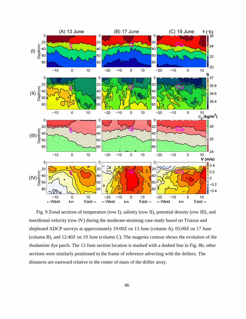
46

Fig. 9 Zonal sections of temperature (row I), salinity (row II), potential density (row III), and

meridional velocity (row IV) during the moderate-straining case study based on Triaxus and

shipboard ADCP surveys at approximately 19:00Z on 13 June (column A), 05:00Z on 17 June

(column B), and 12:40Z on 19 June (column C). The magenta contour shows the evolution of the

rhodamine dye patch. The 13 June section location is marked with a dashed line in Fig. 8b; other

sections were similarly positioned in the frame of reference advecting with the drifters. The

distances are eastward relative to the center of mass of the drifter array.

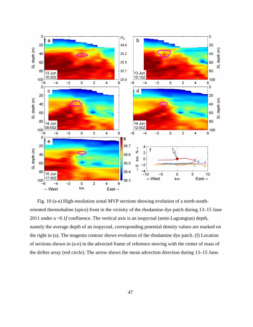
47

Fig. 10 (a-e) High-resolution zonal MVP sections showing evolution of a north-south-

oriented thermohaline (spice) front in the vicinity of the rhodamine dye patch during 13–15 June

2011 under a ~0.1f confluence. The vertical axis is an isopycnal (semi-Lagrangian) depth,

namely the average depth of an isopycnal, corresponding potential density values are marked on

the right in (a). The magenta contour shows evolution of the rhodamine dye patch. (f) Location

of sections shown in (a-e) in the advected frame of reference moving with the center of mass of

the drifter array (red circle). The arrow shows the mean advection direction during 13–15 June.

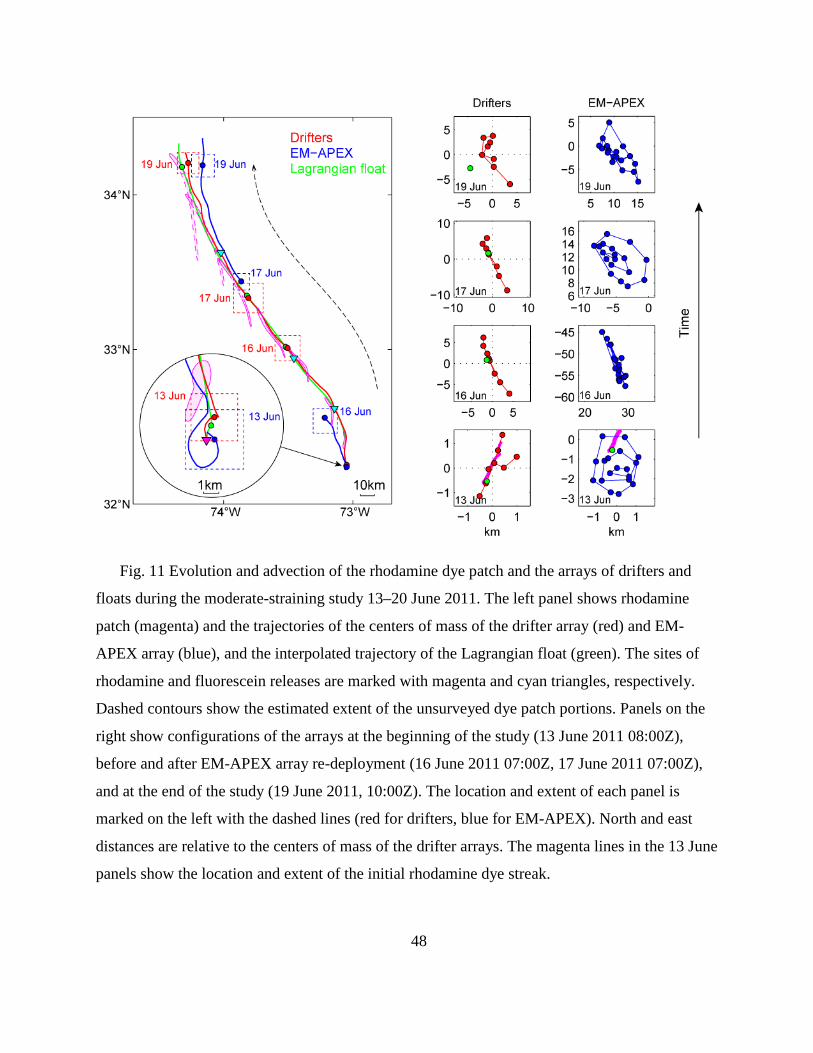
48

Fig. 11 Evolution and advection of the rhodamine dye patch and the arrays of drifters and

floats during the moderate-straining study 13–20 June 2011. The left panel shows rhodamine

patch (magenta) and the trajectories of the centers of mass of the drifter array (red) and EM-

APEX array (blue), and the interpolated trajectory of the Lagrangian float (green). The sites of

rhodamine and fluorescein releases are marked with magenta and cyan triangles, respectively.

Dashed contours show the estimated extent of the unsurveyed dye patch portions. Panels on the

right show configurations of the arrays at the beginning of the study (13 June 2011 08:00Z),

before and after EM-APEX array re-deployment (16 June 2011 07:00Z, 17 June 2011 07:00Z),

and at the end of the study (19 June 2011, 10:00Z). The location and extent of each panel is

marked on the left with the dashed lines (red for drifters, blue for EM-APEX). North and east

distances are relative to the centers of mass of the drifter arrays. The magenta lines in the 13 June

panels show the location and extent of the initial rhodamine dye streak.

49

Fig. 12 Evolution of the mesoscale eddy structure encompassing the moderate-straining study

13–20 June. AVHRR sea surface temperature imagery on a) 15 June, b) 17 June, and c) 19 June

is shown. Red and blue circles show the locations of the centers of mass of drifter and EM-

APEX arrays, respectively, at the time images were acquired. Advection of these arrays over the

course of the study (as in Fig. 11) is shown with dashed lines.

50

Fig. 13 Lidar view of the fluorescein dye release on 15 June 2011, during the moderate-strain

study. Shown is the peak lidar dye return intensity a) 2.5 hours and b) 4 hours after initial dye

injection. North and east distances are relative to position of the Lagrangian float deployed with

the dye. The magenta lines show the location of the initial dye streak, injected at 29 m depth

(potential density 24.8 kg m−3).

51

Fig. 14 a) Cartoon of the Lagrangian float used in near-field dye studies. The float actively

changed its buoyancy to straddle the target isopycnal as measured by CTD’s on its top and

bottom. A chain drive (gray) repeatedly carried dye and temperature sensors across the float’s

length. A Doppler sonar measured the velocity at a point below the float. b) Dye (colors) and

temperature (contours, heavy contour interval 0.1°C, temperature at the center of the float is

about 24.23°C) near the start of a float record during the 15 June dye release. Mapping is from

upcasts of each sensor only. A persistent streak (‘Ref’) results from a reference mark used to

align the sensors. c) Same as b) but later in the record. The float is drawn to scale relative to the

data plots.

52

Fig. 15 Average diapycnal profiles of a) thermal variance dissipation rate, b) turbulent kinetic

energy dissipation rate, and c) diapycnal eddy diffusivity derived from the three deployments of

microstructure EM-APEX floats in weak- (3–10 June, black) and moderate-straining (12–16

June, red; 16–19 June, blue) case studies. The shading shows 95% confidence intervals. The

circles and horizontal bars are values and confidence intervals at the target isopycnals of

rhodamine dye releases.

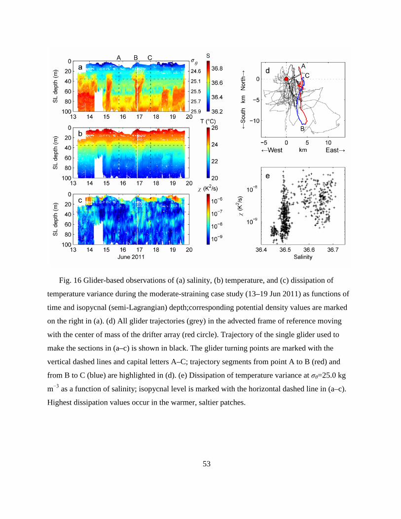
53

Fig. 16 Glider-based observations of (a) salinity, (b) temperature, and (c) dissipation of

temperature variance during the moderate-straining case study (13–19 Jun 2011) as functions of

time and isopycnal (semi-Lagrangian) depth;corresponding potential density values are marked

on the right in (a). (d) All glider trajectories (grey) in the advected frame of reference moving

with the center of mass of the drifter array (red circle). Trajectory of the single glider used to

make the sections in (a–c) is shown in black. The glider turning points are marked with the

vertical dashed lines and capital letters A–C; trajectory segments from point A to B (red) and

from B to C (blue) are highlighted in (d). (e) Dissipation of temperature variance at σθ=25.0 kg

m−3 as a function of salinity; isopycnal level is marked with the horizontal dashed line in (a–c).

Highest dissipation values occur in the warmer, saltier patches.

54

Fig. 17 Numerical submesoscale-resolving simulation of thermohaline front instability. (a)

Zonal and (b) isopycnal sections of salinity 6.7 inertial periods after the initialization. The

vertical axis in (a) is an isopycnal (semi-Lagrangian) depth; corresponding potential density

values are shown on the right. Dashed lines mark the locations of isopycnal (25.52 kg m−3) and

zonal (10 km) sections. The simulation was initialized with the observed thermohaline gradients

(smoothed to 1 km) from the 13 June hydrography (Fig. 9A) and allowed to evolve freely (spin-

down).

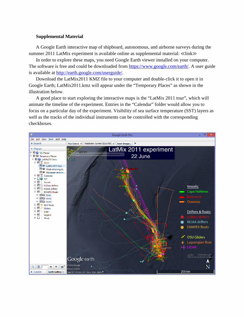
Supplemental Material

A Google Earth interactive map of shipboard, autonomous, and airborne surveys during the summer 2011 LatMix experiment is available online as supplemental material: ≪link≫

In order to explore these maps, you need Google Earth viewer installed on your computer. The software is free and could be downloaded from https://www.google.com/earth/. A user guide is available at http://earth.google.com/userguide/.

Download the LatMix2011 KMZ file to your computer and double-click it to open it in Google Earth; LatMix2011.kmz will appear under the “Temporary Places” as shown in the illustration below.

A good place to start exploring the interactive maps is the “LatMix 2011 tour”, which will animate the timeline of the experiment. Entries in the “Calendar” folder would allow you to focus on a particular day of the experiment. Visibility of sea surface temperature (SST) layers as well as the tracks of the individual instruments can be controlled with the corresponding checkboxes.