The kernel of the Eisenstein ideal by János Csirik B.A. (University of ...

The kernel of the Eisenstein ideal

by

Janos Csirik

B.A. (University of Cambridge) 1994

A dissertation submitted in partial satisfaction of therequirements for the degree of

Doctor of Philosophy

in

Mathematics

in the

GRADUATE DIVISIONof the

UNIVERSITY of CALIFORNIA at BERKELEY

Committee in charge:

Professor Kenneth A. Ribet, ChairProfessor Robert F. ColemanProfessor Steven N. Evans

Spring 1999

The dissertation of Janos Csirik is approved:

Chair Date

Date

Date

University of California at Berkeley

Spring 1999

The kernel of the Eisenstein ideal

Copyright 1999

by

Janos Csirik

1

Abstract

The kernel of the Eisenstein ideal

by

Janos Csirik

Doctor of Philosophy in Mathematics

University of California at Berkeley

Professor Kenneth A. Ribet, Chair

Let N be a prime number, and let J0(N) be the Jacobian of the modular curve X0(N).

Let T denote the endomorphism ring of J0(N). In a seminal 1977 article, B. Mazur intro-

duced and studied an important ideal I ⊆ T, the Eisenstein ideal. In this dissertation we

give an explicit construction of the kernel J0(N)[I] of this ideal (the set of points in J0(N)

that are annihilated by all elements of I). We use this construction to determine the action

of the group Gal(Q/Q) on J0(N)[I]. Then we apply our results to study the structure of the

old subvariety of J0(NM), where M is a prime number distinct from N. Our results were

previously known in the special case where N− 1 is not divisible by 16.

Professor Kenneth A. RibetDissertation Committee Chair

iii

This dissertation is dedicated to

my mother, Erzsebet Czachesz;

my father, Janos Csirik;

and my wife, Susan Harrington.

I thank them for their love and support.

iv

Contents

1 Introduction 1

2 Notation and setup 4

3 The Units of X1(N) 8

4 Some units on X#0 (N) 13

5 The Galois structure of J0(N)[I] 23

6 The old subvariety of J0(NM) 29

7 A unit calculation on X#0 (N,M) 40

Bibliography 48

v

Acknowledgements

First of all, I thank Ken Ribet for many helpful conversations and for suggesting

this problem to me. I also thank Arthur Ogus for telling me some useful facts about etale

cohomology.

I thank Matt Baker and Kevin Buzzard for the many fun conversations and semi-

nars we participated in together. I also learned much from conversations with Hendrik W.

Lenstra, Jr., and Bjorn Poonen.

I thank Donald Knuth for creating TEX, the typesetting system used for this disser-

tation, and for assigning it to the public domain. I also thank the creators of the computer

program PARI–GP [1], which was used for some preliminary calculations for this disserta-

tion.

1

Chapter 1

Introduction

Let N be a prime number and let J0(N) denote the Jacobian of the modular

curve X0(N). The variety J0(N) possesses certain naturally defined endomorphisms T` (for

all primes ` 6= N) and w. These endomorphisms together with Z (the multiplications by

integers) generate the Hecke ring TN of endomorphisms of J0(N). In his celebrated article

Modular Curves and the Eisenstein Ideal [11], Mazur defined the Eisenstein ideal I in TN as

the ideal generated by 1+w and the 1+ `− T` and used it to identify the possible rational

torsion subgroups of elliptic curves defined over the rational numbers. The Galois module

J0(N)(Q)[I] plays an important role in [11] and later studies of the arithmetic geometry of

the curve X0(N).

Mazur proved that

J0(N)[I] ∼= Z/nZ× Z/nZ

as groups, for n = (N − 1)/ gcd(N − 1, 12). In this dissertation we will study the action of

the group Gal(Q/Q) on J0(N)[I]. The group J0(N)[I] has two noteworthy Galois-invariant

subgroups. The cuspidal subgroup C is generated by the divisor c = 0 −∞ (the formal

difference of the two cusps of X0(N)). The group C is cyclic of order n and is pointwise

fixed by Gal(Q/Q). The Shimura subgroup Σ is a finite flat subgroup scheme of J0(N) such

that

Σ(Q) = ker(β∗ : J0(N)→ J1(N)),

where β∗ is induced by the usual degeneracy map β : X1(N)→ X0(N). The group Σ is also

cyclic of order n, but is isomorphic to µn as a group scheme.

2

In this dissertation we shall give an explicit construction of J0(N)[I], and apply

the construction in various ways. Mazur’s paper [11] contains an explicit construction

of J0(N)[I] only in the case N 6≡ 1 (mod 16), although he remarks in a few places that a

general description would be desirable. Our construction identifies the action of Gal(Q/Q)

on J0(N)[I].

If n is odd (equivalently N 6≡ 1 (mod 8)) then C ∩ Σ = 0, so J0(N)[I] ∼= C⊕ Σ and

therefore we know the Galois action on J0(N)[I].

If n is even then C ∩ Σ 6= 0 and more is needed to find the Galois action. In

this case C + Σ has index 2 in J0(N)[I]. Therefore it suffices to find an “extra” point P in

J0(N)[I] that is not in C+Σ. The knowledge of the Galois action on P, Σ and C then gives a

description of the Gal(Q/Q)-action of J0(N)[I]. For the case n ≡ 2 (mod 4) (or equivalently

N ≡ 9 (mod 16)), Mazur finds P by considering the Nebentypus covering X#0 (N) → X0(N)

of degree 2. Using a function constructed by Ogg and Ligozat, he obtains a divisor d on

X#0 (N) which turns out to be the pullback of a certain divisor on X0(N) that gives the extra

point on J0(N).

This dissertation uses other coverings X#0 (N)→ X0(N) to generalize Mazur’s con-

struction and find extra points of J0(N)[I] for any N ≡ 1 (mod 8). To find suitable divisors

on our modular curves X#0 (N), we use the theory of modular units: rational functions on a

modular curve whose divisors are concentrated at the cusps. Our coverings X#0 (N)→ X0(N)

are all intermediate to X1(N) → X0(N), enabling us to rely on the theory of modular units

on X1(N). The units of X(N) are treated in Kubert and Lang’s [8]. We recall some of their

results in Chapter 2. We then use the results of Chapter 2 to develop some results about the

units of X1(N) in Chapter 3. (The references [6, 8] also treat this case but restrict their at-

tention to units whose divisors are supported at the rational cusps, and don’t explicitly give

the data necessary for the descent to X#0 (N).) In Chapter 4, we construct a divisor on X#

0 (N)

and establish properties of the divisor that make our later arguments work. In Chapter 5,

we prove that the extra point we obtain is in J0(N)[I] and use this fact to prove the following

theorem, conjectured by Ribet. For any positive integer k, let χk denote the kth cyclotomic

character Gal(Q/Q)→ (Z/kZ)× obtained via the identification Gal(Q(µk)/Q)) ∼= (Z/kZ)×.

Theorem 1.1 J0(N)[I] has a basis e1, e2 over Z/nZ such that

a) c = e1 + 2e2;

b) e1 generates Σ;

3

c) σ ∈ Gal(Q/Q) acts via left multiplication by χn(σ) (1− χ2n(σ))/2

0 1

with respect to the given basis e1 =

(10

), e2 =

(01

).

In Chapters 6 and 7, we give another application of our construction of J0(N)[I].

Let M be a prime number distinct from N. The old part of J0(NM) is the abelian

subvariety of J0(NM) generated by

A = im(α : J0(N)2 → J0(NM)) and B = im(β : J0(M)2 → J0(NM)),

where α and β are certain naturally defined degeneracy morphisms (to be specified pre-

cisely in Chapter 6). Each of A and B was determined by Ribet in [16]. Therefore, to

complete the description of the old part of J0(NM), we need to determine A ∩ B. This

project was carried out partially by Ribet in [18], where he determined the odd part of

A ∩ B. In [9], Ling went on to obtain partial results about the even part of A ∩ B when nei-

ther N nor M is congruent to 1 modulo 16. In Chapter 6, we prove that A ∩ B is Eisenstein

and we use Theorem 1.1 to completely determine A ∩ B to obtain

Theorem 1.2 Let N and M be distinct primes. Let m = (M − 1)/ gcd(M − 1, 12), and let

D−,− = P1 − PN − PM + PNM ∈ J0(NM). Then A ∩ B is the unique subgroup of order

gcd(n,m) of the cyclic group generated by D−,−.

The symbols P1, PN, PM and PNM are the conventional names for the cusps of

X0(NM). Their meaning will be explained in Chapter 6. Theorem 1.2 answers questions in

[18], [16] and [12].

Chapter 7 contains some modular unit calculations that are used in Chapter 6.

4

Chapter 2

Notation and setup

For any non-zero rational number x, let num(x) denote the numerator of x, that

is, the smallest positive integer n such that n/x is an integer.

We will now briefly summarize the relevant properties of the modular curves we

will be using. The reader can find a thorough treatment of these in [3], as well as in the

references cited below.

Let N be a positive integer. We shall consider the usual modular curves X0(N),

X1(N) and X(N), and their Jacobians J0(N), J1(N) and J(N). These correspond to the

moduli problems of classifying an elliptic curve with a cyclic subgroup of orderN, an elliptic

curve with a point of order N, and an elliptic curve with an embedding of µN × Z/NZcompatible with the Weil pairing, respectively. These curves are all defined over Q, as are

the usual degeneracy maps (which are Galois coverings) α : X(N) → X1(N), β : X1(N) →X0(N) and γ = β α.

The curves X0(N)C, X1(N)C and X(N)C can also be regarded as compactified quo-

tients of the complex upper half plane H∗/Γ0(N), H∗/Γ1(N) and H∗/Γ(N), respectively,

where

Γ0(N) =

(a

c

b

d

)∈ SL2Z : c ≡ 0 (mod N)

,

Γ1(N) =

(a

c

b

d

)∈ SL2Z : c ≡ 0, d ≡ 1 (mod N)

,

Γ(N) =

(a

c

b

d

)∈ SL2Z : a ≡ 1, b ≡ 0, c ≡ 0, d ≡ 1 (mod N)

,

and these subgroups of SL2Z act on the complex upper half plane H via fractional linear

transformations. The points introduced during the compactification are called cusps.

5

Now let N be an odd prime number, and let

r = (N− 1)/2.

The curve X0(N) has two cusps, denoted 0 and ∞. They are both defined over

Q and are distinguished by the fact that under the natural map X0(N)C = H∗/Γ0(N) →X(1)C = H∗/SL2Z, the cusp 0 is ramified with index N and the cusp∞ is unramified.

The curve X1(N) has N − 1 cusps that come in two groups. We shall use Klimek’s

notation in [6] for them. The cusps P1, P2, . . . , Pr are defined over Q and are mapped to

0 under β : X1(N) → X0(N). The cusps Q1,Q2, . . . ,Qr are defined over Q(µN)+ (the

maximal totally real subfield of the Nth cyclotomic field) and are mapped to ∞ under β.

All the cusps of X1(N) are unramified with respect to β.

The curve X(N) has (N2 − 1)/2 cusps and we use Shimura’s notation in [15] to

regard them as pairs ±(xy

)with x, y ∈ FN, not both equal to 0. In this representation,

Gal(X(N)C/X0(N)C) ∼= PSL2FN acts naturally from the left. For 1 ≤ i ≤ r, the cusps(∗i

)are

all defined over Q(µN) and map unramifiedly to Pi under α : X(N)→ X1(N). For 1 ≤ i ≤ r,the cusps

(i0

)are all defined over Q(µN)+ and map to Qi under α with ramification index

N.

Shimura’s notation can be used to label the cusps of any modular curve. We

shall now provide the translations to Shimura’s system of all the names we use. On the

curve X0(N), the cusps 0 and∞ (respectively) are called(01

)and

(10

)(respectively). On the

curve X1(N), for any 1 ≤ t ≤ r, our notation Pt corresponds to(0t

), while Qt corresponds

to(t0

).

Recall that a unit of a modular curve is a rational function on the curve that has

its divisor concentrated at the cusps. (It is a unit of the ring of rational maps from the

noncuspidal points of the curve to the affine line.) In [8], Kubert and Lang determined all

the units of X(N). We briefly recall their results here, using Z/NZ× Z/NZ as the indexing

group instead of their 1NZ/Z ×

1NZ/Z. Let e = (e1, e2) be a pair of integers such that not

both of e1 and e2 are divisible by N. One can use the classical Weierstrass σ and Dedekind

η functions to define the Klein form ke(τ) on H. This form enjoys the properties

∀α =

(a

c

b

d

)∈ SL2Z, ke(ατ) = (cτ+ d)−1keα(τ) (K1)

(where eα denotes usual matrix multiplication) and

∀f = (f1, f2) ∈ NZ×NZ, ke+f(τ) = ε(e, f)ke(τ), (K2)

6

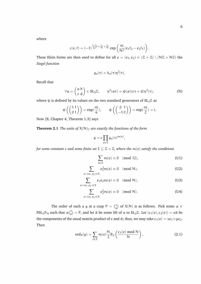
where

ε(e, f) = (−1)f1f2N2

+f1N

+f2N exp

(πi

N2(e1f2 − e2f1)

).

These Klein forms are then used to define for all e = (e1, e2) ∈ (Z × Z) \ (NZ × NZ) the

Siegel function

ge(τ) = ke(τ)η2(τ).

Recall that

∀α =

(a

c

b

d

)∈ SL2Z, η2(ατ) = ψ(α)(cτ+ d)η2(τ), (N)

where ψ is defined by its values on the two standard generators of SL2Z as

ψ

((1

0

1

1

))= exp(

πi

6), ψ

((0

−1

1

0

))= exp(

πi

2) = i.

Now [8, Chapter 4, Theorem 1.3] says

Theorem 2.1 The units of X(N)C are exactly the functions of the form

g = c∏e∈E

ge(τ)m(e),

for some constant c and some finite set E ⊆ Z× Z, where the m(e) satisfy the conditions∑e∈E

m(e) ≡ 0 (mod 12), (U1)

∑e=(e1,e2)∈E

e21m(e) ≡ 0 (mod N), (U2)

∑e=(e1,e2)∈E

e1e2m(e) ≡ 0 (mod N), (U3)

∑e=(e1,e2)∈E

e22m(e) ≡ 0 (mod N). (U4)

The order of such a g at a cusp P =(xy

)of X(N) is as follows. Pick some α ∈

PSL2FN such that α(10

)= P, and let α be some lift of α to SL2Z. Let (c1(e), c2(e)) = eα be

the components of the usual matrix product of e and α; thus, we may take c1(e) = xe1+ye2.

Then

ordP(g) =∑e∈E

m(e)N

2B2

(c1(e) mod N

N

), (2.1)

7

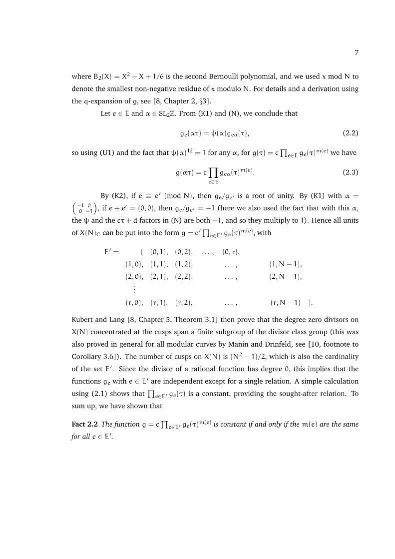
where B2(X) = X2 − X + 1/6 is the second Bernoulli polynomial, and we used x mod N to

denote the smallest non-negative residue of x modulo N. For details and a derivation using

the q-expansion of g, see [8, Chapter 2, §3].

Let e ∈ E and α ∈ SL2Z. From (K1) and (N), we conclude that

ge(ατ) = ψ(α)geα(τ), (2.2)

so using (U1) and the fact that ψ(α)12 = 1 for any α, for g(τ) = c∏e∈E ge(τ)

m(e) we have

g(ατ) = c∏e∈E

geα(τ)m(e). (2.3)

By (K2), if e ≡ e ′ (mod N), then ge/ge ′ is a root of unity. By (K1) with α =(−100

−1

), if e + e′ = (0, 0), then ge/ge ′ = −1 (here we also used the fact that with this α,

the ψ and the cτ+ d factors in (N) are both −1, and so they multiply to 1). Hence all units

of X(N)C can be put into the form g = c ′∏e∈E ′ ge(τ)

m(e), with

E ′ = (0, 1), (0, 2), . . . , (0, r),

(1, 0), (1, 1), (1, 2), . . . , (1,N− 1),

(2, 0), (2, 1), (2, 2), . . . , (2,N− 1),...

(r, 0), (r, 1), (r, 2), . . . , (r,N− 1) .

Kubert and Lang [8, Chapter 5, Theorem 3.1] then prove that the degree zero divisors on

X(N) concentrated at the cusps span a finite subgroup of the divisor class group (this was

also proved in general for all modular curves by Manin and Drinfeld, see [10, footnote to

Corollary 3.6]). The number of cusps on X(N) is (N2 − 1)/2, which is also the cardinality

of the set E ′. Since the divisor of a rational function has degree 0, this implies that the

functions ge with e ∈ E ′ are independent except for a single relation. A simple calculation

using (2.1) shows that∏e∈E ′ ge(τ) is a constant, providing the sought-after relation. To

sum up, we have shown that

Fact 2.2 The function g = c∏e∈E ′ ge(τ)

m(e) is constant if and only if the m(e) are the same

for all e ∈ E ′.

8

Chapter 3

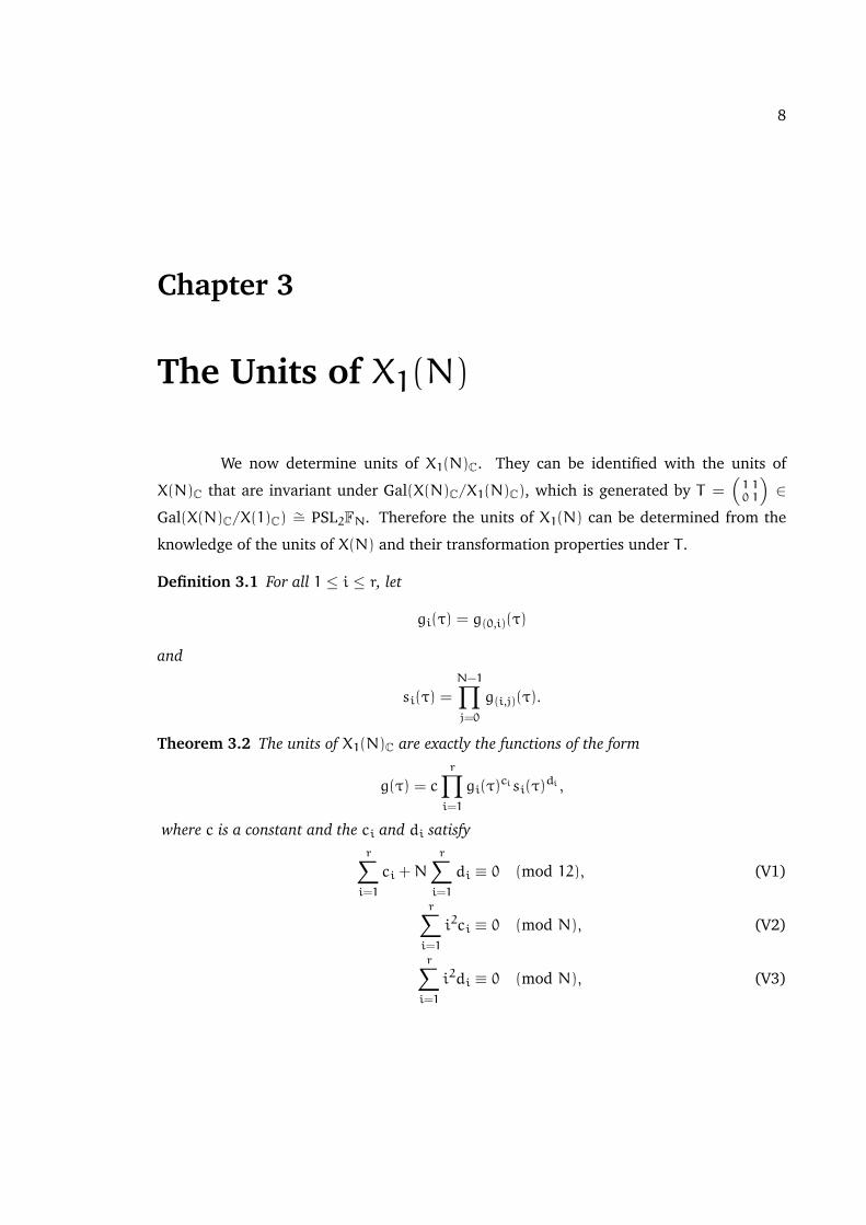
The Units of X1(N)

We now determine units of X1(N)C. They can be identified with the units of

X(N)C that are invariant under Gal(X(N)C/X1(N)C), which is generated by T =(1011

)∈

Gal(X(N)C/X(1)C) ∼= PSL2FN. Therefore the units of X1(N) can be determined from the

knowledge of the units of X(N) and their transformation properties under T .

Definition 3.1 For all 1 ≤ i ≤ r, let

gi(τ) = g(0,i)(τ)

and

si(τ) =

N−1∏j=0

g(i,j)(τ).

Theorem 3.2 The units of X1(N)C are exactly the functions of the form

g(τ) = c

r∏i=1

gi(τ)cisi(τ)

di ,

where c is a constant and the ci and di satisfyr∑i=1

ci +N

r∑i=1

di ≡ 0 (mod 12), (V1)

r∑i=1

i2ci ≡ 0 (mod N), (V2)

r∑i=1

i2di ≡ 0 (mod N), (V3)

9

PROOF. Let g(τ) = c∏e∈E ′ ge(τ)

m(e) be a unit of X(N). By determining the con-

ditions the m(e) must satisfy to be invariant under T , we can find a criterion for g to be a

unit of X1(N). Assume then that g is invariant under the action of T . By (2.3) and Fact 2.2,

m : E ′ → Z must be constant on the orbits of T (acting on E ′ from the right). Since

(e1, e2)T = (e1, e1+ e2), this shows that g can be written as a product of gi and si as above,

with ci = m((0, i)) and di = m((i, 0)) = m((i, 1)) = · · · = m((i,N− 1)).

Condition (U1) translates immediately to (V1).

The condition (U2) translates as∑e∈E ′

e21m(e) = N

r∑i=1

i2di ≡ 0 (mod N),

so it is necessarily satisfied. The condition (U3) translates as

∑e∈E ′

e1e2m(e) =

r∑i=1

i

N−1∑j=0

jdi =

r∑i=1

iNrdi ≡ 0 (mod N),

so it is also necessarily satisfied. Lastly, (U4) in our case is

∑e∈E ′

e22m(e) =

r∑i=0

i2ci +

r∑j=0

N−1∑i=0

i2dj =

r∑i=0

i2ci +N(2N− 1)r

3

r∑j=0

dj ≡ 0 (mod N).

Since N is not divisible by 3, r(2N− 1) must be, so (U4) translates to (V2).

It remains to check that our function g is actually invariant under the action of T ,

as opposed to being just invariant up to multiplication by a constant. This is not automatic,

despite the fact that (2.3) has no extra constant factors. Indeed, by restricting our indexing

set to E ′ we sometimes have to convert some ge (with e 6∈ E ′) occurring in (2.3) to some

ge ′ with e ′ ∈ E ′, thereby introducing a factor of a root of 1.

Using (K2), we can see that when we are acting by T on our g, this factor will be

r∏j=1

j−1∏k=0

ε((j, k), (0,N))dj =

r∏j=1

j−1∏k=0

(−1)dj exp(πi

Njdj

)

=

r∏j=1

(−1)jdi exp(πi

Nj2dj

).

Hence to ensure invariance, we need

N

r∑j=1

jdj +

r∑j=1

j2dj ≡ 0 (mod 2N).

10

The condition mod 2 is automatic since N is odd and j ≡ j2 (mod 2). The condition mod N

is just (V3).

It is also clear from the above calculations that any such g as given in the statement

of the theorem satisfies (U1–4) and hence is actually a T -invariant unit of X(N), so we have

completed the proof.

REMARK. For any i, the Atkin–Lehner involution (associated to the matrix(0

−N10

))

interchanges the functions gi and si up to constants. (For more details, see the proof of The-

orem 3.5.) Therefore, we expect the conditions (V1–3) to be invariant under exchanging

the cis and the dis. This is clear for (V2) and (V3), but it is also true for (V1). Indeed, since

(N, 6) = 1, we have N2 ≡ 1 (mod 12), and hence

12 | C+ND ⇐⇒ 12 | N2C+ND ⇐⇒ 12 | NC+D,

where we used the notation C =∑ri=1 ci and D =

∑ri=1 di.

Theorem 3.3 The order of such a function g (mentioned in Theorem 3.2) at the cusps is

ordPt(g) =

r∑i=1

(ciN

2B2

(it mod N

N

)+di

12

)

ordQt(g) =

r∑i=1

(ci

12+diN

2B2

(it mod N

N

)).

PROOF. A straightforward calculation using (2.1) and the fact that∑ri=1 B2(i/N) =

−r/(6N) gives the order of g at the cusps of X(N). Then, using the ramification indices of

the cusps of X(N) over the cusps of X1(N), we obtain our result.

Finally, we give the transformation properties of our functions under the Galois

group of X1(N)C over X0(N)C.

Definition 3.4 As in [15, §2], for a odd positive integer u, let

·u : Z→ 0, 1, . . . , (u− 1)/2

be the function defined by

au ≡ ±a (mod u).

For brevity, let · denote ·N.

11

Theorem 3.5 For any b ∈ 1, . . . , r and α =(sNh

ft

)∈ Γ0(N), we have

gb(ατ) = ψ(α)κ(α;b)gbt(τ),

with

κ(α;b) = (−1)bh exp(πi

(−b2ht

N

))(−1)bbt/Nc.

Although this fact will not be needed later, for reference we state that for any a ∈ 1, . . . , r

and α as above, we have

sa(ατ) = ψ(α)Nκ ′(α;a)sas(τ),

with

κ ′(α;a) = (−1)af exp(πi

(a2sf

N+ r

a− as

N

))(−1)bas/Nc.

PROOF. Using (2.2) we obtain

gb(ατ) = g(0,b)(ατ) = ψ(α)g(0,b)α(τ) = ψ(α)g(bhN,bt)(τ)

= ψ(α)ε((0, bt), (bhN, 0))g(0,bt)(τ)

= ψ(α)(−1)bh exp(πi

N(−b2ht)

)g(0,bt)(τ).

If bt ≡ bt (mod N) then

g(0,bt)(τ) = ε((0, bt), (0,Nbbt/Nc))g(0,bt)(τ)

= (−1)bbt/Ncgbt(τ).

If bt ≡ −bt (mod N) then

g(0,bt)(τ) = ε((0,−bt), (0,N(bbt/Nc+ 1)))g(0,−bt)(τ)

= (−1)bbt/Ncgbt(τ).

In either case, this completes the proof of the formula for gb(ατ).

For sa(ατ), a similar but more involved calculation can be used. Alternatively,

one might use the Atkin–Lehner involution wN =(0

−N10

)∈ SL2Z and the q-expansion

of g(e1,e2) in [8, Chapter 2, §1, K4] via the identity wN(τ) =(0

−110

)(Nτ) to conclude that

12

ga(wτ)/sa(τ) = c exp(πira/N), for some constant c that does not depend on a, and thereby

reduce the calculation to the one done above.

REMARK. Theorems 3.2 and 3.3 allow us to determine the group of divisors

supported at the cusps for any particular N. For example, consider the conjecture by

Klimek in [6, p. 3]. Let J∞1 (N) denote the group of divisors on X1(N) supported at the

set P1, P2, . . . , Pr. Klimek proved that

#J∞1 (N) = 41−rN∏χ6=1

B2,χ,

(where χ runs over all non-trivial even characters of (Z/NZ)×, and B2,χ denotes the gen-

eralized Bernoulli numbers of Kubota-Leopoldt, see also [8, Chapter 6, Theorem 3.4] for

another proof), and conjectured (presumably without the benefit of a computer) that the

group J∞1 (N) is always cyclic. He confirmed this conjecture for all N ≤ 23. A simple

(computer-aided) calculation using Theorems 3.2 and 3.3 shows that the conjecture is false

for N = 29. We obtain

N J∞1 (N)

2, 3, 5, 7 0

11 Z/5Z

13 Z/19Z

17 Z/584Z

19 Z/4383Z

23 Z/37181Z× Z/11Z29 Z/64427244Z× Z/4Z× Z/4Z31 Z/1772833370Z× Z/10...

...

13

Chapter 4

Some units on X#0(N)

Assume from now on that

N ≡ 1 (mod 8),

(in particular N ≥ 17).

Definition 4.1 Let CN denote the group (Z/NZ)×/± 1.

Since β : X1(N)C → X0(N)C is a cyclic Galois covering of degree r, it has a unique

intermediate covering of X0(N)C of any degree dividing r. Because of its uniqueness, any

such curve is defined over Q (for a thorough treatment of these intermediate curves, see [2,

IV, §3]). Letting n = (N−1)/ gcd(N−1, 12), we know from [11, II, §2] that the intermediate

curve X2(N)C → X0(N)C of degree n (the Shimura covering) is the largest etale covering of

X0(N)C through which β factors. (As remarked before, the cusps of X0(N) are not branch

points for β; it is the points with j = 0 and j = 1728 that ramify in β.)

Definition 4.2 Write n as

n = 2kv

where 2k is the largest power of 2 that divides n (and v = n/2k is an odd integer). Set z = 3 if

N ≡ 1 (mod 3) and z = 1 otherwise. For future use, we also set q = 3/z here.

Let

φ : X#0 (N)→ X0(N)

be the unique covering of degree 2k through which β factors. Let J#0 (N) = Jac(X#0 (N)).

14

Observe that the definitions of k, v, z imply that

r = 2k+1zv.

Since 2k divides n, the Shimura covering factors through φ. This implies that φ is etale and

that Σ0 = ker(φ∗ : J0(N)→ J#0 (N)) is contained in Σ = ker(J0(N)→ J2(N)).

The Galois group X1(N)C over X0(N)C is isomorphic to CN, with(sNh

ft

)mapping

to t. Let ξ be a generator of CN. We will abuse notation to lighten it, and let the same

ξ denote the generator of Gal(X1(N)C/X0(N)C) ∼= CN and the corresponding generator of

the Galois group of the function field extension; so that (ξf)(τ) = f(ξτ) for all functions f

on X1(N). Let Ω denote the set of 2kth powers in CN. Then Ω is the Galois group of X1(N)

over X#0 (N) and

#Ω = 2zv.

By its uniqueness property, X#0 (N) is Galois over X0(N).

The curve X#0 (N) is the coarse moduli space for the problem of classifying elliptic

curves with a point of order N, where (E, P) and (E ′, P ′) are to be considered equivalent if

there is an isomorphism δ : E→ E ′ such that δ(P) = ±b · P ′ for some b ∈ Ω.

We shall now construct some units of X#0 (N). They will first be given as units

of X1(N), and to check that they are actually units of X#0 (N) we shall need the follow-

ing lemmas. In these lemmas (and later), for any element b ∈ CN we let b denote the

representative for b in the set 1, 2, . . . , r. For example,∑b∈CN b =

∑ri=1 i = r(r+ 1)/2.

Lemma 4.3 For any coset Ω ′ of Ω,∑b∈Ω ′

b2 ≡ 0 (mod N)

PROOF. Let µ be a primitive root modulo N. Then a set of representatives for CN

in Z are 1, µ, . . . , µ(N−3)/2. The representatives of a coset Ω ′ of Ω are µj, µj+2k, µj+2·2

k,

. . . , µj+((N−1)/2k+1−1)2k for some 0 ≤ j < 2k. If

b ≡ ±µj+t2k (mod N),

then

b2 ≡ µ2j+t2k+1(mod N),

15

so

∑b∈Ω ′

b2 ≡ µ2j(N−1)/2k+1−1∑

t=0

µ2k+1t = µ2j

µN−1 − 1

µ2k+1

− 1≡ 0 (mod N)

by Fermat’s Little Theorem.

In the proofs of the next two lemmas, we shall use the following convention.

Convention 4.4 For P a statement, let [P] be 1 if P is true, 0 if P is false.

Lemma 4.5 Let t be an integer relatively prime to N. Then

S =∑b∈CN

bbt/Nc

is even if and only if t is a square modulo N.

PROOF. Note that∑b∈CN b = r(r+ 1)/2 is even (since r is divisible by 4), so

S =∑b∈CN

bbt/Nc ≡r∑

b∈CN

bt−∑b∈CN

Nbbt/Nc =∑b∈CN

(bt mod N) (mod 2).

Now bt mod N is either bt or N − bt depending on whether bt mod N ≤ r or not,

respectively. Therefore, we can write S as follows

S ≡∑b∈CN

bt +∑b∈CN

[bt mod N > r](−bt +N− bt)

≡∑b∈CN

b+∑b∈CN

[bt mod N > r](−bt +N− bt)

≡∑b∈CN

[bt mod N > r](N− 2bt) ≡∑b∈CN

[bt mod N > r] (mod 2)

Define m to equal∑b∈CN [bt mod N > r]. Then

(−1)mr! =∏b∈CN

bt ≡∏b∈CN

(bt) = trr! (mod N)

Since N does not divide r!, this implies that

(−1)m ≡ tr (mod N).

Since tr ≡ 1 (mod N) exactly when t is a square modulo N, this proves our lemma.

16

Lemma 4.6 Let Ω ′ be a coset of Ω and s, f, t, h integers with st−Nfh = 1 and t ∈ Ω and

S = h(1− t)∑b∈Ω ′

b+∑b∈Ω ′bbt/Nc.

The parity of S does not depend on the choice of Ω ′.

PROOF. First observe that st − Nfh = 1 implies that if t is even then h must be

odd, so in any case h(1− t) ≡ t+ 1 (mod 2). Therefore,

S ≡ (t+ 1)∑b∈Ω ′

b−N∑b∈Ω ′bbt/Nc =

∑b∈Ω ′

b+∑b∈Ω ′

(bt mod N) (mod 2).

Since t ∈ Ω, for b ranging over Ω the reductions of bt to CN just range over Ω ′, so we

can once again use the method of the proof of Lemma 4.5. Accordingly,

S ≡ 2∑b∈Ω ′

b+∑b∈Ω ′

[bt mod N > r](−bt +N− bt)

≡∑b∈Ω ′

[bt mod N > r] (mod 2).

Let m =∑b∈Ω ′ [bt mod N > r]. Then

(−1)m∏b∈Ω ′

b =∏b∈Ω ′

bt ≡∏b∈Ω ′

(bt) = t#Ω∏b∈Ω ′

b (mod N)

Since N does not divide∏b∈Ω ′ b,

(−1)m ≡ t#Ω (mod N),

and it is plain that the parity of m (which is the same as the parity of S) depends only on

the choice of t and not on the choice of Ω ′.

Recall from Definition 4.2 that q = 3/z.

Theorem 4.7 Define the following three functions on X1(N):

f(τ) =

(∏b∈Ω

gb(τ)2

kq

)∏b∈CN

gb(τ)−q

,g(τ) =

(∏b∈Ω

gb(τ)−q

)∏b∈ξΩ

gb(τ)q

,h(τ) =

(∏b∈Ω

gb(τ)2q

).

Then the following are true:

17

(a) the group Gal(X1(N)C/X#0 (N)C) is the subgroup of Gal(X1(N)C/X0(N)C) that fixes the

function f;

(b) the functions g and h are invariant under Gal(X1(N)C/X#0 (N)C) and can therefore be

regarded as being defined on X#0 (N)C;

(c) ξf = (−1)g2kf;

(d) g(ξg)(ξ2g) . . . (ξ2k−1g) = −1;

(e) the divisor div(f) is divisible by 2k in Div0(X#0 (N)).

REMARK. Henceforth we will regard f, g and h as functions on X#0 (N). By (a)

above, f descends to no smaller cover of X0(N).

NOTE. The function f above is the analogue in our situation of the Ogg–Ligozat

function fOL that was used in [11, II, Proposition (12.2)]. (In that paper, fOL is called f.)

Note however that if we restrict to the case of N ≡ 9 (mod 16) (equivalently n ≡ 2

(mod 4)) considered in that paper, our function f does not equal the function fOL. Instead,

the “correct” function f (the one we are using above) is equal to fqOL. However, since q is

always equal to 1 or 3, and Mazur was constructing a point in a group of exponent two, f

and fOL worked equally well.

PROOF. First we need to check (using Theorem 3.2) that f is actually a function on

X1(N). Conditions (V1) and (V3) are clearly satisfied, since, in the notation of Theorem 3.2,

each di is zero, and∑ci is also zero. For (V2), note that we need that N divide

q

∑b∈Ω

b22k −∑b∈CN

b2

= q

(2k∑b∈Ω

b2 −r(r+ 1)

6N

)

The first term is divisible by N by Lemma 4.3, the second is divisible by N since clearly

r(r+ 1)/6 is an integer.

We have now confirmed that f is defined on X1(N). It remains to check that the

largest subgroup Θ of CN that fixes f is in fact Ω. Since the coefficients in f for those gb

with b ∈ Ω are different from those for which b 6∈ Ω, we must have Θ ⊆ Ω.

To check Θ = Ω then, it remains to show that for any α =(sNh

ft

)∈ Γ0(N) with

t ∈ Ω, we have f(ατ) = f(τ). Using Theorem 3.5 (and (V1) to get rid of the ψ factors),

18

we need to confirm that

C = q

(∑b∈Ω

2k(Nbh− b2ht+Nbbt/Nc)

)−

q

∑b∈CN

(Nbh− b2ht+Nbbt/Nc)

≡ 0 (mod 2N)

The expression C can be thought of as six separate sums, and it turns out that each of them

is divisible by 2N. This is obvious for the first, third, fourth and fifth; follows by Lemma 4.3

for the second; and follows by Lemma 4.5 for the sixth. Hence we have proved (a).

Similarly, we can check that g is defined on X#0 (N). Again using Theorem 3.5, we

need to confirm that

− q(∑b∈Ω

(Nbh− b2ht+Nbbt/Nc))

+ q(∑b∈ξΩ

(Nbh− b2ht+Nbbt/Nc)) ≡ 0 (mod 2N)

The divisibility by N is immediate by Lemma 4.3, and for divisibility by 2 observe that for

any coset Ω ′ of Ω we have

S =∑b∈Ω ′

(Nbh− b2ht+Nbbt/Nc)

≡∑b∈Ω ′

(bh− bht+ bbt/Nc) ≡ h(1− t)∑b∈Ω ′

b+∑b∈Ω ′bbt/Nc (mod 2).

Now an application of Lemma 4.6 completes the proof.

For h(τ), we need 12|2q(#Ω) to verify (V1). But 2q(#Ω) = 2q · 2zv = 12v so this

is clear. The rest of the proof is analogous to the proof for g(τ). This completes the proof

of (b).

To prove (c), we calculate

(ξf)(τ) = f(ξτ) =

(∏b∈Ω

gb(ξτ)2

kq

)∏b∈CN

gb(ξτ)−q

=

(∏b∈Ω

gξb

(τ)2kqκ(ξ; b)2

kq

)∏b∈CN

gξb

(τ)−qκ(ξ; b)−q

,so (since (−1)q = −1) it suffices to show that∏

b∈Ωκ(ξ; b)2

k∏b∈CN

κ(ξ; b)−1 = −1.

19

Pick some(sNh

ft

)∈ Γ0(N) that lifts ξ. Then t will necessarily generate (Z/NZ)×, and in

particular it will be a non-square modulo N. By Theorem 3.5, it suffices to show that

exp

(πi

N

(2k∑b∈Ω

(Nbh− b2ht+Nbbt/Nc)

))×

exp

πiN

−∑b∈CN

(Nbh− b2ht+Nbbt/Nc)

= −1.

The first exponential is clearly 1 by Lemma 4.3 and because 2k is even. Clearly

exp

πiN

−∑b∈CN

(Nbh− b2ht)

= 1,

and we are done with (c) by Lemma 4.5.

For (d), note that

g =

∏b∈Ω

g−q

b

∏b∈ξΩ

gq

b

ξg =

∏b∈ξΩ

g−q

b

∏b∈ξ2Ω

gq

b

(∏b∈Ω

κ(ξ; b)−q

)∏b∈ξΩ

κ(ξ; b)q

ξ2g =

∏b∈ξ2Ω

g−q

b

∏b∈ξ3Ω

gq

b

(∏b∈Ω

κ(ξ; b)−q

)∏b∈ξΩ

κ(ξ; b)q

××

∏b∈ξΩ

κ(ξ; b)−q

∏b∈ξ2Ω

κ(ξ; b)q

=

∏b∈ξ2Ω

g−q

b

∏b∈ξ3Ω

gq

b

(∏b∈Ω

κ(ξ; b)−q

) ∏b∈ξ2Ω

κ(ξ; b)q

...

ξ2k−1g =

∏b∈ξ2k−1Ω

g−q

b

∏b∈Ω

gq

b

(∏b∈Ω

κ(ξ; b)−q

) ∏b∈ξ2k−1Ω

κ(ξ; b)q

.Therefore

g(ξg)(ξ2g) . . . (ξ2k−1g) =

(∏b∈Ω

κ(ξ; b)−q

)2k∏b∈CN

κ(ξ; b)q

=fg2

k

ξf= −1,

20

by (c). Thus the proof of (d) is complete.

We will use Theorem 3.3 to calculate div(f). It is immediately clear that ordQt(f) =

0 for all the cusps Qt. On the other hand, letting Ω ′ denote the coset of Ω containing the

reduction of bt, and using the fact that B2(x) = B2(1− x), we can calculate

ordPt(f) = q

∑b∈Ω

2kN

2B2

(bt mod N

N

)−∑b∈CN

N

2B2

(bt mod N

N

)= q

(2k−1N

∑b∈Ω ′

(b2

N2−b

N+1

6

)−N

2

(−r)

6N

)

= q2k−1∑b∈Ω ′

(b2

N− b

)+ q

(2k−1N

#Ω6

+r

12

).

By Lemma 4.3, the first term is an integer and clearly it is divisible by 2k. Using the identities

#Ω = 2zv, r = 2k+1zv, qz = 3, the latter term in the above sum reduces to

2k−1(N+ 1)v,

which is divisible by 2k since N+ 1 is even. So we have completed the proof (e).

We will need the following lemma. For a curve X defined over Q and a field K

containing Q, denote the function field of X over K by K(X). It is well known that a finite

abelian group equipped with a continuous action of Gal(Q/Q) is the same as a finite etale

commutative group scheme over Q. We will use this identification throughout the rest of

this dissertation.

Lemma 4.8 Let φ : X → Y be a finite etale map of projective curves, with X, Y and φ

defined over Q. Assume that φ is Galois after some finite base extension F/Q. Let Γ =

Gal(Q(X)/Q(Y)) ∼= Gal(F(X)/F(Y)) and assume that Γ is commutative. By the Picard functo-

riality of the Jacobians, we have an exact sequence

0 −−−→ K −−−→ Jac(Y)(Q)φ∗−−−→ Jac(X)(Q)Γ ,

where K denotes the finite Gal(Q/Q)-module ker(φ∗). Then

(a) the group scheme K is isomorphic to ΓD, the Cartier dual of Γ ;

(b) if Γ is cyclic, then φ∗ surjects onto Jac(X)(Q)Γ .

21

REMARK. To make sense of ΓD, we need to consider Γ as an etale group scheme

over Q. The group Γ is naturally acted upon by Gal(Q/Q) as follows: for any σ ∈ Gal(Q/Q)

and τ ∈ Γ , let σ · τ = στσ−1 where σ ∈ Gal(Q(X)/Q(X)) ∼= Gal(Q/Q) is any lift of σ.

PROOF. Taking the exact sequence of low degree terms for the Hochschild–Serre

spectral sequence of the etale cohomology of Gm over the base Q as in [14, III, Theorem

2.20], we obtain

0 −−−→ H1(Γ,H0(Xet,Gm)) −−−→ H1(Yet,Gm) −−−→−−−→ H0(Γ,H1(Xet,Gm)) −−−→ H2(Γ,H0(Xet,Gm))

which is

0 −−−→ H1(Γ,Q×) −−−→ Pic(Y)

φ∗−−−→ Pic(X)Γ −−−→ H2(Γ,Q×).

Now since Γ acts trivially on Q×

, H1(Γ,Q×) ∼= Hom(Γ,Q

×) ∼= ΓD. The kernel of φ∗ :

Pic(Y)→ Pic(X) is contained in Jac(Y), so we have proved (a).

If Γ is cyclic, then by [21, VIII §4], H2(Γ,Q×) ∼= (Q

×)Γ/(Q

×)N = 0. But if φ∗ :

Pic(Y)→ Pic(X)Γ is surjective, then so is φ∗ : Jac(Y)→ Jac(X)Γ , which proves (b).

Now we are almost ready to find extra points in J0(N)[I]. Recall that c denotes the

divisor 0−∞ on X0(N).

Theorem 4.9 Let d = 12k

div(f), considered as a point on J#0 (N). Then

(a) the divisor d is rational over Q;

(b) the divisor d is in the image of φ∗ : J0(N)→ J#0 (N);

(c) 2d = φ∗(v · c).

REMARK. In essence, we are trying to find “one half of c” in the group J0(N)[I]/Σ.

Assertion (c) in the above theorem shows that d is “one half of v · c”. Recall from Definition

4.2 that v is the odd part of n, so this is as good as finding half of c, but some calculations

work out simpler this way. Assertion (b) will be used to show that our point pulls back to

J0(N), and assertion (a) will be used to show that we are actually finding points in J0(N)[I].

PROOF. As can be seen from the proof of Theorem 4.7(e), div(f) is concentrated at

the cusps of X#0 (N) that lie over the cusp 0 of X0(N). All of these cusps are rational over Q,

hence so is d, proving (a).

22

By Lemma 4.8(b), it suffices to check that d is fixed by ξ, the generator of the

group Gal(X#0 (N)/X0(N)). By Theorem 4.7(c), div(f) − div(ξf) = −2k div(g), so

d− ξd =1

2kdiv(f) −

1

2kdiv(ξf) = div(1/g),

which is a principal divisor, so d = ξd in J#0 (N), concluding our proof of (b).

Let d ′ = div(f)/2k−1 − div(h) be a divisor on X#0 (N). Using Theorem 3.3, for

any 1 ≤ t ≤ r,

ordQt(d′) =

1

2k−1

∑b∈Ω

2kq

12−∑b∈CN

q

12

−∑b∈Ω

2q

12= 0− 2zvq/6 = −v,

and

ordPt(d′) =

∑b∈Ω

2kqN

2kB2

(bt mod N

N

)−∑b∈CN

qN

2kB2

(bt mod N

N

)

−∑b∈Ω

2qN

2B2

(bt mod N

N

)= −

qN

2k(−r)

6N= v.

Hence d ′ = φ∗(v · c), so

2d− div(h) = φ∗(v · c)

as divisors. But h is a function defined on X#0 (N) by Theorem 4.7(b), so this proves (c).

23

Chapter 5

The Galois structure of J0(N)[I]

Theorem 5.1 Let D denote the group generated by d in J#0 (N). Let A = (φ∗)−1D. Then

(a) all the points of D are unramified at N;

(b) all the points of A are unramified at N;

(c) the group A is contained in J0(N)[I].

REMARK. Since # ker(φ) = #D = 2k, the group A has cardinality 22k. Therefore

part (c) of the above theorem implies that A is the whole of the 2-primary component of

J0(N)[I]. Since the odd part of J0(N)[I] is the direct sum of the odd parts of C and Σ, we

have now completed the concrete description of J0(N)[I] that we were aiming for.

PROOF. Assertion (a) is immediate from Theorem 4.9(a), since the points of D are

rational. (Note that since the action of Gal(Q/Q) on the cusps of X#0 (N) factors through the

cyclotomic character χN, the only way for a divisor supported at the cusps to be unramified

at N is to be rational.)

Assertion (b) follows from [11, II, Lemma (16.5)]. Note that since the lemma just

cited applies only to points of prime power order, we have to apply it separately to each of

the primary components of the point of A in question.

Multiplication by 2k annihilates d. Therefore 2kA ⊆ ker(φ∗) ⊆ Σ, so certainly

all points in A are torsion points. By [20, Prop. 3.3], all torsion points of J0(N) that are

unramified at N are in J0(N)[I], so we have proved A ⊆ J0(N)[I].

REMARK. For the reader’s convenience we summarize another proof of part (c)

of Theorem 5.1 that avoids invoking [20]. This proof also does not need the results of

24

parts (a) and (b) of Theorem 5.1. We shall use the terminology and notation of [11]. Fix

an embedding QN → Q and let J be the Neron model of J0(N) over ZN. Let J/FN denote

the special fiber of J, and let J0/FN denote the irreducible component of the identity in J/FN .

Let Σ/FN denote the reduction of Σ to J/FN . Note that Σ ∼= µn, and so Σ is unramified at N.

Therefore, by [22, Lemma 2], Σ reduces injectively to Σ/FN . Then, by [11, II, Proposition

(11.9)],

Σ/FN ∩ J0/FN

= 0.

Thus, a point of Σ that reduces to a point in J0/FN must be zero. We shall now use this

observation to show that A ⊆ J0(N)[I].

It suffices to show that for arbitrary point x of A and any element T of I, we have

Tx = 0. The group of irreducible components of J/FN is Eisenstein, as can be seen from the

title (and contents) of [4] (see also [19]). Therefore, the operator T sends the reduction of

x into the identity component. In other words, Tx reduces into J0/FN .

On the other hand, we can use the formulae in [24, Section 2] to define actions of

Tl (for l 6= N) andw on (J1(N) and therefore on) J#0 (N) that are compatible with the actions

defined on J0(N) via the map φ∗, and calculate (in the spirit of the proof of Theorem 4.9(c))

that D is annihilated by each 1 + l − Tl and by 1 + w. Let T ′ be a lift of T to the ring

Z[. . . , Tl, . . . , w] and let T ′′ be the image of T ′ in End(J#0 (N)). Then we have a commutative

diagram

J0(N)φ∗−−−→ J#0 (N)yT yT ′′

J0(N)φ∗−−−→ J#0 (N).

Here x is mapped to φ∗x ∈ D which is annihilated by T ′′. By the commutativity of the

diagram we must have Tx ∈ ker(φ∗) = Σ. This completes our proof that Tx = 0.

Now that we established that A ⊆ J0(N)[I], we will determine the action of

Gal(Q/Q) on A and then assemble what we know to find the action of Gal(Q/Q) on the

whole of J0(N)[I].

Definition 5.2 Let λ : X##0 (N) → X#

0 (N) be a minimal covering of X#0 (N) on which f1/2

kis

defined.

25

By Theorem 4.7, parts (a) and (e), the degree of λ is 2k and λ is etale. In fact, after

base extension to Q(µ2k+1), λ becomes a Galois covering with Galois group Γ . The group Γ

can be regarded as a finite etale group scheme over Q, and by Lemma 4.8(a), A will be its

Cartier dual. This allows us to determine the action of Gal(Q/Q) on A.

Convention 5.3 Choose once and for all a primitive 2k+1st root of unity ζ ∈ Q. Then ζ2 is

the primitive 2kth root of unity that we will use in explicit Cartier duality calculations.

Theorem 5.4 Let K denote the function field of X0(N) over Q and L the function field of

X#0 (N) over Q, so that L(f1/2

k) is the function field of X##

0 (N) over Q.

(a) L(f1/2k, ζ)/K(ζ) is a Galois extension with

Γ = Gal(L(f1/2k, ζ)/K(ζ)) ∼= Z/2kZ× Z/2kZ.

In terms of the basis described in the proof, any element σ of Gal(Q/Q) acts on Γ via the

matrix 1 0

(χ2k+1(σ) − 1)/2 χ2k(σ)

.(b) The abelian group A is isomorphic to Z/2kZ× Z/2kZ, with σ ∈ Gal(Q/Q) acting via χ2k(σ) (1− χ2k+1(σ))/2

0 1

.PROOF. We know that the field extension L/K is Galois of degree 2k with cyclic

Galois group generated by ξ, and this remains true for L(ζ)/K(ζ). Clearly L(f1/2k, ζ)/L(ζ)

is also Galois (and cyclic) of degree 2k. Since K(ζ) (and hence L(ζ)) contains all 2kth

roots of unity, and by Theorem 4.7(c), (ξf)/f = (ζg)2k, we can conclude that L(f1/2

k, ζ) =

L((ξf)1/2k, ζ). This way we obtain that L(f1/2

k, ζ) contains all the 2kth roots of f, ξf, . . . ,

and therefore that L(f1/2k, ζ)/K(ζ) is a Galois extension.

To determine the group Γ = Gal(L(f1/2k, ζ)/K(ζ)), observe that the field extension

L(f1/2k, ζ)/K(ζ) contains all the conjugates of its generator f1/2

k. Therefore it is obtained

as a splitting field of the polynomial F whose roots are all the 2kth roots of all conjugates of

f. Since ξf = (−1)g2kf, the 2kth roots of ξf are ζgf1/2

k, ζ3gf1/2

k, . . . , ζ2

k+1−1gf1/2k. Then

ξ2f = ξ((−1)g2kf) = (−1)(ξg)2

k(ξf)

= (−1)(ξg)2k(−1)g2

kf = (ξg)2

kg2kf,

26

so the 2kth roots of ξ2f are (ξg)gf1/2k,ζ2(ξg)gf1/2

k, . . . , ζ2

k+1−2(ξg)gf1/2k. Hence it is

clear that the roots of F are exactly the

δi,j = ζ2i+j

(j−1∏k=0

(ξkg)

)f1/2

k,

where i and j range over the interval [0, 2k − 1].

To determine Γ , observe that it must act simply transitively on the set of all roots

of F. Let ρ ∈ Γ be such that

ρ : δ0,0 = f1/2k 7→ δ1,0 = ζ2f1/2

k.

Taking 2kth powers, we see that ρ fixes f and hence all of L(f1/2k, ζ). So ρ sends δi,j to δi+1,j

(with δ2k,j to be interpreted as δ0,j).

Now consider the element ξ ∈ Γ for which

ξ : δ0,0 = f1/2k 7→ δ0,1 = ζgf1/2

k.

Taking 2kth powers again, we see that ξ sends f to ξf, so it acts as ξ on L(ζ) (thereby

justifying our choice of name for it). Note that

ξ(δ0,1) = ξ(ζgf1/2k) = ζ(ξg)(ξf1/2

k) = ζ(ξg)ζgf1/2

k= ζ2(ξg)gf1/2

k= δ0,2,

similarly

ξ(δ0,2) = ξ(ζ2(ξg)gf1/2k) = ζ3(ξ2g)(ξg)gf1/2

k= δ0,3,

and so on. Finally, using Theorem 4.7(d) we obtain

ξ(δ0,2k−1) = ξ(ζ2k−1(ξ2

k−2g) . . . (ξg)gf1/2k) = ζ2

k(ξ2

k−1g) . . . (ξg)gf1/2k

= (−1)(−1)f1/2k

= f1/2k

= δ0,0.

Hence ξ sends δi,j to δi,j+1 (with δi,2k to be interpreted as δi,0).

This shows that Γ is generated by two commuting elements of order 2k. In other

words, we have Γ ∼= Z/2kZ×Z/2kZ, and we can represent elements of Γ as column vectors

over Z/2kZ, with ξ corresponding to(10

)and ρ corresponding to

(01

).

As for the action of Gal(Q/Q) on Γ , take some σ ∈ Gal(Q/Q) and consider its

natural action on L(f1/2k, ζ) that leaves L(f1/2

k) fixed. Both σξσ−1 and ρ(χ

2k+1 (σ)−1)/2ξ fix

27

ζ and

σξσ−1 : f1/2k 7→ f1/2

k 7→ ζgf1/2k 7→ ζχ2k+1 (σ)gf1/2

k

ρ(χ2k+1 (σ)−1)/2ξ : f1/2

k 7→ ζgf1/2k 7→ ζχ2k+1 (σ)gf1/2

k.

Therefore σξσ−1 = ρ(χ2k+1 (σ)−1)/2ξ. Similarly both σρσ−1 and ρχ2k (σ) fix ζ and

σρσ−1 : f1/2k 7→ f1/2

k 7→ ζ2f1/2k 7→ ζ2χ2k+1 (σ)f1/2

k

ρχ2k (σ) : f1/2k 7→ ζ2χ2k (σ)f1/2

k= ζ2χ2k+1 (σ)f1/2

k.

Therefore σρσ−1 = ρχ2k (σ). Hence σ ∈ Gal(Q/Q) does act on the elements of Γ (represented

by column vectors) as required. With this the proof of (a) is complete.

For (b), a simple calculation shows that if G is an etale group scheme over Q that

is isomorphic to Z/mZ× Z/mZ with a Galois action described by(a(σ)

c(σ)

b(σ)

d(σ)

): Gal(Q/Q)→ GL2(Z/mZ),

then its Cartier dual GD is also isomorphic to Z/mZ × Z/mZ, but with a Galois action

described in terms of the usual dual basis by(χm(σ)a(σ−1)

χm(σ)b(σ−1)

χm(σ)c(σ−1)

χm(σ)d(σ−1)

): Gal(Q/Q)→ GL2(Z/mZ).

In our case this means thatA ∼= ΓD is isomorphic to Z/2kZ×Z/2kZwith the action

of σ ∈ Gal(Q/Q) described by(χ2k(σ)

0

χ2k(σ)(χ2k+1(σ−1) − 1)/2

1

)in terms of the basis ξD =

(10

), ρD =

(01

). But χ2k(σ)(χ2k+1(σ−1) − 1)/2 ≡ (1 − χ2k+1(σ))/2

(mod 2k) so we have completed the proof of this theorem.

PROOF OF THEOREM 1.1. Since the quotient group Gal(L(ζ)/K(ζ)) of Γ is spanned

by ξ, the dual subgroup Σ0 = ker(J0(N) → J#0 (N)) is spanned by ξD in A. One checks

easily that d ∈ ker(J#0 (N) → J##0 (N)) corresponds to the image of ρ in A/Σ0 under Cartier

duality, so we can see by Theorem 4.9(c) that v · c ∈ A is represented by some vector(∗2

)in

A. But since v · c ∈ A is Gal(Q/Q)-invariant, we can use Theorem 5.4(b) to conclude that

v · c =(12

).

The odd part of J0(N)[I] is a direct product µv×Z/vZ. The constant part is gener-

ated by 2kc, so we can choose a basis g1, 2kc so that for any σ ∈ Gal(Q/Q), σ(g1) = χv(σ)g1

28

and σ(2kc) = 2kc. Taking the basis consisting of g1 and g2 = (2kc − g1)(v + 1)/2 instead,

we have 2kc = g1 + 2g2 and σ acts via(χv(σ)

0

(1− χ2v(σ))/2

1

).

Now pick integers a, b such that va+ 2kb = 1. Then

e1 = aξD + bg1

e2 = aρD + bg2

is a basis of J0(N)[I] that clearly has all properties required in Theorem 1.1.

Finally, observe that if N 6≡ 1 (mod 8), then n = v and the 2-primary part of

J0(N)[I] is 0. So formally setting ξD = ρD = 0, we still have v · c = n · c = 0 = ξD + 2ρD

and ρD ∈ Σ. The above argument about the prime-to-2 part works without a change, so we

have proved Theorem 1.1 in this case too.

REMARK. As described in [20], H. W. Lenstra and K. Ribet proved a version of The-

orem 1.1, where the expression (1 − χ2n(σ))/2 in the statement of the theorem is replaced

by a function

b : Gal(Q/Q)→ Z/nZ,

satisfying the properties that for each σ, τ ∈ Gal(Q/Q),

b(στ) = b(σ) + χn(σ)b(τ),

2b(σ) = 1− χn(σ),

and that the kernel of b cuts out the 2nth cyclotomic field. We shall show here that his

result is strictly weaker than Theorem 1.1.

Indeed, let b0(σ) = (1− χ2n(σ))/2, and let

ε : Gal(Q/Q)→ Z/2Z

be a homomorphism that factors through Gal(Q(µn)/Q). It is easy to check that for any

such ε, the function

b(σ) = b0(σ) +n

2ε(σ)

satisfies all of the above conditions. Since there is more than one choice for such a function

ε when n divisible by 4, we have shown that the above result is weaker than Theorem 1.1.

29

Chapter 6

The old subvariety of J0(NM)

Let N and M be distinct primes. The modular curve X0(NM) classifies elliptic

curves equipped with a subgroup of order NM. (Recall from elementary group theory that

all abelian groups of order NM are cyclic.) Forgetting all but the N-primary part of such a

subgroup yields a subgroup of order N, thereby giving rise to a degeneracy map

π1 : X0(NM)→ X0(N),

which is defined over Q.

The Atkin–Lehner involution

wM : X0(NM)→ X0(NM)

is another morphism defined over Q that can be associated to a moduli-theoretic operation.

The operation is as follows. Let (E,C) denote a pair of an elliptic curve E and a subgroup

C of order NM. Let CN (respectively, CM) be the N-primary (respectively, M-primary)

subgroup of C, so that C = CN × CM. Let γ : E→ E ′ be the degree M isogeny with kernel

CM. Then it is easy to see that the group γ(E[M]) is cyclic of order M, and that the group

γ(CN) is cyclic of order N. Then the operation we are looking for sends the pair (E,C) to

the pair (E ′, γ(E[M])× γ(CN)).

On X0(NM)C = H∗/Γ0(NM), the map wM is induced by the action of the matrix(−aN−NM

bM

)acting on H∗ via the corresponding Moebius transformation, where a and b are

integers chosen so that bN− aM = 1.

The curve X0(NM) has four cusps, called P1, PN, PM and PNM in the notation of

[18]. The morphism π1 : X0(NM)→ X0(N) sends P1 and PM to the cusp 0 on X0(N), with

30

ramification indices M and 1, respectively. The map π1 also sends PN and PNM to the cusp∞ of X0(N), with ramification indices M and 1, respectively. The morphism wM swaps the

points P1 and PM, and it also swaps the points PN and PNM.

Now we can define the degeneracy map

πM : X0(NM)→ X0(N)

by setting πM = π1 wM. This allows us to define the morphisms

α = (π∗1, π∗M) : J0(N)× J0(N)→ J0(NM)

and

β = (π∗1, π∗N) : J0(M)× J0(M)→ J0(NM).

Since w2M is the identity morphism on X0(NM), we can see that w∗Mα(R1, R2) = α(R2, R1).

(Note that we shall use wM to denote w∗M where it is not likely to cause confusion.)

Definition 6.1 Let A = im(α) and B = im(β). The old part of J0(NM) is the abelian subva-

riety of J0(NM) that is generated by A and B.

Since J0(M) has good reduction everywhere away fromM and β is defined overQ,

we can conclude that B has good reduction away from M. Similarly, A has good reduction

away from N. Therefore, A ∩ B has good reduction everywhere and is finite (see [18,

Theorem 3] and [5]).

It was proved in [16] that

ker(α) = (P,−P) ∈ J0(N)2 : P ∈ Σ.

We shall paraphrase this fact by saying that “the kernel of α is Σ, embedded anti-diagonally”.

The analogous result of course also holds for β.

This completes the description of A and B. To completely describe the old part

of J0(NM), we need to find A ∩ B. The odd part of A ∩ B was found in [18]. We shall

complete that description by proving Theorem 1.2. We shall proceed through a sequence of

lemmas.

Lemma 6.2 The preimage of the group A ∩ B under the map α is contained in J0(N)[I]2.

PROOF. Let x ∈ J0(N)2 be such that α(x) ∈ A ∩ B. Then there is some y ∈ J0(M)2

such that β(y) = α(x). The point β(y) = α(x) has finite order, since it is contained in the

31

finite group A ∩ B. Since B has good reduction at N, the point β(y) must be unramified at

N unless its order is divisible by N. But that cannot happen, since, by [18, Corollary 1], the

odd part of the order of β(y) must divide the quantity

gcd(num((N− 1)/24),num((M− 1)/24)),

which is not divisible by N. Therefore, β(y) = α(x) is unramified at N. Now, since

ker(α) = Σ (embedded anti-diagonally), this implies, as in [11, II, Lemma (16.5)], that

x is unramified at N. This in turn implies by [20, Prop. 3.3] that x ∈ J0(N)[I]2 as required.

Lemma 6.3 The image of the divisor c = 0 −∞ on X0(N) under the map π∗1 − π∗M is the

divisor (M− 1)D−,− = (M− 1)(P1 − PN − PM + PNM).

PROOF. This is immediate using the action of wM on X0(NM) and the ramification

indices of the cusps of X0(NM) over the cusps of X0(N). Indeed,

π∗1(c) = π∗1(0−∞) = MP1 + PM −MPN − PNM

and

π∗M(c) = w∗M(π∗1(c)) = MPM + P1 −MPNM − PN.

The difference of the two displayed lines yields the result.

If M < 5 then B = 0 and Theorem 1.2 is true. Therefore, we may assume from

now on that M ≥ 5.Let P be a point that maps to the generator of J0(N)[I]/Σ that we constructed

before. Thus, P can be chosen as the point e2 in Theorem 1.1. If N ≡ 1 (mod 8), let z be

the non-trivial 2-torsion element in Σ.

If N ≡ 1 (mod 8) then Σ[2] = C[2]. Thus, we can express z as

z =n

2· c. (6.1)

This relation, which usually plays the role of an obstacle to be circumvented, now will help

us get a handle on the behavior of z instead.

Now that we have established that the image of J0(N)[I]2 is the only thing we need

to consider when determining A ∩ B, we prove a lemma that allows us to focus on an even

smaller set.

32

Lemma 6.4 Let R ∈ J0(N)[I]2. If α(R) ∈ A ∩ B, then

• if N 6≡ 1 (mod 8) then R lies in the Z-linear span of π∗1(P) − π∗M(P);

• if N ≡ 1 (mod 8) then R lies in the Z-linear span of π∗1(P) − π∗M(P) and π∗1(z).

PROOF. Assume that R = (R1, R2) maps into A ∩ B under α. Note that wM acts

on A ∩ B as multiplication by −1. Indeed, it is well known that β wM = wM β (see for

example [18, “Formulaire”]), and by (the M-analog of) Lemma 6.2, we know that wM acts

as −1 on β−1(A ∩ B). Therefore,

−α(R1, R2) = wMα(R1, R2) = α(R2, R1)

and hence

0 = α(R1 + R2, R1 + R2).

Once again using the fact that ker(α) = Σ (embedded anti-diagonally), we con-

clude that R1 + R2 is an element of Σ[2]. We now complete the proof by examining each of

the possibilities that this allows for R1 + R2.

In case R1+R2 = 0, we can write R1 = aP+σ for some integer a and some σ ∈ Σ.

Then

α(R1, R2) = α(aP + σ,−aP − σ) = aα(P,−P) = a(π∗1(P) − π∗M(P)).

If N ≡ 1 (mod 8) then Σ[2] 6= 0, and therefore it can also happen that R1+R2 = z.

Then we can write R1 = z+aP+σ for some integer a and some σ ∈ Σ. Then R2 = −aP−σ

and

α(R1, R2) = α(z, 0) + aα(P,−P) = π∗1(z) + a(π∗1(P) − π∗M(P)).

In either case, the lemma is proved.

Let us assume from now on that

N ≡ 1 (mod 8).

In the rest of this chapter, we shall frequently use the following argument to prove

that various points on J0(NM) are not equal. Let J be an abelian variety defined over Q (for

33

example, J0(NM)). Given a prime number p, we can consider J to be defined over Qp so

that we can look at its Neron model J /Zp.

Given a point Q in J(Q), we can consider it an element of J(Qp). By the Neron

mapping property, Q even extends to an element of J (Zp). Reducing modulo p, we can

then regard Q as an element of Jp(Fp), where Jp denotes the special fiber of J . The

scheme Jp is a group scheme over Fp, but it is not necessarily irreducible. Let Φp(J) denote

its group of irreducible components. Given our point Q ∈ Jp(Fp), we can check which

element ofΦp(J) it maps to. The argument we shall often use proceeds as follows. Consider

the function

$ : J(Q)→ Φp(J)

described above. Let P,Q ∈ J(Q). If $(P) 6= $(Q) then we must also have P 6= Q. Usually

we shall show that $(P) 6= $(Q) by first showing that $(P) = 0 (that is to say, P maps to

the component of the identity under reduction modulo p), and then showing that$(Q) 6= 0.

This method can work only if Φp(J) has more than one element, which in turn can

happen only if J has bad reduction at p. Since J0(NM) has good reduction away from N

and M, we will always choose p = N or p = M.

Now we prepare the ground for this method by proving that various points are

defined over Q and by studying the components they map to when reduced modulo N or

modulo M.

Lemma 6.5 The points π∗1(P) − π∗M(P) and π∗1(z) are defined over Q, and hence so is every

point of A ∩ B.

PROOF. By Lemma 6.4, (and the fact that J0(NM) is defined overQ), π∗1(P)−π∗M(P)

and π∗1(z) being defined over Q does imply that every point of A ∩ B is defined over Q.

The point c is defined over Q, and hence so is z = (n/2)c. Since the degeneracy

map π1 is also defined over Q, we conclude that π∗1(z) is defined over Q.

By [16, Theorem 4.3], the map π∗1 − π∗M : J0(N) → J0(NM) (which is defined

over Q) factors through J0(N)/Σ → J0(NM) (also defined over Q). Since the image of P

in J0(N)/Σ is also defined over Q by Theorem 1.1, it follows that π∗1(P) − π∗M(P) is defined

over Q.

Lemma 6.6 Every point of A ∩ B reduces to the identity component of J0(NM) modulo N

(and modulo M).

34

PROOF. By symmetry, it suffices to prove the claim for the reduction modulo N.

The variety B has good reduction modulo N, therefore any point in A ∩ B ⊆ B(Q)

reduces to the identity component modulo N.

Lemma 6.7 The point π∗1(z) does not reduce to the identity component of J0(NM) modulo N.

PROOF. Recall from (6.1) that z = (n/2)c. This will enable us to use the results of

[11, Appendix I] to determine exactly where in the component group of J0(N) modulo N

the point π∗1(z) will map. We have

π∗1(z) = π∗1(n

2(0−∞)) =

n

2(MP1 + PM −MPN − PNM) =

=n

2(M+ 1)(0−∞).

Here 0 (respectively ∞) means a cusp of X0(NM) that reduces to the same irreducible

component as the cusp 0 (respectively∞) modulo N.

Using the notation of [11, Appendix I], we have u ∈ 0, 1 and v ∈ 0, 1, with

u = 1 ⇐⇒ N ≡ 7 or 11 (mod 12) and M ≡ 1 (mod 4)

v = 1 ⇐⇒ N ≡ 5 or 11 (mod 12) and M ≡ 1 (mod 3).

We have assumed that N ≡ 1 (mod 8), which excludes the possibilities N ≡ 7, 11(mod 12). Therefore we must have u = 0, and

v = 1 ⇐⇒ N ≡ 2 (mod 3) and M ≡ 1 (mod 3).

Now that we have a good grip on the pair (u, v), we can look up in the table

of [11, Appendix I] the order of the divisor 0 − ∞ in the component group of J0(NM)

modulo N. The table below summarizes the possibilities (for brevity, we use the notation

x = (N− 1)(M+ 1)).

N (mod 3) M (mod 3) n ord(0−∞) π∗1(z)

1 1, 2 (N− 1)/12 x/12 x(0−∞)/24

2 1 (N− 1)/4 x/4 x(0−∞)/8

2 2 (N− 1)/4 x/12 x(0−∞)/8

In each case, we can see that π∗1(z) does not reduce to the identity. This completes

the proof.

35

Lemma 6.8 The point D−,− reduces to the identity component of J0(NM) modulo N and

modulo M.

PROOF. Considering D−,− in the group of components modulo N, we have

D−,− = P1 − PN − PM + PNM = 0−∞− 0+∞ = 0.

The same proof works modulo M.

Lemma 6.9 The point (π∗1 − π∗M)P reduces to the identity component of J0(NM) modulo N.

PROOF. This is a direct consequence of the fact that π∗1 − π∗M annihilates the com-

ponent group of J0(N). (See [17, Theorem 2] and [4, proof of Theoreme 1].)

In view of Lemma 6.4, the following Theorem shall bring us closer to our goal of

proving Theorem 1.2.

Theorem 6.10 The divisor class of (π∗1 − π∗M)(vP) on X0(NM) is equal to the divisor class

of v(M−1)2 D−,−.

REMARK. Note that since π∗1 − π∗M annihilates Σ ⊂ J0(N) and P is “half of c mod-

ulo Σ”, the Theorem 6.10 is consistent with the statement of the Lemma 6.3. Unfortunately,

the Theorem does not follow yet, since there are a lot of ways in which we could take half

of v(M− 1)D−,−, only one of which is consistent with the Theorem.

Since the definition of P involved the cover X#0 (N) of X0(N), we must pause here

to define a cover of X0(NM) that will allow us to determine (π∗1 − π∗M)P.

Let X1,0(N,M) denote the modular curve corresponding to the congruence sub-

group Γ1(N)∩Γ0(M). The curve X1,0(N,M) is defined overQ and corresponds to the moduli

problem of classifying elliptic curves equipped with a point of order N and a subgroup of

order M. The natural degeneracy map

X1,0(N,M)→ X0(NM)

will be denoted by β, by an abuse of notation that is intended to remind the reader to the

similarity of this map to the previously defined β : X1(N)→ X0(N). Specifically, both maps

β have the moduli-theoretic interpretation of taking a point of order N and replacing it by

the subgroup of order N that it generates.

36

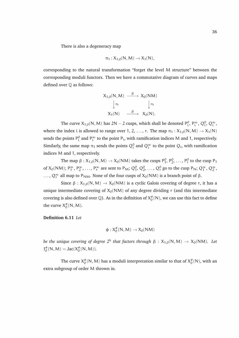
There is also a degeneracy map

π1 : X1,0(N,M)→ X1(N),

corresponding to the natural transformation “forget the level M structure” between the

corresponding moduli functors. Then we have a commutative diagram of curves and maps

defined over Q as follows:

X1,0(N,M)β−−−→ X0(NM)yπ1 yπ1

X1(N)β−−−→ X0(N).

The curve X1,0(N,M) has 2N − 2 cusps, which shall be denoted P0i , P∞i , Q0i , Q

∞i ,

where the index i is allowed to range over 1, 2, . . . , r. The map π1 : X1,0(N,M) → X1(N)

sends the points P0i and P∞i to the point Pi, with ramification indices M and 1, respectively.

Similarly, the same map π1 sends the points Q0i and Q∞i to the point Qi, with ramification

indices M and 1, respectively.

The map β : X1,0(N,M) → X0(NM) takes the cusps P01, P02, . . . , P

0r to the cusp P1

of X0(NM); P∞1 , P∞2 , . . . , P∞r are sent to PM; Q01, Q02, . . . , Q

0r go to the cusp PN; Q∞1 , Q∞2 ,

. . . , Q∞r all map to PNM. None of the four cusps of X0(NM) is a branch point of β.

Since β : X1,0(N,M) → X0(NM) is a cyclic Galois covering of degree r, it has a

unique intermediate covering of X0(NM) of any degree dividing r (and this intermediate

covering is also defined over Q). As in the definition of X#0 (N), we can use this fact to define

the curve X#0 (N,M).

Definition 6.11 Let

φ : X#0 (N,M)→ X0(NM)

be the unique covering of degree 2k that factors through β : X1,0(N,M) → X0(NM). Let

J#0 (N,M) = Jac(X#0 (N,M)).

The curve X#0 (N,M) has a moduli interpretation similar to that of X#

0 (N), with an

extra subgroup of order M thrown in.

37

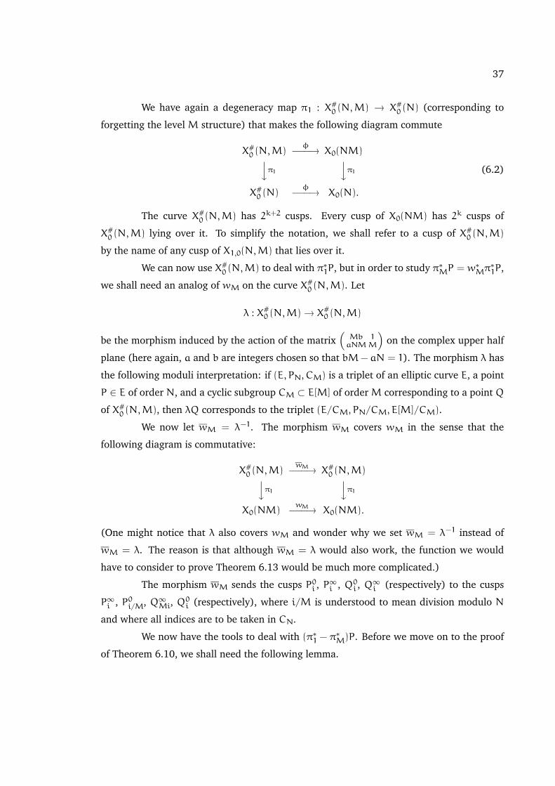
We have again a degeneracy map π1 : X#0 (N,M) → X#

0 (N) (corresponding to

forgetting the level M structure) that makes the following diagram commute

X#0 (N,M)

φ−−−→ X0(NM)yπ1 yπ1X#0 (N)

φ−−−→ X0(N).

(6.2)

The curve X#0 (N,M) has 2k+2 cusps. Every cusp of X0(NM) has 2k cusps of

X#0 (N,M) lying over it. To simplify the notation, we shall refer to a cusp of X#

0 (N,M)

by the name of any cusp of X1,0(N,M) that lies over it.

We can now use X#0 (N,M) to deal with π∗1P, but in order to study π∗MP = w∗Mπ

∗1P,

we shall need an analog of wM on the curve X#0 (N,M). Let

λ : X#0 (N,M)→ X#

0 (N,M)

be the morphism induced by the action of the matrix(MbaNM

1M

)on the complex upper half

plane (here again, a and b are integers chosen so that bM−aN = 1). The morphism λ has

the following moduli interpretation: if (E, PN, CM) is a triplet of an elliptic curve E, a point

P ∈ E of order N, and a cyclic subgroup CM ⊂ E[M] of orderM corresponding to a point Q

of X#0 (N,M), then λQ corresponds to the triplet (E/CM, PN/CM, E[M]/CM).

We now let wM = λ−1. The morphism wM covers wM in the sense that the

following diagram is commutative:

X#0 (N,M)

wM−−−→ X#0 (N,M)yπ1 yπ1

X0(NM)wM−−−→ X0(NM).

(One might notice that λ also covers wM and wonder why we set wM = λ−1 instead of

wM = λ. The reason is that although wM = λ would also work, the function we would

have to consider to prove Theorem 6.13 would be much more complicated.)

The morphism wM sends the cusps P0i , P∞i , Q0i , Q

∞i (respectively) to the cusps

P∞i , P0i/M, Q∞Mi, Q0i (respectively), where i/M is understood to mean division modulo N

and where all indices are to be taken in CN.

We now have the tools to deal with (π∗1 − π∗M)P. Before we move on to the proof

of Theorem 6.10, we shall need the following lemma.

38

Lemma 6.12 The unique non-trivial 2-torsion element in the kernel of

φ∗ : J0(NM)→ J#0 (N,M)

is the point π∗1(z).

PROOF. We can use the fact that z is a 2-torsion element of the kernel φ∗ : J0(N)→J#0 (N) and the commutativity of the diagram (6.2) to conclude that π∗1(z) is a 2-torsion

element of the kernel of φ∗ : J0(NM)→ J#0 (N,M).

The fact that π∗1(z) is not trivial follows from Lemma 6.7.

Since the map φ : X#0 (N,M) → X0(NM) is Galois with cyclic Galois group, there

are no other non-trivial 2-torsion points in its kernel.

Let us now take for granted the following theorem, the proof of which shall be the

subject of Chapter 7.

Theorem 6.13 The divisors

(1−w∗M)π∗1(d) and φ∗(v(M− 1)

2D−,−

)on X#

0 (N,M) are linearly equivalent.

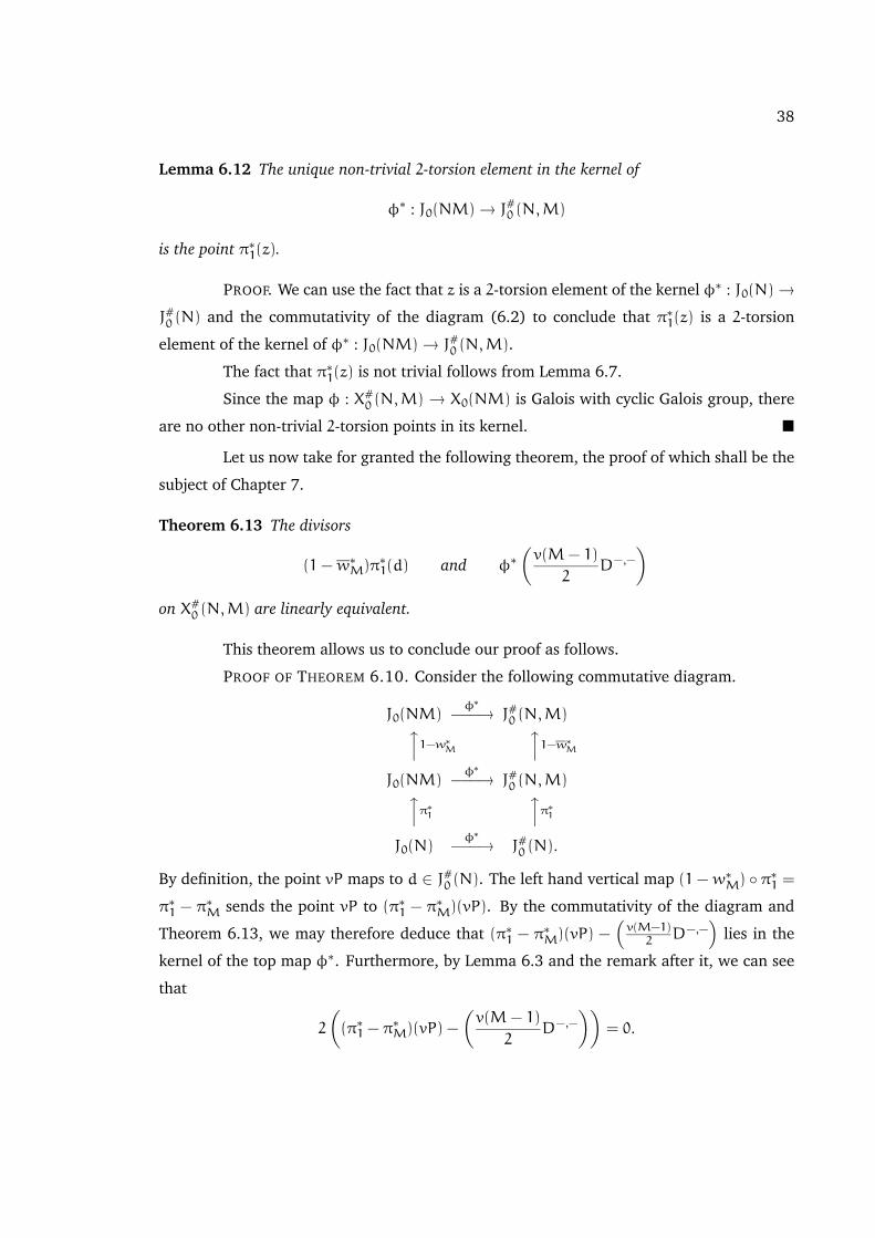
This theorem allows us to conclude our proof as follows.

PROOF OF THEOREM 6.10. Consider the following commutative diagram.

J0(NM)φ∗−−−→ J#0 (N,M)x1−w∗M x1−w∗M

J0(NM)φ∗−−−→ J#0 (N,M)xπ∗1 xπ∗1

J0(N)φ∗−−−→ J#0 (N).

By definition, the point vP maps to d ∈ J#0 (N). The left hand vertical map (1−w∗M) π∗1 =

π∗1 − π∗M sends the point vP to (π∗1 − π∗M)(vP). By the commutativity of the diagram and

Theorem 6.13, we may therefore deduce that (π∗1 − π∗M)(vP) −(v(M−1)2 D−,−

)lies in the

kernel of the top map φ∗. Furthermore, by Lemma 6.3 and the remark after it, we can see

that

2

((π∗1 − π∗M)(vP) −

(v(M− 1)

2D−,−

))= 0.

39

By Lemma 6.12, (π∗1 − π∗M)(vP) −(v(M−1)2 D−,−

)is equal to either 0 or π∗1(z).

However, reduction moduloN lands in the identity component of J0(NM) for (π∗1−π∗M)(vP)

(by Lemma 6.9), and for D−,− (by Lemma 6.8), and away from the identity component for

π∗1(z) (by Lemma 6.7). Therefore

(π∗1 − π∗M)(vP) =

(v(M− 1)

2D−,−

)and we have now completed the proof of Theorem 6.10.

PROOF OF THEOREM 1.2. In this proof, allow N and M to be any pair of distinct

primes. Observe that if N < 11 then A = 0 and Theorem 1.2 is true. Similarly, we may

assume that M ≥ 11.If N 6≡ 1 (mod 8) (equivalently, n is odd), then by Lemmas 6.2 and 6.4, the group

A ∩ B is spanned by a multiple of (π∗1 − π∗M)(P).

On the other hand, ifN ≡ 1 (mod 8) (equivalently, n is even), then by Lemmas 6.2

and 6.4, the group A ∩ B is spanned by a multiple of (π∗1 − π∗M)(P) and π∗(z). However, by

Lemmas 6.6 and 6.7, in fact the group A ∩ B is spanned by multiples of (π∗1−π∗M)(P) alone.

The multiples of (π∗1−π∗M)(P) are exactly the image of the group J0(N)[I]/Σ under

the map π∗1 − π∗M. Since π∗1 − π∗M is injective on J0(N)[I]/Σ, we can see that the image XN

has order n. We will now show that this image lies entirely in the cyclic group spanned

by D−,−.

We shall consider separately the image of the 2-primary part and the odd part of

J0(N)[I]/Σ. The odd part is generated by 2kP = 2k−1c, and its image does lie among the

multiples ofD−,− by Lemma 6.3. The 2-primary part of J0(N)[I]/Σ (which is non-trivial only

if n is even) is generated by vP. An application of Theorem 6.13 completes our argument.

Running the same argument again, but exchanging the roles of N and M, we find

that A ∩ B can also be found in the subgroup XM of order m of the multiples of D−,−.

Therefore, A ∩ B must be the intersection of our groups XN and XM. This completes the

proof.

40

Chapter 7

A unit calculation on X#0(N,M)

We now proceed to give a proof of Theorem 6.13.

Let us use the notation of Chapter 2 to identify our Siegel units. Note that (K1)

and (K2) are still valid (withN replaced byNM), as are (2.2) and (2.3). At the appropriate

points, we shall still massage the indices of our Siegel units into the array E ′ (with N, r

replaced by NM, (NM − 1)/2, respectively). Note that [8, Chapter 4, Theorem 1.3] does

not apply to a level that is not a prime power; thus our Theorem 2.1 does not apply in this

case. However, we shall use the half of Theorem 2.1 which remains valid by [8, Chapter 3,

Theorem 5.2]—namely, a function satisfying conditions (U1–4) is a unit on X(NM). (Note

that (U2–4) are now congruences modulo NM.)

Definition 7.1 Recall from Chapter 4 that Ω denotes the set of 2kth powers in CN. For any

integer y that is not divisible by N,

• let Ωy denote the representatives in the interval [1, r] of the elements of the coset yΩ

of Ω;

• let Jy denote the set of integers x in the interval [1, (NM− 1)/2] such that

– M does not divide x, and

– x maps to Ωy under the natural surjection Z→ CN;

• let

e(x) =∏j∈JM

gq(0,j).

41

We shall need a definition and some lemmas before we can show that div(e) is the

divisor mentioned in Theorem 6.13.

Definition 7.2 For any integer x ∈ [1, r], let φ(x) be the element of [1, r] that satisfies the

congruence

Mφ(x) ≡ ±x (mod N).

(In other words, φ(x) is the representative for x/M in CN.)

The following two lemmas will be useful later. Their proofs are very easy and will

not be given here.

Lemma 7.3 For any integer y that is not divisible by N,

(a) ∑j∈Jy

1 = 2zv(M− 1),

(b) ∑j∈Jy

j =1

2zvN(M− 1)(M+ 1) +

∑b∈Ωy

(b−Mφ(b)),

(c) ∑j∈Jy

j2 =1

6zvN2(M− 1)(M+ 1)M+

∑b∈Ωy

(Mb2 −M2φ(b)2).

Lemma 7.4 Let y be a real number. Then

M

(M−1∑i=0

B2

(y+ iN

NM

))− B2

( yN

)= 0.

We shall need one last lemma.

Lemma 7.5 Let c and d be relatively prime integers. Assume that c is divisible by NM and

that d maps into Ω under the map Z → CN. If y is any integer that is not divisible by N, we

have ∑j∈Jy

⌊dj

NM

⌋≡ (1+ d)

∑j∈Jy

j (mod 2).

42

PROOF. In this proof only, let · denote ·NM, as given in Definition 3.4. All the

congruences below are modulo 2. Proceeding as in the proof of Lemma 4.6, we obtain∑j∈Jy

⌊dj

NM

⌋≡ −d

∑j∈Jy

j+ d∑j∈Jy

j−NM∑j∈Jy

⌊dj

NM

⌋= −d

∑j∈Jy

j+∑j∈Jy

(dj mod NM)

= −d∑j∈Jy

j+ d∑j∈Jy

dj +∑j∈Jy

[dj mod NM > NM/2](−dj +NM− dj)

≡ (1+ d)∑j∈Jy

j+m,

where m =∑j∈Jy [dj mod NM > NM/2]. Then

(−1)m∏j∈Jy

j ≡∏j∈Jy

dj ≡∏j∈Jy

(dj) (mod NM),

which we can divide through by∏j∈Jy j, since no element of Jy is divisible by either N

or M, to obtain

(−1)m ≡ d#Jy (mod NM).

Since M− 1 divides #Jy, we get that

d#Jy ≡ 1 (mod M)

by Fermat’s Little Theorem. On the other hand, since 2(#Ω) divides #Jy, we obtain

d#Jy ≡ 1 (mod N).

(Already raising to the (#Ω)th power will send d ∈ Ω to 1 ∈ CN, which corresponds to

d ≡ ±1 (mod N).) Therefore, m must be even and the proof of the lemma is complete.

Claim 7.6 The function e(τ) is a unit on X#0 (N,M).

PROOF. We just need to check conditions (U1–4) of Theorem 2.1, and that e(τ)

remains invariant under the action of any matrix(acbd

)∈ SL2Z with c ≡ 0 (mod NM) and

d mapping to Ω under the map Z→ CN.

By the definition of the function e and Lemma 7.3(a), (U1) is equivalent to

2zvq(M− 1) ≡ 0 (mod 12).

43

This is always satisfied since 2zq = 6 and M− 1 is even.

It is clear from the definition of e that conditions (U2) and (U3) are satisfied,

because 0 is divisible by NM.

Lemma 7.3(c) shows us that condition (U4) is equivalent to

1

6zvqN2(M− 1)(M+ 1)M+ q

∑b∈Ωy

(Mb2 −M2φ(b)2) ≡ 0 (mod NM).

The condition modulo M is obviously satisfied. For the condition modulo N, observe that

the first term is clearly divisible by N, whereas the second term is divisible by N since for

any b ∈ Ωy,

b2 ≡M2φ(b)2 (mod N),

and hence∑b∈Ωy

(Mb2 −M2φ(b)2) ≡∑b∈Ωy

(Mb2 − b2) ≡ (M− 1)∑b∈Ωy

b2 ≡ 0 (mod N),

where the last congruence used Lemma 4.3.

To check invariance under(acbd

), we proceed as in the proof of Theorem 3.2. First

observe that(acbd

)indeed permutes the indices of functions in e(τ) (after reducing the

indices to E ′). The only thing we need to show is that the transformation factor arising

from reducing the indices to E ′ is 1. Using (K2), this reduces to showing that

c∑j∈JM

j− dc

NM

∑j∈JM

j2 +NM∑j∈JM

⌊dj

NM

⌋≡ 0 (mod 2NM).

(The floor function in bdj/NMc arises in a fashion entirely analogous to how it came up

in the proof of Theorem 3.5.) Since NM divides each of c,∑j2 (see above in our proof

that (U4) is satisfied) and NM (respectively), it must divide the first, second and third term

(respectively) of the above expression. Therefore, we need only check that

c∑j∈JM

j− dc

NM

∑j∈JM

j2 +NM∑j∈JM

⌊dj

NM

⌋≡ 0 (mod 2).

We have, using Lemma 7.5 and Lemma 7.3 parts (b) and (c),

c∑j∈JM

j− dc

NM

∑j∈JM

j2 +NM∑j∈JM

⌊dj

NM

⌋≡ c

∑b∈ΩM

(b− φ(b)) − dc∑b∈ΩM

(b− φ(b)) + (1+ d)∑b∈ΩM

(b− φ(b))

≡ (d+ 1)(c+ 1)∑b∈ΩM

(b− φ(b)) (mod 2).

44

Since c and d are relatively prime integers, at least one of them is odd, and therefore the

number (d+ 1)(c+ 1) must be even. This concludes our proof of the claim.

Claim 7.7 The divisor of e(τ) is

(1−w∗M)π∗1(d) − φ∗(v(M− 1)

2D−,−

).

PROOF. As was mentioned before, we shall prove here that the divisor above is

equal to the divisor of the function e(τ).

The proof of this claim is going to be similar to that of Theorem 4.9(c), but more

complex since there are more kinds of cusps and the objects we are considering are more

complicated.

First, we shall identify the divisors π∗1(d) ∈ J#0 (N,M) and w∗Mπ∗1(d) ∈ J#0 (N,M).

We do this by first recalling what the divisor d ∈ J#0 (N) is. For any 1 ≤ t ≤ r, let

At =q

2k

∑b∈Ω

2kN

2B2

(bt

N

)+∑b∈CN

−N

2B2

(bt

N

) .Then, by the definition of d, for any 1 ≤ t ≤ r we have

ordPt(d) = At, ordQt(d) = 0,

and therefore

ordP0t (π∗1(d)) = MAt, ordQ0t (π

∗1(d)) = 0

ordP∞t (π∗1(d)) = At, ordQ∞t (π∗1(d)) = 0.

By considering the action of w∗M on the cusps, we also obtain that

ordP0t (w∗Mπ∗1(d)) = AMt, ordQ0t (w

∗Mπ∗1(d)) = 0

ordP∞t (w∗Mπ∗1(d)) = MAt, ordQ∞t (w∗Mπ

∗1(d)) = 0.

Before we turn our attention to div(e), we note that

ordP0t (D−,−) = 1, ordQ0t (D

−,−) = −1

ordP∞t (D−,−) = −1, ordQ∞t (D−,−) = 1.

We shall now show for each cusp of J#0 (N,M) that the divisor mentioned in the

statement of the claim and div(e) have the same order.

For a cusp labeled Q∞t for some 1 ≤ t ≤ r (having ramification index 1 over the

cusp of X(1)), we observe that it can be represented by(tNM

)in Shimura’s notation and

45

therefore

ordQ∞t (div(e)) = q(#JM)1

2B2(0) =

2zvq(M− 1)

12=v(M− 1)

2.

Since π∗1(d) and w∗Mπ∗1(d) have order 0 at this cusp, this proves our claim for the cusps Q∞t .

For a cusp labeled Q0t for some 1 ≤ t ≤ r (having ramification index M over

the cusp of X(1)), we observe that it can be represented by(tN

)in Shimura’s notation and

therefore

ordQ0t (div(e)) = q∑j∈JM

M

2B2

(Nj mod NM

NM

)= q

∑j∈JM

M

2B2

(j mod MM

)

= qM(#ΩM)1

2

M−1∑i=1

B2

(i

M

)=

−v(M− 1)

2,

where we used the fact that∑M−1i=1 B2(i/M) is equal to (1 − M)/(6M). Since π∗1(d) and

w∗Mπ∗1(d) have order 0 at this cusp, this proves our claim for the cusps Q0t .

For a cusp labeled P∞t for some 1 ≤ t ≤ r (having ramification index N over

the cusp of X(1)), we observe that it can be represented by(

1Mφ(t)

)in Shimura’s notation.

Therefore, as above,

ordP∞t (div(e)) = q∑j∈JM

N

2B2

(φ(t)j mod N

N

).

Therefore,

ordP∞t (div(e) − π∗1(d) +w∗Mπ∗1(d))

=qN

2

∑j∈JM

B2

(φ(t)j mod N

N

)+ (1−M)

(q∑b∈Ω

N

2B2

(bt

N

)+

qr

12 · 2k

)

=qN

2(1−M)

∑b∈ΩMφ(t)

B2

(b

N

)−∑b∈Ωt

B2

(b

N

)+qr(1−M)

12 · 2k

=qN

2(1−M) · 0+

−2qzv(M− 1)

12=

−v(M− 1)

2,

where the above argument used the fact that modulo N, the set JM can be considered as

M− 1 copies of the set ΩM. Then we used the fact that Mφ(t) and t map to the same

element in CN to cancel out the last two nasty-looking sums. Thereby we completed the

proof for the cusps P∞t .

46

It remains for us to consider the cusps labeled P0t for some 1 ≤ t ≤ r (having ram-

ification index NM over the cusp of X(1)). We observe that such a cusp can be represented

by(0t

)in Shimura’s notation (where we add N to t if it is otherwise divisible by M). Then

ordP0t (div(e)) = q∑j∈JM

NM

2B2

(tjM mod NM

NM

).

Therefore

ordP0t (div(e) − π∗1(d) +w∗Mπ∗1(d)) =

qNM

2

∑j∈JM

B2

(tjM mod NM

NM

)

+qNM

2

∑b∈Ω

B2

(bt

N

)−qNM

2k+1

∑b∈CN

B2

(b

N

)

−qN

2

∑b∈Ω

B2

(btM

N

)+qN

2k+1

∑b∈CN

B2

(b

N

).

We shall separate the above sum of five terms into groups. First of all, note that the sum of

the third and the fifth terms is equal to

qN

2(1−M)

1

2k

∑b∈CN

B2

(b

N

)=qN

2(1−M)

1

2k−r

6N=v(M− 1)

2.

Therefore, to complete the proof of our claim, it suffices to show that the sum of the first,

second and fourth terms is zero. This boils down (after division by qN/2) to showing that

M∑j∈JMt

B2

(j

NM

)+M

∑b∈Ωt

B2

(b

N

)−∑

b∈ΩMt

B2

(b

N

)= 0.

However, the above equation is just the sum of the conclusions of Lemma 7.4 when we

allow the y of the Lemma to run over all elements of ΩM.

PROOF OF THEOREM 6.13. This theorem follows from Claims 7.6 and 7.7.

We shall now make some general comments about studying the cuspidal divisor

group on X#0 (N,M) in the style of our Chapter 3. We find a number of differences from the

case of prime level considered in Chapter 3.

First of all, it is still the case (as can be seen from [8, Chapter 3, Theorem 5.2])

that the functions of the form specified by Theorem 2.1 are units (they are the so-called

Siegel units), but they do not exhaust all the units of X(NM) any more. Instead, the Siegel

units form a subgroup of the group of all units, in such a way that the quotient group is an

47

elementary 2-abelian group. Therefore, the divisor mentioned in Theorem 6.13 might have

been principal without this fact being revealed by an analysis of Siegel units on X#0 (N,M).

Secondly, we cannot expect the analog of our Fact 2.2 to hold in the present case,

since X(NM) has (N2 − 1)(M2 − 1)/2 cusps, whereas there are (N2M2 − 1)/2 essentially

different Siegel units. Therefore, there will be a lot of extra relations between the divisors

of Siegel units that will make it significantly harder to emulate the proof of our Theorem 3.2

to establish the group of Siegel units on X1(NM).

Fortunately, both of the above difficulties can probably be overcome, and we shall

outline a suggested solution now.

Firstly, the non-Siegel units of X(NM) have also been studied extensively. An

analysis of [7] and [23] should probably allow a sufficiently explicit description of all units

and their divisors.

Secondly, although we have too many Siegel units, the relations among them are

well-understood. They are discussed in [8] under the name “distribution relations”. These

relations generally take the form of an “old” unit (i.e., one coming from a lower level) giving

a divisor that is linear combination of divisors of various other Siegel units (some of which

might also be old). It turns out that by the time we descend all the way to X1,0(N,M), we

have 2N − 2 cusps and 2N + 1 Siegel units. Instead of having just two kinds of functions

as in Definition 3.1, we now have eight different kinds of functions. (There are two types

each coming from levels N and M, as well as four kinds of new functions.) Nevertheless,

the relations each work out to be in the form where the product of a subset of the Siegel

units is a constant. Since the three subsets arising form a partition of the set of Siegel units,

it turns out that the arguments of Theorem 3.2 still go through.

48

Bibliography

[1] C. Batut, D. Bernardi, H. Cohen, M. Olivier, PARI–GP, computer software, 1995–1999

[2] P. Deligne and M. Rapoport, Les schemas de modules de courbes elliptiques, pages 143–

316 in P. Deligne and W. Kuyk (eds.), Modular Functions of One Variable II, Lecture

Notes in Mathematics, 349, Springer, 1973

[3] F. Diamond and J. Im, Modular forms and modular curves, pages 39–133 in Seminar

on Fermat’s Last Theorem (Toronto, ON 1993–1994), Canadian Mathematical Society

Conference Proceedings, Vol. 17, 1995

[4] B. Edixhoven, L’action de l’algebre de Hecke sur les groupes de composantes des jacobi-

ennes des courbes modulaires est “Eisenstein”, Asterisque, No. 196–197 (1992), 159–

170

[5] J.-M. Fontaine, Il n’y a pas de variete abelienne sur Z, Invent. math. 81 (1985), 515–

538

[6] P. E. Klimek, Modular functions for Γ1(N), Ph.D. dissertation, Berkeley, 1975

[7] D. S. Kubert, The square root of the Siegel group, Proc. London Math. Soc., (3) 43

(1981), 193–226

[8] D. S. Kubert and S. Lang, Modular Units, Grundlehren der mathematischen Wis-

senschaften 244, Springer, 1981

[9] S. Ling, The old subvariety of J0(pq) and the Eisenstein kernel in Jacobians, Israel Jour-

nal of Mathematics, 84 (1993), 365–384

[10] Ju. I. Manin, Parabolic points and zeta functions of modular curves, (Russian), Izv. Akad.

Nauk SSSR Ser. Math., 36 (1972), 19–66

49

[11] B. Mazur, Modular curves and the Eisenstein ideal, Inst. Hautes Etudes Sci. Publ. Math.

47, 1977, 33–186. See also the Errata on pages 187–188 of [13] for an important cor-

rection for line 18 of page 105. Also note that some typos in Appendix I are corrected

in [4, Section 4.4.1]

[12] B. Mazur, Rational isogenies of prime degree, Invent. math. 44 (1978), 129–162

[13] B. Mazur and A. Wiles, Class fields of abelian extensions of Q, Invent. math. 76 (1984),

179–330

[14] J. S. Milne, Etale Cohomology, Princeton University Press, 1980

[15] A. P. Ogg, Rational points on certain elliptic modular curves, pages 221–231 in Analytic

number theory, Proc. Sympos. Pure Math., Vol. XXIV, AMS, 1973

[16] K. A. Ribet, Congruence relations between modular forms, in Proceedings of the ICM

1983, 503–514

[17] K. A. Ribet, On the component groups and the Shimura subgroup of J0(N), Exp. No.

6, 10, in Seminaire de Theorie des Nombres, 1987–1988 (Talence, 1987–1988), Univ.

Bordeaux I, Talence.

[18] Kenneth A. Ribet, The old subvariety of J0(pq), in G. van der Geer, F. Oort, J. Steenbrink

(eds.), Arithmetic Algebraic Geometry, Progress in Mathematics 89 (1990), 293–307

[19] Kenneth A. Ribet, Irreducible Galois representations arising from component groups of

Jacobians, pages 131–147 in Elliptic curves, modular forms, and Fermat’s last theorem

(Hong Kong, 1993), Ser. Number Theory, I, Internat. Press, Cambridge, MA, 1995

[20] Kenneth A. Ribet, Torsion points on J0(N) and Galois representations, 1998

[21] J.-P. Serre, Local Fields, Graduate Texts in Mathematics 67, Springer, 1979

[22] Jean-Pierre Serre and John Tate, Good reduction of abelian varieties, Ann. of Math. (2)

88 (1968), 492–517

[23] Jing Yu, A cuspidal class number formula for the modular curves X1(N), Math. Ann. 252

(1980), 197–216

[24] A. Wiles, Modular curves and the class group of Q(µp), Invent. math. 58 (1980), 1–35