The IS-LM-BP Approach - University of Warwick · price level constant. A change in the domestic price level will change the price of domestic goods relative to foreign goods. If the

CHAPTER1313The IS-LM-BP Approach

An economy open to international trade and payments will face different

problems than an economy closed to the rest of the world. The typical

introductory economics presentation of macroeconomic equilibrium and

policy is a closed-economy view. Discussions of economic adjustments

required to combat unemployment or inflation do not consider the rest

of the world. Clearly, this is no longer an acceptable approach in an

increasingly integrated world.

In the open economy, we can summarize the desirable economic

goals as being the attainment of internal and external balance.

Internal balance means a steady growth of the domestic economy

consistent with a low unemployment rate. External balance is the

achievement of a desired trade balance or desired international capital

flows. In principles of economics classes, the emphasis is on internal

balance. By concentrating solely on internal goals like inflation, unem-

ployment, and economic growth, simpler-model economies may be used

for analysis. A consideration of the joint pursuit of internal and external

balance calls for a more detailed view of the economy. The slight

increase in complexity yields a big payoff in terms of a more realistic

view of the problems facing the modern policy maker. It is no longer

a question of changing policy to change unemployment or inflation at

home. Now the authorities must also consider the impact on the balance

of trade, capital flows, and exchange rates.

INTERNAL AND EXTERNAL MACROECONOMIC EQUILIBRIUM

The major tools of macroeconomic policy are fiscal policy (government

spending and taxation) and monetary policy (central bank control of the

money supply). These tools are used to achieve macroeconomic equilib-

rium. We assume that macroeconomic equilibrium requires equilibrium

in three major sectors of the economy:

Goods market equilibrium. The quantity of goods and services supplied

is equal to the quantity demanded. This is represented by the IS curve.

245International Money and Finance, Eighth EditionDOI: http://dx.doi.org/10.1016/B978-0-12-385247-2.00013-5

© 2013 Elsevier Inc.All rights reserved.

http://dx.doi.org/10.1016/B978-0-12-385247-2.00013-5

Money market equilibrium. The quantity of money supplied is equal to

the quantity demanded. This is represented by the LM curve.

Balance of payments equilibrium. The current account deficit is equal to

the capital account surplus, so that the official settlements definition of

the balance of payments equals zero. This is represented by the BP

curve.

We will analyze the macroeconomic equilibrium with a graph that

summarizes equilibrium in each market. Figure 13.1 displays the IS-LM-BP

diagram. This graph illustrates various combinations of the domestic interest

rate (i) and domestic national income (Y) that yield equilibrium in the three

markets considered here.

THE IS CURVE

First, let us examine the IS curve, which represents combinations of i and

Y that provide equilibrium in the goods market when everything else

(like the price level) is held constant. Y refers to the total output as well

0Ye

ie

LM

BP

e

IS

Income (Y )

Inte

rest

rat

e (i

)

Figure 13.1 Equilibrium in the goods market (IS), in the money market (LM), and inthe balance of payments (BP).

246 International Money and Finance

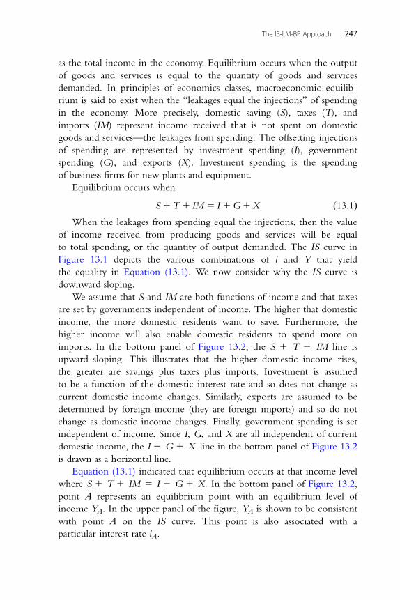
as the total income in the economy. Equilibrium occurs when the output

of goods and services is equal to the quantity of goods and services

demanded. In principles of economics classes, macroeconomic equilib-

rium is said to exist when the “leakages equal the injections” of spending

in the economy. More precisely, domestic saving (S), taxes (T), and

imports (IM) represent income received that is not spent on domestic

goods and services—the leakages from spending. The offsetting injections

of spending are represented by investment spending (I), government

spending (G), and exports (X). Investment spending is the spending

of business firms for new plants and equipment.

Equilibrium occurs when

S1T 1 IM 5 I 1G1X ð13:1ÞWhen the leakages from spending equal the injections, then the value

of income received from producing goods and services will be equal

to total spending, or the quantity of output demanded. The IS curve in

Figure 13.1 depicts the various combinations of i and Y that yield

the equality in Equation (13.1). We now consider why the IS curve is

downward sloping.

We assume that S and IM are both functions of income and that taxes

are set by governments independent of income. The higher that domestic

income, the more domestic residents want to save. Furthermore, the

higher income will also enable domestic residents to spend more on

imports. In the bottom panel of Figure 13.2, the S 1 T 1 IM line is

upward sloping. This illustrates that the higher domestic income rises,

the greater are savings plus taxes plus imports. Investment is assumed

to be a function of the domestic interest rate and so does not change as

current domestic income changes. Similarly, exports are assumed to be

determined by foreign income (they are foreign imports) and so do not

change as domestic income changes. Finally, government spending is set

independent of income. Since I, G, and X are all independent of current

domestic income, the I 1 G 1 X line in the bottom panel of Figure 13.2

is drawn as a horizontal line.

Equation (13.1) indicated that equilibrium occurs at that income level

where S 1 T 1 IM 5 I 1 G 1 X. In the bottom panel of Figure 13.2,

point A represents an equilibrium point with an equilibrium level of

income YA. In the upper panel of the figure, YA is shown to be consistent

with point A on the IS curve. This point is also associated with a

particular interest rate iA.

247The IS-LM-BP Approach

To understand why the IS curve slopes downward, consider what

happens as the interest rate varies. Suppose the interest rate falls. At the

lower interest rate, more potential investment projects become

profitable (firms will not require as high a return on investment when

the cost of borrowed funds falls), so investment increases as illustrated

in the move from I 1 G 1 X to I0 1 G 1 X in Figure 13.2. At this

higher level of investment spending, equilibrium income increases to YB.

Point B on the IS curve depicts this new goods market equilibrium, with

a lower equilibrium interest rate iB and higher equilibrium income YB.

Finally, consider what happens when the interest rate rises. Investment

spending will fall, because fewer potential projects are profitable as the

0

Sav

ing

+ ta

xes

+ im

port

s (S

+ T

+ IM

)In

vesm

ent +

gov

. spe

ndin

g +

expo

rts

(I +

G +

X)

0

iB

Inte

rest

rat

e (i

) iA

iC C

A

B

IS

YC YA YB

S + T + IM

I' + G + X

I + G + X

I'' + G + X

YC

C

Income (Y)

A

B

YA YB

Figure 13.2 Derivation of the IS curve.


cost of borrowed funds rises. At the lower level of investment spending,

the I 1 G 1 X curve shifts down to Iv1 G 1 X in Figure 13.2.

The new equilibrium point C is consistent with the level of income YC.

In the IS diagram in the upper panel we see that point C is consistent with

equilibrium income level YC and equilibrium interest rate iC. The other

points on the IS curve are consistent with alternative combinations of

income and interest rate that yield equilibrium in the goods market.

We must remember that the IS curve is drawn holding the domestic

price level constant. A change in the domestic price level will change the

price of domestic goods relative to foreign goods. If the domestic price

level falls with a given interest rate, then investment, government spend-

ing, taxes, and saving will not change. However, domestic goods are now

cheaper relative to foreign goods, leading to exports increasing and

imports falling. The rise in the I 1 G 1 X curve and the fall in the S 1

T 1 IM curve would both increase income. Because income increases

with a constant interest rate, the IS curve shifts to the right. A rise in the

domestic price level would cause the IS curve to shift left.

THE LM CURVE

The LM curve in Figure 13.1 displays the alternative combinations of i and Y

at which the demand for money equals the supply. Figure 13.3 provides a

derivation of the LM curve. The left panel shows a money demand curve

labeled Md and a money supply curve labeled Ms. The horizontal axis

measures the quantity of money and the vertical axis measures the interest

rate. Note that the Ms curve is vertical. This is so because the central bank

can choose any money supply it wants, independent of the interest rate.

The actual value of the money supply chosen is M0. The money demand

shows, for a fixed amount of wealth, how much people are willing to

hold in money form, as opposed to interest-bearing assets. The money

demand curve slopes downward, indicating that the higher the interest

rate, the lower the quantity of money demanded.

The inverse relationship between the interest rate and quantity of

money demanded is a result of the role of interest as the opportunity cost

of holding money. Since money earns no interest, the higher the interest

rate, the more you must give up to hold money, so less money is held.

The initial money market equilibrium occurs at point A with interest

rate iA. The initial money demand curve, Md, is drawn for a given level

of income. If income increased, then the demand for money would


increase, as seen in the shift from Md to Md0. Money demand increases

because, at the higher level of income, people want to hold more money

to support the increased spending on transactions.

Now let us consider why the LM curve has a positive slope. Suppose

initially there is equilibrium at point A with the interest rate at iA and

income at YA in Figure 13.3. If income increases from YA to YB, money

demand increases from Md to Md0. If the interest rate remains at iA, there

will be an excess demand for money. This is shown in the left panel of

Figure 13.3, as the quantity of money demanded is now MA0. With the

higher income, money demand is given by Md0. At iA, point A0 on the

money demand curve is consistent with the higher quantity of money

demanded, MA0. Since the money supply remains constant at M0, there

will be an excess demand for money given by MA0 2 M0. The attempt to

increase money balances above the quantity of money outstanding will

cause the interest rate to rise until a new equilibrium is established at

point B. This new equilibrium is consistent with a higher interest rate iBand a higher income YB. Points A and B are both indicated on the LM

curve in the right panel of Figure 13.3. The rest of the LM curve reflects

similar combinations of equilibrium interest rates and income.

The LM curve is drawn for a specific money supply. If the supply of

money increases, then money demand will have to increase to restore

M0

Money supply (M)

MA'

Md

Md'

Ms

A' iA

iB

iA

0 0YA YB

Income (Y)

iB

Inte

rest

rat

e (i)

B

A A

LM

B

Figure 13.3 Derivation of the LM curve.


equilibrium. This requires a higher Yor lower i, or both, so the LM curve

will shift right. Similarly, a decrease in the money supply will tend to raise

i and lower Y, and the LM curve will shift to the left.

THE BP CURVE

The final curve portrayed in Figure 13.1 is the BP curve. The BP curve

gives the combinations of i and Y that yield balance of payments equilib-

rium. The BP curve is drawn for a given domestic price level, a given

exchange rate, and a given net foreign debt. Equilibrium occurs when

the current account surplus is equal to the capital account deficit.

Recall from Chapter 3 that if there is a current account deficit, then it

has to be financed by a capital account surplus.

Figure 13.4 illustrates the derivation of the BP curve. The lower panel

of the figure shows a CS line, representing the current account surplus,

and a CD line, representing the capital account deficit. Realistically, the

current account surplus may be negative, which would indicate a deficit.

Similarly, the capital account deficit may be negative, indicating a surplus.

The CS line is downward sloping because as income increases, domestic

imports increase and the current account surplus falls. The capital account

is assumed to be a function of the interest rate and is, therefore, indepen-

dent of income and a horizontal line.

Equilibrium occurs when the current account surplus equals the capital

account deficit, so that the official settlements balance of payments is zero.

Initially, equilibrium occurs at point A with income level YA and interest

rate iA. If the interest rate increases, then domestic financial assets are more

attractive to foreign buyers and the capital account deficit falls to CD0. At theold income level YA, the current account surplus will exceed the capital

account deficit, and income must increase to YB to provide a new equilib-

rium at point B. Points A and B on the BP curve in Figure 13.4 illustrate

that, as i increases, Y must also increase to maintain equilibrium. Only an

upward-sloping BP curve will provide combinations of i and Y consistent

with equilibrium.

EQUILIBRIUM

Equilibrium for the economy requires that all three markets—the goods

market, the money market, and the balance of payments—be in

equilibrium. This occurs when the IS, LM, and BP curves intersect at a

common equilibrium level of the interest rate and income. In Figure 13.1,


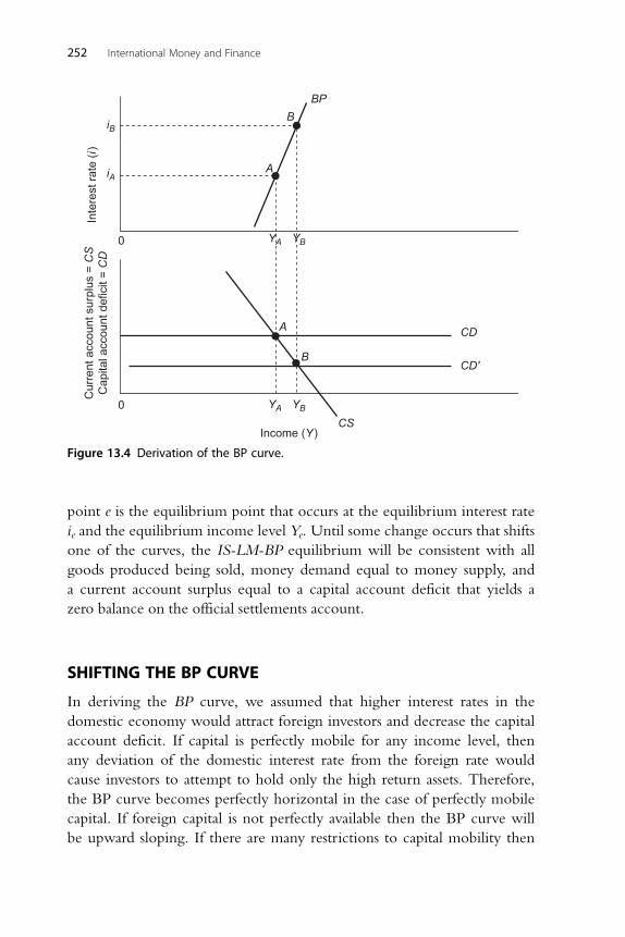
point e is the equilibrium point that occurs at the equilibrium interest rate

ie and the equilibrium income level Ye. Until some change occurs that shifts

one of the curves, the IS-LM-BP equilibrium will be consistent with all

goods produced being sold, money demand equal to money supply, and

a current account surplus equal to a capital account deficit that yields a

zero balance on the official settlements account.

SHIFTING THE BP CURVE

In deriving the BP curve, we assumed that higher interest rates in the

domestic economy would attract foreign investors and decrease the capital

account deficit. If capital is perfectly mobile for any income level, then

any deviation of the domestic interest rate from the foreign rate would

cause investors to attempt to hold only the high return assets. Therefore,

the BP curve becomes perfectly horizontal in the case of perfectly mobile

capital. If foreign capital is not perfectly available then the BP curve will

be upward sloping. If there are many restrictions to capital mobility then

A

A

B

BP

B

CS

CD

CD'

YA YB

YA

iA

iB

YB

Income (Y )

0

0

Cur

rent

acc

ount

sur

plus

= C

SC

apita

l acc

ount

def

icit

= C

DIn

tere

st r

ate

(i)

Figure 13.4 Derivation of the BP curve.


the BP curve will become close to vertical. Figure 13.5 illustrates a per-

fectly horizontal BP curve, and an upward-sloping BP curve.

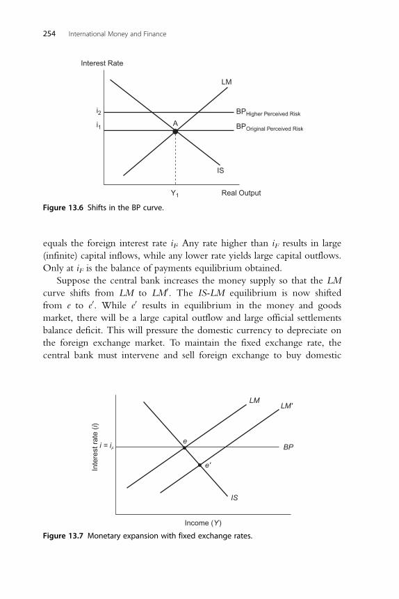
It is also important to realize that the BP curve can shift whether it is

upward sloping or horizontal. For example, a changing foreign perception

of the substitutability shifts the BP curve. This is an intercept change, and

thus the entire schedule shifts. For example, in Figure 13.6 one can see

how an increase in the perception of riskiness of a country’s assets causes

the BP curve to shift upward. Thus, interest rates are not equal across

countries even with perfect capital mobility. For example, Indonesia may

have a positive risk premium, so that investors demand a certain added

premium for financing Indonesia’s trade deficits. However, as long as that

particular risk premium is paid, investors are willing to finance the trade

deficit.

MONETARY POLICY UNDER FIXED EXCHANGE RATES

With fixed exchange rates, the domestic central bank is not free to

conduct monetary policy independently from the rest of the world.

If domestic and foreign assets are perfect substitutes, then they must yield

the same return to investors. Clearly, in this case there is no room for

central banks to conduct an independent monetary policy under fixed

exchange rates.

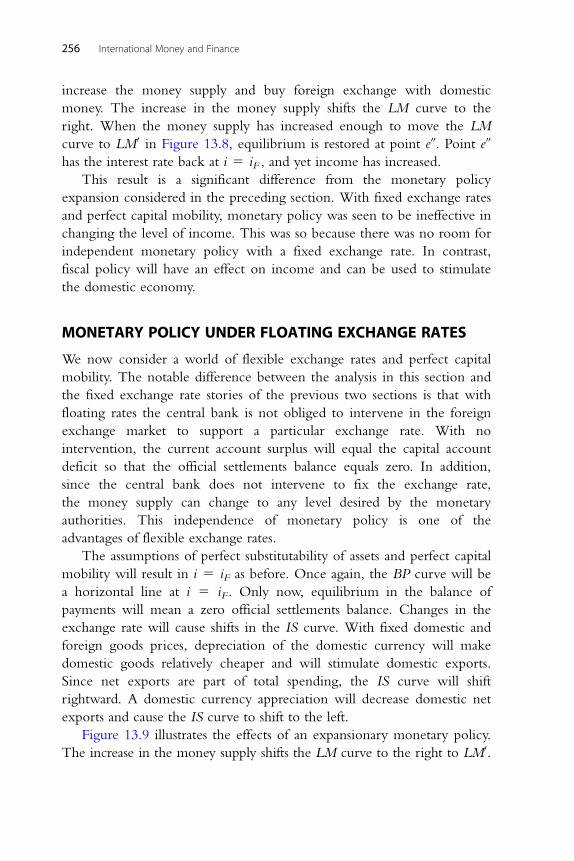
Figure 13.7 illustrates this situation. With perfect asset substitutability,

the BP curve is a horizontal line at the domestic interest rate i, which

LM

BPUpward-sloping

BPHorizontal

Real Output

Interest Rate

i1

IS

A

Y1

Figure 13.5 The slope of the BP curve.


equals the foreign interest rate iF. Any rate higher than iF results in large

(infinite) capital inflows, while any lower rate yields large capital outflows.

Only at iF is the balance of payments equilibrium obtained.

Suppose the central bank increases the money supply so that the LM

curve shifts from LM to LM0. The IS-LM equilibrium is now shifted

from e to e0. While e0 results in equilibrium in the money and goods

market, there will be a large capital outflow and large official settlements

balance deficit. This will pressure the domestic currency to depreciate on

the foreign exchange market. To maintain the fixed exchange rate, the

central bank must intervene and sell foreign exchange to buy domestic

LM

BPHigher Perceived Risk

BPOriginal Perceived Risk

Real Output

Interest Rate

i2

i1

IS

A

Y1

Figure 13.6 Shifts in the BP curve.

ei = iF

e'

IS

BP

LM'LM

Income (Y )

Inte

rest

rat

e (i)

Figure 13.7 Monetary expansion with fixed exchange rates.


currency. The foreign exchange market intervention will decrease

the domestic money supply and shift the LM curve back to LM to restore

the initial equilibrium at e. With perfect capital mobility, this would all

happen instantaneously, so that no movement away from point e is ever

observed. Any attempt to lower the money supply and shift the LM curve

to the left would have just the reverse effect on the interest rate and

intervention activity.

If capital mobility is less than perfect, then the central bank has some

opportunity to vary the money supply. Still, the maintenance of the fixed

exchange rate will require an ultimate reversal of policy in the face of a

constant foreign interest rate. The process is essentially just drawn out

over time rather than occurring instantly.

FISCAL POLICY UNDER FIXED EXCHANGE RATES

A change in government spending or taxes will shift the IS curve.

Suppose an expansionary fiscal policy is desired. Figure 13.8 illustrates the

effects. With fixed exchange rates, perfect asset substitutability, and perfect

capital mobility, the BP curve is a horizontal line at i 5 iF. An increase

in government spending shifts the IS curve right to IS0. The domestic

equilibrium shifts from point e to e0, which would mean a higher interest

rate and higher income. Since point e0 is above the BP curve, the official

settlements balance of payments moves to a surplus because of a reduced

capital account deficit associated with the higher domestic interest rate.

To stop the domestic currency from appreciating, the central bank must

ei = iF

e'

e''

ISIS'

BP

LM'LM

Income (Y )

Inte

rest

rat

e (i)

Figure 13.8 Fiscal expansion with fixed exchange rates.


increase the money supply and buy foreign exchange with domestic

money. The increase in the money supply shifts the LM curve to the

right. When the money supply has increased enough to move the LM

curve to LM0 in Figure 13.8, equilibrium is restored at point ev. Point evhas the interest rate back at i 5 iF , and yet income has increased.

This result is a significant difference from the monetary policy

expansion considered in the preceding section. With fixed exchange rates

and perfect capital mobility, monetary policy was seen to be ineffective in

changing the level of income. This was so because there was no room for

independent monetary policy with a fixed exchange rate. In contrast,

fiscal policy will have an effect on income and can be used to stimulate

the domestic economy.

MONETARY POLICY UNDER FLOATING EXCHANGE RATES

We now consider a world of flexible exchange rates and perfect capital

mobility. The notable difference between the analysis in this section and

the fixed exchange rate stories of the previous two sections is that with

floating rates the central bank is not obliged to intervene in the foreign

exchange market to support a particular exchange rate. With no

intervention, the current account surplus will equal the capital account

deficit so that the official settlements balance equals zero. In addition,

since the central bank does not intervene to fix the exchange rate,

the money supply can change to any level desired by the monetary

authorities. This independence of monetary policy is one of the

advantages of flexible exchange rates.

The assumptions of perfect substitutability of assets and perfect capital

mobility will result in i 5 iF as before. Once again, the BP curve will be

a horizontal line at i 5 iF. Only now, equilibrium in the balance of

payments will mean a zero official settlements balance. Changes in the

exchange rate will cause shifts in the IS curve. With fixed domestic and

foreign goods prices, depreciation of the domestic currency will make

domestic goods relatively cheaper and will stimulate domestic exports.

Since net exports are part of total spending, the IS curve will shift

rightward. A domestic currency appreciation will decrease domestic net

exports and cause the IS curve to shift to the left.

Figure 13.9 illustrates the effects of an expansionary monetary policy.

The increase in the money supply shifts the LM curve to the right to LM0.


The interest rate and income existing at point e0 would yield equilibrium

in the money and goods markets but would cause a larger capital account

deficit (and official settlements deficit) since the domestic interest rate

would be less than iF . Since this is a flexible exchange rate system, the

official settlements deficit is avoided by adjusting the exchange rate to a

level that restores equilibrium. Specifically, the pressure of the official

settlements deficit will cause the domestic currency to depreciate. This

depreciation is associated with a rightward shift of the IS curve as domes-

tic exports increase. When the IS curve shifts to IS0, the new equilibrium

is obtained at ev. At ev, income has increased and the domestic interest

rate equals the foreign rate.

Had there been a monetary contraction instead of an expansion, the

story would have been reversed. A temporarily higher interest rate would

decrease the capital account deficit, causing pressure for the domestic cur-

rency to appreciate. As domestic net exports are decreased, the IS curve

shifts to the left until a new equilibrium is established at a lower level

of income and the original i 5 iF is restored.

In contrast to the fixed exchange rate world, monetary policy can

change the level of income with floating exchange rates. Since the

exchange rate adjusts to yield balance of payments equilibrium, the central

bank can choose its monetary policy independent of other countries’

policies. This world of flexible exchange rates and perfect capital mobility

is often called the Mundell�Fleming model of the open economy.

(Robert Mundell, Nobel Laureate in Economics in 1999, and Marcus

e

0

i = iF

e'

e''

ISIS'

BP

LM'LM

Income (Y )

Inte

rest

rat

e (i)

Figure 13.9 Monetary expansion with floating exchange rates.


Fleming were two early researchers who developed models along the

lines of those presented here.)

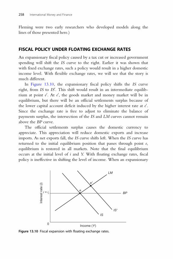
FISCAL POLICY UNDER FLOATING EXCHANGE RATES

An expansionary fiscal policy caused by a tax cut or increased government

spending will shift the IS curve to the right. Earlier it was shown that

with fixed exchange rates, such a policy would result in a higher domestic

income level. With flexible exchange rates, we will see that the story is

much different.

In Figure 13.10, the expansionary fiscal policy shifts the IS curve

right, from IS to IS0. This shift would result in an intermediate equilib-

rium at point e0. At e0, the goods market and money market will be in

equilibrium, but there will be an official settlements surplus because of

the lower capital account deficit induced by the higher interest rate at e0.Since the exchange rate is free to adjust to eliminate the balance of

payments surplus, the intersection of the IS and LM curves cannot remain

above the BP curve.

The official settlements surplus causes the domestic currency to

appreciate. This appreciation will reduce domestic exports and increase

imports. As net exports fall, the IS curve shifts left. When the IS curve has

returned to the initial equilibrium position that passes through point e,

equilibrium is restored in all markets. Note that the final equilibrium

occurs at the initial level of i and Y. With floating exchange rates, fiscal

policy is ineffective in shifting the level of income. When an expansionary

ei = iF

0

e'

ISIS'

BP

LM

Income (Y )

Inte

rest

rat

e (i)

Figure 13.10 Fiscal expansion with floating exchange rates.


fiscal policy has no effect on income, complete crowding out has occurred.

This crowding-out effect occurs because the currency appreciation

induced by the expansionary fiscal policy reduces net exports to a level

that just offsets the fiscal policy effects on income.

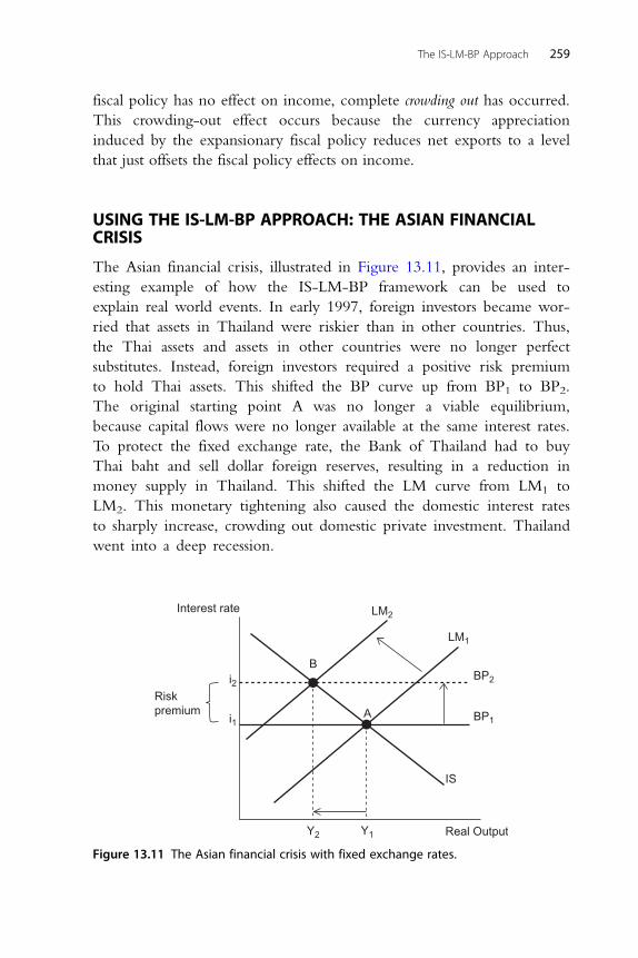
USING THE IS-LM-BP APPROACH: THE ASIAN FINANCIALCRISIS

The Asian financial crisis, illustrated in Figure 13.11, provides an inter-

esting example of how the IS-LM-BP framework can be used to

explain real world events. In early 1997, foreign investors became wor-

ried that assets in Thailand were riskier than in other countries. Thus,

the Thai assets and assets in other countries were no longer perfect

substitutes. Instead, foreign investors required a positive risk premium

to hold Thai assets. This shifted the BP curve up from BP1 to BP2.

The original starting point A was no longer a viable equilibrium,

because capital flows were no longer available at the same interest rates.

To protect the fixed exchange rate, the Bank of Thailand had to buy

Thai baht and sell dollar foreign reserves, resulting in a reduction in

money supply in Thailand. This shifted the LM curve from LM1 to

LM2. This monetary tightening also caused the domestic interest rates

to sharply increase, crowding out domestic private investment. Thailand

went into a deep recession.

Interest rate

Real Output

BP1

BP2

LM1

LM2

i2

i1

Riskpremium

B

A

IS

Y1Y2

Figure 13.11 The Asian financial crisis with fixed exchange rates.


After a considerable effort in trying to protect the fixed exchange rate,

the Thai government and Bank of Thailand decided to allow the

exchange rate to float. With a floating rate the response to the risk pre-

mium demanded by the speculators looks very different. In Figure 13.12,

monetary policy, i.e., the LM curve, is unaffected. However, the sharp

depreciation that happened once the Thai baht was allowed to float

resulted in an increase in the domestic competitiveness, shown in

Figure 13.12 as the IS curve shifting outwards from IS1 to IS2.

The depreciation led to the beginning of a recovery for Thailand.

However, the confidence of speculators was boosted and they continued

to neighboring countries, causing the crisis to spread in Southeast Asia.

FAQ: Who Caused the Asian Financial Crisis?George Soros, a hedge fund investor, has often been blamed for the Asianfinancial crisis. Although he admitted to having speculated against the Thaibaht in 1997, he argued that the speculation did the Thai government a favorby signaling to the authorities that the Thai baht was overvalued. Accordingto Soros, if the central bank of Thailand had allowed the baht to float earlier,then the Asian financial crisis might have been avoided.

In early 1997, the Quantum Fund, led by George Soros, used US$700 mil-lion to bet against the baht. Another fund, the Tiger fund, led by JulianRobertson, bet US$3 billion against the baht at the same time. The centralbank of Thailand did not allow the Thai baht to float, but instead heavily

Interest rate

Real Output

BP1

BP2

LM1

i2

i1

Riskpremium

B

A

IS1

IS2

Y1 Y2

Figure 13.12 Asian financial crisis once the exchange rate is allowed to float.


supported it, spending about US$30 billion in a six-month period. Theresponse by the central bank caused losses to the speculators, but madespeculators even more determined to bet against the Thai baht. The hedgefunds knew that the central bank could not maintain its defense over a lon-ger period, and renewed their bets. On one single day alone, on May 14,1997, speculators had bet US$10 billion against the baht. To compound theproblems for Thailand, Japanese banks decided to move assets out ofThailand. The Japanese banks were some of the biggest investors in Thailand,but were already hurt by domestic debt defaults. Therefore, they were quickto withdraw their assets from Thailand.

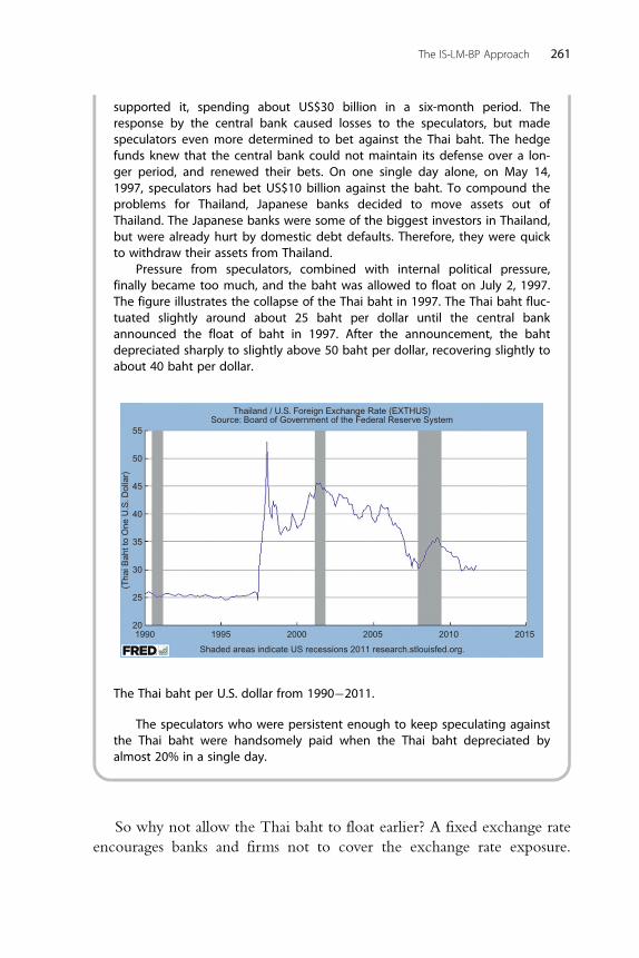
Pressure from speculators, combined with internal political pressure,finally became too much, and the baht was allowed to float on July 2, 1997.The figure illustrates the collapse of the Thai baht in 1997. The Thai baht fluc-tuated slightly around about 25 baht per dollar until the central bankannounced the float of baht in 1997. After the announcement, the bahtdepreciated sharply to slightly above 50 baht per dollar, recovering slightly toabout 40 baht per dollar.

55

50

45

40

35

30

(Tha

i Bah

t to

One

U.S

. Dol

lar)

25

201990 1995

Shaded areas indicate US recessions 2011 research.stlouisfed.org.

Thailand / U.S. Foreign Exchange Rate (EXTHUS)Source: Board of Government of the Federal Reserve System

2000 2005 2010 2015

The Thai baht per U.S. dollar from 1990�2011.

The speculators who were persistent enough to keep speculating againstthe Thai baht were handsomely paid when the Thai baht depreciated byalmost 20% in a single day.

So why not allow the Thai baht to float earlier? A fixed exchange rate

encourages banks and firms not to cover the exchange rate exposure.


Thus, banks had short-term loans in dollars and long-term investments in

Thai baht. A devaluation of the Thai baht would create difficulty for

banks in Thailand, as the cost of paying their debt would exceed the

return on their long-term investments. This is typical for many develop-

ing countries in that the government encourages local investment, and

borrows from capital rich developed countries. Thus, banks in Thailand

had a large number of loans in dollars and payments in baht. After the

depreciation of the dollar, most of the banks and financial firms went

bankrupt, with over 50 banks and financial firms taken over by the Thai

government in the end of 1997.

INTERNATIONAL POLICY COORDINATION

From the early 1970s onwards, the major developed nations have

generally operated with floating exchange rates. The IS-LM-BP frame-

work, analyzed in this chapter, has shown that fiscal and monetary policy

can generate large swings in floating exchange rates. Economists have

been debating how to coordinate policies across countries, because of the

potential disruptive effect of exchange rate volatility on world trade.

The high degree of capital mobility existing among the developed

countries suggests that fiscal actions that lead to a divergence of the domes-

tic interest rate from the given foreign interest rate will quickly be undone

by the influence of exchange rate changes on net exports, as was illustrated

in Figure 13.10. For example, many economists argue that the sharp

increase in the dollar value in the early 1980s was due to the expansionary

fiscal policy followed by the U.S. government. How could such exchange

rate volatility be minimized? If all nations coordinated their domestic poli-

cies and simultaneously stimulated their economies, the world interest rate

would rise. Thus, the pressure for an exchange rate change for a particular

country (in the above case, the U.S.) would disappear. The problem illus-

trated in Figure 13.10 was that of a single country attempting to follow an

expansionary policy while the rest of the world retained unchanged poli-

cies, so that iF remains constant. If iF increased at the same time that i

increased, the BP curve would shift upward and the balance of payments

equilibrium would be consistent with a higher interest rate.

Similarly, changes in exchange rates and net exports induced by

monetary policy can be lessened if central banks coordinate policy so

that iF shifts with i. There have been instances of coordinated foreign

exchange market intervention when a group of central banks jointly


followed policies aimed at a depreciation or appreciation of the dollar.

These coordinated interventions, intended to achieve a target value of the

dollar, also work to bring domestic monetary policies more in line with

each other. If the United States has been following an expansionary

monetary policy relative to Japan, U.S. interest rates may fall relative to

the other country’s rates, so that a larger capital account deficit is induced

and pressure for a dollar depreciation results. If the central banks decide

to work together to stop the dollar depreciation, the Japanese will buy

dollars on the foreign exchange market with their domestic currencies,

while the Federal Reserve must sell foreign exchange to buy dollars.

This will result in a higher money supply in Japan and a lower money

supply in the United States. The coordinated intervention works toward

a convergence of monetary policy in each country.

The basic argument in favor of international policy coordination is

that such coordination would stabilize exchange rates. Whether exchange

rate stability offers any substantial benefits over freely floating rates with

independent policies is a matter of much debate. Some experts argue that

coordinated monetary policy to achieve fixed exchange rates or to reduce

exchange rate fluctuations to within narrow target zones would reduce

the destabilizing aspects of international trade in goods and financial assets

when currencies become overvalued or undervalued. This view empha-

sizes that in an increasingly integrated world economy, it seems desirable

to conduct national economic policy in an international context rather

than by simply focusing on domestic policy goals without a view of the

international implications.

An alternative view is that most changes in exchange rates result from

real economic shocks and should be considered permanent changes.

In this view, there is no such thing as an overvalued or undervalued

currency because exchange rates always are in equilibrium given current

economic conditions. Furthermore, governments cannot change the real

relative prices of goods internationally by driving the nominal exchange

rate to some particular level through foreign exchange market

intervention, because price levels will adjust to the new nominal

exchange rate. This view, then, argues that government policy is best

aimed at lowering inflation and achieving governmental goals that

contribute to a stable domestic economy.

The debate over the appropriate level and form of international policy

coordination has been one of the livelier areas of international finance

in recent years. Many leading economists have participated, but a problem


at the practical level is that different governments emphasize different

goals and may view the current economic situation differently. Ours is

a more complex world in which to formulate international policy agree-

ments than is typically viewed in scholarly debate, where it is presumed

that governments agree on the current problems and on the impact of

alternative policies on those problems. Nevertheless, the research

of international financial scholars offers much promise in contributing

toward a greater understanding of the real-world complexities govern-

ment officials must address.

SUMMARY

1. The desired economic outcome in an open economy is to achieve

both internal balance and external balance at the same time.

2. Internal balance refers to a domestic equilibrium condition such that

goods market and money market are in equilibrium and unemploy-

ment is at its natural level.

3. External balance requires the balance of payments to be in equilib-

rium. The condition implies zero balance on the official settle-

ment—the current account surplus must be equal to the capital

account deficit.

4. The IS curve represents the combinations of income and interest rate

levels that bring the good market to equilibrium (i.e., leakages equals

to injections).

5. The LM curve represents the combinations of income and interest

rate levels that bring the money market to equilibrium (i.e., money

demand equals to money supply).

6. The BP curve represents the combinations of income and interest rate

levels that bring the balance of payments to equilibrium (i.e., current

account surplus equals to capital account deficit).

7. The internal and external equilibriums occur when three curves

intersect at one point.

8. The factors that shift the IS curve are a change in domestic price level,

a change in exchange rate, and a change in fiscal policy variable.

9. The factor that shifts the LM curve is a change in money supply.

10. The slope of the BP curve depends on the degree of capital mobility.

In the case of perfect capital mobility between countries, the BP

curve is horizontal.


11. The factor that shifts the BP curve is a change in perception of asset

substitutability.

12. With perfect substitutability and perfect capital mobility, the domes-

tic interest rate is equal to the foreign interest rate.

13. With fixed exchange rates, a country cannot conduct an independent

monetary policy to change domestic income. Only fiscal policy is

effective in changing equilibrium income.

14. With floating exchange rates, monetary policy is effective in

changing domestic income. However, fiscal policy has no effect on

income because of a complete crowding-out effect from the balance

of payments adjustment.

15. International policy coordination is an idea that aims to stabilize the

exchange rates by coordinating each country’s fiscal and monetary

policies to achieve the best international outcome.

EXERCISES

1. Explain the difference between a closed economy and an open

economy. Explain also how the pursuit of internal equilibrium will be

different between the two types of economies.

2. Consider the IS-LM-BP model of an open economy with a constant

price level, perfect asset substitutability, and perfect capital mobility.

The economy is initially in both internal and external equilibrium.

a. Explain why the BP curve is a horizontal line at i 5 iF, where i is

the domestic nominal interest rate and iF is the foreign nominal

interest rate.

b. Define the internal equilibrium and external equilibrium of the

economy, respectively.

3. From question 2, suppose now that the domestic economy decides to

reduce its money supply.

a. What are the initial effects of this monetary policy on the goods

market, the money market, the foreign exchange market, and the

balance of payments of the domestic economy? Which curve(s)

will shift?

b. What is the adjustment mechanism under a fixed exchange rate

regime? Illustrate and explain which curve(s) will shift during the

adjustment, and then compare the new equilibrium with the initial

equilibrium.


c. What is the adjustment mechanism under a flexible exchange rate



equilibrium.

4. From question 2, suppose now that the domestic government decides

to increase the government spending.

a. What are the initial effects of this fiscal policy on the goods

market, the money market, the foreign exchange market, and the

balance of payments of the domestic economy? Which curve(s)

will shift?

b. What is the adjustment mechanism under a fixed exchange rate



equilibrium.

c. What is the adjustment mechanism under a flexible exchange rate



equilibrium.

5. If a country has a surplus balance of payments, what will be the

appropriate government policy to restore the balance of payments

back to equilibrium? What effects might this have on the country’s

income?

6. What is an international policy coordination? Explain why it is

difficult to adopt an international policy coordination in practice.

FURTHER READINGCanzoneri, M., Cumby, R.E., Diba, B.T., 2005. The need for international policy

coordination: what’s old, what’s new, what’s yet to come? J. Int. Econ. 66 (2),363�384.

Fan, L.S., Fan, C.M., 2002. The Mundell-Fleming model revisited. Am. Econ. 46 (1),42�49.

Fleming, M., 1962. Domestic financial policies under fixed and under floating exchangerates. IMF. Staff. Pap. November.

Ghosh, A., 1986. International policy coordination in an uncertain world. Econ. Lett.(3).King, M., 2001. Who triggered the Asian financial crisis? Rev. Int. Polit. Econ. 8 (3),

438�466.Melvin, M., Taylor, M., 2009. The crisis in the foreign exchange market. J. Int. Money.

Financ. 28 (8), 1317�1330.Mundell, R.A., 1963. Capital mobility and stabilization policy under fixed and flexible

exchange rates. Can. J. Econ. November.Obstfeld, M., Rogoff, K., 1995. Exchange rate dynamics redux. J. Polit. Econ. June.Soros, G., 2000. Open society: Reforming global capitalism. PublicAffairs, New York.


APPENDIX 13A: THE OPEN-ECONOMY MULTIPLIER

We can use the macroeconomic model developed in this chapter to

analyze the effects of changes in spending on the equilibrium level of

national income, assuming the interest rate is unchanged. We begin with

the basic macroeconomic equilibrium conditions seen in the bottom half

of Figure 13.2:

S1T 1 IM 5 I 1G1X ð13:A1ÞIn equilibrium, the planned level of saving plus taxes plus imports

must equal the planned level of investment plus government spending

plus exports. To find the equilibrium levels of national income (Y) and

net exports (X 2 IM), we must make some assumptions regarding the

variables in Equation (13.A1). Specifically, we assume that saving

and imports both depend on the level of national income. The greater

the domestic income, the more people want to save, and the more they

want to spend on imports. The fraction of any extra income that people

want to save is called the marginal propensity to save, which we will denote

as s. The fraction of any extra income that people want to spend on

imports is called the marginal propensity to import, which we will denote

as m. So, S 5 sY and IM 5 mY. The rest of the variables in Equation

(13.A1)—T, I, G, and X—are assumed to be exogenously determined by

factors other than domestic income.

With these assumptions, we can substitute the new specifications of S

and IM and rewrite Equation (13.A1) as

sY 1T 1mY 5 I 1G1X ð13:A2ÞGathering our Y terms and subtracting T from each side of the equa-

tion, we have (s 1 m) Y 5 I 1 G 1 X 2 T. Solving for the equilibrium

level of Y yields

Y 5 ðI 1G1X 2TÞ=ðs1mÞ ð13:A3ÞIf I, G, or X increased by $1, the equilibrium level of Y would

increase by 1/(s 1 m) times $1. An increase in T would cause Y to

fall. The value of 1/(s 1 m) is known as the open-economy multiplier.

This multiplier is equal to the reciprocal of the marginal propensity to

save (s) plus the marginal propensity to import (m). Since s and m will

both be some fraction less than 1, we expect this multiplier to exceed

1, so that an increase in I, G, or X spending would cause the


equilibrium level of national income to rise by more than the change

in spending.

Let’s consider an example of this multiplier effect. Suppose that we

return to the model of Figure 13.2 as redrawn in Figure 13.A1. In this

model economy, the marginal propensity to save is .3, the marginal

propensity to import is .2, taxes equal 20, and investment, government

spending, and exports each equal 10 (assume the units are billions of

dollars). In this case, the macroeconomic model is given by

S1T 1 IM 5 :3Y 1 201 :2Y 5 :5Y 1 20 ð13:A4Þand

I 1G1X 5 101 101 105 30 ð13:A5ÞThese two equations are drawn in Figure 13.A1 as the S 1 T 1 IM

line and the I1 G1 X line. The point of intersection occurs at e, where

the equilibrium level of national income equals $20 billion.

The equilibrium level of income could have been found by using

Equation (13.A3) and substituting the values given for each variable:

Y 5 ðI 1G1X 2T Þ=ðs1mÞ5 10=:55 20 ð13:A6ÞWhether we solve for the equilibrium level of Y algebraically or

graphically, we find the value of $20 billion.

60

50

40

30

20

10

010 20 30 40 50 60 70 80

Income Y(billion $)

(bill

ion

$)

Sav

ing

+ta

xes

+im

port

s (S

+ T

+ IM

)In

vest

men

t+go

vern

men

t spe

ndin

g+

expo

rts

(I +

G +

X)

e'

S + T + IM

I + G + X'

I + G + Xe

ΔY = 20

ΔX = 10

Figure 13.A1 The effect of an increase in exports.


What would happen if exports increased? For instance, suppose exports

increase from $10 to $20 billion. In Figure 13.A1, the I1 G1 X line shifts

up by the amount of the increase in exports to I1 G 1X0. The two lines

are parallel because they differ by a constant $10 billion, the increase in

exports, at each level of income. The new equilibrium level of income

is found by the new point of intersection e0 at an income level of $40

billion. Note that exports increase by 10, yet income increases by 20, from

the original equilibrium level of 20 to the new level of 40. Since the

increase in equilibrium national income is twice the increase in exports,

the open-economy multiplier must equal 2. Algebraically, the multiplier is

1/(s1 m), which, in the example, is 1/(.3 1.2) 5 1/.5 5 2. An increase

in I, G, or X would increase Y by twice the increase in spending in our

example.

The intuition behind the multiplier effect is taught in principles of

economics courses. If spending, such as export spending, rises in some

industry, then there is an increase in the income of factors employed in

that industry. These employed resource owners, such as laborers, will

increase their spending on goods and services and further stimulate

production, which further raises income and spending. This “multiplier

effect” has a finite value because not all of the increased income is spent

in the domestic economy. Some is saved and some is spent on imports.

Saving and imports act as leakages from domestic spending that serve

to limit the size of the multiplier. The larger the marginal propensity

to save, and the larger the marginal propensity to import, the smaller the

multiplier.

In the real world, such multiplier effects will be more complex due to

the presence of taxes and feedback effects from the rest of the world.

However, the essential point—that changes in spending may create much

larger changes in the national income—remains. Stable growth of the

economy requires stable growth of spending.


The IS-LM-BP Approach - University of Warwick · price level constant. A change in the domestic price level will change the price of domestic goods relative to foreign goods. If the

Documents