The Inverse Discrete Cosine Transform (IDCT): A ...courses.cecs.anu.edu.au/courses/CSPROJECTS/16S1/Reports/...Abstract In this report the Inverse Discrete Cosine Transform algorithm

The Inverse Discrete Cosine Transform (IDCT):A performance comparison on OpenCL and

OpenMP

Artem Afanasyev (u5231713)

12 February 2016

Abstract

In this report the Inverse Discrete Cosine Transform algorithm was ex-plored. It has a number of applications, specifically in digital signal pro-cessing and compression algorithms. As part of this project, the IDCTand one IFCT algorithms have been implemented using a simple CPU ap-proach, OpenMP and OpenCL in order to compare performance. It hasbeen found that the IFCT (Inverse Fast Cosine Transform) implemented inOpenCL for the GPU has the best performance in terms of execution speed.This was to be expected, given the known performance of non-graphicalGPU routines. However, we came across a surprising result: OpenCLIDCT (Inverse Discrete Cosine Transform) has executed slower than theOpenMP (multi-threaded) algorithm for IDCT. In terms of accuracy, it hasbeen shown that IDCT produces more accurate results in comparison toIFCT. It has also been confirmed that the accuracy of the particular algo-rithm (IDCT or IFCT) is independent of the implementation framework.

Acknowledgements

I would like to express my gratitude to Dr. Eric McCreath for guiding methrough this project, and taking me on in the first place. I would also liketo thank the Australian National University and the College of Engineer-ing and Computer Science in particular, for giving me an opportunity toundertake this project.

Chapter 1

Introduction

This project aims to explore the Inverse Discrete Cosine Transform (IDCT).In this case, the IDCTs formula is applied to a two-dimensional 8x8 block.The IDCT algorithm is implemented on GPU and multicore systems, withperformances on each system compared in terms of time taken to computeand accuracy.

DCT, or the Discrete Cosine Transform, has multiple applications when itcomes to image and audio compression. When DCT is applied to a finitedata sequence, it is represented in terms of a sum of cosine functions thatoscillate at different frequencies. Discrete Cosine Transform has eight stan-dard variants, four of which are most common. Particularly in image com-pression, the DCT-II is most commonly used. Its inverse, the DCT-III, orIDCT is used for decoding, rather than encoding. Exploring various IDCTalgorithms is the aim of this project.

There are also faster ways to implement IDCT similar to Fast Fourier Trans-forms, one of which is also implemented on GPU and multicore systems.

In short, the Direct Cosine Transform transform the data sequence (inputsignal) from the time domain to frequency domain, like any other Fouriertransforms, whereby the energy of the signal is compacted into low fre-quency bins [1]. DCT outputs a set of coefficients, each of which corre-sponds to a DCT basis function. These are cosine functions with increasingfrequencies [1]. Each of these basis functions is then multiplied by the cor-responding coefficients, and the sum of those values is the reconstructionof the original signal. This process is carried out with the use of the Inverse

1

Discrete Cosine Transform - IDCT[1].

For analysing the complexity of the algorithms we will use Big O notation.When describing complexity of the DCT, N represents the total number ofelements in the matrix, in our case N = 64 elements.Directly computing the DCT requires O(N2) operations, however, it is alsopossible to achieve the same thing with O(N logN) complexity. This isachieved by factorising the computation, similarly to the Fast Fourier Trans-form (FFT). Methods that utilise O(N logN) complexity are known as FastCosine Transform (FCT) algorithms [2].To summarise, the difference between DCT and FCT is the complexityO(N2)for DCT and O(N logN) for FCT.The project implements the simple IDCT approach along with the fasterFCT approach in OpenCL for the GPU and OpenMP for the multicore sys-tems. The performance of different approaches is also discussed.

In summary, the following was carried out over the course of this project:

Implementing IDCT and IFCT algorithms using:

• Simple CPU approachSequential IDCT and IFCT calculation

• Multi-core CPU approachImplementation of IDCT and IFCT using OpenMP framework (multi-threaded approach)

• GPU approachImplementation of IDCT and IFCT using OpenCL framework for GPU

The six of the above approaches are then compared based on the following:

• Time taken to computeAll of the six algorithms have been computed for 1, 1000 and 10,000blocks, and time taken to compute each one has been recorded.

• AccuracyAccuracy was measured by encoding with the most accurate approachof simple DCT, and then decoded using all of the IDCT implementa-tions discussed above. The standard deviation between the input andreconstructed values is then computed.

2

Chapter 2

Background

2.1 Discrete Cosine Transform (DCT)

The discrete cosine transform (DCT) is a technique for converting a sig-nal into elementary frequency components. It is widely used in image andsound compression [3]. Some of the formats DCT is used for include but arenot limited to JPEG, MPEG audio and digital VCR [4]. From a mathemat-ical standpoint, the Discrete Cosine Transforms allows to analyse complexsignal in terms of separate frequency components in a way that is appro-priate for compression.

DCT is used for lossy compression, which is based on the principle ofremoving undetectable components without altering the perceptible de-tails. In practical cases, most of the signal information (or energy) is un-evenly distributed and stored in a few of the low-frequency coefficients ofthe DCT, which implies that many DCT coefficients can be eliminated with-out much loss of information [6].

DCT is used for encoding, and the IDCT, being the inverse of the en-coding transform, is used for decoding of information:

The two-dimensional 8x8 Inverse Discrete Cosine Transform is givenby:

Gu,v =1

4α(u)α(v)

7∑x=0

7∑y=0

gx,y cos[(2x+ 1)uπ

16] cos[

(2y + 1)vπ

16], (2.1)

where:

3

• x is the pixel row (0 ≤ x < 8)

• y is the pixel column (0 ≤ y < 8)

• α(u) is a normalising scale factor that makes the transform orthonor-mal, given by

α(u) =

{1√2, if u = 0

1, otherwise(2.2)

• gx,y is the reconstructed pixel value at coordinates (x, y)

• Gu,v is the reconstructed approximate coefficient at coordinates (u, v)

History and Relationship to Karhunen-Loeve Transform

DCT is used in digital signal processing due to its efficiency. It is real,separable and orthogonal, and approaches the statistically optimal KLT(Karhunen-Loeve transform). The KLT itself suffers from computationalproblems [7].

Karhunen-Loeve transform is a series representation of a given randomfunction (e.g. signal sequence). Mathematical details of the transform arebeyond the scope of this paper, its importance, however, lies within thefact that it completely decorrelates signal in the transform domain. It alsominimises the mean square error between the signal representation and theactual signal [7].

The KLT (Karhunen-Loeve Transform) works by identifying certain sta-tistical properties of the signal and then utilising those properties to con-struct an optimal decomposition. The KLT analysis is however extremelycomplicated, as it involves analysing the signal and constructing a trans-form based on the statistical parameters that cannot be otherwise predeter-mined. This is what makes the KLT an impractical tool when it comes tosignal processing [4],[7].

KLT thus provides a benchmark against which other transforms may bejudged. It has been shown that the DCT-II and DCT-III (or IDCT, which isthe inverse of DCT-II) have the minimal variance distribution compared to

4

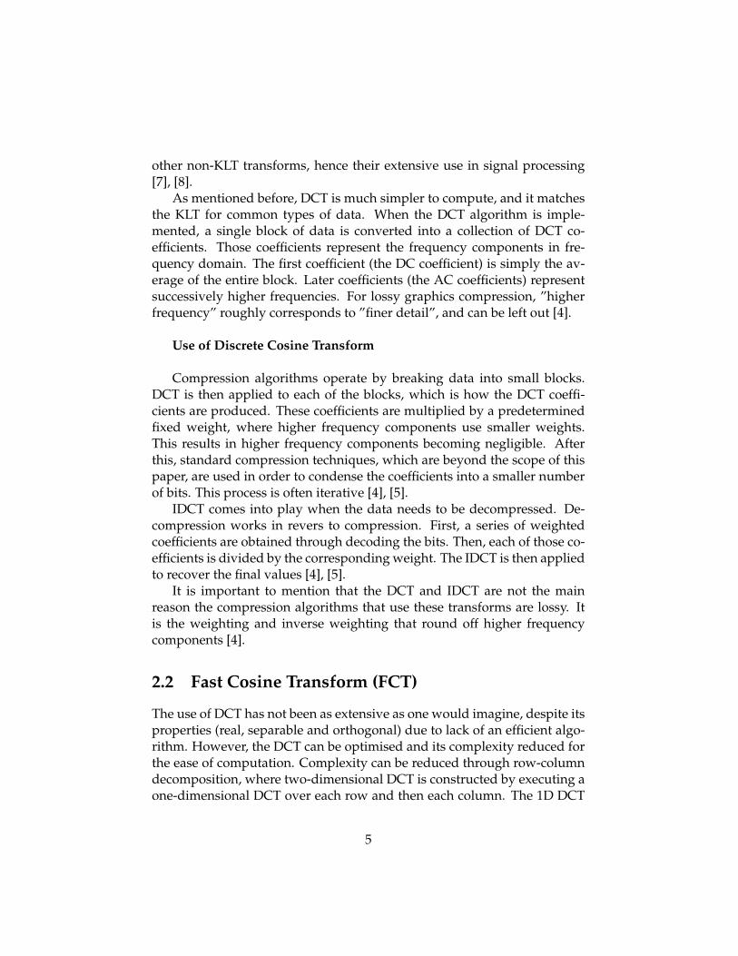
other non-KLT transforms, hence their extensive use in signal processing[7], [8].

As mentioned before, DCT is much simpler to compute, and it matchesthe KLT for common types of data. When the DCT algorithm is imple-mented, a single block of data is converted into a collection of DCT co-efficients. Those coefficients represent the frequency components in fre-quency domain. The first coefficient (the DC coefficient) is simply the av-erage of the entire block. Later coefficients (the AC coefficients) representsuccessively higher frequencies. For lossy graphics compression, ”higherfrequency” roughly corresponds to ”finer detail”, and can be left out [4].

Use of Discrete Cosine Transform

Compression algorithms operate by breaking data into small blocks.DCT is then applied to each of the blocks, which is how the DCT coeffi-cients are produced. These coefficients are multiplied by a predeterminedfixed weight, where higher frequency components use smaller weights.This results in higher frequency components becoming negligible. Afterthis, standard compression techniques, which are beyond the scope of thispaper, are used in order to condense the coefficients into a smaller numberof bits. This process is often iterative [4], [5].

IDCT comes into play when the data needs to be decompressed. De-compression works in revers to compression. First, a series of weightedcoefficients are obtained through decoding the bits. Then, each of those co-efficients is divided by the corresponding weight. The IDCT is then appliedto recover the final values [4], [5].

It is important to mention that the DCT and IDCT are not the mainreason the compression algorithms that use these transforms are lossy. Itis the weighting and inverse weighting that round off higher frequencycomponents [4].

2.2 Fast Cosine Transform (FCT)

The use of DCT has not been as extensive as one would imagine, despite itsproperties (real, separable and orthogonal) due to lack of an efficient algo-rithm. However, the DCT can be optimised and its complexity reduced forthe ease of computation. Complexity can be reduced through row-columndecomposition, where two-dimensional DCT is constructed by executing aone-dimensional DCT over each row and then each column. The 1D DCT

5

is:

Fu =1

2Cu

N−1∑x=0

fx cos(uπ2x+ 1

2N), (2.3)

where:

• x is the coordinate in this now one-dimensional vector

• Cu is some coefficient

• Fu is the reconstructed approximate coefficient at coordinate (u)

• fx is the reconstructed pixel value at coordinate (x)

The complexity of the above equation isO(N2), and running it 2n timesresults in 2D DCT with complexity of O(N3).TheO(N2) DCT algorithm can be replaced yet again with an algorithm thatis factored similarly to a Fast Fourier Transform (FFT), whereby the com-plexity is reduced to O(n log n). The AAN (Arai, Agui, Nakajima - namedafter the authors) algorithm is one of the fastest known one-dimensionalDCTs [9]. This algorithm has been selected and implemented over thecourse of this project.The straightforward DCT approach takes 64 * 64 * 2 multiplication for thefull DCT (which applies for the IDCT as well). In contrast, the AAN DCT(of FCT) uses only 5 multiplications and 8 postmultiplications. These post-multiplications all involve multiplying by powers of two, which furtherspeeds up the algoritm by using bit-shifting [4].

2.3 Pseudo code

This section provides pseudo code for the DCT algorithm and the FCT(faster) algorithm.

2.3.1 DCT

f l o a t output [ 6 4 ] ;

for ( i n t y = 0 ; y < 8 ; y++) {for ( i n t x = 0 ; x < 8 ; x++) {

f l o a t r e s u l t = . 0 ;for ( i n t v = 0 ; v < 8 ; v++) {

6

for ( i n t u = 0 ; u < 8 ; u++) {f l o a t alpha u = u == 0 ? s2 : 1 . 0 ;f l o a t alpha v = v == 0 ? s2 : 1 . 0 ;r e s u l t += alpha u ∗ alpha v ∗ input [ v ∗ 8 + u ]

∗ cos ( ( ( 2 ∗ x + 1) ∗ u ∗ PI ) / 16)∗ cos ( ( ( 2 ∗ y + 1) ∗ v ∗ PI ) / 1 6 ) ;

}}output [ y ∗ 8 + x ] = r e s u l t / 4 ;

}}

2.3.2 FCT

The following flowgraph shows the order of computational operations in1D AAN DCT algorithm. To obtain fast IDCT the graph needs to be re-versed (i.e. read from right to left).

Figure 2.1: Arai, Agui, and Nakajima DCT algorithm. Boxes represent mul-tiplication. a1=0.707, a2=0.541, a3=0.707, a4=1.307, a5=0.383 [10].

The idea behind the faster FCT approach is to separate the two-dimensionaltransformation into two one-dimensional transformations. The pseudo codefor this approach is shown below, and the full FCT algorithm code can befound in Chapter 7 (Appendix).

for ( i n t i = 0 ; i < 8 ; i ++) {/ / t r a n s f o r m rows

}

for ( i n t i = 0 ; i < 8 ; i ++) {/ / t r a n s f o r m columns

}

7

2.4 Findings

In terms of time taken to compute the algorithms and their accuracy, thefollowing has been found:

Time

OpenCL IFCT (GPU) was found to be the fastest, and the single-threadedsequential approach took the longest.There was also one unexpected result: OpenMP DCT has performed bettertime-wise than the OpenCL DCT.In terms of efficiency, OpenMP IDCT has proven to operate at the highestpercentage of the theoretical hardware limit. See results in Table 5.3.

Accuracy

It has been found that IDCT is more accurate than IFCT, as expected. Ithas also been shown that this result is independent of the framework used,as CPU, OpenMP and OpenCL have produced the same results for IDCTand then IFCT.The results are discussed in more detail in Chapter 5.

8

Chapter 3

OpenCL & OpenMP

This chapter provides a background to OpenCL and OpenMP, giving anoverview of the programming model used in these languages. This sectionwill also provide a history of their development.

3.1 OpenCL

GPU, or Graphics Processing Units had not been used for nongraphicalroutines before 2010, and the idea was considered a novelty in the field ofhigh performance scientific computing. The first supercomputer to everuse general purpose GPU computing (GPGPU computing) was the ChineseTianhe-1A, which quickly made it the fastest supercomputer in the worldin 2010. Today, engineers and scientists agree that CPU/GPU systems arethe future of supercomputing, as it has been proven that using GPUs en-sures fast performance of the system as well as power efficiency [11].

With the increasing popularity of these heterogeneous processing platforms,the demand has appeared for a hybrid programming language that wouldtarget both CPU and GPU. OpenCL (Open Computing Language) is a lan-guage for programming hybrid systems that consist of multiple types ofprocessors. It is an open royalty-free standard for parallel programmingacross CPUs, GPUs and other processors, which enables software develop-ers to utilise the full power of the hybrid processing platforms [12].In 2008, OpenCL Working Group was formed as part of the Khronos Group,which is a group of companies that seek to advance graphics and graphicalmedia [11].

9

3.1.1 Advantages of OpenCL

OpenCL is not a programming language in itself, rather it is a standard thatcharacterises a collection of data types, data structures and functions thatenhance C and C++ [11]. The three main advantages that set OpenCL apartare portability, standardised vector processing and parallel programming.These advantages are discussed in more detail below:

PortabilityWith OpenCL there is no need for developers to learn vendor-specific lan-guage to program certain types of hardware. Rather, all OpenCL-compliantdevices are able to compile OpenCL code. Moreover, OpenCL is not de-pendant on the architecture of the device, so OpenCL routines can targetmultiple devices [11].

Standardised Vector ProcessingStandardised vector processing is one of the main advantages of OpenCL.This refers to the definition of computational vector, which is a data struc-ture consisting of multiple elements of the same data type. In computa-tional vectors, each component is operated upon in the same clock cycle[11]. High-performance processors (superscalar and vector processors) op-erate on multiple values at once. Again, with OpenCL, vector programscan be run on any OpenCL-compliant processor.

Parallel ProgrammingOpenCL facilitates parallel programming, whereby computational opera-tions are assigned to multiple processing elements that are performed atthe same time. These tasks are called kernels. OpenCL enables full task-parallelism, which is a form of parallelism that where tasks are assignedto processes or threads; and each processor executes a different thread.This is an advantage OpenCL has over some other parallel programmingtools, which only facilitate data-parallelism, where each processor executesthe same instructions on different types of data [11].

In summary, OpenCL has clear advantages over regular C and C++.However, it is also more complex. In real-world OpenCL applications, mul-tiples data structures need to be created and their operation coordinated.

Over the course of this project, OpenCL was used in order to implementDCT and FCT algorithms on GPU.

10

3.1.2 Example of Code for OpenCL

kernel void square ( g loba l f l o a t ∗ input , g loba l f l o a t ∗ output ) {

i n t id = g e t g l o b a l i d ( 0 ) ;output [ id ] = input [ id ] ∗ input [ id ] ;

}

To be able to use this kernel the host program should do the following:1. Build the kernel from the source;2. Create memory buffers and map memory;3. Set kernel arguments;4. Set up the number of work units per kernel 5. Execute the kernel;6. Read the memory.

3.2 OpenMP

OpenMP is an API that enables shared memory multiprocessing program-ming in C, C++ and Fortran. In other words, OpenMP API is a portable,scalable model that provides developers with a simple user-friendly inter-face for working with parallel applications on a wide range of platforms,from embedded systems to multicore and shared-memory systems [13],[15]. OpenMP was defined by computer hard- and software heavyweights.The OpenMP ARB (Architecture Review Board) is the entity that owns theOpenMP brand and oversees, produces and approves the specification [15].

OpenMP is an implementation of a method of parallelising, whereby a se-ries of instructions are executed sequentially (the master thread), which thenspawn a predefined number of slave threads, and the system then dividesthe task among them. The threads are run concurrently, and are allocatedto different processors [16].

3.2.1 Advantages of OpenMP

The OpenMP Application Programming Interface was intended as a user-friendly, flexible, easy to learn and apply tool for programmers to developmemory-shared parallel applications.It was designed to allow a step-by-step approach to parallelising existingprograms, whereby only parts of the code are parallelised. This idea con-trasts some of the other parallel programming tools, where a single step

11

conversion of the entire program from sequential to parallel is typically re-quired [13].Another argument in favour of OpenMP is that it enables developers toonly work with a single source code. In other words, a single program canbe sequential and parallel at the same time. A set of OpenMP directives isused to tell the compiler which instructions are to be executed in parallel,and how they are to be distributed among the threads. The OpenMP direc-tives are special-format instructions that are only recognised by OpenMPcompilers. To a C/C++ compiler those instruction appear like pragmas,and as regular comments to a Fortran compiler. This enables the programto run sequentially on a non-OpenMP compiler, and change to a parallelprogram on an OpenMP-compatible ones [13].For this project, OpenMP was used to implement DCT and FCT algorithms,in order to utilise multiple CPU cores in parallel.

3.2.2 Example of Code for OpenMP

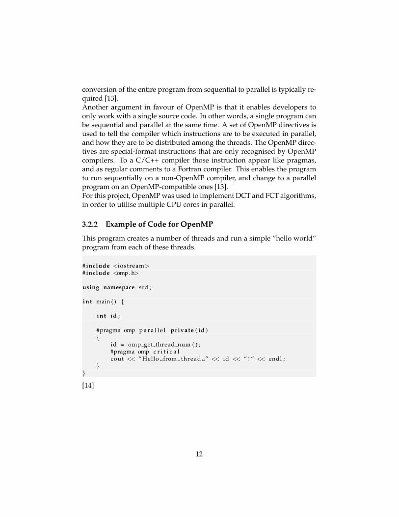
This program creates a number of threads and run a simple ”hello world”program from each of these threads.

# include <iostream># include <omp. h>

using namespace std ;

i n t main ( ) {

i n t id ;

#pragma omp p a r a l l e l private ( id ){

id = omp get thread num ( ) ;#pragma omp c r i t i c a lcout << ” Hello from thread ” << id << ” ! ” << endl ;

}}

[14]

12

Chapter 4

Implementation of IDCT

A description of the implementation of IDCT in OpenCL and OpenMP. Thiswill include an overview of the development and testing framework.

4.1 IDCT and IFCT Development

4.1.1 Simple

The simple IDCT approach implementation simply follows the straightfor-ward approach described in pseudo code in Chapter 2. To avoid repeatingcalculations and to speed up the running time the cosine table was precal-culated and stored in memory. The same principle was applied to the FCTcalculation.

4.1.2 OpenMP

For the OpenMP two different groups of approaches were tested.The idea behind the first approach was to spread the blocks between threads,so 1 thread fully decodes a single block.The second approach aims allocated different parts of the algorithm itselfto different threads. For the IFCT approach, matrix rows and columns wereattempted to be divided into different threads. This approach proved to beinefficient since the single block consists of only 8 rows and 8 columns andthe overhead of thread creating negates the speed effects of parallel execu-tion.

For the both algorithms (IDCT and IFCT) the first approach provedto be faster while the second approach only extended the execution time.

13

Hence, the first approach was used in the final implementation and in thetests described in the next chapters.

4.1.3 OpenCL

To be able to implement the IDCT on a GPU two the code was written intwo parts. The first part is the kernel code which is to be executed by theGPU. The second part is the host code, which compiles and builds the ker-nel, allocates the memory buffer and starts the kernel execution.The blocks to be decoded were merged into a single block of memory andmapped onto the GPU memory. The number of kernel work groups wereset to be equal to the number of blocks to be decoded.For the IDCT approach the kernel accepted 3 arguments: the input matrix,the pre-calculated cosine table and the output matrix. For the IFCT ap-proach, the arguments were only the input and output matrices.After the execution of the kernel, the memory containing the output matri-ces was mapped back onto the CPU memory and split back into separateblocks.The code for both IDCT and IFCT kernels can be found in Chapter 7 (Ap-pendix).

4.2 Testing Framework

To test the performance of the algorithms described above two main met-rics were measured: speed of the execution and accuracy of the calcula-tions.The 8x8 blocks to be encoded were represented by a block class which con-tained a 1-dimensional array of 64 floating point numbers and a range ofmethods to access and manipulate this data.The tests were performed on randomly generated sets of blocks containingnumbers ranging from 0 to 255 which simulated RGB values.A number of functions were established in order to measure the executionspeed. The blocks generation time and any other non-framework relatedoverhead was excluded from the calculations.

14

Chapter 5

Perfomance

This chapter describes the hardware used for evaluation, what experimentswere done to evaluate the overall performance of different algorithms, andthe results obtained

The following hardware was used:

Table 5.1: Hardware usedCPU GPU

Processor Name: Intel Core i5 Model: Intel Iris 5100Core Speed: 2.6 GHz , up to 83.2 GFLOPS Core Speed: 1.3GHz, up to 832 GFLOPS

Peak theoretical bandwidth: 25.6 GB/s Peak theoretical bandwidth: 25.6 GB/sTotal Number of Cores: 4 Pipelines/Execution Units: 40

L2 Cache (per Core): 256 KBL3 Cache: 3 MB

5.1 Speed

To test the speed, the algorithm was run for three different numbers ofblocks (1, 1000 and 10,000 blocks).The purpose of running this algorithm on one block is to represent the setup time overhead for different approaches. It appears that OpenCL has thehighest set up time. To obtain this data, the algorithms were run 1000 timeson a single block and then the average of obtained values was taken. Thedifference between 1000 and 10,000 block demonstrates the proportion offrameworks (OpenCL and OpenMP) overhead time to the actual run time.

15

Figure 5.1: Testing of IDCT speed for different approaches; blocks decoded1; note that the time is represented in µs to better graphically represent the differ-ence between bars

The graphs for 1000 and 10,000 blocks are presented for the purpose ofcomparing the speed of different implementation and determining whetherthere are any anomalies.

16

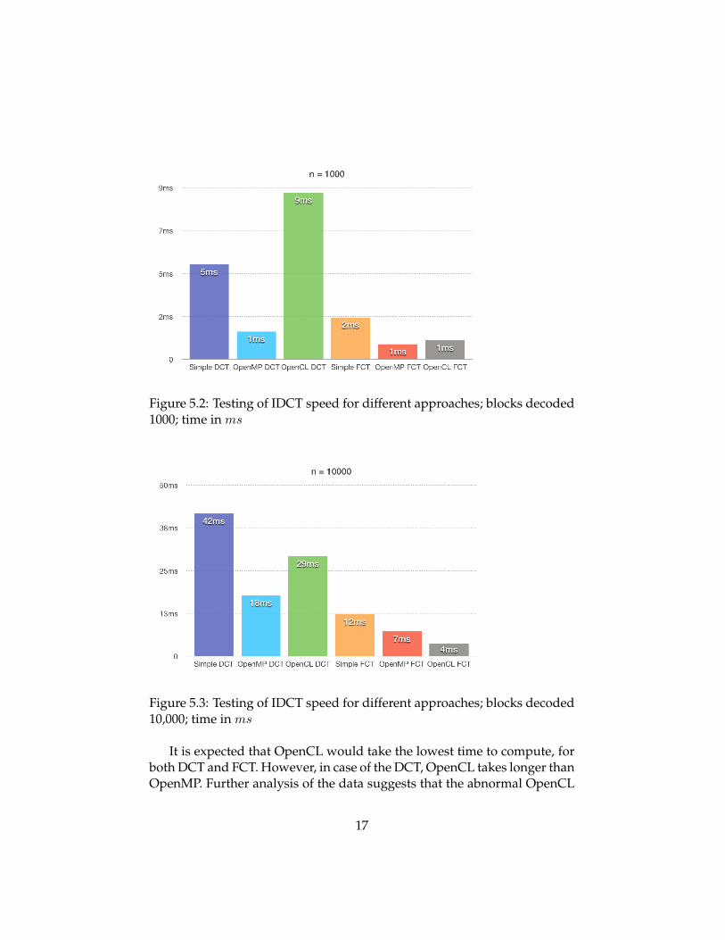
Figure 5.2: Testing of IDCT speed for different approaches; blocks decoded1000; time in ms

Figure 5.3: Testing of IDCT speed for different approaches; blocks decoded10,000; time in ms

It is expected that OpenCL would take the lowest time to compute, forboth DCT and FCT. However, in case of the DCT, OpenCL takes longer thanOpenMP. Further analysis of the data suggests that the abnormal OpenCL

17

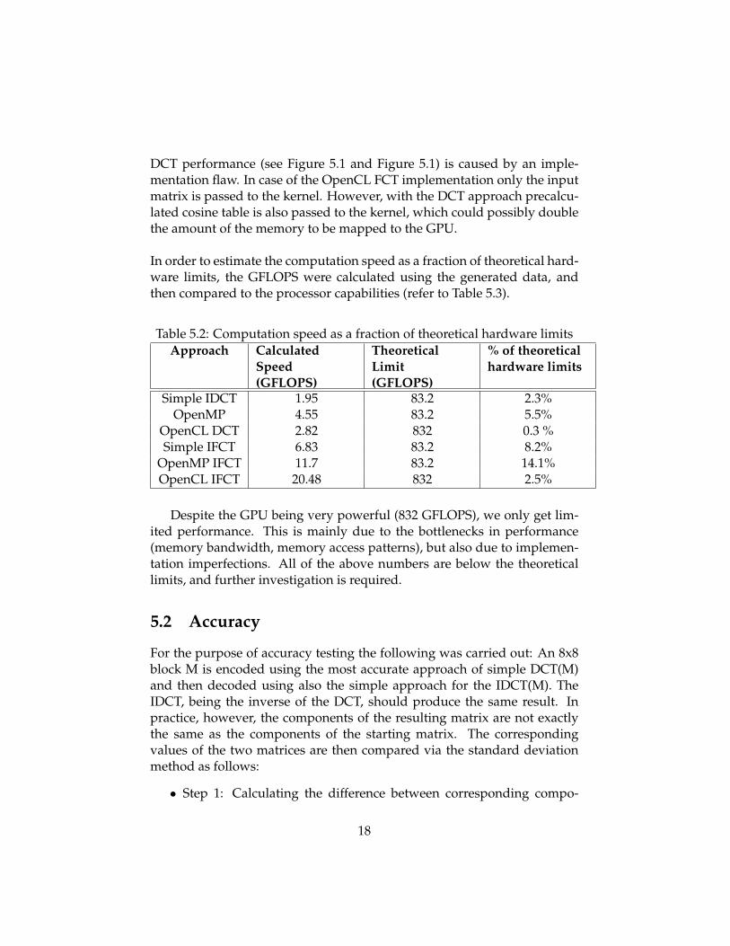
DCT performance (see Figure 5.1 and Figure 5.1) is caused by an imple-mentation flaw. In case of the OpenCL FCT implementation only the inputmatrix is passed to the kernel. However, with the DCT approach precalcu-lated cosine table is also passed to the kernel, which could possibly doublethe amount of the memory to be mapped to the GPU.

In order to estimate the computation speed as a fraction of theoretical hard-ware limits, the GFLOPS were calculated using the generated data, andthen compared to the processor capabilities (refer to Table 5.3).

Table 5.2: Computation speed as a fraction of theoretical hardware limitsApproach Calculated

Speed(GFLOPS)

TheoreticalLimit(GFLOPS)

% of theoreticalhardware limits

Simple IDCT 1.95 83.2 2.3%OpenMP 4.55 83.2 5.5%

OpenCL DCT 2.82 832 0.3 %Simple IFCT 6.83 83.2 8.2%

OpenMP IFCT 11.7 83.2 14.1%OpenCL IFCT 20.48 832 2.5%

Despite the GPU being very powerful (832 GFLOPS), we only get lim-ited performance. This is mainly due to the bottlenecks in performance(memory bandwidth, memory access patterns), but also due to implemen-tation imperfections. All of the above numbers are below the theoreticallimits, and further investigation is required.

5.2 Accuracy

For the purpose of accuracy testing the following was carried out: An 8x8block M is encoded using the most accurate approach of simple DCT(M)and then decoded using also the simple approach for the IDCT(M). TheIDCT, being the inverse of the DCT, should produce the same result. Inpractice, however, the components of the resulting matrix are not exactlythe same as the components of the starting matrix. The correspondingvalues of the two matrices are then compared via the standard deviationmethod as follows:

• Step 1: Calculating the difference between corresponding compo-

18

nents of the two matrices

• Step 2: Calculating the square of the difference from Step 1

• Step 3: Calculating the sum of all values from Step 2**note that for this step the matrix M is represented as a one-dimensionalvector

• Step 4: Computing the square root of the result from Step 3, dividedby 64 (number of components in an 8x8 matrix)

The formula for computing the standard deviation is:

STDEV =

√∑(Mi −M

′i )

64, (5.1)

where Mi is the initial matrix to be encoded and M′i is the final decoded

matrix [17].Note that, for the purposes of accuracy testing, the matrices are treated asone-dimensional vectors, hence they only have one index i.

Decoding was done on matrices with randomised RGB (8-bit) values rang-ing from 0 to 255.

Table 5.3: AccuracyIDCT IFCT

CPU 1.37789e-5 0.515388OpenMP 1.37789e-5 0.515388OpenCL 1.37789e-5 0.515388

19

Chapter 6

Conclusion

To conclude, the algorithms of IDCT and IFCT were explored over thecourse of this project. Both of those algorithms were implemented using thesimple CPU approach, OpenMP for the multicore approach and OpenCLfor the GPU approach. The results were then tested based on their accuracyand time taken to compute, which was also compared to the maximum the-oretical speed the hardware could operate at.To compare the computation speed, the six implementations of IDCT wererun on 1, 1000 and 10,000 blocks. The result obtained for 1-block operationrepresents the set up overhead time. It was concluded that the sequentialalgorithm for IDCT took the longest, and the OpenCL IFCT was the fastest.These results were as expected, based on know performance superiorityof the GPU. The OpenCL algorithm for the IDCT, however, took longer tocompute than the OpenMP IDCT. We speculate that this is perhaps due toan implementation flaw, which is to be investigated in future projects.

Accuracy of IDCT and IFCT was also evaluated. Not surprisingly, it hasbeen confirmed that IDCT is a lot more accurate compared to the IFCT. Itwas also shown that the accuracy of the algorithms is independent of thedevelopment framework.

The following work could be analysed to potentially obtain better results:

• Memory access patterns

• Thread scheduling for the OpenMP approach

• Cache lines performance

20

Chapter 7

Appendix

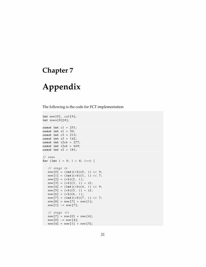
The following is the code for FCT implementation

i n t row [ 9 ] , c o l [ 9 ] ;i n t rows [ 8 ] [ 8 ] ;

const i n t c1 = 2 5 1 ;const i n t s1 = 5 0 ;const i n t c3 = 2 1 3 ;const i n t s3 = 1 4 2 ;const i n t r2c6 = 2 7 7 ;const i n t r2s6 = 6 6 9 ;const i n t r2 = 1 8 1 ;

/ / rowsfor ( i n t i = 0 ; i < 8 ; i ++) {

/ / s t a g e i vrow [ 0 ] = ( i n t ) ( ∗ b ) ( 0 , i ) << 9 ;row [ 1 ] = ( i n t ) ( ∗ b ) ( 1 , i ) << 7 ;row [ 2 ] = (∗b ) ( 2 , i ) ;row [ 3 ] = (∗b ) ( 3 , i ) ∗ r2 ;row [ 4 ] = ( i n t ) ( ∗ b ) ( 4 , i ) << 9 ;row [ 5 ] = (∗b ) ( 5 , i ) ∗ r2 ;row [ 6 ] = (∗b ) ( 6 , i ) ;row [ 7 ] = ( i n t ) ( ∗ b ) ( 7 , i ) << 7 ;row [ 8 ] = row [ 7 ] + row [ 1 ] ;row [ 1 ] −= row [ 7 ] ;

/ / s t a g e i i irow [ 7 ] = row [ 0 ] + row [ 4 ] ;row [ 0 ] −= row [ 4 ] ;row [ 4 ] = row [ 1 ] + row [ 5 ] ;

21

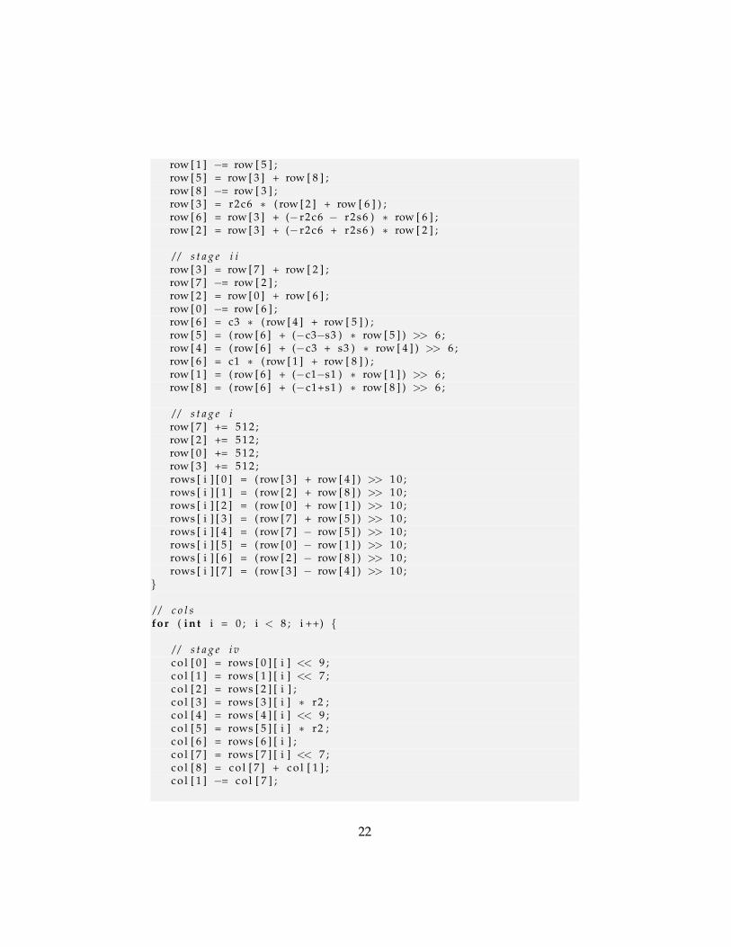
row [ 1 ] −= row [ 5 ] ;row [ 5 ] = row [ 3 ] + row [ 8 ] ;row [ 8 ] −= row [ 3 ] ;row [ 3 ] = r2c6 ∗ ( row [ 2 ] + row [ 6 ] ) ;row [ 6 ] = row [ 3 ] + (− r2c6 − r2s6 ) ∗ row [ 6 ] ;row [ 2 ] = row [ 3 ] + (− r2c6 + r2s6 ) ∗ row [ 2 ] ;

/ / s t a g e i irow [ 3 ] = row [ 7 ] + row [ 2 ] ;row [ 7 ] −= row [ 2 ] ;row [ 2 ] = row [ 0 ] + row [ 6 ] ;row [ 0 ] −= row [ 6 ] ;row [ 6 ] = c3 ∗ ( row [ 4 ] + row [ 5 ] ) ;row [ 5 ] = ( row [ 6 ] + (−c3−s3 ) ∗ row [ 5 ] ) >> 6 ;row [ 4 ] = ( row [ 6 ] + (−c3 + s3 ) ∗ row [ 4 ] ) >> 6 ;row [ 6 ] = c1 ∗ ( row [ 1 ] + row [ 8 ] ) ;row [ 1 ] = ( row [ 6 ] + (−c1−s1 ) ∗ row [ 1 ] ) >> 6 ;row [ 8 ] = ( row [ 6 ] + (−c1+s1 ) ∗ row [ 8 ] ) >> 6 ;

/ / s t a g e irow [ 7 ] += 5 1 2 ;row [ 2 ] += 5 1 2 ;row [ 0 ] += 5 1 2 ;row [ 3 ] += 5 1 2 ;rows [ i ] [ 0 ] = ( row [ 3 ] + row [ 4 ] ) >> 1 0 ;rows [ i ] [ 1 ] = ( row [ 2 ] + row [ 8 ] ) >> 1 0 ;rows [ i ] [ 2 ] = ( row [ 0 ] + row [ 1 ] ) >> 1 0 ;rows [ i ] [ 3 ] = ( row [ 7 ] + row [ 5 ] ) >> 1 0 ;rows [ i ] [ 4 ] = ( row [ 7 ] − row [ 5 ] ) >> 1 0 ;rows [ i ] [ 5 ] = ( row [ 0 ] − row [ 1 ] ) >> 1 0 ;rows [ i ] [ 6 ] = ( row [ 2 ] − row [ 8 ] ) >> 1 0 ;rows [ i ] [ 7 ] = ( row [ 3 ] − row [ 4 ] ) >> 1 0 ;

}

/ / c o l sfor ( i n t i = 0 ; i < 8 ; i ++) {

/ / s t a g e i vc o l [ 0 ] = rows [ 0 ] [ i ] << 9 ;c o l [ 1 ] = rows [ 1 ] [ i ] << 7 ;c o l [ 2 ] = rows [ 2 ] [ i ] ;c o l [ 3 ] = rows [ 3 ] [ i ] ∗ r2 ;c o l [ 4 ] = rows [ 4 ] [ i ] << 9 ;c o l [ 5 ] = rows [ 5 ] [ i ] ∗ r2 ;c o l [ 6 ] = rows [ 6 ] [ i ] ;c o l [ 7 ] = rows [ 7 ] [ i ] << 7 ;c o l [ 8 ] = c o l [ 7 ] + c o l [ 1 ] ;c o l [ 1 ] −= c o l [ 7 ] ;

22

/ / s t a g e i i ic o l [ 7 ] = c o l [ 0 ] + c o l [ 4 ] ;c o l [ 0 ] −= c o l [ 4 ] ;c o l [ 4 ] = c o l [ 1 ] + c o l [ 5 ] ;c o l [ 1 ] −= c o l [ 5 ] ;c o l [ 5 ] = c o l [ 3 ] + c o l [ 8 ] ;c o l [ 8 ] −= c o l [ 3 ] ;c o l [ 3 ] = r2c6 ∗ ( c o l [ 2 ] + c o l [ 6 ] ) ;c o l [ 6 ] = c o l [ 3 ] + (− r2c6 − r2s6 ) ∗ c o l [ 6 ] ;c o l [ 2 ] = c o l [ 3 ] + (− r2c6 + r2s6 ) ∗ c o l [ 2 ] ;

/ / s t a g e i ic o l [ 3 ] = c o l [ 7 ] + c o l [ 2 ] ;c o l [ 7 ] −= c o l [ 2 ] ;c o l [ 2 ] = c o l [ 0 ] + c o l [ 6 ] ;c o l [ 0 ] −= c o l [ 6 ] ;c o l [ 4 ] >>= 6 ;c o l [ 5 ] >>= 6 ;c o l [ 1 ] >>= 6 ;c o l [ 8 ] >>= 6 ;c o l [ 6 ] =c3 ∗ ( c o l [ 4 ] + c o l [ 5 ] ) ;c o l [ 5 ] = ( c o l [ 6 ] + (−c3−s3 ) ∗ c o l [ 5 ] ) ;c o l [ 4 ] = ( c o l [ 6 ] + (−c3+s3 ) ∗ c o l [ 4 ] ) ;c o l [ 6 ] = c1 ∗ ( c o l [ 1 ] + c o l [ 8 ] ) ;c o l [ 1 ] = ( c o l [ 6 ] + (−c1−s1 ) ∗ c o l [ 1 ] ) ;c o l [ 8 ] = ( c o l [ 6 ] + (−c1+s1 ) ∗ c o l [ 8 ] ) ;

/ / s t a g e ic o l [ 7 ] += 1024 ;c o l [ 2 ] += 1024 ;c o l [ 0 ] += 1024 ;c o l [ 3 ] += 1024 ;r es ( i , 0 ) = ( c o l [ 3 ] + c o l [ 4 ] ) >> 1 1 ;r es ( i , 1 ) = ( c o l [ 2 ] + c o l [ 8 ] ) >> 1 1 ;r es ( i , 2 ) = ( c o l [ 0 ] + c o l [ 1 ] ) >> 1 1 ;r es ( i , 3 ) = ( c o l [ 7 ] + c o l [ 5 ] ) >> 1 1 ;r es ( i , 4 ) = ( c o l [ 7 ] − c o l [ 5 ] ) >> 1 1 ;r es ( i , 5 ) = ( c o l [ 0 ] − c o l [ 1 ] ) >> 1 1 ;r es ( i , 6 ) = ( c o l [ 2 ] − c o l [ 8 ] ) >> 1 1 ;r es ( i , 7 ) = ( c o l [ 3 ] − c o l [ 4 ] ) >> 1 1 ;

}

OpenCL kernel

kernel void i d c t ( g loba l f l o a t ∗ input , g loba l const f l o a t ∗ c o s t a b l e ,g loba l f l o a t ∗ output ) {

i n t id = g e t g l o b a l i d ( 0 ) ;

23

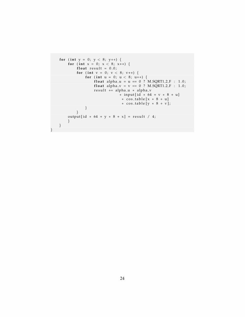
for ( i n t y = 0 ; y < 8 ; y++) {for ( i n t x = 0 ; x < 8 ; x++) {

f l o a t r e s u l t = 0 . 0 ;for ( i n t v = 0 ; v < 8 ; v++) {

for ( i n t u = 0 ; u < 8 ; u++) {f l o a t alpha u = u == 0 ? M SQRT1 2 F : 1 . 0 ;f l o a t alpha v = v == 0 ? M SQRT1 2 F : 1 . 0 ;r e s u l t += alpha u ∗ alpha v

∗ input [ id ∗ 64 + v ∗ 8 + u ]∗ c o s t a b l e [ x ∗ 8 + u ]∗ c o s t a b l e [ y ∗ 8 + v ] ;

}}

output [ id ∗ 64 + y ∗ 8 + x ] = r e s u l t / 4 ;}

}}

24

Bibliography

[1] E. Mikulic. (2014, April 1). Discrete Cosine Transform [Online]. Avail-able: https://unix4lyfe.org/dct-1d/

[2] P. Duhamel and M. Vetterli, ”Fast Fourier Transforms: A tutorial re-view and a state of the art”, Elsevier, Signal Processing 19, pp. 259 -299, October 1989.

[3] A.B. Watson, ”Image Compression Using the Discrete Cosine Trans-form”, Mathematica Journal, vol 4(1), pp.81-88, 1994.

[4] T. Kientzle. (1999, March 1). Algorithm Alley [Online].Available: http://www.drdobbs.com/parallel/algorithm-alley/184410889?pgno=1

[5] T. G. Lane. (1994-1998). USING THE IJG JPEGLIBRARY, JPEG Group, [Online]. Available:http://apodeline.free.fr/DOC/libjpeg/libjpeg.html

[6] C.T. Hsu and J.L. Wu, ”Energy Compaction Capability of the DCT andDHT with CT image constraints”, IEEE vol.1, pp. 345-348, July 1997

[7] K.R. Rao and P. Yip, Discrete Cosine Transform: Algorithms, Advantages,Applications, Academic Press, Inc, 1990

[8] N. Ahmed et al., ”Discrete Cosine Transform”, IEEE Trans. Comput.vol.C-23, pp. 90-93, January 1974

[9] E. Mikulic. (2001, September 1). Discrete Cosine Transform [Online].Available: https://unix4lyfe.org/dct/

[10] W.B. Pennebaker and J.L. Mitchell, ”The Discrete Cosine TransformDCT” in JPEG Still Image Data Compression Standard, Kluwer AcademicPublishers, 1993, p. 52.

25

[11] M. Scarpino, ”Introducing OpenCL” in OpenCL in Action: How to Ac-celerate Graphics and Computation, Manning Publications Co, 2012, pp.3-15.

[12] Khronos OpenCL Working Group. (2015, November 11). TheOpenCL Specification, Version 2.1, Revision 23 [Online]. Available:https://www.khronos.org/registry/cl/specs/opencl-2.1.pdf

[13] B. Chapman et al., ”Introduction” in Using OpenMP: Portable SharedMemory Parallel Programming, MIT Press, 2008

[14] T. Mattson and L. Meadows A ”Hands-on” Introduction to OpenMP [On-line], Available http://openmp.org/mp-documents/omp-hands-on-SC08.pdf

[15] OpenMP ARB. (2015, June 12). About OpenMP and OpenMP.org [On-line]. Available: http://openmp.org/wp/about-openmp/

[16] A. Silberschatz et al. Operating System Concepts, Wiley, 2013

[17] E.W. Weisstein. (1996 - 2016). Standard Deviation [Online]. Available:http://mathworld.wolfram.com/StandardDeviation.html

26