The Interval Constraint Solver For integer and real variables.

The Interval Constraint Solver

For integer and real variables

Outline

Introduction & general overview Integer constraint solving Global constraints Reified constraints Real interval arithmetic Real constraint solving

Usage

Load the interval constraint library by using

:- lib(ic).

at the beginning of your code, or type

lib(ic).

at the top-level ECLiPSe prompt.

Functionality

The IC library implements variables with integer or real domains basic equality, inequality and disequality constraints

over linear and non-linear arithmetic expressions some “global” constraints for integer variables reified constraints search and optimisation facilities

Interval variables

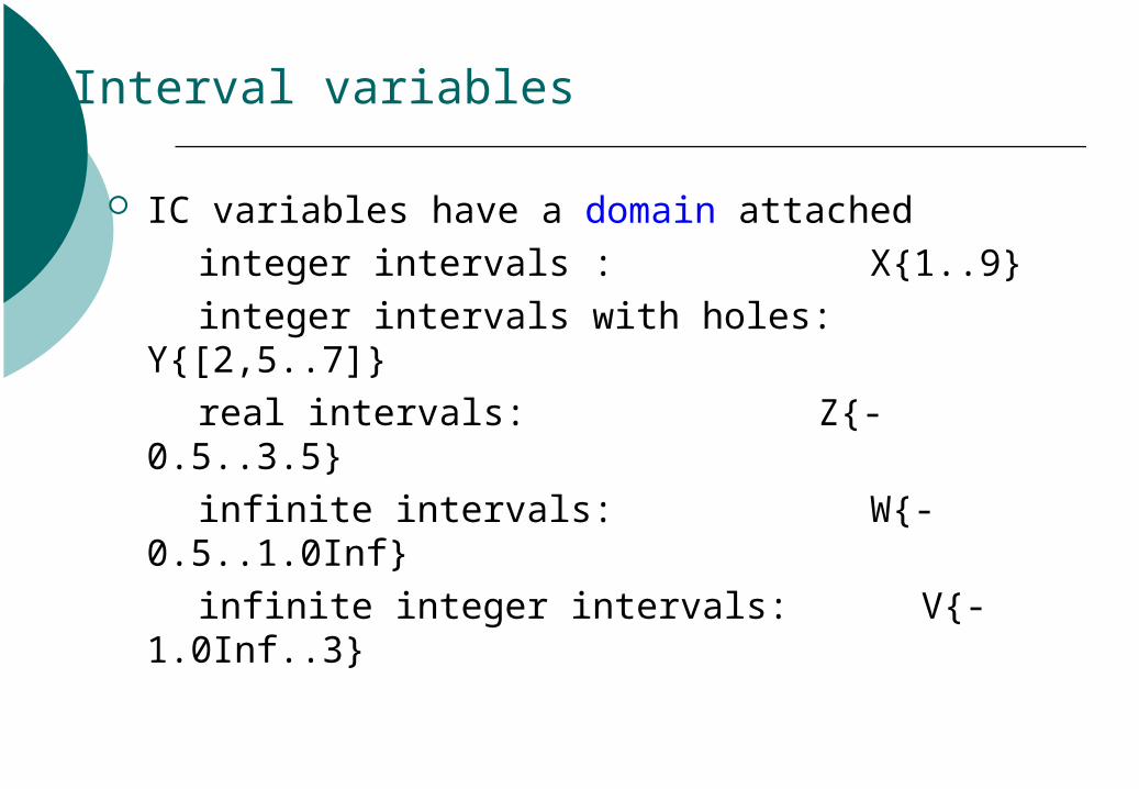
IC variables have a domain attached

integer intervals : X{1..9}

integer intervals with holes: Y{[2,5..7]}

real intervals: Z{-0.5..3.5}

infinite intervals: W{-0.5..1.0Inf}

infinite integer intervals: V{-1.0Inf..3}

Interval variables

Vars :: Domaine.g. X :: 1..9 X #:: 1..9

Y :: [2,5..7] Y #:: [2,5..7]

Z :: -0.5..3.5 Z $:: -0.5..3.5

W :: -0.5..1.0Inf W $:: -0.5..1.0Inf

V :: -1.0Inf..3 V #:: -1.0Inf..3

Attaches an initial domain to a variable or intersects its old domain with the new one.

Type of bounds gives type of variable for ::(1.0Inf is considered type-neutral)

#:: always imposes integrality $:: never imposes integrality

The basic set of constraints

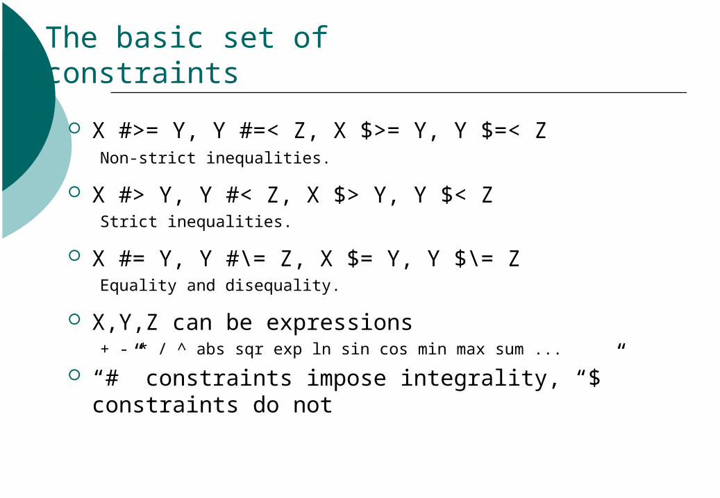
X #>= Y, Y #=< Z, X $>= Y, Y $=< ZNon-strict inequalities.

X #> Y, Y #< Z, X $> Y, Y $< ZStrict inequalities.

X #= Y, Y #\= Z, X $= Y, Y $\= ZEquality and disequality.

X,Y,Z can be expressions+ - * / ^ abs sqr exp ln sin cos min max sum ...

“#” constraints impose integrality, “$” constraints do not

Propagation behaviour

Constraints are active:

?- [X, Y] :: 1..5, X #>= Y + 1.X = X{2 .. 5}, Y = Y{1 .. 4}Delayed goals: ic : (-(X{2 .. 5}) + Y{1 .. 4} =< -1)Yes

?- [X, Y] :: 1..5, X #>= Y + 1, Y #>= 3.X = X{[4, 5]}, Y = Y{[3, 4]}Delayed goals: ic : (-(X{[4, 5]}) + Y{[3, 4]} =< -1)Yes

?- [X, Y] :: 1..5, X #>= Y + 1, Y #>= 4.X = 5, Y = 4Yes

Basic search support

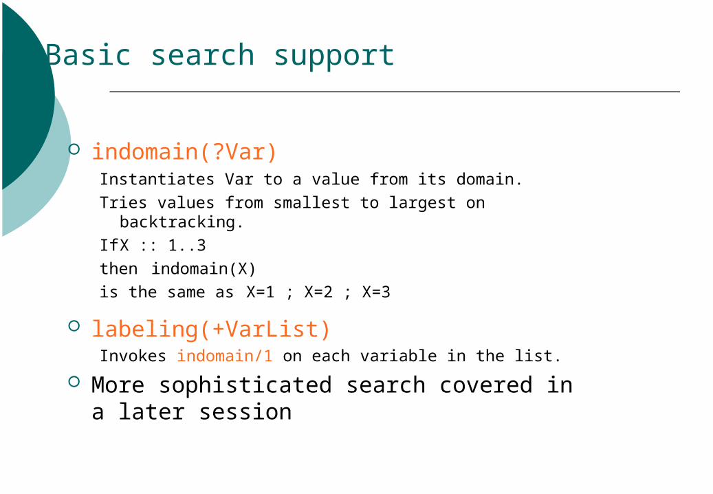
indomain(?Var)Instantiates Var to a value from its domain.

Tries values from smallest to largest on backtracking.

If X :: 1..3

then indomain(X)

is the same as X=1 ; X=2 ; X=3

labeling(+VarList)Invokes indomain/1 on each variable in the list.

More sophisticated search covered in a later session

Exploring the search space

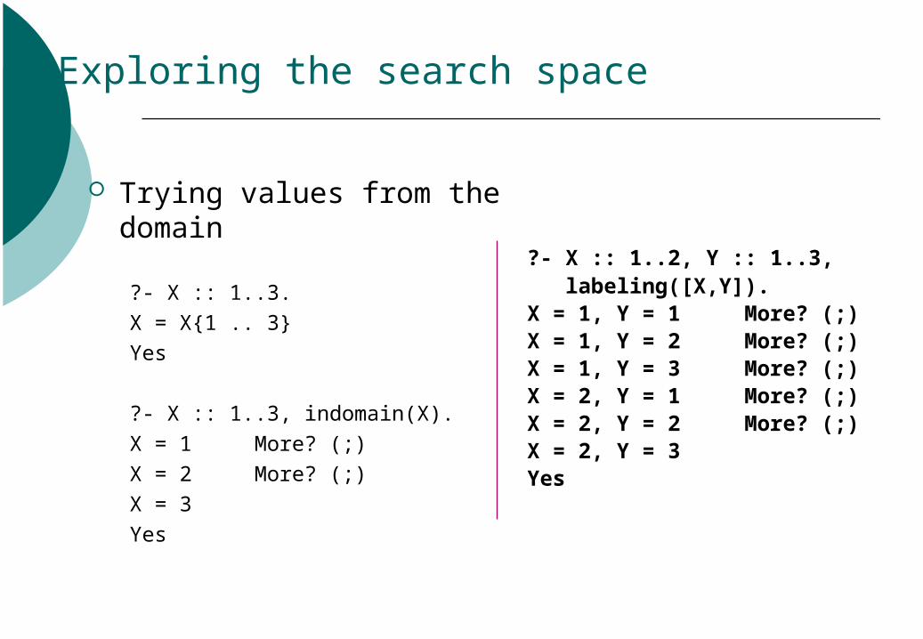
Trying values from the domain

?- X :: 1..3.

X = X{1 .. 3}

Yes

?- X :: 1..3, indomain(X).

X = 1 More? (;)

X = 2 More? (;)

X = 3

Yes

?- X :: 1..2, Y :: 1..3, labeling([X,Y]).X = 1, Y = 1 More? (;) X = 1, Y = 2 More? (;) X = 1, Y = 3 More? (;) X = 2, Y = 1 More? (;) X = 2, Y = 2 More? (;) X = 2, Y = 3Yes

Standard example

sendmore(Digits) :-

Digits = [S,E,N,D,M,O,R,Y],

Digits :: 0..9,

alldifferent(Digits),

S #\= 0, M #\= 0,

1000*S + 100*E + 10*N + D

+ 1000*M + 100*O + 10*R + E

#= 10000*M + 1000*O + 100*N + 10*E + Y,

labeling(Digits).

SEND+ MORE

= MONEY

SEND + MORE= MONEY

Standard example

?- sendmore(Digits).

Digits = [9, 5, 6, 7, 1, 0, 8, 2]

More? (;)

No

9567 + 1085= 10652

Other built-in constraints

alldifferent(+List)All elements of the list are constrained to be pairwise different.

integers(+List)All elements of the list are constrained to be integral.

reals(+List)All elements of the list are constrained to be real.

(Note this doesn’t mean they can’t also be integral: this is equivalent to List :: -1.0Inf..1.0Inf.)

An arithmetic puzzle

Is there a positive number which when divided by 3 gives a remainder of 1; when divided by 4 gives a remainder of 2; when divided by 5 gives a remainder of 3;

and when divided by 6 gives a remainder of 4?

(express the constraints with multiplications rather than divisions)

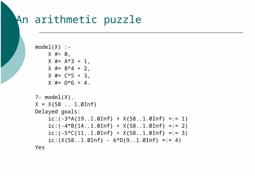
model(X) :- X #> 0, X #= A*3 + 1, X #= B*4 + 2, X #= C*5 + 3, X #= D*6 + 4.

An arithmetic puzzle

model(X) :- X #> 0, X #= A*3 + 1, X #= B*4 + 2, X #= C*5 + 3, X #= D*6 + 4.

?- model(X).X = X{58 .. 1.0Inf}Delayed goals: ic:(-3*A{19..1.0Inf} + X{58..1.0Inf} =:= 1) ic:(-4*B{14..1.0Inf} + X{58..1.0Inf} =:= 2) ic:(-5*C{11..1.0Inf} + X{58..1.0Inf} =:= 3) ic:(X{58..1.0Inf} - 6*D{9..1.0Inf} =:= 4)Yes

An arithmetic puzzle

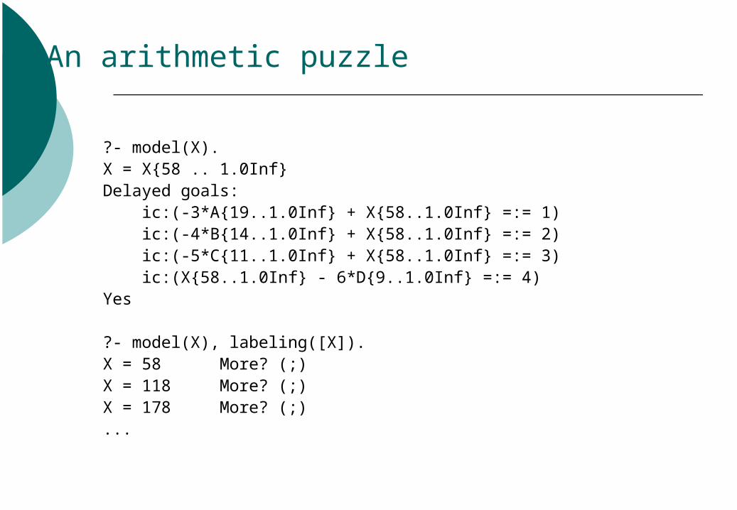
?- model(X).X = X{58 .. 1.0Inf}Delayed goals: ic:(-3*A{19..1.0Inf} + X{58..1.0Inf} =:= 1) ic:(-4*B{14..1.0Inf} + X{58..1.0Inf} =:= 2) ic:(-5*C{11..1.0Inf} + X{58..1.0Inf} =:= 3) ic:(X{58..1.0Inf} - 6*D{9..1.0Inf} =:= 4)Yes

?- model(X), labeling([X]).X = 58 More? (;) X = 118 More? (;) X = 178 More? (;) ...

N-ary constraints in lib(ic)

S #= sum(List)Sum of N variables or sub-expressions.

X #= min(List)Smallest of N variables or sub-expressions.

X #= max(List)Largest of N variables or sub-expressions.

alldifferent(List)All elements of the list are pairwise different.

Global constraints

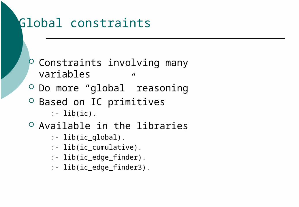
Constraints involving many variables Do more “global” reasoning Based on IC primitives

:- lib(ic).

Available in the libraries:- lib(ic_global).

:- lib(ic_cumulative).

:- lib(ic_edge_finder).

:- lib(ic_edge_finder3).

Different constraint behaviours

lib(ic) implementation of alldifferent/1

?- [A,B,C]::1..3, D::1..5, ic:alldifferent([A,B,C,D]).

A = A{1 .. 3}

B = B{1 .. 3}

C = C{1 .. 3}

D = D{1 .. 5}

Delayed goals:

outof(A{1 .. 3}, [], [B{1 .. 3}, C{1 .. 3}, D{1 .. 5}])

outof(B{1 .. 3}, [A{1 .. 3}], [C{1 .. 3}, D{1 .. 5}])

outof(C{1 .. 3}, [B{1 .. 3}, A{1 .. 3}], [D{1 .. 5}])

outof(D{1 .. 5}, [C{1 .. 3}, B{1 .. 3}, A{1 .. 3}], [])

Yes

Different constraint behaviours

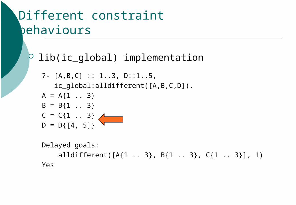
lib(ic_global) implementation

?- [A,B,C] :: 1..3, D::1..5,

ic_global:alldifferent([A,B,C,D]).

A = A{1 .. 3}

B = B{1 .. 3}

C = C{1 .. 3}

D = D{[4, 5]}

Delayed goals:

alldifferent([A{1 .. 3}, B{1 .. 3}, C{1 .. 3}], 1)

Yes

Why is it better?

Global view enables more reasoning:

D

C

B

A

54321

Primitive constraints see only e.g.

54321A

54321D

#\=

alldifferent

More constraints in lib(ic_global) (I)

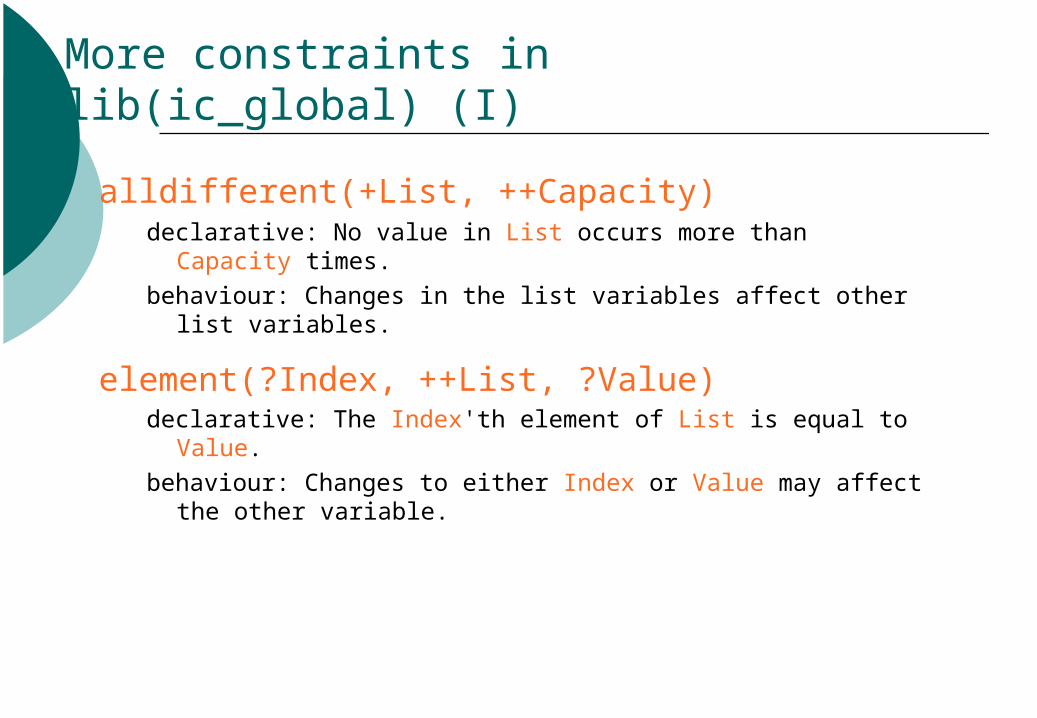
alldifferent(+List, ++Capacity)declarative: No value in List occurs more than Capacity times.

behaviour: Changes in the list variables affect other list variables.

element(?Index, ++List, ?Value)declarative: The Index'th element of List is equal to Value.

behaviour: Changes to either Index or Value may affect the other variable.

The element/3 constraint

Defines a mapping from one variable to another:

?- element(I, [1,3,6,3,2], V).I = I{1 .. 5}V = V{[1 .. 3, 6]}Delayed goals: element(I{1..5}, [1, 3, 6, 3, 2], V{[1..3, 6]})Yes

?- element(I, [1,3,6,3,2], V), V #\= 3.I = I{[1, 3, 5]}V = V{[1, 2, 6]}Delayed goals: element(I{[1, 3, 5]}, [1, 3, 6, 3, 2], V{[1, 2, 6]})Yes

More constraints in lib(ic_global) (II)ordered(++Rel, +List)

declarative: List is an ordered list.behaviour: Changes in the list variables affect other list variables.

ordered_sum(+List, ?Sum)declarative: List is an ordered list and the sum of its elements is Sum.behaviour: Changes in the list variables affect Sum and other list variables,

and vice-versa.

sorted(?List, ?SortedList)declarative: SortedList is a sorted permutation of List.behaviour: Change of bounds in one list may affect the other.

sorted(?List, ?SortedList, ?Positions)declarative: SortedList is a sorted permutation of List, and Positions

describes how the elements are permuted.behaviour: Change of bounds in any list may affect others.

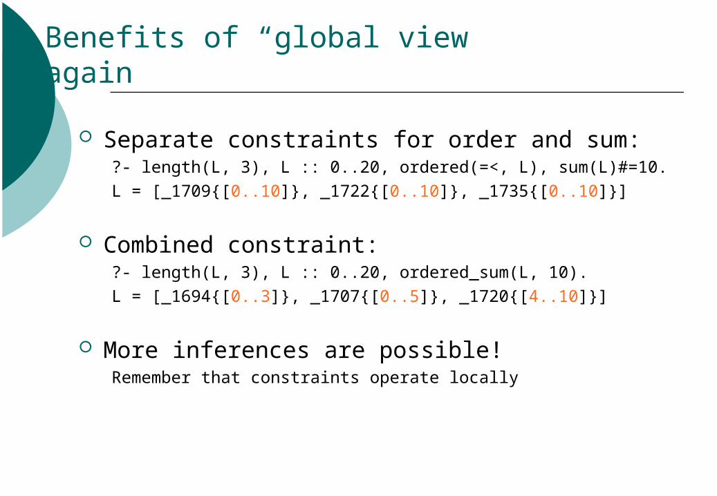
Benefits of “global view” again

Separate constraints for order and sum:?- length(L, 3), L :: 0..20, ordered(=<, L), sum(L)#=10.

L = [_1709{[0..10]}, _1722{[0..10]}, _1735{[0..10]}]

Combined constraint:?- length(L, 3), L :: 0..20, ordered_sum(L, 10).

L = [_1694{[0..3]}, _1707{[0..5]}, _1720{[4..10]}]

More inferences are possible!Remember that constraints operate locally

More constraints in lib(ic_global) (III)

atmost(++N, +List, ++Value)declarative: At most N elements of List have value Value.

behaviour: Changes in the list variables affect other list variables.

occurrences(++Value, +List, ?N)declarative: Value occurs N times in List.

behaviour: Changes in the list variables affect N and vice versa.

lexico_le(+List1, +List2)declarative: List1 is lexicographically less than or equal to List2.

behaviour: Change of bounds in one list may affect the other.

Scheduling constraints

cumulative(+Starts, +Durations, +ResourceUsages, ++ResourceLimit)

2

1

34

1

2

3

4

1 2 3 4 5 6 ...

disjunctive(+Starts, +Durations)Same as cumulative(Starts, Durations, [1,...,1], 1)

cumulative([S1,S2,S3,S4], [1,4,2,2], [1,1,3,2], 4)

Scheduling constraints - implementations

The declarative constraintscumulative(+Starts, +Durations, +ResourceUsages, +

+ResourceLimit)

disjunctive(+Starts, +Durations)

Three implementation variantslib(ic_cumulative) - linear algorithm on each change

lib(ic_edge_finder) - quadratic algorithm

lib(ic_edge_finder3) - cubic algorithm

More work, more propagationEdge-finder detects failures earlier

Edge-finder gives more bound propagation

Reified constraints

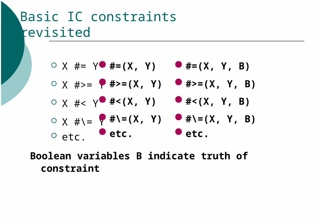
Basic IC constraints revisited

X #= Y

X #>= Y

X #< Y

X #\= Y etc.

#=(X, Y)

#>=(X, Y)

#<(X, Y)

#\=(X, Y) etc.

#=(X, Y, B)

#>=(X, Y, B)

#<(X, Y, B)

#\=(X, Y, B) etc.

Boolean variables B indicate truth of constraint

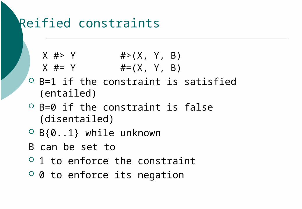
Reified constraints

X #> Y #>(X, Y, B)X #= Y #=(X, Y, B)

B=1 if the constraint is satisfied (entailed) B=0 if the constraint is false (disentailed) B{0..1} while unknown

B can be set to 1 to enforce the constraint 0 to enforce its negation

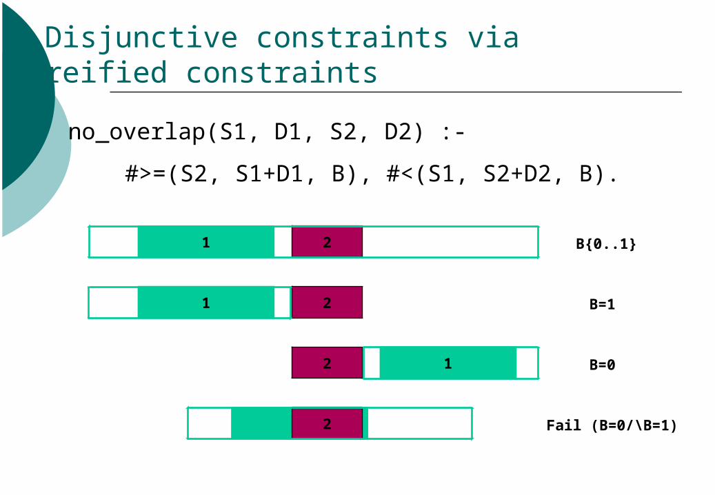
Disjunctive constraints via reified constraints

no_overlap(S1, D1, S2, D2) :-

#>=(S2, S1+D1, B), #<(S1, S2+D2, B).

1

1

2

2

B=1

B=0

2 Fail (B=0/\B=1)

1

1 2 B{0..1}

Constraint connectives

neg C Negation of constraint C

C1 and C2 C1 and C2

C1 or C2 C1 or C2

C1 => C2 C1 implies C2

E.g. X #= 0 => Y #> 0

Embedding reified constraints

Constraints can appear in other expressionsEvaluate to their reified booleanSometimes the easiest way to reify a constraint

B #= (X #>= Y + 2)

1 #= (X1 #< Y1 + (X2 #=< Y2))

This is how the constraint connectives (and, or, etc.) are actually implemented

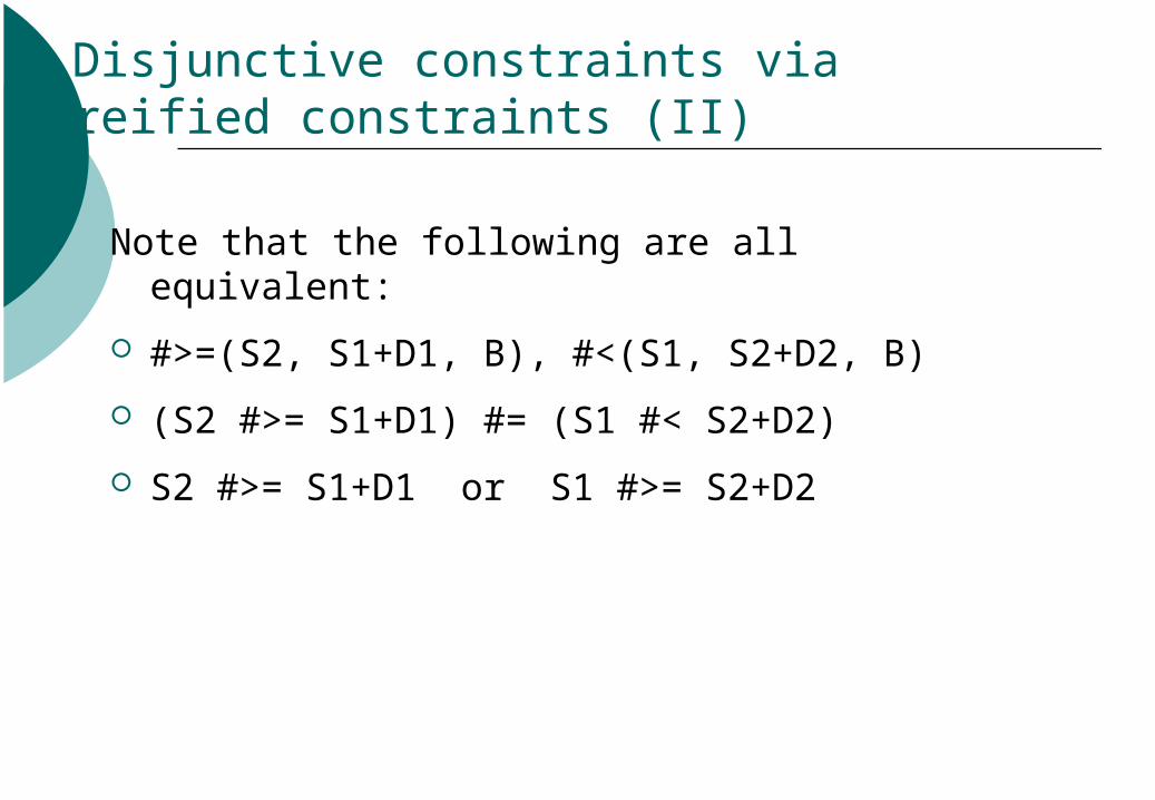
Disjunctive constraints via reified constraints (II)

Note that the following are all equivalent:

#>=(S2, S1+D1, B), #<(S1, S2+D2, B)

(S2 #>= S1+D1) #= (S1 #< S2+D2)

S2 #>= S1+D1 or S1 #>= S2+D2

Interval Arithmetic and Constraints

Interval Arithmetic

Real values often can’t be represented exactly by floating point numbers

Calculations introduce rounding errors

Problems: Is the result really a solution? Were solutions missed?

Interval Arithmetic

Solution: Represent each real value by a pair of floating

point bounds Arithmetic performed on intervals, with

appropriate rounding A ground interval expresses that the exact real

value lies somewhere between its bounds

Two kinds of intervals: “Ground” interval

Approximates a single (ground) real value

Bounds never change

“Variable” intervalApproximates the domain of a real variable

Bounds can be updated

Interval Arithmetic

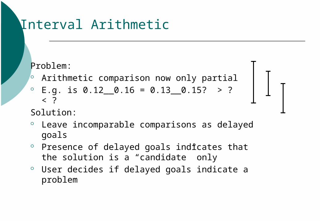
Interval Arithmetic

Problem: Arithmetic comparison now only partial E.g. is 0.12__0.16 = 0.13__0.15? > ? < ?

Solution: Leave incomparable comparisons as delayed goals Presence of delayed goals indicates that the solution is

a “candidate” only User decides if delayed goals indicate a problem

The bounded real data type

Written lwb__upb, where lwb and upb are the lower and upper floating point bounds, respectively (e.g. 0.12__0.16)

Not usually entered directly: normally occur as result of computation

breal/1 tests whether a term is a bounded real

breal/2 converts other numeric types to bounded reals

breal_min/2, breal_max/2 and breal_bounds/3 can

be used to obtain the floating point bounds of a bounded real

The bounded real data type

?- X is sqrt(breal(2)).X = 1.4142135623730949__1.4142135623730954Yes

?- Y is float(1) / 10, X is Y + Y + Y + Y + Y + Y + Y + Y + Y + Y.X = 0.99999999999999989Y = 0.1Yes

?- Y is breal(1) / 10, X is Y + Y + Y + Y + Y + Y + Y + Y + Y + Y.X = 0.99999999999999911__1.0000000000000009Y = 0.099999999999999992__0.10000000000000002Yes

Working with Bounded Reals

Take care with arithmetic comparisons if arguments might be bounded realsE.g. X > 0, X =:= 0, etc. will leave delayed goals behind if X

spans 0

Decide what should happen and design tests appropriatelyE.g. X > 0, not X =< 0, and not not X > 0 are

equivalent for most numeric types, but do different things for bounded reals

IC for real variables

IC’s general constraints ($=/2, $=</2, etc.) work for:real variablesinteger variablesa mix of both

Propagation is performed using safe arithmetic Integrality preserved where possible

Propagation behaviour (I)

For integers, just like integer constraints:

?- [X, Y] :: 1..5, X $>= Y + 1.X = X{2 .. 5}, Y = Y{1 .. 4}Delayed goals: ic : (-(X{2 .. 5}) + Y{1 .. 4} =< -1)Yes

?- [X, Y] :: 1..5, X $>= Y + 1, Y $>= 3.X = X{[4, 5]}, Y = Y{[3, 4]}Delayed goals: ic : (-(X{[4, 5]}) + Y{[3, 4]} =< -1)Yes

?- [X, Y] :: 1..5, X $>= Y + 1, Y $>= 4.X = 5, Y = 4Yes

Propagation behaviour (II)

For reals, uses safe arithmetic:

?- [X, Y] :: 1.0..5.0, X $>= Y + 1.X = X{1.9999999999999998 .. 5.0}Y = Y{1.0 .. 4.0000000000000009}Delayed goals: ic : (-(X{1.9999999999999998 .. 5.0}) + Y{1.0 .. 4.0000000000000009} =< -1)Yes

?- [X, Y] :: 1.0..5.0, X $>= Y + 1, Y $>= 3.X = X{3.9999999999999996 .. 5.0}Y = Y{3.0 .. 4.0000000000000009}Delayed goals: ic : (-(X{3.9999999999999996 .. 5.0}) + Y{3.0 .. 4.0000000000000009} =< -1)Yes

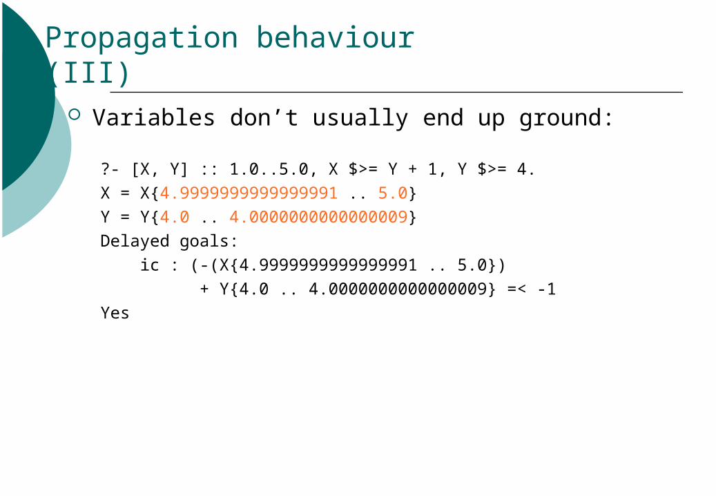
Propagation behaviour (III)

Variables don’t usually end up ground:

?- [X, Y] :: 1.0..5.0, X $>= Y + 1, Y $>= 4.

X = X{4.9999999999999991 .. 5.0}

Y = Y{4.0 .. 4.0000000000000009}

Delayed goals:

ic : (-(X{4.9999999999999991 .. 5.0})

+ Y{4.0 .. 4.0000000000000009} =< -1

Yes

Solving real constraints

IC provides two methods for solving real constraints

locate/2,3 good when there are a finite

number of discrete solutionsWorks by splitting domains

squash/3 good for refining bounds on a

continuous feasible regionWorks by trying to prove parts of domains infeasible

Using locate

Find the intersection of two circles

?- 4 $= X^2 + Y^2, 4 $= (X - 1)^2 + (Y - 1)^2).

X = X{-1.000000000000002 .. 2.0000000000000013}Y = Y{-1.000000000000002 .. 2.0000000000000013}

There are 12 delayed goals.Yes

Using locate

?- 4 $= X^2 + Y^2,

4 $= (X - 1)^2 + (Y – 1)^2,

locate([X, Y], 1e-5).

X = X{-0.82287566035527082 .. -0.822875644848199}

Y = Y{1.8228756448481993 .. 1.8228756603552705}

There are 12 delayed goals.

More ? ;

X = X{1.8228756448481993 .. 1.8228756603552705}

Y = Y{-0.82287566035527082 .. -0.822875644848199}

There are 12 delayed goals.

Yes

Using squash

Find the intersection of two discs and a half-plane

?- 4 $>= X^2 + Y^2, 4 $>= (X - 1)^2 + (Y – 1)^2, Y $>= X.

Y = Y{-1.000000000000002 .. 2.0000000000000013}X = X{-1.000000000000002 .. 2.0000000000000013}

There are 13 delayed goals.Yes

Using squash

?- 4 $>= X^2 + Y^2,

4 $>= (X - 1)^2 + (Y – 1)^2,

Y $>= X,

squash([X, Y], 1e-5, lin).

X = X{-1.000000000000002 .. 1.4142135999632603}

Y = Y{-0.41421359996326107 .. 2.0000000000000013}

There are 13 delayed goals.

Yes

IC Example (modelling, abstraction)

A

C B7

George is contemplating buying a farm which is a very strange shape, comprising a large triangular lake with a square field on each side.

The area of the lake is exactly seven acres. The area of each field is an exact whole

number of acres.

What is the smallest possible total area of the

three fields?

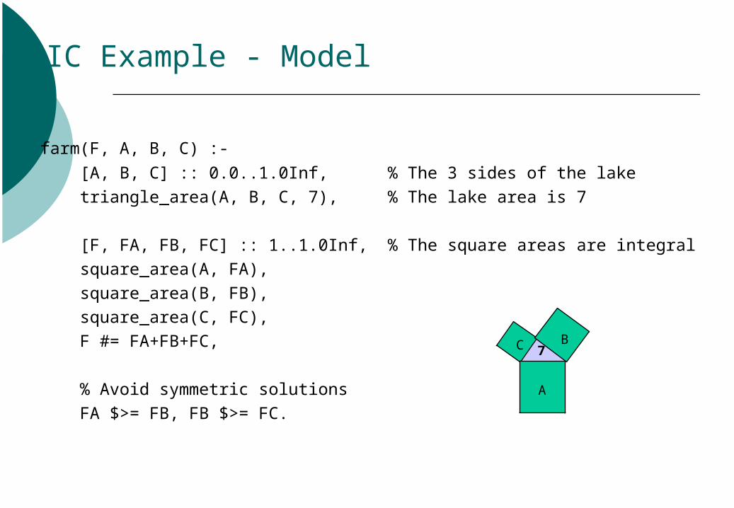
IC Example - Model

farm(F, A, B, C) :-

[A, B, C] :: 0.0..1.0Inf, % The 3 sides of the lake

triangle_area(A, B, C, 7), % The lake area is 7

[F, FA, FB, FC] :: 1..1.0Inf, % The square areas are integral

square_area(A, FA),

square_area(B, FB),

square_area(C, FC),

F #= FA+FB+FC,

% Avoid symmetric solutions

FA $>= FB, FB $>= FC.

A

C B7

IC Example - Abstraction

triangle_area(A, B, C, Area) :- S $>= 0, S $= (A+B+C)/2, Area $= sqrt(S*(S-A)*(S-B)*(S-C)).

square_area(A, Area) :- Area $= sqr(A).

A

C B7

IC Example - Search

solve(F, A, B, C) :- farm(F, A, B, C), % the model indomain(F), % ensure that solution is

minimal locate([A, B, C], 0.01).

?- solve(F, A, B, C).F = 50A = A{4.4721359549995787 .. 4.4721359549995805}B = B{4.12310562561766 .. 4.1231056256176615}C = C{3.6055512754639887 .. 3.6055512754639896}There are 23 delayed goals.More?

A

C B7

Exercises

Try the SEND+MORE=MONEY problem for yourself Try the exercises from “Getting Started with Interval

Constraints” in the tutorial manual (section 8.9 in my copy, on page 84 (+10))

Try the first search exercise Look at “Working with Real Numbers and Variables”

(chapter 9) in the tutorial manual