The Interaction between Human and Physical Capital ... · from differential initial endowments of human capital or physical capital, (ii) ... labor, as well as physical capital, ...

The Interaction between Human and Physical Capital Accumulation and the

Growth-Inequality Trade-off

Aditi Mitra, University of Washington, Seattle WA 98195

Stephen J. Turnovsky*

University of Washington, Seattle WA 98195

November 2011

Abstract

This paper analyzes the effects of technological change on growth and inequality in a two-sector endogenous growth model. We find that the effects on inequality depend upon: (i) whether the underlying source of inequality stems from differential initial endowments of human capital or physical capital, (ii) the time horizon over which the productivity increase occurs. Our results suggest that an increase in the growth rate resulting from productivity enhancement in the human capital sector will increase inequality. Productivity enhancement in the final output sector, although not having permanent growth effects, will reduce inequality. In either case the responses of inequality increase, the more gradually the productivity increase takes place. The model can generate a positive or negative relationship between inequality and growth, depending upon the relative size of these effects, consistent with the diverse empirical evidence.

*Mitra’s research was supported in part by the Corkery Fellowship and Turnovsky’s research by the Castor endowment at the University of Washington.

1

I. Introduction

The early literature on economic growth identified this process with the accumulation of

physical capital. However, the size of the Solow residual estimated in growth accounting exercises

highlighted how in fact only a relatively small fraction of economic growth could be explained by

the accumulation of capital. Other factors clearly were playing an important, and likely dominant,

role in determining a country’s growth performance. As a consequence, stimulated by the

pioneering work of Becker (1964) and Schultz (1963), economists began to devote attention to the

role of education, knowledge, and more generally human capital, as a critical source of economic

growth. Indeed, research conducted by Goldin and Katz (1999, 2001), Abramovitz and David

(2000) has suggested that during the 20th century in the United States the contribution of human

capital accumulation to the overall growth rate almost doubled, while the contribution of physical

capital declined correspondingly. Moreover, this process tended to accelerate during the last two

decades of the century; see Jorgensen, Ho, and Stiroh (2005).

Along with these developments, most advanced economies have experienced increasing

income inequality since the 1980s; see Atkinson (1999), Goldin and Katz (2008). Evidence of this

can also be seen in the rising skill premium in the form of an increase in returns to skilled versus

unskilled labor that has been emerging; see e.g. Mitchell (2005). As a result, the role of human

capital has received increasing attention, both as a source of economic growth and of the observed

rising income inequality.1 The key underlying explanation of this involves the acceleration of

technological progress, requiring more education and skills; see e.g. Galor and Weil (2000), Galor

and Moav (2004), and Goldin and Katz (1998).

Several specific channels relating the accumulation of human capital and inequality have

been identified and extensively discussed. These include: disparities in educational opportunties and

attainment; (e.g. Becker and Tomes, 1979, Benabou, 1996, Durlauf, 1996, Fernandez and Rogerson,

1998, Galor and Moav, 2002, and Viaene and Zilcha, 2009); credit market constraints (e.g. Galor

1 The changing importance of physical and human capital with respect to the overall growth process is studied in detail in an elegant model developed by Galor and Moav (2004). Subsequent work by Galor (2011) has progressed further toward the development of a unified growth theory.

2

and Zeira, 1993, Banerjee and Newman, 1993, Levine, 2005); health and demographic factors (e.g.

Becker and Barro, 1998, de la Croix and Doepke, 2003, Ehrlich and Liu, 1991, Ehrlich and Kim,

2007); political considerations and education (e.g. Saint-Paul and Verdier, 1991, Glomm and

Ravikumar, 1992, Eckstein and Zilcha, 1994).2 Most of this literature employs some form of

overlapping generations model in which the transfer of human capital across generations is a key

element of the growth process. These models typically have the characteristic that the economy

eventually converges to a stationary equilibrium, although important exceptions to this

characterization certainly exist.3

This paper takes a somewhat different approach. We adapt the seminal Lucas (1988) two-

sector production model of human capital and growth, to include both skilled and unskilled (raw)

labor, as well as physical capital, as productive factors. Each agent is equally endowed with raw

labor but has different initial endowments of both physical and human capital. We assume that

aggregate human capital generates an externality, enabling the economy to sustain ongoing growth,

characteristic of the Lucas model and endogenous growth models in general.4 We also assume that

physical capital is specific to the production of final output, in which case the human capital

production sector becomes the fundamental engine of growth, consistent with much of the empirical

evidence. This model focuses on the technological structure rather than the “social” aspects noted

above, highlighting the role of the sectoral production characteristics – which need not be uniform

across the economy – as potentially important determinants of long run growth and associated

inequality. As Lucas argued, this extension of the Uzawa (1965) model and the introduction of

intersectoral factor mobility provides important insights and yields a substantial improvement over

the standard one-sector neoclassical model in explaining the process of economic development.

Our focus is on determining the dynamic responses of the economy to productivity increases,

and on contrasting the impacts on the growth-inequality relationship between a productivity increase

in the final output sector, on the one hand, and and a productivity increase in the human capital 2 A recent paper by Castelló-Climent (2010) provides an empirical investigation of the various channels whereby inequality in human capital influences the growth rate. 3 Exceptions to this characterization include Ehrlich and Liu (1991), Glomm and Ravikumar (1992), Ehrlich and Kim (2007), who embed the overlapping model into an endogenous growth framework. 4 See also Rebelo (1991).

3

producing sector, on the other. We emphasize two critical, and distinct, sources of dynamics that we

can term “external” and “internal”. The first pertain to the time path over which the exogenous

productivity change takes place. We compare the conventional assumption that it all occurs at once,

with the alternative that the same overall increase accumulates gradually. This distinction is relevant

when one considers that technologies are always changing, and that economies approach the

boundaries of known technologies gradually rather than instantaneously. Moreover, the transitional

time path also turns out to have important permanent consequences for wealth and income

inequality. As a result, this source of dynamics permits structurally similar economies to have

substantially different levels of inequality, depending upon the time path over which their (common)

productivity levels may have evolved. This characteristic is consistent with the experiences of

countries in East Asia and Latin America, which have similar levels of per capita income, but very

different income distributions.

The internal dynamics relate to the interaction between the two capital goods in the

accumulation process. While we can provide a general analytical characterization of the long-run

equilibrium, the model is sufficiently complex to require that the dynamics be studied numerically.

Our simulations bring out the stark contrasts between the effects of productivity increases in the two

sectors, as well as their sensitivity to the time horizons over which they are implemented.

Overall, our conclusions are robust and our findings with respect to aggregates and

distribution can be summarized as follows:

(i) A productivity increase in the final output sector has only a transitional effect on the

growth rate. It has no long-run effect on the relative usage of skilled to unskilled labor, which is a

key determinant of the long-run growth rate. Instead, it raises the long-run ratios of physical capital

and output to human capital, leading to a corresponding increase in consumption.

(ii) In contrast, a productivity increase in the human capital sector will lead to a change in

the relative use of skilled and unskilled workers and a positive permanent effect on the growth rate.

(iii) While the long-run responses of the aggregate variables are independent of the time

path followed by the productivity increase (in either sector), there are sharp contrasts in the

4

transitional paths between the cases where the increases occur fully instantaneously (the

conventional case) and where they are implemented gradually over time. For productivity increases

in either sector, the adjustments initially proceed in opposite directions. This is because the

allocation of labor, which drives the adjustments, responds to both the relative price of human to

physical capital and to the shocks themselves. With full instantaneous increases, both effects operate

immediately. But where the productivity increase proceeds gradually, the former dominates in the

early stages. This is because the productivity enhancement takes time to build up and only begins to

become effective later in the transition.

We consider three measures of inequality: wealth inequality, income inequality, and welfare

inequality. In contrast to the aggregates, a productivity increase in the final output sector does have

permanent distributional consequences, and obtain the following conclusions:

(iv) In general, the responses of all three inequality measures depend upon the underlying

source of initial inequality in the economy, i.e. whether it is due to unequal endowments of physical

capital, of human capital inequality, or some combination.

(v) The dynamics of wealth inequality consists of an initial jump following by a gradual

transition. The direction of the initial jump stems from the initial change in the relative price of

human capital and depends upon (a) the source of the initial inequality, and (b) the sectoral location

of the productivity increase. The direction of transitional path depends upon whether consumption

adjusts faster or slower than do wages. For a productivity increase occurring in the final output

sector, consumption does indeed adjust faster and wealth inequality declines, while the opposite is

true for a productivity increase in the human capital sector. Productivity increases that are spread

out over time exacerbate these effects.

(vi) Long-run wealth inequality may either rise or fall, with either form of productivity

increase, depending upon the initial underlying source of the inequality and the speed with which the

productivity increase occurs.

(vii) Income inequality reflects the evolution of both wealth inequality and the share of

income originating from wealth. In the long run, our simulations suggest that the former effect

5

dominates so that the long-run response of income inequality reflects that of wealth inequality. This

contrasts with results obtained using one-sector models where the opposite tends to be the case.5

The difference is largely accounted for by the initial jump in wealth inequality arising from the price

response, identified in (v).

(viii) Long-run wealth inequality exceeds long-run income inequality, which in turn

exceeds long-run welfare inequality.

The remainder of the paper is structured as follows. Section 2 sets out the analytical

framework, while the following section characterizes the aggregate equilibrium. Section 4 derives

the long-run effects of the productivity increases on the equilibrium quantities of the aggregates,

including the growth rate. Section 5 sets out the evolution of the three inequality measures we

consider. Sections 6 and 7 describe the numerical simulations, while Section 8 concludes.

Additional technical details, including the implications for the long-run relative positions of physical

and human capital are set out in the Appendix.

2. The analytical framework

The analytical framework we employ is an adaptation of the two-sector production economy

pioneered by Lucas (1988), augmented to include raw (unskilled) labor as well as human capital.6

2.1 Households

The economy consists of a continuum of infinitely-lived consumers. Agents are indexed by i

and are identical in all respects except for their initial endowments of human capital, ,0iH , and

physical capital, ,0iK . Since we consider a growing economy, we are interested in the shares of

individual i in the accumulating total stocks of human capital, ( ) ( ) ( )i ih t H t H t , and physical

capital, ( ) ( ) ( )i ik t K t K t , where ( ), ( )H t K t denote the corresponding economy-wide average

5 This is true both for the one-sector Romer model and the one-sector Ramsey model; See e.g. García-Peñalosa and Turnovsky (2006, 2011). 6 The model also extends Turnovsky (2011) which adopts a similar framework except that it abstracts from physical capital. With only one capital good (human capital), there are no internal dynamics and in the absence of external dynamics, the economy is always on its balanced growth path. All distribution measures remain unchanged over time.

6

quantities. The initial relative endowments across agents have mean 1, standard deviations ,0 ,0,h k ,

and covariance ,0kh (possibly zero).7

We make two important assumptions with respect to the underlying source and nature of the

heterogeneity. First, there are clearly many sources of heterogeneity, of which initial endowments,

in this case of both human and physical capital, are arguably the most significant. Empirical

evidence supporting this, in the form of inheritance, is provided by Piketty (2011).8 Second, the

distributions of initial endowments can be arbitrary, and therefore consistent with any required non-

negativity constraints. As will become apparent in due course, these initial distributions will be

reflected in the evolving distributions of wealth and income.

Each individual is endowed with a unit of raw labor that can be allocated either to

employment in the final output sector, ,X iL , or to acquiring more human capital, ,Y iL , thus,

, , 1X i Y iL L (1a)

At any point of time the agent has accumulated a stock of human capital, iH , that similarly can be

allocated either to the final output sector or to the further accumulation of human capital

, ,X i Y i iH H H (1b)

Physical capital, however, is employed only in the production of final output and therefore does not

involve a sectoral allocation decision.9

The wage rate earned by raw (unskilled) labor is W , while the returns to human capital and

physical capital are Hr , Kr , respectively, all three being expressed in units of final output. The

agent’s budget constraint, describing his market activities, asserts that the income earned from his

7 Being the standard deviation of the relative capital stock, ,h k are in fact coefficients of variation. 8 Other papers to generate heterogeneity from agents’ initial endowments of wealth include Sorger (2000), Maliar and Maliar (2001), Caselli and Ventura (2000) and Turnovsky and García-Peñalosa (2008). With respect to human capital endowments, Becker and Tomes (1986) assume that parental investment in human capital is the dominant source of heterogeneity among families, while Han and Mulligan (2000), in studying intergenerational mobility consider heterogeneity in ability. An alternative source of heterogeneity in the earlier literature was the rate of time preference, which led to the conclusion that the most patient individual ends up holding all the capital; see Becker (1980). 9 We can also interpret the production function for human capital as including a fixed amount of physical capital [embodied in the term ( )B t ], which is not accumulated further in the human capital sector.

7

three productive factors can be spent either on consumption or accumulating physical capital

, ,i K i H X i X i iK r K r H WL C (1c)

In addition, the agent accumulates human capital in accordance with the Cobb-Douglas

production function (common to all agents)

1

, ,( )i Y i Y iH B t L H H

(1d)

where H denotes the average (aggregate) stock of human capital, and ( )B t denotes the level of

technology in the production of new human capital. This function is analogous to Lucas (1988), in

that it is homogeneous of degree one in the accumulating asset (human capital), with the economy-

wide average stock of human capital providing an externality that enhances the productivity of each

individual’s raw labor. The only way an agent can accumulate human capital is by devoting his own

physical resources to this activity; there is no market where human capital can be purchased.

The representative agent chooses consumption, iC , raw labor allocations, , ,,X i Y iL L , human

capital allocations, , ,,X i Y iH H , and the rates of human capital accumulation, iH and physical capital

accumulation, iK , to maximize the iso-elastic utility function:

0

1 tiC e dt

1 (2)

subject to the constraints (1a) – (1d). The optimality conditions are respectively:

1i iC (3a)

1, ,

,

(1 )i Y ii

i i Y i

L HW B H

H

(3b)

1

2, ,

,

i Y iiH

i i Y i

L Hr B

H

(3c)

2,ii

i i

(3d)

8

iK

i

r

(3e)

together with the transversality conditions

lim 0ti i

tH e

, lim 0t

i it

K e

(3f)

where i is the agent’s shadow value of physical capital, i is his shadow value of an extra unit of

investment in human capital, 1,i is his shadow value of raw labor, 2,i is his shadow value of human

capital. Equations (3a)-(3c) are standard static efficient allocation conditions, while (3d) and (3f) are

familiar arbitrage conditions, equating rates of return across the alternative investment options.

2.2 Firms

There is a single representative firm producing final output, Y, using the aggregate

production function:

( ) X XY A t K H L H 1 (4a)

where ( )A t , is the level of technology in the final output sector, XL is raw labor, and XH is human

capital, both employed in the final output sector. The production function, (4a), is analogous to the

individual production functions for human capital, with economy-wide human capital providing a

productivity-enhancing externality for raw labor.

The firm chooses raw labor, physical capital, and human capital to maximize profits,

( ) X X X K H HA t K H L H WL r K r H (4b)

yielding the optimality conditions

1

( ) X

X X

LW KA t

H H H H

(5a)

1

( ) XK

X X

LKr A t

H H H

(5b)

9

( ) XH

X X

LKr A t

H H H

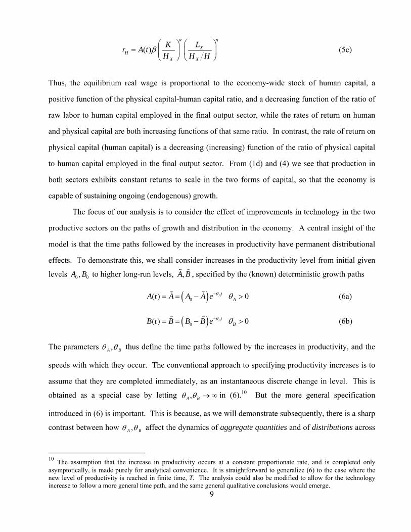
(5c)

Thus, the equilibrium real wage is proportional to the economy-wide stock of human capital, a

positive function of the physical capital-human capital ratio, and a decreasing function of the ratio of

raw labor to human capital employed in the final output sector, while the rates of return on human

and physical capital are both increasing functions of that same ratio. In contrast, the rate of return on

physical capital (human capital) is a decreasing (increasing) function of the ratio of physical capital

to human capital employed in the final output sector. From (1d) and (4) we see that production in

both sectors exhibits constant returns to scale in the two forms of capital, so that the economy is

capable of sustaining ongoing (endogenous) growth.

The focus of our analysis is to consider the effect of improvements in technology in the two

productive sectors on the paths of growth and distribution in the economy. A central insight of the

model is that the time paths followed by the increases in productivity have permanent distributional

effects. To demonstrate this, we shall consider increases in the productivity level from initial given

levels 0 0,A B to higher long-run levels, ,A B , specified by the (known) deterministic growth paths

0( ) 0AtAA t A A A e (6a)

0( ) 0BtBB t B B B e

(6b)

The parameters ,A B thus define the time paths followed by the increases in productivity, and the

speeds with which they occur. The conventional approach to specifying productivity increases is to

assume that they are completed immediately, as an instantaneous discrete change in level. This is

obtained as a special case by letting ,A B in (6).10 But the more general specification

introduced in (6) is important. This is because, as we will demonstrate subsequently, there is a sharp

contrast between how ,A B affect the dynamics of aggregate quantities and of distributions across

10 The assumption that the increase in productivity occurs at a constant proportionate rate, and is completed only asymptotically, is made purely for analytical convenience. It is straightforward to generalize (6) to the case where the new level of productivity is reached in finite time, T. The analysis could also be modified to allow for the technology increase to follow a more general time path, and the same general qualitative conclusions would emerge.

10

agents. As one would expect, they affect the transitional path of the aggregate economy, but not the

aggregate steady state. In contrast, they influence both the time paths and the steady-state levels of

both wealth and income inequality.11

2.3 Aggregation

We have now laid out the basic components, and the next task is to aggregate them to derive

the economy-wide equilibrium. To do this we first note the following aggregation relationships and

market clearing conditions, describing the raw labor and human capital markets, respectively

, , 1;X i Y i X Yi i

L L L L (7a)

, , ;X i Y i X Yi i

H H H H H

(7b)

For notational convenience, let

XX

X

L

H H ; ,

,,

;Y iY i

Y i

L

H H

denote the ratio of raw labor to human capital employed in the final output sector, and the ratio

allocated by individual agent i in the production of human capital, respectively. Using this notation

enables us to express the individual optimality conditions in the form

1i iC (3a)

11,,(1 )i i

X Y ii X i

KW A H B H

H

(3b’)

12,,

i iH X Y i

i X i

Kr A B

H

(3c’)

11 The reason for this is the homogeneity of the utility function (2) which causes individuals to maintain fixed relative consumption over time; see (10’). This introduces a “zero root” into the dynamics of the distributional measures, as a result of which their equilibrium values become path dependent; see Atolia, Chatterjee, and Turnovsky (2011) where this issue is discussed in detail in the context of a Ramsey model.

11

2,ii

i i

(3d)

iK

i

r

(3e)

Dividing (3c’) by (3b’) implies

2,,

1, (1 )iH

Y i Xi

r

W

(8)

from which we immediately see that ,Y i and 2, 1,i i are common across all individuals. This is a

consequence of the assumption that all agents face a common raw wage rate, W, and return on

human capital, Hr . Thus we have

,Y

Y i YY

L

H H

(9)

where Y denotes the common economy-wide ratio of raw labor to human capital employed in the

production of human capital.12 Combining the left hand equality of (3c’) with (3d) and (9) we obtain

1( )iY

i

B

(3d’)

Thus, a further consequence of the common factor intensities across agents in human capital

production, Y , is that the growth rate of the shadow value, i i , is also common to all. We then

immediately deduce from (3b’) and (3d) that 1, 2,,i i i i and hence i i and therefore i i

are also common across agents. Differentiating (3a)

( 1) ( 1)i i

i i

C C

C C

(10)

so that by choosing a common growth rate for the marginal utility of income, agents choose a

common growth rate of consumption, which therefore coincides with the aggregate (average)

economy-wide consumption growth rate. Equation (10) further implies that each agent i maintains a 12 We shall refer to the term, Y , as describing the factor intensity in the human capital sector

12

constant ratio of his consumption to average consumption

i iC C for each i and 1ii

(10’)

where the constant i is to be determined by his relative steady-state wealth [see (26b) below].

Let q ( i i ) denote the common relative shadow price of human capital to

income. With this notation, we may use (3b’) and (3c’) to express the economy-wide equilibrium

allocation of raw labor and human capital:

1(1 )X Y

X

W KA qB

H H

(11a)

1H X YX

Kr A qB

H

(11b)

In addition, substituting for , , , ,K H X Yr r W into (1c) and (1d), the individual rates of accumulation

of physical and human capital accumulation are respectively

1

, ,X i X ii X i i

X X X

H LKK A K K K C

H H L

(12a)

1 ,i Y Y iH B H

(12b)

which in each case is linear in the agent’s factor supply devoted to producing that output, with the

proportionality factor being dependent upon the factor allocation intensity and common across

agents. Thus, summing over all agents yields the corresponding aggregate relationships

1

XX

KK A K C

H

(12a’)

1Y YH B H (12b’)

The fact that the system aggregates exactly is a consequence of two assumptions: (i) the

13

homogeneity of the utility function, and (ii) the assumption that all agents face common returns.13

3. Derivation of aggregate equilibrium

The aggregate economy possesses many of the characteristics of a standard two-sector

endogenous growth model, as pioneered by Lucas (1988), and extended by Bond, Wang, and Yip

(1996). The macro equilibrium includes the following four conditions:

(i) labor market clearance: 1X YL L (13a)

(ii) human capital market clearance: X YH H H (13b)

(iii) goods market clearance: XX

KK A K C

H

(13c)

(iv) human capital accumulation: 1Y YH B H (13d)

In addition, short-run and long-run efficiency conditions must hold and the technology levels evolve

in accordance with (6a) and (6b).

Our procedure is to follow Bond, Wang, and Yip (1996) and to express the macroeconomic

dynamic equilibrium in terms of the ratio of physical capital to human capital, k K H , the ratio of

consumption to human capital, c C H , and the ratio of the shadow value, q, augmented by the

dynamics of A, B. To do so, it is convenient to let Xu H H denote the allocation of human capital

to the production of final output. With this notation, we may express the sectoral allocation

conditions for raw labor and human capital, (11a) and (11b), together with the clearance of both the

raw labor and human capital markets, (13a) and (13b), in the form

1(1 )X Y

W kA qB

H u

(14a)

1H X Y

kr A qB

u

(14b)

13 These assumptions also account for the fact that the aggregate equilibrium is independent of distribution measures, which led Caselli and Ventura (2000) to characterize this type of model as “a representative agent theory of distribution”.

14

(1 ) 1X Yu u (14c)

These three equations can be solved for the sectoral allocations of raw and skilled labor, , ,X Y u ,

in terms of , , ,k q A B , which for convenience we write in the form14

( , , , ), ( , , , ), ( , , , )X X Y Yk q A B k q A B u u k q A B (15)

Dividing (11b) by (11a) we obtain

(1 )X Y Y

(11’)

yielding the standard result that for given productive elasticities, , , , the relative intensities of

raw labor to human capital will move proportionately in the two sectors. The quantity measures

the relative intensities of skilled to unskilled labor in the two sectors. If 1 , human capital is

relatively more intensive than unskilled labor in the human capital sector, and vice versa.

Equations (15) are critical in determining the impact effects of productivity changes. Taking

differentials of (14) one can show that:

1

( 1)X Y

X Y

d d dq dk dA dB

u q k A B

(16a)

1

1( 1)

Y

Y

ddu

u u

(16b)

These relationships highlight how the initial responses of both skilled and unskilled labor allocations

depend upon their relative sectoral intensities and that whatever that response, increases in A and k

operate in one direction, while increases in B and q have the opposite effects. Equation (16a), in

particular, is important in understanding the contrasting short-run effects of gradual versus discrete

productivity changes that we shall identify in Section 7, below.

Taking the time derivative of k K H and substituting from (13c) and (13d) yields the

following equation for k

14 Throughout, we shall assume that all production elasticities remain constant and thus omit them from the solutions.

15

1

1( ) (1 )( )X Y

k k cA B u

k u k

(17a)

Next, taking the time derivative of c C H , and using (3e), (10), and (13d), we obtain

1

11(1 )

1 X Y

c kA B u

c u

(17b)

Finally, taking the time derivative of q , combining with (3c), (3d), (3e) and (11d) implies

1

( ) 1( ) H

K X X

r tq k kr t A A

q q u q u

(17c)

Substituting the solutions for , ,X Y u from (15), equations (17a)-(17c), describe the evolution of

the macroeconomic equilibrium, conditional on the given time path for the technology parameters,

( ), ( )A t B t , as specified by (6a) and (6b). The macrodynamic equilibrium is a modification of that

analyzed by Bond et al. (1996), the differences being: (i) the distinction between skilled and

unskilled labor, and (ii) the assumption that physical capital is specific to the final output sector, and

(iii) the gradual evolution of ( ), ( )A t B t . But the key observation is that the evolution of the

aggregate economy is independent of any distributional measures. As k, c, and q evolve, this will

generate adjustment paths for the rates of return and the sectoral allocation of resources.

One variable of particular interest is the skill premium, which we define as ( / )Hs r W H .

The reason for this is because the supply of raw labor is fixed, whereas human capital grows

indefinitely over time, as a result of which in the long run the return to human capital is constant,

while the return to raw labor grows at the equilibrium rate. We therefore define skill premium as the

ratio of income earned by human capital to the income earned by raw labor. Dividing (14b) by

(14a), we see that the crucial determinant is the equilibrium ratio of raw to skilled labor employed in

the human capital sector, Y .

3.1 Characterization of macrodynamic equilibrium

In section 7 below we shall analyze the local dynamics following a productivity increase by

16

linearizing the above system about its steady state. The formal structure of this system is set out in

the Appendix. A necessary condition for the local dynamics to be a saddlepoint and to generate a

unique stable adjustment path is

(1 )(1 ) (1 )(1 ) (1 ) 0YD (18)

where tilde denotes the steady state. The stable adjustment path is then as characterized in the

Appendix.15 During the transition, physical capital, human capital, output, and consumption grow at

different rates, although if the system is stable they converge to a long-run common growth rate.

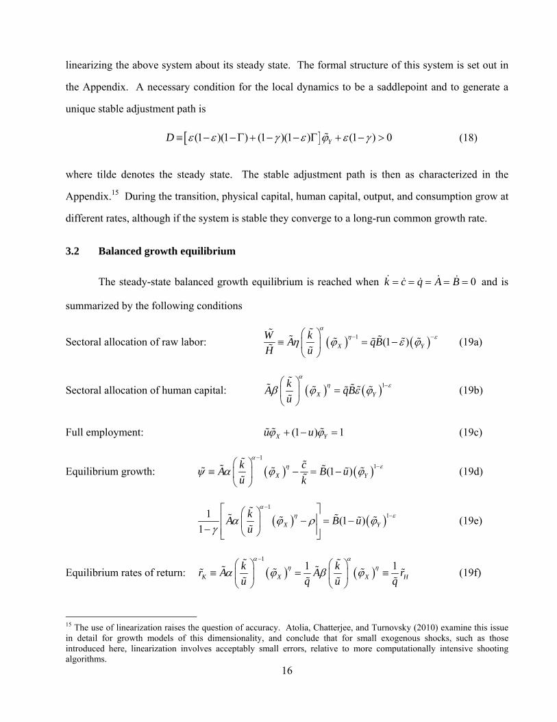
3.2 Balanced growth equilibrium

The steady-state balanced growth equilibrium is reached when 0k c q A B and is

summarized by the following conditions

Sectoral allocation of raw labor: 1(1 )X Y

W kA qB

H u

(19a)

Sectoral allocation of human capital: 1X Y

kA qB

u

(19b)

Full employment: (1 ) 1X Yu u (19c)

Equilibrium growth: 1

1(1 )X Y

k cA B u

u k

(19d)

1

11(1 )

1 X Y

kA B u

u

(19e)

Equilibrium rates of return: 1

1 1K X X H

k kr A A r

u q u q

(19f)

15 The use of linearization raises the question of accuracy. Atolia, Chatterjee, and Turnovsky (2010) examine this issue in detail for growth models of this dimensionality, and conclude that for small exogenous shocks, such as those introduced here, linearization involves acceptably small errors, relative to more computationally intensive shooting algorithms.

17

Given the long-run levels of technology, ,A B , these equations determine the equilibrium values of

, , , , ,X Yu k c q , which then imply the corresponding equilibrium factor rates of return, , ,K HW H r r ,

skill premium, s , and equilibrium growth rate, . In Table 1, which we shall discuss in Section 4,

we summarize the long-run effects of increases in technology on these equilibrium values.

Two critical conditions constrain the equilibrium value of Y (and X ). The first is the

transversality condition, (3f), that each agent must satisfy. This will be met if and only if

lim 0 lim 0i i

t ti i

H H

H H

(20)

which in steady state is equivalent to Kr .16 Using (19b), (19d) and (19f) this in turn is

equivalent to 1u . The other condition is that with no depreciation to human capital, the

equilibrium growth rate is always positive, which in turn implies that 1 u . Combining these two

conditions, together with the full employment condition (19c) and (16), yields the following bounds

on Y for a feasible solution to exist:

If 1: 1 1

(1 ) Y

(21a)

If 1 : 1 1

(1 ) Y

(21b)

4. Long-run effects of productivity increases on aggregate equilibrium

As Table 1 clearly illustrates, the productivity increases in the two sectors have dramatically

different long-run effects on the aggregate economy. These shall be briefly summarized in turn.

4.1 Productivity increase in final output sector, A

These results may be summarized in17

Proposition 1: A productivity increase in the final output sector: 16 This condition also applies to the transversality condition applicable to physical capital. 17 This proposition is analogous to that obtained by Turnovsky (2011), the difference being that the proportionality increases are by a factor 1 (1 ) , rather than 1, reflecting the productivity of physical capital in final output.

18

I. Leads to equi-proportionate increases in (i) the ratio of physical to human

capital (k), (ii) the price of human capital (q), (iii) the rate of return to human

capital ( Hr ), (iv) the return to raw labor (W/H), and (v) the consumption to

human capital ratio (c). This proportionate increase exceeds unity by an

amount that reflects the productivity of physical capital in final output.

II. Has no effect on (i) the sectoral ratios of skilled to unskilled labor ( ,X Y ),

(ii) allocation of human capital across sectors (u), (iii) the return to physical

capital ( Kr ), (iv) the equilibrium growth rate ( ), or (v) the skill premium (s).

The intuition underlying these responses is straightforward. An increase in the productivity,

A, of the final output sector attracts resources to that sector. This raises the productivity of raw labor

and human capital proportionately in that sector, increasing their respective rates of return, , HW H r

equally, so that the skill premium, s, remains unchanged. There is therefore no incentive to

substitute between the two classes of labor, so that the sectoral labor intensities, ,X Y remain

unchanged. The increase in productivity in the final output sector leads to a long-run increase in

capital and output, which is fully consumed. This increase in capital exactly offsets the effect of the

increase in productivity on the return to capital, Kr , which remains unchanged, leaving the long-run

growth rate unchanged as well.

4.2 Productivity increase in the human capital sector, B

In this case the effects of the productivity increase are more complex and involve two critical

parameters, the sectoral intensity of labor, 1 , and the productivity of physical capital. They may

be summarized in

Proposition 2: A productivity increase in the human capital sector has the

following long-run effects:

(i) It leads to an unambiguous increase in the equilibrium growth rate.

(ii) If the human capital sector is relatively more intensive in skilled labor than is

19

the final output sector ( 1) , the wage rate on raw labor will decrease, raising the

skill premium, and causing a substitution toward raw labor in both sectors. The

fraction of human capital employed in the final output sector, u , declines and the rate

of return on physical capital increases.

(iii) If ( 1) the responses in , , ,X Y u s are all reversed. Other variables

experience offsetting effects due to the productivity of physical capital in the final

output sector

The following intuition applies. An increase in the productivity of human capital B will

attract resources from the final output sector to the human capital sector, causing the output of that

sector to rise at the expense of final output. If 1 , so that the human capital sector is relatively

more intensive in human capital, human capital increases in scarcity, relative to raw labor, causing

the rate of return on human capital to rise and that of raw labor to fall, resulting in an increase in the

skill premium and inducing a substitution away from human capital to raw labor in both sectors.

There is, however, another effect in operation. The productivity of raw labor and human

capital are enhanced by their interaction with physical capital in the final output sector. As resources

move away from this sector this effect is reduced, as represented by the term (1 ) for the

corresponding expressions in Table 1. This reinforces the decline in the wage of raw labor and

offsets the increase in the return to human capital.

The most striking contrast between the productivity increases in the two sectors is in the

impact on the long-run growth rate. To see the reason behind this it is constructive to substitute

(19b), (19c), and (19f) into (19e), rewriting it as

1 ( 1)1

1 1Y

Y Y

BB

(19e’)

From the left-hand side equality, we may solve for long-run ratio of raw labor to human capital in

the form ( )Y Y B and substituting into the right-hand side equality, we may write

( , ( ))YB B , highlighting how, both directly and through Y , the productivity of the human

capital sector is the crucial long-run determinant of growth, which by the same token is independent

20

of the productivity in the final output sector.18 The reason that B will increase the growth rate is

because of the limited substitution possibilities in the production function for human capital. With

no possibility for substituting toward physical capital, increasing B directly impacts the ratio of raw

labor to human capital, and thereby increases the equilibrium growth rate.

5. Evolution of wealth inequality, income inequality, and welfare inequality

We turn now to the distributional implications. Since everything is driven by the dynamics

of relative wealth, this is the natural place to start.

5.1 Relative wealth dynamics

At any instant of time, the total wealth of agent i is defined by

( ) ( ) ( ) ( )i i iV t K t q t H t (22)

Differentiating (22) with respect to time, the agent’s rate of wealth accumulation is

( ) ( ) ( ) ( ) ( ) ( )i i i iV t K t q t H t q t H t

where ( )iK t , ( )iH t , and ( )q t are given by (1c) (12b) and (17c), respectively. We may decompose

(12b) and express it in the form

1 1

, , ,(1 )i Y Y i Y Y i Y Y iH B H B H B HL

where we are using the equilibrium condition , ,Y i Y i YL H H Using the equilibrium pricing

relationships (14a) and (14b), we may express agent i’s rate of accumulation of human capital as

, ,

( ) ( )

( ) ( )H

i Y i Y i

r t W tH H L

q t q t

(23)

Combining (23) with (1c) and (12b), while recalling (1a) and (1b), we may express agent i’s rate of

wealth accumulation as

18 Through , the productive elasticities in the final output sector play a role in determining the equilibrium growth rate.

21

( ) ( ) ( ) ( ) ( )i K iV t r t V t W t C t (24)

Both these relationships indicate that in the absence of any market impediments, the shadow value of

human capital, ( )q t , behaves like a price in a competitive market.

Summing (24) over all agents, aggregate wealth evolves in accordance with

( ) ( ) ( ) ( ) ( )KV t r t V t W t C t (24’)

Now define agent i’s relative wealth as ( ) ( ) ( )i iv t V t V t . Taking the time derivative of iv and

combining (24) and (24’), together with the fact that i iC C [see (10’)], we find

1 ( )( ) ( ) ( ) ( ) 1 (1 )

( ) ( )i i i

C tv t C t W t v t

V t V t (25)

In steady state, when all aggregate quantities grow at the same rate

1K

K

rV C W Cr

V V VC

so that19

01

KrC W

V V

(26a)

In addition, setting ( ) 0iv t , (25) implies that agent’s relative consumption, which is constant

throughout the transition, is

11

iKi

V Vr

C

(26b)

Equation (26b) implies that if agent i has above-average long-run wealth, he has above-average

long-run consumption.

As we will see shortly, the dynamics of relative wealth are driven by the aggregate

consumption-wage ratio. For notational convenience we shall denote ( ) ( )C t W t by ( )z t . This

19 The right hand side of (26a) is positive by the transversality condition which requires Kr .

22

enables us to write

11 1i i

zv

z

where 1z

and express (25) in the form

( ) 1( ) ( ) 1 ( ) 1 ( ) 1

( )i i i

W t zv t z t v t z t v

V t z

(25’)

which linearized around the steady state can be approximated by

( )( ) 1 ( ) 1i i i i

W z t zv t z v t v v

V z

(27)

The key point to observe about (27) is that the coefficient of ( ) 0iv t . In order for the agent’s

relative wealth to remain bounded, the solution for ( )iv t is given by the forward-looking solution

1( )( ) 1 1 1

W V z t

i i t

W z zv t v e d

V z

(28a)

Setting 0t we obtain the relationship20

1

0

( )(0) 1 1 1

W V z t

i i

W z zv v e d

V z

(28b)

where

0 0,0 ,0

(0)(0)

(0) (0)i i i

K q Hv k h

V V

(28c)

Equation (28b) determines iv , and taken in conjunction with (28a) determines the entire time path

for ( )iv t , given (0)iv .

This latter term is a weighted average of the agent’s initial relative endowments of the two

forms of capital, and is subject to an initial jump, through (0)q , in response to any structural change;

20 We should point out that the effect of the time path followed by the increase in technology on the wealth distribution, is embedded in the time path of ( )z .

23

see Appendix (A.4c). Suppose that the economy is initially in steady state, and at time t=0

experiences a structural change. One immediate effect of this is to generate a jump in the relative

price (0)q as part of the adjustment to ensure that the economy lies on its new stable saddle path.

From (28c) this causes a jump in agent i’s initial relative wealth,

0 0,0 ,0(0) (0)

(0)i i i

K Hdv h k dq

V (29)

The direction of the initial jump depends upon: (i) the difference in the agent’s initial relative

endowments of human vs. physical capital ( ,0 ,0i ih k ), and (ii) the direction of the change in the

relative price [sgn ( (0)dq ]. Following this jump, ( )iv t evolves in accordance with (28a) and (28b).

In view of the linearity of (28a) and (28b) in iv , we can sum over the agents and transform

these expressions into standard deviations across agents, as convenient measures of inequality

1

1 1

0

( ) ( )( ) 1 1 (0)

W V z t W V z t

v vt

W z z W z zt e d e d

V z V z

(30a)

1

1

0

( )1 (0)

W V z t

v v

W z ze d

V z

(30b)

where

12 2 2

2 20 0 0 0,0 ,0 ,0 2

(0) (0)(0) ( ) ( ) 2

(0) (0) (0)v k h kh

K q H q K H

V V V

(30c)

The solutions (28) and (29) highlight how agent i’s relative wealth at each point of time, t,

and therefore the entire distribution of wealth, is driven by the (expected) future time path of the

consumption to wage ratio from time t forward, as these respond to the underlying structural change,

in this case the increase in the level of technology. As a result, the path followed by ( )z t will have a

permanent effect on the relative stock of wealth and therefore on its distribution across agents. If

( )z t z instantaneously, then (0)v v and the distribution of wealth will remain unchanged

during the transition. For the Romer technology this will occur if there is only one form of capital

24

and the structural change occurs fully on impact, in which case there are no transitional dynamics.21

Both the C H ratio, the W H ratio, and therefore the C W ratio jump immediately to their steady-

state and the distribution of wealth remains unchanged.

In contrast, in the present case, following its initial jump, the evolution of wealth inequality

during the transition will depend upon the relative speeds of adjustment of consumption and wage,

which in turn depend upon the nature of the adjustment path assumed by the increase in technology,

to which they are responding. As we shall discuss in conjunction with the more specific shocks

below, these comprise a combination of the actual implementation of the structural change and its

anticipation, where it occurs gradually. At this point we can state the following proposition:

Proposition 3: If consumption adjusts more (less) rapidly than do wages along the

transitional path, so that z approaches z from below (above), then following an initial

jump, wealth inequality will decline (increase) during the transition.

The intuition for this result is straightforward. If consumption grows faster than do wages on

raw labor, savings grow at a slower rate. Since wealthier people tend to save more, their relative rate

of wealth accumulation declines and wealth inequality declines as well. It is also possible to derive

the components, ,i ik h of an agent’s relative wealth, iv , the steady-state values of which are provided

in Appendix B. These enable us to address issues pertaining to individuals’ tradeoffs between

human capital and physical capital, though space limitations preclude further discussion of that here.

5.2 Income inequality

We next turn to personal income inequality, where agent i’s personal income as measured by

income from wealth plus income from raw labor is given by

( ) ( ) ( ) ( )i K iY t r t V t W t (31)

and summing over all agents gives us the average economy wide personal income

( ) ( ) ( ) ( )KY t r t V t W t (31’)

21 See e.g. García-Peñalosa and Turnovsky (2006). This is also the case in Turnovsky (2011).

25

Dividing (31) by (31’) gives us the relative income of agent , i ii y Y Y

( ) ( ) ( )( ) 1 1 ( ) 1

( ) ( ) ( ) ( )i K

i iK

Y t r t V ty t v t

Y t r t V t W t

(32)

Again, the linearity of (32) allows us to express the relationship between relative income and relative

wealth in terms of the corresponding standard deviations of their respective distributions, ( )v t and

( )y t , namely

( ) ( )

( ) ( ) ( ) ( ); ( ) 1( ) ( ) ( )

Ky v v

K

r t V tt t t t t

r t V t W t

(33)

Hence at any instant of time, income inequality can be expressed as the product of wealth inequality,

and the income from wealth as a share of total income, ( )t , implying that income is more equally

distributed than wealth. Setting 0t , (0) (0) (0)y v , we see that initial income inequality may

potentially undergo two initial jumps, one due to the initial jump in wealth inequality [see (29)], the

other through the adjustments in the rates of return.

The transitional time path of income inequality reflects those of wealth inequality and the

share of income from wealth:

( ) ( ) ( )( )( ) ( ) ( ) ( )

( ) ( ) ( ) ( ) ( ) ( ) ( ) ( ) ( ) ( )y v vK

y v K K v

t t tr tt V t W t W t

t t t r t V t W t r t V t W t t

(34)

where the latter depends upon the evolution of ( ), ( )KV t r t , ( )W t , as they respond to the shock.

5.3 Welfare Inequality

Recalling (2), agent 'i s welfare at time t is ( ) 1i iZ t C . Substituting i iC C into this

expression yields

1( ) ( )i i iZ t C Z t

(35)

where ( )Z t is the average welfare level at time t . Substituting (35) into (2) yields an analogous

relationship for the relative intertemporal welfare evaluated along the equilibrium growth path.

26

( )

( )i i

i

U Z t

U Z t

(36)

At each instant of time, agent 'i s relative welfare remains constant, so that his intertemporal relative

welfare, /iU U remains constant as well. Using (18’) and the fact that c C H and v V H

we can express relative welfare in the form

( )( )

Ω 1 ( 1) ( )1 ( )

Ki ii i i

U Z tr vv z t

U c Z t

(37)

We can now compute a measure of welfare inequality. A natural metric for this is obtained by

applying the following monotonic transformation of relative utility, enabling us to express the

relative utility of individual i in terms of equivalent units of relative consumption flows as

1/ ( )Ω Ω ( ) 1 ( 1)

1K

i i i i

r vu u z t v

c

(37’)

from which we obtain

(1 )u v v

W

C

(38)

Comparing inequality measures (23) and (38), the following ranking among the long-run inequality

measures may be obtained.

v y u (39)

implying in particular that income inequality overstates welfare inequality. 22

Long-run percentage changes in the three inequality measures are related by the following

1

1

y vK

Ky K v

d V Wd ddr

rr V W V W

(40a)

22 By expressing welfare inequality in terms of wealth inequality we are transforming it into a cardinal measure. While this is convenient for purposes of comparison with income inequality, the transformation adopted will affect relative welfare comparisons, although not their rankings.

27

1

1u v

u v

d C Wd d

C W C W

(40b)

The long-run change in income inequality exceeds the change in wealth inequality if and only if the

long-run proportionate changes in the return to capital plus the wealth-wage ratio are positive.

Likewise the change in welfare inequality exceeds the change in wealth inequality if and only if the

long-run change in consumption-wage ratio is positive. In the case of a productivity increase in the

final output sector these effects are all zero, in which case case these three inequality measures all

increase by the same proportionate amount, something that is verified by our simulations.

6. Numerical Simulations

Given the complexity of the model it is necessary to employ numerical simulations to

analyze the dynamics. We begin by calibrating a benchmark economy using the following standard

parameter values representing a typical economy.

Parameter values

Preference parameters 1.5, 0.04 Production parameters 1 / 3, 1 / 3, 1 / 3, 0.6 Productivity levels

0 0.20, 0.22A A ; 0 0.20, 0.22B B

Productivity growth 0.10; 0.10A B

First the preference parameters corresponding to a rate of time preference of 4% and an

intertemporal elasticity of substitution of 0.4 are standard and noncontroversial. The exponents

1 / 3 in the production function for final output approximate the empirical estimates of

the generalized Solow production function obtained by Mankiw, Romer, and Weil (1992).23

Empirical evidence on the production function for human capital is far more sparse. We feel that the

most important input in augmenting the stock of human capital is human capital, followed by raw

labor, with physical capital being the least important, and which we have set to zero. Thus we set

0.60, as a plausible benchmark, which we may note is very close to the calibrated value of 0.62

23They obtain estimates of 0.43, 0.31, 0.28 .

28

obtained by Manuelli and Seshadri (2010). This combination of production elasticities implies

1.5 1 , so that the human capital sector is relatively intensive in skilled labor versus raw labor,

as compared to the final output sector, which we view as being the more plausible case.

The resulting macroeconomic equilibrium is summarized in Table 2, line 1.24 The implied

output-physical capital ratio is 0.31, almost 90% of raw labor is employed in the final out sector,

while over 85% of human capital is allocated to the human capital sector. In addition, the ratio of

human capital to physical capital is around 1.2, the skill premium, as measured by the ratio of the

income earned by human capital to the raw wage is 1.05, and the equilibrium growth rate is 2.56%.

The equilibrium rate of return of both forms of capital, measured in terms of their respective own

units is 10.4%.25

The equilibrium distribution measures (and their evolution) depend upon the distributions of

the initial endowments, and the three panels in Table 2B consider three alternative benchmark cases.

In the first panel, agents’ initial endowments of human capital and physical capital are proportional,

namely, ,0 ,0 0 ,0 0 ,0i i i ik K K H H h . In this case initial wealth inequality, is distributed

proportionately across the two forms of capital. In the second panel, ,0 1ik , so that the initial

distribution of physical capital across agents is uniform, implying that initial wealth inequality is

entirely due to differential human capital endowments. The third panel is the reverse case, ,0 1ih ;

human capital is initially uniformly distributed so that wealth inequality is entirely due to differential

endowments of physical capital. Normalizing the initial distributions by ,0 ,01, 1h k , we see

that in the initial equilibrium v y w , consistent with (39).

While we do not attempt to calibrate to a specific economy, we view these as providing

plausible benchmarks that will facilitate our understanding of the different mechanisms in operation

as the economy evolves over time in response to productivity increases. As we will see, differences

in initial distributions will lead to differences in the distributions of all inequality measures, both in

24 We have experimented with other plausible parameters and find our qualitative results to be robust. In all cases we find that the necessary condition (198) for saddlepoint behavior is satisfied. 25 This implies that the ratio of earnings by skilled workers to unskilled workers is approximately 2. There is an extensive literature measuring the skill premium, which is seen to vary widely with the measure adopted, the group under consideration, and different periods of time. Our equilibrium value of 2 is broadly compatible with the estimates reported in the comprehensive study of Autor, Katz, and Kearny (2008). In assessing the rate of return on physical capital, we should bear in mind that we are abstracting from depreciation.

29

transition as well as in steady state. The results for these polar cases are tabulated in Table 2B.

Regarding the specification of the productivity increase, we adopt the following strategy.

Starting from the initial benchmark, we consider in turn the aggregate and distributional

consequences of 10% increases in productivity in the two sectors. In both instances, these increases

are introduced in two alternative ways. The first is an immediate one-time unanticipated jump in

productivity from 0.2 to 0.22. We refer to this as a discrete increase and it corresponds to the

conventional approach. The second is where the same increase takes place gradually, adjusting at

the known rate of 10% per year. In the latter case, the higher accumulated productivity level is

achieved only asymptotically, although it is straightforward to impose a finite time horizon. The key

point is that the moment the productivity starts to increase, its subsequent levels along the

transitional path become fully anticipated.

7. Increase in productivity in the final output sector

We now consider a 10% increase in productivity in the final output sector, focusing on the

two forms of increase in turn.

7.1 Discrete increase in the productivity

The long-run effects on the aggregate economy are described in line 2 of Table 2.A, and as

noted are the same whether the full increase occurs instantly or gradually over time. These

responses are very simple. The long-run ratio of physical capital to-human capital, the relative price

of human capital, the consumption-human capital ratio, the rate of return on human capital, and the

real wage (in terms of units of human capital) all increase by 15.4%, while the sectoral allocations of

human capital, raw labor and the return on physical capital all remain unchanged, consistent with

Table 1.

The productivity increase in the final output sector has two immediate effects on factor

allocation. From (16) we see that given the relative sectoral labor intensities described by 1,

factor market equilibrium will require a decline in the relative demand for skilled labor, so that

X,Y both fall. At the same time, with forward-looking agents, the fact that the productivity

30

increase will increase k , and therefore the relative scarcity of human capital, causes q(0) to rise on

impact. On balance, the first effect dominates, and X,Y immediately both decline by around 3%.

With the shift in resources toward final output production, which is intensive in raw labor, the skill

premium also declines on impact by 3%. In addition, the productivity increase immediately raises

the real wage. Consumption also rises, but by a lesser proportionate amount, as consumers begin to

adjust their consumption to the higher permanent income, so that the consumption to wage ratio

falls. The productivity increase also increases the returns to both physical capital, Kr , and human

capital, Hr , though by impacting directly on the output sector, the former rises more than does the

latter. The initial shift in resources away from the human capital sector toward the final output

sector stimulates the initial growth of physical capital, while the growth rate of human capital

declines, so that the ratio of physical to human capital begins to rise.

Turning to distribution, the immediate response of wealth inequality depends critically upon

the initial distribution of the relative endowments. If they are proportional across agents, initial

wealth inequality remains unchanged; if they are entirely due to differences in human capital, the

initial increase in (0)q will raise short-run wealth inequality, while if they are due to physical

capital, wealth inequality will immediately decline; see (29). What happens to income inequality,

thus depends upon the size of the initial positive effect from the share of income from capital,

relative to the initial response of wealth inequality. These two effects may be either reinforcing or

offsetting, depending upon the source of the heterogeneity in initial endowments

These initial responses immediately trigger the subsequent intertemporal adjustments, which

are illustrated in figs. 1-5. The fact that the initial increase in Kr exceeds that of Hr , requires

(0) 0q in order for the overall rates of return to be equated and this will tend to cause the initial

decline in ,X Y to be reversed. This is partially offset by the increasing physical to human capital

ratio, though the price effect dominates and on balance ,X Y rise back toward their original steady-

state levels. As resources gradually revert back toward the human capital sector in response to the

rising q, Kr declines, while Hr increases. All growth rates gradually converge back to their original

steady-state rates of 2.56%.

The fact that in the long run wages and consumption must increase by the same proportionate

31

amount (15.4%), while on impact the wage rate increases more than does consumption, implies that

during the transition consumption must increase at a faster rate than does the wage rate. Indeed, fig

2(iii) illustrates how, after the initial decline, the C W ratio increases uniformly during transition.

For reasons discussed previously, this implies that wealth inequality declines during the transition.

Whether wealth inequality ends up being more or less unequal than initially depends upon the initial

jump due to (0)q , the effect of which depends upon the source of the initial wealth inequality. In

the case that wealth inequality is due to variations in the initial endowment of human capital long-

run wealth inequality, w , will increase by 2.8%, while if it is due to differential endowments in

physical capital, it will decline by 5.6%; see Table 2.B.

The time path for income inequality generally mirrors that of wealth inequality. We may

note that if the initial distribution of human capital is uniform across agents that income inequality

will increase in the short run but decline in the long run; see fig. 5 (iii). But with the return on

capital unchanged in the long run, long-run income inequality, y will change by the same

proportionate amount as does wealth inequality. Moreover, the same is true for welfare inequality,

as suggested by (40a), (40b); see Table 2.B.

7.1.2 Gradual increase in the productivity of the output sector

While the long-run responses of the aggregate variables remain as in line 2 of Table 2.A, the

transitional paths in these variables, however, are quite different, leading to substantial differences in

the distributions of income and wealth, both during transition as well as in the steady state. From

figs. 1-3 we see that the time paths of the aggregate variables under the two scenarios are

characterized by two stark differences. First, for a gradual productivity increase they are generally

characterized by non-monotonic adjustments; second, the short-run responses are typically in the

opposite direction to those followed when the productivity increase is discrete.

The key to understanding this difference is again provided by equation (16). In contrast to

the previous case, when the full productivity increase takes effect at time 0t , the level of

productivity, (0)A , now remains unchanged; instead, (0)A begins to increase. Agents now

anticipate an increase in the future productivity level, as a result of the accumulation of the growth

32

rate of along the transitional path.

The anticipation that the productivity will eventually increase by 10% and that human capital

will eventually increase in relative scarcity causes (0)q to increase, though not by as much as when

the productivity increase occurs fully on impact; see fig. 1. Thus, with the level of productivity

remaining unchanged on impact, the total effect on initial labor allocation given by (16a) is now only

the expectational effect which operates through the relative price, and this remains positive.

Consequently, with the level of technology fixed in the short run, ,X Y now increase, rather than

decrease on impact. Hence, the instantaneous impact of this announcement at 0, is a movement

of labor from the output to the human capital sector. This causes an initial fall in final output, and

since capital continues to accumulate (albeit at a slower rate), initial consumption also declines.

This decrease in output is reflected in an initial decline in the wage and in the return to capital.

Over time, as the productivity growth continues, the accumulated increase in the productivity

level A begins to dominate and the decline is gradually reversed. In the case of the declining ratio of

physical cpaital to human capital, this reversal occurs after about 5 periods, and thereafter it

increases monotonically to its new higher steady-state level. This reversal is also reflected in the the

real wage and the factor returns, as well as in the C H ratio.

The response of the consumption to wage ratio is again key to explaining the distribution of

wealth. It initially falls, continuing to do so for the next 5 periods, before the trend reverses and

/ increases towards its original steady state. Compared to the discrete productivity increase, the

decline in wealth inequality is much larger when the productivity change is gradual. This is because

of the slowing down of consumption to wage ratio during the first five periods, which causes the

time spent in transition below the steady state to be much longer than when the shock is discrete.

From the expression (30b) we can see that the farther C W is below its steady state, the greater is

the reduction in wealth inequality. This is seen in Table 2.B, and in fact in the case where the

heterogeneity is due to initial endowment of human capital, long-run wealth inequality declines by

1.4%, in contast to the increase of 2.8% when the productivity increase occurs discretely.

In contrast to the monotonic time path followed by wealth inequality, income inequality

reflects the non-monotonic adjustment of the aggregate variables. The initial decline in income

33

inequality due primarily to the decline in income from capital is followed by a rise for about 5

periods as the return on capital increases, after which it falls towards its new lower steady state, as

the return on capital reverts to its original equilibrium level. As for the case where the productivity

increase occurs discretely, the change in long-run income inequality is proportionate to that of

wealth inequality, as can be seen from Table 2.B.

7.2 Increase in productivity of human capital sector

We now consider a productivity increase in the human capital sector, specified as a 10%

increase in B. These contrast from the long-run responses to an increase in A due to the fact that the

productivity increase in the human sector has a permanent growth effect, which for these simulations

rises from 2.56% to 2.99%. Empirical evidence exists to support this result. Denison (1985) found

that the growth in years of schooling between 1929 and 1982 explained about 25 percent of the

growth in U.S. per capita income during the period. The experiences of nearly one hundred

countries since 1960 suggest that education investments in 1960 are important in explaining

subsequent growth in per capita incomes (Barro 1991).

The long-run aggregate responses are summarized in line 3 of Table 2.A and are independent

of the time path over which they occur. The main point is that the productivity increase in the

human capital sector shifts both skilled and unskilled labor toward the human capital sector so that

both the share of unskilled labor and human capital employed in the final output sector are reduced

by 0.7% and 1% respectively. With the human capital sector being relatively intensive in skilled

labor, equilibrium in both markets requires small permanent increases in ,X Y of around 0.30 per

cent. With the increase in B raising the long-run ratio of human capital to physical capital (i.e.

reducing k ) this reduces the scarcity of human capital, relative to physical capital, and its relative

price, q declines by around 13.2%. The relative increase in skilled labor in the final output sector

raises the return on physical capital, and reduces the real wage. While the increase in X tends to

raise the return on human capital, the reduction in k tends to lower it. On balance this latter effect

dominates and the rate of return on human capital declines, though not by as much the unskilled

wage and the skill premium increases. All of these results are consistent with the analytical results

34

of Table 1.

Moreover, the decline in the return to human capital in conjunction with increasing stocks of

human capital is also consistent with empirical evidence. Goldin and Katz (2001) use U.S. data

from 1915-1999 to show that greater and universally higher levels of education reduced the rate of

return to years of education relative to their extremely high level at the turn of the 20th century.

Using cross-country panel data, Teulings and van Rens (2008), show a clear negative relationship

between the private return to education and the average level of schooling, when workers have

different skill levels.

The short-run transitional responses illustrated in Panel B of Figures 1-5 are approximately

the mirror images of the responses to Panel A and can be explained analogously. Much of the

explanation is again provided by equation (16), where dB operates in the reverse direction to dA ,

and (0)dq now falls rather than rises on impact. The contrasting transitional time paths between the

discrete and gradual increase in B is due to the fact that in the former case, the short-run drop in

(0)q is dominated by the immediate increase in B, so that (0), (0)X Y both rise, whereas in the

latter only the decline in (0)q is immediately operative.

With respect to distribution, since the technology increase now occurs in the human capital

sector, the immediate rise in the wage rate is mitigated. The consumption-wage ratio now rises

rather than falls, but declines through the subsequent transition. For precisely the same reason as

discussed earlier, this causes wealth inequality to increase during the transition. The overall change

must also take account of the initial jump, through (0)q , the effect of which in turn depends upon

the relative initial endowments. In the case where this is uniform, wealth inequality increases by

1%, but it will decline by 2.5%, if the initial heterogeneity is due entirely to variations in the

endowment of human capital. By slowing down the adjustment of the consumption-wage ratio, the

gradual introduction of the increase in technology greatly exacerbates the increase in wealth

inequality. The simulations also suggest that because the share of income due to capital does not

change substantially, the long-run change in income inequality is approximately the same as that of

wealth inquality.

This mechanism may help explain the rise in income inequality that occurred in the US

35

during the last quarter of the 20th century. Between 1975 and 1995 the Gini coefficient for income

inequality increased by 6.4 points, while over roughly the same period the Gini coefficient for

wealth increased by around 6 points (Keister and Moller, 2000). While the increase in wealth

inequality is proportionately larger, it is generally consistent with the conclusions of our model that

the long-run increase in income inequality is driven primarily by growing wealth inequality, rather

than the changing share of income from capital. Furthermore, this period witnessed the gradual

adoption of IT technologies, which typically require a higher level of human capital/skill. The

general long-run decline in real wages of unskilled labor predicted by the model is also consistent

with evidence cited by Acemoglu (2002), who notes that the returns to the low-skilled (10th

percentile) have either stagnated or fallen in that same period. This suggests that the channel

through which the wage inequality generated by the productivity increase in the human capital sector

leads to greater overall income inequality is via its differential effects on savings and the resulting

increase in wealth inequality.

8. Conclusions

This paper has analyzed the effects of technological change on growth and inequality in a

two-sector endogenous growth model comprising a final output sector and a human capital sector. It

has demonstrated the sharply contrasting effects that productivity increases in the two sectors have,

thereby underscoring the importance of disaggregating the economy in this way toward

understanding the growth-inequality relationship. Our analysis has shown that a productivity

increase in the final output sector will have only a transitory effect on the equilibrium growth rate.

In contrast, long-run growth is driven by productivity increases in the human capital sector, which

provides the underlying engine of growth, consistent with the empirical evidence.

The effects on various measures of inequality are complex involving a number of factors.

These include (i) whether the underlying source of inequality in the economy stems from differential

initial endowments of human capital or physical capital, (ii) the time horizon over which the

productivity increase is assumed to occur. With these responses in mind our results suggest that an

increase in the growth rate resulting from productivity enhancement in the human capital sector is

36

likely to be associated with an increase in inequality, a problem that is exacerbated the more

gradually it occurs. In contrast, productivity enhancement in the final output sector, while not

having permanent growth effects, will however, reduce inequality, with this effect being stronger the

more gradual the increase. Overall, the model can generate a positive or negative relationship

between inequality and growth, depending upon the relative size of these effects and consistent with

the diverse empirical evidence which addresses this relationship.26

Combining these results leads to an important policy conclusion. Assuming that the

policymaker wishes to increase an economy’s growth rate, while minimizing any adverse effects on

inequality, our analysis suggests that a strategy to achieve this objective would be to invest rapidly in

productivity enhancement in the human capital sector, while simultaneously investing gradually in

the productivity increase in the final output sector. A judicious combination of these two forms of

productivity enhancement may succeed in increasing the growth rate while simultanously reducing

inequality.

26 There is a voluminous literature examining the issue of whether growth and inequality are positively or negatively related. The evidence on this is mixed, and we have cited many of the relevant studies elsewhere; see e.g. Turnovsky (2011).

Table 1

Steady-state Responses to Productivity Increases

dA

A

dB

B

Y

Y

d

0 ( 1)

YB D

dq

q

1

1

1 (1 )( 1)

11

YB D

d

0 10YB

D

du

u

0

1 ( 1)

1 Y YB D

dk

k

1

1 1 (1 ) 1 ( 1)

1 1 1 Y YB D

dc

c

1

1

1

ˆ ˆ11 X K

kdk A q dr

c

d w H

w H

1

1

1 ( 1)

1 1YB D

H

H

dr

r

1

1

( 1) ( 1)

1 1YB D

K

K

dr

r

0

( 1)1 (1 )

YB D

ds

s

0

( 1)

YB D

Table 2 Steady-State Responses to Productivity Increases

A. Aggregates

k q c u XL X Y Kr Hr W H s

Benchmark

2, 2A B

0.4478

0.5255

0.1284

0.8522

0.8964

1.0519

0.7013

0.1041

0.0547

0.0520

1.0518

0.0256

2.2, 2A B (% change)

0.5166 (15.4)

0.6062 (15.4)

0.1481 (15.4)

0.8522 (0.00)

0.8964 (0.00)

1.0519 (0.00)

0.7013 (0.00)

0.1041 (0.00)

0.0631 (15.4)

0.0600 (15.4)

1.0518 (0.00)

0.0256 (0.00)

2, 2.2A B (% change)

0.3842 (-14.2)

0.4553 (-13.2)

0.1207 (-5.9)

0.8437 (-0.99)

0.8901 (-0.7)

1.0550 (0.29)

0.7033 (0.29)

0.1147 (10.2)

0.0522 (-4.6)

0.0495 (-4.8)

1.0549 (-0.29)

0.0299 (0.43pt)

Table 2B

Distributions

Shocks

Proportional initial

endowments

,0 ,0i ik h

Benchmark 1 0.6608 0.5949

Discrete ↑A by 10 % (% change)

0.9915 (-0.85)

0.6552 (-0.847)

0.5898 (-0.857)

Gradual ↑A by 10 % (% change)

0.96293 (-3.707)

0.63631 (-3.706)

0.5728 (-3.715)

Discrete ↑B by 10 % (% change)

1.0107 (+1.07)

0.6675 (+1.014)

0.5962 (+0.218)

Gradual ↑B by 10 % (% change)

1.0659 (+6.59)

0.70397 (+6.53)

0.6288 (+5.69)

Uniform initial endowments of

physical capital

,0 1ik

Benchmark 0.5399 0.35677 0.3212


0.55544 (+2.878)

0.36704 (+2.869)

0.3304 (+2.864)


0.53187 (-1.487)

0.35147 (-1.493)

0.3164 (-1.494)


0.52637 (-2.50)

0.34764 (-2.56)

0.3105 (-3.331)


0.55895 (+3.52)

0.36916 (+3.46)

0.3297 (+2.646)

Uniform initial endowments of human capital

,0 1ih

Benchmark 0.4601 0.30404 0.2739


0.43426 (-5.616)

0.28696 (-5.605)

0.2582 (-5.626)


0.43106 (-6.312)

0.28484 (-6.315)

0.2564 (-6.38)


0.48437 (+5.27)

0.3199 (+5.23)

0.2857 (+4.384)


0.50695 (+10.18)

0.33481 (+10.12)

0.299 (+9.16)

Comparison Graphs: Instantaneous vs. Gradual Increase in Productivity

Figure 1

Increase in A Increase in B

Capital Ratio K/H

Capital Ratio K/H

Relative price of Human capital: q

Relative price of Human capital: q

Legend:

Pre shock Steady State

Post Shock Steady State (Instantaneous Shock)

Time path when shock is realised instantaneously

Time Path when shock is gradual

Post Shock Steady State (Gradual Shock)

10 20 30 40 50 60t

0.42

0.44

0.46

0.48

0.50

0.52capital ratio

10 20 30 40 50 60t

0.40

0.42

0.44

0.46

capital ratio

10 20 30 40 50 60t

0.56

0.58

0.60

q

10 20 30 40 50 60t

0.47

0.48

0.49

0.50

0.51

0.52

q


Figure 2


Consumption Ratio C/H

Consumption Ratio C/H

Real Wage W/H

Real Wage W/H

Consumption-Wage Ratio (C/W)

Consumption-Wage Ratio (C/W)

10 20 30 40 50 60t

0.120

0.125

0.135

0.140

0.145

consumption ratio

10 20 30 40 50 60t

0.120

0.125

0.130

0.135

0.140

consumption ratio

10 20 30 40 50 60t

0.054

0.056

0.058

0.060

real wage

10 20 30 40 50 60t

0.0500

0.0505

0.0510

0.0515

0.0520

0.0525

0.0530

real wage

10 20 30 40 50 60t

2.25

2.30

2.40

2.45

consumption to wage ratio

10 20 30 40 50 60t

2.50

2.55

2.60

2.65

2.70

2.75

consumption to wage ratio


Figure 2 (continued)


Return to Human Capital

Return to Human Capital

Return to Physical Capital Return to Physical Capital

Skill Premium: /

Unskilled-Skilled Labor Ratio :

Skill Premium: /

Unskilled-Skilled Labor Ratio :

10 20 30 40 50 60t

0.058

0.060

0.062

rH

10 20 30 40 50 60t

0.053

0.054

0.055

0.056

rH

10 20 30 40 50 60t

0.095

0.100

0.105

0.110

0.115

rK

10 20 30 40 50 60t

0.104

0.106

0.108

0.110

0.112

0.114

rK

10 20 30 40 50 60t

1.04

1.06

1.08

1.10unskilled-skilled labour ratio

10 20 30 40 50 60t

1.00

1.02

1.04

1.06

unskilled-skilled labour ratio


Figure 3: Growth Rates


Growth Rate of Human Capital:

Growth Rate of Human Capital:

Growth Rate of Physical Capital:

Growth Rate of Physical Capital:

Growth Rate of Consumption:

Growth Rate of Consumption:

Growth Rate of Total Output:

Growth Rate of Total Output:

10 20 30 40 50 60t

0.025

0.030

0.035

0.040

0.045

growth rate of human capital

10 20 30 40 50 60t

0.00

0.01

0.02

0.03

growth rate of human capital

10 20 30 40 50 60t

0.015

0.020

0.025

0.035

0.040

0.045

growth rate of physical capital

10 20 30 40 50 60t

0.005

0.010

0.015

0.020

0.025

0.030

growth rate of physical capital

10 20 30 40 50 60t

0.022

0.024

0.028

0.030

growth rate of consumption

10 20 30 40 50 60t

0.026

0.027

0.028

0.029

0.030growth rate of consumption

10 20 30 40 50 60t

0.028

0.030

0.032

0.034

0.036

0.038

jQt

10 20 30 40 50 60t

-0.005

0.000

0.005

0.010

0.015

0.020

0.030

jQt


Figure 4 : Relative Wealth Distribution


Distribution of Relative Wealth: ,0 ,0i ih k

Distribution of Relative Wealth: ,0 ,0i ih k

Distribution of Relative Wealth: ,0 1ik

Distribution of Relative Wealth: ,0 1ik

Distribution of Relative Wealth: ,0 1ih

Distribution of Relative Wealth: ,0 1ih

10 20 30 40 50 60t

0.965

0.970

0.975

0.980

0.985

0.990

0.995

1.000

Distribution of relative wealth

10 20 30 40 50 60t

1.01

1.02

1.03

1.04

1.05

1.06


10 20 30 40 50 60t

0.535

0.545

0.550

0.555

0.560


10 20 30 40 50 60t

0.52

0.53

0.54

0.55

0.56Distribution of relative wealth

10 20 30 40 50 60t

0.440

0.445

0.450

0.455

0.460


10 20 30 40 50 60t

0.47

0.48

0.49

0.50



Figure 5 : Relative Income Distribution


Distribution of Relative Income: ,0 ,0i ih k

Distribution of Relative Income: ,0 ,0i ih k

Distribution of Relative Income: ,0 1ik

Distribution of Relative Income ,0 1ik

Distribution of Relative Income: ,0 1ih

Distribution of Relative Income: ,0 1ih

10 20 30 40 50 60t

0.640

0.645

0.650

0.660

0.665

0.670

Distribution of relative income

10 20 30 40 50 60t

0.65

0.66

0.67

0.68

0.69

0.70


10 20 30 40 50 60t

0.355

0.365

0.370

0.375


10 20 30 40 50 60t

0.340

0.345

0.350

0.355

0.360

0.365

0.370Distribution of relative income

10 20 30 40 50 60t

0.285

0.295

0.300


10 20 30 40 50 60t

0.310

0.315

0.320

0.325

0.330

0.335


A1

Appendix

A.1 Dynamics of Aggregate Equilibrium

The aggregate macroeconomic dynamics is described by equations (17a)-(17c), together with

the evolution of ,A B specified by (6a) and (6b). To illustrate this structure we shall focus on the

dynamics in response to A ; B is analogous. To write the equilibrium system it is convenient to note

that by substituting (15) into (5b), (5c), and into (12b’), we may write

1

( , , , )K X K

kr A r k q A B

u

(A.1a)

( , , , )H X H

kr A r k q A B

u

(A.1b)

1(1 ) ( , , , )H Y HB u k q A B (A.1c)

the partial derivatives of which can be obtained from (16).

Using this notation, we can express the dynamics in the form

( ) ( )KH

rk t c k t

(A.2a)

1( ) ( )

1 Kc t r c t

(A.2b)

( ) H Hq t r q r (A.2c)

( ) ( ( ))AA t A A t (A.2d)

Linearizing (17a)-(17c), and (6a) around their steady state, we may write the dynamics as

11 13 14

21 23 24

31 33 34

1( ) ( )

0( ) ( )

0( ) ( )

0 0 0( ) ( )A

a a ak t k t k

a a ac t c t c

a a aq t q t q

A t A t A

(A.2)

A2

where 11 13 14

1 1 1; ;K H K H K Hr r r

a k a k a kk k q q A A

21 23 24

1 1 1; ;

1 1 1K H K H K Hr r r

a c a c a ck k q q A A

31 33 34; ;K H K H K HK

r r r r r ra q a r q a q

k k q q A A

This is a fourth order dynamic system with two sluggish variables, ,k A , and two jump

variables ,c q . It will have a unique stable adjustment path if and only if there are two stable

eigenvalues; (i) A and (ii) , where 0 is the negative root to the cubic equation

3 211 33 11 33 21 13 31 31 23 21 33( ) ( ) ( ) 0a a a a a a a a a a a

A necessary condition for this equation to have one negative root is that 31 23 21 33 0a a a a , which

can be shown be equivalent to 0D in (18). With 0, 0A , the system is a saddlepoint, the

stable solution to which is given by

1 2( ) = Attk t k B e B e (A.4a)

1 21 2 22( ) = Attc t c B e B e (A.4b)

1 31 2 32( ) = Attq t q B e B e (A.4c)

0( ) ( ) ,AtA t A A A e (A.4d)

where 21 31(1 0) , 22 32 0(1 ( ))A A are the normalized eigenvectors associated with the stable

eigenvalues, , A . The arbitrary constants, 1B and 2B , are obtained from initial conditions, given

that the economy starts out with given initial stocks of capital, 0K and technology level 0A . The

system of equations (A.4) provides the basis for the analysis of the transitional dynamics. With

1 2,B B determined by the initial conditions 0K and 0A , the initial values of (0), (0)c q , following a

jump are 1 21 2 22(0) ,c c B B 1 31 2 32(0)q q B B .

A3

A.2 Steady-State Distributions of physical and human capital

In the text we focus on the distribution of total wealth, iv . In this Appendix, we indicate how

we can derive the steady-state distributions of physical capital, ik , and human capital, ih . Beginning

with

i i iV K qH (A.5a)

V K qH (A.5b)

and dividing (A.5a) by (A.5b) yields

1

i i iv kk qhk q

(A.6)

Combining (12b) and (12b’) we obtain the differential equation

1 ,Y iY Y

i iY

HB Hh h

H H

(A.7)

which in steady state implies

,Y ii

Y

Hh

H

(A.8)

Now consider capital accumulation equations (12a) and (12a’). We obtain

1

, ,X i X iiX

i X i X i X i

H LK K K K CA

K H K H K L K

1

XX

K K CA

K H K

Using labor and human capital allocations, for individual and aggregate, we have the following

, , , ,( / )( / ) ( / )(1 )X i i Y i i Y i Y Y i Y i Y

X X

H H H H H H H H H h H H u

H H u u

A4

, , , ,1 1 ( / )( / ) 1 ( / )(1 )

1 1 (1 ) 1 (1 )X i Y i Y Y i Y Y Y Y i Y

X Y Y Y

L L H H H H H H u

L L u u

Focusing on the steady state, when these two growth rates are equal implies

1

, ,( / )(1 ) 1 ( / )(1 )

1 (1 )i Y i Y Y Y i Y

XYi i i

h H H u H H uk cA

u u uk k k

+ 1

X

kA c

u

(A.9)

Using the steady-state condition (A.8) this equation simplifies to

11 (1 )

( ) ( )1 (1 )

Y iX i i i i i

Y

h ukA h k k c k

u u

Thus given , , , , , ,X Y i ik u v c which have been determined previously, these two equations yield

agent i’s steady state relative holdings of of human capital and physical capital, ih and ik

1

i i iv kk qhk q

(A.10a)

1

1 (1 )( ) ( )

1 (1 )Y i

X i i i i iY

h ukA h k k c k

u u

(A.10b)

R1

References

Abramovitz, M., and P.A. David, 2000, “American Macroeconomic Growth in the Era of

Knowledge-based Progress: The Long-run Perspective,” in S.L. Engerman and R.E. Gallman

(eds.) The Cambridge Economic History of the United States, Cambridge University Press,

New York NY.

Acemoglu, D., 2002, “Technical Change, Inequality, and the Labor Market,” Journal of Economic

Literature 40, 7–72.

Atkinson, A.B., 1999, “The Distribution of Income in the UK and OECD Countries in the Twentieth

Century,” Oxford Review of Economic Policy 15, 56-75.

Atolia, M., S. Chatterjee, and S.J. Turnovsky, 2010, “How Misleading is Linearization? Evaluating

the Dynamics of the Neoclassical Growth Model,” Journal of Economic Dynamics and

Control 34, 2010, 1550-1571.

Atolia, M., S. Chatterjee, and S.J. Turnovsky, 2011, “Growth and Inequality: Dependence on the

Time Path of Productivity Increases (and other Structural Changes)”, Journal of Economic

Dynamics and Control, forthcoming.

Autor; D.H., L.F. Katz; and M.S. Kearney, 2008, “Trends in U.S. Wage Inequality: Revising the

Revisionists,” Review of Economics and Statistics 90, 300-323.

Banerjee, A.V. and A. Newman, 1993, “Occupational Choice and the Process of Development,”

Journal of Political Economy 101, 274-298.

Barro, R.J, 1991, “Economic Growth in a Cross Section of Countries,” Quarterly Journal of

Economics 106, 407-43.

Becker, G.S., 1964, Human Capital, Columbia University Press, New York.

Becker, G.S. and R.J. Barro, 1988, “A Reformulation of the Economic Theory of Fertility,”

Quarterly Journal of Economics 103, 1-25.

Becker; G.S. and N. Tomes, 1979, “An Equilibrium Theory of the Distribution of Income and

Intergenerational Mobility,” Journal of Political Economy 87,1153-1189.

R2

Becker G.S. and N. Tomes, 1986, “Human Capital and the Rise and Fall of Families,” Journal of

Labor Economics 4, S1-S39.

Becker, R.A., 1980, “On the Long-run Steady state in a Simple Dynamic Model of Equilibrium with

Heterogeneous Households.” Quarterly Journal of Economics 95, 375–382.

Benabou, R., 1996, “Equity and Efficiency in Human Capital Investment: The Local Connection,”

Review of Economic Studies 63, 237-264.

Bond, E.W., P. Wang, and C.K. Yip, 1996, “A General Two-Sector Model of Endogenous Growth

with Human and Physical Capital: Balanced Growth and Transitional Dynamics,” Journal of

Economic Theory 68, 149-173.

Caselli, F., and J. Ventura, 2000, “A Representative Consumer Theory of Distribution,” American

Economic Review 90, 909-926.

Castelló-Climent, A., 2010, “Channels through which Human Capital Inequality Influences

Economic Growth,” Journal of Human Capital 4, 394-450.

Croix, de la, D. and M. Doepke, 2003, “Inequality and Growth: Why Differential Fertility Matters,”

American Economic Review 93, 1091-1193.

Denison, E., 1985, Trends in American Economic Growth 1929-1982, Brookings Institution,

Washington DC.

Durlauf, S.N., 1996, “A Theory of Persistent Income Inequality,” Journal of Economic Growth 1,

75-94.

Eckstein; Z. and I. Zilcha, 1994, “The Effects of Compulsary Schooling on Growth, Income

Distribution and Welfare,” Journal of Public Economics 54, 339-359.

Ehrlich, I. and F.T. Lui, 1991, “Intergenerational Trade, Longevity, and Economic Growth,” Journal

of Political Economy 99, 1029-1059.

Ehrlich, I. and J. Kim, 2007, “The Evolution of Income and Fertility Inequalities over the course of

Economic Development: A Human Capital Perspective,” Journal of Human Capital 1, 137-

174.

Fernandez, R. and R. Rogerson, 1996, “Income Distribution, Communities, and the Quality of Public

R3

Education,” Quarterly Journal of Economics 111, 135-164.

Galor, O. 2011, Unified Growth Theory, Princeton University Press, Princeton NJ, 2011.

Galor, O. and O. Moav, 2002, “Natural Section and the Origin of Economic growth,” Quarterly

Journal of Economics 117, 469-497.

Galor, O. and O. Moav, 2004, “From Physical Capital to Human Capital Accumulation: Inequality

and the Process of Development,” Review of Economic Studies 71, 1001-1026.

Galor, O. and D.N. Weil, 2000, “Population, Technology, and Growth: From Malthusian Stagnation

to the Demogrpahic Transition and Beyond,” American Economic Review 90, 806-828.

Galor, O. and J. Zeira, 1993, “Income Distribution and Macroeconomics,” Review of Economic

Studies 60, 35-52.

García-Peñalosa, C. and S.J. Turnovsky, 2006, “Growth and Income Inequality: A Canonical

Model,” Economic Theory 28, 25-49.

García-Peñalosa, C. and S.J. Turnovsky, 2011. “Taxation and Income Distribution Dynamics in a

Neoclassical Growth Model,” Journal of Money, Credit, and Banking (forthcoming).

Goldin, C. and L.F Katz, 1999, “The Returns to Skill across the Twentieth Century United States,”

NBER Working Paper No.7126.

Goldin, C. and L.F Katz, 2001, “The Legacy of U.S. Educational Leadership: Notes on Distribution

and Economic Growth in the 20th Century,” American Economic Review, Papers and

Proceedings 91, 18-23.

Goldin, C. and L.F Katz, 2008, The Race between Education and Technology, Harvard University

Press, Cambridge MA

Glomm, G. and B. Ravikumar, 1992, “Public versus Private Investment in Human Capital:

Endogenous Growth and Income Inequality,” Journal of Political Economy 100, 818-834.

Han, S. and C.B. Mulligan, 2001, “Human Capital, Heterogeneity and Estimated Degrees of

Intergenerational Mobility,” Economic Journal 111, 207-243.

Jorgensen, D.W., M.S. Ho, and K.J. Stiroh, 2005, “Projecting Productivity Growth: Lessons from

the US Growth Resurgence,” in W.H. Dutton, B. Kahin, R. O’Callaghan, and A.W. Wyckoff

R4

(eds.), The Economic and Social Implications of Information Technology, MIT Press,

Cambridge MA.

Keister, L.A. and S. Moller, “Wealth Inequality in the United States,” Annual Review of Sociology

26, 63-81.

Levine, R., 2005, “Finance and Growth: Theory and Evidence.” in P. Aghion and S.N. Durlauf (eds.)

Handbook of Economic Growth, Vol. 1A, Elsevier, Amsterdam.

Lucas, R.E., 1988, “On the Mechanics of Economic Development,” Journal of Monetary Economics

22, 3-42.

Maliar, L. and S. Maliar, 2001, “Heterogeneity in Capital and Skills in a Neoclassical Stochastic

Growth Model,” Journal of Economic Dynamics and Control 38, 635-654.

Mankiw, N.G., D. Romer, and D.N, Weil, 1992, “A Contribution to the Empirics of Economic

Growth,” Quarterly Journal of Economics 107, 407-437.

Manuelli, R.E. and A. Seshadri, 2009, “Explaining International Fertility Differences,” Quarterly


Mitchell, M.F., 2005, “Specialization and the Skill Premium in the 20th Century,” International

Economic Review 46, 935-955.

Piketty, T., (2011), “On the Long Run Evolution of Inheritance - France 1820-2050,” Quarterly


Rebelo, S., 1991, “Long-run Policy Analysis and Long-run Growth,” Journal of Political Economy

99, 500-521.

Romer, P.M., 1986, “Increasing Returns and Long-Run Growth,” Journal of Political Economy 94,

1002-37.

Saint-Paul, G. and T. Verdier, 1993, “Education, Democracy, and Growth,” Journal of Development

Economics 42, 399-407.

Schultz, T.W., 1963, The Economic Value of Education, Columbia University Press, New York.

Sorger, G., 2000, “Income and Wealth Distribution in a Simple Growth Model,” Economic Theory

R5

16, 23-42.

Teulings, C. and T. van Rens, 2008, “Education, Growth, and Income Inequality,” Review of

Economics and Statistics 90, 89-104.

Turnovsky, S.J., 2011, “TheAccumulation of Human Capital and Income Inequality in a Two-Sector

Economy,” Journal of Human Capital, (forthcoming).

Turnovsky, S.J. and C. García-Peñalosa, 2008, “Distributional Dynamics in a Neoclassical Growth

Model: The Role of Elastic Labor Supply,” Journal of Economic Dynamics and Control 32,

1399-1431.

Uzawa, H. 1965. “Optimal Technical Change in an Aggregative Model of Economic Growth,”

International Economic Review 6, 18–31.

Viaene, J-M. and I. Zilcha, 2009, “Human Capital and Inequality Dynamics:The Role of Education

Technology,” Economica, 76, 760-778.

The Interaction between Human and Physical Capital ... · from differential initial endowments of human capital or physical capital, (ii) ... labor, as well as physical capital, ...

Documents