The Institute for Integrating Statistics in Decision Sciences

The Institute for Integrating Statistics in Decision Sciences

Technical Report TR-2016-2

Sequential Bayesian Analysis of Multivariate Poisson Count Data

Tevfik AktekinPeter T. Paul College of Business and Economics

University of New Hampshire, USA

Nick PolsonBooth School of Business

University of Chicago, USA

Refik SoyerDepartment of Decision Sciences

The George Washington University, USA

arX

iv:1

602.

0144

5v2

[st

at.M

E]

15

Sep

2016

Sequential Bayesian Analysis of Multivariate Count

Data

Tevfik AktekinDecision Sciences

University of New Hampshire∗

Nicholas G. PolsonBooth School of Business

University of Chicago

Refik SoyerDecision Sciences

George Washington University

Abstract

We develop a new class of dynamic multivariate Poisson count models that allowfor fast online updating and we refer to these models as multivariate Poisson-scaledbeta (MPSB). The MPSB model allows for serial dependence in the counts as wellas dependence across multiple series with a random common environment. Othernotable features include analytic forms for state propagation and predictive likeli-hood densities. Sequential updating occurs through the updating of the sufficientstatistics for static model parameters, leading to a fully adapted particle learning al-gorithm and a new class of predictive likelihoods and marginal distributions whichwe refer to as the (dynamic) multivariate confluent hyper-geometric negative bino-mial distribution (MCHG-NB) and the the dynamic multivariate negative binomial(DMNB) distribution. To illustrate our methodology, we use various simulationstudies and count data on weekly non-durable goods consumer demand.

Keywords: State Space, Count Time Series, Multivariate Poisson, Scaled Beta Prior,Particle Learning

∗Aktekin is an associate professor of decision sciences at the Peter T. Paul College of Business andEconomics in the University of New Hampshire. email: [email protected]. Polson is a Professorof Econometrics and Statistics at the Chicago Booth School of Business. email: [email protected] is a professor of decision sciences at the George Washington University School of Business. email:[email protected].

1

1 Introduction

Data on discrete valued counts pose a number of statistical modeling challenges despitetheir widespread applications in web analytics, epidemiology, economics, finance, oper-ations, and other fields. For instance, Amazon, Facebook and Google often are interestedin modeling and predicting the number of (virtual) customer arrivals during a specifictime period or policy makers require predicting the number of individuals who possessa common trait for resource deployment and allocation purposes. In online settings, thechallenge then is fast and efficient prediction of web trafficking counts from multiplewebsites and pages over time. The total number of clicks over time may be positivelydependent with the counts the main site receives and there is a need for dynamic mul-tivariate count models. Thus, we develop a dynamic (state-space) multivariate Poissonmodel together with particle filtering and learning methods for sequential online updat-ing (Gordon et al., 1993; Carvalho et al., 2010a). We account for dependence over timeand across series, via a scaled beta state evolution and a random common environment.Our model is termed the multivariate Poisson-scaled beta (MPSB). As a by-product,we introduce two new multivariate distributions, the dynamic multivariate negativebinomial (DMNB) and the multivariate confluent hyper-geometric negative binomial(MCHG-NB) distributions which correspond to marginal and predictive distributions.

Recent advances in discrete valued time series can be found in Davis et al. (2015).However, there is little work on count data models which accounts for serial depen-dence. Typically, the dependence between time series of counts can be modeled eitherusing traditional stationary time series models (Al-Osh and Alzaid, 1987; Zeger, 1988;Freeland and McCabe, 2004) which are known as observation driven models (Cox, 1981)or via state space models (Harvey and Fernandes, 1989; Durbin and Koopman, 2000;Fruhwirth-Schnatter and Wagner, 2006; Aktekin and Soyer, 2011; Aktekin et al., 2013; Gamerman et al.,2013) that are known as parameter driven models. In a state space model, the dependencebetween the counts is captured via latent factors who follow some form of a stochas-tic process. These type of models generally assume conditional independence of thecounts given the latent factors as opposed to stationary models where counts are alwaysunconditionally dependent.

Analysis of discrete valued multivariate time series has so far been limited due tocomputational challenges. In particular, little attention has been given to multivariatemodels and our approach is an attempt to fill this gap. For example, Pedeli and Karlis(2011, 2012) use observation driven, more specifically multivariate INAR(1) models.Ravishanker et al. (2014) uses Bayesian observation driven models and introduces a hi-erarcical multivariate Poisson time series model. Markov chain Monte Carlo (MCMC)methods are used for computation where the evaluation of the multivariate Poissonlikelihood requires a significant computational effort. Serhiyenko et al. (2015) developszero-inflated Poisson models for multivariate time series of counts and Ravishanker et al.(2015) study finite mixtures of multivariate Poisson time series. State-space modelsof multivariate count data was presented in Ord et al. (1993) and in Jorgensen et al.(1999) using the EM algorithm. Closely related models of correlated Poisson countsin a temporal setting include research on marked Poisson processes as in Taddy (2010);

2

Taddy and Kottas (2012); Ding et al. (2012).One advantage of parameter driven models is that the previous correlations are cap-

tured by time evolution of the state parameter which we refer to as the random commonenvironment. The correlations among the multiple series are induced by this randomcommon environment that follows a Markovian evolution, as in Smith and Miller (1986);Aktekin et al. (2013); Gamerman et al. (2013), and modulates the behavior of individualseries. The idea of the random common environment is widely used in risk analysis(Arbous and Kerrich, 1951) and reliability (Lindley and Singpurwalla, 1986) literaturesto model dependence. Our strategy of using the random common environment providesa new class of models for multivariate counts that can be considered to be dynamic ex-tensions of models considered in Arbous and Kerrich (1951).

Sequential Bayesian analysis (Polson et al. (2008); Carvalho et al. (2010a)) and fore-casting requires the use of sequential Monte Carlo techniques. MCMC methods via theforward filtering backward sampling (FFBS) of Carter and Kohn (1994) and Fruhwirth-Schnatter(1994) are not computationally efficient since it requires rerunning of chains to obtain fil-tering distributions with each additional observation. Particle filtering (PF) and particlelearning (PL) methods avoid this computational burden to esimate the dynamic state aswell as the static parameters in an efficient manner. As pointed out by Carvalho et al.(2010a), estimating static parameters within the PF framework is notoriously difficultespecially in higher dimensions. However, given the specific structure of the proposedstate space model (as the conditional filtering densities of all the static parameters canbe obtained in closed form with conditional sufficient statistics), it is possible to developsuch a filtering scheme that can be used for both on-line updating and forecasting.

The rest of the paper is organized as follows. Section 2 introduces our multivariatetime series model for counts and develops its properties. Section 3 briefly reviews someof the PF and PL methods with a focus on Poisson count data. The proposed model andestimation algorithms are illustrated in Section 4 using calibration studies and an actualdata set on weekly time series of consumer demand for non-durable goods. Section 5provides concluding remarks, discussion of limitations and future work.

2 Multivariate Poisson-Scaled Beta (MPSB) Model

Suppose that we observe {(Y11, . . . , Y1T ), . . . , (YJ1, . . . , YJT )}, a sequence of evenly spacedcounts observed up until time T for J series. We assume that these J series are exposedto the same external environment similar to the common operational conditions for thecomponents of a system as considered by Lindley and Singpurwalla (1986) in reliabilityanalysis. The analysis of financial and economic time series also includes several se-ries that are affected by the same economic swings in the market. To account for suchdependence, we assume a Bayesian hierarchical model of the form

(Yjt|λj , θt) ∼ Pois(λjθt), for j = 1, . . . , J and t = 1, . . . , T, (1)

where λj is the rate specific to the jth series and θt represents the effects of the randomcommon environment modulating λj . Following Smith and Miller (1986), a Markovian

3

evolution is assumed for θt as

θt =θt−1

γǫt, (2)

where the error terms follow a Beta distribution as,

(ǫt|Dt−1, λ1, . . . , λJ) ∼ Beta[γαt−1, (1− γ)αt−1],

where αt−1 > 0, 0 < γ < 1 and Dt−1 = {Dt−2, Y1,t−1, . . . , YJ,t−1} represents the sequen-tial arrival of data. We refer to this class of models as multivariate Poisson-scaled beta(MPSB) models due to the relationship between the observation and state equations. Wealso note here that the state equation above (as discussed in Smith and Miller (1986)) isdefined conditional on previous counts unlike the state equations in traditional dynamiclinear models.

2.1 Dynamic Online Bayesian Updating

The observation model (1), is a function of both the dynamic environment θt and thestatic parameters, λj ’s. For example, in the case where Yjt represents the weekly con-sumer demand for household j at time t, λj accounts for the effects of the householdspecific rate and θt for the effects of the random common economic environment thatboth households are exposed to at time t. When θt > 1, the environment is said to bemore favorable than usual which leads to a higher overall Poisson rate and vice versa. Inthe evolution equation (2), the term γ acts like a discount factor common for all j series.For notational convenience, we suppress the dependence of all conditional distributionson γ in our discussion below. Having the state evolution as (2) also implies the followingscaled beta density for (θt|θt−1)

p(θt|θt−1,Dt−1,λ) =

Γ(αt−1)

Γ(γαt−1)Γ((1 − γ)αt−1)

( γ

θt−1

)γαt−1

θγαt−1−1t

(

1−γ

θt−1θt

)(1−γ)αt−1

,

(3)

where (θt|θt−1,Dt−1,λ) is defined over (0;

θt−1

γ) and the vector of static parameters is

defined as λ = {λ1, . . . , λJ}.Here, we assume that for component j, given θt’s and λj , Yjt’s are conditionally

independent over time. Furthermore, we assume that at time t, given θt and λj ’s, Yjt’sare conditionally independent of each other.

Conditional on the static parameters, it is possible to obtain an analytically tractablefiltering of the states. At time 0, prior to observing any count data, we assume that(θ0|D

0) ∼ Gamma(α0, β0), then by induction we can show that

(θt−1|Dt−1,λ) ∼ Gamma(αt−1, βt−1), (4)

4

and using (3) and (4) show that the prior for θt would be

p(θt|Dt−1,λ) =

∫

p(θt|θt−1,Dt−1,λ)p(θt−1|D

t−1,λ)dθt−1 (5)

∼ Gamma(γαt−1, γβt−1). (6)

Therefore, the filtering density at time t can be obtained using (1) and (6) as

p(θt|Dt,λ) ∝ p(Y1t, . . . , Yjt|θt,λ)p(θt|D

t−1,λ) (7)

∝

(

∏

j

(θtλj)Yjte−λjθt

)(

θγαt−1−1t e−γβt−1θt

)

, (8)

which is(θt|D

t,λ) ∼ Gamma(αt, βt), (9)

where αt = γαt−1 +(Y1t+ . . .+YJt) and βt = γβt−1 +(λ1+ . . .+λJ). As a consequence,both the effects of all counts as well as the individual effects of each series are used inupdating the random common environment.

2.2 Dynamic Multivariate Negative Binomial (DMNB) Distribution

An important feature of the model is the availability of the marginal distribution of Yjt

conditional on λj ’s for j = 1, . . . , J . This is given by

p(Yjt|λ,Dt−1) =

∫

p(Yjt|θt, λj)p(θt|Dt−1,λ)dθt (10)

=

(

γαt−1 + Yjt − 1

Yjt

)

(

1−λj

γβt−1 + λj

)γαt−1( λj

γβt−1 + λj

)Yjt

, (11)

which is a negative binomial model denoted as NB(γαt−1,λj

γβt−1+λj), where

λj

γβt−1+λjis

the probability of success. From the conditional independence assumptions, we canobtain the multivariate distribution of Yt = {Y1t, . . . , YJt} conditional on λj’s as

p(Yt|λ, Dt−1) =

Γ(γαt−1 +∑

j Yjt)

Γ(γαt−1)∏

j Γ(Yjt + 1)

∏

j

(

λj

γβt−1 +∑

j λj

)Yjt(

γβt−1

γβt−1 +∑

j λj

)γαt−1

.

(12)This is a generalization of the traditional negative binomial distribution. We refer to thisdistribution as the dynamic multivariate negative binomial (DMNB) distribution whichwill play an important role in learning about the discount parameter, γ. Therefore, thebivariate distribution, p(Yit, Yjt|λ,D

t−1), for series i and j, is given by

Γ(γαt−1 + Yit + Yjt)

Γ(γαt−1)Γ(Yit + 1)Γ(Yjt + 1)

( γβt−1

λi + λj + γβt−1

)γαt−1( λi

λi + λj + γβt−1

)Yit( λj

λi + λj + γβt−1

)Yjt

(13)

which is a bivariate negative binomial distribution with integer values of γαt−1. We notethat (13) is the dynamic version of the negative binomial distribution from Arbous and Kerrich

5

(1951) who considered it for modeling the number of industrial accidents in a workplacesuch as a production facility. Furthermore, the conditional distributions of Yjt’s will alsobe negative binomial type distributions. The conditional mean, or the regression of Yjt

given Yit is a linear function Yit given by

E[Yjt|Yit,λ,Dt−1] =

λj(γαt−1 + Yit)

(λi + γβt−1). (14)

The bivariate counts are positively correlated with correlation given by

Cor(Yit, Yjt|λ,Dt−1) =

√

λiλj

(λi + γβt−1)(λj + γβt−1). (15)

Given (15), our proposed model would be suitable for series that are only positivelycorrelated. One of our examples which will be presented in our numerical illustrationsection will include counts of weekly demand for consumer non-durable goods of sev-eral households that are positively correlated with each other. Also, the structure (15)suggests that as γ approaches zero (or very small values), for the same values of λj’s, thecorrelation between two series increases. A similar argument can be made by observingthe state equation (2) where γ was introduced as a common discount parameter. In oursimulations and analysis of real count data, we only consider series that are positivelycorrelated and discuss its implications. Even tough this is a limitation of our model, it ispossible to find positively correlated time series of counts in many fields when the seriesare assumed to be exposed to the same environment.

2.3 Forward Filtering and Backward Sampling (FFBS)

In what follows, we introduce and discuss methods for sequentially estimating the dy-namic state parameters, θt’s, the static parameters, λj ’s and the discount factor γ. Wefirst assume that γ is known.

We assume that apriori λj ’s are independent of each other as well as θ0 and havinggamma priors as

λj ∼ Gamma(aj , bj), for j = 1, . . . , J. (16)

The model can be either estimated using MCMC techniques or particle filteringmethods. For MCMC, one needs to generate samples from the joint posterior of allparameters as in p(θt,λ|D

t) where θt = {θ1 . . . , θt} using a Gibbs sampling scheme viathe following steps

1. Generate θt’s via p(θ1, . . . , θt|λ1, . . . , λj ,Dt)

2. Generate λ′

js via p(λ1, . . . , λj |θ1, . . . , θt,Dt)

In step 1, the forward filtering and backward sampling (FFBS) can be used to esti-mate the conditional joint distribution of the state parameters where the joint density

6

p(θ1, . . . , θt|λ,Dt) can be factored as

p(θt|λ,Dt)p(θt−1|θt,λ,D

t−1) · · · p(θ1|θ2,λ,D1).

The implementation of FFBS would be straightforward in our model as we have thefollowing shifted gamma densities where γθt < θt−1

(θt−1|θt,λ,Dt−1) ∼ Gamma[(1− γ)αt−1, βt−1].

In Step 2, we can use the Poisson-Gamma conjugacy,

p(λj |θ,Dt) ∝ p(Yj1, . . . , Yjt|θt, λj)p(λj)

∝

(

∏

t

(θtλj)Yjte−λjθt

)(

λaj−1j e−bjλj

)

,

which is a gamma density as

(λj |θt,Dt) ∼ Gamma(ajt, bjt), (17)

where ajt = aj + (Yj1 + . . . + Yjt) and bjt = bj + (θ1 + . . . + θt). It is important to ob-serve that given the state parameters, θt and data, λj ’s are conditionally independent.However, unconditionally they will not necessarily be independent whose implicationsare investigated in our numerical example. The availability of (17) and more impor-tantly the sequential updating of its parameters using sufficient statistics is important indeveloping particle learning methods which we discuss in detail in the sequel.

As pointed out by Storvik (2002) and Carvalho et al. (2010a), the issue with MCMCmethods in state space models is that the chains need to be restarted for every data pointobserved and the simulation dimension becomes larger as we observe more data overtime. Furthermore, MCMC methods require convergence of chains via the calibrationof thinning intervals (to reduce autocorrelation of the samples) and the determinationof the burn-in period’s size, both of which would increase the computational burden.Therefore, using MCMC methods would not be ideal for sequential updating whoseimplications we investigate in our numerical example section. However, the FFBS algo-rithm can be used to obtain smoothing estimates in a very straightforward manner since,unlike filtering, smoothing does not require sequentially restarting the chains. In a sin-gle block run of the above FFBS algorithm, one can obtain estimates of (θ1, . . . , θt|D

t) bycollecting the associated samples generated from p(θ1, . . . , θt,λ|D

t). When fast sequen-tial estimation is of interest, an alternative approach is the use of particle filtering (PF)techniques that are based on the idea of re-balancing a finite number of particles of theposterior states given the next data point proportional to its likelihood.

7

3 Particle Learning of the MPSB Model

For sequential state filtering and parameter learning, we make use of the particle learn-ing (PL) method of Carvalho et al. (2010a) to update both the dynamic and the staticparameters. To summarize, the PL approach starts with the resampling of state parti-cles at time t using weights proportional to the predictive likelihood which ensures thatthe highly likely particles are moved forward. The resampling step is followed by thepropagation of the current state (t) to the future state (t + 1). Note that in both the re-sampling and propagation steps, one-step-ahead observations are used. The last stepinvolves updating the static parameters by computing the conditional sufficient statis-tics. Even tough there has been several applications of the PL methods in the literature,none of them focus on the analysis of Poisson count data. Among many other successfulapplications, some recent work of the PL algorithm include Carvalho et al. (2010b) forestimating general mixtures, Gramacy and Polson (2011) for estimating Gaussian pro-cess models in sequential design and optimization, and Lopes and Polson (2016) for es-timating fat-tailed distributions.

Let us first assume that γ is known and define zt as the essential vector of parametersto keep track of at each t. The essential vector will consist of the dynamic state parameter(θt), static parameters (λ) and conditional sufficient statistics st = f(st−1, θt,Yt) forupdating the static parameters. The fully adapted version of PL can be summarized asfollows using the traditional notation of PF methods

1. (Resample) {zt}Ni=1 from z

(i)t = {st,λ}

(i) using weights w(i)t ∝ p(Yt+1|z

(i)t )

2. (Propagate) {θ(i)t } to {θ

(i)t+1} via p(θt+1|z

(i)t ,Yt+1)

3. (Update) s(i)t+1 = f(s

(i)t , θ

(i)t+1,Yt+1)

4. (Sample) (λ)(i) from p(λ|s(i)t+1)

In step 1, note that zt will be stored at each point in time and only includes one stateparameter (θt), hence eliminating the need to update all state parameters (θt) jointly foreach time new data is observed. In step 1, st represents the ensemble of conditionalsufficient statistics for updating the static parameters. From (17), it is easy to see that stshould only consist of Yt and θt if we rewrite ajt = aj,t−1 + Yjt and bjt = bj,t−1 + θt foreach j. In step 3, f(.) represents this deterministic updating of the conditional sufficientstatistic based on the ajt and bjt recursions.

In order for the above PL scheme to work, we need p(Yt+1|z(i)t ), the predictive like-

lihood, for computing the weights in step 1 and p(θt+1|z(i)t ,Yt+1), the propagation den-

sity, for step 2. Note that this propagation density is not the same state evolution equa-tion from (3) due to the inclusion of Yt+1 in the conditioning argument, which ensuresthat the most current data is considered in propagating the states. Next, we present thesummary of how these two quantities can be obtained. A detailed version can be foundin Appendix A. We also show in detail the conjugate nature of our model in the Ap-pendix B with the detailed steps of how the dynamic multivariate version was obtainedstarting with the static univariate model.

8

Step 1: Obtaining the resampling weights

The predictive likelihood is denoted by p(Yt+1|zt) = p(Yt+1|θt,λ,Dt) and is required

to compute the resampling weights in step 1 of the above PL algorithm. Specifically, weneed to compute

wt = p(Yt+1|θt,λ,Dt) =

∫

p(Yt+1|θt+1,λ)p(θt+1|θt,λ,Dt)dθt+1,

where p(Yt+1|θt+1,λ) is the product of the Poisson likelihoods (1) and p(θt+1|θt,λ,Dt)

is the state equation (3). We can show that wt to be equal to

wt =

(

∏

j

λYj,t+1

j

Yj,t+1!

)(

θtγ

)

∑j Yj,t+1

(

Γ(∑

j Yj,t+1 + γαt)Γ(αt)

Γ(∑

j Yj,t+1 + αt)Γ(γαt)

)

CHF (a; a+ b;−c), (18)

where a =∑

j Yj,t+1 + γαt, a+ b =∑

j Yj,t+1 + αt, c = (∑

j λj)θtγ . Here, CHF represents

the confluent hyper-geometric function of Abramowitz and Stegun (1968). For evaluat-ing the CHF function, fast computation methods exist; see for instance the gsl packagein R by Hankin (2006). The resampling weights (18) also represent the predictive like-lihood (marginal) for the proposed class of dynamic multivariate Poisson models. Tothe best of our knowledge, (18) represents the form of a new multivariate distributionwhich we refer to as (dynamic) multivariate confluent hyper-geometric negative bino-mial distribution (MCHG-NB); see the Appendix B for the details.

Step 2: Obtaining the propagation density

The propagation density in step 2 of the PL algorithm can be shown to be

p(θt+1|θt,λ,Yt+1,Dt) ∝ θ

(∑

j Yj,t+1)+γαt−1

t+1

(

1−γ

θtθt+1

)(1−γ)αt−1e−(

∑j λj)θt+1 .

The above form is proportional to a scaled hyper-geometric beta density (see Gordy(1998a)) defined over the range (0; θtγ ), as HGB(a, b, c), with parameters

a = (∑

j

Yj,t+1) + γαt, b = (1− γ)αt and c =∑

j

λj .

To generate samples from the HGB density, it is possible to use a rejection samplingbased approach. First, we can numerically evaluate the maximum of the HGB densityover (0,1) using a non-linear numerical search technique and use the maximum as anenveloping constant for developing a rejection sampling algorithm. We comment onthe performance of the sampling method in our numerical section and also provide analternative below.

Now that we have both the predictive likelihood for computing the resamplingweights and the propagation density, the PL algorithm can be summarized as

9

1. (Resample) {zt}Ni=1 from z

(i)t = {st,λ}

(i) using weights

w(i)t ∝

(

∏

j

λYj,t+1

j

Yj,t+1!

)(

θtγ

)

∑j Yj,t+1

(

Γ(∑

j Yj,t+1 + γαt)Γ(αt)

Γ(∑

j Yj,t+1 + αt)Γ(γαt)

)

CHF (a; a+ b;−c)

2. (Propagate) {θ(i)t } to {θ

(i)t+1} via HGB[(

∑

j Yj,t+1) + γαt, (1 − γ)αt,∑

j λj ] defined

over (0; θtγ )

3. (Update) s(i)t+1 = f(s

(i)t , θ

(i)t+1,Yt+1)

4. (Sample) (λ)(i) from p(λj |s(i)t+1) ∼ Gamma(aj,t+1, bj,t+1) for j = 1, . . . , J .

The availability of the recursive updating for the sufficient statistics of the static pa-rameters makes our model an ideal candidate for applying the PL method. Note thatin step 4, the conditional distributions of the static parameters are coming from (17).Alternatively, if generating from the HGB distribution in step 2 is not computationallyefficient, then one can use another step in the vein of sequential importance samplingby resampling the θt+1’s using weights proportional to the likelihood. For instance, wecan replace step 2 in the above with

• (Propagate) {θt+1}(i) from p(θt+1|θ

(i)t ,λ(i),Dt)

• (Resample) {θt+1}(i) using weights wt+1 ∝ p(Yt|θ

(i)t+1,λ

(i))

We comment on the performance of the above approach in our numerical example.

Updating the discount factor γ

For the sequential estimation of the γ posterior at each point in time, we make use of theavailability of the marginal likelihood conditional on the λj’s which is a dynamic multi-variate negative binomial density. Estimation of a static parameter that does not evolveover time is surprisingly challenging in a PL context. It is not possible to incorporate theestimation of γ in step 5 of the above algorithm using an importance sampling step asit will lead to the well known particle degeneracy issue. Unlike the λj ’s, the conditionalposterior distribution of γ is not a known density with deterministic conditional recur-sive updating. Therefore, for models where γ is treated as an unknown quantity, wesuggest the use of the marginal likelihood conditional on the λj ’s from (11). Therefore,we can write the conditional posterior of γ as

p(γ = k|λ,Dt+1) ∝

K∑

k=1

t+1∏

i=1

p(Yi|λ,Di−1, γ = k)p(γ = k), (19)

where p(γ = k) is a discrete uniform prior defined over (0.001, 0.999) with K categories(we comment on determining the dimension ofK in our simulation studies). To incorpo-rate the learning of (19) at the end of step 4 of our PL algorithm above, we first estimate

10

the discrete posterior distribution of γ using the Monte Carlo average of the updatedsamples of λ1, . . . , λJ at time t+1. Then, we resample particles from this distribution toupdate f(.) in step 3 at time t+ 2.

4 Numerical Examples

To illustrate our MPSB model and the associated estimation algorithms, we considerseveral simulation studies and an actual data on consumer demand for two households.The consumer demand data we were given access to is a subset of a large set used inKim (2013). The data as well as the R code are available upon request via email from theauthors.

4.1 Example: Calibration study

First, we present the results of several simulated studies. We constructed 10 simulatedsets from the data generating process of the MPSB given by (1) and (2). Each sequence ofcounts sampled from the model are realizations from the underlying time series modelwith varying pairwise sample correlations among individual series. The parameter val-ues are unchanged but each simulated set behaves differently as the random commonenvironment differs drastically across simulations even for the same values of the staticparameters.

To initialize the simulations, we set θ0 ∼ G(α0 = 10, β0 = 10) representing the ini-tial status of the random common environment. We explicitly assume that the randomcommon environment is initialized around the unit scale (with mean α0/β0 = 1). Indoing so, one obtains a better understanding of the scale of the static parameters, λj’s,as a function of actual count data. This is especially important when dealing with realcount data when specifying the hyper-parameters of priors for θ0 and the λj ’s which wediscuss in the sequel. We assumed that J = 5, and the static parameters, λj ’s, were 2,2.5, 3, 3.5, and 4, respectively. The values are close to each other to investigate if themodel can distinguish these static parameters. Finally, the common discount parameter,γ was set at 0.30.

Our PL algorithm uses N=1,000 particles. Since all simulated counts are roughly be-tween 0 and 40 with initial values up to 5-6, we set θ0 ∼ G(10, 10) and λj ∼ G(2, 1) for allj (reflecting the fact that very high values of the parameter space does not make practicalsense). Our numerical experiments revealed that having tighter priors especially on λj’shelp identifying the true value of the parameters. Varying the hyper-parameters of thepriors (within reasonable bounds with respect to the scale of the counts) does not havea significant effect on the overall fit of the models. When the priors are vague and un-informative (e.g. G(0.001, 0.001)), our algorithm has difficulty identifying regions closeto the real values of the parameters at the outset. However, in such cases the mean fil-tered estimates, E(θtλj|D

t)’s, are found to be in the near proximity of the real counts.When dealing with real data, this is not a major drawback as long as the model is able toprovide reasonable filtering estimates since the true value of the static parameters willalways be unknown. For practical reasons, we suggest that the initial state prior be set

11

Sim #1 Sim #2 Sim #3 Sim #4 Sim #5

λ1 2.06 (1.83;2.29) 2.05 (1.83;2.25) 1.70 (1.40;2.05) 1.66 (1.42;1.93) 1.91 (1.73;2.10)λ2 2.32 (2.09;2.57) 2.64 (2.39;2.87) 2.22 (1.85;2.61) 2.20 (1.92;2.51) 2.52 (2.31;2.75)λ3 2.69 (2.43;2.97) 2.79 (2.54;3.05) 2.75 (2.37;3.19) 2.38 (2.11;2.70) 2.99 (2.76;3.24)λ4 2.97 (2.70;3.24) 3.54 (3.27;3.86) 2.95 (2.53;3.39) 2.58 (2.27;2.93) 3.42 (3.17;3.67)λ5 3.54 (3.24;3.85) 3.80 (3.52;4.08) 3.57 (3.08;4.02) 3.19 (2.82;3.55) 3.72 (3.47;3.99)γ 0.19 (0.14:0.32) 0.20 (0.12;0.32) 0.37 (0.22;0.50) 0.25 (0.15;0.43) 0.26 (0.15;0.43)

Sim #6 Sim #7 Sim #8 Sim #9 Sim #10

λ1 2.13 (1.83;2.46) 1.96 (1.67;2.26) 2.25 (1.91;2.59) 2.17 (1.94;2.39) 2.01 (1.81;2.21)λ2 2.81 (2.47;3.19) 2.40 (2.10;2.71) 2.50 (2.17;2.87) 2.48 (2.25;2.77) 2.67 (2.43;2.92)λ3 3.01 (2.64;3.37) 2.81 (2.47;3.17) 2.97 (2.59;3.35) 2.72 (2.47;2.98) 3.05 (2.76;3.30)λ4 3.57 (3.18;3.98) 3.26 (2.88;3.65) 3.38 (3.00;3.83) 3.36 (3.08;3.66) 3.25 (2.99;3.53)λ5 4.29 (3.87;4.75) 3.75 (3.35;4.19) 3.96 (3.53;4.44) 3.52 (3.23;3.84) 3.77 (2.50;4.05)γ 0.28 (0.18;0.45) 0.28 (0.17;0.45) 0.26 (0.16;0.41) 0.22 (0.14;0.33) 0.22 (0.14;0.33)

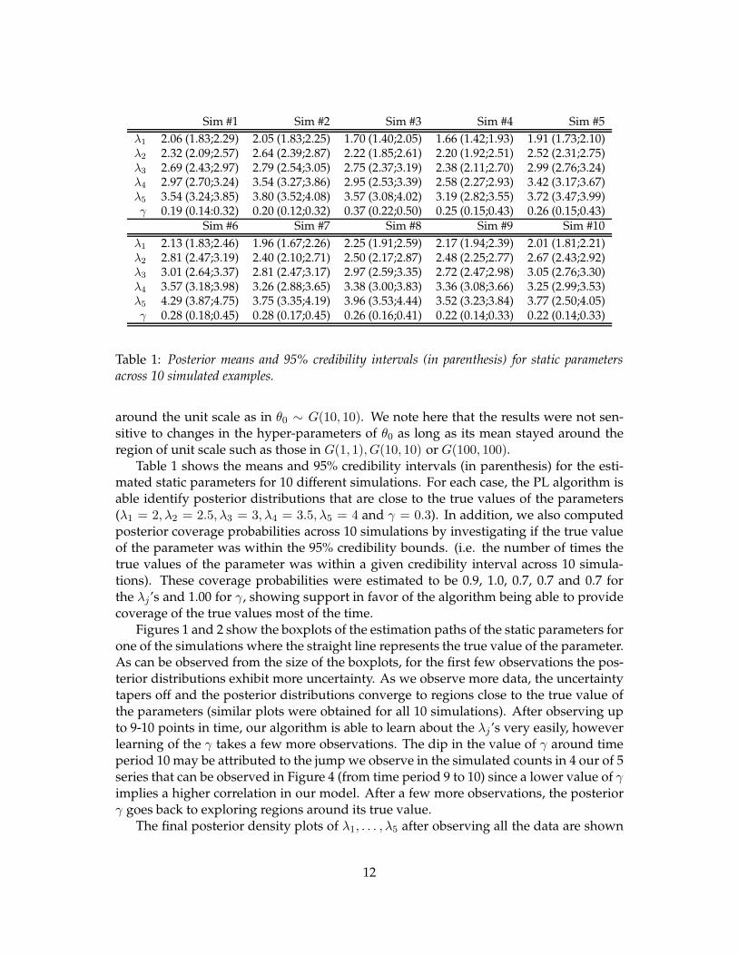
Table 1: Posterior means and 95% credibility intervals (in parenthesis) for static parametersacross 10 simulated examples.

around the unit scale as in θ0 ∼ G(10, 10). We note here that the results were not sen-sitive to changes in the hyper-parameters of θ0 as long as its mean stayed around theregion of unit scale such as those in G(1, 1), G(10, 10) or G(100, 100).

Table 1 shows the means and 95% credibility intervals (in parenthesis) for the esti-mated static parameters for 10 different simulations. For each case, the PL algorithm isable identify posterior distributions that are close to the true values of the parameters(λ1 = 2, λ2 = 2.5, λ3 = 3, λ4 = 3.5, λ5 = 4 and γ = 0.3). In addition, we also computedposterior coverage probabilities across 10 simulations by investigating if the true valueof the parameter was within the 95% credibility bounds. (i.e. the number of times thetrue values of the parameter was within a given credibility interval across 10 simula-tions). These coverage probabilities were estimated to be 0.9, 1.0, 0.7, 0.7 and 0.7 forthe λj’s and 1.00 for γ, showing support in favor of the algorithm being able to providecoverage of the true values most of the time.

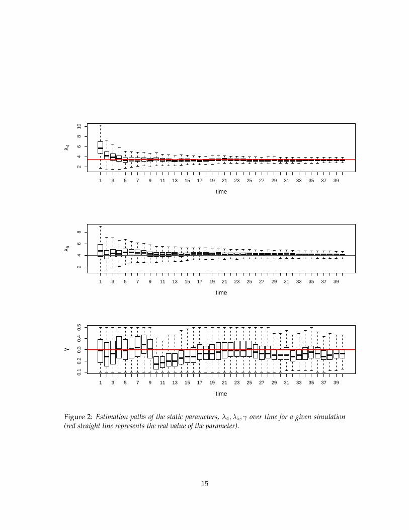
Figures 1 and 2 show the boxplots of the estimation paths of the static parameters forone of the simulations where the straight line represents the true value of the parameter.As can be observed from the size of the boxplots, for the first few observations the pos-terior distributions exhibit more uncertainty. As we observe more data, the uncertaintytapers off and the posterior distributions converge to regions close to the true value ofthe parameters (similar plots were obtained for all 10 simulations). After observing upto 9-10 points in time, our algorithm is able to learn about the λj ’s very easily, howeverlearning of the γ takes a few more observations. The dip in the value of γ around timeperiod 10 may be attributed to the jump we observe in the simulated counts in 4 our of 5series that can be observed in Figure 4 (from time period 9 to 10) since a lower value of γimplies a higher correlation in our model. After a few more observations, the posteriorγ goes back to exploring regions around its true value.

The final posterior density plots of λ1, . . . , λ5 after observing all the data are shown

12

Sim #1 Sim #2 Sim #3 Sim #4 Sim #5

MAPE 0.19 0.14 0.31 0.22 0.18Sim #6 Sim #7 Sim #8 Sim #9 Sim #10

MAPE 0.21 0.25 0.25 0.20 0.23

Table 2: Summary of MAPEs for all simulations.

in the top panel of Figure 3 for one of the simulations. All of the density plots coverthe true value of the parameter as indicated by the vertical straight lines. The posteriordistribution of γ from Figure 3 also shows that most of its support is close to the regionof 0.30 which is the actual value of γ. The posterior mode was between 0.25 and 0.30and the mean was estimated to be 0.27 (as there is more support on the left side of thetrue value in the posterior distribution). In our proposed algorithm, the estimation ofγ discussed in (19) requires that we put a reasonably large value for K which is thenumber of discrete categories for γ. For a discrete uniform prior defined over the region(0.001; 0.999), we experimented with different values for K and explored cases whenK = 5, 10, 30, 50, 100 and 500. For all 10 simulations, the posterior distributions werealmost identical when k was 30 or larger. For relatively smaller values of K as in 5 and10, the posterior distribution did not mix well and did not explore regions wide enoughfor converging to the right distribution. In cases when fast estimation is of interest,we suggest that K is kept in the region of 30-40 since increasing its dimension leads tolosses in estimation speed due to the fact that the negative binomial likelihood needs tobe evaluated for each point in time equal to “K× number of particles”.

Another noteworthy investigation is how good our estimated filters are with respectto actual data across simulations. To assess the model fit, we first computed the absolutepercentage error (APE) for each simulation (a total of 200 observations for each simula-tion) and computed the median of these APEs. The results are shown in Table 2 wherethe estimates range between 14% and 25%. The reason we report the median insteadof the mean APEs is the presence of some outliers which skew the results immensely.Typically the APE estimates range between 0 and 0.30 and some outliers are in the rangeof 3-4, which when we take the average of, show very misleading results. When weplotted the histograms of APEs for each simulation, we were able to observe that themedian and the mode of the distributions were very close to each other with the meanslocated away from these two measures due to 1-2 very high values in the right tail of thedistributions. We did not report the mean squared errors (MSE) as they would not becomparable across simulations since the scale of the counts vary from one simulation toanother even for the same values of the static parameters.

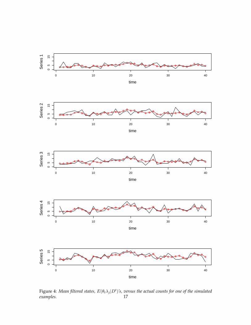
Figure 4 shows the posterior means of the filtered rates, E(θtλj)’s, at each point intime versus the actual counts for a given simulated example. In this example, the serieswere moderately correlated with sample pairwise correlations ranging between 0.59 and0.69. The model is able to capture most swings except for rare cases when all five seriesdo not exhibit similar (upward/downward) patterns at a given point in time. For in-stance, around roughly time period 9, the counts for series 1,2,4 and 5 exhibit a drop

13

1 3 5 7 9 11 13 15 17 19 21 23 25 27 29 31 33 35 37 39

01

23

45

6

time

λ 1

1 3 5 7 9 11 13 15 17 19 21 23 25 27 29 31 33 35 37 39

12

34

56

time

λ 2

1 3 5 7 9 11 13 15 17 19 21 23 25 27 29 31 33 35 37 39

12

34

5

time

λ 3

Figure 1: Estimation paths of the static parameters, λ1, λ2, λ3 over time for a given simulation(red straight line represents the real value of the parameter).

14

1 3 5 7 9 11 13 15 17 19 21 23 25 27 29 31 33 35 37 39

24

68

10

time

λ 4

1 3 5 7 9 11 13 15 17 19 21 23 25 27 29 31 33 35 37 39

24

68

time

λ 5

1 3 5 7 9 11 13 15 17 19 21 23 25 27 29 31 33 35 37 39

0.1

0.2

0.3

0.4

0.5

time

γ

Figure 2: Estimation paths of the static parameters, λ4, λ5, γ over time for a given simulation(red straight line represents the real value of the parameter).

15

2 3 4 5

0.0

0.5

1.0

1.5

2.0

2.5

Den

sity

γ

Fre

quen

cy

0.1 0.2 0.3 0.4 0.5

050

100

150

200

250

300

Figure 3: Posterior distributions of the static parameters, λ1, . . . , λ5 (top) and γ (bottom), for agiven simulation. Vertical lines represent the real value of the parameter.

16

0 10 20 30 40

05

15

time

Ser

ies

1

0 10 20 30 40

05

15

time

Ser

ies

2

0 10 20 30 40

05

15

time

Ser

ies

3

0 10 20 30 40

05

15

time

Ser

ies

4

0 10 20 30 40

05

15

time

Ser

ies

5

Figure 4: Mean filtered states, E(θtλj |Dt)’s, versus the actual counts for one of the simulated

examples. 17

1 3 5 7 9 11 14 17 20 23 26 29 32 35 38

12

34

5

time

θ t

Figure 5: Filtered stochastic evolution for the state of the environment, (θt|Dt)’s, over time for

one of the simulated examples.

whereas series 3 shows an increase. As the dependency across series is based on therandom common environment idea, the filtered states around time period 9 exhibit adecay for all 5 series (not only for series 1,2,4 and 5). Such disagreements lead to ex-tremely large APE estimates as discussed before but are usually no more than 1-2 timesin a given simulated set.

Figure 5 shows the stochastic evolution of the state of the random common environ-ment over time that all five series have been exposed to (i.e. p(θt|D

t) which is free ofthe static parameters) for a given simulation study. For instance, such a common envi-ronment could represent the economic environment financial and economic series areexposed to with swings representing local sudden changes in the market place. In ourmodel, θts dictate the autocorrelation structure of the underlying state evolution andthey induce correlations among the 5 series. The sample partial autocorrelation estimateat lag 1 for the mean of these posterior state parameters was between 0.80 and 0.90 indi-cating a strong first order Markovian behavior in the random common environment.

As a final exercise, we also used the FFBS algorithm introduced in Section 2.3 togenerate the full posterior joint distribution of the model parameters for each time pe-riod t as in, p(θ1, . . . , θt, λ1, . . . , λj |D

t). As pointed out by Storvik (2002), for any MCMCbased sampling method dealing with sequential estimation, the chains would need tobe restarted at each point in time. In addition, issues of convergence, thinning and thesize of the burn-in periods would need to be investigated. Therefore, using the FFBS al-gorithm would not be preferred over the PL algorithm when fast sequential estimationwould be of interest as in the analysis of streaming data in web applications. To showthe differences in computing speed, we estimated one of the simulated examples usingboth algorithms. The models were estimated on a PC running Windows 7 ProfessionalOS with an Intel Xeon @3.2GHz CPU and 6GBs of RAM. The PL algorithm takes about

18

17.25 (or 58.7) seconds with 1,000 (or 5,000) particles and the FFBS algorithm takes about270.74 seconds for 5,000 collected samples (with a thinning interval of 4) where the first1,000 are treated as the burn-in period. In both cases, we kept γ fixed at 0.30 even thoughthe computational burden for its estimation with the FFBS algorithm would have beenhigher with ”K× Number of Samples generated=5,000” versus ”K× Number of par-ticles=1,000”. We also note that the estimated static parameters using the FFBS modelwere very close to those estimated with the PL algorithm from Table 1. We view theFFBS algorithm as an alternative when smoothing is of interest which can be handled ina straightforward manner as discussed in Section 2.3. For sequential filtering and pre-diction, we would prefer the PL algorithm due to its computational efficiency. We wouldlike to note that the results summarized above are based on the version of our algorithmwhich uses the sequential importance sampling step for the state propagation instead ofthe rejection sampling method discussed in Step 2 of our PL algorithm. Even tough theresults were identical in both cases, the computational burden for the rejection samplingalgorithm was very high in some cases. Our numerical experiments revealed that theacceptance rate of the sampler became extremely small for certain values of the HGBdensity parameters, a, b, c. Therefore, unless a very efficient way of generating samplesfrom the HGB density can be developed, we suggest the use of the extra importancesampling step in implementing our PL algorithm.

0 20 40 60 80 100

02

46

810

12

time

Wee

kly

Dem

and

Cou

nts

Figure 6: Time series plot of weekly demand for households 1 (top straight red line) and 2 (bottomdashed black line) for 104 weeks.

19

4.2 Example: Weekly Consumer Demand Data

To show the application of our model with actual data, we used the weekly demand forconsumer non-durable goods (measured by the total number of trips to the super mar-ket) of two households in the Chicago region over a period of 104 weeks (an example fora bivariate model). Therefore, in this illustration, Yjt for t = 1, . . . , 104 and j = 1, 2 arethe demand of household j during the time period t, θt represents the common economicenvironment that the households are exposed to at time t and λj represents the individ-ual random effect for household j. The example is suitable for our proposed model sincea quick empirical study of the data revealed that weekly demand of these householdsexhibit correlated behavior over time (temporal dependence) as well as across house-holds (dependence from the random common environment). The sample correlationbetween the two series was estimated to be 0.41 which is in line with our model struc-ture that requires positively correlated counts. In addition, the partial auto-correlationfunctions of both series also show significant correlations at lag 1, justifying our use ofthe first order Markovian evolution equation for the states. As before, we estimatedthe model using 1,000 particles and used similar priors. Specifically, we assumed thatθ0 ∼ (10, 10) so that the initial state distribution is around the unit scale and assumedthat λj ∼ G(2, 1). Figure 6 shows the time series plot of these two series (straight redline represents household 1 and the dashed black line represents household 2) for 104consecutive weeks.

Figure 7 shows the mean posterior (filtered) estimates (red circles) and the 95% cred-ibility intervals (straight lines) versus the actual data (black dots). We can observe thatin most cases the counts are within the credibility intervals except for the beginning firstroughly ten time periods. This may be attributed to the fact that the counts for thesetwo households were relatively lower and closer to each other initially, resulting withless global uncertainty in the counts and tighter intervals. However, visually the plotssuggest that the model is able to account for sudden changes in the environment (forinstance there is a sudden drop around weeks 80-85) while providing an overall reason-able fit for the counts of both households. Since the sample correlation between the twoseries was 0.41, suggesting a relatively low correlation, there were certain time periodswhen the intervals do not cover the actual data. For instance, the first 10 observationsespecially for series 2, look problematic and the model is slow to adapt to the suddendrop between weeks 80-85. However, approximately more than 90% of the real countsare within the credibility interval bounds of the filtered states. Even tough we do notknow the data generating process unlike the simulated examples, MAPE obtained forthis example was 0.18 which is reasonably low.

The posterior distributions of γ as well as those of λ1 and λ2 are given in Figure 8.A higher value of λ indicates a higher order of spending habit for household 1 as op-posed to household 2 given that both are exposed to the same economic environment.The mean estimates were 3.05 and 2.04, respectively for the two static parameters. Wealso note that the posterior correlation between λ1 and λ2 was estimated to be 0.21, asexpected a positive correlation a posteriori. Furthermore, the posterior mean of γ wasaround 0.29. In our experience with both simulated and demand data, we observed that

20

0 20 40 60 80 100

04

812

time

Ser

ies1

0 20 40 60 80 100

02

46

810

time

Ser

ies2

Figure 7: Mean posterior estimates (red circles) and the 95% credibility intervals (straight lines)versus the actual data (black dots) for the consumer demand data.

21

1.5 2.0 2.5 3.0 3.5

01

23

4

λj

Den

sity

γ

Den

sity

0.1 0.2 0.3 0.4 0.5

01

23

45

6Figure 8: Posterior distributions of the static parameters, λ1, λ2 (left) and γ for the customerdemand data. λ1 and λ2 posterior estimates indicate distinct customer demand behavior for eachhousehold.

the posterior distribution of the static parameter γ did not vary significantly as we ob-serve more data points (say beyond 20-30 observations as argued previously based onFigure 2). Therefore, a practical approach for cases where on-line learning and forecast-ing is of highest importance, would be to treat γ as fixed (either at the posterior mean orthe mode) which can significantly reduce the computational burden by making filteringvery fast.

Figure 9 shows the boxplot of the posterior state parameters, in other words how thecommon environment that both households are exposed to changes over time. We canobserve that the uncertainty about the environment is relatively lower at the beginning(in the first 1-5 time periods) with respect to the following time periods. This is the sameobservation we had drawn from the credibility intervals and could be due to the smalldifference between the counts. Also, the environment is said to be less favorable duringroughly weeks 80-85 as there is a steep drop in the state estimates. We believe that beingable to model and predict household demand would be of interest to operations man-agers for long term as well as short term staffing purposes. For instance, related work inqueuing systems require the modeling of the time varying arrival rates that are used asinputs of a stochastic optimization formulation to determine the optimal staffing levels(see Weinberg et al. (2007) and Aktekin and Soyer (2012) and the references therein forrecent work using Bayesian methods for modeling Poisson arrivals in queuing models).In addition, the marketers may use these models for optimally timing the placementsof advertisements and promotions. For instance, a steep drop in the state parameters(as in the weeks of 80-85 in our illustration) might lead to reductions in staffing for cut-ting operational costs (employees may be diverted to other tasks) or the company maydecide to launch a more aggressive advertisement/promotion campaign to cope with

22

1 5 9 14 20 26 32 38 44 50 56 62 68 74 80 86 92 98

01

23

45

time

θ t

Figure 9: Boxplot of the dynamic state parameters, θt’s for the customer demand example, repre-senting the random common economic environment that the two households are exposed to.

undesirable market conditions.

5 Conclusion

In summary, we introduced a new class of dynamic multivariate Poisson models (whichwe call the MPSB model) that are assumed to be exposed to the same random commonenvironment. We considered their Bayesian sequential inference using particle learningmethods for fast online updating. One of the attractive features of the PL approach asopposed to MCMC counterparts, is how fast it generates particles sequentially in theface of new data, a feature not shared with MCMC methods where the whole chainneeds to be restarted when new data is observed. The model allowed us to obtain ana-lytic forms of both the propagation density and predictive likelihood that are essentialfor the application of PL methods which is a property that not many state space modelspossess in the literature outside of Gaussian models. In addition, our model allowed usto obtain sequential updating of sufficient statistics in learning our static parameters thatis another crucial and desirable feature of the PL method. Further, we showed how theproposed model leads to a new class of predictive likelihoods (marginals) for dynamicmultivariate Poisson time series, which we refer to as the (dynamic) multivariate con-

23

fluent hyper-geometric negative binomial distribution (MCHG-NB) and a new multi-variate distribution which we call the dynamic multivariate negative binomial (DMNB)distribution. To show the implementation of our model, we considered various simu-lations and one actual data on weekly consumer demand for non-durable goods anddiscussed implications of learning both the dynamic state and static parameters.

To conclude, we believe that it is worth noting limitations of our model. The first oneis the positive correlation requirement among series as induced by (15). As the series areassumed to be exposed to the same random common environment, our model requiresthem to be positively correlated. We investigated the implications of this requirementin the estimation paths of our static parameters in Figures 1 and 2 and the real countdata example in Figure 7. Based on these plots, it is possible to infer that initially theremaybe a few observations that do not follow this requirement where the static parameterestimation paths and the filtered means are not inline with their respective real values.However, if the data is overall positively correlated, our model converges to regionsaround the true values of the parameters (Figures 1 and 2) and the mean filtered esti-mates are within the 95% credibility intervals of the real counts (Figure 7) after a 8-10time periods. Another noteworthy limitation is the identifiability issue when the priorsfor the static parameters are uninformative. Even tough, the model keeps the productof the Poisson mean, θt × λj , close to the observed counts, it takes a very long time forthe learning algorithm to explore regions close to the real values of the static parame-ters. To mitigate this issue, we suggest to use a prior centered around unity for θ0 and touse slightly tighter priors on λj ’s as discussed in our numerical example. When dealingwith real count data, we believe that this approach is reasonable as long as the posteriorfiltered estimates provide coverage for the true counts since we will never know the truevalues of the static parameters or the true data generating process.

In addition, we believe that the proposed class of models can be a fertile future areaof research in developing models that can account for sparsity typically observed in mul-tivariate count data. Our current model does not have a suitable mechanism for dealingwith sparsity, however modifying the state equation to account for a transition equationthat can account for sparsity maybe possible and is currently being investigated by theauthors. Another possible extension would be to introduce the same approach in thegeneral family of exponential state space models to obtain a new class of multivariatemodels. This is also currently being considered by the authors with encouraging results.

Appendix A

Obtaining the resampling weights of the PL algorithm in step 1

The predictive likelihood which we denote by p(Yt+1|zt) is required for computing theresampling weights in step 1 of our PL algorithm. Specifically, we have

p(Yt+1|θt,λ,Dt) =

∫

p(Yt+1|θt+1,λ)p(θt+1|θt,λ,Dt)dθt+1

24

where the conditional likelihood is

p(Yt+1|θt+1,λ) =∏

j

(λjθt+1)Yj,t+1

(Yj,t+1)!e−λjθt+1

The conditional prior (state evolution) is given by

p(θt+1|θt,λ,Dt) =

Γ(αt)

Γ(γαt)Γ((1 − γ)αt)

( γ

θt

)γαt

θγαt−1t+1

(

1−γ

θtθt+1

)(1−γ)αt−1

Thus, rearranging the terms we can obtain p(Yt+1|θt,λ,Dt) as

p(Yt+1|θt,λ,Dt) =

∏

j

(

λYj,t+1

j

Yj,t+1!

)

∫ θt/γ

0

Γ(αt)

Γ(γαt)Γ((1 − γ)αt)

( γ

θt

)γαt

θ(∑

j Yj,t+1)+γαt−1

t+1

(

1−γ

θtθt+1

)(1−γ)αt−1e−(

∑j λj)θt+1dθt+1.

In the above, if use the transformation θt+1 =θtγu then we get

p(Yt+1|θt,λ,Dt) =

∏

j

(

λYj,t+1

j

Yj,t+1!

)(

θtγ

)

∑j Yj,t+1

Γ(αt)

Γ(γαt)Γ((1 − γ)αt)

∫ 1

0u(

∑j Yj,t+1)+γαt−1

(1− u)(1−γ)αt−1e−(∑

j λj)θtγudu,

where the term after the integral sign is similar to the hyper-geometric beta density

f(x) = Cxa−1(1− x)be−cx,

as in Gordy (1998b). Therefore, we can write,

C

∫

u(∑

j Yj,t+1)+γαt−1(1− u)(1−γ)αt−1e−(

∑j λj)

θtγudu = 1.

Rewriting the terms we get

wt =∏

j

(

λYj,t+1

j

Yj,t+1!

)(

θtγ

)

∑j Yj,t+1

(

Γ(αt)

Γ(γαt)Γ((1 − γ)αt)

)

1

C,

where the normalization constant C can be obtained as

1

C=

(

Γ(∑

j Yj,t+1 + γαt)Γ((1 − γ)αt)

Γ(∑

j Yj,t+1 + αt)

)

CHF (∑

j

Yj,t+1 + γαt;∑

j

Yj,t+1 + αt;−(∑

j

λj)θtγ)

and CHF represents the confluent hyper-geometric function (Abramowitz and Stegun

25

(1968)). Therefore, the weight can be computed as

wt =

(

∏

j

λYj,t+1

j

Yj,t+1!

)(

θtγ

)

∑j Yj,t+1

(

Γ(∑

j Yj,t+1 + γαt)Γ(αt)

Γ(∑

j Yj,t+1 + αt)Γ(γαt)

)

CHF (a; a+ b;−c),

where a =∑

j Yj,t+1 + γαt, a + b =∑

j Yj,t+1 + αt, c = (∑

j λj)θtγ . wt also represents the

predictive likelihood (marginal) for the proposed class of dynamic multivariate Poissonmodels.

Obtaining the propagation density of the PL algorithm in step 2

The propagation density of the PL algorithm in step 2 can be computed as

p(θt+1|θt,λ,Yt+1,Dt) ∝ p(Yt+1|λ, θt+1)p(θt+1|θt,λ)

∝∏

j

(

(λjθt+1)Yj,t+1e−λjθt+1

)(

θγαt−1t+1

(

1−γ

θtθt+1

)(1−γ)αt−1)

∝ θ(∑

j Yj,t+1)+γαt−1

t+1

(

1−γ

θtθt+1

)(1−γ)αt−1e−(

∑j λj)θt+1 ,

which is proportional to a scaled hyper-geometric beta density defined over the range(0; θtγ ), as HGB(a, b, c), with parameters a = (

∑

j Yj,t+1) + γαt, b = (1 − γ)αt and c =∑

j λj .

Appendix B

Here, we show some of the conjugate nature of our model and show how the multivari-ate dynamic version was obtained starting with the univariate static case.

Static Univariate Case

We start with the general rule as

Prior × Likelihood = Posterior × Marginal

Therefore, we can writep(θ)× p(Y |θ) = p(θ|Y )× p(Y ),

where we assume that θ is gamma, (Y |θ) is Poisson and Y is negative binomial. Thus,we can see the form as

( ba

Γ(a)θa−1e−bθ

)(θy

y!e−θ)

=(b+ 1)(a+y)

Γ(a+ y)θa+y−1e−(b+1)θ

(

a+ y − 1

y

)

( b

b+ 1

)a( 1

b+ 1

)y

Recall,(

a+ y − 1

y

)

=(a+ y − 1)!

y!(a− 1)!

26

Γ(x) = (x− 1)!

Also, note that the marginal model is negative binomial

(y|r, p) ∼ NB(r, p),

where r = a and p = 1b+1 .

Dynamic Univariate Case

This is the version considered in Aktekin et al. (2013),

p(θt+1|Dt)× p(Yt+1|θt+1) = p(θt+1|D

t+1)× p(Yt+1|Dt)

where using the same form from the above static univariate case, we can show that

• The prior is (θt+1|Dt) ∼ Gamma(γαt, γβt)

• The likelihood is (Yt+1|θt+1) ∼ Pois(θt+1)

• The posterior (filtering density) is (θt+1|Dt+1) ∼ Gamma(αt+1, βt+1) with αt+1 =

γαt + Yt+1 and βt+1 = γβt + 1

• The marginal (predictive density) is (Yt+1|Dt) ∼ NB(rt+1, pt+1) with rt+1 = γαt

and pt+1 =1

γβt + 1

Multivariate Dynamic Case (free of the conditioning on θt)

Our multivariate model has been obtained by extending the dynamic univariate case byconditioning on series specific static parameters, λ and by extending the likelihood to jconditionally independent Poisson densities as

p(θt+1|Dt,λ)× p(Yt+1|θt+1,λ) = p(θt+1|D

t+1,λ)× p(Yt+1|Dt,λ)

where λ = {λ1, . . . , λJ} and Yt+1 = {Y1,t+1, . . . , YJ,t+1}. Similarly, we can show that

• The prior is (θt+1|Dt,λ) ∼ Gamma(γαt, γβt)

• The likelihood is (Yt+1|θt+1,λ) =∏

j Pois(λjθt+1)

• The posterior (filtering density) is (θt+1|Dt+1,λ) ∼ Gamma(αt+1, βt+1)with αt+1 =

γαt +∑

j Yj,t+1 and βt+1 = γβt +∑

j λj

• The marginal (predictive density) is (Yt+1|Dt,λ) ∼ DMNB(rt, pt) with rt = γαt

and pt =1

γβt−1 +∑

j λj, where DMNB stands for multivariate negative binomial

distribution.

27

Multivariate Case (with conditioning on θt)

The form presented above would be suitable in the case where MCMC methods areused for estimation. In order to obtain the distributions required for the PL algorithm,we need to add an additional conditioning argument on θt (the state parameter from theprevious period). Therefore, we extend the Bayes’ rule to include θt as

p(θt+1|θt,Dt,λ)× p(Yt+1|θt+1,λ) = p(θt+1|θt,D

t+1,λ)× p(Yt+1|θt,Dt,λ),

based on which we can show that the conditional prior is

(θt+1|θt,Dt,λ) ∼ ScaledBeta(γαt, (1 − γ)αt) defined over

(

0;θtγ

)

The likelihood is(Yt+1|θt+1,λ) =

∏

j

Pois(λjθt+1)

The conditional posterior (propagation density) is a scaled HGB and is

(θt+1|θt,Dt+1,λ) ∼ HGB[(

∑

j

Yj,t+1) + γαt, (1 − γ)αt,∑

j

λj] defined over(

0;θtγ

)

,

where HGB stands for the hyper-geometric beta distribution. The predictive likelihooddensity, (Yt+1|θt,D

t,λ), would be a new multivariate density as shown below. Notealso the forms of the above densities as

• p(θt+1|θt,Dt,λ) = Γ(αt)

Γ(γαt)Γ((1−γ)αt)

(

γθt

)γαt

θγαt−1t+1

(

1− γθtθt+1

)(1−γ)αt−1

• p(Yt+1|θt+1,λ) =∏

j(λjθt+1)

Yj,t+1

(Yj,t+1)!e−λjθt+1

• (θt+1|θt,Dt+1,λ) =

(

γθt

)(∑

j Yj,t+1)+γαt

θ(∑

j Yj,t+1)+γαt−1

t+1

(

1− γθtθt+1

)(1−γ)αt−1×

e−(∑

j λj)θt+1

(

Γ(∑

j Yj,t+1+αt)

Γ(∑

j Yj,t+1+γαt)Γ((1−γ)αt)

)

1

CHF (∑

j Yj,t+1+γαt;∑

j Yj,t+1+αt;−(∑

j λj)θtγ),

where CHF represents the confluent hyper-geometric function. Therefore, we can showthat (Yt+1|θt,D

t,λ) would have the following form

p(Yt+1|θt, Dt,λ) =

(

∏

j

λYj,t+1

j

Yj,t+1!

)(

θtγ

)

∑jYj,t+1

(

Γ(∑

j Yj,t+1 + γαt)Γ(αt)

Γ(∑

j Yj,t+1 + αt)Γ(γαt)

)

CHF (a; a+ b;−c),

where a =∑

j Yj,t+1 + γαt, a+ b =∑

j Yj,t+1 + αt, c = (∑

j λj)θtγ . We refer to the above

distribution as the multivariate confluent hyper-geometric negative binomial (MCHG-NB) distribution. The MCHG-NB density has the same form as the resampling weightobtained in (18) for our PL algorithm.

28

References

Abramowitz, M. and Stegun, I. (1968). Handbook of Mathematical Functions Number 55.Applied Mathematical Series.

Aktekin, T. and Soyer, R. (2011). Call center arrival modeling: A Bayesian state-spaceapproach. Naval Research Logistics, 58(1):28–42.

Aktekin, T. and Soyer, R. (2012). Bayesian analysis of queues with impatient customers:Applications to call centers. Naval Research Logistics, 59(2):441–456.

Aktekin, T., Soyer, R., and Xu, F. (2013). Assessment of mortgage default risk viaBayesian state space models. Annals of Applied Statistics, 7(3):1450–1473.

Al-Osh, M. A. and Alzaid, A. A. (1987). First-order integer valued autoregressive(INAR(1)) process. Journal of Time Series Analysis, 8(3):261–275.

Arbous, A. G. and Kerrich, J. (1951). Accident statistics and the concept of accidentproneness. Biometrics, 7:340–432.

Carter, C. K. and Kohn, R. (1994). On Gibbs sampling for state space models. Biometrika,81(3):541–553.

Carvalho, C., Johannes, M. S., Lopes, H. F., and Polson, N. (2010a). Particle learning andsmoothing. Statistical Science, 25(1):88–106.

Carvalho, C. M., Lopes, H. F., Polson, N. G., and Taddy, M. A. (2010b). Particle learningfor general mixtures. Bayesian Analysis, 5(4):709–740.

Cox, D. R. (1981). Statistical analysis of time series: Some recent developments. Scandi-navian Journal of Statistics, 8:93–115.

Davis, R., Holan, S., Lund, R., and Ravishanker, N. (2015). Handbook of Discrete-ValuedTime Series. Chapman and Hall/CRC.

Ding, M., He, L., Dunson, D., and Carin, L. (2012). Nonparametric Bayesian segmenta-tion of a multivariate inhomogeneous space-time Poisson process. Bayesian Analysis,7(4):813.

Durbin, J. and Koopman, S. (2000). Time series analysis of non-Gaussian observationsbased on state space models from both classical and Bayesian perspectives. Journal ofthe Royal Statistical Society, Series B, 62(1):3–56.

Freeland, R. K. and McCabe, B. P. M. (2004). Analysis of low count time series data byPoisson autocorrelation. Journal of Time Series Analysis, 25(5):701–722.

Fruhwirth-Schnatter, S. (1994). Data augmentation and dynamic linear models. Journalof Time Series Analysis, 15(2):183–202.

29

Fruhwirth-Schnatter, S. and Wagner, H. (2006). Auxiliary mixture sampling forparameter-driven models of time series of counts with applications to state spacemodelling. Biometrika, 93(4):827–841.

Gamerman, D., Dos-Santos, T. R., and Franco, G. C. (2013). A non-Gaussian familyof state-space models with exact marginal likelihood. Journal of Time Series Analysis,34(6):625–645.

Gordon, N. J., Salmon, D. J., and Smith, A. F. (1993). Novel approach to nonlinear/non-Gaussian Bayesian state estimation. IEE Proceedings F (Radar and Signal Processing),140(2):107–113.

Gordy, M. B. (1998a). Computationally convenient distributional assumptions forcommon-value auctions. Computational Economics, 12(1):61–78.

Gordy, M. B. (1998b). A generalization of generalized beta distributions. Technical re-port.

Gramacy, R. B. and Polson, N. G. (2011). Particle learning of gaussian process modelsfor sequential design and optimization. Journal of Computational and Graphical Statistics,20(1).

Hankin, R. K. S. (2006). Special functions in R: Introducing the gsl package. R News, 6.

Harvey, A. C. and Fernandes, C. (1989). Time series models for count or qualitativeobservations. Journal of Business and Economic Statistics, 7(4):407–417.

Jorgensen, B., Lundbye-Christensen, S., Song, P., and Sun, L. (1999). A state space modelfor multivariate longitudinal count data. Biometrika, 86:169–181.

Kim, B. (2013). Essays in Dynamic Bayesian Models in Marketing. PhD thesis, The GeorgeWashington University.

Lindley, D. V. and Singpurwalla, N. D. (1986). Multivariate distributions for the lifelengths of components of a system sharing a common environment. Journal of AppliedProbability, 23:418–431.

Lopes, H. F. and Polson, N. G. (2016). Particle learning for fat-tailed distributions. Econo-metric Reviews, pages 1–26.

Ord, K., Fernandes, C., and Harvey, A. C. (1993). Time series models for multivariateseries of count data. in Developments in Time Series Analysis: In honour of Maurice B.Priestley, T. Subba Rao (ed.), pages 295–309.

Pedeli, X. and Karlis, D. (2011). A bivariate INAR(1) model with application. StatisticalModelling, 11:325–349.

Pedeli, X. and Karlis, D. (2012). On composite likelihood estimation of a multivariateINAR(1) model. Journal of Time Series Analysis, 33:903–915.

30

Polson, N. G., Stroud, J. R., and Muller, P. (2008). Practical filtering with sequential pa-rameter learning. Journal of the Royal Statistical Society: Series B (Statistical Methodology),70(2):413–428.

Ravishanker, N., Serhiyenko, V., and Willig, M. R. (2014). Hierarchical dynamic modelsfor multivariate times series of counts. Statistics and Its Interface, 7:559–570.

Ravishanker, N., Venkatesan, R., and Hu, S. (2015). Dynamic models for time series ofcounts with a marketing application. in Handbook of discrete-valued time series, R. A.Davis, S. H. Holan, R. Lund and N. Ravishanker (eds.), pages 423–445.

Serhiyenko, V., Ravishanker, N., and Venkatesan, R. (2015). Approximate Bayesian esti-mation for multivariate count time series models. in Ordered Data Analysis, Modelingand Health Research Methods, P. K. Choudhary et al. (eds.), pages 155–167.

Smith, R. and Miller, J. E. (1986). A non-Gaussian state space model and application toprediction of records. Journal of the Royal Statistical Society, Series B, 48(1):79–88.

Storvik, G. (2002). Particle filters for state-space models with the presence of unknownstatic parameters. Signal Processing, IEEE Transactions on, 50(2):281–289.

Taddy, M. A. (2010). Autoregressive mixture models for dynamic spatial Poisson pro-cesses: Application to tracking intensity of violent crime. Journal of the American Sta-tistical Association, 105(492):1403–1417.

Taddy, M. A. and Kottas, A. (2012). Mixture modeling for marked Poisson processes.Bayesian Analysis, 7(2):335–362.

Weinberg, J., Brown, L. D., and Stroud, J. R. (2007). Bayesian forecasting of an inhomo-geneous Poisson process with applications to call center data. Journal of the AmericanStatistical Association, 102(480):1185–1198.

Zeger, S. L. (1988). A regression model for time series of counts. Biometrika, 75(4):621–629.

31