The Institute for Food Economics and Consumption Studies

The Institute for Food Economics and Consumption Studies

of the Christian-Albrechts-Universität Kiel

Impacts of social networks, technology adoption and market participation on smallholder

household welfare in Northern Ghana

Dissertation

Submitted for Doctoral Degree

awarded by the Faculty of Agricultural and Nutrition Sciences

of the

Christian-Albrechts-Universität Kiel

Submitted

M.Sc. Yazeed Abdul Mumin

born in Ghana

Kiel, 2020

i

The Institute for Food Economics and Consumption Studies

of the Christian-Albrechts-Universität Kiel

Impacts of social networks, technology adoption and market participation on smallholder

household welfare in Northern Ghana

Dissertation

Submitted for Doctoral Degree

awarded by the Faculty of Agricultural and Nutrition Sciences

of the

Christian-Albrechts-Universität Kiel

Submitted

M.Sc. Yazeed Abdul Mumin

born in Ghana

Kiel, 2020

Dean: Prof. Dr. Karl H. Muehling

1. Examiner: Prof. Dr. Awudu Abdulai

2. Examiner: Prof. Dr. Renan Ulrich Goetz

Day of Oral Examination: 18th November 2020

ii

Gedruckt mit der Genehmigung der Agrar-und Ernährungswissenschaftlichen

Fakultät der Christian-Albrechts-Universität zu Kiel

Diese Arbeit kann als pdf-Dokument unter http://eldiss.uni-kiel.de/ aus dem Internet geladen

werden.

http://eldiss.uni-kiel.de/

iii

Dedication

I dedicate this dissertation to my parents, Alhaji Abdul Mumin Siraj and Hajia Alimatu Fuseini,

my wife, children and my siblings for their support and prayers throughout the study

iv

Acknowledgement

I wish to, first of all, give thanks to the Almighty Allah for all the blessings and favors, and in

particular, for the good health, sustenance and guidance throughout the study. I also wish to

express my sincere thanks and gratitude to my supervisor, Prof. Dr. Awudu Abdulai, for his

valuable and unflinching supervision and support, and also to Prof. Dr. Renan Goetz, for their

wonderful, outstanding and real-time guidance throughout the process of producing this

dissertation. My expressed and profound gratitude go to my family and, particularly to my wife,

Bintu Mohammed Aziz, and my children, Siddiqa and Aadil, for their patience, sacrifice and “co-

authorship” in producing this dissertation. My appreciation and special thanks go to the

Government of Ghana, the Deutscher Akademischer Austauschdienst (DAAD), the University

for Development Studies and the University of Kiel for the financial support throughout the study

period. I extend my appreciation and thanks to the four enumerators who tirelessly and

meticulously assisted in the data collection for this study. My appreciation also goes to all my

colleagues at the University of Kiel: Dr. Sascha Stark, Dr. Lukas Kornher, Dr. Awal Abdul-

Rahaman, Dr. Gazali Issahaku, Dr. Muhammad Faisal Shahzad, Williams Ali, Caroline Dubbert,

Baba Adam, Sadick Mohammed, Christoph Richartz and Asresu Yitayew for their treasured

contributions during the departmental seminars. I also wish to thank the Secretary, Mrs. Anett

Wolf, of the department for her valuable and motherly support, and the “Hiwis” for their

assistance throughout the period of the study.

Kiel, November, 2020 Yazeed Abdul Mumin

v

Table of Contents

Dedication ...................................................................................................................................... iii

Acknowledgement ......................................................................................................................... iv

Table of Contents ............................................................................................................................ v

List of Tables ............................................................................................................................... viii

List of Figures ................................................................................................................................ xi

Abstract ......................................................................................................................................... xii

Zusammenfassung........................................................................................................................ xiv

Chapter One .................................................................................................................................... 1

General Introduction ....................................................................................................................... 1

1.1 Background ........................................................................................................................... 1

1.2 Problem setting and motivation............................................................................................. 3

1.3 Objectives of the study .......................................................................................................... 8

1.4 Significance of the study ....................................................................................................... 9

1.5 Agriculture in Ghana ........................................................................................................... 10

1.6 Agricultural commercialization defined .............................................................................. 12

1.7 Agricultural commercialization in Ghana ........................................................................... 14

1.8 Soybean in Ghana................................................................................................................ 15

1.9 Farmer social networks in Ghana ........................................................................................ 18

1.10 Study area and data collection ........................................................................................... 19

1.11 Structure of thesis .............................................................................................................. 21

References ................................................................................................................................. 22

Chapter Two.................................................................................................................................. 27

The Role of Social Networks in the Adoption of Competing New Technologies in Ghana ........ 27

2.1 Introduction ......................................................................................................................... 28

2.2 Context and data .................................................................................................................. 31

2.3 Theoretical framework ........................................................................................................ 38

2.4. Empirical framework.......................................................................................................... 45

2.5 Empirical results .................................................................................................................. 52

2.6 Conclusions ......................................................................................................................... 67

References ................................................................................................................................. 70

Appendix ................................................................................................................................... 74

vi

Chapter Three................................................................................................................................ 89

Social Learning and the Acquisition of Information and Knowledge - A Network Approach for the

Case of Technology Adoption ...................................................................................................... 89

3.1 Introduction ......................................................................................................................... 90

3.2 Context and data .................................................................................................................. 95

3.3 Theoretical framework ...................................................................................................... 104

3.4. Empirical specification and estimation ............................................................................ 112

3.5 Empirical results and discussions ...................................................................................... 117

3.6 Conclusion ......................................................................................................................... 138

References ............................................................................................................................... 141

Appendix ................................................................................................................................. 146

Chapter Four ............................................................................................................................... 158

Social networks, adoption of improved variety and household welfare: Evidence from Ghana 158

4.1 Introduction ....................................................................................................................... 159

4.2 Conceptual framework ...................................................................................................... 163

4.3 Context and data ................................................................................................................ 165

4.4 Methodology ..................................................................................................................... 172

4.5 Empirical Results .............................................................................................................. 180

4.6 Discussion ......................................................................................................................... 192

4.7 Conclusion ......................................................................................................................... 194

References ............................................................................................................................... 196

Appendix ................................................................................................................................. 200

Chapter Five ................................................................................................................................ 222

Informing Food Security and Nutrition Strategies in Sub-Saharan African countries: An Overview

and Empirical Analysis ............................................................................................................... 222

5.1 Introduction ....................................................................................................................... 223

5.2 Food Security in Africa ..................................................................................................... 227

5.3 Empirical Analysis ............................................................................................................ 236

5.4 Conclusions and Policy Implications ................................................................................ 255

References ............................................................................................................................... 261

Appendix ................................................................................................................................. 267

Chapter Six.................................................................................................................................. 273

Summary, conclusions and policy implications .......................................................................... 273

vii

6.1 Summary of empirical methods ........................................................................................ 273

6.2 Summary of results............................................................................................................ 276

6.3 Policy implications ............................................................................................................ 278

Appendices .................................................................................................................................. 281

Appendix 1: Household survey questionnaire ........................................................................ 281

Appendix 2: Focus group interview guide .............................................................................. 299

viii

List of Tables

Table 2.1 Awareness and main reasons for adoption or non-adoption of the improved varieties 34

Table 2.2 Social network information .......................................................................................... 36

Table 2.3 Variable description, measurement and descriptive statistics ...................................... 39

Table 2.4 SAR MNP estimates based on the absolute number of adopters (influence of non-

adopting neighbors is not taken into account) .............................................................. 53

Table 2.5 SAR MNP estimates based on the proportion of adopters in farmer’s neighborhood

(influence of non-adopting neighbors is taken into account) ....................................... 55

Table 2.6 SAR MNP estimates of distribution in proportion of adopter in farmer’s neighborhood

...................................................................................................................................... 58

Table 2.7 SAR MNP estimates of differences in proportion of adopters of improved varieties in

farmer’s neighborhood ................................................................................................. 61

Table 2.8 SAR MNP Marginal effects .......................................................................................... 64

Table 2.A1 Mean differences in market access and production cost of adopters of respective

varieties ........................................................................................................................ 75

Table 2.A2 Sensitivity of estimates to alternative specifications, network links truncation and

additional market factors .............................................................................................. 76

Table 2.A3 Estimates of Group Fixed-Effects (Table 2.4 continued) .......................................... 77

Table 2.B1 First-stage dyadic regression of network formation by village .................................. 79

Table 2.B2 Instrumenting regression for Wealth in Dyadic model .............................................. 82

Table 2.B3 First-stage probit estimates for liquidity constraint, extension and NGO/Research

equations ....................................................................................................................... 84

Table 3.1. Variable definition, measurement and descriptive statistics ........................................ 98

Table 3.2. Network links by years known .................................................................................... 99

Table 3.3. Contextual (peer) characteristics ............................................................................... 101

Table 3.4. Social network information ....................................................................................... 102

Table 3.5. Adoption spell and adoption by modularity distribution ........................................... 104

Table 3.6. Estimates of Social learning and farmers’ adoption .................................................. 120

Table 3.7. Impact of network modularity on farmers’ adoption ................................................. 126

Table 3.8. Peer adoption squared and resource pooling ............................................................. 131

Table 3.9. Geographic proximity, soil and experience ............................................................... 134

ix

Table 3.10. Bias in estimation of network statistics (modularity, transitivity, degree and

eigenvector centralities) based on model specification in columns (5) and (6) ......... 137

Table 3.B1. Dyadic logit regression of network formation model ............................................. 149

Table 3.B2. Sampled and simulated networks by quintiles of modularity ................................. 152

Table 3.B3. Instrumenting regression for Wealth in Dyadic model ........................................... 153

Table 3.C1. Control and contextual variables in Table 6 ........................................................... 154

Table 3.C2. Control and contextual variables in Table 7 ........................................................... 155

Table 3.D1. First stage probit estimates for credit constraints and extension contact ................ 157

Table 4.1. Descriptive statistics of outcomes by own and quintiles of average peer adoption .. 170

Table 4.2. Variable definition, measurement and descriptive statistics ...................................... 173

Table 4.3. First-stage adoption results of yield and food and nutrients consumption specifications

.................................................................................................................................... 180

Table 4.4. Aggregate Treatment effects of adoption on Yield, food and nutrients consumption183

Table 4.5. Estimates of effects mechanisms ............................................................................... 188

Table 4.6. Policy simulations of the effects of changes in soybean price and distance to soybean

seed source on soybean yield, food and nutrients consumption ................................. 190

Table 4.A1. Difference in community and key household characteristics across different

bandwidths of distance to soybean seed source ......................................................... 202

Table 4.A2. Pairwise correlations between own instruments and peers of peers’ instruments .. 203

Table 4.A3. OLS estimates of the effect of distance to soybean seed source on outcomes ....... 203

Table 4.B1.1. First-stage estimates of peers’ adoption of improved soybean variety ............... 204

Table 4.B1.2. Instrumenting regressions for wealth, extension contact and farm revenue ....... 206

Table 4.B2.1. Dyadic regression of network link formation ...................................................... 208

Table 4.B2.2. Instrumenting regression for Wealth in Dyadic model ........................................ 211

Table 4.C1. Soybean varietal adoption and yield ....................................................................... 212

Table 4.C2. Soybean variety adoption, food and vitamin A consumption ................................. 213

Table 4.C3. Soybean variety adoption and protein consumption ............................................... 214

Table 4.C4. Soybean variety adoption, yield and food consumption with mobile phone coverage

.................................................................................................................................... 215

Table 4.C5. Aggregate treatment effects of adoption on Soybean yield, food and vitamin A:

Sensitivity to different specification of the outcomes and selection equations .......... 218

x

Table 4.C6. Aggregate treatment effects of adoption on outcomes: Sensitivity to use of clustered

standard errors, mobile phone network coverage and household dietary diversity ... 219

Table 4.C7. Aggregate treatment effects of adoption on Soybean yield, food and vitamin A:

Sensitivity to Network Fixed Effects, Unobserved Link formation and differences in

peers............................................................................................................................ 220

Table 4.C8. Estimates of network fixed effects (Tables C1 and C2 continued) ......................... 221

Table 5.1. Means and differences in means of food and nutrient rich food consumption outcomes

across market orientation............................................................................................ 241

Table 5.2. Variable definition, measurement and descriptive statistics ...................................... 242

Table 5.3. First-stage determinants of market orientation .......................................................... 248

Table 5.4. Treatment effects estimates of household market orientation on food and nutrients

outcomes ..................................................................................................................... 253

Table 5.5. Treatment effects between subsistence and commercial, and difference in treatment

effects between subsistence to surplus for non-sellers and those selling less than 25%

.................................................................................................................................... 255

Table 5.A1. Mean differences in household characteristics across market orientation .............. 267

Table 5.B1. Tests of systematic difference among households based on instrument status ....... 268

Table 5.B2. First-stage regressions of the IV-GMM and potential endogeneity of household

income ........................................................................................................................ 269

Table 5.B3. Household crop commercialization and food and nutrients rich food consumption

.................................................................................................................................... 270

Table 5.C1. Second stage estimates of determinants of food and vitamin A rich food consumption

.................................................................................................................................... 271

Table 5.C2. Second stage estimates of determinants of protein and iron rich food consumption

.................................................................................................................................... 272

xi

List of Figures

Figure 1.1 Area cultivated and domestic production of soybean.................................................. 16

Figure 1.2 Map of study area ........................................................................................................ 20

Figure 2.1 Association between own and neighbors’ adoption of Jenguma and Afayak ............. 44

Figure 2.A Networks by distribution of transitivity...................................................................... 74

Figure 3.1 Marginal Effects of peer adoption and production experience ................................. 121

Figure 3.2 Predicted probability of adoption by peer adoption and production experience ....... 122

Figure 3.3 Predicted probability of adoption by modularity, peer adoption and experience...... 127

Figure 3.4 Predicted probability of adoption by modularity, centrality and transitivity ............ 129

Figure 4.1 Common support for Soybean yield and food and nutrition security ....................... 182

Figure 4.2 MTE curves for soybean yield .................................................................................. 185

Figure 4.C1 Counterfactual outcomes ........................................................................................ 216

Figure 4.C2 MTE Functional form sensitivity for food and nutrition security .......................... 217

xii

Abstract

Food insecurity remains a major challenge in many parts of sub-Saharan Africa, despite the

increased access to improved agricultural technologies and markets in the past few decades.

Several attempts have been made to understand the factors accounting for the low uptake of

improved agricultural technologies and smallholder market engagement, and their implications on

household income, food security and nutrition in the sub-region. Social networks have been

recognized as playing important roles in influencing household production decisions in many

developing countries. However, not much has been done, in the empirical literature, on how

heterogeneities in social learning about both benefits and production techniques of improved

technologies, social networks structures and smallholder market orientation affect smallholder

production decisions and welfare. This study, therefore, contributes to these strands of literature

by examining the role of social networks on smallholder adoption of improved soybean varieties,

and the impacts of smallholder adoption and market orientation on household welfare in Northern

Ghana. Specifically, the study first examines the impacts of peer adoption of two improved and

competing soybean varieties on smallholders’ adoption decisions of these varieties using spatial

autoregressive multinomial probit model to account for interdependence across varieties. Second,

random-effects complementary log-log hazard model was used to investigate the role of social

learning, network transitivity, centrality and modularity on the diffusion of these improved

varieties. Third, the study examines the effects of own and peer adoption of the improved varieties

on household soybean yield, food security and nutrition using the marginal treatment effects. It

also explores the effects of policies that either increase affordability or access to improved seeds

on adoption and the outcomes using the policy relevant treatment effects. Finally, the study

employed an ordered probit selection model to examine the impacts of smallholder market-

xiii

orientation on household food security and nutrition. The results show that a farmer’s adoption

decision of a given improved variety is positively influenced by the adopting peers of this variety,

but negatively by the adopting peers of the competing improved variety. Furthermore, when the

relative share of adopting peers are equal, farmers are more likely to wait and not to switch from

the old variety. In addition, the results show that both learning about benefits and production

process are important in accelerating adoption, although the effects of learning about production

process are higher when sufficient peers adopt the improved varieties. Also, the role of transitivity

in the learning and diffusion processes is stronger, compared to centrality, although modularity

tends to slow down the diffusion process, and also constrains the effects of both transitivity and

centrality. The results further show that own and peer adoption of the improved varieties

significantly increase smallholder yield and food consumption, and that adoption tend to make less

endowed households to catchup with more endowed households. Similarly, policies that increase

either affordability or accessibility significantly increase adoption, yield and consumption, but

increasing accessibility appears to deliver somewhat higher food consumption than the

affordability-oriented policies. The estimates also reveal substantial heterogeneity in consumption

gains across market orientations and suggest the need for transition targeted and sensitive policies

in promoting smallholder food security and nutrition through crop commercialization. Similarly,

the findings on adoption suggest the need for policymakers to focus promotion efforts on

demonstrating the relative benefits and production process of improved varieties to farmers. Also,

interventions, such as self-help groups, farmer field-days and training workshops aimed at

promoting smallholder interactions, and enhancing exchange can increase the effectiveness of

social networks in promoting adoption and household welfare.

xiv

Zusammenfassung

Trotz des vermehrten Zugangs zu verbesserten Agrartechnologien und Märkten in den letzten

Jahrzenten, stellt Ernährungssicherung nach wie vor eine große Herausforderung in vielen Teilen

Sub-Sahara Afrikas dar. Viele Versuche wurden unternommen, die Hintergründe der geringen

Aufnahme verbesserter Agrartechnologien und Marktteilnahme von Kleinbauern zu verstehen und

die Implikationen für Haushaltseinkommen, Ernährungssicherung und Ernährungsweise in der

Subregion zu determinieren. Obwohl die Bedeutung Sozialer Netzwerke für die

Haushaltsproduktionsentscheidung in Entwicklungsländern bekannt ist, wurde der Einfluss von

Heterogenität in Sozialem Lernen in Bezug auf Nutzen, Produktionsmethoden verbesserter

Technologien, Sozialer Netzwerkstrukturen und Marktorientierung, auf Produktionsentscheidung

und Wohlfahrt der Kleinbauern in der empirischen Literatur bisher weitestgehend vernachlässigt.

Um diese Lücke schließen, wird in dieser Studie der Einfluss Sozialer Netzwerken auf die

Adoption verbesserter Sojabohnensorten untersucht und die Auswirkungen von Adoption und

Marktorientierung auf die Wohlfahrt kleinbäuerlicher Haushalte in Nord-Ghana analysiert. Am

Beispiel von zwei verbesserten und miteinander konkurrierenden Sojabohnensorten wird zunächst

untersucht, wie sich die Adoptionsentscheidung der Peer-Gruppe auf die eigene Entscheidung

auswirkt. Um Interdependenzen zwischen den Sorten zu berücksichtigen wird hierfür ein

räumlich-autoregressiven Multinomial-Probit Modell verwendet. Anschließend wird anhand eines

Random-Effects Complementary Log-Log Hazard Modells der Einfluss Sozialen Lernens und der

Netzwerkcharkteristika Transitivität, Zentralität und Modularität auf die Verbreitung verbesserter

Sorten untersucht. Schließlich werden anhand marginaler Behandlungseffekte die Auswirkung der

Adoption verbesserter Sojasorten auf Ertrag, Ernährungssicherung und Ernährungweise der

Haushalte untersucht. Darüber hinaus werden mittels politikrelevanter Behandlungseffekte die

xv

Auswirkungen von Politikmaßnahmen auf Adoption und deren Folgen untersucht, die entweder

die Erschwinglichkeit oder den Zugang zu verbessertem Saatgut erhöhen. Schließlich werden

anhand eines Ordered-Probit Selection Modells die Auswirkungen der Marktorientierung von

Kleinbauern auf deren Ernährungssicherheit und Ernährungsweise untersucht. Die Ergebnisse

zeigen, dass die Entscheidung der Adoption einer bestimmte verbesserte Sorte durch die Adoption

ebenjener Sorte durch die Peer Gruppe positiv beeinflusst wird, wohingegen die Aufnahme der

konkurrierenden Sorte einen negativen Effekt hat. Sind die relativen Gruppengrößen der Peers

gleich, so warten die Bauern eher ab und werden die ursprünglich angebaute Sorte nicht wechseln.

Sowohl Lerneffekte bezüglich Gewinn als auch in Bezug auf Produktionsprozesse beschleunigen

die Adoption, obgleich letztere höher ausfallen, wenn genügend Peers die verbesserten Sorten

übernommen haben. Die Rolle von Transitivität in den Lern- und Diffusionsprozessen ist stärker

im Vergleich zu Zentralität, wobei Modularität den Diffusionsprozess abschwächen und die

Effekte von Transitivität und Zentralität mindern kann. Darüber hinaus kann die eigene wie die

Adoption durch Peers den Ertrag und Nahrungsmittelverbrauch der Kleinbauern signifikant

erhöhen und dazu führen, dass weniger gut ausgestattete Haushalte zu besser ausgestatteten

Haushalten aufschließen können. Gleichermaßen führen Politiken, die entweder die

Erschwinglichkeit oder den Zugang fördern, zu einem signifikanten Anstieg von Adoption, Ertrag

und Konsum führen, wobei verbesserter Zugang einen scheinbar höheren Nahrungsmittelkonsum

begünstig als kostenreduzierende Politiken. Die Schätzungen zeigen eine beträchtliche

Heterogenität in dem Konsumzuwachs über die Marktausrichtung hinweg und verdeutlichen die

Notwendigkeit von auf Transition abgezielten, sensiblen Politiken, die durch die

Kommerzialisierung der Anbauprodukte Ernährungssicherheit und Ernährungsweise fördern. In

ähnlicher Weise legen die Ergebnisse der Adoption nahe, dass die politischen Entscheidungsträger

xvi

ihre Werbemaßnahmen darauf konzentrieren müssen, den Landwirten den relativen Nutzen und

den Produktionsprozess verbesserter Sorten aufzuzeigen. Interventionen, wie Selbsthilfegruppen,

Landwirtschaftstage und Workshops, die Interaktion und Austausch der Kleinbauern fördern,

können die adoptions- und wohlfahrtsfördernden Effekte Sozialer Netzwerke zusätzlich

verbessern.

1

Chapter One

General Introduction

1.1 Background

The role of agriculture in the economic development of countries in sub-Saharan Africa (SSA) has

been widely proclaimed. The sector has been estimated to account for about 61% of aggregate

employment, 25% of the gross domestic products (GDP), and 9.2% and 13.4% of total exports and

imports respectively, between 2001 and 2016 (Tralac, 2017). These suggest that agricultural

transformation and development would constitute a bedrock for the growth and development of

developing countries particularly in SSA. For instance, it has been argued that the realization of

the United Nations’ Sustainable Development goal of eradicating extreme poverty, hunger and all

forms of malnutrition depends on raising the productivity of agriculture, particularly in developing

countries (United Nation, 2016).

Despite the important role of agriculture in developing countries, agriculture in sub-Saharan Africa

is faced with several challenges. The most prominent among these is the lack of access to, and

efficient use of improved technologies and inputs by farmers due to infrastructure limitations and

decline in state-funding of agriculture following the implementation of structural adjustment

programs (Markelova et al., 2009). Agriculture in SSA has been characterized by low and

inefficient use of improved technologies despite the increasing availability and access to improved

agricultural technologies in Africa (Suri, 2011). In fact, whereas there has been an expansion in

the use of improved agricultural inputs and technologies in Asian and Latin America, which has

resulted in increased agricultural productivity and reduced poverty, SSA has lagged behind in the

use of improved and modern technologies and has, therefore, not been able to reap the productivity

and welfare benefits of the so-called Green Revolution (Sheahan & Barrett, 2017).

2

The lack of innovation in Africa has been intensified by high cost of dissemination and inadequate

effective demand for improved technologies (Wiggins & Leturque, 2010). Several propositions,

including promotion of farmer market engagement and commercialization, and the use of social

and collective actions have been made in order to enhance smallholder incomes; effective demand

for and dissemination of information about improved technologies in Africa (Conley & Udry,

2010; Ecker, 2018). Agriculture marketing and commercialization have been recognized by

development practitioners and researchers as important mechanisms of addressing smallholder

production and consumption challenges because of its potential in promoting greater

specialization, economies of scope, higher productivity and increased income (Bernard et al.,

2008).

The literature has generally categorized agricultural commercialization into output sales and input

purchases (Wiggins et al., 2011). In terms of output sales, commercialization of farm output can

lead to increase smallholder income, which may lead to increased smallholder spending on

consumer goods and production inputs (Ecker, 2018). At the input side, commercialization leads

to increased access to purchased inputs and use of improved inputs by smallholders (Govereh &

Jayne, 2003; Ecker, 2018). In spite of the importance of commercialization and agricultural

marketing, smallholders in Africa face high costs of marketing (i.e., either in buying farm inputs

or selling of output) due to poor infrastructure, high maintenance costs as well as government and

markets failures (Govereh & Jayne, 2003; Wiggins et al., 2011).

These challenges and following the recent increase in food insecurity and malnutrition in the sub-

Saharan countries, where agriculture is the mainstay of most economies, motivated key policy

priorities such as the Comprehensive Africa Agricultural Development Programmme (CAADP)

3

and the Africa Regional Nutrition Strategy (ARNS) to call for a rethinking and multidimensional

approach to agriculture development in Africa (Sheahan & Barrett, 2017; FAO, ECA & AUC,

2020). Several propositions for promoting the use of improved technologies and agricultural

marketing have been advanced to include trade and macroeconomic policy reforms, development

and liberalization of rural financial and capital markets, investment in and development of

infrastructure and market as well as development of support services (Ariga & Jayne, 2009). In

addition to conventional view of transformation and marketization of agriculture, contemporary

thinking also emphasizes the role smallholder social capital, collective action and cooperation for

agricultural innovations and marketing (Bernard et al., 2008). This thinking is premised on the

assertion that social capital and networks create and strengthen relationships, which drive actors

and actions to be interdependent and enhance exchange of information and resources (Smith &

Christakis, 2008).

Studies have underscored the relevance of social networks in innovation, product and technology

diffusion (Munshi, 2004; Conley & Udry, 2010), insurance, labor and risk sharing (Fafchamps,

2011) as well as in marketing of crops (Bernard et al., 2008). This study attempts to provide a

comprehensive insight into the role of social networks in smallholders’ adoption and diffusion of

improved technologies, and the implications of adoption of improved technologies and

smallholder market-orientation on household welfare in northern Ghana.

1.2 Problem setting and motivation

In developing countries, where the reliance on agriculture is high, enhancement of agricultural

productivity and income growth through adoption of new and improved innovations, and

transformation of the sector from subsistence to more productive commercialize sector remains a

4

major developmental concern (Diao et al., 2010). While studies have shown that improved crop

varieties are responsible for about 50 to 90% of increase in global crop yield (Muange, 2014),

smallholders in SSA appear constrained in the availability and access to new technologies due to

lack of physical infrastructure, failure of markets, high cost of dissemination and lack of effective

demand (Sheahan & Barrett, 2017). In addition, whereas the contribution of agricultural marketing

to smallholder productivity, incomes, and poverty reduction, has been recognized and documented

by policies and researchers (Bernard et al., 2008; FAO, ECA & AUC, 2020), its impacts on food

and nutrition security appear to be inconclusive, especially in SSA (Ogutu et al., 2019).

Several attempts have been made to understand how social networks and groups can be leveraged

as mechanisms by which smallholder adoption of new technologies can be promoted in order to

circumvent some of the challenges imposed by information asymmetries and the high cost of

technology dissemination in developing countries (Bandiera & Rasul, 2006; Conley & Udry,

2010). Many studies have shown that social networks can promote technology diffusion by

allowing farmers either to imitate the adoption choices of their network members or to consciously

learn about the production techniques and the expected benefits of the new technologies from their

social network members (Bandiera & Rasul, 2006; Conley & Udry, 2010).

However, there is lack of empirical evidence on the role of adoption of competing technologies by

smallholders’ social network members on their adoption decisions, and the relative dominance of

these technologies in terms of adoption in smallholders’ social networks. Previous studies have

mainly been theoretical, focusing on the use of economic theory to derive normative results and

predictions of adoption (Arthur, 1989; Kornish, 2006). Yet, smallholders are often faced with the

adoption decision of several competing technologies, where the decision to adopt a given

5

technology depends not only on the adoption rates of that particular technology by the network

members but also on the past and future adoption-rates of each of the competing technologies (e.g.,

Katz & Shapiro, 1986; Kornish, 2006). There is therefore the need to empirically examine the

impacts of social networks on smallholder adoption of multiple and competing improved

technologies.

The literature also provides a number of explanations on how cropping conditions and benefits

influence social learning in technology adoption, although the results have been mixed, with some

authors finding positive impacts of social learning on adoption (Munshi, 2004; Magnan et al.,

2015), while a few find no effects (e.g., Duflo et a., 2011). One possibility of enhancing the

understanding of adoption in social interaction settings and, perhaps, resolving these seemingly

contrasting results is to move beyond the implicit assumption that farmers observe the field trials

of their social network contacts with little friction in the flow of information (BenYishay &

Mobarak, 2018) to examine the roles of heterogeneities of network structures in social learning

since these shape the learning process (Jackson et al., 2017).

Social network structures play important roles in shaping the nature of interaction within networks,

and have been shown to exert overarching effects on many behavioral patterns and other economic

outcomes (Jackson et al., 2017). Many studies have argued that network structures, such as

transitivity1 and modularity2, play important roles in social interactions and influence patterns of

1 Transitivity or local cohesiveness/clustering coefficient measures how close the neighborhood of a farmer is to being a complete

network.

2 Modularity measures the proportion of links that lie within communities (i.e., components or segments) of a network minus the

expected value of the same quantity in a network where links were randomly generated. It shows the extent of partition of the entire

social network into latent groups and such partitioning can condition the flow of information within and across groups (Jackson et

al., 2017).

6

behavior (Karlan et al., 2009). For instance, higher transitivity of a farmer’s neighborhood3, and

low modularity of a network will mean more opportunities for the farmer to learn from peers and

from different neighborhoods in the network. Such opportunities can lead to reduced cost of

learning and increase the possibility of diffusion across the network (Jackson et al., 2017).

However, less is known about the role of these network structures in the social learning process

and technology adoption. It is therefore significant to understand whether learning about both

production techniques and benefits, and these network structures influence smallholders timing of

adoption of improved technologies.

Several studies have evaluated the impact of improved technologies on household welfare

(Shiferaw et al., 2014; Verkaart et al., 2017). However, not much consideration has been given to

the impact of improved crop varietal adoption by households and their peers on household food

and nutrients consumption. In particular, studies that examined the impact of technology adoption

on performance outcomes tend to focus on crop yield and income related measures (e.g., Verkaart

et al., 2017; Wossen et al., 2019). Even though a better understanding of the link between adoption

of improved technology and consumption of food and nutrients is key in helping policy-makers

design policies to promote food and nutrition security, this has received less attention in the

literature.

Moreover, the large literature on social interactions has virtually not provided evidence on the

potential benefits of peer adoption of agricultural technologies on household food and nutrients

consumption. For instance, in addition to the social learning effects on own productivity, income

and consumption, peer adoption that leads to increased peer productivity, income and changes in

3 A farmers neighborhood is defined as the individuals the farmer has contacts with in a social network.

7

peer consumption, can also affect household consumption either due to endogenous peer effect, or

through private cash transfers (De Giorgi et al., 2019). With the exception of a few such as De

Giorgi et al. (2019) who examined endogenous consumption peer effects, and Charles et al. (2009)

who analyzed the effects of race on consumption, this has not been done on peer adoption effects.

Thus, we examine the impact of smallholders’ own and peer adoption of improved technologies

on yield, food security and nutrition.

Furthermore, in spite of the widespread agreement on the role of commercialization in improving

food security and nutrition, the empirical evidence on this issue remain scanty, with mixed findings

(Ogutu et al., 2019; Ochieng et al., 2019). Whereas some argue that income from

commercialization that leads to substitution of purchased food for own produced food can result

in increased food consumption, but not nutrients intake (Ogutu et al., 2019), others argue that these

income gains may lead to preference for higher quality and cost foods and no change in food intake

(Skoufias et al., 2011).

Moreover, most of these studies have often failed to consider the possible market-orientation of

smallholders’ crop sales, which may mask the extent and pattern of gains from crop sales, given

that smallholders’ crop sales are driven by profit and non-profit motives (Pingali & Rosegrant,

1995; Jacoby & Minten, 2009). In particular, production and marketing decisions of smallholders

in Africa are often fragmented and characterized by a blend of subsistence, surplus, commercial

and distress motives, which may have varying implications on the gains from commercialization

across farmers (Pingali & Rosegrant, 1995). Hence, it is therefore important to evaluate the impact

of smallholder market-orientation on household food and nutrients consumption.

8

This dissertation attempts to contribute to the literature by filling these research gaps using recent

data from a survey of 500 farm households in Northern Ghana. The choice of Northern Ghana was

because agriculture is the main economic activity in the area with about 88% of households relying

on agriculture in this area (GSS, 2014). In addition, whereas social networks have been identified

to facilitate exchange of information, credit, labor and land in Ghana (Udry & Conley, 2004) and

could facilitate technology diffusion and agricultural productivity, the northern regions appear to

have the highest incidences of poverty, food insecurity and malnutrition. These make the choice

of the region appropriate in examining the role of social networks, technology adoption and crop

marketing on household welfare.

1.3 Objectives of the study

The main objective of this study is to examine the impacts of social networks, improved technology

adoption and crop commercialization on household welfare of smallholders in the Northern region

of Ghana. The specific objectives are:

1. To analyze the impacts of social networks on smallholder adoption of competing improved

technologies;

2. To examine the role of social learning and social network structures in the diffusion of

improved technology among smallholders;

3. To evaluate the impacts of smallholders’ own and peer adoption of improved technologies

on household welfare;

4. To conduct a review of food security and nutrition strategies in sub-Saharan African

countries, and an empirical analysis of the impact of smallholder market participation on

household welfare.

9

1.4 Significance of the study

First, examining the role of social networks in the adoption and diffusion process could provide

an efficient means of dealing with information asymmetry about the availability, access and

uncertainties of improved technologies. Such information asymmetry has often limited farmers

response to improved technologies and contributed to significant heterogeneities in the cost of

adopting improved technologies in many sub-Saharan countries (Wiggins & Leturque, 2010; Suri,

2011). Also, information about the influence of social networks in adoption decisions in the

context of competing technologies will inform policymakers when to promote single or multiple

improved technologies in a given social setting. This will show the relative adoption of these

improved varieties in networks (i.e., villages), and whether a full-scale introduction and promotion

of all improved varieties, as often done by policymakers and stakeholders in Africa, is meritorious.

Second, examining the influence of social networks structures in the adoption and diffusion

process will inform policymakers about when to leverage social networks in promoting diffusion.

Information about the role of the density of farmers’ neighborhoods in a network and the overall

structure of the network will inform policymakers when, and when not, to rely on the use of central

nodes and extension agents in the diffusion process. For instance, information about the extent of

partition of farmers’ networks will show whether targeting an influential farmer (as suggested by

many studies) or promoting extension contacts with few farmers will be effective in facilitating

diffusion since the extent of information flow will depend on the how dense and segregate the

social network is (i.e., the village).

This study extends the current frontiers of the analyses of impacts of technology adoption on

household welfare by considering the impacts of exogenous social interactions on household

10

welfare. Give the sustainability challenges and problems of lack of exit mechanisms of public

transfer schemes (Holden et al., 2006), understanding the effects of peer adoption on own

consumption will provide an alternative to policy and other stakeholders in their attempt to

promote food and nutrition security through food or cash transfer schemes. The study also provides

insights into the impacts of commercialization by examining such impacts along the lines of farmer

motivation for commercialization in order to disentangle impacts due to commercialization from

those due to other sales such as “distress” (Jacoby & Minten, 2009). This will inform policymakers

on the type of commercialization that matters, in order to develop more informed policies in

promoting food security, nutrition and agriculture transformation in Africa (Pingali & Rosegrant,

1995).

1.5 Agriculture in Ghana

The agriculture sector remains the major source of living for majority of Ghanaians and accounted

for about 22.2% of Ghana’s GDP in 2017 (GSS, 2018). The sector provides employment for over

50% of employed people and for about 82.5% of rural households (GSS, 2014) in Ghana.

Agriculture is predominantly on smallholder basis with about 90% of land holdings being less than

2 hectares (ha) and accounting for about 80% of the total agricultural output in Ghana (MoFA,

2017). Also, almost all economic activities and livelihoods of smallholder farmers depend on

agriculture and related businesses. For instance, over 65% of non-oil manufacturing uses raw

materials from agriculture in the country, and the sector also accounts for more than 25% of the

country’s total foreign exchange earnings (World Bank, 2017).

In Ghana, the food crops subsector, which include rice, maize, yams, groundnuts, soybean, cassava

and plantains, tend to dominate, and accounts for about 70% of the agriculture GDP (MoFA, 2017).

11

Despite the importance of the sector and reported increment in area under farming, the contribution

of the sector to national GDP has consistently decline to 22.2 in 2017, down from 31.2% in 2005.

At the same time, the incidence of poverty increased from 39.2% in 2012/13 to 42.7% in 2016/17

among households engaged in the agricultural sector (GSS, 2018). Low yields of both staple and

cash crops has partly contributed to the declining performance of agriculture in the country.

Existing evidence show that Ghana’s yields of cereals are estimated at 1.7 metric tons (MT)/ha,

which is lower than the regional average of 2.0MT/ha and far less than the national potential yields

of more than 5.0MT/ha (World Bank, 2017). Also, postharvest losses due to market failures and

challenges have been estimated at 20 to 30% for cereals and legumes (MoFA, 2007).

Several factors including climate change, market constraints, poor soils, pests and diseases and

lack of access to, and application of improved inputs have contributed to the low agricultural

productivity in Ghana (MoFA, 2017). For instance, Ghana has been reported as one of the lowest

countries in terms of the appropriateness and precision of inputs and fertilizer (e.g., 12kg/ha)

application, particularly in all of SSA (World Bank, 2017). Furthermore, the low yields and

declining contribution of the sector to GDP have also been attributed to lack of extension services,

lack of availability and access to markets and the limited use of information and communication

technology (ICT) in the sector (MoFA, 2017).

Given these challenges of the agricultural sector, successive governments have sought to promote

the sector in many ways in order to circumvent the declining productivity and to make the sector

an engine of growth through increased farm incomes and job creation in the country (World Bank,

2017). The Food and Agriculture Sector Plans (FASDEP I and II) focused on promoting the

efficiency of the sector through commodity markets and value chains, application of appropriate

12

technologies and improved environmental sustainability (MoFA 2007). This was followed by the

Medium-Term Agriculture Sector Investment Plan (METASIP 2011-2015) which aimed at

increasing the role of agriculture in the transformation of the Ghanaian economy. This emphasized

the need to increase agricultural productivity and food security, creation of decent job and increase

agricultural competitiveness through mechanization, innovation and technology application;

promotion of seed and planting material development and promotion of domestic and international

marketing of commodities (MoFA, 2017).

More recently, the Government of Ghana launched a new program for the agriculture sector under

the name Planting for Food and Jobs (PFJ) with focuses of the promotion of maize, rice, sorghum,

soybean and vegetables (MoFA, 2017). The PFJ also seeks to engender structural transformation

of the country through agriculture by increasing availability of food crops, job creation and

agricultural productivity. Among the major interventions earmarked to achieve this goal are

increased access to, and adoption of improved inputs and promotion of marketing of both crop

inputs and outputs through farmer-based organizations and private sector led networks (MoFA,

2017). The above discussion shows the relevance of improved input adoption and agricultural

marketing to the sector in Ghana, and the keen consideration given to these two issues by

successive governments. These, therefore, justifies the need to examine how adoption of improved

technologies and agricultural marketing can be promoted in order to stimulate national agricultural

productivity and to enhance household welfare.

1.6 Agricultural commercialization defined

Most definitions consider commercialization as the production of goods and services for sale as

opposed to subsistence farming. Strasberg et al. (1999) defined commercialization as the ratio of

13

gross value of all crop sales to gross value of all crop produced multiplied by 100. An obvious

limitation of this definition is that it narrows commercialization to output market participation (see

Wiggins et al., 2011). With this definition, there is also the likelihood of treating “distress” sales

(i.e., sale of crops immediately after harvest due to immediate cash needs) of a farmer as

commercialization (Leavy & Poulton, 2007). Other authors have indicated that mainly focusing

on the crop output market may not be an appropriate indicator of commercialization, and therefore

advocated for the consideration of input market participation (Leavy & Poulton, 2007; Wiggins et

al., 2011). For instance, Leavy and Poulton (2007) defined input commercialization index as the

value of inputs acquired from markets divided by agricultural production value. A broader

definition is the Integration into the Cash Economy (ICE), which measures the ratio of value of

goods and services acquired through cash transaction and total income (von Braun & Kennedy,

1994).

However, the concept of agricultural commercialization mean more than just involvement in

market transactions but also takes into consideration the motive of the farmer (Leavy & Poulton,

2007). Pingale and Rosegrant (1995) categorized farmer commercialization into three namely:

subsistence motive which is characterized by the use of own inputs and produces principally with

the objective of food self-sufficiency; semi-commercial motive which is also characterized by the

use of own and purchased inputs and produces with an objective of selling some surplus. The final

category is the commercial motive, which is characterized by the use of mainly purchased inputs

and with the objective of producing for profit. Finally, FAO (1989) defines agricultural

commercialization by also categorizing farmers into subsistence-oriented if the farmer sells less

than 25% of the harvest; surplus-oriented if the farmer sells between 25 and 50% of the harvest,

and commercial-oriented if the farmer sells at least 50% of the harvest. Given the lack of unified

14

definition, Wiggins et al. (2011) suggest that the choice of definition should depend on the

objective of the study.

1.7 Agricultural commercialization in Ghana

Commercialization of agriculture is considered as an important strategy in Ghana’s current

agricultural policy frameworks and national development plans as these emphasize the relevance

of moving from a subsistence-based small-holder system to a market-oriented production (MoFA,

2015; MoFA, 2017). Despite the importance of agricultural commercialization, the average

marketed surplus of crops is considered low in Ghana. For instance, IFAD-IFPRI (2011) estimated

the average marketed surplus ratio as 33% in Ghana. However, the extent of agricultural

commercialization varies depending on the crop or livestock type and agroecological zone. GSS

(2014) reported that cocoa was the crop with highest value sold in the forest and coastal zones

accounting for 45% and 24% respectively, whereas yam and maize, representing 59% of sales,

were the most important in terms of value of crop sales in the savannah zone. The low national

average marketed surplus and the variations across crops has also been attributed to low crop

productivity and poor market conditions (IFAD-IFPRI, 2011).

These have led to the pursuit of specific programs and interventions by government with the aim

of increasing farmers’ market engagements. The Commercial Development for Farmer-Based

Organization (CDFO) aspect of the Millennium Challenge Account (MCA), and the Ghana

Commercial Agriculture Project (GCAP) are specific cases in point, which encouraged

smallholder market-orientation and also trained and provided them with credit to enhance their

production and sales of farm produce. In particular, the Ghana Commercial Agriculture Project

(GCAP) was initiated by the Government of Ghana to promote integrated commercialization along

15

selected value chains of rice, maize, fruits and vegetables, and soybean (MoFA, 2015). Following

this and other recent policy interventions such as the PFJ, soybean has become an integral crop in

northern Ghana being promoted by most governmental and non-governmental parties [such as the

USAID Feed the Future program, Alliance for Green Revolution in Africa (AGRA), the

Agricultural Development and Value Chain Enhancement project (Advance I and II) and Ghana

Greenfield Investment Program among others] (Gage et al., 2012).

1.8 Soybean in Ghana

Soybean (Glycine max, L) is a commercial crop that has the potential of primarily increasing farm

incomes and also improving nutritional status of farmers and other consumers in Ghana. The crop

also provides feed to support livestock rearing and fish, and raw materials for agribusinesses in the

country (CSIR-SARI, 2013). Production and promotion of soybean in Ghana witnessed significant

increase in the past two decades. Figure 1.1 show that annual domestic production of soybean

increased over four folds from 39,000MT in 2005 to a peak of 170,000MT in 2017, an increase

that is mainly due to increased intervention in the subsector by the government of Ghana and other

development partners (such as USAID ADVANCE4) and expansion in the amount of area

cultivated.

For instance, the area of land cultivated to the crop witnessed a sustained increase from as low as

45,000 hectares (ha) in 2005 to about 101,000ha in 2017. In addition, the soybean market in Ghana

is rapidly growing with an estimated annual demand of about 150,000 MT, which is mainly driven

by the local poultry industry. The increasing demand has led to an increase in national annual

4 ADVANCE refers to the Feed the Future Ghana Agricultural Development and Value Chain Enhancement Project funded by

the United States Agency for International Development (USAID).

16

wholesale price of soybean from about 0.36 USD/Kg in 2008 to over 0.6 USD/Kg in 2015 (MoFA-

SRID, 2015).

Figure 1.1 Area cultivated and domestic production of soybean

Source: FAOSTAT, 2019.

In relation to other legumes (i.e., groundnut and cowpea), soybean appear to have lower

susceptibility to pests and diseases, better shelf life and larger leaf biomass that is important for

soil fertility (CSIR-SARI, 2013). Climatic conditions in Ghana and in particular, northern Ghana,

are considered suitable for its cultivation because of the mean temperature requirement of 20oC to

30oC by the crop for successful cultivation (CSIR-SARI ,2013). Despite the advantages of soybean

over the other grain legumes, the crop still lags behind these other legumes in terms of area

cultivated and domestic production nationally. Whereas the area cultivated to groundnut and

cowpea were estimated at 394,000ha and 159,000ha, respectively, the area cultivated to soybean

17

was estimated at 90,000ha in 2018. Similarly, the national production of groundnut and cowpea

were estimated at 521,000Mt and 215,000Mt, while the production of soybean was estimated at

152,000Mt in 2018 (FOASTAT, 2019).

Also, soybean output in Ghana has been argued as being low with about 46.7% of its attainable

output produced annually. In addition, the average yield of soybean yield has been estimated at

1.68MT/ha which is far less than the potential yields of 3.10MT/ha (MoFA-SRID, 2015). This has

been attributed to a number of production constraints, including lack of extension and training to

ensure good handling, care and storage of soybean seeds; inadequate breeder and foundation seed

supply; reliance on rain-fed, manual and rudimentary production systems and lack of awareness

and use of improved seed varieties (CSIR-SARI, 2013). For instance, access to improved seeds

and other inputs has been estimated at 23% and 9% respectively (SIL, 2015).

Given this low access and use of improved varieties, the Council for Scientific and Industrial

Research (CSIR) and Savannah Agricultural Research Institute (SARI) have over the years

developed and introduced a number of improved seed varieties and other innovations such as

inoculant to promote the cultivation and output of the crop. Initially, two varieties, Anidaso and

Bengbie were released in 1992, but were not well received by farmers. Consequently, seven other

varieties were introduced from 2003 and only two of these (namely Jenguma and Afayak) are still

in cultivation today, in addition to the traditional variety (Salintuya). These improved varieties

have been reported to have higher yield potential of over 2.0 MT/ha, resistant to pod-shattering,

mature in about 35 days earlier compared to the traditional variety and resistant to other

agricultural stress such as pests, diseases, low phosphorous soil and climatic variabilities (CSIR-

SARI, 2013).

18

However, the use of these improved varieties and other technologies are still described as being

far from desired. For instance, studies on the rate of soybean adoption in Ghana have shown that,

despite the high penetration of soybean production, the use of improved seeds has been low and

estimated as ranging between 16% and 33% of soybean farmers (SIL, 2015). Moreover, available

evidence shows that 35% of soybean producers use inoculum, 32% apply phosphorous and 4%

use mechanical planters (SIL, 2015). The low adoption of improved technologies in the midst of

increased availability of improved soybean planting technologies, and the high yield and market

potential of the crop present an interesting and suitable context to investigate the drivers and

impacts of adoption of improved soybean technologies on household welfare in the area.

1.9 Farmer social networks in Ghana

Farmer-based associations and social networks have been integral parts of socio-economic

arrangements and policies to promote smallholder technology adoption and agricultural marketing

in developing countries (Conley & Udry, 2010). This is because social capital has been shown to

have several effects on production, investment and marketing decisions (Udry & Conley, 2004;

Karlan et al., 2009). In Ghana, Udry and Conley (2004) identified four main types of social

networks, namely information, credit, labor and land networks, that tend to influence smallholder

production decisions. Information networks present opportunity for smallholders to learn about

new innovations and technologies from peers. Credit networks involve the exchange of financial

resources between peers, and enable smallholders mitigate or overcome the constraints of credit

in the production process. The third network effect is labor transactions networks where

smallholder in a network tend to exchanged labor during farm operations and finally, land

transaction network which presents an opportunity to redistribute and increase access to land by

19

land constraint farmers. These aspects were taken into consideration in this study in defining social

network links given their influence on learning opportunities and on various productive resources.

1.10 Study area and data collection

Soybean is mainly produced in Northern, Upper West, Volta and Upper East regions of Ghana

with the Northern region, which is the study area, accounting for more than half of the total area

cultivated to the crop (65.72%) and the national output (72%) of the crop (Gage et al., 2012). The

Northern region is the largest region in terms of land mass in Ghana and occupies about 70,384

square kilometers of land. Geographically, it is bounded by Upper West and Upper East regions

to the north, Brong Ahafo and Volta regions to the south (see Figure 1.2), Togo to the east and

Côte d’Ivoire to the west. The region has a total population of 2,479,461 with 69.7% being rural.

The total number of households in the region is 318,119 and the average household size in the

region of 7.7 persons is higher than the national average of 4.4 persons. The literacy level in the

region is very low with only 37.5% of persons who are 11 years and older can read and write a

simple statement with understanding in at least English or a Ghanaian language (GSS, 2013).

Administratively, the region has 26 districts.

Agriculture is the mainstay of the region, engaging about 74% of employed persons and 93% of

rural households in the area (GSS, 2013; GSS, 2018). The main crops cultivated include yam,

maize, millet, guinea corn, rice, groundnuts, beans, soybean and cowpea (GSS, 2013).

Unfortunately, the incidence of poverty and extreme poverty are not only high in the region but

have increase from 50.4% and 22.8% to 61.1% and 30.7%, respectively, between 2012/13 and

2016/17 (GSS, 2018).

20

Figure 1.2 Map of study area

Source: Regional and district map of Ghana, 2017.

Food insecurity and malnutrition have also been the highest in the area compared to the rest of the

country, with an average of 18% of households being severely food insecure. The prominent

causes of food insecurity and malnutrition in this area include inadequate rains, poor soils,

structural constraints and lack of improved inputs, which have often led to low agricultural outputs,

fluctuation in food prices and seasonal constraints in accessing food (WFP & GSS, 2012).

In order to investigate smallholder adoption of improved soybean variety and crop

commercialization as well as their impact of household welfare, cross-sectional household survey

was conducted in five districts in the Northern region between June and September 2017. A

random sample of 500 farm households was drawn in three stages. In the first step, five (5) soybean

21

producing districts was purposively selected based on their intensity of soybean production. Next,

a list of soybean producing villages in each district was obtained from MoFA district offices, and

used to randomly sample 8 villages in Savelugu-Nanton, 6 in Gushegu, 5 in Tolon, 4 in Karaga

and 2 in Kumbungu districts, in proportion to the number of households engaged in agriculture in

each district (GSS, 2014). In the third stage, listing of households in each village was conducted

and a randomly sample of 20 households was selected for interview in each village using a

structured questionnaire. In order to obtain village level information, focus group discussion with

4 to 6 village and farmer group leaders was conducted in each village. (see Appendix for the

questionnaire and the discussion guide).

1.11 Structure of thesis

The dissertation is organized into six chapters including chapter one as the general introduction.

Chapters two to five consist of journal articles. Specifically, chapter two examines the impacts of

social network members’ adoption of competing improved soybean varieties on smallholder

adoption decisions of these varieties and the relative dominance of these varieties in the social

networks. Chapter three explores the influence of social learning about production techniques and

benefits of new technologies, as well as the effects of social network structures: transitivity and

modularity on diffusion of the improved soybean varieties. Chapter four evaluates the impact of

smallholders’ own and peer adoption of the improved varieties on soybean yields, food security

and nutrition. An analysis of the impact of smallholder market-orientation is presented in Chapter

five. Chapter six presents summary, conclusions and policy implications of the study.

22

References

Ariga, J. & Jayne, T.S. (2009). Private Sector Responses to Public Investments and Policy

Reforms: The Case of Fertilizer and Maize Market Development in Kenya. IFPRI

Discussion Paper 00921. Washington

Arthur, W.B. (1989). “Competing technologies, increasing returns, and lock-in by historical

events.” Economic Journal, 99(394): 11-131.

Bandiera, O. & Rasul, I. (2006). Social networks and technology adoption in northern

Mozambique. The Economic Journal, 116(514): 869-902

BenYishay, A. & Mobarak, A.M. (2018). “Social Learning and Incentives for Experimentation

and Communication.” Review of Economic Studies, 0: 1-34.

Bernard, T., Taffesse, A.S. & Gabre-Madhin, E. Z. (2008). Impact of cooperatives on

smallholders’ commercialization behavior: evidence from Ethiopia. Agricultural

Economics, Vol. 39: 147–161.

Charles, K., Hurst, E. & Rousesanov, N. (2009). “Conspicuous Consumption and Race.” Quarterly

Journal of Economics 124(2): 425-467.

Conley, T.G. & Udry, C.R. (2010). Learning about a new technology: Pineapple in Ghana.

American Economic Review, 100(1): 35–69.

Council for Scientific and Industrial Research and Savanna Agricultural Research Institute (CSIR-

SARI). (2013). “Effective farming systems research approach for accessing and developing

technologies for farmers.” Annual Report, SARI: CSIR-INSTI.

De Giorgi, G., A. Frederiksen, & Pistaferri, L. (2019). “Consumption Network Effects.” The

Review of Economic Studies, 87(1): 130-163.

Diao, X, Hazell, P. & Thurlow, J. (2010). “The Role of Agriculture in African Development.”

World Development 38(10):1375-83.

Duflo, E., Kremer, M. & Robinson, J. (2011). “Nudging Farmers to Use Fertilizer: Theory and

Experimental Evidence from Kenya.” American Economic Review, 101(6):2350 – 2390.

Ecker, O. (2018). “Agricultural transformation and food and nutrition security in Ghana: Does

farm production diversity (still) matter for household dietary diversity?” Food Policy 79

(C): 271-282.

23

Fafchamps, M. (2011). Risk Sharing between Households. In Handbook of Social Economics,

Volume 1A, Chapter 24. Elsevier.

FAO, ECA and AUC. (2020). Africa Regional Overview of Food Security and Nutrition 2019.

Accra. https://doi.org/10.4060/CA7343EN.

Food and Agriculture Organization of the United Nations (2019). FAOSTAT statistical database.

[Rome]: FAO.

Food and Agriculture Organization of the United Nation (1989). ‘Horticultural marketing: a

resource and training manual for extension officers.’ [Rome]: FAO.

Gage, D., Bangnikon, J., Abeka-Afari, H., Hanif, C., Addaquay, J., Victor, A., & Hale, A. (2012).

‘The Market for Maize, Rice, Soy and Warehousing in Northern Ghana’. Publication

produced by USAID’s Enabling Agricultural Trade (EAT) Project, implemented by Fintrac

Inc.

Ghana Statistical Service (GSS). (2013). ‘2010 Population and Housing Census. Regional

Analytical Report. Northern Region’. Ghana Statistical Service. Accra, Ghana.

Ghana Statistical Service (GSS). (2014). ‘Ghana Living Standards Survey Round 6’. Ghana

Statistical Service. Accra, Ghana.

Ghana Statistical Service (GSS). (2018). Ghana Living Standards Survey Round 7: Poverty Trends

in Ghana 2005-2017. Ghana Statistical Service. Accra, Ghana.

Govereh, J. & Jayne, T. S. (2003). “Cash cropping and food crop productivity: Synergies or trade‐

offs?” Agricultural Economics 28 (1): 39–50.

Holden, S., Barrett, C. & Hagos, F. (2006). “Food-for-work for Poverty Reduction and the

Promotion of Sustainable Land Use: Can it Work?” Environment and Development

Economics 11 (01): 15-38.

International Fund for Agricultural Development-International Food Policy Research Institute

(IFAD-IFPRI) (2011). Agricultural Commercialization in northern Ghana. Innovative

Policies on Increasing Access to markets for High-Value Commodities and Climate

Change Mitigation. IFAD-IFPRI.

Jackson, M.O., Rogers, B.W. & Zenou, Y. (2017). “The Economic Consequences of Social-

Network Structure.” Journal of Economic Literature, 55(1): 49 – 95.

Jacoby, H. & Minten, B. (2009). “On measuring the benefits of lower transport costs.” Journal of

Development Economics 89 (1): 28-38.

https://doi.org/10.4060/CA7343EN

24

Karlan, D., Mobius, M., Rosenblat, T. & Szeidl, A. (2009). “Trust and Social Collateral.”

Quarterly Journal of Economics, 124(3): 1307-61.

Katz, M.L. & Shapiro, C. (1986). “Technology Adoption in the Presence of Network

Externalities.” Journal of Political Economy, 94(4): 822-841.

Kornish, L.J. (2006). “Technology choice and timing with positive network effects.” European

Journal of Operational Research, 173(1): 268-282.

Leavy, J. & Poulton, C. (2007). “Commercializations in agriculture.” Ethiopian Journal of

Economics, 16 (1): 3-42

Magnan, N., Spielman, D.J., Lybbert, T.J. & Gulati, K. (2015). “Leveling with friends: Social

networks and Indian farmers’ demand for a technology with heterogeneous benefits.”

Journal of Development Economics, 116(C): 223-251.

Markelova, H., Meinzen-Dick, R., Hellin, J. & Dohrn, S. (2009). “Collective action for

smallholder market access”. Food Policy, 32: 1-7.

Ministry of Food and Agriculture (MoFA). (2007). Food and Agriculture Sector Development

Policy (FASDEP II). Ministry of Food and Agriculture. Accra, Ghana.

Ministry of Food and Agriculture (MoFA). (2015). Responsible Agriculture Investment. Ghana

Commercial Agriculture Project (GCAP). Ministry of Food and Agriculture. Accra. Ghana.

Ministry of Food and Agriculture (MoFA). (2017). Planting for Food and Jobs: Strategic Plan for

Implementation (2017–2020). Ministry of Food and Agriculture, Accra, Ghana.

Ministry of Food and Agriculture, MoFA (2015). Agriculture in Ghana – Facts and Figures, 2013.

MoFA – Statistics, Research and Information Directorate (SRID): August, 2014.

Muange, E. N. (2014). ‘Social Networks, Technology Adoption and Technical Efficiency in

Smallholder Agriculture: The Case of Cereal Growers in Central Tanzania’. Unpublished

PhD. Dissertation in the International Ph. D. Program for Agricultural Sciences Goettingen

(IPAG), Georg-August-University Göttingen, Germany.

Munshi, K. (2004). “Social learning in a heterogeneous population: technology diffusion in the

Indian Green Revolution.” Journal of Development Economics. 73(1): 185-213.

Ochieng, J. Knerr, B. Owuor, G., & Ouma, E. (2019). “Food crops commercialization and

household livelihoods: Evidence from rural regions in Central Africa.” Agribusiness: An

International Journal 36 (2):318–338.

25

Ogutu, S.O., Godecke, T., & Qaim, M. (2019). “Agricultural Commercialization and Nutrition in

Smallholder Farm Households.” Journal of Agricultural Economics 71(2): 534-555.

Pingali, P. L. & Rosegrant, M.W. (1995). “Agricultural Commercialisation and Diversification:

Processes and Policies.” Food Policy, Vol. 20 (3): 171-185.

Sheahan, M. & Barrett, C.B. (2017). “Ten striking facts about agricultural input use in Sub-

Saharan Africa.” Food Policy 67: 12-25.

Shiferaw, B., Kassie, M., Jaleta, M., & Yirga, C. (2014). “Adoption of improved wheat varieties

and impacts on household food security in Ethiopia.” Food Policy 44: 272–284.

Skoufias, E., di Maro, V., González-Cossío, T. & Ramirez, S.R. (2011). Food quality, calories and

household income. Applied Economics 43: 4331–4342.

Smith, K.P. & Christakis, N. A. (2008). “Social networks and health.” Annual Review of Sociology

34: 405-429.

Soybean Innovation Lab (SIL). (2015). ‘Soybean Innovation Lab Newsletter’. Tropical Soybean

Information Portal (TSIP). www.tropicalsoybean.com.

Strasberg, P. J., Jayne, T. S., Yamano, T., Nyoro, J., Karanja, D. & Strauss, J. (1999) ‘Effects of

agricultural commercialization on food crop input use and productivity in Kenya’,

Michigan State University, International Development Working Papers No. 71. Michigan,

USA.

Suri, T. (2011). “Selection and Comparative Advantage in Technology Adoption.” Econometrica,

79 (1): 159 – 209.

Tralac. (2017, May 17). The face of African agriculture trade. Retrieved from

https://www.tralac.org/discussions/article/11629-the-face-of-african-agriculture-

trade.html

Udry, C. R. & Conley, T. G. (2004). Social networks in Ghana. Centre Discussion Paper No. 888,

New Haven, CT, Yale University, Economic Growth Centre.

United Nations. (2016). ‘The Sustainable Development Goal Report 2016’. United Nations. New

York.

Verkaart, S., Munyua, B.G., Mausch, K. & Michler, J.D. (2017). “Welfare impacts of improved

chickpea adoption: A pathway for rural development in Ethiopia?” Food Policy 66: 50-61.

von Braun, J. & Kennedy, E. (eds) (1994). Commercialization of Agriculture, Economic

Development and Nutrition. Baltimore, MD: John Hopkins Press.

http://www.tropicalsoybean.com/

https://www.tralac.org/discussions/article/11629-the-face-of-african-agriculture-trade.html

https://www.tralac.org/discussions/article/11629-the-face-of-african-agriculture-trade.html

26

WFP & GSS (Ghana Statistical Service). (2012). Comprehensive Food Security and Vulnerability

Analysis: Ghana 2012; focus on Northern Ghana. Rome, Italy: WFP.

Wiggins, S. & Leturque, H. (2010). Helping Africa to Feed Itself: Promoting agriculture to

address poverty and hunger. A Development Policy Forum (DPF) discussion paper

Wiggins, S., Argwings-Kodhek, G., Leavy, J. & Poulton, C. (2011). Small farm commercialization

in Africa: Reviewing the issues, Future Agricultures Research Paper No. 23, April.

World Bank (2017). Ghana: Agriculture Sector Policy Note. Transforming Agriculture for

Economic Growth, Job Creation and Food Security. Agricultural Global Practice AFR01,

Africa, Washington D.C.

Wossen, T., Alene, A., Abdoulaye, T., Feleke, S., Rabbi, I.Y., & Manyong, V. (2019). “Poverty

Reduction Effects of Agricultural Technology Adoption: The Case of Improved Cassava

Varieties in Nigeria.” Journal of Agricultural Economics 70(2): 392–407.

27

Chapter Two

The Role of Social Networks in the Adoption of Competing New Technologies in Ghana

Yazeed Abdul Mumina), Awudu Abdulaia) and Renan Goetzb)

a) Department of Food Economics and Consumption Studies, University of Kiel, Germany.

b) Department of Economics, University of Girona, Carrer de la Universitat, 10, 17003 Girona, Spain,

This paper was submitted to Economica

Abstract

In this study, we use a unique and detailed dataset to examine the impact of social networks,

conditional on contextual and individual confounders, on farmers’ adoption of competing

improved soybean varieties in Ghana. Based on the contagion conceptual framework, we employ

a spatial autoregressive multinomial probit model to examine how neighbors’ varietal and cross

varietal adoption of improved varieties, affect a farmer’s adoption decision in the social network.

Our results show that adoption decisions in a network tend to converge on one variety, such that

beyond a threshold of adopting neighbors of that improved variety, the cross-varietal effects tend

to lose significance in the network. We also find evidence that farmers are not more likely to adopt

either of the improved variety compared to farmers with no neighbors who have adopted the

improved varieties, if the shares of adopting neighbors of the improved varieties are equal. The

findings demonstrate the significance of neighborhood effects in the adoption of competing

technologies.

Keywords: Social network; Technology adoption; Cross-varietal effect; Threshold; Spatial model

JEL codes: C21; D83; O13; O33

28

2.1 Introduction

In developing countries where the reliance on agriculture is high, enhancement of agricultural

productivity and income growth through the adoption of new and improved innovations are widely

accepted as quite significant. Studies have shown that improved crop varieties are responsible for

about 50% to 90% of increase in world crop yield per ha (Muange, 2014). Unfortunately, adoption

of improved varieties and other forms of new technologies remain quite low, especially among

smallholders in sub-Saharan Africa (Muange, 2014). Walker et al. (2014) argue that out of 20 main

crops grown by farmers in Africa, improved varieties account for only about 35% of the area

cultivated to these crops, which underscores the significance of understanding the determinants of

technology adoption for research and policy.

Modern technologies have often been introduced with the normative anticipation that such

technologies will do well, as they allow peers to learn from each other, thereby displaying

increasing returns as more people adopt (Arthur, 1989). Beyond this, many empirical studies have

shown the importance of social networks in the adoption and diffusion of new agricultural

technologies (e.g., Foster and Rosenzweig, 2010; Bandiera and Rasul, 2006; Conley and Udry,

2010; Beaman and Dillon, 2018; BenYishay and Mobarak, 2018). Unfortunately, there is lack of

empirical evidence on the role of adoption of competing technologies by agents’ neighbors on their

adoption decisions, and the relative dominance of these technologies in terms of adoption in

agents’ social networks. Previous studies on this front have mainly been theoretical, focusing on

the use of economic theory to derive normative results, predicting adoption and characterizing

equilibrium conditions of adoption (Arthur, 1989; Kornish, 2006; Acemoglu et al., 2011).

29

In this article, we investigate the case where farmers are faced with the adoption decision of three

technologies. The farmer’s adoption of a given technology depends not only on the adoption-rate

of this particular technology, but also on the adoption-rate of competing technologies available in

the farmer’s network (see, e.g., Katz and Shapiro, 1986). This study, to the best of our knowledge,

provides the first empirical assessment of farmers’ adoption decisions in a multiple competing

technology setting, where a farmer’s adoption behavior is influenced by that of adopting neighbors

of all available improved technologies. This type of investigation is important for the following

reasons: First, this analysis reflects the situation farmers face in contemporary economic, socio-

political and technological environment, where similar and/or different technologies for the same

purpose are developed (Dorfman, 1996). Second, and perhaps more important in the context of

social network externalities, is that a farmers’ decision about a given technology depends on the

past and future adoption-rates of each of the competing technologies (e.g., Katz and Shapiro, 1986;

Kornish, 2006). The higher the adoption-rate of a particular technology, the higher are the

complementary network externalities for this technology. For instance, a technology incompatible

with other available technologies may become dominant, i.e., in the sense of a standard, so that

previous investments in any other technology may become completely obsolete and their future

net benefits tend to zero.

To guide our empirical analysis, we develop a simple contagion model to show that farmers’

adoption decisions of a given variety depend on the adoption decisions of network neighbors who

are adopters of that variety and neighbors who are adopters of the other varieties. Our model setup

is related to other works on technology adoption and consumer market shares (Arthur, 1989;

Kornish, 2006; Acemoglu et al., 2011). However, as an extension of these previous frameworks,

we allow the status quo technology to affect farmers’ adoption decisions rather than assuming it is

30

an obsolete option with its value normalized to zero. This makes the adoption of the traditional

variety in a farmer’s neighborhood an argument in the value function of farmers’ adoption

decisions in our framework. We then employ spatial econometric techniques similar to Lee (2007),

Lin (2010) and Bramoullé et al. (2009) to examine the impacts of social networks on farmers’

adoption decisions of two improved soybean varieties in Ghana, using unique and detailed

observational data.

Our results show that a farmer’s likelihood of adopting an improved variety is lower than the

proportion of adopting neighbors of that variety when the proportion is below a given threshold.

However, the likelihood of adoption becomes higher than the proportion of adopting neighbors

when the share of neighbors adopting that variety is above this threshold. We also find that a

farmer’s adoption decision of a given improved variety is positively influenced by the adopting

neighbors of this variety, but negatively by the adopting neighbors of the competing improved

variety. This is consistent with contagion effects, where the behaviors of one’s peers change the

likelihood that one engages in those behaviors. We also observe that when the relative share of

adopting neighbors are equal, farmers are not more likely to adopt any of the improved varieties

compared to farmers without adopting neighbors of the improved varieties. This finding offers

additional explanation of the differences in adoption rates of competing technologies and why

some technologies may become dominant, while others end up as subordinates, or even

nonexistent in some circumstances.

Our analysis is novel in the following respects. First, by incorporating endogenous effects,

contextual effects and unobserved correlated fixed effects, we are able to delineate the effects due

to behavioral decisions, average neighbors’ characteristics and those due to unobserved common

31

characteristics. The consideration of all three effects is highly important, as their unbundling helps

in teasing out the effects of behavioral decisions, which is the most important aspect of these

network effects in designing and targeting innovation policies more effectively (Manski, 1993

p.533). Second, we examine cross-variety dependence in the mean part of the model to show how

farmers’ adoption of the improved varieties are related to their neighbors’ adoption decisions. With

this, we are able to circumvent the interpretation problem of the estimated parameters that is

usually associated with the approach of capturing interdependence among alternatives in the

variance-covariance structure5 (Autant-Bernard et al., 2008; LeSage and Pace, 2009; Wang et al.,

2014).

The rest of the paper is structured as follows. The next section describes the context and data. In

Section 2.3, we present the theoretical framework that we use to guide the empirical analysis. We

present the empirical framework and estimation in Section 2.4. In Section 2.5, we report and

discuss the results, and then conclude in Section 2.6.

2.2 Context and data

2.2.1 Context

Soybean is a crop that is mainly cultivated in the northern part of Ghana (Northern, Upper East

and Upper West regions), with the Northern region accounting for 65.72% of the total area

cultivated to the crop in Ghana. It is a commercial crop that has the potential to raise farmers’

incomes and improve their nutritional status. It is also a versatile crop that supports livestock

5 Typically, in order to identify the multinomial probit model, the first diagonal element of the covariance matrix is

set to unity, which makes the interpretation of the dependence among alternatives problematic when captured in the

variance-covariance structure (Autant-Bernard et al., 2008; Chakir and Parent, 2009).

32

rearing, fisheries and provides raw materials for local industries. However, it has not yet been fully

accepted by farmers, because of the perceived cropping and handling difficulties (Plahar, 2006).

Also, available evidence suggests that average yields are as low as 0.8MT/ha, even though there

is the potential to achieve yields as high as 2.5MT/ha, with improved varieties of seeds and proper

agronomic practices (Gage et al., 2012).

In lieu of this, the Council for Scientific and Industrial Research (CSIR) and Savannah Agricultural

Research Institute (SARI) have over the years developed and introduced a number of innovations

including improved seed varieties and inoculant to promote the cultivation and output of the crop.

Two of the improved varieties (namely Jenguma and Afayak) are currently in cultivation, in

addition to the traditional variety (Salintuya). These improved varieties were first introduced to

farmers at demonstration sites in the various districts by SARI, and following adoption of some

farmers, seeds were subsequently made available to these farmers and to extension offices of the

Ministry of Food and Agriculture (MoFA) to promote farmers’ access to the seeds and information

about planting (CSIR-SARI, 2013). These avenues remain the main sources of information about

the cultivation and yield potentials of these varieties.

The improved varieties have higher yield potential of over 2.0 MT/ha, resistant to pod-shattering,

earliness in maturity (i.e., about 35 days less compared to the traditional variety) and resistant to

other agricultural stress such as pests, diseases, low phosphorous soil and climatic variabilities

(CSIR-SARI, 2013). In addition, planting the improved varieties does not require any special

complementary inputs that are different from the inputs required by the traditional variety. These

notwithstanding, studies show that the use of improved soy seed is quite low, with estimates

ranging between 16% and 33% (SIL, 2015) of soybean farmers. The indigenous, late maturing and

33

shattering variety is still in wide use, and CGIAR (2009) reported that this variety constituted more

than 50% of all soybean varieties under cultivation in Ghana.

Table 2.1 provides information on farmers’ awareness and subjective perception of the costs and

expected benefits of adopting the improved varieties. Panel A shows that whereas about 64% and

60% of farmers know about Jenguma and Afayak respectively, the proportion of adopters are 42%

and 26%, respectively. The potential setbacks to adoption identified in the literature are lack of

information about the production techniques and benefits of new technologies, credit constraints

and market6 constraints (Zeller et al., 1998; Croppenstedt et al., 2003; Beaman et al., 2020). Panel

A of Table 2.1 further reports the reasons why farmers adopted the improved varieties. The most

frequent reason given in each case is agronomic and climate resistance of Jenguma and high

yielding advantage of Afayak. The second most frequent reason indicated is the perceived high

yielding potential of Jenguma and agronomic and climatic resistance of Afayak. For non-adopters,

the top reasons for not adopting the improved varieties are due to inadequate information about

the production and agronomic requirements of the improved varieties, and that these improved

varieties are not high yielding compared to the traditional varieties7.

In order to assess the extent to which non-adopters are informed about the yields of the improved

varieties, panel B shows the estimated change in yields between each of the improved varieties

6 The high and excess demand for soybean over its supply, especially by the poultry sector, in Ghana (Plahar, 2006), and the high

integration of the soybean market into the international market (Goldsmith, 2017), suggest that the degree of marketability of

soybean may not be the main barrier to adoption given that all three varieties face similar market conditions. In addition, Table

2.A1 in the appendix shows no systematic difference in market access across farmers’ adoption status.

7 Discussions with MoFA officials and village level key informants revealed that some farmers hold the perception that the

traditional variety grows well and will provide good yield with good management and timely harvest (see also SIL, 2015).

34

and the traditional variety based on computation from the sample and estimates of non-adopting

farmers.

Table 2.1 Awareness and main reasons for adoption or non-adoption of the

improved varieties

%

Panel A

Know about Jenguma 64.4

Know about Afayak 59.8

Why adopted Jenguma

Agronomic and climatic advantages 74.6

High yielding 66.8

High marketability 42.1

Less labor demanding 38.6

Easy to cultivate 8.4

Why adopted Afayak

High yielding 67.2

Agronomic and climatic advantages 62.4

High marketability 44.0

Less labor demanding 36.8

Easy to cultivate 11.2

Why non-adopters did not adopt

Do not know the production and agronomic requirements 76.0

I feel it is not high yielding 34.0

Credit constraints 21.0

Poor prices and market 21.0

Need for other food crops 4.0

Panel B

Estimated yield difference between:

Jenguma and Salintuya from average yields of the sample$ 67.1

Afayak and Salintuya from average yields of the sample 58.8

Jenguma and Salintuya estimated by non-adopters 4.9

Afayak and Salintuya estimated by non-adopters 4.2

Notes: The table consist of two panels. Panel A presents descriptive statistics of farmers’ awareness and farmers’ reasons

for adoption and non-adoption. Panel B presents descriptive statistics of estimated yield difference between each of the

improved varieties and the traditional variety by official sources, computation using average yield of the sampled farmers

and by non-adopters. The official estimates suggest much higher yield potentials of Jenguma and Afayak of 2.8Mt/ha and

2.4Mt/ha, respectively, compared to the yield potential of the traditional variety is 1.0Mt/ha (CSIR-SARI, 2013).

35

There are substantial differences between the change in yields (on average) obtained by adopters

and the estimates (5%) reported by non-adopters. The reported differences suggest that despite the

existence of the improved varieties for some time, and the promotion of the improved variety by

SARI and MoFA through the existing extension system, non-adopters seem to have different

information and perceptions about the production processes and expected benefits of the improved

varieties compared to adopters. This differential access to information among adopters and non-

adopters, and failure of several improved varieties to be accepted by farmers suggest the need to

understand what could possibly explain farmers’ adoption of a particular variety in a context of

multiple improved varieties. This will be useful in the formulation of hypotheses that explain the

underlying drivers of varieties emerging as dominant or marginal in the farmers’ villages (social

networks).

2.2.2 Data

Social networks

The data used in this study were collected from 483 farm households across 5 districts in 25

villages in the Northern region of Ghana, between July and September 2017. The survey design

employed a multistage random sampling technique to first purposively select soybean growing

districts, based on intensity of soybean production8 and then randomly selecting villages and

households, proportionate to the number of households in each district. Finally, random matching

within sample was used, whereby in each village (i.e., a village represents a social network or

group), 20 farm households were randomly selected and each household was matched with 5 other

farm households also randomly drawn from the village sample. For each match, conditioned on

8 This was done in consultation with the Ministry of Food and Agriculture (MoFA) Regional and Districts Offices and

Resilience in Northern Ghana (RING)

36

knowing the matched household, detailed information about the relationship between them were

elicited. For determining existing links in the network, we used both social and locational

indicators in the definition of a farmer’s neighbors (Banerjee et al., 2013). Table 2.2 presents these

social and locational dimensions of social network contacts. The farmer knows on average 3.13 of

the 5 farmers randomly matched to him9. Also, the average farmer has 1.77 agricultural

information contacts, 2.17 relatives, 1.18 friends, and exchanged labor with 1.73 of the known

matched farmers. The farmer, on average, has ever visited 2.18 of the contacts, and has 0.87 or

0.67 of the contacts as farm or residential neighbors, respectively.

Table 2.2 Social network information

Network connections and information Mean S.D. Min Max

Number of random matched known 3.13 1.15 0 5

Conditional on knowing the matched:

Social dimension of contact

Number of agricultural information contacts 1.77 1.79 0 5

Number of neighbors who are relatives 2.17 1.67 0 5

Number of neighbors who are friends 1.18 1.56 0 5

Number of neighbors with same religion 0.64 1.07 0 5

Number of neighbors ever exchanged labour 1.73 1.86 0 5

Number of neighbors ever exchanged credit 0.69 1.35 0 5

Number of neighbors ever exchanged land 0.33 0.95 0 5

Locational dimension of contact

Number ever visited 2.18 1.64 0 5

Number of farm neighbors 0.87 1.20 0 5

Number of residential neighbors 0.67 0.96 0 5

Social links (Social ties)

Number of social contacts 3.12 1.25 0 5

Degree* 3.73 1.51 1 8

Network transitivity 0.46 0.09 0.18 0.60

Proportion of Jenguma adopters in neighborhood (unconditional)** 0.42 0.36 0 1

Proportion of Afayak adopters in neighborhood (unconditional)** 0.29 0.31 0 1

Notes: SD denotes standard deviation and Min and Max are minimum and maximum values respectively.

*The farmer i’s average degree is higher than the number of his/her social ties due to the fact that the number of social ties took

into consideration only directed contacts (from farmer i to farmer j) based on the social and locational dimensions of contacts. The

degree on the other hand is based on undirected relationships where the existence of a link between farmer i and farmer j was

defined as either by i, or by j, or both mentioned having any of these contacts with the other farmer.

** The unconditional implies that the proportion of adopting neighbors (j’s) of each variety does not condition on the

variety adopted by the farmer (i).

9 We use the masculine gender because majority (60%) of the farmers in the sample are males.

37

We define the farmer’s neighbors as those among the 5 farmers randomly assigned to him/her, that

he/she shares any of these social and locational contacts with (i.e. the union of these contacts).

When we take the union of these social and locational contact dimensions, an average farmer has

3.12 social ties (Table 2.2). We use the social and locational contacts to construct our social

network matrix with entries, 𝑤𝑖𝑗, being equal to one if the respondent 𝑖 had any of these

relationships with a matched farmer 𝑗 (i.e., 𝑖 and 𝑗 are neighbors), and zero otherwise (i.e., 𝑖 and 𝑗

are not neighbors). The resulting social network matrix, 𝑊, is a 483 x 483 block-diagonal matrix,

along villages networks. Based on the matrix, 𝑊, the average farmer has 3.73 neighbors in the

social network and a maximum of 8 neighbors as indicative by the term degree in Table 2.2 (see

Figure A.1 for networks). The table also shows that an average farmer has 42% and 29% adopting

network members of Jenguma and Afayak varieties, respectively.

Descriptive statistics

We also elicited detailed information on the household and farm level characteristics. Table 2.3

shows definition, measurement and descriptive statistics of variables for the surveyed households

and of their neighbors. Majority of farmers in the sample are males. The average education attained

by the surveyed farmers is low, about 1.11 years, but with an average experience of about 12.7

years of farming. In addition, the majority (55%) of the farmers and (56%) of their neighbors ever

had contact with extension agents, while only 28% of farmers and 30% of their neighbors ever had

contact with research and non-governmental organization.

Table 2.3, further shows that majority of the farmers and their neighbors, 55%, are credit-

constrained. The proportion of credit constrained farmers are significantly lower for Jenguma

producers (Table 2.A1, panel B), and as noted in Section 2.2.1, suggest that access to credit could

38

affect farmers decisions to adopt this variety. In our analysis such differences in access to credit

are controlled for by using household credit constraints (Table 2.3). Households were classified as

credit-constrained, if they obtained credit, but expressed interest in borrowing more at pertaining

interest rates, and if there was no credit available to them through formal and informal lenders.

Furthermore, about 42% and 26% of the households were adopters of Jenguma and Afayak,

respectively, whereas 32% cultivated Salintuya. Table 2.3 also shows a strong association between

a farmer’s adoption of an improved variety and the proportion of farmers’ neighbors who adopted

that variety. In particular, farmers who adopted Jenguma have up to 88% of their neighbors also

adopting Jenguma. At the same time, about 82% of neighbors of Afayak adopters are themselves

adopters of Afayak, while farmers who are cultivating the traditional variety have about 85% of

their neighbors also producing the traditional variety. This indicates the possibility of farmers

exchanging information about soybean, and/or imitation by copying their neighbors’ cultivation

choices.

2.3 Theoretical framework

In order to motivate our discussion on how local correlations in social networks affect adoption

decisions in our context of multiple and competing technologies, we present a theory of contagion,

which is based on the linear threshold model (Granovetter, 1978; Morris, 2000; Acemoglu et al.,

2011)10. In our study, the technology under consideration is soybean varieties, where two (i.e.,

Jenguma and Afayak) of these are improved and Salintuya is the traditional variety. Thus, we

model adoption as the outcome of optimizing behavior of agents, based on the frameworks

presented in Arthur (1989) and Kornish (2006).

10 The reader is referred to Beaman et al. (2020) for a discussion on the merits of the linear threshold model.

39

Table 2.3 Variable description, measurement and descriptive statistics

Variable Definition Own (X)

Characteristics

Neighbors (WX)

Characteristics

Mean SD Mean SD

Independent variables

Age Age of farmer (years) 44.002 12.007 43.929 7.151

Gender 1 if male; 0 otherwise 0.596 0.491 0.581 0.333

Education No. of years in school 1.112 3.077 1.105 1.810

Experience No. of years in farming 12.677 2.718 12.708 2.006

Household Household size (No. of members) 5.725 2.090 5.722 1.477

Landholding Total land size of household (in hectares) 2.597 1.556 2.626 1.120

Credit 1 if farmer indicated did not obtain sufficient credit or not successful in

applying for credit; 0 otherwise

0.554 0.497 0.554 0.344

Risk Risk of food insecurity (No. of months household was food inadequate) 0.948 1.387 0.925 0.942

Extension 1 if ever had extension contact; 0 otherwise 0.546 0.924 0.563 0.687

NGO/Res. 1 if ever had contact with non-governmental/research organization; 0 otherwise 0.284 0.451 0.295 0.332

Association No. of village-based associations a farmer is a member 1.091 1.285 1.081 0.898

Electronic 1 if own phone, radio and/or television; 0 otherwise 0.817 0.386 0.821 0.264

Soil quality 4=fertile; 3=moderately fertile; 2=less fertile; and 1=infertile 2.962 0.972 2.965 0.688

Price Soybean price in GHS/kg 1.055 0.188 1.062 0.135

Dependent variable

Jenguma Adopters of Jenguma variety (1 if adopted Jenguma; 0 otherwise) 0.418 0.494 0.878+ 0.214

Afayak Adopters of Afayak variety (1 if adopted Afayak; 0 otherwise) 0.258 0.438 0.815+ 0.238

Salintuya Adopters of Salintuya variety (1 if adopted Salintuya; 0 otherwise) 0.322 0.468 0.849+ 0.263

Instruments

Village born 1 if farmer was born in village 0.696 0.461

Authority 1 if any parent of the farmer had an authority in village 0.130 0.337

ExtDistance Distance to the extension office (in kilometers) 9.890 9.140

RNDistance Distance to the nearest agric. research or non-governmental organization (in

Kilometers)

14.561 11.797

FinDistance Distance to the nearest financial institution (in kilometers) 9.256 6.884

Notes: SD denotes standard deviation. “+” implies that the proportion of adopting neighbors (j’s) of each variety is conditional on the farmer (i) adopting that

variety. That is why the proportion of adopting neighbors of each variety in this table is higher than the unconditional proportions in Table 2.2.

40

The main insights in these frameworks are that agents are confronted with the situation of having

to choose among competing technologies, of which one is a status quo (default) technology. Also,

adoption decisions are based on the relative and absolute number of adopting and non-adopting

neighbors and the expected net benefits from adopting these technologies. We define a set of

farmers 1, ,m M in a network represented by an undirected graph ,g m E , where E is a

set of edges ( , )i j that represent the connectivity between farmers i and j . We also define the

neighborhood of a farmer i m as [ | , ]iN g i i j E . That is, iN g consists of the set of the

neighbors of farmer i and i id N g denotes the number of farmers that form part of the

neighborhood.

Farmer i sets out using a traditional variety, 0, and has the choice of adopting any of the two new

improved varieties, denoted as 1 and 2 , from the set 1,2V or retaining the traditional variety.

These new varieties compete for adoption and are assumed not to be sponsored or strategically

manipulated (Arthur, 1989). We further assume that farmer i faces one-time cost of adopting

variety 1 or 2 , denoted by 1 0iC and 2 0iC , respectively. The farmer’s infinite horizon net

benefit function is given by 1 2, , 0i i id d d , where 1 2

i i id d d indicates the number of

neighbors that have adopted none of the improved varieties, with 1

id representing the number of

neighbors that have adopted variety 1 and 2

id the number of neighbors that have adopted variety

2. The farmer’s decision problem is to maximize the expected net benefit from adoption, by

selecting the strategy that offers the highest payoffs. The alternative strategies are characterized

by payoff from (i) adopting variety 1, (ii) adopting 2 and (iii) from maintaining the traditional

variety 0. Let us denote the one-period discount factor by .

41

We define the probability that the next potential adopter has preference for variety 1 as 1 i ih d d

and for variety 2 as 2

i ih d d . Both of these functions are increasing with the shares, 1 /i id d and

2 /i id d , of 1 and 2 adopting neighbors, respectively. Moreover, the conditional probability 1

ip d

that a farmer adopts variety 1, given that he/she has preference for variety 1, is an increasing

function of the number of adopting neighbors of variety 1 1

id . The complement of 1

ip d , given

by 11 ip d , indicates the probability that the farmer does not adopt variety 1. Similarly, the

conditional probability of adopting variety 2 for a potential user is 2

ip d , given that he/she has

preference for variety 2 . Thus, as an example, the term 1 1 i i ip d h d d indicates the conditional

probability of adopting variety 1, given the preference for variety 1 multiplied by the probability

of having these preferences for variety 1. Likewise, one can formulate the probabilities for

adopting variety 2 and for non-adopting variety 1 or 2. Based on these formulations, the farmer’s

decision problem can be formulated as

(1)

1 1 2 1

2 1 2 2

1 11 2 1 2 1 2

1 11 1 2 2 1 2

, , ,

, , ,

ˆ , , max 1 1 1 , ,

1, 1, 1 1, , 1

i i i i

i i i i

i ii i i i i i i i

i i

i ii i i i i i i i

i i

d d d C

d d d C

d dd d d h p d h p d d d d

d d

d dh p d d d d h p d d d d

d d

.

Following equation (1 ), we express the expected net benefits from adopting variety 1, when there

are 1

id adopters of variety 1 and 2

id adopters of variety 2 as

42

(2) 1 1

1 1 2 1 1 1 2 1 1 2, , 1 1 1 , ,i ii i i i i i i i i

i i

d dd d d q d h p d h p d d d d

d d

1 1

1 1 1 2 2 1 1 2 1, 1, 1 1, , 1 ,i ii i i i i i i i

i i


d d

where 1 1

iq d is the periodic benefit of adopting 1, which is a function of the neighbors that have

already adopted variety 1. The term 1 1 2, ,i i id d d accounts for the immediate and discounted

future stream of payoffs, if the farmer does not adopt, and of the discounted stream of future

payoffs, if the farmer adopts variety 1 or variety 2. Similarly, we express the expected net benefit

from adopting variety 2, when there are 1

id adopters of variety 1 and 2

id adopters of variety 2 as,

(3) 1 1

1 2 1 2 22 2 12 2, , 1 1 1 , ,i ii i i i i i i i i

i i

d dd d d q d h p d h p d d d d

d d

1 1

1 1 2 22 1 22 1, 1, 1 1, , 1 .i ii i i i i i i i

i i


d d

The functions 1(.)q , 2(.)q may contain network-dependent and network-independent elements. In

order to express network dependence, it can be seen that the agent’s expected net benefits from

adopting a particular variety are increasing with the number of adopting neighbors of that variety.

Based on observational data, we next explore the nature of .p .h for both varieties, which are

shown in Figures 2.1A and 2.1B. We observe that both the proportions of adopting neighbors of

each improved variety relative to the neighborhood (i.e., 1 2,i i i id d d d , indicated by the dashed

line), and the difference in the share of adopting neighbors of the two improved varieties (i.e.,

1 2( )i i id d d , indicated by the solid line), are important for influencing a farmer’s adoption

decision (Figure 2.1). This distinction is important because the first measure takes into account the

43

number of non-adopting farmers of the two improved varieties, while the second measure focuses

exclusively on the difference in adoption of the two improved varieties. In respect of the

proportions of adopters of the improved varieties in the neighborhood, the curve exhibits an S-

shaped function for the conditional probability of adoption .p , given the probability of the

preference .h for a variety, as a function of the share of neighbors that have adopted this variety.

Thus, when the proportion of adopting neighbors of an improved variety is low, the probability of

a farmer adopting this variety is lower than the proportion of the neighbors who have already

adopted it. However, the likelihood of adopting an improved variety is higher than the proportion

of adopting neighbors of this variety, when the proportion of adopting neighbors of this variety is

high.

Moreover, the solid line, which is based on the difference in the share of adopters of the two

improved varieties, shows stronger effect on adoption than the share of adopters of these varieties

in relation to the whole neighborhood (dashed line). It lies above the dashed line for most part, and

is consistently higher than the 45-degree line in both figures. This suggests that farmers give

significant consideration to the difference in the share of adopting neighbors of the improved

varieties when making adoption decisions. The S-shaped function and the importance of the

difference in relative adoption of the improved varieties by farmer’s neighbors implies that the

adoption process will result in one of the varieties becoming “dominant”, while the other varieties

become “subordinates” in the network. Thus, the neighborhood becomes increasingly ‘locked-in’

on the dominant variety, where a farmer’s likelihood of adopting that variety is higher, if adoption

pushes that variety ahead of the other improved variety in relative and absolute numbers and in

expected net benefits. Thus, we deduce the following hypotheses;

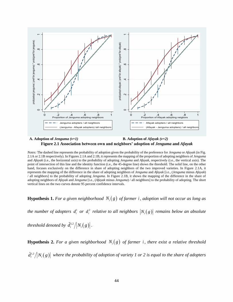
44

A. Adoption of Jenguma (v=1) B. Adoption of Afayak (v=2)

Figure 2.1 Association between own and neighbors’ adoption of Jenguma and Afayak

Notes: The dashed line represents the probability of adoption given the probability of the preference for Jenguma or Afayak (in Fig.

2.1A or 2.1B respectively). In Figures 2.1A and 2.1B, it represents the mapping of the proportion of adopting neighbors of Jenguma

and Afayak (i.e., the horizontal axis) to the probability of adopting Jenguma and Afayak, respectively (i.e., the vertical axis). The

point of intersection of this line and the identity function (i.e., the 45-degree line) shows the threshold. The solid line, on the other

hand, focuses exclusively on the difference in share of adopting neighbors of the two improved varieties. In Figure 2.1A, it

represents the mapping of the difference in the share of adopting neighbors of Jenguma and Afayak [i.e., (Jenguma minus Afayak)

/ all neighbors] to the probability of adopting Jenguma. In Figure 2.1B, it shows the mapping of the difference in the share of

adopting neighbors of Afayak and Jenguma [i.e., (Afayak minus Jenguma) / all neighbors] to the probability of adopting. The short

vertical lines on the two curves denote 95 percent confidence intervals.

Hypothesis 1. For a given neighborhood iN g of farmer i , adoption will not occur as long as

the number of adopters 1

id or 2

id relative to all neighbors iN g remains below an absolute

threshold denoted by 1,2 i id N g .

Hypothesis 2. For a given neighborhood iN g of farmer i , there exist a relative threshold

1,2ˆ i id N g where the probability of adoption of variety 1 or 2 is equal to the share of adopters

45

1,2 .i id N g If this share of adopters is below the relative threshold, the farmer is less likely to

adopt, and if it is above the threshold the farmer is more likely to adopt.

Hypothesis 3. Adoption in a given neighborhood iN g of farmer i will converge towards a

single dominant variety (1 or 2) if the proportion of adopters of this particular variety leads to a

higher adoption probability than the proportion of the non-adopting neighbors of the variety. If

the relative shares of adopters of the improved varieties are equal, the farmers are not more likely

to adopt either the improved variety.

2.4. Empirical framework

In 2.4.1, we first present the base model and then discuss the identification concerns and strategies

we use in the empirical analysis. We next discuss the empirical estimation in 2.4.2, and then the

computation of marginal effects for the control variables in 2.4.3.

2.4.1 The model and identification

The studies of social interaction models have generally focused on the delineation of the effects of

individual or group interactions on individual or group behavior and socio-economic outcomes

(Blume et al., 2010; Lee et al., 2010). Three types of behavioral effects have been identified in the

literature that can arise from social interactions. These are the endogenous effects,

exogenous/contextual effects and correlated effects (Manski, 1993; Moffitt, 2001). To motivate

our discussion on these effects, consider the following linear regression

(4) 0 1 2| ,|i iig d ig d igY E Y g X E X g

where igY is the outcome of individual i in group g , igX is a vector of characteristics of i from

group g , with 1 as the associated parameter estimates, and ig are innovations. The

46

neighborhood mean outcome and characteristics are captured by the terms |idE Y g and |

idE X g

, respectively. The parameter 0 denotes the endogenous network effect, whereas 2 defines the

contextual effects. Manski (1993) showed that specification (4), called the linear-in-means model,

suffers from the “reflection problem”, which is the difficulty in differentiating between

endogenous (behavioral) and exogenous (contextual) factors, since expressing the endogenous

effects |idE Y g as the average behavior or outcome of the group makes it a linear function of the

mean characteristic of the group |idE X g in model (4). This shrouds what each of the two effects

are, and the inherent implications associated with each becomes misleading, as they have been

identified to have effects different in nature and in policy conclusions (Manski, 1993; Lin, 2010).

Another important confounder of the behavioural effects is the argument by Moffitt (2001) that

unobserved factors in ig , noted earlier as correlated effects, may also be a source of correlation

among individuals in a given group (see also Manski, 1993; Calvo-Armengol et al., 2009; Lee et

al., 2010). Moffitt (2001) distinguished between correlations due to similarities or preferences that

drive a group of individuals to group together, and those that are attributable to similar

environmental characteristics, suggesting that any social impact could be a reflection of omitted

variables, or spurious effect. Accordingly, we use a spatial autoregressive (SAR) model, where the

disturbance in equation (4) is decomposed into network-fixed effects, g , (which defines

unobserved characteristics that are similar for all network members) and innovations, ig , to

account for endogenous, contextual and group fixed effects in the group interaction setting as

follows

(5) 0 1 2 0 ,kg kg kg kg kg kg mg g kgY W Y X W X l

47

where 1, ,g G and G is the number of groups (villages) in the sample, gm is the number of

members in the g th group and 1

G

ggk m

is the total number of observations. The term kgY is a

vector of adoption decisions, kgX is a matrix of characteristics for the

gm individuals in group g

, kgW is a non-stochastic k k network weights matrix with zero diagonal elements, which also

captures the group network structure, gml is an

gm vector of ones, with the coefficients 0g

capturing group fixed effects and kg ’s are assumed to be i.i.d, with Var(

kg ) 2

0 gmI .

Studies by Bramoullé et al., (2009), Calvo-Armengol et al., (2009) and Lee et al., (2010)

demonstrate that the SAR model in our setting is identified by accounting for group fixed-effects,

because kgW could have any arbitrary structure, thereby making the interaction patterns

sufficiently different across networks, due to the different structure of each network’s weight

matrix. Given that we define networks at the village level, we account for group fixed-effects by

controlling for village dummies of all the 25 sampled villages. The intuition is that farmers in the

same village face similar environmental and institutional conditions and thus, the inclusion of these

village fixed-effects is expected to account for any unobserved conditions that may affect the

behavior and outcomes of farmers in the same village/network (Lee, 2007).

Whereas the network fixed-effects can account for correlated unobservables at the group level,

these do not account for the issue of endogenous network formation or correlated unobservables

between individuals in the same group, which may result in endogeneity problems (Moffitt, 2001).

To account for this, we use the control function approach suggested by Brock and Durlauf (2001)

to control for the potential endogeneity of neighbors’ adoption, using farmers’ birth status (i.e.,

whether the farmer was born in the village) and the authority of farmers’ parents (i.e., whether any

48

of the farmer’s parents ever had an authority in the traditional chieftaincy structure in the village)

as instruments (see Table 2.2).

The reasoning behind the use of farmers’ birth status as an instrument is that farmers who are born

in the village are expected to have deeply rooted and well-connected social ties with other members

of the village because of the social bond that have evolved overtime. Also, the remote nature of

these villages tends to reduce the incentive of non-natives to move and settle in these village,

making the issue of out-migration more likely than in-migration in these settings. Thus, farmers

who were born in the village are expected to have more social connections and links with other

village members than those who were not born in the village. However, we do not expect a farmers’

birth status in the village to directly affect his decision to adopt any of the improved varieties

except through his interactions with the farmers that he has social ties with, suggesting the

instrument is fairly exogenous to the farmers adoption decisions.

The second instrument is the authority of farmers’ parents in the traditional chieftaincy structure

in the village. We believe this is a relevant instrument because the traditional authority of the

parents affects the farmer by increasing the farmer’s contact with people who contact the parents

through him, and may increase the popularity of the farmer in the village. These are expected to

increase the social connections of the farmer compared to a farmer without such royal privileges.

However, the traditional authority of the parents does not directly affect the farmers adoption,

since this is not directly related to adoption decisions, and that authorities in the traditional system

are mostly predetermined by lineage in these areas. One issue that might threaten the use of this

as an instrument is when privileges due to parents’ authority lead to increase access to production

opportunities and resources which affect adoption through access to land, other resources and

49

information. For this reason, we control for household landholding, credit, and other information

sources on farming in all specifications.

We then use these instruments together with a set of other control variables to estimate a first-stage

conditional edge independence model of network formation (Fafchmaps and Gubert, 2007),

retrieve the predicted residuals and insert them into our adoption equations (5) as control functions

to account for endogeneity of neighbors’ adoption. The inclusion of the residuals controls for the

endogeneity of peer adoption by accounting for the correlation between the endogenous peer

effects and the unobservables that affect farmers’ adoption decisions (Wooldridge 2015). The first-

stage network formation model and the estimates are shown in Appendix B.

2.4.2 Empirical Estimation: Spatial Autoregressive Multinomial Probit

Our theoretical framework shows how a farmer’s decision to adopt a given variety is based on the

expected net benefit from adopting that variety, the proportion of adopters of each of the varieties

in the neighborhood, as well as the expected benefits from adopting other varieties in equations

(2) and (3). Based on equations (2) and (3), and the motivation for identification of network effects

in subsection 2.4.1, as well as the fact that the empirical analysis aims at examining the adoption

of two improved soybean varieties (Jenguma and Afayak) in relation to a conventional variety

(Salintuya), we specify farmers’ adoption decisions in a spatial autoregressive multinomial probit

model.

The spatial autoregressive multinomial probit (SAR MNP) model is based on the random utility

framework, which is expressed as a system of seemingly unrelated regression models, with each

latent choice considered as an equation (LeSage and Pace, 2009; Wang et al., 2014). Thus, we

denote the model as 1kV vector of outcomes '

* * *

,1 ,, , i i VY Y Y , where each of the

50

*' *' *' *'

1 2, , ,i nY Y Y Y elements is expressed as a continuous SAR model. Given this formulation

and following equations (2) and (3), we express our estimation model as:

(6) * * *

, 1 ,1 2 ,2 1, 2, 0, ,gkg V kg kg kg kg kg V kg kg V m g V kg VY W Y W Y X W X l ,

where 1,2V represents the varieties, 1 and 2 are the endogenous effects of variety 1 and 2,

respectively, on the adoption of all varieties. For example, in the equation of variety 2, 1 is the

cross effect of variety 1 and 2 is the own effect of variety 2. The vector X , like the 1kV matrix,

is stacked based on the respective observed choices V , where X represents a 1 r vector of

explanatory variables associated with each choice.

The observed response values of Y are such that iY V , if *

,i VY * *

,1 , max , , 0i i VY Y , and 0 if

*

, 0i VY , 1,2V . The stacked V observations also require the network weight matrix to be re-

casted in order to generate the interaction lags of *

,i VY and to ensure conformability. This involves

repeating each row of the k k weight matrix V times to yield a matrix expressed as; VI W W

, where VI is a V V identity matrix. Typically, the error terms '

1 , ,i Vi and 휀𝑖′ =

(휀1′ , 휀2

′ , … , 휀𝑛′ ) has a covariance matrix as kI , with 2

1 , 12 21 , 2

2 . This is the cross-

variety covariance which is assumed to be identical and independent across individuals, but not

varieties. However, modeling the cross-variety dependence in the mean part of the model implies

restricting VI , as suggested by LeSage and Pace (2009).

The challenges to the estimation of equation (6) are the issues of the multidimensional integrals,

correlations in the error terms and the complexity of the spatial dependence (Kelejian and Prucha,

1999; Fleming, 2004). We use the Markov Chain Monte Carlo (MCMC) sampling, as it is mostly

51

applied in such settings, where the higher dimensional integrals are re-specified into sequence of

draws with sometimes known conditional distribution (Wang et al., 2014). If *

,i VY were observable,

the likelihood function of the model could be expressed as

'1/2

* * *

,

1( | , , Σ) exp

2k Vp Y I W HY X HY X

, with the posterior

distribution given as * *, , Σ | | , , Σ Σp Y p Y , where

,( )k VH I W . However, since *

,i VY is not observable, we apply Bayesian estimation approach

to elicit the conditional posterior distributions *| , , Σp Y and *( | , , Σ)p Y R . The entire

Bayesian estimation approach is presented in the Appendix C.

2.4.3 Marginal effects

Given the estimates of the SAR equation (6), the marginal effect of a variable x on a given variety

v can be calculated as a series of 1V X k k matrices, where 1V is the total number of

varieties, which is 3 in our case; X is the total number of variables and k is the sample size (483).

The direct effects, representing the effect of a given covariate x on the probability of farmer i

adopting this variety, is evaluated as the mean of the diagonal elements of the sociomatrix. The

total effect is computed as the mean of this entire matrix and then the direct effect subtracted to

obtain the indirect effect of this covariate. The indirect effects show the spillover effects and

represent the effect(s) of an individual’s ( i ’s) covariate x on the probability of i ’s neighbors

adopting a given variety (see Wang et al., 2014). The difference in the probability of adoption

among varieties is the change from the original probabilities at the initial value of the covariates

to the new probabilities, given a standard deviation change in the variables.

52

2.5 Empirical results

We present the empirical results in this section, where subsection 5.1 shows the aggregate effects

of adopting neighbors of each improved variety on adoption. In 5.2, we discuss the distribution

effect of adopting neighbors of each improved variety, whereas in 5.3, we consider network effects

in terms of the difference in the shares of adopting neighbors of each improved variety. Finally,

we discuss the effects of other controls and robustness in subsections 5.4 and 5.5, respectively.

2.5.1 Effects of absolute number of adopting neighbors

The Bayesian estimates of the parameters and diagnostics of the spatial autoregressive multinomial

probit model for adoption of improved soybean varieties are reported in Tables 2.4 to 2.7. As

shown by the Geweke diagnostics in Table 2.4, all the variables have test statistics lower than the

critical value of 2.71. This suggests that these parameters meet the convergence test criterion and

the Markov chain of the Gibbs sampler draws attained an equilibrium state. Comparing estimates

in Table 2.5 with those in columns (1) and (2) of Table 2.A2 in the Appendix, obtained without

accounting for group fixed effects, show marked differences. The higher deviance information

criteria (DIC11) and the lower Log-likelihoods for the model without group fixed effects (DIC of

1,212 and -1,009 in Table 2.A2) suggest the models with group fixed effects are best fit, and thus

we account for group fixed effects in all specifications. The estimates of the residuals of the

network formation model are generally not statistically significant in all specifications (see e.g.,

Tables 2.4 and 2.5), suggesting that the results are not driven by endogenous network formation

or other correlated unobservables between individuals in the same group.

11 The DIC is a goodness-of-fit measure proposed by Spiegelhalter et al. (2002) for Bayesian models comparison and

is given as the sum of the effective number of parameters and the expectation of the deviance. Models with smaller

DIC are preferred to models with larger DIC.

53

Table 2.4 SAR MNP estimates based on the absolute number of adopters (influence

of non-adopting neighbors is not taken into account)

Variables Jenguma Afayak

Estimates SD Estimates SD

Endogenous effects

No. Neighbadopt_Jenguma 0.095 [0.095]*** 0.013 -0.028 [0.028]*** 0.010

No. Neighbadopt_Afayak -0.019 [0.019]** 0.009 0.147 [0.146]***

0.007

Own characteristics:

Age 3.40E-04 [0.345] 0.001 0.001 [0.399] 0.001

Gender -0.028 [0.001] 0.024 0.023 [0.001] 0.027

Education 0.004 [0.028]* 0.002 0.014 [0.023]*** 0.005

Experience -0.011 [0.004]*** 0.004 -0.015 [0.014]*** 0.003

Household 0.003 [0.011] 0.005 -0.011 [0.015]** 0.005

Landholding 0.066 [0.004]*** 0.006 0.022 [0.011]*** 0.008

Credit -0.190 [0.066]** 0.089 0.017 [0.022] 0.032

Risk 0.004 [0.191] 0.008 -0.003 [0.017] 0.008

Extension 0.061 [0.004]** 0.024 0.114 [0.003]*** 0.021

NGO/Res 0.002 [0.061] 0.067 0.061 [0.114]** 0.033

Association -0.050 [0.002]*** 0.011 0.020 [0.062]** 0.010

Electronic 0.013 [0.051] 0.025 -0.028 [0.020] 0.027

Soil quality 0.068 [0.014]*** 0.012 -0.010 [0.029] 0.011

Price -0.163 [0.068]** 0.081 -0.103 [0.010] 0.084

Contextual effects:

Age 0.061 [0.167] 0.064 0.088 [0.102]* 0.063

Gender 3.40E-04 [0.063] 0.001 0.001 [0.089]** 0.001

Education 0.011 [0.001] 0.011 0.002 [0.001] 0.014

Experience -0.002 [0.011] 0.002 -0.006 [0.002]** 0.003

Household -0.002 [0.002] 0.002 -0.001 [0.006] 0.002

Landholding 0.001 [0.002] 0.002 0.007 [0.001]** 0.003

Credit -0.013 [0.001]*** 0.003 0.003 [0.008] 0.004

Risk 0.066 [0.013]*** 0.017 0.029 [0.003]* 0.017

Extension 0.001 [0.067] 0.004 0.001 [0.029] 0.004

NGO/Res 0.005 [0.002] 0.009 0.011 [0.001] 0.009

Association -0.049 [0.005]*** 0.014 -0.037 [0.011]** 0.019

Electronic -0.010 [0.049]** 0.005 0.003 [0.037] 0.005

Soil quality 0.026 [0.011]* 0.016 -0.019 [0.003] 0.015

Price -0.007 [0.026] 0.006 -0.001 [0.019] 0.005

Residliquid -0.069 [0.007]* 0.040 -0.055 [0.001] 0.046

Residextens 0.044 [0.070] 0.054 0.017 [0.055] 0.017

ResidNGO 0.003 [0.045] 0.016 -0.009 [0.017] 0.015

Link formation residual 0.019 [0.003] 0.042 -0.015 [0.009] 0.021

Constant 0.341 [0.038]** 0.182 0.399 [0.048]*** 0.136

Network Fes Yes Yes

Notes: Pseudo-R2 = 0.8207; DIC = 2,794.90; Mean Log-likelihood = -2,329.10; n = 483; # of draws = 5000 and burnin = 2000.

Figures in square brackets are Geweke diagnostics test of convergence and it is a Z-test of the null of equality between means of

the first 20% and last 50% of the sample draws. The chi-squared statistics are reported and large values of the statistic imply

rejection of the null of convergence (i.e., equal means). SD denotes standard deviation. In this case, the endogenous and cross

variety effects indicate the effects of an increase in the number of adopters of each variety on the probability of adoption. The

asterisks ***, ** and * denote significance at the 1%, 5% and 10% levels, respectively.

54

Tables 2.4 and 2.5 present estimates of endogenous own and cross varietal effects on adoption of

Jenguma and Afayak, using the absolute numbers of adopting neighbors and the proportion of

adopting neighbors as measures of endogenous effects, respectively as in equations (2) and (3) in

the theoretical framework, and equation (6) in the empirical framework. The endogenous own

varietal effects examine the effects of having Jenguma or Afayak adopting neighbors on adoption

of Jenguma or Afayak, respectively, while the endogenous cross varietal effects consider the

effects of having Afayak or Jenguma adopting neighbors on the adoption of Jenguma or Afayak,

respectively. In terms of absolute numbers in own effects, respondents with adopting neighbors of

Jenguma or Afayak are 9.5 or 14.7 percentage points more likely to adopt Jenguma or Afayak,

respectively, compared to farmers with no adopting neighbors of the improved varieties. Also,

having neighbors adopting cross variety (i.e., Afayak or Jenguma) are 1.9 or 2.8 percentage points

less likely to adopt Jenguma or Afayak, respectively, compared to farmers without adopting

neighbors of any of the improved varieties. These effects are all statistically significant at least at

the 5% level.

Given that farmers could be more concerned with the proportion and not the absolute number of

adopters in their network, as it gives an indication of the skewness of the neighborhood in terms

of adoption, we present in Table 2.5 the estimates of these endogenous effects in terms of

proportion of neighbors adopting a particular variety in the farmer’s neighborhood. The effects are

similar to the effects in Table 2.4 in terms of direction and significance levels of these effects, but

differ in the magnitude of the coefficient. In particular, a farmer with higher proportion of his

neighbors in the network adopting Jenguma or Afayak is 23.1 or 34 percentage points more likely

to adopt Jenguma or Afayak than those with no adopting neighbors of Jenguma or Afayak,

respectively.

55

Table 2.5 SAR MNP estimates based on the proportion of adopters in farmer’s

neighborhood (influence of non-adopting neighbors is taken into account)

Variables Jenguma Afayak


Endogenous effects

Prop. Neighbadopt_Jenguma 0.231*** 0.024 -0.053*** 0.017

Prop. Neighbadopt_Afayak -0.052*** 0.018 0.340*** 0.016


Age 7.6E-5 0.001 0.001 0.001

Gender -0.029 0.022 0.016 0.024

Education 0.002 0.002 0.014*** 0.004

Experience -0.011*** 0.004 -0.013*** 0.003

Household 0.003 0.004 -0.009** 0.005

Landholding 0.057*** 0.006 0.022*** 0.007

Credit -0.142* 0.084 0.013 0.028

Risk 0.001 0.008 -0.003 0.007

Extension 0.050** 0.022 0.100*** 0.019

NGO/Res 0.039 0.063 0.057** 0.031

Association -0.043*** 0.011 0.017** 0.010

Electronic 0.015 0.023 -0.019 0.025

Soil quality 0.062*** 0.011 -0.011 0.010

Price -0.155** 0.075 -0.083 0.075

Contextual effects:

Age 0.138 0.118 0.118 0.110

Gender 0.001 0.001 0.002** 0.001

Education 0.017 0.021 0.004 0.027

Experience -0.001 0.003 -0.012** 0.005

Household -0.002 0.003 2.0E-4 0.003

Landholding 0.001 0.005 0.013** 0.005

Credit -0.020*** 0.006 0.001 0.007

Risk 0.138*** 0.031 0.040* 0.030

Extension 0.005 0.008 0.003 0.008

NGO/Res 0.014 0.016 0.024* 0.018

Association -0.077*** 0.027 -0.069** 0.032

Electronic -0.018** 0.009 0.012 0.010

Soil quality 0.063** 0.026 -0.012 0.026

Price -0.019** 0.011 -0.001 0.010

Residliquid 0.021 0.051 0.021* 0.016

Residextens 0.006 0.014 -0.010 0.013

ResidNGO 0.001 0.039 -0.020 0.018

Constant 0.356** 0.171 0.319** 0.127

Link formation residual 0.029 0.052 -0.051 0.059

Network Fes Yes Yes

Notes: Pseudo-R2 = 0.8390; DIC = 1,171.30; Mean Log-likelihood = -976.07; n = 483; # of draws = 5000 and burnin = 2000. SD

denotes standard deviation. The estimates were obtained from the standardized social weight matrix. Thus, the endogenous and

cross variety effects indicate the effects of an increase in the proportion of adopters of each variety on the probability of adoption.

The Prop. Neighbadopt_Jenguma is the own effect of Jenguma under the Jenguma equation but shows the cross-variety effect of

Jenguma in the Afayak equation. Likewise, the Prop. Neighbadopt_Afayak, is the own effect of Afayak under the Afayak equation

but also shows the cross-variety effect of Afayak in the Jenguma equation. The asterisks ***, ** and * denote significance at the

1%, 5% and 10% levels, respectively.

56

The cross-varietal effects are also negative, suggesting that the likelihood of adopting a given

variety, say Jenguma, by a farmer declines by 5.2 percentage points when a proportion of his

neighbors adopts the other variety, i.e., Afayak, in the neighborhood, compared to a farmer without

adopting neighbors of the improved variety. These findings generally suggest contagion effects,

where farmers adopt the behavior of their neighbors in the network. The endogenous own and

cross variety effects taken together imply substitutability between the new varieties. This

corroborates the argument by Niehaus (2011) that an agent’s marginal valuation of the knowledge

obtained from different neighbors is evaluated in relative terms if different kinds of knowledge is

substitutable in the social learning process.

2.5.2 Effects of the relative number of adopting neighbors

In our theoretical model, the choice of agents between these new varieties depends on meeting a

lower limit id and a threshold in terms of adopting neighbors of each variety îd , as formulated in

hypothesis (1) and (2). However, the number of adopters that needs to be attained before a

significant relationship between the share of adopters of one variety versus the other and the

likelihood of adoption is not quite obvious. To shed some light on this, we consider three ranges

of adopting neighbors of each variety. The results are presented in Table 2.6, where we report

estimates of specifications that include quartiles of Jenguma adopting neighbors only in columns

(1-3), Afayak adopting neighbors only in columns (4-6) and both Jenguma and Afayak adopting

neighbors in columns (7-9).

When we compare the estimates in columns (1-6) to those in columns (7-9), we see the estimates

are relatively similar in direction and even in magnitudes in most of the cases. The results show

that the likelihood of switching from the traditional variety (Salintuya) is higher when a proportion

57

of a farmer’s neighbors adopt any of the new varieties. Specifically, a farmer is more likely to

switch from Salintuya by at least about 12 or 5 percentage points to Jenguma or Afayak when at

most a quarter of the neighbors adopts either Jenguma or Afayak, respectively, compared to those

with no neighbor adopting either of these new varieties (i.e., the reference case), albeit not

statistically significant for Afayak adopting neighbors (col. 7). Also, the likelihood is even higher

when the share of adopters of Jenguma (Afayak) consists of the second and third quartiles of

adopters in the farmer’s neighborhood, with probabilities of switching from Salintuya being at

least 24.1(7.7) and 34.1(19.9) percentage points more than those with no adopting neighbors of

these varieties, respectively. This inclination of switching from Salintuya, is expected in cases

where the traditional variety is relatively inferior, given the growing and environmental

conditions12.

We now turn to the adoption of Jenguma and Afayak (Table 2.6). The likelihood of adopting

Jenguma or Afayak when only a quarter of a farmer’s neighbors adopt Jenguma or Afayak,

respectively, declines with the coefficient of Afayak being statistically significant at 5 percent

significance level. Thus, having at most a quarter of neighbors adopting Jenguma or Afayak is not

sufficient to persuade the farmer to adopt that variety, and in fact this significantly reduces the

likelihood of adopting Afayak by 11 percentage points (cols. 6 and 9). However, in terms of cross

varietal effects, a farmer with only a quarter of the neighbors adopting Afayak (in cols. 5 and 8) is

about 10-13 percentage points more likely than those with no adopting neighbors of Afayak to

adopt Jenguma.

12 This is also the case in our study setting because of the high susceptibility of the traditional variety to environmental

stress, which is quite unfavorable for this variety.

58

Table 2.6 SAR MNP estimates of distribution in proportion of adopter in farmer’s neighborhood Prop. of adopting

neighbors

(1)

Salintuya

(2)

Jenguma

(3)

Afayak

(4)

Salintuya

(5)

Jenguma

(6)

Afayak

(7)

Salintuya

(8)

Jenguma

(9)

Afayak

Estimates Estimates Estimates Estimates Estimates Estimates Estimates Estimates Estimates

3rd Quartile_Jenguma -0.341***

(0.016)

0.314 ***

(0.059)

-0.062**

(0.029)

-0.527***

(0.056)

0.321 ***

(0.063)

-0.002

(0.028)

2nd Quartile_Jenguma -0.241***

(0.042)

0.153***

(0.041)

-0.045*

(0.031)

-0.290***

(0.043)

0.144***

(0.045)

0.012

(0.032)

1st Quartile_Jenguma -0.134***

(0.037)

-0.032

(0.036)

0.107**

(0.039)

-0.119***

(0.042)

-0.032

(0.038)

0.139***

(0.038)

3rd Quartile Afayak -0.199***

(0.043)

-0.066**

(0.031)

0.533***

(0.062)

-0.521***

(0.056)

-0.048*

(0.031)

0.536***

(0.061)

2nd Quartile Afayak -0.077**

(0.037)

-0.037

(0.031)

0.252***

(0.044)

-0.235***

(0.045)

-0.013

(0.032)

0.231***

(0.047)

1st Quartile Afayak 0.021

(0.047)

0.100**

(0.042)

-0.110**

(0.043)

-0.050

(0.046)

0.126***

(0.039)

-0.114**

(0.043)

Own characteristics Yes Yes Yes Yes Yes Yes Yes Yes Yes

Contextual effects Yes Yes Yes Yes Yes Yes Yes Yes Yes

Network Fes Yes Yes Yes Yes Yes Yes Yes Yes Yes

Link formation residual Yes Yes Yes Yes Yes Yes Yes Yes Yes

Constant 0.307***

(0.131)

0.318**

(0.157)

0.387***

(0.118)

0.249**

(0.132)

0.442***

(0.159)

0.218**

(0.111)

0.452***

(0.131)

0.258***

(0.167)

0.294***

(0.114)

Pseudo R2 0.8660 0.8363 0.8712

DIC 1,269.3 999.3 1,125.8

Mean Log-likelihood -1,057.7 -832.7 -938.2

Notes: n = 483; # of draws = 5000 and burnin = 2000. SD denotes standard deviation. The estimates in this table were also obtained from the standardized social weight matrix. The

quartiles denote the distribution of adopting neighbors of each improved variety. Columns (1-3) present estimates of specification where we include only the quartiles of adopting

neighbors of Jenguma in the model, while columns (4-6) present estimates where we include only the quartiles of adopting neighbors of Afayak. Columns (7-9) report estimates of

specification that include both quartiles of Jenguma and Afayak adopting neighbors. The 1st, 2nd and 3rd quartiles were defined as having a proportion of adopting neighbors of an

improved variety falling in 0.0 to 0.25, 0.26 to 0.75 and 0.76 to 1.0, respectively. The estimates show that having adopting neighbors of an improved variety (e.g., Jenguma) in the

1st quartile reduces the likelihood of adopting the traditional (Salintuya) and that improved variety (i.e., Jenguma), but increases the likelihood of adopting the other improved variety

(i.e., Afayak). However, having adopting neighbors of Jenguma in the 2nd and 3rd quartiles increases the likelihood of adopting Jenguma but reduces the likelihood of adopting the

other improved (i.e., Afayak) and the traditional varieties. The values in the parenthesis are standard deviations. The asterisks ***, ** and * denote significance at the 1%, 5% and

10% levels, respectively.

59

Similarly, a farmer with only a quarter of the neighbors adopting Jenguma (in cols. 3 and 9) is

about 11-14 percentage points more likely than those with no adopting neighbors of Jenguma

to adopt Afayak. These effects are statistically significant, but the difference in their magnitudes

across varieties is not significantly different from zero (p>0.3). We also observe that the

probability of adopting a variety increases as the share of adopting neighbors increases and

enters the 2nd and 3rd quartiles. Still in Table 2.6, a farmer is about 15 and 31 percentage points

more likely to adopt Jenguma, when the proportion of his neighbors adopting Jenguma is

within the 2nd and 3rd quartiles, respectively, compared to a farmer without Jenguma adopting

neighbor (cols. 2 and 8).

For Afayak, a farmer with 2nd or 3rd quartile of Afayak adopting neighbors is at least 23 and 53

percentage points more likely than a farmer without Afayak adopting neighbors, to adopt

Afayak (cols. 6 and 9). These effects are statistically significantly different from zero (p<0.01).

Also, the effects of the 3rd quartile are significantly higher than the 2nd quartile effects for each

of the two varieties (p<0.01). Finally, we also find that the cross-variety effects lose their

significance or become negative as more neighbors adopt a particular improved variety. For

instance, in the case of Jenguma or Afayak, the cross-variety effects are generally negative for

the 2nd and 3rd quartiles of adopting neighbors of Afayak or Jenguma, respectively, (cols. 8 and

9).

These estimates suggest self-reinforcement in the adoption process, as shown in the theoretical

model and in Figures 2.1A and 2.1B, where a farmer is less likely to adopt a given variety when

the proportion of adopting neighbors of that variety is low (i.e., less than an absolute threshold)

and more likely, as the proportion of adopting neighbors increases (see also Kornish 2006).

The figures further reveal that for a low share of adopting neighbors, the mapping of the share

of adopters into probability is below the identity function, but above the threshold, the

60

probability lies above the identity function. The observation in the first quartile of the share of

adopters in a farmer’s neighborhood is consistent with our first hypothesis of the need to exceed

an absolute threshold and to meet the relative threshold in terms of adoption shares of the

improved varieties. This is clearly seen in Figures 2.1A and 2.1B, where this relative threshold

is marked by the points of intersection between the dashed line and the 45-degree line, and thus

confirming our second hypothesis formulated previously.

Finally, this also confirms the third hypothesis that adoption behavior in respect of the two

improved varieties, converges towards the variety that leads in meeting the lower limit and

persists in its lead, if the proportion of adopting neighbors of this variety translates to a higher

adoption probability than the proportion of the adopting neighbors of the competing variety13.

Such skewed conditions could lead to a “lock-in” on the lead variety in the neighborhood and

in the network. This result is consistent with the argument of Arthur (1989) that customers’

choice of technologies among competing technologies, in a market, will lock-in on the

technology that by chance and historical events leads in terms of adoption by neighbors, and

that this could continue to the extent that reversal of such pattern of adoption will be impossible

even with policy intervention.

2.5.3 Relative share of adopting neighbors of varieties

Our theoretical model suggests that the expected net benefits (reduction in costs and increase

in potential gains) from adopting the improved variety with more adopting neighbors will be

higher than the improved variety with lower adopting neighbors, because of the reduced risk

and uncertainty that comes with higher rates of adoption among neighbors. In this section, we

estimate the effects of the difference in the share of neighbors adopting Jenguma and Afayak

13 Our interpretation of the convergence process need to be taken with caution as this is a snap shot of adoption

behavior in these social networks (villages) and not overtime. This is a potential area of future empirical research

to examine dynamics and the equilibria state of adoption in these networks overtime.

61

on the likelihood of adopting these two varieties, and present the results in Table 2.7. This

analysis is also significant because it allows us to show the likelihood of adoption when a

farmer has equal proportion of adopting neighbors of each improved variety in the

neighborhood.

Table 2.7 SAR MNP estimates of differences in proportion of adopters of

improved varieties in farmer’s neighborhood Difference in adopting

Neighbors

(1)

Salintuya

(2)

Jenguma

(3)

Afayak

(4)

Salintuya

(5)

Jenguma

(6)

Afayak

Estimates Estimates Estimates Estimates Estimates Estimates

Very High Jenguma -0.275***

(0.035)

0.271 ***

(0.043)

-0.058**

(0.025)

-0.258***

(0.038)

0.265***

(0.046)

-0.061**

(0.027)

Moderately High Jenguma -0.005

(0.036)

0.047*

(0.033)

-0.057**

(0.032)

-0.006

(0.035)

0.048*

(0.033)

-0.058**

(0.031)

Very High Afayak -0.293***

(0.039)

-0.055**

(0.028)

0.451***

(0.044)

-0.278***

(0.040)

-0.056**

(0.029)

0.450***

(0.047)

Moderately High Afayak -0.085**

(0.041)

-0.021

(0.035)

0.142***

(0.039)

-0.085**

(0.040)

-0.015**

(0.035)

0.141***

(0.039)

Equal 0.063

(0.064)

-0.019

(0.056)

-0.041

(0.057)

Both > 0.25 0.047

(0.044)

-0.024

(0.039)

-0.003

(0.041)

Both < 0.25 0.057

(0.050)

0.023

(0.045)

-0.042

(0.047)

Own characteristics Yes Yes Yes Yes Yes Yes

Contextual effects Yes Yes Yes Yes Yes Yes

Network Fes Yes Yes Yes Yes Yes Yes

Link formation residual Yes Yes Yes Yes Yes Yes

Constant 0.412***

(0.128)

0247*

(0.160)

0.188**

(0.111)

0.391***

(0.128)

0.239*

(0.164)

0.191*

(0.109)

Pseudo R2 0.8647 0.8648

DIC 1,048.1 1,035.0

Mean Log-likelihood -873.45 -862.47

Notes: n = 483; # of draws = 5000 and burnin = 2000. SD denotes standard deviation. The estimates in this table were also

obtained from the standardized social weight matrix. The very high Jenguma or Afayak denotes when the difference

between the proportions of Jenguma and Afayak adopters is greater than 0.5 for Jenguma or Afayak, respectively. Also,

the moderately high Jenguma or Afayak denotes when the difference between the proportions of Jenguma and Afayak

adopting neighbors is greater than 0 but less than or equal to 0.5 for Jenguma or Afayak, respectively. Equal means the

proportion of adopting neighbors of Jenguma and Afayak are equal. Both > 0.25 and both < 0.25 denote both the proportion

of Jenguma and Afayak adopting neighbors are greater and less than 0.25, respectively. The base category is those without

any adopting neighbors of the improved varieties and consist of 18.6% of the sample. The values in the parenthesis are

standard deviations. The asterisks ***, ** and * denote significance at the 1%, 5% and 10% levels, respectively.

We find that the likelihood of adopting improved variety 1 (Jenguma) is higher when the

difference in the share of adopting neighbors between the two improved varieties, 1 and 2

(Afayak), is higher for variety 1 than variety 2. This becomes negative for variety 1 when the

62

difference in the share of adopting neighbors is lower for variety 1 than variety 2. Specifically,

relative to farmers with no adopting neighbors of any of the improved varieties, a farmer’s

adoption of Jenguma is 5 percentage points more likely, if the share of neighbors adopting

Jenguma is moderately higher (i.e., 0< difference 0.5) than the share of neighbors adopting

the other (i.e., Afayak), in the neighborhood (cols. 2 and 5).

Similarly, a farmer’s adoption of Afayak is 14 percentage points more likely, if the share of

neighbors adopting Afayak is moderately higher than the share of neighbors adopting Jenguma,

compared to a farmer without adopting neighbors of the improved varieties in the neighborhood

(cols. 3 and 6). The difference in magnitudes of the coefficients across varieties are statistically

(weakly) different from zero (p=0.07). We observe similar pattern, and even stronger effects

in adoption, when the difference in the share of adopters of each variety is very high (i.e.,

difference > 0.5). In particular, a farmer with a very high relative share of neighbors adopting

Jenguma (Afayak) is 27 (45) percentage points more likely to adopt Jenguma (Afayak) than

farmers with no adopting neighbors of these new varieties. The effect of Afayak is significantly

higher than that of Jenguma (p=0.005).

Table 2.7 also shows that, adoption of either of the two improved variety is less likely when

the share of adopting neighbors of these varieties are equal, although the effects are not

statistically significant (cols. 1-3). In order to shed more light on what happens when the share

of adopters of the improved varieties in a farmer’s neighborhood are equal, we examined the

effects of having both shares of adopting neighbors of the improved varieties being higher than

0.25 and the effects of having both shares being lower than 0.25. Interestingly, the results (cols.

4-6) further show a farmer is less likely to adopt any of the improved varieties (and Jenguma),

if both the shares of adopting neighbors of the improved varieties are higher than 0.25 (lower

63

than 0.25), relative to a farmer without adopting neighbors of the improved varieties, albeit not

statistically significant in all cases.

Conversely, a farmer is more likely to continue planting the traditional variety (Salintuya) if

the share of adopters of both improved varieties are higher or lower than 0.25, relative to a

farmer with no adopting neighbors of any of the improved varieties, although the effects are

also not statistically significant. These further confirm our hypothesis 3 that farmers are not

more likely to adopt any of the improved varieties compared to farmers without adopting

neighbors, if the share of adopters of these improved varieties are equal. However, the

likelihood of using the traditional variety (Salintya) declines when the difference in share of

adopting neighbors between the improved varieties becomes higher in favor of any of the

improved varieties. We also see that the magnitudes of the effects of Afayak adopting neighbors

is mostly higher than the effects of Jenguma adopting neighbors, although these differences

are not statistically different (p > 0.1) in all cases.

2.5.4 Effects of other controls

Following the above discussion on differential impact of social network effects and in the

interest of brevity, we discuss the effects of covariates by focusing on the comparison of the

significant variables across the two varieties. Table 2.8 documents the marginal effects of these

controls for all the three varieties. For each variety, the table presents the direct and indirect

(spillover) effects of each variable. We find that a standard deviation (SD) increase in education

covariate of all soybean adopters is estimated to increase Jenguma and Afayak adoption

probabilities by 0.2 and 1.7 percentage points, while decreasing the probability of using

Salintuya by 1.2 percentage points. The spillover effects of education of a farmer is estimated

to increase the probabilities of his neighbors adopting Jenguma and Afayak by 0.1 and 0.4

percentage points, respectively. The effect of education is higher on the adoption of Afayak

64

compared to Jenguma, and generally emphasizes the importance of human capital in learning

about new technologies (Foster and Rosenzweig, 2010).

Table 2.8 SAR MNP Marginal effects

Variables Salintuya Jenguma Afayak

Direct Indirect Direct Indirect Direct Indirect


Age -0.001 -1.60E-04 8.1E-05 1.70E-05 0.001 1.8E-04

Gender -0.029 -0.006 -0.031 -0.006 0.019 0.004

Education -0.012 -0.003 0.002 0.001 0.017 0.004

Experience 0.032 0.007 -0.012 -0.003 -0.017 -0.004

Household 0.005 0.001 0.003 0.001 -0.011 -0.002

Landholding -0.019 -0.004 0.061 0.013 0.027 0.006

Credit 0.024 0.005 -0.152 -0.032 0.017 0.004

Risk -0.003 -0.001 0.001 2.60E-04 -0.004 -0.001

Extension -0.085 -0.019 0.054 0.011 0.123 0.029

NGO/Res -0.090 -0.020 0.041 0.009 0.070 0.016

Association 0.049 0.011 -0.046 -0.009 0.021 0.005

Electronic -0.017 -0.004 0.017 0.003 -0.024 -0.005

Soil quality -0.067 -0.015 0.067 0.014 -0.014 -0.003

Price 0.280 0.063 -0.166 -0.035 -0.102 -0.024

Contextual effects

Age -0.658 -0.149 0.147 0.031 0.144 0.034

Gender 0.001 1.60E-04 4.70E-04 1.00E-04 0.003 0.001

Education -0.035 -0.007 0.018 0.003 0.005 0.001

Experience 0.011 0.003 -0.002 -4.40E-04 -0.015 -0.004

Household 0.008 0.002 -0.003 -0.001 2.40E-04 5.90E-05

Landholding -0.010 -0.002 0.002 4.40E-04 0.016 0.004

Credit 0.021 0.004 -0.022 -0.005 0.001 1.20E-04

Risk -0.168 -0.038 0.148 0.031 0.049 0.011

Extension -0.002 -0.001 0.006 0.001 0.004 0.001

NGO/Res -0.071 -0.016 0.015 0.003 0.030 0.007

Association 0.072 0.016 -0.083 -0.017 -0.084 -0.020

Electronic 0.027 0.006 -0.019 -0.004 0.015 0.003

Soil quality 0.053 0.012 0.067 0.014 -0.015 -0.003

Price 0.001 3.90E-04 -0.021 -0.004 -0.002 -3.90E-04

Notes: Values in bold denote variables that are significant. These are the marginal effects of the other covariates and

the direct effects of own characteristics indicate the effect of the farmer’s characteristics on his adoption decision

whereas indirect effects show the effects of the farmer’s characteristics on the neighbors. Likewise, the direct

contextual effects show the effects of the neighbors on the farmer’s adoption decision and the indirect contextual

effects are the effects of the neighbors’ covariates on their own adoption decisions.

The results further show that the magnitudes of own effects of extension, NGO and research

agents, and association are significantly different from zero across these varieties and are

generally in favor of Afayak adoption. Specifically, a SD increase in extension contact increases

65

the direct [spillover] effects of adopting Jenguma and Afayak by a likelihood of 5.4[1.1] and

12.3[2.9] percentage points, respectively, and decreases the use of Salintuya by 8.5[1.9]

percentage points. These results are qualitatively similar to the effects of NGO/Research agents

on adopting Afayak and could be due to the recent field demonstrations and farmer field-days

carried out by the Ministry of Food and Agriculture, Council for Scientific and Industrial

Research, and Savannah Agricultural Research Institute.

These results suggest that exposure to external and other sources of information (see also

Beaman et al. 2020), and also to public learning are very important in the adoption of new

technologies, particularly in cases where there is the need to induce adoption beyond a

threshold required to trigger adoption in the neighborhood. In addition, access to credit and

soybean seed price appear to significantly reduce the likelihood of adopting Jenguma. For

instance, a credit constrained farmer is significantly less likely to adopt Jenguma by 15.2[3.2]

percentage points. At the same time, a cedi increase in soybean seed price reduces a farmer’s

likelihood of adopting Jenguma by 16.6[3.5] percentage points, but does not significantly affect

Afayak adoption. Similar effects are observed in the contextual effects where a farmer’s

probability of adopting Jenguma decreases with increased proportion of credit constrained

neighbors or in average soybean seed price reported by neighbors.

These suggest that whereas credit constrained and cost of production play important roles in

affecting adoption of Jenguma these are not significant in the case of influencing the adoption

of Afayak. This can possibly be due to differences in locational advantages between Afayak and

Jenguma adopters since Afayak adopters are relatively closer to the district capitals, where most

financial and credit institutions are located, and also obtain higher selling price from soybean

sales (Table 2.A1). The other variables of significant difference in the magnitudes of adoption

66

are landholding and soil quality, where the effects on Jenguma adoption are higher than that

on Afayak.

5.5.5 Robustness

Given the importance of contextual effects and correlated fixed effects in confounding the

network effects and the fact that we captured the cross-variety effects in the mean and not in

the variance-covariance of the equations, we perform robustness to ascertain the sensitivity of

our estimates to different specifications of our empirical model. We first check to see whether

it is important to account for contextual effects in order to obtain best model fit and estimates,

and columns (3-4) in Table 2.A2 in the appendix present estimates of our model without these

effects. The DIC and the loglikelihood are 1,224 and -1,020. These values are, respectively,

higher and lower than the DIC and loglikelihhood values obtained for the model which account

for contextual effects in Table 2.5. We next present estimates where we control for proxies of

farmer access to markets. This is to assess whether differential market conditions and

constraints (as shown in panel A of Table 2.A1) faced by farmers could be driving the

differences in adoption of the improved varieties, which may then confound the observed peer

adoption effects. The results of this specification are reported in columns (5-6) in Table 2.A2.

Interestingly, none of these are statistically significant and the peer adoption effects are much

closer to those observed in Table 2.5.

We further present estimates in columns (7-8) of Table 2.A2, where the cross-varietal effects

are captured by the variance-covariance structure, instead of the mean part of the model

(LeSage and Pace 2009). The cross-variety correlations are also negative and statistically

significant, suggesting that the likelihood of adopting Jenguma (Afayak) is negatively

correlated with the share of adopting neighbors of Afayak (Jenguma). However, these

correlations are difficult to interpret because of the identification restriction imposed on the

67

first element of the variance-covariance matrix (Chakir and Parent 2009). The diagnostics (i.e.,

higher DIC of 2,868 and lower log-likelihood of -2,390) also tend to favor the specification

that captures the cross-varietal effects in the mean part of the equations as in Tables 2.4 to 2.7.

In addition, all the endogenous estimates have similar patterns as in Tables 2.4 and 2.5

suggesting that our results are robust to these alternative specifications.

Finally, we present estimates of alternative specification of the network weight matrix in

columns (9-10) in Table 2.A2 as additional robustness check. This is meant to check whether

the random matching within sample of the 5 households to each farm household, which

truncates the number of links, could severely impact the estimates. As such, farmers who knew

all 5 matched farmers, and/or were neighbors to all 5, who were randomly matched to them

were dropped in this estimation. The estimates still show evidence of social network effects,

and without substantial qualitative differences in most of the estimated endogenous effects

compared with Table 2.5, albeit with attenuation bias in the magnitudes. This suggests that the

social network effects are quite robust to the altered sociomatrix. This is not surprising, because

the truncation at 5 matches is not binding in our sample, since only 4.5% of farmers in the

sample mentioned they knew and/or were neighbors to all randomly matched 5 households (see

also Liu et al. 2017).

2.6 Conclusions

We examine the impacts of social networks on the adoption of two improved soybean varieties

in northern Ghana, using observational data, and find that a farmer’s adoption decision of a

given improved variety depends on the status of neighbor’s adoption of all varieties in the

social network. In aggregate terms, a farmer’s adoption decision of a given improved variety

is positively influenced by the decisions of adopting neighbors of the same variety, but

negatively by the adopting neighbors of the competing variety. However, the interesting

68

aspects of our findings are: For a given new variety, say Jenguma, the effect of the neighbors’

adoption of that variety (i.e., Jenguma) is negative and only becomes positive after at least a

quarter of the neighbors have adopted this variety. When this limit is passed, the effects of

cross varietal adoption by neighbors loses its importance, irrespective of the level of adopting

neighbors of the cross variety in the network. This is suggestive of the existence of thresholds

for each, even in the adoption of multiple and competing improved technologies, such that

when a particular variety leads in meeting the threshold in terms of adopting neighbors, there

is a higher chance that the variety will dominate in the neighborhood or network (i.e., village).

The second aspect is that, when the relative proportion of adopting neighbors of each of the

new varieties are equal, the farmer is not more likely to adopt either of the improved variety

compared to farmers without adopting neighbors of the improved varieties. This could be due

to the fact that, at this stage, farmers are most likely not certain about the expected benefits of

these new varieties and will therefore less likely to switch. This observation is significant

because it gives an insight into why traditional varieties still dominate in some villages, as well

as the persistent use of these traditional varieties, as shown in the literature (CGIAR 2009),

even though the new varieties are significantly superior in terms of yields and resistance to

agro-climatic stress. These findings also suggest the importance of social effects, even under

conditions of multiple and competing improved technology setting. This is further reinforced

by the effects of education, contact with extension and NGO/Research agents, as well as

associations, which normally facilitate individual and public learning in adoption of new

technologies.

Our findings have some implications for policy. First, the result can help explain the differential

adoption rates of competing technologies and why some technologies become dominant in a

particular village, while others end up as subordinate or cease to exist in some circumstances.

69

The findings also suggest the need to do a stepwise introduction of improved varieties before

a full-scale promotion in the villages. This will require first exposing some farmers in the

network to the improved varieties, observing the extent of adoption and then following-up with

a wide-scale introduction and promotion of the variety that leads in adoption in the network.

This will reduce cost associated with the multiple introduction and promotion of competing

technologies, where only one or some will gain acceptance by farmers, despite promotion

efforts and expenditure. Moreover, there is the need for policymakers to focus promotion

efforts on demonstrating the relative benefits of improved varieties introduced to farmers, since

this would be a motivation for farmers to adopt. Finally, the findings suggest that interventions

to promote soybean farming should also consider measures that improve access to financial

resources and enhance the human capital of farmers to reduce challenges of adoption.

70

References

Acemoglu, D., Ozdaglar, A. and Yildiz, E. (2011). “Diffusion of innovations in Social

Networks.” IEEE Conference on Decision and Control (CDC).

Arthur, W.B. (1989). “Competing technologies, increasing returns, and lock-in by historical

events.” Economic Journal, 99(394): 11-131.

Autant-Bernard, C., LeSage, J. P. and Parent, O. (2008). “Firm Innovation Strategies: a spatial

cohort multinomial probit approach.” Annals of Economics and Statistics GENES, 87-

88: 63-80.

Bandiera, O. and Rasul, I. (2006). “Social networks and technology adoption in northern

Mozambique.” The Economic Journal 116(514): 869-902.

Banerjee, A., Chandrasekhar, A.G., Duflo, E. and Jackson, M.O. (2013). “The Diffusion of

Microfinance.” Science 341 1236498.

Beaman, L., BenYishay, A., Magruder, J. and Mobarak, A.M. (2020). “Can Network Theory-

based Targeting Increase Technology Adoption?” Yale University Economic Growth

Center Discussion Paper No. 1062

Beaman, L. and Dillon, A. (2018). “Diffusion of agricultural information within social

networks: Evidence on gender inequalities from Mali.” Journal of Development

Economics, 133(26):147-61.

BenYishay, A. and Mobarak, A.M. (2018). “Social Learning and Incentives for

Experimentation and Communication.” Review of Economic Studies, 0: 1-34.

Blume, L.E., Brock, W.A., Durlauf, S.N. and Ioannide, Y.M. (2010). “Identification of Social

Interactions.” In Handbook of Social Economics SET: 1A, 1B Volume 1, ed. Jess

Benhabib, A. Bisin, and M.O. Jackson, 859-964: Elsevier, North-Holland.

Bramoullé, Y., Djebbari, H. and Fortin, B. (2009). Identification of peer effects through social

networks.” Journal of Econometrics 150(1): 41 – 55.

Calvo-Armengol, A., Patacchini, E. and Zenou, Y. (2009). “Peer Effects and Social Networks

in Education.” Review of Economic Studies 76(1):1239-1267.

Chakir, R. and Parent, O. (2009). “Determinants of land use changes: A spatial multinomial

probit approach.” Papers in Regional Science 88(2):327-44.

Consultative Group on International Agricultural Research (CGIAR). (2009). “Ghana Soybean

Adoption. A consolidated database of crop varietal releases, adoption and research

capacity in Africa south of the Sahara”. Available at:

www.asti.cgiar.org/diiva/ghana/soybeans.

http://www.asti.cgiar.org/diiva/ghana/soybeans

71

Conley, T.G. and Udry, C.R. (2010). “Learning about a new technology: Pineapple in Ghana.”

American Economic Review 100(1): 35–69.

Council for Scientific and Industrial Research and Savanna Agricultural Research Institute

(CSIR-SARI). (2013). “Effective farming systems research approach for accessing and

developing technologies for farmers”. Annual Report, SARI: CSIR-INSTI.

Croppenstedt, A., Demeke, M. and Meschi, M.M. (2003). “Technology Adoption in the

Presence of Constraints: the Case of Fertilizer Demand in Ethiopia.” Review of

Development Economics 7(1): 58-70.

Dorfman, J.F. (1996). “Modeling Multiple Adoption Decisions in a Joint Framework.”

American Journal of Agricultural Economics, 78(3): 547-557.

Fafchamps, M., and F. Gubert. 2007. “The formation of risk sharing networks.” Journal of

Development Economics 83(2) 326–350.

Fleming, M.M. (2004). “Testing for Estimating Spatially Dependent Discrete Choice Models.”

In Advances in Spatial Econometrics, ed. Luc Anselin, Raymond J. G. M. Florex and

Sergio J. Rey, 145-168 Springer, Berlin, Heidelberg

Foster, A.D. and Rosenzweig, M.R. (2010). “Microeconomics of Technology Adoption.”

Annual Review of Economics 2:395-424.

Gage, D., Bangnikon, J., Abeka-Afari, H., Hanif, C., Addaquay, J. and Victor, A., and Hale,

A. (2012). ‘The Market for Maize, Rice, Soy and Warehousing in Northern Ghana’.

Publication produced by USAID’s Enabling Agricultural Trade (EAT) Project,

implemented by Fintrac Inc.

Geweke, J. (1991). “Efficient simulation from the multivariate normal and Student-t

distribution subject to linear constraints and the evaluation of constraint probabilities.”

In Proceedings of 23rd Symposium on the Interface between Computing Science and

Statistics, ed. E. Kermanidas, 571-78.

Goldsmith, P. (2017). “The Faustian Bargain in Tropical Soybean Production.” Commercial

Agriculture in Tropical Environments: Special Issue, 10(1-4).

Granovetter, M. (1978). “Threshold models of collective behavior.” The American Journal of

Sociology, 83(6):1420-1443.

Holloway, G., Shankar, B. and Rahman, S. (2002). “Bayesian spatial probit estimation: A

primer and an application to HYV rice adoption.” Agricultural Economics 27(3): 383-

402.

Katz, M.L. and Shapiro, C. (1986). “Technology Adoption in the Presence of Network

Externalities.” Journal of Political Economy, 94(4): 822-841.

72

Kelejian, H.H. and Prucha, I.R. (1999). “A Generalized Moments Estimator for the

Autoregressive Parameter in a Spatial Model.” International Economic Review 40(2):

509-533.

Kornish, L.J. (2006). “Technology choice and timing with positive network effects.” European

Journal of Operational Research, 173(1): 268-282.

Lee, L. F. (2007). “Identification and estimation of econometric models with group

interactions, contextual factors and fixed effects.” Journal of Econometrics 140(2):

333-74.

Lee, L. F., Liu, X. and Lin, X. (2010). “Specification and estimation of social interaction

models with network structures.” The Econometrics Journal 13(2): 145-76.

LeSage, J. and Pace, R. (2009). Introduction to Spatial Econometrics. Boca Raton, FL: CRC

Press.

Lin, X. (2010). “Identifying Peer Effects in Student Academic Achievement by Spatial

Autoregressive Model with Group Unobservables.” Journal of Labor Economics 28(4):

825-60.

Liu, X., Patacchini, E. and Rainone, E. (2017). “Peer effects in bedtime decisions among

adolescents: a social network model with sampled data.” The Econometrics Journal

20(3): 103-125.

Manski, C.F. (1993). “Identification of endogenous social effects: The reflection problem.”

Review of Economic Studies 60(3): 531–542.

Millennium Development Authority (MiDA) (2010). “Investment opportunity in Ghana:

maize, rice, and soybean”. Accra: MiDA.

Ministry of Food and Agriculture (MoFA) (2010). “Medium Term Agriculture Sector

Investment Plan (Metasip) 2011 – 2015.” Ministry of Food and Agriculture. Accra,

Ghana.

Moffitt, R. (2001). “Policy Interventions, Low-Level Equilibria, and Social Interactions.” In

Social Dynamics, ed. S. Durlauf and H.P. Young, 45-82. Cambridge: MIT Press.

Morris, S. (2000). “Contagion.” Review of Economic Studies 67(1): 57-78.

Muange, E. N. (2014). “Social Networks, Technology Adoption and Technical Efficiency in

Smallholder Agriculture: The Case of Cereal Growers in Central Tanzania.”

Unpublished PhD. Dissertation in the International Ph. D. Program for Agricultural

Sciences Goettingen (IPAG), Georg-August-University Göttingen, Germany.


Indian Green Revolution.” Journal of Development Economics 73(1): 185-213.

http://econpapers.repec.org/article/eeedeveco/

73

Niehaus, P. (2011). “Filtered Social Learning.” Journal of Political Economy, 119(4): 686-720.

Plahar, W. A., (2006). Overview of the Soya Bean Industry in Ghana.

www.wishh.org/workshops/intl/ghana/ghana06/plahar-06.pdf.

Soybean Innovation Lab (SIL). (2015). “Soybean Innovation Lab Newsletter.” Tropical

Soybean Information Portal (TSIP). www.tropicalsoybean.com.

Spiegelhalter, D. J., Best, N. G., Carlin, B. P. and Van der Linde, A. (2002). "Bayesian

Measures of Model Complexity and Fit (with Discussion)." Journal of the Royal

Statistical Society, 64(4):583-616.

Walker, T., Alene, A., Ndjeunga, J., Labarta, R., Yigezu, Y., Diagne, A., Andrade, R., Muthoni

Andriatsitohaina, R., De Groote, H., Mausch, K., Yirga, C., Simtowe, F., Katungi, E.,

Jogo, W., Jaleta, M. and Pandey, S. (2014). “Measuring the effectiveness of crop

improvement research in Sub-Saharan Africa from the perspectives of varietal output,

adoption, and change: 20 crops, 30 countries, and 1150 cultivars in farmers’ fields.”

Report of the Standing Panel on Impact Assessment (SPIA), Rome, Italy, CGIAR

Independent Science and Partnership Council (ISPC) Secretariat. Rome, Italy.

Wang, Y., Kochelman, K.M. and Damien, P. (2014). “A spatial autoregressive multinomial

probit model for anticipating land-use changes in Austin, Texas”. Annals of Regional

Science 52(1): 251-78.

Wooldridge J. M. (2015). “Control Function Methods in Applied Econometrics.” The Journal

of Human Resources 50(2): 420-445.

Zeller, M., Diagna, A. and Mataya, C. (1998). “Market Access by Smallholder farmers in

Malawi: Implications for technology adoption, agricultural Productivity, and crop

income.” Agricultural Economics 19(2): 219-229.

http://www.wishh.org/workshops/intl/ghana/ghana06/plahar-06.pdf

http://www.tropicalsoybean.com/

74

Appendix

Appendix A

Fig. 2.A1 Network with minimum transitivity of

0.182

Fig. 2.A2 Network with the mean transitivity of

0.470

Fig. 2.A3 Network with the 75th transitivity of 0.534 Fig. 2.A4 Network with the highest transitivity of

0.603

Figure 2.A Networks by distribution of transitivity

Notes: Figures 2.A1 - 2.A2 show representations of graphs by the distribution of the transitivity values in the sample

networks. Fig. 2.A1 shows the network with the lowest transitivity value, Fig. 2.A2 shows a network with the average

transitivity of all the networks while Figs. 2.A3 – 2.A4 present the networks with the 75th percentile and with the highest

transitivity, respectively.

X401

X402

X403X404

X405

X406

X407

X408

X409

X410

X411

X412

X413

X414

X415

X416

X417

X418

X419

X420

X461

X462

X463

X464

X465

X466

X467

X468

X469

X470

X471

X472

X473

X474X475

X476

X477

X478

X479

X480

X279

X280

X281X282

X283

X284X285

X286

X287

X288

X289

X290

X291X292

X293

X294

X295

X296

X297

X298

X299

X300X301

X302

X303

X304

X305

X306

X307

X308X309

X310

X311

X312

X313

X314

X315

X316

X317

X318

X319

X320

75

Table 2.A1 Mean differences in market access and production cost of adopters of

respective varieties Salintuya Jenguma Mean

difference

Afayak Mean

difference

Mean

difference

(1) (2) (3) = (2-1) (4) (5) = (4-1) (6) = (4-2)

Panel A: Marketing

Sold in market in the

village (0,1)

36.5

(3.8)

33.7

(3.3)

-2.8

(5.1)

29.6

(4.1)

-6.9

(5.7)

-4.1

(5.3)

Sold in market outside

village (0,1)

53.2

(4.0)

62.4

(3.4)

9.2*

(5.2)

65.6

(4.3)

12.4**

(5.9)

-3.2

(5.4)

Sold to market traders

(0,1)

80.1

(3.2)

79.7

(2.8)

-0.4

(4.3)

81.6

(3.4)

1.5

(4.7)

1.9

(4.5)

Sold to buying

organization (0,1)

12.8

(2.6)

15.8

(2.5)

3.0

(3.7)

14.4

(3.2)

1.6

(4.1)

-1.4

(4.1)

Selling price in GHS/kg 1.27

(0.03)

1.25

(0.02)

-0.02

(0.04)

1.37

(0.04)

0.10**

(0.05)

0.12**

(0.04)

Distance to district centre

in kilometres

18.4

(1.1)

15.1

(0.8)

-3.3**

(1.4)

12.9

(0.7)

-5.4***

(1.4)

-2.2*

(1.2)

Panel B: Seed price and other production cost

Price in GHS/kg 1.06

(0.01)

1.07

(0.01)

0.01

(0.02)

1.04

(0.01)

-0.02

(0.02)

-0.03

(0.02)

Farm size in acres 1.82

(0.08)

2.01

(0.08)

0.19

(0.12)

1.85

(0.08)

0.03

(0.11)

-0.16

(0.12)

Expenditure on seeds in

GHS per acre

7.11

(0.43)

6.57

(0.33)

-0.54

(0.53)

6.95

(0.48)

-0.15

(0.64)

0.39

(0.56)

Exp. on fertilizer in GHS

per acre

0.99

(0.65)

3.85

(1.13)

2.86**

(1.40)

2.18

(0.82)

1.19

(1.03)

-1.68

(1.57)

Exp. on pesticide in GHS

per acre

0.90

(0.29)

1.48

(0.38)

0.58

(0.51)

1.33

(0.33)

0.42

(0.45)

-0.16

(0.55)

Exp. on weedicides in

GHS per acre

15.0

(0.7)

22.5

(2.1)

7.5***

(2.5)

23.7

(3.4)

8.7**

(3.2)

1.2

(3.8)

Labor use in man-days

per acre

14.5

(0.8)

15.0

(0.8)

0.6

(1.1)

15.4

(0.9)

0.9

(1.2)

0.4

(1.2)

Soil quality 2.73

(0.08)

3.47

(0.04)

0.74***

(0.09)

2.87

(0.09)

0.14

(0.12)

-0.60***

(0.09)

Credit constraint (0,1) 0.69

(0.04)

0.42

(0.03)

-0.27***

(0.05)

0.68

(0.04)

-0.01

(0.06)

0.26***

(0.06)

Extension 0.21

(0.03)

0.37

(0.03)

0.14***

(0.04)

0.24

(0.04)

0.03

(0.05)

-0.12**

(0.05)

Risk 1.04

(0.11)

1.02

(0.10)

-0.02

(0.15)

1.04

(0.13)

0.00

(0.17)

0.02

(0.16)

Notes: the table reports comparison of the mean differences in proxies of market access in panel A, and production cost

components across the three varieties. Exp. denotes expenditure. The values in the parenthesis are standard errors. The asterisks

***, ** and * denote significance at the 1%, 5% and 10% levels, respectively.

76

Table 2.A2 Sensitivity of estimates to alternative specifications, network links truncation and additional market factors No Network FEs No contextual effects With additional market

access controls

Cross-choice influence in

variance-covariance

Excludes those who were

neighbors to all 5 matches

(1)

Jenguma

(2)

Afayak

(3)

Jenguma

(4)

Afayak

(5)

Jenguma

(6)

Afayak

(7)

Jenguma

(8)

Afayak

(9)

Jenguma

(10)

Afayak

Estimates Estimates Estimates Estimates Estimates Estimates Estimates Estimates Estimates Estimates

Prop. Neighbadopt_ Jenguma 0.315***

(0.017)

-0.039***

(0.014)

0.283***

(0.016)

-0.058***

(0.015)

0.228***

(0.025)

-0.054***

(0.017)

0.140***

(0.008)

0.133***

(0.011)

-0.027**

(0.010)

Prop. Neighbadopt_Afayak -0.040**

(0.015)

0.361***

(0.014)

-0.076***

(0.016)

0.355***

(0.013)

-0.053***

(0.018)

0.336***

(0.016)

0.158***

(0.005)

-0.007

(0.010)

0.153***

(0.007)

Cov [ 12σ ] of Jenguma and Afayak -1.472**

(0.634)

Cov [ 21σ ] of Afayak and Jenguma -1.472**

(0.634)

Market in village 0.045

(0.052)

-0.047

(0.057)

Market outside village 0.021

(0.047)

0.032

(0.052)

Traders -0.007

(0.043)

-0.036

(0.046)

Organization 0.016

(0.052)

-0.055

(0.055)

Distance to town -0.003

(0.025)

0.001

(0.002)

Selling price -0.026

(0.025)

0.019

(0.028)

Own characteristics Yes Yes Yes Yes Yes Yes Yes Yes Yes Yes

Contextual effects Yes Yes No No Yes Yes Yes Yes Yes Yes

Network Fes No No Yes Yes Yes Yes Yes Yes Yes Yes

Link formation residual Yes Yes Yes Yes Yes Yes Yes Yes Yes Yes

Constant 0.189

(0.156)

0.276**

(0.116)

0.221*

(0.169)

0.326***

(0.118)

0.412**

(0.184)

0.349**

(0.149)

0.615***

(0.132)

0.394***

(0.130)

Pseudo R2 0.718 0.793 0.841 0.639 0.671

DIC 1,211.70 1,224.10 1,279.90 2,868.00 2,340.00

Mean Log-likelihood -1,009.80 -1,020.10 -1,066.60 -2,390.10 -1,950.40

Notes: n = 483; # of draws = 5000 and burnin = 2000. The Cov [ 12σ ] and Cov [ 21σ ] denote the covariance of the two improved variety equations and show the cross variety effects. The estimates in this table were also

obtained from the standardized social weight matrix and thus these estimates represent the effects of these covariates on adoption in terms of proportions. The values in the parenthesis are standard deviations. The asterisks ***, ** and * denote significance at the 1%, 5% and 10% levels, respectively.

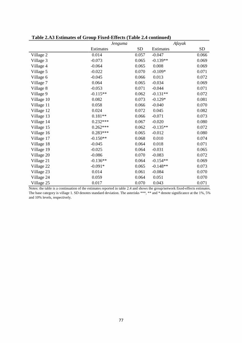
77

Table 2.A3 Estimates of Group Fixed-Effects (Table 2.4 continued)

Jenguma Afayak


Village 2 0.014 0.057 -0.047 0.066

Village 3 -0.073 0.065 -0.139** 0.069

Village 4 -0.064 0.065 0.008 0.069

Village 5 -0.022 0.070 -0.109* 0.071

Village 6 -0.045 0.066 0.013 0.072

Village 7 0.064 0.065 -0.034 0.069

Village 8 -0.053 0.071 -0.044 0.071

Village 9 -0.115** 0.062 -0.131** 0.072

Village 10 0.082 0.073 -0.129* 0.081

Village 11 0.058 0.066 -0.040 0.070

Village 12 0.024 0.072 0.045 0.082

Village 13 0.181** 0.066 -0.071 0.073

Village 14 0.232*** 0.067 -0.020 0.080

Village 15 0.262*** 0.062 -0.135** 0.072

Village 16 0.283*** 0.065 -0.012 0.080

Village 17 -0.150** 0.068 0.010 0.074

Village 18 -0.045 0.064 0.018 0.071

Village 19 -0.025 0.064 -0.031 0.065

Village 20 -0.086 0.070 -0.083 0.072

Village 21 -0.136** 0.064 -0.154** 0.069

Village 22 -0.091* 0.065 -0.148** 0.073

Village 23 0.014 0.061 -0.084 0.070

Village 24 0.059 0.064 0.051 0.070

Village 25 0.017 0.070 0.043 0.071

Notes: the table is a continuation of the estimates reported in table 2.4 and shows the group/network fixed-effects estimates.

The base category is village 1. SD denotes standard deviation. The asterisks ***, ** and * denote significance at the 1%, 5%

and 10% levels, respectively.

78

Appendix B: Network formation and endogeneity

2.B1. Network formation and endogeneity of neighbors’ adoption

The section describes the network formation model estimated and discussed under subsection

2.4.1. We estimated a conditional edge independence model, which assumes links form

independently, conditional on node- and link- level covariates (Fafchamps and Gubert 2007) as

follows;

𝐿𝑖𝑗,𝑔 = 𝛿0 + 𝛿1|𝑐𝑖𝑔 − 𝑐𝑗𝑔| + 𝛿2(𝑐𝑖𝑔 + 𝑐𝑗𝑔) + 𝛿3|ℒ𝑖𝑗𝑔| + 𝜖𝑖𝑗𝑔

where 𝐿𝑖𝑗𝑔 is an 𝑚𝑔 × (𝑚𝑔 − 1) matrix indicating whether there is a link between individuals

𝑖 and 𝑗 in group/village 𝑔 (𝑔 =1,…, 𝐺, and 𝐺 is the number of groups/villages in the sample),

𝑐𝑖𝑔 and 𝑐𝑗𝑔 are characteristics of individual 𝑖 and 𝑗 in group 𝑔. 𝛿1 measures the influence of

differences in their attributes, and 𝛿2 measures the effect of combined level of their attributes.

ℒ𝑖𝑗𝑔 captures attributes of the link between 𝑖 and 𝑗 such as geographical or social distance

between them, and 𝛿3 is the associated parameter estimate. The estimates of this model are

reported in Table 2.B1. We next use the average of the predicted residuals of this link formation

model as control functions in our adoption equation to account for the endogeneity of peer

effects due to unobserved factors that determine link formation.

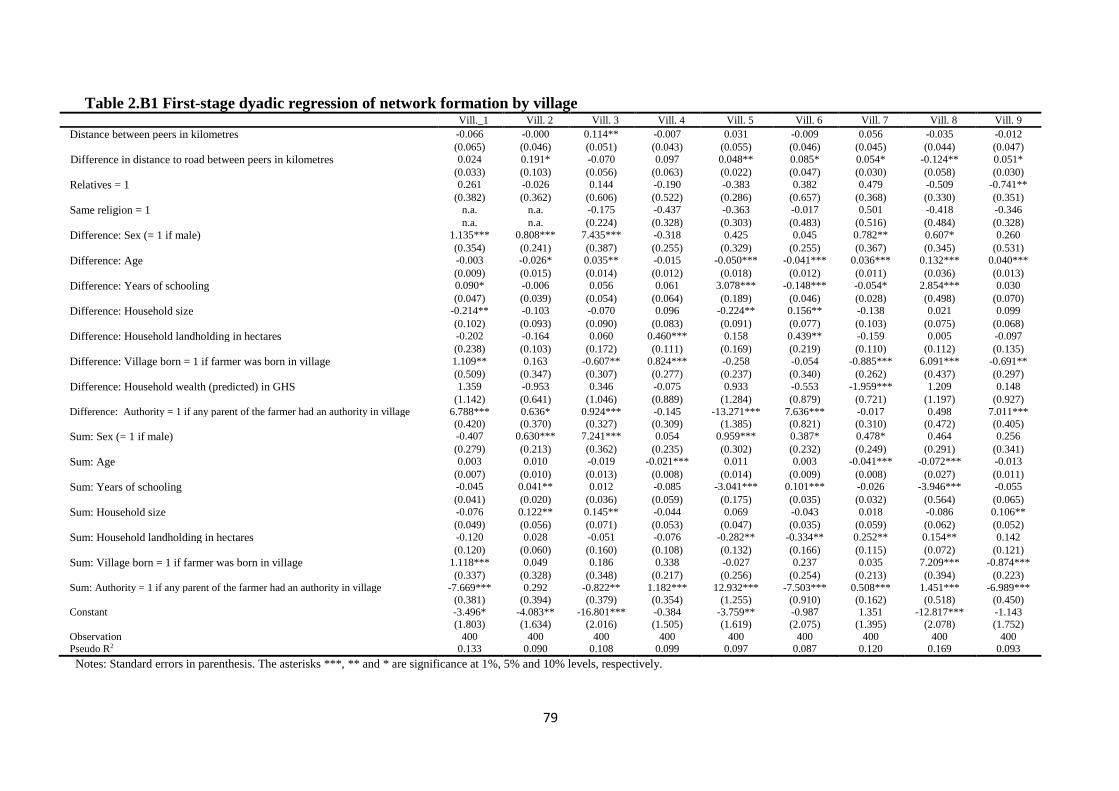
79

Table 2.B1 First-stage dyadic regression of network formation by village Vill._1 Vill. 2 Vill. 3 Vill. 4 Vill. 5 Vill. 6 Vill. 7 Vill. 8 Vill. 9

Distance between peers in kilometres -0.066 -0.000 0.114** -0.007 0.031 -0.009 0.056 -0.035 -0.012

(0.065) (0.046) (0.051) (0.043) (0.055) (0.046) (0.045) (0.044) (0.047)

Difference in distance to road between peers in kilometres 0.024 0.191* -0.070 0.097 0.048** 0.085* 0.054* -0.124** 0.051*

(0.033) (0.103) (0.056) (0.063) (0.022) (0.047) (0.030) (0.058) (0.030)

Relatives = 1 0.261 -0.026 0.144 -0.190 -0.383 0.382 0.479 -0.509 -0.741**

(0.382) (0.362) (0.606) (0.522) (0.286) (0.657) (0.368) (0.330) (0.351)

Same religion = 1 n.a. n.a. -0.175 -0.437 -0.363 -0.017 0.501 -0.418 -0.346

n.a. n.a. (0.224) (0.328) (0.303) (0.483) (0.516) (0.484) (0.328)

Difference: Sex (= 1 if male) 1.135*** 0.808*** 7.435*** -0.318 0.425 0.045 0.782** 0.607* 0.260

(0.354) (0.241) (0.387) (0.255) (0.329) (0.255) (0.367) (0.345) (0.531)

Difference: Age -0.003 -0.026* 0.035** -0.015 -0.050*** -0.041*** 0.036*** 0.132*** 0.040***

(0.009) (0.015) (0.014) (0.012) (0.018) (0.012) (0.011) (0.036) (0.013)

Difference: Years of schooling 0.090* -0.006 0.056 0.061 3.078*** -0.148*** -0.054* 2.854*** 0.030

(0.047) (0.039) (0.054) (0.064) (0.189) (0.046) (0.028) (0.498) (0.070)

Difference: Household size -0.214** -0.103 -0.070 0.096 -0.224** 0.156** -0.138 0.021 0.099

(0.102) (0.093) (0.090) (0.083) (0.091) (0.077) (0.103) (0.075) (0.068)

Difference: Household landholding in hectares -0.202 -0.164 0.060 0.460*** 0.158 0.439** -0.159 0.005 -0.097

(0.238) (0.103) (0.172) (0.111) (0.169) (0.219) (0.110) (0.112) (0.135)

Difference: Village born = 1 if farmer was born in village 1.109** 0.163 -0.607** 0.824*** -0.258 -0.054 -0.885*** 6.091*** -0.691**

(0.509) (0.347) (0.307) (0.277) (0.237) (0.340) (0.262) (0.437) (0.297)

Difference: Household wealth (predicted) in GHS 1.359 -0.953 0.346 -0.075 0.933 -0.553 -1.959*** 1.209 0.148

(1.142) (0.641) (1.046) (0.889) (1.284) (0.879) (0.721) (1.197) (0.927)

Difference: Authority = 1 if any parent of the farmer had an authority in village 6.788*** 0.636* 0.924*** -0.145 -13.271*** 7.636*** -0.017 0.498 7.011***

(0.420) (0.370) (0.327) (0.309) (1.385) (0.821) (0.310) (0.472) (0.405)

Sum: Sex (= 1 if male) -0.407 0.630*** 7.241*** 0.054 0.959*** 0.387* 0.478* 0.464 0.256

(0.279) (0.213) (0.362) (0.235) (0.302) (0.232) (0.249) (0.291) (0.341)

Sum: Age 0.003 0.010 -0.019 -0.021*** 0.011 0.003 -0.041*** -0.072*** -0.013

(0.007) (0.010) (0.013) (0.008) (0.014) (0.009) (0.008) (0.027) (0.011)

Sum: Years of schooling -0.045 0.041** 0.012 -0.085 -3.041*** 0.101*** -0.026 -3.946*** -0.055

(0.041) (0.020) (0.036) (0.059) (0.175) (0.035) (0.032) (0.564) (0.065)

Sum: Household size -0.076 0.122** 0.145** -0.044 0.069 -0.043 0.018 -0.086 0.106**

(0.049) (0.056) (0.071) (0.053) (0.047) (0.035) (0.059) (0.062) (0.052)

Sum: Household landholding in hectares -0.120 0.028 -0.051 -0.076 -0.282** -0.334** 0.252** 0.154** 0.142

(0.120) (0.060) (0.160) (0.108) (0.132) (0.166) (0.115) (0.072) (0.121)

Sum: Village born = 1 if farmer was born in village 1.118*** 0.049 0.186 0.338 -0.027 0.237 0.035 7.209*** -0.874***

(0.337) (0.328) (0.348) (0.217) (0.256) (0.254) (0.213) (0.394) (0.223)

Sum: Authority = 1 if any parent of the farmer had an authority in village -7.669*** 0.292 -0.822** 1.182*** 12.932*** -7.503*** 0.508*** 1.451*** -6.989***

(0.381) (0.394) (0.379) (0.354) (1.255) (0.910) (0.162) (0.518) (0.450) Constant -3.496* -4.083** -16.801*** -0.384 -3.759** -0.987 1.351 -12.817*** -1.143

(1.803) (1.634) (2.016) (1.505) (1.619) (2.075) (1.395) (2.078) (1.752)

Observation 400 400 400 400 400 400 400 400 400 Pseudo R2 0.133 0.090 0.108 0.099 0.097 0.087 0.120 0.169 0.093

Notes: Standard errors in parenthesis. The asterisks ***, ** and * are significance at 1%, 5% and 10% levels, respectively.

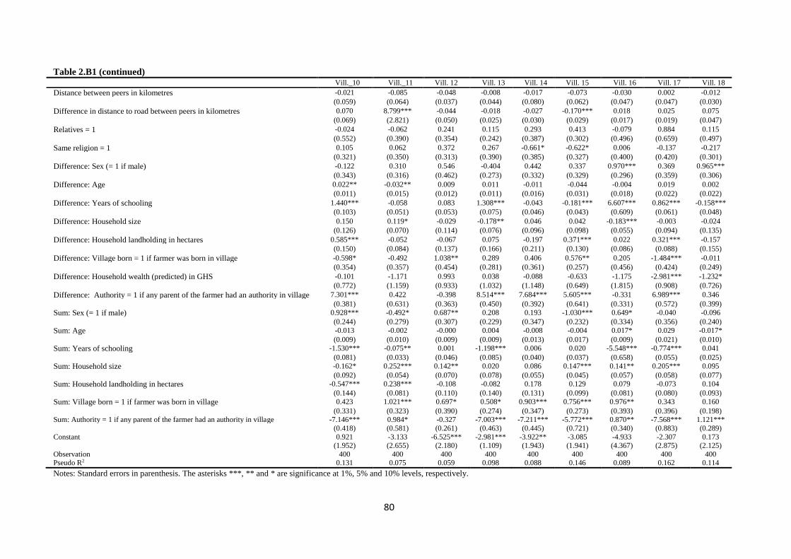
80

Table 2.B1 (continued) Vill._10 Vill._11 Vill. 12 Vill. 13 Vill. 14 Vill. 15 Vill. 16 Vill. 17 Vill. 18

Distance between peers in kilometres -0.021 -0.085 -0.048 -0.008 -0.017 -0.073 -0.030 0.002 -0.012

(0.059) (0.064) (0.037) (0.044) (0.080) (0.062) (0.047) (0.047) (0.030)

Difference in distance to road between peers in kilometres 0.070 8.799*** -0.044 -0.018 -0.027 -0.170*** 0.018 0.025 0.075

(0.069) (2.821) (0.050) (0.025) (0.030) (0.029) (0.017) (0.019) (0.047)

Relatives = 1 -0.024 -0.062 0.241 0.115 0.293 0.413 -0.079 0.884 0.115

(0.552) (0.390) (0.354) (0.242) (0.387) (0.302) (0.496) (0.659) (0.497)

Same religion = 1 0.105 0.062 0.372 0.267 -0.661* -0.622* 0.006 -0.137 -0.217

(0.321) (0.350) (0.313) (0.390) (0.385) (0.327) (0.400) (0.420) (0.301)

Difference: Sex (= 1 if male) -0.122 0.310 0.546 -0.404 0.442 0.337 0.970*** 0.369 0.965***

(0.343) (0.316) (0.462) (0.273) (0.332) (0.329) (0.296) (0.359) (0.306)

Difference: Age 0.022** -0.032** 0.009 0.011 -0.011 -0.044 -0.004 0.019 0.002

(0.011) (0.015) (0.012) (0.011) (0.016) (0.031) (0.018) (0.022) (0.022)

Difference: Years of schooling 1.440*** -0.058 0.083 1.308*** -0.043 -0.181*** 6.607*** 0.862*** -0.158***

(0.103) (0.051) (0.053) (0.075) (0.046) (0.043) (0.609) (0.061) (0.048)

Difference: Household size 0.150 0.119* -0.029 -0.178** 0.046 0.042 -0.183*** -0.003 -0.024

(0.126) (0.070) (0.114) (0.076) (0.096) (0.098) (0.055) (0.094) (0.135)

Difference: Household landholding in hectares 0.585*** -0.052 -0.067 0.075 -0.197 0.371*** 0.022 0.321*** -0.157

(0.150) (0.084) (0.137) (0.166) (0.211) (0.130) (0.086) (0.088) (0.155)

Difference: Village born = 1 if farmer was born in village -0.598* -0.492 1.038** 0.289 0.406 0.576** 0.205 -1.484*** -0.011

(0.354) (0.357) (0.454) (0.281) (0.361) (0.257) (0.456) (0.424) (0.249)

Difference: Household wealth (predicted) in GHS -0.101 -1.171 0.993 0.038 -0.088 -0.633 -1.175 -2.981*** -1.232*

(0.772) (1.159) (0.933) (1.032) (1.148) (0.649) (1.815) (0.908) (0.726)

Difference: Authority = 1 if any parent of the farmer had an authority in village 7.301*** 0.422 -0.398 8.514*** 7.684*** 5.605*** -0.331 6.989*** 0.346

(0.381) (0.631) (0.363) (0.450) (0.392) (0.641) (0.331) (0.572) (0.399)

Sum: Sex (= 1 if male) 0.928*** -0.492* 0.687** 0.208 0.193 -1.030*** 0.649* -0.040 -0.096

(0.244) (0.279) (0.307) (0.229) (0.347) (0.232) (0.334) (0.356) (0.240)

Sum: Age -0.013 -0.002 -0.000 0.004 -0.008 -0.004 0.017* 0.029 -0.017*

(0.009) (0.010) (0.009) (0.009) (0.013) (0.017) (0.009) (0.021) (0.010)

Sum: Years of schooling -1.530*** -0.075** 0.001 -1.198*** 0.006 0.020 -5.548*** -0.774*** 0.041

(0.081) (0.033) (0.046) (0.085) (0.040) (0.037) (0.658) (0.055) (0.025)

Sum: Household size -0.162* 0.252*** 0.142** 0.020 0.086 0.147*** 0.141** 0.205*** 0.095

(0.092) (0.054) (0.070) (0.078) (0.055) (0.045) (0.057) (0.058) (0.077)

Sum: Household landholding in hectares -0.547*** 0.238*** -0.108 -0.082 0.178 0.129 0.079 -0.073 0.104

(0.144) (0.081) (0.110) (0.140) (0.131) (0.099) (0.081) (0.080) (0.093)

Sum: Village born = 1 if farmer was born in village 0.423 1.021*** 0.697* 0.508* 0.903*** 0.756*** 0.976** 0.343 0.160

(0.331) (0.323) (0.390) (0.274) (0.347) (0.273) (0.393) (0.396) (0.198)

Sum: Authority = 1 if any parent of the farmer had an authority in village -7.146*** 0.984* -0.327 -7.003*** -7.211*** -5.772*** 0.870** -7.568*** 1.121***

(0.418) (0.581) (0.261) (0.463) (0.445) (0.721) (0.340) (0.883) (0.289)

Constant 0.921 -3.133 -6.525*** -2.981*** -3.922** -3.085 -4.933 -2.307 0.173 (1.952) (2.655) (2.180) (1.109) (1.943) (1.941) (4.367) (2.875) (2.125)

Observation 400 400 400 400 400 400 400 400 400 Pseudo R2 0.131 0.075 0.059 0.098 0.088 0.146 0.089 0.162 0.114


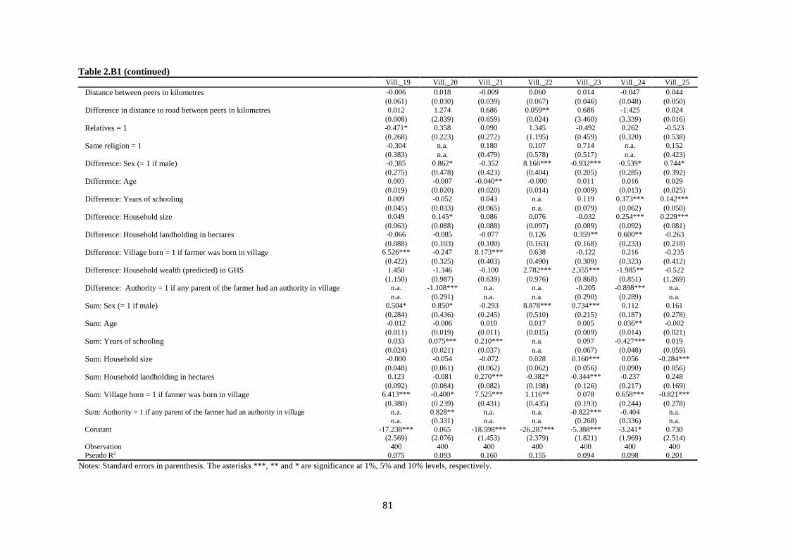
81

Table 2.B1 (continued) Vill._19 Vill._20 Vill._21 Vill._22 Vill._23 Vill._24 Vill._25

Distance between peers in kilometres -0.006 0.018 -0.009 0.060 0.014 -0.047 0.044

(0.061) (0.030) (0.039) (0.067) (0.046) (0.048) (0.050)

Difference in distance to road between peers in kilometres 0.012 1.274 0.686 0.059** 0.686 -1.425 0.024

(0.008) (2.839) (0.659) (0.024) (3.460) (3.339) (0.016)

Relatives = 1 -0.471* 0.358 0.090 1.345 -0.492 0.262 -0.523

(0.268) (0.223) (0.272) (1.195) (0.459) (0.320) (0.538)

Same religion = 1 -0.304 n.a. 0.180 0.107 0.714 n.a. 0.152

(0.383) n.a. (0.479) (0.578) (0.517) n.a. (0.423)

Difference: Sex (= 1 if male) -0.385 0.862* -0.352 8.166*** -0.932*** -0.539* 0.744*

(0.275) (0.478) (0.423) (0.404) (0.205) (0.285) (0.392)

Difference: Age 0.003 -0.007 -0.040** -0.000 0.011 0.016 0.029

(0.019) (0.020) (0.020) (0.014) (0.009) (0.013) (0.025)

Difference: Years of schooling 0.009 -0.052 0.043 n.a. 0.119 0.373*** 0.142***

(0.045) (0.033) (0.065) n.a. (0.079) (0.062) (0.050)

Difference: Household size 0.049 0.145* 0.086 0.076 -0.032 0.254*** 0.229***

(0.063) (0.088) (0.088) (0.097) (0.089) (0.092) (0.081)

Difference: Household landholding in hectares -0.066 -0.085 -0.077 0.126 0.359** 0.600** -0.263

(0.088) (0.103) (0.100) (0.163) (0.168) (0.233) (0.218)

Difference: Village born = 1 if farmer was born in village 6.526*** -0.247 8.173*** 0.638 -0.122 0.216 -0.235

(0.422) (0.325) (0.403) (0.490) (0.309) (0.323) (0.412)

Difference: Household wealth (predicted) in GHS 1.450 -1.346 -0.100 2.782*** 2.355*** -1.985** -0.522

(1.150) (0.987) (0.639) (0.976) (0.868) (0.851) (1.269)

Difference: Authority = 1 if any parent of the farmer had an authority in village n.a. -1.108*** n.a. n.a. -0.205 -0.898*** n.a.

n.a. (0.291) n.a. n.a. (0.290) (0.289) n.a.

Sum: Sex (= 1 if male) 0.504* 0.850* -0.293 8.878*** 0.734*** 0.112 0.161

(0.284) (0.436) (0.245) (0.510) (0.215) (0.187) (0.278)

Sum: Age -0.012 -0.006 0.010 0.017 0.005 0.036** -0.002

(0.011) (0.019) (0.011) (0.015) (0.009) (0.014) (0.021)

Sum: Years of schooling 0.033 0.075*** 0.210*** n.a. 0.097 -0.427*** 0.019

(0.024) (0.021) (0.037) n.a. (0.067) (0.048) (0.059)

Sum: Household size -0.000 -0.054 -0.072 0.028 0.160*** 0.056 -0.284***

(0.048) (0.061) (0.062) (0.062) (0.056) (0.090) (0.056)

Sum: Household landholding in hectares 0.123 -0.081 0.270*** -0.382* -0.344*** -0.237 0.248

(0.092) (0.084) (0.082) (0.198) (0.126) (0.217) (0.169)

Sum: Village born = 1 if farmer was born in village 6.413*** -0.400* 7.525*** 1.116** 0.078 0.658*** -0.821***

(0.380) (0.239) (0.431) (0.435) (0.193) (0.244) (0.278) Sum: Authority = 1 if any parent of the farmer had an authority in village n.a. 0.828** n.a. n.a. -0.822*** -0.404 n.a.

n.a. (0.331) n.a. n.a. (0.268) (0.336) n.a.

Constant -17.238*** 0.065 -18.598*** -26.287*** -5.388*** -3.241* 0.730 (2.569) (2.076) (1.453) (2.379) (1.821) (1.969) (2.514)

Observation 400 400 400 400 400 400 400

Pseudo R2 0.075 0.093 0.160 0.155 0.094 0.098 0.201


82

Table 2.B2 Instrumenting regression for Wealth in Dyadic model Difference of wealth Sum of wealth

Coefficient Robust

S. E.

Dyadic

S. E.

Coefficient Robust

S. E.

Dyadic

S. E.

All regressors as difference All regressors as sums

Sex = 1 if male 0.080 0.036 0.086 -0.237* 0.034 0.154

Years of education of farmer -0.026** 0.004 0.010 -0.040** 0.004 0.017

Born = 1 if born in village -0.106* 0.036 0.069 0.200* 0.034 0.144

Value of inherited land in GHS 0.277*** 0.040 0.089 0.925*** 0.048 0.142

District dummies

1 if farmer resides in district 1 -0.322 0.052 0.262 -0.552* 0.066 0.397

1 if farmer resides in district 2 -0.493** 0.051 0.257 -0.757** 0.066 0.405

1 if farmer resides in district 3 0.298 0.068 0.327 0.429 0.090 0.539

1 if farmer resides in district 4 -0.150 0.082 0.426 -0.369 0.097 0.560

Intercept 1.488*** 0.056 0.214 2.614*** 0.088 0.429

Observations 9500 9500

Notes: the table presents first-stage estimates for instrumenting wealth in the dyadic link formation model. Columns 1, 2 and

3 present results for the difference of wealth between neighbors. Columns 4, 5 and 6 show results of the sum of wealth

estimates. The table also show both the conventional robust standard errors (in columns 2 and 5) and the Fafchamps and Gubert

(2007) group dyadic standard errors (columns 3 and 6). The asterisks ***, ** and * are significance at 1%, 5% and 10% levels,

respectively.

83

2.B2. Endogeneity of other covariates

The variables credit-constrained, extension contact and non-governmental/research

organization (NGO/Res) are potentially endogenous in the specification. In particular, credit-

constrained could be endogenous because adopters of the improved varieties could be farmers

with higher yields and incomes, which provide them an urge in acquiring collaterals and in

meeting minimum savings requirements for accessing credit. Endogeneity of extension and

NGO/Res contacts could result from the fact that extension and NGO/Res officers visit farmers

because they adopted the improved varieties. These potential endogeneity concerns were

addressed through a two-stage generalized residual inclusion estimation procedure suggested

by Wooldridge (2015). We first estimate a probit model for each of the endogenous variables

with a set of explanatory variables and at least an instrument that highly explains these

endogenous variables, but indirectly affects adoption.

The generalized residuals for the first-stage probit estimates are then plugged into the second-

stage adoption equation to account for potential endogeneity of these variables. This approach

provides an optimal test of the null hypothesis that the potential endogenous variable is

exogenous and also makes it possible to consistently estimate the average structural model by

averaging out the generalized errors (Wooldridge, 2015). The first-stage estimates are reported

in Table 2.B3. In the credit constraint equation, distance to the nearest financial institution was

used as an instrument, which affects access to credit, but not the decision to adopt the

technology. With regard to the extension and NGO/Research contacts equations, we employed

distance to the nearest extension office and distance to the nearest NGO/Research station,

respectively, as instruments, which affect extension and NGO/Research contacts but not

adoption of the technology directly. These instruments were excluded from the second-stage

estimation to ensure identification in the estimation of the adoption (structural) equation.

84

Table 2.B3 First-stage probit estimates for liquidity constraint, extension and

NGO/Research equations Variable Model (1) Model (2) Model (3)

Credit constraint Extension contact NGO/Res contact

Coefficient Std

Error

Coefficient Std

Error

Coefficient Std

Error

Constant 4.752*** 1.015 -4.132*** 1.147 -3.759*** 1.218

Own characteristics

Age -0.001 0.006 0.014** 0.006 0.005 0.007

Gender -0.363** 0.157 0.165 0.185 0.040 0.196

Education -0.061 0.044 0.042 0.031 0.046 0.035

Experience -0.084*** 0.030 0.005 0.026 0.098*** 0.029

Household 0.046 0.036 -0.023 0.042 -0.066 0.047

Landholding -0.045 0.062 0.037 0.064 0.117 0.075

Risk 0.117** 0.055 -0.023 0.064 -0.032 0.071

Association -0.238*** 0.067 -0.005 0.078 -0.277*** 0.094

Electronic 0.001 0.209 -0.049 0.217 0.006 0.263

Soil quality -0.178** 0.084 -0.031 0.094 0.068 0.101

Price -1.199* 0.634 1.865*** 0.636 0.132 0.672

Credit - - -0.699*** 0.192 0.027 0.226

Extension -0.382 0.409 - - 0.364** 0.152

NGO/Res -0.055 0.214 0.546*** 0.197 - -

Contextual effects

Age -0.003 0.003 0.004* 0.002 0.003 0.003

Gender -0.048 0.069 0.024 0.074 0.124 0.092

Education -0.006 0.016 0.010 0.013 0.012 0.017

Experience -0.001 0.013 -0.002 0.015 0.011 0.015

Household 0.019 0.017 0.013 0.022 -0.044* 0.023

Landholding -0.019 0.026 0.018 0.028 0.085*** 0.028

Risk 0.011 0.028 -0.035 0.036 -0.184*** 0.046

Association -0.005 0.028 -0.010 0.028 -0.035 0.033

Electronic -0.096 0.111 -0.025 0.151 0.056 0.128

Soil quality -0.074** 0.035 -0.022 0.042 0.022 0.043

Price -0.831 0.802 0.621 0.782 2.014** 0.893

Credit - - -0.255*** 0.082 0.043 0.097

Extension -0.318 0.494 - - 0.132** 0.059

NGO/Res 0.046 0.086 -0.025 0.089 - -

Instruments

FinDistance -0.037*** 0.012 - - - -

ExtDistance - - -0.032*** 0.011 - -

RNDistance - - - - -0.090*** 0.013

Pseudo 2

R 0.378 0.391 0.425

Loglikelihood -205.0 -170.2 -145.3

LR 2

X 249.1 218.2 215.3

Prob 2

X 0.000 0.000 0.000

Notes: table reports first-stage instrumenting probit estimates of household credit constraints in model (1), extension contact

in model (2) and NGO/Research agent contact in model (3). The predicted generalized residuals of these models were used to

account for the potential endogeneity of household credit constrains (Residliquid), extension contact (Residextens) and

NGO/Research agent contact (ResidNGO). Std Error denotes standard error. The asterisks ***, ** and * denote significance

at the 1%, 5% and 10% levels, respectively.

85

Appendix C

Bayesian Estimation Procedure

Conditional distribution of and

Let’s assume an independent normal-Wishart prior for the and Σ parameters, a uniform

prior for and consequently given that the conditional and prior distributions of come from

the same distribution type with updated parameters (Wang et al. 2014), the normal prior of

can be set as ~ , MVN b B . This allows the conditional posterior distribution of to be

expressed as:

* *( | , , Σ) | , , ΣYp Y p

(C1) 1 1 , ( ) , TMVN H X H H MVN b B

, ΣMVN

where 1 ' *Σˆ B b X H Y ; kVH I W ; 1 1Σ X X B

and X is a vector

representing all other controls in equation (6).

Uninformative prior mean distribution 0b and a diffuse prior variance 1 12B e for

were used to avoid biasing estimates and inferences by assuming high prior information.

LeSage and Pace (2009) also show that assuming non-informative and diffuse priors in

sufficiently large samples produce estimates comparable to those obtained from maximum

likelihood. The sampling of the posterior conditional distribution of can be done either by

Metropolis-Hasting (M-H) or by integration and draw by inversion approach (see LeSage and

Pace 2009, chapter 5). The use of these procedures are necessitated by the fact that conditional

posterior distribution of doesn’t lend itself to a known standard distribution like and Σ

86

(Autant-Bernard et al., 2008). Given that the posterior distribution of ij relies on its Beta prior

function of p , the posterior distribution of is expressed as;

(C2) 1

'* * ' *2

1( | , , Σ, )

2ij ijp Y H exp HY X H H HY X p

,

where ij

is a matrix except the ij th element. For the M-H sampling, we require a proposal

distribution from which a potential value for the parameter is to be obtained. This potential

parameter is labeled as * . An acceptable probability for drawing based on a random walk

from a standard normal distribution is computed in equation (C2) using the * , a current value

of defined as P and a tuning parameter T suggested by Holloway et al (2002). The

proposal distribution is expressed as;

(C3) * ~ 0,1P T N .

The tuning of the proposal distribution from the normal distribution is to enable the M-H

sampling process goes through the whole conditional distribution in order for the proposal

distribution to yield draws that are within the dense part of the distribution (LeSage and Pace,

2009). This process is done on each pass of the MCMC sampling steps. Following, Autant-

Bernard et al. (2008), the log-determinant of H was computed with the lattice of values for

, in the feasible range of – 1 and 1, and with the direct sparse matrix LU decomposition

procedure.

Conditional distribution of and *Y

In this study, Σ is restricted to equal VI following LeSage and Pace (2009) because the cross-

choice dependence is being captured in the mean part instead of in the covariance structure of

the model reducing the number of parameters to be estimated. Hence, the variance-covariance

87

matrix also becomes 1

'Ω H H

which is used in the n-steps of the Gibbs sampling

procedure. The latent *Y is the terminal draw to be done and each *Y can be drawn distinctly

given that the observations are considered independent (Autant-Bernard et al. 2008; Wang et

al., 2014). The *Y variable has a conditional distribution which is multivariate normal

truncated14 (Geweke 1991). This takes the form as follows with a mean of and variance-

covariance matrix of . as;

(A4) 1

* 1 '~ , TMVN H X H HY

,

* ~ , TMVY N

subject to the constraint *a dY b where d is the diagonal of an kJ kJ block diagonal

matrix limiting jiY to assume the largest value of *Y if

jiY j or assumes negative if max(

) 0jiY , 1H X , 1

'H H

and a and b are the truncation bounds which depends on

the observed 0,1 values of y . Autant-Bernard et al. (2008) and LeSage and Pace (2009)

modified the Geweke (1991)15 n-step Gibbs sampler for a multinomial setting to generate draws

of kJ variate truncated normal distribution. The procedure uses a precision matrix

' 1Td H Hd with dimensions kJ kJ to sequentially generate draws from the transformed

normal distribution ~ 0, u N subject to the constraint *b z b , where

; b a d b b d and the *z samples are used to produce * 1 *d zY . Following

14 Note the observed response values are such that

iY j if *

,i VY * *

,1 , max , , 0i i VY Y and 0 if *

,0 0iY .

15 Geweke (1991) shows that drawing from * ~ , Y TMVN subject to *a Y b is equivalent to

generating draws from n-variate normal distribution * ~ , z N subject to the linear restriction

*b z b .

88

Wang et al. (2014), *

iz is expressed as a weighted average of the other elements ( *

iz ) plus a

noise tem as;

(A5) * *kV

i i i i i

i

z z V u

,

subject to the constraint * */ ) /nV nV

i i i i i i i i i

i i

b z V u b z V

, where 1

i i i ,

and 12

i iV

. Each pass of the entire n passes samples one element of * iz which is

conditional on the rest of the *

iz ’s and this continues until all the kV *

iz ’s are sampled with

the last pass of *

iz used to impute the *Y using the * 1 *d zY equality. A value of n = 10

was used because Geweke (1991) indicated that even relatively small values of n can produce

fairly desirable estimate.

89

Chapter Three

Social Learning and the Acquisition of Information and Knowledge - A Network

Approach for the Case of Technology Adoption

Yazeed Abdul Mumina, Awudu Abdulaia and Renan Goetzb

1. Department of Food Economics and Consumption Studies, University of Kiel, Germany.

2. Department of Economics, University of Girona, Spain.

This paper was submitted to Quantitative Economics

Abstract

The complexity of agricultural innovations and heterogeneity of circumstances of technology

application, outcomes and social network structures have often led to obstacles in social

learning and sub-optimal adoption. This paper examines technology diffusion in the context of

heterogeneous peer benefits, know-how and network structures, using survey data of 500 farm

households in Northern Ghana and random matching within sampling to generate social

network contacts. We identify network effects and the impact of social learning on adoption,

using a selectivity control function in a discrete survival model. Our results reveal that social

learning favors adoption, if past adopters with increased yields, or even more with profound

knowledge of the cultivation techniques form part of the social network. We also find that

social learning and the likelihood of adoption is higher when peers are central nodes, and

particularly, when they belong to cohesive subgroups, but lower in highly segregated networks.

The results shed a new light on the role of central agents, since highly cohesive neighborhoods

seem to promote diffusion more in high modularity networks than central nodes.

JEL codes: C31, C35, C41, D83, O13, O33

Keywords: Benefits, Know-how, Social learning, Social network structures, Technology

diffusion

90

3.1 Introduction

Adoption of agricultural technologies is comparatively low in developing countries, with sub-

optimal adoption of these technologies by farmers, despite their potential benefits in improving

productivity and agricultural performance (Magnan et al. 2015). Available evidence shows that

improved crop varieties and other inputs have contributed between 40% to 100% increase in

farm yields and profits, food security and poverty gains in sub-Saharan Africa. In spite of these

noteworthy benefits, adoption levels of improved crop varieties in this region are comparatively

low compared to the rest of the world (Suri 2011; Walker et al. 2011). Walker et al. (2014)

estimate the mean level of adoption across 20 improved crop varieties at 35%, with two-thirds

of these crops falling below this mean level. Understanding the way and rationale behind

farmers’ adoption of these technologies is, therefore, important for economic policies meant to

promote agricultural productivity and household welfare through improved technologies.

Numerous studies have shown the significance of social interaction and learning in the

agricultural technology adoption literature, although the results have been mixed, with some

authors finding positive impacts of social learning on adoption (Foster and Rosenzweig 1995;

Munshi 2004; Bandiera and Rasul 2006; Conley and Udry 2010; Beaman et al. 2018), while a

few find no effects (e.g., Duflo, Kremer and Robinson 2011). One possibility of enhancing the

understanding of adoption in social interaction settings and, perhaps, resolving these

contrasting results is to move beyond the implicit assumption that farmers observe the field

trials of their neighbors with little friction in the flow of information (BenYishay and Mobarak

2018) to examine the roles of both benefits and know-how as well as network structures in

social learning, as these shape the learning process (Jackson et al. 2017; Nourani 2019).

The literature provides a number of explanations on how adoption decisions of neighbors,

heterogeneities cropping conditions and benefits (Foster and Rosenzweig 1995; Munshi 2004;

91

Conley and Udry 2010) influence social learning in technology adoption. More recently,

BenYishay and Mobarak (2018) and Beaman et al. (2018) considered the performance of

targeting strategies within networks. Specifically, BenYishay and Mobarak (2018) showed that

performance incentives and social identity of experimenting farmers are important, whereas

Beaman et al. (2018) found that it is the targeting strategy that matters in social learning. Less

is, however, known about the role of know-how (i.e., production process) of the technology16

in the social learning process and whether both benefits and/or know-how17 could play

important roles in the learning process, given the technological context.

Our study first explores the impact of know-how (i.e., knowledge on cultivating the crop) on

adoption of agricultural technologies, and whether given the technology and the social and

agronomic context, both benefits and knowledge among social network members matter in

social learning. Examining the roles of benefits and know-how are important in learning

because farmers decisions to invest in learning about a new technology, and whether to adopt

or not to, depend on the expected benefits, and the associated learning and investment costs of

the technology. When the learning and investment costs are higher than the expected benefits,

farmers may not be inclined to learn and/or adopt the new technology (Beaman et al. 2018;

Nourani, 2019). Thus, learning about benefits (i.e., expected profitability) and know-how are

important in understanding the diffusion process of new technologies18.

16 A notable exception is Beaman and Dillon (2018) who traced how knowledge is aggregated in a network based on the

social distance of a node to a central node, but did not examine how differences in the knowledge accumulated by network

members influences the decision of farmers in the adoption process.

17 Existing studies have either found learning about benefits for ease-to-use (Magnan et al. 2015) or know-how for hard-

to-use (Oster and Thornton 2012) technologies.

18 We conceptualize learning about the expected profitability as farmers’ beliefs about the benefits of the improved variety

which is based on the shares of past adopters among their peers. That is, farmers’ beliefs about profitability vary with the share

of adopting peers such that more adopting peers will stimulate beliefs that the expected benefit of the improved variety is high

and vice versa. Know-how is about farmers’ efforts to acquire knowledge about the production process, which involves cost

in time and commitment that decrease with increased learning opportunities from peers and own experimentation. That is,

learning opportunities (costs) about know-how increase (decrease) with increasing peer experience.

92

Furthermore, examining both benefits and know-how has context relevance for two reasons.

First, the technology (improved soybean variety) we consider has been introduced mainly to

enhance farmers’ incomes (MoFA 2017), but awareness and knowledge of farmers about the

returns are limited (AGRA-SSTP 2017). Second, many farmers are not aware of the standard

agronomic practices19 required for this variety in order to achieve the desired yields, which has

usually resulted in sub-optimal productivity, profitability and weak diffusion of the technology

(Goldsmith 2017). Existing evidence shows that the use of improved soybean seed is quite low,

and ranges between 16% and 33% of soybean farmers in Ghana (Dogbe et al. 2013). In such

setting, it is significant to highlight the differences in benefits and know-how regarding the

application of the innovation by network contacts and their relative roles in the diffusion of the

technology.

Our discussion so far assumes homogenous network structures and hence similar conditions of

learning across networks. However, social network structures play important roles in shaping

the nature of interaction within networks and neighborhoods, and have been shown to exert

overarching effects on many behavioral patterns and other economic outcomes (Jackson et al.

2017). Many studies have argued that network structures, such as transitivity20 and modularity,

play important roles in social interactions and influence patterns of behavior used as social

collateral (Karlan et al. 2009; Jackson et al. 2012), risk sharing (Ambrus et al. 2014; Alatas et

al. 2016), and diffusion processes (Bollobas 2001; Centola 2010; Jackson et al. 2017).

Transitivity or local cohesiveness/clustering coefficient measures how close the neighborhood

of a farmer is to being a complete network. Modularity measures the proportion of links that

19 These agronomic rules and regulations were spelt out by the inspectorate division of the Ministry of Food and Agriculture

(MoFA), Council for Scientific and Industrial Research (CSIR) and the Savannah Agricultural Research Institute (SARI).

20 Assortativity is a related structure which refers to the level of interconnectivity between agents with similar individual

or micro-scale network characteristics. We do not examine it in this study as it has been shown that high transitive networks

display high assortativity and thus are quite correlated (Foster et al. 2011).

93

lie within communities (i.e., components or segments) of a network minus the expected value

of the same quantity in a network where links were randomly generated (Jackson 2008). Higher

transitivity of a farmer’s neighborhood, and low modularity of a network will mean more

opportunities for the farmer to learn from peers and from different neighborhoods in the

network. Such opportunities can lead to reduced cost of learning and increase the possibility of

diffusion across the network. These two network characteristics are also very important for the

understanding of, and in policy design to support learning in social networks (Girvan and

Newman 2002).

This implies that the diffusion rate of a new technology will be different across communities,

if transitivity and modularity of the networks, which condition information externalities, vary

across these communities. For instance, if network structures exhibit the tendency to be less

transitive or highly modular, then there may be friction in the diffusion of information about

benefits and know-how of the technology through the social network, thereby reinforcing

differences in farmers’ response rates to the technology, even under uniform cultivation

conditions and benefits. Hence, higher transitivity (lower modularity) implies the possibility of

effective and efficient spread of information due to the increased number of alternative routes

information can take through the network.

In spite of the significance of these network structures, the empirical literature on social

learning and technology diffusion has focused on the role of central agents, with very few

studies providing evidence on the significance of transitivity and modularity. (Karlan et al.

2009; Beaman et al. 2018). In particular, Karlan et al. (2009) show that multiplicity of routes

associated with higher transitivity enhance the credibility of agents in a network, while Beaman

et al. (2018) demonstrate that understanding of aspects of an innovation that are particularly

difficult to learn requires several interactions among agents.

94

Our study relates to the existing literature on network characteristics, influence of central

agents21, technology conditions and adoption (Jackson et al. 2012; Beaman and Dillon 2018;

BenYishay and Mobarak 2018; Beaman, et al. 2018). However, the current study differs from

these previous studies because it examines the impact of transitivity and network modularity,

and how modularity influences the performance of other network characteristics such as

centrality and transitivity in the diffusion process. This is particularly significant, because the

effectiveness and efficiency of centrality in technology processes depend on the extent to which

modularity and cohesiveness of the neighborhood (transitivity) will allow for it.

Specifically, we use observational data from a recent survey of soybean farmers conducted in

Ghana to show how learning about benefits, know-how and network structures drive adoption

in a dynamic theoretical framework. We estimate the model with a two-step selectivity

approach of network formation and survival analysis to account for correlated unobservables

at the link formation level (Brock and Durlauf 2001), and to investigate the threats of

measurement errors due to missing network data issues (Chandrasekhar and Lewis 2016). The

estimation results suggest that both learning about benefits and know-how are important in

accelerating adoption, although the effects of know-how are higher when sufficient peers adopt

the improved variety in all specifications. We find the role of transitivity in the learning and

diffusion processes to be stronger, compared to centrality, but modularity tends to slow down

the diffusion process, and also limits the significance of both transitivity and centrality.

These results have the following policy implications. First, it will inform policymakers about

when to focus on promoting adoption, directly, through extension services, public learning

and/or training workshops – especially when the share of adopters is low –, and when to focus

21 Few other studies such as Krishnan and Sciubba (2009) considered network architecture among village labor-sharing

networks in explaining farm returns in Ethiopia, and Banerjee et al. (2013) focused on network centrality in microfinance.

95

on module bridging measure that indirectly promote adoption through increased interactions

between adopters and non-adopters, as well as across segments of the village. Second, our

findings on the relative importance of transitivity and centrality will help policymakers to

identify when to leverage influential nodes (centrality) or the cohesiveness of the neighborhood

(transitivity) in encouraging adoption under different complexities of the technology (Beaman

et al. 2018) and in socially structured settings. Finally, an analysis of modularity will show

whether specific biases and/or patterns exist in these villages in terms of social interactions and

structures (Jackson 2008; Jackson et al. 2017), which will be relevant in informing policy

intervention options. For example, the existence of such structures or biases in these villages,

when failed to be considered in policy intervention, could result in policy impacts focusing on

specific segments of the villages instead of the whole village.

The rest of this paper is organized as follows. Section 3.2 describes the context and the data.

Section 3.3 discusses the theoretical framework, showing the role of learning about expected

profitability, know-how and network structures on speed of adoption. The empirical model and

estimations are described in section 3.4. Section 3.5 presents the empirical results, whereas

section 3.6 concludes.


3.2.1 Context

We now describe the context of the technology in question and the data used. Soybean is

primarily a commercial crop mainly cultivated in the Northern, Upper East, Upper West and

Volta regions of Ghana, by smallholder farmers and under rain-fed conditions, with Northern

region alone producing 72% of the national output. The crop has very high local demand and

potential of increasing farmers’ incomes in Ghana (MoFA 2017). The compounded annual

growth in demand for the crop was recorded as 39% from 2008 to 2010, compared to 10.5%

96

and 6.3% for the other two legumes (cowpea and groundnut), respectively over the same period

(AGRA-SSTP 2017). However, the average yield of 1.68MT/ha has been described as below

the national achievable yields of 2.50 – 3.10MT/ha (CSIR-SARI 2013).

Realizing this, the Council for Scientific and Industrial Research (CSIR) and the Savanna

Agricultural Research Institute (SARI) developed and introduced the Jenguma variety, in 2003,

for adoption by farmers in order to circumvent the problems associated with the existing

traditional variety22. This improved variety has higher yield potential of over 2.0 MT/ha,

resistant to pod-shattering, matures about 35 days earlier, and is resistant to other agricultural

stress such as pests, diseases, low phosphorous soil and climatic variabilities (CSIR-SARI

2013). Although the crop was introduced primarily as a commercial crop meant to increase

smallholder farm profitability and incomes (MoFA 2017), there is lack of awareness and

certainty among farmers about the expected yields, market outlets and returns on investments

of this improved variety. This is due to limited investment in promotion events and lack of

continued campaign to demonstrate returns and profitability of this variety (AGRA-SSTP

2017).

Added to this is that cultivation of the improved variety requires adherence to the rules and

regulations of the inspectorate division of the Ministry of Food and Agriculture (MoFA) in

order to achieve potential high yields of 2MT/ha, and to reduce labor cost by about 20% of

total production cost. These requirements include planting depths, row-spacing, quantity of

seeds and timing of sowing, inoculant and phosphorus application, as well as timing of

harvesting and plant growth for effectiveness of other inputs and varietal suitability (Heatherly

and Elmore 2004). The discussion suggests that both knowledge of benefits and of the

22 The traditional variety, Salintuya, has been described as low yielding (about 1.0 MT/ha), early shattering of pods and

susceptible to disease and pests which sometimes lead to complete loss of the crop (Ampadu-Ameyaw et al. 2016).

97

production process are important, and therefore important for the analysis of their impact on

the diffusion of the variety.

3.2.2 Data

We describe our data, before moving to a formal discussion of the theoretical and econometric

aspects of social learning and social network structures. We conducted a survey of 500 farm

households in Northern Ghana between July and September 2017. Five districts were

purposively selected based on their intensity of soybean production23, and then 25 villages were

randomly selected across these districts, with the allocation of villages done in proportion to

the total households in each district. These villages are remote and small with less than 150

households in each. Given this, we randomly selected 20 household heads in each village, and

then used structured questionnaires to interview the primary decision makers in the households.

In addition, a detailed discussion using an interview guide was administered in each village to

a group of village leaders and/or representatives to obtain information on village

characteristics. The study combines modules of household characteristics, social networks and

agricultural production to construct pseudo-panel data for the analysis of timing of adoption of

the improved soybean variety.

Improved soybean adoption and household characteristics

In order to collect data on the year of adoption of the improved soybean variety by households,

we use a question that asked farmers to recall the year they adopted the improved variety.

Responses to this recall question was used to construct the time to adoption variable, 𝐴𝑖𝑡, of a

household. Table 3.1, panel A shows the summary statistics of adoption of the improved

variety by selected years, and depicts an increased adoption overtime since its introduction in

2003. Only 4% of farmers had adopted the improved variety among the sampled farmers in the

23 This was done in consultation with the Ministry of Food and Agriculture and Resilience in Northern Ghana (RING).

98

year of its introduction. By 2007, 28% of farmers had adopted. Adoption continued to increase

from 2007, and by 2012 and 2016, 56% and 67% of farmers had adopted the improved variety,

respectively. Whereas the percentage of adoption in 2012 is more than double that of the rate

in 2007, the percentage of adoption in 2016 suggests a slowdown in uptake of the improved

variety.

Table 3.1. Variable definition, measurement and descriptive statistics

Variables Definition and measurement Mean S.D.

Panel A

Dependent variable

Adopted by

2003 1 if the farmer adopted the improved variety in 2003; 0 censored 0.04 0.19

2007 1 if the farmer adopted the improved variety by 2007; 0 censored 0.28 0.45



Panel B: Control variables

Time-varying

Age in

2003 Age of farmer in 2003 (years) 30.03 12.04




Time-invariant

Gender 1 if male; 0 otherwise 0.59 0.49

Education Number of years in school 1.27 3.27

Experience Number of years in farming 13.06 4.02

Household Household size (No. of members) 5.64 2.14

Landholding Total land size of household (in hectares) 2.56 1.56

Credit 1 if farmer was credit constrained and/or not successful in applying for

credit; 0 otherwise

0.55 0.49

Risk Risk of food insecurity (No. of months household was food inadequate) 0.93 1.37

Extension 1 if ever had extension contact; 0 otherwise 0.34 0.47

Association No. of associations a farmer is a member 1.07 1.27

Price Soybean price in GHS/kg 1.06 0.19

Soil quality 4=fertile; 3=moderately fertile; 2=less fertile; and 1=infertile 2.97 0.97

Panel C

Instruments

G2Credit Proportion of peers of peers who are credit constrained 0.55 0.28

G2Extension Proportion of peers of peers who ever had extension contact 0.35 0.28

Notes: the table depicts the definition, measurement and descriptive statistics of farmers and households. Panel A shows

the proportion of adopting farmers across selected year. Panel B shows that of time-varying and time-invariant characteristics

of the sampled households whereas the descriptive statistics of instruments for the first-stage liquidity constraints and

extensions regressions are in panel C. S. D. denotes Standard deviation. G denotes the network.

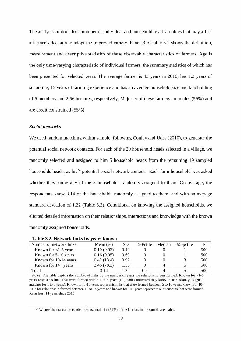
99

The analysis controls for a number of individual and household level variables that may affect

a farmer’s decision to adopt the improved variety. Panel B of table 3.1 shows the definition,

measurement and descriptive statistics of these observable characteristics of farmers. Age is

the only time-varying characteristic of individual farmers, the summary statistics of which has

been presented for selected years. The average farmer is 43 years in 2016, has 1.3 years of

schooling, 13 years of farming experience and has an average household size and landholding

of 6 members and 2.56 hectares, respectively. Majority of these farmers are males (59%) and

are credit constrained (55%).

Social networks

We used random matching within sample, following Conley and Udry (2010), to generate the

potential social network contacts. For each of the 20 household heads selected in a village, we

randomly selected and assigned to him 5 household heads from the remaining 19 sampled

households heads, as his24 potential social network contacts. Each farm household was asked

whether they know any of the 5 households randomly assigned to them. On average, the

respondents knew 3.14 of the households randomly assigned to them, and with an average

standard deviation of 1.22 (Table 3.2). Conditional on knowing the assigned households, we

elicited detailed information on their relationships, interactions and knowledge with the known

randomly assigned households.

Table 3.2. Network links by years known

Number of network links Mean (%) SD 5-Pctile Median 95-pctile N

Known for <1-5 years 0.10 (0.03) 0.49 0 0 1 500

Known for 5-10 years 0.16 (0.05) 0.60 0 0 1 500

Known for 10-14 years 0.42 (13.4) 0.97 0 0 3 500

Known for 14+ years 2.46 (78.3) 1.56 0 4 5 500

Total 3.14 1.22 0.5 4 5 500 Notes: The table depicts the number of links by the number of years the relationship was formed. Known for <1-5

years represents links that were formed within 1 to 5 years (i.e., nodes indicated they know their randomly assigned

matches for 1 to 5 years). Known for 5-10 years represents links that were formed between 5 to 10 years, known for 10-

14 is for relationship formed between 10 to 14 years and known for 14+ years represents relationships that were formed

for at least 14 years since 2016.

24 We use the masculine gender because majority (59%) of the farmers in the sample are males.

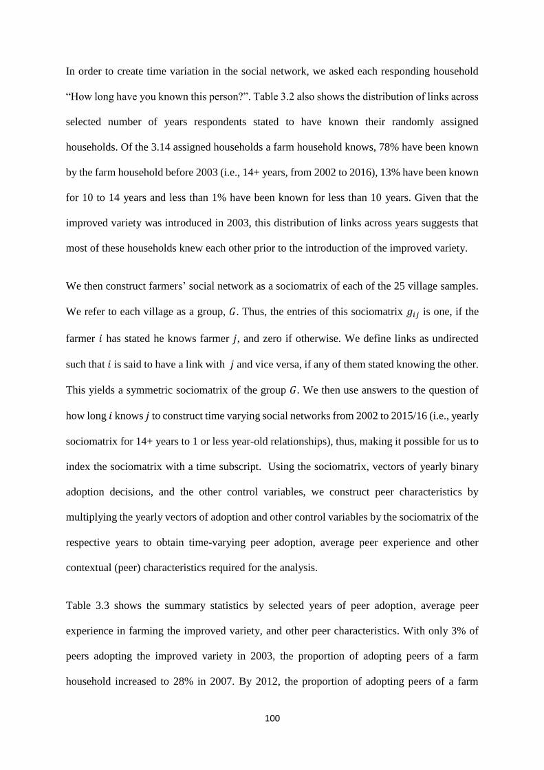
100

In order to create time variation in the social network, we asked each responding household

“How long have you known this person?”. Table 3.2 also shows the distribution of links across

selected number of years respondents stated to have known their randomly assigned

households. Of the 3.14 assigned households a farm household knows, 78% have been known

by the farm household before 2003 (i.e., 14+ years, from 2002 to 2016), 13% have been known

for 10 to 14 years and less than 1% have been known for less than 10 years. Given that the

improved variety was introduced in 2003, this distribution of links across years suggests that

most of these households knew each other prior to the introduction of the improved variety.

We then construct farmers’ social network as a sociomatrix of each of the 25 village samples.

We refer to each village as a group, 𝐺. Thus, the entries of this sociomatrix 𝑔𝑖𝑗 is one, if the

farmer 𝑖 has stated he knows farmer 𝑗, and zero if otherwise. We define links as undirected

such that 𝑖 is said to have a link with 𝑗 and vice versa, if any of them stated knowing the other.

This yields a symmetric sociomatrix of the group 𝐺. We then use answers to the question of

how long 𝑖 knows 𝑗 to construct time varying social networks from 2002 to 2015/16 (i.e., yearly

sociomatrix for 14+ years to 1 or less year-old relationships), thus, making it possible for us to

index the sociomatrix with a time subscript. Using the sociomatrix, vectors of yearly binary

adoption decisions, and the other control variables, we construct peer characteristics by

multiplying the yearly vectors of adoption and other control variables by the sociomatrix of the

respective years to obtain time-varying peer adoption, average peer experience and other

contextual (peer) characteristics required for the analysis.

Table 3.3 shows the summary statistics by selected years of peer adoption, average peer

experience in farming the improved variety, and other peer characteristics. With only 3% of

peers adopting the improved variety in 2003, the proportion of adopting peers of a farm

household increased to 28% in 2007. By 2012, the proportion of adopting peers of a farm

101

household increased to 57%, and subsequently increased to 68% by 2016. Similarly, the

average peer experience witnessed an increasing trend over time.

Table 3.3. Contextual (peer) characteristics

Time-varying variables Characteristics by year of network

2003 2007 2012 2016

A. Learning mechanism

Average adopting peers

0.03

(0.11)

0.28

(0.33)

0.57

(0.39)

0.68

(0.40)

Average peer experience

0.17

(0.45)

0.99

(1.41)

2.30

(1.84)

2.79

(1.87)

B. Other peer characteristics

Average peer age

29.86

(7.16)

34.86

(7.16)

39.86

(7.16)

43.86

(7.16)

Average peer education

1.59

(2.47)

1.59

(2.34)

1.58

(2.29)

1.58

(2.24)

Average peer household size

5.74

(1.50)

5.72

(1.42)

5.73

(1.39)

5.74

(1.38)

Average peer landholding

2.67

(1.10)

2.66

(1.04)

2.66

(1.02)

2.66

(1.01)

Average peer risk of food insecurity

0.78

(0.85)

0.76

(0.79)

0.81

(0.91)

0.76

(0.78)

Average peer group associations

1.18

(0.91)

1.19

(0.85)

1.20

(0.84)

1.21

(0.83)

Average peer soil quality

2.97

(0.68)

2.99

(0.65)

2.99

(0.65)

2.99

(0.65)

Proportion of male peers

0.66

(0.33)

0.65

(0.32)

0.65

(0.31)

0.64

(0.30)

Proportion of liquidity constraint peers

0.49

(0.35)

0.49

(0.33)

0.49

(0.32)

0.49

(0.32

Proportion of peers with extension contact

0.41

(0.35)

0.41

(0.32)

0.42

(0.32)

0.42

(0.32) Notes: the table presents descriptive statistics of time-varying household variables in panel A, and that for peer

characteristics constructed based on the networks defined using the number of years the agent indicated to have known

the peer, in panel B. Columns 2003 to 2016 represent characteristics of households and peers as at the years 2003,

2007, 2012 and 2016 (for the peer characteristics, these are based on the relationships that existed prior to 2003, i.e., J

known for 14+ years; 2007 – J known for 10-14 years; 2012 – J known for 5-10 years; and 2016 – J known for <1-5

years. Each of the contextual (peer) characteristic value was obtained by multiplying the respective variable by the D

to obtain the value of an agents’ peer characteristics in respect of each of these variables. Values in parenthesis are

standard deviations.

We also constructed social network statistics at the individual level (i.e., degree, transitivity

and eigenvector centrality)25 as the effects of these statistics on time-to-adoption are important

in this study. Panel A of table 3.4 presents the descriptive statistics of these across selected

years. The average number of connections (degree) an individual has increases from 3, for the

25 See Appendix A for the calculation of these statistics.

102

14+ year length network, to about 4 persons, for the <1 to 5-year length network. Similarly, the

average transitivity and eigenvector centrality both increase marginally, from 0.12 and 0.44,

for the 14+ year network to 0.18 and 0.47, for the <1 to 5-year network, respectively.

Table 3.4. Social network information

Mean SD Min Max N

Panel A

Degree

J known <1-5 years 3.708 1.868 1 12 500

J known 5-10 years 3.594 1.837 1 12 500

J known 10-14 years 3.437 1.804 1 12 500

J known 14+ years 3.118 1.755 1 11 500

Local transitivity

J known <1-5 years 0.176 0.246 0 1 500

J known 5-10 years 0.178 0.251 0 1 500

J known 10-14 years 0.153 0.235 0 1 500

J known 14+ years 0.123 0.223 0 1 500

Eigenvector centrality

J known <1-5 years 0.472 0.261 0 1 500

J known 5-10 years 0.473 0.267 0 1 500

J known 10-14 years 0.473 0.264 0 1 500

J known 14+ years 0.441 0.280 0 1 500

Panel B

Network modularity

J known <1-5 years 0.284 0.073 0.143 0.414 500

J known 5-10 years 0.293 0.079 0.173 0.424 500

J known 10-14 years 0.294 0.108 0 0.521 500

J known 14+ years 0.352 0.113 0.175 0.678 500 Notes: the table presents descriptive statistics by the number of years a farm household (i.e., node) knows the

respondent who was randomly matched to and known to him. Panel A presents the descriptive statistics of the 5

respondents randomly assigned to, and known to the farm household, and the degree distribution for 4 networks which

were constructed based on the number of years the farmer indicated to have known the contact. Specifically, J known

<1-5 years implies i indicated knowing J for at least from 2012; J known 5-10 years implies i knows J since 2007 but

not later than 2012; J known for 10-14 years represents i mentioned knowing J since 2003 but not late than 2007, and J

known for 14+ years implies i mentioned knowing J since 2002 and earlier. Panel B shows the descriptive statistics of

two node level characteristics (i.e., local transitivity and eigenvector centrality), and one network level statistic (i.e.,

network modularity) by these 4 networks. S.D. is standard deviation. Min is minimum and Max is maximum. N is

observation.

Of particular interest, in this study, is modularity which enables us measure the extent to which

village networks are segregated into latent segments or communities. Suppose a given network

is divided into two groups with 𝛲𝑖 =1 if node 𝑖 belongs to group 1 and 𝛲𝑖 = −1 if the node

belongs to group 2. Let 𝑔𝑖𝑗 be the number of links between nodes 𝑖 and 𝑗, and denote the

103

expected number of links between nodes 𝑖 and 𝑗 if links were generated at random as 𝑑𝑖 𝑑𝑗 2𝑚⁄ ,

then the modularity of the network is calculated following (Newman 2006) as

(1) 𝑀 =1

4𝑚∑ (𝑔𝑖𝑗 −

𝑑𝑖𝑑𝑗

2𝑚) 𝛲𝑖𝛲𝑗𝑖𝑗

where 𝑑𝑖 and 𝑑𝑗 are the degrees of the nodes and 𝑚 =1

2∑ 𝑑𝑖𝑖 is the total number of links in the

network. The statistic ranges from -1 to 1, where a measure of negative values mean segments

are not isolated from others (i.e., integrated components). Positive values of modularity statistic

mean strong segments (i.e., segmented components) and 0 means the components of the

network are not capturing anything.

Panel B of table 3.4 presents modularity statistic of the networks, also across selected years.

For the 14+ year length network, the network (average) modularity is 0.35 and this consistently

declines overtime to 0.28, for the <1 to 5-year network. These values suggest the presence of

latent network structures in these networks, which appears to gradually weaken overtime. This

is unsurprising because of the possibility of social structures to weaken overtime due to changes

in demographics and development. The modularity of a network can condition the rate of

diffusion of the improved technology, such that if the village network is highly segregated into

components (i.e., high modularity), it can slow down diffusion at the village level.

To show such a possibility, we present the summary statistics of the time-taken-to-adopt (i.e.,

adoption spell) and adoption decisions (i.e., failure or adopted) across terciles of modularity,

for the network based on links known for 14+ years and <1 to 5 years, in table 3.5. The average

time-taken-to-adopt increases from about 7 years for the bottom tercile to an average of about

12 years for the top tercile of modularity, with the difference in average time-to-adoption being

significantly higher for the middle and top terciles (p<0.05). Conversely, the proportion of

adopters significantly decreases from 81% in the bottom tercile, for both networks, to about

49% and 47% for the top terciles for the <1 to 5 and 14+ years networks, respectively. These

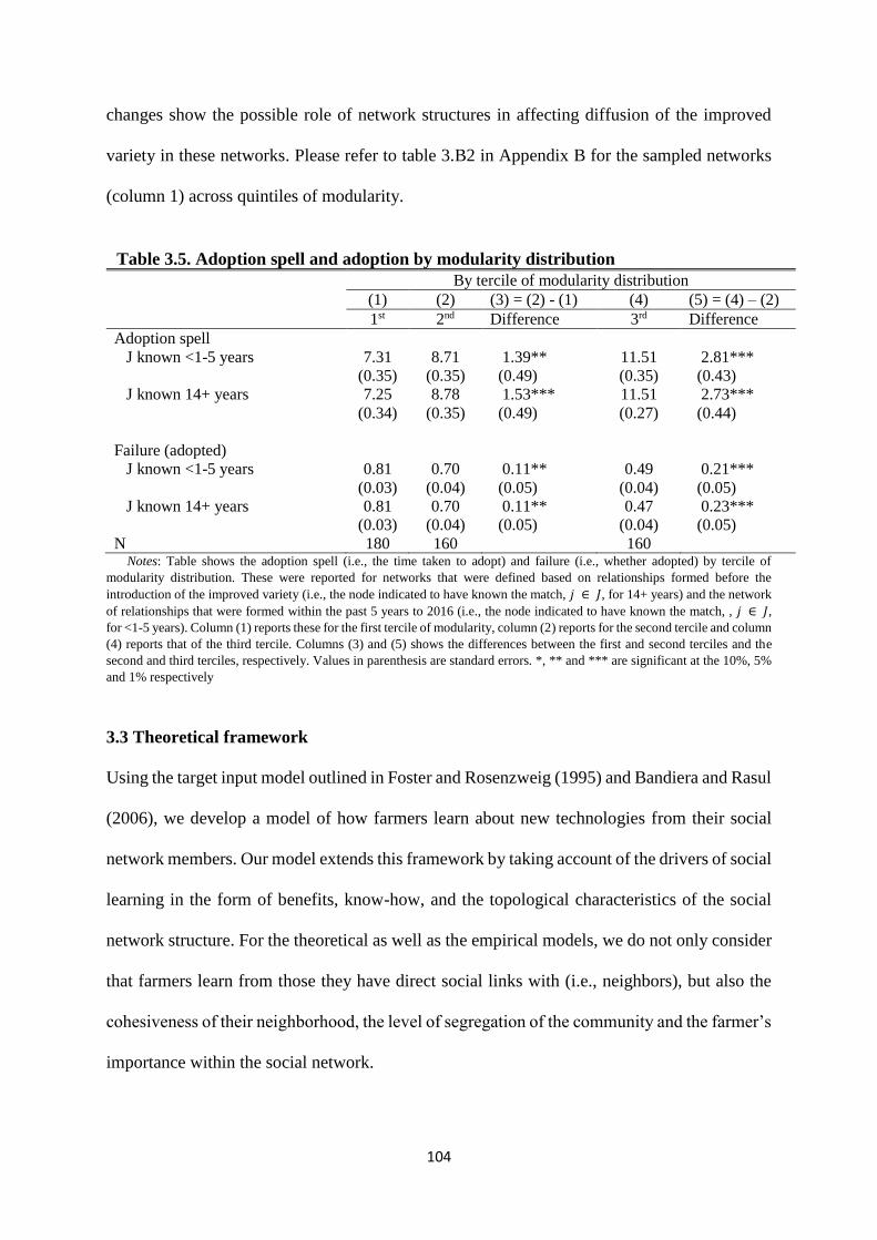
104

changes show the possible role of network structures in affecting diffusion of the improved

variety in these networks. Please refer to table 3.B2 in Appendix B for the sampled networks

(column 1) across quintiles of modularity.

Table 3.5. Adoption spell and adoption by modularity distribution

By tercile of modularity distribution

(1) (2) (3) = (2) - (1) (4) (5) = (4) – (2)

1st 2nd Difference 3rd Difference

Adoption spell

J known <1-5 years 7.31

(0.35)

8.71

(0.35)

1.39**

(0.49)

11.51

(0.35)

2.81***

(0.43)

J known 14+ years 7.25

(0.34)

8.78

(0.35)

1.53***

(0.49)

11.51

(0.27)

2.73***

(0.44)

Failure (adopted)

J known <1-5 years 0.81

(0.03)

0.70

(0.04)

0.11**

(0.05)

0.49

(0.04)

0.21***

(0.05)

J known 14+ years 0.81

(0.03)

0.70

(0.04)

0.11**

(0.05)

0.47

(0.04)

0.23***

(0.05)

N 180 160 160 Notes: Table shows the adoption spell (i.e., the time taken to adopt) and failure (i.e., whether adopted) by tercile of

modularity distribution. These were reported for networks that were defined based on relationships formed before the

introduction of the improved variety (i.e., the node indicated to have known the match, 𝑗 ∈ 𝐽, for 14+ years) and the network

of relationships that were formed within the past 5 years to 2016 (i.e., the node indicated to have known the match, , 𝑗 ∈ 𝐽,

for <1-5 years). Column (1) reports these for the first tercile of modularity, column (2) reports for the second tercile and column

(4) reports that of the third tercile. Columns (3) and (5) shows the differences between the first and second terciles and the

second and third terciles, respectively. Values in parenthesis are standard errors. *, ** and *** are significant at the 10%, 5%

and 1% respectively

3.3 Theoretical framework

Using the target input model outlined in Foster and Rosenzweig (1995) and Bandiera and Rasul

(2006), we develop a model of how farmers learn about new technologies from their social

network members. Our model extends this framework by taking account of the drivers of social

learning in the form of benefits, know-how, and the topological characteristics of the social

network structure. For the theoretical as well as the empirical models, we do not only consider

that farmers learn from those they have direct social links with (i.e., neighbors), but also the

cohesiveness of their neighborhood, the level of segregation of the community and the farmer’s

importance within the social network.

105

3.3.1 Updating profitability belief

The model assumes each farmer i knows the yield TV

iQ of the traditional variety cultivated on

an acre of his land. The average yield of the improved variety IV

iQ is not known. Thus, farmer

i forms beliefs about the profitability of the improved variety 𝑄𝑖𝐼𝑉(𝒷) to guide his decision to

learn or not. Farmers’ beliefs are within the range of 𝒷 ∈ [𝒷, 𝒷], with 0< 𝑄𝑖𝐼𝑉(𝒷) < 𝑄𝑖

𝐼𝑉 <

𝑄𝑖𝐼𝑉(𝒷).

We delineate social learning process in two stages (Nourani 2019).26 In the first-stage, farmers

are interested in knowing whether the expected yield potential of the improved variety is higher

than the expected yield of the traditional variety cultivated on his land. We specify the first-

stage of the social learning process as a DeGroot updating process (DeGroot 1974), where we

assume that the beliefs of the yield are based on the yield potential, i.e., the yields obtained

with excellent production know-how. Since the formation of beliefs about the average yield of

the improved variety is seen as a filter before realizing more intensive social learning based on

Bayesian updating, it is desirable that this stage of the learning process is computationally

simple and immediate. Moreover, DeGroot-updating allows for agents’ beliefs not converging

to the same belief. Instead, groups of agents may reach different consensuses. The occurrence

of different consensuses seem plausible in the case of farmers, since groups of farmers have

context specific conditions, such as agronomic or farmer specific characteristics like, soil

quality, exposition of the land, microclimate, agronomic experience or education.

Communication with other farmers provides farmer i information about other farmers’ beliefs.

Farmer i weights this information according to the reliability or trust he puts on farmer j . Let

26 Nourani (2019) links each stage of the two-stage learning process with a different type of agents. In our theoretical

model each stage is based on all social ties of each agent. However, in the first-stage agents learn about the yield potential and

in the second-stage about the know-how.

106

B be an 𝑁 × 𝑁 interaction matrix between agents, where entries 𝑏𝑖𝑗 indicate the relative weight

or trust farmer i puts on farmer j in comparison with all other farmers ,k k j , he relates to.

As the weight is relative, the entries of each row of the matrix, 𝐵 sum up to one when

normalized. The farmers’ initial beliefs at time 0 are exogenous and denoted by 𝒷𝑖0 for farmer

i . DeGroot updating from time period 1t to period t is given by the following rule 𝒷𝑖𝑡 =

∑ 𝑏𝑖𝑗𝑁𝑗=1 𝒷𝑗𝑡−1. Based on the updated value of 𝒷𝑖𝑡, farmer i decides to learn about the

cultivation technique, once his beliefs 𝒷𝑖𝑡 are higher than a given threshold. It can be given,

for instance by the yield of the traditional variety, i.e., 𝑄𝑖𝐼𝑉(𝒷) > 𝑄𝑖

𝑇𝑉.

3.3.2 Learning about the production process

Farmers can improve their initially rudimentary knowledge about the cultivation of the

improved variety by learning from farmers that have adopted in the past and by their own

experience once they have adopted. We assume that farmers use Bayesian updating to improve

their knowledge about the cultivation technique. To keep the model simple, we do not consider

institutional or public learning and focus on the effect of social learning. Furthermore, we

assume that the price of output is normalized to one, inputs are costless and all farmers own

the same size of land that is entirely cultivated to either the traditional or the improved variety.

The agricultural production of farmer i at time t is a function of the applied input itI . Farmers

know the underlying production function of the improved variety up to a random optimal or

“target” use of the applied input I . The yield of the improved variety ˆ IV

itQ , declines in the

square of the deviation of actual applied input itI and the uncertain target ît . By observing the

obtained yields of the improved variety and the applied input, the farmer learns about optimal

target by his own and other farmers’ experiences. The observed yield of the improved variety

ˆ IV

itQ is expressed as

107

(2) �̂�𝑖𝑡𝐼𝑉 = 𝑄𝑖𝑡

𝐼𝑉 − [𝐼𝑖𝑡 − 𝜃𝑖𝑡]2,

where *ît itu . The term

* represents the mean optimal effective input and itu is the

transitory random shocks that are i.i.d. with 20, uN . At time t , farmers are assumed to be

informed about 2

u and to have prior beliefs about * that are distributed as * 2,it itN . In

each period, farmers learn about the systematic part of the target by observing input and yield

from their own trial and/or from their social network members. This information allows farmers

to update their prior *

t , and infer the systematic component of ̂ . This results in a posterior

belief about the variance over * as

(3) 𝜎𝜃𝑖𝑡

2 =1

𝜋0+𝜋𝑝𝑝𝑖𝑡−1+𝜋𝑝𝐻 (𝐶𝑖𝑡−1,𝜆𝑖,𝜏𝑖,𝑀) ,

where 0

2

0 1/i

is the precision of the farmer’s initial priors about the true value of 𝜃∗,

21/p u , is the precision of the information produced by farmer i ’s own trial or by his peers’

trials, 1itp is an indicator of i ’s cumulative information of his own trial up to time 1t , and

H represents the cumulative information farmer i ´s has obtained from his peers in the past

up to time 1t . The information gathered in the term , 1i tC

is based on the share of peer adopters

in farmer i ´s neighborhood, 𝐴𝑗𝑡−1, farmer i ´s neighbors’ input 1jtI and the yields

1

IV

jtQ of the

improved variety of farmer i ´s neighbors at time 𝑡. Thus, it is given by the function

𝐶𝑖𝑡−1(𝐴𝑗𝑡−1, 𝐼𝑗𝑡−1𝑄𝑗𝑡−1𝐼𝑉 ) ≥ 0.

The term i denotes the centrality of farmers, which accounts for farmer i ’s immediate

learning possibilities from farmers who are directly connected to him, as well as learning from

well-connected neighbors (walks of length one). A high score means that a farmer is connected

to many farmers or to farmers who themselves have high scores. If the number of walks tend

108

to infinity, i stands for eigenvector centrality.27 Farmers learn from others as they receive

information about input and yield. However, farmers may give more or less credibility to the

information, depending on the strength of the social ties between farmer i and farmer j .

Although the strength of social ties cannot be measured directly, it can be assumed to be

stronger if the neighborhood is tied together by mutual friendships, or shared responsibilities.

As a proxy for the strength of social ties, we consider the cohesiveness of the neighborhood

(i.e., farmer i ’s neighbors are also connected among each other). Thus, the more cohesive

farmer i ´s neighborhood is, the more credible is the information that flows to farmer i . The

local cohesiveness of farmer i ’s neighborhood is denoted by i , with [0,1]i in equation (3),

see Appendix A for a precise definition of these network statistics and their corresponding

metrics.

Another influential factor for social learning, and central to this study, is the strength of

segregation of a network into modules (modularity) that is denoted by M . In a highly

segregated community, farmers obtain information from their neighbors, but there is no or only

weak flow of information between the segregated modules. Thus, farmers are more likely to

learn only from others if adopters form part of their module, while their chances of learning

are slim if adopters do not form part of their module. Also, the strength of modularity affects

the structure of the neighborhood of all agents, such that the centrality and cohesiveness are

lower for agents who are not located in the central parts of the module relative to that of agents

at the center of the module. The unbalanced distribution of these topological characteristics

due to modularity can shape the nature of information diffusion and social learning. Thus, the

overall quantity and quality of information gathered from other farmers, together with the effect

27 Paths are possible connections between agents of any length where no agent is visited more than once. Walks are

also connections but agents and links can be visited/traversed multiple times.

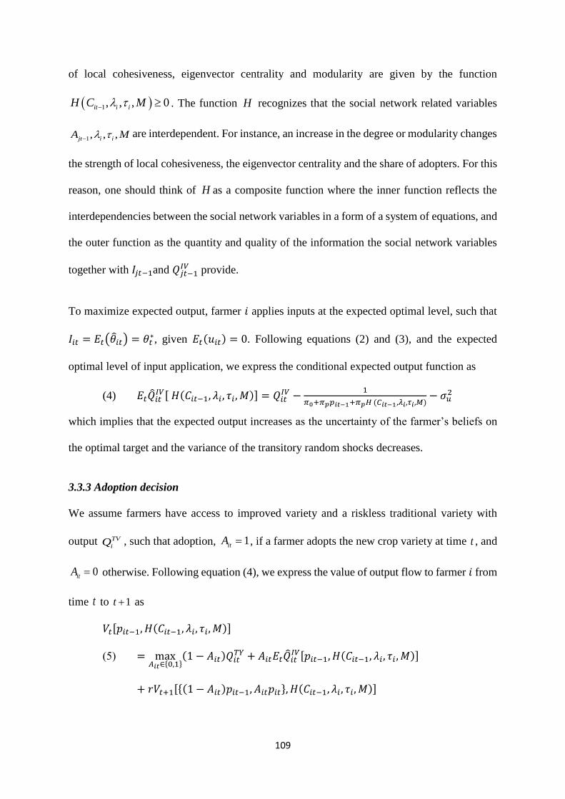
109

of local cohesiveness, eigenvector centrality and modularity are given by the function

1 0, , ,i iitH MC . The function H recognizes that the social network related variables

1, , ,i ijtA M are interdependent. For instance, an increase in the degree or modularity changes

the strength of local cohesiveness, the eigenvector centrality and the share of adopters. For this

reason, one should think of H as a composite function where the inner function reflects the

interdependencies between the social network variables in a form of a system of equations, and

the outer function as the quantity and quality of the information the social network variables

together with 𝐼𝑗𝑡−1and 𝑄𝑗𝑡−1𝐼𝑉 provide.

To maximize expected output, farmer 𝑖 applies inputs at the expected optimal level, such that

𝐼𝑖𝑡 = 𝐸𝑡(𝜃𝑖𝑡) = 𝜃𝑡∗, given 𝐸𝑡(𝑢𝑖𝑡) = 0. Following equations (2) and (3), and the expected

optimal level of input application, we express the conditional expected output function as

(4) 𝐸𝑡�̂�𝑖𝑡𝐼𝑉[ 𝐻(𝐶𝑖𝑡−1, 𝜆𝑖, 𝜏𝑖, 𝑀)] = 𝑄𝑖𝑡

𝐼𝑉 −1

𝜋0+𝜋𝑝𝑝𝑖𝑡−1+𝜋𝑝𝐻 (𝐶𝑖𝑡−1,𝜆𝑖,𝜏𝑖,𝑀)− 𝜎𝑢

2

which implies that the expected output increases as the uncertainty of the farmer’s beliefs on

the optimal target and the variance of the transitory random shocks decreases.

3.3.3 Adoption decision

We assume farmers have access to improved variety and a riskless traditional variety with

output TV

iQ , such that adoption, 1itA , if a farmer adopts the new crop variety at time t , and

0itA otherwise. Following equation (4), we express the value of output flow to farmer 𝑖 from

time t to 1t as

𝑉𝑡[𝑝𝑖𝑡−1, 𝐻(𝐶𝑖𝑡−1, 𝜆𝑖, 𝜏𝑖, 𝑀)]

(5) = max𝐴𝑖𝑡∈{0,1}

(1 − 𝐴𝑖𝑡)𝑄𝑖𝑡𝑇𝑌 + 𝐴𝑖𝑡𝐸𝑡�̂�𝑖𝑡

𝐼𝑉[𝑝𝑖𝑡−1, 𝐻(𝐶𝑖𝑡−1, 𝜆𝑖, 𝜏𝑖 , 𝑀)]

+ 𝑟𝑉𝑡+1[{(1 − 𝐴𝑖𝑡)𝑝𝑖𝑡−1, 𝐴𝑖𝑡𝑝𝑖𝑡}, 𝐻(𝐶𝑖𝑡−1, 𝜆𝑖 , 𝜏𝑖, 𝑀)]

110

where r is the farmer’s discount rate.28 The farmer adopts the new crop variety at time t , if

(6) 𝐸𝑡{�̂�𝑖𝑡𝐼𝑉[𝑝𝑖𝑡−1, 𝐻(𝐶𝑖𝑡−1, 𝜆𝑖, 𝜏𝑖 , 𝑀)] + 𝑟𝑉𝑡+1[𝑝𝑖𝑡, 𝐻(𝐶𝑖𝑡−1, 𝜆𝑖 , 𝜏𝑖, 𝑀)]}

≥ 𝐸𝑡{𝑄𝑖𝑇𝑌 + 𝑟𝑉𝑡+1[𝑝𝑖𝑡−1, 𝐻(𝐶𝑖𝑡−1, 𝜆𝑖, 𝜏𝑖, 𝑀)]} .

Thus, farmer 'i s adoption decision at time t depends on the information obtained from his

neighbors and the change in net value of output from adopting at time t with respect to his

neighbors experiences, 𝐶𝑖𝑡−1, and other social network related information 𝐴𝑗𝑡−1, 𝜆𝑖, 𝜏𝑖 and 𝑀.

Let these five variables form a set denoted by S , with each element denoted by vS , where

𝑣 =1,2,…,5. With respect to an increase in a farmer- or social network-related variable vS , the

derivative of expected stream of net benefits at time t is given by:

[𝜕𝐸𝑡�̂�𝑖𝑡

𝐼𝑉[𝑝𝑖𝑡−1,𝐻(𝐶𝑖𝑡−1,𝜆𝑖,𝜏𝑖,𝑀)]

𝜕𝐻+ 𝑟

𝜕𝐸𝑡{𝑉𝑡+1[𝑝𝑖𝑡,𝐻(𝐶𝑖𝑡−1,𝜆𝑖,𝜏𝑖,𝑀)]−𝑉𝑡+1[𝑝𝑖𝑡−1,𝐻(𝐶𝑖𝑡−1,𝜆𝑖,𝜏𝑖,𝑀)]}

𝜕𝐻]

𝜕𝐻

𝜕𝑆𝑣

(7) = [1

[𝜋0+𝜋𝑝𝑝𝑖𝑡+𝜋𝑝𝐻 (𝐶𝑖𝑡−1,𝜆𝑖,𝜏𝑖,𝑀)]2

+𝑟 ∑ 𝑟𝑢𝑇𝑢=1 {

1

[𝜋0+𝜋𝑝𝑝𝑖𝑡+𝜋𝑝𝐻 (𝐶𝑖𝑡−1,𝜆𝑖,𝜏𝑖,𝑀)]2 −

1

[𝜋0+𝜋𝑝𝑝𝑖𝑡−1+𝜋𝑝𝐻 (𝐶𝑖𝑡−1,𝜆𝑖,𝜏𝑖,𝑀)]2}]

𝜕𝐻

𝜕𝑆𝑣⋚ 0

where the first terms on both sides of the equation indicate the increase in current benefits

resulting from more information, ˆ 0IV

t ítE Q H , conditional on adoption of the improved

variety.29 This indicates the learning externality, as farmer i obtains more and better

information about cultivating the improved variety. The sign of the learning externality is

positive and favors adoption. The second term, enclosed in curly brackets, represents the

difference in the future stream of discounted benefits, between adoption and non-adoption at

28 For instance, if we consider the initial moment of time where 0t , the values of 1tp and tp are given by 0 and 1,

respectively.

29 If the improved variety were not adopted the current benefits would not change as a result of more information.

111

time t . Given that 1

1 1

T T

u u

u u

p p

, the sign of the sum is negative, suggesting that additional

information from farmer i ´s own trials is less valuable than the additional information obtained

from the farmer’s neighbors. Thus, farmer 𝑖 may strategically delay adoption to make use of the

additional and more precise information obtained from his peer adopters. Thus, the sign of

strategic delay is negative and tends to delay adoption. The overall effect of more and better

information about the cultivation of the improved variety depends on the magnitude of these

two effects and the sign of vSH . The latter derivative indicates the marginal effect of

farmer-related and social network-related variables on the quantity and quality of information

received by farmer i from neighbor j .

It is expected that decrease in modularity, and an increase in local cohesiveness i , the

centrality of farmer i in the social network, i , the share of past adopting peers, 𝐴𝑗𝑡−1, and the

peers’ experiences about their input and output lead to more and better information about the

improved variety, i.e., 0vH S . Since the learning externality is always positive and

strategic delay is always negative, the change in the magnitude of these two effects as a result

of more and better information tends to determine whether the farmer adopts or delays

adoption. Although strategic delay is always negative, the difference between the terms in curly

brackets decreases, if the value of H increases and becomes dominant in both denominators.

Thus, the sum of all terms in equation (7) tends to change sign from negative to positive as H

increases and adoption takes place. However, if 0vH S , the opposite result is obtained,

whereby adoption is delayed.

112

Hypothesis 1: When the belief about expected profitability of the improved variety is lower

than a given threshold, higher learning opportunities from experienced peers do not

significantly increase the likelihood of adopting the improved variety.

Hypothesis 2: The likelihood of adoption is low with increased modularity of the social

network, but the influence of modularity on learning from peers for adoption is weaker, if social

learning is among direct peers or within modules.

Hypothesis 3: When increased local cohesiveness and centrality lead to more opportunities

for learning and adoption, lower modularity is more likely to increase the likelihood of

adoption than higher modularity.

The theoretical model describes the signs of the effects of the driving forces on adoption, but

does not offer insights about the strength of the effects. In the next section, we employ

observational data to examine the magnitude of the influence of these unknowns.

3.4. Empirical specification and estimation

3.4.1 Empirical specification

Our theoretical framework shows that the time at which a farmer adopts the new technology

relates to the past adoption decisions of peers, information from past peer experiences, and the

structure and characteristics of the social network. Based on the notation used in the theoretical

framework, we specify our empirical model, by assuming a lag transmission of social network

effects (Manski 1993) as:

(8) 𝑃𝑟[𝑇 = 𝑡|𝑇 ≥ 𝑡, 𝐺, 𝐴0 … 𝐴𝑡 , 𝐶0 … 𝐶𝑡, 𝑋𝑡]

= 𝜌𝐺𝑡𝐴𝑡−1 + 𝛼𝐺𝑡𝐶𝑡 + 𝛽1𝑀𝑡 + 𝛽2𝐷𝑡 + 𝛽3𝐺𝑡𝐷𝑡 + 𝑋𝑡′𝛾1 + 𝑋𝑡

′𝐺𝑡𝛾2 + 𝜄𝑡𝐺 + 휀𝑡,

where 𝑇 is a random variable that denotes the time of adoption of the improved variety, 𝐺𝑡 is a

normalized social network matrix, and 𝐺𝑡𝐴𝑡−1 is the share of past adopting peers. Given that

113

adoption decisions are based on the net expected returns from adoption, as discussed in the

theoretical framework, it follows that changes in peer adoption decisions will inform the farmer

about the profitability of the improved variety. Thus, 𝜌 shows the effect of the association

between share of past peer adoption decisions, which indicates profitability signal, and the

conditional probability of adoption at any given time. 𝐶𝑡 is farmers’ experience in cultivating

the improved variety, 𝐺𝑡𝐶𝑡 is the average peer experience in the cultivation of the variety and

𝛼 is the association between peer experience (i.e., learning about production process) and the

conditional probability of adoption at time 𝑡. 𝐷𝑡 is a vector of farmer level network statistics

[i.e., transitivity (𝜏𝑡) and centrality measures (𝜆𝑡)], 𝐺𝑡𝐷𝑡 is the farmer’s average peer network

statistics, 𝑀𝑡 is the modularity of the network, and 𝛽1, 𝛽2 and 𝛽3 are vectors of parameters to

be estimated, while 휀𝑡 is the error term.

Our specification of the effects of peer adoption decisions differs from the “traditional”

endogenous peer effect as in Manski (1993). Specifically, we define this effect based on

previous peer adoptions, and not contemporaneous adoptions. This simplifies the econometric

framework because of the reflection problem. It also enhances identification, since farmers

react to their peers’ adoption decisions only when observed (i.e., timing between own decision

and peer decisions). However, two critical concerns that arise are the contextual and correlated

effects. Contextual effects refer to similarities in exogenous characteristics among peers, which

can cause behaviors to correlate through such peer exogenous characteristics, and not due to

peer behavior. We control for contextual effects with individual and peer characteristics (i.e.,

𝑋𝑡′ and 𝑋𝑡

′𝐺𝑡, respectively), and the associated parameters to be estimated as 𝛾1 and 𝛾2 in

equation (8).

Next is the possibility of unobservables at the network and individual levels to drive

correlations in individual adoption decisions (i.e., correlated effects) and cause identification

114

problems by confounding the peer effects estimates (Manski 1993; Moffitt 2001; Blume et al.

2011). These are represented with the vector 𝜄𝑡𝐺 in equation (8), which consists of time, village

and environmental factors (i.e., correlated effects) that affect adoption. Available approaches

for accounting for these unobservables in the literature, given our setting, include, the use of a

(i) standard instrumental variable approach, (ii) network fixed-effects to account for potential

network-specific unobserved factors (Lee 2007; Liu and Lee 2010),30 and (iii) the control

function for accounting for self-selection within social interactions (Goldsmith-Pinkham and

Imbens 2013; Hsieh and Lee 2016).

Our approach to accounting for correlated unobservable basically involve the last two: First,

we decompose 𝜄𝑡𝐺 into time, 𝛿𝑡, and network, 𝓋𝐺 , effects and control for both in our

specifications. The second approach (i.e., (iii) above) involves a first-stage model of network

formation, given that link formation is a phenomenon of choice, determined by observed and

unobserved agents’ characteristics. The estimated unobserved determinants of link formation,

defined as �̂�𝑡, at the first-stage, are retrieved and inserted into a second-stage adoption decision

model to account for endogeneity of the network effect. This is similar in spirit to the Heckman

(1979) sample selection approach and the Brock and Durlauf (2001; 2006) generalized

multinomial control function for self-selection corrections with social interactions. Another

merit of the use of this approach is that it allows us account for concerns of measurement errors

due to the use of sampled networks (Chandrasekhar and Lewis 2016), as well as provides a

natural source of instruments for identifying the social interaction effects (Brock and Durlauf

2001) in order to obtain consistent estimates.

30 See Horrace et al. (2016) and Hsieh and Lee (2016) for discussion of these approaches.

115

3.4.2 Empirical estimation

Our interest is in examining the network effects on the conditional probability of adopting

improved soybean variety at time 𝑡 given that the farmer has not adopted until this time. Given

that adoption of the technology in question were observed on annual basis, where observed

durations are clustered at mass points, we model our duration to adoption in a discrete-time

method to account for the banded nature of the survival time. Also, discrete-time methods do

not impose functional form restriction on the time effects (allowing for specific time fixed

effects to be captured) compared to the continuous time proportional hazard models, and make

it possible to account for time-varying covariates (Jenkins 2005).

If we define 𝑛 as the total number of farmers (𝑖 = 1,2,3, …) observed until time 𝑡𝑖, at which

point the farmer either adopts the improved variety (i.e., uncensored) or do not adopt (i.e.,

censored). In this study, the entrance date is 2003 which is the year in which the improved

variety was introduced (i.e., 𝑡 = 1). The exit date of the spell for the farmers who adopt the

improved variety is the year of adoption, and farmers who have not adopted at the 2016 farming

season are right-censored, because the data was collected on farmers’ agricultural production

in the 2016 farming season. If we define 𝑿𝑖𝑡 as a vector of explanatory variables and 𝓑 as the

associated vector of parameters in equation (8), we express the discrete-time hazard rate as

(9) 𝐴𝑖𝑡 = 𝑃𝑟[𝑇𝑖 = 𝑡|𝑇𝑖 ≥ 𝑡, 𝑿𝑖𝑡]

where 𝑇 is the discrete random variable representing the adoption time of the farmer31. In order

to express the dependence of the hazard rate on time and the explanatory variables, we use the

complementary log-log link function which is not sensitive to the length of the time intervals,

compared to the logistic regression function (Allison 1982). The complementary log-log

31 This also represents the conditional probability of adoption at time 𝑡, given that the farmer has not adopted until this time.

116

function assumes the data generating process is based on the continuous-time proportional

hazard model and is express as

(10) 𝐴𝑖𝑡 = 1 −exp[−exp(𝓑′𝑿𝑖𝑡)].

Equation (10) represents the discrete-time proportional hazard model. We estimate the hazard

model by maximizing the likelihood of the function. Given that some of the observations are

censored, we express the likelihood function of the data generation process as

(11) 𝐿 = ∏ [Pr (𝑇𝑖 = 𝑡𝑖)]𝑎𝑖[Pr (𝑇𝑖 > 𝑡𝑖)]1−𝑎𝑖𝑛𝑖=1

where 𝐿 is the likelihood of function, and 𝑎𝑖 is set equal to 1 if 𝑖 is uncensored and zero

otherwise. Expressing each of the probabilities in equation (11) as a function of the hazard rate

and taking the logarithm of this deliver the log-likelihood function as

(12) log 𝐿 = ∑ ∑ 𝑦𝑖𝑡𝑡𝑖𝑠=1

𝑛𝑖=1 log[𝐴𝑖𝑠/(1 − 𝐴𝑖𝑠)] + ∑ ∑ log (1 − 𝐴𝑖𝑠)

𝑡𝑖𝑠=1

𝑛𝑖=1

where 𝑦𝑖𝑡 is a dummy variable equal to 1 if farmer 𝑖 adopted the improved variety at time 𝑡,

and zero otherwise32. Each discrete-time unit for a farmer is treated as a separate observation,

and the dependent variable is coded 1 if the farmer adopted the improved variety in that time

unit and zero otherwise. The farmer contributes to the computation of 𝐴𝑖𝑠, if he adopts the

improved variety at time 𝑡𝑖, and (1 − 𝐴𝑖𝑠) for the period before 𝑡𝑖. If the farmer does not adopt

(i.e., censored) by the 2016 cropping season, he only takes part in the computation of the term

second term of the right-hand size.

Following the discussion of the identification of the peer effects and the hazard model, equation

(8) can now be specified as:

𝐴𝑖𝑡 = 𝜌𝐺𝑡𝐴𝑖𝑡−1 + 𝛼𝐺𝑡𝐶𝑖𝑡 + 𝛽1𝑀𝑡 + 𝛽

2𝐷𝑖𝑡 + 𝛽

3𝐺𝑡𝐷𝑖𝑡

(13) + 𝜌𝛼𝐺𝑡𝐴𝑖𝑡−1 × 𝐺𝑡𝐶𝑖𝑡 + 𝜌𝑀𝐺𝑡𝐴𝑖𝑡−1 × 𝑀𝑡 + 𝛼𝑀𝐺𝑡𝐶𝑖𝑡 × 𝑀𝑡 + 𝛽𝑀𝐺𝑡𝐷𝑖𝑡 × 𝑀𝑡

+ 𝑋𝑖𝑡′ 𝛾1 + 𝑋𝑖𝑡

′ 𝐺𝑡𝛾2 + 𝛿𝑡 + 𝓋𝐺 + �̂�𝑖𝑡 + 𝜖𝑖𝑡,

32 See Allison (1982) for the steps required to arrive at the log-likelihood function.

117

where 𝜌 and 𝛼 represent the effects of learning about profitability and know-how, respectively;

𝛽1, 𝛽2 and 𝛽3 show the effects of network characteristics; 𝛾1 and 𝛾2 represent contextual effects;

𝛿𝑡, 𝓋𝐺 and �̂�𝑖𝑡 account for correlated effects. The parameter 𝛿𝑡 is a flexible baseline hazard

which indicates the pattern of duration dependence in the diffusion process over time, and is

used to account for time fixed effects. The parameter 𝓋𝐺 accounts for network level effects that

might drive peers’ behavior to be correlated. �̂�𝑖𝑡 is a vector of predicted residuals of the link

formation model used to account for unobserved factors that affect network formation at the

farmer level (refer to Appendix B for discussion and estimation of the network-formation

model).

To examine the relationship between learning about profitability, know-how, and network

statistics, the second row of equation (13) shows the interactions among these variables. In

particular 𝜌𝛼 denotes the interaction effects of past adopting, 𝐺𝑡𝐴𝑖𝑡−1, and experienced peers,

𝐺𝑡𝐶𝑖𝑡. 𝜌𝑀 and 𝛼𝑀 show the effects of past adopting, 𝐺𝑡𝐴𝑖𝑡−1, and experienced peers, 𝐺𝑡𝐶𝑖𝑡,

conditioned on modularity of the network, 𝑀𝑡, respectively. 𝛽𝑀 represents the effect of farmer

level network statistics, 𝐺𝑡𝐷𝑖𝑡, (i.e., local transitivity, degree and eigenvector centrality),

conditioned on modularity of the network, 𝑀𝑡, and the rest are as defined in equation (8).

3.5 Empirical results and discussions

This section presents and discusses the results of our empirical estimates. Table 3.6 presents

the unconditional hazard ratio estimates of peer adoption, peer experience and network

statistics on adoption, whereas table 3.7 presents the hazard ratio estimates of these conditioned

on modularity of the social network.

We first consider the unconditional hazard ratios of past peer adoption of the improved variety

on adoption in columns (1, 3, 5 and 7) with degree centrality, and in columns (2, 4, 6 and 8)

with eigenvector centrality, in table 3.6. Columns (1-4), present a restricted specification,

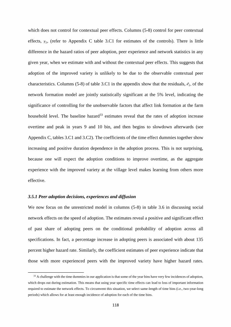
118

which does not control for contextual peer effects. Columns (5-8) control for peer contextual

effects, 𝛾2, (refer to Appendix C table 3.C1 for estimates of the controls). There is little

difference in the hazard ratios of peer adoption, peer experience and network statistics in any

given year, when we estimate with and without the contextual peer effects. This suggests that

adoption of the improved variety is unlikely to be due to the observable contextual peer

characteristics. Columns (5-8) of table 3.C1 in the appendix show that the residuals, �̂�𝑡 , of the

network formation model are jointly statistically significant at the 5% level, indicating the

significance of controlling for the unobservable factors that affect link formation at the farm

household level. The baseline hazard33 estimates reveal that the rates of adoption increase

overtime and peak in years 9 and 10 bin, and then begins to slowdown afterwards (see

Appendix C, tables 3.C1 and 3.C2). The coefficients of the time effect dummies together show

increasing and positive duration dependence in the adoption process. This is not surprising,

because one will expect the adoption conditions to improve overtime, as the aggregate

experience with the improved variety at the village level makes learning from others more

effective.

3.5.1 Peer adoption decisions, experiences and diffusion

We now focus on the unrestricted model in columns (5-8) in table 3.6 in discussing social

network effects on the speed of adoption. The estimates reveal a positive and significant effect

of past share of adopting peers on the conditional probability of adoption across all

specifications. In fact, a percentage increase in adopting peers is associated with about 135

percent higher hazard rate. Similarly, the coefficient estimates of peer experience indicate that

those with more experienced peers with the improved variety have higher hazard rates.

33 A challenge with the time dummies in our application is that some of the year bins have very few incidences of adoption,

which drops out during estimation. This means that using year specific time effects can lead to loss of important information

required to estimate the network effects. To circumvent this situation, we select same-length of time bins (i.e., two-year-long

periods) which allows for at least enough incidence of adoption for each of the time bins.

119

Specifically, a year increase in average peer experience with the improved variety is associated

with about 84 percent higher hazard rate. Thus, signals from increased peer adoption decisions

and experienced peers tend to increase learning opportunities and decrease learning costs,

which consequently can speed up adoption of the improved variety (Beaman et al. 2018).

We also present the distribution of marginal effects of estimates of the main specification in

column (5) in Figure 3.1. These estimates reveal that a 20 percent standard deviation increase

in adopting peers is associated with a 10 percentage points increase in the conditional

probability of adoption in any given year. Similarly, a 20 percent (which translated into 1.4

years) standard deviation increase in average peer experience is associated with about 9

percentage points increase in the probability of adoption in any given year.

The effects of peer experience with the improved variety on the conditional probability of

adoption is lower than the effects of share of adopting peers, when the share of past adopting

peers is below 25 percent. However, the effects of peer experience become higher and remains

so with increasing peer experience in the cultivation of the improved variety, when more than

30 percent of peers have adopted the improved variety. This is expected because the higher

efforts required in learning about the production process will make farmers expect a certain

level of peer adoption in order to increase learning opportunities, as indicated in the theoretical

framework. Past studies found evidence of either learning about hard-to-use (Oster and

Thornton 2012), or easy-to-use technologies in conditions of visible benefits (Magnan et al.

2015). A possible implication of our finding is that network effects could drive both learning

about benefits and application (use) of a technology that is relatively hard-to-apply, and with

visible expected benefits that can be inferred from peer decisions, albeit the precise

mechanisms cannot be determined with the data.

120

Table 3.6. Estimates of Social learning and farmers’ adoption

Notes: Random-effects complementary log-log estimation. Models 1-4 do not include average peer characteristics (i.e., contextual effects). Models 5-8 include these average peer characteristics

(their coefficients and that of other controls are presented in appendix table 3.C1). Correlated effects include time fixed-effects, 𝛿𝑡, link formation residuals, �̂�𝑡, and standard errors clustered at

the village (i.e., network) level, in order to account for village factors that might drive peer behaviors to be correlated, 𝓋𝐺 [we did not use village dummies because of the need to avoid the

incidental parameter problem (Lee et al., 2010) by having to include 25 village dummies, and also the fact that modularity is calculated for the entire network/village]. The asterisks ***, **

and * are significance at 1%, 5% and 10% levels, respectively.

No Contextual Effects Contextual Effects

(1) (2) (3) (4) (5) (6) (7) (8)

Share of peer adopters 𝜌 2.350**

(0.761)

2.319**

(0.746)

1.424

(0.542)

1.417

(0.541)

2.374**

(0.762)

2.348**

(0.746)

1.513

(0.569)

1.503

(0.567)

Peer experience 𝛼 1.840***

(0.232)

1.885***

(0.224)

1.770***

(0.226)

1.818***

(0.220)

1.834***

(0.224)

1.883***

(0.216)

1.771***

(0.216)

1.821***

(0.209)

Peer experience

× Share of peer adopters

𝜌𝛼 1.523

(0.414)

1.512

(0.419)

1.459

(0.382)

1.453

(0.391)

Modularity 𝛽1 0.182**

(0.146)

0.139**

(0.118)

0.166**

(0.129)

0.127**

(0.103)

0.186**

(0.139)

0.126**

(0.103)

0.169**

(0.121)

0.115**

(0.088)

Transitivity 𝛽2 3.146**

(1.340)

3.186**

(1.435)

3.155**

(1.331)

3.191**

(1.424)

3.301**

(1.449)

3.328**

(1.534)

3.303**

(1.438)

3.322**

(1.521)

Degree 𝛽2 1.088

(0.058)

1.090

(0.058)

1.099*

(0.056)

1.102*

(0.057)

Average peer degree 𝛽3 1.124*

(0.074)

1.127*

(0.073)

1.160**

(0.080)

1.163**

(0.081)

Eigenvector 𝛽2 1.092

(0.389)

1.119

(0.397)

1.211*

(0.409)

1.243

(0.419)

Average peer eigenvector 𝛽3 2.170**

(0.793)

2.208**

(0.799)

2.464**

(1.049)

2.509**

(1.066)

Controls 𝛾1 Yes Yes Yes Yes Yes Yes Yes Yes

Contextual effects 𝛾2 No No No No Yes Yes Yes Yes

Correlated effects 𝛿𝑡,𝓋𝐺 ,�̂�𝑡 Yes Yes Yes Yes Yes Yes Yes Yes

𝜌 + 𝜌𝛼 = 0 5.68(0.02) 5.73(0.02)

𝛼 + 𝜌𝛼 = 0 10.67(0.00) 11.04(0.00)

Link Residuals 𝑿𝟓𝟐(p-val) 22.58(0.00) 25.64(0.00) 22.66(0.0

0)

25.59(0.00) 22.71(0.00) 25.65(0.01) 22.99(0.00) 26.21(0.00)

LogLikelihood -972.6 -972.6 -970.3 -971.2 -964.8 -965.8 -963.6 -964.7

Clusters 25 25 25 25 25 25 25 25

N 4,551 4,551 4,551 4,551 4,551 4,551 4,551 4,551

121

Figure 3.1 Marginal Effects of peer adoption and production experience

Notes: Marginal effects of the fully specified model (i.e., column 5 of table 3.6). In each case (e.g., peer

adoption), all variables other than peer adoption are held constant at their mean values. Peer experience is

expressed as a percent of the maximum average peer experience in the sample. Starting from baseline year

adoption probabilities of about 9% and 6% for share of adopting and experienced peers, respectively, the

probability of adoption marginally increases to about 18% with increased peer adoption of the improved variety

(i.e., the thick-dot line), and to about 38% with increased peer experience in farming the improved variety

soybean (i.e., the solid line).

To show the dependence between signals from past peer adoption decisions and peer experience

in soybean farming, we also estimated the conditional network effects by interacting share of past

adopting peers with peer experience [i.e., the first term of row two in specification (13)] in columns

(7) and (8). The estimates reveal that whereas the main effect, 𝜌, and interaction effect, 𝜌𝛼, are

each not statistically significant, the main effect of peer experience, 𝛼, remains positive and

statistically significant. This suggests that a year increase in average peer experience with the

improved variety is associated with a hazard rate of at least 77 percent.

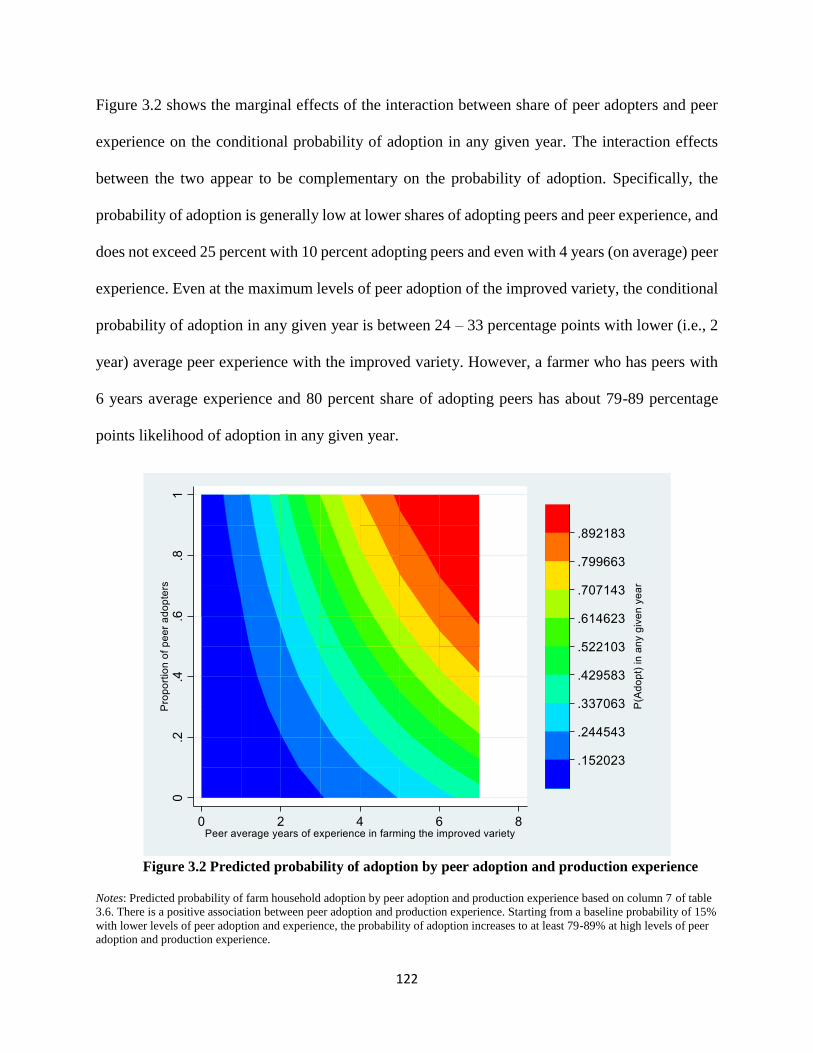
122

Figure 3.2 shows the marginal effects of the interaction between share of peer adopters and peer

experience on the conditional probability of adoption in any given year. The interaction effects

between the two appear to be complementary on the probability of adoption. Specifically, the

probability of adoption is generally low at lower shares of adopting peers and peer experience, and

does not exceed 25 percent with 10 percent adopting peers and even with 4 years (on average) peer

experience. Even at the maximum levels of peer adoption of the improved variety, the conditional

probability of adoption in any given year is between 24 – 33 percentage points with lower (i.e., 2

year) average peer experience with the improved variety. However, a farmer who has peers with

6 years average experience and 80 percent share of adopting peers has about 79-89 percentage

points likelihood of adoption in any given year.

Figure 3.2 Predicted probability of adoption by peer adoption and production experience

Notes: Predicted probability of farm household adoption by peer adoption and production experience based on column 7 of table

3.6. There is a positive association between peer adoption and production experience. Starting from a baseline probability of 15%

with lower levels of peer adoption and experience, the probability of adoption increases to at least 79-89% at high levels of peer

adoption and production experience.

123

This finding suggests that although having many adopting and experienced peers can increase the

learning opportunities and possibly reduces the duration of non-adoption, the effects of learning

about know-how from peer experience on adoption is much higher than the effect of peer adoption

decisions. This is expected because soybean production is quite demanding in terms of labor

inputs, management and timing of other inputs application, making the marginal returns to learning

about production relatively higher than just signal from peer adoption decisions.

3.5.2 Network statistics and diffusion

We next consider the network statistics by first focusing on the individual level statistics (i.e.,

transitivity, degree and eigenvector centralities). In respect of degree and eigenvector centralities,

we focus on the averages of farmers’ peer degree and eigenvector centralities because of our

interest in showing the effects of a farmer’s connection to highly connected or important peers on

the probability of adoption, and not that of the farmer himself. The results, reported in table 3.6,

show a positive and significant association between the transitivity and the conditional probability

of adoption in any given year across all specifications. In addition, farmers’ connections (i.e.,

degree) and farmers’ average peer connections (i.e., farmers’ average peer degrees) in column (7)

as well as farmers’ average peer eigenvector centrality in column (8) each significantly increases

the hazard rate in any given year. Interestingly, however, the hazard rate of transitivity is

significantly higher than the hazard rate of peer degree (p=0.022), but not significantly different

from the hazard rate of farmers’ average peer eigenvector centrality (p>0.1)34.

34 The coefficient of transitivity is also significantly higher than the coefficient of farmers’ own degree (p=0.00) in column (7).

124

This finding suggests that obtaining information on the new technology from multiple and

interconnected sources is very important than from a highly connected farmer. This could be due

to the fact that the influence of central nodes is more local35 (i.e., limited to few known direct

nodes and the unknown nodes just learn by imitation) (e.g., see Banerjee et al. 2014; Beaman and

Dillon 2018), and/or because the central node’s trustworthiness is low. It could also be associated

with the fact that central nodes are unable to communicate intensively over a certain time for other

farmers to get the required information (especially if learning is not easy) (Beaman et al. 2018).

We earlier on argued that the extent of partitioning of the network into groups, which defines

modularity, can affect the rate of interaction and diffusion of the improved variety, particularly if

a network has high modularity statistics (i.e., highly segregated). Estimates of modularity show

significant and negative association with adoption across all specifications in table 3.6. Thus,

farmers who belong to highly segregated networks (i.e., higher modularity network) tend to have

longer duration of non-adoption of the improved variety. Thus, whereas increasing transitivity of

a farmer’s neighborhood is associated with higher hazard rate due to less structural holes and

increased efficiency in information flow and diffusion, increasing modularity leads to lower hazard

rate due to the highly structured latent groups in the networks. This confirms the arguments by

Rogers (1995), Alatas et al. (2016), and Jackson et al. (2017) that the likelihood of information or

behavior to spread from one node to other nodes is high in networks with less latent community

structures and/or highly cohesive subgroups.

35 Beaman and Dillon (2018) found that information does not diffuse to people who are far from the first recipient of the

information

125

3.5.3 Network modularity versus transitivity and centrality on diffusion

To examine whether network modularity conditions the effects of information about peer adoption

decisions, – and for that matter profitability beliefs –, and peer experiences in soybean production

on the conditional probability of adoption by farmers, we interact past peer adoption decision and

peer experiences with modularity in columns (1) and (2) of table 3.7. Although the main effects of

peer adoption decisions and experiences remained significantly positive, it is the interaction effects

of peer experience with modularity that is significant, suggesting that there is some dependence of

learning from peer experiences on modularity.

This is clearly shown in Figure 3.3 where the conditional probability of adoption continues to

increase with increasing peer adoptions but with higher probability at higher levels of adopting

peers and lower modularity (Fig. 4A). Similarly, the conditional probability of adoption increases

with increasing peer experience but appears to show high effect of learning from peer experiences

at higher peer experiences and modularity (Fig. 4B). These relationships suggest that farmers

depend more on their direct peers or peers within their components in the network in learning from

peer experiences, and possibly on both direct and indirect peers or even peers across components

in observing peer adoption decisions.

Our findings substantiate the argument by Jackson et al. (2017) that flow of information or

behavior among nodes is stronger and can possibly reach all nodes, if these nodes belong to the

same component in a network, and that of Nourani (2019) that farmers tend to learn about

production knowledge from strong ties, and about profitability from weak ties. In effect, the figures

show that when the proportion of peer adopters and years of experience are low changes in the

modularity has little effect on adoption. When these values are high changes in the modularity are

highly effective.

126

Table 3.7. Impact of network modularity on farmers’ adoption

(1) (2) (3) (4) Share of peer adopters 𝜌 2.223***

(0.610)

2.194***

(0.588)

2.480**

(0.788)

2.485***

(0.776)

Peer experience 𝛼 1.934***

(0.223)

1.987***

(0.221)

1.773***

(0.214)

1.793***

(0.204)

Modularity 𝛽1 0.159*

(0.115)

0.109**

(0.085)

0.134**

(0.123)

0.127**

(0.119)

Transitivity 𝛽2 3.107**

(1.328)

3.176**

(1.427)

3.462**

(1.531)

3.417**

(1.593)

Degree 𝛽2 1.117**

(0.055)

1.060

(0.052)

Average peer degree 𝛽3 1.171**

(0.082)

1.084

(0.076)

Eigenvector 𝛽2 1.257

(0.413)

1.204

(0.407)

Average peer eigenvector 𝛽3 2.450**

(1.067)

2.194*

(0.866)

Modularity

× Share of peer adopters

𝜌𝑀 1.541

(7.895)

1.297

(6.514)

Modularity

× Peer experience

𝛼𝑀 4.273*

(3.349)

3.544**

(2.679)

Modularity

× Transitivity

𝛽𝑀 2.38E-5***

(8.43E-5)

1.16E-5***

(4.45E-5)

Modularity

× Average peer degree 𝛽𝑀 0.372**

(0.154)

Modularity

× Average peer eigenvector

𝛽𝑀 0.004**

(0.010)

Controls 𝛾1 Yes Yes Yes Yes

Contextual effects 𝛾2 Yes Yes Yes Yes

Correlated effects 𝛿𝑡, 𝓋𝐺 , �̂�𝑡 Yes Yes Yes Yes

LogLikelihood -961.4 -963.2 -958.6 -959.1

Clusters 25 25 25 25

N 4,551 4,551 4,551 4,551 Notes: Random-effects complementary log-log estimation of equation (13). Column 1 controls for the interactions of

modularity on one hand and peer adopters and experience on the other hand as well as agent’s degree and average peer degree.

Column 2 controls for the interactions of modularity on one hand and peer adopters and experience on the other hand but with

agent’s eigenvector centrality and average peer eigenvector centralities. Column 3 controls for the interactions of modularity on

one hand and agent’s local transitivity, degree and average peer degree, whiles column 4 controls for the interactions of modularity

on one hand and agent’s local transitivity, eigenvector centrality and average peer eigenvector centrality. The coefficients of agents’

controls and that of peer characteristics are presented in appendix table 3.C2). Peer experience is the number of years of peer

experience in cultivating the improved variety. Correlated effects include time fixed-effects, 𝛿𝑡, link formation residuals, �̂�𝑡, and

standard errors clustered at the village (i.e., network) level, in order to account for village factors that might drive peer behaviors

to be correlated, 𝓋𝐺 [we did not use village dummies because of the need to avoid the incidental parameter problem (Lee et al.,

2010) by having to include 25 village dummies, and also the fact that modularity is calculated for the entire network/village]. The

asterisks ***, ** and * are significance at 1%, 5% and 10% levels, respectively.

Thus, it is beneficial to target share of adopters through extension services and training workshops

in promoting adoption in the short run, and then focus on measures that facilitate interactions

among farmers at the village level in order to minimize the constraining effects of modularity on

127

social learning in the long run. We next check whether the latent network structures (modularity)

condition the roles of transitivity and centrality in the social learning process, which is the last

term of row two in specification (13). This is important because, the effectiveness of transitivity

and centrality in the diffusion process depend on the extent of modularity of the network. High

modularity networks are expected to constrain the role of transitivity and centrality in enhancing

learning and diffusion in the network and the vice versa.

Figure 3.3 Predicted probability of adoption by modularity, peer adoption and experience Notes: The figure depicts the predicted probability of household adoption by modularity and peer adoption (A) and by modularity

and peer experience (B). Starting from lower levels of adoption probabilities of 7.8% and 11% respectively for A and B, the

probability of adoption increases to about 16% and 85%, with increasing peer adoption and peer experience but at lower and higher

modularity, respectively.

Columns (3) and (4) of table 3.7 show how modularity conditions the effects of these micro-

network structures by interacting transitivity, average peer degree and eigenvector centrality with

128

modularity. Whereas the main effects of transitivity show that increase in transitivity of a farmer’s

neighborhood is associated with higher hazard rate, the coefficients of modularity and the

interaction with transitivity in both columns show lower hazard rates.

Similar effects are observed in the main and interaction effects of average peer degree, and

eigenvector centrality with modularity. The interaction effects of modularity with average peer

degree in column (3), and with average peer eigenvector centrality in column (4) are significant

and less than one. These suggest that latent network structures significantly limit the role of these

node level statistics in promoting social learning and diffusion. Figure 3.4 shows the interaction

plots of modularity and average peer degree (A), average peer eigenvector (B) and farmer’s local

transitivity (C). We find that the association between transitivity, average peer degree and

eigenvector centrality, and the conditional probability of adoption in any given year changes, based

on the level of modularity. Generally, the conditional probability of adoption in any given year

increases with increase in each of these statistics at lower levels of modularity.

The conditional probability of adoption reaches about 14, 10 and 9 percentage points at the highest

levels of local transitivity, average peer eigenvector centrality and average peer degree,

respectively, and at the lowest levels of modularity. However, the conditional probabilities of

adoption are at most about 4 percentage points at the highest levels of local transitivity, average

degree and eigenvector centrality when modularity is above 0.3. Thus, the higher the modularity

of the network, the less effective is the influence of the local transitivity of a farmer’s

neighborhood, and the effect of peers with higher connections and importance in the network. The

rationale is that when the network has many small components, information or behavior that

originates among neighbors or from central and influential nodes in a given component –

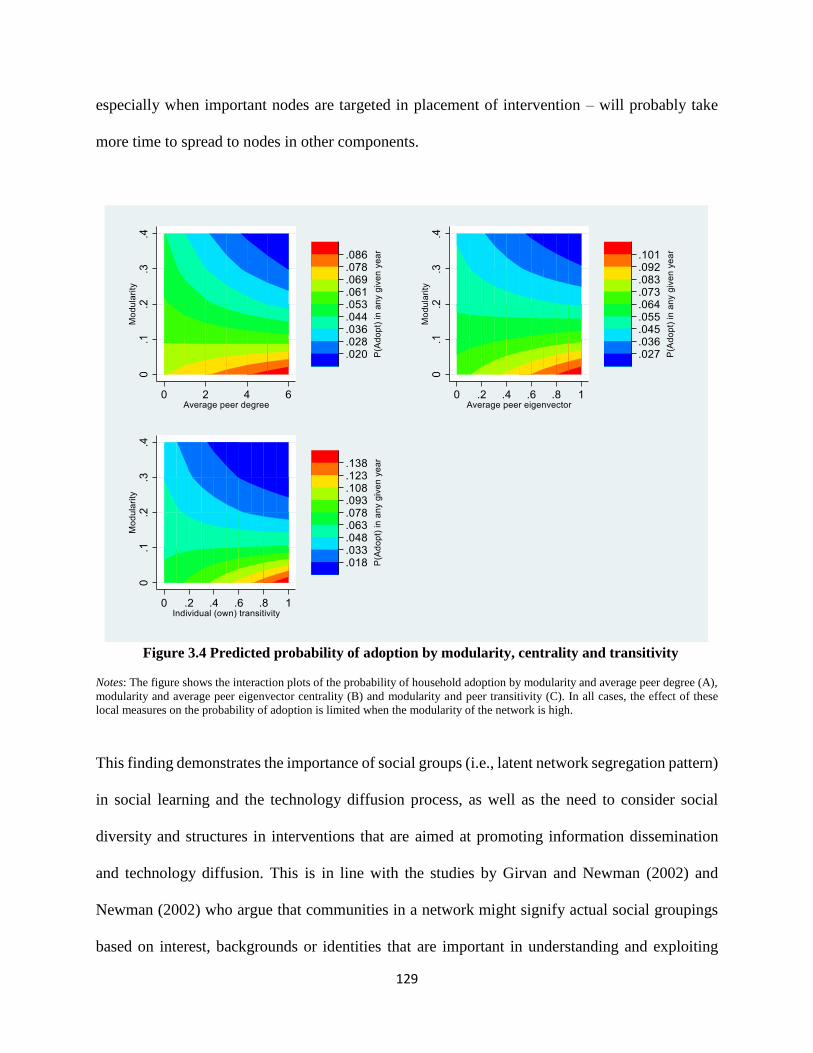
129

especially when important nodes are targeted in placement of intervention – will probably take

more time to spread to nodes in other components.

Figure 3.4 Predicted probability of adoption by modularity, centrality and transitivity Notes: The figure shows the interaction plots of the probability of household adoption by modularity and average peer degree (A),

modularity and average peer eigenvector centrality (B) and modularity and peer transitivity (C). In all cases, the effect of these

local measures on the probability of adoption is limited when the modularity of the network is high.

This finding demonstrates the importance of social groups (i.e., latent network segregation pattern)

in social learning and the technology diffusion process, as well as the need to consider social

diversity and structures in interventions that are aimed at promoting information dissemination

and technology diffusion. This is in line with the studies by Girvan and Newman (2002) and

Newman (2002) who argue that communities in a network might signify actual social groupings

based on interest, backgrounds or identities that are important in understanding and exploiting

130

networks effectively. The implication of this finding is that the common strategy of targeting initial

adopters who are central in their networks may not be sufficient for promoting diffusion of

improved soybean in these villages, if the community structures and diversities that underlie

farmers’ interactions are ignored. The reason being that, the effect of a central member in a network

will be limited in the presence of network structures and diversities. Hence, the use of approaches

(such as farmer field days, self-help groups or multiple targeting) that lead to more interactions

and subsequently creating more connection and increasing the density of contacts among farmers

(as documented by Centola 2010; Magnan et al. 2015; Alatas et al. 2016) will be appropriate in

promoting diffusion at the village (network).

3.5.4 Other possible effects and robustness checks

This section presents robustness checks by investigating the possibility of concerns that might

threaten the effects observed in our analysis. Despite the fact that our specifications account for

some correlated unobservables, with the residuals of the network formation model, and that all the

study villages are in the Northern region of Ghana and have similar agricultural, climatic and

market conditions, we nevertheless cannot completely rule out the possibility that our estimates

could be driven by village and other environmental effects.

Individual ability and spurious correlations

The first concern is the possibility of the peer adoption effects to be spuriously correlated due to

differences in farmers’ and household abilities rather than due to social learning. To check this,

we estimated our baseline models in columns (5) and (6) of table 3.6 with the squared term of peer

adoption decisions, which are reported in column (1) of table 3.8. The coefficients of share of peer

adopters and the share of peer adoption squared show a nonlinear relationship between peer

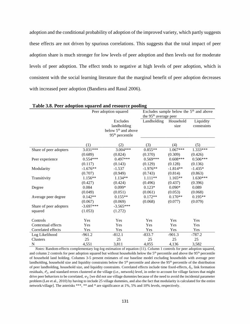
131

adoption and the conditional probability of adoption of the improved variety, which partly suggests

these effects are not driven by spurious correlations. This suggests that the total impact of peer

adoption share is much stronger for low levels of peer adoption and then levels out for moderate

levels of peer adoption. The effect tends to negative at high levels of peer adoption, which is

consistent with the social learning literature that the marginal benefit of peer adoption decreases

with increased peer adoption (Bandiera and Rasul 2006).

Table 3.8. Peer adoption squared and resource pooling Peer adoption squared Excludes sample below the 5th and above

the 95th average peer

Excludes

landholding

below 5th and above

95th percentile

Landholding

Household

size

Liquidity

constraints

(1) (2) (3) (4) (5)

Share of peer adopters 3.031***

(0.689)

3.004***

(0.824)

0.855**

(0.370)

1.067***

(0.309)

1.333***

(0.426)

Peer experience 0.554***

(0.117)

0.497***

(0.143)

0.569***

(0.129)

0.608***

(0.128)

0.506***

(0.136)

Modularity -1.676**

(0.707)

-1.537

(0.949)

-1.976**

(0.743)

-1.814**

(0.814)

-1.435*

(0.863)

Transitivity 1.156**

(0.427)

1.134**

(0.424)

1.111**

(0.496)

1.165**

(0.437)

1.630***

(0.396)

Degree 0.084

(0.049)

0.099*

(0.051)

0.123*

(0.061)

0.090*

(0.053)

0.089

(0.068)

Average peer degree 0.142**

(0.067)

0.155**

(0.069)

0.172**

(0.068)

0.170**

(0.077)

0.195**

(0.079)

Share of peer adopters

squared

-3.697***

(1.053)

-3.565***

(1.272)

Controls Yes Yes Yes Yes Yes

Contextual effects Yes Yes Yes Yes Yes

Correlated effects Yes Yes Yes Yes Yes

Log Likelihood -961.2 -812.1 -833.7 -901.3 -787.2

Clusters 25 25 25 25 25

N 4,551 3,811 4,055 4,136 3,582 Notes: Random-effects complementary log-log estimation of equation (11). Column 1 controls for peer adoption squared,

and column 2 controls for peer adoption squared but without households below the 5th percentile and above the 95th percentile

of household land holding. Columns 3-5 present estimates of our baseline model excluding households with average peer

landholding, household size and liquidity constraints below the 5th percentile and above the 95th percentile of the distribution

of peer landholding, household size, and liquidity constraints. Correlated effects include time fixed-effects, 𝛿𝑡, link formation

residuals, �̂�𝑡, and standard errors clustered at the village (i.e., network) level, in order to account for village factors that might

drive peer behaviors to be correlated, 𝓋𝐺 [we did not use village dummies because of the need to avoid the incidental parameter

problem (Lee et al., 2010) by having to include 25 village dummies, and also the fact that modularity is calculated for the entire

network/village]. The asterisks ***, ** and * are significance at 1%, 5% and 10% levels, respectively.

132

However, Bandiera and Rasul (2006) argue about the possibility of heterogeneities in abilities to

spuriously drive such nonlinear peer relationship, particularly, when relatively low-ability

households tend to be constrained in adoption, and high-ability households with investment

options tend to be less likely to adopt. Thus, we estimated the same specification in column (1) of

table 3.8 by excluding households with landholding below the 5th and above the 95th percentiles.

The results, which are reported in column (2) of table 3.8, show the inverse U-shaped relationship

still persists, suggesting that social learning does play a role in the diffusion process.

Resource effects and not learning

The next concern is resource-sharing effects, where exchanges of resources among peers can speed

up the ability of resource constrained farm households to adopt the improved variety. The

assumption is that households who are relatively resource poor can depend on relatively better

households for resources required for cultivation. Also, gains from peer adoption that ease input

constraints such as land, labor and liquidity can enhance the ability of poor and resource

constrained households to access these inputs for cultivation. This has the potential of showing

effects that are similar to social learning, where a farmer’s conditional probability of adoption

increases as a result of past adoption decisions of peers in the farmer’s network.

To investigate this, we first replicated the results of the baseline model in column (5) of table 3.6

excluding households with average peer landholding, household size and liquidity constraints

below the 5th and the 95th percentiles. These resources are important for soybean production in the

area because the crop is labor intensive and also requires application of inputs such as inoculant,

fertilizer and herbicides to obtained desired output (Heatherly and Elmore 2004). Farmers who are

constrained in these inputs can benefit through increased access, following adoption of their peers,

133

or from better-off peers. Reassuringly, the results remain stable, with positive and significant peer

effects on the conditional probability of adoption in any given year.

Furthermore, we interact farmers’ and peers’ landholding and household size to examine whether

households with more or less own and peer landholding and household size are more or less likely

to adopt faster, and how such dependence in terms of resources affect our results. We report the

results in columns (1) and (2) of table 3.9. Both estimates are small and statistically insignificant,

suggesting that increase in peer landholding (household size), given the farmer’s landholding

(household size) is associated with a delayed (faster) adoption, but statistically not significant. The

estimates of peer adoption decisions and the other network effects remain robust to this exercise.

Threats of geographic proximity

Another challenge has to do with residential and/or farm proximity between farmers and their

peers, where farmers with similar soil quality and features on their plots, that favor a particular

variety, might appear to have similar varietal choices. This may drive adoption decisions between

peers and farmers to be correlated without social learning effect. Column (3) of table 3.9 contains

interaction of farmers’ soil quality with average peer soil quality, and the term shows that farmers

who have peers with high (on average) soil quality have higher conditional probability of adoption,

albeit not statistically significant. This suggests weak dependence in soil quality of farmers and

peers. Columns (4) of table 3.9 investigate the validity of this issue in respect of residential

proximity. We control for the average distance between household locations of farmers and their

peers in this specification. Despite these specifications, the results in terms of magnitudes and

directions of our estimates remain qualitatively similar to the baseline model, suggesting that social

learning does play a role in the adoption of the improved variety.

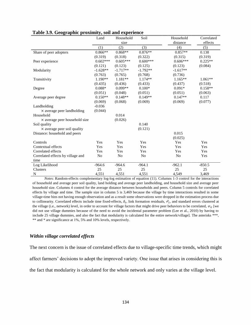
134

Table 3.9. Geographic proximity, soil and experience Land Household

size

Soil Household

distance

Correlated

effects

(1) (2) (3) (4) (5)

Share of peer adopters 0.866**

(0.319)

0.868**

(0.318)

0.876**

(0.322)

0.857**

(0.315)

0.138

(0.319)


(0.121)

0.605***

(0.123)

0.600***

(0.125)

0.606***

(0.123)

0.225**

(0.084)

Modularity -1.628**

(0.763)

-1.717**

(0.765)

-1.792**

(0.768)

-1.617**

(0.736)


(0.435)

1.181**

(0.436)

1.174**

(0.433)

1.165**

(0.437)

1.061**

(0.518)

Degree 0.088*

(0.051)

0.099**

(0.048)

0.100*

(0.051)

0.091*

(0.051)

0.158**

(0.063)


(0.069)

0.148**

(0.068)

0.149**

(0.069)

0.147**

(0.069)

0.117

(0.077)

Landholding

× average peer landholding

-0.036

(0.044)

Household

× average peer household size

0.014

(0.026)

Soil quality

× average peer soil quality

0.140

(0.121)

Distance: household and peers 0.015

(0.025)

Controls Yes Yes Yes Yes Yes

Contextual effects Yes Yes Yes Yes Yes

Correlated effects Yes Yes Yes Yes Yes

Correlated effects by village and

time

No No No No Yes

Log Likelihood -964.6 -964.6 -964.1 -962.1 -850.5

Clusters 25 25 25 25 25

N 4,551 4,551 4,551 4,549 3,469

Notes: Random-effects complementary log-log estimation of equation (11). Columns 1-3 control for the interactions

of household and average peer soil quality, land holding and average peer landholding, and household size and average peer

household size. Columns 4 control for the average distance between households and peers. Column 5 controls for correlated

effects by village and time. The sample size in column 5 is 3,469 because the village by time interactions resulted in some

village-time bins not having enough observation and as a result some observations were dropped in the estimation process due

to collinearity. Correlated effects include time fixed-effects, 𝛿𝑡, link formation residuals, �̂�𝑡, and standard errors clustered at

the village (i.e., network) level, in order to account for village factors that might drive peer behaviors to be correlated, 𝓋𝐺 [we

did not use village dummies because of the need to avoid the incidental parameter problem (Lee et al., 2010) by having to

include 25 village dummies, and also the fact that modularity is calculated for the entire network/village]. The asterisks ***,

** and * are significance at 1%, 5% and 10% levels, respectively.

Within village correlated effects

The next concern is the issue of correlated effects due to village-specific time trends, which might

affect farmers’ decisions to adopt the improved variety. One issue that arises in considering this is

the fact that modularity is calculated for the whole network and only varies at the village level.

135

Hence, the inclusion of modularity, time and village fixed effects, and village × time fixed effects

result in convergence problem during the estimation. As a result, modularity is dropped in this

specification. Column (5) of table 3.9 presents results of the specification that includes time,

village and village × time fixed effects, and shows, with the exception of share of adopters which

loses its significance but still positively correlates with adoption, that most of the coefficients are

qualitatively similar to the baseline results.

Sampled networks and robustness of results

Given that our network data is sampled and not based on a census of connections of households of

these villages, there could be some bias in the estimates. Households were asked whether they

know any of 5 households randomly drawn from the village sample and assigned to them, and

links were defined based on whether the household knew the match or not. This implies that, when

a household is not randomly assigned to a responding household, one cannot determine whether

the responding household knows the non-sampled household (𝑔𝑖𝑗 = 1) or not (𝑔𝑖𝑗 = 0).

To investigate this issue, we use the graphical reconstruction technique developed by

Chandrasekhar and Lewis (2016) to simulate the complete network for each village. We first

estimate a model of network formation, using the sampled network of each village, and then use

the estimated model to simulate the complete networks (i.e., predict the missing links of the

network) (see appendix B for model, estimates and networks). We next calculate our social

network statistics (i.e., modularity, transitivity, degree and eigenvector centrality) using the

complete networks, and then use these statistics to estimate our baseline specification. The results

are reported in columns (1) and (2) of table 3.10 for degree and eigenvector, respectively, and the

key findings remain similar to the baseline estimates.

136

Furthermore, in order to investigate the direction of potential bias associated with the use of the

sample networks in the calculation of the network statistics used in the estimations, we use an

approach similar to Alatas et al. (2016). That is, we explore what would happen to the estimates if

we progressively drop links of the simulated network up to the sample selection ratio of our

sampled networks, which is 34 percent of households in the median village. To explore this, we

first drop 25 percent of links uniformly at random, calculate the network statistics used in the

analysis and estimate the baseline specification with these statistics, with the results, reported in

columns (3) and (4) of table 3.10 with degree and eigenvector centrality, respectively.

We further drop 50 percent of the links, calculate the network statistics and re-estimate our baseline

specification, and these results are reported in columns (5) and (6) of table 3.10. Finally, we drop

70 percent of the links and repeat the analysis and present the results in columns (7) and (8) of

table 3.10. The results, generally, remain qualitatively similar to the baseline in terms of the

direction of their effects, although with generally decreasing levels of the coefficients of these

network statistics, as more links are dropped. This suggest that our point estimates of the effects

of these network statistics using the sample networks are susceptible to measurement errors, which

is shown to be an attenuation bias. Thus, the estimated parameters of the network statistics should

best be considered as a lower bound on the true coefficients.

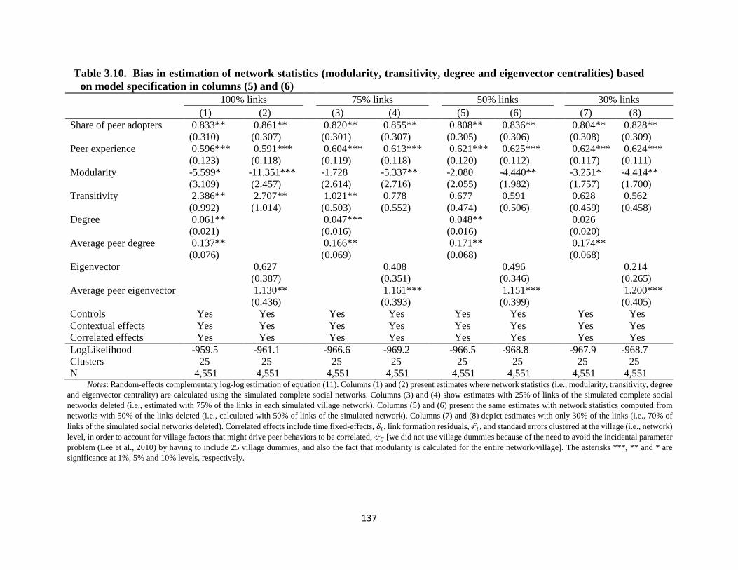
137

Table 3.10. Bias in estimation of network statistics (modularity, transitivity, degree and eigenvector centralities) based

on model specification in columns (5) and (6)

100% links 75% links 50% links 30% links

(1) (2) (3) (4) (5) (6) (7) (8)

Share of peer adopters 0.833**

(0.310)

0.861**

(0.307)

0.820**

(0.301)

0.855**

(0.307)

0.808**

(0.305)

0.836**

(0.306)

0.804**

(0.308)

0.828**

(0.309)


(0.123)

0.591***

(0.118)

0.604***

(0.119)

0.613***

(0.118)

0.621***

(0.120)

0.625***

(0.112)

0.624***

(0.117)

0.624***

(0.111)

Modularity -5.599*

(3.109)

-11.351***

(2.457)

-1.728

(2.614)

-5.337**

(2.716)

-2.080

(2.055)

-4.440**

(1.982)

-3.251*

(1.757)

-4.414**

(1.700)


(0.992)

2.707**

(1.014)

1.021**

(0.503)

0.778

(0.552)

0.677

(0.474)

0.591

(0.506)

0.628

(0.459)

0.562

(0.458)

Degree 0.061**

(0.021)

0.047***

(0.016)

0.048**

(0.016)

0.026

(0.020)


(0.076)

0.166**

(0.069)

0.171**

(0.068)

0.174**

(0.068)

Eigenvector 0.627

(0.387)

0.408

(0.351)

0.496

(0.346)

0.214

(0.265)

Average peer eigenvector 1.130**

(0.436)

1.161***

(0.393)

1.151***

(0.399)

1.200***

(0.405)

Controls Yes Yes Yes Yes Yes Yes Yes Yes

Contextual effects Yes Yes Yes Yes Yes Yes Yes Yes

Correlated effects Yes Yes Yes Yes Yes Yes Yes Yes

LogLikelihood -959.5 -961.1 -966.6 -969.2 -966.5 -968.8 -967.9 -968.7

Clusters 25 25 25 25 25 25 25 25

N 4,551 4,551 4,551 4,551 4,551 4,551 4,551 4,551 Notes: Random-effects complementary log-log estimation of equation (11). Columns (1) and (2) present estimates where network statistics (i.e., modularity, transitivity, degree

and eigenvector centrality) are calculated using the simulated complete social networks. Columns (3) and (4) show estimates with 25% of links of the simulated complete social

networks deleted (i.e., estimated with 75% of the links in each simulated village network). Columns (5) and (6) present the same estimates with network statistics computed from

networks with 50% of the links deleted (i.e., calculated with 50% of links of the simulated network). Columns (7) and (8) depict estimates with only 30% of the links (i.e., 70% of

links of the simulated social networks deleted). Correlated effects include time fixed-effects, 𝛿𝑡, link formation residuals, �̂�𝑡, and standard errors clustered at the village (i.e., network)

level, in order to account for village factors that might drive peer behaviors to be correlated, 𝓋𝐺 [we did not use village dummies because of the need to avoid the incidental parameter

problem (Lee et al., 2010) by having to include 25 village dummies, and also the fact that modularity is calculated for the entire network/village]. The asterisks ***, ** and * are

significance at 1%, 5% and 10% levels, respectively.

138

3.6 Conclusion

Although learning for technology adoption has become an important focus of research and policy

interventions in promoting agricultural advancement, especially in developing countries, the

complexity of the technology itself, heterogeneity of benefits and in understanding the technology,

as well as in the structure of social interactions have often led to sub-optimal adoption and

inconclusive evidence of social network effects. Policy interventions have operated based on the

assumption that farmers can learn from their peers, with little friction in the flow of information.

However, this assumption can be costly in the presence of heterogeneity in social network

structures, which condition the flow of information. We investigated this assertion using

observational data from a survey of 500 farm households in Northern Ghana and random matching

within sample to generate social network contacts.

We first provide a dynamic framework of how social learning and heterogeneity of network

structures influence farmers’ adoption decisions. Second, we estimate the effect of learning from

peers on the speed of adoption, conditional on the transitivity of farmers’ neighborhoods,

connectivity to important peers and modularity of the network. Our approach of accounting for

contextual effects and correlated effects (using the control function approach, clustering at

village/network level, and village and time fixed effects) are key to the identification of the

different network effects.

Our empirical results reveal significant and positive duration dependence in the adoption process,

justifying the relevance of the duration model in this study. Generally, having past adopting peers

and high (on average) experienced peers tend to increase the speed of adoption, but the magnitude

of peer experience on the speed of adoption is higher if the farmer has more peers already adopting

139

the improved variety. Thus, we find evidence that both benefits and production know-how play

important roles in how farmers learn from their network contacts, which suggests the existence of

social learning among network members. The likelihood of adopting faster increases with high

values of transitivity and centrality. However, we generally find the role of local transitivity in the

learning process to be stronger and more efficient in enhancing diffusion, compared to centrality.

This could be attributed to the limited influence of central members to farmers they have direct

contacts with, especially when the frequency and intensity of interactions between groups of agents

is limited by highly segregated network structures. On the other hand, highly cohesive networks

favor the frequency and intensity of interactions, in segregated network structures, that seems

important for social learning.

The findings generally suggest that the common extension strategy of targeting initial and

influential adopters in the network for disseminating information may not be appropriate in

engendering diffusion at the network level. Given the role of transitivity in promoting adoption

and that of modularity in restricting diffusion, and the influence of the other network

characteristics, it will be important for policymakers to consider introducing the technology

through densely subgroups, or using policies and interventions aimed at engineering connections

among farmers (such as farmer field days or self-help groups) to improve information flow. Also,

network-oriented policies such as workshops and seminars or supporting adopters’ association that

is open also to non-adopters can increase the diffusion process. Furthermore, interventions such as

extension services, public learning and training workshops, where people are specifically invited

from different segments of the village at the early stages of adoption, can promote bridges between

modules and diffusion. These would create more avenues for interactions in order to increase links

among farmers and between groups which could overcome the limitations of lowly cohesive or

140

highly segregated networks. Network oriented policies are likely to enhance the role of social

networks in information and diffusion process of the technology.

141

References

Alatas, V., Banerjee, A., Chandrasekhar, A.G., Hanna, R. and Olken, B.A. (2016). “Network

Structures and the Aggregation of Information: Theory and Evidence from Indonesia.”

American Economic Review, 106(7): 1663 -704.

Alliance for Green Revolution in Africa and Scaling Seeds Technologies Partnership (AGRA-

SSTP) (2017). “Ghana Early Generation Seed Study.” United State Agency for International

Development (USAID). Accra.

Allison, P.D. (1982). “Discrete-Time Methods for the Analysis of Event Histories.” Sociological

Methodology, 13: 61-98.

Ambrus, A., Mobius, M. and Szeidl, A. (2014). “Consumption Risk-Sharing in Social Networks.”

American Economic Review, 104(1): 149-82.

Ampadu-Ameyaw, R., Omari,R., Essegbey, G.O. and Dery, S. (2016). “Status of Agricultural

Innovations, Innovation Platforms, and Innovation Investment. 2015.” PARI project

country report: Republic of Ghana. Forum for Agricultural Research in Africa (FARA),

Accra Ghana.

Bandiera, O. and Rasul, I. (2006). “Social networks and technology adoption in northern

Mozambique.” The Economic Journal, 116(514): 869-902.

Banerjee, A., Chandrasekhar, A.G., Duflo, E. and Jackson, M.O. (2013). “The Diffusion of

Microfinance.” Science, 341 1236498.

Banerjee, A., Chandrasekhar, A.G., Duflo, E. and Jackson, M.O. (2014). “Gossip: Identifying

Central Individuals in a Social Network.” NBER Working Papers 20422, National Bureau

of Economic Research, Inc.

Beaman, L. and Dillon, A. (2018). “Diffusion of agricultural information within social networks:

Evidence on gender inequalities from Mali.” Journal of Development Economics,

133(26):147-61.

Beaman, L., BenYishay, A., Magruder, J. and Mobarak, A.M. (2018). “Can Network Theory-

based Targeting Increase Technology Adoption?” Yale University Economic Growth

Center Discussion Paper No. 1062

BenYishay, A. and Mobarak, A.M. (2018). “Social Learning and Incentives for Experimentation

and Communication.” Review of Economic Studies, 0: 1-34.

142

Blume, L.E., Brock, W.A., Durlauf, S.N. and Ioannide, Y.M. (2010). “Identification of Social

Interactions.” In Handbook of Social Economics SET: 1A, 1B Volume 1, ed. Jess Benhabib,

A. Bisin, and M.O. Jackson, 859-964: Elsevier, North-Holland.

Bollobas, B. (2001). “Random Graphs.” Second edition. Cambridge and New York: Cambridge

University Press.

Bramoulle, Y., Djebbari, H. and Fortin, B. (2009). “Identification of peer effects through social

networks.” Journal of Econometrics, 150(1): 41 – 55.

Brock, W.A. and Durlauf, S.N. (2001). “Interaction-Based models.” In Handbook of

Econometrics, Vol. 5, ed. Heckman, J., Leaner, E. pp. 3297 – 3380: North-Holland.

Brock, W.A. and Durlauf, S.N. (2006). “Multinomial choice with social interactions”. In The

Economy as an Evolving Complex System, Vol. III, ed. Blume, L.E., Durlauf, S.N. pp. 175

– 206: Oxford University Press.

Cai, J., de Janvry, A. and Sadoulet, E. (2015). “Social Networks and the Decision to Insure.”

American Economic Journal: Applied Economics, 7(2):81-108.

Centola, D. (2010). “An Experimental Study of Homophily in the Adoption of Health Behavior.”

Science, 334 (6060):1269-72.

Chandrasekhar, A.G. and Lewis, R. (2016). “Economics of sampled networks.” Mimeo,

Massachusetts Institute of Technology.

Conley, T.G. and Udry, C.R. (2010). “Learning about a new technology: Pineapple in Ghana.”


Council for Scientific and Industrial Research and Savanna Agricultural Research Institute (CSIR-

SARI). (2013). “Effective farming systems research approach for accessing and developing

technologies for farmers.” Annual Report, SARI: CSIR-INSTI.

Dogbe, W., Etwire, P. M., Martey, E., Etwire, J. C., Baba, I. I. Y. and Siise, A. (2013). “Economics

of Soybean Production: Evidence from Saboba and Chereponi Districts of Northern Region

of Ghana.” Journal of Agricultural Science, 5(12): 38-46.

Duflo, E., Kremer, M. and Robinson, J. (2011). “Nudging Farmers to Use Fertilizer: Theory and

Experimental Evidence from Kenya.” American Economic Review, 101(6):2350 – 2390.

Foster, A.D. and Rosenzweig, M.R. (1995). “Learning by Doing and Learning from Others:

Human Capital and Technical Change in Agriculture.” Journal of Political Economy,

103(6):1176-1209.

143

Foster, D.V., Foster, J.G., Grassberger, P. and Paczuski, M. (2011). “Clustering drives assortativity

and community structures in ensembles of networks.” Physical Review E 84, 066117: 1-5.

Gerhart, J.D. (1975). “The Diffusion of Hybrid Maize in Western Kenya”. Ph.D. Dissertation,

Princeton University.

Girvan, M. and Newman, M.E.J. (2002). “Community structures in social and biological

networks.” Proceedings of the National Academy of Sciences, 99, 7821-7826.

Goldsmith, P. (2017). “The Faustian Bargain in Tropical Soybean Production.” Commercial

Agriculture in Tropical Environments: Special Issue, 10(1-4).

Goldsmith-Pinkham, P. and Imbens, G.W. (2013). “Social Networks and the Identification of Peer

Effects.” Journal of Business and Economic Statistics, 31(3): 253 – 264.

Heatherly, L.G. and Elmore, R.W. (2004). “Managing inputs for peak production.” In Soybeans:

Improvement, Production and Uses. Agronomy Monograph 16, ed. Boerma H. R., Specht,

J. E. pp. 451-536: American Society of Agronomy, Crop Science Society of America, and

Soil Science Society of America, Madison, Wisconsin, USA.

Heckman, J. (1979). “Sample Selection Bias as a Specification Error.” Econometrica, 47(1): 153

– 161.

Heckman, J. and Singer, B. (1984). “Econometric Duration Analysis.” Journal of Econometrics

24(1-2): 63 – 132.

Horrace, W.C., Liu, X. and Patacchini, E. (2016). “Endogenous network production functions with

selectivity.” Journal of Econometrics, 190(2): 222-32.

Hsieh,C-S. and Lee, L-F. (2016). “A Social Interactions Model with Endogenous Friendship

Formation and Selectivity.” Journal of Applied Econometrics, 31(1): 301 – 319.

Jackson, M.O. (2008). Social and Economic Networks. Princeton University Press.

Jackson, M.O., Rogers, B.W. and Zenou, Y. (2017). “The Economic Consequences of Social-

Network Structure.” Journal of Economic Literature, 55(1): 49 – 95.

Jackson, M.O., Rodriguez-Barraquer, T. and Tan, X. (2012). “Social Capital and Social Quilts:

Network Patterns of Favor Exchange.” American Economic Review, 102(5): 1857 – 1897.

Jenkins, S.P. (2005). Survival Analysis. Unpublished manuscript, Institute for Social and

Economic Research, University of Essex, UK.

Karlan, D., Mobius, M., Rosenblat, T. and Szeidl, A. (2009). “Trust and Social Collateral.”

Quarterly Journal of Economics, 124(3): 1307-61.

144

Krishnan, P. and Sciubba, E. (2009). “Links and Architecture in Village Networks.” The Economic

Journal, 119(537): 917-949.

Lancaster, T. and Nickell, S. (1980). “The Analysis of Re-Employment Probabilities for the

Unemployed.” Journal of the Royal Statistical Society. Series A (General) 143(2):141-165.

Lee, L-F. (2007). “Identification and estimation of econometric models with group interactions,

contextual factors and fixed effects.” Journal of Econometrics, 140(2): 333-74.

Lee, L. F., Liu, X. and Lin, X. (2010). “Specification and estimation of social interaction models

with network structures.” The Econometrics Journal 13(2): 145-76.

Liu, X. and Lee, L-F. (2010). “GMM estimation of social interaction models with centrality.”

Journal of Econometrics, 159(1): 99-115.

Magnan, N., Spielman, D.J., Lybbert, T.J. and Gulati, K. (2015). “Leveling with friends: Social

networks and Indian farmers’ demand for a technology with heterogeneous benefits.”

Journal of Development Economics, 116(C): 223-251.

Manski, C.F. (1993). “Identification of endogenous social effects: The reflection problem.” Review

of Economic Studies, 60(3): 531–542.

Ministry of Food and Agriculture (MoFA) (2017). “Planting for Food and Jobs: Strategic Plan for

Implementation (2017 – 2020).” Ministry of Food and Agriculture. Accra, Ghana.

Moffitt, R. (2001). “Policy Interventions, Low-Level Equilibria, and Social Interactions.” In Social

Dynamics, ed. Durlauf, S. and Young, H.P.: pp. 45-82. Cambridge: MIT Press.


Indian Green Revolution.” Journal of Development Economics, 73(1): 185-213.

Newman, M.E.J. (2002). “The spread of epidemic disease on networks.” Physics Review, E, 66,

016128.

Newman, M.E.J. (2006). “Modularity and community structure in networks.” Proceedings of the

National Academy of Sciences of the United States of America, 103(23): 8577-8582.

Nourani, V. (2019). Multi-objective learning and technology adoption in Ghana: Learning from

friends and reacting to acquaintances. Unpublished working paper, Department of

Economics, Massachusetts Institute of Technology.

Oster, E. and Thornton, R. (2012). “Determinants of technology adoption: Peer effects in Mensural

Cup Take-up.” Journal of the European Economic Association, 10(6): 1263-1293.

https://econpapers.repec.org/article/ecjeconjl/

https://econpapers.repec.org/article/ecjeconjl/

https://econpapers.repec.org/article/eeeeconom/

http://econpapers.repec.org/article/eeedeveco/

145

Rogers, E.M. (1995). Diffusion of Innovations, Fourth edition. New York: Simon and Schuster,

Free Press.

Suri, T. (2011). “Selection and Comparative Advantage in Technology Adoption.” Econometrica,

79 (1): 159 – 209.

Walker, T.S., Alene, A., Diagne, A., Labarta, R., LaRovere, R. and Andrade, R. (2011).

Assessment of the late 1990s IARC commodity by country data on varietal release, cultivar-

specific adoption, and strength of NARS in crop improvement in Sub-Saharan Africa.

Fletcher, North Carolina, USA.

Walker, T., Alene, A., Ndjeunga, J., Labarta, R., Yigezu, Y., Diagne, A., Andrade, R., Muthoni

Andriatsitohaina, R., De Groote, H., Mausch, K., Yirga, C., Simtowe, F., Katungi, E., Jogo,

W., Jaleta, M. and Pandey, S. (2014). “Measuring the effectiveness of crop improvement

research in Sub-Saharan Africa from the perspectives of varietal output, adoption, and

change: 20 crops, 30 countries, and 1150 cultivars in farmers’ fields.” Report of the Standing

Panel on Impact Assessment (SPIA), Rome, Italy, CGIAR Independent Science and

Partnership Council (ISPC) Secretariat. Rome, Italy.

Wooldridge J. M. (2015). “Control Function Methods in Applied Econometrics.” The Journal of

Human Resources, 50(2): 420-445.

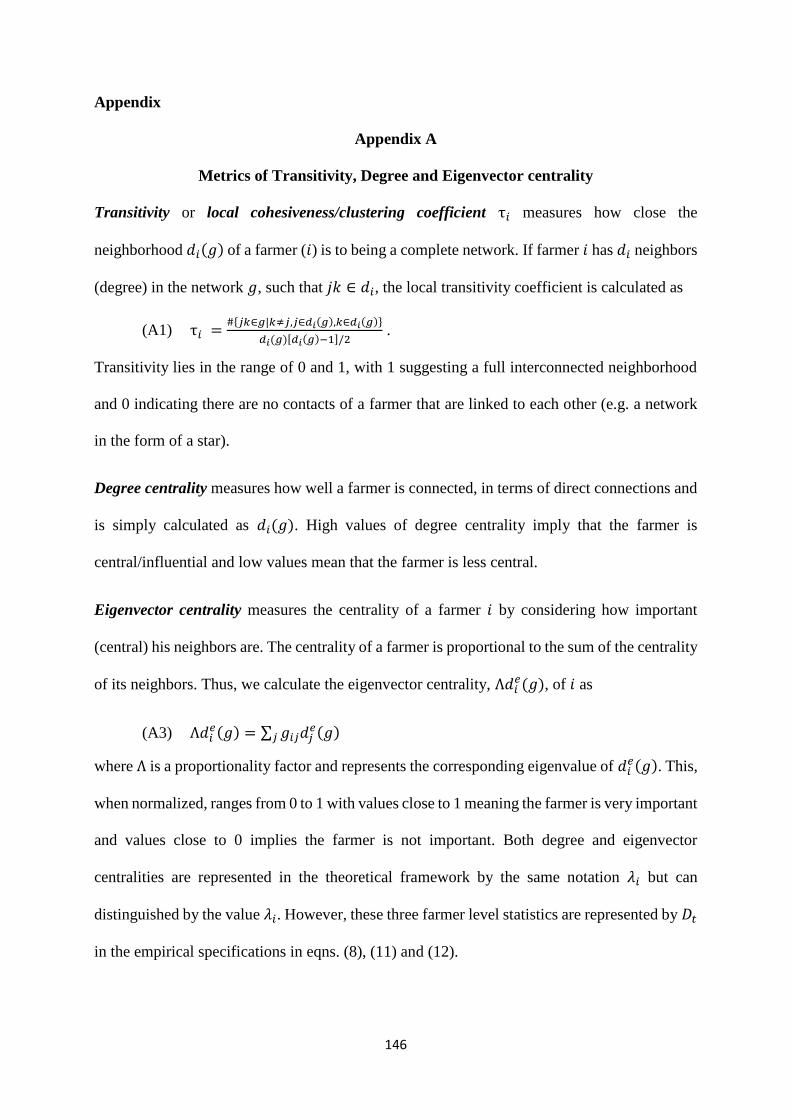
146

Appendix

Appendix A

Metrics of Transitivity, Degree and Eigenvector centrality

Transitivity or local cohesiveness/clustering coefficient τ𝑖 measures how close the

neighborhood 𝑑𝑖(𝑔) of a farmer (𝑖) is to being a complete network. If farmer 𝑖 has 𝑑𝑖 neighbors

(degree) in the network 𝑔, such that 𝑗𝑘 ∈ 𝑑𝑖, the local transitivity coefficient is calculated as

(A1) τ𝑖 =#{𝑗𝑘∈𝑔|𝑘≠𝑗,𝑗∈𝑑𝑖(𝑔),𝑘∈𝑑𝑖(𝑔)}

𝑑𝑖(𝑔)[𝑑𝑖(𝑔)−1]/2 .

Transitivity lies in the range of 0 and 1, with 1 suggesting a full interconnected neighborhood

and 0 indicating there are no contacts of a farmer that are linked to each other (e.g. a network

in the form of a star).

Degree centrality measures how well a farmer is connected, in terms of direct connections and

is simply calculated as 𝑑𝑖(𝑔). High values of degree centrality imply that the farmer is

central/influential and low values mean that the farmer is less central.

Eigenvector centrality measures the centrality of a farmer 𝑖 by considering how important

(central) his neighbors are. The centrality of a farmer is proportional to the sum of the centrality

of its neighbors. Thus, we calculate the eigenvector centrality, Λ𝑑𝑖𝑒(𝑔), of 𝑖 as

(A3) Λ𝑑𝑖𝑒(𝑔) = ∑ 𝑔𝑖𝑗𝑑𝑗

𝑒(𝑔)𝑗

where Λ is a proportionality factor and represents the corresponding eigenvalue of 𝑑𝑖𝑒(𝑔). This,

when normalized, ranges from 0 to 1 with values close to 1 meaning the farmer is very important

and values close to 0 implies the farmer is not important. Both degree and eigenvector

centralities are represented in the theoretical framework by the same notation 𝜆𝑖 but can

distinguished by the value 𝜆𝑖. However, these three farmer level statistics are represented by 𝐷𝑡

in the empirical specifications in eqns. (8), (11) and (12).

147

Appendix B

Network formation model and estimates

B.1 The network formation model

Our model of network formation is based on the behavior of utility maximization. In this

framework, each group member is assumed to have some characteristics that are only observed

by other group members in the same group, and the distances in these observable and

unobservable characteristics between individuals explain their link formation (Hsieh and Lee

2016). Each individual 𝑖, chooses to link to 𝑗, that is 𝑑𝑖𝑗,𝑔 = 1, if 𝑈𝑖𝑗,𝑔(𝑑𝑖𝑗,𝑔 = 1) −

𝑈𝑖𝑗,𝑔(𝑑𝑖𝑗,𝑔 = 0) > 0, and 𝑑𝑖𝑗,𝑔 = 0 otherwise, where 𝑈𝑖𝑗,𝑔 denotes utility function from the

link 𝑖𝑗. We express the above utility differences as

(B1) 𝑈𝑖𝑗,𝑔(𝑑𝑖𝑗,𝑔 = 1) − 𝑈𝑖𝑗,𝑔(𝑑𝑖𝑗,𝑔 = 0) = 𝑉𝑖𝑗,𝑔(𝐿𝑔, 𝒜) + 𝑟𝑖𝑗,𝑔,

where 𝑉𝑖𝑗,𝑔(𝐿𝑔, 𝒜) is the observed link formation due to exogenous effects with specific

elements, 𝑙𝑖𝑗,𝑔, as a vector of observed dyad-specific variables (such as age, sex, years of

schooling etc.) and attributes of the link between 𝑖 and 𝑗 such as geographical and social distance

between them. 𝑟𝑖𝑗,𝑔 is the error term and represents the unobservable characteristics that effect

link formation between 𝑖, 𝑗, and 𝒜 is a vector of parameter estimates.

We implement this by estimating a conditional edge independence model, which assumes links

form independently, conditional on node- and link- level covariates (Fafchamps and Gubert

2007; Chandrasekhar and Lewis 2016) as follows;

(B2) 𝑃𝑖𝑗 = 𝒶0 + 𝒶1|𝑙𝑖,𝑔 − 𝑙𝑗,𝑔| + 𝒶2(𝑙𝑖,𝑔 + 𝑙𝑗,𝑔) + 𝒶3|𝑙𝑖𝑗,𝑔| + 𝑟𝑖𝑗,𝑔

where 𝑃𝑖𝑗 is an 𝑁 × (𝑁 − 1) matrix indicating whether there is a link between individuals 𝑖 and

𝑗, 𝑙𝑖,𝑔 and 𝑙𝑗,𝑔 are characteristics of individual 𝑖 and 𝑗. 𝒶1 measures the influence of differences

in their attributes, and 𝒶2 measures the effect of combined level of their attributes. 𝑙𝑖𝑗,𝑔 captures

148

attributes of the link between 𝑖 and 𝑗 such as geographical or social distance between them, and

𝒶3 is the associated parameter estimate. The estimates of eq. (B1.1) are reported in table 3.B1.

With respect to potential endogeneity due to unobservables at the farmer link formation level,

we retrieved the predicted residuals, �̂�𝑖𝑗,𝑔, and inserted these into our estimation equation to

account for these threats. This also allows us to account for concerns of measurement errors

due to the use of sampled networks (Chandrasekhar and Lewis 2016) by using the predicted

probabilities of links in the respective village networks to simulate the completed networks of

the villages. This is termed the graphical reconstruction approach by Chandrasekhar and Lewis

(2016). With this, we are able to reconstruct the networks and thus able to predict what we

would find if we had the missing part of the networks. This was used to perform sensitivity

checks of our parameters to measurement errors due to the use of the sample data (see figures

in table 3.B2 for a number of the sampled networks and their respective reconstructed versions).

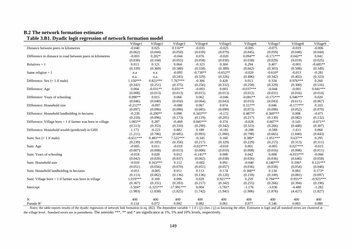
149

B.2 The network formation estimates

Table 3.B1. Dyadic logit regression of network formation model Village1 Village2 Village3 Village4 Village5 Village6 Village7 Village8 Village9

Distance between peers in kilometres -0.040 0.025 0.116** -0.035 -0.025 -0.005 -0.075 -0.019 -0.006

(0.062) (0.044) (0.050) (0.039) (0.079) (0.045) (0.059) (0.048) (0.044)

Difference in distance to road between peers in kilometres -0.003 0.202* -0.044 0.076 -0.020 0.094** -0.171*** 0.042** 0.041

(0.030) (0.104) (0.055) (0.058) (0.030) (0.038) (0.029) (0.019) (0.025)

Relatives = 1 0.013 0.121 0.064 -0.323 0.304 0.294 0.407 -0.001 -0.685**

(0.339) (0.369) (0.580) (0.558) (0.389) (0.662) (0.303) (0.508) (0.349)

Same religion = 1 n.a n.a. -0.095 -0.730** -0.652** -0.020 -0.610* -0.013 -0.281

n.a. n.a. (0.245) (0.329) (0.326) (0.486) (0.342) (0.402) (0.323)

Difference: Sex (= 1 if male) 1.150*** 0.821*** 7.767*** -0.306 0.428 0.013 0.334 0.976*** 0.260

(0.342) (0.251) (0.375) (0.256) (0.332) (0.258) (0.329) (0.300) (0.516)

Difference: Age 0.004 -0.031** 0.031** -0.003 0.003 -0.037*** -0.044 -0.001 0.041***

(0.008) (0.013) (0.013) (0.015) (0.013) (0.012) (0.031) (0.016) (0.014)

Difference: Years of schooling 0.090** 0.015 0.066 0.062 -0.046 -0.081** -0.175*** 6.946*** 0.020

(0.046) (0.040) (0.050) (0.064) (0.043) (0.033) (0.043) (0.611) (0.067)

Difference: Household size -0.212** -0.097 -0.080 0.067 0.074 0.157** 0.046 -0.177*** 0.103

(0.097) (0.096) (0.090) (0.085) (0.099) (0.073) (0.098) (0.052) (0.070)

Difference: Household landholding in hectares -0.239 -0.200** 0.098 0.343*** -0.172 0.487** 0.369*** 0.008 -0.071

(0.218) (0.096) (0.173) (0.119) (0.201) (0.217) (0.130) (0.082) (0.132)

Difference: Village born = 1 if farmer was born in village 1.065** 0.287 -0.469 0.845*** 0.374 -0.028 0.607** 0.143 -0.671**

(0.513) (0.353) (0.310) (0.290) (0.342) (0.323) (0.266) (0.448) (0.307)

Difference: Household wealth (predicted) in GHS 1.173 -0.223 0.882 0.189 -0.181 -0.288 -0.589 -1.611 0.060

(1.211) (0.786) (0.685) (0.993) (1.060) (0.798) (0.665) (1.840) (0.843)

Sum: Sex (= 1 if male) -0.651*** 0.483*** 7.522*** -0.345 0.160 0.380* -1.051*** 0.637** 0.295

(0.239) (0.185) (0.356) (0.217) (0.329) (0.229) (0.215) (0.313) (0.311)

Sum: Age -0.005 0.011 -0.019 -0.023*** -0.010 0.001 -0.005 0.027*** -0.015

(0.007) (0.008) (0.013) (0.008) (0.010) (0.008) (0.016) (0.008) (0.011)

Sum: Years of schooling -0.018 0.028 0.012 -0.141** 0.008 0.042 0.008 -6.015*** -0.066

(0.042) (0.020) (0.037) (0.062) (0.038) (0.026) (0.036) (0.646) (0.058)

Sum: Household size -0.010 0.163*** 0.112 -0.002 0.091 -0.040 0.140*** 0.106* 0.121***

(0.051) (0.056) (0.070) (0.051) (0.057) (0.036) (0.038) (0.054) (0.046)

Sum: Household landholding in hectares -0.051 -0.005 0.011 0.113 0.174 -0.360** 0.134 0.083 0.173*

(0.113) (0.062) (0.136) (0.136) (0.120) (0.159) (0.100) (0.081) (0.097)

Sum: Village born = 1 if farmer was born in village 1.019*** 0.169 0.096 0.029 0.921*** 0.259 0.794*** 0.955** -0.925***

(0.367) (0.331) (0.283) (0.217) (0.342) (0.255) (0.266) (0.394) (0.190)

Intercept -3.504* -5.325*** -17.991*** 0.004 -3.781* -1.176 -3.036 -4.480 -1.282

(1.983) (1.838) (1.825) (1.742) (1.941) (1.986) (1.876) (4.427) (1.827)

N 400 400 400 400 400 400 400 400 400

Pseudo R2 0.114 0.072 0.092 0.082 0.061 0.077 0.146 0.083 0.080

Notes: the table reports results of the dyadic regression of network link formation in eq. (B2). The dependent variable = 1 if 𝑖 (𝑗) cites 𝑖 (𝑗) as knowing the other. Estimator is logit and all standard errors are clustered at

the village level. Standard errors are in parenthesis. The asterisks ***, ** and * are significance at 1%, 5% and 10% levels, respectively.

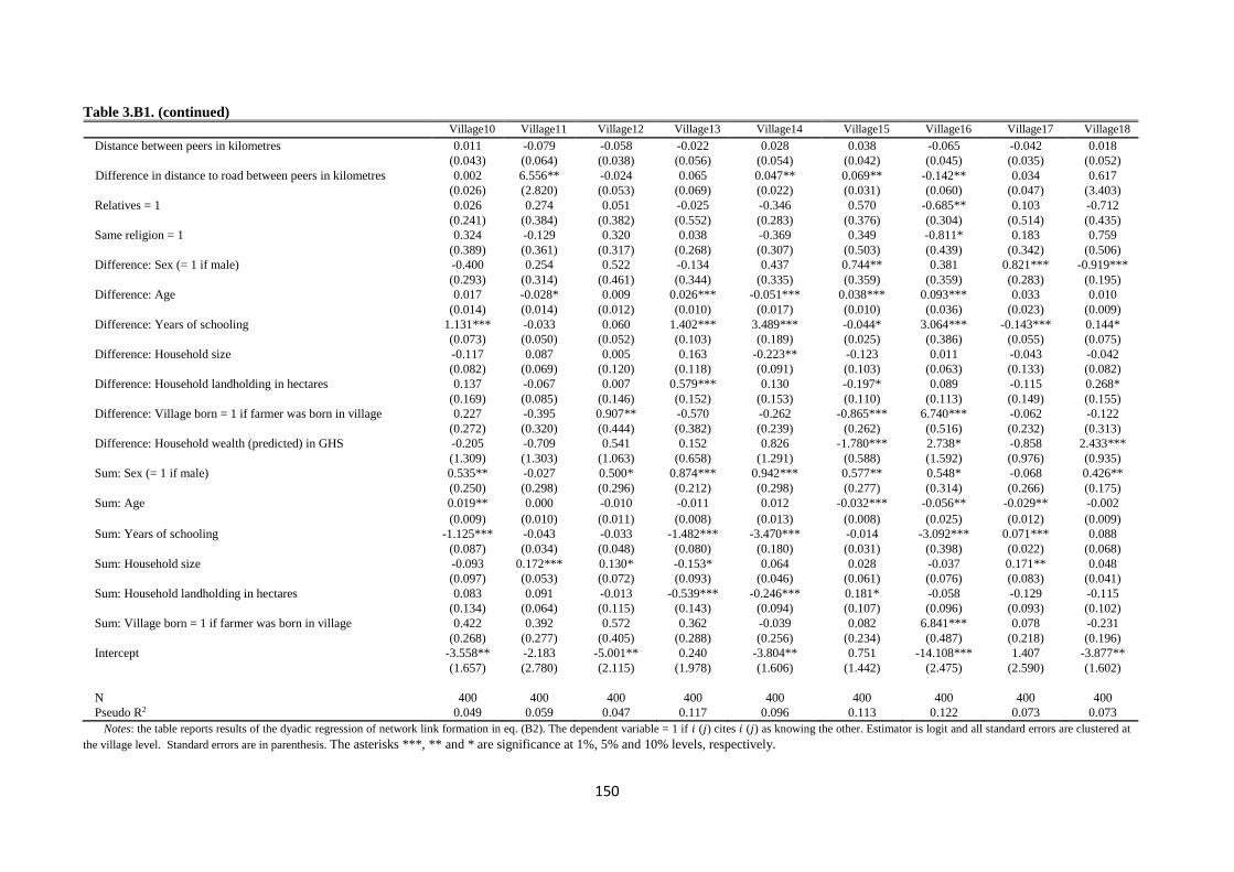
150

Table 3.B1. (continued) Village10 Village11 Village12 Village13 Village14 Village15 Village16 Village17 Village18

Distance between peers in kilometres 0.011 -0.079 -0.058 -0.022 0.028 0.038 -0.065 -0.042 0.018

(0.043) (0.064) (0.038) (0.056) (0.054) (0.042) (0.045) (0.035) (0.052)

Difference in distance to road between peers in kilometres 0.002 6.556** -0.024 0.065 0.047** 0.069** -0.142** 0.034 0.617

(0.026) (2.820) (0.053) (0.069) (0.022) (0.031) (0.060) (0.047) (3.403)

Relatives = 1 0.026 0.274 0.051 -0.025 -0.346 0.570 -0.685** 0.103 -0.712

(0.241) (0.384) (0.382) (0.552) (0.283) (0.376) (0.304) (0.514) (0.435)

Same religion = 1 0.324 -0.129 0.320 0.038 -0.369 0.349 -0.811* 0.183 0.759

(0.389) (0.361) (0.317) (0.268) (0.307) (0.503) (0.439) (0.342) (0.506)

Difference: Sex (= 1 if male) -0.400 0.254 0.522 -0.134 0.437 0.744** 0.381 0.821*** -0.919***

(0.293) (0.314) (0.461) (0.344) (0.335) (0.359) (0.359) (0.283) (0.195)

Difference: Age 0.017 -0.028* 0.009 0.026*** -0.051*** 0.038*** 0.093*** 0.033 0.010

(0.014) (0.014) (0.012) (0.010) (0.017) (0.010) (0.036) (0.023) (0.009)

Difference: Years of schooling 1.131*** -0.033 0.060 1.402*** 3.489*** -0.044* 3.064*** -0.143*** 0.144*

(0.073) (0.050) (0.052) (0.103) (0.189) (0.025) (0.386) (0.055) (0.075)

Difference: Household size -0.117 0.087 0.005 0.163 -0.223** -0.123 0.011 -0.043 -0.042

(0.082) (0.069) (0.120) (0.118) (0.091) (0.103) (0.063) (0.133) (0.082)

Difference: Household landholding in hectares 0.137 -0.067 0.007 0.579*** 0.130 -0.197* 0.089 -0.115 0.268*

(0.169) (0.085) (0.146) (0.152) (0.153) (0.110) (0.113) (0.149) (0.155)

Difference: Village born = 1 if farmer was born in village 0.227 -0.395 0.907** -0.570 -0.262 -0.865*** 6.740*** -0.062 -0.122

(0.272) (0.320) (0.444) (0.382) (0.239) (0.262) (0.516) (0.232) (0.313)

Difference: Household wealth (predicted) in GHS -0.205 -0.709 0.541 0.152 0.826 -1.780*** 2.738* -0.858 2.433***

(1.309) (1.303) (1.063) (0.658) (1.291) (0.588) (1.592) (0.976) (0.935)

Sum: Sex (= 1 if male) 0.535** -0.027 0.500* 0.874*** 0.942*** 0.577** 0.548* -0.068 0.426**

(0.250) (0.298) (0.296) (0.212) (0.298) (0.277) (0.314) (0.266) (0.175)

Sum: Age 0.019** 0.000 -0.010 -0.011 0.012 -0.032*** -0.056** -0.029** -0.002

(0.009) (0.010) (0.011) (0.008) (0.013) (0.008) (0.025) (0.012) (0.009)

Sum: Years of schooling -1.125*** -0.043 -0.033 -1.482*** -3.470*** -0.014 -3.092*** 0.071*** 0.088

(0.087) (0.034) (0.048) (0.080) (0.180) (0.031) (0.398) (0.022) (0.068)

Sum: Household size -0.093 0.172*** 0.130* -0.153* 0.064 0.028 -0.037 0.171** 0.048

(0.097) (0.053) (0.072) (0.093) (0.046) (0.061) (0.076) (0.083) (0.041)

Sum: Household landholding in hectares 0.083 0.091 -0.013 -0.539*** -0.246*** 0.181* -0.058 -0.129 -0.115

(0.134) (0.064) (0.115) (0.143) (0.094) (0.107) (0.096) (0.093) (0.102)

Sum: Village born = 1 if farmer was born in village 0.422 0.392 0.572 0.362 -0.039 0.082 6.841*** 0.078 -0.231

(0.268) (0.277) (0.405) (0.288) (0.256) (0.234) (0.487) (0.218) (0.196)

Intercept -3.558** -2.183 -5.001** 0.240 -3.804** 0.751 -14.108*** 1.407 -3.877**

(1.657) (2.780) (2.115) (1.978) (1.606) (1.442) (2.475) (2.590) (1.602)

N 400 400 400 400 400 400 400 400 400

Pseudo R2 0.049 0.059 0.047 0.117 0.096 0.113 0.122 0.073 0.073

Notes: the table reports results of the dyadic regression of network link formation in eq. (B2). The dependent variable = 1 if 𝑖 (𝑗) cites 𝑖 (𝑗) as knowing the other. Estimator is logit and all standard errors are clustered at

the village level. Standard errors are in parenthesis. The asterisks ***, ** and * are significance at 1%, 5% and 10% levels, respectively.

151

Table 3.B1. (continued) Village19 Village20 Village21 Village22 Village23 Village24 Village25

Distance between peers in kilometers -0.006 -0.040 0.044 0.060 -0.009 0.018 0.009

(0.061) (0.046) (0.050) (0.067) (0.039) (0.030) (0.047)

Difference in distance to road between peers in kilometres 0.012 -1.666 0.024 0.059** 0.686 0.820 0.024

(0.008) (3.250) (0.016) (0.024) (0.659) (2.653) (0.018)

Relatives = 1 -0.471* 0.227 -0.523 1.345 0.090 0.390* 0.717

(0.268) (0.307) (0.538) (1.195) (0.272) (0.205) (0.605)

Same religion = 1 -0.304 n.a. 0.152 0.107 0.180 n.a. -0.014

(0.383) n.a. (0.423) (0.578) (0.479) n.a. (0.384)

Difference: Sex (= 1 if male) -0.385 -0.457 0.744* 8.166*** -0.352 0.849* 0.435

(0.275) (0.278) (0.392) (0.399) (0.423) (0.447) (0.336)

Difference: Age 0.003 -0.009 0.029 -0.000 -0.040** -0.016 0.012

(0.019) (0.012) (0.025) (0.014) (0.020) (0.018) (0.019)

Difference: Years of schooling 0.009 0.421*** 0.142*** n.a. 0.043 -0.054* 0.803***

(0.045) (0.062) (0.050) n.a. (0.065) (0.030) (0.060)

Difference: Household size 0.049 0.252*** 0.229*** 0.076 0.086 0.149* 0.020

(0.063) (0.093) (0.081) (0.097) (0.088) (0.089) (0.082)

Difference: Household landholding in hectares -0.066 0.619*** -0.263 0.126 -0.077 -0.088 0.289***

(0.088) (0.235) (0.218) (0.163) (0.100) (0.105) (0.085)

Difference: Village born = 1 if farmer was born in village 6.526*** 0.210 -0.235 0.638 8.173*** -0.273 -1.469***

(0.422) (0.327) (0.412) (0.490) (0.403) (0.315) (0.419)

Difference: Household wealth (predicted) in GHS 1.450 -2.289*** -0.522 2.782*** -0.100 -1.353 -3.162***

(1.150) (0.794) (1.269) (0.976) (0.639) (0.884) (0.861)

Sum: Sex (= 1 if male) 0.504* 0.219 0.161 8.878*** -0.293 0.810** 0.134

(0.284) (0.173) (0.278) (0.517) (0.245) (0.388) (0.294)

Sum: Age -0.012 0.030** -0.002 0.017 0.010 -0.004 0.016

(0.011) (0.013) (0.021) (0.015) (0.011) (0.013) (0.012)

Sum: Years of schooling 0.033 -0.460*** 0.019 n.a. 0.210*** 0.077*** -0.733***

(0.024) (0.047) (0.059) n.a. (0.037) (0.021) (0.045)

Sum: Household size -0.000 0.099 -0.284*** 0.028 -0.072 -0.044 0.196***

(0.048) (0.085) (0.056) (0.062) (0.062) (0.054) (0.055)

Sum: Household landholding in hectares 0.123 -0.413* 0.248 -0.382* 0.270*** -0.078 -0.063

(0.092) (0.213) (0.169) (0.198) (0.082) (0.085) (0.080)

Sum: Village born = 1 if farmer was born in village 6.413*** 0.725*** -0.821*** 1.116** 7.525*** -0.381 0.213

(0.380) (0.228) (0.278) (0.435) (0.430) (0.240) (0.374)

Intercept -17.238*** -2.388 0.730 -26.287*** -18.598*** -0.160 -0.735

(2.569) (1.844) (2.514) (2.386) (1.453) (1.444) (2.445)

N 400 400 400 400 400 400 400

Pseudo R2 0.075 0.083 0.201 0.155 0.160 0.086 0.155

Notes: the table reports results of the dyadic regression of network link formation in eq. (B2). The dependent variable = 1 if 𝑖 (𝑗) cites 𝑖 (𝑗) as knowing the other. Estimator is logit and all

standard errors are clustered at the village level. Standard errors are in parenthesis. The asterisks ***, ** and * are significance at 1%, 5% and 10% levels, respectively.

152

Table 3.B2. Sampled and simulated networks by quintiles of modularity

1. Sampled network 2. Simulated networks

Fig. 1A. Lowest modularity network (0.143) Fig. 2A. Lowest modularity network (0.163)

Fig. 1B. Mean modularity network (0.289) Fig. 2B. Lowest modularity network (0.205)

Fig. 1C. Median modularity network (0.345) Fig. 2C. Lowest modularity network (0.233)

Fig. 1D. Highest modularity network (0.414) Fig. 2D. Lowest modularity network (0.319) Notes: the table shows plots of some of the social networks by quintiles of modularity in two columns. Column 1 shows a

cross section of the sampled networks used categorized into the network at the lowest (Fig. 1A), at the mean (Fig. 1B), at the

median (Fig. 1C) and at the highest (Fig. 1D) of modularity distribution. Column 2 shows the respective simulated (i.e.,

reconstructed) versions of these sampled networks based on the approach of Chandrasekhar and Lewis (2016). Figs. 1A and 1B

have more interconnected nodes and lower modularity statistics, of 0.143 and 0.289, respectively, than figs. 1C and 1D. Similar

trend is observed in the modularity statistics when calculated with simulated complete versions of these networks in figs. 2A-2D.

We, therefore, expect learning and diffusion to be faster in the case of figures A and B.

X1

X2

X3

X4

X5

X6

X7

X8

X9

X10

X11

X12

X13

X14

X15

X16

X17

X18

X19

X20

V1

V2

V3

V4

V5

V6

V7

V8

V9

V10

V11

V12

V13

V14

V15

V16

V17

V18

V19

V20

V21

V22

V23

V24

V25

V26

V27

V28

V29

V30

V31

V32V33

V34

V35

V36V37

V38

V39V40

V41

V42

V43

V44

V45

V46

V47

V48

V49

V50

V51

V52

V53V54V55

V56

V57

V58

X1

X2

X3

X4

X5

X6

X7

X8

X9

X10

X11

X12

X13

X14

X15

X16

X17X18

X19

X20V1

V2

V3

V4

V5

V6

V7

V8

V9

V10

V11V12

V13

V14

V15

V16

V17

V18

V19V20

V21V22

V23

V24

V25

V26

V27

V28

V29

V30

V31

V32

V33

V34

V35

V36

V37

V38

V39

V40

V41

V42

V43

V44

V45

V46

V47

V48

V49

V50

V51

V52

V53

V54V55

V56

V57

V58

V59V60

V61

V62

V63

X1

X2

X3X4

X5

X6

X7

X8

X9

X10

X11

X12

X13

X14

X15

X16

X17

X18

X19

X20

V1

V2

V3

V4

V5

V6

V7

V8

V9

V10

V11

V12

V13

V14

V15V16

V17

V18

V19

V20V21

V22

V23

V24

V25V26

V27

V28

V29

V30

V31

V32 V33V34

V35

V36

X1

X2

X3

X4

X5

X6 X7X8

X9

X10

X11

X12

X13

X14 X15

X16

X17

X18

X19

X20

V1

V2V3

V4

V5

V6

V7

V8

V9

V10

V11

V12

V13

V14

V15

V16

V17

V18

V19

V20

V21

V22

V23

V24

V25

V26

V27

V28

V29

V30

V31

V32

V33

V34

V35

V36

V37

V38V39

V40V41

V42

V43

V44

V45

V46

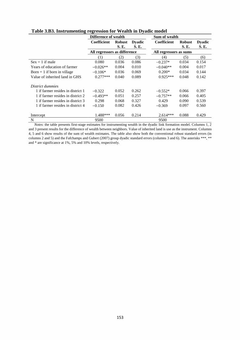
153

Table 3.B3. Instrumenting regression for Wealth in Dyadic model Difference of wealth Sum of wealth

Coefficient Robust

S. E.

Dyadic

S. E.

Coefficient Robust

S. E.

Dyadic

S. E.


(1) (2) (3) (4) (5) (6)

Sex = 1 if male 0.080 0.036 0.086 -0.237* 0.034 0.154




District dummies





Intercept 1.488*** 0.056 0.214 2.614*** 0.088 0.429

N 9500 9500 Notes: the table presents first-stage estimates for instrumenting wealth in the dyadic link formation model. Columns 1, 2

and 3 present results for the difference of wealth between neighbors. Value of inherited land is use as the instrument. Columns

4, 5 and 6 show results of the sum of wealth estimates. The table also show both the conventional robust standard errors (in

columns 2 and 5) and the Fafchamps and Gubert (2007) group dyadic standard errors (columns 3 and 6). The asterisks ***, **


154

Appendix C

Other estimates

Table 3.C1. Control and contextual variables in Table 6 (5) (6) (7) (8)

Coef. S.E. Coef. S.E. Coef. S.E. Coef. S.E.

Household controls, 𝜸𝟏

Age -0.008 0.006 -0.008 0.006 -0.008 0.006 -0.008 0.006

Gender 0.325 0.213 0.355 0.217 0.325 0.210 0.356* 0.215

Education 0.131*** 0.039 0.130*** 0.039 0.129*** 0.040 0.128*** 0.040

Experience -0.229*** 0.041 -0.226*** 0.040 -0.228*** 0.042 -0.225*** 0.040

Household -0.083 0.054 -0.085 0.055 -0.082 0.054 -0.084 0.055

Landholding 0.270*** 0.071 0.263*** 0.071 0.228*** 0.071 0.259*** 0.070

Credit -0.306 0.774 -0.195 0.780 -0.354 0.784 -0.238 0.790

Risk 0.021 0.074 0.027 0.076 0.023 0.075 0.029 0.076

Extension 1.024 0.866 1.157 0.868 0.998 0.870 1.139 0.872

Association -0.322*** 0.100 -0.325*** 0.100 -0.322*** 0.100 -0.326*** 0.100

Price -1.742** 0.621 -1.814*** 0.610 -1.727** 0.616 -1.806*** 0.605

Soil quality 0.530*** 0.155 0.385*** 0.111 0.526*** 0.156 0.526*** 0.157

Contextual (peer) controls, 𝜸𝟐

Gage 0.010 0.012 0.011 0.012 0.009 0.012 0.010 0.012

GGender -0.596* 0.306 -0.551* 0.306 -0.588* 0.302 -0.543* 0.301

GEducation -0.043 0.052 -0.041 0.052 -0.038 0.051 -0.035 0.050

GHousehold -0.009 0.078 -0.005 0.078 0.010 0.076 0.007 0.078

GLandholding -0.061 0.106 -0.053 0.106 -0.054 0.105 -0.046 0.107

GCredit -0.400 0.267 -0.397 0.267 -0.390 0.263 -0.389 0.266

GRisk 0.237 0.164 0.241 0.164 0.233 0.166 0.237 0.163

GExtension 0.337 0.375 0.355 0.375 0.336 0.373 0.354 0.374

GAssociation 0.096 0.143 -0.105 0.143 0.086 0.142 0.095 0.139

GPrice -0.859 0.684 -0.916 0.684 -0.889 0.685 -0.951 0.687

GSoil quality -0.079 0.150 -0.079 0.150 -0.086 0.150 -0.086 0.147

Time effects, 𝜹𝒕

Year 3&4 0.736*** 0.183 0.735*** 0.180 0.739*** 0.190 0.738*** 0.187

Year 5&6 1.081*** 0.339 1.111*** 0.331 1.089*** 0.350 1.120*** 0.341

Year 7&8 1.509*** 0.374 1.535*** 0.367 1.544*** 0.389 1.572*** 0.382

Year 9&10 1.945*** 0.432 1.964*** 0.420 1.985*** 0.445 2.006*** 0.432

Year 11&12 1.798*** 0.467 1.808*** 0.456 1.841*** 0.474 1.853*** 0.462

Year 13&14 1.842*** 0.520 1.785*** 0.516 1.879*** 0.528 1.820*** 0.522

Link residuals, �̂�𝒕

Av.Residual 1st quintile -5.768*** 1.970 -6.142*** 2.011 -5.709*** 1.939 -6.097*** 1.983

Av.Residual 2nd quintile 10.067** 3.823 9.530** 3.945 9.433** 3.671 8.883** 3.791

Av.Residual 3rd quintile 1.265* 0.765 1.029 0.742 1.251* 0.752 1.015 0.729

Av.Residual 4th quintile 0.076 0.122 0.037 0.133 0.080 0.120 0.041 0.131

Av.Residual 5th quintile -0.156 0.097 -0.170* 0.089 -0.162 0.098 -0.178* 0.091

District fixed-effects

SaveluguNanton -0.781*** 0.229 -0.770*** 0.229 -0.768*** 0.234 -0.758*** 0.234

Karaga -0.668* 0.358 -0.580 0.356 -0.663* 0.360 -0.574 0.357

Gushegu -0.984** 0.366 -0.886** 0.372 -0.989** 0.369 -0.888** 0.374

First-stage residuals

Residuals Extension -0.098 0.522 -0.158 0.527 -0.094 0.525 -0.158 0.529

Residuals Liquidity constr. -0.288 0.408 -0.351 0.415 -0.264 0.414 -0.329 0.421

Notes: The table presents coefficients of controls of the models in columns 5-8 of table 3.6. D is the social network. Years 1 and 2

are the reference years. Av.Residual is the average residuals of the link formation model over a given quintile arranged in ascending

order – 1st quintile is average of the predicted residuals of the first four set of peers of a household with the least predicted residuals

(i.e., less likely to link up due to unobserved determinant of link formation). The 2nd quintile is the average residuals of the link

formation model for the next set of four peers and so on until the 5th set of four peers as those with the highest residuals (i.e., those

most likely to link up due to unobserved determinants of link formation). These are used as instruments to account for potential

endogeneity due to correlated unobservables at the link formation level. The asterisks ***, ** and * are significance at 1%, 5% and


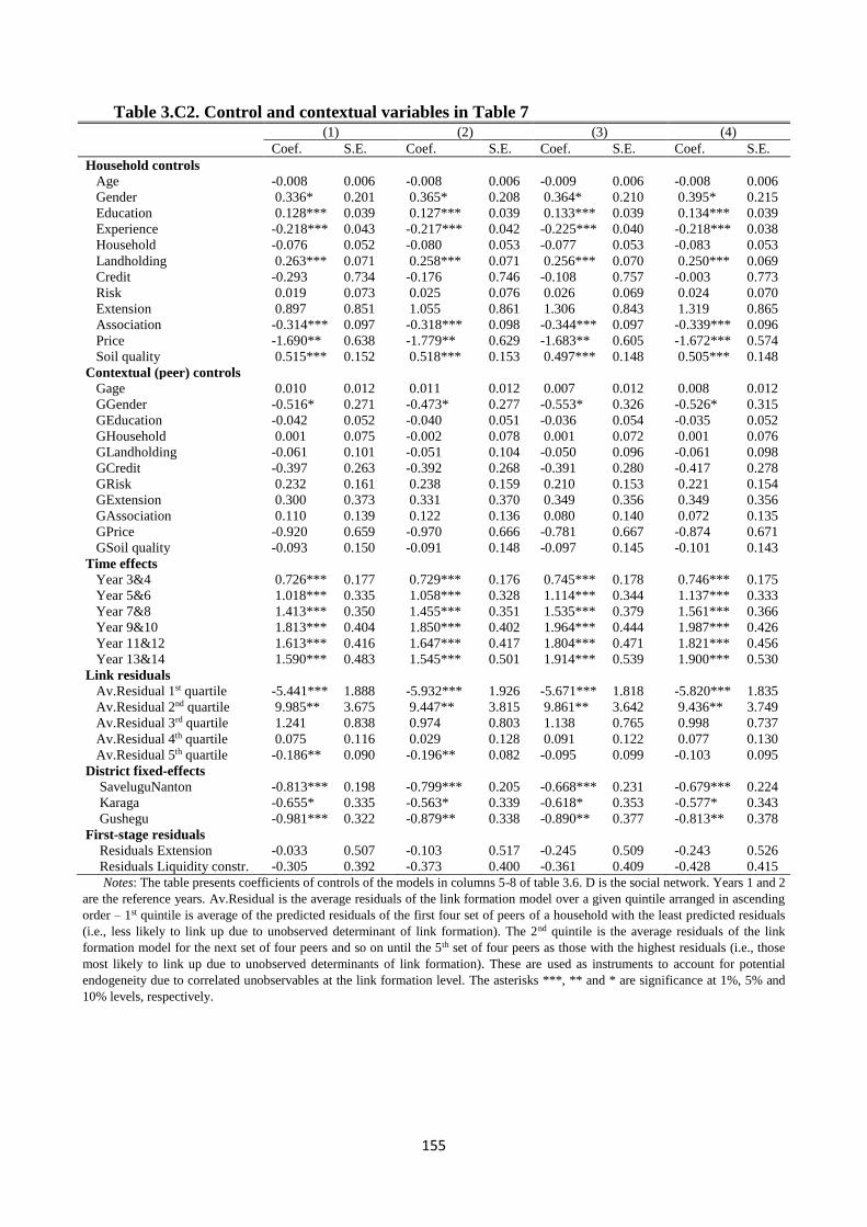
155

Table 3.C2. Control and contextual variables in Table 7 (1) (2) (3) (4)

Coef. S.E. Coef. S.E. Coef. S.E. Coef. S.E.

Household controls

Age -0.008 0.006 -0.008 0.006 -0.009 0.006 -0.008 0.006

Gender 0.336* 0.201 0.365* 0.208 0.364* 0.210 0.395* 0.215

Education 0.128*** 0.039 0.127*** 0.039 0.133*** 0.039 0.134*** 0.039

Experience -0.218*** 0.043 -0.217*** 0.042 -0.225*** 0.040 -0.218*** 0.038

Household -0.076 0.052 -0.080 0.053 -0.077 0.053 -0.083 0.053

Landholding 0.263*** 0.071 0.258*** 0.071 0.256*** 0.070 0.250*** 0.069

Credit -0.293 0.734 -0.176 0.746 -0.108 0.757 -0.003 0.773

Risk 0.019 0.073 0.025 0.076 0.026 0.069 0.024 0.070

Extension 0.897 0.851 1.055 0.861 1.306 0.843 1.319 0.865

Association -0.314*** 0.097 -0.318*** 0.098 -0.344*** 0.097 -0.339*** 0.096

Price -1.690** 0.638 -1.779** 0.629 -1.683** 0.605 -1.672*** 0.574

Soil quality 0.515*** 0.152 0.518*** 0.153 0.497*** 0.148 0.505*** 0.148

Contextual (peer) controls

Gage 0.010 0.012 0.011 0.012 0.007 0.012 0.008 0.012

GGender -0.516* 0.271 -0.473* 0.277 -0.553* 0.326 -0.526* 0.315

GEducation -0.042 0.052 -0.040 0.051 -0.036 0.054 -0.035 0.052

GHousehold 0.001 0.075 -0.002 0.078 0.001 0.072 0.001 0.076

GLandholding -0.061 0.101 -0.051 0.104 -0.050 0.096 -0.061 0.098

GCredit -0.397 0.263 -0.392 0.268 -0.391 0.280 -0.417 0.278

GRisk 0.232 0.161 0.238 0.159 0.210 0.153 0.221 0.154

GExtension 0.300 0.373 0.331 0.370 0.349 0.356 0.349 0.356

GAssociation 0.110 0.139 0.122 0.136 0.080 0.140 0.072 0.135

GPrice -0.920 0.659 -0.970 0.666 -0.781 0.667 -0.874 0.671

GSoil quality -0.093 0.150 -0.091 0.148 -0.097 0.145 -0.101 0.143

Time effects

Year 3&4 0.726*** 0.177 0.729*** 0.176 0.745*** 0.178 0.746*** 0.175

Year 5&6 1.018*** 0.335 1.058*** 0.328 1.114*** 0.344 1.137*** 0.333

Year 7&8 1.413*** 0.350 1.455*** 0.351 1.535*** 0.379 1.561*** 0.366

Year 9&10 1.813*** 0.404 1.850*** 0.402 1.964*** 0.444 1.987*** 0.426

Year 11&12 1.613*** 0.416 1.647*** 0.417 1.804*** 0.471 1.821*** 0.456

Year 13&14 1.590*** 0.483 1.545*** 0.501 1.914*** 0.539 1.900*** 0.530

Link residuals

Av.Residual 1st quartile -5.441*** 1.888 -5.932*** 1.926 -5.671*** 1.818 -5.820*** 1.835

Av.Residual 2nd quartile 9.985** 3.675 9.447** 3.815 9.861** 3.642 9.436** 3.749

Av.Residual 3rd quartile 1.241 0.838 0.974 0.803 1.138 0.765 0.998 0.737

Av.Residual 4th quartile 0.075 0.116 0.029 0.128 0.091 0.122 0.077 0.130

Av.Residual 5th quartile -0.186** 0.090 -0.196** 0.082 -0.095 0.099 -0.103 0.095

District fixed-effects

SaveluguNanton -0.813*** 0.198 -0.799*** 0.205 -0.668*** 0.231 -0.679*** 0.224

Karaga -0.655* 0.335 -0.563* 0.339 -0.618* 0.353 -0.577* 0.343

Gushegu -0.981*** 0.322 -0.879** 0.338 -0.890** 0.377 -0.813** 0.378

First-stage residuals

Residuals Extension -0.033 0.507 -0.103 0.517 -0.245 0.509 -0.243 0.526

Residuals Liquidity constr. -0.305 0.392 -0.373 0.400 -0.361 0.409 -0.428 0.415

Notes: The table presents coefficients of controls of the models in columns 5-8 of table 3.6. D is the social network. Years 1 and 2

are the reference years. Av.Residual is the average residuals of the link formation model over a given quintile arranged in ascending

order – 1st quintile is average of the predicted residuals of the first four set of peers of a household with the least predicted residuals

(i.e., less likely to link up due to unobserved determinant of link formation). The 2nd quintile is the average residuals of the link

formation model for the next set of four peers and so on until the 5th set of four peers as those with the highest residuals (i.e., those

most likely to link up due to unobserved determinants of link formation). These are used as instruments to account for potential

endogeneity due to correlated unobservables at the link formation level. The asterisks ***, ** and * are significance at 1%, 5% and


156

Appendix D

Endogeneity of credit-constraint and extension contact

The final issue we address is the potential endogeneity of credit-constraint and extension

contact. Credit-constraint could be endogenous because farmers with higher yields and incomes

will be less credit-constrained as a result of the associated increased yields and incomes from

adoption. On the other hand, extension contact could be endogenous because extension officers

may be more inclined to visit farmers who adopted than farmers who did not adopt. We used a

two-stage generalized residual inclusion estimation procedure suggested by Wooldridge

(2015), where we first estimate a probit model for each of these endogenous variables using the

variables in the diffusion model (to be estimated in the second-stage) and two instruments in

each case as explanatory variables. The generalized residuals from the first-stage estimation are

then included with the observed values of the potentially endogenous variables in the second-

stage specification.

We use credit-constraint and extension contacts of farmer 𝑖’s indirect, 𝑋𝑖𝑡′ 𝐺𝑡

2,𝔫, [i.e., first (𝑖, 𝑗 +

1) generation] peers (neighbors) as instruments. These are considered valid and relevant

instruments because the credit-constraint and extension contacts of the 𝑗 + 1 peers of farmer 𝑖

relate indirectly to his own credit-constraint and extension contacts through the credit-

constraints and extension contacts of his direct neighbors 𝑗, (i.e., 𝑋𝑡′𝐺𝑡

𝔫) who are direct peers of

the 𝑗 + 1 peers. These variables, however, are not expected to directly affect the farmer’s

conditional probability of adoption. Bramoulle et al. (2009) show that these are valid

instruments once there are intransitive triads36 in the network, so that the characteristics of the

first and higher generation neighbors of the farmer affect the characteristics and outcomes of

36 The average transitivity statistics in table 3.4 is less than 0.2 across the networks, suggesting that majority of triads on

average are intransitive.

157

the farmer through his direct neighbors. Estimates of the first-stage probit are presented in table

3.D1.

Table 3.D1. First stage probit estimates for credit constraints and extension contact Variable Credit constraint Extension

Coefficient S.E. Coefficient S.E.

Age -0.004 0.005 0.003 0.005

Gender -0.489*** 0.141 -0.078 0.147

Education 0.045* 0.022 -0.002 0.021

Experience -0.016 0.020 -0.029 0.019

Household -0.025 0.030 0.001 0.032

Landholding -0.069 0.046 0.094** 0.044

Credit -0.394** 0.141

Risk 0.104* 0.055 -0.157** 0.061

Extension -0.391** 0.147

Association -0.146** 0.057 -0.206*** 0.054

Price -1.410*** 0.417 2.251*** 0.441

Soil quality -0.103 0.071 0.068 0.075

DAge -0.003 0.009 -0.004 0.009

DGender 0.115 0.237 -0.119 0.240

DEducation 0.056** 0.036 -0.039 0.038

DExperience 0.004 0.034 -0.003 0.032

DHousehold 0.044 0.048 -0.017 0.058

DLandholding -0.021 0.077 -0.022 0.086

DCredit -0.267 0.270 -0.080 0.278

DRisk -0.137 0.092 0.123 0.097

DExtension 0.093 0.248 -0.554* 0282

DAssociation -0.014 0.093 0.089 0.095

DPrice -0.279 0.633 0.628 0.661

DSoil quality -0.037 0.109 0.108 0.119

D2Credit 2.942*** 0.483 - -

D2Extension - 2.741*** 0.572

Constant 2.113 1.161 -5.462*** 1.214

Instrument validity 𝑿𝟐(p-value) 37.12(0.000) 23.01(0.000)

Log likelihood -252.34 -227.64

Wald (𝑿𝟐𝟓𝟐 ) 144.35 140.94

p-value 0.000 0.000

Pseudo 𝑹𝟐 0.265 0.288

Notes: the table presents first-stage estimates of credit constraints and extension contacts of households. S.E. is robust

standard errors. The asterisks ***, ** and * are significance at 1%, 5% and 10% levels, respectively.

.

158

Chapter Four

Social networks, adoption of improved variety and household welfare: Evidence from

Ghana

Yazeed Abdul Mumin and Awudu Abdulai

Department of Food Economics and Consumption Studies, University of Kiel, Germany

European Review of Agricultural Economics (Forthcoming)

Abstract

In this study, we examine the effects of own and peer adoption of improved soybean variety on

household yields, food and nutrients consumption, using observational data from Ghana. We

employ the marginal treatment effect approach to account for treatment effects heterogeneity

across households, and a number of identification strategies to capture social network effects.

Our empirical results show that households with higher unobserved gains are more likely to

adopt because of their worse outcomes when not adopting. We also find strong peer adoption

effect on own yield, only when the household is also adopting, and on food and nutrients

consumption when not adopting. However, the peer adoption effect on consumption attenuates

when the household adopts the improved variety. Furthermore, our findings reveal that adoption

tends to equalize households in terms of observed and unobserved gains on consumption, and

can thus serve as a mechanism for promoting food security and nutrition in this area.

JEL codes: C21, D60, D85, O13, O33

Keywords: Improved variety, Technology adoption, Social networks, Marginal treatment

effects, Food and nutrition security

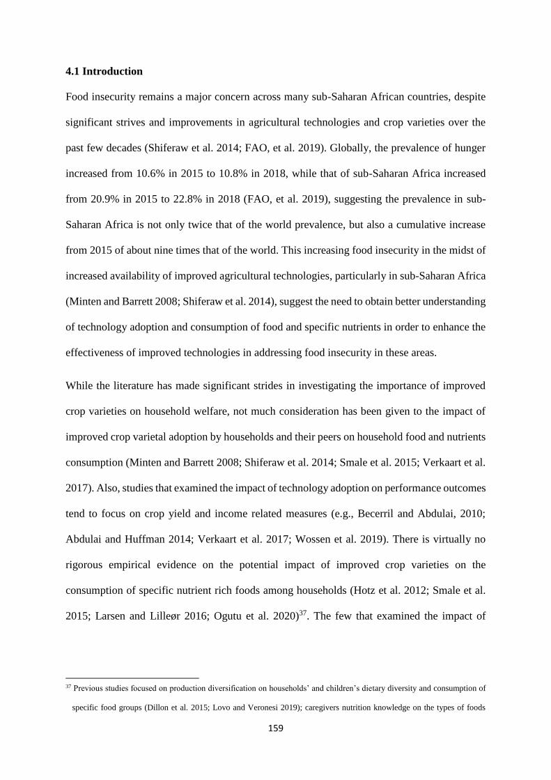
159

4.1 Introduction

Food insecurity remains a major concern across many sub-Saharan African countries, despite

significant strives and improvements in agricultural technologies and crop varieties over the

past few decades (Shiferaw et al. 2014; FAO, et al. 2019). Globally, the prevalence of hunger

increased from 10.6% in 2015 to 10.8% in 2018, while that of sub-Saharan Africa increased

from 20.9% in 2015 to 22.8% in 2018 (FAO, et al. 2019), suggesting the prevalence in sub-

Saharan Africa is not only twice that of the world prevalence, but also a cumulative increase

from 2015 of about nine times that of the world. This increasing food insecurity in the midst of

increased availability of improved agricultural technologies, particularly in sub-Saharan Africa

(Minten and Barrett 2008; Shiferaw et al. 2014), suggest the need to obtain better understanding

of technology adoption and consumption of food and specific nutrients in order to enhance the

effectiveness of improved technologies in addressing food insecurity in these areas.

While the literature has made significant strides in investigating the importance of improved

crop varieties on household welfare, not much consideration has been given to the impact of

improved crop varietal adoption by households and their peers on household food and nutrients

consumption (Minten and Barrett 2008; Shiferaw et al. 2014; Smale et al. 2015; Verkaart et al.

2017). Also, studies that examined the impact of technology adoption on performance outcomes

tend to focus on crop yield and income related measures (e.g., Becerril and Abdulai, 2010;

Abdulai and Huffman 2014; Verkaart et al. 2017; Wossen et al. 2019). There is virtually no

rigorous empirical evidence on the potential impact of improved crop varieties on the

consumption of specific nutrient rich foods among households (Hotz et al. 2012; Smale et al.

2015; Larsen and Lilleør 2016; Ogutu et al. 2020)37. The few that examined the impact of

37 Previous studies focused on production diversification on households’ and children’s dietary diversity and consumption of

specific food groups (Dillon et al. 2015; Lovo and Veronesi 2019); caregivers nutrition knowledge on the types of foods

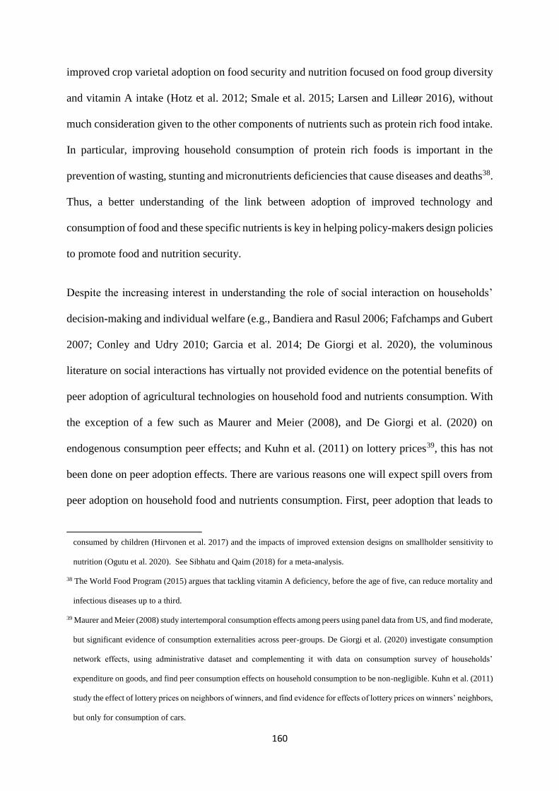
160

improved crop varietal adoption on food security and nutrition focused on food group diversity

and vitamin A intake (Hotz et al. 2012; Smale et al. 2015; Larsen and Lilleør 2016), without

much consideration given to the other components of nutrients such as protein rich food intake.

In particular, improving household consumption of protein rich foods is important in the

prevention of wasting, stunting and micronutrients deficiencies that cause diseases and deaths38.

Thus, a better understanding of the link between adoption of improved technology and

consumption of food and these specific nutrients is key in helping policy-makers design policies

to promote food and nutrition security.

Despite the increasing interest in understanding the role of social interaction on households’

decision-making and individual welfare (e.g., Bandiera and Rasul 2006; Fafchamps and Gubert

2007; Conley and Udry 2010; Garcia et al. 2014; De Giorgi et al. 2020), the voluminous

literature on social interactions has virtually not provided evidence on the potential benefits of

peer adoption of agricultural technologies on household food and nutrients consumption. With

the exception of a few such as Maurer and Meier (2008), and De Giorgi et al. (2020) on

endogenous consumption peer effects; and Kuhn et al. (2011) on lottery prices39, this has not

been done on peer adoption effects. There are various reasons one will expect spill overs from

peer adoption on household food and nutrients consumption. First, peer adoption that leads to

consumed by children (Hirvonen et al. 2017) and the impacts of improved extension designs on smallholder sensitivity to

nutrition (Ogutu et al. 2020). See Sibhatu and Qaim (2018) for a meta-analysis.

38 The World Food Program (2015) argues that tackling vitamin A deficiency, before the age of five, can reduce mortality and

infectious diseases up to a third.

39 Maurer and Meier (2008) study intertemporal consumption effects among peers using panel data from US, and find moderate,

but significant evidence of consumption externalities across peer-groups. De Giorgi et al. (2020) investigate consumption

network effects, using administrative dataset and complementing it with data on consumption survey of households’

expenditure on goods, and find peer consumption effects on household consumption to be non-negligible. Kuhn et al. (2011)

study the effect of lottery prices on neighbors of winners, and find evidence for effects of lottery prices on winners’ neighbors,

but only for consumption of cars.

161

increased learning opportunities and productivity of the household can enhance the household’s

consumption, especially in rural Africa, where the issues of missing and inefficient markets are

prevalent (de Janvry et al. 1991). Second, when peer adoption leads to increased peer

productivity, and changes in peer consumption, can affect household consumption either due to

endogenous peer effect, or through private cash transfers to the household in a form of safety

net.

The purpose of this study is twofold: to investigate the effect of household adoption of improved

crop variety on the consumption of food and specific nutrients among households; and to

examine the effect of peer adoption of the improved crop variety on yield, food and nutrients

consumption. We do this by using detailed data of 500 farm households from northern Ghana

to examine the effect of household and peer adoption of improved soybean variety on crop

yield, and the household’s consumption of food, vitamin A and protein rich foods. Analytically,

we exploit spatial econometric techniques to generate instruments (Bramoullé et al. 2009;

Acemoglu et al. 2015), and then use the instruments, in addition to controlling for network fixed

effects and potential endogeneity of network link formation with the control function approach

by Brock and Durlauf (2001) to identify peer adoption effects on own adoption and outcomes.

We employ the marginal treatment effects (MTE) approach, following Heckman and Vytlacil

(2005) and Cornelissen et al. (2018) to estimate the treatment effects heterogeneities. This

approach is significant in the sense that it allows us to identify, at least, a substantial part of the

range of individual treatment effects, and as a result characterize the extent and pattern of

treatment effects heterogeneity (Cornelissen et al. 2016; 2018)40.

40 Previous studies (e.g., Minten and Barrett 2008; Shiferaw et al. 2014) have assumed homogenous treatment effects, focusing

mainly on addressing selectivity problems arising from unobserved characteristics, and aggregate parameter estimates. As

argued by Cornelissen et al. (2016), this approach can mask important heterogeneity in treatment effects.

162

Poverty incidence and its extreme form have been consistently higher in northern Ghana than

the national average and that of the rest of the country since 2005, and with worsening rates of

extreme poverty, as the incidence increased from 29.7% in 2012/13 to 34.5% in 2016/17 (GSS

2018). This has resulted in higher incidence of food insecurity and malnutrition in the area,

compared to the rest of the country, and the use of a number of strategies including credit

purchases and borrowing from friends and relatives to cope with food insecurity (WFP and GSS

2012). This makes northern Ghana a suitable area for assessing the impact of improved crop

varietal adoption by households and their peers on crop yield, and household food and nutrients

consumption.

Our findings show strong evidence of heterogeneity in returns to adoption in both observed and

unobserved characteristics. Specifically, we find positive selection on gains due to unobserved

characteristics, mainly driven by worse outcomes, of households with less resistance to adopt,

in the non-adoption state. However, adoption appears to make the potential outcomes of

households quite homogenous, irrespective of their level of resistance to adoption. Peer

adoption increases the household’s food and nutrients consumption, when the household is not

adopting the improved variety, but with attenuating effects when the household adopts,

suggesting that non-adopters tend to depend more on adopting peers in terms of food and

nutrients consumption than adopters. We, however, note that the estimated effects cannot be

interpreted as causal-effects in its strictest sense, given that households were not randomly

assigned to treatment and control groups, as in a randomized controlled trial41.

Our study contributes to the literature in threefold: first, it provides empirical insights into the

importance of improved crop varieties on welfare indicators such as crop yields and

consumption of specific nutrient rich foods, while highlighting heterogeneity in returns to

adoption in observed and unobserved characteristics. To the best of our knowledge, this is the

41 We thank the reviewers and editor for suggesting this to us.

163

first study to use this approach to quantify the effects of improved crop variety on food and

nutrients consumption. Second, the paper presents evidence of exogenous interaction effects

(Manski 2013) on food and nutrients consumption of smallholders. As indicated previously,

understanding the relationship between peer adoption and household consumption may present

an alternative to public food and nutrition security interventions through private transfers

among peers, given the challenges of sustainable and exit mechanisms of public food transfer

modalities (Holden et al. 2006). Finally, the study provides insights into the effectiveness of

policy options (i.e., whether to promote affordability or availability of the improved soybean

seeds) that shift some non-adopting households to adopt on the outcomes.

The next section presents the conceptual framework of the analysis. In section 4.3, we present

the context and data used in the analysis. Section 4.4 presents the analytical and empirical

frameworks and estimation. In Section 4.5, we report the results, and then discuss in section

4.6. The final section presents a brief summary and conclusions.

4.2 Conceptual framework

In this section, we explore the conceptual mechanisms by which own and peer adoption may

affect crop yield, food and nutrients consumption. To the extent that the improved variety is

characterized as high yielding, early maturing and resistant to agricultural and climatic stress

(CSIR-SARI 2013), own adoption of the improved variety can lead to increased yields and

reduced production costs, which may result in increased farm income and subsequently

increased food consumption. However, when own adoption and investments in the new variety

is not complemented with good production “know-how”, or soybean market, this may lead to

reduced income and food consumption, since soybean is not a staple food in the area but is

mainly produced for cash sales42. Similarly, food and nutrients consumption may decrease, if

42 The other pathways through which agriculture production can affect food security and nutrition are changes in food prices,

consumption of own production and intra-household dynamics related to gender and resource control. However, we do not

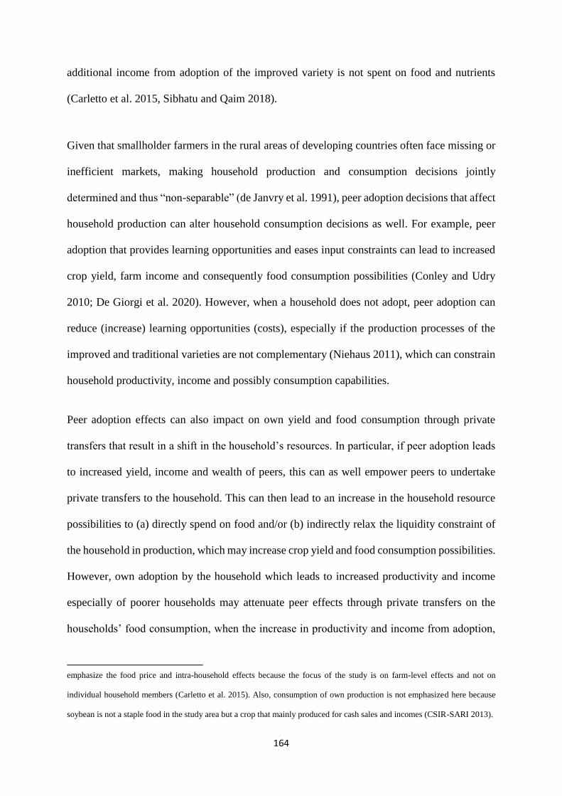
164

additional income from adoption of the improved variety is not spent on food and nutrients

(Carletto et al. 2015, Sibhatu and Qaim 2018).

Given that smallholder farmers in the rural areas of developing countries often face missing or

inefficient markets, making household production and consumption decisions jointly

determined and thus “non-separable” (de Janvry et al. 1991), peer adoption decisions that affect

household production can alter household consumption decisions as well. For example, peer

adoption that provides learning opportunities and eases input constraints can lead to increased

crop yield, farm income and consequently food consumption possibilities (Conley and Udry

2010; De Giorgi et al. 2020). However, when a household does not adopt, peer adoption can

reduce (increase) learning opportunities (costs), especially if the production processes of the

improved and traditional varieties are not complementary (Niehaus 2011), which can constrain

household productivity, income and possibly consumption capabilities.

Peer adoption effects can also impact on own yield and food consumption through private

transfers that result in a shift in the household’s resources. In particular, if peer adoption leads

to increased yield, income and wealth of peers, this can as well empower peers to undertake

private transfers to the household. This can then lead to an increase in the household resource

possibilities to (a) directly spend on food and/or (b) indirectly relax the liquidity constraint of

the household in production, which may increase crop yield and food consumption possibilities.

However, own adoption by the household which leads to increased productivity and income

especially of poorer households may attenuate peer effects through private transfers on the

households’ food consumption, when the increase in productivity and income from adoption,

emphasize the food price and intra-household effects because the focus of the study is on farm-level effects and not on

individual household members (Carletto et al. 2015). Also, consumption of own production is not emphasized here because

soybean is not a staple food in the study area but a crop that mainly produced for cash sales and incomes (CSIR-SARI 2013).

165

leads to a decrease in the private transfers from peers or reduce dependence on peers. Studies

have noted that, when the cost of sharing or altruistic effort is sufficiently higher than the

benefit, then no member will undertake any effort to share (e.g., Alger and Weibull 2012; Di

Falco and Bulte 2013). Finally, peer adoption effect on food consumption could decline,

following own adoption, if own adoption by the household, leads to increased productivity and

results in the need to settle past transfer commitments (Di Falco et al. 2018).

We deduce a number of implications from the foregoing discussion to guide our interpretation

of the empirical results. When the household is not adopting, the impact of peer adoption on

the household’s yield and food consumption could be either positive, if the production processes

of the improved and traditional varieties are complementary, or negative if otherwise, thereby

constraining transferability of production “know-how” and other inputs. The impact of peer

adoption on household food security should be positive, if peer adoption leads to increased

private transfers from peers. When the household adopts, the impact of peer adoption on crop

yield and food consumption could be positive, if own adoption enhances learning and relaxes

input constraints, which leads to increased household productivity, income and spending on

food. On the contrary, the impact of peer adoption on consumption in particular could be

negative, if increased productivity and income due to own adoption either results in reduction

of dependence on social transfers from peers, or in the need to return private transfers received

from peers by the household, indicating peer and own adoption are substitutes (Di Falco et al.

2018).


4.3.1 Context

Ghana is a lower middle-income country that has made steady progress in economic growth,

food security, and in reducing poverty rate from 56.5% in 1991 to 23.4% in 2018 (GSS 2018).

Despite this progress, substantial regional disparities exist, with some of the poorest indicators

166

(i.e., high incidence of poverty, food insecurity and malnutrition) found in the northern part of

the country. In the three northern regions (Northern, Upper East and Upper West regions) of

Ghana, about 16% of all households are food insecure, with diets consisting of staple foods and

occasionally accompanied by oil and vegetables (WFP and GSS 2012). Food insecurity in these

regions is largely associated with poverty, weather constraints, seasonal effects and high food

prices. The major sources of food for households are own production and market purchases,

with more than 65% of food consumption coming from cash purchases during the lean season

months. Similarly, households in this area resort to borrowing food or money from friends and

relatives in coping with food insecurity (WFP and GSS 2012).

Soybean is a viable crop that can enhance the incomes and resilience of the poor households,

because of its commercial potential and also the fact that it is mainly produced in the northern

regions, which are the poorest regions in the country. The climatic conditions in this area are

suitable for soybean cultivation, because of the high temperature requirement of 20oC to 30oC

for successful cultivation. Among the regions of the north, the Northern region, in particular,

which is the study region, accounts for over 65% of the total area cultivated to the crop and

produces about 72% of the national output. The crop is cultivated mostly by smallholder

farmers under rain-fed conditions, and with an average area cultivated of less than two acres. It

has received significant promotion by the Ministry of Food and Agriculture (MoFA) and the

Ghana ADVANCE43 program in value chain enhancement and through seed price subsidies to

farmers aimed at increasing productivity and incomes (MoFA 2017).

The Council for Scientific and Industrial Research (CSIR) and the Savanna Agricultural

Research Institute (SARI) developed and introduced the improved variety in order to

43 ADVANCE refers to the Feed the Future Ghana Agricultural Development and Value Chain Enhancement Project funded

by the United States Agency for International Development (USAID).

167

circumvent the problems associated with the traditional variety44. The improved variety has

higher yield potential of over 2.0 MT/ha, resistant to pod-shattering, matures in about 35 days

earlier, and is resistant to other agricultural and climatic variabilities (CSIR-SARI 2013).

Despite these interventions, the average national yield of 1.68MT/ha has remained below the

national achievable yields of 2.50 – 3.10MT/ha (CSIR-SARI 2013). Also, available evidence

shows that the use of improved soy seed is still quite low, with estimates ranging between 16%

and 33% (CSIR-SARI 2013) of soybean farmers. Although, SARI and the Ministry of Food

and Agriculture (MoFA) have worked with private seed companies and other local input dealers

to enhance supply at the district level, farmers in some communities still travel long distances

to acquire the seeds from input dealers (MoFA 2017).

4.3.2 Data

Data on farm households

We conducted a survey in 25 villages across 5 districts in the Northern region of Ghana between

June and September 2017. A random sample of 500 farm households was drawn in three stages.

In the first step, we purposively sampled five (5) soybean producing districts in the region,

based on their intensity of soybean production. In the second stage, we used a list of soybean

producing villages in each district obtained from the Ministry of Food and Agriculture (MoFA)

offices to randomly sample 8 villages in Savelugu-Nanton, 6 in Gushegu, 5 in Tolon, 4 in

Karaga and 2 in Kumbungu districts, in proportion to the number of households engaged in

agriculture in each district (GSS 2014).

In the third stage, (i.e., the village level), we conducted a listing of households in each village

and randomly selected 20 households in each village for interview and a structured

44 The traditional variety, Salintuya, has been described as low yielding (about 1.0 MT/ha), early shattering of pods and

susceptible to disease and pests, which sometimes lead to complete loss of output (CSIR-SARI 2013).

168

questionnaire was administered to them. We obtained information from households about their

agricultural production for the 2016 cropping year, household land, assets and wealth, 7-day

recall daily food and nutrients consumption; and distance to the nearest soybean seed source

among others. Finally, we organized a focus group discussion with 4 to 6 village leaders in each

village, and village level information such as local farm input prices, wage rate, and distance to

the nearest paved road, market and the district capital was collected from this medium.

Data on social networks

We used the random matching within sample, which involves drawing a random sample from

a population and collecting information on the links among them (Conley and Udry 2010). This

approach offers the advantage of having both households (i.e., nodes45) in any link, randomly

selected (Fafchamps and Gubert 2007). At the beginning of the interview for each household,

we randomly matched 5 households from the rest of the village sample to the household, and

information was collected on the matched households the respondent knew. In particular, we

collected information on exchanges of agricultural information, labor, credit and land; social

relations (i.e., whether relatives and friends) and geographic proximity (i.e., whether farm

neighbors) between the household and the assigned matches the household knew.

We then define the matched households the household shared any of the above exchanges,

social relation and geographical proximity with as the social contacts. Using these social

contacts and denoting the responding household as 𝑖 and a given village as 𝑣, we next construct

a 20 x 20 village social network, which we denote as 𝑁(𝑣). Thus, 𝑁(𝑣) denotes a symmetric

matrix of the set of 20 households randomly sampled in a village, with undirected entries, being

equal to one if the respondent has any of these social contacts with a known match (which

45 Nodes represent agents (i.e., households in this study) in a network. Degree is the number of links of a household (i.e., node)

in an undirected network (Chandrasekhar and Lewis 2016).

169

defines the peers), and zero if otherwise. A household in the network [i.e., 𝑁𝑖(𝑣)]46 has an

average of 4 links (i.e., degree) with other sampled households in the village, and an average

node transitivity of 0.46, suggesting that 46% of triads of a household head and the peers have

links with one another.

Descriptive statistics

This section describes the data used by focusing on the main outcomes which are soybean

yields, food consumption score (food) and nutrient rich food consumption scores. Soybean yield

is measured as the total soybean output in kilograms divided by the acres47 cultivated to the

crop by household. Given that the food and nutrients outcomes measure the frequency of

consumption of food and nutrient rich foods, we ask households the question “How many days

in the last 7 days your household ate the following foods?” We calculated the food consumption

score by first grouping all food items consumed by households into main staple, pulses,

vegetables, fruit, meat and fish, milk, sugar, oils and condiments, and the food consumption

score-nutrition by grouping food items into 15 food groups.

We then categorized these groups into vitamin A rich foods as dairy, organ meat, eggs, orange

and green vegetables, and orange fruits, and protein rich foods as pulses, dairy, flesh meat,

organ meat, fish and eggs (WFP 2015). We next sum all the consumption frequencies of the

food and nutrient rich food items of the same group. For the food consumption score, we

multiply the value obtained for each food group by the group weight to obtain weighted food

group scores, and then add the weighted food groups to generate the food consumption score

46 𝑁𝑖(𝑣) is the 𝑖th row of the network matrix 𝑁(𝑣).

47 The acres cultivated to soybean exclude the proportion of the plots cultivated to vegetables by the 1% of farmers who planted

some vegetables on their soybean plots.

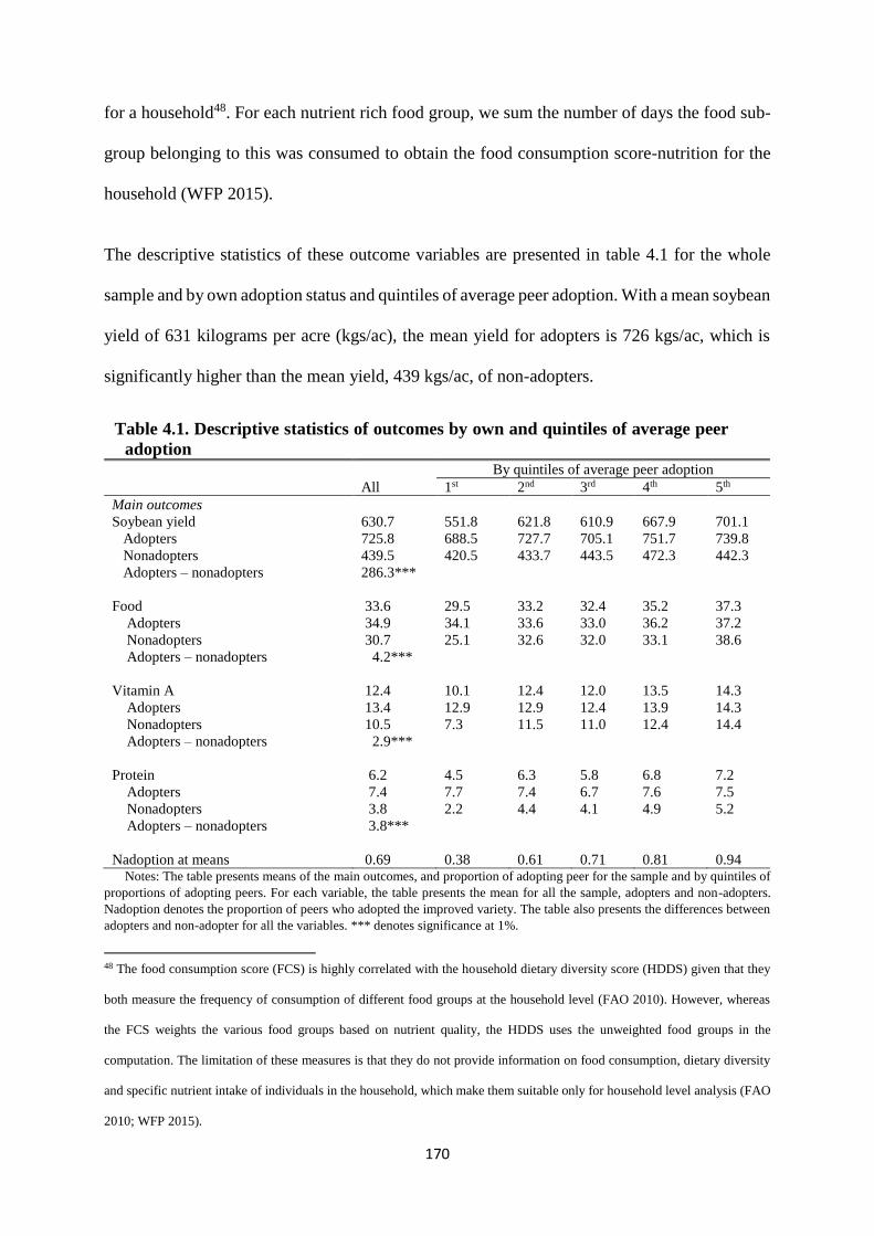
170

for a household48. For each nutrient rich food group, we sum the number of days the food sub-

group belonging to this was consumed to obtain the food consumption score-nutrition for the

household (WFP 2015).

The descriptive statistics of these outcome variables are presented in table 4.1 for the whole

sample and by own adoption status and quintiles of average peer adoption. With a mean soybean

yield of 631 kilograms per acre (kgs/ac), the mean yield for adopters is 726 kgs/ac, which is

significantly higher than the mean yield, 439 kgs/ac, of non-adopters.

Table 4.1. Descriptive statistics of outcomes by own and quintiles of average peer

adoption By quintiles of average peer adoption

All 1st 2nd 3rd 4th 5th

Main outcomes

Soybean yield 630.7 551.8 621.8 610.9 667.9 701.1

Adopters 725.8 688.5 727.7 705.1 751.7 739.8

Nonadopters 439.5 420.5 433.7 443.5 472.3 442.3

Adopters – nonadopters 286.3***

Food 33.6 29.5 33.2 32.4 35.2 37.3

Adopters 34.9 34.1 33.6 33.0 36.2 37.2

Nonadopters 30.7 25.1 32.6 32.0 33.1 38.6


Vitamin A 12.4 10.1 12.4 12.0 13.5 14.3

Adopters 13.4 12.9 12.9 12.4 13.9 14.3

Nonadopters 10.5 7.3 11.5 11.0 12.4 14.4


Protein 6.2 4.5 6.3 5.8 6.8 7.2

Adopters 7.4 7.7 7.4 6.7 7.6 7.5

Nonadopters 3.8 2.2 4.4 4.1 4.9 5.2


Nadoption at means 0.69 0.38 0.61 0.71 0.81 0.94 Notes: The table presents means of the main outcomes, and proportion of adopting peer for the sample and by quintiles of

proportions of adopting peers. For each variable, the table presents the mean for all the sample, adopters and non-adopters.

Nadoption denotes the proportion of peers who adopted the improved variety. The table also presents the differences between

adopters and non-adopter for all the variables. *** denotes significance at 1%.

48 The food consumption score (FCS) is highly correlated with the household dietary diversity score (HDDS) given that they

both measure the frequency of consumption of different food groups at the household level (FAO 2010). However, whereas

the FCS weights the various food groups based on nutrient quality, the HDDS uses the unweighted food groups in the

computation. The limitation of these measures is that they do not provide information on food consumption, dietary diversity

and specific nutrient intake of individuals in the household, which make them suitable only for household level analysis (FAO

2010; WFP 2015).

171

The mean food consumption frequency is 34 for the entire sample, with the mean consumption

of 35 for adopters, being significantly higher than the mean food consumption of 31 for non-

adopters. Similarly, adopters of the improved variety have significantly higher consumption

frequencies of nutrient rich foods (i.e., vitamin A and protein rich foods). These observations

motivate the empirical investigation, where there is significant unequal consumption

frequencies of food and nutrient rich foods that appear to coincide with adoption status.

Given the association between household adoption and food and nutrients consumption

frequencies, we next explore whether peer adoption can possibly be associated with household

food and nutrients consumption by providing descriptive statistics according to quintiles of peer

adoption. The mean soybean yield increases from 552, 689 and 421 kgs/ac for the lowest

quintile to 701, 740 and 442 kgs/ac for all the sample, adopters and non-adopters, respectively,

in the top quintile, an increase that is statistically significant for all sample (p = 0.000) and only

adopters (p = 0.015). The mean food consumption frequency also increases from 30, 34 and 25

for the bottom quintile to 37, 37 and 39 for the top one for the entire sample, adopters and non-

adopters respectively, an increase which is statistically significant (p = 0.000). However, the

food consumption difference between adopters and non-adopters markedly narrows at the top

quintile of peer adoption (p = 0.449).

Similarly, the mean consumption frequencies of nutrient rich foods closely follow that of food

consumption in general. While the consumption of vitamin A and protein rich foods by non-

adopters significantly increase from 7.3 and 2.2 for the bottom quintile to 14.4 and 5.2 for the

top one, respectively, the consumption frequencies of adopters do not witness significant

changes. The weaker correlation between peer adoption and yield of non-adopters and the

stronger association between peer adoption and non-adopters’ food and nutrients consumption,

suggest the possibility of stronger peer adoption effects in the form of risks sharing and private

transfers when the farmer is not adopting.

172

We present definition, measurement and descriptive statistics of characteristics of the sample

and peers in table 4.2. Of particular interest is panel B, which presents the main instrument,

distance to the nearest soybean seed source used to identify household adoption of the improved

variety. In our sample, the average distance from the household location to the nearest seed

source is about 6 kilometres (km). Even though some households are located in less than 2 km

to the nearest soybean seed source, the distance increases to an average of about 11 km for the

households in the highest distance quintile in the sample (see Table 4.A1 in appendix A3).

Panels C of table 4.2, shows that a household has an average of 65% of the peers being males,

aged 44 years and with landholding of 2.7 hectares. Also, 63% of a household’s peers of peers

are males, aged 44 and with landholding of 2.7 hectares (panel D).

4.4 Methodology

4.4.1 Analytical framework

The significant differences between the outcomes of adopters and non-adopters, and the

heterogeneity in these outcomes across the distribution of adopting peers, shown in section 4.3,

suggest the need for a framework that can estimate the effects of own adoption on these

outcomes, while accounting for heterogeneity in gains from peer adoption, as well as other

observed and unobserved characteristics of these farm households. Thus, we use the marginal

treatment effects framework, which is based on the generalized Roy model (Heckman and

Vytlacil 2005; Cornelissen et al. 2016; 2018).

We assume that treatment (adoption) of a household, 𝑖, is a binary variable denoted by 𝐴𝑖, and

the household’s potential outcome (e.g., yield, food and nutrients consumption) under the

hypothetical situation of being an adopter (𝐴𝑖 = 1) and non-adopter (𝐴𝑖 = 0) as 𝑌1𝑖 and 𝑌0𝑖,

respectively. Let 𝐴𝑗 represent peer adoption, with 𝜌1 and 𝜌0 as the parameter estimates showing

the effects of peer (𝑗’s) adoption on own (𝑖) potential outcomes under the situation of the

household adopting and not adopting, respectively.

173

Table 4.2. Variable definition, measurement and descriptive statistics

Variables Definition and measurement Mean SD

Panel A: Household characteristics

Adoption 1 if farmer adopted the improved variety; 0 otherwise 0.67 0.47

Nadoption Proportion of peers who adopted the improved variety 0.69 0.01

Sex 1 if male; 0 otherwise 0.59 0.49

Age Age of farmer (years) 44.03 12.04

Education Number of years in school 1.27 3.27

Hsize Household size (number of persons) 5.64 2.14

HLand Total land size of household (in hectares) 2.56 1.56

HWealth Value of household durable assets in 10,000 GHS 1.29 2.00

HRisk Risk of food insecurity (No. of months household was food inadequate) 0.93 1.37

Soil fertility 4=fertile; 3=moderately fertile; 2=less fertile; and 1=infertile 2.97 0.97

Seed use Quantity of soybean seeds used per acre in kilograms 9.58 4.37

Fertilizer cost Cost of fertilizer applied per acre in GHS 151.4 226.1

Pesticide cost Cost of pesticides applied per acre in GHS 1.45 5.26

Weedicide cost Cost of weedicides applied per acre in GHS 22.52 37.18

Machinery Log of machinery cost per acre 4.16 0.50

Local wage rate Log of local wage rate per day 1.80 0.23

Labor use Number of man-days per acre 14.95 10.21


Farm revenue Total farm revenue of household in 1000 GHS 6.37 4.23

Soybean income Net income from soybean in GHS calculated as total soybean revenue

per acre minus the cost of seeds, fertilizer, weedicide, labor and

machinery used on soybean farm per acre.

Association Number of associations the farmer is a member in the community 1.07 1.27

Town center Distance from community to main town center in kilometers 15.46 11.86

Panel B: Instruments

SoySeed price Soybean seed price in GHS/kilograms 1.06 0.19

SoySeed distance Distance from household location to soybean seed source in kilometers 5.54 3.51 NResident distance Average distance from farmer to peers’ residence in kilometers 5.33 3.48 N2Resident

distance Average distance from peers to peers of peers’ residence in kilometers 5.22 2.06

Panel C: Direct peer characteristics

NSex Proportion of male peers 0.65 0.17

NAge Average age of peers 43.65 4.37

NEducation Average years of schooling of peers 1.58 1.12

NHsize Average households’ size (number of persons) of peers 5.74 0.79

NLandholding Average landholdings of peers 2.67 0.67

NWealth Average value of household durable assets of peers (normalized) 0.03 0.34

NSoil Average soil fertility of peers 3.02 0.31

NExtension Proportion of peers with extension contact ever 0.38 0.15

NFarm revenue Log of average total farm revenue of peers 8.55 0.52

NSoySeed

distance

Average distance from peers’ household locations to soybean seed

source in kilometers

5.52 3.30

Panel D: Indirect peer characteristics

N2Sex Proportion of male peers of peers 0.63 0.13

N2Age Average age of peers of peers 43.73 3.82

N2Education Average years of schooling of peers of peers 1.51 0.92

N2Hsize Average households’ size (number of persons) of peers of peers 5.73 0.74

N2Landholding Average landholdings of peers of peers 2.65 0.59

N2Wealth Average value of household durable assets of peers of peers 0.04 0.31

N2Soil Average soil fertility of peers of peers 3.01 0.29

N2Extension Proportion of peers of peers with extension contact ever 0.38 0.14

N2Farm revenue Log of average total farm revenue of peers of peers 8.56 0.51

N2SoySeed

distance

Average distance from peers of peers household locations to soybean

seed source in kilometers

5.51 3.28

174

Also, let 𝑋𝑖 denote a vector of farmer and household characteristics, with 𝜂1 and 𝜂0 being the

associated vector of parameter estimates under the situation of being an adopter and non-

adopter, respectively; 𝐺𝑖 represents a vector of village characteristics and network fixed effects.

Given these definitions, we model the potential outcomes as

𝑌1𝑖 = 𝜌1(𝐴𝑗) + 𝜂1(𝑋𝑖) + 𝐺𝑖′𝜏 + 𝑈1𝑖,

(1)

𝑌0𝑖 = 𝜌0(𝐴𝑗) + 𝜂0(𝑋𝑖) + 𝐺𝑖′𝜏 + 𝑈0𝑖

where 𝜏 is a vector of parameters to be estimated, while 𝑈1𝑖 and 𝑈0𝑖 represent deviations from

the mean and are assumed to have means of zero. The peer adoption variable, 𝐴𝑗, is obtained

by multiplying the adoption variable, 𝐴𝑖, by the 𝑖th row of the social network matrix 𝑁(𝑣)

[i.e., 𝑁𝑖(𝑣)𝐴𝑖], which we discussed in subsection 4.3.2

We express adoption decision of 𝑖 in the following latent variable (i.e., 𝐴𝑖∗) discrete choice

model:

(2) 𝐴𝑖∗ = Θ𝐴(𝐴𝑗 , 𝑋𝑖, 𝐺𝑖 , 𝑅𝑖) − 휀𝑖 with 𝐴𝑖 = {

1 if 𝐴𝑖∗ ≥ 0

0 otherwise

where 𝐴𝑖 is a binary indicator that equals 1 if household 𝑖 adopts the improved soybean variety

and zero otherwise. The other variables are as defined earlier, and 𝑅𝑖 is an instrument excluded

from eq. (1), and used to identify the effect of household adoption decisions on the outcomes.

Θ𝐴 is a vector of parameters to be estimated. 휀𝑖 is an i.i.d. error term, and because it enters the

selection equation with a negative sign, it represents the unobserved characteristics, also

referred to as resistance, that make individuals less likely to adopt.

If we assume a cumulative distribution function (c.d.f.) of 휀𝑖 as Φ(휀𝑖), then the mean part of eq.

(2) [i.e., Θ𝐴(. )] will represent the propensity score of adoption [defined as Φ(Θ𝐴(. ))≡ 𝑃(𝑍)],

which is based on the observed characteristics. The c.d.f. of 휀𝑖 represents the quantiles of

distribution of the unobserved resistance to adoption [defined as Φ(휀𝑖) ≡ 𝑈𝐴]. A farm household

will adopt, if the propensity score of adoption is greater than the unobserved resistance to

175

adoption [i.e., Φ(Θ𝐴(. )) ≥ Φ(휀𝑖)]. Given the propensity score and eq. (1), we can estimate the

outcome equation as a function of the observed regressors (𝐴𝑗 , 𝑋𝑖, 𝐷𝑖 , 𝐺𝑖) and the propensity

score 𝑃(𝑍) as

𝐸[𝑌|𝐴𝑗 = 𝑎, 𝑋𝑖 = 𝑥, 𝐺𝑖 = 𝑔, 𝑃(𝑍) = 𝑝]

(3)

= 𝐴𝑗𝜌0 + 𝑋𝑖′𝜂0 + 𝐺𝑖𝜏 + 𝐴𝑗

′(𝜌1 − 𝜌0)𝑝 + 𝑋𝑖′(𝜂1 − 𝜂0)𝑝 + 𝐸(𝑈1𝑖 − 𝑈1𝑖)𝑝

where 𝑌 = 𝑌1𝑖 − 𝑌0𝑖, (𝜌1 − 𝜌0)𝑝 and (𝜂1 − 𝜂0)𝑝 measure the returns to adoption for

households with different levels of peer adopters, 𝐴𝑗 , and other observable covariates, 𝑋𝑖,

respectively. These observed gains could be positive or negative depending on whether

households with higher values (such as more adopting peers) have higher or lower than average

returns to adoption (Carneiro et al. 2011). 𝐸(𝑈1𝑖 − 𝑈1𝑖)𝑝 represents the returns to adoption due

to unobserved ability of the household. Suppose that 𝑌 is yield, a positive (negative) effect of

𝐸(𝑈1𝑖 − 𝑈1𝑖)𝑝 will imply a negative (positive) selection on unobserved gains.

Following Heckman and Vytlaci (2005) and Cornelissen et al. (2018) we obtain the marginal

treatment effects (MTE) for 𝐴𝑗 , 𝑋𝑖 and 𝑈𝐴 = 𝑝 by taking the derivative of eq. (3) with respect

to 𝑝 as

(4) MTE(𝑎, 𝑥, 𝑝) =𝜕𝐸[𝑌| . , 𝑃(𝑍)=𝑝]

𝜕𝑝= 𝐴𝑗

′(𝜌1 − 𝜌0) + 𝑋𝑖′(𝜂1 − 𝜂0) +

𝜕𝐾(𝑝)

𝜕𝑝

where 𝐾(𝑝) is a nonlinear function of the propensity score. Equation (4) suggests that treatment

effects heterogeneity can result from both observed and unobserved characteristics. Estimation

of the treatment effects requires a first-stage in which the instrument, 𝑅𝑖, in eq. (2) causes

variation in the probability of adoption, conditional on the observed characteristics [i.e., 𝑅𝑖 ⊥

(𝑈0𝑖, 𝑈1𝑖, 휀𝑖)|(𝐴𝑗, 𝑋𝑖, 𝐺𝑖)]. Given the exclusion instrument, we estimate a first-stage probit eq.

(2) to obtain estimates of the propensity score �̂� = Φ(Θ𝐴(. )). Modeling 𝐾(�̂�) as a polynomial

in degree 2, we estimate the marginal treatment effects (MTE), using the local instrumental

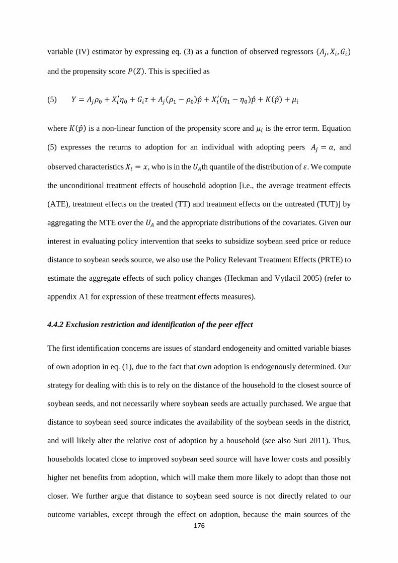
176

variable (IV) estimator by expressing eq. (3) as a function of observed regressors (𝐴𝑗 , 𝑋𝑖, 𝐺𝑖)

and the propensity score 𝑃(𝑍). This is specified as

(5) 𝑌 = 𝐴𝑗𝜌0 + 𝑋𝑖′𝜂0 + 𝐺𝑖𝜏 + 𝐴𝑗(𝜌1 − 𝜌0)�̂� + 𝑋𝑖

′(𝜂1 − 𝜂0)�̂� + 𝐾(�̂�) + 𝜇𝑖

where 𝐾(�̂�) is a non-linear function of the propensity score and 𝜇𝑖 is the error term. Equation

(5) expresses the returns to adoption for an individual with adopting peers 𝐴𝑗 = 𝑎, and

observed characteristics 𝑋𝑖 = 𝑥, who is in the 𝑈𝐴th quantile of the distribution of 휀. We compute

the unconditional treatment effects of household adoption [i.e., the average treatment effects

(ATE), treatment effects on the treated (TT) and treatment effects on the untreated (TUT)] by

aggregating the MTE over the 𝑈𝐴 and the appropriate distributions of the covariates. Given our

interest in evaluating policy intervention that seeks to subsidize soybean seed price or reduce

distance to soybean seeds source, we also use the Policy Relevant Treatment Effects (PRTE) to

estimate the aggregate effects of such policy changes (Heckman and Vytlacil 2005) (refer to

appendix A1 for expression of these treatment effects measures).

4.4.2 Exclusion restriction and identification of the peer effect

The first identification concerns are issues of standard endogeneity and omitted variable biases

of own adoption in eq. (1), due to the fact that own adoption is endogenously determined. Our

strategy for dealing with this is to rely on the distance of the household to the closest source of

soybean seeds, and not necessarily where soybean seeds are actually purchased. We argue that

distance to soybean seed source indicates the availability of the soybean seeds in the district,

and will likely alter the relative cost of adoption by a household (see also Suri 2011). Thus,

households located close to improved soybean seed source will have lower costs and possibly

higher net benefits from adoption, which will make them more likely to adopt than those not

closer. We further argue that distance to soybean seed source is not directly related to our

outcome variables, except through the effect on adoption, because the main sources of the

177

improved soybean variety are agricultural input dealers some of who are located in the district

capitals (CSIR-SARI 2013)49.

Two main possible concerns about the exogeneity of our instrument are that; if soybean seed

dealers chose their location strategically close to their buyers, and if households’ location was

endogenously determined based on the location of input dealers. In respect of the first concern,

we show that this is not the case with results of t-test of differences in means, across different

distance bandwidths, for variables at the village level, household levels and the outcomes in

table 4.A1 in appendix A3. The tests suggest that villages and households located closer to

soybean seed source are not systematically different from those located further away. The

second concern is not likely the case, because soybean is not the main crop cultivated by these

households and thus, it is unlikely that a household will change location because it wants to

access improved soybean seeds. Table 4.A1 further shows no significant difference in distance

and adoption status among households who changed location over the past 5 and 10 years as at

the time of the interviews.

The next critical issue of identification is the peer effects in eqs. (1) and (2). The first concern

is the endogeneity of the peer effects. First, the peer adoption effect (i.e., 𝐴𝑗), in eq. (1) cannot

generally be consistently estimated, especially with OLS, because of the correlation of the error

term in this equation with this term [i.e., cov(𝐴𝑗 , 𝑈1,0𝑖) ≠ 0], possibly due to the omitted effects

of the peer outcomes (Acemoglu et al. 2015). The second aspect is that, the estimation of own

49 Of course, distance to seed source could be correlated with distance to town centre, where households who have their closest

seed source located in the town centre inadvertently live closer to the town centre and therefore more likely to be wealthy

and to be able to buy or trade for food, increasing food security. This could threaten our identification strategy because

distance to soybean source in this case can affect our outcomes through closeness to town centre and household wealth, and

not only through adoption. For this reason, we controlled for distance to town centre and household wealth in all

specifications.

178

and peer adoption (𝐴𝑗 is endogenous effect) in eq. (2) poses endogeneity concerns because of

the Manski’s (1993) “reflection problem” and correlated unobservables [i.e., cov(𝐴𝑗 , 휀𝑖) ≠ 0].

The reflection problem is the result of the coexistence of the endogenous peer effect and the

contextual effect in eq. (2)50.

In order to identify the contextual effect in eq. (1), and the contextual and endogenous effects

in eq. (2), we follow the approaches of Bramoullé et al. (2009) and Acemoglu et al. (2015),

who use the average characteristics of peers of peers [i.e., 𝑁2(𝑣)] as an instrument for the

average adoption of peers. Intuitively, since the characteristics of a household’s peers of peers

are correlated with the behavior and outcome of the household’s peers, but are exogenous to

the behavior and outcome of the household, these satisfy the exclusion restriction of being valid

instruments for the adoption decision of the household’s peers (see Appendix A2 for a case on

social network structures and identification of peer effects). Two key requirements for the use

of this strategy are that the peers of peers characteristics (such as distance to soybean seed

source by peers of peers) that are used as instruments should be uncorrelated with the instrument

used to identify own adoption, and that the peers of peers instrument must be independent of

own outcomes, except through average peer adoption (Acemoglu et al. 2015).

However, given that our main instrument is the distance to soybean seed source, it is likely that

the household’s own distance to seed source will be correlated with the average distance to

soybean seed source by peers of peers. As a result, we use the average distance between the

residence of the household’s peers and the peers of peers as an instrument to identify the effect

of average peer adoption on household own adoption and the outcomes. The reasoning is that,

when farmers are residentially close to each other, they are more likely to interact and exchange

50 These identification issues are discussed in the social networks and peer effects literature (Bramoullé et al. 2009; Acemoglu

et al. 2015; De Giorgi et al. 2020). The formal development of these issues is beyond the scope of this paper. We refer the

reader to Acemoglu et al. (2015) for the formal development and identification problems therein.

179

information and resources, which can increase the likelihood of them influencing the behavior

and decisions of each other. Thus, if a farmer has geographically closed peers whose closer

peers have new and more access to information about the improved variety, that farmer could

receive this information and advice from the peers of peers through the farmer’s peers.

Indeed, whereas the distance to soybean seed source of peers of peers appears to be highly

correlated with own distance (0.942), the average distance between the residence of farmer’s

peers and the peers of peers is uncorrelated with own distance to the seed source (0.010) as

shown in table 4.A2. To test the second assumption, we followed the approach of Di Falco et

al. (2011) by regressing the outcomes of non-adopters on the own and average peer adoption

instruments in table 4.A3. Whereas the estimate generally show that these instruments do not

significantly correlate with the outcomes, tables 4.B1.1 and 4.C1-4.C3 in the supplementary

material show that the instruments significantly explain average peer adoption and own

adoption, respectively.

Thus, to account for the endogeneity of peer adoption, we regress peer adoption on own, 𝑋𝑖,

and peer characteristics (𝑁𝑖(𝑣)𝑋𝑖), as well as the characteristics of the peer of peers (𝑁𝑖2(𝑣)𝑋𝑖),

obtain the predicted peer adoption, and use this as the peer adoption variable in the outcome

(eq.1) and selection (eq.2) equations (see table 4.B1.1 in appendix B1). Finally, we partly

capture correlated effects by including village dummies to account for network fixed effects 𝐺𝑖

(i.e., individuals self-select into networks based on network-specific characteristics). To

account for correlated effects at the link formation level, we estimated a network formation

model and inserted the predicted generalized residuals of this model into eqs. (1) and (2) as

control functions (Brock and Durlauf 2001) (see Appendix B2.).

180

4.5 Empirical Results

4.5.1 First-stage adoption

Table 4.3 reports the marginal effects estimates of the first-stage probit selection model in

column (1) for soybean yield, and in column (2) for food and nutrients consumption. The

distance to the closest soybean seed source is a strong predictor of adoption, and as expected,

the coefficients of the distance suggest a strong relationship between the availability of the

improved seeds and the decision to adopt.

Table 4.3. First-stage adoption results of yield and food and nutrients consumption

specifications (1)

Yield

(2)

Food and nutrients

Coefficient S. E. Coefficient S. E.

𝚯𝑨 𝚯𝑨

Nadoption (Predicted) 0.168*** 0.047 0.110** 0.049

Sex 0.050 0.052 0.011 0.053

Age -0.002 0.001 -0.002 0.001

Education 0.002 0.008 0.004 0.008

Hsize -0.035** 0.013 -0.041*** 0.013

HLand 0.052** 0.022 0.041* 0.021

HWealth (predicted) 0.163*** 0.045 0.169*** 0.045

Soil fertility 0.022 0.026 0.038 0.027

Seed use -0.014** 0.006 -0.015** 0.006

Fertilizer cost -1.8E-5 7.0E-5 -3.9E-5 6.0E-5

Pesticide cost 0.001 0.004 0.003 0.004

Weedicide cost 3.6E-4 0.001 -2.6E-5 0.001

Machinery -0.006 0.052 -0.066 0.059

Labor use 0.001 0.002 0.001 0.002

Extension (predicted) 0.568*** 0.110 0.572*** 0.108

Soy selling price 0.166 0.203 0.088 0.194

Farm revenue (predicted) 0.270*** 0.070

Residuals_NWLink -0.054 0.034 -0.046 0.034

Local wage rate 0.137 0.101 -0.266* 0.151

Network Fes Yes Yes

Town center 0.004* 0.002 0.005** 0.002

NSex -0.240 0.151 -0.498*** 0.163

NAge 0.003 0.005 0.002 0.005

NLand -0.098** 0.040 -0.116** 0.040

SoySeed Distance -0.478*** 0.089 -0.483*** 0.094

N2SoySeed Distance 0.147*** 0.027 0.144*** 0.029

SoySeed price -0.481** 0.193 -0.497** 0.194

The table reports the first-stage adoption results of the yield equation in column (1) and food and nutrients consumption equation in

columns (2). The estimates are marginal effects from probit selection model of adoption decisions (first-stage eq. 2). Our instrument

is distance to soybean seed source, which is normalized about its overall mean. Θ𝐴 is a vector of parameter estimates from equation

(2). Network FEs is network fixed effects and Residuals_NWLink is residuals of the link formation model. S.E. are bootstrapped

standard errors with 50 replications. The asterisks ***, ** and * are significance at 1%, 5% and 10% levels, respectively.

181

As expected, the soybean seed price shows a strong negative correlation with the decision to

adopt. We also report the chi-squared test of the excluded instruments at the bottom panels of

these tables, and based on this, we can, throughout, reject the hypotheses that the excluded

instruments are not relevant. The results suggest that there is a strong and significant

relationship between the adoption decisions of peers and one’s own decision to adopt the

improved variety. To facilitate interpretation, we normalize peer adoption over its mean.

Specifically, a standard deviation (SD) increase in the number of adopters of the improved

variety among a household’s peers, raises the probability of the household’s (own) adoption by

at least about 11 percentage points. The estimated peer adoption effects correct for the potential

endogeneity of the peer adoption variable by using predicted peer adoptions, and account for

correlated unobservables with the network fixed effects and residuals of the link formation

model (Residuals_NWLink) in all specifications.

The first-stage probit generates a large common support for the propensity score P(Z) and this

ranges from 0.1 to at least 0.99 (figure 4.1) for both soybean yield (part A) and food and

nutrients (part B). This satisfies the requirement that the instrument should generate enough

common support for the estimation of the MTE (Cornelissen, et al. 2016).

182

Figure 4.1 Common support for Soybean yield and food and nutrition security

The figure plots the frequency distribution of the propensity score by adopters and non-adopters. The

propensity score is predicted from the baseline first-stage regressions. Part A is based on the regression for

soybean yield and part B is based on the regressions on food and nutrition. We have two different specification

of the first-stage equation, and thus the two propensity score plots because we included extension contact in

both the selection and the outcome stages in the yield equation, but included it only in the first-stage of the food

and nutrients consumption equations. The reason is that whereas extension was conceived as having potential

effects on both adoption and yield directly, we considered the effect of extension on food and nutrients

consumption will be through farm income which we controlled for.

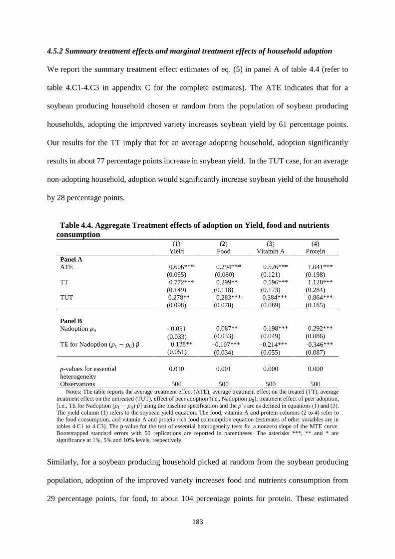
183

4.5.2 Summary treatment effects and marginal treatment effects of household adoption

We report the summary treatment effect estimates of eq. (5) in panel A of table 4.4 (refer to

table 4.C1-4.C3 in appendix C for the complete estimates). The ATE indicates that for a

soybean producing household chosen at random from the population of soybean producing

households, adopting the improved variety increases soybean yield by 61 percentage points.

Our results for the TT imply that for an average adopting household, adoption significantly

results in about 77 percentage points increase in soybean yield. In the TUT case, for an average

non-adopting household, adoption would significantly increase soybean yield of the household

by 28 percentage points.

Table 4.4. Aggregate Treatment effects of adoption on Yield, food and nutrients

consumption (1) (2) (3) (4)

Yield Food Vitamin A Protein

Panel A

ATE 0.606***

(0.095)

0.294***

(0.080)

0.526***

(0.121)

1.041***

(0.198)

TT 0.772***

(0.149)

0.299**

(0.118)

0.596***

(0.173)

1.128***

(0.284)

TUT 0.278**

(0.098)

0.283***

(0.078)

0.384***

(0.089)

0.864***

(0.185)

Panel B

Nadoption 𝜌0 -0.051

(0.033)

0.087**

(0.033)

0.198***

(0.049)

0.292***

(0.086)

TE for Nadoption (𝜌1 − 𝜌0) �̂� 0.128**

(0.051) -0.107***

(0.034)

-0.214***

(0.055)

-0.346***

(0.087)

p-values for essential

heterogeneity

0.010 0.001 0.000 0.000

Observations 500 500 500 500 Notes: The table reports the average treatment effect (ATE), average treatment effect on the treated (TT), average

treatment effect on the untreated (TUT), effect of peer adoption (i.e., Nadoption 𝜌0), treatment effect of peer adoption,

[i.e., TE for Nadoption (𝜌1 − 𝜌0) �̂�] using the baseline specification and the 𝜌’s are as defined in equations (1) and (3).

The yield column (1) refers to the soybean yield equation. The food, vitamin A and protein columns (2 to 4) refer to

the food consumption, and vitamin A and protein rich food consumption equation (estimates of other variables are in

tables 4.C1 to 4.C3). The p-value for the test of essential heterogeneity tests for a nonzero slope of the MTE curve.

Bootstrapped standard errors with 50 replications are reported in parentheses. The asterisks ***, ** and * are

significance at 1%, 5% and 10% levels, respectively.

Similarly, for a soybean producing household picked at random from the soybean producing

population, adoption of the improved variety increases food and nutrients consumption from

29 percentage points, for food, to about 104 percentage points for protein. These estimated

184

parameters are all statistically significant at the 1% level. Also, the TT estimates show that for

an average adopting household, adoption results in 30 percentage points increase in food

consumption, and 60 to 113 percentage points increase in nutrients consumption. These

parameters are significantly different from zero, at least, at the 5% level. The significance of

adoption is still observed, even in the untreated case, where the food and nutrients consumption

of non-adopters will increase by 28 to 86 percentage points, if they adopt the improved variety.

The summary measures of treatment effects suggest possible treatment effect heterogeneity

among soybean producing households. In particular, all parameter estimates in table 4.4 show

that the TT is greater than the ATE, which is also greater than the TUT. This is suggestive of

positive selection on gains, where individuals who are more likely to adopt (perhaps because

of their innate ability or variation in the quality of adoption and production conditions) tend to

benefit more from adoption in terms of yield and food/nutrients consumption. However, as

indicated earlier, these summary measures mask such treatment effects heterogeneity and thus,

we show the marginal treatment effects (MTEs) in figures 4.2. These figures relate the

unobserved parts of the outcomes ( 𝑈1 − 𝑈0) to that of the adoption decision ( 𝑈𝐴). Higher

values of 𝑈𝐴 imply lower probabilities of adoption (i.e., higher resistance to adoption).

The MTE curves decline with increasing resistance to treatment in all instances, and indicate a

pattern of positive selection on gains. In effect, given the unobserved characteristics,

households who are most likely to adopt the improved variety appear to benefit the most from

adoption. Thus, the slopes of the MTE curves in each case suggest a pattern of heterogeneity in

returns to adoption, that is significantly different from zero at the 5% level (see the p-values for

the test of essential heterogeneity at the bottom of table 4.4). Part A of figure 4.2 depicts the

MTE for yield and shows that for households who are more likely to adopt than the average

household ( 𝑈𝐴 < 0.5), their returns to adoption are higher than the average household albeit not

significantly different from the returns to adoption of an average household. For the households

185

with higher resistance to adoption than the average household, their yield returns to adoption is

significantly lower than that of the average household selected at random for the 30% of

households with the highest resistance to adoption ( 𝑈𝐴 > 0.7).

Figure 4.2 MTE curves for soybean yield

The figure shows the marginal treatment effect (MTE) curves for yield, food and nutrient rich food consumption at the

average values of the covariates based on specifications in equations (4 and 5). U_A denotes unobserved resistance to

treatment/adoption. Part A is the MTE curve for soybean yield. Part B depicts the MTE curve for food consumption, part C

shows the MTE curve for vitamin A rich foods consumption and part D is the MTE curve for protein rich foods consumption.

The dashed lines are the average treatment effects (ATE). The 95% confidence interval (95% CI) is based on bootstrapped

standard errors with 50 replications.

Figure 4.2 also shows there is clear heterogeneity in returns to adoption in terms of food and

nutrients consumption. We observe a similar pattern of positive selection on gains, with returns

to adoption significantly higher than the average household, at least, for the 20%, for food

consumption, and 25% for nutrients consumption of households who are most likely to adopt.

Figure 4.2 further shows that returns to adoption in terms of food and nutrients consumption

186

decrease and fall below that of the average soybean producing household, for the households

with over 33% (i.e., 𝑈𝐴 > 0.33) resistance to adoption.

In order to probe for the source of this treatment effect heterogeneities, we check whether the

positive gains on selection on unobserved characteristics (i.e., 𝑈1 − 𝑈0| 𝑈𝐴 = 𝑢𝐴) are because

of heterogeneity in the outcomes when not adopting [i.e., upward sloping in 𝐸( 𝑌0| 𝑈𝐴 = 𝑢𝐴)],

when adopting [i.e., downward sloping 𝐸( 𝑌1| 𝑈𝐴 = 𝑢𝐴)], or both. We report the plot of 𝑌1 and

𝑌0 for the various outcomes in figure 4.C1. The figure shows, across all outcomes that, the

differences in the outcomes are driven by worse outcomes in the non-adoption state, as shown

by the increasing dashed-dotted lines. However, the outcomes in the adoption state (i.e., dotted

lines) are more homogenous throughout.

4.5.3 Treatment effect heterogeneity in peer adoption

For easy reference, we report the estimates of peer adoption effects in panel B of table 4.4,

where we first present the effect for the case when the household is not adopting (i.e., 𝜌0) and

when the household is adopting [i.e., (𝜌1 − 𝜌0) �̂�]. The results show that in the non-adoption

state, a standard deviation increase in the number of adopting peers of the improved soybean

variety, is associated with a decrease in one’s own soybean yield, although not statistically

significant. However, the treatment effect of peer adoption is significantly positive and

increases own yield by about 13 percentage points.

In respect of food and nutrients consumption, the results show that when not adopting, a

standard deviation increase in peer adoption increases food consumption of the household by 9

percentage points, and consumption of vitamin A and protein rich foods by 20 and 29

percentage points, respectively. These effects are significant at least at the 5% level, and suggest

that non-adopting households benefit from their adopting peers in terms of enhanced food and

nutrients consumption. Interestingly, when the household adopts, the treatment effect of a

187

standard deviation increase in adopting peers is negative (i.e., (𝜌1 − 𝜌0) �̂�), suggesting that

household adoption of the improved variety significantly reduces the heterogeneity in food and

nutrients consumption due to adopting peers by 11, 21 and 35 percentage points for food,

vitamin A and protein consumption, respectively. These results indicate that households with

more (fewer) adopting peers tend to gain more in terms of increased soybean yields (food and

nutrients consumption), when they adopt than their counterparts with fewer (more) adopting

peers. This is not surprising because as shown in table 4.1, non-adopters appear to have lower

yields and food consumption.

4.5.4 Effect mechanisms

Given the generally positive effects of adoption of the improved variety on yields, food and

nutrients consumption, we next investigate the mechanisms by which adoption can affect food

and nutrients consumption in particular. Our conceptual framework suggests that own adoption

can enhance consumption through increased yields and changes in household income,

consumption of own production, food prices and intra-household dynamics51. This analysis is

shown explicitly in table 4.5, where we first estimate the levels and heterogeneity effects of

gains in yield from adoption on soybean income, food and nutrients consumption (cols. 1-4).

The estimates reveal a significantly positive association between gains in yield and income

from soybean. In particular, a log percentage point increase in yield from adoption of the

improved variety significantly increases the gains in soybean income by over GHS 700 [i.e.,

(𝜂1 − 𝜂0)𝑝], which is about 30% higher than the mean soybean income of non-adopters.

51 Given the macro nature of food prices and the focus of the analysis on farm level links, and the limitation of data on the

sources of households’ food and nutrients consumption (i.e., whether from own production or purchases), we are unable to

show the effects of changes in food prices and consumption of own produce on food and nutrients consumption.

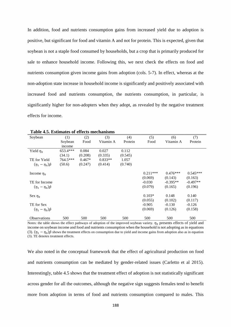
188

In addition, food and nutrients consumption gains from increased yield due to adoption is

positive, but significant for food and vitamin A and not for protein. This is expected, given that

soybean is not a staple food consumed by households, but a crop that is primarily produced for

sale to enhance household income. Following this, we next check the effects on food and

nutrients consumption given income gains from adoption (cols. 5-7). In effect, whereas at the

non-adoption state increase in household income is significantly and positively associated with

increased food and nutrients consumption, the nutrients consumption, in particular, is

significantly higher for non-adopters when they adopt, as revealed by the negative treatment

effects for income.

Table 4.5. Estimates of effects mechanisms Soybean (1)

Soybean

income

(2)

Food

(3)

Vitamin A

(4)

Protein

(5)

Food

(6)

Vitamin A

(7)

Protein

Yield 𝜂0 653.4***

(34.1)

0.084

(0.208)

0.027

(0.335)

0.112

(0.545)

TE for Yield

(𝜂1 − 𝜂0)�̂�

764.5***

(50.6)

0.467*

(0.247)

0.833**

(0.414)

1.057

(0.740)

Income 𝜂0 0.211***

(0.069)

0.476***

(0.143)

0.545***

(0.163)

TE for Income

(𝜂1 − 𝜂0)�̂�

-0.030

(0.079)

-0.395**

(0.165)

-0.497**

(0.196)

Sex 𝜂0 0.103*

(0.055)

0.148

(0.102)

0.140

(0.117)

TE for Sex

(𝜂1 − 𝜂0)�̂�

-0.905

(0.069)

-0.130

(0.126)

-0.126

(0.158)

Observations 500 500 500 500 500 500 500

Notes: the table shows the effect pathways of adoption of the improved soybean variety. 𝜂0 presents effects of yield and

income on soybean income and food and nutrients consumption when the household is not adopting as in equations

(3). (𝜂1 − 𝜂0)�̂� shows the treatment effects on consumption due to yield and income gains from adoption also as in equation

(3). TE denotes treatment effects.

We also noted in the conceptual framework that the effect of agricultural production on food

and nutrients consumption can be mediated by gender-related issues (Carletto et al 2015).

Interestingly, table 4.5 shows that the treatment effect of adoption is not statistically significant

across gender for all the outcomes, although the negative sign suggests females tend to benefit

more from adoption in terms of food and nutrients consumption compared to males. This

189

finding confirms that the main mechanism by which adoption affects food and nutrients

consumption is through increased soybean yields and household income. It further suggests that

the attenuating treatment effects of peers observed when a farmer adopts can be attributed to

increased household income following own adoption.

4.5.5 Policy strategies

Our results so far, have demonstrated that adoption of the improved variety does not only lead

to increased soybean yield, but also contributes to increasing food and nutrients consumption

of not only adopters, but that of non-adopters should they adopt. This implies that policies that

seek to overcome structural barriers and induce people to adopt can be much rewarding. Thus,

we show the effects of a policy that reduces soybean seed price by 50% (in line with current

Government policy in Ghana), and a policy that reduces the distance of the household to the

nearest soybean seed source to a maximum of four kilometres, using the policy-relevant

treatment effects (PRTE). Whereas the subsidy policy seeks to improve affordability, the

distance policy attempts to enhance availability of the seeds of the improved variety.

Table 4.6 (col. 1) shows the propensity score at the baseline policy, columns (2) and (3) show

the propensity scores and the PRTE, respectively, for soybean seed price subsidy, and columns

(4) and (5) show the propensity scores and PRTE, respectively, for the policy of reducing

distance to soybean seed source. The estimates show that subsidizing soybean seed price by

50%, and reducing the distance to soybean seed source to a maximum of four kilometres shift

households with high unobserved resistance to adoption into adoption, and as a result

significantly increase soybean yield by 42 and 36 percentage points, respectively, per household

shifted from non-adoption into adoption. The magnitude of the price subsidy effect on yield is

higher than that of the distance to seed source. We find statistically significant policy effects

for both policies in food and nutrients consumption, but with marginally higher effects for the

reduction in distance to seed source. These findings show that, whereas reducing distance to

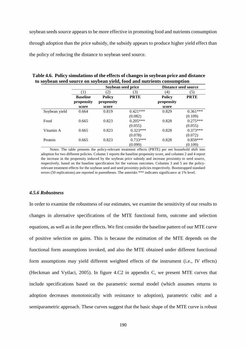
190

soybean seeds source appears to be more effective in promoting food and nutrients consumption

through adoption than the price subsidy, the subsidy appears to produce higher yield effect than

the policy of reducing the distance to soybean seed source.

Table 4.6. Policy simulations of the effects of changes in soybean price and distance

to soybean seed source on soybean yield, food and nutrients consumption

Soybean seed price Distance seed source

(1) (2) (3) (4) (5)

Baseline

propensity

score

Policy

propensity

score

PRTE Policy

propensity

score

PRTE

Soybean yield 0.664 0.819 0.421***

(0.082)

0.829 0.361***

(0.109)

Food 0.665 0.823 0.205***

(0.055)

0.828 0.275***

(0.055)

Vitamin A 0.665 0.823 0.323***

(0.078)

0.828 0.373***

(0.072)

Protein 0.665 0.823 0.733***

(0.099)

0.828 0.859***

(0.109) Notes: The table presents the policy-relevant treatment effects (PRTE) per net household shift into

adoption for two different policies. Column 1 reports the baseline propensity score, and columns 2 and 4 report

the increase in the propensity induced by the soybean price subsidy and increase proximity to seed source,

respectively, based on the baseline specification for the various outcomes. Columns 3 and 5 are the policy-

relevant treatment effects for the soybean seed and seed proximity policies respectively. Bootstrapped standard

errors (50 replications) are reported in parentheses. The asterisks *** indicates significance at 1% level.

4.5.6 Robustness

In order to examine the robustness of our estimates, we examine the sensitivity of our results to

changes in alternative specifications of the MTE functional form, outcome and selection

equations, as well as in the peer effects. We first consider the baseline pattern of our MTE curve

of positive selection on gains. This is because the estimation of the MTE depends on the

functional form assumptions invoked, and also the MTE obtained under different functional

form assumptions may yield different weighted effects of the instrument (i.e., IV effects)

(Heckman and Vytlaci, 2005). In figure 4.C2 in appendix C, we present MTE curves that

include specifications based on the parametric normal model (which assumes returns to

adoption decreases monotonically with resistance to adoption), parametric cubic and a

semiparametric approach. These curves suggest that the basic shape of the MTE curve is robust

191

to different functional forms, and generally show a similar pattern as in the baseline

specification.

We next consider the sensitivity of our ATE, TT and TUT to different specifications, as these

put most weights in different segments of the MTE, and therefore could be sensitive to changes

in the estimated MTE (Carneiro, et al. 2011). In panel A of table 4.C5, we present estimates

from a model where we control for other contextual peer effects (i.e., peers’ sex, age,

landholding and soil fertility) in the outcome equations (cols. 1-3) to assess whether the

observed peer and treatment effects could be driven by contextual effects or correlation in soil

conditions between farmers and their peers. In columns 4 to 6, we present estimates of a

specification that excludes the effects of peer adoption to examine these estimates under the

stable unit treatment value assumption (SUTVA)52. The estimates are marginally low and high

for yield and food consumption (col. 4-6), and suggest expansion and attenuation biases,

respectively, albeit similar in directions and significance to the baseline estimates.

In columns 1 to 3 of panel B, we report estimates when estimating the first-stage with a squared

term of distance to nearest soybean seed source as additional instrument to account for the fact

that at longer distances to seed sources, the probability of adoption will become very low. In

columns 4 to 6 of panel B, we interact distance to soybean seed source with household wealth

and household size, because the effect of our instrument is likely to vary across households,

based on their observed resource status (Carneiro, et al. 2011). Table 4.C6 reports results that

show the sensitivity of the estimates to the use of standard errors clustered at the village level

in columns (1) to (3) (Cameron, et al. 2008), and when we control for mobile phone network

52 The SUTVA requires that the potential outcomes of treatment observed on one farm household should not be affected by the

treatment of other farm households. The inclusion of the peer adoption effects violates this assumption but Manski (2013)

provides characterization of bounds on the treatment effects under social interactions, and thus our estimates should be

interpreted as bounds and not necessarily as the point estimates.

192

coverage in the village in columns (4) and (5). In order to show the sensitivity of the results to

changes in the measure of household food consumption, we report treatment effects of adoption

on household dietary diversity in column (6) of table 4.C6 (FAO 2010). In spite of these

exercises, the treatment effects estimates remain qualitatively similar to those reported in table

4.4.

Finally, table 4.C7, columns (1) to (3) of panel A explore the sensitivity of the estimates to peer

effects through means other than peer adoption. Recall from subsection 4.3.2 that links in our

networks are defined using social and farm plot proxies, and some of these (such as labor and

land exchanges) can present effects similar to peer adoption effects. We explore this by

accounting for household (node) degree, which is the total number of connections a household

has in the network. A related concern is the issue of the use of the sampled networks which

truncate the number of households’ social connections and could lead to important links and

nodes not observed, which can bias the estimates (Chandrasekhar and Lewis 2016).

In order to examine the sensitivity of our estimates to this issue, we follow the approach of Liu

et al. (2017) by re-running our models without households with links with all the 5 randomly

matched households to them. Finally, in columns (1) to (3) of panel B, we report estimates with

difference in adopting peers of a household between a year after the introduction of the

improved variety (i.e., 2004) and the 2016 cropping season. The results of these exercises

remain very similar to our baseline results in table 4.4, suggesting that our findings of the pattern

of selection and the treatment effects are robust to various functional forms and specifications.

4.6 Discussion

We find significant effects of household adoption on yield, food and nutrients consumption as

expected, which can be partly attributed to the yield, income and agro-climatic advantages of

the improved over the traditional variety (CSIR-SARI, 2013). The high magnitudes of these

193

effects, especially on food and nutrients consumption can be explained by the interplay of two

factors: one is the timing of the survey, as it was conducted in the lean season when households

rely heavily on food consumption from cash purchases, and the commercial status of soybean,

as an income enhancing crop for households (see also WFP and GSS 2012; Carletto et al. 2015).

Our findings of heterogeneity in returns to adoption show that households with low resistance

to adoption do much worse than an average soybean producing household without adoption of

the improved variety. However, these households become relatively similar with adoption. This

is perhaps because the production of the traditional variety is more demanding (in terms of time

and labor), and requires farmers to invest more resources to minimize the production

challenges. This could increase the risk of vulnerable households who are not able to meet these

production requirements of losing their crops or entire investment due to early shattering. But

the improved variety is quite resistant to these issues (CSIR-SARI 2013).

Whereas peer adoption effect has significant and positive effect on households’ yields when

adopting, we find no significant peer effect on yield when the household is not adopting. A

potential interpretation is that when the household is not adopting, increased peer adoption

could reduce private learning opportunities from peers, especially if the production processes

of the improved and traditional varieties are not complementary. However, household adoption

increases private learning and imitation opportunities from adopting peers (Niehaus 2011).

Our findings on peer adoption effect on food and nutrients consumption in the non-adoption

state are suggestive of some form of private transfer among peers, since consumption increases

with peer adoption in the non-adoption state. However, own adoption leads to attenuating peer

adoption effects and this can primarily be attributed to the yield and income gains from the

improved soybean variety that tend to substantially increase the consumption of non-adopters

when they adopt. This indicates that consumption benefits from peer adoption tend to decline

194

with own adoption, suggesting that increased own productivity and household income lead to

reduction in farmers’ dependence on peers (Alger and Weibull 2012; Di Falco et al. 2018).

4.7 Conclusion

This paper examined the impact of adoption of improved soybean variety on soybean yield, and

household food and nutrients consumption, using household survey data from Ghana. In

particular, we estimated the marginal treatment effects of adoption of the improved variety on

these outcomes, and thus, show heterogeneities in returns to adoption due to observed and

unobserved characteristics of households. The results generally show positive association

between adoption and the outcomes, but do not necessarily establish causality. We note three

main findings: First, a pattern of positive selection on unobserved gains from adoption of the

improved variety is observed across all outcomes, which is due to the fact that households who

are more likely to adopt the improved variety have lower returns, than that of an average

soybean producing household, when not adopting. This finding is in line with the hypothesis of

adoption based on comparative advantage (Suri, 2011). However, adoption of the improved

variety tends to make these households quite homogeneous across these outcomes, suggesting

that adoption can serve as means by which poorer households can narrow the gaps in yields,

and food and nutrients consumption with better and richer households.

Second, we find that households benefit, in terms of increased soybean yield, from having peers

who are adopters only when the households also adopt, suggesting the possibility of social

learning, imitation and/or exchange of resources that are complementary in the soybean

cultivation process. However, on food and nutrients consumption, we find that having adopting

peers results in increased household food and nutrients consumption, when the household is not

adopting, but attenuates when the household adopts. This suggests that households tend to

depend on peers more in meeting food and nutrients consumption, when not adopting (possibly

in the form of private transfers) which decreases when the household adopts. These findings

195

suggest that network effects can be an important means of promoting adoption of the improved

variety and food and nutrients consumption of vulnerable households. Interventions, such as

self-help groups and/or farmer field-days, aimed at promoting interactions among farm

households, and enhancing exchange can increase the effectiveness of social networks in

promoting adoption, soybean yield, and household food security and nutrition.

Finally, subsidizing soybean seed price, and reducing distance to soybean seed source are

estimated to increase adoption, soybean yield, and household food and nutrients consumption.

This implies that interventions to minimize production and structural constraints to adoption

could be an important strategy in mitigating the cost associated with technology adoption, at

least in the setting at hand. Whereas our evidence suggests that input subsidy is likely to be a

move in the right direction in enhancing adoption and household outcomes, the option of

increasing access by reducing the distance to soybean seed source could produce some

additional gains in food and nutrients consumption. Hence, government and development

partners can consider increasing access through availability of the improved seeds at the local

levels, such as empowering village level shops or community-based groups to engage in input

marketing.

196

References

Abdulai, A. and Huffman, W. (2014). The adoption and impact of soil and water conservation

technology: An endogenous switching regression application. Land Economics 90(1):117-

130

Acemoglu, D., Garci-Jimeno, C. and Robinson, J.A. (2015). State capacity and economic

development: A network approach. American Economic Review 105(8): 2364 – 2409.

Alger, I., and Weibull, J. (2012). A generalization of Hamilton’s rule - love; others how much?

Journal of Theoretical Biology 299(4): 42-54.

Bandiera, O. and Rasul, I. (2006). Social networks and technology adoption in northern

Mozambique. The Economic Journal 116(514): 869-902.

Becerril, J. and Abdulai, A. (2010). The impact of improved maize varieties on poverty in

Mexico: A propensity score-matching approach. World Development 38(7): 1024-1035.

Bramoullé, Y., Djebbari, H. and Fortin, B. (2009). Identification of peer effects through social

networks. Journal of Econometrics 150(1): 41 – 55.

Brock, W.A. and Durlauf, S.N. (2001). Interaction-based models. In Handbook of

Econometrics, Vol. 5, ed. Heckman, J., Leaner, E. pp. 3297 – 3380: North-Holland.

Cameron, A. C., Gelbach, J.B. and Miller, D.L. (2008). Bootstrap-based improvements for

inference with clustered errors. Review of Economics and Statistics 90 (3): 414–427.

Carletto, G., Ruel, M., Winters, P. and Zezza, A. (2015). Farm-level pathways to improve

nutritional status: Introduction to the special issue. Journal of Development Studies, 51 (8):

945-57

Carneiro, P., Heckman, J.J. and Vytlacil, E.J. (2011). Estimating marginal returns to education.

The American Economic Review 101 (6): 2754–81.

Chandrasekhar, A.G. and Lewis, R. (2016). Econometrics of sampled networks. Mimeo,

Massachusetts Institute of Technology.

Conley, T.G. and Udry, C.R. (2010). Learning about a new technology: Pineapple in Ghana.


Cornelissen, T., Dustmann, C., Raute, A. and Schönberg, U. (2016). From LATE to MTE:

Alternative methods for the evaluation of policy interventions. Labour Economics. 41:47–

60.

Cornelissen, T., Dustmann, C., Raute, A. and Schönberg, U. (2018). Who benefits from

universal child care? Estimating marginal returns to early child care attendance. Journal of

Political Economy 126(6): 2356 – 2407.

197

Council for Scientific and Industrial Research and Savanna Agricultural Research Institute

(CSIR-SARI). (2013). Effective farming systems research approach for accessing and

developing technologies for farmers. Annual Report, SARI: CSIR-INSTI.

De Giorgi, G., Frederiksen, A. and Pistaferri, L. (2020). Consumption network effects. Review

of Economic Studies, 87(1): 130-163.

de Janvry, A., Fafchamps, M. and Sadoulet, E. (1991). Peasant household behaviour with

missing markets: Some paradoxes explained. Economic Journal 101(409): 1400-1417.

Di Falco, S., Veronesi, M. and Yesuf, M. (2011). Does adaptation to climate change provide

food security? A micro-perspective from Ethiopia. American Journal of Agricultural

Economics, 93(3): 829 – 846.

Di Falco, S., and Bulte, E. (2013). The impact of kinship networks on the adoption of risk-

mitigating strategies in Ethiopia. World Development, 43(3): 100-110.

Di Falco, S., Feri, F., Pin, P. and Vollenweider, X. (2018). Ties that bind: Network redistributive

pressure and economic decisions in villages economics. Journal of Development

Economics 131 (3): 123-131.

Dillon, A., McGee, K. and Oseni, G. (2015). Agricultural production, dietary diversity, and

climate variability. Journal of Development Studies 51 (8): 976–995.

Fafchamps, M., and Gubert, F. (2007). The formation of risk sharing networks. Journal of

Development Economics 83(2) 326–350.

FAO, IFAD, UNICEF, WFP and WHO. (2019). The State of Food Security and Nutrition in

the World 2018. Building climate resilience for food security and nutrition. Rome, FAO.

Food and Agriculture Organization (FAO). (2010). Guidelines for Measuring Household and

Individual Dietary Diversity. Food and Agriculture Organization, Rome Available at.

http://www.fao.org/3/i1983e/i1983e00.htm, Accessed date: 10 November 2020.

Garcia, S., Kere, E.N. and Stenger, A. (2014). Econometric analysis of social interactions in the

production decisions of private forest owners. European Review of Agricultural Economics

41(2): 177 -198.

Ghana Statistical Service (GSS). (2014). 2010 Population and Housing Census. District

Analytical Reports. Northern Region. Ghana Statistical Service. Accra, Ghana.

Ghana Statistical Service (GSS). (2018). Ghana Living Standards Survey Round 7: Poverty

Trends in Ghana 2005-2017. Ghana Statistical Service. Accra, Ghana.

Heckman, J.J. and Vytlaci, E.J. (2005). Structural equations, treatment effects, and econometric

policy evaluation. Econometrica 73 (3): 669–738.

http://www.fao.org/3/i1983e/i1983e00.htm

198

Hirvonen, K., Hoddinott, J., Minten, B, and Stifel, D. (2017). Children's diets, nutrition

knowledge, and access to markets. World Development 95: 303–315.

Holden, S., Barrett, C. and Hagos, F. (2006). Food-for-work for poverty reduction and the

promotion of sustainable land use: Can it work? Environment and Development Economics

11 (01): 15-38.

Hotz, C., Loechl, C., de Brauw, A., Eozenou, P., Gilligan, D., Moursi, M., Munhaua, B., van

Jaarsveld, P., Carriquiry, A. and Meenakshi, J.V. (2012). A large-scale intervention to

introduce orange sweet potato in rural Mozambique increases vitamin A intakes among

children and women. British Journal of Nutrition 108(1): 163-76.

Kuhn, P., Kooreman, P., Soetevent, A. and Kapteyn, A. (2011). The effects of lottery prizes on

winners and their neighbors: Evidence from the Dutch postcode lottery. American

Economic Review 101(5): 2226-2247.

Larsen, A.F. and Lilleør, H.B. (2016). Can agricultural interventions improve child nutrition?

Evidence from Tanzania. World Bank Economic Review 31(3):767-85.

Liu, X., Patacchini, E. and Rainone, E. (2017). Peer effects in bedtime decisions among

adolescents: a social network model with sampled data. The Econometrics Journal 20(3):

103-125.

Lovo, S. and Veronesi, M. (2019). Crop diversification and child health: Empirical evidence

from Tanzania. Ecological Economics 158(C):168-179.

Manski, C.F. (1993). Identification of endogenous social effects: The reflection problem.

Review of Economic Studies 60(3): 531–542.

Manski, C.F. (2013). Identification of treatment response with social interactions. The

Econometrics Journal (16): S1–S23.

Maurer, J. and Meier, A. (2008). Smooth It Like the ‘Joneses’? Estimating peer-group effects

in intertemporal consumption choice. The Economic Journal, 118 (527): 454-76.

Minten, B. and Barrett, C.B. (2008). Agricultural technology, productivity, and poverty in

Madagascar. World Development 36 (5), 797–822.

Ministry of Food and Agriculture (MoFA). (2017). Planting for Food and Jobs: Strategic Plan

for Implementation (2017–2020). Ministry of Food and Agriculture, Accra, Ghana.

Niehaus, P. (2011). Filtered social learning. Journal of Political Economy 119(4): 686-720.

Ogutu, S. O., Fongar, A., Godecke, T., Jackering, L, Mwololo, H., Njuguna, M., Wollin, M.

and Qaim, M. (2020). How to make farming and agricultural extension more nutrition-

sensitive: evidence from a randomised controlled trial in Kenya. European Review of

Agricultural Economics 47(1): 95 – 118.

199

Shiferaw, B., Kassie, M., Jaleta, M. and Yirga, C. (2014). Adoption of improved wheat varieties

and impacts on household food security in Ethiopia. Food Policy 44 (2014) 272–284.

Sibhatu, K.T. and Qaim, M. (2018). Meta-analysis of the association between production di-

versity, diets, and nutrition in smallholder farm households. Food Policy 77, 1–18.

Smale, M., Moursi, M. and Birol, E. (2015). How does adopting hybrid maize affect dietary

diversity on family farms? Micro-evidence from Zambia. Food Policy 52, 44–53.

Suri, T. (2011). Selection and comparative advantage in technology adoption. Econometrica 79

(1): 159 – 209.

Verkaart, S., Munyua, B.G., Mausch, K. and Michler, J.D. (2017). Welfare impacts of improved

chickpea adoption: A pathway for rural development in Ethiopia? Food Policy 66: 50-61.

World Food Program and Ghana Statistical Service (WFP and GSS). (2012). Comprehensive

Food Security and Vulnerability Analysis: Ghana 2012; focus on Northern Ghana. Rome,

Italy: WFP.

World Food Programme (WFP). (2015). Food Consumption Score Nutritional Quality

Analysis. Rome, Italy: WFP.

Wossen, T., Alene, A., Abdoulaye, T., Feleke, S., Rabbi, I.Y. and Manyong, V. (2019). Poverty

reduction effects of agricultural technology adoption: The case of improved cassava

varieties in Nigeria. Journal of Agricultural Economics 70(2): 392–407.

200

Appendix

Appendix A1: Expressions of treatment effects measures

A.1.1 Conventional treatment effects measures

E.1 ATE = 𝐸[𝑌1 − 𝑌0] = 𝐸[𝜂1(𝑋𝑖) − 𝜂0(𝑋𝑖)];

E.2 TT = 𝐸[𝑌1 − 𝑌0|𝐴𝑖 = 1] = 𝐸[𝜂1(𝑋𝑖) − 𝜂0(𝑋𝑖)|𝐴𝑖 = 1] + 𝐸[𝑈1𝑖 − 𝑈0𝑖|𝐴𝑖 = 1]

E.3 TUT = 𝐸[𝑌1 − 𝑌0|𝐴𝑖 = 0] = 𝐸[𝜂1(𝑋𝑖) − 𝜂0(𝑋𝑖)|𝐴𝑖 = 0] + 𝐸[𝑈1𝑖 − 𝑈0𝑖|𝐴𝑖 = 0].

A.1.2 Policy Relevant Treatment Effects (PRTE)

Given that the conventional treatment parameters often present estimates of effects of

interventions in gross terms (Heckman & Vytlacil 2005), we use the Policy Relevant Treatment

Effects (PRTE) to estimate the aggregate effects of policy intervention that seek to subsidize

soybean seed price or reduce distance to soybean seeds source. Such a policy only changes who

selects into adoption but does not change the underlying distribution of treatment effects or

preference for treatment (Cornelissen et al. 2016). Suppressing the 𝑖 subscript, if 𝐴 represents

adoption under the prevailing state, and �̃� as the adoption under the alternative policy (i.e., after

the subsidy or seed availability intervention), the unconditional PRTE is defined as

(6) PRTE= 𝐸[𝑌1 − 𝑌0|�̃� = 1]𝐸[�̃�] − [𝑌1 − 𝑌0|𝐴 = 1]𝐸[𝐴] + 𝐸[𝑈1−𝑈0|𝐴=1]𝐸[𝐴]−[𝑈1−𝑈0|𝐴=1]𝐸[𝐴]

𝐸[𝐴]−𝐸[𝐴] .

This is the mean effect of going from the prevailing policy to the alternative policy per net

person shift (Heckman & Vytlacil 2005; Cornelissen et al. 2016).

201

Appendix A2: Note on social network structures and identification of peer effects

Manski’s linear-in-means model assumed individuals in a group are affected by all members of

the group, and not by members outside. The simultaneity in behaviour of same group members

creates perfect collinearity between the behavioural peer effect and the contextual effects,

which causes identification problem. However, in majority of social networks, individuals are

influenced by their direct connections or peers, making the impact of members on individuals

not even in the network. In this case, the structure of the social network can be relied on to

identify peer effects. This makes it possible to identify the two effects if there exist

intransitivities in the network such that if individuals 𝑖 and 𝑗 are connected and 𝑗 and 𝑘 are

connected but 𝑖 and 𝑘 are not connected, then the characteristics of 𝑘 can be used as an

instrument to identify the effect of 𝑗 on 𝑖 (Bramoullé et al. 2009; Di Giorgi et al 2019).

202

Appendix A3: Excluded instruments

Table 4.A1. Difference in community and key household characteristics across

different bandwidths of distance to soybean seed source

Quartiles 1 2 1-2 3 1-3 4 1-4 5 1-5

Distance bandwidth

in kilometres (km)

0.30

to

2.50

2.70

to

4.00

4.10

to

5.40

5.5

to

8.00

8.30

to

17.00

Community characteristics

Periodic market (0,1) 0.45

(0.05)

0.53

(0.05)

-0.08

(0.07)

0.43

(0.05)

0.02

(0.07)

0.40

(0.05)

0.05

(0.07)

0.41

(0.05)

0.04

(0.07)

Mobile phone

network (0,1)

0.75

(0.04)

0.71

(0.05)

0.04

(0.06)

0.73

(0.05)

0.02

(0.06)

0.64

(0.05)

0.11*

(0.06)

0.77

(0.04)

-0.02

(0.06)

Nearest paved road

(Distance in km)

7.81

(0.68)

9.26

(0.78)

-1.45

(1.04)

7.90

(0.68)

-0.09

(0.96)

9.41

(0.74)

-1.60

(1.00)

8.13

(0.53)

-0.32

(0.87)

Local wage rate (in

GHS)

6.21

(0.11)

6.20

(0.13)

0.01

(0.18)

6.08

(0.15)

0.12

(0.18)

6.49

(0.13)

-0.28

(0.17)

6.22

(0.12)

-0.01

(0.16)

Local soybean price

(in GHS)

1.06

(0.02)

1.06

(0.02)

0.00

(0.03)

1.04

(0.02)

0.02

(0.03)

1.05

(0.02)

0.01

(0.03)

1.05

(0.02)

0.01

(0.03)

Household

Wealth (in 10,000

GHS)

1.61

(0.31)

1.23

(0.16)

0.34

(0.35)

1.20

(0.18)

0.41

(0.36)

1.22

(0.13)

0.39

(0.33)

1.16

(0.17)

0.45

(0.36)

Landholding (in

hectares)

2.89

(0.17)

2.44

(0.16)

0.46*

(0.23)

2.48

(0.15)

0.41*

(0.22)

2.62

(0.17)

0.27

(0.23)

2.36

(0.12)

0.53**

(0.21)

Household size 5.37

(0.20)

5.24

(0.20)

0.12

(0.28)

5.52

(0.20)

-0.15

(0.29)

5.47

(0.22)

-0.10

(0.29)

6.67

(2.16)

-1.31***

(0.29)

Farmer education (in

years)

1.55

(0.37)

2.13

(0.42)

-0.57

(0.56)

0.86

(0.24)

0.69

(0.45)

0.80

(0.24)

0.75*

(0.44)

1.01

(0.31)

0.54

(0.49)

Change location in

5yrs (0,1)

0.02

(0.01)

0.03

(0.02)

-0.01

(0.02)

0.02

(0.01)

0.00

(0.02)

0.01

(0.01)

0.01

(0.02)

0.03

(0.02)

-0.01

(0.02)

Change location in

10yrs (0,1)

0.04

(0.02)

0.06

(0.02)

-0.02

(0.03)

0.03

(0.02)

0.01

(0.03)

0.06

(0.02)

-0.02

(0.03)

0.05

(0.02)

-0.01

(0.03)

Outcomes

Soybean yield 638.6

(15.4)

641.3

(15.7)

-2.6

(22.0)

626.2

(17.2)

12.4

(23.0)

626.4

(15.5)

12.1

(21.9)

620.0

(18.0)

18.6

(23.5)

Food cons. score 32.6

(0.7)

33.9

(0.7)

-1.4

(1.1)

33.4

(0.8)

-0.8

(1.1)

33.5

(0.8)

-0.9

(1.1)

34.4

(0.9)

-1.8

(1.2)

Vitamin A Cons. 12.0

(0.4)

12.7

(0.4)

-0.7

(0.5)

12.4

(0.4)

-0.4

(0.5)

12.6

(0.4)

-0.6

(0.5)

12.3

(0.4)

-0.3

(0.6)

Protein Cons. 6.4

(0.4)

6.7

(0.3)

-0.3

(0.5)

6.0

(0.3)

0.4

(0.5)

5.9

(0.3)

0.4

(0.5)

5.9

(0.4)

0.5

(0.5)

Hem iron Cons. 3.9

(0.2)

4.1

(0.2)

-0.2

(0.3)

3.7

(0.2)

0.2

(0.3)

3.6

(0.2)

0.3

(0.3)

3.6

(0.2)

0.3

(0.3)

Mean (in km) 1.46

(0.73)

3.46

(0.46)

4.95

(0.27)

6.79

(0.75)

11.46

(2.15)

Observations 101 103 96 107 93 Notes: the table reports results of t-test of community and household level characteristics by different bandwidths of the

distance of farm households to the closest soybean seed source. Distance to seed source was categorized into 5 quantiles and

the closest bandwidth (i.e., columns 1) was compared with the rest of the bandwidths. The asterisks ***, ** and * are

significance at 1%, 5% and 10% levels, respectively

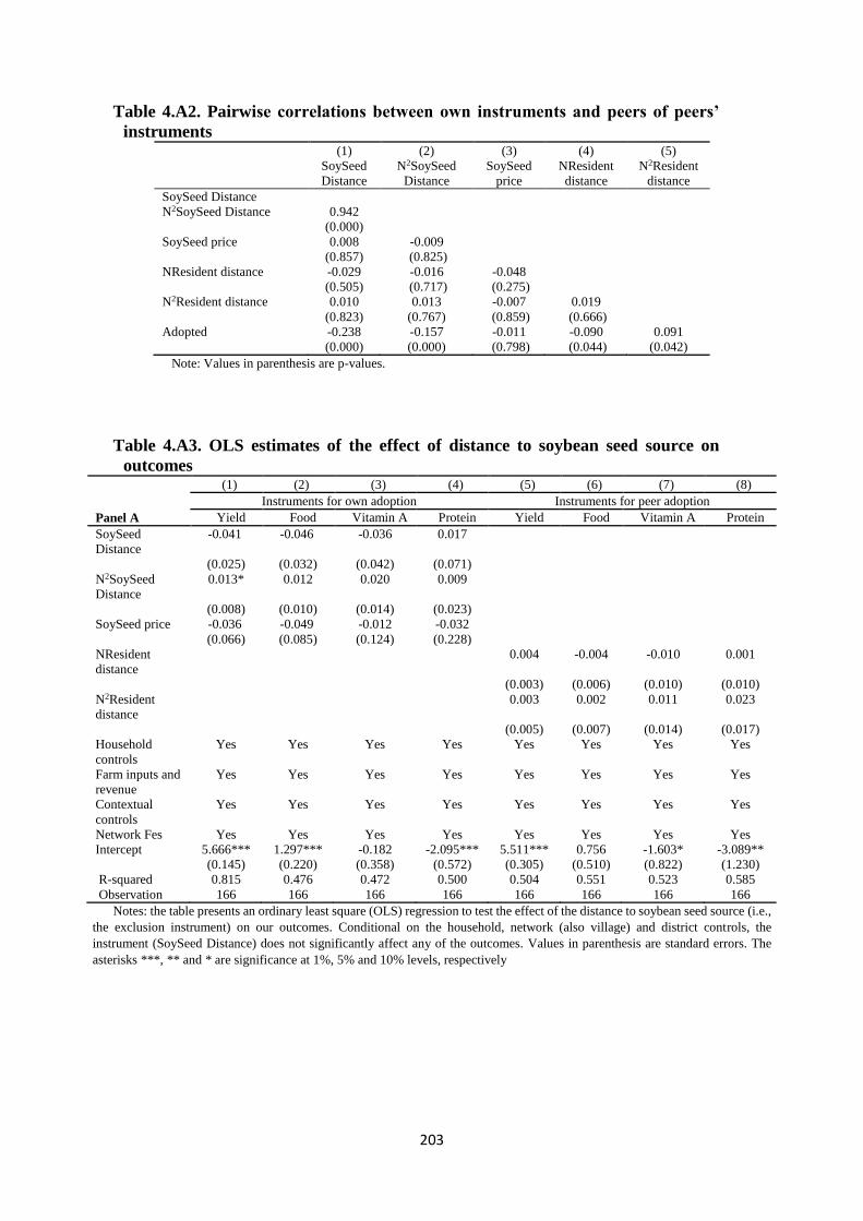
203

Table 4.A2. Pairwise correlations between own instruments and peers of peers’

instruments (1) (2) (3) (4) (5)

SoySeed

Distance

N2SoySeed

Distance

SoySeed

price

NResident

distance

N2Resident

distance

SoySeed Distance

N2SoySeed Distance 0.942

(0.000)

SoySeed price 0.008

(0.857)

-0.009

(0.825)

NResident distance -0.029

(0.505)

-0.016

(0.717)

-0.048

(0.275)

N2Resident distance 0.010

(0.823)

0.013

(0.767)

-0.007

(0.859)

0.019

(0.666)

Adopted -0.238

(0.000)

-0.157

(0.000)

-0.011

(0.798)

-0.090

(0.044)

0.091

(0.042)

Note: Values in parenthesis are p-values.

Table 4.A3. OLS estimates of the effect of distance to soybean seed source on

outcomes (1) (2) (3) (4) (5) (6) (7) (8)

Instruments for own adoption Instruments for peer adoption

Panel A Yield Food Vitamin A Protein Yield Food Vitamin A Protein

SoySeed

Distance

-0.041 -0.046 -0.036 0.017

(0.025) (0.032) (0.042) (0.071)

N2SoySeed

Distance

0.013* 0.012 0.020 0.009

(0.008) (0.010) (0.014) (0.023)

SoySeed price -0.036 -0.049 -0.012 -0.032

(0.066) (0.085) (0.124) (0.228)

NResident

distance

0.004 -0.004 -0.010 0.001

(0.003) (0.006) (0.010) (0.010)

N2Resident

distance

0.003 0.002 0.011 0.023

(0.005) (0.007) (0.014) (0.017)

Household

controls

Yes Yes Yes Yes Yes Yes Yes Yes

Farm inputs and

revenue


Contextual

controls


Network Fes Yes Yes Yes Yes Yes Yes Yes Yes

Intercept 5.666*** 1.297*** -0.182 -2.095*** 5.511*** 0.756 -1.603* -3.089**

(0.145) (0.220) (0.358) (0.572) (0.305) (0.510) (0.822) (1.230)

R-squared 0.815 0.476 0.472 0.500 0.504 0.551 0.523 0.585

Observation 166 166 166 166 166 166 166 166

Notes: the table presents an ordinary least square (OLS) regression to test the effect of the distance to soybean seed source (i.e.,

the exclusion instrument) on our outcomes. Conditional on the household, network (also village) and district controls, the

instrument (SoySeed Distance) does not significantly affect any of the outcomes. Values in parenthesis are standard errors. The

asterisks ***, ** and * are significance at 1%, 5% and 10% levels, respectively

204

Appendix B1: First stage estimates

Table 4.B1.1. First-stage estimates of peers’ adoption of improved soybean variety Peer adoption

Coefficients S.E.

Sex 0.004 0.010

Age -0.000 0.000

Education -0.002 0.001

Hsize 0.005** 0.002

HLand 0.002 0.003

HWealth (predicted) 0.001 0.005

Soil fertility -0.009 0.005

Seed use 0.001 0.001

Fertilizer cost 0.000 0.000

Pesticide cost 0.001 0.001

Weedicide cost 0.000 0.000

Machinery -0.005 0.008

Labor use -0.001** 0.000

Local wage rate -0.192*** 0.032

Soyseed price -0.002 0.019

Extension (predicted) -0.037 0.032

Residuals_NWLink 0.007 0.006

Degree 0.006 0.004

NSex 0.053* 0.030

NAge -0.002 0.002

NEducation -0.000 0.009

NHsize 0.007 0.014

NLandholding 0.042** 0.017

NWealth 0.111*** 0.041

NSoil -0.110** 0.047

NExtension -0.198 0.129

NResident distance -0.002** 0.001

N2Sex -0.312*** 0.055

N2Age 0.001 0.002

N2Education 0.016 0.012

N2Hsize -0.055*** 0.014

N2Landholding -0.081*** 0.017

N2Wealth 0.110** 0.055

N2Soil 0.294*** 0.058

N2Soyseed price 0.822*** 0.137

N2Extension -0.154 0.162

N2Resident distance -0.005*** 0.002

Town centre -0.002*** 0.001

Network Fes Yes

Intercept -0.229 0.181

R-squared 0.882

Observation 500

Notes: table reports first-stage estimates of peer adoption equations used to predict the peer

adoption variable. Columns 1 and 2 present results for the soybean yield specification, whereas

columns 3 and 4 display the results for the food and nutrition specification. S.E. are reported robust

standard errors. The asterisks ***, ** and * are significance at 1%, 5% and 10% levels, respectively.

205

B1.2. Further empirical Issues

Our final concern is the potential endogeneity of household wealth, extension contact and farm

revenue. In the adoption and outcome equations, household wealth and farm revenues are

potentially endogenous because households who adopted the improved variety are expected to

have higher yields, which will likely translate into higher farm revenues, incomes and more

assets. Also, given that soybean is a market-oriented crop, one can expect that households who

are food secured will more likely invest in the new variety, which could lead to increased yield,

farm revenues and enhanced wealth. Extension contact could also be endogenous because

extension officers may be more inclined to visit farmers who adopted (or performing farmers)

than non-adopting (or nonperforming farmers).

To account for this, we use predicted instead of the observed values of these variables obtain

from a regression of each of these variables on the entire set of exogenous characteristics and

at least an instrument. For the wealth equation, we use whether any parent of the farmer or

spouse ever had authority in the community, as instrument. We believe this to be valid and

relevant instrument because the authority of the parents in the traditional political system are

mostly predetermined by lineage, and can therefore be reasonably assumed to be exogenous.

Also, the traditional authority system gives the parent access to land and other natural resources

in the village, which the children can benefit from. One issue that might threaten the use of

these as instruments is when access to these resources are able to affect our outcomes through

a different route, such as household landholding, as well. For this reason, we control for

household landholding in all specifications. In the extension contact and farm revenue,

following the network literature, we use the extension contact and farm revenues, respectively,

of direct and indirect peers, respectively, as instruments. The first-stage instrumenting

regressions are presented in table 4.B1.2.

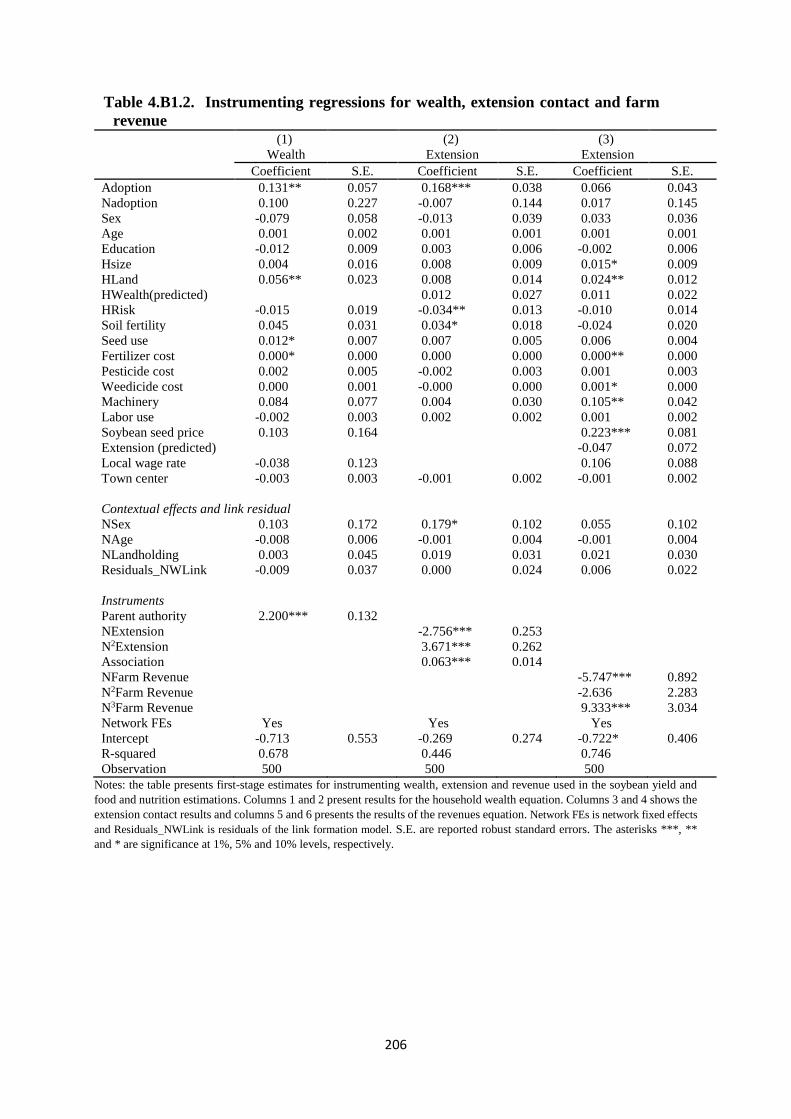
206

Table 4.B1.2. Instrumenting regressions for wealth, extension contact and farm

revenue (1) (2) (3)

Wealth Extension Extension

Coefficient S.E. Coefficient S.E. Coefficient S.E.

Adoption 0.131** 0.057 0.168*** 0.038 0.066 0.043

Nadoption 0.100 0.227 -0.007 0.144 0.017 0.145

Sex -0.079 0.058 -0.013 0.039 0.033 0.036

Age 0.001 0.002 0.001 0.001 0.001 0.001

Education -0.012 0.009 0.003 0.006 -0.002 0.006

Hsize 0.004 0.016 0.008 0.009 0.015* 0.009

HLand 0.056** 0.023 0.008 0.014 0.024** 0.012

HWealth(predicted) 0.012 0.027 0.011 0.022

HRisk -0.015 0.019 -0.034** 0.013 -0.010 0.014

Soil fertility 0.045 0.031 0.034* 0.018 -0.024 0.020

Seed use 0.012* 0.007 0.007 0.005 0.006 0.004

Fertilizer cost 0.000* 0.000 0.000 0.000 0.000** 0.000

Pesticide cost 0.002 0.005 -0.002 0.003 0.001 0.003

Weedicide cost 0.000 0.001 -0.000 0.000 0.001* 0.000

Machinery 0.084 0.077 0.004 0.030 0.105** 0.042

Labor use -0.002 0.003 0.002 0.002 0.001 0.002

Soybean seed price 0.103 0.164 0.223*** 0.081

Extension (predicted) -0.047 0.072

Local wage rate -0.038 0.123 0.106 0.088

Town center -0.003 0.003 -0.001 0.002 -0.001 0.002

Contextual effects and link residual

NSex 0.103 0.172 0.179* 0.102 0.055 0.102

NAge -0.008 0.006 -0.001 0.004 -0.001 0.004

NLandholding 0.003 0.045 0.019 0.031 0.021 0.030

Residuals_NWLink -0.009 0.037 0.000 0.024 0.006 0.022

Instruments

Parent authority 2.200*** 0.132

NExtension -2.756*** 0.253

N2Extension 3.671*** 0.262

Association 0.063*** 0.014

NFarm Revenue -5.747*** 0.892

N2Farm Revenue -2.636 2.283

N3Farm Revenue 9.333*** 3.034

Network FEs Yes Yes Yes

Intercept -0.713 0.553 -0.269 0.274 -0.722* 0.406

R-squared 0.678 0.446 0.746

Observation 500 500 500

Notes: the table presents first-stage estimates for instrumenting wealth, extension and revenue used in the soybean yield and

food and nutrition estimations. Columns 1 and 2 present results for the household wealth equation. Columns 3 and 4 shows the

extension contact results and columns 5 and 6 presents the results of the revenues equation. Network FEs is network fixed effects

and Residuals_NWLink is residuals of the link formation model. S.E. are reported robust standard errors. The asterisks ***, **


207

Appendix B2 First-stage network formation model and estimates

B2.1. Network formation model

The section describes the network formation model estimated. We estimated a conditional edge

independence model, which assumes links form independently, conditional on node- and link-

level covariates as follows;

(B2.1) 𝐿𝑖𝑗 = 𝛽0 + 𝛽1|𝑐𝑖 − 𝑐𝑗| + 𝛽2(𝑐𝑖 + 𝑐𝑗) + 𝛽3|ℒ𝑖𝑗| + 𝜇𝑖𝑗

where 𝐿𝑖𝑗 is an 𝑁 × (𝑁 − 1) matrix indicating whether there is a link between individuals 𝑖 and

𝑗, 𝑐𝑖 and 𝑐𝑗 are characteristics of individual 𝑖 and 𝑗. 𝛽1 measures the influence of differences in

their attributes, and 𝛽2 measures the effect of combined level of their attributes. ℒ𝑖𝑗 captures

attributes of the link between 𝑖 and 𝑗 such as geographical or social distance between them, and

𝛽3 is the associated parameter estimate. The estimates of eq. (B2.1) are reported in table 4.B2.1.

We next use the average of the predicted residuals of the link formation model as control

functions in our selection and outcome equations to account for the endogeneity of peer effects

due to unobserved factors that determine link formation.

208

Table 4.B2.1. Dyadic regression of network link formation Village1 Village2 Village3 Village4 Village5 Village6 Village7 Village8 Village9

Distance between peers in kilometers -0.040 0.025 0.116** -0.035 0.028 -0.005 0.038 -0.065 -0.006

(0.062) (0.044) (0.050) (0.039) (0.054) (0.045) (0.042) (0.045) (0.044)

Difference in distance to road between peers in kilometres -0.003 0.202* -0.044 0.076 0.047** 0.094** 0.069** -0.142** 0.041

(0.030) (0.104) (0.055) (0.058) (0.022) (0.038) (0.031) (0.060) (0.025)

Relatives = 1 0.013 0.121 0.064 -0.323 -0.346 0.294 0.570 -0.685** -0.685**

(0.339) (0.369) (0.580) (0.558) (0.283) (0.662) (0.376) (0.304) (0.349)

Same religion = 1 n.a n.a. -0.095 -0.730** -0.369 -0.020 0.349 -0.811* -0.281

n.a. n.a. (0.245) (0.329) (0.307) (0.486) (0.503) (0.439) (0.323)

Difference: Sex (= 1 if male) 1.150*** 0.821*** 7.767*** -0.306 0.437 0.013 0.744** 0.381 0.260

(0.342) (0.251) (0.375) (0.256) (0.335) (0.258) (0.359) (0.359) (0.516)

Difference: Age 0.004 -0.031** 0.031** -0.003 -0.051*** -0.037*** 0.038*** 0.093*** 0.041***

(0.008) (0.013) (0.013) (0.015) (0.017) (0.012) (0.010) (0.036) (0.014)

Difference: Years of schooling 0.090** 0.015 0.066 0.062 3.489*** -0.081** -0.044* 3.064*** 0.020

(0.046) (0.040) (0.050) (0.064) (0.189) (0.033) (0.025) (0.386) (0.067)

Difference: Household size -0.212** -0.097 -0.080 0.067 -0.223** 0.157** -0.123 0.011 0.103

(0.097) (0.096) (0.090) (0.085) (0.091) (0.073) (0.103) (0.063) (0.070)

Difference: Household landholding in hectares -0.239 -0.200** 0.098 0.343*** 0.130 0.487** -0.197* 0.089 -0.071

(0.218) (0.096) (0.173) (0.119) (0.153) (0.217) (0.110) (0.113) (0.132)

Difference: Village born = 1 if farmer was born in village 1.065** 0.287 -0.469 0.845*** -0.262 -0.028 -0.865*** 6.740*** -0.671**

(0.513) (0.353) (0.310) (0.290) (0.239) (0.323) (0.262) (0.516) (0.307)

Difference: Household wealth (predicted) in GHS 1.173 -0.223 0.882 0.189 0.826 -0.288 -1.780*** 2.738* 0.060

(1.211) (0.786) (0.685) (0.993) (1.291) (0.798) (0.588) (1.592) (0.843)

Sum: Sex (= 1 if male) -0.651*** 0.483*** 7.522*** -0.345 0.942*** 0.380* 0.577** 0.548* 0.295

(0.239) (0.185) (0.356) (0.217) (0.298) (0.229) (0.277) (0.314) (0.311)

Sum: Age -0.005 0.011 -0.019 -0.023*** 0.012 0.001 -0.032*** -0.056** -0.015

(0.007) (0.008) (0.013) (0.008) (0.013) (0.008) (0.008) (0.025) (0.011)

Sum: Years of schooling -0.018 0.028 0.012 -0.141** -3.470*** 0.042 -0.014 -3.092*** -0.066

(0.042) (0.020) (0.037) (0.062) (0.180) (0.026) (0.031) (0.398) (0.058)

Sum: Household size -0.010 0.163*** 0.112 -0.002 0.064 -0.040 0.028 -0.037 0.121***

(0.051) (0.056) (0.070) (0.051) (0.046) (0.036) (0.061) (0.076) (0.046)

Sum: Household landholding in hectares -0.051 -0.005 0.011 0.113 -0.246*** -0.360** 0.181* -0.058 0.173*

(0.113) (0.062) (0.136) (0.136) (0.094) (0.159) (0.107) (0.096) (0.097)

Sum: Village born = 1 if farmer was born in village 1.019*** 0.169 0.096 0.029 -0.039 0.259 0.082 6.841*** -0.925***

(0.367) (0.331) (0.283) (0.217) (0.256) (0.255) (0.234) (0.487) (0.190)

Intercept -3.504* -5.325*** -17.991*** 0.004 -3.804** -1.176 0.751 -14.108*** -1.282

(1.983) (1.838) (1.825) (1.742) (1.606) (1.986) (1.442) (2.475) (1.827)

Observation 400 400 400 400 400 400 400 400 400

Pseudo R2 0.114 0.072 0.092 0.082 0.096 0.077 0.113 0.122 0.080

Notes: the table reports results of the dyadic regression of network link formation in eq. (B2.1). The dependent variable = 1 if 𝑖 (𝑗) cites 𝑖 (𝑗) as ever having any of the social and locational contact dimensions discussed

under section 4.2.2. Estimator is logit and all standard errors are clustered at the village level. Standard errors are in parenthesis. n.a. denotes not available. The asterisks ***, ** and * are significance at 1%, 5% and


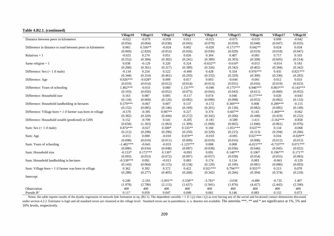
209

Table 4.B2.1. (continued) Village10 Village11 Village12 Village13 Village14 Village15 Village16 Village17 Village18

Distance between peers in kilometers -0.022 -0.079 -0.058 0.011 -0.025 -0.075 -0.019 0.009 -0.042

(0.056) (0.064) (0.038) (0.043) (0.079) (0.059) (0.048) (0.047) (0.035)

Difference in distance to road between peers in kilometres 0.065 6.556** -0.024 0.002 -0.020 -0.171*** 0.042** 0.024 0.034

(0.069) (2.820) (0.053) (0.026) (0.030) (0.029) (0.019) (0.018) (0.047)

Relatives = 1 -0.025 0.274 0.051 0.026 0.304 0.407 -0.001 0.717 0.103

(0.552) (0.384) (0.382) (0.241) (0.389) (0.303) (0.508) (0.605) (0.514)

Same religion = 1 0.038 -0.129 0.320 0.324 -0.652** -0.610* -0.013 -0.014 0.183

(0.268) (0.361) (0.317) (0.389) (0.326) (0.342) (0.402) (0.384) (0.342)

Difference: Sex (= 1 if male) -0.134 0.254 0.522 -0.400 0.428 0.334 0.976*** 0.435 0.821***

(0.344) (0.314) (0.461) (0.293) (0.332) (0.329) (0.300) (0.336) (0.283)

Difference: Age 0.026*** -0.028* 0.009 0.017 0.003 -0.044 -0.001 0.012 0.033

(0.010) (0.014) (0.012) (0.014) (0.013) (0.031) (0.016) (0.019) (0.023)

Difference: Years of schooling 1.402*** -0.033 0.060 1.131*** -0.046 -0.175*** 6.946*** 0.803*** -0.143***

(0.103) (0.050) (0.052) (0.073) (0.043) (0.043) (0.611) (0.060) (0.055)

Difference: Household size 0.163 0.087 0.005 -0.117 0.074 0.046 -0.177*** 0.020 -0.043

(0.118) (0.069) (0.120) (0.082) (0.099) (0.098) (0.052) (0.082) (0.133)

Difference: Household landholding in hectares 0.579*** -0.067 0.007 0.137 -0.172 0.369*** 0.008 0.289*** -0.115

(0.152) (0.085) (0.146) (0.169) (0.201) (0.130) (0.082) (0.085) (0.149)

Difference: Village born = 1 if farmer was born in village -0.570 -0.395 0.907** 0.227 0.374 0.607** 0.143 -1.469*** -0.062

(0.382) (0.320) (0.444) (0.272) (0.342) (0.266) (0.448) (0.419) (0.232)

Difference: Household wealth (predicted) in GHS 0.152 -0.709 0.541 -0.205 -0.181 -0.589 -1.611 -3.162*** -0.858

(0.658) (1.303) (1.063) (1.309) (1.060) (0.665) (1.840) (0.861) (0.976)

Sum: Sex (= 1 if male) 0.874*** -0.027 0.500* 0.535** 0.160 -1.051*** 0.637** 0.134 -0.068

(0.212) (0.298) (0.296) (0.250) (0.329) (0.215) (0.313) (0.294) (0.266)

Sum: Age -0.011 0.000 -0.010 0.019** -0.010 -0.005 0.027*** 0.016 -0.029**

(0.008) (0.010) (0.011) (0.009) (0.010) (0.016) (0.008) (0.012) (0.012)

Sum: Years of schooling -1.482*** -0.043 -0.033 -1.125*** 0.008 0.008 -6.015*** -0.733*** 0.071***

(0.080) (0.034) (0.048) (0.087) (0.038) (0.036) (0.646) (0.045) (0.022)

Sum: Household size -0.153* 0.172*** 0.130* -0.093 0.091 0.140*** 0.106* 0.196*** 0.171**

(0.093) (0.053) (0.072) (0.097) (0.057) (0.038) (0.054) (0.055) (0.083)

Sum: Household landholding in hectares -0.539*** 0.091 -0.013 0.083 0.174 0.134 0.083 -0.063 -0.129

(0.143) (0.064) (0.115) (0.134) (0.120) (0.100) (0.081) (0.080) (0.093)

Sum: Village born = 1 if farmer was born in village 0.362 0.392 0.572 0.422 0.921*** 0.794*** 0.955** 0.213 0.078

(0.288) (0.277) (0.405) (0.268) (0.342) (0.266) (0.394) (0.374) (0.218)

Intercept

0.240 -2.183 -5.001** -3.558** -3.781* -3.036 -4.480 -0.735 1.407

(1.978) (2.780) (2.115) (1.657) (1.941) (1.876) (4.427) (2.445) (2.590)

Observation 400 400 400 400 400 400 400 400 400

Pseudo R2 0.117 0.059 0.047 0.049 0.061 0.146 0.083 0.155 0.073

Notes: the table reports results of the dyadic regression of network link formation in eq. (B2.1). The dependent variable = 1 if 𝑖 (𝑗) cites 𝑖 (𝑗) as ever having any of the social and locational contact dimensions discussed

under section 4.2.2. Estimator is logit and all standard errors are clustered at the village level. Standard errors are in parenthesis. n. a. denotes not available. The asterisks ***, ** and * are significance at 1%, 5% and


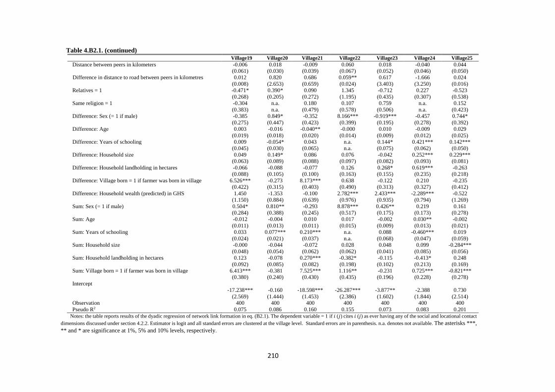
210

Table 4.B2.1. (continued) Village19 Village20 Village21 Village22 Village23 Village24 Village25

Distance between peers in kilometers -0.006 0.018 -0.009 0.060 0.018 -0.040 0.044

(0.061) (0.030) (0.039) (0.067) (0.052) (0.046) (0.050)

Difference in distance to road between peers in kilometres 0.012 0.820 0.686 0.059** 0.617 -1.666 0.024

(0.008) (2.653) (0.659) (0.024) (3.403) (3.250) (0.016)

Relatives = 1 -0.471* 0.390* 0.090 1.345 -0.712 0.227 -0.523

(0.268) (0.205) (0.272) (1.195) (0.435) (0.307) (0.538)

Same religion = 1 -0.304 n.a. 0.180 0.107 0.759 n.a. 0.152

(0.383) n.a. (0.479) (0.578) (0.506) n.a. (0.423)

Difference: Sex (= 1 if male) -0.385 0.849* -0.352 8.166*** -0.919*** -0.457 0.744*

(0.275) (0.447) (0.423) (0.399) (0.195) (0.278) (0.392)

Difference: Age 0.003 -0.016 -0.040** -0.000 0.010 -0.009 0.029

(0.019) (0.018) (0.020) (0.014) (0.009) (0.012) (0.025)

Difference: Years of schooling 0.009 -0.054* 0.043 n.a. 0.144* 0.421*** 0.142***

(0.045) (0.030) (0.065) n.a. (0.075) (0.062) (0.050)

Difference: Household size 0.049 0.149* 0.086 0.076 -0.042 0.252*** 0.229***

(0.063) (0.089) (0.088) (0.097) (0.082) (0.093) (0.081)

Difference: Household landholding in hectares -0.066 -0.088 -0.077 0.126 0.268* 0.619*** -0.263

(0.088) (0.105) (0.100) (0.163) (0.155) (0.235) (0.218)

Difference: Village born = 1 if farmer was born in village 6.526*** -0.273 8.173*** 0.638 -0.122 0.210 -0.235

(0.422) (0.315) (0.403) (0.490) (0.313) (0.327) (0.412)

Difference: Household wealth (predicted) in GHS 1.450 -1.353 -0.100 2.782*** 2.433*** -2.289*** -0.522

(1.150) (0.884) (0.639) (0.976) (0.935) (0.794) (1.269)

Sum: Sex (= 1 if male) 0.504* 0.810** -0.293 8.878*** 0.426** 0.219 0.161

(0.284) (0.388) (0.245) (0.517) (0.175) (0.173) (0.278)

Sum: Age -0.012 -0.004 0.010 0.017 -0.002 0.030** -0.002

(0.011) (0.013) (0.011) (0.015) (0.009) (0.013) (0.021)

Sum: Years of schooling 0.033 0.077*** 0.210*** n.a. 0.088 -0.460*** 0.019

(0.024) (0.021) (0.037) n.a. (0.068) (0.047) (0.059)

Sum: Household size -0.000 -0.044 -0.072 0.028 0.048 0.099 -0.284***

(0.048) (0.054) (0.062) (0.062) (0.041) (0.085) (0.056)

Sum: Household landholding in hectares 0.123 -0.078 0.270*** -0.382* -0.115 -0.413* 0.248

(0.092) (0.085) (0.082) (0.198) (0.102) (0.213) (0.169)

Sum: Village born = 1 if farmer was born in village 6.413*** -0.381 7.525*** 1.116** -0.231 0.725*** -0.821***

(0.380) (0.240) (0.430) (0.435) (0.196) (0.228) (0.278)

Intercept

-17.238*** -0.160 -18.598*** -26.287*** -3.877** -2.388 0.730

(2.569) (1.444) (1.453) (2.386) (1.602) (1.844) (2.514)

Observation 400 400 400 400 400 400 400

Pseudo R2 0.075 0.086 0.160 0.155 0.073 0.083 0.201

Notes: the table reports results of the dyadic regression of network link formation in eq. (B2.1). The dependent variable = 1 if 𝑖 (𝑗) cites 𝑖 (𝑗) as ever having any of the social and locational contact

dimensions discussed under section 4.2.2. Estimator is logit and all standard errors are clustered at the village level. Standard errors are in parenthesis. n.a. denotes not available. The asterisks ***,

** and * are significance at 1%, 5% and 10% levels, respectively.

211

Table 4.B2.2. Instrumenting regression for Wealth in Dyadic model Difference of wealth Sum of wealth

Coefficient Robust

S. E.

Dyadic

S. E.

Coefficient Robust

S. E.

Dyadic

S. E.


Sex = 1 if male 0.080 0.036 0.086 -0.237* 0.034 0.154




District dummies





Intercept 1.488*** 0.056 0.214 2.614*** 0.088 0.429


Notes: the table presents first-stage estimates for instrumenting wealth in the dyadic link formation model. Columns 1, 2 and

3 present results for the difference of wealth between neighbors. Columns 4, 5 and 6 show results of the sum of wealth estimates.

The table also show both the conventional robust standard errors (in columns 2 and 5) and the Fafchamps and Gubert (2007)

group dyadic standard errors (columns 3 and 6). S.E. denotes standard errors. The asterisks ***, ** and * are significance at

1%, 5% and 10% levels, respectively.

212

Appendix C: Results

Table 4.C1. Soybean varietal adoption and yield Selection Outcome


Panel A 𝚯𝑨 𝝆𝟎, 𝜼𝟎

Nadoption (Predicted) 0.168*** 0.047 -0.051 0.033

Sex 0.050 0.052 -0.028 0.053

Age -0.002 0.001 0.001 0.002

Education 0.002 0.008 0.029*** 0.008

Hsize -0.035** 0.013 -0.005 0.011

HLand 0.052** 0.022 0.047 0.029

HWealth (predicted) 0.163*** 0.045 0.069 0.074

Soil fertility 0.022 0.026 0.009 0.026

Seed use -0.014** 0.006 0.005 0.006


Pesticide cost 0.001 0.004 -0.006 0.012

Weedicide cost 3.6E-4 0.001 0.002** 0.001

Machinery -0.006 0.052 0.102 0.095

Labor use 0.001 0.002 -0.001 0.002

Extension (predicted) 0.568*** 0.110 -0.021 0.127

Soy selling price 0.166 0.203 -0.046 0.130

Residuals_NWLink -0.054 0.034 0.055* 0.031

Intercept 5.435*** 0.406

Panel B (𝝆𝟏 − 𝝆𝟎) �̂�, (𝜼𝟏 − 𝜼𝟎) �̂�

Nadoption (Predicted) 0.128** 0.050

Sex 0.053 0.061

Age -0.002 0.002

Education -0.013 0.010

Hsize 0.001 0.014

HLand -0.036 0.032

HWealth (predicted) -0.061 0.078

Soil fertility 0.012 0.032

Seed use -0.004 0.007

Fertilizer cost 6.1E-5 1.0E-4


Weedicide cost -0.003*** 0.001

Machinery -0.106 0.104

Labor use 0.001 0.002

Extension (predicted) 0.066 0.139

Soy selling price 0.018 0.176

Residuals_NWLink -0.042 0.042

Intercept 1.106** 0.460

Panel C (𝝉 ) Local wage rate 0.137 0.101 -0.013 0.042

Network FEs Yes Yes

Town center 0.004* 0.002 -0.001 0.001

NSex -0.240 0.151

NAge 0.003 0.005

NLand -0.098** 0.040

SoySeed Distance -0.478*** 0.089

N2SoySeed Distance 0.147*** 0.027

SoySeed price -0.481** 0.193

X2: excluded instruments 36.99

p-value: excluded instruments 0.000

p-value: observed heterogeneity 0.000


Notes: The “selection” column reports the marginal effects from probit selection model of adoption decisions, with Θ𝐴 as the

vector of parameter estimates, equation (2). Our instrument is distance to soybean seed source, which is normalized about its overall

mean. �̂� is the predicted propensity score from the estimated first-stage adoption equation. The “outcome” column shows the estimates

of the soybean yield equations (1 and 5). 𝜌0, 𝜂0 in panel A denote effects of covariates on the outcome when the household is not

adopting as in equations (3). (𝜌1 − 𝜌0) �̂�, (𝜂1 − 𝜂0)�̂� in panel B denote the treatment effects of the covariates on the outcome due to

gains from adoption as in equation (3). 𝜏 is a parameter vector of village characteristics and network fixed effects (Network Fes).

Residuals_NWLink is residuals of the link formation model. S.E. are bootstrapped standard errors with 50 replications. The asterisks

***, ** and * are significance at 1%, 5% and 10% levels, respectively.

213

Table 4.C2. Soybean variety adoption, food and vitamin A consumption Selection Outcome

Food Vitamin A

Coefficient S. E. Coefficient S. E. Coefficient S. E.

Panel A 𝚯𝑨 𝝆𝟎, 𝜼𝟎 𝝆𝟎, 𝜼𝟎

Nadoption (predicted) 0.110** 0.049 0.087** 0.033 0.198*** 0.048

Sex 0.011 0.053 0.103* 0.055 0.148 0.102

Age -0.002 0.001 -0.002 0.002 0.003 0.003

Education 0.004 0.008 0.022** 0.010 0.040*** 0.011

Hsize -0.041*** 0.013 -0.035*** 0.011 -0.016 0.027

HLand 0.041* 0.021 0.058** 0.027 0.036 0.043

HWealth (predicted) 0.169*** 0.045 0.127* 0.076 0.190** 0.087

Soil fertility 0.038 0.027 0.030 0.035 -0.045 0.048

Seed use -0.015** 0.006 0.003 0.007 0.007 0.010

Fertilizer cost -3.9E-5 6.0E-5 2.4E-5 6.8E-5 -3.8E-5 1.3E-4

Pesticide cost 0.003 0.004 0.012* 0.007 0.015 0.011

Weedicide cost -2.6E-5 0.001 -8.6E-5 0.001 1.7E-4 0.001

Machinery -0.066 0.059 0.056 0.090 0.023 0.128

Labor use 0.001 0.002 0.007** 0.002 0.010** 0.004

Farm revenue (predicted) 0.270*** 0.070 0.211*** 0.064 0.476*** 0.127


Soybean selling price 0.088 0.194 0.227* 0.137 0.073 0.270

Intercept 0.519 0.669 -2.980*** 0.920

Panel B (𝝆𝟏 − 𝝆𝟎) �̂�, (𝜼𝟏 − 𝜼𝟎) �̂� (𝝆𝟏 − 𝝆𝟎) �̂�, (𝜼𝟏 − 𝜼𝟎) �̂�

Nadoption (predicted) -0.107*** 0.033 -0.214*** 0.055 Sex -0.095 0.069 -0.130 0.126 Age 0.003 0.003 -0.002 0.004 Education -0.024** 0.010 -0.042*** 0.014 Hsize 0.041** 0.015 0.026 0.035 HLand -0.075** 0.030 -0.035 0.047 HWealth (predicted) -0.135 0.083 -0.195* 0.100 Soil fertility -0.030 0.047 0.068 0.062 Seed use 0.003 0.009 -0.004 0.013 Fertilizer cost -1.2E-5 8.7E-5 1.1E-4 1.8E-4 Pesticide cost -0.013* 0.008 -0.017 0.013 Weedicide cost 3.4E-4 0.001 3.6E-5 0.002 Machinery -0.006 0.098 0.050 0.149 Labor use -0.011*** 0.003 -0.014** 0.005 Farm revenue (predicted) -0.030 0.068 -0.395** 0.145 Residuals_NWLink -0.039 0.040 -0.091 0.073 Soybean selling price -0.232 0.179 -0.120 0.337 Intercept 1.072 0.761 3.931*** 0.995 Panel C (𝝉 ) (𝝉 ) Extension (predicted) 0.572*** 0.108

Local wage rate -0.266* 0.151 0.015 0.040 0.166** 0.065


Town center 0.005** 0.002 0.001 0.001 0.005*** 0.001

NSex -0.498*** 0.163

NAge 0.002 0.005

NLand -0.116** 0.040






p-value: observed heterogeneity 0.000 0.000

Observations 500 500 500




of the food and vitamin A foods consumption equations (1 and 5). 𝜌0, 𝜂0 in panel A denote effects of covariates on the outcomes when

the household is not adopting as in equations (3). (𝜌1 − 𝜌0) �̂�, (𝜂1 − 𝜂0)�̂� in panel B denote the treatment effects of the covariates on

the outcomes due to gains from adoption as in equation (3). 𝜏 is a parameter vector of village characteristics and network fixed effects

(Network Fes). Residuals_NWLink is residuals of the link formation model. S.E. are bootstrapped standard errors with 50 replications.

The asterisks ***, ** and * are significance at 1%, 5% and 10% levels, respectively.

214

Table 4.C3. Soybean variety adoption and protein consumption Selection Protein


Panel A 𝚯𝑨 𝝆𝟎, 𝜼𝟎 Nadoption (predicted) 0.110** 0.049 0.292*** 0.086

Sex 0.011 0.053 0.140 0.117

Age -0.002 0.001 0.001 0.005

Education 0.004 0.008 0.074** 0.027

Hsize -0.041*** 0.013 -0.031 0.036

HLand 0.041* 0.021 0.076 0.058

HWealth (predicted) 0.169*** 0.045 0.440*** 0.118

Soil fertility 0.038 0.027 0.068 0.065

Seed use -0.015** 0.006 0.019 0.019


Pesticide cost 0.003 0.004 -0.005 0.024

Weedicide cost -2.6E-5 0.001 0.002 0.003

Machinery -0.066 0.059 -0.070 0.243

Labor use 0.001 0.002 0.010 0.007

Farm revenue (predicted) 0.270*** 0.070 0.546*** 0.157

Residuals_NWLink -0.046 0.034 0.008 0.068

Soybean selling price 0.088 0.194 -0.194 0.253

Intercept -4.702*** 1.440

Panel B (𝝆𝟏 − 𝝆𝟎) �̂�, (𝜼𝟏 − 𝜼𝟎) �̂�

Nadoption (predicted) -0.346*** 0.087

Sex -0.126 0.158

Age 0.003 0.007

Education -0.101*** 0.033

Hsize 0.030 0.047

HLand -0.045 0.065

HWealth (predicted) -0.510*** 0.145

Soil fertility -0.001 0.096

Seed use -0.012 0.025

Fertilizer cost 1.6E-4 2.5E-4


Weedicide cost -0.002 0.004

Machinery 0.219 0.295

Labor use -0.015* 0.008

Farm revenue (predicted) -0.497** 0.200

Residuals_NWLink -0.039 0.095

Soybean selling price 0.185 0.316

Intercept 4.319** 1.837

Panel C (𝝉 ) Extension (predicted) 0.572*** 0.108

Local wage rate -0.266* 0.151 0.310** 0.121

Network FEs Yes Yes

Town center 0.005** 0.002 0.011*** 0.002

NSex -0.498*** 0.163

NAge 0.002 0.005

NLand -0.116** 0.040






p-value: observed heterogeneity 0.000





of the protein foods consumption equations (1 and 5). 𝜌0, 𝜂0 in panel A denote effects of covariates on the outcome when the household

is not adopting as in equations (3). (𝜌1 − 𝜌0) �̂�, (𝜂1 − 𝜂0)�̂� in panel B denote the treatment effects of the covariates on the outcome

due to gains from adoption as in equation (3). 𝜏 is a parameter vector of village characteristics and network fixed effects (Network

Fes). Residuals_NWLink is residuals of the link formation model. S.E. are bootstrapped standard errors with 50 replications. The

asterisks ***, ** and * are significance at 1%, 5% and 10% levels, respectively.

215

Table 4.C4. Soybean variety adoption, yield and food consumption with mobile

phone coverage Selection Outcome

Yield Food

Coefficient S. E. Coefficient S. E. Coefficient S. E.

Panel A 𝚯𝑨 𝝆𝟎, 𝜼𝟎 𝝆𝟎, 𝜼𝟎

Nadoption (predicted) 0.138** 0.052 -0.064 0.037 0.097*** 0.097

Sex 0.043 0.052 -0.027 0.045 0.103** 0.103

Age -0.002 0.001 0.001 0.002 -0.002 -0.002

Education 0.001 0.008 0.030*** 0.009 0.022** 0.022

Hsize -0.034** 0.013 -0.004 0.011 -0.035** -0.035

HLand 0.054** 0.022 0.049 0.034 0.057** 0.057

HWealth (predicted) 0.159*** 0.045 0.056 0.139 0.128 0.128

Soil fertility 0.021 0.026 0.011 0.027 0.032 0.032

Seed use -0.014** 0.006 0.005 0.006 0.003 0.003

Fertilizer cost -1.7E-05 7.0E-05 -1.9E-05 8.9E-05 2.2E-05 2.2E-05

Pesticide cost 0.001 0.004 -0.009 0.010 0.013 0.013

Weedicide cost 0.001 0.001 0.002*** 0.001 -9.9E-05 -9.9E-05

Machinery -0.008 0.051 0.125 0.089 0.048 0.048

Labor use 0.001 0.002 -0.001 0.002 0.007*** 0.007

Extension (predicted) 0.580*** 0.111 -0.021 0.114

Farm revenue (predicted) -0.064 0.029 0.215*** 0.215


Soybean selling price 0.161 0.205 -0.052 0.148 0.234* 0.234

Intercept 5.376*** 0.477 0.524 0.524

Panel B (𝝆𝟏 − 𝝆𝟎) �̂�, (𝜼𝟏 − 𝜼𝟎) �̂� (𝝆𝟏 − 𝝆𝟎) �̂�, (𝜼𝟏 − 𝜼𝟎) �̂�

Nadoption (predicted) 0.137** 0.059 -0.111*** 0.033

Sex 0.049 0.051 -0.094* 0.055

Age -0.001 0.002 0.002 0.003

Education -0.014 0.010 -0.024** 0.011

Hsize 0.001 0.015 0.039** 0.016

HLand -0.039 0.037 -0.075*** 0.024

HWealth (predicted) -0.047 0.150 -0.137 0.092

Soil fertility 0.009 0.031 -0.032 0.031

Seed use -0.004 0.007 0.003 0.008

Fertilizer cost 5.0E-05 1.1E-04 -7.6E-06 9.2E-05

Pesticide cost 0.011 0.012 -0.014 0.009

Weedicide cost -0.003*** 0.001 0.001 0.001

Machinery -0.135 0.099 0.008 0.087

Labor use 0.002 0.003 -0.011*** 0.003

Extension (predicted) 0.066 0.131

Farm revenue (predicted) -0.033 0.077

Residuals_NWLink -0.041 0.044 -0.036 0.034

Soybean selling price 0.043 0.192 -0.241 0.152

Intercept 1.163** 0.536 1.082 0.745

Panel C (𝝉 ) (𝝉 ) Local wage rate 0.145 0.101 -0.019 0.036 0.014 0.046

Mobile network 0.112 0.098 0.018 0.029 0.033 0.027


Town center 0.004 0.002 0.001 0.001 0.002*** 0.001

NSex -0.254* 0.154

NAge 0.002 0.005

NLand -0.068 0.046




p-value: observed heterogeneity 0.000 0.000





of the soybean yield and food consumption equations (1 and 5). 𝜌0, 𝜂0 in panel A denote effects of covariates on the outcomes when

the household is not adopting as in equations (3). (𝜌1 − 𝜌0) �̂�, (𝜂1 − 𝜂0)�̂� in panel B denote the treatment effects of the covariates on

the outcomes due to gains from adoption as in equation (3). 𝜏 is a parameter vector of village characteristics and network fixed effects

(Network Fes). Residuals_NWLink is residuals of the link formation model. S.E. are bootstrapped standard errors with 50 replications.

The asterisks ***, ** and * are significance at 1%, 5% and 10% levels, respectively.

216

Figure 4.C1 Counterfactual outcomes

The figure shows the treatment effects and potential outcomes (unobserved) as a function of resistance to treatment (U_A) for

all the outcomes, based on the baseline specification. In each case, it displays the marginal treatment effects, MTE (solid line),

and average treatment effects, ATE (dashed line). More importantly, it shows the distribution of the outcomes, Y0 and Y1, in

the non-adoption (dashed-dot line) and adoption (dotted line) states, respectively.

217

Figure 4.C2 MTE Functional form sensitivity for food and nutrition security

Figure 4.C2 shows the marginal treatment effects (MTE) functional form robustness checks based on the same specifications

in figure 4.3, evaluated at average values of the covariates. U_A denotes unobserved resistance to treatment/adoption. Part A

depicts MTE curves for soybean yield, part B shows the MTE curve for food consumption, part C is the MTE curve for vitamin

A rich foods consumption, while part D is the MTE curve for protein rich foods consumption. The solid MTE curve refers to

our baseline specification, where we include the propensity score and its square in the specification. The figure also displays

three additional specifications that allow for a specification without square of the propensity score (i.e., normal), one with cubic

of the propensity score (third order) and a specification obtained from semiparametric approach (Semiparametric).

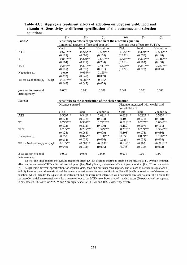
218

Table 4.C5. Aggregate treatment effects of adoption on Soybean yield, food and

vitamin A: Sensitivity to different specification of the outcomes and selection

equations (1) (2) (3) (4) (5) (6)

Panel A Sensitivity to different specification of the outcome equation

Contextual network effects and peer soil Exclude peer effects for SUTVA

Yield Food Vitamin A Yield Food Vitamin A

ATE 0.671***

(0.119)

0.276***

(0.093)

0.589***

(0.164)

0.527***

(0.122)

0.329***

(0.070)

0.566***

(0.128)

TT 0.867***

(0.164)

0.279**

(0.129)

0.677***

(0.234)

0.625***

(0.163)

0.374***

(0.103)

0.716***

(0.188)

TUT 0.284**

(0.115)

0.271***

(0.076)

0.411***

(0.101)

0.333**

(0.127)

0.241***

(0.077)

0.267***

(0.086)


(0.037)

0.088**

(0.040)

0.155**

(0.069)

TE for Nadoption (𝜌1 − 𝜌0) �̂� 0.157***

(0.043) -0.085**

(0.047)

-0.135*

(0.079)


heterogeneity

0.002 0.011 0.001 0.041 0.001 0.000

Panel B Sensitivity to the specification of the choice equation

Distance squared Distance interacted with wealth and

household size


ATE 0.569***

(0.124)

0.342***

(0.072)

0.621***

(0.133)

0.622***

(0.105)

0.292***

(0.071)

0.535***

(0.118)

TT 0.723***

(0.172)

0.380**

(0.111)

0.742***

(0.190)

0.791***

(0.159)

0.287**

(0.107)

0.604***

(0.161)

TUT 0.265**

(0.124)

0.265***

(0.063)

0.379***

(0.079)

0.287**

(0.103)

0.299***

(0.074)

0.394***

(0.086)


(0.034)

0.075**

(0.027)

0.180***

(0.056)

-0.059

(0.035)

0.089**

(0.033)

0.198***

(0.058)


(0.049) -0.089**

(0.031)

-0.188**

(0.065)

0.136**

(0.048) -0.108

(0.038)

-0.211***

(0.063)


heterogeneity

0.003 0.000 0.000 0.001 0.001 0.001

Notes: The table reports the average treatment effect (ATE), average treatment effect on the treated (TT), average treatment

effect on the untreated (TUT), effect of peer adoption (i.e., Nadoption 𝜌0), treatment effect of peer adoption, [i.e., TE for Nadoption

(𝜌1 − 𝜌0) �̂�] using different specification for soybean yield, food and nutrients consumption. The 𝜌’s are as defined in equations (1)

and (3). Panel A shows the sensitivity of the outcome equations to different specifications. Panel B dwells on sensitivity of the selection

equation, which includes the square of the instrument and the instrument interacted with household size and wealth. The p-value for

the test of essential heterogeneity tests for a nonzero slope of the MTE curve. Bootstrapped standard errors (50 replications) are reported

in parentheses. The asterisks ***, ** and * are significance at 1%, 5% and 10% levels, respectively.

219

Table 4.C6. Aggregate treatment effects of adoption on outcomes: Sensitivity to use

of clustered standard errors, mobile phone network coverage and household

dietary diversity (1) (2) (3) (4) (5) (6)

Sensitivity to:

Use of clustered errors Mobile network HDDS

Yield Food Vitamin A Yield Food

ATE 0.606***

(0.105)

0.294***

(0.078)

0.526***

(0.143)

0.617***

(0.103)

0.295***

(0.077)

1.317**

(0.521)

TT 0.772***

(0.142)

0.299**

(0.101)

0.596**

(0.188)

0.788***

(0.166)

0.296**

(0.107)

1.206*

(0.727)

TUT 0.278**

(0.121)

0.283***

(0.086)

0.384***

(0.106)

0.280**

(0.119)

0.294***

(0.065)

1.532***

(0.451)


(0.033)

0.087**

(0.028)

0.198***

(0.057)

0.064

(0.037)

0.097***

(0.030)

0.455**

(0.226)


(0.045)

-0.107***

(0.033)

-0.214***

(0.053)

0.137**

(0.059)

-0.111***

(0.033)

-0.613**

(0.245)


heterogeneity

0.004 0.001 0.003 0.016 0.001 0.045

Observations 500 500 500 500 500 500

Notes: The table reports the average treatment effect (ATE), average treatment effect on the treated (TT), average treatment

effect on the untreated (TUT), effect of peer adoption (i.e., Nadoption 𝜌0), treatment effect of peer adoption, [i.e., TE for Nadoption

(𝜌1 − 𝜌0) �̂�]. The 𝜌’s are as defined in equations (1) and (3). Columns (1) to (3) report estimates where standard errors are clustered

at the village level following Cameron et al. (2008). Columns (4) and (5) present estimates where we accounted for village mobile

phone network coverage, whiles column (6) presents estimates where household food dietary diversity score (HDDS) is used as the

outcome. The p-value for the test of essential heterogeneity tests for a nonzero slope of the MTE curve. Bootstrapped standard errors

(50 replications) are reported in parentheses in columns (4) to (6). The asterisks ***, ** and * are significance at 1%, 5% and 10%

levels, respectively.

220

Table 4.C7. Aggregate treatment effects of adoption on Soybean yield, food and

vitamin A: Sensitivity to Network Fixed Effects, Unobserved Link formation and

differences in peers (1) (2) (3) (4) (5) (6)

Panel A Sensitivity to farmers’ degree and truncation of links due to sampling

Degree Without those with links with all 5


ATE 0.627***

(0.115)

0.312***

(0.082)

0.547***

(0.128)

0.618***

(0.096)

0.316***

(0.093)

0.549***

(0.123)

TT 0.796***

(0.165)

0.346***

(0.119)

0.671***

(0.188)

0.789***

(0.139)

0.335**

(0.146)

0.629***

(0.181)

TUT 0.293**

(0.113)

0.244***

(0.066)

0.301***

(0.090)

0.296**

(0.108)

0.279***

(0.059)

0.396***

(0.096)


(0.046)

0.128**

(0.046)

0.279***

(0.074)

-0.045

(0.032)

0.082***

(0.032)

0.198***

(0.049)

Degree 𝜌0,𝑑 0.042

(0.070)

-0.071

(0.061)

-0.122

(0.121)

TE for Nadoption (𝜌1 − 𝜌0) �̂� 0.113*

(0.058)

-0.165***

(0.055)

-0.328***

(0.098)

0.122**

(0.047)

-0.101**

(0.037)

-0.215***

(0.054)

TE for Degree (𝜌1,𝑑 − 𝜌0,𝑑) �̂� 0.045

(0.078)

0.146

(0.072)

0.278*

(0.147)


heterogeneity

0.005 0.006 0.018 0.000 0.000 0.000

500 500 500 478 478 478

Panel B Sensitivity to changes in adopting peers over time and use of HDDS

Difference in peer adopters: 2016 – 2004

Yield Food Vitamin A

ATE 0.598***

(0.119)

0.298***

(0.076)

0.540***

(0.131)

TT 0.760***

(0.169)

0.307***

(0.106)

0.615***

(0.179)

TUT 0.279**

(0.109)

0.281***

(0.078)

0.390***

(0.091)


(0.039)

0.075**

(0.029)

0.176***

(0.075)


(0.050) -0.101***

(0.031)

-0.203***

(0.059)


heterogeneity

0.006 0.000 0.000


Notes: The table reports the average treatment effect (ATE), average treatment effect on the treated (TT), average treatment effect

on the untreated (TUT), effect of peer (i.e., 𝜌0 and 𝜌0,𝑑 for peer adoption and degree, respectively), treatment effect of peers [i.e.,

(𝜌1 − 𝜌0) �̂� and (𝜌1,𝑑 − 𝜌0,𝑑) �̂� for peer adoption and degree, respectively] and the p-value for the test of essential heterogeneity

using different specification for soybean yield, food and nutrients consumption. Panel A shows the sensitivity of our estimates to

household degree and measurement errors due to the use of the sampled networks. Panel B dwells on sensitivity of the estimates the

use of differenced peer adoption. The p-value for the test of essential heterogeneity tests for a nonzero slope of the MTE curve.

Bootstrapped standard errors (50 replications) are reported in parentheses. The asterisks ***, ** and * are significance at 1%, 5% and


221

Table 4.C8. Estimates of network fixed effects (Tables C1 and C2 continued) (1) (2) (3) (4)

Selection equations Outcome equations

Yield Food Yield Food

Village 2 184.375*** 178.404*** 0.063 -0.030

(64.354) (62.591) (0.077) (0.074)

Village 3 128.749*** 124.759*** -0.031 -0.123*

(44.421) (43.226) (0.076) (0.067)

Village 4 126.167*** 122.800*** 0.002 -0.065

(44.058) (42.831) (0.057) (0.067)

Village 5 117.003*** 113.338*** 0.052 -0.124**

(41.210) (40.053) (0.091) (0.062)

Village 6 43.525*** 42.898*** -0.032 -0.142**

(14.861) (14.426) (0.075) (0.069)

Village 7 375.646*** 363.032*** -0.024 -0.053

(130.379) (126.753) (0.057) (0.064)

Village 8 78.181*** 75.635*** -0.030 0.015

(28.067) (27.265) (0.098) (0.080)

Village 9 121.510*** 115.719*** -0.024 -0.037

(41.596) (40.539) (0.066) (0.093)

Village 10 -100.812*** -99.107*** 0.113 0.021

(34.630) (33.657) (0.076) (0.085)

Village 11 -100.972*** -99.779*** -0.086 -0.053

(35.957) (34.953) (0.073) (0.105)

Village 12 -78.137*** -77.489*** -0.007 -0.036

(27.630) (26.847) (0.054) (0.094)

Village 13 -9.003* -9.642** -0.151 -0.061

(4.933) (4.772) (0.095) (0.121)

Village 14 -50.025*** -48.998*** 0.050 -0.027

(17.612) (17.047) (0.071) (0.072)

Village 15 -18.533** -18.862** -0.183** -0.101

(8.561) (8.315) (0.091) (0.114)

Village 16 -5.114* -5.135* -0.071 -0.054

(2.727) (2.687) (0.068) (0.085)

Village 17 138.474*** 132.801*** -0.013 -0.011

(48.015) (46.701) (0.058) (0.069)

Village 18 -38.725*** -37.550*** -0.019 -0.048

(13.670) (13.328) (0.051) (0.057)

Village 19 -6.225*** -6.795*** 0.005 0.037

(1.926) (1.913) (0.063) (0.073)

Village 20 30.308*** 28.587*** 0.022 0.024

(10.833) (10.501) (0.056) (0.058)

Village 21 -92.361*** -90.162*** -0.157 -0.026

(30.394) (29.590) (0.142) (0.128)

Village 22 -134.078*** -129.525*** -0.180 0.015

(44.845) (43.647) (0.186) (0.138)

Village 23 59.334*** 58.869*** -0.126 -0.147

(19.061) (18.561) (0.077) (0.100)

Village 24 65.202*** 63.404*** -0.038 -0.171**

(22.110) (21.540) (0.067) (0.067)

Village 25 n.a. n.a. 0.024 0.090

n.a. n.a. (0.103) (0.078)

Notes: Bootstrapped standard errors (50 replications) are reported in parentheses. The

asterisks ***, ** and * are significance at 1%, 5% and 10% levels, respectively. n.a. denotes not

available.

222

Chapter Five

Informing Food Security and Nutrition Strategies in Sub-Saharan African countries: An

Overview and Empirical Analysis

Yazeed Abdul Mumin and Awudu Abdulai

Department of Food Economics and Food Policy, University of Kiel, Germany

Published in Applied Economic Perspectives and Policy

(https://doi.org/10.1002/aepp.13126)

Abstract

This article presents a systematic review of the literature on policy options to improve food

security and nutrition in developing countries, and an empirical analysis of the impact of

smallholder market participation on food security and nutrition in Ghana. The review focuses

on the impacts of policy strategies such as structural changes in relative prices, agricultural

infrastructure, economic incentives and agricultural technologies. In order to account for threats

of selection bias and omitted variable problem, the empirical analysis uses an ordered probit

selection model to jointly estimate households’ market orientation decisions and food and

nutrients consumption. The empirical results show that transitioning from one market

orientation to another significantly increase households’ food and nutrients consumption.

Keywords: Food security, Nutrition, Market orientation, Crop commercialization, Treatment

effects

JEL codes: D12, Q13, Q18

https://doi.org/10.1002/aepp.13126

223

5.1 Introduction

Food insecurity in sub-Saharan Africa remains a major developmental challenge, despite

several interventions to improve food security and nutrition in many developing regions. Recent

official estimates suggest that hunger and malnutrition appear to be increasing in most sub-

Saharan African countries, a situation that is in contrast to the rest of the world (FAO, ECA and

AUC 2020)53. The increasing food insecurity in Africa, combined with the fact that persistent

food insecurity contributed to the failure of countries in the region in meeting the Millennium

Development Goal (MDG) of halving the number of hungry people by 2015 (Abdulai and

Kuhlgatz 2012), suggest the need for continuous efforts in supporting and promoting measures

to improve food security in the region. While the worsening food situation can partly be

attributed to climate change (Abdulai 2018; FAO, ECA and AUC 2020), as well as poor and

weakening market conditions, the impact of agricultural markets on food security and nutrition

appears to be far from being conclusive (Carletto et al. 2017; Linderhof et al. 2019; Ehui 2020).

Many authors have emphasized the role of new agricultural technologies, specialization and

commercialization in increasing farm productivity and household welfare through enhanced

efficiency, competitiveness and gains from comparative advantage (Govereh and Jayne 2003;

Ochieng et al. 2019). However, prohibitive transaction costs imposed by underdeveloped

market systems and infrastructure, market failures, and inadequate access to finance and

technologies in most developing countries have often hindered the efficiency of food market

systems, and limited the potentials of agricultural marketing in these areas (Fafchamps 1992;

Abdulai and Birachi 2009; Abdul-Rahaman and Abdulai 2020). Notwithstanding these

53 Whereas there was no increase in the prevalence of undernourishment in the rest of world between 2014-2018, growth in

prevalence for the whole of Africa and sub-Saharan Africa was 1.7 and 2.0 percentage points, respectively, over the same period

(FAO, ECA and AUC 2020).

224

constraints, smallholder marketing has been shown to increase farmers’ access to improved

crop inputs, productivity and income (Ashraf et al. 2009; Abdul-Rahaman and Abdulai 2020).

Despite the widespread agreement on the role of smallholder marketing in improving food

security and nutrition, the empirical evidence on this issue remain scanty, with mixed findings

(Carletto et al. 2017; Linderhof et al. 2019; Kuma et al. 2018). While studies such as Ochieng

et al. (2019) analyzed the impact of commercialization of bananas and legumes on dietary

diversity in central Africa, and Kuma et al. (2018), who examined the effects of coffee

production on household food security in Ethiopia show that commercialization improved

household dietary diversity and food security, others authors report that the impacts of

commercialization on food consumption and nutrition is either negative or non-existent (e.g.,

Carletto et al. 2017; Linderhorf et al. 2019).

Moreover, most of these studies have often failed to consider the possible market orientation54

of smallholders’ crop sales, which may mask the extent and pattern of gains from crop sales,

given that smallholders’ crop sales are driven by profit and non-profit motives (Pingali and

Rosegrant 1995; Jacoby and Minten 2009). Production and marketing decisions of smallholders

in Africa are often fragmented and characterized by a blend of subsistence, surplus, commercial

and distress55 motives, which may have various implications on the gains and impacts of

commercialization across farmers (Pingali and Rosegrant 1995). For instance, if households are

54 Household market orientation in developing countries has been classified into three (FAO 1989; Pingali and Rosegrant 1995).

1) Subsistence farmer where the farmer’s objective is food self-sufficiency, produces wide range of products and/or sells not

more than 25% of the output; 2) Transitional or surplus farmer where the farmer produces for household consumption and sale

of surplus, but sells at least 25% and less than 50% of the output; and 3) Commercial farmer where the farmer is profit oriented,

highly specialized and with high market engagement, and sells more than 50% of the output.

55 Distress sales usually arise when farmers are forced to sell their harvest to meet immediate financial requirements (such as

servicing of debts or meeting other household needs) (Jacoby and Minten 2009).

225

subsistence-oriented or surplus-oriented, they may choose to produce different crop mix in

order to secure food self-sufficiency, and to spread market-related risks due to market

imperfections and lack of risk mitigating mechanisms such as insurance and credit markets

(Zanello 2012; Ecker 2018). If, however, farm households are commercial-oriented, then

production and marketing decisions could be based on profit and some market intelligence,

which can result in higher ‘gains’ from trade, increased household income and improved food

security and nutrition (Pingali and Rosegrant 1995; Abdulai and Huffman 2000).

In this paper, our goal is twofold: First, to provide an overview of the literature on food security

and nutrition strategies in developing countries. While food security and nutrition are of interest

in their own rights, we focus on the survey of the literature on economic policies and micro

strategies of promoting smallholder food security and nutrition in sub-Saharan Africa. Second

is to provide an empirical example of how smallholder market orientation impacts on food

security and nutrition in Ghana. The empirical analysis builds on the review by showing how

commercially/profit-oriented market engagement by smallholders can serve as a food security

and nutrition enhancing strategy in the area. While previous studies have considered the role of

smallholder market participation and commercialization on food security and nutrition, there is

almost no study on how smallholder market orientation affects the impacts of

commercialization on food security and nutrition56. The empirical analysis is partly justified by

the fact that the extent of smallholder market integration is closely associated with the motive

56 Some studies examine the impacts of smallholder market participation and commercialization by focusing on market

participation decisions, cultivation and sale of cash crops, as well as the value of total crop harvest sold. Strasberg et al. (1999),

Govereh and Jayne (2003), Zanello (2012) and Kuma et al. (2018), for instance, focus on smallholder marketing decisions, and

cultivation and sales of cash crops, and Carletto et al. (2017) and Linderhof et al. (2019) focus on the value of crops sold.

Notable exceptions are Ochieng et al. (2019) who focus on the effect of households moving from non-commercialized to

commercialized, and Ogutu et al. (2019) who emphasis the effects of commercialization in a continuum (i.e., continuous

treatment effects), but not on how market orientation affects food security and nutrition.

226

of production, which tends to have varied impacts on household welfare (Abdulai and Huffman

2000; Ecker 2018). This, therefore, allows us to delineate smallholder market participation

effects on household food security and nutrition under different motives of market engagement

by smallholders.

Second, the empirical analysis allows us to highlight the impact of smallholder transition from

subsistence to commercial on the consumption of specific nutrient rich foods. The analysis on

specific nutrients intake is significant in this setting for at least two reasons: First, unlike most

previous studies that focused on calorie and/or food consumption (Kuma et al. 2018; Ochieng

et al. 2019), which do not enhance the understanding of individual nutrients intake patterns,

analysis of the consumption of nutrient rich foods provide insights into specific nutrients intake

and therefore, serve as a wedge between food patterns and food quality (Freisling et al. 2010).

Second, the distinction between food/calorie and specific nutrient rich foods is important,

because many African countries, including the study country, face deficiencies in specific

nutrients such as vitamins, protein and iron, in spite of appreciable or relatively normal levels

of food and calorie intake (Abdulai and Kuhlgatz 2012; Colen et al. 2018). This, coupled with

the fact that the recent deteriorating food security and nutrition situation in Africa has been

partly attributed to adverse food market conditions, underscore the need to further understand

how smallholder market orientation affects the impact of commercialization on household food

security and nutrition.

The rest of the paper is organized into three main sections as follows: The next section presents

an overview of food security research in Africa, with particular emphasis on food security and

nutrition promotion strategies in the literature. Section 5.3 shows the empirical example of

smallholder market participation as a food security and nutrition enhancing strategy. Section

5.4 concludes and highlights some policy and future research implications.

227

5.2 Food Security in Africa

The recent increase in the incidence of food insecurity and malnutrition in sub-Saharan African

(SSA) countries calls for the need to seriously assess and find ways to promote food security in

the sub-region. Evidence shows that the prevalence of food insecurity and malnutrition have

risen from 18.2% in 2014 to 20% in 2018 in Africa, with that of sub-Saharan Africa, increasing

from 20.8% to 22.8% over the same period (FAO, ECA and AUC 2020). Estimates from the

FAO, ECA and AUC (2020) reveal that about 239 million in the region were undernourished

in 2018. The number of undernourished people in Nigeria, which is the most populated country

in the region, was estimated to be over 25 million in 2018, which is about 180% increase over

the past decade (FAO, ECA and AUC 2020). This development suggests that, as was in the

case of the failure to achieve the Millennium Development Goal of halving the incidence of

hunger by 2015, the realization of the Sustainable Development Goal two of eradicating hunger

and improving nutrition by 2030 may not be realized, if concerted efforts are not made to

overcome the barriers to improving food security and nutrition in the region (OECD 2016).

The state of food security and nutrition in developing countries has been a consequence of

environmental and economic factors including climate shocks; conflicts; unemployment; low

wages and food price inflation; lack of access to and adoption of improved technologies; and

lack of institutions, structures and markets for farmers and consumers (Weber et al. 1988;

Abdulai and Kuhlgatz 2012; Abdulai and Huffman 2014; FAO, ECA and AUC 2020). In this

section, we provide an overview of the literature on how these factors have impacted food

security and nutrition, as well as general household welfare.

5.2.1 Economic Policies and Food Security

In most African countries, the fundamental agricultural policy objectives have been to increase

productivity and private sector engagement in agriculture, reduce state involvement, improve

innovation and technology, opening up markets and allowing prices to determine the allocation

228

of factors of production (Abdulai and Huffman 2000). Food security policies in many of these

economies have also focused on improving food trade and market integration through enhanced

infrastructure, private and state trade support policies, and public buffer stocks. These policies

have resulted in key policy initiatives such as the Comprehensive Africa Agricultural

Development Programme (CAADP) and the African Regional Nutrition Strategy (ARSN)

aimed at increasing investment in research and development, agricultural infrastructure,

extension services and the subsidization of farm inputs to increase productivity, trade and food

security (Sheahan and Barrett 2017; FAO, ECA and AUC 2020). Also, in the wake of the

COVID-19 pandemic, which has resulted in border closures, lockdowns and curfews, and the

consequent disruption in supply chains as well as projected contraction of agricultural

production, ministers for agriculture of African Union members have publicly committed to

implementing measures to minimize food system disruptions and ensure food security and

nutrition for their citizens (Ehui 2020).

The issue of food prices has been a key focus of interest in food security policies in many

developing countries. Such policies aim at improving food access through lower market prices

and stabilization of consumption in times of high food price inflation (Barrett 2002; OECD

2016). Two main approaches have been widely used to implement these policies in the past.

These included universal price subsidies that benefit net buyers of food, and limited access

subsidies that provide rationed quantities at reduced prices (Byerlee et al. 2006; Abdulai and

Kuhlgatz 2012). However, the limitations of these policies have been the lack of sustainability

and exit mechanisms, and the accruals of greater shares of rationed food gains to political actors

and groups at the expense of the poor. Moreover, a number of these price policies did not

sufficiently incorporate country specific price and production risk factors. This resulted in the

failure of several food price policies to produce the desired results with respect to food security

and nutrition measures (Barrett 2002; Byerlee et al. 2006).

229

Similarly, the Structural Adjustment Programs that were implemented by many African

governments in the 1980s also contributed to food security dynamics in many of these countries.

Available evidence shows that the response of the agriculture sector in Africa to these policy

reforms was encouraging, because output and productivity increased in the countries that

pursued reforms compared to countries that failed to implement these reforms (Byerlee et al.

2006; Abdulai and Kuhlgatz 2012). However, the reduction or removal of subsidies on farm

inputs following the structural reforms also led to increased input prices, which later led to

reduced farm output and productivity, and increased food insecurity and malnutrition (Abdulai

and Huffman 2000). This suggests the need for policy-makers and researchers to put particular

emphasis on how long-term policies and interventions can ensure a balance between state

efficiency and productivity, without compromising food security and nutrition goals.

5.2.2 Climate Change and Food Security

Climate change and shocks continue to have serious adverse effects on agricultural production

and food security, particularly in developing countries (Abdulai 2018; Eastin 2018; Shahzad

and Abdulai 2020; FAO, ECA and AUC 2020). In particular, high temperatures, heat, water

stress and related weather extremes tend to affect poor people in developing countries the most,

because of their heavy reliance on agriculture for their livelihoods, low economic

diversification and their inability to cope with food price inflation and income shocks (Abdulai

and CroleRees 2001; Eastin 2018). Several attempts have been made to address or mitigate the

adverse impacts of climate change in Africa, with some prominent strategies being the

development of irrigation systems and the adoption of climate-smart agricultural practices

(Lipper et al. 2014; Abdulai 2018). Climate-smart agriculture is an embodiment of practices

that seek to promote the reliance on agricultural systems and livelihoods to promote production,

and reduce risks of food insecurity and malnutrition for the current and future generations

(Lipper et al. 2014; Issahaku and Abdulai 2020).

230

The literature has shown a variety of climate-smart practices that include conservation

agriculture, use of improved and drought-tolerant crop varieties, adoption of improved

technologies, crop rotation and mixed cropping, matching livestock to supply of grazing land

as well as crop diversification and economic diversification into non-farm income activities

(Abdulai and CroleRees 2001; Di Falco and Veronesi 2013; FAO 2016; Shahzad and Abdulai

2020). Earlier studies on the impact of climate change focused on crop productivity at the

country, regional and global levels, and only provided insights into the impacts of climate

change in aggregate terms (Di Falco et al. 2011). However, the need to promote resilience of

the poorest and vulnerable segments of rural population in developing countries (Eastin 2018),

resulted in the need to understand smallholder adaptation strategies (Di Falco et al. 2011;

Issahaku and Abdulai 2020). Thus, recent studies have focused on understanding the drivers of

smallholder adaptation to climate change in developing countries, and also quantifying the

effects of adaptation strategies on farm performance and household welfare measures such as

yields, net returns, poverty reduction, and food security and nutrition (FAO 2016; Eastin 2018;

Issahaku and Abdulai 2020; Shahzad and Abdulai 2020).

Promotion of drought resistant crop varieties, and conservation agriculture remain top of the

list of climate change adaptation practices, since these have been shown to have substantial

impacts on household resilience to climate change and on household welfare in Africa (Di Falco

et al. 2011; Abdulai 2018). Many studies have shown positive effects of climate change

adaptation practices such as changing crop varieties, soil and water conservation practices,

water harvesting and irrigation, tree planting, matching livestock to supply of grazing land, and

economic diversification on household welfare in Africa and Asia (e.g., Di Falco et al. 2011;

FAO 2016; Issahaku and Abdulai 2020; Shahzad and Abdulai 2020). For instance, Issahaku

and Abdulai (2020) show that smallholder adaptation to climate change increases household

231

dietary diversity and reduces household food insecurity by about 15% and 35%, respectively in

Ghana.

Despite the benefits of these practices, adoption of specific climate-smart practices remains low

in many African countries (Walker et al. 2014; Abdulai and Huffman 2014; Issahaku and

Abdulai, 2020). Whereas available evidence estimates the average adoption of climate-smart

practices at about 66% (Di Falco et al. 2011; Issahaku and Abdulai 2020), the incidence of

adoption of specific strategies have been quite low. For instance, Di Falco and Veronesi (2013)

show that farmers’ adoption of water strategies ranges from 4 to 16%, while their adoption of

other strategies such as the use of new technologies and diversification into off-farm jobs stand

at 1.35% and 6.83%, respectively. Also, in spite of the burgeoning literature on impact of

adaptation to climate change, discourse between adaptation and food security and nutrition in

developing countries is quite limited (Di Falco et al. 2011; Di Falco and Veronesi 2013;

Issahaku and Abdulai 2020).

5.2.3 Adoption of Technology and Food Security

In addition to the issues of climate-smart and sustainable agriculture, the association between

adoption of improved agricultural technologies and household welfare has received

considerable attention among policymakers and researchers (Abdulai and Huffman 2005;

Foster and Rosenzweig 2010). This is due to the long recognition that productivity growth in

agriculture partly depends on the availability of improved technologies and the adoption of

these technologies (Foster and Rosenzweig 2010; Pannell and Zilberman 2020). Studies on this

front can be broadly categorized into those that focus on understanding the drivers of

technology adoption and diffusion in developing countries, and those that examine the impacts

of adoption on household welfare (Foster and Rosenzweig 2010; Abdulai and Huffman 2014;

Wossen et al. 2019; Huffman 2020).

232

In the case of the former, many factors have been found to be associated with the lack of

adoption of improved technologies, particularly in sub-Saharan Africa. Prominent among these

factors are credit constraints, absence of insurance and other risk mitigating schemes, high

transaction costs due to lack of market infrastructure and efficient markets, lack of access to

extension services and some behavioral limitations (Foster and Rosenzweig 2010; Pannell and

Zilberman 2020). Information failure has also been identified as an important factor that limits

farmers awareness, understanding and adoption of improved technologies in many developing

countries. This contributed to increased interest in understanding the role of social learning and

other peer effects in the adoption and diffusion of improved technologies in Africa (Abdulai

and Huffman 2005; Foster and Rosenzweig 2010; Huffman 2020).

The other strand of adoption studies focused on understanding the impacts of adoption on

household welfare (e.g., Becerril and Abdulai 2010; Abdulai and Huffman 2014; Kassie et al.

2017; Wossen et al. 2019). Most of these studies show that adoption of improved technologies

tends to increase household productivity, income and consumption, with some of the studies

reporting impacts of 24% and 16% increase in smallholder crop yields and farm net returns,

respectively (Abdulai and Huffman 2014; Kassie et al. 2017; Wossen et al. 2019).

Unfortunately, despite the significance of improved technologies for farm productivity and

income, Africa has lagged behind in the use of improved and modern technologies, and as such

has not been able to reap the productivity and welfare benefits of the so-called Green revolution

(Sheahan and Barrett 2017). For instance, Walker et al. (2014) estimate the mean level of

adoption across 20 improved crop varieties at 35% in Africa, with two-thirds of these crops

having adoption rates lower than this mean level.

Similarly, in spite of the high interest in understanding the impact of agricultural technologies

on household welfare, not much has been done on the impacts of adoption of improved crop

varieties on food security and, in particular, on the consumption of specific nutrient rich foods

233

in Africa. Previous studies mostly focused on adoption, farm returns and to a lesser extent on

food security (Abdulai and Huffman 2014; Kassie et al. 2017; Wossen et al. 2019), and when

attempts are made in the realm of specific nutrients consumption, the focus has been on calorie-

income and price elasticities (Abdulai and Aubert 2004; Colen et al. 2018). There is therefore

the need for an in-depth examination and understanding of the impacts of specific food security

promotion strategies such as adoption of new technologies, smallholder diversification and

marketing, as well as the associated impact mechanisms on specific food nutrients intake. Such

information would be relevant in informing the design and implementation of pro-poor policies

in Africa, and in increasing the effectiveness of food security and nutrition policies in realizing

the Sustainable Development Goal of eradicating hunger, achieving food security and improved

nutrition, and promoting sustainable agriculture (Abdulai 2018; Colen et al. 2018).

Thus, the empirical analysis considers the role of smallholder market engagement as a

diversification strategy that can enhance the resilience of smallholders to food and nutrition

insecurity. Smallholder farmers market engagement generally include non-farm employment,

diversification into cash cropping, selling of harvest and purchases of food to minimize seasonal

variation in food availability (Abdulai and CroleRees 2001; Wiggins et al. 2011; Di Falco and

Veronesi 2013; Kuma et al. 2018), and these have been recognized as food insecurity coping

mechanisms (Di Falco and Veronesi 2013; Shahzad and Abdulai 2020). Also, the integration

of smallholders into output and input markets can result in increased motivation of smallholders

to produce for profit maximization, which may lead to increased household welfare (Abdulai

and Huffman 2000). Thus, the next section focuses on the issues of agricultural

commercialization and household food security and nutrition.

5.2.4 Market Engagement and Food Security

Agricultural marketing or commercialization has been conceived in the literature as involving

smallholder participation in non-farm economic activities, participation in output and input

234

markets, as well as the profit motive or orientation of the farm business (Pingali and Rosegrant

1995; Abdulai and Delgado 1999; Wiggins et al. 2011; Dithmer and Abdulai 2017; Carletto et

al. 2017). A considerable body of empirical research has focused on understanding the role of

smallholder non-farm work and market participation on household welfare (Abdulai and

Delgado 1999; Abdulai and CroleRees 2001; Zanello 2012; Carletto et al. 2017). This is due to

the fact that non-farm engagement or marketing has long been recognized as a means by which

smallholders can move from subsistence farming to a more commercialized one, and also

minimize agricultural risks, given the failure or absence of consumption and insurance markets

in developing countries (Pingali and Rosegrant 1995; Reardon et al. 2006). These studies place

more emphasis on understanding the determinants of smallholder participation in non-farm

work or marketing, and the impact of such participation on smallholder welfare indicators such

as productivity, net returns and income (Abdulai and Delgado 1999; Abdulai and CroleRees

2001; Wiggins et al. 2011; Zanello 2012).

Many factors such as education, availability of markets and other infrastructure, household

access to credit, income and capital have been reported as influencing smallholders’ decisions

to participate in non-farm work or economic diversification, since the lack of access to these

factors appears to make it difficult for smallholders in many developing countries to diversify

away from subsistence agriculture (Abdulai and CroleRees 2001; Wiggins et al. 2011). Also,

studies have shown that transaction costs, wealth and assets, contractual and cooperative

marketing substantially affect smallholders’ marketing decisions and the quantities of inputs

and outputs traded (Abdulai and Birachi 2008; Zanello 2012; Abdul-Rahaman and Abdulai

2020). In particular, recent studies show that smallholder contract and cooperative marketing

tend to reduce market risks, increase smallholders’ bargaining power, and contribute to increase

farm productivity, income and household welfare in some Asian and African countries (Abdulai

and Birachi 2008; Ma et al. 2018; Abdul-Rahaman and Abdulai 2020).

235

In addition, several studies have examined the impacts of non-farm work and diversification

(Holden et al. 2004; Owusu et al. 2011; Ecker 2018), sale and purchase of food (Zanello 2012;

Ogutu et al. 2019), and contracting or cooperative marketing (Ma et al. 2018; Abdul-Rahaman

and Abdulai 2020) on household welfare. Smallholder marketing has contributed to increased

household productivity and farm returns in Asia and Africa (Ma et al. 2018; Abdul-Rahaman

and Abdulai 2020; Ogutu et al. 2019; Ochieng et al. 2019), although its impacts on food security

and particularly nutrients intake remain inconclusive (Zanello 2012; Carletto et al. 2017; Ogutu

et al. 2019).

One possibility of resolving the mixed and inconclusive findings on the impacts of smallholder

marketing on food security and nutrition is to consider the fact that consumption gains from

commercialization could be heterogeneously distributed among households, and also within

household members (Carletto et al. 2017; Ogutu et al. 2019). However, studies have mostly

failed to consider these dimensions in examining the impacts of commercialization on

household welfare (Carletto et al. 2017). In addition, existing studies have completely neglected

smallholder profit or market orientation on welfare gains, in spite of the fact that smallholders’

production and marketing decisions in developing countries are characterized by different

motives, including “distress sales” (Pingali and Rosegrant 1995; Reardon 2006; Jacoby and

Minten 2009). A notable exception is Ogutu et al. (2019), who examined the heterogeneity in

the impacts of agricultural commercialization on household calorie and micronutrients

consumption, but did not consider the profit motive or market-orientation of smallholders.

The empirical analysis builds on these previous studies, by examining the impact of smallholder

market-orientation on household food and nutrient rich food consumption. This is partly

justified by the fact that the extent of smallholder market integration is closely associated with

the motive of production, which has been argued as having varied impacts on household welfare

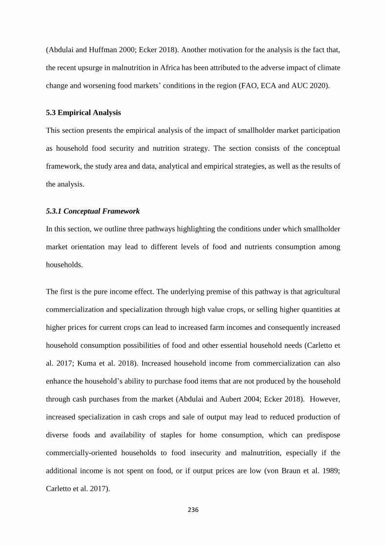
236

(Abdulai and Huffman 2000; Ecker 2018). Another motivation for the analysis is the fact that,

the recent upsurge in malnutrition in Africa has been attributed to the adverse impact of climate

change and worsening food markets’ conditions in the region (FAO, ECA and AUC 2020).

5.3 Empirical Analysis

This section presents the empirical analysis of the impact of smallholder market participation

as household food security and nutrition strategy. The section consists of the conceptual

framework, the study area and data, analytical and empirical strategies, as well as the results of

the analysis.

5.3.1 Conceptual Framework

In this section, we outline three pathways highlighting the conditions under which smallholder

market orientation may lead to different levels of food and nutrients consumption among

households.

The first is the pure income effect. The underlying premise of this pathway is that agricultural

commercialization and specialization through high value crops, or selling higher quantities at

higher prices for current crops can lead to increased farm incomes and consequently increased

household consumption possibilities of food and other essential household needs (Carletto et

al. 2017; Kuma et al. 2018). Increased household income from commercialization can also

enhance the household’s ability to purchase food items that are not produced by the household

through cash purchases from the market (Abdulai and Aubert 2004; Ecker 2018). However,

increased specialization in cash crops and sale of output may lead to reduced production of

diverse foods and availability of staples for home consumption, which can predispose

commercially-oriented households to food insecurity and malnutrition, especially if the

additional income is not spent on food, or if output prices are low (von Braun et al. 1989;

Carletto et al. 2017).

237

Second is that cash income from crop sales can enhance households’ access to and affordability

of improved farm inputs and better technologies that can be used for staple crop production

(Minten et al. 2011). Likewise, households who diversify their crops may enjoy economies of

scope, where skills, experiences and inputs acquired to grow staple crops for domestic

consumption can also be used to produce cash crops, and vice versa (Abdulai and CroleRees

2001; Govereh and Jayne 2003; Ecker 2018). However, missing, inefficient or very volatile

food markets can lead to high transaction costs or interrupted input supply, which may tend to

limit households access to inputs and other market opportunities, and can result in reduced

household income, food purchases and consumption (Fafchamps1992; Abdul-Rahman and

Abdulai 2020). This could present a situation where subsistence or surplus-oriented households

tend to have higher food and calorie intake than commercially-oriented households.

Finally, when there is considerable seasonal variation in household food availability and food

prices, which is often due to climatic shocks and inadequate infrastructure, this can lead to

farmers who grow more cash or high valued crops benefiting more in terms of food and

nutrients consumption (WFP and GSS 2012; Kuma et al. 2018; Issahaku and Abdulai 2020). In

sum, the effects of crop commercialization on household food and nutrients consumption will

be higher for commercial and perhaps surplus than subsistence households, if market conditions

are favorable and additional incomes from crop sales are spent on food consumption, and lower

if otherwise. In addition, commercially-oriented households may benefit more if seasonality of

food supply tends to increase households’ reliance on purchased food in times of household

food deficits. Finally, the magnitude of the effects of commercialization will be much higher

for the consumption of food items that are largely purchased from the market. We examine

these issues based on the case of smallholder farmers in the Northern region of Ghana.

238

5.3.2 Study Area

Despite the importance of agriculture as a source of livelihood of the majority of the population

in Ghana, the incidence of poverty was highest among households engaged in the agriculture

sector (42.7%) in 2016-2017. Also, the incidence of poverty in the northern regions have been

higher than the rest of the country since 2006 (GSS 2018). Food insecurity and malnutrition

have also been the highest in these regions, compared to the rest of the country, with an average

of 18% of households being severely food insecure. Farm households in these regions are faced

with inadequate rains, structural constraints and poor soils, which have often led to low

agricultural output, fluctuation in food prices, and food insecurity (WFP and GSS 2012). In

spite of efforts made to promote commercialization of agriculture and smallholders in the

northern regions, the average marketed crop surplus across the three regions remains low,

ranging from 15% in the Upper East region to 34% in the Northern region (IFAD-IFPRI 2011).

The high incidence of poverty, food insecurity and malnutrition in the Northern region amid

slightly higher proportion of marketed crops than the national average of 33%, presents an

apparent paradox that provides an appropriate context for the investigation of the impact of

households’ crop commercialization on food and nutrients consumption.

5.3.3 Data and Descriptive Statistics

We conducted a survey of 500 farm households in the Northern region of Ghana between July

and September 2017. Five districts were purposively selected based on their intensity of

cultivation of both staple and cash food crops, and then 25 villages were randomly selected

across these districts, with the allocation of villages done in proportion to the total households

in each district. These villages are remote and small, with less than 150 households in each.

Given this, we randomly selected 20 household heads in each village, and then used structured

questionnaires to interview the primary decision-makers in the households. In addition, a

detailed discussion using an interview guide was administered in each village to a focus group

239

of village leaders and representatives to obtain information on village characteristics. The

survey combined modules of household characteristics, agricultural production and marketing

to collect household data for the 2015-2016 cropping season.

Given our interest in measuring commercialization from the output market participation side,

and in terms of sales of all crops cultivated by the household in the 2015-2016 season, we use

the Household crop commercialization index (HCCI) suggested by Strasberg et al. (1999). The

index is expressed as:

𝐻𝐶𝐶𝐼 =∑ �̅�𝑣,𝑐𝑀𝑖,𝑐

�̅�𝑐=1

∑ �̅�𝑣,𝑐,𝑄𝑖,𝑐�̅�𝑐=1

× 100 [1]

where �̅�𝑣,𝑐 is the average village level crop 𝑐 price in village 𝑣, 𝑀𝑖,𝑐 is the quantity of crop 𝑐

marketed by household 𝑖, 𝑄𝑖,𝑐 is total quantity of crop 𝑐 produced by the household 𝑖, and 𝑐 is

an index of crops produced, with 𝑐 =1,…, 𝑐̅. On the basis of this measure, a household’s degree

of commercialization can be expressed in a continuum that ranges from pure subsistence of

HCCI = 0 to completely commercialized production of HCCI = 100. In order to characterize

households’ market orientation, we use the categorization by FAO (1989), which categorizes

households into three orientations, based on the proportion of crop output sold (see also Pingali

and Rosegrant 1995). Thus, we classify our farmers into subsistence-oriented, if the farmer sells

less than 25% of the output; surplus-oriented, if the farmer sells at least 25%, but less than 50%

of the output; and commercial-oriented if the farmer sells more than 50% of the output.

The outcomes of interest in this study are food consumption score (food) and food consumption

scores-nutrition. Given that these outcomes measure the frequency of consumption of food and

nutrient rich foods, we asked households the question “How many days in the last 7 days your

household ate the following foods?” (refer to notes under table 5.1 for details). We next sum all

the consumption frequencies of the food and nutrient rich food items of the same group. For the

food consumption score, we multiply the value obtained for each food group by the group

240

weight to obtain weighted food group scores, and then add the weighted food groups to generate

the food consumption score for a household. With regards to the nutrient consumption, we sum

the number of days that foods belonging to each nutrient sub-group (i.e., vitamin A, protein and

hem iron) were consumed in the household to obtain the food consumption score-nutrition for

the household (WFP 2015).

In order to explore how food and nutrients consumption vary by household market orientation,

we present the mean differences in food and nutrient rich foods consumption by household

market orientation in table 5.1. We first present the means for the whole sample in column (1).

In columns (2) to (4), we compare the mean differences of households who did not report any

sales and those who reported sales of 0 < HCCI < 25%. The table suggests that households who

did not sell any of their harvest have slightly lower food and nutrient rich food consumption

than those who sold at most 25% of the harvest, albeit not statistically significant across all

outcomes. This justifying our classification of households with less than 25% HCCI as

subsistence-oriented.

Columns (5) to (7) present the means and the mean differences between subsistence and

surplus-oriented households, while columns (8) to (10) report the comparison between

commercial on the one hand and surplus and subsistence households, on the other hand. The

comparison shows that both surplus and commercial-oriented households have significantly (at

the 1% level) higher income, food and nutrient rich foods consumption than subsistence-

oriented households. At the same time, commercial-oriented farm households appear to have

significantly higher income, food and nutrients consumption than surplus-oriented households.

These suggest the possibility of significant differences in the returns to household crop

commercialization across market orientations.

241

Table 5.1. Means and differences in means of food and nutrient rich food consumption outcomes across market orientation All sample Sell

none

Sell <

25%

Difference Subsistence-

oriented

Surplus-

oriented

Difference Commercial-

oriented

Difference Difference

(1) (2) (3) (4) = (3-2) (5) (6) (7) = (6-5) (8) (9) = (8-5) (10) = (8-6)

Food consumption score 33.55

(8.23)

27.95

(1.03)

30.08

(0.67)

2.13

(1.85)

29.83

(0.61)

33.73

(0.52)

3.90***

(0.79)

39.11

(0.59)

9.28***

(0.89)

5.38***

(0.83)

Vitamin A 12.43

(3.83)

10.18

(0.69)

10.56

(0.34)

0.38

(0.94)

10.52

(0.31)

12.55

(0.24)

2.03***

(0.38)

15.23

(0.18)

4.71***

(0.41)

2.68***

(0.34)

Protein 6.18

(3.46)

3.13

(0.57)

4.26

(0.24)

1.12

(0.69)

4.13

(0.23)

6.14

(0.22)

2.01***

(0.31)

9.52

(0.15)

5.39***

(0.31)

3.38***

(0.31)

Hem iron 3.77

(2.26)

1.91

(0.37)

2.48

(0.16)

0.57

(0.45)

2.41

(0.15)

3.75

(0.14)

1.34***

(0.21)

5.96

(0.09)

3.55***

(0.19)

2.21***

(0.20)

Log income 8.39

(0.71)

7.93

(0.14)

8.23

(0.04)

0.30***

(0.12)

8.19

(0.04)

8.33

(0.04)

0.14**

(0.06)

8.83

(0.09)

0.64***

(0.09)

0.49***

(0.08)

Notes: the table shows the descriptive statistics and the differences in means across household market orientation for the food and nutrient rich foods consumption outcomes and household annual income.

Column (1) presents the means of household consumption of food and nutrients, and household income for the entire sample. Columns (2) and (3) depict the means for households who did not sell any of

the output and those who sold less than 25% of the output, respectively, while column (4) shows the differences in these means. Columns (5), (6) and (8) present the means for subsistence-oriented, surplus-

oriented and commercial-oriented households. Column (7) reports the differences in means between subsistence and surplus-oriented households, whiles column (9) presents the differences in means between

subsistence and commercial-oriented households. Column (10) shows the differences in means between surplus and commercial-oriented households. Values in parenthesis are standard deviations in column

(1) and standard errors in columns (2) to (10). The asterisks *** and ** are significance at 1% and 5% levels, respectively.

We calculated the food consumption score by first grouping all food items consumed by households into main staple, pulses, vegetables, fruits, meat and fish, milk, sugar, oils and condiments and

the food consumption score-nutrition by grouping food items into 15 food groups under vitamin A rich foods (i.e., dairy, organ meat, eggs, orange and green vegetables; and orange fruits), protein rich

foods (pulses, dairy, flesh meat, organ meat, fish and eggs) and iron rich foods (flesh meat, organ meat and fish) (WFP 2015).

242

Table 5.2. Variable definition, measurement and descriptive statistics Variables Definition and measurement Mean S.D.

Panel A: Commercialization

HCCI Household crop commercialization index (in percentage) 36.76 19.02

Subsistence-oriented 1 if household sells less than 25% of harvest; 0 otherwise 0.36 0.48

Surplus-oriented 1 if household sells between 25% & 49.99% of harvest; 0 otherwise 0.41 0.49

Commercial-oriented 1 if household sells at least 50% of harvest; 0 otherwise 0.23 0.41

Panel B: Household characteristics

HHAge Age of household head (years) 44.03 12.04

HHSex 1 if household head is male; 0 otherwise 0.59 0.49

HHEducation Number of years in school by household head 1.27 3.27

HHSize Household size (number of persons) 5.63 2.14

HHLandholding Total land size of household (in hectares) 2.56 1.56

CB_Assoiations Number of associations the farmer is a member in the community 1.07 1.27

Log HHIncome Log of total household annual income 8.39 0.71

Log HHLivestock Log value of household livestock at beginning of 2015 season 7.65 2.19

Log HHDAsset Log value of household durable assets at beginning of 2015 season 9.11 0.88


Save money 1 if household regularly save money; 0 otherwise 0.72 0.45

Save food 1 if household at least save some food surplus; 0 otherwise 0.06 0.23

Panel C: Community variables and district Fes

Town distance Distance from community to main town centre in kilometres 15.46 11.86

Local wage Local wage rate per day in GHS 6.22 1.34

Gushegu 1 if household resides in Gushegu district; 0 otherwise 0.24 0.43

Karaga 1 if household resides in Karaga district; 0 otherwise 0.15 0.36

Savelugu-Nanton 1 if household resides in Savelugu-Nanton district; 0 otherwise 0.32 0.46

Tolon 1 if household resides in Tolon district; 0 otherwise 0.19 0.39

Kumbungu 1 if household resides in Kumbungu district; 0 otherwise 0.09 0.28

Panel D: Instruments

PreProductContract 1 if farmer has no pre-planting input contract in the past 5 years, 0

otherwise

0.18 0.39

HHMobileNetwork 1 if household location has a telecommunication network coverage, 0

otherwise

0.72 0.45

CMarket 1 if household resides in community with market, 0 otherwise 0.44 0.49

Farm_shock 1 if household experience any shock in farming due to weather or

bush/wildfires in the past 5 years, 0 otherwise

0.59 0.49

NonEmployTravel 1 if a household member left the community for non-employment

reasons (such as marriage, education or religion) in the past year, 0

otherwise

0.23 0.42

Panel E: Other covariates of the First-stage household income model

Tractor Tractor cost per acre in GHS 57.28 40.85

SeedUse Quantity of crop seeds used per acre in kilograms 67.15 207.32

SeedPrice Average seed price in GHS 32.01 177.68

Fertilizer Cost of fertilizer applied per acre in GHS 56.94 67.01

Pesticides Cost of pesticides applied per acre in GHS 1.47 5.98

Weedicides Cost of weedicides applied per acre in GHS 20.65 30.28

Labor Number of man-days per acre 22.98 10.68

Soil fertility 4=fertile; 3=moderately fertile; 2=less fertile; and 1=infertile 1.20 0.36

Notes: the table depicts the definition, measurement and descriptive statistics of household crop commercialization, instruments

and other controls. Panel A shows the household crop commercialization index (HCCI) and the proportion of households under

each market orientation. Panels B and C consist of household, community and district controls, while panel D contains the

instruments used for exclusive restriction in the first-stage market orientation model as well as the first-stage household income

regression to account for potential endogeneity of household income. Panel E consists of farm inputs and soil characteristics of

households. GHS is Ghana cedis, which is the Ghanaian currency.

243

Table 5.2 presents the definition, measurement and descriptive statistics of all the variables used

in the analysis for the entire sample. Panel A shows that 36% of the farm households surveyed

are subsistence-oriented, 41% are surplus-oriented, and 23% are commercial-oriented. Also,

the average household head is 44 years old and with 1.27 years of schooling. The average

household size and landholding are 5.63, and 2.6 hectares, respectively (panel B). The average

distance from the villages to the nearest town centre is about 15 kilometres, and the mean village

wage rate is about 6 GHS. We also compare the differences in the main controls between market

orientation in table 5.A1 in the appendix, and this shows significant differences mostly in the

household characteristics across market orientation.

5.3.4 Analytical Framework and Empirical Strategy

Our conceptual framework shows how smallholder food and nutrients consumption tend to

depend on household market orientation and market conditions. Given the categorization of

smallholders’ market orientation into subsistence, surplus and commercial-oriented, based on

the proportion of output marketed, we model household market orientation as an ordered choice

(Heckman et al. 2006). We define the latent variable 𝐶𝑖𝑗∗ , which denotes sorting of farm

households 𝑖 into the 3 categories of market orientation, based on an ordered probit selection

rule as;

𝐶𝑖𝑗∗ = 𝛼𝑗

′𝒁𝑖 + 𝜇𝑖𝑗,

where

𝐶𝑖𝑗 = 𝟏[𝜏𝑗(𝑤𝑗) < 𝛼𝑗′𝒁𝑖 + 𝜇𝑖𝑗 ≤ 𝜏𝑗+1(𝑤𝑗+1)], [2]

𝑗 = 1, 2…𝐽 ̅

and the cutoffs satisfy

𝜏𝑗(𝑤𝑗) ≤ 𝜏𝑗+1(𝑤𝑗+1), 𝜏0(𝑤0) = −∞, and 𝜏𝐽̅(𝑤𝐽̅) = ∞

where 𝐶𝑖𝑗 is a multivalued observed treatment variable, 𝒁𝑖 is a vector of observed controls,

𝛼𝑗′𝒁𝑖 + 𝜇𝑖𝑗 is a latent linear index, 𝛼𝑗 is a vector of parameters to be estimated, 𝑤𝑗 is a vector of

244

observed regressors, 𝜏𝑗(𝑤𝑗) are threshold parameters, which are allowed to depend on the

regressors57, and 𝜇𝑖𝑗 are error terms. To the extent that we are interested in the estimation of the

impact of farm household market orientation (𝐶𝑖𝑗) on food and nutrients consumption, we

denote the observed food and nutrients consumption outcomes as 𝑌𝑖𝑗 for the three market

orientations. We express the outcomes as linear functions of a vector of observed independent

variables, 𝑋𝑖 as;

𝑌𝑖𝑗 = {

𝛽1′𝑋𝑖 + 𝜖𝑖1 𝑖𝑓 𝐶𝑖 = 1

𝛽2′ 𝑋𝑖 + 𝜖𝑖2 𝑖𝑓 𝐶𝑖 = 2

𝛽3′ 𝑋𝑖 + 𝜖𝑖3 𝑖𝑓 𝐶𝑖 = 3

[3]

where the vector of coefficients, 𝛽𝑗, of 𝑋𝑖 are allowed to depend on the treatment options, and

𝜖𝑖𝑗 is assumed to have a zero mean and variance of 𝜎𝑗2, for each 𝑗 = 1,2,3.

Households’ market orientation in this study are non-random and implies that orientation status

of farmers could differ systematically due to self-selection of households into categories.

Selection bias can result from both observed factors (such as education, landholding, wealth

etc) and unobserved factors (such as innate abilities). Such factors may simultaneously drive

correlations in households’ market orientation and the outcomes, which will result in omitted

variable problem (Heckman et al. 2018). As a result, estimation of equation (3) with ordinary

least squares will generally result in biased and inconsistent estimates. We can control for the

observed sources of selection (to the extent possible) with detailed household and contextual

data, but the unobservable factors remain a source of concern for this analysis.

In order to account for the threats of selection bias and omitted variable problem in the light of

the ordered nature of the selection variable, we employ the ordered probit selection model

57 Such a model is referred to as the generalized ordered probit model, as opposed to the classical ordered choice model which

assumes the distribution of 𝑤𝑗 are degenerate, and thus the thresholds 𝜏𝑗 are assumed constants (Heckman et al. 2006).

245

(Heckman et al. 2006). This is a parametric model that assumes joint normality of the errors in

equations (2) and (3) (i.e., 𝜖𝑖𝑗, 𝜇𝑖𝑗), and utilizes full information maximum likelihood procedure

to jointly estimate a first-stage ordered probit of household market orientation in equation (2),

and a second-stage outcome models for the three regimes of market orientation (equation 3).

The process accounts for selection bias and omitted variable problem by inserting calculated

inverse Mills ratios from the first-stage ordered choice model into the second-stage food and

nutrients consumption model. The coefficients of the inverse Mills ratios, which we denote as

𝜌𝑗 = Corr(𝜖𝑖𝑗 , 𝜇𝑖𝑗), define the correlation between the errors in equations (2) and (3).

Significance of the correlation coefficients, 𝜌𝑗, will suggest the presence of selection bias

indicating that households’ market orientation decisions are endogenous. The signs of the 𝜌𝑗’s

show the pattern of correlation.

A critical concern is that the estimation of the selection and outcome equations requires an

exclusion restriction, or a source of variation to avoid collinearity and enhance identification.

However, an issue that complicates the exclusion restriction in the ordered choice setting is the

need for an instrument for each transition (Heckman et al. 2006). The three ordered choices

give two transitions (i.e., subsistence to surplus, and surplus to commercial) which intuitively

suggest the need for at least two instruments. In this study, we use farmers’ access to pre-

planting input contract for the past 5 years prior to the 2015 cropping season,

telecommunication network coverage at the location of the household and the presence of at

least periodic market in the village as instruments.

Past pre-planting input contract, is correlated with farmer market orientation, because it

contributes to minimizing market risks and transaction costs (Mishra et al. 2018). Whereas we

do not expect past pre-planting contract to directly affect current food and nutrients

consumption, it is possible that it may affect current consumption through past food stored for

current consumption. Table 5.2 (panel B) shows this is not a threat, because very few (6%)

246

households reported saving food from previous season. Also, these households do not

systematically differ across market orientation (table 5.A1, panel C) and past pre-planting

contract status in table 5.B1 in appendix B. Access to telecommunication network coverage and

village markets in Ghana vary substantially across villages (Zanello 2012), and are expected to

be good predictors of household market orientation, because these can increase households’

access to real-time market information, and reduce transaction cost of marketing, which are key

constraints to market engagement in these areas (MoFA 2017). However, these instruments

should not directly affect households’ current food and nutrients consumption, other than

through households’ market engagement. We further control for distance to the town centre,

household income and assets to ensure that the instruments are not picking up any proximity,

wealth and income effects.

The final issue is the potential endogeneity of household income. Household income may be

endogenous in the market orientation equation, because increased commercialization can lead

to increased farm income through high price premiums. In the food and nutrients consumption

equation, household income may be endogenous because of the joint production and

consumption decisions among agricultural households in developing countries (Fafchamps

1992). To account for the potential endogeneity, we employ the Control Function approach

(Woodridge 2010; Abdulai and Huffman 2014), using households experience of any shock on

the farm due to weather or wildfires in the past 5 years as instrument. Such shocks are usually

exogenously determined by idiosyncratic factors and are expected to be good predicters of

households’ total income, because of the association between such shocks and household crop

output and income. Given this, we estimate a first-stage generalized linear model of household

income on the instrument and other controls, and then insert the predicted residuals into the

selection and the outcome equations to account for the potential endogeneity of household

income.

247

Given the correction for sample selection and the identification issues, we estimate the average

treatment effects for transitioning between two orientations, 𝑗 and 𝑗 + 1, on the population

(ATE†), on everyone at the transition point between 𝑗 and 𝑗 + 1 (ATE), on the treated (ATT)

and on the untreated (ATU). The difference between ATE† and ATE shows the difference in

the characteristics of farmers in the entire population and those at the transition between two

market orientations. In addition, the difference between the ATT and ATE measures sorting on

gains, whereas the difference between ATU and ATE measures sorting losses (Heckman et al.

2018). Finally, the relationship among ATE, ATT and ATU shows the pattern of sorting on

gains, such that if ATT > ATE >ATU, this will suggest positive selection on gains, and if ATU

>ATE>ATT will indicate reverse selection on gains (Cornelissen et al. 2018).

5.3.5 Results and Discussion

This section presents and discusses the results of our estimations. We first present the results of

the first-stage estimates of households’ market orientation and the second-stage estimates of

food and nutrient rich foods consumption. We next report the results of the treatment effects of

households’ market orientation.

First- and Second-Stage Results

We report the marginal effects of the first-stage ordered probit estimates of determinants of

household market orientation in table 5.3, with subsistence-oriented as the base category. The

estimates show that household income and wealth significantly affect market orientation. In

particular, a percentage increase in household income decreases the probabilities of being

subsistence and surplus-oriented by 0.14 and 0.13, respectively, and increases the probability

of being commercial-oriented by about 0.27. The estimates show that a percentage increase in

household livestock value significantly increases the probability of being commercial-oriented

by about 0.04.

248

Table 5.3. First-stage determinants of market orientation

Subsistence-oriented

(1)

Surplus-oriented

(2)

Commercial-oriented

(3)

Marginal

effect

S.E. Marginal

effect

S.E. Marginal

effect

S.E.

HHAge -0.001 0.001 0.001 0.001 9.1E-5 0.001

HHSex -0.029 0.053 0.137** 0.057 -0.108** 0.042

HHEducation -0.009 0.008 0.005 0.008 0.003 0.005

HHSize 0.013 0.011 -0.017 0.012 0.004 0.008

HHLandholding -0.014 0.017 0.007 0.018 0.006 0.012

CB_Assoiations 0.022 0.019 -0.047** 0.020 0.025 0.015

Log HHIncome -0.144** 0.064 -0.130** 0.064 0.274*** 0.047

Log HHLivestock -0.016 0.011 -0.020 0.014 0.036*** 0.012

Log HHDAsset -0.107*** 0.029 0.096*** 0.030 0.010 0.021

Town distance -0.001 0.021 0.006** 0.003 -0.005** 0.002

Local wage 0.041* 0.021 -0.062** 0.023 0.020 0.018

Gushegu 0.060 0.084 -0.246** 0.108 0.186* 0.092

Karaga 0.041 0.087 -0.352*** 0.110 0.310*** 0.094

Savelugu-Nanton 0.140 0.085 -0.386*** 0.097 0.245*** 0.084

PreProductContract 0.272*** 0.061 -0.220*** 0.063 -0.051 0.046

HHMobileNetwork -0.228*** 0.054 0.100* 0.056 0.128*** 0.037

CMarket -0.039 0.048 -0.099* 0.053 0.138*** 0.040

HHIncomeResid 0.139 0.089 0.075 0.089 -0.214*** 0.056

Log likelihood -426.27

LR X2(36) 217.65

Prob X2 0.000

X2 (3) Excluded Instruments 39.60

Prob X2 0.000

Number of observations 180 206 114

Notes: First-stage generalized ordered probit estimation of equation (2). Column (1) presents the marginal effects and the

standard errors (S.E.) of the various covariates on the likelihood of being a subsistence-oriented household. Columns (2) and

(3) report the marginal effects and standard error of the covariates on the likelihood of being a surplus-oriented and commercial-

oriented household respectively. The asterisks ***, ** and * are significance at 1%, 5% and 10% levels, respectively.

Similarly, the probability of being subsistence-oriented household decreases by about 0.11,

while that of being surplus and commercial-oriented households increase by 0.09 and 0.01

respectively, when the value of household durable assets increases by 1%, albeit not significant

for commercial-oriented. These estimates generally suggest that wealthy households appear to

be more commercially inclined than less wealthy households. These results confirm the finding

by Abdulai and CroleRees (2001) that household income and wealth play important roles in

households’ diversification away from subsistence agriculture. Wealthy households tend to be

less vulnerable to risks of market failures and exposure to food insecurity, because of the

249

relatively high security due to their wealth and income, compared to poorer households who

are severely affected by market imperfections and inefficiencies (von Braun et al. 1989; Abdulai

and Aubert 2004; Ogutu et al. 2019).

Our results further show that the instruments strongly predict the probability of either being

subsistence, surplus or commercial-oriented household. The estimates show that households

with past pre-planting input contracts are more likely to be surplus-oriented, whereas those with

access to telecommunication network and markets in the village are more likely to be

commercial-oriented. We test the validity of the instrument by regressing the respective

outcomes on our set of controls and the instruments in part B of table 5.B3, and the results show

that all the instruments are valid, as they do not significantly explain food and nutrients

consumption.

We further check the relevance and validity of these instruments by presenting test diagnostics

of a generalized method of moments (IV-GMM)58 estimations of the effect of

commercialization on the outcomes in table 5.B2. The diagnostics test statistics reported at the

bottom of table 5.B2 (col. 1) further suggest the instruments are together relevant, and as such,

good predictors of household degree of commercialization. Specifically, the Cragg-Donald F-

statistic of 14.75, the Kleibergen-Paap rk Wald F-statistic of 45.98 and the associated Angrist

and Pischke (2009) p-value (p=0.000) all reject the null hypothesis that the instruments are

weak. Moreover, given the Hansen J test statistic of 3.452 and the p-value of 0.178, we cannot

reject the null hypothesis of zero correlation between the instruments and the error term (the

second-stage estimates are reported in part A of table 5.B3).

58 We use the IV-GMM estimator because of its efficiency over the conventional two-stage least squares when the equation is

over-identified (which is the case in our application as the number of instruments, three, exceed the number of endogenous

regressors of one) and its robustness to heteroskedasticity (Kuma et al. 2018).

250

We report results of the second-stage estimates of food and nutrients consumption in tables

5.C1 and 5.C2. The estimates show that education significantly increases the consumption of

food, protein and hem iron rich foods for subsistence-oriented households, and the consumption

of food and only vitamin A rich foods for surplus-oriented households. This confirms past

findings that education is positively associated with better food and dietary diversity (Issahaku

and Abdulai 2020). In addition, an increase in household size results in increased consumption

of food and vitamin A rich foods, although weakly significant at the 10% level, for surplus-

oriented households. This suggests the labor effect of household size, which contributes to

increased crop production, outweighs the dependency effect for the surplus-oriented

households, and thus, explains the positive effect of the household size59 in this case.

The results further reveal that household income significantly increases food and vitamin A

food consumption for surplus-oriented households, and the consumption of protein and hem

iron foods for surplus and commercial-oriented households, lending support to past studies that

income growth tend to increase calorie intake (Abdulai and Aubert 2004; Colen et al. 2018;

Kuma et al. 2018). However, household income generally reduces food and nutrient rich food

consumption for subsistence-oriented households, although not statistically significant. This

suggests that some sales of crops by subsistence-oriented households are due to distress that

results in a trade-off between household food and nutrients consumption on one hand and the

household income on the other hand. This incidence has been reported in the context of

developing countries where farmers are forced to sell their harvest to meet immediate financial

requirements (such as servicing of debts or other household needs) and later on have to buy

food from the market, or borrow food to meet household food needs (Reardon et al. 2006;

Jacoby and Minten 2009).

59 Family labour is an important part of household labor in the sample and constitutes about 74% of the total labor days used

on households’ farms in the sample.

251

Similarly, household wealth plays an important role in enhancing food and nutrients

consumption. In particular, an increase in the value of household livestock significantly

increases household food and nutrient rich food consumption for subsistence, while

significantly increasing the consumption of only nutrient rich foods for surplus-oriented

households. Furthermore, an increase in the value of household durable assets is estimated to

significantly increase food consumption for subsistence and surplus-oriented households, and

increase nutrient rich foods consumption for all groups.

We report the 𝜌s, which show the correlation between the errors in equations (2) and (3) at the

bottom of tables 5.C1 and 5.C2. The estimated correlations are weakly significantly different

from zero (p<0.1) for protein and hem iron foods consumption in the commercial-oriented

category, indicating the presence of self-selection. This implies that transitioning into

commercial-orientation may not have the same effect on protein and hem iron foods

consumption for the other two market orientations if they transition (Heckman et al. 2006;

Abdulai and Huffman 2014). The positive signs of the coefficients indicate reverse selection on

unobserved gains, suggesting that farm households with more than average protein and iron

rich food consumption have lower probabilities of transitioning into commercial-oriented

category.

Treatment Effects Measures

Table 5.4 presents the treatment effects estimates of farm households’ transition between

market orientation. Panel A presents the treatment effects between subsistence and surplus-

oriented, while panel B reports the treatment effects between surplus and commercial-oriented.

We report the treatment effects between subsistence and commercial-oriented in panel A of

table 5.5, although we mainly focus on table 5.4 in what follows.

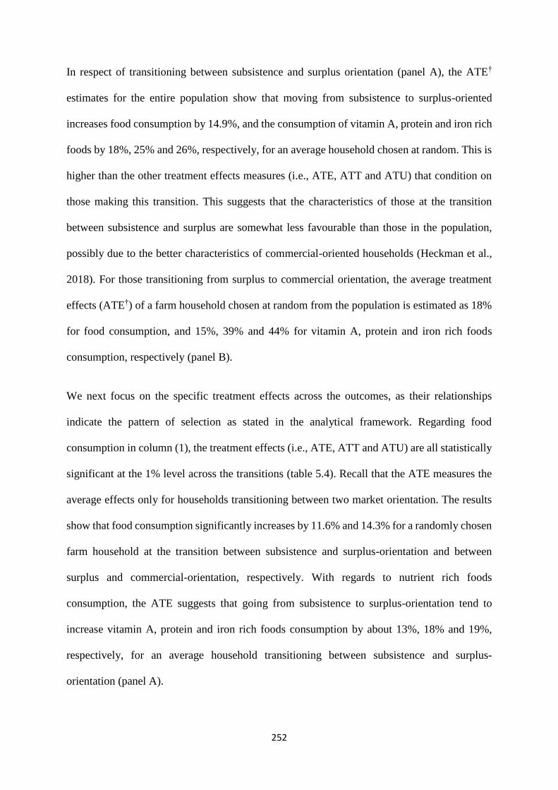
252

In respect of transitioning between subsistence and surplus orientation (panel A), the ATE†

estimates for the entire population show that moving from subsistence to surplus-oriented

increases food consumption by 14.9%, and the consumption of vitamin A, protein and iron rich

foods by 18%, 25% and 26%, respectively, for an average household chosen at random. This is

higher than the other treatment effects measures (i.e., ATE, ATT and ATU) that condition on

those making this transition. This suggests that the characteristics of those at the transition

between subsistence and surplus are somewhat less favourable than those in the population,

possibly due to the better characteristics of commercial-oriented households (Heckman et al.,

2018). For those transitioning from surplus to commercial orientation, the average treatment

effects (ATE†) of a farm household chosen at random from the population is estimated as 18%

for food consumption, and 15%, 39% and 44% for vitamin A, protein and iron rich foods

consumption, respectively (panel B).

We next focus on the specific treatment effects across the outcomes, as their relationships

indicate the pattern of selection as stated in the analytical framework. Regarding food

consumption in column (1), the treatment effects (i.e., ATE, ATT and ATU) are all statistically

significant at the 1% level across the transitions (table 5.4). Recall that the ATE measures the

average effects only for households transitioning between two market orientation. The results

show that food consumption significantly increases by 11.6% and 14.3% for a randomly chosen

farm household at the transition between subsistence and surplus-orientation and between

surplus and commercial-orientation, respectively. With regards to nutrient rich foods

consumption, the ATE suggests that going from subsistence to surplus-orientation tend to

increase vitamin A, protein and iron rich foods consumption by about 13%, 18% and 19%,

respectively, for an average household transitioning between subsistence and surplus-

orientation (panel A).

253

Table 5.4. Treatment effects estimates of household market orientation on food and nutrients outcomes (1)

Food

(2)

Vitamin A

(3)

Protein

(4)

Hem iron

Treatment

effect

% of base

choice

Treatment

effect

% of base

choice

Treatment

effect

% of base

choice

Treatment

effect

% of base

choice

Panel A

Subsistence vs. Surplus

ATE† 4.405***

(0.159) 14.89 1.893***

(0.087) 17.73 1.231***

(0.072) 25.27 0.780***

(0.049) 26.42

ATE 3.462***

(0.151) 11.62 1.338***

(0.079) 12.51 0.825***

(0.065) 17.89 0.517***

(0.046) 18.66

ATT 3.971***

(0.530) 13.34 1.705***

(0.254) 15.72 1.102***

(0.179) 21.89 0.668***

(0.117) 21.66

ATU 2.879***

(0.490) 9.65 0.919***

(0.245) 8.73 0.509**

(0.179) 12.33 0.345***

(0.115) 14.30

Panel B

Surplus vs. Commercial

ATE† 6.107***

(0.206) 17.97 1.892***

(0.087) 15.05 2.360***

(0.078) 38.67 1.635***

(0.053) 43.79

ATE 4.959***

(0.256) 14.29 1.639***

(0.116) 12.41 1.917***

(0.099) 27.67 1.303***

(0.067) 30.42

ATT 2.664***

(0.619) 7.31 0.831***

(0.261) 5.77 1.164***

(0.228) 13.93 0.724***

(0.149) 13.81

ATU 6.229***

(0.427) 18.46 2.087***

(0.179) 16.63 2.333***

(0.130) 38.02 1.623***

(0.085) 43.25

Notes: the table shows ordered Heckman treatment effects estimates of the impact of household market orientation on households’ food, vitamin A, protein and hem iron rich

foods consumption between subsistence and surplus in panel A, and between surplus and commercial in panel B. ATE† is the average treatment effects for the entire population;

ATE is the average treatment effects for those at the point of deciding between two orientation, ATT is average treatment effects on the treated and ATU is average treatment

effects on the untreated. Values in parenthesis are robust standard errors. The asterisks *** and ** are significance at 1% and 5% levels, respectively.

254

Similarly, going from surplus to commercial-orientation increases consumption of foods rich

in vitamin A, protein and iron by about 12%, 28% and 30%, respectively, for an average

household transitioning between surplus and commercial-orientation (panel B). The ATT

estimates for food consumption indicate that for a surplus-oriented household, going from

subsistence to surplus-orientation results in 13.3% increase in food consumption, whereas for

a commercial-oriented household, going from surplus to commercial-orientation increases food

consumption by 7.3%.

The results of the ATT for vitamin A, protein and iron rich foods consumption suggest that for

an average surplus-oriented household, going from subsistence to surplus-orientation increases

the consumption of foods rich in these nutrients by 16%, 22% and 22%, respectively. At the

same time, going from surplus to commercial-orientation increases vitamin A, protein and iron

rich foods consumption by about 6%, 14% and 14%, respectively, for a commercial-oriented

household. We also considered what the returns to marketing will be should subsistence-

oriented households become surplus-oriented, or surplus-oriented households become

commercial-oriented in the estimates of the ATU.

For subsistence-oriented household, going from subsistence to surplus-orientation increases

food consumption by 9.7%, while transitioning from surplus to commercial-orientation

increases food consumption by 18.5%. The estimates for the nutrient rich food consumption

show that for a subsistence-oriented household, going from subsistence to surplus-orientation

increases consumption of vitamin A, protein and iron rich foods by 8.7%, 12.3% and 14.3%,

respectively, if they transition into surplus-orientation. Similarly, going from surplus to

commercial-orientation increases the consumption of vitamin A, protein and iron rich foods by

about 16.6%, 38% and 43.3%, respectively.

255

Table 5.5. Treatment effects between subsistence and commercial, and difference

in treatment effects between subsistence to surplus for non-sellers and those

selling less than 25% Food Vitamin A Protein Hem iron

Panel A

Subsistence to commercial (1) (2) (3) (4)

ATE† 10.512***

(0.172)

3.785***

(0.095)

3.592***

(0.076)

2.415***

(0.049)

ATE 10.730***

(0.218)

3.781***

(0.120)

3.701***

(0.095)

2.502***

(0.060)

ATT 10.263***

(0.576)

4.602***

(0.259)

3.769***

(0.187)

2.393***

(0.119)

ATU 11.026***

(0.399)

3.261***

(0.202)

3.658***

(0.135)

2.571***

(0.087)

Panel B

Subsistence to surplus

ATU for 0< sales < 25% of output 2.912

(0.232)

0.986

(0.120)

0.569

(0.095)

0.391

(0.068)

ATU for 0 sales of output 2.642

(0.721)

0.434

(0.325)

0.078

(0.095)

0.011

(0.184)

Difference in ATUs 0.270

(0.675)

0.552

(0.344)

0.490*

(0.275)

0.379*

(0.194)

Notes: the table shows ordered Heckman treatment effects estimates of the impact of household market orientation on household

food and nutrient rich foods consumption. In panel A, ATE† is the average treatment effects for the entire population; ATE is

the average treatment effects for those at the point of deciding between two transition, ATT is average treatment effects on the

treated and ATU is average treatment effects on the untreated. Panel B compares the treatment effects of subsistence farmers

transitioning from subsistence to surplus-oriented (i.e., ATU) between non-selling farm households and those who sell less

than 25% of the output. Values in parenthesis are robust standard errors. The asterisks *** and * are significance at 1% and


5.4 Conclusions and Policy Implications

Food insecurity and malnutrition remain major challenges in sub-Saharan Africa, despite many

interventions like the Millennium Development Goals and the Sustainable Development Goals,

which aimed at reducing poverty and hunger in the world. Similarly, several authors have

analyzed the policy options which have been implemented and their impacts on household

welfare measures such as income, wages, as well as food security and nutrition. In this article,

we presented a systematic overview of the literature on policies and strategies to improve food

security and nutrition in Africa, as well as an empirical analysis on the impact of smallholder

market participation as a strategy for enhancing food security and nutrition in Ghana.

The survey of the literature shows that most food security and nutrition policies and

interventions in Africa have centred around indirect measures such as improving agricultural

256

infrastructure and economic incentives, as well as providing smallholders with new agricultural

technologies, and climate-smart practices to increase farm output and productivity. These

indirect policy options have gained considerable attention over the past three decades. In

addition to these, some direct interventions such as structural changes in relative prices and

targeted food subsidies have been implemented with the aim of improving food access through

lower market prices and the stabilization of consumption in times of high food price inflation.

However, lack of proper targeting of the poor, removal of subsidies, as well as the lack of

sustainability and exit mechanisms of these direct interventions have often led to the failure of

many of these policies. These have led to governments using measures that stimulate sufficient

levels of demand to improve food security and nutrition. These measures commonly involve

cash transfers, income diversification strategies and increased access to markets.

To this end, several studies have examined the effects of market participation on household

productivity, income and calorie intake. However, the impacts of smallholder market

participation, especially on food security and nutrition, varies across food and nutrition

outcomes, and also over smallholder market orientation. The results from the empirical analysis

on Ghana show that gains from commercialization are higher for protein and iron rich foods

consumption compared to that of food and vitamin A rich food consumption, which are mainly

due to increased farm and household incomes. Household income tend to increase vitamin A

rich food consumption of surplus oriented smallholders, and protein and iron rich foods

consumption of both surplus and commercial oriented smallholders. This is not surprising,

given the low dietary quality in the area and the fact that most foods rich in protein and iron

such as meat, fish and eggs are generally from cash purchases compared to staple foods, which

are mostly from own production (WFP and GSS 2012; GSS 2018).

In addition, food and nutrient rich foods consumption are generally higher for smallholders

transitioning from surplus to commercial, compared to their counterparts transitioning between

257

subsistence and surplus. This is probably because the level of market integration, albeit

generally low among the farmers, is comparatively higher for commercial-oriented households,

due to the high profit and market orientation (von Braun et al. 1989; Pingali and Rosegrant

1995). In fact, we see that there is no substantial difference in consumption between pure

subsistence smallholders and those who sell some but not more than 25% of the output in panel

B of table 5.5. These findings imply that smallholders will benefit more from marketing if they

are able to sell more with the motive of making profit.

Furthermore, the pattern of consumption gains differs across market orientation. There is

positive selection on gains in transitioning from subsistence-orientation to surplus-orientation,

suggesting that more endowed subsistence-oriented households tend to benefit more in terms

of consumption when they move to surplus-oriented, than their less endowed counterparts.

However, less endowed households appear to benefit more in going from surplus to

commercial-orientation, suggesting reverse selection on gains, where disadvantaged

households who are less likely to transition from surplus to commercial tend to benefit more if

they move from surplus to commercial. Thus, when less endowed subsistence and surplus-

oriented households are able to overcome existing market constraints and transition into

commercial orientation, this will substantially increase their food and nutrients consumption

through increased income (Pingali and Rosegrant 1995; Abdulai and Huffman 2000). In effect,

the overview of the literature and the empirical analysis suggest the following policy directions:

To the extent that ineffective targeting of the poor has been partly responsible for the

failure of many policies in sub-Saharan Africa, public policies need to move beyond

“broader targeting”, where sectors and subsectors that are conceived to strongly affect

the poor are targeted. Thus, “narrow targeting”, where poor locations and segments of

the population are earmarked and targeted for food security and nutrition interventions

could be considered. It is also important to promote collaboration between government

258

and other development partners at national and local levels to develop workable criteria,

and to supervise the intervention process to eschew the accrual of intervention gains to

political actors and influential groups.

Structural reforms that were implemented by many African countries, initially

contributed to increased output and productivity. However, the reduction or removal of

subsidies on farm inputs in many cases led to increased input prices, reduced

productivity, and increased food insecurity and malnutrition in the long run.

Policymakers should put emphasis on how policies and interventions can ensure a

balance in state efficiency and productivity, without compromising food security and

nutrition in the long run. Governments can consider measures such as promotion of

market access and efficient supply chains, income diversification and other productivity

enhancing interventions that stimulate sufficient and sustained levels of production and

demand.

Smallholder commercialization can promote household food security and nutrition

through increased household income, as shown by the empirical analysis. Smallholder

commercialization therefore can serve as a strategy for stimulating household demand

for food and nutrients, although inadequate market information and access often limit

their market participation. Thus, policies should consider providing platforms such as

mobile agriculture services and trainings on market intelligence and promotion services

to increase smallholder commercial orientation and market integration.

Smallholder transition from subsistence to surplus-orientation tend to favor more

endowed households in terms of consumption. Policymakers can consider measures that

minimize smallholders resource constraints and stimulate household crop productivity

in order to enhance the capacity of less endowed subsistence households. Such measures

259

may include cash crop programmes that support farmers with inputs, and training to

increase their access to improved inputs and innovations, and also to facilitate other

spill-over benefits between food and cash crop cultivation (Govereh and Jayne 2003).

Conversely, less endowed households appear to benefit more in transitioning from

surplus to commercial-oriented. Thus, promotion of higher smallholder

commercialization will require in addition to output augmenting measures the

mitigation of some of the market barriers and failure (such as, market availability,

physical access and information, market standards, inadequate credits etc) that limit

poor smallholders from engaging in sales for profit (see also Wiggins et al. 2011; Abdul-

Rahaman and Abdulai 2020). Interventions such as market information platforms,

farmer cooperatives and collective actions as well as contract buying, which provides

ready markets for farmers, will be quite rewarding (Ma et al. 2018).

In addition to these policy directions, there are some potential areas future research efforts could

consider to increase our understanding of the role of smallholder market engagement, and the

impacts of policies and strategies to enhance food security and nutrition in developing countries.

One of such areas will be to examine how smallholder engagement in input markets, and the

integration into the rural cash economy impact food security and nutrition (von Braun et al.

1989). This is because past studies in this area tend to focus on output market participation and

drivers of diversification (Abdulai and Delgado 1999; Abdulai and ColeRess 2001). Also,

studies that examined the impacts of non-farm work mostly neglect the nutritional aspect of

food security, in spite of the income elasticity differences among various food and nutrient

elements (Abdulai and Aubert 2004; Colen et al. 2018; Owusu et al. 2011).

Another area related to the empirical analysis in this article is how farmers’ market orientation,

and marketing affect intra-household production decisions and food consumption distribution,

260

since their effects could be heterogeneously distributed across individuals and various

demographic groups of household members (Carletto et al. 2017; Ogutu et al. 2019). In

particular, there is the need to understand the effects of smallholder marketing and

diversification on intra-household power and decision-making, domestic violence, and poverty.

It will be interesting to also know which demographic groups are the most affected by food and

nutrition insecurity, and to what extent do smallholder market engagement and related policies

contribute to intra-household distributive impacts on food and nutrition insecurity.

Moreover, not much has been done on how heterogeneities in costs and returns to climate-smart

adaptation practices affect smallholder adaptation, although there is some growing interest in

the literature (Di Falco et al. 2011; Issahaku and Abdulai 2020). There is, therefore, the need

for future studies to also examine heterogeneities in returns to climate change adaptation

practices, given that such returns may be different across households and adaptation strategies.

In particular, it will be interesting to examine how climate change, climate shocks and socio-

cultural norms impact vulnerable groups (such as the physically challenged, aged, women and

children) who are normally disadvantaged in productive capacities, and in economic and

geographical mobility. It is also important to understand how smallholder market and non-farm

engagement can be used as climate change resilience strategies, particularly for vulnerable

groups in developing countries, given the reliance of many of such groups on crop marketing,

and the fact that agriculture is the hardest hit sector by climate change in these regions.

261

References

Abdulai, A. 2018. Simon brand memorial Address: the challenges and adaptation to climate

change by farmers in Sub-Saharan Africa. Agrekon 57(1): 28-39.

Abdulai, A. and D. Aubert. 2004. A cross-section analysis of household demand for food and

nutrients in Tanzania. Agricultural Economics 31(1): 67-79.

Abdulai, A. and E.A. Birachi. 2008. Choice of coordination mechanism in the Kenyan fresh

milk supply chain. Review of Agricultural Economics 31(1): 103-121.

Abdulai, A. and A. CroleRees. 2001. Determinants of income diversification amongst rural

households in Southern Mali. Food Policy 26(4):437-452.

Abdulai, A. and C.L. Delgado. 1999. Determinants of nonfarm earnings of farm-based husband

and wives in northern Ghana. American Journal of Agricultural Economics 81(1): 117-

130.

Abdulai, A. and W.E. Huffman. 2014. The adoption and impacts of soil and water conservation

technology: An endogenous switching regression approach. Land Economics 90(1): 26-

43.

Abdulai, A. and W.E. Huffman. 2000. Structural adjustment and economic efficiency of rice

farmers in northern Ghana. Economic Development and Cultural Change 48(3): 503-520.

Abdulai, A. and W.E. Huffman. 2005. The diffusion of new agricultural technologies: The case

of crossbred-cow technology in Tanzania. American Journal of Agricultural Economics

87(3): 645-659.

Abdulai, A. and C. Kuhlgatz. 2012. Food Security Policy in Developing Countries. The Oxford

Handbook on the Economics of Food Consumption and Policy. 344.

Abdul-Rahaman, A. and A. Abdulai. 2020. Vertical coordination mechanisms and farm

performance amongst smallholder rice farmers in northern Ghana. Agribusiness 36(2):

259-280.

Angrist, J. D. and J.-S. Pischke. 2009. Mostly harmless econometrics: An empiricist’s

companion, Princeton University Press.

Ashraf, N., Giné, X. and D. Karlan. 2009. Finding missing markets (and a disturbing epilogue):

Evidence from an export crop adoption and marketing intervention in Kenya. American

Journal of Agricultural Economics 91 (4), 973–990.

Barrett, C. B. 2002. Food Security and Food Assistance Programs. In Handbook of Agricultural

Economics 2, B. Gardner, G. Rausser, eds. Amsterdam: Elsevier.

Becerril, J. and A. Abdulai. 2010. The impact of improved maize varieties on poverty in

Mexico: a propensity score-matching approach. World Development 38(7): 1024-1035.

262

Byerlee, D., T. S. Jayne, and R.J. Myers. 2006. Managing Food Price Risks and Instability in a

Liberalizing Market Environment: Overview and Policy Options. Food Policy 31: 275-

87.

Carletto, C., P. Corral, and A. Guelfi. 2017. Agricultural Commercialization and Nutrition

Revisited: Empirical Evidence from Three African Countries. Food Policy 67: 106-118.

Colen, L., P.C. Melo, Y. Abdul-Salam, D. Roberts, S. Mary, and S. Gomez Y Paloma. 2018.

Income elasticities for food, calories and nutrients across Africa: A meta-analysis. Food

Policy 77: 116-132.

Cornelissen, T., C. Dustmann, A. Raute, and U. Schönberg. 2018. Who Benefits from Universal

Child Care? Estimating Marginal Returns to Early Child Care Attendance. Journal of

Political Economy 126(6): 2356 – 2407.

Di Falco, S. and M. Veronesi. 2013. How Can African Agriculture Adapt to Climate Change?

A Counterfactual Analysis from Ethiopia. Land Economics 89(4): 743-766.

Di Falco, S., M. Veronesi, and M. Yesuf. 2011. Does Adaptation to Climate Change Provide

Food Security? A Micro-Perspective from Ethiopia. American Journal of Agricultural

Economics 93(3): 829-846.

Dithmer, J. and A. Abdulai. 2017. Does trade openness contribute to food security? A dynamic

panel analysis. Food Policy 69: 218-230.

Eastin, J. 2018. Climate change and gender equality in developing states. World Development

107: 289-305.

Ecker, O. 2018. Agricultural transformation and food and nutrition security in Ghana: Does

farm production diversity (still) matter for household dietary diversity? Food Policy 79

(C): 271-282.

Ehui, S. 2020. “Protecting Food Security in Africa during COVID-19.” Africa in Focus (blog),

Brookings Institution. May 14, 2020. https://www.brookings.edu/ blog/africa-in-

focus/2020/05/14/protecting-food-security-in-africa-during-covid-19/.

Fafchamps, M. 1992. Cash crop production, food price volatility, and rural market integration

in the third world. American Journal of Agricultural Economics 74 (I): 90-99.

FAO, ECA and AUC. 2020. Africa Regional Overview of Food Security and Nutrition 2019.

Accra. https://doi.org/10.4060/CA7343EN.

FAO. 2016. Livestock and Climate Change. Rome, FAO of the United Nations.

FAO. 1989. Horticultural marketing: a resource and training manual for extension officers,

Rome, FAO of the United Nations.

https://www.brookings.edu/

https://doi.org/10.4060/CA7343EN

263

Foster, A.D. and M.R. Rosenzweig. 2010. Microeconomics of Technology Adoption. Annual

Review of Economics 2:395-424.

Freisling, H., M.T. Fahey, A. Moskal, M.C. Ocke, P. Ferrari, et al. 2010. Region specific

nutrient intake patterns exhibit a geographical gradient within and between European

countries. Journal of Nutrition 140 (7): 1280–1286.

Govereh, J. and T.S. Jayne. 2003. Cash cropping and food crop productivity: Synergies or trade‐

offs? Agricultural Economics 28 (1): 39–50.

GSS (Ghana Statistical Service). 2018. Ghana Living Standards Survey Round 7: Poverty

Trends in Ghana 2005-2017. Ghana Statistical Service. Accra, Ghana.

Heckman, J.J., J.E. Humphries, and G. Veramendi. 2018. Returns to Education: The Causal

Effects of Education on Earnings, Health, and Smoking. Journal of Political Economy

126 (1): 197-246.

Heckman, J.J., S. Urzua, and E.J. Vytlacil. 2006. Understanding Instrumental Variables in

Models with Essential Heterogeneity. Review of Economics and Statistics 88 (3): 389-

432.

Holden, S.T., S. Shiferaw, and J. Pender. 2004. Non-farm income, household welfare, and

sustainable land management in less-favoured area in the Ethiopian Highlands. Food

Policy 29(4): 369-392.

Huffman, W.E. 2020. Human Capital and Adoption of Innovations: Policy Implications.

Applied Economic Perspectives and Policy 42 (1): 92-99.

International Fund for Agricultural Development-International Food Policy Research Institute

(IFAD-IFPRI). 2011. Agricultural Commercialization in northern Ghana. Innovative

Policies on Increasing Access to markets for High-Value Commodities and Climate

Change Mitigation. IFAD-IFPRI Partnership Newsletter. https://ifadifpri.files.

wordpress.com/2010/08/ifad-ifpri-newsletter-market-access-may-2011.pdf.

Issahaku, G. and A. Abdulai. 2020. Can Farm Household Improve Food and Nutrition Security

through Adoption of Climate-smart Practices? Empirical Evidence from Northern Ghana.

Applied Economic Perspectives and Policy 42(3): 559-579.

Jacoby, H. and B. Minten. 2009. On measuring the benefits of lower transport costs. Journal of

Development Economics 89 (1): 28-38.

Kassie, M., P. Marenya, Y. Tessema, D. Zeng, M. Jaleta, O. Erenstein, and D.B. Rahut. 2017.

Measuring farm and market level economic impacts of improved maize production

technologies in Ethiopia: Evidence from panel data. Journal of Agricultural Economics

69: 76–95.

https://ifadifpri.files/

264

Kuma, T., M. Dereje, K. Hirvonen, and B. Minten. 2018. Cash Crops and Food Security:

Evidence from Ethiopian Smallholder Coffee Producers. Journal of Development Studies

55(6): 1267-1284.

Linderhof, V., V. Janssen, and T. Achterbosch. 2019. Does Agricultural Commercialization

Affect Food Security: The Case of Crop-Producing Households in the Regions of Post-

Reform Vietnam? Sustainability 11, 1263.

Lipper, L.P., B.M. Thornton, T. Campbell, A. Baedeker, M. Braimoh, P. Bwalya, A. Caron, et

al. 2014. Climate-Smart Agriculture for Food Security. Nature Climate Change 4: 1038–

2437.

Ma, W. A. Abdulai, and R. Goetz. 2018. Agricultural cooperatives and investment in organic

soil amendments and chemical fertilizer in China. American Journal of Agricultural

Economics 100(2):502-520.

Minten, B., L. Randrianarison, and J.F.M. Swinnen. 2011. Global Retail Chains and Poor

Farmers: Evidence from Madagascar. World Development 37 (11): 1728–41.

Mishra, A.K., A. Kumar, P.K. Joshi, and A. D’Souza. 2018. Production Risks, Risk Preferences

and Contract Farming: Impact on Food Security in India. Applied Economic Perspectives

and Policy 40(3): 353-378.

MoFA (Ghana Ministry of Food and Agriculture). 2017. Planting for Food and Jobs: Strategic

Plan for Implementation (2017–2020). Ministry of Food and Agriculture, Accra, Ghana.

Ochieng, J. B. Knerr, G. Owuor, and E. Ouma. 2019. Food crops commercialization and

household livelihoods: Evidence from rural regions in Central Africa. Agribusiness: An

International Journal 36 (2):318–338.

OECD. 2016. Better policies for sustainable development 2016: A new framework for policy

coherence. Paris, Organization for Economic Cooperation and Development (OECD).

Ogutu, S.O., T. Godecke, and M. Qaim. 2019. Agricultural Commercialization and Nutrition

in Smallholder Farm Households. Journal of Agricultural Economics 71(2): 534-555.

Owusu, V., A. Abdulai, and S. Abdul-Rahman. 2011. Non-farm work and food security among

farm households in Northern Ghana. Food Policy 36(2): 108-118.

Pannell, D. and D. Zilberman. 2020. Understanding Adoption of Innovations and Behavior

Change to Improve Agricultural Policy. Applied Economic Perspectives and Policy 42

(1): 3-7.

Pingali, P. L. and M.W. Rosegrant. 1995. Agricultural commercialization and diversification:

Processes and policies. Food Policy 20: 171–185.

265

Reardon, T., J. Berdegué, C.B. Barrett, and K. Stamoulis. 2006. Household income

diversification into rural nonfarm activities. In Transforming the rural nonfarm economy

(pp. 115–140), S. Haggblade, P. Hazell, T. Reardon eds. Baltimore, MD: John Hopkins

University Press. Retrieved from. http://papers.ssrn.com/abstract=1846821.

Shahzad, M.F. and A. Abdulai. 2020. Adaptation to extreme weather conditions and farm

performance in rural Pakistan. Agricultural Systems 180: 102772.

Sheahan, M. and C.B. Barrett. 2017. Ten striking facts about agricultural input use in Sub-

Saharan Africa. Food Policy 67: 12-25.

Strasberg, P.J., T.S. Jayne, T. Yamano, J. Nyoro, D. Karanja, and J. Strauss. 1999. Effects of

Agriculture Commercialization on Food Crop Input Use and Productivity in Kenya, MSU

International Development Working Papers No. 71.

Von Braun, J., E. Kennedy, and H. Bouis. 1989. Comparative Analyses of the Effects of

Increased Commercialization of Subsistence Agriculture on Production, Consumption,

and Nutrition, International Food Policy Research Inst. Technical Report 199106.

Washington, DC. IFPRI.

https://ntrl.ntis.gov/NTRL/dashboard/searchResults/titleDetail/PB91126540.xhtml.

Walker, T., A. Alene, J. Ndjeunga, R. Labarta, Y. Yigezu, A. Diagne, R. Andrade, R. Muthoni

Andriatsitohaina, H. De Groote, K. Mausch, C. Yirga, F. Simtowe, E. Katungi, W. Jogo,

M. Jaleta, and S. Pandey. 2014. Measuring the Effectiveness of Crop Improvement

Research in Sub-Saharan Africa from the Perspectives of Varietal Output, Adoption, and

Change: 20 Crops, 30 Countries, and 1150 Cultivars in Farmers’ Fields. Report of the

Standing Panel on Impact Assessment (SPIA), Rome, Italy. Rome, Italy: CGIAR

Independent Science and Partnership Council (ISPC) Secretariat.

Weber, M. T., J.M. Staatz, J.S. Holtzman, E.W. Crawford, and R.H. Bernsten. 1988. Informing

Food Security Decisions in Africa: Empirical Analysis and Policy Dialogue. American

Journal of Agricultural Economics 70(5): 1044–52.

WFP (World Food Programme). 2015. Food Consumption Score Nutritional Quality Analysis.

Rome, Italy: WFP.

WFP and GSS (Ghana Statistical Service). 2012. Comprehensive Food Security and

Vulnerability Analysis: Ghana 2012; focus on Northern Ghana. Rome, Italy: WFP.

Wiggins, S., G. Argwings-Kodhek, J. Leavy and C. Poulton. 2011. Small farm

commercialization in Africa: Reviewing the issues, Future Agricultures Research Paper

No. 23, April. https://www.future-agricultures.org/wp-content/uploads/pdf-archive/

Research%20Paper23.pdf

http://papers.ssrn.com/abstract=1846821

https://ntrl.ntis.gov/NTRL/dashboard/searchResults/titleDetail/PB91126540.xhtml

https://www.future-agricultures.org/wp-content/uploads/pdf-archive/

266

Wooldridge, J. M. 2010. Econometric Analysis of Cross Section and Panel Data. 2nd ed.

Cambridge, MA: MIT Press.

Wossen, T., A. Alene, T. Abdoulaye, S. Feleke, I.Y. Rabbi, and V. Manyong. 2019. Poverty

Reduction Effects of Agricultural Technology Adoption: The Case of Improved Cassava

Varieties in Nigeria. Journal of Agricultural Economics 70(2): 392–407.

Zanello, G. 2012. Mobile Phones and Radios: Effects on Transactions Costs and Market

Participation for Households in Northern Ghana. Journal of Agricultural Economics 63

(3): 694-7

267

Appendix

Appendix A: Differences in characteristics between market orientations

Table 5.A1. Mean differences in household characteristics across market

orientation Subsistence Surplus Difference Commercial Difference Difference

(1) (2) (3) = (2-1) (4) (5) = (4-1) (6) = (4-2)

Panel A: Household characteristics

HHAge 43.73

(0.86)

44.45

(0.86)

0.73

(1.22)

43.74

(1.16)

0.01

(1.42)

-0.72

(1.44)

HHSex 0.58

(0.04)

0.62

(0.03)

0.04

(0.05)

0.58

(0.05)

0.00

(0.06)

-0.04

(0.06)

HHEducation 0.65

(0.18)

1.18

(0.22)

0.53*

(0.28)

2.43

(0.40)

1.79***

(0.39)

1.23***

(0.42)

HHSize 5.64

(0.16)

5.55

(0.14)

0.09

(0.22)

5.73

(0.21)

0.08

(0.26)

0.17

(0.25)

HHLandholding 2.20

(0.09)

2.57

(0.11)

0.37**

(0.15)

3.09

(0.16)

0.89***

(0.18)

0.51**

(0.19)

CB_Assoiations 1.11

(0.10)

1.01

(0.08)

0.10

(0.13)

1.13

(0.11)

0.02

(0.15)

0.12

(0.14)

Log HHIncome 8.19

(0.04)

8.33

(0.04)

0.14**

(0.05)

8.82

(0.08)

0.63***

(0.08)

0.49***

(0.08)

Log HHLivestock 7.01

(0.20)

7.65

(0.13)

0.64**

(0.23)

8.68

(0.11)

1.66***

(0.27)

1.02***

(0.19)

Log HHDAsset 8.83

(0.05)

9.19

(0.06)

0.36***

(0.08)

9.40

(0.09)

0.57***

(0.10)

0.21**

(0.10)

Panel B: Community level variables and districts

Town distance 15.33

(0.92)

15.78

(0.80)

0.44

(1.22)

15.09

(1.09)

-0.24

(1.45)

-0.69

(1.35)

Local wage 6.29

(0.09)

6.18

(0.10)

-0.11

(0.13)

6.19

(0.12)

-0.10

(0.15)

0.01

(0.16)

Gushegu 0.27

(0.03)

0.23

(0.03)

-0.04

(0.04)

0.21

(0.04)

-0.06

(0.05)

-0.02

(0.05)

Karaga 0.11

(0.02)

0.14

(0.02)

0.04

(0.03)

0.24

(0.04)

0.14***

(0.04)

0.10**

(0.04)

Savelugu-Nanton 0.37

(0.04)

0.27

(0.03)

-0.10**

(0.05)

0.32

(0.04)

-0.05

(0.06)

0.05

(0.05)

Tolon 0.16

(0.03)

0.24

(0.03)

0.08**

(0.04)

0.15

(0.03)

-0.01

(0.04)

-0.09**

(0.04)

Kumbungu 0.08

(0.02)

0.09

(0.02)

0.01

(0.03)

0.07

(0.02)

-0.01

(0.03)

-0.02

(0.03)

Panel C: Identification instruments

PreProductContract 0.29

(0.03)

0.14

(0.02)

-0.14***

(0.04)

0.07

(0.03)

-0.22***

(0.04)

-0.07*

(0.04)

HHMobileNetwork 0.59

(0.04)

0.75

(0.03)

0.15***

(0.05)

0.85

(0.03)

0.26***

(0.05)

0.11**

(0.05)

CMarket 0.42

(0.04)

0.41

(0.03)

-0.01

(0.05)

0.53

(0.05)

0.10*

(0.06)

0.11*

(0.06)

Save money 0.71

(0.03)

0.70

(0.03)

-0.01

(0.05)

0.76

(0.04)

0.06

(0.05)

0.07

(0.05)

Save food 0.07

(0.02)

0.06

(0.02)

-0.01

(0.02)

0.04

(0.02)

0.03

(0.03)

0.02

(0.03)

Notes: the table reports the means and the differences in means of the controls in panels A and B, and the instruments, in

panel C, across household market orientation. Columns (1), (2) and (4) show the means of these variables for subsistence-

oriented, surplus-oriented and commercial-oriented households. Column (3) shows the differences in the means of subsistence

and surplus-oriented households. Column (5) shows the mean differences in the variables for subsistence and commercial-

oriented households, while column (6) depicts the mean differences in these covariates for surplus and commercial-oriented

households. Values in parenthesis are standard errors. The asterisks ***, ** and * are significance at 1%, 5% and 10% levels,

respectively.

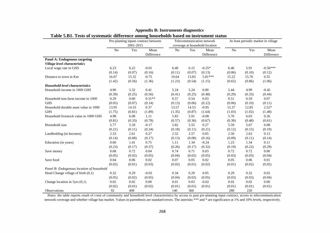
268

Appendix B: Instruments diagnostics

Table 5.B1. Tests of systematic difference among households based on instrument status Pre-planting inputs contract between

2001-2015

Telecommunication network

coverage at household location

At least periodic market in village

No Yes Mean

Difference

No Yes Mean

Difference

No Yes Mean

Difference

Panel A: Endogenous targeting

Village level characteristics

Local wage rate in GHS 6.23

(0.14)

6.22

(0.07)

-0.01

(0.16)

6.40

(0.11)

6.15

(0.07)

-0.25*

(0.13)

6.46

(0.06)

5.91

(0.10)

-0.56***

(0.12)

Distance to town in Km 16.07

(1.42)

15.32

(0.56)

-0.75

(1.36)

19.64

(1.23)

13.83

(0.54)

5.81***

(1.15)

15.22

(0.65)

15.76

(0.86)

0.55

(1.06)

Household level characteristics

Household income in 1000 GHS 4.90

(0.39)

5.32

(0.25)

0.41

(0.56)

5.24

(0.41)

5.24

(0.25)

0.00

(0.48)

5.44

(0.29)

4.99

(0.33)

-0.45

(0.44)

Household non-farm income in 1000

GHS

0.29

(0.05)

0.60

(0.07)

0.31**

(0.14)

0.57

(0.13)

0.54

(0.06)

0.03

(0.12)

0.51

(0.06)

0.59

(0.10)

0.07

(0.11)

Household durable asset value in 1000

GHS

13.95

(1.75)

14.33

(0.81)

0.37

(1.89)

13.57

(1.35)

14.53

(0.87)

-0.95

(1.64)

15.37

(1.03)

12.85

(1.02)

2.52*

(1.48)

Household livestock value in 1000 GHS 4.98

(0.81)

6.08

(0.33)

1.11

(0.78)

5.83

(0.57)

5.91

(0.36)

-0.08

(0.67)

5.76

(0.39)

6.03

(0.48)

0.26

(0.61)

Household size 5.77

(0.21)

5.59

(0.11)

-0.17

(0.24)

5.82

(0.18)

5.55

(0.11)

0.27

(0.21)

5.59

(0.12)

5.67

(0.15)

0.08

(0.19)

Landholding (in hectares) 2.33

(0.14)

2.61

(0.08)

0.27

(0.17)

2.52

(0.13)

2.57

(0.08)

0.05

(0.16)

2.50

(0.09)

2.63

(0.11)

0.13

(0.14)

Education (in years) 0.66

(0.23)

1.41

(0.17)

0.75

(0.37)

1.11

(0.26)

1.34

(0.17)

-0.24

(0.32)

1.23

(0.19)

1.34

(0.22)

0.11

(0.29)

Save money 0.68

(0.05)

0.72

(0.02)

0.04

(0.05)

0.74

(0.04)

0.71

(0.02)

0.03

(0.05)

0.72

(0.03)

0.72

(0.03)

0.00

(0.04)

Save food 0.04

(0.02)

0.06

(0.01)

0.02

(0.03)

0.07

(0.02)

0.05

(0.01)

0.02

(0.02)

0.05

(0.01)

0.06

(0.02)

0.01

(0.02)

Panel B: Endogenous location of household

Head Change village of birth (0,1) 0.32

(0.05)

0.29

(0.02)

-0.03

(0.05)

0.34

(0.04)

0.29

(0.02)

0.05

(0.05)

0.29

(0.03)

0.32

(0.03)

0.02

(0.04)

Change location in 5yrs (0,1) 0.02

(0.02)

0.02

(0.01)

0.00

(0.02)

0.01

(0.01)

0.03

(0.01)

-0.02

(0.01)

0.02

(0.01)

0.02

(0.01)

0.00

(0.01)

Observations 92 408 140 360 280 220

Notes: the table reports result of t-test of community and household level characteristics by access to past pre-planting input contract, access to telecommunication

network coverage and whether village has market. Values in parenthesis are standard errors. The asterisks *** and * are significance at 1% and 10% levels, respectively.

269

Table 5.B2. First-stage regressions of the IV-GMM and potential endogeneity of

household income

Notes: the table presents firsts-stage estimations of the IV-GMM regression of household HCCI on the set of controls

and the instruments as in our first-stage market orientation model reported in table 5.3, and the first-stage household income

regression. S.E. denotes robust standard errors, AIC denotes Akaike information criterion and BIC represents the Bayesian

information criterion. The asterisks ***, ** and * are significance at 1%, 5% and 10% levels, respectively.

First-stage IV-GMM

(1)

First-stage Household

Income

(2)

Coefficient S.E. Coefficient S.E.

HHAge 5.3E-5 0.001 -3.1E-5 1.2E-4

HHSex -0.029* 0.016 0.010** 0.005

HHEducation 0.001 0.002 0.002** 0.001

HHSize -0.002 0.003 -0.002** 0.001

HHLandholding 0.004 0.005 0.002* 0.001

CB_Assoiations 0.005 0.006

Log HHIncome 0.125*** 0.020

Log HHDAsset 0.009** 0.003 0.007** 0.002

Log HHLivestock 0.015* 0.009 0.003** 0.001

Town distance -1.6E-4 0.001 5.0E-4* 3.0E-4

Local wage -2.9E-4 0.007 0.001 0.001

Gushegu 0.030 0.027 -0.019** 0.009

Karaga 0.029 0.025 -0.024*** 0.007

Savelugu-Nanton 0.039 0.026 -0.055*** 0.008

HHIncomeResid -0.093** 0.038

PreProductContract -0.083*** 0.020

HHMobileNetwork 0.069*** 0.016

CMarket 0.041** 0.016 -0.009* 0.004

HHExtension 0.020*** 0.006

Tractor -1.2E-4* 6.9E-5

SeedUse 6.3E-5** 2.7E-5

SeedPrice -3.4E-5 5.8E-5

Fertilizer 4.9E-5* 2.8E-5

Pesticides -2.4E-4 3.0E-4

Weedicides 1.1E-4 1.0E-4

Labor 6.1E-5 4.1E-5

Soil fertility 0.089*** 0.009

Farm_shock -0.033*** 0.007

NonEmployTravel -0.018*** 0.005

Constant -0.961*** 0.170 1.946*** 0.031

R2 0.849

Weak identification tests:

Cragg-Donald F-statistic 14.49

Kleibergen-Paap rk Wald F statistic 45.17

P-value of Angrist-Pischke F-test 0.000

Over identification test:

Hansen J 3.452

p-value 0.178

Log likelihood -287.46

AIC 1.25

BIC -2859.49

Number of observations 500 500

270

Table 5.B3. Household crop commercialization and food and nutrients rich food consumption Part A: IV-GMM Part B: OLS

Food

(1)

Vitamin A

(2)

Protein

(3)

Hem iron

(4)

Food

(5)

Vitamin A

(6)

Protein

(7)

Hem iron

(8)

Coef. S.E. Coef. S.E. Coef. S.E. Coef. S.E. Coef. S.E. Coef. S.E. Coef. S.E. Coef. S.E.

HCCI 14.20** 5.37 6.05** 2.58 4.84** 2.34 3.02* 1.53 12.93*** 1.71 6.60*** 0.89 8.01*** 0.65 5.29*** 0.43

HHAge -0.01 0.02 -0.01 0.01 0.01 0.01 0.01 0.01 -0.02 0.02 -0.01 0.01 0.01 0.01 0.01 0.01

HHSex 0.39 0.61 0.28 0.27 0.11 0.26 0.07 0.16 0.37 0.64 0.28 0.27 0.20 0.25 0.14 0.13

HHEducation 0.28*** 0.09 0.11*** 0.03 0.06* 0.03 0.04* 0.02 0.30*** 0.08 0.12*** 0.04 0.06 0.04 0.04* 0.02

HHSize 0.04 0.13 0.08 0.06 0.01 0.05 0.01 0.03 0.05 0.15 0.08 0.07 0.01 0.06 0.01 0.03

HHLandholding 0.01 0.18 0.07 0.09 0.10 0.08 0.06 0.05 0.02 0.20 0.05 0.09 0.08 0.07 0.05 0.05

CB_Assoiations 0.30 0.24 0.01 0.10 -0.08 0.09 -0.09 0.05 0.30 0.23 0.01 0.12 -0.09 0.08 -0.10* 0.05

Log HHIncome 2.33** 1.03 0.67 0.45 1.05** 0.40 0.75*** 0.26 2.38** 0.84 0.53 0.39 0.62** 0.28 0.43** 0.16

Log HHLivestock 0.28* 0.14 0.26*** 0.07 0.22*** 0.05 0.14*** 0.03 0.32** 0.15 0.26*** 0.06 0.20*** 0.05 0.12*** 0.03

Log HHDAsset 1.60*** 0.32 0.73*** 0.14 0.68*** 0.13 0.45*** 0.08 1.64*** 0.36 0.72*** 0.16 0.62*** 0.12 0.42*** 0.07

Town distance -0.01 0.03 -0.03** 0.01 -0.02* 0.01 -0.01* 0.01 -0.01 0.03 -0.03** 0.01 -0.02* 0.01 -0.01* 0.01

Local wage 0.14 0.26 0.06 0.12 0.08 0.11 0.03 0.07 0.14 0.29 0.06 0.11 0.08 0.11 0.03 0.06

Gushegu -6.79*** 1.03 -2.47*** 0.46 -0.41 0.41 -0.29 0.25 -6.29*** 1.04 -2.33*** 0.46 -0.47 0.35 -0.33 0.23

Karaga -3.69*** 0.98 -0.28 0.40 1.43*** 0.39 0.88*** 0.25 -3.29*** 1.01 -0.20 0.36 1.35*** 0.38 0.82*** 0.22

Savelugu-Nanton -4.54*** 1.03 -2.61*** 0.48 -0.47 0.44 -0.27 0.28 -4.36*** 1.04 -2.63*** 0.50 -0.60* 0.34 -0.38 0.29

PreProductContract 0.51 0.72 0.30 0.31 0.30 0.38 0.17 0.20

HHMobileNetwork 0.96 0.71 0.27 0.33 -0.11 0.26 -0.07 0.18

CMarket -0.50 0.52 -0.17 0.24 -0.22 0.26 -0.21 0.13

HHIncomeResid -0.76 1.17 0.01 0.52 -0.26 0.49 -0.28 0.32 -0.68 1.33 0.14 0.47 0.07 0.39 -0.02 0.26

Constant -5.56 7.99 -3.34 3.35 -13.40*** 3.02 -9.33*** 1.95 -6.82 7.34 -2.54 2.70 -10.16*** 1.94 -6.89*** 1.27

R2 0.48 0.50 0.47 0.47 0.48 0.50 0.50 0.50

Wald X2 606.76 759.58 1788.07 1136.52

p-value 0.00 0.00 0.00 0.00

F-statistic 25.50 27.64 30.55 31.54

p-value 0.00 0.00 0.00 0.00

Number of

observations

500 500 500 500 500 500 500 500

Notes: the table shows the second-stage of the two-stage least squared generalized methods of moments (IV-GMM) and the ordinary least square (OLS) estimations of the impact of household crop

commercialization on food and nutrient rich foods consumption. The coef. and S.E. are coefficient and standard errors, respectively. The asterisks ***, ** and * are significance at 1%, 5% and 10% levels, respectively.

271

Appendix C: Second-stage estimates of the model

Table 5.C1. Second stage estimates of determinants of food and vitamin A rich food consumption Food Vitamin A

Subsistence- oriented Surplus-oriented Commercial-oriented Subsistence- oriented Surplus-oriented Commercial-oriented

Coefficient S.E. Coefficient S.E. Coefficient S.E. Coefficient S.E. Coefficient S.E. Coefficient S.E.

HHAge -0.041 0.042 -0.043 0.029 0.022 0.048 0.001 0.021 -0.018 0.014 -0.011 0.014

HHSex 0.631 1.174 -0.101 0.888 0.087 1.255 0.112 0.593 0.614 0.416 -0.194 0.345

HHEducation 0.451* 0.229 0.391*** 0.116 0.171 0.164 0.196 0.124 0.221*** 0.047 0.028 0.040

HHSize -0.221 0.239 0.442* 0.235 0.107 0.229 0.023 0.120 0.210* 0.113 0.008 0.075

HHLandholding 0.584 0.409 -0.011 0.216 -0.618 0.409 0.299 0.223 0.001 0.118 -0.102 0.112

CB_Assoiations 0.238 0.432 0.823* 0.411 0.023 0.420 0.050 0.208 0.213 0.147 -0.143 0.131

Log HHIncome -1.400 2.003 4.556*** 1.358 1.811 2.134 -1.289 0.944 1.968*** 0.524 0.599 0.545

Log HHLivestock 0.401* 0.234 0.210 0.217 0.023 0.434 0.350*** 0.115 0.186* 0.110 0.105 0.130

Log HHDAsset 2.489*** 0.791 0.930* 0.468 0.982 0.613 1.102*** 0.311 0.517** 0.233 0.546*** 0.183

Town distance 0.040 0.071 -0.091* 0.048 0.118 0.082 2.505** 1.123 -0.081 0.586 -0.649 0.494

Local wage 0.130 0.592 0.341 0.382 0.091 0.471 -0.044 0.031 -0.032 0.021 0.017 0.020

Gushegu -7.979*** 2.090 -6.090*** 1.484 -3.124* 1.785 -3.490*** 0.930 -1.512** 0.624 -1.435** 0.657

Karaga -4.544** 2.016 -3.335** 1.458 -2.660 1.935 -0.978 0.924 0.619 0.614 -0.521 0.542

Savelugu-Nanton -6.899*** 2.061 -2.798* 1.649 -1.961 1.933 -4.570*** 0.984 -1.363* 0.759 -1.294** 0.579

HHIncomeResid 3.466 2.390 -0.375 1.462 -1.903 1.661 0.104 0.283 0.235 0.184 -0.167 0.151

Constant 19.330 18.397 -14.045 11.852 14.832 26.894 9.925 8.072 -11.621** 4.919 6.202 6.318

𝜌𝜖𝜇 -0.304 0.316 -0.082 0.212 -0.292 0.676 -0.225 0.229 0.101 0.235 0.192 0.470

LR 𝑋2(3) (𝜌𝜖𝜇 = 0) 1.29 1.01

Prob 𝑋2 0.732 0.798


LR X2(18) 143.42 142.73

Prob X2 0.000 0.000

Number of

observations

180

206

114

180

206

114

Notes: the table shows the second-stage ordered Heckman estimations of equation (3) for food consumption score and vitamin A rich foods consumption frequencies. 𝜌𝜖𝜇 denotes the correlation between

the unobservables in the first-stage ordered probit selection equation (2) and the second-stage outcome equations (3). S.E. denotes robust standard errors. The asterisks ***, ** and * are significance at 1%,

5% and 10% levels, respectively.

272

Table 5.C2. Second stage estimates of determinants of protein and iron rich food consumption Protein Hem iron

Subsistence- oriented Surplus-oriented Commercial-oriented Subsistence- oriented Surplus-oriented Commercial-oriented

Coefficient S.E. Coefficient S.E. Coefficient S.E. Coefficient S.E. Coefficient S.E. Coefficient S.E.

HHAge 0.011 0.017 0.014 0.014 -0.002 0.012 0.006 0.010 0.005 0.009 -0.002 0.007

HHSex -0.195 0.512 0.599 0.467 -0.257 0.294 -0.073 0.330 0.432 0.310 -0.221 0.176

HHEducation 0.170** 0.076 0.113 0.072 -0.024 0.029 0.117** 0.052 0.068 0.046 -0.013 0.018

HHSize -0.049 0.072 0.036 0.110 -0.016 0.067 -0.030 0.045 0.053 0.071 -0.014 0.041

HHLandholding 0.351** 0.171 -0.016 0.135 -0.057 0.137 0.214* 0.110 -0.009 0.087 -0.046 0.083

CB_Assoiations -0.087 0.164 -0.100 0.156 0.105 0.123 -0.097 0.107 -0.114 0.105 0.041 0.072

Log HHIncome -0.281 0.696 1.904*** 0.584 0.930*** 0.307 -0.248 0.443 1.330*** 0.387 0.597*** 0.187

Log HHLivestock 0.222*** 0.074 0.257** 0.100 0.065 0.100 0.151*** 0.048 0.151** 0.065 0.035 0.061

Log HHDAsset 1.037*** 0.232 0.627** 0.244 0.301* 0.163 0.694*** 0.146 0.411** 0.161 0.201** 0.094

Town distance -0.038 0.027 -0.023 0.026 0.006 0.014 -0.026 0.017 -0.015 0.016 0.002 0.008

Local wage 0.160 0.204 0.107 0.185 0.053 0.134 0.071 0.132 0.088 0.121 -0.024 0.083

Gushegu -1.350* 0.748 0.472 0.652 0.156 0.489 -0.959** 0.465 0.369 0.421 0.004 0.303

Karaga -0.043 0.855 2.310*** 0.663 1.491*** 0.469 -0.042 0.566 1.552*** 0.435 0.723** 0.296

Savelugu-Nanton -2.207** 0.779 -0.046 0.756 1.018** 0.491 -1.484*** 0.493 0.109 0.487 0.475 0.301

HHIncomeResid 0.989 0.817 0.157 0.743 -0.787** 0.337 0.642 0.516 -0.036 0.488 -0.506** 0.216

Constant -4.447 6.017 -19.547*** 5.592 -3.222 2.608 -2.434 3.784 -13.744*** 3.694 -1.488 1.601

𝜌𝜖𝜇 -0.006 0.218 0.245 0.239 0.307* 0.158 0.033 0.212 0.258 0.239 0.269* 0.153

LR 𝑋2(3) (𝜌𝜖𝜇 = 0) 2.05 2.03

Prob 𝑋2 0.562 0.566


LR X2(18) 142.76 142.65

Prob X2 0.000 0.000

Number of observations 180 206 114 180 206 114

Notes: the table shows the second-stage ordered Heckman estimations of equation (3) for protein and hem iron rich foods consumption frequencies. 𝜌𝜖𝜇 denotes the correlation between the unobservables

in the first-stage ordered pobit selection equation (2) and the second-stage outcome equations (3). S.E. denotes standard errors. The asterisks ***, ** and * are significance at 1%, 5% and 10% levels,

respectively

273

Chapter Six

Summary, conclusions and policy implications

The low uptake of innovations and improved technologies, and the recent increase in food

insecurity and malnutrition in sub-Saharan Africa, in the midst of increased availability of

improved agricultural technologies in the continent motivated the need to investigate the role

of social networks in technology adoption, and the implications of improved technology

adoption and crop commercialization on household welfare. This study contributes to the

existing literature by examining the impact of social networks, technology adoption and

smallholder market-orientation on household welfare in developing countries. First, the study

examined the impacts of smallholders’ peer adoption of two improved and competing soybean

varieties on their adoption decisions of these varieties, showing the instances under which a

given improved variety is likely to become dominant in terms of adoption in a farmer’s social

networks and when a farmer is likely to defer adoption of any of the improved varieties.

Second, the study investigated the role of learning about both production techniques and

expected benefits of improved soybean varieties from peers on diffusion of these varieties, and

the influence of social network structures, specifically transitivity and modularity on diffusion

of these improved soybean varieties. Following these, the study then examined the effects of

own and peer adoption of the improved variety on household soybean yield, food consumption,

as well as the consumption of vitamin A, and protein rich foods. Finally, the study explored the

impacts of smallholder market-orientation on household food consumption, and on the

consumption of nutrient (such as vitamin A, protein and hem iron) rich foods.

6.1 Summary of empirical methods

Given the endogeneity and identifications concerns of social network effects, and the threats of

sample selection and missing variable biases, this study utilized a number of empirical methods

in the analysis depending the nature of the problem and the issue of being investigated. In

274

particular, the study used the spatial autoregressive multinomial approach, Bayesian estimation

approach, Markov Chain Monte Carlo (MCMC), random-effects complementary log-log

hazard model, graphical reconstruction of social networks, marginal treatment effects, and

ordered-Probit selection model.

Chapter two employed a spatial autoregressive multinomial probit model (SAR Probit) to

examine how neighbors’ varietal and cross varietal adoption of improved varieties, affect a

farmer’s adoption decision in the social network. Due to challenges of multidimensional

integrals, correlations in the error terms and the complexity of the spatial dependence in the

estimation of spatial models in a multinomial setting, the study used the Markov Chain Monte

Carlo (MCMC) sampling, which is a Bayesian estimation framework, to estimate the SAR

Probit model since this allows for the higher dimensional integrals to be re-specified into

sequence of draws. This spatial autoregressive model directly accounts for contextual network

effects in order to identify the endogenous network effect. Finally, network fixed-effects and

the control function approach were used to account for correlated network effects due to similar

institutional and environment conditions faced by farmers in the same network and unobserved

determinants of link formation between individuals, respectively.

In chapter three, a Random-effects complementary log-log hazard function was employed to

estimate the conditional probability of adoption in a small-time interval for a farmer who has

not adopted the technology up to this time. Given that adoption of the improved varieties was

observed on annual basis, the duration to adoption was modelled in a discrete-time method to

account for the banded nature of the survival time. In order to identify endogenous from

exogenous, the model controlled for contextual peer characteristics. Given that the network

structure, modularity, was measured at the network level, which makes the use of network

dummies to control for network fixed-effects challenging due to the incidental parameter

problem, the study accounted for correlated effects in a network by controlling for time fixed-

275

effects, use of residuals of link formation model as control functions and clustering standard

errors at the village (i.e., network) level. To investigate the extent of bias due to the use of

sampled networks, instead of complete networks, in the construction of the network structures,

the study used the graphical reconstruction approach to simulate complete networks, and then

used these to calculate the network structures for estimation of the hazard model as robustness.

Chapter four used spatial econometric techniques to generate instruments, and then use the

instruments, in addition to controlling for network fixed-effects and for potential endogeneity

of network link formation with the control function approach to identify peer adoption effects

on own adoption and outcomes. The marginal treatment effects (MTE) approach was used to

estimate the treatment effects heterogeneities across households. The MTE approach allows an

identification of a substantial part of the range of individual treatment effects, and as a result

characterize the extent and pattern of treatment effects heterogeneity from adoption due to

observed and unobserved characteristics. It also shows the pattern of selectivity and allows for

computation of average treatment effects (ATE), average treatment effects on the treated (TT)

and the average treatment on the untreated (TUT). The Policy Relevant Treatment Effect

(PRTE) was used to estimate the effects of policies that either increase affordability of soybean

seeds through input subsidy, or increase access to soybean seeds by reducing distance to the

nearest soybean seed source.

Chapter five provides a review of food security and nutrition strategies in sub-Saharan Africa

countries, and an empirical analysis of smallholder market participation as a food security and

nutrition strategy. Smallholders were classified based on their market-orientation into

subsistence-oriented, surplus-oriented and commercial-oriented. To the extent that the

treatment of farm households in this study is non-random implies that market-orientation status

of farmers could differ systematically due to self-selection of households into categories. In

order to account for the threats of selection bias and omitted variable problem due to observed

276

and unobserved factors in the light of the ordered nature of the selection variable, the study

employed the ordered-Probit selection model. This is a parametric model that utilizes full

information maximum likelihood procedure to jointly estimate a first-stage ordered-Probit of

smallholder market-orientation, and a second-stage outcome models for the three regimes of

market-orientation. The process accounts for selection bias and omitted variable problem by

inserting calculated inverse Mills ratios from the first-stage ordered choice model into the

second-stage food and nutrients consumption model. Finally, the approach allows for the

calculation of average treatment effects (ATE) for the entire population and for those at one of

the transition stages, the average treatment effects on the treated (ATE) and the average

treatment effects on the untreated (ATU).

6.2 Summary of results

The results of chapter two show that a farmer’s likelihood of adopting an improved variety is

lower than the proportion of adopting neighbors of that variety when the proportion is below a

threshold. However, the likelihood of adoption becomes higher than the proportion of adopting

neighbors when the share of neighbors adopting that variety is above this threshold. The results

also show that a farmer’s adoption decision of a given improved variety is positively influenced

by the adopting neighbors of this variety, but negatively by the adopting neighbors of the

competing improved variety. Furthermore, when the relative share of adopting neighbors are

equal, farmers are more likely to wait and not to switch from the old variety. Similarly, when

the proportion of adopters of both improved varieties in a farmer’s neighborhood are less than

25% or greater than 25%, then the farmer is more likely to defer adoption of improved varieties.

In chapter three, the results reveal a positive and significant effect of past share of adopting

peers on the conditional probability of adoption across all specifications. Similarly, there is a

positive and significant effect of peer experience in the cultivation of the improved varieties on

the speed of adoption. These suggest that both learning about benefits and production process

277

are important in accelerating adoption, although the effects of experience are higher when

sufficient peers adopt the improved varieties. The interaction effects between the past adopting

peers and peer experience with the improved varieties appear to be complementary on the

conditional probability of adoption up to an average peer experience of 5 years, after which it

begins to exhibit decreasing probability of adoption with increasing peer experience. The results

of the network structures show the role of transitivity in the learning and diffusion processes to

be stronger, compared to centrality. However, modularity tends to slow down the diffusion

process, and limits the significance of both transitivity and centrality.

The results of chapter four show that own adoption tend to significantly increase yield, food

and nutrients consumption of the household, albeit the effects of adoption on nutrients rich food

consumption are stronger and higher in magnitudes than the effect on food consumption. The

results reveal positive selection on gains due to unobserved characteristics, mainly driven by

worse outcomes, of households with less resistance to adopt, in the non-adoption state.

However, adoption tends to make the potential outcomes of households quite homogenous,

irrespective of their level of resistance to adoption. The results show that peer adoption tends

to strongly affect own yield, only when the household is also adopting, which is in line with the

notion of social learning or contagion effects. In terms of food and nutrients consumption, the

results show that peer adoption tends to increase own food and nutrients consumption when not

adopting, and attenuating peer adoption effects when adopting, which are suggestive of stronger

private transfers received from peers in the form of cash or food safety nets when the household

is not adopting.

The impact of commercialization on food and nutrients rich food consumption is generally

shown to be positive across transitions of smallholder market-orientation in Chapter five, which

is mainly due to increased farm and household income. Specifically, transitioning from

subsistence to surplus orientation increases household consumption across all food and nutrient

278

items. Also, transitioning from surplus to commercial orientation substantially increases

household food and nutrients consumption. However, the magnitudes of the treatment effects

for protein and iron rich food consumption are higher compared to that of food and vitamin A

food consumption. The results also show substantial heterogeneities in gains (i.e., sorting gains

and losses), where positive selection on gains is shown, in transitioning between subsistence

and surplus orientations, while reverse selection on gains is revealed in transitioning between

surplus and commercial orientations. These suggest that less (more) endowed and constrained

households who are less (more) likely to transition from surplus (subsistence) to commercial

(surplus) orientation tend to gain more in food and nutrients consumption if they go from

surplus (subsistence) to commercial (surplus)-oriented.

6.3 Policy implications

The findings of this study show that social networks are important in promoting technology

adoption, diffusion, and household welfare. These have some implications for policy. The

findings of the differential adoption rates of competing technologies and the ultimate

dominance of varieties in networks suggest the need to do a stepwise introduction of improved

varieties before a full-scale promotion in the villages. It will be rewarding to first expose some

farmers in the network (i.e., village) to the improved varieties, observe the extent of adoption

and then following-up with a wide-scale introduction and promotion of the variety that leads in

adoption in the network. This will reduce the prohibitive costs associated with promotion of

several varieties at the same time. The finding that information about benefits and production

process matter in the diffusion process, and that farmers are likely not to adopt the improved

varieties when the proportion of adopting neighbors of the improved varieties are equal suggest

the need for policymakers to focus promotion efforts on demonstrating the relative benefits and

production process of improved varieties introduced to farmers, since these would motivate

farmers to adopt.

279

The finding on the role of transitivity in promoting adoption and that of modularity in restricting

diffusion, and the influence of the other network characteristics suggest that the common

extension strategy of targeting initial and influential adopters in a network for disseminating

information may not be appropriate in enabling diffusion at the network level. Given that

networks can be important means of increasing yield, and promoting welfare of vulnerable

households, interventions, such as self-help groups and/or farmer field-days, aimed at

promoting interactions among farm households, and enhancing exchange can increase the

effectiveness of social networks in these respects. Also, training workshops, where people are

specifically invited from different segments of the village at the early stages of adoption, can

promote bridges between network components and diffusion. The policy simulation suggests

that interventions to minimize production and structural constraints to adoption could be an

important strategy in mitigating the cost associated with technology adoption. Hence,

government and development partners can consider increasing access through availability of

the improved seeds at the local levels, such as empowering village level shops or community-

based groups to engage in input marketing.

Finally, the findings show substantial heterogeneity in consumption gains across market-

orientations and suggest the need for transition-sensitive policies in promoting smallholder food

security and nutrition through crop commercialization. Thus, promoting food security and

nutrition among subsistence-oriented households need to consider productivity enhancing

measures such as cash crop programmes that support farmers with inputs to facilitate spill-over

benefits between food and cash crop cultivation, and promotion of policies to increase their

access to improved inputs and innovations. Also, the promotion of higher smallholder

commercialization will require in addition to output augmenting measures the mitigation of

some of the market barriers and failures (such as, markets availability, physical access and

information) that limit poor smallholders from engaging in sales for profit. Interventions such

280

as promotion of market information platforms, farmer cooperatives and collective actions as

well as contract buying, which provides ready markets for farmers, will be more rewarding.

281

Appendices

Appendix 1: Household survey questionnaire

Social Networks, Technology Adoption and Agriculture Commercialization on Smallholder Welfare in the Northern Region of Ghana

Introduction Good day Sir/Madam and thank you for talking to me. We are conducting a survey of smallholder farmers to examine the impacts of farmer individual social and

economic networks, adoption of technologies and agricultural commercialization on their welfare. The specific purposes of this survey are to assess the impacts of

farmers’ perceptions about technology features and social networks on technology adoption; roles of social networks and technology adoption on household

agriculture commercialization processes and to examine the impacts of agriculture commercialization on household welfare. The information gathered will provide

significant input into the write-up of a PhD thesis in Agriculture and Food Economics at the University of Kiel, Germany. The interview will take about 1 hour 30

minutes and your participation is entirely by choice. Your name, identity and individual responses will be kept confidential.

Do you wish to participate in this survey? 0 =No 1 =Yes

Survey identification Questionnaire number: ___________ Name of enumerator: _____________________________ Enumerator’s ID: ____________

Date of interview: |_____|_____|_______| Start time (24hr Clock): |___:____| End time (24hr Clock): |___:____|

Location 1. District name: ____________________________________________ 2. District code: __________________________________

3. Name of community: ______________________________________ 4. Community ID: ________________________________

5. Head of Household (name): _________________________________ 6. Household ID: _________________________________

Note on soybean varieties: Afayak: (a bit yellowish compared to jenguma & matures in 85 to 90 days) Jenguma: (Short, whitish & matures in 90 days)

Suong-Pungun: (More yellowish at maturity and matures in 75 days) Salintuya: (tall, can be intercropped and matures in 120 days)

Put “99” for “Not Applicable” and “Don’t know”

Christian-Albrechts University of Kiel, Germany

Institute of Food Economics and Consumption Studies

282

Section A: General information

A1 A2 A3 A4

What is/are the main languages spoken at

home?

Codes A

What is the ethnicity of the household

head

Codes B

What is the family type of the

household?

Codes D

What type of marriage is the household head

practicing?

Codes E

Section B: Socio-demographic characteristics B1 B2 B3 B4 B5 B6 B7 B8 B9 B10 B11 B12 B13

What is the

farmer’s

relationship

with the

household

head?

Codes F

Sex of

farmer?

0=F

1=M

How

old is

the

farmer?

What is

farmer’s

educational

level? (In

completed

years of

schooling)

What is

farmer’s

religion?

Codes C

What is

farmer’s

marital

status?

Codes G

What is

farmer’s

main

occupation?

Codes H

Number

of years

farmer is

living in

the

village

Farmer’s

experience

(years) in

own

farming

activities

Farmer’s

experience

(years) in

cultivating

maize

Does the

household

head hold

any of the

following

authorities

at the

community

level?

Codes I

Does the

household

head’s spouse

hold any of the

following

authorities at

the community

level?

Codes I

Household

size (number

of persons

who share

cooking

arrangement/

under your

care)

Codes A

1. Likpakpaln (Konkomba) 10. Sissali

2. Chekosi 11. Gruni

3. Mampruli 12. Kasem

4. Dagbali (Dagbani) 13. Nankan

5. Nanunli 14. Kusaal

6. Gonja 15. Twi

7. Hausa 16. Ewe

8. Bimoba 17. Ga

9. Dagaare/Wali 18. Other (specify)

Codes B

1. Konkombas 10. Sissalas

2. Chekosi 11. Grunsi

3. Mamprusi 12. Kassenas

4. Dagombas 13. Nankan

5. Nanumbas 14. Kusasi

6. Gonjas 15. Akans

7. Hausas 16. Ewes

8. Bimobas 17. Gas

9. Dagaabas/Walas 18. Other (specify)

Codes C

0 No religion

1 Muslim

2 Christian

3 Traditional

4 Other (specify)

__________________

Codes E

1 Polygynous

2 Monogamous

3 Other (specify)

___________________

Codes G

0 Never married

1 Married

2 Consensual union

3 Separated

4 Divorced

5 Widowed

Codes I

0 None

1 Chief/community leader

2 Chief council member

3 Assembly/unit committee

member

4 Religious leader

5 Youth leader

6 Women leader

7 Political party leader

Codes D

1 Nuclear

2 Extended

3 Other (specify)

______________

Codes F

1 Head 6 Son/Daughter-in-law

2 Spouse 7 Other relative

3 Child 8 Adopted/Foster/Stepchild

4 Grandchild 9 House help

5 Parent/Parent-in-law 10 Non-relative

Codes H

1 Farming (crop and/or livestock)

2 Housekeeping

3 Casual labour on another farm

4 Non-farm business (shops, trade, etc)

283

Please complete the table below on the age composition and non-farm work of the household members

B14 B15 B16 B17 B18 B19

(less than 16 years) (16 - 30 years) (31 - 60 years) (above 60 years) Family non- farm workers

Male Female Male Female Male Female Male Female Male

Female

Please complete the table on the household and household head’s social issues

# Question I # Question II # Question III

B20 What is household head’s settlement status in the

community?

0 =Settler 1 =Native

B28 If no, how long has the household head been

in this community?

_______ (Years)

B36 Did any member of the household experience any court, police or

major theft incidence in last 5 years?

0 =No 1 =Yes

B21 Has the household head a royal lineage?

0 =No 1 =Yes B29 How many times has the household head

travelled outside the village in last 12

months? _______ (times)

B37 Did you or any member of the household undertake any lumpy

expenditure (such as construction of house and/or room) in last 5

years? 0 =No 1 =Yes

B22 Has any of the parents of the household head or spouse

any important position or representation in the traditional

political or authority system?

0 =No 1 =Yes

B30 Has the household change location in the

past….

5 years? 0 =No 1 =Yes

10 years? 0 =No 1 =Yes

B38 Did you experience any shock or loss in your farming activities in

last 5 years?

0 =No >>B41 1 =Yes

B23 Has any member of the household been away from the

community for more than 6 months in the last 12 months?

0 =No >>B26 1 =Yes

B31 Did you have a wedding ceremony in the

household in the past 2 years?

0 =No >>B33 1 =Yes

B39 If yes, which of the following did you experience?

1 =Weather shocks 2 =bush/wildfires

3 =Other (specify)______________________

B24 If yes, how many people?

_________

B32 If yes, how many times?

_______ (times) B40 If yes, how regular is the incidence of these shocks/losses?

1 =Very regular 2 =Regular 3 =Occasional

B25 For what reason did the person move away?

Codes A

B33 Did you have an outdooring ceremony in

the household in the past 2 years?

0 =No >>B35 1 =Yes

B41 Did you experience a sudden death of any household/family

member in last 5 years?

0 =No >>B43 1 =Yes

B26 Was the household head born in this community?

0 =No 1 =Yes B34 If yes, how many times?

_______ (times) B42 If yes, how many times did you experience this in the past 5 years?

_________ (times)

B27 Did the household head grow-up in this community?

0 =No 1 =Yes >>B29

B35 Did any household member fall sick in the

in last 12 months?

0 =No 1 =Yes

B43 Did you experience a long period of sickness of a household

member which led to his/her death in last 5 years?

0 =No 1 =Yes

Codes A

1. Job transfer 2. Seeking employment 3. Spouse’s employment

4. Marriage 5. Other family reason 6. Education

7. Political/religious 8. Ethnic/chieftaincy conflict 9. Other (specify)____

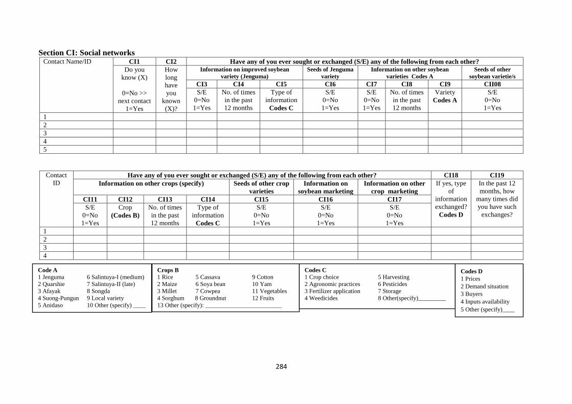
284

Section CI: Social networks Contact Name/ID CI1 CI2 Have any of you ever sought or exchanged (S/E) any of the following from each other?

Do you

know (X)

0=No >>

next contact

1=Yes

How

long

have

you

known

(X)?

Information on improved soybean

variety (Jenguma)

Seeds of Jenguma

variety

Information on other soybean

varieties Codes A

Seeds of other

soybean varietie/s

CI3 CI4 CI5 CI6 CI7 CI8 CI9 CII08

S/E

0=No

1=Yes

No. of times

in the past

12 months

Type of

information

Codes C

S/E

0=No

1=Yes

S/E

0=No

1=Yes

No. of times

in the past

12 months

Variety

Codes A

S/E

0=No

1=Yes

1

2

3

4

5

Contact

ID Have any of you ever sought or exchanged (S/E) any of the following from each other? CI18 CI19

Information on other crops (specify) Seeds of other crop

varieties

Information on

soybean marketing

Information on other

crop marketing

If yes, type

of

information

exchanged?

Codes D

In the past 12

months, how

many times did

you have such

exchanges?

CI11 CI12 CI13 CI14 CI15 CI16 CI17

S/E

0=No

1=Yes

Crop

(Codes B)

No. of times

in the past

12 months

Type of

information

Codes C

S/E

0=No

1=Yes

S/E

0=No

1=Yes

S/E

0=No

1=Yes

1

2

3

4

Crops B

1 Rice 5 Cassava 9 Cotton

2 Maize 6 Soya bean 10 Yam

3 Millet 7 Cowpea 11 Vegetables

4 Sorghum 8 Groundnut 12 Fruits

13 Other (specify): _________________________

Codes C

1 Crop choice 5 Harvesting

2 Agronomic practices 6 Pesticides

3 Fertilizer application 7 Storage

4 Weedicides 8 Other(specify)_________

Codes D

1 Prices

2 Demand situation

3 Buyers

4 Inputs availability

5 Other (specify)____

Code A

1 Jenguma 6 Salintuya-I (medium)

2 Quarshie 7 Salintuya-II (late)

3 Afayak 8 Songda

4 Suong-Pungun 9 Local variety

5 Anidaso 10 Other (specify) ____

285

Contact

ID

Have any of you ever sought or exchanged (S/E) any of the following from each other?

Labor for soybean activities Credit and/or gift transactions Land exchange/transaction

CI20 CI21 CI22 CI23 CI24 CI25 CI26 CI27 CI28 CI29

S/E

0=No

1=Yes

No. of times

in the past 12

months

No. of man-

days per

exchange

S/E

0=No

1=Yes

Nature of

exchange

Codes A

No. of times

in the past

12 months

Amount received

GHS______ and/or given

GHS______

S/E

0=No

1=Yes

Nature of the

exchange

Codes B

If rented, how

much was

paid? (GHS)

1

2

3

4

5

Section CII Social learning Please tell me about contact (X) soybean farming activities during the 2015/16 season

(NOTE: Ask if respondent at least know contact even if nothing was sought or no exchange between respondent and contact). Put “99” for “Don’t know”

Contact

ID

CII1 If yes, i.e. (X) cultivated soybean Did (X)

cultivate

soybean

0 =No >>

next contact

1=Yes

CII2 CII3 CII4 CII5 CII6 CII7 CII8 CII9 CII10 CII11

When did (X)

started

cultivating

soybean?

Codes C

Soybean

varieties

cultivated

Codes D

Where did

(X) get seeds

of soybean

varieties?

Codes E

Did (X) use

fertilizer on

soybean

plot?

0= No

1= Yes

Did (X) use

manure on

soybean plot?

0= No

1= Yes

Did (X) use

pesticides

on soybean

plot?

0= No

1.=Yes

Did (X) use

weedicides

on soybean

plot?

0=No

1=Yes

How

much

soybean

did (X)

harvest

(100kg)?

Did (X)

sell the

soybean

harvest?

0= No

1= Yes

If yes, at

what price

(GHS/kg)?

1

2

3

4

5

Codes A

1 Credit

2 Gift

3 Both

Codes B

1 Purchased 4 Allocated free of charge

2 Tenant rented (for cash or kind) 5 Begged

3 Sharecropped 6 Borrowed

6 Other (specify)______________________________________

Codes C

1 Not yet 3 At the same time as me

2 Before me 4 After me

Code D



3 Afayak 8 Songda



Codes E

0 Own storage 6 Local seed producers

1 Agro-input dealer 7 Extension officer (MoFA)

2 Purchased from market 8 NGO

3 Exchange (farmer) 9 Gift

4 Private aggregator 10 SARI/CSI

5 FBO (cooperative)

11 Other (specify) ___________

286

Contact

ID

CII12 CII14 CII15 CII16 CII17 CII18 CII19 CII20 CII21 CII22

I will now ask you information about contacts’ maize cultivation

Did X

cultivate

maize?

0=No

1=Yes

Was crop

of modern

variety?

0=No

1=Yes

Where did

(X) get seeds

of crop

varieties?

Codes A

Did (X) use

fertilizer on

crop plot?

0=No

1=Yes

Did (X) use

manure on crop

plot?

0=No

1=Yes

Did (X) use

pesticides on crop

plot?

0=No

1=Yes

Did (X) use

weedicides

on crop plot?

0=No

1=Yes

How much

maize did

(X) harvest

(100kg)?

Did (X) sell

the maize

harvest?

0=No

1=Yes

If yes, at

what price

(GHS/kg)?

1

2

3

4

5

I will like to ask you about the social and physical proximity issues between you and the matched contacts

Contact

ID

CII23 CII24 CII25 CII26 CII27 CII28 CII29 CII30

How is (X)

related to

you?

Codes B

Have same

family name

0=No

1=Yes

Do you and contact

families trace your origin

to same region?

0=No

1=Yes

Have you ever visited

the home of (X)?

0=No >> CII28

1=Yes

If yes, number

of visits per

month to (X)

home?

Where does

this person

live?

Codes C

Approximately how

far does this person

live from you (in

minutes of walking)?

Is (X)’s field/ plot

adjacent to yours?

0=No

1=Yes

1

2

3

4

5

Codes B

1 Parent 8 Friend

2 Child 9 Same family lineage;

3 Sibling 10 Neighbor;

4 Grandparent 11 Attend same church/ mosque

5 Grandchild 12 belong to same association

6 In-law 13 Professional/business colleague

7 Other relative 14 Other (specify)____________

Codes C

1 Next house/neighbor

2 Neighbor of my neighbor

3 Not neighbor of me

or of my neighbor

Codes A






5 FBO (cooperative)


287

Contact

ID

CII31 CII32 CII33 CII34 CII35 How frequent do you attend…

Do you pass by X's

field when going to

field?

0=No

1=Yes >> CII33

If no, have you ever

passed by the field of

(X)?

0=No

1=Yes

Do you perceive the soil

conditions of your farm(s)

as similar with (X)?

0=No

1=Yes

How many of

these contacts

know one

another?

Generally speaking,

would you say that

most people can be

trusted?

Codes A

CII36 CII37

…social events

(such as weddings,

funerals and

festivals)?

Codes E

…religious events

(such as visiting

mosque, church or

shrine)?

Codes E

1

2

3

4

5

Section CIII: Famers networks of family and friends/acquaintances I will like to ask you about your network of close relatives and friends your share farming information and resources with, in the community.

Network members CIII1 CIII2 CIII3 CII

I4

CII

I5

CII

I6

CII

I7

CII

I8

CII

I9

CII

I10

CII

I11

CII

I12

CII

I13

CIII14 CIII15

How many people do

you consider relevant

for exchanging

information about

agronomic issues

with?

How

many of

them

know each

other?

How many

of them

cultivate

soybean?

How many of them cultivate soybean variety?

(varieties codes B)

In general, how

many cultivators

of soybean do

you know in the

community?

How

many of

them

cultivate

maize?

1 2 3 4 5 6 7 8 9 10

Family

Friends/acquaintances

Family & Friends

Network members CIII17 CIII18 CIII19 CIII20 CIII21 CIII22 CIII23 CIII24 CIII25 CIII26

How many of them implement the following agronomic practices on the soybean

farm? (Practice codes C)

How many of them uses the following in threshing

soybean? (Threshing code D)

1 2 3 4 5 6 0 1 2 3

Family


Code B



3 Afayak 8 Songda



Codes D

0 Manual with sticks

1 Tractor

2 Thresher

3 Other (specify) _____

Codes A scale of 1 to 6

1 = Cannot be too careful

2

3

4

5

6 = Most can be trusted

Codes C

1 Recommended depth of planting

2 Row planting

3 Inoculant use

4 Crop rotation

5 No burn of crop residue

6 Other (specify) _____________

Codes E

1 Daily

2 Biweekly

3 Weekly

4 Fortnightly

5 Monthly

6 Yearly

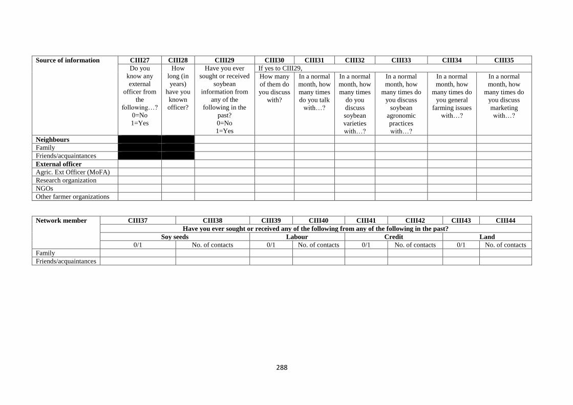
288

Source of information CIII27 CIII28 CIII29 CIII30 CIII31 CIII32 CIII33 CIII34 CIII35

Do you

know any

external

officer from

the

following…?

0=No

1=Yes

How

long (in

years)

have you

known

officer?

Have you ever

sought or received

soybean

information from

any of the

following in the

past?

0=No

1=Yes

If yes to CIII29,

How many

of them do

you discuss

with?

In a normal

month, how

many times

do you talk

with…?

In a normal

month, how

many times

do you

discuss

soybean

varieties

with…?

In a normal

month, how

many times do

you discuss

soybean

agronomic

practices

with…?

In a normal

month, how

many times do

you general

farming issues

with…?

In a normal

month, how

many times do

you discuss

marketing

with…?

Neighbours

Family


External officer

Agric. Ext Officer (MoFA)

Research organization

NGOs

Other farmer organizations

Network member CIII37 CIII38 CIII39 CIII40 CIII41 CIII42 CIII43 CIII44

Have you ever sought or received any of the following from any of the following in the past?

Soy seeds Labour Credit Land

0/1 No. of contacts 0/1 No. of contacts 0/1 No. of contacts 0/1 No. of contacts

Family


289

Agricultural Production

Section DI: Soybean varieties I will like to ask you about your farming activities now starting with issues of soybean cultivation

DI1 DI2 DI3 DI4 DI5 DI6 DI7 DI8 DI9 DI10 DI11 DI12 DI13 DI14

Which

soybean

varieties

do you

know?

Codes A

When

(year)

did you

first hear

about the

variety?

From

whom did

you first

hear about

it?, rank up

to three

Code F

Have

you ever

planted

the

variety?

0=No

>> next

variety

1=Yes

How

many

times

have

you

planted

it in the

past?

Years cultivated soybean and acreage Did you

cultivate

variety in the

2015/2016

cropping

season?

0=No

1=Yes

Did you

use

certified

seed?

0=No

1=Yes

Acres

under

certified

seeds

If No, to

DI11

why

not?

Codes

G, rank

3

Yr1 Acre Yr2 Acre Yr3 Acre Yr4 Acre Yr5 Acre

DI15 DI16 DI17 DI18 DI19 DI20 DI21 DI22 DI23 DI24

Hypothetical

question, what is

the minimum

addition to net

benefit that made

you adopt for sure?

(%)

If No to DI4,

hypothetical question,

please estimate the

average yield of

soybean varieties if you

had adopted last year?

(%)

Which of the following agronomic practices do you implement

and what proportion of the field is under this?

Codes B

If the farmer

rotated soybean

with another

crop, which

crop(s)?

Codes D

Before adopting

did you see the

variety in the

field?

0=No >> DI24

1=Yes

If yes,

where

was this

plot

located?

Codes C

Have you

ever

attended any

training on

soybean

cultivation?

Prac.

code

Acres Prac.

code

Acres Prac.

code

Acres Prac.

code

Acres

Codes F

1 Telephone/cell phone 7 Extension officer

2 Friends or relatives 8 Demonstrations/Field days

3 Neighbor 9 Agro-input dealer

4 Radio/TV 10 GOs/NGOs

5 Traders 11 FBO

6 Newspaper 12 ICT platform (e.g ESOKO)

13 Neighboring community 14 Other, specify _______

Codes G

1 Cannot get seed at all 8 Low yielding variety

2 Lack of cash to buy seed 9 Poor prices

3 Susceptible to field pests/diseases 10 No market

4 Susceptible to storage pests 11 Requires high skills

5 Poor taste 12 Seeds are expensive

6 Requires more rainfall 13 Cannot get credit

7 Don’t know how to use it 14 Need for other crops

15 Other (specify) ____

Codes B

1 Recommended depth of planting

2 Row planting

3 Inoculant use

4 Crop rotation

5 No burn of crop residue

6 Other (specify) _____________

Codes D

1 Rice 7 Cowpea

2 Maize 8 Groundnut

3 Millet 9 Cotton

4 Sorghum 10 Yam

5 Cassava 11 Vegetables

6 Soya bean 12 Fruits

13 Other (specify): _____________ Codes C

1 Next to my plot

2 On the way to my plot

3 Different locality area in the community

4 Outside the community

Code A

1 Jenguma 6 Salintuya-I (medium) 2 Quarshie 7 Salintuya-II (late)

3 Afayak 8 Songda

4 Suong-Pungun 9 Local variety 5 Anidaso 10 Other (specify) ____

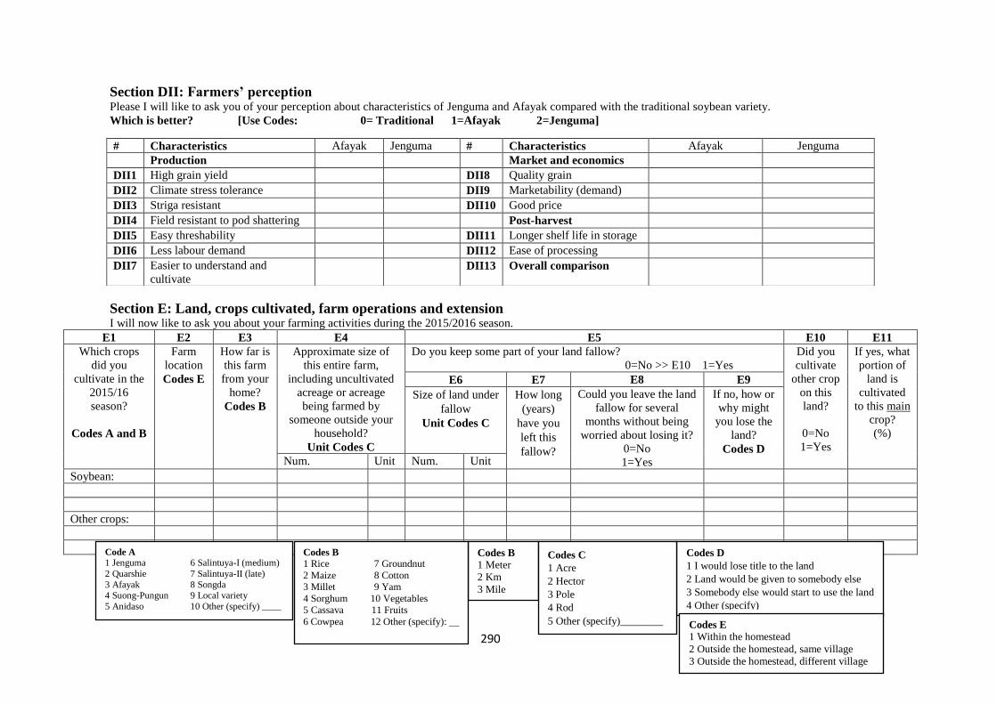
290

Section DII: Farmers’ perception Please I will like to ask you of your perception about characteristics of Jenguma and Afayak compared with the traditional soybean variety.

Which is better? [Use Codes: 0= Traditional 1=Afayak 2=Jenguma]

Section E: Land, crops cultivated, farm operations and extension I will now like to ask you about your farming activities during the 2015/2016 season.

E1 E2 E3 E4 E5 E10 E11

Which crops

did you

cultivate in the

2015/16

season?

Codes A and B

Farm

location

Codes E

How far is

this farm

from your

home?

Codes B

Approximate size of

this entire farm,

including uncultivated

acreage or acreage

being farmed by

someone outside your

household?

Unit Codes C

Do you keep some part of your land fallow?

0=No >> E10 1=Yes

Did you

cultivate

other crop

on this

land?

0=No

1=Yes

If yes, what

portion of

land is

cultivated

to this main

crop?

(%)

E6 E7 E8 E9

Size of land under

fallow

Unit Codes C

How long

(years)

have you

left this

fallow?

Could you leave the land

fallow for several

months without being

worried about losing it?

0=No

1=Yes

If no, how or

why might

you lose the

land?

Codes D Num. Unit Num. Unit

Soybean:

Other crops:

# Characteristics Afayak Jenguma # Characteristics Afayak Jenguma

Production Market and economics

DII1 High grain yield DII8 Quality grain

DII2 Climate stress tolerance DII9 Marketability (demand)

DII3 Striga resistant DII10 Good price

DII4 Field resistant to pod shattering Post-harvest

DII5 Easy threshability DII11 Longer shelf life in storage

DII6 Less labour demand DII12 Ease of processing

DII7 Easier to understand and

cultivate DII13 Overall comparison

Codes D

1 I would lose title to the land

2 Land would be given to somebody else

3 Somebody else would start to use the land

4 Other (specify)____________________

Codes B

1 Meter

2 Km

3 Mile

Codes C

1 Acre

2 Hector

3 Pole

4 Rod

5 Other (specify)________

Codes B

1 Rice 7 Groundnut

2 Maize 8 Cotton

3 Millet 9 Yam

4 Sorghum 10 Vegetables

5 Cassava 11 Fruits

6 Cowpea 12 Other (specify): __

Code A



3 Afayak 8 Songda 4 Suong-Pungun 9 Local variety


Codes E

1 Within the homestead

2 Outside the homestead, same village

3 Outside the homestead, different village

291

Crop

Codes

E12 E13 E14 E15 E16 E17 E18 E19 E20

How

fertile is

the soil

on this

farm?

Codes A

What is the

dominant

texture of soils

on this farm?

Codes B

How wet is this land compared

to other lands in your

community?

1…less wet

2….same

3…more wet

Slope of this

land

1 = Plain

2 =Gentle

3 =Hilly

Is the land

watered from

a source other

than rain?

0=No

1=Yes

If yes, what is

your primary

source of

watering?

Codes C

How did you

obtain this plot,

or gain the right

to farm this plot?

Codes D

If tenant, what

type of tenancy

arrangement do

you operate?

Codes E

If fixed

rent, what

is the

duration

of tenure?

Soy:

Other:

Crop

Codes

E21 E22 E23 E26 E27 E28 Did you use items on plot in the 2015/16 farming season?

If share

cropping, what

are the terms of

this rent? (i.e.

harvest shared)

How long have

you been

farming this

land?

(Yrs)

Do you practice

soil and water

conservation?

0=No

1=Yes

If yes, which

type(s) do you

practice?

Codes F

Average

size of land

under this

practice

(acres)

Does water

log on plot?

0=No

1=Yes

E29 E30 E31 E32

Tractor

0=No

1=Yes

Cost (give

money value

if in kind)

GHS

Drought

animal

0=No

1=Yes

Cost (give

money value

if in kind)

GHS

Soy:

Other:

Codes B

1 Sandy

2 Rocky/gravely

3 Clay-filled

4 Silty

5 Loamy

Codes A

1 Fertile

2 Moderately fertile

3 Less fertile

4 Infertile

Codes D

1 Owner 5 Allocated free of charge

2 Purchased 6 Begged

3 Inherited from deceased 7 Borrowed

family member 8 Other (specify)__________

4 Tenant Rented (cash/kind)

Codes F

1 Crop rotation

2 Land enriching cover crops

3 Legumes

4 Zero tillage

5 Minimal tillage

6 Composting

7 Agroforestry

8 Other (specify) ________

Codes E

1 Fixed rent

2 Sharecropped

Codes C

1 Well

2 Borehole

3 Pond/tank

4 Weir

5 River/stream

6 Other (specify)____

292

Section F: Inputs (seeds and materials) Please I will like to ask you about your inputs applications during the 2015/2016 cropping season

Crop

Codes

F1 F2 F3 F4 F5 F6 F7 F8 F9

What quantity of

crop seeds did

you use on farm?

(Kg)

What type or variety

of the seed did you

plant on farm?

Codes D

How did you

obtain the crop

seeds planted

on this farm?

Codes C

If any seeds were

purchased, what

quantity was

purchased?

(kg)

How much did

you pay for the

purchased seeds

used on farm?

(GHS)

Did you apply

fertilizer to

farm?

0=No

1=Yes

Which

type did

you

apply?

Codes E

What

quantity

was

applied?

(Kg)

What

was the

unit

price?

(GHS)

Soy:

Other:

Crops

Codes

F10 F14 F18 F19 F20

Did you apply pesticides? 0=No 1=Yes Did you apply weedicides? 0=No 1=Yes Did you

apply green

manure?

0=No

1=Yes

Did you apply

animal

manure?

0=No

1=Yes

Did you apply

composted

manure?

0=No

1=Yes

F11 F12 F13 F15 F16 F17

Which types

did you apply?

Codes F

Quantity

applied on farm

(litres/kg)

Total expenditure

on pesticides?

(GHS)

Which types

did you apply?

Codes F

Quantity

applied on

farm (litres)

Total expenditure

on weedicides?

(GHS)

Soy:

Other:

Codes F

0 None

1 Powder/Comdemn

2 Sarosate

3 Insecticide

4 Fungicide

5 Tintani

6 Other (specify)________

Codes E

1 Fertilizer: NPK (15-15-15)

2 Fertilizer: ammonium sulphate (SA)

3 Fertilizer 23-10-5 (Actyva)

4 Other compound fertilizer

5 Fertilizer: Other (specify)

6 Urea

7 Commercial organic fertilizer

(including Fertisoil, Cocopeat)

8 Phosphorus

9 Sulfan

10 Inoculant


Code A



3 Afayak 8 Songda



Codes C






5 FBO (cooperative)


Codes D 0 Local 1 Improved

Codes E

1 Rice 7 Groundnut

2 Maize 8 Cotton

3 Millet 9 Yam


5 Cassava 11 Fruits


293

Section G: Labour and credit Please I will like to ask about your labour use in farming during the 2015/2016 farming season

Crop

Codes

G1

Family

G2 G3

Hired Communal

Did you use hired labour? 0=No 1=Yes Did you use communal labour?

0=No 1=Yes

Males Females Children Males Females Males Females

Num. Days Num. Days Num. Days Num. Days Rate(GHS)/

Codes A Num. Days Rate(GHS)/

Codes A Num. Days Num. Days

Soybean:

Other crops:

Please I will now like to ask about your credit needs and access during the 2015/2016 cropping season

G4 During the cropping season, did you have liquidity constraints in financing production

(inputs)? 0=No 1=Yes G10 If no, how much were you given? ___________(GHS)

G5 If yes, did you apply/ask for any loan to finance production? 0=No >> H 1=Yes G11 Was collateral required in getting the loan facility? 0=No 1=Yes

G6 If yes, were you granted? 0=No 1=Yes G12 What did you use as collateral? Codes C

G7 Where did you access the credit? Codes D

G13 What was the interest you paid on the credit facility?

_________GHS

G8 How much did you apply for? ______(GHS)

G9 Were you given all you applied for? 0=No 1=Yes

Activity codes:

1 Clearing

2 Ploughing

3 Planting

4 Chemical application

5 Weeding

6 Harvesting

Codes A

1 Day

2 Acre

Codes D

1 Friends or relatives

2 Local moneylenders

3 Banks

4 NGOs (specify) ________

5 Nonbank financial institution (including MFI)

6 Private aggregator

7 Input dealer

8 Outgrower

9 FBO

10 Others (specify)_________

Codes C

1 Land 4 Building

2 Livestock 5 Household asset

3 Farm produce 6 Other (specify)

__

294

Section H: Harvest, storage and marketing Crop

Codes

H1 H2 H3 For soybean H9 H10

What quantity of

crop was harvested

from plot over the

2015/2016 farming

season?

Was any crop

lost during

harvesting on

field?

0=No

1=Yes

How much

of crop did

you lose in

total? (%)

How did

you store

crop?

Codes H

Do you treat

harvest under

storage with

chemicals?

0=No

1=Yes

H4 H5 H6 H7 H8

How was

it

harvested?

Codes E

How was

it

threshed?

Codes F

On what

was it

threshed?

Codes G

Was any crop

lost during

threshing?

0=No

1=Yes

How much

of crop did

you lose in

total? (%)

Soybean:

Other crops:

Codes F

0 Manual with sticks

1 Tractor

2 Thresher

3 Other (specify) _____

Codes E

0 Hand

1 Combine harvester

2 Other(specify) ___

Code A



3 Afayak 8 Songda



Codes G

0 On the floor

1 Fertilizer sacks

2 Tapolin

Codes B

1 Rice 7 Groundnut

2 Maize 8 Cotton

3 Millet 9 Yam


5 Cassava 11 Fruits


Codes H

0 Not stored 3 With private aggregator

1 Local silo at home/farm 4 Cooperative/FBO facility

2 In bags at home/farm 5 Communal storage unit

6 Other (specify)

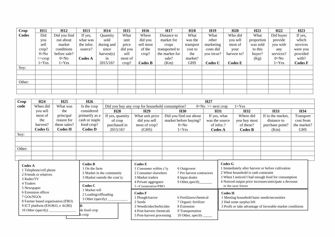
295

Crop

Codes

H11 H12 H13 H14 H15 H16 H17 H18 H19 H20 H21 H22 H23

Did

you

sell

crop?

0=No

>>crop

1=Yes

Did you find

out about

market

conditions

before sale?

0=No

1=Yes

If yes,

what was

the infor.

source?

Codes A

Quantity

sold

during and

since

harvest(s)

in

2015/16?

What

unit

price

did you

sell

most of

crop?

Where

did you

sell most

of the

crop?

Codes B

Distance to

market for

crops

transported to

the market for

sale?

(Km)

What

was the

transport

cost to

the

market?

GHS

What

other

marketing

costs did

you incur?

Codes C

Who did

you sell

most of

your

harvest to?

Codes E

What

proportion

was sold

to this

buyer?

(Kg)

Did buyer

provide

you with

any

services?

0=No

1=Yes

If yes,

which

services

were you

provided

with?

Codes F

Soy:

Other:

Crop

code

H24 H25 H26 H27

When did

you sell

most of

the

harvest?

Codes G

What was

the

principal

reason for

these sales?

Codes H

Is the crop

considered

primarily as a

cash or staple

food crop?

Codes D

Did you buy any crop for household consumption? 0=No >> next crop 1=Yes

H28 H29 H30 H31 H32 H33 H34

If yes, quantity

of crop

purchased in

2015/16?

What unit price

did you sell

most of crop?

(GHS)

Did you find out about

market before buying?

0=No

1=Yes

If yes, what

was the source

of infor.?

Codes A

Where did

you buy most

of these?

Codes B

If in the market,

distance to

purchase point?

(Km)

Transport

cost from

the market?

GHS

Soy:

Other:

Codes D

0 =Staple food crop

1 =Cash crop

Codes A

1 Telephone/cell phone

2 Friends or relatives

3 Radio/TV

4 Traders

5 Newspaper

6 Extension officer

7 GOs/NGOs

8 Farmer based organisation (FBO)

9 ICT platform (ESOKO, e AGRI)

10 Other (specify) _______________

Codes E

1 Consumer within c’ty 6 Outgrower

2 Consumer elsewhere 7 Pre harvest contractors

3 Market traders 8 Input dealer

4 Private aggregator 9 Other,specify_______

5 =Cooperative/FBO

Codes G

1 Immediately after harvest or before cultivation

2 When household is cash constraint

3 When I noticed I had enough food for consumption

4 Noticed output price increases/anticipate a decrease

in the near future

Codes H

1 Meeting household basic needs/necessities 2 Had some surplus left

3 Profit or take advantage of favorable market conditions

Codes B

1 On the farm

2 Market in the community

3 Market outside the com’ty

Codes C

1 Market toll

2 Loading/offloading


Codes F

1 Plough/tractor 6 Fertilizers/chemical

2 Seeds 7 Organic fertilizer

3 Weedicides/herbicides 8 Extension

4 Post-harvest chemicals 9 Transportation

5 Post-harvest processing 10 Other, specify _____

296

H35 Do you have a mobile phone in the household? 0=No 1=Yes H43 If yes, how many agricultural associations are you involved in?

H36 Is there a mobile phone reception at the location of the household?

0=No 1=Yes H44 Do you attend association meetings?

0=No 1=Yes

H37 Have you ever used mobile phone (either yours/someone’s) to call for market

information? 0=No >> H39 1=Yes H45 How many times did you attend meetings during the 2015/16 season?

H38 If yes, how many times in the 2015/16 copping season? H46 Have you ever had contract with an entity/individual in your farming in the past 5 years

prior to the 2015-2016 farming season? 0=No >> Section I 1=Yes

H39

H40

When you sold most output, did you negotiate and/or bargain with buyer(s)?

0=No 1=Yes

Did you sell crop to any official source? 0=No 1=Yes

H47 If yes, which crops,

quantity and unit

price did you sell to

contractors?

Crop code Quantity (Kg) Unit price (GHS)

H41 Did you purchase crop from an official source? 0=No 1=Yes H48 When were prices determined between you and the contractor(s)?

0 =Before cultivation 1 =After harvest

H42 Do you belong to an agricultural association? 0=No 1=Yes H49 Which services did the contractor provide you? Codes A

Section I: Income, financing and expenditure Please indicate the annual income you earn from the following sources:

Source of income Amount/GHS

I1 Annual income from sale of farm produce/crops

I2 Annual income from sale of livestock

I3 Annual income from non-farm activities

I4 Gifts and remittances

I5 Aid (from NGO/Gov’t)

I6 Other not classified

Please indicate which of the following apply to you: Finance Response

I7 Does the household often save food for household consumption in the next year? 0=No 1=Yes

I8 Does the household head regularly save money? 0=No 1=Yes

I9 Do you hold a bank account? 0=No 1=Yes

I10 Do you hold other financial assets? 0=No 1=Yes

I11 Do you often borrow money to meet regular expenditure requirements? 0=No 1=Yes

Please indicate the household expenditure on the under listed items: I12 Expenditure item Expenditure (GHS)

I13 How much did you spend on food in a regular month? [GHS]

I14 How much did you spend on other regular non-food items (e.g.) in a regular month? [GHS]

I15 Other expenditures (e.g. funerals, remittance, gifts, weddings e.t.c) over the past year? [GHS]

Codes A

0 None

1 Plough/tractor

2 Fertilizer/other chemicals

3 Seeds In bags at home/farm

6 Extension

3 Harvest and post-harvest services

5 Transportation

6 Other (specify) __________

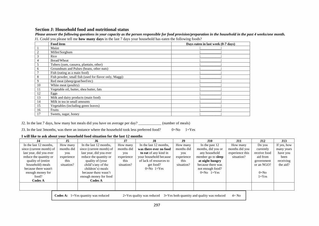
297

Section J: Household food and nutritional status Please answer the following questions in your capacity as the person responsible for food provision/preparation in the household in the past 4 weeks/one month.

J1. Could you please tell me how many days in the last 7 days your household has eaten the following foods?

Food item Days eaten in last week (0-7 days)

1 Maize |____________|

2 Millet/Sorghum |____________| 3 Rice |____________| 4 Bread/Wheat |____________| 5 Tubers (yam, cassava, plantain, other) |____________| 6 Groundnuts and Pulses (beans, other nuts) |____________| 7 Fish (eating as a main food) |____________| 8 Fish powder, small fish (used for flavor only, Maggi) |____________| 9 Red meat (sheep/goat/beef/etc) |____________| 10 White meat (poultry) |____________| 11 Vegetable oil, butter, shea butter, fats |____________| 12 Eggs |____________| 13 Milk and dairy products (main food) |____________| 14 Milk in tea in small amounts |____________| 15 Vegetables (including green leaves) |____________| 16 Fruits |____________| 17 Sweets, sugar, honey |____________|

J2. In the last 7 days, how many hot meals did you have on average per day? ____________ (number of meals)

J3. In the last 3months, was there an instance where the household took less preferred food? 0=No 1=Yes

I will like to ask about your household food situation for the last 12 months

J4 J5 J6 J7 J8 J9 J10 J11 J12 J13

In the last 12 months,

since (current month) of

last year, did you ever

reduce the quantity or

quality of (entire

household) meals

because there wasn't

enough money for

food?

Codes A

How many

months did

you

experience

this

situation?


since (current month) of

last year, did you ever

reduce the quantity or

quality of (your

child’s/any of the

children’s) meals

because there wasn’t

enough money for food

Codes A

How many

months did

you

experience

this

situation?


was there ever no food

to eat of any kind in

your household because

of lack of resources to

get food?

0=No 1=Yes

How many

months did

you

experience

this

situation?

In the past 12

months, did you or

any household

member go to sleep

at night hungry because there was

not enough food?

0=No 1=Yes

How many

months did you

experience this

situation?

Do you

currently

receive food

aid from

government

or an NGO?

0=No

1=Yes

If yes, how

many years

have you

been

receiving

the aid?

Codes A: 1=Yes quantity was reduced 2=Yes quality was reduced 3=Yes both quantity and quality was reduced 4= No

298

Section K: Livestock and other assets Please I will like to ask about your livestock and other assets of the household.

K1

Do you own any of these animals in the household? Cattle Sheep Goat Pigs Poultry Others_____ Others_____

0=No

1=Yes

0=No

1=Yes

0=No

1=Yes

0=No

1=Yes

0=No

1=Yes

0=No

1=Yes

0=No

1=Yes

K2 If yes, how many does the household own?

K3 How many did you sell in the 2015/16 season?

K4 At what price did you sell most of this? (GHS)

K5 How many did you buy in the 2015/16 season?

K6 At what price did you buy most of this? (GHS)

K7 Do you seek for veterinary services for them?

0=No 1=Yes

K8 If yes, how much did it cost you to vaccinate them in

the last 12 months? GHS

Please complete the table below on the asset owned by your household

# Asset/Item Do you have

item?

0=No 1=Yes

If yes, how many

in all?

If yes, how many as at

the beginning of 2015?

How much did you

purchase the most current

item? GHS

Price if you were to

sell it now GHS

1 Cutlass

2 Hoe

3 Knapsack

4 Irrigation pump/kit

5 Radio

6 Television

7 Bicycle

8 Motorcycle

9 Car/Moto-King/kia

10 Bullock/ Donkey

11 Thresher

12 Tractor

13 Mechanized sheller

14 House

15 Other (specify)……

16 Other (specify)……

End of interview and thank you for participating

299

Appendix 2: Focus group interview guide

Main ethnicity and religion

1. What is/are the main languages spoken in the community?

2. Which ethnic group is the dominant?

3. Which religion is the dominant?

Farm labour wage rate

4. What was the wage rate per day during 2015/2016 season? _____________ GHS

5. Was the wage rate same for male and female? 0=No 1=Yes

6. If no, what was the wage rate for a female worker during 2015/2016 growing season?

___________ GHS

Transactions costs

7. What is the distance to the nearest tared road? ______________ Km

8. What is the most used means of transport to the nearest road?

9. How many minutes does it take you from the community to the nearest tared road using this

most common means? ____________________Mins

Codes

1. Likpakpaln (Konkomba) 7. Hausa 13. Nankan

2. Chekosi 8. Bimoba 14. Kusaal

3. Mampruli 9. Dagaare/Wali 15. Twi

4. Dagbali (Dagbani) 10. Sissali 16. Ewe

5. Nanunli 11. Gruni 17. Ga

6. Gonja 12. Kasem 18. Other (specify) ________

Codes

1. Konkombas 7. Hausas 13. Nankan

2. Chekosi 8. Bimobas 14. Kusasi

3. Mamprusi 9. Dagaabas/Walas 15. Akans

4. Dagombas 10. Sissalas 16. Ewes

5. Nanumbas 11. Grunsi 17. Gas

6. Gonjas 12. Kassenas 18. Other (specify)________

Codes C

0 No religion

1 Muslim 3 Traditional

2 Christian 6 Other (specify) __________________

Codes

0 Foot 2 Bicycle 4 Motor King 6 Truck

1 Animal 3 Motor bike 5 Tractor 7 Other (specify) ______________

Christian-Albrechts University of Kiel, Germany

Institute of Food Economics and Consumption Studies

300

10. What is the distance to the district capital? ______________ Km

11. What is the distance to the nearest agriculture office? ______________ Km

12. What is the distance to the nearest agriculture extension officer? ______________

Km

13. What is the distance to the nearest NGO or Research organization? ________________Km

Market

14. Do you have at least periodic market in the community? 0=No 1=Yes

15. What was the average soybean price in the community last year ____ GHS

16. What is the distance to the nearest market center? ______________ Km

17. What is the distance to the nearest financial institution? _________________Km

18. How many days per week a car/vehicle plies the community? ______________Days

19. Does the entire community has mobile phone service? 0=No 1=Yes

20. If no to 19, do you have mobile phone service in some sections of the community?

0=No 1=Yes

21. If yes to 19, how many of such spots do you know of in the community?

____________

The Institute for Food Economics and Consumption Studies

Documents