83 REGIS BARNICHON Centre de Recerca en Economia Internacional, Barcelona CHRISTOPHER J. NEKARDA Board of Governors of the Federal Reserve System The Ins and Outs of Forecasting Unemployment: Using Labor Force Flows to Forecast the Labor Market ABSTRACT This paper presents a forecasting model of unemployment based on labor force flows data that, in real time, dramatically outperforms the Sur- vey of Professional Forecasters, historical forecasts from the Federal Reserve Board’s Greenbook, and basic time-series models. Our model’s forecast has a root-mean-squared error about 30 percent below that of the next-best forecast in the near term and performs especially well surrounding large recessions and cyclical turning points. Further, because our model uses information on labor force flows that is likely not incorporated by other forecasts, a combined fore- cast including our model’s forecast and the SPF forecast yields an improve- ment over the latter alone of about 35 percent for current-quarter forecasts, and 15 percent for next-quarter forecasts, as well as improvements at longer horizons. F orecasting the unemployment rate is an important and difficult task for policymakers, especially surrounding economic downturns. Typically, unemployment rate forecasts are made using one of two approaches. The first is based on the historical time-series properties of the unemployment rate and, perhaps, near-term indicators of the labor market. The second is based on the relationship between output growth and unemployment changes known as Okun’s law. In this paper we develop a new approach that incorporates information on labor force flows as directed by economic theory to form forecasts for the unemployment rate. A simple analogy helps explain the main idea behind our approach. Unemployment at a given time can be thought of as the amount of water in

Welcome message from author
This document is posted to help you gain knowledge. Please leave a comment to let me know what you think about it! Share it to your friends and learn new things together.
Transcript
83
regis barnichonCentre de Recerca en Economia Internacional, Barcelona
christopher j. nekardaBoard of Governors of the Federal Reserve System
The Ins and Outs of Forecasting Unemployment: Using Labor Force Flows
to Forecast the Labor Market
ABSTRACT This paper presents a forecasting model of unemployment based on labor force flows data that, in real time, dramatically outperforms the Sur-vey of Professional Forecasters, historical forecasts from the Federal Reserve Board’s Greenbook, and basic time-series models. Our model’s forecast has a root-mean-squared error about 30 percent below that of the next-best forecast in the near term and performs especially well surrounding large recessions and cyclical turning points. Further, because our model uses information on labor force flows that is likely not incorporated by other forecasts, a combined fore-cast including our model’s forecast and the SPF forecast yields an improve-ment over the latter alone of about 35 percent for current-quarter forecasts, and 15 percent for next-quarter forecasts, as well as improvements at longer horizons.
Forecasting the unemployment rate is an important and difficult task for policymakers, especially surrounding economic downturns. Typically,
unemployment rate forecasts are made using one of two approaches. The first is based on the historical time-series properties of the unemployment rate and, perhaps, near-term indicators of the labor market. The second is based on the relationship between output growth and unemployment changes known as Okun’s law. In this paper we develop a new approach that incorporates information on labor force flows as directed by economic theory to form forecasts for the unemployment rate.
A simple analogy helps explain the main idea behind our approach. Unemployment at a given time can be thought of as the amount of water in
84 Brookings Papers on Economic Activity, Fall 2012
a bathtub, a stock. Given an initial water level, the level at some future time is determined by the rate at which water flows into the tub from the faucet and the rate at which water flows out of the tub through the drain. When the inflow rate equals the outflow rate, the amount of water in the tub remains constant. But if the inflow rate increases and the outflow rate does not, we know that the water level will be higher in the future. In other words, the inflow rate and the outflow rate together provide information about the future water level—or in this case, of unemployment.
This insight forms one of two cornerstones of our approach: we exploit this convergence property whereby the actual unemployment rate con-verges toward the rate implied by the labor force flows. The other is forecasting those underlying flows directly. Because the individual flows have different time-series properties and their contributions change over the business cycle, focusing on the flows allows us to better capture the asymmetric nature of unemployment movements.
For near-term forecasts, our model dramatically outperforms the Survey of Professional Forecasters (SPF), historical forecasts from the Federal Reserve Board’s Greenbook, and basic time-series models, achieving a root-mean-squared error (RMSE) about 30 percent below that of the best alternative forecast. Moreover, our model has the highest predictive ability surrounding business cycle turning points and large recessions.
In addition, our model is a particularly useful addition to the exist-ing set of forecasting models because it uses information—data on labor force flows—that is likely not incorporated by other forecasts. Thus, combining the forecasts from our model, the SPF, and a simple time-series model yields a reduction in RMSE, relative to the SPF forecast alone, of about 35 percent for the current-quarter forecast, 15 percent for the next-quarter forecast, and smaller improvements at longer horizons.
Finally, our model can also be used to forecast the labor force par-ticipation rate. Here the improvement in forecast performance is more modest than for the unemployment rate: our model improves on the Greenbook only for the current-quarter forecast. Nevertheless, combining the forecasts of our model and the Greenbook yields a sizable reduction in RMSE.
To facilitate analysis and discussion of real-time developments in the labor market, updated forecasts from our model will be posted on the Brookings Papers website each month following the release by the Bureau of Labor Statistics (BLS) of that month’s employment report.
regis barnichon and christopher j. nekarda 85
I. Using Labor Force Flows to Forecast Unemployment
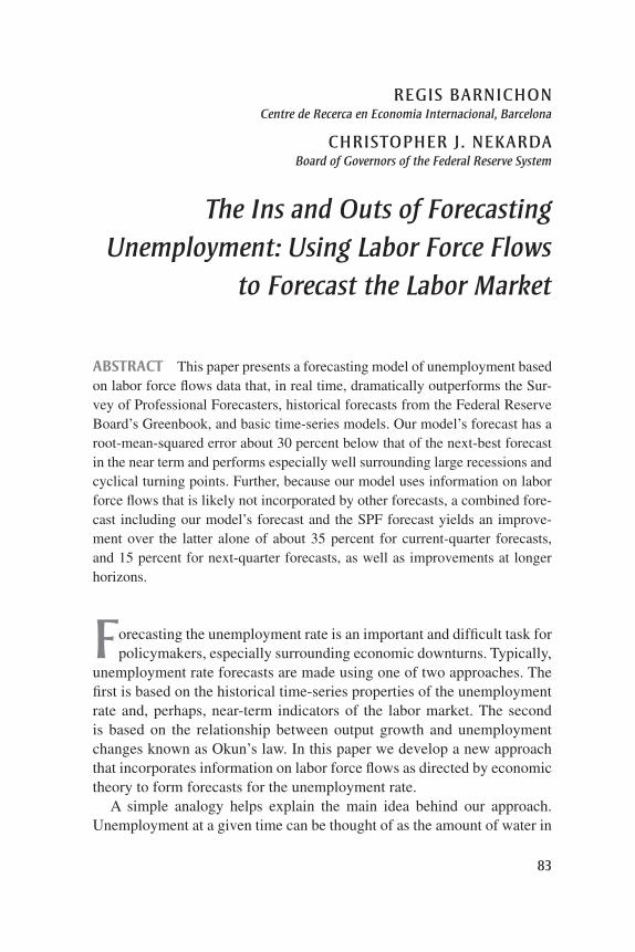
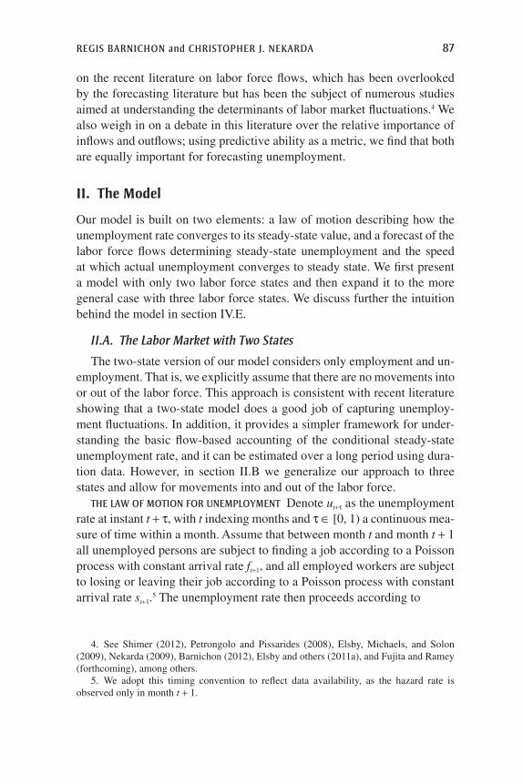
We incorporate information from labor force flows through the concept of the conditional steady-state unemployment rate, which is the rate of unemployment that would eventually prevail were the flows into and out of unemployment to remain at their current rates. In steady state these flows are balanced. However, if the inflow rate were to jump, as tends to hap-pen at the onset of a recession, then the conditional steady-state un-employment rate would also jump. With no additional shocks to either flow, the unemployment rate would progressively rise toward this new steady state. Moreover, because this convergence process typically takes 3 months or more, the conditional steady-state rate provides information about the unemployment rate in the near future.
Figure 1 shows the tight, leading relationship between the steady-state unemployment rate, u*, and the actual unemployment rate, u. As shown by
Source: Bureau of Labor Statistics data and authors’ calculations.a. Quarterly averages of monthly data. Shading indicates recessions.b. Defined as u* = s/(s + f), where s and f are flow rates into and out of unemployment, respectively;
see equation 3 in the text.
−0.50.00.51.0
3
4
5
6
7
8
9
10
11
Percent
201020001990198019701960
Deviation(right scale)
ActualSteady-stateb
(left scale)
Figure 1. Unemployment rate, actual and steady-state, 1950–2012a
86 Brookings Papers on Economic Activity, Fall 2012
the deviation (u* - u) plotted at the bottom of the figure, in periods when u* is above the actual rate, the unemployment rate tends to rise, and, con-versely, when u* lies below u, the unemployment rate tends to fall.
However, relying solely on current labor force flows constrains our approach to very near term forecasts, because the steady state to which the actual unemployment rate converges also changes over time as the under-lying flows change. Thus, we forecast the underlying labor force flows using a time-series model and feed those forecasts into a law of motion relating these flows to the unemployment rate to generate unemployment forecasts at longer horizons. Directly forecasting the flows into and out of unemployment rather than the unemployment stock itself, as is customary, is another reason that our model outperforms other approaches. It allows our model to better capture the dynamics of unemployment, because the unemployment stock is driven by flows with different time-series proper-ties, and because the contributions of the different flows change through-out the cycle (Barnichon 2012).
An additional advantage of focusing on labor force flows is that it allows us to capture the asymmetric nature of unemployment movements—in par-ticular, the fact that increases tend to be steeper than decreases.1 Although our model is not explicitly asymmetric, it relies on the unemployment flows that are responsible for the asymmetry of unemployment (Barnichon 2012). By using such information as inputs in the forecasts, our model can incorporate the impulses that generate this asymmetry.2 Thanks to this property, we find that our model outperforms a baseline time-series model around turning points and large recessions (Montgomery and others 1998, Baghestani 2008). This is particularly useful since these are the times when accurate unemployment forecasts are most valuable.
This paper builds on the influential work of Alan Montgomery and others (1998) and extends the growing literature aimed at improving the performance of unemployment forecasting models.3 We draw especially
1. A long literature discusses the apparent asymmetry of unemployment: for example, Mitchell (1927), Neftçi (1984, corrected by Sichel 1989), Rothman (1991), and more recently, Hamilton (2005), Sichel (2007), and Rothman (2008).
2. Moreover, unlike standard time-series models used to capture asymmetries (such as threshold models or Markov switching models), our model does not rely on a thresh-old (which may change) to introduce asymmetry. A comprehensive study by Stock and Watson (1999) concluded that linear models generally dominated nonlinear models for out-of-sample forecasts of most macroeconomic time series. The unemployment rate is an exception; see, for example, Milas and Rothman (2008).
3. See, for example, Rothman (1998), Golan and Perloff (2004), Brown and Moshiri (2004), and Milas and Rothman (2008).
regis barnichon and christopher j. nekarda 87
on the recent literature on labor force flows, which has been overlooked by the forecasting literature but has been the subject of numerous studies aimed at understanding the determinants of labor market fluctuations.4 We also weigh in on a debate in this literature over the relative importance of inflows and outflows; using predictive ability as a metric, we find that both are equally important for forecasting unemployment.
II. The Model
Our model is built on two elements: a law of motion describing how the unemployment rate converges to its steady-state value, and a forecast of the labor force flows determining steady-state unemployment and the speed at which actual unemployment converges to steady state. We first present a model with only two labor force states and then expand it to the more general case with three labor force states. We discuss further the intuition behind the model in section IV.E.
II.A. The Labor Market with Two States
The two-state version of our model considers only employment and un-employment. That is, we explicitly assume that there are no movements into or out of the labor force. This approach is consistent with recent literature showing that a two-state model does a good job of capturing unemploy-ment fluctuations. In addition, it provides a simpler framework for under-standing the basic flow-based accounting of the conditional steady-state unemployment rate, and it can be estimated over a long period using dura-tion data. However, in section II.B we generalize our approach to three states and allow for movements into and out of the labor force.
the law oF motion For Unemployment Denote ut+t as the unemployment rate at instant t + t, with t indexing months and t ∈ [0, 1) a continuous mea-sure of time within a month. Assume that between month t and month t + 1 all unemployed persons are subject to finding a job according to a Poisson process with constant arrival rate ft+1, and all employed workers are subject to losing or leaving their job according to a Poisson process with constant arrival rate st+1.5 The unemployment rate then proceeds according to
4. See Shimer (2012), Petrongolo and Pissarides (2008), Elsby, Michaels, and Solon (2009), Nekarda (2009), Barnichon (2012), Elsby and others (2011a), and Fujita and Ramey (forthcoming), among others.
5. We adopt this timing convention to reflect data availability, as the hazard rate is observed only in month t + 1.
88 Brookings Papers on Economic Activity, Fall 2012
( ) ,1 11 1
d
d
us u f ut
t t t t
++ + + += −( ) −τ
τ ττ
as changes in unemployment are given by the difference between the inflows and the outflows. Solving equation 1 yields
( ) * ,2 11 1 1u u ut t t t t+ + + += ( ) + − ( )[ ]τ β τ β τ
where
( ) *3 11
1 1
us
s ft
t
t t
++
+ +
≡+
denotes the conditional steady-state unemployment rate, and bt+1(t) ≡ 1 - e− +( )+ +s ft t1 1 is the rate of convergence to that steady state.
Equation 2 relates variation in the unemployment stock ut+t over the course of a month to variation in the underlying flow hazards, ft+1 and st+1. A 1-month-ahead forecast for the unemployment rate, ut+1|t, can thus be obtained from
( ) ˆ ˆ * ˆ ,4 11 1 1 1u u ut t t t t t+ + + += + −( )β β
where b t+1 is the month t forecast of bt+1, the convergence speed between month t and month t + 1.
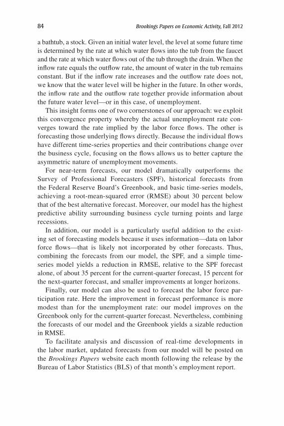
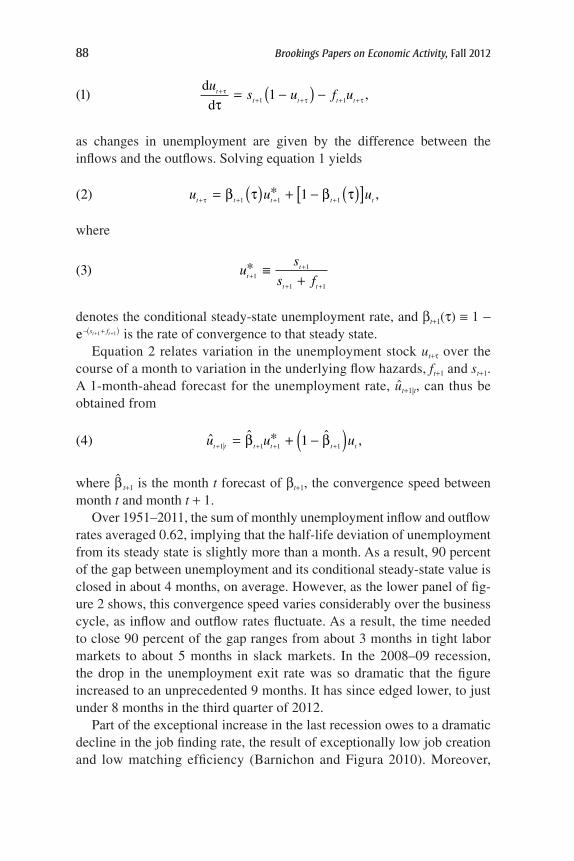
Over 1951–2011, the sum of monthly unemployment inflow and outflow rates averaged 0.62, implying that the half-life deviation of unemployment from its steady state is slightly more than a month. As a result, 90 percent of the gap between unemployment and its conditional steady-state value is closed in about 4 months, on average. However, as the lower panel of fig-ure 2 shows, this convergence speed varies considerably over the business cycle, as inflow and outflow rates fluctuate. As a result, the time needed to close 90 percent of the gap ranges from about 3 months in tight labor markets to about 5 months in slack markets. In the 2008–09 recession, the drop in the unemployment exit rate was so dramatic that the figure increased to an unprecedented 9 months. It has since edged lower, to just under 8 months in the third quarter of 2012.
Part of the exceptional increase in the last recession owes to a dramatic decline in the job finding rate, the result of exceptionally low job creation and low matching efficiency (Barnichon and Figura 2010). Moreover,
regis barnichon and christopher j. nekarda 89
Michael Elsby and others (2011b) show that this exceptional decline was also in part an artifact of measurement, because not all persons flowing into unemployment had a duration of less than 5 weeks. This phenom-enon became much more prevalent in the recent recession, where a larger fraction of persons moving from employment to unemployment reported a duration of more than 5 weeks, leading the duration-based measure of the unemployment exit rate to suffer from a larger downward bias. As we discuss in section VII, to the extent that the bias is stronger than in previous recessions, forecasting performance could deteriorate.
Forecasting labor Force Flows Because equation 4 can forecast the unemployment rate only 1 month ahead given the current values of the haz-ard rates, forecasting the unemployment rate at longer horizons requires making forecasts of the hazard rates. A simple approach is to assume that the hazard rates remain constant at their last observed value over the
3.23.43.63.84.04.24.44.6
0.91.01.11.21.31.41.51.6
Log pointsUnemployment inflows and outflows
3456789
MonthsTime to convergenceb
Source: Authors’ calculations based on Bureau of Labor Statistics data.a. Quarterly averages of monthly data. Shading indicates recessions.b. Time needed to close 90 percent of the gap between the actual and the steady-state unemployment rate.
Log points
201020001990198019701960
201020001990198019701960
Inflows (left scale)Outflows (right scale)
Figure 2. Unemployment inflow and outflow hazard rates and convergence to steady-state Unemployment rate, 1950–2012a
90 Brookings Papers on Economic Activity, Fall 2012
forecast horizon. However, in real time a forecaster does not observe st+1
and ft+1, but only st and ft, because at month t one can observe labor force flows only from month t - 1 to month t.6 Thus, the j-period-ahead forecast of the unemployment rate can be formed from the month t values of s and f as follows:7
( ) ˆ * .5 1u u ut j tj f s
tj f s
tt t t t
+− +( ) − +( )= −[ ] +e e
If the hazard rates are persistent enough, equation 5 will provide reasonable forecasts.8 However, as figure 2 shows, the hazard rates do change, and with them the conditional steady-state unemployment rate and the speed of convergence.
Because the hazard rates are not sufficiently persistent, we use a vector autoregression (VAR) to forecast both the inflow and the outflow rates. We also include two leading indicators of labor force flows: vacancy postings and initial claims for unemployment insurance. Specifically, let
y t t t t t ts f u uic hwi= ∆ ∆( )ln , ln , ln , ln , ln ,′
where uic is the monthly average of weekly initial unemployment insur-ance claims and hwi is Barnichon’s (2010) composite help-wanted index. Note that, given our timing convention for the flows, the hazard rates effec-tively enter the VAR lagged by 1 month. We estimate the VAR
( )6 1 2y c y yt t t t= + + +− −Φ Φ1 2 ε
over a 15-year rolling window.9
6. A concrete example helps clarify this point. Last September’s employment report (published on October 5, 2012) provided information on the stock of unemployment in September and the average unemployment inflow and outflow rates between August and September (st and ft). Looking back at equation 4, this information allows us to measure bt, u*t , and ut. Thus, forecasting ut+1|t (the unemployment rate in October) requires forecasts of ft+1|t and st+1|t (that is, the flows from September to October).
7. This law of motion forms the basis of Elsby and others’ (2011a) strategy to generalize Shimer’s (2012) unemployment decomposition to incorporate out-of-steady-state dynamics.
8. In section IV we consider a forecast based only on the convergence to the steady-state unemployment rate.
9. We found that, in real time, a rolling window (in which the model is estimated over the previous K months) yielded more accurate forecasts than a recursive window (in which the model is estimated over the entire observed history), likely because of the low-frequency patterns; windows of 15 years were superior to 10- and 20-year windows. We also considered lag lengths between 1 and 12.
regis barnichon and christopher j. nekarda 91
After generating forecasts of the hazard rates, we obtain j-period-ahead forecasts of unemployment by iterating on the following:10
( ) ˆ ˆ ˆ* ˆ ˆ7 1u u ut j t t j t j t j t j t+ + + + += + −( )β β
with
( ) ˆ*ˆ
ˆ ˆ8 us
s ft j
t j t
t j t t j t
+
+
+ +
=+
and
( ) ˆ .ˆ ˆ9 1β t j
s ft j t t j t
+− +( )= − + +e
With month t + j forecasts of the flow rates in hand, we can calculate the month t + j values of u* and b. The month t + j unemployment fore-cast is then obtained by taking a weighted average of the previous-period (month t + j - 1) unemployment rate and the current-period (month t + j) conditional steady-state unemployment rate, with the weights determined by the speed of convergence to steady state.
II.B. The Labor Market with Three States
So far we have considered only a labor market with two states: employed or unemployed. However, not all those without jobs are unemployed. Indeed, flows into and out of the labor force dwarf those into and out of unemployment.11 This section considers a model that incorporates flows among all three labor force states.
An important advantage of the three-state model is its ability to capture more accurately the flows taking place in the labor market. For instance, the unemployment inflow rate comprises both those losing or leaving jobs and those entering or reentering the labor force. Since these two flows (and in fact all six flows) display different time-series properties, a
10. Because ût+jt is a nonlinear function of ft+jt and st+jt, Jensen’s inequality, in theory, prohibits us from directly forecasting the unemployment rate from equation 7 and forecasts of ft+jt and st+jt. To avoid this problem, we use Monte Carlo simulation and sample with replacement from the VAR residuals {ef, es} and form forecasts (equations 8 and 9) using the sampling distribution of ef and es. In practice, given the magnitude of the inflows and out-flows, the unemployment rate forecasts obtained by Monte Carlo simulation are not different from those formed from equation 7. For simplicity, we use that approximation.
11. See Blanchard and Diamond (1990) for the seminal study of gross flows.
92 Brookings Papers on Economic Activity, Fall 2012
three-state model may produce better forecasts than a two-state model.12 In addition, the three-state model can be used to forecast the labor force participation rate.
To generalize our two-state framework to three states, we need to spec-ify and solve the system of differential equations governing the number of people in unemployment, U; in employment, E; or out of the labor force, N. Between month t and month t + 1, individuals can transit from state a ∈ {E, U, N} to state b ∈ {E, U, N} according to a Poisson process with constant arrival rate lab
t+1. The stocks of unemployed, employed, and persons not in the labor force satisfy the following system:13
�U E Nt tEU
t tNU
t tUE
tUN
+ + + + + + += + − +( )τ τ τλ λ λ λ1 1 1 1 UUE U N
t
t tUE
t tNE
t tEU
+
+ + + + + += + −τ
τ τ τλ λ λ( )10 1 1 1� ++( )
= + −+ +
+ + + + +
λλ λ λ
τ
τ τ τ
tEN
t
t tEN
t tUN
t
EN E U
1
1 1�
ttNE
tNU
tN+ + ++( )1 1λ τ .
For instance, as the first line shows, changes in unemployment are given by the difference between the inflows to unemployment (workers losing or quitting their jobs and seeking work, and persons joining or rejoining the labor force) and the outflows from unemployment (unemployed persons finding a job or dropping out of the labor force).
Then, using the initial and terminal conditions, the one-step-ahead forecasts of the three stocks can be solved as functions of the transition probabilities (the labs in equation 10). The appendix gives the details of the solution. We then use the solution to these equations to generate one-period-ahead forecasts of the unemployment rate and the labor force participation rate from
( ) ˆˆ
ˆ ˆ11 1
1
1 1
uU
U Et t
t t
t t t t
+
+
+ +
=+
and
( )ˆ ˆ
ˆ ˆ ˆ12 1
1 1
1 1
lfprU E
E U Nt t
t t t t
t t t t
�+
+ +
+ +
=+
+ + tt t+1
.
12. See Barnichon and Figura (2010) for more on the properties of the different flows.13. Equation 10 assumes that Pt is constant within a month and that inflows and outflows
to the civilian noninstitutional population aged 16 and older are negligible. This assumption is reasonable given that the working-age population increases by about 150,000 per month, an order of magnitude or two larger than the flows into and out of E, U, or N.
regis barnichon and christopher j. nekarda 93
Note that, in effect, what we assume for population growth does not affect our forecasts, because we forecast population shares.
As with the two-state model, to construct forecasts beyond one period ahead, we use a VAR to forecast the six transition probabilities. Specifi-cally, we estimate
( )13 1 2 3y c y y yt t t t t= + + + +− − −Φ Φ Φ1 2 3 ε
over a 10-year rolling window, where
y t tEU
tUE
tEN
tNE
tNU
tUN
t tu uic= ln , , , , , , , ,λ λ λ λ λ λ hhwit( )′.
Note that in this specification, the unemployment rate and the help-wanted index enter in levels, rather than in changes, because this yielded better forecasts.
III. Data
We construct measures of the transition rates in the two-state and three-state models using different approaches: an indirect one (using information on the stocks of unemployment and of short-term unemployment to infer the transition rates) for the two-state model, and a direct one (using mea-sures of labor force flows) for the three-state model.
For the two-state model, we follow Robert Shimer (2012) and use infor-mation on the number of persons unemployed, Ut, and of those unemployed for less than 5 weeks, US
t, to infer job finding and job separation hazard rates.14 Specifically, we calculate the unemployment outflow probability, F, from
FU U
Ut
t tS
t
++ += −
−1
1 11 ,
with ft+1 = -ln(1 - Ft+1) the hazard rate. The unemployment inflow rate, s, is then obtained by solving equation 1 forward over [t, t + 1) and finding the value of st+1 that solves
Us
f sU Et
f st
t t
t t
t t
+
− +( )+
+ +
=−[ ]
++( ) +
+ +
1
1
1 1
1 1 1eee− +( )+ +f s
tt t U1 1 .
14. See also the pioneering work by Perry (1972).
94 Brookings Papers on Economic Activity, Fall 2012
Note that in this accounting, given a value for the unemployment out-flow rate (which also captures movements out of the labor force) and the stock of unemployed persons, the inflow rate is the rate that explains the observed stock of unemployed persons in the next month. As a result, the inflow rate incorporates all movements in unemployment not accounted for by the unemployment outflow rate.
For the three-state model, we use aggregate labor market transition probabilities among employment, unemployment, and nonparticipa-tion calculated from longitudinally matched Current Population Survey (CPS) micro data. We construct the transition rates from labor market flows as lt
ab ≡ ABt /At-1, where At-1 is the number of persons observed in state a in month t - 1, and ABt is the number who transitioned from state a in month t - 1 to state b in month t. (The time series of the ABs are col-lectively referred to as “gross flows.”) For example, UEt is the number of persons who moved from unemployed to employed, and UEt /Ut-1 is the corresponding transition probability. The BLS publishes a research series of gross flows that begins in February 1990. For contemporary forecasts, the published data have a sufficiently long history to allow estimation of the model. However, to evaluate historical model fore-casts before February 2000, we need data with a longer history. Thus, we construct measures of gross flows that cover June 1967 to January 1990, allowing us to begin our evaluation with 1976. From 1976 to 1990 we construct gross flows from Nekarda’s (in preparation) Longitudinal Population Database. Before 1976 we use gross flows tabulated by Joe Ritter (see Shimer 2012).
Finally, weekly initial claims for unemployment insurance are published by the Department of Labor’s Employment and Training Administration. Our measure of vacancy posting is, as noted before, the composite help-wanted index presented in Barnichon (2010).
IV. Forecasting Performance
We evaluate the performance of our flows models by comparing their unemployment rate forecasts with alternative forecasts along two dimen-sions. First, we assess the RMSEs of out-of-sample forecasts. Second, because it is harder to forecast the unemployment rate around recessions, we assess our model’s performance relative to a baseline time-series model over the business cycle. In what follows we refer to the two-state model as “SSUR-2” and the three-state model as “SSUR-3.”
regis barnichon and christopher j. nekarda 95
IV.A. Real-Time Forecasts
Our objective in this section is to evaluate our models’ forecasts against the best alternative forecasts, both those of professional forecasters and those derived from other time-series models. We consider five alternative forecasts of the unemployment rate. The first two are from professional forecasters. We consider historical forecasts from the Greenbook, which the literature has generally shown to be the benchmark forecast, and the median forecast from the SPF.15
The other three alternative forecasts are our own estimates from time-series models and are intended to disentangle the mechanisms behind the performance of our model. We consider a basic univariate time-series model, intended as a “naive” forecast that takes into account no other information but the past unemployment rate. Following Montgomery and others (1998), we use an ARIMA (2,0,1) model for the unemploy-ment rate. We also consider the unemployment rate forecast from a VAR that includes the labor force flows and the two leading indicators, initial claims and the help-wanted index. By comparing our SSUR models’ fore-casts against those of the VAR, we can directly evaluate the nonlinear relationship implied by the theory compared with an atheoretical linear time-series model using the same information set. Our last alternative is the unemployment rate forecast derived from our law of motion for the unemployment rate (equation 5), holding the inflow and outflow rates constant at their last known value. We call this the u* model. Shutting down the variation in the hazard rates isolates the contribution of the current conditional steady-state unemployment rate. The alternative time-series models are estimated over a 15-year rolling window.
To reflect the environment within which forecasters must operate, we estimate our models and generate forecasts using real-time data, except for initial claims and the help-wanted index.16 The historical forecasts were necessarily made with only the data in hand at the time. Some economic data, such as real GDP and payroll employment, are subject to substantial revision over time. For these variables, the current-vintage data may differ substantially from the historical data used to make those forecasts. In the case of the unemployment rate, however, the revisions are relatively minor. The labor force data obtained from the CPS are revised only to reflect
15. See, for example, Romer and Romer (2000), Sims (2002), Faust and Wright (2007), and Tulip (2009).
16. Real-time vintages were obtained from the Federal Reserve Bank of St. Louis’s “ArchivaL Federal Reserve Economic Data.”
96 Brookings Papers on Economic Activity, Fall 2012
updated estimates of seasonal fluctuations. Indeed, the not-seasonally-adjusted stocks of employment and unemployment are never revised, reflecting their origin from a point-in-time survey of households. Never-theless, even the small revisions to seasonal factors may have important consequences for our models’ performance.
To construct real-time estimates of the hazard rates, we begin with monthly vintages of the published seasonally adjusted stocks of employed, unemployed, and short-term unemployed workers.17 For each month we estimate the time series of the inflow and outflow hazard rates from the real-time stocks as described in section III. These series are then used in the VAR to forecast the hazard rates. Real-time data for initial claims and the help-wanted index are not available, so current-vintage data are used in the VAR. As with the unemployment rate, revisions to these series are relatively small.18 Nonetheless, in section IV.C we assess the implications of this limitation.
The SPF sends out its survey questionnaire sometime in the first month of a quarter, and the survey participants are asked to mail back the com-pleted questionnaire by the middle of the second month of the quarter. Thus, the forecasts included in the SPF incorporate labor market data from the first month of each quarter. To make forecasts comparable, our model forecasts are made treating the first month’s unemployment rate as data.
The information set for the historical Greenbook forecasts is more irreg-ular. Because the publication of the forecast is dictated by the date of the upcoming Federal Open Market Committee meeting, Greenbook forecasts are made at different points in a quarter; as a result, some forecasts have no monthly labor market data for the current quarter whereas others have 2 months of data. For example, at the time the March 2004 Greenbook was published, the unemployment rate was known through February 2004, and thus the quarter t + 0 forecast was made with data for the first 2 months of the quarter. However, when the April 2004 Greenbook was published, the unemployment rate was known only through March 2004, and thus the quarter t + 0 forecast (for the second quarter of 2004) was made without any published data for the quarter. We are careful to mimic the information
17. An alternative approach that sidesteps the issue of seasonal revisions altogether is to forecast the not-seasonally-adjusted unemployment rate from not-seasonally-adjusted CPS data. That model performed similarly to the two-state model we present here.
18. There are no revisions to the print help-wanted index. Real-time data for initial claims are available beginning in June 2009. Over the 39 months for which real-time data are available, the maximum absolute variation in the monthly-average level of weekly initial claims over this period was tiny (about 3 percent).
regis barnichon and christopher j. nekarda 97
set for each Greenbook forecast. Finally, because the Greenbook forecasts are made public with a 5-year lag, our comparison using the Greenbook ends in 2006.
IV.B. Forecast Errors
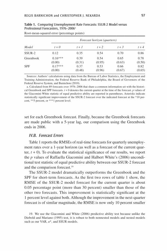
Table 1 reports the RMSEs of real-time forecasts for quarterly unemploy-ment rates over a 1-year horizon (as well as a forecast of the current quar-ter, t + 0). To evaluate the statistical significance of our results, we report the p values of Raffaella Giacomini and Halbert White’s (2006) uncondi-tional test statistic of equal predictive ability between our SSUR-2 forecast and the comparison forecast.19
The SSUR-2 model dramatically outperforms the Greenbook and the SPF for short-term forecasts. As the first two rows of table 1 show, the RMSE of the SSUR-2 model forecast for the current quarter is about 0.05 percentage point (more than 30 percent) smaller than those of the other two forecasts. This improvement is statistically significant at the 1 percent level against both. Although the improvement in the next-quarter forecast is of similar magnitude, the RMSE is now only 10 percent smaller
Table 1. comparing Unemployment rate Forecasts: ssUr-2 model versus professional Forecasters, 1976–2006a
Root-mean-squared error (percentage points)
Forecast horizon (quarters)
Model t + 0 t + 1 t + 2 t + 3 t + 4
SSUR-2 0.12 0.35 0.54 0.70 0.86
Greenbook 0.16*** 0.39 0.54 0.65 0.78(0.00) (0.31) (0.95) (0.63) (0.50)
SPF 0.17*** 0.37 0.53 0.66 0.82(0.00) (0.48) (0.96) (0.67) (0.65)
Sources: Authors’ calculations using data from the Bureau of Labor Statistics, the Employment and Training Administration, the Federal Reserve Bank of Philadelphia, the Board of Governors of the Federal Reserve System, and Barnichon (2010).
a. Calculated from 89 forecasts over 1976–2006 that share a common information set with the histori-cal Greenbook and SPF forecasts. t + 0 denotes the current quarter at the time of the forecast. p values of the Giacomini-White statistic of equal predictive ability are reported in parentheses. Asterisks indicate statistically significant improvement of the SSUR-2 forecast over the indicated forecast at the *10 per-cent, **5 percent, or ***1 percent level.
19. We use the Giacomini and White (2006) predictive ability test because unlike the Diebold and Mariano (1995) test, it is robust to both nonnested models and nested models such as our VAR, u*, and SSUR models.
98 Brookings Papers on Economic Activity, Fall 2012
than those of the alternatives, and the difference is not statistically signifi-cant. At longer horizons the improvement over the SPF and the Greenbook disappears: SSUR-2 performs about 0.05 percentage point worse than either professional forecast on average. Nevertheless, it is striking that our model performs only slightly worse than the Greenbook and the SPF at a 1-year horizon, considering that their forecasts are based on an array of economic data and models of the broader economy, whereas SSUR-2 is a statistical model that incorporates only near-term information about the labor market.
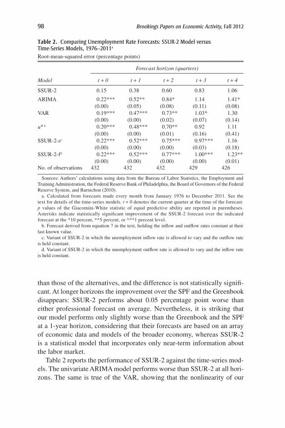
Table 2 reports the performance of SSUR-2 against the time-series mod-els. The univariate ARIMA model performs worse than SSUR-2 at all hori-zons. The same is true of the VAR, showing that the nonlinearity of our
Table 2. comparing Unemployment rate Forecasts: ssUr-2 model versus time-series models, 1976–2011a
Root-mean-squared error (percentage points)
Forecast horizon (quarters)
Model t + 0 t + 1 t + 2 t + 3 t + 4
SSUR-2 0.15 0.38 0.60 0.83 1.06
ARIMA 0.22*** 0.52** 0.84* 1.14 1.41*(0.00) (0.05) (0.08) (0.11) (0.08)
VAR 0.19*** 0.47*** 0.73** 1.03* 1.30(0.00) (0.00) (0.02) (0.07) (0.14)
u* b 0.20*** 0.48*** 0.70** 0.92 1.11(0.00) (0.00) (0.01) (0.16) (0.41)
SSUR-2-sc 0.22*** 0.52*** 0.75*** 0.97*** 1.16(0.00) (0.00) (0.00) (0.03) (0.18)
SSUR-2-fd 0.22*** 0.52*** 0.77*** 1.00*** 1.23**(0.00) (0.00) (0.00) (0.00) (0.01)
No. of observations 432 432 432 429 426
Sources: Authors’ calculations using data from the Bureau of Labor Statistics, the Employment and Training Administration, the Federal Reserve Bank of Philadelphia, the Board of Governors of the Federal Reserve System, and Barnichon (2010).
a. Calculated from forecasts made every month from January 1976 to December 2011. See the text for details of the time-series models. t + 0 denotes the current quarter at the time of the forecast. p values of the Giacomini-White statistic of equal predictive ability are reported in parentheses. Asterisks indicate statistically significant improvement of the SSUR-2 forecast over the indicated forecast at the *10 percent, **5 percent, or ***1 percent level.
b. Forecast derived from equation 7 in the text, holding the inflow and outflow rates constant at their last known value.
c. Variant of SSUR-2 in which the unemployment inflow rate is allowed to vary and the outflow rate is held constant.
d. Variant of SSUR-2 in which the unemployment outflow rate is allowed to vary and the inflow rate is held constant.
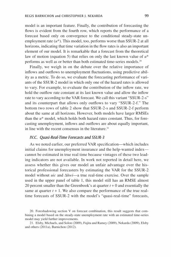
regis barnichon and christopher j. nekarda 99
model is an important feature. Finally, the contribution of forecasting the flows is evident from the fourth row, which reports the performance of a forecast based only on convergence to the conditional steady-state un-employment rate (u*). This model, too, performs worse than SSUR-2 at all horizons, indicating that time variation in the flow rates is also an important element of our model. It is remarkable that a forecast from the theoretical law of motion (equation 5) that relies on only the last known value of u* performs as well as or better than both estimated time-series models.20
Finally, we weigh in on the debate over the relative importance of inflows and outflows to unemployment fluctuations, using predictive abil-ity as a metric. To do so, we evaluate the forecasting performance of vari-ants of the SSUR-2 model in which only one of the hazard rates is allowed to vary. For example, to evaluate the contribution of the inflow rate, we hold the outflow rate constant at its last known value and allow the inflow rate to vary according to the VAR forecast. We call this variant “SSUR-2-s” and its counterpart that allows only outflows to vary “SSUR-2-f.” The bottom two rows of table 2 show that SSUR-2-s and SSUR-2-f perform about the same at all horizons. However, both models have larger RMSEs than the u* model, which holds both hazard rates constant. Thus, for fore-casting unemployment, inflows and outflows are about equally important, in line with the recent consensus in the literature.21
IV.C. Quasi-Real-Time Forecasts and SSUR-3
As we noted earlier, our preferred VAR specification—which includes initial claims for unemployment insurance and the help-wanted index—cannot be estimated in true real time because vintages of these two lead-ing indicators are not available. In work not reported in detail here, we assess whether this gives our model an unfair advantage over the his-torical professional forecasters by estimating the VAR for the SSUR-2 model without uic and Dhwi—a true real-time exercise. Over the sample used in the upper panel of table 1, this model still has an RMSE almost 20 percent smaller than the Greenbook’s at quarter t + 0 and essentially the same at quarter t + 1. We also compare the performance of the true real-time forecasts of SSUR-2 with the model’s “quasi-real-time” forecasts,
20. Foreshadowing section V on forecast combination, this result suggests that com-bining a model based on the steady-state unemployment rate with an estimated time-series model may yield further improvements.
21. Elsby, Michaels, and Solon (2009), Fujita and Ramey (2009), Nekarda (2009), Elsby and others (2011a), Barnichon (2012).
100 Brookings Papers on Economic Activity, Fall 2012
where we use the same rolling estimation and forecasting procedure as in the real-time exercise but use the current-vintage data at all points; that is, we omit all variation associated with revisions to the seasonal factors. Over the same sample (results not reported), the truly real-time forecasts are actually slightly better than the quasi-real-time forecasts at all but the current-quarter horizon, where they perform equally well. This suggests that evaluating the models in quasi-real time likely does not significantly alter the spirit of the real-time exercise.
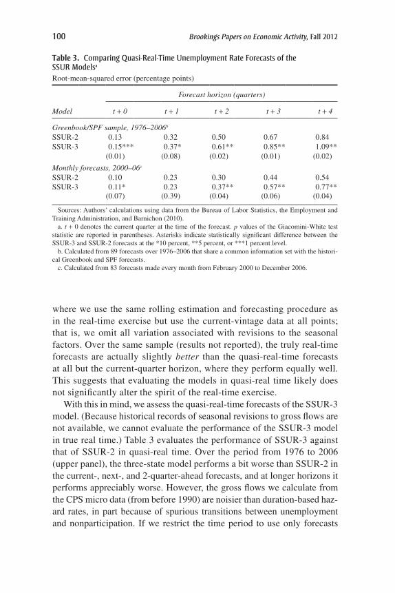
With this in mind, we assess the quasi-real-time forecasts of the SSUR-3 model. (Because historical records of seasonal revisions to gross flows are not available, we cannot evaluate the performance of the SSUR-3 model in true real time.) Table 3 evaluates the performance of SSUR-3 against that of SSUR-2 in quasi-real time. Over the period from 1976 to 2006 (upper panel), the three-state model performs a bit worse than SSUR-2 in the current-, next-, and 2-quarter-ahead forecasts, and at longer horizons it performs appreciably worse. However, the gross flows we calculate from the CPS micro data (from before 1990) are noisier than duration-based haz-ard rates, in part because of spurious transitions between unemployment and nonparticipation. If we restrict the time period to use only forecasts
Table 3. comparing Quasi-real-time Unemployment rate Forecasts of the ssUr modelsa
Root-mean-squared error (percentage points)
Forecast horizon (quarters)
Model t + 0 t + 1 t + 2 t + 3 t + 4
Greenbook/SPF sample, 1976–2006b
SSUR-2 0.13 0.32 0.50 0.67 0.84SSUR-3 0.15*** 0.37* 0.61** 0.85** 1.09**
(0.01) (0.08) (0.02) (0.01) (0.02)
Monthly forecasts, 2000–06c
SSUR-2 0.10 0.23 0.30 0.44 0.54SSUR-3 0.11* 0.23 0.37** 0.57** 0.77**
(0.07) (0.39) (0.04) (0.06) (0.04)
Sources: Authors’ calculations using data from the Bureau of Labor Statistics, the Employment and Training Administration, and Barnichon (2010).
a. t + 0 denotes the current quarter at the time of the forecast. p values of the Giacomini-White test statistic are reported in parentheses. Asterisks indicate statistically significant difference between the SSUR-3 and SSUR-2 forecasts at the *10 percent, **5 percent, or ***1 percent level.
b. Calculated from 89 forecasts over 1976–2006 that share a common information set with the histori-cal Greenbook and SPF forecasts.
c. Calculated from 83 forecasts made every month from February 2000 to December 2006.
regis barnichon and christopher j. nekarda 101
that were estimated using the published gross flows data (lower panel), the differences are small at horizons of up to 2 quarters ahead. As with the longer sample, SSUR-3 performs appreciably worse than SSUR-2 at fore-cast horizons of t + 3 and beyond.
IV.D. Forecasting Performance over the Business Cycle
The unemployment stock is driven by flows with different time-series properties, and the contributions of the different flows change throughout the cycle.22 For instance, inflows are responsible for the sharp increase in unemployment at the onset of recessions, but outflows are the main driving force of unemployment in normal times.
This property suggests that the performance of our flows model may vary over the business cycle. For instance, because the SSUR-2 model incorporates the unemployment inflow rate, which is responsible for the asymmetry of unemployment, it may better capture the asymmetric nature of unemployment than standard models. Thus, it may perform better dur-ing recessions, especially compared with standard models, which do not include labor force flows.
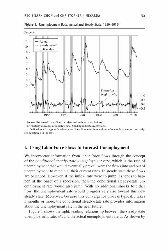
To test this idea and evaluate whether SSUR-2 performs differently over the course of the business cycle, we use Giacomini and Barbara Rossi’s (2010) predictive ability test in unstable environments. The test develops a measure of the relative local forecasting performance of two models and is ideal for testing whether the performance of our model varies over the cycle relative to that of a benchmark model. We use as the benchmark the ARIMA model presented in table 2. We evaluate local forecasting perfor-mance over a 5-year window using monthly forecasts spanning November 1968 to February 2012.
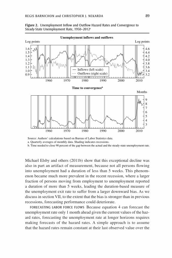
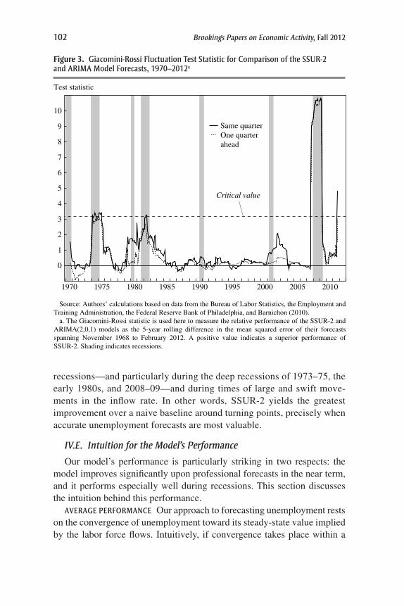
Figure 3 plots the Giacomini and Rossi fluctuation test statistic for current-quarter and 1-quarter-ahead forecasts; the corresponding 5 percent critical value is also shown. The unit of the y axis is the (standardized) roll-ing difference in mean squared error between the two models, a measure of their relative performance, defined such that a positive value indicates a superior performance of SSUR-2.
The SSUR-2 forecasts are almost always more accurate than those of the benchmark model, but SSUR-2 performs especially well around
22. At a quarterly frequency, the autocorrelation of the outflow rate is 0.91, but that of the inflow rate is only 0.73 (Shimer 2012). Further, whereas the distribution of the (detrended) inflow rate is positively skewed and highly kurtotic, the distribution of the (detrended) out-flow rate exhibits no skewness and low kurtosis (Barnichon 2012).
102 Brookings Papers on Economic Activity, Fall 2012
recessions—and particularly during the deep recessions of 1973–75, the early 1980s, and 2008–09—and during times of large and swift move-ments in the inflow rate. In other words, SSUR-2 yields the greatest improvement over a naive baseline around turning points, precisely when accurate unemployment forecasts are most valuable.
IV.E. Intuition for the Model’s Performance
Our model’s performance is particularly striking in two respects: the model improves significantly upon professional forecasts in the near term, and it performs especially well during recessions. This section discusses the intuition behind this performance.
average perFormance Our approach to forecasting unemployment rests on the convergence of unemployment toward its steady-state value implied by the labor force flows. Intuitively, if convergence takes place within a
0
1
2
3
4
5
6
7
8
9
10
1970 1975 1980 1985 1990 1995 2000 2005 2010
Test statistic
Source: Authors’ calculations based on data from the Bureau of Labor Statistics, the Employment and Training Administration, the Federal Reserve Bank of Philadelphia, and Barnichon (2010).
a. The Giacomini-Rossi statistic is used here to measure the relative performance of the SSUR-2 and ARIMA(2,0,1) models as the 5-year rolling difference in the mean squared error of their forecasts spanning November 1968 to February 2012. A positive value indicates a superior performance of SSUR-2. Shading indicates recessions.
Critical value
Same quarterOne quarterahead
Figure 3. giacomini-rossi Fluctuation test statistic for comparison of the ssUr-2 and arima model Forecasts, 1970–2012a
regis barnichon and christopher j. nekarda 103
couple of months, knowing the current values of the flows provides infor-mation on the future level of unemployment, and the SSUR model will perform well over the next couple of months.
In this subsection we develop this intuition further and discuss the rea-sons behind the quantitative performance of the model. Specifically, our ability to improve forecasting accuracy depends on three parameters: the level of the flows, the persistence of the flows, and whether different flows have different time-series properties.
First, as equation 2 makes clear, the level of the flows governs the speed of convergence to steady state. Since these flows are relatively large in the United States, convergence occurs relatively rapidly (in 3 to 5 months), and the current flows help forecast unemployment in the near term. This explains why, with U.S. data, SSUR-2 performs especially well for current- and next-quarter forecasts. If the flows were larger, the speed of conver-gence would be even higher, and the model would perform best at an even shorter horizon. At the extreme, if convergence were instantaneous, the current values of the flows would not help forecast unemployment. In con-trast, if the flows were much smaller, convergence would occur much more slowly and performance might be best at longer horizons.
If flows were very small, could their current values help us forecast unemployment in the very long run? The reason why this is unlikely comes from the second crucial parameter, the persistence of the flows. The performance of SSUR depends on the interaction between the speed of convergence (the levels of the flows) and the persistence of the flows. The model is good at forecasting unemployment only if the flows are sufficiently persistent that their values can be well predicted over the time needed to converge to steady state. For the U.S. labor market, the model performs well in the near term because the persistence of the flows is sufficiently high.
The third important characteristic behind the performance of SSUR stems from our focus on forecasting the flows rather than the stock. A model of the stock (such as the ARIMA model previously described) cannot perform as well as SSUR, because the flows differ in their time-series properties and because the contributions of the different flows change throughout the cycle. A model of the stock can capture the aver-age time-series properties of the stock, but it cannot allow for different time-series properties at different stages of the cycle.
perFormance over the bUsiness cycle The SSUR model performs especially well during recessions and around turning points because the unemployment rate displays steepness asymmetry: increases tend to be
104 Brookings Papers on Economic Activity, Fall 2012
steeper than decreases. This asymmetry manifests itself most forcefully during recessions, but a model of the stock is ill equipped to capture it unless one imposes an arbitrary threshold to introduce asymmetry, as is done in threshold autoregressive models. Although SSUR is not explicitly asymmetric, it relies on the labor force flows that are responsible for the asymmetry of unemployment. Indeed, it is the different behavior of the inflows and outflows over the cycle that is responsible for the steepness asymmetry of unemployment (Barnichon 2012). By incorporating flow information and using it as inputs in the forecasts, our model can incorpo-rate the impulses responsible for the asymmetry of unemployment.
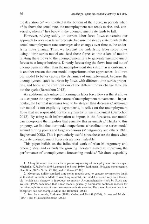
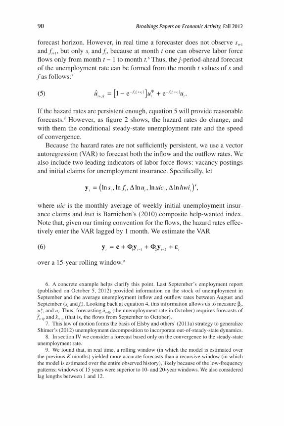
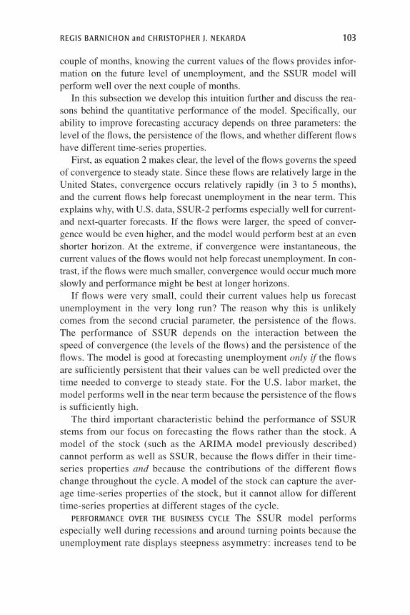
Specifically, the beginning of a recession is typically marked by a sharp increase in the inflow rate: figure 4 plots the impulse responses from our estimated VAR to a shock to the inflow rate.23 Whereas the inflow rate itself displays a sharp increase with fairly rapid reversion to the mean, the out-flow rate displays a delayed, U-shaped response with much slower mean reversion. These different impulse responses give rise to the steepness asymmetry of unemployment: following the initial shock, the inflow rate reverts relatively quickly to its mean, but the outflow rate takes longer to return to steady state and thus prevents the unemployment rate from decreasing as rapidly as it increased. By relying on a VAR forecast of the flow rates, following an initial disturbance to the inflow rate at the onset of a recession, SSUR can propagate the cyclical behavior of the flows and thus capture the steepness asymmetry of unemployment.
−2
−1
0
1
2
Quarter
Inflow
−2
−1
0
1
2
Quarter
Outflow
−2
−1
0
1
2
Quarter
Unemployment rate
120 2 4 6 8 10120 2 4 6 8 10120 2 4 6 8 10
Standard deviations
Source: Authors’ calculations using data from the Bureau of Labor Statistics.a. Impulse response functions to a 1-standard-deviation shock to the inflow rate, calculated from a
VAR of yt = ln(ft, st, urt)' with two lags that was estimated using quarterly data over 1951–2007.Shading represents 95 percent confidence intervals.
Figure 4. impulse responses to a shock to the Unemployment inflow ratea
23. See Fujita (2011) for more evidence on the response of the inflow and outflow rates to aggregate shocks.
regis barnichon and christopher j. nekarda 105
V. Combining Forecasts
The array of forecasting models we have considered reflect different infor-mation sets. The SSUR models’ forecasts rely mainly on labor force flows data and other labor market indicators but not on information from outside the labor market. In contrast, the professional (SPF and Greenbook) fore-casts are based on an array of economic data and models beyond the labor market, but they may ignore information on labor force flows. The ARIMA model forecasts unemployment from its past behavior.
Given these different information sets, a natural question is whether these unemployment forecasts can be further improved by combining our flows models’ forecasts with a professional forecast such as the SPF and with a simple time-series model such as the ARIMA, to exploit the dif-ferences in correlation among the forecast errors (see Granger and New-bold 1986). We construct such a combined forecast by taking a weighted average of forecasts from SSUR-2, the SPF, and the ARIMA model. The weights are determined by ordinary least squares regression, with a con-stant included to account for any systematic biases in the estimate. We estimate weights separately for each forecast horizon. The evaluation is a real-time exercise where, for each forecast at a given time, the weights are determined using available history only. These weights allow us to evalu-ate the marginal contributions of each model over the SPF forecast. If the SSUR-2 model forecast contributes no incremental benefit over the SPF forecast, the weight on the SSUR-2 forecast will be zero.
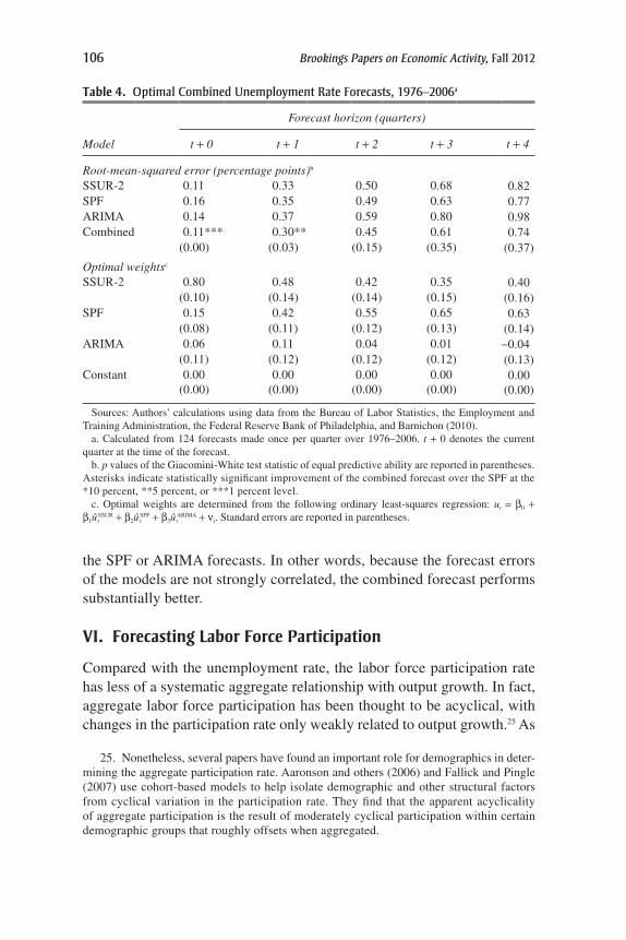
As table 4 shows, this is not the case: combining the SSUR-2 model with the SPF and the ARIMA improves forecasting performance signifi-cantly at horizons up to 2 quarters ahead. Compared with the baseline SPF forecast, the combined forecast achieves a reduction in RMSE of about 35 percent for current-quarter forecasts, 15 percent for 1-quarter-ahead forecasts, and almost 10 percent for 2-quarter-ahead forecasts, with smaller improvements at longer horizons. The combined current-quarter and 1-quarter-ahead forecasts are statistically significantly better than the SPF forecast alone.
The optimal weights reflect the contribution of the SSUR-2 model for short-term forecasting, and the combined forecast puts much more weight on SSUR-2 at short-term horizons.24 Importantly, the fact that the com-bined forecast performs significantly better than any single forecast indi-cates that the flows model brings relevant information not contained in
24. The reported optimal weights are the weights estimated over the full sample.
106 Brookings Papers on Economic Activity, Fall 2012
the SPF or ARIMA forecasts. In other words, because the forecast errors of the models are not strongly correlated, the combined forecast performs substantially better.
VI. Forecasting Labor Force Participation
Compared with the unemployment rate, the labor force participation rate has less of a systematic aggregate relationship with output growth. In fact, aggregate labor force participation has been thought to be acyclical, with changes in the participation rate only weakly related to output growth.25 As
Table 4. optimal combined Unemployment rate Forecasts, 1976–2006a
Forecast horizon (quarters)
Model t + 0 t + 1 t + 2 t + 3 t + 4
Root-mean-squared error (percentage points)b
SSUR-2 0.11 0.33 0.50 0.68 0.82SPF 0.16 0.35 0.49 0.63 0.77ARIMA 0.14 0.37 0.59 0.80 0.98Combined 0.11*** 0.30** 0.45 0.61 0.74
(0.00) (0.03) (0.15) (0.35) (0.37)
Optimal weightsc
SSUR-2 0.80 0.48 0.42 0.35 0.40(0.10) (0.14) (0.14) (0.15) (0.16)
SPF 0.15 0.42 0.55 0.65 0.63(0.08) (0.11) (0.12) (0.13) (0.14)
ARIMA 0.06 0.11 0.04 0.01 -0.04(0.11) (0.12) (0.12) (0.12) (0.13)
Constant 0.00 0.00 0.00 0.00 0.00(0.00) (0.00) (0.00) (0.00) (0.00)
Sources: Authors’ calculations using data from the Bureau of Labor Statistics, the Employment and Training Administration, the Federal Reserve Bank of Philadelphia, and Barnichon (2010).
a. Calculated from 124 forecasts made once per quarter over 1976–2006. t + 0 denotes the current quarter at the time of the forecast.
b. p values of the Giacomini-White test statistic of equal predictive ability are reported in parentheses. Asterisks indicate statistically significant improvement of the combined forecast over the SPF at the *10 percent, **5 percent, or ***1 percent level.
c. Optimal weights are determined from the following ordinary least-squares regression: ut = b0 + b1ût
SSUR + b2ûtSPF + b3ût
ARIMA + nt. Standard errors are reported in parentheses.
25. Nonetheless, several papers have found an important role for demographics in deter-mining the aggregate participation rate. Aaronson and others (2006) and Fallick and Pingle (2007) use cohort-based models to help isolate demographic and other structural factors from cyclical variation in the participation rate. They find that the apparent acyclicality of aggregate participation is the result of moderately cyclical participation within certain demographic groups that roughly offsets when aggregated.
regis barnichon and christopher j. nekarda 107
a result, forecasting the labor force participation rate was often seen as less of a priority than forecasting the unemployment rate.
The large and unexpected decline in labor force participation during and after the 2008–09 recession challenged that conventional wisdom and highlighted the importance of forecasting the labor force participation rate. However, given the historical absence of a strong relationship between out-put and labor force participation, forecasters have few models to turn to.
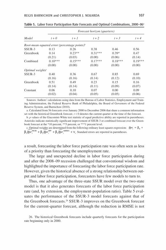
Thus, one advantage of the three-state SSUR model over the two-state model is that it also generates forecasts of the labor force participation rate (and, by extension, the employment-population ratio). Table 5 eval-uates the performance of the SSUR-3 model forecasts against that of the Greenbook forecasts.26 SSUR-3 improves on the Greenbook forecast for the current-quarter forecast, although the reduction in RMSE is not
Table 5. labor Force participation rate Forecasts and optimal combinations, 2000–06a
Forecast horizon (quarters)
Model t + 0 t + 1 t + 2 t + 3 t + 4
Root-mean-squared error (percentage points)b
SSUR-3 0.13 0.26 0.38 0.46 0.56Greenbook 0.14 0.23** 0.31*** 0.39* 0.47
(0.21) (0.03) (0.00) (0.06) (0.14)Combined 0.10*** 0.15*** 0.17*** 0.18*** 0.19***
(0.00) (0.00) (0.00) (0.00) (0.00)
Optimal weightsc
SSUR-3 0.40 0.36 0.67 0.85 0.69(0.16) (0.16) (0.14) (0.12) (0.10)
Greenbook 0.51 0.49 0.23 0.15 0.16(0.14) (0.14) (0.11) (0.09) (0.07)
Constant 0.06 0.10 0.07 0.00 0.09(0.02) (0.04) (0.05) (0.05) (0.06)
Sources: Authors’ calculations using data from the Bureau of Labor Statistics, Employment and Train-ing Administration, the Federal Reserve Bank of Philadelphia, the Board of Governors of the Federal Reserve System, and Barnichon (2010).
a. Calculated from 56 forecasts over January 2000 to December 2006 that share a common information set with the historical Greenbook forecast. t + 0 denotes the current quarter at the time of the forecast.
b. p values of the Giacomini-White test statistic of equal predictive ability are reported in parentheses. Asterisks indicate statistically significant improvement of SSUR-3 or combined forecast over the Green-book forecast at the *10 percent, **5 percent, or ***1 percent level.
c. Optimal weights are determined from the following ordinary least squares regression: lfprt = +β0
β β β1 2 3lfpr lfpr lfprt t t t� � �SSUR SPF ARIMA+ + + ν . Standard errors are reported in parentheses.
26. The historical Greenbook forecasts include quarterly forecasts for the participation rate beginning only in 2000.
108 Brookings Papers on Economic Activity, Fall 2012
statistically significant. At longer forecast horizons, SSUR-3 performs markedly less well than the Greenbook.
However, SSUR-3 forecast errors need not be correlated with Green-book forecast errors, so that, again, a combined forecast may generate sig-nificant improvement. The third row of table 5 confirms this intuition. The optimal labor force participation rate forecast combining the Greenbook and SSUR-3 forecasts performs significantly better than either alone at all horizons considered, and especially at longer horizons. The reduction in RMSE is trivial for current-quarter forecasts but grows to between 0.1 and 0.3 percentage point at longer horizons. The large weight on SSUR-3 at all horizons reflects superior performance compared with the Greenbook.27
VII. Recent Performance and Near-Term Prospects
Thus far the sample period used in our evaluation against professional forecasts has ended in 2006, shortly before the Great Recession. A crucial question, however, is how the SSUR models perform during that reces-sion and the ongoing recovery. In particular, can the models capture the steep increase in unemployment and the lack of rapid decline following this latest recession compared with other deep recessions?
Beyond 2006, we can no longer compare our models with the Greenbook; we therefore use the SPF as the benchmark instead. As table 1 showed, the SPF and Greenbook forecasts have roughly similar RMSEs over a 1-year forecast horizon.
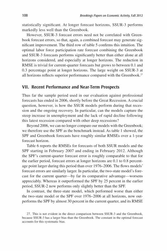
Table 6 reports the RMSEs for forecasts of both SSUR models and the SPF starting in February 2007 and ending in February 2012. Although the SPF’s current-quarter forecast error is roughly comparable to that for the earlier period, forecast errors at longer horizons are 0.1 to 0.8 percent-age point larger during this period than over 1976–2006. The flows models’ forecast errors are similarly larger. In particular, the two-state model’s fore-cast for the current quarter—by far its comparative advantage—worsens appreciably. Whereas it outperformed the SPF by 25 percent in the earlier period, SSUR-2 now performs only slightly better than the SPF.
In contrast, the three-state model, which performed worse than either the two-state model or the SPF over 1976–2006 at all horizons, now out-performs the SPF by almost 30 percent in the current quarter, and its RMSE
27. This is not evident in the direct comparison between SSUR-3 and the Greenbook, because SSUR-3 has a larger bias than the Greenbook. The constant in the optimal forecast accounts for this systematic bias.
regis barnichon and christopher j. nekarda 109
is even a bit smaller 1 quarter ahead. We point to three factors to explain this striking difference.
First, the gross flows are much better measured in the published data than in the historical tabulations. Because for much of the 1976–2006 sam-ple the model was estimated using the transitions we calculated from the micro data (rather than from the published data), the three-state model per-forms worse than the two-state model. Indeed, table 3 showed that SSUR-3 performed about the same as the two-state model when estimated using only the published gross flows data.
Second, the two-state model uses cross-sectional data on unemployment to infer the outflow rate and backs out the inflow rate using an unemploy-ment accounting identity. As Elsby and others (2011b) note, a key assump-tion needed to derive the hazards appears to have broken down starting in 2009. They show that, historically, the two measures of unemployment outflows moved closely together over the business cycle, but that since 2009, Shimer’s (2012) measure has exhibited a much larger decline than the flow from unemployment to employment. They show that the discrepancy is being driven by the large increase in the unemployment duration of per-sons flowing into unemployment, whereas Shimer’s calculation assumes that all unemployment inflows have a duration of 5 weeks or less.
Third, and most important, the two-state model by design abstracts from movements into and out of the labor force. Historically, the labor force par-ticipation rate has not exhibited much cyclicality. However, in the recent recession and recovery, the participation rate has fallen 2½ percentage points. The Congressional Budget Office’s August 2012 estimate of the trend labor force suggests that about 1 percentage point of this decline can
Table 6. performance of Unemployment rate Forecasts of the ssUr model and the spF, 2007–12a
Root-mean-squared error (percentage points)
Forecast horizon (quarters)
Model t + 0 t + 1 t + 2 t + 3 t + 4
SPF 0.17 0.46 0.77 1.17 1.58SSUR-2 0.16 0.58 0.96 1.47 1.94SSUR-3 0.13 0.45 0.93 1.50 2.11No. of observations 23 22 21 20 19
Sources: Authors’ calculations using data from the Bureau of Labor Statistics, the Employment and Training Administration, the Federal Reserve Bank of Philadelphia, and Barnichon (2010).
a. Calculated from forecasts made once per quarter over 2007Q1 to 2012Q3. t + 0 denotes the current quarter at the time of the forecast.
110 Brookings Papers on Economic Activity, Fall 2012
be accounted for by declining trend participation (primarily due to aging of the population). The remainder likely reflects an unusually large cycli-cal decline. The two-state model cannot account for the cyclical decline and thus projects an employment-population ratio that is systematically too high. In contrast, the flows in the three-state model reflect the declining participation rate.
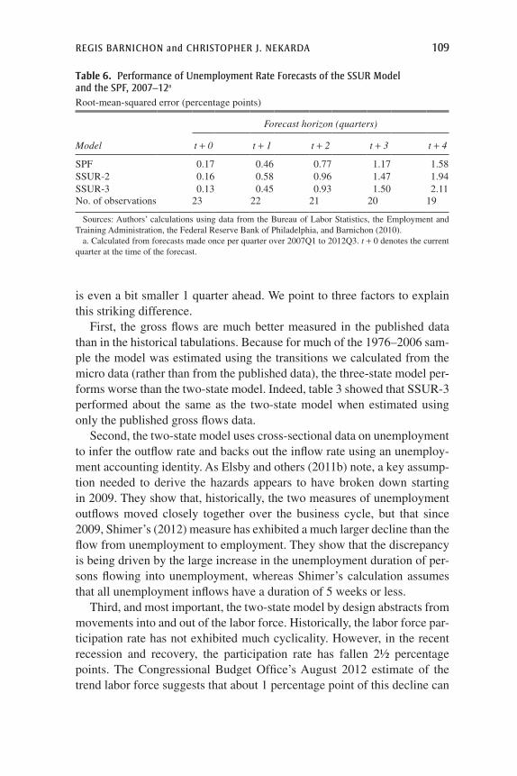
Figure 5 shows the time pattern of recent unemployment rate forecast misses by the SPF and the two SSUR models for both the current-quarter forecast (2 months of forecast; upper panel) and the next-quarter forecast (5 months of forecast; lower panel). A positive value indicates that the unemployment rate was higher than the model predicted. As the un-employment rate starts to increase, rising from 4.5 percent in the first quar-ter of 2007 to 4.8 percent at the end of 2007, the SPF and the SSUR models show relatively small upside surprises at both the t + 0 and t + 1 horizons (the unemployment rate was higher than projected). The unemployment rate then accelerates over 2008 and the first half of 2009, rising from 5 percent to 9½ percent. In 2008 the SSUR models and the SPF alike
−0.40.00.40.8
Percentage points
Percentage points
Current quarter
SPF
−0.4
0.0
0.4
0.8
One quarter ahead
Q4Q3Q1Q2Q4Q3Q1Q2Q4Q3Q1Q2Q4Q3Q1Q2Q4Q3Q1Q2Q4Q3Q1Q2201220112010200920082007
Q4Q3Q1Q2Q4Q3Q1Q2Q4Q3Q1Q2Q4Q3Q1Q2Q4Q3Q1Q2Q4Q3Q1Q2201220112010200920082007
Source: Authors’ calculations based on data from the Bureau of Labor Statistics, the Employment and Training Administration, and Barnichon (2010).
SSUR−3SSUR−2
Figure 5. Unemployment Forecast errors of the ssUr models and the spF, 2007–12
regis barnichon and christopher j. nekarda 111
show modest surprises to the upside in their current-quarter forecasts, with misses of about ¼ percentage point. However, from 2009 forward the three-state model consistently outperforms the SPF and the two-state model in the current quarter, with misses to both the upside and the down-side. At the 1-quarter-ahead horizon, the two-state model does noticeably worse than the SPF or the three-state model from 2009 on.
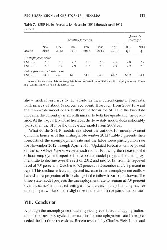
What do the SSUR models say about the outlook for unemployment 6 months hence as of this writing in November 2012? Table 7 presents their forecasts of the unemployment rate and the labor force participation rate for November 2012 through April 2013. (Updated forecasts will be posted on the Brookings Papers website each month following the release of the official employment report.) The two-state model projects the unemploy-ment rate to decline over the rest of 2012 and into 2013, from its reported level of 7.9 percent in October to 7.8 percent in December and 7.5 percent in April. This decline reflects a projected increase in the unemployment outflow hazard and a projection of little change in the inflow hazard (not shown). The three-state model projects the unemployment rate to remain at 7.9 percent over the same 6 months, reflecting a slow increase in the job finding rate for unemployed workers and a slight rise in the labor force participation rate.
VIII. Conclusion
Although the unemployment rate is typically considered a lagging indica-tor of the business cycle, increases in the unemployment rate have pre-ceded the last three recessions. Recent research by Charles Fleischman and
Table 7. ssUr model Forecasts for november 2012 through april 2013Percent
Monthly forecastsQuarterly averages
ModelNov. 2012
Dec. 2012
Jan. 2013
Feb. 2013
Mar. 2013
Apr. 2013
2012 Q4
2013 Q1
Unemployment rateSSUR-2 7.9 7.8 7.7 7.7 7.6 7.5 7.8 7.7SSUR-3 7.9 7.9 7.9 7.9 7.9 7.9 7.9 7.9
Labor force participation rateSSUR-3 64.0 64.0 64.1 64.1 64.2 64.2 63.9 64.1
Sources: Authors’ calculations using data from Bureau of Labor Statistics, the Employment and Train-ing Administration, and Barnichon (2010).
112 Brookings Papers on Economic Activity, Fall 2012
John Roberts (2011) finds that the unemployment rate provides the best single signal about the state of the business cycle in real time. Nevertheless, despite extensive research on the topic, forecasters and policymakers often rely on Okun’s law or basic time-series models to forecast the unemploy-ment rate.
This paper has presented a nonlinear unemployment rate forecasting model based on labor force flows that, in real time, dramatically outper-forms basic time-series models, the SPF, and the Federal Reserve Board’s Greenbook forecast at short horizons. Our model is built on two elements: a nonlinear law of motion describing how the unemployment rate con-verges to its conditional steady state (the rate of unemployment implied by the flows into and out of unemployment), and forecasts of these labor force flows. The model’s performance, in turn, stems from two factors: the convergence of unemployment to its conditional steady state with a lag of 3 to 5 months, and the fact that flows into and out of unemployment have different time-series properties than the stock.
Empirically, the two-state model has a root-mean-squared forecast error about 30 percent smaller than the next-best forecast for the current quarter, and 10 percent smaller for the next-quarter forecast. Moreover, our model has the highest predictive ability of those we analyze surrounding business cycle turning points and large recessions. And because the model brings new information to the forecast, a combination of our model’s forecast and the SPF forecast yields an improvement of about 35 percent for the current- quarter forecast and of 25 percent for the next-quarter forecast, with smaller improvements at longer horizons.
The two new models that we propose have both advantages and dis-advantages relative to each other. The two-state model is easier to under-stand conceptually and to implement. The duration-based unemployment inflow and outflow hazard rates have a longer history and are somewhat less noisy. However, these hazard rates are not directly measured but rather inferred from a theoretical model. More important, a key assumption for deriving the hazards appears to have broken down starting in 2009.
The three-state model is a more realistic characterization of the labor market and produces internally consistent forecasts for the unemployment rate, the labor force participation rate, and the employment-population ratio. Although the three-state model’s unemployment rate forecasts at longer horizons tend to be worse than those of the two-state model, since 2007 the three-state model outperforms the two-state model—as well as the SPF, in the near term—in part because it accounts for the large decline in labor force participation during this cycle.
regis barnichon and christopher j. nekarda 113
a p p e n d i x
Solving the Three-State Model
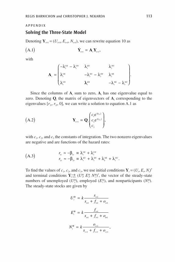
Denoting Yt+t = (Ut+t, Et+t, Nt+t), we can rewrite equation 10 as
A. ,1( ) =+ +�Y A Yt t tτ τ
with
At
tUE
tUN
tEU
tNU
tUE
tEU
tEN
tNE
tUN
=
− −
− −
λ λ λ λ
λ λ λ λ
λ λλ λ λtEN
tNE
tNU− −
.
Since the columns of At sum to zero, At has one eigenvalue equal to zero. Denoting Qt the matrix of eigenvectors of At corresponding to the eigenvalues [r1t, r2t, 0], we can write a solution to equation A.1 as
Aee. ,2
1
2
3
1
2( ) =
+
( )
( )Y Qt t
r
r
ccc
t
tτ
τ
τ
with c1, c2, and c3 the constants of integration. The two nonzero eigenvalues are negative and are functions of the hazard rates:
A.3 1 1
2 2
( ) ≈ − ≡ +≈ − ≡ + +
rr
t t tUE
tUN
t t tEU
tEN
β λ λβ λ λ λ tt
NEtNU+ λ .
To find the values of c1, c2, and c3, we use initial conditions Yt = (Ut, Et, Nt)′ and terminal conditions Y→
t→∞ (U*t, E*t, N*t )′, the vector of the steady-state numbers of unemployed (U*t ), employed (E*t ), and nonparticipants (N*t ). The steady-state stocks are given by
U ks
s f o
E kf
s f o
t
t
t t t
t
t
t t
*
*
=+ +
=+ +
+
+ + +
+
+ +
1
1 1 1
1
1 1 tt
t
t
t t t
N ko
s f o
+
+
+ + +
=+ +
1
1
1 1 1
* ,
114 Brookings Papers on Economic Activity, Fall 2012
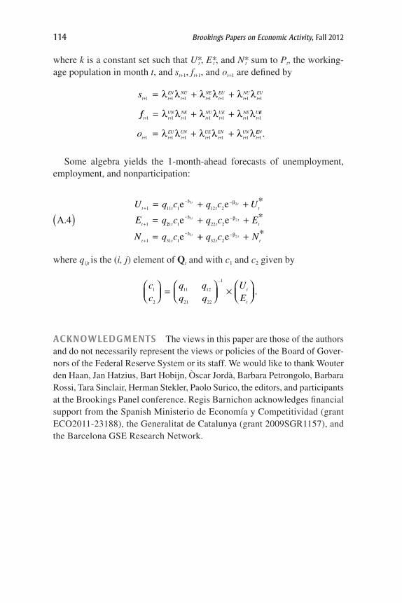
where k is a constant set such that U*t , E*t , and N*t sum to Pt, the working-age population in month t, and st+1, ft+1, and ot+1 are defined by
st tEN
tNU
tNE
tEU
tNU
tEU
+ + + + + + += + +1 1 1 1 1 1 1λ λ λ λ λ λ
fft tUN
tNE
tNU
tUE
tNE
tU
+ + + + + + += + +1 1 1 1 1 1 1λ λ λ λ λ λ EE
t tEU
tUN
tUE
tEN
tUN
to + + + + + + += + +1 1 1 1 1 1 1λ λ λ λ λ λEEN.
Some algebra yields the 1-month-ahead forecasts of unemployment, employment, and nonparticipation:
U q c q c U
E qt t t t
t
t t+
−
+
= + +
( ) =
−
1 11 1 12 2
1
1 2
4
e e
A
β β *
. 221 1 22 2
1 31 1
1 2
1
t t t
t t
c q c E
N q c
t t
t
e e
e
−
−
+ +
=
−
+
β
β
β *
++ +−q c Nt tt
32 22e β *
where qijt is the (i, j) element of Qt and with c1 and c2 given by
cc
q qq q
UE
t
t
1
2
11 12
21 22
1
=
×
−
.
ACKNOWLEDGMENTS The views in this paper are those of the authors and do not necessarily represent the views or policies of the Board of Gover-nors of the Federal Reserve System or its staff. We would like to thank Wouter den Haan, Jan Hatzius, Bart Hobijn, Òscar Jordà, Barbara Petrongolo, Barbara Rossi, Tara Sinclair, Herman Stekler, Paolo Surico, the editors, and participants at the Brookings Panel conference. Regis Barnichon acknowledges financial support from the Spanish Ministerio de Economía y Competitividad (grant ECO2011-23188), the Generalitat de Catalunya (grant 2009SGR1157), and the Barcelona GSE Research Network.
regis barnichon and christopher j. nekarda 115
References
Aaronson, Stephanie, Bruce Fallick, Andrew Figura, Jonathan Pingle, and William Wascher. 2006. “The Recent Decline in the Labor Force Participation Rate and Its Implications for Potential Labor Supply.” BPEA, no. 1: 169–54.
Baghestani, Hamid. 2008. “Federal Reserve versus Private Information: Who Is the Best Unemployment Rate Predictor?” Journal of Policy Modeling 30, no. 1: 101–10.
Barnichon, Regis. 2010. “Building a Composite Help-Wanted Index.” Economics Letters 109, no. 3: 175–78.
———. 2012. “Vacancy Posting, Job Separation, and Unemployment Fluctua-tions.” Journal of Economic Dynamics and Control 36, no. 3: 315–30.
Barnichon, Regis, and Andrew Figura. 2010. “What Drives Movements in the Unemployment Rate?” Finance and Economics Discussion Series no. 2010-48. Washington: Board of Governors of the Federal Reserve System.
Blanchard, Olivier Jean, and Peter Diamond. 1990. “The Cyclical Behavior of the Gross Flows of U.S. Workers.” BPEA, no. 2: 85–155.
Brown, Laura, and Saeed Moshiri. 2004. “Unemployment Variation over the Busi-ness Cycles: A Comparison of Forecasting Models.” Journal of Forecasting 23, no. 7: 497–511.
Congressional Budget Office. 2012. “Key Assumptions in Projecting Potential GDP—August 2012 Baseline.” Washington. www.cbo.gov/publication/43541.
Diebold, Francis X., and Roberto S. Mariano. 1995. “Comparing Predictive Accu-racy.” Journal of Business & Economic Statistics 13, no. 3: 253–63.
Elsby, Michael W. L., Bart Hobijn, and Aysegül Sahin. 2011a. “Unemploy-ment Dynamics in the OECD.” Working paper. Federal Reserve Bank of San Francisco.
Elsby, Michael W. L., Bart Hobijn, Aysegül Sahin, and Robert G. Valletta. 2011b. “The Labor Market in the Great Recession—An Update to September 2011.” BPEA, no. 2: 353–71.
Elsby, Michael W. L., Ryan Michaels, and Gary Solon. 2009. “The Ins and Outs of Cyclical Unemployment.” American Economic Journal: Macroeconomics 1, no. 1: 84–110.
Fallick, Bruce, and Jonathan Pingle. 2007. “A Cohort-Based Model of Labor Force Participation.” Finance and Economics Discussion Series no. 2007-09. Wash-ington: Board of Governors of the Federal Reserve System.
Faust, Jon, and Jonathan H. Wright. 2007. “Comparing Greenbook and Reduced Form Forecasts Using a Large Realtime Dataset.” Working Paper no. 13397. Cambridge, Mass.: National Bureau of Economic Research.
Fleischman, Charles A., and John M. Roberts. 2011. “From Many Series, One Cycle: Improved Estimates of the Business Cycle from a Multivari-ate Un observed Components Model.” Finance and Economics Discussion Series no. 2011-46. Washington: Board of Governors of the Federal Reserve System.
116 Brookings Papers on Economic Activity, Fall 2012
Fujita, Shigeru. 2011. “Dynamics of Worker Flows and Vacancies: Evidence from the Sign Restriction Approach.” Journal of Applied Econometrics 26, no. 1: 89–121.
Fujita, Shigeru, and Garey Ramey. 2009. “The Cyclicality of Separation and Job Finding Rates.” International Economic Review 50, no. 2: 415–30.
———. Forthcoming. “Exogenous vs. Endogenous Separation.” American Eco-nomic Journal: Macroeconomics.
Giacomini, Raffaella, and Barbara Rossi. 2010. “Forecast Comparisons in Un stable Environments.” Journal of Applied Econometrics 25, no. 4: 595–620.
Giacomini, Raffaella, and Halbert White. 2006. “Tests of Conditional Predictive Ability.” Econometrica 74, no. 6: 1545–78.
Golan, Amos, and Jeffrey M. Perloff. 2004. “Superior Forecasts of the U.S. Unemployment Rate Using a Nonparametric Method.” Review of Economics and Statistics 86, no. 1: 433–38.
Granger, Clive W., and Paul Newbold. 1986. Forecasting Economic Time Series. New York: Academic Press.
Hamilton, James D. 2005. “What's Real about the Business Cycle?” Federal Reserve Bank of St. Louis Review 87, no. 4: 435–52.
Milas, Costas, and Philip Rothman. 2008. “Out-of-Sample Forecasting of Un employment Rates with Pooled STVECM Forecasts.” International Jour-nal of Forecasting 24, no. 1: 101–21.
Mitchell, Wesley C. 1927. Business Cycles: The Problem and Its Setting. Cam-bridge, Mass.: National Bureau of Economic Research.
Montgomery, Alan L., Victor Zarnowitz, Ruey S. Tsay, and George C. Tiao. 1998. “Forecasting the U.S. Unemployment Rate.” Journal of the American Statistical Association 93, no. 442: 478–93.
Neftçi, Salih N. 1984. “Are Economic Time Series Asymmetric over the Business Cycle?” Journal of Political Economy 92, no. 2: 307–28.
Nekarda, Christopher J. 2009. “Understanding Unemployment Dynamics: The Role of Time Aggregation.” Washington: Board of Governors of the Federal Reserve System.
———. In preparation. “The Longitudinal Population Database.” Washington: Board of Governors of the Federal Reserve System.
Perry, George L. 1972. “Unemployment Flows in the U.S. Labor Market.” BPEA, no. 2: 245–78.
Petrongolo, Barbara, and Christopher A. Pissarides. 2008. “The Ins and Outs of European Unemployment.” American Economic Review 98, no. 2: 256–62.
Romer, Christina D., and David H. Romer. 2000. “Federal Reserve Information and the Behavior of Interest Rates.” American Economic Review 90, no. 3: 429–57.
Rothman, Philip A. 1991. “Further Evidence on the Asymmetric Behavior of Unemployment Rates over the Business Cycle.” Journal of Macroeconomics 13, no. 2: 291–98.
———. 1998. “Forecasting Asymmetric Unemployment Rates.” Review of Eco-nomics and Statistics 80, no. 1: 164–68.
regis barnichon and christopher j. nekarda 117
———. 2008. “Reconsideration of the Markov Chain Evidence on Unemployment Rate Asymmetry.” Studies in Nonlinear Dynamics and Econometrics 12, no. 3.
Shimer, Robert. 2012. “Reassessing the Ins and Outs of Unemployment.” Review of Economic Dynamics 15, no. 2: 127–48.
Sichel, Daniel E. 1989. “Are Business Cycles Asymmetric? A Correction.” Journal of Political Economy 97, no. 5: 1255–60.
———. 2007. “Business Cycle Asymmetry: A Deeper Look.” Economic Inquiry 31, no. 2: 224–36.
Sims, Christopher A. 2002. “The Role of Models and Probabilities in the Monetary Policy Process.” BPEA, no. 2: 1–62.
Stock, James H., and Mark W. Watson. 1999. “A Comparison of Linear and Non-linear Univariate Models for Forecasting Macroeconomic Time Series.” In Cointegration, Causality, and Forecasting: A Festschrift in Honor of Clive W. J. Granger, edited by Robert Engle and Halbert White. Oxford University Press.
Tulip, Peter. 2009. “Has the Economy Become More Predictable? Changes in Greenbook Forecast Accuracy.” Journal of Money, Credit and Banking 41, no. 6: 1217–31.
118
Comments and Discussion
Comment ByJAn HAtZIUS AnD SVen JARI SteHn We like the focus of this paper by Regis Barnichon and Christopher Nekarda, because the unemploy-ment rate is our “desert island” U.S. economic indicator, the one we would choose if we had to choose only one indicator to provide information about the economy. One reason is its value for estimating the amount of slack in the economy. As Federal Reserve Chairman Ben Bernanke noted in his August 2012 speech at Jackson Hole, “following every previous U.S. recession since World War II, the unemployment rate has returned close to its pre-recession level.” Although there are certainly more sophisticated ways to measure the output gap, one could do worse than start from the observation that the unemployment rate in the fall of 2012 is about 2 per-centage points above its postwar average of 5.8 percent.
But an equally important reason why we view the unemployment rate as so important is its value in diagnosing recessions. This is one of the most important, yet most daunting, jobs for business forecasters such as ourselves. On the one hand, we are all painfully aware that we as a pro-fession have a terrible track record in recognizing recessions when they occur—not to mention forecasting them successfully. On the other hand, we also know that nothing destroys one’s reputation as reliably as crying wolf about a recession that then fails to materialize. And of course, that is the reason why forecasters tend to be late in calling recessions. Being human, we want to be reasonably sure before we stick our necks out.
Thus, any tool that allows forecasters to get a leg up in forecasting or diagnosing a recession is highly valuable, and one of our favorite tools is the plain old unemployment rate. Over the 64 years since monthly unem-ployment data first became available, the (unrounded) unemployment rate has never risen more than 0.35 percentage point on a 3-month moving-
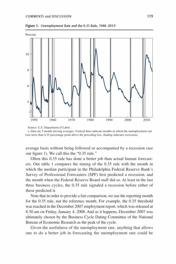
comments and discussion 119
average basis without being followed or accompanied by a recession (see our figure 1). We call this the “0.35 rule.”
Often this 0.35 rule has done a better job than actual human forecast-ers. Our table 1 compares the timing of the 0.35 rule with the month in which the median participant in the Philadelphia Federal Reserve Bank’s Survey of Professional Forecasters (SPF) first predicted a recession, and the month when the Federal Reserve Board staff did so. At least in the last three business cycles, the 0.35 rule signaled a recession before either of these predicted it.
Note that in order to provide a fair comparison, we use the reporting month for the 0.35 rule, not the reference month. For example, the 0.35 threshold was reached in the December 2007 employment report, which was released at 8.30 am on Friday, January 4, 2008. And as it happens, December 2007 was ultimately chosen by the Business Cycle Dating Committee of the National Bureau of Economic Research as the peak of the cycle.
Given the usefulness of the unemployment rate, anything that allows one to do a better job in forecasting the unemployment rate could be
Source: U.S. Department of Labor.a. Data are 3-month moving averages. Vertical lines indicate months in which the unemployment rate
rose more than 0.35 percentage point above the preceding low; shading indicates recessions.
4
6
8
10
Percent
1950 1960 1970 1980 1990 2000 2010
Figure 1. unemployment Rate and the 0.35 Rule, 1948–2012a
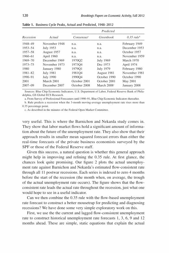
120 Brookings Papers on Economic Activity, Fall 2012
table 1. Business cycle Peaks, Actual and Predicted, 1948–2012
Predicted
Recession Actual Consensusa Greenbook 0.35 ruleb
1948–49 November 1948 n.a. n.a. February 19491953–54 July 1953 n.a. n.a. December 19531957–58 August 1957 n.a. n.a. October 19571960–61 April 1960 n.a. n.a. November 19591969–70 December 1969 1970Q2 July 1969 March 19701973–75 November 1973 1973Q4 Dec 1973 April 19741980 January 1980 1979Q1 July 1979 February 19801981–82 July 1981 1981Q4 August 1981 November 19811990–91 July 1990 1990Q4 October 1990 October 19902001 March 2001 October 2001 October 2001 May 20012007–09 December 2007 October 2008 March 2008c January 2008
Sources: Blue Chip Economic Indicators, U.S. Department of Labor, Federal Reserve Bank of Phila-delphia, GS Global ECS Research.
a. From Survey of Professional Forecasters until 1990–91, Blue Chip Economic Indicators thereafter.b. Rule predicts a recession when the 3-month moving-average unemployment rate rises more than
0.35 percentage point.c. As described in the minutes of the Federal Open Market Committee.
very useful. This is where the Barnichon and Nekarda study comes in. They show that labor market flows hold a significant amount of informa-tion about the future of the unemployment rate. They also show that their approach results in smaller mean squared forecast errors than either the real-time forecasts of the private business economists surveyed by the SPF or those of the Federal Reserve staff.
Given this success, a natural question is whether this general approach might help in improving and refining the 0.35 rule. At first glance, the chances look quite promising. Our figure 2 plots the actual unemploy-ment rate against Barnichon and Nekarda’s estimated flow-consistent rate through all 11 postwar recessions. Each series is indexed to zero 4 months before the start of the recession (the month when, on average, the trough of the actual unemployment rate occurs). The figure shows that the flow-consistent rate leads the actual rate throughout the recession, just what one would hope to see in a useful indicator.
Can we then combine the 0.35 rule with the flow-based unemployment rate forecast to construct a better mousetrap for predicting and diagnosing recessions? We have done some very simple exploratory work on this.
First, we use the the current and lagged flow-consistent unemployment rate to construct historical unemployment rate forecasts 1, 3, 6, 9 and 12 months ahead. These are simple, static equations that explain the actual
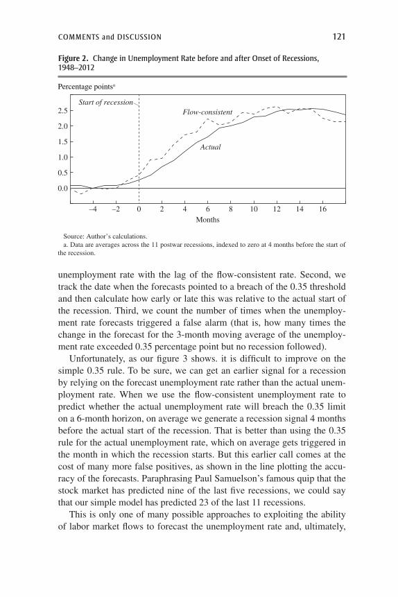
comments and discussion 121
unemployment rate with the lag of the flow-consistent rate. Second, we track the date when the forecasts pointed to a breach of the 0.35 threshold and then calculate how early or late this was relative to the actual start of the recession. Third, we count the number of times when the unemploy-ment rate forecasts triggered a false alarm (that is, how many times the change in the forecast for the 3-month moving average of the unemploy-ment rate exceeded 0.35 percentage point but no recession followed).
Unfortunately, as our figure 3 shows. it is difficult to improve on the simple 0.35 rule. To be sure, we can get an earlier signal for a recession by relying on the forecast unemployment rate rather than the actual unem-ployment rate. When we use the flow-consistent unemployment rate to predict whether the actual unemployment rate will breach the 0.35 limit on a 6-month horizon, on average we generate a recession signal 4 months before the actual start of the recession. That is better than using the 0.35 rule for the actual unemployment rate, which on average gets triggered in the month in which the recession starts. But this earlier call comes at the cost of many more false positives, as shown in the line plotting the accu-racy of the forecasts. Paraphrasing Paul Samuelson’s famous quip that the stock market has predicted nine of the last five recessions, we could say that our simple model has predicted 23 of the last 11 recessions.
This is only one of many possible approaches to exploiting the ability of labor market flows to forecast the unemployment rate and, ultimately,
Figure 2. change in unemployment Rate before and after onset of Recessions, 1948–2012
Source: Author’s calculations.a. Data are averages across the 11 postwar recessions, indexed to zero at 4 months before the start of
the recession.
0.0
0.5
1.0
1.5
2.0
2.5
Actual
Flow-consistent
Months–4 –2 0 2 4 6 8 10 12 14 16
Start of recession
Percentage pointsa
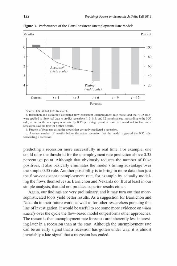
122 Brookings Papers on Economic Activity, Fall 2012
predicting a recession more successfully in real time. For example, one could raise the threshold for the unemployment rate prediction above 0.35 percentage point. Although that obviously reduces the number of false positives, it also basically eliminates the model’s timing advantage over the simple 0.35 rule. Another possibility is to bring in more data than just the flow-consistent unemployment rate, for example by actually model-ing the flows themselves as Barnichon and Nekarda do. But at least in our simple analysis, that did not produce superior results either.
Again, our findings are very preliminary, and it may turn out that more-sophisticated tools yield better results. As a suggestion for Barnichon and Nekarda in their future work, as well as for other researchers pursuing this line of investigation, it would be useful to see some more evidence on when exactly over the cycle the flow-based model outperforms other approaches. The reason is that unemployment rate forecasts are inherently less interest-ing later in a recession than at the start. Although the unemployment rate can be an early signal that a recession has gotten under way, it is almost invariably a late signal that a recession has ended.
Figure 3. Performance of the Flow-consistent unemployment Rate modela
Source: GS Global ECS Research.a. Barnichon and Nekarda's estimated flow-consistent unemployment rate model and the “0.35 rule”
were applied to historical data to predict recessions 1, 3, 6, 9, and 12 months ahead. According to the 0.35 rule, a rise in the unemployment rate by 0.35 percentage point or more is considered to forecast a recession. See the text for further details.
b. Percent of forecasts using the model that correctly predicted a recession.c. Average number of months before the actual recession that the model triggered the 0.35 rule,
forecasting a recession.
20
40
60
80
100
4
3
2
1
0
Accuracyb
(right scale)
Current
Forecast
t + 1 t + 3 t + 6 t + 9 t + 12
Months Percent
Timingc
(right scale)
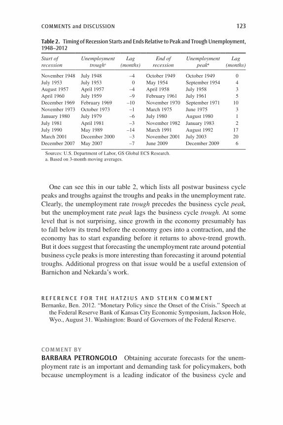
comments and discussion 123
table 2. timing of Recession starts and ends Relative to Peak and trough unemployment, 1948–2012
Start of recession
Unemployment trougha
Lag (months)
End of recession
Unemployment peaka
Lag (months)
November 1948 July 1948 –4 October 1949 October 1949 0July 1953 July 1953 0 May 1954 September 1954 4August 1957 April 1957 –4 April 1958 July 1958 3April 1960 July 1959 –9 February 1961 July 1961 5December 1969 February 1969 –10 November 1970 September 1971 10November 1973 October 1973 –1 March 1975 June 1975 3January 1980 July 1979 –6 July 1980 August 1980 1July 1981 April 1981 –3 November 1982 January 1983 2July 1990 May 1989 –14 March 1991 August 1992 17March 2001 December 2000 –3 November 2001 July 2003 20December 2007 May 2007 –7 June 2009 December 2009 6
Sources: U.S. Department of Labor, GS Global ECS Research.a. Based on 3-month moving averages.
One can see this in our table 2, which lists all postwar business cycle peaks and troughs against the troughs and peaks in the unemployment rate. Clearly, the unemployment rate trough precedes the business cycle peak, but the unemployment rate peak lags the business cycle trough. At some level that is not surprising, since growth in the economy presumably has to fall below its trend before the economy goes into a contraction, and the economy has to start expanding before it returns to above-trend growth. But it does suggest that forecasting the unemployment rate around potential business cycle peaks is more interesting than forecasting it around potential troughs. Additional progress on that issue would be a useful extension of Barnichon and Nekarda’s work.
R e F e R e n c e F o R t h e h A t z i u s A n d s t e h n c o m m e n tBernanke, Ben. 2012. “Monetary Policy since the Onset of the Crisis.” Speech at
the Federal Reserve Bank of Kansas City Economic Symposium, Jackson Hole, Wyo., August 31. Washington: Board of Governors of the Federal Reserve.
Comment ByBARBARA PetRonGoLo Obtaining accurate forecasts for the unem-ployment rate is an important and demanding task for policymakers, both because unemployment is a leading indicator of the business cycle and
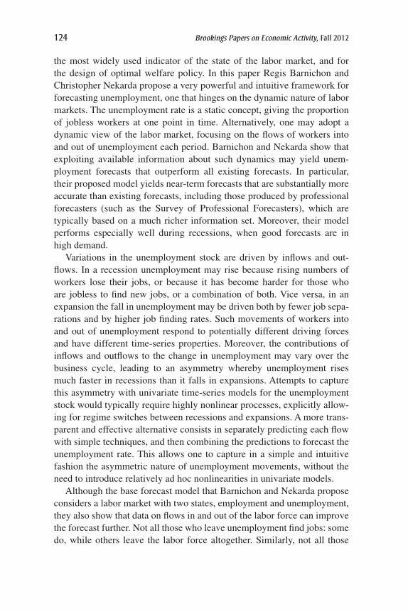
124 Brookings Papers on Economic Activity, Fall 2012
the most widely used indicator of the state of the labor market, and for the design of optimal welfare policy. In this paper Regis Barnichon and Christopher Nekarda propose a very powerful and intuitive framework for forecasting unemployment, one that hinges on the dynamic nature of labor markets. The unemployment rate is a static concept, giving the proportion of jobless workers at one point in time. Alternatively, one may adopt a dynamic view of the labor market, focusing on the flows of workers into and out of unemployment each period. Barnichon and Nekarda show that exploiting available information about such dynamics may yield unem-ployment forecasts that outperform all existing forecasts. In particular, their proposed model yields near-term forecasts that are substantially more accurate than existing forecasts, including those produced by professional forecasters (such as the Survey of Professional Forecasters), which are typically based on a much richer information set. Moreover, their model performs especially well during recessions, when good forecasts are in high demand.
Variations in the unemployment stock are driven by inflows and out-flows. In a recession unemployment may rise because rising numbers of workers lose their jobs, or because it has become harder for those who are jobless to find new jobs, or a combination of both. Vice versa, in an expansion the fall in unemployment may be driven both by fewer job sepa-rations and by higher job finding rates. Such movements of workers into and out of unemployment respond to potentially different driving forces and have different time-series properties. Moreover, the contributions of inflows and outflows to the change in unemployment may vary over the business cycle, leading to an asymmetry whereby unemployment rises much faster in recessions than it falls in expansions. Attempts to capture this asymmetry with univariate time-series models for the unemployment stock would typically require highly nonlinear processes, explicitly allow-ing for regime switches between recessions and expansions. A more trans-parent and effective alternative consists in separately predicting each flow with simple techniques, and then combining the predictions to forecast the unemployment rate. This allows one to capture in a simple and intuitive fashion the asymmetric nature of unemployment movements, without the need to introduce relatively ad hoc nonlinearities in univariate models.
Although the base forecast model that Barnichon and Nekarda propose considers a labor market with two states, employment and unemployment, they also show that data on flows in and out of the labor force can improve the forecast further. Not all those who leave unemployment find jobs: some do, while others leave the labor force altogether. Similarly, not all those
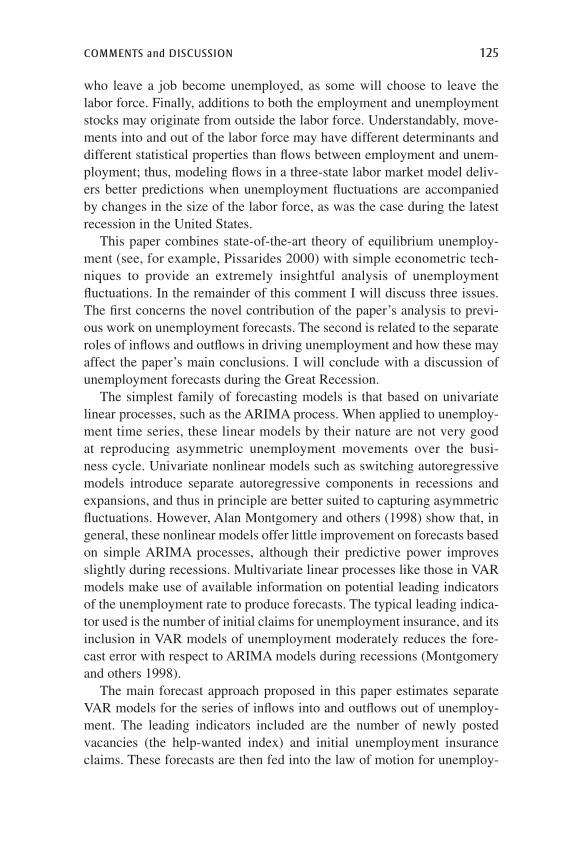
comments and discussion 125
who leave a job become unemployed, as some will choose to leave the labor force. Finally, additions to both the employment and unemployment stocks may originate from outside the labor force. Understandably, move-ments into and out of the labor force may have different determinants and different statistical properties than flows between employment and unem-ployment; thus, modeling flows in a three-state labor market model deliv-ers better predictions when unemployment fluctuations are accompanied by changes in the size of the labor force, as was the case during the latest recession in the United States.
This paper combines state-of-the-art theory of equilibrium unemploy-ment (see, for example, Pissarides 2000) with simple econometric tech-niques to provide an extremely insightful analysis of unemployment fluctuations. In the remainder of this comment I will discuss three issues. The first concerns the novel contribution of the paper’s analysis to previ-ous work on unemployment forecasts. The second is related to the separate roles of inflows and outflows in driving unemployment and how these may affect the paper’s main conclusions. I will conclude with a discussion of unemployment forecasts during the Great Recession.
The simplest family of forecasting models is that based on univariate linear processes, such as the ARIMA process. When applied to unemploy-ment time series, these linear models by their nature are not very good at reproducing asymmetric unemployment movements over the busi-ness cycle. Univariate nonlinear models such as switching autoregressive models introduce separate autoregressive components in recessions and expansions, and thus in principle are better suited to capturing asymmetric fluctuations. However, Alan Montgomery and others (1998) show that, in general, these nonlinear models offer little improvement on forecasts based on simple ARIMA processes, although their predictive power improves slightly during recessions. Multivariate linear processes like those in VAR models make use of available information on potential leading indicators of the unemployment rate to produce forecasts. The typical leading indica-tor used is the number of initial claims for unemployment insurance, and its inclusion in VAR models of unemployment moderately reduces the fore-cast error with respect to ARIMA models during recessions (Montgomery and others 1998).
The main forecast approach proposed in this paper estimates separate VAR models for the series of inflows into and outflows out of unemploy-ment. The leading indicators included are the number of newly posted vacancies (the help-wanted index) and initial unemployment insurance claims. These forecasts are then fed into the law of motion for unemploy-
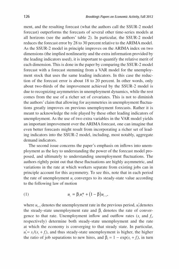
126 Brookings Papers on Economic Activity, Fall 2012
ment, and the resulting forecast (what the authors call the SSUR-2 model forecast) outperforms the forecasts of several other time-series models at all horizons (see the authors’ table 2). In particular, the SSUR-2 model reduces the forecast error by 28 to 30 percent relative to the ARIMA model. As the SSUR-2 model in principle improves on the ARIMA index on two dimensions (the implied nonlinearity and the extra information provided by the leading indicators used), it is important to quantify the relative merit of each dimension. This is done in the paper by comparing the SSUR-2 model forecast with a forecast stemming from a VAR model for the unemploy-ment stock that uses the same leading indicators. In this case the reduc-tion of the forecast error is about 18 to 20 percent. In other words, only about two-thirds of the improvement achieved by the SSUR-2 model is due to recognizing asymmetries in unemployment dynamics, while the rest comes from the use of a richer set of covariates. This is not to diminish the authors’ claim that allowing for asymmetries in unemployment fluctua-tions greatly improves on previous unemployment forecasts. Rather it is meant to acknowledge the role played by these other leading indicators of unemployment. As the use of two extra variables in the VAR model yields an important improvement over the ARIMA forecast, one can imagine that even better forecasts might result from incorporating a richer set of lead-ing indicators into the SSUR-2 model, including, most notably, aggregate demand indicators.
The second issue concerns the paper’s emphasis on inflows into unem-ployment as the key to understanding the power of the forecast model pro-posed, and ultimately to understanding unemployment fluctuations. The authors rightly point out that these fluctuations are highly asymmetric, and variations in the rate at which workers separate from existing jobs can in principle account for this asymmetry. To see this, note that in each period the rate of unemployment ut converges to its steady-state value according to the following law of motion
(1)
u u ut t t t= + −( ) −β β* ,1 1
where ut-1 denotes the unemployment rate in the previous period, ut*denotes
the steady-state unemployment rate and bt denotes the rate of conver-gence to that rate. Unemployment inflow and outflow rates (st and ft, respectively) determine both steady-state unemployment and the rate at which the economy is converging to that steady state. In particular, ut
*= st/(st + ft), and thus steady-state unemployment is higher, the higher the ratio of job separations to new hires, and bt = 1 - exp(st + ft), in turn
comments and discussion 127
implying that a labor market with high turnover (through inflows or out-flows or both) will converge to its steady state faster. Consider the case in which unemployment fluctuations at business cycle frequencies are driven by fluctuations in the unemployment inflow rate. In a recession, the rise in the inflow rate raises both steady-state unemployment and the rate at which the economy converges to it, leading to a sharp increase in unem-ployment. In the following expansion, when the inflow rate reverts to its prerecession level, steady-state unemployment falls but convergence to its new value is slower, and the resulting fall in the unemployment rate is thus more gradual.
This mechanism is quite intuitive but may not fit the evidence so well if unemployment fluctuations have an important outflow component as well. To take a simple example, if unemployment fluctuations were solely driven by fluctuations in its outflow rate, my equation 1 would imply that unemployment rises slowly in recessions and falls sharply in expansions. Although this represents an extreme scenario, evidence on labor market flows clearly indicates that fluctuations in the outflow rate cannot be easily overlooked. Indeed, the recently renewed interest in the “ins and outs of unemployment” was largely prompted by Robert Hall’s Review of Eco-nomic and Statistics lecture, and in particular his claim that “In the modern U.S. economy, recessions do not begin with a burst of layoffs. Unemploy-ment rises because jobs are hard to find, not because an unusual number of people are thrown into unemployment” (Hall 2005, p. 397). There is now a large and growing literature that decomposes unemployment fluctuations over the business cycle into inflow- and outflow-driven components. Rob-ert Shimer (2012) reports findings that are close in spirit to Hall’s (2005) claim, concluding that fluctuations in the job finding probability account for three-quarters of unemployment fluctuations in the postwar period, and even more than that in the past two decades, including the Great Recession. Other papers (such as Elsby, Michaels, and Solon 2009, Fujita and Ramey 2009, and Barnichon 2012) use slightly different measurements and meth-odologies from those in Shimer (2012) and agree in documenting more balanced roles of inflows and outflows in accounting for unemployment cycles. Even so, the common thread is that the outflow rate from unem-ployment is responsible for at least half of the observed unemployment dynamics over the business cycle.
Given the existing evidence, one may regard this paper’s emphasis on the role of unemployment inflows as less than fully justified. Indeed, one of the leading indicators of unemployment used is the help-wanted index, which is one of the main determinants of the job finding rate, and this is
128 Brookings Papers on Economic Activity, Fall 2012
shown to improve the unemployment forecasts relative to models with a poorer information set. This result in itself stresses the role of the outflow rate in an unemployment forecast model. A final observation on the inflow-outflow split is provided by the bottom two rows in the authors’ table 2, which illustrate what happens to unemployment forecasts when one shuts off the feed from either flow on the unemployment rate and predicts unem-ployment solely from a VAR model for the other flow. Whether one shuts down the inflow or the outflow channel, the forecast error is virtually iden-tical at all horizons, again emphasizing the importance of both flows.
My third issue addresses the predictive power of a flow-based fore-cast model applied to data from the Great Recession. The labor market downturn that accompanied that recession in the United States delivered the sharpest increase in unemployment of the postwar era: the jobless rate doubled within 2 years, reaching a peak of 10 percent by the end of 2009. The recovery that followed was slow and uneven. When used to forecast these developments, the SSUR-2 model tends to fare worse than in previ-ous recessions, and worse than the SPF. One possible explanation rests on the forecast used for the unemployment outflow. In other words, my previous concern about adequately recognizing the role of the exit rate from unemployment applies even more forcefully to the Great Recession, which was marked by an unprecedented fall in the exit rate from about 50 percent in early 2008 to 24 percent in late 2010 (see Elsby, Hobijn, and Sahin 2010 and Elsby and others 2011). Such a sharp and massive fall may be hard to forecast accurately with the VAR specification adopted. More-over, the consequent increase in the incidence of long-term unemployment would hinder recovery, insofar as job finding rates fall with unemployment duration, further complicating subsequent unemployment forecasts. This problem calls for richer models for outflow forecasts, possibly taking into account the distribution of duration across unemployment spells.
The other potential explanation for the relative failure of the SSUR-2 model since 2007 stems from another unique feature of the Great Reces-sion, namely, the record fall in labor force participation since the end of 2008—its steepest decline since the 1950s (Elsby and others 2011). As noted above, a two-state labor market model will fail to capture these developments, but this is precisely where the authors’ flow model can sub-stantially improve the forecast, by incorporating flows into and out of the labor force as their SSUR-3 model does. Although the behavior of the labor force participation rate was largely acyclical during 2007 and 2008, the forecast miss of the SSUR-3 model was indeed quite similar to that of the SSUR-2 model. But since labor force participation started to fall in early
comments and discussion 129
2009, the SSUR-3 model has tended to outperform the SSUR-2, and at times the SPF as well. This again highlights how modeling labor market flows can deliver a simple yet powerful and versatile toolkit for forecasting unemployment.
R e F e R e n c e s F o R t h e P e t R o n g o l o c o m m e n tBarnichon, Regis. 2012. “Vacancy Posting, Job Separation and Unemployment
Fluctuations.” Journal of Economic Dynamics and Control 36: 315–30.Elsby, Michael, Bart Hobijn, and Aysegül Sahin. 2010. “The Labor Market in the
Great Recession.” BPEA (Spring): 1–48.Elsby, Michael, Ryan Michaels, and Gary Solon. 2009. “The Ins and Outs of Cycli-
cal Unemployment.” American Economic Journal: Macroeconomics 1: 84–110.Elsby, Michael, Bart Hobijn, Aysegül Sahin, and Robert Valletta. 2011. “The Labor
Market in the Great Recession: An Update.” BPEA (Fall): 353–71.Fujita, Shigeru, and Garey Ramey. 2009. “The Cyclicality of Separation and Job
Finding Rates.” International Economic Review 50: 415–30.Hall, Robert. 2005. “Employment Efficiency and Sticky Wages: Evidence from
Flows in the Labor Market.” Review of Economics and Statistics 87: 397–407.Montgomery, Alan, Victor Zarnowitz, Ruey Tsay, and George Tiao. 1998. “Fore-
casting the U.S. Unemployment Rate.” Journal of the American Statistical Association 93: 478–93.
Pissarides, Christopher. 2000. Equilibrium Unemployment Theory, 2nd ed. MIT Press.
Shimer, Robert. 2012. “Reassessing the Ins and Outs of Unemployment.” Review of Economic Dynamics 15: 127–48.
GeneRAL DISCUSSIon John Haltiwanger commended the paper’s focus on unemployment flows but suspected that its model did not predict outflow rates very well, and those were precisely the puzzle in today’s economy. He pointed out that the 1981–82 recession looked similar to the most recent recession on the inflow side but that the two differed greatly on the outflow side, with the earlier recession showing a much swifter recovery. The paper’s emphasis on inflows, in Haltiwanger’s view, caused it to miss that difference.
George Perry felt that the authors were being too hard on themselves in comparing their model’s predictions with those of the Greenbook and other professional forecasters: whereas the latter drew on a great variety of information sources, the authors’ model limited its information set to employment flows alone. He thought the fact that the model did so well in that comparison despite its restricted information set should be applauded.
130 Brookings Papers on Economic Activity, Fall 2012
Ricardo Reis was enthusiastic about the paper but was dissatisfied with its theoretical justification of its flows-based approach. He could think of reasons why the approach might do worse than the traditional approach in theory even though it seemed to do better in practice: the job finding and job separation rates could vary greatly, for example, or the unemployment rate might be more linear than the job finding and job separation rates, in which case the model’s linear VAR estimate would not yield better esti-mates than a traditional model. Reis also agreed with Barbara Petrongolo that the flow-based approach might not be providing additional informa-tion. He therefore thought the authors needed to explain more convinc-ingly why their approach worked as well as it did.
Reis also raised an issue of forecast methodology: is it better to fore-cast the sum of two rates directly or to forecast each rate separately and sum the forecasts? He argued that the first approach works better in the case of GDP and wondered why the authors believed the second was bet-ter for unemployment. Similarly, Reis asked, was it better to forecast the unemployment rate one year out directly or to forecast for each month or quarter iteratively to arrive at an annual estimate?
Robert Moffitt noted that the aggregate unemployment rate is dispro-portionately affected by the long-term unemployed. Given that fact, he wondered whether the model’s predictive ability could be improved by categorizing the unemployed by duration of unemployment and then esti-mating flows between lengths of unemployment.
Justin Wolfers, citing the importance of revealed preferences, asked Jan Hatzius whether Goldman Sachs had begun running a flow-based model of unemployment. Hatzius replied that it had.
Valerie Ramey suggested that the authors compare their results against those in a 2005 paper by James Hamilton, which also noted the asymme-tries and nonlinearities in the unemployment rate. Hamilton used a three-stage Markov model, and Ramey suggested that some of his techniques might be incorporated into the authors’ flow model.
Robert Hall suggested using aggregate labor demand to predict whether unemployment would increase or decrease and then using a labor match-ing function to estimate the job finding rate. He also suggested that one reason the authors’ model outperformed those of professional forecasters might be simply that the latter pay less attention to the unemployment rate than to other macroeconomic variables and therefore devote fewer resources to forecasting it.
Responding to the discussion, Regis Barnichon said that he and Nekarda understood the intuition behind their model’s success to have two parts: the
comments and discussion 131
first was their simple bathtub analogy, which says that, given flows, one can calculate what the future stock will be. However, to do that, one first needs to forecast the flows, and the model is good at forecasting unemploy-ment because the flows are sufficiently persistent to be well predicted over the time needed to converge to steady state. The second part was that their model can capture the asymmetry in unemployment, because the asymme-try comes from the different behavior of the inflow and outflow rates over the cycle. In recessions, inflows rise rapidly but also revert to the mean rapidly, while outflows fall and rise more gradually.
Barnichon explained that their three-stage model does not explain the unemployment rate well before 1990 because the data for that period are of much poorer quality. When better data become available, the forecasts of the three-stage model should improve substantially. Replying to Halti-wanger, Barnichon said that the model does not predict the outflows to unemployment well because it does not address the efficiency matching problem. But the model uses a 15-year rolling window to predict the out-flow rate and thus slowly incorporates the fact that the outflow rate has fallen below historical norms.
Christopher Nekarda added that the model is methodologically very simple: flows are estimated by a linear VAR model. Additional informa-tion about these flows would substantially improve the forecast. As Bar-nichon had noted, the model has a strong tendency to revert to historical means, and that was one reason the model performs poorly after 2007: actual unemployment outflows have been much lower than their histori-cal average. Nekarda agreed with Hatzius that the unemployment rate is noisy but argued that a threshold is used precisely to overcome the noise. Thus, the model’s early forecasts remain valuable. Lastly, Nek-arda agreed with Moffitt that examining differences in unemployment duration might be valuable, but he conjectured that because duration is determined by the flows, integrating over the flows would reproduce the duration of unemployment.

Related Documents