THE INFLUENCE OF THE SITE FACTOR WIND EXPOSURE ON WOOD QUALITY Final Report: Project FAIR CT 98 5038 Period: 5.10.1998 – 4.10.2000 A European Commission funded Training Grant with Assistance from the Forestry Commission, James Jones and Sons Ltd., and the Building Research Establishment. Franka Brüchert Forestry Commission, Northern Research Station Roslin, Midlothian EH25 9SY, Scotland

Welcome message from author
This document is posted to help you gain knowledge. Please leave a comment to let me know what you think about it! Share it to your friends and learn new things together.
Transcript

THE INFLUENCE OF THE SITE FACTOR WIND
EXPOSURE ON WOOD QUALITY
Final Report: Project FAIR CT 98 5038
Period: 5.10.1998 – 4.10.2000
A European Commission funded Training Grant with Assistance from
the Forestry Commission, James Jones and Sons Ltd., and the Building
Research Establishment.
Franka Brüchert Forestry Commission, Northern Research Station
Roslin, Midlothian EH25 9SY, Scotland

Table of contents
1 Objectives: ......................................................................................................................................... 7
2 Working Programme: ........................................................................................................................ 8
3 Methodology...................................................................................................................................... 9
3.1 Stand and tree selection: ................................................................................................................ 9
3.1.1 Stand selection ....................................................................................................................... 9
3.1.2 Tree selection......................................................................................................................... 9
3.2 Sampling strategy ........................................................................................................................ 11
3.3 Tree characterisation.................................................................................................................... 12
3.3.1 Spatial competition and tree morphometry.......................................................................... 12
3.3.2 The mechanical properties of the standing stem.................................................................. 14
3.4 Internal stem structure ................................................................................................................. 15
3.4.1 Density of fresh disc material .............................................................................................. 15
3.4.2 Density of air-dry disc material: .......................................................................................... 15
3.4.3 Ring width............................................................................................................................ 15
3.5 Roundwood and saw log assessment ........................................................................................... 16
3.5.1 Branchiness.......................................................................................................................... 17
3.5.2 Ring width............................................................................................................................ 17
3.5.3 Spiral grain........................................................................................................................... 17
3.5.4 Position of the pith............................................................................................................... 18
3.5.5 Log taper .............................................................................................................................. 18
3.6 End-product ................................................................................................................................. 18
3.6.1 Machine stress grading ........................................................................................................ 19
3.6.2 Kiln drying........................................................................................................................... 20
3.6.3 Dimensional stability ........................................................................................................... 21
3.6.4 Modulus of Elasticity, Modulus of Rupture......................................................................... 21
3.6.5 Juvenile wood ...................................................................................................................... 21
3.6.6 Density ................................................................................................................................. 22
3.6.7 Knottiness ............................................................................................................................ 22
3.6.8 Grain angle........................................................................................................................... 23
3.6.9 Compression wood .............................................................................................................. 23
4 Results.............................................................................................................................................. 25
4.1 Selection and characterisation of the site. General stand characteristics ..................................... 25
4.2 Characterisation of the sample trees: ........................................................................................... 26
4.2.1 Size and shape of the sample trees....................................................................................... 26
4.2.2 Straightness score ................................................................................................................ 29

3
Table of content (cont.)
4.2.3 Mechanical properties of the standing trees......................................................................... 30
4.2.3.1 Static pulling tests, structural Young’s modulus (MOEstruct) ....................................... 30
4.2.3.2 Dynamic pulling tests, swaying frequency .................................................................. 34
4.2.4 Internal stem structure ......................................................................................................... 37
4.2.4.1 Density of the fresh discs ............................................................................................. 37
4.2.4.2 Density of air dry discs ................................................................................................ 38
4.2.4.3 Radial increment .......................................................................................................... 39
4.3 Roundwood and saw log assessment ........................................................................................... 41
4.3.1 Branchiness.......................................................................................................................... 41
4.3.2 Ring width............................................................................................................................ 43
4.3.3 Spiral grain........................................................................................................................... 45
4.3.4 Position of the pith (log eccentricity)................................................................................... 47
4.3.5 Log taper .............................................................................................................................. 48
4.3.6 Log ovality........................................................................................................................... 50
4.3.7 Proportion of juvenile wood ................................................................................................ 52
4.3.8 Log classification according to ENV 1927-1....................................................................... 53
4.4 End product, quality of battens .................................................................................................... 55
4.4.1 Stress grading....................................................................................................................... 55
4.4.2 Modulus of elasticity, modulus of rupture ........................................................................... 57
4.4.3 Distortion ............................................................................................................................. 61
4.4.3.1 Twist ............................................................................................................................ 61
4.4.3.2 Bow.............................................................................................................................. 63
4.4.3.3 Spring........................................................................................................................... 64
4.4.4 Structural characteristics of the battens ............................................................................... 66
4.4.4.1 Density ......................................................................................................................... 66
4.4.4.2 Juvenile wood .............................................................................................................. 67
4.4.4.3 Compression wood....................................................................................................... 68
4.4.4.4 Grain angle................................................................................................................... 69
4.4.4.5 Knottiness .................................................................................................................... 70
5 Summary.......................................................................................................................................... 72
6 References........................................................................................................................................ 74

4
Table of figures
Figure 1: Variation of the normalised bending moment of the sample trees ............................................. 9
Figure 2: Position of the measurement lines within the site in relation to the edge ................................ 10
Figure 3: Variation of bending moment of the sample trees with age ..................................................... 11
Figure 4: Sampling pattern of saw logs and stem discs ........................................................................... 11
Figure 5: triangle method to estimate crown projection area................................................................... 13
Figure 6: Set up for tree pulling and tree swaying experiments .............................................................. 14
Figure 7: Cutting scheme of logs............................................................................................................. 19
Figure 8: Types of distortion of sawn timber........................................................................................... 21
Figure 9: Setup of grain angle measurements on battens......................................................................... 23
Figure 10: Setup for measuring compression wood area........................................................................ 24
Figure 11: Variation of mean and standard deviation of dbh, height and height-to-diameter-ratio ........ 27
Figure 12: Variation of tree height and the height of the crown variables .............................................. 28
Figure 13: Variation of crown projection area and crown asymmetry .................................................... 29
Figure 14: Variation of the straightness score in relation to distance from the stand edge ..................... 30
Figure 15: Variation of the structural Young’s modulus within the tested lines ..................................... 31
Figure 16: Inter-tree variation of structural Young’s modulus for individual sampling trees ................. 32
Figure 17: Variation of structural Young’s modulus within the stem for individual sampling trees ...... 33
Figure 18: Distribution of the intra-tree heterogeneity of MOEstruct ....................................................... 34
Figure 19: Variation of strain at different stem heights due to tree swaying for an individual tree ........ 35
Figure 20: Variation of the swaying frequency and tree height............................................................... 35
Figure 21: Natural swaying frequency of the sample trees...................................................................... 36
Figure 22: Variation of the fresh density within the tested lines ............................................................. 37
Figure 23: Variation of the air-dry disc density within the tested lines ................................................... 39
Figure 24: Difference in radial increment in windward and leeward direction ....................................... 40
Figure 25: Variation of the diameter of the thickest branch per log ........................................................ 41
Figure 26: Percentage logs per grade - branchiness................................................................................. 42
Figure 27: Variation of mean ring width ................................................................................................. 44
Figure 28: percentage of logs per grade – ring width .............................................................................. 44
Figure 29: Variation of the spiral grain angle......................................................................................... 46
Figure 30: Percentage of logs per grade – according to spiral grain (butt logs only) .............................. 46

5
Table of figures (cont.)
Figure 31: Variation of log eccentricity................................................................................................... 47
Figure 32: Percentage of logs per grade due to eccentricity only............................................................ 48
Figure 33: Variation of the log taper........................................................................................................ 49
Figure 34: Percentage of logs per grade – log taper ................................................................................ 50
Figure 35: Variation of log ovality .......................................................................................................... 51
Figure 36: Variation of the proportion of juvenile wood......................................................................... 52
Figure 37: Results log grading – classification after ENV 1927-1 .......................................................... 53
Figure 38: Percentage of logs graded by the individual criteria .............................................................. 54
Figure 39: Variation of MOEmin of central positioned battens from the butt and the top log .................. 55
Figure 40: Distribution of battens qualifying for C24, C16, reject.......................................................... 56
Figure 41: Change in strength classification between grading specifications ......................................... 57
Figure 42: Variation of mean MOEstat ................................................................................................... 58
Figure 43: Variation of MOEstat for battens from the different positions ................................................ 59
Figure 44: Variation of MOR .................................................................................................................. 60
Figure 45: Variation of MOR (different positions within the stem) ........................................................ 60
Figure 46: Variation of twist.................................................................................................................... 62
Figure 47: Variation of bow..................................................................................................................... 63
Figure 48: Variation of spring ................................................................................................................. 65
Figure 49: Variation of air dry density (battens) ..................................................................................... 66
Figure 50: Variation of juvenile wood..................................................................................................... 67
Figure 51: Variation of the mean compression wood ratio...................................................................... 68
Figure 52: Variation of grain angle.......................................................................................................... 70
Figure 53: Variation of mean knot diameter............................................................................................ 70
Figure 54: Variation of knot area on batten surface ................................................................................ 71

6
Table of tables
Table 1: Selected limits for log assessment according to ENV 1927-1 (1998) ....................................... 17
Table 2: Drying schedule for kiln drying test battens.............................................................................. 20
Table 3: An abbreviated tariff of the Kilmichael site .............................................................................. 25
Table 4: Statistical model to predict MOEstruct from line and stem height............................................... 31
Table 5: Regression models of the relation between absolute stem height x and MOEstruct..................... 32
Table 6: Regression models of the relation between absolute stem height and fresh disc density.......... 38
Table 7: Statistical model to predict air-dry disc density from line and stem height............................... 38
Table 8: Regression models of the relation between absolute stem height and air-dry disc density ....... 39

1 Objectives:
The influence of wind loading on tree form effects fundamentally morphological, anatomical and
chemical modifications in wood formation, modifying cell size and shape, cell wall thickness,
microfibril angles and lignin content in the cell wall. These changes are manifest at a larger scale as
changes in wood density and ring width, the presence of reaction wood and growth stresses.
The overall objective of this project is to predict from stand characteristics and measurements on
individual trees the wood quality of timber produced from a wind-exposed stand and of the potential
end products. The high variability in properties of trees and wood indicates a great potential for
optimisation of timber production and utilisation. The project links forest production and sawmill
utilisation in order to deal with stands subjected to large mechanical impacts from wind. Investigations
on the effect of wind exposure and slope on tree form and mechanical properties of the entire stem will
enlarge the understanding of the abiotic risks to the stability of trees apart from the importance of the
root anchorage. This knowledge will be incorporated into existing stand stability models and will make
it possible to develop forest management options specifically for stand protection on windy or steep-
sloped sites.
The quality and the yield of timber produced from exposed plantations have been the subject of limited
research so far. Therefore the investigations on timber yield and quality will improve and adapt existing
timber processing procedures, in particular with respect to end-user specifications. This will allow a
more precise description of wood quality based on the special demands of the end-user.

8
2 Working Programme:
The project considers four hierarchical levels to investigate the effect of wind on tree and timber quality.
The working programme was designed to follow the entire process from timber production to end
product in order to correlate the final timber quality assessment with the environmental conditions and
silvicultural treatment of the raw material (forest-wood-chain).
Level I. Forest : detailed description of the selected site in order to qualify and quantify the effects
of the environmental and silvicultural conditions on the trees
Level II. Tree: detailed description of each sample tree in order to understand the growth reaction
of the tree for the particular growth situation. The characterisation of each tree includes
its outer size and shape, its static and dynamic mechanical response to loads and
investigations on the internal distribution of selected wood properties
Level III. Round wood, saw logs: the description of each saw log will allow an assessment of the
quality of raw material, in order to link between the tree and the conversion into the final
product at the sawmill
Level IV. End-product: detailed measurements on the performance of final product with respect to
the end-user’s requirements will allow an assessment of the overall quality of raw wood
material from exposed sites, to validate existing yield and timber quality models and
allow advice on silvicultural treatment on exposed sites.

3 Methodology
3.1 Stand and tree selection :
3.1.1 Stand selection
The revised site selection protocol (progress report, 1999) altered the number of chosen sites from
4 to 1 site in order to keep as many site and stand characteristics such as elevation, aspect, slope,
temperature regime, microclimate and soil type constant. The site was described by
location
grid reference,
exposure, aspect, DAMS score (windiness score) (Quine & White, 1993)
planting year, planting density, silvicultural treatment,
top height, mean diameter, yield class (GYC) (Forestry Commission, 1991)
abbreviated tariff of 8 circular 0.01 ha plots measuring dbh of each tree above 7cm dbh and the height of the thickest tree in each plot
3.1.2 Tree selection
In total 60 trees were sampled from four lines parallel with the stand edge and at different
distances. Within a stand the mean wind speed decreases rapidly from the edge to the inner stand
(Peltola & Kellomaeki, 2000; Stacey et al., 1994) (Figure 1).
Figure 1: Variation of the normalised bending moment of the sample trees with distance from the stand edge for unthinned Sitka spruce YC10 with 1.7m initial spacing (after Stacey et al., 1994; Gardiner et al., 2000)
0
0.2
0.4
0.6
0.8
1
0 20 40 60 80 100
distance from edge [m]
norm
aliz
ed b
endi
ng m
omen
t [/]
21 years31 years41 years51 years
9

Distances from the edge to the mid-forest were chosen (later referred as line No 1, 2, 3, 4) representing
the varying wind exposure to the trees. Each line consists of three planting rows; the middle row
represents the exact distance in actual tree height(s). Figure 2 illustrates the positions of the lines used in
the experiments. An abbreviated tariff of 8 rectangular plots consisting of 12 trees each was untertaken
in order to characterise the mean dbh and top height of the selected lines. In each plot, the dbh of each
tree above 7cm dbh was measured and the height of the thickest tree in each plot.
15 trees were selected from each line. The trees were selected for a dbh which must allow the identified
cutting scheme (Figure 7) which required a top diameter of minimum 24.4 cm at the top of a 4m butt log
.
5 rows d= tree height d= 2 tree heightsFigure 2: Position of the measurement lines within the site in relation to the edge
line1: 5 planting rows back from the edge in order to avoid edge effects on
the tree growth due to the one-sided light regime at the stand edge
lines 2, 3, 4: 1, 2, 4 tree heights (20m) back from line No1; these three distances
represent the decreasing mean wind speed from the edge to the site
centre and effect a varying bending moment of the stem
The mechanical impact (shown as normalised bending moment) on the sample trees during their growth
is shown in Figure 3.
10

0.0
0.1
0.2
0.3
0.4
0.5
0.6
0.7
0.8
0 20 40 60 8
Age
norm
aliz
ed b
endi
ng m
omen
t [/]
10 m30 m50 m90 m
0
Figure 3: Variation of bending moment of the sample trees with age for the different wind exposure scenarios
3.2 Sampling strategy Altogether 60 trees, respectively 15 trees from each of the identified lines 1 to 4, were selected for the
experiments. After the characterisation of the standing trees by their outer shape and size and the
mechanical characterisation, the trees were felled. Saw logs and stem discs were sampled in a way to
allow both an analysis of the internal structure for the entire tree and an analysis of sawn timber in
construction dimensions. The sampling strategy is illustrated in Figure 4.
disc b1
disc b2disc m3
disc m4disc t5 disc t6
top log
butt log
Figure 4: Sampling pattern of saw logs and stem discs
11

12
The logs were selected to represent two positions in the tree which differed in the impact of wind
exposure. The butt log of each tree was taken at stock height and represents the wood formation at two
stages: the inner core we find the wood formation effected by higher wind exposure as the stand was
more open, the outer wood cylinder was formed under a smaller wind exposure with increasing stand
closure. The top logs represent the wood formed under the constraints of higher wind exposure as wind
speed increases with height from the ground. The logs were selected in a way that at least one, but
regularly two reference heights of other measurements (tree pulling) were included in the log length.
The top diameter of the logs also had to meet the dimension requirements of 24.4cm (butt) respectively
14.5cm (top) in order to allow the cutting scheme of the battens. The logs were about 4m long and
allowed for two thin discs to be taken at both ends of the log. The butt logs were all taken at the same
absolute height, the top logs were taken at different absolute and relative stem height due to the
restrictions of the stem dimension. A mid log was considered for the log quality assessment, but was not
further investigated with regards to end products.
In addition to the saw logs, 6 discs per tree were sampled in order to investigate the internal structure of
the stem. The discs were taken from top and bottom end of each log.
3.3 Tree characterisation
3.3.1 Spatial competition and tree morphometry
In each line 15 trees with diameters between 27 and 41 cm dbh were randomly selected which
allowed for the selected cutting scheme for the battens. Each tree has been characterised by
its spatial competition calculated from the distance to the surrounding trees and the dbh
of these trees,
the external dimension and shape of each tree stem: dbh, tree height, height-to-diameter
ratio, timber height, stem taper, stem straightness
dbh is defined as stem diameter at 1.3m stem height, measured in two perpendicular
directions,
tree height is defined as total length of the stem,
height-to-diameter ratio gives an estimate of the mechanical stability of the stem,
timber height is defined as stem height with 7cm radius over bark,
stem taper is defined as reduction of diameter in centimetre per meter stem length,

stem straightness: the butt 6 m stem length have been assessed using a scoring system
1-7 classifying the length and the number of straight logs according to the following
system (Macdonald et al 2001):
SCORE No of straight log counted in butt 6m ≥5m ≥4m<5m ≥3m < 4m ≥2<3m
1 2 1 3 2 4 1 5 1 1 6 1 7 1
the size and shape of the crown: crown length, crown projection area and crown
asymmetry, position of whorls, weight of branches:
crown length: is defined as length between lowest green whorl (2/3 to 3/4 of branches
alive) and tree top, additional record of height of lowest green branch,
crown projection: the crown extension in 4 directions (windward, leeward and
perpendicular direction in radius) and the crown projection area was estimated by the
triangle method,
crown asymmetry was described by the quotient “largest crown radius/smallest crown
radius”;
Figure 5: triangle method to estimate crown projection area
13

3.3.2 The mechanical properties of the standing stem: bending stiffness, structural Young’s modulus, swaying frequency
bending stiffness, structural Young’s modulus: a pulling rope was attached to the stem at the point
where the diameter was 14 cm and eight strain gauges were attached from 1.5m stem height up to
the rope attachment. A continuously increasing load was slowly applied to effect a slight bending
of the stem. The recorded force and strain of the peripheral fibres of the stem allow calculation of
the bending stiffness of the stem and the elastic properties of the stem material (structural Young’s
modulus). For a full description of the methodology of static bending tests on standing trees refer to
BRÜCHERT ET AL. (2000);
swaying frequency: after relaxing the tree from the static pull, the tree had been pulled strongly and
was let swaying freely until no further movements recording the variation of the strain in all 8
heights of the stem ,
Figure 6: Set up for tree pulling and tree swaying experiments
14

15
3.4 Internal stem structure The internal structure of the stem was analysed on 6 stem discs per tree if the number of discs was not
restricted by the size of the tree or the size of the disc (discs over 40 cm could not be CT scanned). The
variables were the annual radial increment of each growth ring in order to analyse the incremental
variation over time. Secondly, the density of each disc was measured on the fresh material and the air-
dried disc (to constant weight) as wood density is known as one of the main characteristics which
effects the mechanical properties of wood. The integrated density of the entire disc was preferred over
measurements on small samples as the data were used for correlation with MOEstruct which also
integrates over the cross section of the stem.
3.4.1 Density of fresh disc material:
After cutting the discs were immediately packed in plastic bags and stored in a cold-room at 4°C to
prevent any moisture loss. The fresh density [kg/m³] (mass/volume) was calculated from the mass
and the volume of each disc. The mass was measured by weighing the discs on an electronic scale
Sartorius MC1 to 0.1g. The volume was measured using the water displacement method. The
density of the fresh stem discs represents the integrated density of the fully saturated wood, but also
small proportions of the fresh density of pith and bark.
3.4.2 Density of air-dry disc material:
The discs were dried in a unheated polyester tunnel for 10 months to constant weight. The density
was measured by Computer-Tomography Scanning. The resulting Hounsfield units per pixel were
transformed into density values using the equation (Lindström, 2000):
density [kg/m³] = [Hounsfield unit + 1024]/1.024
Hounsfield units smaller than H = –921 were ignored as they represent air or other
artefacts which were not included in the calculation of the mean air-dried density of the
disc.
3.4.3 Ring width
The mean ring width was measured on all discs sampled except for the bottom disc of the butt logs.
The width of each growth ring was measured on four radii (windwards, leewards and two radii
perpendicular) using the software package WinDendro version 6.4a. The ringwidth data measured
on disc b2 (4m stem height) were used to analyse the annual increment in diameter in order to
calculate to eccentricity and stem ovality.

16
3.5 Roundwood and saw log assessment The roundwood quality was assessed by parameters which between others are used for log grading
according to the European standard ENV 1927-1 (1998). The assessment follows the log grading
standards in parts, but not full terms. The parts of the set of branch characteristics, reaction wood, resin
pockets and minor defects such as stains, insects, fungi were not assessed. The results of the log grade
assessment are, therefore, restricted in the overall evaluation of the grades.
For the log assessment, the particular parts of the entire pole have been distinguished. Two 4 m logs
(butt and top log) and one log of 1m length (mid log) have been sampled from each tree. This sampling
scheme covers stem parts of mature and juvenile wood formation, and stem parts of exposed and less
exposed phases of the tree during the wood formation.
ENV 1927 classifies four grades of log quality:
Quality class “A” First grade timber suitable for veneering and cabinet work. Normally, this
is the butt log with no knots and with few restriction to its use.
Quality class “B” Timber of good to average quality, with no requirements for clear wood
only. Knots are allowed to an extent, as is considered average for each
species.
Quality class “C” Timber of average to poor quality, allowing all quality characteristics
which do not degrade the natural characteristic of the clear wood.
Quality class “D” Timber that can be sawn into usable wood, which, because of its
characteristics, falls into none of the quality classes A, B, C.
The following characteristics have been used to qualify the roundwood and the saw logs. Table 1 gives
the limits for the evaluation of the individual characteristics for the different grades.

17
grade A B C D
Sound branches not allowed ≤ 4 cm allowed allowed
Dead branches not allowed ≤ 3 cm ≤ 6 cm allowed
Ring width ≤ 4 cm ≤ 7 cm no restriction no restriction
log diameter < 20 cm unlimited 1cm no restriction no restriction
log diameter ≤ 35 cm unlimited 1.5 cm no restriction no restriction
Log taper
log diameter ≥ 35 cm unlimited 2 cm no restriction no restriction
Table 1: Selected limits for log assessment according to ENV 1927-1 (1998)
3.5.1 Branchiness
For the log assessment, the diameter of the thickest branch [cm] in every meter of the pole length
was considered. The status of the branches were classified as follows:
Sound branches: each branch measured within the crown length has been classified as living
and sound.
Dead branches: each branch between bottom and crown height was classified as dead branches
rotten branches were not measured
3.5.2 Ring width
The ringwidth of the individual log was assessed from the measurements of ringwidth on the
sampled discs. For the final evaluation, the disc representing the larger mean ring width (lower log
grade) was used for the assessment.
3.5.3 Spiral grain
It was measured with a sharp needle at 1.5 m stem height (butt log). Spiral grain was not measured
for the middle and the top log.

18
3.5.4 Position of the pith (eccentricity, %)
It was calculated from the ring width analysis on four radii (two diameter perpendicular to each
other). For each diameter, the eccentricity of the pith was calculated and assessed separately. For
each disc, the larger eccentricity (lower quality grade) was taken into consideration. For each log,
the lower grade of both discs was used for the grading.
3.5.5 Log taper
Log taper was derived from the difference between the average diameters at the bottom and the
top end of each log (cm/m).
Not assessed: number and size of resin pockets (not relevant for Sitka spruce), reaction wood in the log
(detailed measurements on the final product), log straightness, shakes, insect attack, rot and stain.
Additionally measured:
The stem ovality was derived from the ratio between largest and smallest diameter at each end of each
log. It gives an external measure for the asymmetry of a log which needs to be considered
during sawmilling.
The size and cross-section proportion of juvenile wood in the stem was calculated from the ring width
data of each disc. The juvenility in wood formation is shown to last up to approximately
12 years of cambial age . After 12 years, fundamental wood properties such as cell wall
thickness, cell wall-to-lumen-ratio or microfibril angle change in a way during the wood
formation that physical properties (density) and mechanical characteristics of wood
improve with regards to timber utilisation. The proportion of juvenile wood in a log
defines the proportion of end products with less favoured characteristics in terms of
dimension stability and lower mechanical strength.
3.6 End-product The final product is battens of construction timber in the dimensions of 10.5 x 5.0 x 400 cm (dimension
fresh condition). The cutting scheme for the different log dimensions is shown in Figure 7. The cutting
model took into account the orientation of the prevailing wind exposure to investigate the influence of
the position of the batten in the cross section of the stem.
The statistical analysis of the effect of wind exposure on batten quality was undertaken on two sub-sets
of the original data set, comparing separately (I) battens from the butt log (battens from the inner core

versus battens from the outer stem) and (II) battens cut close to the pith (butt logs versus top logs). The
first approach allows analysis of the effect of increasing wind constraints at the same stem height as the
trees grow larger and the mechanical loading increases. The second sub-set allows comparison of wood
which has been formed at the same physiological age of the cambium but under different mechanical
constraints as windspeed generally increases with height. Comparing butt and top battens of the same
position within the stem allows quantification the wind exposure effects within the tree.
LEEWARDwind
slope
Figure 7: Cutting scheme of logs
3.6.1 Machine stress grading
The mechanical behaviour of the battens was tested under fresh conditions on a commercial stress-
grading machine Telemach Ltd. System SG-AF. The battens were bent by 3-point bending to 5.4
mm deflection and the required force was recorded in 100 mm intervals. Testing speed was 60
m/min. Each batten was tested twice, changing the direction of deflection. The average deflection
of both measurements was used to calculate the MOE automatically. The minimum MOE was
derived over the length of the batten and used for the strength classification.
19

20
The battens were graded for two different combinations of strength classes: “C24, C16,
reject” and “C16, reject” with the following limits:
C24 C16
C24/C16/reject MOE ≥ 6761 [N/mm²] MOE ≥ 5721 [N/mm²]
C16/reject MOE ≥ 3987 [N/mm²]
3.6.2 Kiln drying
The battens were dried in a conventional high temperature kiln in two loads. The drying schedule is
given in table 2. The battens were placed onto a frame and were not loaded to allow to move freely
during the drying process. Thus the battens dried without any constraints and could develop their
maximum distortion. After drying the battens were immediately placed on a trailer.
Phases Heat up Drying Drying Conditioning Cooling
Variables 1 2 3 3
T Dry Bulb (°C) 20 - 55 60 65 65 65-20
T Wet Bulb (°C) 20 - 54 55 50 64 64-20
RH (%) 97 77 46 98
EMC (%) 21 13 7 21
M/C Initial (%) approx. 120
M/C Final (%) 15 Total
Time (Hours) 12 48 60 12 12 123
Table 2: Drying schedule for kiln drying test battens

3.6.3 Dimensional stability
Distortion was measured on all battens after drying and cooling. Distortion was recorded as twist,
spring and bow (Figure 8). All measurements were undertaken over the central 2000mm of the
batten. All measurements were recorded to 0.5mm accuracy. Additionally, the moisture content
was recorded at three points (centre, +/- 1000 mm from batten centre) to correlate the distortion to
the actual moisture content of the wood and account for possible effects of the moisture variations
on the distortion.
Figure 8: Types of distortion of sawn timber
3.6.4 Modulus of Elasticity, Modulus of Rupture
MOE and MOR were measured on all battens using a universal-testing machine. The tests were
performed by shear free 4-point bending tests according to standard EN 408 (1995) with a span l
=1800 mm, distance between force application d=600 mm and gauge length l1 = 500 mm. The
battens came to failure within 3 to 7 min of the beginning of the loading.
3.6.5 Juvenile wood
Before sawing the battens, the juvenile core of 12 growth rings were marked on the cross-cut logs
at each end. The raw marked ends remained on each batten during the whole protocol of timber
grading and testing and were finally cut off as small blocks in a last stage of examination. The ratio
of juvenile wood in a batten was measured by the paper weight method. The outer shape of each
block and the corresponding contour of the juvenile wood was traced onto transparent paper and
the ratio determined by weighing both parts of each traced picture on a scale. The values for the top
and the bottom block were averaged.
21

22
3.6.6 Density
For each batten the density of the conditioned battens was measured on a central block taken out of
the batten closely to the point of failure after the tests to determine MOR. The volume of the pieces
was determined by the water displacement method, the mass of the piece by weighing.
Detailed measurements on selected trees from line 1 and line 4.
For more detailed examination of the batten quality a sub-sample of battens were selected from
material sampled in the most extreme exposure situations of the site (most exposed, line 1; most
sheltered, line 4). Out of these 30 trees 6 trees each for both lines were chosen by random for
further investigations on knottiness, compression wood presence and grain angle. The following
trees have been selected:
line trees
1 4, 5, 6, 7, 10, 11
4 3, 7, 8, 12, 13, 15
3.6.7 Knottiness
The occurrence of knots was recorded in a central length of 800mm as this length represents the
area a failure is most likely to occur when testing for MOR. The knots were measured and recorded
starting at the top end of the 800 mm length and working towards the bottom, but their actual
position along the length were not noted. Knots were measured if they were:
a single knot on the face greater than 38 mm diameter.
A single knot on the edge greater than 25 mm diameter
any knot greater than 15 mm if in a group (i.e. knots within 150mm length along the
batten), ignoring any that were 15 mm or less.
When the knot was oval, the mean diameter was used. All four surfaces of each batten were
examined.
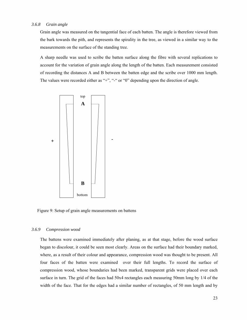
3.6.8 Grain angle
Grain angle was measured on the tangential face of each batten. The angle is therefore viewed from
the bark towards the pith, and represents the spirality in the tree, as viewed in a similar way to the
measurements on the surface of the standing tree.
A sharp needle was used to scribe the batten surface along the fibre with several replications to
account for the variation of grain angle along the length of the batten. Each measurement consisted
of recording the distances A and B between the batten edge and the scribe over 1000 mm length.
The values were recorded either as “+”, “-“ or “0” depending upon the direction of angle.
Figure 9: Setup of grain angle measurements on battens
top
bottom
A
B
+ -
3.6.9 Compression wood
The battens were examined immediately after planing, as at that stage, before the wood surface
began to discolour, it could be seen most clearly. Areas on the surface had their boundary marked,
where, as a result of their colour and appearance, compression wood was thought to be present. All
four faces of the batten were examined over their full lengths. To record the surface of
compression wood, whose boundaries had been marked, transparent grids were placed over each
surface in turn. The grid of the faces had 50x4 rectangles each measuring 50mm long by 1/4 of the
width of the face. That for the edges had a similar number of rectangles, of 50 mm length and by
23

1/4 of the width of the edge. By viewing the batten surface through the grid, those grid rectangles
that corresponded with areas of compression wood could be noted. Cells were recorded as “blank”
for compression wood absent and “1” for compression wood present. Grid rectangles were
recorded as having compression wood present when either totally occupied, or having half or more
in both directions, along and across the batten surface.
Figure 10: Setup for measuring compression wood area
The summary values have been calculated as follows (FAIR CT 1996-1915 STUD Final Report).
For each of the 16 rows of the grid rectangles, which run along the batten length a total has been
calculated which is the sum of al the “1” values in that row. Six row totals have then been added
together to give an outer quarter total for each face or edge. It was felt that simply summing the
rows for the 4 rows was not adequate to represent the amount of compression wood present within
the cross section. When considering what compression wood has contributed to the spring or the
bow, then the difference between the levels in the outer portions on the opposite side of the cross-
section is crucial. The sum of the 4 row totals on a particular surface plus the total of the first rows
of the adjacent surfaces better represent this. However, it is acknowledged that this does not give a
full picture of the extent of the compression wood within the cross-section.
1
1 11 11 1 1 1 1
1
plastic gridcompression woodinner
outer
12
1 2 3 45678
12 11 10 9
16151413
24

25
4 Results
4.1 Selection and characterisation of the site. General stand characteristics
The selected, slightly sloping site is located at Kilmichael Forest, Argyll Forest District, (grid
reference NR 904 918, Long 5°21’40’’W, Lat 56°04’37’’N) with a NW exposed old edge. The
distance to the opposite edge in the NW direction is 55 m, this stand showing a top height of
16.7 m and closure at 11.3 m height. The area in between is covered with Sitka spruce planted in
1990 (actual height 1 to 4 m), leaving a 14.5 m wide gap with no planting (drains on both side of
the forest road and grassland). DAMS score for the site reads as 17. This reading represents severe
wind exposure. Above 17 no thinning is allowed and above DAMS 20 no planting is undertaken
due to very poor growth rate and high wind throw risk.
The even-aged stocking of the site consists of predominantly Sitka spruce with small patches of
Logepole pine (suppressed and dead) along two narrow rides perpendicular to the forest road. Trees
close to the rides were neglected for sample selection. Planting year 1953 with planting at
1.5 by 1.7 m spacing giving an initial stand density of 3900 stems/ha. There has been no thinning,
but self-thinning and distinct differentiation of the stocking have led to a wide range of diameter
distribution and to formation of tree classes from predominant to suppressed.
Table 3: An abbreviated tariff of the Kilmichael site
Sample No Mean top
height [m]
Minimum
top height
[m]
Maximum
top height
[m]
Mean
diameter
[cm]
Minimum
diameter
[cm]
Maximum
diameter
[cm]
Site 20.6 15.5 25.6 19.2 7.0 39.0
Line 1 22.0 16.2 29.5 19.9 7.0 48.0
Line 2 26.2 20.9 37.0 23.1 9.0 54.0
Line 3 27.3 21.6 31.8 23.0 11.0 52.0
Line 4 27.6 24.2 34.4 25.0 12.0 46.0

26
The top height of the site was 20.6m, which represents a medium productive Sitka spruce plantation
(general yield class GYC 10).
From line No 1 to line No 4, from the edge to the mid-forest, the top tree height of each line is
increasing from 22.0 m to 27.6m, the trees in line No1 being significantly smaller than in line No3
and No 4. The same variation holds also true for the dbh distribution in this transect. The mean dbh
increases from approximately 20 cm in line No1 to 25 cm in line No 4. The inner-forest lines differ
significantly in mean dbh from the edge line No 1.
The comparison of the height and diameter characteristics in the different lines with the tree
characteristics of the overall site show that the trees in the most wind exposed line No 1 close to the
edge copy the characteristics of the site, whereas the trees in line No 2, 3 and 4 are higher and thicker
than the site mean. These lines therefore do not represent the mean of the site in terms of height, dbh
and standing timber volume.
4.2 Characterisation of the sample trees:
4.2.1 Size and shape of the sample trees
Height, diameter at breast height, height-to-diameter ratio
Figure 11 a, b, c show the means and standard deviation of dbh, height and height-to-diameter-ratio
for the sample trees. As the trees have been sampled within a particular diameter range, there is no
difference in the mean dbhs. The dbh variation of the sample trees within line No 3 is slightly larger
than in the other sample lines. All sample trees were members of the higher tree classes “pre-
dominant”, “dominant” and “co-dominant”. The mean tree height for the sample trees increases
slightly from the edge to the stand centre from 24.9m to 27.4 m, however, no significant difference
was found between the four different lines. Height-to-diameter-ratio increases from 75.5 to 87.6,
indicating an increasing slenderness of the central grown trees under more sheltered conditions. The
height-to-diameter ratio of exposed trees close to the edge in line 1 is significant lower than for the
two central lines 3 and 4.

Figure 11: Variation of mean and standard deviation of dbh, height and height-to-diameter-ratio of the sample trees in relation to distance from the edge
0
5
10
15
20
25
30
35
0 20 40 60 80 100distance from the edge [m]
heig
ht [m
]
0.0
0.1
0.2
0.3
0.4
0 20 40 60 80 100distance from the edge [m]
dbh
[m]
0
20
40
60
80
100
0 20 40 60 80 100distance from the edge [m]
heig
ht-t
o-di
amet
er-r
atio
[/]
27

0
5
10
15
20
25
30
0 20 40 60 80 100
distance from edge [m]
heig
ht [m
] -
mea
n ±
stan
dard
err
or
first dead whorlfirst green branchfirst green whorllargest whorl masstree height
Figure 12: Variation of tree height and the height of the crown variables in relation to distance from, the regression lines are least square fits of 2nd order polynoms
Figure 12 shows the relation of the main crown parameters: height of first dead whorl, height of the
first green branch and of the first green whorl and the height of the largest weight of a whorl. From
line 1 to line 4 (exposed to sheltered) increases the stem height of these crown parameters except for
the height of the lowest dead whorl which decreases towards the centre of the site. The statistical
analysis by ANOVA shows that the stem height for the living, green branches (lowest green branch,
lowest green whorl, height of largest whorl mass) differs significantly between line 1 and line 4. The
increase in height is probably less due to the degree of shelter than the decreasing intensity and the
decreasing amount of light in the centre of the site which leads to earlier branch death and self-
pruning of the trees.
Figure 13 shows the mean variation of the vertical and the horizontal crown projection area and the
crown asymmetry in relation to the distance from the edge. The average vertical crown area varies
between 9.4m² to 4.8m², with the significant larger crown area for the trees close to the edge
(p=0.05). The horizontal crown projection area changes in a comparable way, generally decreasing
from 33m² in line 1 to 22m² in line 4. The mean crown asymmetry varies from 2.01 to 3.23 with no
28

distinct tendency from the edge to the mid-forest due to the large variation between the trees within
the individual lines. The vertical and horizontal mean crown projection area of the sample trees in
line 1 (close to the edge) is therefore larger but more symmetric than trees in the centre of the forest.
Figure 13: Variation of crown projection area and crown asymmetry in relation to distance from the edge the regression lines are least square fits of 2nd order polynoms
0
5
10
15
20
25
30
35
40
0 20 40 60 80 100
distance from edge [m]
area
[m²]
- m
ean
± st
anda
rd e
rror
0.0
0.5
1.0
1.5
2.0
2.5
3.0
3.5
4.0
ecce
ntri
city
[/] -
mea
n ±
stan
dard
err
or
vertical projection area horizontal projection area crown eccentricity
4.2.2 Straightness score
The straightness score is a measure on how many straight sawlogs of a particular length can be
expected from the bottom 6m of a tree. The stand scores an average of 5.8. Within the plot the
straightness score increases from 5.0 in the exposed line 1 close to the stand edge to 6.2 respective
6.1 in the sheltered centre of the stand (Figure 14) with a generally lower straightness score in line 1
than in line 3 and line 4. Thus the trees in the less exposed parts of the stand formed straighter stems.
This might be due to the fact that these trees in general have been subject to less mechanical
perturbation than the trees closer to the edge.
29

0
1
2
3
4
5
6
7
0 20 40 60 80 100distance from edge [m]
stra
ight
ness
sco
re -
mea
n +/
- sta
ndar
d er
ror
Figure 14: Variation of the straightness score in relation to distance from the stand edge (n=15)
4.2.3 Mechanical properties of the standing trees
4.2.3.1 Static pulling tests, structural Young’s modulus (MOEstruct)
4.2.3.1.1 The variation of MOEstruct with stem height
The analysis of the static bending tests shows a large variation of the MOEstruct between the trees in each
particular line and within individual trees (Figure 15). The MOEstruct varies between 2.89 and 13.48
[GN/m²] over all trees, the line average MOEstruct over all stem heights varies between 5.08 and 5.42
[GN/m²] with no significant difference between the lines. The correlation analysis for linear relations
between the stem and crown variables of the tree and the mean MOEstruct (tree) found no strong linear
correlation for any of the tested variables. The correlation coefficients are given in Appendix 1.
The statistical analysis of the source of variation for MOEstruct showed a significantly negative effect of
the stem height and a positive effect of the position of the tree on site, respectively the degree of
exposure (p=0.05). A line.height interaction was excluded from further modelling as the effect was
found to be not significant; an analysis after square root transformation of the data obtained the same
general relations.
30

The statistical model on the entity of the data set to predict MOEstruct is given in Table 4
MOEstruct = 8.208-0.1933*height+el
Line el
Line 1 0.0000 Line 2 0.2913 Line 3 0.0883 Line 4 1.1109
Table 4: Statistical model to predict MOEstruct from line and stem height
0
5
10
15
0 5 10 15 20 25stem height [m]
stru
ctur
al Y
oung
's m
odul
us [G
N/m
²]
10 m 30 m 50 m 90 m
Figure 15: Variation of the structural Young’s modulus within the tested lines. The regression lines represent least square fits of 2nd order polynomials
The analysis shows that MOEstruct decreases strongly in longitudinal direction from the bottom to the top
(Figure 15, Figure 16). A regression analysis (separately for each line) shows that a least square 2nd
order polynomial function fits the data best. Table 5 shows the equations and the R2 of the polynomial
fits. There is a trend of an increase of MOEstruct from line 1 to line 4, but due to the large variation
between the trees the MOEstruct in line 4 is not significantly higher than in line 1, 2, and 3.
31

line Equation R²
line 1 (10 m) MOEstruct = 7.537 - 0.0785x - 0.0033x² 0.1507
line 2 (30 m): MOEstruct = 7.929 - 0.0413x - 0.0074x² 0.4062
line 3 (50 m): MOEstruct = 7.859 - 0.0571x - 0.0069x² 0.5293
line 4 (90 m): MOEstruct = 9.145 - 0.1041x - 0.0055x² 0.4657
Table 5: Regression models of the relation between absolute stem height x and MOEstruct
0
2
4
6
8
10
0 5 10 15 20stem height [m]
stru
ctur
al Y
oung
's m
odul
us
[GPa
]
tree 4_2 tree 2_12tree 2_4 tree 1_5
Figure 16: Inter-tree variation of structural Young’s modulus for individual sampling trees (signature refers to: line_tree ID)
4.2.3.1.2 Heterogeneity of MOEstruct
Further analysis shows the degree of intra-tree variation of MOEstruct within the individual tree (Figure
17). The difference in MOEstruct between two adjacent points varies up to 3.2 GN/m² per meter distance.
The heterogeneity of MOEstruct (var) was classified in three groups:
I. var > 1.0 GPa/m,
II. 0.5 GPa/m < var ≤ 1.0 GPa/m
III. var < 0.5 GPa/m
32

0
2
4
6
8
10
12
0 5 10 15 20stem height [m]
stru
ctur
al Y
oung
's m
odul
us
[GPa
]
tree 1_4 tree 3_13
Figure 17: Variation of structural Young’s modulus within the stem for individual sampling trees (signature refers to: line_tree number)
Figure 18 shows the distribution of the heterogeneity in these three classes. The proportion of very small
changes of MOEstruct in axial direction increases slightly from 60% to 70% from exposed line 1 to
sheltered line 3 and 4. At the same time there is a decrease in the proportion of large “jumps“ of
MOEstruct over 1 GN/m² per m length in line 1 (16%) to between 5-7% in line 2, 3 and 4. χ² tests for
differences in the frequency show that within each line the frequency of negligible and small local
changes in MOEstruct are similar whereas the frequency of large local changes is significantly lower in
these three lines. The inter-line comparison shows that in line 1 the frequency of large local changes in
MOEstruct is significantly higher than in line 2, 3 and 4 (Appendix 2).
However, the analysis of the stem shape and branch characteristics showed that these irregularities in
MOEstruct were not related to structural heterogeneity such as branches or whorls, as no relation could be
found between the change in MOEstruct and the positions where the strain gauges had been placed (at a
whorl, close to a whorl or between two whorls). Thus within the site, the exposed line 1 shows
onaverage the lowest MOEstruct and the largest degree of heterogeneity in MOEstruct.
33

0
20
40
60
80
100
10 30 50 90distance from edge [m]
perc
enta
ge o
f MO
E str
uct v
aria
tion
[%]
var >1.0 GPa/m0.5 GPa/m< var < 1.0 GPa/mvar <0.5 GPa/m
Figure 18: Distribution of the intra-tree heterogeneity of MOEstruct in relation to the degree of exposure
4.2.3.2 Dynamic pulling tests, swaying frequency
Figure 19 shows a typical pattern in variation of the strain on the stem surface during several swaying
cycles. Due to damping initiated by crown clashing and internal energy loss in the stem the swaying
amplitude reduces in a regular pattern.
34

-400
-300
-200
-100
0
100
200
300
1 6 11 16 21 26 31 36 41 46 51 56 61 66 71 76 81 86 91 96 101
106
111
116
121
126
131
136
141
146
151
156
161
stra
in [d
igits
]
1.0m3.1m5.1m7.2m10.2m13.2m15.2m17.3m
Figure 19: Variation of strain at different stem heights due to tree swaying for an individual tree over time (sec)
0
0.1
0.2
0.3
0 20 40 60 80 100distance from edge [m]
sway
ing
freq
uenc
y [H
z] -
mea
ns ±
sta
ndar
d er
ror
0
10
20
30
tree
hei
ght [
m]
swaying frequencytree height
Figure 20: Variation of the swaying frequency and tree height in relation to the distance from the edge an increasing shelter
Figure 20 shows the variation of the natural swaying frequency within the stand. The frequency varies
for all tree between 0.13Hz and 0.41Hz. The mean swaying frequency decreases from 0.27 Hz in line 1
to 0.22 Hz for line 4. The ANOVA shows that in general there are no statistical significant difference in
35

the swaying behaviour of the trees between the four lines due to the large variation within each line
(p=0.05). The largest variation in swaying frequency within a line is found in line 1 close to the edge.
The statistical analysis shows that the variation in swaying frequency is not directly related to the degree
of exposure represented by line 1 to line 4, but is closely related to the height and the dbh of the tree
which vary between the lines. Swaying frequency decreases with increasing tree height and increases
with increasing dbh. Both variables have a strongly significant linear relation to the frequency
(p<0.001). We also tested for the effects of stem shape, crown parameters (crown length, crown
eccentricity, sailing area, crown radii), of the MOEstruct and the effect of the competition index
(Appendix 3). There were no other significant sources of the variation of the swaying frequency than
tree height and dbh. As we selected the trees to have a small variation of diameter (Figure 11b) the
reduction of the swaying frequency from line 1 to line 4 is mainly due to the increase in tree height
(Figure 11a). A linear model fitted the data best and accounts for 49.8% of the variation.
f=0.3960-0.01429*h+0.685*dbh
Figure 21 shows the relation between stem form and swaying frequency. There is a wide variation for
the tested trees. The strong linear relation as given in Gardiner (1989) could not be found for the tested
trees.
y = 929.35xR2 = 0.3868
0.0
0.1
0.2
0.3
0.4
0 0.0001 0.0002 0.0003 0.0004 0.0005
radius at stem base/ tree height2
sway
ing
freq
uenc
y [H
z]
10 m30 m50 m90 m
Figure 21: Natural swaying frequency of the sample trees. The regression line for all data represents a least square fit and is forced through the origin.
36

4.2.4 Internal stem structure
4.2.4.1 Density of the fresh discs
Figure 22 shows the variation and the linear regression fits of the density of the fully saturated stem
discs. The fresh density of the individual discs varies in all lines in a wide range from 492 [kg/m³] to
1062 [kg/m³]. Due to the large differences between the individual trees, there is no statistical significant
difference in the means of the fresh density of trees of all four lines (p=0.05).
The analysis by Wald test identified the tree height as the main source of variation of fresh disc density
(Appendix 4). The position of the tree within the site (line-effect) was not identified as a statistical
significant source of variation, neither did we find a line.height interaction effect. Further analysis
showed that the percentage of explained variation does not increase when considering height2 and
height3 and thus these terms were not included in the model. The linear model is given below.
δfresh = 718.0 + 5.807*height [kg/m3]
0
200
400
600
800
1000
1200
0 5 10 15 20 25
stem height [m]
fres
h di
sc d
ensi
ty [k
g/m
³]
10 m 30 m 50 m 90 m
Figure 22: Variation of the fresh density within the tested lines. The regression lines represent least square fits of linear relations.
37

38
In all lines the fresh disc density increases with increasing stem height. In the most extreme lines line 1
and line 4 the slope of increase appears to be similar (Table 6), but the basic fresh density seems lower
in line 4. The intermediate lines line 2 and line 3 show a smaller increase of fresh density with stem
height. The basic density is slightly higher in line 2 and lower in line 3 than in line 1.
line Equation R² line 1 (10 m) δfresh = 732.59 +7.12x 0.1346 line 2 (30 m): δfresh = 753.16 + 2.20x 0.0212 line 3 (50 m): δfresh = 703.32 + 4.80x 0.1101 line 4 (90 m): δfresh = 691.83 + 7.17x 0.1654
Table 6: Regression models of the relation between absolute stem height and fresh disc density of the individual lines
4.2.4.2 Density of air dry discs
The density of the air-dried discs also shows a large variation between 323 [kg/m³] and 603 [kg/m³].
The Wald analysis found a significant effect of the tree height and of the degree of exposure (line effect)
as source of the variation (p=0.05) (Appendix 5). The analysis also showed a height.line interaction as
additional source of variation which was also included in the statistical model to predict air-dry disc
density as given in Table 7.
δair-dry = 419.4 + (2.87+ e1)*height + e2
Line e1 e2
Line 1 0.000 0.00 Line 2 -3.117 -3.80 Line 3 -1.407 -29.60 Line 4 -0.098 -34.59
Table 7: Statistical model to predict air-dry disc density from line and stem height
As for the fresh disc density we found an increasing air-dry disc density with increasing stem height.
Line 1 closest to the stand edge shows the highest average disc density both in fresh and air-dry
condition. In line 4 we found on average the lowest disc density at the stem base and the steepest
increase in density to the top. For line 2 and 3 we found an intermediate density at the base and the
lowest density towards the top of the stem.

0
100
200
300
400
500
600
700
0 5 10 15 20 25
stem height [m]
air-
dry
disc
den
sity
[kg/
m³]
10 m 30 m 50 m 90 m
Figure 23: Variation of the air-dry disc density within the tested lines. The regression lines represent least square fits of linear relations.
line Equation R² line 1 (10 m) δair-dry = 429.96 +1.7058x 0.0319 line 2 (30 m): δair-dry = 419.66 - 0.5278x 0.0037 line 3 (50 m): δair-dry = 395.35 +0.9944x 0.0153 line 4 (90 m): δair-dry = 381.94 +3.0089x 0.1238
Table 8: Regression models of the relation between absolute stem height and air-dry disc density
4.2.4.3 Radial increment
In order to analyse the effect of exposure on the growth pattern of a tree we focused on the two radii
representing the windwards and the leewards side of the stem. The disc at 4m stem height was
considered the most appropriate disc as it represents a stem age with a large number of growth rings, a
long time period of wind exposure, and a ring structure not influenced by buttresses or the root stock
which could cover the exposure effect in the growth pattern. The radial growth was analysed in 5 years
intervals taking the ring ages of 5 years, 10 years, 15 years, 20 years and 25 years.
39

0
0.02
0.04
0.06
0.08
0 10 20 30
ring age at 4m stem height [years]
∆ra
dius
l-w n
orm
aliz
ed b
y m
ean
diam
eter
tot
10 m30 m50 m90 m
Figure 24: Difference in radial increment in windward and leeward direction – the symbols represent the mean of a line, the error barrs represent the standard error of the mean
Figure 24 shows the normalised difference between both radii. The difference in leewards and
windwards radius increases with age for all lines which corresponds with an increasing eccentricity of
the stem. In line 1 we found the largest difference between the radius in leewards and windwards
direction, in line 4 the smallest, line 2 und 3 were intermediate. For the youngest age there appears no
difference in growth between all four lines. When the trees getting older, the edge trees in line 1 grow
more eccentric than the trees in lines 2, 3 and 4. Correspondingly the most sheltered trees in line 4 show
the smallest stem eccentricity. At an age of 25 years, the difference in eccentricity between line 1 and
line 4 is found to be statistical significant different (p=0.05) (Appendix 6). From this it follows that the
more exposed trees are when growing the more they lay down wood on one side, the leewards side of
the stem and the more they develop reaction (compression) wood in comparison to more sheltered trees
which grow in a more homogenous manner.
40

4.3 Roundwood and saw log assessment
4.3.1 Branchiness
Branchiness is one of the most important criteria for log quality. The occurence of branches on a log
represents a combination of unwelcome log and wood properties which will be carried along the chain
to the final product. Branchiness represents a local heterogeneity of the fibre structure, leading to a
weakening of the mechanical strength of the wood and different drying characteristics. The standard
ENV 1927 classifies saw logs based on the status of a branch (ingrown or sound, dead, unsound) and
the branch diameter.
0
10
20
30
40
50
60
70
butt mid top
position of log in the stem
diam
eter
of t
he th
icke
st b
ranc
h pe
r log
[mm
] - m
ean
+/- s
tand
ard
erro
r
10 m30 m50 m90 m
Figure 25: Variation of the diameter of the thickest branch per log
The individual diameters of the thickest branch per log varied in a wide range between 15 mm and
104 mm (Appendix 7). The average branch density of the thickest branch per log (butt, mid, top) and
line 1, 2, 3, 4 varied between 25 mm and 55 mm with the largest variance for the top logs in line 1 (10m
from the edge) (Figure 25). The lowest minimum values occurred on the logs from the butt position of
the stem. The largest branch diameters were measured on the top logs. The statistical analysis showed
two trends of variation for the branch diameter. Independently for all lines, there is an increase in branch
diameter from the bottom of the tree to the top which follows the general development of the canopy.
41

The variance analysis showed that the increase in branch diameter between the bottom and the top log is
significant in all lines except line 2 and is even significant between mid log and top log in line 4
(p=0.05).
The increase of branch diameter with height varies with distance from the edge. In each group of log
position (butt, mid, top), the branch diameter decreases from line 1 to line 4, but the differences in
diameter are not statistically significant (p=0.05). The analysis also showed no significant line.log
interactions. However, the overall decrease of branch diameter from the edge to the centre of the site is
less the effect of changing shelter than the effect of canopy shading and lower light availability in the
centre of the site which leads to more effective self-pruning.
0
10
20
30
40
50
60
70
80
90
100
10 30 50 90 all
distance from edge [m]
perc
enta
ge o
f log
s pe
r gra
de [%
] -
bran
chin
ess
grade Dgrade Cgrade Bgrade A
Figure 26: Percentage logs per grade - branchiness
The classification of the logs according to ENV 1927 – 1 (1998) is shown in Figure 26. Due to the
fact that all trees showed dead branches to the bottom of the stem no log was graded as grade A,
which requires a defect-free surface without branches. In total, 30% of the logs were classified as
grade B, 55% as grade C and 15% as grade D. The comparison between the individual lines shows
a similar distribution. In all lines, logs of grade C have the largest proportion of between 44% to
42

43
68%. A lower percentage of logs of between 23% to 36 % were classified as a higher quality grade
B and between 7% and 23% were graded in the lowest quality grade D. Chi-square tests showed
that within each line the frequencies of grades B, C and D are significantly different. The
comparison between the lines shows that for each grade B, C, D the frequency of the individual
grades is very similar and does not differ on a significant level (p=0.05).
The frequencies of the grades separated by log positions (butt, mid, top) reflect strongly the
variation of branch diameter from bottom to top. Whereas 60% of the butt logs were graded as
grade B and 3% as grade D, the distribution changed drastically for the top logs with 6% of the top
logs classified as B, but 30% graded as D.
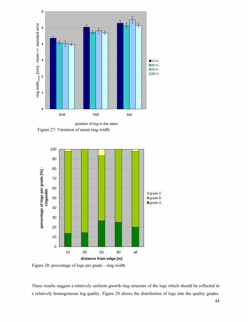
4.3.2 Ring width
Ring width is closely related to the wood density and gives a first indication of the density variation of a
log. Average ring width is very important for log quality because it gives a first indication on the
average wood density and the density contrast in the cross section. For the individual logs the average
ring width varied between 2.8 mm and 7.5 mm.
Figure 27 shows the variation of mean average ring width for the measured logs. The mean ring width
of log position by line varied between 4.0 mm and 5.5 mm, for position butt log and mid log the mean
ring width decreases by about 9% (0.4 mm) from line 1 (close to edge) and line 4 (centre of site). The
top logs do not show such trend. However, the statistical analysis showed that there is no statistical
significant difference between the lines. The variation of mean ring width can only be explained by the
log position, not by line effects or line.log interactions. The comparison between butt log and top log
shows a increase of average ring width from bottom to top. The reason is the presence of a high
proportion of pith-related juvenile wood which is characterised by a generally larger ring width in order
to support quick and efficient water transport in young shoots.
0
1
2
3
4
5
6
butt mid top
position of log in the stem
ring
wid
thm
ean [
mm
] - m
ean
+/- s
tand
ard
erro
r
10 m30 m50 m90 m
Figure 27: Variation of mean ring width
0
10
20
30
40
50
60
70
80
90
100
10 30 50 90 all
distance from edge [m]
perc
enta
ge o
f log
s pe
r gra
de [%
] - ri
ngw
idth grade C
grade Bgrade A
Figure 28: percentage of logs per grade – ring width
These results suggest a relatively uniform growth ring structure of the logs which should be reflected in
a relatively homogeneous log quality. Figure 28 shows the distribution of logs into the quality grades.
44

45
The average ring width of the logs between 4 mm and 5.5 mm results in a very high percentage of logs
classified as grade B (between 67 % and 86%, average 78%). Additionally, the lower percentage in
grade B corresponded with a higher proportion of logs in grade A adding up to 98% of all logs graded
into the best two quality grades. Grade C was only present in line 1 and line 3 and did not exceed 7%.
The discrepancy between the results on eccentricity of the radial increment parallel to the wind direction
(4.2.4 Internal stem structure) and the homogeneous results on ring width with regards to log grading
indicates a problem of the grading standard ENV 1927. As the standard asks for representative radii on
a cross cut, the measurement integrates over the whole area and discriminates local heterogeneity which
could be important in further timber processing.
4.3.3 Spiral grain
Spiral grain describes the degree of angular orientation of the wood fibres of the stem. The spiral grain
is reflected on battens by the grain angle which is known to influence the level of distortion following
drying. The data presented were only obtained from the butt logs.
For the tested trees the orientation of the fibres varied between of 0 [cm/m] and 21 [cm/m]. Figure 29
presents the variation of the means of spiral grain per line. The means of each line range between 3
[cm/m] and 5 [cm/m] with a large variation for each line. The ANOVA analysis showed that there is
difference between the lines and the degree of shelter, respectively.
The quality classification of the logs with respect to the spiral grain reflects the heterogeneous picture of
the stand (Figure 30). All possible grades A to C are present with a varying proportion for the different
lines. The low mean spiral grain in line 4 is directly reflected by the high percentage of 53% “A“ grade
logs. Correspondingly, the high mean spiral grain in line 2 resulted in a low percentage of high quality
logs. Line 3 also shows a high percentage of grade “A“ log (47 %), but with a high mean of grain angle.
The large variance in line 3, however, indicates a large proportion of logs characterised by big fibre
angles. These logs, subsequently were graded into grade C, the lowest possible quality grade resulting
from spiral grain. Nonetheless, despite the detailed picture of grade distribution for the logs, chi-square
tests showed no differences for the frequencies of the individual groups.

0
1
2
3
4
5
6
7
10 30 50 90
distance from edge [m]
spira
l gra
in [c
m/m
] - m
ean
+/- s
tand
ard
erro
r
buttFigure 29: Variation of the spiral grain angle
0
10
20
30
40
50
60
70
80
90
100
10 30 50 90 all
distance from edge [m]
perc
enta
ge o
f log
s pe
r gra
de [%
] -
spira
l gra
in
grade Cgrade Bgrade A
Figure 30: Percentage of logs per grade – according to spiral grain (butt logs only)
46

4.3.4 Position of the pith (log eccentricity)
The pith position and the subsequent degree of eccentricity of a log strongly influence the procedures of
timber processing which thus affect the quantitative out-turn and the yield. Figure 31 shows the
eccentricity of the tested logs normalised by the stem diameter, grouped by log position and degree of
exposure. Individual log eccentricitynorm varied in a wide range between 0.02 and 0.70, the means vary
in the range between 0.22 and 0.30 with a large variation in each group. In the bottom log the
eccentricity decreases from the most exposed line 1 to most sheltered line 4. For the top logs the
opposite trend holds true, the eccentricity increases from stand edge to the centre of the site. The mid
logs in all lines showed a similar eccentricity except line 3 which is even more eccentric than the top
logs in line 4. However, the statistical analysis shows that there is no statistical difference between the
single groups due to their large variance.
The analysis of the variance show that neither line (exposure) nor the log position (butt, mid, top)
explained much of the variation in eccentricity of the logs.
0.00
0.05
0.10
0.15
0.20
0.25
0.30
0.35
0.40
butt mid top
position of log in the stem
ecce
ntric
ityno
rmal
ised
- m
ean
+/- s
tand
ard
erro
r
10 m30 m50 m90 m
Figure 31: Variation of log eccentricity
47

Due to the large variation of log eccentricity the classification of the logs resulted in 35% logs in grade
“A”, the frequencies of 39% in grade “B” and 26% in grade “C” with no difference in the frequencies
on a statistical significant level (p=0.05). The detailed analysis of the distribution of the logs into the
three quality grades show that this holds true for all lines. It appears that there is a slightly lower
percentage of logs grade “C” (20 to 30%) than grade “A“ and “B“. However, this means that one third
of the logs are graded into the lowest possible quality class which allows only a restricted utilisation of
the timber.
0
10
20
30
40
50
60
70
80
90
100
10 30 50 90 all
distance from edge [m]
perc
enta
ge o
f log
s pe
r gra
de [%
] -ec
cent
ricity
grade Cgrade Bgrade A
Figure 32: Percentage of logs per grade due to eccentricity only
4.3.5 Log taper
The log taper (the reduction in diameter per tree length) varied in a wide range between 0.21 cm/m and
3.87 cm/m.
Figure 33 shows the variation of the means with respect to the log positions and the four levels of
exposure. Both “line” and “log position” account for about 31% of the variation of the log taper, there is
no significant line.log interaction (p=0.05, Appendix 11). The trend of variation is the same for all four
lines, a high taper for the butt logs, a decline in taper for the mid logs and again an increase in taper for
the top logs. The results of the post-hoc-tests for differences between the means is given in Appendix
48

11. Due to the large variation within each group there is no statistical significant difference in the means
between the four lines when comparing the logs of the three different stem positions.
0.0
0.5
1.0
1.5
2.0
butt mid top
position of batten in the stem
log
tape
r [cm
/m] -
mea
n +/
- sta
ndar
d er
ror
10 m30 m50 m90 m
Figure 33: Variation of the log taper
For butt logs (Figure 33: Variation of the log taper) the log taper only used diameter measurements from
1.3m upwards in order to eliminate the effect of stem swelling by buttresses for the log grading.
However, comparing these taper data with the “actual” tapering from the bottom end of the log to its top
end, one finds a larger effect of buttresses in line 1 and line 2, which are both more exposed to wind
constraints. The mean stem taper increases by 0.5 to 0.6 cm/m when considering the bottom 1m stem
length in these two lines, while the taper increases only by 0.2cm/m in line 3 and line 4. Thus the mean
of taper exceeds the limits the limits for grade “B” in line 1 and line 2 for trees with a dbh larger than 35
cm, which results in a classification in the lowest quality grade.
49

The grading of logs considering the taper separately does not allow any grade “A” by its own. Taper
only is considered to grading in combination with other grading parameters (ENV 1927-1, 1998). The
log grading considering the log taper individually resulted in a distribution of grade “B” and “C” as
shown in Figure 34. The majority of the log (83% overall) were classified as higher grade “B” leaving
only 17% in the lower log grade. The frequency analysis by Chi-square tests showed that this
distribution is not different between all four lines (p=0.05). The comparison broken down by log
position, however, showed the butt logs showed the highest percentage of grade “C” logs with 35%
(mid: 2%, top: 15%).
0
10
20
30
40
50
60
70
80
90
100
10 30 50 90 all
distance from edge [m]
perc
enta
ge o
f log
s pe
r gra
de [%
] -
log
tape
r
grade Cgrade Bgrade A
Figure 34: Percentage of logs per grade – log taper
4.3.6 Log ovality
The log ovality describes the ration between the largest and the smallest diameter on a log. It therfore
combines information of log diameter and log eccentricity as the first criterion does not give a picture of
the log shape and the later only describes that individual diameter which is characterised by the largest
radial contrast. However, log ovality is not included in the standards as a parameter to classify logs.
50
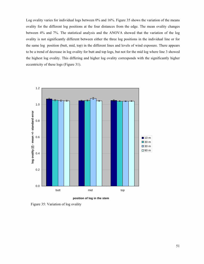
Log ovality varies for individual logs between 0% and 16%. Figure 35 shows the variation of the means
ovality for the different log positions at the four distances from the edge. The mean ovality changes
between 4% and 7%. The statistical analysis and the ANOVA showed that the variation of the log
ovality is not significantly different between either the three log positions in the individual line or for
the same log position (butt, mid, top) in the different lines and levels of wind exposure. There appears
to be a trend of decrease in log ovality for butt and top logs, but not for the mid log where line 3 showed
the highest log ovality. This differing and higher log ovality corresponds with the significantly higher
eccentricity of these logs (Figure 31).
0.0
0.2
0.4
0.6
0.8
1.0
1.2
butt mid top
position of log in the stem
log
oval
ity [/
] - m
ean
+/- s
tand
ard
erro
r
10 m30 m30 m90 m
Figure 35: Variation of log ovality
51

4.3.7 Proportion of juvenile wood
Pith related juvenile wood is mainly characterised by thin cell walls and large cells resulting in a low
wood density and a large microfibril angle. Both characteristics are closely related to a reduced
mechanical strength of the wood and a large tendency to distortion of the timber. The proportion of
juvenile wood in a log thus directly determines the proportion of sawn products affected by less
favourable wood properties. The juvenile core was defined to include the first 12 years of growth. Thus
the dimension of the juvenile core for the different log positions gives an indication on the early wood
formation of the stem at this particular stage of stem development.
0
10
20
30
40
50
60
70
80
butt mid top
position of log in the stem
juve
nile
cor
e [%
of l
og v
olum
e] -
mea
n +/
- sta
ndar
d er
ror
10 m30 m50 m90 m
Figure 36: Variation of the proportion of juvenile wood
Figure 36 presents the mean proportion of juvenile wood volume per log for butt, mid and top logs. The
means per log position increase significantly from the butt log position to the top log position which is
due to the decreasing diameter of the tree with increasing height. The log position accounts for 82% of
the observed variation of juvenile wood share in logs, the level of wind exposure (line effect) and
line.log interactions were not found to be significant in helping to explain the variation. These results
indicate that the formation of the stem in the first twelve years was not effected by varying mechanical
52

constraints and lead to a relatively similar wood formation which might be reflected by the properties of
the battens produced from these inner stem parts.
4.3.8 Log classification according to ENV 1927-1 “Qualitative classification of softwood round wood – Part 1: Spruces and firs”
The log classification by ENV 1927-1 classifies a log by a range of different characteristics and
properties which have to meet particular limits. The parameter which presents the lowest quality of the
log determines the overall classification of the log. Only an extremely favourable performance in one
characteristic can compensate for a small deviation from the required limit in another characteristic. The
test material has been classified by the characteristics presented above.
0
10
20
30
40
50
60
70
80
90
100
10 30 50 90 all
distance from edge [m]
perc
enta
ge o
f log
s pe
r gra
de [%
]
grade Dgrade Cgrade Bgrade A
Figure 37: Results log grading – classification after ENV 1927-1
The results of the log classification are shown in Figure 37. The tested logs were graded into the grades
“B”, “C” and “D”. The highest grade “A” which occurred for individual characteristics were
“downgraded” by a less good performance according to other properties. The largest proportion of logs
(70%) was classified as “C, timber of average to poor quality with characteristics which do not degrade
the natural characteristics of the clear wood”, 15% of the log were classified as grade “B” and 15% as
grade “D”. The frequencies for grade “B”, “C” and “D” varied slightly between the different lines of
53

wind exposure, but not at a statistical significant level (p=0.05, Appendix 14). Thus in general the trees
grown under the largest wind exposure did not perform differently in terms of log quality from the most
sheltered trees on the site.
Figure 38 presents the analysis on which criterion determined the final log grade. Between 50% and
68% (61% overall) of the logs were downgraded by a poor performance in branchiness, only 2% to 15%
(10% overall) were downgraded due to a large stem taper. The combination of branchiness and taper
accounts for another 4% to 25% (9% overall) of logs downgraded. It is obvious that the performance in
branchiness appears more important for the grading results and the log quality than the stem form and
shape. However, branchiness is strongly affected by the planting density and the stocking of the site and
less strongly by wind exposure.
0
10
20
30
40
50
60
70
80
90
100
10 30 50 90 all
distance from edge [m]
perc
enta
ge o
f log
s do
wng
rade
d [%
]
all grades equal
spiral grain, eccentricity,ringwidthbranchiness & taper
taper
branchiness
Figure 38: Percentage of logs graded by the individual criteria • “branchiness“ summarise the singular effect of branchiness and combinations of
branchiness and other criteria except “taper“, • “taper“ summarise the singular effect of taper and combinations of taper with other
criteria except “branchiness, • “spiral grain, eccentricity, ringwidth“ represent occurrence of the singular effects of
each criteria.
54

4.4 End product, quality of battens
4.4.1 Stress grading
The overall comparison of the batten performance in stress grading showed three significant
components for the observed variation in (minimum) MOEmin: wind orientation (leewards/ windwards),
log position (butt, top) and exposure (line 1 to 4) (p=0.05). There was no interactions found between the
main factors “orientation”, “position” and “line”. The comparison of the entity of the data set which did
not separate between the different lines showed that in general the top log battens had only a slightly
lower mean MOEmin than the butt log battens. Battens cut from the windward side of the stem/log had a
higher mean MOEmin compared with battens from the leeward side of the log. However, there occurred a
difference in MOEmin between the centrally positioned and the more peripherally positioned butt battens.
Within the site, the MOEmin increased generally with increasing distance from the edge and increasing
wind shelter.
0
2
4
6
8
0 20 40 60 80 1distance from edge [m]
MO
E min
[GPa
]
butt battens leewardsbutt battens windwardstop battens leewardstop battens windwards
00
Figure 39: Variation of MOEmin of central positioned battens from the butt and the top log (symbols represent the mean of each line, the error bars the standard error)
Figure 39 shows a comparison of the central positioned battens from the top and the butt log close to the
pith. There was a general increase in MOEmin for the central butt battens from the exposed edge to the
sheltered centre of the stand from 5.4 GPa (mean of leeward and windward battens) to 6.2 GPa. At the
same time, the MOEmin in the top battens declined from 6.73 GPa to 6.00 GPa from line 1 to line 4. The
orientation with respect to the wind did not alter the MOEmin of these battens from either the butt or the
top logs within each line.
55

0%
20%
40%
60%
80%
100%
10 30 50 90distance from edge [m]
perc
enta
ge o
f bat
tens
C 24 C 16 reject
Figure 40: Distribution of battens qualifying for C24, C16, reject
Figure 40 shows the distribution of the battens for grading C24/C16/reject which stands for a higher
quality grading. About 30% of the battens were rejected overall, about 38% were graded as C24 suitable
for higher quality requirements (Appendix 15). The distribution of quality grades switched between
battens from line 1 (most exposed) to lines 2, 3 and 4 (more sheltered). In line 1 almost 45% of the
battens were rejected due to low MOEmin. and only 55% of the battens were classified as suitable for
higher quality purposes. For line 2, 3 and 4, the out-turn of suitable battens was higher at 74% to 77%.
However, grading according to classification “C16/reject”, which classifies for a lower strength,
identified only 2% of rejected battens in each line. The detailed analysis shows that about 42% of the
battens from line 1 had been down graded from “C16” in “C16/reject” to “reject” in “C24/C16/reject”
whereas 28% had been upgraded from C16 to C24 (Figure 41). For line 2, 3 and 4, the trend was the
other way around, more battens were upgraded than down graded. However, the overall out-turn from
the site is higher for the lower strength classification which will be preferred as the financial outcome is
also higher overall than for the higher classification but lower number of battens (BRE, oral
communication).
56

0
10
20
30
40
50
0 20 40 60 80 100distance from edge [m]
perc
enta
ge o
f bat
tens
gra
ded
diffe
rent
ly
down graded (C 16 to reject)upgraded (C 16 to C 24 )
Figure 41: Change in strength classification between grading specifications “C24/C16/reject” and “C16/reject”
4.4.2 Modulus of elasticity, modulus of rupture
MOE and MOR are the main properties to describe mechanical suitability for construction purposes of
timber. The MOE represents the stiffness of the material, the MOR its strength.
The mean MOEstat of the battens varied strongly between 6400 N/mm² and 9600 N/mm² in the different
positions of the tree (Figure 42). The analysis of the variance showed that “wind orientation” of batten
and “ position of batten in the cross section” were significant effects to explain the variation of MOEstat
(p=0.05), interaction effects between line, log position and line.log.batten position also did add up to
explain some of the variance. However, only about 20% of the variance were explained by the analysed
factors. Due to the large variations there was no significant differences between the individual positions
of battens in the logs with respect to the entire data set (p=0.05) (Appendix 16).
57

0
2000
4000
6000
8000
10000
12000
14000
butt c
entra
l
butt i
nner
leeward
s
butt o
uter le
eward
s
butt i
nner
windward
s
butt o
uter w
indward
s
top in
ner le
eward
s
top o
uter le
eward
s
top i
nner
windward
s
position of batten in the stem
MO
E sta
t [N
/mm
2 ] - m
ean
+/- s
tand
ard
erro
r
10 m30 m50 m90 m
Figure 42: Variation of mean MOEstat
The detailed analysis of MOEstat on sub-data set (1) (butt versus top, inner position) showed the highest
values of MOEstat for battens from the top logs from line 1 (Figure 43a). Comparing the different lines,
the MOE of the battens of the same position decreased from line 1 to line 2, 3, and 4, while the MOE of
the inner battens increased from the edge to the centre of the site. Similarly to the analysis of the whole
data set, the variation within each group did not allow testing for significant differences between the
groups. Only in line 1 were the battens from the top logs significantly stiffer than the battens cut from
the bottom log. The comparison of battens converted from the butt logs showed a similar pattern of
variation independently from the line (Figure 43b). There was an increase in MOEstat from line 1 to line
2 and line 3, but a slight decrease towards the most sheltered line 4. However, this was not significantly
different in mean MOEstat. The increase in MOE was most distinct for battens “outer leewards” between
line 1 and line 2. These battens were cut from a position in the cross section where the wood was
influenced by compression wood on one hand but was also characterised by a homogenous wood
structure due to decreasing ring width with age (Figure 27). In line 2 the exposure to wind was already
reduced to a degree that a stiffer wood structure was developed locally. The trees did not react to
perturbation by the wind as much as the trees did in line 1. With increasing age this difference in wood
58

formation became most obvious at the stem position where generally the highest bending stresses
appeared.
0
2000
4000
6000
8000
10000
0 20 40 60 80 1distance from edge [m]
MO
E sta
t [N
/mm
2 ]
butt inner leewardsbutt inner windwardstop leewardstop windwards
00 0 20 40 60 80 10distance from edge [m]
butt outer leewardsbutt inner leewardsbutt inner windwardsbutt outer windwards
0
Figure 43: Variation of MOEstat for battens from the different positions (a – inner positions butt compared to top positions; b- butt positions close to pith and periphery)
Figure 44 presents the variation of MOR with batten position. The MOR of individual battens varied
between 25 N/mm² and 42 N/mm². The analysis of variance showed that the orientation with respect to
the prevailing wind direction and the position of the battens within the stem had a significant effect on
the variation of MOR, with no interactions between those factors (p=0.05) (Appendix 16). Due to the
large variation within each group, the ANOVA analysis on the entire data-set showed no significant
difference either between the lines nor between battens from butt log or top logs nor between battens
from the windwards or leewards half of the log.
The analysis on the sub-sets of the data showed the variation of the MOR in more detail (Figure 45).
The wood close to the pith characterised appeared very heterogenous in MOR. The different batten
positions showed no obvious trend. The MOR of “butt inner windwards” positioned battens increased
slightly from “exposed” (line 1) to “sheltered” (line4) as did the MOEstat. The MOR of the most exposed
positioned “top battens” decreased from line 1 to line 4, however. The comparison to the butt positions
showed the differentiation in MOR. The “outer butt position, windwards”, characterised by the most
homogenous and densest wood showed the highest MOR in all four lines. The outer leewards batten
position followed in strength, probably due to its increased density, and both inner positions, leewards
and windwards, turned out to be the weakest.
59

0
5
10
15
20
25
30
35
40
45
50
butt c
entra
l
butt i
nner
leeward
s
butt o
uter le
eward
s
butt i
nner
windward
s
butt o
uter w
indward
s
top in
ner le
eward
s
top o
uter le
eward
s
top i
nner
windward
s
top o
uter w
indward
s
MO
R [N
/mm
2 ] - m
ean
+/- s
tand
ard
erro
r
10 m30 m50 m90 m
Figure 44: Variation of MOR
0
10
20
30
40
0 20 40 60 80 1distance from edge [m]
MO
R [N
/mm
2 ]
butt inner leewardsbutt inner windwardstop leewardstop windwards
00
0
10
20
30
40
0 20 40 60 80 1distance from edge [m]
butt outer leewardsbutt inner leewardsbutt inner windwardsbutt outer windwards
00
Figure 45: Variation of MOR (different positions within the stem) with distance from stand edge
60

61
However, the results suggest that for the entity of the battens the wind exposure did not modify the
mechanical properties in such a way that a separation of battens appears reasonable for practical use.
This is supported by the results of the stress grading tests.
4.4.3 Distortion (twist, spring, bow)
The distortion of the sawn and dried product is the second main group of characteristics to determine
timber quality. Non-straight battens cannot be used for high quality construction purposes and need
additional treatment such as planing in order to re-shape the piece. This reduces the yield and the
financial out-turn from production. Distortion comprises four different types of warp: twist, spring, bow
and cupping. The later will not be presented in this report as it is more important to boards than to cants
and battens.
4.4.3.1 Twist
The twist of the battens varied individually between 0 mm and 55 mm for all the battens. The variation
of the means is presented in Figure 46. The average twist values ranged between 2.6mm and 33.9mm
with a large variation within each group. The analysis of variance showed that the “line”, “log position”
and “position in the cross section” accounted for 46% of the observed variance (p=0.05) (Appendix 17).
There was no interaction effect between the main factors.
For the entity of the data set, the test for differences in the means did not show a statistical significant
difference between the lines. Thus there is no evidence for the effect of wind exposure on whole trees
which change the wood characteristics related to twist.
The analysis of variance of the sub-data set (1) “butt log versus, top log, inner positions” did not find
wind exposure (line effect) to be significant for the variation of twist in these battens. Wald tests found
“log position”, the orientation with respect to the wind within the log and the interaction between these
two factors to be significant for the variation in twist (p=0.05). Twist increased with height (butt log to
top log) and with position of the batten towards the wind-facing half of the log. Wald tests for the sub-
data set (2) (butt log, inner versus outer position) also showed the effects of cross-sectional position of
the battens on the variation of twist to be significant (log transformed data, p=0.05). Twist decreased
from the inner position to the outer position in the cross section from juvenile to mature wood. It also
slightly increased from leewards to windwards. However, the difference between these two positions
was not as large as between butt and top log. Therefore, the structure of juvenile wood (inner position
butt log, top logs) seems to have a higher disposition to twist than mature wood.

0
5
10
15
20
25
30
35
40
45
butt c
entra
l
butt i
nner
leeward
s
butt o
uter le
eward
s
butt i
nner
windward
s
butt o
uter w
indward
s
top in
ner le
eward
s
top o
uter le
eward
s
top i
nner
windward
s
top o
uter w
indward
s
position of batten in the stem
twis
t [m
m] -
mea
n +/
- sta
ndar
d er
ror
10 m30 m50 m90 m
Figure 46: Variation of twist
These findings may be interpreted as follows: the higher wind exposure for the trees in line 1 did not
change the wood formation in such a way as to cause general more twist. The differences in twist
between the windwards and the leewards halves of the logs suggest that the local stress distribution in
the cross section and within the stem during wind loading seems to be more important for modifications
of the wood structure than overall wind exposure. As battens cut out of top logs also show a large twist,
the deformation could be related both to the proportion of juvenile and compression wood in these
battens. Both wood types are characterised by a low microfibril angle, which causes large shrinkage
during the drying process. In combination with grain angle this could be the reason for the large twist
values measured.
62

4.4.3.2 Bow
The bow describes the deformation of the batten over the flat face (Figure 8). Bow takes place when
uneven shrinkage of wood occurs on the two flat surfaces of a batten during wood drying. The tested
battens showed individual bow values between 0 mm and 35 mm, the mean values varied between 1mm
and 13.5mm with a large variation within each group (Figure 47). The analysis of variance found a
significant effect of the log position for the variation of bow in the entity of the data set. An interaction
between line and cross-sectional position of the log (inner, outer) was also found to be significant
(p=0.05) (Appendix 17). The interaction effect is probably due to the large differences in bow for the
battens from line 1 and line 3 from the top outer leewards position, and the high values for battens from
top inner leewards position in line 4. ANOVA analysis found the values of bow to be significantly
higher for battens from the top logs than from the butt logs in line 3 and line 4. The more exposed lines
1 and 2 showed a higher mean bow for the butt battens, but due to the large variation the means were
not significantly different.
0
2
4
6
8
10
12
14
16
butt c
entra
l
butt i
nner
leeward
s
butt o
uter le
eward
s
butt i
nner
windward
s
butt o
uter w
indward
s
top in
ner le
eward
s
top o
uter le
eward
s
top i
nner
windward
s
top o
uter w
indward
s
position of batten in the stem
bow
[mm
] - m
ean
+/- s
tand
ard
erro
r
10 m30 m50 m90 m
Figure 47: Variation of bow
63

64
The detailed analysis of the sub-data set (1) “butt versus top, inner positions” found the log position, and
line-by-log and orientation with respect to wind-by-log interactions to have a significant influence on
the variation of the bow (log transformed data, p=0.05). The derived model predicted a small decrease
in bow from line 1 to line 4 (exposed to sheltered), and an increase from butt log to top log battens. Bow
also increased from leewards orientation to windwards orientation. However, the interaction effects
modified the bow in a way that the “top windwards” position is slightly reduced in bow in comparison
to “butt leewards”. The line log interaction on the other hand showed an increase in bow towards the top
battens from line 4.
Wald analysis of the subset (2) “butt, inner position versus outer position” showed that the wind
exposure on the whole tree (line effect) had a significant influence on the variation of bow for battens
from the butt logs (p=0.05, log transformed data). Orientation with respect to wind within the cross
section or position relative to the pith did not explain variation in the bow.
These findings indicate that bow seems not to be influenced by the variation of wood structure found at
the same stem height. Varying wood structure due to reaction wood or juvenile wood in comparison to
normal wood did not change the bow of the battens. However, the differences in wood structure
between battens from the inner parts of the butt logs and battens from the top logs seem to cause distinct
differences in bow.
4.4.3.3 Spring
Uneven shrinkage of the wood on the narrow faces of a batten (Figure 8) causes the deformation type
called “spring”. Figure 48 presents the variation of the mean values of spring recorded for the different
batten positions within the logs. The means varied between 1.5mm and 6.0mm with a large variance
within each tested group. In general, battens from line 1 had the most severe spring developed except
for the central positions created when the pith was boxed. However, due to the large variation no
significant differences of the means could be found (p=0.05). The analysis of variance showed that the
log position and an interaction between line, log, orientation with respect to wind and batten position
within the cross section had a significant influence on the variation of spring testing for the entire data
set. (Appendix 17).

0
2
4
6
8
10
12
butt c
entra
l
butt i
nner
leeward
s
butt o
uter le
eward
s
butt i
nner
windward
s
butt o
uter w
indward
s
top in
ner le
eward
s
top o
uter le
eward
s
top i
nner
windward
s
top o
uter w
indward
s
position of batten in the stem
sprin
g [m
m] -
mea
n +/
- sta
ndar
d er
ror
10 m30 m50 m90 m
Figure 48: Variation of spring
The detailed analysis of the sub data sets (1) “butt versus top, inner position” and (2) “butt log, inner
versus outer position” identified the particular position characteristics of the data sets to be important for
the variation in spring (p=0.05, square root transformed data). The spring increased for battens from the
top logs, t-tests found the means to be significantly different for the sheltered lines 3 and 4. For battens
from the butt logs, the spring was significantly smaller for battens cut from the outer cross-sectional
position compared to those from close to the pith.
These results suggest that the wood structure which characterises juvenile wood might be most
responsible for spring deformation. However, modifications in the wood structure of juvenile wood in
the top logs might be due to increased wind exposure in the crowns. Differences in the wood structure
due to the presence of compression wood or normal wood did not alter the spring significantly.
65

4.4.4 Structural characteristics of the battens: density, juvenile wood, compression wood, grain angle, knottiness
4.4.4.1 Density
The air dry batten density varied in a broad range around 400 kg/m³ (Figure 49) which is about the same
value that Brazier&Mobbs (1993) reported for Sitka spruce from Kilmichael Forest [453 kg/m³
respectively 426 kg/m³ for 1.6m spacing respectively 1.7m spacing] and slightly higher than the values
cited in the literature (390 kg/m³) (Harding, 1988). For each batten position except “butt inner
windwards” and “top outer leewards” the density seems be highest for the battens from line 1. The butt
battens in general showed a smaller density. These results correspond with the findings for fresh and air-
dry discs (Figure 22, Figure 23). This is probably due to a higher proportion of high density
compression wood for this line (Figure 23, Figure 51).
The statistical analysis of the variation showed a significant effect of the main factors “exposure” (line),
“log position” (butt, top), the “wind orientation within the log” and the “position of the batten in the
cross section” (close to pith or periphery) and some of the interactions between the main factors.
Appendix 18). However all these effects did not explain more than 18% of the total variance of the
batten density.
0
100
200
300
400
500
600
butt c
entra
l
butt i
nner
leeward
s
butt o
uter le
eward
s
butt i
nner
windward
s
butt o
uter w
indward
s
top in
ner le
eward
s
top o
uter le
eward
s
top i
nner
windward
s
position of batten in the stem
batte
n de
nsity
[kg/
m³]
- mea
n +/
- sta
ndar
d er
ror
10 m30 m50 m90 m
Figure 49: Variation of air dry density (battens)
66

4.4.4.2 Juvenile wood
Juvenile wood is known to be an important factor for timber quality as its cell wall structure and density
properties strongly differ from mature wood. It causes serious deformation due to uneven shrinkage
during the drying process and reduces wood strength due to short fibre length and low microfibril angle.
Juvenile wood becomes particularly important when silvicultural practice supports a vigorous early
growth of young trees in wide spacing. For this project it was defined to consist of the first 12 years
developed around the pith.
Figure 50 shows the variation of the mean proportion of juvenile wood in the battens. As follows from
the cutting scheme, the inner battens and the top battens consisted of substantially larger proportion of
juvenile wood than the outer battens. The proportion of juvenile wood varied between 6% and 96%,
with statistical significant differences between the outer positioned battens, the inner butt battens and
the top positioned battens. There was no significant difference in the means of juvenile wood percentage
between the different lines.
0
20
40
60
80
100
120
butt c
entra
l
butt i
nner
leeward
s
butt o
uter le
eward
s
butt i
nner
windward
s
butt o
uter w
indward
s
top in
ner le
eward
s
top o
uter le
eward
s
top i
nner
windward
s
top o
uter w
indward
s
position of batten in the stem
mea
n ju
veni
le w
ood
[%] -
mea
n +/
- sta
ndar
d er
ror
10 m30 m50 m50 m
Figure 50: Variation of juvenile wood
67

4.4.4.3 Compression wood
The most important factor in wood structure with respect to wind exposure is compression wood
(Seeling, 1999). It is known to reduce timber quality due to its different cell wall chemistry and cell wall
structure. The high lignin content and low microfibril angle are responsible for a decrease in mechanical
strength and a disposition to warp. The analysis of the presence and proportion of compression wood
focussed on material sampled from the most different exposure situations on site: line 1 (most exposed)
and line 4 (most sheltered).
0.0
0.1
0.2
0.3
0.4
0.5
0.6
0.7
0.8
0.9
1.0
butt o
uter le
eward
s
butt i
nner
leeward
s
butt c
entra
l
butt i
nner
windward
s
butt o
uter w
indward
s
top ou
ter le
eward
s
top i
nner
leeward
s
top i
nner
windward
s
top o
uter w
indward
s
position of batten in the stem
com
pres
sion
woo
d [r
atio
of b
atte
n su
rfac
e] -
mea
n +/
- sta
ndar
d er
ror
10 m90 m
Figure 51: Variation of the mean compression wood ratio
The variation of compression wood ratio on the batten surface is illustrated in Figure 51. The means
varied between 25% and 83% for the different batten positions in the stem with the highest values
recorded for battens from line 1 in the positions “butt centre” and “top inner leewards”. The overall
mean of compression wood in line 1 was significantly higher than the amount of compression wood
found for line 4 (student-t test). However, statistical analysis showed a large variance of compression
wood proportion within each group. Thus the proportion of compression wood in battens from the wind-
facing half of the log are significantly higher in line 1 than in line 4 (Appendix 19).
68

69
The distribution of compression wood in the butt log from line 1 showed a more heterogeneous
orientation of the compression wood, in particular in the inner log parts, as is reflected by its high
compression wood ratio for battens from position “inner windwards”.
Analysis of the variance of all battens found the direction relative to the wind of the batten position had
a significant effect on the variation of compression wood ration (p=0.05), whereas line and log position
effect (top or butt) were not found to be significant (pline=0.08, plog=0.055). However, the orientation
with respect to the wind only accounts for 21.6% of the variance (Appendix 19).
For further analysis we split the data set for battens solely from the butt logs of both lines (I) and for
battens from the inner core in butt and top logs (II). Wald tests were used to analyse these data sets
separately for effect of exposure (line), log position, orientation relative to the wind and position in the
cross section. For battens from the inner positions of butt and top log, the effect of the orientation of the
battens with respect to the wind is significant for the amount of compression wood, whereas line effect
and line-by-log interactions are found to be just not significant. In contrast, for the battens from butt
logs the variation of compression wood showed a significant effect of exposure (line), but no effect of
the orientation to the direction relative to the wind, the position of the batten in relation to the pith or
any significant interactions between these components.
4.4.4.4 Grain angle
In combination with juvenile wood and compression wood, the grain angle is also known to cause
severe distortion by twist during the drying process. The tested battens from line 1 and line 4 varied
widely in mean grain angle between 0° (straight fibres) and 5°. The analysis of variance showed that
none of the tested factors “line”, “log position”, “orientation relative to the wind” or “position in the
cross section” (close to pith or periphery) had a significant effect to explain the variation of grain angle.
Due to the large variation within each group, the differences of the means between the lines and
between the different batten positions were found to be not significant (ANOVA analysis, t-tests,
p=0.05).

0.0
0.5
1.0
1.5
2.0
2.5
3.0
3.5
4.0
butt c
entra
l
butt i
nner
leeward
s
butt o
uter le
eward
s
butt i
nner
windward
s
butt o
uter w
indward
s
top in
ner le
eward
s
top o
uter le
eward
s
top i
nner
windward
s
top o
uter w
indward
s
position of batten in the stem
grai
n an
gle
[deg
ree]
- m
ean
+/- s
tand
ard
erro
r
10 m90 m
Figure 52: Variation of grain angle
4.4.4.5 Knottiness
Figure 53: Variation of mean knot diameter
0
2
4
6
8
10
12
14
16
10 90
distance from edge [m]
mea
n kn
ot d
iam
eter
[mm
] - m
ean
+/- s
tand
ard
erro
r
inner faceedge 1outer faceedge 2
70

Knots are known to weaken the wood structure and to reduce wood strength as they alter the fibre
direction on a batten. The knot diameter and knot area on the batten surface also determine whether
battens can be used for high quality purposes. In this project, the visual assessment of batten knots was
undertaken on a sub-sample of 6 trees each from line 1 and line 4 in order to identify the importance of
knots for the most exposed and most sheltered exposure chosen on the site. Only substantial knots were
recorded which were known to weaken wood strength.
The mean knot diameter as assessed on the broad and the narrow faces of each batten varied in a wide
range up to 58 mm, the lower limits for recording were set at 38 mm for a single knot and at 15 mm for
a number of knots within 150 mm distance. Figure 53 shows the variation of mean knot diameter as
recorded on the four different faces. There was no particular trend for knot diameter on battens from
different positions within the tree. Due to the large variation within each group, no statistically
significant differences in the means between line 1 and line 4 could be found (p=0.05).
0
2
4
6
8
10
12
14
10 90
distance from edge [m]
knot
are
a [%
sur
face
bat
ten]
- m
ean
+/- s
tand
ard
erro
r
butt innerbutt outertop inner
Figure 54: Variation of knot area on batten surface
The mean knot area of the central part of each batten varied between 2% and 7%. In a similar manner to
the knot size there was no obvious difference found between line 1 and line 4. This partly corresponds
with the findings on the branchiness of the logs (section 4.3). The logs did show a slightly decrease in
branch diameter from line 1 to line 4 due to decline in light availability and self pruning. However, the
knot diameter strongly depends on the absolute position of the batten and where relative to whorl the
piece was cut.
71

72
5 Summary
The overall objective of this project was to investigate the influence of wind exposure on tree growth and wood characteristics. The investigations linked tree characteristics in the forest, conversion at the saw mill and quality assessment of resulting battens in order to follow the complete chain from the forest to the product. This allowed a precise judgement on the effect of wind exposure on timber quality with respect to the potential high quality utilisation.
The methodology considered three different levels: tree, saw log and batten. 60 trees (15 each grown under different wind exposure from 4 lines at 10m, 30m, 50m, 90m distance from the stand edge) were selected and characterised by their size, shape and their mechanical properties while standing (MOEstruct, swaying frequency). 178 logs (butt, mid and top) were cross cut from these trees and assessed by their outer form (taper, ovality) and internal structure (ring width, eccentricity of pith, juvenile wood) in a procedure similar to the log grading standard prEN 1927-1. Top logs and butt logs were converted into battens of size 5x10x400 mm (fresh) using a cutting scheme which separated battens from the windward and the leeward sides of the stem and between juvenile and mature wood. Stress grading, static bending tests and visual assessment of distortion and wood structure were undertaken on the battens. The separation of battens from different stem positions allowed a fine assessment of the effect on wind exposure within the stem.
At the tree level it appears that wind exposure affects the outer shape of the tree to a larger degree than it modifies the mechanical properties of the whole stem. There appeared to be a trend for stems to grow stiffer in the more sheltered locations, but trees varied much more individually within one line than did the mean of each line. Close to the edge, the trees grew shorter and thicker. This phenomenon is known as thigmomorphogenesis (Telewski, 1995) which is controlled by growth regulators. Tree stability is largely controlled by the outer shape of the tree and to a smaller degree by the stem material properties (Brüchert et al., 2000, Gardiner et al 2000). The shorter, more tapered stems at the stand edge are better adapted to wind and these trees will sway less, which might help to prevent the root system being weakened. However, it is quantitatively not known at the moment, how much the movement of the root plate influences the development of the tree form, but adaptive root development as a result of different loading on both sides of a trunk has been reported by Nicoll & Ray (1996) and Watson (2000).
The classification of the logs also showed no significant influence of the different levels of wind exposure on the log quality. The main factor for log quality was the size of branches (61%). Only 10% of the log were graded due to the eccentricity of the pith. However, the grading of the logs was undertaken without detailed measurements of the log straightness which is recognised as an important characteristic for log quality both in prENV 1927 and FC log grading rules.
In contrast to the “homogenous” appeareance of the trees and logs grown under different wind exposure, we found a significant difference in the growth pattern of the stems and the variaton of wood structure in the cross section. The trees close to the edge grew increasingly more eccentric with age in comparison to the more sheltered trees. We also found a larger proportion of compression wood in trees growing close to the exposed edge than in more sheltered trees. The distribution of compression wood

73
in the cross-section showed a more heterogeneous orientation in the exposed trees, in particular in the inner log parts. This is probably due to larger stem deflections in all directions at the stand edge. However, all trees showed a relatively high proportion of compression wood at this site indicating that overall it was very wind exposed.
The generally small differences in tree and log performance between the four different levels of wind exposure are reflected by generally small differences in the mechanical and physical properties of the battens. However, machine stress grading classified 45% of battens from the most exposed trees as not suitable for C24/C16 grades whereas only 25% were rejected for the more sheltered trees. The detailed analysis of all tested properties (MOEstat, MOR, distortion) showed a much stronger influence of the position in the stem where the batten had been cut from than the influence of wind exposure to the tree. Whether the batten was cut from the butt log or top log or from the windwards or the leewards side or from the juvenile or the mature wood accounted for larger differences in wood structure and performance than did the wind exposure on the tree.
The internal variation of the wood structure in the stem (windwards, leewards, juvenile wood, mature wood, butt top) appeared to be important for the batten performance. These findings could have practical consequences for wood processing such as cutting schemes and automatic sorting based on the variation of the internal structure of the logs. Automatic sorting would allow collection of products with similar performance in order to form homogenous packages which would be easier to handle in ongoing processing.
The results on external characteristics, wood structure and performance of the end products show a large individual reaction of the tree growth situation which is reflected by the large variation in each tested characteristic. An obvious growth reaction of the trees to the influence of wind was the development of eccentric cross sections due to the formation of reaction wood which occurred in a significantly higher proportion in the exposed trees. For the tested material, the presence of compression wood did not alter the performance of the battens in a significant way. The absolute difference in wind exposure which effected the tree growth was not large enough to cause a general difference in wood properties integrated over the stem. However, the tested material showed generally the features of strong exposure such as the presence of compression wood in almost all battens. To separate out the effects of wind exposure completely, it would be necessary to investigate other sites which have a different wind regime.

74
6 References
ANONYMUS (1998): ENV 1927-1: Qualitative Classification of softwood round wood Part 1: Spruces and firs.
BRAZIER J.D., MOBBS I.D. (1993): The influence of Planting Distance on Structural Wood Yields of Unthinned Sitka Spruce. - Forestry Vol 66 No 4: 333-352
BRÜCHERT F., SPECK T., BECKER G. (2000): The mechanics of Norway spruce [Picea abies (L.) Karst]: the mechanical properties of standing trees from different thinning regimes. - Forest Ecology and Management 135, 45-62.
EDWARDS P.N., CHRISTIE J.M. (1981): Yield Models For Forest Management. - Forestry Commission Booklet 48. Forestry Commission, Farnham.
FAIR CT 1996-1915 STUD Final Report, The Building Research Establishment, oral communication.
FAIR CT 98-5038 (1999) “The Influence of the site factor wind exposure on wood quality”. - Annual report.
FORESTRY COMMISSION (1993): Classification and presentation of softwood sawlogs. – Forestry Commission Field Book 9. HMSO, London.
GARDINER B.A. (1989): Mechanical Characteristics of Sitka Spruce. - Forestry Commission Occasional Paper 24. Forestry Commission Publications. Edinburgh.
GARDINER B.A, PELTOLA H., Kellomäki S. (2000): Comparison of two models for predicting the critical wind speeds required to damage coniferous trees. - Ecological Modelling 129: 1-23.
HARDING T. (1988): British Softwoods – Properties and Uses. - Forestry Commission Bulletin 77.
41p.
MACDONALD E., MOCHAN S., CONNOLLY T. (2001): Protocol for Stem Straightness Assessment
in Sitka Spruce. - Forestry Commission Information Note 39.
LINDSTROM H. (2000): Intra-tree models of basic density in Norway spruce as an input to simulation software. - Silva Fennica 34 (4): 411- 421.
NICOLL B.C., RAY D. (1996): Adaptive growth of tree root systems in response to wind action and site conditions. - Tree Physiology 16: 899-904.
QUINE C.P., WHITE I.M.S. (1993): Revised windiness scores for the windthrow hazard classification: the revised scoring method. - Forestry Commission Research Information Note 230. Forestry Commission Publications. Edinburgh.
SEELING U. (1999): Einfluss von Richtgewebe (“Druckholz”) auf Festigkeit und Elastizität des Fichtenholzes. - Holz als Roh- und Werkstoff 57 (2): 81-91.
STACEY G.R., BELCHER R.E., WOOD, C.J., GARDINER B.A (1994): Wind Flows and Forces in a Model Spruce Forest. - Boundary - Layer Meteorology 69: 311-334.
TELEWSKI F.W. (1995): Wind-induced physiological and developmental responses in trees. - In: Coutts, M.P., Grace, J. (eds.). Wind and Trees. Cambridge: 237-263.
WATSON A. (2000): Wind-induced forces in the near-surface lateral roots of radiata pine. - Forest Ecology and Management 135: 133-142.

75

76
Appendix 1: Statistical analysis of the variation of MOEstruct
Descriptive statistics: MOEstruct
LINE N mean s.e. s.d. min max 1 117 5.26 0.17 1.81 2 12 2 120 5.41 0.13 1.41 2 10 3 113 5.08 0.13 1.38 2 9 4 113 5.13 0.12 1.31 2 8
ANOVA MOEstruct
Sums of square df mean of squares F sig. Between the groups 7.882 3 2.627 1.182 0.316 Within the groups 1019.991 459 2.222 Total 1027.873 462
Post-Hoc test: Scheffé
(I) LINE (J) LINE
mean difference
(I-J) s.e sig. 95%-conf. lower
limit upper limit
1 2 -0.16 0.19 0.881 -0.70 0.39 3 0.18 0.20 0.845 -0.37 0.73 4 0.13 0.20 0.936 -0.42 0.68 2 1 0.16 0.19 0.881 -0.39 0.70 3 0.34 0.20 0.400 -0.21 0.88 4 0.29 0.20 0.546 -0.26 0.83 3 1 -0.18 0.20 0.845 -0.73 0.37 2 -0.34 0.20 0.400 -0.88 0.21 4 -5.06E-02 0.20 0.996 -0.61 0.51 4 1 -0.13 0.20 0.936 -0.68 0.42 2 -0.29 0.20 0.546 -0.83 0.26 3 5.06E-02 0.20 0.996 -0.51 0.61 *significantly different (p=0.05)

77
Pearson’s correlation coefficients mean MOEstruct, tree
N coefficient sign
Johann-Zahlmean 60 0.282* 0.029
tree height [m] 60 0.147 0.264
diameter [m] 60 -0.195 0.136
stem ovalitymean [/] 60 -0.166 0.204
log taper [cm/m length] -0.154 0.239
angle spiral grain [°] 52 0.004 0.979
relative crown length [/] 60 -0.290* 0.025
height 1. dead whorl [m] 60 -0.070 0.595
height 1. Green branch [m] 60 0.240 0.065
height 1. Green whorl [m] 60 0.276* 0.032
relative height 1. dead whorl [/] 60 -0.071 0.590
relative height 1.green branch [/] 60 0.243 0.061
relative height 1.green whorl [/] 60 0.290* 0.025
height largest branch mass [m] 60 0.321* 0.012
vertical crown projection area [m²] 60 -0.275* 0.034
horizontal crown projection area sailing area [m²] 60 -0.161 0.218
crown max. spread [m] 60 -0.051 0.697
crown min. spread [m] 60 -0.280* 0.030
crown eccentricity [max/min] [/] 60 0.311* 0.016
crown mass [kg] 60 -0.229 0.078
canopy volume [m³] 60 -0.212 0.104
crown density [kg/m³] 60 0.040 0.761 ** the correlation is significant (p= 0,01) (2-sided) * the correlation is significant (p= 0,05) (2-sided)

78
Wald tests for fixed effects “absolute height“ and “line“
Fitted model Tested model Fixed term Wald statistic d.f. Wald statistic d.f. Absolute height 481.7* 1 484.6* 1 Line 11.1* 3 11.1* 3 height.line 5.8 3 *significantly different (p=0.05) Statistical model
Effects for constant 8.208 s.e. 0.2746 Effects for height -0.1933 s. e. 0.008793 Effects for line 1 2 3 4 0.0000 0.2913 0.0883 1.1109 s.e.d. average 0.3730 maximum 0.3736 minimum 0.3723 Appendix 2: Test for differences in heterogeneity of MOEstruct
χ²− test
MOEstruct variation line
observed N
expected N residual
none 1 61 65.8 -4.8 2 71 65.8 5.3 3 65 65.8 -0.8 4 66 65.8 0.3 total 263
small 1 25 24.0 1.0 2 29 24.0 5.0 3 20 24.0 -4.0 4 22 24.0 -2.0 total 96
large 1 16 8.0 8.0 2 5 8.0 -3.0 3 6 8.0 -2.0 4 5 8.0 -3.0 total 32

79
Statistics for χ²− test MOEstruct variation Line None χ² 0.772 df 3 sig. 0.856 Small χ² 1.917 df 3 sig. 0.590 Large χ² 10.750 df 3 sig. 0.013
Appendix 3: Statistical analysis of tree swaying frequency
Descriptive statistics: swaying frequency
LINE N mean s.e. s.d. min max
1 15 .268523 1.73277E-02 6.71097E-02 .1281 .4051 2 15 .246517 7.06384E-03 2.73581E-02 .2011 .2842 3 15 .230630 7.81069E-03 3.02507E-02 .1649 .2859 4 15 .218367 1.13609E-02 4.40005E-02 .1453 .2862 ANOVA: swaying frequency, accumulated analysis of variance Change d.f s.s. m.s. v.r. F pr. + height 1 0.049562 0.049562 44.83 <0.001 + diameter 1 0.019768 0.019768 17.88 <0.001 + line 3 0.000279 0.000093 0.08 0.968 + ovality 1 0.000076 0.000076 0.07 0.795 + MOEstruct 1 0.001042 0.001042 0.94 0.337 + rclength 1 0.001932 0.001932 1.75 0.193 + hlbmass 1 0.000050 0.000050 0.05 0.833 + vcpa 1 0.007999 0.007999 7.24 0.010 + cmaxA 1 0.000601 0.000601 0.54 0.465 + cminA 1 0.000021 0.000021 0.02 0.891 + eccent 1 0.002416 0.002416 2.19 0.147 + cmass 1 0.003754 0.003754 3.40 0.073 + sailarea 1 0.001098 0.001098 0.99 0.325 + cvolume 1 0.000210 0.000210 0.19 0.665 + cdensity 1 0.000235 0.000235 0.21 0.648 + jz 1 0.000191 0.000191 0.17 0.679 Residual 41 0.045328 0.001106 Total 59 0.134563 0.002281

80
Accumulated analysis of variance Change d.f. s.s. m.s. v.r. F pr. + height 1 0.049562 0.049562 43.61 <0.001 + diameter 1 0.019768 0.019768 17.40 <0.001 + vcpa 1 0.001594 0.001594 1.40 0.241 Residual 56 0.063638 0.001136 Total 59 0.134563 0.002281
ANOVA: swaying frequency, summary of analysis
Source of variation d.f.(m.v.) s.s. m.s. v.r. cov.ef. F pr. Line 3 0.000279 0.000093 0.08 0.87 0.972 covariates 2 0.048493 0.024247 20.16 <0.001
height 1 0.033350 0.033350 27.73 <0.001 dbh 1 0.015143 0.015143 12.59 <0.001
Residual 54 0.064953 0.001203 1.68 Total 59 0.134563
Tables of means line 1 2 3 4. total 0.2433 0.2398 0.2431 0.2379 0.2410
Standard errors of differences of means, least significant differences of means (5% level) rep. d.f. s.e.d. l.s.d. line 15 54 0.01354 0.02715
Statistical model
estimate s.e. t (57) t pr.
Constant 0.3960 0.0561 7.06 p<0.001
Height -0.01429 0.00186 -7.69 p<0.001
Diameter at 1.3m 0.685 0.165 4.16 p<0.001
f=0.3960-0.01429*h+0.685*dbh

81
Appendix 4 : Statistical analysis of variation of fresh disc density
Descriptive statistics: fresh disc density
LINE N mean s.e. s.d. min max
1 88 793.2932 11.5644 108.4841 564.80 1062.40 2 84 772.3702 9.9332 91.0393 592.60 970.90 3 89 747.9382 9.5508 90.1023 559.50 985.20 4 85 756.6282 11.9620 110.2843 492.10 1054.10
ANOVA
Sums of square df mean of squares F sig. Between the groups 104640.916 3 34880.305 3.460 0.017 Within the groups 3447883.874 342 10081.532 total 3552524.790 345 Post-Hoc test: Scheffé
(I) LINE (J) LINE
mean difference
(I-J) s.e sig. 95%-conf. lower
limit upper limit
1 2 20.9229 15.3160 0.601 -2.1068 63.9527 3 45.3550* 15.0943 0.030 2.9481 87.7619 4 36.6649 15.2699 0.126 -6.2351 79.56502 1 -20.9229 15.3160 0.601 -3.9527 22.1068 3 24.4320 15.2740 0.466 -8.4795 67.3436 4 15.7420 15.4475 0.792 -7.6570 59.14113 1 -45.3550* 15.0943 0.030 -7.7619 -2.9481 2 -24.4320 15.2740 0.466 -7.3436 18.4795 4 -8.6900 15.2277 0.955 -1.4715 34.09154 1 -36.6649 15.2699 0.126 -9.5650 6.2351 2 -15.7420 15.4475 0.792 -9.1411 27.6570 3 8.6900 15.2277 0.955 -4.0915 51.4715*significantly different (p=0.05)

82
Wald tests for fixed effects “line“ and “absolute height“
Fitted model Tested model Fixed term Wald statistic d.f. Wald statistic d.f. Line 3.9 3 5.3 3 Absolute height 72.3* 1 93.7* 1 Absolute height (sq.) 63.7* 1 Absolute height (cube) 12.5* 1 line.absolute height 7.3 3 11.7* 3 line.absolute height (sq) 0.5 3 line.absolute height (cube) 6.8 3 *significantly different (p=0.05) Statistical model
effects for constant 718.0 s.e. 10.92 effects for absolute height 5.807 s.e. 0.6915
Appendix 5 : Statistical analysis of variation of air dried disc density
Descriptive statistics: air-dry disc density
LINE N mean s.e. s.d. min max
1 75 445.98862 5.52135 47.81633 360.727 555.996
2 75 414.67290 5.36958 46.50191 323.145 546.609
3 77 405.25587 5.30696 46.56842 333.971 564.659
4 72 413.36858 5.55900 47.16966 339.399 603.338
ANOVA Sums of square df mean of squares F sig.
Between the groups 72675.874 3 24225.291 10.961 .000 Within the groups 652001.649 295 2210.175 total 724677.523 298

83
Post –hoc-test: Scheffé
(I) LINE (J) LINE mean
difference (I-J) s.e sig. 95%-conf. lower limit upper limit
1 2 31.31572* 7.67711 .001 9.73003 52.90140 3 40.73275* 7.62709 .000 19.28769 62.17781 4 32.62004* 7.75667 .001 10.81066 54.42942 2 1 -31.31572* 7.67711 .001 -2.90140 -9.73003 3 9.41703 7.62709 .677 -2.02803 30.86210 4 1.30433 7.75667 .999 -0.50505 23.11371 3 1 -40.73275* 7.62709 .000 -2.17781 -9.28769 2 -9.41703 7.62709 .677 -0.86210 12.02803 4 -8.11271 7.70717 .775 -9.78291 13.55750 4 1 -32.62004* 7.75667 .001 -4.42942 -10.81066 2 -1.30433 7.75667 .999 -3.11371 20.50505 3 8.11271 7.70717 .775 -3.55750 29.78291 *significantly different (p=0.05)
Wald tests for fixed effects “absolute height“ and “line“
Fixed term Wald statistic d.f. Absolute height 13.8 1 Line 15.5 3 height.line 8.0 3 Statistical model Effects for constant 419.4 s.e. 12.36
Effects for height 2.870 s. e. 0.9579
Effects for line 1 2 3 4 0.00 -3.80 -29.60 -34.59 s.e.d. average 16.94 maximum 17.34 minimum 16.55 a.v.d. 287.2 Effects for height.line 1 2 3 4 0.000 -3.117 -1.407 -0.098 s.e.d. average 1.241 maximum 1.297 minimum 1.183 a.v.d. 1.542

84
Appendix 6: Analysis of variance of radial growth in leewards and windwards direction of the stem
Variate: yr[5] difference between radiusleewards and radiuswindwards
Source of variation d.f.(m.v.) s.s. m.s. v.r. F pr. Line 3 0.0001231 0.0000410 0.26 0.857 Residual 54(2) 0.0086445 0.0001601 Total 57(2) 0.0087657
Tables of means
line 1 2 3 4. total
0.0078 0.0079 0.0044 0.0063 0.0066 Standard errors of differences of means, least significant differences of means (5% level) rep. d.f. s.e.d. l.s.d. line 15 54 0.00462 0.00926
Variate: yr[10] difference between radiusleewards and radiuswindwards
Source of variation d.f.(m.v.) s.s. m.s. v.r. F pr. Line 3 0.0002594 0.0000865 0.17 0.915 Residual 54(2) 0.0272428 0.0005045 Total 57(2) 0.0274972
Tables of means
line 1 2 3 4. total
0.0182 0.0126 0.0139 0.0146 0.0148 Standard errors of differences of means, least significant differences of means (5% level) rep. d.f. s.e.d. l.s.d. line 15 54 0.00820 0.01644
Variate: yr[15] difference between radiusleewards and radiuswindwards
Source of variation d.f.(m.v.) s.s. m.s. v.r. F pr. Line 3 0.001768 0.000589 0.45 0.719 Residual 54(2) 0.070948 0.001314 Total 57(2) 0.072680
Tables of means
line 1 2 3 4. total
0.0356 0.0263 0.0245 0.0209 0.0268 Standard errors of differences of means, least significant differences of means (5% level) rep. d.f. s.e.d. l.s.d. line 15 54 0.01324 0.02654

85
Variate: yr[20] difference between radiusleewards and radiuswindwardsSource of variation d.f.(m.v.) s.s. m.s. v.r. F pr. Line 3 0.008467 0.002822 1.37 0.261 Residual 54(2) 0.111001 0.002056 Total 57(2) 0.119136
Tables of means line 1 2 3 4. total
0.0543 0.0404 0.0402 0.0210 0.0390 Standard errors of differences of means, least significant differences of means (5% level) rep. d.f. s.e.d. l.s.d. line 15 54 0.01656 0.03319
Variate: yr[25] difference between radiusleewards and radiuswindwards
Source of variation d.f.(m.v.) s.s. m.s. v.r. F pr. Line 3 0.015000 0.005000 1.89 0.142 Residual 52(4) 0.137308 0.002641 Total 55(4) 0.151308
Tables of means
line 1 2 3 4. total
0.0701 0.0472 0.0476 0.0253 0.0475 Standard errors of differences of means, least significant differences of means (5% level) rep. d.f. s.e.d. l.s.d. line 15 52 0.01876 0.03765
Appendix 7: Statistical analysis of the branchiness ofthe saw logs
Descriptive statistics: thickest branch per log [mm]
Log position butt, mid, top LINE N mean s.e. s.d. min max
b 1 14 33.3214 3.1122 11.6448 17.00 61.50 2 15 31.2533 2.2284 8.6304 15.00 46.00 3 15 27.7333 2.1962 8.5060 17.00 46.00 4 15 24.9667 1.4626 5.6646 17.00 35.00
m 1 14 42.1429 3.4575 12.9369 23.00 74.00 2 14 38.6214 3.5891 13.4293 22.20 72.00 3 15 41.0467 3.5106 13.5964 24.00 65.70 4 15 37.4000 1.6791 6.5033 30.00 52.00 t 1 15 55.3733 4.3022 16.6623 37.00 103.60 2 15 45.0133 2.6376 10.2153 30.50 71.00 3 15 50.4200 2.6773 10.3691 32.00 79.00 4 15 48.5000 2.8847 11.1724 34.00 75.00

86
ANOVA Log position butt, mid, top
Sums of square df
mean of squares F sig.
b between the groups 601.980 3 200.660 2.586 0.062 within the groups 4267.748 55 77.595 total 4869.727 58
m between the groups 205.988 3 68.663 0.482 0.697 within the groups 7700.355 54 142.599 total 7906.343 57 t between the groups 840.687 3 280.229 1.825 0.153 within the groups 8600.551 56 153.581 total 9441.237 59
ANOVA
LINE Sums of square df
mean of squares F sig.
1.00 between the groups 3584.464 2 1792.232 9.161 .001 within the groups 7825.387 40 195.635 total 11409.852 42 2.00 between the groups 1422.306 2 711.153 6.014 .005 within the groups 4848.198 41 118.249 total 6270.504 43 3.00 between the groups 3898.945 2 1949.473 16.035 .000 within the groups 5106.235 42 121.577 total 9005.180 44 4.00 between the groups 4158.078 2 2079.039 31.310 .000 within the groups 2788.833 42 66.401 total 6946.911 44

87
Post –hoc-test: Scheffé
Log position Butt, Mid, Top (I) LINE (J) LINE
mean difference (I-J) s.e sig. 95%-conf.
lower limit upper limitb 1.00 2.00 2.0681 3.2735 .940 -7.3727 11.5088 3.00 5.5881 3.2735 .413 -3.8527 15.0288 4.00 8.3548 3.2735 .102 -1.0860 17.7955 2.00 1.00 -2.0681 3.2735 .940 -11.5088 7.3727 3.00 3.5200 3.2165 .754 -5.7566 12.7966 4.00 6.2867 3.2165 .293 -2.9899 15.5632 3.00 1.00 -5.5881 3.2735 .413 -15.0288 3.8527 2.00 -3.5200 3.2165 .754 -12.7966 5.7566 4.00 2.7667 3.2165 .863 -6.5099 12.0432 4.00 1.00 -8.3548 3.2735 .102 -17.7955 1.0860 2.00 -6.2867 3.2165 .293 -15.5632 2.9899 3.00 -2.7667 3.2165 .863 -12.0432 6.5099 m 1.00 2.00 3.5214 4.5135 .894 -9.5031 16.5459 3.00 1.0962 4.4376 .996 -11.7094 13.9018 4.00 4.7429 4.4376 .767 -8.0627 17.5484 2.00 1.00 -3.5214 4.5135 .894 -16.5459 9.5031 3.00 -2.4252 4.4376 .960 -15.2308 10.3804 4.00 1.2214 4.4376 .995 -11.5842 14.0270 3.00 1.00 -1.0962 4.4376 .996 -13.9018 11.7094 2.00 2.4252 4.4376 .960 -10.3804 15.2308 4.00 3.6467 4.3604 .873 -8.9362 16.2295 4.00 1.00 -4.7429 4.4376 .767 -17.5484 8.0627 2.00 -1.2214 4.4376 .995 -14.0270 11.5842 3.00 -3.6467 4.3604 .873 -16.2295 8.9362 t 1.00 2.00 10.3600 4.5252 .168 -2.6835 23.4035 3.00 4.9533 4.5252 .754 -8.0902 17.9968 4.00 6.8733 4.5252 .516 -6.1702 19.9168 2.00 1.00 -10.3600 4.5252 .168 -23.4035 2.6835 3.00 -5.4067 4.5252 .700 -18.4502 7.6368 4.00 -3.4867 4.5252 .897 -16.5302 9.5568 3.00 1.00 -4.9533 4.5252 .754 -17.9968 8.0902 2.00 5.4067 4.5252 .700 -7.6368 18.4502 4.00 1.9200 4.5252 .981 -11.1235 14.9635 4.00 1.00 -6.8733 4.5252 .516 -19.9168 6.1702 2.00 3.4867 4.5252 .897 -9.5568 16.5302 3.00 -1.9200 4.5252 .981 -14.9635 11.1235 *significantly different (p=0.05)

88
Scheffé-Prozedur
LINE (I) logpos (J) logpos mean
difference (I-J) s.e sig. 95%-conf. lower limit upper limit 1.00 butt mid -8.8214 5.2866 .260 -22.2616 4.6188 top -22.0519* 5.1977 .001 -35.2662 -8.8376 mid butt 8.8214 5.2866 .260 -4.6188 22.2616 top -13.2305* 5.1977 .050 -26.4448 -1.6163E-02 top butt 22.0519* 5.1977 .001 8.8376 35.2662 mid 13.2305* 5.1977 .050 1.616E-02 26.4448 2.00 butt mid -7.3681 4.0410 .202 -17.6320 2.8958 top -13.7600* 3.9707 .005 -23.8454 -3.6746 mid butt 7.3681 4.0410 .202 -2.8958 17.6320 top -6.3919 4.0410 .297 -16.6558 3.8720 top butt 13.7600* 3.9707 .005 3.6746 23.8454 mid 6.3919 4.0410 .297 -3.8720 16.6558 3.00 butt mid -13.3133* 4.0262 .008 -23.5306 -3.0961 top -22.6867* 4.0262 .000 -32.9039 -12.4694 mid butt 13.3133* 4.0262 .008 3.0961 23.5306 top -9.3733 4.0262 .078 -19.5906 .8439 top butt 22.6867* 4.0262 .000 12.4694 32.9039 mid 9.3733 4.0262 .078 -.8439 19.5906 4.00 butt mid -12.4333* 2.9755 .001 -19.9842 -4.8825 top -23.5333* 2.9755 .000 -31.0842 -15.9825 mid butt 12.4333* 2.9755 .001 4.8825 19.9842 top -11.1000* 2.9755 .002 -18.6508 -3.5492 top butt 23.5333* 2.9755 .000 15.9825 31.0842 mid 11.1000* 2.9755 .002 3.5492 18.6508 *significantly different (p=0.05)
grade
LINE grade observed
N expected
N residual 1 B 10 14.7 -4.7 C 24 14.7 9.3 D 10 14.7 -4.7 total 44
2 B 11 14.7 -3.7 C 30 14.7 15.3 D 3 14.7 -11.7 total 44
3 B 16 15.0 1.0 C 20 15.0 5.0 D 9 15.0 -6.0 total 45
4 B 16 15.0 1.0 C 25 15.0 10.0 D 4 15.0 -11.0 total 45

89
Statistics for χ² - test - grade LINE χ² df sig. 1 8.909 2 .012 2 26.227 2 .000 3 4.133 2 .127 4 14.800 .001 χ²− test - grade
logpos grade observed
N expected
N residual butt B 36 20.0 16.0
C 22 20.0 2.0 D 2 20.0 -18.0 total 60
mid B 13 19.3 -6.3 C 39 19.3 19.7 D 6 19.3 -13.3 total 58
top B 4 20.0 -16.0 C 38 20.0 18.0 D 18 20.0 -2.0 total 60
Statistics for χ²test - grade logpos χ² df sig. butt 29.200 2 .000 mid 31.276 2 .000 top 29.200 2 .000
χ²-test - line
grade line observed
N expected
N residual B 1 10 13.3 -3.3 2 11 13.3 -2.3 3 16 13.3 2.8 4 16 13.3 2.8 total 53
C 1 24 24.8 -.8 2 30 24.8 5.3 3 20 24.8 -4.8 4 25 24.8 .3 total 99
D 1 10 6.5 3.5 2 3 6.5 -3.5 3 9 6.5 2.5 4 4 6.5 -2.5 total 26

90
Statistics for χ²test - line grade χ² df sig.
grade B 2.321 3 .509 grade C 2.051 3 .562 grade D 5.692 3 .128
Appendix 8: Statistical analysis of the mean ring width of saw log
Descriptive statistic of mean ringwidth of year [mm]
Log position butt, mid, top LINE N mean s.e. s.d. min max
b 1 15 4.3656 .1224 .4741 3.6830 5.2399 2 14 4.0750 .1147 .4291 3.2029 4.9033 3 15 4.0176 .1737 .6726 2.8289 4.8958 4 15 3.9575 .0731 .2832 3.3966 4.3529 total 59 4.1044 .0650 .4994 2.8289 5.2399
m 1 28 5.0359 .1468 .7769 3.4668 6.6867 2 26 4.7171 .1132 .5772 3.6361 5.9877 3 29 4.8049 .1705 .9183 3.2422 6.1977 4 27 4.6891 .1168 .6067 3.5450 6.0095 total 110 4.8145 .0707 .7410 3.2422 6.6867 t 1 29 5.2755 .1784 .9605 3.6130 7.0237 2 29 5.1406 .1345 .7244 3.9662 6.7276 3 30 5.4833 .2057 1.1264 3.6210 7.4752 4 30 5.1390 .1108 .6069 3.9173 6.2245 total 118 5.2605 .0809 .8788 3.6130 7.4752
ANOVA mean ringwidth of year [mm]
Log position butt, mid, top
Sums of square df
mean of squares F sig.
b between the groups 1.472 3 .491 2.076 .114 within the groups 12.996 55 .236 total 14.468 58
m between the groups 2.046 3 .682 1.251 .295 within the groups 57.809 106 .545 total 59.855 109 t between the groups 2.355 3 .785 1.017 .388 within the groups 88.000 114 .772 total 90.356 117

91
Post Hoc test, Scheffé-procedure Log position Butt, Mid, Top (I) LINE (J) LINE
mean difference (I-J) s.e sig. 95%-conf.
lower limit upper limit b 1 2 .291 .181 .466 -.230 .812 3 .348 .177 .290 -.164 .860 4 .408 .177 .165 -.104 .920 2 1 -.291 .181 .466 -.812 .230 3 .057 .181 .992 -.464 .578 4 .117 .181 .935 -.404 .638 3 1 -.348 .177 .290 -.860 .164 2 -.057 .181 .992 -.578 .464 4 .060 .177 .990 -.452 .572 4 1 -.408 .177 .165 -.920 .104 2 -.117 .181 .935 -.638 .404 3 -.060 .177 .990 -.572 .452 m 1 2 .319 .201 .476 -.253 .890 3 .231 .196 .708 -.325 .787 4 .347 .199 .391 -.219 .913 2 1 -.319 .201 .476 -.890 .253 3 -.088 .199 .979 -.654 .479 4 .028 .203 .999 -.548 .605 3 1 -.231 .196 .708 -.787 .325 2 .088 .199 .979 -.479 .654 4 .116 .197 .951 -.445 .677 4 1 -.347 .199 .391 -.913 .219 2 -.028 .203 .999 -.605 .548 3 -.116 .197 .951 -.677 .445 t 1 2 .135 .231 .952 -.520 .790 3 -.208 .229 .843 -.857 .441 4 .136 .229 .949 -.513 .786 2 1 -.135 .231 .952 -.790 .520 3 -.343 .229 .526 -.992 .307 4 .002 .229 1.000 -.648 .651 3 1 .208 .229 .843 -.441 .857 2 .343 .229 .526 -.307 .992 4 .344 .227 .514 -.299 .988 4 1 -.136 .229 .949 -.786 .513 2 -.002 .229 1.000 -.651 .648 3 -.344 .227 .514 -.988 .299 * significantly different at p=0.05

92
χ²-test - line
LINE grade observed
N expected
N residual 1 A 6 14.7 -8.7 B 37 14.7 22.3 C 1 14.7 -13.7 total 44 2 A 6 21.0 -15.0 B 36 21.0 15.0 total 42 3 A 12 15.0 -3.0 B 30 15.0 15.0 C 3 15.0 -12.0 total 45 4 A 11 22.0 -11.0 B 33 22.0 11.0 total 44
Statistics for χ²test - line
LINE χ² df sig. 1 51.864 2 .000 2 21.429 1 .000 3 25.200 2 .000 4 11.000 1 .001
χ²-test - logpos
Logpos grade observed
N expected
N residual butt A 24 29.5 -5.5 B 35 29.5 5.5 total 59 mid A 8 28.5 -20.5 B 49 28.5 20.5 total 57 top A 3 19.7 -16.7 B 52 19.7 32.3 C 4 19.7 -15.7 total 59 Statistics of the test - logpos
logpos χ² df sig. butt 2.051 1 .152 mid 29.491 1 .000 top 79.763 2 .000

93
χ²-test - grade
grade line observed
N expected
N residual grade A 1 6 8.8 -2.8 2 6 8.8 -2.8 3 12 8.8 3.3 4 11 8.8 2.3 total 35 grade B 1 37 34.0 3.0 2 36 34.0 2.0 3 30 34.0 -4.0 4 33 34.0 -1.0 total 136 grade C 1 1 2.0 -1.0 3 3 2.0 1.0 total 4 Statistics of the test - line
grade χ² df sig. grade A 3.514 3 .319 grade B .882 3 .830 grade C 1.000 1 .317
Appendix 9: Statistical analysis of the spiral grain
Descriptive statistic of spiral grain [cm/m]
LINE N mean s.e. s.d. min max 1 15 4.4067 .7198 2.7876 .00 8.70 2 15 5.1133 .9596 3.7165 .00 12.30 3 15 5.1200 1.4097 5.4597 .00 21.30 4 15 3.1333 .9359 3.6247 .00 10.50 ANOVA spiral grain [cm/m]
spiral grain [cm/m]
Sums of square df
mean of squares F sig.
between the groups 39.363 3 13.121 .813 .492 within the groups 903.424 56 16.133 total 942.787 59

94
Post Hoc test, Scheffé-procedure spiral grain [cm/m] (I) LINE (J) LINE
mean difference (I-J) s.e sig. 95%-conf.
lower limit upper limit 1 2 -.7067 1.4666 .972 -4.9341 3.5208 3 -.7133 1.4666 .971 -4.9408 3.5141 4 1.2733 1.4666 .860 -2.9541 5.5008 2 1 .7067 1.4666 .972 -3.5208 4.9341 3 -6.6667E-03 1.4666 1.000 -4.2341 4.2208 4 1.9800 1.4666 .613 -2.2474 6.2074 3 1 .7133 1.4666 .971 -3.5141 4.9408 2 6.667E-03 1.4666 1.000 -4.2208 4.2341 4 1.9867 1.4666 .610 -2.2408 6.2141 4 1 -1.2733 1.4666 .860 -5.5008 2.9541 2 -1.9800 1.4666 .613 -6.2074 2.2474 3 -1.9867 1.4666 .610 -6.2141 2.2408 * significantly different at p=0.05 ANALYSIS OF VARIANCE spiral grain [degree] SOURCE of variation
df s.s m.s. F Sig.
line 3 12.850 4.283 .821 .488 residual 56 292.000 5.214 total 59 304.850
χ²-test - line
LINE grade observed
N expected
N residual 1 A 4 5.0 -1.0 B 9 5.0 4.0 C 2 5.0 -3.0 total 15 2 A 4 5.0 -1.0 B 6 5.0 1.0 C 5 5.0 .0 total 15 3 A 7 5.0 2.0 B 4 5.0 -1.0 C 4 5.0 -1.0 total 15 4 A 8 5.0 3.0 B 4 5.0 -1.0 C 3 5.0 -2.0 total 15 Statistics of the test - line
LINE χ² df sig. 1 5.200 2 .074 2 .400 2 .819 3 1.200 2 .549 4 2.800 2 .247
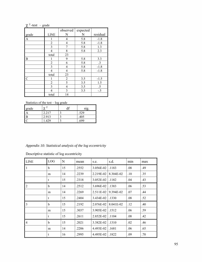
95
χ²-test - grade
grade LINE observed
N expected
N residual A 1 4 5.8 -1.8 2 4 5.8 -1.8 3 7 5.8 1.3 4 8 5.8 2.3 total 23 B 1 9 5.8 3.3 2 6 5.8 .3 3 4 5.8 -1.8 4 4 5.8 -1.8 total 23 C 1 2 3.5 -1.5 2 5 3.5 1.5 3 4 3.5 .5 4 3 3.5 -.5 total 14 Statistics of the test – log grade
grade χ² df sig. A 2.217 3 .529 B 2.913 3 .405 C 1.429 3 .699
Appendix 10: Statistical analysis of the log eccentricity
Descriptive statistic of log eccentricity
LINE LOG N mean s.e. s.d. min max
1 b 15 .2552 3.056E-02 .1183 .08 .49
m 14 .2239 2.219E-02 8.304E-02 .10 .35
t 15 .2318 3.052E-02 .1182 .04 .43
2 b 14 .2512 3.696E-02 .1383 .06 .53
m 14 .2269 2.511E-02 9.394E-02 .07 .44
t 15 .2404 3.434E-02 .1330 .08 .52
3 b 15 .2192 2.076E-02 8.041E-02 .12 .40
m 15 .3037 3.905E-02 .1512 .06 .59
t 15 .2611 2.852E-02 .1104 .08 .42
4 b 15 .2021 3.382E-02 .1310 .02 .46
m 14 .2206 4.493E-02 .1681 .06 .65
t 16 .2995 4.495E-02 .1822 .09 .70

96
ANOVA max eccentricity. log
Eccentricity log Sums of square df mean of
squares F sig.
b between the groups 2.913E-02 3 9.710E-03 .689 .563 within the groups .755 55 1.410E-02 total .805 58 m between the groups 7.078E-02 3 2.359E-02 1.402 .253 within the groups .892 53 1.683E-02 total .963 56 t between the groups 4.090E-02 3 1.363E-03 .735 .535 within the groups 1.038 56 1.854E-02 total 1.079 59
Post Hoc test, Scheffé-procedure
s.e sig. 95%-conf. max eccent. log (I) LINE (J) LINE mean difference (I-J)
lower limit upper limit b 1 2 3.998E-03 4.412E-02 1.000 -.1233 .1313 3 3.604E-02 4.336E-02 .875 -8.8999E-02 .1611 4 5.312E-02 4.336E-02 .684 -7.1921E-02 .1782 2 1 -3.9985E-03 4.412E-02 1.000 -.1313 .1233 3 3.204E-02 4.412E-02 .912 -9.5211E-02 .1593 4 4.912E-02 4.412E-02 .744 -7.8133E-02 .1764 3 1 -3.6043E-02 4.336E-02 .875 -.1611 8.900E-02 2 -3.2045E-02 4.412E-02 .912 -.1593 9.521E-02 4 1.708E-02 4.336E-02 .984 -.1080 .1421 4 1 -5.3122E-02 4.336E-02 .684 -.1782 7.192E-02 2 -4.9123E-02 4.412E-02 .744 -.1764 7.813E-02 3 -1.7078E-02 4.336E-02 .984 -.1421 .1080 m 1 2 -2.9036E-03 4.903E-02 1.000 -.1445 .1387 3 -7.9709E-02 4.821E-02 .442 -.2189 5.950E-02 4 3.375E-03 4.903E-02 1.000 -.1382 .1450 2 1 2.904E-03 4.903E-02 1.000 -.1387 .1445 3 -7.6805E-02 4.821E-02 .475 -.2160 6.240E-02 4 6.279E-03 4.903E-02 .999 -.1353 .1479 3 1 7.971E-02 4.821E-02 .442 -5.9496E-02 .2189 2 7.681E-02 4.821E-02 .475 -6.2400E-02 .2160 4 8.308E-02 4.821E-02 .405 -5.6121E-02 .2223 4 1 -3.3749E-03 4.903E-02 1.000 -.1450 .1382 2 -6.2785E-03 4.903E-02 .999 -.1479 .1353 3 -8.3084E-02 4.821E-02 .405 -.2223 5.612E-02 t 1 2 -8.6054E-03 4.972E-02 .999 -.1519 .1347 3 -2.9304E-02 4.972E-02 .950 -.1726 .1140 4 -6.7688E-02 4.972E-02 .606 -.2110 7.563E-02 2 1 8.605E-03 4.972E-02 .999 -.1347 .1519 3 -2.0699E-02 4.972E-02 .982 -.1640 .1226 4 -5.9083E-02 4.972E-02 .704 -.2024 8.423E-02 3 1 2.930E-02 4.972E-02 .950 -.1140 .1726 2 2.070E-02 4.972E-02 .982 -.1226 .1640 4 -3.8384E-02 4.972E-02 .897 -.1817 .1049 4 1 6.769E-02 4.972E-02 .606 -7.5628E-02 .2110 2 5.908E-02 4.972E-02 .704 -8.4233E-02 .2024 3 3.838E-02 4.972E-02 .897 -.1049 .1817

97
ANALYSIS OF VARIANCE max eccent. log SOURCE of variation
df s.s m.s. F Sig.
LINE 3 1.689E-02 5.631E-03 .341 .795
LOG 2 2.059E-02 1.029E-03 .309 .537
LINE * LOG 6 .124 2.069E-02 1.254 .282
residual 164 2.706 1.650E-02
total 175 2.868
χ²-test – log_grade
Statistics of the test -
LOG χ² df sig. b 11.424 2 .003
m 9.579 2 .008
t .300 2 .861
χ²-test – log_grade Statistics of the test -
LINE χ² df sig. 1 2.909 2 .234
2 4.233 2 .120
3 .533 2 .766
4 1.273 2 .529
χ²-test - LINE Statistics of the test -
Grade_log χ² df sig. A 1.355 3 .716
B 1.087 3 .780
C 1.311 3 .726

98
Appendix 11: Statistical analysis of the log taper
Descriptive statistic of log taper [cm/m length]
LINE LOG N mean s.e. s.d. min max 1 b 15 1.6897 .2275 .8813 .21 3.87
m 14 .9014 8.646E-02 .3235 .55 1.75
t 15 1.3382 7.226E-02 .2798 .80 1.77
2 b 15 1.5582 .1404 .5439 .77 2.53
m 14 .8358 6.130E-02 .2294 .54 1.38
t 15 1.1732 5.056E-02 .1958 .70 1.43
3 b 15 1.2425 .1156 .4479 .75 2.11
m 15 .9314 6.211E-02 .2405 .64 1.44
t 15 1.1880 9.835E-02 .3809 .57 1.89
4 b 15 1.3698 .1601 .6199 .42 2.48
m 15 .7433 5.973E-02 .2313 .35 1.19
t 15 .9634 6.599E-02 .2556 .57 1.52
ANOVA log taper cm/m length
LINE Sums of square df mean of
squares F sig.
1 between the groups 4.508 2 2.254 6.932 .003
within the groups 13.330 41 .325
total 17.838 43
2 between the groups 3.791 2 1.896 14.493 .000
within the groups 5.363 41 .131
total 9.154 43
3 between the groups .828 2 .414 3.079 .057
within the groups 5.649 42 .135
total 6.478 44
4 between the groups 3.030 2 1.515 9.033 .001
within the groups 7.044 42 .168
total 10.074 44

99
Post Hoc test, Scheffé-procedure log taper cm/m length
LINE (I) log_pos (J) log_pos
mean difference (I-J) s.e sig. 95%-conf.
lower limit upper limit 1 butt mid .7883* .2119 .003 .2501 1.3265 top .3515 .2082 .252 -.1773 .8804 mid butt -.7883* .2119 .003 -1.3265 -.2501 top -.4367 .2119 .133 -.9749 .1015 top butt -.3515 .2082 .252 -.8804 .1773 mid .4367 .2119 .133 -.1015 .9749 2 butt mid .7223* .1344 .000 .3810 1.0637 top .3849* .1321 .021 4.953E-02 .7204 mid butt -.7223* .1344 .000 -1.0637 -.3810 top -.3374 .1344 .053 -.6787 3.987E-03 top butt -.3849* .1321 .021 -.7204 -4.9528E-02 mid .3374 .1344 .053 -3.9870E-03 .6787 3 butt mid .3111 .1339 .079 -2.8714E-02 .6510 top 5.450E-02 .1339 .921 -.2853 .3943 mid butt -.3111 .1339 .079 -.6510 2.871E-02 top -.2566 .1339 .172 -.5965 8.321E-02 top butt -5.4500E-02 .1339 .921 -.3943 .2853 mid .2566 .1339 .172 -8.3214E-02 .5965 4 butt mid .6264* .1495 .001 .2469 1.0059 top .4063* .1495 .033 2.686E-02 .7858 mid butt -.6264* .1495 .001 -1.0059 -.2469 top -.2201 .1495 .348 -.5996 .1594 top butt -.4063* .1495 .033 -.7858 -2.6860E-02 mid .2201 .1495 .348 -.1594 .5996 * significantly different at p=0.05
Analysis of variance log taper [cm/m length]
SOURCE of variation
df s.s m.s. F Sig.
LINE 3 1.907 .636 3.362 .020
LOG_POSI 2 11.040 5.520 63.677 .000
LINE * LOG_POSI 6 1.203 .201 1.061 .388
residual 166 31.386 .233
total 177 45.597

100
χ²-test – line - grade
LINE grade observe
d N expected
N residual 1 grade B 32 22.0 10.0 grade C 12 22.0 -10.0 2 grade B 37 22.0 15.0 grade C 7 22.0 -15.0 3 grade B 39 22.5 16.5 grade C 6 22.5 -16.5 4 grade B 39 22.5 16.5 grade C 6 22.5 -16.5
Statistics of the test - grade_taper_num
LINE χ² df sig. 1 9.0961 1 .003 2 20.455 1 .000 3 24.200 1 .000 4 24.200 1 .000
χ²-test – log position - grade Log position grade observed N expected N residual b grade B 39 30.0 9.0 grade C 21 30.0 -9.0 total 60 m grade B 57 29.0 28.0 grade C 1 29.0 -28.0 total 58 t grade B 51 30.0 21.0 grade C 9 30.0 -21.0 total 60
Statistics of the test - log grade
LOG POS χ² df sig. B 5.400 1 .020 M 54.069 1 .000 T 29.400 1 .000

101
χ²-test – log grade - line LOG_GRAD line observed N expected N residual B 1 32 36.8 -6.0
2 37 36.8 -1.0
3 39 36.8 3.0
4 39 36.8 4.0
total 147
C 1 12 7.8 4,3
2 7 7.8 -.8
3 6 7.8 -1.8
4 6 7.8 -1.8
total 31
Statistics of the test - log grade -line
LOG POS χ² df sig. B .891 3 .828
C 3.194 3 .363
Appendix 12: Statistical analysis of the log ovality
Descriptive statistic of log ovality [/]
LINE LOG N mean s.e. s.d. min max 1 b 15 1.0673 1.148E-02 4.448E-02 1.00 1.16
m 14 1.0457 9.182E-03 3.435E-02 1.01 1.14
t 15 1.0513 8.215E-03 3.182E-02 1.01 1.14
2 b 15 1.0547 9.096E-03 3.523E-02 1.01 1.11
m 14 1.0500 7.263E-03 2.717E-02 1.00 1.09
t 15 1.0427 5.729E-03 2.219E-02 1.01 1.10
3 b 15 1.0487 9.605E-03 3.720E-02 .99 1.10
m 15 1.0747 1.207E-02 4.673E-02 1.02 1.20
t 15 1.0400 4.577E-03 1.773E-02 1.02 1.08
4 b 15 1.0453 8.387E-03 3.248E-02 .98 1.10
m 15 1.0447 6.239E-03 2.416E-02 1.02 1.10
t 15 1.0420 4.899E-03 1.897E-02 1.01 1.07

102
ANOVA log ovality [/]
Log position Sums of
square df mean of squares F sig.
b between the groups 4.227E-03 3 1.409E-03 .996 .401
within the groups 7.921E-02 56 1.415E-03
total 8.344E-02 59
m between the groups 8.898E-03 3 2.966E-03 2.515 .068
within the groups 6.369E-02 54 1.179E-03
total 7.259E-02 57
t between the groups 1.133E-03 3 3.778E-04 .693 .560
within the groups 3.051E-02 56 5.448E-04
total 3.164E-02 59
Post Hoc test, Scheffé-procedure log taper cm/m length
LINE (I) LINE (J) LINE mean difference (I-J) s.e sig. 95%-conf.
lower limit upper limit b 1 2 1.267E-02 1.373E-02 .837 -2.6918E-02 5.225E-02
3 1.867E-02 1.373E-02 .608 -2.0918E-02 5.825E-02
4 2.200E-02 1.373E-02 .470 -1.7585E-02 6.158E-02
2 1 -1.2667E-02 1.373E-02 .837 -5.2252E-02 2.692E-02
3 6.000E-03 1.373E-02 .979 -3.3585E-02 4.558E-02
4 9.333E-03 1.373E-02 .927 -3.0252E-02 4.892E-02
3 1 -1.8667E-02 1.373E-02 .608 -5.8252E-02 2.092E-02
2 -6.0000E-03 1.373E-02 .979 -4.5585E-02 3.358E-02
4 3.333E-03 1.373E-02 .996 -3.6252E-02 4.292E-02
4 1 -2.2000E-02 1.373E-02 .470 -6.1585E-02 1.758E-02
2 -9.3333E-03 1.373E-02 .927 -4.8918E-02 3.025E-02
3 -3.3333E-03 1.373E-02 .996 -4.2918E-02 3.625E-02
m 1 2 -4.2857E-03 1.298E-02 .991 -4.1743E-02 3.317E-02
3 -2.8952E-02 1.276E-02 .175 -6.5780E-02 7.876E-03
4 1.048E-03 1.276E-02 1.000 -3.5780E-02 3.788E-02
2 1 4.286E-03 1.298E-02 .991 -3.3172E-02 4.174E-02
3 -2.4667E-02 1.276E-02 .302 -6.1495E-02 1.216E-02
4 5.333E-03 1.276E-02 .981 -3.1495E-02 4.216E-02
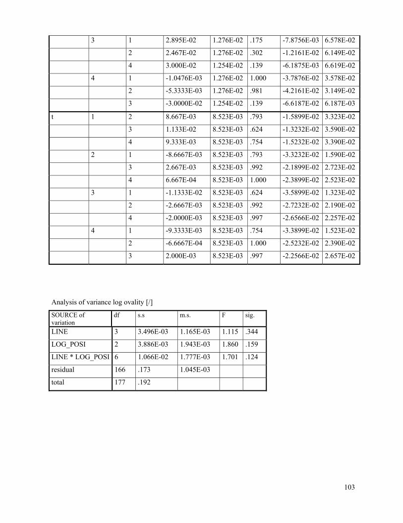
103
3 1 2.895E-02 1.276E-02 .175 -7.8756E-03 6.578E-02
2 2.467E-02 1.276E-02 .302 -1.2161E-02 6.149E-02
4 3.000E-02 1.254E-02 .139 -6.1875E-03 6.619E-02
4 1 -1.0476E-03 1.276E-02 1.000 -3.7876E-02 3.578E-02
2 -5.3333E-03 1.276E-02 .981 -4.2161E-02 3.149E-02
3 -3.0000E-02 1.254E-02 .139 -6.6187E-02 6.187E-03
t 1 2 8.667E-03 8.523E-03 .793 -1.5899E-02 3.323E-02
3 1.133E-02 8.523E-03 .624 -1.3232E-02 3.590E-02
4 9.333E-03 8.523E-03 .754 -1.5232E-02 3.390E-02
2 1 -8.6667E-03 8.523E-03 .793 -3.3232E-02 1.590E-02
3 2.667E-03 8.523E-03 .992 -2.1899E-02 2.723E-02
4 6.667E-04 8.523E-03 1.000 -2.3899E-02 2.523E-02
3 1 -1.1333E-02 8.523E-03 .624 -3.5899E-02 1.323E-02
2 -2.6667E-03 8.523E-03 .992 -2.7232E-02 2.190E-02
4 -2.0000E-03 8.523E-03 .997 -2.6566E-02 2.257E-02
4 1 -9.3333E-03 8.523E-03 .754 -3.3899E-02 1.523E-02
2 -6.6667E-04 8.523E-03 1.000 -2.5232E-02 2.390E-02
3 2.000E-03 8.523E-03 .997 -2.2566E-02 2.657E-02
Analysis of variance log ovality [/]
SOURCE of variation
df s.s m.s. F sig.
LINE 3 3.496E-03 1.165E-03 1.115 .344
LOG_POSI 2 3.886E-03 1.943E-03 1.860 .159
LINE * LOG_POSI 6 1.066E-02 1.777E-03 1.701 .124
residual 166 .173 1.045E-03
total 177 .192

104
Appendix 13: Statistical analysis - proportion of juvenile wood
Descriptive statistics - % juv volume
LINE LOG N mean s.e. s.d. min max 1 b 15 21.2333 1.0784 4.1767 15.50 28.30
m 14 43.7857 2.4581 9.1973 28.10 61.00
t 14 60.1929 3.7106 13.8837 36.40 83.70
2 b 14 21.9786 1.0472 3.9182 16.90 29.30
m 12 46.8083 2.2859 7.9185 36.00 60.60
t 14 64.2286 2.3747 8.8855 53.60 81.00
3 b 15 19.8600 2.1485 8.3211 4.70 32.60
m 14 44.2000 2.4268 9.0801 19.10 58.60
t 15 64.5333 2.6190 10.1432 51.30 80.20
4 b 14 20.6143 1.6916 6.3294 8.80 31.50
m 13 47.3615 1.6071 5.7946 36.50 54.20
t 14 63.2071 1.6738 6.2628 53.80 74.20
ANOVA % juv volume
LINE Sums of square df mean of
squares F sig.
1 between the groups 11123.663 2 5561.832 57.789 .000
within the groups 3849.760 40 96.244
total 14973.423 42
2 between the groups 12610.730 2 6305.365 121.784 .000
within the groups 1915.681 37 51.775
total 14526.411 39
3 between the groups 15006.110 2 7503.055 88.358 .000
within the groups 3481.589 41 84.917
total 18487.699 43
4 between the groups 12962.840 2 6481.420 171.799 .000
within the groups 1433.617 38 37.727
total 14396.458 40

105
ANOVA - % juv volume
LOG Sums of square df mean of
squares F sig.
b between the groups 35.316 3 11.772 .329 .805
within the groups 1933.990 54 35.815
total 1969.306 57
m between the groups 130.293 3 43.431 .652 .586
within the groups 3264.157 49 66.615
total 3394.450 52
t between the groups 167.066 3 55.689 .538 .658
within the groups 5482.500 53 103.443
total 5649.567 56
Analysis of variance - % juv volume
SOURCE of variation df s.s m.s. F sig. LINE 3 159.146 53.049 .775 .510
LOG 2 51451.080 25725.540 375.744
.000
LINE * LOG 6 180.618 30.103 .440 .851
residual 156 10680.648 68.466
total 167 62590.793

106
Appendix 14: Statistical analysis – Log classification according to ENV 1927-1
χ²-test – log grade - line
LINE LOG observed N
expected N residual
1 b grade B 1 5.0 -4.0
grade C 12 5.0 7.0
grade D 2 5.0 -3.0
m grade B 2 4.7 -2.7
grade C 10 4.7 5.3
grade D 2 4.7 -2.7
t grade B -4.0 1 5.0
grade C 8 5.0 3.0
grade D 6 5.0 1.0
2 b grade B 1 7.5 -6.5
grade C 14 7.5 6.5
m grade B 3 4.7 -1.7
grade C 10 4.7 5.3
grade D 1 4.7 -3.7
t grade B 1 5.0 -4.0
grade C 12 5.0 7.0
grade D 2 5.0 -3.0
3 b grade B 7 7.5 -.5
grade C 8 7.5 .5
m grade B 3 5.0 -2.0
grade C 9 5.0 4.0
grade D 3 5.0 -2.0
t grade C 9 7.5 1.5
grade D 6 7.5 -1.5
4 b grade B 5 7.5 -2.5
grade C 10 7.5 2.5
m grade B 2 7.5 -5.5
grade C 13 7.5 5.5
t grade C 11 7.5 3.5
grade D 4 7.5 -3.5
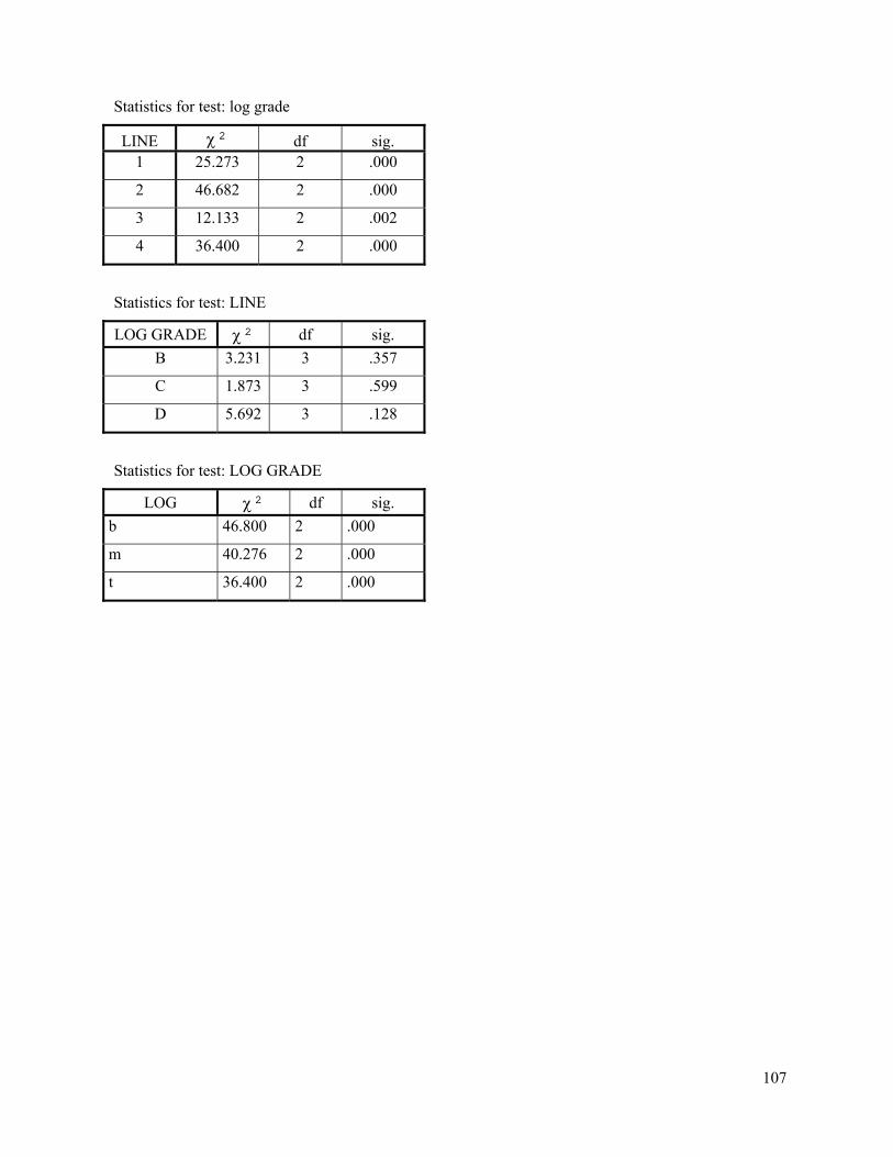
107
Statistics for test: log grade
LINE χ² df sig. 1 25.273 2 .000
2 46.682 2 .000
3 12.133 2 .002
4 36.400 2 .000
Statistics for test: LINE
LOG GRADE χ² df sig. B 3.231 3 .357
C 1.873 3 .599
D 5.692 3 .128
Statistics for test: LOG GRADE
LOG χ² df sig. b 46.800 2 .000
m 40.276 2 .000
t 36.400 2 .000
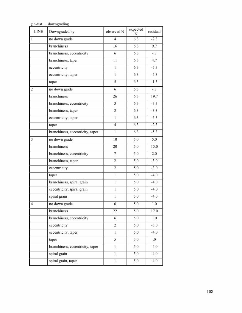
108
χ²-test – downgrading
LINE Downgraded by observed N expected N residual
1 no down grade 4 6.3 -2.3
branchiness 16 6.3 9.7
branchiness, eccentricity 6 6.3 -.3
branchiness, taper 11 6.3 4.7
eccentricity 1 6.3 -5.3
eccentricity, taper 1 6.3 -5.3
taper 5 6.3 -1.3
2 no down grade 6 6.3 -.3
branchiness 26 6.3 19.7
branchiness, eccentricity 3 6.3 -3.3
branchiness, taper 3 6.3 -3.3
eccentricity, taper 1 6.3 -5.3
taper 4 6.3 -2.3
branchiness, eccentricity, taper 1 6.3 -5.3
3 no down grade 10 5.0 5.0
branchiness 20 5.0 15.0
branchiness, eccentricity 7 5.0 2.0
branchiness, taper 2 5.0 -3.0
eccentricity 2 5.0 -3.0
taper 1 5.0 -4.0
branchiness, spiral grain 1 5.0 -4.0
eccentricity, spiral grain 1 5.0 -4.0
spiral grain 1 5.0 -4.0
4 no down grade 6 5.0 1.0
branchiness 22 5.0 17.0
branchiness, eccentricity 6 5.0 1.0
eccentricity 2 5.0 -3.0
eccentricity, taper 1 5.0 -4.0
taper 5 5.0 .0
branchiness, eccentricity, taper 1 5.0 -4.0
spiral grain 1 5.0 -4.0
spiral grain, taper 1 5.0 -4.0

109
Appendix 15: Statistical analysis – Stress grading
Statistics for test : difference in frequency of LINE C24 – C16 - reject
LINE χ² df sig. 1 5.239 2 .073 2 4.308 2 .116 3 5.097 2 .078 4 5.067 2 .079
Statistics for test : difference in frequency of C24-C16-reject LINE
grade χ² df sig. C16 1.448 3 .694 C24 3.746 3 .290
reject 10.000 3 .019
Appendix 16: Statistical analysis – Mechanical properties MOE, MOR
Descriptive statistics : MOEstat
LINE N mean s.e. s.d. min max 1 90 7807.5321 282.6766 2681.7058 4104.22 23809.71
2 92 8243.6739 207.9312 1994.4057 4184.00 15250.00
3 92 8266.6522 187.7372 1800.7115 4153.00 13533.00
4 90 7870.6751 252.1708 2392.3024 3852.00 17377.00
Descriptive statistics : MOR LINE N mean s.e. s.d. min max 1 91 32.1819 .9401 14.09 54.98 8.9675
2 92 34.5435 .8435 11.93 50.67 8.0905
3 94 32.6932 .9518 .00 57.91 9.2276
4 90 31.6126 .9298 12.61 61.04 8.8212

110
Analysis of variance - MOE [N/mm2]
SOURCE of variation df s.s m.s. F sig. LINE 12474782.918 3 4158260.973 .919 .432
LOG_POS 5382859.089 1 5382859.089 1.189 .276
WIND_DIR 54501513.106 3 18167171.035 4.014 .008
BAT_POS 31384323.406 2 15692161.703 3.467 .032
LINE * LOG_POS 99284688.489 3 33094896.163 7.312 .000
LINE * WIND_DIR 8333012.474 5 1666602.495 .368 .870
LOG_POS * WIND_DIR 4737361.368 1 4737361.368 1.047 .307
LINE * LOG_POS *
WIND_DIR
6270287.170 3 2090095.723 .462 .709
LINE * BAT_POS 23474306.302 3 7824768.767 1.729 .161
LOG_POS * BAT_POS 65487.296 1 65487.296 .014 .904
LINE * LOG_POS *
BAT_POS
28561653.140 2 14280826.570 3.155 .044
WIND_DIR * BAT_POS 6319715.281 1 6319715.281 1.396 .238
LINE * WIND_DIR *
BAT_POS
11770201.940 3 3923400.647 .867 .459
LOG_POS * WIND_DIR *
BAT_POS
5124873.221 1 5124873.221 1.132 .288
LINE * LOG_POS *
WIND_DIR * BAT_POS
10753197.598 1 10753197.598 2.376 .124
residual 1471069628.299 325 4526368.087
total 1822398534.199 363

111
Analysis of variance MOR [N/mm²]
SOURCE of variation df s.s m.s. F sig. LINE 112.585 3 37.528 .556 .644
LOG_POS 9.156 1 9.156 .136 .713
WIND_DIR 1203.911 3 401.304 5.950 .001
BAT_POS 670.221 2 335.111 4.968 .007
LINE * LOG_POS 246.858 3 82.286 1.220 .302
LINE * WIND_DIR 383.555 5 76.711 1.137 .340
LOG_POS * WIND_DIR 168.585 1 168.585 2.500 .115
LINE * LOG_POS *
WIND_DIR
102.483 3 34.161 .506 .678
LINE * BAT_POS 125.196 3 41.732 .619 .603
LOG_POS * BAT_POS 174.601 1 174.601 2.589 .109
LINE * LOG_POS *
BAT_POS
263.060 2 131.530 1.950 .144
WIND_DIR * BAT_POS .277 1 .277 .004 .949
LINE * WIND_DIR *
BAT_POS
78.624 3 26.208 .389 .761
LOG_POS * WIND_DIR *
BAT_POS
23.389 1 23.389 .347 .556
LINE * LOG_POS *
WIND_DIR * BAT_POS
3.075 1 3.075 .046 .831
residual 22055.320 327 67.447
total 27403.671 365

112
Appendix 17: Statistical analysis – Distortion –twist, bow, spring
Descriptive analysis “twist”
line log exposure inner outer
twist counts
twist average [mm]
twist st.dev [mm]
twist se [mm]
twist max [mm]
twist min [mm]
1 b 0 0 8 25.1 10.2 3.6 35 4 1 b l 1 15 11.9 9.4 2.4 29 2.5 1 b l 2 16 4.3 2.6 0.7 9.5 0 1 b w 1 14 14.8 11.4 3.0 45 1 1 b w 2 11 4.1 2.5 0.8 6 1 1 t l 1 13 16.6 9.6 2.7 33 1 1 t l 2 2 16.5 0.7 0.5 17 16 1 t w 1 11 18.0 6.0 1.8 28 8 1 t w 2 2 b 0 0 6 20.4 8.4 3.4 35 10 2 b l 1 14 9.8 8.3 2.2 33.5 2 2 b l 2 13 2.6 2.7 0.7 8.5 0.5 2 b w 1 14 16.5 11.0 3.0 34 1 2 b w 2 14 4.2 4.1 1.1 14 0.5 2 t l 1 15 14.9 8.3 2.1 32.5 4 2 t l 2 1 13.5 13.5 13.5 2 t w 1 12 18.6 6.5 1.9 30 11 2 t w 2 3 b 0 0 8 23.3 6.8 2.4 37 15 3 b l 1 15 5.5 3.9 1.0 14.5 1 3 b l 2 15 2.8 2.0 0.5 7 0.5 3 b w 1 15 11.3 10.2 2.6 34 3 3 b w 2 10 4.5 3.7 1.2 13 1 3 t l 1 13 14.7 5.1 1.4 20.5 5.5 3 t l 2 2 15.8 7.4 5.3 21 10.5 3 t w 1 13 14.2 4.4 1.2 20.5 4.5 3 t w 2 1 7.5 7.5 7.5 4 b 0 0 5 33.9 14.5 6.5 55.5 16 4 b l 1 14 11.3 8.2 2.2 32.5 1.5 4 b l 2 13 3.8 3.3 0.9 10.5 0.5 4 b w 1 14 17.8 13.4 3.6 41 1 4 b w 2 14 4.9 3.2 0.9 10.5 0.5 4 t l 1 13 17.6 9.2 2.5 33 0 4 t l 2 4 12.5 12.9 6.5 31 2.5 4 t w 1 9 17.7 8.2 2.7 28 6.5 4 t w 2 3 11.5 8.7 5.0 19 2

113
Descriptive analysis “bow”
line log exposure inner outer bow counts
bow average [mm]
bow stabw [mm]
bow se [mm]
bow max [mm]
bow min [mm]
1 b 0 0 8 3.35 1.80 0.63 5.5 0 1 b l 1 15 3.27 2.40 0.62 10.5 0 1 b l 2 16 4.81 5.90 1.47 21 1 1 b w 1 14 3.29 2.02 0.54 7.5 1.5 1 b w 2 11 6.30 9.93 2.99 33 0 1 t l 1 13 6.46 6.64 1.84 22 0 1 t l 2 2 13.50 0.71 0.50 14 13 1 t w 1 11 3.95 2.77 0.84 10 1.5 1 t w 2 2 b 0 0 6 3.50 0.84 0.34 5 3 2 b l 1 14 2.71 2.06 0.55 7 0 2 b l 2 13 1.85 1.63 0.45 5 0.5 2 b w 1 14 4.14 2.13 0.57 9 1 2 b w 2 14 2.00 1.22 0.33 5 0 2 t l 1 15 4.33 4.06 1.05 17 1 2 t l 2 1 1.00 1 1 2 t w 1 12 4.29 4.87 1.41 17.5 0.5 2 t w 2 3 b 0 0 8 3.19 2.43 0.86 8 0 3 b l 1 15 1.83 1.42 0.37 4.5 0 3 b l 2 15 2.73 2.84 0.73 9 0 3 b w 1 15 1.83 1.16 0.30 4 0 3 b w 2 10 1.70 1.55 0.49 6 0.5 3 t l 1 13 4.92 3.64 1.01 13 1 3 t l 2 2 10.00 1.41 1.00 11 9 3 t w 1 13 4.46 3.42 0.95 12 0.5 3 t w 2 1 7.00 7 7 4 b 0 0 5 4.00 3.24 1.45 8 1 4 b l 1 14 2.89 1.70 0.45 7 0.5 4 b l 2 13 2.65 2.24 0.62 8 0 4 b w 1 14 4.00 3.78 1.01 14 0.5 4 b w 2 14 2.79 2.38 0.64 10 1 4 t l 1 13 9.35 9.58 2.66 35 1 4 t l 2 4 5.25 3.30 1.65 10 3 4 t w 1 9 4.50 2.32 0.77 8 1 4 t w 2 3 4.67 2.08 1.20 7 3

114
line log exposure
inner outer
spring counts
spring average [mm]
spring stabw [mm]
spring se [mm]
spring max [mm]
spring min [mm]
1 b 0 0 8 3.9 2.2 0.8 8 1 1 b l 1 15 3.1 1.9 0.5 7 1 1 b l 2 16 2.7 3.0 0.7 12 0 1 b w 1 14 3.3 2.1 0.6 7 1 1 b w 2 11 2.1 0.8 0.3 4 1 1 t l 1 13 3.3 1.6 0.5 7 1 1 t l 2 2 3.5 0.7 0.5 4 3 1 t w 1 11 3.8 3.1 0.9 12 1 1 t w 2 2 b 0 0 6 4.1 2.5 1.0 8 1 2 b l 1 14 2.1 1.4 0.4 5 0.5 2 b l 2 13 1.8 0.9 0.2 3 0.5 2 b w 1 14 2.4 0.9 0.3 4 1 2 b w 2 14 2.0 1.9 0.5 7 0 2 t l 1 15 2.7 2.2 0.6 9 1 2 t l 2 1 2.5 2.5 2.5 2 t w 1 12 3.0 1.3 0.4 5.5 1.5 2 t w 2 3 b 0 0 8 4.5 3.5 1.2 11 2 3 b l 1 15 2.0 1.0 0.3 4 0.5 3 b l 2 15 2.0 1.2 0.3 5 0 3 b w 1 15 2.2 1.5 0.4 5 0.5 3 b w 2 10 1.5 0.8 0.3 3.5 1 3 t l 1 13 3.4 2.3 0.6 10 1 3 t l 2 2 6.0 5.7 4.0 10 2 3 t w 1 13 3.5 2.4 0.7 8.5 1 3 t w 2 1 2.0 2 2 4 b 0 0 5 3.5 0.6 0.3 4.5 3 4 b l 1 14 2.5 2.1 0.5 8 0 4 b l 2 13 1.9 0.8 0.2 3.5 1 4 b w 1 14 2.7 2.2 0.6 9 1 4 b w 2 14 1.5 0.7 0.2 3 0.5 4 t l 1 13 4.3 3.0 0.8 9.5 0.5 4 t l 2 4 1.5 0.6 0.3 2 1 4 t w 1 9 3.7 1.8 0.6 6.5 1.5 4 t w 2 3 4.3 1.3 0.7 5.5 3
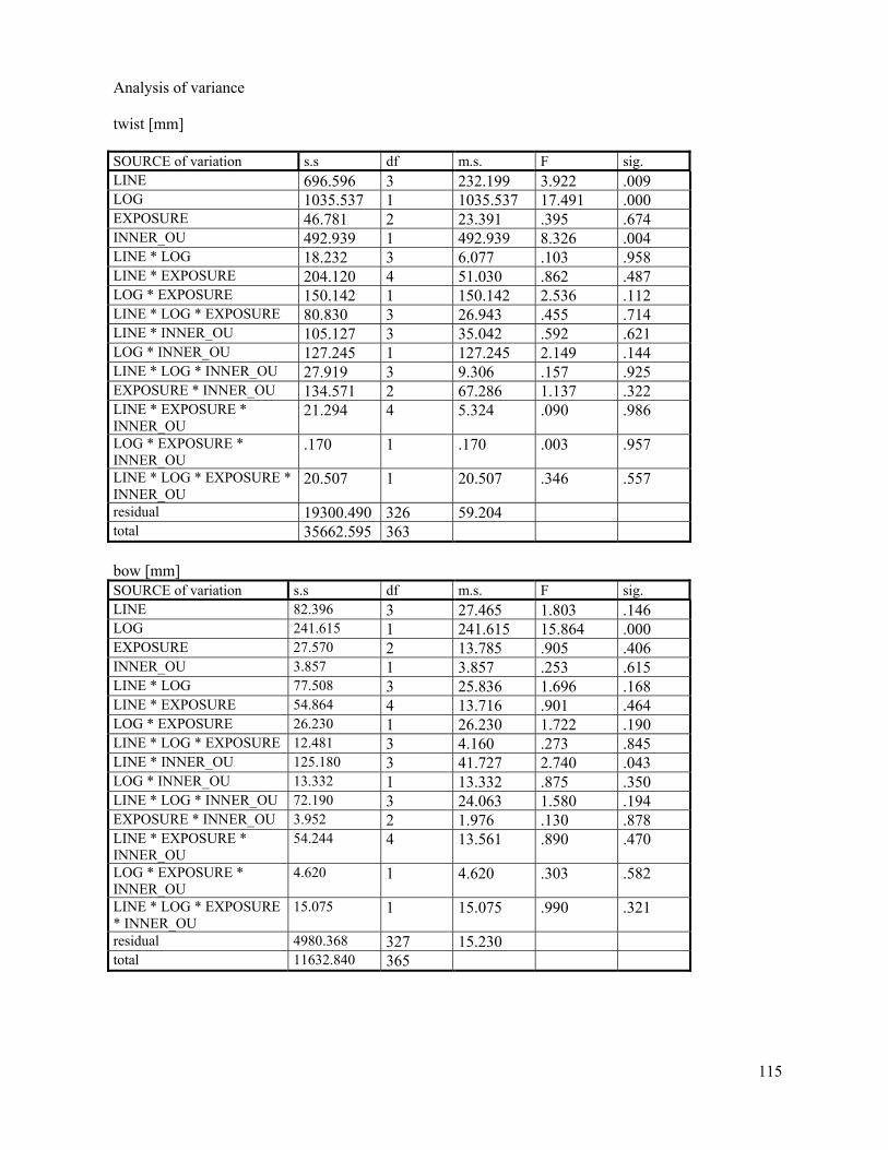
115
Analysis of variance
twist [mm]
SOURCE of variation s.s df m.s. F sig. LINE 696.596 3 232.199 3.922 .009 LOG 1035.537 1 1035.537 17.491 .000 EXPOSURE 46.781 2 23.391 .395 .674 INNER_OU 492.939 1 492.939 8.326 .004 LINE * LOG 18.232 3 6.077 .103 .958 LINE * EXPOSURE 204.120 4 51.030 .862 .487 LOG * EXPOSURE 150.142 1 150.142 2.536 .112 LINE * LOG * EXPOSURE 80.830 3 26.943 .455 .714 LINE * INNER_OU 105.127 3 35.042 .592 .621 LOG * INNER_OU 127.245 1 127.245 2.149 .144 LINE * LOG * INNER_OU 27.919 3 9.306 .157 .925 EXPOSURE * INNER_OU 134.571 2 67.286 1.137 .322 LINE * EXPOSURE * INNER_OU
21.294 4 5.324 .090 .986
LOG * EXPOSURE * INNER_OU
.170 1 .170 .003 .957
LINE * LOG * EXPOSURE * INNER_OU
20.507 1 20.507 .346 .557
residual 19300.490 326 59.204 total 35662.595 363 bow [mm] SOURCE of variation s.s df m.s. F sig. LINE 82.396 3 27.465 1.803 .146 LOG 241.615 1 241.615 15.864 .000 EXPOSURE 27.570 2 13.785 .905 .406 INNER_OU 3.857 1 3.857 .253 .615 LINE * LOG 77.508 3 25.836 1.696 .168 LINE * EXPOSURE 54.864 4 13.716 .901 .464 LOG * EXPOSURE 26.230 1 26.230 1.722 .190 LINE * LOG * EXPOSURE 12.481 3 4.160 .273 .845 LINE * INNER_OU 125.180 3 41.727 2.740 .043 LOG * INNER_OU 13.332 1 13.332 .875 .350 LINE * LOG * INNER_OU 72.190 3 24.063 1.580 .194 EXPOSURE * INNER_OU 3.952 2 1.976 .130 .878 LINE * EXPOSURE * INNER_OU
54.244 4 13.561 .890 .470
LOG * EXPOSURE * INNER_OU
4.620 1 4.620 .303 .582
LINE * LOG * EXPOSURE * INNER_OU
15.075 1 15.075 .990 .321
residual 4980.368 327 15.230 total 11632.840 365

116
spring [mm] SOURCE of variation df s.s m.s. F sig. LINE 3 5.302 1.767 .474 .700 LOG 1 32.859 32.859 8.820 .003 EXPOSURE 1 .347 .347 .093 .760 INNER_OU 1 4.368 4.368 1.172 .280 LINE * LOG 3 7.594 2.531 .679 .565 LINE * EXPOSURE 3 16.403 5.468 1.468 .223 LOG * EXPOSURE 1 3.746E-
02 3.746E-02
.010 .920
LINE * LOG * EXPOSURE
3 13.382 4.461 1.197 .311
LINE * INNER_OU 3 6.025 2.008 .539 .656 LOG * INNER_OU 1 .924 .924 .248 .619 LINE * LOG * INNER_OU
3 1.895 .632 .170 .917
EXPOSURE * INNER_OU 1 1.445 1.445 .388 .534 LINE * EXPOSURE * INNER_OU
3 19.713 6.571 1.764 .154
LOG * EXPOSURE * INNER_OU
1 .188 .188 .051 .822
LINE * LOG * EXPOSURE * INNER_OU
1 18.852 18.852 5.060 .025
Fehler 325 1210.779 3.725 Gesamt 359 4194.750

117
Appendix 18: Statistical analysis – Batten density Descriptive statistics LINE LOG WIND BAT_POS N mean s.e. s.d. min max 1 B .00 6 456.2256 20.4494 50.0906 411.31 550.20 L 1.00 9 405.4302 14.3748 43.1243 342.18 474.70 2.00 9 421.0704 12.4577 37.3730 345.63 474.29 W 1.00 9 413.0841 17.6820 53.0459 369.35 530.14 2.00 6 391.7466 8.2219 20.1394 360.21 414.11 T 1.00 2 425.8028 2.5820 3.6515 423.22 428.38 2.00 2 444.3617 13.4840 19.0692 430.88 457.85 L 1.00 7 482.1906 30.0412 79.4814 382.36 600.25 2.00 2 495.4801 16.7975 23.7553 478.68 512.28 W 1.00 5 433.1723 15.2187 34.0301 387.08 464.84 2 B .00 6 396.3272 17.1895 42.1054 325.52 439.66 L 1.00 14 385.1406 14.0553 52.5901 291.30 483.70 2.00 12 373.2310 10.1134 35.0337 298.53 439.26 W 1.00 14 409.1312 16.0238 59.9555 339.52 544.04 2.00 13 382.1505 9.8319 35.4494 310.77 436.37 T 1.00 1 364.2954 . . 364.30 364.30 2.00 1 343.1189 . . 343.12 343.12 L 1.00 15 428.1921 11.3869 44.1014 347.05 510.54 2.00 2 427.4591 17.6056 24.8981 409.85 445.06 W 1.00 12 427.7618 11.5446 39.9917 350.59 510.90 3 B .00 8 421.4638 13.3558 37.7759 372.52 471.88 L 1.00 15 363.5846 11.2149 43.4350 295.20 439.82 2.00 13 388.7106 11.6150 41.8783 314.07 455.36 W 1.00 13 389.0029 15.4403 55.6709 284.76 517.06 2.00 12 376.8140 13.3028 46.0824 305.03 476.80 T L 1.00 14 404.3491 9.4331 35.2953 342.15 466.73 2.00 2 509.5062 58.5178 82.7567 450.99 568.02 W 1.00 13 399.9692 8.1853 29.5124 350.22 464.71 2.00 1 389.5979 . . 389.60 389.60 4 B .00 4 430.9347 24.8504 49.7008 379.74 495.76 L 1.00 9 395.0298 18.5186 55.5558 331.38 493.95 2.00 9 413.0553 19.0727 57.2181 324.59 514.23 W 1.00 10 418.5667 16.0582 50.7805 349.80 516.37 2.00 9 381.4871 13.5445 40.6334 319.95 427.99 T L 1.00 5 435.0472 40.3812 90.2952 365.02 572.92 2.00 2 387.2692 2.5753 3.6420 384.69 389.84 W 1.00 7 413.7069 19.3521 51.2010 346.56 484.27

118
Analysis of variance
DENSITY
SOURCE of variation s.s df m.s. F sig. LINE 28505.158 3 9501.719 4.292 .006 LOG 15168.044 2 7584.022 3.426 .034 WIND 24481.454 2 12240.727 5.529 .004 BAT_POS 521.512 1 521.512 .236 .628 LINE * LOG 17699.390 3 5899.797 2.665 .048 LINE * WIND 9898.397 4 2474.599 1.118 .349 LOG * WIND 16030.531 1 16030.531 7.241 .008 LINE * LOG * WIND 1481.654 3 493.885 .223 .880 LINE * BAT_POS 22518.717 3 7506.239 3.391 .019 LOG * BAT_POS 276.461 1 276.461 .125 .724 LINE * LOG * BAT_POS 13266.188 3 4422.063 1.997 .115 WIND * BAT_POS 16369.660 2 8184.830 3.697 .026 LINE * WIND * BAT_POS 2420.046 4 605.011 .273 .895 LOG * WIND * BAT_POS 3133.569 1 3133.569 1.415 .235 LINE * LOG * WIND * BAT_POS
.000 0 . . .
residual 566743.089 256 2213.840 total 781620.211 293
Appendix 19: Statistical analysis –Reaction wood
Descriptive statistics – compression wood ratio to batten surface
LOG_POS WIND LINE N mean s.e. s.d. min max butt centre 1.00 2 .8300 1.400E-02 1.980E-02 .82 .84 4.00 1 .6580 . . .66 .66 leewards 1.00 11 .6099 8.762E-02 .2906 .21 1.00 4.00 10 .4396 7.535E-02 .2383 .13 .76 windwards 1.00 9 .6146 .1032 .3097 .20 1.00 4.00 10 .2789 6.930E-02 .2191 .04 .60 top leewards 1.00 6 .8352 6.333E-02 .1551 .58 1.00 4.00 5 .7152 .1240 .2772 .34 1.00 windwards 1.00 6 .5305 .1375 .3368 .05 1.00 4.00 5 .3976 4.244E-02 9.491E-02 .23 .46

119
ANOVA - CW_MEAN
LOG_POS WIND
Sums of
square df
mean of
squares F sig.
butt centre between the groups 1.972E-02 1 1.972E-02 50.313 .089 within the groups 3.920E-04 1 3.920E-04 total 2.011E-02 2 leewards between the groups .152 1 .152 2.130 .161 within the groups 1.355 19 7.134E-02 total 1.507 20 windwards between the groups .534 1 .534 7.565 .014 within the groups 1.199 17 7.055E-02 total 1.733 18 top leewards between the groups 3.925E-02 1 3.925E-02 .826 .387 within the groups .428 9 4.753E-02 total .467 10 windwards between the groups 4.817E-02 1 4.817E-02 .719 .418 within the groups .603 9 6.701E-02 total .651 10
Analysis of variance Compression wood ratio
SOURCE of variation df s.s m.s. F sig. LINE .209 1 .209 3.179 .080 LOG_POS .253 1 .253 3.851 .055 WIND .701 3 .234 3.560 .020 LINE * LOG_POS 5.642E-02 1 5.642E-02 .860 .358 LINE * WIND 3.193E-02 2 1.597E-02 .243 .785 LOG_POS * WIND
.191 1 .191 2.919 .093
LINE * LOG_POS * WIND
2.046E-02 1 2.046E-02 .312 .579
residual 3.673 56 6.560E-02 total 5.524 66 a R-Quadrat = .335 (korrigiertes R-Quadrat = .216)
Related Documents