The influence of synoptic airflow on UK daily precipitation extremes: observed spatio-temporal relationships

The influence of synoptic airflow on UK daily precipitationextremes. Part I: Observed spatio-temporal relationships

Douglas Maraun • Timothy J. Osborn •

Henning W. Rust

Received: 13 May 2009 / Accepted: 7 November 2009 / Published online: 1 December 2009

� Springer-Verlag 2009

Abstract We study the influence of synoptic scale

atmospheric circulation on extreme daily precipitation

across the United Kingdom, using observed time series

from 689 rain gauges. To this end we employ a statistical

model, that uses airflow strength, direction and vorticity as

predictors for the generalised extreme value distribution of

monthly precipitation maxima. The inferred relationships

are connected with the dominant westerly flow, the orog-

raphy, and the moisture supply from surrounding seas. We

aggregated the results for individual rain gauges to regional

scales to investigate the temporal variability of extreme

precipitation. Airflow explains a significant fraction of the

variability on subannual to decadal time scales. A large

fraction of the especially heavy winter precipitation during

the 1980s and 1990s in north Scotland can be attributed to a

prevailing positive phase of the North Atlantic Oscillation.

Our statistical model can be used for statistical downscal-

ing and to validate regional climate model output.

Keywords Extreme precipitation � Synoptic airflow �United Kingdom � Climate variability � Extreme value

statistics � Vector generalised model � Covariates �Statistical downscaling

1 Introduction

Extreme precipitation is one of the major natural hazards in

the United Kingdom. Hall et al. (2005) estimate the aver-

age annual damage caused by flooding to be £1billion; and

according to the Association of British Insurers, the 2007

summer floods alone cost £3billion (ABI 2007). Under

global warming, the magnitude and pattern of extreme

precipitation are expected to change (Trenberth et al.

2003). The increasing water holding capacity of the

atmosphere will intensify precipitation events, and changes

in the atmospheric circulation will redistribute moisture

globally. Changes in the water cycle have already been

observed. Trenberth et al. (2007) found an increase in

annual-mean precipitation for the mid-latitudes, and a

decrease for the subtropics; yet the intensity of precipita-

tion has grown in most extra-tropical regions (Alexander

et al. 2006). In agreement with global scale observations,

Osborn et al. (2000) and Maraun et al. (2008) found

positive trends in the contribution of heavy precipitation

events to the total winter precipitation throughout the last

century (to a lesser extend also for spring and autumn).

Similarly, Fowler and Kilsby (2003) reported a positive

1961–2000 trend in extreme precipitation in North Scot-

land. However, especially for precipitation on regional

scales, it is difficult to distinguish these observed trends

from natural variability and to attribute them to external

forcing such as anthropogenic greenhouse gases (Hegerl

et al. 2007).

Electronic supplementary material The online version of thisarticle (doi:10.1007/s00382-009-0710-9) contains supplementarymaterial, which is available to authorized users.

D. Maraun � T. J. Osborn

Climatic Research Unit, School of Environmental Sciences,

University of East Anglia, Norwich NR4 7TJ, UK

Present Address:D. Maraun (&)

Department of Geography, University of Giessen,

Giessen, Germany

e-mail: [email protected];

[email protected]

H. W. Rust

Laboratoire des Sciences du Climat et de l’Environnement,

91191 Gif-sur-Yvette, France

e-mail: [email protected]

123

Clim Dyn (2011) 36:261–275

DOI 10.1007/s00382-009-0710-9

http://dx.doi.org/10.1007/s00382-009-0710-9

For the 21st century, Meehl et al. (2007) project a fur-

ther increase in precipitation intensity on a global scale. In

Northern Europe, mean precipitation for 2080-2099 is

expected to increase relative to the 1980–1999 mean,

whereas a decrease in mean precipitation is expected for

the Mediterranean (Christensen et al. 2007). The intensity

of extreme precipitation, however, is projected to increase

over almost the whole of Europe (Christensen et al. 2007),

including the United Kingdom (Fowler et al. 2005;

Ekstrom et al. 2005).

To assess the impact of future extreme precipitation and

to implement adaptation measures accordingly, one needs

to distinguish sustained trends from natural variability, and

to accurately predict further changes. The processes con-

trolling variability and trends of extreme precipitation—

atmospheric moisture and atmospheric circulation—might

affect precipitation differently. For a reliable climate model

simulation and prediction of precipitation variability and

trends, it is therefore not only important to reliably repre-

sent these processes themselves, but also to understand and

accurately simulate how they affect precipitation.

The principal large-scale atmospheric circulation pattern

affecting United Kingdom precipitation is the North

Atlantic Oscillation (NAO, e.g., Marshall et al. 2001;

Wilby et al. 1997): an increased atmospheric pressure

gradient between Iceland and the Azores drives more storm

tracks towards northern Europe and generally leads to

wetter weather. On an intermediate synoptic scale, the

atmospheric circulation across the United Kingdom can be

represented by airflow indices (Jenkinson and Collison

1977; Jones et al. 1993). These airflow indices have been

used extensively in empirical studies of the relationship

between atmospheric circulation and UK climate (e.g.,

Conway et al. 1996, reported relationships between airflow

and mean precipitation for various UK regions; Wilby

1998, used similar relationships to statistically downscale

climate change scenarios for the UK; Osborn et al. 1999

used these relationships to evaluate the performance of a

climate model simulation for the UK; Osborn and Jones

2000, attempted to identify and remove the influences of

variations in these airflow indices on seasonal rainfall

across the UK).

In this paper, we analyse the influence of synoptic-scale

airflow on United Kingdom extreme precipitation: in par-

ticular, how do airflow strength, direction and vorticity

influence the occurrence of heavy 1-day precipitation

events? To model the distribution of heavy precipitation,

we employ extreme value statistics (Coles 2001;

Embrechts et al. 1997; Leadbetter et al. 1983), a frame-

work that has been widely used in hydrology and clima-

tology (e.g. Katz et al. 2002; Naveau et al. 2005). We

divide the precipitation time series into blocks of one

month length, and model the distribution of block maxima

using the generalised extreme value distribution (GEV). To

describe the airflow influence on extreme precipitation, we

use a vector generalised linear model (Yee and Wild 1996;

Yee and Stephenson 2007), which has been developed in

Maraun et al. (2009b). This class of regression models is,

in combination with the GEV, particularly suitable to

describe the tail of a distribution.

The impacts of extreme precipitation events—flooding

and subsequent damages of infrastructure and agriculture—

occur on local scales; to model these impacts, accurate

precipitation data sets with a high resolution are necessary.

Atmosphere ocean general circulation models (AOGCMs)

are not yet capable to produce the required output, and

some form of downscaling has to be carried out. In fact, our

approach to model the link between large-scale atmo-

spheric circulation and local-scale precipitation can be used

for statistical downscaling. The UK air flow indices have

frequently been used for statistical downscaling of pre-

cipitation, though rarely with a focus on extreme precipi-

tation. One exception is Haylock et al. (2006), who

assessed the downscaled heavy precipitation from a range

of methods including some (e.g., Wilby et al. 2003) that

used air flow indices as predictors. Neither of these pre-

vious papers presents any details of the relationships

between air flow and heavy precipitation. In this paper, we

do not focus on the downscaling aspect; we are primarily

interested in the physical links between large and small

scales as an end in themselves: how they change across the

United Kingdom; how they vary within the year, on

interannual and on decadal scales; and how much vari-

ability of the precipitation extremes can be explained by

airflow on different scales.

In a forthcoming second part, we will transfer our

analysis to an ensemble of regional climate model (RCM)

simulations. Our findings help to evaluate the ability of

different RCMs to simulate the link between atmospheric

circulation and precipitation extremes. Compared to a

validation of RCM climatologies, this validation assesses

physical processes which may evolve differently in a

changing climate. It thus increases the credibility of future

precipitation scenarios.

In the first section, we present the data sets used for the

analysis. The actual statistical model and the necessary

statistical background are introduced in Sect. 3; more

extensive description of the model selection process is

given in Maraun et al. (2009b). Section 4 discusses the

results. In Sect. 4.1, three examples illustrate the inferred

relationships for individual rain gauges. Subsequently, we

study the spatial patterns of these relationships in Sect. 4.2.

Regionally averaged observational time series and the

corresponding predictions of the statistical model are cal-

culated to study the temporal variability of extreme pre-

cipitation and the explanatory power of the statistical

262 D. Maraun et al.: Airflow and UK precipitation extremes

123

model on different time scales (Sect. 4.3). Our conclusions

and suggestions for further research are given in Sect. 5.

2 Data

Our study is based on a subset of the land surface obser-

vation data from the Met Office Integrated Data Archive

System (MIDAS), which are available from the British

Atmospheric Data Centre (BADC, http://www.badc.nerc.

ac.uk). We choose the selection from Maraun et al. (2008)

comprising daily time series from 689 rain gauges covering

the whole UK, which have been selected mainly based on

record length and a low number of missing values. All

available data in the range 1 Jan 1900– 31 Dec 2006 are

used. Most gauges commence recording only in 1961, and

some gauges provide no data for approximately the last

decade. The gauge coverage is dense in England, with a

sparser network especially in the north west of Scotland.

Details about the selection can be found in Maraun et al.

(2008).

The synoptic scale atmospheric circulation is repre-

sented by daily airflow strength, direction and vorticity,

derived from sea level pressure evaluated at 16 grid points

from 45�N to 65�N and 20�W to 10�E (under the geo-

strophic approximation, strength is proportional to the

norm of the pressure gradient, direction is perpendicular to

the pressure gradient, and vorticity the norm of the curl of

the velocity field, i.e. the Laplacian of the pressure field).

For information on the calculation, refer to Jenkinson and

Collison (1977) and Jones et al. (1993). The three airflow

indices are close to being orthogonal: at daily resolution,

only weak (though significant) correlations between airflow

strength and vorticity at 0.20 exist. The mutual information

(Papoulis 1991) is low but not vanishing between strength

and direction (0.011 for base 2), and vanishes between

vorticity and direction (0.002 for base 2). The distribution

of these airflow indices has been analysed in Osborn et al.

(1999). Airflow strength is closely related to the North

Atlantic Oscillation (NAO, Marshall et al. 2001) which, as

the pressure gradient between the Azores high and the

Icelandic low, is a measure of westerly airflow over the

Atlantic. A strong correlation with airflow strength exists at

a monthly resolution: 0.46 for the whole year, and 0.75

during winter. Correlations between NAO and the other

airflow indices at monthly resolution are vanishing.

3 Methods

To model the magnitude of extreme precipitation events,

we employ the generalised extreme value distribution

(GEV, e.g. Coles 2001). The universal role of the GEV to

describe block maxima is motivated by the Fisher–Tippett

theorem. This framework has been widely used to model

extremes in climatology (e.g. Naveau et al. 2005) and

hydrology (e.g. Katz et al. 2002). To model the relation-

ship between large-scale airflow indices and local preci-

pitation, we use a vector generalised linear model (VGLM,

Yee and Wild 1996; Yee and Stephenson 2007). In contrast

to standard generalised models, which can model only the

mean of a distribution belonging to the exponential family,

this concept allows one to model a vector of parameters of

a wide class of distributions, and so to specifically account

for the variability and tail behaviour. We use the maximum

likelihood (MLE) approach to estimate the model para-

meters (e.g. Coles 2001, MLE for GEV; or Yee and

Stephenson 2007, MLE for VGLM). The model is cross

validated by skill scores (Friederichs and Hense 2007).

3.1 Generalised extreme value distribution

Assume a sequence of random variables Xt, t = 1..n, which

are independent and identically distributed (iid), but with

an unknown distribution. This sequence could represent,

e.g., the magnitude of daily precipitation. The Fisher-

Tippett theorem describes the distribution of the maximum

of this sequence,

Mn ¼ maxfX1; . . .;Xng; ð1Þ

as follows: if the probability distribution of the rescaled

maximum z converges for increasing block length (n ??)

to a limiting distribution G(z), then G(z) belongs to the

family of GEV distributions

Gðz; l; r; nÞ ¼ exp � 1þ nz� l

r

� �h i�1=n� �

; ð2Þ

defined on {z : 1 ? n(z - l)/r[ 0 }, where -?\ l\?, r[ 0 and -?\ n\?. The location parameter ldetermines the position of the distribution, the scale

parameter r the width, and the shape parameter n the tail:

For n\ 0, the tail has a finite upper value (Weibull dis-

tribution), for n[ 0 the tail is long with a power law decay

(Frechet distribution); in the limit n?0, the tail has an

exponential decay (Gumbel distribution, e.g., Coles 2001).

Leadbetter et al. (1983) have shown that the iid condition

can be relaxed such that the Fisher-Tippet theorem also

holds for a wide class of stationary, but not necessarily

independent, stochastic processes.

In many cases, one obtains a reasonable approximation

of the GEV for finite values of n. One can therefore often

divide an observational time series xi into m finite blocks of

sufficient block length n, and model the distribution of the

m block maxima zi by a GEV distribution. In climatology,

the standard choice is to model annual maxima, not only

because of the block length but also to avoid an explicit

D. Maraun et al.: Airflow and UK precipitation extremes 263

123

http://www.badc.nerc.ac.uk

http://www.badc.nerc.ac.uk

modelling of the seasonal cycle. Maraun et al. (2009a) and

Rust et al. (2009) have shown that, in the case of United

Kingdom daily precipitation, a block length n = 1 month

yields a reasonable trade-off between bias and variance. In

comparison to block lengths of one year, the amount of

data is increased by a factor of 12, and the intra-annual

structure of extremes can be analysed. However, modelling

monthly maxima using the GEV is not always possible.

First, in arid regions the distribution of monthly maxima

could potentially degenerate for zero magnitudes. Second,

the stronger the time dependence of the underlying process,

the less accurate the GEV distribution will approximate the

monthly maxima distribution (Coles 2001; Rust 2009). Yet

for the UK, zero precipitation for a whole month is rather

unlikely. Furthermore, in our case the monthly precipita-

tion maxima are virtually independent, especially when

conditioned on airflow parameters (not shown).

3.2 Covariates and vector generalised linear models

The magnitude of precipitation depends on external, time-

varying influences. For instance, stronger airflow might

cause heavier precipitation; also, the magnitude of rainfall

might depend on the season, or steadily increase because of

global warming. Such relationships can often be described

by regression models, and the process of interest (here

precipitation magnitude) is called the dependent variable,

whereas the external influences are called independent

variables or covariates. A popular class of regression

models are generalised linear models (GLMs, McCullagh

and Nelder 1983): the expected value l of a dependent

variable y is written as a linear combination of a set of

covariates, transformed by a link function g(.):

l ¼ g�1 b0 þX

j

bjxjÞ !

: ð3Þ

The distribution of y is chosen from the exponential family.

GLMs have been used for statistical downscaling (e.g.

Chandler and Wheater 2002). For extremes, however, they

are inherently less suitable: since they are restricted to

model the mean of a distribution within the exponential

family, they cannot capture the full influence of covariates

on the variability, let alone the tail of a distribution.

Against this background, generalised linear models have

been extended to model a vector of parameters of a much

wider class of distributions, e.g. the location, scale and

shape parameter of the GEV. This class of regression

models has been coined vector generalised linear models

(Yee and Wild 1996, VGLMs,). For instance, a linear

dependency of l on a covariate x(t) can be written

as l(t) = l0 ? bl x(t), and similarly for r or n. Coles

(2001), e.g., has modelled sea level extremes dependent on

a linear trend x(t) = t, Maraun et al. (2009a) have mod-

elled the annual cycle of extreme precipitation as a sine

function x(t) = sin(xann t), and Katz et al. (2002) have

modelled the influence of El Nino/Southern Oscillation on

extreme river discharge as a covariate x(t) = SOI(t). In this

context, the GEV distribution becomes a time dependent

(non-stationary) probability distribution function.

In our case, we use the observed airflow at discrete times

ti, namely airflow strength si (in hPa per 10� latitude at

55�N, for details about the units please refer to Osborn

et al. 1999), vorticity vi (in hPa per 10� latitude at 55�N)

and direction di (in degrees), and the annual cycle as pre-

dictands to predict the location and scale parameters of the

GEV of monthly maxima of daily precipitation:

li ¼ l0 þ fl;sðsiÞ þ fl;vðviÞ þ fl;dðdiÞ þ fl;tðtiÞri ¼ expðr0 þ fr;sðsiÞ þ fr;vðviÞ þ fr;dðdiÞ þ fr;tðtiÞÞni ¼ n0:

ð4Þ

We model fl,s(si) and fl,v(vi) (and the corresponding func-

tions for r) as natural cubic splines (Press et al. 1992) with

two degrees of freedom.1 To ensure parsimony and circular

boundary conditions, the direction dependency is modelled

as a phase shifted sine fl,d(di) = al sin d ? bl cos d. The

annual cycle is represented by a phase shifted sine with a

period of one year, fl;tðdiÞ ¼ al sin 2pti365:25

þ bl cos 2pti365:25

:

The link function g-1 = exp(.) ensures positive values of rfor any values of the covariates. Apart from the link

function, the model for the annual cycle is the same as in

Maraun et al. (2009a). For each rain gauge, we assume a

constant shape parameter n, as motivated in Maraun et al.

(2009a) and Rust et al. (2009). This choice is common

practice in extreme value statistics, because the shape

parameter is difficult to estimate due to a very limited

number of observations in the tail. Estimating a variable

shape parameter usually leads to an unacceptably high

uncertainty (e.g. Coles 2001). The parameterisation of f(.)

as natural cubic splines with two degrees of freedom, and

the decomposition of the phase shifted sines in a linear

superposition of sine and cosine with zero phase, ensures a

model linear in the parameters. Choosing a VGLM allows

us to both model nonlinearities in the covariates, and to use

standard maximum likelihood estimation (MLE) to esti-

mate the parameters of this model. This approach provides

confidence intervals based on the curvature of the log-

likelihood at the maximum, and allows for a simple

1 Cubic splines are piecewise third order polynomial functions,

which are smoothly connected at a set of knots (i.e. the function and

its first and second derivatives are continuous). Natural splines require

vanishing curvature at the beginning and end of the data interval.

With only one knot (here in the centre of the data interval), a natural

cubic spline has two degrees of freedom.


123

incorporation of covariates. It is also implemented in the

R-package VGAM (Yee and Stephenson 2007).

For non-independent iid processes, the confidence

intervals broaden accordingly. However, in the case at

hand, the auto-correlation of the residuals (precipitation

maxima minus mean of the predicted GEV) vanishes for

non-zero lags (not shown), such that the standard confi-

dence intervals can be used.

Maraun et al. (2009b) used the Akaike information

criterion (Akaike 1973) to select among several reasonable

model hypotheses, and evaluated the predictive power

using quantile verification scores (QVS) (Friederichs and

Hense 2007). For the validation, a particular model is fitted

to a training data set, and then covariates (si, di, vi) from an

independent validation data set are used to predict the a-

quantiles qa(si, di, vi) of the corresponding GEV. Given a

validation set of N precipitation observations, the quantile

verification score QVSa for this model is defined as

QVSa ¼XN

i¼1

qaðyi � qaðsi; di; viÞÞ; i ¼ 1. . .N; ð5Þ

with

qaðuÞ ¼au if u� 0

ða� 1Þu if u\0:

�ð6Þ

The QVSa is a proper score (Wilks 2006) in the sense that its

expected value is minimal if and only if the predicted

a-quantile equals the a-quantile of the distribution that gen-

erated the observations. The QVSa can be used to evaluate

and compare the ability of different model structures and

predictors to predict high quantiles. In contrast to, e.g. the

AIC, improvements relative to a reference model (e.g.

climatology) can be easily interpreted, and the predictive

power of a model fitted to the whole year can be assessed for

individual seasons. Maraun et al. (2009b) found that the

additive statistical model based on airflow indices with the

highest predictive power is the one described by Eq. (4),

which generally performs better than either the annual cycle

alone, or the airflow indices without an additional annual

cycle, or four independent VGLMs for each season.

In the block maxima approach, only the magnitude of

the block maximum is modelled by the GEV, but not its

occurrence time within the block. This does not pose a

challenge when fitting the statistical model to given

observations of the extremes and the covariates, nor to

investigating the behaviour during the historical record

when maxima occurrence times are known. Our GEV-

based statistical model is, however, limited in its utility for

making actual predictions: the times at which the covariate

ought to be evaluated are not known a priori. On the one

hand, evaluating the covariate on the day the maximum

occurred introduces information (the occurrence time)

which is not modelled and thus cannot be used for a pre-

diction in its classical meaning. On the other hand, using a

value representative of the entire block (e.g. the mean of

the covariate) that avoids introducing non-modelled infor-

mation weakens the relationship between the covariate and

the GEV parameters. This dilemma also occurs in the peak

over threshold approach, where exceedances over a high

threshold are modelled using the Generalised Pareto dis-

tribution (e.g., Coles 2001). In our case, the derived rela-

tionships hold—strictly speaking—only on those days

where precipitation maxima occur. However, the distribu-

tion of airflow on days of precipitation maxima is very

similar to the distribution of airflow on days where pre-

cipitation exceeds a high threshold, such that the results are

valid for all extreme precipitation situations (not shown).

The dilemma can only be resolved by modelling the full

extreme precipitation process as a point process, where

both threshold exceedance and occurrence time are mod-

elled (e.g. Coles 2001). This, however, is beyond the scope

of this manuscript: we do not intend to predict occurrence

and magnitude of daily extreme precipitation using daily

observed airflow indices. We rather aim to infer physical

relationships between airflow and the magnitude of pre-

cipitation extremes, as well as their spatio-temporal vari-

ability in general. Thus, when using the term ‘‘prediction’’

in the following context, we refer to the quantiles of the

fitted GEV distribution, given a specific value of the

covariates.

4 Results

For each of the 689 selected rain gauge time series of

monthly precipitation maxima, we estimated the parame-

ters of the VGLM (Eq. 4). As covariates, we used the

corresponding airflow time series and the annual cycle,

evaluated at the days of the precipitation maxima. Since at

different rain gauges, the maximum of a particular month

might occur on different days, the airflow time series

entering the fit will be different for each rain gauge. In the

following section, we present examples of the derived

relationships at individual stations, the spatial patterns of

these relationships, as well as the temporal and frequency

resolved variability of extreme daily precipitation on

regional scales.

4.1 Example stations

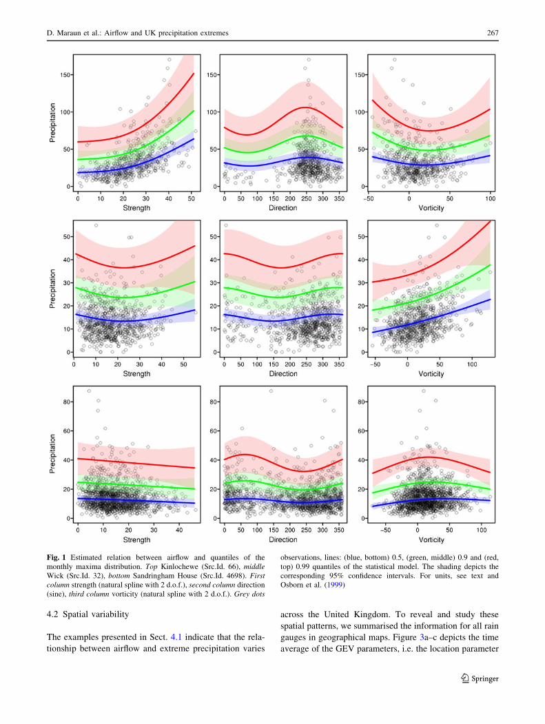
Figure 1 illustrates the structure of the VGLM for three

selected rain gauges: at Kinlochewe in North West Scot-

land (top row, 5�1802900W, 57�3604700N, Met Office Source

Identifier 66), Wick in North East Scotland (middle,


123

3�0502000W, 58�2701400N, Src.Id. 32) and Sandringham

House in East Anglia (bottom, 0�3101600E, 52�4905200N,

Src.Id. 4698). The left column shows the relation between

airflow strength at the day of the precipitation maximum

and the precipitation maximum, the middle column shows

the relation between airflow direction and precipitation,

and the right column shows the corresponding relation

between airflow vorticity and precipitation. The annual

cycle has been analysed in detail in Maraun et al. (2009a)

and is not shown here; it has only been marginally affected

by including the airflow indices. The grey dots in Fig. 1

show the observed monthly maxima, plotted against the

covariate on the day of occurrence. The blue lines depict

the 50% quantile (median) of the predicted distribution,

given a specific value of the actual covariate plus the

average influence (in time) of the other covariates. The

green and red lines show the 90 and 99% quantiles,

respectively. The corresponding pointwise 95% confidence

intervals are indicated by colour shading. Showing the

quantiles instead of the covariates’ influence on individual

GEV parameters (i.e. the fl,.(.) and fr,.(.) in Eq. (4)) sum-

marises the information and concentrates on directly

observable and physically-relevant information.2

These example stations sustain clear relations during the

whole year. Kinlochewe is dominated by airflow strength:

the stronger the airflow, the higher the magnitude of

extreme precipitation. Almost all these extremes happen to

occur under westerly flow, reducing the power of airflow

direction to predict their magnitude.3 A typical weather

situation for extreme precipitation in Kinlochewe associ-

ated with strong westerly flow occurred on 6/7 Jan 2005,

where a low over the Greenland Sea and a high over south

western Europe drove strong and almost zonal flow across

the United Kingdom, causing heavy rain of 142.7 mm

within 24 h.

Interestingly, vorticity exhibits a negative influence on

extreme precipitation. Most heavy events occur for nega-

tive or zero vorticity, which is associated with anticyclones

south of the British Isles. Such a weather situation occurred

on 4 Feb 1999, when an anticyclone over the Bay of Biscay

together with a low over Iceland drove moderately strong

westerly flow across northern Scotland, causing heavy rain

of 34.6 mm within 24 h. For highly positive vorticity this

relationship might reverse. Given the width of the confi-

dence intervals, it is not obvious whether this relationship

is real or just due to sampling variability, yet similar

relationships occur for other rain gauges in the Scottish

Highlands, increasing the overall confidence.

Wick is dominated by airflow vorticity: the stronger the

vorticity, the stronger the expected precipitation. Given the

close distance to Kinlochewe (\160 km), the difference in

the airflow dependency between the two gauges illustrates

the importance of orography for local-scale precipitation.

Whereas Kinlochewe is close to the Scottish west coast and

almost directly exposed to the westerlies, Wick lies at the

rather flat Scottish east coast, in the rain shadow of the

Highlands. There are still heavy rains for westerly airflow,

but they are much weaker than in Kinlochewe, and the

strongest extremes are expected for northerly flow. The

influence of airflow strength is rather weak. Two examples

for weather situations causing extreme precipitation in

Wick occurred on 25 Oct 1998 and 2 Nov 2006. In the

former case, a strong cyclone passed Scotland from the

west, resulting in 26.2 mm of rain. The latter case is an

example for a direction-caused event in Wick: 31.2 mm of

rain fell, as an anticyclone over Ireland circled a warm

front from the north west over east Scotland.

Sandringham is dominated by airflow direction: highest

precipitation maxima are expected for easterly flow coming

from the North Sea. The vorticity relationship is rather

weak: the expected magnitudes increase with vorticity,

saturating for positive values, and with highest variability

around zero vorticity. Strength shows a slightly negative

influence on precipitation extremes.4

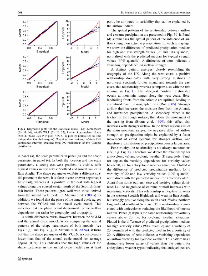
To check the validity of the statistical model, we cal-

culated diagnostic plots (e.g. Coles 2001); they are pre-

sented in Fig. 2, for Kinlochewe, Wick and Sandringham

House in the top, middle and bottom row respectively. The

left column depicts probability–probability (P–P) plots, the

right column quantile–quantile (Q–Q) plots. In both cases,

the model and the observations are rescaled to a standard

Gumbel distribution to account for the effects of the

covariates. The red lines show 95% confidence intervals

derived from 999 realisations of a Gumbel distribution.

P–P plots show the empirical frequency distribution against

the predicted probability distribution of the fitted VGLM

and focus on the centre of mass of the distribution. Q–Q

plots show the predicted quantiles against the empirical

quantiles and focus on the tail of the distribution. In all

three cases, the values lie well within the confidence bands,

confirming that the models are not considerably

misspecified.

2 Often, the estimators for l, r and n are correlated, and compensate

for each other. E.g. a low estimate for r could partly compensate for a

high estimate of n, leaving some quantiles basically unchanged. In

this context, only the quantiles have a unique and physically-relevant

meaning.3 This, however, does not imply that airflow in Kinlochewe almost

always flows from the west.

4 The density of data points for low airflow strength values is higher

than for high strength values. Consequently also the probability to

observe high precipitation values decreases with higher strength. This

creates a spurious impression of a negative relationship between

airflow strength and precipitation. For a general discussion refer to

Maraun et al. (2009b).


123

4.2 Spatial variability

The examples presented in Sect. 4.1 indicate that the rela-

tionship between airflow and extreme precipitation varies

across the United Kingdom. To reveal and study these

spatial patterns, we summarised the information for all rain

gauges in geographical maps. Figure 3a–c depicts the time

average of the GEV parameters, i.e. the location parameter

Fig. 1 Estimated relation between airflow and quantiles of the

monthly maxima distribution. Top Kinlochewe (Src.Id. 66), middleWick (Src.Id. 32), bottom Sandringham House (Src.Id. 4698). Firstcolumn strength (natural spline with 2 d.o.f.), second column direction

(sine), third column vorticity (natural spline with 2 d.o.f.). Grey dots

observations, lines: (blue, bottom) 0.5, (green, middle) 0.9 and (red,

top) 0.99 quantiles of the statistical model. The shading depicts the

corresponding 95% confidence intervals. For units, see text and

Osborn et al. (1999)


123

in panel (a), the scale parameter in panel (b) and the shape

parameter in panel (c). In both the location and the scale

parameters, a strong east-west gradient is visible, with

highest values in north-west Scotland and lowest values in

East Anglia. The shape parameter exhibits a different spa-

tial pattern: in the west, it is close to zero or even negative (a

finite tail), whereas it is positive in the east with highest

values along the coastal stretch north of the Scottish–Eng-

lish border. These patterns agree well with those derived

from the annual cycle model of Maraun et al. (2009a). In

addition, we found that the phase of the annual cycle agrees

between the VGLM and the annual cycle model. This

indicates that the phase is not determined by the airflow

dependency but rather by geography and orography.

A subtle difference exists, however, between the VGLM

and the annual cycle model. When comparing the spatial

patterns of the shape parameters of both models (see

Figs. 3(c), and Fig. 7 (g) in Maraun et al. 2009a), it turns

out that the shape parameter of the VGLM is considerably

lower than that of the annual cycle model (on average

approx. 0.05). This indicates that the high values of the

shape parameter in the annual cycle model can at least

partly be attributed to variability that can be explained by

the airflow indices.

The spatial patterns of the relationship between airflow

and extreme precipitation are presented in Fig. 3d–h. Panel

(d) summarises the spatial pattern of the influence of air-

flow strength on extreme precipitation: for each rain gauge,

we show the difference of predicted precipitation medians

for high and low strength values (90 and 10% quantile),

normalised with the predicted median for typical strength

values (50% quantile). A difference of zero indicates a

vanishing dependence on airflow strength.

A distinct pattern emerges, closely resembling the

orography of the UK. Along the west coast, a positive

relationship dominates with very strong relations in

northwest Scotland; further inland and towards the east

coast, this relationship reverses (compare also with the first

column in Fig. 1). The strongest positive relationship

occurs at mountain ranges along the west coast. Here,

landfalling fronts from the Atlantic are uplifted, leading to

a confined band of orographic rain (Roe 2005). Stronger

airflow then increases the moisture flow from the Atlantic

and intensifies precipitation. A secondary effect is the

friction of the rough surface, that slows the movement of

the passing front (Braun et al. 1999); this effect also

increases with stronger airflow. In the flatter regions east of

the main mountain ranges, the negative effect of airflow

strength on precipitation might be explained by a faster

movement of cloud systems for stronger airflow, and

therefore a distribution of precipitation over a larger area.

For vorticity, the relationship is not always monotonous

(see, e.g. Fig. 1). Therefore we depict the relationship for

anticyclonic (e) and cyclonic weather (f) separately. Panel

(e) depicts the vorticity dependence for vorticity values

below 20, i.e. for anticyclonic weather situations. Plotted is

the difference of predicted precipitation medians for a

vorticity of 20 and low vorticity values (10% quantile),

normalised with the predicted median for a vorticity of 20.

Apart from some outliers, zero and positive values domi-

nate, i.e. the magnitude of extreme rainfall increases with

increasing vorticity. This relationship is negative or weak

in the western Scottish Highlands and weak in East Anglia,

but strongly positive along the south coast, Wales, northern

England and southeast Scotland. This relationship is asso-

ciated with anticyclones reducing the likelihood of intense

rainfall. Panel (f) depicts the same relationship for vorticity

values above 20, i.e. for cyclonic weather situations.

Plotted is the difference of predicted precipitation medians

for high vorticity values (90% quantile) and a vorticity of

20, normalised with the predicted median for a vorticity of

20. A difference of zero indicates a vanishing dependence

on airflow vorticity for cyclonic weather. This pattern has a

distinctively lower range of values than the pattern for

anticyclonic weather types, indicating that anticyclones are

Fig. 2 Diagnostic plots for the statistical model. Top Kinlochewe

(Src.Id. 66), middle Wick (Src.Id. 32), bottom Sandringham House

(Src.Id. 4698). Left P–P plot, right Q–Q plot (re-normalised to time

independent Gumbel margins). Grey dots observations, red lines 95%

confidence intervals obtained from 999 realisations of this Gumbel

distribution


123

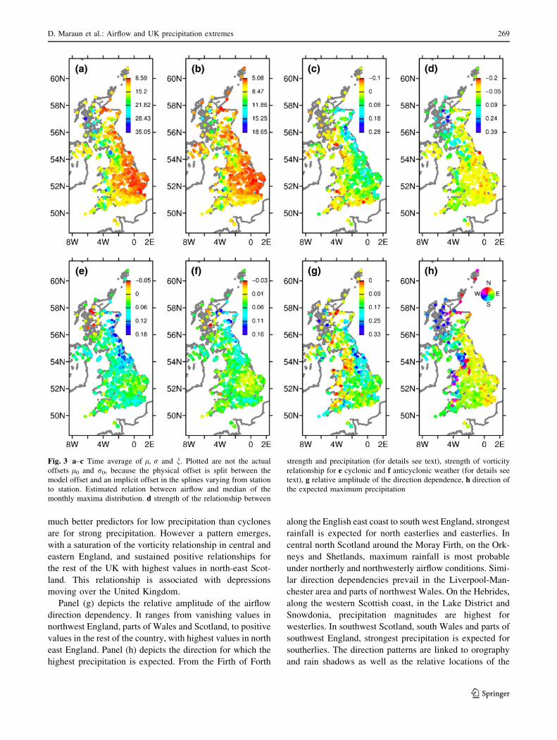
much better predictors for low precipitation than cyclones

are for strong precipitation. However a pattern emerges,

with a saturation of the vorticity relationship in central and

eastern England, and sustained positive relationships for

the rest of the UK with highest values in north-east Scot-

land. This relationship is associated with depressions

moving over the United Kingdom.

Panel (g) depicts the relative amplitude of the airflow

direction dependency. It ranges from vanishing values in

northwest England, parts of Wales and Scotland, to positive

values in the rest of the country, with highest values in north

east England. Panel (h) depicts the direction for which the

highest precipitation is expected. From the Firth of Forth

along the English east coast to south west England, strongest

rainfall is expected for north easterlies and easterlies. In

central north Scotland around the Moray Firth, on the Ork-

neys and Shetlands, maximum rainfall is most probable

under northerly and northwesterly airflow conditions. Simi-

lar direction dependencies prevail in the Liverpool-Man-

chester area and parts of northwest Wales. On the Hebrides,

along the western Scottish coast, in the Lake District and

Snowdonia, precipitation magnitudes are highest for

westerlies. In southwest Scotland, south Wales and parts of

southwest England, strongest precipitation is expected for

southerlies. The direction patterns are linked to orography

and rain shadows as well as the relative locations of the

Fig. 3 a–c Time average of l, r and n. Plotted are not the actual

offsets l0 and r0, because the physical offset is split between the

model offset and an implicit offset in the splines varying from station

to station. Estimated relation between airflow and median of the

monthly maxima distribution. d strength of the relationship between

strength and precipitation (for details see text), strength of vorticity

relationship for e cyclonic and f anticyclonic weather (for details see

text), g relative amplitude of the direction dependence, h direction of

the expected maximum precipitation


123

Atlantic Ocean, the Irish Sea and the North Sea, where air-

masses can absorb moisture. The eastern parts of the United

Kingdom lie within the rain shadow of the main mountain

ranges. Therefore, airflow direction plays an important role

in triggering heavy precipitation in these regions. North-

easterly moist airflow from the North Sea landfalls and

causes heavy precipitation. During winter, this will pre-

dominantly be associated with fronts, which might precipi-

tate already before landfall. However, low frontal clouds

might be uplifted in the higher elevated regions in north east

England, causing additional orographic rain, whereas simi-

lar fronts might pass the flat East Anglian counties without

strong precipitation. During summer, moist airflow from the

North Sea might become unstable over the relatively warm

land surface, causing convective precipitation.

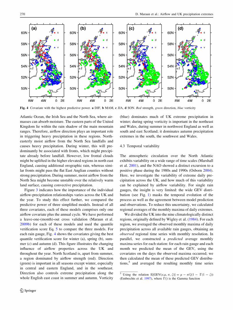
Figure 3 indicates how the importance of the individual

airflow-precipitation relationships varies across the UK and

the year. To study this effect further, we compared the

predictive power of three simplified models. Instead of all

three covariates, each of these models comprises only one

airflow covariate plus the annual cycle. We have performed

a leave-one-(month)-out cross validation (Maraun et al.

2009b) for each of these models and used the quantile

verification score Eq. 5 to compare the three models. For

each rain gauge, Fig. 4 shows the covariates giving the best

quantile verification score for winter (a), spring (b), sum-

mer (c) and autumn (d). This figure illustrates the changing

influence of airflow properties across the UK and

throughout the year. North Scotland is, apart from summer,

a region dominated by airflow strength (red). Direction

(green) is important in all seasons except winter, especially

in central and eastern England, and in the southeast.

Direction also controls extreme precipitation along the

whole English east coast in summer and autumn. Vorticity

(blue) dominates much of UK extreme precipitation in

winter; during spring vorticity is important in the northeast

and Wales, during summer in northwest England as well as

south and east Scotland; it dominates autumn precipitation

extremes in the south, the southwest and Wales.

4.3 Temporal variability

The atmospheric circulation over the North Atlantic

exhibits variability on a wide range of time scales (Marshall

et al. 2001), and the NAO showed a distinct excursion to a

positive phase during the 1980s and 1990s (Osborn 2004).

Here, we investigate the variability of extreme daily pre-

cipitation across the UK, and how much of this variability

can be explained by airflow variability. For single rain

gauges, the insight is very limited: the wide GEV distri-

bution (see Fig. 1) masks the temporal evolution of the

process as well as the agreement between model prediction

and observations. To reduce this uncertainty, we calculated

regional averages of the monthly maxima of daily extremes.

We divided the UK into the nine climatologically distinct

regions, originally defined by Wigley et al. (1984). For each

region, we averaged the observed monthly maxima of daily

precipitation across all available rain gauges, obtaining an

observed regional time series with monthly resolution. In

parallel, we constructed a predicted average monthly

maxima series for each station: for each rain gauge and each

month we predicted the mean of the GEV, using the

covariates on the days the observed maxima occurred; we

then calculated the mean of these predicted GEV distribu-

tions,5 and averaged the resulting monthly time series

Fig. 4 Covariate with the highest predictive power. a DJF, b MAM, c JJA, d SON. Red strength, green direction, blue vorticity

5 Using the relation E[GEV(x;l, r, n)] = l - r/n(1 - C(1 - n))

(Embrechts et al. 1997), where C() is the Gamma function


123

across the rain gauges within a region. To minimise jumps

due to changing station coverage in time, we divided each

rain gauge time series by their 1961–1990 average (for the

predicted series, after fitting the GEV). Therefore, the

resulting series are normalised to one during the reference

period 1961–1990, and only represent relative changes.

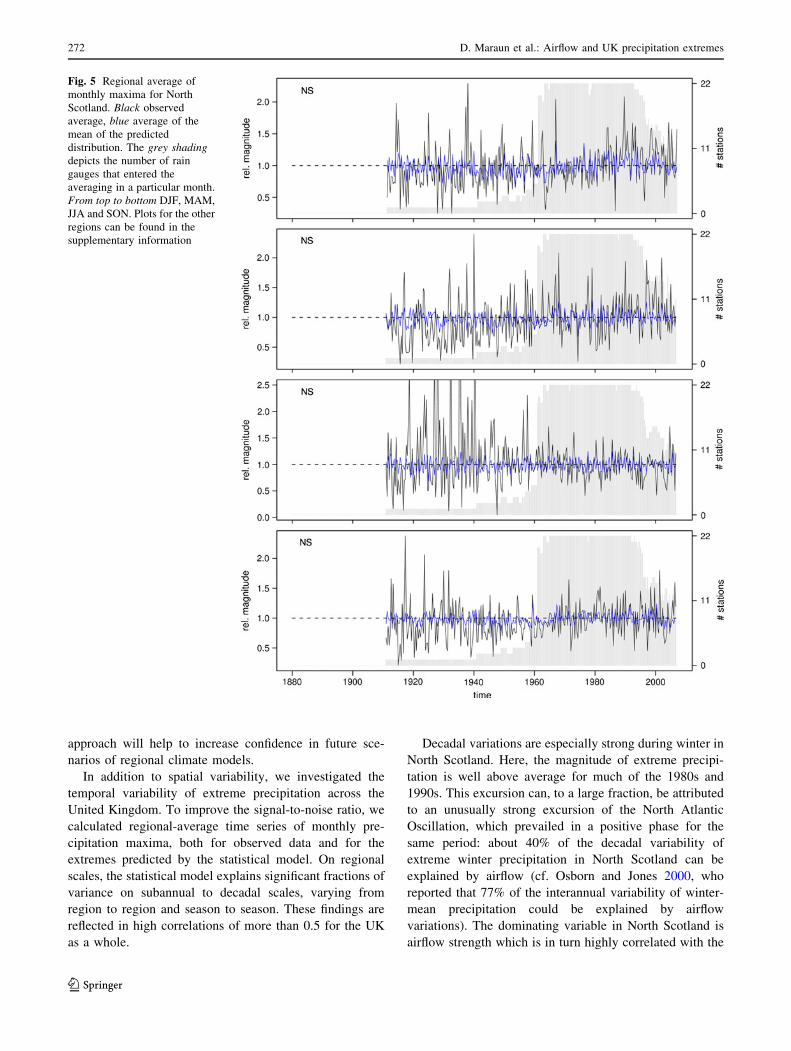
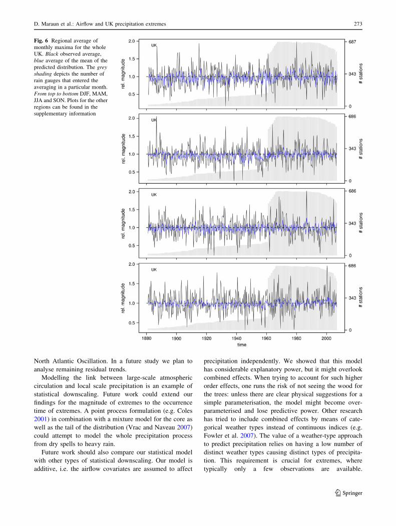
Figures 5 and 6 show the monthly resolved results,

separately for each season, for North Scotland and the

whole UK, respectively. For the other regions refer to the

supplementary information. The observed regional mean is

plotted in black, the predicted mean in blue. The changing

station coverage is indicated by the grey shading. Espe-

cially in Scotland, the rain gauge density is low before

1961, weakening the agreement between the observed and

the predicted time series (see also Table 1). Apparently, the

variability of the predicted time series is much lower than

that of the observed one. This is simply owing to the fact

that not the whole variability is explained by airflow

indices. Therefore, we do not attempt to predict individual

precipitation maxima, but the probability distribution of

these maxima; shown is only the mean of this distribution.

Yet on closer inspection, a striking agreement between

observations and model predictions becomes obvious on a

wide range of time scales: very low and high values for

individual months are often well modelled, as are fluctua-

tions on interannual and decadal time scales. This agree-

ment is reflected in high correlations of up to 0.56

depending on region and season, and 0.59 for a UK wide

average (see Table 1). Decadal variations are apparent

especially in North Scotland during winter (Fig. 5, top), but

also in other regions and seasons, see Supplementary

information. Given that the Scottish west coast is domi-

nated by airflow strength during winter, a relation with the

NAO is obvious. In fact, the anomalously strong extremes

in North Scotland during the 1980s and 1990s are caused

by a corresponding pattern of strong airflow strength (see

also Fig. 7 below), which is in turn related to the above-

mentioned positive phase of the NAO. When investigating

the residual time series between the regionally-averaged

observations and the model prediction, residual trends

remain for several regions and seasons (not shown). Their

detailed study is beyond the scope of this manuscript.

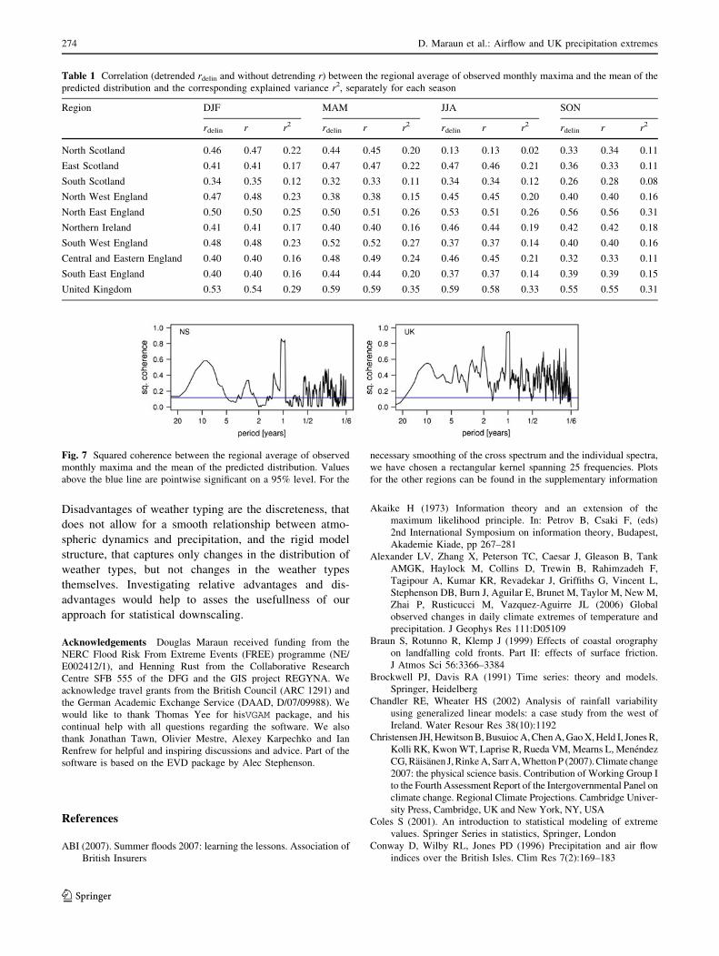
To quantify the fraction of variance explained by the

statistical model on different time scales, we estimated the

squared coherence (Brockwell and Davis 1991) between the

observed and the predicted monthly regional average time

series (Fig. 7). The coherence is the frequency-domain

equivalent of the correlation: a value of one indicates a

perfect linear relationship at a particular frequency, a value

of zero stands for a vanishing relationship. The squared

coherence can be interpreted as explained fractions of the

total variance on a particular frequency. The analysis was

carried out for the whole year, without distinguishing

between different seasons. We have chosen this approach to

improve the information on sub-annual scales. Since we

model the annual cycle explicitly, a perfect coherence

occurs on the 1-year scale.6 We show frequencies ranging

from the Nyquist-frequency of 1/2 months-1 to 1/20

years-1. All regions have in common a significant coher-

ence on sub-annual scales, confirming the visual comparison

(see Fig. 5 for North Scotland and Fig. 6 for the UK). In

addition, many regions show a significant coherence also on

interannual (e.g. South West England) and decadal scales

(e.g. North West England), see Supplementary information.

For the whole UK, the model explains a significant fraction

of the variance on all scales ranging from 2 months to at

least 20 years. A particularly interesting feature is the strong

decadal scale coherence for North Scotland: on average,

around 40% of the observed decadal variability is explained

by the model. This quantifies and further backs the expla-

nation given above, that the large decadal-scale excursion

towards heavy winter precipitation in North Scotland has

mainly been caused by the NAO via its influence on airflow

strength (in qualitative agreement with Scaife et al. 2008).

5 Conclusions

We studied the influence of synoptic-scale atmospheric

circulation on extreme daily precipitation across the United

Kingdom, using observed time series from 689 rain gauges.

We employed extreme value statistics (Coles 2001;

Embrechts et al. 1997; Leadbetter et al. 1983) and a vector

generalised linear model (Yee and Stephenson 2007),

developed by Maraun et al. (2009b). In this model, airflow

strength, direction and vorticity are used to predict the

generalised extreme value distribution of local monthly

maxima of daily precipitation.

The inferred relationships show distinct spatial patterns,

linked to the interplay of the prevailing westerly airflow

and its variability represented by the North Atlantic

Oscillation, the orography of the main north/south moun-

tain ranges, and the moisture supply by the seas sur-

rounding the United Kingdom. In the course of a year, the

relative importance of airflow strength, direction and vor-

ticity changes depending on the region. In a forthcoming

paper, we will repeat this analysis with simulated data from

regional climate models. A comparison between the

observed and the simulated relationships will serve as a

more informative climate model validation than simply

comparing precipitation climatologies: the focus is on

atmospheric dynamics and extreme precipitation. This

6 Due to the smoothing necessary to obtain meaningful coherence

estimates, coherence peaks are smeared out to neighbouring frequen-

cies, see e.g. Brockwell and Davis (1991).


123

approach will help to increase confidence in future sce-

narios of regional climate models.

In addition to spatial variability, we investigated the

temporal variability of extreme precipitation across the

United Kingdom. To improve the signal-to-noise ratio, we

calculated regional-average time series of monthly pre-

cipitation maxima, both for observed data and for the

extremes predicted by the statistical model. On regional

scales, the statistical model explains significant fractions of

variance on subannual to decadal scales, varying from

region to region and season to season. These findings are

reflected in high correlations of more than 0.5 for the UK

as a whole.

Decadal variations are especially strong during winter in

North Scotland. Here, the magnitude of extreme precipi-

tation is well above average for much of the 1980s and

1990s. This excursion can, to a large fraction, be attributed

to an unusually strong excursion of the North Atlantic

Oscillation, which prevailed in a positive phase for the

same period: about 40% of the decadal variability of

extreme winter precipitation in North Scotland can be

explained by airflow (cf. Osborn and Jones 2000, who

reported that 77% of the interannual variability of winter-

mean precipitation could be explained by airflow

variations). The dominating variable in North Scotland is

airflow strength which is in turn highly correlated with the

Fig. 5 Regional average of

monthly maxima for North

Scotland. Black observed

average, blue average of the

mean of the predicted

distribution. The grey shadingdepicts the number of rain

gauges that entered the

averaging in a particular month.

From top to bottom DJF, MAM,

JJA and SON. Plots for the other

regions can be found in the

supplementary information


123

North Atlantic Oscillation. In a future study we plan to

analyse remaining residual trends.

Modelling the link between large-scale atmospheric

circulation and local scale precipitation is an example of

statistical downscaling. Future work could extend our

findings for the magnitude of extremes to the occurrence

time of extremes. A point process formulation (e.g. Coles

2001) in combination with a mixture model for the core as

well as the tail of the distribution (Vrac and Naveau 2007)

could attempt to model the whole precipitation process

from dry spells to heavy rain.

Future work should also compare our statistical model

with other types of statistical downscaling. Our model is

additive, i.e. the airflow covariates are assumed to affect

precipitation independently. We showed that this model

has considerable explanatory power, but it might overlook

combined effects. When trying to account for such higher

order effects, one runs the risk of not seeing the wood for

the trees: unless there are clear physical suggestions for a

simple parameterisation, the model might become over-

parameterised and lose predictive power. Other research

has tried to include combined effects by means of cate-

gorical weather types instead of continuous indices (e.g.

Fowler et al. 2007). The value of a weather-type approach

to predict precipitation relies on having a low number of

distinct weather types causing distinct types of precipita-

tion. This requirement is crucial for extremes, where

typically only a few observations are available.

Fig. 6 Regional average of

monthly maxima for the whole

UK. Black observed average,

blue average of the mean of the

predicted distribution. The greyshading depicts the number of

rain gauges that entered the

averaging in a particular month.

From top to bottom DJF, MAM,

JJA and SON. Plots for the other

regions can be found in the

supplementary information


123

Disadvantages of weather typing are the discreteness, that

does not allow for a smooth relationship between atmo-

spheric dynamics and precipitation, and the rigid model

structure, that captures only changes in the distribution of

weather types, but not changes in the weather types

themselves. Investigating relative advantages and dis-

advantages would help to asses the usefullness of our

approach for statistical downscaling.

Acknowledgements Douglas Maraun received funding from the

NERC Flood Risk From Extreme Events (FREE) programme (NE/

E002412/1), and Henning Rust from the Collaborative Research

Centre SFB 555 of the DFG and the GIS project REGYNA. We

acknowledge travel grants from the British Council (ARC 1291) and

the German Academic Exchange Service (DAAD, D/07/09988). We

would like to thank Thomas Yee for hisVGAM package, and his

continual help with all questions regarding the software. We also

thank Jonathan Tawn, Olivier Mestre, Alexey Karpechko and Ian

Renfrew for helpful and inspiring discussions and advice. Part of the

software is based on the EVD package by Alec Stephenson.

References

ABI (2007). Summer floods 2007: learning the lessons. Association of

British Insurers

Akaike H (1973) Information theory and an extension of the

maximum likelihood principle. In: Petrov B, Csaki F, (eds)

2nd International Symposium on information theory, Budapest,

Akademie Kiade, pp 267–281

Alexander LV, Zhang X, Peterson TC, Caesar J, Gleason B, Tank

AMGK, Haylock M, Collins D, Trewin B, Rahimzadeh F,

Tagipour A, Kumar KR, Revadekar J, Griffiths G, Vincent L,

Stephenson DB, Burn J, Aguilar E, Brunet M, Taylor M, New M,

Zhai P, Rusticucci M, Vazquez-Aguirre JL (2006) Global

observed changes in daily climate extremes of temperature and

precipitation. J Geophys Res 111:D05109

Braun S, Rotunno R, Klemp J (1999) Effects of coastal orography

on landfalling cold fronts. Part II: effects of surface friction.

J Atmos Sci 56:3366–3384

Brockwell PJ, Davis RA (1991) Time series: theory and models.

Springer, Heidelberg

Chandler RE, Wheater HS (2002) Analysis of rainfall variability

using generalized linear models: a case study from the west of

Ireland. Water Resour Res 38(10):1192

Christensen JH, Hewitson B, Busuioc A, Chen A, Gao X, Held I, Jones R,

Kolli RK, Kwon WT, Laprise R, Rueda VM, Mearns L, Menendez

CG, Raisanen J, Rinke A, Sarr A, Whetton P (2007). Climate change

2007: the physical science basis. Contribution of Working Group I

to the Fourth Assessment Report of the Intergovernmental Panel on

climate change. Regional Climate Projections. Cambridge Univer-

sity Press, Cambridge, UK and New York, NY, USA

Coles S (2001). An introduction to statistical modeling of extreme

values. Springer Series in statistics, Springer, London

Conway D, Wilby RL, Jones PD (1996) Precipitation and air flow

indices over the British Isles. Clim Res 7(2):169–183

Fig. 7 Squared coherence between the regional average of observed

monthly maxima and the mean of the predicted distribution. Values

above the blue line are pointwise significant on a 95% level. For the

necessary smoothing of the cross spectrum and the individual spectra,

we have chosen a rectangular kernel spanning 25 frequencies. Plots

for the other regions can be found in the supplementary information

Table 1 Correlation (detrended rdelin and without detrending r) between the regional average of observed monthly maxima and the mean of the

predicted distribution and the corresponding explained variance r2, separately for each season

Region DJF MAM JJA SON

rdelin r r2 rdelin r r2 rdelin r r2 rdelin r r2

North Scotland 0.46 0.47 0.22 0.44 0.45 0.20 0.13 0.13 0.02 0.33 0.34 0.11

East Scotland 0.41 0.41 0.17 0.47 0.47 0.22 0.47 0.46 0.21 0.36 0.33 0.11

South Scotland 0.34 0.35 0.12 0.32 0.33 0.11 0.34 0.34 0.12 0.26 0.28 0.08

North West England 0.47 0.48 0.23 0.38 0.38 0.15 0.45 0.45 0.20 0.40 0.40 0.16

North East England 0.50 0.50 0.25 0.50 0.51 0.26 0.53 0.51 0.26 0.56 0.56 0.31

Northern Ireland 0.41 0.41 0.17 0.40 0.40 0.16 0.46 0.44 0.19 0.42 0.42 0.18

South West England 0.48 0.48 0.23 0.52 0.52 0.27 0.37 0.37 0.14 0.40 0.40 0.16

Central and Eastern England 0.40 0.40 0.16 0.48 0.49 0.24 0.46 0.45 0.21 0.32 0.33 0.11

South East England 0.40 0.40 0.16 0.44 0.44 0.20 0.37 0.37 0.14 0.39 0.39 0.15

United Kingdom 0.53 0.54 0.29 0.59 0.59 0.35 0.59 0.58 0.33 0.55 0.55 0.31


123

Ekstrom M, Fowler HJ, Kilsby CG, Jones PD (2005) New estimates

of future changes in extreme rainfall across the UK using

regional climate model integrations. 2. Future estimates and use

in impact studies. J Hydrol 300:234–251

Embrechts P, Kluppelberg C, Mikosch T (1997) Modelling Extremal

events for insurance and finance. Applications in mathematics,

Springer, Berlin

Fowler HJ, Kilsby CG (2003) Implications of changes in seasonal and

annual extreme rainfall. Geophys Res Lett 30(13):1720. doi:

10.1029/2003GL017327

Fowler HJ, Ekstrom M, Kilsby CG, Jones PD (2005) New estimates

of future changes in extreme rainfall across the UK using

regional climate model integrations. 1. Assessment of control

climate. J Hydrol 300:212–233

Fowler HJ, Blenkinsop S, Tebaldi C (2007) Linking climate change

modelling to impacts studies: recent advances in downscaling

techniques for hydrological modelling. Int J Climatol 27:1547–

1578

Friederichs P, Hense A (2007) Statistical downscaling of extreme

precipitation events using censored quantile regression. Mon

Weather Rev 135(6):2365–2378

Hall J, Sayers P, Dawson R (2005) National-scale assessment of

current and future flood risk in England and Wales. Nat Hazard

36(1-2):147–164

Haylock MR, Gawley GC, Harpham C, Wilby RL, Goodess CM

(2006) Downscaling heavy precipitation over the UnitedKing-

dom: a comparison of dynamical and statistical methods and

their future scenarios. Int J Climatol 26(10):1397–1415

Hegerl GC, Zwiers FW, Braconnot P, Gillett NP, Luo Y, Marengo

Orsini JA, Nicholls N, Penner JE, Stott PA (2007) Climate

change 2007: the physical science basis. Contribution of

Working Group I to the Fourth Assessment Report of the

Intergovernmental Panel on climate change. Understanding and

attributing climate change. Cambridge University Press, Cam-

bridge, UK and New York, NY, USA.

Jenkinson A, Collison F (1977) An initial climatology of gales over

the north sea. Technical report, Synoptic Climatology Branch

Memorandum No. 62, Meteorological Office, Bracknell.

Jones P, Hulme M, Briffa K (1993) A comparison of lamb circulation

types with an objective classification scheme. Int J Climatol

13:655–663

Katz RW, Parlange MB, Naveau P (2002) Statistics of extremes in

hydrology. Adv Water Resour 25(8-12):1287–1304

Leadbetter MR, Lindgren G, Rootzen H (1983) Extremes and related

properties of random sequences and processes. Springer Series in

Statistics, Springer, New York

Maraun D, Osborn TJ, Gillett NP (2008) United Kingdom daily

precipitation intensity: improved early data, error estimates and

an update from 2000 to 2006. Int J Climatol 28(6):833–842. doi:

10.1002/joc.1672

Maraun D, Rust HW, Osborn TJ (2009a) The annual cycle of heavy

precipitation across the UK: a model based on extreme value

statistics. Int J Climatol. doi:10.1002/joc.1811

Maraun D, Rust HW, Osborn TJ (2009b) Synoptic airflow and UK

daily precipitation extremes. Development and validation of a

vector generalised model. Extremes (submitted)

Marshall J, Kushnir Y, Battisti D, Chang P, Czaja A, Dickson R,

Hurrell J, McCartney M, Saravanan R, Visbeck M (2001) North

Atlantic climate variability: phenomena, impacts and mecha-

nisms. Int J Climatol 21:1863–1898

McCullagh P, Nelder JA (1983) Generalized linear models. Chapman

and Hall, London

Meehl GA, Stocker TF, Collins WD, Friedlingstein P, Gaye AT,

Gregory JM, Kitoh A, Knutti R, Murphy JM, Noda A, Raper

SCB, Watterson IG, Weaver AJ, Zhao ZC (2007). Climate

change 2007: the physical science basis. Contribution of

Working Group I to the Fourth Assessment Report of the

Intergovernmental Panel on climate change. Global climate

projections. Cambridge University Press, Cambridge, UK and

New York, NY, USA

Naveau P, Nogaj M, Ammann C, Yiou P, Cooley D, Jomelli V (2005)

Statistical methods for the analysis of climate extremes. C R

Geosci 337(10-11):1013–1022

Osborn TJ (2004) Simulating the winter North Atlantic Oscillation:

the roles of internal variability and greenhouse gas forcing. Clim

Dyn 22:605–623

Osborn TJ, Jones PD (2000) Air flow influences on local climate:

observed United Kingdom climate variations. Atmos Sci Lett

1:62–74

Osborn T, Conway D, Hulme M, Gregory J, Jones P (1999) Air flow

influences on local climate: observed and simulated mean rela-

tionships for the United Kingdom. Clim Res 13:173–191

Osborn TJ, Hulme M, Jones PD, Basnett TA (2000) Observed trends

in the daily intensity of United Kingdom precipitation. Int J

Climatol 20:347–364

Papoulis A (1991) Probability, random variables and stochastic

processes, 3rd edn. McGraw-Hill, New York

Press WH, Teukolsky SA, Vetter WT, Flannery BP (1992) Numerical

recipes in C, 2nd edn. Cambridge University Press, Cambridge

Roe G (2005) Orographic precipitation. Annu Rev Earth Planet Sci

33:645–671

Rust HW (2009) The effect of long-range dependence on modelling

extremes with the generalised extreme value distribution. Eur

Phys J Spec Top, pp 91–97

Rust HW, Maraun D, Osborn TJ (2009) Modelling seasonality in

extreme rainfall: a UK case study. Eur Phys J Spec Top,

pp 99–111

Scaife AA, Folland CK, Alexander LV, Moberg A, Knight JR (2008)

European climate extremes and the North Atlantic Oscillation.

J Clim 31(1):72–83

Trenberth KE, Dai A, Rasmussen RM, Parsons DB (2003) The

changing character of precipitation. Bull Am Meteorol Soc

84:1205–1217

Trenberth KE, Jones PD, Ambenje P, Bojariu R, Easterling D, Klein

Tank A, Parker D, Rahimzadeh F, Renwick JA, Rusticucci M,

Soden B, Zhai P (2007) Climate change 2007: the physical

science basis. Contribution of Working Group I to the Fourth

Assessment Report of the Intergovernmental Panel on climate

change. Observations: surface and atmospheric climate change.

Cambridge University Press, Cambridge, UK and New York,

NY, USA

Vrac M, Naveau P (2007) Stochastic downscaling of precipitation:

from dry events to heavy rainfalls. Water Resour Res

43(7):W07402

Wigley TML, Lough JM, Jones PD (1984) Spatial patterns of

precipitation in England and Wales and a revised, homogeneous

England and Wales precipitation series. J Climatol 4:1–25

Wilby RL (1998) Statistical downscaling of daily precipitation using

daily airflow and seasonal teleconnection indices. Clim Res

10(3):163–178

Wilby RL, O’Hare G, Barnsley N (1997) The North Atlantic

Oscillation and British Isles climate variability. Weather

52:266–276

Wilby RL, Tomlinson OJ, Dawson C (2003) Multi-site simulation of

precipitation by conditional resampling. Clim Res 23(3):183–

194

Wilks DS (2006) Statistical Methods in the Atmospheric Sciences, 2

edn. Academic Press, San Diego

Yee TW, Wild CJ (1996) Vector generalized additive models. J. R.

Stat. Soc. B 58:481–493

Yee TW, Stephenson AG (2007) Vector generalized linear and

additive extreme value models. Extremes 10:1–19


123

http://dx.doi.org/10.1029/2003GL017327

http://dx.doi.org/10.1002/joc.1672

http://dx.doi.org/10.1002/joc.1811

The influence of synoptic airflow on UK daily precipitation extremes: observed spatio-temporal relationships

Documents