The influence of suspension and tyre modelling on vehicle handling simulation Blundell, M.V. Submitted version deposited in CURVE June 2010 Original citation: Blundell, M.V. (1997) The influence of suspension and tyre modelling on vehicle handling simulation. Unpublished PhD Thesis. Coventry: Coventry University in collaboration with Rover Group and SP Tyres UK Ltd. Copyright © and Moral Rights are retained by the author. A copy can be downloaded for personal non-commercial research or study, without prior permission or charge. This item cannot be reproduced or quoted extensively from without first obtaining permission in writing from the copyright holder(s). The content must not be changed in any way or sold commercially in any format or medium without the formal permission of the copyright holders. CURVE is the Institutional Repository for Coventry University http://curve.coventry.ac.uk/open

Welcome message from author
This document is posted to help you gain knowledge. Please leave a comment to let me know what you think about it! Share it to your friends and learn new things together.
Transcript

The influence of suspension and tyre modelling on vehicle handling simulation Blundell, M.V. Submitted version deposited in CURVE June 2010 Original citation: Blundell, M.V. (1997) The influence of suspension and tyre modelling on vehicle handling simulation. Unpublished PhD Thesis. Coventry: Coventry University in collaboration with Rover Group and SP Tyres UK Ltd. Copyright © and Moral Rights are retained by the author. A copy can be downloaded for personal non-commercial research or study, without prior permission or charge. This item cannot be reproduced or quoted extensively from without first obtaining permission in writing from the copyright holder(s). The content must not be changed in any way or sold commercially in any format or medium without the formal permission of the copyright holders.
CURVE is the Institutional Repository for Coventry University http://curve.coventry.ac.uk/open

THE INFLUENCE OF SUSPENSION AND TYRE
MODELLING ON VEHICLE HANDLING SIMULATION
M. V. Blundell
A thesis submitted in partial fulfilment
of the University's requirements
for the Degree of Doctor of Philosophy
November 1997
Coventry University in collaboration
with Rover Group and SP Tyres UK Ltd

THE INFLUENCE OF SUSPENSION AND TYRE MODELLING ON
VEHICLE HANDLING SIMULATION
ABSTRACT
A study has been carried out in order to investigate the influence of suspension and tyre
modelling on the outputs predicted by vehicle handling simulations. The computer models have
been generated using data for a Rover vehicle, for which instrumented track test measurements
were also available. The results obtained from a high speed lane change manoeuvre have been
used as a benchmark for comparison of the various computer modelling strategies. This
investigation addresses two main areas. The first of these is the influence of suspension
modelling on calculated outputs. The second and more complex area investigates the influence
of models representing the effects of the tyres. In each case a primary aim has been to assess
the accuracy of models which use a simplified approach, reduce the number of model
parameters and may hence be more amenable to vehicle and tyre design studies. Comparison of
the results from this study indicate that for quite an extreme manoeuvre a relatively simple
vehicle and tyre model can be used to carry out a simulation with a good level of accuracy. A
sensitivity study has also been carried out to illustrate how the models respond to design
changes for both vehicle and tyre parameters.
The multibody systems analysis program ADAMS (Automatic Dynamic Analysis of
Mechanical Systems) has been used to generate the models, formulate and solve the equations
of motion, and postprocess the results. An initial literature survey has been carried out
investigating this analysis discipline and its usage in vehicle dynamics. Previous work in the
areas of vehicle handling simulation, tyre theory, and computer modelling of both vehicles and
tyres has also been studied.
Initial investigations have been carried out looking at the modelling of the suspension
systems and the steering system. Information from this phase has been used to provide inputs
for a set of four full vehicle models ranging in complexity from a model where the suspensions
are treated as lumped masses, a model where the suspensions are treated as swing arms, a
model based on roll stiffness and a fmal detailed model which represents the suspension

linkages as fitted on the vehicle. Of the three simple models it will be shown that the roll
stiffness model is most suitable for further comparisons with the detailed linkage model, where
aspects of tyre modelling are considered.
Tyre testing has been carried out at SP Tyres UK Ltd. and at Coventry University. A
set of FORTRAN subroutines, which interface with ADAMS, has been developed in
association with a computer model of a tyre test rig to represent and validate the various tyre
models. The provision of these tools forms part of a new system developed during this study
and is referred to as the CUTyre System due to its origins at Coventry University. The tyre
models compared include a well known and accurate model which requires up to fifty model
parameters and a more simple model requiring only ten parameters. An interpolation method is
also used as a benchmark for the comparisons.
To the author's knowledge the work described in this thesis can be considered to make
an original contribution to the body of knowledge involving the application of multibody
systems analysis in vehicle dynamics by:
(i) Providing a detailed comparison of vehicle suspension modelling strategies with the
ADAMS program.
(ii) Developing a tyre modelling and validation tool which can interface directly with the
ADAMS software.
(iii) Providing a comparison between a sophisticated and a simple tyre model in ADAMS. Of
particular significance is the assessment of the influence of the tyre models on simulation
outputs and not just the shape of the tyre force and moment curves.

ACKNOWLEDGEMENTS
I would like to express my appreciation to Dr B.D.A. Phillips who as my supervisor was able
during this programme of work to provide me with many insights into the complicated field of
tyre and vehicle behaviour.
I would also like to thank D. Skelding and J. Forbes of Rover Group who were able to
provide the valuable vehicle data which formed the basis of this study. The vehicle body
graphics used for animations in ADAMS were also provided by J. Forbes.
Thanks are also due to Dr. A.R. Williams and P. Stephens of SP Tyres UK Ltd. who
provided the tyres and facilities to carry out the tyre testing involved in this work. Mr Stephens
was also able to provide many valuable opinions in the area of tyre modelling.
Special thanks are also due to many of the students who showed such an interest in my
studies and were often able to contribute through their own project work. Finally I would like
to thank my colleagues within the School of Engineering for their enthusiasm, encouragement
and support during this investigation.
This thesis is dedicated to the memory of Beatrice Alice Blundell

CONTENTS
List of Figures
List of Tables
Nomenclature
1.0 INTRODUCTION
1.1 Background
1.2 Project aims and objectives
1.3 Programme of work
2.0 LITERATURE REVIEW
2.1 Introduction
2.2 Road vehicle dynamics
2.3 Computer modelling and simulation
2.4 The ADAMS program
2.5 Tyre models
2.6 Summary
3.0 SIMULATION SOFTWARE
3.1 Multibody systems analysis
3.2 The ADAMS program
3 .2.1 Overview
3.2.2 Modelling features
3.2.3 Analysis capabilities
3.2.4 Pre- and postprocessing
3.3 ADAMS theory
3.3.1 Background
3.3.2 Equations of motion for a part
3.3.3 Force and moment definition
3.3.4 Formulation of constraints
n
Page
1
1
5
7
11
11
13
15
22
25
27
29
29
31
31
32
35
36
38
38
38
44
46

CONTENTS (Continued)
Page
4.0 MODELLING AND ANALYSIS OF SUSPENSION SYSTEMS 53
4.1 General 53
4.2 Modelling approach 54
4.3 Modelling the front suspension system 57
4.4 Modelling the rear suspension system 60
4.5 Suspension calculations 63
4.5.1 Camber angle 63
4.5.2 Caster angle 64
4.5.3 Steer angle 65
4.5.4 Track change 66
4.5.5 Calculation of wheel rate 67
4.6 Calculation of instant centre and roll centre height 67
4.6.1 Front suspension 67
4.6.2 Rear suspension 69
4.6.3 Implementation in ADAMS 71
4.7 Results 72
4.8 Summary 74
5.0 MODELLING OF VEHICLE SYSTEMS 78
5.1 Introduction 78
5.2 Vehicle body, coordinate frames and rigid part definitions 78
5.3 Modelling of suspension systems 83
5.3.1 Overview 83
5.3.2 Linkage model 85
5.3.3 Lumped mass model 86
5.3.4 Swing arm model 87
5.3.5 Roll stiffness model 89
5.3.6 Model size 90
111

CONTENTS (Continued)
5.4 Detennination of roll stiffness and damping
5.4.1 Modelling approach
5 .4.2 Calculation check
5.5 Road springs and dampers
5.5.1 Modelling of springs and dampers in
the linkage model
5.5.2 Modelling of springs and dampers
in the lumped mass and swing ann models
5.6 Roll bars
5.7 Steering system
5.7.1 Modelling with the linkage model
5.7 .2 Steering ratio test
6.0 TYRE MODELLING
6.1 Introduction
6.2 Interpolation models
6.3 The "Magic Fonnula" tyre model
6.4 The Fiala tyre model
6.4.1 Input parameters
6.4.2 Tyre geometry and kinematics
6.4.3 Force calculations
6.4.4 Road surface/terrain definition
6.5 Experimental Tyre Testing
6.5.1 Introduction
6.5 .2 Tyre testing at SP TYRES
6.5.3 Tyre testing at Coventry University
lV
Page
92
92
95
98
98
100
104
105
105
106
112
112
117
118
127
127
128
132
134
135
135
136
137

CONTENTS (Continued)
Page
6.6 Tyre model data 139
6.6.1 Data for TYRE A 139
6.6.2 Data for TYRE B 142
6.7 The CUTyre System 145
6.7.1 Implementation of tyre models in ADAMS 145
6.7.2 ADAMS tyre rig model 146
7.0 VEHICLE HANDLING SIMULATIONS 151
7.1 Introduction 151
7.2 Handling test data 153
7.3 Computer Simulations 155
8.0 RESULTS 161
8.1 Introduction 161
8.2 Tyre model study 161
8.2.1TyreA 161
8.2.2 Tyre B 163
8.3 Lane change manoeuvre ( Interpolation model - TYRE A) 164
8.4 Sensitivity of lane change manoeuvre to tyre data and model 166
8.5 Final sensitivity studies 17 6
8.6 The effect of model size on computer simulation time 177
9.0 CONCLUSIONS AND RECOMMENDATIONS 180
10.0 REFERENCES 188
v

APPENDIX A
APPENDIXB
APPENDIXC
APPENDIXD
APPENDIXE
APPENDIXF
APPENDIXG
APPENDIXH
APPENDIX I
APPENDIXJ
APPENDIX K
APPENDIX L
CONTENTS (Continued)
SYSTEM SCHEMATICS
SUSPENSION ANALYSIS OUTPUT PLOTS
RESULTS OF EXPERIMENTAL TESTING ON TYRE B
FORTRAN TYRE MODEL SUBROUTINES
TYRE MODEL PLOTS FROM THE CUTyre RIG MODEL (TYRE A)
TYRE MODEL PLOTS FROM THE CUTyre RIG MODEL (TYRE B)
INVESTIGATION OF LANE CHANGE MANOEUVRE
(INTERPOLATION MODEL- TYRE A)
INVESTIGATION OF LANE CHANGE MANOEUVRE
SENSITIVITY TO TYRE DATA AND MODELS
(LINKAGE MODEL)
INVESTIGATION OF LANE CHANGE MANOEUVRE
SENSITIVITY TO TYRE DATA AND MODELS
(ROLL STIFFNESS MODEL)
SUMMARY OF RESULTS FOR TYRE MODEL VARIATION
USING TYRE A AND TYRE B
SENSITIVITY STUDIES BASED ON TYRE B AND THE
ROLL STIFFNESS MODEL
ASSOCIATED PUBLICATIONS
VI

List of Figures
Figure 3.1 Typical joints provided with ADAMS
Figure 3.2 Graphical output of vehicle handling manoeuvres
Figure 3.3 The location and orientation of a part
Figure 3.4 Orientation of the part frame by Euler angles
Figure 3.5 Applied forces and torques on a body
Figure 3.6 Atpoint constraint element
Figure 3.7 Inplane constraint element
Figure 3.8 Perpendicular constraint element
Figure 3.9 Angular constraint element
Figure 4.1 Double wishbone suspension modelled with bushes
Figure 4.2 Double wishbone suspension modelled with joints
Figure 4.3 Assembly of parts in the front suspension system
Figure 4.4 Modelling the front suspension with bushes
Figure 4.5 Modelling the front suspension using rigid joints
Figure 4.6 Distortion in front bushes at full bump
Figure 4. 7 Assembly of parts in the rear suspension system
Figure 4.8 Modelling the rear suspension using bushes
Figure 4.9 Modelling the rear suspension using rigid joints
Figure 4.10 Calculation of camber angle
Figure 4.11 Calculation of caster angle
Figure 4.12 Calculation of steer angle
Figure 4.13 Calculation of track change
Figure 4.14 Construction of the instant centre and roll centre for the front suspension
Figure 4.15 Construction of the instant centre and roll centre for the rear suspension
Figure 5.1 Co-ordinate systems
Figure 5.2 Vehicle ground reference frame (GRF)
Figure 5.3 Euler angle approach
Figure 5.4 The XP-ZP method for marker orientation
Figure 5.5 Modelling of suspension systems
Figure 5.6 The Linkage model
vii

Figure 5.7 The Lumped Mass model
Figure 5.8 The Swing Arm model
Figure 5.9 The Roll Stiffness model
Figure 5.10 Determination of front end roll stiffness
Figure 5.11 Determination of rear end roll stiffness
Figure 5.12 Front end roll test
Figure 5.13 Rear end roll test
Figure 5.14 Calculation of roll stiffness due to road springs
Figure 5.15 Calculation of roll stiffness due to the roll bar
Figure 5.16 Location of spring and damper elements in the linkage model
Figure 5.17 Nonlinear force characteristics for the front and rear dampers
Figure 5.18 Road spring in the Linkage and Lumped mass models
Figure 5.19 Installation of the road spring in the Swing Arm model
Figure 5.20 Equivalent spring acting at the wheel centre
Figure 5.21 Scaling a linear spring to the wheel centre position
Figure 5.22 Modelling the roll bars
Figure 5.24 Modelling the steering system
Figure 5.29 Toe change in front wheels at static equilibrium for simple models
Figure 5.25 Coupled steering system model
Figure 5.26 Front suspension steering ratio test
Figure 5.27 Results of steering ratio test for ADAMS front right suspension model
Figure 6.1 A simple tyre model for ride and vibration studies
Figure 6.2 A radial spring terrain enveloping tyre model
Figure 6.3 Interaction between vehicle model and tyre model
Figure 6.4 Interpolation of measured tyre test data
Figure 6.5 Typical form of tyre force and moment curves from steady state testing
Figure 6.6 Coefficients used in the "Magic Formula" tyre
Figure 6.7 Generation of an asymmetric curve
Figure 6.8 Cornering stiffness as a function of vertical load at zero camber angle
Figure 6.9 ADAMS/Tire model geometry
Figure 6.10 Definition of geometric terms in ADAMS!fire
Figure 6.11 Tyre geometry and kinematics
V1ll

Figure 6.12 Linear tyre to road friction model
Figure 6.13 Definition of road surface for the Fiala tyre model
Figure 6.14 High Speed Dynamics Machine for tyre testing at SP TYRES UK Ltd.
Figure 6.15 Flat Bed Tyre Test machine at Coventry University
Figure 6.16 Overview of the CUTyre System
Figure 6.17 Orientation of tyre coordinate systems on the full vehicle model
Figure 6.18 ADAMS model of a flat bed tyre test machine
Figure 6.19 ADAMS graphics of the CUTyre rig model
Figure 7.1 Steering input for the lane change manoeuvre
Figure 7.2 ISO 3888 Lane change manoeuvre
Figure 7.3 Graphical animation of lane change manoeuvre
Figure 8.1 Camber angle comparison - Linkage and Roll stiffness models
Figure 8.2 Slip angle comparison- Linkage and Roll stiffness models
Figure 8.3 Vertical tyre force comparison- Linkage and Roll stiffness models
Figure 8.4 Vertical tyre force comparison- Linkage and Roll stiffness models
Figure 8.5 Vertical tyre force comparison- Linkage and Roll stiffness models
Figure 8.6 Vertical tyre force comparison- Linkage and Roll stiffness models
Figure 8.7 Comparison of steering inputs at different speeds
Figure A.1 Front suspension components
Figure A.2 Front suspension with rigid joints
Figure A.3 Front suspension with bushes
Figure A.4 Front suspension numbering convention
Figure AS Rear suspension components
Figure A.6 Rear suspension with rigid joints
Figure A.7 Rear suspension with bushes
Figure A.8 Rear suspension numbering convention
Figure A.9 Steering system components and joints
Figure A.10 Steering system numbering convention
Figure A.11 Front roll bar system components and joints
Figure A.12 Front roll bar system numbering convention
Figure A.13 Rear roll bar system components and joints
Figure A.14 Rear roll bar system numbering convention
IX

Figure A.15 Lumped mass model suspension components and joints
Figure A.16 Lumped mass model suspension numbering convention
Figure A.17 Swing arm model suspension components and joints
Figure A.18 Swing arm model suspension numbering convention
Figure A.19 Roll stiffness model suspension components and joints
Figure A.20 Roll stiffness model suspension numbering convention
Figure B.l Front suspension- camber angle with bump movement
Figure B.2 Front suspension - caster angle with bump movement
Figure B.3 Front suspension - steer angle with bump movement
Figure B.4 Front suspension- roll centre height with bump movement
Figure B.S Front suspension- track change with bump movement
Figure B.6 Front suspension - vertical force with bump movement
Figure B.7 Rear suspension- camber angle with bump movement
Figure B.8 Rear suspension - caster angle with bump movement
Figure B.9 Rear suspension - steer angle with bump movement
Figure B.lO Rear suspension- roll centre height with bump movement
Figure B.ll Rear suspension - track change with bump movement
Figure B.12 Rear suspension- vertical force with bump movement
Figure C.l Lateral force Fy with slip angle a
Figure C.2 Aligning moment Mz with slip angle a
Figure C.3 Lateral force Fy with aligning moment Mz (Gough Plot)
Figure C.4 Cornering stiffness with load
Figure C.5 Aligning stiffness with load
Figure C.6 Lateral force Fy with camber angle y
Figure C.7 Aligning moment Mz with camber angle y
Figure C.8 Camber stiffness with load
Figure C.9 Aligning camber stiffness with load
Figure C.lO Braking force with slip ratio
Figure E.l Interpolation model (TYRE A) - lateral force with slip angle
Figure E.2 Interpolation model (TYRE A) - lateral force with slip angle at near zero slip
Figure E.3 Interpolation model (TYRE A) - aligning moment with slip angle
Figure E.4 Interpolation model (TYRE A) - lateral force with aligning moment
X

Figure E.5 Interpolation model (TYRE A) - lateral force with camber angle
Figure E.6 Fiala model (TYRE A) - lateral force with slip angle
Figure E.7 Fiala model (TYRE A) -lateral force with slip angle at near zero slip
Figure E.8 Fiala model (TYRE A) - aligning moment with slip angle
Figure E.9 Fiala model (TYRE A) - lateral force with aligning moment
Figure E.l 0 Fiala model (TYRE A) - lateral force with slip angle
Figure E.ll Fiala model (TYRE A) - lateral force with slip angle at near zero slip
Figure E.12 Fiala model (TYRE A) - aligning moment with slip angle
Figure E.13 Fiala model (TYRE A) - lateral force with aligning moment
Figure E.14 Fiala model (TYRE A)- lateral force with slip angle
Figure E.15 Fiala model (TYRE A)- lateral force with slip angle at near zero slip
Figure E.16 Fiala model (TYRE A) -aligning moment with slip angle
Figure E.17 Fiala model (TYRE A) - lateral force with aligning moment
Figure E.18 Pacejka model (TYRE A) - lateral force with slip angle
Figure E.19 Pacejka model (TYRE A)- lateral force with slip angle at near zero slip
Figure E.20 Pacejka model (TYRE A) - aligning moment with slip angle
Figure E.21 Pacejka model (TYRE A) -lateral force with aligning moment
Figure E.22 Pacejka model (TYRE A) - lateral force with camber angle
Figure F.l Interpolation model (TYRE B) - lateral force with slip angle
Figure F.2 Interpolation model (TYRE B) - lateral force with slip angle at near zero slip
Figure F.3 Interpolation model (TYRE B) - aligning moment with slip angle
Figure F.4 Interpolation model (TYRE B) - lateral force with aligning moment
Figure F.5 Interpolation model (TYRE B)- lateral force with camber angle
Figure F.6 Interpolation model (TYRE B)- lateral force with slip angle
Figure F.7 Interpolation model (TYRE B) -aligning moment with slip angle
Figure F.8 Interpolation model (TYRE B)- lateral force with camber angle
Figure F.9 Interpolation model (TYRE B)- lateral force with slip angle
Figure F.lO Fiala model (TYRE B) -lateral force with slip angle
Figure F.ll Fiala model (TYRE B) -lateral force with slip angle at near zero slip
Figure F.12 Fiala model (TYRE B) -aligning moment with slip angle
Figure F.13 Fiala model (TYRE B) -lateral force with aligning moment
Figure F.14 Fiala model (TYRE B) -lateral force with slip angle
xi

Figure F.15 Fiala model (TYRE B)- lateral force with slip angle at near zero slip
Figure F.16 Fiala model (TYRE B) -aligning moment with slip angle
Figure F.17 Fiala model (TYRE B)- lateral force with aligning moment
Figure F.18 Fiala model (TYRE B) -lateral force with slip angle
Figure F.19 Fiala model (TYRE B) -lateral force with slip angle at near zero slip
Figure F.20 Fiala model (TYRE B) -aligning moment with slip angle
Figure F.21 Fiala model (TYRE B)- lateral force with aligning moment
Figure F.22 Pacejka model (TYRE B) -lateral force with slip angle
Figure F.23 Pacejka model (TYRE B) -lateral force with slip angle at near zero slip
Figure F.24 Pacejka model (TYRE B) - aligning moment with slip angle
Figure F.25 Pacejka model (TYRE B) - lateral force with aligning moment
Figure G. I Lateral acceleration comparison -lumped mass model and test
Figure G.2 Lateral acceleration comparison- swing arm model and test
Figure G.3 Lateral acceleration comparison- roll stiffness model and test
Figure G.4 Lateral acceleration comparison- linkage model and test
Figure G.5 Roll angle comparison -lumped mass model and test
Figure G.6 Roll angle comparison- swing arm model and test
Figure G.7 Roll angle comparison- roll stiffness model and test
Figure G.8 Roll angle comparison- linkage model and test
Figure G.9 Yaw rate comparison -lumped mass model and test
Figure G.lO Yaw rate comparison- swing arm model and test
Figure G.ll Yaw rate comparison - roll stiffness model and test
Figure 0.12 Yaw rate comparison -linkage model and test
Figure F.24 Yaw rate comparison - linkage model and test
Figure G.l Lateral acceleration comparison -lumped mass model and test
Figure G.2 Lateral acceleration comparison- swing arm model and test
Figure G.3 Lateral acceleration comparison- roll stiffness model and test
Figure G.4 Lateral acceleration comparison- linkage model and test
Figure G.5 Roll angle comparison- lumped mass model and test
Figure G.6 Roll angle comparison- swing arm model and test
Figure G.7 Roll angle comparison -roll stiffness model and test
Figure G.8 Roll angle comparison- linkage model and test
xii

Figure 0.9 Yaw rate comparison -lumped mass model and test
Figure 0.10 Yaw rate comparison- swing arm model and test
Figure 0.11 Yaw rate comparison- roll stiffness model and test
Figure 0.12 Roll angle comparison- linkage model and test
Figure 0.13 Vehicle velocity during lane change without traction
Figure 0.14 Vehicle velocity during lane change with traction
Figure 0.15 Lateral acceleration com paris on - linkage model ( with traction ) and test
Figure 0.16 Body roll angle comparison- linkage model (with traction) and test
Figure 0.17 Yaw rate comparison -linkage model (with traction) and test
Figure 0.18 Camber angle comparison -linkage and roll stiffness models
Figure 0.19 Slip angle comparison -linkage and roll stiffness models
Figure 0.20 Vertical tyre force comparison- linkage and roll stiffness models
Figure 0.21 Vertical tyre force comparison -linkage and roll stiffness models
Figure 0.22 Vertical tyre force comparison- linkage and roll stiffness models
Figure 0.23 Vertical tyre force comparison -linkage and roll stiffness models
Figure H.1 Lateral acceleration comparison - Interpolation model TYRE A and test
Figure H.2 Lateral acceleration comparison - Interpolation model TYRE A and test
Figure H.3 Lateral acceleration comparison- Pacejka model TYRE A and test
Figure H.4 Lateral acceleration comparison - Pacejka model TYRE A and test
Figure H.5 Lateral acceleration comparison- Fiala model TYRE A and test
Figure H.6 Roll angle comparison - Interpolation model TYRE A and test
Figure H.7 Roll angle comparison- Interpolation model TYRE A and test
Figure H.8 Roll angle comparison- Pacejka model TYRE A and test
Figure H.9 Roll angle comparison - Pacejka model TYRE A and test
Figure H.lO Roll angle comparison - Fiala model TYRE A and test
Figure H.11 Yaw rate comparison - Interpolation model TYRE A and test
Figure H.12 Yaw rate comparison- Interpolation model TYRE A and test
Figure H.13 Yaw rate comparison - Pacejka model TYRE A and test
Figure H.14 Yaw rate comparison - Pacejka model TYRE A and test
Figure H.15 Yaw rate comparison- Fiala model TYRE A and test
Figure H.l6 Lateral acceleration comparison- Interpolation model TYRE Band test
Figure H.17 Lateral acceleration comparison - Interpolation model TYRE B and test
X111

Figure H.18 Lateral acceleration comparison - Pacejka model TYRE B and test
Figure H.19 Lateral acceleration comparison- Fiala model TYRE B and test
Figure H.20 Roll angle comparison - Interpolation model TYRE B and test
Figure H.21 Roll angle comparison- Interpolation model TYRE Band test
Figure H.22 Roll angle comparison- Pacejka model TYRE Band test
Figure H.23 Roll angle comparison - Fiala model TYRE B and test
Figure H.24 Yaw rate comparison- Interpolation model TYRE Band test
Figure H.25 Yaw rate comparison - Interpolation model TYRE B and test
Figure H.26 Yaw rate comparison - Pacejka model TYRE B and test
Figure H.27 Yaw rate comparison- Fiala model TYRE Band test
Figure 1.1 Lateral acceleration comparison- Interpolation model TYRE A and test
Figure 1.2 Lateral acceleration comparison- Interpolation model TYRE A and test
Figure 1.3 Lateral acceleration comparison - Pacejka model TYRE A and test
Figure 1.4 Lateral acceleration comparison - Pacejka model TYRE A and test
Figure 1.5 Lateral acceleration comparison - Fiala model TYRE A and test
Figure 1.6 Roll angle comparison- Interpolation model TYRE A and test
Figure 1.7 Roll angle comparison- Interpolation model TYRE A and test
Figure 1.8 Roll angle comparison- Pacejka model TYRE A and test
Figure 1.9 Roll angle comparison - Pacejka model TYRE A and test
Figure 1.10 Roll angle comparison - Fiala model TYRE A and test
Figure 1.11 Yaw rate comparison- Interpolation model TYRE A and test
Figure 1.12 Yaw rate comparison- Interpolation model TYRE A and test
Figure 1.13 Yaw rate comparison - Pacejka model TYRE A and test
Figure 1.14 Yaw rate comparison- Pacejka model TYRE A and test
Figure 1.15 Yaw rate comparison- Fiala model TYRE A and test
Figure 1.16 Lateral acceleration comparison - Interpolation model TYRE B and test
Figure 1.17 Lateral acceleration comparison - Interpolation model TYRE B and test
Figure 1.18 Lateral acceleration comparison- Pacejka model TYRE Band test
Figure 1.19 Lateral acceleration comparison- Fiala model TYRE B and test
Figure 1.20 Roll angle comparison - Interpolation model TYRE B and test
Figure 1.21 Roll angle comparison- Interpolation model TYRE B and test
Figure 1.22 Roll angle comparison- Pacejka model TYRE Band test
XIV
Figure I.23 Roll angle comparison - Fiala model TYRE B and test
Figure I.24 Yaw rate comparison - Interpolation model TYRE B and test
Figure I.25 Yaw rate comparison - Interpolation model TYRE B and test
Figure 1.26 Yaw rate comparison- Pacejka model TYRE Band test
Figure I.27 Yaw rate comparison- Fiala model TYRE Band test
Figure J.l Lateral acceleration comparison using Linkage model and TYRE A
Figure J.2 Lateral acceleration comparison using Roll Stiffness model and TYRE A
Figure J.3 Roll angle comparison using Linkage model and TYRE A
Figure J.4 Roll angle comparison using Roll Stiffness model and TYRE A
Figure J.5 Yaw rate comparison using Linkage model and TYRE A
Figure J.6 Yaw rate comparison using Roll Stiffness model and TYRE A
Figure J.7 Trajectory comparison using Linkage model and TYRE A
Figure J.8 Trajectory comparison using Roll Stiffness model and TYRE A
Figure J.9 Lateral acceleration comparison using Linkage model and TYRE A
Figure J.IO Lateral acceleration comparison using Roll Stiffness model and TYRE A
Figure J.ll Roll angle comparison using Linkage model and TYRE A
Figure J.12 Roll angle comparison using Roll Stiffness model and TYRE A
Figure J.13 Yaw rate comparison using Linkage model and TYRE A
Figure J.l4 Yaw rate comparison using Roll Stiffness model and TYRE A
Figure J.15 Trajectory comparison using Linkage model and TYRE A
Figure J.16 Trajectory comparison using Roll Stiffness model and TYRE A
Figure J.17 Lateral acceleration comparison using Linkage model and TYRE B
Figure J.18 Lateral acceleration comparison using Roll Stiffness model and TYRE B
Figure J.19 Roll angle comparison using Linkage model and TYRE B
Figure J.20 Roll angle comparison using Roll Stiffness model and TYRE B
Figure J.21 Yaw rate comparison using Linkage model and TYRE B
Figure J.22 Yaw rate comparison using Roll Stiffness model and TYRE B
Figure J.23 Trajectory comparison using Linkage model and TYRE B
Figure J.24 Trajectory comparison using Roll Stiffness model and TYRE B
Figure J.25 Lateral acceleration comparison using Linkage model and TYRE B
Figure J.26 Lateral acceleration comparison using Roll Stiffness model and TYRE B
Figure J.27 Roll angle comparison using Linkage model and TYRE B
XV

Figure J.28 Roll angle comparison using Roll Stiffness model and TYRE B
Figure J.29 Yaw rate comparison using Linkage model and TYRE B
Figure J.30 Yaw rate comparison using Roll Stiffness model and TYRE B
Figure J.31 Trajectory comparison using Linkage model and TYRE B
Figure J.32 Trajectory comparison using Roll Stiffness model and TYRE B
Figure K.l Yaw rate comparison for varying cornering stiffness
Figure K.2 Yaw rate comparison for varying friction coefficient
Figure K.3 Roll angle comparison for varying radial stiffness
Figure K.4 Roll angle comparison for varying mass centre height
Figure K.5 Roll angle comparison for roll centre height
Figure K.6 Yaw rate comparison for rear wheel toe angle study
xvi

List of Tables
Table 3.1 Basic constraint element equations
Table 3.2 Force contribution for basic constraint elements
Table 3.3 Moment contributions for basic constraint elements
Table 3.4 Joint constraints in ADAMS
Table 4.1 Calculation of the roll centre height using the VARIABLE statement
Table 4.2 FORTRAN subroutine to calculate roll centre height
Table 4.3 ADAMS data input for a joint, linear bush and nonlinear bush
Table 4.4 The impact of modelling nonlinear bushes on project timescales
Table 5.1 Degrees of freedom constrained by joints
Table 5.2 Vehicle models sizes
Table 5.3 Relationship between steering column rotation and road wheel angle
Table 6.1 Pure slip equations for the "Magic Formula" tyre model (Monte Carlo Version)
Table 6.2 Pure slip equations for the "Magic Formula" tyre model (Version 3)
Table 6.3 Fiala tyre model input parameters
Table 6.4 Source of tyre model data for TYRE A and TYRE B
Table 6.5 Lateral force interpolation arrays for TYRE A
Table 6.6 Aligning moment interpolation arrays for TYRE A
Table 6.7 Fiala tyre model parameters for TYRE A (Average wheel load)
Table 6.8 Fiala tyre model parameters for TYRE A (Front wheel load)
Table 6.9 Fiala tyre model parameters for TYRE A (Rear wheel load)
Table 6.10 Pacejka tyre model parameters (Monte Carlo version) for TYRE A
Table 6.11 Interpolation arrays for TYRE B
Table 6.12 Fiala tyre model parameters for TYRE B (Average wheel load)
Table 6.13 Fiala tyre model parameters for TYRE B (Front wheel load)
Table 6.14 Fiala tyre model parameters for TYRE B (Rear wheel load)
Table 6.15 Pacejka tyre model parameters (Version 3) for TYRE B
Table 6.16 Degree of freedom balance for the tyre rig model
Table 7.1 Measured vehicle outputs for instrumented testing
Table 7.2 Possible handling simulations
Table 7.3 ADAMS statements for lane change steering inputs
XVll

Table 8.1 Comparison of vehicle model results with track test (Interpolation model - TYRE A)
Table 8.2 Comparison of tyre model results with track test (Linkage model- TYRE A)
Table 8.3 Comparison of tyre model results with track test (Roll Stiffness model - TYRE A)
Table 8.4 Comparison of tyre model results (Linkage model- TYRE B)
Table 8.5 Comparison of tyre model results (Roll Stiffness model- TYRE B)
Table 8.6 Computer simulation times for a 60 kph control response manoeuvre
Table 8.7 Computer simulation times for a 100 kph lane change manoeuvre
Table 8.8 Computer simulation times for varying tyre models -100 kph lane change
xviii

Nomenclature
ADAMS Modelling and Theory
GRF
WBid
WCid
DX(I,J)
DY(I,J)
DZ(I,J)
TKid
BK.id
WFid
FGid
ICY
ICZ
LPRF
QP
QG
\jl
e
<1>
ZP
XP
Kt
K
DM(I,J)
L
VR(I,J)
{Rn}l
{Vn}t
{~}t
Ground Reference Frame
Wheel Base Marker
Wheel Centre Marker
Displacement in X-direction of I marker relative to J marker parallel to GRF
Displacement in Y -direction of I marker relative to J marker parallel to GRF
Displacement in Z-direction of I marker relative to J marker parallel to GRF
Top Kingpin Marker
Bottom Kingpin Marker
Wheel Front Marker
Fixed Ground Marker
Y Coordinate of Instant Centre
Z Coordinate of Instant Centre
Local Part Reference Frame
Position vector of a marker relative to the LPRF
Position vector of a marker relative to the GRF
1st Euler Angle Rotation
2nd Euler Angle Rotation
3rd Euler Angle Rotation
Position vector of a point on a marker z-axis
Position vector of a point on a marker x-axis
Roll Stiffness
Spring Stiffness
Magnitude of displacement of I marker relative to J marker
Free length of spring
Radial line of sight velocity of I marker relative to J marker
Position vector for part n resolved parallel to frame 1 (GRF)
Velocity vector for part n resolved parallel to frame 1 (GRF)
Angular velocity vector for part n resolved parallel to frame 1 (GRF)
xix

[B]
{Yn}e
C}j
T
[In]
{An}!
{Pnth
M
{FnAh
{Fnch
{Porh
{MnA}e
Angular velocity vector for part n resolved parallel to frame e
Euler matrix for part n
Frame 1 (GRF)
Frame for part n
Euler axis frame
Transformation matrix from frame Oe to On
Set of Euler angles for part n
Set of part generalised coordinates
Kinetic energy for a part
Inertia tensor for a part
Acceleration vector for part n resolved parallel to frame 1 (GRF)
Translational momenta vector for part n resolved parallel to frame 1 (GRF)
Mass of a part
Applied force vector on part n resolved parallel to frame 1 (GRF)
Constraint force vector on part n resolved parallel to frame 1 (GRF)
Rotational momenta vector for part n resolved parallel to frame 1 (GRF)
Applied moment vector on part n resolved parallel to frame e
{Mnc}e Constraint moment vector on part n resolved parallel to frame e
{FAh {FB}J ... Applied force vectors at points A, B, .... resolved parallel to frame 1(GRF)
{TAh {TBh··· Applied torque vectors at points A, B, .... resolved parallel to frame 1 (GRF)
m{gh Weight force vector for a part resolved parallel to frame 1 (GRF)
{RAG}n
{RBG}n
{Ri}1
{Rjh
Oi
Oj
{ri}1
{rJ} 1
{ <I>a}J
{ du} 1
{A.h
Position vector of point A relative to mass centre G resolved parallel to frame n
Position vector of point B relative to mass centre G resolved parallel to frame n
Position vector of frame i on part i resolved parallel to frame 1 (GRF)
Position vector of frame j on part j resolved parallel to frame 1 (GRF)
Reference frame for part i
Reference frame for part j
Position vector of marker I relative to frame i resolved parallel to frame 1 (GRF)
Position vector of marker J relative to frame j resolved parallel to frame 1(GRF)
Vector constraint equation resolved parallel to frame 1 (GRF)
Position vector of marker I relative to J resolved parallel to frame 1 (GRF)
Reaction force vector resolved parallel to frame 1 (GRF)
XX

{aJ} 1 Unit vector at marker J resolved parallel to frame 1 (GRF)
{ a1}I Unit vector at marker I resolved parallel to frame 1 (GRF)
<l>d Scalar constraint expression for constraint d
Ad Magnitude of reaction force for constraint d
<l>p Scalar constraint expression for constraint p
A.p Magnitude of reaction force for constraint p
<I> a. Scalar constraint expression for constraint a
Aa. Magnitude of reaction force for constraint a ~
{x1h Unit vector along x-axis of marker I resolved parallel to frame 1 (GRF)
{y1h Unit vector along y-axis of marker I resolved parallel to frame 1 (GRF)
{zi} 1 Unit vector along z-axis of marker I resolved parallel to frame 1 (GRF)
{x1h Unit vector along x-axis of marker J resolved parallel to frame 1 (GRF)
{yJ h Unit vector along y-axis of marker J resolved parallel to frame 1 (GRF)
{ z1 h Unit vector along z-axis of marker J resolved parallel to frame 1 (GRF)
Pacjeka Tyre Model
Fx Longitudinal tractive or braking tyre force
Fy Lateral tyre force
fz Vertical tyre force
Mz Tyre self aligning moment
a Tyre slip angle
1( Longitudinal slip (Pacjeka)
Sh Horizontal shift
Sv Vertical shift
D Peak value
c Shape factor
B Stiffness factor
E Curvature factor
Ys Asymptotic value at large slip
'Y Camber angle
XX1

Fiala Tyre Model
llo
Ill
{Us}
{Ur}
{Xsaeh
{Ysaeh
{Zsaeh
{Rw}l
{Rp}t
{Vp}t
Vy
Vz
SL
Sa
SLa
Fz
Fzc
Fzk
Unloaded tyre radius
Tyre carcass radius
Tyre radial stiffness
Tyre longitudinal stiffness
Tyre lateral stiffness due to slip angle
Tyre lateral stiffness due to camber angle
Rolling resistance moment coefficient
Radial damping ratio
Tyre to road coefficient of static friction
Tyre to road coefficient of sliding friction
Unit vector acting along spin axis of tyre
Unit vector normal to road surface at tyre contact point
Unit vector acting at tyre contact point in Xsae direction referenced to frame 1
Unit vector acting at tyre contact point in Ysae direction referenced to frame 1
Unit vector acting at tyre contact point in Zsae direction referenced to frame 1
Position vector of wheel centre relative to frame 1, referenced to frame 1
Position vector of tyre contact point relative to frame 1, referenced to frame 1
Velocity vector of tyre contact point referenced to frame 1
Longitudinal slip velocity of tyre contact point
Lateral slip velocity of tyre contact point
Vertical velocity of tyre contact point
Longitudinal slip ratio
Lateral slip ratio
Comprehensive slip ratio
Vertical tyre force
Vertical tyre force due to damping
Vertical tyre force due to stiffness
Mass oftyre
Critical value of longitudinal slip
Critical slip angle
xxii

1.0 INTRODUCTION
1.1 Background
For a modem commercial road vehicle the handling and road holding are aspects of vehicle
performance which not only contribute to the customers' perception of the vehicle quality but
are also significant in terms of road transport safety. There is often confusion over the use of
terminology when referring to vehicle handling. The road holding or stability of a vehicle can
be considered to be the performance for extreme manoeuvres such as cornering at speed for
which measured outputs such as the lateral acceleration, roll angle and yaw rate can be used to
indicate performance. The handling quality of a vehicle is thought to be more subtle and to
indicate the feeling and confidence the driver has in the vehicle due to its responsiveness and
feedback through the steering system. In any case the series of tests carried out on the track or
simulated on the computer are often collectively referred to as falling into the general area of
vehicle handling.
Deciding whether a vehicle has good or bad handling characteristics is often a matter
of human judgement based on the response or feel of the vehicle, or how easy the vehicle is to
drive through certain manoeuvres. To a large extent automotive manufacturers still rely on
track measurements and the instincts of experienced test engineers as to whether the design has
produced a vehicle with the required handling qualities. It is however possible with certain
tests such as steady state cornering to make quantitative measurements which will identify the
basic under or oversteering characteristics of the vehicle and hence provide an indication of it's
handling response and stability. Without computer simulation or rough analysis this
information would not usually be available until the design has progressed to the build of a
prototype and expensive track testing takes place.
Although modem computer programs (1) can be used to model and simulate the
handling performance of a vehicle the complicated forces and moments acting at the tyre road
interface need to be represented in some way. Before a computer simulation can be performed
the design of the tyre is required and the tyre force and moment data must be found either by
experimental test or mathematical modelling. The design of the tyre is one of the most
1

significant elements of the total vehicle design when considering handling and stability
performance. In the design of a new vehicle the prediction of handling performance is of
paramount importance. In modem road vehicles the critical control forces which determine
how a vehicle turns, brakes and accelerates are generated at the tyre-road contact patch. Apart
from aerodynamic forces the motion of the vehicle is developed by forces in four contact
patches each about the size of a man's hand (2). Considering also the tread pattern and the road
texture it is clear that the actual contact area is reduced even more significantly.
The design of the tyre is one of the most important elements if the overall vehicle
design is to result in good and safe handling qualities. One of the key factors in the vehicle
modelling process is the method chosen to represent the complex combination of forces
generated between the tyre and the surface of the road. There are two basic methods by which
these forces can be represented in a full vehicle model:
(i) Test the tyre using a tyre test machine and measure the resulting force and moment
components for various camber angles, slip angles and values of vertical force. The measured
data is set up in tabular form which is interpolated during the computer simulation in order to
transfer the forces to the full vehicle model.
(ii) Mathematical functions are used to fit equations to the measured test data. These equations
provide a mathematical tyre model which can be incorporated into the full vehicle model. This
method requires the generation of a number of parameters which must be derived from the
measured data before the simulation can proceed.
Both of these methods require that the tyre actually exists and has been tested before
any computer modelling can take place, although in theory a model based on parameters could
be adapted and used to represent a new tyre for a similar vehicle.
2

At this stage it is worth outlining the general sequence of events usually followed by a
tyre company when developing a new tyre:
(i) The automotive manufacturer will submit a requirement to the tyre company for a tyre to fit
a new vehicle design. The requirement is likely to be quite basic specifying the tyre geometry in
terms of radius and aspect ratio.
(ii) Based on this requirement the tyre company will commence work on the new tyre design.
Tyres are not designed from scratch. The new design will be a development of an existing
similar tyre which has previously been used.
(iii) The tyre company will then obtain a vehicle from the manufacturer and embark on a series
of track tests. The tests may be carried out with up to four variations on a tyre design with the
final selection based on the comments of the test driver.
(iv) The new tyre design is then forwarded to the car manufacturer who then carry out their
own program of tests using tyres submitted from a range of tyre companies. Based on the
feedback from their own test drivers the car companies will then decide which tyres to fit on
the new vehicle, which tyres to recommend for future use, and which tyres will not be
recommended.
There appears to be a fundamental problem with this whole approach in that the design
and testing of the tyre is not addressed until the vehicle design has progressed to the stage
where an actual vehicle has been built. Clearly the use of simplified computer models will
benefit studies involving the tyre earlier in the design process.
The use of industry standard software to carry out dynamic studies involving vehicle
suspensions is well established (3,4) and has been extended to the use of full vehicle models for
ride and handling studies (5,6). There is however some debate over the level of modelling
refinement required when preparing full vehicle models for a handling simulation. Analysts in
industry will often generate very complex models which attempt to recreate exactly all
suspension linkage geometry and also to include the nonlinear characteristics of all the
3

suspension bushes. Experienced academic researchers reinforce the view (7), that typical full
vehicle models used in industry are over complex and inefficient as design tools. In terms of
developing the sort of full vehicle models described in this paper it is worth quoting Sharp in
reference (7):-
"Models do not possess intrinsic value. They are for solving problems. They should be
thought of in relation to the problem or range of problems which they are intended to solve.
The ideal model is that with minimum complexity which is capable of solving the problems of
concern with an acceptable risk of the solution being "wrong". This acceptable risk is not
quantifiable and it must remain a matter of judgement. However, it is clear that diminishing
returns are obtained for model elaboration."
The concept of refming a model for a particular analysis is well established in fmite
element modelling and can be considered as a two stage process. The first stage is to define an
idealisation for the model. This involves making experienced judgements such as how to
constrain a model, apply loads, exploit symmetry or select element types. The result is an
idealisation or in other words a model which is 'ideal'. The second phase is more
straightforward and involves deciding on the size and distribution of elements throughout the
model. This is referred to as the discretisation. Typically an analyst would refme the
distribution of elements until the calculated stresses converged on a realistic value. Many finite
element programs can now automate this process.
For the multibody systems analyst involved in setting up a vehicle model for a handling
simulation the process is not so straightforward. There is no discretisation as such. All
decisions are in fact in the area of setting up an idealisation. The modelling issues will be
fundamental and may include how to represent the suspension, roll bars, whether to include
body flexibility, to model bushes as linear, nonlinear or not at all. The selection of a tyre model
is a major issue and forms a significant part of the investigation described in this thesis.
4

1.2 Project aim and objectives
This programme of work was initiated through contact with SP Tyres UK Ltd. and can be
considered to have the following overall aim:
This thesis aims to demonstrate the influence of vehicle and tyre models on the
accuracy of predicted outputs for a typical handling simulation. The manoeuvre chosen is a
lane change at 100 kph. By comparing detailed models with simpler models using reduced
numbers of parameters, it is intended to indicate the levels of accuracy that can be expected by
tyre and vehicle designers using the simplified approach.
In attempting to meet this broad aim this project can be considered to have four
fundamental objectives. These are listed in the chronological order which they have been
addressed during this study and not necessarily in terms of importance.
(i) The first objective of the work described in this thesis was to establish a level of suspension
modelling suitable for vehicle handling simulation. The ability to show that relatively simple
representations of a suspension could be incorporated into a full vehicle model and produce
accurate handling simulation outputs is of particular significance to the vehicle and tyre
designers who want to make more use of computer simulation at an earlier stage in the design
process when suspension geometry has not been fixed.
(ii) The second objective was to compare methods used to model the forces and moments
occurring at the tyre to road surface contact patch. By comparing a simple and sophisticated
tyre model with an established interpolation model using test data, it was intended to
demonstrate the influence of the tyre model on the calculated vehicle response.
(iii) Having investigated the influence of suspension and tyre model refinement, the third
objective was to demonstrate the outcomes when changing from one tyre to a tyre of another
design and to also consider the sensitivity of the models when making parametric variations in
tyre and vehicle design characteristics.
5
(iv) The final objective was to develop a working design and analysis system tool based around
a set of data files and routines. These files could be considered to be a set of deliverables which
would allow tyre designers to rapidly assemble a vehicle model and investigate the influence of
tyre design changes on handling and stability. These files and routines would work with the
ADAMS software and can be summarised as:
(a) A basic ADAMS data file defining the vehicle and usmg a simplified modelling
approach for which broad vehicle design parameters such as roll stiffness can be easily
identified and changed.
(b) A command file which runs a typical handling simulation such as the lane change but
can be readily modified to recreate other manoeuvres. The commands which control the
steering inputs, simulation time and number of output steps would be contained in these
files.
(c) A postprocessing command file to automatically animate the manoeuvre and plot all
the relevant vehicle response time histories.
(d) A set of FORTRAN subroutines which can be used to represent a simple tyre model,
a sophisticated tyre model and an interpolation tyre model. These subroutines would
interface with the ADAMS program.
(e) An ADAMS model of a tyre test machine and a command file to run simulations
which automatically read and plot the tyre force and moment curves. This is essentially a
modelling tool which allows the analyst to validate a tyre model and the associated data
before integrating it into a full vehicle model.
6

1.3 Programme of work
In order to meet the aim and objectives of this work the following programme of work has
been followed:
(i) An initial literature survey has been carried out with emphasis in the following areas:
(a) Research into vehicle dynamics has been carried out in order to establish the sorts of
manoeuvres carried out on the proving ground when developing a new vehicle.
Information has been obtained through published papers, text books, international
standards and direct contacts with automotive manufacturers. Background reading was
carried out in order to become more familiar with vehicle dynamics terminology and to
establish the measured outputs from handling testing.
(b) A review of multibody systems analysis software systems has been carried out.
Different analytical approaches have been studied and available commercial packages
identified. Particular emphasis has been placed on obtaining papers describing the theory
and application of the ADAMS program which was the simulation tool adopted for this
study.
(c) The complex area of tyre testing and computer modelling has been researched by
accessing published papers and text books. Initial work focused on the underlying theory
describing the tyre force and moment characteristics as applied to vehicle handling. This
was followed by a study of the mathematical methods used to model these characteristics
for multibody systems simulation.
(ii) The data required to model a vehicle needed to be obtained and collated. This data included
the vehicle and suspension geometry, spring and damper data, roll bar and steering data,
nonlinear bush properties and the mass and inertial properties of all relevant parts. This
information needed to be organised carefully. In order to administer this task successfully many
system and subsystem schematics were prepared.
7

(iii) An initial study was carried out to model the front and rear suspension systems and to
simulate these moving vertically relative to the vehicle body. These models were used to obtain
information such as roll centres, instant centres and suspension rates which were later used for
simplified full vehicle modelling studies. A direct comparison of the modelling of connections
with rigid joints, linear bushes or full nonlinear bushes was also carried out in order to
determine a suitable bush modelling strategy for a full vehicle model including linkages.
(iv) A separate computer analysis was carried out of the steering system and front suspension
in order to establish a linear ratio between the rotation at the steering column and the steer
change at the road wheels. The influence of suspension movement on this ratio was also
investigated. The information obtained from this study was then used later for simplified full
vehicle modelling studies.
(v) A roll analysis of the vehicle was also carried out using ADAMS in order to establish the
front and rear roll stiffnesses of the vehicle for use later with a simplified full vehicle model
based on roll stiffness. This work involved building detailed models of the vehicle and
suspensions and then carrying out roll simulations for the front and rear suspensions in
isolation. Calculations were also carried out in order to check the results at this stage.
(vi) A range of full vehicle models has been developed and compared in order to establish the
influence of suspension modelling on the measured outputs for a typical vehicle handling
simulations. A variety of manoeuvres were considered but in order to keep the information in
this thesis to a manageable size the results for a lane change at 100 kph have been used for the
basis of comparison. At this stage the tyre model was fixed using an interpolation approach
together with the data for the tyre fitted on the vehicle during track testing. The suspension
modelling approaches which have been generated and are presented here are:
(a) A model where the suspension linkages and compliant bush connections have been
modelled in great detail in order to recreate as closely as possible the actual assemblies
on the vehicle. This is referred to as the Linkage Model.
8

(b) A model where the suspensions have been simplified to act as single lumped masses
which can only slide in the vertical direction with respect to the vehicle body. This is
referred to as the Lumped Mass Model.
(c) A model where the suspensions are treated as single swing arms which rotate about a
pivot point located at the instant centres for each suspension. This is referred to as the
Swing Arm Model.
(d) A final model where the body rotates about a single roll axis which is fixed and
aligned through the front and rear roll centres. This is referred to as the Roll Stiffness
Model.
(vii) A separate tyre modelling tool known as the CUTyre System has been developed. This
includes an ADAMS model of a tyre test rig which will automatically read the data for a tyre
model and then plot the relevant curves which illustrate the tyre force and moment
characteristics. This allows the tyre model and data to be studied and presented graphically
before integration into a full vehicle handling simulation. In addition FORTRAN subroutines
have been developed which can model tyre test data in three ways. One approach utilises a
sophisticated model based on work by Pacejka (8-1 0) which is known to be accurate but can
require up to fifty parameters. Another approach has been to use the relatively simple Fiala
model (11,12) requiring less than ten parameters to represent the tyre. In addition tyre models
based on interpolation of the test data have been used and provide a benchmark for comparison
of the other two models. The CUTyre System was a valuable development during this study
and would be useful to any organisation engaged in handling simulations using ADAMS.
(viii) Tyre testing has been carried out both at SP Tyres UK Ltd. and using the tyre test rig
within the School of Engineering at Coventry University. The tyre force and moment data
obtained has been used as the basis for the various tyre models compared in this study. In
addition the handling results obtained using this tyre were compared with those obtained using
model data supplied by Rover for the actual tyre used during the vehicle testing on the proving
ground. Of the three simple models it will be shown later that the Roll Stiffness model was the
most suitable for further comparison with the Linkage model. Various comparisons have been
9

carried out, using the lane change as the basic manoeuvre. The range of simulations can be
summarised as:
(a) A detailed suspension model, Linkage Model, running with an Interpolation tyre model.
(b) A detailed suspension model, Linkage Model, running with the Pacejka tyre model.
(c) A detailed suspension model, Linkage Model, running with the Fiala tyre model.
(d) A simple suspension model,Roll Stiffness Model, running with an Interpolation tyre model.
(e) A simple suspension model, Roll Stiffness Model, running with the Pacejka tyre model.
(f) A simple suspension model, Roll Stiffness Model, running with the Fiala tyre model.
The above modelling strategies were investigated with data for the tyre supplied by
Rover and data for the tyre tested at SP Tyres UK Ltd. This range of tests was intended to
compare the influence of suspension and tyre modelling on simulation accuracy when
comparing data for different tyres.
(ix) The fmal objective in this project was to demonstrate how the system of models and
routines developed could be used to cany out sensitivity studies by making parametric
variations in tyre and vehicle design parameters and establishing the influence of these changes
on the calculated vehicle response for the lane change manoeuvre. Using the results for the tyre
tested at SP Tyres UK Ltd., the Roll Stiffness Model has been used together with the Fiala tyre
model to investigate the influence on simulation outputs for variations in:
(a) Tyre cornering stiffness
(b) Tyre to road friction coefficient
(c) Tyre radial stiffness
(d) Vehicle centre of mass height
(e) Vehicle roll centre height
(f) Rear wheel toe angle
10

2.0 LITERATURE REVIEW
2.1 Introduction
There are a number of distinct areas of expertise which are integrated into this research study
and have formed the basis of a supporting literature survey. In broad terms the subject matter
can be considered to fall into areas covering vehicle dynamics and handling, computer
modelling and simulation, the ADAMS program, and the modelling of tyre force and moment
characteristics. Some of the papers and material which have been reviewed focus specifically in
one of these areas but generally authors researching in this field will discuss several if not all
the above areas when publishing. In documenting this literature survey an attempt has been
made to categorise material into these main subject areas but given the integrated nature of the
material there is inevitably a cross over when discussing any one particular reference. The
approach therefore has been to attempt a review of a particular publication as a whole
whether it addresses one or more of the above subject areas and to locate it in the section of
the survey which is most applicable.
Wherever possible the relevance of the published work to the research described in this
thesis is also discussed. It should also be noted that the work of some authors such as Pacejka
(8-10) is so relevant to this project as to require a very detailed analysis of the published
material. For that reason publications such as these are mentioned briefly in this section of the
report but are discussed in more detail in later sections of the report such as those specifically
dealing with the theory of tyre models.
In the general field of vehicle dynamics references have been identified going as far
back as the 1950's in order to chart the development of vehicle handling theory, modelling and
simulation. Many of these texts are general covering most areas of interest in this survey. In
many cases the ADAMS program is referenced as an established program for vehicle handling
but is often criticised for encouraging inefficient modelling practices. Papers describing the
models, simulation tools and practices of analysts from both academia and industry have been
obtained and are reviewed here, in order to set the scene for the programme of research
described in this thesis.
11

Material has also been obtained to identify the work carried out by researchers and
vehicle engineers describing the tests and measurements carried out during instrumented
testing on the proving ground. The relevant British and International standards associated with
the testing of handling performance have also been obtained. Information has also been
obtained directly from Rover documenting the series of tests carried out on the vehicle.
A review has been carried out of published literature describing the computer dynamic
analysis software available in this field. Particular emphasis has been placed on studying the
application of multibody systems analysis software to problems in ground vehicle dynamics.
The formulation of software based on numerical or symbolic solutions is also reviewed. A
review has been carried out of literature describing applications of ADAMS with the main
emphasis again in the area of vehicle dynamics and suspension design. The general capabilities
and some of the specialist modules within the system are also described. The way in which the
program is used to model vehicle systems is dealt with in a separate section of this report. For
completeness references have been obtained which describe the theoretical basis of ADAMS
and the associated solution processes. Information from this literature has been collated and
used to prepare a description of ADAMS theory describing the equations using three
dimensional vector algebra. This is also dealt with in a separate section of this report.
The modelling of the forces and moments occurring at the tyre to road surface contact
patch required detailed consideration. The literature describing the sophisticated 'Magic
Formula' tyre model developed by Pacejka (8-1 0) has been obtained and the theoretical
content summarised here. The theoretical basis of the more simple Fiala tyre model (11,12)
which has been used in this project has also been obtained and documented.
12

2.2 Road vehicle dynamics
A suitable starting point for any researcher about to embark on a programme of study in the
area of road vehicle dynamics is the paper by Crolla (13). As suggested by the title, "Vehicle
dynamics - theory into practice", this paper provides a contemporary review of vehicle
dynamics theory and the contribution to practical vehicle design, with a particular focus on
advanced simulation of actively controlled components such as four wheel steering and active
suspensions. In addition the author identifies the main types of computer based tools which can
be used for vehicle dynamic simulation and categorises these as:
(i) Purpose designed simulation codes
(ii) Multibody simulation packages which are numerical such as ADAMS
(iii) Multibody simulation packages which are algebraic
(iv) Toolkits such as MATLAB
For each of these methods strengths and weaknesses are identified. In the case of
programs such as ADAMS weaknesses such as having limited use in design and excessive
computer time are highlighted. In the case of ADAMS it could be argued that the library of
elements and features encourages analysts to 'over model' a vehicle leading to the weaknesses
that Crolla has identified. For the work described in this thesis it will be shown that with
sensible modelling computer times are not excessive and that an efficient model based on
relevant parameters can be useful in design.
One of the major conclusions that Crolla draws is that it is still generally the case that
the ride and handling performance of a vehicle will be developed and refined mainly through
subjective assessments. Most importantly he suggests that in concentrating on sophistication
and precision in modelling, practising vehicle dynamicists may have got the balance wrong.
This is an important issue which reinforces the main approach in this thesis which is to establish
the suitability of simple models for a particular application.
Crolla's paper also provides an interesting historical review which highlights an
important meeting at !MechE headquarters in 1956, "Research in automobile stability and
13

control and tyre performance". The author states that in the field of vehicle dynamics the
papers presented at this meeting are now regarded as seminal and are referred to in the USA as
simply "The IME Papers".
One of the authors at that meeting Segel, can be considered to be a pioneer in the field
of vehicle dynamics. His paper (14) is one of the first examples where classical mechanics has
been applied to an automobile in the study of lateral rigid body motion resulting from steering,
inputs. The paper describes work carried out on a Buick vehicle for General Motors and is
based on transferable experience of aircraft stability gained at the Flight Research Department,
Cornell Aeronautical Laboratory (CAL). The main thrust of the project was the development
of a mathematical vehicle model which included the formulation of lateral tyre forces and the
experimental verification using instrumented vehicle tests.
In 1993 almost forty years after embarking on this early work in vehicle dynamics Segel
again visited the !MechE to present a comprehensive review paper (15), "An overview of
developments in road vehicle dynamics: past, present and future".
This paper provides a historical review which considers the development of vehicle
handling theory in three distinct phases:
Period 1- Invention of the car to early 1930's.
Period 2- Early 1930's to 1953
Period 3 - 1953 to present
In describing the start of Period 3 Segel references his early " IME paper" (14). In
terms of preparing a review of work in the area of vehicle dynamics there is an important point
made in the paper regarding the rapid expansion in literature which makes any comprehensive
summary and critique difficult. This is highlighted by the example of the 1992 FISIT A
Congress where a total of seventy papers were presented under the general title of "Total
Vehicle Dynamics".
14

In the present world of vehicle dynamics there is no fixed legislation that requires
manufacturers to meet a certain standard of handling performance. A number of tests are
recommended in British Standards (16-18) and computer simulation is often used to recreate
these tests. The procedure for the lane change manoeuvre which forms the basis of this study is
described in (19). Vehicle manufacturers will often have there own set of tests which broadly
follow the recommended standards but may be modified to meet their own particular
requirements for the particular marque of vehicle under development. For the vehicle analysed
in this study the Rover document (20) summarises the full range of tests carried out with the
vehicle.
2.3 Computer modelling and simulation
In industry vehicle manufacturers make use of commercial computer software packages such
as ADAMS to study suspension designs and vehicle ride and handling. These programs have a
general capability and can be used to perform large displacement static, kinematic or dynamic
analysis of systems of interconnected rigid bodies. In the past this discipline has been referred
to by various labels amongst which are dynamics, kinematics, mechanism or linkage analysis.
In fact none of these completely describe the methodology and in recent years the term
Multibody Systems Analysis (MBS) has gained favour as collectively describing the above.
ADAMS is not the only program which has this general capability and a review of the most
widely used packages which perform Multibody Systems Analysis is given in (21).
A general description of how MBS is used in vehicle design is given in (22). This paper
identifies applications of MBS within the automotive industry such as:
(i) Calculation of suspension characteristics such as camber angle, steer angle and caster angle
as a function of vertical suspension movement.
(ii) Prediction of joint and bush reaction forces for various loadcases at the tyre to road surface
contact patch.
(iii) Full vehicle ride and handling simulations.
(iv) Advanced simulation of features such as Antilock Braking Systems (ABS).
15

A similar approach based on industrial experiences is given in (5) where it is suggested
that the development of a full vehicle model with a program such as ADAMS can be described
by the following stages of activity:
(i) Stage 1
Initial studies can involve the development of kinematic models of both the front and rear
suspension units (quarter models). At this stage it is not necessary to include the road
springs dampers, tyres or bushings. The simulations investigate movements between full
bump to full rebound and steering rack displacement inputs.
(ii) Stage 2
During this stage the quarter models can be developed to introduce the compliances and
the full bump to full rebound simulations from Stage 1 are repeated. In addition the
effects of longitudinal braking and driving forces can be examined for both front and rear
suspensions. At this stage the simulations can be run quasi-statically.
(iii) Stage 3
In this phase dynamic analyses may be run on separate front and rear half models of the
vehicle. The simulations can involve the input of vertical displacements to a moving
ground patch below the tyres in order to represent the effects of a high speed kerb
impact.
(iv) Stage 4
The fmal stage will require the assembly of the full-vehicle model and can consist of a
series of handling simulations. The full-vehicle model can be driven using torques input
at the differential and transferred via the driveline to the wheels. Typical handling
simulations can involve:-
(a) A fixed steering input of 90 degrees with a constant torque input at the differential
(b) Steady state cornering at various speeds using a speed controller to maintain constant
velocity
(c) Lane change manoeuvres around fixed obstacles with again a constant torque input at
the differential.
16

The authors in (23) give further insights into how computer models and simulation
programs are used by industry in the field of road vehicle dynamics. In this case the company is
Lotus. Additional information about the work at Lotus in the field of vehicle dynamics and
simulation is also given in (24). In (23) the paper describes how simulation tools can be used at
various stages in the design process. This includes the manner in which ADAMS is used to
'tune' a suspension design during development to produce for example very low but accurately
controlled levels of steer change during suspension stroke. This sort of modelling of
suspension systems with ADAMS was also a necessary component of this project and is
described in Section 4 of this thesis.
The authors in (23) continue to describe how for vehicle handling they use their own
Simulation and Analysis Model (SAM). This is a functional model which requires a minimum
of design information and uses input parameters which can be obtained by measurement of
suspension characteristics using a static test rig. The SAM model has 17 rigid body degrees of
freedom (DOF). The paper identifies that the vehicle body contributes 6 of these DOF and that
each comer suspension unit has 2 DOF, one of which will be the rotation of the road wheel
and the other will allow vertical movement relative to the vehicle body. In fact the suspensions
are modelled to pivot about an instant centre which is the same approach used with the Swing
Arm Model described in this thesis. The model also has 3 DOF associated with steering which
suggests steering torque inputs and the modelling of compliance in the steering system. The
SAM model uses the early tyre model proposed by Pacejka in (8).
The use of ADAMS by Lotus for handling simulations is also described in this paper
(23). In this case an example output shows good correlation between ADAMS and test
measurements when comparing yaw rate for an 80 kph lane change manoeuvre. It is also stated
however that this model has over 200 DOF and uses the Pacejka model which requires up to
50 parameters. This is an example of the practice often carried out in industry which is referred
to by Sharp in (7) and can be considered to be over elaboration in modelling. This is certainly
relevant to the work described in this thesis where a Roll Stiffness Model which only has 12
DOF and a Fiala tyre model which only uses 10 parameters is later shown to give good
agreement between ADAMS and test data when comparing yaw rate for a 100 kph lane
change manoeuvre.
17

At Leeds University a vehicle specific system has been developed and is described by
Crolla (25). In this case all the commonly required vehicle dynamics studies have been
embodied in their own set of programs known as VDAS (Vehicle Dynamics Analysis
Software). Examples of the applications incorporated in this system include, ride/handling,
suspensions, natural frequencies, mode shapes, frequency response and steady state handling
diagrams. The system includes a range of models and further new models can be added using a
preprocessor. This paper also discusses software in general. Purpose designed simulation codes
are described as those where the equations of motion have been developed and programmed
for a specific model. Model parameters can be changed but the model is fixed unless the
program is changed and recompiled.
For MBS programs ADAMS is identified as the most widely used but is suggested to
encourage building complex models which are as close as possible to the real vehicle. This is
again relevant to the work in this thesis which demonstrates that although programs such as
ADAMS may have the capability for detailed modelling there is no reason the software can not
be also used for efficient simple models. The authors also define two fundamental types of
MBS program, the first of which are those such as ADAMS where the equations are generated
in numerical format, can not be inspected and are solved directly using numerical integration
routines embedded in the package. The second and more recent type of MBS program
identified formulates the equations in symbolic form and often uses an independent soh·er.
With these systems the equations of motion can be inspected if so desired.
The authors in (25) also describe toolkits as collections of routines which generate
models, formulate and solve equations, and present results. Their own VDAS system IS
identified as falling into this category of computer software used for vehicle dynamics.
Other examples of more recently developed codes formulate the equations algebraically
and use a symbolic approach (26-28) during solution. A comparison of tl1e differences
between a numeric and symbolic code is again given in (29). As stated MBS programs will
usually automatically formulate and solve the equations of motion although in some cases such
as with the work described in (30-33) a program SDFAST has been used to formulate the
18

equations of motion in symbolic form and another program ACSL (Automatic Continuous
Simulation Language) has been used to generate a solution.
For any institution planning to obtain a MBS program the following criteria are
identified in (22) as typical of those which would be involved in the decision making process.
(i) General: The establishment of the software as an industry standard tool may be of primary
importance. A company providing components to a major manufacturer, for example, will be
heavily influenced to use the same software. Other aspects will include the size of the software
vendor company, their location and reputation for support. Some programs may also be
targeted at a specific area such as the rail or road industries. The cost of the software and the
availability of experienced staff to recruit will also have a bearing.
(ii) Modelling Capability: The choice of software may also be influenced by a specialist need
such as modelling of a rolling contact or incorporating elastic bodies. For the automotive
industry the most obvious requirement would be the availability of tyre models which can be
integrated with the package.
(iii) Analysis Modes: Most programs will be able to perform static, kinematic and dynamic
analysis. Additional capabilities such as quasi-static or modal analysis may also influence the
choice.
(iv) Pre- and Post-processing: The capability to prepare models using an interactive pre
processor is desirable but not so essential as in the case of finite element modelling. Of more
importance is the capability to post-process using graphics, animation and XY plotting of time
histories. Interfaces to other programs, finite element packages or CAD systems may also be
significant.
A detailed comparison between the various codes is beyond the capability of most
companies when selecting a MBS program. For the automotive industry additional information
is available in (34,35) where the authors have undertaken a comprehensive benchmarking
exercise of all the main codes with the emphasis on vehicle system dynamics.
19

This exercise was organised by the International Association for Vehicle System
Dynamics (IA VSD). In this study the various commercially available MBS programs have been
used to benchmark two problems. The first is to model the litis military vehicle and the second
is a five link suspension system. This is discussed further in (36) where some of the difficulties
involved with such a wide ranging study are discussed. An example of the problems involved
would be the comparison of results. With different investigators using the various programs at
wide spread locations a simple problem occurred when the results were sent in plotted form
using different size plots and inconsistent axes making direct comparisons between the codes
extremely difficult. It was also very difficult to ensure that a consistent modelling approach was
used by the various investigators so that the comparison was based strictly on the differences
between the programs and not the models used. An example of this with the litis vehicle would
be modelling a leaf spring for which in many, if not all programs such as ADAMS, there is no
standard element within the main code.
The authors in (37) have carried out an interesting study where they have used two
vehicles to make a comparison of three different vehicle simulation methodologies. They have
also made use of the Iltis, a vehicle of German design, which at that time was the current small
utility vehicle used by the Canadian military. The litis was a vehicle which was considered to
have performed well and had very different characteristics to the M-151 jeep which was the
other vehicle in this study. The authors state that the M-151 vehicle, also used by the Canadian
military, had been declared unsafe due to a propensity for rolling over. In this study the authors
have compared three simulation methods. The authors describe how they have made use of the
Highway-Vehicle-Object Simulation Model (HVOSM) which is based on direct derivation of
the equations of motion for a four-wheeled vehicle by Segal (15). Although this work (37)
addresses using different simulation tools it does not provide a detailed description of the
models or simulations. There is also no inclusion of plotted time history outputs by which a
comparison in accuracy could be made by the reader. The authors do state that the ADAMS
model resulted in over 500 equations for what they consider an analyst would regard as a 10
degrees-of-freedom model. They also state that using the ADAMS package was time
consuming and required an input file in excess of 1000 lines, and that computer simulation time
with ADAMS was an "order of magnitude" greater than the other two methods. On this
20

evidence it would appear that they have adopted the modelling approach with ADAMS which
is common; that is to model everything that is there whether it is significant for the simulation
in hand or not. These are some of the issues which this thesis attempts to address.
Special purpose programs are designed and developed with the objective of solving
only a specific set of problems. As such they are aimed at a specific group of problems. A
typical example of this sort of program would be AUTOSIM (26,38,39,40) which is intended
for vehicle handling and has been developed as a symbolic code in order to produce very fast
simulations. Programs such as this can be considered to be special purpose as they are
specifically developed for a given type of simulation but do however allow flexibility as to the
choice and complexity of the model. An extension of this is where the equations of motion for
a fixed vehicle modelling approach are programmed and cannot be changed by the user such as
the HVOSM (Highway-Vehicle-Object Simulation Model) developed at the University of
Michigan Transport Research Institute (UMTRI) (39). The program includes tyre and
suspension models and can be used for impact studies in addition to the normal ride and
handling simulations. The authors in (29) indicate that the University of Missouri has also
developed a light vehicle dynamics simulation (L VDS) program which runs on a PC and can
produce animated outputs. In the mid 1980's Systems Technology Inc. developed a program
for vehicle dynamics analysis non-linear (VDANL) simulation. This program is based on a 13
degree of freedom, lumped parameter model (41) and has been used by researchers at Ohio
State University for sensitivity analysis studies (42).
To conclude the review of vehicle models for simulation, work has been carried out at
the University of Bath (43) which is relevant to the work in this thesis. In this case the authors
have compared ADAMS with their own hydraulic and simulation package. The results for both
programs are compared with measured vehicle test data provided in this case by Ford. The
Bath model is similar to the Roll Stiffness Model described in this thesis but in is based on a
force roll centre as described by Dixon in (44). This requires the vehicle to actually exist so
that the model can use measured inputs obtained through static rig measurements, using
equipment of the type described in (45) and (46). The work in this current thesis is based on a
kinematic roll centre which is based on suspension geometry as described in Section 4 of this
report. This form of model can be used during design before the vehicle exists.
21

As a guide to the complexity of the models discussed in (43), the Bath model required
91 pieces of information and the ADAMS model although not described in detail needed 380
pieces of information. It is also stated in this paper that the ADAMS model used 150 sets of
nonlinear data pairs which suggests detailed modelling of all the nonlinear properties of
individual bushes throughout the vehicle. This again reflects the apparently common
conception that to develop a model with ADAMS requires the very detailed modelling which
this thesis will investigate.
2.4 The ADAMS program
General purpose programs such as ADAMS have been developed with a view to
commercial gain and as such are able to address a much larger set of problems across a wide
range of engineering industries. In addition to the automotive industry ADAMS is a well
established tool within the aerospace, large construction, electro-mechanical and the general
mechanical engineering industries. The general nature of the program means that within any
one industry the class of applications may develop and extend over a broad range. A
comprehensive overview of ADAMS is provided by the author in (1) although since the date of
that publication the development of the software has moved on considerably, particularly in the
area of graphical pre and post-processing. The typical range of applications for a program such
as ADAMS throughout industry is outlined in ( 47) and is discussed further in Section 3 of this
thesis.
Before the evolution of MBS programs such as ADAMS engmeers analysed the
behaviour of mechanisms such as cam-followers and four bar linkages on the basis of pure
kinematic behaviour. Graphical methods were often used to obtain solutions. In (48) the author
summarises the early programs which lead to the development of the ADAMS program. One
of the first programs was KAM (Kinematic Analysis Method) (49) which performed
displacement, velocity and acceleration analysis and determined reaction forces for a limited set
of linkages and suspension models. Another early program was COMMEND (50) (Computer
Orientated Mechanical Engineering Design) which was used for planar problems.
22

The origin of ADAMS can be traced back to a program of research initiated by Chace
at the University of Michigan in 1967. By 1969 Chace and Korybalski had completed the
original version of DAMN (Dynamic Analysis of Mechanical Networks) (51-53). This was
historically the first general program to solve time histories for systems undergoing large
displacement dynamic motion. This work lead in 1971 to a new program DRAM (Dynamic
Response of Articulated Machinery) which was further enhanced by Angel (54).
The first program known as ADAMS was completed by Orlandea in 1973 (55-56).
This was a development of the earlier two-dimensional programs to a three-dimensional code
but without some of the impact capability which was in DRAM at that time. In 1980 the
company Mechanical Dynamics Incorporated (MDI) was formed and the ADAMS program
became commercially available
In (5) the author describes how the ADAMS software is used to study the behaviour of
systems consisting of rigid or flexible parts connected by joints and undergoing large
displacement motion and in particular the application of ADAMS in vehicle dynamics. The
paper also discusses a number of other systems based on ADAMS which have been developed
specifically for automotive vehicle modelling applications. Several of the larger vehicle
manufacturers have at some time integrated ADAMS into their own in-house vehicle design
systems. Examples of these are the AMIGO system at Audi (57), and MOGESSA at
Volkswagen (58). The WOODS system based on user defined worksheets has also been
developed by German consultants for FORD in the UK (59).
The ADAMS/View pre- and postprocessor is provided with the ADAMS software and
allows users to define models and evaluate results using the same graphical environment, with
the capability to build a model, submit the analysis, and evaluate the results. The postprocessor
will output results in tabular format, x-y plots and graphic animation. Before the introduction
of ADAMSNiew many users of ADAMS simply prepared the input deck for ADAMS using a
text editor and a logical numbering system for the parts, markers and other system elements.
That is the approach used for the work described in this thesis and also by some other users of
ADAMS within industry (60). Another past approach to pre-processing made use of a macro
programming language to prepare a model and generate an ADAMS input deck. This macro
23

language, known as the Data Modification Program (DMP) was originally developed by MDI
as a pre-processor to ADAMS and gained favour with many automotive companies
particularly in Europe. To a large extent the program has become outdated with the arrival of
graphical interfaces although there is evidence that it still forms the basis of some customised
applications used by the automotive industry (61). In this paper the authors describe how
programs such as ADAMS and DMP have been integrated into a system known as SARAH
(Suspension Analyses Reduced ADAMS Handling). This is another in house system for the
automotive industry which has in this case been developed by the Fiat Research Centre ~
Handling Group and uses a suspension modelling technique which ignores suspension layout
but focuses on the final effects of wheel centre trajectory and orientation.
As a pre-processor the DMP program was most useful to more experienced ADAMS
users with good programming skills. It was essentially a data management tool which allowed
users to assemble large and sophisticated models in a structured manner. Although it had no
graphical interface it allowed users to build up a library or 'tool kit' of macros for vehicle
applications. The input to DMP was prepared in a language known as the Data Modification
Language (DML) which allowed users to define macro descriptions of major full-vehicle
subsystems. The macros which would be used to generate a full vehicle model are described in
(5,62).
Many of these macros were developed by Fischer (62) who during the late 1980's and
early 1990's was involved in consulting and research activities with several European
Automotive manufacturer's (59) and was widely regarded as the most experienced ADAMS
user outside of the USA. Fischer also went on to become one of the first users to implement
Pacejka's "Magic Tyre" model (8-10) in ADAMS (63).
The DMP program was also used to generate a very large and complex full vehicle
model with in excess of 160 degrees of freedom ( 64 ). This model \Vas produced through
consulting work with Rolls Royce Motor Cars Ltd. and was intended to include as much deuil
as possible and to be suitable for a wide range of applications including ride. handling and
durability studies. The model was not efficient for any one analysis and contrasts \\ith the
modelling approach which this thesis attempts to present
24

The model was however an early example of a parameter based model in ADAMS due
to the way DMP macros could utilise program variables and was intended at that time to be a
model database which could be used for a wide range of simulations while not being efficient
for any particular one.
With the decline of DMP as a pre-processor there was another development of a
customised ADAMS vehicle based pre-processor. ADAMS/Vehicle was originally developed
by the consulting group of Mechanical Dynamics Inc. in the USA and became a commercially
available product (65) which has been used by engineers from the Newman!Hass Indy Car
racing team (66). The program allows a suspension model to be created, carry out an analysis
and post-process the results without specialist knowledge of ADAMS. The program could also
be used to automatically generate a full vehicle model, hence the title. The pre-processor
included a number of established suspension configurations where the data was input via
screen templates using familiar suspension terminology.
2.5 Tyre models
The modelling of the tyre forces and moments at the tyre to road contact patch is one of the
most complex issues in vehicle handling simulation. The models used are not predictive but are
used to represent the tyre force and moment curves. For the work described in this thesis it
was necessary to become familiar with the theory of tyres before studying the more difficult
aspects of integrating the theory into tyre models which can interface with a vehicle model
during a handling simulation. The tyre models which have been investigated in this programme
of study include:
(i) A sophisticated tyre model known as the "Magic Formula". This tyre model has been
developed by Pacejka and his associates (8-10) and is known to give an accurate
representation of measured tyre characteristics. The model uses modified trigonometric
functions to represent the shape of curves which plot tyre forces and moments as functions of
longitudinal slip or slip angle. It would have been impossible to carry out a research program in
this field without considering this model as in recent years the work of Pacejka has become
widely known throughout the vehicle dynamics community. The result of this is a tyre model
25

which is now widely used both by industry and institutions and is undergoing continual
improvement and development. The complexity of the model does however mean that up to 50
parameters may be needed to define a tyre model and that software must be obtained or
developed to derive the parameters from measured test data. It should also be noted that
although known to be accurate the physical significance of many of the parameters is not
always obvious.
(ii) The second model considered is known as the Fiala tyre model (11,12) and is provided as
the default tyre model in ADAMS. This is a much simpler model which also uses mathematical
equations to represent the tyre force and moment characteristics. Although not so widely
recognised as Pacejka' s model the fact that this model is the default in ADAMS and is simpler
to use lead to its inclusion in this study. The advantage of this model is that it only requires 10
parameters and that the physical significance of each of these is easy to comprehend. The
parameters can also be quickly and easily derived from measured test data without recourse to
special software. It should also be noted however that this model unlike Pacejka' s is not
suitable for combined braking and cornering and can only be used under pure slip conditions as
with the lane change described in this thesis.
(iii) The third modelling approach was to use a straightforward interpolation model. This was
the original tyre modelling method used in ADAMS and is referred to in (1). This methodology
has to a large extent been superseded by more recent parameter based models but has been
included as a useful benchmark for the other two tyre models being compared. It should also
be noted that interpolation tyre models are often described as using excessive computer
simulation time although as will be shown later this was not found to be the case in this thesis.
The modelling of tyres is discussed at length in Section 6 of this thesis and for that
reason a far more detailed review of the literature associated with tyre modelling is included in
that Section. This is particularly necessary for the work of Pacejka. In order to develop
FORTRAN models for this model a detailed study of the mathematical formulations given in
(8-10) was necessary and is therefore documented in Section 6 of this thesis.
26

2.6Summary
The literature survey presented here has established that there is a wide range of approaches in
adapting vehicle dynamics theory to model and simulate handling performance. The main areas
covered include:
(i) The type and complexity of vehicle model which is to be used.
(ii) The method of modelling the tyre force and moment characteristics.
(iii) The choice of simulation program/tools to be used.
Throughout the literature there appears to be a consistent view point, particularly from
academia, that programs such as ADAMS encourage detailed modelling, are therefore
inefficient and require excessive computer solution times. Authors also observe that these
models have little value as a design tools due to the large number of model parameters. These
conceptions are validated in several cases by publications from industry which indicate in some
cases the use of full vehicle models having in excess of 200 degrees of freedom. Despite this
the evidence from the literature is that ADAMS is recognised as the program most often used
by automotive companies and vehicle manufacturers. ADAMS is also used at Rover Group
and at SP Tyres UK Ltd, the two institutions which have supported this project.
A disappointing aspect of many of the references is the lack of information regarding
the vehicle models used. In many cases there is no detail at all and certainly no schematics
which would be useful in interpreting the modelling approach. In some cases different
simulation tools or methodologies are compared but do not use the same model.
It is interesting to note from the literature that the inefficient modelling of vehicle
systems is often discussed but little mention is given regarding the use of efficient tyre models.
The Pacejka tyre model is very widely used despite having a complicated mathematical basis
and requiring a large number of parameters. Papers which discuss or compare tyre modelling
focus on showing the correlation of the tyre model with measured test data. This does not
27

always appear to be extended to the issue of demonstrating how well the tyre model performs
when used to simulate the performance of a vehicle.
Having considered the issues raised by this literature survey the work in this thesis
attempts to make a contribution in the field of vehicle dynamics by addressing the following:
(i) Although it has been shown that the ADAMS program encourages the use of over complex
models it will be shown here that the program need not necessarily be used in this manner. As
an industry standard tool it is useful to demonstrate that ADAMS can be readily used to
generate simple and efficient models which are accurate for a chosen application.
(ii) The literature survey has indicated a lack of detail in describing models in published
material and comparisons of different models using different simulation tools from which
conclusions are difficult to draw. The work described here presents four vehicle modelling
approaches and compares the outcomes for a particular application using a fixed solution
method.
(iii) From the evidence provided in this literature survey the comparison of a simple model such
as the Fiala model with a complex model such as the Pacejka model will provide new insights
into the use of tyre models in handling simulations. If models are to be efficient for a particular
application this should extend from the vehicle to include the tyre model.
(iv) Integration of a tyre model into a multibody systems program requires developing separate
routines or software modules. During this programme of work a system referred to as the
CUTyre System has been developed to include a set of FORTRAN tyre models which interface
with the main ADAMS code.
The next section of this report provides an overview of ADAMS and its underlying
theory. Readers already familiar with this material may prefer to move on to Section 4, where
an account of the main body of work in this study commences.
28

3.0 SIMULATION SOFTWARE
3.1 Multibody systems analysis
In industry vehicle manufacturers make use of commercial computer software packages such
as ADAMS to study suspension designs and vehicle ride and handling. These programs have a
general capability and can be used to perform large displacement static, kinematic or dynamic
analysis of systems of interconnected rigid bodies. The computer based analysis methodology
known as multibody systems analysis (MBS) became established as a tool for engineering
designers and analysts during the 1980's in a similar manner to the growth in finite element
analysis (FEA) during the previous decade. The accompanying advances in computer
technology at this time resulted in a growth in hardware capability and reduction in costs. The
general thrust to exploit these developments contributed to the growth of computer aided
engineering (CAE) programs and led to increased usage of MBS in many fields of engineering.
As with other areas of computer modelling and simulation, the dynamic analysis capabilities of
these programs can enhance the development of new products by reducing the time taken to
bring them to the market place and getting them almost 'right first time'.
Multibody systems analysis is applicable to mechanical systems which may be built up
from an assembly of rigid bodies. Applications arise across a wide range of industries and the
scale of problems can vary form those involved in spacecraft dynamics to the mechanisms in a
compact disc player. In some cases, although rarely, a fmite element representation may be
incorporated to account for the flexibility of a body. The most common example of this is the
modelling of flexible solar panel deployment during a satellite orbit simulation. The relative
motion between the bodies is constrained using constraint elements, or joints which represent
real mechanical connectors such as universal joints. It is also possible to model flexible
connectors such as the rubber bushes so commonly used to isolate vibration in vehicle
suspensions. System elements such as springs and dampers can also be included. The non
linear force characteristics can also be modelled. This is particularly required for dampers
which are not only nonlinear but also asymmet1ic having different properties during
compression in bump or extension in rebound. Multibody systems analysis programs are mainly
intended to analyse systems which move through large displacement motion. The most general
29

programs will have a graphical user interface which can be used to develop or pre-process a
model and also during postprocessing for the animated and plotted presentation of results.
Computer programs which carry out MBS are used by engineers and designers to
study the behaviour of systems subject to dynamic motion. The range of applications which can
be solved using MBS is vast and will often encompass problems which can also be solved using
the nonlinear analysis capabilities of FEA programs. The main difference between the two
methods is that MBS programs consider systems consisting of rigid bodies connected by joints,
rather than representing geometric shapes with discrete elements as in FEA. Consequently the
output from MBS programs is generally confined to displacements, velocities, accelerations
and forces and not stresses and strains.
The main users of MBS software have always been the automotive industry followed
by aerospace, general machinery, electro-mechanical and heavy construction or agricultural
equipment industries. During concept or feasibility studies engineers may conduct sensitivity
studies, investigating certain trends due to successive variations in a design parameter, and the
effects on the predicted motion of the system. At this stage the model may be quite simplistic
gaining sophistication as the design progresses and more hard data becomes available. The
initial prediction of loads acting on components may be used as inputs to finite element models
and then the MBS process repeated after more detailed design of individual components.
At a later stage MBS may be used to evaluate the performance of existing designs or in
parallel with the development and testing of full prototypes. In some cases the software may be
used to investigate extreme operating conditions which could lead to a dangerous or expensive
failure if attempted with a prototype. The software may also be used to reconstruct or
investigate the behaviour of an existing system which is not operating correctly or is
experiencing repeated failures. In some cases this may involve determining the reasons for an
accident involving a vehicle or the operation of a mechanical system.
Within the automotive industry the main usage by manufacturers is by design groups in
the area of chassis engineering involved with the design and analysis of the vehicle suspension
systems and the prediction of the ride and handling performance of the total vehicle. Apart
30

from this applications of ADAMS within the automotive industry have also been known to
include engine design, transmission systems, wiper mechanisms or door and tailgate latching
simulation.
A more detailed description of the ADAMS program follows. It should be noted that
commercial software such as ADAMS is undergoing continual development. The description
provided here is limited to software features relevant to this study.
3.2 The ADAMS program
3.2.1 Overview
General purpose programs such as ADAMS are able to address a large set of problems
across a wide range of engineering industries. The general nature of the program means that
within any one industry the class of applications may develop and extend over a broad range.
The main use of ADAMS within the automotive industry is to simulate the performance
of suspension systems and full vehicle models. The analyst will often wish to validate the
performance of a suspension model over a range of displacements between full bump to
rebound before the assembly of a full vehicle model. The fmal model may be used for ride and
handling, durability or crash studies. A detailed model may include representations of the body,
subframes, suspension arms, struts, roll bars, steering system, engine, drivetrain and tyres.
The main analysis code consists of a number of integrated programs that perform three
dimensional kinematic, static, quasi-static or dynamic analysis of mechanical systems. In
addition there are a number of auxiliary programs which can be supplied to link with ADAMS.
These programs can be used to perform modal analysis, model vehicle tyre characteristics, pre
process using a library of macros, automatically generate vehicle suspensions and full vehicle
models, or model the human body. Once a model has been defined ADAMS will assemble the
equations of motion and solve them automatically. It is also possible to include differential
equations directly in the solution which allows the modelling of active suspensions or steering,
braking and speed controllers.
31
The output from ADAMS will be calculated at selected points in time during the
simulation. Results include displacements, velocities, accelerations and forces. These results
can be resolved globally or relative to any other part in the system. Users can also formulate
their own customised output using any mathematical combination of the normal request
output. The output can be presented as tabular data or as X-Y plots where results can be
displayed in the time or frequency domain. It is also possible to visualise the results of a
simulation either as still frames or continuous graphic animation.
3.2.2 Modelling features
The first step in any simulation is to prepare the ADAMS data set which will define the vehicle
being modelled. This will include a description of the rigid parts, connecting joints, motion
generators, forces and compliances. The ADAMS data set is user friendly in that the data
statements are easily understood with few restrictions on format. It is also possible to
formulate complicated force and motion equations directly within the data deck. For advanced
applications users can also prepare their own user-written subroutines in FORTRAN-77 which
can be linked with the main ADAMS code.
For each rigid body in the system it is necessary to include a part statement defining the
mass, centre of mass location, and mass moments of inertia. Each part will possess a set of
markers which can be defmed in global or local coordinate systems and are considered to move
with the part during the simulation. Markers are used to define centre of mass locations, joint
locations and orientations, force locations and directions. In every ADAMS model it is also
necessary to include one non-moving part which is referred to as the ground part.
The relative motion between different parts in the system can be constrained using
joints, joint primitives, couplers, gears and user defined constraints. The most direct method of
connecting any two parts is to use standard joints provided with the software. Examples of
eight of the most commonly used are described in (5) and shown here in Figure 3.1.
32

o~y-···· ~ Revolute Spherical Cylindrical Translational
Planar Screw Universal Rack & Pinion
Figure 3.1 Typical joints provided with ADAMS
Where the type of connection between two parts can not be represented by a joint it is
possible to access a set of six joint primitives. The joint primitives can be used to directly
couple selected translational or rotational degrees of freedom between two parts. It is also
possible to set up models for differentials, gear pairs and steering boxes using gear and coupler
elements. The next step in building the· model would typically be the definition of external
forces and internal force elements. External forces can be constant, time histories or
functionally dependent on any state variable. These forces can also be defined to be
translational or torsional. They can act in the global system or can act in the local system of the
part so that they effectively 'follow' the part during the simulation. In ADAMS terminology
external forces are referred to as Action-Only forces.
Users can also set up internal force elements acting between two parts to represent
springs, dampers, cables or rubber mounts. Internal force elements will always act along the
line of sight between the points the force element connects on the two parts. These force
33

elements are referred to as Action-Reaction forces as they always produce equal and opposite
forces on the two parts connected by the force element. The element can be defined to act in
only tension, compression or both and may be linear or nonlinear. The user may define
complicated mathematical equations for force within the input deck using the ADAMS
'FUNCTION' capability. This enables the user to formulate an expression involving user
defmed constants, system constants, system variables, arithmetic IF's, FORTRAN-77 library
functions, standard mathematical functions or 'off-the-shelf ADAMS-supplied functions. The
access to system variables can be a powerful modelling tool. The user can effectively access
any displacement, velocity, acceleration or other force in the system when defining the force
equation. Forces can also be defmed as a function of time to vary or switch on and off as the
simulation progresses.
Enforced displacement input can be defmed at certain joints to be either constan.t or
time dependent. When a motion is defmed at a joint it may be translational or rotational. The
motion effectively provides another constraint so that the degree of freedom at that joint is lost
to the motion. Motion inputs can only be defined at translational, revolute or cylindrical joints.
It is however fairly easy to build a simple jack element which can provide a displacement input
anywhere in the system. Users in the automotive industry often do this to input vertical
displacements at the base of a road wheel in order to study suspension characteristics. Motion
expressions can be defmed using all the functions available as for force defmitions except that
the only system variable which can be accessed is time. Users can also write there own user
written subroutines for motion inputs. ADAMS provides a number of elements which provide
the capability to model flexibility of bodies and elastic connections between parts. Statements
are available for modelling beam elements, rubber bushings or mounts, plus a general stiffness
and damping field element. At various positions in a model rigid parts can be elastically
connected together in preference to using a rigid constraint element such as a joint or joint
primitive. Vehicle suspension bushes can be represented by a set of six action-reaction forces
which will hold the two parts together. The equations of force are linear and uncoupled. The
user is only required to provide the six diagonal coefficients of stiffness and damping. For more
complicated cases the general purpose field statement can be used to provide a linear or
nonlinear representation of a flexible body. In some cases the flexible body structure can be
34

modelled using a finite element program which has superelement or substructuring facilities in
order to determine the terms required by ADAMS.
For full vehicle applications it is important to obtain an accurate model for the tyres and
the associated forces generated at the tyre-road surface contact patch. For each tyre on the
vehicle model the program will calculate the three orthogonal forces and three orthogonal
torques acting at the wheel centre as a result of the conditions at the tyre-road surface contact
patch. In order to perform these calculations it is necessary to continuously update the tyre
model regarding the position, velocity and orientation of the wheel centre marker and any
changes in the topography of the road surface. Once this information has been received the tyre
model must then calculate the set of forces acting at the contact patch. Once these forces have
been calculated they can be resolved back to the wheel centre. ADAMS will then integrate
through time to find the new position and orientation of the vehicle and then the process can be
repeated. A more detailed treatment of tyre modelling with ADAMS is given in Section 6 of
this thesis.
3.2.3 Analysis capabilities
Once the model has been assembled the main ADAMS code may be used to carry out
kinematic, static, quasi-static or dynamic analyses. Kinematic analysis is applicable to systems
possessing zero rigid body degrees of freedom. Any movement in this type of system will be
due to prescribed motions at joints. ADAMS uncouples the equations of motion and force and
then solves separately and algebraically for displacements, velocities accelerations, and forces.
For static analysis ADAMS sets the velocities and accelerations to zero and the applied
loads are balanced against the reaction forces until an equilibrium position is found. This may
involve the system moving through large displacements between the initial definition and the
equilibrium position and therefore ADAMS will perform a number of iterations until it
converges on the solution closest to the initial configuration. Static analysis is often performed
as a preliminary to a dynamic analysis. An example would be to perform a static analysis on a
full vehicle model before a dynamic handling simulation. This establishes the configuration of
the vehicle at 'kerb height' before the vehicle moves forward during the dynamic phase of the
35

simulation. Quasi-static analysis is a series of static equilibrium solutions at selected time steps.
Although the system can be considered to be moving the dynamic response is not required. An
example would be to perform a quasi-static analysis on a vehicle mounted on a tilting surface.
As the surface rotates to different angles with time the static equilibrium of the vehicle can be
calculated at selected angles.
Dynamic analysis is performed on systems with one or more degrees of freedom. The
differential equations representing the system are automatically formulated and then
numerically integrated to provide the position, velocities, accelerations and forces at
successively later times. Although the user will select output at various points in time the
program will often compute solutions at many intermediate points in time. The interval
between each of these solution points is known as an integration time step. In ADAMS the size
of the integration time step is constantly adjusted using internal logic although the user may
override the system defaults if so desired. More experienced users can also use sensors to alter
the integration parameters just before the introduction of some highly nonlinear event such as
an impact. It is also possible to extract the linearised state-space plant model in a format
suitable for input to a control system design package such as MA TRIXx. The application of
these methods is described in more detail in Reference (67).
3.2.4 Pre- and postprocessing
The ADAMS program is undergoing a continual process of development and improvement
particularly in the area of graphical pre-· and postprocessing. As such the information in this
section does not cover all the latest capabilities of the ADAMS program in this area, but can be
considered relevant for the activities described in this thesis.
For any full vehicle study involving ADAMS the pre and post-processing stages can
represent a considerable part of the work. Most of the major CAD packages have interfaces to
and from ADAMS. This allows the user to assemble components created in a geometry
modeller and output an ADAMS input deck. The analysis is then run using ADAMS and the
results passed back to the CAD package for postprocessing. In finite element analysis this is a
36

method often used but does not appear to be so common in the case of ADAMS, where the
program's own pre- and postprocessing package is usually used.
The ADAMS/View pre- and postprocessor which is provided with the ADAMS
software and allows users to define models and evaluate results using the same graphical
environment. The postprocessor has been used to prepare the results presented in this thesis
and has the capability to output results in tabular format, x-y plots and continuous graphic
animation. An example of the animated output from ADAMS is included here in Figure 3.2.
Figure 3.2 Graphical output of vehicle handling manoeuvres
37

3.3 ADAMS theory
3.3.1 Background
The ADAMS user manuals do not give a comprehensive description of the theory behind the
software and there are no text books which provide this information specifically for the
ADAMS program. Numerically based programs such as ADAMS have been criticised in the
past (7) as, unlike symbolic codes, the equations of motion are embedded in the program and
are not available for inspection by the user. It was considered necessary therefore to include
the following sections which outline the formulation in ADAMS, for any rigid body, of the
equations of motion, the representation of forces and moments and the constraint equations.
The following sections of theory owe much to the text prepared by Wielenga (68). The vector
terminology has been modified from Wielenga's notation to a system which is used for
teaching automotive engineering students at Coventry University. Where possible figures have
been added to aid in the comprehension.
3.3.2 Equations of motion for a part
In ADAMS kinematic variables are required to represent the location and orientation of a part
with respect to the ground reference frame (GRF) as shown in Figure 3.3.
PARTn
x1
Figure 3.3 The location and orientation of a part
38

The location of any part is specified by a vector {Rnh from the GRF to the centre of
mass, G, of the part. In this case the part is labelled as the nth part in the system and the GRF is
taken to be the first frame 0 1• The components of the vector {Rn}t are resolved parallel to
the axes of the GRF as indicated by the subscript 1. The velocity is obtained using:
(3.1)
The orientation of the part reference frame is specified by the set of Euler angles
(\jl,<j>,S). The Euler angles are stored within ADAMS in an order that differs from the sequence
used to change the orientation of a reference frame. In order to define the orientation of the
part frame a series of successive rotations are applied, starting with a rotation 'I' about the z
axis (Z) of the GRF. The sequence is shown in Figure 3.4. The second rotation 8 is about the
new x axis (Xt) of the rotated frame. The fmal rotation <j> is about the z axis (Z1) of the part
frame.
z
Figure 3.4 Orientation of the part frame by Euler angles
There are three frames of interest during the transformation. The first is the GRF
(X,Y,Z) which is also frame Ot. The second is a frame made up of the axes about which each
of the rotations take place. This is known as the Euler-axis frame (Z.Xt.Zt) and will be referred
to as frame Oe. Note that this is not a reference frame in the true sense as the three axes are not
perpendicular to one another. The third frame is the resulting part frame (X2,Y3,Z1). For the nth
39

part in a system this would be the part frame On. The matrix [Atnl is the Euler matrix for part n
and petforms the transformation from the part frame On to the GRF 0 1•
[
cos\jf.cos<j> - sin\jf.cos8.sin<j> - cos\jf.sin<j> - sin\jf.cos8.cos<j>
[Atn] = sin\jl.cos<j> + cos\jl.cose.sin<j> - sin\jl.sin<j> + cos\jl.cose.cos<j>
sine.sin<j> sine.cos<j>
sin\jf.sin8l
-COS\jl.sine (3.2)
cos8
Note that the inverse of this matrix [And is simply the transpose and performs the
transformation from the GRF to the part frame. Another matrix [B] performs the
transformation from the Euler-axis frame Oe (Z,Xt,Zt) to the part frame On (X2,Y3,Zt).
[B] = [
sine.sin<j>
sine.cos<j>
cose
0
0
1
cos<j> l -sin<j>
0
(3.3)
Note that this matrix becomes singular when sine= 0. This corresponds to the situation
where Z and Z1 are parallel and point in the same direction (e = 0), or parallel and point in the
opposite direction (e = 180 degrees). When this occurs ADAMS makes an internal adjustment
to set up a new part frame where the Z1 axis is rotated through 90 degrees. Note also that the
[B] matrix corresponds with an internal reordering of the Euler angles in ADAMS to
(Z,Zt,Xt).
For large rotations the set of Euler angles for the nth part {yn}e = [\jfn <j>n en ]T cannot
actually be represented by a vector as indicated here although they can be considered to make
up a set of kinematic orientation variables for the nth part. An infinitesimal change in orientation
in the part frame On can, however, be represented by a vector which will be denoted { &yn }n.
In a similar manner an infinitesimal change in the Euler angles can be represented by a vector
{ &yn} e . The angular velocity vector for the part in the local part frame can also be specified by
{ Cll1 }n. ADAMS also requires the components of these vectors in the Euler-axis frame Oe. The
angular velocity in the Euler-axis frame is simply the time derivative of the Euler angles.
(3.4)
40

The transformation between the part frame and the Euler-axis frame is established using
the [B] matrix.
{ &yn}n = [B] { &yn}e
{ ron}n = [B] { ron}e
(3.5)
(3.6)
In summary there are now a set of kinematic position and velocity variables for the nth
part with components measured in the GRF and also a set of orientation and angular velocity
variables measured about the Euler-axis frame.
{Rn}I = [ Rnx Rny Rnz]T (3.7)
{Vn}t = [ Vnx Vny Vnz]T (3.8)
{"((l}e = [ \jill <!>n en ]T (3.9)
{ron}e = [ Ol1 ron ron ]T (3.10)
There is also a set of kinematic equations associated with the part which may be simply
stated as:
{Vn}t = d/ddRnh
{ Oll}e = d/dt { "((l}e
(3.11)
(3.12)
The remaining part variables and equations are those obtained by considering the
equations of motion for a rigid body. Each part can be considered to have a set of six
generalised coordinates given by:
CJ.i = [Rnx, Rny, Rnz, \jln, en, <)>n] (3.13)
The translational coordinates are the translation of the centre of mass measured parallel
to the axes of the ground reference frame while the rotational coordinates are provided by the
Euler angles for that part. For any part the translational forces are therefore summed in the X
Y and Z directions of the GRF while the summation of moments takes place at the centre of
41

mass and about each of the axes of the Euler-axis frame. Using a form of the Lagrange
equations this can be shown as:
n
dldt(dT/d(v)- dT/O'li -Q + L o<I>Ja'li Ai= o (3.14)
i=l
The kinetic energy Tis expressed in terms of the generalised coordinates 'li and is given
by:
(3.15)
The mass properties are specified by m which is the mass of the part and [In] which is the mass
moment of inertia tensor for the part and given by:
~XX
[In] = Iyx
Izx
lxy
Iyy (3.16)
In most cases the user will specify a part frame which corresponds with the principal
axes of the body and makes all off diagonal terms zero in the above tensor. The terms <I>
and A represent the reaction force components acting in the direction of the generalised
coordinate 'li· The terms Q represents the sum of the applied force components acting on the
part and in the direction of the generalised coordinate 'li· The equation can be simplified by
introducing a term for the momenta Pj associated with motion in the 'li direction, and a term Cj
to represent the constraints:
(3.17)
n
Cj = L 0 <I>/~ 'li Ai (3.18) i=l
This results in the equation:
• Pj - o T/0 'li - Q + Cj = 0 (3.19)
42

By way of example consider first the equations associated with the translational
coordinates. The generalised translational momenta {Pnt}1 for the part can be obtained from:
{Anh = d/dt{Vnh
{Pndt = oT/o{Vn}I = M{Vn}t
d/dt{Pnt}t = m{An}t
(3.20)
(3.21)
(3.22)
where {An} 1 is the acceleration of the centre of mass for that part. It should also be noted that
the kinetic energy is dependent on the velocity but not the position of the centre of
mass, o T/ o {Rnh is equal to zero. We can now write the equation associated with
translational motion in the familiar form:
(3.23)
where { FnA} 1 and { Fnc} 1 are the individual applied and constraint reaction forces acting
on the body. The rotational momenta {Pnr }e for the part can be obtained from:
We can now write the equations associated with rotational motion in the form:
{Pnr}e - oT/d{)'Il}e - E{MnA}e + E{Mnc}e= 0
{Pnr }e = [B]T [In ] [B]{ ron }e
(3.24)
(3.25)
(3.26)
In this case {MnA}e and {Mnde are the individual applied and constraint reaction
moments acting about the Euler-axis frame at the centre of mass of the body. Introducing the
equation above for the rotational momenta introduces an extra three variables and equations
for each part.
43

The fifteen variables for each part are:
{Rn}t = [ Rnx Rny
{Vn}t = [ Vnx Vny
{"fll}e = [ \jln qm { Oll}e = [ Ol1 Ol1
{ Pnr} e = [ P\jln P<j>n
The fifteen equations for each part are:
{Vn}t = d/ddRn}t
{ Oll}e = d/dt {"fll}e
Rnz]T
Vnz]T
8n ]T
ron ]T
P8n]T
{Pnr}e = [B]T [In] [B]{Oll}e
m{An}t - r{FnA}t + L!Fnc}t = 0
{Pnr}e - oT/o{yn}e - r{MnA}e + r{Mnc}e= 0
3.3.3 Force and moment definition
(3.27)
(3.28)
(3.29)
(3.30)
(3.31)
(3.32)
(3.33)
(3.34)
(3.35)
(3.36)
An applied force or moment can be defmed using an equation to specify the magnitude, which
may be functionally dependent on displacements, velocities, other applied forces and time.
Using the example in Figure 3.5 there is an applied force {FAh acting at point A, the weight of
the body m{g}t acting at the centre of mass G, a force {Fa}t and a torque {Tah due to a field
element such as a bush or beam connection to another part. In addition there is an applied
torque {Tch acting at point C. Note that at this stage all the force and torque vectors are
assumed to be resolved parallel to the GRF and that { g }t is the vector of acceleration due to
gravity and is again measured in the GRF.
44

z
X
(Tsh/j {Fah
m {gh
Figure 3.5 Applied forces and torques on a body
The summation of applied forces resolved in the GRF as required in equation (3.35) is
obtained in this example by:
(3.37)
The summation of moments about G is not so straight forward. ADAMS performs the
moment calculations about the axes of the Euler-axis frame. It is therefore necessary to use the
transformation matrix [Ant] to transform forces and torques to the part frame On and to use
[Bn]T to transform from the part frame to the Euler-axis frame.
{FA}n = [Ant] {FA}t
{Fa}n = [And {Fah
{Ta}n = [Ant] {TB}t
{Tc}n = [And {Tch
45
(3.38)
(3.39)
(3.40)
(3.41)
It is now possible to calculate the moments at G due to the forces at A and B working
in the part frame.
{MA}n = {RAG}n X {FA}n
{MB}n == {RBG}n X {FB}n
(3.42)
(3.43)
The next step is to transform the moments and torques to the Euler-axis frame and to
summate as required in equation (3.36).
(3.44)
3.3.4 Formulation of constraints
The relative motion between two parts can be constrained using standard joints, joint
primitives, motion inputs, gears and couplers. Each of these introduces equations and reaction
forces associated with the relative motion which is prevented between any two parts. The
reaction forces and moments produced by a constraint do not develop any work in the system
since the corresponding displacements are zero. The various joints and joint primitives can be
developed using combinations of four basic constraint elements. For each constraint the
resulting forces and moments need to be added into the force and moment balance for a part
working in generalised coordinates in a similar manner as that described for applied forces in
Section 3.3.3.
Consider first the basic atpoint constraint element shown in Figure 3.6 which constrains
a point I on one part to remain at the same location in space as a point J on another part, but
does not prevent any relative rotation between the two points.
46

Partj
X
Coincident Points
GRF
Figure 3.6 Atpoint constraint element
Part i
This constraint can be represented by a vector constraint equation working in the
generalised coordinates parallel to the axes of the GRF.
(3.45)
This expression may be simplified by introducing a vector term { du} 1 to represent the
constrained displacement between the I and the J marker.
(3.46)
The reaction force on part i can be represented by the vector{ A }r with a moment given
by {r1h X fAh. Applying Newton's third law the reaction force on partj can be represented
by the vector -t'Ah with a moment given by -tAh X {r1}r. In order to complete the
calculation the contribution to the term E {Mnc}e in equation (3.36) must be obtained by
transforming the moments into the generalised coordinates of the part Euler-axis frame. For
part i this would be achieved using [Bi]T {r1h X [Ail ] {Ah . For part j this would be
achieved using - [Bj] T { r1 h X [ Ajr ] {A h .
47

The second basic constraint element constrains a point on one part to remain
fixed within a plane on another part and is known as the inplane constraint. As such it removes
one degree of freedom, out of the plane as shown in Figure 3.7.
Figure 3.7 Inplane constraint element
The plane is defined by a unit vector { a1} 1 fixed in part j and perpendicular to the plane.
The I marker belonging to part i is constrained to remain in the plane using the vector dot
(scalar) product to enforce perpendicularity:
(3.47)
Expanding this using the definition given for { du} 1 in equation (3.46) gives the full
expression for the constraint <I>d:
(3.48)
48

This constraint can be represented by a vector constraint equation working in the
generalised coordinates parallel to the axes of the GRF. The magnitude of the reaction force
corresponding to this constraint can be represented by a scalar term Ad . The reaction force on
Part i can be represented by the vector { aJ} 1 Ad with a moment given by { r1} 1 X { a1} 1 A, d Applying Newton's third law again the reaction force on Part j can be represented by the
vector - { a1} 1 Ad . The moment contribution to part j is given by - ( { r1} 1 + { du} 1) X { aJ} 1 A d.
Expanding this again using the defmition given for { du} 1 in equation (3.46)
gives - ({Rd1 + {r1h - {Rjh ) X {aJh Ad . In order to co~plete the calculation the
contribution to the term r {Mnc}e in equation (3.36) must be obtained by transforming the
moments into the generalised coordinates of the part Euler-axis frame.
For part i this would be achieved using [Bi]T {r1h X [Aij] {aJh Ad. For partj this would be achieved using [Bj]T{a1}j X [Aji] ({Ri} 1 + [Ali]{rdi- {Rjh) ~ .
The third basic constraint element constrains a unit vector fixed in one part to remain
perpendicular to a unit vector located in another part and is known as the perpendicular
constraint. The constraint shown in Figure 3.8 is defined using a unit vector { a1 h located at the
J marker in part j and a unit vector { a1h located at the I marker belonging to part I.
Figure 3.8 Perpendicular constraint element
49

The vector dot (scalar) product is used to enforce perpendicularity as shown in
equation (3.49).
(3.49)
The constraint can be considered to be enforced by equal and opposite moments acting
on part i and part j. The constraint does not contribute any forces to the part equations but
does include the scalar term Ap in the formulation of the moments. The moment acting on part
i is given by {a1h X {a1h Ap. Applying Newton's third law the moment acting on partj is given -
by-{ a1h X { a1 hAp . The moments must be transformed into the generalised coordinates of the
part Euler-axis frame. For part i this would be achieved using [Bi]T { a1h X [Aij] { a1 }j Ap . For
partj this would be achieved using [Bj]T {aJ}j X [Aji]{a1h Ap.
The fourth and fmal basic constraint element is the angular constraint which prevents
the relative rotation of two parts about a common axis. The constraint equation is:
(3.50)
In applying this constraint it is assumed that other system constraints will maintain the z
axes of the two parts to remain parallel as shown Figure 3.9.
{ ZJ }t
J
{YJh No relative rotation .--..l----- about this axis
{xi}t
Figure 3.9 Angular constraint element
50

The moment acting on part i is given by {zdt Aa and on part j by -{zj}~a
Transforming into the Euler axis system for each part gives a moment in the generalised
coordinate system for part i equal to [Bi]T{zih A a and on partj by- [Bj]T{zj}j Aa.
The equations associated with each of the four basic constraint elements are
summarised in Table 3.1.
Table 3.1 Basic constraint element equations
Constraint Full Equation Abbreviated Form
Atpoint {<l>ah = ({Ri}1 + {ri}t)- ({Rjh +{rJ}t) {duh
Inplane <l>d = [({Rih+{ri}t)- ({Rjh+{rJ}t)]• {aJ}1 {duh• {aJ}1
Perpendicular <I>p = { ai}1 • { a1 h { ai}1 • { a1h
Angular <I>a = tan-1 ( {xih•{yjh 1 {xdt• {xj h ) au
The force and moment contributions to each part in the generalised coordinates is
summarised in Table 3.2 and Table 3.3.
Table 3.2 Force contributions for basic constraint elements
Constraint Part I Force Part J Force
Atpoint {A} -{'A}
In plane [AtjHaJ}j Ad -[AtjHaJ}j Ad Perpendicular 0 0
Angular 0 0
51

Table 3.3 Moment contributions for basic constraint elements
Constraint Part I Moment Part J Moment
Atpoint [Bi]T{ri}i X[Aitl A [Bj]T { rJ h X[Ajl ] A In plane [Bi]T { r1h X[Aij]{ a1 }),,d [Bj]T {aJ}jX[Ajt]({Ri}J+[Ali] {ri}i-{Rj}J)Ad
Perpendicular [Bi]T{ ai}iX[Aij]{ a1 }j Av [Bj]T { a1 }jX [Aji] { a1h Av Angular [Bif{zi}i Aa -[Bjf {zj}j A a
The main constraint elements in ADAMS are selected from a set of joints, joint
primitives, motion inputs, gears and couplers. While it is not intended to describe all of these
some of the most commonly used joints are tabulated in Table 3.4 by way of example.
Table 3.4 Joint constraints in ADAMS
Joint Constraints Abbreviated
Type Trans' Rot' Total Equation
Spherical 3 0 3 {duh = 0
Planar 1 2 3 {zi}i'{xJ}j=O {zi}t {yJ}j=O {du}l'{zJ}j=O
Universal 3 1 4 {duh = 0 {zi}i'{z1}j= 0
Cylindrical 2 2 4 {zih'{XJ}j=O {zi}i'{yJ}j=O {duh•{xJ}j=O {duh'{yJ}j=O
Revolute 3 2 5 {duh = 0 { z1}i'{ XJ }j=O { zi}i"{yJ }j =0
52

4.0 MODELLING AND ANALYSIS OF SUSPENSION SYSTEMS
4.1 General
The front and rear suspensions for the vehicle were initially modelled as separate units (quarter
models) and then simulated moving through the full range of vertical movement between the
bump and the rebound positions. The output from these analyses is mainly geometric and
allows results such as camber angle or roll centre position to be plotted graphically against
vertical wheel movement. The front suspension is a variation on a double wishbone design
although the bushes connecting the links to the body are not colinear on the lower arm as
would be normal in this type of design. The rear suspension is a combination of a McPherson
strut and a trailing arm. The front suspension system is a development of a suspension system
the rationale for which is discussed in (69). This paper outlines the constraints due to
packaging a suspension system in a given space due to styling requirements and the front wheel
drive transmission, whilst attempting to meet specified performance goals.
The primary role of the bushes in a suspension system is to isolate the vehicle and
driver from small amplitude high frequency road inputs, or in other words to improve the ride
quality of the vehicle. The effects of the bushes on vehicle handling will depend on whether the
bushes have any influence on geometric changes in the suspension and road wheel as the wheel
moves vertically relative to the vehicle body. In the more modem multilink suspensions such
as the rear suspension on the Mercedes Model W201 (70) this would appear to be the case.
For this type of arrangement it would appear impossible to build an ADAMS model without
including the compliance in the bushes. For the vehicle considered in this thesis both the front
and rear suspensions are assembled in such a way that suggested a dependence on the bushes
for the way in which they move.
Obtaining data for bushes and modelling them in ADAMS can add considerably to the
amount of time and effort required to prepare a model for a vehicle handling simulation. This
study had a main objective of investigating the influence of modelling the bushes on the
calculated suspension outputs that are likely to influence vehicle handling behaviour.
53

For both the front and rear suspension systems three types of model have been
considered:
(i) Modelling bushes as non-linear
(ii) Modelling bushes as linear
(iii) Modelling with rigid joints (kinematic analysis)
A secondary objective from this phase of work was to establish for both front and rear
suspensions the instant centre and the roll centre positions. The positions of the instant centre
are used later as pivot points for a full vehicle handling model where the suspensions are
represented by single swing arms. The roll centres are used for a full vehicle handling model
based on roll stiffness.
4.2 Modelling approach
One of the earliest applications of ADAMS by the automotive industry (3) was the use of the
software to analyse suspension geometry. The suspension linkages are modelled as rigid parts
connected using either joints or bushes and the suspension is moved between the full bump and
full rebound positions. As the suspension moves the position and orientation of the wheel is
calculated and used to plot results such as camber angle or track change against vertical wheel
movement. At this stage of the analysis work supporting a vehicle design it is desirable if
possible to produce a zero degree of freedom model, connected by rigid joints and to perform
a kinematic analysis. If the design of the suspension is such that it relies significantly on the
compliance in the bushes as it moves it will not be possible to perform a kinematic analysis and
it will be necessary to obtain the stiffness of the bushes before an analysis is performed.
This modelling issue is best explained by an example using the established double
wishbone suspension system, also referred to as a short-long arm (SLA) suspension system in
the USA. The modelling of the suspension using bushes to connect the upper and lower arms
to the vehicle body is shown in Figure 4.1. Vertical motion is imparted to the suspension using
a jack part connected to the ground part by a translational joint. A translational motion is
applied at this joint to move the jack over a range of vertical movement equivalent to moving
54

between the full bump and full rebound positions. Although the jack is shown below the wheel
in Figure 4.1 the jack is connected to the wheel using an inplane joint primitive acting at the
wheel centre. The joint primitive constrains the wheel centre to remain in the plane at the top
of the jack but does not constrain the wheel to change orientation or to move in the lateral or
longitudinal directions A zero motion input is applied at the revolute joint connecting the wheel
to the wheel knuckle in order to constrain the spin freedom of the wheel.
UNI
Tie ~ Rod I SPH
co
INPLANE
Jock ITII MOTION
~TRANS
SPH
Wheel Knuckle
Figure 4.1 Double wishbone suspension modelled with bushes
For the suspension modelled in this manner it is possible to calculate the degrees of
freedom for the system as follows:
Parts 6 x 6 = 36
Trans 1 x -5 = -5
Rev 1 x -5 = -5
Uni 1 x -4 = -4
Sphs 3 x -3 = -9
Inplane1x-l =-1
Motion 2 x -1 = -2
L DOF = 10
55

The double wishbone suspension shown in Figure 4.1 can be simplified to represent the
bushes connecting the upper arm and the lower arm to the vehicle body by revolute joints as
shown in Figure 4.2 .
REV
UNI
Tie Rod
~
I £> SPH Upper
(L) Arm
INPLANE '"" m 1 MaTION
~lRANS
Wheel Knuckle
Figure 4.2 Double wishbone suspension modelled with joints
For the suspension modelled in this manner it is possible to calculate the degrees of
freedom for the system as follows:
Parts 6 x 6 = 36
Trans 1 X: -5 = -5
Rev 3 x -5 = -15
Uni 1 x -4 = -4
Sphs 3 x -3 = -9
Inplane 1 x -1 = -1
Motion 2 x -1 = -2
L DOF = 0
This generates a model which has zero degrees of freedom and allows a kinematic
analysis to be performed in ADAMS. For this suspension changing from bushes to revolute
56

joints has little effect on the calculated changes in suspension geometry due to vertical
movement. There is therefore, little merit in modelling the bushes in this suspension if the
model is to be included in a full vehicle model intended for handling simulation and not for ride
studies or durability investigations.
4.3 Modelling the front suspension system
The assembly of parts used to make up the front suspension system is shown schematically in
Figure 4.3.
Road Wheel
Upper
__ A_nn __ --~----
i Upper Damper
~ Lower Damper
--~ -- --.
Figure 4.3 Assembly of parts in the front suspension system
The modelling of the suspension system using bushes is shown in Figure 4.4. The upper
link is attached to the body using a connection which is rigid enough to be modelled as a
revolute joint. Bushes were used to model the connection of the lower arm and the tie bar to
the vehicle body. Bushes were also used to model the connections at the top and bottom of the
damper unit. Where the tie bar is bolted to the lower arm a fix joint has been used to rigidly
connect the two parts together. This joint removes all six relative degrees of freedom between
the two parts creating in effect a single lower wishbone.
57

REV SPH --~ 0 ---- ~-----
BUSH' C'YL
BUSH BUSH --~-.
~H~USH ~-INPLANE
ffiJMOTION ~TRANS
Figure 4.4 Modelling the front suspension using bushes
The modelling issue raised here is that rotation will take place about an axis through
these two bushes but that the bushes are not aligned with this axis. As rotation takes place the
bushes must distort in order to accommodate this. This can be seen quite clearly form the
graphics obtained from ADAMS at full bump position shown in Figure 4.6. The modelling of
these connections as non-linear, linear or as a rigid joint was therefore investigated to establish
the effects on suspension geometry changes during vertical movement.
For the suspension modelled in this manner it is possible to calculate the degrees of
freedom for the system as follows:
Parts 9x6 =54
Fix 1 X -6 = -6
Trans 1 X -5 = -5
Rev 2 X -5 = -10
Uni 1 X -4 = -4
Cyl 1 X -4 = -4
Sphs 3 X -3 = -9
Inplane 1 x -1 = -1
Motion 2 x -1 = -2
L DOF = 13
58

In order to produce a zero degree of freedom model for this suspension the bushes at
the top and bottom of the strut have been replaced by a universal and a spherical joint. The
bushes connecting the lower arm and the tie rod to the vehicle body have been replaced by a
single revolute joint with an axis aligned between the two bushes as shown in Figure 4.5.
SPH REV t?\ --~ \l...l ---- -.::::.tJ-----
INPLANE SPH
m 1 MOTION
~ lRANS
Figure 4.5 Modelling the front suspension using rigid joints
For the suspension modelled in this manner using rigid joints it is possible to calculate
the degrees of freedom for the system as follows:
Parts 9x6 =54
Fix 1 X -6 = -6
Trans 2 X -5 = -10
Rev 3 X -5 = -15
Uni 2 X -4 = -8
Sphs 4x-3=-12
Inplane 1 x -1 = -1
Motion 2 x -1 = -2
LoaF = 0
59

At this stage the question of whether the use of a rigid revolute joint on the lower arm
is suitable is foremost, given the level of distortion in the bushes at full bump as shown in
Figure 4.6. In this case the deformed plot of the bushes has been obtained using the model with
110n-linear characteristics.
Figure 4.6 Distortion in front bushes at full bump
4.4 Modelling the rear suspension system
The assembly of parts used to make up the rear suspension system is shown schematically in
Figure 4.7.
Figure 4.7 Assembly of parts in the rear suspension system
60

The modelling of the suspension system using bushes is shown in Figure 4.8. The
trailing ann and the transverse arm connect not only to the vehicle body but also to the wheel
knuckle using bushes. The upper damper is also connected to the vehicle body using a bush.
BUSH
6 c:::::::> C=:> c:::::::>
BUSH
BUSH c::p ---~----~ --
INPLANE
lfll MOTION
~TRANS
Figure 4.8 Modelling the rear suspension using bushes
For the suspension modelled in this manner it is possible to calculate the degrees of
freedom for the system as follows:
Parts 6 x 6 = 36
Trans 1 x -5 = -5
Rev 1 x -5 = -5
Cyl 1 X -4 = -4
Inplane 1 x -1 = -1
Motion 2 x -1 = -2
L DOF = 19
Producing a model of this suspension system which uses rigid joints and has zero
degrees of freedom is less straightforward than for the front suspension system. The system
used is shown in Figure 4.9.
61

SPH
({)
1RANS
Figure 4.9 Modelling the rear suspension using rigid joints
For the suspension modelled in this manner using rigid joints it is possible to calculate
the degrees of freedom for the system as follows:
Parts 6 x 6 = 36
Trans 2 x -5 = -10
Rev 2x-5 =-10
Uni 1 X -4 = -4
Sph 3 X -3 = -9
Inplane 1 x -1 = -1
Motion 2 x -1 = -2
L DOF = 0
For this arrangement the zero degree of freedom model allows a kinematic analysis to
be performed in ADAMS.
62

4.5 Suspension calculations
For both the front and rear suspension systems it was necessary to program calculations related
to the changes in suspension geometry and to relate these to the vertical movement of the
suspension. The calculated outputs are presented as XY plots and are summarised as follows:
(i) Camber angle (deg) with Bump Movement (mm)
(ii) Caster angle (deg) with Bump Movement (mm)
(iii) Steer angle (deg) with Bump Movement (mm)
(iv) Track Change (mm) with Bump Movement (mm)
(v) Roll Centre Height (mm) with Bump Movement (mm)
(vi) Vertical Force (N) with Bump Movement (mm)
In each case the plots are presented with the bump movement on the x-axis. The
calculation of these outputs was programmed using the VARIABLE statement to create a
variable which was a function of displacement system variables within the suspension. The
calculation of each of these is explained in more detail.
4.5.1 Camber angle
Camber angle is defined as the angle measured in the front elevation between the wheel plane
and the vertical. Camber angle is measured in degrees and taken as positive if the top of the
wheel leans outwards as shown in Figure 4.10.
The calculation of camber angle is converted from radians to degrees by the factor
(180ht) and is based on the following system variables:
DY(WCid,WBid) - the Y component of the displacement of the wheel centre marker relative
to the wheel base marker referenced to the Ground Reference Frame (GRF).
DZ(WCid,WBid)- the Z component of the displacement of the wheel centre marker relative to
the wheel base marker referenced to the Ground Reference Frame (GRF).
63

Wheel Centre Marker (WCid)
I
I iri I
z
Wheel Base Marker (WBid)
8 = (l80/1t). ATAN (DY (WCid,WBid)/DZ(WCid,WBid))
Figure 4.10 Calculation of camber angle
4.5.2 Caster angle
Caster angle is defined as the angle measured in the side elevation between the kingpin axis and
the vertical. Caster angle is measured in degrees and taken as positive if the top of the kingpin
leans towards the rear as shown in Figure 4.11.
Top Kingpin Marker (TKid)
Bottom Kingpin Marker (BKid)
z
~~,---
....... ·
--r-----.
I</>= (180/1t). ATAN (DX (TKid,BKid)/DZ(TKid,BKid)) I
Figure 4.11 Calculation of caster angle
64

The calculation of caster angle is converted from radians to degrees by the factor
(18017t) and is based on the following system variables:
DX(TKid,BKid) - the X component of the displacement of the top kingpin marker relative to
the bottom kingpin marker referenced to the Ground Reference Frame (GRF).
DZ(TKid,BKid) - the Z component of the displacement of the top kingpin marker relative to
the bottom kingpin marker referenced to the Ground Reference Frame (GRF).
4.5.3 Steer angle
The steer or toe angle, a, is defined as the angle measured in the top elevation between the
longitudinal axis of the vehicle and the line of intersection of wheel plane and road surface.
Steer angle is measured in degrees and taken as positive if the front of the wheel points
inwards as shown in Figure 4.12.
Wheel Centre Marker (WCid)
Wheel Front Marker (WFid)
a= (18017t). ATAN (DY (WCid,WFid)/DX(WCid,WFid))
Figure 4.12 Calculation of steer angle
65

The calculation of steer angle is converted from radians to degrees by the factor
(180/n) and is based on the following system variables:
DX(WCid,WFid) - the X component of the displacement of the wheel centre marker relative to
the wheel front marker referenced to the Ground Reference Frame (GRF).
DY(WCid,WBid) - the Y component of the displacement of the wheel centre marker relative
to the wheel front marker referenced to the Ground Reference Frame (GRF).
4.5.4 Track change
Track change is taken as the lateral movement of the wheel base from a fixed point on the
ground. Track change is measured in millimetres and taken as positive if the wheel base moves
outwards relative to the vehicle as shown in Figure 4.13.
WheelBase Marker (WBid)
z
:" ···········: y~ IGRFI
·y . . . . . . . . . . . . . . '·····-··· ···'
Fixed Ground Marker (FGid)
I oTR = oY(WBid,FGid)
Figure 4.13 Calculation of track change
The calculation of track change is based on the following system variable:
DY(WBid,FGid) - theY component of the displacement of the wheel base marker relative to
the fixed ground marker referenced to the Ground Reference Frame (GRF).
66

4.5.5 Calculation of wheel rate
The calculation of wheel rate for the suspension system can be determined from the plot of
vertical force (N) with bump movement (mm). The vertical force is obtained by requesting the
force acting between the two markers which make up the translational joint connecting the jack
part to the ground. The bump movement is obtained by requesting the displacement between
the two markers which make up the translational joint connecting the jack part to the ground.
The gradient of this curve will give the wheel rate for the suspension (N/mm).
4.6 Calculation of instant centre and roll centre height
The determination of the instant centre and the roll centre position is more complicated than
any of the previous calculations. The methods used are based on the traditional graphical
construction described in (2). There are two approaches which can be adopted to perform
these calculations in ADAMS:
(i) Programming in the input deck using the VARIABLE statement.
(ii) Preparing a user-written FORTRAN subroutine and linking with ADAMS.
4.6.1 Front suspension
The methods used to determine the instant centre and roll centre position for the front
suspension are based on the construction ·shown in Figure 4.14.
Centre Line
-·--·-· - --~--~~
-·-·-·-·- I
·-·- ·---·-·-·!-·-·-·-·-·-·-·-·- Instant Centre ·-~-: __ .·:;;;;;-
0 .. L.---·-·-.::-.::-.:.:-.:.:-·- .-· ---·-·-·-·Roll Centre _ _.._.-·==-· j
A-----..._, .. I
_.-------------1 Roll Centre Height -·-· y_jz ~
Wheel Base (WB) ~
Figure 4.14 Construction of the instant centre and roll centre for the front suspension
67
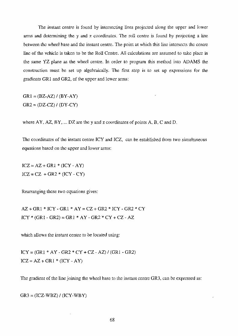
The instant centre is found by intersecting lines projected along the upper and lower
arms and determining the y and z coordinates. The roll centre is found by projecting a line
between the wheel base and the instant centre. The point at which this line intersects the centre
line of the vehicle is taken to be the Roll Centre. All calculations are assumed to take place in
the same YZ plane as the wheel centre. In order to program this method into ADAMS the
construction must be set up algebraically. The first step is to set up expressions for the
gradients GRI and GR2, of the upper and lower arms:
GRI = (BZ-AZ) I (BY-AY)
GR2 = (DZ-CZ) I (DY-CY)
where AY, AZ, BY, ... DZ are they and z coordinates of points A, B, C and D.
The coordinates of the instant centre ICY and ICZ, can be established from two simultaneous
equations based on the upper and lower arms:
ICZ = AZ + GRI *(ICY- AY)
ICZ = CZ + GR2 * (ICY - CY)
Rearranging these two equations gives:
AZ + GRI * ICY- GRI * A Y = CZ + GR2 * ICY- GR2 * CY
ICY* (GRI- GR2) = GRI * AY- GR2 * CY + CZ- AZ
which allows the instant centre to be located using:
ICY= (GRI *A Y- GR2 * CY + CZ- AZ) I (GRl - GR2)
ICZ = AZ + GRI *(ICY- AY)
The gradient of the line joining the wheel base to the instant centre GR3, can be expressed as:
GR3 = (ICZ-WBZ) I (ICY-WBY)
68

where WBY and WBZ are they and z coordinates of the wheel base.
which allows the roll centre to be located using:
RCY=O.O
RCZ = WBZ + GR3 * (RCY - WBY)
The roll centre height RCH, can be defined by:
RCH =RCZ- RZ
where RZ is the z coordinate of the road .
4.6.2 Rear suspension
The methods used to determine the instant centre and roll centre position for the rear
suspension are based on the construction shown in Figure 4.15.
------·-Wheel Base (WB)
A
-·- ..............
Centre Line
I I
-·- I ·-·-·-·- I
·-·-------L : ------------- .. _ Instant Centre I -·-1 ·---
: -----·-:·:.:.-::.:::..~-:_;.,-,:,-... D --r----·:-: .. :_ .. -----
-0-·-·-· Roll Centre ·-+·-·-· - -..,..i,-------- I ----
" 1 z Roll Centre Height u ~
----------·------
Figure 4.15 Construction of the instant centre and roll centre for the rear suspension
The instant centre is found by intersecting lines projected along the transverse arm and
perpendicular to the axis of the strut. The roll centre is found by projecting a line between the
69
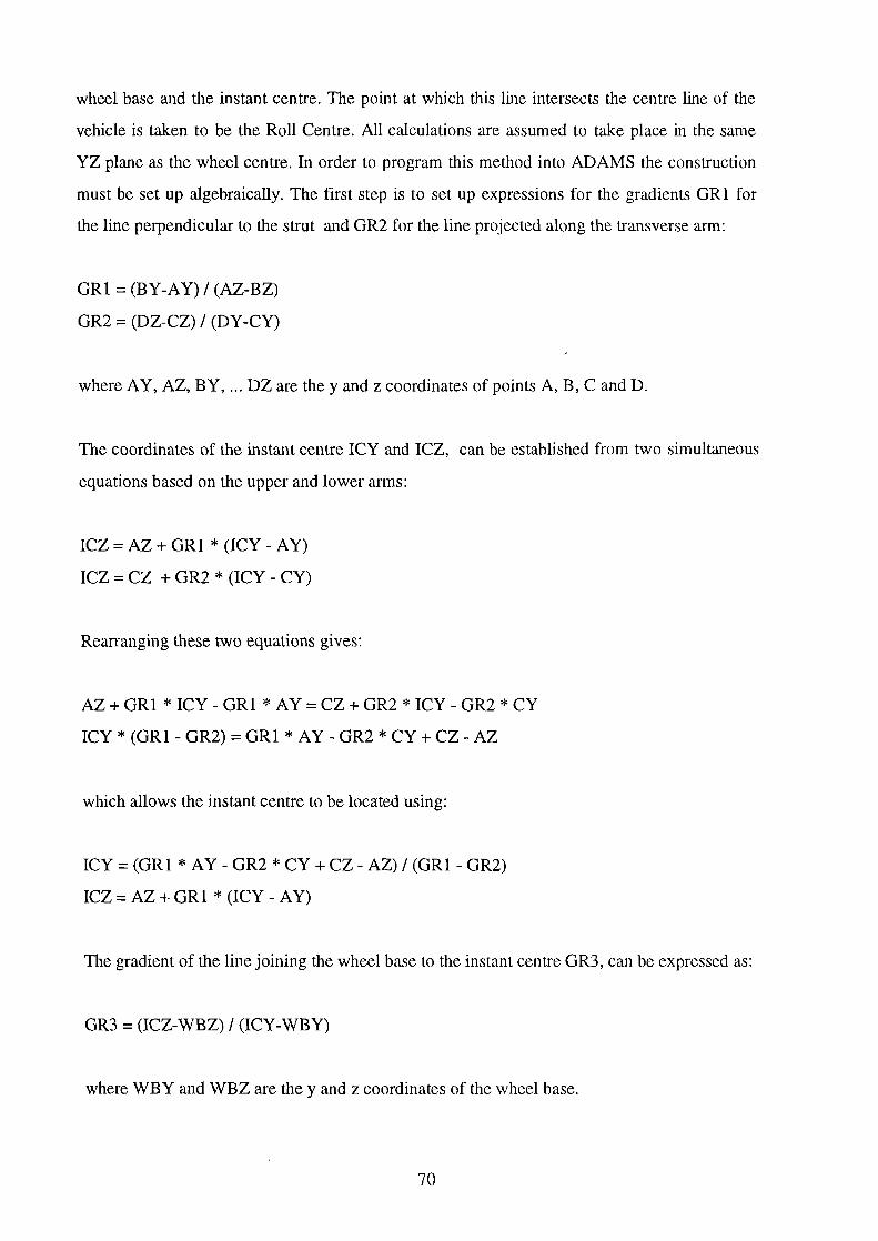
wheel base and the instant centre. The point at which this line intersects the centre line of the
vehicle is taken to be the Roll Centre. All calculations are assumed to take place in the same
YZ plane as the wheel centre. In order to program this method into ADAMS the construction
must be set up algebraically. The first step is to set up expressions for the gradients GRl for
the line perpendicular to the strut and GR2 for the line projected along the transverse arm:
GRl =(BY-A Y) I (AZ-BZ)
GR2 = (DZ-CZ) I (DY-CY)
where AY, AZ, BY, ... DZ are they and z coordinates of points A, B, C and D.
The coordinates of the instant centre ICY and ICZ, can be established from two simultaneous
equations based on the upper and lower arms:
ICZ=AZ+GRl *(ICY-AY)
ICZ = CZ + GR2 * (ICY - CY)
Rearranging these two equations gives:
AZ + GRl * ICY- GRl * A Y = CZ + GR2 * ICY - GR2 * CY
ICY* (GRl- GR2) = GRl * AY- GR2 * CY + CZ- AZ
which allows the instant centre to be located using:
ICY= (GRl *A Y- GR2 * CY + CZ- AZ) I (GRl - GR2)
ICZ = AZ + GRl *(ICY- AY)
The gradient of the line joining the wheel base to the instant centre GR3, can be expressed as:
GR3 = (ICZ-WBZ) I (ICY-WBY)
where WBY and WBZ are they and z coordinates of the wheel base.
70

which allows the roll centre to be located using:
RCY=O.O
RCZ = WBZ + GR3 * (RCY - WBY)
The roll centre height RCH, can be defined by:
RCH =RCZ- RZ
where RZ is the z coordinate of the road .
4.6.3 Implementation in ADAMS
As stated earlier the calculation of instant centre and roll centre position can be implemented
either by programming in the input deck with the VARIABLE statement or by preparing a
user-written FORTRAN subroutine. By way of example these methods are demonstrated for
the front suspension system only. Using the VARIABLE statement it is possible to program
the equations laid out in Section 4.6.1 as shown in Table 4.1.
Table 4.1 Calculation of roll centre height using the VARIABLE statement
V AR/14,1C= 1,FU=DZ(1414, 1411)/(DY(1414, 1411)+ 1E-6)
V AR/15,1C=1,FU=DZ(1216,1213)/{DY(1216,1213)+1E-6)
V AR/16,1C=1,FU=((V ARV AL(14)*DY(1411))
,-{V ARV AL(15)*DY(1213))+DZ(1213)
,-DZ(1411))/(V ARV AL{14)-V ARV AL(15)+ 1E-6)
V AR/17,FU=DZ(14ll)+V ARV AL(14)*{V ARV AL(16)-DY(1411))
V AR/18,FU=(V ARV AL(17)-DZ(1029))/(V ARV AL(16)-DY(1029)+ 1E-6)
V AR/19,FU=DZ(1029)+V ARVAL(l8)*(0.0-DY(1029))
V AR/20,FU=VARV AL(l9)+152.6
REQ/1,F2=V ARV AL(l6)\F3=V ARV AL(17)\F4=V ARV AL(20)\
,TITLE=NULL:ICY:ICZ:RCH:NULL:NULL:NULL:NULL
71
! GRl
!GR2
! ICY
! ICZ
!GR3
!RCZ
!RCH

The variables such as BZ-AZ are defined using ADAMS system variables which
measure components of displacements between markers such as DZ(l414,1411). The
REQUEST statement REQ/1 shows how to access the information calculated by the
VARIABLE statements.
The alternative method of writing a FORTRAN subroutine is demonstrated in Table
4.2 by the listing of a user written REQSUB developed specifically for the front suspension of
the ROVER. The subroutine would be called from the ADAMS input deck as follows:
REQUEST/id,FUNCTION=USER(l,parl,par2,par3,par4,par5,par6,par7,par8,par9)
Where the parameters parl,par2, ... par9 are the various items of data outlined in the
subroutine. The FORTRAN method was used with an earlier version of ADAMS and replaced
with the VARIABLE method at a later date. The VARIABLE method has been used for the
plots in this report.
4.7 Results
The system schematics used to generate the models for this study are provided in Appendix A
For both the front and rear suspensions the results are plotted graphically and are included in
Appendix B. In each plot the vertical displacement ( Bump movement ) is plotted on the X
axis. The front suspension has been moved from 90 mm displacement in rebound to 110 mm
displacement in bump. The rear suspension has been moved from 85 mm displacement in
rebound to 100 mm in bump.
For the front suspension it was possible to compare the ADAMS results with measured
test data provided by Rover which shows the variation of:
(i) Camber angle (deg) with Bump Movement (mm)
(ii) Steer angle (deg) with Bump Movement (mm)
(iii) Vertical Force (N) with Bump Movement (mm)
72
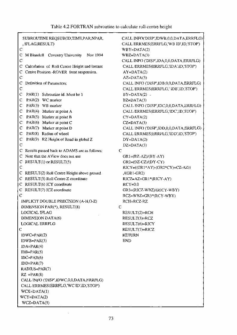
Table 4.2 FORTRAN subroutine to calculate roll centre height
c
SUBROUTINE REQSUB(ID,TIME,P AR,NP AR,
, IFLAG,RESULT)
C M Blundell Coventry University Nov 1994
c C Calculation of Roll Centre Height and Instant
C Centre Position -ROVER front suspension.
c C Definition of Parameters:
c C PAR(l) Subroutine id. Must be 1
C PAR(2) WC marker
C PAR(3) WB marker
C PAR( 4) Marker at point A
C P AR(S) Marker at point B
C PAR(6) Marker at point C
C P AR(7) Marker at point D
C PAR(8) Radius of wheel
C PAR(9) RZ Height of Road in global Z
c C Results passed back to ADAMS are as follows:
C Note that the A View does not use
C RESULT(l) or RESULT(5)
c C RESUL T(2) Roll Centre Height above ground
C RESULT(3) Roll Centre Z coordinate
C RESUL T(6) ICY coordinate
C RESUL T(7) ICZ coordinate
c IMPLICIT DOUBLE PRECISION (A-H,O-Z)
DIMENSION PAR(*), RESULT(8)
LOGICAL IFLAG
DIMENSION DATA(6)
LOGICAL ERRFLG
c IDWC=P AR(2)
IDWB=P AR(3)
IDA=PAR(4)
IDB=PAR(5)
IDC=PAR(6)
IDD=PAR(7)
RADIUS=P AR(7)
RZ =PAR(8) CALL INFO ('DISP',IDWC,O,O,DATA,ERRFLG)
CALL ERRMES(ERRFLG,'WC ID',ID,'STOP')
WCX=DATA(l)
WCY=DATA(2)
WCZ=DATA(3)
c
c
73
CALL INFO('DISP',IDWB,O,O,DAT A,ERRFLG)
CALL ERRMES(ERRFLG,'WB ID',ID,'STOP')
WBY=DATA(2)
WBZ=DATA(3)
CALL INFO ('DISP',IDA,O,O,DATA,ERRFLG)
CALL ERRMES(ERRFLG,'IDA',ID,'STOP')
AY=DATA(2)
AZ=DATA(3)
CALL INFO ('DISP',IDB,O,O,DA T A,ERRFLG)
CALL ERRMES(ERRFLG,' IDB',ID,'STOP')
BY=DATA(2) ~
BZ=DATA(3)
CALL INFO ('DISP',IDC,O,O,DATA,ERRFLG)
CALL ERRMES(ERRFLG,'IDC',ID,'STOP')
CY=DATA(2)
CZ=DATA(3) CALL INFO ('DISP',IDD,O,O,DAT A,ERRFLG)
CALL ERRMES(ERRFLG,'IDD',ID,'STOP')
DY=DATA(2)
DZ=DATA(3)
GRl=(BZ-AZ)/(BY -A Y)
GR2=(DZ-CZ)/(DY -CY)
RICY=((GRl *A Y)-(GR2*CY)+CZ-AZ))
,/(GR1-GR2)
RICZ=AZ+GRl *(RICY -A Y)
RCY=O.O
GR3=(RICZ-WBZ)/(RICY-WB Y)
RCZ=WBZ+GR3*(RCY-WBY)
RCH=RCZ-RZ
RESUL T(2)=RCH
RESUL T(3)=RCZ
RESULT(6)=RICY
RESUL T(7)=RICZ
RETURN
END

4.8 Summary
Examination of the results given in Appendix B for both the front and rear suspension models
indicates that, except for the steer change in the rear suspension, models using rigid joints,
linear bushes or non-linear bushes could be used. It is noticeable with the front suspension that
the plots begin to deviate when approaching the full bump or full rebound positions. This is
due to the forces building up in the bump stop or rebound stop which are reacted through the
suspension to the bushes. The reaction forces at the bushes lead to distortion which results in
the changes in suspension geometry as shown in the plots. This effect is not present in the
models using rigid joints which have zero degrees of freedom. Geometry changes are entirely
dependent on the position and orientation of the joints.
On the rear suspension the range of vertical movement is such that the effects of the
bump and rebound stops are clearly not as evident as for the front suspension. When
considering the merits of each modelling approach it appears from the curves plotted that for
the range of vertical movement expected of a handling model there is little difference between
models using rigid joints, linear bushes or non-linear bushes, except for the plots which show
the steer change of the wheel as a function of vertical movement. This is particularly noticeable
with the rear suspension as shown in Figure B.9.
The steer angle curve for the rigid joint model diverges from the curves for the
linear bush and non-linear bush model. This is due to the design of this suspension which does
not easily allow kinematic modelling with the same level of accuracy as a double wishbone
suspension as described earlier.
The results of this study indicate that for a handling model of this vehicle based on
modelling the suspension linkages either the linear bush or non-linear bush models could be
incorporated but that the rigid joint model may not be suitable due to the bump-steer
characteristics, particularly in the rear suspension. The use of the non-linear model will
significantly increase the effort required to model the vehicle. This is evident from Table 4.3
which compares the ADAMS data inputs required to model the connection of the front
suspension lower arm to the vehicle body. As can he seen there is a significant amount of data
74

required to model a non-linear bush. The modelling of a linear bush requires only a reasonable
amount of extra data input when compared with the rigid joint model.
From Table 4.3 it is clear that the modelling of non-linear bushes has a significant
impact on the preparation of the ADAMS input deck. There is however a great deal of extra
effort which needs to be documented. For the non-linear bushes in these models the
characteristics were entered in the form of X-Y pairs making up a non-linear spline. It is
important to check that the spline that ADAMS fits through the data is consistent with the test
figures. For each of the non-linear splines used here the data has been and checked. In some
cases the spline fit is poor leading to an oscillatory characteristic in the spline. In these cases it
is necessary to fit additional points in the test data to ensure a smooth curve fit. It is also very
easy to make an error when entering such large amounts of non-linear data in the ADAMS
input deck. The plotting of non-linear data is therefore a necessary activity in terms of the
quality assurance of the model but very time consuming.
The testing of the bushes is also an activity which will impact on the timescales of a
simulation project. Research project work carried out in parallel to this project within the
School of Engineering has required physical testing of the bushes on a similar vehicle. Based
on the physical testing of the bushes for that vehicle and the plotting and checking of data an
estimate of the effort, in man-days, required to prepare the bush data for a typical suspension is
given in Table 4.4.
75

Table 4.3 ADAMS data input for a joint, linear bush and nonlinear bush
~OINT
J0/16,REV,1=1216,J=0116
LINEAR BUSH
BUSH/16,1=1216,1=0116 ,K=7825,7825,944 ,KT=2.5E6,2.5E6,500 ,C=35,35,480 ,CT =61 000,61000,40
NON-LINEAR BUSH
BUSH/16,1=1216,}=0116 ,K=O,O,O ,KT=0,0,500 ,C=35,35,480 ,CT=61000,61 000,40
GFORCE/16,1= 1216,JFLOAT =0 11600,RM= 1216 ,FX=CUBSPL(DX(1216,0116,1216),0,161)\ ,FY=CUBSPL(DY(1216,0116,1216),0,161)\ ,FZ=CUBSPL(DZ(l216,0116,1216),0, 162)\ ,TX=CUBSPL(AX(1216,0116),0, 163)\ ,TY=CUBSPL(AY(1216,0116),0,163)\ ,TZ=O.O\
SPLINE/161 ,X=-1.8,-1.5 ,-1.4,-1.22,-1.123,-1.0,-0.75 ,-0.5,-.25,0,0.25 ,0.5,0.75 ,1.0, 1.123, 1.22, 1.4, 1.5, 1.8 'y =15350,10850,9840,6716,5910,5059,3761 ,2507' 1253,0,-1253,-2507,-3761,-5059,-5910, ,-6716,-9840,-10850,-15350 SPLINE/ 162, ,X=-5,-4,-3,-2.91 ,-2.75,-2.5,-2,-1.5,-1 ,-0.5,0,0.5, 1 ,1.5,2,2.5,2.75,2.91 ,3,4,5 ,Y =7925,3925, 1925,1790,1626,1450,1136,830,552,276,0,-276,-552,-830 ,-1136,-1450,-1626,-1790,-1925,-3925,-7925 SPLINE/163, ,X=-0.22682,-0.20939,-0.19196,-0.17453,-0.1571,-0.13963,-0.10472,-0.06981 ,-.03491,0,0.03491,0.06981,0.10472,0.13963,0.1571,0.17453,0.19196,0.20939,0.22682 ,Y=241940,198364,160018, 125158,93387,75415,52951,35702,18453,0,-18453,-35702 ,-52951,-75415,-93387,-125158,-160018,-198364,-241940
76

Table 4.4 The impact of modelling nonlinear bushes on project timescales
Obtaining bushes and planning tests
Design of brackets to support bushes in test rig
Manufacture of brackets
Static Testing of bushes
Dynamic testing of bushes
Checking test data
Preparing ADAMS spline data
Plotting and checking of spline data
2 day
5 day
5 days
1 day
2 days
2days
2 days ~
2 days
Total 21 man-days
For the Linkage model which is described in the next section of this thesis it has been
decided to model the suspensions using the linear bush approach. As discussed earlier the rigid
jomt model may work for the front suspension but for the rear suspension the bump steer
characteristics are not accurate. The nonlinear bush model does not appear to be any more
accurate than the linear bush model so the suspensions will be modelled using linear bushes.
77

5.0 MODELLING OF VEHICLE SYSTEMS
5.1 Introduction
One of the main objectives of this thesis has been to investigate the influence of modelling on
handling simulations. With regard to this the modelling issues can be considered to divide into
two main areas:
(i) The modelling of the forces and moments occurring at the tyre to road surface contact
patch.
(ii) The modelling of the rest of the vehicle systems, namely the suspension systems, roll bars,
vehicle body, steering system, steering inputs, and drive inputs to the road wheels. Although
not considered here more advanced systems such as traction control or anti-lock braking
systems may also be considered.
This section of the report will address the modelling of vehicle systems. The modelling
of tyre characteristics is a large and complex subject and is therefore addressed separately in
Section 6 of this report. Detailed schematics for all the models described here are included in
Appendix A
5.2 Vehicle body, coordinate frames and rigid part definitions
For each rigid body in the system it is necessary to include a statement defining the mass,
centre of mass location, and mass moments of inertia. These statements are referred to as Part
statements. The mass moments of inertia are defined with respect to an inertial reference
frame. Throughout this project each part has utilised a reference frame which is located at the
mass centre and aligned with the principal axes of the body. This means that it was only
necessary to define the principal mass moments of inertia (Ixx, Iyy, Izz) and not include
product moments of inertia (Ixy, Iyz, Izx). The use of coordinate systems is now explained in
more detail but for the vehicle body it will be seen later that Ixx is associated with roll, Iyy with
pitch and Izz with yaw.
78

It is also possible to model the flexibility of bodies using different methods depending
on the geometry of the part. For example, a component such as a tie bar or roll bar could be
modelled using a beam element with the usual stiffness matrix formulation as used in finite
element analysis. Such an element is available as a standard modelling feature in ADAMS.
A more complex modelling approach for flexible bodies is used where the geometry is
more detailed such as for a suspension arm or the vehicle body itself. In these cases the
component or body may be modelled in a finite element program ensuring that nodes exist in
coincident positions to those required for joint or force attachments in the multibody systems
program. The stiffness matrix is condensed in the finite element program to a matrix which
references these locations. The resulting stiffness matrix, which is sometimes referred to as a
superelement can then be included in the multibody systems program. An example of this is
given in (71) which describes work carried out by the Ford Light Truck division in the USA. In
this case suspension arms have been modelled in a fmite element program and included in an
ADAMS model used for handling simulations. For an open top sports vehicle the torsional
stiffness of the body may also be of concern when trying to predict handling performance. In
this case a fmite element approach may again be used. Alternatively a more simplistic
representation of the torsional stiffness of the body may be used as in (64). In that case the
vehicle body was modelled as two rigid masses connected by a revolute joint aligned along the
longitudinal axis of the vehicle and located at the mass centre. The relative rotation of the two
body masses about the axis of the revolute joint was resisted by a torsional spring with a
stiffness corresponding to the torsional stiffness of the whole body.
Each rigid part possesses a set of markers which can be defined in global or local
coordinate systems and are considered to move with the part during the simulation. Markers
are used to define centre of mass locations, joint locations and orientations, force locations and
directions. It is also necessary to include one non moving part which is referred to as the
ground part.
For the modelling work carried out here there are three types of right-handed Cartesian
coordinate systems which may be used:
79

(i) The ground reference frame (GRF) is fixed and is the datum from which all other reference
frames are defmed.
(ii) The local part reference frame (LPRF) can be defined as a local system belonging to and
moving with any part in the model. The LPRF is defined relative to the ground reference
frame.
(iii) Markers are the essential reference frame used to define physical data such as mass
centres, spring attachment points or joint positions and orientation. The markers belong to,
move with and change orientation with a given part. As such they are defined relative to the
LPRF for that part. If an LPRF has not been defined for that part then the initial position of the
marker is defined with respect to the GRF.
The positioning of the reference frames described above is illustrated in Figure 5.1.
The position of the LPRF is defined by the vector QG which has components measured parallel
to the GRF. The position of a marker is defined by the vector QP which has components
measured parallel the LPRF or as shown, parallel to the GRF in the absence of an LPRF for
that part.
ZG
G:kYG XG • • ••• ••
NoLPRF defined
PART
Figure 5.1 Co-ordinate systems
80

For the vehicle models described in this thesis there was no use made of LPRFs and all
markers were defined relative to a single GRF as shown in Figure 5.2. The GRF is located near
the centre of the vehicle and is orientated with the x-axis pointing aft, the z-axis upwards and
the y-axis towards the left of the vehicle. This means that for most manoeuvres the vehicle is
defined with initial negative x-components of velocity.
Figure 5.2 Vehicle ground reference frame (GRF)
In addition to defining the position of a marker relative to the GRF using the QP vector
it is also necessary to define any required change in orientation. The first method shown in
Figure 5.3 makes use of successive Euler angle rotations, psi, theta and phi. Note that for this
work no LPRFs were defined so that the rotations are relative to the GRF.
In some instances it is more convenient to define the orientation of a marker by defining
a point ZP at any position along the z-axis of the new marker reference frame. This is often all
that is required as for example in the case where the z-axis of the marker is used to define the
axis of a revolute joint. If the orientation of the x and y-axes are also required this can be
achieved by defining any point XP on the new zx plane. ADAMS can then manipulate the
vectors to cross the new z-axis with the XP coordinate in the marker frame to obtain the y
axis.
81

z
GRF
X y
~
QP
Z' e?
r~ X'
Figure 5.3 Euler angle approach
z
MARKER
Z'
y
Y"' Y"
The new y and z-axes can then be used in a similar manner to obtain the x-axis. Tills
method is shown in Figure 5.4. Note that for the vehicle work described here LPRFs were not
used so that the XP and ZP vectors when used were defined relative to the GRF.
z
X
~
ZP
~
XP
~
QP
Figure 5.4 The XP-ZP method for marker orientation
82
y
X

5.3 Modelling of suspension systems
5.3.1 Overview
The study described in Section 4 of this report has laid the ground work for the further
investigation described here. As described earlier the four suspension modelling approaches
which have been compared are:
(i) The Linkage Model where the suspension linkages and compliant bush connections have
been modelled in detail in order to recreate as closely as possible the actual assemblies on the
vehicle.
(ii) The Lumped Mass Model where the suspensions have been simplified to act as single
lumped masses which can only slide in the vertical direction with respect to the vehicle body.
(iii) The Swing Arm Model where the suspensions are treated as single swing arms which
rotate about a pivot point located at the instant centres for each suspension.
(iv) The Roll Stiffness Model where the body rotates about a single roll axis which is fixed and
aligned through the front and rear roll centres.
The four suspension arrangements are shown schematically in Figure 5.5 and described
in more detail in the following sections.
83

LINKAGE MODEL ~
<. ~ LUMPED MASS MODEL
~e-~··.Jt ~ . ········ ... ~+ rn~
SWING ARM MODEL ~ I
0 ~t - ~t···· ~~~:~--. 9 ~tV
I
ROLL STIFFNESS MODEL ...... .
... ~ '
... 0) ....... ..:. . ' .· ...... , .... o ...... ':
....... . ..
I I
......
'~ . a::DW I I
~ I I
Figure 5.5 Modelling of suspension systems
84
I
tV I

5.3.2 Linkage model
The model based on linkages as shown in Figure 5.6 is the model which most closely
represents the actual vehicle. The work discussed in Section 4 lead to the decision to model
the bushes as linear. This sort of vehicle model is the most common approach adopted by
ADAMS users in the automotive industry even extending the model definition to include full
nonlinear bush characteristics as with the work in (64).
a~ .. ~~ ~-·,····.
Figure 5.6 The Linkage model
85

A simplification of a model based on linkages is to treat the joints as rigid and generate
a kinematic representation of the suspension system. As described in Section 4 a double
wishbone arrangement is typical of a suspension system that can be modelled in this way and
used for handling simulations. This has been confirmed in (24) where a kinematic modelling
approach was discussed for vehicles with double wishbone suspensions. Note that although for
completeness the schematic in Figure 5.6 also shows the front and rear roll bars the modelling
of these is discussed in more detail in Section 5.6 of this report.
5.3.3 Lumped Mass model
For the Lumped Mass model the suspension components are considered to be lumped together
to form a single mass. The mass is connected to the vehicle body at the wheel centre by a
translational joint which only allow vertical sliding motion. This means that there is no change
in the relative camber angle between the road wheels and the body. The camber angle between
the road wheels and the road will therefore be directly related to the roll angle of the vehicle.
Spring and damper forces act between the suspensions and the body.
The front wheel knuckles were modelled as separate parts connected to the lumped
suspension parts by revolute joints. The steering motion required for each manoeuvre was
achieved by applying time dependent rotational motion inputs about these joints. Each road
wheel was modelled as a part connected to the suspension by a revolute joint. The Lumped
Mass model is shown schematically in Figure 5.7.
86

Spring Damper
~ 1RANS
O)o[]Jl Rear Right Sliding Mass
5.3.4 Swing Arm model
Spring Damper
Rear Left Sliding Mass
TRANS
Figure 5.7 The Lumped Mass model
Spring Damper
t&~4 QREV
I I
Front Left Sliding Mass and Wheel Knuckle
This model was developed from the lumped mass model by using revolute joints to allow the
suspensions to 'swing' relative to the vehicle body rather than using translational joints which
only allow sliding motion to take place. The revolute joints were located at the instant centres
of the actual suspension linkage assembly. These positions were found by modelling the
87

suspensions separately as described in Section 4. The swing arm model has an advantage over
the lumped mass model in that it allows the wheels to change camber angle relative to the
vehicle body. The Swing Arm model is shown schematically in Figure 5.8.
Spring Damper
Spring Damper
~t ---c==~&=-_ tK&~REV REV ~ SwmgArm
Spring
Drunper ~t REV
Front Right Swing Arm
Swing Arm
Spring ~t Damper =F
~~' , ,~',,S Ql ,, G ,, I ... ..... --..... I ,, '
,, Front Left :
Swing Arm and Wheel Knuckle
©)of+J REVcb and Wheel Knuckle
Figure 5.8 The Swing Arm model
88

5.3.5 Roll Stiffness model
This model was a further simplification treating the front and rear suspensions as rigid axles
connected to the body by revolute joints at the roll centres. The roll centre positions were
obtained from the study described in Section 4. A torsional spring was located at the front and
rear roll centres to represent the roll stiffness of the vehicle. The determination of the roll
stiffness of the front and rear suspensions required a detailed investigation which is described
in the following section. The Roll Stiffness model is shown schematically in Figure 5.9.
Torsional Spring damper
I I
Torsional Spring damper
~: ,J.
~!~ '--4-"
Wheel Knuckles
Figure 5.9 The Roll Stiffness model
89
I I cp

5.3.6 Model size
For each of the vehicle models described here it is possible to estimate the model size in terms
of the degrees of freedom in the model and the number of equations which ADAMS is using to
formulate a solution. The calculation of the number of degrees of freedom (DOF) in a system is
based on the Greubler equation:
DOF = 6 x (No. of Parts)- (Constraints from Joints and Motions)
Note that each Part has six rigid body degrees of freedom. The ground part is not
included in the calculation as it does not move. An example, for some of the joints used in this
study, of the degrees of freedom removed by constraints is given in Table 5.1.
Table 5.1 Degrees of freedom constrained by joints
ADAMS Translational Rotational Total
Joint Constraints Constraints Constraints
Cylindrical 2 2 4
Fixed 3 3 6
Planar 1 2 3
Revolute 3 2 5
Spherical 3 0 3
Translational 2 3 5
Universal 3 1 4
It is therefore possible for any of the vehicle models to calculate the degrees of freedom
in the model. An example is provided here for the Roll Stiffness model where the degrees of
freedom can be calculated as follows:
Parts 9 x 6 = 54
Rev 8 x -5 = -40
Motion 2 x -1 = -2
L DOF = 12
90

In physical terms it is more meaningful to describe these degrees of freedom in relative
terms as follows. The body part has 6 degrees of freedom. The two axle parts each have 1
rotational degree of freedom relative to the body. Each of the four wheel parts has 1 spin
degree of freedom relative to the axles making a total of 12 degrees of freedom for the model.
When a simulation is run in ADAMS the program will also report the number of
equations in the model. As discussed in Section 3 ADAMS will formulate 15 equations for
each part in the model and additional equations corresponding to all the constraint and applied
forces in the model. On this basis the size of all the models is summarised in Table 5.2.
Table 5.2 Vehicle model sizes
Model Degrees of freedom
Linkage 78
Lumped Mass 14
Swing Arm 14
Roll Stiffness 12
Number of Equations
961
429
429
265
The size of the model and the number of equations is not the only consideration when
describing efficiency in vehicle modelling. Of perhaps more importance is the engineering
significance of the model parameters. The Roll Stiffness model, for example, may be preferable
to the Lumped Mass model. It is not only a smaller model but is also based on parameters such
as roll stiffness which will have relevance to a vehicle engineer. The roll stiffness can be
measured on an actual vehicle or estimated during vehicle design.
91

5.4 Determination of roll stiffness and damping
5.4.1 Modelling approach
In order to develop the full vehicle model based on roll stiffness it was necessary to determine
the roll stiffness and damping of the front and rear suspension elements separately. The
estimation of roll damping was obtained by assuming an equivalent linear damping and using
the positions of the dampers relative to the roll centres to calculate the required coefficients.
The positions of the front and rear roll centres were already established using the quarter
suspension models and the methods set out in Section 4. The procedure used to fmd the roll
stiffness for the front suspension elements involved the development of a model as shown in
Figure 5.10. This model included the vehicle body which was constrained to rotate about an
axis aligned through the front and rear roll centres. The vehicle body was attached to the
ground part by a cylindrical joint located at the front roll centre and aligned with the rear roll
centre. The rear roll centre was attached to the ground by a spherical joint in order to prevent
the vehicle sliding along the roll axis. A motion input was applied at the cylindrical joint to
rotate the body through a given angle. By requesting the resulting torque acting about the axis
of the joint it was possible to calculate the roll stiffness associated with the front end of the
vehicle. The front suspensions were modelled using the suspension model where bushing
characteristics were treated as linear. The springs were also included as was the complete front
roll bar model. The road wheel parts were not included nor were the tyre properties. The
wheel centres on either side were constrained to remain in a horizontal plane using in plane joint
primitives. Although the damper force elements were retained in the suspension models they
have no contribution as the roll stiffness was determined using static analysis. The steering
system, although not shown in Figure 5.10, was also included in the model. A motion input
was used to lock the steering in the straight ahead position during the roll simulation.
For the rear end of the vehicle the approach was essentially the same as for the front
end, with in this case a cylindrical joint located at the rear roll centre and a spherical joint
located at the front roll centre. The model used for the rear roll analysis is shown in Figure
5.11.
92

SPH
Applied Roll Angle M>tion
INPLANE
<;;i . INPLANE
Front Roll Centre
c::on CYL ~ 'J
INPLANE
Applied Roll Angle Mooon
Figure 5.10 Determination of front end roll stiffness
(\ RearRoll ~ i Centre
'Qo__ CYL
Figure 5.11 Determination of rear end roll stiffness
93
SPH
Front Roll Centre

For both the front and rear models the vehicle body was rotated through an angle of ten
degrees either side of the vertical. In each case a quasi-static analysis was performed over
three seconds with thirty output steps. The roll motion was defined as a function of time to roll
the model at a rate of ten degree per second. During the first second the model rotates ten
degrees to the left and then back to the upright position between one and two seconds. Over
the third second the model rotates ten degrees to the right.
The results for the front and rear end models are plotted in Figure 5.12 and Figure 5.13
and are linear to within 2% for the front and 4% for the rear. The~ data from these curves has
been used to obtain the values of torsional stiffness used in the roll stiffness model.
Front End
Kt = 608.459 103 Nmm/deg
Kt = 34.862 106 N mm/rad
Roll Moment (Nmm)
6.0E+06
4.0E+OB
2.0E+OB
o.o
-2.0E+Oe
v /
/ /
-4.0E+OB
-S.OE+OB
/
-8.0 -4.0 -1 0.0 -6.0
Rear End
Kt = 496.459 103 Nmm/deg
Kt = 28.445 106 Nmm/rad
/ /
v v
/
/ v
/ /
0.0 4.0 8.0 -2.0 2.0 6.0 1 0.0
Roll Angle (deg)
Figure 5.12 Front end roll test
94

Roll Moment (Nmm)
6.0E+06
0.0
~
/ v
/ v
/ v
/ ~
4.0E+06
2.0E+06
-2.0E+D6
/ v -4.0E+06
-6.0E+06 -6.0 -4.0 0.0 4.0 6.0
-10.0 -6.0 -2.0 2.0 6.0 1 0.0
Roll Angle (deg)
Figure 5.13 Rear end roll test
5.4.2 Calculation check
As a check on the values for roll stiffness obtained from the ADAMS simulations a hand
calculation has been performed for the roll stiffness at the front end of the vehicle. The
deformed geometry used for the calculation has been obtained by producing a scaled drawing
of the rolled vehicle. The maximum roll angle of ten degrees has been used to facilitate the
drawing and measuring of the dimensions used in the hand calculation. The value obtained
from the hand calculation is compared with the value computed by ADAMS. The roll stiffness
due to the road springs and the roll stiffness due to the roll bar have been calculated separately
and then added to get a total roll stiffness. The calculation of the contribution due to the
springs is based on the forces due to spring deformation and the moment of these forces about
the roll centre. The deformation of the springs and the moment arms were measured from the
scaled drawing based on a roll angle 8, of ten degrees. This is illustrated in Figure 5.14 which
is not to scale.
95

e
····-·····-·····-··--···--·····-···· -···
..... :-.i::) r.:::!:-:.t
;--------------·····
LL----+-+IV' ~ Roll
Centre
\ Figure 5.14 Calculation of roll stiffness due to road springs
The spring stiffness is given as:
k = 31.96 N/mm
The deformation in the left spring and extension in the right spring are equal and were found
to be:
bL= 110 mm
The forces FL and FR can be calculated as:
FL = k . bL = 3516 N
FR = k. bL = 3516 N
The moment arms a and b were found to be:
a= 630 mm b = 600 mm
This gives a moment Ms due to the springs acting at the roll centre:
Ms =FL. a+ FR. b = 4324.7 103 Nmm
96

The roll bars have been modelled in ADAMS as two rigid parts connected at the
vehicle centre line by a torsional spring. In order to calculate the moment acting at the roll
centre due to the roll bar it is first necessary to calculate the relative angle of twist between the
two parts representing the roll bar. This is shown below in Figure 5.15.
F
Figure 5.15 Calculation ofroll stiffness due to the roll bar
The angle <1> was found to be :
<I> =25°
The torsional stiffness of the roll bar Kt is given as:
Kt = 490.0 103 Nmm/rad
The torque T required to produce an angle of twist of <I> on each side of the roll bar is given by:
T = Kt. <1>. ( n/180) = 213.8 103 Nmm
The lever arm L from the roll bar to the wheel centre is given as:
L=298 mm
The force F required to produce the torque is given by:
F=T/L=717.5N
97

The moment MR due to the roll bar acting at the roll centre is given by multiplying the
force F by the track Tr:
Tr = 1488 mm
MR =F. Tr = 1067.5 103 Nmm
The total moment M acting at the roll centre is found by adding the contribution due to
the springs Ms and the contribution due to the roll bar MR:
M = Ms + MR = 5392.2 103 Nmm
The roll stiffness KlF of the front end of the vehicle can be found from:
K1F = M I 8 = Nmm/deg = 539.2 103 Nmm/deg
KlF = M I [8. ( n/180 )] = 30895.0 103 Nmrn/rad
Comparing this value with the roll stiffness computed by the ADAMS model gives a
difference of 9.8%. On this basis the hand calculation appears to validate the modelling
approach and analyses used in ADAMS to determine roll stiffness for the front and rear end of
the vehicle.
5.5 Road Springs and dampers
5.5.1 Modelling of springs and dampers in the linkage model
The treatment of road springs in a vehicle where the suspensions have been modelled using
linkages and the suspension geometry is usually straightforward and allows a linear formulation
to be used. The spring is defined as connecting two points, referred to as an I marker and a J
marker. For the front suspension shown schematically in Figure 5.16 the spring force acts
between an I marker which is taken as belonging to the body representing the upper part of the
damper and a J marker which is taken as belonging to the body representing the lower part of
the damper. For the rear suspension the spring force is taken as acting between an I marker
98

which belongs to the vehicle body and a J mar~er which belongs to the suspension arm. For
both the front and rear suspension the damper forces act between the upper and lower parts
used to model the damper body.
Front Suspension Rear Suspension
~ - --.
Figure 5.16 Location of spring and damper elements in the linkage model
The force in the springs when treated as linear is given by:
F = K * ( OM (I,J)-L)
where:
L = Free Length of Spring ( at zero force )
DM(I,J) = Magnitude of Displacement between I and J Marker
K = Spring Stiffness
In this case K and L are model parameters and DM(I,J) is a system variable which is
continually calculated and updated by ADAMS during an analysis. The sign convention used is
that the equation for the spring will return a val~e which is positive when the spring is in
compression and negative in tension.
The damper forces were modelled as nonlinear and dependent on the relative velocity
between the I marker and J marker used to define the damper force. The system variable used
99

to represent the velocity is VR(I,J) also known as the radial line of sight velocity. The sign
convention used is that during bump when a positive force is needed VR(I,J) is negative and
that during rebound when I and J are separating the sign convention is reversed.
The nonlinear damper forces are defined in ADAMS using xy data sets where the x
values represent velocity and the y values are the force. During the analysis the force values are
extracted using a cubic spline fit. The curves for the front and rear dampers are shown in
Figure 5.17.
FRONT DAMPER- SOLID, REAR DAMPER- DASH
12000.0
9000.0 ~
" 6000.0 ""' ' .....
z 3000.0
(])
2 0.0 0
LJ...
-3000.0
-6000.0
~ ~'-....... 1'--.
......... -....
~ --~ --~ -...... -- ........
~ ........
~ -9000.0
-5000.0 -3000.0 -1000.0 1000.0 3000.0 5000.0 -6000.0 -4000.0 -2000.0 0.0 2000.0 4000.0 6000.0
Velocity ( mm/s )
Figure 5.17 Nonlinear force characteristics for the front and rear dampers
5.5.2 Modelling of springs in the Lumped Mass and Swing Arm models
For the simplified modelling approach used in the Lumped Mass and Swing Arm models it was
discovered that the road springs could not be directly installed in the vehicle model as with the
linkage model. Consider the Lumped Mass model when compared with the Linkage model as
shown in Figure 5.18.
100

LINKAGE MODEL LUMPED MASS MODEL
OS
ow ow I
M I I
I· lw j
8s !!: (ls/lw)8w 8s =8w
Figure 5.18 Road spring in the Linkage and Lumped Mass models
Clearly there is a mechanical advantage effect in the Linkage model which is not
present in the Lumped Mass vehicle model. At a given roll angle for the Lumped Mass model
the displacement and hence the force in the spring will be too large when compared with the
corresponding situation in the Linkage model.
For the Swing Arm model as shown in Figure 5.19 the instant centre about which the
suspension pivots is actually on the other side of the vehicle. In this case the displacement in
the spring is approximately the same as at the wheel and a similar problem occurs as with the
Lumped Mass model.
101

ow
·······
SWING ARM MODEL
........ ............. ........ ······ ...........
8s f!: 8w
.......... ............ ······· ...........
Instant centre
Figure 5.19 Installation of the road spring in the Swing Arm model
For the Lumped Mass and Swing Arm models this problem has been overcome as
shown in Figure 5.20 by using an 'equivalent' spring which acts at the wheel centre. From the
work with the quarter suspension model described in Section 4 it was possible to measure the
force and displacement at the wheel centre and plot this as shown in Figure B.6 for the front
suspension and Figure B.12 for the rear suspension.
Equivalent spring acting at the wheel ~ntre ~~
VEIDCLEBODY
Figure 5.20 Equivalent spring acting at the wheel centre
102

Although not used in the work described here a similar approach could be used in
concept design when detailed geometry is not available and a wheel rate curve can not be
obtained using the methods described in Section 4 of this report. This would involve scaling
the initial estimates of a linear spring out to the wheel centre and is illustrated in Figure 5.21.
kw
I I
M ow
I I
I· lw j
Figure 5.21 Scaling a linear spring to the wheel centre position
For the standard road spring the basic force displacement relationship gives:
Fs = ks.os
For the equivalent spring we also have:
Fw=kw.ow
Mechanical advantage gives:
Fw = (Ls/Lw) Fs
Geometry gives:
os = (Ls/Lw) ow
Therfore:
kw = Fw/ow = (Ls/Lw) Fs I (Lw/Ls) os = (Ls!Lw)2 ks
103

The introduction of a square function in the ratio can be considered a combination of
two effects:
(i) The extra mechanical advantage in moving the road spring to the wheel centre.
(ii) The extra spring compression at the wheel centre.
5.6 Roll bars
As shown in Figure 5.22 the roll bars were modelled using two parts connected to the
vehicle body by revolute joints and connected to each other by a torsional spring located on the
centre line of the vehicle. The roll bars were not modelled in detail, rather each roll bar part
was connected to the suspension using an inplane joint primitive which allowed the vertical
motion of the suspension to be transferred to the roll bars and hence produce a relative
twisting motion between the two sides.
Right Roll Bar
REV
INPLANE
Revolute Joints to Vehicle Body
Front Wheel Knuckle
REV
~orsional . Spring
Figure 5.22 Modelling the roll bars
104
Left Roll Bar
INPLANE ·. ··. ·· .....
Front Wheel Knuckle
····· .... EJ
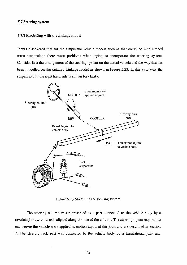
5. 7 Steering system
5.7.1 Modelling with the linkage model
It was discovered that for the simple full vehicle models such as that modelled with lumped
mass suspensions there were problems when trying to incorporate the steering system.
Consider first the arrangement of the steering system on the actual vehicle and the way this has
been modelled on the detailed Linkage model as shown in Figure 5.23. In this case only the
suspension on the right hand side is shown for clarity.
Steering column part
Revolute joint to vehicle body
Steering motion applied at joint
COUPLER .... ..
Steering rack part
Translational joint to vehicle body
Figure 5.23 Modelling the steering system
The steering column was represented as a part connected to the vehicle body by a
revolute joint with its axis aligned along the line of the column. The steering inputs required to
manoeuvre the vehicle were applied as motion inputs at this joint and are described in Section
7. The steering rack part was connected to the vehicle body by a translational joint and
105

connected to the tie rod by a universal joint. The translation of the rack was related to the
rotation of the steering column by a coupler statement which defines the ratio as follows:
COUPLER/51 0502,JOINTS=50 1 ,502,TYPE=T:R,SCALES=8.44898D, 1.0
In this case joint 501 is the translational joint and 502 is the revolute joint. the coupler
statement ensures that for every 8.44898 degrees of column rotation there will be 1 mm of
steering rack travel.
5. 7.2 Steering ratio test
Initial attempts to incorporate the steering system into the simple models using lumped masses,
swing arms and roll stiffness met with a problem when connecting the steering rack to the
actual suspension part. This is best explained by considering the situation shown in Figure
5.24.
I I I
d_) I I I I 0
Motion on the steering system is 'locked' during the initial static analysis
Downward motion of vehicle body and steering rack relative to suspension during static equilibrium
Connection of tie rod causes the front wheels to toe out
Figure 5.24 Toe change in front wheels at static equilibrium for simple models
106

The geometry of the tie rod has been established for the suspension and works well for
the linkage model. Physically connecting the tie rod to the simple suspensions does not work.
During the initial static analysis the rack moves down with the vehicle body relative to the
suspension system. This has a pulling effect on the tie rod which actually causes the front
wheels to toe out during the initial static analysis. This is similar to a bump steer effect. The
solution to this was to establish the relationship between the steering column rotation and the
steer change in the front wheels and to model this as a direct ratio using two coupler
statements to link the rotation between the steering column and each of the front wheel joints
as shown in Figure 5.25.
COUPLER
I I I
C0 I I I
. .
""'·· COUPLER .. . .. ··. ..
Figure 5.25 Coupled steering system model
During the track testing of the actual vehicle described in (20), a steering test was
carried out to measure the ratio between the steering wheel rotation and the road wheel steer
angle. This ratio was found to be 20:1. In order to check this with the ADAMS models a
separate study was carried out using the front right suspension system modelled with linear
bushes and connected to the ground part instead of the vehicle body. The modelling of these
two subsystems is shown in Figure 5.26.
107

Translational joint to ground
INPLANE
Jack Part
fT>IlMOTION ~TRANS
Translational joint to ground
Steering rack part
~MOTION
Steering motion inputs applied at the rack to ground translational joint
Figure 5.26 Front suspension steering ratio test model
The approach of using a direct ratio to couple the rotation between the steering column
and the steer angle of the road wheels was considered to have two main limitations which
should be investigated before continuing with the development of the simplified full vehicle
models:
(i) In the real vehicle and the Linkage model the ratio between the column rotation and the
steer angle at the road wheels would vary as the vehicle rolls due to the bump steer effects
generated by the suspension geometry.
(ii) For either wheel the ratio of toe out or toe in as a ratio of left or right steering wheel angle
rotation would not be exactly symmetric.
108
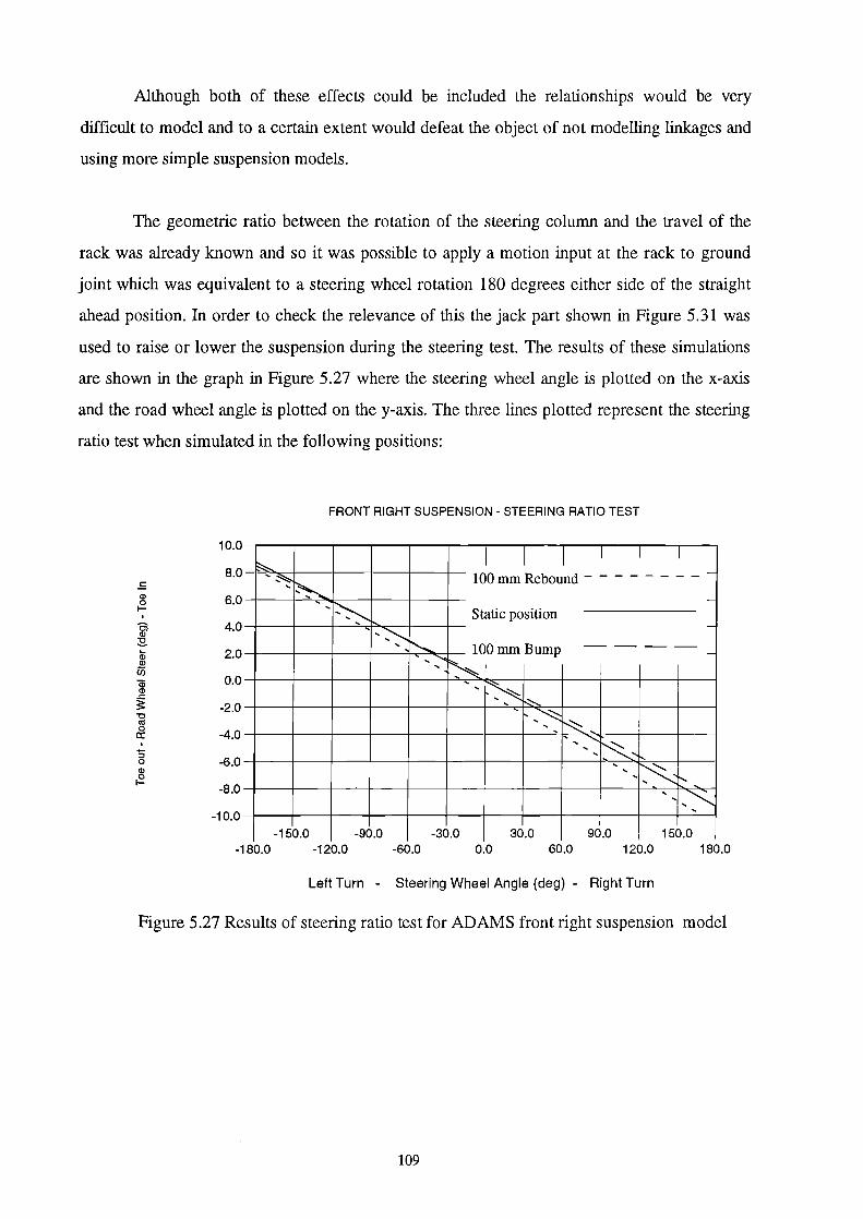
Although both of these effects could be included the relationships would be very
difficult to model and to a certain extent would defeat the object of not modelling linkages and
using more simple suspension models.
The geometric ratio between the rotation of the steering column and the travel of the
rack was already known and so it was possible to apply a motion input at the rack to ground
joint which was equivalent to a steering wheel rotation 180 degrees either side of the straight
ahead position. In order to check the relevance of this the jack part shown in Figure 5.31 was
used to raise or lower the suspension during the steering test. The results of these simulations
are shown in the graph in Figure 5.27 where the steering wheel angle is plotted on the x-axis
and the road wheel angle is plotted on the y-axis. The three lines plotted represent the steering
ratio test when simulated in the following positions:
FRONT RIGHT SUSPENSION- STEERING RATIO TEST
10.0
8.0 -= CD 6.0 0 1-
' o; 4.0 CD
:!:!. iii 2.0 CD (ij
0.0 Qi
~ I I I -f''e', "><~o-,+-~-,-+---t---t--+- 100 mm Rebound - - - - - - - - -
-' '~ Static position
',~
---+---+--+--+--' +1'..........--"'"'-::-:t-- 100 mm Bump - - - - _ '""!=>:.
' : ~ ' ""
I I I
-
CD ..c: :s: -2.0 "0
"' 0 -4.0 a:
' '5 -6.0 0
CD
~ -8.0
-10.0 -150.0 -90.0 -30.0 30.0 90.0 150.0
-180.0 -120.0 -60.0 0.0 60.0 120.0 180.0
Left Turn - Steering Wheel Angle (deg) - Right Turn
Figure 5.27 Results of steering ratio test for ADAMS front right suspension model
109

The lines plotted are reasonably linear but the bump and rebound results indicate an
offset from the normal static position due to the bump steer effect. A more detailed analysis of
the results is available in Table 5.3 where for each increment in steer angle the road wheel
angle has been computed and the ratio between the two calculated.
Table 5.3 Relationship between steering column rotation and road wheel angle
Steering Normal Static 100 mm Bump 100 mm Rebound
Wheel Angle
(Degrees) Toe Angle Ratio Toe Angle Ratio Toe Angle Ratio
(Degrees) (Degrees) (Degrees)
-180 8.76855 20.5279 8.50155 21.1726 8.23804 21.8499
-160 7.79887 20.5158 7.58745 21.0875 7.23006 22.1298
-140 6.82707 20.5066 6.67076 20.9871 6.22003 22.5079
-120 5.85285 20.5028 5.75122 20.8651 5.20761 23.0432
-100 4.87588 20.5091 4.82854 20.7102 4.19242 23.8525
-80 3.89582 20.5348 3.90240 20.5002 3.17410 25.2040
-60 2.91233 20.6021 2.97249 20.1851 2.15224 27.8779
-40 1.92502 20.7790 2.03848 19.6224 1.12642 35.5108
-20 0.93351 21.4245 1.10001 18.1816 0.09618 207.940
20 -1.06382 18.8002 -0.79181 25.2586 -1.97946 10.1038
40 -2.07054 19.3186 -1.74598 22.9098 -3.02591 13.2192
60 -3.08329 19.4597 -2.70623 22.1711 -4.07887 14.7100
80 -4.10260 19.4999 -3.67305 21.7803 -5.13896 15.5673
100 -5.12903 19.4969 -4.64693 21.5196 -6.20686 16.1112
120 -6.16321 19.4704 -5.62843 21.3203 -7.28327 16.4761
140 -7.20578 19.4289 -6.61812 21.1541 -8.36897 16.7285
160 -8.25746 19.3764 -7.61662 21.0067 -9.46483 16.9047
180 -9.31901 19.3154 -8.62462 20.8705 -10.5718 17.0265
110

The results in Table 5.5 show that for this vehicle the ratio between the steering column
rotation and the toe angle change at the wheels does vary as the wheel moves between bump
and rebound positions and is not symmetric for left or right lock. This is particularly noticeable
in rebound at about -20 degrees of steering lock when the influence of the suspension
geometry results in an angle at the road wheel of close to zero degrees and distorts the
calculation of the ratio value. On the basis of the above and the measured test data a ratio of
20: I has been used.
111

6.0 TYRE MODELLING
6.1 Introduction
The modelling of the forces acting at the contact patch between the tyre and the surface of the
road can be considered to be one of the most complicated aspects of a multibody systems
computer model which is developed for vehicle handling simulation. As mentioned earlier, it
has been stated (2) that with the exception of aerodynamic effects the forces which dictate the
motion of a typical vehicle are developed over the four tyre contact patches each of which has
an area about the size of a man's hand. In fact if the tread pattern on the tyre and the texture of
the road surface is taken into account then these small areas are reduced significantly further.
The modelling of the forces and moments at the tyre contact patch has been the subject
of extensive research in recent years. A review of some of the most common models is given
by Pacejka and Sharp in (72) where the authors stated that it is necessary to compromise
between the accuracy and complexity of the model. This reflects one of the objectives
undertaken in this thesis to compare a complex and relatively simple tyre model. The authors in
(72) also state that the need for accuracy must be considered with reference to various factors
including the manufacturing tolerances in tyre production and the effect of wear on the
properties of the tyre. This would appear to be a very valid point not only from the
consideration of computer modelling and simulation but also in terms of track testing where
new tyres are used to establish levels of vehicle performance. A more realistic measurement of
how a vehicle is going to perform in service may be to consider track testing with different
levels of wear or incorrect pressure settings.
One of the methods discussed in (72) focuses on a multi-spoke model developed by
Sharp where the tyre is considered to be a series of radial spokes fixed in a single plane and
attached to the wheel hub. The spokes can deflect radially and bend both circumferentially and
laterally. Sharp provides more details on the radial spoke model approach in (73-75). The
other method of tyre modelling reviewed is based on the 'Magic Formula' (8-1 0) which will be
discussed in more detail later in this section. Another review of tyre models is given by Pacejka
112

in (76) where the role of the tyre is discussed with regard to 'active' control of vehicle motion
and the radial-spoke and 'Magic Formula' models are again discussed.
Before considering tyre models in more detail it should be stated that tyre models are
generally developed according to the type of application the vehicle simulation will address.
For ride and vibration studies the tyre model is often required to transmit the effects from a
road surface where the inputs are small but of high frequency. In the most simple form for this
work the tyre may be represented as a simple spring and damper acting between the wheel
centre and the surface of the road. The simulation may in fact 1'ecreate the physical testing
using a four poster test rig with varying vertical inputs at each wheel. A concept of the tyre
model for this type of simulation is provided in Figure 6.1. where for clarity only the right side
of the vehicle is shown.
I Translational motion inputs to represent road
-......;::--..J....--::;....--- surface irregularities
Simple spring damper tyre model
Figure 6.1 A simple tyre model for ride and vibration studies
113

In suspension loading or durability studies the tyre model must accurately represent the
contact forces generated when the tyre strikes obstacles such as potholes and road bumps. In
these applications the deformation of the tyre as it contacts the obstacle is of importance and is
a factor in developing the model. These sort of tyre models are often developed for agricultural
or construction type vehicles used in an off road environment and dependent on the tyre to a
larger extent in isolating the driver from the terrain surface inputs. An example of this sort of
tyre model is described in (77) where a radial spring model was developed to envelop irregular
features of a rigid terrain. The tyre is considered to be a set of equally spaced radial springs
which when in contact with the ground will provide a deformed profile of the tyre as it
envelops the obstacle. The deformed shape is used to redefme the rigid terrain with an
"equivalent ground plane". The concept of an equivalent ground plane model was used in the
early ADAMSffire model (78) for the durability application but has the main limitation that the
model is not suitable for very small obstacles which the tyre might completely envelop. This is
clarified in (77) where it is stated that the wave length of surface variations in the path of the
tire should be at least three times the length of the tyre to ground contact patch. The other and
most basic limitation of this type of model is that the simulation is restricted to straight line
motion and would only consider the vertical and longitudinal forces being generated by the
terrain profile. An example of a radial spring tyre model is shown in Figure 6.2.
Figure 6.2 A radial spring terrain enveloping tyre model
114

The work carried out in (79) describes how two different programs have been
interfaced to carry out a vehicle simulation where the interaction between the tyre and the road
surface has been calculated using an advanced non-linear finite element analysis program. The
technology used to model the tyre with finite elements is similar to that used to carry out a
fmite element analysis for a crash study involving an air bag.
For vehicle handling studies of the type studied here we are considering the
manoeuvring of the vehicle on a flat road surface. The function of the tyre model is to establish
the forces and moments occurring at the tyre to road contact patch and resolve these to the
wheel centre and hence into the vehicle as indicated in Figure 6.3.
Fz
Fz
Figure 6.3 Interaction between vehicle model and tyre model
115

For each tyre the tyre model will calculate the three orthogonal forces and the three
orthogonal moments which result from the conditions arising at the tyre to road surface
contact patch. These forces and moments are applied at each wheel centre and control the
motion of the vehicle. In terms of modelling the vehicle is actually 'floating' along under the
action of these forces at each comer. For a handling model the forces and moment at the tyre
to road contact patch which are usually calculated by the tyre model are:
(a) Fx - longitudinal tractive or braking force
(b) Fy - lateral cornering force
(c) Fz - vertical normal force
(d) Mz- aligning moment
The other two moments which occur at the patch, Mx the overturning moment and My
the rolling resistance moment are generally not significant for a handling tyre model. The
calculation of the these forces and moments at the contact patch is the essence of a tyre model
and will be discussed in more detail later.
As a simulation progresses and the equations for the vehicle and tyre are solved at each
solution point in time there is a flow of information between the vehicle model and the tyre
model. The tyre model must continually receive information about the position, orientation and
velocity at each wheel centre and also the topography of the road surface in order to calculate
the forces and moment at the contact patch. The road surface is usually flat but may well have
changing frictional characteristics to represent varying surface textures or changes between
dry, wet or ice conditions. The information from the wheel centre such as the height, camber
angle, slip angle, spin velocity and so on are the inputs to the tyre model at each point in time
and will dictate the calculation of the new set of forces at the contact patch.
These newly computed tyre conditions are then fed back the vehicle model at each
wheel centre. This will produce a change in the vehicle position at the next solution point in
time. The conditions at each wheel centre will change and will be relayed back to the tyre
model again. A new set of tyre forces and moment will then be calculated and so the process
will continue.
116

6.2 Interpolation models
Early tyre models such as the initial ADAMSffire model (78) used the results of laboratory rig
testing directly to generate 'look up' tables of data which were used directly by the tyre model
to interpolate the lateral force and aligning moment at the contact patch. Figure 6.4. illustrates
a sample of some results which might typically be obtained from a tyre rig test where for
variations in vertical load Fz the lateral forces Fy are plotted as a function of changes in positive
slip angle and the camber angle is zero.
Fy(N) Lateral Force Measurements
Camber Angle= 0
,. ... ·+··· ................... + .......... ,-t. ........... + ............ ·+· Fz = 8 kN
... 0.
//-f .... -+ ......... + ......... + ......... + ............. + ........... +. Fz = 6 kN
f ....... +· ./ ... +_ ....... + .......... + ......... :.t ............ + ............. + Fz = 4 kN
.,f.:' .:t=' .:of·
0/
000°
00
:+: 0
0°
00
,••+••••""'+"""""+""""'+"""""" .... """"""+• Fz = 2 kN ... . -.f .·· ·-+'
.{:L~:t:::: ....... ··· Slip Angle (degrees)
Figure 6.4 Interpolation of measured tyre test data
For this set of data the independent variables which are set during the test are the
camber angle, the vertical force, and the slip angle. The measured dependent variable is the
lateral force. Using this measured data the tyre model uses the curve fit to obtain a value for
the lateral force for the value of Fz and slip angle determined by the wheel centre position and
orientation. If the instantaneous camber angle lies between two sets of measured data at
different camber angles set during the test then the tyre model can use linear interpolation
117

between the two camber angles. If the instantaneous camber angle is for example 2.4 degrees
and measured data is available at 2 and 3 degrees, then the curve fitting as a function of Fz and
slip angle is carried out at the two bounding camber angles and the linear interpolation is
carried out between these two points. The approach described here for lateral force is applied
in exactly the same manner when determining by interpolation a value for the aligning moment.
The data for an interpolation model is contained in a separate tyre data file. There are some
disadvantages in using an interpolation tyre model:
(i) The process of interpolating large quantities of data at every integration step in time may
not be an efficient simulation approach and is often considered to result in increases in
computer solution times for the analysis of any given manoeuvre.
(ii) This sort of model does not lend itself to any design modification or optimisation involving
the tyre. The tyre must already exist and have been tested. In order to investigate the influence
of tyre design changes on vehicle handling and stability then the tyre model must be reduced to
parameters which can be related to the tyre force and moment characteristics. This has lead to
the development of tyre models represented by formulae which will now be discussed.
6.3 The "Magic Formula" tyre model
The tyre model which is now most well established and has generally gained favour is based on
the work by Pacejka and is often referred to as the "Magic Formula" (8-10). The "Magic
Formula" is not a predictive tyre model but is used to represent the tyre force and moment
curves and is undergoing continual development. The early version (8,9) is sometimes referred
to as the "Monte Carlo version" due to the conference location (9) at which this model was
presented. The tyre models discussed here are based on the formulations described in (9) and
that in (10) which was referred to as Version 3 of the "Magic Formula". Other authors have
developed systems based around the "Magic Formula". The BNPS model (80) is a particular
version of the "Magic Formula" that automates the development of the coefficients working
from measured test data. The model name BNPS is in honour of Messrs. Baker, Nyborg and
Pacejka who originated the "Magic Formula" and the S indicates the particular implementation
118

developed by Smithers Scientific Services Inc. This particular tyre model was also introduced
in ADAMS Version 8.0 where it was simply referred to as the "Smithers" model.
In the original "Magic Formula" paper the authors in (8) discuss the use of formulae to
represent the force and moment curves using established techniques based on polynomials or
Fourier series. The main disadvantage with this approach is that the coefficients used have no
engineering significance in terms of the tyre properties and as with interpolation methods the
model would not lend itself to design activities. This is also reflected in (81) where the author
describes a representation based on polynomials where the curves are divided into five regions
but this still has the problem of using coefficients which do not typify the tyre force and
moment characteristics.
The general acceptance of the "Magic Formula" is reinforced by the work carried out
at Michelin and described in (82). In this paper the authors describe how the 'Magic Formula'
has been tested at Michelin and 'industrialised' as a self-contained package for the pure lateral
model which is the level of modelling investigated in this thesis. The authors in (82) also
considered modifications to the "Magic Formula" to deal with the complicated situation of
combined slip.
The "Magic Formula" model is undergoing continual development which is reflected in
a recent publication (83) where the model is not restricted to small values of slip and the wheel
may also run backwards. The authors also discuss a relatively simple model for longitudinal
and lateral transient responses restricted to relatively low time and path frequencies. The tyre
model in this paper has also acquired a new name and is referred to as the 'Delft Tyre 97'
version.
The "Magic Formula" has been developed using mathematical functions which relate:
(i) The lateral force Fy as a function of slip angle a..
(ii) The aligning moment Mz as a function of slip angle a..
(iii) The longitudinal force Fx as a function of longitudinal slip K.
119

When these curves are obtained from steady state tyre testing and plotted the general
shape of the curves is similar to that indicated in Figure 6.5. It is important to note that the
data used to generate the tyre model is obtained from steady state testing. The lateral force Fy
and the aligning moment Mz are measured during pure cornering, i.e. cornering without
braking, and the longitudinal braking force during pure braking, i.e. braking without cornering.
,", -----------------'- I ............ ___ F
....... ,, j ..... --·-·-·-·-----x
··~ '•
·· .... ······· ... ..
............ ,' .. ····· ···.. ·-·-·-·-·-' ···-- ...... ,, i .. ~ ·· .. ' i / ·· .. ',, i ./ ··· ...
', / .... ···· .... ' . ' ' ',
Slip Angle a ···· ... ··~
··....... . .•......
.... · ' ' Slip Ratio K ', ' ····· .....
· .. ................ ' ...
' .... , __ ---------------
Figure 6.5 Typical form of tyre force and moment curves from steady state testing
The basis of this model is that tyre force and moment curves obtained under pure slip
conditions and shown in Figure 6.5 look like sine functions which have been modified by
introducing an arctangent function to "stretch" the slip values on the x-axis.
The general form of the model as presented in (10) is:
where
y(x) = D sin [ C arctan{ Bx- E ( Bx- arctan ( Bx ))}]
Y(X) = y(x) + Sv
x = x + sh
sh = horizontal shift
Sv = vertical shift
120

In this case Y is either the side force Fy, the aligning moment Mz or the longitudinal
force Fx and X is either the slip angle a or the longitudinal slip K. The physical significance of
the coefficients in the formula become more meaningful when considering Figure 6.6.
y
D r
___________________________ L ________________ L __________ ~x
Figure 6.6 Coefficients used in the "Magic Formula" tyre
For lateral force or aligning moment the offsets Sv and Sh arise due to adding camber
or physical features in the tyre such as conicity and ply steer. For the longitudinal braking force
this is due to rolling resistance.
121

Working from the offset xy axis system the main coefficients are:
D - is the peak value.
C - is a shape factor that controls the "stretching" in the x direction. The value is
determined by whether the curve represents lateral force, aligning moment, or
longitudinal braking force. These values can be taken as the constants given in (10):
1.30 - lateral force curve.
1.65 - longitudinal braking force curve.
2.40 - aligning moment curve.
B - is referred to as a "stiffness" factor. From Figure 6.6 it can be seen that BCD is the
slope at the origin, i.e. the cornering stiffness when plotting lateral force. Obtaining
values forD and C leads to a value for B.
E - is a "curvature" factor which effects the transition in the curve and the position Xm at
which the peak value if present occurs. E is calculated using:
Bxm - tan ( 1C I 2C) E =
Bxm- arctan ( Bxm)
Ys- is the asymptotic value at large slip values and is found using:
Ys = D sin ( 1t C I 2)
The curvature factor E can be made dependent on the sign of the slip value plotted on
the x-axis.
E = Eo + ~E sgn (x)
122

This will allow for the lack of symmetry between the right and left side of the diagram
when comparing tractive and braking forces or to introduce the effects of camber angle y. This
effect is illustrated in (10) by the generation of an asymmetric curve using coefficients C = 1.6,
E0 = 0.5 and ~E = 0.5. This is recreated here using the curve shape illustrated in Figure 6.7.
Note that the plots have been made non-dimensional by plotting y/D on they-axis and BCx on
the x-axis.
y/D
1.0 C= 1.6 E = 0.5 + 0.5 * sgn (x)
0.5 . ,·
I
... ..............................................
.. ·"""-
0.0 .....__-------------.f.------------1
-0.5 / .... .
1 0 ···-·-······- ... - . ~- ........................ _ .............. -... · ...
-10 -8 -6 -4 -2 0 2 4
Figure 6.7 Generation of an asymmetric curve
INoT TO SCALE I
6 8 BCx
10
At zero camber the cornering stiffness BCDy reaches a maximum value defmed by the
coefficient a3 at a given value of vertical load Fz which equates to the coefficient ~- This
relationship is illustrated in Figure 6.8 where the slope at zero vertical load is taken as 2a3/~.
This model has been extended to deal with the combined slip situation where braking and
cornering occur simultaneously. This complex situation is not covered here where the
modelling is concerned only with the pure slip situation. A detailed account of the combined
slip model is given in (10). The equations for pure slip only and as developed for the Monte
Carlo model (9) are summarised in Table 6.1 and similarly for Version 3 ( 1 0) in Table 6.2. As
can be seen a large number of parameters are involved and great care is needed to avoid
confusion between each version.
123

BCDy (Nirad)
0 Fz(N)
Figure 6.8 Cornering stiffness as a function of vertical load at zero camber angle
Apart from implementing the model into a multibody systems analysis program for
vehicle simulation some method is needed to obtain the coefficients from raw test data. In (84)
a suggested approach is to use an appreciation of the properties of the "Magic Formula" is to
fix C based on the values suggested in ( 1 0) for lateral force, longitudinal force and aligning
moment. For each set of load data it is then possible to obtain the peak value D and the
position at which this occurs Xm. Using the slope at the origin and the values for C and D it is
now possible to determine the stiffness factor B and hence obtain a value for E. Having
obtained these terms at each load the various coefficients are determined using curve fitting
techniques to express B, C, D and E as functions of load. An issue which occurs when deriving
the coefficients for this model is whether those which have physical significance should be
fixed to match the tyre or set to values which give the best curve fit.
The authors in (85) describe their work using measured data and software developed at
the TNO Road-Vehicles Research Institute to apply a regression method and obtain the
coefficients. The authors in (80) have also automated the process for the BNPS version of the
model. Comparisons of output from the "Magic Formula" with measured test data (8-1 0)
indicate good correlation. A study in (86) comparing the results of this model with those
obtained from vehicle testing under pure slip conditions also indicates the high degree of
accuracy which can be obtained using this tyre model.
124

Table 6.1 Pure slip equations for the "Magic Formula" tyre model (Monte Carlo Version)
General Formula
y(x)=Dsin[Carctan { Bx -E(Bx-arctan(Bx) )]
Y(X) = y(x) + Sv
x=X+Sh
B == stiffness factor
C = shape factor
D = peak factor
sh =horizontal shift
sh = vertical shift
B= dyldx<x=O) I CD
C = (21n) arcsin (yJD)
D=ymax
E = (Bxm-tan(7ti2C))I(Bxm- arctan (Bxm))
Lateral Force
Xy=a
Yy=Fy
Dy= IJ.y Fz
IJ.y = atFz + az
BCDy = a3 sin(2 arctan(F/34)) (1 - a51 'Y I)
Cy= ao
Ey = Ci6Fz+a7
By= BCDy I CyDy
Shy= as"{+ a9 Fz + a10
Svy = auFz Y + a12 Fz + a13
125
Longitudinal Force
Xx=K
Yx=Fx
Dx= llx Fz
llx = btFz + bz
BCDx = (b3 F/ + b4Fz) exp( -bsFz)
Cx= bo
Ex= b6Fz2 + b1Fz + bs
Bx = BCDx I CxDx
Shx = b9Fz + bw
Svy = 0
Aligning Moment
Xz=a
Yz=Mz
Dz = CtFz2 + CzFz
BCDz = ( C3F/ +c4Fz)(l-c6 I y I) exp ( -csFz)
Cz =Co
Ez = (c1F/ + csFz+ C9) (1- Cto I yl)
Bz = BCDz I CzDz
shz = Cn "{ + c12 Fz + C13
Svz = (Ct4F/ + CtsFz)"{ + Ct6Fz + C17

Table 6.2 Pure slip equations for the "Magic Formula" tyre model (Version 3)
General Formula
y(x)=Dsin[Carctan{Bx-E(Bx-arctan(Bx))]
Y(X) = y(x) + Sv
x =X+ sh
B = stiffness factor
C = shape factor
D = peak factor
sh =horizontal shift
sh = vertical shift
B== dy/dx<x=<>) I CD
C = (21rr:) arcsin (yJD)
D ==ymax
E = (Bxm-tan(1t/2C))/(Bxm- arctan (Bxm))
Lateral Force
Xy=CX
Yy=Fy
Dy== jly Fz
jly = (a1Fz + az) (1 - a1s Y)
BCDy = a3 sin(2 arctan(FJ<4)) (1 - asl "{I)
Cy= ao
Ey = (a.;Fz+a7)(1- (at6Y+ a17)sgn(a + Sby))
By= BCDy I CyDy
Shy== asFz + a9 + a1oY
Svy == auFz + a12 + (anFz2 + a14F2)y
126
Longitudinal Force
Xx=K
Yx=Fx
Dx= !lx Fz
!lx = b1Fz + bz
BCDx = (b3 Fz2 + b4Fz) exp(-bsFz)
Cx= bo
Ex= (b6Fz2 + b1Fz + bs)(l-bl3sgn(K + Sbx))
Bx = BCDx I CxDx
Sbx = b9Fz + bw
Svy == buFz + b12
Brake force only (b11 = b12 = b13 = 0)
Aligning Moment
Xz ==a
Yz=Mz
Dz = ( c1F/ + CzFz) (1 - CtsY)
BCDz = (c3F/+c4Fz)(l-c61 yl) exp (-csFz)
Cz =Co
Ez = (c7Fz2 + CsFz + Cg) (1 - (c19Y + C2o)*
*sgn(a + S11z)) I (l - cw I y I )
Bz = BCDz I CzDz
shz = cuFz + Ct2 + CuY
Svz = CJ4Fz + CJs + (CJ6F/ + cnFz)Y

6.4 The Fiala tyre model
6.4.1 Input parameters
The Fiala tyre model was developed in ( 11) and has been adapted as a standard tyre model
supplied with the ADAMS program (12). This model has the advantage that it only requires
ten input parameters and that these are directly related to the physical properties of the tyre.
The input parameters are shown in Table 6.3
Table 6.3 Fiala tyre model input parameters
R1 - The unloaded tyre radius (units - length)
R2 - The tyre carcass radius (units- length)
kz - The tyre radial stiffness (units - force/length)
Cs - The longitudinal tyre stiffness. This is the slope at the origin of the braking force Fx when plotted against slip ratio (units- force)
Ca Lateral tyre stiffness due to slip angle. This is the cornering stiffness or the slope at the origin of the lateral force Fy when plotted against slip angle a. (units - force I radians)
C1 Lateral tyre stiffness due to camber angle. This is the cornering stiffness or the slope at the origin of the lateral force Fy when plotted against camber angle y (units -force I radians)
Cr The rolling resistant moment coefficient which when multiplied by the vertical force Fz produces the rolling resistance moment My (units - length)
l.: The radial damping ratio. The ratio of the tyre damping to critical damping. A value of zero indicates no damping and a value of one indicates critical damping (dimensionless)
J.lo The tyre to road coefficient of "static" friction. This is the y intercept on the friction coefficient versus slip graph
J.lt The tyre to road coefficient of "sliding" friction occurring at 100% slip with pure sliding
127

In fact the parameters R1, R2, kz, ~ , are all used to formulate the vertical load in the
tyre and are required for all tyre models that are used, including the Pacejka and Interpolation
models. The Fiala model also ignores camber so the coefficient which defmes lateral stiffness
due to camber angle, C1 , is not used. In this study the rolling resistance has also been ignored
so the Cr coefficient is set to zero. This means that the generation of longitudinal forces, lateral
forces and aligning moments with the Fiala model can be controlled using just 4 parameters
( Cs, Ca , J.lo and J.lt ).
6.4.2 Tyre geometry and kinematics
The tyre is modelled using the input radii R1 and Rz as shown in Figure 6.9.
Tyre Dimensions Model Geometry
-..,,---
Rz
Rt
Figure 6.9 ADAMS/Tire model geometry
Using the tyre model geometry based on a torus it is possible to determine the
geometric outputs which are used in the subsequent force and moment calculations. Consider
first the view in Figure 6.10 looking along the wheel plane at the tyre inclined on a flat road
surface.
128

{Us}
ROAD SURFACE
Figure 6.10 Definition of geometric terms in ADAMS!fire
The vector {Us} is a unit vector acting along the spin axis of the tyre. The vector {Ur}
is a unit vector which is normal to the road surface and points towards the centre of the tyre
carcass at C. The contact point P between the tire and the surface of the road is determined as
the point at which the vector {Ur} intersects the road surface. For the purposes of this
document it is assumed the road is flat and only one point of contact occurs.
The camber angle y between the wheel plane and the surface of the road is calculated
usmg:
y= n/2- 8
where
The vertical penetration of the tyre liz at point P is given by:
liz= R2- ICPI
In order to calculate the tyre forces and moment it is also necessary to determine the
velocities occurring in the tyre. In Figure 6.11 the SAE coordinate system (87) is introduced at
the contact point P. This is established by the three unit vectors {Xsaeh, {Ysaeh and {Zsaeh·
129

Note that the subscript 1 indicates that the components of a vector are resolved parallel to
reference frame 1 which in this case is the Ground Reference Frame (GRF).
{Us}t
{V}t
Figure 6.11 Tyre geometry and kinematics
Using the triangle law of vector addition it is possible to locate the contact point P
relative to the fixed Ground Reference Frame 0 1 :
If the angular velocity vector of the wheel is denoted by { mh then the velocity {Vp }t
of point P is given by:
{Vp}t = {Vwh + {Vpw}t
130

where
{Vpw h = { ro}J X {Rpw h
It is now possible to determine the components of {VP h which act parallel to the SAE
coordinate system superimposed at P. The longitudinal slip velocity Vxc of point Pis given by:
The lateral slip velocity Vy of point P is given by:
The vertical velocity Vz at point P which will be used to calculate the damping force in the tyre
is given by:
Considering the angular velocity vector of the wheel { ro} 1 in more detail we can
consider it to be developed as follows. The wheel develops a slip angle a which is measured
about {Zsaeh, a camber angle y which is measured about {Xsaeh and a spin angle <I> which is
measured about {Us h. The total angular velocity vector of the wheel is the summation of all
three motions and is given by:
• . • ! {ro}J = a{Zsaeh + y{Xsaeh + IJl{Ush
It is possible to consider an angular velocity vector { ros} 1 which only considers the
spinning motion of the wheel and does not contain the contributions due to a and y. This
vector for angular velocity which only considers spin is given by:
• {rosh= <j>{Ush
131

The Fiala tyre model considers the lateral slip of the contact patch relative to the road
due to the slip angle a. The slip angle a is defined as:
a= tan -1 {Vv/Vx}
A lateral slip ratio Sa is computed as:
Sa = I tan a I = I Vv /V x I
During cornering Sa will have a value of zero when Vv 1s zero and can have a
maximum value of 1.0 which equates to a slip angle a of 45 degrees.
6.4.3 Force calculations
The calculation of the vertical force Fz acting at point P in the tyre contact patch has a
contribution due to stiffness Fz~c and a contribution due to damping Fzc. These forces act in the
direction of the {ZsAEh vector shown in Figure 6.11 and are hence specified as negative to
indicate that the forces actually act upwards.
where
Cz = 2.0 ~Vffit kz
mt = mass of tyre
fz = Fzk + Fzc
Fzk = -kz 8z
Fzc = -Cz Vz
kz :::: radial tyre stiffness
~ :::: radial damping ratio
132

The instantaneous value of the tyre to road friction coefficient IJ. is obtained by linear
interpolation:
and:
Friction Coeff.
0.0
1J. = IJ.o - Sa ( IJ.o - 1J.1 )
1.0 Slip
Figure 6.12 Linear tyre to road friction model
For the lateral force a critical slip angle a* is calculated using:
If I a I is less than a* then the tyre is considered to be in a state of elastic deformation
H = 1 - Ca"l tan a I I 3 !J.I Fz I
Fy =- 1J. I Fz I ( 1 - H3) sgn (a)
If I a I is greater than a* then the tyre is considered to be sliding and:
The rolling resistance moment My is given by:
My = -Cr Fz (forward motion)
My = Cr Fz (backward motion)
For the work here Cr has been set to zero.
133

For the aligning moment Mz if lal is less than a* (Elastic deformation state) then:
H = 1 - Cx I tan a I/ 3 111 Fz I
Mz = 2 111 Fz I R2 ( 1 -H) H3 sgn (a)
If I a I is greater than a* (Complete sliding state) then:
Mz=O.O
6.4.4 Road surface/terrain definition
The geometry and frictional characteristics of the road surface are defined in a separate file
using a finite element approach as shown in Figure 6.13.
4 3
2
5
Figure 6.13 Definition of road surface for the Fiala tyre model
The road surface is defined as a system of triangular patches. As with finite elements
the outward normal or road surface is defined by numbering the nodes for each element using a
sequence which is positive when considering a rotation about the outward normal. For each
element it is possible to define frictional constants 110 and 111 which are factored with the 110
and 111 parameters in the tyre property file. This would allow simulations when the vehicle
encounters changing road conditions as with driving from dry to wet conditions.
134

6.5 Experimental tyre testing
6.5.1 Introduction
For the studies described in this report two tyres were used to provide the data for the
comparisons. These are referred to as TYRE A and TYRE B.
TYRE A was the tyre fitted to the vehicle during the actual track testing, the results of
which are used to correlate the models and simulations here. Rover were able to provide test
data and parameters for the Monte Carlo version of the Pacejka model.
TYRE B was the DUNLOP 08 195/65 R15 provided by SP TYRES UK and tested as
described in the following sections. The results of the tyre testing were used to extract the
parameters for the Fiala tyre model and to generate the arrays for an Interpolation modeL The
parameters for the Pacejka model were provided by SP Tyres UK but did not include terms
representing camber effects. A summary is given in Table 6.4 for both tyres indicating the
source of information for the three separate modelling approaches.
Table 6.4 Source of tyre model data for TYRE A and TYRE B
MODEL/TYRE TYREA TYREB
Fiala Extracted from test data Extracted from test data
Pacejka Provided by Rover Provided by SP Tyres UK
Interpolation Extracted from test data Extracted from test data
135

6.5.2 Tyre testing at SP TYRES
In order to obtain the data needed for the tyre modelling investigations carried out in this thesis
a series of tests were carried out with TYRE B using tyre testing facilities within the dynamics
laboratory at SP Tyres UK Ltd. The tyre was tested using the High Speed Dynamics Machine
which is illustrated in Figure 6.14. This machine is capable of generating speeds of up to 230
kph with a 2.39m diameter test drum and sophisticated hydraulic controls to measure the
handling properties of tyres. The tyre testing was carried out at a speed of 20 kph and with an
internal pressure of 2.0 bar.
Courtesy of SP TYRES UK l1d.
Figure 6.14 High Speed Dynamics Machine for tyre testing at SP TYRES UK Ltd.
136

The following tests were carried out and measurements of forces and moments were
taken using the SAE coordinate system (87).
(i) Varying the vertical load in the tyre 200, 400, 600, 800 kg
(ii) For each increment of vertical load the camber angle was varied from -10 to 10 degrees
with measurements taken at 2 degree intervals. During this test the slip angle was fixed at 0
degrees.
(iii) For each increment of vertical load the slip angle was varied from -10 to 10 degrees with
measurements taken at 2 degree intervals. During this test the camber angle was fixed at 0
degrees. The results of the test have been plotted and are included in Appendix C. In summary
the plots provided show:
(i) Lateral force Fy with slip angle a
(ii) Aligning moment Mz with slip angle a
(iii) Lateral force Fy with aligning moment Mz (Gough Plot)
(iv) Cornering stiffness with load
(v) Aligning stiffness with load
(vi) Lateral force Fy with camber angle y
(vii) Aligning moment Mz with camber angle y
(viii) Camber stiffness with load
(ix) Aligning camber stiffness with load
6.5.3 Tyre testing at Coventry University
Additional testing was carried out with TYRE Bat Coventry University using the Flat Bed tyre
test machine shown in Figure 6.15. The testing was carried out in order to measure the
variation of braking force with slip ratio for vertical loads of 1, 2, 3, and 4kN. The measured
data has been plotted and is shown in Figure C 10.
137

Figure 6.15 Flat Bed Tyre Test machine at Coventry University
The following tests were also carried out as a check against the tests carried out on the
drum machine at SP Tyres UK Ltd.
(i) Varying the vertical load in the tyre 1kN, 2kN, 3kN, 4kN, 5kN, 6kN.
(ii) For each increment of vertical load the camber angle was varied from -6 to 6 degrees with
measurements taken at 1 degree intervals. During this test the slip angle was fixed at 0 degrees.
(iii) For each increment of vertical load the slip angle was varied from -6 to 6 degrees with
measurements taken at 1 degree intervals. During this test the camber angle was fixed at 0
degrees. The results of the test have been plotted using an interpolation tyre model and are
included in Appendix E.
138

6.6 Tyre model data
6.6.1 Data for TYRE A
The data for TYRE A was supplied by Rover in the form of test data and parameters for the
Pacejka tyre model. The data from the tests carried out on TYRE A has been used to extract
the necessary lateral force and aligning moment values and to set these up in interpolation
arrays. This has been achieved using the ADAMS spline statements as shown in Table 6.5. for
the lateral force data and Table 6.6 for the aligning moment data./The numerical values set up
in the spline statements have been reformatted from the tabular printed values which were
written to computer files during the tyre testing. In each spline the X values correspond to
either the slip or camber angle and are measured in degrees. The first value in each Y array
corresponds to the vertical load measured in kg. The following values in the Y arrays are the
measured lateral forces (N) or the aligning moments (Nm) which correspond with the matching
slip angles in the X arrays. All the required conversions to the vehicle model units are carried
out in the FORTRAN subroutine for the tyre models listed in Appendix D.
Table 6.5 Lateral force interpolation arrays for TYRE A
LATERAL FORCE (N) WITH SLIP ANGLE (DEG) AT CAMBER = -5 DEG SPLINF11 .X=-9,-6,-4,-2,-1,0, 1,2,4,6,9 ,Y =185, 1988,1929,1706,1050,567,-80,-741,-1210,-1861,-2055,-2059 'y =370,3438,3323,2866, 1685,843,-188,-1257,-2186,-3562,-3899,-3 749 'y =491,4222,4079,3353, 1858,895,-230,-1381,-2471,-4251,-4875,-4697 'y =615,5043,4709,3597' 1858,817,-293,-1393,-2522,-4533,-5640,-5543 'y =800,6147,5051,3410, 1582,603,-377,-1408,-2393,-4364,-6097,-6673 LATERAL FORCE (N) WITH SLIP ANGLE (DEG) AT CAMBER= 0 DEG SPLINE/2 ,X=-9,-6,-4,-2,-1,0,1,2,4,6,9 'y = 185,2044,2016,1843,1223,761,127,-590,-1096,-1824,-2050,-2121 'y =370,3684,3 615,3277,2159,1282,205,-955,-1905,-3229,-3678,-3 703 'y =491,4553,44 77,3928,2392,1345,171,-1048,-2148,-3826,-4491,-4664 ,Y =615,5341,5184,4244,2382, 1287,146,-1023,-2143,-4078,-5145,-5408 ,Y =800,6431,5797 ,4105,2156,1145,78,-940,-1971,-3954,-5618,-6527 LATERAL FORCE (N) WITH SLIP ANGLE (DEG) AT CAMBER= 5 DEG SPLINE/3 ,X=-9,-6,-4,-2,-1,0, 1,2,4,6,9 'y =185,2058,2045, 1871,1323,888,280,-400,-942,-1698,-1926,-1968 ,Y =370,3642,3817 ,3571,2445,1539,492,-574,-1508,-2828,-3338,-3424 'y =491,4 721,4 782,4340,27 44,1690,529,-610,-1642,-3278,-4055,-4289 ,Y =615,5520,5626,4708,2767, 1686,552,-578,-1662,-3490,-4629,-5058 ,Y =800,6775,6316,4573,2608,1574,582,-430,-1431,-3311,-4915,-611
139

Table 6.6 Aligning moment interpolation arrays for TYRE A
ALIGNING MOMENT (NM) WITH SLIP ANGLE (DEG) AT CAMBER== -5 DEG SPLINE/4 ,X==-9,-6,-4,-2,-1,0, 1,2,4,6,9 ,Y = 185,2.4,-10.7 ,-17 .5,-18,-19 .4,-9.2,0, 1.9,6.8,0,-2.4 ,Y =370,-3.4,-31.1,-66.6,-62. 7,-51,-17, 16,36.9,49 .1,26.3,4.4 ,Y =491,-15.6,-64.2,-116.2,-101.1 ,-71.9,-21.4,30.6,71.5,98.2,50.6, 14.6 'y =615,-48.1,-115. 7,-169.2,-133 .7,-88.5,-22.8,45.7' 103.5, 158.5, 101.6,34 'y =800,-126.4,-260.6,-274.7,-188.6,-113.3,-26.3,63 0 7,143 .9,245,211.5,93 .8 ALIGNING MOMENT (NM) WITH SLIP ANGLE (DEG) AT CAMBER= 0 DEG SPLINE/5 ,X=-9,-6,-4,-2,-1 ,0, 1,2,4,6,9 ,Y =185,4.9,-4.4,-9.3,-15.1,-11.2,-2.9,7.8, 11.7,14.2,5.9,0 ,Y =370,8.8,-20,-50.8,-55 .6,-41 ,-9 .3,28.3,51.2,55.6,29 .8, 7.8 ,Y =491, 1,-46.4,-98.1,-95 .6,-65.4,-13 .7 ,42.5,84.9, 105 .9,62.5, 16.1 'y ::615,-26.4,-84.9,-162.5,-134.2,-84.9,-18.5,54. 7,109 .3, 161.5, 103.5,35.6 'y ::800,-81,-217 .6,-264.5,-181.5,-110.3,-18.5,68.8, 148.4,243,237 .2,1 04.9 ALIGNING MOMENT (NM) WITH SLIP ANGLE (DEG) AT CAMBER== 5 DEG SPLINE/6 ,X=-9,-6,-4,-2,-1,0,1,2,4,6,9 ,Y = 185, 12.2, 1.9,-2.4,-7 .3,-3.9,8.3, 15.6,17 .5,21.4, 12.6,-1.5 ,Y =370, 17,-10.7,-37 .9,-47 .6,-28.7, 1.5,36,58.8,68.1 ,39 .4, 13.1 'y =491,4.4,-31.1,-89,-86.5,-56.4,-4.4,48.1 ,89, 114,71,25.3 ,Y =615,-13.6,-76.8,-159.5,-126.4,-79.2,-9.2,59.3, 113.8, 165.3, 119.6,54.4 'y =800,-62.2,-192.5,-260.6,-177 ,-103.1 ,-18.5, 77 .3, 155.1,256.7 ,270.3, 131.3
The parameters for the Fiala tyre model, as described in Section 6.4.1, have been
derived from the test data and are given in Table 6.7 using data derived at the average of the
front and rear wheel loads. Data at front and rear wheel loads as used with the simulation
models is given in Tables 6.8 and 6.9. The parameters supplied for TYRE A using the Monte
Carlo version of the Pacejka tyre model are shown in Table 6.10.
Table 6.7 Fiala tyre model parameters for TYRE A (Average wheel load)
R1 = 318.5 mm
kz = 160 N/mm
C~ = 59885 N/rad
Cr= O.Omm
~o= 1.15
140
R2 =97.5 mm
Cs = 30000 N
Cy = 3240 N/rad
~ = 0.05
~1 = 0.9

Table 6.8 Fiala tyre model parameters for TYRE A (Front wheel load)
Rr = 318.5 mm
kz = 160 N/mm
Cx = 63210 N/rad
Cr= O.Omm
Jlo = 1.15
R2 = 97.5 mm
Cs= 30000 N
Cy = 4095 N/rad
~ = 0.05
Ill= 0.9
Table 6.9 Fiala tyre model parameters for TYRE A (Rear wheel load)
R1 = 318.5 mm
kz = 160 N/mm
Cx = 56555 N/rad
Cr= 0.0 mm
Jlo = 1.15
R2 =97.5 mm
Cs = 30000 N
C1 = 2385 N/rad
~ = 0.05
Ill= 0.9
Table 6.10 Pacejka tyre model parameters (Monte Carlo version) for TYRE A
Lateral Force Aligning Moment
A0=1.3 C0=2.4 A1=-46.8451 C1=-3.98725 A2=1185.46 C2=-2.70372 A3=1146.06 C3=0.552334 A4=4.92921 C4=-6.22588 A5=0.005477 48 C5=-0.225629 A6=-0.655688 C6=0.00142515 A7=1.86868 C7=-0.0175979 A8=-0.0280612 C8=-0.143857 A9=0.0147439 C9=-0.822518 Al0=-0.212575 C10=0.0174298 A111=-13.4328 C11=-0.0244277 A112=0.428945 C12=0.0116074 A12=-3.71929 Cl3=-0.322245 A13=33.6686 Cl4=0.0210605
C15=-0.565934 C16=0.376785 C17=-2.3039
141

6.6.2 Data for TYRE B
The data from the tests carried out on TYRE B has been used to extract the necessary lateral
force and aligning moment values and to set these up in interpolation arrays. This has been
achieved using the ADAMS spline statements as shown in Table 6.11. The numerical values
set up in the spline statements have been reformatted from the tabular printed values which
were written to computer files during the tyre testing at SP Tyres UK Ltd.
Table 6.11 Interpolation arrays for TYRE B
LATERAL FORCE (N) WITH SLIP ANGLE (DEG) AND LOAD (KG) SPLINE/100 .X=-10,-8,-6,-4,-2,0,2,4,6,8, 10 ,Y =200,2148,2050, 1806,1427,867,16,-912,-1508,-1881,-2067,-2151 ,Y=400,3967,3760,3409,2727,1620,75,-1587,-2776,-3482,-3759,-3918 'y =600,5447 ,5099,4436,3385,1962,94,-1893,-3397,-45 57,-5049,-5269 'y =800,6738,5969 ,4859,35 33,2030,66,-1971,-3662,-5122,-6041,-6500 ALIGNING MOMENT (NM) WITH SLIP ANGLE (DEG) AND LOAD (KG) SPLINE/200 ,X=-10,-8,-6,-4,-2,0,2,4,6,8, 10 ,Y =200,4.6,-0.1,-6,-11.1,-10.9,-l.3, 10.6, 11.2,7.9,3.2,-0.3 ,Y =400,-4.8,-19.6,-39,-52.1 ,-41.9,-6.7,35 .8,49 .1,38.6,23.4, 10.1 'y =600,-36.5,-73.1,-102.6,-107 .9 ,-78.7 ,-14.2,60.6,96.2,93.4,65.8,40. 7 ,Y =800,-105.1,-181.1,-206.1,-172.4,-116.0,-23.6,79.9, 143.3, 172.2, 141.5,98.5 LATERAL FORCE (N) WITH CAMBER ANGLE (DEG) AND LOAD (KG) SPLINE/300 .X=-10,-8,-6,-4,-2,0,2,4,6,8, 10 ,Y = 100,-123.3,-96.3,-64.6,-39 .3,-3, 19,46,80.6, 1 08.3, 146,173.3 ,Y =200,-142.6,-106.6,-57 .3,-14.6,28, 78,127,169 .6,212.3,255,285.6 ,Y =300,-173.6,-1 06.6,-44,20.6,87 .6, 159,223.6,291.3,344.3,393.3,443.6 'y =400,-194,-115 .6,-31.3,53, 141.6,237,319 .6,396.3,468.6,526.3,579 'y =500,-219 .6,-121.6,-17.3,91, 199,304,403.3,487,572.6,651.3,717 ,Y=600,-247.6,-128.3,-9.3,109.3,234,351,453.3,557.3,651.6,734.6,829.6 ,Y=700,-278,-138.6,-3.6,126.3,254,381,499.3,616,723,827,922.6 ,Y=800,-318.6,-165,-21,128,261.3,404.0,524.3,656,780,895,1012 ALIGNING MOMENT (NM) WITH CAMBER ANGLE (DEG) AND LOAD (KG) SPLINE/400 .X=-10,-8,-6,-4,-2,0,2,4,6,8,10 ,Y =100,-5,-5,-4.3,-2.2,-0.9, 1.2,2.6,4.2,5.8, 7 ,6.4 ,Y =200,-14.6,-13.7,-12,-9.2,-4.9,-0.9,3.6,6.7,9.6, 11,11.7 ,Y=300,-24.1,-22.6,-19.6,-16.7 ,-11.1,-4.2,2.8,8.1, 11.9, 15.2,17 'y =400,-34.2,-31.8,-28.5,-22.9,-15.8,-8.2,-0.3,6.5, 12.2,15 .6, 17.7 ,Y =500,-41.5,-38,-32.7 ,-26.5,-18.8,-1 0.8,-2.5,3.9, 10. 7, 16.5,19 .6 'y =600,-48.7 ,-43 .6,-38,-31.6,-23.9,-15.9,-8.1,-0.4,6.4, 12.1, 16.8 'y =700,-52.5,-47 .5,-40.9 ,-34.4,-26.6,-19 .5,-11.9,-4.7, 1.3, 7 .2, 12.6 , y =800,-56.9,-51.3,-44.2,-37 .9,-30.7 ,-23 .9,-16.7,-1 0.1 ,-4,2.4,8.3
142

In each spline the X values correspond to either the slip or camber angle and are
measured in degrees. The first value in each Y array corresponds to the vertical load measured
in kg. The following values in theY arrays are the measured lateral forces (N) or the aligning
moments (Nm) which correspond with the matching slip or camber angles in the X arrays. All
the required conversions to the vehicle model units are carried out in the FORTRAN
subroutine for the interpolation tyre model listed in Appendix D.
The parameters for the Fiala tyre model have been derived from the test data and are
given in Table 6.12 using data derived at the average of the front and rear wheel loads. Data at
front and rear wheel loads as used with the simulation models is given in Tables 6.13 and 6.14.
Table 6.12 Fiala tyre model parameters for TYRE B (Average wheel load)
R1 = 318.5 mm kz = 150 N/mm Ca = 51560 N/rad Cr= O.Omm llo = 1.05
Rz =97.5 mm Cs= 110000 N Cy = 2580 N/rad ~ = 0.05 llt = 1.05
Table 6.13 Fiala tyre model parameters for TYRE B (Front wheel load)
Rt = 318.5 mm kz = 150 N/mm C~ = 54430 N/rad Cr= O.Omm llo = 1.05
Rz =97.5 mm Cs = 110000 N Cy = 2750 N/rad ~ = 0.05 Ill= 1.05
Table 6.14 Fiala tyre model parameters for TYRE B (Rear wheel load)
R1 = 318.5 mm kz = 150 N/mm Ca = 46980 N/rad Cr= O.Omm llo = 1.05
143
Rz =97.5 mm Cs = 110000 N Cy = 2350 N/rad ~ = 0.05 Ill= 1.05

The Pacejka tyre model parameters (Version 3) were derived from the test data for
TYRE B by SP Tyres UK Ltd. and are shown in Table 6.15. It should be noted that the
parameters due to camber effects were not available from this set of tests.
Table 6.15 Pacejka tyre model parameters (Version 3) for TYRE B
Lateral Force Aligning Moment
A0=.103370E+01 C0=.235000E+O 1 Al=-.224482E-05 C1=.266333E-05 A2=.132185E+Ol C2=.249270E-02 A3=.604035E+05 C3=-.159794E-03 A4=.877727E+04 C4=-.254777E-01 A5=0.0 C5=.142145E-03 A6=.458114E-04 C6=0.00 A7=.468222 C7 =.197277E-07 A8=.381896E-06 C8=-.359537E-03 A9=.516209E-02 C9=.630223 AlO=O.OO ClO=O.OO All=-.366375E-01 Cll=.l20220E-06 A12=-.568859E+02 C12=.275062E-02 Al3=0.00 C13=0.00 A14=0.00 C14=-.172742E-02 A15=0.00 C15=.544249E+Ol A16=0.00 C16=0.00 A17=.379913 Cl7=0.00
C18=0.00 C19=0.00 C20=0.00
144

6.7 The CUTyre System
6.7.1 Implementation of tyre models in ADAMS
The Fiala tyre model is the default in ADAMS and can be implemented directly without any
special programs. Implementation of the Pacejeka tyre model and the Interpolation model
requires writing a FORTRAN program and linking this in with ADAMS to provide a
customised user executable of ADAMS. These subroutines together with the ADAMS tyre rig
model described in the following section form the basis of a tyre modelling, checking and
plotting facility which has been developed as part of this study at Coventry University and is
hence referred to as the CUTyre System.
The interface between ADAMS and a user programmed FORTRAN tyre model is
through a user-written TIRSUB subroutine (88). The subroutine defmes a set of three forces
and three torques acting at the tyre to road surface contact patch and formulated in the SAE
coordinate system (87). The equations used to formulate these forces and moments have been
programmed into the subroutines to represent the various tyre models. The transformation of
the forces and moments from the contact patch to the wheel centre is performed internally by
the ADAMS program. The TIRSUB subroutine is called from within the ADAMS input deck
by a TIRE statement for each tyre on the vehicle. Tyre data can be passed from the TIRE
statement, from SPLINE and ARRAY statements within the input deck, or programmed into
the subroutine. In addition ADAMS passes a number of variables which describe the current
set of contact properties and may be used in any model formulation. These variables, which are
computed in the SAE coordinate system, are listed below:
(i) Longitudinal Slip Ratio
(ii) Lateral slip angle (radians)
(iii) Camber angle (radians)
(iv) Normal deflection of tyre into road surface
(v) Normal velocity of penetration of tyre into road surface
(vi) Longitudinal sliding velocity of contact patch
(vii) Distance from wheel centre to contact point (loaded radius)
145

(viii) Angular velocity about the spin axis of the tyre
(ix) Longitudinal velocity of tyre tread base
(x) Lateral velocity of tyre tread base
The FORTRAN TIRSUB subroutines which have been developed to support this
project are included in Appendix D. Although the Fiala tyre model is coded in ADAMS as a
default an example subroutine which programs the Fiala model equations is also included. In
summary the following subroutines are included in Appendix D. The Interpolation routines are
referred to as "full" or "limited". The full version uses results where a full range of slip angle
variation tests have been carried out at different camber angles. The limited version uses results
from a slip angle variation test at zero camber angle and a camber angle variation test at zero
slip angle. These subroutines have also been adapted to run without camber effects to allow
comparison with the Fiala model.
(i) D. I Fiala tyre model subroutine
(ii) D.2 Full Interpolation tyre model subroutine
(iii) D.3 Full Interpolation tyre model subroutine (No Camber)
(iii) D.4 Pacejka tyre model subroutine (Monte Carlo Version)
(iv) D.5 Limited Interpolation tyre model subroutine
(v) D.6 Limited Interpolation tyre model subroutine (No Camber)
(vi) D.7 Pacejka tyre model subroutine (Version 3)
6.7.2 ADAMS tyre rig model
A functional model of the Flat Bed Tyre Test machine has been developed in ADAMS and
forms part of the CUTyre System described here. The ADAMS model is in fact conceptually
the same as the tyre test machine within the School of Engineering at Coventry University,
where running at low speed it is possible to measure lateral force Fy and aligning moment Mz
for variations in vertical load Fz, slip angle a and camber angle y.
The rig model has been developed in order to address the situation where a tyre data
file has been supplied for a particular model but the test data is not available either in tabular
146

format or graphically as plotted curves. It is clearly desirable to use the tyre data parameters or
coefficients to generate the sort of plots produced from a tyre test programme and to inspect
these plots before using the data files with an actual full vehicle model. The tyre rig model is
also useful where test data has been used to extract mathematical model parameters. The plots
obtained from the mathematical model can be compared with test data to ensure the
mathematical parameters are accurate and represent the actual tyre. The tyre test rig model
performs a useful function for any vehicle simulation system activities developed around
ADAMS. The process which this involves is shown conceptually in Figure 6.16. The system
has been developed so that it can currently read the Fiala, Pacejka and Interpolation models
described in this report.
FIALA MODEL
PACEJKA MODELS
INTERPOLATION MODELS
+ + / ~--~------------~--------~ Check plots in ADAMS tyre rig model
Fy ,...--------/-::------
/ ;....---------#--------.-4 Slip --------r ------~ ------ , ______ __.-/
Vehicle Model
Figure 6.16 Overview of the CUTyre System
The orientation of the global axis system and the local axis system for the tyre has been
set up using the same methodology as that required when generating a full vehicle model in
147

ADAMS as shown in Figure 6.17. The usual approach with full vehicle modelling is to set up a
global coordinate system or Ground Reference Frame (GRF) where the x-axis points back
along the vehicle, the y-axis points to the right of the vehicle and the z-axis is up. The local z
axis of each tyre part is orientated to point towards the left side of the vehicle so that the wheel
spin vector is positive when the vehicle moves forward during normal motion. Note that this is
the coordinate system as set up at the wheel centre and should not be confused with the SAE
coordinate system (87) which is used at the tyre contact patch in order to describe the forces
and moments occurring there.
Figure 6.17 Orientation of tyre coordinate systems on the full vehicle model
The model of the tyre test machine which has been developed in ADAMS contains a
tyre part which rolls forward on a flat uniform road surface in the same way that the tyre
interacts with a moving belt in the actual machine. In the ADAMS model the road is
considered fixed as opposed to the machine where the belt represents a moving road surface
and the tyre is stationary. Considering the system schematic of this model shown in Figure 6.18
the tyre part 02 is connected to a carrier part 03 by a revolute joint aligned with the spin axis of
the wheel. The carrier part 03 is connected to another carrier part 04 by a revolute joint which
is aligned with the direction of travel of the vehicle. A motion input applied at this joint is used
to set the required camber angle during the simulation of the test process. The carrier part 04 is
connected to a sliding carrier part 05 by a cylindrical joint which is aligned in a vertical
direction. A rotational motion is applied at this joint which will set the slip angle of the tyre
148

during the tyre test simulation. The cylindrical joint allows the carrier part 04 to slide up or
down relative to 05 which is important as a vertical force is applied downwards on the carrier
part 04 at this joint and effectively forces the tyre down on to the surface of the road. The
model has been set up to ignore gravitational forces so that this load can be varied and set
equal to the required wheel vertical load which would be set during the tyre test process. The
sliding carrier part 05 is connected to the ground part 01 by a translational joint aligned with
the direction of travel of the wheel. A motion input applied at this joint will control the forward
velocity of the tyre during the test.
Tyre Model Forces
Applied force equal to required wheel load
MOTION input controls the camber angle y of
the wheel .....
MOTION input controls .............__ the forward velocity of
-............_ thewheel
Figure 6.18 ADAMS model of a flat bed tyre test machine
The ADAMS model of the tyre test machine has two rigid body degrees of freedom as
demonstrated by the calculation of the degree of freedom balance in Table 6.16.
149

Table 6.16 Degree of freedom balance equation for the tyre rig model
Model Component DOF Number Total DOF
Parts 6 4 24
Revolutes -5 2 -10
Translational -5 1 -5
Cylindrical -4 1 -4
Motions -1 3 -3
Loop = 2
One degree of freedom is associated with the spin motion of the tyre which is
dependent on the longitudinal forces generated and the slip ratio. The other degree of freedom
is the height of the wheel centre above the road which is controlled by the applied force
representing the wheel load. The tyre test rig model has been used to read the tyre model data
files used in this study and to plot tyre force and moment graphs. The ADAMS graphics of the
tyre rig model are shown in Figure 6.19.
Figure 6.19 ADAMS graphics of the CUTyre rig model
150

7.0 VEHICLE HANDLING SIMULATIONS
7.11ntroduction
Vehicle handling simulations are intended to recreate the manoeuvres and tests which
vehicle engineers carry out using prototype vehicles on the test track or proving ground.
Standards exists (16-19) which outlines a series of recommended tests in order to substantiate
the handling performance of a new vehicle. Manufacturers will generally follow these
procedures but may modify the procedures in line with their own experience and the class of
vehicles they produce. The goal of excellence in handling performance will be driven not by the
need to meet fixed legislation but rather the ever increasing demands of a competitive
marketplace.
The use of instrumented vehicles to investigate handling performance can be traced
back to the work of Segal in the early 1950's which as mentioned earlier was the subject of
one of the well known "IME Papers" (15). Testing was carried out using a 1953 Buick Super,
four-door Sedan, to investigate steady state behaviour with a fixed steering input at various
speeds and also transient response to sudden pulse inputs at the steering wheel. The
instrumentation used at that time allowed the measurement of the following:
(i) Left front wheel steer
(ii) Right front wheel steer
(iii) Steering wheel rotation
(iv) Lateral acceleration
(v) Roll angle
(vi) Pitch angle
(vii) Yaw rate
(viii) Roll rate
(ix) Forward velocity
Computer based full vehicle handling simulations generally aim to reproduce the
manoeuvres performed on the test track. There are a wide range of possible tests in any
151

handling study many of which may be vehicle dependent. For the work carried out in (64) a
very large ADAMS model with approximately 160 degrees of freedom was used to carry out
handling simulations. Working with the vehicle manufacturers the following set of manoeuvres
were chosen for computer simulation.
(i) Straight line running.
(ii) Fixed steering input.
(iii) Steady state cornering.
(iv) Lane change manoeuvre.
(v) Sinusoidal steering input.
(vi) Braking in a turn
For the work described in this thesis a set of track tests had been performed by Rover
(20) and are summarised in the following section. The results of these tests provided a valuable
input to this project for the following:
(i) To provide guidance on a full range of tests and the associated measured outputs for a
modem road vehicle.
(ii) To provide time history measurements of steering wheel angles obtained on the test track
during a manoeuvre such as the I.S.O. Lane Change test (19). These measurements could then
be included in the computer models as measured XY pairs and interpolated using a cubic spline
fit to get the steering inputs.
(iii) To provide time history measurements of vehicle responses such as roll angle, yaw rate
and lateral acceleration from which comparative assessments could be made of any computer
modelling assumptions.
152

7.2 Handling test data
The documentation in (20) provides a full description of the series of tests carried out for
which a summary is given here. Before the main handling tests were performed a steering ratio
test was carried out in order to establish the steering wheel to road wheel turning ratio which
was found to be 20: 1. As described in Section 5 of this thesis this information was used when
checking the ADAMS modelling of the steering system. During track testing the following
range of manoeuvres were investigated:
(i) Steady State Cornering - where the vehicle was driven around a 33 metre radius circle at
constant velocity. The speed was increased slowly maintaining steady state conditions until the
vehicle became unstable. The test was carried out for both right and left steering lock.
(ii) Steady State with Braking - as above but with the brakes applied at a specified deceleration
rate (in steps from 0.3g to 0.7g) when the vehicle has stabilised at 50 kph.
(iii) Steady State with Power On/Off - as steady state but with the power on (wide open
throttle) when the vehicle has stabilised at 50 kph. As steady state but with the power off when
the vehicle has stabilised at 50 kph.
(iv) On Centre - application of a sine wave steering wheel input (+I - 25 deg.) during straight
line running at 100 kph.
(v) Control Response - with the vehicle travelling at 100 kph, a steering wheel step input was
applied ( in steps from 20 to 90 deg. ) for 4.5 seconds and then returned to the straight ahead
position. This test was repeated for left and right steering locks.
(vi) I.S.O. Lane Change (ISO 3888) - The ISO lane change manoeuvre was carried out at a
range of speeds. The test carried out at 100 kph has been used for the study described here.
(vii) Straight line braking- a vehicle braking test from 100 kph using maximum pedal pressure
(ABS) and moderate pressure (no ABS).
153

For each handling manoeuvre it is necessary for vehicle engineers to decide what
physical outputs are to be measured during the testing process. Many of these outputs will be
common to more than one manoeuvre and may have more or less significance for any
particular test. For example, the measurement of pitch angle may be useful for a braking test
but of less interest for a lane change manoeuvre. During discussions and correspondence with
staff at Rover a series of outputs for a range of tests were identified (89), where for each test
the more important outputs could be classified as recommended and those of less significance
as optional. Outputs which have no relevance to a given manoeuvre are classified as not
applicable. This information is summarised in Table 7.1.
Table 7.1 Measured vehicle outputs for instrumented testing
Manoeuvre~easurement 1 2 3 4 5 6 7 8 9 10 11 12
Steady State Cornering R R R R 0 R R R N R N N
Braking in a turn R 0 R R R R 0 R 0 0 N R
Power on/off in a turn R 0 R R R R 0 R 0 0 R N
On Centre R 0 R R N R R R N R N N
Control Response R 0 R R 0 R R R N R N N
Lane Change R R R R R R R R N R N N
Straight Line Braking 0 0 0 0 R R N R R 0 0 R
R - Recommended 0- Optional N- Not applicable
1 -Steering wheel angle 7 - Roll angle
2- Steering wheel torque 8- Yaw rate
3- Road wheel angle 9- Pitch angle
4 - Lateral acceleration 10- Sideslip angle (lat. & long. vel.)
5 - Longitudinal acceleration/ deceleration 11 - Throttle monitoring
6 - Longitudinal velocity 12 - Brake monitoring
154
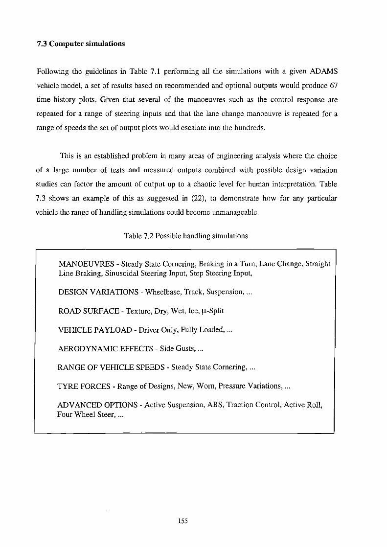
7.3 Computer simulations
Following the guidelines in Table 7.1 performing all the simulations with a given ADAMS
vehicle model, a set of results based on recommended and optional outputs would produce 67
time history plots. Given that several of the manoeuvres such as the control response are
repeated for a range of steering inputs and that the lane change manoeuvre is repeated for a
range of speeds the set of output plots would escalate into the hundreds.
This is an established problem in many areas of engineering analysis where the choice
of a large number of tests and measured outputs combined with possible design variation
studies can factor the amount of output up to a chaotic level for human interpretation. Table
7.3 shows an example of this as suggested in (22), to demonstrate how for any particular
vehicle the range of handling simulations could become unmanageable.
Table 7.2 Possible handling simulations
MANOEUVRES - Steady State Cornering, Braking in a Turn, Lane Change, Straight Line Braking, Sinusoidal Steering Input, Step Steering Input,
DESIGN VARIATIONS - Wheelbase, Track, Suspension, ...
ROAD SURFACE- Texture, Dry, Wet, Ice, ~-Split
VEHICLE PAYLOAD- Driver Only, Fully Loaded, ...
AERODYNAMIC EFFECTS -.Side Gusts, ...
RANGE OF VEHICLE SPEEDS - Steady State Cornering, ...
TYRE FORCES- Range of Designs, New, Worn, Pressure Variations, ...
ADVANCED OPTIONS - Active Suspension, ABS, Traction Control, Active Roll, Four Wheel Steer, ...
155

The simulation work described in this thesis can be summarised as:
(i) Comparing four methods of modelling the main vehicle using a linkage model, lumped mass
model, swing arm model and a roll stiffness model.
(ii) Comparing three methods of modelling the tyre using the Fiala model, the Pacejka model
and an interpolation model.
(iii) Using data for two sets of tyres, TYRE A and TYRE B
In addition to this investigations have been carried out comparing tyre models with and
without camber effects, and sensitivity studies involving variations in tyre parameters such as
cornering stiffness, radial stiffness and coefficients of friction. Sensitivity studies were also
performed varying vehicle parameters such as mass centre position, roll centre heights and the
toe in angle of the rear wheels.
In order to keep this study manageable it was clearly necessary to focus on a set of
simulations and measured outputs which could provide the most relevant information. As this
project was primarily concerned with transient lateral response and did not involve combined
slip situations resulting from simultaneous braking it was decided to use the lane change
manoeuvre at 100 kph.
For each simulation it was also decide to limit the amount of measured and plotted
output. In some cases the investigation has required additional plotted output concerning tyre
forces and geometry but in general the plotted outputs for each simulation are:
(i) Lateral acceleration
(ii) Roll angle
(iii) Yaw rate
The actual trajectory followed by the vehicle was not available from the test data
provided. This is in fact difficult to obtain using instrumentation but can be obtained quite
156

practically by laying a trail of dye on the track during the test and taking measurements before
the next run. Obtaining the trajectory of the vehicle from the ADAMS simulation is
straightforward and has been used when comparing the roll stiffness and linkage models in
association with the various tyre models.
For the lane change manoeuvre the measured steering wheel angles from the test
vehicle have been extracted and put into ADAMS as a set of XY pairs which can be
interpolated using a cubic spline fit. The time history plot for the steering inputs is shown in
Figure 7.1.
STEERING INPUT -100 KPH LANE CHANGE
120.0
80.0 o; (])
~ ~ 40.0 Cl c <(
Qj 0.0 (])
.r::. $: Cl
-40.0 c -~ (])
U5 -80.0
-120.0
5.0 0.0 2.0 4.0
Time (s)
Figure 7.1 Steering input for the lane change manoeuvre
The test procedure for the lane change manoeuvre is outlined in the international
standard (19) and is summarised in Figure 7.2. By way of example the ADAMS statements
which apply the steering motion to the steering column to body revolute joint and the spline
data are shown in Table 7 .3. The x values are points in time and the y values are the steering
inputs in degrees. Examples of the animated graphical outputs from ADAMS are given in
Figures 7.3.
157

30m t 25m t 25m t 30m t 15m
•·····r···•·········•···································-·································•····t····•··········•
A C .-CJ •.... .+................ • .... J ...•.........• •····r··•·········•
B
•···*--··•·········· A - 1.3 times vehicle width + 0.25m
B - 1.2 times vehicle width + 0.25m
C - 1.1 times vehicle width + 0.25m
Figure 7.2 ISO 3888 Lane change manoeuvre
Table 7.3 ADAMS statements for lane change steering inputs
MOTION/502,JOINT=502,ROT ,FUNC=(PI/180)*CUBSPL(TIME,0,1000)
SPLINE/1000 ,X=0,1,2,3,4,5,6,7,8,9 ,9.1,9.2,9.3,9.4,9.5,9.6,9.7 ,9 .8,9.9, 10,10.1 ,10.2,1 0.3,10.4, 1 0.5,10.6,1 0. 7,1 0.8, 10.9,11 ,11.1,11.2,11.25, 1 1.3, 11.4, 1 1.5, 11.6, 11.7' 11.8, 11.9, 12,12.1 ,12.2,12.3,12.4,12.5,12.6, 12.7' 12.8, 12.9, 13, 13.1, 13.2, 13.3 ,13.4,13.5,13.6,13.7 ,13.75, 13.8, 13.9, 14,14.1' 14.2, 14.3, 14.4, 14.5 ,14.6,14. 7' 14.8, 14.9,15 ,){=0,0,0,0,0,0,0,0,0,0 ,O,O,O,O,O,O,O ,0,0,-5,-17 ,-40,-55,-57 ,-52,-43,-30,-5, 15,35,55,72,75,70,65,45, 10 ,-10,-17,-11,-7 ,15,50,75,67 ,66,60,50,35,0,-50,-95,-110,-100,-70,-35,0 ,20,20,35,55 ,20,-6,-3,-2,-1 ,0,0,0,0,0,0
158

I front 110atyaia=L.ANE fifne::, 9.8000 Frarne::99 I
pn CICIJ QCIJ b.-- l l ........ _m;:lll_ -a
[ ~ - ........, w.JIJ I;IUI] -
~
,_ front anatysis=l.ANE Time= 9.0000 Frame=99 .. 001 analysls=LANE T me= 7 5000 Frame=76
Figure 7.3 Graphical animation of the lane change manoeuvre
159

To conclude this section of the report the full range of comparisons and simulations
which have been carried out are summarised. A study of this kind generates large amounts of
plotted outputs which have been collated in the following appendices:
(i) Appendix G - This contains results from comparisons of each of the four vehicle modelling
approaches (lumped mass, swing arm, roll stiffness and linkage models). As this phase of the
study was concerned with comparing vehicle models an interpolation tyre model was used
together with data for TYRE A which was fitted to the vehicle during the actual test. The
results are discussed in more detail in the next section where it is explained why the roll
stiffness model was selected to progress, with the linkage model, to the tyre model study
phase.
(ii) Appendix H - This contains results where the linkage model has been used with the full
range of tyre models ( Interpolation, Pacejka and Fiala) using data for each model from
TYRE A and TYRE B. The effects of omitting camber from each model are also included to
investigate the significance of the shortcoming in the Fiala model where the lateral force and
aligning moment due to camber are not computed.
(iii) Appendix I - This contains results repeating the tyre model comparisons carried out in
Appendix H but this time using the roll stiffness rather than the linkage model. The objective
of this phase of work being to ascertain whether a simple model such as the roll stiffness model
could be as sensitive as the linkage model to changes in tyre model and tyre data.
(iv) Appendix J - The plots in this appendix summarise the results from all the simulations
plotted in Appendix H and Appendix I. For both the linkage and roll stiffness models the
results obtained using the three tyre models are plotted on the same graphs to help interpret the
comparison.
(v) Appendix K - This fmal section uses the roll stiffness vehicle model and the Fiala tyre
model together with data for TYRE B. Results are provided to demonstrate how the models
could be used for vehicle and tyre parameter variation studies.
160

8.0 DISCUSSION
8.1 Introduction
The plotted outputs from the various studies undertaken here have been organised in
appendices at the rear of this report. The results in each appendix are based on separate sets of
investigations into modelling the vehicle and modelling the tyres. A fmal section investigates
the use of the Roll Stiffness model combined with the Fiala tyre model to make systematic
changes to vehicle and tyre design parameters.
The work involving the CUTyre System rig model and the three tyre modelling
approaches is discussed next. The plots obtained help to provide insights into the effectiveness
of the three modelling approaches. The plots also provide a graphical comparison of the force
and moment characteristics of TYRE A and TYRE B.
8.2 Tyre model validation
8.2.1 Tyre A
The results obtained using the CUTyre System to investigate tyre model performance using
data for TYRE A are presented in Appendix E of this report. Figures E.l to E.5 show the
results obtained using an Interpolation tyre model together with the test data provided for this
tyre. Test data was available for slip angles ranging from -9 to +9 degrees of slip angle
measured at three camber angles of -5, 0 and +5 degrees. This allowed use of the "full"
interpolation tyre subroutine. In Figure E.l the lateral force is plotted as a function of slip
angle and it is interesting to note that the lateral force curves for this tyre appear to flatten out
at high slip angles. Figure E.2 provides a zoom on the origin of the lateral force versus slip
angle graph and clearly shows the offsets due to ply steer and conicity. The variation in
cornering stiffness is also evident as is the fact that cornering stiffness is increasing with
vertical load. In Figure E.3 the aligning moment is plotted as a function of slip angle and it can
be seen that apart from a slight negative value at -9 degrees slip angle and 200 kg load the
aligning moments remain positive at high slip angles. In Figure E.5 the lateral force is plotted
161

as a function of camber angle. The curves are approximately linear and the presence of offsets
at zero camber angle is more obvious due to the lower lateral forces generated with camber
angle variation than those obtained with slip angle variation. The increase in camber stiffness
with vertical load is also evident from this plot. It should be noted that these curves have been
plotted using the zero slip angle values from slip angle variation tests at fixed camber angles of
-5, 0 and 5 degrees thus providing only three points for each curve. An alternative method of
testing, as performed with TYRE B, is to fix the slip angle at zero and vary the camber angle
over a greater range and provide more measurements to plot.
The Fiala model has been used with data derived from TYRE A using the cornering
stiffness measured at the vehicle front wheel load, rear wheel load and the average of these.
From Figure E.6 it can be seen that using the Fiala model all the curves of lateral force with
slip angle are symmetric for positive or negative values of slip. For the curves at 200 kg of
vertical load the lateral force levels out or saturates at about 3 degrees of slip angle while at the
higher loads it can be seen that the lateral force is still increasing at 10 degrees of slip angle.
The plot shown in Figure E. 7 is a zoom on the origin of the lateral force with slip angle plot
and confirms that the Fiala model ignores offsets due to conicity or ply steer and that there is
no apparent variation in cornering stiffness with load. Figure E.8 plots aligning moment as a
function of slip angle and confirms that at very high slip angles the Fiala moment does not
consider the possibility for the aligning moment to change sign and simply sets the aligning
moment to zero once the critical slip angle has been reached. For a vertical load of 200 kg this
point is reached at about 5 degrees and for 400 kg the limit is 10 degrees. For the higher loads
the limit is not reached but the aligning moment is reducing after 6 degrees.
Considering the plots obtained using the Pacejka terms for TYRE A it can be seen that
in many ways these are quite different than those for the Fiala model. In Figure E.18 it is
evident that after the peak values of lateral force are attained the curves show significant signs
of flattening out and even decrease slightly at high values of slip angle. Figure E.19 is a zoom
on the origin for this set of data and shows clearly that the Pacejka model accounts for vertical
and horizontal offsets and that the cornering stiffness is varying with the vertical loads. In this
respect the model is clearly more realistic than the Fiala model. In Figure E.20 the aligning
162

moment is plotted as a function of slip angle for the Pacejka model. It can be seen that these
curves are quite different from those obtained using the Fiala model.
Comparing the Pacejka model with the Interpolation model it can be seen from Figures
E.l and E.l8 that the Pacejka model develops lateral force more rapidly at lower slip angles.
This can be seen at 4 degrees of slip angle where for higher vertical loads the Pacejka model
clearly produces higher lateral force than the Interpolation model. It can also be seen from the
Pacejka model in Figure E.20 that the aligning moment changes sign at higher slip angles
although the Interpolation model shows in Figure E.23 that this does not actually happen with
this tyre. Close inspection also reveals that the aligning stiffness varies with vertical load and
that peak values are obtained at much lower slip angles than with the Interpolation model. The
curves also indicate that the Pacejka model is including vertical and horizontal offsets.
8.2.2 Tyrell
The results obtained using the CUTyre System to investigate tyre model performance using
data for TYRE B are presented in Appendix F of this report. Figures F.1 to F.5 show the
results obtained using an Interpolation tyre model together with the data obtained from testing
on the machine at SP Tyres UK Ltd. In Figure F.5 it can be seen that the lateral force offsets at
zero camber angle are larger than would be expected reaching 400 N for a vertical load of 800
kg. The same tyre was tested using the flat bed machine at Coventry University for which the
results are shown in Figures F.6 to F.9. The smaller machine at Coventry was limited to a
range of -6 to +6 degrees of slip or camber angle and a maximum of 600 kg of vertical load.
Using this machine much smaller offsets in lateral force were obtained at zero camber angle but
using such a large tyre on a small machine it was not possible to produce such smooth curves
as those obtained on the SP Tyres machine. In Figure F.9 the danger of using an interpolation
routine outside the range of measured data is clearly illustrated. In this case the interpolation
has been carried out up to 10 degrees using data only up to 6 degrees. Between 6 and 10
degrees the extrapolation is clearly unstable. This is an example of how useful the CUTyre
System can be in validating a tyre model before use in a vehicle handling simulation.
163

The plots obtained using the interpolation model for TYRE B have been checked
against the plots from the actual rig tests which are shown in Appendix C. Figure F.l which
shows the lateral force curves varying with slip angle provides good agreement for the Fiala
model curves which are shown in Figure F.lO. The zoom on the origin shown in Figure F.2
indicates a low cornering stiffness at 200 kg and confirms typical tyre characteristics as the
cornering stiffness becomes more constant at higher values of vertical load.
The Fiala model has been used with data from TYRE B using the cornering stiffness
measured at the vehicle front wheel load, rear wheel load and the average of these. Figure F.lO
shows the variation of lateral force with slip angle. The Fiala model seems to be particularly
suited to the characteristics of TYRE B where the lateral force continues to increase gradually
at higher loads and slip angles. Figure F.ll which shows a zoom on the origin again confirms
that the Fiala model does not vary cornering stiffness with load or consider offsets. The curves
confirm that the cornering stiffness for TYRE B is lower than that used for the model of
TYRE A. Figure F.12 shows the aligning moment curves as a function of slip angle. The
agreement with the Interpolation model is reasonable although the peak values tend to be
larger and occur at lower slip angles. It is also interesting that the aligning moment does not
appear to change sign at higher slip angles for TYRE B.
Considering the Pacejka model for TYRE B the lateral force curves shown in Figures
F.22 and F.23 show good agreement with the interpolation model. The aligning moment
curves shown in Figure F.24 do not correspond as well as the lateral force curves but appear to
be a better representation than the Fiala model in that the maximum values are about the same
as the Interpolation model but still occur at lower slip angles. It is again evident that the
Pacejka model also changes sign at higher slip angles which does not appear to happen in the
test data or with the interpolation model.
8.3 Lane change manoeuvre (Interpolation model - TYRE A)
Appendix G contains plots produced for the lane change manoeuvre. At this stage the four
vehicle models were being compared using results from the actual track test to assess the
effectiveness of the models. The Interpolation tyre model was used as this was considered to
164

be the closest to using actual measured data. This phase of the study focused therefore on
comparing the vehicle modelling without any influence from a tyre model. The data from
TYRE A, which was the tyre used during track testing, was used throughout this phase of the
investigation.
With the exception of the roll angle predicted by the Lumped Mass model, all three of
the simple models appear to perform well when compared with the test data and the Linkage
model. Of all the simple models inspection of the results indicates that the Roll Stiffness model
consistently provides good agreement. This is particularly evident when comparing the yaw
rate time history plots for both the Roll Stiffness and Linkage models shown in Figures G.ll
and 0.12.
In assessing the accuracy of the models a visual inspection of the graphs gives an initial
indication of model performance when comparing the curves from ADAMS with those from
the track test. In order to obtain some numerical measure of model accuracy the results were
compared at the point in time when the first set of peak values arise. During the simulation the
first peak values occur after 0.95 seconds. The results at this point in time were therefore
extracted in order to calculate the percentage error when comparing the simulation results with
measured test data. These results are shown in Table 8.1.
Table 8.1 Comparison of vehicle model results with track test (Interpolation model - TYRE A)
Lateral Acceleration Roll Angle Yaw Rate
(g) Error(%) (deg.) Error(%) (deg/s) Error(%)
Track Test 0.600 -- 4.50 -- 13.00 --
Lumped Mass Model 0.560 -6.7 5.49 22.0 11.92 -8.3
Swing Arm Model 0.549 -8.5 4.46 -0.9 11.92 -8.3
Roll Stiffness Model 0.568 -5.3 4.34 -3.6 12.61 -3.0
Linkage Model 0.585 -2.5 4.65 3.3 13.24 1.8
165

On the basis of this comparison the Roll Stiffness model compares very favourably with
the Linkage model for the results extracted. The Lumped Mass model appears to have a
problem in over estimation of roll angle which would also favour selecting the Roll Stiffness
model for further studies. Discussions with SP Tyres also indicated the Roll Stiffness model to
be favourable due to the capability to use laboratory test facilities to measure parameters for
this vehicle model.
8.4 Sensitivity of lane change manoeuvre to tyre data and model
The Linkage model has been used to compare the accurate modelling of a tyre using the
Pacejka approach with the more simple formulation of the Fiala model and the benchmark
Interpolation model. The results of this investigation are presented in Appendix H. All three
tyre modelling methods have been used with data for TYRE A and TYRE B. As usual the
ADAMS results are plotted with the track test results for comparison. It should be noted that
with TYRE B this is not a true comparison as this was not the tyre fitted during the test but the
plots are useful in any case when comparing the different tyre models used with TYRE B. The
track test results are plotted with TYRE B to provide a measure for comparing TYRE A and
TYRE B and the different tyre models, rather than to correlate TYRE B results with track test
results.
The Fiala model does not consider camber angle and the Pacejka parameters provided
for TYRE B also did not account for camber. To aid the comparison and judge the influence of
camber the interpolation tyre models were run with and without camber. The Pacejka model
for TYRE A was also run with and without camber. The effect of omitting camber angle from
the model can be discerned by close inspection of the curves but does not appear to be a
significant factor in obtaining correlation. Clearly the camber effects are dominated by the
forces and moments produced by slip angle when performing this type of manoeuvre and to a
certain extent this justifies the use of the simple Fiala model which ignores camber angle.
An important consideration of this study was to establish whether the Roll Stiffness
model would provide similar sensitivity to changes in tyre model and tyre data as the Linkage
model. Appendix I therefore contains, for the Roll Stiffness model, a repeat of the plots
166

provided in Appendix H for the Linkage model. To assist with this comparison the results are
summarised in Appendix J where results for all three tyre models are plotted on the same
graphs. On each page the results for the Linkage model are followed immediately by the results
for the Roll Stiffness model to aid the comparison. The results shown in Appendix J indicate
that the Roll Stiffness model despite a lack of sophistication performs surprisingly well when
compared with the detailed Linkage model. The results in Appendix J again indicate that the
effects of including camber thrust in the tyre model appear to be marginal.
In order to assist the various comparisons the results corresponding to the first set of
peak values occurring after 0.95 seconds of simulation time have been extracted. Using the
results for TYRE A the track test results have again been used as a measure for comparison.
With TYRE B the Interpolation tyre model results are used as the benchmark. The results are
tabulated in Tables 8.2 to 8.5.
Table 8.2 Comparison of tyre model results with track test (Linkage model- TYRE A)
Lateral Acceleration Roll Angle Yaw Rate
(g) Error(%) (deg.) Error(%) (deg/s) Error(%)
Track Test 0.600 -- 4.50 -- 13.00 --
Interpolation Model 0.585 -2.5 4.65 3.3 13.24 1.8
Interpolation Model 0.597 -0.5 4.84 7.6 12.89 -0.9
(No Camber)
Fiala Model 0.611 1.8 4.77 6.0 15.13 16.4
Pacejka Model 0.660 10.0 5.48 21.8 14.21 9.3
Pacejka Model 0.663 10.5 5.53 22.9 14.04 8.0
(No Camber)
167

Table 8.3 Comparison of tyre models results with track test (Roll Stiffness model - TYRE A)
Lateral Acceleration Roll Angle Yaw Rate
(g) Error(%) (deg.) Error(%) (deg/s) Error(%)
Track Test 0.600 -- 4.50 -- 13.00 --
Interpolation Model 0.568 -5.3 4.34 -3.6 12.61 -3.0
Interpolation Model 0.577 -3.8 4.42 -1.8 12.72 -2.2
(No Camber)
Fiala Model 0.591 -1.5 4.46 -0.89 14.73 12.4
Pacejka Model 0.643 7.2 4.84 7.6 13.52 4.0
Pacejka Model 0.642 7.0 4.87 8.2 13.58 4.5
(No Camber)
Table 8.4 Comparison of tyre models results (Linkage model- TYRE B)
Lateral Acceleration Roll Angle Yaw Rate
(g) Error(%) (deg.) Error(%) (deg/s) Error(%)
Interpolation --Model 0.554 4.41 -- 14.84 --
Interpolation Model 0.567 2.3 4.55 3.2 14.67 -1.1
(No Camber)
Fiala Model 0.566 2.2 4.40 -0.2 15.47 4.2
Pacejka Model 0.581 4.9 4.68 6.1 15.64 5.4
(No Camber)
168

Table 8.5 Comparison of tyre models results (Roll Stiffness model- TYRE B)
Lateral Acceleration Roll Angle Yaw Rate
(g) Error(%) (deg.) Error(%) (deg/s) Error(%)
Interpolation Model 0.543 -- 4.14 -- 14.15 --
Interpolation Model 0.549 1.1 4.20 1.5 14.27 0.8
(No Camber)
Fiala Model 0.551 1.5 4.17 0.7 15.07 7.2
Pacejka Model 0.561 3.3 4.27 3.1 15.07 7.2
(No Camber)
The numerical comparisons presented when studied in conjunction with the time history
plots provided in the Appendices lead to the following:
The Roll Stiffness model is a good model given the level of simplicity when compared
with the Linkage model. The Roll Stiffness model is based on 12 rigid body degrees of
freedom whereas the Linkage model for this vehicle requires 78. Given also the great reduction
in data and modelling effort the Roll Stiffness model appears to be very good value.
When comparing tyre models it is clear that the results for TYRE B show better
agreement than those for TYRE A. This is not so much a function of the tyre models but more
the tyre characteristics and model parameters. The model based on Pacejka parameters for
TYRE A appears to overestimate peak values. This is not due to a flaw in the Pacejka model
but rather the lack of accuracy in this set of parameters in fitting the model. Some
understanding of this can be obtained by referring again to the tyre curves for this data
produced by the CUTyre System and shown in Figure E.18. At higher loads the lateral force
reaches a peak value and saturates at lower slip angles, than is evident with the Interpolation
169

model curves shown in Figure E.l. In order to improve the agreement it would be necessary to
iterate on the derivation of the Pacejka coefficients until a more realistic set were obtained for
TYRE A and then repeat the simulations.
The Interpolation tyre models used here have as expected given good results. Although
these models are no longer fashionable and have little use in design studies they have proven
useful for benchmark comparisons and validations of other tyre models. As such they are a
useful component within the CUTyre System.
The Interpolation models have also proven useful in determining the influence of
omitting camber angle effects from a tyre model. On the evidence of this study the effect seems
small and certainly appears to be dominated by the quality of the model and parameters used to
fit the tyre lateral force characteristics as a function of slip angle.
The results for TYRE B provide very good agreement due to the following. The
Pacejka coefficients provided give a much better fit for this model than those given for TYRE
A. This can be seen by comparing the plots produced by the CUTyre System in Appendix F. In
this case the Pacejka model curves for lateral force shown in Figure F.22 show good
agreement with the Interpolation model shown in Figure F.l. Corresponding with this the
results for the lane change also show good agreement despite the fact that camber is again not
represented in this tyre model.
The characteristics of TYRE B also seem to suit the simple Fiala tyre model as can be
seen by the good agreement shown in Figure F.l 0. This tyre has the characteristic that the
lateral force curves do not flatten out at higher loads which appears to assist when getting a
good fit with the Fiala model. For this sort of tyre and others with similar characteristics
produced by SPTYRES UK the implication at this stage would appear to be that the Roll
Stiffness model and the Fiala tyre model would provide, in association with the CUTyre
System, a useful set of tools to investigate the influence of tyre design changes on handling
simulation outputs.
170

As a final step at this stage of the investigation it was decided to examine results for the
tyres and to compare the Roll Stiffness model and the Linkage model. An important aspect of
using a simplified vehicle model such as the Roll Stiffness model is the accuracy obtained in the
prediction of the vertical load, slip angle and camber angle for each road wheel. These outputs
from the vehicle model become inputs to whatever tyre model is chosen and are hence highly
significant in terms of the overall simulation model. Using results obtained with an
Interpolation model of TYRE B a direct comparison of the Linkage and Roll Stiffness models
can now be made. In Figure 8.1 it can be seen that the Roll Stiffness model with a maximum
value of about 1.5 degrees underestimates the amount of camber angle produced during the
simulation when compared with the Linkage model where the camber angle approaches 5
degrees. Clearly the Roll Stiffness model does not have a camber degree of freedom relative to
the rigid axle parts and the camber angle produced here is purely due to tyre deflection.
More importantly though the slip angle comparison shown in Figure 8.2 shows good
agreement. It is worth remembering that the slip angle at the front wheels is determined by the
transfer of the steering inputs through the suspension to the road wheel. The Linkage model
accounts for changes in steering ratio as the vehicle rolls whereas the Roll Stiffness model
assumes a constant ratio. Future studies may require more detailed investigations in this area as
an accurate prediction of slip angle is clearly a critical factor in the model. The inaccuracy in
the Roll Stiffness model with regard to camber angle will have no effect here with the Fiala
model as the current formulations here ignore the influence of camber angle. Future studies
may however focus on extending the Roll Stiffness model to refine this area of prediction.
The comparison of tyre load for all four tyres shown in Figures 8.3 to 8.6 also show
good agreement. This shows that the weight transfer in the Roll Stiffness model agrees well
with the Linkage model. A consideration which could be noted at this stage is that the Roll
Stiffness model does not include the pitch of the body relative to the wheels as would be
present in the Linkage model. For this simulation involving pure lateral slip that modelling
decision appears to be justified. An extension of this work to braking or combined slip
situations would need to investigate if this was still justified. Figures 8.3 to 8.6 also confirm
that there is at no time any loss in tyre contact at any wheel during this aggressive manoeuvre.
171

c:; <Il :3. <Il Cl c < Qj
..0 E ell 0
c:; <Il :3. <Il Ol c < .Q. en
FRONT RIGHT TYRE- 100 KPH LANE CHANGE
6.0
5.0 Roll Stiffness Model -------4.0 Linkage Model
3.0
2.0
1.0
0.0
-1.0
-2.0
-3.0
-4.0
-5.0
-6.0 1.0 3.0 5.0
0.0 2.0 4.0
Time (s)
Figure 8.1 Camber angle comparison - linkage and roll stiffness models
6.0
5.0
4.0
3.0
2.0
1.0
0.0
-1.0
-2.0
-3.0
-4.0
-5.0
-6.0
0.0
FRONT RIGHT TYRE- 100 KPH LANE CHANGE
Roll Stiffness Model Linkage Model
1.0 2.0
3.0 4.0
Time (s)
5.0
Figure 8.2 Slip angle comparison - linkage and roll stiffness models
172

FRONT RIGHT TYRE- 100 KPH LANE CHANGE
10000.0
9000.0 Roll Stiffness Model -------8000.0 Linkage Model
~ 7000.0
Q) 6000.0 (.)
0 5000.0 LL
(ij (.)
4000.0 'E Q)
> 3000.0 ~ .../,
2000.0
1000.0
0.0 1.0 3.0 5.0
0.0 2.0 4.0
Time (s)
Figure 8.3 Vertical tyre force comparison -linkage and roll stiffness models
FRONT LEFT TYRE - 100 KPH LANE CHANGE
10000.0
9000.0 Roll Stiffness Model -------8000.0 Linkage Model
~ 7000.0
Q) 6000.0 (.)
0 5000.0 LL
(ij (.) 4000.0 'E Q)
> 3000.0 h
2000.0
1000.0
0.0
1.0 3.0 5.0 0.0 2.0 4.0
Time (s)
Figure 8.4 Vertical tyre force comparison -linkage and roll stiffness models
173

~ ()) (.)
0 LL (ij (.)
t ())
>
-~ ()) (.)
0 LL (ij (.)
t ())
>
REAR RIGHT TYRE - 100 KPH LANE CHANGE
10000.0
9000.0 Roll Stiffness Model -------
8000.0 Linkage Model
7000.0
6000.0 " 5000.0
4000.0 -.;::;:
3000.0 ~
2000.0
1000.0
0.0
1.0 3.0 5.0 0.0 2.0 4.0
Time (s)
Figure 8.5 Vertical tyre force comparison -linkage and roll stiffness models
10000.0
9000.0
8000.0
7000.0
6000.0
5000.0
4000.0
3000.0
2000.0
1000.0
0.0
0.0
REAR LEFT TYRE -100 KPH LANE CHANGE
Roll Stiffness Model Linkage Model
1.0 2.0
3.0
Time (s)
5.0 4.0
Figure 8.6 Vertical tyre force comparison -linkage and roll stiffness models
174

A general observation from the study was that the comparison of vehicle and tyre
models was less accurate towards the end of the manoeuvre. In the simulation, this period is
between 4 and 5 seconds as the vehicle pulls out of the last turn having reached a lateral
acceleration of about 0.8g. This is particularly noticeable when comparing the results provided
in Appendix J where different tyre models have been used with data for TYRE B. A further
examination of the steering inputs measured during the track test and used as inputs to the
sunulation models shows that these are quite extreme in order to control the vehicle as it
approaches the limit of stability. The severity of these steering inputs can be seen by comparing
the steering inputs measured for the same lane change manoeuvre but at a reduced speed. This
is illustrated in Figure 8.7 where the steering inputs at 70 kph are compared with those used in
this study at 100 kph.
o; (])
~ ..Q2 Cl c <(
Q5 (]) .c 5: Cl c -~ (])
U5
STEERING INPUT- LANE CHANGE MANOEUVRE
120.0-r-------------------------,
70 kph - - - - - - -
80.0 100 kph
40.0
0.0
-40.0
-80.0
1.0 5.0 0.0 2.0 4.0
Time (s)
Figure 8.7 Comparison of steering inputs at different speeds
As can be seen the steering inputs at the reduced speed are much smoother. It can also
be seen that in order to control the vehicle at 100 kph there is an additional "overshoot" in the
steering input after 4 seconds. Future studies could extend the investigation in two ways. The
first of these would investigate the accuracy of the models using less extreme manoeuvres such
175

as the 70 kph lane change shown here. The second extension of the work could move in the
other direction comparing models for manoeuvres approaching the limit of stability and
possibly involving the spin out or roll over of vehicles.
8.5 Final sensitivity studies
The fmal set of studies carried out in this project involved demonstrating how the combination
of the simple roll stiffness vehicle model and the simple Fiala tyre model could be used to carry
out handling sensitivity studies at potentially very early stages in the design of the tyre and the
vehicle. The results of this investigation are included in Appendix K and involve parametric
design variations to both vehicle data parameters and tyre data parameters. All the
comparisons have been carried out using the SP Tyres data for TYRE B.
The first set of variations concentrate on looking at a range of values for individual
parameters in the Fiala data file. In Figure K.l the yaw rate has been plotted to indicate the
change in vehicle response for systematic changes in cornering stiffness. The plots indicate that
going from low to high cornering stiffness leads to increased rates of change in yaw rate and
could indicate the sort of design variations investigated in establishing how responsive a
vehicle is.
In Figure K.2 the yaw rate has again been plotted where in this case the coefficient of
tyre to road surface friction has been varied. The plots indicate that at lower coefficients of
friction which could be those associated with water or ice contamination of road surfaces there
is a loss of stability which will lead to the vehicle "spinning out" at very low values.
In Figure K.3 the roll angle has been plotted to show the effects of reducing the radial
stiffness of the tyres. This could perhaps be considered also as investigating a reduction in tyre
pressures. The resulting increase in roll angle can be seen when the radial stiffness is reduced
from the standard value to one which is one half of that.
In Figure K.4 the first in the series of vehicle parameter changes is demonstrated where
the effects on the roll angle have been established for the situation where the mass centre of the
176

vehicle is raised by 100 mm. This sort of situation could be considered to represent a case for a
particular vehicle where loads are carried by a roof rack altering the mass centre position.
In Figure K.5 the effects of moving the roll axis of the vehicle have been demonstrated.
The roll angle is plotted for the roll axis in the original position and then in a situation where
the roll axis is at ground level. This is a situation which theoretically corresponds to a parallel
link suspension. It should be noted that this change in model parameter was easy with the Roll
Stiffness model but would require quite a bit of effort to modify the ADAMS data set for a
Linkage model which includes all the suspension geometry.
The fmal demonstration of a vehicle design parameter change was influenced by
another current research programme within the School of Engineering at Coventry University
and involves track testing with a Rover vehicle (90). Early indications from that programme of
work and based on subjective assessments are that a small amount of toe in at the rear wheels
can lead to an improved handling feel or response of the vehicle. By way of example this has
also been considered in Figure K.6 where the effects of one degree of toe in or toe out are
compared with the zero toe angle case. The plot indicates that with one degree of toe in the
vehicle develops yaw rate more rapidly which may be indicative of a more responsive vehicle.
8.6 The effect of model size on computer simulation time
This final section has been instigated by consistent reference in many publications to the effects
of inefficient modelling practices on computer simulation time. The information summarised in
Table 8.6 was presented in (91). These times are based on some initial work during this study
where a control response manoeuvre was simulated at 60 kph. The times are for simulations
running on a Viglen 4DX266 personal computer. The Fiala tyre model was used with data for
TYREA.
177

Table 8.6 Computer simulation times for a 60 kph control response manoeuvre
Model Degrees of freedom
Linkage
Lumped Mass
Swing Arm
Roll Stiffness
78
14
14
12
Number of Equations
961
429
429
265
CPU Time (s)
146.0
108.0
93.0
68.0
The comparison shown in Table 8.7 is for the lane change carried out in this study.
These times are based on the simulations presented in Appendix G where the four vehicle
models have been run with an Interpolation model of TYRE A.
Table 8.7 Computer simulation times for a 100 kph lane change manoeuvre
Model Degrees of freedom
Linkage
Lumped Mass
Swing Arm
Roll Stiffness
78
14
14
12
Number of Equations
961
429
429
265
CPU Time (s)
301.0
160.0
188.0
90.0
As can be seen from these comparisons the computer simulation time can not be scaled
directly from the model size and does not scale directly from one sort of simulation to another.
It is encouraging to note however, that the best performance is by the Roll Stiffness model
which for the lane change runs more than three times faster than the Linkage model. This is
clearly beneficial where a model is to be used in design studies involving parametric variations
and repeated simulation runs.
178

Another comparison made in Table 8.8 shows the effect of the chosen tyre model when
running this lane change simulation with both the Linkage and Roll Stiffness models. The data
is again based on the study involving TYRE A.
Table 8.8 Computer simulation times for varying tyre models- 100 kph lane change
TyreModel
Fiala
Pacejka
Interpolation
Linkage model
255.0 s
270.0 s
301.0 s
Roll Stiffness model
88.0 s
9l.Os
90.0 s
It is again interesting to note that the times for the different tyre models do not scale
directly between the two vehicle models. The times for the Linkage model are as expected with
the simple Fiala model running fastest and the Interpolation model taking the longest time. For
the Roll Stiffness model the effect of changing tyre model appear to have negligible effect. A
possible explanation for this is that the efficiency of the Roll Stiffness model means that
simulation times are dominated by overheads, such as file handling or calling the tyre model
subroutine, which are less significant for longer runs with more complex models.
179

9.0 CONCLUSIONS AND RECOMMENDATIONS
9.1 Conclusions
Based on the investigations and studies which have been carried out and are described in this
thesis the following conclusions are offered:
(i) From the literature review it is apparent that the use of relatively new computer based
methods such as multibody systems analysis is still evolving as a working tool in the solution of
problems in vehicle dynamics. Experiences in industry, and the literature reviewed indicate that
the practice of modelling suspensions in very fine detail has often been followed when a
simpler and more efficient modelling strategy may have been possible. It is likely that the issue
of accurate vehicle modelling will be debated for some time with two possible streams of
thought.
(a) The first of these will be that any model should be the most efficient for any given
type of simulation and therefore likely to be the most useful for making rapid design
decisions.
(b) The second approach is that a single detailed model could act as a database and be
used for the full range of simulations needed to support vehicle design, but will be
inefficient and less likely to assist with positive design decisions in any one application.
Vehicle engineers who use sophisticated analysis tools such as ADAMS will be
encouraged by the capability of these programs to build complicated models. The main thrust
of this thesis has been to follow the first approach and demonstrate the use of models which
are as simple and efficient as possible in order to achieve the desired accuracy for the
simulation under consideration.
180

(ii) On the issue of model simplification for vehicle handling, the focus from the literature
appears to be on the actual vehicle and mainly the suspension systems. The effects of model
simplification in the tyre does not seem to have received the same level of discussion. In
addition to this, research in the field of tyre modelling has led to the development of complex
and accurate tyre models which are widely accepted. The publications associated with this type
of work appear in the main to concentrate on comparing the fit of tyre model data with tyre
test data rather than demonstrating the accuracy of the tyre model when used for a given
vehicle handling simulation. This has been one of the main areas this thesis has attempted to
address.
(iii) An initial investigation of suspension modelling procedures has been carried out here
with the particular emphasis on the influence of modelling the compliance in the bushes and the
effect on suspension kinematics during movement between bump and rebound positions. It has
been noted that for a full vehicle model based on linkages, the kinematic method of modelling
suspensions is not always possible and that has proven to be the case here with the rear
suspension on this vehicle. The modelling of suspensions using a rigid joint representation may
became more difficult as modem multi-link suspensions gain popularity. The development of
suspensions such as these has lead to the situation that they depend on the compliance in the
bushes to control the way they move and will therefore create a greater need to obtain detailed
bush information to support computer simulations.
(iv) It has been shown here that there is a large increase in modelling effort and also a
greatly increased chance of modelling or data errors when moving from a simple rigid joint
representation through to models using linear and non-linear bushes. For the Linkage model
considered here a rigid joint representation would not work due to the geometry steer
characteristics of the rear suspension.
181

(v) It has been shown here that the modelling of the steering system needs careful
consideration if the suspension linkages are not modelled. Attaching the rack to a simplified
suspension model via a tie rod is not effective due to the introduction of steer changes during
the initial static equilibrium analysis. It has been shown that it is necessary to use a
mathematical coupling ratio in the steering model to overcome this. This method does not
account for geometry steer and will require further study with other vehicle models.
(vi) A method to obtain both the front and rear roll stiffness from a detailed ADAMS model
has been demonstrated. In practice vehicle engineers should be able to make an estimate of the
roll stiffness during initial design studies or take measurements off an actual vehicle at a later
stage. The method used here will hold good however, should a detailed ADAMS model be
available during the vehicle design process.
(vii) For vehicle handling simulations it has been shown here that simple models such as the
Roll Stiffness model can provide good levels of accuracy. It is known however, that roll
centres will "migrate" as the vehicle rolls, particularly as the vehicle approaches limit
conditions. The plots in Appendix B show the vertical movement of the roll centre along the
centre line of the vehicle as the suspension moves between bump and rebound. On the
complete vehicle the roll centre will also move laterally off the centre line as the vehicle rolls.
For the simulations carried out here the fixed roll centre model appears to have worked well
despite approaching the lateral accelerations of O.Sg and roll angles of 6 degrees or more.
(viii) A new computer system has ·been developed as part of this project to handle tyre
models and is referred to as the CUTyre System. The system includes a range of FORTRAN
subroutines which can be used to model tyre characteristics and then interface with the main
ADAMS program. The CUTyre rig model has been developed and has proven to be useful
during this study by providing a graphical check on tyre models and tyre data before
integrating these into a full vehicle handling simulation.
182

(ix) The Interpolation models generated here were used to show that ignoring camber does
not appear to have a significant effect on the accuracy of the simulation. This was a useful
discovery since the Fiala model does not include camber effects and it has also been shown
here that the Roll Stiffness model does not give a good prediction of road wheel camber
compared with the Linkage model. The results for TYRE B give a good correlation between
all three models and would indicate that for this sort of simulation the Fiala model is highly
suitable in terms of accuracy and the limited number of parameters required. One of the main
outcomes of this project has been to show that the Roll Stiffness model combined with the
Fiala tyre model compares well with the Linkage model combined with the Pacejka tyre model,
although caution should be exercised as further investigation is needed before assuming these
modelling strategies can be used with other vehicles and manoeuvres.
(x) An interesting discovery during this study has been the effect of the modelling approach
on computer simulation times. Criticisms in the literature surveyed, of complicated models
running in programs such as ADAMS consistently identify excessive computation time as one
of the drawbacks. From this study the computer times on a personal computer do not appear
excessive given the complexity of the problem being solved. The Roll Stiffness model produces
the lowest times which should prove useful for design applications.
(xi) In summary this study has attempted to make an original contribution in the field of
vehicle dynamics by:
(a) Comparing suspension models for a full vehicle handling simulation and establishing
using ADAMS t11e influence of model simplifications on predicted outputs.
(b) Developing the CUTyre System to provide institutions and companies such as SP
Tyres UK with tools which will validate tyre models and model parameters and interface
these with an ADAMS full vehicle model.
(c) Comparing Interpolation tyre models, the Pacejka model and the Fiala nwdcl and
establishing using ADAMS the influence of tyre model selection on the results of a
handling simulation.
183

9.2 Recommendations
Following on from the work described in this thesis there are a number of avenues of further
research and development which could be followed:
(i) For the simulations carried out here the fixed roll centre model appears to have worked
well despite approaching lateral accelerations of 0.8g and roll angles of 6 degrees or more.
Future studies could investigate how well this modelling approach transfers to other designs of
vehicle and also to consider the modelling issues involved with considering a moving roll
centre during a simulation. An extension of the model to include camber change of the road
wheel could also be considered with a view to more detailed study of the influence of camber
angle for different vehicles and manoeuvres.
(ii) For handling simulations a suspensiOn modelling approach which has not been
considered here but may form the basis of future studies is a method sometimes referred to as
using suspension derivatives. This approach is conceptually more accurate than the three
simple modelling approaches used here and involves modelling the road wheel and suspension
as a single rigid body. The movement and change in orientation of this body relative to the
vehicle body is controlled in the same way as it would be if the full suspension linkages were
modelled. From an individual quarter suspension model it is possible to establish the path in
space that the wheel centre follows and also to establish the change in angles such as camber
and steer as the wheel moves along this path. These measurements could also be obtained by
laboratory testing. The rates at which these angles change with vertical movement can be
thought of as the suspension derivatives. The derivatives could be obtained for example, by
considering the gradients at the origin of plots from individual suspension studies such as those
shown in Appendix B. The advantage of a modelling approach such as this is that as with the
roll stiffness model it involves parameters that vehicle engineers could estimate early in a
design before the detailed suspension geometry is established, or otherwise could be measured
in the laboratory at a later stage when the vehicle exists. Future studies could focus on
investigating the derivation of these models and establishing for what sort of manoeuvres there
could be an advantage over the roll stiffness model used here.
184

(iii) It has been shown in this project that detailed modelling of suspension linkages and
bushes can be avoided by using a simplified model for the lane change simulation. Future
studies can extend this to consider if the assumptions are valid for simulations including
features such as ABS with braking and cornering on uneven ground. If other simulations do
prove to have dependence on the properties of bushes to produce accurate outputs this raises
some questions which could be the subject of future studies such as:
(a) It may be necessary to establish for extreme variations between hot and cold
temperature, the effects on the characteristics of a bush, and the subsequent vehicle
performance.
(b) During the life of a vehicle bushes will be subject to ageing and general wear which
will alter their properties. Future maintenance may also involve using non original
replacement bushes. Investigations could be carried out in order to establish whether this
would have an effect on suspension and vehicle performance.
(iv) It should also be noted that the work carried out here is for quite extreme manoeuvres
which could be said to be more associated with handling stability rather than handling "feel".
Future work needs to consider manoeuvres where the perturbations to vehicle motion may
only be slight, and establish the level of modelling complexity required to obtain useful
feedback. It is likely that this would involve some monitoring of steering reaction torques
together with vehicle responses such as yaw rate. The challenge with these sort of studies will
be to correlate the objective outputs from a computer simulation with the subjective
assessments of good vehicle handling feel.
185

(v) The CUTyre System could be developed further and enhanced so as to provide a tool
for engineers at companies such as Rover Group and SP Tyres UK Ltd. Some of the
developments which could be considered are:
(a) The set of subroutines could be combined into one CUTyre subroutine which holds
all the tyre models. The appropriate model could be selected based on a parameter inside
the ADAMS data set that identifies which tyre model the subroutine should use.
(b) A FORTRAN program could be developed which can read the tyre test data files
produced by SP Tyres UK Ltd. The program could automatically derive the Fiala model
terms and generate a Fiala tyre property file. In a similar manner the program could be
used to generate the ADAMS spline data which is needed for an interpolation model.
Developments such as this could augment the existing routines at SP Tyres UK Ltd.
which can generate the terms for Version 3 of the Pacejka tyre model.
(c) This project has demonstrated how tyre design parameters could be varied in order to
investigate the influence of tyre design changes on vehicle performance. A potential
extension of this capability could be developed around the current CUTyre System. At
the moment it is possible to develop a set of tyre plots from a starting point of all three
models discussed here, where the interpolation model can be considered to represent the
raw test data. An advanced development of this would allow the tyre designer to distort
the shape of the curves on the computer screen using point, click and drag type mouse
operations. The plotting program developed could also provide numerical updates on the
screen of how curve distortions change relevant tyre design parameters such as
cornering stiffness in the Fiala model data. This would allow an experienced tyre
designer to modify the curves until the desired appearance was obtained and then submit
the tyre model and automatically perform the vehicle simulation. Given the rapid
increases in computer hardware the turn around time for such interactive procedures is
constantly reducing making the proposed system a feasible extension of the work
described here.
186

(vi) From the work carried out here it can be seen that the Fiala model does not consider
the change in sign of aligning moment at high slip angles. For any future work where advanced
simulations attempt to assess the 'feel' of a vehicle this may be important. The transition in
aligning moment may produce a steering feeling which appears to lose stiffness or is suddenly
'free'. More work is needed in this difficult area and the Pacejka model would have an
advantage here. Additional studies could also consider modifying the Fiala subroutine provided
in Appendix D to improve the aligning moment formulation.
(vii) As this work has been restricted to pure slip conditions a natural extension would
appear to be the case of combined slip during simultaneous cornering and braking. Although
the Pacejka model can deal with this the Fiala model can not. Future work could focus on
identifying the most efficient combination of vehicle and tyre model for this situation and could
possibly even involve enhancing the Fiala model to cater for this.
(viii) There is substantially more data associated with the Linkage model than with the Roll
Stiffness model. Future work could focus on even further simplification using a parameter
based Roll Stiffness model which requires the very minimum of input information such as track
and wheelbase to generate the model.
(ix) It has been demonstrated that using the simple combination of the Roll Stiffness model
and the Fiala tyre model design sensitivity studies can be carried out. Of particular interest may
be the study carried out where the rear toe in angle of the wheels was varied. As mentioned in
Section 8 this study was prompted by a parallel research project (90) within the School of
Engineering at Coventry University. This project involves track testing with a Rover vehicle
and making subjective assessments and objective measurements of as to how changes such as
the toe in angle effect handling quality. Future work could include using the Roll Stiffness
model and the Fiala tyre model to represent this vehicle, and to recreate the track manoeuvres
in ADAMS. Using manoeuvres such as the lane change described here it should be possible to
compare ADAMS outputs such as yaw rate or yaw acceleration with measured data and the
subjective test assessments.
187

REFERENCES
1. Ryan, R. ADAMS - Multibody Systems Analysis Software. Multibody Systems
Handbook/W. Schielen (Editor), Springer-Verlag, Berlin, 1990.
2. Gillespie, T. D. Fundamentals of Vehicle Dynamics. SAE Publications, Society of
Automotive Engineers, 400 Commonwealth Drive, Warrendale, PA 15096, USA.
3. Orlandea, N. and Chase, M. Simulation of a Vehicle Suspension with the ADAMS
computer program. SAE paper 770053, Society of Automotive Engineers, 400 Commonwealth
Drive, Warrendale, PA 15096, USA, 1977.
4. Rai, N.S. and Soloman, A.R. Computer simulation of suspension abuse tests using
ADAMS. SAE paper 820079, Society of Automotive Engineers, 400 Commonwealth Drive,
Warrendale, PA 15096, USA, 1982.
5. Blundell M.V. Full vehicle modelling and simulation using the ADAMS software system.
!MechE Paper C427!16/170, Autotech '91, Birmingham, November 1991.
6. Antoun, R. J., Hackert, P. B., O'Leary, M.C., Sitchen, A. Vehicle dynamic handling
computer simulation - Model development, correlation, and application using ADAMS. SAE
paper 860574, Society of Automotive Engineers, 400 Commonwealth Drive, Warrendale,
PA 15096, USA, 1986.
7. Sharp, R.S. Computer codes for road vehicle dynamic models. !MechE Paper 427116/064,
Autotech '91, Birmingham, November 1991.
8. Bakker E., Nyborg L. & Pacejka, H.B. Tyre modelling for use in vehicle dynamics
studies, SAE paper 870421, Society of Automotive Engineers, 400 Commonwealth Drive,
Warrendale, PA 15096, USA, 1986.
188

9. Bakker E., Pacejka H.B. & Linder L. A new tyre model with application in vehicle
dynamics studies, SAE paper 800087, 4th Auto Technologies Conference, Monte Carlo, 1989.
10. Pacejka H.B. & Bakker E. The magic formula tyre model, Tyre models for vehicle
dynamic analysis: Proc. 1st international colloquium on tyre models for vehicle dynamic
analysis, ed. H. B. Pacejka, Swets & Zeitlinger, Lisse, 1993, pp. 1-18.
11. Fiala, E. Seitenkrafte am rollenden Luftreifen, VD!-Zeitschrift 96, 973, 1954.
12. Mechanical Dynamics Inc. ADAMSffire (6.1) User's Manual, Mechanical Dynamics
Inc., 2301 Commonwealth Blvd., Ann Arbor, Michigan, USA, October 1992.
13. Crolla, D.A. Vehicle dynamics - theory into practice, Automobile Division Chairman's
Address, !MechE, 1995.
14. Segel, L. Theoretical prediction and experimental substantiation of the response of the
automobile to steering control, Proc. of Automobile Division, !MechE, 1956-57, pp31 0-330.
15. Segel, L. An overview of developments in road vehicle dynamics: past, present and future,
Proc. !MechE Conference on "Vehicle Ride and Handling", London, 1993, pp 1-12.
16. British Standards Institution, BS AU 189: Steady state cornering behaviour for road
vehicles, British Standards Institution, 2 Park Street, London, W1A 2BS.
17. British Standards Institution, BS AU 205: Effect of braking on steady state cornering
behaviour of road vehicles, British Standards Institution, 2 Park Street, London, W1A 2BS.
18. British Standards Institution, BS AU 230: Methods of test for lateral transient response
behaviour of passenger cars, British Standards Institution, 2 Park Street, London, W1A 2BS.
189

19. International Organization for Standardization, Road vehicles - Test procedure for a
severe lane-change manoeuvre, ISO/TR 3888 - 1975 (E), International Organization for
Standardization, 1975.
20. Rover Group. Internal Rover Report No: MBK 90488, Rover Handling Tests
Supplementary Data, 23 April1990.
21. Schielen, W. (Editor) Multibody Systems Handbook. Springer-Verlag, Berlin, 1990.
22. Blundell M. V., Phillips B.D.A. and Mackie A. The role of multibody systems analysis in
vehicle design. Journal of Engineering Design, Vol. 7, No.4, pp. 377-396, December 1996.
23. Hogg S.S., Dickison J.G., Maddison S.J., Yardley A.J. Design and prediction of vehicle
handling and stability, !MechE paper C389/122, FISITA92, 1992.
24. Pilling, M. Tyres from the car's point of view, Institute of Materials, Wolverhampton, February 1995.
25. Crolla D.A., Horton, D.N.L., Brooks, P.C., Firth, G.R., Shuttleworth, D.W., Yip,
C.N. A systematic approach to vehicle design using VDAS (Vehicle Dynamics Analysis
Software), SAE paper 940230, Society of Automotive Engineers, 400 Commonwealth Drive,
Warrendale, PA 15096, USA.
26. Sayers, M.W. Automated formulation of efficient vehicle simulation codes by symbolic
computation (AUTOSIM), Proceedings 11th /A VSD Symposium of Vehicles on Roads and
Tracks, Kingston, Ontario, Swets and Zeitlinger, Lisse, 1990.
27. Wittenburg, J. and Wolz, U. MESA VERDE: a symbolic program for non-linear
articulated rigid body dynamics. Proceedings of Tenth ASME Design Engineering Division
Conference on Mechanical vibration and noise, Cincinnati, 1985 (ASME).
28. Austin, A. and Hollars, M.G. Concurrent design and analysis of mechanisms. Kinematics
and Dynamics of Multi-body Systems Seminar (S057), I.Mech.E., November 1992.
190

29. Crolla, D.A., Horton, D. & Firth, G. Applications of multibody systems software to
vehicle dynamics problems, Kinematics and Dynamics of Multi-body Systems Seminar (S057),
J.Mech.E., 1992.
30. Costa, A.N. Application of multibody systems techniques to vehicle modelling.
Colloquium Model Building Aids for Dynamic Simulation, lEE Digest No. 1991/196, 1991.
31. Holt, M.J. and Cornish, R.H. Simulation tools for vehicle handling dynamics, Kinematics
and Dynamics of Multi-body Systems Seminar (S057), I.Mech.E., November 1992.
32. Holt, M.J. Simulation tools for vehicle handling dynamics, Multi-body System dynamics
Codes for Vehicle Dynamics Applications Seminar (S275), I.Mech.E., 1994.
33. Cherry, A. Vehicle Modelling for Automotive control studies using SD/FAST, ACSL and
MATLAB, Multi-body System Dynamics Codes for Vehicle Dynamics Applications Seminar
(S275), I.Mech.E., 1994.
34. Kortum, W., Sharp, R.S. & de Pater, A.D. Application of multibody computer codes to
vehicle system dynamics, Progress Report to the 12th IAVSD Symposium on a Workshop and
Resulting Activities, Lyon, 1991.
35. Kortum, W., Sharp, R.S. (Editors), Multibody computer codes m vehicle system
dynamics, Supplement to Vehicle System Dynamics, Volume 22, 1993.
36. Sharp, R.S. Review of Currently Available Codes - Benchmarking Attempt, Multi-body
System Dynamics Codes for Vehicle Dynamics Applications Seminar (S275), I.Mech.E., 1994.
37. Anderson, R. J. and Hanna, D.M Comparison of three vehicle simulation methodologies.
Proceedings 11th /A VSD symposium 1989.
191

38. Sharp, R.S. Use of the symbolic modelling code AUTOSIM for vehicle dynamics, School
of Mechanical Engineering, Cranfield University, 1997.
39. Sayers, M.W. Computer modelling and simulation of vehicle dynamics, UMTRI Research
Review, Volume 23, Number 1, July 1992.
40. Mousseau, C.W., Sayers, M.W. and Fagan D.J. Symbolic quasi-static and dynamic
analyses of complex automobile models. In The dynamics of vehicles on roads and on tracks
(Ed. G. Sauvage), Proceedings of the Twelth IAVSD Symposium, 1992, pp. 446-459 (Swets
and Zeitlinger, Lisse).
41. Allen, R.W., Rosenthal, T.J. and Szostak, H.T. Steady State and Transient Analysis of
Ground Vehicle Handling, SAE Paper 870495, Society of Automotive Engineers, 400
Commonwealth Drive, Warrendale, PA 15096, USA, 1987.
42. Tandy, K., Heydinger, G.T., Christos, J.P. and Guenther, D.A. Improving vehicle
handling simulation via sensitivity analysis, !MechE paper C389/396, FISITA92, 1992.
43. Ross-Martin, T.J., Darling, J. and Woolgar, R. The simulation of vehicle dynamics
using the roll centre concept, !MechE paper C389/047, FISITA92, 1992.
44. Dixon J.C. The roll-centre concept in vehicle handling dynamics, Proc. !MechE, Vol. 210
No. D1, pp 69-78, 1987.
45. Coovert, D.A., Chen, H.F. and Guenther, D.A. Design and operation of a new-type
suspension parameter measurement device, SAE paper 920048.
46. Whitehead, J. Rig measurement to aid suspension design and development, MIRA report
MIRA-9524-KCJ-02, MIRA, June 1995.
47. Blundell M.V. Automatic dynamic analysis of mechanical systems. Proc. Computer
Vision UK Users Group- Summer Conference, Birmingham, June 1990.
192

48. Chace, M.A. Modeling of Dynamic Mechanical Systems, CAD/CAM Robotics and
Automation Institute, Tucson, Arizona, February 1985.
49. Cooper, D.W., Bitonti, F., Frayne, D.N. and Hansen, H.H. Kinematic Analysis Method
(KAM), Society of Automotive Engineers, Paper No. SP-272, May 1965.
50. Knappe, L.F. A Computer-Orientated Mechanical System, Mechanical Engineering,
ASMEvol.87, no. 5, May 1965.
51. Chace, M.A. A Network-Variational Basis for Generalised Computer Representation of
Multifreedom, Constrained, Mechanical Systems, Design Automation Conference, Miami,
Florida, 1969.
52. Chace, M.A. DAMN-A Prototype Program for the Design Analysis of Mechanical
Networks, 7th Annual Share design Automation Workshop, San Francisco, California, June
1970.
53. Chace, M.A. and Korybalski, K.E. Computer Graphics in the Schematic Representation
of Nonlinear, Constrained, Multifreedom Mechanical Systems, Computer Graphics 70
Conference, Brunei University, April1970.
54. Chace, M.A. and Angel, J.C. ·Interactive Simulation of Machinery with Friction and
Impact Using DRAM, SAE paper No. 770050, February 1977.
55. Orlandea, N., Chace, M.A. and Calahan, D.A. A Sparsity-Orientated Approach to the
Dynamic Analysis and Design of Mechanical Systems- Part I , Paper No. 76-DET-19, ASME
Mechanisms Conference, Montreal, October 1976. (also Trans. ASME Journal of
Engineering for Industry, 1977.)
193

56. Orlandea, N., Chace, M.A. and Calahan, D.A. A Sparsity-Orientated Approach to the
Dynamic Analysis and Design of Mechanical Systems - Part II , Paper No. 76-DET-20, ASME
Mechanisms Conference, Montreal, October 1976. (also Trans. ASME Journal of
Engineering for Industry, 1977.)
57. Hudi, J. AMIGO- A Modular System for Generating ADAMS Models. Proceedings of
the Sh European ADAMS News Conference, Tedas GmbH, Marburg, FR Germany, Oct.
1988.
58. Terlinden, M.W., Langer, W., and Hache, M. MOGESSA - A Modular Full Vehicle
Simulation System Based on ADAMS. Proceedings of the 41h European ADAMS News
Conference, Tedas GmbH, Marburg, FR Germany, Sept. 1987.
59. Kaminski, S. WOODS - A Worksheet Orientated Design System. Proceedings of the 6'h
European ADAMS News Conference, Kurhaus Wiesbaden, FR Germany, Apri/1990.
60. Dorey, A. A Range Rover handling model in ADAMS, Multi-body System Dynamics
Codes for Vehicle Dynamics Applications Seminar (S275), I.Mech.E., 1994.
61. Scapaticci, D., Coeli, P., Minen, D. ADAMS implementation of synthetic trajectories of
the wheels with respect to the car body for handling manoeuvres simulations. Proceedings of
the 8th European ADAMS News Conference, Munich, October, 1992.
62. Fischer E. Full Vehicle Modelling Seminar - Course Notes, Tedas GmbH, Marburg,
Germany, 1989.
63. Fischer E. TINA Users Manual, Tedas GmbH, Marburg, Germany, 1989.
64. Blundell M.V. Full Vehicle Modelling and Simulation of a Rolls Royce, Internal
consulting report to Rolls Royce Motor Cars Ltd., Tedas Ltd., Coventry, 1990.
194

65. Mechanical Dynamics Inc. ADAMS/Vehicle User's Manual, Mechanical Dynamics Inc.,
2301 Commonwealth Blvd., Ann Arbor, Michigan, USA, December 1990.
66. Trungle, C.V. Engineering a winner at Newman/Bass Racing, Dynamic Dimensions,
Volume 2 Number 3, Mechanical Dynamics Inc., 1991.
67. Heath,R., Olszewski,W. Control System Design Using ADAMS and MATRIXx,
Proceedings of the 6th European ADAMS News Conference, Kurhaus Wiesbaden, FR
Germany, April 1990.
68. Wielenga, T. Analysis methods and model representation in ADAMS, MDI Technical
Paper No. 41, Mechanical Dynamics Inc., 2301 Commonwealth Blvd., Ann Arbor, Michigan,
USA, October 1987.
69. Kami, Y. and Minikawa, M. Double-Wishbone Suspension for Honda Prelude, SAE
Paper No. 841186, 1984.
70. von der Ohe M. Front and Rear Suspension of the New Mercedes Model W201, SAE
Paper No. 831045, 1983.
71. Pintar S. & McGuan S. ADAMS/FEA gives Ford engineers new insight into product
performance, Dynamic Dimensions, Volume 3 Number I, Mechanical Dynamics Inc., 1992.
72. Pacejka, H.B. & Sharp, R.S. Shear force generation by pneumatic tyres in steady state
conditions: A review of modelling aspects, Vehicle System Dynamics, 20 1991, pp. 121-176.
73. Sharp, R. S. & El-Nashar, M. A. A generally acceptable digital computer based model
for the generation of shear forces by pneumatic tyres, Vehicle System Dynamics, 15, 1986, pp.
187-209.
195

74. Sharp, R. S. On the accurate representation of tyre shear forces by a multi-radial-spoke
model, Proc. 11th /A VSD symposium on the dynamics of vehicles on roads and tracks, ed. R.
J. Anderson, Swets & Zeitlinger, Lisse, 1990, pp. 528-541.
7 5. Sharp, R. S. Tyre structural mechanics influencing shear force generation: Ideas from a
multi-radial-spoke model, Tyre models for vehicle dynamic analysis: Proc.1 st international
colloquium on tyre models for vehicle dynamic analysis, ed. H. B. Pacejka, Swets &
Zeitlinger, Lisse, 1993, pp. 145-155.
76. Pacejka, H.B. The role of tyre dynamic properties, Seminar on Smart Vehicles, delft,
February 1995. Proceedings: Vehicle System Dynamics, Special Issue.
77. Davis,D.C. A radial-spring terrain-enveloping tire model, Vehicle System Dynamics 3
(1974), pp. 55-69.
78. Mechanical Dynamics Inc. ADAMS!fire (5.2.1) User's Manual, Mechanical Dynamics
Inc., 2301 Commonwealth Blvd., Ann Arbor, Michigan, USA, November 1989.
79. Kisielewicz, L.T., and Ando, K. Accurate simulation of road tire vehicle interactions
using PAM_CRASH™/ADAMS™ coupled solution, '92 /SID ADAMS Users Conference -
Tokyo, November 1992.
80. Schuring, D.J., Pelz, W. & Pottinger, M.G. The BNPS Model - An automated
implementation of the "Magic Formula" concept, IPC-7 Conference and Exposition, Phoenix,
1993.
81. Sitchen, A., Acquisition of transient tire force and moment data for dynamic vehicle
handling simulations, SAE paper 831790,Society of Automotive Engineers, 400
Commonwealth Drive, Warrendale, PA 15096, USA, 1983.
82. Bayle, P., Forissier, J.F. and Lafon, S. A new tyre model for vehicle dynamic
simulations, Autonwtive Technology International, 1993, pp 193-198.
196

83. Pacejka, H.B. and Besselink, I.J.M. Magic formula tyre model with transient properties,
Proc. Berlin Tyre Colloquium, Vehicle System Dynamics Supplement 27, Swets & Zeitlinger,
Lisse, 1997, pp. 145-155.
84. Sharp, R.S. Magic formula method for representation of tyre forces and moments, Course
notes, Cranfield Institute of Technology, 1992.
85. J. J. M. van Oosten & Bakker, E. Determination of magic tyre model parameters, Tyre
models for vehicle dynamic analysis: Proc. 1st international colloquium on tyre models for
vehicle dynamic analysis, ed. H. B. Pacejka, Swets & Zeitlinger, Lisse, 1993, pp. 19-29.
86. Makita, M. & Torii, S. An analysis of tire cornering characteristics using a magic
formula tire model, JSAE paper 923063, Proc. Int. Symp. Advanced Vehicle Control 1992
(AVEC 92), Yokohama, Sept. 92.
87. SAE Publication, Vehicle Dynamics Terminology, Handbook Supplement, SAE 1670e,
Society of Automotive Engineers, 400 Commonwealth Drive, Warrendale, PA 15096, USA.
88. Mechanical Dynamics Inc. ADAMS/Solver Subroutine Reference Manual, Mechanical
Dynamics Inc., 2301 Commonwealth Blvd., Ann Arbor, Michigan, November, 1994.
89. Forbes J. Description of suggested measured outputs during track testing, Private
communiction, 1992.
90. Griffiths, P.J. The quality engineering of concept design, Cooperative research proposal
between Rover Group and Coventry University, September 1995.
91. Blundell M.V. Full vehicle modelling and the requirements for accurate handling
simulations, /MechE book publication "Automotive Refinement" ( 1 86058 021 1 ),
C49817/005/95, pp. 77-91, July 1996.
197

APPENDIX A
VEHICLE MODEL SYSTEM SCHEMATICS

Road Wheel
Upper Arm
(() Tie Rod
--~ ----- ~-----
I ({)-.......... Wheel
.........._Knuckle
o~·1 (()
Upper Damper
Lower Damper
--E2e --> --- --
Tie Bar
Figure A 1 Front suspension components
UNI ~ SPH REV
--~ ----- ~-----
SPH UNI
TRA
'
SPH ~REV
MOTION ({)
INPLANE SPH
TRANS I MOTION
Figure A.2 Front suspension with joints

INPLANE
TRANS
Parts 0 Points Q
UNI ~ SPH REV --~ (Q ----- ~-----
BUSH
SPH CYL
(()
o~~-(Q
MOTION SPH
BUSH
BUSH
1 MOTION
Figure A.3 Front suspension with bushes ..
BUSH
BODY/GROUND
~--···· ~-··~
@ ({)
@
Figure A.4 Front suspension numbering convention
' '
loll ~
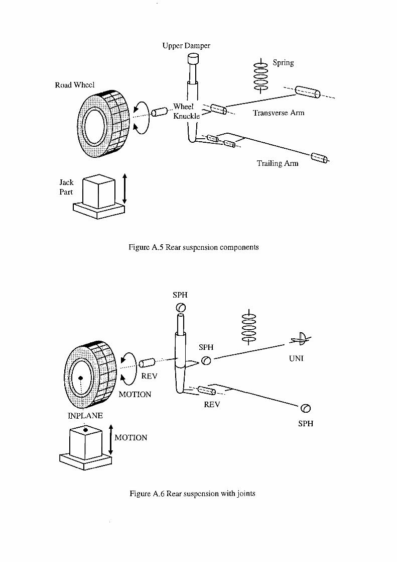
Road Wheel
INPLANE
Upper Damper
6 Spring c:::> <::::> c:::> <p ---~
_('\ Wheel --~ ----\) .Q::::)··· Knuckle >'-"tl--. Transverse Ann
l1~ ~--
Trailing Arm
Figure A.5 Rear suspension components
SPH
({) 6 c:::> c:::>
SPH ~~ (LJ ------ UNI
I MOTION
SPH
Figure A.6 Rear suspension with joints

INPLANE
Parts D Points Q
.G~---·· t.;J~v MOTION
I MOTION
BUSH
cS <::::> c::::::::::> c::::::::::>
BUSH
BUSH cp ---~---~~ -
BUSH
Figure A 7 Rear suspension with bushes
BODY/GROUND
~
Figure AS Rear suspension numbering convention

Steering column part
MOTION
Revolute joint to vehicle body
Steering motion applied at joint
COUPLER
Steering rack part
Translational joint to vehicle body
Figure A.9 Steering system components and joints
Parts D Points Q
Figure A.lO Steering system numbering convention

Right Roll Bar
Parts D Points Q
Revolute Joints to Vehicle Body
REV
REV
-~~orsional INPLANE
A Front Wheel U Knuckle
Spring
Left Roll Bar
INPLANE .. ··. ·.
Front Wheel Knuckle
·. ·.
·rJ
Figure All Front roll bar system components and joints
············ ... @
~-u
Figure A.l2 Front roll bar system numbering convention

Right Roll Bar
Revolute Joints to Vehicle Body
REV
REV
-®Torsional Spring
INPLANE
m RearWheel Knuckle
Left Roll Bar
• ..... ·. IN PLANE
· . .....
Rear Wheel Knuckle
· ..
Figure A.l3 Rear roll bar system components and joints
Parts 0 Points Q
Figure A.l4 Rear roll bar system numbering convention
············ ... § · .. ..

Spring Damper ~t ~~ier ~t
Rear Right rJ' g Slidmg Mass Spring
Slid" amper mg Mass ' ~ TRANS
1 ~f~per ~
~~ 1 TRANS w~Q?~ ~ 6 9REV
REV : Front Right Sliding Mass
Figure A.15 Lum
and Wheel Kn uckle
ped mass mod 1 e suspension comp
@(ij)
~t :!W@
.·.·.· [!]I~ ~mr==?11 ~T:~ 08
I I
Front Left Sli ding Mass and Wheel Kn
onents and .. JOints
Points Q
Figure A.16 Lum ped mass mod 1 e suspension numbe . . nng convention
uckle

Spring Damper
~,. ---~::~---rc::::::-:::::~~~co ~:
REV
Spring ~,. Damper .. c0(j
Rear Left REV Swing Arm
Rear Right Swing Arm
Spring Spring ::!;.!, Damper ~,. Damper ~·~· l Q),' ,.: ·. .
1 REV REV~~ : -- - : . -- f:Jj ' .. <CJID~-----c-::-_9----- ~ REV
1 Front Right F Q 1 S 0 ront Left 1
REV,..:~ wmgAnn S · ' '-+-"' and W wmg Arm 1 heel Kn kl d , uc e an Wheel Kn
Figure Ao17 S 0 wmg arm m d o el suspe 0 nswn co mponents and joints
@~,.@ @ @oQ}
[@]
Figure A.18 Swin g arm model sus 0 pension numb 0 enng convention
uckle

Torsional Spring damper
I I
rnl
a::J --~ . ; ~:~ '-+-"'
Torsional Spring damper 0
Wheel Knuckles
I I
0
Figure A.l9 Roll stiffness model suspension components and joints
Parts 0 Points Q
~a:DO" lf!§l\'P I
0
Figure A.20 Roll stiffness model suspension numbering convention

APPENDIXB
SUSPENSION ANALYSES OUTPUT PLOTS

FRONT SUSPENSION
4.0 I I I I I
3.0 Rigid joints ----------- -
2.0
1.0 Cl (I)
0.0 "0
(I) -1.0 Cl c <( -2.0 iii ..0 -3.0 E t1l
-4.0 ()
-5.0
Linear bushes ---- -
7 ~ Nonlinear bushes -- -I :--- Test data ------
~ -....._ ~
"""' ~ ~ ~
"(: r--~
...
-6.0
-7.0 -80.0 -40.0 0.0 40.0 80.0 120 .0
-100.0 -60.0 -20.0 20.0 60.0 100.0
Bump Movement ( mm )
Figure B.l Front suspension - camber angle with bump movement
FRONT SUSPENSION
7.0 I I I I I Rigid joints ----------- ~
6.0 - -unear bushes -----~
5.0 Cl (I)
"0
~ 4.0
Cl c <( 3.0 ~
(I)
iii
Nonlinear bushes ~
~
L ~
~
P-< <~ ... ~
~ ~ \
, _, :"-;;;.,- - - - - ::, ~ ~ -
t1l () 2.0
1.0
0.0 -80.0 -40.0 0.0 40.0 80.0 120 .0
-100.0 -60.0 -20.0 20.0 60.0 100.0
Bump Movement ( mm )
Figure B.2 Front suspension - caster angle with bump movement
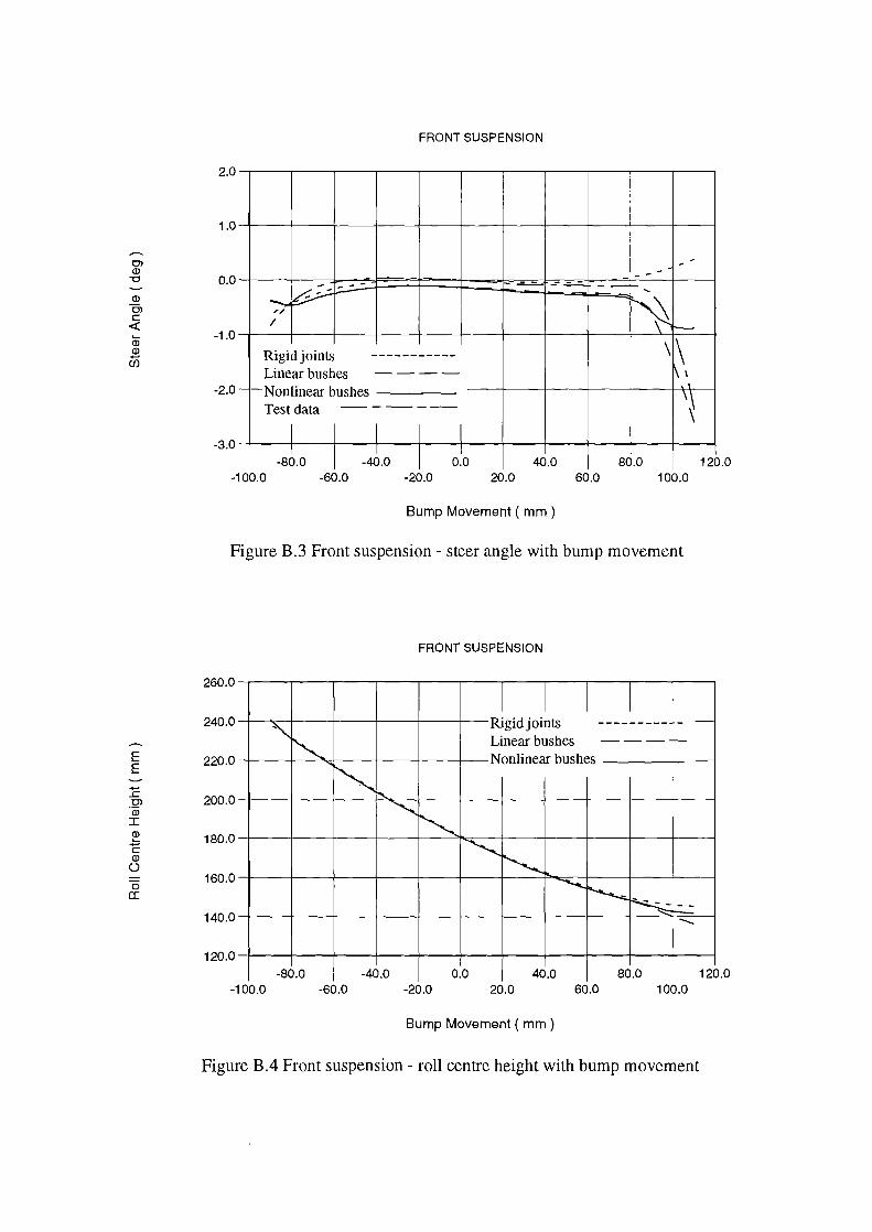
FRONT SUSPENSION
2.0
1.0
Cl , , (IJ "0 0.0 (IJ
Cl c <(
-1.0 (ij (IJ
U5
- - , - -
~ r==-- - - - --=-=..- - - ....
"::';"' ~ / -Rigid joints ----------- '\ Linear bushes ------ \ I
-2.0 -~Nonlinear bushes I
Test data ----- \~ \
-3.0 I I I -86.o -~.0 o:o 40.0 80.0 120 .0
-100.0 -60.0 -20.0 20.0 60.0 100.0
Bump Movement ( mm )
Figure B.3 Front suspension - steer angle with bump movement
FRONT SUSPENSION
260.0
I I I I I 240.0
E 220.0 E
1: 200.0 Cl
"Q) I
~ 180.0 c (IJ
(.) 160.0
0 a:
140.0
" Rigid joints ----------- -
~ Linear bushes ----Nonlinear bushes -
~ ~
~
~ ~ ~
-........... "--.......,_ ~ 1-=_ -
120.0 -80.0 -40.0 0.0 40.0 80.0 120 .0
-100.0 -60.0 -20.0 20.0 60.0 100.0
Bump Movement ( mm )
Figure B.4 Front suspension- roll centre height with bump movement

FRONT SUSPENSION
30.0 /
20.0
E 10.0
E Q) 0.0 Cl c t1l .c -10.0 () ~ (.)
~ -20.0 f-
-30.0
)'
~ ~ --~
~ -v ~
/
__,4 /
v Rigid joints -----------,/ Linear bushes ------J' Nonlinear bushes
-40.0 I I I 0~0 I I
-80.0 -40.0 40.0 80.0 120 .0 -100.0 -60.0 -20.0 20.0 60.0 100.0
Bump Movement ( mm )
Figure B.5 Front suspension- track change with bump movement
FRONT SUSPENSION
7000.0
6000.0
5000.0 z Q) 4000.0 (.)
0 lL (ij 3000.0
'L
v v ~
~__.....,... -~ ~ -------= J'o
~ ~ --~ _;, ~-
(.)
t Q)
Rigid joints -----------> 2000.0 Linear bushes ----
Nonlinear bushes
1000.0 Test data ------
0.0 I I -50.0 -30.0 1~.0 I
-10.0 30.0 50.0 -60.0 -40.0 -20.0 0.0 20.0 40.0 60.0
Bump Movement ( mm )
Figure B.6 Front suspension- vertical force with bump movement

REAR SUSPENSION
4.0
3.0
2.0 Cl (l)
"U 1.0 (l)
OJ 0.0 c <X: ~
(l)
-1.0 .0 E ell () -2.0
-~ I I I I I -
~ Rigid joints -----------Linear bushes -----
~ -
Nonlinear bushes 1'---
'-.....
""' "" ~"'--... - -..... ~
" .......... ~
-3.0
-4.0 -80.0 -40.0 0.0 40.0 80.0 120 .0
-100.0 -60.0 -20.0 20.0 60.0 100.0
Bump Movement ( mm )
Figure B.7 Rear suspension- camber angle with bump movement
REAR SUSPENSION
-2.0 I I I I I
-3.0
Cl -4.0 (l)
"U
~ Cl -5.0 c
<X: ~
(l)
u; -6.0 ell ()
-7.0
\ Rigid joints -----------
~~ Linear bushes ---- -
Nonlinear bushes ~ ~
' ~
~ ~
~
.............
~ ~
I'---8.0
-80.0 -40.0 0.0 40.0 80.0 120 .0 -100.0 -60.0 -20.0 20.0 60.0 100.0
Bump Movement ( mm )
Figure B.8 Rear suspension- caster angle with bump movement

REAR SUSPENSION
0.5 I I I I I 0.4 _-Rigid joints -----------
Linear bushes -----0.3 --Nonlinear bushes
0.2 ,
, C) Q)
""C 0.1 , ,
, , ,
, , , , Q) , -, OJ 0.0 c
,
I , ,
, <(
-0.1 Co Q)
, , ,
, , -, ,
Ci5 -0.2
-0.3
-0.4
-0.5 -80.0 -40.0 0.0 40.0 80.0 120 .0
-100.0 -60.0 -20.0 20.0 60.0 100.0
Bump Movement ( mm )
Figure B.9 Rear suspension- steer angle with bump movement
REAR SUSPENSION
250.0
I I I I I 225.0
E 200.0
E
~ Rigid joints ----------- -
~ Linear bushes ----
......... Nonlinear bushes -
~ :E 175.0 C)
"(j) 150.0 I
~ c 125.0 Q)
()
0 100.0 II
75.0
~
"" ~ "' "' " ""
50.0 -80.0 -40.0 0.0 40.0 80.0 120 .0
-100.0 -60.0 -20.0 20.0 60.0 100.0
Bump Movement ( mm )
Figure B.IO Rear suspension- roll centre height with bump movement

REAR SUSPENSION
20.0
10.0
E 0.0 E Q) Ol
-10.0 c til
..c () ~
-20.0 (.)
~ 1-
-30.0
~ - - - -
----~
/ /
/ v
-v Rigid joints -----------Linear bushes ----
1 Nonlinear bushes -
-40.0 I I -80.0 -40.0 0.0 ~.0 a6.o 120 .0
-100.0 -60.0 -20.0 20.0 60.0 100.0
Bump Movement ( mm )
Figure B.ll Rear suspension - track change with bump movement
REAR SUSPENSION
5000.0
4500.0
4000.0
z 3500.0
Q) (.)
0 3000.0 LL
ca (.)
2500.0 t Q)
> 2000.0
1500.0
Rigid joints -------------Linear bushes ---- ~
~ v~
Nonlinear bushes .,/ -- v v /
~ / ___,
~ ~
~-;...:::-
?-~
1000.0 -50.0 -30.0 -10.0 10.0 30.0 50.0
-60.0 -40.0 -20.0 0.0 20.0 40.0 60.0
Bump Movement ( mm )
Figure B.l2 Rear suspension- vertical force with bump movement

APPENDIXC
RESULTS OF EXPERIMENTAL TYRE TESTING

LATERAL FORCE FY N
<aoo. 0
490 0
0
c 0 .... I
0
q) I
0
,rc
7000.00
SIZE 195/65R15 (OST5064/B) TYRE DUNLOP DS. IP--2.0 BAA. SPEED (KPH) -+oo020
LOAD KG SLIP ANGLE DEG
-7000.00
0
0 ""1
Figure C. I Lateral force Fy with slip angle a
490 0 ·o
<aoo. 0
4o0 ·0

Gl 0 0
0
ALIGNING TORQUE MZ NM.
200.00
SIZE 195/65R15 (OST5064 B) TYRE DUNLOP 08. !P::o2.0 BAR. SPEED (KPH) s+00020
0
0
I Cl
0
I A.
0
0
-200.00
800. 600. 400. 200.
0
(!)
LOAD KG
0
SLIP ANGLE DEG
Figure C.2 Aligning moment Mz with slip angle a.
0
0 ..-1
0

LATERAL FORCE FY N
-200.00
800. 600. 400. 200.
LOAD KG
0 o·
~p
SLIP ANGLE DEG
7000.00
SIZE 195/65R15 (OST5064/BJ TYRE DUNLOP DB. IP~2.0 BAR. SPEED (KPH) =+00020
ALIGNING TORQUE MZ NM
a.o
-7000.00
200.00
& ·o
Figure C.3 Lateral force Fy with aligning moment Mz (Gough Plot)

1000.0
CORNERING STIFFNESS N/OEG.
SIZE 195/65R15 (OST5064/A) TYRE DUNLOP DB. 1P=-2.0 BAR. SPEED (KPH) =-+00020
.00~1--+-~--;-~~-r--~-r--+--+--+-~--~~--~--r-_,
.00
Figure C.4 Cornering stiffness with load
800.00 LOAD KG

ALIGNING STIFFNESS NM/OEG.
50. o SIZE 195/65R15 (OST5064/B) TYRE DUNLOP DS. !P=-2.0.BAR. SPEED (KPH) ~+00020
.00
Figure C.5 Aligning stiffness with load
800.00 LOAD KG

LOAD KG
0
"" I
0
LATERAL FORCE FY N
1000.00 0
0
0
(?) 0
0 '\0
0 <oo
0
0 o·
/>.0
0 \.oo.
SIZE 195/65R15 (OST5064/A) TYRE DUNLOP DB. IP•2.0 BAR. SPEED (KPH) =+00020
CAMBER ANGLE DEG
-1000.00
Figure C.6 Lateral force Fy with camber angle y

I .... 0
0
ALIGNING TORQUE ~z ~M.
50.00
SIZE 195/65R15 (OST5064 A) TYRE DUNLOP D8. !P-2.0 BAR. SPEED (KPH) -+00020
I (II
0
I m 0
I A
0
I ru 0
l
-50.00
ru 0
A
0
800. 700. 600. 500. 400. 300. 200. 100.
m 0
LOAD KG
(II
0
CAMBER ANGLE OEG
· Figure C. 7 Aligning moment Mz with camber angle y
.... 0
0
0 o·
~0

100.00
CAMBER SriFFNESS N/OEG.
SIZE 195/65R15 (OST5064/A) TYRE DUNLOP DB. !P-2.0 BAR. SPEED (KPH) -+00020
(AT ZERO CAMBER ANGLE)
.OOrl--+-~~-r--+-~~-+--+-~~-+--~--r--+--+---r--+--~
.00
Figure C.8 Camber stiffness with load
800.00 LOAD KG

ALIGNING CAMBER STIFFNESS NM/0
10.0 SIZE 195/65R15 (OST5064/A) TYRE DUNLOP DB. IP-2.0 BAR. SPEED (KPH) -+00020
I
I
(AT ZERO CAMBER ANGLE)
.0~--r--+--+--+--+-~--4-~--~--~-+--+--+--~~--~
.00
Figure C.9 Aligning camber stiffness with load

5000.0
4000.0
~ Q) 3000.0 ()
0 u.. Cl c: ~ 2000.0 Cll ....
CD
1000.0
0.0
TYRE BRAKING FORCE TEST- TYRE 8 195/65 R15 Vertical Load Increments- 1kN 2kN 3kN 4kN
I I i
/f
( I I !
v I ! ' I I rrl
I
v I
0.0
l
l
I I I
' 0.1 0.3
0.2
I I i
i
i i ! I
I I
I : I
I
'
' i I
! I 0.5 0.7
0.4 0.6
Slip Ratio
Figure C.IO Braking force with slip ratio
I '
'
I i I
I
0.9 0.8
i i
1.0

APPENDIXD
FORTRAN TYRE MODEL SUBROUTINES

D.l Fiala Tyre Model Subroutine
SUBROUTINE TIRSUB ( ID, TIME, TO, CPROP, TPROP, MPROP, & PAR, NPAR, STR, NSTR, DFLAG, & !FLAG, FSAE, TSAE, FPROP )
c C This program is part of the CUTyre system - M Blundell, Feb 1997 C This source code defines the Fiala tyre model as provided with the main ADAMS program. C Modifications have been included to introduce new variables for any future work to extend C the model to account for camber effects. c C Inputs: c
c
INTEGER ID, NPAR, NSTR DOUBLE PRECISION TIME, TO DOUBLE PRECISION CPROP(*), TPROP(*), MPROP(*), PAR(*) CHARACTER *80 STR(*) LOGICAL DFLAG, IFLAG
C Outputs: c
DOUBLE PRECISION FSAE(*), TSAE(*), FPROP(*) c C Local Variables: c
DOUBLE PRECISION SLIP, ALPHA, DEFL, DEFLD DOUBLE PRECISION R2, CZ, CS, CA, CR, DZ, AMASS, WSPIN
c C Camber variables c
c
c
c
DOUBLE PRECISION GAMMA, CG, HA, HG, FY A, FYG, TZA, TZG
INTEGER lORD DOUBLE PRECISION ZERO, ONE, SCFACT, DELMAX DOUBLE PRECISION FX, FY, FZ, FXl, FX2, TY, TZ, H, ASTAR, SSTAR DOUBLE PRECISION U, FZDAMP, FZDEFL, WSPNMX LOGICAL ERFLG
PARAMETER PARAMETER PARAMETER PARAMETER
(ZERO=O.O) (ONE=l.O) (IORD=O) (WSPNMX=5 .OD-1)
C EXECUTABLE CODE c C Extract data from input arrays c
c
c
SLIP = CPROP(l) ALPHA = CPROP(2) DEFL = CPROP(4) DEFLD = CPROP(5) WSPIN = CPROP(8)
AMASS = MPROP(l)
R2 = TPROP(2) CZ = TPROP(3) CS = TPROP(4)

c
CA = TPROP(5) CR = TPROP(7) DZ = TPROP(8) U = TPROP(ll)
C Camber c
c
GAMMA= CPROP (3) CG = TPROP (6)
C Initialize force values c
c
c
FX= O.DO FY= O.DO FZ= O.DO TY = O.DO TZ= O.DO
IF(DEFL .LE. O.DO) THEN GOTO 1000
END IF
C Calculate normal loads due to stiffness (always .LE. zero) c
FZDEFL = -DEFL*CZ c C Calculate normal loads due to damping c
FZDAMP =- 2.DO*SQRT(AMASS*CZ)*DZ*(DEFLD) c C Calculate total normal force (fz) c
FZ = MIN (O.ODO, (FZDEFL + FZDAMP) ) c C Calculate critical longitudinal slip value c
SSTAR = ABS(U*FZ/(2.DO*CS)) c C Compute longitudinal force (fx) c
c
IF(ABS(SLIP) .LE. ABS(SSTAR)) THEN FX = -CS*SLIP
ELSE FXl = U*ABS(FZ) FX2 = (U*FZ)**2/(4.DO*ABS(SLIP)*CS) FX = -(FX1-FX2)*SIGN(l.ODO,SLIP) END IF
C Calculate critical value of slip angle c
ASTAR = ATAN(ABS(3.DO*U*FZ/CA)) c C Compute lateral force and aligning torque (FY A & TZA) due to slip c
IF(ABS(ALPHA) .LE. l.D-10) THEN FYA=O.DO TZA=O.DO
ELSE IF( ABS(ALPHA) .LE. AST AR) THEN

c
HA = l.DO- CA*ABS(TAN(ALPHA))/(3.DO*U*ABS(FZ)) FY A= -U*ABS(FZ)*(l.DO-HA**3)*SIGN(l.ODO,ALPHA) TZA = U* ABS(FZ)*2.DO*R2*(1.DO-HA)*(HA **3)*SIGN(l.ODO,ALPHA)
ELSE FY A= -U*ABS(FZ)*SIGN(l.ODO,ALPHA) TZA= O.DO
END IF
C Compute lateral force and aligning torque (FYG & TZG) due to camber C Currently set to zero, example of futire modifications - FYG =CG*GAMMA c
c
FYG= 0.0 TZG=O.DO
C Compute total lateral force and aligning torque (FY & TZ) c
c
FY=FYA+FYG TZ=TZA+TZG
C Copy the calculated values for FX, FY, FZ, TY & TZ to FSAE C and TSAE arrays c 1000 FSAE(l) = FX
FSAE(2) = FY FSAE(3) = FZ TSAE(l) = 0.0 TSAE(2) = TY TSAE(3) = TZ FPROP(l) = 0.0 FPROP(2) = 0.0 RETURN END

D.2 Full Interpolation Tyre Model Subroutine
SUBROUTINE TIRSUB ( ID, TIME, TO, CPROP, TPROP, MPROP, & PAR, NP AR, STR, NSTR, DFLAG, & IFLAG, FSAE, TSAE, FPROP)
c C This program is part of the CUTyre system- M Blundell, Feb 1997 C This version is based on an interpolation approach using measured C tyre test data which is include in SPLINE statements. It is referred to as the Full model C as it accounts for a larger range of tests varying slip at given camber angles C Cubic interpolation is used for varying slip with linear interpolation between camber angles C Fx based on Fiala model C This model is used for full interpolation and is tested on TYRE A C Camber inputs are at -5, 0 and 5 degrees c C The coefficients in the model asume the following units: C slip angle: degrees C camber angle: degrees C Fz (load): kg C Fy andFx: N C Tz: Nm c C Inputs: c
c
INTEGER ID,NPAR,NSTR DOUBLE PRECISION TIME, TO DOUBLE PRECISION CPROP(*), TPROP(*), MPROP(*), PAR(*) CHARACTER *80 STR(*) LOGICAL DFLAG, IFLAG, ERRFLG
C Outputs: c
DOUBLE PRECISION FSAE(*), TSAE(*), FPROP(*), ARRA Y(3) c C Local Variables: c
c
c
c
c
DOUBLE PRECISION SLIP, ALPHA, DEFL, DEFLD DOUBLE PRECISION R2, CZ, CS, CA, CR, DZ, AMASS, WSPIN
DOUBLE PRECISION GAMMA,CG,RALPHA,RGAMMA,FZL,TZL,TZLA,TZLG DOUBLE PRECISION CFY,DFY,EFY,SHFY,SVFY,PHIFY,TZLl,TZL2,TZL3 DOUBLE PRECISION CTZ,DTZ,ETZ,BTZ,SHTZ,SVTZ,PHITZ DOUBLE PRECISION CFX,DFX,EFX,BFX,SHFX,SVFX,PHIFX
INTEGER lORD DOUBLE PRECISION ZERO, ONE, SCFACT, DELMAX,FY1,FY2,FY3 DOUBLE PRECISION FX, FY, FZ, FXl, FX2, TY, TZ, H, ASTAR, SSTAR DOUBLE PRECISION U, FZDAMP, FZDEFL, WSPNMX, DTOR, RTOD LOGICAL ERFLG
PARAMETER PARAMETER PARAMETER PARAMETER PARAMETER PARAMETER
(ZERO=O.O) (ONE=l.O) (IORD=O) (WSPNMX=5.0D-1) (DTOR=0.017453292) (RTOD=57.29577951)
C EXECUTABLE CODE

C Extract data from input arrays c
SLIP = CPROP(l) DEFL = CPROP(4) DEFLD = CPROP(5) WSPIN = CPROP(8)
c AMASS = MPROP(l)
c R2 = TPROP(2) cz = TPROP(3) cs = TPROP(4) CA = TPROP(5) CR = TPROP(7) DZ = TPROP(8) u = TPROP(ll)
c RALPHA = CPROP(2) RGAMMA = CPROP (3) CG = TPROP (6) ALPHA=RALPHA*RTOD GAMMA=RGAMMA *RTOD
c c Initialize force values c
FX= O.DO FY= O.DO FZ= O.DO TY = O.DO TZ= O.DO
c IF(DEFL .LE. O.DO) THEN
GOTO 1000 END IF
c C Calculate normal loads due to stiffness (always .LE. zero) c
FZDEFL = -DEFL*CZ c C Calculate normal loads due to damping c
FZDAMP =- 2.DO*SQRT(AMASS*CZ)*DZ*(DEFLD) c C Calculate total normal force (fz) c
FZ = MIN (O.ODO, (FZDEFL + FZDAMP) ) c C Convert to kg and change sign c
FZL = -FZ/9.81 c C Calculate critical longitudinal slip value c
SST AR = ABS(U*FZ/(2.DO*CS)) c C Compute longitudinal force c
IF(ABS(SLIP) .LE. ABS(SSTAR)) THEN

c
FX = -CS*SLIP ELSE FXl = U*ABS(FZ) FX2 = (U*FZ)**2/(4.DO*ABS(SLIP)*CS) FX = -(FX1-FX2)*SIGN(l.ODO,SLIP) END IF
C Compute lateral force at gamma= -5, 0 and 5 degrees c
c
CALL CUBSPL (ALPHA,FZL,lOl,O,ARRA Y,ERRFLG) FYl=ARRA Y(l) CALL CUBSPL (ALPHA,FZL,102,0,ARRA Y,ERRFLG) FY2=ARRA Y(l) CALL CUBSPL (ALPHA,FZL,103,0,ARRA Y,ERRFLG) FY3=ARRA Y(l)
C Use linear interpolation to get FY for actual Gamma c
c
IF (GAMMA.GE.-5.and.GAMMA.LT.O) THEN FY =FYI +((FY2-FY1)*((GAMMA+5)/5)) ELSE FY=FY2+((FY3-FY2)*((GAMMA-0)/5)) END IF
C Compute self aligning moment c
c
CALL CUBSPL (ALPHA,FZL,104,0,ARRA Y,ERRFLG) TZLl=ARRA Y (1) CALL CUBSPL (ALPHA,FZL,105,0,ARRA Y,ERRFLG) TZL2=ARRA Y (1) CALL CUBSPL (ALPHA,FZL,106,0,ARRA Y,ERRFLG) TZL3=ARRA Y(l)
C Use linear interpolation to get TZL for actual Gamma c
c
IF (GAMMA.GE.-5.and.GAMMA.LT.O) THEN TZL=TZLl+((TZL2-TZLl)*((GAMMA+5)/5)) ELSE TZL=TZL2+((TZL3-TZL2)*((GAMMA-0)15)) END IF
C Convert to Nmm c
TZ = TZL*lOOO.O c C Copy tl1e calculated values for FX, FY, FZ, TY & TZ to FSAE C and TSAE arrays c 1000 FSAE(l) = FX
FSAE(2) = FY FSAE(3) = FZ TSAE(l) = 0.0 TSAE(2) = 0.0 TSAE(3) = TZ FPROP(l) = 0.0 FPROP(2) = 0.0
RETURN END

D.3 Full Interpolation Tyre Model Subroutine (No Camber)
SUBROUTINE TIRSUB ( ID, TIME, TO, CPROP, TPROP, MPROP, & PAR, NPAR, STR, NSTR, DFLAG, & IFLAG,FSAE,TSAE,FPROP)
c C This program is part of the CUTyre system- M Blundell, Feb 1997 C tyre test data which is include in SPLINE statements. It is referred to as the Full model C as it accounts for a larger range of tests varying slip at given camber angles C Cubic interpolation is used for varying slip with linear interpolation between camber angles C Fx based on Fiala model c c c c c c c c c
This model is used for full interpolation and is tested on TYRE A Camber inputs are not included here - results only used at camber= 0 The coefficients in the model asume the following units: slip angle: degrees camber angle: degrees Fz (load): kg Fy and Fx: N Tz: Nm
C Inputs: c
c
INTEGER ID, NPAR, NSTR DOUBLE PRECISION TIME, TO DOUBLE PRECISION CPROP(*), TPROP(*), MPROP(*), PAR(*) CHARACTER*80 STR(*) LOGICAL DFLAG, IFLAG, ERRFLG
C Outputs: c
DOUBLE PRECISION FSAE(*), TSAE(*), FPROP(*), ARRA Y(3) c C Local Variables: c
c
c
c
c
DOUBLE PRECISION SLIP, ALPHA, DEFL, DEFLD DOUBLE PRECISION R2, CZ, CS, CA, CR, DZ, AMASS, WSPIN
DOUBLE PRECISION GAMMA,CG,RALPHA,RGAMMA,FZL,TZL,TZLA,TZLG DOUBLE PRECISION CFY,DFY,EFY,SHFY,SVFY,PHIFY,TZLl,TZL2,TZL3 DOUBLE PRECISION CTZ,DTZ,ETZ,BTZ,SHTZ,SVTZ,PHITZ DOUBLE PRECISION CFX,DFX,EFX,BFX,SHFX,SVFX,PHIFX
INTEGER lORD DOUBLE PRECISION ZERO, ONE, SCFACT, DELMAX,FYI,FY2,FY3 DOUBLE PRECISION FX, FY, FZ, FXl, FX2, TY, TZ, H, ASTAR, SSTAR DOUBLE PRECISION U, FZDAMP, FZDEFL, WSPNMX, DTOR, RTOD LOGICAL ERFLG
PARAMETER PARAMETER PARAMETER PARAMETER PARAMETER PARAMETER
(ZERO=O.O) (ONE=l.O) (IORD=O) (WSPNMX=5.0D-1) (DTOR=0.017453292) (RTOD=57.29577951)
C EXECUTABLE CODE C Extract data from input arrays c

SLIP = CPROP(l) DEFL = CPROP(4) DEFLD = CPROP(5) WSPIN = CPROP(8)
c AMASS = MPROP(l)
c R2 = TPROP(2) cz = TPROP(3) cs = TPROP(4) CA = TPROP(5) CR = TPROP(7) DZ = TPROP(8) u = TPROP(ll)
c RALPHA = CPROP(2) RGAMMA = CPROP (3) CG = TPROP (6) ALPHA=RALPHA*RTOD GAMMA=RGAMMA *RTOD
c c Initialize force values c
FX= O.DO FY= O.DO FZ= O.DO TY = O.DO TZ= O.DO
c IF(DEFL .LE. O.DO) THEN
GOTO 1000 END IF
c C Calculate normal loads due to stiffness (always .LE. zero) c
FZDEFL = -DEFL*CZ c C Calculate normal loads due to damping c
FZDAMP =- 2.DO*SQRT(AMASS*CZ)*DZ*(DEFLD) c C Calculate total normal force (fz) c
FZ = MIN (O.ODO, (FZDEFL + FZDAMP) ) c C Convert to kg and change sign c
FZL = -FZ/9.81 c C Calculate critical longitudinal slip value c
SST AR = ABS(U*FZ/(2.DO*CS)) c C Compute longitudinal force c
IF(ABS(SLIP) .LE. ABS(SSTAR)) THEN FX = -CS*SLIP
ELSE

c
FXl = U*ABS(FZ) FX2 = (U*FZ)**2/(4.DO*ABS(SLIP)*CS) FX = -(FX1-FX2)*SIGN(l.ODO,SLIP) END IF
C Compute lateral force c
c
CALL CUBSPL (ALPHA,FZL,102,0,ARRA Y,ERRFLG) FY=ARRA Y(l)
C Compute self aligning moment c
c
CALL CUBSPL (ALPHA,FZL,105,0,ARRA Y,ERRFLG) TZL=ARRA Y(l)
C Convert to Nmm c
TZ = TZL*lOOO.O c C Copy the calculated values for FX, FY, FZ, TY & TZ to FSAE C and TSAE arrays c 1000 FSAE(l) = FX
FSAE(2) = FY FSAE(3) = FZ TSAE(l) = 0.0 TSAE(2) = 0.0 TSAE(3) = TZ FPROP(l) = 0.0 FPROP(2) == 0.0 RETURN END

D.4 Pacjeka Tyre Model (Monte Carlo Version) Subroutine
SUBROUTINE TIRSUB ( ID, TIME, TO, CPROP, TPROP, MPROP, & PAR, NPAR, STR, NSTR, DFLAG, & IFLAG, FSAE, TSAE, FPROP )
c C This program is part of the CUTyre system - M Blundell, Feb 1997 C This version is based on the Pacjeka tyre model as described C in SAE paper 890087. This also referred to as the "Monte Carlo" version. c c c c c c c c c c c c c
The coefficients in the model assume the following units: slip angle: degrees camber angle: degrees slip ratio% Fz (load): kN Fy and Fx: N Tz: Nm
Note sign changes between Paceka formulation and SAE convention
If camber is not included set A6,A8,All,C6,ClO,Cll,C14,Cl5 to zero
C Inputs: c
c
INTEGER ID,NPAR,NSTR DOUBLE PRECISION TIME, TO DOUBLE PRECISION CPROP(*), TPROP(*), MPROP(*), PAR(*) CHARACTER*80 STR(*) LOGICAL DFLAG, IFLAG
C Outputs: c
DOUBLE PRECISION FSAE(*), TSAE(*), FPROP(*) c C Local Variables: c
c
c
c
DOUBLE PRECISION SLIP, ALPHA, DEFL, DEFLD DOUBLE PRECISION R2, CZ, CS, CA, CR, DZ, AMASS, WSPIN
DOUBLE PRECISION GAMMA,CG,RALPHA,RGAMMA,FXP,FZP,FYP,TZP,SLIPCENT DOUBLE PRECISION AO,Al,A2,A3,A4,A5,A6,A 7,A8,A9,A10,Alll,A112,Al3 DOUBLE PRECISION BO,B l,B2,B3,B4,B5,B6,B7,B8,B9,B lO,B ll,B 12 DOUBLE PRECISION CO,Cl,C2,C3,C4,C5,C6,C7,C8,C9,C10,Cll,Cl2,Cl3 DOUBLE PRECISION C14,C15,C16,Cl7 DOUBLE PRECISION CFY,DFY,EFY,SHFY,SVFY,PHIFY DOUBLE PRECISION CTZ,DTZ,ETZ,BTZ,SHTZ,SVTZ,PHITZ DOUBLE PRECISION CFX,DFX,EFX,BFX,SHFX,SVFX,PHIFX
INTEGER lORD DOUBLE PRECISION ZERO, ONE, SCFACT, DELMAX DOUBLE PRECISION FX, FY, FZ, FXl, FX2, TY, TZ, H, ASTAR, SSTAR DOUBLE PRECISION U, FZDAMP, FZDEFL, WSPNMX, DTOR, RTOD LOGICAL ERFLG
PARAMETER PARAMETER PARAMETER
(ZERO=O.O) (ONE=l.O) (IORD=O)

c c c
c
c c c c
c
c
PARAMETER PARAMETER PARAMETER
(WSPNMX=5.0D-1) (DTOR=0.017453292) (RTOD=57.29577951)
Define Pacejka Coefficients
A0=1.68638 A1=-46.8451 A2=1185.46 A3=1146.06 A4=4.92921 A5=0.00547748 A6=-0.655688 A7=1.86868 A8=-0.0280612 A9=0.0147439 A10=-0.212575 A111=-13.4328 A112=0.428945 A12=-3.71929 A13=33.6686
C0=2.41195 Cl=-3.98725 C2=-2.70372 C3=0.552334 C4=-6.22588 C5=-0.225629 C6=0.00142515 C7=-0.0175979 C8=-0.143857 C9=-0.822518 C10=0.0174298 Cll=-0.0244277 C12=0.0116074 C13=-0.322245 C14=0.0210605 C15=-0.565934 Cl6=0.376785 C17=-2.38039
EXECUTABLE CODE Extract data from input arrays
SLIP = CPROP(1) DEFL = CPROP(4) DEFLD = CPROP(5) WSPIN = CPROP(8)
AMASS = MPROP(1)
R2 = TPROP(2) cz = TPROP(3) cs = TPROP(4) CA = TPROP(5) CR = TPROP(7) DZ = TPROP(8) u = TPROP(ll)

c
c
RALPHA = CPROP(2) RGAMMA = CPROP (3) CG = TPROP (6) ALPHA=RALPHA*RTOD GAMMA=RGAMMA *RTOD
C Initialize force values c
c
c
FX = O.DO FY= O.DO FZ= O.DO TY = O.DO TZ= O.DO
IF(DEFL .LE. O.DO) THEN GOTO 1000
END IF
C Calculate normal loads due to stiffness (always .LE. zero) c
FZDEFL = -DEFL*CZ c C Calculate normal loads due to damping c
FZDAMP =- 2.DO*SQRT(AMASS*CZ)*DZ*(DEFLD) c C Calculate total normal force (fz) c
FZ = MIN (O.ODO, (FZDEFL + FZDAMP) ) c C Convert to kN and change sign c
FZP = -FZ/1000.0 c C Compute longitudinal force c
c
IF(ABS(SLIP) .LE. ABS(SSTAR)) THEN FX = -CS*SLIP
ELSE FXl = U*ABS(FZ) FX2 = (U*FZ)**2/(4.DO*ABS(SLIP)*CS) FX = -(FX1-FX2)*SIGN(l.ODO,SLIP) END IF
C Compute lateral force c
CFY=1.3 DFY=Al *FZP**2+A2*FZP EFY =A6*FZP+A 7 BFY =((A3*SIN(2* AT AN(FZP/ A4)))*(1-A5* ABS(GAMMA)))/(CFY +DFY) SHFY=A8*GAMMA+A9*FZP+Al0
C SVFY=Al2*FZP+Al3+(All2*FZP**2+Alll *FZP)*GAMMA
c
SVFY =All *FZP*GAMMA+Al2*FZP+A13 PHIFY ={1-EFY)*(ALPHA+SHFY)+(EFY /BFY)* AT AN (BFY*(ALPHA+SHFY)) FYP=DFY*SIN(CFY* AT AN(BFY*PHIFY))+SVFY
C Change sign

c FY=-FYP
c C Compute self aligning moment c
c
CTZ=2.4 DTZ=Cl *FZP**2+C2*FZP ETZ=(C7*FZP**2+C8*FZP+C9)/(1-C10* ABS(GAMMA)) BTZ=((C3*FZP**2+C4*FZP)*(l-C6*ABS(GAMMA))*EXP(-C5*FZP))/(CTZ+DTZ) SHTZ=Cll *GAMMA+Cl2*FZP+C13 SVTZ=(C14*FZP**2+C15*FZP)*GAMMA+Cl6*FZP+C17 PIDTZ=(l-ETZ)*(ALPHA+SHTZ)+(ETZ/BTZ)* AT AN(BTZ*(ALPHA+SHTZ)) TZP=DTZ*SIN(CTZ* AT AN(BTZ*PHITZ))+SVTZ
C Convert to Nmm and change sign c
TZ = -TZP*lOOO.O c C Copy the calculated values for FX, FY, FZ, TY & TZ to FSAE C and TSAE arrays c 1000 FSAE(l) = FX
FSAE(2) = FY FSAE(3) = FZ
c
c
c
TSAE(l) = 0.0 TSAE(2) = 0.0 TSAE(3) = TZ
FPROP(l) = 0.0 FPROP(2) = 0.0
RETURN END
D.S Limited Interpolation Tyre Model Subroutine
SUBROUTINE TIRSUB ( ID, TIME, TO, CPROP, TPROP, MPROP, & PAR, NP AR, STR, NSTR, DFLAG, & IFLAG, FSAE, TSAE, FPROP )
c C This program is part of the CUTyre system - M Blundell, Feb 1997 C This version is based on an interpolation approach using measured C tyre test data which is include in SPLINE statements. The model is referred to as the C limited version based on the limited testing where camber and slip are varied C independently. C Fx based on Fiala model c C The coefficients in the model asume the following units: C slip angle: degrees C camber angle: degrees C Fz (load): kg C Fy and Fx: N C Tz: Nm c C Note this subroutine is developed to not accounr for offsets C twice. The offsets are include for slip interpolation C but for camber the offset at zero camber is subtracted. c C Inputs: c
c
INTEGER ID, NPAR, NSTR DOUBLE PRECISION TIME, TO DOUBLE PRECISION CPROP(*), TPROP(*), MPROP(*), PAR(*) CHARACTER *80 STR(*) LOGICAL DFLAG, IFLAG, ERRFLG
C Outputs: c
DOUBLE PRECISION FSAE(*), TSAE(*), FPROP(*), ARRA Y(3) c C Local Variables: c
c
c
c
DOUBLE PRECISION SLIP, ALPHA, DEFL, DEFLD DOUBLE PRECISION R2, CZ, CS, CA, CR, DZ, AMASS, WSPIN
DOUBLE PRECISION GAMMA,CG,RALPHA,RGAMMA,FZL,TZL,TZLA,TZLG DOUBLE PRECISION CFY,DFY,EFY,SHFY,SVFY,PHIFY,TZLGO,TZLGl DOUBLE PRECISION CTZ,DTZ,ETZ,BTZ,SHTZ,SVTZ,PHITZ DOUBLE PRECISION CFX,DFX,EFX,BFX,SHFX,SVFX,PHIFX
INTEGER lORD DOUBLE PRECISION ZERO, ONE, SCFACT, DELMAX,FY A,FYG,FYGO,FYGl DOUBLE PRECISION FX, FY, FZ, FXl, FX2, TY, TZ, H, ASTAR, SSTAR DOUBLE PRECISION U, FZDAMP, FZDEFL, WSPNMX, DTOR, RTOD LOGICAL ERFLG
PARAMETER PARAMETER PARAMETER PARAMETER PARAMETER PARAMETER
(ZERO=O.O) (ONE=l.O) (IORD=O) (WSPNMX=5.0D-1) (DTOR=0.017453292) (RTOD=57.29577951)

c c C EXECUTABLE CODE c c C Extract data from input arrays c
c
c
c
c
SLIP = CPROP(l) DEFL = CPROP(4) DEFLD = CPROP(S) WSPIN = CPROP(8)
AMASS = MPROP(l)
R2 = TPROP(2) CZ = TPROP(3) CS = TPROP(4) CA = TPROP(S) CR = TPROP(7) DZ = TPROP(8) U = TPROP(ll)
RALPHA = CPROP(2) RGAMMA = CPROP (3) CG = TPROP (6) ALPHA=RALPHA*RTOD GAMMA=RGAMMA *RTOD
C Initialize force values c
c
c
FX= O.DO FY = O.DO FZ= O.DO TY = O.DO TZ=O.DO
IF(DEFL .LE. O.DO) THEN GOTO 1000
END IF
C Calculate normal loads due to stiffness (always .LE. zero) c
FZDEFL = -DEFL*CZ c C Calculate normal loads due to d.:'Ullping c
FZDAMP =- 2.DO*SQRT(AMASS*CZ)*DZ*(DEFLD) c C Calculate total nonnal force (fz) c
FZ = MIN (O.ODO, (FZDEFL + FZDAMP) ) c C Convert to kg and change sign c
FZL = -FZ/9.81 c C Calculate critical longitudinal slip value c
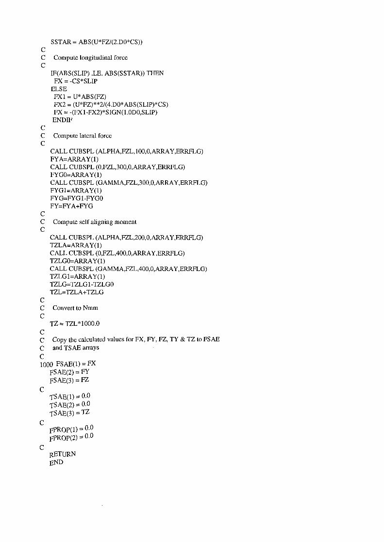
SST AR = ABS(U*FZ/(2.DO*CS)) c C Compute longitudinal force c
c
IF(ABS(SLIP) .LE. ABS(SSTAR)) THEN FX = -CS*SLIP
ELSE FXI = U*ABS(FZ) FX2 = (U*FZ)**2/(4.DO* ABS(SLIP)*CS) FX = -(FX1-FX2)*SIGN(l.ODO,SLIP) ENDIF
C Compute lateral force c
c
CALL CUBSPL (ALPHA,FZL,IOO,O,ARRA Y,ERRFLG) FY A=ARRA Y(l) CALL CUBSPL (0,FZL,300,0,ARRA Y,ERRFLG) FYGO=ARRA Y(l) CALL CUBSPL (GAMMA,FZL,300,0,ARRA Y,ERRFLG) FYGl=ARRA Y(l) FYG=FYGI-FYGO FY=FYA+FYG
C Compute self aligning moment c
c
CALL CUBSPL (ALPHA,FZL,200,0,ARRA Y,ERRFLG) TZLA=ARRA Y(l) CALL CUBSPL (O,FZL,400,0,ARRAY,ERRFLG) TZLGO=ARRA Y(l) CALL CUBSPL (GAMMA,FZL,400,0,ARRA Y,ERRFLG) TZLGI=ARRA Y(l) TZLG=TZLG 1-TZLGO TZL=TZLA+TZLG
C Convert to Nmm c
TZ = TZL*lOOO.O c C Copy the calculated values for FX, FY, FZ, TY & TZ to FSAE C and TSAE arrays
c 1000 FSAE(l) = FX
FSAE(2) = FY FSAE(3) = FZ
c TSAE(l) = 0.0 rSAE(2) = 0.0 TSAE(3) =TZ
c FPROP(l) = O.O fPROP(2) = O.O
c RETURN END

D.6 Limited Interpolation Tyre Model Subroutine (No Camber)
SUBROUTINE TIRSUB ( ID, TIME, TO, CPROP, TPROP, MPROP, & PAR, NPAR, STR, NSTR, DFLAG, & IFLAG,FSAE,TSAE,FPROP)
c C This program is part of the CUTyre system - M Blundell, Feb 1997 C This version is based on an interpolation approach using measured C tyre test data which is include in SPLINE statements. The model is referred to as the C limited version based on the limited testing where camber and slip are varied C independently. c C Note that in this version the effects of camber have been omitted. c C Fx based on Fiala model c C The coefficients in the model asume the following units: C slip angle: degrees C camber angle: degrees C Fz (load): kg C Fy and Fx: N C Tz: Nm c C Note this subroutine is developed to not account for offsets C twice. The offsets are include for slip interpolation C but for camber the offset at zero camber is subtracted. c C Inputs: c
c
INTEGER ID, NPAR, NSTR DOUBLE PRECISION TIME, TO DOUBLE PRECISION CPROP(*), TPROP(*), MPROP(*), PAR(*) CHARACTER *80 STR(*) LOGICAL DFLAG, IFLAG, ERRFLG
C Outputs: c
DOUBLE PRECISION FSAE(*), TSAE(*), FPROP(*), ARRA Y(3) c C Local Variables: c
c
c
c
DOUBLE PRECISION SLIP, ALPHA, DEFL, DEFLD DOUBLE PRECISION R2, CZ, CS, CA, CR, DZ, AMASS, WSPIN
DOUBLE PRECISION GAMMA,CG,RALPHA,RGAMMA,FZL,TZL,TZLA,TZLG DOUBLE PRECISION CFY,DFY,EFY,SHFY,SVFY,PHIFY,TZLGO,TZLGl DOUBLE PRECISION CTZ,DTZ,ETZ,BTZ,SHTZ,SVTZ,PHITZ DOUBLE PRECISION CFX,DFX,EFX,BFX,SHFX,SVFX,PHIFX
INTEGER lORD DOUBLE PRECISION ZERO, ONE, SCFACT, DELMAX,FY A,FYG,FYGO,FYGl DOUBLE PRECISION FX, FY, FZ, FXl, FX2, TY, TZ, H, ASTAR, SSTAR DOUBLE PRECISION U, FZDAMP, FZDEFL, WSPNMX, DTOR, RTOD LOGICAL ERFLG
PARAMETER PARAMETER PARAMETER
(ZERO=O.O) (ONE=l.O) (IORD=O)

c c
PARAMETER PARAMETER PARAMETER
(WSPNMX=5.0D-1) (DTOR=0.017453292) (RTOD=57.29577951)
C EXECUTABLE CODE c C Extract data from input arrays c
c
c
c
c
SLIP = CPROP(l) DEFL = CPROP(4) DEFLD = CPROP(5) WSPIN = CPROP(8)
AMASS = MPROP(l)
R2 = TPROP(2) CZ = TPROP(3) CS = TPROP(4) CA = TPROP(5) CR = TPROP(7) DZ = TPROP(8) U = TPROP(ll)
RALPHA = CPROP(2) RGAMMA = CPROP (3) CG = TPROP (6) ALPHA=RALPHA*RTOD GAMMA=RGAMMA *RTOD
C Initialize force values c
c
c
FX= O.DO FY= O.DO FZ= O.DO TY = O.DO TZ= O.DO
IF(DEFL .LE. O.DO) THEN GOTO 1000
END IF
C Calculate normal loads due to stiffness (always .LE. zero) c
FZDEFL = -DEFL*CZ c C Calculate normal loads due to damping c
FZDAMP = - 2.DO*SQRT(AMASS*CZ)*DZ*(DEFLD) c C Calculate total nonnal force (fz) c
FZ = MIN (O.ODO, (FZDEFL + FZDAMP) ) c C Convert to kg and change sign c
FZL = -FZ/9.81 c

C Calculate critical longitudinal slip value c
SST AR = ABS(U*FZ/(2.DO*CS)) c C Compute longitudinal force c
c
IF(ABS(SLIP) .LE. ABS(SSTAR)) THEN FX = -CS*SLIP
ELSE FXl = U* ABS(FZ) FX2 = (U*FZ)**2/(4.DO*ABS(SLIP)*CS) FX = -(FX1-FX2)*SIGN(l.ODO,SLIP) END IF
C Compute lateral force c
CALL CUBSPL (ALPHA,FZL,lOO,O,ARRA Y,ERRFLG) FY A=ARRA Y(l)
c CALL CUBSPL (O,FZL,300,0,ARRA Y,ERRFLG) c FYGO=ARRA Y(l) c CALL CUBSPL (GAMMA,FZL,300,0,ARRA Y ,ERRFLG) c FYGl=ARRA Y(l) c FYG=FYGl-FYGO
FY=FYA c C Compute self aligning moment c
CALL CUBSPL (ALPHA,FZL,200,0,ARRA Y,ERRFLG) TZLA=ARRA Y(l)
c CALL CUBSPL (O,FZL,400,0,ARRA Y,ERRFLG) c TZLGO=ARRAY(l) c CALL CUBSPL (GAMMA,FZL,400,0,ARRA Y,ERRFLG) c TZLGl=ARRA Y(l) c TZLG=TZLG 1-TZLGO
TZL=TZLA c C Convert to Nmm c
TZ = TZL*lOOO.O c C Copy the calculated values for FX, FY, FZ, TY & TZ to FSAE C and TSAE arrays c 1000 FSAE(l) = FX
FSAE(2) = FY FSAE(3) = FZ
c TSAE(l) = 0.0 TSAE(2) = 0.0 TSAE(3) =TZ
c FPROP(l) = 0.0 FPROP(2) = 0.0
c RETURN END

D. 7 Pacjeka Tyre Model (Version 3) Subroutine
SUBROUTINE TIRSUB ( ID, TIME, TO, CPROP, TPROP, MPROP, & PAR, NP AR, STR, NSTR, DFLAG, & IFLAG,FSAE,TSAE,FPROP)
c C This program is part of the CUTyre system - M Blundell, Feb 1997 C This version is based on the Pacjeka tyre model (Version 3). C Coefficients are for TYRE B c c c c c c c c c c c c
The coefficients in the model assume the following units: slip angle: radians camber angle: radians slip ratio% Fz (load): N Fy and Fx: N Tz: Nm Note sign changes between Paceka formulation and SAE convention If camber is not included set A5,AlO,Al3,Al4,Al5,Al6 and C6,ClO,Cl3,Cl6,Cl7,Cl8,Cl9,C20 to zero
C Inputs: c
c
INTEGER ID,NPAR,NSTR DOUBLE PRECISION TIME, TO DOUBLE PRECISION CPROP(*), TPROP(*), MPROP(*), PAR(*) CHARACTER*80 STR(*) LOGICAL DFLAG, IFLAG
C Outputs: c
DOUBLE PRECISION FSAE(*), TSAE(*), FPROP(*) c C Local Variables: c
c c c
c
c
DOUBLE PRECISION SLIP, ALPHA, DEFL, DEFLD DOUBLE PRECISION R2, CZ, CS, CA, CR, DZ, AMASS, WSPIN
DOUBLE PRECISION GAMMA,CG,RALPHA,RGAMMA,FXP,FZP,FYP,TZP DOUBLE PRECISION AO,Al,A2,A3,A4,A5,A6,A 7,A8,A9,AlO,All,A12,Al3 DOUBLE PRECISION A14,Al5,Al6,A17,SLIPCENT DOUBLE PRECISION CO,Cl,C2,C3,C4,C5,C6,C7,C8,C9,C10,Cll,Cl2,Cl3 DOUBLE PRECISION C14,C15,Cl6,Cl7,Cl8,Cl9,C20 DOUBLE PRECISION CFY,DFY,EFY,SHFY,SVFY,PHIFY DOUBLE PRECISION CTZ,DTZ,ETZ,BTZ,SHTZ,SVTZ,PHITZ DOUBLE PRECISION CFX,DFX,EFX,BFX,SHFX,SVFX,PHIFX,DUMTZ,DUMFY
INTEGER lORD DOUBLE PRECISION ZERO, ONE, SCFACT, DELMAX DOUBLE PRECISION FX, FY, FZ, FXl, FX2, TY, TZ, H, ASTAR, SSTAR DOUBLE PRECISION U, FZDAMP, FZDEFL, WSPNMX, DTOR, RTOD LOGICAL ERFLG
PARAMETER PARAMETER PARAMETER
(ZERO=O.O) (ONE=l.O) (IORD=O)

c
PARAMETER PARAMETER PARAMETER
(WSPNMX=5.0D-1) (DTOR=0.017453292) (RTOD=57.29577951)
C Define Pacejka Coefficients c
c c
c c
A0=.103370E+Ol Al=-.224482E-05 A2=.132185E+Ol A3= .60403 5E+05 A4=.877727E+04 A5=0.0 A6=.458114E-04 A7=.468222 A8=.381896E-06 A9=.516209E-02 A10=0.00 All=-.366375E-01 A12=-.568859E+02 A13=0.00 A14=0.00 A15=0.00 Al6=0.00 A17=.379913
C0=.235000E+01 C1=.266333E-05 C2=.249270E-02 C3=-.159794E-03 C4=- .254 777E-O 1 C5=.142145E-03 C6=0.00 C7=.197277E-07 C8=-.359537E-03 C9=.630223 C10=0.00 Cll=.120220E-06 C12=.275062E-02 C13=0.00 C14=-.172742E-02 C15=.544249E+01 C16=0.00 C17=0.00 C18=0.00 C19=0.00 C20=0.00
C EXECUTABLE CODE c c C Extract data from input arrays c
SLIP = CPROP(l) DEFL = CPROP(4) DEFLD = CPROP(5) WSPIN = CPROP(8)

c
c
c
AMASS = MPROP(l)
R2 = TPROP(2) CZ = TPROP(3) CS = TPROP(4) CA = TPROP(5) CR = TPROP(7) DZ = TPROP(8) U = TPROP(ll)
C Convert sign on alpha c
c
RALPHA = CPROP(2) RGAMMA = CPROP (3) CG = TPROP (6) ALPHA=-RALPHA GAMMA=RGAMMA
C Initialize force values c
c
c
FX= O.DO FY= O.DO FZ= O.DO TY = O.DO TZ= O.DO
IF(DEFL .LE. O.DO) THEN GOTO 1000
END IF
C Calculate normal loads due to stiffness (always .LE. zero) c
FZDEFL = -DEFL*CZ c C Calculate normal loads due to damping c
FZDAMP =- 2.DO*SQRT(AMASS*CZ)*DZ*(DEFLD) c C Calculate total normal force (fz) c
FZ = MIN (O.ODO, (FZDEFL + FZDAMP) ) c C Convert to kN and change sign c
FZP= -FZ c C Compute longitudinal force c c C In absence of Pacjeka terms use the fiala Fx model c
IF(ABS(SLIP) .LE. ABS(SSTAR)) THEN FX = -CS*SLIP
ELSE FXl = U*ABS(FZ) FX2 = (U*FZ)**2/(4.DO*ABS(SLIP)*CS) FX = -(FX1-FX2)*SIGN(l.ODO,SLIP)

END IF c C Compute lateral force c
c
CFY=AO SHFY=A8*FZP+A9+AlO*GAMMA DFY=(Al *FZP+A2)*(1-Al5*GAMMA**2)*FZP IF(ALPHA+SHFY .LT.O.O)THEN DUMFY=-1.0 ELSE
DUMFY=l.O END IF EFY=(A6*FZP+A7)*(1-(Al6*GAMMA+A17)*DUMFY) BFY =((A3*SIN(2* AT AN(FZP/ A4)))*(1-A5* ABS(GAMMA)))/(CFY +DFY) SVFY=All *FZP+A12+(A13*FZP**2+A14*FZP)*GAMMA PHIFY=(l-EFY)*(ALPHA+SHFY)+(EFY/BFY)*ATAN(BFY*(ALPHA+SHFY)) FYP=DFY*SIN(CFY* AT AN(BFY*PHIFY))+SVFY
C Change sign c
FY=FYP c C Compute self aligning moment c
c
CTZ=CO SHTZ=Cll *FZP+C12+C13*GAMMA DTZ=(Cl *FZP**2+C2*FZP)*(l-C18*GAMMA **2) IF(ALPHA+SHTZ.LT.O.O)THEN DUMTZ=-1.0 ELSE
DUMTZ=l.O END IF ETZ=(C7*FZP**2+C8*FZP+C9)*(1-(C19*GAMMA+C20)*DUMTZ) ETZ=ETZ/(1-ClO*ABS(GAMMA)) B TZ=( (C3 *FZP**2+C4 *FZP)*(l-C6* AB S (GAMMA) )*EXP( -C5*FZP) )/(CTZ+ DTZ) SVTZ=C14*FZP+C15+(C16*FZP**2+C17*FZP)*GAMMA PHITZ=(l-ETZ)*(ALPHA+SHTZ)+(ETZ/BTZ)* AT AN(BTZ*(ALPHA+SHTZ)) TZP=DTZ*SIN(CTZ* AT AN(BTZ*PHITZ))+SVTZ
C Convert to Nmm and change sign c
TZ = TZP*lOOO.O c C Copy the calculated values for FX, FY, FZ, TY & TZ to FSAE C and TSAE arrays c 1000 FSAE(l) = FX
FSAE(2) = FY FSAE(3) = FZ
c
c
TSAE(l) = 0.0 TSAE(2) = 0.0 TSAE(3) = TZ FPROP(l) = 0.0 FPROP(2) = 0.0
RETURN END

APPENDIXE
TYRE MODEL PLOTS FROM THE CUTyre RIG MODEL USING DATA FOR TYRE A

~ Q)
~ 0 u.. tii (jj a; _J
~ Q)
~ 0 u.. ~ Q)
a; _J
10000.0
8000.0
6000.0
4000.0
2000.0
0.0
-2000.0
-4000.0
-6000.0
-8000.0
-10000.0
-10.0
INTERPOLATION TYRE MODEL- TYRE A 195/65 R15 Vertical Load Increments- 200kg 400kg 600kg 800kg
~ -~ --~ ~ r--
" 1---
~
-8.0 -4.0 0.0 4.0 8.0 -6.0 -2.0 2.0 6.0
Slip Angle (deg)
10.0
Figure E.l Interpolation model (TYRE A) - lateral force with slip angle
INTERPOLATION TYRE MODEL- TYRE A 195/65 R15 Vertical Load Increments- 200kg 400kg 600kg 800kg
0.0
0.0 -2.0 2.0
Slip Angle (deg)
Figure E.2 Interpolation model (TYRE A) - lateral force with slip angle at near zero slip

E E ~ c (1)
E 0 ~ Cl
-~ c .21 <(
~ (1) ()
0 LL
~ (1)
ro _J
3.0E+05
2.5E+05
2.0E+05
1.5E+05
100000.0
50000.0
0.0
-50000.0
-1.0E+05
-1.5E+05
-2.0E+05
-2.5E+05
-3.0E+05
-10.0
INTERPOLATION TYRE MODEL- TYRE A 195/65 R15 Vertical Load Increments- 200kg 400kg 600kg 800kg
/ "" / "" I v ~ "" 1/ - I~ k_ 1--- ....... r--- ~--- r-...... A
"t'-,. - -/1 " '"' ~ / V/
"" - v
~ / ........__ v
-8.0 -4.0 0.0 4.0 8.0 -6.0 -2.0 2.0 6.0
Slip Angle (deg)
10.0
Figure E.3 Interpolation model (TYRE A) - aligning moment with slip angle
10000.0
8000.0
6000.0
4000.0
2000.0
0.0
-2000.0
-4000.0
-6000.0
-8000.0
-10000.0
INTERPOLATION TYRE MODEL- TYRE A 195/65 R15 Vertical Load Increments - 200kg 400kg 600kg 800kg
( ~ --'-............. \
1-- "'-- c ------....:: t::-- ~\
~ ~ --) ~ --~ __..,.., /
-2.5E+05 -1.5E+05 -50000.0 50000.0 1.5E+05 2.5E+05 -3.0E+05 -2.0E+05 -100000.0 0.0 1.0E+05 2.0E+05 3.0E+05
Aligning Moment (Nmm)
Figure E.4 Interpolation model (TYRE A) - lateral force with aligning moment

~ Q)
~ 0
LL
~ Q)
"'iii _J
z Q) ()
0 LL
~ Q)
"'iii _J
700.0
600.0
500.0
400.0
300.0
200.0
100.0
0.0
-100.0
-200.0
-300.0
-400.0
-500.0
INTERPOLATION TYRE MODEL- TYRE A 195/65 R15 Vertical Load Increments- 200kg 400kg 600kg 800kg
~ /
.4?
/~ '/ --/ ~ .{._
~~ ----// / _,/ ~ /
/ _,../ / ~~ /
/
/ ~ ~/ 200 kg ~ 400 kg ~ / ----/ 600 kg ----------
/
800 kg ------
I I
I -8.0 -4.0 0.0 4.0 8.0 -10.0 -6.0 -2.0 2.0 6.0 10.0
Camber Angle (deg)
Figure E.5 Interpolation model (TYRE A) - lateral force with camber angle
10000.0
8000.0
6000.0
4000.0
2000.0
0.0
-2000.0
-4000.0
-6000.0
-8000.0
-10000.0
FIALA TYRE MODEL- TYRE A (Average Wheel Load) 195/65 R15 Vertical Load Increments - 200kg 400kg 600kg 800kg
t-----~ ~ --....::::::: ~
-...;
~ ~ l--~ ~
~ ~ ---
-8.0 -4.0 0.0 4.0 8.0 -10.0 -6.0 -2.0 2.0 6.0 10.0
Slip Angle (deg)
Figure E.6 Fiala model (TYRE A)- lateral force with slip angle

z (])
2 0
LL
~ (])
1ii _J
E E ~ c (])
E 0 ~ Ol c c
.!21 <(
FIALA TYRE MODEL- TYRE A (Average Wheel Load) 195/65 R15 Vertical Load Increments- 200kg 400kg 600kg BOOkg
2000.0 ----r-------------r-------------,
0.0
-2000.0 -+------------+-------------1 0.0
-2.0 2.0
Slip Angle (deg)
Figure E.7 Fiala model (TYRE A)- lateral force with slip angle at near zero slip
3.0E+05
2.5E+05
2.0E+05
1.5E+05
100000.0
50000.0
0.0
-50000.0
-1.0E+05
-1.5E+05
-2.0E+05
-2.5E+05
-3.0E+05
FIALA TYRE MODEL- TYRE A (Average Wheel Load) 195/65 R15 Vertical Load Increments- 200kg 400kg 600kg BOOkg
_,.f...-""" --v r----/- --- ......__
/ ---1-- -------!-......., -r--..... _/
1-- 1-- v 1--- ~ -- -I-""
-8.0 -4.0 0.0 4.0 8.0 -10.0 -6.0 -2.0 2.0 6.0 10.0
Slip Angle (deg)
Figure E.8 Fiala model (TYRE A) -aligning moment with slip angle

~ Q) ()
0 LL
~ Q)
(i:j _J
z Q)
~ 0
LL (U Qj (i:j _J
FIALA TYRE MODEL- TYRE A (Average Wheel Load) 195/65 R15 Vertical Load Increments - 200kg 400kg 600kg 800kg
10000.0
8000.0
6000.0
4000.0
2000.0
0.0
-2000.0
-4000.0
-6000.0
L
( /"' ~
-" ~ ( ~ K-
~ ~ __) \' "' 1- / ) - v
-8000.0
-10000.0 -2.5E+05 -1.5E+05 -50000.0 50000.0 1.5E+05 2.5E+05
-3.0E+05 -2.0E+05 -100000.0 0.0 1.0E+05 2.0E+05 3.0E+05
Aligning Moment (Nmm)
Figure E.9 Fiala model (TYRE A) - lateral force with aligning moment
10000.0
8000.0
6000.0
4000.0
2000.0
0.0
-2000.0
-4000.0
-6000.0
-8000.0
-10000.0
FIALA TYRE MODEL- TYRE A (Front Wheel Load) 195/65 R15 Vertical Load Increments - 200kg 400kg 600kg 800kg
r------~ ~ ---::::: ~
-~
~ r-
~ t::::--~ :::::::::--1-=
r---
-8.0 -4.0 0.0 4.0 8.0 -10.0 -6.0 -2.0 2.0 6.0 10.0
Slip Angle (deg)
Figure E.l 0 Fiala model (TYRE A) - lateral force with slip angle

~ Q) 0
0 LL
Cii Q; "'iii _J
E E ~ c Q)
E 0 ~ Ol c ·c:
.!2'1 <(
0.0
FIALA TYRE MODEL- TYRE A (Front Wheel Load) 195/65 R15 Vertical Load Increments- 200kg 400kg 600kg BOOkg
0.0 -2.0
Slip Angle (deg)
2.0
Figure E.ll Fiala model (TYRE A) - lateral force with slip angle at near zero slip
3.0E+05
2.5E+05
2.0E+05
1.5E+05
100000.0
50000.0
0.0
-50000.0
-1.0E+05
-1.5E+05
-2.0E+05
-2.5E+05
-3.0E+05
FIALA TYRE MODEL- TYRE A (Front Wheel Load) 195/65 R15 Vertical Load Increments- 200kg 400kg 600kg BOOkg
..,.,..... - -r-. v ---......_ .......
/' 1-- 1---/ ...............
t- ----"--------- -~--- __/ -..........__ I-- 4 .........
-........_ --:::7 --- -- ..,.,.....
-8.0 -4.0 0.0 4.0 8.0 -10.0 -6.0 -2.0 2.0 6.0 10.0
Slip Angle (deg)
Figure E.12 Fiala model (TYRE A) - aligning moment with slip angle

~ Q) (.)
0 u.. al Q) 1ii _I
~ Q) (.)
0 u..
~ Q)
1ii _I
10000.0
8000.0
6000.0
4000.0
2000.0
0.0
-2000.0
-4000.0
-6000.0
-8000.0
-10000.0
FIALA TYRE MODEL- TYRE A (Front Wheel Load) 195/65 R15 Vertical Load Increments- 200kg 400kg 600kg BOOkg
/ f.--
( /' ...-
-......... ~ ( ~ K..
~ ~ ~ \' ~
1- ./ ) ...-....... v
-2.5E+05 -1.5E+05 -50000.0 50000.0 1.5E+05 2.5E+05 -3.0E+05 -2.0E+05 -100000.0 0.0 1.0E+05 2.0E+05 3.0E+05
Aligning Moment (Nmm)
Figure E.13 Fiala model (TYRE A) - lateral force with aligning moment
10000.0
8000.0
6000.0
4000.0
2000.0
0.0
-2000.0
-4000.0
-6000.0
-8000.0
-10000.0
FIALA TYRE MODEL- TYRE A (Rear Wheel Load) 195/65 R15 Vertical Load Increments- 200kg 400kg 600kg BOOkg
r--r----: ~ f::::::.... -~ ~
-....::
~ ~ ;;;;:-_
~ ~-r---....;::::;:
~ :::------------8.0 -4.0 0.0 4.0 8.0
-10.0 -6.0 -2.0 2.0 6.0 10.0
Slip Angle (deg)
Figure E.14 Fiala model (TYRE A)- lateral force with slip angle

b ())
~ 0
LL
ca (jj 1ii _.J
"E E b c ())
E 0 ~ Cl
-~ c .!2> <(
FIALA TYRE MODEL- TYRE A (Rear Wheel Load) 195/65 R15 Vertical Load Increments- 200kg 400kg 600kg 800kg
2000.0-.-------------...,..---------------,
0.0
-2000.0 -+-----------+-------------; 0.0
-2.0 2.0
Slip Angle (deg)
Figure E.15 Fiala model (TYRE A) -lateral force with slip angle at near zero slip
3.0E+05
2.5E+05
2.0E+05
1.5E+05
100000.0
50000.0
0.0
-50000.0
-1.0E+05
-1.5E+05
-2.0E+05
-2.5E+05
-3.0E+05
FIALA TYRE MODEL- TYRE A (Rear Wheel Load) 195/65 R15 Vertical Load Increments- 200kg 400kg 600kg 800kg
---- ---,Y --r- ---- ............... t"-----,
v ...______ -r---__ r--r---- -r-- _,/ 1:-----. ....... ,..__ -V' ~
1--- ~ --- ----8.0 -4.0 0.0 4.0 8.0
-10.0 -6.0 -2.0 2.0 6.0 10.0
Slip Angle (deg)
Figure E.16 Fiala model (TYRE A) -aligning moment with slip angle

~ Q) 0 ...._ 0 u.. (ij Qj (U _J
~ Q)
~ 0 u.. ~
Q)
(U _J
10000.0
8000.0
6000.0
4000.0
2000.0
0.0
-2000.0
-4000.0
-6000.0
-8000.0
-10000.0
FIALA TYRE MODEL- TYRE A (Rear Wheel Load) 195/65 R15 Vertical Load Increments - 200kg 400kg 600kg 800kg
/
( / v
-"" ~ ( ~ K..
") ~ ~ ~ t'-.....
;;...... 7 } - I/
-2.5E+05 -1.5E+05 -50000.0 50000.0 1.5E+05 2.5E+05
-3.0E+05 -2.0E+05 -100000.0 0.0 1.0E+05 2.0E+05 3.0E+05
Aligning Moment (Nmm)
Figure E.17 Fiala model (TYRE A) - lateral force with aligning moment
10000.0
8000.0
6000.0
4000.0
2000.0
0.0
-2000.0
-4000.0
-6000.0
-8000.0
-10000.0
PACEJKA (Monte Carlo Version) TYRE MODEL- TYRE A 195/65 R15 Vertical Load Increments- 200kg 400kg 600kg 800kg
::::::: ~ ~ 1'.. -~
I~ t--
""' ~ ~ ~
-8.0 -4.0 0.0 4.0 8.0 -10.0 -6.0 -2.0 2.0 6.0 10.0
Slip Angle (deg)
Figure E.l8 Pacejka model (TYRE A) - lateral force with slip angle

~ (]) ()
0 LL
tii (jj iii _J
PACEJKA (Monte Carlo Version) TYRE MODEL- TYRE A 195/65 R15 Vertical Load Increments- 200kg 400kg 600kg 800kg
2000.0 -.-----,::~---------,---------------,
0.0
-2000.0 -t--------------+--------~""""-----1
0.0 -2.0 2.0
Slip Angle (deg)
Figure E.19 Pacejka model (TYRE A) -lateral force with slip angle at near zero slip
E E ~ c (])
E 0
:::?! Cl .£ c
.!21 <{
3.0E+05
2.5E+05
2.0E+05
1.5E+05
100000.0
50000.0
0.0
-50000.0
-1.0E+05
-1.5E+05
-2.0E+05
-2.5E+05
-3.0E+05
PACEJKA (Monte Carlo Version) TYRE MODEL- TYRE A 195/65 R15 Vertical Load Increments- 200kg 400kg 600kg SOOkg
r-
I \ I \ II r\ \ -- :-...... II/' \. 1\ _,
~ It--~ r--."-.
"" ""~ ----rl
~
1\'\ '-../A -.............. --:: ~ 1\. // \ I \ / ~
-8.0 -4.0 0.0 4.0 8.0 -10.0 -6.0 -2.0 2.0 6.0 10.0
Slip Angle (deg)
Figure E.20 Pacejka model (TYRE A) - aligning moment with slip angle

~ (])
e 0
LL
Cii (jj (ii .....J
~ (]) 0 ..... 0
LL
~ (])
(ii .....J
10000.0
8000.0
6000.0
4000.0
2000.0
0.0
-2000.0
-4000.0
-6000.0
-8000.0
-10000.0
PACEJKA (Monte Carlo Version) TYRE MODEL- TYRE A 195/65 R15 Vertical Load Increments- 200kg 400kg 600kg 800kg
!..--!---= ~ r---L-- ----l--1-- J--- ~ 1.--'
< v-1---t---t:::-- _<.... t-. (
v ~ r--:::::: - 1--
v-v l--' t5 ----~ L---~ - t-- ~
-2.5E+05 -1.5E+05 -50000.0 50000.0 1.5E+05 2.5E+05
-3.0E+05 -2.0E+05 -100000.0 0.0 1.0E+05 2.0E+05 3.0E+05
Aligning Moment (Nmm)
Figure E.21 Pacejka model (TYRE A) -lateral force with aligning moment
700.0
600.0
500.0
400.0
300.0
200.0
100.0
0.0
-100.0
-200.0
-300.0
-400.0
-500.0
PACEJKA (Monte Carlo Version) TYRE MODEL- TYRE A 195/65 R15 Vertical Load Increments- 200kg 400kg 600kg 800kg
_.. -;::--;:
--~ ~ , r.;:.-:-, , .......-::::
, ~ ~ ]..... --::,
~-~ ~ ~
~,,; v , ~
~ ~, -......
_..- ~~
v- -~~ 200 kg -...:::
v 400 kg ----// 600 kg ----------800 kg ------
I I -r 1
-8.0 -4.0 0.0 4.0 8.0 -10.0 -6.0 -2.0 2.0 6.0 10.0
Camber Angle (deg)
Figure E.22 Pacejka model (TYRE A) -lateral force with camber angle

APPENDIXF
TYRE MODEL PLOTS FROM THE CUTyre RIG MODEL USING DATA FOR TYRE B

~ (]) 0
0 u.. (ij (D (ij _J
g (]) 0
0 u.. (ij (D -ca
_J
10000.0
8000.0
INTERPOLATION TYRE MODEL- TYRE B 195/65 R15 Vertical Load Increments- 200kg 400kg 600kg 800kg
6000.0 t--- SP TYRES UK LTD.
4000.0
2000.0
0.0
-2000.0
-4000.0
-6000.0
1-- ~ TEST MACHINE 1::::::-... -~ ~ --~
~ :---~ ;:::--~ f::::::
-8000.0
-10000.0
-8.0 -4.0 0.0 4.0 8.0 -10.0 -6.0 -2.0 2.0 6.0
Slip Angle (deg)
-
10.0
Figure F.l Interpolation model (TYRE B) - lateral force with slip angle
INTERPOLATION TYRE MODEL- TYRE B 195/65 R15 Vertical Load Increments- 200kg 400kg 600kg 800kg
SP TYRES UK LTD. TEST MACHINE
0.0
-2000.0 -+-------------1----------------"1 0.0
-2.0 2.0
Slip Angle (deg)
Figure F.2 Interpolation model (TYRE B)- lateral force with slip angle at near zero slip

E E ~ c (])
E 0 ~ Cl
.£; c .2> <
~ (]) (..) L..
0 LL (ij (ij iii _J
3.0E+05
2.5E+05
2.0E+05
1.5E+05
100000.0
50000.0
0.0
-50000.0
-1.0E+05
-1.5E+05
-2.0E+05
-2.5E+05
-3.0E+05
INTERPOLATION TYRE MODEL- TYRE B 195/65 R15 Vertical Load Increments- 200kg 400kg 600kg 800kg
-f--SP TYRES UK LTD.
TEST MACHINE ----f---.....
/ ~ ./. p:::.-- ----1--
p 1-' 1---r---r----:: 1--- ~ r-.. 1--
.............. 1--- _........-~
""' /
"-... _.../" v
1'---..
-8.0 -4.0 0.0 4.0 8.0 -10.0 -6.0 -2.0 2.0 6.0 10.0
Slip Angle (deg)
Figure F.3 Interpolation model (TYRE B) - aligning moment with slip angle
INTERPOLATION TYRE MODEL- TYRE B 195/65 R15 Vertical Load Increments - 200kg 400kg 600kg 800kg
10000.0
8000.0 I I I I I
6000.0 --!--- SP TYRES UK LTD. -
t [,..-- j.- TEST MACHINE 4000.0
2000.0
0.0
-2000.0
-4000.0
-6000.0
~ )'-....\ v--- -
['-..
~ ~ ~ ~ _/ ~ ~
J_.-' ) !-----"""
-8000.0
-10000.0 -2.5E+05 -1.5E+05 -50000.0 50000.0 1.5E+05 2.5E+05
-3.0E+05 -2.0E+05 -100000.0 0.0 1.0E+05 2.0E+05 3.0E+05
Aligning Moment (Nmm)
Figure F.4 Interpolation model (TYRE B)- lateral force with aligning moment

INTERPOLATION TYRE MODEL- TYRE 8 195/65 R15 Vertical Load Increments- 200kg 400kg 600kg 800kg
1200.0 I I I I
1000.0
800.0
z 600.0
(])
e 0 400.0 u.. (ij (D
200.0 1ii _J
0.0
SP TYRES UK LTD. TEST MACHINE
~ v
~ .---f..--"""" L_ v - !-----
~ -----~ ............ ~
...-::::. ---- ~ --~ v ~
r--
~ f-..--~ --200.0 ~
v
v -400.0
-8.0 -4.0 0.0 4.0 8.0 -10.0 -6.0 -2.0 2.0 6.0 10.0
Camber Angle (deg)
Figure F.5 Interpolation model (TYRE B)- lateral force with camber angle
INTERPOLATION TYRE MODEL- TYRE 8 195/65 R15 Vertical Load Increments - 200kg 400kg 600kg
5000.0
4000.0
3000.0
z 2000.0
(]) 1000.0 ()
0 0.0 u..
~ -1000.0 (])
1ii _J
-2000.0
-3000.0
--------..._ COVENTRY UNIVERSITY ---- ~ TEST MACHINE
~ ! ===== ~ ~ ~ ---
s:---........__ r--
-4000.0
-5000.0
-4.0 0.0 4.0 -6.0 -2.0 2.0 6.0
Slip Angle (deg)
Figure F.6 Interpolation model (TYRE B)- lateral force with slip angle

INTERPOLATION TYRE MODEL- TYRE B 195/65 R15 Vertical Load Increments- 200kg 400kg 600kg
1.6E+05
1.2E+05
E 80000.0 E ~ 40000.0 c Q)
E 0.0 0 ~ Cl -40000.0 £ c
.!21 <{ -80000.0
- I I COVENTRY UNIVERSITY v -------- TEST MACHINE /
/~ ~
£--:;? ---- -/
-1.2E+05 I'-.. / -1.6E+05
-4.0 0.0 4.0 -6.0 -2.0 2.0 6.0
Slip Angle (deg)
Figure F.7 Interpolation model (TYRE B) -aligning moment with slip angle
INTERPOLATION TYRE MODEL - TYRE B 195/65 R15 Vertical Load Increments- 200kg 400kg 600kg
400.0
300.0
200.0
~ 100.0 Q)
~ 0 0.0 LL
~ Q)
-100.0 (ij _J
-200.0
-300.0
I I --- - COVENTRY UNIVERSITY
~ TEST MACHINE / - -
~ /
/ ~ ~ ~ ~
~ ~ ~
-400.0 -4.0 0.0 4.0
-6.0 -2.0 2.0 6.0
Camber Angle (deg)
Figure F.8 Interpolation model (TYRE B)- lateral force with camber angle

~ (]) (.)
0 u.. (ij .... (])
1ii _J
~ (]) (.) .... 0
u.. ~ (])
1ii _J
INTERPOLATION TYRE MODEL- TYRE B 195/65 R15 Vertical Increments - 200kg 400kg 600kg 800kg
20000.0
16000.0
12000.0
1\ I I I I
\ COVENTRY UNIVERSITY -
TEST MACHINE
\ -
Interpolation past range 8000.0
4000.0
0.0
-4000.0
-8000.0
-12000.0
!'----~ of test data -
t---- ~
/ ~ ~ ,/ v ~ !---"""""
~ --~ ~ ~
-8.0 -4.0 0.0 4.0 8.0 -10.0 -6.0 -2.0 2.0 6.0 10.0
Slip Angle (deg)
Figure F.9 Interpolation model (TYRE B)- lateral force with slip angle
10000.0
8000.0
6000.0
4000.0
2000.0
0.0
-2000.0
-4000.0
-6000.0
-8000.0
-10000.0
FIALA TYRE MODEL- TYRE B (Average Wheel Load) 195/65 R15 Vertical Load Increments - 200kg 400kg 600kg 800kg
-..:::::: ~ -~ ~ -...;::
~ ~ ;;:-~ ~ r---~ t;::-
-8.0 -4.0 0.0 4.0 8.0 -10.0 -6.0 -2.0 2.0 6.0 10.0
Slip Angle (deg)
Figure F.IO Fiala model (TYRE B) -lateral force with slip angle

~ Q) 0 0
LL
~ Q)
10 _J
"E E z -c Q)
E 0 ~ C)
.s c
.!21 <(
FIALA TYRE MODEL- TYRE B (Average Wheel Load) 195/65 R15 Vertical Load Increments - 200kg 400kg 600kg 800kg
2000.0 -r-------------r-------------,
0.0
-2000.0 -t--------------t------------1 0.0
-2.0 2.0
Slip Angle (deg)
Figure F.ll Fiala model (TYRE B) -lateral force with slip angle at near zero slip
3.0E+05
2.5E+05
2.0E+05
1.5E+05
100000.0
50000.0
0.0
-50000.0
-1.0E+05
-1.5E+05
-2.0E+05
-2.5E+05
-3.0E+05
FIALA TYRE MODEL- TYRE B (Average Wheel Load) 195/65 R15 Vertical Load Increments- 200kg 400kg 600kg 800kg
= ~ ---:-::--,
~ -- ----b-
L ---- ------1---. - r-- _/ r-- --t-- .-v r--. r-- ~ - -
-8.0 -4.0 0.0 4.0 8.0 -10.0 -6.0 -2.0 2.0 6.0 10.0
Slip Angle (deg)
Figure F.12 Fiala model (TYRE B) -aligning moment with slip angle

~ Q)
~ 0
LL
~ Q)
(ij ...J
z Q) 0 .... 0
LL (ij .... Q)
(ij ...J
FIALA TYRE MODEL- TYRE B (Average Wheel Load) 195/65 R15 Vertical Load Increments- 200kg 400kg 600kg 800kg
10000.0
8000.0
6000.0
4000.0
2000.0
0.0
-2000.0
-4000.0
-6000.0
( / !..--
" ~ ( p-
I" K._ ")-~
..-D ~ :--..... -v )
-8000.0
-10000.0 -2.5E+05 -1.5E+05 -50000.0 50000.0 1.5E+05 2.5E+05
-3.0E+05 -2.0E+05 -100000.0 0.0 1.0E+05 2.0E+05 3.0E+05
Aligning Moment (Nmm)
Figure F.13 Fiala model (TYRE B) - lateral force with aligning moment
10000.0
8000.0
6000.0
4000.0
2000.0
0.0
-2000.0
-4000.0
-6000.0
-8000.0
-10000.0
FIALA TYRE MODEL- TYRE B (Front Wheel Load) 195/65 R15 Vertical Load Increments- 200kg 400kg 600kg 800kg
t--
r---::: ~ t:---~ ~ -...;:
~ ~ t:-~ ~ f--
....;:::
~ t:----~
-8.0 -4.0 0.0 4.0 8.0 -10.0 -6.0 -2.0 2.0 6.0 10.0
Slip Angle (deg)
Figure F.14 Fiala model (TYRE B)- lateral force with slip angle

~ Q) (.) '-0
LL
~ Q)
1ii _J
E' E ~ c Q)
E 0 :2 Ol .£ c
.!:2> <t:
FIALA TYRE MODEL- TYRE B (Front Wheel Load) 195/65 R15 Vertical Load Increments - 200kg 400kg 600kg 800kg
2000.0--.---------------,---------------,
0.0
-2000.0 -+------------+--------------! 0.0
-2.0 2.0
Slip Angle (deg)
Figure F.15 Fiala model (TYRE B) -lateral force with slip angle at near zero slip
3.0E+05
2.5E+05
2.0E+05
1.5E+05
100000.0
50000.0
0.0
-50000.0
-1.0E+05
-1.5E+05
-2.0E+05
-2.5E+05
-3.0E+05
FIALA TYRE MODEL- TYRE B (Front Wheel Load) 195/65 R15 Vertical Load Increments - 200kg 400kg 600kg 800kg
= -= ~ -.......
L -- ----/ -------......_ --r---- -1--- ./ r--
1--... r--- ~ -- -:;::/' - --8.0 -4.0 0.0 4.0 8.0
-10.0 -6.0 -2.0 2.0 6.0 10.0
Slip Angle (deg)
Figure F.16 Fiala model (TYRE B) -aligning moment with slip angle

~ (])
~ 0
LL
~ (])
1ii _J
z -(]) (.)
0 LL
""§ (])
1ii _J
10000.0
8000.0
6000.0
4000.0
2000.0
0.0
-2000.0
-4000.0
-6000.0
-8000.0
-10000.0
FIALA TYRE MODEL - TYRE B (Front Wheel Load) 195/65 R15 Vertical Load Increments- 200kg 400kg 600kg 800kg
( / v
" ~ L_ --~ z
--::;-~ --l--J ~ " __....,. / )
-2.5E+05 -1.5E+05 -50000.0 50000.0 1.5E+05 2.5E+05 -3.0E+05 -2.0E+05 -100000.0 0.0 1.0E+05 2.0E+05 3.0E+05
Aligning Moment (Nmm)
Figure F.17 Fiala model (TYRE B) - lateral force with aligning moment
10000.0
8000.0
6000.0
4000.0
2000.0
0.0
-2000.0
-4000.0
-6000.0
-8000.0
-10000.0
FIALA TYRE MODEL- TYRE B (Rear Wheel Load) 195/65 R15 Vertical Load Increments - 200kg 400kg 600kg 800kg
P===::: ~ - ~~ --.;:::
~ ~ ~
.......... ~ ...__ ~ ~
-8.0 -4.0 0.0 I 4.0 8.0 -10.0 -6.0 -2.0 2.0 6.0 10.0
Slip Angle (deg)
Figure F.l8 Fiala model (TYRE B)- lateral force with slip angle

~ Q)
2 0
LL (ij (ij co _J
E E ~ c Q)
E 0
:::2: 0> -~ c .!2l <
FIALA TYRE MODEL- TYRE B (Rear Wheel Load) 195/65 R15 Vert1cal Load Increments- 200kg 400kg 600kg 800kg
2000.0----,------------.,--------------,
0.0
-2000.0 -+------------+-------------i 0.0
-2.0 2.0
Slip Angle (deg)
Figure F.l9 Fiala model (TYRE B) -lateral force with slip angle at near zero slip
3.0E+05
2.5E+05
2.0E+05
1.5E+05
100000.0
50000.0
0.0
-50000.0
-1.0E+05
-1.5E+05
-2.0E+05
-2.5E+05
-3.0E+05
FIALA TYRE MODEL- TYRE B (Rear Wheel Load) 195/65 R15 Vertical Load Increments- 200kg 400kg 600kg 800kg
~
~ -1---
~ ~ - -.... '/ --r--- r---
--- --r-- ./ --t--- ::::;;; v - 1-- v --8.0 -4.0 0.0 4.0 8.0
-10.0 -6.0 -2.0 2.0 6.0 10.0
Slip Angle (deg)
Figure F.20 Fiala model (TYRE B) -aligning moment with slip angle

~ (]) (.)
0 LL (ij
CD 1U _J
~ (]) (.)
0 LL (ij
CD 1U _J
10000.0
8000.0
6000.0
4000.0
2000.0
0.0
-2000.0
-4000.0
-6000.0
-8000.0
-10000.0
FIALA TYRE MODEL- TYRE B (Rear Wheel Load) 195/65 R15 Vertical Load Increments - 200kg 400kg 600kg 800kg
( /~
' ~ C_ -~ <.
-=> ~ ~ ~ 1'\.
~/ )
-2.5E+05 -1.5E+05 -50000.0 50000.0 1.5E+05 2.5E+05
-3.0E+05 -2.0E+05 -100000.0 0.0 1.0E+05 2.0E+05 3.0E+05
Aligning Moment (Nmm)
Figure F.21 Fiala model (TYRE B)- lateral force with aligning moment
PACJEKA TYRE MODEL (VERSION 3)- TYRE B 195/65 R15 Vertical Load Increments- 200kg 400kg 600kg 800kg
10000.0
8000.0
6000.0
4000.0
2000.0
0.0
-2000.0
-4000.0
-6000.0
1---1-----=::: ~ - t--== ~ ......
~ --~ h--~ ;::----
--.....:::::: :::::::- --8000.0
-10000.0
-8.0 -4.0 0.0 4.0 8.0 -10.0 -6.0 -2.0 2.0 6.0 10.0
Slip Angle (deg)
Figure F.22 Pacejka model (TYRE B)- lateral force with slip angle

PACJEKA TYRE MODEL (VERSION 3)- TYRE 8 195/65 R15 Vertical Load Increments - 200kg 400kg 600kg 800kg
~ (]) (.)
0 0.0 LL (ii (ij co __J
-2000.0 --+-------------+------------4 0.0
-2.0 2.0
Slip Angle (deg)
Figure F.23 Pacejka model (TYRE B) -lateral force with slip angle at near zero slip
PACJEKA TYRE MODEL (VERSION 3)- TYRE 8 195/65 R15 Vertical Load Increments- 200kg 400kg 600kg 800kg
3.0E+05
2.5E+05
2.0E+05
E' 1.5E+05 E 100000.0 ~ c 50000.0 (])
E 0.0 0 ~ -50000.0 Cl £
-1.0E+05 c .2> < -1.5E+05
-2.0E+05
r----... I ~
1/ ~ ~ ~ ::::-~ ~
---1----------::----- /l -~ ~ /1
" ~ --; ~ /
-2.5E+05
-3.0E+05 -8.0 -4.0 0.0 4.0 8.0
-10.0 -6.0 -2.0 2.0 6.0 10.0
Slip Angle (deg)
Figure F.24 Pacejka model (TYRE B)- aligning moment with slip angle

PACJEKA TYRE MODEL (VERSION 3)- TYRE B 195/65 R15 Vertical Load Increments- 200kg 400kg 600kg 800kg
10000.0
8000.0
6000.0
4000.0 ~ (]) 2000.0 0 .... 0 0.0 lL (ij
iii -2000.0 -tU _J
-4000.0
-6000.0
/
l---v v --- /
_L_ ........ ~ / ........_
t-- <.... ,.._ (
r ......... --V,. v -v v ~ I-"" /
------..,/
-8000.0
-10000.0 -2.5E+05 -1.5E+05 -50000.0 50000.0 1.5E+05 2.5E+05
-3.0E+05 -2.0E+05 -100000.0 0.0 1.0E+05 2.0E+05 3.0E+0
Aligning Moment (Nmm)
Figure F.25 Pacejka model (TYRE B) -lateral force with aligning moment

APPENDIX G
INVESTIGATION OF LANE CHANGE
MANOEUVRE (INTERPOLATION MODEL - TYRE A)

§ c 0
~ (])
a> (.) (.) <(
(ij a; (ii ....J
§ c 0 :; a; a> (.) (.) <(
(ij a; (ii ....J
1.0
0.8
0.6
0.4
0.2
0.0
-0.2
-0.4
-0.6
-0.8
-1.0
LUMPED MASS MODEL (TYRE A/INTERPOLATION)- 100 KPH LANE CHANGE
'/ '/
0.0
Track test - - - -ADAMS
1.0 2.0
\ ,;
3.0
Time (s)
4.0 5.0
Figure G .1 Lateral acceleration com paris on - lumped mass model and test
1.0
0.8
0.6
0.4
0.2
0.0
-0.2
-0.4
-0.6
-0.8
-1.0
0.0
SWING ARM MODEL (TYRE A/INTERPOLATION) -100 KPH LANE CHANGE
Track test - - - -ADAMS
1.0
7 I
I \ I
\....
2.0
Time (s)
,;
3.0 4.0
5.0
Figure 0.2 Lateral acceleration comparison -swing arm model and test

§ c 0
~ (])
(j) () () <(
(ij Qj -co
_.1
§ c 0
~ Qj (j) () () <(
(ij Qj Cii _.1
1.0
0.8
0.6
0.4
0.2
0.0
-0.2
-0.4
-0.6
-0.8
-1.0
ROLL STIFFNESS MODEL (TYRE A/INTERPOLATION)- 100 KPH LANE CHANGE
0.0
Track test - - - -ADAMS
~
~
1.0
7 I
I ~ I
\.....
2.0
Time (s)
,;
3.0 4.0
5.0
Figure 0.3 Lateral acceleration comparison- roll stiffness model and test
1.0
0.8
0.6
0.4
0.2
0.0
-0.2
-0.4
-0.6
-0.8
-1.0
0.0
LINKAGE MODEL (TYRE A/INTERPOLATION) -100 KPH LANE CHANGE
I '/
Track test - - - -ADAMS
1 ~
1.0 2.0
Time (s)
,;
3.0 4.0
5.0
Figure 0.4 Lateral acceleration comparison- linkage model and test

Ci Q)
~ <D til c <(
0 a:
Ci Q)
~ <D til c <(
0 a:
8.0
6.0
4.0
2.0
0.0
-2.0
-4.0
-6.0
-8.0
0.0
LUMPED MASS MODEL (TYRE A/INTERPOLATION) -100 KPH LANE CHANGE
1.0
Track test - - - -ADAMS
3.0 2.0
Time (s)
4.0
Figure 0.5 Roll angle comparison- lumped mass model and test
8.0
6.0
4.0
2.0
0.0
-2.0
-4.0
-6.0
-8.0
0.0
SWING ARM MODEL (TYRE A/INTERPOLATION)- 100 KPH LANE CHANGE
'I f
'/ ~
1.0
Track test - - - -ADAMS
2.0
Time (s)
/
3.0 4.0
Figure 0.6 Roll angle comparison- swing arm model and test
5.0
5.0

Cl (])
~ (])
rn c <(
0 a:
Cl (])
~ (])
rn c <(
0 a:
ROLL STIFFNESS MODEL (TYRE A/INTERPOLATION) -100 KPH LANE CHANGE
8.0
6.0
4.0
2.0
0.0
-2.0
-4.0
-6.0
-8.0
0.0
8.0
6.0
4.0
2.0
0.0
-2.0
-4.0
-6.0
-8.0
0.0
Track test - - - -ADAMS ~
~
1.0 2.0
Time (s)
3.0 5.0 4.0
Figure 0.7 Roll angle comparison- roll stiffness model and test
LINKAGE MODEL (TYRE A/INTERPOLATION) -100 KPH LANE CHANGE
Track test - - - -ADAMS
'/
I
1.0 2.0
\
Time (s)
v
...__
3.0 4.0
Figure 0.8 Roll angle comparison- linkage model and test
5.0

LUMPED MASS MODEL (TYRE A/INTERPOLATION)- 100 KPH LANE CHANGE
40.0
Track test - - - -30.0 ADAMS
20.0
(i) '/ -- 10.0 Cl
Q)
'/ ~ Q) 0.0 ~
iii a: 3: -10.0 C1l >-
-20.0 --30.0
-40.0 1.0 3.0 5.0
0.0 2.0 4.0
T1me (s)
Figure 0.9 Yaw rate comparison- lumped mass model and test
SWING ARM MODEL (TYRE A/INTERPOLATION)- 100 KPH LANE CHANGE
40.0
Track test - - - -30.0 ADAMS
20.0
:§' 10.0 / ~ Cl
Q)
'/ ~ \ .$ 0.0 C1l
~
\ I a:
\ I 3: -10.0 C1l
~ '/ >--20.0 / / --30.0
-40.0
1.0 3.0 5.0 0.0 2.0 4.0
Time (s)
Figure 0.10 Yaw rate comparison- swing arm model and test
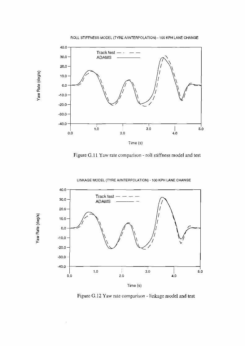
ROLL STIFFNESS MODEL (TYRE A/INTERPOLATION) -100 KPH LANE CHANGE
40.0
Track test - - - -30.0 ADAMS
20.0
Ul '/ ~ -- 10.0 Ol Q)
'/ \ ~ Q) 0.0 ~ I iii \ a:
\ I ;:: -10.0 Cll
~ 'I >--20.0 '/
-30.0
-40.0
1.0 3.0 5.0 0.0 2.0 4.0
Time (s)
Figure G.ll Yaw rate comparison - roll stiffness model and test
LINKAGE MODEL (TYRE A/INTERPOLATION) -100 KPH LANE CHANGE
40.0
Track test - - - -30.0 ADAMS
20.0
Ul -..,
-- 10.0 / Ol Q)
'/ ~ 2 0.0 ~ 7 Cll a: 'I ;:: -10.0 f/ Cll >-
-20.0 --30.0
-40.0 1.0 3.0 5.0
0.0 2.0 4.0
Time (s)
Figure 0.12 Yaw rate comparison -linkage model and test

Oi (])
~ (])
Cl c <{ .... (]) ..a E Ill ()
Oi (])
~ (])
"'5l c <{
.Q..
en
6.0
5.0
4.0
3.0
2.0
1.0
0.0
-1.0
-2.0
-3.0
-4.0
-5.0
-6.0
0.0
FRONT RIGHT TYRE- 100 KPH LANE CHANGE
1.0
_,....., - -
2.0
Time (s)
3.0 4.0
Figure 0.13 Camber angle comparison- linkage and roll stiffness models
FRONT RIGHT TYRE- 100 KPH LANE CHANGE
6.0
5.0
4.0
3.0
2.0
1.0
0.0
-1.0
-2.0
-3.0
-4.0
-5.0
-6.0
1.0 3.0 0.0 2.0 4.0
Time (s)
Figure 0.14 Slip angle comparison - linkage and roll stiffness models
5.0
5.0

~ (]) ()
0 LL (ij ()
t (])
>
z (]) () .... 0
LL (ij ()
t (])
>
FRONT RIGHT TYRE- 100 KPH LANE CHANGE
10000.0
9000.0 Roll Stiffness Model -------
8000.0 Linkage Model
7000.0
6000.0
5000.0
4000.0 #
A 3000.0 /.: ~ /-
2000.0
1000.0
0.0 1.0 3.0 5.0
0.0 2.0 4.0
Time (s)
Figure 0.15 Vertical tyre force comparison- linkage and roll stiffness models
10000.0
9000.0
8000.0
7000.0
6000.0
5000.0
4000.0
3000.0
2000.0
1000.0
0.0
0.0
FRONT LEFT TYRE - 100 KPH LANE CHANGE
h
Roll Stiffness Model ------Linkage Model
1.0 2.0
Time (s)
3.0 5.0 4.0
Figure 0.16 Vertical tyre force comparison- linkage and roll stiffness models

REAR RIGHT TYRE- 100 KPH LANE CHANGE
10000.0
9000.0
Roll Stiffness Model -------8000.0
Linkage Model
z 7000.0
CD 6000.0 "" (.)
0 5000.0 LL
til (.)
4000.0
" 'E CD '-'= > 3000.0 #:;:;:,_
\ f 2000.0 '7 ~::::::"'
1000.0
0.0 1.0 3.0 5.0
0.0 2.0 4.0
Time (s)
Figure G .17 Vertical tyre force com paris on - linkage and roll stiffness models
REAR LEFT TYRE- 100 KPH LANE CHANGE
10000.0
9000.0
Roll Stiffness Model -------8000.0
Linkage Model
~ 7000.0
CD 6000.0 (.)
/"_--.. ,c;-.... 0
5000.0 ~ ~ LL
til ': (.)
4000.0 'E CD > 3000.0
2000.0
1000.0
0.0
1.0 3.0 5.0 0.0 2.0 4.0
Time (s)
Figure G.18 Vertical tyre force comparison -linkage and roll stiffness models

APPENDIXH
INVESTIGATION OF LANE CHANGE MANOEUVRE SENSITIVITY TO TYRE DATA AND MODELS (LINKAGE MODEL)

:§ c 0 :; ~ Q) 0 0 <(
~ 2 ell _J
:§ c 0
~ m Qi 0 0
<(
(ij m 10 _J
LINKAGE MODEL (TYRE A/INTERPOLATION)- 100 KPH LANE CHANGE
1.0
0.8 Track test - - - -
0.6 ADAMS 1 ~
0.4 I 0.2 '/
0.0
-0.2
-0.4
-0.6
-0.8 '-../
-1.0 1.0 3.0 5.0
0.0 2.0 4.0
Time (s)
Figure H.l Lateral acceleration comparison - Interpolation model TYRE A and test
1.0
0.8
0.6
0.4
0.2
0.0
-0.2
-0.4
-0.6
-0.8
-1.0
0.0
LINKAGE MODEL (TYRE A/INTERPOLATION)- 100 KPH LANE CHANGE
Track test - - - -ADAMS
~ [Effects of Camber not modelled]
1.0 3.0 2.0
Time (s)
4.0 5.0
Figure H.2 Lateral acceleration comparison- Interpolation model TYRE A and test

:§ c 0
~ ~ Q) 0 0 <(
~ .$ t1l
_J
~ c 0
~ Q)
(j) 0 0
<(
~ .$ t1l
_J
LINKAGE MODEL (TYRE AIPACEJKA)- 100 KPH LANE CHANGE
1.0
0.8 Track test - - - -
I 0.6 ADAMS ~ 0.4 I \ 0.2 I \
I \ 0.0 I \ I -0.2 I \;
-0.4 I -0.6 I -0.8 '-I '/
-1.0
1.0 3.0 5.0 0.0 2.0 4.0
Time (s)
Figure H.3 Lateral acceleration comparison- Pacjeka model TYRE A and test
1.0
0.8
0.6
0.4
0.2
0.0
-0.2
-0.4
-0.6
-0.8
-1.0
0.0
LINKAGE MODEL (TYRE AIPACEJKA)- 100 KPH LANE CHANGE
1.0
Track test - - - -ADAMS [Effects of Camber not modelled]
7
3.0 2.0
Time (s)
4.0 5.0
Figure H.4 Lateral acceleration comparison- Pacjcka model TYRE A and test

:§ c 0
~ (D
Q) () ()
<(
~ $ ro
....J
o; Q)
~ Q)
0> c
<(
0 a:
1.0
0.8
0.6
0.4
0.2
0.0
-0.2
-0.4
-0.6
-0.8
-1.0
0.0
LINKAGE MODEL (TYRE A/FIALA)- 100 KPH LANE CHANGE
1.0
Track test - - - -ADAMS
\ I '--
(\ I \
I \ I ~
I '-._)
3.0 5.0 2.0 4.0
Time (s)
Figure H.5 Lateral acceleration comparison- Fiala model TYRE A and test
8.0
6.0
4.0
2.0
0.0
-2.0
-4.0
-6.0
-8.0
0.0
LINKAGE MODEL (TYRE A/INTERPOLATION)- 100 KPH LANE CHANGE
1.0
Track test - - - -ADAMS
3.0 2.0
Time (s)
4.0 5.0
Figure H.6 Roll angle comparison - Interpolation model TYRE A and test

Ci (])
~ (])
Cl c < 0 a:
Cl (])
~ J!! Cl c < 0 a:
8.0
6.0
4.0
2.0
0.0
-2.0
-4.0
-6.0
-8.0
0.0
LINKAGE MODEL (TYRE A/INTERPOLATION)- 100 KPH LANE CHANGE
1.0
Track test - - - -ADAMS [Effects of Camber not modelled]
3.0 2.0
Time (s)
4.0 5.0
Figure H.7 Roll angle comparison- Interpolation model TYRE A and test
LINKAGE MODEL (TYRE A/PACEJKA)- 100 KPH LANE CHANGE
8.0
6.0 Track test - - - -
4.0 ADAMS
2.0
0.0
-2.0
-4.0
-6.0
-8.0
1.0 3.0 5.0 0.0 2.0 4.0
Time (s)
Figure H.8 Roll angle comparison- Pacejka model TYRE A and test

o; Q)
~ Q)
c;, c <(
0 a:
o; Q)
~ Q)
c;, c
<(
0 a:
LINKAGE MODEL (TYRE A/PACEJKA)- 100 KPH LANE CHANGE
8.0
6.0- Track test - - - -ADAMS
4.0
2.0
0.0
-2.0
-4.0
-6.0
-8.0
1.0 3.0 5.0 0.0 2.0 4.0
Time (s)
Figure H.9 Roll angle comparison- Pacejka model TYRE A and test
8.0
6.0
4.0
2.0
0.0
-2.0
-4.0
-6.0
-8.0
0.0
LINKAGE MODEL (TYRE A/FIALA)- 100 KPH LANE CHANGE
'/ f/
1.0
Track test - - - -ADAMS
3.0 2.0
Time (s)
4.0
I
5.0
Figure H.IO Roll angle comparison - Fiala model TYRE A and test

LINKAGE MODEL (TYRE A/INTERPOLATION)- 100 KPH LANE CHANGE
40.0
30.0 Track test - - - -ADAMS
20.0
U) ........., -..
10.0 / Cl (])
I ~ .$ 0.0 ~ r. <1l a: ;: -10.0 <1l >-
-20.0
-30.0
-40.0
1.0 3.0 5.0 0.0 2.0 4.0
Time (s)
Figure H. II Yaw rate comparison - Interpolation model TYRE A and test
LINKAGE MODEL (TYRE A/INTERPOLATION)- 100 KPH LANE CHANGE
40.0
30.0 Track test - - - -/~ ADAMS
20.0 [Effects of Camber not modelled] I ~ :§' I Cl 10.0 (]) I ~ .$ 0.0 ~ I \\ I & <1l
\ a: I I ;: <1l
-10.0 'I \ I >-
-20.0 ~ / ...__
-30.0
-40.0
1.0 3.0 5.0 0.0 2.0 4.0
Time (s)
Figure H.l2 Yaw rate comparison- Interpolation model TYRE A and test

LINKAGE MODEL (TYRE A/PACEJKA) -100 KPH LANE CHANGE
40.0
30.0 Track test - - - -
20.0 ADAMS
~ --...
Cl 10.0 / Q)
I ~ Q) 0.0 :0/ (ii a: ;: -10.0 ra >-
-20.0
-30.0
-40.0 1.0 3.0 5.0
0.0 2.0 4.0
Time (s)
Figure H.13 Yaw rate comparison- Pacejka model TYRE A and test
LINKAGE MODEL (TYRE A/PACEJKA)- 100 KPH LANE CHANGE
40.0
30.0 Track test - - - -ADAMS
20.0 [Effects of Camber not modelled] (j) --... ....._
10.0 / Cl Q)
I ~ Q) 0.0 :0/ '/ (ii a: '/ ;: -10.0 ra >-
-20.0 ...._
-30.0
-40.0 1.0 3.0 5.0
0.0 2.0 4.0
Time (s)
Figure H.14 Yaw rate comparison- Paccjka mndel TYRE A and test

~ Cl (])
~ (])
(ij a: :s: en >-
:§ c .Q (ij Qj
Q) () () <(
(ij Qj (ij __J
40.0
30.0
20.0
10.0
0.0
-10.0
-20.0
-30.0
-40.0
0.0
LINKAGE MODEL (TYRE A/FIALA)- 100 KPH LANE CHANGE
1.0
Track test - - - -ADAMS
2.0
Time (s)
3.0 4.0
Figure H.15 Yaw rate comparison- Fiala model TYRE A and test
1.0
0.8
0.6
0.4
0.2
0.0
-0.2
-0.4
-0.6
-0.8
-1.0
0.0
LINKAGE MODEL (TYRE B/INTERPOLATION)- 100 KPH LANE CHANGE
1.0
Track test - - - -ADAMS
\ I '-
3.0 2.0
Time (s)
~ I
4.0
5.0
5.0
Figure H.16 Lateral acceleration comparison - Interpolation model TYRE B and test

LINKAGE MODEL (TYRE B/INTERPOLATION)- 100 KPH LANE CHANGE
1.0
0.8 Track test - - - -
0.6 ADAMS § [Effects of Camb~r not moddled]
0.4 c 0
~ 0.2 Q)
Qj 0.0 0 0 <( -0.2 (ij ..... Q) -0.4 (U
_J
-0.6
-0.8
-1.0
1.0 3.0 5.0 0.0 2.0 4.0
Time (s)
Figure H.17 Lateral acceleration comparison- Interpolation model TYRE B and test
§ c .Q (U ..... Q)
Qj 0 0 <(
~ .$ «<
_J
1.0
0.8
0.6
0.4
0.2
0.0
-0.2
-0.4
-0.6
-0.8
-1.0
0.0
LINKAGE MODEL (TYRE B/PACEJKA)- 100 KPH LANE CHANGE
1.0
Track test - - - -ADAMS [Effects of Camber not modelled]
3.0 2.0
Time (s)
4.0 5.0
Figure H.18 Lateral acceleration comparison- Pacejka model TYRE Band test

:§ c .Q (ij (jj a> 0 0
<(
~ 2 CCI _J
Cl (])
~ ~ Ol c <(
0 a:
1.0
0.8
0.6
0.4
0.2
0.0
-0.2
-0.4-
-0.6
-0.8
-1.0
0.0
LINKAGE MODEL (TYRE B/FIALA)- 100 KPH LANE CHANGE
1.0
Track test - - - -ADAMS
2.0
\ I ,;
3.0
Time (s)
4.0 5.0
Figure H.19 Lateral acceleration comparison- Fiala model TYRE B and test
8.0
6.0
4.0
2.0
0.0
-2.0
-4.0
-6.0
-8.0
0.0
LINKAGE MODEL (TYRE 8/INTERPOLATION)- 100 KPH LANE CHANGE
1.0
Track test - - - -ADAMS
(\
I \ I \
I
\ /
3.0 2.0
Time (s)
'/
4.0 5.0
Figure H.20 Roll angle compmison - Interpolation model TYRE B and test

0> Q)
~ Q)
Cl c <(
0 a:
0> Q)
~ Q)
Cl c <(
0 a:
8.0
6.0
4.0
2.0
0.0
-2.0
-4.0
-6.0
-8.0
0.0
LINKAGE MODEL (TYRE B/INTERPOLATION)- 100 KPH LANE CHANGE
1.0
Track test - - - -ADAMS [Effects of Camber not modelled]
\ /
3.0 2.0
Time (s)
4.0 5.0
Figure H.21 Roll angle compmison- Interpolation model TYRE Band test
8.0
6.0
4.0
2.0
0.0
-2.0
-4.0
-6.0
-8.0
0.0
LINKAGE MODEL (TYRE B/PACEJKA)- 100 KPH LANE CHANGE
Track test - - - -ADAMS
"'\: [Effect~ of Camber not modelled]
I
1.0 2.0
1\ I \
I \
Time (s)
3.0 4.0
I
5.0
Figure H.22 Roll angle comparison - Pacejka model TYRE B and test

Ol Q)
~ Q)
0> c
<t: 0 a:
:§' Ol Q)
~ Q)
-ca a: == tU >-
8.0
6.0
4.0
2.0
0.0
-2.0
-4.0
-6.0
-8.0
0.0
LINKAGE MODEL (TYRE B/FIALA)- 100 KPH LANE CHANGE
1.0
Track test - - - -ADAMS
\
3.0 2.0
Time (s)
/
4.0
I
5.0
Figure H.23 Roll angle comparison - Fiala model TYRE B and test
40.0
30.0
20.0
10.0
0.0
-10.0
-20.0
-30.0
-40.0
0.0
LINKAGE MODEL (TYRE B/INTERPOLATION)- 100 KPH LANE CHANGE
1.0
Track test - - - -ADAMS
\ / ...._
3.0 2.0
Time (s)
4.0 5.0
Figure H.24 Yaw rate comparison- Interpolation model TYRE Band test

~ Cl Q)
:s. Q) ...... co a: 3: co >-
~ Cl Q)
:s. 2 co a: 3: co >-
40.0
30.0
20.0
10.0
0.0
-10.0
-20.0
-30.0
-40.0
0.0
LINKAGE MODEL (TYRE B/INTERPOLATION) -100 KPH LANE CHANGE
1.0
Track test - - - -ADAMS [Effects of Camber not modelled]
3.0 2.0
Time (s)
4.0 5.0
Figure H.25 Yaw rate comparison- Interpolation model TYRE Band test
40.0
30.0
20.0
10.0
0.0
-10.0
-20.0
-30.0
-40.0
0.0
LINKAGE MODEL (TYRE B/PACEJKA)- 100 KPH LANE CHANGE
1.0
Track test - - - -ADAMS [Effects of Camber not modelled]
r--
1 ~
I. /
3.0 2.0
Time (s)
~'\ v '\
\ \ \ \
4.0
\ I \.
5.0
Figure H.26 Yaw rate comparison- Pacejka model TYRE Band test

LINKAGE MODEL (TYRE B/FIALA)- 100 KPH LANE CHANGE
40.0
30.0 Track test - - - -ADAMS '\
20.0 \ -;n -..._
10.0 v ~ \ Ol (]) r \ ~ r-
(]) 0.0 I ~ (U \ a: I \ 3: -10.0 I I «< >- \.
-20.0 \ ...._
-30.0
-40.0
1.0 3.0 5.0 0.0 2.0 4.0
Time (s)
Figure H.27 Yaw rate comparison- Fiala model TYRE Band test

APPENDIX I
INVESTIGATION OF LANE CHANGE MANOEUVRE SENSITIVITY TO TYRE DATA AND MODELS (ROLL STIFFNESS MODEL)

1.0
0.8
0.6
§ 0.4 c 0
~ 0.2
~ 0.0 Q)
(.) (.)
<(
~ -0.2
Q) -0.4 iU _J
-0.6
-0.8
-1.0
ROLL STIFFNESS MODEL (TYRE A/INTERPOLATION)- 100 KPH LANE CHANGE
1.0 0.0
Track test - - - -ADAMS
3.0 2.0
Time (s)
5.0 4.0
Figure I. I Lateral acceleration comparison -Interpolation model TYRE A and test
1.0
0.8
0.6 o;
0.4 -c 2 0.2 ~ Q)
Q) 0.0 (.) (.)
<( -0.2 Iii .._ ~ -0.4 (1l -J
-0.6
-0.8
-1.0
ROLL STIFFNESS MODEL (TYRE AIINTERPOLA TION) - 100 KPH LANE CHANGE
0.0
Track test - - - -ADAMS
1:\ [Effects of Camber not modelled]
1.0
' I '-
7 '/
I
2.0
,;
3.0
Time (s)
5.0 4.0
Figure 1.2 Lateral acceleration comparison -Interpolation model TYRE A and test

-.9 c 0
~ (ij (jj (.) (.)
<(
~ Q)
"iii ......J
.9 c 0
~ ..!1:1 Q) (.) (.)
<(
ROLL STIFFNESS MODEL (TYRE AlP A CEJKA) - 100 KPH LANE CHANGE
1.0
0.8
0.6
0.4
0.2
0.0
-0.2
-0.4
-0.6
-0.8
-1.0
1.0 3.0 5.0 0.0 2.0 4.0
Time (s)
Figure I.3 Lateral acceleration comparison - Pacjeka model TYRE A and test
ROLL STIFFNESS MODEL (TYRE AlP A CEJKA) - 100 KPH LANE CHANGE
1.0----.-------------------------,
0.8
0.6
0.4
0.2
0.0
-0.2
-0.4
-0.6
-0.8
Track test - - - -ADAMS
[Effects of Camber not modelled]
I
I I
I I I I I I
~ f \ 7 \;
-1.0 --+----.,....-------.-----...,--------,-------1 1.0 3.0 5.0
0.0 2.0 4.0
Time (s)
Figure I.4 Lateral acceleration comparison - Pacjeka model TYRE A and test

~ c 0
~ Q)
a> (.) (.)
<(
C1l (jj ia _J
o; Q)
~ ~ Ol c
<(
0 a:
1.0
0.8
0.6
0.4
0.2
0.0
-0.2
-0.4
-0.6
-0.8
-1.0
0.0
ROLL STIFFNESS MODEL (TYRE A/FIALA) -100 KPH LANE CHANGE
1.0
Track test - - - -ADAMS
3.0 2.0
Time (s)
4.0 5.0
Figure 1.5 Lateral acceleration comparison - Fiala model TYRE A and test
8.0
6.0
4.0
2.0
0.0
-2.0
-4.0
-6.0
-8.0
ROLL STIFFNESS MODEL (TYRE A/INTERPOLATION) -100 KPH LANE CHANGE
1.0 0.0
Track test - - - -ADAMS
3.0 2.0
Time (s)
4.0 5.0
Figure 1.6 Roll angle comparison- Interpolation model TYRE A and test

c; Q)
~ Q)
0> c
<(
0 a:
c; Q)
~ Q)
0> c
<(
0 a:
8.0
6.0
4.0
2.0
0.0
-2.0
-4.0
-6.0
-8.0
ROLL STIFFNESS MODEL (TYRE A/INTERPOLATION) -100 KPH LANE CHANGE
1.0 0.0
Track test - - - -ADAMS
~ [Effects of Camber not modelled]
3.0 2.0
Time (s)
4.0
5.0
Figure 1.7 Roll angle comparison- Interpolation model TYRE A and test
8.0
6.0
4.0
2.0
0.0
-2.0
-4.0
-6.0
-8.0
0.0
ROLL STIFFNESS MODEL (TYRE AlP A CEJKA) - 100 KPH LANE CHANGE
1.0
Track test - - - -ADAMS
3.0 2.0
Time (s)
4.0 5.0
Figure 1.8 Roll angle comparison- Pacejka model TYRE A and test

Ol Q)
~ ~ Ol c <(
0 a:
-Ol Q)
~ Q)
""6l c <(
0 a:
ROLL STIFFNESS MODEL (TYRE A/PACEJKA) - 100 KPH LANE CHANGE
8.0
6.0 Track test - - - -ADAMS
4.0 [Effects of Camber not modelled]
2.0
0.0
-2.0
-4.0
-6.0
-8.0
1.0 3.0 5.0 0.0 2.0 4.0
Time (s)
Figure I.9 Roll angle comparison - Pacejka model TYRE A and test
8.0
6.0
4.0
2.0
0.0
-2.0
-4.0
-6.0
-8.0
0.0
ROLL STIFFNESS MODEL (TYRE A/FIALA) -100 KPH LANE CHANGE
1.0
Track test - - - -ADAMS
3.0 2.0
Time (s)
4.0 5.0
Figure I. I 0 Roll angle comparison - Fiala model TYRE A and test

ROLL STIFFNESS MODEL (TYRE A/INTERPOlATION) -100 KPH lANE CHANGE
40.0
30.0 Track test - - - -
20.0 ADAMS
(/) ..._ 10.0 Cl
Q)
~ Q) 0.0 ?/ iii a: :;:: -10.0 til >-
-20.0 --30.0
-40.0 1.0 3.0 5.0
0.0 2.0 4.0
Time (s)
Figure I.ll Yaw rate comparison- Interpolation model TYRE A and test
ROLL STIFFNESS MODEL {TYRE A/INTERPOlATION)- 100 KPH lANE CHANGE
40.0
30.0 Track test - - - -ADAMS
20.0 [Effects of Camber not modelled]
(/) ..._ 10.0 Cl
Q)
~
2 0.0 ?/ til a: :;:: -10.0 til >-
-20.0 --30.0
-40.0
1.0 3.0 5.0 0.0 2.0 4.0
Time (s)
Figure 1.12 Yaw rate comparison - Interpolation model TYRE A and test

Ul --Ol (])
~ (])
(ii a: ~ al >-
Ul --Ol (])
"'0
(])
(ii a: ~ al >-
ROLL STIFFNESS MODEL (TYRE NPACEJKA) - 100 KPH LANE CHANGE
40.0
30.0 Track test - - - -ADAMS
20.0
10.0 /
I 0.0 ~
-10.0
-20.0 --30.0
-40.0
1.0 3.0 0.0 2.0 4.0
Time (s)
Figure !.13 Yaw rate comparison- Pacejka model TYRE A and test
40.0
30.0
20.0
10.0
0.0
-10.0
-20.0
-30.0
-40.0
0.0
ROLL STIFFNESS MODEL (TYRE NPACEJKA) - 100 KPH LANE CHANGE
~
1.0
Track test - - - -ADAMS [Effects of Camber not modelled]
~ .
\ \ ~
-
3.0 2.0
Time (s)
4.0
5.0
5.0
Figure !.14 Yaw rate comparison- Pacejka model TYRE A and test

(i) -.. Cl (])
~ 2 <1l a: 3: <1l >-
~ r:::: 0
~ ~ (]) (.) (.)
<(
<1l (ij co _J
40.0
30.0
20.0
10.0
0.0
-10.0
-20.0
-30.0
-40.0
1.0
0.8
0.6
0.4
0.2
0.0
-0.2
-0.4
-0.6
-0.8
-1.0
ROLL STIFFNESS MODEL {TYRE A/FIALA) -100 KPH LANE CHANGE
Track test - - - -ADAMS
1.0 3.0 5.0 0.0 2.0 4.0
Time (s)
Figure LIS Yaw rate comparison- Fiala model TYRE A and test
ROLL STIFFNESS MODEL {TYRE B/INTERPOLATION) -100 KPH LANE CHANGE
1.0 0.0
Track test - - - -ADAMS
3.0 2.0
Time (s)
4.0 5.0
Figure I.l6 Lateral acceleration comparison- Interpolation model TYRE Band test

.3 c 0
~ Q)
(jj (.) (.) <(
~ Q)
(ij _J
1.0
0.8
0.6
0.4
0.2
0.0
-0.2
-0.4
-0.6
-0.8
-1.0
ROLL STIFFNESS MODEL (TYRE B/INTERPOLATION) -100 KPH LANE CHANGE
1.0 0.0
Track test - - - -ADAMS [Effects of Camber not modelled]
3.0 2.0
Time (s)
4.0 5.0
Figure 1.17 Lateral acceleration comparison - Interpolation model TYRE B and test
ROLL STIFFNESS MODEL (TYRE B/PACEJKA)- 100 KPH LANE CHANGE
1.0--.--------------------------.,
0.8
0.6
0.4
0.2
0.0
-0.2
-0.4
-0.6
-0.8
~
Track test - - - -ADAMS [Effects of Camber not modelled]
\ \ \ \ \ \ I
\..,
-1.0 -+-----,-----r------r----....,..--------1 1.0 3.0 5.0
0.0 2.0 4.0
Time (s)
Figure 1.18 Lateral acceleration comparison - Pacejka model TYRE B and test
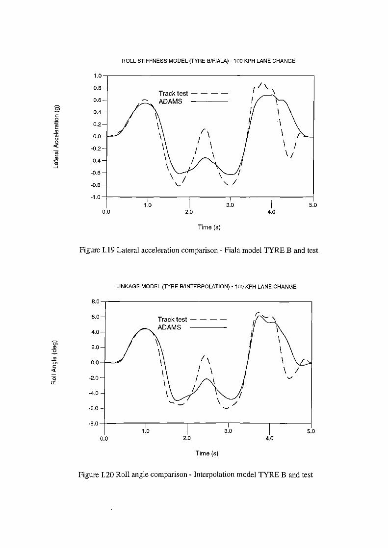
-.9 c 0
~ (])
(i) (.) (.) <{
Cll (D (ii _J
Cl (])
~ (])
Cl c <{
0 a:
1.0
0.8
0.6
0.4
0.2
0.0
-0.2
-0.4
-0.6
-0.8
-1.0
0.0
ROLL STIFFNESS MODEL (TYRE 8/FIALA) -100 KPH LANE CHANGE
1.0
Track test - - - -ADAMS
3.0 2.0
Time (s)
4.0 5.0
Figure 1.19 Lateral acceleration comparison- Fiala model TYRE Band test
8.0
6.0
4.0
2.0
0.0
-2.0
-4.0
-6.0
-8.0
0.0
LINKAGE MODEL (TYRE 8/INTERPOLATION)- 100 KPH LANE CHANGE
1.0
Track test - - - -ADAMS
3.0 2.0
Time (s)
4.0 5.0
Figure 1.20 Roll angle comparison - Interpolation model TYRE B and test

Cl Q)
::s ~ Ol c
<X:
0 a:
Ol Q)
::s ~ Ol c
<X:
0 a:
8.0
6.0
4.0
2.0
0.0
-2.0
-4.0
-6.0
-8.0
ROLL STIFFNESS MODEL (TYRE 8/INTERPOLATION) -100 KPH LANE CHANGE
1.0 0.0
Track test - - - -ADAMS [Effects of Camber not modelled]
./
3.0 2.0
Time (s)
4.0 5.0
Figure 1.21 Roll angle comparison- Interpolation model TYRE Band test
8.0
6.0
4.0
2.0
0.0
-2.0
-4.0
-6.0
-8.0
0.0
ROLL STIFFNESS MODEL (TYRE 8/PACEJKA) -100 KPH LANE CHANGE
1.0
Track test - - - -ADAMS [Effects of Camber not modelled]
3.0 2.0
Time (s)
4.0 5.0
Figure 1.22 Roll angle comparison - Pacejka model TYRE B and test

Ol Q)
:£. Q)
Ol c <(
0 a:
en ..._ Ol Q)
:£. Q)
(ii a: ;: Cll >-
8.0
6.0
4.0
2.0
0.0
-2.0
-4.0
-6.0
-8.0
40.0
30.0
20.0
10.0
0.0
-10.0
-20.0
-30.0
-40.0
0.0
ROLL STIFFNESS MODEL (TYRE B/FIALA) -100 KPH LANE CHANGE
1.0
Track test - - - -ADAMS
2.0
Time (s)
./
3.0 4.0
5.0
Figure I.23 Roll angle comparison - Fiala model TYRE B and test
ROLL STIFFNESS MODEL (TYRE B/INTERPOLATION) -100 KPH LANE CHANGE
1.0 0.0
Track test - - - -ADAMS
/ -
3.0 2.0
Time (s)
4.0 5.0
Figure !.24 Yaw rate comparison - Interpolation model TYRE B and test

(j) ...._ Ol aJ ~ aJ co a: 3: Cll >-
(j) ...._ Ol aJ ~ 2 Cll a: 3: Cll >-
ROLL STIFFNESS MODEL (TYRE 8/INTERPOLATION) -100 KPH LANE CHANGE
40.0
30.0
20.0
10.0-
0.0
-10.0
-20.0
-30.0
-40.0 1.0
0.0
Track test - - - -ADAMS [Effects of Camber not modelled]
3.0 2.0
Time (s)
5.0 4.0
Figure 1.25 Yaw rate comparison - Interpolation model TYRE B and test
40.0
30.0
20.0
10.0
0.0
-10.0
-20.0
-30.0
-40.0
0.0
ROLL STIFFNESS MODEL (TYRE 8/PACEJKA) -100 KPH LANE CHANGE
1.0
Track test - - - -ADAMS [Effects of Camber not modelled]
. 3.0 2.0
Time (s)
4.0 5.0
Figure 1.26 Yaw rate comparison- Pacejka model TYRE Band test

40.0
30.0
20.0
Ul -- 10.0 Cl Q)
~ Q) 0.0 (U a: 3:: -10.0 (1j
>--20.0
-30.0
-40.0
0.0
ROLL STIFFNESS MODEL (TYRE 8/FIALA) -100 KPH LANE CHANGE
1.0
Track test - - - -ADAMS
-3.0
2.0
Time (s)
~
\ \ \ \
4.0
\ I \,
5.0
Figure 1.27 Yaw rate comparison - Fiala model TYRE B and test

APPENDIXJ
SUMMARY OF RESULTS FOR TYRE MODEL VARIATION USING TYRE A ANDTYREB

:§ c 0
~ ~ (]) () ()
<(
co (ij a; _J
-9 c 0
~ ~ (]) () () <(
co (ij a; _J
1.0
0.8
0.6
0.4
0.2
0.0
-0.2
-0.4
-0.6
-0.8
-1.0
0.0
LINKAGE MODEL (TYRE A) -100 KPH LANE CHANGE
1.0
Fiala Pacejka Interpolation
~ ~
2.0 3.0
4.0
Time (s)
5.0
Figure J.l Lateral acceleration comparison using linkage model and TYRE A
ROLL STIFFNESS MODEL (TYRE A) - 100 KPH LANE CHANGE
1.0
0.8
0.6
0.4
0.2
0.0
-0.2
-0.4
-0.6
-0.8
-1.0 1.0 3.0 5.0
0.0 2.0 4.0
Time (s)
Figure J.2 Lateral acceleration comparison using roll stiffness model and TYRE A

Cl (])
~ ~ Cl c <(
0 a:
Oi (])
~ ~ Cl c <(
0 a:
8.0
6.0
4.0
2.0
0.0
-2.0
-4.0
-6.0
-8.0
8.0
6.0
4.0
2.0
0.0
-2.0
-4.0
-6.0
-8.0
LINKAGE MODEL (TYRE A) -100 KPH LANE CHANGE
jt ,, ,, ,, ,, ,, w I
1.0 3.0 5.0 0.0 2.0 4.0
Time (s)
Figure J.3 Roll angle comparison using linkage model and TYRE A
0.0
ROLL STIFFNESS MODEL (TYRE A)- 100 KPH LANE CHANGE
1.0
Fiala Pacejka Interpolation
2.0 3.0
4.0
Time (s)
5.0
Figure J.4 Roll angle comparison using roll stiffness model and TYRE A

(j) ....... Ol Q)
~ Q)
Ia a: 3:: ca >-
(j) ....... Ol Q)
~ Q)
Ia a: 3:: ca >-
40.0
30.0
20.0
10.0
0.0
-10.0
-20.0
-30.0
-40.0
40.0
30.0
20.0
10.0
0.0
-10.0
-20.0
-30.0
-40.0
LINKAGE MODEL (TYRE A) -100 KPH LANE CHANGE
..__'I
1.0 3.0 5.0 0.0 2.0 4.0.
Time (s)
Figure J.5 Yaw rate comparison using linkage model and TYRE A
0.0
ROLL STIFFNESS MODEL (TYRE A)- 100 KPH LANE CHANGE
Fiala Pacejka Interpolation -----
-1.0
2.0
Time (s)
3.0 4.0
5.0
Figure J.6 Yaw rate comparison using roll stiffness model and TYRE A

E' s c Q)
E Q) (.) C1l
Ci. en 0 ~ Q)
(ii _J
"E' s c Q)
E Q) (.) C1l Ci. en 0 ~ Q)
(ii _J
10000.0
8000.0
6000.0
4000.0
2000.0
0.0
-2000.0
-4000.0
-6000.0
-8000.0
-10000.0
0.0
LINKAGE MODEL (TYRE A) -100 KPH LANE CHANGE
Fiala Pacejka Interpolation
40000.0 80000.0
Distance (mm)
1.2E+OE
Figure J.7 Trajectory comparison using linkage model and TYRE A
10000.0
8000.0
6000.0
4000.0
2000.0
0.0
-2000.0
-4000.0
-6000.0
-8000.0
-10000.0
0.0
ROLL STIFFNESS MODEL (TYRE A)- 100 KPH LANE CHANGE
Fiala Pacejka Interpolation
40000.0
-- ,.._
80000.0
Distance (tnm)
1.2E+OE
Figure J.8 Trajectory comparison using roll stiffness model and TYRE A

LINKAGE MODEL (TYRE A) -100 KPH LANE CHANGE
1.0
0.8
0.6
:§ 0.4
c 0
~ 0.2 ~ Q) 0.0 (.) (.) <(
-0.2 (ij (D
-0.4 (ii _J
-0.6
-0.8 * NC - No Camber
-1.0 1.0 3.0 5.0
0.0 2.0 4.0
Time (s)
Figure J.9 Lateral acceleration comparison using linkage model and TYRE A
ROLL STIFFNESS MODEL (TYRE A) -100 KPH LANE CHANGE
1.0
0.8
0.6
:§ 0.4 c
0
~ 0.2
Fiala ---- _ Pacejka (NC) !(, / lnterpolation(NC) ----- 1 I
I' I I
~ Q) 0.0 (.) (.) <(
-0.2 C1l (D
-0.4 (ii _J
~I I I I
I -0.6 * NC - No Camber
-0.8
-1.0 1.0 3.0 5.0
0.0 2.0 4.0
Time (s)
Figure J.IO Lateral acceleration comparison using roll stiffness model and TYRE A

c; Q)
:s. Q)
0! c <(
0 a:
c; Q)
:s. Q)
0! c <(
0 a:
8.0
6.0
4.0
2.0
0.0
-2.0
-4.0
-6.0
-8.0
0.0
LINKAGE MODEL (TYRE A) -100 KPH LANE CHANGE
1.0
Fiala Pacejka (NC) lnterpolation(NC) ----- 1 I
~I \ II \ ~ ~I \ \\ II
2.0
Time (s)
3.0
ft I
'\ \
I \
~ \
'\:.> ~
* NC - No Camber
5.0 4.0
Figure J.ll Roll angle comparison using linkage model and TYRE A
8.0
6.0
4.0
2.0
0.0
-2.0
-4.0
-6.0
-8.0
0.0
ROLL STIFFNESS MODEL (TYRE A) -100 KPH LANE CHANGE
1.0
Fiala - - - - fl Pacejka (NC) 7 .~""' lnterpolation(NC) ---- 1 I ~ r, \ . II
~I 1/
~I I
* NC - No Camber
3.0 2.0 4.0
Time (s)
5.0
Figure J.l2 Roll angle comparison using roll stiffness model and TYRE A

~ Cl (I)
~ 2 c:ll a: :: c:ll >-
(j) --Cl (I)
~ (I)
Cii a: :: c:ll >-
40.0
30.0
20.0
10.0
0.0
-10.0
-20.0
-30.0
-40.0
40.0
30.0
20.0
10.0
0.0
-10.0
-20.0
-30.0
-40.0
0.0
LINKAGE MODEL (TYRE A) -100 KPH LANE CHANGE
Fiala Pacejka (NC) lnterpolation(NC) ----
1.0 3.0 2.0
Time (s)
-
* NC - No Camber
5.0 4.0
Figure J.13 Yaw rate comparison using linkage model and TYRE A
0.0
ROLL STIFFNESS MODEL (TYRE A) -100 KPH LANE CHANGE
Fiala Pacejka (NC) lnterpolation(NC) ----
-1.0 3.0
2.0
Time (s)
* NC - No Camber
5.0 4.0
Figure J.l4 Yaw rate comparison using roll stiffness model and TYRE A

"E .s c Q)
E Q) (.) ca c.. rn 0 ~ Q)
Cii _J
"E E
c Q)
E Q) (.) ca c.. rn 0 ""§ Q)
Cii _J
LINKAGE MODEL (TYRE A) -100 KPH LANE CHANGE
10000.0
8000.0 Fiala
6000.0 Pacejka (NC) lnterpolation(NC) -----
4000.0
2000.0
0.0
-2000.0
-4000.0
-6000.0 * NC - No Camber -8000.0
-10000.0
0.0 40000.0 80000.0 1.2E+OE
Distance (mm)
Figure J.15 Trajectory comparison using linkage model and TYRE A
10000.0
8000.0
6000.0
4000.0
2000.0
0.0
-2000.0
-4000.0
-6000.0
-8000.0
-10000.0
0.0
ROLL STIFFNESS MODEL (TYRE A)- 100 KPH LANE CHANGE
Fiala Pacejka (NC) lnterpolation(NC) ----
~----~~ . ~
40000.0 80000.0
Distance (mm)
~
" -......... --......... --
* NC - No Camber
1.2E+OE
Figure J.16 Trajectory comparison using roll stiffness model and TYRE A

:§ c 0
~ (])
(ij (.) (.) <(
~ 2 c:u
_J
~ c 0
~ J!1 (]) (.) (.) <(
~ (])
[ii _J
1.0
0.8
0.6
0.4
0.2
0.0
-0.2
-0.4
-0.6
-0.8
-1.0
0.0
LINKAGE MODEL (TYRE B) -100 KPH LANE CHANGE
1.0
Fiala Pacejka (NC) Interpolation
2.0
* NC - No Camber
3.0 4.0
Time (s)
5.0
Figure J.17 Lateral acceleration comparison using linkage model and TYRE B
ROLL STIFFNESS MODEL (TYRE B) -100 KPH LANE CHANGE
1.0
0.8 Fiala ----Pacejka (NC)
0.6 Interpolation -----
0.4
0.2
0.0
-0.2
-0.4
-0.6 * NC - No Camber
-0.8
-1.0 1.0 3.0 5.0
0.0 2.0 4.0
Time (s)
Figure J.18 Lateral acceleration comparison using roll stiffness model and TYRE B
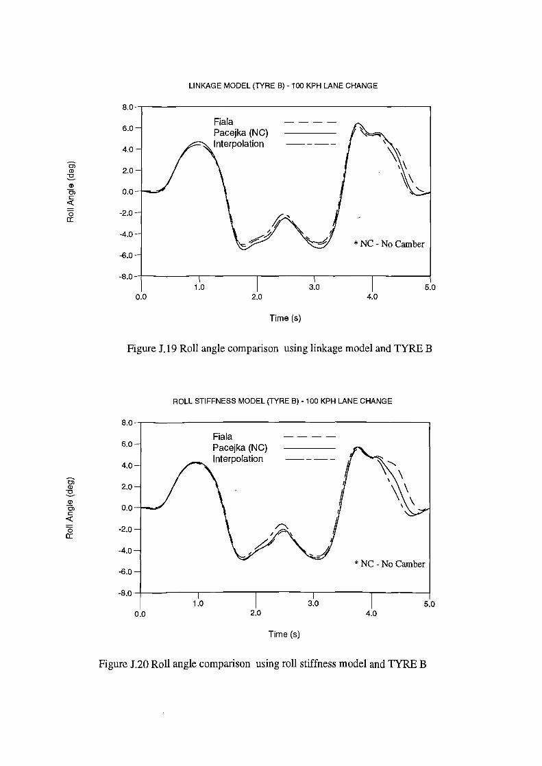
Cl Q)
~ Q)
0> c
<X: 0 a:
o; Q)
~ Q)
0> c
<X: 0 a:
8.0
6.0
4.0
2.0
0.0
-2.0
-4.0
-6.0
-8.0
0.0
LINKAGE MODEL (TYRE B) -100 KPH LANE CHANGE
1.0
Fiala Pacejka (NC) Interpolation
2.0
Time (s)
\
* NC - No Camber
3.0 4.0
5.0
Figure J.19 Roll angle comparison using linkage model and TYRE B
8.0
6.0
4.0
2.0
0.0
-2.0
-4.0
-6.0
-8.0
0.0
ROLL STIFFNESS MODEL (TYRE B) - 100 KPH LANE CHANGE
1.0
Fiala Pacejka (NC) Interpolation
2.0
Time (s)
* NC - No Camber
3.0 5.0 4.0
Figure J.20 Roll angle comparison using roll stiffness model and TYRE B

Vi" -.... Ol Q)
~ 2 Cll a: :;: Cll >-
Vi" -.... Ol Q)
~ Q)
ta a: :;: Cll >-
40.0
30.0
20.0
10.0
0.0
-10.0
-20.0
-30.0
-40.0
40.0
30.0
20.0
10.0
0.0
-10.0
-20.0
-30.0
-40.0
0.0
LINKAGE MODEL (TYRE B) -100 KPH LANE CHANGE
Fiala Pacejka (NC) Interpolation
1.0 2.0
Time (s)
* NC - No Camber
3.0 5.0 4.0
Figure J.21 Yaw rate comparison using linkage model and TYRE B
0.0
ROLL STIFFNESS MODEL (TYRE B)- 100 KPH LANE CHANGE
Fiala Pacejka (NC) Interpolation
1.0 2.0
Time (s)
* NC - No Camber
3.0 5.0 4.0
Figure J.22 Yaw rate comparison using roll stiffness model and TYRE B

E' .s c (])
E (]) (.)
..!!! 0.. (fJ
0 ~ (])
Cii __J
E' .s c (])
E (]) (.) (1l
a. (fJ
0 ~ 2 (1l
__J
10000.0
7500.0
5000.0
2500.0
0.0
-2500.0
-5000.0
-7500.0
-10000.0
0.0
LINKAGE MODEL (TYRE B)- 100 KPH LANE CHANGE
Fiala Pacejka (NC) Interpolation
40000.0
Distance (mm)
* NC - No Camber
80000.0 1.2E+OE
Figure J.23 Trajectory comparison using linkage model and TYRE B
10000.0
7500.0
5000.0
2500.0
0.0
-2500.0
-5000.0
-7500.0
-10000.0
0.0
ROLL STIFFNESS MODEL (TYRE B)- 100 KPH LANE CHANGE
Fiala Pacejka (NC) Interpolation
40000.0
Distance (mm)
* NC - No Camber
80000.0 1.2E+OE
Figure J.24 Trajectory comparison using roll stiffness model and TYRE B

LINKAGE MODEL (TYRE B) -100 KPH LANE CHANGE
1.0
0.8 Fiala
0.6
:§ 0.4
Pacejka (NC) lnterpolation(NC) ----- d
c 0
~ 0.2 ~ Q) 0.0 (.)
0 (.) <(
-0.2 (U (0
-0.4 "'iii _J
-0.6
-0.8 * NC - No Camber
-1.0 1.0 3.0 5.0
0.0 2.0 4.0
Time (s)
Figure J.25 Lateral acceleration comparison using linkage model and TYRE B
ROLL STIFFNESS MODEL (TYRE B)- 100 KPH LANE CHANGE
1.0
0.8 Fiala ----
0.6
:§ 0.4
c
Pacejka (NC) v lnterpolation(NC) ----- i
0
~ 0.2 ~ Q) 0.0 (.) (.) <(
-0.2 ~ Q)
-0.4 "'iii _J
-0.6 * NC - No Camber
-0.8
-1.0 1.0 3.0 5.0
0.0 2.0 4.0
Time (s)
Figure J.26 Lateral acceleration comparison using roll stiffness model and TYRE B

Oi (])
~ ~ Cl c <(
0 a:
Cl (])
~ (])
0> c
<(
0 a:
8.0
6.0
4.0
2.0
0.0
-2.0
-4.0
-6.0
-8.0
0.0
LINKAGE MODEL (TYRE B) -100 KPH LANE CHANGE
1.0
Fiala Pacejka (NC) lnterpolation(NC) -----
3.0 2.0
Time (s)
\ \ ~'-
* NC - No Camber
4.0 5.0
Figure J.27 Roll angle comparison using linkage model and TYRE B
8.0
6.0
4.0
2.0
0.0
-2.0
-4.0
-6.0
-8.0
0.0
ROLL STIFFNESS MODEL (TYRE B) - 100 KPH LANE CHANGE
1.0
Fiala Pacejka (NC) lnterpolation(NC) -----
3.0 2.0
Time (s)
* NC - No Camber
4.0 5.0
Figure J.28 Roll angle comparison using roll stiffness model and TYRE B

~ CD ~ 2 as a: ~ as
>-
~ CD ~ 2 as a: ~ as >-
40.0
30.0
20.0
10.0
0.0
-10.0
-20.0
-30.0
-40.0
0.0
LINKAGE MODEL (TYAE B)· 100 KPH LANE CHANGE
Fiala Pacejka (NC) lnterpolation(NC) ----
1.0 3.0 2.0
T:me (s)
* NC - No Camber
5.0 4.0
Figure 1.29 Yaw rate comparison using linkage model and TYRE B
40.0
30.0
20.0
10.0
0.0
-10.0
-20.0
-30.0
-40.0
0.0
ROLL STIFFNESS MODEL (TYRE B)- 100 KPH LANE CHANGE
Fiala Pacejka (NC) lnterpolation(NC) ----
1.0 3.0 2.0
Time (s)
* NC - No Camber
5.0 4.0
Figure J.30 Yaw rate comparison using roll stiffness model and TYRE B

E .s c Q)
E Q) (.) ca
Q_ CJ)
0 ~ Q)
(ii _J
E E
c Q)
E Q) (.) ca
Q_ CJ)
0 ~ Q)
(ii _J
10000.0
7500.0
5000.0
2500.0
0.0
-2500.0
-5000.0
-7500.0
-10000.0
0.0
LINKAGE MODEL (TYRE B) -100 KPH LANE CHANGE·
Fiala Pacejka (NC) lnterpolation(NC) ----
40000.0
Distance (mm)
* NC - No Camber
80000.0 1.2E+O!:
Figure J.31 Trajectory comparison using linkage model and TYRE B
10000.0
7500.0
5000.0
2500.0
0.0
-2500.0
-5000.0
-7500.0
-10000.0
0.0
ROLL STIFFNESS MODEL (TYRE B)- 100 KPH LANE CHANGE
Fiala Pacejka (NC) lnterpolation(NC) -----
40000.0
Distance (mm)
* NC - No Camber
80000.0 1.2E+O!:
Figure J.32 Trajectory comparison using roll stiffness model and TYRE B

APPENDIXK
SENSITIVITY STUDIES BASED ON TYRE BAND THE ROLL STIFFNESS MODEL

en .._ Ol Q)
~ Q) -ell a: ~ ell >-
en ..._ Ol Q)
~ (])
co a: ~ ell >-
40.0
30.0
20.0
10.0
0.0
-10.0
-20.0
-30.0
-40.0
0.0
ROLL STIFFNESS MODEL- 100 KPH LANE CHANGE CORNERING STIFFNESS COMPARISON- TYRE 8
Cu=30000N/rad ---Cu=60000N/rad - - - -Cu=90000N/rad ----
1.0 2.0
Time (s)
3.0 4.0
Figure K.l Yaw rate comparison for varying cornering stiffness
40.0
30.0
20.0
10.0
0.0
-10.0
-20.0
-30.0
-40.0
0.0
ROLL STIFFNESS MODEL- 100 KPH LANE CHANGE FRICTION COEFFICIENT COMPARISON- TYRE 8
J.l = 1 .0 J.l = 0.6 J.l = 0.2
1.0 2.0
3.0 4.0
Time (s)
Figure K.2 Yaw rate comparison for varying friction coefficient
5.0
5.0

Oi Q)
~ Q)
Ol c <{
0 a:
8.0
6.0
4.0
2.0
0.0
-2.0
-4.0
-6.0
-8.0
0.0
ROLL STIFFNESS MODEL- 100 KPH LANE CHANGE RADIAL STIFFNESS COMPARISON - TYRE B
Kz= 150 N/mm Kz=75 N/mm
/........_
I \ II ~
1.0 3.0 2.0 4.0
Time (s)
Figure K.3 Roll angle comparison for varying radial stiffness
ROLL STIFFNESS MODEL- 100 KPH LANE CHANGE CENTRE OF MASS HEIGHT COMPARISON - TYRE B
5.0
8.0--r------------------------,
Original 6.0 Raise lOOmm ___ _
/........_ 4.0 I \
2.0 II \
~ Q)
Ol 0.0 c <{
0 -2.0 a:
-4.0
-6.0
-8.0 -1-----r--------r-----...----------r-------1 1.0 3.0 5.0
0.0 2.0 4.0
Time (s)
Figure K.4 Roll angle comparison for varying mass centre height

(])
ROLL STIFFNESS MODEL- 100 KPH LANE CHANGE ROLL CENTRE HEIGHT COMPARISON- TYRE B
8.0-r---------------------------.,
6.0
4.0
2.0
0> 0.0 c <(
0 a: -2.0
-4.0
-6.0
-8.0--t------.-----.-------r----....,-------l
0.0 1.0 3.0 5.0
2.0 4.0
Time (s)
Figure K.5 Roll angle comparison for varying roll axis position
ROLL STIFFNESS MODEL- 100 KPH LANE CHANGE REAR WHEEL TOE ANGLE STUDY
~.0-r---------------------------.,
One degree toe in - - - -30.0 Zero toe angle
One degree toe out -----20.0
~ fir 10.0 ~ ~ 0.0 a: ~ -10.0 >-
-20.0
-30.0
-40.0 --t------.-----.-------r----....,-------l
1.0 3.0 5.0 0.0 2.0 4.0
Time (s)
Figure K.6 Yaw rate comparison for rear wheel toe angle study

APPENDIXL
ASSOCIATED PUBLICATIONS

1. Blundell M. V. Automatic dynamic analysis of mechanical systems. Proc. Computer Vision
UK Users Group- Summer Conference, Birmingham, June 1990.
2. Blundell M.V. Full vehicle modelling and simulation using the ADAMS software system.
!MechE Paper C427/161170, Autotech '91, Birmingham, November 1991.
3. Manning A.S. and Blundell M.V. The modelling and simulation of automotive suspension
systems. Proc. Thirteenth lASTED International Conference - Modelling, Identification and
Control ( MIC '94), ISBN 0-88986-183-8, pp 83-85, Grindelwald, February 1994.
4. Blundell M.V. The use of multibody systems analysis software for an engineering student
project. Proc. Thirteenth lASTED International Conference - Modelling, Identification and
Control ( MIC '94), ISBN 0-88986-183-8, pp 462-464, Grindelwald, February 1994.
5. Blundell M.V. Vehicle suspension and handling studies. Proc. !MechE Seminar S275,
Multi-Body System Dynamic Codes for Vehicle Dynamic Applications, London, June 1994.
6. Blundell M. V., Phillips B.D.A. and Mackie A. The modelling and simulation of
suspension systems, tyre forces and full vehicle handling performance. Proc. Tenth
International Conference on Systems Engineering (ICSE '94), ISBN 090594234, pp 111-118,
Coventry, September 1994.
7. Manning A.S. and Blundell M.V. The modelling requirements of automotive suspension
systems for accurate handling simulations. Proc Fourteenth lASTED International Conference
- Modelling, Identification and Control (MIC'95), ISBN 0-88986-212-5, pp 158-160,
Innsbruck, February 1995.
8. Blundell M. V., Phillips B.D.A. and Mackie A. A comparison of three full vehicle models
for vehicle handling simulation. Proc. Fourteenth lASTED International Conference -
Modelling, Identification and Control (MIC'95), ISBN 0-88986-212-5, pp 155-157,
Innsbruck, February 1995.

9. Mackie A., Blundell M.V. and Phillips B.D.A. The modelling and simulation of Anti
Lock Braking systems in ADAMS. Proc. Fourteenth lASTED International Conference -
Modelling, Identification and Control (MIC'95), ISBN 0-88986-212-5, pp 161-163,
Innsbruck, February 1995.
10. Blundell M. V. and Mackie A. Mechanical system simulation - a possible tool for product
design students. Proc. of the 2nd National Conference on Product Design Education, PDE95,
Coventry, July 1995.
11. Blundell M.V. Prediction of dynamic loads for finite element models. The Fifth
International Conference on Structural Failure, Product Liability and Technical Assurance -
SPT-5, Vienna, July 1995.
12. Blundell M. V., Phillips B.D.A. and Mackie A. The modelling and simulation of vehicle
handling and braking. Pro c. of the 2nd International Conference on Road Vehicle Automation,
ROVA '95, Bolton, September 1995.
13. Blundell M.V. Full vehicle modelling and the requirements for accurate handling
simulations. !MechE Conference, Autotech '95, Birmingham, November 1995.
14. Manning A.S. and Blundell M.V. A range of full vehicle models for transient handling
simulations. Proc Fifteenth lASTED International Conference- Modelling, Identification and
Control (MIC'96), ISBN 0-88986-193-5, pp 194-196, Innsbruck, February 1996.
15. Dunn W.H. and Blundell M.V. Simulation as a tool to predict vehicle handling. Proc
29th ISATA Conference - Simulation, Diagnosis, and Virtual Reality Applications in the
Automotive Industry, ISBN 0-947719-80-6, pp 129-136, Florence, June 1996.
16. Mackie A.R., Blundell M.V. and Dunn W.H. Simulation as a tool to predict anti-lock
braking performance. Proc 29th ISATA Conference - Simulation, Diagnosis, and Virtual
Reality Applications in the Automotive Industry, ISBN 0-947719-80-6, pp 69-75, Florence,
June 1996.

17. Blundell M. V. Full vehicle modelling and the requirements for accurate handling
simulations. !MechE book publication "Automotive Refinement" ( 1 86058 021 1 ),
C49817/005!95, pp. 77-91, July 1996.
18. Blundell M.V., Phillips B.D.A. and Mackie A. The role of multibody systems analysis in
vehicle design. Journal of Engineering Design, Vol. 7, No. 4, pp. 377-396, December 1996.
19. Blundell M.V. Prediction of dynamic loads for finite element models. ISTL Special
Publication 3, Failures and the Law, (Structural Failure, Product Liability and Technical
Insurance 5 ), E & FN SPON (An Imprint of Chapman & Hall), ISBN 0-419-22080-1, pp 523-
531, 1996.
20. Blundell M. V., Dunn W.H. and Manning A.S. The development of suspension models
for vehicle handling simulation. Proc. of the IASTED/ISMM International Conference -
Modelling and Simulation, ISBN 0-88986-221-4, pp 247-249, Pittsburgh, May 1997.
21. Blundell M.V., Dunn W.H. and Manning A.S. The interpretation of tyre models for
vehicle handling simulation. Proc. of the IASTEDIISMM International Conference - Modelling
and Simulation, ISBN 0-88986-221-4, pp 250-253, Pittsburgh, May 1997.
22. Blundell M. V., Phillips B.D.A. and Mackie A. The modelling and simulation of vehicle
handling and braking. Road Vehicle Automation II, edited by C. Nwagboso, Wiley,
ISBN 0-471-96726-2, pp 133-14, 1997.
23. Blundell M. V. The modelling and simulation of a vehicle lane change manoeuvre. 3rd
International Conference on Road Vehicle Automation, ROVA '97, Salamanca, September
1997.
Coventry University
Related Documents


![Genuine Husqvarna · PDF file40 Trimmer & brushcutter accessories ... Replacement parts for pro forest and pro arborist helmet 505 67 53-18 [1] Sweatband 505 67 53-30 [2] 6 pt suspension](https://static.cupdf.com/doc/110x72/5aa066f87f8b9a0d158e1f97/genuine-husqvarna-trimmer-brushcutter-accessories-replacement-parts-for-pro.jpg)