The Influence of Kerosene on Microbiomes of Diverse Soils

�����������������

Citation: Shelyakin, P.V.; Semenkov,

I.N.; Tutukina, M.N.; Nikolaeva, D.D.;

Sharapova, A.V.; Sarana, Y.V.; Lednev,

S.A.; Smolenkov, A.D.; Gelfand, M.S.;

Krechetov, P.P.; et al. The Influence of

Kerosene on Microbiomes of Diverse

Soils. Life 2022, 12, 221. https://

doi.org/10.3390/life12020221

Academic Editor: Tanya Soule

Received: 17 December 2021

Accepted: 27 January 2022

Published: 31 January 2022

Publisher’s Note: MDPI stays neutral

with regard to jurisdictional claims in

published maps and institutional affil-

iations.

Copyright: © 2022 by the authors.

Licensee MDPI, Basel, Switzerland.

This article is an open access article

distributed under the terms and

conditions of the Creative Commons

Attribution (CC BY) license (https://

creativecommons.org/licenses/by/

4.0/).

life

Article

The Influence of Kerosene on Microbiomes of Diverse SoilsPavel V. Shelyakin 1,2,†, Ivan N. Semenkov 3,*,† , Maria N. Tutukina 1,4,5,†, Daria D. Nikolaeva 1,4,†,Anna V. Sharapova 3, Yulia V. Sarana 4, Sergey A. Lednev 3, Alexander D. Smolenkov 6, Mikhail S. Gelfand 1,4,‡,Pavel P. Krechetov 3,‡ and Tatiana V. Koroleva 3,‡

1 Institute for Information Transmission Problems (Kharkevich Institute), Russian Academy of Sciences,127051 Moscow, Russia; [email protected] (P.V.S.); [email protected] (M.N.T.);[email protected] (D.D.N.); [email protected] (M.S.G.)

2 Department of Computational Biology, N.I. Vavilov Institute of General Genetics,Russian Academy of Sciences, 119333 Moscow, Russia

3 Faculty of Geography, M.V. Lomonosov Moscow State University, 119991 Moscow, Russia;[email protected] (A.V.S.); [email protected] (S.A.L.); [email protected] (P.P.K.);[email protected] (T.V.K.)

4 Center of Molecular and Cellular Biology, Skolkovo Institute of Science and Technology,121205 Moscow, Russia; [email protected]

5 Lab of Functional Genomics and Cellular Stress, Institute of Cell Biophysics RAS, 142290 Moscow, Russia6 Faculty of Chemistry, M.V. Lomonosov Moscow State University, 119991 Moscow, Russia; [email protected]* Correspondence: [email protected]† These authors contributed equally to this work.‡ These authors contributed equally to this work.

Abstract: One of the most important challenges for soil science is to determine the limits for thesustainable functioning of contaminated ecosystems. The response of soil microbiomes to kerosenepollution is still poorly understood. Here, we model the impact of kerosene leakage on the composi-tion of the topsoil microbiome in pot and field experiments with different loads of added kerosene(loads up to 100 g/kg; retention time up to 360 days). At four time points we measured keroseneconcentration and sequenced variable regions of 16S ribosomal RNA in the microbial communities.Mainly alkaline Dystric Arenosols with low content of available phosphorus and soil organic matterhad an increased fraction of Actinobacteriota, Firmicutes, Nitrospirota, Planctomycetota, and, to alesser extent, Acidobacteriota and Verrucomicobacteriota. In contrast, in highly acidic Fibric Histosols,rich in soil organic matter and available phosphorus, the fraction of Acidobacteriota was higher,while the fraction of Actinobacteriota was lower. Albic Luvisols occupied an intermediate positionin terms of both physicochemical properties and microbiome composition. The microbiomes ofdifferent soils show similar response to equal kerosene loads. In highly contaminated soils, theproportion of anaerobic bacteria-metabolizing hydrocarbons increased, whereas the proportion ofaerobic bacteria decreased. During the field experiment, the soil microbiome recovered much fasterthan in the pot experiments, possibly due to migration of microorganisms from the polluted area.The microbial community of Fibric Histosols recovered in 6 months after kerosene had been loaded,while microbiomes of Dystric Arenosols and Albic Luvisols did not restore even after a year.

Keywords: soil metagenome; jet-fuel; soil pollution; ecological indicators; controlled study; gasoline;biodegradation; total petroleum hydrocarbons; bearing capacity; xenobiotic compounds

1. Introduction

Hydrocarbons serve as the main fuel for transportation engines worldwide, makingenvironmental pollution by hydrocarbons one of the major current ecological threats. Hy-drocarbons disrupt intra-soil habitat conditions by filling in the pore spaces and impairingthe water and air exchange, thus transforming the composition of soil microorganisms. Incase of contamination, most groups die out while the fitter ones resist or even expand.

Life 2022, 12, 221. https://doi.org/10.3390/life12020221 https://www.mdpi.com/journal/life

Life 2022, 12, 221 2 of 22

Only a few studies have addressed the bacterial communities of terrestrial soils con-taminated with different hydrocarbons, such as [1]. Still, they provide insufficient dataon the sensitivity and resistance of various groups of soil microorganisms to kerosenecontamination in natural conditions. Kerosene is a combustible hydrocarbon liquid derivedfrom petroleum and widely used in industry as a jet-fuel. Particularly, according to theavailable data, the duration of hydrocarbon biodegradation in different environmentsmay vary from several months to several decades [2–7]. Although a wide range of hy-drocarbons may adversely affect ecosystems, the research mainstream has focused on theimpact of crude and tank oil on aquatic and coastal ecosystems, paying little attention tokerosene-contaminated soils.

Recent studies have identified bacteria from more than 79 genera capable of de-grading petroleum hydrocarbons [8]. In undisturbed soils, the proportion of bacteriacapable of decomposing hydrocarbons is negligible [9], while the hydrocarbon contamina-tion results in an increase in their abundance, e.g., Pseudomonas and Burkholderia in man-groves polluted by tank oil in Okinawa [10]. Bacteria from the Achromobacter, Acinetobacter,Alkanindiges, Alteromonas, Arthrobacter, Burkholderia, Dietzia, Enterobacter, Kocuria, Marinobacter,Mycobacterium, Pandoraea, Pseudomonas, Rhodococcus, Staphylococcus, Streptobacillus, andStreptococcus genera play vital roles in degrading petroleum hydrocarbons [11]. Interest-ingly, that some initially rare taxa, e.g., Alkanindiges sp., can even become dominant inresponse to such pollution [11].

As alkanes from C5 to C9 are highly volatile, quickly evaporate from the topsoil [12,13],and are not highly toxic to humans, their impact on soil properties and microbiome isunderstudied. Following the one health approach [14], it is important to understand thedanger of certain substances for each component of a whole ecosystem. It is necessaryto analyze their impact on the soil microbiota, even if they are non-toxic or little-toxicfor humans.

This study bridges the gap in our knowledge on the environmental consequences ofcontamination with TS-1 kerosene, which is the fuel most commonly used for commercialaviation in Russia [15]. We investigated three contrast soil reference groups and analyzedthe topsoil physicochemical properties and the microbiome composition. We conducted alaboratory pot experiment with the Dystric Arenosols (N 45◦43′20′′ E 63◦11′40′′) sampledin Kazakhstan and Albic Luvisols (N 55◦11′5′′ E 36◦25′5′′) of Russia and a field experimentwith Fibric Histosols (N 55◦11′03′′ E 36◦24′58′′) and the same Albic Luvisols in Russia.

Our research objective was to characterize the responses of soil microbiomes tokerosene contamination under humid and semi-arid climates. We observed that thekerosene content decreased faster under natural conditions than in a laboratory experiment.The response of soil microbiomes to kerosene contamination was similar in the laboratoryand field experiments, that is, in the steady and natural environments, respectively.

2. Materials and Methods

The selected soils are representative of humid landscapes of temperate mixed forests(the Kaluga region in the Russian Federation) and semi-arid landscapes of deserts (theKyzylorda region in the Republic of Kazakhstan).

The Kaluga region is located at the south-east of the Smolensk–Moscow Upland. Theregion is characterized by a snowy fully humid climate with a warm summer [16] andwith an annual precipitation of about 650 mm. The growing season lasts from May toSeptember. The parent rocks of well-drained interfluves and slopes are the Quaternaryloess-like loams at least 2 m thick underlain by lacustrine sediments. Fibric Histosols with apeat thickness of about 1.5 m are formed in local depressions of the interfluves, on the clayicor loamic rocks under the sphagnum mosses. Albic Luvisols represent the predominantsoil in this region.

The Baikonur Cosmodrome area encompasses a part of the Daryalyk residual plateaurepresented by an undulating plain composed of stony clay loams and sandy loams, and apart of a terraced valley of the Syr Darya river [17]. Arenosols, Calcisols, and Gypsisols

Life 2022, 12, 221 3 of 22

are the most typical soils of the region. The region is characterized by a cold arid desertclimate [16], with the annual precipitation of about 100–120 mm. The most favorablehydrothermal regime for the biota development takes place in the periods from March toJune and from September to November [7,17].

2.1. Pot Experiment

Two A-horizon soil samples (20 kg, natural moisture) were sieved using sieves witha 3 mm mesh, cleaned of roots and other coarse fractions, and dried to the air-dry state.Before the pot experiment, the samples were moistened to a level of 60% of the maximumfield capacity. To reach the uniform absorption of distilled water, the soil was thoroughlymixed each time after water was added. The soil moisture before the kerosene contamina-tion, determined gravimetrically, was 22.7 ± 0.5% and 5.2 ± 0.3% for Albic Luvisols andDystric Arenosols, respectively. Then, the samples were stored in plastic bags (temperature18–22 ◦C) for three days to activate the soil microbiome and were carefully and periodicallystirred to homogenize while preserving soil micro-aggregates [18].

After three days (time point 0), both soil samples were divided into six subsamples(Supplementary Figure S1). One subsample without any contamination was used as acontrol. The remaining five subsamples were treated with various loads (1, 5, 10, 25, and100 g/kg of soil, separately) of kerosene. Low kerosene loads (1, 5, and 10 g/kg) wereapplied as a spray. High loads (25 and 100 g/kg) were applied from a watering can.The loads were selected based on the previous results on the response of vegetation [18],cultivated soil microorganisms [19], and cellulolytic bacteria [20] to kerosene contamination.

All subsamples (12 in total) were placed into the glass containers with hermeticallysealed iron lids to the bulk density of 1.47 ± 0.04 and 0.92 ± 0.09 kg/dm3, which is typicalof natural Dystric Arenosols and Albic Luvisols, respectively. The experiment lasted for12 months in 2019–2020 at a temperature of 18–22 ◦C. Every 5 days, the containers wereopened for ventilation and, if needed, moisturized with distilled water.

2.2. Field Experiment

The field experiment was conducted on Albic Luvisols under a spruce–aspen forestand Fibric Histosols under a subshrub–sphagnum pine forest in the Kaluga region in2020–2021.

Experimental plots with a size of 50 × 50 cm (Supplementary Figure S2) were selectedbased on the microtopography, comprising spatial homogeneous microsites without visiblemicroslopes of the soil surface. The surface of each plot was cleared of plant litter to reducepossible redistribution of kerosene over the soil surface and to achieve better absorptioninto the topsoil. Plots were contaminated with the same kerosene TS-1 loads for the 0–10 cmtopsoil layer as in the pot experiment.

The field experiment lasted for 12 months from 2020–2021 under the natural conditions(Supplementary Table S1). Topsoil samples were collected in summer (3 and 360 days aftertreatment), fall (90 days), and early winter (180 days).

2.3. Soil Sampling and Chemical Analysis

In total, 288 topsoil (0–10 cm) samples, 50 g each, were collected, in triplicate, 3, 90, 180,and 360 days after the kerosene contamination. For the chemical analysis, each replicatewas placed into a glass jar with metal lids. Then, subsamples of 1–2 g were collected for theisolation of total DNA.

In 96 soil samples (1 mixed sample of the triplicate replicas), chemical analysis wasperformed immediately after soil sampling using routine techniques for pH, moisture,cation exchange capacity (CEC), content of soil organic matter (SOM), available phosphorus(Pav) and potassium (Kav), exchangeable ammonium (NH4

+), and water-soluble nitrate(NO3

−), as described in Supplementary Table S2.In 288 soil samples, kerosene concentration was determined using the original method

partially reported in [21]. Briefly, we used a system of the Agilent 7890 V gas chromatograph

Life 2022, 12, 221 4 of 22

by Agilent Technologies (Santa Clara, CA, USA) equipped with a 5977 A quadrupole mass-spectrometric detector. Samples of natural moisture weighing 1–2 g were placed into glassflasks. After that, 0.2 cm3 of 1 g/dm3 1-chlorooctadecane solution (internal standard), 2 g ofNa2SO4, and 10–20 cm3 of dichloromethane were added, and the flasks were loosely closed.The extraction was carried out for 15 min in an ultrasonic bath. The extract was filteredthrough a paper filter (a red ribbon), previously washed with 3 cm3 of dichloromethane.The flask and the filter were rinsed with 5 cm3 of dichloromethane. The filtrates werecombined and transferred into 2 cm3 glass vials. Two parallel measurements were made.To calibrate the chromatograph, we used the soil samples unpolluted with kerosene and jet-fuel used for experiments. The retention time range of the components of kerosene and theretention time of the internal standard were determined using the obtained chromatograms.We found the total area of all peaks on the chromatogram using the total ion current and thearea of the internal standard and calculated the ratio of the total peak area of all kerosenecomponents to the peak area of the internal standard.

2.4. DNA Extraction, Amplification and Sequencing

Total DNA from soil subsamples was isolated using DNeasy PowerSoil (Qiagen,Hilden, Germany). Three independent samples were collected from each pot and plot.Further, they were placed immediately either into a PowerBead tube, or into a sterile 1.5 mLtube and stored at −20 ◦C prior to extraction. Each sample of 300 mg was placed intoa PowerBead tube, then 60 µL of the C1 buffer were added, and the tube was inverted4–5 times to mix the reagents. The samples were then disrupted using TissueLyser II orTissueLyser LT (Qiagen, Hilden, Germany, 10 min, 30 Hz). Further DNA purification wasmade according to the manufacturer’s protocol.

DNA concentration was measured on the Qubit 1 fluorimeter using the Qubit DNA HSkit (Thermo Fisher Scientific, Waltham, MA, USA) and ranged from 2 to 3 ng/µL. Variable16S rRNA regions were amplified with two primer combinations, V3/V4 and V4/V5(341F 5′–CCTAYGGGRBGCASCAG–3′ and 806R 5′–GGACTACNNGGGTATCTAAT–3′;515F 5′–GTGCCAGCMGCCGCGGTAA–3′ and 907R 5′–CCGTCAATTCCTTTGAGTTT–3′,respectively) using the Phusion polymerase (New England Biolabs, Ipswich, MA, USA)and the following program:

Step 1: 95 ◦C 2 min (initial DNA melting);24 cycles as follows:Step 2: 95 ◦C 30 s (melting);Step 3: 58 ◦C 30 s (primer annealing);Step 4: 72 ◦C 40 s (synthesis);Step 5: 72 ◦C 5 min.To prepare sequencing libraries, amplicons were purified using the AMPure XP beads

(Beckman Coulter, Brea, CA, USA) according to the manufacturer’s protocol. The ampliconconcentrations were measured on the Qubit 1 fluorimeter using the Qubit DNA HS kit(Thermo Fisher Scientific, Waltham, MA, USA) and ranged from 0.8 to 40 ng/µL. Samplescontaining no DNA processed in the same laboratory were used as negative controls, theirconcentrations were in the range of 0.2–0.6 ng/µL.

To skip the adaptor ligation step, all primers already contained Illumina 1 (forwardprimer) or Illumina 2 (reverse primer) adaptors. Index PCR was made using the Phusionpolymerase (New England Biolabs, Waltham, MA, USA) and the Nextera XT Index kit(Illumina, San Diego, CA, USA) following the manufacturer’s protocols. The libraryconcentrations were measured on the Qubit 1 fluorimeter using the Qubit DNA HS kit(Thermo Fisher Scientific, Ipswich, MA, USA), and the libraries were sequenced on IlluminaMiSeq with the read length of 250 bp (MiSeq Reagent Kit v2). The average number of readswas 75,000 per sample.

Life 2022, 12, 221 5 of 22

2.5. 16S rRNA Sequencing Data Analysis

The quality of reads was analyzed with FastQC [22]. Quality filtering, denoising,paired reads merging, and chimera filtering were performed using the R package DADA2v. 1.14.1 [23]. Parameters for DADA2 were modified to lose less than 50% of reads in thepipeline (maxEE = c(3,3), minOverlap = 8, maxMismatch = 1, minFoldParentOverAbun-dance = 8). The obtained Amplicon Sequence Variants (ASV) tables were analyzed andfiltered of potential contaminants using the R package phyloseq [24] and decontam [25],respectively, taking into account the amplicon concentrations and ASVs found in negativecontrols. Low total numbers of reads in negative controls and the results of the decontamanalysis indicated low levels of contamination. After filtration and removing the singletonASVs, the mean number of reads in the samples was approximately 52,000.

Taxonomic labels were assigned to ASVs using IdTaxa [26] from the R package deci-pher [27] trained on 16S rRNA gene sequences from the SILVA database [28]. After that,ASVs assigned to “Chloroplast” and ASVs not classified at the domain level were filteredout and all samples were rarefied to a standard number of reads (10,000 reads) in order toaccount for differences in sequencing depth.

Multiple alignment of ASVs and construction of phylogenetic trees was conductedusing AlignSeqs [29] from the decipher package and FastTree v.2.1.11 [30], respectively.

The metabolic potential of microbial communities in the samples was predicted withPicrust2 [31]. Principal Component Analysis (PCA) (function prcomp in R) on the relativeabundance of predicted MetaCyc pathways was used to visualize metabolic potentialsimilarities between the samples.

2.6. Assessment of Soil Microbial Community Diversity and Statistical Analysis

The diversity analysis was carried out using the R package vegan [32]. The within-sample (alpha) diversity was estimated using the Shannon index. The between-samples(beta) diversities were estimated using the Bray–Curtis dissimilarity and weighted Unifrac.To visualize the between-sample diversity, dimensionality reduction with the PrincipalCoordinate Analysis (PCoA) was performed.

To ensure that changes in bacterial communities did not result only from their deathunder high kerosene concentrations, the relative amount of bacteria in soil samples withor without kerosene load at different time points was measured by quantitative PCR with341F–806R primers. qPCR was performed using qPCRMix HS-SYBR (Evrogen, Moscow,Russia) and DT-Lite machine (DNA Technology, Moscow, Russia). Each sample wasassayed in triplicate. The differences were calculated using ∆Ct.

Permutational Multivariate Analysis of Variance (PERMANOVA) using distance ma-trices implemented in the adonis function from the vegan package was used to estimatethe significance of microbiome differences between the studied conditions. The FDR correc-tion (Benjamini-Hochberg) for multiple testing was applied separately for different testsin different soils. Aldex2 [33] was used to search for bacterial groups which proportionsignificantly differed between the studied conditions.

3. Results and Discussion

The chosen soils are most representative for studying kerosene contamination. Thesoils of the Kaluga region could be considered as the background for the Moscow region [20].The latter’s contamination with kerosene occurs because it is the largest aviation hub inRussia. Dystric Arenosols are the most vulnerable soils in the Baikonur Cosmodrome area,where ‘Soyuz’ vehicles propelled by kerosene are launched and an airport is situated [7,15].

Since the choice of a 16S rRNA region for sequencing may introduce a bias to the finalresults [34], we tested two different sets of primers for 16S rRNA region V3V4 and V4V5.The results obtained with these two 16S rRNA regions were highly consistent (Spearmancorrelation on bacterial family abundance greater than 0.75), while V3V4 resolved moremicrobial families (Supplementary Figure S3). For example, Pseudomonadaceae, Chtho-niobacteraceae, and Moraxellaceae, highly abundant in several samples, were observed

Life 2022, 12, 221 6 of 22

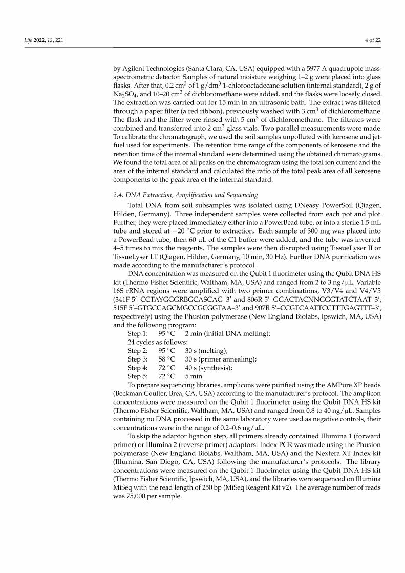
with V3V4 but almost not detected with V4V5. The estimated alpha-diversity was alsogenerally higher in case of the V3V4 analysis (Figure 1). An exception was representedby the Dystric Arenosols samples, where several bacterial families, i.e., Alcaligenaceaeand Nocardiaceae were relatively more abundant when V4V5 was used. For simplicity,in the main text, the V3V4 data are used for plots, while the plots for V4V5 are providedin the Supplementary Materials. These discrepancies are minor and do not influencethe conclusions.

Life 2022, 12, x FOR PEER REVIEW 6 of 23

microbial families (Supplementary Figure S3). For example, Pseudomonadaceae, Chthoniobacteraceae, and Moraxellaceae, highly abundant in several samples, were ob-served with V3V4 but almost not detected with V4V5. The estimated alpha-diversity was also generally higher in case of the V3V4 analysis (Figure 1). An exception was repre-sented by the Dystric Arenosols samples, where several bacterial families, i.e., Alcali-genaceae and Nocardiaceae were relatively more abundant when V4V5 was used. For simplicity, in the main text, the V3V4 data are used for plots, while the plots for V4V5 are provided in the Supplementary Material. These discrepancies are minor and do not influ-ence the conclusions.

Figure 1. Alpha-diversity estimated by the Shannon index at the ASV level. The numbers above the histograms represent the initial kerosene loads, in g/kg. 16S rRNA regions are shown by the dot (V3V4) and triangle (V4V5).

The microbiomes of the topsoils of different properties (Dystric Arenosols, Fibric His-tosols, and Albic Luvisols) showed similar responses to equal kerosene loads. In most of the contaminated soils, the proportion of anaerobic bacteria-metabolizing hydrocarbons was elevated, whereas the proportion of aerobic bacteria was reduced. During the field experiment, the soil microbiome recovered faster than in the pot experiments, possibly due to migration of organisms from the surrounding uncontaminated environment.

3.1. Soil Similarities and Differences in Physicochemical Properties and Microbiome Composition Prior to kerosene pollution, all soil communities under consideration were domi-

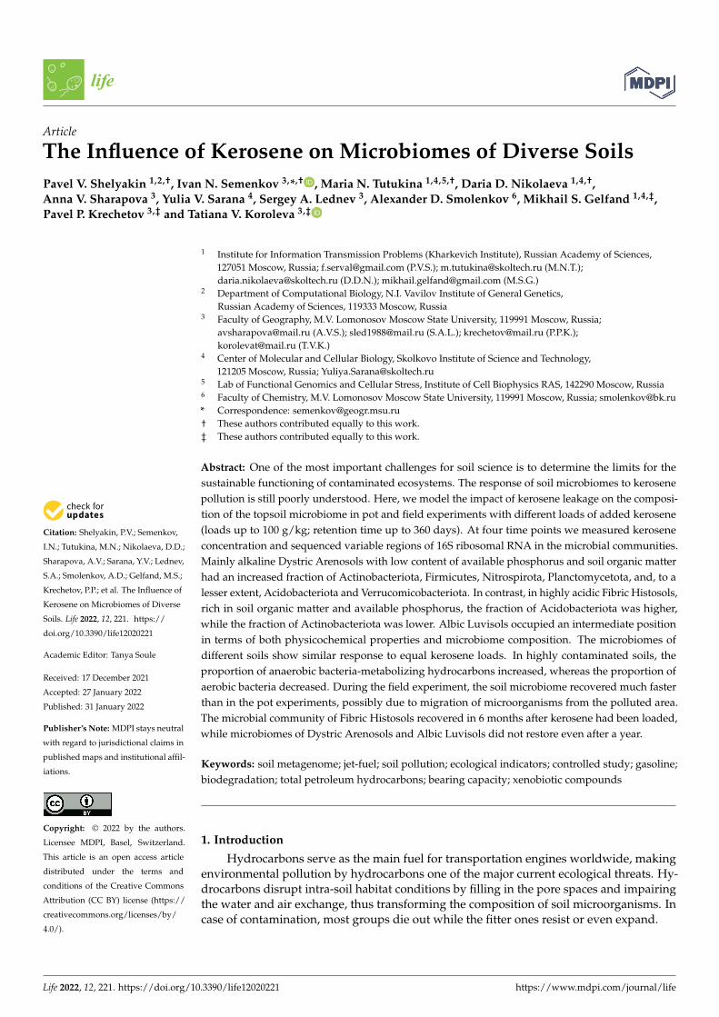
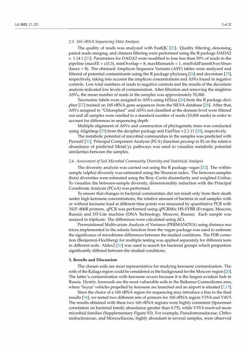
nated by Proteobacteria, Actinobacteriota, Acidobacteriota, Verrucomicrobiota, and Bac-teroidota. These phyla comprised nearly 80% of all bacteria in communities (Figures 2C and 3A), consistent with the previous results on soil microbiomes [35,36], in particular on Aridisols of (semi)arid regions [37,38], Albic Luvisols [39–42], and Fibric Histosols [43–46] of humid environments. Dystric Arenosols with the alkaline environment and the mini-mal available phosphorus and SOM (Figure 2A) had an increased fraction of Actinobac-teriota, Firmicutes, Nitrospirota, Planctomycetota and less Acidobacteriota, Verrucomico-bacteriota (Figure 2C). In highly acidic Fibric Histosols with the maximal content of SOM and available phosphorus (Figure 2A), the fraction of Acidobacteriota was higher, while the fraction of Actinobacteriota was lower (Figure 2C). Albic Luvisols occupied an

Figure 1. Alpha-diversity estimated by the Shannon index at the ASV level. The numbers above thehistograms represent the initial kerosene loads, in g/kg. 16S rRNA regions are shown by the dot(V3V4) and triangle (V4V5).

The microbiomes of the topsoils of different properties (Dystric Arenosols, FibricHistosols, and Albic Luvisols) showed similar responses to equal kerosene loads. In mostof the contaminated soils, the proportion of anaerobic bacteria-metabolizing hydrocarbonswas elevated, whereas the proportion of aerobic bacteria was reduced. During the fieldexperiment, the soil microbiome recovered faster than in the pot experiments, possibly dueto migration of organisms from the surrounding uncontaminated environment.

3.1. Soil Similarities and Differences in Physicochemical Properties and Microbiome Composition

Prior to kerosene pollution, all soil communities under consideration were dominatedby Proteobacteria, Actinobacteriota, Acidobacteriota, Verrucomicrobiota, and Bacteroidota.These phyla comprised nearly 80% of all bacteria in communities (Figures 2C and 3A),consistent with the previous results on soil microbiomes [35,36], in particular on Aridis-ols of (semi)arid regions [37,38], Albic Luvisols [39–42], and Fibric Histosols [43–46] ofhumid environments. Dystric Arenosols with the alkaline environment and the minimalavailable phosphorus and SOM (Figure 2A) had an increased fraction of Actinobacteriota,Firmicutes, Nitrospirota, Planctomycetota and less Acidobacteriota, Verrucomicobacteriota(Figure 2C). In highly acidic Fibric Histosols with the maximal content of SOM and availablephosphorus (Figure 2A), the fraction of Acidobacteriota was higher, while the fraction ofActinobacteriota was lower (Figure 2C). Albic Luvisols occupied an intermediate positionin terms of both physicochemical properties and the microbiome composition (Figure 2).

Life 2022, 12, 221 7 of 22

Life 2022, 12, x FOR PEER REVIEW 7 of 23

intermediate position in terms of both physicochemical properties and the microbiome composition (Figure 2).

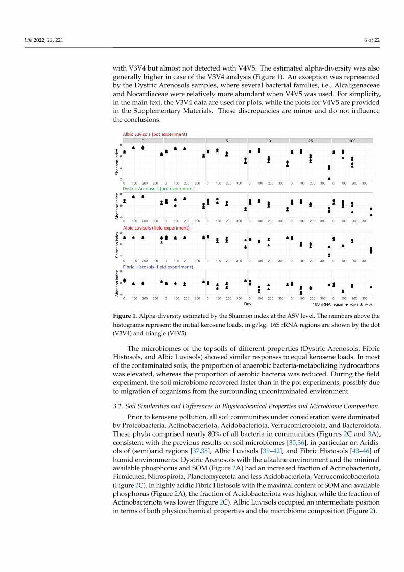
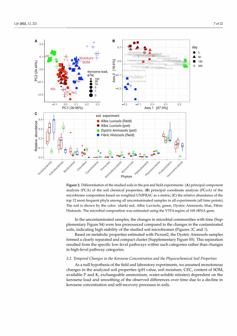
Figure 2. Differentiation of the studied soils in the pot and field experiments: (A) principal compo-nent analysis (PCA) of the soil chemical properties; (B) principal coordinate analysis (PCoA) of the microbiome composition based on weighted UNIFRAC as a metric; (C) the relative abundance of the top 12 most frequent phyla among all uncontaminated samples in all experiments (all time points). The soil is shown by the color: (dark) red, Albic Luvisols; green, Dystric Arenosols; blue, Fibric Histosols. The microbial composition was estimated using the V3V4 region of 16S rRNA gene.

In the uncontaminated samples, the changes in microbial communities with time (Supplementary Figure S4) were less pronounced compared to the changes in the contam-inated soils, indicating high stability of the studied soil microbiomes (Figures 2C and 3).

Based on metabolic properties estimated with Picrust2, the Dystric Arenosols sam-ples formed a clearly separated and compact cluster (Supplementary Figure S5). This sep-aration resulted from the specific low-level pathways within such categories rather than changes in high-level pathway categories.

3.2. Temporal Changes in the Kerosene Concentration and the Physicochemical Soil Properties As a null hypothesis of the field and laboratory experiments, we assumed monoto-

nous changes in the analyzed soil properties (pH value, soil moisture, CEC, content of SOM, available P and K, exchangeable ammonium, water-soluble nitrates) dependent on the kerosene load and smoothing of the observed differences over time due to a decline in kerosene concentration and self-recovery processes in soils.

Figure 2. Differentiation of the studied soils in the pot and field experiments: (A) principal componentanalysis (PCA) of the soil chemical properties; (B) principal coordinate analysis (PCoA) of themicrobiome composition based on weighted UNIFRAC as a metric; (C) the relative abundance of thetop 12 most frequent phyla among all uncontaminated samples in all experiments (all time points).The soil is shown by the color: (dark) red, Albic Luvisols; green, Dystric Arenosols; blue, FibricHistosols. The microbial composition was estimated using the V3V4 region of 16S rRNA gene.

In the uncontaminated samples, the changes in microbial communities with time (Sup-plementary Figure S4) were less pronounced compared to the changes in the contaminatedsoils, indicating high stability of the studied soil microbiomes (Figures 2C and 3).

Based on metabolic properties estimated with Picrust2, the Dystric Arenosols samplesformed a clearly separated and compact cluster (Supplementary Figure S5). This separationresulted from the specific low-level pathways within such categories rather than changesin high-level pathway categories.

3.2. Temporal Changes in the Kerosene Concentration and the Physicochemical Soil Properties

As a null hypothesis of the field and laboratory experiments, we assumed monotonouschanges in the analyzed soil properties (pH value, soil moisture, CEC, content of SOM,available P and K, exchangeable ammonium, water-soluble nitrates) dependent on thekerosene load and smoothing of the observed differences over time due to a decline inkerosene concentration and self-recovery processes in soils.

Life 2022, 12, 221 8 of 22Life 2022, 12, x FOR PEER REVIEW 8 of 23

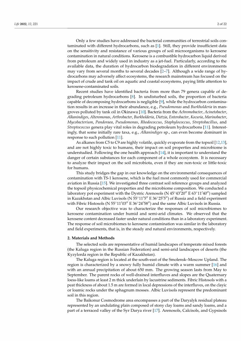
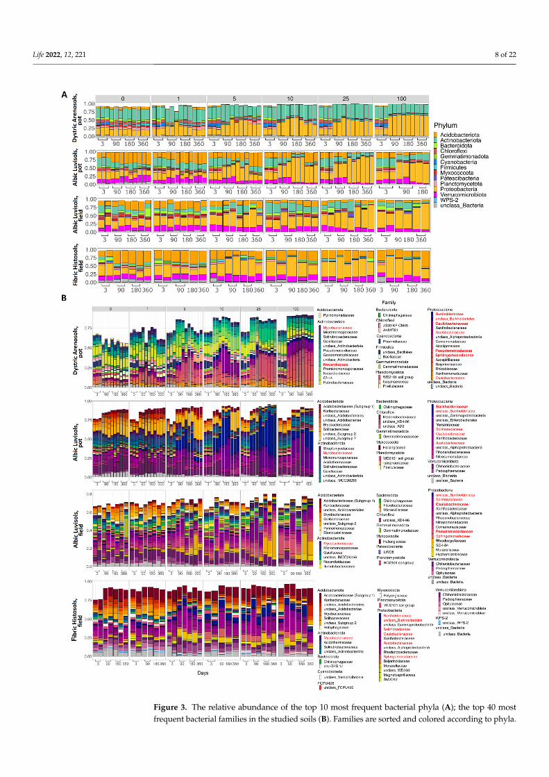
Figure 3. The relative abundance of the top 10 most frequent bacterial phyla (A); the top 40 most frequent bacterial families in the studied soils (B). Families are sorted and colored according to Figure 3. The relative abundance of the top 10 most frequent bacterial phyla (A); the top 40 most

frequent bacterial families in the studied soils (B). Families are sorted and colored according to phyla.

Life 2022, 12, 221 9 of 22

The numbers above the histograms represent the initial kerosene loads, in g/kg. The bacterialcomposition was assessed using the V3V4 region of 16S rRNA; the results for the V4V5 regionare provided in Supplementary Figures S12 and S13. The families whose relative abundance wasincreased after kerosene pollution in all, or almost all, soils are shown in red in the legend. Thedominant families whose relative abundance increased after kerosene pollution in a specific soil typeand experiment setup are shown in bold.

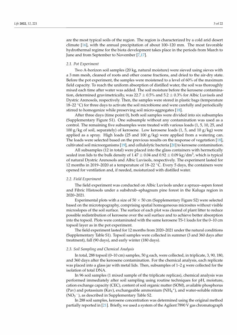
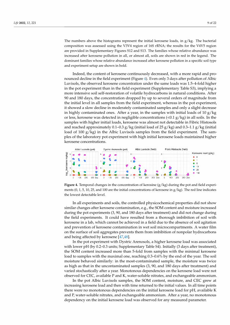
Indeed, the content of kerosene continuously decreased, with a more rapid and pro-nounced decline in the field experiment (Figure 4). Even only 3 days after pollution of AlbicLuvisols, the observed kerosene concentration under the same loads was 1.5–4-fold higherin the pot experiment than in the field experiment (Supplementary Table S3), implying amore intensive soil self-restoration of volatile hydrocarbons in natural conditions. After90 and 180 days, the concentration dropped by up to several orders of magnitude fromthe initial level in all samples from the field experiment, whereas in the pot experiment,it showed a slow decline in moderately contaminated samples and only a slight decreasein highly contaminated ones. After a year, in the samples with initial loads of 10 g/kgor less, kerosene was detected in negligible concentrations (<0.1 g/kg) in all soils. In thesamples with higher initial loads, kerosene was almost not detectable in Fibric Histosolsand reached approximately 0.1–0.3 g/kg (initial load of 25 g/kg) and 0.3–1.1 g/kg (initialload of 100 g/kg) in the Albic Luvisols samples from the field experiment. The sam-ples of the laboratory pot experiment with high initial kerosene loads maintained higherkerosene concentrations.

Life 2022, 12, x FOR PEER REVIEW 9 of 23

phyla. The numbers above the histograms represent the initial kerosene loads, in g/kg. The bacterial composition was assessed using the V3V4 region of 16S rRNA; the results for the V4V5 region are provided in Supplementary Figures S12 and S13. The families whose relative abundance was in-creased after kerosene pollution in all, or almost all, soils are shown in red in the legend. The dom-inant families whose relative abundance increased after kerosene pollution in a specific soil type and experiment setup are shown in bold.

Indeed, the content of kerosene continuously decreased, with a more rapid and pro-nounced decline in the field experiment (Figure 4). Even only 3 days after pollution of Albic Luvisols, the observed kerosene concentration under the same loads was 1.5–4-fold higher in the pot experiment than in the field experiment (Supplementary Table S3), im-plying a more intensive soil self-restoration of volatile hydrocarbons in natural conditions. After 90 and 180 days, the concentration dropped by up to several orders of magnitude from the initial level in all samples from the field experiment, whereas in the pot experi-ment, it showed a slow decline in moderately contaminated samples and only a slight decrease in highly contaminated ones. After a year, in the samples with initial loads of 10 g/kg or less, kerosene was detected in negligible concentrations (<0.1 g/kg) in all soils. In the samples with higher initial loads, kerosene was almost not detectable in Fibric Histo-sols and reached approximately 0.1–0.3 g/kg (initial load of 25 g/kg) and 0.3–1.1 g/kg (in-itial load of 100 g/kg) in the Albic Luvisols samples from the field experiment. The samples of the laboratory pot experiment with high initial kerosene loads maintained higher ker-osene concentrations.

Figure 4. Temporal changes in the concentration of kerosine (g/kg) during the pot and field experi-ments (0, 1, 5, 10, 25, and 100 are the initial concentrations of kerosene in g/kg). The red line indicates the lowest detectable level.

In all experiments and soils, the controlled physicochemical properties did not show similar changes after kerosene contamination, e.g., the SOM content and moisture in-creased during the pot experiments (3, 90, and 180 days after treatment) and did not change during the field experiments. It could have resulted from a thorough imbibition of soil with kerosene in a lab, which cannot be achieved in a field due to the absence of soil agitation and prevention of kerosene contamination in wet soil microcompartments. A water film on the surface of soil aggregates prevents them from imbibition of nonpolar hydrocarbons and being affected by kerosene [47,48].

In the pot experiment with Dystric Arenosols, a higher kerosene load was associated with lower pH (by 0.2–0.3 units; Supplementary Table S4). Initially (3 days after treat-ment), the SOM content increased more than 5-fold from samples with the minimal kero-sene load to samples with the maximal one, reaching 0.3–0.6% by the end of the year. The soil moisture behaved similarly: in the most-contaminated sample, the moisture was twice as high as that in the uncontaminated samples (3, 90, and 180 days after treatment) and varied stochastically after a year. Monotonous dependencies on the kerosene load were not observed for CEC, available P and K, water-soluble nitrates, and exchangeable ammo-nium.

In the pot Albic Luvisols samples, the SOM content, moisture, and CEC grew at in-creasing kerosene load and then with time returned to the initial values. In all time points there were no monotonous dependencies on the initial kerosene load for pH, available K

Figure 4. Temporal changes in the concentration of kerosine (g/kg) during the pot and field experi-ments (0, 1, 5, 10, 25, and 100 are the initial concentrations of kerosene in g/kg). The red line indicatesthe lowest detectable level.

In all experiments and soils, the controlled physicochemical properties did not showsimilar changes after kerosene contamination, e.g., the SOM content and moisture increasedduring the pot experiments (3, 90, and 180 days after treatment) and did not change duringthe field experiments. It could have resulted from a thorough imbibition of soil withkerosene in a lab, which cannot be achieved in a field due to the absence of soil agitationand prevention of kerosene contamination in wet soil microcompartments. A water filmon the surface of soil aggregates prevents them from imbibition of nonpolar hydrocarbonsand being affected by kerosene [47,48].

In the pot experiment with Dystric Arenosols, a higher kerosene load was associatedwith lower pH (by 0.2–0.3 units; Supplementary Table S4). Initially (3 days after treatment),the SOM content increased more than 5-fold from samples with the minimal keroseneload to samples with the maximal one, reaching 0.3–0.6% by the end of the year. The soilmoisture behaved similarly: in the most-contaminated sample, the moisture was twiceas high as that in the uncontaminated samples (3, 90, and 180 days after treatment) andvaried stochastically after a year. Monotonous dependencies on the kerosene load were notobserved for CEC, available P and K, water-soluble nitrates, and exchangeable ammonium.

In the pot Albic Luvisols samples, the SOM content, moisture, and CEC grew atincreasing kerosene load and then with time returned to the initial values. In all time pointsthere were no monotonous dependencies on the initial kerosene load for pH, available Kand P, water-soluble nitrates, and exchangeable ammonium. After a year, no monotonousdependency on the initial kerosene load was observed for any measured parameter.

Life 2022, 12, 221 10 of 22

In the field Albic Luvisols experiment, the content of available K (during the wholeobservation period) and exchangeable ammonium (days 3 and 180) increased with thekerosene load, whereas there was no monotonicity for pH, SOM, available P, water-solublenitrates, moisture, and CEC.

In Fibric Histosols, no monotonous trends relative to the kerosene load were identifiedfor any of the analyzed parameters. Therefore, the physicochemical properties of this soiltend to be the most susceptible to kerosene influence.

Previously, it was reported that the kerosene pollution yielded an increase in the con-centration of organic carbon and a decrease of available nitrogen and phosphorus [49–51].Injection of kerosene only weakly influenced CEC and the exchangeable acidity of soils [51],although the soil pH shifted towards neutral values [50,51].

3.3. Taxonomic Composition of Soil Samples Treated with Kerosene

In untreated Albic Luvisols and Fibric Histosols from the field experiment, only weakseasonal variability was observed in the microbiome composition (Figures 2C and 3).

The treatment of soil samples with kerosene led to significant changes in the soil micro-bial composition and diversity (Supplementary Figures S4 and S6, Figure 1), which stronglydepended on the kerosene load, forming three distinct patterns for slightly (0 and 1 g/kg),moderately (5 and 10 g/kg), and heavily (25 and 100 g/kg) contaminated samples.

The alpha-diversity of slightly contaminated samples stayed almost stable for all soilsand dramatically decreased in heavily contaminated samples (Figure 1). In moderatelycontaminated samples, the alpha-diversity decreased until 180 days and then started toincrease towards the initial levels for some of the samples, while continuing to decrease forothers. The Fibric Histosol samples were an exception, since even in heavily contaminatedsamples the alpha-diversity started to restore after 180 days. In the pot experiments weobserved an increase of the alpha-diversity throughout 90 days after treatment, possiblyarising from the ongoing adaptation of soil microbial communities to the laboratory condi-tions. We also observed a decrease of diversity by 360 days even in the control samplespossibly due to the exhaustion of nutrients and the lack of migration opportunity in aclosed system.

To verify that the observed changes did not stem solely from the eliminating sensitivephyla, we performed qPCR for some of the samples (Supplementary Figure S7); thisshowed that in the field experiment both with Fibric Histosols and Albic Luvisols, the totalabundance of 16S rRNA amplicons did not change with time both in the control and highlycontaminated samples, compared to the abundance in control samples at day 3. However,in the highly contaminated samples of Albic Luvisols (pot experiment), the abundance ofamplicons dramatically decreased with time, while being stable in the control. While the 16SrRNA sequencing demonstrated the similarities of the microbiome response in the pot andfield experiments with all treated soils, particularly, an increase in the relative abundanceof kerosene-degrading bacteria, the absolute bacterial abundance did not reach the levelobserved before contamination, indicating that the contamination in the pot conditions wasmuch more stressful for the microbiome than in the field experiment. A natural caveat isthat limitations of the qPCR analysis, e.g., different copy number of the 16S rRNA loci ordifferent efficiency of PCR for bacterial taxa could have impacted the observations.

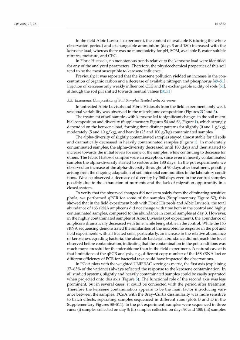
In PCoA plots with the weighted UNIFRAC serving as metric, the first axis (explaining37–63% of the variance) always reflected the response to the kerosene contamination. Inall studied systems, slightly and heavily contaminated samples could be easily separatedwhen projected onto this axis (Figure 5). The functional role of the second axis was lessprominent, but in several cases, it could be connected with the period after treatment.Therefore the kerosene contamination appears to be the main factor introducing vari-ance between the samples. PCoA with the Bray–Curtis dissimilarity was more sensitiveto batch effects, separating samples sequenced in different runs (plots B and D in theSupplementary Figures S8–S11). In the pot experiment, samples were sequenced in threeruns: (i) samples collected on day 3; (ii) samples collected on days 90 and 180; (iii) samples

Life 2022, 12, 221 11 of 22

collected on day 360. Using Bray–Curtis dissimilarity for estimate beta-diversity betweenthe samples from these three runs resulted in clearly distinct clusters along the Axis 1 onPCoA plots (Supplementary Figures S8 and S9), while use of weighted UNIFRAC pre-vented such clustering. For instance, control samples from different days were closer toeach other rather than to highly contaminated samples from the same run. All samplesfrom the field experiment were sequenced in one run and for them we did not observe anydrastic difference between PCoA plots based on Bray–Curtis dissimilarity and weightedUNIFRAC (Supplementary Figures S8 and S9).

Life 2022, 12, x FOR PEER REVIEW 11 of 23

batch effects, separating samples sequenced in different runs (plots B and D in the Sup-plementary Figures S8–S11). In the pot experiment, samples were sequenced in three runs: (i) samples collected on day 3; (ii) samples collected on days 90 and 180; (iii) samples col-lected on day 360. Using Bray–Curtis dissimilarity for estimate beta-diversity between the samples from these three runs resulted in clearly distinct clusters along the Axis 1 on PCoA plots (Supplementary Figures S8 and S9), while use of weighted UNIFRAC pre-vented such clustering. For instance, control samples from different days were closer to each other rather than to highly contaminated samples from the same run. All samples from the field experiment were sequenced in one run and for them we did not observe any drastic difference between PCoA plots based on Bray–Curtis dissimilarity and weighted UNIFRAC (Supplementary Figures S8 and S9).

Figure 5. Principal coordinate analysis (PCoA) plots for soils with different initial kerosene loads. The load in g/kg is shown by the dot color, and the day after kerosene treatment is shown by the dot shape (see legend). The beta-diversity is estimated by the weighted UNIFRAC metric (the V3V4 16S rRNA region). The names of the most abundant bacterial families mark the main shifts in the soil microbial composition. The families whose relative abundance increased after kerosene pollu-tion in all, or almost all, soils are in red. Dominant families whose relative abundance increased after

Figure 5. Principal coordinate analysis (PCoA) plots for soils with different initial kerosene loads.The load in g/kg is shown by the dot color, and the day after kerosene treatment is shown by the dotshape (see legend). The beta-diversity is estimated by the weighted UNIFRAC metric (the V3V4 16SrRNA region). The names of the most abundant bacterial families mark the main shifts in the soilmicrobial composition. The families whose relative abundance increased after kerosene pollutionin all, or almost all, soils are in red. Dominant families whose relative abundance increased afterkerosene pollution in a specific soil type and experimental setup are in boldface. The PCoA for theV4V5 region and for Bray–Curtis dissimilarity are in Supplementary Figures S8–S11.

Life 2022, 12, 221 12 of 22

In the pot experiment, the samples collected on the third day after kerosene treatmentformed a dense cluster with smaller mean beta-diversity between samples with differentkerosene loads, as compared to the field experiment (Figures 5 and S4). This discrepancymight result from several causes. All pot microbiomes could be highly and similarlystressed by the soil preparation procedure and environmental change, while the DNAof bacteria that died immediately following the kerosene pollution could be preservedlonger as the surviving bacteria were suppressed and inactive. On the other hand, in thefield experiments, the bacterial community could react actively to the kerosene treatmentas some soil microcompartments might be uncontaminated and bacteria could migratenaturally. However, these differences were relatively small and statistically significant inthe pot experiment and insignificant in the field one. The cause might have lain in the smallnumber of samples and a high diversity between those from the same group in the fieldexperiment (Supplementary Table S5).

Compared to the control samples (zero kerosene pollution, day > 3), the highlycontaminated samples (kerosene loads of 25 and 100 g/kg, day > 3) demonstrated thatthe fractions of Burkholderiaceae and Sphingomonadaceae increased in response to thekerosene contamination at least at some time points in all studied soils. Moreover, the frac-tions of Acetobacteraceae, Caulobacteraceae, Mycobacteriaceae, Nocardiaceae, Oxalobacteraceae,Pseudomonadaceae, and Solimonadaceae, as well as unclassified families of the Burkholderialesorder were elevated in three out of four studied systems (Figures 3b, S12 and S13).

At the phylum level, the most remarkable changes at high kerosene loads were theincrease of the relative abundance of Proteobacteria in all soils and a decrease of Aci-dobacteriota and Actinobacteriota (Figures 3A and S14). Given that, the increased relativeabundance of Proteobacteria suggested that the observed changes were not caused bysurvival of spore-forming bacteria as opposed to extinction of most other bacteria, sinceProteobacteria do not form endospores [52].

In all soils except Fibric Histosols, upon the high kerosene load, we observed severaldominant bacterial families that expanded up to 50% of the total bacterial community(Figure 3B). For example, in Albic Luvisols in the pot experiment, Burkholderiaceae andYersiniaceae became dominant families in the moderately and highly contaminated samples,reaching, respectively, up to 56% and 22% of the total community in some samples. Suchrelative increase of abundance was not soil-specific, because in the field experiment, otherbacterial families became dominant in the same Albic Luvisols soil; for example, in sev-eral highly contaminated samples, Rhodocyclaceae constituted 38% of the total community.Caulobacteraceae and Pseudomonadaceae increased in almost all soils and represented the dom-inant family in several samples of two different soils, field Albic Luvisols (Caulobacteraceaeup to 10%, Pseudomonadaceae up to 15%) and pot Dystric Arenosols (Caulobacteraceae upto 12%, Pseudomonadaceae 22%). Similarly, in Dystric Arenosols, the families that wereenriched in almost all soils, such as Sphingomonadaceae (up to 21%) and Nocardiaceae (up to16%), were predominant in the moderately and highly contaminated samples.

Most bacterial families that either increased their relative abundance in most of thestudied soils, or became dominant in some samples, belonged to Proteobacteria. Anincrease in Proteobacteria is a frequent response to soil contamination by crude oil orits derivates [53–56]. Some families belonged to the phylum Actinobacteria, also knownto respond to contamination [53]. Bacterial families that were expanded in moderatelyand highly contaminated soils comprise representatives with a known ability to sur-vive and degrade aliphatic or/and aromatic hydrocarbons. For instance, Burkholderiaceaeand Sphingomonadales are well-known for their ability to degrade polycyclic aromatichydrocarbons [57]. Some Sphingomonadales can degrade petroleum hydrocarbons includ-ing polycyclic aromatic hydrocarbons [58]. Burkholderiaceae are enriched in many oil-contaminated soils [53,59], whereas Pseudomonadaceae dominate bacterial communitiesof oil-contaminated mangrove sediments [10]. Members of Pseudomonadaceae are amongthe main bacteria responding to biodiesel contamination [56], degrade diesel in Antarc-tic soils [60] and are dominant degraders of polycyclic aromatic hydrocarbons in Arc-

Life 2022, 12, 221 13 of 22

tic soils [61]. Caulobacteraceae are highly enriched in oil contaminated soils [53,62], andSolimonadaceae have been extracted from oil contaminated water samples [63]. Represen-tatives of Rhodocyclaceae degrade aromatics compounds both in aerobic and anaerobicconditions [64]. Oxalobacteraceae, while being members of uncontaminated soil commu-nities [53,62], also act as key functional n-alkene degraders in crude-oil contaminatedsoils [65]. Several members of Acetobacteraceae degrade hydrocarbons in slightly acidicenvironments [66].

Members of phylum Actinobacteria, e.g., Nocardioidaceae, can degrade alkane andaromatic compounds in contaminated soils [67], Mycobacteriaceae are propagated in soilscontaminated with petroleum and diesel [68].

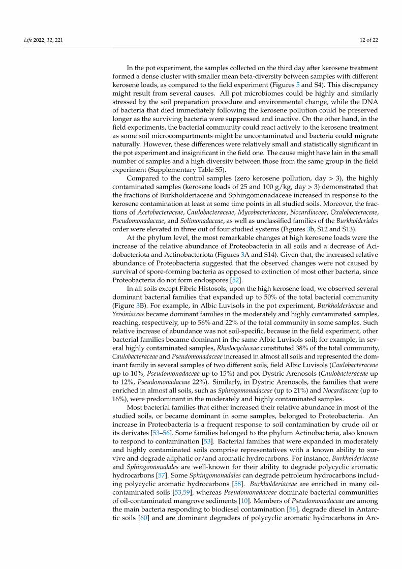
The metabolic potential determined with Picrust2 clearly differentiates slightly con-taminated (kerosene load is less than 1 g/kg) and moderately and highly contaminated(5–100 g/kg) samples (Figures 6 and S15). On the PCA plot, the moderately and highlycontaminated samples were shifted in the same direction as compared to the slightlycontaminated samples in all soils. This could indicate that in response to kerosene contam-ination, abundance of similar metabolic pathways decreased or increased. Interestingly,such a shift appeared in the samples from the pot experiment starting from day 90, whilethe samples from the field experiment responded faster and showed the shift from day 3.The Aldex2 analysis of MetaCyc pathways differentially abundant in slightly and highlycontaminated samples showed that the highly contaminated samples featured a larger num-ber of degradative pathways, specifically, the degradation of aromatic compounds, aminoacids, and secondary metabolites (Supplementary Figures S16 and S17). This could resultfrom an increase in the relative abundance of bacteria capable of degrading aromatic hy-drocarbons from kerosene. Slightly contaminated samples featured more pathways relatedto the biosynthesis of cofactors, nucleotides, amino-acids, lipids, carbohydrates, secondarymetabolites, and aromatic compounds; still, several pathways of polymer degradation andrespiration were enriched.

Life 2022, 12, x FOR PEER REVIEW 13 of 23

mangrove sediments [10]. Members of Pseudomonadaceae are among the main bacteria re-sponding to biodiesel contamination [56], degrade diesel in Antarctic soils [60] and are dominant degraders of polycyclic aromatic hydrocarbons in Arctic soils [61]. Caulobacter-aceae are highly enriched in oil contaminated soils [53,62], and Solimonadaceae have been extracted from oil contaminated water samples [63]. Representatives of Rhodocyclaceae de-grade aromatics compounds both in aerobic and anaerobic conditions [64]. Oxalobacter-aceae, while being members of uncontaminated soil communities [53,62], also act as key functional n-alkene degraders in crude-oil contaminated soils [65]. Several members of Acetobacteraceae degrade hydrocarbons in slightly acidic environments [66].

Members of phylum Actinobacteria, e.g., Nocardioidaceae, can degrade alkane and ar-omatic compounds in contaminated soils [67], Mycobacteriaceae are propagated in soils contaminated with petroleum and diesel [68].

The metabolic potential determined with Picrust2 clearly differentiates slightly con-taminated (kerosene load is less than 1 g/kg) and moderately and highly contaminated (5–100 g/kg) samples (Figures 6 and S15). On the PCA plot, the moderately and highly con-taminated samples were shifted in the same direction as compared to the slightly contam-inated samples in all soils. This could indicate that in response to kerosene contamination, abundance of similar metabolic pathways decreased or increased. Interestingly, such a shift appeared in the samples from the pot experiment starting from day 90, while the samples from the field experiment responded faster and showed the shift from day 3. The Aldex2 analysis of MetaCyc pathways differentially abundant in slightly and highly con-taminated samples showed that the highly contaminated samples featured a larger num-ber of degradative pathways, specifically, the degradation of aromatic compounds, amino acids, and secondary metabolites (Supplementary Figures S16 and S17). This could result from an increase in the relative abundance of bacteria capable of degrading aromatic hy-drocarbons from kerosene. Slightly contaminated samples featured more pathways re-lated to the biosynthesis of cofactors, nucleotides, amino-acids, lipids, carbohydrates, sec-ondary metabolites, and aromatic compounds; still, several pathways of polymer degra-dation and respiration were enriched.

Figure 6. PCA plot based on the relative abundance of metabolic pathways in samples, as predicted by Picrust2 on the V3V4 data. All soils were plotted together in one plane and then separated to four subplots for better readability. Separate PCA plots for individual soils are shown in Supple-mentary Figure S15.

Furthermore, the soils of the same geographic origin demonstrated stronger similar-ity to each other in the fraction of metabolic pathways. Fibric Histosols and Albic Luvisols from the humid environments of the Kaluga region being the most similar, and the soils of semi-arid environments in Kazakhstan were significantly different from the Kaluga re-gion soils.

While the studied soils had quite different initial microbial communities, several groups of bacteria simultaneously decreased the relative abundance in response to the kerosene contamination in almost all soils (Supplementary Figure S13); these were unclas-sified Acidobacteriae, Bryobacteraceae, Haliangiaceae, Nitrosomonadaceae, Pedosphaeraceae,

Figure 6. PCA plot based on the relative abundance of metabolic pathways in samples, as pre-dicted by Picrust2 on the V3V4 data. All soils were plotted together in one plane and then sepa-rated to four subplots for better readability. Separate PCA plots for individual soils are shown inSupplementary Figure S15.

Furthermore, the soils of the same geographic origin demonstrated stronger similarityto each other in the fraction of metabolic pathways. Fibric Histosols and Albic Luvisolsfrom the humid environments of the Kaluga region being the most similar, and the soilsof semi-arid environments in Kazakhstan were significantly different from the Kalugaregion soils.

While the studied soils had quite different initial microbial communities, severalgroups of bacteria simultaneously decreased the relative abundance in response to thekerosene contamination in almost all soils (Supplementary Figure S13); these were un-classified Acidobacteriae, Bryobacteraceae, Haliangiaceae, Nitrosomonadaceae, Pedosphaeraceae,Pyrinomonadaceae, Solibacteraceae, unclassified Kapabacteriales, Polyangia, and RCP2-54, as wellas the WD2101 soil group. The resolution at genus level is shown in Supplementary Figure S18.

Life 2022, 12, 221 14 of 22

3.3.1. Albic Luvisols, the Pot Experiment

In the PCoA plot with weighted UNIFRAC (Figure 5), all samples were arrangedacross two axes that visually correlated well with the experimental conditions. All samplesfrom the time point 0 (day 3) clustered together in one corner (upper left) of the plot(p-value < 0.0001 for the V3V4 data on; however, this was insignificant for the V4V5 data,Supplementary Table S5).

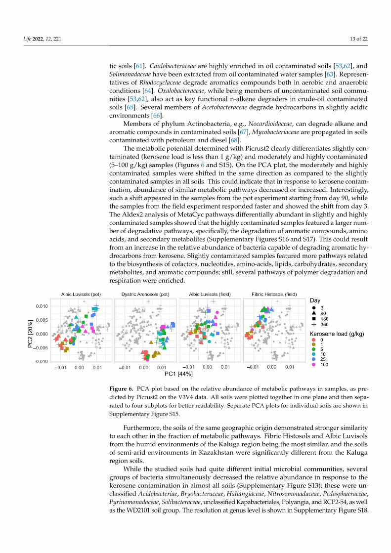
With time, the moderately and highly contaminated samples were shifted along Axis1 (explaining 63% of variation), whereas the slightly contaminated samples were shiftedalong Axis 2 (approximately 16% of variation). Therefore, Axis 1 may reflect the response tokerosene treatment, while Axis 2 reflects the influence of laboratory conditions. Given that,the samples with high kerosene loads tended to move faster along the Axis 1, while thesamples with intermediate loads showed some recovery potential, as after 1 year of incuba-tions they were more similar to the controls than after 6 months. The main bacterial familiesthat increased during this shift along the Axis 1 were Yersiniaceae, Burkholderiaceae, andSolimonadaceae; bacterial families that considerably changed in relative abundance in thecontaminated samples are shown in Figure 7 and Supplementary Figure S19.

Life 2022, 12, x FOR PEER REVIEW 14 of 23

Pyrinomonadaceae, Solibacteraceae, unclassified Kapabacteriales, Polyangia, and RCP2-54, as well as the WD2101 soil group. The resolution at genus level is shown in Supplemen-tary Figure S18.

3.3.1. Albic Luvisols, the Pot Experiment In the PCoA plot with weighted UNIFRAC (Figure 5), all samples were arranged

across two axes that visually correlated well with the experimental conditions. All sam-ples from the time point 0 (day 3) clustered together in one corner (upper left) of the plot (p-value < 0.0001 for the V3V4 data on; however, this was insignificant for the V4V5 data, Supplementary Table S5).

With time, the moderately and highly contaminated samples were shifted along Axis 1 (explaining 63% of variation), whereas the slightly contaminated samples were shifted along Axis 2 (approximately 16% of variation). Therefore, Axis 1 may reflect the response to kerosene treatment, while Axis 2 reflects the influence of laboratory conditions. Given that, the samples with high kerosene loads tended to move faster along the Axis 1, while the samples with intermediate loads showed some recovery potential, as after 1 year of incubations they were more similar to the controls than after 6 months. The main bacterial families that increased during this shift along the Axis 1 were Yersiniaceae, Burkholderi-aceae, and Solimonadaceae; bacterial families that considerably changed in relative abun-dance in the contaminated samples are shown in Figure 7 and Supplementary Figure S19.

Figure 7. Heatmap with the relative abundance of bacterial families with a significant difference between highly contaminated (kerosene load = 25 or 100, day > 3) and control (kerosene load = 0,

Figure 7. Heatmap with the relative abundance of bacterial families with a significant differencebetween highly contaminated (kerosene load = 25 or 100, day > 3) and control (kerosene load = 0,day > 3) samples of Albic Luvisols, the pot experiment. In the left panel, the abundance of eachbacteria family is scaled (Z-score) across all samples to highlight the relative changes between samples.In the right panel, the medians of-centered log-ratio (clr) transformed abundances of bacterial familiesin highly contaminated and control samples are shown. The V3V4 data are shown, a similar heatmapfor the V4V5 region is shown in Supplementary Figure S19.

Life 2022, 12, 221 15 of 22

3.3.2. Dystric Arenosols, the Pot Experiment

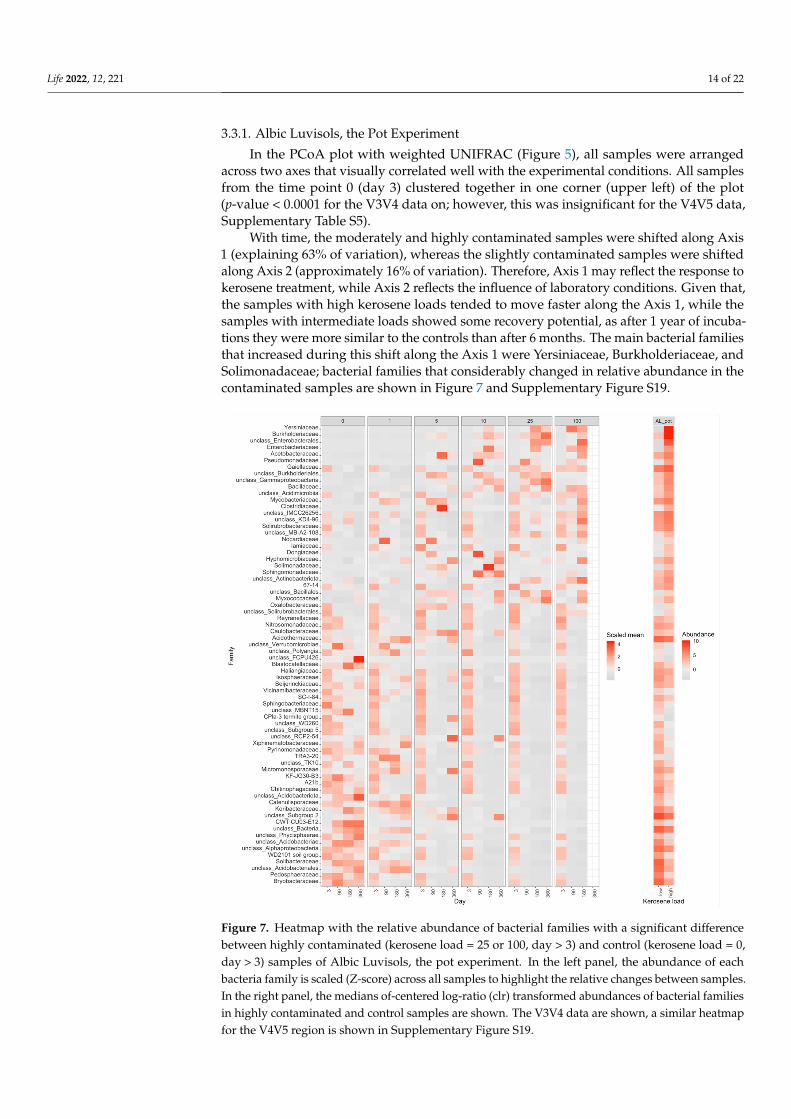
In the PCoA plot, samples again arrange across Axis 1, according to the added keroseneload, with more contaminated samples located farther from the control samples (Figure 5).However, by day 360, the samples with the lowest kerosene load (1 g/kg) and moderatelycontaminated samples appear to move back, somewhat closer to the control samples, un-like the highly contaminated ones. This might result from the reconstitution of the soilcommunities. In moderately contaminated samples, this effect was seen in the taxonomicbarplot, as in Proteobacteria, the relative abundance of which had increased in the initialresponse to kerosene and declined after 1 year of incubation (Figure 3A). Bacterial fami-lies that considerably changed in abundance in the contaminated samples are shown inFigures 8, S20 and S21.

Life 2022, 12, x FOR PEER REVIEW 15 of 23

day > 3) samples of Albic Luvisols, the pot experiment. In the left panel, the abundance of each bacteria family is scaled (Z-score) across all samples to highlight the relative changes between sam-ples. In the right panel, the medians of-centered log-ratio (clr) transformed abundances of bacterial families in highly contaminated and control samples are shown. The V3V4 data are shown, a similar heatmap for the V4V5 region is shown in Supplementary Figure S19.

3.3.2. Dystric Arenosols, the Pot Experiment In the PCoA plot, samples again arrange across Axis 1, according to the added kero-

sene load, with more contaminated samples located farther from the control samples (Fig-ure 5). However, by day 360, the samples with the lowest kerosene load (1 g/kg) and mod-erately contaminated samples appear to move back, somewhat closer to the control sam-ples, unlike the highly contaminated ones. This might result from the reconstitution of the soil communities. In moderately contaminated samples, this effect was seen in the taxo-nomic barplot, as in Proteobacteria, the relative abundance of which had increased in the initial response to kerosene and declined after 1 year of incubation (Figure 3A). Bacterial families that considerably changed in abundance in the contaminated samples are shown in Figures 8, S20 and S21.

Figure 8. Heatmap with the relative abundance of the top 50 most abundant bacterial families with significant differences between highly contaminated (kerosene load = 25 or 100, day > 3) and control (kerosene load = 0, day > 3) samples of Dystric Arenosols, the pot experiment. Notation as in Figure 7. The V3V4 data are shown. All bacterial families with significant differences between highly con-taminated and control samples according to V3V4 data are shown in Supplementary Figure S20, a similar heatmap for the V4V5 region is shown in Supplementary Figure S21.

Figure 8. Heatmap with the relative abundance of the top 50 most abundant bacterial familieswith significant differences between highly contaminated (kerosene load = 25 or 100, day > 3) andcontrol (kerosene load = 0, day > 3) samples of Dystric Arenosols, the pot experiment. Notation as inFigure 7. The V3V4 data are shown. All bacterial families with significant differences between highlycontaminated and control samples according to V3V4 data are shown in Supplementary Figure S20, asimilar heatmap for the V4V5 region is shown in Supplementary Figure S21.

3.3.3. Albic Luvisols, the Field Experiment

Microbial communities in the field experiments were expected to exhibit a noisierbehavior compared to the pot experiment due to environmental seasonal changes, and afaster recovery due to kerosene removal by natural degradation (oxidation, illuviation, and

Life 2022, 12, 221 16 of 22

evaporation) and possible colonization by bacteria from adjacent, untreated areas. Despitesoil sampling in summer, autumn, and winter, the alpha-diversity in slightly contaminatedsamples showed an elevated temporal stability (Figure 1C), while in highly contaminatedsamples, it decreased after the treatment and was not restored to the initial state even1 year after the treatment, continuing to decrease. Hence, 1 year after treatment in the fieldexperiment, the microbial communities in highly contaminated soils were still stressedin spite of the low concentration of kerosene in all samples. In moderately contaminatedsamples, the alpha-diversity initially declined, but 1 year later, it could become even higherthan at the initial time point, as in the series with the initial kerosene load 10 g/kg and inone of the two series with kerosene load 5 g/kg (the other one showing a slight decrease ofthe alpha-diversity). This could be interpreted as microbiome recovery.

In PCoA, the difference between samples can be observed already on day 3, withhighly contaminated samples being located separately from others (p-value < 0.0001,Supplementary Table S5, Figure 5). Similar to Dystric Arenosols, the slightly contaminatedsamples formed a tight cluster in one half of the plot, while the moderately and highlycontaminated samples were shifted along the Axis 1, the shift being more pronounced forthe highly contaminated samples.

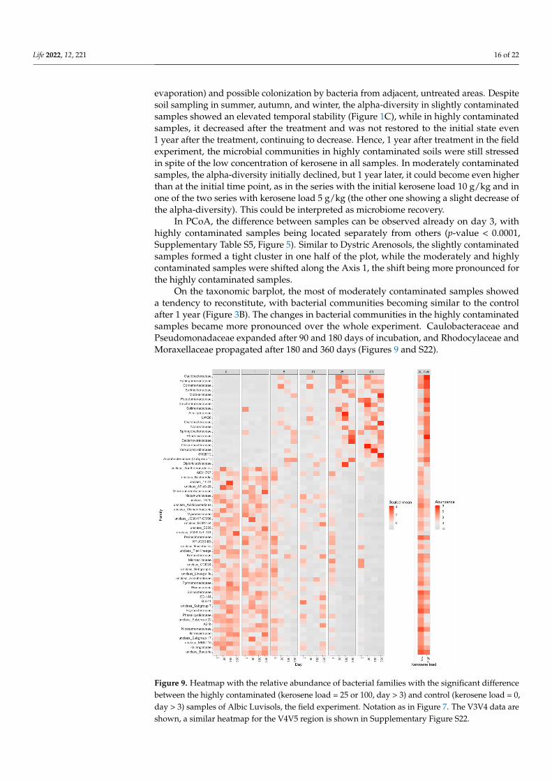
On the taxonomic barplot, the most of moderately contaminated samples showeda tendency to reconstitute, with bacterial communities becoming similar to the controlafter 1 year (Figure 3B). The changes in bacterial communities in the highly contaminatedsamples became more pronounced over the whole experiment. Caulobacteraceae andPseudomonadaceae expanded after 90 and 180 days of incubation, and Rhodocylaceae andMoraxellaceae propagated after 180 and 360 days (Figures 9 and S22).

Life 2022, 12, x FOR PEER REVIEW 17 of 23

Figure 9. Heatmap with the relative abundance of bacterial families with the significant difference between the highly contaminated (kerosene load = 25 or 100, day > 3) and control (kerosene load = 0, day > 3) samples of Albic Luvisols, the field experiment. Notation as in Figure 7. The V3V4 data are shown, a similar heatmap for the V4V5 region is shown in Supplementary Figure S22.

3.3.4. Fibric Histosols, the Field Experiment Soil communities in Fibric Histosols showed the most pronounced ability to restore

the alpha-diversity after kerosene contamination (Figure 1). This might result from fast soil recovery from kerosene, its level being not detectable in most samples after 6 months. In the moderately and highly contaminated samples, the alpha-diversity was the lowest after 90 days, but was at least partially restored by day 180. After 360 days, the alpha-diversity was similar to the initial level in most samples of the series.

The differences in average beta-diversity were insignificant both between groups of samples with different kerosene loads at the same day, or between groups with the same kerosene load on different timepoints (Supplementary Table S5). This is most likely caused by the high heterogeneity of the Fibric Histosols samples. However, the moder-ately and highly contaminated samples were shifted compared to the slightly contami-nated samples along Axis 1 of the PCoA plot (Figure 5). Interestingly, this shift decreased with time in most samples. Addition of moderate and high amounts of kerosene reduced the fraction of Acidobacteriota and increased the fraction of Proteobacteria. These changes were already observed by day 3 (Figure 3A). Burkholderiaceae, Moraxellaceae, Mycobac-teriaceae, Chthoniobacteraceae, and unclassified Vampirivibrionia expanded in relative abundance from day 3 to day 180 (Figures 3B, 10 and S23), but then the fraction of these families decreased again. Hence, while the alpha-diversity of communities was almost

Figure 9. Heatmap with the relative abundance of bacterial families with the significant differencebetween the highly contaminated (kerosene load = 25 or 100, day > 3) and control (kerosene load = 0,day > 3) samples of Albic Luvisols, the field experiment. Notation as in Figure 7. The V3V4 data areshown, a similar heatmap for the V4V5 region is shown in Supplementary Figure S22.

Life 2022, 12, 221 17 of 22

3.3.4. Fibric Histosols, the Field Experiment

Soil communities in Fibric Histosols showed the most pronounced ability to restorethe alpha-diversity after kerosene contamination (Figure 1). This might result from fast soilrecovery from kerosene, its level being not detectable in most samples after 6 months. Inthe moderately and highly contaminated samples, the alpha-diversity was the lowest after90 days, but was at least partially restored by day 180. After 360 days, the alpha-diversitywas similar to the initial level in most samples of the series.

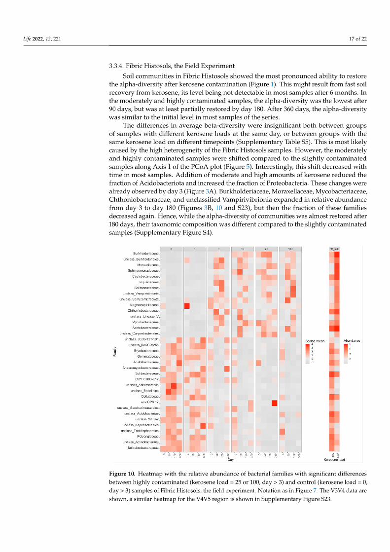
The differences in average beta-diversity were insignificant both between groupsof samples with different kerosene loads at the same day, or between groups with thesame kerosene load on different timepoints (Supplementary Table S5). This is most likelycaused by the high heterogeneity of the Fibric Histosols samples. However, the moderatelyand highly contaminated samples were shifted compared to the slightly contaminatedsamples along Axis 1 of the PCoA plot (Figure 5). Interestingly, this shift decreased withtime in most samples. Addition of moderate and high amounts of kerosene reduced thefraction of Acidobacteriota and increased the fraction of Proteobacteria. These changes werealready observed by day 3 (Figure 3A). Burkholderiaceae, Moraxellaceae, Mycobacteriaceae,Chthoniobacteraceae, and unclassified Vampirivibrionia expanded in relative abundancefrom day 3 to day 180 (Figures 3B, 10 and S23), but then the fraction of these familiesdecreased again. Hence, while the alpha-diversity of communities was almost restored after180 days, their taxonomic composition was different compared to the slightly contaminatedsamples (Supplementary Figure S4).

Life 2022, 12, x FOR PEER REVIEW 18 of 23

restored after 180 days, their taxonomic composition was different compared to the slightly contaminated samples (Supplementary Figure S4).

Figure 10. Heatmap with the relative abundance of bacterial families with significant differences between highly contaminated (kerosene load = 25 or 100, day > 3) and control (kerosene load = 0, day > 3) samples of Fibric Histosols, the field experiment. Notation as in Figure 7. The V3V4 data are shown, a similar heatmap for the V4V5 region is shown in Supplementary Figure S23.

4. Conclusions Our results demonstrate that kerosene cannot be considered as a safe substance for

soil bacteria, having a detrimental effect on soil microbiome. Even after its clearance, the composition of microbiome (especially at high loads) can drastically differ from the initial one, which we call a ‘kerosene label’. Kerosene pollution should be taken into account when conducting ecological soil monitoring and for agricultural purposes. Moreover, the obtained results may guide the selection of candidate bacteria for bioremediation and en-able ranging soils according to their resistance or vulnerability to hydrocarbon contami-nation.

We show that kerosene disappears faster in the natural conditions of a field experi-ment as compared to a laboratory experiment with limited aeration, drainage, and the migration of bacteria and substances. One year after the treatment all studied soils con-tained no more than 1.4 g/kg of kerosene upon a high initial kerosene load (>25 g/kg) and were kerosene-free at lower initial loads. Consistent changes in the physicochemical prop-erties of soils were observed in even shorter periods and only in the pot experiment.

The response of the studied soil systems to adverse kerosene impact were somewhat similar, as the proportion of bacteria resistant to hydrocarbons and/or able to metabolize hydrocarbons was increased. After kerosene input, the alpha-diversity of all moderately and highly contaminated soils decreased due to extinction of many minor bacterial groups

Figure 10. Heatmap with the relative abundance of bacterial families with significant differencesbetween highly contaminated (kerosene load = 25 or 100, day > 3) and control (kerosene load = 0,day > 3) samples of Fibric Histosols, the field experiment. Notation as in Figure 7. The V3V4 data areshown, a similar heatmap for the V4V5 region is shown in Supplementary Figure S23.

Life 2022, 12, 221 18 of 22

4. Conclusions

Our results demonstrate that kerosene cannot be considered as a safe substance forsoil bacteria, having a detrimental effect on soil microbiome. Even after its clearance, thecomposition of microbiome (especially at high loads) can drastically differ from the initialone, which we call a ‘kerosene label’. Kerosene pollution should be taken into accountwhen conducting ecological soil monitoring and for agricultural purposes. Moreover, theobtained results may guide the selection of candidate bacteria for bioremediation and enableranging soils according to their resistance or vulnerability to hydrocarbon contamination.

We show that kerosene disappears faster in the natural conditions of a field experimentas compared to a laboratory experiment with limited aeration, drainage, and the migrationof bacteria and substances. One year after the treatment all studied soils contained nomore than 1.4 g/kg of kerosene upon a high initial kerosene load (>25 g/kg) and werekerosene-free at lower initial loads. Consistent changes in the physicochemical propertiesof soils were observed in even shorter periods and only in the pot experiment.

The response of the studied soil systems to adverse kerosene impact were somewhatsimilar, as the proportion of bacteria resistant to hydrocarbons and/or able to metabolizehydrocarbons was increased. After kerosene input, the alpha-diversity of all moderatelyand highly contaminated soils decreased due to extinction of many minor bacterial groupsand the development of dominant bacteria taxa comprising the degraders of aliphatic andaromatic hydrocarbons. Despite the fact that kerosene was gradually dissipated and thesoil physicochemical properties generally restored to the initial levels, the microbiomecomposition in moderately and highly contaminated samples recovered slowly, and notin all studied systems. In the highly contaminated soils (25–100 g/kg), the changes wereirreversible within 1 year in Dystric Arenosols and Albic Luvisols, but reversible in FibricHistosols. The microbocenoesis of the moderately contaminated samples (5–10 g/kg ofsoil) of Albic Luvisols restored faster during the field experiment and remained disturbedin the pot experiment. Adding 1 g/kg of kerosene only slightly changed the compositionof all studied soil microbiomes. During the pot experiment, the alpha-diversity of the soilmicrobial community continued to decline after 1 year even in the control samples.

We conclude with the following useful practical suggestions. (1) Weak seasonal varia-tion of the microbiome composition of untreated soils in the field experiments from Summerto Fall and Winter allows for the comparative analysis of soil bacterial communities sampledin different seasons. (2) As the data obtained with two 16S rRNA regions were consistent,and more bacterial families could be identified using the V3V4 region compared withthe V4V5 region, the former is more suitable for the characterization of soil microbiomes.(3) Weighted UNIFRAC accounting for the phylogenetic relationships of the soil bacteria ismore robust to sequencing errors than the Bray–Curtis dissimilarity measure.

Supplementary Materials: The following are available online at https://www.mdpi.com/article/10.3390/life12020221/s1. Supplementary Table S1. Meteorological conditions for the period of the fieldexperiment with Albic Luvisols and Fibric Histosols. Supplementary Table S2. Methods of soil chemi-cal analyses used. Supplementary Table S3. Temporal changes (mean and standard deviation) in theconcentration of kerosine during the pot (P) and field (F) experiment (g/kg). Supplementary Table S4.Temporal changes in soil physicochemical properties during the pot (P) and field (F) experiment.Supplementary Table S5. Significance of the differences between the topsoil samples (16S rRNA) inpot (P) and field (F) experiments grouped according to the initial kerosene load or a day after treatmentand assessed using PERMANOVA on weighted UNIFRAC beta-diversity. Supplementary Figure S1.Soil treatment with kerosene and soil sampling. A. Kerosene treatment of the soil stored in a plasticbag (1 g/kg load). B. The subsamples placed in 400 cm3 glass containers with hermetically sealediron lids. C. The structure of the A-horizon of Arenosols preserved after kerosene treatment. D.The structure of the A-horizon of Luvisols preserved after kerosene treatment. E. The soil subsam-ples ready for transportation to the laboratory. F. Soil subsamples subjected to the DNA isolation.Supplementary Figure S2. Experimental plots with a size of 50 × 50 cm. Supplementary Figure S3.Bacterial abundances estimated using different 16S rRNA. Supplementary Figure S4. The mean betadistance (weighted UNIFRAC) of the microbiomes to the microbiomes from the control samples

Life 2022, 12, 221 19 of 22

collected on the same day. Supplementary Figure S5. A PCA plot on fractions of the abundanceof MetaCyc pathways in the samples without added kerosene, based on Picrust2 predictions forthe V3V4 region. Supplementary Figure S6. The mean beta distance (weighted UNIFRAC) of mi-crobiomes to the microbiomes from the samples with the same kerosene load collected on day 3.Supplementary Figure S7. A log fold change of the amplicon concentration estimated with qPCRrelative to the mean amplicon concentration in control samples collected on day 3. SupplementaryFigure S8. Principal coordinate analysis (PCoA) plots for the samples of Albic Luvisols (pot ex-periment). Supplementary Figure S9. Principal coordinate analysis (PCoA) plots for the samplesof Dystric Arenosols (pot experiment). Supplementary Figure S10. Principal coordinate analy-sis (PCoA) plots for the samples of Albic Luvisols (field experiment). Supplementary Figure S11.Principal coordinate analysis (PCoA) plots for the samples of Fibric Histosols (field experiment).Supplementary Figure S12. The relative abundance of the top 40 most frequent bacterial familiesin the studied soils. The bacterial composition was assessed using the V4V5 region of 16S rRNA.Supplementary Figure S13. The number of common bacterial families significantly increased and de-creased in their relative abundance in highly contaminated soil samples. Supplementary Figure S14.The relative abundance of bacterial phyla in the studied soils assessed using the V4V5 region of 16SrRNA. Supplementary Figure S15. PCA plots based on the relative abundance of metabolic pathwayspredicted with Picrust2 on the V3V4 data. Supplementary Figure S16. The number of differentiallyabundant MetaCyc pathways from different categories in highly contaminated and slightly contami-nated samples in all soils. Supplementary Figure S17. Number of differentially abundant MetaCycpathways from high-level categories in highly contaminated and slightly contaminated samples inall soils. Supplementary Figure S18. The relative abundance of the top 10 most frequent bacterialgenera in the studied soils. Bacterial composition was assessed using the V3V4 and V4V5 regionsof 16S rRNA. Supplementary Figure S19. Heatmap of the relative abundance of bacterial familieswith significant difference in abundance between highly contaminated and control samples of AlbicLuvisols (pot experiment). The V4V5 data are shown. Supplementary Figure S20. Heatmap ofthe relative abundance of bacterial families with significant differences in abundance between thehighly contaminated and control samples of Dystric Arenosols (pot experiment). The V3V4 data areshown. Supplementary Figure S21. Heatmap of the relative abundance of bacterial families withsignificant differences in abundance between highly contaminated and control samples of DystricArenosols (pot experiment). The V4V5 data are shown. Supplementary Figure S22. Heatmap ofthe relative abundance of bacterial families with significant difference in abundance between highlycontaminated and control samples of Albic Luvisols, (field experiment). The V4V5 data are shown.Supplementary Figure S23. Heatmap of the relative abundance of bacterial families with significantdifferences in abundance between the highly contaminated and control samples of Fibric Histosols,(field experiment). The V4V5 data are shown.

Author Contributions: Conceptualization, methodology, I.N.S., M.N.T., P.V.S., A.V.S., M.S.G., P.P.K.and T.V.K.; resources, I.N.S., M.N.T.; field work and sampling, I.N.S., M.N.T., A.V.S., S.A.L. andP.P.K.; chemical analysis, A.D.S.; metagenome analysis, M.N.T., Y.V.S.; software, P.V.S. and D.D.N.;validation, M.N.T., P.V.S. and D.D.N.; formal analysis, I.N.S., M.N.T., P.V.S. and D.D.N.; data curation,I.N.S., M.N.T., P.V.S. and D.D.N.; writing—original draft preparation, I.N.S.; writing—review andediting, I.N.S., M.N.T., P.V.S., D.D.N., A.V.S., S.A.L., M.S.G., P.P.K. and T.V.K.; visualization, I.N.S.,P.V.S. and D.D.N.; supervision, I.N.S., M.S.G. and T.V.K.; project administration, I.N.S., T.V.K.; fundingacquisition, T.V.K. All authors have read and agreed to the published version of the manuscript.

Funding: The study was carried out within the framework of the RFBR project No. 19-29-05206(field work and interpretation of the results) and additionally supported by the RFBR project No.18-29-13011 (computational analysis) and the M.V. Lomonosov Moscow State University (the Inter-disciplinary Scientific and Educational School of “Future Planet and Global Environmental Change”and project I.4. “Anthropogenic geochemical transformation of the components of landscapes”)(chemical-analytical work).

Institutional Review Board Statement: Not applicable.

Informed Consent Statement: Not applicable.

Data Availability Statement: Raw sequencing reads are deposited at SRA PRJNA786393.

Life 2022, 12, 221 20 of 22

Acknowledgments: Sequencing service was provided by the Genomics Core Facility of the SkolkovoInstitute of Science and Technology.

Conflicts of Interest: The authors declare no conflict of interest. The funders had no role in the designof the study; in the collection, analyses, or interpretation of data; in the writing of the manuscript, orin the decision to publish the results.

References1. Bao, Y.J.; Xu, Z.; Li, Y.; Yao, Z.; Sun, J.; Song, H. High-throughput metagenomic analysis of petroleum-contaminated soil

microbiome reveals the versatility in xenobiotic aromatics metabolism. J. Environ. Sci. 2017, 56, 25–35. [CrossRef] [PubMed]2. Walker, D.A.; Webber, P.J.; Everett, K.R.; Brown, J. Effects of Crude and Diesel Oil Spills on Plant Communities at Prudhoe Bay,

Alaska, and the Derivation of Oil Spill Sensitivity Maps. Arctic 1978, 31, 242–259. [CrossRef]3. Hutchinson, T.C.; Freedman, W. Effects of experimental crude oil spills on subarctic boreal forest vegetation near Norman Wells,

N.W.T., Canada. Can. J. Bot. 1978, 56, 2424–2433. [CrossRef]4. Racine, C.H. Long-term recovery of vegetation on two experimental crude oil spills in interior Alaska black spruce taiga. Can. J.

Bot. 1994, 72, 1171–1177. [CrossRef]5. Holt, S. The effects of crude and diesel oil spills on plant communities at Mesters Vig, northeast Greenland. Arct. Alp. Res. 1987,

19, 490–497. [CrossRef]6. Bay, C. Effects of Experimental Spills of Crude and Diesel Oil on Arctic Vegetation. A Long-Term Study on High Arctic Terrestrial Plant

Communities in Jameson Land, Central East Greenland; NERI Technical Report; Ministry of Environment and Energy, NationalEnvironmental Research Institute: Aarhus C, Denmark, 1997.

7. Koroleva, T.V.; Semenkov, I.N.; Sharapova, A.V.; Krechetov, P.P.; Lednev, S.A. Ecological consequences of space rocket accidents inKazakhstan between 1999 and 2018. Environ. Pollut. 2021, 268, 115711. [CrossRef]

8. Tremblay, J.; Yergeau, E.; Fortin, N.; Cobanli, S.; Elias, M.; King, T.L.; Lee, K.; Greer, C.W. Chemical dispersants enhance theactivity of oil- and gas condensate-degrading marine bacteria. ISME J. 2017, 11, 2793–2808. [CrossRef]

9. Khan, S.R.; Kumar, J.I.N.; Banker, M.; Kumar, R.N. Ex-Situ Studies on Biodegradation of Artificially Enriched Kerosene and DieselSoils by Fungal Isolates. Soil Sediment Contam. 2015, 24, 796–810. [CrossRef]

10. Bacosa, H.P.; Suto, K.; Inoue, C. Degradation potential and microbial community structure of heavy oil-enriched microbialconsortia from mangrove sediments in Okinawa, Japan. J. Environ. Sci. Health Part A 2013, 48, 835–846. [CrossRef]

11. Xu, X.; Liu, W.; Tian, S.; Wang, W.; Qi, Q.; Jiang, P.; Gao, X.; Li, F.; Li, H.; Yu, H. Petroleum Hydrocarbon-Degrading Bacteria forthe Remediation of Oil Pollution Under Aerobic Conditions: A Perspective Analysis. Front. Microbiol. 2018, 9, 2885. [CrossRef]

12. Karthikeyan, R.; Kulakow, P.A. Soil plant microbe interactions in phytoremediation. Adv. Biochem. Eng. Biotechnol. 2003, 78, 52–74.[CrossRef]

13. Kim, K.D. Effects of diesel and kerosene on germination and growth of coastal wetland plant species. Bull. Environ. Contam.Toxicol. 2014, 93, 596–602. [CrossRef] [PubMed]

14. Mackenzie, J.S.; Jeggo, M. The one health approach-why is it so important? Trop. Med. Infect. Dis. 2019, 4, 88. [CrossRef]15. Koroleva, T.V.; Krechetov, P.P.; Semenkov, I.N.; Sharapova, A.V.; Lednev, S.A.; Karpachevskiy, A.M.; Kondratyev, A.D.; Kasimov,

N.S. The environmental impact of space transport. Transp. Res. Part D Transp. Environ. 2018, 58, 54–69. [CrossRef]16. Lednev, S.A.; Koroleva, T.V.; Semenkov, I.N.; Klink, G.V.; Krechetov, P.P.; Sharapova, A.V.; Karpachevskiy, A.M.; Klink, G.V. The

natural regeneration of desert ecosystem vegetation at the 2013 crash site of a Proton-M launch vehicle, Republic of Kazakhstan.Ecol. Indic. 2019, 101, 603–613. [CrossRef]

17. Kottek, M.; Grieser, J.; Beck, C.; Rudolf, B.; Rubel, F. World Maps of Köppen-Geiger climate classification updated. Meteorol.Zeitschrift. 2006, 15, 259–263. [CrossRef]

18. Lednev, S.A.; Semenkov, I.N.; Klink, G.V.; Krechetov, P.P.; Sharapova, A.V.; Koroleva, T.V. Impact of kerosene pollution on groundvegetation of southern taiga in the Amur Region, Russia. Sci. Total Environ. 2021, 772, 144965. [CrossRef]

19. Dorokhova, M.F.; Krechetov, P.P.; Koroleva, T.V.; Sharapova, A.V. Algo-cyanobacterial communities as indicators of soil pollutionwith jet-fuel. Algae Cyanobacteria Nat. Agric. Ecosyst. In Proceedings of the II Int. Sci. Pract. Conf. Dedic. to 105th Anniv. BirthProfr. Emilia Adrianovna Shtina, Kirov, Russia, 19–23 October 2015; Vyatskaya GSHA: Kirov, Russia, 2015; pp. 118–122.

20. Sharapova, A.V.; Semenkov, I.N.; Krechetov, P.P.; Lednev, S.A.; Koroleva, T.V. The Effect of Kerosene Pollution on the CellulolyticActivity of Albic Retisols and Protic Arenosols: A Laboratory Experiment. Eurasian Soil Sci. Sci. 2022, 55, 233–239. [CrossRef]

21. Bolotnik, T.A.; Timchenko, Y.V.; Plyushchenko, I.V.; Levkina, V.V.; Pirogov, A.V.; Smolenkov, A.D.; Popik, M.V.; Shpigun, O.A. Useof Chemometric Methods of Data Analysis for the Identification and Typification of Petroleum and Petroleum Products. J. Anal.Chem. 2019, 74, 1336–1340. [CrossRef]

22. Andrews, S. A Quality Control Tool for High Throughput Sequence Data. 2019. Available online: https://www.bioinformatics.babraham.ac.uk/projects/fastqc/ (accessed on 16 December 2021).

23. Callahan, B.J.; McMurdie, P.J.; Rosen, M.J.; Han, A.W.; Johnson, A.J.A.; Holmes, S.P. DADA2: High-resolution sample inferencefrom Illumina amplicon data. Nat. Methods 2016, 13, 581–583. [CrossRef]

24. McMurdie, P.J.; Holmes, S. Phyloseq: An R Package for Reproducible Interactive Analysis and Graphics of Microbiome CensusData. PLoS ONE 2013, 8, e61217. [CrossRef] [PubMed]

Life 2022, 12, 221 21 of 22

25. Davis, N.M.; Proctor, D.M.; Holmes, S.P.; Relman, D.A.; Callahan, B.J. Simple statistical identification and removal of contaminantsequences in marker-gene and metagenomics data. Microbiome 2018, 6, 226. [CrossRef] [PubMed]

26. Murali, A.; Bhargava, A.; Wright, E.S. IDTAXA: A novel approach for accurate taxonomic classification of microbiome sequences.Microbiome 2018, 6, 140. [CrossRef]

27. Wright, E.S. Using DECIPHER v2.0 to analyze big biological sequence data in R. R J. 2016, 8, 352–359. [CrossRef]28. Kim, G.; Bae, J.; Kim, M.J.; Kwon, H.; Park, G.; Kim, S.J.; Choe, Y.H.; Kim, J.; Park, S.H.; Choe, B.H.; et al. The SILVA ribosomal

RNA gene database project: Improved data processing and web-based tools. Nucleic Acids Res. 2019, 41, D590–D596.29. Wright, E.S. DECIPHER: Harnessing local sequence context to improve protein multiple sequence alignment. BMC Bioinform.

2015, 16, 322. [CrossRef] [PubMed]30. Price, M.N.; Dehal, P.S.; Arkin, A.P. FastTree 2—Approximately maximum-likelihood trees for large alignments. PLoS ONE 2010,

5, e9490. [CrossRef]31. Douglas, G.M.; Maffei, V.J.; Zaneveld, J.R.; Yurgel, S.N.; Brown, J.R.; Taylor, C.M.; Huttenhower, C.; Langille, M.G.I. PICRUSt2 for

prediction of metagenome functions. Nat. Biotechnol. 2020, 38, 685–688. [CrossRef]32. Dixon, P. VEGAN, a package of R functions for community ecology. J. Veg. Sci. 2003, 14, 927–930. [CrossRef]33. Gloor, G. ALDEx2: ANOVA-Like Differential Expression tool for compositional data. ALDEX Man. Modul. 2019, 20, 1–11.34. Abellan-Schneyder, I.; Matchado, M.S.; Reitmeier, S.; Sommer, A.; Sewald, Z.; Baumbach, J.; List, M.; Neuhaus, K. Primer,

Pipelines, Parameters: Issues in 16S rRNA Gene Sequencing. Msphere 2021, 6, e01202-20. [CrossRef] [PubMed]35. Fierer, N.; Leff, J.W.; Adams, B.J.; Nielsen, U.N.; Bates, S.T.; Lauber, C.L.; Owens, S.; Gilbert, J.A.; Wall, D.H.; Caporaso, J.G.

Cross-biome metagenomic analyses of soil microbial communities and their functional attributes. Proc. Natl. Acad. Sci. USA 2012,109, 21390–21395. [CrossRef]

36. Janssen, P.H. Identifying the dominant soil bacterial taxa in libraries of 16S rRNA and 16S rRNA genes. Appl. Environ. Microbiol.2006, 72, 1719–1728. [CrossRef] [PubMed]

37. Andronov, E.E.; Petrova, S.N.; Pinaev, A.G.; Pershina, E.V.; Rakhimgaliyeva, S.; Akhmedenov, K.M.; Gorobets, A.V.; Sergaliev,N.K. Analysis of the structure of microbial community in soils with different degrees of salinization using T-RFLP and real-timePCR techniques. Eurasian Soil Sci. 2012, 45, 147–156. [CrossRef]

38. McHugh, T.A.; Compson, Z.; van Gestel, N.; Hayer, M.; Ballard, L.; Haverty, M.; Hines, J.; Irvine, N.; Krassner, D.; Lyons, T.; et al.Climate controls prokaryotic community composition in desert soils of the southwestern United States. FEMS Microbiol. Ecol.2017, 93, fix116. [CrossRef] [PubMed]

39. Dilly, O.; Bloem, J.; Vos, A.; Munch, J.C. Bacterial Diversity in Agricultural Soils during Litter Decomposition. Appl. Environ.Microbiol. 2004, 70, 468–474. [CrossRef]

40. Naliukhin, A.N.; Khamitova, S.M.; Glinushkin, A.P.; Avdeev, Y.M.; Snetilova, V.S.; Laktionov, Y.V.; Surov, V.V.; Siluyanova, O.V.;Belozerov, D.A. Changes in the Metagenome of Prokaryotic Community as an Indicator of Fertility of Arable Soddy-PodzolicSoils upon Fertilizer Application. Eurasian Soil Sci. 2018, 51, 321–326. [CrossRef]

41. Semenov, M.V.; Manucharova, N.A.; Krasnov, G.S.; Nikitin, D.A.; Stepanov, A.L. Biomass and Taxonomic Structure of MicrobialCommunities in Soils of the Right-Bank Basin of the Oka River. Eurasian Soil Sci. 2019, 52, 971–981. [CrossRef]

42. Vilkiene, M.; Mockeviciene, I.; Karcauskiene, D.; Suproniene, S.; Doyeni, M.O.; Ambrazaitiene, D. Biological indicators of soilquality under different tillage systems in retisol. Sustainability 2021, 13, 9624. [CrossRef]

43. Basiliko, N.; Henry, K.; Gupta, V.; Moore, T.R.; Driscoll, B.T.; Dunfield, P.F. Controls on bacterial and archaeal community structureand greenhouse gas production in natural, mined, and restored Canadian peatlands. Front. Microbiol. 2013, 4, 215. [CrossRef]

44. Sun, H.; Terhonen, E.; Koskinen, K.; Paulin, L.; Kasanen, R.; Asiegbu, F.O. Bacterial diversity and community structure alongdifferent peat soils in boreal forest. Appl. Soil Ecol. 2014, 74, 37–45. [CrossRef]

45. Grodnitskaya, I.D.; Trusova, M.Y.; Syrtsov, S.N.; Koroban, N.V. Structure of microbial communities of peat soils in two bogs inSiberian tundra and forest zones. Microbiology 2018, 87, 89–102. [CrossRef]

46. Aksenov, A.S.; Shirokova, L.S.; Kisil, O.Y.; Kolesova, S.N.; Lim, A.G.; Kuzmina, D.; Pouillé, S.; Alexis, M.A.; Castrec-Rouelle, M.;Loiko, S.V.; et al. Bacterial number and genetic diversity in a permafrost peatland (Western Siberia): Testing a link with organicmatter quality and elementary composition of a peat soil profile. Diversity 2021, 13, 328. [CrossRef]

47. Qi, B.; Chen, Y.; Chen, D.; Chen, Y.; Ma, L.; Tian, X.; Li, Y.; Long, Y. Insight into Washing of Wet and Dry Crude Oil-ContaminatedSoil, Clean—Soil, Air. Water 2021, 49, 2000440. [CrossRef]

48. Yuan, L.; Habibi, A.; Dehghanpour, H. Liquid imbibition in tight rocks: The role of disjoining pressure, Colloids Surfaces A.Physicochem. Eng. Asp. 2021, 627, 127037. [CrossRef]

49. Obire, O.; Nwaubeta, O.; Oofojekwu, P.C.; Ezenwaka, I.S.; Alegbeleye, W.O. Effects of Refined Petroleum Hydrocarbon on SoilPhysicochemical and Bacteriological Characteristics. J. Appl. Sci. Environ. Manag. 2002, 6, 39–44. [CrossRef]

50. Fallah, M.; Shabanpor, M.; Ebrahimi, S. Evaluation of petroleum impacts on some properties of loamy sand soil with the mainfocus on hydraulic properties. Environ. Earth Sci. 2015, 74, 4751–4762. [CrossRef]

51. Nseabasi, N.O.; Antai, S.P.; Bassey, I.U.; Iwatt, G.D.; Unimke, A.A. Chronic Kerosene Contamination and Variation in thePhysicochemical and Heavy Metal Content of the Soil in Calabar, Cross River State, Nigeria. Imp. J. Interdiscip. Res. 2016, 2,2094–2099. Available online: https://www.researchgate.net/publication/316668945_Chronic_Kerosene_Contamination_and_Variation_in_the_Physicochemical_and_Heavy_Metal_Content_of_the_Soil_in_Calabar_Cross_River_State_Nigeria (accessed on16 December 2021).

Life 2022, 12, 221 22 of 22

52. Beskrovnaya, P.; Fakih, D.; Morneau, I.; Hashimi, A.; Bello, D.G.; Xing, S.; Nanci, A.; Huan, T.; Tocheva, E.I. No EndosporeFormation Confirmed in Members of the Phylum Proteobacteria. Appl. Environ. Microbiol. 2021, 87, 1–11. [CrossRef]

53. Yang, S.; Wen, X.; Shi, Y.; Liebner, S.; Jin, H.; Perfumo, A. Hydrocarbon degraders establish at the costs of microbial richness,abundance and keystone taxa after crude oil contamination in permafrost environments. Sci. Rep. 2016, 6, 37473. [CrossRef]

54. Shapiro, T.; Chekanov, K.; Alexandrova, A.; Dolnikova, G.; Ivanova, E.; Lobakova, E. Revealing of non-cultivable bacteriaassociated with the mycelium of fungi in the kerosene-degrading community isolated from the contaminated jet fuel. J. Fungi2021, 7, 43. [CrossRef]

55. Bacosa, H.; Suto, K.; Inoue, C. Preferential degradation of aromatic hydrocarbons in kerosene by a microbial consortium. Int.Biodeterior. Biodegrad. 2010, 64, 702–710. [CrossRef]

56. Mitter, E.K.; Germida, J.J.; de Freitas, J.R. Impact of diesel and biodiesel contamination on soil microbial community activity andstructure. Sci. Rep. 2021, 11, 10856. [CrossRef] [PubMed]

57. Bacosa, H.P.; Steichen, J.; Kamalanathan, M.; Windham, R.; Lubguban, A.; Labonté, J.M.; Kaiser, K.; Hala, D.; Santschi, P.H.;Quigg, A. Polycyclic aromatic hydrocarbons (PAHs) and putative PAH-degrading bacteria in Galveston Bay, TX (USA), followingHurricane Harvey (2017). Environ. Sci. Pollut. Res. 2020, 27, 34987–34999. [CrossRef] [PubMed]

58. Dominguez, J.J.A.; Bacosa, H.P.; Chien, M.F.; Inoue, C. Enhanced degradation of polycyclic aromatic hydrocarbons (PAHs) in therhizosphere of sudangrass (Sorghum × drummondii). Chemosphere 2019, 234, 789–795. [CrossRef] [PubMed]

59. Chikere, C.B.; Tekere, M.; Adeleke, R. Microbial communities in field-scale oil-polluted soil remediation using 16S rRNA ampliconsequencing. Int. J. Environ. Stud. 2021, 78, 410–426. [CrossRef]

60. Shukor, M.Y.; Hassan, N.A.A.; Jusoh, A.Z.; Perumal, N.; Shamaan, N.A.; MacCormack, W.P.; Syed, M.A. Isolation and characteri-zation of a Pseudomonas diesel-degrading strain from Antarctica. J. Environ. Biol. 2009, 30, 1–6.

61. Ma, Y.; Wang, L.; Shao, Z. Pseudomonas, the dominant polycyclic aromatic hydrocarbon-degrading bacteria isolated fromAntarctic soils and the role of large plasmids in horizontal gene transfer. Environ. Microbiol. 2006, 8, 455–465. [CrossRef]

62. Yang, S.; Wen, X.; Zhao, L.; Shi, Y.; Jin, H. Crude oil treatment leads to shift of bacterial communities in soils from the deep activelayer and upper permafrost along the China-Russia Crude Oil Pipeline route. PLoS ONE 2014, 9, e96552. [CrossRef]

63. Byrne, E.R.; Roche, K.M.; Schaerer, L.G.; Techtmann, S.M. Temporal variation of crude and refined oil biodegradation rates andmicrobial community composition in freshwater systems. J. Great Lakes Res. 2021, 47, 1376–1385. [CrossRef]

64. Bradford, L.M.; Vestergaard, G.; Táncsics, A.; Zhu, B.; Schloter, M.; Lueders, T. Transcriptome-Stable Isotope Probing ProvidesTargeted Functional and taxonomic insights into microaerobic pollutant-degrading aquifer microbiota. Front. Microbiol. 2018,9, 2696. [CrossRef] [PubMed]

65. Wang, X.; Zhao, X.; Li, H.; Jia, J.; Liu, Y.; Ejenavi, O.; Ding, A.; Sun, Y.; Zhang, D. Separating and characterizing functional alkanedegraders from crude-oil-contaminated sites via magnetic nanoparticle-mediated isolation. Res. Microbiol. 2016, 167, 731–744.[CrossRef] [PubMed]

66. Mukherjee, S.; Juottonen, H.; Siivonen, P.; Lloret Quesada, C.; Tuomi, P.; Pulkkinen, P.; Yrjälä, K. Spatial patterns of microbialdiversity and activity in an aged creosote-contaminated site. ISME J. 2014, 8, 2131–2142. [CrossRef]

67. Zhang, S.; Hu, Z.; Wang, H. A retrospective review of microbiological methods applied in studies following the DeepwaterHorizon oil spill. Front. Microbiol. 2018, 9, 520. [CrossRef] [PubMed]

68. Makut, M.D.; Ishaya, P. Bacterial species associated with soils contaminated with used petroleum products in Keffi town, Nigeria.Afr. J. Microbiol. Res. 2010, 4, 1698–1702.