NBER WORKING PAPER SERIES THE INEFFICIENT MARKETS HYPOTHESIS: WHY FINANCIAL MARKETS DO NOT WORK WELL IN THE REAL WORLD Roger E.A. Farmer Carine Nourry Alain Venditti Working Paper 18647 http://www.nber.org/papers/w18647 NATIONAL BUREAU OF ECONOMIC RESEARCH 1050 Massachusetts Avenue Cambridge, MA 02138 December 2012 This study is supported by French National Research Agency Grant (ANR-08-BLAN-0245-01) and was awarded the inaugural 2013 Maurice Allais Prize in Economic Science. We have presented versions of our work at the Federal Reserve Bank of San Francisco, the Federal Reserve Bank of St. Louis, the International Monetary Fund, the Paris School of Economics, Harvard University, the Bank of England, the London School of Economics, the European Central Bank, Bocconi University, Manchester University, Tsinghua University, the London Business School, Birmingham University, Brunel University, the University of Konstanz, the University of Bonn, the Barcelona GSE Summer School, the Stanford SITE conference, the 2013 PET conference in Lisbon, the 2013 SAET conference in Paris and the 2013 ASSET conference in Bilbao. We would like to thank Hippolyte d’Albis, Emmanuelle Augeraud-Véron, Antoine d’Autume, Bob Becker, Stefano Bosi, Ian Dew-Becker, Nick Bloom, John Cochrane, Jean-Pierre Drugeon, Frédéric Dufourt, Emmanuel Fahri, Aditya Goenka, Jean-Michel Grandmont, Thomas Hintermaier, Pamela Labadie, Cuong LeVan, Greg Mankiw, Alberto Martin, Bertrand Munier, Thomas Seegmuller, Jaume Ventura, Annette Vissing-Jorgensen, Ivan Werning and participants at these conferences and workshops for their valuable feedback. We also thank C. Roxanne Farmer for invaluable editorial assistance. The views expressed herein are those of the authors and do not necessarily reflect the views of the National Bureau of Economic Research. NBER working papers are circulated for discussion and comment purposes. They have not been peer- reviewed or been subject to the review by the NBER Board of Directors that accompanies official NBER publications. © 2012 by Roger E.A. Farmer, Carine Nourry, and Alain Venditti. All rights reserved. Short sections of text, not to exceed two paragraphs, may be quoted without explicit permission provided that full credit, including © notice, is given to the source.

Welcome message from author
This document is posted to help you gain knowledge. Please leave a comment to let me know what you think about it! Share it to your friends and learn new things together.
Transcript

NBER WORKING PAPER SERIES
THE INEFFICIENT MARKETS HYPOTHESIS:WHY FINANCIAL MARKETS DO NOT WORK WELL IN THE REAL WORLD
Roger E.A. FarmerCarine NourryAlain Venditti
Working Paper 18647http://www.nber.org/papers/w18647
NATIONAL BUREAU OF ECONOMIC RESEARCH1050 Massachusetts Avenue
Cambridge, MA 02138December 2012
This study is supported by French National Research Agency Grant (ANR-08-BLAN-0245-01) andwas awarded the inaugural 2013 Maurice Allais Prize in Economic Science. We have presented versionsof our work at the Federal Reserve Bank of San Francisco, the Federal Reserve Bank of St. Louis,the International Monetary Fund, the Paris School of Economics, Harvard University, the Bank ofEngland, the London School of Economics, the European Central Bank, Bocconi University, ManchesterUniversity, Tsinghua University, the London Business School, Birmingham University, Brunel University,the University of Konstanz, the University of Bonn, the Barcelona GSE Summer School, the StanfordSITE conference, the 2013 PET conference in Lisbon, the 2013 SAET conference in Paris and the2013 ASSET conference in Bilbao. We would like to thank Hippolyte d’Albis, Emmanuelle Augeraud-Véron,Antoine d’Autume, Bob Becker, Stefano Bosi, Ian Dew-Becker, Nick Bloom, John Cochrane, Jean-PierreDrugeon, Frédéric Dufourt, Emmanuel Fahri, Aditya Goenka, Jean-Michel Grandmont, Thomas Hintermaier,Pamela Labadie, Cuong LeVan, Greg Mankiw, Alberto Martin, Bertrand Munier, Thomas Seegmuller,Jaume Ventura, Annette Vissing-Jorgensen, Ivan Werning and participants at these conferences andworkshops for their valuable feedback. We also thank C. Roxanne Farmer for invaluable editorialassistance. The views expressed herein are those of the authors and do not necessarily reflect the viewsof the National Bureau of Economic Research.
NBER working papers are circulated for discussion and comment purposes. They have not been peer-reviewed or been subject to the review by the NBER Board of Directors that accompanies officialNBER publications.
© 2012 by Roger E.A. Farmer, Carine Nourry, and Alain Venditti. All rights reserved. Short sectionsof text, not to exceed two paragraphs, may be quoted without explicit permission provided that fullcredit, including © notice, is given to the source.

The Inefficient Markets Hypothesis: Why Financial Markets Do Not Work Well in the RealWorldRoger E.A. Farmer, Carine Nourry, and Alain VendittiNBER Working Paper No. 18647December 2012, Revised December 2013JEL No. E44,G01,G12,G14
ABSTRACT
Existing literature continues to be unable to offer a convincing explanation for the volatility of thestochastic discount factor in real world data. Our work provides such an explanation. We do not relyon frictions, market in completeness or transactions costs of any kind. Instead, we modify a simplestochastic representative agent model by allowing for birth and death and by allowing for heterogeneityin agents’ discount factors. We show that these two minor and realistic changes to the timeless Arrow-Debreuparadigm are sufficient to invalidate the implication that competitive financial markets efficientlyallocate risk. Our work demonstrates that financial markets, by their very nature, cannot be Paretoefficient except by chance. Although individuals in our model are rational; markets are not.
Roger E.A. FarmerUCLADepartment of EconomicsBox 951477Los Angeles, CA 90095-1477and [email protected]
Carine NourryGREQAM2 rue de la Charite13236 Marseille cedex 02Franceand [email protected]
Alain VendittiGREQAM2 rue de la Charite13236 Marseille cedex 02Franceand [email protected]

THE INEFFICIENT MARKETS HYPOTHESIS: WHY FINANCIALMARKETS DO NOT WORK WELL IN THE REAL WORLD
ROGER E.A. FARMER, CARINE NOURRY AND ALAIN VENDITTI
Abstract. Existing literature continues to be unable to o er a convincing explana-
tion for the volatility of the stochastic discount factor in real world data. Our work
provides such an explanation. We do not rely on frictions, market incompleteness or
transactions costs of any kind. Instead, we modify a simple stochastic representa-
tive agent model by allowing for birth and death and by allowing for heterogeneity
in agents’ discount factors. We show that these two minor and realistic changes
to the timeless Arrow-Debreu paradigm are su cient to invalidate the implication
that competitive nancial markets e ciently allocate risk. Our work demonstrates
that nancial markets, by their very nature, cannot be Pareto e cient, except by
chance. Although individuals in our model are rational; markets are not.
I. Introduction
Discount rates vary a lot more than we thought. Most of the puzzles
and anomalies that we face amount to discount-rate variation we do
not understand. Our theoretical controversies are about how discount
rates are formed. Cochrane (2011, Page 1091).
Date: November 4, 2013.This study is supported by French National Research Agency Grant (ANR-08-BLAN-0245-01)
and was awarded the inaugural 2013 Maurice Allais Prize in Economic Science. We have presented
versions of our work at the Federal Reserve Bank of San Francisco, the Federal Reserve Bank of
St. Louis, the International Monetary Fund, the Paris School of Economics, Harvard University, the
Bank of England, the London School of Economics, the European Central Bank, Bocconi University,
Manchester University, Tsinghua University, the London Business School, Birmingham University,
Brunel University, the University of Konstanz, the University of Bonn, the Barcelona GSE Summer
School, the Stanford SITE conference, the 2013 PET conference in Lisbon, the 2013 SAET conference
in Paris and the 2013 ASSET conference in Bilbao. We would like to thank Hippolyte d’Albis,
Emmanuelle Augeraud-Véron, Antoine d’Autume, Bob Becker, Stefano Bosi, Ian Dew-Becker, Nick
Bloom, John Cochrane, Jean-Pierre Drugeon, Frédéric Dufourt, Emmanuel Fahri, Aditya Goenka,
Jean-Michel Grandmont, Thomas Hintermaier, Pamela Labadie, Cuong Le Van, Greg Mankiw,
Alberto Martin, Bertrand Munier, Thomas Seegmuller, Jaume Ventura, Annette Vissing-Jorgensen,
Ivan Werning and participants at these conferences and workshops for their valuable feedback. We
also thank C. Roxanne Farmer for invaluable editorial assistance.1

THE INEFFICIENT MARKETS HYPOTHESIS 2
Since the work of Paul Samuelson and Eugene Fama, writing in the 1960’s, (Samuel-
son, 1963; Fama, 1963, 1965a,b), the e cient markets hypothesis (EMH) has been
the starting point for any discussion of the role of nancial markets in the allocation
of risk. In his 1970 review article, Fama (1970) de nes an e cient nancial market
as one that “re ects all available information”. If markets are e cient in this sense,
uninformed traders cannot hope to pro t from clever trading strategies. To re ect
that idea we say there is “no free lunch”.
Although the e cient markets hypothesis is primarily about the inability to make
money in nancial markets, there is a second implication of the EMH that follows
from the rst welfare theorem of general equilibrium theory; this is the idea that
complete, competitive nancial markets lead to Pareto e cient allocations. Richard
Thaler, (2009), writing in a review of Justin Fox’s (2009) book, The Myth of the
Rational Market, refers to this second dimension of the EMH as “the price is right”.
We argue here that competitive nancial markets do not lead to Pareto e cient
outcomes, except by chance, and that the failure of complete nancial markets to
deliver socially e cient allocations has nothing to do with nancial constraints, trans-
actions costs or barriers to trade. We show that the rst welfare theorem fails in any
model of nancial markets that re ects realistic population demographics. Although
individuals in our model are rational; markets are not.
In their seminal paper, Cass and Shell (1983) di erentiate between uncertainty
generated by shocks to preferences, technology or endowments — intrinsic uncertainty
— and shocks that do not a ect any of the economic fundamentals — extrinsic un-
certainty. When consumption allocations di er in the face of extrinsic uncertainty,
Cass and Shell say that sunspots matter. Our paper demonstrates that the existence
of equilibria with extrinsic uncertainty has important practical implications for real
world economies. We show that sunspots really do matter: And they matter in a big
way in any model that is calibrated to t realistic probabilities of birth and death.
The paper is structured as follows. Sections II and III explain how our ndings are
connected with the literature on the excess volatility of stock market prices. Section
IV provides an informal description of our model along with a description of our
main results. Section V provides a series of de nitions, lemmas and propositions
that formalize our results. In Section VI, we provide some computer simulations of
the invariant distribution implied by our model for a particular calibration. Finally,
Section VII presents a short conclusion and a summary of our main ideas.
THE INEFFICIENT MARKETS HYPOTHESIS 3
II. Related literature
Writing in the early 1980s, Leroy and Porter (1981) and Shiller (1981) showed
that the stock market is too volatile to be explained by the asset pricing equations
associated with complete, frictionless nancial markets. The failure of the frictionless
Arrow-Debreu model to explain the volatility of asset prices in real world data is
referred to in the literature as ‘excess volatility’.
To explain excess volatility in nancial markets, some authors introduce nancial
frictions that prevent rational agents from exploiting Pareto improving trades. Ex-
amples include, Bernanke and Gertler (1989, 2001); Bernanke, Gertler, and Gilchrist
(1996) and Carlstom and Fuerst (1997) who have developed models where net worth
interacts with agency problems to create a nancial accelerator.
An alternative way to introduce excess volatility to asset markets is to drop as-
pects of the rational agents assumption. Examples of this approach include Barsky
and DeLong (1993), who introduce noise traders, Bullard, Evans, and Honkapohja
(2010) who study models of learning where agents do not have rational expectations
and Lansing (2010), who describes bubbles that are ‘near-rational’ by dropping the
transversality condition in an in nite horizon framework.
It is also possible to explain excess volatility by moving away from a standard
representation of preferences as the maximization of a time separable Von-Neuman
Morgenstern expected utility function. Examples include the addition of habit per-
sistence in preferences as in Campbell and Cochrane (1999), the generalization to
non time-separable preferences as in Epstein and Zin (1989, 1991) and the models of
behavioral nance surveyed by Barberis and Thaler (2003).
In a separate approach, a large body of literature follows Kiyotaki andMoore (1997)
who developed a model where liquidity matters as a result of credit constraints. A
list of papers, by no means comprehensive, that uses related ideas to explain nancial
volatility and its e ects on economic activity would include the work of Abreu and
Brunnermeier (2003); Brunnermeir (2012); Brunnermeir and Sannikov (2012); Farmer
(2013); Fostel and Geanakoplos (2008); Geanakoplos (2010); Miao and Wang (2012);
Gu and Wright (2010) and Rochetau and Wright (2010).
There is a further literature which includes papers by Caballero and Krishnamurthy
(2006); Fahri and Tirole (2012) and Martin and Ventura (2011, 2012), that explains
nancial volatility and its e ects using the overlapping generations model. Our work
di ers from this literature. Although we use a version of the overlapping generations
framework, our results do not rely on frictions of any kind.
THE INEFFICIENT MARKETS HYPOTHESIS 4
Models of nancial frictions have received considerable attention in the wake of
the 2008 recession. But models in this class have not yet been able to provide a
convincing explanation for the size and persistence of the rate of return shocks that
are required to explain large nancial crises. The importance of shocks of this kind is
highlighted by the work of Christiano, Motto, and Rostagno (2012), who estimate a
dynamic stochastic general equilibrium model with a nancial sector. They nd that
a shock they refer to as a “risk shock” is the most important driver of business cycles.
In e ect, the risk shock changes the rate at which agents discount the future.
New Keynesian explanations of nancial crises also rely on a discount rate shock
and, to explain the data following major nancial crises, this shock must be large and
persistent (Eggertsson andWoodford, 2002; Eggertsson, 2011). Eggertsson (2011), for
example, requires a 5.47% annualized shock to the time preference factor to account
for the large output and in ation declines that occurred following the stock market
crash of 1929.
The literature reviewed in this section continues to be unable to o er a convincing
explanation for volatility of the stochastic discount factor of the magnitude that is
required to explain real world data. This work provides such an explanation. Our
explanation is simple and general and the logic of our argument applies to any model
of nancial markets with realistic population demographics.
We do not rely on frictions, market incompleteness or transactions costs of any
kind. Instead, we modify a simple stochastic representative agent model by allowing
for birth and death and by allowing for heterogeneity in agents’ discount factors. We
show that these two minor, and realistic, changes to the timeless Arrow-Debreu par-
adigm are su cient to invalidate the implication that competitive nancial markets
e ciently allocate risk. Our work demonstrates that nancial markets, by their very
nature, cannot be Pareto e cient, except by chance. In our model, nancial markets
do not work well because population demographics close down the insurance oppor-
tunities that are required to support optimality. Our framework is able to replicate
the volatility of the stochastic discount factor that we observe in real world data; this
fact suggests that nancial markets are not only Pareto ine cient in our model, they
are Pareto ine cient in the real world.
III. Why equilibria are inefficient
Ine ciency occurs in overlapping generations models for two reasons. First, dy-
namic ine ciency occurs because there is a double in nity of agents and commodities.

THE INEFFICIENT MARKETS HYPOTHESIS 5
Second, sunspot ine ciency occurs because agents are unable to insure against events
that occur before they are born.
It has long been understood that the overlapping generations model, (Allais 1947,
Samuelson 1958) leads to equilibria that are dynamically ine cient.1 The cause of
that ine ciency was identi ed by Shell (1971) who showed that, even if all agents
could trade contingent commodities at the beginning of time, the non-stochastic OLG
model would still contain equilibria that are dynamically ine cient. The rst welfare
theorem fails in that environment because the wealth of all individuals is nite in
an ine cient equilibrium even when social wealth is unbounded. We do not rely on
dynamic ine ciency in this paper, and in the absence of uncertainty, our model has
a unique dynamically e cient equilibrium.
The second source of ine ciency in overlapping generations models arises from the
absence of insurance opportunities. In their (1983) paper, Cass and Shell showed
that equilibria may be ine cient if some agents are unable to participate in markets
that open before they are born and Azariadis (1981) provided a dynamic example
of a model where sunspots in uence economic activity.2 The example that Cass and
Shell provided in the body of their paper relied on the existence of multiple equilibria
in the underlying, non-stochastic economy. As a result, the majority of the work on
sunspots that followed Cass and Shell and Azariadis has sought to construct examples
of models where there are multiple equilibria in the underlying economy as in the work
of Farmer and Woodford (1984, 1997), Benhabib and Farmer (1994); Farmer and Guo
(1994), Farmer (1999, 2010, 2014) and Wen (1998).
We build on this literature. Unlike previous papers that have constructed calibrated
examples of sunspot models, our work does not rely on randomizing over the multiple
equilibria of an underlying non-stochastic model. Instead, as in Farmer (2012b), and
the example constructed in the appendix to Cass and Shell (1983), equilibrium in the
non-stochastic version of our model is unique.
1See Malinvaud (1987) for a discussion of the genesis of the history of the overlapping generations
model. Although the model is often attributed to Samuelson (1958) it appears earlier in the Appendix
2 to Allais’ book, Economie et Intérêt (1947). Allais also provides the rst discussion of the optimal
rate of capital accumulation, later known as the Golden Rule (Swan 1956, Phelps 1961).2Cass and Shell (1983) distinguished between ex ante and ex post optimality. Ex post optimality
distinguishes between the same person, call him Mr. ( ) who is born into state of the world
and Mr. ( 0) who is the same person born into the state of the world 0. Using an ex post Pareto
criterion, sunspot equilibria are Pareto optimal because people born into di erent states of the world
are di erent people. In this paper, we adopt an ex-ante de nition of Pareto e ciency.

THE INEFFICIENT MARKETS HYPOTHESIS 6
Angeletos and La’O (2013) and Benhabib, Wang, and Wen (2012) also construct
sunspot models where there is a unique underlying equilibrium. Unlike their work,
however, our model does not rely on informational frictions, nor do we assume that
there are credit constraints, borrowing constraints or liquidity constraints. Signi -
cantly, our only departure from a frictionless, timeless, Arrow Debreu model is the
assumption that agents cannot participate in nancial markets that open before they
are born.
When agents have realistic death probabilities and discount factors ranging from
2% to 10%, we nd that the human wealth of new-born agents can di er by a factor
of 25% depending on whether they are born into a boom or into a recession. These
numbers are similar in magnitude to the long-term costs of job loss reported by
Oreopoulos, Von-Wachter, and Heisz (2012) in their study of the e ects of severe
recessions. Although we do not provide an explicit model of unemployment in this
paper, related work by Farmer (2010, 2012a,c, 2013), Farmer and Plotnikov (2012)
and Plotnikov (2012) does provide a mechanism that translates asset price shocks into
persistent unemployment. This body of research, in conjunction with the current
paper, provides an explanation for the large welfare costs of business cycles that
Oreopoulos, Von-Wachter and Heisz nd in the data.
IV. An informal description of the environment
This section provides an informal description of our model. We study a pure trade
economy with a stochastic aggregate endowment, , that we refer to interchangeably
as income or GDP. Our economy is populated by patient type 1 agents and impatient
type 2 agents. Time is discrete and, as in Blanchard (1985), both types survive into
period + 1 with age invariant probability . Each type maximizes the expected
present discounted value of a logarithmic utility function. These assumptions allow
us to nd simple expressions for the aggregate consumption of type {1 2} as afunction of type ’s wealth.
We model a stationary population by assuming that in every period a fraction
(1 ) of each type dies and is replaced by a fraction (1 ) of newborns of the
same type. Agents are sel sh and do not leave bequests to their descendents. Type 1
agents own a fraction of the aggregate endowment and type 2 agents own a fraction
1 .
We assume that there is a perfect annuities market, mediated by a set of com-
petitive, zero-pro t, nancial intermediaries. Agents borrow and lend to nancial
intermediaries at a gross interest rate that exceeds the market rate. If an agent dies

THE INEFFICIENT MARKETS HYPOTHESIS 7
with positive nancial wealth, the agent’s assets are returned to the nancial inter-
mediary, and on the other side of this market, agents who borrow are required to take
out life insurance contracts that settle their debts when they die.
IV.1. Our main results. Our work builds on earlier work (Farmer, 2002a,b; Farmer,Nourry, and Venditti, 2011) which developed methods for adding aggregate uncer-
tainty to Blanchard’s (1985) perpetual youth model. Here, we apply the results of
these earlier works to characterize equilibria as a pair of stochastic di erence equations
in two state variables that we call 1 and .
The variable 1 is the present discounted value of the endowment of all living type
1 agents, divided by aggregate GDP. The variable is the present discounted value
of the endowments of all living agents, (both type 1 and type 2) divided by aggregate
GDP. We call these variables, the type 1 human wealth ratio and the aggregate human
wealth ratio.
Let be a vector of random variables realized at date that may be in uenced
by either intrinsic or extrinsic uncertainty and let { 0 1 } be the history ofrealizations of from date 0 to date . Subscripts denote date realizations of and
superscripts denote histories.
We de ne the pricing kernel, +1 ( +1) to be the price paid at date in history
, in units of consumption, for delivery of one unit of the consumption commodity
at date + 1 in state +1. We de ne a second variable
˜ +1¡
+1¢= +1
¡+1¢ ( +1)
( +1)(1)
where ¡+1¢ +1 (
+1)
( )(2)
is endowment growth in history +1 and¡+1¢
(3)
is the probability that state +1 occurs conditional on history . We refer to˜ +1 ( +1) as the normalized pricing kernel.
The main contribution of our paper is a direct application of the results of Farmer,
Nourry, and Venditti (2011), who derive an expression for the normalized pricing
kernel as a function of the aggregate human wealth ratio at date and the type 1
human wealth ratio at date + 1
˜ +1 = ˜ ( 1 +1) (4)
Their result follows from the following argument.

THE INEFFICIENT MARKETS HYPOTHESIS 8
The model has two types of agents, each with logarithmic preferences. Consider
an agent of type , born at date . The consumption plan of this agent { }must satisfy the following rst order condition for each pair of consecutive histories,
{ +1}+1¡
+1¢=
( +1) ( )
+1 (+1)
(5)
We can add up this expression over all type agents alive at date to give
+1¡
+1¢=
( +1) ( )¯
+1 ( +1)(6)
where ( ) is the consumption of all type agents alive at date . Note however,
that ¯ +1 (+1) is not the consumption of all type agents alive at date + 1;
it is the consumption of the subset of those agents who were also alive at date .
The di erence is that between periods and + 1, some agents died and some new
agents were born. We seek an expression for ¯ +1 (+1) in terms of variables we can
observe. To nd such an expression we note that
¯+1
¡+1¢= +1
¡+1¢
+1+1
¡+1¢
(7)
where +1 (+1) is the aggregate consumption of all type agents alive in history
+1 and +1+1 (
+1) is the consumption in history +1 of the new born agents.
To complete the argument we note that Equation (6) holds for type 1 and type
2 agents and we make use of four facts. First, the goods market must clear. This
implies that
1
¡ ¢+ 2
¡ ¢= (8)
for all histories . Second, the assumption of logarithmic preferences implies that
consumption of each type is linear in wealth; this fact implies that,¡ ¢=
£ ¡ ¢+
¡ ¢¤(9)
where is the human wealth of all type agents, is the nancial wealth
held by agents of type and is a parameter that depends on type 0 discount
factor and the survival probability. Third, asset market clearing implies that
1
¡ ¢+ 2
¡ ¢= 0 (10)
Finally, the assumption of no bequests implies that the consumption of new-born
agents is linear in human wealth. Putting all of these pieces together allows us to
THE INEFFICIENT MARKETS HYPOTHESIS 9
derive an expression for ˜ +1 ( ) as a rational polynomial in the aggregate human
wealth ratio at date and the type 1 human wealth ratio at date + 1
˜ ( 1 +1) =1μ
4 + 2
1 + 3 1 +1
¶(11)
where 2 3 and 4 are known functions of the four structural parameters, 1, 2
and .
By applying this expression to the de nitions of the type 1 human wealth ratio
and to the aggregate human wealth ratio, we are able to characterize equilibria as
solutions to the following pair of stochastic di erence equations,
1 = +n˜ ( 1 +1) 1 +1
o(12)
= 1 +n˜ ( 1 +1) +1
o(13)
Notice that, although the endowment uctuates, Equations (12) and (13) do not
explicitly involve terms in the random aggregate endowment. Although human wealth
is a random variable, there is an equilibrium in which the human wealth ratio is not.
This equilibrium is represented by a non-stochastic solution to Equations (12) and
(13).
Not all sequences that solve equations (12) and (13) are consistent with market
clearing because very high or very low values of human wealth would require negative
consumption of one of the two types. If a sequence is consistent with an interior
equilibrium at all points in time we say that the solution is admissible. We prove that
the non-stochastic system represented by the equations
1 = + ˜ ( 1 +1) 1 +1 (14)
= 1 + ˜ ( 1 +1) +1 (15)
has a unique admissible steady state which is a saddle. We show further that the
model has a single initial condition represented by the human wealth ratio of type 1
agents at date 0. It follows, that the model has a unique fundamental equilibrium,
represented by the stable branch of the saddle.
We derive an explicit closed-form solution for the equation that characterizes this
equilibrium. This solution is a rst order di erence equation in , found by replacing
1 in Equations (14) and (15) with the equality,
1 = (16)

THE INEFFICIENT MARKETS HYPOTHESIS 10
at all dates. This substitution leads to a function, (·) for the stable branch of thesaddle which is found by solving the equation
= 1 + ˜ ( +1) +1 (17)
for +1 as a function of . Given this function, the sequence { }, de ned as theunique solution to the di erence equation
+1 = ( ) 0 = 0̄3 (18)
is an equilibrium of our model economy. The initial condition is determined by
asset and goods market clearing in the rst period and it is natural to impose an
initial condition where agents of type 1 and type 2 are each born with zero nancial
obligations. We refer to the sequence { }, constructed in this way, as the fundamentalequilibrium of our model economy.
IV.2. Properties of the fundamental equilibrium. The fundamental equilibriumhas the following properties. Given the initial value 0, human wealth converges to
a unique steady state value, , and once this steady state has been reached, the
normalized pricing kernel remains constant at a xed value ˜ .
Recall that the pricing kernel is de ned by the expression,
+1 = ˜ (19)
where ˜ is the value of the normalized pricing kernel at the steady state. This
equation implies that, in the fundamental equilibrium, the price of an Arrow security
will uctuate in proportion to shocks to the stochastic endowment process. This
mirrors the pricing equation associated with a representative agent economy where
the agent has logarithmic preferences and where ˜ plays the role of the representative
agent’s discount factor.
In the fundamental equilibrium, all uncertainty is intrinsic. Newborn agents trade
a complete set of Arrow securities with nancial intermediaries, and depending on
type, these agents may start life as net borrowers (these are the type 2 agents) or
net lenders (these are the type 1 agents). As time progresses, the measure of agents
born at date shrinks exponentially and the age distribution of each type converges
to an exponential distribution. Long-lived type 1 agents eventually consume more
than their endowments as they accumulate nancial assets. Long-lived type 2 agents
3The initial values of the human wealth ratio of type 1 agents and the aggregate human wealth
ratio are related as 1̄ 0 = 0̄.
THE INEFFICIENT MARKETS HYPOTHESIS 11
eventually consume less than their endowments as they devote an ever larger fraction
of their incomes to debt repayment.
IV.3. Equilibria where sunspots matter. Imagine an economy with no funda-mental uncertainty that has attained the fundamental steady state equilibrium. Now
suppose that at some special date, date , it is common knowledge that a prominent
nancial journalist will write an article that has important implications for the asset
markets. The journalist is credible and his pronouncement will be believed and acted
upon. There are two possible states of the world that may occur at date . If state
occurs, the journalist will make a pessimistic pronouncement. In that event, the
stochastic discount factor will be low, the real interest rate will be high, and the value
of human wealth at date will be low. In state , the journalist will make an opti-
mistic pronouncement. In that event, the value of the stochastic discount factor will
be high (close to 1), the real interest rate will be low, and the value of human wealth
will be high. In both states, the normalized stochastic discount factor, following the
shock, will converge back slowly to its steady state value ˜
It is important to note that nothing real has changed across states and . The
economy, by assumption, has a single unit of the endowment in every period. The
ownership of this unit is split between three groups; type 1 agents alive at date 1,
type 2 agents alive at date 1, and the new born agents of both types. We
show in this paper that, even when the rst two groups can write insurance contracts
contingent on the realization of the announcement; there will still exist an equilibrium
in which the announcement has real e ects. The reason for the existence of this non-
fundamental equilibrium is that the unborn agents are unable to participate in the
insurance market that opens before they are born.
Suppose that state occurs. Then the new-born agents are born into a state of
the world in which they are poor. Because the endowment is unchanged, this fact
implies that there has been a wealth transfer from the unborn to the existing agents.
And because these agents have di erent rates of time preference, the patient agents
will increase their lending to the impatient agents. If state occurs, the reverse
happens. In this state there is wealth transfer from the existing agents to the unborn,
and since both types are now poorer, the patient agents will lend less to the impatient
types. We show that this desire to change the amounts borrowed or lent across states
is exactly enough to make the change in the stochastic discount factor self-ful lling.
One might conjecture that this e ect cannot be very large if the model is calibrated
to reasonable parameter values. That conjecture would be mistaken. We calibrate
the average life expectancy to 50 years, the discount rates to 2% and 10% and the

THE INEFFICIENT MARKETS HYPOTHESIS 12
fraction of patient agents to 50%. With this calibration we are able to generate
non-fundamental equilibria in which the human wealth of a new born agent can di er
by 25% across states. The reason for this huge e ect is that the stochastic discount
factor is incredibly persistent. It is not just the 2% of agents born in each year,
that cannot insure against the shock; it is all future agents that will be a ected by a
shock that dies out very slowly. We think that this feature of our model captures the
real world fact that nancial crises are persistent and generate large intergenerational
transfers.
In our paper, we capture the e ects of non-fundamental shocks by adding repeated
sunspot shocks of this kind. We show that our model has many sunspot equilibria,
represented by stochastic processes for that satisfy the following analog of Equation
(17).
= 1 +n˜ ( +1) +1
o(20)
We construct these equilibria by multiplying ˜ in Equation (20) by a mean 1 random
variable, +1 and solving the resulting expression for a function
+1 = ( +1) (21)
that describes a class of sunspot equilibria.
V. A formal description of the environment
This section consists of a series of formal de nitions, propositions and lemmas that
establish formally, the properties described in Section IV.
Uncertainty each period is indexed by a nite set of states S = { 1 }. De nethe set of -period histories S recursively as follows:
S1 = S
S = S 1 × S = 2(22)
We will use to denote a generic element of S realized at date , to denote an
element of S realized at and |S | to denote the number of elements in S Let the
probability that +1 occurs at date + 1, conditional on history , be given by
( +1) and assume that this probability is independent of time.
We de ne to be the discount factor of type and we assume
0 2 1 1 (23)
Throughout the paper, we use the following transformed parameters,
(1 ) (24)
THE INEFFICIENT MARKETS HYPOTHESIS 13
and from Equation (23) it follows that,
2 1 (25)
A household of type , born at date , solves the problem,
max
(X=
( ) log¡ ¢)
(26)
such that|S|X+1 S
+1¡
+1¢
+1
¡+1¢ ¡ ¢
+¡ ¢ ¡ ¢
= (27)
¡ ¢= 0 (28)
The solution to this problem satis es the Euler equation
+1¡
+1¢=
( +1) ( )
+1 (+1)
(29)
for each history and each of its |S| successors +1, where ( ) is the consumption
at date in history , of a member of type , born at date , and ( ) is the agent’s
nancial wealth.
Let ( ) be type 0 human wealth, de ned as¡ ¢=
¡ ¢+
X+1
+1¡
+1¢
+1
¡+1¢
= 0 (30)
Since each member of type has the same endowments and the same probability of
dying, the human wealth of all members of type will be the same across generations.
We assume that
lim 1¡ ¢ ¡ ¢
= 0, for all S (31)
which implies that human wealth is well de ned and can be represented as the net
present value of future endowments summed over all possible future histories,
¡ ¢=X=
|S |XS
( ) ( ) (32)
Using these results and the properties of logarithmic preferences, we have that,¡ ¢=
£ ¡ ¢+
¡ ¢¤(33)
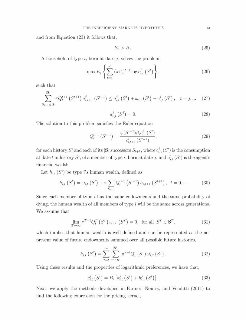
Next, we apply the methods developed in Farmer, Nourry, and Venditti (2011) to
nd the following expression for the pricing kernel,
THE INEFFICIENT MARKETS HYPOTHESIS 14
Proposition 1. The pricing kernel can be expressed as
+1¡
+1¢=
( +1) (1 ) ( )
+1 ( +1) (1 ) +1 ( +1)(34)
where ( ) is the aggregate consumption of all agents of type alive at date in
history and +1 (+1) is the human wealth of agents of type at date + 1 in
history +1.
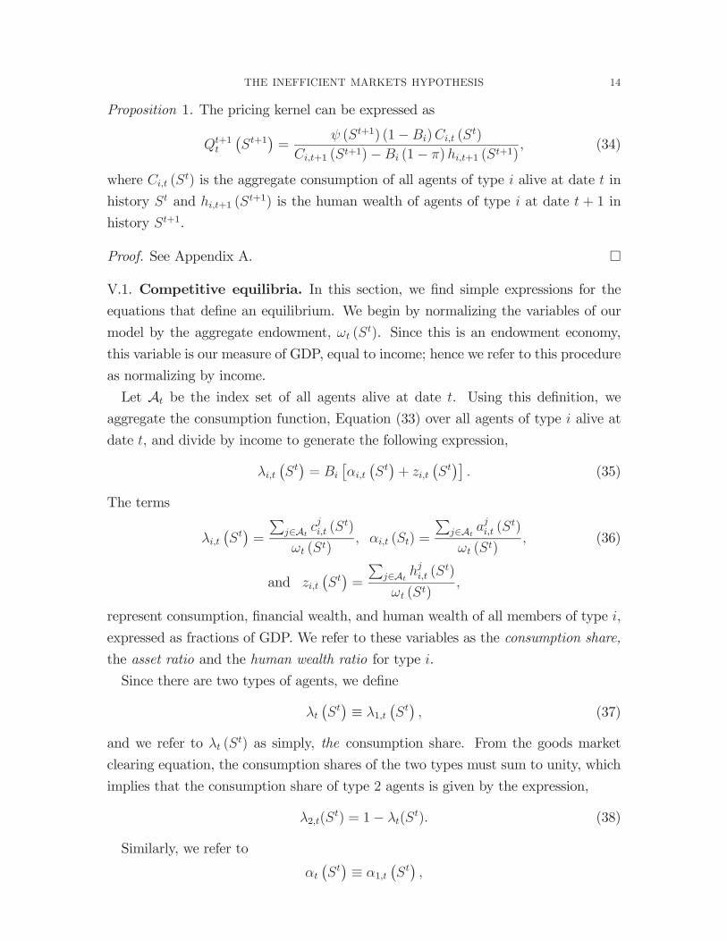
Proof. See Appendix A. ¤
V.1. Competitive equilibria. In this section, we nd simple expressions for the
equations that de ne an equilibrium. We begin by normalizing the variables of our
model by the aggregate endowment, ( ). Since this is an endowment economy,
this variable is our measure of GDP, equal to income; hence we refer to this procedure
as normalizing by income.
Let A be the index set of all agents alive at date . Using this de nition, we
aggregate the consumption function, Equation (33) over all agents of type alive at
date , and divide by income to generate the following expression,¡ ¢=
£ ¡ ¢+
¡ ¢¤(35)
The terms ¡ ¢=
PA ( )
( )( ) =
PA ( )
( )(36)
and¡ ¢
=
PA ( )
( )
represent consumption, nancial wealth, and human wealth of all members of type ,
expressed as fractions of GDP. We refer to these variables as the consumption share,
the asset ratio and the human wealth ratio for type .
Since there are two types of agents, we de ne¡ ¢1
¡ ¢(37)
and we refer to ( ) as simply, the consumption share. From the goods market
clearing equation, the consumption shares of the two types must sum to unity, which
implies that the consumption share of type 2 agents is given by the expression,
2 ( ) = 1 ( ) (38)
Similarly, we refer to ¡ ¢1
¡ ¢

THE INEFFICIENT MARKETS HYPOTHESIS 15
as the asset ratio, since from the asset market clearing equation, the nancial assets
of type 1 agents must equal the nancial liabilities of type 2 agents, and
2
¡ ¢=
¡ ¢(39)
Corresponding to the de nition of ( ) as the share of income consumed by type
1 agents, we will de ne
=1
1 =2 (40)
to be the share of income owned by type 1 agents.
Using these newly de ned terms, we have the following de nition of a competitive
equilibrium.
De nition 1. A competitive equilibrium is a set of sequences for the consumption
share, { ( )}, the asset ratio { ( )}, and the human wealth ratios { 1 ( )}and { ( )} and a sequence of Arrow security prices © +1 ( +1)
ªsuch that each
household of each generation maximizes expected utility, taking their budget con-
straint and the sequence of Arrow security prices as given and the goods and asset
markets clear. An equilibrium is admissible if { ( )} (0 1) for all
In the remainder of the paper, we drop the explicit dependence of , 1
and on to make the notation more readable.
V.2. Equilibria with intrinsic uncertainty. In their paper, ‘Do Sunspots Mat-ter?’ Cass and Shell (1983) distinguish between intrinsic uncertainty and extrinsic
uncertainty. Intrinsic uncertainty in our model is captured by endowment uctua-
tions. In this section, we study the case where this is the only kind of uncertainty
to in uence the economy. Before characterizing equilibrium sequences, we prove the
following lemma.
Lemma 1. Let = 1 2 and = 1 1 and recall that 2 1. There exists
an increasing a ne function : ˆ [ ] [0 1] such that for all values of the
aggregate human wealth ratio, ˆ the equilibrium consumption share [0 1] is
given by the expression
= ( )1 2
2 1
μ1
2
¶(41)
De ne the real number
0 = 1 ( 2 1) (42)
THE INEFFICIENT MARKETS HYPOTHESIS 16
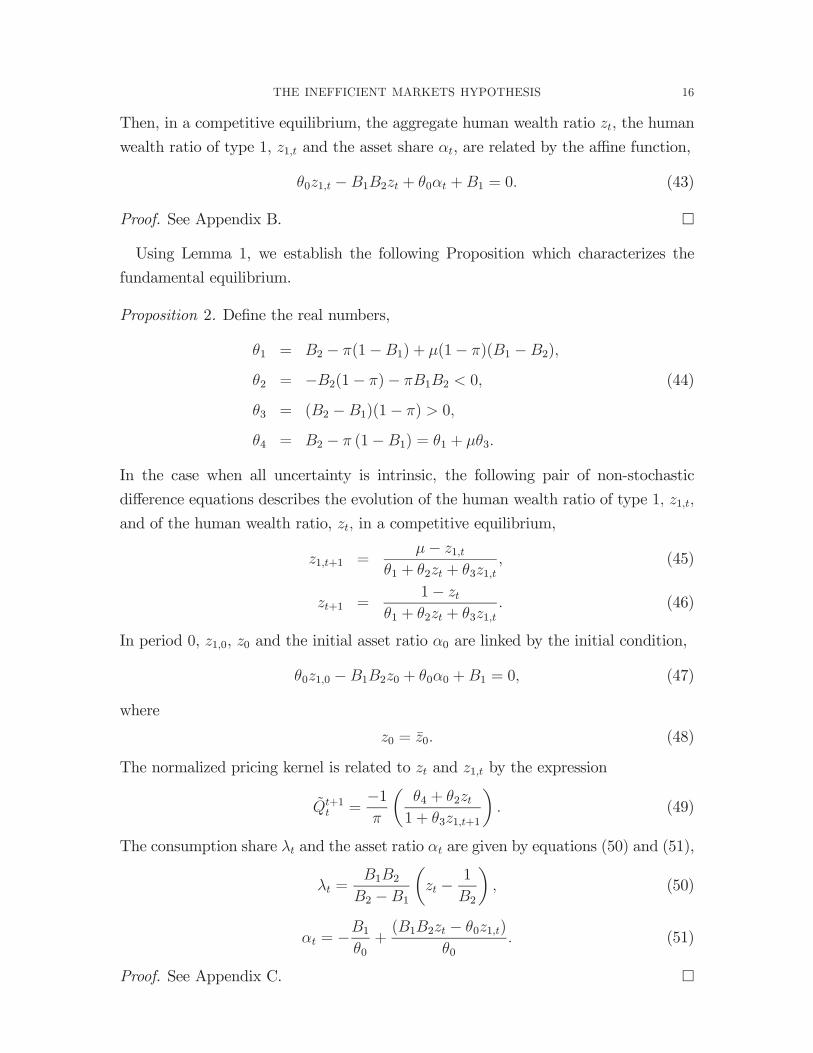
Then, in a competitive equilibrium, the aggregate human wealth ratio , the human
wealth ratio of type 1, 1 and the asset share , are related by the a ne function,
0 1 1 2 + 0 + 1 = 0 (43)
Proof. See Appendix B. ¤
Using Lemma 1, we establish the following Proposition which characterizes the
fundamental equilibrium.
Proposition 2. De ne the real numbers,
1 = 2 (1 1) + (1 )( 1 2)
2 = 2(1 ) 1 2 0 (44)
3 = ( 2 1)(1 ) 0
4 = 2 (1 1) = 1 + 3
In the case when all uncertainty is intrinsic, the following pair of non-stochastic
di erence equations describes the evolution of the human wealth ratio of type 1 1
and of the human wealth ratio, in a competitive equilibrium,
1 +1 =1
1 + 2 + 3 1(45)
+1 =1
1 + 2 + 3 1(46)
In period 0, 1 0, 0 and the initial asset ratio 0 are linked by the initial condition,
0 1 0 1 2 0 + 0 0 + 1 = 0 (47)
where
0 = 0̄ (48)
The normalized pricing kernel is related to and 1 by the expression
˜ +1 =1μ
4 + 2
1 + 3 1 +1
¶(49)
The consumption share and the asset ratio are given by equations (50) and (51),
=1 2
2 1
μ1
2
¶(50)
=1
0+( 1 2 0 1 )
0(51)
Proof. See Appendix C. ¤
THE INEFFICIENT MARKETS HYPOTHESIS 17
Equations (45) and (46) constitute a two-dimensional system in two variables with
a single initial condition, represented by Equation (47). These equations are non-
stochastic, even when the economy is hit by fundamental shocks, because we have
normalized 1 and ˜ +1 by the random endowment. Although and 1 uctuate
in response to random shocks, and 1 do not.
Removing the time subscripts from equations (45) and (46) we de ne a steady state
equilibrium to be a solution to the equations
1 ( 1 + 2 + 3 1) = 1 (52)
( 1 + 2 + 3 1) = 1 (53)
The following proposition characterizes the properties of a steady state equilibrium
and nds two equivalent representations of an equilibrium sequence; one using as
a state variable and one using ˜ +1.
Proposition 3. Equations (52) and (53) have a unique admissible steady state equi-
librium, { 1} such that ( ) and 1 = . The Jacobian of the system
(45) and (46), evaluated at { }, has two real roots, one less than 1 in absolutevalue and one greater than 1. It follows that { } is a saddle. The stable branchof this saddle is described by a set ˆ [ ], 1 = for any 0 and a function
(·) : ˆ ˆ such that the rst order di erence equation
+1 = ( ) (54)
where
( )1
1 + ( 2 + 3)(55)
de nes a competitive equilibrium sequence for { +1}. For all initial values of 0 and
1 0 where
0ˆ
1 0 = 0
(56)
converges to . There is an equivalent representation of equilibrium as a di erence
equation in ˜. In this representation there exists a set ˆ = [ ] and a function
(·) : ˆ ˆ, such that any sequencen˜ +1
ogenerated by the di erence equation
˜ +2+1 =
³˜ +1
´10
ˆ (57)
is a competitive equilibrium sequence. The set ˆ and the function (·) are de nedby equations (58) and (59),
=1 + ( 2 + 3)
=1 + ( 2 + 3) (58)
THE INEFFICIENT MARKETS HYPOTHESIS 18³˜ +1
´ 1 1 (1 1)(1 2)˜ +1
(59)
Every sequence generated by Equation (57), converges to the steady state ˜ where˜ is de ned in Equation (60),
˜ 1 + ( 2 + 3)=1 1 +
p(1 + 1)2 + 4( 2 + 3)
2(60)
Proof. See Appendix D. ¤
Proposition 3 implies that the two-dimensional dynamical system in { 1 } canbe reduced to a one-dimensional di erence equation, represented by Equation (55),
which describes the dynamics of the system on the saddle path.
In Figure 1 we have plotted +1 on the vertical axis and on the horizontal axis.
This gure illustrates the dynamics of , the human wealth ratio, for a parameterized
example. To construct this gure, we set the survival probability to 0 98, which
implies that the expected lifetime, conditional on being alive today, is 50 years. The
discount factor of type 1 agents is 0 98, the discount factor of type 2 agents is 0 9 and
there are equal shares of each type in the population.

THE INEFFICIENT MARKETS HYPOTHESIS 19
8 10 12 14 16 18 20 22 24 26−0.5
−0.4
−0.3
−0.2
−0.1
0
0.1
0.2
0.3
Human wealth ratio at date t
Cha
nge
in h
uman
wea
lth r
atio
1/B2 1/B1
Steady state z*
z is decreasingz is increasing
Admissible set
Figure 1: The dynamics of the human wealth equation
V.3. Equilibria with extrinsic uncertainty. Although we assume that agents areable to trade a complete set of Arrow securities, that assumption does not insulate the
economy from extrinsic uncertainty. In our model, the human wealth ratio and the
normalized pricing kernel ˜ +1 can uctuate simply as a consequence of self-ful lling
beliefs. That idea is formalized in the following proposition.
Proposition 4. Let be a sunspot random variable with support [ ] where
=[ 4(1 3) + 2 2] +
q[ 4(1 3) + 2 2]2
24(1 + 3)2
(1 + 3)2(61)
=( 4 + 2 )
(1 )(1 + 3 )(62)
and [ +1] = 1. Then there exist a set [ 0 ], a function (·) : ×and a stochastic process de ned by the equation
+1 = ( +1) (63)

THE INEFFICIENT MARKETS HYPOTHESIS 20
where
( +1)(1 ) +1
( 4 3 +1) + ( 2 + 3 +1)(64)
such that any sequence { } generated by (64) for 0 , is a competitive equilibrium
sequence. Further, there is an equivalent representation of equilibrium as the solution
to a stochastic di erence equation in ˜. In this representation, there exists a function
( 0 ), such that
˜ +1 =³˜
1 +1
´(65)
where,
³˜
1 +1
´( +1) +
( +1)˜
1
(66)
( +1)1½
( 2 + 3 +1)
( 2 + 3 )4 + 3 +1
¾(67)
and
( +1)12
½( 2 + 4) ( 2 + 3 +1)
( 2 + 3 )
¾(68)
The sequencen˜ +1
o, generated by a solution to Equation (65), is a competitive
equilibrium sequence for ˜.
Proof. See Appendix E. ¤
Figure 2 illustrates the method used to construct sunspot equilibria. The solid curve
represents the function ( 1) and the upper and lower dashed curves represent the
functions ( ) and ( ). We have exaggerated the curvature of the function
(·) by choosing a value 1 = 0 98 and 2 = 0 3. The large discrepancy between 1
and 2 causes the slopes of these curves to be steeper for low values of and atter
for high values, thereby making the graph easier to read.

THE INEFFICIENT MARKETS HYPOTHESIS 21
0 5 10 15 20 25 300
5
10
15
20
25
30
Human wealth ratio at date t
Hum
an w
ealth
brat
io a
t dat
e t+
1
Admissible Set
Suppport of Invariant Distribution
Za’ ZbZa
Figure 2: The dynamics of sunspot equilibria
Figure 2 also contrasts the admissible set ˆ [ ] with the support of the in-
variant distribution [ 0 ] The three vertical dashed lines represent the values0 and The lower bound of the largest possible invariant distribution, 0 is de-
ned as the point where ( ) is tangent to the 45 line. Recall that the admissible
set is the set of values of for which the consumption of both types is non-negative
and notice that 0 is to the right of , the lower bound of the admissible set. Figure
2 illustrates that the support of the largest possible invariant distribution is a subset
of the admissible set. It follows from the results of Futia (1982) that, as uctuates
in the set [ ], converges to an invariant distribution with support [ 0 ].4
VI. Simulating the invariant distribution
Because we know the exact law of motion for the state we are able to compute the
moments of any of the variables of our model that are functions of that state. We are
also able to simulate individual sequences of arti cial data and compare them with
data from the real world. This section carries out that exercise.
To compute moments of the invariant distribution, we used the di erence equation
(63), to construct an approximation to the transition function
( ) (69)
4The proof builds on Futia (1982) and is identical to the argument used in Farmer and Woodford
(1997) Theorem 3, Page 756.

THE INEFFICIENT MARKETS HYPOTHESIS 22
where { } is the value of the state at date and is a set that represents
possible values that and might take at date + 1. For every value of , (· )
is a measurable function and for every value of ( ·) is a probability measure(Stokey, Lucas, and Prescott, 1989, Chaper 8). If ( ) is the probability that the
system is in state at date then
0 ( 0) =Z
( 0) ( ) (70)
is the probability that it is in state 0 at date + 1 By iterating on this operator
equation for arbitrary initial we arrive at an expression for the invariant measure.
This invariant measure, ( ), is the unconditional probability of observing the system
in state = { }.In a technical appendix to this paper, available from the authors, we explain how
to compute a discrete Markov chain approximation to Equation (70). The simulation
results reported in gures 3 and 4 were computed using this discrete approximation.
In addition to the four parameters, , 1, 2 and , which we set to
= 0 98 1 = 0 98 2 = 0 9 = 0 5
as in the earlier part of the paper, we calibrated three additional parameters. We as-
sumed that endowment growth is a geometric random walk with mean 1 and variance2 and that exp ( ) is normal with mean 1 and variance 2 In our baseline calibra-
tion we set the correlation coe cient between and equal to zero. We also
experimented with values of from 0 99 to +0 99 with little e ect on the results.
The calibrated values of , and were set to
= 0 015 = 0 035 = 0
The choice of was set to equal the standard deviation of consumption growth in
post war U.S. data and the standard deviation of was set to the largest value
that was consistent with minimal truncation bias.5 Figure 3 depicts the invariant
distribution ( ) for these parameter values.
5Larger values of cause the invariant distribution piling up at the end points as a consequence
of truncation bias.

THE INEFFICIENT MARKETS HYPOTHESIS 23
0.95
1
1.05
10
15
20
250
1
2
3
4
5
6
7
8
9
x 10−3
Consumption GrowthWealth Ratio
Inva
riant
Figure 3: The joint invariant distribution of consumption growth and the human wealth ratio
12 14 16 18 20 22 24 260
0.02
0.04
0.06
0.08
0.1
0.12
Human Wealth
Mar
gina
l pdf
Figure 4: The marginal invariant distribution of the human wealth ratio
In Figure 4 we report the marginal distribution over the human wealth ratio. The
median human wealth ratio is a little over 20, but there is considerable probability
mass that this ratio will be less than 18 or greater than 23. That di erence represents
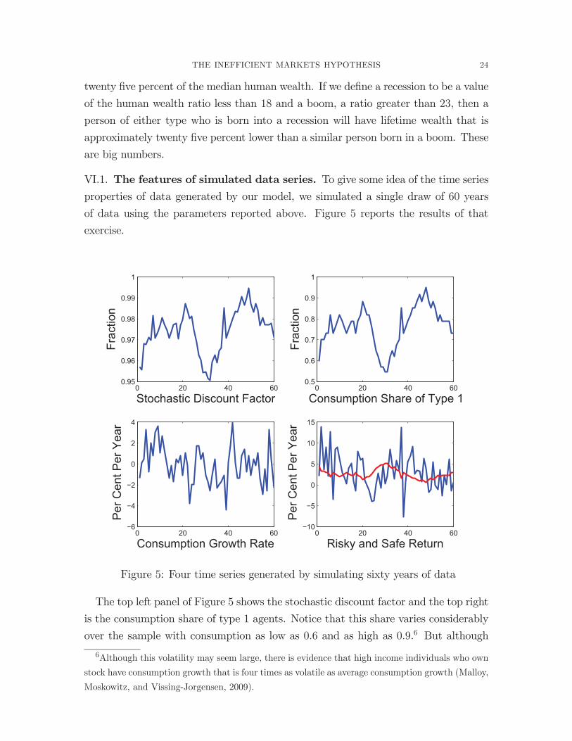
THE INEFFICIENT MARKETS HYPOTHESIS 24
twenty ve percent of the median human wealth. If we de ne a recession to be a value
of the human wealth ratio less than 18 and a boom, a ratio greater than 23, then a
person of either type who is born into a recession will have lifetime wealth that is
approximately twenty ve percent lower than a similar person born in a boom. These
are big numbers.
VI.1. The features of simulated data series. To give some idea of the time seriesproperties of data generated by our model, we simulated a single draw of 60 years
of data using the parameters reported above. Figure 5 reports the results of that
exercise.
0 20 40 600.95
0.96
0.97
0.98
0.99
1
Stochastic Discount Factor
Frac
tion
0 20 40 600.5
0.6
0.7
0.8
0.9
1
Consumption Share of Type 1
Frac
tion
0 20 40 60−6
−4
−2
0
2
4
Consumption Growth Rate
Per
Cen
t Per
Yea
r
0 20 40 60−10
−5
0
5
10
15
Risky and Safe Return
Per
Cen
t Per
Yea
r
Figure 5: Four time series generated by simulating sixty years of data
The top left panel of Figure 5 shows the stochastic discount factor and the top right
is the consumption share of type 1 agents. Notice that this share varies considerably
over the sample with consumption as low as 0 6 and as high as 0 9.6 But although
6Although this volatility may seem large, there is evidence that high income individuals who own
stock have consumption growth that is four times as volatile as average consumption growth (Malloy,
Moskowitz, and Vissing-Jorgensen, 2009).

THE INEFFICIENT MARKETS HYPOTHESIS 25
the consumption fraction of type 1 agents is volatile, aggregate consumption growth,
shown in the bottom left panel, matches the volatility found in U.S. data. The
standard deviation of aggregate consumption growth in the invariant distribution is
equal to 0 015, the same as in the post-war U.S. The bottom right panel shows that
the mean equity return is much more volatile than the safe return which is relatively
smooth, just as we nd in U.S. data.
The returns to debt and equity in our model were computed as follows. Since our
model does not contain capital, a claim to equity is the same thing as a claim to the
endowment stream of a living agent. Let
(71)
be the price of a ‘cum-dividend’ traded claim to the endowment stream. We can
express the return to this claim as¡+1¢=
( +1)
( )
μ( +1)
( ) 1
¶ ¡+1¢
(72)
where the in the numerator of this expression represents the fact that the claim
has a probability of being repaid. We can also price a safe claim to a unit of the
consumption good, ¡ ¢=X
+1¡
+1¢
(73)
which o ers a risk free gross return of,¡+1¢=
1
( )(74)
Using these de nitions we found that when and are uncorrelated, the Sharpe
ratio in the invariant distribution is 0 007. By increasing the correlation to 0 9, it
is possible to increase this to 0 02. While this is a factor of ten larger than the
representative agent model when preferences are logarithmic, it is still a factor of
ten too small compared with time series data. Although we are able to explain the
volatility of the pricing kernel, our model does not help us to explain the equity
premium.
VII. Conclusion
The rst welfare theorem of general equilibrium theory asserts that every compet-
itive equilibrium is Pareto optimal. When nancial markets are complete, and when
all agents are able to participate in nancial markets, this theorem implies that un-
restricted trade in nancial assets will lead to the e cient allocation of risk to those
who are best able to bear it.
THE INEFFICIENT MARKETS HYPOTHESIS 26
We have shown, in this paper, that competitive nancial markets do not lead to
Pareto e cient outcomes and that the failure of complete nancial markets to deliver
socially e cient allocations has nothing to do with frictions, market incompleteness
or transactions costs of any kind. The rst welfare theorem fails because participation
in nancial markets is necessarily incomplete as a consequence of the fact that agents
cannot trade risk in nancial markets that open before they are born. For this reason,
nancial markets do not work well in our model and we conjecture that for the same
reason, they do not work well in the real world.
The Ramsey-Cass-Koopmans model (Ramsey, 1928; Koopmans, 1965; Cass, 1965)
underpins not only all of modern macroeconomics, but also all of modern nance
theory. Existing literature modi es this model by adding frictions of one kind or
another to explain why free trade in competitive markets cannot achieve an e cient
allocation of risk. It has not, as yet, o ered a convincing explanation for the volatility
of the stochastic discount factor in real world data. Although our work is close to
the Ramsey-Cass-Koopmans model, we do not need to assume frictions of any kind.
In our model, nancial markets are not Pareto e cient, except by chance. Although
individuals in our model are rational; markets are not.
Appendix
Appendix A.
Proof of Proposition 1. If we sum Equation (29) over all agents of type who were
alive at date , we arrive at the equation,
+1¡
+1¢=
( +1)P
A ( )PA +1 (
+1)(A.1)
The consumption at date +1 of everyone of type who was alive at date , is equal
to the consumption of all agents of type minus the consumption of the new borns.
For any date +1 and any variable let be the quantity of that variable held by a
household of generation and let be the aggregate quantity. Let A be the index
set of all agents alive at date and let N +1 denote the set of newborns at period
+ 1. Then, XA
+1 +XN +1
+1 =XA +1
+1 = +1 (A.2)
Using Equation (A.2) we can write the denominator of Equation (A.1) as,
XA
+1
¡+1¢=1 X
A +1
+1
¡+1¢ X
N +1
+1
¡+1¢
(A.3)

THE INEFFICIENT MARKETS HYPOTHESIS 27
The rst term on the right-hand-side of this equation is aggregate consumption of
type , which we de ne as
+1
¡+1¢ X
A +1
+1
¡+1¢
(A.4)
The second term is the consumption of the newborns of type . Because these agents
are born with no nancial assets, their consumption is proportional to their human
wealth. This leads to the expressionXN +1
+1
¡+1¢= (1 ) +1
¡+1¢
(A.5)
where the coe cient (1 ) is the fraction of newborns of type . Using equations
(A.3)-(A.5) we can rewrite (A.1) as
+1¡
+1¢=
( +1) (1 ) ( )
+1 ( +1) (1 ) +1 ( +1)(A.6)
which is Equation (34), the expression we seek. ¤
Appendix B.
Proof of Lemma 1. From Equation(35), evaluated for types 1 and 2 we get
=1
1 (B.1)
=1
22 (B.2)
Summing (B.1) and (B.2) and rearranging leads to Equation (41). The fact that is
increasing in follows from the assumption, 2 1 The domain of is found by
evaluating 1 for values of = 0 and = 1.
From (41) we have that,
=1 2
2 1
μ1
2
¶(B.3)
which expresses the consumption share as a function of the aggregate human wealth
ratio. From the consumption function of type 1 agents, Equation (35), we have the
following expression linking the consumption share with the asset share, and with the
type 1 human wealth ratio,
= 1 ( + 1 ) (B.4)
Combing equations (B.3) and (B.4) gives
1 ( + 1 ) =1 2
2 1
μ1
2
¶(B.5)
Using de nition, (42), this leads to Equation (43), the expression we seek. ¤

THE INEFFICIENT MARKETS HYPOTHESIS 28
Appendix C.
Proof of Proposition 2. From Proposition 1 and the restriction to perfect foresight
equilibria, we have that
=1 2
2 1
μ1
2
¶(C.1)
Leading Equation (C.1) one period gives,
+1 =1 2
2 1
μ+1
1
2
¶(C.2)
Dividing the numerator of Equation (34), by and dividing the denominator by
+1 leads to the following expressions that relate the normalized pricing kernel to
the consumption share and to the human wealth ratio of each type,
˜ +1 =(1 1)
+1 1 (1 ) 1 +1(C.3)
˜ +1 =(1 2) (1 )
(1 +1) 2 (1 ) 2 +1(C.4)
These expressions follow from the fact that agents of each type equate the marginal
rate of substitution to the pricing kernel, state by state.
Next, we divide the human wealth equation, (30), by the aggregate endowment.
That leads to the following di erence equation in the human wealth ratio for type ,
= +h˜ +1
+1
i(C.5)
Adding up Equation (C.5) over both types leads to the following expression for the
aggregate human wealth ratio,
= 1 +h˜ +1
+1
i(C.6)
From equations (C.3) and (C.4),
˜ +1 =(1 2) (1 )
1 +1 2 (1 ) 2 +1(C.7)
˜ +1 =(1 1)
+1 1 (1 ) 1 +1(C.8)
Substituting for and +1 from equations (C.1) and (C.2) into (C.8), we obtain the
following expression for 2 +1 as a function of and 17
2 +1 =( 1 1 1 2) 1 +1 + + ( 1 + 2) 1 +1 1
( 2 2 1 2) + ( 2 + ( 1 1))(C.9)
7The algebra used to derive (C.9) was checked using Maple in Scienti c Workplace. The code is
available from the authors on request.

THE INEFFICIENT MARKETS HYPOTHESIS 29
De ne the following transformed parameters
1 = 2 (1 1) + (1 )( 1 2)
2 = 2(1 ) 1 2 0
3 = ( 2 1)(1 )
4 = 2 (1 1) = 1 + 3
(C.10)
Combining equation (C.1)—(C.3) with (C.5), using (C.9) and (C.10) gives the following
expression for the normalized pricing kernel,
˜ +1 =1 + 3 + 2
1 + 3 1 +1=
4 + 2
1 + 3 1 +1(C.11)
Because we have normalized all variables by income, none of the equations of our
model contain random variables. Hence we may drop the expectations operator and
write the human wealth equations, (C.5) and (C.6) as follows,
1 = + ˜ +11 +1 (C.12)
= 1 + ˜ +1+1 (C.13)
Rearranging Equations (C.12) and (C.13), replacing ˜ +1 from (C.11), gives,
1 +1 =1
1 + 2 + 3 1(C.14)
+1 =1
1 + 2 + 3 1(C.15)
which are the expressions for equations (45) and (46) that we seek. The initial condi-
tion, Equation (47), follows from Proposition 1 and the expression for the normalized
pricing kernel. ¤
Appendix D.
Proof of Proposition 3. Evaluating equations (C.14) and (C.15) at a steady state
( 1 ) = ( 1 ), and considering their ratio gives 1 = . It follows that a
steady state equilibrium is a solution of the following second degree polynomial
P( ) = 2( 2 + 3) + (1 + 1) 1 = 0 (D.1)
De ne the discriminant
= (1 + 1)2 + 4( 2 + 3) (D.2)
Using the fact that 2 1, it follows from the de nitions of 1, 2 and 3 that
1 2 (1 1) 3 0 (D.3)
and hence
2 + 3 2 (D.4)

THE INEFFICIENT MARKETS HYPOTHESIS 30
Using inequalities (D.3) and (D.4) to replace ( 2 + 3) by 2 and replacing 2 by its
de nition, it follows that
[ 2 + 1 (1 1)]2 4 2[1 (1 1)] = [ 2 1 + (1 1)]
2 0 (D.5)
Since the discriminant is non-negative, there exist two real solutions to Equation
(D.1), and given by the expressions,
=1 + 1 +
2( 2 + 3)=
1 + 1
2( 2 + 3)(D.6)
We next check that these two solutions belong to the admissible set ( ). Con-
sider rst the lower solution . Rearranging the de nition of it follows that
1 2 if and only if
1 + 1 +2( 2 + 3)
2(D.7)
Squaring both sides of (D.7) and substituting for from (D.2) implies that, equiva-
lently,
1 + 1 2 +2 + 3
20 (D.8)
Substituting the expressions for 1, 2 and 3 into this inequality and rearranging
terms leads to the following expression for the left-hand side of (D.8),
(1 )( 2 1)1 2
20 (D.9)
where the inequality in (D.9) follows since 1 2 1 0 and 1. It follows
that and hence is not an admissible steady state.
Consider now the larger of the two solutions, . The same computation as previ-
ously allows us to conclude that . We must next show that 1 1.
Using the de nition of , this occurs if and only if
1 + 1 +2( 2 + 3)
1(D.10)
A necessary condition for this inequality to hold is that the left-hand side is negative.
Using the de nitions of 1 2 and 3, we may write the left side of (D.10) as the
following second degree polynomial in 1
G( 1) = 1 [1 + 2 (1 1) + (1 )( 1 2)]
2 [ 2(1 ) + 1 2 + (1 )( 1 2)] (D.11)
The left-hand side of (D.10) is then negative when G( 1) 0. Notice that G( 1)
is convex with G(± ) = + . Further, as G( 1) is de ned over the set (0 2), we
have that G(0) = 2 2(1 )(1 ) 0 and G( 2) = 2(1 )(1 2) 0.

THE INEFFICIENT MARKETS HYPOTHESIS 31
It follows that for any 1 (0 2), G( 1) 0 and thus the left-hand side of (D.10)
is negative. Squaring both sides of (D.10) and substituting for from (D.2) implies
that inequality (D.10) holds if and only if
1 + 1 1 +2 + 3
10 (D.12)
Substituting the expressions for 1, 2 and 3 into this inequality and simplifying the
expression yields to the following formulation for the left-hand side of (D.12)
(1 )(1 )(1 1)( 2 1) 0 (D.13)
This inequality establishes that ˆ and hence is an admissible steady state.
We study the stability properties of by linearizing the dynamical system (45)—(46)
around . Using the steady state relationships (52) and (53), we get after some
simpli cation, the following Jacobian matrix
J =
Ã1(1 + 2 ) ( 1) 3
( 1) 21(1 + 3 )
!(D.14)
The associated characteristic polynomial is
1(1 + 2 )
¸1(1 + 3 )
¸( 1)2 2 3
=
μ1
¶μ1 1
1
¶= 0 (D.15)
with characteristic roots
1 =1
1 (D.16a)
2 =1 1
1(D.16b)
We next establish that this steady state is a saddle and that the dynamical system
(45)—(46) is globally stable. Since, from (D.16a), 1 is positive and greater than
one, we need only establish a general property to guarantee global conclusion and
that 1 2 1 Let us rst consider the derivative of ( ) for any , 0( ) =
(1 1 ) ( 1). Since 1, we have 0( ) 1 for any ( ) if 1 1 0,
which holds since 2 1. This property implies that 2 1. Moreover, we get0( ) 0 if and only if 2 1 0, which again holds as 2 1. We then establish
that 2 1. From (D.16b), this follows if and only if 2 (1+ 1) 0. Equivalently
using the de nitions of 1 and , together with the fact that 2+ 3 0, 2 1 if
THE INEFFICIENT MARKETS HYPOTHESIS 32
and only if
4( 2 + 3) + (1 + 1)h1 + 1 +
i= + (1 + 1)
=h1 + 1 +
i0 (D.17)
We derive from (C.10) that
1 + 1 = 2 [1 (1 )] + 1 (1 ) + 1 (1 1) 0 (D.18)
and thus 2 1. Since 1 1 we conclude that is saddle-point stable. It follows
that the equilibrium must be unique and given by the stable branch of the saddle-
point since any other path will violate the feasibility conditions. Consider then the
ratio of equations (C.14) and (C.15). We get:
1 +1
+1=
1
1(D.19)
Obviously, this ratio admits 1 = for all as a solution. Uniqueness of the
equilibrium implies that this solution is the unique equilibrium of the dynamical
system (C.14)—(C.15) in ( 1 ) which can then be reduced to the one-dimensional
di erence equation de ned by Equation (55). Further, is globally stable for anyˆ
Next we turn to an equivalent representation of the system using ˜ +1 as a state
variable. Replacing 1 +1 from (45) in Equation (49), and simplifying the resulting
expression gives,˜ +1 =
1 + 2 + 3 1 (D.20)
Substituting the restriction 1 = into Equation (D.20) and inverting the equation
to nd as a function of ˜ +1, leads to
=˜ +1 + 1
2 + 3(D.21)
Substituting this expression into (55) and rearranging terms leads to the di erence
equation˜ +2+1 =
³˜ +1
´(D.22)
where ³˜ +1
´ 1 1+
1 + 2 + 3
2 ˜ +1=1 1 (1 1)(1 2)
˜ +1(D.23)
which provides an equivalent representation of the equilibrium in terms of ˜. Using
the same arguments as previously, it follows that for all 10 ( ) with
=1 + ( 2 + 3)
=1 + ( 2 + 3) (D.24)

THE INEFFICIENT MARKETS HYPOTHESIS 33
there exists a sequence of equilibrium asset prices described by the di erence equation
(D.22), that converges to the steady state pricing kernel. ¤
Appendix E.
Proof of Proposition 4. Consider the de nition of human wealth,
= 1 +h˜ +1
+1
i(E.1)
In Proposition 2, Equation (C.11), we derived an expression for the pricing kernel˜ +1 ( 1 +1), that we write below as Equation (E.2).
˜ +1 =
μ4 + 2
1 + 3 1 +1
¶(E.2)
Replacing (E.2) in (E.1), and restricting attention to the stable branch of the saddle
by setting 1 = , we arrive at the following functional equation,
= 1 +
μ4 + 2
1 + 3 +1
¶+1
¸(E.3)
Since Equation (E.3) characterizes equilibria, it follows that any admissible sequence
{ } that satis es Equation (E.3) is an equilibrium sequence. We now show how to
construct a stochastic process for { } that generates admissible solutions to (E.3).Let +1, be a bounded, i.i.d. random variable with support [ ] such that
( +1) = 1 (E.4)
and consider sequences for { }, ( 0 ) that satisfy the equation,
( 1) +1 =
μ4 + 2
1 + 3 +1
¶+1 (E.5)
Rearranging (E.5), using the fact that 4 3 = 1, we may de ne a function
(·) : ×
+1 =(1 ) +1
( 4 3 +1) + ( 2 + 3 +1)= ( +1) (E.6)
This is the analog of Equation (55) in Proposition 3. Any admissible sequence must
lie in the set ˆ [ ] where 12 and 1
1 . We now show how to
construct the largest set ˆ such that all sequences { } generated by (E.6) areadmissible. Note rst, that
( )=
(1 ) ( 4 + 2 )
[( 4 3 ) + ( 2 + 3 ) ]2(E.7)
where 4 + 2 = 2(1 ) 0 and 4 + 2 = (1 )[ 1 + 2(1 )] 0.
Because 1, it follows that ( ) 0 for any ( ). Moreover,
THE INEFFICIENT MARKETS HYPOTHESIS 34
(1 ) = 0 for any . We conclude that the graph of the function ( ) rotates
counter-clockwise around = 1 as increases. The upper bound is then obtained
as the solution of the equation, = ( ). A straightforward computation yields
=( 4 + 2 )
(1 )(1 + 3 )(E.8)
Starting from the upper bound , can be decreased down to the point where
the graph of the function ( ) becomes tangent with the 45 line. Consider the
equation ( ) = which can be rearranged to give the equivalent second degree
polynomial2( 2 + 3 ) + [ 4 + (1 3)] = 0 (E.9)
We denote by 0 , the value of for which the two roots of (E.9) are equal and hence
the discriminant of (E.9) is equal to zero. Equation (E.10) de nes a polynomial in
such that this discriminant condition is satis ed and is the larger of the two values
of such that this condition holds;
[ 4 + (1 3)]2 + 4 ( 2 + 3 ) = 0
2(1 + 3)2 + 2 [ 4(1 3) + 2 2] +
24 = 0
(E.10)
Using the formula for the roots of a quadratic, we obtain the following explicit ex-
pression for ;
=[ 4(1 3) + 2 2] +
q[ 4(1 3) + 2 2]2
24(1 + 3)2
(1 + 3)2(E.11)
This establishes the rst part of Proposition 4.
We now derive an equivalent di erence equation in ˜ +1. Here we use (E.2) and
(E.3) to give the following expression for ˜ +1
˜ +1 =( 4 3 +1) ( 2 + 3 +1) (E.12)
Rearranging (E.12) gives,
=( 4 3 +1)
( 2 + 3 +1)
˜ +1
( 2 + 3 +1)(E.13)
Substitute (E.12) into (E.13) to give
˜ +1 = ( +1) +( +1)˜
1
³˜
1 +1
´(E.14)
where, using the fact that 1 + 2 + 3 2 + 4, we de ne,
( +1)1½
( 2 + 3 +1)
( 2 + 3 )4 3 +1
¾(E.15)
THE INEFFICIENT MARKETS HYPOTHESIS 35
( +1) =12
½( 2 + 4) ( 2 + 3 +1)
( 2 + 3 )
¾(E.16)
Equation (E.14) is the analog of Equation (57). This establishes the second part of
Proposition 4 ¤
References
Abreu, D., and M. K. Brunnermeier (2003): “Bubbles and Crashes,” Econo-
metrica, 71(1), 173—204.
Allais, M. (1947): Economie et Intérêt. Imprimerie Nationale, Paris (English tra-
duction forthcoming in 2013 at Chicago University Press).
Angeletos, G.-M., and La’O (2013): “Sentiments,” Econometrica, 81(2), 739—779.
Azariadis, C. (1981): “Self-ful lling Prophecies,” Journal of Economic Theory,
25(3), 380—396.
Barberis, N., and R. Thaler (2003): “A Survey of Behavioral Finance,” in Hand-
book of the Economics of Finance, ed. by R. Stulz, and M. Harris. Noth Holland,
Amsterdam.
Barsky, R. B., and J. B. DeLong (1993): “Why Does the Stock Market Fluctu-
ate,” Quarterly Journal of Economics, 107, 291—311.
Benhabib, J., and R. E. A. Farmer (1994): “Indeterminacy and Increasing Re-
turns,” Journal of Economic Theory, 63, 19—46.
Benhabib, J., P. Wang, and Y. Wen (2012): “Sentiments and Agregate Fluctu-
ations,” NBER working paper 18413.
Bernanke, B., M. Gertler, and S. Gilchrist (1996): “The Financial Acceler-
ator and the Flight to Quality,” The Review of Economics and Statistics, 78(1),
1—15.
Bernanke, B. S., and M. Gertler (1989): “Agency Costs, Net Worth and Busi-
ness Fluctuations,” American Economic Review, 79(1), 14—31.
(2001): “Should Central Banks Respond to Movements in Asset Prices?,”
American Economic Review, 91(2), 253—257.
Blanchard, O. J. (1985): “Debt, De cits, and Finite Horizons,” Journal of Political
Economy, 93(April), 223—247.
Brunnermeir, M. K. (2012): “Macroeconomics with Financial Frictions,” in Ad-
vances in Economics and Econometrics. Cambridge University Press.
Brunnermeir, M. K., and Y. Sannikov (2012): “Redistributive Monetary Pol-
icy,” Paper presented at the 2012 Jackson Hole Conference, August 31st - Septem-
ber 2nd 2012.

THE INEFFICIENT MARKETS HYPOTHESIS 36
Bullard, J., G. Evans, and S. Honkapohja (2010): “A Model of Near-Rational
Exuberance,” Macroeconomic Dynamics, 14, 106—88.
Caballero, R. J., and A. Krishnamurthy (2006): “Bubbles and Capital Flow
Volatility: Causes and Risk Management,” Journal of Monetary Economics, 53(1),
35—53.
Campbell, J. Y., and J. H. Cochrane (1999): “By Force of Habit: A
Consumption-Based Explanation of Aggregate Stock Market Behavior,” Journal
of Political Economy, 107, 205—251.
Carlstom, C., and T. S. Fuerst (1997): “Agency Costs, Net Worth and Business
Fluctuations: A Computable General Equilbrium Analysis,” American Economic
Review, 87(5), 893—910.
Cass, D. (1965): “Optimum Growth in an Aggregative Model of Capital Accumula-
tion,” Review of Economic Studies, 32, 233 — 240.
Cass, D., and K. Shell (1983): “Do Sunspots Matter?,” Journal of Political Econ-
omy, 91, 193—227.
Christiano, L., R. Motto, and M. Rostagno (2012): “Risk Shocks,” North-
western University mimeo.
Cochrane, J. H. (2011): “Presidential Adress: Discount Rates,” The Journal of
Finance, 66(4), 1047—1108.
Eggertsson, G. (2011): “What Fiscal Policy is E ective at Zero Interest Rates?,”
in NBER Macroeconomics Annual 2010, vol. 25, pp. 59—112. National Bureau of
Economic Research Inc.
Eggertsson, G. B., and M. Woodford (2002): “The Zero Bound on Interest
Rates and Optimal Monetary Policy,” Brookings Papers on Economic Activity, 2,
139—211.
Epstein, L., and S. Zin (1989): “Substitution, Risk Aversion and the Temporal
Behavior of Consumption and Asset Returns: An Empirical Analysis,” Journal of
Political Economy, 99, 263—286.
(1991): “Substitution, Risk Aversion and the Temporal Behavior of Con-
sumption and Asset Returns: A Theoretical Framework,” Econometrica, 57, 937—
969.
Fahri, E., and J. Tirole (2012): “Bubbly Liquidity,” The Review of Economic
Studies, 79(2), 678—706.
Fama, E. F. (1963): “Mandelbrot and the Stable Paretian Hypothesis,” Journal of
Business, 36, 420—429.

THE INEFFICIENT MARKETS HYPOTHESIS 37
(1965a): “The Behavior of Stock Market Prices,” Journal of Business, 38,
34—105.
(1965b): “RandomWalks in Stock Market Prices,” Financial Analysts Jour-
nal, 21, 55—59.
(1970): “E cient Capital Markets: A Review of Theory and Empirical
Work,” Journal of Finance, 25(2), 383—417.
Farmer, R. E. A. (1999): The Macroeconomics of Self-Ful lling Prophecies. MIT
Press, Cambridge, MA, second edn.
(2002a): “Business Cycles with Heterogeneous Agents,” UCLA mimeo, Pa-
per prepared for a conference at GREQAM on "New Perspectives of (In)Stability,
the Role of Heterogeneity", Marseilles, June 2011.
(2002b): “Fiscal Policy, Equity Premia, and Heterogeneous Agents,” UCLA
mimeo, Paper presented to the conference "New Developments in Fiscal Policy
Analysis" at Universitat Pompeu Fabra, Barcelona, May 2002.
(2010): Expectations, Employment and Prices. Oxford University Press, New
York.
(2012a): “Con dence, Crashes and Animal Spirits,” Economic Journal,
122(559).
(2012b): “Qualitative Easing: How it Works and Why it Matters,” NBER
working paper 18421 and CEPR discussion paper 9153.
(2012c): “The Stock Market Crash of 2008 Caused the Great Recession:
Theory and Evidence,” Journal of Economic Dynamics and Control, 36, 697—707.
(2013): “Animal Spirits, Financial Crises and Persistent Unemployment,”
Economic Journal, 123(568).
(2014): “The Evolution of Endogenous Business Cycles,” Macroeconomic
Dynamics, (forthcoming).
Farmer, R. E. A., and J. T. Guo (1994): “Real Business Cycles and the Animal
Spirits Hypothesis,” Journal of Economic Theory, 63, 42—73.
Farmer, R. E. A., C. Nourry, and A. Venditti (2011): “Debt De cits and
Finite Horizons, the Stochastic Case,” Economics Letters, 111, 47—49.
Farmer, R. E. A., and D. Plotnikov (2012): “Does Fiscal Policy Matter? Blinder
and Solow Revisited,” Macroeconomic Dynamics, 16(Supplement 1), 149—166.
Farmer, R. E. A., and M. Woodford (1984): “Self-ful lling Prophecies and the
Business Cycle,” Caress Working Paper 84-12.
(1997): “Self-ful lling Prophecies and the Business Cycle,” Macroeconomic
Dynamics, 1(4), 740—769.

THE INEFFICIENT MARKETS HYPOTHESIS 38
Fostel, A., and J. Geanakoplos (2008): “Leverage Cycles and the Anxious
Economy,” American Economic Review, 98(4), 1211—1234.
Fox, J. (2009): The Myth of the Rational Market. Harper Collins.
Futia, C. A. (1982): “Invariant Distributions and the Limiting Behavior of Mar-
kovian Economic Models,” Econometrica, 50(2), 377—408.
Geanakoplos, J. (2010): “The Leverage Cycle,” in NBER Macroeconomics Annual
2009, ed. by D. Acemoglu, K. Rogo , and M. Woodford. University of Chicago
Press.
Gu, C., and R. Wright (2010): “Endogenous Credit Cycles,” University of Wis-
consin, mimeo.
Kiyotaki, N., and J. H. Moore (1997): “Credit Cycles,” Journal of Political
Economy, 105(3), 739—764.
Koopmans, T. C. (1965): “On the Concept of Optimal Economic Growth,” in The
Econometric Approach to Development Planning, pp. 225—300. North Holland.
Lansing, K. J. (2010): “Rational and Near-Rational Bubbles Without Drift,” Eco-
nomic Journal, 549, 1149—1174.
Leroy, S., and R. Porter (1981): “Stock Price Volatility: A Test based on Implied
Variance Bounds,” Econometrica, 49, 97—113.
Malinvaud, E. (1987): “The Overlapping Generations Model in 1947,” Journal of
Economic Literature, 25, 103—105.
Malloy, C. J., T. J. Moskowitz, and A. Vissing-Jorgensen (2009): “Long-
Run Stockholder Consumption Risk and Asset Returns,” The Journal of Finance,
64(6), 2427—2479.
Martin, A., and J. Ventura (2011): “Theoretical Notes on Bubbles and the
Current Crisis,” IMF Economic Review, 59(1), 6—40.
(2012): “Economic Growth with Bubbles,” American Economic Review,
102(6), 3033—3058.
Miao, J., and P. Wang (2012): “Bubbles and Total Factor Productivity,” American
Economic Review: Papers and Proceedings, 102(3), 82—87.
Oreopoulos, P., T. Von-Wachter, and A. Heisz (2012): “The Short- and Long-
Term Career E ects of Graduating in a Recession: Hysteresis and Heterogeneity
in the Market for College Graduates,” American Economic Journal: Applied Eco-
nomics, 4(1), 1—29.
Plotnikov, D. (2012): “Hysterisis in Unemployment and Jobless Recoveries,”
mimeo, UCLA.

THE INEFFICIENT MARKETS HYPOTHESIS 39
Ramsey, F. P. (1928): “A Mathematical Theory of Saving,” Economic Journal,
Vol. 38, No 152, pp.543-559, 38(152), 543—559.
Rochetau, G., and R. Wright (2010): “Liquidity and Asset Market Dynamics,”
University of Wisconsin mimeo.
Samuelson, P. A. (1963): “Proof that Properly Anticipated Prices Fluctuate Ran-
domly,” Industrial Management Review, 6, 41—49.
Shell, K. (1971): “Notes on the Economics of In nity,” Journal of Political Econ-
omy, 79, 1002—1011.
Shiller, R. J. (1981): “Do Stock Prices Move too Much to be Justi ed by Subse-
quent Changes in Dividends?,” American Economic Review, 71, 421—436.
Stokey, N. L., R. E. Lucas, Jr., and w. E. C. Prescott (1989): Recursive
Methods in Economic Dynamics. Harvard University Press, Cambridge, MA.
Thaler, R. (2009): “Markets can be Wrong and the Price is not Always Right,”
Financial Times, August 4th.
Wen, Y. (1998): “Capacity Utilization under Increasing Returns to Scale,” Journal
of Economic Theory, 81(1), 7—36.
UCLA, Aix-Marseille University (Aix-Marseille School of Economics), CNRS-
GREQAM, EHESS, and Aix-Marseille University (Aix-Marseille School of Econom-
ics), CNRS-GREQAM, EHESS & EDHEC
Related Documents