Federal Reserve Bank of New York Staff Reports The Incentive Effects of Higher Education Subsidies on Student Effort Ayşegül Şahin Staff Report no. 192 August 2004 This paper presents preliminary findings and is being distributed to economists and other interested readers solely to stimulate discussion and elicit comments. The views expressed in the paper are those of the author and are not necessarily reflective of views at the Federal Reserve Bank of Ne w York or the Federal Reserve System. Any errors or omissions are the responsibility of the author.

Welcome message from author
This document is posted to help you gain knowledge. Please leave a comment to let me know what you think about it! Share it to your friends and learn new things together.
Transcript

8/8/2019 The Incentive Effects of Higher Education Subsidies on Student Effort
http://slidepdf.com/reader/full/the-incentive-effects-of-higher-education-subsidies-on-student-effort 1/39
Federal Reserve Bank of New York
Staff Reports
The Incentive Effects of Higher Education
Subsidies on Student Effort
Ayşegül Şahin
Staff Report no. 192
August 2004
This paper presents preliminary findings and is being distributed to economists and
other interested readers solely to stimulate discussion and elicit comments. The views
expressed in the paper are those of the author and are not necessarily reflective of views
at the Federal Reserve Bank of New York or the Federal Reserve System. Any errors or omissions are the responsibility of the author.

8/8/2019 The Incentive Effects of Higher Education Subsidies on Student Effort
http://slidepdf.com/reader/full/the-incentive-effects-of-higher-education-subsidies-on-student-effort 2/39
The Incentive Effects of Higher Education Subsidies on Student Effort
Ayşegül Şahin
Federal Reserve Bank of New York Staff Reports, no. 192
August 2004
JEL classification: D64, D82, I21, I28
Abstract
This paper uses a game-theoretic model to analyze the disincentive effects of low-tuition policies on student effort. The model of parent and student responses to tuition subsidies is then
calibrated using information from the National Longitudinal Survey of Youth 1979 and theHigh School and Beyond Sophomore Cohort: 1980-92. I find that although subsidizing tuition
increases enrollment rates, it reduces student effort. This follows from the fact that a high-
subsidy, low-tuition policy causes an increase in the percentage of less able and less highlymotivated college graduates. Additionally—and potentially more important—all students, even
the more highly motivated ones, respond to lower tuition levels by decreasing their effort
levels. This study adds to the literature on the enrollment effects of low-tuition policies by
demonstrating how high-subsidy, low-tuition policies have both disincentive effects on
students’ study time and adverse affects on human capital accumulation.
Şahin: Research and Market Analysis Group, Federal Reserve Bank of New York
(e-mail: [email protected]). The author thanks Mark Bils for his encouragement and most
valuable suggestions, and Elizabeth Caucutt, Krishna Kumar, Toshihiko Mukoyama, and Bruce
Weinberg for highly beneficial discussions. The author also thanks Atila Abdulkadiroğlu, Jack Barron,William Blankenau, Gabriele Camera, Gordon Dahl, Jeremy Greenwood, Fatih Güvenen, HugoHopenhayn, Per Krusell, John Laitner, Bahar Leventoğlu, Lance Lochner, and Josef Perktold for very
helpful discussions and comments. In addition, this study benefited from comments by seminar
participants at Clemson University, Concordia University, Koç University, Sabanci University, the StateUniversity of New York at Buffalo, the University of Rochester, the University of Southern California,
York University, and the participants in the 2002 Society for Economic Dynamics Annual Meeting. The
author thanks Brian Roberson for excellent research assistance. Any errors are the responsibility of the
author. The views expressed in the paper are those of the author and do not necessarily reflect the position of the Federal Reserve Bank of New York or the Federal Reserve System.

8/8/2019 The Incentive Effects of Higher Education Subsidies on Student Effort
http://slidepdf.com/reader/full/the-incentive-effects-of-higher-education-subsidies-on-student-effort 3/39
1 Introduction
The primary goal of higher education subsidies has been to promote college enrollment by
reducing tuition costs. Most studies do, in fact, find that education subsidies make a college
education more accessible by increasing families’ ability to pay for college.1 What is less ob-
vious, however, is how subsidizing higher education affects students’ academic effort choices.
When faced with lower educational costs, parents are likely to have lower expectations about
their child’s academic success; parents might send their child to college even if the child’s
expected benefit from college education is not as high; and parents might continue to pay
for their child’s college education even if a lower educational outcome, (i.e. grade) occurs.
Consequently, students might reduce their effort by studying less. This paper studies thepotential disincentive effects of higher education subsidies on student effort by analyzing the
parents’ decision to send their child to college and the child’s academic effort choice. The
results point out the presence of potentially important disincentive effects that adversely
affect human capital accumulation.
In the U.S., higher education subsidies take two basic forms: means-tested grant and loan
programs and operating subsidies to public postsecondary institutions. Operating subsidies,
which are primarily funded by the state and local governments, constitute the major part of
higher educations subsidies. For example, in 1997, the state and local governments provided
$56.4 billion in subsidies to public institutions, which is considerably more than the total
amount offered by federal grant and loan programs. Not surprisingly, at the average public
four-year institution more than 50% of the educational expenditures are subsidized.2 Unlike
means-tested grant and loan programs which have certain eligibility criteria, operating sub-
sidies keep tuition low for all students who are admitted to college, thereby decreasing the
expenses faced by families from all income groups. The lower tuition caused by the operating
subsidies, accordingly, results in an increase in college enrollment. This paper concentrates onanalyzing the effects of operating subsidies on parental expectations and student motivation.
The focus of operating subsidies was chosen due to the fact that operating subsidies con-
1See McPherson and Shapiro (1991) and the references therein for a detailed study of the enrollment effects
of higher education subsidies.2See Kane (1999) and McPherson and Shapiro (1997) for a descriptive summary and empirical study of
financial aid programs and detailed statistics.
1

8/8/2019 The Incentive Effects of Higher Education Subsidies on Student Effort
http://slidepdf.com/reader/full/the-incentive-effects-of-higher-education-subsidies-on-student-effort 4/39
stitute the major part of higher education subsidies, and operating subsidies result in lower
tuition for all students which is more likely to create disincentives than the means-tested or
merit-based financial aid programs.
The National Longitudinal Survey of Youth 1979 (NLSY79) data set is used to examine
the relationship between tuition, family income, ability, and study time of students. The
main finding is a positive relationship between the total time spent on academic activities
and the tuition paid by a student controlling for ability and family income. Additionally,
students in states with higher public tuition do study harder.
A game-theoretic model of the parents’ decision to send their child to college and the
child’s academic effort decision is constructed as follows. As suggested by Becker (1974,
1981) the parents are altruistic, i.e., they care about the well-being of their offspring, and the
child is rotten , i.e. derives utility only from her own consumption and leisure.3 In addition,
parents assign no value to the child’s utility from leisure. As in Becker and Tomes (1976,
1979), altruism is the underlying reason for parental investment in the child’s human capital.
Specifically, parents invest in their child’s human capital by paying for her college education.
College education increases the human capital of the child and thus college educated workers
earn more. Moreover, the return to college education depends both on the ability and the
effort of the child. Children differ both in their intellectual ability and motivation. Parentsknow their child’s ability, however, they do not have perfect information about their child’s
motivation.4 This feature along with the assumption that parents and children do not share
the same preferences creates a conflict of interest between the parents and the child.
College education is modelled as two periods. At the beginning of the first period, parents
decide whether or not to send their child to college. If they decide to do so, they pay for the
first period of college and the child chooses an academic effort level, i.e. how much to study.
At the end of the first period, parents observe a noisy measure of the child’s academic effort,
i.e. grades. The parents then update their beliefs about the child’s motivation and decide
whether or not to keep the child in college. Knowing that staying at college depends on her
grades, the child studies harder to influence her parents’ decision. However, when parents
3The expression “the rotten kid” is originally from Becker (1974).4Asymmetric information in the context of family has been an ongoing assumption in similar problems.
See, for example, Loury (1981), Kotlikoff and Razin (2001), and Villanueva (1999).
2

8/8/2019 The Incentive Effects of Higher Education Subsidies on Student Effort
http://slidepdf.com/reader/full/the-incentive-effects-of-higher-education-subsidies-on-student-effort 5/39
pay lower tuition, they tend to keep the child in college even if they observe low grades.
Hence, the child is tempted to study less.
The model is then calibrated by using the High School and Beyond (HS&B) Sophomore
Cohort: 1980-92 and the NLSY79 data sets. The calibrated model is used to simulate the
enrollment and effort choices of students under different tuition policies. The simulation
results imply that subsidizing tuition increases enrollment rates and graduation rates (the
enrollment effect of tuition subsidies). However, subsidizing tuition creates two distinct ad-
verse effects on human capital. First a low-tuition, high-subsidy strategy causes an increase
in the ratio of less able and less highly-motivated students among college graduates (the com-
position effect of tuition subsidies). Secondly, all students, even the more highly-motivated
ones, respond to lower tuition levels by decreasing their effort levels (the disincentive effect
of tuition subsidies). Specifically, the simulation results find that the composition effect and
disincentive effect of tuition subsidies result in a potential loss of human capital of around
30%. Decomposition of this loss shows that approximately half of the total loss can be
attributed to the disincentive effect.
This paper also analyzes how grade inflation can arise in this environment. If students
have more information about the difficulty of courses than their parents do, then students
can self-select themselves into easier courses. Clearly, this informational asymmetry over thedifferences in grading practices could result in decreased student effort and grade inflation.
The findings of this paper are complementary to Caucutt and Kumar (2003) and Blanke-
nau and Camera (2001). These studies concentrate on different aspects of education subsidies
and address related, yet different issues. Caucutt and Kumar (2003) argue that a policy that
aims to maximize the fraction of college-educated labor, by sending as many children as
possible to college, results in little or no welfare gain. They show that if the government sub-
sidizes children without making the subsidy contingent on the child’s ability (as in the case
of operating subsidies), the subsidy can actually decrease educational efficiency. Blankenau
and Camera (2001) study the role of education by separating human capital accumulation
from the educational investment decision. In their framework, as in the case of this study,
student effort is necessary for skill formation during education. They show, by using a search-
theoretic model, that lowering educational costs does not necessarily increase skill formation
3

8/8/2019 The Incentive Effects of Higher Education Subsidies on Student Effort
http://slidepdf.com/reader/full/the-incentive-effects-of-higher-education-subsidies-on-student-effort 6/39
unless incentives to student effort are provided.
This study is also related to the educational standards literature. The impact of educa-
tional standards on students’ achievements and earnings has received considerable attention.
Costrell (1994) and Betts (1998) are recent examples. Both of these studies analyze how a
policy maker chooses the educational standards and how students respond to these standards.
The main focus of these studies is on policy makers and parents play no role in setting the
standards in either of these studies. Alternatively, this paper considers a framework where
students respond to standards that are implicitly set by their parents. Parents, while com-
paring the cost and the return of a college education, implicitly set a standard for their child
to meet.5
The framework used in this paper is related to that of Weinberg (2001), which models
children as utility maximizing agents whose behavior is affected by their parents’ incentive
schemes and also assumes that parents and children have different preferences over the child’s
action (similar to the preferences used in this paper). Weinberg (2001) then emphasizes the
role of parental incentives in human capital accumulation and argues that at low incomes
parents’ ability to provide incentives through reward/punishment schemes is limited.
The rest of this paper is laid out as follows. Section 2 presents the results from the
NLSY79 data set. Section 3 describes the game-theoretic model of the parents’ decision tosend their child to college and the child’s academic effort decision. Section 4 addresses the
calibration of the model. Section 5 discusses the simulation results. Section 6 presents a
model of grade inflation, and Section 7 concludes.
2 Differences in Study Time Across Students
The NLSY79 Time Use Survey is used to examine the relationship between tuition, family
income, ability, and study time of students. This survey was conducted in 1981, and it
contains responses to a set of questions regarding each respondent’s use of time during the
5Since parents generally argue that schools set standards below what parents would like and higher ed-
ucation requires considerable parental contribution, this specification seems natural. For instance, National
Survey of Student Engagement 2000 Report argues that there is a mismatch between what many postsec-
ondary institutions say they want from students and the level of performance for which they actually hold
students accountable.
4

8/8/2019 The Incentive Effects of Higher Education Subsidies on Student Effort
http://slidepdf.com/reader/full/the-incentive-effects-of-higher-education-subsidies-on-student-effort 7/39
0 10 20 30 40 50 60 70 80 90 1000
0.01
0.02
0.03
0.04
0.05
0.06
0.07
0.08
0.09
Hours
Study Time of College Students
Figure 1: Distribution of the weekly study time for college students from the NLSY79 Time
Use Survey in 1981.
past seven days, e.g., how much time was spent on attending school, studying, sleeping,
etc. Figure 1 shows the distribution of weekly study time for college students. Study time
is defined as the sum of total time spent on studying and time spent at school, at classes,
library, etc. As Figure 1 points out, study time varies considerably across students. The
average study time is 38.5 hours per week. The average weekly study time for the top third,
60.2 hours, is drastically different from that of the bottom third, 18.7 hours. This observation
clearly demonstrates heterogeneity in student motivation.6
To examine the relation between the tuition paid, family income, ability, and the study
time for students, the family income and the Armed Forces Qualification Test (AFQT) scores
for 1476 students who reported attending college in 1981 from the NLSY79 are utilized. The
Federal Interagency Committee on Education (FICE) codes of the postsecondary institutions
are used to identify the colleges that the respondents attended.7 The FICE codes are then
6However, the empirical evidence should be evaluated carefully. The time use observations are available
only for a certain week of a student’s college education. Since a student’s study effort can change significantly
throughout her college education, part of the variation suggested by Figure 1 might result from the individual
variations in study time. Study time averaged over the whole course of college education would be a much
better measure of study time. However, data limitations make it impossible to study the variation in this
parameter.7For the NLSY79, the FICE codes are available starting from 1984. In 1984 respondents were asked the
5

8/8/2019 The Incentive Effects of Higher Education Subsidies on Student Effort
http://slidepdf.com/reader/full/the-incentive-effects-of-higher-education-subsidies-on-student-effort 8/39
Dependent Variable
Independent Variables Study Time
Constant 14.20
(9.16)log(Tuition) 3.64
(0.79)
log(Family Income) -0.62
(0.90)
AFQT Score 0.056
( 0.034)
Number of Obs. 591
R2 0.05
Table 1: Ordinary least squares estimation. Standard errors are in parentheses.
merged with the Higher Education General Information Survey (HEGIS) data set to obtain
the tuition levels of the colleges.
A relationship between academic effort, which is proxied by the total time spent on
academic activities, and the variables of interest is estimated by OLS as follows:
S i = X iβ + i, (1)
where S i is the study time by student i and X i represents the variables of interest, such asparental income, AFQT score, and tuition level of the college that the student has attended.
As Table 1 shows, there is a positive relationship between the total time spent on academic
activities and the tuition level. However, one might argue that this effect is driven by
the selection of highly-motivated students to more selective schools. Since tuition levels
at public postsecondary institutions vary dramatically across states, a natural strategy for
the estimation is to analyze how the study time of college students differs across states.
In order to examine how the study time of students differs across states, the following
relationship is estimated by weighted least squares:
S j = Z jγ + j . (2)
S j is calculated from the NLSY79 Time Use Survey as in Table 1 and the weights reflect
name of the most recently attended college. The sample is formed by checking whether the students reported
the same school for 1982-1984. This is why the sample size is small.
6

8/8/2019 The Incentive Effects of Higher Education Subsidies on Student Effort
http://slidepdf.com/reader/full/the-incentive-effects-of-higher-education-subsidies-on-student-effort 9/39
Dependent Variable
Independent Variables Study Time
Constant 168.22
(49.04)log(State Public Tuition) 4.04
(1.61)
log(Median Family Income) -17.28
(5.05)
Average SAT Score 0.039
(0.016)
Number of Obs. 48
R2 0.30
Table 2: Weighted least squares estimation. Standard errors are in parentheses.
the number of observations in each state.8 The state-specific regressors are average public
tuition, median family income, and average Scholastic Aptitude Test (SAT) score for that
state. Average public tuition is formed by using data from the Higher Education Coordinating
Board’s Survey on Tuition and Fee Rates. Median family income for four-person families in
1981 for each state is taken from the U.S. Census Bureau. The results given in Table 2 imply
a positive relationship between the total time spent on academic activities and public tuition.
At the same time, there is a negative and significant relationship between the study time and
median family income. The finding that study time is positively related to tuition combined
with the wide differences in study time for college students, point to potential disincentive
effects of operating subsidies.9
8The sample has 1476 observations from the NLSY79. The respondents are then grouped by states. Since
one does not need to identify the postsecondary institution that the respondent has attended, sample size is
larger compared to the regression in Table 1. The District of Columbia and Maine are not included since the
data set does not contain observations from these states.9Admittedly, these regressions do not necessarily identify the causal impact on study time. A natural attack
would b e to ask how students react when tuition policies change. However, the Time Use data set is available
only for 1981, making it impossible to analyze how students’ study time changes as tuition policies change.Cross-sectional IV estimation is difficult due to the small sample size and the lack of obvious instruments.
For these reasons, I focus attention on a model calibrated as reasonably as possible to micro data.
7

8/8/2019 The Incentive Effects of Higher Education Subsidies on Student Effort
http://slidepdf.com/reader/full/the-incentive-effects-of-higher-education-subsidies-on-student-effort 10/39
3 The Model Economy
This section develops the dynamic game-theoretic model of the parents’ decision to send their
child to college and the child’s academic effort decision. In particular, the model focuses on
the interaction between parents and their children prior to and during the college education
and analyzes how student behavior responds to different tuition policies.10 Before developing
the model, the basic elements and assumptions of the model are presented.
3.1 Student
Every student is assumed to be endowed with a certain level of intellectual ability, a. Ability
is fixed and known to both the student and her parents. In addition to differences in ability,
an additional source of heterogeneity, motivation , is introduced to capture the differences
in academic effort. Specifically, there are two types of students: high-motivation students
and low-motivation students. The high-motivation type is represented by θh and the low-
motivation type is represented by θl where θh > θl . The type of the student is orthogonal to
her ability, i.e., there is no correlation between the student’s type and her ability. High-type
and low-type students differ in their assessment of the utility of leisure. The utility of leisure
for a college student is
1θ
log(1− e), (3)
where e is the academic effort choice. Since θh > θl, high-type students assign less weight to
the utility of leisure compared to the low-type students.
After a student enters the labor market, she supplies a fixed amount of labor, which is
the same for all workers. Let e correspond to the effort level required for a full-time job, then
the utility of leisure when working is
1
θlog(1− e). (4)
If e > e, the student’s effort is greater while in college than while working and if e < e, the
student enjoys more leisure while in college than while working.
10Since students, unlike workers, do not make decisions on effort independently but are, instead, influenced
by their parents a family analysis is more appropriate for a study of student effort as Owen (1995) argues.
8

8/8/2019 The Incentive Effects of Higher Education Subsidies on Student Effort
http://slidepdf.com/reader/full/the-incentive-effects-of-higher-education-subsidies-on-student-effort 11/39
3.2 Earnings
In order to analyze the parents’ decision to send their child to college and the child’s academic
effort decision, it is necessary to model the future return to college education. The literature
on return to schooling finds that college graduates on average earn more than less-educated
workers.11 However, the return to college education varies considerably across individuals:
more able students and more highly motivated students acquire more cognitive and social
skills in college.12 Loury and Garman (1995) show that college performance and ability are
important determinants of future wages. Using SAT scores as a proxy for ability and using
college grade point average (GPA) and choice of major as proxies for college performance,
they find that there are significant positive effects of both effort and ability on future earnings.
In order to incorporate effort and ability in the determination of future earnings, a Mincer
type earnings specification is used. The standard Mincer specification predicts a relation of
the following form between one’s earnings, the years of education and the years of experience:
w(s, t) = exp(α0 + µs + ρ0t + ρ1t2 + ξ), (5)
where w(s, t) is the wage earnings for an individual with s years of schooling and t years of
work experience. The coefficient µ is interpreted as the causal effect of schooling and ξ is
the random error term. Following Loury and Garman (1995) and Barron et al. (2003), thereturn to college is partitioned into two parts: the return to ability and the return to effort.
The college education is assumed to be two periods. Each period corresponds to two
years of college education. An individual who only completes the first period of college is
a college dropout or equivalently a two-year college graduate. The completion of the two
periods (four years) of college education is necessary to be a college graduate.
For all education groups future earnings depend on ability and experience.13 In particular,
a high-school graduate with ability a and years of experience t earns
w(a, t) = exp(α + a + ρ0t + ρ1t2). (6)
11See Mincer (1974), Card (1995) and Heckman et al. (2001) for a thorough examination of the Mincer
regression and the return to schooling literature.12Peer group effects reinforce this effect. As Epple et al. (2003) argue, there is substantial stratification of
students by ability among p ostsecondary institutions. So a more able and more highly-motivated student is
more likely to be surrounded by high-quality peers which will yield higher returns.13It is assumed that ξ is zero, i.e., Mincer specification predicts earnings perfectly.
9

8/8/2019 The Incentive Effects of Higher Education Subsidies on Student Effort
http://slidepdf.com/reader/full/the-incentive-effects-of-higher-education-subsidies-on-student-effort 12/39
Similarly, a college dropout’s earnings are
w(a, e1, t) = exp(α + a + µ1a + η1e1 + ρ0t + ρ1t2), (7)
where µ1 is the return to ability and η1 is the return to effort for the first period of college
education. For a college graduate, earnings take the form of
w(a, e1, e2, t) = exp(α + a + µ1a + η1e1 + µ2a + η2e2 + ρ0t + ρ1t2), (8)
where µ2 is the return to ability and η2 is the return to effort for the second period of college
education.
3.3 Parents
In the model, parents are altruistic, i.e. they care about their child’s prosperity. However,
they do not exactly share their child’s preferences. Specifically, it is assumed that parents do
not assign any value to their child’s leisure. Because of this feature of the model, there is a
conflict of interest between the parents and the child.14 This type of disagreement between
parents and children has been discussed in the literature before. In A Treatise on the Family ,
Gary Becker discusses the discrepancies between the utility functions of the parents and their
child. In the words of Becker,
“Even altruistic parents do not merely accept the utility functions of young chil-
dren who are too inexperienced to know what is good for them. Parents may
want children to study longer, or be more obedient than the children want to.
The conflict with older children is usually less severe, and altruistic parents are
more willing to contribute dollars that the children can spend as they wish.”
Pollak (1988) also studies a model where parents and their child might disagree about how
the child should allocate her time or use her resources and he labels this type of preferences
as “paternalistic” preferences. In this particular situation the child wants more leisure than
her parents desire for her. According to Pollak (1988) parents generally try to influence the
14This is not the only way of modelling the disagreement between parents and their children. Another pos-
sibility is to assume that parents and children value the future rewards of education differently and introduce
different discount factors. Even though the modelling strategy is different, this assumption will not change
the main findings of the paper.
10

8/8/2019 The Incentive Effects of Higher Education Subsidies on Student Effort
http://slidepdf.com/reader/full/the-incentive-effects-of-higher-education-subsidies-on-student-effort 13/39
child’s decisions by making transfers of particular consumption goods rather than money.
For example paying for college is an example of tied transfers.
In the model, as in Becker and Tomes (1976, 1979), parents, motivated by an alturistic
concern, invest in their child’s human capital. In particular, parents pay for their child’s
college education. This assumption has considerable empirical support. Even though under-
graduate borrowing has become more widespread and borrowing limits have increased for
college students, the bulk of the burden is still on the parents.15
It is assumed that parents have perfect information about their child’s ability, a, however
they do not have perfect information about their child’s motivation, θ. Instead, parents only
know the prior distribution of their child’s motivation, i.e., θ = θh with probability λ and
θ = θl with probability 1 − λ. Additionally, both the parents and the child are assumed to
have logarithmic utility functions that represent their preferences.
3.4 Cost of College Education and Grades
The total cost of college is C 1 + C 2 where C 1 is the cost of the first period and C 2 is the
cost of the second period. The cost of college includes education expenditures and living
expenses of students. In particular, parents provide a certain level of consumption for their
child during college, which is denoted by c. Hence, the total cost of a 4-year college is
C 1 + C 2 =4
t=1
Tuition(t) + c
(1 + r)t−1. (9)
After the first period of college, parents might discontinue paying for the college education
of the child, in this case, the child drops-out and starts working.
Parents cannot observe their child’s academic effort perfectly. But they can observe her
GPA, which is a noisy measure of her academic effort. Grades are assumed to be a function
of ability as well as of effort. This specification is supported by the study of Schuman et al.
(1985) which argues that there are strong and monotonic relations between grades and both
aptitude measures and class attendance. In particular, average grade, y is assumed to be
y = α1a + α2e + ε, (10)
15For example in 1997, a dependent student was only allowed to borrow, through subsidized Stafford Loan
program, up to $2,625 in her freshmen year.
11

8/8/2019 The Incentive Effects of Higher Education Subsidies on Student Effort
http://slidepdf.com/reader/full/the-incentive-effects-of-higher-education-subsidies-on-student-effort 14/39
d d d d
Nature
θh θl
0 01 1
d d
d d d d
¡ ¡ ¡ ¡
e e e e
¡ ¡ ¡ ¡
e e e e
Student Student
e1h e1l
Parents
Parents
' Prior λ
' Observe gradesUpdate λ to λ
d d
d d d d
1 0 10
Student Student ¡ ¡ ¡ ¡
e e e e
¡ ¡ ¡ ¡
e e e e
e2h e2l
Figure 2: Game tree associated with the model.
where ε is the random error term with distribution function f ε(ε). It is assumed that f ε(ε)
satisfies the strict single crossing property.16
3.5 The Model
At the beginning of the first period, parents make their decision about sending their child to
college given the child’s ability (a) and the prior distribution of θ (θ = θh with probability λ
and θ = θl with probability 1 − λ). If parents decide to send their child to college, then the
parents pay for all of the child’s college costs in the first period. The child then chooses how
much time to allocate between leisure and studying given her motivation type and ability
level. At the end of the first period, the educational outcome, i.e. the GPA, is observed by
the parents and the child. After the outcome is observed, parents update their beliefs about
the child’s motivation type. Formally, they derive the posterior distribution of θ given the
observed outcome (GPA) and the prior distribution. If the observed outcome is higher than
the cut-off grade threshold, then the parents keep the child in college, and the child chooses
her second-period effort level. If the observed outcome is below the cut-off grade threshold,
then the child drops out of college and enters the labor market.
Figure 2 summarizes the timing of the decisions:
16This condition is frequently used to ensure monotone comparative statistics in similar models. See Mas-
Colell, Whinston, and Green (1995).
12

8/8/2019 The Incentive Effects of Higher Education Subsidies on Student Effort
http://slidepdf.com/reader/full/the-incentive-effects-of-higher-education-subsidies-on-student-effort 15/39
• In the first period parents decide whether or not to send their child to college; decision
D1(·).
• The child chooses the first period effort level, e1(·), given the fact that parents will
update their beliefs according to the observed outcome (GPA).
• After observing the first period’s outcome, the parents update their beliefs about the
child’s motivation type, and the parents decide whether or not to keep the child in
college; decision D2(·). Equivalently, parents choose a cut-off grade threshold y(·)
which represents the lowest possible first period GPA for which parents will keep their
child in college for the second period.
• The child chooses the second period effort level, e2(·).
These strategies and beliefs form a Perfect Bayesian Equilibrium iff
1. {e2(·)} is optimal for the child given that the child stays at college for the second period.
2. {y(·), D2(·)} is optimal for parents given e1(·) and the posterior probability λ.
3. {e1(·)} is optimal for the child given y(·) and the fact that the parents’ second period
decision depends on {e1(·)}.
4. D1(·) is optimal for parents given subsequent strategies.
5. The posterior probability, λ, is derived from the prior, the child’s strategy {e1(·)}, and
the observed outcome by using Bayes’s rule.
First-Period:
At the beginning of the first period, parents decide whether they should send their child to
college. To make this decision, parents compare their expected lifetime utilities from both of the possible choices. Thus, the parents’ decision problem at the beginning of the first period
is
maxD1∈{0,1}
{U P (w, 0) + γ U HS (a, T ), p U P (w, C 1 + C 2) + (1 − p) U P (w, C 1) + γE (U Child)} ,
(11)
13
8/8/2019 The Incentive Effects of Higher Education Subsidies on Student Effort
http://slidepdf.com/reader/full/the-incentive-effects-of-higher-education-subsidies-on-student-effort 16/39
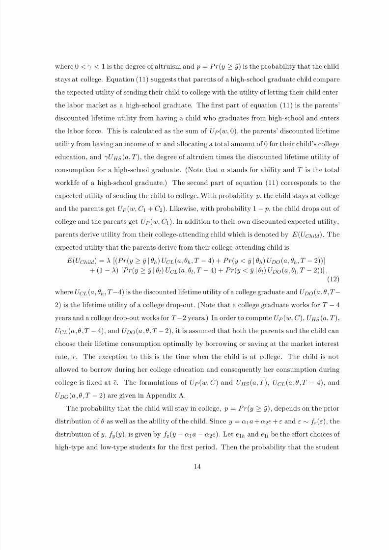
where 0 < γ < 1 is the degree of altruism and p = P r(y ≥ y) is the probability that the child
stays at college. Equation (11) suggests that parents of a high-school graduate child compare
the expected utility of sending their child to college with the utility of letting their child enter
the labor market as a high-school graduate. The first part of equation (11) is the parents’
discounted lifetime utility from having a child who graduates from high-school and enters
the labor force. This is calculated as the sum of U P (w, 0), the parents’ discounted lifetime
utility from having an income of w and allocating a total amount of 0 for their child’s college
education, and γU HS (a, T ), the degree of altruism times the discounted lifetime utility of
consumption for a high-school graduate. (Note that a stands for ability and T is the total
worklife of a high-school graduate.) The second part of equation (11) corresponds to the
expected utility of sending the child to college. With probability p, the child stays at college
and the parents get U P (w, C 1 + C 2). Likewise, with probability 1 − p, the child drops out of
college and the parents get U P (w, C 1). In addition to their own discounted expected utility,
parents derive utility from their college-attending child which is denoted by E (U Child). The
expected utility that the parents derive from their college-attending child is
E (U Child) = λ [(P r(y ≥ y | θh) U CL(a, θh, T − 4) + P r(y < y | θh) U DO(a, θh, T − 2))]
+ (1 − λ) [P r(y ≥ y | θl) U CL(a, θl, T − 4) + P r(y < y | θl) U DO(a, θl, T − 2))] ,(12)
where U CL(a, θh, T −4) is the discounted lifetime utility of a college graduate and U DO(a,θ,T −
2) is the lifetime utility of a college drop-out. (Note that a college graduate works for T − 4
years and a college drop-out works for T −2 years.) In order to compute U P (w, C ), U HS (a, T ),
U CL(a,θ,T − 4), and U DO(a,θ,T − 2), it is assumed that both the parents and the child can
choose their lifetime consumption optimally by borrowing or saving at the market interest
rate, r. The exception to this is the time when the child is at college. The child is not
allowed to borrow during her college education and consequently her consumption during
college is fixed at c. The formulations of U P (w, C ) and U HS (a, T ), U CL(a,θ,T − 4), andU DO(a,θ,T − 2) are given in Appendix A.
The probability that the child will stay in college, p = P r(y ≥ y), depends on the prior
distribution of θ as well as the ability of the child. Since y = α1a + α2e + ε and ε ∼ f ε(ε), the
distribution of y, f y(y), is given by f ε(y − α1a − α2e). Let e1h and e1l be the effort choices of
high-type and low-type students for the first period. Then the probability that the student
14

8/8/2019 The Incentive Effects of Higher Education Subsidies on Student Effort
http://slidepdf.com/reader/full/the-incentive-effects-of-higher-education-subsidies-on-student-effort 17/39
will complete college is given by
p = P r(y ≥ y) = P r(θ = θh)P r(y ≥ y | θh) + P r(θ = θl)P r(y ≥ y | θl)
= λ F ε (α1a + α2e1h − y) + (1 − λ) F ε (α1a + α2e1l − y) ,(13)
where F ε(·) is the cumulative distribution function for ε.
Once the parents have decided to send their child to college, the child chooses an academic
effort level by maximizing her expected lifetime utility. Thus, for a given cut-off grade
threshold, y, a student of type θ chooses her first-period effort level, e1, according to
maxe1
1 + β
θlog(1− e1)+ P r(y < y | θ)
T t=3
β t−1
θlog(1− e) + U DO(a,θ,T − 2)
+P r(y ≥ y | θ)
(1 + β )β 2
θlog(1− e2) +
T t=5
β t−1
θlog(1− e) + U CL(a,θ,T − 4)
. (14)
The first part of equation (14) is the child’s utility from leisure in the first period of college.
The second and third parts of equation (14) correspond to the child’s expected utility condi-
tional on grades. If y < y, the student drops out of college, supplies e units of labor for T −2
years and gets a lifetime utility of U DO(a,θ,T − 2) from consumption. Likewise if y ≥ y,
the student stays at college for the second period and studies for e2 units of time. After she
completes college, the student supplies e units of labor for T − 4 years and gets a lifetime
utility of U CL(a,θ,T − 4) from consumption.
The first order condition for the student’s academic effort choice problem, stated in
equation (14), is
1 + β
θ(1 − e1)= α2f ε (α1a + α2e1 − y) [U CL(a,θ,T − 4) − U DO(a,θ,T − 2)]
+P r(y ≥ y | θ) U CL(a,θ,T − 4) + P r(y < y | θ) U DO(a,θ,T − 2), (15)
where U CL(·) and U DO(·) are the first derivatives of the student’s lifetime utility with respect
to first-period effort. The left hand side of the first order condition is the change in the utility
of leisure. The first term on the right hand side is the change in utility due to the increased
probability of staying in college and the second term on the right hand side is the direct
effect of higher effort on utility. The student simply increases her effort until the disutility of
effort exceeds the future reward of effort. Since high-motivation type students value leisure
15

8/8/2019 The Incentive Effects of Higher Education Subsidies on Student Effort
http://slidepdf.com/reader/full/the-incentive-effects-of-higher-education-subsidies-on-student-effort 18/39
less than low-motivation students and their return from completing college is higher, they
choose to study more than low-motivation type students.17
Second-Period:
After parents observe the child’s grades, y1, they decide whether they should keep the child
in college for the second period. Parents’ second period decision problem is
maxD2∈{0,1}
U P (w, C 1) + γ [λU DO(a, θh, T − 2) + (1 − λ) U DO(a, θl, T − 2)],
U P (w, C 1 + C 2) + γ
λU CL(a, θh, T − 4) + (1 − λ) U CL(a, θl, T − 4)
, (16)
where λ, the posterior probability that θ = θh given that observed grade is y1, is
λ = P r(θ = θh | y = y1) = λf ε(α1a + α2e1h − y1)λf ε(α1a + α2e1h − y1) + (1 − λ)f ε(α1a + α2e1l − y1)
. (17)
Parents’ second-period decision is a binary one: keeping the child in college or not. After
parents observe the child’s grade they update their beliefs about the child’s motivation. Since
f ε(·) is assumed to satisfy the strict single crossing property, the higher the observed grade,
the higher the probability that the child is a high-motivation type. Thus, this binary decision
can be summarized in terms of a cut-off grade threshold, y. Cut-off grade threshold y is the
value of grades that makes the parents indifferent between keeping the child at college and
not.18 The cut-off grade threshold depends on the tuition, the degree of altruism, the ability
of the child, and the parents’ income since all of these parameters affect the future lifetime
utility of parents.
The choice of the cut-off grade threshold, y, and the first period effort choice, e1, are
dependent on each other. When choosing her effort level, the student takes into account that
her parents will update their beliefs about her type according to her grades. Similarly, parents
consider what the effort choices of the student would be for all possible y values. Solving
equation (14) and equation (16) simultaneously gives the equilibrium values of y, e1h, ande1l. Equation (16) shows how parents choose the cut-off grade threshold. This solution is not
17One can see that in the simulations, however showing this result analytically requires making simplifying
assumptions.18Note that since e2h > e2l, as will be shown next, high-motivation type students gain more from completing
college education than low-motivation type students; U CL(a, θh, T − 4)− U DO(a, θh, T − 2) > U CL(a, θl, T −
4)− U DO(a, θl, T − 2).
16

8/8/2019 The Incentive Effects of Higher Education Subsidies on Student Effort
http://slidepdf.com/reader/full/the-incentive-effects-of-higher-education-subsidies-on-student-effort 19/39
always interior: for low values of tuition, parents would always keep their child in college.
Thus, the child will not have an incentive to put forth a high effort. This feature of the model
suggests that students are more likely to go to college and stay at college when tuition is low.
Similarly, for very wealthy parents, the cut-off grade threshold is likely to be lower. Thus,
students from high-income families are more likely to stay at college compared to students
from low income families. These predictions are consistent with the empirical findings.
The second period effort levels e2h and e2l are easy to solve. The optimal effort choices
for high-type and low-type students are
e∗2h = 1 −1 + β
β 2 η2 θhke∗2l = 1 −
1 + β
β 2 η2 θlk(18)
where k =
T t=5 β t−1wt
ct. Since θh > θl, e2h > e2l.
The equilibrium values of effort choices and parents’ optimal decisions can be solved by
using backward induction. However, the model does not have a closed form solution. The
presence of updating makes the analytical solution of the model very complex. This is why
I concentrate on calibrating the model and analyzing the numerical experiments.
4 Calibration
This section explains the choice of each parameter in detail. To calibrate the parameters, the
HS&B Sophomore Cohort: 1980-92 and the NLSY79 data sets were used. Since the NLSY79
Time Use Survey was only conducted in 1981, the model is calibrated to the U.S. Economy
in 1981.
Average Worklife: The average worklife of a high-school graduate is assumed to be 40
years. It is 38 years for college drop-outs and 36 years for college graduates, respectively.
These values are consistent with the values from the U.S. Bureau of Labor Statistics, Em-
ployment and Earnings, which reports that the remaining expected years of paid work at age25 for male workers is 33.4 for high-school graduates, 34.5 for workers with some college, and
35.8 for college graduates.
Return to Experience and Labor Supply: Return to experience parameters ρ0 and ρ1
are set to 0.05 and -0.0010 following Murphy and Welch (1992). Average weekly hours of
full-time paid workers is around 40 hours/week. After sleep, meals, and transportation are
17

8/8/2019 The Incentive Effects of Higher Education Subsidies on Student Effort
http://slidepdf.com/reader/full/the-incentive-effects-of-higher-education-subsidies-on-student-effort 20/39
−1 −0.8 −0.6 −0.4 −0.2 0 0.2 0.4 0.6 0.8 10
0.02
0.04
0.06
0.08
0.1
0.12
0.14
Ability
Figure 3: Generated ability distribution.
accounted for, a person has approximately 96 hours to allocate for work. The fraction of
time spent on working is 40/96 ≈ 0.4. So e is set to 0.4.
Ability: To determine the ability distribution, the wages of 1148 workers from the NLSY79
with 12-16 years of schooling are used. Specifically, a Mincer earnings specification is esti-
mated using this data set and the residual of this Mincer regression is used as the ability
distribution. The underlying assumption is that when the average return to schooling and
experience are deducted, the remaining wage differences should come from differences in abil-
ity. From the Mincer regression, ability is assumed to be normal with mean 0 and standard
deviation of 0.35. Figure 3 shows the generated ability distribution.
From the Mincer regression, the annual earnings of a high-school graduate can be com-
puted as
w(a, t) = exp(7.98 + 1.08 (1 + a) + ρ0t + ρ1t2) (19)
where a is the ability and t is the experience of the worker.Earnings: The estimates for the return to postsecondary education are taken from Kane
and Rouse (1995). The return for the first two-years of college for an individual with average
intellectual ability a and average effort level e is set to 0.16 and the total return to college is
18

8/8/2019 The Incentive Effects of Higher Education Subsidies on Student Effort
http://slidepdf.com/reader/full/the-incentive-effects-of-higher-education-subsidies-on-student-effort 21/39
1 2 3 4 5 6 7
x 104
0
0.02
0.04
0.06
0.08
0.1
0.12
0.14
Family Income
Figure 4: Generated Family Income Distribution.
set to 0.36 following Kane and Rouse (1995). This specification suggests that
µ1(1 + a) + η1e = 0.16 and µ2(1 + a) + η2e = 0.20 (20)
where the mean ability, a, is 0 and the average study time, e, is 0.4.19 However, this is not
enough information to calibrate η1, η2, µ1, and µ2. The relative weights of ability and effort
on future earnings are ambiguous. To resolve this problem, it is assumed that a student
who chooses to study for 38 hours per week is indifferent between studying for one more
additional hour and working. For a college student, the increase in the discounted future
earnings provided by one additional hour of studying is the same as the hourly wage earned
by working for one hour. According to this calculation
η1 = 0.12, η2 = 0.125, µ1 = 0.112, µ2 = 0.15 (21)
which suggests that roughly one third of the total return to college is due to effort and theremaining two thirds is due to intellectual ability.20 The annual earnings of a college drop-out
19Note that the average ability is 0. In order to ensure that the average return to ability is µ1, ability is
normalized to 1 + a.20Note that this is a conservative estimate for η2. Barron at al. (2003) find that the role of effort is
higher than the role of ability on future earnings, which implies that more than half of the return to college
is associated to effort. The nature of the results of this paper does not change if we use higher η2 values.
Moreover, the disincentive effects become quantitatively more important.
19
8/8/2019 The Incentive Effects of Higher Education Subsidies on Student Effort
http://slidepdf.com/reader/full/the-incentive-effects-of-higher-education-subsidies-on-student-effort 22/39
can be computed as
w(a, e1, t) = exp(7.98 + (1.08 + 0.112)(1 + a) + 0.12e1 + ρ0t + ρ1t2), (22)
and the annual earnings of a college graduate are
w(a, e1, e2, t) = exp(7.98+(1.0 8 + 0.112+0.15)(1 + a) + 0.12e1 + 0.125e2 + ρ0t + ρ1t2). (23)
Parental Income: According to the Current Population Report 1981, the median family
income was $23,873 in 1981. The parental income is assumed to have a lognormal distribution.
Figure 4 shows the generated family income distribution. Parents from all income groups
can finance their child’s higher education through borrowing, i.e. there are no borrowing
constraints.21
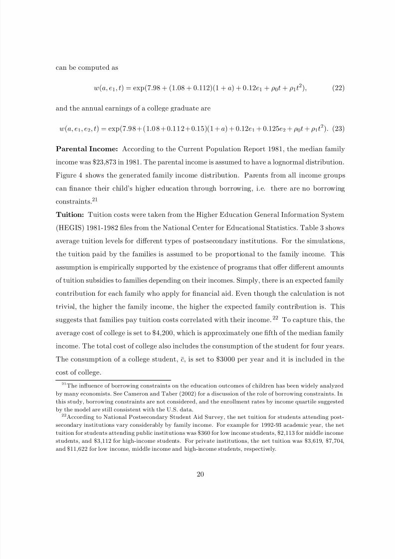
Tuition: Tuition costs were taken from the Higher Education General Information System
(HEGIS) 1981-1982 files from the National Center for Educational Statistics. Table 3 shows
average tuition levels for different types of postsecondary institutions. For the simulations,
the tuition paid by the families is assumed to be proportional to the family income. This
assumption is empirically supported by the existence of programs that offer different amounts
of tuition subsidies to families depending on their incomes. Simply, there is an expected family
contribution for each family who apply for financial aid. Even though the calculation is not
trivial, the higher the family income, the higher the expected family contribution is. This
suggests that families pay tuition costs correlated with their income.22 To capture this, the
average cost of college is set to $4,200, which is approximately one fifth of the median family
income. The total cost of college also includes the consumption of the student for four years.
The consumption of a college student, c, is set to $3000 per year and it is included in the
cost of college.
21The influence of borrowing constraints on the education outcomes of children has been widely analyzed
by many economists. See Cameron and Taber (2002) for a discussion of the role of borrowing constraints. Inthis study, borrowing constraints are not considered, and the enrollment rates by income quartile suggested
by the model are still consistent with the U.S. data.22According to National Postsecondary Student Aid Survey, the net tuition for students attending post-
secondary institutions vary considerably by family income. For example for 1992-93 academic year, the net
tuition for students attending public institutions was $360 for low income students, $2,113 for middle income
students, and $3,112 for high-income students. For private institutions, the net tuition was $3,619, $7,704,
and $11,622 for low income, middle income and high-income students, respectively.
20

8/8/2019 The Incentive Effects of Higher Education Subsidies on Student Effort
http://slidepdf.com/reader/full/the-incentive-effects-of-higher-education-subsidies-on-student-effort 23/39
In-state Out-of-state
N Tuition Tuition Room Board
Private 4-year 1,218 $3,444 $3,444 $883 $1,103
Public 4-year 458 $842 $2,076 $857 $972Private 2-year 343 $2,531 $2,531 $924 $1,032
Public 2-year 878 $444 $1,482 $640 $979
Table 3: Average tuition levels, HEGIS (1981-1982).
Type (θ): The values of θh and θl determine the equilibrium effort choices of students.
As noted in Figure 1, the average weekly study time for college students was 38.5 hours
per week. The average weekly study time for the top third of the distribution was 60.2
hours, and the average weekly study time was 18.7 hours for the bottom third. The values
of θh and θl are chosen so that the equilibrium effort choices would be consistent with the
effort values implied by Figure 1. On average, low type students choose an effort level
of 0.2 (approximately 20 hours/week) and high-type students choose an effort level of 0.6
(approximately 60 hours/week). To be consistent with these values, θh was set to 1.5 and θl
was set to 0.75.23
GPA: Recall that the GPA is assumed to be
y = α1a + α2e + ε, (24)
where ε ∼ f ε(ε) is the random error term. To mimic the relative impacts on wages, the
relative weight of ability in the GPA function is assumed to be two thirds and the relative
weight of effort is set to one third.
It is assumed that ε is normally distributed with a mean value of 0 and a variance of
σε.24 The choice of the standard deviation of the random error term, σε, is nontrivial. In
order to calibrate the error term, the standard deviations of the first-year GPAs and of the
overall GPAs of 2364 college students from the HS&B Sophomore Cohort: 1980-92 were
23Since, there is a closed form solution for the second period effort choice of students, it is possible to solve
for θh and θl by using equation (20). First, e2h is set to 0.6 and e2l is set to 0.2 in equation (20) and θh and θl
can be solved for. After setting θh and θl to the implied values, the first period effort choices were computed.
Since there is no closed form solution for the first period effort choice in terms of θh and θl, one needs to
repeat the simulations by changing θh and θl by small steps until the desired equilibrium effort values are
obtained.24For the parameter values that are used, the distribution of ε satisfies the strict single crossing property.
21
8/8/2019 The Incentive Effects of Higher Education Subsidies on Student Effort
http://slidepdf.com/reader/full/the-incentive-effects-of-higher-education-subsidies-on-student-effort 24/39
Observation GPA Std. Dev.
First year 2364 2.65/4.00 0.630
Overall 2364 2.80/4.00 0.465
Table 4: GPA of college graduates, HS&B Sophomore Cohort: 1982-1990.
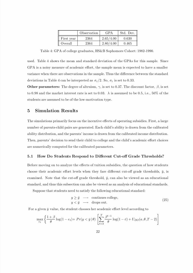
used. Table 4 shows the mean and standard deviation of the GPAs for this sample. Since
GPA is a noisy measure of academic effort, the sample mean is expected to have a smaller
variance when there are observations in the sample. Thus the difference between the standard
deviations in Table 4 can be interpreted as σε/2. So, σε is set to 0.33.
Other parameters: The degree of altruism, γ , is set to 0.37. The discount factor, β , is set
to 0.98 and the market interest rate is set to 0.03. λ is assumed to be 0.5, i.e., 50% of the
students are assumed to be of the low-motivation type.
5 Simulation Results
The simulations primarily focus on the incentive effects of operating subsidies. First, a large
number of parents-child pairs are generated. Each child’s ability is drawn from the calibrated
ability distribution, and the parents’ income is drawn from the calibrated income distribution.
Then, parents’ decision to send their child to college and the child’s academic effort choices
are numerically computed for the calibrated parameters.
5.1 How Do Students Respond to Different Cut-off Grade Thresholds?
Before moving on to analyze the effects of tuition subsidies, the question of how students
choose their academic effort levels when they face different cut-off grade thresholds, y, is
examined. Note that the cut-off grade threshold, y, can also be viewed as an educational
standard, and thus this subsection can also be viewed as an analysis of educational standards.
Suppose that students need to satisfy the following educational standard:
y ≥ y −→ continues college,
y < y −→ drops out.(25)
For a given y value, the student chooses her academic effort level according to
maxe1
1 + β
θlog(1− e1)+ P r(y < y | θ)
T t=3
β t−1
θlog(1− e) + U DO(a,θ,T − 2)
22

8/8/2019 The Incentive Effects of Higher Education Subsidies on Student Effort
http://slidepdf.com/reader/full/the-incentive-effects-of-higher-education-subsidies-on-student-effort 25/39
0 0.5 1 1.5 2 2.5 3 3.5 40
0.5
1
Low Type
High Type
0 0.5 1 1.5 2 2.5 3 3.5 40
0.5
1
High Type
Low Type
0 0.5 1 1.5 2 2.5 3 3.5 40
0.5
1
Cut−off Grade
Low Type
High Type
Figure 5: Effort choices of high-motivation type and low-motivation type students with
different intellectual ability, a = −0.35, a = 0 and a = 0.35, respectively.
+P r(y ≥ y | θ)
(1 + β )β 2
θlog(1− e2) +
T t=5
β t−1
θlog(1− e) + U CL(a,θ,T − 4)
. (26)
Figure 5 shows the effort choices of a student for different levels of cut-off grade thresholds,
y and abilities, a. Recall that ability, a, is normally distributed with a mean value of 0 and
a standard deviation of 0.35. Ability is set to three different values to illustrate the behavior
of students with different intellectual ability. The first example is for a = −0.35, which is
one standard deviation below the mean ability. The second example is for a = 0, which is
the mean ability level, and the third example is for a = 0.35, which is one standard deviation
above the mean ability level. For low values of y, P r(y ≥ y | θ)=1 for both high-motivation
and low-motivation types. This implies that the student will stay in college with probability
1. As y increases, the student will drop out with a positive probability unless she puts in more
academic effort. Consequently, the student tries to meet the higher standards by increasing
her effort level. For higher values of y, the student no longer tries to meet the standards and
sets her academic effort level to maximize the first part of equation (26).
How does this analysis change across the different motivational types? Initially, low-
motivation type’s effort choice increases as y increases. Hence, higher educational standards
provide low-motivation type students with an incentive to increase their academic effort levels
23

8/8/2019 The Incentive Effects of Higher Education Subsidies on Student Effort
http://slidepdf.com/reader/full/the-incentive-effects-of-higher-education-subsidies-on-student-effort 26/39
up to a certain point. However, since low-motivation type students assign more weight to the
utility of leisure, they start lowering their effort levels when confronted with higher standards.
Consequently, high-motivation type students match the standards up to a higher threshold
than the low-motivation type students.
Figure 5 also shows that for students with different intellectual ability, effort peaks at dif-
ferent values of y. Higher ability students continue to meet standards up to higher thresholds
than lower ability students.
Figure 5 highlights several implications about educational standards. When educational
standards are set too low or too high, they might have adverse effects on student effort. High
standards might discourage students, especially low ability and/or low-motivation students.
On the other hand, low standards might cause students, especially, high-ability ones, to shirk.
Consequently, at colleges where ability is widely dispersed, grading will be a challenging task.
5.2 The Effect of Tuition Subsidies
In Section 5.1 we have seen that students respond to different cut-off grade thresholds (or
equivalently different parental expectations) by changing their academic effort choices. Since
high tuition subsidies will lower the cost of higher education and decrease the cut-off grade
thresholds, tuition subsidies are likely to have disincentive effects on students. This sub-
section analyzes the effects of tuition subsidies, in particular operating subsidies, on college
enrollment and on students’ study time. For this analysis, simulations with various ratios of
tuition to family income are performed. For the baseline case, the ratio of tuition to family
income is 0.18. This ratio is then decreased to 0.16 and to 0.14. When tuition to family
income ratio is decreased from 0.18 to 0.14, the average tuition paid decreases by $1,000.
These simulations mimic the effect of operating subsidies provided to the public post-
secondary institutions by the state and local governments. Note that changing the ratio
of tuition to family income implies a higher transfer to middle- and high-income students.
Interestingly, this is the case for operating subsidies.25 Students from high-income families
are more likely to attend four-year public postsecondary institutions. This follows from the
fact that admission to these institutions is positively correlated with standardized test scores
25See Kane (1999) for a discussion of this point.
24

8/8/2019 The Incentive Effects of Higher Education Subsidies on Student Effort
http://slidepdf.com/reader/full/the-incentive-effects-of-higher-education-subsidies-on-student-effort 27/39
U.S. Data tuition/w = 0.18 tuition/w = 0.16 tuition/w = 0.14
Average tuition $4,000-$4,500 $4,200 $3,700 $3,200
Enrollment rate 0.54 0.53 0.62 0.69
Graduation rate 0.57 0.59 0.63 0.67
Table 5: The enrollment effect : the effect of tuition on enrollment and college graduation
rates; U.S. Data from the Condition of Education, 1981. Note that tuition/w=0.18 is the
baseline case.
and standardized test scores are positively correlated with family income. Since four-year
public postsecondary institutions get higher subsidies from the state and local governments
compared to two-year public institutions, students from high-income families collect a higher
share of subsidies compared to students from low income families.Table 5 looks at the enrollment effect of tuition subsidies and reports the enrollment rates
and graduation rates. The enrollment rate is defined as the fraction of high-school graduates
who enroll in college, and the graduation rate is defined as the fraction of college students who
graduate from college. The baseline case generates similar statistics with the U.S. Data.26
As Table 5 shows, high operating subsidies encourage college enrollment by decreasing the
cost of a college education. Students are more likely to enroll in college and stay at college
when the cost of a college education is lower. The simulations suggest that a $1,000 decrease
in the average tuition increases the enrollment rate by 16%. This finding is consistent with
the the literature on the enrollment effects of tuition subsidies.
tuition/w = 0.18 tuition/w = 0.16 tuition/w = 0.14
Average tuition $4,200 $3,700 $3,200
% of students who are low type 0.50 0.50 0.50
% of graduates who are low type 0.26 0.31 0.36
Avg. ability of students 0.22 0.18 0.14
Avg. ability of graduates 0.30 0.27 0.24
Table 6: The composition effect: the effect of tuition subsidies on the ability and the type
distribution of college students.
Table 5 shows that the decision to enroll in college responds positively to tuition cuts.
Another important effect of the operating subsidies is how these subsidies change the ability
26Recall that the model is calibrated to the U.S. Economy in 1981.
25

8/8/2019 The Incentive Effects of Higher Education Subsidies on Student Effort
http://slidepdf.com/reader/full/the-incentive-effects-of-higher-education-subsidies-on-student-effort 28/39
tuition/w = 0.18 tuition/w = 0.16 tuition/w = 0.14
Average tuition $4,200 $3,700 $3,200
1st-period effort 0.51 0.46 0.43
2nd-period fffort 0.46 0.44 0.42Average effort 0.49 0.45 0.43
Average GPA 2.96 2.85 2.76
Cut-off grade level 1.93 1.67 1.46
Table 7: The disincentive effect: the effect of tuition subsidies on student effort.
and type composition of college students, i.e. the composition effect of tuition subsidies.
Table 6 looks at the effect of tuition subsidies on the ability and the type distribution of college
students and shows that when tuition levels are lower, the average ability of college studentsand college graduates decreases. Similarly, a higher fraction of less highly-motivated students
graduate from college. Recall that the calibration assumed that student type and ability are
not correlated. Due to this orthogonality assumption, the fraction of low-motivation type
students who enroll in college does not change. However, a higher fraction of low-motivation
type students graduate from college. One might expect high-ability, low-income students
to benefit from the tuition cut thereby increasing the average ability of college students.
However, this is not the case. Since the financial aid is not conditional on ability, academic
success, or family income, the net effect is a decrease in the average ability of college students.
Clearly, a financial aid system that depends on student ability and family income would be
more successful in encouraging enrollment of high-ability, low-income students.
As mentioned earlier, when tuition rates are lower, college graduation rates are higher.
This increase in the graduation rate is partly due to an increase in the ratio of low-motivation
type students who complete college. For instance, consider the case where tuition/w = 0.18.
In this case, the fraction of college students who are low-motivation type is 0.50 and the
fraction of college graduates who are low-motivation type is only 0.26. On the other hand,for the tuition/w = 0.14 case, the fraction of college graduates that are of the low-motivation
type is 0.36. Thus, the average ability of a college graduate decreases as a result of the increase
in subsidy.
Table 7 looks at the disincentive effect of operating subsidies. The simulations suggest
26

8/8/2019 The Incentive Effects of Higher Education Subsidies on Student Effort
http://slidepdf.com/reader/full/the-incentive-effects-of-higher-education-subsidies-on-student-effort 29/39
tuition/w = 0.18 tuition/w = 0.16 tuition/w = 0.14
Average tuition $4,200 $3,700 $3,200
1st-period effort 0.51 0.48 0.46
Table 8: The effort choices of students who would have attended college for all three tuition
policies.
that as higher education becomes less costly, the cut-off grade threshold decreases. This fol-
lows from the fact that as the cost of a college education decreases, the expected return that
makes the parents indifferent between paying and not paying decreases. As Table 7 shows
the cut-off grade threshold averaged over all college students decreases as tuition becomes
cheaper relative to family income. The first-period academic effort, on average, decreases as
a response to the change in parental expectations (decrease in implicit cut-off grade thresh-
olds). Average first-period effort decreases from 0.49 to 0.43, implying, approximately, a
6 hour/week decrease in average study time. The second-period academic effort choice is
not affected by the tuition cut (see equation (18)). However due to the increased ratio of
low-motivation type college students, second period effort on average decreases as well. To
sum up, the model predicts that a 10% decrease in tuition would be accompanied by a 5%
decrease in the average study time.27
The simulations show that low-tuition policies change the composition of the college
student body. Is this the only effect of low tuition policies? Is the decrease in the average effort
coming only from the higher number of low-motivation type students who complete college?
To answer these questions, one can look at the academic effort choices of students who would
have enrolled in college under all three of the different tuition policies. Table 8 summarizes
the first-period academic effort choices of these students. Table 8 shows that when tuition
subsidies increase, these students also respond to changes in parental expectations by lowering
their effort levels. Thus, the decrease in the average academic effort of students is not
completely due to the increase in the ratio of low-motivation type students who graduate
from college.
The key findings of the simulations are that low-tuition, high-subsidy policies cause an
27Table 7 shows that as a result of the decrease in average ability and the average effort, GPA decreases
implying grade deflation. In section 6, a variant of the model with informational asymmetry, where a decrease
in student effort could be accompanied by grade inflation, is considered.
27

8/8/2019 The Incentive Effects of Higher Education Subsidies on Student Effort
http://slidepdf.com/reader/full/the-incentive-effects-of-higher-education-subsidies-on-student-effort 30/39
increase in the ratio of less highly-motivated students among the college graduates and that
even the highly-motivated ones respond to lower tuition levels by choosing to study less.
5.3 Human Capital
When college enrollment rates and college graduation rates increase, the amount of human
capital accumulation is typically expected to increase. However, the human capital acquired
during college depends on both the effort and the ability of the students, and when tuition
subsidies increase, the average ability of college students and the average amount of study
time decrease. In this subsection, the change in the amount of human capital accumulation,
when subsidies increase, is examined. In this examination, it is assumed that the human
capital accumulation has the same functional form as the earnings equation, as in Bils and
Klenow (2000).
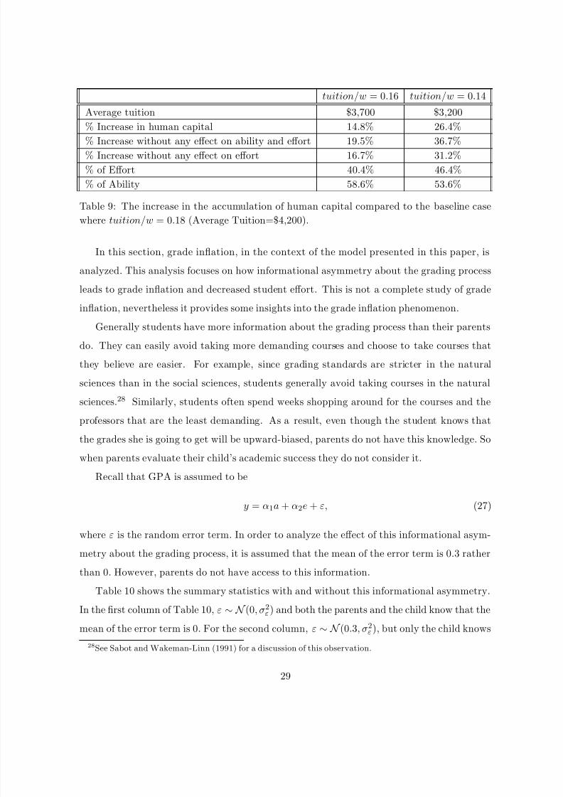
Table 9 shows the percentage increase in the amount of total human capital accumulation
at college when tuition subsidies increase. If the ability distribution and the effort choices
of college students were unaffected by the policy change, then the increase in human capital
would have been higher. For example, when the tuition to income ratio is 0.14, the amount
of human capital increases by approximately 26% compared to the baseline case. However,
if the ability distribution and the effort choices of college students were unchanged, then the
amount of human capital would have increased by almost 37%. Table 10 also shows the
decomposition of this effect into ability and effort. Almost half of the potential loss in the
human capital is due to the decrease in effort.
These experiments show that even though total human capital in the economy increases,
the average human capital endowment of a college graduate decreases as a result of the
increase in operating subsidies.
6 Grade Inflation
In the U.S., the grades at postsecondary institutions have been increasing for the last 30
years. For example in 1969, 7% of all undergraduate students received grades A- or higher,
by 1993, this proportion has risen to 20%. In contrast, grades of C or less moved from 25%
to 9% in 1993. This phenomenon is referred to as grade inflation.
28
8/8/2019 The Incentive Effects of Higher Education Subsidies on Student Effort
http://slidepdf.com/reader/full/the-incentive-effects-of-higher-education-subsidies-on-student-effort 31/39
tuition/w = 0.16 tuition/w = 0.14
Average tuition $3,700 $3,200
% Increase in human capital 14.8% 26.4%
% Increase without any effect on ability and effort 19.5% 36.7%% Increase without any effect on effort 16.7% 31.2%
% of Effort 40.4% 46.4%
% of Ability 58.6% 53.6%
Table 9: The increase in the accumulation of human capital compared to the baseline case
where tuition/w = 0.18 (Average Tuition=$4,200).
In this section, grade inflation, in the context of the model presented in this paper, is
analyzed. This analysis focuses on how informational asymmetry about the grading process
leads to grade inflation and decreased student effort. This is not a complete study of grade
inflation, nevertheless it provides some insights into the grade inflation phenomenon.
Generally students have more information about the grading process than their parents
do. They can easily avoid taking more demanding courses and choose to take courses that
they believe are easier. For example, since grading standards are stricter in the natural
sciences than in the social sciences, students generally avoid taking courses in the natural
sciences.28 Similarly, students often spend weeks shopping around for the courses and the
professors that are the least demanding. As a result, even though the student knows that
the grades she is going to get will be upward-biased, parents do not have this knowledge. So
when parents evaluate their child’s academic success they do not consider it.
Recall that GPA is assumed to be
y = α1a + α2e + ε, (27)
where ε is the random error term. In order to analyze the effect of this informational asym-
metry about the grading process, it is assumed that the mean of the error term is 0.3 ratherthan 0. However, parents do not have access to this information.
Table 10 shows the summary statistics with and without this informational asymmetry.
In the first column of Table 10, ε ∼ N (0, σ2ε) and both the parents and the child know that the
mean of the error term is 0. For the second column, ε ∼ N (0.3, σ2ε), but only the child knows
28See Sabot and Wakeman-Linn (1991) for a discussion of this observation.
29

8/8/2019 The Incentive Effects of Higher Education Subsidies on Student Effort
http://slidepdf.com/reader/full/the-incentive-effects-of-higher-education-subsidies-on-student-effort 32/39
Mean=0.0 Mean=0.3
Enrollment rate 0.53 0.53
Graduation rate 0.59 0.67
% of college graduates who are low type 0.26 0.32Average effort 0.49 0.47
Average GPA 2.96 3.21
Table 10: The summary statistics without and with informational asymmetry about the
mean value of ε.
that the true mean of the error term is 0.3 rather than 0. As a result of this informational
asymmetry, the graduation rate and average GPA increase. However, the average student
effort decreases.
These simulations show how an informational asymmetry coupled with the differences in
grading policies for different courses or different academic majors could create disincentives
for students. Thus, grade inflation could be accompanied by a decrease in student effort.
One can identify the lack of consistency in grading standards as one of the reasons for grade
inflation in the U.S.
7 Conclusion
Tuition subsidies have a positive impact on enrollment rates, however as this paper has shown,
these subsidies also have adverse effects on human capital accumulation. This can be seen
in the simulation results, which indicate the existence of two potential adverse effects. First,
a low-tuition, high-subsidy policy causes an increase in the ratio of less able and less highly-
motivated students among college graduates. Secondly, all students, even the more highly-
motivated ones, respond to lower tuition levels by choosing to study less. The simulations
of the calibrated game-theoretic model suggest that a 10% decrease in tuition would be
accompanied by a 5% decrease in the average study time. Additionally, the potential loss of
human capital, caused by the composition effect and disincentive effect of tuition subsidies,
is around 30%. Decomposition of this loss shows that approximately half of the total loss
can be attributed to the disincentive effect.
This study also has implications for educational standards. Educational standards that
30
8/8/2019 The Incentive Effects of Higher Education Subsidies on Student Effort
http://slidepdf.com/reader/full/the-incentive-effects-of-higher-education-subsidies-on-student-effort 33/39
are set too low or too high might have adverse effects on student effort. For example high
standards might discourage students, especially low ability and/or low-motivation students.
On the other hand, low standards might cause students, especially high-ability ones, to shirk.
Consequently, at colleges with high ability dispersion, grading will be a challenging task.
Grade inflation may also arise in this environment. If students have more information
about the difficulty of courses, compared to their parents, then students can self-select them-
selves into easier courses. Clearly, this informational asymmetry over differences in grading
practices could result in grade inflation. Thus, the lack of consistency in grading standards
may be one reasons of grade inflation in the U.S.
One might argue that parents can set higher standards for their child and by doing
so can make them work harder. Sahin (2002) considered a model like this and looked at
the disincentive effects in an environment where parents set the cut-off grade thresholds
optimally in the first-period and commit to these standards in the second period. In this
case, parents can set the cut-off grade threshold, y, at the level which will make the child
choose a higher effort level. The simulation results show that if parents can actually commit
to higher standards, disincentive effect on students’ study time is negligibly small. However,
the commitment assumption is crucial and hard to justify in the context of family.29 Parents
most of the time have difficulty in implementing the reward/punishment scheme that theyoffer to their child.
This paper mainly focused on analyzing the effect of operating subsidies that are directly
offered to higher education institutions. An interesting research question would be to analyze
the effect of different financial aid programs and try to design the optimal financial aid
system. As a first step, Sahin (2002) has studied the effects of a different type of subsidy:
a subsidy that lowers the tuition by the same amount for all students regardless of their
family income. Hope Scholarship credit, which was created in 1997, is very similar to that
kind of subsidy. This program provides a tax credit of 100% of tuition expenses for up to
$1,000. Since tuition expenses are almost always higher than $1,000, the tax credit lowers
tuition by $1,000 for almost all students. These experiments suggest that a subsidy that is
provided directly to students is more effective in encouraging human capital accumulation
29See Laitner (1997) for a discussion of commitment in the context of family.
31

8/8/2019 The Incentive Effects of Higher Education Subsidies on Student Effort
http://slidepdf.com/reader/full/the-incentive-effects-of-higher-education-subsidies-on-student-effort 34/39

8/8/2019 The Incentive Effects of Higher Education Subsidies on Student Effort
http://slidepdf.com/reader/full/the-incentive-effects-of-higher-education-subsidies-on-student-effort 35/39
Appendix A
The discounted lifetime utility of consumption, U HS (a, T ), can be computed by solving the
straightforward optimal consumption problem
U HS (a, T ) = maxst+1, ct
T t=1
β t−1uc(ct), (28)
s.t.
sT +1 = 0, s1 = 0,
st+1 = (1 + r)st + wt − ct,
(29)
where wt = w(a, t) is the earnings, uc(·) is the utility function of the child, st is the savings,
ct is the consumption, r is the market interest rate, and β is the discount factor.
The expected lifetime utility of consumption for a college graduate is
U CL(a,θ,T − 4) = (1 + β + β 2 + β 3) uc(c) + maxst+1, ct
T t=5
β t−1uc(ct),
s.t. sT +1 = 0, s5 = 0,
st+1 = (1 + r)st + wt − ct.(30)
Note that wt = w(a, e1, e2, t) = exp (α + a + µ1a + η1e1 + µ2a + η2e2 + ρ0t + ρ1t2) and c is the
amount of consumption that parents provide for their child during the college education.
Similarly, for a college dropout, the expected lifetime utility of consumption is
U DO(a,θ,T − 2) = (1 + β ) uc(c) + maxst+1, ct
T t=3
β t−1uc(ct),
s.t. sT +1 = 0, s3 = 0,
st+1 = (1 + r)st + wt − ct.(31)
Note that wt = w(a, e1, t) = exp(α + a + µ1a + η1e1 + ρ0t + ρ1t2) and c is the amount of
consumption that parents provide for their child during the college education.
The discounted lifetime utility of parents with annual earnings w, U p(w, C ), is
U p(w, C ) = maxst+1, ct
T
t=1
β t−1uc(ct), (32)
s.t. sT +1 = 0, s1 = −C,
st+1 = (1 + r)st + wt − ct,(33)
where wt is the earnings, uc(·) is the utility function of the parents, and C is total amount
used for education of the child. Note that all debts must be repaid in full at the time of
death.
33

8/8/2019 The Incentive Effects of Higher Education Subsidies on Student Effort
http://slidepdf.com/reader/full/the-incentive-effects-of-higher-education-subsidies-on-student-effort 36/39
Appendix B
NLSY79: The National Longitudinal Survey of Youth 1979 (NLSY79) consists of data on
respondents’ labor force participation, labor market attachment, and investments in educa-
tion and training. In 1981, the National Institute of Education sponsored a set of time-use
questions. This survey contains responses to the special set of questions, asked in the 1981
survey, about each respondent’s use of time during the past seven days, e.g., how much time
was spent on working, commuting, attending school, studying, sleeping, etc. The total study
time variable in the regressions was formed from the data in this survey. The NLSY79 also
collected information about the Federal Interagency Committee on Education (FICE) codes
of the postsecondary institutions that the respondents have attended starting from 1984. I
have used the FICE codes to identify the institutions attended by the respondents.
HS&B: The High School and Beyond (HS&B) survey began in 1980, and the data were
collected on over 58,000 high-school seniors and sophomores. In this study, the Sophomore
Cohort: 1980:1992 data set is used. The follow-up surveys were conducted in 1982, 1986
and 1992. The supplement for the Postsecondary Education Transcript Study (PETS) of the
HS&B Sophomore Cohort was used to get estimates of the grade point averages of college
students. These grade point averages were then used in the calibration of the model.
Tuition and Fee Rates: The Washington State Higher Education Coordinating Board
surveys state institutions and prepares a report of tuition and fee rates at public institutions
in the 50 states. The data used in this study contains an average for each state from a
number of 4-year comprehensive universities for 1981.
HEGIS: The Higher Education General Information Survey (HEGIS) includes information
about postsecondary institutions in the United States such as revenues and expenditures, en-
rollment statistics including number of students by residence status, basic characteristics of
educational institutions, numbers of full and part-time employees, and faculty compensation.
The FICE codes were merged with the NLSY79 data and the tuition levels of the schools
that respondents have attended were obtained.
34

8/8/2019 The Incentive Effects of Higher Education Subsidies on Student Effort
http://slidepdf.com/reader/full/the-incentive-effects-of-higher-education-subsidies-on-student-effort 37/39
References
[1] Barron, John M.; Kelly H. Blanchard; Vera Brencic; and Aysegul Sahin (2003). “Perspi-
ration or Inspiration: What do Grades Measure?” working paper. Purdue University.
[2] Becker, Gary S. (1974).“A Theory of Social Interactions,” Journal of Political Economy
82, 1063-1093.
[3] Becker, Gary S. (1981). A Treatise on the Family, Cambridge, Mass.: Harvard Univ.
Press.
[4] Becker, Gary S. and , Nigel Tomes (1976). “Child Endowments and the Quantity and
Quality of Children,” Journal of Political Economy 84, 143-162.
[5] Becker, Gary S. and Nigel Tomes (1979). “An Equilibrium Theory of the Distribution
of Income and Intergenerational Mobility,” Journal of Political Economy 87, 1153-1189.
[6] Betts, Julian R. (1998). “The Impact of Educational Standards on the Level and Dis-
tribution of Earnings,” American Economic Review 88, 266-275.
[7] Bils, Mark and Peter J. Klenow (2000). “Does Schooling Cause Growth?” American
Economic Review 90, 1160-1183.
[8] Blankenau, William and Gabriele Camera (2001). “Productive Education or a Mar-
ketable Degree?” mimeo. Kansas State University and Purdue University.
[9] Cameron, Stephen and Christopher Taber (2002). “Borrowing Constraints and the
Returns to Schooling,” mimeo. Columbia University and Nortwestern University.
[10] Card, David (1995). “Earnings, Schooling, and Ability Revisited,” in Research in Labor
Economics 14, 23-48.
[11] Caucutt, Elizabeth M. and Krishna B. Kumar (2003). “Higher Education Subsidies
and Heterogeneity-A Dynamic Analysis,” Journal of Economic Dynamics and Control
27, 1459-1502.
35

8/8/2019 The Incentive Effects of Higher Education Subsidies on Student Effort
http://slidepdf.com/reader/full/the-incentive-effects-of-higher-education-subsidies-on-student-effort 38/39
[12] Costrell, Robert M. (1994). “A Simple Model of Educational Standards,” American
Economic Review 84, 956-971.
[13] Epple, Dennis; Richard Romano; and and Holger Sieg (2003). “Peer Effects, Financial
Aid, and Selection into Colleges and Universities: An Empirical Analysis,” Journal of
Applied Econometrics, forthcoming.
[14] Heckman, James J.; Lance Lochner; and Petra E. Todd (2001). “Fifty Years of Mincer
Earnings Regressions,” mimeo. University of Chicago, University of Rochester, and
University of Pennsylvania.
[15] Kane, Thomas J. (1999). The Price of Admission. Washington, DC: Brookings Insti-
tution.
[16] Kane, Thomas J. and Cecilia Rouse (1995). “Labor-Market Returns to Two-and Four-
Year College,” American Economic Review 85, 600-614.
[17] Kotlikoff, Laurance J. and Assaf Razin (2001). “Making Bequests without Spoiling
Children: Bequests as an Implicit Optimal Tax Structure and the Possibility that
Altruistic Bequests are not Equalizing,” in Saving, Bequests, and Altruism , The MIT
Press.
[18] Laitner, John (1997). “Intergenerational and Interhousehold Economic Links,” in Hand-
book of Population and Family Economics (M.R. Rosenzweig and O. Stark, Eds) 189-
238 B.V., Amsterdam.
[19] Loury, Glenn C. and David Garman (1995). “College Selectivity and Earnings,” Journal
of Labor Economics 13, 289-308.
[20] Loury, Linda D. (1981). “Intergenerational Transfers and the Distribution of Earnings,”Econometrica 49, 843-867.
[21] Mas-Colell, Andreu; Michael D. Whinston, and Jerry R. Green (1995). Microeconomic
Theory . New York: Oxford University Press.
36

8/8/2019 The Incentive Effects of Higher Education Subsidies on Student Effort
http://slidepdf.com/reader/full/the-incentive-effects-of-higher-education-subsidies-on-student-effort 39/39
[22] McPherson, Michael and Morton Owen Shapiro (1991). Keeping College Affordable.
Washington, DC: Brookings Institution.
[23] McPherson, Michael and Morton Owen Shapiro (1997). The Student Aid Game. Prince-
ton University Press.
[24] Mincer, Jacob (1974). Schooling, Experience, and Earnings. New York: Columbia Uni-
versity Press.
[25] Murphy, Kevin M. and Finis Welch (1992). “The Structure of Wages,” Quarterly Jour-
nal of Economics 107, 285-326.
[26] Owen, John D. (1995). Why Our Kids Don’t Study, An Economist’s Perspective. Bal-
timore, The Johns Hopkins University Press.
[27] Pollak, Robert A. (1988). “Tied Transfers and Paternalistic Preferences,” American
Economic Review 78, 240-244.
[28] Sabot, Richard and John Wakeman-Linn (1991). “Grade Inflation and Course Choice,”
Journal of Economic Perspectives 5, 159-170.
[29] Sahin, Aysegul (2002). “The Incentive Effects of Social Policies on Education and LaborMarkets,” Ph.D. Dissertation, University of Rochester.
[30] Schuman, Howard; Edward Walsh; Camille Olso; and Barbara Etheridge (1985). “Effort
and Reward: The Assumption that Grades are Affected by Quantity of Study,” Social
Forces 63, 945-966.
[31] Villanueva, Ernesto (1999). “Parental Altruism under Imperfect Information: Theory
and Evidence,” mimeo. Northwestern University.
[32] Weinberg, Bruce (2001). “Parental Incomes and Children’s Outcomes in an Incentive
Model,” Journal of Political Economy 109, 266-280.
37
Related Documents