The Implicit Function as Squashing Time Model: A Novel Parallel Nonlinear EEG Analysis Technique Distinguishing Mild Cognitive Impairment and Alzheimer's Disease Subjects with High

Hindawi Publishing CorporationComputational Intelligence and NeuroscienceVolume 2007, Article ID 35021, 15 pagesdoi:10.1155/2007/35021

Research ArticleThe Implicit Function as Squashing Time Model:A Novel Parallel Nonlinear EEG Analysis TechniqueDistinguishing Mild Cognitive Impairment and Alzheimer’sDisease Subjects with High Degree of Accuracy

Massimo Buscema,1 Massimiliano Capriotti,1 Francesca Bergami,1 Claudio Babiloni,2, 3, 4

Paolo Rossini,3, 5, 6 and Enzo Grossi7

1 Semeion Research Centre of Sciences of Communication, Via Sersale, 117, 00128 Rome, Italy2 Department of Human Physiology and Pharmacology, University of Rome La Sapienza, 00185 Rome, Italy3 Ospedale San Giovanni Calibita “Fatebenefratelli”, Isola Tiberina, 00153 Rome, Italy4 Casa di cura San Raffaele Cassino (Frosinone), San Raffaele Pisana, Rome, Italy5 IRCCS Centro San Giovanni di Dio Fatebenefratelli, 25100 Brescia, Italy6 Department of Clinical Neurosciences, University of Rome Campus Biomedico, 00155 Rome, Italy7 Bracco SpA Medical Department, Via E. Folli, 50, 20134 Milan, Italy

Correspondence should be addressed to Massimo Buscema, [email protected]

Received 19 December 2006; Revised 7 June 2007; Accepted 1 August 2007

Recommended by Saied Sanei

Objective. This paper presents the results obtained using a protocol based on special types of artificial neural networks (ANNs)assembled in a novel methodology able to compress the temporal sequence of electroencephalographic (EEG) data into spatial in-variants for the automatic classification of mild cognitive impairment (MCI) and Alzheimer’s disease (AD) subjects. With referenceto the procedure reported in our previous study (2007), this protocol includes a new type of artificial organism, named TWIST.The working hypothesis was that compared to the results presented by the workgroup (2007); the new artificial organism TWISTcould produce a better classification between AD and MCI. Material and methods. Resting eyes-closed EEG data were recorded in180 AD patients and in 115 MCI subjects. The data inputs for the classification, instead of being the EEG data, were the weightsof the connections within a nonlinear autoassociative ANN trained to generate the recorded data. The most relevant features wereselected and coincidently the datasets were split in the two halves for the final binary classification (training and testing) performedby a supervised ANN. Results. The best results distinguishing between AD and MCI were equal to 94.10% and they are considerablebetter than the ones reported in our previous study (∼92%) (2007). Conclusion. The results confirm the working hypothesis thata correct automatic classification of MCI and AD subjects can be obtained by extracting spatial information content of the restingEEG voltage by ANNs and represent the basis for research aimed at integrating spatial and temporal information content of theEEG.

Copyright © 2007 Massimo Buscema et al. This is an open access article distributed under the Creative Commons AttributionLicense, which permits unrestricted use, distribution, and reproduction in any medium, provided the original work is properlycited.

1. INTRODUCTION

The electroencephalogram (EEG), since its introduction,was considered the only methodology allowing a directand online view of the “brain at work.” At the sametime, abnormalities of the “natural” aging of the brainhave yet been noticed in different types of dementias.The introduction of different structural imaging technolo-gies in the 1970’s and 1980’s (computed tomography and

magnetic resonance imaging) and the good results in thestudy of brain function obtained with techniques dealingwith regional metabolism, glucose and oxygen consump-tion, and blood flow (single-photon emission computed to-mography, positron emission tomography, functional mag-netic resonance imaging) during the following two decadescloset the role of EEG in a secondary line, particularly inthe evaluation of Alzheimer’s dementia (AD) and relateddementias.

2 Computational Intelligence and Neuroscience

Lately, EEG computerized analysis in aged people hasbeen enriched by various modern techniques able to man-age the large amount of information on time-frequency pro-cesses at single recording channels (wavelet, neural networks,etc.) and on spatial localization of these processes [2–10].The results have encouraged the scientific community in ex-ploring electromagnetic brain activity, which changes by ag-ing and can greatly deteriorate, through the different stages ofthe various forms of dementias. The use of neural networksrepresents an alternative and very promising attempt to makeEEG analysis suitable for clinical applications in aging—thanks to their ability in extracting specific and smooth char-acteristics from huge amounts of data. Computerized pro-cessing of a large quantity of numerical data in wakeful re-laxed subjects (“resting” EEG) made easier the automaticclassification of the EEG signals, providing promising resultseven using relatively simple linear classifiers such as logis-tic regression and discriminant analysis. Using global fieldpower (i.e., the sum of the EEG spectral power across all elec-trodes) as an input, some authors reached an accurate differ-ential diagnosis between AD and MCI subjects with accu-races of 84% and 78%, respectively[11, 12]. Using evaluationof spectral coherence between electrode pairs (i.e., a measureof the functional coupling) as an input to the classification,the correct classification reached 82% when comparing theAD and normal aged subjects [13, 14].

Spatial smoothness and temporal fluctuation of the EEGvoltage are considered as measures of the synaptic impair-ment, along with the notion that cortical atrophy can affectthe spatiotemporal pattern of neural synchronization gener-ating the scalp EEG. These parameters have been used to suc-cessfully discriminate the respective distribution of probableAD and normal aged subjects [15]. The interesting new ideain that study [15] was the analysis of resting EEG potentialdistribution instant by instant rather than the extraction of aglobal index along periods of tens of seconds or more.

Table 1 summarizes the results of a higher preclassifica-tion rate with ANN’s analysis than with standard linear tech-niques, such as multivariate discriminatory analysis or thenearest-neighbour analysis [16]. Some authors [17] devel-oped a system consisting of recurrent neural nets processingspectral data in the EEG. They succeeded in classifying ADpatients and non-AD patients with a sensitivity of 80% anda specificity of 100%. In other studies, classifiers based onANNs, wavelets, and blind source separation (BSS) achievedpromising results [18, 19]. In a study from the same work-group of this paper, we used a sophisticated technique basedon blind source separation and wavelet preprocessing devel-oped by Vialatte et al. [18] and Cichocki et al. [20–22] re-cently, whose results appear to be the best in the field whencompared to the literature. We named this method BWBmodel (blind source separation + wavelet + bumping mod-eling), [1]. The results obtained in the classifications tasks,comparing AD patients to MCI subjects, using the BWBmodel, ranged from 78.85% to 80.43% (mean = 79.48%).

The aim of this study is to assess the strength of a novelparallel nonlinear EEG analysis technique in the differentialclassification of MCI subjects and AD patients, with a highdegree of accuracy, based on special types of artificial neural

networks (ANNs) assembled in a novel methodology able tocompress the temporal sequence of electroencephalographic(EEG) data into spatial invariants. The working hypothesisis that this new approach to EEG based on nonlinear ANNs-based methods can contribute to improving the reliance ofthe diagnostic phase in association with other clinical and in-strumental procedures. Compared to the results already pre-sented by the workgroup [1], the included new artificial or-ganism TWIST could produce a better classification betweenAD and MCI.

2. MATERIAL AND METHODS

The IFAST method includes two phases.

(1) A squashing phase: an EEG track is compressed in or-der to project the invariant patterns of that track onthe connections matrix of an autoassociated ANN. TheEGG track/subject is now represented by a vector ofweights, without any information about the target (ADor MCI).

(2) “TWIST” (training with input selection and testing)phase: a technique of data resampling based on the ge-netic algorithm GenD, developed at Semeion ResearchCenter. The new dataset which is composed by theconnections matrix (output of the squashing phase),plus the target assigned to each vector, is splitted intotwo sub samples, each one for five times with a similarprobability density function, in order to train, test, andvalidate the ANN models.

2.1. The IFAST method

2.1.1. General philosophy

The core of this new methodology is that the ANNs do notclassify subjects by directly using the EEG data as an input.Rather, the data inputs for the classification are the weights ofthe connections within a recirculation (nonsupervised) ANNtrained to generate the recorded EEG data. These connec-tion weights represent a model of the peculiar spatial featuresof the EEG patterns at the scalp surface. The classification,based on these weights, is performed by a standard super-vised ANN.

This method, named IFAST (acronym for implicit func-tion as squashing time), tries to understand the implicitfunction in a multivariate data series compressing the tem-poral sequence of data into spatial invariants and it is basedon three general observations.

(1) Every multivariate sequence of signals coming fromthe same natural source is a complex asynchronous dy-namic highly nonlinear system, in which each chan-nel’s behavior is understandable only in relation to allthe others.

(2) Given a multivariate sequence of signals generatedfrom the same source, the implicit function defin-ing the above-mentioned asynchronous process isthe conversion of that same process into a complex

Massimo Buscema et al. 3

Table 1: EEG automatic classification (∗ = severe AD ∗∗ = mild AD; S. no. = Sample; N. aged = normal aged; ANN = artificial neuralnetworks; LDA = linear discriminant analysis; ACC = accuracy (%); SE = sensibility; SP = specificity).

Author year S. no. AD N. aged MCI Length (s)Classificators

ACC SE SPANN LDA

Pritchard et al. (1994) 39 14 25 nd x x 85 nd nd

Besthorn et al. (1997) nd nd nd nd x x 86.60

Huang et al. [6, 11] 93 38 24 31 nd x 81 84 78

Knott et al. (2001) 65 35 30 nd x 75

Petrosian et al. [17] 20 10 10 120 x 90 80 100

Cichocki et al. [20] 60 38 22 20 x 78.25 73 84

Melissant et al. [16] 36 15∗ 21 40 x 94 93 95

Melissant et al. [16] 38 28∗∗ 10 40 x 82 64 100

hypersurface, representing the interaction in time ofall the channels’ behavior.

(3) The 19 channels in the EEG represent a dynamic sys-tem characterized by asynchronous parallelism. Thenonlinear implicit function that defines them as awhole represents a metapattern that translates intospace (hypersurface) that the interactions among allthe channels create in time.

The idea underlying the IFAST method resides in think-ing that each patient’s 19-channel EEG track can be syn-thesized by the connection parameters of an autoassociatednonlinear ANN trained on the same track’s data.

There can be several topologies and learning algorithmsfor such ANNs; what is necessary is that the selected ANN beof the autoassociated type (i.e., the input vector is the targetfor the output vector) and that the transfer functions defin-ing it benon linear and differentiable at any point.

Furthermore, it is required that all the processing madeon every patient be carried out with the same type of ANN,and that the initial randomly generated weights have to bethe same in every learning trial. This means that, for everyEEG, every ANN has to have the same starting point, even ifthat starting point is random.

We have operated in two ways in order to verify thismethod’s efficiency.

(1) Different experiments were implemented based on thesame samples. By “experiment,” we mean a completeapplication of the whole procedure to every track ofthe sample.

(2) The second way is using autoassociated ANNs withdifferent topologies and algorithms on the entire sam-ple in order to prove that any autoassociated ANN cancarry out the task of translating into the space domainthe whole EEG track through its connections.

2.1.2. The squashing phase

The first application phase of the IFAST method may be de-fined as “squashing.” It consists in compressing an EEG track

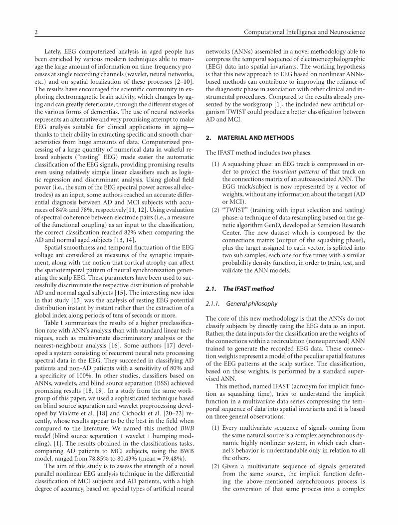
1 2 N· · ·

1 2 N· · ·

InputX(n)

Connection matrix Wi, j

Wi, j = 0

OutputX(n + 1)

Autoassociative backpropagation with two layers

Figure 1: Autoassociative backpropagation ANN with Wj, j = 0, asthe connections on the main diagonal are not present.

in order to project the invariant patterns of that track on theconnections of an auto-associated ANN.

More formallyif

Fi() = implicit function of the i-th EEG track

Xi =matrix of the values of the i-th EEG

W∗i j,k = trained matrix of the connections of the i-th

EEG (∗ = objective of the squashing)

W0 j,k = random starting matrix, the same for all EEGsthen in the case of a two-layered autoassociated ANN

Xi = Fi(Xi,W∗i j,k ,W0 j,k ); conW0 j, j = 0.

Wij, j = 0 means that every ith EEG track is pro-cessed by the two-layered autoassociated ANN inwhich Wj, j = 0, as the connections on the main di-agonal are not present (see Figure 1).

It is possible to use different types of autoassociatedANNs to run this search for spatial invariants in everyEEG.

(1) A backpropagation without a hidden unit layer andwithout connections on the main diagonal (for short,AutoBp):

4 Computational Intelligence and Neuroscience

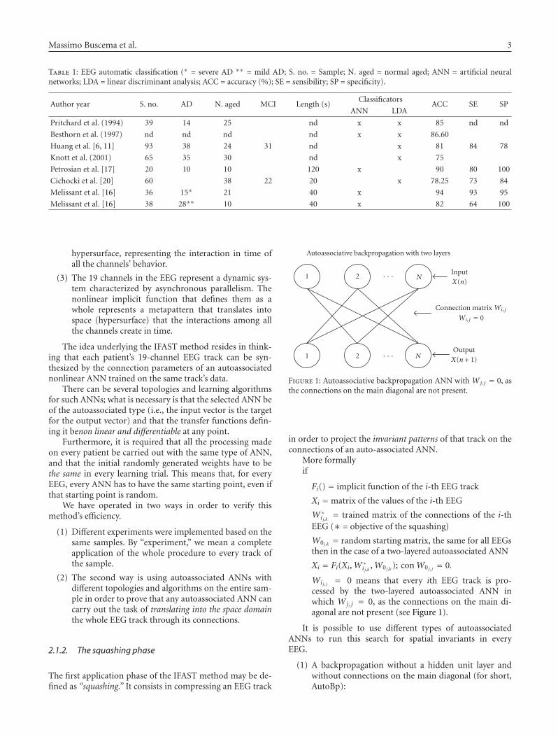
1 2 N· · ·

1 2 N· · ·

InputX(n)

OutputX(n + 1)

First hiddenlayer

Second hiddenlayer

New recirculation network

Figure 2: New recirculation network (NRC), with one connectionmatrix and four layers of nodes: one input layer, one output layer,and two layers of hidden nodes.

This is an ANN featuring an extremely simple learningalgorithm:

Outputi = f

( N∑j

Input j·Wi, j + Biasi

)

= 1

1 + e−(ΣNj Input j·Wi, j+Biasi), Wi,i = 0;

δi =(Inputi −Outputi

)· f ′(Outputi)

= (Inputi −Outputi)·Outputi·

(1−Outputi

);

ΔWi, j = LCoef·δi·Input j , LCoef ∈ [0,1],

ΔBiasi = LCoef·δi.(1)

AutoBP is an ANN featuring N2 − N internode connectionsand N bias inside every exit node, for a total of N2 adaptiveweights. This algorithm works similarly to logistic regressionand can be used to establish the dependency of variables fromeach others.

The advantage of AutoBP is due to its learning speed,in turn due to the simplicity of its topology and algorithm.Moreover, at the end of the learning phase, the connec-tions between variables, being direct, have a clear conceptualmeaning. Every connection indicates a relationship of fadedexcitement, inhibition, or indifference between every pair ofchannels in the EEG track of any patient.

The disadvantage of AutoBP is its limited convergencecapacity, due to that same topological simplicity. That is tosay, complex relationships between variables may be approx-imated or ignored (for details, see [23, 24]).

(2) New recirculation network (for short, NRC) is an orig-inal variation [25] of an ANN that has existed in theliterature [26] and was not considered to be useful tothe issue of autoassociating between variables.

The topology of the NRC which we designed includesonly one connection matrix and four layers of nodes: oneinput layer, corresponding to the number of variables; oneoutput layer whose target is the input vector; two layers ofhidden nodes with the same cardinality independent fromthe cardinality of the input and output layers. The matrixbetween input-output nodes and hidden nodes is fully con-

nected and in every learning cycle, it is modified both ways,according to the following equations:

Hidden1i = f

( N∑j

Input j·Wi, j + BiasHiddeni

)

= f(NetHidden1

i

) = 1

1 + e−NetH1i

;

Output j = R·Input j + (1− R)

· f( M∑

i

Hidden1i·Wj,i + BiasOutput j

)

= R·Input j + (1− R)· f (NetOutputj

)= R·Input j + (1− R)· 1

1 + e−NetOutputj

;

R ∈ [0, 1]/∗Projection Coefficient∗ /

Hidden2i = R·Hidden1i + (1− R)

· f( N∑

j

Output j·Wi, j + BiasHiddeni

)

= R·Hidden1i + (1− R)· f (NetHidden2i

)= R·Hidden2i + (1− R)· 1

1 + e−NetHidden2i

;

ΔWj,i = LCoef·(Input j −Output j)·Hidden1i;

ΔBiasOutput j = LCoef·(Input j −Output j);

LCoef ∈ [0, 1]/∗Learning Coefficient∗ /

ΔWi·i = LCoef·(Hidden1i −Hidden2i)·Output j ;

ΔBiasHiddeni = LCoef·(Hidden1i −Hidden2i).

(2)

NRC then features N2 internode adaptive connections and2·N intranode adaptive connections (bias). The advantagesof NRC are its excellent convergence ability on complexdatasets and, as a result, an excellent ability to interpolatecomplex relations between variables.

The disadvantages mainly have to do with the vector cod-ification that the hidden units run on the input vectors mak-ing the conceptual decoding of its trained connections diffi-cult.

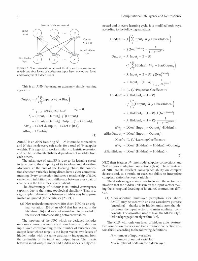
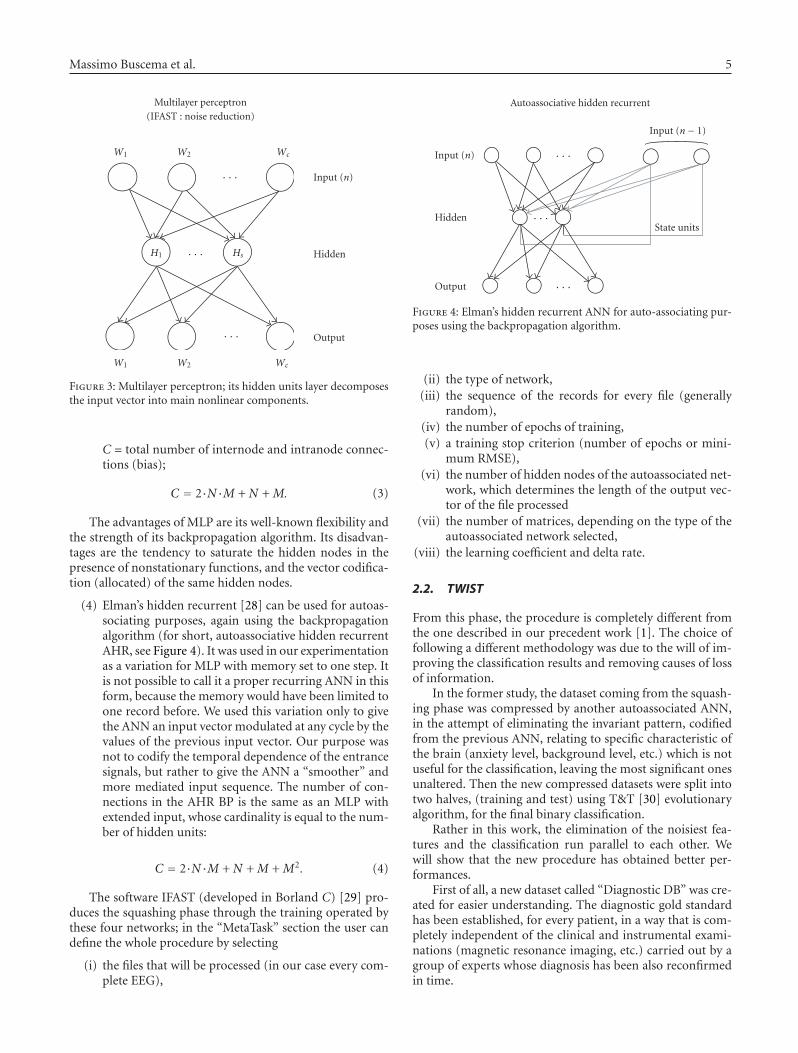
(3) Autoassociative multilayer perceptron (for short,AMLP) may be used with an auto-associative purpose(encoding)— thanks to its hidden units layer, that de-composes the input vector into main nonlinear com-ponents. The algorithm used to train the MLP is a typ-ical backpropagation algorithm [27].

The MLP, with only one layer of hidden units, featurestwo connection matrices and two intranode connection vec-tors (bias), according to the following definitions:

N = number of input variables= number of output variables;

M = number of nodes in the hidden layer;

Massimo Buscema et al. 5

W1 W2 Wc

H1 Hs

· · ·

· · ·

· · ·

W1 W2 Wc

Input (n)

Hidden

Output

Multilayer perceptron(IFAST : noise reduction)

Figure 3: Multilayer perceptron; its hidden units layer decomposesthe input vector into main nonlinear components.

C = total number of internode and intranode connec-tions (bias);

C = 2·N·M + N + M. (3)

The advantages of MLP are its well-known flexibility andthe strength of its backpropagation algorithm. Its disadvan-tages are the tendency to saturate the hidden nodes in thepresence of nonstationary functions, and the vector codifica-tion (allocated) of the same hidden nodes.

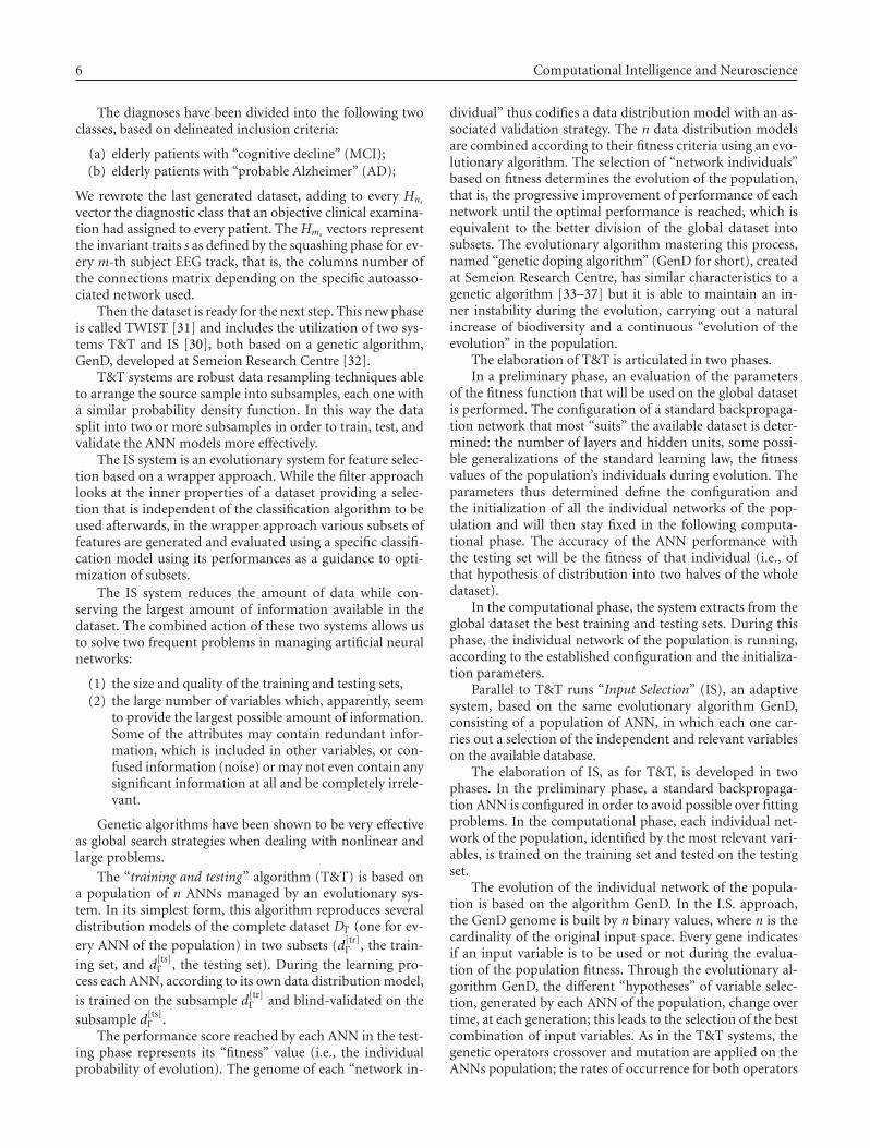
(4) Elman’s hidden recurrent [28] can be used for autoas-sociating purposes, again using the backpropagationalgorithm (for short, autoassociative hidden recurrentAHR, see Figure 4). It was used in our experimentationas a variation for MLP with memory set to one step. Itis not possible to call it a proper recurring ANN in thisform, because the memory would have been limited toone record before. We used this variation only to givethe ANN an input vector modulated at any cycle by thevalues of the previous input vector. Our purpose wasnot to codify the temporal dependence of the entrancesignals, but rather to give the ANN a “smoother” andmore mediated input sequence. The number of con-nections in the AHR BP is the same as an MLP withextended input, whose cardinality is equal to the num-ber of hidden units:

C = 2·N·M + N + M + M2. (4)

The software IFAST (developed in Borland C) [29] pro-duces the squashing phase through the training operated bythese four networks; in the “MetaTask” section the user candefine the whole procedure by selecting

(i) the files that will be processed (in our case every com-plete EEG),

Input (n)

Hidden

Output

Input (n− 1)

State units

· · ·

· · ·

· · ·

Autoassociative hidden recurrent

Figure 4: Elman’s hidden recurrent ANN for auto-associating pur-poses using the backpropagation algorithm.

(ii) the type of network,(iii) the sequence of the records for every file (generally

random),(iv) the number of epochs of training,(v) a training stop criterion (number of epochs or mini-

mum RMSE),(vi) the number of hidden nodes of the autoassociated net-

work, which determines the length of the output vec-tor of the file processed

(vii) the number of matrices, depending on the type of theautoassociated network selected,

(viii) the learning coefficient and delta rate.

2.2. TWIST

From this phase, the procedure is completely different fromthe one described in our precedent work [1]. The choice offollowing a different methodology was due to the will of im-proving the classification results and removing causes of lossof information.

In the former study, the dataset coming from the squash-ing phase was compressed by another autoassociated ANN,in the attempt of eliminating the invariant pattern, codifiedfrom the previous ANN, relating to specific characteristic ofthe brain (anxiety level, background level, etc.) which is notuseful for the classification, leaving the most significant onesunaltered. Then the new compressed datasets were split intotwo halves, (training and test) using T&T [30] evolutionaryalgorithm, for the final binary classification.

Rather in this work, the elimination of the noisiest fea-tures and the classification run parallel to each other. Wewill show that the new procedure has obtained better per-formances.

First of all, a new dataset called “Diagnostic DB” was cre-ated for easier understanding. The diagnostic gold standardhas been established, for every patient, in a way that is com-pletely independent of the clinical and instrumental exami-nations (magnetic resonance imaging, etc.) carried out by agroup of experts whose diagnosis has been also reconfirmedin time.

6 Computational Intelligence and Neuroscience

The diagnoses have been divided into the following twoclasses, based on delineated inclusion criteria:

(a) elderly patients with “cognitive decline” (MCI);(b) elderly patients with “probable Alzheimer” (AD);

We rewrote the last generated dataset, adding to every Hns

vector the diagnostic class that an objective clinical examina-tion had assigned to every patient. The Hms vectors representthe invariant traits s as defined by the squashing phase for ev-ery m-th subject EEG track, that is, the columns number ofthe connections matrix depending on the specific autoasso-ciated network used.

Then the dataset is ready for the next step. This new phaseis called TWIST [31] and includes the utilization of two sys-tems T&T and IS [30], both based on a genetic algorithm,GenD, developed at Semeion Research Centre [32].

T&T systems are robust data resampling techniques ableto arrange the source sample into subsamples, each one witha similar probability density function. In this way the datasplit into two or more subsamples in order to train, test, andvalidate the ANN models more effectively.

The IS system is an evolutionary system for feature selec-tion based on a wrapper approach. While the filter approachlooks at the inner properties of a dataset providing a selec-tion that is independent of the classification algorithm to beused afterwards, in the wrapper approach various subsets offeatures are generated and evaluated using a specific classifi-cation model using its performances as a guidance to opti-mization of subsets.

The IS system reduces the amount of data while con-serving the largest amount of information available in thedataset. The combined action of these two systems allows usto solve two frequent problems in managing artificial neuralnetworks:

(1) the size and quality of the training and testing sets,(2) the large number of variables which, apparently, seem

to provide the largest possible amount of information.Some of the attributes may contain redundant infor-mation, which is included in other variables, or con-fused information (noise) or may not even contain anysignificant information at all and be completely irrele-vant.

Genetic algorithms have been shown to be very effectiveas global search strategies when dealing with nonlinear andlarge problems.

The “training and testing” algorithm (T&T) is based ona population of n ANNs managed by an evolutionary sys-tem. In its simplest form, this algorithm reproduces severaldistribution models of the complete dataset DΓ (one for ev-ery ANN of the population) in two subsets (d[tr]

Γ , the train-

ing set, and d[ts]Γ , the testing set). During the learning pro-

cess each ANN, according to its own data distribution model,

is trained on the subsample d[tr]Γ and blind-validated on the

subsample d[ts]Γ .

The performance score reached by each ANN in the test-ing phase represents its “fitness” value (i.e., the individualprobability of evolution). The genome of each “network in-

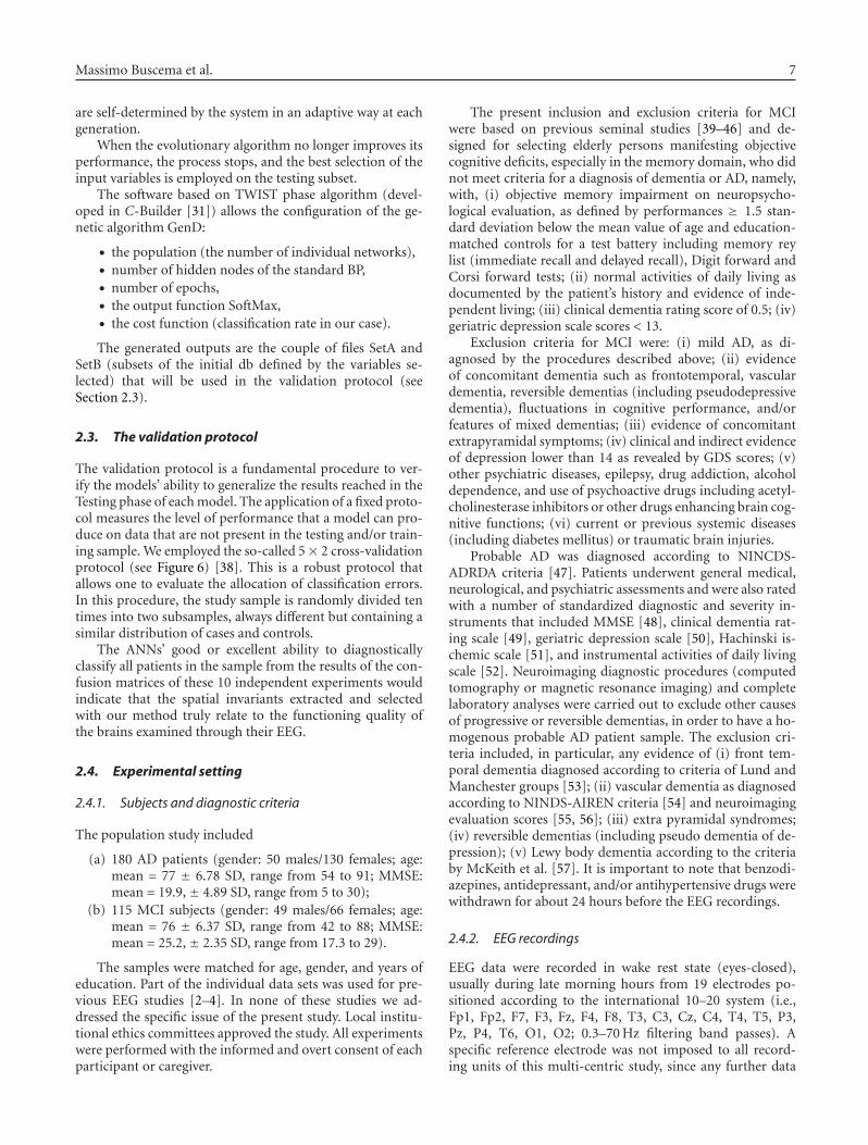
dividual” thus codifies a data distribution model with an as-sociated validation strategy. The n data distribution modelsare combined according to their fitness criteria using an evo-lutionary algorithm. The selection of “network individuals”based on fitness determines the evolution of the population,that is, the progressive improvement of performance of eachnetwork until the optimal performance is reached, which isequivalent to the better division of the global dataset intosubsets. The evolutionary algorithm mastering this process,named “genetic doping algorithm” (GenD for short), createdat Semeion Research Centre, has similar characteristics to agenetic algorithm [33–37] but it is able to maintain an in-ner instability during the evolution, carrying out a naturalincrease of biodiversity and a continuous “evolution of theevolution” in the population.

The elaboration of T&T is articulated in two phases.In a preliminary phase, an evaluation of the parameters

of the fitness function that will be used on the global datasetis performed. The configuration of a standard backpropaga-tion network that most “suits” the available dataset is deter-mined: the number of layers and hidden units, some possi-ble generalizations of the standard learning law, the fitnessvalues of the population’s individuals during evolution. Theparameters thus determined define the configuration andthe initialization of all the individual networks of the pop-ulation and will then stay fixed in the following computa-tional phase. The accuracy of the ANN performance withthe testing set will be the fitness of that individual (i.e., ofthat hypothesis of distribution into two halves of the wholedataset).

In the computational phase, the system extracts from theglobal dataset the best training and testing sets. During thisphase, the individual network of the population is running,according to the established configuration and the initializa-tion parameters.

Parallel to T&T runs “Input Selection” (IS), an adaptivesystem, based on the same evolutionary algorithm GenD,consisting of a population of ANN, in which each one car-ries out a selection of the independent and relevant variableson the available database.

The elaboration of IS, as for T&T, is developed in twophases. In the preliminary phase, a standard backpropaga-tion ANN is configured in order to avoid possible over fittingproblems. In the computational phase, each individual net-work of the population, identified by the most relevant vari-ables, is trained on the training set and tested on the testingset.

The evolution of the individual network of the popula-tion is based on the algorithm GenD. In the I.S. approach,the GenD genome is built by n binary values, where n is thecardinality of the original input space. Every gene indicatesif an input variable is to be used or not during the evalua-tion of the population fitness. Through the evolutionary al-gorithm GenD, the different “hypotheses” of variable selec-tion, generated by each ANN of the population, change overtime, at each generation; this leads to the selection of the bestcombination of input variables. As in the T&T systems, thegenetic operators crossover and mutation are applied on theANNs population; the rates of occurrence for both operators

Massimo Buscema et al. 7

are self-determined by the system in an adaptive way at eachgeneration.

When the evolutionary algorithm no longer improves itsperformance, the process stops, and the best selection of theinput variables is employed on the testing subset.

The software based on TWIST phase algorithm (devel-oped in C-Builder [31]) allows the configuration of the ge-netic algorithm GenD:

• the population (the number of individual networks),• number of hidden nodes of the standard BP,• number of epochs,• the output function SoftMax,• the cost function (classification rate in our case).

The generated outputs are the couple of files SetA andSetB (subsets of the initial db defined by the variables se-lected) that will be used in the validation protocol (seeSection 2.3).

2.3. The validation protocol

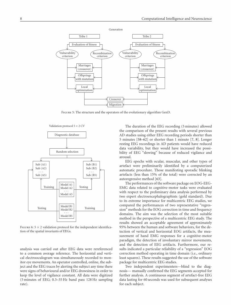
The validation protocol is a fundamental procedure to ver-ify the models’ ability to generalize the results reached in theTesting phase of each model. The application of a fixed proto-col measures the level of performance that a model can pro-duce on data that are not present in the testing and/or train-ing sample. We employed the so-called 5× 2 cross-validationprotocol (see Figure 6) [38]. This is a robust protocol thatallows one to evaluate the allocation of classification errors.In this procedure, the study sample is randomly divided tentimes into two subsamples, always different but containing asimilar distribution of cases and controls.

The ANNs’ good or excellent ability to diagnosticallyclassify all patients in the sample from the results of the con-fusion matrices of these 10 independent experiments wouldindicate that the spatial invariants extracted and selectedwith our method truly relate to the functioning quality ofthe brains examined through their EEG.

2.4. Experimental setting

2.4.1. Subjects and diagnostic criteria

The population study included

(a) 180 AD patients (gender: 50 males/130 females; age:mean = 77 ± 6.78 SD, range from 54 to 91; MMSE:mean = 19.9, ± 4.89 SD, range from 5 to 30);

(b) 115 MCI subjects (gender: 49 males/66 females; age:mean = 76 ± 6.37 SD, range from 42 to 88; MMSE:mean = 25.2, ± 2.35 SD, range from 17.3 to 29).

The samples were matched for age, gender, and years ofeducation. Part of the individual data sets was used for pre-vious EEG studies [2–4]. In none of these studies we ad-dressed the specific issue of the present study. Local institu-tional ethics committees approved the study. All experimentswere performed with the informed and overt consent of eachparticipant or caregiver.

The present inclusion and exclusion criteria for MCIwere based on previous seminal studies [39–46] and de-signed for selecting elderly persons manifesting objectivecognitive deficits, especially in the memory domain, who didnot meet criteria for a diagnosis of dementia or AD, namely,with, (i) objective memory impairment on neuropsycho-logical evaluation, as defined by performances ≥ 1.5 stan-dard deviation below the mean value of age and education-matched controls for a test battery including memory reylist (immediate recall and delayed recall), Digit forward andCorsi forward tests; (ii) normal activities of daily living asdocumented by the patient’s history and evidence of inde-pendent living; (iii) clinical dementia rating score of 0.5; (iv)geriatric depression scale scores < 13.

Exclusion criteria for MCI were: (i) mild AD, as di-agnosed by the procedures described above; (ii) evidenceof concomitant dementia such as frontotemporal, vasculardementia, reversible dementias (including pseudodepressivedementia), fluctuations in cognitive performance, and/orfeatures of mixed dementias; (iii) evidence of concomitantextrapyramidal symptoms; (iv) clinical and indirect evidenceof depression lower than 14 as revealed by GDS scores; (v)other psychiatric diseases, epilepsy, drug addiction, alcoholdependence, and use of psychoactive drugs including acetyl-cholinesterase inhibitors or other drugs enhancing brain cog-nitive functions; (vi) current or previous systemic diseases(including diabetes mellitus) or traumatic brain injuries.

Probable AD was diagnosed according to NINCDS-ADRDA criteria [47]. Patients underwent general medical,neurological, and psychiatric assessments and were also ratedwith a number of standardized diagnostic and severity in-struments that included MMSE [48], clinical dementia rat-ing scale [49], geriatric depression scale [50], Hachinski is-chemic scale [51], and instrumental activities of daily livingscale [52]. Neuroimaging diagnostic procedures (computedtomography or magnetic resonance imaging) and completelaboratory analyses were carried out to exclude other causesof progressive or reversible dementias, in order to have a ho-mogenous probable AD patient sample. The exclusion cri-teria included, in particular, any evidence of (i) front tem-poral dementia diagnosed according to criteria of Lund andManchester groups [53]; (ii) vascular dementia as diagnosedaccording to NINDS-AIREN criteria [54] and neuroimagingevaluation scores [55, 56]; (iii) extra pyramidal syndromes;(iv) reversible dementias (including pseudo dementia of de-pression); (v) Lewy body dementia according to the criteriaby McKeith et al. [57]. It is important to note that benzodi-azepines, antidepressant, and/or antihypertensive drugs werewithdrawn for about 24 hours before the EEG recordings.

2.4.2. EEG recordings

EEG data were recorded in wake rest state (eyes-closed),usually during late morning hours from 19 electrodes po-sitioned according to the international 10–20 system (i.e.,Fp1, Fp2, F7, F3, Fz, F4, F8, T3, C3, Cz, C4, T4, T5, P3,Pz, P4, T6, O1, O2; 0.3–70 Hz filtering band passes). Aspecific reference electrode was not imposed to all record-ing units of this multi-centric study, since any further data

8 Computational Intelligence and Neuroscience

Generation

Tribe 1 Tribe 2

Evaluation of fitness Evaluation of fitness

Vulnerabilitycriterion

Recombinationcriterion

Vulnerabilitycriterion

Recombinationcriterion

Marriages(crossover)

Marriages(crossover)

Offspringswith mutation

Offspringswith mutation

Localoptimization

Localoptimization

Crossover

Migration

Figure 5: The structure and the operators of the evolutionary algorithm GenD.

Validation protocol 5× 2 CV

Diagnostic database

Random selection

Sub (A1)Sub (A2)· · ·

Sub (A5)

Sub (B1)Sub (B2)· · ·

Sub (B5)

Training TestingModel A1Model A2· · ·

Model A5

Model B1Model B2· · ·

Model B5

Testing Training

Figure 6: 5 × 2 validation protocol for the independent identifica-tion of the spatial invariants of EEGs.

analysis was carried out after EEG data were rereferencedto a common average reference. The horizontal and verti-cal electrooculogram was simultaneously recorded to mon-itor eye movements. An operator controlled, online, the sub-ject and the EEG traces by alerting the subject any time therewere signs of behavioural and/or EEG drowsiness in order tokeep the level of vigilance constant. All data were digitized(5 minutes of EEG; 0.3–35 Hz band pass 128 Hz samplingrate).

The duration of the EEG recording (5 minutes) allowedthe comparison of the present results with several previousAD studies using either EEG recording periods shorter than5 minutes [58–62] or shorter than 1 minute [7, 8]. Longerresting EEG recordings in AD patients would have reduceddata variability, but they would have increased the possi-bility of EEG “slowing” because of reduced vigilance andarousal.

EEG epochs with ocular, muscular, and other types ofartefact were preliminarily identified by a computerizedautomatic procedure. Those manifesting sporadic blinkingartefacts (less than 15% of the total) were corrected by anautoregressive method [63].

The performances of the software package on EOG-EEG-EMG data related to cognitive-motor tasks were evaluatedwith respect to the preliminary data analysis performed bytwo expert electroencephalographists (gold standard). Dueto its extreme importance for multicentric EEG studies, wecompared the performances of two representative “regres-sion” methods for the EOG correction in time and frequencydomains. The aim was the selection of the most suitablemethod in the perspective of a multicentric EEG study. Theresults showed an acceptable agreement of approximately95% between the human and software behaviors, for the de-tection of vertical and horizontal EOG artifacts, the mea-surement of hand EMG responses for a cognitive-motorparadigm, the detection of involuntary mirror movements,and the detection of EEG artifacts. Furthermore, our re-sults indicated a particular reliability of a “regression” EOGcorrection method operating in time domain (i.e., ordinaryleast squares). These results suggested the use of the softwarepackage for multicentric EEG studies.

Two independent experimenters—blind to the diag-nosis— manually confirmed the EEG segments accepted forfurther analysis. A continuous segment of artefact-free EEGdata lasting for 60 seconds was used for subsequent analysesfor each subject.

Massimo Buscema et al. 9

EEG signal Squashing Weights matrix

Twist phaseNew features

Classification

Trainingsubset

Testingsubset

· · ·

T&T + IS

· · ·500 1000 1500 2000 2500 3000 3500

0

0.1

0.2

0.3

0.4

0.5

0.6

0.7

0.8

0.9

1

1 5 9 13 17 21 25 29 33 37 41 45 49 53 57 61 65 69 73 77

0

0.1

0.2

0.3

0.4

0.5

0.6

0.7

0.8

0.9

1

1 5 9 13 17 21 25 29 33 37 41 45 49 53 57 61 65 69 73 77

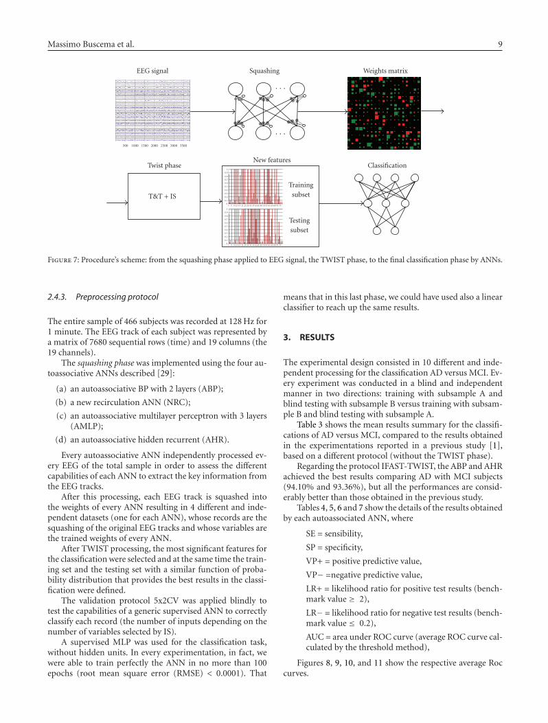
Figure 7: Procedure’s scheme: from the squashing phase applied to EEG signal, the TWIST phase, to the final classification phase by ANNs.

2.4.3. Preprocessing protocol

The entire sample of 466 subjects was recorded at 128 Hz for1 minute. The EEG track of each subject was represented bya matrix of 7680 sequential rows (time) and 19 columns (the19 channels).

The squashing phase was implemented using the four au-toassociative ANNs described [29]:

(a) an autoassociative BP with 2 layers (ABP);

(b) a new recirculation ANN (NRC);

(c) an autoassociative multilayer perceptron with 3 layers(AMLP);

(d) an autoassociative hidden recurrent (AHR).

Every autoassociative ANN independently processed ev-ery EEG of the total sample in order to assess the differentcapabilities of each ANN to extract the key information fromthe EEG tracks.

After this processing, each EEG track is squashed intothe weights of every ANN resulting in 4 different and inde-pendent datasets (one for each ANN), whose records are thesquashing of the original EEG tracks and whose variables arethe trained weights of every ANN.

After TWIST processing, the most significant features forthe classification were selected and at the same time the train-ing set and the testing set with a similar function of proba-bility distribution that provides the best results in the classi-fication were defined.

The validation protocol 5x2CV was applied blindly totest the capabilities of a generic supervised ANN to correctlyclassify each record (the number of inputs depending on thenumber of variables selected by IS).

A supervised MLP was used for the classification task,without hidden units. In every experimentation, in fact, wewere able to train perfectly the ANN in no more than 100epochs (root mean square error (RMSE) < 0.0001). That

means that in this last phase, we could have used also a linearclassifier to reach up the same results.

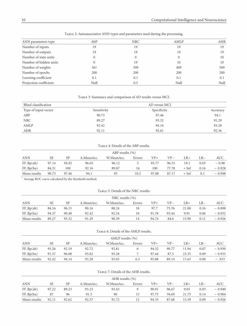
3. RESULTS

The experimental design consisted in 10 different and inde-pendent processing for the classification AD versus MCI. Ev-ery experiment was conducted in a blind and independentmanner in two directions: training with subsample A andblind testing with subsample B versus training with subsam-ple B and blind testing with subsample A.

Table 3 shows the mean results summary for the classifi-cations of AD versus MCI, compared to the results obtainedin the experimentations reported in a previous study [1],based on a different protocol (without the TWIST phase).

Regarding the protocol IFAST-TWIST, the ABP and AHRachieved the best results comparing AD with MCI subjects(94.10% and 93.36%), but all the performances are consid-erably better than those obtained in the previous study.

Tables 4, 5, 6 and 7 show the details of the results obtainedby each autoassociated ANN, where

SE = sensibility,

SP = specificity,

VP+ = positive predictive value,

VP− =negative predictive value,

LR+ = likelihood ratio for positive test results (bench-mark value ≥ 2),

LR− = likelihood ratio for negative test results (bench-mark value ≤ 0.2),

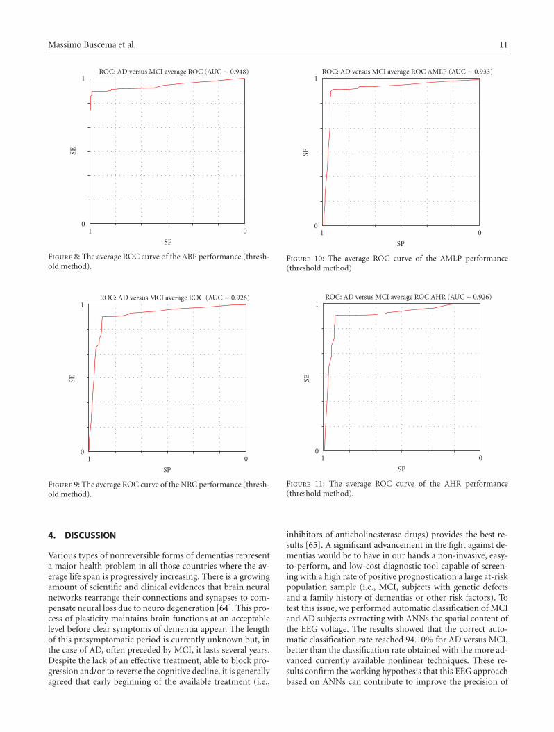
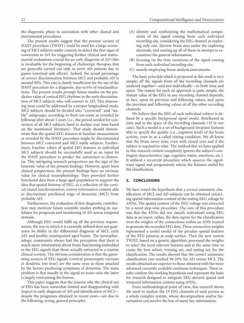
AUC = area under ROC curve (average ROC curve cal-culated by the threshold method),

Figures 8, 9, 10, and 11 show the respective average Roccurves.

10 Computational Intelligence and Neuroscience

Table 2: Autoassociative ANN types and parameters used during the processing.

ANN parameters type AbP NRC AMLP AHR

Number of inputs 19 19 19 19

Number of outputs 19 19 19 19

Number of state units 0 0 0 10

Number of hidden units 0 19 10 10

Number of weights 361 399 409 509

Number of epochs 200 200 200 200

Learning coefficient 0.1 0.1 0.1 0.1

Projection coefficient Null 0.5 Null Null

Table 3: Summary and comparison of AD results versus MCI.

Blind classification AD versus MCI

Type of input vector Sensitivity Specificity Accuracy

ABP 90.73 97.46 94.1

NRC 89.27 93.32 91.29

AMLP 92.42 94.14 93.28

AHR 92.11 92.61 92.36

Table 4: Details of the ABP results.

ABP results (%)

ANN SE SP A.MeanAcc. W.MeanAcc. Errors VP+ VP− LR+ LR− AUC

FF Bp(ab) 97.14 94.92 96.03 96.12 5 95.77 96.55 19.1 0.03 ∼ 0.98

FF Bp(ba) 84.31 100 92.16 89.87 16 100 77.78 + Inf 0.16 ∼ 0.928

Mean results 90.73 97.46 94.1 93 10.5 97.88 87.17 + Inf 0.1 ∼ 0.948∗

Average ROC curve calculated by the threshold method.

Table 5: Details of the NRC results.

NRC results (%)

ANN SE SP A.MeanAcc. W.MeanAcc. Errors VP+ VP− LR+ LR− AUC

FF Bp(ab) 84.16 96.15 90.16 88.24 18 97.7 75.76 21.88 0.16 ∼ 0.898

FF Bp(ba) 94.37 90.48 92.42 92.54 10 91.78 93.44 9.91 0.06 ∼ 0.932

Mean results 89.27 93.32 91.29 90.39 14 94.74 84.6 15.90 0.11 ∼ 0.926

Table 6: Details of the AMLP results.

AMLP results (%)

ANN SE SP A.MeanAcc. W.MeanAcc. Errors VP+ VP− LR+ LR− AUC

FF Bp(ab) 93.26 92.19 92.72 92.81 6 94.32 90.77 11.94 0.07 ∼ 0.930

FF Bp(ba) 91.57 96.08 93.82 93.28 7 97.44 87.5 23.35 0.09 ∼ 0.935

Mean results 92.42 94.14 93.28 93.05 6.5 95.88 89.14 17.65 0.08 ∼ .933

Table 7: Details of the AHR results.

AHR results (%)

ANN SE SP A.MeanAcc. W.MeanAcc. Errors VP+ VP− LR+ LR− AUC

FF Bp(ab) 97.22 89.23 93.23 93.43 9 90.91 96.67 9.03 0.03 ∼ 0.940

FF Bp(ba) 87 96 91.5 90 15 97.75 78.69 21.75 0.14 ∼ 0.904

Mean results 92.11 92.62 92.37 91.72 12 94.33 87.68 15.39 0.09 ∼ 0.926

Massimo Buscema et al. 11

0

SE1

1

SP

0

ROC: AD versus MCI average ROC (AUC ∼ 0.948)

Figure 8: The average ROC curve of the ABP performance (thresh-old method).

0

SE

1

1

SP

0

ROC: AD versus MCI average ROC (AUC ∼ 0.926)

Figure 9: The average ROC curve of the NRC performance (thresh-old method).

4. DISCUSSION

Various types of nonreversible forms of dementias representa major health problem in all those countries where the av-erage life span is progressively increasing. There is a growingamount of scientific and clinical evidences that brain neuralnetworks rearrange their connections and synapses to com-pensate neural loss due to neuro degeneration [64]. This pro-cess of plasticity maintains brain functions at an acceptablelevel before clear symptoms of dementia appear. The lengthof this presymptomatic period is currently unknown but, inthe case of AD, often preceded by MCI, it lasts several years.Despite the lack of an effective treatment, able to block pro-gression and/or to reverse the cognitive decline, it is generallyagreed that early beginning of the available treatment (i.e.,

0

SE

1

1

SP

0

ROC: AD versus MCI average ROC AMLP (AUC ∼ 0.933)

Figure 10: The average ROC curve of the AMLP performance(threshold method).

0

SE1

1

SP

0

ROC: AD versus MCI average ROC AHR (AUC ∼ 0.926)

Figure 11: The average ROC curve of the AHR performance(threshold method).

inhibitors of anticholinesterase drugs) provides the best re-sults [65]. A significant advancement in the fight against de-mentias would be to have in our hands a non-invasive, easy-to-perform, and low-cost diagnostic tool capable of screen-ing with a high rate of positive prognostication a large at-riskpopulation sample (i.e., MCI, subjects with genetic defectsand a family history of dementias or other risk factors). Totest this issue, we performed automatic classification of MCIand AD subjects extracting with ANNs the spatial content ofthe EEG voltage. The results showed that the correct auto-matic classification rate reached 94.10% for AD versus MCI,better than the classification rate obtained with the more ad-vanced currently available nonlinear techniques. These re-sults confirm the working hypothesis that this EEG approachbased on ANNs can contribute to improve the precision of

12 Computational Intelligence and Neuroscience

the diagnostic phase in association with other clinical andinstrumental procedures.

The present results suggest that the present variant ofIFAST procedure (TWIST) could be used for a large screen-ing of MCI subjects under control, to detect the first signs ofconversion to AD for triggering further clinical and instru-mental evaluations crucial for an early diagnosis of AD (thisis invaluable for the beginning of cholinergic therapies thatare generally carried out only in overt AD patients due togastro intestinal side effects). Indeed, the actual percentageof correct discrimination between MCI and probable AD isaround 94%. This rate is clearly insufficient for the use of theIFAST procedure for a diagnosis, due to 6% of misclassifica-tions. The present results prompt future studies on the pre-dictive value of cortical EEG rhythms in the early discrimina-tion of MCI subjects who will convert to AD. This interest-ing issue could be addressed by a proper longitudinal study.MCI subjects should be divided into “converted” and “sta-ble” subgroups, according to final out-come as revealed byfollowup after about 5 years (i.e., the period needed for con-version of all MCI subjects fated to decline over time basedon the mentioned literature). That study should demon-strate that the spatial EEG features at baseline measurementas revealed by the IFAST procedure might be discriminatedbetween MCI converted and MCI stable subjects. Further-more, baseline values of spatial EEG features in individualMCI subjects should be successfully used as an input bythe IFAST procedure to predict the conversion to demen-tia. This intriguing research perspectives are the sign of theheuristic value of the present findings. However, apart fromclinical perspectives, the present findings have an intrinsicvalue for clinical neurophysiology. They provided furtherfunctional data from a large aged population to support theidea that spatial features of EEG, as a reflection of the corti-cal neural synchronization, convey information content ableto discriminate preclinical stage of dementia (MCI) fromprobable AD.

Furthermore, the evaluation of that diagnostic contribu-tion may motivate future scientific studies probing its use-fulness for prognosis and monitoring of AD across temporaldomain.

Although EEG would fulfil up all the previous require-ments, the way in which it is currently utilized does not guar-antee its ability in the differential diagnosis of MCI, earlyAD, and healthy nonimpaired aged brains. The neurophys-iologic community always had the perception that there ismuch more information about brain functioning embeddedin the EEG signals than those actually extracted in a routineclinical context. The obvious consideration is that the gener-ating sources of EEG signals (cortical postsynaptic currentsat dendritic tree level) are the same ones as those attackedby the factors producing symptoms of dementia. The mainproblem is that usually in the signal-to-noise ratio the latteris largely overcoming the former.

This paper suggests that the reasons why the clinical useof EEG has been somewhat limited and disappointing withrespect to early diagnosis of AD and identification of MCI—despite the progresses obtained in recent years—are due tothe following, erring, general principles:

(A) identify and synthesizing the mathematical compo-nents of the signal coming from each individualrecording site, considering the EEG channel as explor-ing only one, discrete brain area under the exploringelectrode, and suming up all of them in attempt to re-construct the general information;

(B) focusing on the time variations of the signal comingfrom each individual recording site,

(C) mainly employing linear analysis instruments.

The basic principle which is proposed in this work is verysimple; all the signals from all the recording channels areanalyzed together—and not individually—in both time andspace. The reason for such an approach is quite simple; theinstant value of the EEG in any recording channel depends,in fact, upon its previous and following values, and uponthe previous and following values of all the other recordingchannels.

We believe that the EEG of each individual subject is de-fined by a specific background signal model, distributed intime and in the space of the recording channels (19 in ourcase). Such a model is a set of background invariant featuresable to specify the quality (i.e., cognitive level) of the brainactivity, even in so a called resting condition. We all knowthat the brain never rests, even with closed eyes and if thesubject is required to relax. The method that we have appliedin this research context completely ignores the subject’s con-tingent characteristics (age, cognitive status, emotions, etc.).It utilized a recurrent procedure which squeezes the signif-icant signal and progressively selects the features useful forthe classification.

5. CONCLUSIONS

We have tested the hypothesis that a correct automatic clas-sification of MCI and AD subjects can be obtained extract-ing spatial information content of the resting EEG voltage byANNs. The spatial content of the EEG voltage was extractedby a novel step-wise procedure. The core of this procedurewas that the ANNs did not classify individuals using EEGdata as an input; rather, the data inputs for the classificationwere the weights of the connections within an ANN trainedto generate the recorded EEG data. These connection weightsrepresented a useful model of the peculiar spatial featuresof the EEG patterns at scalp surface. Then the new systemTWIST, based on a genetic algorithm, processed the weightsto select the most relevant features and at the same time tocreate the best subset, training set, and testing set, for theclassification. The results showed that the correct automaticclassification rate reached 94.10% for AD versus MCI. Theresults obtained are superior to those obtained with the moreadvanced currently available nonlinear techniques. These re-sults confirm the working hypothesis and represent the basisfor research designed to integrate EEG-derived spatial andtemporal information content using ANNs.

From methodological point of view, this research showsthe need to analyze the 19 EEG channels of each person asa whole complex system, whose decomposition and/or lin-earization can involve the loss of many key information.

Massimo Buscema et al. 13

The present approach extends those of previous EEGstudies applying advanced techniques (wavelet, neural net-works, etc.) on the data of single recording channels; it alsocomplements those of previous EEG studies in aged people,evaluating the spatial distributions of the EEG data instant byinstant and the brain sources of these distributions [2–10].

With complex systems, it is not possible to establish a pri-ori which information is relevant and which is not. Nonlin-ear autoassociative ANNs are a group of methods to extractfrom these systems the maximum of linear and nonlinear as-sociations (features) able to explain their “strange” dynamics.

This research also documents the need to use differentarchitectures and topologies of ANNs and evolutionary sys-tems within complex procedures in order to optimize a spe-cific medical target. This study’s EEG analysis used

(1) different types of nonlinear autoassociative ANNs forsquashing data;

(2) a new system, TWIST, based on a genetic algorithm,which manages supervised ANNs in order to select themost relevant features and to optimize the distributionof the data in training and testing sets;

(3) a set of supervised ANNs for the final patterns recog-nition task.

It is reasonable to conclude that ANNs and other adaptivesystems should be used as cooperative adaptive agents withina structured project for complex, useful applications.

NOTE

IFAST is a european patent (application no. EP06115223.7—date of receipt 09.06.2006). The owner of the patent is Se-meion Research Center of Sciences of Communication, ViaSersale 117, Rome 00128, Italy. The inventor is MassimoBuscema. For software implementation, see [53]. Dr. C. D.Percio (Associazione Fatebenefratelli per la Ricerca) orga-nized the EEG data cleaning.

REFERENCES

[1] M. Buscema, P. Rossini, C. Babiloni, and E. Grossi, “TheIFAST model, a novel parallel nonlinear EEG analysistechnique, distinguishes mild cognitive impairment andAlzheimer’s disease patients with high degree of accuracy,” Ar-ificial Intelligence in Medicine, vol. 40, no. 2, pp. 127–141, 2007.

[2] C. Babiloni, G. Binetti, E. Cassetta, et al., “Mapping dis-tributed sources of cortical rhythms in mild Alzheimer’s dis-ease. A multicentric EEG study,” NeuroImage, vol. 22, no. 1,pp. 57–67, 2004.

[3] C. Babiloni, G. Frisoni, M. Steriade, et al., “Frontal white mat-ter volume and delta EEG sources negatively correlate in awakesubjects with mild cognitive impairment and Alzheimer’s dis-ease,” Clinical Neurophysiology, vol. 117, no. 5, pp. 1113–1129,2006.

[4] C. Babiloni, L. Benussi, G. Binetti, et al., “Apolipoprotein Eand alpha brain rhythms in mild cognitive impairment: a mul-ticentric electroencephalogram study,” Annals of Neurology,vol. 59, no. 2, pp. 323–334, 2006.

[5] N. Tsuno, M. Shigeta, K. Hyokid, P. L. Faber, and D. Lehmann,“Fluctuations of source locations of EEG activity during tran-sition from alertness to sleep in Alzheimer’s disease and vascu-

lar dementia,” Neuropsychobiology, vol. 50, no. 3, pp. 267–272,2004.

[6] C. Huang, L.-O. Wahlund, T. Dierks, P. Julin, B. Winblad,and V. Jelic, “Discrimination of Alzheimer’s disease and mildcognitive impairment by equivalent EEG sources: a cross-sectional and longitudinal study,” Clinical Neurophysiology,vol. 111, no. 11, pp. 1961–1967, 2000.

[7] T. Dierks, R. Ihl, L. Frolich, and K. Maurer, “Dementia of theAlzheimer type: effects on the spontaneous EEG described bydipole sources,” Psychiatry Research, vol. 50, no. 3, pp. 151–162, 1993.

[8] T. Dierks, V. Jelic, R. D. Pascual-Marqui, et al., “Spatial pat-tern of cerebral glucose metabolism (PET) correlates with lo-calization of intracerebral EEG-generators in Alzheimer’s dis-ease,” Clinical Neurophysiology, vol. 111, no. 10, pp. 1817–1824, 2000.

[9] T. Dierks, L. Frolich, R. Ihl, and K. Maurer, “Correlation be-tween cognitive brain function and electrical brain activity indementia of Alzheimer type,” Journal of Neural Transmission,vol. 99, no. 1–3, pp. 55–62, 1995.

[10] J. Hara, W. R. Shankle, and T. Musha, “Cortical atrophy inAlzheimer’s disease unmasks electrically silent sulci and lowersEEG dipolarity,” IEEE Transactions on Biomedical Engineering,vol. 46, no. 8, pp. 905–910, 1999.

[11] C. Huang, L.-O. Wahlund, T. Dierks, P. Julin, B. Winblad,and V. Jelic, “Discrimination of Alzheimer’s disease and mildcognitive impairment by equivalent EEG sources: a cross-sectional and longitudinal study,” Clinical Neurophysiology,vol. 111, no. 11, pp. 1961–1967, 2000.

[12] K. Bennys, G. Rondouin, C. Vergnes, and J. Touchon, “Diag-nostic value of quantitative EEG in Alzheimer’s disease,” Neu-rophysiologie Clinique, vol. 31, no. 3, pp. 153–160, 2001.

[13] M. Nuwer, “Assessment of digital EEG, quantitative EEG, andEEG brain mapping: report of the American Academy of Neu-rology and the American Clinical Neurophysiology Society,”Neurology, vol. 49, no. 1, pp. 277–292, 1997.

[14] G. Adler, S. Brassen, and A. Jajcevic, “EEG coherencein Alzheimer’s dementia,” Journal of Neural Transmission,vol. 110, no. 9, pp. 1051–1058, 2003.

[15] T. Musha, T. Asada, F. Yamashita, et al., “A new EEG methodfor estimating cortical neuronal impairment that is sensitiveto early stage Alzheimer’s disease,” Clinical Neurophysiology,vol. 113, no. 7, pp. 1052–1058, 2002.

[16] C. Melissant, A. Ypma, E. E. E. Frietman, and C. J.Stam, “A method for detection of Alzheimer’s disease usingICA-enhanced EEG measurements,” Artificial Intelligence inMedicine, vol. 33, no. 3, pp. 209–222, 2005.

[17] A. A. Petrosian, D. V. Prokhorov, W. Lajara-Nanson, and R. B.Schiffer, “Recurrent neural network-based approach for earlyrecognition of Alzheimer’s disease in EEG,” Clinical Neuro-physiology, vol. 112, no. 8, pp. 1378–1387, 2001.

[18] F. Vialatte, A. Cichocki, G. Dreyfus, T. Musha, S. L. Shishkin,and R. Gervais, “Early detection of Alzheimer’s disease byblind source separation, time frequency representation, andbump modeling of EEG signals,” in Proceedings of the 15th In-ternational Conference on Artificial Neural Networks: BiologicalInspirations (ICANN ’05), vol. 3696 of Lecture Notes in Com-puter Science, pp. 683–692, Springer, Warsaw, Poland, Septem-ber 2005.

[19] J. Jeong, “EEG dynamics in patients with Alzheimer’s disease,”Clinical Neurophysiology, vol. 115, no. 7, pp. 1490–1505, 2004.

[20] A. Cichocki, S. L. Shishkin, T. Musha, Z. Leonowicz, T.Asada, and T. Kurachi, “EEG filtering based on blind source

14 Computational Intelligence and Neuroscience

separation (BSS) for early detection of Alzheimer’s disease,”Clinical Neurophysiology, vol. 116, no. 3, pp. 729–737, 2005.

[21] A. Cichocki, “Blind signal processing methods for analyzingmultichannel brain signals,” International Journal of Bioelec-tromagtism, vol. 6, no. 1, 2004.

[22] A. Cichocki and S.-I. Amari, Adaptive Blind Signal and ImageProcessing: Learning Algorithms and Applications, Wiley, NewYork, NY, USA, 2003.

[23] D. E. Rumelhart, P. Smolensky, J. L. McClelland, and G. E.Hinton, “Schemata and sequential thought processes in PDPmodels,” in Parallel Distributed Processing: Explorations in theMicrostructure of Cognition, J. L. McClelland and D. E. Rumel-hart, Eds., vol. 2, pp. 7–57, The MIT Press, Cambridge, Mass,USA, 1986.

[24] M. Buscema, “Constraint satisfaction neural networks,” Sub-stance Use & Misuse, vol. 33, no. 2, pp. 389–408, 1998, specialissue on artificial neural networks and complex social systems.

[25] M. Buscema, “Recirculation neural networks,” Substance Use& Misuse, vol. 33, no. 2, pp. 383–388, 1998, special issue onartificial neural networks and complex social systems.

[26] G. E. Hinton and J. L. McClelland, “Learning representationby recirculation,” in Proceedings of IEEE Conference on NeuralInformation Processing Systems, Denver, Colo, USA, November1988.

[27] Y. Chauvin and D. E. Rumelhart, Eds., Backpropagation: The-ory, Architectures, and Applications, Lawrence Erlbaum Asso-ciates, Hillsdale, NJ, USA, 1995.

[28] J. L. Elman, “Finding structure in time,” Cognitive Science,vol. 14, no. 2, pp. 179–211, 1990.

[29] M. Buscema, “I FAST Software, Semeion Software #32,” Rome,Italy, 2005.

[30] M. Buscema, E. Grossi, M. Intraligi, N. Garbagna, A. Andriulli,and M. Breda, “An optimized experimental protocol based onneuro-evolutionary algorithms: application to the classifica-tion of dyspeptic patients and to the prediction of the effec-tiveness of their treatment,” Artificial Intelligence in Medicine,vol. 34, no. 3, pp. 279–305, 2005.

[31] M. Buscema, “TWIST Software, Semeion Software #32,”Rome, Italy, 2005.

[32] M. Buscema, “Genetic doping algorithm (GenD): theory andapplications,” Expert Systems, vol. 21, no. 2, pp. 63–79, 2004.

[33] L. Davis, Handbook of Genetic Algorithms, Van Nostrand Rein-hold, New York, NY, USA, 1991.

[34] S. Harp, T. Samed, and A. Guha, “Designing application-specific neural networks using the genetic algorithm,” in Ad-vances in Neural Information Processing Systems, D. Touretzky,Ed., vol. 2, pp. 447–454, Morgan Kaufman, San Mateo, Calif,USA, 1990.

[35] M. Mitchell, An Introduction to Genetic Algorithms, The MITPress, Cambridge, Mass, USA, 1996.

[36] D. Quagliarella, J. Periaux, C. Polani, and G. Winter, GeneticAlgorithms and Evolution Strategies in Engineering and Com-puter Science, John Wiley & Sons, Chichester, UK, 1998.

[37] G. Rawling, Foundations of Genetic Algorithms, Morgan Kauf-man, San Mateo, Calif, USA, 1991.

[38] T. G. Dietterich, “Approximate statistical tests for comparingsupervised classification learning algorithms,” Neural Compu-tation, vol. 10, no. 7, pp. 1895–1923, 1998.

[39] E. H. Rubin, J. C. Morris, F. A. Grant, and T. Vendegna, “Verymild senile dementia of the Alzheimer type I. Clinical assess-ment,” Archives of Neurology, vol. 46, no. 4, pp. 379–382, 1989.

[40] M. Albert, L. A. Smith, P. A. Scherr, J. O. Taylor, D. A.Evans, and H. H. Funkenstein, “Use of brief cognitive tests

to identify individuals in the community with clinically di-agnosed Alzheimer’s disease,” International Journal of Neuro-science, vol. 57, no. 3-4, pp. 167–178, 1991.

[41] C. Flicker, S. H. Ferris, and B. Reisberg, “Mild cognitive im-pairment in the elderly,” Neurology, vol. 41, no. 7, pp. 1006–1009, 1991.

[42] M. Zaudig, “A new systematic method of measurement anddiagnosis of “mild cognitive impairment” and dementia ac-cording to ICD-10 and DSM-III-R criteria,” International Psy-chogeriatrics, vol. 4, supplement 2, pp. 203–219, 1992.

[43] D. P. Devanand, M. Folz, M. Gorlyn, J. R. Moeller, and Y. Stern,“Questionable dementia: clinical course and predictors of out-come,” Journal of the American Geriatrics Society, vol. 45, no. 3,pp. 321–328, 1997.

[44] R. C. Petersen, G. E. Smith, R. J. Ivnik, et al., “ApolipoproteinE status as a predictor of the development of Alzheimer’s dis-ease in memory-impaired individuals,” Journal of the AmericanMedical Association, vol. 273, no. 16, pp. 1274–1278, 1995.

[45] R. C. Petersen, G. E. Smith, S. C. Waring, R. J. Ivnik, E. Kok-men, and E. G. Tangelos, “Aging, memory, and mild cognitiveimpairment,” International Psychogeriatrics, vol. 9, no. 1, pp.65–69, 1997.

[46] R. C. Petersen, R. Doody, A. Kurz, et al., “Current conceptsin mild cognitive impairment,” Archives of Neurology, vol. 58,no. 12, pp. 1985–1992, 2001.

[47] G. McKhann, D. Drachman, M. Folstein, R. Katzman, D. Price,and E. M. Stadlan, “Clinical diagnosis of Alzheimer’s disease:report of the NINCDS-ADRDA work group under the aus-pices of department of health and human services task forceon Alzheimer’s disease,” Neurology, vol. 34, pp. 939–944, 1984.

[48] M. F. Folstein, S. E. Folstein, and P. R. McHugh, “Mini mentalstate: a practical method for grading the cognitive state of pa-tients for the clinician,” Journal of Psychiatric Research, vol. 12,no. 3, pp. 189–198, 1975.

[49] C. P. Hughes, L. Berg, W. L. Danziger, L. A. Coben, and R. L.Martin, “A new clinical scale for the staging of dementia,” TheBritish Journal of Psychiatry, vol. 140, pp. 566–572, 1982.

[50] J. A. Yesavage, T. L. Brink, T. L. Rose, et al., “Development andvalidation of a geriatric depression screening scale: a prelimi-nary report,” Journal of Psychiatric Research, vol. 17, no. 1, pp.37–49, 1983.

[51] W. G. Rosen, R. D. Terry, P. A. Fuld, R. Katzman, and A. Peck,“Pathological verification of ischemic score in differentiationof dementias,” Annals of Neurology, vol. 7, no. 5, pp. 486–488,1980.

[52] M. P. Lawton and E. M. Brody, “Assessment of older peo-ple: self maintaining ad instrumental activities of daily living,”Gerontologist, vol. 9, no. 3, pp. 179–186, 1969.

[53] A. Brun, B. Englund, L. Gustafson, et al., “Consensus on clini-cal and neuropathological criteria for fronto-temporal demen-tia,” Journal of Neurology, Neurosurgery and Psychiatry, vol. 57,pp. 416–418, 1994.

[54] G. C. Roman, T. K. Tatemichi, T. Erkinjuntti, et al., “Vasculardementia: diagnostic criteria for research studies: report of theNINDS-AIREN international workshop,” Neurology, vol. 43,no. 2, pp. 250–260, 1993.

[55] G. B. Frisoni, A. Beltramello, G. Binetti, et al., “Computed to-mography in the detection of the vascular component in de-mentia,” Gerontology, vol. 41, no. 2, pp. 121–128, 1995.

[56] S. Galluzzi, C. F. Sheu, O. Zanetti, and G. B. Frisoni, “Distinc-tive clinical features of mild cognitive impairment with sub-cortical cerebrovascular disease,” Dementia and Geriatric Cog-nitive Disorders, vol. 19, no. 4, pp. 196–203, 2005.

Massimo Buscema et al. 15

[57] I. G. McKeith, D. Galasko, K. Kosaka, et al., “Consensus guide-lines for the clinical and pathologic diagnosis of dementia withLewy bodies (DLB): report of the consortium on DLB inter-national workshop,” Neurology, vol. 47, no. 5, pp. 1113–1124,1996.

[58] R. J. Buchan, K. Nagata, E. Yokoyama, et al., “Regional corre-lations between the EEG and oxygen metabolism in dementiaof Alzheimer’s type,” Electroencephalography and Clinical Neu-rophysiology, vol. 103, no. 3, pp. 409–417, 1997.

[59] E. Pucci, N. Belardinelli, G. Cacchio, M. Signorino, and F.Angeleri, “EEG power spectrum differences in early and lateonset forms of Alzheimer’s disease,” Clinical Neurophysiology,vol. 110, no. 4, pp. 621–631, 1999.

[60] B. Szelies, R. Mielke, J. Kessler, and W.-D. Heiss, “EEG powerchanges are related to regional cerebral glucose metabolism invascular dementia,” Clinical Neurophysiology, vol. 110, no. 4,pp. 615–620, 1999.

[61] G. Rodriguez, P. Vitali, C. De Leo, F. De Carli, N. Girtler, and F.Nobili, “Quantitative EEG changes in Alzheimer patients dur-ing long-term donepezil therapy,” Neuropsychobiology, vol. 46,no. 1, pp. 49–56, 2002.

[62] C. Babiloni, R. Ferri, D. V. Moretti, et al., “Abnormal fronto-parietal coupling of brain rhythms in mild Alzheimer’s disease:a multicentric EEG study,” European Journal of Neuroscience,vol. 19, no. 9, pp. 2583–2590, 2004.

[63] D. V. Moretti, F. Babiloni, F. Carducci, et al., “Computerizedprocessing of EEG-EOG-EMG artifacts for multi-centric stud-ies in EEG oscillations and event-related potentials,” Interna-tional Journal of Psychophysiology, vol. 47, no. 3, pp. 199–216,2003.

[64] Y. Stern, “Cognitive reserve and Alzheimer disease,” AlzheimerDisease and Associated Disorders, vol. 20, no. 2, pp. 112–117,2006.

[65] S. G. Gauthier, “Alzheimer’s disease: the benefits of early treat-ment,” European Journal of Neurology, vol. 12, no. 3, pp. 11–16,2005.