The impacts of alternative policy instruments on environmental … · The impacts of alternative policy instruments on environmental performance: A rm level study of temporary and

The impacts of alternative policy instruments on

environmental performance: A �rm level study of temporary

and persistent e�ects∗

Brita Bye§ Marit E. Klemetsen¶

September 1, 2016

Abstract

Using a rich Norwegian panel data set that includes information about environmental regula-

tions such as environmental taxes, non-tradable emission quotas and technology standards, all

kinds of polluting emissions, and a large number of control variables, we analyze the e�ects

of direct and indirect environmental regulations on environmental performance. We identify

positive and signi�cant e�ects of both direct and indirect policy instruments. Moreover, we test

whether the two types of regulations lead to positive and persistent e�ects on environmental

performance. We �nd evidence that direct regulations promote such e�ects. Indirect regula-

tions, on the other hand, will only have potential persistent e�ects if environmental taxes are

increasing over time.

Keywords: emission intensity, environmental performance, environmental regulation,

command-and-control, environmental taxes, long-term e�ects

JEL classi�cation: C01, C23, D04, D22, H23, L51, Q51, Q58

∗We are grateful to Arvid Raknerud for many valuable suggestions and comments. Thanks also to TerjeSkjerpen, Diana Iancu, Cathrine Hagem, Reyer Gerlagh, and participants at the 5th WCERE Congress inIstanbul and the 4th CREE workshop at Lysebu. Øyvind Hetland of the Norwegian Environment Agencyhas given us access to data and provided helpful information. While carrying out this research, the authorshave been associated with CREE - Oslo Centre for Research on Environmentally friendly Energy. TheCREE Centre acknowledges �nancial support from The Research Council of Norway, the University of Oslo,and user partners.§Statistics Norway, corresponding author, [email protected]¶University of Oslo/Statistics Norway, [email protected]

1 Introduction

During the recent decades, environmental concerns have attracted increasing attention. Dif-

ferent kinds of environmental regulations have been introduced in order to curb polluting

emissions to air, soil, and water. The regulations have been multifaceted ranging from di-

rect pollution regulations (�command-and-control�), such as technology standards and non-

tradable emission quotas, to indirect (�incentive-based�) regulations, such as environmental

taxes and tradable emission quotas.1

Conventional economic theory predicts two main advantages of indirect regulations over

direct regulations. Firstly, indirect policy instruments will result in more cost-e�cient

emission reductions2 (Maloney and Yandle, 1984; Tietenberg, 1990; Keohane et al., 1998;

Stavins, 2001; Newell and Stavins, 2003; Perman et al., 2011). Numerical simulation experi-

ments con�rm that the costs of direct regulations may be considerable (Perman et al., 2011),

although this is not con�rmed by empirical studies (Cole and Grossman, 1999). Secondly,

the literature predicts that indirect regulations will provide �continuous dynamic incentives�

by providing permanent incentives, through constant or increasing emissions prices, for re-

ducing emissions through technological improvement, in contrast to direct regulation (Ja�e

and Stavins, 1995; OECD, 2001; Perman et al., 2011). On the other hand, direct regulations

may be characterized by a binary switch as the required target is reached, and the literature

suggests that there are no incentives for further technological improvements.

Other studies illustrate how the dualistic categorization of instruments as either incentive-

based or command-and-control is misleading (see e.g., Bohm and Russel, 1985). The di�er-

ences between these types of instruments are typically over-emphasized (Cole and Grossman,

1999), as several incentives arise from direct forms of regulations that are not fundamentally

di�erent from those that arise from taxes and tradable quotas. This is also evident from

empirical analyses, see e.g., Cole et al. (2005) and Féres and Reynaud (2012). Studies

1Heine et al. (2012) is a recent contribution that summarizes principles and practices of environmental tax reformsthat also includes administrative and direct regulations.

2For a �ow pollutant or a uniform-mixed stock pollutant, Perman et al. (2011).

1

typically focus on the evaluation criteria economic e�ciency (a policy's aggregate net ben-

e�ts) and cost-e�ectiveness (Goulder and Parry, 2008). No single policy instrument ranks

�rst on all the dimensions of policy comparison (Palmer, 1980; Wiener, 1999; Goulder and

Parry, 2008; Perman et al., 2011). A natural but quite unexplored criterion is environmental

performance.

In this paper we examine the impacts of direct and indirect policy instruments on environ-

mental performance, measured as emission intensity. Moreover, we compare the long-term

e�ects of direct and indirect regulations on environmental performance. We do this by

testing the notion from the literature that indirect regulations provide �continuous dynamic

incentives� that lead to persistent e�ects on emissions through technological improvement,

in contrast to direct regulations, through an asymmetry test with regard to �rms' responses

to stricter versus more lax regulations.

We contribute to the existing literature in three ways. Firstly, we measure environmental

regulations and environmental performance at the �rm level. Both regulations and emissions

vary greatly across �rms and a study of the e�ects of regulations should be carried out at

the �rm level. In addition to information on environmental taxes and tradable quotas that

the �rms face, our data include measures of direct regulations as technology standards

and non-tradable emission quotas that enable us to identify the �rms' regulatory costs of

the regulations. Inspection violation status � the regulator's assessment of the severity

of a violation � captures the risk that a �rm may be sanctioned for violating its emission

permit. Secondly, our data allow us to test whether the regulations provide persistent e�ects

on environmental performance. Thirdly, we include the total range of Norwegian �rms'

land-based pollutant emissions, that includes a whole range of industries, in our measure

of environmental performance. We use the detailed emissions data in combination with

weighted damage cost estimates (Rosendahl, 2000; Håndbok V712, 2006; de Bruin et al.,

2010) to calculate monetary estimates of the emission damages. These monetary estimates

allow us to include and compare the whole range of emissions that cause very di�erent types

2

of damages, ranging from cancer risks or loss of fertility to global warming. Including all

types of emissions is particularly important in a study of direct regulations, since emissions

other than green house gases are still often regulated through technology standards and

non-tradable emission quotas. Studies of the e�ects of di�erent types of regulations on

environmental performance have until recently been quite scarce, with Cole et al. (2005)

and Féres and Reynaud (2012) as earlier examples of direct regulations. Wagner et al.

(2014), Klemetsen et al. (2016a), among others3, analyze the e�ects of the European Union

emission trading system. Féres and Reynaud (2012) analyzes the impact of formal (direct)

regulations and informal regulations (community pressure, etc.) on the environmental and

economic performance of a regional group of Brazilian manufacturing �rms. However, their

formal regulations are partially measured as the number of inspections and do not include

indirect regulations. We are not aware of any study using micro-data that includes indirect

regulations in the form of environmental taxes as well as direct regulations.

In line with Cole et al. (2005) and Féres and Reynaud (2012) among others, we identify

positive and signi�cant e�ects of non-tradable emission quotas and technology standards

on environmental performance. Moreover, we �nd positive and signi�cant e�ects of envi-

ronmental taxes. We also �nd evidence that direct regulations provide persistent e�ects.

Indirect regulations, on the other hand, will only induce potential persistent e�ects if en-

vironmental taxes are increasing over time.4 The results indicate that the dualistic catego-

rization of the instruments as either �incentive-based� or �command-and-control� is overly

simplistic.

The rest of the paper is organized as follows. A theoretical motivation for our econometric

model is presented in Section 2. Section 3 contains a description of the data, while the

econometric model and results are presented in Section 4. Finally, Section 5 concludes and

suggests some policy implications.

3See Martin et al. (2016) for a review of the empirical evidence for the EU ETS so far.4Martin et al. (2014) �nds a negative e�ect of the UK carbon tax on �rms' energy intensity. They do not, however,

measure the e�ect on emission intensity or test for persistent e�ects.

3

2 A production function with clean and dirty inputs

In order to identify e�ects of the di�erent regulations on environmental performance, we

need a �exible production function. Polluting emissions are (mostly) related to the input of

materials for the production processes and the use of dirty energy. We therefore specify a

production function that includes clean and dirty inputs. Whereas labor L, capital K, and

renewable energy are examples of clean inputs, oil products and dirty materials, such as

coke and coal, are examples of dirty inputs. Assume that we have two types of intermediary

inputs: clean inputs, Z1, and dirty inputs, Z2, which are imperfect substitutes, and that

the production function is separable in (Z1,Z2) and (L,K) as follows:

Qit = f

(Kit, Lit,

[Zδ1it + (b2itZ2it)

δ] 1δ

), (1)

where Qit is output, and total intermediary input is a Constant Elasticity of Substitution

(CES) aggregate of Z1 and Z2, where Z1 is the numeraire input (with b1it = 1) and the

parameter b2it determines the e�ciency of input factor 2 (dirty intermediary inputs) relative

to factor 1 (clean intermediary inputs). The elasticity of substitution between Z1 and Z2

is ρ = 1/(1−δ). Cost-minimization, with respect to Z1 and Z2 given �rm-speci�c prices for

input factor k, Pkit, means solving the problem

minZkit P1itZ1it + P2itZ2it s.t.[Zδ1it + (b2itZ2it)

δ] 1δ

= y,

(2)

where y denotes the intermediate aggregate. This has the well-known solution

Zkit = ybρkit

(PkitP

)−ρ

, k = 1, 2 (3)

4

where P is the price index of the intermediate aggregate:

P =

[2∑k=1

(Pkitbkit

)γ] 1γ

with γ =δ

δ − 1. (4)

The relative demand between input of dirty and clean intermediates is given by

lnZ2it − lnZ1it = ρ ln b2it − ρ lnP2it

P1it

. (5)

We assume that the total damage costs of emissions Dit from the use of dirty input are

given by

Dit =∑n

antλnitZ2it ≡ κitZ2it, (6)

where ant is the unit price (in euros) of damage from emissions of component n and λnit is

the emissions (in physical units) of component n from the use of one unit of dirty input Z2

in �rm i at time t. This implies that there is a linear relationship between emissions from

dirty inputs and the total damage costs. We can interpret κit as the emission coe�cient

from the use of dirty input Z2, at time t measured as damage costs. Inserting equation (6)

into equation (5) and taking logarithms gives the following equation for the damage costs

of emissions from �rm i at time t relative to the use of clean input, Z1:

lnDit − lnZ1it = lnκit + lnZ2it − lnZ1it ⇔

lnDit

Z1it

= git − ρ lnP2it

P1it

, (7)

where git = lnκit+ρ ln (b2it), which will be represented in terms of observed and unobserved

variables to be speci�ed in Sections 3 and 4. The left-hand side of equation (7) is then a

measure of emission intensity: the damage costs from dirty input relative to the use of clean

input.

5

We choose this measure of emission intensity as our measure of environmental perfor-

mance. An emission intensity is usually measured as emissions in physical units divided by

the use of the corresponding dirty input, while environmental performance is often measured

as emissions divided by income or production level, as in the literature of Environmental

Kuznets Curves5. Unfortunately, the physical emission intensity is only applicable to the

very few factors where we can observe both physical input and emissions, while emissions di-

vided by de�ated operating income will include substitution-, scale- and technology e�ects,

as well as revenue components that are often volatile. By de�ning environmental perfor-

mance as in equation (7), we are able to capture any subsitution e�ects (and technology

e�ects) resulting from relative energy prices. From equation (7) we see that environmental

performance is a function of the relative price between dirty intermediary input and clean

intermediary input, P2it/P1it, the elasticity of substitution, ρ, and �rm-speci�c e�ects, git,

which will be speci�ed in Sections 3 and 4. It may not be random to the �rm what kind of

regulations are implemented by the authorities. This may cause an endogeneity problem. In

order to identify causal e�ects, we di�erentiate equation (7) to remove �rm-�xed e�ects and

unit roots. We later show that both ln (Dit/Z1it) and ln (P2it/P1it) are highly non-stationary

time series (at the aggregate level). Hence, di�erentiation is necessary to remove stochas-

tic (unit root) and linear trends in both the dependent and explanatory variables. Our

econometric model in Section 4 is based on the di�erentiated version of equation (7):

4 lnDit

Z1it

= 4git − ρ4 lnP2it

P1it

(8)

Equation (8) states that environmental performance, measured as an emission intensity

depends on the relative price between dirty and clean intermediary input, in addition to

5As economies have become richer, support has been found for the existence of an Environmental Kuznets Curve(EKC), which implies an inverse u-shaped relationship between emissions (even for green-house gas emissions, Coleet al., 2005) and country income (GDP), Andreoni and Levinson (2001). There are di�erent hypotheses for theexistence of an EKC, but it is reasonable to believe that the growing environmental and political concern aboutregulating polluting emissions has contributed to this inverse u-shape. The contributions to this u-shaped curvecan be decomposed into substitution-, technology-, and scale e�ects (Bruvoll and Medin, 2003; Bruvoll et al., 2003;Bruvoll and Larsen, 2004).

6

several �rm speci�c e�ects. The emission intensity measure will pick up substitution between

electricity and other pollutants, although technology e�ects are also likely to be captured.

More details on the econometric speci�cation is given in Section 4.

3 Data sources and description of variables

Our �rm-level panel data draws on several data sources. All data sets are merged using

organization number as the �rm identi�er. The data set spans 20 years, from 1993 to

2012. A key data set is the data from the Norwegian Environment Agency (NEA) on

annual emissions of more than 260 di�erent pollutants emitted to air and water, emission

permits, assigned risk classes, inspections, and violations from inspections of all land-based

Norwegian �rms that have emission permits from the NEA. We use this data set as the

basis for our sample selection, as emissions are only reported for these �rms. The NEA

data are supplemented with annual data from three di�erent registers at Statistics Norway:

the Accounts statistics, the Environmental Accounts, and the National Accounts. Hence,

our data set also includes �rm-level economic variables, prices of electricity and fossil fuels

(which include energy- and environmental taxes), electricity and fossil fuel use measured in

kWh, and tradable carbon emission quotas. A detailed description of the key variables is

provided below, where they are grouped into three main categories: energy and emissions,

environmental regulations, and other determinants of environmental perfomance (control

variables).

3.1 Energy and Emissions

Our dataset from the NEA includes emissions of various pollutants, ranging from heavy

metals to green-house gases. The emissions are measured in a wide range of physical units

and cause di�erent types of damage, ranging from cancer risks or loss of fertility to global

warming. To study the empirical e�ects of di�erent environmental policies on our measure

7

of environmental performance � the damage costs of dirty factor input relative to clean

input (Section 2, equation (7)) � we need to transform the emissions data into a common

measurement scale. We use shadow prices of damages for each kind of emission to calculate

the total damage in terms of monetary costs. Shadow prices are constructed prices for goods

or production factors that are not traded in markets. Measuring shadow prices of polluting

emissions is challenging in several ways. Firstly, it requires sophisticated methodology

and in-depth knowledge about chemical compounds, as well as about the recipients in the

environment. Secondly, it requires simplifying assumptions, that must be transparent and

thoroughly discussed. Moreover, there are several examples of studies that do not rely

on expert comparisons of damages from various chemical compounds, but instead involve

measures based on the naive assumption that one unit of any compound causes the same

damage (!) (Lucas et al., 1992). Obviously, chemical compounds are di�erent: an emission

of a kilo of hazardous mercury and a kilo of CO2 cause very di�erent types and degrees of

damage.

There is no comprehensive study of the damage costs of Norwegian emissions, but by

collecting damage estimates from di�erent sources (Håndbok V712, 2006; Rosendahl, 2000),

we are able to establish data for Norwegian damage costs from many of the emissions. In

addition, we use damage costs estimates evaluated at shadow prices that re�ect the marginal

damage of the �rm's annual emissions constructed in de Bruin et al. (2010)6. These damage

estimates are averages for the Netherlands in 2008, and as local conditions may vary, we

prefer to use Norwegian damage estimates whenever they are available. Especially damages

from emissions to air can di�er signi�cantly between the Netherlands and Norway due to

the considerably smaller population density in Norway. de Bruin et al. (2010) provides

6The Shadow Prices handbook (de Bruin et al., 2010) is developed by CE Delft, an independent research andconsultancy organization. The Handbook is available on the website of CE Delft. We use the damage estimatesfor a large proportion of the several hundred substances listed in Tables 50 (Damage costs for emissions to air) and52 (Damage costs for emissions to water) in the Annexes to this report. The damage costs for emissions to air areobtained using NEEDS damage costs. The NEEDS project is an ExternErelated European study on the externalcosts of energy use. The damage costs for emissions to water are obtained using direct valuation of ReCiPe endpointcharacterization factors. Since this method is less reliable than using NEEDS damage costs, damage estimates foremissions to water are only approximate.

8

010

2030

1993

1994

1995

1996

1997

1998

1999

2000

2001

2002

2003

2004

2005

2006

2007

2008

2009

2010

2011

2012

Particulates Green house gasesAcidification and ozone precursers

Euro/kWh

Figure 1: Emission intensities. Monetary values (�xed 2008 euros) of total estimated dam-age of emissions relative to total electricity use (kWh). Norwegian land-based �rms withemission permits.

an extensive methodology for estimating shadow prices and deriving weighting factors for

individual types of environmental impact. The assumptions are explicitly detailed and the

methodology employed thoroughly described. We thus have a scienti�c background for the

damage estimates used in this study. This enables us to obtain a linear approximation of

aggregated damage estimates. Linear aggregate damage costs may overestimate or under-

estimate the true damage costs, depending on whether the observed emissions in our data

are lower or higher than the emission levels the marginal damage costs were estimated for.

Marginal damage costs will often increase with the level of emissions.

Our measure of environmental performance is given by the emission intensity (D/Z1)

(Section 2, equation (7)). We estimate the damage costs of a �rm's total annual emissions

D by multiplying the annual emission levels in kg by the damage estimates in �xed 2008

euros/kg, for each �rm-year. We measure clean intermediary input, Z1 as the �rm's use of

electricity measured in kWh. Electricity amounts to 85 percent of �rms' total energy use

9

0

10 mill

20 mill

30 mill

40 mill

Sum

of f

irms'

ene

rgy

use

(kW

h)

1993

1995

1997

1999

2001

2003

2005

2007

2009

2011

Electricity Petroleum products

Gas

a)

0 .1

.2

.3

1993

1995

1997

1999

2001

2003

2005

2007

2009

2011

Electricity intensity Petroleum intensity

Gas intensity Total energy intensity

b)

11.

52

2.5

Indi

ces,

199

3=1

1993

1995

1997

1999

2001

2003

2005

2007

2009

2011

Real income Electricity use (kWh)

c)

Ene

rgy

inte

nsity

: Ene

rgy

use

(kW

h) re

lativ

e to

real

inco

me

Figure 2: a): Total energy use (kWh). b): Energy use (kWh) relative to mean real operatingincome (de�ated by PPI). c): Indices, mean real operating income (de�ated by PPI) andelectricity use (kWh). Norwegian land-based �rms with emission permits.

in Norway, and hydro-power has been the main source of electricity during the estimation

period.7 Therefore, the use of electricity is an appropriate measure of clean factor input.

We have data on �rm-level electricity use from the Energy Statistics. Figure 1 illustrates

the trend in the estimated emission intensity of three examples of pollutants: particulates,

green-house gases, and acidi�cation and ozone precursors. All three groups of pollutants

exhibit a downward trend in emission intensity. Particulates and green-house gases have

the largest reductions in emission intensities of 62 and 83 percent respectively, whereas the

reduction for acidi�cation and ozone precursors is 25 percent.

Our emission intensity measure can be positively a�ected by either reducing the damage

costs (numerator) or by increasing the input of clean energy (denominator). Figure 2 pro-

vides calculated trends for energy use by Norwegian on-shore �rms with emission permits.

7Norway is part of the European power market, but the exchange of power has been but minor in the estimationperiod.

10

Chart a) illustrates that electricity use has remained relatively constant over time, with a

dip in 2009 of nearly 20 percent, following the �nancial crisis (NVE, 2013). The use of

petroleum products (except gas) has followed a downward trend since 1997, while the use

of gas has more than doubled over the period. Chart b) shows the development in di�erent

energy intensity measures. Measured relative to real operating income (de�ated by the pro-

ducer price index (PPI)), total energy intensity fell sharply until 2000-2001, and afterwards

increased until 2003, then fell again, reaching a new low in 2007-2008, before increasing and

then �attening out. Decomposing the energy intensity into electricity intensity and gas-

and petroleum intensities, we see that the wobbly path is caused by changes in electricity

use, as indicated by Chart a). The petroleum intensity follows a downward-sloping path,

whereas the gas intensity is largely stable from the year 2000 onwards. The use of electricity

�uctuates around +/- 10 percent in the time period, so the fall in electricity intensity is

caused by the increase in real operating income over the period, Chart c). Hence, the main

driving force behind the improvements in our measure of environmental performance over

the period (see Figure 1) is related to emission reductions and not to increased electricity

use.

As mentioned in Section 2, another relevant measure of emission intensity would be the

total environmental damage costs divided by de�ated operating income. From Figure 2,

Chart c), we see that mean operating income �uctuates signi�cantly more than electricity

use, especially from 2003 until 2010. Therefore, our measure of emission intensity is more

robust towards volatile price- and income e�ects. Electricity use is a particularly good

measure of the activity level in energy-intensive industries like manufacturing.

11

3.2 Environmental regulations

3.2.1 Direct regulations: non-tradable emission quotas and technology stan-

dards

In Norway, any emission that harms or may harm the environment is, as a general rule,

prohibited.8 Non-tradable emission quotas combined with technology restrictions are ad-

ministered by the NEA and have existed since 1974. If a �rm wishes to emit polluting

substances it has to apply for a permit from the NEA. The NEA should in principle have

an overview of most of the polluting activities that take place. It regulates and monitors

the environmental performance of polluting operations involving more than 260 pollutants

to air and water. Our data set includes everything from climate gases, such as CO2, to

pollutants associated with high cancer risk, such as heavy metals. The regulations con-

sist of both non-tradable emission quotas and technology standards. Technology standards

can either be designed as prohibitions on polluting production technologies or as a require-

ment of a speci�c clean technology. Such regulations are frequently used when a regulator

faces complexities, such as multiple emission types and targets, heterogeneous recipients,

and uncertainty with regard to marginal damage. This regulation is typically categorized

as a direct policy instrument (�command-and-control�). However, such regulations involve

several regulatory costs that provide �rms with incentives for behavioral change. These

incentives are not fundamentally di�erent from those arising from indirect instruments.

To measure the incentive or the regulatory costs of this form of direct regulation, we

need to identify when the regulation is binding, and how strict the regulation is, if binding.

We follow Ja�e and Stavins (1995) and Klemetsen et al. (2016b) in assuming that the

incentives for changes in environmental behavior are related to the possibility or threat of

being sanctioned for violating a permit. The �rm must weigh the need to produce and emit

against the costs of possible sanctions of violations. A �rm facing a binding emission permit

can reduce the restrictions on production by substituting to less emission intensive factor

8Law prohibiting harmful pollution: http://www.lovdata.no/all/nl-19810313-006.html

12

inputs, reduce production or purchase or develop a more e�cient technology. An important

factor when the regulator considers using sanctions is the severity of the violation. Our data

let us use the inspection violation status of the �rm as a probability of being sanctioned

(see below for a detailed description of this variable), in contrast to Ja�e and Stavins (1995)

that use the excess level of emission pollutants as a proxy for the probability of being

sanctioned. The reason for our choice is that regulators cannot observe emission levels, but

must rely on self-reported levels.9 Monitoring emissions is costly (and in practice di�cult

given current technologies), and hence, the regulators tend to focus on technology and

institutional violations when meting out sanctions. A large majority of the �rms whose

emissions simply exceed the permits are neither sanctioned nor issued with warnings of

sanctions. Compared to a measure using excess emissions, our measure more accurately

re�ects the risk that a �rm will be sanctioned unless it takes action to comply.10

When a �rm is granted an emission permit, the NEA assigns each �rm to a risk class, R,

based on the strength of the recipient of the emission (e.g. the vulnerability of a river, its

wind and stream conditions, popularity of a recreation area, etc., i.e. location speci�c) and

the pollutant speci�c emission level. The risk classes vary from 1 (the highest) to 4 (the

lowest), where risk class 1 comprises �rms considered to be potentially highly environmen-

tally harmful. A higher risk class (lower R) is associated with higher regulatory costs for

the �rm in several ways, see Table 1. They are subject to more frequent and more costly

inspections (columns 2-4), and warnings of higher �nes (column 5).

Firms with emission permits are subject to regular inspections. If a violation is detected

during an inspection, the �rm receives a letter from the NEA with a warning of sanctions

that will be imposed on the �rm should it remain noncompliant.11 The data on violations are

9However, �rms may underreport emissions. A potential source of bias related to self-reported emissions is if afteran inspection, �rms found in violation report emissions more correctly (i.e. an increase in the reported emissions). Ifthis is the case, the e�ect of direct regulations would be underestimated.

10Féres and Reynaud (2012) measure formal regulations as the number of inspections and average e�ciency ofwarnings and �nes from the local environmental agencies. The only �rm-level variable connected to direct regulationsis a dummy variable that describes the license status of the �rm.

11When inspecting plants, the NEA focuses on violations of procedures and general maintenance of equipmentrather than on actual emissions (Telle, 2004). The complete permits also contain a number of qualitative requirementsconcerning institutional, technological as well as formal aspects of the plant. The data on the �rms' violations probably

13

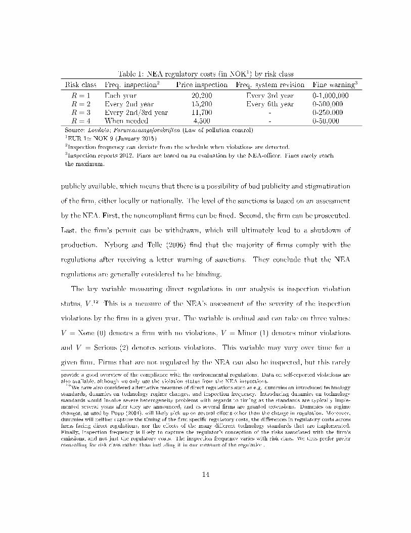
Table 1: NEA regulatory costs (in NOK1) by risk class

Risk class Freq. inspection2 Price inspection Freq. system revision Fine warning3

R = 1 Each year 20,200 Every 3rd year 0-1,000,000R = 2 Every 2nd year 15,200 Every 6th year 0-500,000R = 3 Every 2nd/3rd year 11,700 - 0-250,000R = 4 When needed 4,500 - 0-50,000

Source: Lovdata; Forurensningsforskriften (Law of pollution control)1EUR 1' NOK 9 (January 2015)2Inspection frequency can deviate from the schedule when violations are detected.3Inspection reports 2012. Fines are based on an evaluation by the NEA-o�cer. Fines rarely reach

the maximum.

publicly available, which means that there is a possibility of bad publicity and stigmatization

of the �rm, either locally or nationally. The level of the sanctions is based on an assessment

by the NEA. First, the noncompliant �rms can be �ned. Second, the �rm can be prosecuted.

Last, the �rm's permit can be withdrawn, which will ultimately lead to a shutdown of

production. Nyborg and Telle (2006) �nd that the majority of �rms comply with the

regulations after receiving a letter warning of sanctions. They conclude that the NEA

regulations are generally considered to be binding.

The key variable measuring direct regulations in our analysis is inspection violation

status, V .12 This is a measure of the NEA's assessment of the severity of the inspection

violations by the �rm in a given year. The variable is ordinal and can take on three values:

V = None (0) denotes a �rm with no violations, V = Minor (1) denotes minor violations

and V = Serious (2) denotes serious violations. This variable may vary over time for a

given �rm. Firms that are not regulated by the NEA can also be inspected, but this rarely

provide a good overview of the compliance with the environmental regulations. Data on self-reported violations arealso available, although we only use the violation status from the NEA inspections.

12We have also considered alternative measures of direct regulations such as e.g. dummies on introduced technologystandards, dummies on technology regime changes, and inspection frequency. Introducing dummies on technologystandards would involve severe heterogeneity problems with regards to timing as the standards are typically imple-mented several years after they are announced, and as several �rms are granted extensions. Dummies on regimechanges, as used by Popp (2004), will likely pick up on several e�ects other than the change in regulation. Moreover,dummies will neither capture the timing of the �rm speci�c regulatory costs, the di�erences in regulatory costs across�rms facing direct regulations, nor the e�ects of the many di�erent technology standards that are implemented.Finally, inspection frequency is likely to capture the regulator's conception of the risks associated with the �rm'semissions, and not just the regulatory costs. The inspection frequency varies with risk class. We thus prefer prefercontrolling for risk class rather than including it in our measure of the regulation.

14

occurs. More serious violations involve a higher risk of being sanctioned. However, other

factors than the severity of the violation can also be taken into account when the regulator

considers possible sanctions.13

Our measure of regulatory costs, violation status, is likely to capture only a part of the

incentive stemming from direct regulations. More speci�cally, violation status will capture

the incentive for �rms that are struggling to comply (speci�c deterrence). It is likely that

many �rms adapt to the technology requirements in time to avoid non-compliance entirely

(general deterrence). Hence, the e�ect of violation status (V ) on environmental performance

represents a lower bound on the total impact of direct regulation. It is this lower bound

that we estimate in Section 4.

3.2.2 Indirect regulations

A number of indirect regulations have also been introduced in Norway. Carbon taxes

and tradable carbon emission permits were introduced to follow up the Kyoto Protocol and

commitments to the EU's 20-20-20 goal for reductions in greenhouse gas emissions. Norway

is part of the European Union Emission Trading Scheme (EU ETS), which regulates carbon

emissions in the EU and EFTA area.14 The EU ETS covers approximately 50 percent

of the carbon emissions in Norway. Emissions that are not covered by the EU ETS are

mainly covered by the CO2-tax. The CO2-tax was introduced and levied on oil and gas

from 1991, and it has varied greatly between fossil fuel types and end uses. There are

also taxes on sulphur dioxide (SO2) and nitrogen oxide (NOx) emissions that are regulated

by the Gothenburg Protocol, and taxes on emissions of hydro�uorocarbons (HFCs) and

per�uorocarbons (PFCs) that are regulated by the Montreal Treaty.15 There is also a tax

13Examples of possible factors are the likelihood that the �rm will comply without sanctions being imposed, theability of the �rm to handle the requirement economically or practically, and �nally, the risk class of the �rm. Thethreats of sanctions tend to be more severe for the �rm the higher is the risk class (the lower is R) and therefore wecontrol for the risk class, see Section 4. Firms with e.g. low economic performance may receive lower �nes, o�settinga possible bias for weak economic �rms to be more prone to comply after the warning in order to avoid the �ne.

14The period 2005-2007 was a pilot �rst phase for EU ETS in EU and Norway. See the EU's quota directive(2003/87/EF) and European Environment Agency (2005). The oil and gas industry in Norway was not includedin the �rst phase, but was included in the second from 2008. The processing industries, except for the aluminumindustry, have been included since 2005; see also Ministry of the Environment (2011).

15Emissions of SO2 have been liable to environmental taxation since 1970, starting with a di�erentiated tax on

15

on electricity use for some industries/�rms.16

Ideally, we would like to investigate the e�ect of environmental taxes, which are mostly

levied on energy goods. However, in the data we cannot separate the energy pre-tax prices

from the emission taxes. In any case, the �rm likely adjusts to the total energy prices,

including taxes and pre-tax prices. Energy prices as proxies for environmental taxes is thus

common in the literature, see, e.g., Ja�e and Stavins (1995). Prices on dirty energy inputs

at the �rm level are calculated as the sum of the �rm's expenditures on petroleum products

and gas divided by the use of petroleum and gas in kWh. We calculate electricity prices at

the �rm level by dividing total expenditures on electricity by electricity use in kWh.17

Figure 3 (Chart a)) shows the development in the �rms' mean real input prices (de�ated

by the PPI) of electricity, petroleum products, gas and materials.18 We see that petroleum,

gas, and materials have experienced a real price increase over the whole period, in spite of

some wobbly periods in between. Especially real gas prices were considerably higher around

2000. The real electricity price has increased only slightly over the period, and it dropped

in 2011.

According to equation (7) (Section 2) the relative price responsiveness between �dirty�

and �clean� intermediary inputs in�uence the environmental performance of �rms. We proxy

the indirect regulations as the relative factor input price19 between the �rm's dirty factor

input price (cost-share weighted average of petroleum, gas and material prices) divided by

the �rm's electricity price. This variable is illustrated in Chart b) in Figure 3, and shows

mineral oils and extended to include a SO2-tax on coke and coal in 1999. In 2002, this tax on coke and coal wasreplaced by a memorandum of understanding between the Ministry of the Environment and the Association forProcessing industries. Taxes on HFC and PFC were introduced in 2003. The NOx-tax was introduced in 2007 on allNOx-emissions except those from the processing industry, combined with a NOx-fund for several industries (Hagemet al., 2012). A tax on the chemicals trichloroethene and tetrachloroethene was introduced in 2000.

16Ministry of Finance (2007) gives a detailed description of energy and environmental taxation in Norway in recentdecades and of the international environmental agreements that Norway has signed.

17Electricity prices are �rm-speci�c in the energy-intensive part of the manufacturing industries, because pricesare regulated by long-term contracts (http://www.ssb.no/energi-og-industri/statistikker/elkraftpris). Firmsoutside the manufacturing industries purchase electricity at market prices.

18The input price of materials are proxied by Production Input Prices (Statistics Norway). This variable is at adetailed industry level. Firm variation is achieved through the dirty and clean energy prices.

19Using factor input prices, e.g. energy prices as proxies for environmental taxes is common in the literature, see,e.g., Ja�e and Stavins (1995). Fluctuations in relative energy prices caused by e.g. world market oil price changescontribute to sharper estimated coe�cients of relative price changes � our measure of indirect regulations such astaxes.

16

11.

52

2.5

33.

5Rea

l pric

e in

dice

s

1993

1994

1995

1996

1997

1998

1999

2000

2001

2002

2003

2004

2005

2006

2007

2008

2009

2010

2011

2012

Electricity Petroleum products

Gas Producer Input Prices

.81

1.2

1.4

1.6

Rel

ativ

e in

term

edia

ry in

put p

rices

1993

1994

1995

1996

1997

1998

1999

2000

2001

2002

2003

2004

2005

2006

2007

2008

2009

2010

2011

2012

a) b)

Figure 3: Chart a): Mean price indices. Chart b): Relative mean input prices between�dirty� and �clean� input factors. Norwegian land-based �rms with emission permits.

an increasing trend. Variations in the relative factor input price includes both changes in

pre-tax prices and changes in environmental taxes. Since environmental taxes are mostly

directed towards energy related emissions, we perform a separate robustness analysis of the

e�ect of relative dirty/clean input prices on a subsample of the emissions that are related to

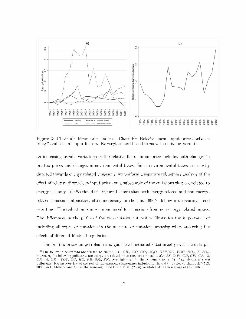
energy use only (see Section 4).20 Figure 4 shows that both energy-related and non-energy-

related emission intensities, after increasing in the mid-1990's, follow a decreasing trend

over time. The reduction is most pronounced for emissions from non-energy related inputs.

The di�erences in the paths of the two emission intensities illustrates the importance of

including all types of emissions in the measure of emission intensity when analyzing the

e�ects of di�erent kinds of regulations.

The pre-tax prices on petroleum and gas have �uctuated substantially over the data pe-

20The following pollutants are related to energy use: CH4, CO, CO2, N2O, NMVOC, V OC, NOx, S, SOx.Moreover, the following pollutants are energy use related when they are emitted to air: AS, C2F6, CD, CF4, CR−3,CR − 6, CR − TOT , CU , HG, PB, SF6, ZN . See Table A.1 in the Appendix for a list of de�nitions of thesepollutants. For an overview of the rest of the emission components included in the data we refer to Håndbok V712,2006, and Tables 50 and 52 (in the Annexes) in de Bruin et al. (2010), available at the homepage of CE Delft.

17

1015

2025

30

1993

1994

1995

1996

1997

1998

1999

2000

2001

2002

2003

2004

2005

2006

2007

2008

2009

2010

2011

2012

Emissions from energy related inputs Emissions from non-energy related inputs

Figure 4: Mean �rm-year emission intensity 1993-2012. Norwegian land-based �rms withemission permits.

riod, such that identifying separate e�ects of taxes and quota-prices is di�cult. Fluctuations

in relative energy prices caused by e.g. world market oil price changes contribute to sharpen

the estimated coe�cient of relative price changes � our measure of indirect regulations such

as taxes. As we come back to in Section 4.2, we can interpret the estimated coe�cient

related to relative energy prices as an elasticity. We include a dummy which is equal to 1 if

the �rm is part of the EU ETS in the given year. Our measure of indirect regulations � the

relative price of �dirty� and �clean� energy inputs � may include potential e�ects on pre-tax

energy prices from the tradable emission quota system. However, since the EU ETS quota

prices have been very low, this e�ect should be minor so that the relative price between

dirty and clean inputs capture the e�ects of environmental taxes.

18

4550

5560

6570

0-10 11-50 51-200 >200Number of employees

0

10

20

30

40

50

0-100 100-300 300-600 >600Capital intensity, K/L

b)a)

Figure 5: Firm characteristics (horizontal axes) and polluting �rms' mean emission intensity(vertical axes). Norwegian land-based �rms with emission permits.

3.3 Other determinants of environmental performance

Other �rm-speci�c characteristics may also be important drivers of environmental perfor-

mance. Figure 5 shows that both the number of employees and capital intensity are highly

correlated with emission intensity and should be included as control variables when analyz-

ing environmental performance. Chart a) illustrates how emission intensity decreases with

�rm size measured as the number of employees. This relationship could be due to scale

advantages as larger �rms may have more e�cient production. In absolute numbers, emis-

sion levels are likely to increase with �rm size, but larger �rms tend to be more emission

e�cient. Moreover, capital intensity, measured as the capital stock relative to the number

of employees, and emission intensity are positively related, as illustrated in Chart b). More

capital-intensive �rms may have more polluting production processes and use more dirty

energy and material inputs.

Figure 6 shows that emission intensity di�ers systematically across industries. In addition

to the aforementioned control variables, we include risk class dummies (see Section 3.2.1 for

details) of the �rms, as well as year- and industry dummies as control variables to account

19

010

2030

40

Primary

Mining, quarrying

Oil/gas e

xtractio

n

Textiles, f

ood

Wood, pulp, paper

Chemicals,

pharma., rubber, p

lastic

Maschinery,

electronics

Metals, minerals

Power prod., recyc

ling

Constructio

n

Transport

Retail trade

Services

Euro/kWh

Figure 6: Mean �rm-year emission intensity per industry. Norwegian land-based �rms withemission permits.

for common trends (see Figure 4) and industry-speci�c e�ects.

3.4 Sample summary statistics

Our initial sample of 741 incorporated Norwegian land-based �rms with emission permits

includes 741 �rms and 7209 �rm-year observations for the years 1993 to 2012. Table 2

presents descriptive statistics for the main variables. After dropping observations with

missing values, the �nal unbalanced panel data set consists of 3,187 (�rm-year) observations

and 421 �rms. All variables contain �rm-level variation. The industry aggregation of the

sample in the given time period is illustrated in Table 3. A majority of the polluting �rms

are in the manufacturing industries.21

21Since we only include �rms with emission permits we only study �rms that are dirty. There are few dirty �rmsin less pollution intensive industries as services, retail trade, construction and transport.

20

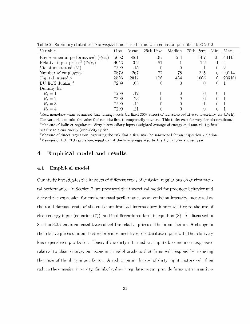
Table 2: Summary statistics: Norwegian land-based �rms with emission permits, 1993-2012

Variable Obs Mean 25th Perc Median 75th Perc Min Max

Environmental performance1 (D/Z1) 5002 88.1 .07 2.4 14.7 0 40415Relative input prices2 (P2/P1) 4053 3.2 .81 1 1.2 .1 4Violation status3 (V ) 7209 .45 0 0 1 0 2Number of employees 5872 267 22 78 225 0 20114Capital intensity 5595 2017 176 434 1065 0 235161EU ETS dummy4 7209 .05 0 0 0 0 1Dummy forRt = 1 7209 .12 0 0 0 0 1Rt = 2 7209 .23 0 0 0 0 1Rt = 3 7209 .44 0 0 1 0 1Rt = 4 7209 .21 0 0 0 0 1

1Real monetary value of annual �rm damage costs (in �xed 2008-euros) of emissions relative to electricity use (kWh).

The variable can take the value 0 if e.g. the �rm is temporarily inactive. This is the case for very few observations.2Measure of indirect regulation: dirty intermediary input (weighted average of energy and material) prices

relative to clean energy (electricity) price.3Measure of direct regulation, capturing the risk that a �rm may be sanctioned for an inspection violation.4Measure of EU ETS regulation, equal to 1 if the �rm is regulated by the EU ETS in a given year.

4 Empirical model and results

4.1 Empirical model

Our study investigates the impacts of di�erent types of emission regulations on environmen-

tal performance. In Section 2, we presented the theoretical model for producer behavior and

derived the expression for environmental performance as an emission intensity, measured as

the total damage costs of the emissions from all intermediary inputs relative to the use of

clean energy input (equation (7)), and in di�erentiated form in equation (8). As discussed in

Section 3.2.2 environmental taxes a�ect the relative prices of the input factors. A change in

the relative prices of input factors provides incentives to substitute inputs with the relatively

less expensive input factor. Hence, if the dirty intermediary inputs become more expensive

relative to clean energy, our economic model predicts that �rms will respond by reducing

their use of the dirty input factor. A reduction in the use of dirty input factors will then

reduce the emission intensity. Similarly, direct regulations can provide �rms with incentives

21

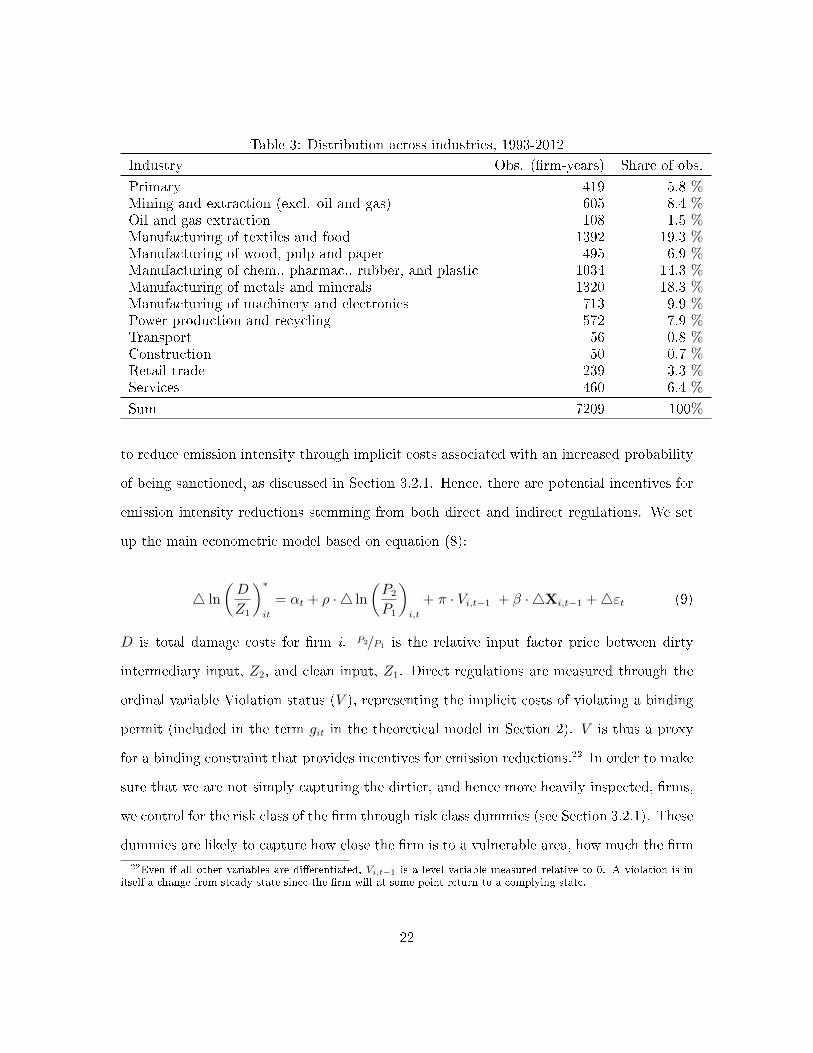
Table 3: Distribution across industries, 1993-2012

Industry Obs. (�rm-years) Share of obs.

Primary 419 5.8 %Mining and extraction (excl. oil and gas) 605 8.4 %Oil and gas extraction 108 1.5 %Manufacturing of textiles and food 1392 19.3 %Manufacturing of wood, pulp and paper 495 6.9 %Manufacturing of chem., pharmac., rubber, and plastic 1034 14.3 %Manufacturing of metals and minerals 1320 18.3 %Manufacturing of machinery and electronics 713 9.9 %Power production and recycling 572 7.9 %Transport 56 0.8 %Construction 50 0.7 %Retail trade 239 3.3 %Services 460 6.4 %

Sum 7209 100%

to reduce emission intensity through implicit costs associated with an increased probability

of being sanctioned, as discussed in Section 3.2.1. Hence, there are potential incentives for

emission intensity reductions stemming from both direct and indirect regulations. We set

up the main econometric model based on equation (8):

4 ln

(D

Z1

)∗

it

= αt + ρ · 4 ln

(P2

P1

)i,t

+ π · Vi,t−1 + β · 4Xi,t−1 +4εt (9)

D is total damage costs for �rm i. P2/P1 is the relative input factor price between dirty

intermediary input, Z2, and clean input, Z1. Direct regulations are measured through the

ordinal variable Violation status (V ), representing the implicit costs of violating a binding

permit (included in the term git in the theoretical model in Section 2). V is thus a proxy

for a binding constraint that provides incentives for emission reductions.22 In order to make

sure that we are not simply capturing the dirtier, and hence more heavily inspected, �rms,

we control for the risk class of the �rm through risk class dummies (see Section 3.2.1). These

dummies are likely to capture how close the �rm is to a vulnerable area, how much the �rm

22Even if all other variables are di�erentiated, Vi,t−1 is a level variable measured relative to 0. A violation is initself a change from steady state since the �rm will at some point return to a complying state.

22

pollutes, and, �nally, the di�ering numbers of inspections of the �rm. Hence, this control

variable is likely to capture some of the incentives for emission reductions, and thus lead to

underestimation of the true e�ect of direct regulations on environmental performance.

We also include other control variables that may in�uence environmental performance,

represented by the vector X: capital intensity, number of employees, and whether the �rm

is part of the EU ETS � represented by a dummy variable for the relevant years.23 Finally,

4ε is the di�erentiated error term, which we allow to have an auto regressive structure of

order 1. This is realistic since potential omitted variables captured in the error term are

likely to be correlated within a given �rm.

The coe�cient ρ re�ects the average e�ect of indirect regulations represented by relative

input factor prices, π re�ects the average e�ect associated with the risk of being sanctioned

for violating direct regulations, and β represents a vector of coe�cients for the control

variables. We consider relative factor input prices to be exogenous to the �rms. The other

explanatory variables are lagged one year to deal with potential issues of reversed causality.

We estimate equation (9) as a mixed model, where the coe�cients of ln (P2/P1)i,t and

Vi,t−1 are �rm-speci�c. ρ and π in equation (9) are the average values of the �rm-speci�c ρi

and πi parameters, respectively. Thus, we allow �rms to have heterogeneous responses to

environmental regulations. It is essential to allow for heterogeneous treatment e�ects since

�rms may have di�erent price elasticities, and thus respond di�erently to relative price

changes. Moreover, �rms may respond di�erently to inspection violations. For example,

one can envisage some �rms that purchase the required technology when a violation is

detected, and some �rms that purchase the required technology when the regulator detects

and classi�es the violation as a serious one. We do not allow for random coe�cients in the

control variables in X, because they are of secondary interest.

23 By including the EU ETS dummy we separate the potential e�ect of the environmental taxes from the e�ects of

the tradable EU ETS quotas, although they are probably very small, see also Section 3.2.2.

23

4.2 Results of the main speci�cation

The results of the estimations of the main speci�cation, equation (9), are shown in Table

4. We perform the analysis for the whole sample denoted alternative I, and an alterna-

tive sample, where we only include the energy-related emissions in the response variable,

4 ln (D/Z1), denoted alternative II. This could potentially be of importance since indirect

regulations are mainly directed towards energy related emissions. The sample in alternative

II is thus more likely to identify the causal e�ects from indirect regulations.

If the response variable � the emission intensity � increases, the �rm becomes less ef-

�cient. If environmental taxes through increased relative input price create incentives for

emission intensity reductions, we expect the estimated coe�cients on ln (P2/P1) to be nega-

tive. This is the case for the estimated coe�cient ρ which is equal to -0.10 and signi�cant

well below the 10 percent level (alternative I). This estimated coe�cient can be interpreted

as an elasticity: A 1 percent increase in the relative price leads to a 0.1 percent improvement

in the emission intensity.

If the measure of direct regulation, V , increases, the �rm is assumed to experience the

regulation as stricter. Hence, if this creates an incentive for reducing the emission intensity,

we expect a negative sign on the estimated coe�cient of this variable. This is the case,

as π is -0.08 and signi�cant at the 5 percent level. Direct regulations also improve �rms'

environmental performance, in line with Cole et al. (2005) and Féres and Reynaud (2012)

� among others. This coe�cient is smaller than the estimated coe�cient of the relative

input price. However, we cannot compare the estimated coe�cients directly, as the measure

of direct regulations is an ordinal variable. In addition, as mentioned in Section 3.2.1, our

measure of direct regulations � Violation status � will not capture the entire e�ect from

this policy, since many �rms are likely to adapt when they are required to, thus avoiding

non-compliance. π should thus be interpreted as a lower bound for the e�ect of direct

regulations.

24

Regarding the control variables, the dummy variable for risk class 1 is omitted because

there is no within-�rm variation (the NEA seldom makes changes in the risk class catego-

rization of �rms). As expected, the estimated coe�cients for risk class 2 are higher than for

risk class 3 with both alternatives since a change to a stricter risk class (2 is stricter than

3) means that the �rm is now considered by the NEA to be more pollutive or close to an

area that is now considered more vulnerable. The estimate related to capital intensity is

positive (0.09) and signi�cant at the 10 percent level. Hence, more capital intensive �rms

seem in general to be more dependent on dirty factor inputs and/or more pollution intensive

processes. The number of employees has a negative estimated coe�cient, signi�cant at the

10 percent level. This indicates that there are positive scale e�ects, so that larger �rms may

have more e�cient technology. The estimated coe�cient of the EU ETS dummy is negative,

but not signi�cant. This variable is only used as a control variable, as a study of the causal

e�ect of the EU ETS requires a di�erent methodological approach (see Klemetsen et al.

(2016a) for the e�ects of the EU ETS on Norwegian plants. The estimated coe�cient of the

auto-regressive part of the di�erentiated error term is negative and highly signi�cant, as is

typically the case with error terms in di�erences.

Alternative II reports the results from the estimation using only the subsample of energy-

related emissions. Compared to alternative I, the sample size is reduced from 3187 to 2100.

Some drop in signi�cance levels is therefore expected. The positive results with respect to

the e�ects of indirect regulations on environmental performance are strengthened as ρ is

-0.14, signi�cant at the 5 percent level. This is expected, since we now only include energy-

related emissions, the types of emission that are typically regulated by taxes. On the other

hand, direct regulations are generally directed towards other types of emissions than energy-

related ones. Therefore the drop in π to -0.05, as well as the loss of signi�cance is expected,

since few of the emissions in this sample are subjected to direct regulations. This is also the

explanation for the loss in signi�cance of the risk class dummies. This sample is preferred

for estimating the e�ects of indirect regulations, while alternative I provides the preferred

25

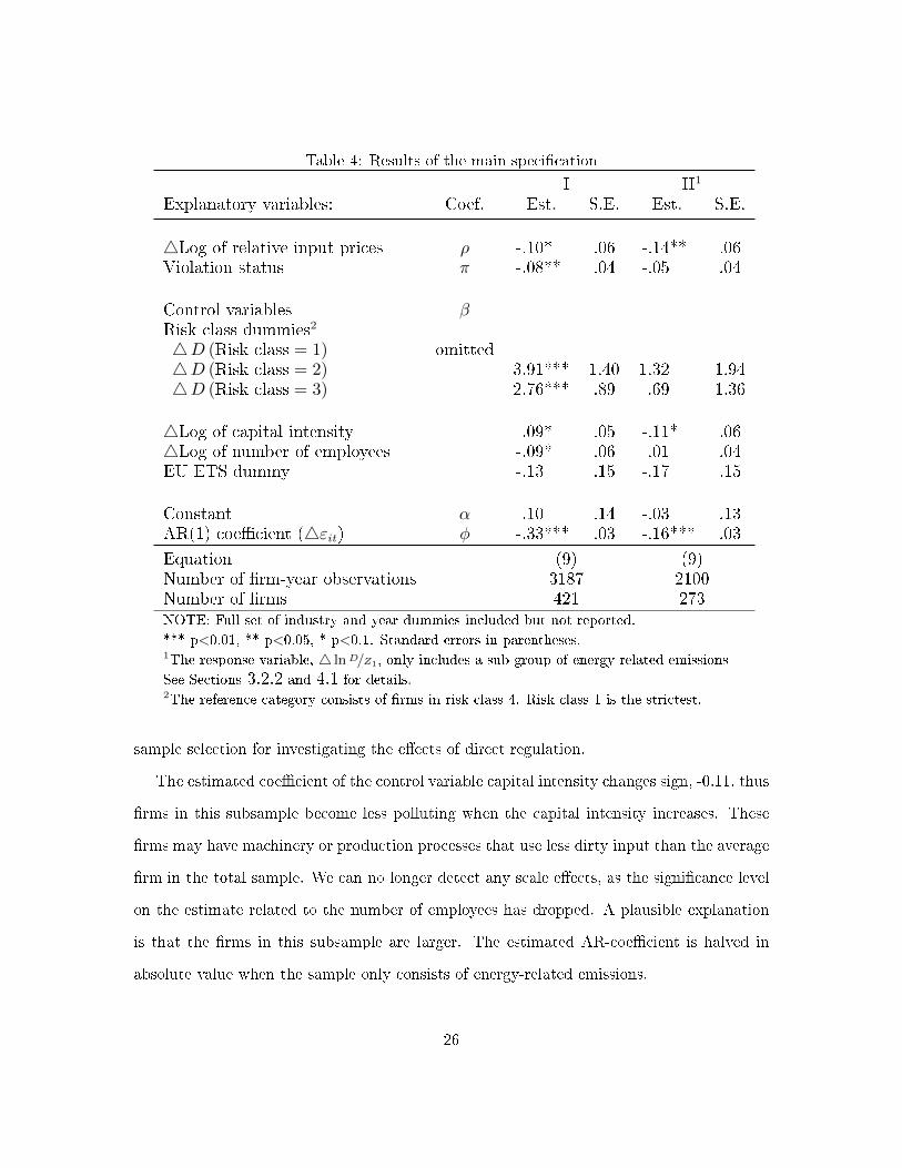
Table 4: Results of the main speci�cation

I II1

Explanatory variables: Coef. Est. S.E. Est. S.E.

4Log of relative input prices ρ -.10* .06 -.14** .06Violation status π -.08** .04 -.05 .04

Control variables βRisk class dummies2

4D (Risk class = 1) omitted4D (Risk class = 2) 3.91*** 1.40 1.32 1.944D (Risk class = 3) 2.76*** .89 .69 1.36

4Log of capital intensity .09* .05 -.11* .064Log of number of employees -.09* .06 .01 .04EU ETS dummy -.13 .15 -.17 .15

Constant α .10 .14 -.03 .13AR(1) coe�cient (4εit) φ -.33*** .03 -.16*** .03

Equation (9) (9)Number of �rm-year observations 3187 2100Number of �rms 421 273NOTE: Full set of industry and year dummies included but not reported.

*** p<0.01, ** p<0.05, * p<0.1. Standard errors in parentheses.1The response variable, 4 lnD/Z1, only includes a sub-group of energy-related emissions

See Sections 3.2.2 and 4.1 for details.2The reference category consists of �rms in risk class 4. Risk class 1 is the strictest.

sample selection for investigating the e�ects of direct regulation.

The estimated coe�cient of the control variable capital intensity changes sign, -0.11, thus

�rms in this subsample become less polluting when the capital intensity increases. These

�rms may have machinery or production processes that use less dirty input than the average

�rm in the total sample. We can no longer detect any scale e�ects, as the signi�cance level

on the estimate related to the number of employees has dropped. A plausible explanation

is that the �rms in this subsample are larger. The estimated AR-coe�cient is halved in

absolute value when the sample only consists of energy-related emissions.

26

4.3 Allowing Violation status to have non-linear e�ects

In the main speci�cation (equation (9)), we have assumed linear e�ects from our measure

of direct regulations, Violation status. This assumption might not hold. In this robustness

analysis, we investigate whether Violation status have non-linear e�ects by including it

through dummy variables. Instead of using the variable V ∈ [0, 1, 2] we include dummies

for V = 1 (denoted by V1) and V = 2 (denoted by V2). The reference category is no

violations (V = 0). The new speci�cation of the model is

4 ln

(D

Z1

)∗

it

= αt + ρ · 4 ln

(P2

P1

)i,t

+ π1 · V1,t−1 + π2 · V2,t−1 + β · 4Xi,t−1 +4εt (10)

Table 5 shows the results of the estimations of equation (10). The estimated coe�cient

of the dummy variable for a minor violation is -0.10, signi�cant at the 10 percent level,

and the estimated coe�cient of the dummy variable for a serious violation is -0.18, which is

signi�cant at the 5 percent level. The coe�cients are monotonically increasing as expected

with the highest incentive for environmental improvements when the �rm is detected with

a serious violation, i.e., having the highest probability of being sanctioned. The results for

the main model in Table 4 are thus con�rmed. The rest of the results in Table 5 are almost

identical to alternative I in Table 4.

4.4 Persistent (long-term) e�ects

Finally, we test whether the two types of regulations provide persistent e�ects on environ-

mental performance. We test whether such persistent e�ects exist by performing a test of

asymmetric responses to stricter and more lax regulations, respectively. If the improvement

is not o�set when the regulation is relaxed, there are persistent e�ects of the regulation.

Firms can respond di�erently to stricter regulations. They can purchase or develop new

technology (which is likely to lead to persistent e�ects since technology shifts are irreversible

27

Table 5: Results when V is represented through dummy variables

Explanatory variables: Coef. Est. St.E.

4Log of relative input prices ρ -.10* .06Violation status dummiesViolation status = 1 π1 -.10* .06Violation status = 2 π2 -.18** .09

Control variables βRisk class dummies1

4D (Risk class = 1) omitted4D (Risk class = 2) 3.91*** 1.404D (Risk class = 3) 2.76*** .89

4Log of capital intensity .09* .054Log of number of employees -.06* .04EU ETS dummy -.13 .15

Constant α .10 .15AR(1) coe�cient (4εit) φ -.35*** .04

Equation (10)Number of �rm-year observations 3187Number of �rms 421NOTE: Full set of industry and year dummies included but not reported

*** p<0.01, ** p<0.05, * p<0.1. Standard errors in parentheses.1The reference category consists of �rms in risk class 4. Risk class 1 is the strictest.

� at least in the short run), or they can adjust their production activity and substitute

clean for dirty input factors (temporary adaptations). Persistent e�ects are proven to exist

if stricter regulations make the �rm adapt e.g., by purchasing new and cleaner technology,

and that this adaptation is not reversed if the regulation becomes more lax. On the other

hand, if the regulation only makes the �rm adapt by, e.g., adjusting its production activity

through factor substitution, it is likely that the e�ect of a stricter regulation will cease if

the regulation is reversed. Formally, this is a test of the hypothesis that the sum of the

coe�cients corresponding, respectively, to positive and negative changes in the measures of

regulatory stringency (relative input price and violation status) is zero over time. Symmet-

28

ric responses to stricter and more lax regulations imply that an increase in environmental

performance over time can only be achieved by continuously enforcing stricter direct regu-

lations or by increasing the relative factor input price. We return to this when discussing

the results. Our �rst step is to estimate the equation:

4 ln

(D

Z1

)∗

it

= αt + ρ+·D(4 ln

(P2

P1

)it

> 0

)·4 ln

(P2

P1

)it

+ ρ−·D(4 ln

(P2

P1

)it

< 0

)·4 ln

(P2

P1

)it

+ π+ ·D (4Vi,t−1 > 0) · Vi,t−1 + π− ·D (4Vi,t−1 < 0) · Vi,t−1 + β · 4Xi,t−1 +4εt (11)

We want to test the long-term e�ects of a temporary change in V and ln (P2/P1). A

temporary change in the regulatory measure in year t is characterised by Vt−1 = 0, Vt =

1, Vt+1 = 0; or ln (P2/P1)t+1 = ln (P2/P1)t−1. The long-term e�ect on ln (D/Z1)t is zero if

4 ln (D/Z1)t +4 ln (D/Z1)t+1 = 0, which is equivalent to symmetric e�ects from stricter and

more lax regulations: i) ρ+ − ρ− = 0 and ii) π+ − π− = 0.

The results are reported in Table 6, were alternative I entails the whole sample of emis-

sions and alternative II entails energy-related emissions. Again, alternative I is appropriate

for analyzing the e�ects of direct regulations whereas alternative II is appropriate for ana-

lyzing the e�ects of indirect regulations. The results of alternative I imply that there might

be persistent e�ects of direct regulations. The estimated e�ect of an increase in the prob-

ability of being sanctioned (4V = 1) has a negative and signi�cant e�ect on the emission

intensity, whereas, when this regulatory enforcement vanishes (4V = −1), the estimated

e�ect is not reversed (as the estimated coe�cient is even positive but not signi�cant). The

results of alternative II implies that the estimated e�ect of indirect regulations are symmet-

ric, however. An increase in the relative factor input price has only a slightly greater e�ect

on emission intensity than the e�ect from a decrease in relative factor price. We investigate

this further by testing the null hypothesis if the sum of the e�ect of stricter regulations and

29

the e�ect of more lax regulations is equal to zero, i.e., we test the hypotheses i) and ii)

above.

From Table 7, we see that hypothesis ii) π+− π− = 0 can be rejected well within the 10

percent signi�cance level (p-value 0.064). Direct regulations thus provide persistent e�ects

on the emission intensity. This result challenges the notion from the literature (Ja�e and

Stavins, 1995; OECD, 2001; Perman et al., 2011) that direct regulations do not provide

continous dynamic incentives. Firms that are exposed to direct regulations are still contin-

uously incentivized to minimize the costs of achieving a given level of pollution even if the

quota is �xed. Direct regulations may imply a high implicit (or shadow) cost of emissions,

providing incentives for technological change and emissions reductions as con�rmed by our

data. Moreover, technology standards typically require �rms to either use a speci�c Best

Available Technology (BAT), or prohibit a speci�c dirty type of technology. If the standard

is designed as a prohibition, �rms may see it as pro�table to develop the technology that

later is de�ned as the BAT, as this may have a large market value (Perman et al., 2011;

Klemetsen et al., 2016b). Prohibiting dirty technologies can thus spur a positive demand

for clean technology alternatives. Finally, �rms can be motivated by considerations of pre-

emptiveness (Maxwell et al., 2000), anticipating that the regulation is likely to become more

stringent over time.

Moreover, continuous dynamic e�ects is only one of several factors that can generate

persistent e�ects. There is considerable uncertainty about future prices and the development

of clean technologies. Firms facing indirect regulations may want to postpone technology

shifts due to this uncertainty. A bene�t of direct regulations is that they send transparent

signals to the �rms. Insofar as technology shifts are irreversible in the short run, persistent

e�ects of direct regulations are thus expected.

30

Table 6: Results of the dynamic speci�cation (persistent e�ects)

I II

Explanatory variables: Coef. Est. St.E. Est. St.E.

4Log of relative input prices

4Log of relative input prices: 4 > 0 ρ+ -.12* .07 -.12** .05

4Log of relative input prices: 4 < 0 ρ− -.11* .07 -.10 .08

Violation status

4Violation status:4 > 0 π+ -.15** .07 -.06 .06

4Violation status:4 < 0 π− .03 .04 .03 .11

Control variables β

Risk class dummies1

4D (Risk class = 1) omitted omitted

4D (Risk class = 2) 3.88*** 1.33 1.41 1.82

4D (Risk class = 3) 2.70*** .89 0.76 1.25

4Log of capital intensity .11 .07 -.14 .11

4Log of number of employees -.06 .13 .03 .10

EU ETS dummy -.13 .26 -.20 .18

Constant α .07 .16 .10 .20

AR(1) coe�cient (4εit) φ -.34*** .02 -.19*** .03

Equation (11) (11)

Number of �rm-year observations 2734 1792

Number of �rms 384 241

NOTE: Full set of industry and year dummies included but not reported.

*** p<0.01, ** p<0.05, * p<0.1. Standard errors in parentheses.1The reference category consists of �rms in risk class 4. Risk class 1 is the strictest.

Table 7: Tests of signi�cance of long-term coe�cients

I II

Long-term coe�cient H0 Est. p-value Est. p-value

ρ+ − ρ− ρ+ − ρ− = 0 -.01 .9230 -.02 0.8333

π+ − π− π+ − π− = 0 -.18 .0664 -.12 0.5490

31

Next, we see that the hypothesis i) ρ+− ρ− = 0 cannot be rejected (p-value 0.8333 with

alternative II). This result implies that a temporary stricter regulation (tax increase) will

not have a persistent e�ect since the �rms will simply substitute back to the initial factor

input combinations when the relative input price decreases. However, Figure 3, Chart b)

illustrates a positive trend in the relative input price in Norway in the estimation period.

Hence we cannot exclude persistent e�ects of indirect regulations. The policy implication

is that indirect regulations only have potential persistent e�ects on the emission intensity if

environmental taxes (or purchaser prices on dirty energy) are increasing over time. Constant

and/or increasing environmental taxes are necessary for tax instruments to create persistent

and positive e�ects on environmental performance. This result is in line with the literature

on, e.g., optimal carbon tax paths when induced technological change is present, see e.g.,

Goulder and Mathai (2000).

With regard to the estimated coe�cients of the control variables (Table 6), they are not

very di�erent from the main model (alternative I) in Table 4. However, we see that the

signi�cance levels of the log of capital intensity, log of number of employees and the EU

ETS dummy have dropped.

We have also tested how long it takes until the regulation has full e�ect by including

lagged versions of each regulation variable. By starting backwards and removing insignif-

icant lags until rejection, we �nd that both types of regulation on average take two years

to reach full e�ect. The sum of the e�ects of indirect regulations over two years is found

to be 0.22 (the sum of the estimated coe�cients is signi�cantly di�erent from zero at the

5 percent level). The estimated full e�ect of direct regulations is 0.20 (signi�cantly di�er-

ent from zero at the 10 percent level). Omitting lags of the explanatory variables means

that our estimated main model speci�cations can be interpreted as long-run (steady-state)

relationships between dependent and independent variables.

32

5 Conclusions

In this paper, we have analysed the e�ects on environmental performance measured as an

emission intensity of both direct and indirect environmental regulations. Moreover, we test

whether direct and indirect regulations generate persistent e�ects on emission intensities

through technological improvements. Our �rm-level data set allows us to analyze the e�ects

of di�erent types of regulations such as environmental taxes, non-tradable emission quotas,

and technology standards.

Our results show that the dualistic categorization of the instruments as either �incentive-

based� or �command-and-control� is overly simplistic. We identify a positive and signi�cant

e�ect of non-tradable emission quotas and technology restrictions on environmental perfor-

mance. Moreover, we �nd positive and signi�cant e�ects of environmental taxes proxied

by the relative price between dirty and clean input factors. However, we �nd that �rms

respond symmetrically to increases and decreases in the relative factor input price. Hence,

constant and/or increasing environmental taxes are necessary if tax instruments are to have

persistent e�ects on environmental performance. Finally, we �nd evidence that direct regu-

lations lead to persistent e�ects on environmental performance. Even if the quota is �xed,

non-tradable quotas may create an incentive for a �rm to reach this level at the lowest cost

by reorganizing the production process, or investing in new technologies. Moreover, �rms

can realize the scope for commercializing a cheaper and more e�cient technology. The likely

increased demand and the lucrative possibility of patenting a BAT technology may generate

large future income for the �rm. There is considerable uncertainty about the development

of future clean technologies and BAT, and �rms facing indirect regulations may want to

postpone technology shifts due to this uncertainty (see, e.g., Reinelt and Keith, 2007). Di-

rect regulations send transparent signals to �rms. Finally, �rms can be motivated by other

strategic concerns.

Insofar as environmental performance improvements are an aim for environmental regu-

33

lations, or if cost-e�ciency may be di�cult to obtain, there are no reasons to prefer one type

of regulation over another. Hence, we may still use direct regulations when the conditions

for these regulations are better.

34

References

Andreoni, J, Levinsohn, A. (2001): The simple analytics of the Environmental Kuznets

Curve, Journal of Public Economics 80, 269-286.

Bohm, P., Russel, C. (1985): Comparative Analysis of Alternative Policy Instrument, in

Kneese, A.V. and Sweeney, J.L., (eds.). Handbook of Natural Resource and Energy Eco-

nomics 1 (10). Elseviers Science Publishers, Amsterdam.

de Bruin, S., Korteland, M., Markowska, A., Davidson, M., de Jong, F., Bles, M., Seven-

ster, M. (2010): The Shadow Price Handbook - Valuation and weighting of emissions and

environmental impacts. CE Delft, Delft. Available at the homepage of CE Delft

Bruvoll, A., Fæhn, T., Strøm, B. (2003): Quantifying central hypotheses on environmen-

tal Kuznets curves for a rich economy: A computable general equilibrium study, Scottish

Journal of Political Economy 50, 149-173.

Bruvoll, A., Medin, H. (2003): Factors behind the Environmental Kuznet's Curve, evidence

from Norway, Environmental and Resource Economics 24, 27-48.

Bruvoll, A., Larsen, B.M. (2004): Greenhouse gas emissions in Norway: Do carbon taxes

work?, Energy Policy 32(4), 493-505.

Cole, D., Grossman, P. (1999): When Is Command-and-Control E�cient? Institutions,

Technology, and the Comparative E�ciency of Alternative Regulatory Regimes for Envi-

ronmental Protection. Wisconsin Law Review 5, 887-938.

Cole, M.A., Elliott, R.J.R., Shimamoto, K. (2005): Industrial characteristics, environmen-

tal regulations and air pollution: an analysis of the UK manufacturing sector, Journal of

Environmental Economics and Management 50, 121-143.

Directive 2003/87/EC of the European Parliament and of the Council of 13 October 2003,

establishing a scheme for greenhouse gas emission allowance trading within the Community

and amending Council Directive 96/61/EC, OJ L 275, 25/10/2003, 32-46.

35

Féres, J., Reynaud, A. (2012): Assessing the Impact of Formal and Informal Regulations

on Environmental and Economic Performance of Brazilian Manufacturing Firms, Environ-

mental and Resource Economics 52, 65-85.

Goulder, L., Mathai, K. (2000): Optimal CO2-abatement in the presence of induced tech-

nological change, Journal of Environmental Economics and Management 39, 1-28.

Goulder, L., Parry, W. (2008): Instrument Choice in Environmental Policy. Review of

Environmental Economics and Policy, 2(2), 152-174.

Heine, D., Norregaard, J., Parry, W.H. (2012): Environmental Tax Reform: Principles from

Theory and Practice to Date, IMF Working Paper, WP/12/180.

Håndbok V712 - Konsekvensanalyser (2006): The Norwegian Public Roads Administration

(NPRA)/Vegdirektoratet, Norway. Available at the website of NPRA

Ja�e, A., Stavins, R. (1995): Dynamic incentives of environmental Regulations: The ef-

fects of alternative policy instruments on technology di�usion. Journal of Environmental

Economics and Management 29, 43-63.

Johnstone N., Hascis, I., Popp, D. (2010): Renewable energy policies and technological

innovation: Evidence based on patent counts, Environmental and Resource Economics 45,

133-155.

Keohane, N., Revesz, R., Stavins, R. (1998): The choice of regulatory instruments in envi-

ronmental policy. Harvard Environmental Law Review 22(2), 313-367.

Klemetsen, M., Rosendahl, K. E., Jacobsen, A. L. (2016a): ,The impacts of the EU ETS

on Norwegian Plants' environmental and economic performance, Discussion Papers 833,

Statistics Norway.

Klemetsen, M., Bye, B., Raknerud, A. (2016b): Can non-market regulations spur innova-

tions in environmental technologies? A study on �rm level patenting, forthcoming in The

Scandinavian Journal of Economics.

36

Lucas, R.E,B� Wheeler, D., Hettige, H. (1992): Economic Development, Environmental

Regulation, and the International Migration of Toxic Industrial Pollution: 1960-88. Policy

Research Working Papers No. 1062, the World Bank.

Maloney, M., Yandle, B. (1984): Estimation of the Cost of Air Pollution Control Regulation,

Journal of Environmental Economics and Management 11, 244-263.

Martin, R., de Preux, L., Wagner, U.J. (2014): The impact of carbon tax on manufacturing:

Evidence from microdata, Journal of Public Economics 117 (Sept.), 1-14.

Martin, R., Muûls, M., Wagner, U. J. (2016). The impact of the European Union Emis-

sions Trading Scheme on regulated �rms: What is the evidence after ten years? Review of

Environmental Economics and Policy 10 (1), 129-148.

Maxwell, J., Lyon, T., Hackett, S. (2000): Self Regulation and Social Welfare: The Political

Economy of Corporate Environmentalism. Journal of Law and Economics 43(2), 583-618.

Ministry of Finance (2007): En vurdering av særavgiftene, NOU 2007:8.

Ministry of Finance (2013): Nasjonalbudsjettet 2013, St. meld. Nr 1 (2013�2014).

Newell, R., Stavins, R. (2003): Cost Heterogeneity and the Potential Savings from Market-

Based Policies. Journal of Regulatory Economics 23(1), 43-59.

NVE (2013): Energiintensiv industri: En beskrivelse og økonomisk analyse, Rapport 69/2013,

Norges vassdrag- og energidirektorat.

Nyborg, K., Telle, K. (2006): Firms' Compliance to Environmental Regulation: Is There

Really a Paradox? Environmental and Resource Economics 35, 1-18.

OECD (2001): Tax and the Economy. A Comparative Assessment of OECD Countries.

Tax Policy Studies No. 6, Organisation for economic co-operation and development, Paris.

Palmer, A.R., Mooz, W.E., Quinn, T.H., Wolf, K.A. (1980): Economic Implications of

Regulating Chloro�uorocarbon emissions from nonaerosol applications, Document Number:

R-2524-EPA, U.S Environmental Protection Agency.

37

Perman, R., Ma, Y., Common, M., Maddison, D., McGilvray, J. (2011). Natural Resource

and Environmental Economics, 218-221, 4th ed. London: Longman.

Reinelt, P. S., Keith, D. W. (2007): Carbon Cature Retro�ts and the Cost of Regulatory

Uncertainty, Energy Journal 28(4), 101-128.

Rosendahl, K. E. (2000): Luftforurensninger � e�ekter og verdier (LEVE): Helsee�ekter

og samfunnsøkonomiske kostnader av luftforurensning., Report, (TA-1718/2000), Statens

forurensningstilsyn.

Stavins, R. (2001): �Experience with Market-Based Environmental Policy Instruments�.

Handbook of Environmental Economics 1(9), 355-435.

Telle, K. (2004): E�ects of inspections on plants' regulatory and environmental performance

- Evidence from Norwegian manufacturing industries. Discussion Papers 381, Statistics

Norway.

Tietenberg, T. (1990): Economic Instruments for Environmental Regulation. Oxford Review

of Economic Policy 6(1), 17-33.

Wagner, U. J., Muûls, M., Martin, R.,Colmer, J. (2014). The causal e�ects of the European

Union Emissions Trading Scheme: Evidence from French manufacturing plants. Unpub-

lished.

Wiener, J. (1999). Global environmental regulation: Instrument choice in legal context.

The Yale Law Journal 108(4), 677-800.

38

Appendix

Table A.1: Energy use related emissions

Compound Formula

Carbon dioxide CO2

Carbon monoxide CO

Methane CH4

Sulfur S

Sulfur oxides SOxNitrous oxide (laughing gas) N2O

Nitrogen oxides NOxNon-methane volatile organic compounds NMVOC

Volatile organic compounds V OC

Arsenic AS

Hexa�uoroethane C2F6

Cadmium CD

Per�uoromethane CF4

Chromium(III) CR− 3

Chromium(VI) CR− 6

Chromium total CR− TOTCopper CU

Mercury HG

Lead PB

Sulfur hexa�uoride SF6

Zinc ZN

NOTE: The 9 �rst pollutants are related to energy use. The remaining

12 are energy use related when emitted to air.

39