The impact on geological and hydrogeological mapping results of moving from ground to airborne TEM

The Impact on Geological and Hydrogeological Mapping Results of Moving from Ground toAirborne TEM

Vincenzo Sapia1, Andrea Viezzoli2, Flemming Jørgensen3, Greg A. Oldenborger4 and Marco Marchetti11Istituto Nazionale di Geofisica e Vulcanologia, Via di Vigna Murata 605, 00143, Rome, Italy

2Aarhus Geophysics Aps, C.F. Møllers Alle 4, Aarhus C 8000, Denmark3Geological Survey of Denmark and Greenland, Lyseng Alle 1, DK-8270 Højbjerg, Denmark

4Geological Survey of Canada, Natural Resources Canada, 601 Booth Street, Ottawa, Ontario, Canada

ABSTRACT

In the past three decades, airborne electromagnetic (AEM) systems have been used for

many groundwater exploration purposes. This contribution of airborne geophysics for both

groundwater resource mapping and water quality evaluations and management has increased

dramatically over the past ten years, proving how these systems are appropriate for large-scale

and efficient groundwater surveying. One of the major reasons for its popularity is the time and

cost efficiency in producing spatially extensive datasets that can be applied to multiple purposes.

In this paper, we carry out a simple, yet rigorous, simulation showing the impact of an AEMdataset towards hydrogeological mapping, comparing it to having only a ground-based

transient electromagnetic (TEM) dataset (even if large and dense), and to having only boreholes.

We start from an AEM survey and then simulate two different ground TEM datasets: a high

resolution survey and a reconnaissance survey. The electrical resistivity model, which is the final

geophysical product after data processing and inversion, changes with different levels of data

density. We then extend the study to describe the impact on the geological and hydrogeological

output models, which can be derived from these different geophysical results, and the potential

consequences for groundwater management. Different data density results in significantdifferences not only in the spatial resolution of the output resistivity model, but also in the

model uncertainty, the accuracy of geological interpretations and, in turn, the appropriateness

of groundwater management decisions. The AEM dataset provides high resolution results and

well-connected geological interpretations, which result in a more detailed and confident

description of all of the existing geological structures. In contrast, a low density dataset from a

ground-based TEM survey yields low resolution resistivity models, and an uncertain description

of the geological setting.

Introduction

The transient electromagnetic (TEM) technique has

been applied for hydrogeological mapping in numerous

cases, in very different parts of the world, and with

different levels of success (Auken et al., 2003; Fitterman

and Stewart, 1986). The technique owes its popularity to

its relative ease of operation, cost efficiency, and a strong

affinity between its output and key geological and

hydrogeological parameters. The ground-based TEM

method has been used extensively in Denmark in the past

decade and has proven to be a powerful tool in

hydrogeophysical investigations as well as groundwater

exploitation management (Auken et al., 2003).

The logistical simplicity of the TEM methods

results from the inductive energizing of the subsurface

over a relatively small area of the Earth’s surface, while

at the same time obtaining significant penetration

depths; the TEM ratio of penetration depth to loop

size can be much greater than 1, as opposed to

geoelectrics, where deep penetration always comes at a

cost of much longer electrode arrays. An experienced

crew can acquire 5–10 ground-based TEM soundings in

different locations per day, covering large areas in a

relatively short time and hence, at low cost.

In terms of data processing, 1-D inversions for

electrical resistivity can provide a very good represen-

tation of the ‘‘true’’ geometry of the subsurface,

particularly for layered sedimentary environments. In

some cases, resistivity models can then be directly

transformed into representations of aquifers and aqui-

tards. Refer to Nabighian and Macnae (1991) and

53

JEEG, March 2014, Volume 19, Issue 1, pp. 53–66 DOI: 10.2113/JEEG19.1.53

Dow

nloa

ded

06/0

3/14

to 1

30.2

25.0

.227

. Red

istr

ibut

ion

subj

ect t

o SE

G li

cens

e or

cop

yrig

ht; s

ee T

erm

s of

Use

at h

ttp://

libra

ry.s

eg.o

rg/

Christiansen et al. (2009) for an in-depth discussion on

the ground-based TEM methodology. In this paper, we

focus on the improvements to the geophysical and

geological modeling and mapping and the hydrogeolo-

gical management that can be obtained by moving from

ground-based to airborne TEM data.

The application of airborne electromagnetic

(AEM) methods to hydrogeological mapping of large

areas has been on the rise over the past decade (Wynn,

2002; Jørgensen et al., 2003; Paine et al., 2005; Møller

et al., 2009; and Oldenborger et al., 2013). Geological

survey organizations across the globe have promoted

(Australia, Canada), carried out (e.g., Germany) and/or

supervised (e.g., Denmark, U.S.) large AEM surveys.

Private enterprises dealing with large-scale hydrogeolo-

gical mapping have also turned to AEM, integrated with

other sources of information. The most important

reasons for its popularity are the time and cost efficiency

in producing high quality, spatially-extensive datasets

that can be applied to multiple purposes. Here we carry

out a simple, yet rigorous, simulation showing the

impact of an AEM dataset towards hydrogeological

mapping and management, compared to having only a

ground-based TEM dataset, as well as to having only

borehole data.

We investigate the differences between airborne

and ground TEM surveys not only in terms of spatial

resolution of the output resistivity model, but also in

terms of the level of accuracy of the geological

interpretation, keeping in mind the uncertainty in

groundwater resources evaluation and management.

We carry out the simulation by down-sampling an

AEM dataset over the Spiritwood Valley Aquifer in

Manitoba, Canada, down to the data density charac-

teristic of high resolution large-scale ground TEM

surveys.

Geological Setting

Buried valleys are a common feature in glacial

terrains of the Canadian Prairies. Particularly where the

underlying bedrock consists of easily eroded sediments,

such as shale, numerous valleys were cut into Cretaceous

and Tertiary bedrock units prior to the initiation of

continental glaciations (Batcher et al., 2005). Alluvial

deposits, in particular sands and gravels, are generally

thought to have been transported from the Rocky

Mountains to the west and rest on the underlying

bedrock in parts of many of these valleys. During the

Pleistocene, considerable modification occurred to many

of the older valleys and new valleys were formed by

meltwater erosion most likely during glacial retreats. By

the end of the Pleistocene, many of the valleys had been

partially or completely infilled with glacial sediment

(Russel et al., 2004; Cummings et al., 2012). Cummings

et al. (2012) presented a conceptual geological model

for Prairie buried-valley incision, pointing out ‘‘clasts

provenance’’ as one of the main criterion used to

interpret buried valley origin. Preglacial fluvial incision

driven by tectonic uplift and tilting is typically invoked

to explain buried valleys lined with Rocky Mountain

clasts (Andriashek, 2003). Buried valleys that cross

bedrock slope, stratigraphically overlie till, and contain

Precambrian Shield clasts along their bases are com-

monly inferred to have been incised by proglacial

meltwater streams (Kehew et al., 1986). A subglacial

origin has been inferred for some buried valleys that

stratigraphically overlie till and contain Precambrian

Shield clasts (Andriashek, 2003).

The Spiritwood Valley Aquifer system lies within a

till plain with little topographic relief. The underlying

bedrock is the electrically conductive, fractured silicious

shale related to the Odanah Member of the Pierre

Formation (Randich and Kuzniar, 1984). The stratig-

raphy within the valley is variable and includes a basal

shaly sand and gravel overlain by clay-rich and silty till

units. Where coarse-grained sediments fill the eroded

valleys, the potential for significant aquifers exists.

Introduction to AEM

Airborne electromagnetic systems have been used

for more than 50 years. Initial AEM development was

driven by mineral exploration, with the survey objectives

being to cover large areas at a reasonable cost and to

detect anomalies in the measured data. Therefore, a

significant consideration has always been the achieve-

ment of high signal-to-noise ratios in order to better

detect potential mineralization. AEM systems are being

constantly improved in terms of increased sensitivity to

small, shallow-intermediate as well as deeper structures

with the use of a wider range of frequencies and different

coil configurations. As a result of AEM improvements,

the method has been adapted and employed for

hydrogeological studies, which leads to the possibility

to obtain quantitative information for groundwater

modeling and management. Some of the AEM systems

most widely applied, with different levels of success, to

hydrogeological mapping in the past decade around the

world are Resolve (frequency domain EM) (Abraham

et al., 2012), Tempest (Fixed wing TEM) (Sattel and

Kgotlhang, 2004), SkyTEM, AeroTEM and VTEM

(Helicopter TEM) (Cannia et al., 2012; Oldenborger

et al., 2013; Legault et al., 2012). Allard (2007), Thomson

et al. (2007), Fountain (2008) and Sattel (2009) provide

reviews of recent developments of some AEM systems.

A typical AEM survey measures on the order of

1,000 line km of data, with cross-line spacing ranging

54

Journal of Environmental and Engineering Geophysics

Dow

nloa

ded

06/0

3/14

to 1

30.2

25.0

.227

. Red

istr

ibut

ion

subj

ect t

o SE

G li

cens

e or

cop

yrig

ht; s

ee T

erm

s of

Use

at h

ttp://

libra

ry.s

eg.o

rg/

from 100 m for very high resolution mapping, to greater

than 1 km for regional mapping. As a consequence, the

surface covered ranges typically from 100 km2 to greater

than 1,000 km2, with data density on the order of tens to

hundreds of soundings/km2.

AEM systems have a distinct advantage over

ground-based methods in that they can be deployed in

transition zones such as rivers (Fitzpatrick et al., 2007),

lakes, lagoons (Kirkegaard et al., 2011), wetlands,

coasts, the open sea (shallow bathymetry) and in rough

topographic conditions.

Spiritwood Valley AeroTEM Survey

As part of its Groundwater Geoscience Program,

the Geological Survey of Canada (GSC) has been

investigating buried valley aquifers in Canada using

airborne TEM techniques. To obtain a regional three-

dimensional assessment of complex aquifer geometries

for the Spiritwood Valley Aquifer, both geophysical and

geological investigations were performed. Buried valleys

are important hydrogeological structures in Canada

providing sources of ground water for drinking,

agriculture and industrial applications. Hydrogeological

exploration methods such as pumping tests, borehole

corings, or ground-based geophysical methods (seismic

and electrical resistivity tomography) are limited in

spatial extent and are inadequate to efficiently charac-

terize these aquifers at the regional scale.

In 2010, the Geological Survey of Canada

contracted an airborne electromagnetic (AeroTEM III)

survey covering 1,062 km2 (3,000 line km) over the

Spiritwood Valley Aquifer in southern Manitoba (Old-

enborger, 2010a, 2010b). Refer to Fig. 1 for the location

of the survey. This survey required approximately five

days of flight time to cover the entire survey block

(although weather restrictions resulted in approximately

four weeks of deployment time). A thorough re-

processing and inversion of the AeroTEM data with

Spatially Constrained Inversion (SCI) (Viezzoli et al.,

2008), including different iterations to fine tune the

results, took approximately three months. The total

number of 1-D models extracted from this dataset is on

the order of 100,000, equal to a spatial density of

approximately 100 soundings/km2.

The AeroTEM system is based on a rigid,

concentric-loop geometry with the receiver coils placed

in the center of the transmitter loop (Balch et al., 2003).

A transient current in the transmitter loop produces a

primary magnetic field which gives rise to eddy currents

in the earth. The induced currents generate a secondary

magnetic field detected by a receiver coil sensor. The

transmitter waveform is a triangular current pulse of

1.75 ms duration operating at a base frequency of 90 Hz.

The transmitter loop has an area of 78.5 m2, with a

maximum current of 480 A. The receiver coils are

oriented one in a vertical plane (Z-axis) and one in an in-

line horizontal plane (X-axis). The collected data consist

of a series of 16 on-time gates and 17 variable width off-

time gates (70 ms to 3 ms after turn-off). Raw collected

data are stacked, compensated, drift corrected and

microleveled.

A disadvantage of concentric coil systems is that

the strong primary field present during the on-time can

extend into the off-time as a high system transient and

overpower the weaker secondary field. The AeroTEM

system overcomes the primary field problem on some of

the earlier gates by means of a bucking coil that reduces

the amplitude of the primary field at the Z-axis receiver

coil by greater than four orders of magnitude (Walker

et al., 2008). Variations in the residual primary field are

then removed from the Z-axis coil by a post-processing

algorithm that includes deconvolution of the system’s

current waveform.

During Fall 2011, Geotech also conducted a

helicopter-borne geophysical survey over the Spiritwood

Valley. This area was chosen as a test area for the full

waveform VTEM system implementation (Legault et al.,

2012). The VTEM data strategically cover the Spirit-

wood area with a few lines to the north, the center and

the south part of the AeroTEM survey block. It is not

the purpose of this article to provide a detailed

comparison between the two AEM systems, nor in-

depth discussion on the accuracy of the AEM data.

Several ground-based datasets have also been

collected at the Spiritwood survey area in the past few

years, including 42 km of high resolution landstreamer

seismic reflection data (Pugin et al., 2009) and over

10 km of electrical resistivity data (Oldenborger et al.,

2013). In addition, downhole resistivity logs were

collected that provide information on the electrical

model relative to the geological layers (Crow et al.,

2012).

Simulated Ground TEM Survey

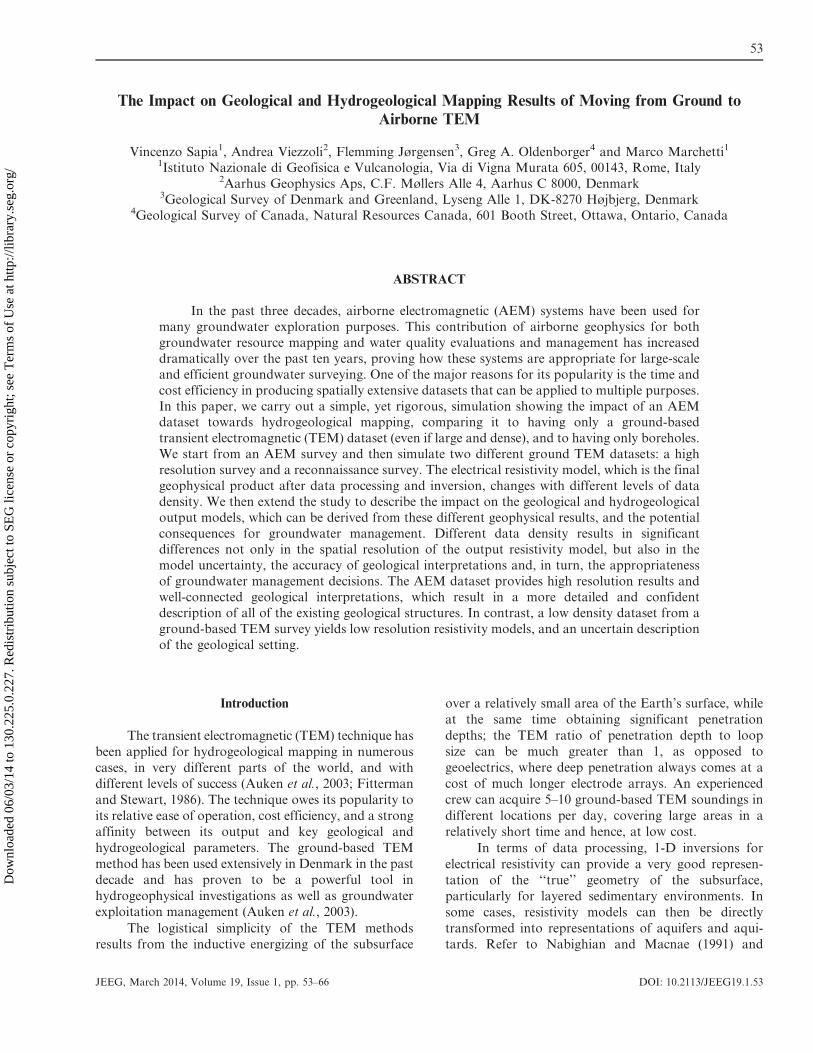
To simulate the ground TEM dataset, we start

from the AEM dataset. These data are then spatially

down-sampled to a uniform sounding density over the

entire survey block. We produced two versions of the

ground TEM survey. The high resolution survey has less

than 1 sounding/km2 and a total of 700 soundings

(Fig. 1(B)). The reconnaissance survey has ,0.1 sound-

ing/km2 and a total of 100 soundings (Fig. 1(C)). Recall

that the AEM survey provided approximately 100,000

soundings, and 100 soundings/km2.

The simulated ground TEM soundings were

obtained with an energizing moment of 250,000 Am2,

55

Sapia et al.: Moving from Ground to Airborne TEM Data

Dow

nloa

ded

06/0

3/14

to 1

30.2

25.0

.227

. Red

istr

ibut

ion

subj

ect t

o SE

G li

cens

e or

cop

yrig

ht; s

ee T

erm

s of

Use

at h

ttp://

libra

ry.s

eg.o

rg/

equal to that of the AeroTEM system. Given that a

standard ground TEM system outputs up to 10 Amps,

but more often less, a ground loop of greater than

100-m 3 100-m sides or multiple turns is required

to achieve this moment. To carry out both the high

resolution and reconnaissance ground-based TEM

surveys would be lengthy and logistically demanding.

We estimate that the high resolution survey (700 ground

soundings) would require no less than 15 weeks of

continuous acquisition for a crew with three operators

in conditions of clean paddocks and crop fields.

Similarly, the reconnaissance survey (100 soundings)

would require 3–5 weeks. Weather constraints, tempo-

rary limitations to site accessibility (e.g., because of

ground thawing or presence of crops) invariably add a

significant amount of time to complete the survey.

Another relevant, time consuming, and at times un-

surpassable obstacle to a ground survey aiming at

obtaining an even data density throughout the area are

the permits needed to access the station sites, even in

periods when no crops are on the fields. Beside dataacquisition, approximately 2–4 weeks would be needed

to carry out the detailed processing and inversion of the

data for hydrogeological applications.

Description of Processing and Inversion Methodology

For both ground-based and airborne EM data, the

aim of data processing is to prepare data for the

inversion. This includes data import, altitude correc-tions (for airborne only), and filtering and discarding of

distorted or noisy data contaminated by culture. Data

Figure 1. Spiritwood Valley Aquifer location map (adapted from Google Earth satellite image). The black box indicates

the survey area. A) Black dots indicate the 1,062 km2 HTEM survey block. B) Simulated high resolution ground TEM

survey. The AEM data have been averaged spatially using a trapezoid filter of 100 seconds resulting in approximately 1

sounding/km2. C) Simulated reconnaissance survey. 100 soundings were picked manually over the area to obtain a data

density of about 1 sounding every 3 km2.

56

Journal of Environmental and Engineering Geophysics

Dow

nloa

ded

06/0

3/14

to 1

30.2

25.0

.227

. Red

istr

ibut

ion

subj

ect t

o SE

G li

cens

e or

cop

yrig

ht; s

ee T

erm

s of

Use

at h

ttp://

libra

ry.s

eg.o

rg/

are then averaged spatially using trapezoid filters that

allow increasing signal-to-noise levels without compro-

mising lateral resolution. Inversions are carried out

using the quasi 3-D Spatially Constrained Inversion

(Viezzoli et al., 2008). Oldenborger et al. (2013)

presented a resistivity model for the Spiritwood area

using a conductive depth image (CDI) technique (Huang

and Rudd, 2008), and noted that the recovered

resistivity appeared to be underestimated and of reduced

range, with respect to ground electrical resistivity

tomography (ERT) measurements. Given the existing

differences between the induced currents into the ground

from the two methods (horizontal for EM and

vertical\horizontal for ERI/DC methods), as noted by

Keller and Frischknecht (1966) and Christensen (2000),

Oldenborger et al. (2013) attribute much of the reduced

range to the CDI algorithm, concluding that ‘‘discrim-

ination of aquifer material is hampered.’’

As opposed to the CDI, the SCI is a full non-linear

damped least-squares inversion based on exact forward

solution, in which the transfer function of the instru-

mentation is modeled. The system transfer function

includes transmitter current, turn-on and turn-off

ramps, gate times, low pass filters and system altitude.

The SCI is therefore expected to provide a better

agreement with the ERT than the CDI. In the SCI

scheme, the model parameters for different soundings

are tied together spatially with a partially dependent

covariance which is scaled according to distance.

Models are constrained spatially to reflect the lateral

homogeneity expected from the geology (either vertical

or horizontal layer resistivity, boundary thickness or

depth). Constraints include boundary conditions and

delimit changes of values within a defined deviation. The

flight altitude is included as an inversion parameter, but

with an a priori value and standard deviation assigned.

However, over very densely forested areas (which is not

the case for the Spiritwood area), canopy effects might

affect a proper altitude estimation of the frame. This

requires additional manual corrections of the altitude

data to avoid shallow artifacts in the output resistivity

model. The depth of investigation (DOI), based on an

analysis of the Jacobian matrix, was also calculated for

the output models. The DOI represents the maximum

depth at which there is sensitivity to the model

parameters (Christiansen et al., 2012). The inversions

are started with a homogeneous half space of 20 V-m.

Before data inversion, late time noise assessment was

performed to maximize resolution at depth and to

remove effects caused by the raw data leveling from

flight to flight. Despite primary field compensation and

leveling, self-system response is still observable for some

time gates (i.e., primary field bias). Therefore, we have

removed the first two time gates (with gate centers

earlier than 100 ms) and the last time gate from all

inversions. The inversion is parameterized with 29

layers, each having a fixed thickness, but a free

resistivity (with moderate vertical constraints). The

model was discretized to 200-m depth, with layers of

logarithmically increasing thickness.

We have treated the simulated ground TEM data

as if they really had been acquired with a ground TEM

system. They were processed for noise and coupling

individually (Fig. 2). No lateral averaging was carried

out. Even the leveling that is usually carried out on the

EM data as preprocessing by the AEM contractors

before they are delivered has insignificant effect over

kilometric distances between soundings.

The inversions were carried out with the same

forward and inversion algorithms used for the AEM

data, the only difference being that no spatial con-

straints were applied to the model parameters, as a

consequence of the significant distance between sound-

ings. The derived resistivity maps from the 1-D models

were then interpolated with a kriging algorithm applying

a search radius of 5,000 m and a node spacing of 100 m

for the simulated TEM survey.

Geophysical Results and Derived

Geological Interpretations

Before deriving geological interpretations from the

geophysical results and comparing the results between

those of the actual AEM survey and the simulated

ground TEM surveys, we elaborate further on the

representativeness of the simulated ground TEM data

of a true ground TEM survey in terms of depth of

investigation and lateral resolution. Arguably, while

having the same transmitter (Tx) moment, a ground

TEM system can obtain better signal-to-noise ratio

(even closer to, i.e., a power line) than an airborne

system. This is because of significantly greater stacking,

a smaller footprint, the absence of motion induced noise

in the receiver, and better coupling between the ground

and the Tx coil. On the contrary, dense sounding

spacing of the AEM data allows noise to be better

identified, particularly for galvanic coupling response

(Danielsen et al., 2003). One might argue that in the

simulated ground soundings the signal falls into noise

faster as compared to true ground TEM soundings.

However, in this particular case, this bears very little

influence, as the conductive bedrock (Cretaceous shale)

is shallow enough to be resolved by the simulated

soundings, and conductive and thick enough to make

any deeper layer irresolvable by virtually any TEM

system. This can be readily seen by comparing the

AeroTEM results to the VTEM data from coinciding

lines (Fig. 3). Despite its significantly better signal-to-

57

Sapia et al.: Moving from Ground to Airborne TEM Data

Dow

nloa

ded

06/0

3/14

to 1

30.2

25.0

.227

. Red

istr

ibut

ion

subj

ect t

o SE

G li

cens

e or

cop

yrig

ht; s

ee T

erm

s of

Use

at h

ttp://

libra

ry.s

eg.o

rg/

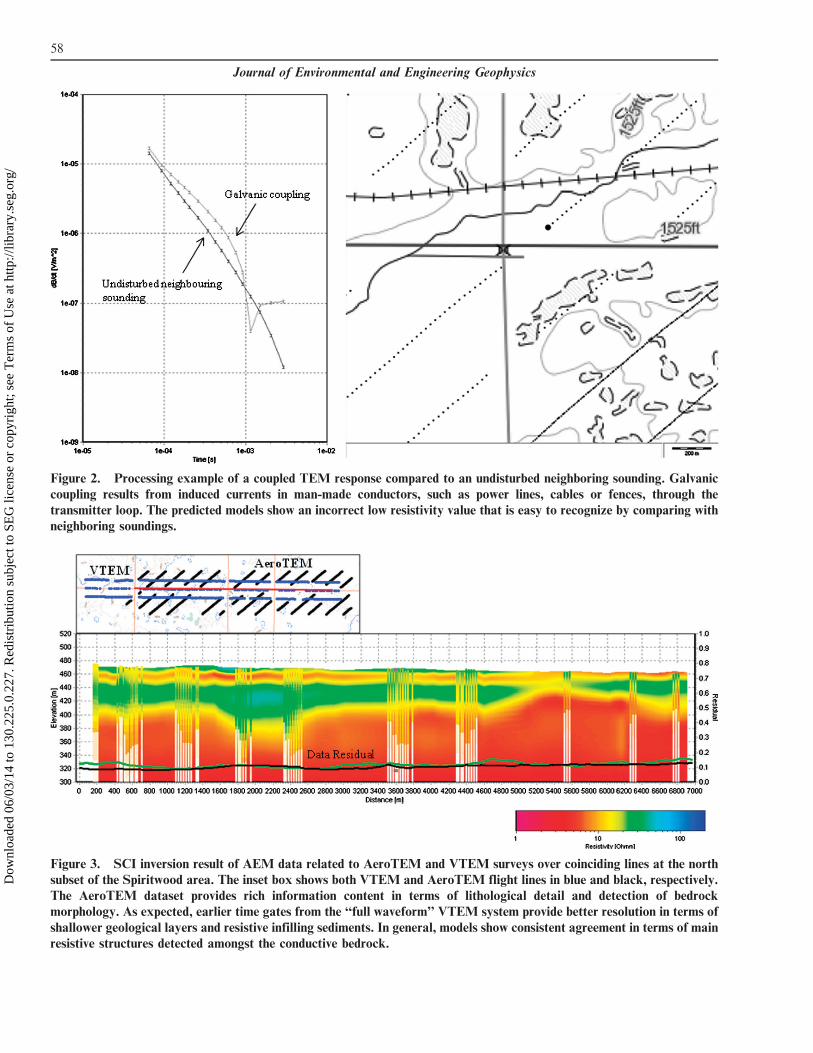
Figure 2. Processing example of a coupled TEM response compared to an undisturbed neighboring sounding. Galvanic

coupling results from induced currents in man-made conductors, such as power lines, cables or fences, through the

transmitter loop. The predicted models show an incorrect low resistivity value that is easy to recognize by comparing with

neighboring soundings.

Figure 3. SCI inversion result of AEM data related to AeroTEM and VTEM surveys over coinciding lines at the north

subset of the Spiritwood area. The inset box shows both VTEM and AeroTEM flight lines in blue and black, respectively.

The AeroTEM dataset provides rich information content in terms of lithological detail and detection of bedrock

morphology. As expected, earlier time gates from the ‘‘full waveform’’ VTEM system provide better resolution in terms of

shallower geological layers and resistive infilling sediments. In general, models show consistent agreement in terms of main

resistive structures detected amongst the conductive bedrock.

58

Journal of Environmental and Engineering Geophysics

Dow

nloa

ded

06/0

3/14

to 1

30.2

25.0

.227

. Red

istr

ibut

ion

subj

ect t

o SE

G li

cens

e or

cop

yrig

ht; s

ee T

erm

s of

Use

at h

ttp://

libra

ry.s

eg.o

rg/

noise ratio, the VTEM system does not penetrate below

the shale. The only exception to the argument above

could be in areas where tunnel valleys erode deep into the

shale where a ground TEM sounding might have reached

the shale in places where the simulated one does not.

On a sounding by sounding basis, the footprint of

the simulated soundings in the near surface is slightly

lower (i.e., higher lateral resolution) than that of an

actual 100-m 3 100-m loop. In the deeper parts of the

models, they are almost equivalent. It is worth noticing

also that, in general, ground-based soundings are less

affected by system bias (primary field not completely

removed) than airborne soundings. This is because of

the decreasing level of secondary signal resulting from

the vertical displacement of the Tx with respect to the

ground. Some AEM systems are more effective than

others in the removal of the primary field, with the

AeroTEM III deployed in the Spiritwood being one of

the worse. The simulated ground TEM survey might

therefore reveal less near-surface resolution than an

actual one. We contend that the individual simulated

TEM soundings are a good representation of actual

ones, especially in the context of deeper features, and

that the illustrative purpose of this paper remains

valid.

Average resistivity maps at different depth inter-

vals are produced to visualize the results of the inversion

of the different datasets (Fig. 4). Figure 5 shows the

average resistivity maps in a close up where particularly

interesting features are in focus. The average resistivity

maps in Fig. 4(B) clearly show the existence of a valley

as an elongate, resistive feature (known as the Spirit-

wood Valley Aquifer). It is approximately 10-km wide

and has a conductive background, which according to

boreholes consists of the Cretaceous shale bedrock.

Along the middle of this valley we observe a much more

narrow structure (1 km), interpreted to be an inset valley

that follows the main valley from the north to the south

(Fig. 4(C, D), left). In addition to the main incised

valleys, multiple valley-like features outside of the main

valley are observed (Fig. 6(B, C), left) (see also Old-

enborger et al., 2013). Some of the observed buried

valleys are very narrow and reveal a complex glacial

setting with many cross-cutting buried valleys of several

generations (Fig. 4(C), left and Fig. 5(C), left), which

are also documented in similar settings in Denmark

(Jørgensen and Sandersen, 2006).

In general, the electrical resistivities from the AEM

model are normally below 10 V-m for the Cretaceous

shale layers, between 20 and 30 V-m for clay till to silty/

sandy till, and above 40 V-m for sandy and gravely

layers. To obtain this range of values, a statistical

approach in the model space in addition to the observed

similarities with water well stratigraphy information

and, not shown here, direct comparison between

electrical resistivity tomography has been performed.

AEM spatially constrained inversion results reveal,

with good correlation of absolute values, the resistive

and conductive structures imaged by the ERT profile.

However, AeroTEM system limitations to resolve the

near-surface (early time data) make it difficult to

provide similar detail of the near surface. The depths

of the main buried valleys are recorded to exceed 100–

110 m, while most of the secondary valleys are between

40- and 80-m deep (Fig. 4(C, D) and Fig. 5(C, D)).

The resistive features attributable to sand and

gravel filling the main buried valleys are well defined in

the obtained resistivity models. However, inversion

results of the AEM dataset provide a high variability

of the resistivity values across the whole area (Fig. 4,

left). Therefore, it indicates that those resistive sedi-

ments, interpreted to be the response of sand and gravel,

fill the main valley as well as partially covering the two

inset valleys and the other small valleys. According to

resistivity maps, another resistive body is found in the

center of the survey area (Fig. 4(A), left). As noted by

Wiecek (2009), inter-till sands are found down to a

depth of approximately 30 m in this area, so the resistive

body could likely be corresponding to these sands

(Oldenborger et al., 2013).

In the following, we describe how a first approx-

imation of hydrogeological units can be derived directly

from the geophysical datasets with semi-automated

procedures. As an example, we can produce a map of

elevation of (or depth to) the shale, applying given

search criteria so as to query the model space. See for

example, on Fig. 6, where the solid line represents

the elevation of the bedrock (as a surface) obtained

searching through the resistivity model for a deep

conductor (resistivity , 15 V-m). In particular, a

statistical analysis of the relative frequency of model

values indicates a general bi-modal distribution. We

interpret the low resistivity peak (around 8–9 V-m) in

the histogram to be attributable to the shale bedrock,

and we use these parameters to guide the search criteria

to draw out this surface. It is obvious that similar

derived products, which are based on empirical corre-

lation of different parameters, are more robust the

greater the statistical population. Beyond that, applying

spatial constraints in the inversion over dense datasets,

like AEM, improve the lateral coherence of the

resistivity models, and hence of the derived products.

Figure 7 shows the surface of the resulting elevation of

the shale over the entire area for the AEM, the high

resolution and the reconnaissance survey. For reference,

we also present the shale elevation map derived from

water well data alone, which has required extensive

interpolation with a 3-km wide search radius (as the

59

Sapia et al.: Moving from Ground to Airborne TEM Data

Dow

nloa

ded

06/0

3/14

to 1

30.2

25.0

.227

. Red

istr

ibut

ion

subj

ect t

o SE

G li

cens

e or

cop

yrig

ht; s

ee T

erm

s of

Use

at h

ttp://

libra

ry.s

eg.o

rg/

same for the reconnaissance survey) since the boreholes

are not evenly spaced (Fig. 8).

In terms of water well data, the direct comparison

of water well data to TEM results is complicated by two

factors. Firstly, the water wells are not high-quality

geotechnical boreholes and the stratigraphic logs repre-

sent driller’s observations, which are subject to well-to-

well inconsistency and observational errors. Secondly,

provincial water well locations are reported on a

quarter-section basis such that the true well location is

not known and several wells from different locations

may be assigned to the center of the same quarter

section. In effect, the water well locations have an

uncertainty of approximately 6600 m in the case of the

Spiritwood. Figure 9 shows a profile along the longest

inset valley that includes all the water wells located

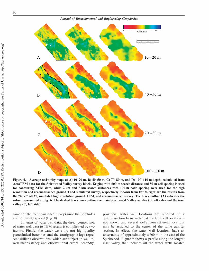
Figure 4. Average resistivity maps at A) 10–20 m, B) 40–50 m, C) 70–80 m, and D) 100–110 m depth, calculated fromAeroTEM data for the Spiritwood Valley survey block. Kriging with 600-m search distance and 50-m cell spacing is used

for contouring AEM data, while 2-km and 5-km search distances with 100-m node spacing were used for the high

resolution and reconnaissance ground TEM simulated survey, respectively. Shown from left to right are the results from

the ‘‘true’’ AEM, simulated high resolution ground TEM, and reconnaissance survey. The black outline (A) indicates the

subset represented in Fig. 6. The dashed black lines outline the main Spiritwood Valley aquifer (B, left side) and the inset

valley (C, left side).

60

Journal of Environmental and Engineering Geophysics

Dow

nloa

ded

06/0

3/14

to 1

30.2

25.0

.227

. Red

istr

ibut

ion

subj

ect t

o SE

G li

cens

e or

cop

yrig

ht; s

ee T

erm

s of

Use

at h

ttp://

libra

ry.s

eg.o

rg/

above the thalweg of the valley. Out of the eight wells

encountered, four wells indicate the presence of shale

bedrock where the AEM model suggests the presence of

a resistive body, interpreted to represent the infilling

materials of the buried valley. From a geological

perspective, we could assume that this bedrock contact

should be easily recognized because of the significant

lithological contrast (although this may not always be the

case for hard tills, fractured shale and water well logs that

are based on cutting observations and drill resistance).

Therefore, we attribute this discrepancy to the combina-

tion of low resolution of the water well locations and a

high degree of spatial heterogeneity associated with the

inset valley. As a consequence, even large-scale geological

structures like the main Spiritwood Valley are difficult to

map in detail using existing water wells alone. This also

implies the difficulty to compare well data with other

available geophysical data to generate a reliable geolog-

ical model. However, the well data seem generally to

agree with the geophysical data on a regional scale, for

example with regard to the presence of a sloping bedrock

towards the east, northeast and southeast (Fig. 8).

Compared to the full AEM survey, the results of

the simulated ground survey (both data density levels)

show much less detail in terms of structural geometry of

features; the clear network of secondary valley features

disappears completely (Fig. 4 and Fig. 7). For the

reconnaissance survey (Fig. 4, right side), we still

observe the bulk of the main Spiritwood Valley as a

resistive signature that crosses the entire area, but with

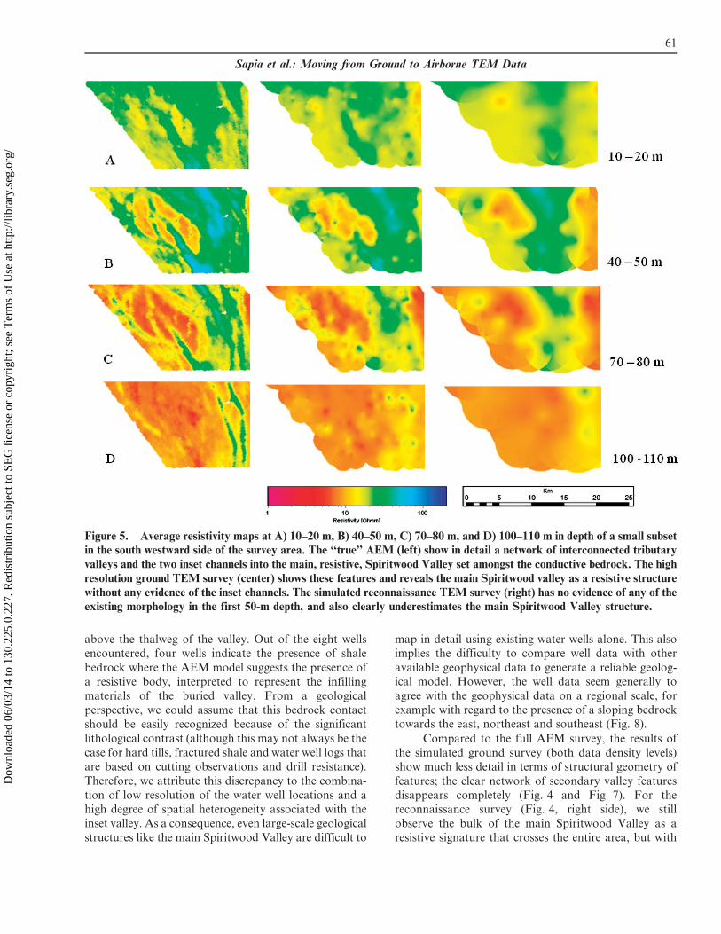
Figure 5. Average resistivity maps at A) 10–20 m, B) 40–50 m, C) 70–80 m, and D) 100–110 m in depth of a small subsetin the south westward side of the survey area. The ‘‘true’’ AEM (left) show in detail a network of interconnected tributary

valleys and the two inset channels into the main, resistive, Spiritwood Valley set amongst the conductive bedrock. The high

resolution ground TEM survey (center) shows these features and reveals the main Spiritwood valley as a resistive structure

without any evidence of the inset channels. The simulated reconnaissance TEM survey (right) has no evidence of any of the

existing morphology in the first 50-m depth, and also clearly underestimates the main Spiritwood Valley structure.

61

Sapia et al.: Moving from Ground to Airborne TEM Data

Dow

nloa

ded

06/0

3/14

to 1

30.2

25.0

.227

. Red

istr

ibut

ion

subj

ect t

o SE

G li

cens

e or

cop

yrig

ht; s

ee T

erm

s of

Use

at h

ttp://

libra

ry.s

eg.o

rg/

diffuse boundaries and uncertain total extent and

geometry. The same picture is seen in Fig. 7 in terms

of bedrock elevation, where the valley incision into the

bedrock gets very diffuse and difficult to follow for

the reconnaissance survey. The high resolution ground

survey (Fig. 4, central panels) provides a sharper image

than the reconnaissance survey of the long, resistive

middle feature, and also hints towards the presence of

possible secondary elements of the valley network.

The above observations are more evident in Fig. 5.

It is obvious, particularly for the reconnaissance survey,

that there is no evidence of the detailed valley network

filled with resistive materials. In the derived maps of the

elevation of the shale (Fig. 7), the difference in the

resolution of the valley network between the surveys is

even more pronounced than in the resistivity maps.

The near-surface inter-till area in the central part

of the area (Fig. 4(A)) is seen in all surveys, but its

appearance loses detail in the ground TEM surveys. The

overall scale of this geological structure is large enough

to be captured by the limited spacing of the TEM

soundings, but it appears that the scale length of

detailed features related to the structure is not rendered

adequately.

In general, the spatial variability of the resistive

sediments within the valleys, both large and small, as

well as within the inter-till formation, is captured by the

true AEM survey, but much less by the ground surveys.

Figure 6. Example of an AEM flight line SCI inversion result. We interpret the high resistivity range to be attributable

to the valley fill materials (till, sand and gravel), and the low resistivity peak to be attributable to the conductive shale

bedrock. The black solid line represents the obtained elevation for the conductive shale bedrock.

Figure 7. Maps represent the derived elevation surfaces of the bedrock (conductive shale) from AEM results (left), and

the two simulated ground TEM surveys (high resolution in the center and reconnaissance survey on the right).

62

Journal of Environmental and Engineering Geophysics

Dow

nloa

ded

06/0

3/14

to 1

30.2

25.0

.227

. Red

istr

ibut

ion

subj

ect t

o SE

G li

cens

e or

cop

yrig

ht; s

ee T

erm

s of

Use

at h

ttp://

libra

ry.s

eg.o

rg/

A very high data density is required for delineating the

detail in the inter-till formation and to outline and

orientation of the buried valleys in complicated systems

like the Spiritwood Valley. It is difficult to establish the

connection between individual buried valleys if the only

geophysical contribution comes from sparse ground

TEM measurements.

Discussion on the Implications for Hydrogeological

Interpretations and Management

As mentioned above, the ground TEM surveys

would take approximately 3–5 months and 1–2 months,

for the high resolution and the reconnaissance survey,

respectively. Even though such difference in time will be

reflected in the costing, we estimate the cost of such

undertakings to be on the order of a hundred thousand

dollars (USD). In comparison, the AEM survey took

approximately four weeks to acquire, and a couple of

months for accurate re-processing and inversions, with

a total investment estimated at 2 to 3 times higher than

the simulated ground-based surveys. However, the unit

cost of one sounding drops two orders of magnitude

from the ground surveys (a few hundred USD/sounding)

to the airborne survey (few USD/sounding). In our

opinion, the extra bulk budgetary investment required

for an AEM survey should be given serious consider-

ation, given the added value in large-scale groundwater

programs.

In general terms, we will discuss the issue of

general hydrogeological mapping of aquifer geometry,

aquifer vulnerability, and flow models for sustainable

development of groundwater resources.

As demonstrated, AEM provides high resolution

results and detailed geological interpretations, which

result in a more connected (and hopefully more accurate)

description of the entire set of existing structures. On the

contrary, a low density dataset based on ground TEM

surveys (i.e., reconnaissance survey) results in a low

resolution resistivity model and a less detailed and

disconnected description of the geological setting; small-

scale but potentially important structures are lost and

these omissions can propagate into hydrogeological

models. For example, bedrock elevation or aquitard

elevation is often an important starting point for a variety

of hydrogeological investigations such as groundwater

modeling or siting exploitation drilling. However, the

elevation maps of the conductive bedrock derived from

insufficient data would result in an incorrect contribution

to this crucial part of the hydrogeological understanding

(compare Fig. 7(C) with 7(A)).

In a hydrogeological context like this, where

potential aquifers appear to be relatively small and

complex, the most relevant implication for groundwater

resource mapping and management is the ability to

resolve the aquifer geometry. If we only consider a

ground TEM result, e.g., the reconnaissance survey, any

mapping of aquifers is almost impossible because of the

low density of collected data. Most of the deep aquifer

targets in the area are situated within relatively small

valley structures and, without the detailed AEM data,

these aquifers are very difficult to map and target for

drilling. Given only the ground-based surveys, drill

targets for finding high potential aquifers would be

sporadic along the long inset valley (Fig. 4(C), middle

and right), but the uncertainty related to putting the

boreholes at most optimized locations is high. Estab-

lishing locations for new groundwater exploration

drillings or well fields is much safer with the maps

generated from the AEM data at hand, i.e., location

of a lot of small aquifers are indicated by the scattered

resistive bodies within the valley structures, and op-

timized positions for drilling can be determined by

locating the exact position of the valley thalwegs from

the shale elevation map (Fig. 7(A)). This is an important

aspect since the presence of resistive material enhances

permeability into the valleys and may result in a

potential groundwater reservoir. Despite the obvious

advantage in using AEM for mapping groundwater

resources at high resolution, it must also be pointed that

ground TEM data alone did produce results that

allowed better hydrogeological mapping than the one

based solely on boreholes.

Figure 8. Shale elevation surface derived from waterwell information. The low density of wells results in a

limited estimation of the bedrock topography.

63

Sapia et al.: Moving from Ground to Airborne TEM Data

Dow

nloa

ded

06/0

3/14

to 1

30.2

25.0

.227

. Red

istr

ibut

ion

subj

ect t

o SE

G li

cens

e or

cop

yrig

ht; s

ee T

erm

s of

Use

at h

ttp://

libra

ry.s

eg.o

rg/

According to the AEM data, the valley aquifers

are often covered by clayey to silty\sandy sediments (i.e.,

till) giving them some kind of natural protection against

pollution from the surface. However, where the valleys

are cut by younger valleys filled by sandy material they

can be exposed and vulnerable. Thus, vulnerability

assessments of important deep aquifers in the area

would also be much harder and complicated to perform

solely based on the ground-based surveys. In the area

where extensive inter till sands are interpreted to cover

the deeper setting including aquifer-hosting valleys, a

detailed knowledge of the spatial extension and internal

composition of this sand formation is important. Like

the buried-valley geology, this formation is much better

resolved by the true AEM survey than by the ground

survey.

Glaciated areas are typically complex, and detailed

information and models are essential if the goal is to

predict groundwater pathways to well fields based on

flow modeling (Troldborg et al., 2008; Troldborg et al.,

2007). Especially with the presence of buried-valley

geology, such predictions are challenging and require

high resolution models, where the individual valleys

must be resolved (Shaver and Pusc, 1992; Jørgensen

et al., 2008; Andersen et al., in press). Groundwater

flow will tend to follow the often coarse-grained

sediments in the valleys, but in cases where clay-filled

valleys cut such pathways they can constitute effective

barriers. Therefore, the groundwater flow in the

Spiritwood area is intricately connected to the existing

geometry of the valley aquifer. The true AEM survey

maps the valley network in detail, whereas the ground-

based survey does not. Thus, a flow model based solely

on the true AEM survey would be able to produce

useful results for groundwater management, i.e., cat-

chment area calculation.

Given the effective mapping of aquifer location

and potential for detailed groundwater flow prediction,

a true AEM survey can identify virgin aquifers to be

exploited as local resources of fresh water. In addition,

an accurate, wide area, high resolution model obtained

from AEM can assist the managing body with identifying

and assessing issues linked to the varying quality of

ancillary information. For example, it can serve as a base

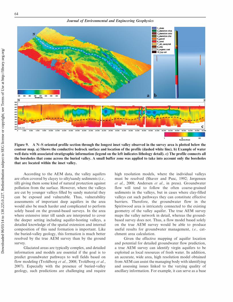
Figure 9. A N–S oriented profile section through the longest inset valley observed in the survey area is plotted below the

contour map. a) Shows the conductive bedrock surface and location of the profile (dashed white line). b) Example of water

well data with associated stratigraphic information (legend on the left indicates lithology detail). c) The profile connects all

the boreholes that come across the buried valley. A small buffer zone was applied to take into account only the boreholes

that are located within the inset valley.

64

Journal of Environmental and Engineering Geophysics

Dow

nloa

ded

06/0

3/14

to 1

30.2

25.0

.227

. Red

istr

ibut

ion

subj

ect t

o SE

G li

cens

e or

cop

yrig

ht; s

ee T

erm

s of

Use

at h

ttp://

libra

ry.s

eg.o

rg/

to screen for inconsistencies in existing databases, e.g.,

borehole stratigraphy.

Complementary AEM and Ground-based TEM Surveys

AEM and ground-based TEM can serve a comple-

mentary role in a hydrogeophysics survey. Ground TEM

can probably provide greater depth of investigation in

areas where the AEM might fail to reach the target.

Perhaps an even more important contribution would be

to deploy a calibrated ground-based TEM system tocheck and post-calibrate, if necessary and possible, the

AEM dataset. Provided a ground TEM system had been

calibrated, as was done by Foged et al. (2013) over the

Danish national test site of Lyngby, then it could be used

to acquire data over diverse locations within the AEM

survey area to provide a series of local 1-D resistivity

reference models for comparison with the AEM data and

derived models. If necessary, the reference models couldbe used to re-calibrate the AEM data.

Conclusions

In this paper, we describe the shortcomings in

hydrogeological interpretation and management that

could arise if a ground TEM survey is used rather than

an AEM survey. Output resistivity models from ground-

based TEM data reveal how the mapping of hydro-

geological features of great relevance, such as buried

valleys as well as minor valley networks, could beinaccurate and poorly detailed in terms of structures

morphology. Furthermore, derived products of high

density AEM inversion results, i.e., elevation of

bedrock, can be readily integrated and compared with

other available data, either geophysical or geological.

Integrated with ancillary information, AEM pro-vides rapid and cost effective robust results in terms of

aquifer geometry and vulnerability mapping. It also

provides a solid basis for subsequent flow modeling.

Acknowledgments

The Spiritwood Valley AEM dataset is made freely

available by the Geological Survey of Canada. We are greatful

to H. Russell, D. Sharpe, A. Pugin, M. Hinton and H. Crow

for helpful discussions about the geological setting of the study

area. C. Logan is thanked for providing the water well records.

We are greatly thankful to I-GIS for their important support

and training on the use of the Geoscene 3D software.

References

Abraham, J.D., Cannia, J.C., Bedrosian, P.A., Johnson, M.R.,

Ball, L.B., and Sibray, S.S., 2012, Airborne electromagnetic

mapping of the base of aquifer in areas of western

Nebraska: USGS, North Platte Natural Resources District,

the South Platte Natural Resources District, and the

Nebraska Environmental Trust Scientific Investigations

Report 2011-5219.

Allard, M., 2007, On the origin of the HTEM species: in

Proceedings: Fifth Decennial International Conference

on Mineral Exploration, 355–374.

Andersen, T.S., Poulsen, S.E., Christensen, S., and Jørgensen,

F., 2013, A synthetic study of geophysics-based model-

ling of groundwater flow in catchments with a buried

valley: Hydrogeological Journal. in press.

Andriashek, L.D., 2003, Quaternary geological setting of the

Athabasca Oil Sands (in situ) area, northeast Alberta:

Alberta Energy and Utilities Board/Alberta Geological

Survey, Earth Sciences report 2002–2003.

Auken, E., Jørgensen, F., and Sørensen, K.I., 2003, Large-

scale TEM investigation for groundwater: Exploration

Geophysics, 33, 188–194.

Balch, S.J., Boyko, W.P., and Paterson, N.R., 2003, The

AeroTEM airborne electromagnetic system: The Lead-

ing Edge, 22, 562–566.

Betcher, R.N., Matille, G., and Keller, G., 2005, Yes Virginia,

there are buried valley aquifers in Manitoba: in

Proceedings: 58th Canadian Geotechnical Conference,

6E–519.

Cannia, J.C., Abraham, J.D., and Peterson, S.M., 2012, Using

geophysical data to improve an optimization ground-

water model evaluating the effectiveness of intentional

recharge in the North Platte River Valley, western

Nebraska, USA: in Symposium of Water: Science,

Practice and Policy, Lincoln, Nebraska, U.S.A.

Christensen, N.B., 2000, Difficulties in determining electrical

anisotropy in subsurface investigations: Geophysical

Prospecting, 48, 1–19.

Christiansen, A.V., Auken, E., and Sørensen, K., 2009, The

transient electromagnetic method: in Groundwater Geo-

physics (2nd ed.): Springer Berlin Heidelberg (publisher),

179–226.

Christiansen, A.V., and Auken, E., 2012, A global measure for

depth of investigation: Geophysics, 77, 171–177.

Crow, H.L., Knight, R.D., Medioli, B.E., Hinton, M.J.,

Plourde, A., Pugin, A.J.-M., Brewer, K.D., Russell,

H.A.J., and Sharpe, D.R., 2012, Geological, hydro-

geological, geophysical, and geochemistry data from a

cored borehole in the Spiritwood buried valley, south-

west Manitoba: Geological Survey of Canada, Open

File 7079.

Cummings, D.I., Russell, H.A.J., and Sharpe, D., 2012,

Buried-valleys in the Canadian Prairies: Geology,

hydrogeology, and origin: Canadian Journal of Earth

Sciences, 49, 987–1004.

Danielsen, J.E., Auken, E., Jørgensen, F., Søndergaard, V.H.,

and Sørensen, K.I., 2003, The application of the

transient electromagnetic method in hydrogeophysical

surveys: Journal of Applied Geophysics, 53, 181–198.

Fitterman, D.V., and Stewart, M.T., 1986, Transient electro-

magnetic sounding for groundwater: Geophysics, 51,

995–1005.

65

Sapia et al.: Moving from Ground to Airborne TEM Data

Dow

nloa

ded

06/0

3/14

to 1

30.2

25.0

.227

. Red

istr

ibut

ion

subj

ect t

o SE

G li

cens

e or

cop

yrig

ht; s

ee T

erm

s of

Use

at h

ttp://

libra

ry.s

eg.o

rg/

Fitzpatrick, A., and Munday, T., 2007, The application of

airborne geophysical data as a means of better

understanding the efficacy of disposal basins along the

Murray River: An example from Stockyard Plains,

South Australia: in Extended Abstracts: ASEG, 2007.

Foged, N., Auken, E., Christiansen, A.V., and Sørensen, K.I.,

2013, Test site calibration and validation of airborne and

ground based TEM-systems: Geophysics, 78, 95–106.

Fountain, D., 2008, 60 years of airborne EM - Focus on the

last decade: in Proceedings: 5th International Confer-

ence on Airborne Electromagnetics, Haikko Manor,

Finland.

Huang, H., and Rudd, J., 2008, Conductivity-depth imaging of

helicopter-borne TEM data based on a pseudolayer

half-space model: Geophysics, 73, 115–120.

Jørgensen, F., Sandersen, Peter B.E., and Auken, E., 2003,

Imaging buried Quaternary valleys using the transient

electromagnetic method: Journal of Applied Geophys-

ics, 53, 199–213.

Jørgensen, F., and Sandersen, P.B.E., 2006, Buried and open

tunnel valleys in Denmark—Erosion beneath multiple

ice sheets: Quaternary Science Reviews, 25, 1339–1363.

Jørgensen, F., Damgaard, J., and Olesen, H., 2008, Impact of

geological modelling on groundwater models—A case

study from an area with distributed, isolated aquifers,

in Calibration and reliability in groundwater modeling,

Refsgaard, J.C., Kovar, K., Haarder, E., and Nygaard,

E.. (eds.), IAHS Publication, Wallingford, (Int. Assoc.

Hydrol. Sci.) 320, 337–344.

Kehew, A.E., and Boettger, W.M., 1986, Depositional

environments of buried-valley aquifers in North Dako-

ta: Ground Water, 24, 728–734.

Keller, G.V., and Frischknecht, F.C., 1966. Electrical methods

in geophysical prospecting: Pergamon Press, Inc.

Kirkegaard, C., Sonnenborg, T., Auken, E., and Jørgensen, F.,

2011, Salinity distribution in heterogeneous coastal

aquifers mapped by airborne electromagnetic: Vadose

Zone Journal, 10, 125–135.

Legault, J.M., Prikhodko, A., Dodds, D.J., Macnae, J.C., and

Oldenborger, G.A., 2012, Results of recent VTEM

helicopter system development testing over the Spirit-

wood Valley aquifer, Manitoba: in Expanded Abstracts:

25th Symposium on the Application of Geophysics to

Engineering and Environmental Problems, 17 pp.

Møller, I., Søndergaard, V.H., Jørgensen, F., Auken, E., and

Christiansen, A.V., 2009, Integrated management and

utilization of hydrogeophysical data on a national scale:

Near Surface Geophysics, 7, 647–659.

Nabighian, M.N., and Macnae, J.C., 1991, Time domain

electromagnetic prospecting methods: in Electromagnet-

ic methods in applied geophysics, Nabighian, M.N.

(ed.), Society of Exploration Geophysicists.

Oldenborger, G.A., 2010a, AeroTEM III Survey, Spiritwood

Valley, Manitoba, parts of NTS 62G/3, 62G/4, Mani-

toba: in Geological Survey of Canada: Open File 6663.

Oldenborger, G.A., 2010b, AeroTEM III Survey, Spiritwood

Valley, Manitoba, parts of NTS 62G/3, 62G/4, 62G/5,

62G/6, Manitoba: in Geological Survey of Canada,

Open File 6664.

Oldenborger, G.A., Pugin, A.J.-M., and Pullan, S.E., 2013,

Airborne time-domain electromagnetics, electrical resis-

tivity and seismic reflection for regional three-dimen-

sional mapping and characterization of the Spiritwood

Valley Aquifer, Manitoba, Canada: Near Surface

Geophysics, 11, 63–74.

Paine, J.G., and Minty, B.R.S., 2005, Airborne hydrogeophy-

sics: Hydrogeophysics, 50, 333–357.

Pugin, A.J.-M., Pullan, S.E., Hunter, J.A., and Oldenborger,

G.A., 2009, Hydrogeological prospecting using P- and

S-wave landstreamer seismic reflection methods: Near

Surface Geophysics, 7, 315–327.

Randich, P.G., and Kuzniar, R.L., 1984, Geology of Towner

County, North Dakota: North Dakota State Water

Commission, County Groundwater Studies, 36, Part III.

Russell, H.A.J., Hinton, M.J., van der Kamp, G., and Sharpe,

D., 2004, An overview of the architecture, sedimentol-

ogy and hydrogeology of buried-valley aquifers in

Canada: in Proceedings: 57th Canadian Geotechnical

Conference, 26–33.

Sattel, D., 2009, An overview of helicopter time-domain EM

systems: in Extended Abstracts: ASEG, 2009.

Sattel, D., and Kgotlhang, L., 2004, Groundwater exploration

with AEM in the Boteti area, Botswana: Exploration

Geophysics, 35(2), 147–156.

Shaver, R.B., and Pusc, S.W., 1992, Hydraulic Barriers in

Pleistocene Buried-Valley Aquifers: Ground Water,

30(1), 21–28.

Thomson, S., Fountain, D., and Watts, T., 2007, Airborne

geophysics—Evolution and revolution: in Proceedings

of Exploration 07: Fifth Decennial International Con-

ference on Mineral Exploration, 19–37.

Troldborg, L., Refsgaard, J., Jensen, K., and Engesgaard, P.,

2007, The importance of alternative conceptual models

for simulation of concentrations in multi-aquifer system:

Hydrogeology Journal, 15, 843–860.

Troldborg, L., Jensen, K., Engesgaard, P., Refsgaard, J., and

Hinsby, K., 2008, Using environmental tracers in

modeling flow in a complex shallow aquifer system:

Journal of Hydrologic Engineering, 12(11), 1037–1048.

Viezzoli, A., Christiansen, A.V., Auken, E., and Sørensen, K.,

2008, Quasi-3D modeling of airborne TEM data by

spatially constrained inversion: Geophysics, 73, 105–113.

Walker, S., and Rudd, J., 2008, Airborne resistivity mapping

with helicopter TEM: An oil sands case study: in

Proceedings: 5th International Conference on Airborne

Electromagnetics, 06–03.

Wiecek, S., 2009. Municipality of Killarney, Turtle Mountain

groundwater assessment study: W.L. Gibbons & Asso-

ciates Inc.

Wynn, J., 2002, Evaluating groundwater in arid lands using

airborne magnetic/EM methods. An example in the

southwestern U.S. and northern Mexico: The Leading

Edge, 21, 62–64.

66

Journal of Environmental and Engineering Geophysics

Dow

nloa

ded

06/0

3/14

to 1

30.2

25.0

.227

. Red

istr

ibut

ion

subj

ect t

o SE

G li

cens

e or

cop

yrig

ht; s

ee T

erm

s of

Use

at h

ttp://

libra

ry.s

eg.o

rg/