The Impact of Welfare Reform and State Budgets on State-Level

1

Wesleyan University The Honors College

The Impact of Welfare Reform and State Budgets on State-Level Poverty and Inequality Measures

by

William Benjamin Monson

Class of 2011

A thesis submitted to the faculty of Wesleyan University

in partial fulfillment of the requirements for the Degree of Bachelor of Arts

with Departmental Honors in Economics

Middletown, Connecticut April, 2011

2

Table of Contents

Abstract……………………………………………………………………………………………..pg. 5 I. Introduction………………………………………………………………………………....pg. 6 II. Literature Review and Theory…………………………………………………….…pg. 9 a. Background…………………………………………………………………….....pg. 9 b. Individual Effect………………………………………………………………....pg. 15 c. Effect on Poverty Levels………………………………..………………….…pg. 21 d. Fiscal Federalism Literature…………………………………...…………..pg. 23 e. The Medicaid Story………………………………………………...………..…pg. 31 f. Earned Income Tax Credit and Food Stamp Program………......pg. 36 g. Hypothesis…………………………………………………………………………pg. 37 III. Data and Methods………………………………………………………...……………….pg. 38 a. Model and Explanation of Data…………………………………………...pg. 38 b. Methods………………………………………………………………………….…pg. 51 c. Econometric Problems…………………………………………………….…pg. 56 IV. Results and Discussion………………………………………………………………….pg. 59 a. Percentile Threshold (Absolute Measures of Well-Being)…….pg. 59 b. Discussion of Percentile Threshold Measures……………………...pg. 69 c. Inequality Ratios (Relative Measures of Well-Being)…………....pg. 77 d. Discussion of Percentile Inequality Ratios…………………………...pg. 85 e. Robustness Checks……………………………………………………………..pg. 89 f. Future Work…………………………………………………………………….pg. 101 V. Conclusion……………………………………………………………………………...…..pg. 104 Bibliography………………………………………………………………………………….…pg. 106

3

Figures and Tables

• Figure 1: U.S. Welfare Caseload and Expenditure Levels Over Time…………………………………………………………………………………...pg. 16 • Figure 2: State Expenditures of Cash Assistance Under Different Grant Types………………………………………….……………….……...pg. 26 • Figure 3: Federal Medicaid Grants (Real Thousands of Dollars), 1961-2009…………………………………………………………………..…pg. 32 • Figure 4: Impact of EITC Expansion at Various Income Levels…….….pg. 49 • Table 1: Estimated Impacts on the 10th Percentile Income Threshold………………………………………………………………………………….…pg. 59 • Table 2: Correlation Matrix of 10th Percentile Regression Variables……………………………………………………………………………………..pg. 63 • Table 3: Estimated Impacts on the 20th Percentile Income Threshold……………………………………………………………………………………pg. 65 • Table 4: Estimated Impacts on the 30th Percentile Income Threshold………………………………………………………………………………….…pg. 67 • Table 5: Joint Impact of TANF at 10th Percentile and P-Values………...pg. 71 • Figure 5: EITC Maximum Benefit Increase (In Dollars)……………….…..pg. 76 • Table 6: Estimated Impact on the 90/10 Inequality Ratio……………....pg. 79 • Table 7: Estimated Impact on the 90/20 Inequality Ratio……………….pg. 82 • Table 8: Estimated Impact on the 90/30 Inequality Ratio……………....pg. 84 • Table 9: Regression Results Using Robust Standard Errors……………..pg. 90 • Table 10: Regression Results Using Log of Inequality Ratios………………………………………………………………………..…pg. 94 • Table 11: Regression Results with Waiver Dummy Variable………..….pg. 95 • Table 12: Regression Results with Medicaid Expenditures/Population…………………………………………………………..….pg. 97 • Table 13: Poverty Percentage as Dependent Variable…………………..pg. 100

4

Acknowledgements

First and foremost, I would like to thank Professor Wendy Rayack for her wisdom and guidance throughout this project. I have learned so much from working with her throughout my time at Wesleyan and I am very grateful for the opportunities that she has given me. I’d like to thank Manolis and his Stata boot camp for aspiring wizards, as well as Kevin for his research help. I am also appreciative for the support and love of my parents and brother, as well as their editorial input on my work over the years. Lastly, many thanks to Liz and my housemates- Brenna, Brian, Gabe, and Matt for being awesome and making my time outside of the thesis carrel so much fun.

5

Abstract This study investigates the relationship between the implementation of TANF and two measures of well-being, absolute and relative well-being, and how welfare reform altered the vulnerability of these measures of well-being to fluctuations in the business cycle. I find that while TANF significantly improves absolute well-being during periods of low unemployment, it significantly worsens absolute well-being when the unemployment rate is high. In addition, the sensitivity to the unemployment rate increased significantly as a result of TANF, causing more vulnerability to downturns for all three low-income percentiles. The impact of TANF on the relative measure of well-being, ratios of inequality, showed an estimated increase in inequality, indicating a fall in relative well-being. However, these results are not stable or significant across all robustness checks.

6

I. Introduction My thesis looks at fluctuations in measures of well-being from 1977 to 2004 and examines how the implementation of the 1996 welfare reform affected these measures over the course of several business cycles. I evaluate two indicators of well-being in this research, an absolute measure and a relative measure. The absolute measure uses income thresholds associated with specific percentiles of the income distribution. These income thresholds indicate the income level below which a family would be categorized in a particular income percentile in a given state and year. In this paper, I explore the impact of Temporary Aid for Needy Families (TANF), the new welfare program created after welfare reform, at the 10th, 20th, and 30th income percentiles. The relative measure of well-being uses the ratio of the 90th percentile income threshold to each of the low-income percentile thresholds. This metric shows how much high and low incomes diverge during recessions. In this case, an increase in the inequality ratio would signal a drop in relative well-being. These measures of well-being naturally fluctuate with the business cycle, rising during boom periods, and falling during recessions. I hypothesize that as a result of welfare reform, these fluctuations have been accentuated, resulting in low-income individuals being more vulnerable to drops in well-being in recessions. The theory behind this hypothesis is that the Personal Responsibility and Work Opportunity Act (PRWORA) legislation that initiated welfare reform fundamentally changed the incentive for state funding of cash assistance

7

programs. In addition, the stricter policies in the TANF legislation forced many recipients off of welfare roles. As a result, low-income populations who typically rely on welfare during downturns in the business cycle had a diminished safety net to fall back on, resulting in larger drops in well-being. In addition, there were many concurrent policy changes occurring in the 1990s that play a role in this study. The expansion of the Earned Income Tax Credit (EITC) program to supply more working-poor families with additional benefits certainly had an impact on changes in well-being. States further expanded benefits to the working poor by creating state EITC programs of their own. The enormous growth of the Medicaid program affected state finances as well, potentially crowding out legislators’ ability to pay for other state programs such as cash assistance. My thesis also explores various robustness checks to determine the strength of the estimated impact from TANF. I also explore alternative independent variables and the impact on an alternative measure of well-being, state poverty percentages. In summary, my regression estimates yield the following observations: • During periods of extremely low unemployment, TANF significantly improves absolute well-being for the three low-income percentiles. • During periods of high unemployment, TANF significantly worsens absolute well-being for the three low-income percentiles. • The sensitivity to the unemployment rate increased significantly as a result of TANF, causing significantly more vulnerability to downturns for

8

all three low-income percentiles. • The results listed above were stable according to robustness checks. • The impact of TANF on the ratios of inequality showed an estimated increase in inequality, indicating a fall in relative well-being. However, these results are not stable or significant across all robustness checks. • Using state poverty percentages for the dependent variable does not show significant regression estimates for the impact of TANF on this measure of well-being The rest of this thesis is organized as follows. Chapter one goes through the prior literature and explains the theory within the context of this existing framework. Chapter two discusses the composition and origin of the variables used in the regression equation. It then presents the model used in my estimation and the various techniques utilized in this study. Chapter three walks through the results for both the absolute and relative well-being measures and provides discussion analyzing the estimated coefficients. I also include a section for robustness checks and alternative variables to use in the model.

9

II. Literature Review and Theory

Background: The original welfare program, Aid to Families with Dependent Children (AFDC), originated in the New Deal era as a means to support children who had lost the support of a working parent. Essentially the program was designed to provide a pension to mothers when their husband died. At that time, very few women worked in the labor market and funding from AFDC allowed single mothers to stay at home and care for their children. The federal government financed the program through matching grants to states, but it was up to the states to decide how much to grant to AFDC recipients, as well as who was eligible. As a result, differences in the state programs varied far more than cost-of-living expenses could account for, with some states such as Alaska granting $923 in monthly benefits while others such as Mississippi granting a mere $120 a month by AFDC’s demise in 1996 (Committee on Ways and Means, 2000). Furthermore, AFDC had a 100 percent tax rate on earned income, meaning that welfare benefits were removed when earned income rose on a dollar-for-dollar basis. While this policy would seem to be a clear disincentive to work, it is important to remember that the program was not initially designed to promote work, merely to support disadvantaged widows (Grogger and Karoly, 2005). It was not until the 1960s and 70s that a change in culture prompted a rebellion against the structure of such a welfare program.

10

During this time period, the majority of welfare recipients shifted from widows to divorced or never-married mothers. As a result, the public perception of AFDC changed from a program that served justifiably needy widows to one that rewarded lazy, undeserving mothers who were tearing apart the moral fiber of society. The program that was once thought of as a solution to social problems was now discredited as a catalyst to these problems. In response, there were numerous initiatives to improve AFDC by introducing various incentives to curb the growing population of single mothers. Some initiatives, such as the 1967 amendments to the Social Security Act, emphasized a “carrot” approach by lowering the benefit reduction rate for AFDC. Other efforts, like the JOBS program in 1988, utilized a “stick” tactic by imposing sanctions on individuals who did not meet new work requirements. However, these various efforts had a limited effect on the growth in caseload numbers. Frustrated by the lack of progress on the national level, many state legislators took it upon themselves to reform welfare by petitioning the Department of Health and Human Services for permission to change aspects of AFDC in their own state. Using these welfare waivers, states expanded on previous reform attempts by targeting specific policies that they felt were particularly effective, or not stringent enough. In the period before the PRWORA legislation in 1996, states enacted waiver-based reforms that targeted the earned income disregard, age-related exemptions for the JOBS program, severity of sanctions for failing to participate in the JOBS program, time limits on receipt of welfare payments, and caps on increases in benefits for an increase in the

11

welfare recipient’s family size. By the time of the PRWORA reforms, 37 states had approved at least one of these waivers, although not all of the states had implemented the new policies before the new welfare law was passed (Crouse, 1999). The PRWORA legislation drew on this existing resentment of AFDC by promising to end handouts to undeserving recipients and to move people off of welfare roles and into the workforce. The intentions of the new law were made clear in the bill’s introduction: “The purpose of this part is to increase the flexibility of States in operating a program designed to— (1) provide assistance to needy families so that children may be cared for in their own homes or in the homes of relatives; (2) end the dependence of needy parents on government benefits by promoting job preparation, work, and marriage; (3) prevent and reduce the incidence of out-of-wedlock pregnancies and establish annual numerical goals for preventing and reducing the incidence of these pregnancies; and (4) encourage the formation and maintenance of two-parent families.” (PL 104-193) While one of the tenets of the bill promises to provide economic assistance to families in need, the main focus of the bill was to end the social problems of welfare dependency and the demise of marriage, which politicians thought were exacerbated under AFDC. Under the new welfare program, Temporary Assistance for Needy Families (TANF), families were no longer entitled to unfettered cash assistance from the government. While destitute families would still receive welfare payments, it was contingent on several requirements designed to promote personal responsibility. TANF differs from

12

AFDC in three major ways. First, federal assistance is no longer indefinite but has a lifetime limit of 60 months, and assistance is only granted if the parent takes action to seek employment while receiving payments. Second, TANF mandates that at least half of a state’s welfare caseload must be actually working or in a work-related activity. In order to qualify, a recipient must be engaged in this activity for at least 30 hours a week. This provision is similar to the requirements under AFDC’s JOBS program, except that it has a much narrower set of exemptions and requires more work effort on the part of the recipient. The third and most important difference is that funds for cash assistance are no longer transferred to states via a matching grant, but rather through a block grant, which gives states an annual lump sum of money equal to an individual state’s 1994 AFDC grant. Legislators reasoned that a block grant would provide states with a financial incentive to decrease their welfare caseloads. Under AFDC, states received more federal funding for each additional family on welfare, and less money for each family that leaves welfare, creating a perverse financial incentive for states to increase their welfare roles. Under a block grant, there is no additional financial incentive for raising the number of caseloads. Therefore, legislators thought that block grants would provide an incentive to lower caseloads, as states could then use those savings towards other social programs (Haskins, 365). Under the TANF block grant, the federal government gives states $16.5 billion annually and allows them to design their own welfare program

13

requirements, so long as they adhere to the four tenets outlined in the preamble and meet a minimum Maintenance of Effort (MOE) requirement on cash assistance spending. Influenced by the use of state waivers earlier in the decade, as well as the pressure of state governors during the bill’s creation, TANF offers a high degree of flexibility to states. While states are limited by federal time limits and work requirements, they are still allowed to adjust their earned-income disregards, age-related exemptions, severity of sanctions, and family caps. Even for time limits, they can choose less than 60 months if they wanted more of a stick approach, or could grant more than 60 months so long as they used state funds to do so. By allowing so much variation among states, TANF essentially created 50 different welfare programs. States such as Idaho, which had no exemptions, the strictest sanctions, and only a 24-month lifetime limit, differed drastically from more generous states such as Vermont, which had no time limit (Grogger and Karoly, 32). In the years following the 1996 welfare reform, there was a plethora of studies released that sought to disentangle the effects of TANF from concurrent economic phenomena and assess TANF’s level of success. When Congress was debating the PRWORA bill, the majority of the debate focused on how much better (or worse) the current population of welfare recipients would fare under the proposed system. Not surprisingly, the bulk of the literature on welfare reform focuses on changes in welfare recipients’ behavior in response to TANF at the individual level. When I initially began my research on welfare reform, I

14

focused on these same impacts since I was following in the path of the existing literature. The widely held conclusion within the existing literature is that welfare reform significantly raised employment and earnings among single mothers while simultaneously decreasing their participation in welfare, even after taking into account the spectacular boom in the economy in the late 1990s. While these studies tell one part of the story, further research suggests important qualifications to the claimed success. These qualifications motivated my own research. Seeking a new approach to investigating the impacts of welfare reform, I broadened the scope of the literature to include studies that focused on issues that were not central tenets of 1996 debates. Within these studies are analyses examining the state fiscal response to the new welfare system along with studies on how TANF affected not just the welfare recipients but the poor and near poor in general. This literature gives insight into some less successful aspects of welfare reform. For example, Blank (2007) writes about the deep poverty rate and the difficulties that hard-to-employ individuals have had under the TANF program. I also draw on fiscal federalism literature for this paper, and to my knowledge, is the only paper that incorporates arguments from this particular literature in an assessment of well-being measures after welfare reform. The articles in this literature address the influence of business cycles in state legislators’ budget decisions and the implications that this influence had for cash assistance spending.

15

While there is no literature that directly addresses the precise issues and impacts that I investigate in this paper, all of the various bodies of literature that I mentioned above have helped to formulate my particular research questions and methods. In the discussion that follows, I will explain the findings of the prior literature and show how these findings have influenced the current analysis.

Individual Effect The years after the enactment of TANF saw a dramatic decline in caseload numbers, accompanied by an equally dramatic rise in single mothers’ labor force participation and earnings. While many supporters were quick to claim a victory in the name of their legislation, there were a number of significant changes that happened concurrently. The most noteworthy simultaneous event was the strong, sustained, unprecedented growth of the United States’ economy in the late 90s, coinciding closely with the timing of welfare reforms. Following the recession in the early 90s, unemployment rates fell to historic lows, remaining at or below five percent from 1997 until the 2001 recession. Unemployment rates for women were the lowest in decades, and even the unemployment rate for high school dropouts was down to six percent, from a high of 11 percent at the end of the previous recession (Blank and Schmidt, 75). As a result, there was a unique availability of opportunities for single, less educated mothers, the same demographic most likely to be on TANF. Therefore, any analysis on the

16

effectiveness of welfare reform must take into account the relative economic conditions. As the motivations of the legislators who created TANF were grounded in reforming individuals’ behavior and personal responsibility, most of the studies that analyze the effects of welfare focus on its impact on recipients’ behavior. Did welfare reform have a significant impact on lowering caseloads, raising labor force participation or earnings, ceteris paribus? Did TANF significantly reduce out-of-wedlock births and encourage the formation of two-parent families?

How effective were individual carrot or stick policies in reaching the goals outlined in the preamble of the 1996 legislation? These are the questions that the majority of the researchers have asked in the literature since TANF’s

Figure 1: U.S. Welfare Caseload and Expenditure Levels Over Time

Source: Moffitt, 2008

17

inception, and it was these questions that spurred my interest in the topic of welfare reform in the first place. While there have been some qualitative studies of the effects of TANF, the literature that I have been concerned with are econometric analyses of welfare reform’s impact. Helpful overviews on the relevant welfare literature are Blank, 2002 and Grogger et al., 2002. While there are numerous studies on this subject, most follow a similar framework. They use individual-level or state-level data in a panel data framework with state and time fixed effects. They also include some demographic variables to account for differences at the individual level, a measure of the economy’s strength, and various other policy and demographic control variables. Although these studies used different dependent variables in their models, the methods and control variables were helpful in designing my particular model. The impact of waivers on caseload and employment statistics was an important factor that many of the studies addressed. In particular, Schoeni and Blank (2000) and O’Neill and Hill (2001) provide an illustrative example on the inclusion of waivers in their model. Schoeni and Blank’s article uses a wide array of dependent variables to address changes in welfare participation, employment, earnings, marital status, and poverty status. To observe the impact of reforms across different levels of education, they interact state-specific waiver and TANF dummy variables with three different levels of education, less than 12

18

years, 12 years, and more than 12 years1. In order to account for the effect of waivers, they include a dummy variable for the approval of a significant waiver in a particular year and state. This dummy variable then becomes zero when the state enacts TANF. Similar studies simply use a dummy variable equal to one to signify the year in which a state implemented a waiver or TANF. However, there is a big difference between states that implement a waiver reform in January, as opposed to states that implement a reform in December, although this would not be evident from the dummy variable. Given that there is significant variation among states as to which in month a waiver (or TANF) is implemented, O’Neill and Hill use a fraction for the dummy variable in the first year of implementation. I adopt this approach in my analysis, as it more accurately captures the implementation of waivers and TANF. A related issue that divides the literature is whether to assess the impact of welfare reform as a package, or whether to examine specific components of TANF to determine which specific policy is the most effective. Grogger (2003) examines the impact of the most drastic change in welfare policy, the introduction of lifetime limits on individuals. In order to account for time limits, he includes a dummy variable that has a value of one when the time limit policy is implemented in a particular state and year. In addition, he has a general welfare reform dummy variable that has a value of one in all years after a state has implemented a statewide welfare reform through either waivers or TANF. In 1 This approach was also interesting in that they interacted their welfare dummy variables with another explanatory variable, an approach that I utilize in my model, albeit to answer a different question. The majority of the literature merely included a dummy variable by itself in the model.

19

his results, he finds that time limits have a large effect on employment and welfare participation among families with young children. The theory behind this finding is that families with young children often decide to “bank” their benefits so that the benefits last until the youngest child turns 18 (2003, 394). Other studies prefer to account for welfare reform as a bundle by including a dummy variable in the year TANF was implemented in a state. Both Meyer and Rosenbaum (2001) and Fang and Keane (2004) utilize this approach, as they believe that attempting to parse out the effect of specific reforms leads to econometric problems. Fang and Keane state, “studies that focus on only a few policy variables may yield biased estimates of the effects of the policies in question, because they exclude other important policy and environmental factors” (2004, pg. 7). Due to the complexity of disentangling the individual effects of welfare reform, along with the various problems that accompany such an approach, I simply evaluate welfare reform as a whole in my analysis. One article that was particularly influential to the development of this paper was Rebecca Blank’s article “Improving the Safety Net for Single Mothers Who Face Serious Barriers to Work”. Blank discusses the population of women who for one reason or another face an impediment to work, beyond a simple reliance on welfare. Blank writes, “the number of single mothers who are neither working nor on welfare has grown significantly over the past ten years. Such ‘disconnected’ women now make up 20 to 25 percent of all low-income single mothers, and reported income in these families is extremely low” (2007, pg. 183). This finding illustrates an important point regarding the positive

20

conclusions from prior literature: while a regression may show that employment and earnings are on average increasing among the population of welfare-recipients, this does not mean that every person’s well-being is raised under the new welfare system. In spite of the evidence that certain goals of welfare reform were successful, there still remains a disadvantaged group of individuals who have exhausted their welfare time limits and now have no safety net. Given recent findings on the long-term effects of household stress and deprivation, impacts that are particularly strong in the early childhood years, these “disconnected” households suggest a major concern for policy makers. Blank’s finding of increased numbers facing dire circumstances despite strong economic growth deepens concern over the possible consequences of the new welfare environment for working poor and near poor in periods of high unemployment. In particular, what happens over time as the business cycle shifts, and people have exhausted their guaranteed TANF benefits? Policy-makers face the risk that the people struggling in this group will no longer be the 2.2 million reported by Blank, but instead expand to include additional people with limited human capital and work skills. Many of these people may have managed without welfare benefits in the economic boom of the late nineties, but will they have such success when the business cycle turns? Blank evokes interesting questions by discussing this marginalized group of the labor force.

21

Effect on Poverty Levels

Moving beyond the literature that focuses solely on caseload and labor force changes, I sought literature that focuses more on the low-income population’s well-being. Prior literature provides fairly extensive coverage of individual labor supply and welfare participation decisions. To add a new dimension to the existing literature, I decided to focus my attention on the effect of PRWORA on income when unemployment rates are rising. While this topic would seem inextricable from any discussion on welfare reform, it remains strikingly absent from the language of the PRWORA bill and under-emphasized in much of the subsequent literature. Two exceptions to this void in the literature are Rodgers and Payne (2007) and McKernan and Ratcliffe (2006), who examine the effect of welfare reform on changes in poverty rates. While they do not explore the interaction of welfare reform with unemployment changes, their examination of poverty rates provides a helpful starting point. One aspect of these studies that influenced the construction of this paper is the inclusion of demographics in the list of explanatory variables. Rodgers and Payne in particular theorize, “States with larger minority populations will have higher rates of child poverty” (2007, pg. 7). In their findings, they announce that states with larger minority populations tended to spend less on cash assistance, and that minorities living in a state with low minority use of welfare are likely to be treated better than in states with high minority use of welfare (2007, pg. 15).

22

In my study, I include a measure of the African-American population as a percentage of each state’s total population in a given year. A more significant insight that I gleaned from these studies, however, is the importance of looking at welfare impacts at the state level, and in particular the relationship between welfare reform, state finances, and their collective impact on measures of well-being (in the case McKernan and Ratcliffe and Rodgers and Payne, poverty). As I discussed above, the 1996 welfare reform was unique in that it delegated so much choice to state governments in how to structure and implement welfare in their own state. As a result, states chose a range of program elements that varied in strictness, along with levels of spending on TANF that varied in generosity. Rodgers and Payne hypothesize that states with higher levels of spending on TANF will have lower child poverty rates (2007, pg. 6). Similarly, McKernan and Ratcliffe find in their results that more generous TANF programs in a state lead to a reduction in deep poverty, defined as the population earning less than half of the official poverty line (2006, pg. 2). This last finding brings up another important point: impacts from welfare reform may affect populations at various levels of income differently. Welfare’s emphasis on moving recipients into the job market may have had more of an effect on recipients who were already working in some capacity, or at least had access to some form of income, as opposed to individuals who were completely cut off from the labor market.

23

These two articles also revealed a link between the role of state legislators’ decisions in the story of welfare reform and the subsequent impact on well-being. In order to pursue this link more fully, I decided to explore literature on fiscal federalism to see how a change in welfare’s funding and program structure may have affected state expenditure decisions.

Fiscal Federalism Literature The PRWORA welfare reforms presented a major change not just to welfare recipients, but to state governments as well. In addition to increased freedom among state legislators to design and implement their own welfare system, Federal funding for welfare also changed from a matching grant program to a block grant program. Under the new design, each state would receive a fixed amount of money, equivalent to their 1994 AFDC grant, to spend towards TANF and related activities. This amount was set until TANF’s reauthorization in 2002, and would not adjust for inflation or economic cycle or caseload changes (Weaver, 2002). As a result, state expenditures have lost much of their real value over time, especially after the 2001 recession (Gais, 2009). By transferring finance responsibilities from the federal government to state governments, welfare reform reduced the incentive for states to increase spending on cash assistance, a response that was particularly evident among poor states (Lewin Group, 2004). Naturally, the most pressing question in the fiscal federalism literature is how the new welfare system would hold up during

24

a significant recession (Boyd et al., 2003, The Lewin Group, 2004, Dye and McGuire, 1999, McGuire and Merriman, 2008, Gais, 2009). Even though there is no monetary adjustment in TANF funding to account for recessions, there are some safeguards available to states. For example, states are allowed to carry over unused TANF funds if they have a surplus in a given year. The states studied by Boyd et al. (2003) all showed considerable cash assistance savings during the years after PRWORA due to the massive decline in caseload numbers. Although surplus funding was in theory available from year to year, states tended to spend any surplus money from their block grant on other social assistance programs such as Medicaid or child care development programs. Additionally, states can borrow a certain amount from the federal government, which can be repaid at market interest rates (Weaver, 2002). It seems unlikely, however, that state legislators would be willing to exercise this option to take on extra debt when state revenues were falling in a recession, and it was not utilized during the 2001 recession. In addition to the variance in welfare program structure among the 50 states, there is also a vast difference in both the need for welfare services and the ability to finance such services. Therefore two studies (Lewin Group, 2004, Gais, 2009) examine the trend of expenditures in the post-TANF era among states of different fiscal capacity. The studies by The Lewin Group and by Gais suggest that the effect of welfare reform on state expenditure varies depending on a state’s relative wealth. Although I do not address it within this study, these studies show that a state’s relative wealth might alter the effect of welfare

25

reform on measures of well-being, and is a topic worth exploring in future studies. A key contribution of the fiscal federalism literature is an understanding of how the change in welfare’s funding structure would alter state legislators’ expenditure decisions. To help me with this question, I drew upon the work of Jha (1998) and King (1984). In fiscal federalism, grants are classified by two criteria: whether a grant is matching or lump sum and whether it is conditional or unconditional. Under AFDC, states received a conditional matching grant, with an average of 55 cents in grant funding for every dollar that the state spent on welfare (McGuire and Merriman, 2006). Under TANF, states received a semi-conditional block grant. States received a lump-sum transfer equivalent to their 1994 AFDC grant, but they were not obligated to spend all of their grant money on funding for TANF. State legislators had the freedom to use money from their TANF block grant to fund jobs programs, childcare subsidies, marriage incentives, tax credits and a number of other projects, so long as they sustained a “Maintenance of Effort” (MOE) minimum spending level on cash assistance. As caseload numbers declined in the late 1990s, average state spending of TANF block grant funds on cash assistance fell from 76 percent in 1996 to 41 percent in 2000 (Assessing New Federalism, 10). The distinction between these two types of federal grants is important in understanding the behavioral effect on the recipient of the federal funds, in this case state legislators. Depending on the type of grant, the legislators’

26

preferences will be influenced by either an income effect or a substitution effect, as illustrated in Figure 2 (Jha, 1998). With no federal grant transfer, state social welfare spending would reach equilibrium at E1, with a certain level of state funds devoted to cash assistance and the rest towards other programs. Under the AFDC matching grant however, the relative price of cash assistance is lowered from the perspective of the state. The state’s budget line rotates out from A0A1 to A0B1, and the new equilibrium is now at E2. The relative price change results in a substitution effect, as states increase their spending on cash assistance since it is now relatively cheaper compared to other programs. However, the price drop also

E3E2

E1

A1 C1 B1

C0

Cash Assistance

Other Programs

O

A0

Source: Author’s rendition of Jha’s (1998) diagram

Figure 2: State Expenditures of Cash Assistance Under Different Grant Types

27

causes an income effect which increases spending on all normal goods. For the cash assistance, the impact is unambiguously positive as the two effects work in the same direction. For the other programs, the impact is ambiguous as the two effects work in opposite directions. Under TANF, though, states receive funds for cash assistance from a semi-conditional block grant, which is now illustrated with the budget line A0C1. Since states are obliged to keep a basic MOE level of spending on cash assistance, the first part of the budget line is horizontal, representing funds devoted to TANF. However, after the conditional spending is accounted for, state legislators are free to spend money from the block grant on other social assistance programs. For the state legislators, the resulting effect of this grant type is purely an income effect, and results in equilibrium E3. An important difference between equilibrium under AFDC and equilibrium under TANF, E2 and E3 respectively, is that E3 is on a higher indifference curve, indicating that it is more preferred by state legislators. This sentiment was reflected when the PRWORA legislation was being drafted in Washington, as state governors played a large role in the bill’s development. More important, however, is the difference in spending on cash assistance. Under AFDC state legislators are influenced to spend more on cash assistance relative to other social assistance programs. One possible objection to this theory is that state spending on cash assistance is not completely discretionary: people who qualify for the program are entitled to benefits from the state. While this aspect is true, state legislators are able to set their own benefit levels under both programs, even though they

28

cannot designate a specific amount of spending in a given year. Furthermore, there is still a substitution effect from the change in program structure and the subsequent change in the relative price for funding each program. Therefore, from this theory I would hypothesize that welfare reform altered state legislators’ expenditure behavior by inducing them to spend less on cash assistance. The fiscal federalism article that most closely reflects my research methods on this issue and was influential to the development of my questions on welfare reform is McGuire and Merriman’s article “State Spending on Social Assistance Programs Over the Business Cycle” (2006). Their analysis focuses on whether spending on state programs, including cash assistance, has been affected by the change in funding from a matching grant to a block grant as a result of PRWORA. They note that the effect of a recession on state social assistance spending is ambiguous. On the one hand, spending might increase as people become unemployed and rely on such programs as a safety net. On the other hand, states facing budget shortfalls in recessions may cut discretionary spending, which might include social assistance (2006, 289). In order to empirically test whether welfare reform has influenced the responsiveness of state spending to recessions, McGuire and Merriman include in their regression equation a variable that measures state unemployment rates and dummy variables that indicate Republican control of the state government. For their dependent variables, they use data from the U.S. Census Bureau’s State

Government Finances database, which has data on state expenditures across

29

many categories over time. Their model also includes a variable that interacts a post-1997 dummy variable with the unemployment rate so as to examine whether the responsiveness of state spending to the unemployment rate has changed in the post-PRWORA era. They find that while the estimated coefficients on total spending are negative and significant, indicating procyclical spending, spending on cash assistance is positive and significant. This result indicates that after the implementation of TANF, each one-percentage point increase in the unemployment rate was estimated to increase cash assistance spending by $2.57 per person, leading them to conclude that state cash assistance spending was no less generous or less responsive to unemployment as a result of welfare reform (2006, 304). However, they offer a couple of caveats to this conclusion. First is that states were in an unusually strong fiscal position prior to 2001, so they were more able to adapt to changes in revenue. Second, their data only includes the 2001 recession, which was relatively mild. An analysis that includes the 2007-2009 recession might yield different results. In addition to these caveats, it is noteworthy that the estimated coefficient on the interaction term is not economically significant. The predicted change of $2.57 is not a large increase in spending, which is why the authors claim cash assistance is no less generous rather than more generous. Furthermore, they run additional regressions to check the robustness of the estimated coefficients. For two of these regressions, one weighted by population and the other with a lag of the dependent variable, the estimated coefficient for

30

cash assistance is negative, albeit insignificant. These two observations, along with their stated caveats would lead one to be cautious before taking their findings as the definitive word on this subject. Although my study looks uses well-being measures instead of expenditure variables for the dependent variable, the motivation is similar: It asks whether the relationship of our dependent variable with respect to the unemployment rate changed in the post-welfare reform era. In order to test this question, both the McGuire and Merriman study and the current study use a variable that interacts a post-PRWORA dummy variable with each state’s unemployment rate. Given the predictions of the fiscal federalism literature, it is somewhat surprising that McGuire and Merriman’s findings do not show a decrease in cash assistance expenditures. Their estimate that cash assistance spending in the post-TANF period increased by $2.57 per person for a one percentage point increase in the unemployment rate would suggest that the change in funding influenced legislators to increase expenditures on TANF. However, while we ask similar questions, there is some variation in our respective approaches to answering our question that could explain a different outcome. One difference is that McGuire and Merriman use a dummy variable that only has the value one from 1997 onward. My dummy variable takes into account more precisely when each individual state implemented TANF by utilizing fractions to represent different months of the year. In addition, their model regresses various categories of expenditures on only the unemployment

31

rate, the interaction term, and various political controls indicating when Republicans had political control of a state. They ignore the effect that the growth in other expenditures categories and federal programs might have on cash assistance expenditures. In my analysis, I account for the rapid growth in the Medicaid program, EITC, and food stamp programs and explore their impact on measures of well-being.

The Medicaid Story In 1965, the Social Security Act created Medicaid as an entitlement program to provide medical assistance to individuals with low incomes and resources. The federal government and the state governments fund Medicaid jointly, with the federal government matching state medical expenditures with a Federal Medical Assistance Percentage (FMAP). The FMAP for each state is calculated annually and is inversely proportional to a state’s average personal income, relative to the national average. As of 2009, the FMAP for each state varies from 50 percent to as high as 76 percent, with a state average of 55 percent (Smith et al., 2008). Although Medicaid was initially created as the medical equivalent to cash assistance programs, its scope quickly expanded far beyond its original confines. The primary reasons behind Medicaid’s growth are an increase in both the availability of the program and the cost of healthcare. Over the program’s history, state legislators have increased eligibility to a wider population of recipients, including people who are well above the poverty line (Gais et al.,

32

2009). In addition, legislative action sought to increase the quality of care and number of benefits offered under the program. Meanwhile, rising populations of both the aged and disabled have accounted for a disproportionate amount of spending for their care. New drugs and procedures covered by Medicaid have also been costly additions to the state budget.

With the FMAP, an increase in state spending brings an increase in federal grant money to states, creating an important incentive for states to maintain spending for health and long-term care services. In 2007, Medicaid

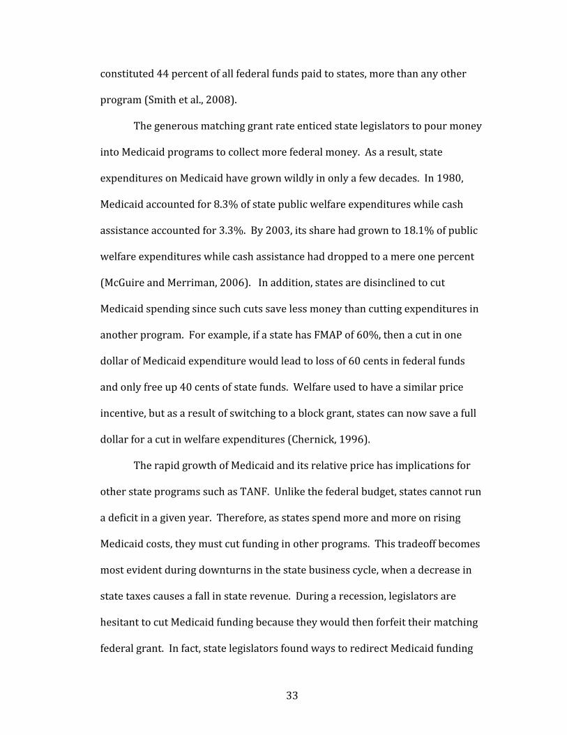
Figure 3: Federal Medicaid Grants (Real Thousands of Dollars), 1961-2009

Source: Census Bureau, Statistical Abstract; BLS, Medical Component of CPI

33

constituted 44 percent of all federal funds paid to states, more than any other program (Smith et al., 2008). The generous matching grant rate enticed state legislators to pour money into Medicaid programs to collect more federal money. As a result, state expenditures on Medicaid have grown wildly in only a few decades. In 1980, Medicaid accounted for 8.3% of state public welfare expenditures while cash assistance accounted for 3.3%. By 2003, its share had grown to 18.1% of public welfare expenditures while cash assistance had dropped to a mere one percent (McGuire and Merriman, 2006). In addition, states are disinclined to cut Medicaid spending since such cuts save less money than cutting expenditures in another program. For example, if a state has FMAP of 60%, then a cut in one dollar of Medicaid expenditure would lead to loss of 60 cents in federal funds and only free up 40 cents of state funds. Welfare used to have a similar price incentive, but as a result of switching to a block grant, states can now save a full dollar for a cut in welfare expenditures (Chernick, 1996). The rapid growth of Medicaid and its relative price has implications for other state programs such as TANF. Unlike the federal budget, states cannot run a deficit in a given year. Therefore, as states spend more and more on rising Medicaid costs, they must cut funding in other programs. This tradeoff becomes most evident during downturns in the state business cycle, when a decrease in state taxes causes a fall in state revenue. During a recession, legislators are hesitant to cut Medicaid funding because they would then forfeit their matching federal grant. In fact, state legislators found ways to redirect Medicaid funding

34

during recessions to state programs that had previously been funded solely with state expenditures (McGuire and Merriman, 2006). Comparatively, other public assistance programs seem relatively more expensive since they are funded solely by state general expenditures. Furthermore, the highest costs in Medicare result from long-term care for the elderly and disabled and it is more politically palatable to take funding away from potential “welfare queens” than to “pull the plug on grandma”. This idea of growth in Medicaid expenditures disrupting state expenditures on other programs has been labeled as “crowding out” by some of the fiscal federalism literature (Lewin Group, 2004, Steuerle and Mermin, 1997). There is not an extensive literature devoted to the concept of Medicaid crowding out other programs, but one article by Thomas Kane, Peter Orszag and Emil Apostolov (2005) uses econometric techniques to analyze this effect on higher education appropriations. First, they find statistical evidence that states with higher per capita Medicaid spending at the end of the 1980s suffered larger cuts in higher education in the beginning of the next decade. Their second piece of evidence is the offsetting pattern in the time trends of both Medicaid and higher education spending in their regression results. This result shows that when Medicaid spending growth was below its long-term trend, higher education spending was rising. Similarly, when Medicaid spending accelerated, higher education expenditures began to slow. Their regression results show that a dollar increase in Medicaid is associated with 39 to 58 cent decline in higher education spending per capita (Kane et al., 2005).

35

While it is not an exact comparison, this potential crowding out might influence the relationship between state expenditures on cash assistance under TANF and Medicaid spending. State expenditures on cash assistance fell during the late 1990s due to a booming economy and a subsequent decline in welfare caseloads. From 1980 to 2003 state cash assistance spending fell 3.2 percentage points while Medicaid rose nearly 10 percentage points (McGuire and Merriman, 2006). Increases in Medicaid would in theory have an effect similar to the result that Kane et al. found on higher education spending. This effect may be even more pronounced during recessions, as both cash assistance spending and Medicaid are likely to be highly counter-cyclical while higher education is less so. Medicaid growth is not expected to level off anytime soon. As the baby-boomers become senior citizens, there will be an outpouring of Medicaid expenditures on long-term care for the elderly, already one of the most expensive components of the program. This demographic shift will only intensify the crowding out effect observed on other state programs and will wrap state legislators in a tighter fiscal bind. In response to the most recent recession, the year-on-year growth rate of Medicaid spending has increased rapidly to 5.8 percent in 2008 from its record low growth rate of 1.3 percent in 2006 (Smith et al., 2008). This growth is expected to increase over 2009 as more people lose health benefits as a result of unemployment and fall back on Medicaid.

36

Earned Income Tax Credit and Food Stamp Program

The growth of Medicaid over time is similar to the expansion of the Earned Income Tax Credit program. Since its inception in 1975, it has grown from $3.9 billion (in real dollars) to $31.5 billion in 2000 (Hotz and Scholz, 2003). When the program began, it featured a 10% phase-in rate, where earned income up to a designated amount was augmented by a negative tax rate. The max credit at that time was a mere $400. In the 1990s, it expanded the most rapidly, differentiating benefits by number of children and jumping to its present phase-in rates of 34% and 40% for families with a single child and two or more children, respectively. By the end of the decade, families with one child could receive a maximum benefit of $2,428 while ones with two or more could receive over $4,000 (Hotz and Scholz, 2003). The program only benefits workers who can claim earned income and thereby receive a tax credit through the program. Therefore, it in theory has a positive effect on overall labor force participation as people not already in the labor force are enticed to join by higher relative wage rates. As the majority of the EITC program’s expansion occurred concurrently with increases in Medicaid and welfare reform in the 1990s, it is thought to be a contributing factor to both increased labor force participation and welfare caseload declines. Fang and Keane (2004) find that the EITC program accounted for 26 percent of the welfare participation decline from 1993-2002, as well as 33 percent of the increase in work participation among single mothers (2004, pg. 81). As EITC

37

acts as a work incentive, it will have an effect on measures of well-being and should be included in my model. The food stamp program, like EITC, is mainly a federal program that combats hunger among the low-income population. The program provides an important safety net for this population because there is no family composition or earned income eligibility requirements. During recessions, it helps supplement low-income households’ income by covering the cost of food. Also like EITC, the program has expanded since its early days, growing from its 1977 level by 88% as of 2004.

Hypothesis Prior studies find no increased sensitivity to business cycles as a consequence of TANF. In contrast, my own review of TANF and the fiscal federalism literature suggests that the 1996 welfare reform affected state expenditure decisions which, in turn, altered the well-being of low-income households over business cycles. I am interested in exploring whether poor and low-income families are more, equally, or less vulnerable to downturns than they were in the pre-TANF period under AFDC. Furthermore, I plan to investigate whether state spending behavior has played a role in maintaining or altering this sensitivity to business cycles under the TANF program. I hypothesize that TANF has increased the vulnerability of low-income families to high and rising unemployment rates and that state spending behavior on other programs has also contributed to this increased sensitivity.

38

III. Data and Methods

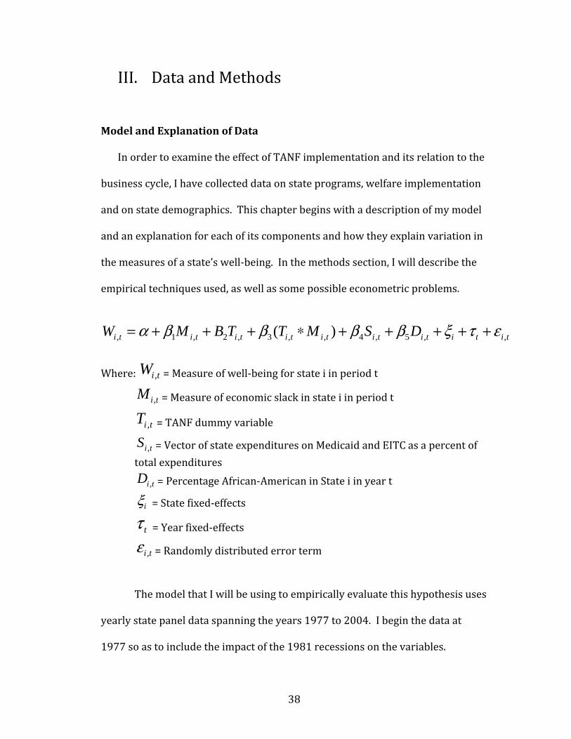
Model and Explanation of Data In order to examine the effect of TANF implementation and its relation to the business cycle, I have collected data on state programs, welfare implementation and on state demographics. This chapter begins with a description of my model and an explanation for each of its components and how they explain variation in the measures of a state’s well-being. In the methods section, I will describe the empirical techniques used, as well as some possible econometric problems. , 1 , 2 , 3 , , 4 , 5 , ,( )i t i t i t i t i t i t i t i t i tW M B T T M S Dα β β β β ξ τ ε= + + + ∗ + + + + + Where: ,i tW = Measure of well-being for state i in period t ,i tM = Measure of economic slack in state i in period t ,i tT = TANF dummy variable

,i tS = Vector of state expenditures on Medicaid and EITC as a percent of total expenditures ,i tD = Percentage African-American in State i in year t iξ = State fixed-effects tτ = Year fixed-effects ,i tε = Randomly distributed error term The model that I will be using to empirically evaluate this hypothesis uses yearly state panel data spanning the years 1977 to 2004. I begin the data at 1977 so as to include the impact of the 1981 recessions on the variables.

39

For this model I use two measures of well-being, an absolute measure and relative measure, both in 2002 dollars. These two measures were created by Joshua Guetzkow, Bruce Western, and Jake Rosenfeld for research on inequality at the Russell Sage Foundation and are available for download on their website. The data is initially constructed from Current Population Survey (CPS) data, and contain data on family earned income and other income in a given state and year. Within the other income category, the construction of the dependent variable includes payments from public assistance, such welfare or Medicaid. It does not include benefits from Food stamps or the Earned Income Tax Credit. One additional caveat with this data is that the researchers exclude observations that report zero annual income. Such an omission would not take into account families who were forced off of welfare and have no form of income, thereby underestimating the effect of TANF on measures of economic well-being. Ideally, the well-being measure would include the most current data, which for other variables includes 2008 data. However, since the data was created for their research in 2004, my time series is limited to this year. The first measure of well-being is the income threshold level of a particular percentile. The other is a measure of inequality consisting of the ratio between the 90th percentile income threshold level and a particular low-income threshold level. The former variable measures the income level below which a family would be considered in a certain percentile of income within that state and year. Therefore, if this value falls, it would signify that the population in that particular percentile income group was worse off in that particular state and

40

year. The latter is a measure of income inequality, and if this rises it indicates that there is a wider gap between that income percentile group and everyone else. For both measures I will evaluate the effect of welfare reform at the 10th, 20th, and 30th percentile income threshold. Evaluating the effect of welfare reform across these three income groups is important because welfare reform may have a greater impact on different income groups. In theory, the effect of welfare reform on the poorest group, the 10th percentile, is ambiguous. The impact from downturns in the business cycle might be limited for this group since many of them are out of work in the first place, or buffered from the effects of the new welfare law through reliance on other social assistance programs. Therefore it is interesting to look at the working poor, those occupying the 20th and 30th percentiles. These individuals are the people most affected by downturns in the business cycle as they tend to occupy low-tier jobs in the labor market and are the first to be laid off in a recession. In this case, the new welfare rules emphasizing work might have a greater impact on this group’s well-being, as measured by income. Originally, I was interested in using the percentage of a state’s population below the poverty line as a measure of well-being. I ultimately decided to use the income thresholds associated with particular percentiles for two reasons. First, as I described above, looking at particular income thresholds allows me to assess impacts for different segments of the income distribution. Second, as noted by Ruggles (1990), there are numerous problems in using a measurement such as the poverty line. The primary problem is that it is difficult to assign an

41

objective “minimum” level of income, especially over time and geographical location. The poverty threshold was created decades ago and does not reflect the changes in typical consumption habits over time. In addition, it does not allow us to account for people hovering above the poverty line, a population which represents a large portion of the working poor. Ruggles points out this flaw (1990, p. 14), noting that “a person with an income one dollar below the poverty line is not dramatically different in economic well-being from one with an income one dollar above the poverty line”. This problem would obscure the effect of welfare reform if I used poverty percentages in my model; welfare reform could raise or lower a family’s income significantly but as long as it didn’t cross the threshold it would not be picked up in the dependent variable. One complaint against relative measures of poverty is that they would not reflect an increase in the low-income population’s economic well-being if everyone’s income is rising at an equal rate. This complaint does not apply to my first dependent variable, percentile income thresholds, since they merely show the overall level of income among the people at different levels of income. If everyone were to rise together, this variable would reflect the rise in income for that particular percentile. However, the second dependent variable, the measure of income inequality, is vulnerable to such criticism. If all incomes were rising in proportion, my inequality measure, the ratio of two percentiles, would fail to show any increase in well-being, despite the fact that the poor are better off. However, if the two income levels are rising or falling at unequal rates, the ratio would reflect this change. Therefore, the two dependent variables provide

42

different, but equally useful pieces of information. Together, the threshold levels and threshold ratios reflect the age-old interest in both absolute and relative deprivation. As a robustness check, I also present results using the official poverty line, although my primary focus in this study is on the percentile measures. Despite the problems with an absolute measure of poverty, it is still worthwhile to test this model using poverty as the dependent variable. The common focus on the official poverty line raises interest in how the results would change with state poverty rates as the dependent variable. The vector M captures macroeconomic fluctuations in an individual state’s economy. State business cycles are not necessarily the same as the business cycle of the whole United States. Certain states experience different economic cycles at different times and it is important to capture this distinction. Prior studies have tried to capture this fluctuation using either state unemployment rates or Gross State Product (GSP). Unfortunately, the GSP data provided by the BEA underwent a change in data collection in 1997, making data from before that change incompatible with data collected after. Although a dummy variable could be added to my regression analysis to account for the change in data collection, that technique would provide only a rough and ad hoc fix. In addition, in order to identify a recession, I would need to transform the GSP variable so that it reflected the gap between normal output and actual output in a given year. Even with that transformation, the GSP output gap might not affect the income of low-wage households until unemployment rates start to rise. While GSP is a concurrent indicator of business cycles, unemployment

43

tends to lag behind recessions and to remain high even after recovery has begun. Use of the GSP would require lagging the output gap for an uncertain number of periods. As using the GSP measure would complicate the model, I decided to use state unemployment rates to capture cyclical sensitivity, as most of the literature has done. State annual unemployment rates are available from the Bureau of Labor Statistics. The dummy variable T has a value of one after TANF legislation has been enacted in a particular state. It has a t subscript because the new legislation was not put into effect at the same time in each state. The data on state implementation of either waivers or TANF was meticulously created by Crouse (1999) and is available online. To account for different months given annual data, past literature have used fractions (e.g. - if a state enacted TANF on July 1st, 1997, the dummy variable would be equal to 6/12 for that year). One element that this method does not take into account however is the impact of the state waivers under AFDC from the early 1990s. As other studies in the literature have pointed out, declines in welfare caseloads and increases in employment among single mothers began before the implementation of TANF, indicating that waivers might have a significant effect on well-being measures. In order to test the effect of waivers in the model, a different set of dummy variables would be used instead of TANF dummy variables in vector T. These “Waiver” dummies would have the value one (or a fraction) in the years after a state implemented any waivers. If a state never implemented a waiver, than its first non-zero dummy variable would be in the year it implemented TANF. The federal grant

44

structure under the waivers would have been the matching grant program of the AFDC years rather than the block grant program of the TANF years. Therefore it would be interesting to compare the results of the model using both the TANF and Waiver dummy variables. The coefficient 3β on the interaction term is the primary coefficient of interest. It measures the additional impact that a recession (or boom) has on the well-being measure in the post-PRWORA time period. If this value is statistically significant, I can reject the null hypothesis that implementing TANF has zero impact on the response of the low-income threshold to fluctuations in the state business cycle. A significant and negative coefficient would indicate that recessions are more harmful to low-income families in the post-welfare reform era. Conversely, booms are more beneficial to these same families than before. Likewise, a significant and positive coefficient would indicate that low-income families are less vulnerable to downturns in the business cycle after the implementation of TANF. In theory, the expected sign and significance for 3β is ambiguous. On the one hand, the reduction of cash assistance entitlement benefits for non-working families, along with pressures to take marginal jobs could increase household vulnerability. On the other hand, TANF may have generated a net benefit by raising earnings and labor-market attachment in a significant portion of low-income workers enough to moderate or negate the impact of recessions on this particular population of low-income families. The S vector captures spending on other social assistance programs. The two programs of primary importance are Medicaid and the Earned Income Tax

45

Credit (EITC) program. Data on Medicaid expenditures, as well as other state expenditures, comes from the U.S. Census Bureau’s State Government Finances database. Numerous articles within the fiscal federalism literature use this database, most notably McGuire and Merriman (2006). The variable in the database is technically labeled “medical vendor payments” and includes a few minor expenditures in addition to Medicaid. However, Medicaid expenditures by far make up the bulk of this data. Therefore, it is a legitimate variable to use in this equation. Medicaid’s presence in the equation is important because it will measure the level of crowding out present in that state. The use of the term crowding out in this case is not synonymous with the term that refers to the crowding out of private sector investment caused by public spending and higher interest rates. Instead, it describes the observation that increased state expenditures in one program, assuming a fixed state budget, will necessarily lead to decreased expenditures in another program. More specifically, as state legislators spend more and more on Medicaid over time, as they have done, they will have fewer resources to devote to cash assistance spending. I explore the hypothesis that Medicaid has had a similar crowding-out effect on cash assistance expenditures. Before using data on state Medicaid expenditures, it is important to account for the relative size of each state when comparing expenditures. In order to correct for this problem, I divide Medicaid expenditures in a given state and year by its total direct expenditures on public welfare in a given state and year. An increase in this variable measures Medicaid’s growth relative to other

46

programs, therefore isolating the crowding out effect that such growth has on the programs such as cash assistance. One problem with this measurement, however, is that it will not account for the relative size of states as well as a measure of population. While larger states will tend to have larger expenditures than smaller states, there will be nothing to account for states that are more parsimonious than others. A small generous state will therefore appear equal in size to a large state that is not as generous. An additional problem with this metric is that total expenditures in a given year will fluctuate with business cycles along with the measurements of well-being, and therefore might introduce bias into the equation. Population, on the other hand, is not significantly influenced by business cycles, which would make it a more reliable independent variable in my analysis. Therefore, I will use a measure of Medicaid spending per capita in a robustness check to determine how this data change will affect well-being measures. Data on population levels come from the United States Census. State population levels only exist in census years, so information on the years in between is estimated through interpolation. Growth in population is sufficiently linear to use this estimation approach. Any amount of error through such a technique would be negligible as there is a relatively small percent change in state population from year to year. By dividing through by the population, I get a measurement of each state’s relative level of spending on social assistance programs. One problem with this technique, however, is that it does not fully reflect the impact of crowding out occurring in states over time. If Medicaid

47

spending increases, the data does not show that spending on cash assistance is decreasing as a result. A measure of population does not indicate any less spending on other social assistance programs. In addition, the regression model used in this paper will include measurements of the Earned Income Tax Credit (EITC). By including levels of spending on the EITC program, the model accounts for the fact that other assistance programs have picked up the slack left by the decrease in cash assistance in the post-reform welfare state. Data on Federal EITC rates and benefits and state EITC programs comes from Fang and Keane (2004), who used the same data in their study on welfare reform. Even though EITC is largely a federal program, it will have implications on changes in the poor’s well-being, specifically the working poor. In order to account for this variable, I will follow Fang and Keane’s (2004) method of including two EITC variables in the model. The first is the federal EITC rate, which is the rate at which income is negatively taxed, up to a certain maximum level of income. The second is the maximum income benefit level that a family of a particular size may attain under the EITC. Since the program went through numerous expansions, these variables are different at different points in time and therefore have an impact on well-being, particularly after expansions. One additional problem to worry about when including EITC among the independent variables is the construction of the dependent variable. The EITC program would tend to raise overall income through tax credits. However, the researchers who I obtained the dependent variables from used income variables

48

taken from the Current Population Survey (CPS), which means that they included post-transfer income but not post-tax income, and that measure would not include the gains from EITC. Therefore, the effect of an increase in the EITC phase-in rate on pre-tax income is ambiguous. Depending on an individual’s level of work participation, the implementation of higher EITC rates and the subsequent income and substitution effects could either increase or decrease labor hours and consequently, pre-tax income. The figure below is adapted from a figure in Hotz and Scholz’s (2003) article on the EITC program. This particular figure shows the behavioral effects of a rise in the EITC phase-in rate and the maximum benefit rate for three different labor force participants. The line from point a to point e represents the tradeoff between earnings and leisure, and has a slope equal to the corresponding wage rate. The path along points a, b, c, and d represent the income path of an individual participating in the first EITC program. The higher path along points a, b’, c’, and d’ represent the expanded EITC program with a higher phase-in rate and maximum benefit. The first individual, represented by utility curve 1, is a person who was not in the labor force before the EITC expansion. After the expansion, there is a pure substitution effect on this person’s decision to work, and they will likely enter the labor force since there is a higher opportunity cost for leisure. Hence, there is an unambiguous positive effect on income for this individual.

49

The second individual, on utility curve 2, also faces the incentive to work more hours due to the substitution effect. However, she also faces an income effect from the immediate jump in income for the hours she has already worked via the increased level of tax credits. This effect creates an incentive to decrease total work hours assuming that leisure is a normal good. The resulting effect on pre-tax income is ambiguous, as it is unclear which effect would dominate. The third individual, represented in the figure above by utility curve 3, is a person who is in the labor market, but earned too much to qualify for EITC benefits before the expansion. After the expansion, there is again an income and substitution effect, and it is ambiguous which effect dominates.

ab

cd e

Hours of Leisure U1 U’1

Disposable Income

b’c’ U’2

U’3

U2

U3

Source: Hotz and Scholz (2003)

d’

Figure 4: Impact of EITC Expansion at Various Income Levels

50

In addition to the impact on individual work decisions, there is further ambiguity added to the analysis by the use of family income percentile thresholds. If one member of the family gains from an increase in EITC earnings and increases his earnings, other members of the family might decrease their hours of work in response. However, if they also gain from the EITC expansion, they might increase their hours as well. In summation, the impact of a rise in the EITC phase-in rate and maximum benefit rate has an ambiguous effect on family pre-tax income percentile thresholds. My model will also include a dummy variable indicating whether a state has enacted a state EITC program in a given year. Fang and Keane (2004) include this measure in their analysis as well, as it presents another source of income that would affect measures of well-being. I would also like to include a measure of food stamps in a given state in the model as well, since the drastic rise in food stamps could help account for any changes in earned income apparent in the income percentile thresholds. An increase in the value of food stamps granted in a given state and year would act as an income effect on labor hours, theoretically having a negative impact. However, there might be some difficulties in including both the unemployment rate and food stamp expenditures in the same model, since they will both account for variance from fluctuations in the business cycle. Therefore, I will run the model both with and without a measure of food stamps. Finally, D accounts for state demographic percentages measured by the percent of total population that is African-American. Data on this variable was

51

gathered from various years of the Statistical Abstract and interpolated to fill the in between years. Like total population growth, this method is permissible due to the steady and relatively slow growth of the African-American population over time in states. Prior studies use this variable because states with high populations of minorities or single mothers generally have higher levels of poverty (McKernan and Ratcliffe, 2006). In this model, levels of minorities and single mothers are significant because people in this demographic are more likely to be caught in what Wolff (2009) describes as the secondary labor market. Jobs in this labor market are generally low-wage, low skilled and hold little chance for promotion or developing human capital. More importantly, these types of jobs are generally the first to go during a recession, as it is relatively easy to hire a replacement worker later and little training is required. Therefore, a state with a higher percentage of secondary workers in the labor force will be more vulnerable to changes in the business cycle. In addition, if the African-American population is correlated with both income percentile thresholds and another independent variable, it will bias the estimated coefficient on that regressor. Methods

As the data section noted, this model utilizes panel data on annual state variables. With panel data, the two estimators that are primarily used in regression analysis are a fixed effects estimator and a random effects estimator. Both estimators include a variable that captures unobserved effects among

52

cross-sectional observations, denoted by in my model. They differ, however, in their assumptions as to how the unobserved effects relate to the other explanatory variables and the means of removing them from the model. With a fixed effects estimator, data for each variable is averaged over the given time period, and then subtracted from each individual observation. The resulting time-demeaned data eliminates the unobserved effect , since its value is constant across all time periods. The motivation for eliminating this factor, as explained in Wooldridge (2009), is the assumption that it is correlated with both the dependent variable and one or more explanatory variables. Since there is no data to quantify it, the unobserved term falls into the error term. As a result, the estimated coefficients on the regressors in the model would be biased if this term were not accounted for or removed from the equation (2009, 482). Unfortunately, any constant explanatory terms included in the model would also be eliminated under this method. The motivation behind the random effects estimator differs from the fixed effects estimator in that when using random effects, we assume that the unobserved effect is uncorrelated with each explanatory variable across all time periods. A random effects estimator uses quasi-demeaned data to eliminate the problem of serial correlation caused by the unobserved factor in the error term. Since the regressors are subtracted by a fraction of their average over time, constant terms in the model are still included in the regression (2009, 489). I will use fixed effects in my model since my main explanatory variable is not

53

constant and I do not want to assume that the unobserved effect is uncorrelated with each explanatory variable. In addition to including fixed effects for state cross-sectional observations, the model includes year fixed effects. I account for the year fixed effects by including a dummy variable for each year from 1977 to 2004 (not including the first year, which will be factored into the intercept for comparison). Like state fixed effects, characteristics of a significant event in one year can have lasting implications on future years. The most obvious event is the implementation of TANF in particular years, which is accounted for explicitly in the model. However, there are numerous minor events in any given year that will be picked up in the error term if they are not included in the model, thereby creating a problem with serial correlation. By including a dummy variable for each year in the data, I am accounting for the variance from any particular event in a given year. One drawback to this approach, of course, is that it requires many degrees of freedom, as each year is included as a separate independent variable. However, since I have observations on 50 states over 28 years, I have a comfortable number of degrees of freedom to include these dummy variables in my regression analysis. The primary coefficient of interest in the model is , which captures the marginal effect of each state’s TANF coefficient interacted with its respective unemployment rate. This method is a departure from much of the prior literature, which generally only included the TANF dummy without any interaction term. These articles, especially studies that focus on TANF’s impact

54

on individual behavior such as Bavier (2002) or McKernan and Ratcliffe (2006), use the solitary dummy variable to determine if TANF as a whole, or individual policies of TANF, affect various measures of income, caseload numbers or poverty rates. While they generally use unemployment rates to control for macroeconomic changes in the model, by not interacting the TANF and unemployment variables, the results fail to show the dynamic relationship between a given dependent variable and the business cycle in the post-reform era. Herbst (2008) notes this absence in the literature, stating, “previous research focuses on estimating average effects of social policy reforms that are assumed to hold equally during periods of economic expansion and contraction” (pg 868). In his article, Herbst studies the impact of various welfare reform policies on employment growth across varying labor market conditions. My work in this thesis comes from a similar motivation in evaluating TANF’s impact on well-being over time in relation to the business cycle. However, Herbst’s method involves interacting social policy reform variables with four different unemployment rate dummy variables, each representing a quartile of the state unemployment rate. Also, instead of studying the impact on an individual labor decision such as employment and participation in the labor force, I am using an interaction term between policy reform and the unemployment rate to study changes in income percentile thresholds. Since I hypothesize that TANF has left measurements of income thresholds more vulnerable to fluctuations in the business cycle, the predicted sign on the coefficient of the interaction term is negative. Similarly, the

55

predicted sign on the unemployment rate coefficient would be negative and significant, as a recession tends to lower incomes. The coefficient on the TANF dummy is ambiguous. While TANF negatively impacted a certain population of single mothers who face significant barriers to work, as discussed by Blank (2007), it did raise overall employment and earnings levels when evaluated equally across all labor market conditions, as much of the prior literature as shown. Therefore, it is likely that this coefficient will show a positive impact on income thresholds, as it does not take into account the dynamic relationship across different rates of unemployment. The expected sign on Medicaid is also ambiguous. I will divide it by both population and total state expenditure to determine the level of crowding out present in a state. As an increase in Medicaid spending would lead to a crowding out, and therefore decrease, of spending on cash assistance, this could lead the coefficient to produce a negative sign. However, an increase in Medicaid spending would also be reflected in the income percentile thresholds, as these variables draw on post-transfer income, which would include payments from Medicaid. The sign on the EITC variables is ambiguous for the reason discussed above; the sign will depend on whether the income or the substitution effect dominates. The percentage of a state’s population that is African-American will probably have a negative relationship with income levels, as this demographic tends to receive lower earnings relative to white workers. However, it could be insignificant since there is limited variation in states’ African-American populations over time.

56

Econometric Problems: Heteroskedasticity: This term describes the problem when the variance of the error term given the value of a regressor is not constant, but rather, varies according to different levels of the explanatory variable. While this problem does not introduce bias into the estimated regression output, it does affect the estimated variances of the coefficients, thereby making it impossible to produce usable estimated standard errors and t-statistics. Since its existence hinders our ability to draw statistical inferences from the data, it is a potential problem that merits attention. The statistical test that I will use to test for this problem is an ado file called xttest3, created by Christopher Baum of Boston College for Stata statistical software. This particular test calculates a modified Wald statistic for groupwise heteroskedasticity in the residuals of a fixed effects panel data regression model. With panel data, the most likely deviation from homoskedastic errors is likely to be in the error variances specific to the cross-sectional unit. Therefore xttest3 tests whether 2iσ σ= for all cross-sectional units. The resulting test statistic uses a Chi-squared distribution under the null hypothesis of homoskedasticity. If heteroskedasticity is present within a set of data, there are two ways to address the problem. The exact form of heteroskedasticity can be estimated through a Feasible General Least Squares (FGLS) estimator by obtaining an estimate of the appropriate weights in the data and then using a Weighted Least Squares (WLS) regression. A less precise method is to simply run the regression on the original model and apply heteroskedasticity-robust standard errors.

57

Therefore, if the results still hold even when standard errors have been adjusted to reflect the possibility of heteroskedasticity, the coefficient estimates are still valid. Multicollinearity: The problem of multicollinearity results when there is a high (but not perfect) correlation between two or more independent variables. Multicollinearity is not necessarily a problem in regression, since it still satisfies the assumption of no perfect collinearity. Furthermore, it does not bias the estimated coefficients. Instead, it widens estimated standard errors, decreasing the likelihood of finding statistical significance by making it difficult to disentangle the independent effects of particular variables. However, it becomes problematic to draw causal effects from a certain regressor if a large percentage of the variance is explained by other variables in the model. Given the interconnectedness of states’ economies, as well as the connections within a state’s social programs, multicollinearity usually exists to some extent. Unfortunately, there is no solution to this problem except to collect more observations, and since there have been a given number of states for a given number of years, this is not an option. However, as long as there is not a great degree of correlation between the main explanatory and the other variables in the model, multicollinearity is not a large issue. The other variables exist to provide an unbiased, ceteris paribus estimate of the key regressor’s marginal effect. Endogeneity: There is a potential problem of endogeneity, as policy decisions reflected in the right hand side variables might have been influenced by changes

58

in the poverty threshold. The variable that is most likely to suffer from endogeneity are the EITC measures. Although politicians did raise phase-in rates and maximum benefit levels in response to the program’s success in raising low-income workers’ labor force participation, there does not seem to be any evidence that the EITC program was altered due to a drastic rise or fall in threshold levels.

59

IV. Results and Discussion

Percentile Threshold (Absolute Measures of Well-Being)

10th Percentile Model 1 Model 2 Model 3 Model 4 Model 5

ur -188.19808*** -181.07685*** -177.17961*** -60.149374* -66.498024**

tanf -53.114009 952.75075* 1200.8414** 1862.301*** 1730.3898***

interact_tanf -216.45029*** -282.62852*** -330.31138*** -345.33158***

med_exp 2674.4734** 2870.946** 2640.5114**

snap_pop -22.314234*** -22.153349***

eitc2up (omitted)

maxeitc2up 0.15267356

SEITCdummy -197.23802

afamperc -108.27481**

_cons 18107.563*** 18060.675*** 17834.101*** 18323.485*** 19280.856***

R-Sq Within 0.2834 0.2923 0.2933 0.3585 0.3646

# Obvs 1480 1480 1400 1400 1400

Legend: *p<0.05 **p<0.01 ***p<0.001 The dependent variable in the first set of regressions is the family income threshold for the 10th, 20th, and 30th percentiles of the income distribution. As discussed in the data and methods section, this measure is an absolute measure of well-being, similar to the poverty measure. The regressions use a fixed-effect estimation technique. I also include yearly dummy variables to account for year-specific shocks that could influence observations in subsequent years.

Table 1: Estimated Impacts on the 10th Percentile Income Threshold

60

Table 1 displays estimates for the 10th percentile household-income threshold. In a given state and year, ten percent of households have income below this level. The average income threshold for this group across all states and years in my sample is $16,074.88. Model 1 in Table 1 includes only the unemployment rate and the TANF implementation dummy variable. In this first regression, the state unemployment rate has a negative and significant impact, as expected, while the estimated effect of TANF is negative but insignificant. However, when the interaction term between the unemployment and TANF is added in Model 2, the estimated coefficient on the TANF dummy variable turns positive and becomes significant while the estimated coefficient on the interaction terms is significant but negative. Therefore, the addition of the interaction term seems to have teased out both a positive and negative impact of TANF’s implementation. The coefficient on this interaction term is the primary coefficient of interest. It suggests that a rising unemployment rate now not only lowers the income threshold, but lowers it significantly more in the post-PRWORA period than in the pre-PRWORA period. Specifically, while a one-percentage point jump in the state unemployment rate lowers the income threshold by $181 in the pre-PRWORA period, in the post-PRWORA period it lowers the threshold by an additional and significant $216. The total impact in the post-PRWORA period, therefore, is a loss of $397 for each percentage point rise in the unemployment rate. A Wald test on these two coefficients shows that they are jointly significant at the 0.1% level.

61

The results from Model 2 also provide estimates of the impact on the 10th percentile income thresholds of changing to a TANF regime from the pre-TANF environment. A finding that is particularly interesting shows that TANF has a positive impact when state unemployment levels are low, but yields a negative impact when state unemployment rates are high2. For example, if the unemployment rate had been at 1% in the period after PRWORA, TANF would have raised the income threshold of this percentile group by an estimated $737. In contrast, when the unemployment rate is at 5.96%, the mean value of the sample, the estimated impact of TANF is a drop in the threshold level of $334. Furthermore, if the unemployment rate rises to 10%, as it did nationally in the last recession, TANF lowers the income threshold by an estimated $1,207. Finally, if the unemployment rate rises to 15%, as it did in Michigan in July of 2009, then TANF would lower the income threshold by an estimated $2,287. A Wald test for the joint significance of B2 and B3 at these four unemployment rates shows that the joint impact when the unemployment rate is at 1% is significant at the 5% level, while the impact when the unemployment rate is at 10% and 20% is significant at the 0.1%. The two coefficients are not jointly significant when the unemployment rate is set at the mean unemployment rate. Models 3 and 4 in Table 1 include state expenditures on Medicaid as a percentage of total expenditures and total food stamp benefits per capita in a given state and year. Medicaid expenditures have a strong positive effect on 2 By totally differentiating the model and holding unemployment rate constant, the resulting equation shows: 953 216( )dP

UdTANF

= − where P is the percentile threshold and U is the level of the unemployment rate.

62

well-being in model 4, raising the 10th percentile income threshold by $2,871 for a one percentage point increase in Medicaid relative to total spending. This estimate is significant at the 1% level. Food stamps, on the other hand, are negatively related to income at the 10th percentile. An increase in expenditures of one dollar per capita is associated with a decrease in the income threshold of $22, and is also significant at the .1% level. This link most likely reflects reverse causality. When incomes fall for households in the bottom 10th of the income distribution, food stamp expenditures are designed to cushion the drop in income. In model 4, the coefficients of both the TANF dummy and the interaction term have the same direction as in prior models, but they have a higher magnitude. The estimated coefficient on TANF dummy rises to $1,862 while the estimated impact of the interaction term is a negative $330. Both of these estimates are significant at the 0.1% level. Again, together these results suggest that TANF has a positive impact under low unemployment rates, but an overall negative impact when unemployment rates are high. Wald tests for the joint impact of these two estimated coefficients are significant at the 0.1% when the unemployment rate is at 1%, 10%, and 20%. One other noteworthy result is the change in the impact of the unemployment rate from model 3 to model 4, when the food stamps variable is added. The magnitude of the coefficient on the unemployment rate in model 4 drops to $60 for a one-percentage point rise in the unemployment rate, and is only significant at the 5% level when the Food stamps variable is added to the model. The results suggest that, pre-TANF, a one-percentage point increase in

63

the unemployment rate lowers the 10th percentile income threshold by only $60 while, after TANF implementation, the same one-percentage point rise in unemployment rates lowers the income threshold by $390. In other words, controlling for Medicaid and food stamps produces a wider estimated gap between pre-TANF and post-TANF impacts on the unemployment rate. Corr p10faminc ur tanf interact med_exp snap_pop eitc2 maxeitc2 SEITC afamperc

p10faminc 1.00

ur -0.22 1.00

tanf 0.11 -0.39 1.00

interact 0.08 -0.29 0.96 1.00

med_exp 0.06 -0.28 0.51 0.51 1.00

snap_pop -0.38 0.47 -0.17 -0.10 0.12 1.00

eitc2up 0.08 -0.47 0.82 0.79 0.66 -0.05 1.00

maxeitc2up 0.09 -0.45 0.85 0.83 0.66 -0.05 0.99 1.00

SEITC 0.22 -0.20 0.23 0.22 0.27 -0.13 0.28 0.29 1.00

afamperc -0.03 0.13 0.02 0.04 0.21 0.41 0.05 0.05 -0.08 1.00 The final model presented in Table 1 features the complete form of the model, and includes the phase-in rate for a family with two or more children in the Federal EITC program, the Federal EITC maximum benefit level, a dummy variable indicating whether a state has its own EITC program in a given year, and the percentage of a state’s population that is African-American in a given year. The EITC phase-in rate was automatically dropped from the regression by

Table 2: Correlation Matrix of 10th Percentile Regression Variables

64

the Stata regression software due to high collinearity with other variables in the model3. The maximum benefit variable has a small, positive magnitude but is not significant, while the state EITC dummy variable was negative but also not significant. The coefficient on the African-American variable shows that for a one-percentage point rise in this population, the 10th percentile income threshold falls by $108, and is significant at the 1% level. More importantly, in the full model regression the estimated coefficients for the main explanatory variables keep their direction and magnitude, along with their significance levels. The estimate for the interaction term shows that in the post-welfare reform era, a one-percentage point rise in the unemployment rate decreases the 10th percentile’s income threshold by $345 more in the post-TANF period than in the pre-TANF period. Table 3 shows estimates for the 20th percentile income threshold, which averages $25, 018 over the sample period. The first two models show estimates similar to the 10th percentile regressions. After including the interaction term, the impact of the TANF dummy variable changes from positive and insignificant to significant. Both the unemployment rate and the interaction term continue to show negative impacts that are significantly different from zero. Prior to welfare reform, a one-percentage point rise in the unemployment rate significantly lowers the income threshold by $176. According to the estimated impacts of the 3 In these regression models, I tried different combinations of the EITC variables and the logs of these variables. Unfortunately, Stata continued to drop the EITC phase-in rate variable due to collinearity. Perhaps this problem could be solved with more data.

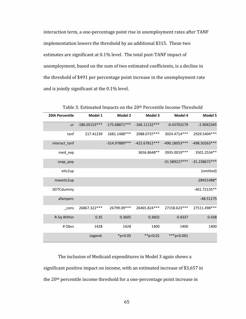
65

Table 3: Estimated Impacts on the 20th Percentile Income Threshold

interaction term, a one-percentage point rise in unemployment rates after TANF implementation lowers the threshold by an additional $315. These two estimates are significant at 0.1% level. The total post-TANF impact of unemployment, based on the sum of two estimated coefficients, is a decline in the threshold of $491 per percentage point increase in the unemployment rate and is jointly significant at the 0.1% level. 20th Percentile Model 1 Model 2 Model 3 Model 4 Model 5

ur -186.05153*** -175.68871*** -166.11132*** -0.43703179 -2.9042345

tanf 217.41239 1681.1488*** 2088.0737*** 3024.4714*** 2929.5404***

interact_tanf -314.97889*** -422.67812*** -490.18053*** -498.50263***

med_exp 3656.8648** 3935.0019*** 3501.2534**

snap_pop -31.589227*** -31.238672***

eitc2up (omitted)

maxeitc2up .28451488*

SEITCdummy -401.72135**

afamperc -48.51175

_cons 26867.322*** 26799.09*** 26465.824*** 27158.623*** 27511.498***

R-Sq Within 0.35 0.3605 0.3602 0.4337 0.438

# Obvs 1428 1428 1400 1400 1400

Legend: *p<0.05 **p<0.01 ***p<0.001 The inclusion of Medicaid expenditures in Model 3 again shows a significant positive impact on income, with an estimated increase of $3,657 in the 20th percentile income threshold for a one-percentage point increase in

66

Medicaid as a percent of total spending. Furthermore, the addition of Medicaid to the model boosts the magnitude of the TANF dummy and the interaction term. The fourth model shows that food stamp expenditures per capita are negatively related to the income threshold level and significant. In addition, with the food stamps variable included, the magnitudes on TANF, the interaction term and Medicaid expenditures are all increased and significant at the 0.1% level. The estimated coefficient on the unemployment rate drops to -0.44 cents and is no longer significant when food stamps are added to the model. However, the impact of a one-percentage point increase in the unemployment rate post-TANF is a negative and significant $491. The post-TANF impact of the unemployment rate is again significantly larger than the pre-TANF impact. In the last model, the EITC phase-in rate for a family with two children is again automatically dropped from the regression by Stata, but the maximum benefit level has a positive impact that is significant at the 5% level. The impact was both smaller and lacking in significance for income at the 10th percentile. Households at the 20th percentile are more affected by the maximum EITC benefit, a result that makes sense as this group is both more attached to the labor force and more likely to benefit from an increased maximum benefit. The estimated impact for this variable is a 28-cent increase in the income threshold level for every dollar that the maximum benefit is increased. The dummy variable that indicates a state EITC program has an estimated impact that is significant at the 1% level. It indicates that the presence of a state EITC program is associated with an income threshold for the 20th percentile that is lower by

67

$402. There are two likely factors to explain this outcome. First, the state with more inequality might tend to implement state EITC in an attempt to share income more equally. Second, a state EITC may induce reductions in work hours for secondary workers in the household. The primary worker might also reduce work hours if the income effect exceeds the substitution effect of the state EITC4. Once again, the interaction term in the full regression shows that a one-percentage point increase in the unemployment rate decreases the 20th percentile income threshold by a magnitude of $501 under the TANF program. A Wald test shows that these two coefficients are jointly significant at the 0.1% level. 30th Percentile Model 1 Model 2 Model 3 Model 4 Model 5

ur -228.64189*** -212.43749*** -201.7415*** -31.846221 -32.327432

tanf -341.50466 1947.3472*** 2373.4213*** 3333.6761*** 3301.2933***

interact_tanf -492.53404*** -607.47606*** -676.69827*** -679.11056***

med_exp 4425.6917** 4710.9151** 4517.0128**

snap_pop -32.394045*** -32.234204***

eitc2up (omitted)

maxeitc2up .70933658***

SEITCdummy -181.58191

afamperc -11.505103

_cons 34473.305*** 34366.61*** 33995.872*** 34706.321*** 34536.123***

R-Sq Within 0.4313 0.447 0.447 0.4941 0.4946

# Obvs 1428 1428 1400 1400 1400

Legend: *p<0.05 **p<0.01 ***p<0.001 4 Also, it should be noted again that income from EITC is not included in the construction of the dependent variable.

Table 4: Estimated Impacts on the 30th Percentile Income

68

Table 4 explores the impact of the various models on the 30th percentile income threshold, which has a mean value of $32,998.85 over the given time period. The regression estimates follow largely the same pattern as the results of the 20th percentile income threshold, only with larger magnitudes that reflect the larger income levels. The first model of Table 4 shows familiar results where the TANF implementation variable is negative and insignificant in the absence of the interaction term. In Model 2, the addition of the interaction term again switches the coefficient the on TANF dummy variable from negative and insignificant to positive and significant. The estimated coefficient on this variable indicates that for a one-percentage point rise in the unemployment rate, there is an additional decline in the income threshold of $493, making the total impact on the threshold in the post-welfare reform era a decrease of $705, significant at the 0.1% level. Once again, the addition of the food stamp variable has a negative, significant impact on the income threshold, and reduces both the estimated impact and significance of the unemployment rate in the pre-TANF period. The estimated Medicaid impact is an increase in the threshold by $3,935 for a percentage point increase in Medicaid spending as part of total spending. The last model shows that a one-percentage point increase in the unemployment rate reduces the 30th percentile income threshold by $679 more in the post-TANF than in the pre-TANF period, and the difference is significant at the 0.1% level again. One interesting result in this last regression is the impact of a dollar increase in the maximum EITC benefit for families with two or more

69

kids. The estimated coefficient is an increase of 71 cents in the income threshold, much higher than the impact on the 20th percentile income threshold. Again, greater attachment to the labor market is a likely explanation for this larger impact. This estimated impact is also significant at the 0.1% level. The state EITC dummy variable and the African-American population percentage variable are no longer significant for the 30th percentile income threshold. Discussion of the Percentile Threshold Measures The most important explanatory variable in this study is the interaction between a state’s TANF indicator and that state’s unemployment rate in a given year. Estimates for the 10th percentile found that this interaction term negatively affects income thresholds, indicating a decrease in well-being. Furthermore, this negative result is consistent across all estimated equations, and is always statistically significant at the 0.1% level. In addition to testing threshold responses at the 10th percentile across the various models, I analyzed income thresholds for two additional percentiles. This allowed me to observe the effect of welfare reform at different points in the income distribution and for different segments of the low-income population. Results for the 20th and 30th income percentiles were quite similar to those for the 10th percentiles. Again, income thresholds were significantly more vulnerable to recessions in the post-TANF era. The estimated impact is highest for the 30th percentile, reflecting this group’s higher level of income. The post-TANF increase in cyclical sensitivity ($711 for each percentage point rise in the unemployment rate) is significant in

70

both a statistical and an economic sense. The $711 represents 2.2% of the income threshold for this percentile. If the unemployment rate were to rise by 5 percentage points, as it did between December of 2005 and December of 2009, this increased sensitivity associated with TANF transforms into a $3,555 loss, an amount equal to 11% of the income threshold for this group. Seemingly in contrast with the estimated impact of the interaction term is the estimated coefficient on the TANF implementation dummy alone. Across all of the various models and income percentile groups, this variable has a statistically significant, positive effect on percentile income levels. The only example where this variable is not significant is in the first model, the one without the interaction term. Once the interaction term is added to the model, both estimated coefficients become significant, but with opposite signs. Therefore both variables need to be present in the model to parse out the opposing effects of the TANF implementation dummy variable. While the estimated coefficients on the interaction term support my hypothesis on increased vulnerability from TANF, the estimates from the TANF dummy deserve attention. For all three percentile thresholds, the regression results for this variable indicate that, at very low levels of state unemployment, the TANF impact is significant and positive. To illustrate this example, I have compiled the joint estimated impact of TANF in the post-PRWORA era at the 10th income percentile, as well as the p-values of the Wald test for joint significance, in the table below.

71

UR 1% 2% 3% 4% 5% 6% 7% 8% 9% 10%

Joint Impact $1,385 $1,040 $695 $350 $5 -$340 -$685 -$1,030 -$1,375 -$1,720P-Value 0.0000 0.0008 0.0163 0.2102 0.9893 0.2353 0.0251 0.0020 0.0002 0.0000 In Table 5, TANF has a positive estimated impact on the 10th income percentile threshold at low levels of unemployment. However, this impact decreases as the unemployment level rises, until it has an estimated negative effect when the unemployment level is between 5% and 6%. Furthermore, using a 5% significance level, this joint impact does not become significant again until the unemployment rate is 7%. This result reinforces the findings from much of the previous literature; in its early years, when unemployment rates were low, TANF, on average, had a net positive impact on earnings and employment. However, the reader should not interpret this estimated value as evidence against my hypothesis. My question concerns the increased cyclical sensitivity of well-being measures in the post-welfare reform era, not their overall trend since PRWORA. The question posed by my thesis is answered by the interaction term, and the estimated impact of that term provides evidence of increased vulnerability. Moreover, the estimates demonstrated that TANF impacts depend on the level of a state’s unemployment rate. While TANF has a positive impact when state unemployment rates are low, TANF’s impact on income thresholds for the bottom percentiles is negative when state unemployment rates are moderate to high. For all three income percentiles, there is an estimated negative impact

Table 5: Joint impact of TANF at 10th Percentile and P-Values

72

when the unemployment rate rises to rates between 4% and 6%, but these results are not statistically significant. The positive estimated coefficients on Medicaid expenditure as a percent of total state expenditures are consistently significant and have magnitudes in the thousands of dollars. While this estimate may seem impressive at first, it is important to remember that the dependent variables include income from Medicaid payments. Therefore, it is hardly surprising that an increase in state Medicaid expenditures as a percent of total state spending would lead to higher income levels. If there is any indirect effect from decreased cash assistance as a result of the crowding out effect that I described in the theory section, it is masked by the effect of a direct income transfer from Medicaid payments. Income from food stamps benefits, on the other hand, is not included in the measurement of the family income variable, and therefore the coefficients for this variable do not have large estimated impacts similar to Medicaid expenditures. Nonetheless, the estimated magnitude on food stamp benefits is still surprising. The estimated coefficient for this variable of -31.24 in the 20th percentile regression is significant at the 0.1% level. At first glance, this result seems to indicate that for a one-dollar increase in per capita food stamp benefits, there is a decline in the income threshold by $31.24. The food stamp program is an in-kind program, meaning that recipients do not receive cash benefits, but rather credits to put towards food purchases. An argument could therefore be made that there is a strong income effect from this in-kind transfer that shifts individuals’ behavior to consume more leisure. However, such a drastic shift

73

seems hardly likely for households which are food-poor. Instead, a more reasonable explanation is the possibility of reverse causality in the model, where a change in income threshold levels affects the level of food stamp benefits. This result would reflect the fact that the food stamps program is designed to cushion falls in income, which would explain the negative and significant estimate. This estimated result therefore reflects the responsiveness of food stamp expenditures to declines in well-being. Across all three percentiles, the use of controls for food stamps in the regression analysis has an added effect of decreasing both the magnitude and significance of the estimated coefficient on the pre-TANF unemployment rate. As the food stamps variable does not seem to have a noticeable effect on any other variable besides the unemployment rate, it appears to be acting as a proxy for the business cycle. In other words, the results suggest multicollinearity between the unemployment rate and the food stamps measure. Although the two variables only have a 0.48 correlation coefficient, the cyclicality picked up in the food stamps variable is affecting the pre-TANF estimate for the unemployment rate. However, the post-TANF impact of unemployment is largely unchanged in both magnitude and significance. The EITC variables showcase a variety of estimated effects on the various measures of well-being. The first variable, the EITC phase-in rate for families with two or more children, is dropped from the full regression due to its high collinearity with the other main explanatory variables. This issue results from

74

expansions of the EITC program throughout the 1990s, therefore making it correlated with the PRWORA legislation and the implementation of TANF. The maximum EITC benefit for a family with two children becomes significant at different income thresholds. The first group of regressions shows that a dollar increase in the maximum benefit has no significant effect on the well-being of families at the 10th percentile income level. However, among families at the 20th percentile income level, an increase of one dollar in the federal EITC maximum benefit leads to an increase of 28 cents in the income threshold, significant at the 5% level. The reader should note that the EITC tax credit, whether federal or state, is not reflected in the income components of the dependent variable. In other words, the estimated impact is not spurious. At the 30th percentile, the magnitude not only increases to 0.71, but it is now significant at the 0.1% level. This increase in both magnitude and significance across income groups suggests that the EITC program is more effective among families that are relatively better off economically. The obverse of this finding, however, is that people at the very bottom of the income distribution are not benefitting much from the EITC program, as they do not have a significant amount of earned income. In this respect, the program is not well targeted to the poorest and those with the weakest foothold in the labor market. In contrast to the estimated results of the federal EITC benefit level, the dummy variable indicating a state EITC program consistently has a negative sign across the three percentiles and across all models for each percentile. While this variable is statistically significant only for the 20th percentile regression, for that

75

group it lowers the threshold by an estimated $402. One possible explanation is a decline in other transfer income or a loss of eligibility for other transfer programs as a result of participation in a new state EITC program. Another possible explanation for this drop is an income effect exceeding the substitution effect of the state EITC program. In other words, the deterioration in the income threshold might reflect a decrease in earnings resulting from individuals’ decisions to work less in response to an increase in income. However, as the state EITC also subsidizes the after-tax wage rate, a substantial substitution effect is also theoretically possible. The lowered threshold estimated for the 20th percentile suggests that the income effect dominates the substitution effect for this group. This drop in earnings might reflect the decisions of the primary earner in the household, or it might reflect decisions of secondary earners for whom the addition of a state EITC would cause a pure income effect. The different signs on these estimates for the two EITC variables are somewhat striking. Why should one measurement of EITC have a positive impact on well-being, while another slightly different measurement has a negative impact? One possible explanation is the different EITC effects that each variable captures. The state EITC dummy variable takes on a value of one in the year that a state implements an EITC program, and has a value of one for every year afterward. The creation of a completely new program could have a large effect on individuals’ work decisions, as it would bestow a large tax credit immediately. Individuals newly eligible under the new program would receive a substantial immediate transfer of additional income from tax credits, resulting in

76

a substantial income effect. This income effect would explain the decrease in income levels that result from the implementation of a state EITC program. The maximum EITC benefit, on the other hand, is a much more subtle measure. Each year, the maximum benefit that a family with two or more children can receive is increased slightly, even if the phase-in rate is not changed. This change is illustrated in figure 5 below. At an increased maximum benefit, as illustrated by the dotted line in the figure, there is both an income effect and a substitution effect as more workers have access to the phase-in rate representing a subsidized wage rate and causing a substitution of work for leisure. At the same time, more income for those already working causes an effect encouraging reduced work hours. Finally, if fewer people are subject to the phase-out rate, then fewer people face this work-discouraging implicit tax. In

Figure 5: EITC Maximum Benefit Increase (in Dollars) Program tax credits

Earned Income

77

sum, the theory again points to both income and substitution effects. However, the empirical estimates in this study suggest that, in the case of the Federal program, the substitution effect dominates the income effect, creating a net positive impact on work decisions and consequently on the income threshold level as well. The key difference is that the federal EITC benefit variable estimates the impact of a one dollar change in benefits, while the state EITC dummy variable estimates the impact of a whole new program. The smaller magnitude expressed in the EITC benefits variable leads to a positive estimated change in income levels. The variable that captures the African-American percentage of a state’s population shows an estimated negative sign in all regressions. The negative sign indicates that a higher proportion of African-Americans in a particular state lower the income threshold for the bottom income percentile. However, the variable is significant only in the 10th percentile regression. These findings reflect the fact that African-American workers not only tend to earn less than white workers on average, but also tend to be disproportionately represented in the lowest tier of the economic stratum. Inequality Ratios (Relative Measures of Well-Being) The next set of regressions uses inequality ratios created by dividing the income level for the 90th percentile threshold by the aforementioned low-income percentile thresholds. This measure is a relative measure of well-being, displaying the gap between high incomes and low incomes. These regressions

78

also use a fixed-effect estimation technique and include yearly dummy variables to account for year-specific shocks that could influence observations in subsequent years. The analysis of the estimated regression coefficients using inequality ratios for the dependent variable differs substantially from the regressions using the income threshold levels. First, the signs on the coefficients have a reversed interpretation in terms of their effect of well-being. While a negative sign in the threshold-level regression signified a drop in income levels and therefore a decline in absolute well-being, a negative sign in the inequality regressions indicates a decrease in inequality and consequently an increase in relative well-being. Second, the interpretation of the magnitudes on the coefficients is not as intuitive as it is for the income level regressions. For each state and year, three inequality ratios are created by dividing the 90th percentile income threshold by the bottom three income percentile thresholds. The resulting data can therefore be interpreted as the top income levels as a multiple of the lower income level. For example, the average ratio across states and years for the 90/10 income inequality measure is 6.68, which indicates that the income threshold for families at the 90th percentile was, on average, 6.68 times greater than the income threshold for families at the bottom of the income distribution. From year to year, this magnitude fluctuates with the business cycle as different income groups are more or less affected than other groups by booms and recessions. The estimated regression results are therefore interpreted as the

79

additional magnitude that is added to or subtracted from the existing disparity between the two income levels. The first set of regressions uses an inequality ratio measured by the 90th percentile income threshold, divided by the 10th percentile income threshold for a given state and year. In model 1, the TANF implementation dummy variable has a negative coefficient that is significant. In the first model, the implementation of TANF decreases the ratio of inequality by 0.259 significant at the 5% level. The unemployment rate in this first model, on the other hand, increases this ratio by 0.80, significant at the 0.1% level. 90/10 Ratio Model 1 Model 2 Model 3 Model 4 Model 5

ur .07990623*** .077934*** .07155072*** .0620841*** .06716943***

tanf -.25874072* -.53731594** -.48418887** -.53769456** -.45299557**

interact_tanf .05994612** .05016611* .0540232* .06486159**

med_exp -0.57083821 -0.58673094 -0.56738453

snap_pop .00180501* .00181441*

eitc2up (omitted)

maxeitc2up .00046903***

SEITCdummy 0.00193734

afamperc .08364032***

_cons 5.0702682*** 5.083254*** 5.1494397*** 5.1098532*** 4.1404978***

R-Sq Within 0.6631 0.6647 0.6607 0.6617 0.6677

# Obvs 1428 1428 1400 1400 1400

Legend: *p<0.05 **p<0.01 ***p<0.001

Table 6: Estimated Impacts on the 90/10 Inequality Ratio

80

Once the variable that interacts the TANF implementation variable with the unemployment rate is added to the equation in model 2, the interpretation of both the unemployment rate and the impact of TANF are altered. The estimated impact of the unemployment rate now represents the increase in the inequality ratio pre-TANF. The coefficient on the interaction term indicates the gap between the pre and post-TANF impacts of a one-percentage point rise in the unemployment rate on the inequality ratio. This additional, post-TANF impact raises the inequality ratio by 0.060, and is significant at the 1% level. The total impact of a rise in the unemployment rate after PWORA is estimated by the joint impact of the unemployment rate and the interaction term. When combined, these coefficients show an increase in the inequality ratio of 0.138 for every one-percentage point increase in the unemployment rate. A Wald test shows that this impact is jointly significant at the 0.1% level. Over the next three models, the estimated coefficient on the interaction term remains unchanged as the rest of the variables are added to the model. In model 5, the interaction term significantly raises the magnitude of inequality by 0.065 for a one-percentage point rise in the unemployment rate after PRWORA, significant at the 1% level. In other words, the gap between the pre and post-TANF impact of the unemployment rate on inequality is significant. The unemployment rate alone has a similar estimated magnitude but shows the impact of a rise in unemployment pre-TANF, and is significant at the 0.1% level. The estimated joint impact of a one-percentage point rise in the unemployment

81

rate under TANF is 0.132, and a Wald test shows that this estimate is jointly significant at the 0.1% level. The TANF implementation variable has an estimated impact of decreasing the inequality ratio by 0.453, significant at the 1% level. Like the percentile threshold regressions in the last section, the impact of TANF varies by unemployment rate. At low levels of unemployment, the joint impact of TANF decreases the ratio of inequality. However, this joint impact switches to positive, raising the level of inequality, when the unemployment rate is between 6% and 7%. These results are not statistically significant at the 5% level. A Wald test shows significance only at the 10% level when the unemployment rate is below 4% or at 15% and higher. Both food stamps and the maximum EITC benefit show a positive impact on inequality. In model 5 food stamps increases inequality by an estimated 0.0018 which is significant at the 5% level while the EITC benefit level increases inequality by just 0.0005 but is significant at the 0.1% level. Finally, the African-American percentage of state population increases the inequality ratio between the 90th and 10th income percentiles by 0.0836 and is significant at the 0.1% level The results for the models using the 90th percentile over the 20th income percentile for the dependent variable show findings similar to the first set of regressions. In the first model, the unemployment rate has an estimated impact of raising the inequality ratio, while the implementation of TANF is shown to

82

decrease the inequality ratio. However, the addition of the interaction term in the model 2 again changes this interpretation. 90/20 Ratio Model 1 Model 2 Model 3 Model 4 Model 5

ur .03159721*** .03063204*** .02571693*** .02239809*** .02497068***

tanf -.20355611** -.33988608*** -.31954619*** -.33830442*** -.29424719***

interact_tanf .02933661* .0265867* .02793893* .03349073**

med_exp -0.34954754 -0.35511927 -0.33580051

snap_pop 0.00063281 0.00062959

eitc2up (omitted)

maxeitc2up .00029233***

SEITCdummy 0.00998212

afamperc .04249056***

_cons 3.4565628*** 3.4629179*** 3.5086154*** 3.4947371*** 2.9803692***

R-Sq Within 0.7173 0.7186 0.7215 0.7219 0.7272

# Obvs 1428 1428 1400 1400 1400

Legend: *p<0.05 **p<0.01 ***p<0.001 In this model, the interaction term shows the additional impact of a rise in the unemployment rate in the post-TANF era. This variable is shown to raise the inequality ratio between the 90th and 20th percentiles by 0.029, on top of the unemployment rate’s original impact of 0.031, making their joint impact a rise in the inequality ratio by 0.060. The combined impact is jointly significant in a Wald test at the 0.1% level. In model 5, the impact of TANF is again shown to increase inequality at higher levels of unemployment, but it needs a higher unemployment rate than

Table 7: Estimated Impacts on the 90/20 Inequality Ratio

83

the 90/10th percentile ratios for the overall impact of TANF to turn positive. The joint estimated impact of TANF’s implementation only raises the inequality ratio when the unemployment rate is between 8% and 9%. However, a Wald test finds that this combined estimated impact is not jointly significant. TANF does not have a statistically significant negative impact (increase in inequality) until the unemployment rate hits 17%, and even then it is only significant at the 10% level. Neither Medicaid nor food stamps have a significant impact on this dependent variable, but the maximum EITC benefit again has a positive significant estimate. This variable increases inequality in Model 5 by an estimated 0.0003 for each dollar increase in the benefit level, and is significant at the 0.1% level. The African-American population variable is again significant at the 0.1% level, raising the magnitude of inequality by 0.0425 for a one-percentage point rise in the African-American population as a percent of the total state population. The final set of inequality regressions uses a ratio of the 90th percentile over the 30th percentile income threshold. Again, through all forms of the model, the estimated impacts follow trends similar to the other inequality ratio regressions. In Model 5, the combined estimated coefficients for the unemployment rate and the interaction term show that there is an increase in the inequality ratio of 0.046 for a one-percentage point rise in the unemployment rate. This estimate is jointly significant at the 0.1% level.

84

90/30 Ratio Model 1 Model 2 Model 3 Model 4 Model 5

ur .02024277*** .01929903*** .01560264*** .01794225*** .02005222***

tanf -.09530922* -.22861063*** -.19539476*** -.18217116*** -.14954127**

interact_tanf .0286849*** .02252521** .02157196** .02592595**

med_exp -.3000889* -.29616111* -.30793999*

snap_pop -0.0004461 -0.00042562

eitc2up (omitted)

maxeitc2up .00018962***

SEITCdummy -0.01790154

afamperc .03433315***

_cons 2.7097409*** 2.7159548*** 2.7499658*** 2.7597494*** 2.3636241***

R-Sq Within 0.7304 0.733 0.7374 0.7378 0.7449

# Obvs 1428 1428 1400 1400 1400

Legend: *p<0.05 **p<0.01 ***p<0.001 The joint impact of TANF is again similar to the prior models, decreasing inequality at low levels of unemployment, but increasing the inequality ratio when unemployment rises. This switch to a negative impact on relative well-being occurs when the unemployment rate is between 5% and 6%. However, a Wald test shows that this positive combined coefficient is only statistically significant at the 10% level when the unemployment rate is at 10%. In contrast to the prior regression outputs, Medicaid expenditures are significant in this model, decreasing the level of inequality by 0.308 in the last model significantly at the 5% level. The state EITC dummy variable again showed no estimated impact, but the maximum federal EITC benefit was

Table 8: Estimated Impacts on the 90/30 Inequality Ratio

85

significantly positive. The estimated impact for the benefit variable is a rise in inequality by 0.0002 for each additional dollar in benefits, and is significant at the 0.1% level. Finally, the African-American population variable is again significant at the 0.1% level with an estimated impact of increasing the magnitude of inequality by 0.034 for a one-percentage point rise in the state African-American population.

Discussion of Percentile Inequality Ratios The regression estimates from the models using inequality ratios as measurements of well-being on the whole show results similar to the findings from the income threshold level regressions. Across all three percentile-inequality measures the unemployment rate has a statistically significant, positive estimated impact. These positive effects indicate that for a one-percentage point rise in the unemployment rate, the magnitude of difference between the 90th percentile income threshold and the 10th, 20th, and 30th percentile income thresholds is increased. These results therefore show that a rise in unemployment, indicating a downturn in the business cycle, leads to a decrease in relative well-being, as indicated by a divergence of income levels. As incomes tend to fall during recessions (as evidenced by the absolute measures of poverty in the prior section), these results suggest that the poorer population’s income falls disproportionately faster than the wealthier population’s income during recessions. The estimated coefficients on the interaction term indicate that a rise in the unemployment rate increases inequality significantly more in

86

the post-PRWORA era than in the pre-PRWORA era. Across all three regression tables, the joint impact of these two variables show that the overall impact of unemployment under TANF raises inequality ratios. The estimated impacts of TANF, both in the dummy implementation variable and in the interaction term with the unemployment rate, again display opposite impacts on the measure of well-being. The implementation dummy variable shows a significantly negative estimated coefficient across all models and regressions, indicating a lowering of inequality as a result of TANF implementation. The estimated impact of the TANF implementation dummy variable is a decrease in inequality, but the interaction term indicates that at higher rates of unemployment, the overall impact of TANF turns negative. This result is true across all regression tables, but Wald tests show that the joint impacts are not statistically significant at the 10% level when the unemployment rate is between 3% and 10%. The explanation for this result is also similar to the explanation for the impact of TANF in the income threshold level regressions. Incomes among the poor population rose since the implementation of TANF during the boom of the late 1990s when unemployment was lower. The various carrot and stick policies of welfare reform either enticed or forced individuals off of welfare and mostly into the labor force, causing aggregate incomes to rise among this group of people. As individuals at higher income levels are not affected by the policies of TANF, their income threshold level remained unchanged by the implementation

87

of TANF. As a result, the magnitude in difference between the two incomes narrowed in the period following PRWORA, ceteris paribus. However, when the unemployment rate rises during a downturn in the business cycle, these various policies that aim to bring low-income populations off of welfare and into the labor market prove detrimental to the incomes of such families. As there are fewer jobs available for the labor market as a whole and especially for people at the low end of the income distribution, the combination of TANF and a high unemployment rate has the impact of lowering income levels faster for this group than for higher income groups. As a result, inequality ratios between these two income groups tend to diverge in the post-PRWORA era faster than they did before welfare reform. The consistency of the estimates on the interaction term across all of the regressions indicates that TANF has made the population at all three income levels more vulnerable to drops in relative well-being as a result of recessions. One of the more surprising findings from the inequality regressions is the result for the Medicaid expenditure as a percentage of total state spending. The estimated coefficients for this variable are only significant in the last set of regressions, using 90/30th percentile measurements. In addition, the estimated impact of a decrease in inequality by 0.308 is rather anomalous, as it is a larger magnitude than any of the other estimated coefficients in that model. Part of this explanation lies in the fact that income from Medicaid is included in the construction of the dependent variable, as noted in the threshold level discussion. However, it is still strange that the inequality measures are only

88

significant in the 90/30th percentile regressions, but not the two poorer income groups. Perhaps families at a slightly higher income level are more adept at negotiating the Medicaid system than lower income families. In any case, this is an interesting question that deserves further research. Food stamps, on the other hand, have the opposite effect. Their effect on measures of well-being is significant only in the 90/10th percentile regressions, where an increase in one dollar per capita spending on food stamps in a given state is correlated with a 0.0018 increase in the magnitude of inequality between these two income groups. This puzzling result is most likely the result of the same reverse causality problem noted in the prior discussion section. A significant decrease in income at the 10th percentile is needed to increase food stamp benefits, while changes in income at the 90th percentile have little effect on food stamp benefits. The maximum EITC benefit variable is significant at the 0.1% level for all three dependent variables. In the 90/20th percentile regression, it has an estimated coefficient of 0.0003. This result indicates that for a dollar increase in the maximum EITC benefit level, the magnitude of inequality between these two income groups increases by 0.0003. This result is surprising, since in the threshold level regression this variable was estimated to increase the income level of the 20th percentile population. Why then would the gap between the rich and poor increase as a result of an increase in EITC benefits? It is unlikely that a rise in EITC would affect wealthier incomes. However, the estimated coefficient

89

is relatively small, and therefore, although statistically significant, may not be economically significant. Finally, the results show that a higher African-American population in a state leads to an increase in inequality between the two income percentile groups. In the first set of regressions, a one-percentage point increase in the African-American population is correlated with a 0.084 increase in income disparity between the 90th percentile and the 10th percentile. Furthermore, this result is significant at the 0.1% level. This decrease in relative well-being for the poor in states with a high percent of African-Americans reflects the historical observation that African-Americans, on average, receive lower earnings relative to white workers. At higher income percentiles, this estimated impact becomes smaller in magnitude. This finding emphasizes that changes in African-American population have more of an effect at lower incomes since they make-up a greater proportion of this income percentile relative to other income percentiles. Robustness Checks While the prior two sections have displayed compelling evidence that welfare reform has made both absolute and relative measures of well-being more sensitive to business cycles, there are numerous robustness checks that are necessary to check the strength of these arguments. The first part of this section will address the various econometric problems that I discussed in the methods chapter. Next, I will check the log of the inequality ratio to address a specific problem with the construction of this ratio. Finally, I will try alternative

90

specifications of the model to check if the inclusion of other variables changes the interpreted impact of welfare reform. The first problem that I will address in the model is the issue of heteroskedasticity. As discussed in the methods section, this problem does not bias the estimated coefficients, but it does undermine the strength of the estimated standard errors, disrupting the ability to draw statistical inferences. The results of the xttest3 test on all of the regression models show that I can reject the null hypothesis of homoskedasticity with 99 percent confidence. Therefore, I rerun the regression models using robust standard errors to account for the impact of heteroskedasticity in the new estimates.

Robust SEs 10th Perc 20th Perc 30th Perc 90/10th Perc 90/20th Perc 90/30th Perc

ur -66.498024 -2.9042345 -32.327432 .06716943* .02497068* .02005222**

tanf 1730.3898* 2929.5404*** 3301.2933*** -0.45299557 -0.29424719 -0.14954127

interact_t~f -345.33158** -498.50263** -679.11056*** 0.06486159 0.03349073 0.02592595

med_exp 2640.5114 3501.2534 4517.0128 -0.56738453 -0.33580051 -0.30793999

snap_pop -22.153349*** -31.238672*** -32.234204*** 0.00181441 0.00062959 -0.00042562

eitc2up (omitted) (omitted) (omitted) (omitted) (omitted) (omitted)

maxeitc2up 0.15267356 0.28451488 .70933658*** .00046903*** .00029233*** .00018962***

SEITCdummy -197.23802 -401.72135 -181.58191 0.00193734 0.00998212 -0.01790154

afamperc -108.27481 -48.51175 -11.505103 .08364032* .04249056* .03433315**

_cons 19280.856*** 27511.498*** 34536.123*** 4.1404978*** 2.9803692*** 2.3636241***

R-sq Within 0.3646 0.438 0.4946 0.6677 0.7272 0.7449

# Obvs 1400 1400 1400 1400 1400 1400

Legend: *p<0.05 **p<0.01 ***p<0.001

Table 9: Regression Results Using Robust Standard Errors

91

In Table 9 above, I estimated the fully specified model, model 5, for all six measures of well-being using robust standard errors. The new results for the absolute well-being measurements are not affected by the addition of robust standard errors. Estimates for coefficients on Medicaid expenditures, African-American population, and EITC variables are no longer statistically significant. However, the most important term, the interaction term between TANF implementation and the unemployment rate, still shows statistically significant impacts across all three income percentiles. More importantly, Wald tests show significant joint impacts similar to the regression estimates without robust standard errors. Therefore, despite the presence of heteroskedasticity, the results are strong enough to conclude that welfare reform made these income groups more vulnerable to recessions. The inequality ratios, meanwhile, are not as convincing. Under robust standard errors, increases in the unemployment rate, the maximum EITC benefit level, and the African-American population percentage all still lead to statistically significant increases in the inequality ratio. However, the interaction term is no longer significant in these estimate results. The joint impact of the implementation of TANF also has insignificant results in a Wald test. The joint impact of the unemployment rate and interaction term is insignificant at the first two inequality ratios, but is significant at the 0.1% level for the 90/30th percentile ratio. These results show that the estimates are not robust for the inequality measures. The estimated coefficients for this variable

92

still show a negative impact, but they are no longer significantly different from zero. An additional problem that I encountered with the inequality ratio is an ambiguity as to its correct specification. The ratio of inequality can be constructed by either dividing the 90th percentile by each low-income percentile threshold, as I did in my model, or the ratio can be flipped and each low-income threshold can be divided by the 90th percentile threshold. Although the interpretation of the coefficient magnitudes for this alternate ratio is harder to verbalize, I initially wanted to use it in the model because it would produce coefficients that have the same directional interpretation as the income percentile thresholds. A positive coefficient would signal a rise in relative well-being, while a negative coefficient would signal a drop in relative well-being. However, in the regression output, this alternative inequality ratio produced statistically insignificant coefficient estimates. This finding was surprising because the inverse of this ratio construction produces significant results, as evidenced by the earlier section in this chapter. There was no change in the data, besides their position in the ratio, so why should there be any new variance introduced to the estimates? The problem seems to be that the units of measurement change when we flip the ratio. In other words, we may need a unit-free measure. The change in results from inverting the ratio is problematic because it is ambiguous which ratio construction is the “right” one to use in this model. It appears that the units in the inequality ratios introduce new ambiguity in

93

interpreting the results, depending on how the ratio is constructed. To eliminate this problem, I use the log of the inequality ratios that I presented earlier in this study in a robustness test to see the estimated impact with a unit-free measure. The results of these new log-inequality ratios are provided below at all three low-income percentile thresholds. The results of Table 10 do not use robust standard errors in the regression estimate, since I wanted to determine how the log of the inequality ratio affected the original inequality results that I presented earlier in the paper. In the results, neither the TANF implementation dummy variable, nor the interaction term is statistically significant in the 10th percentile regressions. In the 20th percentile full regression model, only the TANF implementation variable is significant, and in the 30th percentile full model regression only the interaction term is significant. This result is significant at the 5% level and can be interpreted as the percent change in income inequality ratio for a one-percentage point rise in the unemployment rate, post-PRWORA. The only variables that are consistently significant across all income thresholds are the unemployment rate, the maximum EITC benefits level, and the African-American population variable. The results of the logarithmic robustness test show that the initially significant estimates for the measurements of inequality are not as strong as they seemed. The significance of the results does not hold up under robust standard errors or logarithmic transformations of the dependent variable. This result might be altered by data covering a longer time period, or it might in fact represent a general lack of cyclical responsiveness in the relative well-being. However,

94

while the interaction term has a significant individual effect only in the log (90/30th) percentile model, the joint effect with the unemployment rate is consistently significant across all income percentiles. Log Ineq ln(90/10) ln(90/20) ln(90/30)

ur .00950177*** .00534419*** .00593386***

tanf -0.04128052 -.04641333* -0.02908625

interact_t~f 0.00642097 0.00507722 .00574056*

med_exp -0.10901785 -.10532137* -.11739071**

snap_pop 0.00022808 0.00012447 -0.0001444

eitc2up (omitted) (omitted) (omitted)

maxeitc2up .00007145*** .00006864*** .00005877***

SEITCdummy 0.00015301 0.00343597 -0.0048127

afamperc .01629543*** .01291931*** .01253675***

_cons 1.4707161*** 1.1144118*** .88046387***

R-Sq Within 0.6879 0.7394 0.7532

# Obvs 1400 1400 1400

Legend: *p<0.05 **p<0.01 ***p<0.001 For each full regression model, I used a Wald test for joint significance and found with 99% confidence that these two variables jointly have a negative effect on the measures of relative well-being. Therefore, while the unemployment rate does not have a significantly larger impact on inequality post-PRWORA versus pre-PRWORA, the joint impact of the two unemployment variables is significant and indicates a slightly larger magnitude of impact in the post-PRWORA period. A Wald test on the significance of the TANF dummy

Table 10: Regression Results Using Log of Inequality Ratios

95

variable and the interaction term show that TANF has a negative impact on inequality only at high levels of unemployment and only for the log(90/30) ratio. Waiver 10th Perc 20th Perc 30th Perc 90/10th Perc 90/20th Perc 90/30th Perc

ur -62.087506 -2.6691607 -28.872917 .06555523* .02480992* .01958682**

waiver 1799.0168** 2355.4609** 2855.8772*** -0.55332308 -0.26745297 -0.16187865

interact_w~r -310.46536** -423.29311*** -514.97372*** 0.09092962 0.04728629 0.03009223

med_exp 2587.3796 3440.9837 4255.5196 -0.62183982 -0.36962453 -0.31284748

snap_pop -21.347928*** -29.667923*** -30.694898*** 0.0015639 0.00044936 -0.00049377

eitc2up (omitted) (omitted) (omitted) (omitted) (omitted) (omitted)

maxeitc2up 0.05558894 .29865536* .51502534** .00044876*** .00025507*** .00018289***

SEITCdummy -242.90457 -467.74504 -256.54631 0.01635492 0.01790525 -0.01346211

afamperc -110.97786 -64.065657 -8.4944814 .08983605* .04761843* .03564708**

_cons 19273.621*** 27558.736*** 34499.319*** 4.1229119*** 2.963794*** 2.3619553***

R-Sq Within 0.3653 0.4343 0.4872 0.6702 0.7286 0.7462

# Obvs 1400 1400 1400 1400 1400 1400

*p<0.05 **p<0.01 ***p<0.001 In addition to the above robustness checks, I wanted to try alternative variables in the model to observe how the altered model specifications would change the estimated impacts of the other independent variables. The first alteration that I test is replacing the TANF implementation variable with a state-waiver implementation variable. As discussed in the data section, this variable has a fraction representing the month and year that a state implemented any welfare waiver, and has a value of one for every year afterwards. If a state did not implement any waivers, than this variable captures the state implementation

Table 11: Regression Results with Waiver Dummy Variable

96

of TANF. The results with robust standard errors for all six dependent variables are displayed in Table 11 above. In these new estimation results, the results are very similar to the estimated coefficients in regressions that include the TANF implementation variable. The measurement of total food stamp benefits is still significant for all threshold level estimates while the maximum EITC benefit level is still significant for all regression model estimates except at the 10th percentile level. One difference is that the percentage of the population that is African-American no longer has a significant impact on the three different inequality ratios. The welfare-implementation dummy variable, like the TANF dummy, is only significant in the threshold level regression estimates. Most importantly, the interaction term estimates are still significant in the threshold level regression estimate. The only change is that the interaction term at the 20th percentile is significant at the 0.1% level rather than the 1% level. The magnitudes of the estimates are smaller than the magnitudes in the models that include the TANF-interaction term. For example, at the 30th income percentile the TANF-interaction term decreases the income threshold level by an estimated $679 (as seen in Table 4), while the waiver interaction term in the above table decreases income by an estimated $515. The joint impacts of the unemployment rate and the interaction term are all significant at the 0.1% level and show that a rise in unemployment in the post-waiver era significantly lowered income thresholds. The impact of waiver at various levels of unemployment show similar results to the TANF implementation regressions.

97

The motivation for testing the impact of waivers is the observed drop in welfare caseloads starting in the early nineties, well before the PRWORA welfare reform. This observation led many researchers in earlier literature to postulate that waivers had a significant effect on many of the trends that welfare reform is given credit for initiating. Based on the findings in the above regressions, it seems that waivers do not have a significantly different impact from TANF on income threshold levels over business cycles. Med/ Pop 10th Perc 20th Perc 30th Perc 90/10th Perc 90/20th Perc 90/30th Perc

ur -67.500123 -3.9661434 -32.33724 .06678463** .02479805* .02010111**

tanf 3275.4495*** 1715.3516* 2909.6571*** -0.44989242 -0.29239884 -0.14780202

interact_tanf -724.11768*** -374.93837** -540.46877*** 0.0773141 0.04030132 0.03006854

med_pop 1.9540685* 1.2431865 1.7313155* -0.00045352 -0.0002513 -0.00016609

snap_pop -32.842809*** -22.552076*** -31.80266*** 0.00197944 0.00071997 -0.00037013

eitc2up (omitted) (omitted) (omitted) (omitted) (omitted) (omitted)

maxeitc2up .65535105*** 0.11206291 0.22323015 .00049448*** .00030585*** .00019625***

SEITCdummy -279.44635 -255.99463 -480.90276 0.01742245 0.01888423 -0.01072539

afamperc -38.449378 -125.51633 -72.598103 .09009898* .04606018* .03665577**

_cons 34925.167*** 19509.252*** 27815.145*** 4.0896236*** 2.9504249*** 2.3367848***

R-Sq Within 0.3709 0.4452 0.4994 0.6707 0.7301 0.7472

# Obvs 1400 1400 1400 1400 1400 1400

*p<0.05 **p<0.01 ***p<0.001 The next variable substitution that I test in a robustness check is a variable that captures real annual state Medicaid expenditures per capita. The previous Medicaid variable, Medicaid expenditures as a percentage of total

Table 12: Regression Results with Medicaid Expenditures/ Population

98

expenditures, was preferred in the main regression model because it would more accurately reflect the crowding out effect that I discussed in the theory chapter. A variable that captures Medicaid expenditures per capita is advantageous, however, in that the denominator would not be influenced by cyclicality in the business cycle, unlike total state expenditures. The results of the regressions using this new variable on all six dependent variables are displayed in Table 12 above. The estimates show that there is not a significant difference between the regression estimates that use Medicaid as percentage of total spending and per capita expenditures. The interaction term is significant for the same dependent variables, but the estimated magnitudes are now larger than before. One interesting change in the estimates is with the Medicaid variable itself. With the change in units, there is now a completely different estimated magnitude and interpretation of the coefficient. In addition, this variable is significant at the 20th and 30th percentile income thresholds. The new Medicaid coefficient in the income threshold level regressions signifies the dollar increase in the percentile threshold level for each additional dollar of Medicaid spending per capita in a given state and year. The estimated coefficients of $1.73 and $1.93 at the 20th and 30th percentiles, respectively, indicate that there are increasing benefits for each dollar invested in Medicaid. As discussed before, part of this impact stems from the fact that Medicaid payments are included in the construction of the dependent variable.

99

The last robustness check uses a new dependent variable, percent of the state population below the poverty line. In the data chapter, I discussed the merits of using income percentiles over the poverty threshold. By regressing the poverty variable on my model, I can compare the results and see how the interaction term captures fluctuations in this measure of well-being. In the first regression model, I use the original model of independent variables. The next two regressions show the results of the two robustness tests: the first with the waiver-implementation dummy variable and the second with the Medicaid spending per capita measure. In the resulting estimates, the only three significant variables are the unemployment rate, food stamp benefits, and the African-American population measurement. The unemployment rate is shown to significantly raise the poverty rate by a half-percentage point for a one-percentage point rise in the unemployment rate. The effect of food stamps and the African-American population are less effective, raising the poverty level by 0.03 and 0.24 of a percentage point, respectively. The EITC phase-in rate is again dropped due to high collinearity with the poverty rate. The main finding from these regressions is that the interaction term is not statistically significant. In the first regression model, there is an estimated impact suggesting that a rise in unemployment raises the poverty rate by an additional 0.14 of a percentage point in the post-PRWORA era, but the estimate is not significantly different from zero.

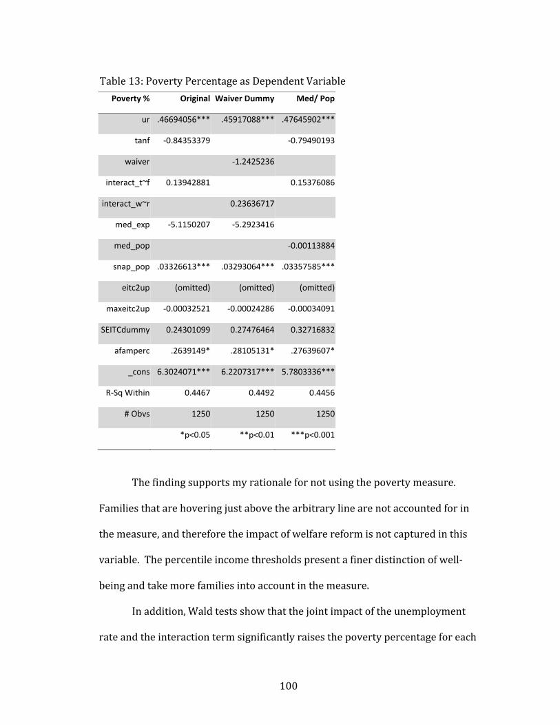
100

Poverty % Original Waiver Dummy Med/ Pop

ur .46694056*** .45917088*** .47645902***

tanf -0.84353379 -0.79490193

waiver -1.2425236

interact_t~f 0.13942881 0.15376086

interact_w~r 0.23636717

med_exp -5.1150207 -5.2923416

med_pop -0.00113884

snap_pop .03326613*** .03293064*** .03357585***

eitc2up (omitted) (omitted) (omitted)

maxeitc2up -0.00032521 -0.00024286 -0.00034091

SEITCdummy 0.24301099 0.27476464 0.32716832

afamperc .2639149* .28105131* .27639607*

_cons 6.3024071*** 6.2207317*** 5.7803336***

R-Sq Within 0.4467 0.4492 0.4456

# Obvs 1250 1250 1250

*p<0.05 **p<0.01 ***p<0.001 The finding supports my rationale for not using the poverty measure. Families that are hovering just above the arbitrary line are not accounted for in the measure, and therefore the impact of welfare reform is not captured in this variable. The percentile income thresholds present a finer distinction of well-being and take more families into account in the measure. In addition, Wald tests show that the joint impact of the unemployment rate and the interaction term significantly raises the poverty percentage for each

Table 13: Poverty Percentage as Dependent Variable

101

percentage point increase in unemployment. However, the joint impact of either TANF or welfare waivers are not significant at any level of unemployment. Therefore, unemployment does have a significant impact on poverty post-PRWORA, but not a significantly higher impact after welfare reform. In addition, the implementation of TANF does not have a significant impact on poverty as measured by the official poverty line. Future Work:

There is plenty of room for additional research on this topic to expand beyond the scope of this study. The foremost future research initiative would be to expand the scope of the time frame to the current period. While the income percentile thresholds that I used for my dependent variables had numerous advantages, its truncation at 2004 was a disappointment in that it missed the major effect of the past recession. The impact of this major recession was one of the primary motivations for undertaking this study on well-being, as poverty rates spiked in its wake. Although the 2001 recession resulted in a drop in well-being, the 2007 recession was much more severe and prolonged, exactly the type of recession that critics of the 1997 welfare reforms speculated about when TANF was implemented. In addition, many more TANF recipients would have exhausted their lifetime benefits by this recession than in the 2001 recession, making the recession additionally deleterious to low-income families’ economic well-being. In short, the addition of data encompassing the 2007 recession would most likely bolster my earlier findings on the income percentile threshold.

102

However, it could provide more robust support for the inequality findings. Nonetheless, the performance of TANF during this major recession would be a topic of further interest, particularly as data becomes available for the years following the recession. In addition to extending the time frame of the data, an additional future project would be to examine the effect of TANF on economic well-being within different groups of states. Some earlier studies in the literature explore this impact by dividing states into four levels of relative wealth, based on each state’s Per Capita Personal Income (PCPI). By breaking states up by wealth, we could observe the impact of TANF over the business cycle of rich and poor states and see how their impacts on well-being in those states differ. Poorer states in recessions are at a more severe disadvantage, since in addition to having a higher proportion of low-income residents, they don’t have the fiscal resources to respond to recessions as easily as high income states. On the other hand, many of the wealthier states are the states facing the largest budget crises currently, so perhaps they would fare worse during a downturn. An analysis by relative wealth would illuminate state differences in how well TANF works during recessions in different states. A similar state difference that is worth investigating is evaluating states by levels of TANF strictness. Rodgers and Payne (2007) take this approach in their evaluation of welfare reform’s impact on child poverty. In their study, they categorize each state’s individual welfare program based on its level of generosity and inclusiveness. A similar undertaking could be used to rank states

103

in a study on TANF’s impact on well-being. Do low-income families in states that emphasize a stronger “stick” approach fare worse in recessions than families in more generous states, or does the harsher approach drive enough families into the labor market to increase earnings over families in the generous states? By ranking states by these categories, we can glean additional insight on how TANF influences economic well-being over business cycles. Finally, the exact level of heteroskedasticity can be determined with a Feasible General Least Squares (FGLS) estimation technique. I use robust standard errors in my analysis, which gives a rough correction for the problem of heteroskedasticity. This measurement is appropriate for the percentile threshold level regressions, since the results are sufficiently robust to remain significant even with larger errors to approximate the effect of heteroskedasticity. However, an FGLS approach might be more suitable for the analysis of the inequality ratios, as these estimate results are not as robust.

104

V. Conclusion For the relative well-being measures, the inequality ratios, the regression results are sensitive to model specification and robustness tests. That finding could reflect the fact that the time period covered by the data is not sufficiently long. Nonetheless, the definitive answer on that question awaits collection of more recent data. In contrast, for the absolute measures of well-being, the threshold levels, the regression estimates are robust. The estimates indicate that the implementation of TANF following the 1996 welfare reform significantly altered the cyclical sensitivity of well-being, measured by percentile income thresholds. For each one-percentage point increase in the unemployment rate, there was a significantly larger estimated drop in the income thresholds post-TANF relative to pre-TANF. Furthermore, this result was consistent across each of the three bottom income percentiles in the years after PRWORA, indicating an increase in vulnerability among these families. The estimated impact of changing from the pre-TANF environment to a TANF regime is more complex. The combined estimated effect of the TANF dummy variable and the interaction term indicates that TANF has a different impact at different levels of unemployment. When the unemployment rate is low, TANF is shown to have an overall positive impact. This finding is consistent with earlier literature on welfare reform, which found that the strict provisions of TANF effectively pushed recipients off of welfare and into the labor market during the economic boom of the late 1990s. However, when the unemployment rate is high, TANF has an overall negative estimated

105

impact, indicating that TANF actually undermines family well-being for the lowest income percentiles during periods of high unemployment.

106

Bibliography Blank, R., and Lucie Schmidt (2001). Work, Wages, and Welfare. The New World of Welfare. R. Blank, and Ron Haskins. Washington, D.C., The Brookings Institution. Blank, R. (2002). Evaluating Welfare Reform in the United States. Cambridge, National Bureau of Economic Research. Blank, R. (2002). Welfare and the Economy. Welfare Reform and Beyond: The Future of the Safety Net. I. V. Sawhill, R. Kent Weaver, Ron Haskins, and Andrea Kane. Washington, D.C., The Brookings Institution. Blank, R. (2007). "Improving the Safety Net for Single Mothers Who Face Serious Barriers to Work." The Future of Children 17(2): 183-197. Blank, R. M. (2001). "Declining Caseloads/ Increased Work: What Can We Conclude About the Effects of Welfare Reform?" FRBNY Economic Policy Review September. Boyd, D. J., Patricia L. Billen, Phil Dearborn, Carol Meyers, and Jane McNeil (2003). The Fiscal Effects of Welfare Reform: State Social Service Spending Before and After Welfare Reform, Department of Health and Human Services. Chernick, H., and Andrew Reschovsky (1996). "State Responses to Block Grants: Will the Social Safety Net Hold?" The LaFollette Policy Report 7(2). Crouse, G. (1999). "State Implementation of Major Changes to Welfare Policies 1992-1998." from http://aspe.hhs.gov/hsp/Waiver-Policies99/Table_B.htm. Dye, R. F., and Therese J. McGuire (1999). State Fiscal Systems and Business Cycles. Washington, D.C., The Urban Institute. Fang, H., and Michael P. Keane (2004). "Assessing the Impact of Welfare Reform on Single Mothers." Brookings Papers on Economic Activity 1. Gais, T. L. (2009). "Stretched Net: The Retrenchment of State and Local Social Welfare Spending Before the Recession." The Journal of Federalism 39(3): Pgs 557-579. Gais, T. L., Lucy Dadayan and Suho Bae (2009). The Decline of States in Financing the U.S. Safety Net: Retrenchment in State and Local Socail Welfare Spending, 1977-2007, Rockefeller Institute of Government.

107

Grogger, J., Lynn A. Karoly, and Jacob Alex Klerman (2002). Consequences of Welfare Reform: A Research Synthesis, RAND. Grogger, J. (2003). "The Effects of Time Limits, the EITC, and Other Policy Changes on Welfare Use, Work, and Income Among Female-Headed Families." The Review of Economics and Statistics 85(2): 394-408. Grogger, J., and Lynn A. Karoly (2005). Welfare Reform: Effects of a Decade of Change. Cambridge, Harvard University Press. Gruber, J. (2003). Medicaid. Means Tested Programs. R. Moffitt. Chicago, University of Chicago Press. Gruber, J. (2011). Public Finance and Public Policy. New York, Worth Publishers. Haskins, R. (2001). Effects of Welfare Reform on Family Income and Poverty. The New World of Welfare. R. a. R. H. Blank. Washington, D.C., Brookings Institution Press. Haskins, R. (2006). Work Over Welfare: The Inside Story of the 1996 Welfare Reform Law. Washington, D.C., Brookings Institution Press. Herbst, C. M. (2008). "Do Social Policy Reforms Have Different Impacts on Employment and Welfare Use as Economic Conditions Change?" Journal of Policy Analysis and Management 27(4): Pgs 867-894. Hotz, V. J., and John Karl Scholz (2003). The Earned Income Tax Credit. Means Tested Transfer Programs. R. Moffitt. Chicago, University of Chicago Press. Jha, R. (1998). Modern Public Economics. London, Routledge. Kane, T. J., Peter R. Orszag and Emil Apostolov (2005). "Higher Education Appropriations and Public Universities: Role of Medicaid and the Business Cycle." Brookings-Wharton Papers on Urban Affairs. King, D. (1984). Fiscal Tiers: The Economics of Multi-Level Government. London, George Allen & Unwin. Klees, B. S., et al. (2009). Brief Summaries of Medicare and Medicaid. Washington, D.C., Department of Health and Human Services. Levinson, A. (1998). "Balanced Budgets and Business Cycles: Evidence from the States." National Tax Journal 51(4): 715-32.

108

Lewin Group and Nelson A. Rockefeller Institute of Government (2004). Spending on Social Welfare Programs in Rich and Poor States. Washington, D.C., Department of Health and Human Services. Li, H., and Mukti Upadhyay (2008). "Has the 1996 Welfare Reform Reduced the U.S. Poverty Rate? An Empirical Analysis Using Panel Data." Economics Bulletin 9(2). McGuire, T. J., and David F. Merriman (2006). State Spending on Social Assistance Programs Over the Business Cycle. Working and Poor. R. M. Blank, Danziger, Sheldon H., Schoeni, Robert F. New York, Russell Sage Foundation: 289-311. McKernan, S.-M., and Caroline Ratcliffe (2006). The Effect of Specific Welfare Policies on Poverty. Washington, D.C., The Urban Institute. Merriman, D. (2000). Sources of Data about State Government Revenues and Expenditures. Washington, D.C., The Urban Institute. Meyer, B. D., and Dan T. Rosenbaum (2001). "Welfare, the Earned Income Tax Credit, and the Labor Supply of Single Mothers." Quarterly Journal of Economics August. Moffitt, R. (2008). "A Primer on U.S. Welfare Reform." Focus 26(1): 12. Moffitt, R. A. (2003). The Temporary Assistance for Needy Families Program. Means Tested Transfer Programs. R. Moffitt. Chicago, University of Chicago Press. O'Neill, J. E., and M. Anne Hill (2001). Gaining Ground? Measuring the Impact of Welfare Reform on Welfare and Work. Civic Report. New York, Center for Civic Innovation. Rodgers, H. R., and Lee Payne (2007). "Child Poverty in the American States: The Impact of Welfare Reform, Economics, and Demographics." The Policy Studies Journal 35(1). Ruggles, P. (1990). Drawing the Line. Washington, D.C., The Urban Institute Press. Sawhill, I. V., R. Kent Weaver, Ron Haskins, and Andrea Kane, Ed. (2002). Welfare Reform and Beyond: The Future of the Safety Net. Washington, D.C., The Brookings Institution.

109

Schoeni, R. F., and Rebecca M. Blank (2000). What Has Welfare Reform Accomplished? Impacts on Welfare Participation, Employment, Income, Poverty, and Family Structure. Cambridge, MA, National Bureau of Economic Research. Smith, V., et al. (2008). Headed for a Crunch: An Update on Medicaid Spending, Coverage and Policy Heading into an Economic Downturn. Washington, D.C., Kaiser Commission on Medicaid and the Uninsured. Steuerle, C. E., and G. Mermin (1997). Devolution as Seen from the Budget. Washington, D.C., Urban Institute. U.S. Census Bureau (Various Years). State Government Finances. Washington, D.C., U.S. Census Bureau. U.S. Census Bureau (Various Years). Statistical Abstract of the United States. Washington, D.C., U.S. Census Bureau. U.S. House, Committee on Ways and Means (Various Years). Green Book. Washington, D.C., Government Printing Office. Weaver, R. K. (2002). The Structure of the TANF Block Grant. Welfare Reform and Beyond: The Future of the Safety Net. I. V. Sawhill, R. Kent Weaver, Ron Haskins, and Andrea Kane. Washington, D.C., The Brookings Institution. Wolff, E. N. (2009). Poverty and Income Distribution. Chichester, West Sussex, United Kingdom, Wiley-Blackwell. Wooldridge, J. M. (2009). Introductory Econometrics. Mason, OH, South-Western.