The Impact of Taxes on Income Mobility

The Impact of Taxes on Income Mobility∗

Mario Alloza†

BANK OF SPAIN and CfM

First Version: September 15, 2015This Version: September 1, 2018

Abstract

This paper investigates how taxes affect relative mobility in the income distri-

bution in the US. Household panel data drawn from the PSID between 1967 and

1996 is employed to analyse the relationship between marginal tax rates and the

probability of staying in the same income decile. Exogenous variation in marginal

tax rates is identified by using counterfactual rates based on legislated changes in

the tax schedule. I find that higher marginal tax rates reduce income mobility. An

increase in one percentage point in marginal tax rates causes a decline of around

0.8 percentage points in the probability of changing to a different income decile.

Tax reforms that reduce marginal rates by 7 percentage points are estimated to

account for around a tenth of the average movements in the income distribution

in a year. Additional results suggest that the effect of taxes on income mobility

differs according to the level of human capital and that it is particularly significant

when considering mobility at the bottom of the distribution.

Keywords : income mobility, inequality, marginal tax rate.

JEL classification: E24, E62, D31, D63, H24, H31.

∗I am indebted to Morten Ravn for invaluable guidance and support and also to Raffaella Giacominiand Vincent Sterk for very helpful discussions and insightful suggestions. I also want to thank AndrewChesher, Mariacristina De Nardi, Eric French, Valerie Lechene, Attila Lindner, Fabien Postel-Vinayand audience at UCL, University of Essex, Bank of England, Bank of Spain, CREST, UniversitatAutonoma de Barcelona, Queen Mary University of London, University of Manchester, NazarbayevUniversity, Uppsala University, the 2017 Royal Economic Society Annual Conference, Halle Institutefor Economic Research and the 16th Journees Louis-Andre Gerard-Varet for their comments and usefulconversations.

†Mario Alloza: Banco de Espana, Calle Alcala 48, 28014, Madrid (Spain), [email protected].

mailto:[email protected]

1 Introduction

The last four decades have witnessed a sustained increase in income and wealth inequal-

ity in the US, particularly at the top end of the distribution.1 This phenomenon has

received substantial attention in academic research,2 policy debates as mentioned in

President Obama’s Economic Report (see Council of Economic Advisers (2015)), and

popular opinion (e.g. protest movements such as Occupy Wall Street). As noted in Ar-

row and Intriligator (2015), inequality is a highly relevant normative issue, since society

perceives an unequal distribution of income as an unjust outcome of market economies.

However, there are other features of the income distribution beyond inequality that

have welfare implications for the society and are relevant from a policy point of view.

Overlooking some of these aspects may yield an incomplete or inaccurate picture of the

effects of policies that address economic disparities.

This paper looks at the impact of fiscal policy on another aspect of the income

distribution different to inequality. Particularly, I investigate the relationship between

taxes and income mobility. While inequality reflects changes in the variance (and

higher moments) of the income distribution, income mobility is the result of variations

in the covariance of income between two periods of time.3 For any given level of

income inequality, mobility reduces the association between the positions of origin and

destination in the income distribution, increasing equality of opportunity. Therefore, to

the extent that income mobility is a desirable feature of an economy, it is then relevant

to consider how fiscal policy may affect it.4

I analyse the impact of taxes on the probability of moving in the income distribu-

tion in the US using data from the Panel Study of Income Dynamics (PSID). I measure

income mobility as changes in the relative position of households in the income dis-

tribution (i.e. changes in deciles or quintiles) across time. Income is defined as the

Adjusted Gross Income (AGI) of the household. I assess the degree of mobility across

three specifications for the income distribution that consider pre-tax income, post-tax

income and post-tax and post-transfer income respectively. Then, I construct the fed-

1See Piketty and Saez (2003) for long-run trends in income inequality and Saez and Zucman (2014)or Quadrini and Rıos-Rull (2015) for the case of wealth.

2Piketty (2014) provides extensive evidence of income and wealth inequality around the world whileStiglitz (2012) highlights its consequences: “the impact of inequality on societies is now increasinglywell understood -higher crime, health problems, and mental illness, lower educational achievements,social cohesion and life expectancy” (inside cover).

3See Gottschalk (1997).4Kopczuk et al. (2010) argue for the need to study income inequality and mobility jointly. Income

mobility is a determinant of inequality in the long run: when there is no mobility in the incomedistribution, short-run inequality perpetuates.

2

eral individual tax liabilities faced by each household in the sample using the NBER

TAXSIM simulator. With these data in hand, I estimate a linear probability model to

understand how changes in the marginal tax rate affect the likelihood that households

are mobile in the income distribution during two adjacent years. My identification ap-

proach accounts for endogeneity in the marginal rates by isolating the variation in taxes

that is only due to legislative changes. I exploit this source of exogenous variation as

an instrument in the regressions.

The results obtained suggest that higher marginal tax rates reduce income mobility.

Particularly, I find that an increase of one percentage point (pp) in the marginal rate

is associated with declines of about 0.5-1.3pp in the probability of changing deciles of

income. A decrease of 7 percentage points in the marginal tax rate (slightly smaller

than a standard deviation of non-zero changes in the rates) can account for about a

tenth of the average income mobility in a year. The effect of taxes on mobility arises

in specifications that consider income distributions both before and after taxes and

transfers, suggesting that the impact of taxation on mobility goes beyond redistribution

effects. The economic mechanism that induces this impact seems to be related to the

labour market incentives created by changes in the tax schedule. Additional results

suggest that the effect of taxation on income mobility differs according to the level of

human capital (measured as the education of the head of the household) and that it is

particularly significant when considering mobility at the bottom of the distribution.

The evidence that taxes have a negative impact on income mobility has important

implications for the design of policies that aim to address economic disparities. While

some studies have pointed out to the importance of progressive taxation in addressing

inequality,5 the results from this paper suggest that such changes may have a detrimen-

tal impact on income mobility. Therefore, the design of optimal fiscal policy should

consider the overall impact on welfare of the trade-off that might arise when jointly

addressing income inequality and mobility.

This paper relates to different strands of literature. First, it is connected to the

literature that investigates the effects of tax changes on taxable income (elasticity of

taxable income, or ETI), as reviewed in Saez et al. (2012). This research finds that

taxable income only reacts moderately to changes in the marginal tax rate.6 Mertens

(2013) suggests that accounting for empirical difficulties in the estimation of the ETI at

5See Piketty and Saez (2007) and Diamond and Saez (2011).6Saez et al. (2012) suggest a range of estimates from 0.12 to 0.40 for the ETI. The authors argue

that responses for the top-earners can be substantially higher. For example, Slemrod (1996) finds thatthe Tax Revenue Act of 1986 explains to a large extent the increase in reported income of the topearners.

3

the aggregate level (such as policy endogeneity or timing) results in larger elasticities

for different income groups beyond the top earners. My paper relates to some method-

ological aspects of this literature,7 but I focus on the effects of taxes on measures of

household’s mobility across the income distribution as opposed to the individual’s re-

sponse of reported taxable income (for this purpose I employ a different type of data,

the PSID, that allows me to control for relevant demographic factors).

My paper relates to an extensive literature on income mobility surveyed in Fields and

Ok (1999) and Jantti and Jenkins (2015).8 Early works on the measurement of income

mobility include Shorrocks (1978a) and Shorrocks (1978b), which lay down many of

the tools currently used to measure mobility. A number of papers have investigated

the degree and evolution of mobility in terms of income (broadly defined) and earnings.

Hungerford (1993) uses family income data from the PSID to analyse trends in mobility,

focusing on changes in the position in the income distribution between 7 year-periods in

both annual and permanent income. The author compares mobility between the 1970s

and 1980s to find considerable movement within the income distribution (although he

finds less evidence of sizeable upward or downward movements). Also using PSID data,

Gottschalk (1997) looks at earnings mobility in one-year and seventeen-year periods.

The author concludes that the degree of mobility is high enough to support the view

that people are not stuck at the bottom or the top of the distribution. Kopczuk et al.

(2010) employs individual data from the Social Security Administration to investigate

the evolution of both short-term mobility (measured by changes in rank correlation in

year-to-year earnings and in mobility indices defined over periods of 3-5 years) and long-

term mobility (i.e. across the working life). More recently, Bradbury (2011) looks at

various indices of income mobility using the PSID between 1969-2006 and time intervals

spanning 11 years.

Although the concepts of mobility and samples used differ, these papers find a

similar evolution of mobility in the US: a relatively flat profile during the 1970s and a

somewhat decreasing trend after that. I measure mobility in comparable ways to this

literature, however, since my main goal is to identify the effects of tax changes, I instead

7I use variation in legislated taxes to address endogeneity following Gruber and Saez (2002).8During this paper, I will refer to income mobility as intragenerational mobility. Jantti and Jenkins

(2015) also survey the literature on intergenerational or social mobility (the degree of associationbetween parents and children income). There has been a recent increase in the research aiming tounderstand the degree of intergenerational mobility and its factors. For example, Chetty et al. (2014a)analyses the geographical differences of intergenerational mobility in the US and Chetty et al. (2014b)explores its evolution over time, which has remained fairly constant despite rising inequality. Thedeterminants of social mobility are explored in Chetty and Hendren (2015), who investigate howneighbourhoods affect intergenerational mobility through childhood exposure effects.

4

consider mobility across two adjacent years.9

The literature on the effect of taxes on income mobility is more limited. Lerman and

Yitzhaki (1995) analyse the effects of the 1991 tax reform on the income distribution

recognising two potential channels: higher taxes can reduce the income gaps between

people and, in some cases, change their relative position by means of redistribution.

The authors decompose the evolution of the Gini coefficient due to income changes

holding the relative position constant and due to changes in the relative position holding

income constant, and find that this second effect is important in understanding the

redistribution effects of the the 1991 tax reform. Larrimore et al. (2015) analyse the

determinants of income mobility between two-year periods using a panel of tax returns

between 1999 and 2011. They compute the difference between income before and after

federal taxes as a measure of the stabilising power of taxes.

In contrast to both Lerman and Yitzhaki (1995) and Larrimore et al. (2015), I

analyse the effects of taxes on mobility that can also be due to changes on the pre-tax

income (i.e. because of a change in the labour supply), not only due to the redistribution

effect of the tax system. More substantially, my paper uses a different methodology

to asses the impact of taxes on income mobility by exploiting exogenous variation in

the marginal tax rates, over a relatively long panel of data that includes several tax

reforms.

This paper also relates to the literature that investigates the aggregate impact of

taxes such as Romer and Romer (2010) and Barro and Redlick (2011). Both studies find

substantial effects of changes in taxes on economic activity. Romer and Romer (2010)

estimate the impact of a tax increase of 1 percent of GDP to amount to a reduction

of output by 3% over the course of three years. Barro and Redlick (2011) find that

the effect of taxes on GDP act mainly through substitution effects, with increases in

the average marginal tax rates significantly reducing GDP.10 Mertens and Ravn (2013)

highlight the importance of distinguishing between different type of taxes, estimating

large effects of taxes on output in the short run. Zidar (2015) exploits variation in US

states to find aggregate effects on employment resulting from tax cuts for lower-income

groups (as opposed to tax cuts for the top 10% of the income distributions, which are

not found to have a large effect on employment growth).

Income and wealth inequality have been the object of extensive study in macroeco-

9Gottschalk (1997) notes that accounting for longer periods is not necessarily more appropriatethan one-year periods to analyse mobility and inequality, given the fact that low-income householdsare more likely to face borrowing constraints over longer horizons.

10Barro and Redlick (2011) find that GDP falls 1.1 for each dollar increase in federal taxes, withone year lag.

5

nomics.11 Piketty and Saez (2003) use a long panel of tax returns to analyse income

inequality trends in the US since 1917. The authors find that income inequality, as

measured by the share of income by the top decile earners, sharply decreased during

World War II and started to increase from the 1970s.12 Piketty (2014) compiles exten-

sive empirical evidence on the evolution of income and wealth inequality for the US and

other countries, finding a noticeable increase in both variables. The author suggests

that this increase in inequality is a feature of capitalist economies (given that the rate

of return of capital is found to exceed that of economic growth) and advocates for fiscal

reforms that establish a global wealth tax and a more progressive income taxation.

In order to understand the causes of wealth inequality, macroeconomic models have

relaxed the assumption of a representative agent, allowing for heterogeneity in earnings

and other characteristics, in the spirit of Aiyagari (1994).13 Quadrini and Rıos-Rull

(2015) survey the literature on the theories used the explain the causes of inequality, and

its implications for the aggregate economy. While economic models predict that wealthy

households tend to dissave, this is at odds with the data. De Nardi (2015) surveys the

mechanisms that have been used to explain the reasons for wealthy individuals to

exhibit a high rate of savings and its implications for wealth inequality. This literature

has found that differences in the degree of patience among individuals, the transmission

of human capital (skills passed from parents to children) and voluntary bequests across

generations or the decisions to become an entrepreneur are plausible reasons that can

explain some aspects of the distribution of wealth.

The rest of the paper is organised as follows. Section 2 develops a simple frame-

work to understand the relevant mechanisms behind the effect of taxation and income

mobility. Section 3 describes how the data regarding income mobility and taxes are

constructed. The empirical strategy and the main results are described in Section 4.

Section 5 contains several robustness checks. Further empirical results on the hetero-

geneous effects of taxes on income mobility are explored in Section 6. Lastly, Section 7

concludes and discusses potential extensions.

11Aghion et al. (2015) investigate the relationship between innovativeness and both top-incomeinequality and social mobility.

12Building on the same dataset, Saez and Zucman (2014) capitalise income to produce measures ofwealth inequality, and find that this variables has substantially increased in the last few years.

13See Heathcote et al. (2009).

6

2 A Simple Theoretical Framework

Before turning to the empirical analysis, I consider a simple model of labour supply

to highlight the key determinants of the relationship between taxation and income

mobility.

Consider an economy populated by two households (i = 1, 2) with quasilinear pref-

erences:

U(ci,t, ni,t) = σici,t −Xi

1 + 1ηi

n1+ 1

ηit

where ci,t and ni,t represent consumption and hours worked for household i at date

t. Preference parameters can potentially depend on each household characteristics: σi

represents the relative weight of consumption in the utility function, Xi denotes pref-

erences regarding labour supply (which could be determined by demographic variables,

family composition, etc.) and ηi ≥ 0 is the Frisch elasticity of labour supply (a key

element in this framework).

Individuals face a budget constraint ci,t = (wi,tni,t) − T (wi,tni,t), where wages wi,t

evolve exogenously following wi,t = w(1 ± εi,t), with εi > 0. In each period, wages are

equal to w1,t = w(1 + ε1,t) for household i = 1 and w2,t = w(1 − ε2,t) for household 2

with probability π > 0. With probability 1 − π wages become w1,t = w(1 − ε1,t) and

w2,t = w(1 + ε2,t). The tax system is assumed to be given as:

T ′(wi,tni,t) =

{τL + τ if (wi,tni,t) ≥ (1 + ε)wnH∗

i,t

τL if (wi,tni,t) < (1 + ε)wnH∗i,t

(1)

where τL and τL + τ are the marginal tax rates faced by households with a low or high

wage realisation, respectively. nH∗i,t and nL∗

i,t are the labour supply functions that result

from optimality in consumption-leisure decisions:

nH∗

i,t =

((1− τL − τ)(1 + ε)w

σi

Xi

)ηi

nL∗

i,t =

((1− τL)(1− ε)w

σi

Xi

)ηi

Assuming that preferences are the same for both type of households (η1 = η2 = η,

σ1 = σ2 = σ, X1 = X2 = X), when τ = 0 the tax schedule becomes proportional

and the household with a higher realisation of wages (say, i = 1) is ranked first in the

7

income distribution:

(1− τL)(1 + ε)wnH∗

1,t > (1− τL)(1− ε)wnL∗

2,t

Conditional on an initial distribution of income, the relative income mobility in this

economy is given by Pr (move|w2,t−1 = w(1 + ε)) = π.

When τ is positive, the tax schedule is progressive and both labour-supply functions

are related by:

nH∗

i,t =

((1− τ

1− τL

)(1 + ε

1− ε

))η

nL∗

i,t

In any given period, the optimal labour supply choice weights two opposing effects:

(i) a higher wage 1+ε1−ε

increases the price of leisure and makes the household willing

to supply more labour and (ii) a higher rate τ makes the tax system more progressive

and reduces the incentives to supply more hours of work. As long as τ < (1 − τLt )2ε1+ε

the household will have incentives to take advantage of a higher wage draw and will

optimally choose to supply more labour nH∗i,t > nL∗

i,t . When τ is high enough, the tax

schedule eliminates the incentives to work induced by a a high-wage shock. Particularly,

when τ = (1 − τLt )2ε1+ε

the household will decide to not to increase the hours of work

due to the wage shock and nH∗i,t = nL∗

i,t .14

In the case of τ = (1 − τLt )2ε1+ε

, both households supply the same amount of hours

worked. In the presence of preference shocks Xi that counteract the effects of the wage

shocks, less progressive taxation would render the labour supply of the households more

sensitive to changes in wages, resulting in higher income mobility.

This simple framework allows us to derive the following implications. First and

most important, the tax system can reduce income mobility by disincentivizing labour

supply. This effect arises because households take less advantage of economic oppor-

tunities when the marginal tax rate is very high. The final effect on mobility depends

crucially on the Frisch elasticity of labour supply (and whether it is homogeneous across

households) since this parameter governs how much the taxes distort the incentives to

work. Preferences regarding consumption also matter. A wealth effect on labour sup-

ply, which is absent in this minimal framework, will make households more willing to

supply work when taxes increase (although this effect will be mitigated by a progressive

tax schedule). Another important factor in determining mobility is the wealth accu-

mulation. When savings are allowed, households face an intertemporal optimisation

14When we consider τL = 0.25 (approximately the US average federal marginal tax rate on individualincome during 1967-1996), w = 10 and productivity shocks representing 5% of the base wage w, thenwe have that the value of τ such that nH∗

i,t = nL∗

i,t is τ = 0.07, resulting in τL + τ = 0.32.

8

problem. Those households who are lucky and obtain subsequent realisations of high

wages will be able to build up savings. The return obtained from these savings will

increase total income, making it less likely to move down in the income distribution.

Therefore, while taxes are likely to have an effect on income mobility, the precise

impact remains an empirical question. When estimating this effect, it will be important

to use data that allows separating household effects (as, for example, taste for leisure)

from household shocks. The PSID, given its panel nature, is an attractive dataset to

address this question.

3 Data and Trends

The PSID (Panel Study of Income Dynamics) is an annual survey elaborated by the

University of Michigan since 1968.15 It follows the same families and their split-offs

over time, creating a panel structure. The survey was originally created from two

samples: the Survey Research Center (SRC) or core sample (representative at the

national level), and the Survey of Economic opportunity (SEO) or Census sample,

which over-represents low income households. The PSID provides weights that render

the combination of both samples representative of the US population while accounting

for the attrition that occurs over time when families are stopped being interviewed.

I restrict the whole sample by considering main adults (the heads and their spouses)

of households that are led by a male working head aged 25 to 60 who is not self-

employed. Following Aaronson and French (2009), families with a head working less

than 300 or more than 4,500 hours per year, earning less than $3 or more than $200

per hours in 1996 prices are considered outliers and dropped from the sample. This

selection criteria is based on the intention to reflect changes in the income mobility that

arise as a result of labour market interactions. In Section 5, I check the robustness of

the results when considering a more inclusive sample. This selection leads to a total

of 5,430 (continuously married) households representing a total of 50,471 observations

between 1967 and 1996. The final date of the sample is dictated by the change in the

PSID frequency produced in 1997 (referring to data from 1996), when the periodicity

of data releases switched from annual to biannual.

15The survey contains data from 1967, since some of the variables asked (e.g. income) refer to theprevious year.

9

3.1 Measuring income mobility

This section discusses issues related to income mobility measure and explores its dy-

namics in the US over the sample period.

Consider an ordering of income in time t in N different ranks (i.e. quantiles of

income). Let snt denote the households with income belonging to rank n ∈ [1, N ]. The

mobility process can be represented by a vector st = (s1t , s2t , . . . , s

Nt ) and a probability

matrix P with dimension n× n and rows adding up to 1 such that:

st = Ptst−1 (2)

The vector st−1 summarises the probability distribution of income in period t − 1.

The matrix Pt characterises the mobility process by determining the probability that

a household in income group n at time t − 1 remains in the same decile next period

(entry P n,nt in matrix Pt) or transits to another decile k = n.16

There are different indices that can be used to measure the degree of income mobil-

ity.17 The immobility ratio (IR) summarises changes in relative positions by computing

the degree of concentration along the diagonal of matrix Pt, i.e. the fraction of house-

holds that remain in the same income group during two periods of time. In the case of

extreme immobility (no household changes deciles between t and t− 1), IR= 1.

In a similar vein, the normalised trace index (NTI) proposed by Shorrocks (1978b)

uses the elements in the diagonal of Pt to measure mobility:

NTIt =N − trace(Pt)

N − 1

When Pt is the identity matrix, the sum of the diagonal of matrix Pt is equal to N and

the NTI becomes 0.

Both the IR and NTI indices use information from the diagonal of matrix Pt. The

Average Jump Index (Bartholomew (1973)) exploits other information in Pt to asses

the degree of mobility by counting the number of income thresholds (e.g. deciles) that a

households passes through between two periods. This index is computed as the average

of absolute changes in income ranks for all the sample. A value of 0 indicates perfect

immobility (origin independence).

16In the special case when vector st−1 contains all the necessary information to predict st, i.e.Prob(st|st−1, st−2,, . . . , st−k) = Prob(st|st−1) ∀k ≥ 1 and t, the process st is said to be Markovian. Pt

becomes the Markov matrix and transitions along the income distribution between k periods can beobtained from st+k = stP

k.17See Fields and Ok (1999) or Jantti and Jenkins (2015) for exhaustive reviews of the different tools

available to measure income mobility.

10

There are other measures that are not restricted to the relative position of house-

holds in the income distribution. This is the case of the Pearson correlation (rt), defined

as:

rt = corr(log(inct−1), log(inct)

)where inct is the real level of income at time t. The Hart index (Hart (1976)) is a

variant of this measure and is defined by Ht = 1 − rt. When income between two

periods is perfectly correlated, we have the case of complete immobility and Ht = 0.

Income is constructed as the Adjusted Aggregate Income (AGI) based on the joint

taxable income of the head and spouse in the household.18 Different measures of income

(before taxes, after taxes, and after transfers) are used to assess mobility.

Figure 1 plots the evolution of the mobility indices described above using a pre-

tax measure of income, setting N = 10 (income is divided in deciles) and allowing t

to represent a year. While many studies in the literature focus on a longer horizon to

analyse mobility (e.g. five years), I choose to use a shorter horizon to be able to identify

the effect of taxation on income mobility.

The degree of co-movement between the indices of mobility is high: 1-IR and NTI

have a correlation of 95%. The correlation between those two indices and the measure

of income ranks passed is of 90 and 88%, respectively. The correlation between the

Hart index and the rest of mobility measures ranges between 70 and above 80%.

The evolution of these indices shows a flat profile from the end of the 1960s to the

end of the 1970s, although the NTI index exhibits a slightly upward trend during this

period. Mobility declines somewhat during the decade of the 80s. It increases more

noticeably at the beginning of 1990s (particularly the 1-IR index), but then returns to

previous levels towards the end of the sample. The comparison of this evidence with that

found in the literature is difficult, since many studies focus on income mobility during

a longer time horizon (see for example Hungerford (1993) and those cited in Jantti

and Jenkins (2015)). However, Gittleman and Joyce (1999) considers similar mobility

indices for 1, 5 and 10-year windows between 1969 and 1990. The authors find a mild

reduction in mobility during the 1970s and an upwards trends until 1990. Gottschalk

(1997) reports a transition matrix across quintiles of income between 1973 and 1974

using PSID which is largely similar to my estimation of matrix Pt in Equation 2 for

those years (not shown).

While Figure 1 displays the probability of mobility overall, it is also interesting to

18A broader definition of income would include other sources within the family (e.g. children orother relatives). However this would require making assumptions on how to identify tax units withinthe household and limit the availability of data. Section 5 explores the robustness of the results todifferent definition of income.

11

analyse whether these trends in mobility are shared across particular income ranks.

Figure A1 shows the evolution of 1−P 1,1t and 1−PN,N

t (where P k,kt is the k, k element

of matrix Pt in Equation 2) for pre-tax and post-tax distributions of income. The

probability that a household moves away from the first decile of income (Panel A) has

recorded an upward trend during most of the time horizon, only to be reverted towards

the end of the sample period. The evolution of the probability of not remaining in the

top decile shows a pattern that resembles that of the 1-IR index commented in the

previous paragraph: a downwards trend initiated after 1975 which changes direction

since the beginning of the 1990s.

3.2 Taxation in the US during the sample period

I use the NBER’s TAXSIM program to construct the federal tax liabilities faced by

each household in the sample. This tax simulator recreates each year’s tax law by

taking into account features of the US tax code such as the Earned Income Tax Credit

(EITC), the Alternative Minimum Tax (AMT) or deductions and exemption phase-

outs. Since TAXSIM only computes state taxes since 1977 and due to the regressive

nature of Social Security taxes (FICA), the main empirical results in Section 4 make

use of a longer horizon (and additional tax reforms) by exclusively considering changes

in federal taxation. The effects of including state and social security taxes are explained

in Section 5.

TAXSIM computes the effective marginal tax rates by increasing taxable income

by 1$.19 For many households in the PSID sample these tax rates are determined by

the statutory tax rates associated with each income bracket. However, the effective

marginal tax rate of other households will also be determined by the phase-out and

other features of the tax code.

Marginal tax rates from TAXSIM are calculated based on tax year, marital status

(since the sample only considers (legally) married people, I assume them to file taxes

jointly), number of dependants (including those under 17 years), labour income from

the head of the household and his spouse, asset income (arising from rentals, dividends

or interests), taxable pensions, Social Security Income, property taxes and deductions

on mortgage interests.20

Federal marginal tax rates have experienced substantial variation during the period

considered (1967-1996). Figure 2 (Panel A) shows the evolution of the average marginal

19See Feenberg and Coutts (1993) for an introduction to the TAXSIM program.20Since mortgage interests are not available in the PSID for all the time horizon, I follow Aaronson

and French (2009) and assume that 80% of mortgage payments go to interest to impute this variable.

12

tax rate for each income decile in US during 1967-1996.21 The broken line shows the

average marginal tax rate for federal individual income taxes from Barro and Redlick

(2011).22 Marginal tax rates show a marked increase during the 1970s, mainly as the

result of high inflation that pushed households’ income to higher tax brackets because

of imperfect indexation of the tax schedule. This upward trend was more substantial for

higher incomes: the average marginal tax rate for those in the top decile increased 22

percentage points between 1967 and 1980 (from 26.9% up to 49%) while the increase for

the bottom three deciles ranged between 5 and 7 percentage points. This upward trend

was substantially reverted during the decade of 1980s. This was the result of major

reforms such as Reagan’s Tax Reform Act of 1986, which lowered the top statutory

rate from 50% to 28% (although the bottom tax rate increased by 4 percentage points).

Some smaller tax increases occurred during the early 1990s (e.g. a tax hike to high

income earners during Clinton’s presidency increased the marginal tax rate of the top

decile from 31.3% to almost 33% in 1994).The increase of the average marginal tax rate

for the bottom decile since the end of the 1980s and even above the average marginal

tax rates of other deciles is the result of the expansion of the EITC.23

Panel B in Figure 2 shows the individual federal income tax rates for the PSID

households computed using the NBER calculator.24 The figure distinguishes between

tax rates before and after the Reagan 1968 reform. The plot shows the noticeable trans-

formation of the tax code following the Tax Reform Act of 1986, which substantially

simplified the US tax code.

The high variation of taxes over time and across individuals depicted in Figure 2

supports the identification of the causal impact of tax reforms on income mobility.

3.3 The relationship between taxation and Income mobility

This subsections explores the relationship between income mobility and taxation at

the aggregate level. The correlation between the indices of mobility 1-IR and NTI

(described in Section 3.1) and the AMTR from Barro and Redlick (2011) ranges between

21See Figure A2 for the evolution of the average tax rate during the same period.22Barro and Redlick (2011) uses data from a random sample on actual tax files and computes the

average marginal tax rate with TAXSIM.23Note that while alterations of the EITC and other provisions have increased the average marginal

rate of the bottom deciles, the tax pressure of this group (as measured by the average tax rate shownin Figure A2) has lowered since 1986.

24The PSID provided an estimation of the marginal tax rate on federal income during 1976-1991based on question in the survey regarding exemptions, filling status, etc. The correlation with mymarginal tax rate computed through TAXSIM is above 90%. Butrica and Burkhauser (1997) explorethe differences between the PSID simulations and TAXSIM.

13

35-45%. However, the evolution of the AMTR is not exclusively restricted to taxes in

legislation, but also the result of macroeconomic developments (e.g. inflation increasing

the taxable income of households and pushing them to higher tax brackets).

In order to isolate changes in the US tax code from macroeconomic developments, I

use the measure of legislated tax changes developed by Romer and Romer (2010). The

authors produce a narrative series of changes in federal tax revenues (as a percentage

of GDP) by documenting legislated tax changes in the postwar US. Table A1 shows the

correlation between the mobility indices mentioned in Section 3.1 and the Romer and

Romer (2010) measure of legislated tax changes (τRomer). The relationship between tax

changes and mobility appears to be negative, albeit small. An OLS regression of the

percentage of households changing deciles (of net income) on the narrative series τRomer

yields a slope coefficient of 0.0159 (robust standard error of 0.0064), suggesting that

legislated tax changes that increase tax revenues by 1% of GDP reduces the percentage

of households changing deciles by about 1.6 percentage points.25

The correlations from Table A1 should not be given a causal interpretation. Legis-

lated changes in the tax code are sometimes the result of contemporaneous economic

developments, what could result in a problem of endogeneity when using aggregate data.

In this context, the observed negative correlation between mobility and taxes would be

the result of the state of the economy, as opposed to the disincentives produced by the

tax system.

To further explore the relationship between income mobility and taxes and the

direction of causality, I consider an alternative measure to τRomer that only includes tax

changes not motivated by economic developments. Romer and Romer (2010) produce

such narrative by exploring the motivation behind each tax change and classifying them

as endogenous (motivated by economic meanings) or exogenous (motivated by ideology

or other concerns uncorrelated to the current state of the economy). Mertens and Ravn

(2013) and Mertens (2013) further refine this series by considering only those exogenous

tax changes that affect employment taxes or individual income that became effective

within one year of their legislation.26

Figure 3 plots the relationship between some relevant indices of mobility based on net

25The effect of τRomer on other measures of mobility as described in Section 3.1 ranges between -0.0242 and -0.0073 depending on the index considered, the definition of income, and number of incomeranks (deciles or quantiles). However, some of these coefficients are estimated with high standarderrors.

26This last criterion accounts for the effect of anticipation (i.e. the case where the econometricianhas less information than the economic agents). See Mertens and Ravn (2011) and Mertens and Ravn(2012) for an analysis and evidence on the effects of anticipation in taxes, and Ramey (2011) for thecase of anticipation in government spending.

14

income (1-IR, NTI and the number of income thresholds passed) and the two narrative

measures of exogenous legislated tax changes (τ exo−TOT and τ exo−PI) described in the

previous paragraph. Large tax cuts seem to be associated with higher values of the

mobility indices (more relevant when considering the measure based on unanticipated

personal income tax changes, τ exo−PI). Correlations between these two variables range

from −11% to −35%. However, the limited number of tax changes meeting the above

criteria makes it difficult to obtain conclusive results from this preliminary analysis. The

next section analyses further this question by exploiting the disaggregated information

contained in the PSID data.

4 Empirical Analysis

4.1 Estimation Strategy

The objective of this section is to quantify the effect of taxation on income mobility. To

estimate this effect I regress measures of mobility that vary on the definition of income

and the number of ranks used to divide the income distribution on the marginal tax

rate. I estimate the following regression:

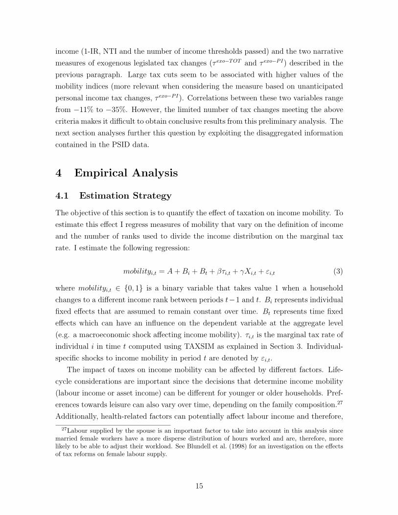
mobilityi,t = A+Bi +Bt + βτi,t + γXi,t + εi,t (3)

where mobilityi,t ∈ {0, 1} is a binary variable that takes value 1 when a household

changes to a different income rank between periods t−1 and t. Bi represents individual

fixed effects that are assumed to remain constant over time. Bt represents time fixed

effects which can have an influence on the dependent variable at the aggregate level

(e.g. a macroeconomic shock affecting income mobility). τi,t is the marginal tax rate of

individual i in time t computed using TAXSIM as explained in Section 3. Individual-

specific shocks to income mobility in period t are denoted by εi,t.

The impact of taxes on income mobility can be affected by different factors. Life-

cycle considerations are important since the decisions that determine income mobility

(labour income or asset income) can be different for younger or older households. Pref-

erences towards leisure can also vary over time, depending on the family composition.27

Additionally, health-related factors can potentially affect labour income and therefore,

27Labour supplied by the spouse is an important factor to take into account in this analysis sincemarried female workers have a more disperse distribution of hours worked and are, therefore, morelikely to be able to adjust their workload. See Blundell et al. (1998) for an investigation on the effectsof tax reforms on female labour supply.

15

mobility.28 To account for all these factors, vector Xi,t in equation 3 includes the age of

the head and wife, the size of family, number of children below 18 in the household, a

dummy for a working spouse and a dummy for the health status of the head as control

variables.

I will consider specifications where the dependent variable mobilityi,t differs in how

income is measured: income before federal taxes, income after federal taxes but before

transfers, and income after taxes and transfers.29 In this way, we will be able to

distinguish whether the potential impact of taxes on income mobility is restricted to

the redistributive effect of the tax and transfer system or has a more fundamental

reason such as affecting the labour supply choices (as described in Section 2). I will

also consider specifications where the dependent variable mobilityi,t differs in how ranks

of the income distribution are defined, distinguishing between deciles and quintiles in

order to further support the robustness of the results.

4.2 Results from OLS regressions

Table 1 shows the results of estimating Equation 3 using OLS. The effect of the marginal

rate on the probability that the household moves to a different decile of pre-tax income

is negative and highly significant: the point estimate is −0.383 (standard error of

0.06).30 The results are robust to the inclusion of control variables regarding life-cycle,

demographics, spouse labour supply or health status.

Table 2 explores the effects of taxation on alternative measures of income and income

ranks. Columns 1-3 report the impact on the probability of changing deciles of income

before taxes and transfers, income after taxes and before transfers, and income after

taxes and transfers, respectively. Columns 4-6 use the same measures of income but

consider instead the effects on the probability of changing quintiles of income. The

estimated coefficient of the marginal tax rate is significant above the 99% level for all

six specifications. The size of the effect is about -0.40/-0.35 for most regressions, with

the specification that considers changes in quantiles of post-transfer income reporting a

slightly smaller estimate (-0.285). Overall, these result suggest that there is a negative

28See French (2005) for an investigation on how health affects labour supply and retirement decisions.29Transfers include both non-taxable public income (e.g. Supplemental Security Income (SSI) bene-

fits) and income transferred from other sources (e.g. relative). During the period considered, the PSIDdoes not offer exact information on public transfers alone (SSI is reported, but others are not) withyearly frequency. However, the percentage of non-public income in the transfers variable consideredhere was only about 0.4% in 1980, on average.

30Throughout this paper, models that estimate a binary outcome report estimates that can beinterpreted as changes in probability. For example, an estimate of -0.383 represents a reduction ofsuccess of the dependent variable of 0.383 percentage points.

16

relationship between taxes and income mobility.

4.3 Results from IV regressions

The US tax code is progressive and the marginal tax rate depends therefore on income.

This causes τi,t in Equation 3 to be endogenous: when a shock εi,t affects income

positively, the household will be pushed to a higher tax bracket, and rendering the OLS

estimation of Equation 3 biased. In principle, the direction of the endogeneity bias

is not clear since it depends on how a shock to εi,t affects τi,t. Consider the case of

a positive individual shock (e.g. a time varying preference shock) that raises income

and, as result of it, mobility. Since the individual will face a higher tax bracket, the

relationship between the shock and τi,t is positive, making the OLS upward biased. In

the opposite case, a shock that decreases income (but still increases mobility) reduces

the tax bracket, inducing a downward bias in the OLS estimations. If we consider that

positive shocks to εi,t are more likely to drive income up (because households have more

margin to increase hours worked and income in the face of positive preference shocks

as opposed to shocks that make them willing to cut hours and income), then the first

effect dominates, and the correlation between εi,t and τi,t is positive, making the OLS

estimates biased towards positive values.

To address this problem of endogeneity, I construct an instrument that isolates the

variation in τi,t that is only due to changes in the tax reforms.31 The instrument is

defined as:

∆τ t−1i,t = τ ti,t − τ t−1

i,t (4)

where τ ti,t is the actual tax rate faced by household i, with income earned in time t

and employing the tax code for fiscal year t. τ t−1i,t is the counterfactual tax rate that

a household i with current income from time t would have faced had the tax schedule

from time t − 1 remained present. Both the actual and the counterfactual tax rates

are computed using TAXSIM as described in Section 3. When ∆τ t−1i,t is positive, a

household faces a higher tax pressure as a result of a fiscal reform. Conversely, negative

values of ∆τ t−1i,t indicates that tax reforms relevant for household i have resulted in

lower tax pressure.

Panel A of Figure 4 shows the average of ∆τ t−1i,t for each income decile. The figure

illustrates the extent to which new tax legislation has affected federal income liabilities.

31This strategy has been also employed in the income elasticity literature: see Gruber and Saez(2002) for an example and Saez et al. (2012) for a review of this literature and its identificationapproaches.

17

As mentioned in Section 3, the US has experienced several tax reforms during 1967-

1996. These reforms feature prominently in Figure 4, showing significant variation

over time and across income deciles. These are the cases of, for example the generalised

decrease in statutory tax rates of the Tax Reform Act of 1986, or the increase in the rate

schedule of high income households as a result of the Omnibus Budget Reconciliation

Act of 1993. Panel B of Figure 4 shows the percentage of people in the sample that are

affected by tax reforms (i.e. those with ∆τ t−1i,t = 0). The figure shows that while some

reforms affected most of households (the case of tax legislation during 1980-1989), some

tax legislations only targeted low income earners (between 1974-1978), while others

were focused on richer households (the case of Omnibus Budget Reconciliation Act of

1993).32

Table 3 shows the results of estimating Equation 3 using tax reforms as an instru-

ment for the marginal tax rate.33 The estimated coefficients of the marginal tax rates

are almost double the size compared to the OLS estimators, suggesting that the latter

suffer from an upward bias. The probability of changing to a different decile of income

when the tax rate goes up by one percentage point is estimated to be reduced by about

0.8 percentage points (columns 1-3 in Table 3): -0.813 when using a pre-tax measure

of income or -0.769 when considering income after federal taxes, with a standard error

of 0.23.

The effect of taxes on mobility when using a distribution of income ordered in quin-

tiles is also negative, although slightly smaller in magnitude (but bigger in absolute

value than the equivalent OLS estimates). The change in the probability that house-

holds’ income remains in the same quintile after an increase of one percentage point in

the marginal tax rate is estimated to be around 0.5 percentage points (columns 4-6 in

Table 3), significant at levels of confidence of 95%.

To understand the magnitude of this effect, consider a reduction in the marginal

rate of 7 percentage points, which is slightly smaller than the standard deviation of

non-zero changes in the actual tax rate τi,t. The probability that a household moves to

a different decile in the income distribution increases by about 5.4-5.7 percentage points

(depending on the definition of income). Or, in other words, a 7 percentage point cut

in the marginal rate makes the household about 5.5pp less likely to remain in the same

32A systematic correlation between income and changes in tax legislation would threat the validityof ∆τ t−1

i,t as an exogenous instrument. Including a long panel where tax reforms are the result ofdifferent ideological positions mitigates this problem. Section 5 checks the robustness of the results toincluding lag income (see Gruber and Saez (2002) for a discussion).

33The F-statistic from the first-stage regressions shows a a very high value above 1500 for all thespecifications, indicating that the instrument is relevant. Some specifications reduce considerably thisvalue, although it always remains well above 10.

18

income decile. This represents a tenth of the average likelihood of moving to a different

income decile within one year.34

The magnitudes are remarkably similar when considering movements across quintiles

of income. A 7 percentage point decrease in the marginal rate results in households

being around 3.5 percentage points more likely to move to a different income quintile.

As before, this also represents a tenth of the average probability of movement in the

income quintile distribution over the course of a year.

4.4 Average and marginal tax rates

Tax reforms can impact on effective marginal rates directly through changes in the

statutory tax rates or by introducing provisions that affect deductions, tax credits or

coverage. Therefore, while some changes in the US tax code have an effect through the

marginal tax rates, others reduce the tax liabilities and affect the average tax rate.

In this subsection I try to isolate the effects of changes in marginal tax rates τi,t and

average marginal tax rates τi,t, by exploiting variation over time and across individuals

in average and marginal tax rates. I estimate a version of Equation 3 that includes the

average tax rate τi,t.35 I construct and instrument in the same fashion as in Equation 4:

I compute the difference between the actual average tax rate in time t and a counter-

factual average tax rate based on income obtained in time t taxed using the code of

year t− 1. Figure A3 shows the evolution in time and across income deciles of this new

instrument.

Table 4 displays the results of estimating the impact of marginal tax rates and

average tax rates on different income mobility variables. The inclusion of the average

tax rate and the use of the new instrument mentioned in the previous paragraph,

increase the estimated coefficients on the marginal tax rate. The effect of a percentage

point reduction in marginal tax rates fosters relative income mobility across deciles

(of pre-tax and post-tax income, columns 1 and 2 in Table 4) by about 1pp (with a

standard errors of 0.18). Similarly, households are about 6pp more likely to stay in the

same quintile of income when the marginal tax rates goes up by one percentage point

(columns 4-6 in Table 4).

While the coefficient on marginal tax rate is significant at confidence levels above

99% across all specifications, that of the average marginal tax rate is not. The reported

34The average probability of changing deciles between between two years is 55% for the pre-tax andpost-tax definitions of income, and 57% for income post-transfers. The average likelihood of changingquintiles of income is smaller: 35% for pre-tax and post-tax income and 36% for post-transfer income.

35Average tax rates are constructed by dividing federal income liabilities by income. Figure A2 plotthe evolution of these tax rates in the US between 1967 and 1996, averaged across income deciles.

19

coefficients are high and negative,36 but none of them are significant at usual significance

levels. Therefore, when both marginal and average tax rates are accounted for, only

the former has a significant (and negative) effect on the relative mobility.

This evidence suggests that the economic mechanism that determines the effect of

taxes on income mobility is based on incentives (the substitution of leisure by labour

as shown in Section 2) as opposed to the wealth effects originated by a reduction in

available income. This view is consistent with Barro and Redlick (2011) and Mertens

(2013), who use time series evidence to analyse the impact of tax reforms. This finding

has important implications for the design of fiscal policy since reforms that provide

more incentives to work are more likely to foster income mobility as opposed to those

that only reduce tax pressure without affecting the marginal tax rate.37

5 Robustness

This section checks the robustness of previous results along several dimensions. Partic-

ularly, I depart from the benchmark estimations by considering alternative definitions

of distribution of income, adding further controls the regressions, including state and

payroll taxes, checking the stability of the results to samples that differ in time horizon

and selection criteria, employing and alternative measure to asses mobility and con-

sidering specification with different lags of the explanatory variables. The results from

this section contribute to support the evidence of the negative effect of taxes on income

mobility.

Alternative definitions of income. The results in Section 4 are based on measures

of income defined as Adjusted Gross Income (AGI) before taxes, after taxes but before

transfers and after taxes and transfers. Tables 5 and 6 report IV estimates of Equa-

tion 3 using alternative definitions of income to determine the probability of moving

to different ranks. Columns 1 and 2 in Table 5 report the estimated effect of marginal

tax rates on mobility across deciles of pre-taxes and post-taxes of joint taxable income

of head and wife. The coefficients are slightly higher than those in Table 3, with IV

estimates close to -1 (and standard errors slightly above 0.2) and highly significant.

Columns 3 and 4 of Table 5 display the effects on income mobility based on labour

36With the exception of specification of column 3 (using deciles of post-transfers income) where theestimated coefficient is close to zero but slightly positive.

37As an additional exercise to further support this claim, one could consider episodes of tax reformsthat did not affect marginal tax rates but reduced tax liabilities. These episodes are however veryscarce and usually much smaller in size, therefore I do not pursue this avenue.

20

income of the head and wife. The point estimation when using pre-tax income is

slightly below -1 (-1.06, with standard error of 0.24) while it is somewhat smaller when

considering post-tax income (-0.74, with standard error of 0.24). Both estimates are

significant at confidence levels of 99%.38

Column 5 of Table 5 report the results when only asset income of the head and

wife is used to determine income mobility. The point estimate is, as expected, smaller

(−0.402) but significant at levels of 90%. Column 6 considers a broader definition of

income that includes other sources of income from other people living in the family.39

The point estimation is also smaller (-0.472) but significant as well.

Table 6 reports the same specifications using the alternative measures of income, but

determining mobility in terms of quintiles of income. Results using the taxable income

and labour income of head and wife (columns 1-4) are highly significant at levels of

99%. The magnitude of the effects when considering taxable income is about -0.63 and

0.72 (for post-tax and pre-tax income respectively, with standard errors of 0.23), and

higher when considering labour income (-1.03 for pre-tax income and -0.88 for post-

tax income, with same standard errors). The estimated coefficients when considering

asset income or (adjusted) family income (columns 5 and 6 of Table 6 respectively) are

negative but small and not significant.

Further controls. The benchmark estimates control for a number of life cycle and

demographic factors. Section 2 pointed out that accumulated wealth could reduce

mobility since households with higher asset income are less likely to move down the

income distribution when labour income is lower. Since information on wealth is not

measured frequently in the PSID during the period considered,40 I use net home equity

(self-reported house value minus the remaining mortgage on the house) to proxy for

net worth.41 Columns 1-3 in Table 7 report the IV estimates of the marginal tax rate

on income mobility when including wealth as a control. The coefficient of this variable

(measured in thousands of 1996 dollars) is negative as expected: an increase of 100,000

in house equity increases the probability of staying in the same income decile by about 5

percentage points. The estimated coefficient of the marginal tax rate is close to -0.8 for

38Interestingly, the estimated coefficient on the dummy variable for working wife in the householdbecome larger and more significant than in other specifications.

39This measure of income is divided by the square root of the number of people living in the familyto adjust it for family size. See Jantti and Jenkins (2015).

40PSID data only includes snapshots of wealth for year 1984, 1989 and 1994, and since 1999 onwards.41Information on household equity is included yearly in the PSID, with the exception of years 1973

and 1974. Fairlie and Krashinsky (2012) reports that net home equity represents 60% of the averagehomeowner wealth (64% for the median homeowner).

21

all three specifications considered (which vary in how income is measured) and remains

highly significant (at levels of 99%).

Next, I consider dummy variables of the position in the income distribution in year

t−1 as controls. This aims to take into account two potential issues. First, the previous

position in the income distribution can be informative of the likelihood of moving to

other income rank. And second, related to the previous point, people positioned in the

first or last income rank (e.g. the 1st and 10th decile) are, by definition, less likely

to move (since their movements are restricted to one direction). Columns 4-6 of in

Table 7 shows the results of including these new controls. The new variables have

large and positive estimated coefficients,42 which seem to suggest that households with

income belonging to the central part of the distribution (deciles 4-7) are more likely to

experience movements along the income ranks. Regarding the estimated coefficients on

the marginal tax rates, controlling for the previous position in the income distribution

reduces the impact of marginal tax rates slightly (by about 0.1 percentage points), but

the coefficients remain significant at confidence levels of 99%.

As discussed in Section 4, a systematic relation between the instrument ∆τ t−1i,t and

previous income levels can lead to biased estimations if the error term εi,t in Equation 3

also depends on previous income. To address this issue, columns 1-3 in Table 8 report

the effect of marginal tax rates on the probability of income mobility when controlling

for previous income (measured by AGI). The inclusion of the variable supports the

validity of the instrument while also controls for non-labour income (e.g. asset income).

The estimated coefficients are not noticeably changed with respect to the main results

(see Table 3): they remain in the region of -0.8 (standard errors of 0.22) and are

statistically significant at levels of confidence of 99%.

Lastly, columns 4-6 in Table 8 include absolute changes in income (AGI) as an

additional control. By definition of the mobility variables (which capture the probability

that income in period t belongs to a different income rank than that of period t−1), this

variable explain most of the likelihood of relative income movements. The inclusion of

this variable strengthens the effect of marginal tax rate on income mobility by about 0.2

percentage points: the estimated coefficients become close to -1 (with standard errors

of 0.22), while remaining significant.

State and Payroll tax rates. So far, only federal income tax liabilities have been

considered in the analysis. However, the total effective tax pressure in the US also

42This specification highlights a common problem with linear probability models: the sum of theestimated coefficients can be in excess of 100, which is not conceptually possible.

22

includes payroll tax liabilities (FICA) and state-level tax liabilities. Payroll taxes are

charged at the federal level to both employees and employers in order to fund social

benefits programs (Social Security and Medicare). The FICA marginal tax rate has

been relatively low until 1979 with substantially less variation than federal income

taxes.43 On the other hand, TAXSIM can only compute marginal tax rates at the state

level from 1977.

To check the robustness of the results to the inclusion of payroll and state tax li-

abilities, I compute the marginal and average tax rate on total tax liabilities (federal

income, FICA and sate) from 1978 to 1996 using TAXSIM.44 The number of available

observations in the PSID sample is reduced by about a third, down to about 35,400.

Table 9 shows the estimated coefficients of the marginal tax rate on the probability of

changing deciles (columns 1-3) and quintiles (columns 4-6) of income. The estimated

coefficients are lower by about 0.25 percentage points when compared to those in Ta-

ble 3, but still significant across all specifications considered at confidence levels of at

least 90%. When considering pretax income, household are 0.565pp (standard error of

0.20) less likely to move to a different income decile when the marginal tax rate goes up

by one percentage point. Specifications considering transition across income quantiles

report estimated coefficients ranging from -0.38 to -0.33 (with standard errors of 0.19

and 0.20).

Sample stability. The Tax Reform Act of 1986 had a substantial impact on the

US tax code in many different dimensions (e.g. significant cuts in statutory tax rates,

elimination of several provisions). To account for potential sample instability in the

estimations due to this major reform, Table 10 reports the coefficients of marginal tax

rates and average tax rates on the probability of moving to a different decile of income

considering a sample before 1986 (columns 1-3) and from 1986 onwards (columns 4-

6). The differences in the coefficients before and after are not statistically different

from each other (probably because of the higher standard errors resulting from lower

sample size). For example, the estimated coefficient of the marginal tax rate is -0.835

(standard error of 0.41) considering pre-tax income before 1986, and -1.018 (standard

error of 0.26) after 1986. All the estimated coefficients are statistically significantly

different from 0 at confidence levels of 99%.

The estimated coefficients do however show differences between before and after

43FICA marginal tax rate has averaged 0.03% between 1967 and 1978. Its standard deviationbetween 1967-1996 is half of the federal income tax rates, and about a third of it during 1967-1997.See Barro and Redlick (2011).

44Figure A4 plots the variation across individuals in total marginal tax rates during this period.

23

1986. While the coefficients are always negative, they are not significant after 1986

(in line with the results from Table 4) and significant across some specifications (using

pre-tax and post-tax income) before 1986.This could suggest that the effect of average

tax rates diminishes when taxes and, most noticeably, transfers are introduced (before

1986). However, a counterfactual analysis of tax reforms would be required to add

support to this interpretation.

Sample selection. The PSID sample selected for this paper responds to the goal

of targeting households that are actively involved in the labour market. I now check

whether the results presented in Section 4 are robust to different sample specifications.

As described in Section 3, PSID includes two subsamples: a US-representative sam-

ple (core or SRC sample) and a sub-sample that over-represents low-income (the Survey

of Economic Opportunity, SEO, a project from which PSID was originated). To insure

representability, the PSID provides weights to account for different sampling probabil-

ities and attrition. Columns 1 and 2 of Table 11 presents results when only the core

sample (and no weights) are used. This represents a reduction of almost 40% in the

sample size. However, the estimated effect of marginal tax rates on the probability

of changing income deciles is still negative and highly significant at 99%: point esti-

mates of -0.95 and -0.72 (standard errors of 0.25) when considering pre-tax and post-tax

income respectively.

Columns 3 and 4 of Table 11 display the estimations based on a sample that ad-

ditionally includes households with a head younger than 25 or older than 60 years.45

The estimated coefficients of the marginal tax rates are smaller (but still significant

at confidence levels of 90%), suggesting that the income mobility of very young or old

households is not as much determined by changes in taxation compared to households

with a head aged 25-60.

Next, I consider whether the benchmark sample criteria may induce a bias due to

households being self selected into groups. These would be the case if higher taxes

affect the decision of work at the extensive margin (a head of household decides to

become unemployed when taxes go up) or to become self-employed.46 To address this,

columns 3 and 4 of Table 11 report the estimates when the sample is extended to include

households with a self-employed status. The point estimates of the effect of marginal

tax rates remain similar (and highly significant) to the benchmark estimations: -0.88

45These thresholds are often considered to determine the prime age for labour market engagement.See for example Keane (2011).

46The potential effect of taxes on the probability of becoming an entrepreneur is further discussedin Section 7.

24

(standard error of 0.20) and -0.84 (standard error of 0.21) when considering pre-tax

and post-tax income, respectively.

Alternatively, columns 5 and 6 display the estimates when the sample also includes

households whose head is unemployed.47 Marginal tax rates are estimated to reduce

income mobility by 0.72 and 0.74 percentage points (for pre-tax and post-tax income,

respectively; standard errors of 0.22). These coefficients are statistically significant at

confidence levels of 99%.

Lastly, I extend the sample to include families whose head is a female.48 Columns

9 and 11 show the estimates when considering this enlarged sample (these include a

dummy variable for male heads). The estimated coefficients are quantitatively similar

to the benchmark results, and marginal taxes are found to increase the probability

of households remaining in the same pre-tax income decile by about 0.6pp (0.8pp for

post-tax income, standard errors of 0.23 and 0.24, respectively).

Alternative dependent variable. The dependent variable mobilityi,t used in the

main results exploits the information in the diagonal of the probability matrix Pt in

Equation 2: it computes the probability that a household with income belonging to

rank k in period t − 1 remains in the same position in time t. An alternative way to

measure mobility is to calculate the number of income ranks that a household crosses

when moving in the income distribution. For example, this new variable, jumpi,t, takes

value of 3 if a household moves in the income distribution from income decile k in time

t− 1 to income rank k + 3 or k − 3 in period t. Hence, this allows to analyse mobility

by effectively using information in the rest of the cells in matrix Pt apart from those in

its diagonal.49

Table 12 reproduces the main results of Table 3 but switching the dependent variable

mobilityi,t by the newly created measure of mobility jumpi,t.50 A cut in the marginal

tax rate of 1 percentage point increases the average number of income deciles that a

household would cross while moving in the pre-tax income distribution by 0.013 (stan-

dard error of 0.001, column 1 of Table 12). The estimated coefficient when considering

a post-tax income distribution is very similar (point estimate of -0.012, standard er-

47A dummy for heads who are employed is added to these specifications.48PSID usually assigns the role of the head of the household to a male when he is present. But in

some, occasions this role corresponds to the wife (e.g. when the female prefers to be designated as thehead).

49The average of variable jumpi,t in the sample is 0.89. The average number of income ranks crossedby those who move in the income distribution is 1.61.

50Estimations in Table 12 also include the average tax rate as an explanatory variable. The estimatedcoefficients on the marginal tax rates remain quantitatively the same when average tax rate is notincluded, but are estimated with higher standard errors, reducing their statistical significance.

25

ror of 0.01, column 2) and slightly smaller (point estimate of -0.008, column 3) when

considering a post-transfers income distribution.

Results are, as expected, reduced by half when the number of ranks are lowered from

10 (deciles) to 5 (quintiles). Columns 4-6 of Table 12 report these results, with point

estimates between -0.005 and -0.006 depending on the measure of income considered.

All the coefficients of the marginal tax rates on Table 12 are significant at confidence

levels of 95%.

Dynamic specifications. Following the model described in Section 2, the effect of

taxation on the probability of income mobility is determined in the labour market,

which is the result of a static optimisation problem. There are however reasons for

believing the idea that this effect could have some dynamic structure. For example,

decisions on changes in asset income as a result of variation in taxes may take more

than a period to take effect (since wealth accumulation is the result of an inter-temporal

problem).

To account for these effects, I estimate versions of Equation 3 that differ in the dy-

namic effect of the marginal tax rate τi,t on the probability of income mobility. Table 13

(columns 1 and 2) reports the estimated coefficients of the marginal tax rate when its

effect is assumed to be lagged one period. The point estimates (-0.57 and -0.41 for pre-

tax and post-tax income specifications; standard errors of 0.24) are smaller although

still significantly different from zero (at levels of confidence of 90 and 95%). When the

tax rate is lagged two periods (columns 3 and 4), the effect is positive but insignificant

when considering pre-tax income, and positive and only marginally significant when

considering post-tax income.51 Further lags of the tax rate results on negative but

insignificant coefficients: columns 5 and 6 report the estimates for τt−3. Lags beyond

3 remain negative but are usually insignificant (not reported). These results suggest

that the effect of taxes on income mobility is most noticeable on impact and during the

following year. I do not find significant evidence on the effect of tax reforms on income

mobility beyond that time.

Table 13 replicates the robustness check described in the previous paragraph but

considering mobility across income quintiles. As with the case of deciles, the estimated

coefficients on the lagged marginal tax rate are negative and significant (above 95%),

but slightly higher: -0.79 and -0.53 (with standard errors of 0.23 and 0.24) for the spec-

ifications of pre-tax and post-tax income. Lagging the marginal rate further, results in

51This is the only specification where the effect of τi,t−2 is both positive and significant. Specificationswhen considering income quintiles (see Table14), post-transfer income (not reported) or further controls(not reported) do not find this coefficient to be significant.

26

estimated coefficients not statistically different from 0 (in the case of a two-period lag,

the coefficients are positive and insignificant, but become negative -and still insignifi-

cant, for long horizons).

6 Additional Evidence on Taxation and Mobility

6.1 The heterogenous effects of taxes

This subsection analyses how different are the effects of changes in marginal taxation

on income mobility across different levels of education. The degree of education can

be a proxy for labour market skills. It is therefore interesting to analyse the income

mobility dynamics for two sub-samples: households led by a head that has completed

college education and households whose head has a level of education below college

graduate.

I now re-estimate Equation 3 with different dependent variables. First, I create a

binary variable to describe upward movements in the income distribution, upi,t, taking

value 1 when the income of a households move up to a higher income rank. Similarly,

I create a variable that considers downward movements in the income distribution,

downi,t (with value of 1 when income rank moves to a lower position). For comparison

I also define a variable determining immobility as stayi,t = 1−mobilityi,t.

Table 15 shows the estimated coefficients of the marginal tax rates in the income

mobility variables described in the previous paragraph for the sample of non-college

households.52 It is worth noting that, for this sample of non-college graduates, the

spouse’s participation in the labour market is an important determinant of income

mobility: a working spouse increases the likelihood of moving up by about 17 percentage

points (columns 1 and 2, standard error of 1.09), while it reduces the probability of

moving down by about 18pp (columns 5 and 6, standard error of 1.44). A one percentage

point increase in the marginal tax rate increases the probability of moving down to lower

deciles of income by about 1 percentage point (columns 5 and 6, standard error of 0.4)

and increases the likelihood of moving up in the income distribution to a higher extent,

by around 1.5pp (columns 1 and 2, standard errors of 0.27). Consistently with the

52The estimated coefficients for the mobility variables are related by βmove = βup + βdown, whereβmove = −βstay. In the regressions shown in Tables 15 and 16 we have that βup+βstay +βdown is notusually 0. This is due to differences in the samples used: specifications for variable upi,t (columns 1 and2) exclude households with an income in time t − 1 belonging to the 10th decile, while specificationsfor variable downi,t (columns 5 and 6) exclude households with an income in time t − 1 belongingto the 1st decile. This sample adjustment is done to account for the fact that households in the top(bottom) decile cannot experience further upward (downward) movements in the income distribution.

27

results of Table 3, higher tax rates lead to a higher probability of remaining in the

same income decile: point estimates of 0.915 and 0.728pp (standard errors of 0.26) for

specifications of pre-tax income (column 3) and post-tax income (column 4).53

Table 16 reports the results for a sub-sample of households led by a head with

completed college education. The estimated coefficient on the dummy of working spouse

is still large and significant, but smaller compared to those in Table 15.54 Marginal tax

rates are found to reduce the probability of moving down in the income distribution

(columns 5 and 6), with point estimates of -1 and -1.3 (standard errors of 0.49) for

the pre-tax and post-tax specifications, respectively. The effect on the probability of

moving up in the income distribution, despite being positive, is not significant at usual

confidence levels. For this sub-sample, higher tax rates also reduce mobility: by 1.1pp

when considering a distribution of post-tax income, although the point estimate of 0.5

is not significant for specifications of pre-tax income (standard errors of 0.51 in both

cases).

To sum up, higher marginal tax rates increase mobility in both samples (less clearly

in the case of college graduates). But the effects on upward and downward mobility

are the opposite: non-college are, on average, more likely to move down in the income

distribution, while college households are likely to move up (or, at least, less likely to

move down) as a result of an increase in the marginal tax rates. These results, although

should be taken with caution due to the increased uncertainty resulting from smaller

samples, have important policy implications. Fiscal reforms that homogeneously reduce

marginal tax rates seem to contribute to income mobility by making households with

non-college education more likely to occupy relatively higher positions within the income

distribution (and vice versa for college-graduated households).

6.2 Do taxes increase mobility at the tails of the distribution?

This subsection analyses how changes in taxation affect mobility at the tails of the

income distribution. Particularly, I estimate the effect of changes in the marginal tax

rates on the probability that households in the bottom or top deciles of income remain

in that position.

As in the previous subsection, I estimate Equation 3 with different dependent vari-

able. For households in the bottom decile of income, I construct a new dependent

53The results in the regressions in Tables 15 and 15 are robust to the inclusion of lag income as andadditional control (not reported).

54This is probably the result of a higher percentage of employed wifes in the college-graduated sample(75% versus 68%).

28

(binary) variable, upi,t, that takes value of 1 when the household moves up to a dif-

ferent decile. Similarly, variable downi,t takes value of 1 when a household in the top

decile of income moves down in the distribution.55

Table 17 reports the estimates for households in the bottom decile (columns 1-3)

and households in the top decile (4-5). The effect of an increase in the marginal tax rate

on the probability that a poor households climbs to an upper position of the income

distribution is negative and highly significant: point estimates range between -1.71 and

-1.44 (standard errors of 0.23-0.26).

To understand the magnitude of this effect, consider a decrease of the marginal

tax rate by 7 percentage points. This tax cut can explain around a quarter of the

probability of leaving the bottom decile.56

The effect of tax rates on mobility in the top decile is less clear. The point esti-

mates are negative, what would suggest that higher taxes increase the probability that

households in the top decile remain in that position. However, the point estimates are

associated to very high standard errors (in excess of 0.90) and therefore not significant

at conventional levels.

7 Conclusion

Rising inequality has triggered a debate on what is the role that fiscal policy should play

in addressing economic disparities. However, taxes are likely to have an impact on other

features of the income distribution beyond inequality. This paper considers the effect of

fiscal policy on income mobility. I exploit the variation in marginal tax rates originated

by several reforms in the US to estimate how likely is that the relative position of a

household in the income distribution changes when taxes vary. The resulting evidence

suggest that lower marginal tax rates foster mobility along the income distribution.

Particularly, an increase of one percentage point in the marginal tax rate causes a

decline of around 0.8 percentage points in the probability that a household’s income

changes to a different decile of the income distribution. A change in the marginal tax

rate of 7pp accounts for around a tenth of the average likelihood of movements in the

income distribution (and around a quarter of the average probability that a household

in the bottom decile moves to a higher position). The mechanism that brings about

this effect seems to be based on the distortions induced by taxes in the labour market

55The aggregate probability of moving away from the tails of the income distribution, i.e. 1− P 1,1t

and 1− P 10,10t of mobility matrix Pt in Equation 2 are shown in Figure A1.

56The average likelihood of leaving the bottom decile is 45%.

29

decisions.

These empirical results have important implications for the design of fiscal policy.

Tax reforms that reduce marginal rates are more likely to increase equality of oppor-

tunity (as measured by the degree of income mobility). This is because an attenuation

of the distortionary effects of taxes in the labour market would make households more

likely to take advantage of economic opportunities and move up in the income distribu-

tion. Therefore, fiscal policies that aim to reduce inequality should weight the trade-off

in households’ welfare induced by the effect on income mobility.

This analysis can be extended in several ways. First, this paper highlights the

need to address the potentially different effects of taxation on income inequality and

income mobility. A comprehensive analysis of fiscal policy should jointly address these

issues. The interaction of a progressive tax schedule with income inequality and mobility

necessitates a structural general equilibrium model that generates heterogeneity in the

spirit of Aiyagari (1994) while allowing for relevant labour supply decisions. This

framework would allow for a quantification of the impact of welfare of fiscal policies

that address inequality, both in terms of income and wealth.

This paper has restricted its attention to mobility in the short run. Another in-

teresting avenue is to explore the effects of taxation on social (or intergenerational)

mobility. A low degree of association between parents’ and children’s income is an indi-

cator of higher equality of opportunity. Nybom and Stuhler (2014) note the importance

of shocks affecting the parents in determining current intergenerational mobility. It is

therefore highly relevant from a policy standpoint to understand whether major fiscal

reforms as Tax Revenue Act of 1986 can have a noticeable impact on children’s future

position in the income distribution.

Finally, my analysis can also be extended to understand the effects of taxation on

other dimensions such as job mobility and the decision of becoming an entrepreneur.

The macroeconomic literature that investigates the sources of wealth inequality has

often relied on entrepreneurship as a key element to understand why rich households

accumulate so much wealth (see De Nardi (2015)).57 Whether the incidence of personal

income or corporate income taxation is a factor determining the decision to become

self-employed (beyond wealth accumulation) has important policy implications.

57However, Hurst and Lusardi (2004) highlights that wealth accumulation is only an importantfactor on the entrepreneurial decisions for those individuals above the 95% percentile of wealth.

30

References

Aaronson, D. and French, E. (2009). The Effects of Progressive Taxation on LaborSupply when Hours and Wages are Jointly Determined. Journal of Human Resources,44(2):386–408.

Aghion, P., Akcigit, U., Bergeaud, A., Blundell, R., and Hemous, D. (2015). Innovationand Top Income Inequality. Working paper, Harvard University.

Aiyagari, S. R. (1994). Uninsured Idiosyncratic Risk and Aggregate Saving. QuarterlyJournal of Economics, 109(3):659–684.

Arrow, K. J. and Intriligator, M. D. (2015). Introduction to the Series. In Atkinson,A. B. and Bourguignon, F., editors, Handbook of Income Distribution, volume 2 ofHandbook of Income Distribution, pages xvii –lxiii. Elsevier.

Barro, R. J. and Redlick, C. J. (2011). Macroeconomic Effects from Government Pur-chases and Taxes. Quarterly Journal of Economics, 126(1):51–102.

Bartholomew, D. (1973). Stochastic Models for Social Processes. Wiley series in prob-ability and mathematical statistics. J. Wiley.

Blundell, R., Duncan, A., and Meghir, C. (1998). Estimating Labor Supply ResponsesUsing Tax Reforms. Econometrica, 66(4):827–861.

Bradbury, K. L. (2011). Trends in US Family Income Mobility, 1969-2006. WorkingPapers 11-10, Federal Reserve Bank of Boston.

Butrica, B. A. and Burkhauser, R. V. (1997). Estimating Federal Income Tax Burdensfor Panel Study of Income Dynamics (PSID) Families Using the National Bureau ofEconomic Research TAXSIM Model. Syracuse University Center for Policy ResearchAging Studies Program Paper, 12.

Chetty, R. and Hendren, N. (2015). The Impacts of Neighborhoods on IntergenerationalMobility: Childhood Exposure Effects and County-Level Estimates. Working paper,Harvard University.

Chetty, R., Hendren, N., Kline, P., and Saez, E. (2014a). Where is the Land of Oppor-tunity? The Geography of Intergenerational Mobility in the United States. WorkingPaper 19843, National Bureau of Economic Research.

Chetty, R., Hendren, N., Kline, P., Saez, E., and Turner, N. (2014b). Is the UnitedStates Still a Land of Opportunity? Recent Trends in Intergenerational Mobility.Working Paper 19844, National Bureau of Economic Research.

Council of Economic Advisers (2015). Economic Report of the President. USA Gov-ernment Printing Office, Washington.

De Nardi, M. (2015). Quantitative Models of Wealth Inequality: A Survey. WorkingPaper 21106, National Bureau of Economic Research.

31

Diamond, P. and Saez, E. (2011). The Case for a Progressive Tax: From Basic Researchto Policy Recommendations. Journal of Economic Perspectives, 25(4):165–190.

Fairlie, R. W. and Krashinsky, H. A. (2012). Liquidity Constraints, Household Wealth,and Entrepreneurship Revisited. Review of Income and Wealth, 58(2):279–306.

Feenberg, D. and Coutts, E. (1993). An Introduction to the TAXSIM Model. Journalof Policy Analysis and Management, 12(1):189–194.

Fields, G. and Ok, E. (1999). The Measurement of Income Mobility: An Introductionto the Literature. In Silber, J., editor, Handbook of Income Inequality Measurement,volume 71 of Recent Economic Thought Series, pages 557–598. Springer Netherlands.

French, E. (2005). The Effects of Health, Wealth, and Wages on Labour Supply andRetirement Behaviour. Review of Economic Studies, 72(2):395–427.

Gittleman, M. and Joyce, M. (1999). Have Family Income Mobility Patterns Changed?Demography, 36(3):299–314.

Gottschalk, P. (1997). Inequality, Income Growth, and Mobility: The Basic Facts.Journal of Economic Perspectives, 11(2):21–40.

Gruber, J. and Saez, E. (2002). The Elasticity of Taxable Income: Evidence andImplications. Journal of Public Economics, 84(1):1–32.

Hart, P. (1976). The Comparative Statics and Dynamics of Income Distributions.Journal of the Royal Statistical Society. Series A, 139(1):108–125.

Heathcote, J., Storesletten, K., and Violante, G. L. (2009). Quantitative Macroeco-nomics with Heterogeneous Households. Annual Review of Economics, 1(1):319–354.

Hungerford, T. L. (1993). US Income Mobility in the Seventies and Eighties. Reviewof Income and Wealth, 39(4):403–417.

Hurst, E. and Lusardi, A. (2004). Liquidity Constraints, Household Wealth, and En-trepreneurship. Journal of Political Economy, 112(2):319–347.

Jantti, M. and Jenkins, S. P. (2015). Income Mobility. In Atkinson, A. B. and Bour-guignon, F., editors, Handbook of Income Distribution, volume 2 of Handbook ofIncome Distribution, pages 807 – 935. Elsevier.

Keane, M. P. (2011). Labor Supply and Taxes: A Survey. Journal of Economic Liter-ature, 49(4):961–1075.

Kopczuk, W., Saez, E., and Song, J. (2010). Earnings Inequality and Mobility in theUnited States: Evidence from Social Security Data Since 1937. Quarterly Journal ofEconomics, 125(1):91–128.

32

Larrimore, J., Mortenson, J., Splinter, D., et al. (2015). Income and Earnings Mobilityin US Tax Data. Working paper, Board of Governors of the Federal Reserve System(US).

Lerman, R. I. and Yitzhaki, S. (1995). Changing Ranks and the Inequality Impacts ofTaxes and Transfers. National Tax Journal, 48(1):pp. 45–59.

Mertens, K. (2013). Marginal Tax Rates and Income: New Time Series Evidence.Working Paper 19171, National Bureau of Economic Research.

Mertens, K. and Ravn, M. O. (2011). Understanding the Aggregate Effects of An-ticipated and Unanticipated Tax Policy Shocks. Review of Economic Dynamics,14(1):27–54.

Mertens, K. and Ravn, M. O. (2012). Empirical Evidence on the Aggregate Effects ofAnticipated and Unanticipated US Tax Policy Shocks. American Economic Journal:Economic Policy, 4(2):145–81.

Mertens, K. and Ravn, M. O. (2013). The Dynamic Effects of Personal and CorporateIncome Tax Changes in the United States. American Economic Review, 103(4):1212–47.

Nybom, M. and Stuhler, J. (2014). Interpreting Trends in Intergenerational Mobility.Working paper, Universidad Carlos III.

Piketty, T. (2014). Capital in the Twenty-First Century. Harvard University Press.

Piketty, T. and Saez, E. (2003). Income Inequality in the United States, 1913–1998.Quarterly Journal of Economics, 118(1):1–41.

Piketty, T. and Saez, E. (2007). How Progressive is the US Federal Tax System? AHistorical and International Perspective. Journal of Economic Perspectives, 21(1):3–24.

Quadrini, V. and Rıos-Rull, J.-V. (2015). Inequality in Macroeconomics. In Atkinson,A. B. and Bourguignon, F., editors, Handbook of Income Distribution, volume 2 ofHandbook of Income Distribution, pages 1229 – 1302. Elsevier.

Ramey, V. (2011). Identifying Government Spending Shocks: It’s All in the Timing.Quarterly Journal of Economics, 126(1):1.

Romer, C. and Romer, D. (2010). The Macroeconomic Effects of Tax Changes: Es-timates Based on a New Measure of Fiscal Shocks. American Economic Review,100(3):763–801.

Saez, E., Slemrod, J., and Giertz, S. H. (2012). The Elasticity of Taxable Income withRespect to Marginal Tax Rates: A Critical Review. Journal of Economic Literature,pages 3–50.

33

Saez, E. and Zucman, G. (2014). Wealth Inequality in the United States since 1913:Evidence from Capitalized Income Tax Data. Working Paper 20625, National Bureauof Economic Research.

Shorrocks, A. (1978a). Income Inequality and Income Mobility. Journal of EconomicTheory, 19(2):376 – 393.

Shorrocks, A. F. (1978b). The Measurement of Mobility. Econometrica, 46(5):1013–1024.

Slemrod, J. (1996). High-Income Families and the Tax Changes of the 1980s: TheAnatomy of Behavioral Response. In Feldstein, M. and Poterba, J., editors, Empiricalfoundations of household taxation, pages 169–192. University of Chicago Press.

Stiglitz, J. (2012). The price of inequality. Penguin UK.

Zidar, O. M. (2015). Tax Cuts For Whom? Heterogeneous Effects of Income TaxChanges on Growth and Employment. Working Paper 21035, National Bureau ofEconomic Research.

34

Figure 1: Evolution of mobility indices (1967-1996)

0.2

.4.6

.81

Mobili

ty

1970 1975 1980 1985 1990 1995

move trace

jump correl

Note: Evolution of indices of mobility between 1967-1996. Blue line (move) is 1-IR, i.e. the percentage

of people that change income deciles after a year. Red line (trace) is the normalised trace indicator,

defined as NTI= N−trace(P )N−1 . The green line (jump) represents the average number of income classes

(e.g. deciles) than a household goes through after a year. The yellow line (correl) is one minus the

absolute correlation of income between two adjacent years. The definition of income is Adjusted Gross

Income (AGI) before taxes. The evolution is very similar when using definitions of income after taxes

or after taxes and transfers.

35

Figure 2: Variation in Marginal Tax Rates (1967-1996)

PANEL A:

��

��

��

��

��

��

��

��

��

��

��

��

� ��

� ��

� ��

� ��

� ��

� ��

� ��

� ��

� ��

� ��

��

PANEL B:

02

04

06

0m

arg

ina

l fe

de

ral ra

te

0 50000 100000 150000 200000real AGI (1996 prices)

before 1986 (red) from 1986 (blue)

Note: Panel A shows the evolution between 1967-1996 of the average marginal tax rates for each income

decile (solid lines) calculated using TAXSIM and PSID data. The dashed line is the economy-wise

average marginal tax rate from Barro and Redlick (2011). Panel B shows the relationship between

the federal marginal rates on individual income for each household and year in the PSID before and

after the 1986 tax reform (in red and blue, respectively) and the real Adjusted Gross Income (in 1996

dollars). 36

Figure 3: Relationship between taxes (R&R, exogenous) and mobility

.5.5

2.5

4.5

6.5

8m

ob

ility

(%

mo

ve

rs)

−1.5 −1 −.5 0 .5

.5.5

2.5

4.5

6.5

8m

ob

ility

(%

mo

ve

rs)

−1 −.5 0 .5

.56

.58

.6.6

2.6

4.6

6m

ob

ility

(N

TI)

−1.5 −1 −.5 0 .5

.56

.58

.6.6

2.6

4.6

6m

ob

ility

(N

TI)

−1 −.5 0 .5

.75

.8.8

5.9

.95

mo

bili

ty (

jum

p)

−1.5 −1 −.5 0 .5tax changes (% GDP)

.75

.8.8

5.9

.95

mo

bili

ty (

jum

p)

−1 −.5 0 .5PI tax changes (% income)

Note: Relationship between indices of mobility and tax changes. Graphs in the left column depict the

correlation of mobility with the narrative measure of unanticipated exogenous legislated tax changes

(as percentage of nominal GDP) from Romer and Romer (2010). Graphs in the right column use a

subset of the Romer and Romer series that only considers legislated tax changes that directly affect

individual income tax (as a percentage of reported income) from Mertens (2013). Mobility indices are

the percentage of people changing income deciles (first row), the normalised trace index (NTI, second

row) and the average number of income thresholds passed by a household between two adjacent years.

37

Figure 4: The evolution of tax reforms (1967-1996)

PANEL A: Variations in the tax rate due to legislated tax changes

��

��

��

�

��

��

��

��

�

�

��

��

��

��

��

��

��

��

��

��

��

��

��

PANEL B: Percentage of households affected by tax reforms

�

��

��

��

��

�

��

� ��

� ��

� ��

� ��

� ��

� ��

� ��

� ��

� ��

� ��

Note: Panel A shows the evolution between 1967 and 1996 of the instrument ∆τ t−1i,t = τ ti,t − τ t−1

i,t

(difference between the actual marginal tax rate and a counterfactual marginal tax rate computed

using TAXSIM). Grey bars represent the narrative measure of legislated tax changes (as percentage of

nominal GDP) from Romer and Romer (2010). These are classified as endogenous tax changes (related

to the current state of the economy, in light grey) and exogenous tax changes (unrelated to the state of

economy, in dark grey). Panel B shows the (weighted) percentage of people for each decile of income

that experience a change in their marginal tax rate in a given year, i.e. ∆τ t−1i,t = 0.

38

Table 1: OLS estimation (with different controls)

(1) (2) (3) (4) (5)move (D)post-tax

move (D)post-tax

move (D)post-tax

move (D)post-tax

move (D)post-tax

τt -0.383∗∗∗ -0.381∗∗∗ -0.390∗∗∗ -0.402∗∗∗ -0.401∗∗∗

(0.06) (0.06) (0.06) (0.07) (0.07)

age (H) -0.578∗ -0.618∗∗ -0.620∗∗ -0.622∗∗

(0.31) (0.31) (0.31) (0.31)

age (W) 0.136 0.134 0.134 0.132(0.30) (0.30) (0.30) (0.30)

family size -0.511 -0.533 -0.535(0.66) (0.65) (0.65)

num children -0.308 -0.268 -0.264(0.65) (0.65) (0.65)

working wife 0.972 0.972(0.85) (0.85)

health status 1.084(1.26)

N 50769 50748 50748 50748 50748

Note: OLS estimates of the effects of marginal tax rates on the probability of moving to a different

decile of post-tax income. Time span is 1967-1996. All regressions use panel data and include time

and individual fixed effects. Robust standard errors are reported in brackets. ∗ pvalue p < 0.1, ∗∗pvalue p < 0.05, ∗ ∗ ∗ pvalue p < 0.01.

39

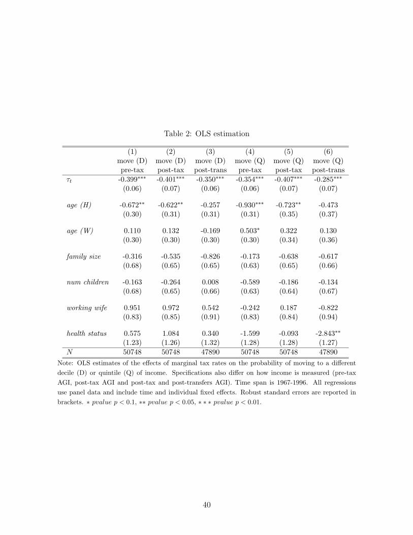
Table 2: OLS estimation

(1) (2) (3) (4) (5) (6)move (D)pre-tax

move (D)post-tax

move (D)post-trans

move (Q)pre-tax

move (Q)post-tax

move (Q)post-trans

τt -0.399∗∗∗ -0.401∗∗∗ -0.350∗∗∗ -0.354∗∗∗ -0.407∗∗∗ -0.285∗∗∗

(0.06) (0.07) (0.06) (0.06) (0.07) (0.07)

age (H) -0.672∗∗ -0.622∗∗ -0.257 -0.930∗∗∗ -0.723∗∗ -0.473(0.30) (0.31) (0.31) (0.31) (0.35) (0.37)

age (W) 0.110 0.132 -0.169 0.503∗ 0.322 0.130(0.30) (0.30) (0.30) (0.30) (0.34) (0.36)

family size -0.316 -0.535 -0.826 -0.173 -0.638 -0.617(0.68) (0.65) (0.65) (0.63) (0.65) (0.66)

num children -0.163 -0.264 0.008 -0.589 -0.186 -0.134(0.68) (0.65) (0.66) (0.63) (0.64) (0.67)

working wife 0.951 0.972 0.542 -0.242 0.187 -0.822(0.83) (0.85) (0.91) (0.83) (0.84) (0.94)

health status 0.575 1.084 0.340 -1.599 -0.093 -2.843∗∗

(1.23) (1.26) (1.32) (1.28) (1.28) (1.27)

N 50748 50748 47890 50748 50748 47890

Note: OLS estimates of the effects of marginal tax rates on the probability of moving to a different

decile (D) or quintile (Q) of income. Specifications also differ on how income is measured (pre-tax

AGI, post-tax AGI and post-tax and post-transfers AGI). Time span is 1967-1996. All regressions

use panel data and include time and individual fixed effects. Robust standard errors are reported in

brackets. ∗ pvalue p < 0.1, ∗∗ pvalue p < 0.05, ∗ ∗ ∗ pvalue p < 0.01.

40

Table 3: IV estimations

(1) (2) (3) (4) (5) (6)move (D)pre-tax

move (D)post-tax

move (D)post-trans

move (Q)pre-tax

move (Q)post-tax

move (Q)post-trans

τi,t -0.813∗∗∗ -0.769∗∗∗ -0.775∗∗∗ -0.516∗∗ -0.478∗∗ -0.506∗∗

(0.23) (0.23) (0.23) (0.23) (0.23) (0.23)

age (H) -0.582∗∗ -0.542∗∗ 4.481∗∗ -0.895∗∗∗ -0.708∗∗∗ 2.560(0.27) (0.27) (1.87) (0.26) (0.27) (1.76)

age (W) 0.078 0.104 -0.198 0.490∗ 0.317 0.114(0.26) (0.26) (0.27) (0.25) (0.26) (0.26)

family size -0.206 -0.437 -0.695 -0.130 -0.619 -0.548(0.60) (0.61) (0.64) (0.58) (0.58) (0.62)

num children -0.418 -0.490 -0.261 -0.688 -0.230 -0.274(0.61) (0.62) (0.65) (0.59) (0.59) (0.62)

working wife 1.927∗∗ 1.839∗ 1.549 0.140 0.355 -0.297(0.96) (0.97) (0.99) (0.95) (0.95) (0.98)

health status 0.250 0.794 0.028 -1.727 -0.149 -3.006∗∗

(1.25) (1.26) (1.32) (1.22) (1.23) (1.28)

1st stage F-stat 1577 1577 1602 1577 1577 1602N 50745 50745 47791 50745 50745 47791

Note: IV (2SLS) estimates of the effects of marginal tax rates on the probability of moving to a different

decile (D) or quintile (Q) of income. Tax reforms are used as an instrument for the marginal tax rate

τ . Specifications also differ on how income is measured (pre-tax AGI, post-tax AGI and post-tax and

post-transfers AGI). Time span is 1967-1996. All regressions use panel data and include time and

individual fixed effects. Robust standard errors are reported in brackets. ∗ pvalue p < 0.1, ∗∗ pvalue

p < 0.05, ∗ ∗ ∗ pvalue p < 0.01.

41

Table 4: IV Estimation with average tax rate

(1) (2) (3) (4) (5) (6)move (D)pre-tax

move (D)post-tax

move (D)post-trans

move (Q)pre-tax

move (Q)post-tax

move (Q)post-trans

τt -1.028∗∗∗ -0.993∗∗∗ -0.771∗∗∗ -0.590∗∗∗ -0.627∗∗∗ -0.561∗∗∗

(0.18) (0.18) (0.16) (0.15) (0.16) (0.15)

τt -4.037 -4.209 0.092 -1.391 -2.798 -1.167(3.71) (3.77) (3.50) (2.98) (3.16) (3.35)

age (H) -0.077 -0.016 4.462∗∗ -0.721∗ -0.358 2.801(0.51) (0.52) (2.00) (0.42) (0.45) (1.89)

age (W) -0.151 -0.135 -0.194 0.411 0.158 0.055(0.34) (0.34) (0.32) (0.30) (0.31) (0.31)

family size 0.465 0.263 -0.710 0.102 -0.154 -0.353(0.84) (0.85) (0.83) (0.73) (0.76) (0.79)

num children -4.534 -4.781 -0.170 -2.107 -3.083 -1.430(3.73) (3.79) (3.42) (2.98) (3.16) (3.27)

working wife 10.105 10.365 1.365 2.959 6.022 2.048(7.19) (7.30) (6.67) (5.67) (6.04) (6.37)

health status -1.860 -1.404 0.074 -2.454 -1.611 -3.589∗

(2.22) (2.24) (2.08) (1.86) (1.95) (2.00)

1st stage F-stat 944 944 949 944 944 949N 50745 50745 47791 50745 50745 47791

Note: IV (2SLS) estimates of the effects of marginal and average tax rates on the probability of moving

to a different decile (D) or quintile (Q) of income. Tax reforms are used as instruments for the marginal

tax rate τt and the average tax rate τt. Specifications also differ on how income is measured (pre-tax

AGI and post-tax AGI and post-tax and post-transfers AGI). Time span is 1967-1996. All regressions



42

Table 5: Robustness to alternative definitions of income (deciles)

(1) (2) (3) (4) (5) (6)tax inc.(pre-tax)

tax inc.(post-tax)

labour inc.(pre-tax)

labour inc.(post-tax)

asset inc.(pre-tax)

fam. inc.(pre-tax)

τi,tt -0.979∗∗∗ -0.939∗∗∗ -1.065∗∗∗ -0.742∗∗∗ -0.402∗ -0.473∗∗

(0.23) (0.24) (0.23) (0.24) (0.24) (0.23)

age (H) -0.775∗∗∗ -0.418 -0.684∗∗∗ -0.640∗∗ -0.692∗∗∗ 1.410∗∗∗

(0.27) (0.27) (0.26) (0.27) (0.27) (0.26)

age (W) 0.298 -0.013 0.170 0.243 0.475∗ -0.128(0.26) (0.26) (0.25) (0.26) (0.26) (0.25)

family size -0.756 -0.572 -0.304 -0.091 3.891∗∗∗ 0.560(0.61) (0.61) (0.61) (0.62) (0.61) (0.59)

num children -0.528 -0.492 -0.991 -1.397∗∗ -5.090∗∗∗ -1.752∗∗∗

(0.62) (0.62) (0.62) (0.62) (0.62) (0.60)

working wife 2.271∗∗ 2.350∗∗ 3.857∗∗∗ 2.944∗∗∗ 0.813 1.158(0.96) (0.97) (0.97) (0.97) (0.97) (0.93)

health stastus 1.678 0.865 0.767 0.644 3.081∗∗ -0.324(1.25) (1.27) (1.26) (1.27) (1.28) (1.23)

1st stage F-stat 1577 1577 1577 1577 1577 1577N 50745 50745 50745 50745 50745 50745


decile of income. Tax reforms are used as an instrument for the marginal tax rate τ . Specifications

differ in how income is defined: columns 1-2 refer to taxable income of head and wife, columns 3-4

refer to labour income of head and wife, column 5 refers to asset income of head and wife, and column

6 refers to adjusted family income (the adjustment consists on dividing family income by the square

root of family size). Specifications also differ on how income is measured (pre-tax AGI, post-tax AGI

and post-tax and post-transfers AGI). Time span is 1967-1996. All regressions use panel data and

include time and individual fixed effects. Robust standard errors are reported in brackets. ∗ pvalue

p < 0.1, ∗∗ pvalue p < 0.05, ∗ ∗ ∗ pvalue p < 0.01.

43

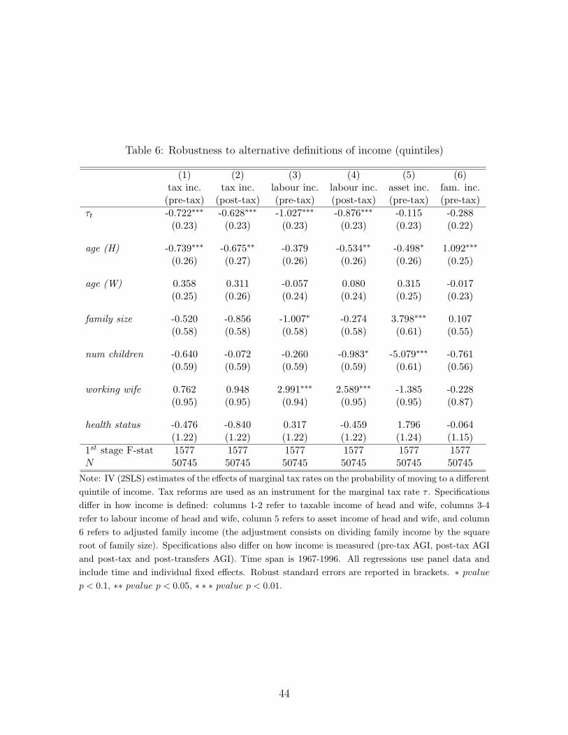
Table 6: Robustness to alternative definitions of income (quintiles)

(1) (2) (3) (4) (5) (6)tax inc.(pre-tax)

tax inc.(post-tax)

labour inc.(pre-tax)

labour inc.(post-tax)

asset inc.(pre-tax)

fam. inc.(pre-tax)

τt -0.722∗∗∗ -0.628∗∗∗ -1.027∗∗∗ -0.876∗∗∗ -0.115 -0.288(0.23) (0.23) (0.23) (0.23) (0.23) (0.22)

age (H) -0.739∗∗∗ -0.675∗∗ -0.379 -0.534∗∗ -0.498∗ 1.092∗∗∗

(0.26) (0.27) (0.26) (0.26) (0.26) (0.25)

age (W) 0.358 0.311 -0.057 0.080 0.315 -0.017(0.25) (0.26) (0.24) (0.24) (0.25) (0.23)

family size -0.520 -0.856 -1.007∗ -0.274 3.798∗∗∗ 0.107(0.58) (0.58) (0.58) (0.58) (0.61) (0.55)

num children -0.640 -0.072 -0.260 -0.983∗ -5.079∗∗∗ -0.761(0.59) (0.59) (0.59) (0.59) (0.61) (0.56)

working wife 0.762 0.948 2.991∗∗∗ 2.589∗∗∗ -1.385 -0.228(0.95) (0.95) (0.94) (0.95) (0.95) (0.87)

health status -0.476 -0.840 0.317 -0.459 1.796 -0.064(1.22) (1.22) (1.22) (1.22) (1.24) (1.15)

1st stage F-stat 1577 1577 1577 1577 1577 1577N 50745 50745 50745 50745 50745 50745


quintile of income. Tax reforms are used as an instrument for the marginal tax rate τ . Specifications

differ in how income is defined: columns 1-2 refer to taxable income of head and wife, columns 3-4

refer to labour income of head and wife, column 5 refers to asset income of head and wife, and column

6 refers to adjusted family income (the adjustment consists on dividing family income by the square

root of family size). Specifications also differ on how income is measured (pre-tax AGI, post-tax AGI

and post-tax and post-transfers AGI). Time span is 1967-1996. All regressions use panel data and



44

Table 7: Robustness to further controls(1) (2) (3) (4) (5) (6)

move (D)pre-tax

move (D)post-tax

move (D)post-trans

move (D)pre-tax

move (D)post-tax

move (D)post-trans

τt -0.828∗∗∗ -0.789∗∗∗ -0.795∗∗∗ -0.695∗∗∗ -0.648∗∗∗ -0.655∗∗∗

(0.23) (0.24) (0.23) (0.23) (0.23) (0.23)

age (H) -0.461 -0.436 4.533∗∗ -0.444∗ -0.403 4.512∗∗

(0.28) (0.28) (1.89) (0.26) (0.27) (1.85)

age (W) 0.114 0.178 -0.099 -0.022 0.002 -0.320(0.27) (0.27) (0.28) (0.25) (0.26) (0.27)

family size 0.018 -0.314 -0.578 -0.305 -0.543 -0.819(0.64) (0.64) (0.68) (0.60) (0.60) (0.63)

num children -0.530 -0.473 -0.115 -0.365 -0.435 -0.207(0.64) (0.65) (0.69) (0.61) (0.61) (0.64)

working wife 1.964∗∗ 2.315∗∗ 1.633 1.612∗ 1.506 1.131(0.99) (0.99) (1.02) (0.93) (0.94) (0.96)

health status 0.290 1.232 0.468 0.116 0.660 -0.071(1.29) (1.29) (1.36) (1.24) (1.25) (1.31)

wealth -0.045∗∗∗ -0.051∗∗∗ -0.044∗∗∗

(0.01) (0.01) (0.01)

decilet−1 = 2 13.310∗∗∗ 13.321∗∗∗ 13.297∗∗∗

(1.39) (1.38) (1.40)

decilet−1 = 3 18.715∗∗∗ 18.945∗∗∗ 17.955∗∗∗

(1.42) (1.42) (1.45)

decilet−1 = 4 22.120∗∗∗ 22.462∗∗∗ 22.363∗∗∗

(1.38) (1.38) (1.42)

decilet−1 = 5 22.615∗∗∗ 23.142∗∗∗ 23.509∗∗∗

(1.35) (1.36) (1.40)

decilet−1 = 6 21.808∗∗∗ 22.334∗∗∗ 20.967∗∗∗

(1.34) (1.34) (1.38)

decilet−1 = 7 20.199∗∗∗ 20.797∗∗∗ 22.558∗∗∗

(1.35) (1.34) (1.38)

decilet−1 = 8 17.285∗∗∗ 17.825∗∗∗ 18.513∗∗∗

(1.39) (1.38) (1.43)

decilet−1 = 9 11.684∗∗∗ 11.852∗∗∗ 12.171∗∗∗

(1.40) (1.39) (1.44)

1st stage F-stat 1570 1570 1597 1567 1567 1596N 47508 47508 44547 50745 50745 47791


decile of income. Tax reforms are used as an instrument for the marginal tax rate τt. Specifications

also differ on how income is measured (pre-tax AGI, post-tax AGI and post-tax and post-transfers

AGI). Variable wealth is measured in thousands of 196 dollars. decilet−1 = k is a dummy variable

equal to 1 if the income decile in the previous period was k. Time span is 1967-1996. All regressions



Table 8: Robustness to income controls

(1) (2) (3) (4) (5) (6)move (D)pre-tax

move (D)post-tax

move (D)post-trans

move (D)pre-tax

move (D)post-tax

move (D)post-trans

τt -0.800∗∗∗ -0.762∗∗∗ -0.771∗∗∗ -1.053∗∗∗ -1.009∗∗∗ -0.983∗∗∗

(0.22) (0.22) (0.22) (0.22) (0.22) (0.22)

age (H) -0.714∗∗ -0.615∗∗ 4.466∗∗ -0.437∗ -0.397 3.568∗∗

(0.28) (0.28) (1.88) (0.25) (0.25) (1.75)

age (W) 0.089 0.110 -0.195 0.039 0.065 -0.208(0.26) (0.26) (0.27) (0.24) (0.24) (0.26)

family size -0.253 -0.464 -0.712 0.046 -0.184 -0.441(0.60) (0.61) (0.63) (0.57) (0.58) (0.62)

num children -0.402 -0.481 -0.255 -0.413 -0.486 -0.274(0.61) (0.62) (0.65) (0.58) (0.59) (0.63)

working wife 1.771∗∗ 1.753∗ 1.500 2.940∗∗∗ 2.855∗∗∗ 2.410∗∗

(0.90) (0.90) (0.93) (0.91) (0.91) (0.94)

health status 0.321 0.834 0.048 -1.114 -0.573 -1.079(1.24) (1.25) (1.32) (1.18) (1.19) (1.27)

log incomet−1 1.649 0.906 0.552(1.66) (1.68) (1.69)

abs (∆incomet) 94.612∗∗∗ 94.837∗∗∗ 87.523∗∗∗

(2.22) (2.22) (2.00)

1st stage F-stat 1791 1791 1802 1581 1581 1605N 50741 50741 47788 50736 50736 47783


decile of income. Tax reforms are used as an instrument for the marginal tax rate τt. Specifications

also differ on how income is measured (pre-tax AGI, post-tax AGI and post-tax and post-transfers

AGI). Additional controls account for lagged income and absolute income changes, where income is

measured as household’s AGI. Time span is 1967-1996. All regressions use panel data and include

time and individual fixed effects. Robust standard errors are reported in brackets. ∗ pvalue p < 0.1,

∗∗ pvalue p < 0.05, ∗ ∗ ∗ pvalue p < 0.01.

46

Table 9: IV Estimation with State and Payroll Tax rates

(1) (2) (3) (4) (5) (6)move (D)pre-tax

move (D)post-tax

move (D)post-trans

move (Q)pre-tax

move (Q)post-tax

move (Q)post-trans

τt -0.565∗∗∗ -0.451∗∗ -0.334∗ -0.379∗ -0.356∗ -0.335∗

(0.20) (0.21) (0.20) (0.19) (0.20) (0.19)

τt 1.820 5.246 1.777 0.519 3.168 1.137(4.19) (5.03) (4.28) (3.87) (4.32) (3.96)

age (H) 0.079 -0.323 -0.313 -0.521 -0.097 -0.240(0.43) (0.49) (0.44) (0.41) (0.45) (0.41)

age (W) -0.678 -0.317 -0.101 0.263 -0.324 0.018(0.42) (0.48) (0.43) (0.40) (0.45) (0.40)

family size -1.385 -1.997 -2.023 -0.726 -1.341 -0.940(1.34) (1.53) (1.35) (1.25) (1.36) (1.27)

num children 2.093 5.196 2.366 0.563 3.253 1.261(5.06) (6.03) (5.15) (4.69) (5.20) (4.77)

working wife -3.635 -11.042 -4.178 -1.522 -8.103 -3.984(10.10) (11.99) (10.29) (9.37) (10.37) (9.57)

health status 2.007 3.240 2.657 -1.541 1.737 -0.342(2.56) (2.91) (2.58) (2.41) (2.61) (2.45)

1st stage F-stat 1416 1416 1412 1416 1416 1412N 35408 35408 35374 35408 35408 35374


decile (D) or quintile (Q) of income. Taxes include federal income, payroll and state liabilities. Tax

reforms are used as instruments for the marginal tax rate τt and the average tax rate τt. Specifications

also differ on how income is measured (pre-tax AGI and post-tax AGI and post-tax and post-transfers

AGI). Time span is 1967-1996. All regressions use panel data and include time and individual fixed

effects. Robust standard errors are reported in brackets. ∗ pvalue p < 0.1, ∗∗ pvalue p < 0.05, ∗ ∗ ∗pvalue p < 0.01.

47

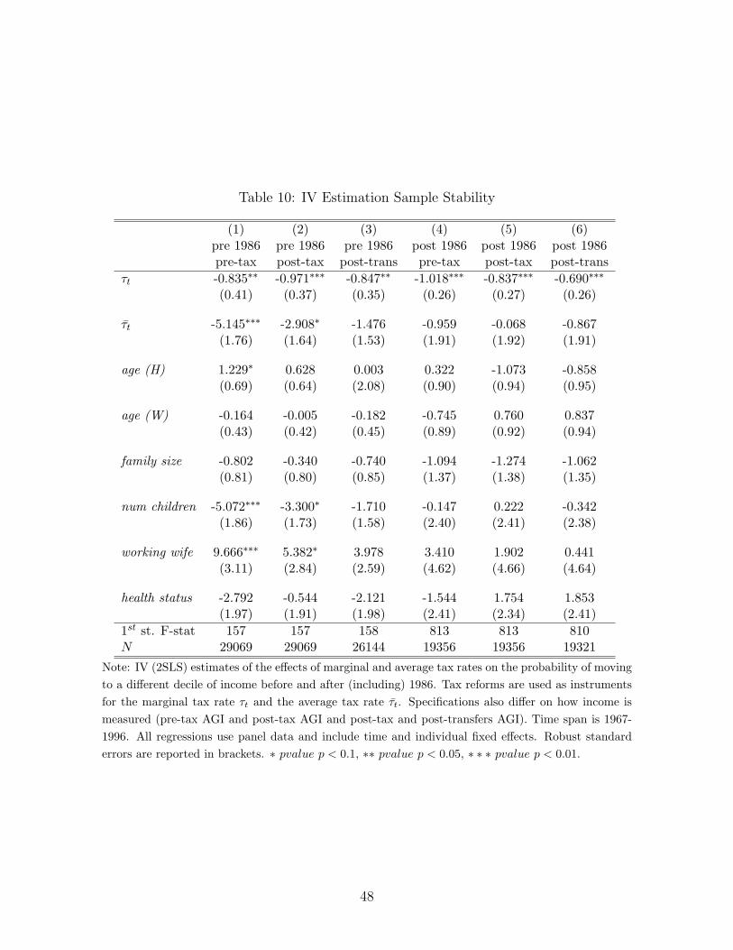
Table 10: IV Estimation Sample Stability

(1) (2) (3) (4) (5) (6)pre 1986pre-tax

pre 1986post-tax

pre 1986post-trans

post 1986pre-tax

post 1986post-tax

post 1986post-trans

τt -0.835∗∗ -0.971∗∗∗ -0.847∗∗ -1.018∗∗∗ -0.837∗∗∗ -0.690∗∗∗

(0.41) (0.37) (0.35) (0.26) (0.27) (0.26)

τt -5.145∗∗∗ -2.908∗ -1.476 -0.959 -0.068 -0.867(1.76) (1.64) (1.53) (1.91) (1.92) (1.91)

age (H) 1.229∗ 0.628 0.003 0.322 -1.073 -0.858(0.69) (0.64) (2.08) (0.90) (0.94) (0.95)

age (W) -0.164 -0.005 -0.182 -0.745 0.760 0.837(0.43) (0.42) (0.45) (0.89) (0.92) (0.94)

family size -0.802 -0.340 -0.740 -1.094 -1.274 -1.062(0.81) (0.80) (0.85) (1.37) (1.38) (1.35)

num children -5.072∗∗∗ -3.300∗ -1.710 -0.147 0.222 -0.342(1.86) (1.73) (1.58) (2.40) (2.41) (2.38)

working wife 9.666∗∗∗ 5.382∗ 3.978 3.410 1.902 0.441(3.11) (2.84) (2.59) (4.62) (4.66) (4.64)

health status -2.792 -0.544 -2.121 -1.544 1.754 1.853(1.97) (1.91) (1.98) (2.41) (2.34) (2.41)

1st st. F-stat 157 157 158 813 813 810N 29069 29069 26144 19356 19356 19321

Note: IV (2SLS) estimates of the effects of marginal and average tax rates on the probability of moving

to a different decile of income before and after (including) 1986. Tax reforms are used as instruments

for the marginal tax rate τt and the average tax rate τt. Specifications also differ on how income is

measured (pre-tax AGI and post-tax AGI and post-tax and post-transfers AGI). Time span is 1967-

1996. All regressions use panel data and include time and individual fixed effects. Robust standard

errors are reported in brackets. ∗ pvalue p < 0.1, ∗∗ pvalue p < 0.05, ∗ ∗ ∗ pvalue p < 0.01.

48

Tab

le11:Rob

ustnessto

sample

selection

(1)

(2)

(3)

(4)

(5)

(6)

(7)

(8)

(9)

(10)

core

pre-tax

core

post-tax

allages

pre-tax

allages

post-tax

self-emp.

pre-tax

self-emp.

post-tax

unem

p.

pre-tax

unem

p.

post-tax

female

pre-tax

female

post-tax

τ t-0.719

∗∗∗

-0.953

∗∗∗

-0.449

∗∗-0.417∗

-0.877∗∗

∗-0.839∗

∗∗-0.721∗∗

∗-0.740∗∗

∗-0.759∗

∗∗-0.804∗∗

∗

(0.25)

(0.25)

(0.21)

(0.22)

(0.20)

(0.21)

(0.22)

(0.22)

(0.24)

(0.23)

age

(H)

-0.730

∗∗-0.735

∗∗-0.565

∗∗-0.571∗∗

-0.295

-0.197

-0.553∗∗

-0.447∗

-0.576∗

∗-0.531∗∗

(0.29)

(0.29)

(0.23)

(0.23)

(0.22)

(0.22)

(0.27)

(0.27)

(0.27)

(0.27)

age

(W)

0.278

0.267

0.039

0.129

-0.048

-0.171

0.076

0.048

0.033

0.116

(0.28)

(0.28)

(0.22)

(0.22)

(0.21)

(0.21)

(0.26)

(0.26)

(0.26)

(0.26)

familysize

-0.731

-0.455

0.206

-1.000∗

-0.825

-0.591

0.031

-0.532

-0.209

-0.575

(0.66)

(0.67)

(0.57)

(0.58)

(0.54)

(0.54)

(0.60)

(0.61)

(0.61)

(0.61)

num

children

-0.292

-0.848

-0.956

0.206

-0.209

-0.191

-0.628

-0.515

-0.488

-0.390

(0.68)

(0.68)

(0.58)

(0.59)

(0.55)

(0.55)

(0.61)

(0.61)

(0.62)

(0.62)

healthstatus

0.597

-0.764

2.476∗∗

2.881∗∗

-0.505

-0.416

1.165

1.129

0.746

0.792

(1.35)

(1.36)

(1.14)

(1.15)

(1.11)

(1.11)

(1.24)

(1.25)

(1.25)

(1.26)

workingwife

2.730∗∗

∗2.982∗∗

∗1.674∗

3.176∗

∗∗1.238

0.787

2.110∗∗

1.569∗

1.934∗∗

1.520

(0.99)

(0.99)

(0.89)

(0.89)

(0.84)

(0.84)

(0.94)

(0.94)

(0.96)

(0.97)

workinghead

-10.210

-9.993

(6.96)

(6.91)

male

head

-27.764

-29.135

(22.27)

(22.37)

1stst.F-stat

1392

1392

1650

1650

1321

1321

1192

1192

1576

1576

N32090

32090

60253

60253

60231

60231

51620

51620

50768

50768

Note:

IV(2SLS)estimates

oftheeff

ects

ofmarginal

taxrateson

theprobabilityofmov

ingto

adifferentdecileofincome.

Taxreform

sare

usedasan

instrumentforthemarginal

taxrate

τ t.Specification

salso

differ

onhow

incomeismeasured(pre-taxAGIorpost-taxAGI)

andonalterationsofthe

benchmarksamplefrom

Tab

le3.

Columns1an

d2dropsthehou

seholdsfrom

theSEO

subsample(w

hichover-represents

low-incomefamilies)

anduses

equal

weigh

tsforallob

servations.

Columns3an

d4expan

dsthesample

toincludehouseholdswithaworkingheadfrom

allages

(notonly

between

25-60years).

Columns5an

d6ad

dhou

seholdswithaheadwhois

self-employed.Columns7and8alsoincorporate

householdswithanunem

ployed

head,includingan

additional

control

(workinghead,adummyforem

ployedheadsofhouseholds).Columns9and10extendthebenchmark

sample

withhou

seholdsthat

also

haveafemalehead(a

dummyvariab

leformale

headsis

alsoincluded).

Tim

espanis

1967-1996.Allregressionsuse

panel

dataan

dincludetimean

dindividual

fixed

effects.Rob

ust

stan

dard

errors

are

reported

inbrackets.

∗pvaluep<

0.1,∗∗

pvaluep<

0.05,∗∗∗pvalue

p<

0.01.

49

Table 12: IV Estimation Jumps with ATR

(1) (2) (3) (4) (5) (6)jump (D)pre-tax

jump (D)post-tax

jump (D)post-trans

jump (Q)pre-tax

jump (Q)post-tax

jump (Q)post-trans

τt -0.013∗∗∗ -0.012∗∗∗ -0.008∗∗ -0.006∗∗∗ -0.006∗∗∗ -0.005∗∗

(0.00) (0.00) (0.00) (0.00) (0.00) (0.00)

τt -0.112 -0.126 -0.002 -0.045 -0.062 -0.029(0.08) (0.09) (0.08) (0.04) (0.05) (0.05)

age (H) -0.000 0.002 0.067 -0.005 -0.000 0.042(0.01) (0.01) (0.05) (0.01) (0.01) (0.03)

age (W) 0.001 -0.001 0.005 0.004 0.001 0.001(0.01) (0.01) (0.01) (0.00) (0.00) (0.00)

family size 0.016 0.014 -0.006 0.002 0.001 -0.005(0.02) (0.02) (0.02) (0.01) (0.01) (0.01)

num children -0.139∗ -0.148∗ -0.022 -0.055 -0.067 -0.032(0.08) (0.09) (0.08) (0.04) (0.05) (0.04)

working wife 0.174 0.202 -0.060 0.068 0.106 0.024(0.16) (0.17) (0.15) (0.08) (0.09) (0.09)

health status -0.042 -0.041 -0.016 -0.037 -0.025 -0.047∗

(0.05) (0.05) (0.04) (0.03) (0.03) (0.03)

1st stage F-stat 944 944 948 944 944 948N 50745 50745 47742 50745 50745 47742

Note: IV (2SLS) estimates of the effects of marginal tax rates on the number of income ranks (in

deciles, D, or quintiles, Q) crossed along the income distribution. Tax reforms are used as instruments

for the marginal tax rate τt and the average tax rate τt. Specifications also differ on how income is

measured (pre-tax AGI, post-tax AGI and post-tax and post-transfers AGI). Time span is 1967-1996.

All regressions use panel data and include time and individual fixed effects. Robust standard errors

are reported in brackets. ∗ pvalue p < 0.1, ∗∗ pvalue p < 0.05, ∗ ∗ ∗ pvalue p < 0.01.

50

Table 13: Robustness to different lags of the marginal tax rate (deciles of income)

(1) (2) (3) (4) (5) (6)move (D)pre-tax

move (D)post-tax

move (D)pre-tax

move (D)post-tax

move (D)pre-tax

move (D)post-tax

τt−1 -0.569∗∗ -0.414∗

(0.24) (0.24)

τt−2 0.231 0.484∗

(0.27) (0.27)

τt−3 -0.280 -0.264(0.30) (0.30)

age (H) -0.633∗∗ -0.652∗∗ -0.175 0.510 2.814 0.105(0.29) (0.29) (2.17) (2.17) (2.29) (2.29)

age (W) 0.229 0.177 0.613∗ 0.271 0.096 0.255(0.28) (0.28) (0.34) (0.34) (0.40) (0.40)

family size -0.657 -0.804 -0.444 -0.435 -0.876 -0.963(0.61) (0.61) (0.65) (0.65) (0.69) (0.69)

num children 0.128 -0.066 0.355 0.061 0.211 -0.132(0.62) (0.62) (0.67) (0.67) (0.71) (0.71)

working wife 0.900 -0.082 0.435 0.039 0.781 0.961(0.84) (0.84) (0.89) (0.89) (0.96) (0.96)

health status 1.236 0.613 2.123 2.292 1.619 2.295(1.27) (1.29) (1.40) (1.43) (1.52) (1.54)

1st stage F-stat 1583 1583 1395 1395 1180 1180N 48507 48507 41118 41118 35449 35449

Note: IV (2SLS) estimates of the effects of marginal tax rates on the probability of moving to a

different decile (D) or quintile (Q) of income. Tax reforms are used as an instrument for the marginal

tax rate τt. Specifications also differ on how income is measured (pre-tax AGI, post-tax AGI and

post-tax and post-transfers AGI). Time span is 1967-1996. All regressions use panel data and include


∗∗ pvalue p < 0.05, ∗ ∗ ∗ pvalue p < 0.01.

51

Table 14: Robustness to different lags of the marginal tax rate (quintiles of income)

(1) (2) (3) (4) (5) (6)move (Q)pre-tax

move (Q)post-tax

move (Q)pre-tax

move (Q)post-tax

move (Q)pre-tax

move (Q)post-tax

τt−1 -0.790∗∗∗ -0.529∗∗

(0.23) (0.24)

τt−2 0.129 0.153(0.26) (0.26)

τt−3 -0.270 -0.321(0.28) (0.28)

age (H) -0.744∗∗∗ -0.594∗∗ 1.484 1.687 2.203 0.395(0.29) (0.29) (2.03) (2.02) (2.18) (2.16)

age (W) 0.574∗∗ 0.318 0.889∗∗∗ 0.682∗∗ 0.249 0.450(0.27) (0.28) (0.33) (0.32) (0.37) (0.37)

family size 0.149 -0.720 0.607 -0.130 0.144 -0.103(0.59) (0.58) (0.62) (0.62) (0.66) (0.66)

num children -0.956 -0.173 -0.508 -0.491 -0.462 -0.738(0.60) (0.59) (0.63) (0.63) (0.67) (0.67)

working wife -0.297 -0.296 -1.639∗ -1.022 -1.705∗ -1.194(0.83) (0.83) (0.87) (0.87) (0.94) (0.94)

health status -1.328 -1.387 -0.668 -0.971 0.535 0.722(1.25) (1.25) (1.37) (1.36) (1.47) (1.47)

1st stage F-stat 1583 1583 1395 1395 1180 1180N 48507 48507 41118 41118 35449 35449

Note: IV (2SLS) estimates of the effects of marginal tax rates on the probability of moving to a

different decile (D) or quintile (Q) of income. Tax reforms are used as an instrument for the marginal

tax rate τt. Specifications also differ on how income is measured (pre-tax AGI, post-tax AGI and

post-tax and post-transfers AGI). Time span is 1967-1996. All regressions use panel data and include


∗∗ pvalue p < 0.05, ∗ ∗ ∗ pvalue p < 0.01.

52

Table 15: IV estimates: households without college educations

(1) (2) (3) (4) (5) (6)up

pre-taxup

post-taxstay

pre-taxstay

post-taxdownpre-tax

downpost-tax

τt -1.435∗∗∗ -1.468∗∗∗ 0.915∗∗∗ 0.728∗∗∗ 0.916∗∗ 1.132∗∗∗

(0.27) (0.27) (0.26) (0.26) (0.39) (0.39)

age (H) -0.162 0.059 0.492 0.315 -0.164 -0.231(0.32) (0.33) (0.31) (0.32) (0.33) (0.34)

age (W) -0.300 -0.426 -0.114 -0.017 0.325 0.380(0.31) (0.31) (0.30) (0.31) (0.31) (0.32)

family size -0.824 -1.254∗ 0.187 0.369 0.302 0.665(0.69) (0.70) (0.67) (0.68) (0.77) (0.78)

num children 0.992 1.616∗∗ -0.225 -0.432 -0.498 -1.032(0.72) (0.73) (0.70) (0.71) (0.80) (0.81)

working wife 16.792∗∗∗ 16.364∗∗∗ -2.830∗∗ -2.099∗ -18.930∗∗∗ -19.024∗∗∗

(1.09) (1.09) (1.10) (1.10) (1.44) (1.44)

health status -0.002 -0.523 -0.292 -0.942 1.082 2.748(1.47) (1.48) (1.39) (1.39) (1.66) (1.68)

1st stage F-stat 1181 1181 1181 1181 781 781N 38417 38417 39766 39766 32229 32229

Note: IV (2SLS) estimates of the effects of marginal tax rates on the probability of moving up to

a higher income decile (columns 1 and 2), staying in the same decile (columns 3 and 4) or moving

down to a lower decile (columns 5 and 6). Sample is restricted to observations where the head of the

household has not completed college education. Households with income in time t−1 belonging to the

10th decile are excluded from specifications 1 and 2. Households with income in time t− 1 belonging

to the 1st decile are excluded from specifications 5 and 6. Tax reforms are used as an instrument for

the marginal tax rate τt. Specifications also differ on how income is measured (pre-tax AGI, post-tax

AGI and post-tax and post-transfers AGI). Time span is 1967-1996. All regressions use panel data and



53

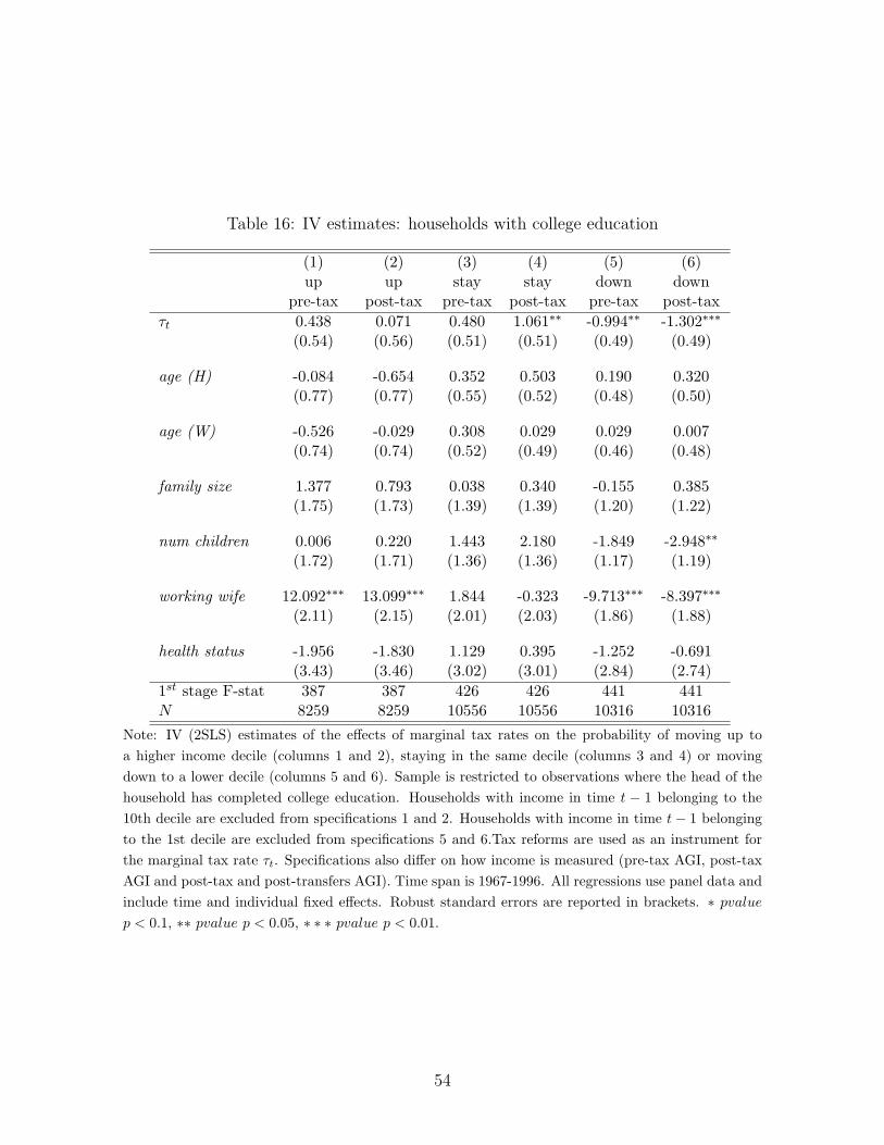
Table 16: IV estimates: households with college education

(1) (2) (3) (4) (5) (6)up

pre-taxup

post-taxstay

pre-taxstay

post-taxdownpre-tax

downpost-tax

τt 0.438 0.071 0.480 1.061∗∗ -0.994∗∗ -1.302∗∗∗

(0.54) (0.56) (0.51) (0.51) (0.49) (0.49)

age (H) -0.084 -0.654 0.352 0.503 0.190 0.320(0.77) (0.77) (0.55) (0.52) (0.48) (0.50)

age (W) -0.526 -0.029 0.308 0.029 0.029 0.007(0.74) (0.74) (0.52) (0.49) (0.46) (0.48)

family size 1.377 0.793 0.038 0.340 -0.155 0.385(1.75) (1.73) (1.39) (1.39) (1.20) (1.22)

num children 0.006 0.220 1.443 2.180 -1.849 -2.948∗∗

(1.72) (1.71) (1.36) (1.36) (1.17) (1.19)

working wife 12.092∗∗∗ 13.099∗∗∗ 1.844 -0.323 -9.713∗∗∗ -8.397∗∗∗

(2.11) (2.15) (2.01) (2.03) (1.86) (1.88)

health status -1.956 -1.830 1.129 0.395 -1.252 -0.691(3.43) (3.46) (3.02) (3.01) (2.84) (2.74)

1st stage F-stat 387 387 426 426 441 441N 8259 8259 10556 10556 10316 10316

Note: IV (2SLS) estimates of the effects of marginal tax rates on the probability of moving up to

a higher income decile (columns 1 and 2), staying in the same decile (columns 3 and 4) or moving

down to a lower decile (columns 5 and 6). Sample is restricted to observations where the head of the

household has completed college education. Households with income in time t − 1 belonging to the

10th decile are excluded from specifications 1 and 2. Households with income in time t− 1 belonging

to the 1st decile are excluded from specifications 5 and 6.Tax reforms are used as an instrument for





54

Table 17: IV estimates: households in bottom and top deciles

(1) (2) (3) (4) (5) (6)up

pre-taxup

post-taxup

post-transdownpre-tax

downpost-tax

downpost-trans

τt -1.564∗∗∗ -1.719∗∗∗ -1.441∗∗∗ -0.620 -0.713 -0.644(0.23) (0.25) (0.26) (0.94) (0.91) (0.91)

age (H) 1.237 1.218 2.850 0.303 0.764 2.790(0.81) (0.77) (4.51) (0.63) (0.66) (5.09)

age (W) -0.303 -0.269 0.004 -0.103 -0.364 0.133(0.80) (0.76) (0.78) (0.63) (0.64) (0.60)

family size 0.238 -0.831 -0.201 -2.026 -0.997 -0.058(1.54) (1.55) (1.77) (1.52) (1.61) (1.63)

num children 2.588 4.343∗∗∗ 4.509∗∗ -0.742 -2.839∗ -4.887∗∗∗

(1.60) (1.65) (1.95) (1.62) (1.69) (1.78)

working wife 22.714∗∗∗ 22.091∗∗∗ 20.406∗∗∗ -16.340∗∗∗ -17.331∗∗∗ -17.583∗∗∗

(1.90) (1.92) (2.02) (3.78) (3.65) (3.96)

health status -1.449 -0.469 1.695 8.676∗∗ 10.286∗∗ 7.548∗

(2.89) (3.01) (3.26) (3.91) (4.46) (4.58)

1st stage F-stat 456 439 438 90 91 73N 6961 6830 6313 3330 3379 3170

Note: IV (2SLS) estimates of the effects of marginal tax rates on the probability of moving up to a

higher income decile for households in the bottom decile (columns 1-3) or the probability of moving to

a lower decile for households in the top decile (columns 4-6). Tax reforms are used as an instrument for





55

Appendix

Figure A1: Evolution of the probability of transition matrix (1967-1996)

PANEL A: Bottom decile

.15

.2.2

5.3

.35

.4M

ob

ility

1970 1975 1980 1985 1990 1995

1−P1,1

(pre−tax) 1−P1,1

(post−tax)

PANEL B: Top decile

.15

.2.2

5.3

.35

.4M

ob

ility

1970 1975 1980 1985 1990 1995

1−P10,10

(pre−tax) 1−P10,10

(post−tax)

Note: Evolution of indices of mobility at the bottom and top deciles between 1967-1968. Panel A

shows the evolution of the probability that a households leave the first decile of income (i.e. 1−P 1,1 in

Equation 2). Panel B shows the evolution of the probability that a households moves down from the

top decile of income (i.e. 1− P 10,10 in Equation 2). The distribution is computed using both pre-tax

and post-tax income.

56

Figure A2: Variation in Average Tax Rates (1967-1996)

��

��

��

��

��

��

��

��

��

��

��

��

��

��

��

��

��

��

��

Note: Evolution of the average tax rates between 1967-1968.The figure displays the average ratio of

total federal income tax liabilities to adjusted gross income (AGI) for each income decile. Tax liabilities

are computed using TAXSIM and data from PSID.

57

Figure A3: Variations in Average Tax Rates due to legislated tax changes (1967-1996)

��

��

��

�

��

��

��

��

��

��

�

�

�

��

��

��

��

��

��

��

��

��

��

��

��

��

Note: Evolution between 1967 and 1996 of the instrument ∆ ¯τ t−1i,t = τ ti,t − τ t−1

i,t (difference between the

actual average tax rate and a counterfactual average tax rate computed using TAXSIM). Grey bars

represent the narrative measure of legislated tax changes (as percentage of nominal GDP) from Romer

and Romer (2010). These are classified as endogenous tax changes (related to the current state of the

economy, in light grey) and exogenous tax changes (unrelated to the state of economy, in dark grey).

58

Figure A4: Variation in total marginal tax rates (1977-1996)

Note: Relationship between total marginal tax rates and real Adjusted Gross Income (1996 US dollars).

Total marginal tax rates include the federal marginal rates on individual income, payroll and Social

Security liabilities and State marginal tax rates for each household and year in the PSID before and

after the 1986 tax reform (in red and blue, respectively).

59

Table A1: Correlations between taxes (R&R, total) and mobility

τRomer

move (P) pre-tax -0.192move (P) post-tax -0.303move (Q) pre-tax -0.199move (Q) post-tax -0.263trace (P) pre-tax -0.112trace (P) post-tax -0.169trace (Q) pre-tax -0.173trace (Q) pre-tax -0.216jump (pre-tax) -0.206jump (post-tax) -0.225

Note: Correlation between indices of mobility and the narrative measure of total legislated tax changes

(as percentage of nominal GDP) from Romer and Romer (2010). Mobility indices are the percentage

of people changing income deciles (rows 1-2) or quintiles (rows 3-4), the normalised trace index (NTI,

rows 5-6 for deciles and 7-8 for quintiles) and the average number of income deciles passed by a

household between two adjacent years. The mobility indices are computed using both income before

taxes (pre-tax) and after taxes (post-tax).

60

The Impact of Taxes on Income Mobility

Documents