The Impact of Regional and Sectoral Productivity …erossi/RSSUS.pdfThe Impact of Regional and Sectoral Productivity Changes on the U.S. Economy Lorenzo Caliendo Fernando Parro Yale

The Impact of Regional and Sectoral Productivity Changes

on the U.S. Economy∗

Lorenzo Caliendo Fernando Parro

Yale University Johns Hopkins University

Esteban Rossi-Hansberg Pierre-Daniel Sarte

Princeton University FRB Richmond

July 17, 2017

Abstract

We study the impact of intersectoral and interregional trade linkages in propagating disaggregated

productivity changes to the rest of the economy. Using U.S. regional and industry data, we obtain the

aggregate, regional and sectoral elasticities of measured TFP, GDP, and employment to regional and

sectoral productivity changes. We find that the elasticities vary significantly depending on the sectors

and regions affected, and are importantly determined by the spatial structure of the economy. We use

our calibrated model to perform a variety of counterfactual exercises including several specific studies of

the aggregate and disaggregate effects of shocks to productivity and infrastructure. The specific episodes

we study include the boom in California’s computer industry, the productivity boom in North Dakota

associated with the shale oil boom, the disruptions in New York’s finance and real state industries during

the 2008 crisis, as well as the effect of the destruction of infrastructure in Louisiana following hurricane

Katrina.

1. INTRODUCTION

Fluctuations in aggregate economic activity result from a wide variety of aggregate and disaggregated

phenomena. These phenomena can reflect underlying changes that are sectoral in nature, as in the recent

high-tech boom, or regional in nature, as in the destruction in the U.S. state of Louisiana that resulted from

hurricane Katrina. In other cases, fundamental productivity changes are actually specific to a sector and a

location, as in the large contraction in the financial sector in New York that followed the 2008 crisis. The

heterogeneity of these potential changes in productivity and structures at the sectoral and regional levels

implies that the particular sectoral and regional composition of an economy is essential in determining their

aggregate impact. That is, regional trade, the presence of local factors such as land and structures, regional∗Correspondence: Caliendo: [email protected], Parro: [email protected], Rossi-Hansberg: [email protected], and

Sarte: [email protected]. We thank Treb Allen, Costas Arkolakis, Arnaud Costinot, Dave Donaldson, Jonathan Eaton,Gene Grossman, Tom Holmes, Miklos Koren, Samuel Kortum, Peter Schott, Steve Redding, Richard Rogerson, Harald Uhlig,Kei-Mu Yi and many seminar participants for useful conversations and comments. We thank Sonya Ravindranath Waddell,Robert Sharp, and Jonathon Lecznar for excellent research assistance. The views expressed in this paper are those of theauthors and do not necessarily reflect those of the Federal Reserve Bank of Richmond, the Federal Reserve Board, or theFederal Reserve System.

1

migration, as well as input-output relationships between sectors, all determine the impact of a disaggregated

sectoral or regional productivity change on aggregate outcomes. In this paper, we propose and quantify

a detailed model of the U.S. economy and use it to measure the impact of changes in local and sectoral

productivity and infrastructure.

The major part of research in macroeconomics has traditionally emphasized aggregate disturbances as

sources of aggregate changes.1 Exceptions to this approach were Long and Plosser (1983), and Horvath

(1998, 2000) who posited that because of input-output linkages, productivity disturbances at the level of an

individual sector would propagate throughout the economy in a way that led to notable aggregate move-

ments.2 More recently, a series of papers has characterized and verified empirically the condition under

which sector and firm level disturbances can have aggregate consequences.3 Notably, Acemoglu, Carvalho,

Ozdaglar, and Tahbaz-Salehi (2012) characterize the conditions under which the network structure of pro-

duction linkages effectively amplifies the impact of microeconomic shocks,4 while empirically, Foerster, Sarte,

and Watson (2011) find support for sectoral shocks as determinants of aggregate effects.

We follow this strand of the literature, but note that to this point, the literature studying the aggregate

implications of disaggregated productivity disturbances has largely abstracted from the regional composition

of sectoral activity. A decomposition of the productivity changes experienced by the U.S. economy between

2002 and 2007 (or 2007 to 2012) into a local, a sectoral, and a residual component reveals that such an

abstraction is unjustified. We find that the regional component is at least as important as the sectoral

component, if not more, and that the residual component —which includes local sectoral shocks—is important

as well. Hence, motivated by these findings, we build on the empirical evidence from Acemoglu, et al.

(2015) and Acemoglu, Akcigit, and Kerr (2015), that production networks amplify regional-local shocks,

and contribute to this literature by integrating sectoral production linkages with those that arise by way of

inter-regional linkages. The resulting framework allows for the analysis, by way of region-specific production

structures where inputs are traded across regions, of more granular disturbances that may vary at the level

of a sector within a region. Regional considerations, therefore, become key in explaining the aggregate,

sectoral, and regional effects of microeconomic disturbances.

The distribution of sectoral production across regions in the U.S. is far from uniform. This has two

important implications. First, to the degree that economic activity involves a complex network of interactions

between sectors, these interactions take place over potentially large distances by way of regional trade, but

trading across distances is costly.5 Second, since sectoral production has to take place physically in some

location, it is influenced by a wide range of changing circumstances in that location, from changes in policies

affecting the local regulatory environment or business taxes to natural disasters. Added to these regional

considerations is that some factors of production are fixed locally and unevenly distributed across space,

such as land and structures, while others are highly mobile, such as labor.6 How then do geographical

1This emphasis, for example, permeates the large Real Business Cycles literature that followed the seminal work of Kydlandand Prescott (1982).

2See also Jovanovic (1987) who shows that strategic interactions among firms or sectors can lead micro disturbances toresemble aggregate factors.

3Even absent of network effects, Gabaix (2011) shows that granular disturbances do not necessarily average out when thesize distribution of firms or sectors is suffi ciently fat-tailed. Carvalho and Gabaix (2013) find that idiosyncratic shocks canaccount for large swings in macroeconomic volatility, as exemplified by the “great moderation”and its recent undoing.

4Oberfield (2013) provides a theoretical foundation for such a network structure.5We find that eliminating U.S. regional trading costs associated with distance would result in aggregate TFP gains of

approximately 50 percent, and in aggregate GDP gains on the order of 126 percent (see Appendix A.7).6See Kennan and Walker (2011) for a recent detailed empirical study of migration across U.S. states. Blanchard and Katz

(1992), and more recently Fogli, Hill and Perri (2012), provide empirical evidence that factors related to geography, such aslabor mobility across states, matter importantly for macroeconomic adjustments to disturbances. Furthermore, because inputs

2

considerations play out in determining the effects of disaggregated productivity changes? What are the

associated key mechanisms and what is their quantitative importance? We take up these issues and use our

findings to analyze the aggregate consequences of a variety of recent specific shocks to the U.S. economy.

To study how these different aspects of economic geography influence the effects of disaggregated pro-

ductivity disturbances, we develop a quantitative model of the U.S. economy broken down by regions and

sectors. Our framework builds on Eaton and Kortum (2002) and the growing international trade literature

that extends their model to multiple sectors.7 However, the geographic nature of our problem, namely the

presence of labor mobility, local fixed factors, and heterogeneous productivities, introduce a different set of

mechanisms through which changes in fundamental productivity affect production across sectors and space

relative to most studies in the literature. In our modeled economy, there are two factors of production in

each region: labor and a composite factor comprising land and structures. Following Blanchard and Katz

(1992) labor is allowed to move across both regions and sectors. Land and structures can be used by any

sector but are fixed locally. Sectors are interconnected by way of input-output linkages but, in contrast to

Long and Plosser (1983) and its ensuing literature, shipping materials to sectors located in other regions is

costly in a way that varies with distance. We use data on pairwise trade flows across states by industry, as

well as other regional and industry data, to quantify the model. Hence, for a given change in productivity

of structures located within a particular sector and region, the model delivers the effects of this change on

all sectors and regions in the economy.

We find that disaggregated productivity changes can have different aggregate implications depending on

the regions and sectors affected. These effects arise in part by way of endogenous changes in the pattern

of regional trade through a selection effect that determines what types of goods are produced in which

regions. They also arise by way of labor migration towards regions that become more productive. When

such migration takes place, the inflow of workers strains local fixed factors in those regions and, therefore,

mitigates the direct effects of any productivity increases.8 For example, the aggregate GDP elasticity of a

regional fundamental productivity increase in Florida is 0.89.9 In contrast, the aggregate GDP elasticity of

a regional fundamental productivity increase in New York state, which is of comparable employment size

relative to aggregate employment (6.1% versus 6.2%, respectively), is 1.6. Thus, the effects of disaggregated

productivity changes depend in complex ways on the details of which sectors and regions are affected, and

how these are linked through input-output and trade relationships to other sectors and regions.

These spatial effects impact significantly the magnitude of the aggregate elasticity of sectoral shocks; for

example, failure to account for regional trade understates the aggregate GDP elasticity of an increase in

productivity in the Petroleum and Coal industry — the most spatially concentrated industry in the U.S.

must be traded across space when production varies geographically, trade costs also play a role in determining macroeconomicallocations and welfare, consistent with the findings of Fernald (1999), and Duranton, Morrow, and Turner (2014), on theeconomic relevance of road networks.

7For instance Caliendo and Parro (2015), Caselli, et al. (2012), Costinot, Donaldson, and Komunjer, (2012), Levchenkoand Zhang, (2012), and Tombe and Zhu, (2015). Eaton and Kortum (2012) and Costinot and Rodriguez-Clare (2013) presentsurveys of recent quantitative extensions of the Ricardian model of trade. Our paper relates closely to Finicelli, Pagano, andSbracia (2013) where they emphasize the selection effects in the Ricardian model. From a more regional perspective, tworelated papers, Redding (2012) and Allen and Arkolakis (2013), study the implications of labor mobility for the welfare gainsof trade, but abstract from studying the role of sectoral linkages or from presenting a quantitative assessment of the effects ofdisaggregated fundamental productivity changes on U.S. aggregate measures of TFP, GDP, or welfare.

8 In very extreme cases, regional productivity increases can even have negative effects on aggregate GDP (although welfareeffects are always positive). In our calibration this happens only for Hawaii (See Figure 5f).

9To highlight the mechanisms at play, aggregate elasticities throughout the paper are normalized to abstract from effectsarising simply from variations in state size. Thus, in a model without sectoral or trade linkages, the elasticity of aggregate TFPwith respect to a productivity change in a given state will be one for all states, rather than simply reflecting that state’s weightin production.

3

economy—by about 10% but overstates it by 19% in the Transportation Equipment industry —an industry

that exhibits much less spatial concentration. Ultimately, regional trade linkages, and the fact that materials

produced in one region are potentially used as inputs far away, are essential in propagating productivity

changes spatially and across sectors. We emphasize this point, and the use of the elasticities we present,

through several specific applications. We start by studying the impact of the TFP gains in the Computers

and Electronics industry in California, over the period 2002-2007; an example of a region and industry

specific productivity increase in a tradable industry. To study a regional shock that affects all sectors, we

study the increases in productivity across industries in North Dakota associated with the shale oil boom. We

also study the disruptions in the Finance and Real State industries in New York during the 2008 economic

crisis; an example of a negative productivity shock to a nontradable industry. In a final application, we

go beyond productivity changes and study the effect of the destruction in structures created by hurricane

Katrina in Louisiana. This last case provides a novel, as far as we know, general equilibrium evaluation of

the economic costs of this event.

The rest of the paper is organized as follows. Section 2 describes the composition of U.S. economic

activity. We make use of maps and figures to show how economic activity varies across U.S. states and

sectors. Section 3 presents the quantitative model. Section 4 describes in detail how to compute and

aggregate measures of TFP, GDP, and welfare across different states and sectors, and shows how these

measures relate to fundamental productivity changes. Section 5 describes the data, shows how to carry out

counterfactuals, and how to calibrate the model to 50 U.S. states and 26 sectors. Section 6 quantifies the

effects of different disaggregated fundamental productivity changes. In particular, we measure the elasticity

of aggregate productivity and output to sectoral, regional, as well as sector and region specific productivity

changes. Section 7 presents several applications of these results to specific events. Section 8 concludes.

2 THE COMPOSITION OF U.S. ECONOMIC ACTIVITY

Throughout the paper, we break down the U.S. economy into 50 U.S. states and 26 sectors pertaining

to the year 2007, our benchmark year. We motivate and describe in detail this particular breakdown in

Section 5. As shown in Figure 1a, shares of GDP vary greatly across states. In part, these differences stem

from differences in geographic size. However, as Figure 1a makes clear, differences in geographic size are not

large enough to explain observed regional differences in GDP. New York state’s share of GDP, for example, is

slightly larger than Texas’even though its geographic area is several times smaller. The remaining differences

cannot be explained by any mobile factor such as labor, equipment, or other material inputs, since those just

follow other local characteristics. In fact, as illustrated in Figure 1b, the distribution of employment across

states, although not identical to that of GDP, matches it fairly closely. Why then do some regions produce

so much more than others and attract many more workers? The basic approach in this paper argues that

three local characteristics, namely total factor productivity, local factors, and access to products in other

states, are essential to the answer. Specifically, we postulate that changes to total factor productivity (TFP)

that are sectoral and regional in nature, or specific to an individual sector within a region, are fundamental

to understanding local and sectoral output changes. Furthermore, these changes have aggregate effects that

are determined by their geographic and sectoral distribution.

One initial indication that different regions indeed experience different circumstances is presented in Figure

1c, which plots average annualized percentage changes in regional GDP across states for the period 2002-

2007 (Section 5 describes in detail the disaggregated data and calculations that underlie aggregate regional

4

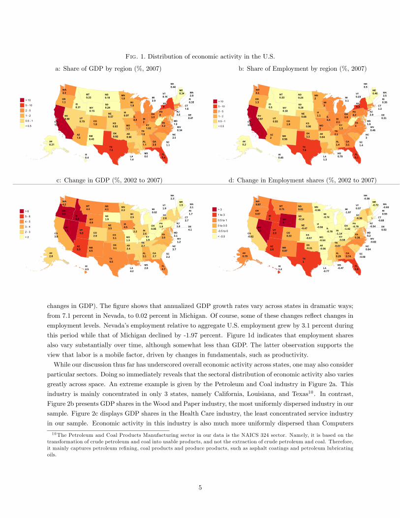
Fig. 1. Distribution of economic activity in the U.S.

a: Share of GDP by region (%, 2007) b: Share of Employment by region (%, 2007)

LL

111

LK

1111

LZ

119

LR

1166

AL

1515

AO

118

AT

116

EE

1177

LL

517

AL

119

II

117

IE

1157

IL

718IN

1

IL

1197

KS

1185KY

1111

LL

117

EE

1157

EE

119

EL

118EI

119

EN

119

ES

116

EO

117

ET

1115

NE

1157NV

1198

NI

1177

NJ

515

NE

1175

NY

8

NA

119

NE

1118

OI

515

OK

1181

OR

115

AL

7

RI

1155

SA

111

SE

1117

TN

118

TX

716

TT

1179

VT

1116

VL

511

AL

115

AV

1157

AI

118AY

1115

AL1.4

AK0.2

AZ2

AR0.84

CA11.7

CO1.8

CT1.3

DE0.31

FL6.1

GA3.1

HI0.45

ID0.5

IL4.4 IN

2.1

IA1.1

KS0.96 KY

1.3

LA1.3

ME0.46

MD1.9

MA2.5

MI3.1

MN2

MS0.79

MO2

MT0.33

NE0.66NV

0.97

NH0.5

NJ2.9

NM0.56

NY6.2

NC3

ND0.24

OH3.9

OK1.1

OR1.3

PA4.2

RI0.35

SC1.4

SD0.28

TN2.1

TX7.6

UT0.93

VT0.23

VA3

WA2.1

WV0.46

WI2

WY0.18

c: Change in GDP (%, 2002 to 2007) d: Change in Employment shares (%, 2002 to 2007)

AL3.1

AK2.8

AZ5.5

AR2.4

CA3.8

CO2.9

CT2.7

DE4.1

FL4.7

GA2.7

HI4.5

ID6.6

IL2.2 IN

2.6

IA4.5

KS3.1 KY

1.9

LA4.2

ME1.5

MD3.1

MA2.1

MI0.02

MN2.3

MS2.8

MO1.3

MT4.4

NE3.5NV

7.1

NH2.3

NJ1.8

NM4.5

NY2.8

NC3.7

ND4.1

OH0.95

OK3.1

OR8.6

PA1.8

RI1.7

SC2.2

SD1.9

TN2.7

TX4.5

UT5.3

VT1.9

VA3.6

WA4.2

WV1.2

WI2.5

WY4.9

AL0.29

AK0.79

AZ2.6

AR-0.56

CA-0.02

CO0.22

CT-0.68

DE0.53

FL1.5

GA0.74

HI1.4

ID2

IL-0.78 IN

-1.14

IA-0.56

KS-0.67 KY

-0.59

LA-0.77

ME-0.72

MD0.2

MA-0.93

MI-1.97

MN-0.56

MS-0.47

MO-0.54

MT0.71

NE-0.47NV

3.1

NH-0.36

NJ-0.54

NM0.87

NY-0.36

NC0.64

ND0.01

OH-1.42

OK-0.31

OR0.67

PA-0.79

RI0.55

SC-0.09

SD-0.14

TN-0.07

TX1

UT2.3

VT0.37

VA0.36

WA0.87

WV-0.82

WI-0.74

WY6

changes in GDP). The figure shows that annualized GDP growth rates vary across states in dramatic ways;

from 7.1 percent in Nevada, to 0.02 percent in Michigan. Of course, some of these changes reflect changes in

employment levels. Nevada’s employment relative to aggregate U.S. employment grew by 3.1 percent during

this period while that of Michigan declined by -1.97 percent. Figure 1d indicates that employment shares

also vary substantially over time, although somewhat less than GDP. The latter observation supports the

view that labor is a mobile factor, driven by changes in fundamentals, such as productivity.

While our discussion thus far has underscored overall economic activity across states, one may also consider

particular sectors. Doing so immediately reveals that the sectoral distribution of economic activity also varies

greatly across space. An extreme example is given by the Petroleum and Coal industry in Figure 2a. This

industry is mainly concentrated in only 3 states, namely California, Louisiana, and Texas10 . In contrast,

Figure 2b presents GDP shares in the Wood and Paper industry, the most uniformly dispersed industry in our

sample. Figure 2c displays GDP shares in the Health Care industry, the least concentrated service industry

in our sample. Economic activity in this industry is also much more uniformly dispersed than Computers

10The Petroleum and Coal Products Manufacturing sector in our data is the NAICS 324 sector. Namely, it is based on thetransformation of crude petroleum and coal into usable products, and not the extraction of crude petroleum and coal. Therefore,it mainly captures petroleum refining, coal products and produce products, such as asphalt coatings and petroleum lubricatingoils.

5

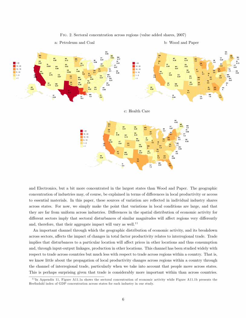
Fig. 2. Sectoral concentration across regions (value added shares, 2007)

a: Petroleum and Coal b: Wood and Paper

LL

2222

LK

2222

LZ

2222

LR

2226

AL

2422

AO

2267

AT

2227

EE

2222

LL

222

AL

222

II

2222

IE

22222

IL

429IN

222

IL

2226

KS

222KY

2292

LL

2929

EE

2222

EE

2222

EL

2227EI

2292

EN

227

ES

229

EO

2226

ET

2292

NE

22222NV

2222

NI

2229

NJ

224

NE

2227

NY

2242

NA

2229

NE

2222

OI

222

OK

222

OR

2229

AL

222

RI

2222

SA

2229

SE

2224

TN

2294

TX

2227

TT

2279

VT

2222

VL

2242

AL

222

AV

2222

AI

2224AY

2229

LL

666

LK

2622

LZ

267

LR

161

AL

666

AO

2667

AT

2611

EE

2666

LL

266

AL

669

II

2626

IE

2666

IL

161IN

2

IL

166

KS

261KY

261

LL

266

EE

169

EE

2666

EL

161EI

262

EN

162

ES

161

EO

261

ET

2611

NE

2621NV

2617

NI

261

NJ

169

NE

2619

NY

266

NA

6

NE

2616

OI

169

OK

2691

OR

1

AL

662

RI

2611

SA

6

SE

2622

TN

166

TX

661

TT

2662

VT

2626

VL

261

AL

1

AV

2667

AI

761AY

2627

c: Health Care

AL1.2

AK0.24

AZ1.9

AR0.77

CA11

CO1.4

CT1.6

DE0.35

FL5.9

GA2.5

HI0.4

ID0.38

IL4.3 IN

2

IA0.9

KS0.88 KY

1.2

LA1.2

ME0.57

MD2.1

MA3.4

MI3.2

MN2.2

MS0.67

MO2

MT0.31

NE0.62NV

0.64

NH0.53

NJ3.5

NM0.52

NY8.1

NC2.6

ND0.25

OH4.1

OK0.97

OR1.3

PA5.2

RI0.46

SC0.96

SD0.31

TN2.2

TX6.6

UT0.61

VT0.25

VA2.7

WA2.1

WV0.55

WI2.1

WY0.13

and Electronics, but a bit more concentrated in the largest states than Wood and Paper. The geographic

concentration of industries may, of course, be explained in terms of differences in local productivity or access

to essential materials. In this paper, these sources of variation are reflected in individual industry shares

across states. For now, we simply make the point that variations in local conditions are large, and that

they are far from uniform across industries. Differences in the spatial distribution of economic activity for

different sectors imply that sectoral disturbances of similar magnitudes will affect regions very differently

and, therefore, that their aggregate impact will vary as well.11

An important channel through which the geographic distribution of economic activity, and its breakdown

across sectors, affects the impact of changes in total factor productivity relates to interregional trade. Trade

implies that disturbances to a particular location will affect prices in other locations and thus consumption

and, through input-output linkages, production in other locations. This channel has been studied widely with

respect to trade across countries but much less with respect to trade across regions within a country. That is,

we know little about the propagation of local productivity changes across regions within a country through

the channel of interregional trade, particularly when we take into account that people move across states.

This is perhaps surprising given that trade is considerably more important within than across countries.

11 In Appendix 11, Figure A11.1a shows the sectoral concentration of economic activity while Figure A11.1b presents theHerfindahl index of GDP concentration across states for each industry in our study.

6

Trade across regions amounts to about two thirds of the economy and it is more than twice as large as

international trade. This evidence underscores the need to incorporate regional trade in the analysis of the

effects of productivity changes, as we do here.12

While interregional trade and input-output linkages have the potential to amplify and propagate techno-

logical changes, they do not generate them. Furthermore, if all disturbances were only aggregate in nature,

regional and sectoral channels would play no role in explaining aggregate changes.

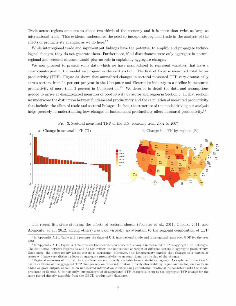
We now proceed to present some data which we have manipulated to represent variables that have a

clear counterpart in the model we propose in the next section. The first of those is measured total factor

productivity (TFP). Figure 3a shows that annualized changes in sectoral measured TFP vary dramatically

across sectors, from 14 percent per year in the Computer and Electronics industry to a decline in measured

productivity of more than 2 percent in Construction.13 We describe in detail the data and assumptions

needed to arrive at disaggregated measures of productivity by sector and region in Section 5. In that section,

we underscore the distinction between fundamental productivity and the calculation of measured productivity

that includes the effect of trade and sectoral linkages. In fact, the structure of the model driving our analysis

helps precisely in understanding how changes in fundamental productivity affect measured productivity.14

Fig. 3. Sectoral measured TFP of the U.S. economy from 2002 to 2007

a: Change in sectoral TFP (%) b: Change in TFP by regions (%)

-10

-5

0

5

10

15

C

ompu

ter

and

Ele

ctro

nic

T

rans

port

atio

n E

quip

men

t

F

ood,

Bev

erag

e, T

obac

co

Inf

orm

atio

n S

ervi

ces

T

rans

port

Ser

vice

s

M

achi

nery

M

isce

llane

ous

T

extil

e, A

ppar

el, L

eath

er

E

lect

rical

Equ

ipm

ent

P

last

ics

and

Rub

ber

Woo

d an

d P

aper

Prin

ting

Fur

nitu

re

Rea

l Est

ate

Che

mic

al

Who

lesa

le a

nd R

etai

l Tra

de

Fin

ance

and

Insu

ranc

e

Art

s an

d R

ecre

atio

n

A

ccom

. and

Foo

d S

ervi

ces

H

ealth

Car

e

O

ther

Ser

vice

s

N

onm

etal

lic M

iner

al

Prim

ary

and

Fab

ricat

ed M

etal

Edu

catio

n

Con

stru

ctio

n

Pet

role

um a

nd C

oal

a. Change in sectoral TFP (%)

AL0.97

AK0.005

AZ1.7

AR1.3

CA1.3

CO0.65

CT0.88

DE1.8

FL0.95

GA0.59

HI0.36

ID1.9

IL0.77 IN

1.4

IA1.9

KS1.2 KY

1.2

LA1.2

ME0.23

MD0.55

MA0.73

MI1.1

MN1.1

MS1.3

MO0.58

MT1.03

NE1.1NV

1.4

NH0.83

NJ0.38

NM-0.07

NY0.85

NC1.1

ND1.2

OH0.81

OK1.04

OR2.5

PA0.44

RI0.14

SC0.94

SD1.7

TN1.1

TX1.9

UT1.2

VT2.1

VA1.1

WA1.1

WV0.1

WI1.1

WY0.11

The recent literature studying the effects of sectoral shocks (Foerster et al., 2011, Gabaix, 2011, and

Acemoglu, et al., 2012, among others) has paid virtually no attention to the regional composition of TFP

12 In Appendix A.11, Table A11.1 presents the share of U.S. international trade and interregional trade over GDP for the year2007.13 In Appendix A.11, Figure A11.2a presents the contribution of sectoral changes in measured TFP to aggregate TFP changes.

The distinction between Figures 3a and A11.2a reflects the importance or weight of different sectors in aggregate productivity.Once more, the heterogeneity across sectors is surprising. Moreover, this heterogeneity implies that changes in a particularsector will have very distinct effects on aggregate productivity, even conditional on the size of the changes.14Regional measures of TFP at the state level are not directly available from a statistical agency. As explained in Section 5,

our calculations of disaggregated TFP changes rely on other information directly observable by region and sector, such as valueadded or gross output, as well as on unobserved information inferred using equilibrium relationships consistent with the modelpresented in Section 3. Importantly, our measures of disaggregated TFP changes sum up to the aggregate TFP change for thesame period directly available from the OECD productivity database.

7

changes. Figure 3b shows that this lack of attention is potentially misguided. Changes in measured TFP

vary widely across regions. Furthermore, the contribution of regional changes in measured TFP to variations

in aggregate TFP is also very large.15

The change in TFP over the period 2002-2007 was 1.4 percent per year in Nevada but 1.1 percent in

Michigan. These differences in TFP experiences naturally contributed to differences in employment and GDP

changes in those states. More generally, variations across states result in part from sectoral productivity

changes as well as changes in the distribution of sectors across space which, as we have argued, is far from

uniform. However, even if all the variation in Figure 3b was ultimately traced back to sectoral changes, their

uneven regional composition would influence their impact on trade and, ultimately, aggregate TFP.

One of the key economic determinants of income across regions is the stock of land and structures. To

our knowledge, there is no direct measure of this variable. However, as we explain in detail in Section 5,

we can use the equilibrium conditions from our model to infer the regional distribution of income from land

and structures across U.S. states. Per capita income from land and structures in 2007 U.S. dollars varies

considerably across states. The range varies from a low of 10,200 and 13,000 dollars per capita for the case

of Vermont and Wisconsin respectively, to a high of 47,000 dollars in Delaware.16 We will argue that this

regional dispersion of land and structures across regions in the U.S. is central to understanding the aggregate

effects of disaggregated fundamental productivity changes.

We conclude this section with an evaluation of the relative importance of regional and sectoral changes in

TFP for the aggregate economy. To do so, we follow Koren and Tenreyro (2007)’s methodology to decompose

measured TFP into a regional, a sectoral, and a regional-sectoral component. The results for measured TFP

changes from 2002 to 2007 are presented in Table 1. The regional component accounts for 28.9% of the

changes in measured TFP, while the sectoral component accounts for 21.1% of the variation and the region-

sector component for the remaining 50%. In Appendix A.5, we describe in detail the methodology, as well as

all the data and steps needed to perform the decomposition. We also show that the results for measured TFP

changes between 2007 and 2012 are similar.17 In all cases we find that regional productivity changes, either

for all sectors or for specific sectors, account for more than three fourths of the variation in measured TFP.

The next section proposes a macroeconomic framework with spatial detail to quantify these relationships.

Table 1. Importance of Regional and Sectoral TFP ChangesVariation in measured TFP changes for 2002-2007 explained byRegional component 28.9%Sectoral component 21.1%Residual 50.0%

N o t e : T h i s t a b le s h ow s S o b o l’s S e n s i t iv i ty in d e x , d efin e d in A p p e n d ix A .5 .

3. THE MODEL

Our goal is to produce a quantitative model of the U.S. economy disaggregated across regions and sectors.

For this purpose, we develop a static two factor model with N regions and J sectors. We denote a particular

15Appendix A.11, Figure A11.2b presents the contribution of regional changes in measure TFP. The difference betweenFigures 3a and A11.2b reflects the weight of different states in aggregate productivity.16Appendix A.11 Figure A11.3 shows the per capita income from land and structures in 2007 for all U.S. states.17 In Appendix A.5 we also present the results where instead of using measured TFP we use fundamental TFP, a model-based

concept of productivity that represents production effi ciency in the production of value added in the absence of trade andselection effects. The results are again similar. Please refer to Table A5.1 in Appendix A.5 to see the results.

8

region by n ∈ {1, ..., N} (or i), and a particular sector by j ∈ {1, ..., J} (or k). The economy has two factors,labor and a composite factor comprising land and structures. Labor can freely move across regions and

sectors. Land and structures, Hn, are a fixed endowment of each region but can be used by any sector. We

denote total population size by L, and the population in each region by Ln. A given sector may be either

tradable, in which case goods from that sector may be traded at a cost across regions, or non-tradable.

Throughout the paper, we abstract from international trade and other international economic interactions.

3.1 Consumers

Agents in each location n ∈ {1, ..., N} order consumption baskets according to Cobb-Douglas preferencesgiven by

U (Cn) =∏J

j=1(cjn)α

j

where∑J

j=1αj = 1,

with shares αj , over their consumption of final domestic goods cjn, bought at prices Pjn, in all sectors

j ∈ {1, ..., J}. Agents move freely across regions. In equilibrium, households are indifferent between livingin any region. Hence,

U =InPn

for all n ∈ {1, ..., N} , (1)

where In is income earned by agents residing in region n, Pn =∏J

j=1

(P jn/α

j)αj

is the ideal price index

in region n, and U is determined in equilibrium. All prices are denoted in terms of a numéraire which we

choose to be the price of aggregate output in the U.S.

3.2 Asset Holdings and Regional Deficits

A quantitative model of the U.S. economy should accommodate the large observed regional trade imbal-

ances.18 We model imbalances in our framework by determining the asset holdings of agents in each location.

We assume that local factors are partly owned by local governments that redistribute their rents to local

residents. The remaining share of local factors is aggregated in a national portfolio that is owned by all

residents.

We assume that a fraction ιn ∈ [0, 1] of the rents to the local factor go into the national portfolio of

local assets. All residents hold an equal number of shares in the national portfolio and so receive the same

proportion of its returns. The remaining share, (1− ιn), of local factors is owned by the local government in

region n. The returns to this fraction of the local factors is distributed lump-sum to all local residents. This

ownership structure of local factors result in a model that is flexible enough (through the determination of

ιn) to match almost exactly observed trade imbalances across states (see Section 5). It allows individuals

living in certain states to receive higher returns from local factors but avoids the complications of individual

wealth effects, and the resulting heterogeneity across individuals, that result from individual ownership of

local assets. We refer to 1− ιn as the share of local rents from land and structures.

The income of an agent residing in region n is therefore In = wn +χ+ (1− ιn) rnHn/Ln, where wn is the

wage and rn is the rental rate of structures and land, and rnHn/Ln, is the per capita income from renting

land and structures to firms in region n. The term χ represents the return per person from the national18The international trade literature usually abstracts from modelling trade imbalances across countries, either by assuming

that trade is balanced, or by assuming these imbalances are constant. The U.S. economy presents substantial trade imbalancesacross regions. For instance, Florida and Texas had trade deficits of about US 40 billion in 2007, while Wisconsin and Indianahave surpluses of about the same magnitude. Here we propose a practical way to deal with these imbalances in a static model.

9

portfolio of land and structures from all regions. In particular, χ =∑Ni=1 ιiriHi

/∑Ni=1 Li.

The remittances by region n to the national portfolio are given by ιnrnHn. Hence, the difference between

the remittances and the income in region n, generates imbalances given by

Υn ≡ ιnrnHn − χLn. (2)

The excess of income generated by these imbalances in region n is spent by agents in local goods. The

magnitude of these imbalances will change in our model with changes in fundamental productivity, as they

will impact the wages and the rental rate of structures. Increases in fundamental productivity in region

n relative to the U.S. economy will increase the remittances sent to the national portfolio relative to the

transfers from it; thus, increasing the likelihood of surpluses in region n, Υn. Note that if ιn < 1, so part of

the rents from local assets are owned and redistributed by the local government, the competitive equilibrium

is not effi cient. The reason is that agents do not internalize the effect of their migration decisions on the

local rents distributed to other agents.19

3.3 Technology

Technology in our model follows closely Eaton and Kortum (2002). Sectoral final goods are used for

consumption and as material inputs into the production of intermediate goods in all industries. In each

sector, final goods are produced using a continuum of varieties of intermediate goods in that sector. We refer

to the intermediate goods used in the production of final goods as ‘intermediates,’and to the final goods

used as inputs in the production of intermediate goods as ‘materials.’

3.3.1 Intermediate Goods

Representative firms, in each region n and sector j, produce a continuum of varieties of intermediate goods

that differ in their idiosyncratic productivity level, zjn. In each region and sector, this productivity level is a

random draw from a Fréchet distribution with shape parameter θj and location parameter 1. Note that θj

varies only across sectors. We assume that all draws are independent across goods, sectors, and regions. The

productivity of all firms producing varieties in a region-sector pair (n, j) is also determined by a deterministic

productivity level, T jn, specific to that region and sector. We refer to Tjn as fundamental productivity. The

production function for a variety associated with idiosyncratic productivity zjn in (n, j) is given by

qjn(zjn) = zjn

[T jn[hjn(zjn)

]βn [ljn(zjn)](1−βn)]γjn∏J

k=1

[M jkn (zjn)

]γjkn , (3)

19An alternative option is to allow some immobile agents in each state to own state-specific shares of a national portfoliothat includes all the rents of the immobile factor (namely χ =

∑i riHi). As long as these shares sum to one, and the rentiers

cannot move, such a model is as tractable as the one we propose in the main text. We have computed our main resultswith this alternative model and find similar results. For example, the correlation of the elasticities of aggregate TFP and realGDP to regional fundamental productivity changes between the model we propose and this alternative model is 95.2% and95.1%, respectively. Ultimately, although not particular important given these numbers, the choice between having some localdistribution of rents, or some immobile agents that own all the shares in the national portfolio, involves choosing betweensimilar, albeit perhaps not ideal, simplifying assumptions. See Appendix A.10 to additional computations using this effi cientversion of the model.

10

where hjn(·) and ljn(·) denote the demand for structures and labor respectively20 , M jkn (·) is the demand for

final material inputs by firms in sector j from sector k (variables representing final goods are denoted with

capital letters), γjkn > 0 is the share of sector j goods spent on materials from sector k, and γjn > 0 is the

share of value added in gross output. We assume that the production function has constant returns to scale,

namely that∑Jk=1 γ

jkn = 1− γjn.21 Observe that we specified the technology in (3) such that T jn scales value

added and not gross output. This implies that an increase in T jn, for all j and n, has a proportional effect

on aggregate real GDP (of course, this normalization only has consequences conditional on a calibration of

the model).

Let xjn denote the cost of the input bundle needed to produce intermediate good varieties in (n, j) . Then

xjn = Bjn[rβnn w1−βnn

]γjn∏J

k=1

[P kn]γjkn , (4)

where Bjn =[γjn (1− βn)

(1−βn) ββnn

]−γjn∏J

k=1

[γjkn]−γjkn . The unit cost of an intermediate good with idio-

syncratic draw zjn in region-sector pair (n, j) is then given by xjn/(

zjn[T jn]γjn) . Firms located in region n

and operating in sector j will be motivated to produce the variety whose productivity draw is zjn as long

as its price matches or exceeds xjn/(

zjn[T jn]γjn) . Assuming a competitive market for intermediate goods,

firms that produce a given variety in (n, j) will price it according to its corresponding unit cost.

3.3.2 Final Goods

Final goods in region n and sector j are produced by combining intermediate goods in sector j. Denote

the quantity of final goods in (n, j) by Qjn, and denote by qjn(zj) the quantity demanded of an intermediate

good of a given variety such that, for that variety, the particular vector of productivity draws received by

the different n regions is zj = (zj1, zj2, ...z

jN ). The production of final goods is given by

Qjn =

[∫qjn(zj)1−1/η

jnφj

(zj)dzj]ηjn/(ηjn−1)

, (5)

where φj(zj) = exp{−∑Nn=1

(zjn)−θj}

denotes the joint density function for the vector zj , with marginal

densities given by φjn(zjn) = exp{−(zjn)−θj}

, and the integral is over RN+ . For non-tradeable sectors, theonly relevant density is φjn

(zjn)since final good producers use only locally produced goods.

There is free entry in the production of final goods with competition implying zero profits.

3.4 Prices and Regional Trade

Final goods are non-tradable. Intermediate goods in tradable sectors are costly to trade. One unit of any

intermediate good in sector j shipped from region i to region n requires producing κjni ≥ 1 units in i, with

κjnn = 1 and, for intermediate goods in non-tradable sectors, κjni =∞. Thus, the price paid for a particularvariety whose vector of productivity draws is zj , pjn(zj), is given by the minimum of the unit costs across

20Our model will not ignore capital, as most static models do. We take a longer view of the economy and treat capital asmaterials (after all, capital is just a type of intermediate, which depreciates slowly). When we take the model to the data weare careful in accounting for capital in this particular way.21 In order to avoid a cumbersome notation, we decided to define the sectoral share of goods spent on materials from other

sectors inclusive of the share of value added. Namely, γjkn =(1− γjn

)γjkn , where

∑Jk=1 γ

jkn = 1.

11

locations, adjusted by the transport costs κjni.

Given our assumptions governing the distribution of idiosyncratic productivities, zji , we follow Eaton and

Kortum (2002) to solve for the distribution of prices. Having solved for the distribution of prices, when

sector j is tradeable, the price of final good j in region n is given by

P jn = Γ(ξjn)1−ηjn [∑N

i=1

[xjiκ

jni

]−θj [T ji

]θjγji]−1/θj, (6)

where Γ(ξjn)is a Gamma function evaluated at ξjn = 1 +

(1− ηjn

)/θj . When j denotes a non-tradeable

sector, the price index is instead given by P jn = Γ(ξjn)1−ηjn xjn [T jn]−γjn .

Let πjni denote the share of region n’s total expenditures on sector j’s intermediate goods purchased from

region i. Following Eaton and Kortum (2002), and Alvarez and Lucas (2007), using the properties of the

Frechet distribution, we can solve for the expenditure shares πjni, given by

πjni =

[xjiκ

jni

]−θjTj θjγjii

N∑m=1

[xjmκ

jnm

]−θjT j θ

jγjmm

. (7)

In non-tradable sectors, κjni =∞ for all i 6= n so that πjnn = 1.

3.5 Labor Mobility and Market Clearing

Regional labor market clearing requires that

∑J

j=1Ljn =

∑J

j=1

∫ ∞0

ljn(z)φjn (z) dz = Ln, for all n ∈ {1, ..., N} , (8)

where Ljn is the number of workers in (n, j) , and national labor market clearing is given by∑N

n=1Ln = L.

In a regional equilibrium, land and structures must satisfy

∑J

j=1Hjn =

∑J

j=1

∫ ∞0

hjn(z)φjn (z) dz = Hn, for all n ∈ {1, ..., N} , (9)

where Hjn denotes land and structure use in (n, j) .

Profit maximization by intermediate goods producers, together with these equilibrium conditions, implies

that rnHn(1 − βn) = βnwnLn, for all n ∈ {1, ..., N} . Then, defining ωn ≡ [rn/βn]βn [wn/(1− βn)]

(1−βn) ,

free mobility gives us

Ln = Hn

[ωn

PnU + un

] 1βn

,

where un ≡ Υn/Ln = ιnrnHn/Ln−χ denotes the trade surplus per capita in n. Combining these conditionswith the labor market clearing condition, yields an expression for labor input in region n,

Ln =Hn

[ωn

PnU+un

]1/βn∑N

i=1Hi

[ωi

PiU+ui

]1/βi L. (10)

12

Equilibrium condition (10) states that the employment share in region n is increasing in its endowment

of land and structures Hn, and in factor prices as captured by ωn. Conversely, employment in region n is

decreasing in the size of trade surplus in that region un, as larger transfers to the global portfolio reduces

per-capita income available in region n.

It remains to describe market clearing in final and intermediate goods markets. Regional market clearing

in final goods is given by

Lncjn +

∑J

k=1Mkjn = Lnc

jn +

∑J

k=1

∫ ∞0

Mkjn (z)φkn (z) dz = Qjn, (11)

for all j ∈ {1, ..., J} and n ∈ {1, ..., N} , where Mkjn represents the use of materials of sector j in sector k at

n.

Let Xjn denote total expenditures on final good j in region n (or total revenue). Then, regional market

clearing in final goods implies that

Xjn =

∑J

k=1γkjn

∑N

i=1πkinX

ki + αjInLn, (12)

In equilibrium, in any region n, total expenditures on intermediates purchased from other regions must

equal total revenue from intermediates sold to other regions, formally,∑J

j=1

∑N

i=1πjniX

jn + Υn =

∑J

j=1

∑N

i=1πjinX

ji . (13)

Trade is, in general, not balanced within each region since a particular region can be a net recipient of

national returns on land and structures while another might be a net contributor. As such, our model,

through its ownership structure, accounts for trade imbalances and how these imbalances are affected by

changes in fundamental productivity. In Section 5 we explain how to use information on regional trade

imbalances to estimate the parameters that determine the ownership structure, {ιn}Nn=1.

Definition: Given factor supplies, L and {Hn}Nn=1, a competitive equilibrium for this economy is a utility

level U, a set of factor prices in each region, {rn, wn}Nn=1, a set of labor allocations, structure allocations, finalgood expenditures, consumption of final goods per person, and final goods prices, {Ljn, Hj

n, Xjn, c

jn, P

jn}

N,Jn=1,j=1,

pairwise sectoral material use in every region, {M jkn }

N,J,Jn=1,j=1,k=1, regional transfers {Υn}Nn=1, and pairwise

regional intermediate expenditure shares in every sector, {πjni}N,N,Jn=1,i=1,j=1, such that the optimization condi-

tions for consumers and intermediate and final goods producers hold, all markets clear - equations (2), (4),

(6), (7), (8), (9), (11), (12) hold -, aggregate trade is balanced - (13) holds- , and utility is equalized across

regions, - (10) holds.

4. AGGREGATION AND CHANGES IN MEASURED TFP, GDP, AND WELFARE

Given the model we have just laid out, this section describes how to arrive at measures of total factor

productivity, GDP, and welfare, that are disaggregated across both regions and sectors. These calculations

of measures at the level of sector in a region, using available industry and regional trade data for the U.S.,

underlie Figure 3 and the discussion in Section 2, as well as all calculations in the rest of the paper.

13

4.1 Measured TFP

Measured sectoral total factor productivity in a region-sector pair (n, j) is commonly calculated as

lnAjn = lnwnL

jn + rnH

jn +

∑Jk=1 P

knM

jkn

P jn− (1− βn) γjn lnLjn − βnγjn lnHj

n −∑J

k=1γjkn lnM jk

n . (14)

The first term is gross output revenue over price —a measure of gross production in (n, j) which we denote

by Y jn/Pjn, and which is equal to Q

jn in the case of non-tradables—, while the last three terms denote the

log of the aggregate input bundle.22 This last equation assumes that we use gross output and final good

prices to calculate region-sector TFP. Observe that the equilibrium factor demands of the intermediate good

producers imply that

Y jn = wnLjn + rnH

jn +

∑J

k=1P knM

jkn =

wnLjn

γjn (1− βn). (15)

Therefore, we may calculate changes in measured TFP, Ajn, following a change in fundamental productivity,

T jn , using the ratio of the change in the cost of the input bundle to the change in the price of final goods.23

That is,

ln Ajn = lnxjn

P jn= ln

[T jn]γjn

[πjnn]1/θj, (16)

where the second equality follows from (7).

Equation (16) is central to understanding the sources of changes in measured productivity in an individual

sector within a region following a change in fundamental productivity, T jn.24

Consider first an economy with infinite trading costs κjni =∞ for all j, so that trade is non-operative and

πjnn = 1 in every region. Furthermore, let us abstract from material input use so that the share of value

added in gross output is equal to one, γjn = 1. In such an economy, Equation (16) implies that changes

in measured productivity Ajn are identical to changes in fundamental productivity, Tjn. Any fundamental

productivity change at the level of a sector within a region translates into an identical change in measured

productivity in that sector and region, and has otherwise no effect on the productivity of any other sector

or region.

This exact relationship between fundamental and measured productivity, ln Ajn = ln T jn, no longer holds

22One can prove that total gross output in (n, j) uses this aggregate input bundle. To do so, we aggregate the equilibrium factordemands of the intermediate good producers. After that, it is straightforward to derive that factor usage for an intermediateis just the revenue share of that intermediate in gross revenue, Y jn . Substituting in Equation (3), and using the fact that pricesof produced intermediates are equal to unit costs, leads to

Y jn

P jn=xjn

P jn

[(Hjn

)βn (Ljn)(1−βn)]γjn∏J

k=1

(Mjkn

)γjkn,

where Ajn = xjn/Pjn measures region and sector specific TFP.

23The ‘hat’notation denotes A′/A, where A′ is the new level of total factor productivity.24 Note from (16) that the key distinction between measured and fundamental TFP is the selection effect. Empirically, the

U.S. Bureau of Labor Statistics (BLS) is the statistical agency that measures TFP changes. In order to control for changesin the production structure of the economy (due to selection effects), the BLS periodically (every five years according to Page10, Chapter 14, Handbook of Methods) changes the weights in their producer prices indexes (PPI), which are used for theconstruction of Multifactor Productivity by the Bureau of Economic Analysis (BEA) and the BLS. Given this, in periodsbetween changes in weights, one can directly infer changes in fundamental TFP from changes in the measured TFP calculatedby the BEA and BLS as Ajn = (T jn)

γjn , as we do later for the case of Computers and Electronics in California. For furtherdiscussion on the implications of trade models for the computation of TFP and GDP as measured by statistical agencies seeBurstein and Cravino (2015).

14

once either trade or sectoral linkages are operative. Consider first adding sectoral linkages, so that γjn < 1,

but still abstracting from trade. In that case, Equation (16) indicates that the effect of a change, T jn, improves

measured productivity less than proportionally. The reason is that the change affects the productivity of

value added in that region and sector but not the productivity of sectors and regions in which materials

are produced. Therefore, in the presence of input output linkages, the effect of a fundamental productivity

change T jn on measured productivity in (n, j) falls with 1− γjn =∑Jk=1 γ

jkn .

This last result follows from our assumption that productivity changes scale value added and not gross

output (as in Acemoglu et al. 2012). If productivity instead affected all of gross output, a sector that

just processed materials, without adding any value by way of labor or capital, would see an increase in

output at no cost. That alternative modelling implies that aggregate fundamental productivity changes

have abnormally large effects on real GDP while, with our technological assumption, aggregate fundamental

changes have proportional effects on real GDP. This distinction matters greatly in quantitative exercises.

Evidently, with trade still shut down, a region and sector specific change in this economy has no effect on

the measured productivity of any other region or sector. In contrast, with trade, productivity changes are

propagated across sectors and regions. The main effect of regional trade on productivity arises by way of a

selection effect. Thus, let κjni be finite for tradable sectors, and consider first the region-sector (n, j) that

experiences a change or increase in fundamental productivity, T jn. Equation (16) implies that the effect of

trade is ultimately summarized through the change in the region’s share of its own intermediate goods, πjnn.

Since an increase in fundamental productivity in (n, j) raises its region and sector comparative advantage,

it generally also leads to an increase in πjnn so that πjnn > 1. Similarly, it reduces πkii, for i 6= n and all

k, since other regions and sectors now buy more sector-j intermediates from region n. Hence, since θj > 0,

trade reduces the effect of a fundamental productivity increase to (n, j) on measured productivity in that

region-sector while, at the same time, raising measured productivity in other regions and sectors.

Intuitively, the selection effect underlying the change in expenditure shares works as follows. As every-

one purchases more goods from the region-sector pair (n, j) that experienced a fundamental productivity

increase, that region-sector pair now produces a greater variety of intermediate goods. However, the new

varieties of intermediate goods, since they were not being initially produced, are associated with idiosyncratic

productivities that are relatively worse than those of varieties produced before the change. This negative

selection effect in (n, j) partially offsets the positive consequences of the fundamental productivity change,

relative to an economy with no trade, in that region-sector pair. In other region-sector pairs, (i, j) for i 6= n,

the opposite effect takes place. As the latter regions do not directly experience the fundamental productivity

change, their own trade share of intermediates decreases. As a result, the varieties of intermediate goods that

continue being produced in those regions have relatively higher idiosyncratic productivities, thereby yield-

ing higher measured productivity in those locations. All of these trade-related effects are present whether

material inputs are considered or are absent from the analysis.

Measured TFP at the level of a sector in a region is calculated based on gross output in equation (14),

so we use gross output revenue shares to aggregate these TFP measures into regional, sectoral, or national

measures. Our aggregate TFP measures are described in more detail in Appendix A.8.

4.2 GDP

Real GDP is calculated by taking the difference between real gross output and expenditures on materials.

Given the equilibrium factor demands of the intermediate good producers, as well as factor market equilib-

15

rium conditions, changes in real GDP may be written as ln GDPj

n = ln wn + ln Ljn − ln P jn. This expression

simplifies further since, from (7), P jn = [πjnn]1

θj xjn[T jn]−γji , so that GDP changes in a region-sector pair (n, j),

resulting from changes in fundamental TFP, T jn, are given by

ln GDPj

n = ln Ajn + ln Ljn + ln

(wn

xjn

), (17)

using Equation (16). Given that real GDP is a value added measure, we use value added shares in constant

prices to aggregate changes in GDP.25

Equation (17) represents a decomposition of the effects of a change in fundamental productivity on GDP.

The first term reflects the effect of the change on measured productivity discussed in Section 4.1. This effect

is such that measured TFP and output move proportionally. In other words, the selection effect associated

with intermediates and input-output linkages acts identically on measured TFP and real GDP. In addition to

these effects, GDP is also influenced by two other forces captured by the second and third terms in Equation

(17).

The second term in Equation (17) describes the effect of labor migration across regions and sectors on

GDP. A positive productivity change that attracts population to a given region-sector pair (n, j) will increase

GDP proportionally to the amount of immigration, ln Ljn. The reason is that all factors in (n, j) change in the

same proportions and the production function of intermediates in Equation (3) is constant-returns-to-scale.

The effect of migration will be positive when the change in fundamental TFP is positive.

The third term in Equation (17) corresponds to the change in factor prices associated with the change

in fundamental TFP. Consider first a case without materials. In that case, ln(wn/x

jn

)= βn ln (wn/rn) =

βn ln 1/Ln. Since land and structures are fixed, and therefore do not respond to changes in T jn, while labor is

mobile across locations, a positive productivity change that attracts people to the region will increase land

and structure prices more than wages. This mechanism leads to a reduction in real GDP, relative to the

proportional increase associated with the first two terms. The presence of decreasing returns resulting from

a regionally fixed factor implies that shifting population to a location strains local resources, such as local

infrastructure, in a way that offsets the positive GDP response stemming from the inflow of workers. In

regions that do not experience the productivity increase, the opposite is true so that the second and third

terms in (17) will be negative and positive respectively. These forces are also present when we consider

material inputs although, in that case, the relevant ratio is that of changes in wages to changes in the

cost of the input bundle, xjn. The input bundle includes the rental rate, but it also includes the price of

all materials. An overall assessment of the effects of fundamental productivity changes then requires a

quantitative evaluation.

As we consider the aggregate economy-wide effects of a positive T jn, the end result for GDP may be larger

or smaller than the original change. The overall impact of the last two terms in Equation (17) will depend on

whether the direct effect of migration dominates the strain on local resources in the region experiencing the

change, n, as well as the intensiveness with which this fixed factor is used in the regions workers leave behind,

i 6= n. Thus, the size and sign of these effects depend on the overall distribution of Hn and population Lnin the economy and, therefore, on whether the productivity change increases the dispersion of the wage-cost

bundle ratio, wn/xn, across regions. If a productivity change leads to migration towards regions that lack

abundant land and structures, the aggregation of the last two terms in Equation (17) may be negative or

very small. In contrast, if a change moves people into regions with an abundance of local fixed factors,

25 In Appendix A.8 we describe the aggregate GDP measures at the regional, sectoral, and national levels.

16

the impact of these last two terms will be positive. Evidently, whatever the case, one must still add the

direct effect of the fundamental productivity change on measured productivity. These different mechanisms

underscore the importance of geography, and that of the sectoral composition of technology changes, in order

to assess the magnitude of such changes. In very extreme cases (only Hawaii in our numerical exercises),

these mechanisms may even lead to negative aggregate GDP effects of productivity increases. However, even

though the equilibrium allocation is not Pareto effi cient, in practice positive technological changes always

lead to welfare gains.

Finally, it is worth noting that in the case of aggregate productivity changes, the distribution of population

across locations is unchanged since people do not seek to move when all locations are similarly affected.

Therefore, measured productivity and GDP unambiguously increase proportionally in that case.

4.3 Welfare

We end this section with a brief discussion of the welfare effects that result from changes in fundamental

productivity. Using (1), and the equilibrium factor demands of the intermediate good producers, it follows

that the change in welfare, in consumption equivalent units, is given by U = In/Pn. Then, using the

definition of Pn and equations (7) and (16), we have that

ln U =∑J

j=1αj(

ln Ajn + ln

($n

wn

xjn+ (1−$n)

χ

xjn

)), (18)

where $n = (1−βnιn)wn(1−βnιn)wn+(1−βn)χ

. Note that if ιn = 0 for all n, then χ = 0 and $n = 1. In that case

ln U =∑Jj=1 α

j(

ln Ajn + ln wnxjn

).

A change in fundamental productivity, T jn, affects welfare through three main channels. First, the change

affects welfare through changes in measured productivity, ln Ajn, in all sectors (which in turn are influenced

by the selection effect in intermediate goods production described earlier), weighted by consumption shares,

αj . Second, the productivity change affects welfare through changes in the cost of labor relative to the input

bundle, ln(wn/x

jn

). As in the case of GDP, when we abstract from materials, the second term is equivalent

to the change in the price of labor relative to that of land and structures or, alternatively, the inverse of the

change in population. Therefore, when a region-sector pair (n, j) experiences an increase in fundamental

productivity, it benefits from the additional measured productivity but loses from the inflow of population. In

other regions that did not experience the productivity increase, population falls while measured productivity

tends to increase (through a selection effect where remaining varieties in those regions are more productive),

so that both effects on welfare are positive. These mechanisms are more complex once sectoral linkages are

taken into account by way of material inputs, and their analysis then requires us to compute and calibrate

the model. As Equation (18) indicates, welfare also simply reflects a weighted average across sectors of real

GDP per capita. Third, welfare is affected by the change in the returns to the national portfolio, which

constitutes part of the real income received by individuals.

The international trade literature has studied the welfare implications of a similar class of models in detail,

as discussed in Arkolakis et al. (2012). Relative to these models, the study of the domestic economy compels

us to include multiple sectors, input-output linkages, and two factors, one of which is mobile across sectors

and the other across locations and sectors. Finally, our model also endogenizes trade surpluses and deficits.

If we were to close all of these margins, it is straightforward to show that the implied change in welfare

simply reduces to the change in measured productivity in the resulting one-sector economy, reproducing the

17

formula highlighted by Arkolakis et. al. (2012).

5. CALCULATING COUNTERFACTUALS AND CALIBRATION

From the discussion in the last section, it should be clear that the ultimate outcome of a given change

in fundamentals on the U.S. economy will depend on various aspects of its particular sectoral and regional

composition. Therefore, to assess the magnitude of the responses of measured TFP, GDP and welfare to

fundamental technology changes, one needs to compute a quantitatively meaningful variant of the model.

This requires addressing four practical issues.

First, the U.S. economy exhibits aggregate trade deficits and surpluses between states. The model pre-

sented in Section 3 allows for the possibility of sectoral trade imbalances across states as well as aggregate

trade imbalances due to inter-regional transfers of the returns from land and structures, (see equation 13).

By incorporating variation in regional contributions to the national portfolio through the parameters ιn, our

model is capable of matching quite well the observed aggregate trade imbalances in the U.S. economy.26 In

the next subsection we provide further details on how we measure ιn.

The second issue relates to our model incorporating regional but no international trade. Fortunately, the

trade data across U.S. states that we use to calibrate the model, which is described in detail below, gives us

expenditures in domestically produced goods across states. Even then, small adjustments are needed but,

overall, we are able to use these data to assess the behavior of the domestic economy without considering

international economic links.27 Thus, we study the domestic economy subject to the small data adjustments

described below.

The third issue of practical relevance is that solving for the equilibrium requires identifying technology

levels in each region-sector pair (n, j) , bilateral trade costs between regions for different sectors (n, i, j) ,

and the elasticity of substitution across varieties, all of which are not directly observable from the data.

Following the method first proposed by Dekle, Eaton and Kortum (2008), and adapted to an international

context with multiple sectors and input-output linkages by Caliendo and Parro (2015), we bypass this third

issue by computing the model in changes. In particular, let x be an equilibrium outcome given fundamental

productivity T, and x′ be a new equilibrium outcome given a new fundamental productivity T ′. Let us

denote by x = x′/x the relative change of x given a change in fundamental productivity from T to T ′ that

we denote by T = T ′/T. Rather than solving the model in levels, we will solve for changes in equilibrium

allocations given changes in productivities T . In Appendix A.2, we show that this method works well in

our setup and present the equilibrium conditions of the model in relative changes. In particular, given

a set of parameters {θj , αj , βn, ιn, γjn, γjkn }N,J,Jn=1,j=1,k=1, data for {In, Ln,Υn, π

jni}

N,N,Jn=1,i=1,j=1, and changes

in exogenous variables {T jn, κjni}

N,N,Jn=1,i=1,j=1, the system of 2N + 3JN + JN2 equations yields the values

of {wn, Ln, xjn, P jn, Xjn, π

jni}

N,N,Jn=1,i=1,j=1, where X

jn and π

jni denote expenditures and trade shares following

fundamental changes {T jn, κjni}

N,N,Jn=1,i=1,j=1. Note that, although transport cost levels (κjni) are essential to

determine the impact of, say, productivity changes in our framework, we do not need direct information on

transport costs since all the relevant information is embedded in the observed trade flows, πjni.

We use all 50 U.S. states and 26 sectors, where 15 sectors produce tradable manufactured goods. Ten

26Unless one writes a dynamic model in which imbalances are the result of fundamental sources of fluctuations, one cannotexplain either the level, or the potential changes, in the value of ιn. Explaining the observed ownership structure is certainlyan interesting direction for future research, but one that is currently beyond reach in a rich quantitative model comparable tothe one studied in this paper.27 In principle, one might potentially think of the ‘rest of the world’as another region in the model but, to the best of our

knowledge, information on international trade by states is not systematically recorded.

18

sectors produce services and we add construction for a total of 11 non-tradeable sectors. The next section

briefly describes the data sources and Appendix A.4 provides greater details. Assessing the quantitative

effects on the U.S. economy of fundamental changes at the level of a sector within a region then requires

solving a system of 69,000 equations and unknowns (endogenous variables to be determined in equilibrium).

This system can be solved in blocks recursively using well established numerical methods. The exact al-

gorithm is described in Appendix A.3. Having carried out these calculations, it is then straightforward to

obtain any other variable of interest such as rn, πjnn, A

jn, GDP

j

n and U , among others.

Finally, the fourth issue relates to our assumption that labor can move freely across regions. The potential

concern is that, in practice, there are frictions to labor mobility across regions in the U.S. Hence, our model

could systematically generate too much labor mobility as a result of fundamental productivity changes. In

order to study the extent to which the omission of mobility frictions can affect our results, we perform a set of

exercises where we introduce the observed changes in fundamental TFP for all regions and sectors from 2002

to 2007 into the model and calculate the implied changes in employment shares.28 We find that the model

generates changes in employment that are of the same order of magnitude as in the data. For instance, the

mean annualized percentage change in employment shares implied by the model is 0.257 while the observed

change was 0.213. Of course, we do not expect the results of this exercise to match the observed changes

in employment given that several factors, other than productivity changes, could have impacted the U.S.

economy during this period. Still, the message from this exercise is that, although migration frictions might

hinder mobility in the short run, over a five-year period the changes in employment generated by observed

productivity changes in our model are similar to those observed in the data.

5.1. Taking the model to the data

In order to generate a calibrated model of the U.S. economy that gives a quantitative assessment of the

effects of disaggregated changes in fundamental productivity, we need to obtain values for all parameters,

{θj , αj , βn, ιn, γjn, γjkn }N,J,Jn=1,j=1,k=1 and variables {In, Ln,Υn, π

jni}

N,N,Jn=1,i=1,j=1. We now briefly describe how

we obtain the parameters. Appendix A.4 describes in greater detail the data underlying our calculations and

presents a detailed account of the calibration strategy.

Our main data sources are the Bureau of Economic Analysis (BEA) and the Commodity Flow Survey

(CFS). Using data from the CFS, we obtain the bilateral trade flows across sectors, and regions in the U.S,

{Xjni}

N,N,Jn=1,i=1,j=1 for a total of 15 manufacturing tradable sectors. Using trade flows, we can compute the

bilateral trade shares as πjni = Xjni/∑N

i=1Xjni, and the regional trade surpluses {Υn}Nn=1.

From the BEA we obtain data on total employment across U.S. states, {Ln}Nn=1, data on value addedand gross production across sectors and regions which we denote as {V Ajn, Y jn}

N,Jn=1,j=1, U.S. input-output

linkages, and data on the compensation of employees. Using these data, we compute the shares of value

added in gross output {γjn}N,Jn=1,j=1. Using these shares and the information contained in the U.S. input-

output matrix, we compute the input-output coeffi cients γjkn as the share of intermediate consumption of

sector j in sector k over the total intermediate consumption of sector j times the share of materials in

gross output in sector j, 1 − γjn. Final consumption shares, αj , are calculated by taking aggregate sectoralexpenditure, subtracting the intermediate goods expenditure and dividing by total final absorption.

In our model, we include capital equipment as materials, and we include structures in value added. Using

28 To compute changes in observed fundamental TFP we use equation (16) . Note that the change in fundamental TFP is thesame as the change in measured TFP, scaled by the share of value added in gross output, if the selection channel is not active.This is the case when using price indexes with constant weights as reported from 2002 to 2007 (see Footnote 24).

19

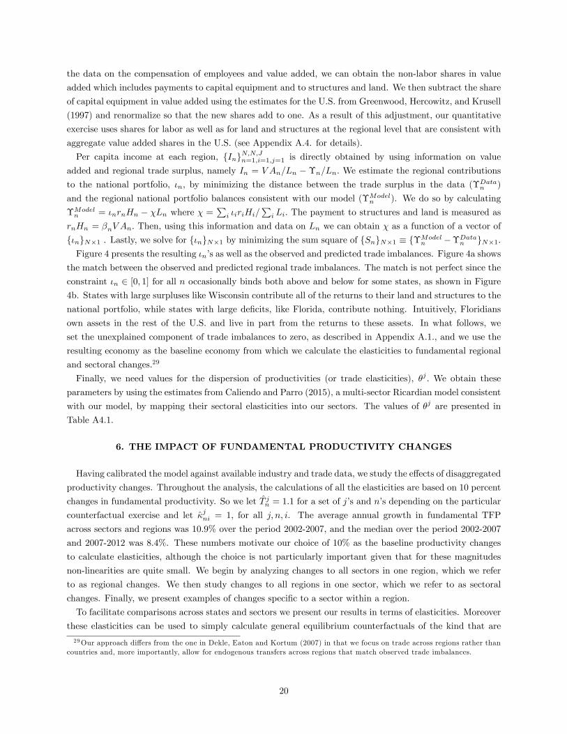
the data on the compensation of employees and value added, we can obtain the non-labor shares in value

added which includes payments to capital equipment and to structures and land. We then subtract the share

of capital equipment in value added using the estimates for the U.S. from Greenwood, Hercowitz, and Krusell

(1997) and renormalize so that the new shares add to one. As a result of this adjustment, our quantitative

exercise uses shares for labor as well as for land and structures at the regional level that are consistent with

aggregate value added shares in the U.S. (see Appendix A.4. for details).

Per capita income at each region, {In}N,N,Jn=1,i=1,j=1 is directly obtained by using information on value

added and regional trade surplus, namely In = V An/Ln − Υn/Ln. We estimate the regional contributions

to the national portfolio, ιn, by minimizing the distance between the trade surplus in the data (ΥDatan )

and the regional national portfolio balances consistent with our model (ΥModeln ). We do so by calculating

ΥModeln = ιnrnHn − χLn where χ =

∑i ιiriHi/

∑i Li. The payment to structures and land is measured as

rnHn = βnV An. Then, using this information and data on Ln we can obtain χ as a function of a vector of

{ιn}N×1 . Lastly, we solve for {ιn}N×1 by minimizing the sum square of {Sn}N×1 ≡ {ΥModeln −ΥData

n }N×1.Figure 4 presents the resulting ιn’s as well as the observed and predicted trade imbalances. Figure 4a shows

the match between the observed and predicted regional trade imbalances. The match is not perfect since the

constraint ιn ∈ [0, 1] for all n occasionally binds both above and below for some states, as shown in Figure

4b. States with large surpluses like Wisconsin contribute all of the returns to their land and structures to the

national portfolio, while states with large deficits, like Florida, contribute nothing. Intuitively, Floridians

own assets in the rest of the U.S. and live in part from the returns to these assets. In what follows, we

set the unexplained component of trade imbalances to zero, as described in Appendix A.1., and we use the

resulting economy as the baseline economy from which we calculate the elasticities to fundamental regional

and sectoral changes.29

Finally, we need values for the dispersion of productivities (or trade elasticities), θj . We obtain these

parameters by using the estimates from Caliendo and Parro (2015), a multi-sector Ricardian model consistent

with our model, by mapping their sectoral elasticities into our sectors. The values of θj are presented in

Table A4.1.

6. THE IMPACT OF FUNDAMENTAL PRODUCTIVITY CHANGES

Having calibrated the model against available industry and trade data, we study the effects of disaggregated

productivity changes. Throughout the analysis, the calculations of all the elasticities are based on 10 percent

changes in fundamental productivity. So we let T jn = 1.1 for a set of j’s and n’s depending on the particular

counterfactual exercise and let κjni = 1, for all j, n, i. The average annual growth in fundamental TFP

across sectors and regions was 10.9% over the period 2002-2007, and the median over the period 2002-2007

and 2007-2012 was 8.4%. These numbers motivate our choice of 10% as the baseline productivity changes

to calculate elasticities, although the choice is not particularly important given that for these magnitudes

non-linearities are quite small. We begin by analyzing changes to all sectors in one region, which we refer

to as regional changes. We then study changes to all regions in one sector, which we refer to as sectoral

changes. Finally, we present examples of changes specific to a sector within a region.

To facilitate comparisons across states and sectors we present our results in terms of elasticities. Moreover

these elasticities can be used to simply calculate general equilibrium counterfactuals of the kind that are

29Our approach differs from the one in Dekle, Eaton and Kortum (2007) in that we focus on trade across regions rather thancountries and, more importantly, allow for endogenous transfers across regions that match observed trade imbalances.

20

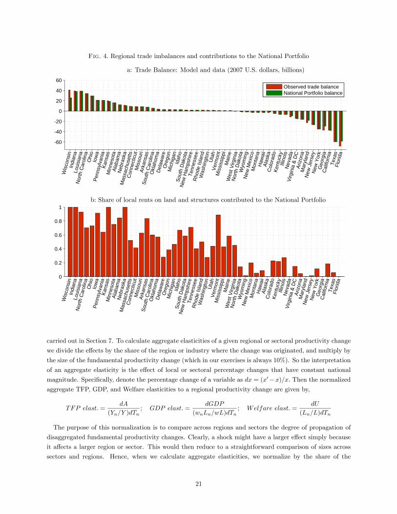
Fig. 4. Regional trade imbalances and contributions to the National Portfolio

a: Trade Balance: Model and data (2007 U.S. dollars, billions)

-60

-40

-20

0

20

40

60

W

isco

nsin

Indi

ana

L

ouis

iana

Nor

th C

arol

ina

O

hio

Io

wa

Pen

nsyl

vani

a

K

ansa

s

Min

neso

ta

A

laba

ma

Neb

rask

a M

assa

chus

etts

C

onne

ctic

ut

M

isso

uri

Ark

ansa

sS

outh

Car

olin

a

O

klah

oma

Del

awar

e

O

rego

n

M

ichi

gan

Id

aho

Sou

th D

akot

a N

ew H

amps

hire

T

enne

ssee

Rho

de Is

land

W

ashi

ngto

n

Uta

h

V

erm

ont

M

issi

ssip

pi

Mai

ne W

est V

irgin

ia N

orth

Dak

ota

Wyo

min

g

New

Mex

ico

Mon

tana

H

awai

i

A

lask

a

C

olor

ado

Ken

tuck

y

Ill

inoi

s

N

evad

a V

irgin

ia &

DC

Ariz

ona

Mar

ylan

d

New

Jer

sey

New

Yor

k

G

eorg

ia

Cal

iforn

ia

Tex

as

F

lorid

a

Observed trade balanceNational Portfolio balance

b: Share of local rents on land and structures contributed to the National Portfolio

0

0.2

0.4

0.6

0.8

1

W

isco

nsin

Indi

ana

L

ouis

iana

Nor

th C

arol

ina

O

hio

Io

wa

Pen

nsyl

vani

a

K

ansa

s

Min

neso

ta

A

laba

ma

Neb

rask

a M

assa

chus

etts

C

onne

ctic

ut

M

isso

uri

Ark

ansa

sS

outh

Car

olin

a

O

klah

oma

Del

awar

e

O

rego

n

M

ichi

gan

Id

aho

Sou

th D

akot

a N

ew H

amps

hire

T

enne

ssee

Rho

de Is

land

W

ashi

ngto

n

Uta

h

V

erm

ont

M

issi

ssip

pi

Mai

ne W

est V

irgin

ia N

orth

Dak

ota

Wyo

min

g

New

Mex

ico

Mon

tana

H

awai

i

A

lask

a

C

olor

ado

Ken

tuck

y

Ill

inoi

s

N

evad

a V

irgin

ia &

DC

Ariz

ona

Mar

ylan

d

New

Jer

sey

New

Yor

k

G

eorg

ia

Cal

iforn

ia

Tex

as

F

lorid

acarried out in Section 7. To calculate aggregate elasticities of a given regional or sectoral productivity change

we divide the effects by the share of the region or industry where the change was originated, and multiply by

the size of the fundamental productivity change (which in our exercises is always 10%). So the interpretation

of an aggregate elasticity is the effect of local or sectoral percentage changes that have constant national

magnitude. Specifically, denote the percentage change of a variable as dx = (x′−x)/x. Then the normalized

aggregate TFP, GDP, and Welfare elasticities to a regional productivity change are given by,

TFP elast. =dA

(Yn/Y )dTn; GDP elast. =

dGDP

(wnLn/wL)dTn; Welfare elast. =

dU

(Ln/L)dTn

The purpose of this normalization is to compare across regions and sectors the degree of propagation of

disaggregated fundamental productivity changes. Clearly, a shock might have a larger effect simply because

it affects a larger region or sector. This would then reduce to a straightforward comparison of sizes across

sectors and regions. Hence, when we calculate aggregate elasticities, we normalize by the share of the

21

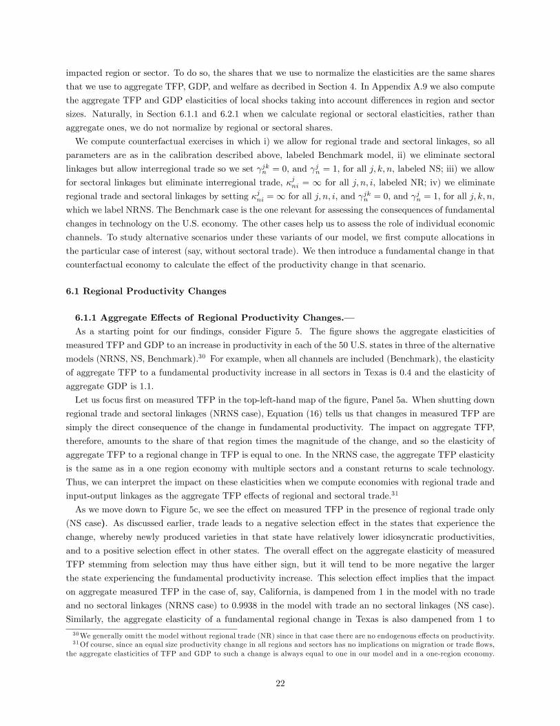
impacted region or sector. To do so, the shares that we use to normalize the elasticities are the same shares

that we use to aggregate TFP, GDP, and welfare as decribed in Section 4. In Appendix A.9 we also compute

the aggregate TFP and GDP elasticities of local shocks taking into account differences in region and sector

sizes. Naturally, in Section 6.1.1 and 6.2.1 when we calculate regional or sectoral elasticities, rather than

aggregate ones, we do not normalize by regional or sectoral shares.

We compute counterfactual exercises in which i) we allow for regional trade and sectoral linkages, so all

parameters are as in the calibration described above, labeled Benchmark model, ii) we eliminate sectoral

linkages but allow interregional trade so we set γjkn = 0, and γjn = 1, for all j, k, n, labeled NS; iii) we allow

for sectoral linkages but eliminate interregional trade, κjni = ∞ for all j, n, i, labeled NR; iv) we eliminate

regional trade and sectoral linkages by setting κjni =∞ for all j, n, i, and γjkn = 0, and γjn = 1, for all j, k, n,

which we label NRNS. The Benchmark case is the one relevant for assessing the consequences of fundamental

changes in technology on the U.S. economy. The other cases help us to assess the role of individual economic

channels. To study alternative scenarios under these variants of our model, we first compute allocations in

the particular case of interest (say, without sectoral trade). We then introduce a fundamental change in that

counterfactual economy to calculate the effect of the productivity change in that scenario.

6.1 Regional Productivity Changes

6.1.1 Aggregate Effects of Regional Productivity Changes.–As a starting point for our findings, consider Figure 5. The figure shows the aggregate elasticities of

measured TFP and GDP to an increase in productivity in each of the 50 U.S. states in three of the alternative

models (NRNS, NS, Benchmark).30 For example, when all channels are included (Benchmark), the elasticity

of aggregate TFP to a fundamental productivity increase in all sectors in Texas is 0.4 and the elasticity of

aggregate GDP is 1.1.

Let us focus first on measured TFP in the top-left-hand map of the figure, Panel 5a. When shutting down

regional trade and sectoral linkages (NRNS case), Equation (16) tells us that changes in measured TFP are

simply the direct consequence of the change in fundamental productivity. The impact on aggregate TFP,

therefore, amounts to the share of that region times the magnitude of the change, and so the elasticity of

aggregate TFP to a regional change in TFP is equal to one. In the NRNS case, the aggregate TFP elasticity

is the same as in a one region economy with multiple sectors and a constant returns to scale technology.

Thus, we can interpret the impact on these elasticities when we compute economies with regional trade and

input-output linkages as the aggregate TFP effects of regional and sectoral trade.31

As we move down to Figure 5c, we see the effect on measured TFP in the presence of regional trade only

(NS case). As discussed earlier, trade leads to a negative selection effect in the states that experience thechange, whereby newly produced varieties in that state have relatively lower idiosyncratic productivities,

and to a positive selection effect in other states. The overall effect on the aggregate elasticity of measured

TFP stemming from selection may thus have either sign, but it will tend to be more negative the larger

the state experiencing the fundamental productivity increase. This selection effect implies that the impact

on aggregate measured TFP in the case of, say, California, is dampened from 1 in the model with no trade

and no sectoral linkages (NRNS case) to 0.9938 in the model with trade an no sectoral linkages (NS case).

Similarly, the aggregate elasticity of a fundamental regional change in Texas is also dampened from 1 to

30We generally omitt the model without regional trade (NR) since in that case there are no endogenous effects on productivity.31Of course, since an equal size productivity change in all regions and sectors has no implications on migration or trade flows,

the aggregate elasticities of TFP and GDP to such a change is always equal to one in our model and in a one-region economy.

22

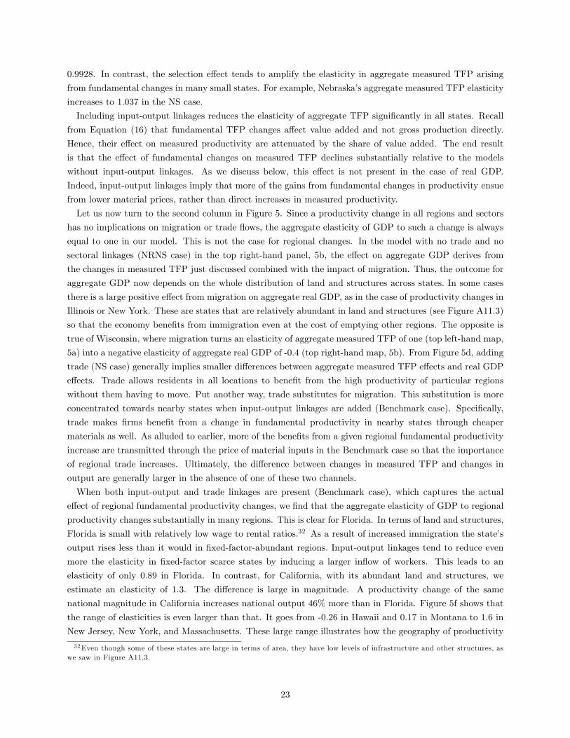
0.9928. In contrast, the selection effect tends to amplify the elasticity in aggregate measured TFP arising

from fundamental changes in many small states. For example, Nebraska’s aggregate measured TFP elasticity

increases to 1.037 in the NS case.

Including input-output linkages reduces the elasticity of aggregate TFP significantly in all states. Recall

from Equation (16) that fundamental TFP changes affect value added and not gross production directly.

Hence, their effect on measured productivity are attenuated by the share of value added. The end result

is that the effect of fundamental changes on measured TFP declines substantially relative to the models

without input-output linkages. As we discuss below, this effect is not present in the case of real GDP.

Indeed, input-output linkages imply that more of the gains from fundamental changes in productivity ensue

from lower material prices, rather than direct increases in measured productivity.

Let us now turn to the second column in Figure 5. Since a productivity change in all regions and sectors

has no implications on migration or trade flows, the aggregate elasticity of GDP to such a change is always

equal to one in our model. This is not the case for regional changes. In the model with no trade and no

sectoral linkages (NRNS case) in the top right-hand panel, 5b, the effect on aggregate GDP derives from

the changes in measured TFP just discussed combined with the impact of migration. Thus, the outcome for

aggregate GDP now depends on the whole distribution of land and structures across states. In some cases

there is a large positive effect from migration on aggregate real GDP, as in the case of productivity changes in

Illinois or New York. These are states that are relatively abundant in land and structures (see Figure A11.3)

so that the economy benefits from immigration even at the cost of emptying other regions. The opposite is

true of Wisconsin, where migration turns an elasticity of aggregate measured TFP of one (top left-hand map,

5a) into a negative elasticity of aggregate real GDP of -0.4 (top right-hand map, 5b). From Figure 5d, adding

trade (NS case) generally implies smaller differences between aggregate measured TFP effects and real GDP

effects. Trade allows residents in all locations to benefit from the high productivity of particular regions

without them having to move. Put another way, trade substitutes for migration. This substitution is more

concentrated towards nearby states when input-output linkages are added (Benchmark case). Specifically,

trade makes firms benefit from a change in fundamental productivity in nearby states through cheaper

materials as well. As alluded to earlier, more of the benefits from a given regional fundamental productivity

increase are transmitted through the price of material inputs in the Benchmark case so that the importance

of regional trade increases. Ultimately, the difference between changes in measured TFP and changes in

output are generally larger in the absence of one of these two channels.

When both input-output and trade linkages are present (Benchmark case), which captures the actual

effect of regional fundamental productivity changes, we find that the aggregate elasticity of GDP to regional

productivity changes substantially in many regions. This is clear for Florida. In terms of land and structures,

Florida is small with relatively low wage to rental ratios.32 As a result of increased immigration the state’s

output rises less than it would in fixed-factor-abundant regions. Input-output linkages tend to reduce even

more the elasticity in fixed-factor scarce states by inducing a larger inflow of workers. This leads to an

elasticity of only 0.89 in Florida. In contrast, for California, with its abundant land and structures, we

estimate an elasticity of 1.3. The difference is large in magnitude. A productivity change of the same

national magnitude in California increases national output 46% more than in Florida. Figure 5f shows that

the range of elasticities is even larger than that. It goes from -0.26 in Hawaii and 0.17 in Montana to 1.6 in

New Jersey, New York, and Massachusetts. These large range illustrates how the geography of productivity

32Even though some of these states are large in terms of area, they have low levels of infrastructure and other structures, aswe saw in Figure A11.3.

23

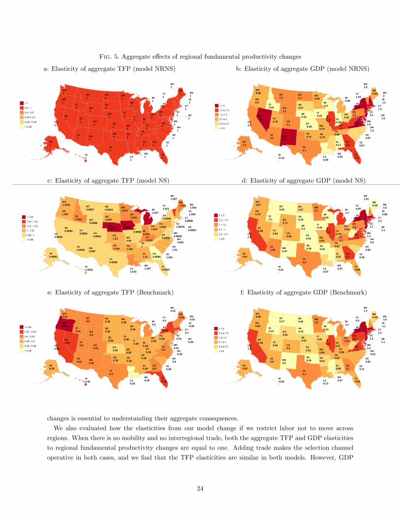
Fig. 5. Aggregate effects of regional fundamental productivity changes

a: Elasticity of aggregate TFP (model NRNS) b: Elasticity of aggregate GDP (model NRNS)

AL1

AK1

AZ1

AR1

CA1

CO1

CT1

DE1

FL1

GA1

HI1

ID1

IL1 IN

1

IA1

KS1 KY

1

LA1

ME1

MD1

MA1

MI1

MN1

MS1

MO1

MT1

NE1NV

1

NH1

NJ1

NM1

NY1

NC1

ND1

OH1

OK1

OR1

PA1

RI1

SC1

SD1

TN1

TX1

UT1

VT1

VA1

WA1

WV1

WI1

WY1

AL0.17

AK1.2

AZ1.1

AR0.73

CA1.1

CO1.1

CT1.3

DE1.2

FL1.3

GA1.3

HI-0.15

ID0.34

IL1.5 IN

0.26

IA0.22

KS-0.05 KY

1.3

LA0.09

ME0.93

MD1.8

MA2

MI0.99

MN0.88

MS0.53

MO0.73

MT1.2

NE0.16NV

1.8

NH2.5

NJ2.3

NM1.5

NY1.8

NC0.57

ND1.1

OH0.61

OK0.72

OR0.9

PA1.1

RI1.1

SC0.67

SD0.57

TN0.86

TX1.1

UT0.75

VT1.04

VA1.5

WA0.88

WV1.4

WI-0.4

WY1.2

c: Elasticity of aggregate TFP (model NS) d: Elasticity of aggregate GDP (model NS)

AL1.01

AK0.9992

AZ0.9925

AR1.001

CA0.9938

CO0.9951

CT0.9898

DE0.9953

FL0.9923

GA0.9899

HI1.0001

ID1.011

IL0.9996 IN

1.016

IA1.036

KS1.01 KY

1.019

LA1.015

ME1.013

MD0.9958

MA1.004

MI1.037

MN1.013

MS1.007

MO0.99

MT0.9957

NE1.037NV

0.9955

NH1.007

NJ0.9978

NM0.997

NY0.9949

NC1.01

ND0.9944

OH1.007

OK1.004

OR1.007

PA1.002

RI1.004

SC1.001

SD1.003

TN1

TX0.9928

UT0.9981

VT1.021

VA0.9955

WA1.0001

WV1.002

WI1.016

WY0.9998

AL0.52

AK0.97

AZ1.02

AR0.42

CA1.3

CO0.94

CT1.3

DE1.1

FL0.98

GA1.2

HI0.22

ID0.1

IL1.4 IN

0.76

IA0.49

KS0.43 KY

1.1

LA0.67

ME0.39

MD1.3

MA1.6

MI1.3

MN1.1

MS0.41

MO0.83

MT0.25

NE0.4NV

0.99

NH1.01

NJ1.7

NM0.47

NY1.6

NC0.82

ND0.67

OH0.93

OK0.39

OR0.75

PA1.2

RI0.98

SC0.58

SD0.35

TN0.81

TX1.2

UT0.63

VT0.05

VA1.3

WA0.97

WV0.3

WI0.05

WY0.71

e: Elasticity of aggregate TFP (Benchmark) f: Elasticity of aggregate GDP (Benchmark)

AL0.38

AK0.39

AZ0.41

AR0.38

CA0.42

CO0.41

CT0.4

DE0.36

FL0.42

GA0.4

HI0.42

ID0.41

IL0.39 IN

0.39

IA0.38

KS0.36 KY

0.39

LA0.35

ME0.41

MD0.41

MA0.42

MI0.4

MN0.39

MS0.39

MO0.38

MT0.4

NE0.38NV

0.42

NH0.41

NJ0.41

NM0.41

NY0.42

NC0.4

ND0.39

OH0.38

OK0.38

OR0.44

PA0.39

RI0.39

SC0.38

SD0.38

TN0.38

TX0.4

UT0.4

VT0.4

VA0.4

WA0.41

WV0.39

WI0.39

WY0.4

AL0.68

AK0.92

AZ0.9

AR0.61

CA1.3

CO0.9

CT1.3

DE1.1

FL0.89

GA1.1

HI-0.26

ID0.23

IL1.4 IN

0.9

IA0.66

KS0.51 KY

0.96

LA0.73

ME0.59

MD1.2

MA1.6

MI1.1

MN1.2

MS0.47

MO0.84

MT0.17

NE0.53NV

0.94

NH1.1

NJ1.6

NM0.4

NY1.6

NC0.91

ND0.46

OH1.01

OK0.45

OR0.83

PA1.2

RI1.1

SC0.71

SD0.42

TN0.82

TX1.1

UT0.65

VT0.2

VA1.2

WA0.96

WV0.52

WI0.34

WY0.65

changes is essential to understanding their aggregate consequences.

We also evaluated how the elasticities from our model change if we restrict labor not to move across

regions. When there is no mobility and no interregional trade, both the aggregate TFP and GDP elasticities

to regional fundamental productivity changes are equal to one. Adding trade makes the selection channel

operative in both cases, and we find that the TFP elasticities are similar in both models. However, GDP

24

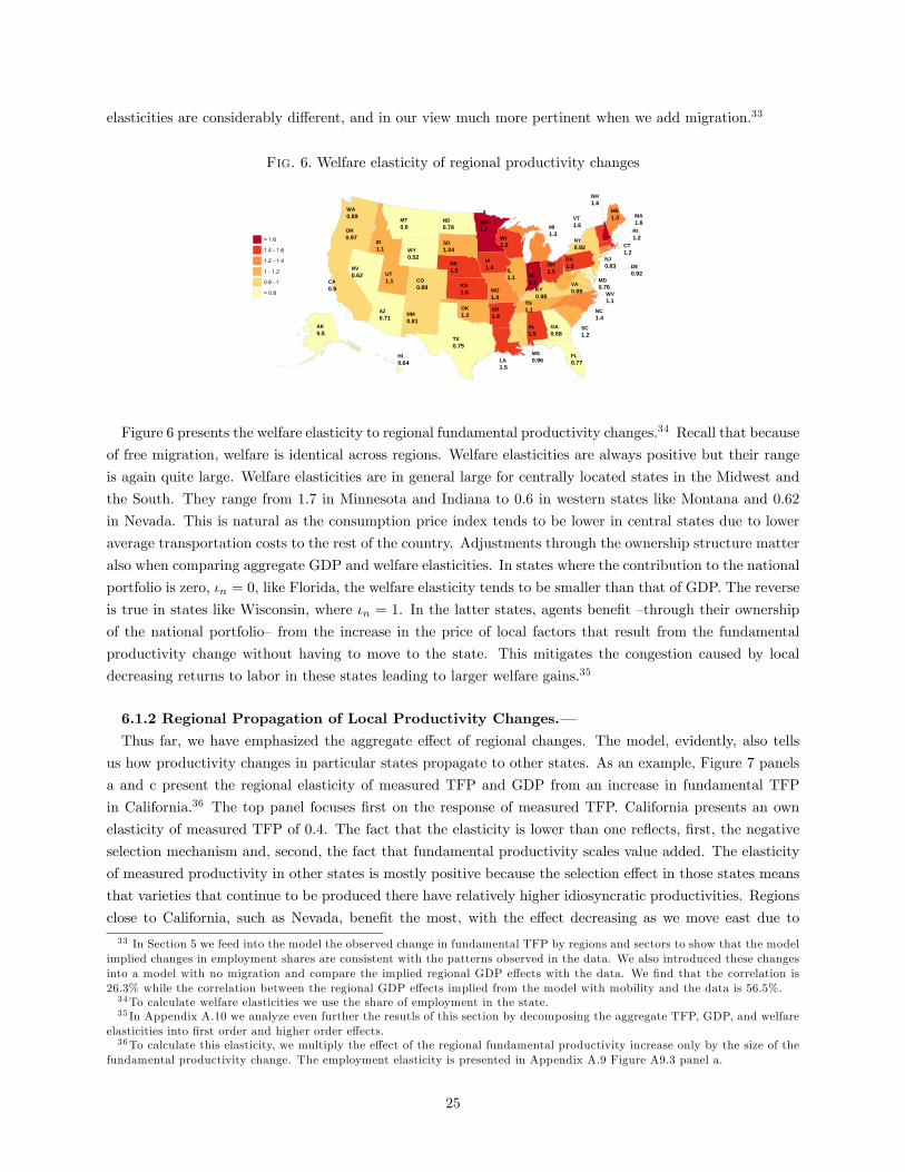
elasticities are considerably different, and in our view much more pertinent when we add migration.33

Fig. 6. Welfare elasticity of regional productivity changes

AL1.5

AK0.5

AZ0.71

AR1.4

CA0.9

CO0.89

CT1.2

DE0.92

FL0.77

GA0.68

HI0.64

ID1.1

IL1.1 IN

1.7

IA1.4

KS1.5 KY

0.98

LA1.5

ME1.3

MD0.76

MA1.6

MI1.3

MN1.7

MS0.96

MO1.4

MT0.6

NE1.5NV

0.62

NH1.6

NJ0.83

NM0.81

NY0.92

NC1.4

ND0.78

OH1.5

OK1.2

OR0.97

PA1.5

RI1.2

SC1.2

SD1.04

TN1.1

TX0.75

UT1.1

VT1.6

VA0.89

WA0.89

WV1.1

WI1.5

WY0.52

Figure 6 presents the welfare elasticity to regional fundamental productivity changes.34 Recall that because

of free migration, welfare is identical across regions. Welfare elasticities are always positive but their range

is again quite large. Welfare elasticities are in general large for centrally located states in the Midwest and

the South. They range from 1.7 in Minnesota and Indiana to 0.6 in western states like Montana and 0.62

in Nevada. This is natural as the consumption price index tends to be lower in central states due to lower

average transportation costs to the rest of the country. Adjustments through the ownership structure matter

also when comparing aggregate GDP and welfare elasticities. In states where the contribution to the national

portfolio is zero, ιn = 0, like Florida, the welfare elasticity tends to be smaller than that of GDP. The reverse

is true in states like Wisconsin, where ιn = 1. In the latter states, agents benefit —through their ownership

of the national portfolio— from the increase in the price of local factors that result from the fundamental

productivity change without having to move to the state. This mitigates the congestion caused by local

decreasing returns to labor in these states leading to larger welfare gains.35

6.1.2 Regional Propagation of Local Productivity Changes.–Thus far, we have emphasized the aggregate effect of regional changes. The model, evidently, also tells

us how productivity changes in particular states propagate to other states. As an example, Figure 7 panels

a and c present the regional elasticity of measured TFP and GDP from an increase in fundamental TFP

in California.36 The top panel focuses first on the response of measured TFP. California presents an own

elasticity of measured TFP of 0.4. The fact that the elasticity is lower than one reflects, first, the negative

selection mechanism and, second, the fact that fundamental productivity scales value added. The elasticity

of measured productivity in other states is mostly positive because the selection effect in those states means

that varieties that continue to be produced there have relatively higher idiosyncratic productivities. Regions

close to California, such as Nevada, benefit the most, with the effect decreasing as we move east due to

33 In Section 5 we feed into the model the observed change in fundamental TFP by regions and sectors to show that the modelimplied changes in employment shares are consistent with the patterns observed in the data. We also introduced these changesinto a model with no migration and compare the implied regional GDP effects with the data. We find that the correlation is26.3% while the correlation between the regional GDP effects implied from the model with mobility and the data is 56.5%.34To calculate welfare elasticities we use the share of employment in the state.35 In Appendix A.10 we analyze even further the resutls of this section by decomposing the aggregate TFP, GDP, and welfare

elasticities into first order and higher order effects.36To calculate this elasticity, we multiply the effect of the regional fundamental productivity increase only by the size of the

fundamental productivity change. The employment elasticity is presented in Appendix A.9 Figure A9.3 panel a.

25

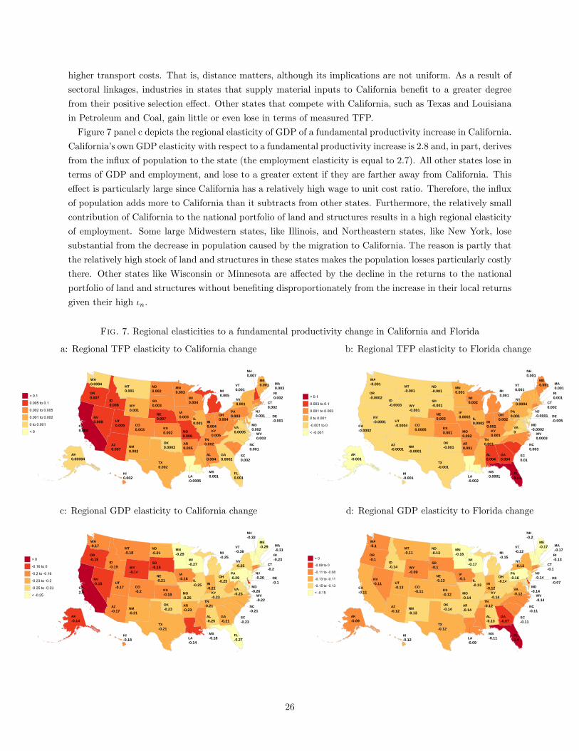
higher transport costs. That is, distance matters, although its implications are not uniform. As a result of

sectoral linkages, industries in states that supply material inputs to California benefit to a greater degree

from their positive selection effect. Other states that compete with California, such as Texas and Louisiana

in Petroleum and Coal, gain little or even lose in terms of measured TFP.

Figure 7 panel c depicts the regional elasticity of GDP of a fundamental productivity increase in California.

California’s own GDP elasticity with respect to a fundamental productivity increase is 2.8 and, in part, derives

from the influx of population to the state (the employment elasticity is equal to 2.7). All other states lose in

terms of GDP and employment, and lose to a greater extent if they are farther away from California. This

effect is particularly large since California has a relatively high wage to unit cost ratio. Therefore, the influx

of population adds more to California than it subtracts from other states. Furthermore, the relatively small

contribution of California to the national portfolio of land and structures results in a high regional elasticity

of employment. Some large Midwestern states, like Illinois, and Northeastern states, like New York, lose

substantial from the decrease in population caused by the migration to California. The reason is partly that

the relatively high stock of land and structures in these states makes the population losses particularly costly

there. Other states like Wisconsin or Minnesota are affected by the decline in the returns to the national

portfolio of land and structures without benefiting disproportionately from the increase in their local returns

given their high ιn.

Fig. 7. Regional elasticities to a fundamental productivity change in California and Florida

a: Regional TFP elasticity to California change b: Regional TFP elasticity to Florida change

AL0.004

AK0.00004

AZ0.007

AR0.005

CA0.402

CO0.003

CT0.002

DE-0.001

FL0.001

GA0.0002

HI0.002

ID0.008

IL0.001 IN

0.004

IA0.003

KS0.002 KY

0.005

LA-0.0005

ME0.001

MD0.002

MA0.003

MI0.005

MN0.003

MS0.001

MO0.006

MT0.001

NE0.007NV

0.008

NH0.007

NJ0.001

NM0.002

NY0.001

NC0.001

ND0.002

OH0.004

OK0.0003

OR0.007

PA0.003

RI0.002

SC0.002

SD0.003

TN0.002

TX0.002

UT0.009

VT0.001

VA0.0005

WA0.0004

WV0.003

WI0.004

WY0.001

AL0.004

AK-0.001

AZ-0.0001

AR0.001

CA-0.0002

CO0.0005

CT0.002

DE-0.005

FL0.41

GA0.004

HI-0.001

ID-0.0003

IL0.0002 IN

0.002

IA0.0002

KS0.001 KY

0.001

LA-0.002

ME0.001

MD-0.0002

MA0.001

MI0.001

MN0.001

MS0.0001

MO0.002

MT-0.001

NE0.003NV

-0.0001

NH0.001

NJ-0.0001

NM-0.0001

NY0.0004

NC0.003

ND-0.001

OH0.002

OK-0.001

OR-0.0002

PA0.001

RI0.001

SC0.01

SD-0.001

TN0.001

TX-0.001

UT-0.0004

VT0.001

VA0

WA-0.001

WV0.0003

WI0.002

WY-0.001

c: Regional GDP elasticity to California change d: Regional GDP elasticity to Florida change

AL-0.25

AK-0.14

AZ-0.17

AR-0.23

CA2.8

CO-0.2

CT-0.2

DE-0.1

FL-0.27

GA-0.21

HI-0.18

ID-0.19

IL-0.25 IN

-0.21

IA-0.16

KS-0.18 KY

-0.23

LA-0.14

ME-0.29

MD-0.26

MA-0.31

MI-0.25

MN-0.29

MS-0.18

MO-0.25

MT-0.18

NE-0.21NV

-0.15

NH-0.32

NJ-0.26

NM-0.21

NY-0.25

NC-0.21

ND-0.21

OH-0.25

OK-0.23

OR-0.15

PA-0.29

RI-0.23

SC-0.23

SD-0.16

TN-0.21

TX-0.21

UT-0.17

VT-0.36

VA-0.23

WA-0.17

WV-0.22

WI-0.27

WY-0.14

AL-0.13

AK-0.09

AZ-0.12

AR-0.14

CA-0.11

CO-0.11

CT-0.1

DE-0.07

FL3.4

GA-0.07

HI-0.12

ID-0.14

IL-0.13 IN

-0.12

IA-0.1

KS-0.12 KY

-0.14

LA-0.09

ME-0.17

MD-0.14

MA-0.17

MI-0.15

MN-0.16

MS-0.11

MO-0.14

MT-0.11

NE-0.13NV

-0.11

NH-0.2

NJ-0.14

NM-0.13

NY-0.13

NC-0.11

ND-0.13

OH-0.14

OK-0.14

OR-0.1

PA-0.16

RI-0.13

SC-0.11

SD-0.1

TN-0.12

TX-0.12

UT-0.13

VT-0.22

VA-0.12

WA-0.1

WV-0.14

WI-0.17

WY-0.09

26

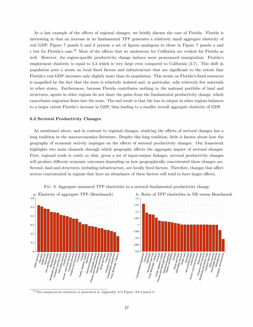
As a last example of the effects of regional changes, we briefly discuss the case of Florida. Florida is

interesting in that an increase in its fundamental TFP generates a relatively small aggregate elasticity of

real GDP. Figure 7 panels b and d present a set of figures analogous to those in Figure 7 panels a and

c but for Florida’s case.37 Most of the effects that we underscore for California are evident for Florida as

well. However, the region-specific productivity change induces more pronounced immigration. Florida’s

employment elasticity is equal to 3.3 which is very large even compared to California (2.7). This shift in

population puts a strain on local fixed factors and infrastructure that are significant to the extent that

Florida’s real GDP increases only slightly more than its population. This strain on Florida’s fixed resources

is magnified by the fact that the state is relatively isolated and, in particular, sells relatively few materials

to other states. Furthermore, because Florida contributes nothing to the national portfolio of land and

structures, agents in other regions do not share the gains from the fundamental productivity change, which

exacerbates migration flows into the state. The end result is that the loss in output in other regions balances

to a larger extent Florida’s increase in GDP, thus leading to a smaller overall aggregate elasticity of GDP.

6.2 Sectoral Productivity Changes

As mentioned above, and in contrast to regional changes, studying the effects of sectoral changes has a

long tradition in the macroeconomics literature. Despite this long tradition, little is known about how the

geography of economic activity impinges on the effects of sectoral productivity changes. Our framework

highlights two main channels through which geography affects the aggregate impact of sectoral changes.

First, regional trade is costly so that, given a set of input-output linkages, sectoral productivity changes

will produce different economic outcomes depending on how geographically concentrated these changes are.

Second, land and structures, including infrastructure, are locally fixed factors. Therefore, changes that affect

sectors concentrated in regions that have an abundance of these factors will tend to have larger effects.

Fig. 8. Aggregate measured TFP elasticities to a sectoral fundamental productivity change

a: Elasticity of aggregate TFP (Benchmark) b: Ratio of TFP elasticities in NR versus Benchmark

0

0.1

0.2

0.3

0.4

0.5

0.6

Oth

er S

ervi

ces

Edu

catio

n

Hea

lth C

are

R

eal E

stat

e

A

rts

and

Rec

reat

ion

M

isce

llane

ous

Who

lesa

le a

nd R

etai

l Tra

de

C

ompu

ter

and

Ele

ctro

nic

Inf

orm

atio

n S

ervi

ces

C

onst

ruct

ion

A

ccom

. and

Foo

d S

ervi

ces

T

rans

port

Ser

vice

s

Fin

ance

and

Insu

ranc

e

F

urni

ture

Prin

ting

T

extil

e, A

ppar

el, L

eath

er

M

achi

nery

Ele

ctric

al E

quip

men

t

Non

met

allic

Min

eral

Prim

ary

and

Fab

ricat

ed M

etal

P

last

ics

and

Rub

ber

Woo

d an

d P

aper

Che

mic

al

P

etro

leum

and

Coa

l

T

rans

port

atio

n E

quip

men

t

F

ood,

Bev

erag

e, T

obac

co

Change in aggregate TFP (%,model RS)

0.8

0.85

0.9

0.95

1

1.05

1.1

1.15

1.2

T

rans

port

atio

n E

quip

men

t

C

hem

ical

Mac

hine

ry

P

etro

leum

and

Coa

l

F

ood,

Bev

erag

e, T

obac

co

F

urni

ture

T

extil

e, A

ppar

el, L

eath

er

Prim

ary

and

Fab

ricat

ed M

etal

Ele

ctric

al E

quip

men

t

P

last

ics

and

Rub

ber

Prin

ting

Woo

d an

d P

aper

Inf

orm

atio

n S

ervi

ces

H

ealth

Car

e

E

duca

tion

A

rts

and

Rec

reat

ion

C

onst

ruct

ion

A

ccom

. and

Foo

d S

ervi

ces

R

eal E

stat

e

Fin

ance

and

Insu

ranc

e

Who

lesa

le a

nd R

etai

l Tra

de

T

rans

port

Ser

vice

s

O

ther

Ser

vice

s

N

onm

etal

lic M

iner

al

Mis

cella

neou

s

C

ompu

ter

and

Ele

ctro

nic

37The employment elasticity is presented in Appendix A.9 Figure A9.3 panel b.

27

6.2.1. Aggregate Effects of Sectoral Productivity Changes.–Figure 8 presents aggregate responses of measured productivity to changes in fundamental productivity

in each sector. In this case, a fundamental change in a given sector is identical across all regions in which

the sector is represented. We present aggregate elasticities for the case in which all channels are operative

(Benchmark), as well as the ratio of the elasticity in the cases without and with regional trade, NR and

Benchmark. The latter case is the one absent in standard multisector macroeconomic models.38 Absent

sectoral linkages, a given sectoral fundamental TFP change does not affect the distribution of employment

across regions. Therefore, in both the NRNS and NS cases, the aggregate TFP elasticity with respect to

changes in sectoral fundamental productivity is equal to one for all sectors. Figure 8a shows that introducing

material inputs reduces significantly the aggregate TFP elasticity with respect to a given sectoral productivity

change. Input-output linkages also skew the distribution of aggregate sectoral effects. These differences

arise because material inputs serve as an insurance mechanism against changes that are idiosyncratic to a

particular sector. That is, with input-output linkages, output in any sector depends on the productivity in

other sectors. Trade influences this mechanism because intermediate inputs cannot be imported costlessly

from other locations. For example, as Figure 8b shows, eliminating trade leads to an elasticity of aggregate

TFP that is about 15% larger in the Transportation Equipment industry, but about 10% smaller in the

Computer and Electronics industry.

When we focus on the elasticity of aggregate GDP, it is even clearer that in sectors that are very con-

centrated geographically, this influence of regional trade is smaller than in sectors that are more dispersed

across regions. The Petroleum and Coal industry, for instance, is concentrated across less than a handful

of states. Hence failure to account for regional trade understates the aggregate elasticity of GDP in that

sector by about 10% (see 9b). In contrast in the relatively dispersed Transportation Equipment industry

disregarding regional trade overstates the elasticity by 19%. Trade has a negligible effect on the aggregate

elasticities of changes to non-tradable sectors.

Figure 10 illustrates the welfare implications of sectoral changes in productivity. As with regional pro-

ductivity changes, these exhibit a fairly large range. A fundamental productivity change in the Wood and

Paper industry —the most dispersed industry in the U.S.—has an effect on welfare that is about 10% lower

than in the much more concentrates Petroleum and Coal and Chemical industries (see Figure A11.1b). The

sectoral distribution of welfare elasticity is also less skewed than that of GDP since measured TFP in general

responds less than employment to changes in fundamental productivity (see Equation (18)).

Because they lack a geographic dimension, disaggregated structural models that have been used to study

the effects of sectoral productivity changes have been silent on the consequences of these changes across

regions. While improvements or worsening conditions in a given sector have aggregate consequences, it is

also the case that these effects have a geographic distribution that is typically not uniform across states. So

in the next section we study the aggregate and regional effects of four actual regional and sectoral shocks

experienced by the U.S. economy.39

38Under the maintained assumptions that the share of land and structures in value added is constant across sectors (βn), andthat the share of consumption across sectors is identical across regions (αj), trade matters for the aggregate effects of sectoralfundamental TFP changes only in the presence of sectoral linkages.39 In Appendix A.9.1 we present two further examples that highlight and describe the regional propagation of sectoral shocks.

28

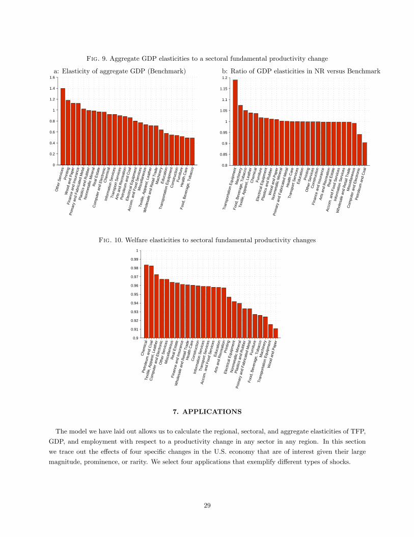
Fig. 9. Aggregate GDP elasticities to a sectoral fundamental productivity change

a: Elasticity of aggregate GDP (Benchmark) b: Ratio of GDP elasticities in NR versus Benchmark

0

0.2

0.4

0.6

0.8

1

1.2

1.4

1.6

Oth

er S

ervi

ces

Prin

ting

Woo

d an

d P

aper

Fin

ance

and

Insu

ranc

e

Prim

ary

and

Fab

ricat

ed M

etal

P

last

ics

and

Rub

ber

N

onm

etal

lic M

iner

al

Rea

l Est

ate

C

ompu

ter

and

Ele

ctro

nic

Che

mic

al

I

nfor

mat

ion

Ser

vice

s

Tra

nspo

rt S

ervi

ces

A

rts

and

Rec

reat

ion

P

etro

leum

and

Coa

l

E

lect

rical

Equ

ipm

ent

A

ccom

. and

Foo

d S

ervi

ces

M

isce

llane

ous

T

extil

e, A

ppar

el, L

eath

er

Who

lesa

le a

nd R

etai

l Tra

de

M

achi

nery

Edu

catio

n

T

rans

port

atio

n E

quip

men

t

Con

stru

ctio

n

F

urni

ture

H

ealth

Car

e

F

ood,

Bev

erag

e, T

obac

co

Change in aggregate GDP (%,model RS)

0.8

0.85

0.9

0.95

1

1.05

1.1

1.15

1.2

T

rans

port

atio

n E

quip

men

t

M

achi

nery

F

ood,

Bev

erag

e, T

obac

co

T

extil

e, A

ppar

el, L

eath

er

C

hem

ical

Fur

nitu

re

Ele

ctric

al E

quip

men

t

P

last

ics

and

Rub

ber

Woo

d an

d P

aper

N

onm

etal

lic M

iner

al

Prim

ary

and

Fab

ricat

ed M

etal

H

ealth

Car

e

T

rans

port

Ser

vice

s

E

duca

tion

Prin

ting

Oth

er S

ervi

ces

C

onst

ruct

ion

Fin

ance

and

Insu

ranc

e

Art

s an

d R

ecre

atio

n

Rea

l Est

ate

A

ccom

. and

Foo

d S

ervi

ces

Inf

orm

atio

n S

ervi

ces

Who

lesa

le a

nd R

etai

l Tra

de

Mis

cella

neou

s

C

ompu

ter

and

Ele

ctro

nic

P

etro

leum

and

Coa

l

Fig. 10. Welfare elasticities to sectoral fundamental productivity changes

0.9

0.91

0.92

0.93

0.94

0.95

0.96

0.97

0.98

0.99

1

Che

mic

al

P

etro

leum

and

Coa

l

T

extil

e, A

ppar

el, L

eath

er

C

ompu

ter

and

Ele

ctro

nic

Oth

er S

ervi

ces

M

isce

llane

ous

R

eal E

stat

e

Fin

ance

and

Insu

ranc

e

Who

lesa

le a

nd R

etai

l Tra

de

Hea

lth C

are

C

onst

ruct

ion

Inf

orm

atio

n S

ervi

ces

T

rans

port

Ser

vice

s

A

ccom

. and

Foo

d S

ervi

ces

Edu

catio

n

A

rts

and

Rec

reat

ion

Prin

ting

Ele

ctric

al E

quip

men

t

Non

met

allic

Min

eral

P

last

ics

and

Rub

ber

Prim

ary

and

Fab

ricat

ed M

etal

Fur

nitu

re

F

ood,

Bev

erag

e, T

obac

co

M

achi

nery

T

rans

port

atio

n E

quip

men

t

W

ood

and

Pap

er

Welfare elasticity

7. APPLICATIONS

The model we have laid out allows us to calculate the regional, sectoral, and aggregate elasticities of TFP,

GDP, and employment with respect to a productivity change in any sector in any region. In this section

we trace out the effects of four specific changes in the U.S. economy that are of interest given their large

magnitude, prominence, or rarity. We select four applications that exemplify different types of shocks.

29

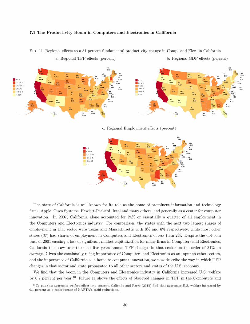
7.1 The Productivity Boom in Computers and Electronics in California

Fig. 11. Regional effects to a 31 percent fundamental productivity change in Comp. and Elec. in California

a: Regional TFP effects (percent) b: Regional GDP effects (percent)

AL0.002

AK0.03

AZ-0.004

AR0.03

CA0.85

CO0.08

CT-0.03

DE-0.01

FL-0.01

GA0.01

HI-0.04

ID-0.001

IL0.001 IN

0.01

IA0.02

KS0 KY

-0.01

LA-0.004

ME0.002

MD0.02

MA0.02

MI0.01

MN0.02

MS0.003

MO0.01

MT0.02

NE0.02NV

0.04

NH0.13

NJ0.01

NM-0.02

NY0.003

NC-0.002

ND0.01

OH-0.01

OK0.01

OR-0.14

PA0.004

RI0.05

SC0.01

SD0.05

TN-0.01

TX0.02

UT0.07

VT-0.09

VA0.01

WA0.29

WV0.03

WI0.02

WY0.02

AL-0.17

AK0.27

AZ-0.91

AR0.01

CA4.3

CO-0.13

CT-0.46

DE-0.03

FL-0.73

GA0.12

HI-0.9

ID-0.93

IL-0.26 IN

-0.07

IA-0.03

KS-0.19 KY

0.01

LA0.01

ME-0.13

MD-0.58

MA-0.87

MI0.05

MN-0.33

MS0.28

MO-0.03

MT0.04

NE-0.1NV

-0.15

NH-0.39

NJ-0.25

NM-1.07

NY-0.44

NC-0.12

ND-0.21

OH-0.02

OK-0.15

OR-1.53

PA-0.14

RI0.19

SC-0.07

SD0.13

TN-0.31

TX-0.23

UT-0.04

VT-0.91

VA-0.25

WA1.05

WV0.15

WI-0.002

WY-0.14

c: Regional Employment effects (percent)

AL-0.3

AK0.12

AZ-1.24

AR-0.14

CA3

CO-0.39

CT-0.58

DE-0.16

FL-0.91

GA0.03

HI-1.3

ID-1.2

IL-0.42 IN

-0.2

IA-0.17

KS-0.3 KY

-0.1

LA-0.09

ME-0.23

MD-0.76

MA-1.06

MI-0.07

MN-0.46

MS0.24

MO-0.17

MT-0.15

NE-0.24NV

-0.36

NH-0.61

NJ-0.39

NM-1.4

NY-0.6

NC-0.23

ND-0.35

OH-0.13

OK-0.3

OR-1.96

PA-0.25

RI0.12

SC-0.21

SD0.03

TN-0.44

TX-0.38

UT-0.22

VT-0.95

VA-0.39

WA0.75

WV0.05

WI-0.11

WY-0.37

The state of California is well known for its role as the home of prominent information and technology

firms, Apple, Cisco Systems, Hewlett-Packard, Intel and many others, and generally as a center for computer

innovation. In 2007, California alone accounted for 24% or essentially a quarter of all employment in

the Computers and Electronics industry. For comparison, the states with the next two largest shares of

employment in that sector were Texas and Massachusetts with 8% and 6% respectively, while most other

states (37) had shares of employment in Computers and Electronics of less than 2%. Despite the dot-com

bust of 2001 causing a loss of significant market capitalization for many firms in Computers and Electronics,

California then saw over the next five years annual TFP changes in that sector on the order of 31% on

average. Given the continually rising importance of Computers and Electronics as an input to other sectors,

and the importance of California as a home to computer innovation, we now describe the way in which TFP

changes in that sector and state propagated to all other sectors and states of the U.S. economy.

We find that the boom in the Computers and Electronics industry in California increased U.S. welfare

by 0.2 percent per year.40 Figure 11 shows the effects of observed changes in TFP in the Computers and

40To put this aggregate welfare effect into context, Caliendo and Parro (2015) find that aggregate U.S. welfare increased by0.1 percent as a consequence of NAFTA’s tariff reductions.

30

Electronics industry specific to California, a sector that amounts to 5.5% of value added in that state, on

measured regional TFP, GDP, and employment in other regions and states. The regional effect on measured

TFP, GDP, or employment, can be computed by multiplying the size of the productivity change in California

by the relevant elasticity in the region of interest.41 Thus, a 31% fundamental TFP increase in Computers and

Electronics in California, which corresponds to a 14.6% yearly increase in measured TFP, results in a 0.85%

increase in overall measured TFP in that state per year. This finding reflects in part the weight of Computers

and Electronics relative to other sectors in California, and in part the dampening effects associated with

negative selection, whereby newer varieties have relatively lower idiosyncratic productivities. States in the

West that trade with California, such as Arizona, Oregon, and Idaho, now experience losses in TFP on the

order of -0.01%, -0.14% and -0.01% respectively. Recall from Section 6.2 that, when a productivity change

to Computer and Electronics affects all regions, the latter states were those that experienced the largest

gains in measured TFP. Other states benefited from the productivity increase in Computer and Electronics

mainly through a positive selection effect that left remaining varieties with relatively higher productivities.

When the TFP increase in Computer and Electronics is specific to California, states that are close by and

compete with California now experience productivity losses.

Following the change to Computer and Electronics in California, population tends to relocate to California.

In addition, since the productivity change is more localized in space, this relocation is larger than that

observed for a change in Computers and Electronics that affected all regions. Population tends to migrate

mainly from regions that compete directly with California. Therefore, a more localized change in a given

industry results in a larger GDP increase in California and generally in larger declines in other states.

Observe, in particular, that annual declines in regional GDP tend to be larger not only in neighboring states

such as Oregon (-1.53%), Arizona (-0.91%), and New Mexico (-1.07%), but also in states farther out that

compete directly with California in Computers and Electronics such as Massachusetts (-0.87%).

Aside from the effects related to Computers and Electronics, the productivity improvement in California

in that industry also means that California now possesses a lower comparative advantage in other sectors.

Other states, therefore, benefit through sectors not related to Computers and Electronics, especially where

these other sectors are relatively large such as for Petroleum and Coal in the states of Washington and West

Virginia. These other sectors also see a reduction in material costs. Ultimately, while employment in the

computer industry falls in the states of Washington and West Virginia, other sectors such as Petroleum and

Coal, Non-Metallic Minerals, and non-tradables, experience an increase in employment that more than offsets

the decline in employment in computers. Thus, Washington, but also a state as far away from California as

West Virginia with little production in Computers and Electronics, see their GDP rise by 1.05% and 0.15%

respectively.

41 In this section we compute all the results by feeding the annual observed change in fundamental TFP between 2002 and2007 into the model. Alternatively, we could have computed these results by multiplying the fundamental TFP changes by therelevant regional or sectoral elasticities, as we have argued in the text. The difference between both calculations is related to themodel’s non-linearities. In this case, we find that the aggregate welfare gain is similar at 0.18 percent per year. Furthermore thedifferences between the two methods are negligible when we look at the implications for every state-region, with a correlationof 0.996, 0.996, and 0.995 and mean absolute deviation of 0.01%, 0.04% and 0.04% for the regional TFP, GDP and laborreallocation, respectively.

31

7.2 The Regional Productivity Boom in North Dakota

Since mid-2000s, the U.S. economy experienced a well-documented productivity slowdown.42 According

to our calculations average annual measured TFP growth slowed from 1 percent in 2002-2007 to 0.1 percent

in 2007-2012 (see Figure 3b for the period 2002-2007 and Figure A5.1 for the period 2007-2012 in Appendix

A.5).43 This estimated measured TFP slowdown masks unequal TFP growth rates across states. For

example, North Dakota’s measured TFP growth accelerated during the period. This state experienced the

highest measured TFP growth in the country. The annual measured TFP growth in North Dakota from 2007

to 2012 was 1.8 percent compared to 1.2 percent over 2002-2007; about 20 times higher than the average

TFP growth over this period. This is an example of a stark region-wide productivity change.

The solid performance of North Dakota’s TFP growth is likely the result, at least in part, of the shale oil

boom that started in 2007 that had a broad economic impact in the region.44 In our model, we abstract

from agriculture and mining, owing to their small employment shares, and so cannot strictly incorporate the

increase in shale technology directly. However, the evidence suggests that the gains in measured productivity

were broadly distributed across sectors. What was the impact of this rapid TFP growth on GDP and

employment in North Dakota? How did this economic boom impact the rest of the U.S. states as well as

the aggregate economy? To answer these questions, we feed into the model the estimated annual changes in

fundamental TFP across all sectors in North Dakota, and then compute the effects on measured TFP, GDP

and employment across all regions, as well as the aggregate welfare effects. Figure 12 shows the results.

Fig. 12. Regional effects of the productivity boom in North Dakotaa: Regional GDP effects (percent) b: Regional Employment effects (percent)

AL-0.02

AK-0.02

AZ-0.03

AR-0.03

CA-0.02

CO-0.02

CT-0.02

DE-0.01

FL-0.03

GA-0.02

HI-0.01

ID-0.03

IL-0.02 IN

-0.02

IA0.004

KS-0.02 KY

-0.03

LA-0.01

ME-0.03

MD-0.02

MA-0.04

MI-0.03

MN0.01

MS-0.001

MO-0.02

MT0.07

NE-0.02NV

-0.02

NH-0.05

NJ-0.03

NM-0.03

NY-0.03

NC-0.02

ND14.4

OH-0.03

OK-0.02

OR-0.02

PA-0.03

RI0.001

SC-0.03

SD0.01

TN-0.02

TX-0.02

UT-0.02

VT-0.04

VA-0.03

WA-0.02

WV-0.02

WI-0.03

WY-0.01

AL-0.04

AK-0.03

AZ-0.04

AR-0.04

CA-0.04

CO-0.03

CT-0.03

DE-0.02

FL-0.04

GA-0.03

HI-0.01

ID-0.05

IL-0.03 IN

-0.04

IA-0.01

KS-0.04 KY

-0.04

LA-0.03

ME-0.05

MD-0.03

MA-0.05

MI-0.04

MN-0.01

MS-0.01

MO-0.04

MT0.06

NE-0.03NV

-0.03

NH-0.06

NJ-0.04

NM-0.04

NY-0.04

NC-0.04

ND14.3

OH-0.04

OK-0.03

OR-0.04

PA-0.04

RI-0.01

SC-0.04

SD-0.01

TN-0.04

TX-0.04

UT-0.03

VT-0.06

VA-0.04

WA-0.03

WV-0.04

WI-0.05

WY-0.02

The boom in North Dakota increased U.S. welfare by a mere 0.01 percent, a 20 times smaller impact

compared to the boom in Computers and Electronics in California. Importantly, the size of the shock in

productivity in that sector in California was only 8 times larger than the one in North Dakota. Furthermore,

the Computers and Electronics sector has about the same employment size as North Dakota’s economy.

The reason the impact of North Dakota’s boom on welfare is so much smaller than the technology boom in

California is that North Dakota is much more isolated than California in terms of regional and sectoral trade.

The productivity boom was a local event that did not spread out to the rest of the economy. Aggregate

42See e.g. Byrne, Fernald, and Reinsdorf (2016), and Syverson (2016).43These numbers represent the average growth rates across states rather than aggregate measured TFP growth.44The economic boom in North Dakota due to the shale gas exploration has been described in many articles and reports, for

instance, see the New York Times article “North Dakota Went Boom”(Jan.31, 2013).

32

U.S. GDP is essentially unaffected, since the 0.03 percent increase contributed by North Dakota is balanced

by a similar decline in the rest of the country. As Figure 12b shows employment moved to North Dakota,

especially from neighboring states, to take advantage of the productivity boom.45

In sum, the effects of the boom in North Dakota associated with the shale oil boom are quite isolated

in that state. Only the state of Montana experienced significant effects, while the rest of the country lost

employment and experienced small declines in production. A clear example of the importance of the location

of a regional shock.46

7.3 Finance and Real Estate Contraction in New York

The U.S. financial crisis of 2007-2008 has naturally created a substantial body of work trying to understand

its sources and consequences. However, this literature has focused on financial linkages and not on the real

linkages emphasized here.47 In this application, we study the aggregate, regional and sectoral real effects of

the associated measured TFP decline in the two industries at the center of that episode, namely, Finance

and Insurance and Real Estate. These two industries are large in New York state, the home of Wall Street

and of one of the most iconic skylines in the U.S and the world. In contrast to the previous applications, this

crisis involves two service industries that we model as non-tradable. Furthermore, they concentrate in a state

that is home to New York city, one of the most densely populated cities in the country, and the epicenter of

the largest economic region in the U.S. We compute the changes in fundamental TFP in the Finance and

Insurance and the Real Estate sectors over the period 2006-2008, that is, from the year before the crisis

started to the year in which the crisis was triggered in New York with the collapse of Lehman Brothers. As

a result, we feed into our model a computed decline in fundamental TFP in Finance and Insurance of 7.2

percent and in the Real Estate sector of 3.5 percent over 2006-2008.

The decline in fundamental TFP in these sectors in New York resulted in a decline in U.S. welfare of

0.06 percent and an aggregate U.S. GDP fall of 0.14 percent. Figure 13 shows the employment effects of

this productivity decline. As seen in the figure, the productivity fall in Finance and Real Estate in New

York had large employment relocation effects across U.S. states. Note that they are much larger than for the

economic boom in North Dakota, even though the size of the change in fundamental TFP is of a similar order

of magnitude, albeit localized in only two industries. The heterogeneity between these two states explains

these results. North Dakota is an isolated state with little trade and infrastructure so the economic boom

attracts fewer workers from other regions (although migration nevertheless has a significant impact on North

Dakota given its small size). On the contrary, New York is a state with a large endowment of infrastructure

and well-connected to the rest of the economy in terms of regional and sectoral trade; thus, a productivity

45The substantial increase in employment in North Dakota as a consequence of the shale oil boom is con-sisting with the finding in several reports. See, for instance, the Minneapolis Fed reports available athttps://www.minneapolisfed.org/publications/special-studies/bakken/oil-production,46The computations above use general equilibrium counterfactuals to measure the effect of the economic boom in North

Dakota. We could also have simply multiplied the fundamental TFP change with the regional elasticities to such a shock inNorth Dakota in order to measure its aggregate and regional effects. This simpler calculation (once all the elasticities havebeen computed) yields very similar numbers. The corresponding aggregate effects are .03%, .04% and .08%, for TFP, GDP andwelfare, respectively. For regional effects, the correlation between both calculations are all 0.999. The mean absolute deviationfor the regional TFP, GDP, and employment are 0.01%, 0.07%, and 0.07%. Note that in this exercise we are applying a commonregional elasticity to the fundamental TFP change in each sector in North Dakota. If we were to use the specific region-sectorelasticities, the differences between both calculation would be even smaller.47 Ideally, we would also study the propagation of the shock through trade in financial and other services. Adding this extra

channel of propagation could lead to larger and broader effects on the economy. Unfortunately, data on trade in financialservices across U.S. state is not available.

33

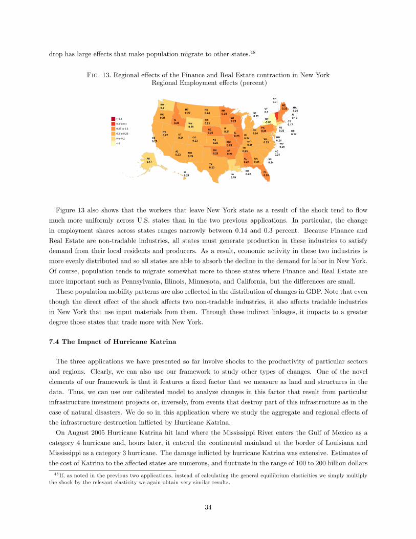
drop has large effects that make population migrate to other states.48

Fig. 13. Regional effects of the Finance and Real Estate contraction in New YorkRegional Employment effects (percent)

AL0.27

AK0.17

AZ0.23

AR0.26

CA0.22

CO0.22

CT0.17

DE0.14

FL0.26

GA0.21

HI0.24

ID0.25

IL0.25 IN

0.24

IA0.21

KS0.23 KY

0.25

LA0.19

ME0.25

MD0.24

MA0.26

MI0.25

MN0.29

MS0.22

MO0.28

MT0.22

NE0.26NV

0.22

NH0.3

NJ0.22

NM0.24

NY-3.83

NC0.21

ND0.24

OH0.24

OK0.25

OR0.21

PA0.26

RI0.19

SC0.24

SD0.21

TN0.23

TX0.23

UT0.24

VT0.3

VA0.23

WA0.2

WV0.25

WI0.29

WY0.19

Figure 13 also shows that the workers that leave New York state as a result of the shock tend to flow

much more uniformly across U.S. states than in the two previous applications. In particular, the change

in employment shares across states ranges narrowly between 0.14 and 0.3 percent. Because Finance and

Real Estate are non-tradable industries, all states must generate production in these industries to satisfy

demand from their local residents and producers. As a result, economic activity in these two industries is

more evenly distributed and so all states are able to absorb the decline in the demand for labor in New York.

Of course, population tends to migrate somewhat more to those states where Finance and Real Estate are

more important such as Pennsylvania, Illinois, Minnesota, and California, but the differences are small.

These population mobility patterns are also reflected in the distribution of changes in GDP. Note that even

though the direct effect of the shock affects two non-tradable industries, it also affects tradable industries

in New York that use input materials from them. Through these indirect linkages, it impacts to a greater

degree those states that trade more with New York.

7.4 The Impact of Hurricane Katrina

The three applications we have presented so far involve shocks to the productivity of particular sectors

and regions. Clearly, we can also use our framework to study other types of changes. One of the novel

elements of our framework is that it features a fixed factor that we measure as land and structures in the

data. Thus, we can use our calibrated model to analyze changes in this factor that result from particular

infrastructure investment projects or, inversely, from events that destroy part of this infrastructure as in the

case of natural disasters. We do so in this application where we study the aggregate and regional effects of

the infrastructure destruction inflicted by Hurricane Katrina.

On August 2005 Hurricane Katrina hit land where the Mississippi River enters the Gulf of Mexico as a

category 4 hurricane and, hours later, it entered the continental mainland at the border of Louisiana and

Mississippi as a category 3 hurricane. The damage inflicted by hurricane Katrina was extensive. Estimates of

the cost of Katrina to the affected states are numerous, and fluctuate in the range of 100 to 200 billion dollars

48 If, as noted in the previous two applications, instead of calculating the general equilibrium elasticities we simply multiplythe shock by the relevant elasticity we again obtain very similar results.

34

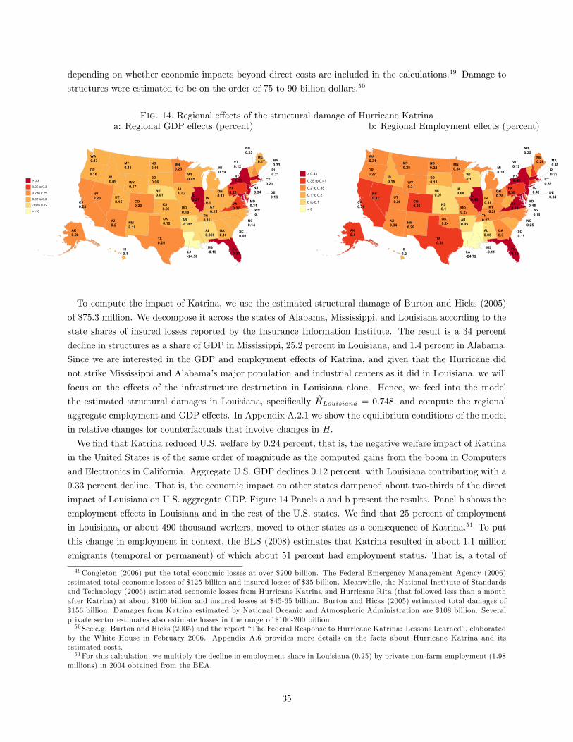
depending on whether economic impacts beyond direct costs are included in the calculations.49 Damage to

structures were estimated to be on the order of 75 to 90 billion dollars.50

Fig. 14. Regional effects of the structural damage of Hurricane Katrinaa: Regional GDP effects (percent) b: Regional Employment effects (percent)

AL0.005

AK0.25

AZ0.2

AR-0.005

CA0.25

CO0.23

CT0.21

DE0.18

FL0.33

GA0.16

HI0.1

ID0.09

IL0.31 IN

0.1

IA0.02

KS0.06 KY

0.15

LA-24.58

ME0.17

MD0.31

MA0.33

MI0.19

MN0.23

MS-0.15

MO0.18

MT0.15

NE0.01NV

0.23

NH0.25

NJ0.34

NM0.19

NY0.33

NC0.14

ND0.11

OH0.17

OK0.18

OR0.16

PA0.26

RI0.21

SC0.06

SD0.06

TN0.16

TX0.25

UT0.15

VT0.12

VA0.27

WA0.17

WV0.1

WI0.05

WY0.17

AL0.05

AK0.4

AZ0.34

AR0.05

CA0.39

CO0.36

CT0.36

DE0.34

FL0.45

GA0.3

HI0.2

ID0.15

IL0.45 IN

0.18

IA0.08

KS0.1 KY

0.26

LA-24.72

ME0.26

MD0.45

MA0.47

MI0.31

MN0.34

MS-0.11

MO0.27

MT0.25

NE0.07NV

0.37

NH0.35

NJ0.49

NM0.29

NY0.49

NC0.25

ND0.22

OH0.28

OK0.24

OR0.27

PA0.38

RI0.33

SC0.15

SD0.13

TN0.27

TX0.38

UT0.25

VT0.19

VA0.41

WA0.31

WV0.19

WI0.1

WY0.3

To compute the impact of Katrina, we use the estimated structural damage of Burton and Hicks (2005)

of $75.3 million. We decompose it across the states of Alabama, Mississippi, and Louisiana according to the

state shares of insured losses reported by the Insurance Information Institute. The result is a 34 percent

decline in structures as a share of GDP in Mississippi, 25.2 percent in Louisiana, and 1.4 percent in Alabama.

Since we are interested in the GDP and employment effects of Katrina, and given that the Hurricane did

not strike Mississippi and Alabama’s major population and industrial centers as it did in Louisiana, we will

focus on the effects of the infrastructure destruction in Louisiana alone. Hence, we feed into the model

the estimated structural damages in Louisiana, specifically HLouisiana = 0.748, and compute the regional

aggregate employment and GDP effects. In Appendix A.2.1 we show the equilibrium conditions of the model

in relative changes for counterfactuals that involve changes in H.

We find that Katrina reduced U.S. welfare by 0.24 percent, that is, the negative welfare impact of Katrina

in the United States is of the same order of magnitude as the computed gains from the boom in Computers

and Electronics in California. Aggregate U.S. GDP declines 0.12 percent, with Louisiana contributing with a

0.33 percent decline. That is, the economic impact on other states dampened about two-thirds of the direct

impact of Louisiana on U.S. aggregate GDP. Figure 14 Panels a and b present the results. Panel b shows the

employment effects in Louisiana and in the rest of the U.S. states. We find that 25 percent of employment

in Louisiana, or about 490 thousand workers, moved to other states as a consequence of Katrina.51 To put

this change in employment in context, the BLS (2008) estimates that Katrina resulted in about 1.1 million

emigrants (temporal or permanent) of which about 51 percent had employment status. That is, a total of

49Congleton (2006) put the total economic losses at over $200 billion. The Federal Emergency Management Agency (2006)estimated total economic losses of $125 billion and insured losses of $35 billion. Meanwhile, the National Institute of Standardsand Technology (2006) estimated economic losses from Hurricane Katrina and Hurricane Rita (that followed less than a monthafter Katrina) at about $100 billion and insured losses at $45-65 billion. Burton and Hicks (2005) estimated total damages of$156 billion. Damages from Katrina estimated by National Oceanic and Atmospheric Administration are $108 billion. Severalprivate sector estimates also estimate losses in the range of $100-200 billion.50See e.g. Burton and Hicks (2005) and the report “The Federal Response to Hurricane Katrina: Lessons Learned”, elaborated

by the White House in February 2006. Appendix A.6 provides more details on the facts about Hurricane Katrina and itsestimated costs.51For this calculation, we multiply the decline in employment share in Louisiana (0.25) by private non-farm employment (1.98

millions) in 2004 obtained from the BEA.

35

574 thousand workers moved out of Louisiana. Our model, therefore, captures virtually all of the movement

in population, with the difference likely the result of other effects of the hurricane not related to structures.52

Figure 14 Panel b shows that, consistent with the pattern reported by the BLS, population relocated

across all states, including far away regions. Still, we find that population tends to migrate more to states

such as California, Texas, and some states in the east coast that compete with Louisiana in industries such

as Petroleum. Overall, we find that large states such as Virginia, California, New York and Texas received

the biggest inflows of workers after Katrina. The fall in employment in Louisiana resulted in a GDP drop

of a similar order of magnitude (Figure 14 Panel a). GDP increases in other states that benefited from

migration, especially some states in the east coast and midwest that are abundant in structures. Finally,

the impact of Katrina on measured TFP is generally small. Louisiana’s measured TFP rose due to selection

effects; in particular, structural damages increased the cost of producing goods in Louisiana so that it started

importing a larger set of goods that previously were produced domestically with relative lower effi ciency.

The impact on measured TFP in other regions is small, reflecting the fact that Louisiana is relatively isolated

in terms of regional and sectoral trade.

8. CONCLUDING REMARKS

Motivated by our finding that productivity changes that are specific to a region, or a region and sector,

account for most of the changes in measured and fundamental productivity in the U.S., we study the effects

of disaggregated productivity changes in a model that recognizes explicitly the role of geographical factors

in determining allocations. This geographical element is manifested in several ways.

First, following a long tradition in macroeconomics, we take account of interactions between sectors, but we

further recognize that these interactions take place over potentially large distances by way of costly regional

trade. Thus, borrowing from the recent international trade literature, we incorporate multiple regions and

transport costs in our analysis. Second, we consider the mobility and spatial distribution of different factors

of production. Specifically, while labor tends to be mobile across regions, other factors, such as land and

structures, are fixed locally and unevenly distributed across space. We calibrate the model to match data

on pairwise trade flows across U.S. states by industry and other regional and industry data. Given this

calibration, we are then able to provide a quantitative assessment of how different regions and sectors of the

U.S. economy adjust to disaggregated productivity disturbances.

We find that disaggregated productivity changes can have dramatically different aggregate quantitative

implications depending on the regions and sectors affected. Furthermore, particular disaggregated funda-

mental changes have very heterogenous effects across different regions and sectors. These effects arise in part

because disaggregated productivity disturbances lead to endogenous changes in the pattern of trade. These

changes in turn are governed by a selection effect that ultimately determines which regions produce what

types of goods. Furthermore, labor is a mobile factor so that regions that become more productive tend to

see an inflow of population. This inflow increases the burden on local fixed resources in those regions and,

therefore, attenuates the direct effects of any productivity increases. In addition, the different estimated

ownership structures of the fixed factor across states implies that changes in the returns to these factors

are unequally distributed across regions, thereby exacerbating the role of geography in determining aggre-

gate and regional elasticities. These implications of the model are the direct result of the observed trade

52For details, see the report “Hurricane Katrina evacuees: Who they are, Where they are, and How they are faring”preparedby the BLS in March 2008.

36

imbalances across states.

Armed with our quantitative model of the U.S. economy we explore the role of specific disturbances in the

U.S. economy. We study four different applications that study productivity changes in different industries

and sectors, as well as changes in infrastructure. These applications are of interest in their own right, but

also exemplified how the elasticities presented and studied in the paper can be used to study a wide variety

of phenomena. Our hope is that they are used in the future to understand the impact of other events in the

future. Importantly, the evaluations permitted by these elasticities fully include general equilibrium effects as

well as the dispersion of shocks through the trade and input-output network. So although extremely easy to

use, these elasticities are the key element in producing full macroeconomic counterfactuals to disaggregated

disturbances.

One missing aspect of our analysis is that land and infrastructures are fixed and so do not respond dynam-

ically to shocks. Future work might further explore how local factors that can be gradually adjusted over

time, such as private structures or infrastructure in the form of public capital, affect how regional and sectoral

variables interact in responding to productivity disturbances. While the accumulation of local factors might

attenuate somewhat the effects of migration, these effects depend on the stock of structures which moves

slowly over time. The quantitative implications of this adjustment margin, therefore, are not immediate.

The framework we develop might also be extended to assess the effects of different regional policies, such

as state taxes or regulations (as in Fajgelbaum et al., 2016). Other extensions of this line or research could

endogenize technology diffusion through migration, or study how regional and sectoral productivity shocks

impact the employment and wages across different skill groups.53 Finally, dynamic adjustments in trade

imbalances would also be informative with respect to the behavior of regional trade deficits in the face of

fundamental productivity disturbances, and how this behavior then relates to macroeconomic adjustments.

For now, this paper suggests that the regional characteristics of an economy appear essential to the study

of the macroeconomic implications of productivity changes.

REFERENCES

[1] Acemoglu, Daron, David Autor, David Dorn, Gordon H. Hanson, and Brendan Price (2015): “Import Com-petition and the Great U.S. Employment Sag of the 2000s,”Journal of Labor Economics, forthcoming.

[2] Acemoglu, Daron, Vasco M. Carvalho, Asuman Ozdaglar, and Alireza Tahbaz-Salehi (2012): “The NetworkOrigins of Aggregate Fluctuations,”Econometrica, 80(5), 1977-2016.

[3] Acemoglu, Daron, Ufuk Akcigit, and William Kerr (2015): “Networks and the Macroeconomy: An EmpiricalExploration,”NBER Macroeconomics Annual, forthcoming.

[4] Akcigit, Ufuk, Salome Baslandze, and Stefanie Stantcheva (2016): “Taxation and the International Mobilityof Inventors,”American Economic Review, forthcoming.

[5] Allen, Treb, and Arkolakis, Costas (2013): “Trade and the Topography of the Spatial Economy,”QuarterlyJournal of Economics, forthcoming.

[6] Alvarez, Fernando, and Robert E. Lucas (2007): “General Equilibrium Analysis of the Eaton-Kortum Modelof International Trade,”Journal of Monetary Economics, 54(6), 726—68.

[7] Alvarez, Fernando, Buera, Francisco, and Robert E. Lucas (2013): “Idea Flows, Economic Growth, andTrade,”NBER Working Paper No. 19667.

53Recent estimates of how innovators respond to local market conditions from Akcigit, Baslandze, and Stancheva (2016) couldbe used as a guide to build on models where trade affects the distribution of technologies (see Alvarez, Buera and Lucas 2013,and Buera and Oberfield 2016).

37

[8] Anderson, James E., and Eric van Wincoop (2003): “Gravity with Gravitas: A Solution to the BorderPuzzle,”American Economic Review, 93(1), 170-192.

[9] Arkolakis, Costas, Arnaud Costinot, and Andres Rodriguez Clare (2012): “New Theories, Same Old Gains?,”American Economic Review, 102(1), 94-130.

[10] Blanchard, Olivier, and Lawrence F. Katz (1992): “Regional Evolutions,” Brooking Papers of EconomicActivity, 1, 1-75.

[11] Buera, Francisco, and Ezra Oberfield (2016): “The Global Diffusion of Ideas,”NBER Working Paper No.21844.

[12] Bureau of Labor Statistics (2008): “Handbook of Methods.”

[13] Bureau of Labor Statistics (2008): “Hurricane Katrina Evacuees: Who They Are, Where They Are, andHow They Are Faring,”March, available at http://www.bls.gov/opub/mlr/2008/03/art3full.pdf.

[14] Burstein, Ariel, and Javier Cravino (2015): “Measured Aggregate Gains from International Trade,”AmericanEconomic Journal: Macroeconomics, 7(2), 181-218.

[15] Burton, Mark L. and Michael J.Hicks (2005): “Hurricane Katrina: Preliminary Estimates of Commercial andPublic Sector Damages,”Center for Business and Economic Research, Marshall University, September.

[16] Byrne, David M., John G. Fernald, and Marshall B. Reinsdorf (2016): “Does the United States have aproductivity slowdown or a measurement problem?,”Brooking Papers on Economic Activity, March.

[17] Caliendo, Lorenzo, and Fernando Parro (2015): “Estimates of the Trade and Welfare Effects of NAFTA,”The Review of Economic Studies, 82(1), 1-44.

[18] Carvalho, Vasco, and Xavier Gabaix (2013): “The Great Diversification and its Undoing,”American Eco-nomic Review, 103(5), 1697-1727.

[19] Caselli, Francesco, Miklos Koren, Milan Lisicky, and Silvana Tenreyro (2012): “Diversification throughTrade,”mimeo LSE.

[20] Congleton, Roger D. (2006): “The Story of Katrina: New Orleans and the Political Economy of Catastrophe,”Public Choice, 127(1), 5-30.

[21] Costinot, Arnaud, Dave Donaldson, and Ivana Komunjer (2012): “What Goods Do Countries Trade? AQuantitative Exploration of Ricardo’s Ideas?,”Review of Economic Studies, 79(2), 581-608.

[22] Costinot, Arnaud, and Andres Rodriguez-Clare (2013): “Trade Theory with Numbers: Quantifying theConsequences of Globalization,”Handbook of International Economics, forthcoming.

[23] Dekle, Robert, Jonathan Eaton, and Samuel S. Kortum (2008): “Global Rebalancing with Gravity: Mea-suring the Burden of Adjustment,”IMF Staff Papers, 55(3), 511-540.

[24] Department of Housing and Urban Development (2006): “Current Housing Unit Dam-age Estimates: Hurricanes Katrina, Rita, and Wilma,” February 12, available athttps://www.huduser.gov/publications/pdf/GulfCoast_Hsngdmgest.pdf.

[25] Disdier, Anne-Célia and Keith Head (2008) “The Puzzling Persistence of the Distance Effect on BilateralTrade,”Review of Economics and Statistics, 90(1), 37-48.

[26] Dolfman, Michael, Solidelle Fortier Wasser, and Bruce Bergman (2007): “The Effects of Hurricane Katrinaon the New Orleans Economy,”Monthly Labor Review, June.

[27] Dupor, William (1999): “Aggregation and Irrelevance in Multi-Sector Models,”Journal of Monetary Eco-nomics, 43(2), 391-409.

38

[28] Duranton, Gilles, Morrow, Peter and Matthew Turner (2014): “Roads and Trade: Evidence from the U.S.,”Review of Economic Studies, 81(2), 621-724.

[29] Eaton, Jonathan, and Samuel S. Kortum (2002): “Technology, Geography, and Trade,”Econometrica, 70(5),1741—1779.

[30] Eaton, Jonathan, and Samuel S. Kortum (2012): “Putting Ricardo to Work,”Journal of Economic Perspec-tives, 26(2): 65—90.

[31] Fajgelbaum, Pablo, Eduardo Morales, Juan Suarez and Owen Zidar (2016) “State Taxes and Spatial Misal-location,”NBER Working Paper No. 21760.

[32] Federal Emergency Management Agency (2006): “Summary Report on Building Performance: HurricaneKatrina 2005,”FEMA 548, April.

[33] Fernald, John (1999): “Roads to Prosperity? Assessing the Link between Public Capital and Productivity,”American Economic Review, 89(3), 619-638.

[34] Finicelli, Andrea, Patrizio Pagano, Massimo Sbracia (2013): “Ricardian Selection,”Journal of InternationalEconomics, 89(1), 96-109.

[35] Foerster, Andrew T, Pierre-Daniel G Sarte, and Mark W. Watson (2011): “Sectoral vs. Aggregate Shocks:A Structural Factor Analysis of Industrial Production,”Journal of Political Economy, 119:1, 1-38.

[36] Fogli, Alessandra, Enoch Hill, and Fabrizio Perri (2012): “The Geography of the Great Recession,”NBERWorking Paper No 18447.

[37] Feyrer, James (2009): “Distance, Trade, and Income - The 1967 to 1975 Closing of the Suez Canal as aNatural Experiment. National Bureau of Economic Research,”NBER Working Paper No 16806.

[38] Gabaix, Xavier (2011): “The Granular Origins of Aggregate Fluctuations,”Econometrica, 79(3), 733-772.

[39] Greenwood, Jeremy, Zvi Hercowitz, and Krusell, Per (1997) “Long-Run Implications of Investment-SpecificTechnological Change,”American Economic Review, 87(3), 342-362.

[40] Head, Keith, and John Ries (2001): “Increasing Returns versus National Product Differentiation as anExplanation for the Pattern of U.S.-Canada Trade,”American Economic Review, 91(4), 858-876.

[41] Horvath, Michael (1998): “Cyclicality and Sectoral Linkages: Aggregate Fluctuations from IndependentSectoral Shocks,”Review of Economic Dynamics, 1, 781-808.

[42] Horvath, Michael (2000): “Sectoral Shocks and Aggregate Fluctuations,”Journal of Monetary Economics,45, 69-106.

[43] Insurance Information Institute (2006): “Hurricane Katrina Fact File”, available athttp://www.iii.org/sites/default/files/docs/pdf/Hurricane%20Katrina%20Fact%20File.pdf.

[44] Jovanovic, Boyan (1987): “Micro Shocks and Aggregate Risk,”Quarterly Journal of Economics, 102(2),395-409.

[45] Kennan, John, and James R. Walker (2011): “The Effect of Expected Income on Individual MigrationDecisions,”Econometrica, 79(1), 211—251.

[46] Koren, Miklós, and Silvana Tenreyro (2007): "Volatility and Development," The Quarterly Journal of Eco-nomics, 122 (1), 243-287.

[47] Kydland, Finn., and Edward C. Prescott (1982): “Time to Build and Aggregate Fluctuations,”Econometrica,50, 1345—1370.

[48] Levchenko, Andrei, and Jing Zhang (2011): “The Evolution of Comparative Advantage: Measurement andWelfare Implications,”NBER Working Paper No 16806.

39

[49] Long, John B., Jr., and Charles I. Plosser (1983): “Real Business Cycles,”Journal of Political Economy, 91,39-69.

[50] Minneapolis Fed (2016): “The Bakken Oil Boom”, articles available athttps://www.minneapolisfed.org/publications/special-studies/bakken/oil-production.

[51] National Institute of Standards and Technology (2006): “Performance of Physical Structures in Hur-ricane Katrina and Hurricane Rita: Reconnaissance Findings and Recommendations,” available athttp://www.nist.gov/el/disasterstudies/weather/upload/Hurricane Katrina-Rita Brie ng.pdf.

[52] New York Times (2013): “North Dakota Went Boom,” available athttp://www.nytimes.com/2013/02/03/magazine/north-dakota-went-boom.html?_r=0.

[53] Oberfield, Ezra (2012): “Business Networks, Production Chains, and Productivity: A Theory of Input-Output Architecture,”mimeo Princeton University.

[54] Redding, Stephen (2012): “Goods Trade, Factor Mobility and Welfare,”NBER Working Paper No18008.

[55] Sobol, Ilya M. (1990): “Sensitivity estimates for nonlinear mathematical models,”Matematicheskoe Mod-elirovanie 2, 112—118. in Russian

[56] Sobol, Ilya M. (1993): “Sensitivity estimates for nonlinear mathematical models,”Mathematical Modeling& Computational Experiment (Engl. Transl. of Sobol, 1990) 1, 407—414.

[57] Syverson, Chad (2016): “Challenges to Mismeasurement Explanations for the U.S. Productivity Slowdown,”NBER Working Paper No21974.

[58] Tombe, Trevor, and Xiaodong Zhu (2015): “Trade, Migration, and Productivity: A Quantitative Analysisof China ,”mimeo Toronto University.

40

APPENDIX

A.1 Equilibrium Conditions with Exogenous Inter-regional Trade Deficit

Income of households in region n is given by In = wn+χ+(1− ιn) rnHnLn−sn, where sn = Sn/Ln represents

the part of observed per-capita trade surplus in region n unexplained by the model. Utility of an agent inregion n is given by U = In

Pn. Using the equilibrium condition rnHn = βn

1−βnwnLn, and the definition of

ωn = (rn/βn)βn (wn/ (1− βn))

1−βn , we can express wages as wn1−βn

= ωn

(HnLn

)βn. Therefore, U may be

expressed as

U =

(Hn

Ln

)βn ωnPn− unPn− snPn

,

where un = Υn/Ln = (ιnrnHn − χLn) /Ln. Solving for Ln and use the labor market clearing condition∑N

n=1Ln = L, to solve for U

U =1

L

∑N

n=1

(ωnPn

(Hn)βn L1−βnn − Υn

Pn− SnPn

).

Finally we can use these conditions to obtain,

Ln =Hn

[ωn

PnU+un+sn

]1/βn∑N

i=1Hi

[ωi

PiU+ui+si

]1/βi L.The expenditure shares are given by

πjni =

[xjiκ

jni

]−θjTj θjγjii

N∑m=1

[xjmκ

jnm

]−θjT j θ

jγjmm

.

the input bundle and prices by

xjn = Bjn[rβnn w1−βnn

]γjn∏J

k=1

(P kn)γjkn

P jn = Γ(ξjn)1−ηjn [ N∑

i=1

[xjiκ

jni

]−θj (T ji

)θjγji]−1/θj

Regional market clearing in final goods is given by

Xjn =

∑kγkjn

∑iπkinX

ki + αj

(ωn (Hn)

βn (Ln)1−βn −Υn − Sn

)Trade balance then is given by∑J

j=1Xjn + Υn + Sn =

∑J

j=1

∑N

i=1πjinX

ji .

Note that combining trade balance with goods market clearing we end up with the following equilibriumcondition,

ωn (Hn)βn (Ln)

1−βn =∑

jγjn∑N

i=1πjinX

ji .

41

A.2 Equilibrium Conditions in Relative Changes

Input bundle (JN equations):

xjn = (ωn)γjn

∏J

k=1(P kn )γ

jkn . (A. 1)

Price index (JN equations):

P jn =

(∑N

i=1πjni

[κjnix

ji

]−θjTj θjγjii

)−1/θj. (A. 2)

Trade shares (JN2 equations)

πj′

ni = πjni

(xji

P jnκjni

)−θjTj θjγjii . (A. 3)

Labor mobility condition (N equations):

Ln =

(ωn

ϕnPnU+(1−ϕn)bn

)1/βn∑

iLi

(ωi

ϕiPiU+(1−ϕi)bi

)1/βi L. (A. 4)

Regional market clearing in final goods (JN equations):

Xj′n =

∑J

k=1γk,jn

(∑N

i=1πk′inX

k′i

)+ αj

(ωn

(Ln

)1−βn(InLn + Υn + Sn)− S′n −Υ′n

). (A. 5)

Labor market clearing (N equations)

ωn

(Ln

)1−βn(LnIn + Υn + Sn) =

∑jγjn∑

iπ′jinX

′ji ,

where bn =u′n+s

′n

un+sn, ϕn = 1

1+Υn+SnLnIn

, U = 1L

∑nLn

(1ϕn

ωnPn

(Ln

)1−βn− 1−ϕn

ϕn

LnbnPn

), and Pn =

∏J

j=1

(P jn

)αj.

The total number of unknowns is: ωn (N), Ln (N), Xj′n (JN), P

jn (JN), π

j′ni (J ×N ×N), xjn (JN). For

a total of 2N + 3JN + JN2 equations and unknowns.

A.2.1 Allowing for Changes in Structures.–Equilibrium conditions with changes in structures Hn.The labor mobility condition now becomes:

Ln =Hn

(ωn

ϕnPnU+(1−ϕn)bn

)1/βn∑i LiHi

(ωi

ϕiPiU+(1−ϕi)bi

)1/βi Lwith U = 1

L

∑n Ln

(1ϕn

ωnPn

(Hn

)βn (Ln

)1−βn− 1−ϕn

ϕn

LnbnPn

). From the labor market clearing one obtains:

ωn

(Hn

)βn (Ln

)1−βn(LnIn + Υn + Sn) =

∑j γ

jn

∑i π′jinX

′ji

and in the same way, the regional market clearing in final goods condition becomes

Xj′

n =∑Jk=1 γ

k,jn + αj

(ωn

(Hn

)βn (Ln

)1−βn(LnIn + Υn + Sn)− S′n −Υ′n

)

42

where Υ′n =

(ιnωn

(Hn

)βn (Ln

)1−βnrnHn − κ′LnLn

)/LnLn, and with κ′ =

∑iιiωn(Hn)

βn(Ln)1−βnriHi

L .

A.3 Computation: Solving for Counterfactuals

Consider an exogenous change in S′n, κjni, Hn, and/or T

jni. To solve for the counterfactual equilibrium in

relative changes, we proceed as follows: Guess the relative change in regional factor prices ω.Step 1. Obtain P jn and x

jn consistent with ω using (A.1) and (A.2).

Step 2. Solve for trade shares, πj′

ni (ω), consistent with the change in factor prices using P jn (ω) andxjn (ω) as well as the definition of trade shares given by (A.3).Step 3. Solve for the change in labor across regions consistent with the change in factor prices Ln (ω) ,

given P jn (ω) , and xjn (ω) , using (A.4).Step 4. Solve for expenditures consistent with the change in factor prices Xj′

n (ω) , using (A.5) , whichconstitutes N × J linear equations in N × J unknown, {Xj′

n (ω)}N×J . This can be solved through matrixinversion. Observe that carrying out this step first requires having solved for Ln (ω) .Step 5. Obtain a new guess for the change in factor prices, ω∗n, using

ω∗n =

∑j γ

jn

∑iπ′jin (ω)X ′ji (ω)

Ln (ω)1−βn (LnIn + Υn + Sn)

.

Repeat Steps 1 through 5 until ||ω∗ − ω|| < ε.

A.4 Data and Calibration

We calibrate the model to the 50 U.S. states and a total of 26 sectors classified according to the NorthAmerican Industry Classification System (NAICS), 15 of which are tradable goods, 10 service sectors, andconstruction. We assume that all service sectors and construction are non-tradable. We present below alist of the sectors that we use, and describe how we combine a subset of these sectors to ease computations.As stated in the main text, carrying out structural quantitative exercises on the effects of disaggregated

fundamental changes requires data on{In, Ln,Υn, π

jni

}N,N,Jn=1,i=1,j=1

, as well as values for the parameters{θj , αj , βn, γ

jn, γ

jkn

}N,J,Jn=1,j=1,k=1

. We now describe the main aspects of the data.

A.4.1 Regional Employment and Income.–We set L = 1 so that, for each n ∈ {1, ..., N}, Ln is interpreted as the share of state n’s employment in

total employment. Regional employment data is obtained from the Bureau of Economic Analysis (BEA),with aggregate employment across all states summing to 137.3 million in 2007.

A.4.2 Interregional Trade Flows and Surpluses.–To measure the shares of expenditures in intermediates from region-sector (i, j) for each state n, πjni, we

use data from the Commodity Flow Survey (CFS). The dataset tracks pairwise trade flows across all 50states for 18 sectors of the U.S. economy (three of these are aggregated for a total of 15 tradable goodssectors as described in A.4.5). The CFS contains data on the total value of trade across all states whichamounts to 5.2 trillion in 2007 dollars. The most recent CFS data covers the year 2007 and was released in2012. This explains our choice of 2007 as the baseline year of our analysis.Even though the CFS aims to quantify only domestic trade, and leaves out all international transactions,

some imports to a local destination that are then traded in another domestic transaction are potentiallyincluded. To exclude this imported part of gross output, we calculate U.S. domestic consumption of domesticgoods by subtracting exports from gross production for each NAICS sector using sectoral measures of grossoutput from the BEA and exports from the U.S. Census. We then compare the sectoral domestic shipment ofgoods implied by the CFS for each sector to the aggregate measure of domestic consumption. As expected,the CFS domestic shipment of goods is larger than the domestic consumption measure for all sectors, by a

43

factor ranging from 1 to 1.4. We thus adjust the CFS tables proportionally so that they represent the totalamount of domestic consumption of domestic goods.A row sum in a CFS trade table associated with a given sector j represents total exports of sector j goods

from that state to all other states. Conversely, a column sum in that trade table gives total imports ofsector j goods to a given state from all other states. The difference between exports and imports allows usto directly compute domestic regional trade surpluses in all U.S. states. We obtain In by calculating totalvalue added in each state using BEA data and adding interregional trade deficits from the CFS data anddividing the result by total population for that state in 2007.Given {ιn}N×1, we use information on value added by regions to calculate regional national portfolio

balances, Υn = ιnrnHn − χLn, where χ =∑i ιiriHi/

∑i Li. We then solve for {Sn}N×1 as the difference

between observed trade surplus in the data and the one implied by regional national portfolio balances. Wethen solve for {ιn}N×1 by minimizing the sum square of {Sn}N×1.

A.4.3 Value Added Shares and Shares of Material Use.–In order to obtain value added shares observe that, for a particular sector j, each row-sum of the corre-

sponding adjusted CFS trade table equals gross output for that sector in each region,{∑N

i=1 πjinX

ji

}Nn=1

.

Hence, we divide value added from the BEA in region-sector pair (n, j) by its corresponding measure ofgross output from the trade table to obtain the share of value added in gross output by region and sectorfor all tradeable goods, {γjn}

N,15n=1,j=1. For the 11 non-tradeable sectors, gross output is not available at the

sectoral level by state. In those sectors, we assume that the value added shares are constant across states andequal to the national share of value added in gross output , γjn = γj ∀n ∈ {1, ..., N} and j > 15. Aggregatemeasures of gross output and value added in non-tradeable sectors are obtained from the BEA.While material input shares are available from the BEA by sector, they are not disaggregated by state.

Given the structure of our model, it is nevertheless possible to infer region-specific material input sharesfrom a national input-output (IO) table and other available data. The BEA Use table gives the value ofinputs from each industry used by every other industry at the aggregate level. This use table is available at5 year intervals, the most recent of which was released for 2002 data. A column sum of the BEA Use tablegives total dollar payments from a given sector to all other sectors. Therefore, at the national level, we cancompute γjk, the share of material inputs from sector k in total payments to materials by sector j. Since∑Nk=1 γ

jk = 1, one may then construct the share of payments from sector j to material inputs from sectork, for each state n, as γjkn = (1− γjn)γjk where recall that γjn’s are region-sector specific value added shares.

A.4.4 Share of Final Good Expenditure.–The share of income spent on goods from different sectors is calculated as follows,

αj =Y j +M j − Ej −

∑k γ

k,j(1− γk

)Y k∑

j (Y j +M j − Ej −∑k γ

k,j (1− γk)Y k),

where Ej denotes total exports from the U.S. to the rest of the world, M j represents total imports to theU.S., and all intermediate input shares are national averages.

A.4.5 Payments to Labor and Structure Shares.–As noted in the previous section, we assume that the share of payments to labor in value added, {1−βn}Nn=1,

is constant across sectors. Disaggregated data on compensation of employees from the BEA is not availableby individual sector in every state. To calculate 1−βn in a given region, we first sum data on compensation ofemployees across all available sectors in that region, and divide this sum by value added in the correspondingregion. The resulting measure, denoted by 1 − βn, overestimates the value added share of the remainingfactor in our model, βn, associated with land and structures. That is, part of the remaining factor used inproduction involves equipment in addition to fixed structures. Accordingly, to adjust these shares, we relyon estimates from Greenwood, Hercowitz, and Krusell (1997) who measure separately the share of labor,structures, and equipment, in value added for the U.S. economy. These shares amount to 70 percent, 13percent, and 17 percent respectively. We thus use these estimates to infer the share of structures in value

44

added across regions by taking the share of non-labor value added by region, βn, subtracting the share ofequipment, and renormalizing so that the new shares add to one. Specifically, we calculate the share of landand structures as βn = (βn − 0.17)/0.83. Since our model explicitly takes materials into account, we assignthe share of equipment to that of materials. In other words, we adjust the share of value added to 0.83γjn,and adjust all calculations above accordingly. In this way, our quantitative exercise uses shares for labor aswell as for land and structures at the regional level that are consistent with aggregate value added shares inthe U.S.

A.4.6 List of Sectors.–The paper uses data from the Commodity Flow Survey (CFS), jointly produced by the Census and the

Bureau of Transportation. The trade tables resulting from the CFS was released for the first time in December2010 and last revised in 2012 for data pertaining to 2007. Each trade table corresponds to a particular sectorand is a 50×50 matrix whose entries represent pairwise trade flows for that sector among all U.S. states. TheCFS contains comprehensive data for 18 manufacturing sectors with a total value of trade across all statesamounting to 5.2 trillion in 2007 dollars. These sectors are Food Product & Beverage and Tobacco Product,(NAICS 311 & 312), Textile and Textile Product Mills, (NAICS 313 & 314), Apparel & Leather and AlliedProduct, (NAICS 315 & 316), Wood Product, (NAICS 321), Paper, (NAICS 322), Printing and Relatedsupport activities, (NAICS 323), Petroleum & Coal Products, (NAICS 324)54 , Chemical, (NAICS 325),Plastics & Rubber Products, (NAICS 326), Nonmetallic Mineral Product, (NAICS 327), Primary Metal,(NAICS 331), Fabricated Metal Product, (NAICS 332), Machinery, (NAICS 333), Computer and ElectronicProduct, (NAICS 334), Electrical Equipment and Appliance, (NAICS 335), Transportation Equipment,(NAICS 336), Furniture & Related Product, (NAICS 337), Miscellaneous, (NAICS 339). We aggregate 3subsectors. Sectors Textile and Textile Product Mills (NAICS 313 & 314) together with Apparel & Leatherand Allied Product (NAICS 315 & 316), Wood Product (NAICS 321) with Paper (NAICS 322) and sectorsPrimary Metal (NAICS 331) with Fabricated Metal Product (NAICS 332). We end up with a total of 15manufacturing tradable sectors.The list of non-tradable sectors are: Construction, Wholesale and Retail Trade, (NAICS 42 - 45), Transport

Services, (NAICS 481 - 488), Information Services, (NAICS 511 - 518), Finance and Insurance, (NAICS 521- 525), Real Estate, (NAICS 531 - 533), Education, (NAICS 61), Health Care, (NAICS 621 - 624), Arts andRecreation, (NAICS 711 - 713), Accom. and Food Services, (NAICS 721 - 722), Other Services, (NAICS 493& 541 & 55 & 561 & 562 & 811 - 814)

A.4.7 Sectoral Distribution of Productivities.–We obtain the dispersion of productivities from Caliendo and Parro (2015). They compute this parameter

for 20 tradable sectors, using data at two-digit level of the third revision of the International StandardIndustrial Classification (ISIC Rev. 3). We match their sectors to our NAICS 2007 sectors using theinformation available in concordance tables. In five of our sectors Caliendo and Parro present estimatesat an either more aggregated or disaggregated level. When Caliendo and Parro report separates estimatesfor sub-sectors which we aggregate into a single sector, we use their data to compute the dispersion ofproductivity in our aggregate sector. In cases where a sector in our data is integrated to another sector inCaliendo and Parro, we input that elasticity.The dispersion of productivity for our sector “Wood and Paper”(NAICS 321-322) is estimated separately

for wood products and paper products in Caliendo and Parro. In this case, using their data we proceed toestimate the aggregate dispersion of productivity for these two sub-sectors. Similarly, they present separateestimates for primary metals and fabricated metals (NAICS 331-332), thus we use their data to estimatethe aggregate elasticity of these two sectors. We also estimate the dispersion of productivity for TransportEquipment (NAICS 336), which is divided into motor vehicles, trailers and semi-trailers, and other transportequipment in Caliendo and Parro. Our sector “Printing and Related Support Activities” (NAICS 323) isestimated together with pulp and paper products (ISIC3 21-22) in Caliendo and Parro, thus we input thatestimate. Similarly, Furniture (NAICS 337) is estimated together with other manufacturing (ISIC 3 36-37)

54The Petroleum and Coal Products Manufacturing sector is based on the transformation of crude petroleum and coal intousable products. The dominant process is petroleum refining, but it also includes further refined petroleum and coal productsand produce products, such as asphalt coatings and petroleum lubricating oils.

45

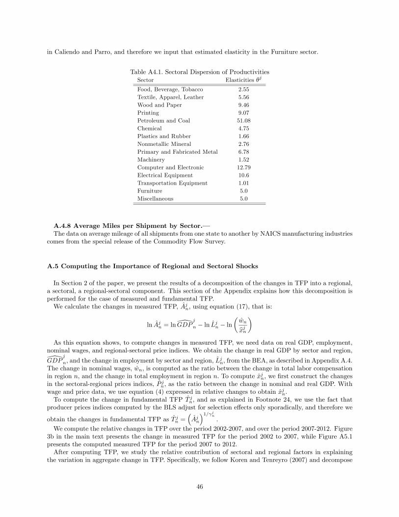
in Caliendo and Parro, and therefore we input that estimated elasticity in the Furniture sector.

Table A4.1. Sectoral Dispersion of ProductivitiesSector Elasticities θj

Food, Beverage, Tobacco 2.55Textile, Apparel, Leather 5.56Wood and Paper 9.46Printing 9.07Petroleum and Coal 51.08Chemical 4.75Plastics and Rubber 1.66Nonmetallic Mineral 2.76Primary and Fabricated Metal 6.78Machinery 1.52Computer and Electronic 12.79Electrical Equipment 10.6Transportation Equipment 1.01Furniture 5.0Miscellaneous 5.0

A.4.8 Average Miles per Shipment by Sector.–The data on average mileage of all shipments from one state to another by NAICS manufacturing industries

comes from the special release of the Commodity Flow Survey.

A.5 Computing the Importance of Regional and Sectoral Shocks

In Section 2 of the paper, we present the results of a decomposition of the changes in TFP into a regional,a sectoral, a regional-sectoral component. This section of the Appendix explains how this decomposition isperformed for the case of measured and fundamental TFP.We calculate the changes in measured TFP, Ajn, using equation (17), that is:

ln Ajn = ln GDPj

n − ln Ljn − ln

(wn

xjn

)As this equation shows, to compute changes in measured TFP, we need data on real GDP, employment,

nominal wages, and regional-sectoral price indices. We obtain the change in real GDP by sector and region,

GDPj

n, and the change in employment by sector and region, Ljn, from the BEA, as described in Appendix A.4.

The change in nominal wages, wn, is computed as the ratio between the change in total labor compensationin region n, and the change in total employment in region n. To compute xjn, we first construct the changesin the sectoral-regional prices indices, P jn, as the ratio between the change in nominal and real GDP. Withwage and price data, we use equation (4) expressed in relative changes to obtain xjn.To compute the change in fundamental TFP T jn, and as explained in Footnote 24, we use the fact that

producer prices indices computed by the BLS adjust for selection effects only sporadically, and therefore we

obtain the changes in fundamental TFP as T jn =(Ajn

)1/γjn.

We compute the relative changes in TFP over the period 2002-2007, and over the period 2007-2012. Figure3b in the main text presents the change in measured TFP for the period 2002 to 2007, while Figure A5.1presents the computed measured TFP for the period 2007 to 2012.After computing TFP, we study the relative contribution of sectoral and regional factors in explaining

the variation in aggregate change in TFP. Specifically, we follow Koren and Tenreyro (2007) and decompose

46

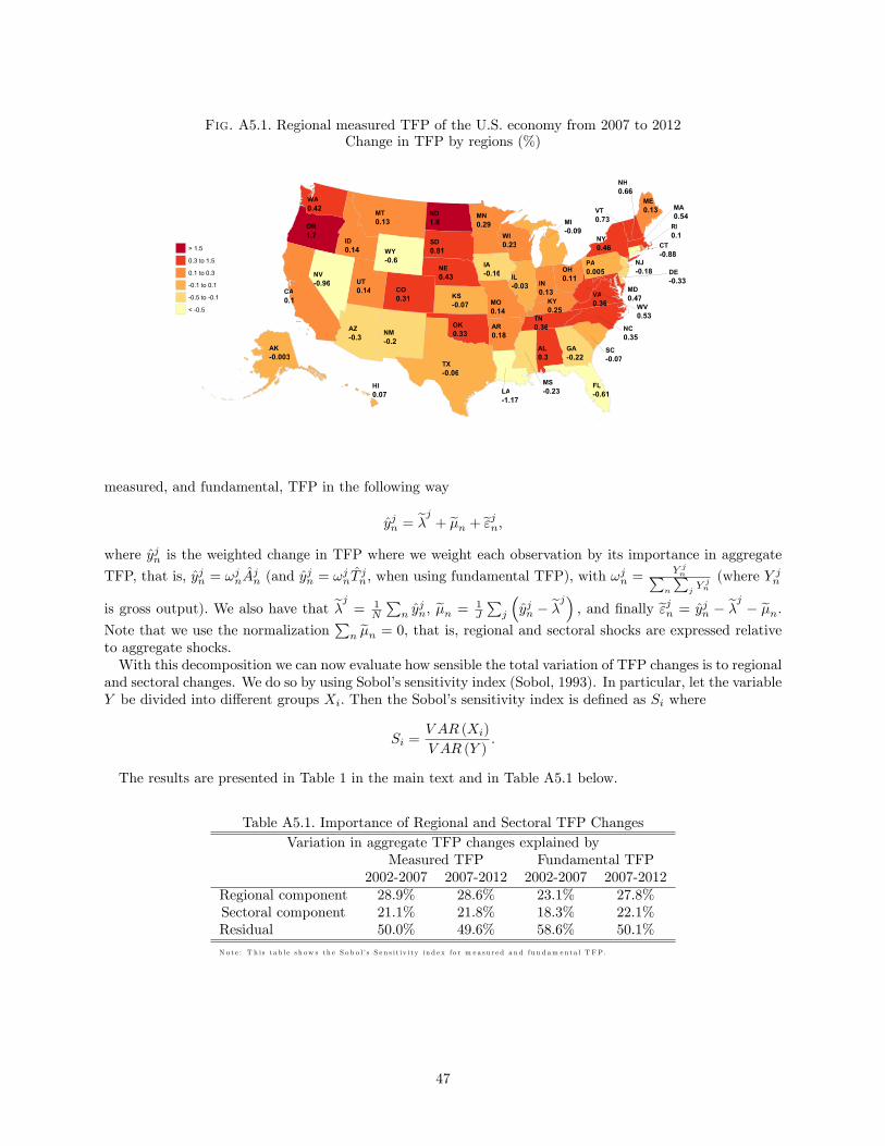
Fig. A5.1. Regional measured TFP of the U.S. economy from 2007 to 2012Change in TFP by regions (%)

AL0.3

AK-0.003

AZ-0.3

AR0.18

CA0.1

CO0.31

CT-0.88

DE-0.33

FL-0.61

GA-0.22

HI0.07

ID0.14

IL-0.03 IN

0.13

IA-0.16

KS-0.07 KY

0.25

LA-1.17

ME0.13

MD0.47

MA0.54

MI-0.09

MN0.29

MS-0.23

MO0.14

MT0.13

NE0.43NV

-0.96

NH0.66

NJ-0.18

NM-0.2

NY0.46

NC0.35

ND1.8

OH0.11

OK0.33

OR1.7

PA0.005

RI0.1

SC-0.07

SD0.81

TN0.36

TX-0.06

UT0.14

VT0.73

VA0.36

WA0.42

WV0.53

WI0.23

WY-0.6

measured, and fundamental, TFP in the following way

yjn = λj

+ µn + εjn,

where yjn is the weighted change in TFP where we weight each observation by its importance in aggregate

TFP, that is, yjn = ωjnAjn (and y

jn = ωjnT

jn, when using fundamental TFP), with ω

jn =

Y jn∑n

∑jY jn(where Y jn

is gross output). We also have that λj

= 1N

∑n y

jn, µn = 1

J

∑j

(yjn − λ

j), and finally εjn = yjn − λ

j− µn.

Note that we use the normalization∑n µn = 0, that is, regional and sectoral shocks are expressed relative

to aggregate shocks.With this decomposition we can now evaluate how sensible the total variation of TFP changes is to regional

and sectoral changes. We do so by using Sobol’s sensitivity index (Sobol, 1993). In particular, let the variableY be divided into different groups Xi. Then the Sobol’s sensitivity index is defined as Si where

Si =V AR (Xi)

V AR (Y ).

The results are presented in Table 1 in the main text and in Table A5.1 below.

Table A5.1. Importance of Regional and Sectoral TFP ChangesVariation in aggregate TFP changes explained by

Measured TFP Fundamental TFP2002-2007 2007-2012 2002-2007 2007-2012

Regional component 28.9% 28.6% 23.1% 27.8%Sectoral component 21.1% 21.8% 18.3% 22.1%Residual 50.0% 49.6% 58.6% 50.1%

N o t e : T h i s t a b le s h ow s t h e S o b o l’s S e n s i t iv i ty in d e x fo r m e a s u r e d a n d fu n d am en t a l T F P.

47

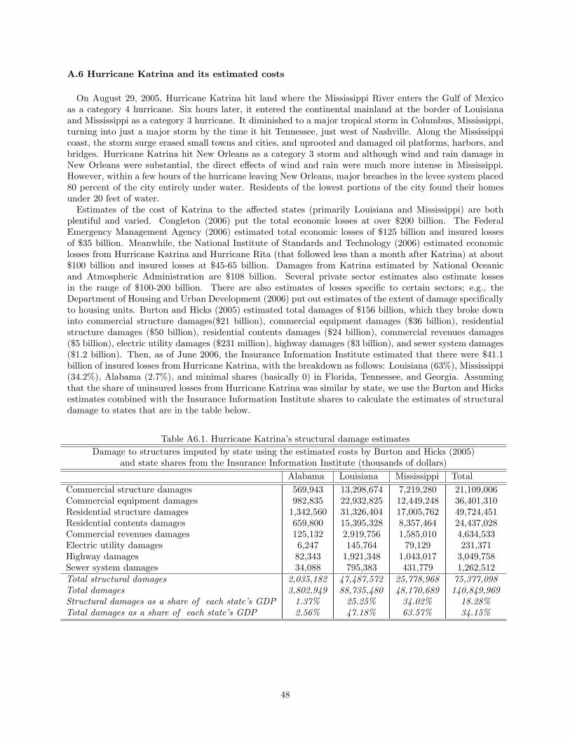
A.6 Hurricane Katrina and its estimated costs

On August 29, 2005, Hurricane Katrina hit land where the Mississippi River enters the Gulf of Mexicoas a category 4 hurricane. Six hours later, it entered the continental mainland at the border of Louisianaand Mississippi as a category 3 hurricane. It diminished to a major tropical storm in Columbus, Mississippi,turning into just a major storm by the time it hit Tennessee, just west of Nashville. Along the Mississippicoast, the storm surge erased small towns and cities, and uprooted and damaged oil platforms, harbors, andbridges. Hurricane Katrina hit New Orleans as a category 3 storm and although wind and rain damage inNew Orleans were substantial, the direct effects of wind and rain were much more intense in Mississippi.However, within a few hours of the hurricane leaving New Orleans, major breaches in the levee system placed80 percent of the city entirely under water. Residents of the lowest portions of the city found their homesunder 20 feet of water.Estimates of the cost of Katrina to the affected states (primarily Louisiana and Mississippi) are both

plentiful and varied. Congleton (2006) put the total economic losses at over $200 billion. The FederalEmergency Management Agency (2006) estimated total economic losses of $125 billion and insured lossesof $35 billion. Meanwhile, the National Institute of Standards and Technology (2006) estimated economiclosses from Hurricane Katrina and Hurricane Rita (that followed less than a month after Katrina) at about$100 billion and insured losses at $45-65 billion. Damages from Katrina estimated by National Oceanicand Atmospheric Administration are $108 billion. Several private sector estimates also estimate lossesin the range of $100-200 billion. There are also estimates of losses specific to certain sectors; e.g., theDepartment of Housing and Urban Development (2006) put out estimates of the extent of damage specificallyto housing units. Burton and Hicks (2005) estimated total damages of $156 billion, which they broke downinto commercial structure damages($21 billion), commercial equipment damages ($36 billion), residentialstructure damages ($50 billion), residential contents damages ($24 billion), commercial revenues damages($5 billion), electric utility damages ($231 million), highway damages ($3 billion), and sewer system damages($1.2 billion). Then, as of June 2006, the Insurance Information Institute estimated that there were $41.1billion of insured losses from Hurricane Katrina, with the breakdown as follows: Louisiana (63%), Mississippi(34.2%), Alabama (2.7%), and minimal shares (basically 0) in Florida, Tennessee, and Georgia. Assumingthat the share of uninsured losses from Hurricane Katrina was similar by state, we use the Burton and Hicksestimates combined with the Insurance Information Institute shares to calculate the estimates of structuraldamage to states that are in the table below.

Table A6.1. Hurricane Katrina’s structural damage estimatesDamage to structures imputed by state using the estimated costs by Burton and Hicks (2005)

and state shares from the Insurance Information Institute (thousands of dollars)

Alabama Louisiana Mississippi Total

Commercial structure damages 569,943 13,298,674 7,219,280 21,109,006Commercial equipment damages 982,835 22,932,825 12,449,248 36,401,310Residential structure damages 1,342,560 31,326,404 17,005,762 49,724,451Residential contents damages 659,800 15,395,328 8,357,464 24,437,028Commercial revenues damages 125,132 2,919,756 1,585,010 4,634,533Electric utility damages 6,247 145,764 79,129 231,371Highway damages 82,343 1,921,348 1,043,017 3,049,758Sewer system damages 34,088 795,383 431,779 1,262,512Total structural damages 2,035,182 47,487,572 25,778,968 75,377,098Total damages 3,802,949 88,735,480 48,170,689 140,849,969Structural damages as a share of each state’s GDP 1.37% 25.25% 34.02% 18.28%Total damages as a share of each state’s GDP 2.56% 47.18% 63.57% 34.15%

48

A.7 The Importance of Geographic Distance as a Trade Barrier

Once regional trade is taken into account, selection plays an essential role in understanding the impactof regional and sectoral productivity changes on aggregate measured TFP, GDP, and welfare. The twofundamental determinants of intermediate-goods-firm selection in a given region-sector pair (n, j) are i) itsfundamental productivity, and ii) the bilateral regional trade barriers it faces. Furthermore, the internationaltrade literature has identified geographic distance as the most important barrier to international tradeflows (see e.g. Disdier and Head 2008). The importance of the selection mechanism emphasized by tradeconsiderations, therefore, is closely related to the role of distance as a deterrent to regional trade. In thissection, we evaluate the importance of geographic distance for aggregate TFP and GDP in the U.S. We do soby first separating the trade costs of moving goods across U.S. states into a geographic distance componentand other regional trade barriers. We then quantify the aggregate effects arising from a reduction in each ofthese components of trade costs.

A.7.1 Gains from Reductions in Trade Barriers.–To construct our measure of geographic distance, we use data on average miles per shipments between any

two states for all 50 states and for the 15 tradable sectors considered in this paper. The data is available fromthe CFS which tracks ton-miles and tons shipped (in thousands) between states by NAICS manufacturingindustries. We compute average miles per shipment by dividing ton-miles by tons shipped between states ineach of our sectors. Average miles per shipment for goods shipped from each region of the U.S. range from996 miles for goods shipped from Indiana to 4,154 miles for goods shipped from Hawaii.To identify bilateral trade costs, we rely on the gravity equation implied by the model.55 Using Equation

(7), and taking the product of sector j goods shipped between two regions in one direction, and sector jgoods shipped in the opposite direction, and dividing this product by the domestic expenditure shares ineach region, we obtain that

πjniπjin

πjnnπjii

=(κjniκ

jin

)−θj.

Notice that the ratio πjniπjin

/πjnnπ

jii is invariant to all the determinants of bilateral trade flows including

prices and technology, except for trade frictions κ. In other words, κjni identifies pure trade frictions andtherefore, we do not need to regress them on fixed effects that proxy for prices, technologies, etc. Assumingthat the cost of trading across regions is symmetric,56 we can then infer bilateral trade costs for each sectorj as

κjni =

(πjniπ

jin

πjnnπjii

)−1/2θj.

Following Anderson and Van Wincoop (2003) and others, we explore how domestic bilateral trade costsvary with geographic distance using a log-linear relationship. Thus, we estimate the following trade-costequation

log κjni = δj log djni/djmin + ηn + εjni, (A. 6)

where djni denotes average miles per shipment from region i to region n in sector j, which we normalizeby the minimum bilateral distance in that sector, djmin.

57 εjni is an error assumed to be orthogonal to ourdistance measure. OLS estimates from this regression may be used to decompose domestic bilateral tradecosts, κjni, into a distance component, (δ

j log djni/dj,minni ), and other trade barriers (ηn + εjni).

Specification (A. 6) is our preferred specification. Note that it decomposes trade frictions into distance

55This approach is commonly used in the international trade literature. See, for example, Head and Ries (2001), or Eatonand Kortum (2002).56Here, we follow the literature that infers trade costs from observable trade flows, as in Head and Ries (2001), Anderson and

van Wincoop (2003) and Waugh (2010).57The minimum, djmin, is computed for each sector j across all n and i. This normalization allows us to estimate a sectoral

distance coeffi cient that is comparable across sectors. Note that this is equivalent to adding a distance-sectoral fixed effect tothe specification.

49

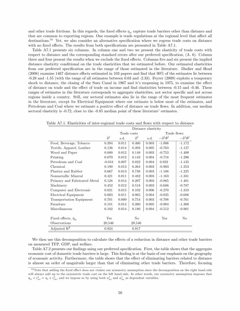
and other trade frictions. In this regards, the fixed effects ηn capture trade barriers other than distance andthat are common to exporting regions. One example is trade regulations at the regional level that affect alldestinations.58 Yet, we also consider an alternative specification where we regress trade costs on distancewith no fixed effects. The results from both specifications are presented in Table A7.1.Table A7.1 presents six columns. In column one and two we present the elasticity of trade costs with

respect to distance and the corresponding standard errors after our preferred specification, (A. 6). Columnthree and four present the results when we exclude the fixed effects. Columns five and six present the implieddistance elasticity conditional on the trade elasticities that we estimated before. Our estimated elasticitiesfrom our preferred specification are in the range of those estimated in the literature. Disdier and Head(2008) examine 1467 distance effects estimated in 103 papers and find that 90% of the estimates lie between-0.28 and -1.55 (with the range of all estimates between 0.03 and -2.33). Feyrer (2009) exploits a temporaryshock to distance, the closing of the Suez Canal in 1967 and it’s reopening in 1975, to examine the effectof distance on trade and the effect of trade on income and find elasticities between -0.15 and -0.46. Theseranges of estimates in the literature corresponds to aggregate elasticities, not sector specific and not acrossregions inside a country. Still, our sectoral estimates also lie in the range of the most frequent estimatesin the literature, except for Electrical Equipment where our estimate is below most of the estimates, andPetroleum and Coal where we estimate a positive effect of distance on trade flows. In addition, our mediansectoral elasticity is -0.72, close to the -0.85 median point of these literature’estimates.

Table A7.1. Elasticities of inter-regional trade costs and flows with respect to distanceDistance elasticity

Trade costs Trade flowsδj s.d. δj s.d. −δjθj −δjθj

Food, Beverage, Tobacco 0.394 0.011 0.460 0.003 -1.006 -1.172Textile, Apparel, Leather 0.126 0.014 0.203 0.005 -0.703 -1.127Wood and Paper 0.080 0.012 0.148 0.003 -0.753 -1.400Printing 0.079 0.012 0.143 0.004 -0.718 -1.296Petroleum and Coal -0.018 0.007 0.022 0.004 0.932 -1.135Chemical 0.190 0.013 0.264 0.003 -0.903 -1.253Plastics and Rubber 0.667 0.013 0.738 0.003 -1.108 -1.225Nonmetallic Mineral 0.421 0.011 0.482 0.003 -1.163 -1.331Primary and Fabricated Metal 0.128 0.014 0.207 0.003 -0.865 -1.401Machinery 0.452 0.012 0.518 0.003 -0.686 -0.787Computer and Electronic 0.021 0.015 0.102 0.006 -0.270 -1.310Electrical Equipment 0.003 0.011 0.065 0.004 -0.035 -0.686Transportation Equipment 0.701 0.009 0.754 0.003 -0.708 -0.761Furniture 0.181 0.014 0.260 0.005 -0.904 -1.300Miscellaneous 0.102 0.014 0.180 0.004 -0.512 -0.901

Fixed effects, ηn Yes No Yes NoObservations 20,546 20,546

Adjusted R2 0.924 0.917

We then use this decomposition to calculate the effects of a reduction in distance and other trade barrierson measured TFP, GDP, and welfare.Table A7.2 presents our findings using our preferred specification. First, the table shows that the aggregate

economic cost of domestic trade barriers is large. This finding is at the basis of our emphasis on the geographyof economic activity. Furthermore, the table shows that the effect of eliminating barriers related to distanceis almost an order of magnitude larger than that of eliminating other trade barriers. Therefore, focusing

58Note that adding the fixed effect does not violate our symmetry assumption since the decomposition on the right hand sidewill always add up to the symmetric trade cost on the left hand side. In other words, our symmetry assumption imposes thatηn + εjni = ηi + εjin, and we impose so by using both κ

jni and κ

jin as dependent variables.

50

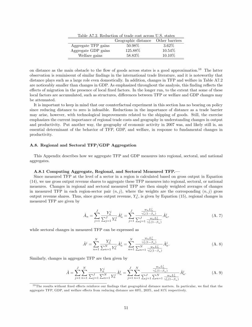
Table A7.2. Reduction of trade cost across U.S. statesGeographic distance Other barriers

Aggregate TFP gains 50.98% 3.62%Aggregate GDP gains 125.88% 10.54%

Welfare gains 58.83% 10.10%

on distance as the main obstacle to the flow of goods across states is a good approximation.59 The latterobservation is reminiscent of similar findings in the international trade literature, and it is noteworthy thatdistance plays such as a large role even domestically. In addition, changes in TFP and welfare in Table A7.2are noticeably smaller than changes in GDP. As emphasized throughout the analysis, this finding reflects theeffects of migration in the presence of local fixed factors. In the longer run, to the extent that some of theselocal factors are accumulated, such as structures, differences between TFP or welfare and GDP changes maybe attenuated.It is important to keep in mind that our counterfactual experiment in this section has no bearing on policy

since reducing distance to zero is infeasible. Reductions in the importance of distance as a trade barriermay arise, however, with technological improvements related to the shipping of goods. Still, the exerciseemphasizes the current importance of regional trade costs and geography in understanding changes in outputand productivity. Put another way, the geography of economic activity in 2007 was, and likely still is, anessential determinant of the behavior of TFP, GDP, and welfare, in response to fundamental changes inproductivity.

A.8. Regional and Sectoral TFP/GDP Aggregation

This Appendix describes how we aggregate TFP and GDP measures into regional, sectoral, and nationalaggregates.

A.8.1 Computing Aggregate, Regional, and Sectoral Measured TFP.–Since measured TFP at the level of a sector in a region is calculated based on gross output in Equation

(14), we use gross output revenue shares to aggregate these TFP measures into regional, sectoral, or nationalmeasures. Changes in regional and sectoral measured TFP are then simply weighted averages of changesin measured TFP in each region-sector pair (n, j), where the weights are the corresponding (n, j) grossoutput revenue shares. Thus, since gross output revenue, Y jn , is given by Equation (15), regional changes inmeasured TFP are given by

An =

J∑j=1

Y jn∑Jj=1 Y

jn

Ajn =

J∑j=1

wnLjn

γjn(1−βn)∑Jj=1

wnLjn

γjn(1−βn)

Ajn, (A. 7)

while sectoral changes in measured TFP can be expressed as

Aj =

N∑n=1

Y jn∑Nn=1 Y

jn

Ajn =

N∑n=1

wnLjn

γjn(1−βn)∑Nn=1

wnLjn

γjn(1−βn)

Ajn. (A. 8)

Similarly, changes in aggregate TFP are then given by

A =

J∑j=1

N∑n=1

Y jn∑Jj=1

∑Nn=1 Y

jn

Ajn =

J∑j=1

N∑n=1

wnLjn

γjn(1−βn)∑Jj=1

∑Nn=1

wnLjn

γjn(1−βn)

Ajn. (A. 9)

59The results without fixed effects reinforce our findings that geographical distance matters. In particular, we find that theaggregate TFP, GDP, and welfare effects from reducing distance are 69%, 203%, and 81% respectively.

51

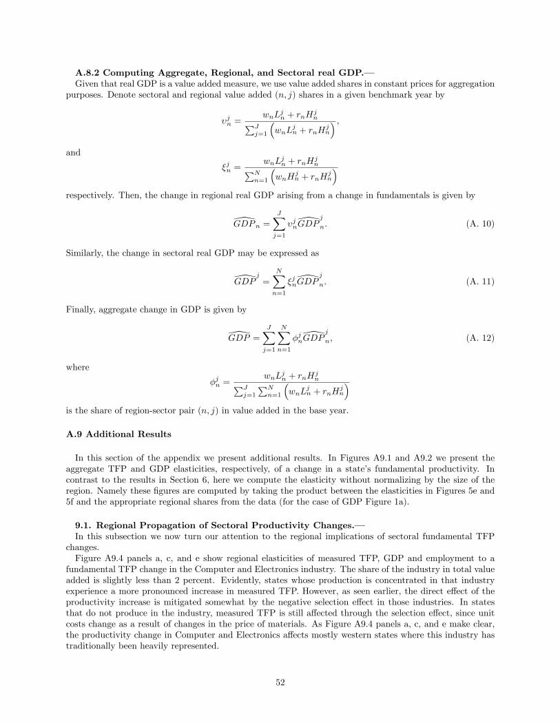
A.8.2 Computing Aggregate, Regional, and Sectoral real GDP.–Given that real GDP is a value added measure, we use value added shares in constant prices for aggregation

purposes. Denote sectoral and regional value added (n, j) shares in a given benchmark year by

υjn =wnL

jn + rnH

jn∑J

j=1

(wnL

jn + rnH

jn

) ,and

ξjn =wnL

jn + rnH

jn∑N

n=1

(wnH

jn + rnH

jn

)respectively. Then, the change in regional real GDP arising from a change in fundamentals is given by

GDPn =

J∑j=1

υjnGDPj

n. (A. 10)

Similarly, the change in sectoral real GDP may be expressed as

GDPj

=

N∑n=1

ξjnGDPj

n. (A. 11)

Finally, aggregate change in GDP is given by

GDP =

J∑j=1

N∑n=1

φjnGDPj

n, (A. 12)

where

φjn =wnL

jn + rnH

jn∑J

j=1

∑Nn=1

(wnL

jn + rnH

jn

)is the share of region-sector pair (n, j) in value added in the base year.

A.9 Additional Results

In this section of the appendix we present additional results. In Figures A9.1 and A9.2 we present theaggregate TFP and GDP elasticities, respectively, of a change in a state’s fundamental productivity. Incontrast to the results in Section 6, here we compute the elasticity without normalizing by the size of theregion. Namely these figures are computed by taking the product between the elasticities in Figures 5e and5f and the appropriate regional shares from the data (for the case of GDP Figure 1a).

9.1. Regional Propagation of Sectoral Productivity Changes.–In this subsection we now turn our attention to the regional implications of sectoral fundamental TFP

changes.Figure A9.4 panels a, c, and e show regional elasticities of measured TFP, GDP and employment to a

fundamental TFP change in the Computer and Electronics industry. The share of the industry in total valueadded is slightly less than 2 percent. Evidently, states whose production is concentrated in that industryexperience a more pronounced increase in measured TFP. However, as seen earlier, the direct effect of theproductivity increase is mitigated somewhat by the negative selection effect in those industries. In statesthat do not produce in the industry, measured TFP is still affected through the selection effect, since unitcosts change as a result of changes in the price of materials. As Figure A9.4 panels a, c, and e make clear,the productivity change in Computer and Electronics affects mostly western states where this industry hastraditionally been heavily represented.

52

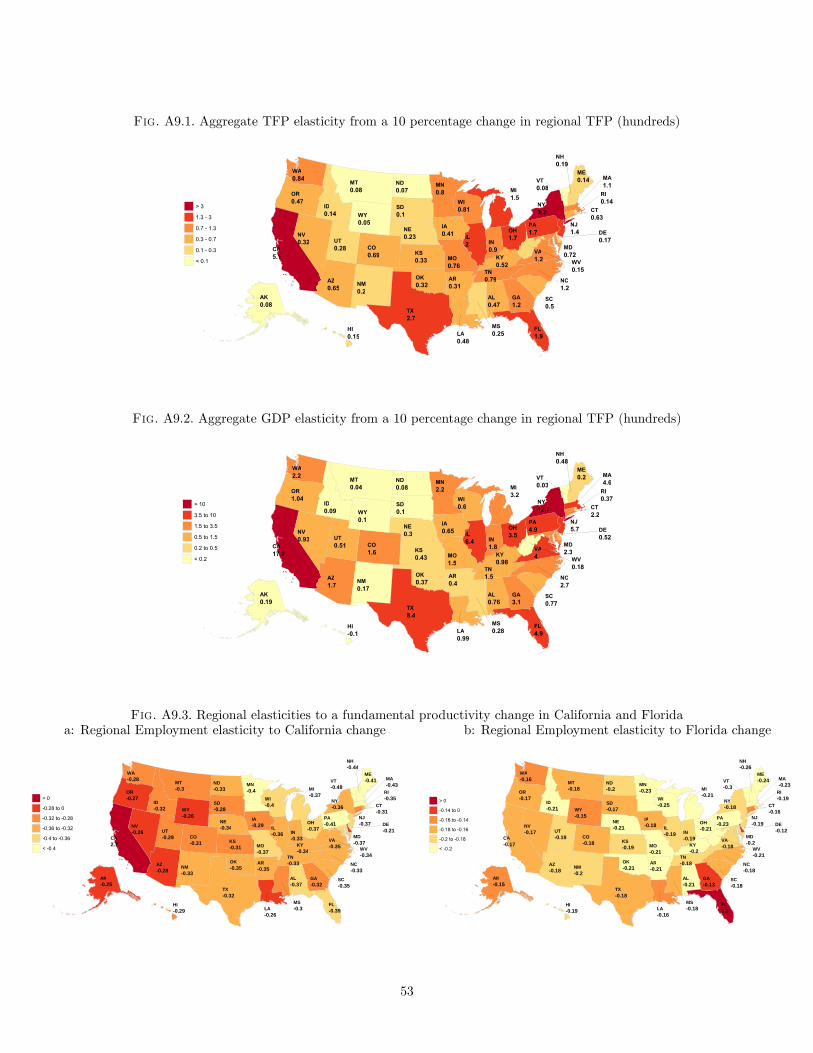
Fig. A9.1. Aggregate TFP elasticity from a 10 percentage change in regional TFP (hundreds)

AL0.47

AK0.08

AZ0.65

AR0.31

CA5.1

CO0.69

CT0.63

DE0.17

FL1.9

GA1.2

HI0.15

ID0.14

IL2 IN

0.9

IA0.41

KS0.33 KY

0.52

LA0.48

ME0.14

MD0.72

MA1.1

MI1.5

MN0.8

MS0.25

MO0.76

MT0.08

NE0.23NV

0.32

NH0.19

NJ1.4

NM0.2

NY3.2

NC1.2

ND0.07

OH1.7

OK0.32

OR0.47

PA1.7

RI0.14

SC0.5

SD0.1

TN0.79

TX2.7

UT0.28

VT0.08

VA1.2

WA0.84

WV0.15

WI0.81

WY0.05

Fig. A9.2. Aggregate GDP elasticity from a 10 percentage change in regional TFP (hundreds)

AL0.76

AK0.19

AZ1.7

AR0.4

CA17.2

CO1.6

CT2.2

DE0.52

FL4.9

GA3.1

HI-0.1

ID0.09

IL6.4 IN

1.8

IA0.65

KS0.43 KY

0.98

LA0.99

ME0.2

MD2.3

MA4.6

MI3.2

MN2.2

MS0.28

MO1.5

MT0.04

NE0.3NV

0.93

NH0.48

NJ5.7

NM0.17

NY12.7

NC2.7

ND0.08

OH3.5

OK0.37

OR1.04

PA4.9

RI0.37

SC0.77

SD0.1

TN1.5

TX8.4

UT0.51

VT0.03

VA4

WA2.2

WV0.18

WI0.6

WY0.1

Fig. A9.3. Regional elasticities to a fundamental productivity change in California and Floridaa: Regional Employment elasticity to California change b: Regional Employment elasticity to Florida change

AL-0.37

AK-0.25

AZ-0.28

AR-0.35

CA2.7

CO-0.31

CT-0.31

DE-0.21

FL-0.39

GA-0.32

HI-0.29

ID-0.32

IL-0.36 IN

-0.33

IA-0.29

KS-0.31 KY

-0.34

LA-0.26

ME-0.41

MD-0.37

MA-0.43

MI-0.37

MN-0.4

MS-0.3

MO-0.37

MT-0.3

NE-0.34NV

-0.26

NH-0.44

NJ-0.37

NM-0.33

NY-0.36

NC-0.33

ND-0.33

OH-0.37

OK-0.35

OR-0.27

PA-0.41

RI-0.35

SC-0.35

SD-0.28

TN-0.33

TX-0.32

UT-0.29

VT-0.48

VA-0.35

WA-0.28

WV-0.34

WI-0.4

WY-0.26

AL-0.21

AK-0.15

AZ-0.18

AR-0.21

CA-0.17

CO-0.18

CT-0.16

DE-0.12

FL3.3

GA-0.13

HI-0.19

ID-0.21

IL-0.19 IN

-0.19

IA-0.18

KS-0.19 KY

-0.2

LA-0.16

ME-0.24

MD-0.2

MA-0.23

MI-0.21

MN-0.23

MS-0.18

MO-0.21

MT-0.18

NE-0.21NV

-0.17

NH-0.26

NJ-0.19

NM-0.2

NY-0.18

NC-0.18

ND-0.2

OH-0.21

OK-0.21

OR-0.17

PA-0.23

RI-0.19

SC-0.18

SD-0.17

TN-0.18

TX-0.18

UT-0.19

VT-0.3

VA-0.18

WA-0.16

WV-0.21

WI-0.25

WY-0.15

53

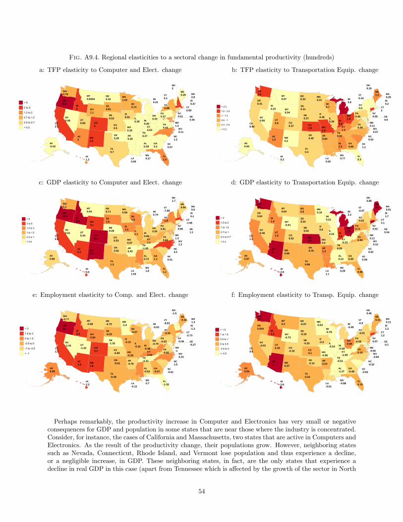
Fig. A9.4. Regional elasticities to a sectoral change in fundamental productivity (hundreds)

a: TFP elasticity to Computer and Elect. change b: TFP elasticity to Transportation Equip. change

AL0.28

AK-0.02

AZ2

AR0.18

CA2.1

CO2

CT0.59

DE0.35

FL1.4

GA0.2

HI1.2

ID4

IL0.39 IN

0.26

IA0.52

KS0.5 KY

0.03

LA0.06

ME0.29

MD1.3

MA2.8

MI0.21

MN1.03

MS0.17

MO0.16

MT0.0004

NE0.53NV

0.48

NH2

NJ0.51

NM3.4

NY0.98

NC1.2

ND0.42

OH0.23

OK0.26

OR6.4

PA0.37

RI0.47

SC0.07

SD0.81

TN0.27

TX0.7

UT0.69

VT0.1

VA0.44

WA0.79

WV0.11

WI0.74

WY1.1

AL1.3

AK0.05

AZ1.2

AR0.84

CA0.46

CO0.37

CT2

DE0.6

FL0.3

GA0.66

HI0.3

ID0.22

IL0.39 IN

2.2

IA0.38

KS2.5 KY

1.3

LA0.55

ME1.2

MD0.11

MA0.25

MI2.8

MN0.41

MS0.77

MO1.5

MT0.07

NE0.37NV

0.06

NH0.15

NJ0.05

NM0.2

NY0.2

NC0.52

ND0.33

OH1.9

OK0.45

OR0.41

PA0.46

RI0.2

SC1.1

SD0.31

TN0.93

TX0.4

UT0.6

VT0.14

VA0.39

WA1.6

WV0.57

WI0.7

WY0.04

c: GDP elasticity to Computer and Elect. change d: GDP elasticity to Transportation Equip. change

AL0.72

AK0.89

AZ5.1

AR0.43

CA5.5

CO6.1

CT-1.08

DE1.1

FL1.1

GA1.1

HI5.5

ID9.5

IL1.1 IN

0.89

IA1.5

KS0.53 KY

1.1

LA1.04

ME0.94

MD1.3

MA5.6

MI0.74

MN0.59

MS1.8

MO0.97

MT0.44

NE0.28NV

0.01

NH1.7

NJ0.95

NM7.3

NY1.8

NC4.2

ND0.71

OH0.55

OK0.91

OR22.3

PA0.81

RI0.1

SC0.51

SD1.6

TN-1.05

TX1.3

UT0.44

VT-7.89

VA0.62

WA1.1

WV1.3

WI1.8

WY3.1

AL0.12

AK0.87

AZ3

AR1.3

CA1.1

CO0.52

CT3.1

DE0.54

FL0.88

GA0.55

HI2.8

ID1.4

IL0.23 IN

1.6

IA0.6

KS3.1 KY

-0.23

LA1.1

ME2.1

MD0.11

MA0.91

MI2.3

MN0.18

MS0.29

MO0.5

MT0.64

NE0.54NV

0.46

NH0.88

NJ0.53

NM0.96

NY0.53

NC0.52

ND0.8

OH2.3

OK0.75

OR0.64

PA0.71

RI1.7

SC0.58

SD0.54

TN0.55

TX0.96

UT1.3

VT-0.07

VA0.99

WA4.4

WV0.12

WI0.21

WY-0.01

e: Employment elasticity to Comp. and Elect. change f: Employment elasticity to Transp. Equip. change

AL-0.54

AK0.09

AZ1.6

AR-0.76

CA1.7

CO2.2

CT-2.73

DE-0.27

FL-1.32

GA-0.07

HI2.2

ID2.4

IL-0.32 IN

-0.48

IA-0.15

KS-0.89 KY

0.02

LA-0.12

ME-0.32

MD-1

MA1.3

MI-0.62

MN-1.4

MS0.7

MO-0.29

MT-0.68

NE-1.32NV

-1.41

NH-1.5

NJ-0.46

NM1.8

NY-0.32

NC1.5

ND-0.75

OH-0.79

OK-0.41

OR11

PA-0.52

RI-1.3

SC-0.61

SD-0.22

TN-2.31

TX-0.38

UT-1.32

VT-8.81

VA-0.82

WA-0.77

WV0.23

WI-0.07

WY0.84

AL-1.37

AK0.54

AZ2

AR0.24

CA0.4

CO-0.16

CT1.2

DE-0.1

FL0.15

GA-0.46

HI2.6

ID1.1

IL-0.53 IN

-0.58

IA-0.3

KS0.1 KY

-1.59

LA-0.01

ME0.31

MD-0.55

MA0.11

MI-0.48

MN-0.63

MS-0.88

MO-0.96

MT0.2

NE-0.25NV

-0.03

NH0.46

NJ0.07

NM0.47

NY-0.01

NC-0.32

ND-0.07

OH0.69

OK-0.14

OR0.004

PA-0.08

RI1.3

SC-0.65

SD-0.16

TN-0.51

TX0.24

UT0.25

VT-0.9

VA0.15

WA1.7

WV-0.84

WI-0.78

WY-0.73

Perhaps remarkably, the productivity increase in Computer and Electronics has very small or negativeconsequences for GDP and population in some states that are near those where the industry is concentrated.Consider, for instance, the cases of California and Massachusetts, two states that are active in Computers andElectronics. As the result of the productivity change, their populations grow. However, neighboring statessuch as Nevada, Connecticut, Rhode Island, and Vermont lose population and thus experience a decline,or a negligible increase, in GDP. These neighboring states, in fact, are the only states that experience adecline in real GDP in this case (apart from Tennessee which is affected by the growth of the sector in North

54

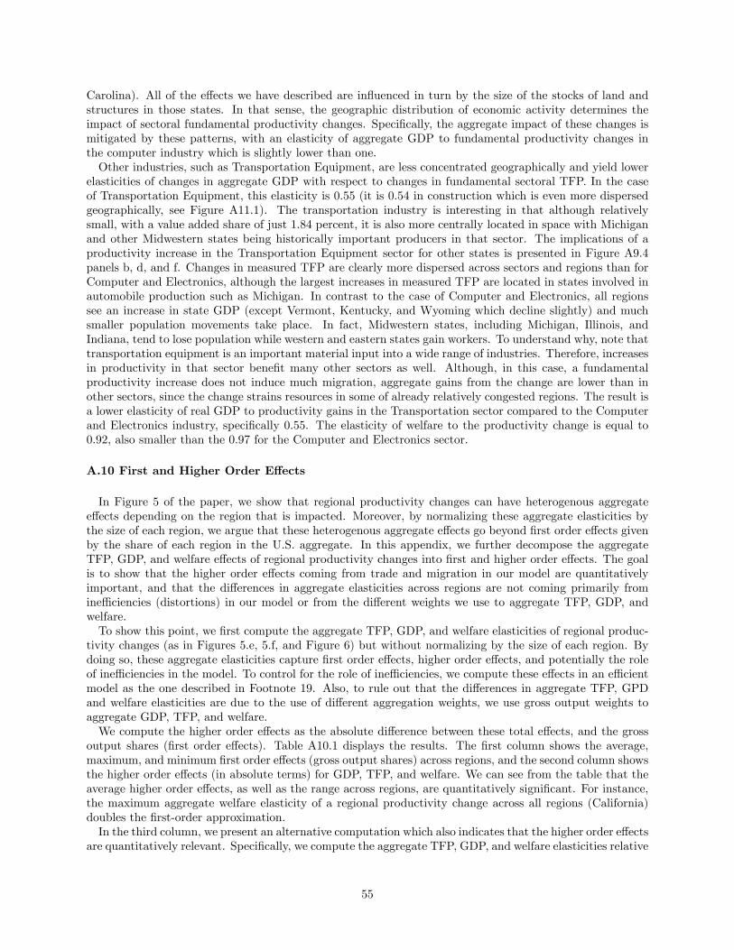
Carolina). All of the effects we have described are influenced in turn by the size of the stocks of land andstructures in those states. In that sense, the geographic distribution of economic activity determines theimpact of sectoral fundamental productivity changes. Specifically, the aggregate impact of these changes ismitigated by these patterns, with an elasticity of aggregate GDP to fundamental productivity changes inthe computer industry which is slightly lower than one.Other industries, such as Transportation Equipment, are less concentrated geographically and yield lower

elasticities of changes in aggregate GDP with respect to changes in fundamental sectoral TFP. In the caseof Transportation Equipment, this elasticity is 0.55 (it is 0.54 in construction which is even more dispersedgeographically, see Figure A11.1). The transportation industry is interesting in that although relativelysmall, with a value added share of just 1.84 percent, it is also more centrally located in space with Michiganand other Midwestern states being historically important producers in that sector. The implications of aproductivity increase in the Transportation Equipment sector for other states is presented in Figure A9.4panels b, d, and f. Changes in measured TFP are clearly more dispersed across sectors and regions than forComputer and Electronics, although the largest increases in measured TFP are located in states involved inautomobile production such as Michigan. In contrast to the case of Computer and Electronics, all regionssee an increase in state GDP (except Vermont, Kentucky, and Wyoming which decline slightly) and muchsmaller population movements take place. In fact, Midwestern states, including Michigan, Illinois, andIndiana, tend to lose population while western and eastern states gain workers. To understand why, note thattransportation equipment is an important material input into a wide range of industries. Therefore, increasesin productivity in that sector benefit many other sectors as well. Although, in this case, a fundamentalproductivity increase does not induce much migration, aggregate gains from the change are lower than inother sectors, since the change strains resources in some of already relatively congested regions. The result isa lower elasticity of real GDP to productivity gains in the Transportation sector compared to the Computerand Electronics industry, specifically 0.55. The elasticity of welfare to the productivity change is equal to0.92, also smaller than the 0.97 for the Computer and Electronics sector.

A.10 First and Higher Order Effects

In Figure 5 of the paper, we show that regional productivity changes can have heterogenous aggregateeffects depending on the region that is impacted. Moreover, by normalizing these aggregate elasticities bythe size of each region, we argue that these heterogenous aggregate effects go beyond first order effects givenby the share of each region in the U.S. aggregate. In this appendix, we further decompose the aggregateTFP, GDP, and welfare effects of regional productivity changes into first and higher order effects. The goalis to show that the higher order effects coming from trade and migration in our model are quantitativelyimportant, and that the differences in aggregate elasticities across regions are not coming primarily fromineffi ciencies (distortions) in our model or from the different weights we use to aggregate TFP, GDP, andwelfare.To show this point, we first compute the aggregate TFP, GDP, and welfare elasticities of regional produc-

tivity changes (as in Figures 5.e, 5.f, and Figure 6) but without normalizing by the size of each region. Bydoing so, these aggregate elasticities capture first order effects, higher order effects, and potentially the roleof ineffi ciencies in the model. To control for the role of ineffi ciencies, we compute these effects in an effi cientmodel as the one described in Footnote 19. Also, to rule out that the differences in aggregate TFP, GPDand welfare elasticities are due to the use of different aggregation weights, we use gross output weights toaggregate GDP, TFP, and welfare.We compute the higher order effects as the absolute difference between these total effects, and the gross

output shares (first order effects). Table A10.1 displays the results. The first column shows the average,maximum, and minimum first order effects (gross output shares) across regions, and the second column showsthe higher order effects (in absolute terms) for GDP, TFP, and welfare. We can see from the table that theaverage higher order effects, as well as the range across regions, are quantitatively significant. For instance,the maximum aggregate welfare elasticity of a regional productivity change across all regions (California)doubles the first-order approximation.In the third column, we present an alternative computation which also indicates that the higher order effects

are quantitatively relevant. Specifically, we compute the aggregate TFP, GDP, and welfare elasticities relative

55

to the first-order approximations.60 On average, the GDP, TFP, and welfare first-order approximations mustbe multiplied by a factor of 0.9, 0.4, and 2.3, respectively, to obtain the correct aggregate elasticities. Therange of these factors across regions is also significant. From these exercises we conclude that the higherorder effects are quantitatively important, and that ineffi ciencies do not play an essential role in explainingthe heterogenous aggregate elasticities in Figure 5.Finally, the last row of Table A10.1 shows the correlation between the first order and the higher order

effects. The correlations are high, specially for TFP and welfare, which suggests that in addition to ourfinding that the higher order effects are large, they also tend to be related to the size of each region. Thisresult is somehow expected since larger regions, for instance California, also tend to be more interconnectedwith the rest of the country through trade and migration. That is, the aggregate TFP or welfare elasticityof a regional shock is close to proportional to gross output shares but the factor of proportionality variessubstantially across regions. Computing these factors is a key contribution of our paper.

Table A10.1. First and higher order effects in the effi cient modelFirst order effects Higher order effects Total effects relative(GO shares) (absolute value) to first order effects

GDP, TFP, and Welfare GDP TFP Welfare GDP TFP WelfareAverage 2.00 0.48 1.19 2.51 0.90 0.40 2.31Max 12.57 2.76 7.24 13.93 1.79 0.45 3.26Min 0.16 0.001 0.10 0.16 0.18 0.36 1.32

Correlations between first and higher order effectsGDP TFP Welfare

Correl. 0.577 0.999 0.982

A.11 Composition of U.S. Economic Activity

Fig. A11.1. Economic activity across sectors in the U.S.

a: Sectoral concentration (GDP share, 2007) b: Regional concentration (Herfindahl, 2007)

0

2

4

6

8

10

12

14

16

18

20

Oth

er S

ervi

ces

R

eal E

stat

e

Who

lesa

le a

nd R

etai

l Tra

de

Fin

ance

and

Insu

ranc

e

Hea

lth C

are

C

onst

ruct

ion

Inf

orm

atio

n S

ervi

ces

A

ccom

. and

Foo

d S

ervi

ces

T

rans

port

Ser

vice

s

C

hem

ical

T

rans

port

atio

n E

quip

men

t

C

ompu

ter

and

Ele

ctro

nic

Prim

ary

and

Fab

ricat

ed M

etal

F

ood,

Bev

erag

e, T

obac

co

Pet

role

um a

nd C

oal

Edu

catio

n

A

rts

and

Rec

reat

ion

Mac

hine

ry

W

ood

and

Pap

er

M

isce

llane

ous

P

last

ics

and

Rub

ber

Ele

ctric

al E

quip

men

t

N

onm

etal

lic M

iner

al

P

rintin

g

T

extil

e, A

ppar

el, L

eath

er

F

urni

ture

Share of GDP by sector (%, 2007)

0

0.02

0.04

0.06

0.08

0.1

0.12

0.14

0.16

P

etro

leum

and

Coa

l

C

ompu

ter

and

Ele

ctro

nic

T

extil

e, A

ppar

el, L

eath

er

A

rts

and

Rec

reat

ion

Che

mic

al

Inf

orm

atio

n S

ervi

ces

T

rans

port

atio

n E

quip

men

t

Rea

l Est

ate

Fin

ance

and

Insu

ranc

e

M

isce

llane

ous

Edu

catio

n

O

ther

Ser

vice

s

M

achi

nery

C

onst

ruct

ion

Who

lesa

le a

nd R

etai

l Tra

de

A

ccom

. and

Foo

d S

ervi

ces

Prim

ary

and

Fab

ricat

ed M

etal

Fur

nitu

re

F

ood,

Bev

erag

e, T

obac

co

P

rintin

g

Tra

nspo

rt S

ervi

ces

H

ealth

Car

e

Non

met

allic

Min

eral

Ele

ctric

al E

quip

men

t

P

last

ics

and

Rub

ber

Woo

d an

d P

aper

60Note that, since we are averaging and some of the higher order effects are negative, the third column is not simply the sumof the first and second column values over the first column value.

56

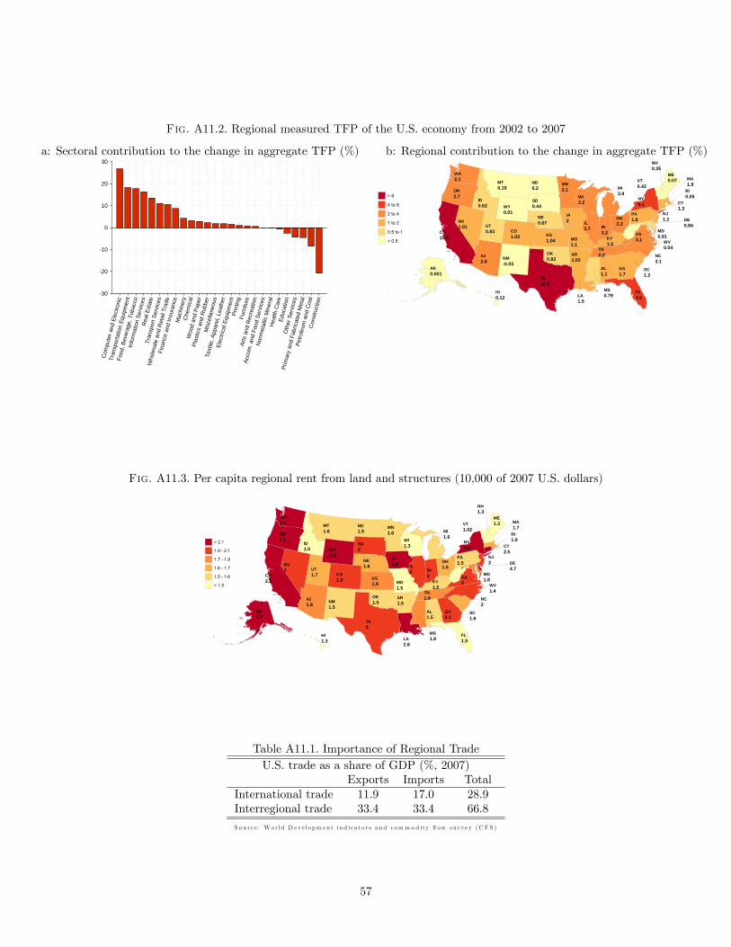
Fig. A11.2. Regional measured TFP of the U.S. economy from 2002 to 2007

a: Sectoral contribution to the change in aggregate TFP (%) b: Regional contribution to the change in aggregate TFP (%)

-30

-20

-10

0

10

20

30

C

ompu

ter

and

Ele

ctro

nic

T

rans

port

atio

n E

quip

men

t

F

ood,

Bev

erag

e, T

obac

co

Inf

orm

atio

n S

ervi

ces

R

eal E

stat

e

Tra

nspo

rt S

ervi

ces

Who

lesa

le a

nd R

etai

l Tra

de

Fin

ance

and

Insu

ranc

e

M

achi

nery

Che

mic

al

Woo

d an

d P

aper

P

last

ics

and

Rub

ber

M

isce

llane

ous

T

extil

e, A

ppar

el, L

eath

er

E

lect

rical

Equ

ipm

ent

Prin

ting

Fur

nitu

re

A

rts

and

Rec

reat

ion

A

ccom

. and

Foo

d S

ervi

ces

N

onm

etal

lic M

iner

al

Hea

lth C

are

Edu

catio

n

O

ther

Ser

vice

s

Prim

ary

and

Fab

ricat

ed M

etal

P

etro

leum

and

Coa

l

Con

stru

ctio

n

b. Sectoral contribution to the change in aggregate TFP (%)

AL1.1

AK0.001

AZ2.6

AR1.02

CA15.5

CO1.03

CT1.3

DE0.84

FL4.2

GA1.7

HI0.12

ID0.62

IL3.7 IN

3.2

IA2

KS1.04 KY

1.5

LA1.5

ME0.07

MD0.91

MA1.9

MI3.9

MN2.1

MS0.79

MO1.1

MT0.19

NE0.67NV

1.01

NH0.35

NJ1.2

NM-0.03

NY6.1

NC3.1

ND0.2

OH3.3

OK0.82

OR2.7

PA1.8

RI0.05

SC1.2

SD0.44

TN2.2

TX12.3

UT0.83

VT0.42

VA3.1

WA2.1

WV0.04

WI2.2

WY0.01

Fig. A11.3. Per capita regional rent from land and structures (10,000 of 2007 U.S. dollars)

AL1.5

AK2.7

AZ1.8

AR1.5

CA2.2

CO1.9

CT2.5

DE4.7

FL1.5

GA2.1

HI1.3

ID1.5

IL2 IN

2

IA2.2

KS1.9 KY

1.5

LA2.8

ME1.3

MD1.8

MA1.7

MI1.6

MN1.6

MS1.8

MO1.5

MT1.6

NE1.6NV

2

NH1.3

NJ2

NM1.5

NY2.2

NC2

ND1.5

OH1.6

OK1.5

OR2.1

PA1.5

RI1.9

SC1.6

SD2

TN1.8

TX2

UT1.7

VT1.02

VA2

WA2.4

WV1.4

WI1.3

WY2.3

Table A11.1. Importance of Regional TradeU.S. trade as a share of GDP (%, 2007)

Exports Imports TotalInternational trade 11.9 17.0 28.9Interregional trade 33.4 33.4 66.8

S o u r c e : W o r ld D e v e lo pm e n t in d ic a t o r s a n d c om m o d i ty flow su r v e y (C F S )

57

The Impact of Regional and Sectoral Productivity …erossi/RSSUS.pdfThe Impact of Regional and Sectoral Productivity Changes on the U.S. Economy Lorenzo Caliendo Fernando Parro Yale

Documents