International Journal of Science Commerce and Humanities Volume No 3 No 2 March 2015 117 The impact of rand volatility on inflation in South Africa Azwifaneli Innocentia (Mulaudzi) Nemushungwa Department of Economics, University of Venda, South Africa Abstract: The floating exchange rate regime, coupled with a more open trade policy and the growth in imports, leaves South Africa vulnerable to the effects of exchange rate behavior on import, producer and consumer prices, which all contribute to inflation. Given the central role that inflation targeting occupies in South Africa’s monetary policy, this necessitates the need to examine the effect of exchange rate shocks on consumer prices. To this end, this paper analyses the impact of an exchange rate shocks on consumer prices in South Africa, using a battery of econometric tests (Toda and Yamamoto (1995)’s VAR procedure, Granger (non-) Causality Test, Impulse response functions and Variance decompositions). Furthermore, it explores whether the direction and size of changes in the exchange rate have different pass-through effects on import prices, examine the extent and the speed of the pass through to consumer prices, and the key drivers thereof and; also determine the causal relationship among variables under review. The paper uses monthly data covering the period January 1994 to December 2013.The Impulse response functions results show that exchange rate shocks to consumer prices was modest during the period under review. This suggests that exchange rate depreciation is a potentially not important source of inflation in South Africa. Consistent with other studies for developing countries, thevariance decomposition results show a modest exchange rate pass-through to inflation, although inflation is mainly driven by own shocks The variance decompositions also reveal that foreign exchange rate shocks (REER) contribute relatively more to inflation than money supply shocks (M3).This suggests that South African inflation process is not basically influenced by money supply changes. Keywords: exchange rate, pass-through, consumer prices, Granger (non-) causality VAR, South Africa. 1. Introduction Since 1980, South Africa has experienced three distinct monetary policy regimes. During the first period (1980 to 1989), monetary policy was not successful in containing inflation. The second period (1990 to 2000) saw a significant improvement in the pursuit of a lower inflation rate. The third period (2000 till present), also sees the South African Reserve Bank (SARB) in pursuit of low inflation. However, unlike during the second period, the SARB is now pursuing an official and explicit inflation target (Burger and Marinkov, 2008). In February 2000, the South African Reserve Bank announced its aim to adopt an explicit inflation targeting monetary policy as an official target regime. Under this approach, the CPIX (the overall consumer price index, excluding the mortgage interest cost) basket was introduced as the targeted inflation measure, as this excludes the direct impact of monetary policy, namely interest rates. The inflation target aims to achieve a rate of increase in the CPIX of between 3 and 6 percent per year (van der Merwe, 2004). Unlike in the period of implicit inflation targeting, where the SARB protected both the internal and external value of the rand, with explicit inflation targeting, only the internal value of the rand is protected. This was done with the view that low and stable inflation will, without the need for policy intervention, translate into a stable exchange rate. In the inflation targeting era, the SARB abandoned its pre-commitment of protecting both the internal value (interest rate parity) and external value of the rand(exchange rate parity).It was only protecting

Welcome message from author
This document is posted to help you gain knowledge. Please leave a comment to let me know what you think about it! Share it to your friends and learn new things together.
Transcript
International Journal of Science Commerce and Humanities Volume No 3 No 2 March 2015
117
The impact of rand volatility on inflation in South Africa
Azwifaneli Innocentia (Mulaudzi) Nemushungwa
Department of Economics, University of Venda, South Africa
Abstract:
The floating exchange rate regime, coupled with a more open trade policy and the growth in imports, leaves
South Africa vulnerable to the effects of exchange rate behavior on import, producer and consumer prices,
which all contribute to inflation. Given the central role that inflation targeting occupies in South Africa’s
monetary policy, this necessitates the need to examine the effect of exchange rate shocks on consumer prices.
To this end, this paper analyses the impact of an exchange rate shocks on consumer prices in South Africa,
using a battery of econometric tests (Toda and Yamamoto (1995)’s VAR procedure, Granger (non-) Causality
Test, Impulse response functions and Variance decompositions). Furthermore, it explores whether the direction
and size of changes in the exchange rate have different pass-through effects on import prices, examine the
extent and the speed of the pass through to consumer prices, and the key drivers thereof and; also determine the
causal relationship among variables under review. The paper uses monthly data covering the period January
1994 to December 2013.The Impulse response functions results show that exchange rate shocks to consumer
prices was modest during the period under review. This suggests that exchange rate depreciation is a
potentially not important source of inflation in South Africa. Consistent with other studies for developing
countries, thevariance decomposition results show a modest exchange rate pass-through to inflation, although
inflation is mainly driven by own shocks The variance decompositions also reveal that foreign exchange rate
shocks (REER) contribute relatively more to inflation than money supply shocks (M3).This suggests that South
African inflation process is not basically influenced by money supply changes.
Keywords: exchange rate, pass-through, consumer prices, Granger (non-) causality VAR, South Africa.
1. Introduction
Since 1980, South Africa has experienced three distinct monetary policy regimes. During the first period (1980
to 1989), monetary policy was not successful in containing inflation. The second period (1990 to 2000) saw a
significant improvement in the pursuit of a lower inflation rate. The third period (2000 till present), also sees the
South African Reserve Bank (SARB) in pursuit of low inflation. However, unlike during the second period, the
SARB is now pursuing an official and explicit inflation target (Burger and Marinkov, 2008).
In February 2000, the South African Reserve Bank announced its aim to adopt an explicit inflation targeting
monetary policy as an official target regime. Under this approach, the CPIX (the overall consumer price index,
excluding the mortgage interest cost) basket was introduced as the targeted inflation measure, as this excludes
the direct impact of monetary policy, namely interest rates. The inflation target aims to achieve a rate of
increase in the CPIX of between 3 and 6 percent per year (van der Merwe, 2004).
Unlike in the period of implicit inflation targeting, where the SARB protected both the internal and external
value of the rand, with explicit inflation targeting, only the internal value of the rand is protected. This was done
with the view that low and stable inflation will, without the need for policy intervention, translate into a stable
exchange rate. In the inflation targeting era, the SARB abandoned its pre-commitment of protecting both the
internal value (interest rate parity) and external value of the rand(exchange rate parity).It was only protecting

International Journal of Science Commerce and Humanities Volume No 3 No 2 March 2015
118
the internal value of the rand, thus the exchange rate was left to be determined by market forces, making it
more volatile (Ncube and Ndou, 2011).
The floating exchange rate regime, coupled with a more open trade policy and the growth in imports, leaves
South Africa vulnerable to the effects of exchange rate behavior on import, producer and consumer prices,
which all contribute to inflation (SARB, 2001; Karoro, 2008). The transmission of exchange rate fluctuations to
import prices, producer prices and finally to consumer prices, is referred to as exchange rate pass-through
(Karoro, 2008).
To this end, this paper analyses the impact of an exchange rate shocks on consumer prices in South Africa,
using a battery of econometric tests (Toda and Yamamoto (1995)‘s VAR procedure, Granger (non-) Causality
Test, Impulse response functions and Variance decompositions). Furthermore, it explores whether the direction
and size of changes in the exchange rate have different pass-through effects on import prices, examine the
extent and the speed of the pass through to consumer prices, and the key drivers thereof and; also determine the
causal relationship among variables under review.
The rest of the chapter is organized as follows: section 2 reviews theoretical and empirical literature. Section 3
present theoretical framework and model specification. In section 4 data sources and time domain are presented.
Estimation techniques and empirical results are given in sections 5 and 6. Section 7 contains conclusions.
2. Literature Review
2.1. Theoretical Literature Review There are several possible channels through which exchange rate changes may affect prices (Tandrayen-
Ragoobur and Chicooree, 2012). The two main channels of exchange rate pass through are direct channel and
indirect channel.
The direct channel stresses that a depreciated exchange rate will imply that imported inputs have become more
expensive; consequently there will be a rise in production costs. The higher production costs will then be
pushed to local consumers in the form of higher prices. Alternatively, a depreciated exchange rate may also
imply that imports of finished goods have become more expensive. Consumers will then have to pay higher
prices on imported goods.
The direct channel arises mainly because of the ―law of one price ―and the purchasing power parity (PPP) in its
aggregation. The relative version of PPP claims that, starting from a base of an equilibrium exchange rate
between two currencies, the future of the exchange rate between the two currencies will be determined by the
relative movements in the price levels in the two countries. For a given import price, changes in the exchange
rate will translate directly into higher domestic prices. Therefore,
𝑃 = 𝐸 .𝑃∗ P
Where E is the exchange rate in terms of domestic currency per unit of foreign currency; P* represents the
foreign currency price of the imported good and P is the domestic currency price of the imported good. The
pass-through is only complete (=100 percent) if:
(a) Markups of prices over costs are constant and
(b) Marginal costs are constant

International Journal of Science Commerce and Humanities Volume No 3 No 2 March 2015
119
The indirect channel, on the other hand, stresses that a depreciated exchange rate will result in an increase in
local demand for import substitutes, consequently substitute goods will become more expensive and in turn,
the general (consumer) price level will increase. A depreciated exchange rate also implies that export prices
have become cheaper and as a result there will be an increase in demand for exports. There will therefore be an
increase in demand for labour to expand production and in turn the price of labour (wages) will increase.
Producers will then be forced to push these higher costs to consumers by charging higher prices to final
products.
The indirect channel of exchange rate pass-through arises because of the impact on aggregate demand. A
depreciation of the exchange rate makes domestic products relatively cheaper for foreign consumers, and hence,
exports and aggregate demand will rise relative to potential output, inducing an increase in the domestic price
level. Since nominal wage contracts are fixed in the short run, real wages will decrease and output will
eventually increase. However, when real wages return to their original level over time, production costs then
increases, the overall price level increases and; output falls. Thus, in the end the exchange rate depreciation
leaves a permanent increase in the price level with only a temporary increase in output (Laflèche, 1996).
2.2. Empirical Literature Review
Results on studies conducted for developed countries are conclusive on the idea that low exchange rate pass-
through occurs during periods of low inflation.
McCarthy (2000) presents a comprehensive study of exchange rate pass-through on the aggregate level for a
number of industrialized countries. Using vector autoregressive (VAR) model and data from 1976 up until
1998, he estimates ERPT to import, producer and consumer-price. In most of the countries analyzed, the
exchange rate pass-through to consumer prices is found to be modest. The rate of pass-through is, furthermore,
shown to be positively correlated with the openness of the country and with the persistence of and exchange rate
change, and negatively correlated with the volatility of the exchange rate.
Goldfajn and Werlang (2000) estimate ERPT to consumer prices for 71 countries (both developed and
emerging), using panel estimation methods on data from 1980 to 1998. They report that the pass-through effects
on consumer prices increase over time and reach a maximum after 12 months. The degree of pass-through is,
furthermore, found to be substantially higher in emerging market economies than in developed economies.
Studies conducted on developing countries show contradicting results. Adeyemi and Samuel (2013) using the
Variance Decomposition analyses within the framework a structural Vector autoregressive, estimate the pass-
through effect of exchange rate changes to consumer prices in Nigeria for the period 1970 to 2008. The results
show a substantial large ERPT, although it is incomplete. The findings by Tandrayen-Ragoobur and Chicooree
(2012) also show that ERPT to consumer is highest, followed by producer prices, while the ERPT to import
prices is lowest.
Bwire et al. (2013) examines the degree of exchange rate pass through to inflation in Uganda for the period
1999Q3 to 2012Q2 using vector error correction method (VECM) and structural VAR (SVAR) models. The
findings show a modest pass-through to domestic inflation, although incomplete. Ocran (2010), using impulse
response functions and variance decompositions within the framework of unrestricted VAR that incorporates a
distribution chain, examines the degree of ERPT to import, producer and consumer prices in South Africa for
the period 2001:1 to 2009:5.The results show that ERPT to producer prices is modest (at 19%) and very modest
to consumer prices (at 13 percent).

International Journal of Science Commerce and Humanities Volume No 3 No 2 March 2015
120
3. Theoretical framework and Model Specification
3.1. Theoretical framework
The model by Macfarlane (2002) is one of the earliest theories that examine the link between exchange rate
volatility and consumer price inflation. It focuses on the influence of the direct channel of pass-through. In this
context the pass-through relation can be expressed most simply by the PPP relation in logs i.e.
𝑝 = 𝛽𝑝∗ +𝜆𝑒………………………………………………………………. (1)
Where 𝑝 𝑖𝑠 the log of the general (consumer) price level, 𝑝 ∗ is the log of foreign price and; 𝑒is the log of the
exchange rate.
The ―law of one price‖ implies that 𝛽 = 𝜆 = 1 in which case changes in the exchange rate completely pass
through to the domestic price of the traded good.
3.2. Model Specification
This study is a modified version of Parsely and Popper (1998) and Macfarlane (2002) models, which embrace
the Central Bank‘s behaviour, by including base money and interest rates. The present study uses M3 money
supply as a proxy of base money. The model is then presented as follows:
𝑝 = 𝛽𝑝∗ +𝜆1𝑒𝑡 +𝜆2𝑚3𝑡+𝜆3𝑟𝑡……………………………………………… (2)
Where 𝑚3𝑡 𝑖𝑠 the broad money supply and; 𝑟𝑡 is the rate of interest.
Central banks that target consumer price inflation will try to insulate prices from exchange rate movements.
Neglecting the behavior of policy variables may distort the true consequences of exchange rate variations on
consumer prices. By including policy variables, the observed relationship between prices and exchange rates
would take into account the central bank‘s behavior rather than the direct influence of exchange rates on prices
(McFarlane, 2002).
3.3. Data Sources and Time Domain
The data consists of 240 monthly observations, covering the period from 1994m1 to 2013m12. The sample span
is chosen so as to include both the period of single managed floating (1995 to January 2000) and an
independently floating exchange rate regime (February 2000 till present).The beginning of the sample
corresponds with the launch of the first South African Democratic government in 1994.The data used are
obtainable from the South African Reserve Bank (SARB) online database.
3.4. Specification of Variables
Foreign Price (p*) is proxies by foreign exchange rate (REER), that is the real value of the rand against its 15
major trading partners. The real exchange rate is used to absorb external (foreign) shocks.
Nominal Effective Exchange rate (NEER) is the proxy for the exchange rate. It is calculated as the trade
weighted average of the country's exchange rate against other currencies and it was chosen as a measure of the
exchange rate rather than the bilateral exchange rate, because countries engage in trade with more than one
country, implying that one should consider not only how changes in the bilateral rate affects prices, but how
changes in the currency against the currencies of its major trade partners affect consumer prices. The index
therefore represents the ratio of the rand‘s period average exchange rate to a weighted geometric average of
exchange rates of the currencies of South Africa‘s fifteen main trading partners. The NEER series is measured
International Journal of Science Commerce and Humanities Volume No 3 No 2 March 2015
121
in foreign currency terms, thus an increase in this variable indicates an appreciation of the rand, while a
decrease indicates depreciation thereof.
The consumer price Index (CPI) is the core inflation. It is also expressed as an index. It excludes certain items
that face volatile price movements. It therefore, eliminates products that can have temporary price shocks as
these shocks can diverge from the overall inflation trend and give a false measure of inflation.
The real prime lending rate(RPRIMRATE) is used as a proxy for the short-term interest rate. The choice of
the prime rate is based on the assumption that, the series for the Central Banks repurchase rate only starts in the
eleventh month of 1999. The real prime lending rate is used as it is closely linked with the policy rate.
Money Supply (M3) is used as a proxy for base money supply. It is simply the broadly defined money supply.
The seasonally adjusted time series for M3 money supply were used.
Money supply and real prime lending rate are used to absorb monetary shocks.
4. Estimation Techniques
4.1. Toda and Yamamoto (1995)’s VAR procedure
It is an improved Granger causality procedure. Unlike Johansen (1990) co integration procedure, Toda and
Yamamoto‘s (1995) VAR procedure or simply T-Y VAR, is a methodology of statistical inference, which
makes parameter estimation valid even when the VAR system is not co-integrated.
The following are the basic steps followed when conducting Toda and Yamamoto (1995) procedure:
1. Testing each of the time-series to determine their order of integration, using stationary test
2. Letting the maximum order of integration for the group of time-series be m. So, if there are two time-
series and one is found to be I(1) and the other is I(2), then m = 2. If one is I(0) and the other is I(1), then
m = 1, etc.
3. Setting up a VAR model in the levels of the data, regardless of the orders of integration of the various
time-series. Most importantly, we must not difference the data, no matter what we found at Step 1.
4. Determining the appropriate maximum lag length for the variables in the VAR, say p, using the usual
methods. Specifically, we should base the choice of p on the usual information criteria, such asAkaike
information criterion and Schwarz information criterion.
5. Making sure that the VAR is well-specified. This is done by conducting diagnostic tests such as serial
autocorrelation test (to ensure that there is no serial correlation in the residuals. If need be, we should
increase p until any autocorrelation issues are resolved).
6. If two or more of the time-series have the same order of integration, at Step 1, we then test to see if they
are co integrated, preferably using Johansen's methodology (based on our VAR) for a reliable
result.(This is not a compulsory, as the T-Y VAR procedure can be conducted without testing co
integration or transforming VAR into ECM.No matter what we conclude about co integration at Step 6,
this is not going to affect what follows. It just provides a possible cross-check on the validity of our
results at the very end of the analysis).
7. We now take the preferred VAR model and add in madditional lags of each of the variables into each of
the equations.
8. Testing for Granger non-causality as follows. For expository purposes, suppose that the VAR has two
equations, one for X and one for Y. We test the hypothesis that the coefficients of (only) the first p
lagged values of X are zero in the Y equation, using a standard Wald test. We then do the same thing for
the coefficients of the lagged values of Y in the X equation.
9. It's essential that we don’t include the coefficients for the 'extra' m lags when we perform the Wald tests.
They are there just to fix up the asymptotics.
International Journal of Science Commerce and Humanities Volume No 3 No 2 March 2015
122
10. The Wald test statistics will be asymptotically chi-square distributed with p degrees of freedom., under
the null.
11. Rejection of the null implies a rejection of Granger non-causality. That is, a rejection supports the
presence of Granger causality (Giles, 2011).
One advantage of Toda and Yamamoto procedure is that it makes Granger-Causality test easier. As mentioned
earlier, one does not have to test co integration or transform VAR into ECM
A. Unit root testing
There is a variety of tests used to test for the presence of unit root. Amongst them are the Augmented Dickey-
Fuller (1979) and Phillips-Perron (1988), the GLS-detrended Dickey-Fuller (Elliot, Rothenberg, and Stock,
1996), Kwiatkowski,Phillips, Schmidt, and Shin (KPSS, 1992), Elliott, Rothenberg, and Stock Point Optimal
(ERS, 1996), and Ng and Perron (NP, 2001) unit root tests. This study uses the Augmented Dickey-Fuller
(ADF) and Phillips-Perron (PP) test.
B. Selection of lag-length criteria
According to Brooks (2002: 335) financial theory has little to say on what an appropriate lag length used for a
VAR model should be and how long changes in the variables should persist to work through the system.
However, the optimal lag length selected should produce the number and form of co-integration relations that
conform to all the a priori knowledge associated with economic theory (Seddighiet al. 2000: 309).
Three most popular information criteria (ICs) used to determine optimal lag length are the Akaike (1974)
information criterion (AIC), Schwarz‘s (1978) Bayesian information criterion (SBIC) and the Hannan-Quinn
information criterion (HQIC). However, these information criteria sometimes produce conflicting vector
autoregressive (VAR) order selections.
C. Diagnostic Tests
Diagnostic checks for serial correlation, normality and heteroskedasticity are performed on the residuals from
the VAR. These tests are most often used to detect model misspecification and as a guide for model
improvement (Norat, 2005: 256) and aid in the validation of the parameter estimation outcomes achieved by the
model (Karoro, 2007).The tests include serial correlation test, heteroskedasticity test and normality test.
i. Testing for Serial Correlation
Testing for serial correlation helps to identify any relationships that may exist between the current values of the
regression residuals (𝜇𝑡) and any of its lagged values (Brooks, 2002: 156). Such tests can be done via graphical
exploration or by using formal statistical tests such as the Durbin-Watson test or the Lagrange Multiplier (LM)
test. Although the first step in testing for autocorrelation would be to plot the residuals and look for any
patterns, graphical methods may not be easy to interpret (Brooks, 2002: 156). In this study, the LM test is used
to investigate residual serial correlation. According to Harris (1995: 82), the lag order for the LM test should be
the same as lag order chosen for the VAR. The null hypothesis of the LM test is that the residuals are not
serially correlated, while the alternative is that the residuals are serially correlated.
ii. Testing for Heteroskedasticity According to Brooks, (2002: 445), heteroskedasticity describes a scenario where the variance of the errors in a
model is not constant. Thus a problem arises when errors are heteroscedastic but are assumed to be
homoscedastic (constant variance). The result of such an assumption would be that the standard error estimates
International Journal of Science Commerce and Humanities Volume No 3 No 2 March 2015
123
might be wrong (Brooks, 2002: 445). In this study, the test for heteroscedasticity is done using an extension of
White‘s (1980) test to systems of equations. The null hypothesis of the test is that the errors are homoscedastic
and independent of the regressors, and that there is no problem of misspecification. In performing the test, each
of the cross products of the residuals is regressed on the cross products of the regressors, testing for the joint
significance of the regression. If the test statistic produced from this process is significant, the null hypothesis of
homoscedasticity (no heteroscedasticity) and no misspecification will be rejected.
iii. Testing for Normality
In this study, the Jarque-Bera normality test is used to ascertain whether the regression errors are normally
distributed. Under the null hypothesis of normally distributed errors, the test statistic has a Chi-Square
distribution with two degrees of freedom (Brooks, 2002: 181). Thus, if the Jarque-Bera statistic is not
significant, that is, the p-value is greater than 0.05, then the null of normality is not rejected at the 5 percent
level of significance (Brooks, 2002: 181).
D. Granger (non-) Causality Test
According to the concept of Granger‘s causality test (Granger, 1969; 1988), a time series 𝑥𝑡Granger-causes
another time series 𝑦𝑡 if series 𝑦𝑡 can be predicted with better accuracy by using past values of 𝑥𝑡 rather than by
not doing so, other information is being identical.
We can test for the absence of Granger causality by estimating the following VAR model:
In the case of two time-series variables, X and Y:
𝒀𝒕=𝒂𝟎+𝒂𝟏𝒀𝒕−𝟏+….𝒂𝒑𝒀𝒕−𝒑+𝒃𝟏𝑿𝒕−𝟏+….𝒃𝒑𝑿𝒕−𝒑+𝝁𝟏………………………….(15)
𝑿𝒕=𝒄𝟎+𝒄𝟏𝑿𝒕−𝟏+…. 𝒄𝒑𝑿𝒕−𝒑+𝒅𝟏𝒀𝒕−𝟏+….𝒅𝒑𝒀𝒕−𝒑+𝝁𝟐…………………………(16)
Then, testing the null hypothesis,𝐻0: 𝑏1= 𝑏2 = ⋯ . 𝑏𝑝against the alternative hypothesis.
similarly, testing the null hypothesis,𝐻0:𝑑1= 𝑑2 = ⋯ .𝑑𝑝against the alternative hypothesis.
In each case, a rejection of the null implies there is Granger causality.
E. Impulse Response and Variance Decomposition
The second-stage of ERPT is analyzed by estimating the impulse responses and variance decompositions of
consumer prices to shocks from exchange rate changes. These tests are important in determining whether
changes in the exchange rate has a positive or negative effect on the consumer prices, determining how long it
would take for that effect to work through the system, as well as establishing the variables in the model that
have a significant impact on the future values of each of the other variables in the system (Brooks, 2002).
i. Impulse response function
An impulse response can be described as a shock to the i-thvariable that not only affects the i-th variable
directly, but is also transmitted to all the other endogenous variables through the dynamic (lag) structure of the
VAR. Impulse responses determine the responsiveness of the dependent variables in the VAR to fluctuations of
each of the other variables (Brooks, 2002: 341; Elder, 2003:1).Thus, for each variable from each equation, a
unit shock to the error is analyzed in order to determine the effects upon the VAR system over time (Brooks
2002: 341). In the case of this study, the impulse response function will be able to reveal the sign, size and
persistence of shocks from the exchange rate to consumer prices.

International Journal of Science Commerce and Humanities Volume No 3 No 2 March 2015
124
Two approaches are commonly used in econometrics literature to estimate impulse responses. These are the
generalized impulse response and the Cholesky decomposition. The main advantage of the generalized impulse
response is that it does not require orthogonalization of innovations and is invariant of the ordering of the
variables in VAR (Pesaran and Shin, 1998: 17 in Aziakpono, 2006: 8). However, similar to Kiptuiet al. (2005),
this study uses the Cholesky decomposition because, unlike other approaches, it incorporates a small sample
degrees of freedom adjustment when estimating the residual covariance matrix used to derive the Cholesky
factor (Lutkepohl, 1991).
.
ii. Variance decomposition
Variance decompositions highlight the proportion of the movements in the dependent variables which are a
result of their own shocks, versus shocks from the other variables. Brooks (2002: 342) notes that in practice,
self or own series shocks explain most of the (forecast) error variance of the series in a VAR.
5. Empirical Tests Results
A. Unit root tests
We use the traditional Augmented Dickey-Fuller test, supplemented by the Phillips-Peron (PP) tests which are
structured under the null hypothesis of a unit root against stationary alternative to check for the unit root in each
variable and thereby determine the order of integration. Both tests indicate that some the variables are stationary
at levels, that is, they are integrated of order 0 or I (0), whereas others are stationary after first differencing,
which is I (1).
In this chapter, assumption 1 was selected, which presupposes that there is no deterministic trend but intercept
in the data. Therefore, unit root tests shows the results of the variables with intercept only.
Table 1: Augmented Dickey Fuller test
Variable 5% calculated t-
statistic(at level)
t*value (at level) 5% calculated
t-statistic I (1)
t*value I (1)
CPI -2.873543 -4.958542I(0) -2.874143 -6.460138I(1)
NEER -1.339132 -2.873492I(0) -2.873543 -15.29617I(1)
M3 -2.874200 1.927321 -2.873755 -10.62113I(1)
Rprimrate -2.873492 -1.339132 -2.873492 -9.819903I(1)
FOIL -2.460670 -2.874143 I(0) -6.460138 -2.874143
Table 2: Phillips-Perron test
Variable 5% calculated
t-statistic (at
level)
t*value (at level) 5% calculated
t-statistic I (1)
t*value I (1)
CPI -2.873440 -13.42851 I(0) -2.873492 -8.621502I(1)
NEER -2.873440 -13.69166 I(0) -2.873492 -23.75669I(1)
M3 -2.873440 -1.117924 -2.873492 -29.67013I(1)
rprimrate -2.873440 -3.249689 I(0) -2.873492 -8.621502 I(1)
FOIL -2.873492 -103.4693 I(0) -2.873440 -13.69166 I(1)

International Journal of Science Commerce and Humanities Volume No 3 No 2 March 2015
125
B. Lag structure
i. Selection of lag Order Criteria
Table 3: VAR lag Order Selection Criteria
Lag LogL LR FPE AIC SC HQ
0 -5503.693 NA 2.90e+14 47.48873 47.56301 47.51869
1 -4330.572 2285.564 1.46e+10 37.59113 38.03683 37.77088
2 -4204.737 239.7360 6.11e+09 36.72187 37.53899* 37.05141*
3 -4175.756 53.96581 5.91e+09 36.68755 37.87608 37.16687
4 -4148.979 48.70576* 5.82e+09* 36.67223* 38.23218 37.30134
5 -4132.596 29.09360 6.29e+09 36.74652 38.67788 37.52542
6 -4111.432 36.67226 6.52e+09 36.77959 39.08236 37.70827
7 -4095.074 27.64007 7.06e+09 36.85408 39.52828 37.93256
8 -4087.581 12.33665 8.26e+09 37.00501 40.05062 38.23327
* indicates lag order selected by the criterion
LR: sequential modified LR test statistic (each test at 5%
level)
FPE: Final prediction error
AIC: Akaike information criterion
SC: Schwarz information criterion
HQ: Hannan-Quinn information criterion
The LR, FPE and AIC indicate lag order selection at level 4, whereas SC and HQ selects lag 2, which is lower.
Thus this study uses the Schwartz information criteria to select the appropriate lag order.
C. Diagnostic tests
i. AR Roots
Figure 1: AR Roots
-1.5
-1.0
-0.5
0.0
0.5
1.0
1.5
-1.5 -1.0 -0.5 0.0 0.5 1.0 1.5
Inverse Roots of AR Characteristic Polynomial

International Journal of Science Commerce and Humanities Volume No 3 No 2 March 2015
126
The reported inverse roots of the AR polynomial have roots with modulus less than one and lie inside the unit
circle, indicating that the estimated VAR is stable (stationary). This is a very favorable result because if the
VAR were not stable, certain results, such as impulse response standard errors, would not be valid making the
model results and conclusions questionable.
ii. Serial Autocorrelation test
Table 4: Serial Autocorrelation
LM test
Null Hypothesis: no serial
correlation at lag order h
Lags LM-Stat Prob
1 62.88407 0.0000
2 55.52037 0.0004
3 33.47199 0.1197
4 20.23011 0.7347
5 38.86774 0.0380
6 25.45159 0.4373
7 28.54878 0.2832
8 32.84909 0.1349
Probs from chi-square with 25 df.
Most of the p-values are greater than 0.05 at the 5% level of significance, therefore we cannot reject the null
hypothesis that the residuals are not serial correlated. Thus, we conclude that misspecification does not exist,
that is the model is well specified.
iii. Normality test
Table 5: Jarque-Bera test
Component Jarque-Bera df Prob.
1 47.47232 2 0.0000
2 30883.61 2 0.0000
3 28.58675 2 0.0000
4 337.2948 2 0.0000
5 192.5373 2 0.0000
Joint 31489.50 10 0.0000
As the p-value of the Jacque-Bera test is less than 0.05, we therefore reject the null hypothesis that normal
distribution does not occur. Therefore, there is normal distribution.

International Journal of Science Commerce and Humanities Volume No 3 No 2 March 2015
127
iv. Heteroscedasticity test
Table 6: VAR Residual Heteroskedasticity Tests: Includes Cross Terms
Joint test:
Chi-sq df Prob.
1569.259 975 0.0000
Individual components:
Dependent R-squared F(65,172) Prob. Chi-sq(65) Prob.
res1*res1 0.344670 1.391741 0.0474 82.03145 0.0753
res2*res2 0.603918 4.034662 0.0000 143.7324 0.0000
res3*res3 0.686258 5.788015 0.0000 163.3294 0.0000
res4*res4 0.714453 6.620802 0.0000 170.0398 0.0000
res5*res5 0.248559 0.875287 0.7283 59.15714 0.6807
res2*res1 0.517851 2.842099 0.0000 123.2486 0.0000
res3*res1 0.517363 2.836545 0.0000 123.1324 0.0000
res3*res2 0.523796 2.910606 0.0000 124.6633 0.0000
res4*res1 0.519113 2.856499 0.0000 123.5489 0.0000
res4*res2 0.528899 2.970804 0.0000 125.8780 0.0000
res4*res3 0.702579 6.250838 0.0000 167.2138 0.0000
res5*res1 0.313063 1.205954 0.1709 74.50909 0.1965
res5*res2 0.391505 1.702530 0.0034 93.17812 0.0125
res5*res3 0.536557 3.063618 0.0000 127.7006 0.0000
res5*res4 0.560880 3.379891 0.0000 133.4896 0.0000
The chi-square value of almost all residuals are greater than the critical value (84.821), therefore we cannot
reject the null hypothesis that there is homoscedasticity.
D. Granger (non-) causality test
The results from table 9 (on appendix) show that bi-directional causality occurs between CPI and NEER, CPI
and REER, M3 and REER and; RPRIMRATE and REER.Uni-directional causality runs from NEER to REER,
from M3 to CPI and NEER and; from RPRIMRATE to CPI and NEER. We therefore reject the null hypothesis
that there is non-granger causality among the variables under review.
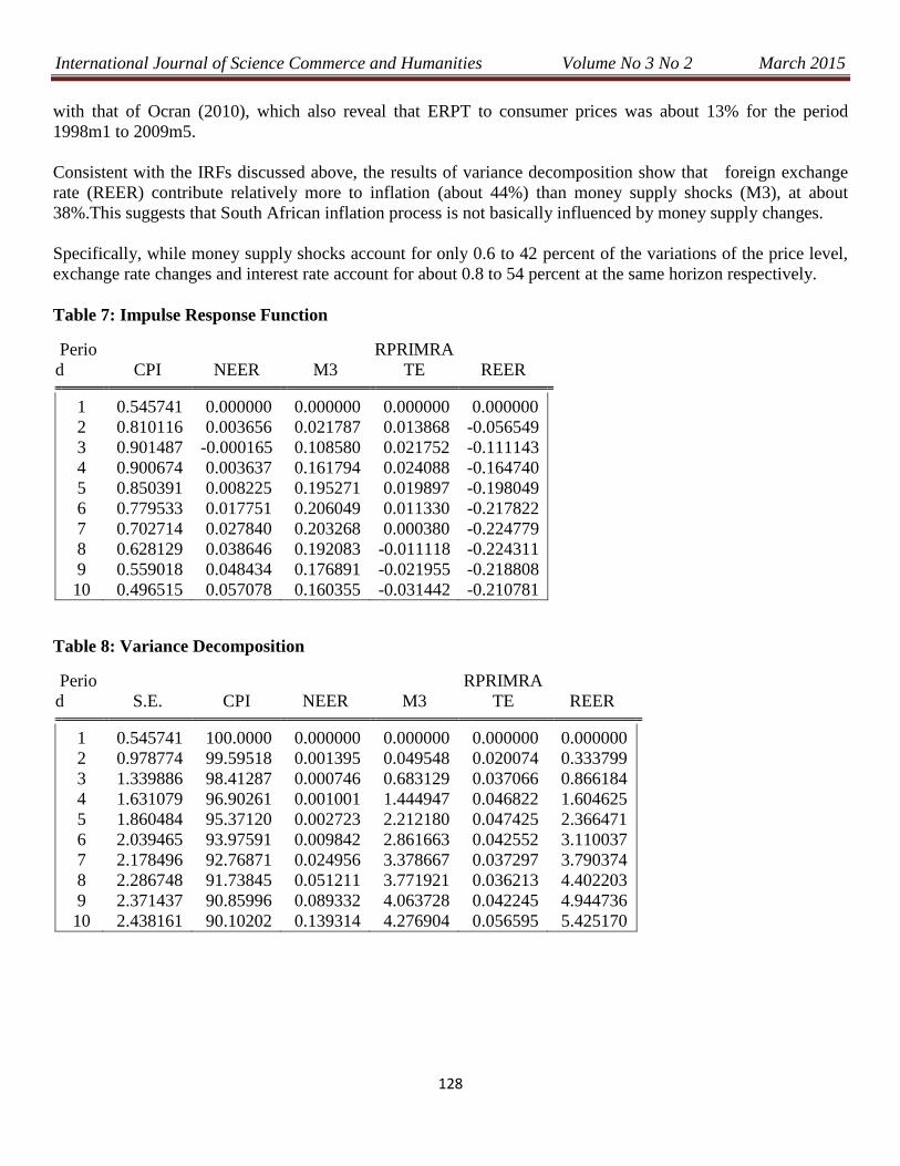
E. Impulse Response Function and Variance Decomposition
The Table below shows the response of price to a structural one standard deviation shock to each of the
variables. According to the table, the immediate effect of a shock to money supply (M3) at period 8 is about 19
percent increase in the price level. However, the effect of exchange rate shock (REER) is modest, at about 22
percent. The results show low average pass-through for nominal than for real shocks. The results are consistent
International Journal of Science Commerce and Humanities Volume No 3 No 2 March 2015
128
with that of Ocran (2010), which also reveal that ERPT to consumer prices was about 13% for the period
1998m1 to 2009m5.
Consistent with the IRFs discussed above, the results of variance decomposition show that foreign exchange
rate (REER) contribute relatively more to inflation (about 44%) than money supply shocks (M3), at about
38%.This suggests that South African inflation process is not basically influenced by money supply changes.
Specifically, while money supply shocks account for only 0.6 to 42 percent of the variations of the price level,
exchange rate changes and interest rate account for about 0.8 to 54 percent at the same horizon respectively.
Table 7: Impulse Response Function
Perio
d CPI NEER M3
RPRIMRA
TE REER
1 0.545741 0.000000 0.000000 0.000000 0.000000
2 0.810116 0.003656 0.021787 0.013868 -0.056549
3 0.901487 -0.000165 0.108580 0.021752 -0.111143
4 0.900674 0.003637 0.161794 0.024088 -0.164740
5 0.850391 0.008225 0.195271 0.019897 -0.198049
6 0.779533 0.017751 0.206049 0.011330 -0.217822
7 0.702714 0.027840 0.203268 0.000380 -0.224779
8 0.628129 0.038646 0.192083 -0.011118 -0.224311
9 0.559018 0.048434 0.176891 -0.021955 -0.218808
10 0.496515 0.057078 0.160355 -0.031442 -0.210781
Table 8: Variance Decomposition
Perio
d S.E. CPI NEER M3
RPRIMRA
TE REER
1 0.545741 100.0000 0.000000 0.000000 0.000000 0.000000
2 0.978774 99.59518 0.001395 0.049548 0.020074 0.333799
3 1.339886 98.41287 0.000746 0.683129 0.037066 0.866184
4 1.631079 96.90261 0.001001 1.444947 0.046822 1.604625
5 1.860484 95.37120 0.002723 2.212180 0.047425 2.366471
6 2.039465 93.97591 0.009842 2.861663 0.042552 3.110037
7 2.178496 92.76871 0.024956 3.378667 0.037297 3.790374
8 2.286748 91.73845 0.051211 3.771921 0.036213 4.402203
9 2.371437 90.85996 0.089332 4.063728 0.042245 4.944736
10 2.438161 90.10202 0.139314 4.276904 0.056595 5.425170

International Journal of Science Commerce and Humanities Volume No 3 No 2 March 2015
129
6. Conclusion
This chapter analyzes the impact of exchange rate volatility on inflation (exchange rate pass-through to prices)
in South Africa for the period 1994m1 to 2013m12, using Granger (non-) causality test within the framework of
Toda-Yamamoto (1995) VAR procedure. Impulse response functions and variance decomposition of consumer
prices to shocks from exchange rate changes are also estimated.
The IRFs results show that ERPT to consumer prices was modest during the period under review. The
immediate effect of a shock to the exchange rate (REER) at period 8 is about 0.22 (22 percent) increase in the
price level. This is consistent with literature on developed countries, which suggest that exchange rate pass-
through (ERPT) in an environment of low inflation is more subdued. Since the implementation of inflation
targeting, the South African Reserve Bank was able to contain inflation with the target range most of the times.
Consistent with other studies for developing countries, the variance decomposition results show a modest
exchange rate pass-through to inflation, although inflation is mainly driven by own shocks (see Bwire et. al,
2013).The variance decompositions also reveal that foreign exchange rate shocks (REER) contribute relatively
more to inflation than money supply shocks (M3).This suggests that South African inflation process is not
basically influenced by money supply changes.
The results from the Granger causality show that bi-directional causality occurs between CPI and NEER, CPI
and REER, M3 and REER and; RPRIMRATE and REER.Uni-directional causality runs from NEER to REER,
from M3 to CPI and NEER and; from RPRIMRATE to CPI and NEER. We therefore reject the null hypothesis
that there is non-granger causality among the variables under review.
References
1. Bwire, T et al.(2013).Research Department Bank of Uganda .March 2013 Working Paper Series
.Working Paper No. 05/2013
2. Campa, J. M. and L. S. Goldberg (2005). "Exchange Rate Pass-through into Import Prices. ―The Review
of Economics and Statistics 87(4).
3. Campa, J., and L. Goldberg, 2006, ―Distribution Margins, Imported Inputs, and the Sensitivity of the
CPI to Exchange Rates,‖ NBER working paper no. 12121.
4. Gagnon, J. E. and Ihrig, J. (2001). ‗Monetary Policy and Exchange Rate Pass-Through.‘ Federal
Reserve System, International Finance Discussion Paper No.704.
5. Goldberg, P. K. and M. M. Knetter (1997). "Goods Prices and Exchange Rates: What Have We
Learned?" Journal of Economic Literature 35(3): 1243.Government of Ghana (1998) Ghana —
Enhanced Structural Adjustment Facility Economic and Financial Policy Framework Paper, 1998–2000,
http://www.imf.org/external/np/pfp/ghana/ghana0.htm, IMF.
6. Ihing J. Marnass, M. and Rothenberg A., 2006. Exchange Rate Pass-through in the G. 7 countries.
International finance discussion paper NO. 851, Federal Reserve Board of Governors
7. Krugman (1987). ―Pricing to Market when the Exchange Rate Changes‖, in Sven W. Arndt, and J.
David
8. Krugman, P. (1986). "Pricing to Market When the Exchange Rate Changes." NBER Working Paper No.
w1926.
9. Laflèche, T., 1996. The impact of exchange rate movements on consumer prices. Bank of Canada
Review, Winter 1996-1997, 21-32.

International Journal of Science Commerce and Humanities Volume No 3 No 2 March 2015
130
10. Mann, C.L., 1986. Prices, Profits Margins, and Exchange Rates. Federal Reserve Bulletin, 72 (6), 366-
79.
11. McCarthy, J. (2000), ―Pass-Through of Exchange Rates and Import Prices to Domestic Inflation in
Some Industrialized Economies.‖ Working Paper No. 79, Bank for International Settlements, Basel.
12. Ocran,M.K ( 2010). ‗Exchange Rate Pass-Through to Domestic Prices: The case of South Africa‘.
Prague Economic Papers, 4, 2010.
13. South African Reserve Bank (2008). ―Monetary Policy Review. © South African Reserve Bank.
November, 2008. South African Reserve Bank South African Reserve Bank South African Reserve
Bank.
14. Tandrayen-Ragoobur and Chicooree, (2012) .Exchange Rate Pass Through to Domestic Prices:
Evidence from Mauritius, Department of Economics and Statistics, University of Mauritius ICITI 2012
ISSN: 16941225.
15. van der Merwe, E. 2004. ―Inflation Targeting in South Africa‖. Occasional Paper No. 19, .July. Pretoria:
South African Reserve Bank.
Related Documents