Stockholm School of Economics Master Thesis in Finance The Impact of Oil Price Fluctuations on Stock Prices - Evidence from three Asian Countries Jens Ewert ♦ Ellinor Hult ♠ May 2006 ABSTRACT This paper examines the relationship between oil price changes and the stock market and tests whether changes in the oil price can forecast stock returns. In order to investigate this query a regression-based approach is employed using the stock indices of three Asian emerging markets, namely Indonesia, India and China for the period January 1993 – April 2006. These countries have all experienced a rapidly growing oil demand during the investigated time period. Being the most populous countries in the world, excluding the U.S., this will have a hefty impact on global oil consumption. Also, as oil prices during the last few years have been at their highest levels since the oil crisis in the seventies, this study assesses if different levels of the oil price affect this factor’s liaison with stock returns. Our results indicate of the presence of an oil effect in the case of the Indian stock index, whereas no such effect can be identified for the Indonesian or the Shanghai index. Nor do we find significant evidence of an altered oil effect at different oil price levels. Tutor: Stefan Engström Dissertation: 2 June 09.15-11.00 Venue: 191 Discussants: Michael Fritzell (19752) and John Hansveden (19916) ♦ [email protected], ♠ [email protected] Acknowledgements: We would like to express our gratitude to our academic advisor Stefan Engström for helpful feedback and support throughout the process of writing this thesis. Further, we wish to thank Birgit Strikholm, Per-Olov Edlund and Helinä Laakkonen for their insightful comments and guidance on statistical matters. We also thank Nicholas Regan at Credit Suisse for giving us access to valuable research material. Finally, we thank Gustav Rehnman at Asia Growth Investors for sharing his view on the Asian stock markets.

Welcome message from author
This document is posted to help you gain knowledge. Please leave a comment to let me know what you think about it! Share it to your friends and learn new things together.
Transcript

Stockholm School of Economics Master Thesis in Finance
The Impact of Oil Price Fluctuations on Stock Prices -
Evidence from three Asian Countries
Jens Ewert♦ Ellinor Hult♠
May 2006
ABSTRACT This paper examines the relationship between oil price changes and the stock market and tests whether changes in the oil price can forecast stock returns. In order to investigate this query a regression-based approach is employed using the stock indices of three Asian emerging markets, namely Indonesia, India and China for the period January 1993 – April 2006. These countries have all experienced a rapidly growing oil demand during the investigated time period. Being the most populous countries in the world, excluding the U.S., this will have a hefty impact on global oil consumption. Also, as oil prices during the last few years have been at their highest levels since the oil crisis in the seventies, this study assesses if different levels of the oil price affect this factor’s liaison with stock returns. Our results indicate of the presence of an oil effect in the case of the Indian stock index, whereas no such effect can be identified for the Indonesian or the Shanghai index. Nor do we find significant evidence of an altered oil effect at different oil price levels.
Tutor: Stefan Engström Dissertation: 2 June 09.15-11.00 Venue: 191 Discussants: Michael Fritzell (19752) and John Hansveden (19916) ♦[email protected], ♠[email protected]
Acknowledgements: We would like to express our gratitude to our academic advisor Stefan Engström for helpful feedback and support throughout the process of writing this thesis. Further, we wish to thank Birgit Strikholm, Per-Olov Edlund and Helinä Laakkonen for their insightful comments and guidance on statistical matters. We also thank Nicholas Regan at Credit Suisse for giving us access to valuable research material. Finally, we thank Gustav Rehnman at Asia Growth Investors for sharing his view on the Asian stock markets.

2
TABLE OF CONTENTS
1 INTRODUCTION............................................................................................................ 3
2 THEORY........................................................................................................................... 4
2.1 BACKGROUND ................................................................................................................................ 4 2.2 WHAT ARE THE DRIVING FORCES BEHIND OIL PRICE MOVEMENTS AND WHAT IS THE LINK
TO STOCK MARKETS?...................................................................................................................... 6 2.3 THE IMPORTANCE OF OIL IN THREE ASIAN COUNTRIES ............................................................ 8 2.4 VARIABILITY IN OIL PRICES ......................................................................................................... 10 2.5 WHAT WOULD ECONOMIC THEORY SUGGEST? ......................................................................... 11
3 HYPOTHESES ................................................................................................................12
4 DATA ................................................................................................................................13
4.1 SAMPLE SELECTION AND RELIABILITY OF DATA ....................................................................... 13 4.2 EXPLANATORY VARIABLES .......................................................................................................... 14 4.3 OMITTED VARIABLES ................................................................................................................... 16 4.4 SAMPLE CHARACTERISTICS.......................................................................................................... 17
5 METHOD.........................................................................................................................20
5.1 METHODOLOGY........................................................................................................................... 20 5.2 TRANSFORMING THE DATA ......................................................................................................... 20 5.3 OIL REGIMES................................................................................................................................. 21 5.4 TESTING FOR AN OIL EFFECT ..................................................................................................... 22 5.5 INCLUSION OF CONTROL VARIABLES.......................................................................................... 22 5.6 FINAL MODELS ............................................................................................................................. 23 5.7 TESTING THE OIL REGIMES ......................................................................................................... 24
6 EMPIRICAL RESULTS...................................................................................................24
6.1 TESTING FOR AN OIL EFFECT ..................................................................................................... 24 6.2 SUBSEQUENT TEST INCLUDING CONTROL VARIABLES ............................................................. 25 6.3 FINAL MODELS ............................................................................................................................. 26 6.4 TESTING THE OIL REGIMES ......................................................................................................... 29 6.5 ROBUSTNESS ................................................................................................................................. 34
7 ANALYSIS ........................................................................................................................35
7.1 THE IMPACT AND PREDICTIVE POWER OF OIL PRICE CHANGES .............................................. 35 7.2 IMPLICATIONS OF OIL PRICE LEVELS .......................................................................................... 38 7.3 OTHER EXPLANATIONS FOR OUR FINDINGS.............................................................................. 39
8 CONCLUSIONS ..............................................................................................................40
9 SUGGESTIONS FOR FURTHER RESEARCH............................................................40
APPENDIX A: DESCRIPTION OF VARIABLES .................................................................44
APPENDIX B: STATISTICAL PROPERTIES AND ASSUMPTIONS ................................45
APPENDIX C: REGRESSIONS AND HYPOTHESES.........................................................47

3
1 Introduction
On April 13th 2006, the WTI oil price once again exceeded USD 70 per barrel, its highest price in
eight months. On that occasion it was hurricane Katrina that caused the rise. Currently, the world is
anxious about the risk of a military invasion in Iran, the fourth largest oil producer in the world.
Simultaneously, disturbances in Nigeria, Africa’s largest producer of crude oil and an important
supplier of high quality oil that is most suitable for making petrol, cause analysts to bite their nails.
The oil price is currently hovering around USD 70 per barrel and we are currently facing stagnation in
the extraction of this resource. In that perspective, the fact that rapidly growing countries like China,
Indonesia and India are experiencing an increasing demand for energy, it does not seem too drastic to
imagine a scenario when oil prices go beyond USD 100 per barrel. Then one might ask what
implications such a scenario would have for stock markets?
The relationship between the oil price and economic activity is quite well documented and has been
found to be negative in many studies. One of the most frequently quoted researchers within the field,
Hamilton (1983), argues that all recessions in the post-World War II period, at least to some extent,
can be explained by increases in the oil price. Having a documented negative relationship between oil
price movements and economic output, it is intuitive to draw similar conclusions about the linkage
between the oil price and financial markets. If higher oil prices affect economic output negatively,
they should also affect stock prices through the means of lowered expected earnings. However, the
amount of research made on this connection is rather limited. Furthermore, most of the research
done has been concentrated on developed economies and the periods examined have not included
the last years of peaking oil prices.
The purpose of this thesis is to investigate the relationship between oil price movements and stock
prices. Previous research has suggested that investors underreact to news announcements under
certain circumstances, contradicting with the Efficient Market Hypothesis. By employing a
regression-based approach using stock market indices in China, India and Indonesia, we will examine
the oil price’s ability to forecast stock returns. China and India, the two most populous countries in
the world, are today experiencing rapid economic growth and consequently so are also their demands
for energy, yet maybe not for the same underlying reasons.1 Finally we have Indonesia, a member of
OPEC,2 which, at least historically, has been a net exporter of oil and should therefore react
differently from oil price movements than the other two countries. Moreover we will construct three
different regimes of oil prices to test if the impact and/or prediction ability varies with different oil
1 Due to their diverse GDP drivers, their required quantities of oil are not at the same level and consequently India only consumes a third of the oil that China does on a daily basis. Source: Nation Master web page. 2 Organization of Petroleum Exporting Countries.

4
price levels. While previous research has examined data from periods before 2003 this study covers
the period January 1993-April 2006.
The thesis is organized as follows. Section 2 summarizes the theoretical framework for the study. In
Section 3 the hypotheses investigated are specified. Section 4 and 5 provide a discussion of the
methodology used for the study and a description of the data. In section 6 we present the empirical
results and findings which in turn are analyzed in section 7. Finally, section 8 concludes the results.
2 Theory
In this section essential background and concepts are presented. Provided is previous research
followed by an overview of the markets investigated as well as the oil price development. A
discussion on economic theories finalizes the section.
2.1 Background
Crude oil is the most actively traded commodity in the world.3 As briefly mentioned in the
introduction, the relationship between oil and the macroeconomy has been explored by many
researchers. In a paper by the IMF (2000) five channels through which a higher oil price affects the
global economy are pointed out. In short these are; 1) a transfer of income from oil consumers to oil
producers, 2) a rise in the cost of production of goods and services, putting pressure on profit
margins, 3) an impact on the price level and on inflation (the magnitude varies with monetary policy),
4) both direct and indirect impact on financial markets, 5) a change in relative prices, creating
incentives for energy suppliers to boost investments and production and for oil consumers to
economize. By running simulations of a USD 5 per barrel increase they estimate the level of global
output to reduce by 0.25 percent over a period of four years. The IMF is not alone about
documenting a relationship between oil prices and economic output. However, there is no common
agreement amongst previous research concerning the precise effect of changes in the oil price
(Driesprong et al., 2005). Also, more interesting for the purpose of this paper, the discussion on the
oil price and its effect on stock markets is limited and the conclusions various.
Jones and Kaul (1996), in one of the most comprehensive studies in this field, test if reactions in
stock prices due to oil price shocks are justified by considering changes in real cash flows. While
reactions in the U.S. and the Canadian stock markets can be validated, this is not the case of the U.K.
and Japan. Sadorsky (1999) who uses a different model, a vector autoregression model on monthly
data, shows that both oil prices and oil price volatility do have important roles in affecting real stock
returns. He also concludes that oil price volatility shocks have an asymmetric effect on the economy,
3 NYMEX webpage.

5
in that decreases in the oil price have a much weaker, if any, effect on real stock returns while
increases have a clear negative effect.
In contrast to the two previously mentioned authors’ conclusions, Huang et al. (1996), using data
from 1979 to 1990, do not find any evidence of a significant relationship between oil futures prices
and aggregate stock returns. Neither do Chen et al (1986) find any evidence suggesting that oil
constitutes an economic pricing factor in their sample of U.S. equities. Kaneko and Lee (1995)
investigate the effect of oil price shocks in the U.S. and Japanese stock markets and do indeed find
that oil prices play an important role for the Japanese- but not for the U.S. stock market.
More recent work includes a study by Hammoudeh and Li from 2005, which focuses on two stock
indices, the main Mexican and the main Norwegian, in addition to two industry sectors from each of
those countries, a transport index and an oil industry index. Even though their study shows that the
oil price has an effect on both nations’ indices as well as on the industry sectors, it also shows that the
systematic risk from the world market index is of greater importance than the oil effect. In another
study by Hammoudeh and Aleisa (2004) five members of GCC4 are investigated. Using daily data
they only find the oil price to have significant impact on the stock index in Saudi Arabia.
One of few studies that relates oil to stock returns in a prediction setting is the one by Driesprong et
al (2005), which also in many ways has inspired the work of this thesis. Controlling for other more
widely accepted predictors, they find that oil price changes significantly predict stock market returns
and that investors underreact to rises in the oil price. Even though emerging markets are included in
their investigation,5 most attention is paid to the developed countries’ stock markets. As the authors
conclude that the prediction ability of oil is stronger in countries with high oil consumption per capita
their findings regarding India are counterintuitive. The Indian consumption per capita ranks as low as
163rd on a world wide ranking list,6 which opens for further investigation. In this study we focus on
three emerging countries that do not have very high oil consumptions per capita, nevertheless are
experiencing a rapidly growing overall oil demand.
4 Gulf Corporation Council Saudi Arabia was a prime mover in setting up the Gulf Cooperation Council in 1981. Other members are Bahrain, Kuwait, Oman, Qatar and the United Arab Emirates (UAE). 5 Serving as an out of sample test. 6 Nation Master website.

6
Table I
Summary of Previous Research including Results Study Purpose Method and sample data Conclusion(s)
Hamilton 1983 To test the effect of oil price changes on the U.S economy.
VAR-method using quarterly data on GNP growth, inflation and unemployment rate.
Oil price shocks are related to recessions in the U.S. economy.
Jones and Kaul 1986
To test if reactions in stock prices due to oil price shocks are justified considering changes in real cash flows.
Using excess returns and monthly data. Model includes changes in industrial production, term spread, risk premium and dividend yields.
In the U.S. and the Canadian stock markets such reactions can be justified, but not the U.K. and Japan.
Chen et al. 1986
To test whether innovations in macroeconomic variables are risks that are rewarded by the stock market.
Using multi-factor asset pricing model on U.S. equities.
Find no evidence that the oil price constitutes as a pricing factor.
Huang et al. 1996
To test oil futures prices’ relationship to aggregate stock returns.
Use VAR-approach to test on the S&P Index.
Do not find any significant relationship between those factors.
Sadorsky 1999 To test oil prices’ and their volatilities’ impact on real stock returns.
VAR- approach using 3-month T-bill rate, Industrial Production and real stock returns.
Both oil prices and volatility have significant impact on stock returns.
Hammoudeh and Alesia 2004
To study the relationship between oil and the stock markets in GCC countries.
With daily data they investigate a bi-directional relationship.
Find that oil price only affects the stock market in one of the five members.
Driesprong et al. 2005
To test if oil prices can forecast stock returns.
Using a thirty-year sample of monthly data for thirty developed stock markets and a shorter time period for some emerging markets.
Oil prices predict stock market returns. Investors underreact to information in the oil price.
2.2 What are the driving forces behind oil price movements and what is the link to stock markets?
In this section we will describe the linkage between oil and stock prices on a general and intuitive
level. The approach is similar to the one used in previous work by Huang et al (1996).
To value a company and hence to price its stock, expected cash flows are discounted by using a
discount rate (e.g. average cost of capital). From this follows that movements in either the expected
cash flows or the discount rate will affect the stock return and the stock price. Oil prices can affect
both these two parameters in different ways and for different reasons. As oil is an essential input to
the production of many goods, changes in the price of oil certainly should have impact on the costs
for many companies. This could be compared to other input variables such as labor or capital.
Whether the effect of the changes in the oil price on stock prices is positive or negative is
consequently determined by the character the company. While a producer of oil would expect higher

7
earnings if oil prices increased consumers would expect lower earnings. This argument holds on a
microeconomic level as well as for an international level.7
Oil prices can also, at least indirectly, influence stock prices via the discount rate. The reasoning
behind this is that the expected discount rate is an amalgamation of the expected inflation rate and
the expected real interest rate, which can both affect the oil price. Considering a net oil importing
country, higher oil prices would affect the trade balance negatively, which in turn would depress the
foreign exchange rate and put an upward pressure on the domestic inflation rate. Consequently, a
higher expected inflation rate is positively related to the discount rate and hence negatively related to
stock returns. Taking the argumentation one step further one could use the oil price as a proxy for
the inflation rate, since oil is a commodity. Also the real interest rate is closely linked to the oil price.
As oil is one of the major resources in the world wide economy, a higher oil price by itself can put
upward pressure on the real interest rate (Huang et al., 1996).
The correlation between oil price changes and stock indices is however more complex and cannot
only been explained by higher cost for oil consuming economies and higher revenues for oil
producing ones. Increases in oil prices occur for many different reasons and do not necessarily affect
the economy in the same way every time. On the one hand, an increase in the demand for oil, which
is driven by growth but assumed not to be offset by an increase in supply, will lead to higher oil
prices. In that scenario, the increased demand is accompanied by a strong and growing economy.
Hence it is also likely that companies are performing well and thus intuitive to expect a positive
correlation between the oil price and stock performance. Another way for the demand to increase is
driven by speculation. For example motorists, distributors and other intermediaries may fill up their
reserves if they believe that oil is becoming a more scarce resource for which the cost is lower today
than it will be in the future (Lemieux, 2005). On the other hand, the oil price can fluctuate due to
changes in the supply, as a response to e.g., hurricanes and conflicts in oil producing countries. In this
case the correlation between the oil price and stock performance depends only on companies’ costs
and revenues, which in turn are altered by oil price changes.
Considering the discussion above it is not completely straightforward to expect to find any direct
impacts on broadly-inclusive stock indices caused by oil price changes. Oil prices relate to so many
macroeconomic factors that we should consider any isolated significant effects quite surprising.
7 Compare for example an oil producing company to a transport company and a country such as Saudi-Arabia to China.

8
2.3 The importance of oil in three Asian countries
Figure I. GDP composition by sector. Source: www.cia.gov
Having discussed the link between oil and the financial market it is natural to study the investigated
markets’ sources of income, consumption- and production patterns. The figure above depicts the
GDP composition by sector in each country. Comparing them, China stands out as greatly dependent
on the industry sector while for the other two have the largest part of their GDP comes from the
service sector. For this reason it is interesting to see whether the effect of oil price fluctuations differs
between the markets.
0
1000
2000
3000
4000
5000
6000
7000
8000
1965
1968
1971
1974
1977
1980
1983
1986
1989
1992
1995
1998
2001
2004
Year
Thousands barrels daily
China consumption
India consumption
Indonesia consumption
China production
Indonesia production
India production
Figure II. Oil consumption and production in China, India and Indonesia for the period 1965-2004. Source: BP Statistical Review of World Energy, April 2006 (www.bp.com)
The figure above shows the oil consumption as well as the oil production for the three countries
between 1965 and 2004. Looking at China it is clearly the case that consumption has been shooting
up relatively the production. In fact, in the recent years it has become the fourth largest net importer
of oil globally (Garner, 2005). Indonesia, too, shows an upward trend in consumption while the
production has decreased since the beginning of the nineties. For India it can be noted that
consumption has increased significantly over the last years while production has been fairly stable.
Figure III below shows the oil consumption for different geographical regions. Also here it can be
China
Agriculture
14%
Industry
53%
Services
33%
India
Agriculture
21%
Industry
28%
Services
51%
Indones ia
Agriculture
15%
Industry
31%
Services
54%
9
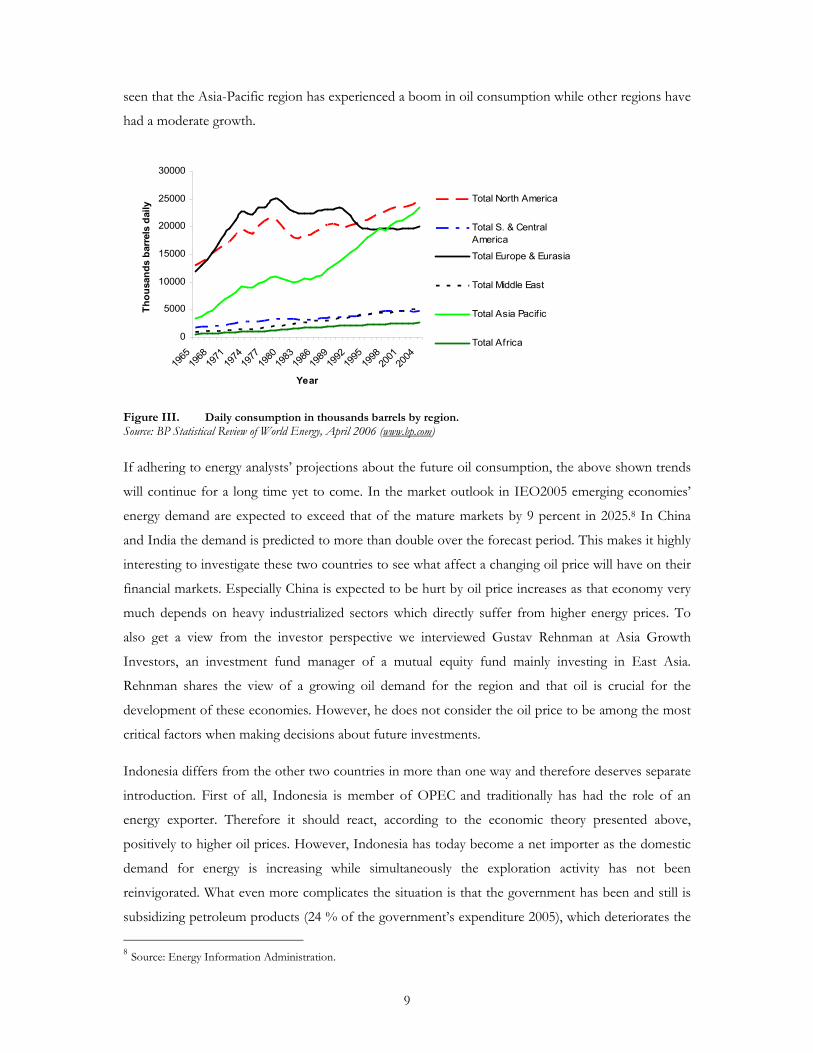
seen that the Asia-Pacific region has experienced a boom in oil consumption while other regions have
had a moderate growth.
0
5000
10000
15000
20000
25000
30000
1965
1968
1971
1974
1977
1980
1983
1986
1989
1992
1995
1998
2001
2004
Year
Thousands barrels daily
Total North America
Total S. & Central
America
Total Europe & Eurasia
Total Middle East
Total Asia Pacif ic
Total Africa
Figure III. Daily consumption in thousands barrels by region. Source: BP Statistical Review of World Energy, April 2006 (www.bp.com)
If adhering to energy analysts’ projections about the future oil consumption, the above shown trends
will continue for a long time yet to come. In the market outlook in IEO2005 emerging economies’
energy demand are expected to exceed that of the mature markets by 9 percent in 2025.8 In China
and India the demand is predicted to more than double over the forecast period. This makes it highly
interesting to investigate these two countries to see what affect a changing oil price will have on their
financial markets. Especially China is expected to be hurt by oil price increases as that economy very
much depends on heavy industrialized sectors which directly suffer from higher energy prices. To
also get a view from the investor perspective we interviewed Gustav Rehnman at Asia Growth
Investors, an investment fund manager of a mutual equity fund mainly investing in East Asia.
Rehnman shares the view of a growing oil demand for the region and that oil is crucial for the
development of these economies. However, he does not consider the oil price to be among the most
critical factors when making decisions about future investments.
Indonesia differs from the other two countries in more than one way and therefore deserves separate
introduction. First of all, Indonesia is member of OPEC and traditionally has had the role of an
energy exporter. Therefore it should react, according to the economic theory presented above,
positively to higher oil prices. However, Indonesia has today become a net importer as the domestic
demand for energy is increasing while simultaneously the exploration activity has not been
reinvigorated. What even more complicates the situation is that the government has been and still is
subsidizing petroleum products (24 % of the government’s expenditure 2005), which deteriorates the
8 Source: Energy Information Administration.

10
economy’s export capabilities (Credit Suisse Equity Research, 2005). Furthermore, subsidies are
planned to gradually be removed which will have important implications for the population as well as
for foreign investors. Thus, there is a large uncertainty regarding the effect of oil price changes in
Indonesia, a view which also is supported by Gustav Rhenman at Asian Growth Investors. Possibly
we could expect a positive impact from higher oil prices from the earlier part of the sample period
while less pronounced or even negative during the last years.
2.4 Variability in oil prices
0,00
10,00
20,00
30,00
40,00
50,00
60,00
1946
1949
1952
1955
1958
1961
1964
1967
1970
1973
1976
1979
1982
1985
1988
1991
1994
1997
2000
2003
2006
Year
$ per barrel
Figure IV. Nominal average annual crude oil prices since 1946 in USD per barrel. Source: www.inflationdata.com
The figure above depicts the oil price movements since 1946. Before the Yom Kippur War and the
OPEC-crisis in the seventies, fluctuations in the oil price had been limited. This can be one reason
why previous research on oil price fluctuations and their relations to the financial market is rather
limited. Even though oil prices today, as mentioned in the introduction, are at very high levels, prices
adjusted for inflation are yet not as high as the prices around 1980. So what qualified guesses can be
made about future oil prices? While energy analysts seem to agree that lower oil prices are to be
expected, some groups of geologists claim that the world is running out of oil which will eventually
cause an economic disaster (The Economist, 2006). What we all, however, can agree on is that oil
and oil prices are subject for a very topical debate among experts as well as laymen. If oil prices are
watched very carefully it seems unlikely that changes should be incorporated into stock prices with a
delay. Thus we could expect reactions to oil price changes today to differ from those of earlier time
periods. For this reason our investigation, including the last years’ oil price rally, could contribute with
valuable information.
In order to take this fact into account when conducting a study of oil price changes and their effects
on stock indices, one approach could be to break up the oil price into different levels that each

11
represents a different regime. At the lowest price regime, it would be reasonable to expect that the
effects of the price of oil are taken into account and discounted with a certain delay, whereas at
higher prices, the market would be prepared to pay more attention to changes in this important input
factor in many industries and discount it immediately. In other words, each of the regimes contains
different conditions possibly affecting the relationship between stock returns and oil price returns.
2.5 What would economic theory suggest?
One of the most central propositions in finance is the Efficient Market Hypothesis (EMH), which in
its classic configuration was defined as a financial market place in which security prices always fully
reflect all available information (Shleifer, 2000). Even though the EMH (see for example Malkiel,
2003) is not unanimously accepted among researchers and other observers, it is often referred to in
the literature. According to it there should not be any delayed reactions in stock returns due to
changes in the oil price, as oil prices are public information and readily available for all observers.
Thus news, such as a rise in the price of fuel today, should not make stock prices go down tomorrow.
All information is quickly observed and should therefore be incorporated in prices right away.
Extensive research has also shown that this indeed is the case. For example, stock prices react within
ten minutes to earnings announcements (Jones et al., 2003). The EMH does, besides the concept of
absorbing news, also state that the response to news announcements should be of the correct
magnitude, meaning that the market will neither underreact nor overreact to new information.
Regarding this, however, there is less evidence from empirical research. Thus, it might be that the
stock market reacts to changes in oil prices, but that the reaction could be too weak or too strong. In
contrast to the EMH, Grossman and Stiglitz (1980) argue that such efficiency (in its strong form)9 is
not plausible. The reason is that arbitrageurs, who collect costly information, need to be compensated
with trading profits, otherwise no one would have incentive to gather such information. Thus prices
only reflect information partially. Also, contrary to the EMH, more recent research argues that there
indeed are factors that can forecast stock returns (Cochrane, 2001). However the oil price as such a
factor has, to our knowledge, received little attention.
Hong and Stein (1999) develop a model featuring two different types of agents who are both
rationally bounded, namely newswatchers10 and momentum traders11. They argue that if each
newswatcher observes a certain piece of information, but has difficulties in deciphering how other
newswatchers’ use their private knowledge concerning that same information in order to arrive at
their evaluation of it, then information diffuses gradually across the population. Consequently, an
9 Meaning that prices reflect all relevant information, also including private information. 10 Newswatchers make forecasts based on signals that they privately observe about future fundamentals. They do not condition on current or past prices. 11 Traders that make judgments based on historical prices. They can find arbitrage opportunities in the difference between the true value of a stock and its prevailing market value, caused by the underreaction on behalf of the newswatchers. However, their forecasts are limited to be simple (univariate) functions of past prices.

12
underreaction in stock prices occurs in the short run. Even though their study mainly relates to
private information, the model also holds for public information under certain conditions. Such
circumstances may take place when the available public information is difficult to convert into a
judgment concerning the value of the stock, i.e. it requires additional, private, information. Thus it
might still be the case that the market underreacts to news, even though is public and available to all
observers at the same time. Hence, Hong and Stein (1999) conclude that the market’s response to
publicly accessible news involves an aggregation of private signals. Strong evidence for this
hypothesis is found by Hong, Tourus and Valkanov (2004) who further argue that, because of limited
information-processing capacity, investors cannot possibly pay attention simultaneously to asset
prices in markets, in which they are not specialized. Also argued is that information travels slowly,
since valuable information that starts off in one market reaches investors in other markets with a
delay. In their paper “Do Industries Lead Stock Markets?” they find the petroleum industry, amongst
others, to predict stock market movements by one month.
Not only do Hong and Stein (1999) argue that there exists an underreaction in stock prices to news in
the short run but they also claim that there follows an overreaction in the long run. The reason
behind this is that momentum traders, limited to simple strategies, who are trying to extract profit
from the mentioned underreaction will eventually set off an overreaction in the market. Different
models and theories on under- and overreaction to news announcements that attempt to forecast
stock returns have been developed by numerous researchers. Shleifer (2000) gives an excellent
overview of this discussion and also introduces a model founded in experimental psychological
evidence on failures of individual judgment under the pressure of uncertainty, which however is
beyond the scope of this study and is therefore not presented here.
The argumentation above has important implications for the purpose of this study. We know from
previous research that changes in oil prices do have an impact on economic activity. We also know
that the Efficient Market Hypothesis is quite questionable. Furthermore, investors may have
difficulties in evaluating the precise effect of oil price changes and/or may pay attention to the
information at different points in time. Thus, we do have reasons to believe that investors may
underreact as well as overreact to new information about the oil price.
3 Hypotheses
There is vast research that documents the impact of oil price changes on economic activity, which
argues that higher oil prices have a negative effect on the overall economy. The effect on stock
markets is, however, less explored, neither is it found to be the same among researchers. Assuming
that observers actually do have difficulties in assessing the impact of oil price changes on stock

13
returns and may react to oil price changes at different times, we expect higher oil prices to predict
lower stock returns. Consequently we expect declining oil prices to predict higher stock returns.
A less documented, but equally interesting, effect is the one of inconsistent conditions related to
different levels of the oil price. One could argue that at low oil price levels or regimes as denoted
above, investors would not be as observant of oil price changes, which suggests a slight delay in their
reactions to this factor. Following that argument, at higher prices, one would expect oil price changes
to be taken into account immediately. Accordingly, our hypotheses are the following:
Hypothesis 1: A rising oil price predicts lower stock returns. Hypothesis 2: A declining oil price predicts higher stock returns. Hypothesis 3: The impact varies in different price regimes.
4 Data Building a model that attempts to explain or predict asset prices is indeed not a simple task. Many
times researchers “go fishing” for explanatory variables that make their models successful, meaning
that the models cannot be rejected as capable of pricing assets. However, there is no consensus
concerning what right-hand side variables are to be included in a regression analysis. Models like the
CAPM and the APT are perhaps the most well-known models in asset pricing, nonetheless they are
hardly accepted as the perfect measurement tools. In order to avoid “fishing”, Cochrane (2001)
recommends that regressors be robust out of sample and across different markets and also to have
some relation to macroeconomic fundamentals. In addition to our investigated oil factor, which at
least fulfills the latter condition, we have included more commonly used predictors of stock returns
such as lagged returns, interest rates, industrial production, and inflation. By including these variables,
we attempt to protect our findings from being inflated by time varying risk (Hong et al., 2004).
Below we discuss the different data used to perform this study and the reasoning behind our
selections. An overview of the data sample characteristics finalizes the section.
4.1 Sample selection and reliability of data For the purpose of this study all data used was gathered from Datastream through Thomson
Financial. Thomson Financial is a globally leading supplier of financial information and can therefore
be considered a reliable source. The study is performed for the period January 1993-April 2006, the
longest dataset available that holds for the variables for the different countries. In total the sample
consists of 160 observations of monthly data. We chose a monthly frequency as we expected the
effect of oil price changes to show up in the longer perspective. Nevertheless we have performed all
tests also on a weekly as well as on a daily basis, however, with less significant results. One might
reason that the oil price is public information that is announced on a daily basis and should therefore

14
give an effect on daily data. However, it seems as if examining changes in such a short time
perspective is not the most sensible approach. One reason for this is that even if the oil price
increases strongly one day, it could very well decrease again the day after and therefore it would not
be sound for investors to base their investment decisions on the daily fluctuations of the oil price.
Yet, the levels of oil prices in a longer time perspective are highly relevant, as they are indicators of
the prevailing and future price levels that have an important impact on the macroeconomy.
4.2 Explanatory variables
Oil The crude oil market comprises of various types and qualities aimed for different purposes. As there
are so many types of crude oil one usually quotes prices of three types, which serve as benchmarks.
These are West Texas Intermediate (WTI, U.S.), Brent (Europe) and Dubai which is the benchmark
for Middle East oil flowing to the Asia-Pacific region. One might argue that the most proper oil
reference to be used for our investigated markets is Minas (Indonesia). However, as long data sets for
Minas were not available, we chose to use Dubai. This should, however, not have any severe
implications as the oil prices fluctuate rather closely even if the Dubai oil tends to trade at slightly
lower prices than e.g. WTI. As stated in the hypotheses, we expect the oil variable to move in the
opposite direction to the dependent stock indices and hence the sign of the coefficient should be
negative.
Lagged endogenous stock indices Using lagged values of the dependent variable among the explanatory variables is called an
autoregressive model. Controlling for those lagged stock returns we may capture important dynamic
structure in the dependent variable that might be caused of other factors (Brooks, 2002).
S&P 500, Hong Kong Stock Exchange and Nikkei Even though the magnitude of influence from the U.S economy differs among our selected markets,
they do all rely on exports to U.S. to some extent. China in particular is very much dependent on the
U.S. purchasing power, while Indonesia is the least affected country. We have chosen to include the S
& P 500 as a proxy for the overall state of the U.S. economy. Furthermore, in our preliminary
regression model we have included the Hong Kong Stock Exchange as well as the Japanese stock
index Nikkei. We expect these variables to have a positive relationship with all investigated markets.
Interest rates Comparing macro variables in emerging markets like China, India and Indonesia is not
straightforward and has to be done with some caution. In this study we have tried to find one short-
and one long-term interest rates for each country. However, how these are defined can sometimes
differ quite a lot between the investigated countries. For example, a ten-year treasury bond serves as
the long interest rate in India while the same in Indonesia is the one-year rate. In Appendix A a

15
detailed description including type of rate, names and times to maturity for the different rates is
found. Interest rates can affect stock returns for different underlying reasons. Firstly, increased
interest rates will cause debt to become more expensive which consequently will compress margins
and profitability for companies. The amount of cash flow available to reinvest in growth diminishes
which in turn lowers the stock price of the company. Secondly, higher interest rates make the choice
of investing in bonds more attractive relative to equities. Finally, interest rates affect the consumption
behavior in a population. Higher rates make mortgages more expensive and fewer people can afford
them. This lowers the disposable income and consumption will go down, slowing the economy down
and stock prices fall. Thus we expect the interest rates’ coefficients to have negative signs.
Term spread To capture the influence of the shape of the term structure we define another variable; term spread,
which is the long bond yield less the short bond yield for each country respectively. Thinking of stock
dividends as bond coupons plus risk, we should expect any bond premium to be reflected in stock
returns. A larger positive difference between the long and short term yield is commonly seen as a sign
of a good state of the economy. The reason is that investors require a higher yield on long term
assets. A rising short term yield signals that the government is concerned about inflation. Falling long
term yields indicate investors’ concern about the inflation and the level of economic activity. Thus a
narrower gap between the rates is likely to slow down the growth of an economy. Consequently we
expect the term spread to be positively correlated with stock returns.
Industrial Production The industrial production is measured using each country’s reported industrial production index not
seasonally adjusted on a monthly basis. Theoretically, an increase in industrial production should have
a positive effect on the economy. If this is true, companies earn higher profits and dividends, which
consequently should raise stock prices. On the other hand, a strongly growing economy implies
higher interest rates which can, as mentioned in the previous section, dampen or at least
accommodate stock returns. However, we believe the first effect to be stronger and hence we expect
the industrial production to show a positive sign. As the reporting of this variable is done on a
monthly basis, on the 15th of every month to be more exact, it would seem reasonable to use lagged
values for it in a regression model so that it is last month’s value that is expected to affect this
month’s index returns. However, we believe, in the case of this particular variable, that the effect of
the increased production will have a direct affect on the economy and thereby the stock markets,
even though the actual Industry Production figure has yet to be announced.

16
Inflation The relationship between inflation and stock returns has been investigated in by numerous
researchers. Empirical evidence can be found for a positive- as well as for a negative relationship.12
To be consistent with the Fisher Hypothesis13 we should not expect the inflation to have any real
impact on stock returns. Earnings should, according to that theory, be consistent with the inflation
rate and consequently real stock returns should remain unaffected. As our study uses nominal stock
returns we expect the coefficient for inflation to show a positive sign. However it is important to
remember, before drawing any conclusions, that higher oil prices lead to higher inflation and that we
might therefore just be picking up the same effect.
Table II
Explanatory Variables and Expected Signs on the Coefficients of the Regression:
Variable Description Expected Sign i
tCPI Consumer Price Index +
i
tIP Industrial Production Index +
Short
tBond Yield on short-term bond -
Long
tBond Yield on long-term bond -
spread
tr Term Spread +
i
jtr − Return on lagged stock index +
PS
tr& Return on S&P 500 +
HK
tr Return on Hong Kong Stock Exchange +
NIK
tr Return on Nikkei 500 +
oil
tr Return on oil price (Dubai) -
4.3 Omitted variables An omitted variable is defined as, in a regression, an excluded independent variable that might have
influence on the dependent variable. As long as this variable is uncorrelated with the included
explanatory variables this is not a severe problem and estimates are still unbiased. However, in case of
having an omitted variable that is correlated with some of the other independent variables, OLS
regression generally produces biased and inconsistent variables (Brooks, 2002). In this study we have
strived to include all available explanatory variables based on their economical and statistical
relevance. Even though some of the most frequently used control variables, in regressions that
attempt to forecast stock returns, are included, others are left out. The reasons for this vary. In some
cases we did not have access to appropriate data (e.g. dividend yields) while other factors such as
12 See for example Firth and Gultekin for a documented positive relationship or Fama (1981) for a negative relationship. 13 The Fisher hypothesis is the proposition by Irving Fisher that the real interest rate is independent of monetary measures, especially the nominal interest rate. Thus, real interest rate is the nominal interest rate minus inflation.

17
season anomalies are not very well documented and appear in different ways in the different
markets.14
4.4 Sample Characteristics All regressions have been carried out on a monthly- as well as on a weekly basis. Here we report the
characteristics for the monthly data as it gave most significant results. The way of using the economic
variables to explain or predict stock returns differs widely in the literature. In order to choose
between different lags we have run a regression for each explanatory variable separately for the
individual countries. The version of each variable, still theoretically motivated, that was most
significant has then been included in the larger model. Below we first show all significant variables
across all countries and then statistics for each country individually.
Table III
Descriptive Statistics This table presents the descriptive statistics for those variables that are relevant across all three countries. The sample covers the period January 1993 – April 2006 and contains monthly data. The total number of months in the observation period is 160. All descriptive statistics are denoted in percent.
Variable Min. Max. Mean σ
Dubai
tr -36.547 33.872 0.837 8.799
PS
tr& -15.759 9.232 0.685 4.103
HK
tr -34.413 28.376 0.489 8.030
NIK
tr -16.483 14.673 0.250 6.334
A few observations can be made from Table III. The returns on the Dubai oil price are positive for
this whole period, which is in line with expectations, since the oil price has increased quite
significantly during that same period, seen clearly in Figure V below. We can also note that the
volatility in the oil price has been rather high during this period as compared to that of the major
stock markets, Dow Jones and Nasdaq. One should bear in mind that the volatility of those two
markets can be assumed to be greater than otherwise, however due to the terrorist attacks on
September 11th 2001.
14 For example, the fiscal year in China ends in January while it in India ends in March.

18
Table IV
Descriptive Statistics This table presents the descriptive statistics for those variables that are relevant for Indonesia only. The sample covers the period January 1993 – April 2006 and contains monthly data. The total number of months in the observation period is 160. All descriptive statistics are denoted in percent.
Variable Min. Max. Mean σ
Indonesia
tr -52.274 43.404 0.022 14.324
Indonesia
tCPI -1.057 12.005 1.024 1.686
Indonesia
tIP -31.923 27.687 0.062 9.699
Short
tBond -38.566 57.941 -0.367 9.269
Long
tBond -32.850 54.972 -0.407 7.852
spread
tr -41.689 27.763 -0.040 6.516
In Table IV above, there are some things that need to be noted. Firstly, the return on the index has
during this period been positive, which is in accordance with theory as Indonesia has until today been
a net exporter of oil. However, the market has been rather volatile during this period, indicating that
the positive return has been associated with quite some risk. It should be noted that the values for
both Industrial Production (IP) and Consumer Price Index (CPI) are quoted in terms of return, not in
actual levels. It can be seen that, in the case of Indonesia, CPI has increased, for the most part,
gradually the last five years. Concerning the return on IP the mean is near zero, yet there has been a
lot of volatility in this variable. Please note that the bonds are much more volatile than in more
developed countries, indicating some of the instability that is inherent in this economy.
Table V
Descriptive Statistics This table presents the descriptive statistics for those variables that are relevant for India only. The sample covers the period January 1993– April 2006 and contains monthly data. The total number of months in the observation period is 160. All descriptive statistics are denoted in percent.
Variable Min. Max. Mean σ
India
tr -25.393 19.904 0.687 8.410
India
tCPI -2.182 3.149 0.524 0.863
India
tIP -22.423 15.439 0.514 5.291
Short
tBond -35.667 76.214 -0.246 10.666
Long
tBond -11.310 17.869 -0.337 -3.784
spread
tr -58.345 30.877 -0.011 9.623
From the above table we see that the Indian stock market as well as the Indonesian one has a positive
mean and exhibits quite high volatility. CPI is more stable for this country than for the latter, as is IP.
Concerning both of the bonds, the Indian economy shows more volatility than what would be

19
expected for a more developed economy. The positive trend in the Indian stock market is contrary
the theory that higher oil prices lower stock returns.
Table VI
Descriptive Statistics This table presents the descriptive statistics for those variables that are relevant for China only. The sample covers the period January 1993– April 2006 and contains monthly data. The total number of months in the observation period is 160. All descriptive statistics are denoted in percent.
Variable Min. Max. Mean σ
Shanghai
tr -48.477 86.228 0.116 12.940
Shanghai
tCPI -1.903 1.944 -0.048 0.738
Shanghai
tIP -42.453 32.649 1.117 12.857
Short
tBond -37.807 31.508 -0.678 5.691
Long
tBond -44.629 25.490 -0.785 6.001
spread
tr -21.187 25.489 -0.108 4.035
In the case of the return on the Shanghai index in China, this sample period has had, as previous
countries, positive returns. Again this would be in opposition with our initial hypothesis that when
the oil price increases, that should have a negative effect on the stock market. However if looking at
the last years peaking oil price, we can observe a decline in the Chinese stock index. The bond market
demonstrates a low negative return which is in line with economic theory as the stock market has
increased. The rate for the IP has increased rather strongly during this period. This factor is as volatile
as for Indonesia.
0
50
100
150
200
250
300
350
400
450
Dubai
Indonesia
0
50
100
150
200
250
300
350
400
450
India
Dubai

20
0
50
100
150
200
250
300
350
400
450
China
Dubai
Figure V. The relative stock index development contra the oil price using 1993 as base year for the different countries.
5 Method
In this section the methodology used for the study is described and discussed. The different steps
leading to the final models are described as well as our constructed oil price regimes. Also provided is
the transformation of our raw data. All regressions and statistical tests have been carried out using the
software package Intercooled Stata 9.1.
5.1 Methodology The subjects for this study are the stock markets in China, India and Indonesia for the period January
1993-April 2006.15 In order to measure the impact of oil price fluctuations we conduct a separate
regression-based model, for each of the different countries, on the major stock indices for each
market. Choosing what variables to include in a regression-based model that aims at explaining or
predicting variations in stock returns is not a simple task. Previous research provides evidence for
that certain variables have forecasting power, however there is no consensus among researchers on
one appropriate combination of factors (Cremers, 2002). The motivations for including each of the
variables in our model were described in the data section. Testing for an oil effect we started by
including, apart from some more widely used variables, lagged oil prices up to sixth months, in
accordance with Driesprong et al (2005).
5.2 Transforming the data
When attempting to establish a relationship between the oil effects and stock returns all variables
were transformed into returns rather than prices as we are more concerned with the effect of changes
in the return on the oil price on the return on stock indices, as opposed to examining the relationship
between the oil price and the stock index price. Therefore, the first step was to transform all variables
that were quoted in prices into returns, as is shown below for the stock index variable.
)ln(ln100 1
index
t
index
t
index
t PPr −−∗= (1)
15 This was the longest period for which we could find appropriate data from Datastream.

21
When it comes to the variables Industrial Production and the Consumer Price Index variables we also
transformed them into “returns”, even though their original values were not in prices, but rather in
index values. (This was done in order to enable comparison of variables of the same nature, so that all
variables could be interpreted as percentage changes in a final model.)
5.3 Oil regimes
When converting all data into returns, some important information is lost concerning the actual levels
of the oil price. Thus, to take into account and test for the fact that the oil price has been at some of
its highest levels ever in the last few years, a method of using so-called oil regimes was employed.
This in essence means that the oil price was divided into three different levels that indicate whether
the oil price is Low (below USD 20), Medium (between USD 20 and USD 34) or High (above USD
34). They were set in such a way that each regime should capture a meaningful spectrum of oil price
levels, including enough observations for valid tests to be conducted. Dummy variables were used to
distinguish between each of the regimes. The objective was thereafter to include regime dummies in
the final model discussed in section 5.6 below. With that model, we could test if different levels of oil
price could add any information to the full-period model. In the figure below, the Dubai oil price is
shown including the three oil price regimes.
Table VII
Descriptive Statistics for Oil Price Regimes This table presents the different price levels that divide the Dubai oil price into different regimes. The sample covers the period January 1993– April 2006 and contains monthly data. The total number of months in the observation period is 160. All figures are in USD.
Regime Min. Max. Mean σ
All levels 10.17 60.83 23.35 11.18
Low 10.17 19.82 15.60 2.33
Medium 20.48 33.19 25.34 3.06
High 34.01 60.83 46.69 9.36

22
0
10
20
30
40
50
60
70
1992
1993
1994
1995
1996
1997
1998
1999
2000
2001
2002
2003
2004
2005
Figure VI. Crude Oil-Arab Gulf Dubai USD/BBL with constructed price regimes. Source: Datastream
5.4 Testing for an Oil effect
To see at an early stage if an oil effect could be established two different tests were conducted. The
first was to, in accordance with Driesprong et al. (2005), simply incorporate one lag of the oil return
in a regression with the index return for each of the countries.16
i
t
oil
r
iii
t rr εβα ++= −1 (2)
where iα is the constant term estimated by the regression and i
tε is the error term, the superscript i
indicating each of the countries. With a standard t-test it was then tested if the coefficients estimated
for iβ significantly differed form zero. Should the null hypothesis be rejected, it could be claimed at
this early stage that there is evidence of an oil effect.
5.5 Inclusion of control variables
The next step in determining if an oil effect is present amongst the determinants for stock prices is to
put together a model containing all of the relevant regressors discussed in the data section above. To
determine which lags of the variables that were most significant for forecasting stock returns, each of
the variables was regressed, including lags zero through six of that same variable on each of the three
stock indices. The lag that gave the most significant results was selected to be included in a first-draft
model (exclusive of the oil regressors), which is referred to as the restricted model. An example of
the restricted model and unrestricted (for India) model is shown below:
16 Also tested were later lags as well the unlagged version of the oil variable. However, as we considered the one month lagged oil price to be most economically motivated, we chose not to present these equations here. This expectation also showed to hold when running the different regressions.

23
t
NIK
t
HK
t
PS
t
Long
ttttt
rr
rBondIPCPIrr
εββ
βββββα
+++
+++++= −−−
87
&
64131211 (3)
To that model we then added all the lags of oil to arrive at the unrestricted model.
t
NIK
t
HK
t
PS
t
Long
t
tt
oil
t
oil
t
oil
ttt
rrrBond
IPCPIrrrrr
εββββ
ββββββα
+++++
+++++++= −−−−−
1413
&
1211
110196813211 .... (4)
Each of these will be run on the three countries of interest. Then they are to be compared with an F-
test to see if the oil lags are significantly different from zero, in which case we can conclude that there
is evidence of an oil effect. The F-test statistic is calculated as follows:
)/(
/)(
knRSS
mRSSRSSF
UR
URR
−
−= which is F distributed with m and n-k degrees of freedom.
The corresponding hypotheses for each country are the following:
:0H 01413121091 ====== ββββββ
:1H1312111091 ,,,,, ββββββ and/or 14β ≠ 0
5.6 Final models
In order to finally end up with a model that takes into account as many significant variables as
possible, without including too many, we strived at finding a model for each of the three countries,
which maximizes the predictive power for the stock index returns. As R2 is a non-decreasing function
of the number of regressors in a model, we decided to use adjusted R2 instead, which is corrected for
the number of degrees of freedom in a regression model (Gujarati, 2003). Thus, maximizing that
goodness of fit measure aids in finding a regression model that predicts as much of the index
fluctuations as possible, without losing degrees of freedom by including excessive variables. The
approach taken was to start off with a model that included all the economically justifiable variables
that could contribute in explaining the returns on the three indices, and then reduce that regression
model. By eliminating the least significant variables, one at a time, with the aim of maximizing the
adjusted R2, we finally ended up with three different models, which are presented in section 6.3. The
starting point was thus to estimate Regression 417 (also denoted as the unrestricted model above) for
each month t for all of the countries. In other words, a model that was found reasonable was
deliberately over-fitted and then, in the described top-down approach, reduced until a meaningful
result was obtained. One might ponder over the risks of constructing a spurious model when
17 Please note that this is the regression for relevant for India. The corresponding regressions for Indonesia and China are presented in Appendix C.

24
attempting this approach. A spurious relationship is one that is nonsensical, yet has a very high
explanatory value, R2. It is common that non-stationary variables regressed on each other exhibit
statistically significant correlations, without there actually being any correlation between them
whatsoever (Gujarati, 2003). Therefore, we tested all variables for a unit root process, which was
rejected at the ten percent level in favor of the alternative hypothesis of stationarity.18
5.7 Testing the oil regimes When the final models for each of the countries had been acquired, these were used to investigate
whether there are any significant differences between the oil price regimes. In order to do this we re-
estimated the final models, this time splitting them up into three separate parts by using dummy
multipliers for each oil price regime. Using the estimated coefficients from the combined regression
we test, with an F-test as in section 5.5, if the variables multiplied by the regime dummies are
significantly different from zero. If that is the case, the null hypothesis, which states that the oil
regimes do not contain any supplementary information with respect to the information obtained
from the combined model, can be rejected. A simplified version of this may look as follows:
mZiHXhHgHZfMXeMdMZcLXbLaLY +⋅+⋅++⋅+⋅++⋅+⋅+= (5)
For Regime Low: For Regime Medium: For Regime High:
:0H 0=== cba :0H 0=== fed :0H 0=== ihg
:1H ba, and/orc≠ 0 :1H ed , and/or f ≠ 0 :1H hg, and/or i ≠ 0
6 Empirical Results
6.1 Testing for an Oil effect One first approach to examine the predictive effect of oil price changes for stock returns is to run
simple regressions including only oil, in different forms, as explanatory variable. In this first
assessment, we chose to test if the return on oil from one month prior to today, had any significant
explanatory value for the current month’s stock return.19 Table VIII summarizes the results from our
regression with one lag of the oil price for each of the stock markets.
18 Please see Appendix B for more details. 19 As also mentioned in footnote 16 in section 5.4, regressions were also made on the oil variable in all different forms. Again, as these did not show any significant results, we have chosen to only present the result for the one month lagged oil price.

25
Table VIII
Initial Oil Effect Test This table shows the relation between lagged oil return and return on market indices for the three markets. The following
regression is estimate using OLS regression: i
t
oil
r
iii
t rr εβα ++= −1. The values in parentheses are t-values. * denotes
significance at the 10 percent level; ** denotes significance at the 5 percent level; *** denotes significance at the 1 percent level (two-tailed test).
Market Constant oil
rr 1− 2R.Adj N
Indonesia 0.052 (0.40)
-0.016 (-1.01)
-0.005
158
India 0.808 (0.23)
-0.155** (-2.05)
0.020 158
Shanghai -0.130 (-0.13)
-0.015 (-0.14)
-0.006 158
For China and Indonesia we cannot reject the null hypothesis that the oil coefficient is significantly
different from zero, i.e. there are no indications of an oil effect for these countries. For India,
however, we do find a significant relationship between the oil price and the Indian stock index. The
negative estimated coefficient for oil
rr 1− of –0.155 can be interpreted to mean that if last month’s oil
price return increased by one percent, then this month’s stock return would decrease by 0.155
percent. Or, given that the surrounding conditions remain constant, this would imply that if the
current month’s oil price return is positive that predicts the stock returns in the next month to be
negative. This result is statistically significant at the five percent level.
Interpreting the results is not straightforward. According to our hypotheses not only the Indian stock
market should exhibit a negative significant relationship, but also the Chinese index. From Indonesian
stocks, on the other hand, oil price movements were expected to predict stock returns in the same
direction, i.e. that oil price increases should predict increases in the share index as well. That these
two countries do not show any significant results does not necessarily mean that there is no effect on
stock returns from oil price fluctuations, but could be the result of not having enough of data. Before
taking the analysis further or drawing any conclusions from this evidence, the models for each
country are expanded with various widely-used predictors below.
6.2 Subsequent test including control variables Having no unison conclusions from the first regression with only oil as explanatory variables, the
model is extended by including a number of well-known predictors of stock returns as described
under section 5.5 above. Moreover, several lags of oil are included, namely those ranging from today’s
oil return to the oil return with a time lag of six periods. The reasoning behind the inclusion of all of
these is that such an approach allows for the detection of delayed oil effects, in addition to those that

26
occur in a short time perspective. Table IX below contains the results for each market from testing
the unrestricted model against the restricted one.
Table IX
Subsequent Oil Effects Test These tables show the result from testing whether the unrestricted model, inclusive of oil lags, adds significant explanatory value in addition to the explanatory value provided by the restricted model. The estimates result from the regression tests under section 5.5 above.
Market Number of
Parameters, m Degrees of
Freedom, n-k
Unrestricted 2R.Adj
Restricted 2R.Adj
F(m,(n-k)) Prob > F
Indonesia 7 124 0.36 0.37 0.74 0.638
India 7 116 0.33 0.28 2.30 0.031
Shanghai 7 140 0.03 0.06 0.52 0.819
The results presented in Table IX above are in line with those found by the initial test for oil effects.
In other words, in the case of both Indonesia and China there is no evidence of that the oil variables
have contributed with any supplementary information through their incorporation in the unrestricted
model. This can be confirmed by the fact that adjusted R2 for the restricted model is higher than for
the unrestricted models, clearly indicating that the oil lags do not add enough explanatory value to
compensate for the loss of degrees of freedom that their inclusion results in.20
However, turning to the case of the Indian stock exchange’s dependency of oil, also this test gives
evidence for there being an oil price effect. Here, the addition of the seven oil variables have
contributed enough to the unrestricted model for the difference between it and the restricted one to
be statistically significant. Again, this is further shown by the fact that the adjusted R2 for the
unrestricted model is higher than for restricted model.
6.3 Final models From the regression inclusive of all variables discussed in section 4.2 the model has been reduced by
eliminating the least significant variables, one at a time, and striving to maximize adjusted R2 to finally
end up with one final model for each country. Please also note in the case of Indonesian and Indian
regression models, we have included lagged variables of the regressands in order to correct for
autocorrelation.21 Tables X-XII contains the results from the final estimations for the different
countries.
20 Please see Appendix C for further details. 21 Please see Appendix B for further details.

27
Table X
Final Model Indonesia
This table shows the relation between the stock index and all those explanatory variables that were necessary when maximizing adjusted R2. The following regression are estimated using standard OLS:
t
NIK
t
HK
t
spread
t
Long
t
Short
tt
oil
t
oil
t
Indonesia
t
Indonesia
t
Indonesia
t
IndonesiaIndonesia
t
rr
rBondBondIPrrrrrr
εββ
βββββββββα
+++
+++++++++= −−−−−−−−
1110
49847565544432211
The values in parentheses are t-values. * denotes significance at the 10 percent level; ** denotes significance at the 5 percent level; *** denotes significance at the 1 percent level (two-tailed test).
Constant Indonesia
tr 1− Indonesia
tr 2− Indonesia
tr 4− oil
tr 4− oil
tr 5− Indonesia
tIP 5− -0.344* (-0.37)
0.209*** (3.03)
-0.216*** (-3.29)
0.214*** (3.21)
0.179* (1.71)
-0.115 (-1.11)
-0.290*** (-2.89)
Short
tBond 4− Long
tBond spread
tr 4− HK
tr
NIK
tr 2R.Adj N
0.245** (2.04)
-0.338*** (-2.61)
0.751*** (4.16)
0.733*** (5.54)
0.280 (1.63)
0.48
141
As we can see from the estimated coefficients that result from the final model for Indonesia, only two
lags of oil regressors are left after reducing the regression into a model that explains the returns in the
Indonesian index in the most satisfactory way, given the set of data acquired. This model’s adjusted
R2 is 0.48, meaning that it is capable of explaining 48 percent of the returns in the stock index. Even
though it could be higher, we consider this explanatory power to be satisfactory, as the determinants
for stock return in this country are also heavily dependant on such factors as political climate and
other country specific risk factors which have a large impact on investors’ willingness to trade in these
stocks. When taking a closer look at some of the estimated coefficients, we can note that all three
lagged variants of the dependant variable are significant at the one percent level, giving the model
some autoregressive characteristics. Of the two oil lags remaining in the model, only lag four is
significant at the ten percent level. That particular lag has a positive estimated coefficient, which goes
along with our above stated expectations. The interpretation of its estimated coefficient would be that
a positive return on the oil price at time t would predict a positive return on the stock index at time
4+t , given that all other variables are held constant. However, as the subsequent oil lag, lag 5, is
negative, we cannot draw any too strong conclusions from these estimated coefficients.
Some of the other important explanatory variables for the Indonesian stock index are the long bond
and the term spread. These are both significant at the one percent level and have coefficients that are
aligned with expectations. Estimated coefficients show that the Hong Kong stock index return also
has a strong influence on the returns on the Indonesian one which, again, is expected since the prior
market is much more strongly integrated in the global stock market than the latter. The coefficients
that have turned out to go against our expectations are the industrial production and the short bond,
which both have negative coefficients and are significant. Perhaps these variables go against

28
expectations because they are lagged four and five periods, respectively. It is reasonable to think that
certain relationships and effects are altered in a longer time perspective.
Table XI
Final Model India
This table shows the relation between the stock index and all those explanatory variables that were necessary when maximizing adjusted R2. We estimate the following regression using standard OLS:
t
HK
t
NIK
t
Long
t
India
t
oil
t
oil
t
oil
t
oil
t
India
t
India
t
India
t rrBondCPIrrrrrrr εββββββββββα +++++++++++= −−−−−− 10987665544133211
The values in parentheses are t-values. * denotes significance at the 10 percent level; ** denotes significance at the 5 percent level; *** denotes significance at the 1 percent level (two-tailed test).
Constant India
tr 1− India
tr 3− oil
tr 1− oil
tr 4− oil
tr 5− oil
tr 6−
0.795 (1.15)
-0.066 (-0.88)
-0.144* (-1.91)
-0.110* (-1.66)
0.125* (1.90)
0.097 (1.48)
0.148** (2.28)
India
tCPI Long
tBond HK
tr NIK
tr 2R.Adj N
-1.771** (-2.60)
-0.622*** (-3.92)
0.120 (1.47)
0.506*** (4.88)
0.36
133
In the case of the Indian stock index four lags of oil return remain in the final model. The first of
these is negative, as expected, and significant at the ten percent level. It indicates that a positive oil
return at the present time, time t , predicts negative stock returns at time 1+t , or, that negative oil
returns predict positive stock returns, with the same time perspective. However as inflation, contrary
to expectations, also shows a negative relationship, it makes it harder to draw any strong conclusions
regarding the isolated effect from an oil price change. Subsequent oil return lags are all positive. The
fourth and sixth are significant at the ten and five percent levels, respectively, while the fifth is not. As
well as for Indonesian market’s model, this one contains lagged versions of the dependant variable.
Here, the third lag is significant at the ten percent level and has a negative sign. The other two most
significant explanatory variables are the return on the long bond and the return on the Japanese stock
index, Nikkei. Both of these variables’ estimated coefficients are of expected signs. Concerning the
adjusted R2 for this model, it is a bit lower than for that of the Indonesian market. However, we still
consider it quite satisfactory, particularly in the light of the fact that the country’s economy, like many
other developing countries’ economies, has changed drastically during the sample period, which
makes it hard to find a model that captures enough of the dimensions that affect stock returns in this
index.

29
Table XII
Final Model China
This table shows the relation between the stock index and all those explanatory variables that were necessary when maximizing adjusted R2. We estimate the following regression using standard OLS: Please note that this regression was estimated using Huber-White sandwich estimators22 of variance in place of ordinary ditto, thus no adjusted R2 values can be presented, why R2 values are given.
t
NIK
t
Long
t
China
t
oil
t
oil
t
Shanghai
t
Shanghai
t rBondCPIrrrr εββββββα +++++++= −−−− 2655443211
The values in parentheses are t-values. * denotes significance at the 10 percent level; ** denotes significance at the 5 percent level; *** denotes significance at the 1 percent level (two-tailed test).
Constant Shanghai
tr 1− oil
tr oil
tr 4− China
tCPI 5− Long
tBond NIK
tr 2− 2R N
-0.435 (-0.51)
-0.102 (-0.75)
-0.112 (-1.01)
0.126 (0.92)
-2.848** (-2.10)
-0.302* (-1.84)
0.254 (1.41)
0.10
154
For the Chinese stock index, the final regression model is not nearly as good in terms of explanatory
value as for the two previous countries.23 It is only able to explain ten percent of the index returns for
this market. The model still includes two oil variables, one for the current time and one for four
months prior to today’s date, none of which is statistically significantly different from zero. The two
variables that are indeed significant are the lagged consumer price index and the long-term bond. CPI,
which is a measurement of inflation, does not have the sign we expected. Rather than being positively
correlated with the stock index, it is quite negatively correlated with the index. The other variable that
is significant, this time at the ten percent level, is the long-term bond, which has a negative estimated
coefficient along with expectations. Perhaps it should be remarked upon the fact that, rather contrary
to expectations, the Hong Kong stock index return did not make it to the final model as major
explanatory model. This, along with the fact that the explanatory value is so low, forces us to be
prudent when drawing any conclusions from the Chinese model.
6.4 Testing the oil regimes The approach of testing if different price levels of oil affect the predictive property of oil return on
stock index returns is applied to each of the countries’ final models. Since each stock index has a
proprietary model, each model will be presented together with the results that are shown for one
country at a time. The regression models are the same as the final models above, yet they are split up
by the oil regimes Low, Medium and High. Each regression is estimated and tested in three separate
groupings to see if the set of coefficients adhering to the same regime are different from zero. In the
case of Indonesia, the full model for this estimation is the following:
22 Huber/White/sandwich estimators give heteroskedasticity-consistent estimates. Source: Stata web page 23 As there was a need to correct for some issues with model diagnostics to obtain the more significance levels for each estimated coefficients, adjusted R2 is no longer a relevant measure. Thus, we comment on the R2 value instead, which is rather low.

30
Regression 6, for Indonesia:
oil
tL
oil
tL
Indonesia
tL
Indonesia
tL
Indonesia
tLLL
Indonesia
t rrrrrRr 5544432211( −−−−− +++++= βββββα
)11104984756
NIK
tL
HK
tL
spread
tL
Long
tL
Short
tL
Indonesia
tL rrrBondBondIP ββββββ +++++ −−−
oil
tM
oil
tM
Indonesia
tM
Indonesia
tM
Indonesia
tMMM rrrrrR 5544432211( −−−−− ++++++ βββββα
)11104984756
NIK
tM
HK
tM
spread
tM
Long
tM
Short
tM
Indonesia
tM rrrBondBondIP ββββββ +++++ −−−
oil
tH
oil
tH
Indonesia
tH
Indonesia
tH
Indonesia
tHHH rrrrrR 5544432211( −−−−− ++++++ βββββα
t
NIK
tH
HK
tH
spread
tH
Long
tH
Short
tH
Indonesia
tH rrrBondBondIP εββββββ ++++++ −−− )11104984756
Table XIII
Oil Regime Effects – Indonesia Index These tables show the result from testing whether the regimes significantly differ from each other with respect to the each country’s full model. The estimates result from the Regression 6 and the tests correspond to the hypotheses listed above. * denotes significance at the 10 percent level; ** denotes significance at the 5 percent level; *** denotes significance at the 1 percent level (two-tailed test).
Regime Number of
Parameters, m Degrees of
Freedom, n-k F(m,(n-k)) Prob > F
High 11 106 0.61 0.813
Medium 11 106 2.90*** 0.002
Low 12 106 9.92*** 0.000
The way to interpret the above results is that the regimes that are significant add information that
differs from the remaining part of the regression. Thus, for the Indonesian stock index, this implies
that in the Low regime the regression estimated differs from the remaining two periods that it is
compared to in with the F-test. The same applies to the Medium regime. The tests indicate that, at
such price levels of oil, there is some difference in the relationships between the explanatory variables
and the dependant variable.
To see which of the coefficients that actually are significantly different between the oil price regimes,
we also tested the pair of corresponding coefficients across the regimes to see if they differed
significantly from each other. The only estimated coefficients that were statistically different from
zero were the below presented ones.

31
Table XIV
Differing Coefficients – Indonesian Index This table shows the coefficients obtained from Regression 6 that significantly differs in a pair wise comparison across the regimes for the Indonesian stock index. Please note that this comparison test was carried out for all variables in the model, but that only the significant ones are presented here. The values in parentheses are t-values. * denotes significance at the 10 percent level; ** denotes significance at the 5 percent level; *** denotes significance at the 1 percent level (two-tailed test).
Regimes Variable Est. Coefficient
Low Est. Coefficient
Medium F(m,(n-k)) Prob > F
Low –Medium Indonesia
tr 1− 0.321*** (3.42)
0.013 (0.10)
3.80* 0.054
Low-Medium Indonesia
tr 2− -0.342*** (-3.85)
-0.058 (-0.48)
3.57* 0.062
In this case we see that the coefficients that differed between the regimes were the lags of the
dependant variable, the stock index returns. For both of these lags, the coefficients have changed
from being significant explanatory variables at the low price levels of oil to insignificant ones. Their
signs have remained the same, however. The lags of oil have not turned out as variables that obtain
significantly diverse estimated coefficients depending on the level of the oil price. Thus, it does not
seem as if the oil price in the case of Indonesia has a stronger or weaker effect on the stock index
returns if the price per barrel of oil is high or low.
Regression 7, for India:
oil
tL
oil
tL
oil
tL
oil
tL
India
tL
India
tLLL
India
t rrrrrrRr 665544133211( −−−−−− ++++++= ββββββα
)10987
NIK
tL
HK
tL
Long
tL
India
tL rrBondCPI ββββ ++++oil
tM
oil
tM
oil
tM
oil
tM
India
tM
India
tMMM rrrrrrR 665544133211( −−−−−− ++++++ ββββββα
)10987
NIK
tM
HK
tM
Long
tM
India
tM rrBondCPI ββββ ++++oil
tH
oil
tH
oil
t
a
H
oil
tH
India
tH
India
t
a
HHH rrrrrrR 665544133211( −−−−−− ++++++ ββββββα
t
NIK
tH
HK
tH
Long
tH
India
tH rrBondCPI εββββ +++++ )10987
Table XV
Oil Regime Effects – India Index These tables show the results from testing whether the regimes significantly differ from each other with respect to the India’s full model. The estimates result from the Regression 7 and the tests correspond to the hypotheses listed above. * denotes significance at the 10 percent level; ** denotes significance at the 5 percent level; *** denotes significance at the 1 percent level (two-tailed test).
Regime Number of
Parameters, m Degrees of
Freedom, n-k F(m,(n-k)) Prob > F
High 10 100 1.76* 0.078
Medium 11 100 5.30*** 0.000
Low 11 100 3.51*** 0.000
For India, all of the oil price regimes are significantly different from the two remaining ones to which
they are compared. This indicates that the estimated sub-regression for each oil price level has a

32
different impact on the index than the other two do when they are combined. Therefore each regime
of oil is characterized by diverse conditions. The question is then to see which of the variables that
differ on an individual base when compared pair wise.
Table XVI
Differing Coefficients – India Index This table shows the coefficients obtained from Regression 7 that significantly differs in a pair wise comparison across the regimes for the Indian stock index. Please note that this comparison test was carried out for all variables in the model, but that only the significant one is presented here. The values in parentheses are t-values. * denotes significance at the 10 percent level; ** denotes significance at the 5 percent level; *** denotes significance at the 1 percent level (two-tailed test).
Regimes Variable Est. Coefficient
Low Est. Coefficient
High F(m,(n-k)) Prob > F
Low –High HK
tr 0.007 (0.07)
1.350* (1.88)
3.44* 0.066
Somewhat contrary to expectations, we find that the only variable differing strongly between the
regimes is the return on the Hong Kong stock index. It changes from being an insignificant
independent variable for the low period to being a significant variable with a positive estimated
coefficient in the high oil price regime. The fact that only one variable was found to differ between
the regimes on this individual basis when the jointly tested regime coefficients seem to contain
different information, could be for one of several reasons. Firstly, it could be that each estimated
coefficient has changed only slightly, which is not enough to be captured by the individual test carried
out above, but their added effect is substantial enough for each period to contribute with a different
set of information than the other ones. Secondly, most observations in each regime often follow each
other chronologically, meaning that the low oil price regime contains mostly observations from the
first years of the times series and the high oil price regime contains observations from the latter end
of the dataset. This results in that several factors will be captured in the regimes that are related to
economic conditions in general, which would have a greater impact on the returns on each stock
index than can be captured by a simple regression model.
Regression 8, for Shanghai:
)( 2655443211
NIK
tL
Long
tL
China
tL
oil
tL
oil
tL
Shanghai
tLLL
Shanghai
t rBondCPIrrrRr −−−− ++++++= ββββββα
)( 2655443211
NIK
tM
Long
tM
China
tM
oil
tM
oil
tM
Shanghai
tMMM rBondCPIrrrR −−−− ++++++ ββββββα
)( 2655443211
NIK
tH
Long
tH
China
tH
oil
tH
oil
tH
Shanghai
tHHH rBondCPIrrrR −−−− ++++++ ββββββα tε+

33
Table XVII
Oil Regime Effects – Shanghai Index These tables show the result from testing whether the regimes significantly differ from each other with respect to the each country’s full model. The estimates result from the Regression 8 and the tests correspond to the hypotheses listed above. * denotes significance at the 10 percent level; ** denotes significance at the 5 percent level; *** denotes significance at the 1 percent level (two-tailed test).
Regime Number of
Parameters, m Degrees of
Freedom, n-k F(m,(n-k)) Prob > F
High 7 134 15.0*** 0.000
Medium 5 134 1.33 0.257
Low 7 134 1.61 0.137
As seen from Table XVII above, the high oil price regime is the only one that is significant for the
estimated regression for the Chinese stock index. This implies that, since the Dubai oil price reached
and exceeded USD 34 per barrel, some economic condition that affects the predictive characteristics
of the explanatory variables changed, as compared to the two other oil price periods. These
differences will be further investigated by comparing the coefficients across the regime levels. Since
we see that the F statistics are rather similar for regimes Low and Medium, we would not expect them
to have any coefficients that differ when compared pair wise, however we would expect there to be
differences when comparing either one of those regimes with the High oil price regime.
Table XVIII
Differing Coefficients – Shanghai Index These tables show the coefficients obtained form Regression 8 that significantly differ in a pair wise comparison across the regimes for the Shanghai stock index. Please note that this comparison test was carried out for all variables in the model, but that only the significant ones are presented here. The values in parentheses are t-values. * denotes significance at the 10 percent level; ** denotes significance at the 5 percent level; *** denotes significance at the 1 percent level (two-tailed test).
Regimes Variable Est. Coefficient
Low Est. Coefficient
High F(m,(n-k)) Prob > F
Low –High oil
tr -0.248 (-1.20)
0.240 (1.22)
2.92* 0.090
Low –High oil
tr 4− 0.402 (1.33)
-0.403** (-2.39)
5.40** 0.022
Low –High China
tCPI 5− -4.807** (-2.48)
2.476** (2.16)
10.44*** 0.002
Regimes Variable Est. Coefficient
Medium Est. Coefficient
High F(m,(n-k)) Prob > F
Medium –High oil
tr 4− -0.082 (0.279)
-0.403** (-2.39)
3.04* 0.084
Medium –High NIK
tr 2− 0.174 (1.46)
-0.210 (-1.16)
3.14* 0.079
In the tables above our expectations are confirmed, in that there are a number of coefficients that
differ when comparing across the regimes. In addition, all of these involve the High oil price regime.
First of all, when comparing the Low and High regimes, between which it is reasonable to expect to
find the greatest differences, two oil variables have contrasting estimated coefficients, namely the

34
current time, time 0t ’s oil return and the oil return corresponding to four months prior to the index
return, time 4−t . For both variables the estimated coefficients have almost turned out to be the
opposite in the High oil price regime as compared to the Low regime. In the Low oil regime the
coefficient for oil
tr was negative, indicating that a current high oil price should be associated with a
high return in the index today. Whereas, the coefficient for the same regime, but for the lagged oil
variable, is positive and thus indicates that a positive return on the oil price today speaks for a positive
index return at time 4+t . The opposite seems to be true for the High regime, in which the current
oil price coefficient is positive and the lagged one is negative. The other factor that has changed a lot
between the High and Low regimes is CPI. It has gone from significantly negative in the low price
regime to significantly positive in the high one. Our expectations on this variable was for it to be
positively correlated with the index returns, however there is a certain disagreement in the literature,
as mentioned in section 4.2, that suggests that this variable could have either a positive or a negative
correlation with stock performance. Certainly, the influence of inflation has changed, but exactly what
those changes have been are beyond the scope of this paper.
In the Medium and High regime comparison the oil lag again shows up as a variable that, in the
regressions, receives a different estimated coefficient depending on which oil price level one focuses
on. In the Medium oil regime, the lagged oil return’s estimated value is very weekly negative and
insignificantly different from zero, while in the High price level, as discussed above, it is more
negative and a significant estimator at the five percent level. The other variable that has a significant
difference in its estimated value in the Medium to the High price regime is the lagged return on the
Nikkei stock index. Neither one of its estimated coefficients is significant at the ten percent level.
However, since it goes from being a positive estimator for the Medium price regime, to a negative
estimator in the High price regime, it is captured by this test as a variable that varies with different
periods of oil price levels.
6.5 Robustness Since we found, in the regime tests above, that the estimated coefficients either differed individually
or in terms of their joint effect, it could be appropriate to carry out a complementary assessment to
check if the regression models are robust over time. Therefore the dataset was divided into two equal-
sized periods and the regressions re-estimated, however, this time including a variable that indicates
the second time period. Finally, we tested if the second time period’s coefficients added any
information to the full period regression.24
24 For stated regressions and corresponding hypotheses, please see Appendix C.

35
Table XIX
Robustness over Time This table presents the results from testing whether the regression model for each county is robust over time with an F test. The first period cover the period January 1993 through July 1999. The second period runs from August 1999 to April 2006. * denotes significance at the 10 percent level; ** denotes significance at the 5 percent level; *** denotes significance at the 1 percent level (two-tailed test).
Market Number of
Parameters, m Degrees of
Freedom, n-k F(m,(n-k)) Prob > F
Indonesia 12 117 1.92** 0.039
India 11 111 2.02** 0.033
Shanghai 7 140 1.29 0.261
To a certain extent the results obtained in this robustness test mirror the results from the regime
tests. Given that the oil price regimes for Medium and High oil prices collectively correspond rather
well to the second period of the robustness test, it is likely that the results obtained from the tests are
quite similar to those for the Low regime. In other words, it is expected that robustness over time is
likely to be rejected for India and Indonesia, but not for Shanghai. In the case of the latter stock
market, it seems as if the first two regimes are rather similar, while the last one differs substantially
from the two prior ones. In the robustness test this difference within period two cannot be captured,
instead that whole period’s estimated coefficients will be some type of average of the Medium and
High regimes, why the differences will be less pronounced than in the robustness test above.
7 Analysis
7.1 The impact and predictive power of oil price changes
This study was carried out with an expectation for there to be a significant predictive quality in oil
returns on at least the Chinese and Indonesian stock indices. However, the results obtained have
shown that the impact of oil price returns is minor in those two countries, while it does have
predictive power in the case of the Indian stock index. This was identified already in the initial and
subsequent oil effect tests, as the one month lagged oil price return had a significant effect on that
stock index. Also, the comparison of the unrestricted and the restricted model showed that oil
variables contributed with significant information. At first glance, these results might sound too
counter-intuitive to be true. China, which is thoroughly dependant on oil as an input for its massive
manufacturing industry, ought to be more affected by oil price changes than India. Indonesia, which
is an oil producer that nowadays is becoming a net oil importer, also relies heavily on oil. In contrast,
India has a low oil production and consumption on a per capita basis.25 Its industries are mostly
25 Source: Nation Master. In an oil consumption per capita ranking list comprised of 207 countries, China ranked 136th with 0.049 bbls/day per 10 people, Indonesia ranked 137th with 0.048 bbls/day per 10 people and India ranked 163rd with 0.021 bbls/day for 10 people.

36
software and IT services related, why its energy demand is relatively lower than for the global heavy-
industry hub, China. Then one might ask oneself why the Indian stock exchange shows a significant
relationship with the oil return variables.
Considering that, in these two oil dependant countries, much greater attention is paid by investors to
the changes in the oil price since it is such a vital input factor. This then relates to the Efficient
Market Hypothesis in that the oil price is public information that is readily accessible to all investors.
Therefore, that factor should be discounted momentarily. Hence, there should not be any predictive
power by the oil price on stock indices, especially for those indices that are located in countries in
which this input factor is an important one, like in China or Indonesia. However, in the case of India,
a different situation could set the standards. Investors in that region may not view the oil price as a
factor that must be carefully considered and observed. That could be why more predictive power
resides in the oil price movements in the case of that index.
When including other, more established, predictors for stock market fluctuations in each of the final
models, in addition to several lags of the oil price returns, oil seems to have somewhat more
explanatory value. In all of the final models at least two oil variables have subsisted after the
elimination of redundant variables. These are not always individually significant by measure of t-
statistics, but they still contribute to the predictive capability of the model. An explanation for this
could be that all the factors that cause stock price changes are so complexly intertwined that some of
the generally accepted variables need to be present for the oil price effects to be able to be addressed.
In the case of the Indonesian model one of the two oil variables is significant at the ten percent level.
It is the four-month lagged oil price return, oil
tr 4−, that gives evidence of a positive correlation with the
index returns. As mentioned before, we expected a positive correlation between the Indonesian index
and oil regressors. By that token, this result could one the one hand be seen as pleasing. It may very
well be interpreted to indicate that oil has a predictive effect on the Indonesian index, which in this
instance entails that if the oil price return is positive at time 0t that should foretell a positive oil return
in four months time. On the other hand, the other lag of oil that is present in that very same model,
namely lag five of the oil return, oil
tr 5−, which is insignificant at the ten percent level, has a negative
estimated coefficient. Therefore, this evidence cannot be viewed upon as being reliable enough for
any conclusions to be drawn. Instead, it is more sensible and correct to say, that in the case of
Indonesia, there is some relationship, although weak, between oil- and stock returns. From this
sample and investigation approach it appears as if the connection between the two factors is positive
or neutral, but that is as far as it would be prudent to draw conclusions.

37
In the Indian model there is more evidence of there indeed being an oil effect that influences future
returns on the stock index. In that regression, three of the four oil variables are significant at the five
or ten percent level. Here, the estimated coefficient for the first significant oil regressor, oil
tr 1−, is
negative and significant. It can therefore be interpreted as is done under section 6.3, that a positive oil
price return at time 0t is likely to result in a negative return on the index at time 1+t . The coefficients
for the regressors oil
tr 2− and oil
tr 3− are not significantly different from zero. But subsequently following
are the lagged oil returns for lags four, five and six, of which all have positive estimated coefficients.
In this pattern of first negative returns followed by positive returns one could possibly identify an
under- and overreaction behavior on behalf of the investors. As described under section 2.6 Hong
and Stein (1999) discuss how newswatchers and momentum traders together create a market place
that, as a united entity, frequently first underreacts to information in the market, to later overreact to
the same news in the long run. If investors that focus on the Indian stock market are not primarily
concerned with the oil price as a key factor in their decision-making processes or if they have
difficulties in assessing the impact on stock prices, it is likely that they would underreact to changing
oil prices. In other words that means that in response to an increase in the oil price at time 0t , the
market does not react with the correct magnitude at time 0t by adjusting the stock price up if oil
prices have decreased or down in oil prices have increased.
What is seen in the case of the Indian stock index is that, rather than there being a reaction at the
time of the oil price change, it is delayed. The market most likely observes the change in the oil price,
but either it does not know how to interpret it, or it does not dare to discount that piece of
information harshly enough. This can possibly explain why we see a negative reaction at lag 1−t . The
two following lags are not significantly different from zero. At that point the market seems to be in
some type of recovery state under which returns neither improve nor worsen. In the thereafter
subsequent lags there again is a positive reaction which could then be interpreted as an overreaction.
This whole reasoning is based on the assumption that there is some stickiness in the market that
makes reactions come slowly at first, after which all investors react simultaneously resulting in the
overreaction.
For the Chinese model and its estimated coefficients, we see a similar pattern as noted for the Indian
index in that the first oil price return variable is negative and the lagged variable is positive. In this
case it is the current time, 0t ’s oil return that is negative, whereas for India it was the one time-period
lagged variable. That fact has different implications, meaning that the Chinese market reacts
immediately to changes in the oil price. One plausible explanation may be that the Efficient Market
Hypothesis holds in that traders involved in this market have experience with oil price fluctuations
and enjoy the right tools to discount the changing oil price more efficiently than in other markets.

38
Since oil is an economically important factor for this country, it is also possible that investors have
learnt not only how to discount the public information in the market, but they might also have built
an understanding as to how other investors are likely to react to the flow of news. That makes the
market more swift at reacting to information and doing so with a closer to correct magnitude, rather
than under- and overreacting interchangeably until efficiency has been achieved. However, as this
model shows rather unsatisfactory explanatory capability, in addition to the fact that neither of the oil
coefficients is significant, we will not attempt to draw any more extensive conclusions from that
model.
7.2 Implications of oil price levels
The interpretation of the above discussed results is rather intricate as they differ across the countries
investigated. This also goes for the results from the regimes that were utilized in order to detect any
disparities in the correspondence between oil price returns and stock returns at different levels of the
oil price. The reasoning behind this was that at higher prices we would expect the oil price to be a
more crucial factor in the eyes of shareholders than when oil prices remain more stable at lower
levels. Hence, first tests were carried out to see if any of the regimes differed significantly from the
combined two other regimes, to which it was compared. Then, in order to understand which factors
were the main stimulators of this difference, a pair wise comparison of each of the factors’
coefficients was carried out. The results obtained were somewhat unsatisfactory in that they did not
correspond to expectations. We would have expected the highest regime to differ from the two
others rather distinctively, since it represents a period during which oil prices practically skyrocketed.
Concerning the results obtained for Indonesia, the Low and Medium regimes differed significantly in
comparison to the others and the only pair wise compared variables that were different across the
regimes were two lagged versions of the dependant variable. Thus, it cannot be claimed that the
existence of oil effects could be supported by this finding.
The results obtained from the same tests on the estimated regression for India were also somewhat
unexpected. Here, all regimes differed from the other two, meaning that each and every one of them
had contrasting explanatory conditions. However, on an individual basis, the estimated oil
coefficients failed to differ when compared across oil price regimes. Thus, one cannot assert that
there be evidence of an oil effect that differs in conjunction with the levels of the oil price, even
though each regime can be said to be characterized by separate economic conditions.
The only stock market that gave the results that were aspired for was the Shanghai stock index. Here
the High oil regime was significantly different from the other two. It thus seemed to carry
information that could not be extracted from the relationship between the oil and stock returns at
lower oil prices. Also, when inspecting which of the coefficients that differed between the High

39
regime and the two other regimes, it was found that oil return in its current time variant, oil
tr , and in
its four period lagged variant, oil
tr 4− , were significant. However, with respect to the actual estimated
coefficients, the results were not exactly in line with expectations. The only statistically significant
variable was oil
tr 4− and its estimated value was rather strongly negative. In addition, it was early on in
this thesis concluded that the model estimated for Shanghai was not of such quality that it could be
used for any extensive conclusion drawing. Then, you might wonder, why we present its results in the
paper.
One reason for why we decided to persist with this country’s stock index was that we have made note
of that China has been excluded from some previous research of which we have taken part in the
preparation for this thesis (see for example Driesprong et al., 2005). We therefore were curious to
find out what type of results it would give.
7.3 Other explanations for our findings
To round off this analysis it should be mentioned that what has been shown in this study is in
support of the previous research that claims that oil has a limited direct effect on stock returns. Also,
the countries explored here are developing ones that have gone through rather radical development
changes during the sample period. This can be confirmed by the robustness test performed which
shows that neither the Indonesian nor Indian stock markets could be claimed to be robust over the
sample period. In the case of Shanghai stock market, robustness cannot be rejected by the equally-
split sample test, but it is probable that it would not be robust over time if a different split up of the
sample period were utilized.
Some other reasons why the effect of oil price changes appear so limited in this study is that they
have been related to changes in the major stock indices for each country. One should then keep in
mind that these indices are comprised of stocks from many different industries that are affected in
diverse ways by oil price changes. Some of which can be assumed to be positively correlated with oil
return, some negatively and others not at all. Therefore, their combined effects may be cancelling
each other out, resulting in that no effect is shown. It is feasible to assume that investors that hold
stocks in a particular country aim at having a certain weight of for example Indian shares in their
portfolio. They might therefore reallocate their capital within that country’s stock market as a
response to oil price changes, resulting in a zero net effect in the index.

40
8 Conclusions
The purpose of this thesis was to examine the relationship between oil price movements and the
stock market and test if changes in the oil price can forecast stock returns. More specifically three
Asian emerging economies were examined, which are expected to consume an increasing share of the
world’s oil reserves in the future. Our hypotheses that rising oil prices predict lower stock returns and
declining oil prices predict higher stock returns were tested on aggregated data for the period January
1993-April 2006. Furthermore, we tested if this effect varied with different oil price levels.
While the findings for India suggest a relationship and that oil price changes do predict stock returns
in accordance with our hypotheses, the results for Indonesia and China give too weak evidence of an
oil effect for any conclusions to be drawn with respect to oil’s influence on stock returns. The results
for India contradict the theory of true market efficiency as we find that there is a delayed response to
oil price changes. However, the fact that India is identified as a country with an oil effect, while the
other two countries investigated are not, is supported by previous findings by for example
Driesprong et al. (2005). Concerning the utilized oil price regimes we found no strong evidence
suggesting that these altered the relationship between oil- and stock returns.
As discussed in the opening theoretical paragraphs of this paper, previous research does not give one,
cohesive message as to whether stock returns can be predicted by oil price changes. Some research
concludes that so is the case, while others, like Chen et al. (1986) and Huang et al. (1996), find no
evidence for any such relationship. Therefore, the conclusions arrived at in this paper are supported
by that latter group of researchers.
As a final remark, we should point out the fact that the models and techniques used in this thesis are
non-exhaustive. Thus, even though we find little evidence of an oil effect by the means of this study,
we will not go so far as to claim that an oil effect is an inconceivable influence on stock returns.
9 Suggestions for further research
After having summarized the results obtained in this study, we can conclude that the findings do not
give much satisfactory indications concerning there to be important impacts of oil price changes on
stock indices. Hoping for oil to show up as a predictor of stock returns in the enormous noise of
different factors affecting financial markets is perhaps not evident. However, using different methods
or approaches, we still believe that there is more evidence to find in this area. For example, it would
be interesting to perform an event study considering shocks in the oil price, defined as certain
percentage change. Furthermore, it could be interesting to examine different sectors of companies,
which also has been done for other markets in previous research. Finally, as these emerging

41
economies provide relatively limited data sets, future research might be able to find more information
on the impact of oil prices on stock returns.

42
10 References
Literature
Brooks, C., 2002, Introductory Econometrics for Finance, Cambridge: University press.
Chen, N.F., Roll, R., and S.A. Ross, 1986, Economic Forces and the Stock Market, Journal of Business 59, pp. 383-403.
Credit Suisse First Boston, 2005, Indonesia Energy Outlook, Boom or Bust? Credit Suisse Equity Research, Sector Review, 25 Nov 2005.
Cremers, K.J. Martijn, 2002, Stock Return Predictability: A Bayesian Model Selection Perspective, The Review of Financial Studies, 15(4), pp. 1225-1226. Chocrane, J.H., 2001, Asset Pricing, Princeton University, Princeton and Oxford. Driesprong, G., Jacobsen, B., and B. Maat, 2005, Stock Markets and Oil Prices, Rotterdam School of Management. The Economist, 2006, Why the World is Not to Run Out About Oil, April 20th. Fama, E.F., 1981, Stock Returns, Real Activity, Inflation and Money, American Economic Review, pp. 1346-1355. Firth, M., 1979, The Relationship between Stock Market Returns and Rates of Inflation, Journal of Finance, pp. 743-749. Garner, J., 2005, The Rise of the Chinese Consumer, Credit Suisse First Boston (Europe) Limited, John Wiley & Sons Ltd, West Sussex, England. Grossman, J.S. and J.E. Stiglitz, 1980, On the Impossibility on Informationally Efficient Markets, The American Economic Review, Vol. 70, No. 3, pp. 393-408. Gujarati, D.N., 2003, Basic Econometrics (4th ed.), New York: McGraw-Hill. Gultekin, N.B, 1983, Stock Market Returns and Inflation: Evidence from other Countries, Journal of Finance, pp. 49-65. Hamilton, J.D., 1983, Oil and the Macroeconomy since World War II, The Journal of Political Economy, Vol. 91, No. 2, pp. 228-248. Hammoudeh, S. and E. Aleisa, 2004, Dynamic Relationships among GCC Stock Markets and NYMEX Oil Futures. Contemporary Economic Policy, Vol. 22, No. 2, 250-269. Hammoudeh, S. and H. Li, 2005, Oil Sensitivity and Systematic Risk in Oil Sensitive Stock Indices, Journal of Economics and Business, Vol. 57, No. 1, pp. 1-21. Hong, H., Tourus, W., and Rossen Valkanov, 2004, Do Industries Lead Stock Markets?, Working Paper, Princeton, UCLA.

43
Hong, H., and J. Stein, 1999, A Unified Theory of Underreaction, Momentum Trading and Overreaction in Assets Markets, The Journal of Finance, Vol.54 No. 6, pp. 2143-2148. Huang, R.D., Masulis, R.W. and H.R. Stoll, 1996, Energy shocks and financial markets, Journal of Futures Markets, Vol. 16, No. 1, 1-27.
International Monetary Found, 2000, The Impact of Higher Oil Prices on the Global Economy, Prepared by the Research Department. Jones, L.S, and Jeffry M. Netter, 2003, Efficient Capital Markets, The Concise Encyclopedia of Economics. Lemieux, P., 2005, The Oil Price Mirage, Department of Management Sciences of the Université du Québec in Outaouais, Financial Post (Toronto), August 19. Malkiel, B.G., 2003, The Efficient Market Hypothesis and Its Critics, Princeton University, CEPS Working Paper No. 91. Sadorsky, P., 1999, Oil Price Shocks and Stock Market Activity, Energy Economics, 21, pp. 449-469. Shleifer, A., Inefficient Markets, An Introduction to Behavioural Finance, Oxford University, New York, USA.
Web Pages
Energy Information Administration: http://www.eia.doe.gov/oiaf/ieo/world.html, May 3rd, 2006.
Nation Master: http://www.nationmaster.com/graph-T/ene_oil_con_percap May 14th, 2006. NYMEX: http://www.nymex.com/lsco_pre_agree.aspx, April 28th, 2006.
Stata F & Q: http://www.stata.com/support/faqs/stat/robust_ref.html, May 12th, 2006.
Interviews
Rehnman, Gustav, Asia Growth Investors, 21st April 2006 Stockholm.
Databases
Datastream through Thomson Financial.

44
Appendix A: Description of variables
Table A.1
Description of explanatory variables
Market Variable Code Type Time period
China Long-term interest rate Time Deposit Rate 5Y – Middle Rate
Monthly 1992-12-31-2006-04-01
China Short-term interest rate Time Deposit Rate 3M – Middle Rate
Monthly 1992-12-31-2006-04-01
China Consumer Price Index CPI China Monthly 1992-12-31-2006-04-01
China Industrial Production Industrial Production NADJ Monthly 1992-12-31-2006-04-01
India Long-term interest rate Treasury Bond Yield: 10 Y Monthly 1992-12-31-2006-04-01
India Short-term interest rate India T-Bill Primary 91 Day – Middle Rate
Monthly 1992-12-31-2006-04-01
India Consumer Price Index Change in CPI NADJ Monthly 1992-12-31-2006-04-01
India Industrial Production Industrial Production NADJ Monthly 1992-12-31-2006-04-01
Indonesia Long-term interest rate Deposit 1 Y – Middle Rate Monthly 1992-12-31-2006-04-01
Indonesia Short-term interest rate Deposit 1 M – Middle Rate Monthly 1992-12-31-2006-04-01
Indonesia Consumer Price Index ID CPI NADJ Monthly 1992-12-31-2006-04-01
Indonesia Industrial Production ID Industrial Production Voln Monthly 1992-12-31-2006-04-01
All markets Oil Crude Oil-Arab Gulf Dubai FOB U$/BBL
Monthly 1992-12-31-2006-04-01
All markets S&P 500 S&P 500 Composite
Monthly 1992-12-31-2006-04-01
All markets Hong Kong Stock Exchange
Hong Kong Stock Exchange Monthly 1992-12-31-2006-04-01
All markets Nikkei Nikkei 500 Monthly 1992-12-31-2006-04-01
Table A.2
Description of stock indices
Market Index Code Type Time period
Indonesia Jakarta Stock Exchange MSCI Indonesia Monthly 1992-12-31-2006-04-01
India Indian stock index MSCI India Monthly 1992-12-31-2006-04-01
China Shanghai Stock Exchange Shanghai SE Composite Monthly 1992-12-31-2006-04-01

45
Appendix B: Statistical Properties and Assumptions
In this appendix we provide a discussion on the stationary properties of our data sample.
Furthermore, we discuss underlying assumptions related to the classical linear regression model that
are necessary for the estimation technique, Ordinary Least Squares (OLS), to give valid and reliable
results (Brooks, 2002).
Stationarity Properties
One first step when analyzing financial time series is to determine the stationary or non-stationary
variables. A Dickey-Fuller test was carried out for the oil variable as well as for all other variables and
autocorrelation functions were examined. As often is the case for financial time series we find them
to be non-stationary in original form, however, by estimating all variables in their first differences we
could take this problem into account.
1. Zero Mean Value and Normally Distributed Error Term
This assumption states that the average value of the error term shall be zero. This means that not
included variables in the model must not systematically affect the value of the dependent variable.
Calculating the mean value of the error term for the different regressions we find that they are 1.69 x
10-9 %, 2.63 x 10⁻⁹ %, -2.38 x 10⁻⁸ %, for Indonesia, India and China, respectively. Thus they can
practically be taken to be zero.
Also required according the OLS assumptions is that the error term is normally distributed. In order
to test for this we performed the Sharpiro-Wilk offered in the STATA software package test for the
different regressions. As often is the case for financial time series we find the error term to follow a
leptokurtic distribution, which is characterized by fatter tails and more peaked at the mean than the
normal distributed random variable. However, even in absence of error normality, test statistics will
asymptotically follow the appropriate distributions, appealing to the central limit theorem (Brooks,
2002).
2. Zero Covariance Between Explanatory Variables and Error Term
In order to fulfill this assumption we need our explanatory variables to be non-stochastic and also our
first assumption of a zero mean error term to hold. The latter condition is, as above mentioned,
fulfilled and as the explanatory variables by definition are non-stochastic this assumption is also
fulfilled.

46
3. No Serial Correlation and Homoscedasticity
No serial correlation means that deviations of any two values of the dependent variable from their
mean must not show any systematic pattern. Homoscedasticity means that the errors have constant
variance. Testing for autocorrelation we used a Portmanteau test for white noise in addition to
Durbin’s alternative test for serial autocorrelation. Here, some evidence of autocorrelation was found.
To correct for this problem we included the lags of the dependant variable that corresponded to the
significant lags in correlograms for the residuals, in the case of Indonesia and India. For China the
significant lags were too distant to make any economic sense to be included in the regression model.
In order to detect any problems with heteroscedasticity we conducted the Breusch-Pagan and Cook
and Weisberg test for our regressions. For Indonesia and India, we could not find evidence of the
presence of heteroscedasticity. In the case of China, we found there to be some issues with
homoscedasticity why we used robust standard errors to correct for the possible errors in the t
statistics. However, even under the violation of these assumptions, estimates are unbiased and
consistent (Brooks, 2002).
5. No Specification Bias
This assumption states that the model is correctly specified. Starting with a large set of explanatory
variables that were economically motivated we reduced our model to only include the most significant
variables. However, there might be other factors not included in the models that would add
explanatory power. Especially for China one can doubt the model specification as it shows a quite
low R2.

47
Appendix C: Regressions and hypotheses
Oil effect tests
The unrestricted models used for the subsequent test for oil effects are presented below. The
restricted models are not explicitly presented as they are the same as the unrestricted ones, yet
without any of the oil variables. In addition, they are shown above each results table.
Indonesia:
t
NIK
t
HK
t
PS
t
Spread
t
Long
t
Short
t
Indonesia
t
Indonesia
t
oil
t
oil
t
oil
t
oil
t
oil
t
oil
t
Indonesia
t
Indonesia
t
rrrrBondBond
IPCPIrrrrrrrr
εββββββ
βββββββββα
+++++++
+++++++++=
−−
−−−−−−−−−
1514
&
1341211410
591867564534231211
India:
t
NIK
t
HK
t
PS
t
Long
t
India
t
India
t
oil
t
oil
t
oil
t
oil
t
oil
t
oil
t
India
t
India
t
rrrBondIP
CPIrrrrrrrr
εβββββ
ββββββββα
++++++
++++++++=
−
−−−−−−−
1312
&
111019
867564534231211
Shanghai:
t
NIK
t
Long
t
China
t
oil
t
oil
t
oil
t
oil
t
oil
t
oil
t
oil
t
Shanghai
t
Shanghai
t
rBondCPI
rrrrrrrrr
εβββ
ββββββββα
++++
++++++++=
−−
−−−−−−−
22159
685746352413211
Table C.1
Unrestricted Model Indonesia
This table shows the coefficients estimated with standard OLS for the unrestricted model for Indonesia.
t
NIK
t
HK
t
PS
t
Spread
t
Long
t
Short
t
Indonesia
t
Indonesia
t
oil
t
oil
t
oil
t
oil
t
oil
t
oil
t
Indonesia
t
Indonesia
t
rrrrBondBond
IPCPIrrrrrrrr
εββββββ
βββββββββα
+++++++
+++++++++=
−−
−−−−−−−−−
1514
&
1341211410
591867564534231211
The values in parentheses are t-values. * denotes significance at the 10 percent level; ** denotes significance at the 5 percent level; *** denotes significance at the 1 percent level (two-tailed test).
Constant Indonesia
tr 1−
oil
tr oil
tr 1− oil
tr 2− oil
tr 3− oil
tr 4− oil
tr 5− oil
tr 6− Indonesia
tCPI 1−
1.218 (-0.87)
0.180** (2.28)
0.042 (0.34)
-0.028 (-0.21)
0.128 (1.06)
0.024 (0.21)
0.209* (1.73)
-0.132 (-1.13)
0.024 (0.20)
0.514 (0.76)
Indonesia
tIP 5− Short
tBond 4−
Long
tBond Spread
tr 4− PS
tr&
HK
tr NIK
tr 2R.Adj N
-0.260 (-2.31)
0.161 (1.19)
-0.314** (-2.13)
0.556*** (2.80)
0.072 (0.21)
0.724*** (4.27)
0.238 (1.18)
0.36
141

48
Table C.2
Restricted Model Indonesia
This table shows the coefficients estimated with standard OLS for the restricted model for Indonesia: t
NIK
t
HK
t
PS
t
Spread
t
Long
t
Short
t
Indonesia
t
Indonesia
t
Indonesia
t
Indonesia
t rrrrBondBondIPCPIrr εβββββββββα ++++++++++= −−−−− 98
&
746544531211
The values in parentheses are t-values. * denotes significance at the 10 percent level; ** denotes significance at the 5 percent level; *** denotes significance at the 1 percent level (two-tailed test).
Constant Indonesia
tr 1− Indonesia
tCPI 1− Indonesia
tIP 5− Short
tBond 4− Long
tBond
-0.699 (-0.58)
0.183** (2.39)
0.241 (0.39)
-0.281** (-2.58)
0.144 (1.09)
-0.365** (-2.55)
Spread
tr 4− PS
tr&
HK
tr NIK
tr 2R.Adj N
0.482** (2.55)
0.132 (0.43)
0.708*** (4.39)
0.209 (1.11)
0.37
141
Table C.3
Unrestricted Model India
This table shows the coefficients estimated with standard OLS for the unrestricted model for India. t
NIK
t
HK
t
PS
t
Long
t
India
t
India
t
oil
t
oil
t
oil
t
oil
t
oil
t
oil
t
India
t
India
t rrrBondIPCPIrrrrrrrr εβββββββββββββα ++++++++++++++= −−−−−−−− 1312
&
111019867564534231211
The values in parentheses are t-values. * denotes significance at the 10 percent level; ** denotes significance at the 5 percent level; *** denotes significance at the 1 percent level (two-tailed test).
Constant India
tr 1− oil
tr 1− oil
tr 2− oil
tr 3− oil
tr 4− oil
tr 5− oil
tr 6−
0.725 (0.97)
-0.086 (-1.12)
0.062 (1.89)
0.020 (0.28)
-0.017 (-0.25)
0.149** (2.23)
0.109 (1.59)
0.149 (2.23)
India
tCPI India
tIP 1− Long
tBond PS
tr&
HK
tr NIK
tr 2R.Adj N
-1.80** (-2.46)
-0.090 (-0.70)
-0.613*** (-3.72)
0.019 (0.10)
0.149 (1.52)
0.434*** (3.83)
0.33
133
Table C.4
Restricted Model India
This table shows the coefficients estimated with standard OLS for the restricted model for India:
t
NIK
t
HK
t
PS
t
Long
t
India
t
India
t
India
t
India
t rrrBondIPCPIrr εβββββββα ++++++++= −− 1211
&
11101911The values in parentheses are t-values. *
denotes significance at the 10 percent level; ** denotes significance at the 5 percent level; *** denotes significance at the 1 percent level (two-tailed test).
Constant India
tr 1− India
tCPI India
tIP 1− Long
tBond PS
tr&
HK
tr NIK
tr 2R.Adj N
1.191 (1.62)
-0.079 (-1.02)
-2.15*** (-2.91)
-0.068 (-0.52)
-0.614*** (-3.67)
0.046 (0.26)
0.109 (1.12)
0.453*** (4.12)
0.28
133

49
Table C.5
Unrestricted Model China
This table shows the coefficients estimated with standard OLS for the unrestricted model for Shanghai.
t
NIK
t
Long
t
China
t
oil
t
oil
t
oil
t
oil
t
oil
t
oil
t
oil
t
Shanghai
t
Shanghai
t rBondCPIrrrrrrrrr εβββββββββββα ++++++++++++= −−−−−−−−− 22159685746352413211
The values in parentheses are t-values. * denotes significance at the 10 percent level; ** denotes significance at the 5 percent level; *** denotes significance at the 1 percent level (two-tailed test).
Constant Shanghai
tr 1− oil
tr oil
tr 1− oil
tr 2− oil
tr 3− oil
tr 4− oil
tr 5−
-0.613 (-0.63)
-0.097 (-1.19)
-0.104 (-0.97)
0.034 (0.31)
0.082 (0.73)
-0.032 (-0.29)
0.142 (1.33)
0.008 (0.07)
oil
tr 6− China
tCPI 5− Short
tBond Long
tBond NIK
tr 2− 2R.Adj N
0.033 (0.31)
-2.964** (-2.32)
-0.137 (-0.53)
-0.212 (-0.86)
0.214 (1.33)
0.03
153
Table C.6
Restricted Model China
This table shows the coefficients estimated with standard OLS for the restricted model for Shanghai.
t
NIK
t
Long
t
China
t
oil
t
oil
t
oil
t
oil
t
oil
t
oil
t
oil
t
Shanghai
t
Shanghai
t rBondCPIrrrrrrrrr εβββββββββββα ++++++++++++= −−−−−−−−− 22159685746352413211
The values in parentheses are t-values. * denotes significance at the 10 percent level; ** denotes significance at the 5 percent level; *** denotes significance at the 1 percent level (two-tailed test).
Constant Shanghai
tr 1− China
tCPI 5− Short
tBond Long
tBond NIK
tr 2− 2R.Adj N
-0.424 (-0.46)
-0.106 (-1.37)
-2.811** (-2.27)
-0.136 (-0.54)
-0.168 (-0.71)
0.244 (1.67)
0.06
154
Regime testing
Example of regime hypothesis testing including the hypotheses for each regime as shown below: Regression for India:
oil
tL
oil
tL
oil
tL
oil
tL
India
tL
India
tLLL
India
t rrrrrrRr 665544133211( −−−−−− ++++++= ββββββα
)10987
NIK
tL
HK
tL
Long
tL
India
tL rrBondCPI ββββ ++++oil
tM
oil
tM
oil
tM
oil
tM
India
tM
India
tMMM rrrrrrR 665544133211( −−−−−− ++++++ ββββββα
)10987
NIK
tM
HK
tM
Long
tM
India
tM rrBondCPI ββββ ++++oil
tH
oil
tH
oil
t
a
H
oil
tH
India
tH
India
t
a
HHH rrrrrrR 665544133211( −−−−−− ++++++ ββββββα
t
NIK
tH
HK
tH
Long
tH
India
tH rrBondCPI εββββ +++++ )10987

50
Corresponding regime hypotheses:
Table C.7
Regime hypotheses This table shows the hypotheses tested for each of the countries’ regime regressions under section 6.4. Please note that the, regressions vary in length why the hypotheses must be adjusted for the number of regressors.
Regime Low Medium High
:0H 0... 111 ==== LLL ββα 0... 111 ==== MMM ββα 0... 111 ==== HHH ββα
:1H 10,..., LL βα and/or
11Lβ ≠ 0 10,..., MM βα and/or
11Mβ ≠ 0 10,..., HH βα and/or
11Hβ ≠ 0
Robustness tests
The following equations were the ones used in order to test robustness: Period 1: January 1993-July 1999
Period 2: August 1999 – April 2006
Regression for Indonesia:
oil
t
oil
t
Indonesia
t
Indonesia
t
Indonesia
t
Indonesia
t rrrrrr 5544432211 −−−−− +++++= βββββαNIK
t
HK
t
Spread
t
Long
t
Short
t
Indonesia
t rrrBondBondIP 11104984756 ββββββ +++++ −−−
oil
tD
oil
tD
Indonesia
tD
Indonesia
tD
Indonesia
tDD rrrrrD 5544432211( −−−−− ++++++ βββββα
t
NIK
tD
HK
tD
Spread
tD
Long
tD
Short
tD
Indonesia
tD rrrBondBondIP εββββββ ++++++ −−− )11104984756
Regression for India:
oil
t
oil
t
oil
t
oil
t
India
t
India
t
India
t rrrrrrr 665544133211 −−−−−− ++++++= ββββββαNIK
t
HK
t
Long
t
India
t rrBondCPI 10987 ββββ ++++oil
tD
oil
tD
oil
tD
oil
tD
India
tD
India
tDD rrrrrrD 665544133211( −−−−−− +++++++ ββββββα
t
NIK
tD
HK
tD
Long
tD
India
tD rrBondCPI εββββ +++++ )10987
Regression for Shanghai:
NIK
t
Long
t
China
t
ioil
t
oil
t
Shanghai
t
Shanghai
t rBondCPIrrrr 2655443211 −−−− ++++++= ββββββα
)( 2655443211
NIK
tD
Long
tD
China
tD
oil
tD
oil
tD
Shanghai
tDDD rBondCPIrrrR −−−− ++++++ ββββββα tε+
Corresponding hypothesis for the robustness test (example for India):
:0H 0... 101 ==== DDD ββα
:1H 5,..., DD βα and/or 10Dβ ≠ 0
Related Documents