The impact of microcredit on child education: Quasi-experimental evidence from rural China

Electronic copy available at: http://ssrn.com/abstract=2256569

The impact of microcredit on child education: quasi-experimental evidence from rural China

1 Renmin University of China

* Corresponding author

[email protected]

2 University of Cape Coast, Ghana

[email protected] Brooks World Poverty Institute ISBN : 978-1-909336-01-8

Jing You1* Samuel Annim2

April 2013

BWPI Working Paper 183

Creating and sharing knowledge to help end poverty

www.manchester.ac.uk/bwpi

Electronic copy available at: http://ssrn.com/abstract=2256569

2

Abstract

This paper assesses causal effects of formal microcredit on children’s educational outcomes

by using household panel data (2000 and 2004) in a poor province of northwest rural China.

The unobservables between borrowers and non-borrowers are controlled in static and

dynamic regression-discontinuity designs. The static analysis reveals significant positive

impact of microcredit on children’s schooling years (captured by late entry, failed grades and

suspended schooling from time to time) in 2000 only, and no indication of influence on

academic performance for both rounds of survey. The dynamic analysis shows progressive

treatment effects of microcredit on both longer schooling years and higher average scores.

Formal microcredit appears to improve education in the longer term compared to the short

term, and hence may have potential in relaxing the grip of educational poverty traps.

Keywords: microfinance, education, regression-discontinuity design, dynamic treatment

effect, rural China

Jing You is Lecturer, School of Agricultural Economics and Rural Development, Renmin

University of China, and an External Associate of the Brooks World Poverty Institute.

Samuel Annim is Senior Lecturer, Department of Economics, University of Cape Coast,

Ghana and External Associate of the Brooks World Poverty Institute.

Acknowledgements This research is supported by the Fundamental Research Funds for the Central Universities

and the Research Funds of Renmin University of China, 13XNF049. The authors are grateful

for helpful comments and suggestions from an anonymous reviewer and from participants of

the seminar in the School of Economics at Shandong University and of the Royal Economic

Society Annual Conference held at the University of London, Royal Holloway, 3-5 April 2013.

The usual disclaimer applies.

3

1. Introduction

The first two goals of the Millennium Development Goals (MDGs) attest to the indispensable

relevance of education to the course of reducing poverty and achieving desired economic

growth and development. In rural China, high educational costs, together with out-of-pocket

costs of illness, are reported to be the main causes of poverty (Gustafsson and Li, 2004).

Moreover, low education could breed poverty traps. Based on a national household survey in

2002, Knight et al. (2009, 2010) find that educational enrolment and investment could be

discouraged by households’ low income, and less education received by children in turn

tends to undermine their capability of generating income in adulthood, which possibly

constitutes a poverty trap.

Credit constraints – a major factor that stifles growth of income – would further aggravate the

above vicious circle. Under the government’s rigorous intervention on financial institutions in

rural sectors, coupled with the absence of well-functioning financial markets, lack of credit

has been prevailing among Chinese rural households (Park and Ren, 2001). Rui and Xi

(2010) estimate a share of 71 percent of credit rationed rural households in 10

representative Chinese provinces in 2003 and the losses of 12-13 percent in income and 15-

16 percent in consumption induced by the lack of credit. Using another dataset for northern

China in 2008, Dong et al. (2010) further show that not only income and consumption, but

also agricultural productivity is deterred by 31.6 percent as farming households cannot take

full advantage of agricultural inputs and their capabilities and education without sufficient

access to capital. In addition to the economic situation, credit and liquidity constraints put

huge barriers on children’s educational attainment in rural China (Brown and Park, 2002; Yi,

et al., 2012). Given the importance of early childhood investment, the constraints on credit

for education faced by Chinese rural households are likely to impair the lifetime

accumulation of human capital for the children and therefore incur inter-generational transfer

of poverty (Lochner and Monge-Naranjo, 2011).

Microfinance seems to equip both scholars and practitioners with an innovative instrument to

combat poverty and raise economic wellbeing in developing countries where credit

constraints are binding; for example, Khandker (2005) for Bangladesh, Imai et al. (2010) for

India, Lensink and Pham (2012) for Vietnam, and Liverpool and Winter-Nelson (2010) for

Ethiopia. For rural China, however, rigorous empirical research on the impact of

microfinance is still limited. Li et al. (2004) evaluate the impact of a Grameen Bank-style

microcredit programme implemented by the United Nations Development Programme

(UNDP) in 1999 in southwest China (Sichuan province). They find that access to microcredit

did not stimulate asset accumulation as expected, but increased income by bringing more

off-farm working opportunities to rural households, typically out-migration. Using a recent

panel dataset between 2002 and 2008 in a central province, Li et al. (2011a) find that

participation in Rural Credit Cooperatives (RCCs), which are the largest formal microcredit

providers in rural China, could increase borrowing households’ annual income by

approximately five percent and consumption by three percent. They also show that the larger

the loan size, the more the income and consumption would increase.

4

These studies appear to reveal a positive role of microcredit in improving the economic

situation for Chinese rural households. Falling in this line of research, this paper also deals

with the issue of effectiveness of formal microcredit programmes in rural China,1 but focuses

on the non-economic wellbeing of the beneficiaries that is an integral element to reducing

chronic poverty: child education.

It is widely acknowledged that microfinance not only brings about more income by allowing

households to engage in more profitable production and investment (Weiss and

Montgomery, 2005), but also functions as an insurance to mitigate adverse shocks on

income and consumption smoothing (Islam and Maitra, 2012) and therefore prevents

reduction in educational and health expenditure (Armendáriz de Aghion and Morduch, 2005).

However, expanded production and investment materialised by microfinance could pull

children out of schools, because the borrowing family may require more child labour for its

businesses and/or for substituting parents’ care of his/her siblings and housework (Hazarika

and Sarangi, 2008).

In accordance with the above two-folded arguments, there is mixed empirical evidence on

the impact of microfinance on education. Doan et al. (2011) document a positively causal

effect of formal microcredit on household educational expenditure in Vietnam. Maldonado

and González-Vega’s (2008) study shows that microcredit increases child schooling in the

Bolivian context. On the contrary, however, Coleman (1999) and Banerjee et al. (2009) find

no linkage between access to microfinance and higher education expenditure in Thai and

Indian slums. Furthermore, the existing studies reveal only short-term evaluation, while little

attention has been put on the medium- or long-term impact of borrowing behaviour. Islam

(2011) argues that it may take time for households to build reputation for a large loan to be

invested and the returns to an investment may also vary in different time horizons. Thus

consistent and repeated microfinance loans may be particularly relevant to education

investment. It might be the case that obtaining a loan in one year makes households earn

more in the following years and, therefore, their children would be able to stay longer in

school, although currently being pulled out for expanded family business.

At the same time, there are methodological flaws revolving around the assessment of the

impact of microfinance, which results in many inconclusive findings on the outcome of

microfinance (Hermes and Lensink, 2011). Credible impact evaluation of microcredit

programmes relies on addressing two key challenges: selection bias for the individual and

the non-random placement bias for the microcredit programme. The former refers to the

inherent factors that determine the decision to participate in a microfinance programme and

can arise from both observed and unobserved reasons for taking a loan. The majority of

aforementioned literature (e.g., Doan et al., 2011; Li et al., 2011a; Maldonado and González-

1 We do not consider non-governmental microfinance institutions (MFIs), considering their limited

capacity in making appreciable differences nationwide to rural households’ livelihood. As summarised by Zhang et al. (2010), the first reason for the limited role of non-governmental MFIs is that most of them locate in affluent provinces of east China, which is likely to incur a programme placement bias and therefore makes the impact evaluation imprecise. Second, the international donor agencies cannot decide their project locations or local partner agencies, which are affected by political interference. Since 2003, only governmental banks and RCCs have been allowed to engage in rural microfinance, while non-governmental MFIs are not legally sanctioned.

5

Vega, 2008) draws upon a ‘quasi-experiment’ method, typically instrumental variable

estimation, difference-in-difference and propensity score matching approaches. However,

many microfinance schemes do not have strictly exogenous criteria to enforce participation

(Weiss and Montgomery, 2005) and the matching methods fail to correct for household

unobserved characteristics that affect simultaneously participation and the outcomes (Smith

and Todd, 2005). To alleviate these problems, recent advancement is the usage of

randomised control trials as in Banerjee et al. (2009). However, it is costly to implement and

panel data for measuring long-term effects are even scarcer than existing survey data. The

placement bias refers to the situation that microfinance institutions implement programmes

in affluent areas under the pressure of financial self-sustainability, as poorer clients are

deemed to have lower demand for credit and higher risk of default. Either of the two

problems would make borrowers systematically different from non-borrowers and would

therefore bias the estimated impact.

To sum up, much remains to be learned about the role of microfinance in improving

education for clients in rural China, nor is the previous finding credible for causal inferences.

The aim of this paper is to fill in both gaps and evidence from rural China that will contribute

to an improved understanding of the effectiveness of microcredit programmes in developing

countries. Specifically, we investigate whether children can benefit from their families’

borrowing behaviour through formal microcredit in both the short and medium term. The

analysis is based on household panel data in Gansu, a poor and land-locked province in

northwest China which has overcome the potential effect of placement bias in view of the

presence and distribution of microfinance programmes in the area. Selection bias of

borrowing households, particularly the unobservables distinguishing borrowers from non-

borrowers, is controlled for in static and dynamic regression-discontinuity designs (RDD),

respectively. They do not only mimic a quasi-experimental environment with random

assignment of the treatment, but also allow us to distinguish between immediate and

prolonged effects of borrowing behaviour.

We find a causal impact of accessing formal microcredit on schooling by nearly three years

in 2000 only, but no influence on children’s academic performance for both rounds of the

survey. When taking into account the progressive effects of obtaining loans, previous

borrowing behaviour in 2000 brought about not only four months more schooling

subsequently in 2004, but also a significant rise of average scores, had the household been

unable/unwilling to borrow in all subsequent years after 2000. The results of this study serve

as inputs to policy makers in constructing ‘inclusive financial institutions’ that not only

alleviate monetary poverty measured by income or consumption, but also improve the

general wellbeing of beneficiaries in terms of building up their human capital in the longer

term.

The paper proceeds as follows. The next section describes our dataset. Section 3 sets up

the analytical framework. Section 4 justifies our use of RDD and presents the estimation

results. Section 5 concludes by discussing some possible implications for policy.

6

2. Data

2.1. Data source and description of the study areas and population

We employ the Gansu Survey of Children and Families (GSCF) in 2000 and 2004. This

longitudinal project collected information on rural children’s education and welfare status, as

well as background information on their families, teachers, schools, villages and counties. It

was initially supported by the World Bank, the Spencer Foundation, and the United States

National Institutes of Health, and recently has been supported by the United Kingdom

Economic and Social Research Council/Department for International Development

(ESRC/DfID) Joint Scheme for Research on International Poverty Reduction. The survey

was conducted locally by the National Bureau of Statistics Gansu Branch in collaboration

with Northwest Normal University and the Centre for Disease Control. The first survey in

year 2000 interviewed 2,000 children aged between nine and 12 equally residing in 100

villages across 20 counties (see Figure 1 for the study areas). The same 1,918 children were

re-interviewed in 2004. We include those with full information on variables of our interests in

the constructed panel. This leads to 1,916 observations in our analysis in each wave, with

53.3 percent being boys.

Figure 1: Study areas in the dataset

Source: Map 1 in Hannum and Kong (2007: 8).

Note: Study counties are highlighted in yellow.

As displayed in Figure 1, Gansu is landlocked in northwest China. Only one-third of sample

counties have basically plain land, while the rest – two-thirds – are hilly or mountainous.

Agriculture dominated productive activities in all sample villages: 88.8 percent of the average

per capita net income could be attributed to agriculture; households in 36 out of 100 villages

7

did not engage in non-agricultural work and in the rest of villages, the average share of non-

agricultural households within the village was only 6.9 percent.

Gansu has long been one of the poorest provinces in China, with its average rural household

per capita net income being within the bottom three out of 31 provinces over the last two

decades (1990-2010). Although rural households’ income in Gansu is growing steadily over

time, they have been increasingly lagging behind many of their counterparts: the average

rural household per capita net income in Gansu amounted to 63 percent of the national

mean in 1990, but this share consistently declined to 58 percent.2 In our constructed panel,

30.8 percent of households were poor in 2000 if measuring their per capita consumption

against the Chinese government’s official poverty line, and this poverty rate dropped to 16.4

percent in 2004 due to increased income and consumption at the national level. If referring

to the World Bank international poverty line at US$1.25/day adjusted to the rural-urban price

gap in China,3 the poverty rates were higher in both years (59.3 percent and 35.5 percent,

respectively), but a decreasing trend still holds. Moreover, it is notable that the magnitude of

poverty reduction rate is higher (23.8 percentage points) at US$1.25/day than that under the

Chinese official poverty line (14.4 percentage points). As the latter line is only about two-

thirds of the former, this indicates that the not-so-poor households around the international

poverty line grew proportionately faster than the ultra-poor. Poverty seemed to be a longer-

term phenomenon for households at the bottom of the consumption distribution.

Education in poor rural areas of northwest China is still under-developed. The law of nine-

year compulsory education in these areas cannot be fully realised and drop-out occurs

frequently.4 Gansu is no exception.5 Although the enrolment rate in 2000 was 98.7 percent

(1,891 out of 1,916 children),6 11.8 percent of them (223 children) left schools in the 2004 re-

2 Figures in this and the previous sentences are authors’ calculation based on data from China

Statistical Yearbook 2011 published by the National Bureau of Statistics. 3 Ravallion and Chen (2007) suggest adjusting the poverty line to the rural-urban price gap in China to

measure rural or urban poverty more precisely. Here we adopt their calculation that the same consumption basket in rural areas is 37 percent cheaper than in urban areas. 4 One may be concerned with possible impact of implementation of this law on our finding in regards

to the years of schooling, as implementation of this law would make our estimates of the impact of microcredit imprecise and less valid. However, the law cannot be fully abided by, especially in remote poor areas, and there are many drop-outs and suspended education for various reasons, such as liquidity constraints, poor academic performance and high opportunity costs due to huge migration and increasing wages (Yi et al., 2012). Of these, financial difficulty appears to be a central obstacle – this will be discussed in following paragraphs. According to Yi et al.’s (2012) survey for 7,800 rural children from 2009 to 2010, drop-outs were particularly high in junior high schools (14.2 percent) and even higher for students from poor households and those with sick parents, which could breed liquidity constraints. Using the longitudinal National Fixed-point Survey from the Research Center of Rural Economy (RCRE), the Ministry of Agriculture from 1987 to 2002, Sun and Yao (2010) find that only 58.4 percent of rural students who entered primary schools after the launch of the law finished junior high school, i.e. nine-year education. Our data also suggest that, of our sample children, only 12.47 percent in 2000 and 12.53 percent in 2004 had zero educational gap – such an indicator will be explained with greater detail in Section 2.2. In view of this, the law might not substantially bias our estimates of the impact of microcredit on child education, especially in the settings of very poor areas like Gansu. 5 See Hannum and Kong (2007) for a comprehensive investigation of child education in Gansu

province based on the GSCF. 6 This is largely due to the campaign to eliminate illiteracy in rural areas, which has long been

emphasised by the Chinese government. Another reason could be that 71 out of 100 sample villages

8

visit. In addition to drop-out, being held back happens from time to time among rural

students. By 2000, 37.3 percent (707 children) had ever repeated grades in primary schools.

Of these children, the majority (84.9 percent) were held back in Grade 1 or 2; 81 percent

(573 children) repeated grades once, while at least twice among the rest 19 percent. In

2004, the number of children having repeated grades declined to 483, out of which 100 had

been held back at least twice. The majority of those being held back were in Grades 2-4 in

primary schools, indicating that many of those reporting repeated grades in 2000 might be

held back again over the period of 2000 and 2004. The progression rate from primary to

junior high schools was particularly hindered. The median village progression rate was only

41.1 percent. The enrolment age was also largely delayed. Only 13.1 percent of sample

children first attended primary school at the age of five or six, while the majority have

delayed attendance until the ages of seven to nine.

As a result of financial decentralisation and an education law put into practice in 1995,

secondary schools and below began to be financed by local governments. This aggravates

education inequality, especially in secondary schooling, as in poor areas local governments

are constrained by tight budgets and low capacity (Knight et al., 2011). The proportion of

sample schools’ expenditure supported by governments decreased quickly, from 16.1

percent in 2000 to 7.7 percent in 2004, while the village-support part increased from 1.8

percent to 8.1 percent. Out of 232 sample schools, 159 (68.6 percent) were responsible for

any waiver of students’ fees rather than the government. This imposed great pressure on

poor villages and schools and would in turn add up to educational inequality. As shown in

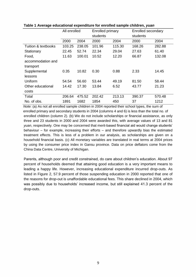
Table 1, the average educational expenditure for sample children in 2004 was 2.3 times that

of 2000. This was driven primarily by more costly secondary education, which was 1.5 times

as much in 2004 as in 2000.

The increasing financial burden was ultimately transferred to students. In a country-wide

survey from Brown and Park (2002), school fees accounted for half of the rural households’

consumption expenditure. In the study areas of Gansu, on average 29.4 percent of our

sample households borrowed money through either formal or informal channels, particularly

for paying education-related fees. As shown in Table 2, the household educational

expenditure per child accounted for 43.78 percent of its per capital net income in 2000 and

this share rose dramatically to 64 percent in 2004. The burden for the poor living below the

international poverty line was about 10 percentage points higher in both years than for the

non-poor.

run primary schools by themselves and 95 villages reported that children studied in the primary schools locating in the village.

9

Table 1 Average educational expenditure for enrolled sample children, yuan

All enrolled Enrolled primary

students

Enrolled secondary

students

2000 2004 2000 2004 2000 2004

Tuition & textbooks 103.25 238.05 101.96 115.30 168.26 282.88

Stationary 22.45 52.74 22.34 29.04 27.63 61.40

Food,

accommodation and

transport

11.63 100.01 10.52 12.20 66.87 132.08

Supplemental

lessons

0.35 10.82 0.30 0.88 2.33 14.45

Uniform 54.54 56.60 53.44 49.19 81.50 58.44

Other educational

costs

14.42 17.30 13.84 6.52 43.77 21.23

Total 206.64 475.52 202.42 213.13 390.37 570.48

No. of obs. 1891 1682 1854 450 37 1212

Note: (a) As not all enrolled sample children in 2004 reported their school types, the sum of

enrolled primary and secondary students in 2004 (columns 4 and 6) is less than the total no. of

enrolled children (column 2). (b) We do not include scholarships or financial assistance, as only

three and 23 students in 2000 and 2004 were awarded this, with average values of 13 and 81

yuan, respectively. One may be concerned that merit-based financial aid would change students’

behaviour – for example, increasing their efforts – and therefore upwardly bias the estimated

treatment effects. This is less of a problem in our analysis, as scholarships are given on a

household financial basis. (c) All monetary variables are translated in real terms at 2004 prices

by using the consumer price index in Gansu province. Data on price deflators come from the

China Data Centre, University of Michigan.

Parents, although poor and credit constrained, do care about children’s education. About 97

percent of households deemed that attaining good education is a very important means to

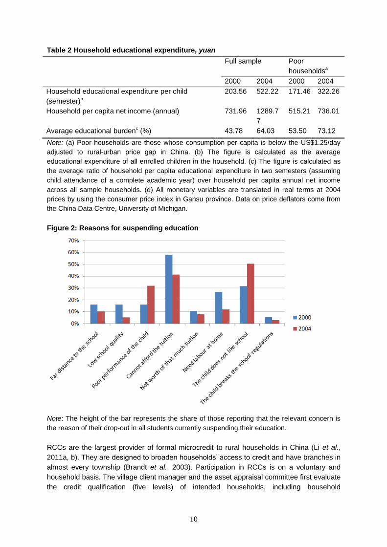
leading a happy life. However, increasing educational expenditure incurred drop-outs. As

listed in Figure 2, 57.9 percent of those suspending education in 2000 reported that one of

the reasons for drop-out is unaffordable educational fees. This share declined in 2004, which

was possibly due to households’ increased income, but still explained 41.3 percent of the

drop-outs.

10

Table 2 Household educational expenditure, yuan

Full sample Poor

householdsa

2000 2004 2000 2004

Household educational expenditure per child

(semester)b

203.56 522.22 171.46 322.26

Household per capita net income (annual) 731.96 1289.7

7

515.21 736.01

Average educational burdenc (%) 43.78 64.03 53.50 73.12

Note: (a) Poor households are those whose consumption per capita is below the US$1.25/day

adjusted to rural-urban price gap in China. (b) The figure is calculated as the average

educational expenditure of all enrolled children in the household. (c) The figure is calculated as

the average ratio of household per capita educational expenditure in two semesters (assuming

child attendance of a complete academic year) over household per capita annual net income

across all sample households. (d) All monetary variables are translated in real terms at 2004

prices by using the consumer price index in Gansu province. Data on price deflators come from

the China Data Centre, University of Michigan.

Figure 2: Reasons for suspending education

Note: The height of the bar represents the share of those reporting that the relevant concern is

the reason of their drop-out in all students currently suspending their education.

RCCs are the largest provider of formal microcredit to rural households in China (Li et al.,

2011a, b). They are designed to broaden households’ access to credit and have branches in

almost every township (Brandt et al., 2003). Participation in RCCs is on a voluntary and

household basis. The village client manager and the asset appraisal committee first evaluate

the credit qualification (five levels) of intended households, including household

11

demographic and economic information and past history of borrowing, and then issue

accordingly a certificate of loan stating the maximum amount of loans permitted. The loan

allowed by RCCs varies from 1,000 to 50,000 yuan in the study areas, supporting clients’

various activities, including both production and consumption plans.7 The client decides

whether, when and how much to borrow within their credit limit. The repayment is on a

quarterly basis and the certificate of loan is re-evaluated annually, according to the client’s

up-to-date situation. Households in our panel showed relatively high access to RCCs. In

2000 and 2004, respectively, 43.3 percent and 35.2 percent took loans. The real average

amount of loans borrowed by households was 1,825.8 yuan in 2000 and 3413.7 yuan in

2004, registering an increase of 87 percent. However, the difficulty of borrowing was

intensified over time. In 2004, 60.5 percent of sample households felt that it was difficult to

obtain loans from RCCs compared to the situation three years ago. This might explain the

lower share of borrowers in 2004 than in 2000.

2.2. Variable description

As our dependent variable, children’s educational outcome is measured by two indicators, to

take into account both quantity and quality of education: schooling and academic

performance. For the former, we follow Maldonado and González-Vega (2008) and construct

a variable of schooling gap to capture the phenomena of late entry, failed grades and

suspended schooling from time to time, as described in Section 2.1. That is,

max 0, schooling gap expected schooling observed total years of schooling (1)

where the expected schooling is defined as

0 6

6 7

if ageexpected schooling

age if age

(2)

and

observed total years of schooling = actual (levels) years of schooling - repeated grades (3)

The schooling gap reflects the difference between children’s actual years of schooling since

their first enrolment in primary schools and the desired years of schooling at their age. It is

zero for those successfully completing their education without any late entry, repeated

grades or drop-out. The presence of any one of these problems will make the value of

schooling gap positive. For academic performance, we use the average score of the sample

child’s Chinese and mathematical tests in the most recent semester they attended.

The most important independent variable of interest is households’ borrowing of microcredit.

The models used are briefly explained in the next section. Here we introduce first four other

categories of control variables that are susceptible to influencing children’s educational

outcomes based on previous studies (e.g., Brown and Park, 2002; Zhao and Glewwe, 2010).

Table 3 presents descriptive statistics for all variables in our analysis.

7 For detailed information on credit levels, see

http://www.gsrcu.com/www/ContentsDisp.asp?id=930&ClassId=14 [in Chinese, accessed June 4, 2012].

12

Table 3 Descriptive statistics

Variable 2000 2004

Mean S.D. Mean S.D.

Schooling gap 1.707 1.143 2.282 1.916

Average scores 73.179 13.279 73.310 13.551

Microcredit (yes=1) 0.457 0.498 0.352 0.478

Age 11.042 1.153 15.088 1.159

Gender (boy=1) 0.533 0.499 0.533 0.499

Ethnic minority (yes=1) 0.019 0.136 0.019 0.136

Health status 4.246 0.949 4.090 0.925

Birth order 1.724 0.804 1.718 0.786

Siblings’ education 12.590 7.018 1.677 0.809

Child labour 2.878 6.183 8.925 10.356

Attending the nearest school (yes=1) 0.975 0.157 0.922 0.268

Capability of studying 2.954 0.747 3.311 0.937

Father’s education 6.954 3.518 6.818 3.962

Mother’s education 3.875 4.345 4.200 3.629

Parents’ attitude: child education 3.567 0.704 3.825 0.473

Parents’ attitude: child’s future income 2.032 0.582 2.080 0.589

Women’s empowerment on child education 1.886 0.474 1.887 0.502

Ln(hh wealth) 7.089 1.068 7.397 1.084

Ln(tuition fees per child) 5.203 0.611 5.923 0.801

Ln(other education cost per child) 4.491 1.023 5.330 1.264

Teacher’s education 12.025 0.949 14.152 1.160

Student-teacher ratio 24.241 8.704 22.496 13.290

% of unsafe classrooms 0.198 0.297 0.226 0.353

Village distance to the nearest primary school (km) 0.579 0.876 3.273 3.100

Village distance to the nearest junior middle school (km) 1.051 0.333 4.310 4.235

Age at the first enrolment in the village 6.674 0.672 6.295 0.886

Proceed to secondary education in villagea 0.892 0.201 0.113 0.162

% of RCCs borrowers in the village 0.591 0.286 0.301 0.242

Ln(village per capita income) 5.754 2.651 6.352 2.346

Note: (a) It is proxied by the enrolment rate of junior high school in village in 2000 and the share

of completing junior high school in village primary students in 2004. Due to data limitations, we

cannot obtain exactly same indicators in two surveys.

First, we consider the sample child’s characteristics, such as age, gender, ethnic identity,

health status, whether attending the nearest schools, capability of studying according to the

teachers’ perception and child labour in terms of the time spent in housework. In particular,

we include birth order and siblings’ average schooling to reflect the competition of resources

for children within the household. We also explicitly control for the sample child’s tuition fees

and other educational costs separately, considering the educational reform of cancelling

tuition fees of primary and secondary education beginning in 2006.

Second, we include parents’ educational backgrounds, women’s empowerment measured

by mothers’ power in decision-making relating to children’s education, and the household

13

characteristics like the wealth level. It is notable that here we may face difficulties in

identification, as higher educational achievement is often associated with more power in

families’ decision-making and there might be sorting in marriage (Duflo, 2011). Including

siblings’ average schooling, as mentioned above, could help us address the identification

problem. Meanwhile, we also add parents’ attitudes towards the sample child’s education by

using the following two indicators: to what extent they expect the sample child to receive

more education; and willingness to provide financial assistance to them in the future. These

factors control explicitly for parents’ underlying intention for children’s education and

therefore, help in identifying the impact of parents’ education.

Third, the sample children’s teachers and schools are taken into account, given that good

educational resources are crucial for better educational outcomes (see Glewwe et al., 2011

for a recent comprehensive review). More specifically, we include teachers’ educational

levels and, at the school level, the student-teacher ratio and the share of unsafe classrooms.

Fourth, the local geographical, cultural and economic situation could also affect child-rearing.

Our selected indicators at the village level are distances to the nearest primary or junior high

school, average age at the first enrolment, the share of primary students completing junior

high schools, the share of households having access to RCCs and the village income per

capita.8

With these variables on hand, we proceed to set up the RDD to investigate the attributes of

children’s education outcomes, emphasising the role of household borrowing behaviour of

microcredit.

3. Methodology

3.1. Regression-discontinuity design with a time-variant assignment variable

Given that RCCs do not set a single criterion for lending, but their managers evaluate the

risk of intended households, we first construct an ‘assignment variable’ in the literature of

RDD, which determines the household’s treatment receipt of RCCs. Specifically, we

estimate households’ borrowing behaviour by a standard probit regression:

0 1 2Pr 1| , Pr 0i i i v i v ip B Z Z Z Z u (4)

where iB equals 1 when the household actually borrows RCCs and 0 otherwise; ip takes

the value of one if the household i is a debtor to RCCs at time t and zero otherwise. The

selection of explanatory variables is compatible with the regulations by which the client

manager issues RCCs9 and other possible determinants based on the past literature. In

particular, iZ denotes household characteristics. First, it includes household size, the

8 It is notable that although we tried to take into account many possible attributes in order to help

purge the causal impact from borrowing behaviour of other potential causes, there are underlying factors that may significantly affect the household’s ability and willingness to borrow, but could not be included due to data limitation, like membership in the Communist Party and location near a useful road. 9 For detailed regulations in Gansu province, see

http://www.gsrcu.com/www/ContentsDisp.asp?id=1015&ClassId=48 [in Chinese, accessed June 4, 2012].

14

number of family members currently not living in the household, the number of employed

members, average educational level and age of all household members, household

perception of its total income in the previous year (i.e., whether its income was enough to

support daily life), the quality of housing, the ratio of irrigated land over the total farmland

owned by the household and the wealth status of the household among the village. These

are considered by the manager to estimate the client’s risk of default and the ability of

repayment. Second, iZ variables are (1) whether borrowing RCCs for educational purposes

and (2) availability of informal loans for the households, such as from friends, neighbours

and relatives. These are selected out of consideration of household consumption demand for

credit and of the fact that informal lending has long been prevailing in rural China. A recent

study by Turvey and Kong (2010) finds that about two-thirds of rural households borrow from

friends or relatives, given strong trust in Chinese rural communities and informal lending

tends to crowd out the borrowing of RCCs. vZ is a set of village dummies in order to control

for common time trend and other unobserved heterogeneity.

The predicted probability of borrowing ˆip serves as the ‘assignment variable’. Given that ˆ

ip

is derived by considering various factors affecting the credit level/limit assigned for the

household by the manager and the household’s real demand for credit, it can also be

understood as an index of the household ability/willingness to borrow. A household is

considered to borrow RCCs, that is, receiving the treatment, if its ability/willingness to borrow

is higher than 50 percent. Therefore, the probability of being treated can be written by a

function that is discontinuous at 0.5.10

ˆ1 0.5

ˆ0 0.5

i

i

i

if pb

if p

(5)

In the context of more than one cross-sectional data, the treatment receipt of RCCs hinges

on household changing ability/willingness to borrow over time relative to the cut-off that

confines the outcome of whether or not the household would borrow (Van der Klaauw,

2008). Here we follow Van der Klaauw (2008) and repeat the above estimation for each

round of the surveys to obtain the household ability, ˆitp , which could vary over time for the

same household i. By doing so, we actually treat two surveys separately, as if they are

independent from each other. We will take into account dynamic treatment in the next sub-

section.

The description of RCCs in Section 2 suggests that households do not necessarily borrow

up to their credits limits, although their qualification allows this (higher than 0.5). The

imperfect compliance among those ‘eligible’ clients conforms to a ‘fuzzy’ regression-

discontinuity design (FRD in Imbens and Lemieux, 2008), which will be elaborated in the rest

of this sub-section.

10

We cannot bypass the arbitrariness in defining the assignment threshold. The sensitivity of our estimation to the choice of cut-off will be discussed in Footnote 16 in Section 4.2.

15

In the presence of self-selection of borrowing RCCs, there are the unobservables relating to

both households’ ability/willingness to borrow and their actual treatment status. However,

since households are unable to precisely control for their ability/willingness to borrow,

everyone close to the assignment threshold would have a similar chance of having their

ability index higher or lower than 0.5. In other words, borrowing RCCs is randomly assigned

for households whose predicted probability of borrowing is within a narrow interval around c,

which is akin to a quasi-experiment (a local randomised experiment in Lee and Lemieux,

2010). Therefore, the causal impact of households’ borrowing of RCCs on their children’s

education outcomes can be identified locally by comparing those children with their families’

predicted probability of borrowing barely passing the threshold c (the treatment group) with

those barely below it (the control group), i.e., the local average treatment effect (LATE).

Based on Eq. (5), the actually observed educational outcome for the sample child i at time t

can be expressed by 1 1 0it it it it ity b y b y , where 1ity and 0ity are the

outcomes with and without borrowing RCCs, respectively. The outcome ity is written by:

0it it ity b (6)

where 00it ity and 1 0it ity y . This leads to expression of the idea of

comparing the treatment and control groups at the cut-off as:

ˆ ˆ

ˆ ˆ ˆ ˆ0.5 0.5 0.5 0.5

ˆ ˆ ˆ| 0.5 lim | lim |

ˆ ˆ ˆ ˆ lim | lim | lim | lim |

it it it it itp c p c

it it it it it it it itp p p p

E p E y p E y p

E b p E b p E p E p

(7)

In the quasi-experimental environment around the threshold, households’ imprecise control

over their ability/willingness to borrow means that ˆ| itE p and ˆ|it itE p are continuous

at the cut-off (Hahn et al., 2001).11 It follows Eq. (7) that the LATE is formulated as:

0

ˆ ˆ0.5 0.5

ˆ ˆ0.5 0.5

ˆ ˆ| 0.5 lim | 0.5 0.5 1, 0.5

ˆ ˆlim | lim |

ˆ ˆlim | lim |

it it it it it ite

it it it itp p

it it it itp p

E p E b e b e p

E y p E y p

E b p E b p

(8)

Empirically, we adopt three different methods to estimate Eq. (8) in an effort to attain

robustness. First, Hahn et al.’s (2001) ‘local Wald’ estimator is employed for the non-

parametric case. Drawing only upon information of observations in the neighbourhood of the

cut-off, the limits in Eq. (8) are calculated as ˆ 0.5

ˆlim | t

t

it iti

it itp

iti

y wE y p

w

,

11

This assumption will be tested in Section 4.1.

16

ˆ 0.5

1ˆlim |

1

t

t

it iti

it itp

iti

y wE y p

w

,

ˆ 0.5ˆlim | t

t

it iti

it itp

iti

b wE d p

w

and

ˆ 0.5

1ˆlim |

1

t

t

it iti

it itp

iti

b wE b p

w

where the indicator variable ˆ0.5 0.5it it tw I p h

defines whether the observation lies above the cut-off with the optimal bandwidth th

selected by Imbens and Kalyanaraman’s (2009) procedures at time t;

ˆ| 0.5 0.5t t it ti i h p h is the sub-sample containing those residing in the

vicinity of the cut-off.12

Second, in the semi-parametric case, we employ Van der Klaauw’s (2008) two-step

estimation which offers a useful complement to the LATE by making use of the information

of full sample. Specifically, the first step estimates the probability of treatment receipt in a

standard probit specification,

ˆ ˆ ˆ ˆ| Pr 1| 0.5it it it it it itE b p b p p g p 1 (9)

where measures the discontinuity at the cut-off; ˆitg p is a quadratic piecewise function

parameterised by:

22

0 1 2 3 3ˆ ˆ ˆ ˆ ˆ ˆ0.5 0.5 0.5it it it it it itg p p p p p p 1 (10)

In the second step, using Eq. (9) in the outcome regression yields a reduced-form control-

function augmented outcome equation:

0 1 2 3 4ˆ ˆ|it it it it ht st vt t it ity E b p X X X X k p (11)

where Xit and Xht represent sample children and their families’ characteristics described in

Section 2.2; the school and village information is controlled by Xst and Xvt; and t denotes the

time fixed effects. We further include a control function ˆitk p for ˆ|it itE p to control for

the potential association between the household ability/willingness to borrow and children’s

educational outcomes. ˆitk p

ought to be a smooth and continuous function to ensure that

in the absence of the treatment, the educational outcomes are a smooth function of the

ability/willingness to borrow and hence, deferential educational outcomes are the only

source of discontinuity around the cut-off. Empirically, we let it take a semi-parametric form,

1

ˆ ˆJ j

it j itjk p p

, to accommodate non-linearity, where the power J is left determined by

12

We also estimated the left- and right-hand sides of the limits relative to the cut-off in Eq. (8) by using the triangle kernel putting more weights to observations closer to the cut-off and having proved better properties at boundaries (Ludwig and Miller, 2010). The results are broadly similar to the local Wald estimators in Tables 4-5.

17

generalised cross-validation of data. reflects the average treatment effect defined in Eq.

(8) (Van der Klaauw, 2008).

Third, as a variant to Van der Klaauw (2008), we use a standard instrumental variable (IV)

approach to estimate Eq. (11). The instruments consist of the random treatment assignment

bit acting as the excluded instrument for households’ observed borrowing status of RCCs

(Hahn et al., 2001) and the independent variables except ˆ|it itE b p in Eq. (11) serving as

the included instruments.

It is worth noting that as the above estimation is implemented to each survey separately, in

response to year-to-year variation in households’ ability/willingness to borrow relative to the

cut-off, captures essentially a short-term effect of obtaining RCCs on children’s education

outcomes.13 Moreover, given the imperfect compliance for those whose ability is higher than

0.5, should be treated as a lower bound of the true causal impact of RCCs.

3.2. Dynamic regression-discontinuity design

In the context of panel data, multiple treatments become available. The dynamics in bit

means that a household which did not borrow RCCs before might change their mind in

subsequent years. The causal effect of RCCs therefore contains two different kinds, given its

nature of voluntary borrowing: the intent-to-treat (ITT) effect; and the treatment-on-the-

treated (TOT) effects. ITT exogenously makes a household able and willing to borrow RCCs

in one year and compares the eligible borrowers with non-eligible borrowers at the threshold,

leaving the household’s observed borrowing behaviour of RCCs in subsequent years as it is.

By contrast, TOT prohibits new borrowers. It measures the effect of borrowing years ago

on the child’s current educational outcomes, had the household been unable to obtain RCCs

in all subsequent years.

The LATE defined in Eq. (8) equals the ITT divided by the fraction of individuals induced to

borrow RCCs at the cut-off of their ability/willingness index. In the context of dynamic

treatment assignment, however, TOT might be a more relevant indicator, considering that in

the presence of voluntary borrowing of RCCs, those who have not participated in RCCs will

never be required to borrow. Moreover, one cannot conclude the role of RCCs by looking at

the ITT only, as the estimated impact of RCCs in later years might be overshadowed by the

cumulative effect of loans having been obtained before. By exploiting the panel data, we are

able to disentangle the cumulative impact of RCCs on child education from the average

treatment effect in Section 3.1 – that is, the dynamic ITT and TOT effects separately over

time.

Suppose that the child i’s educational outcomes are measured in year t, while the RCCs

became available 0,1,2, ,T years ago for the family h with the child i. The family h

decides whether to borrow at t , ,i tb , and has a record of borrowing behaviour in

13

If estimating the pooled sample instead, actually measures an average treatment effect of RCCs

in different years within the sample period.

18

subsequent years, , 1, ,i t itb b . Adopting Cellini et al.’s (2010) dynamic RD strategy, we

estimate the ITT by the following outcome regression:

0 1 2 3 4ˆITT

it it it ht st vt t it ity b X X X X k p (12)

where represents fixed effects for years relative to the borrowing; other variables are

defined as before. As shown by the subscripts in Eq. (12), the observations in the standard

panel data need to be rearranged in the form of child-calendar-years relative to the

borrowing. In other words, there could be multiple observations in the new dataset for the

same child in the same calendar year, but with different time elapsed compared to the year

of borrowing. The OLS is applied to the rearranged dataset to estimate Eq. (12). Taking

Cellini et al.’s (2010) suggestion, we cluster standard errors by child to account for possible

dependence across observations ,i t and serial correlation in it caused by the multi-use

of observations ,i t .

As Cellini et al. (2010), we then expand the equation of the definition of the ITT effect of the

household’s initial borrowing decision in year t on its child’s education outcomes at t:

, 1 , 2

, , , 1 , , 2 , ,

,

1, , ,

d dd d

d d d d

d

d

i t i tITT it it it it it it

i t i t i t i t i t i t it i t

i t hit it

hi t i t h i t

TOT

b by y y y y b

b b b b b b b b

by y

b b b

1

TOT

h h

h

(13)

where 0 0

ITT TOT and ,

,

d

d

i t h

h

i t

b

b

measures the effect of borrowing RCCs in year t

on the probability of borrowing RCCs again h years later. ˆh can be obtained by estimating

Eq. (12) with the dependent variable being replaced by itb . Reverting Eq. (13) yields our

recursive estimates of TOT

:

1

TOT ITT TOT

h h

h

(14)

Arguably the TOT effects depend only on the time elapsed since the borrowing behaviour at

t , i.e., h, while irrelevant to the time t or the history of past borrowing behaviour.

19

4. Estimation results and discussion

We begin by discussing the internal validity of our RDD set-up.14 We test for the assumptions

ensuring successful identification of the treatment effect of borrowing RCCs. The results of

the static and dynamic RDD models in Section 3 are then presented in turn.

4.1. Identification problems in RDD

The RDD is regarded as having higher internal validity than other ‘quasi-experimental’

methods, which, however, needs to be justified as the estimated treatment effect hinges on

some important setting of the dataset (Imbens and Lemieux, 2008).

First, to validate the quasi-experimental environment and therefore the causal inferences

around the cut-off, the treatment should be randomly assigned for the sub-sample near the

cut-off of the assignment variable that we have observed. Households may influence the

assignment variable, i.e., their ability/willingness to borrow, through their characteristics and

action (e.g., the explanatory variables in Eq. 4), while also experiencing a random

unobserved component affecting their chance of having a particular level of ability. This latter

makes RDD similar to a randomised experiment in a neighbourhood around the cut-off.

Thus, the treatment status should by construct be independent of the pre-determined

(baseline) covariates (Lee and Lemieux, 2010), which means that the differences in

educational outcomes between borrowers and non-borrowers are not confounded by either

observed or unobserved omitted variables. We test for this by re-calculating the local Wald

estimator of LATE by adding other covariates in Eq. (6), including the characteristics of the

sample children and their families, schools and villages. The results are broadly same as

columns 1 and 5 of Tables 4-5,15 implying that borrowing behaviour is the only source of

differential educational outcomes.

Second, the above assumption of randomised experiments at the cut-off also requires that

the average educational outcomes for children whose families’ abilities to borrow fall barely

below the cut-off should ideally form a valid counterfactual to be compared with those in the

treated group. It is therefore necessary to investigate whether households can fully

‘manipulate’ the assignment variable, so that they self-select into groups of borrowers or

non-borrowers. If so, borrowers would be systematically different from non-borrowers. We

implement the density test formulated by McCrary (2008). The conditional density of

household ability index on two potential types of households distinguished by the cut-off is

expected to be continuous without manipulation. Therefore, a household experiences equal

chance of falling above or below the cut-off, irrespective of the type that it belongs to. As

seen in Figure 3, although the estimated conditional density seems to give some indication

of discontinuity around the cut-off, the ‘jump’ of the conditional density function at the cut-off

is statistically insignificant in both years. The null hypothesis of zero discontinuity in the

14

The external validity of RDD in the non-parametric case is less than other ‘quasi-experimental’ methods, since the LATE draws upon sub-samples close to the cut-off only. However, this may not be a serious problem, as we also employed Van der Klaauw’s (2008) semi-parametric estimation and standard IV estimation, taking advantage of full sample and cross-compared our estimation results in Section 4.2. 15

Results are not shown in the paper, given limited space, but are available upon request from the authors.

20

Table 4: FRD estimates of impacts of borrowing RCCs on the schooling gap

Independent variable

2000 2004

Local Wald

(1)

Two-step

CF (2)

Two-step CF

(3)

Standard IV

(4)

Local Wald

(5)

Two-step

CF (6)

Two-step

CF (7)

Standard IV

(8)

ˆ ˆ0.5 0.5

ˆ ˆlim | lim |it it it itp p

E y p E y p

-0.317*

(0.187)

-0.336

(0.280)

ˆ ˆ0.5 0.5

ˆ ˆlim | lim |it it it itp p

E b p E b p

0.110

(0.091)

0.102

(0.072)

ˆ| 0.5it itE p -2.884

(3.134)

-3.276

(3.563)

-2.853**

(1.259)

-2.557**

(1.194)

-5.430

(7.872)

-1.260

(2.205)

-0.094

(1.579)

-0.039

(1.758)

Child characteristics

Age 0.447***

(0.033)

0.481***

(0.038)

0.526***

(0.153)

0.551***

(0.067)

0.405***

(0.122)

0.402***

(0.124)

Gender -0.046

(0.062)

-0.006

(0.080)

0.050

(0.271)

-0.112

(0.121)

0.513***

(0.191)

0.514***

(0.191)

Health status -0.127***

(0.042)

-0.135***

(0.045)

-0.161

(0.144)

-0.046

(0.092)

0.071

(0.125)

0.073

(0.130)

Ethnic minority -0.218

(0.413)

0.676

(0.489)

0.535

(1.231)

0.289

(1.161)

-0.518

(0.784)

-0.507

(0.790)

Birth order 0.308***

(0.080)

0.437***

(0.091)

0.606

(0.484)

0.036

(0.134)

0.124

(0.205)

0.125

(0.204)

Child labour -0.011*

(0.006)

-0.015**

(0.006)

-0.019

(0.015)

0.007

(0.015)

0.003

(0.007)

0.003

(0.007)

Capability of studying -0.068

(0.052)

-0.128*

(0.067)

-0.231

(0.314)

-0.113*

(0.065)

-0.201

(0.126)

-0.200

(0.126)

Siblings’ education -0.030***

(0.007)

-0.057***

(0.012)

-0.065*

(0.038)

-0.152

(0.132)

0.094

(0.275)

0.092

(0.273)

Attending the nearest school -0.607*

(0.323)

-0.489*

(0.300)

-0.342

(0.903)

-0.606

(0.444)

-0.898**

(0.389)

-0.898**

(0.389)

Parents’ characteristics

Father’s education -0.016

(0.011)

-0.036**

(0.015)

-0.053

(0.058)

-0.052**

(0.023)

-0.049

(0.046)

-0.049

(0.047)

Mother’s education -0.024***

(0.008)

0.001

(0.008)

0.007

(0.027)

0.013

(0.020)

-0.011

(0.042)

-0.011

(0.042)

Parents’ attitude: child education -0.169***

(0.052)

-0.155**

(0.061)

-0.157

(0.188)

-0.203

(0.148)

-0.259

(0.273)

-0.256

(0.274)

21

Parents’ attitude: child’s income -0.019

(0.054)

0.018

(0.060)

0.040

(0.187)

0.075

(0.086)

0.099

(0.173)

0.101

(0.174)

Women’s empowerment on child

education

-0.128**

(0.061)

0.008

(0.053)

0.055

(0.193)

-0.012

(0.083)

0.139

(0.226)

0.133

(0.236)

Household characteristics

Ln(hh wealth per capita) 0.127*

(0.070)

0.131*

(0.070)

0.250

(0.361)

0.101

(0.107)

0.147

(0.131)

0.146

(0.132)

Ln(sample child’s tuition) -0.240**

(0.106)

-0.115

(0.102)

-0.112

(0.227)

-0.904***

(0.260)

-0.021

(0.300)

-0.018

(0.302)

Ln(sample child’s other edu. costs) -0.122**

(0.053)

-0.086*

(0.048)

-0.143

(0.199)

-0.065

(0.113)

-0.225

(0.163)

-0.229

(0.168)

Teacher and school characteristics

Teachers’ average edu. -0.243**

(0.060)

-0.252

(0.178)

-1.137***

(0.159)

-1.137***

(0.159)

Student-teacher ratio -0.020***

(0.008)

-0.032

(0.036)

0.0003

(0.006)

0.0002

(0.006)

% unsafe classrooms 0.159

(0.229)

-0.023

(0.793)

1.055**

(0.410)

1.048**

(0.415)

Village characteristics

Distance to the nearest primary

school

-0.037

(0.055)

-0.051

(0.139)

0.215

(0.140)

0.213

(0.149)

Distance to the nearest junior

middle school

-0.118

(0.102)

-0.164

(0.370)

0.047

(0.050)

0.048

(0.052)

Age at the first enrolment 0.164**

(0.069)

0.179

(0.195)

-0.189

(0.228)

-0.186

(0.233)

Proceed to secondary education 0.278

(0.380)

0.269

(1.074)

-2.672**

(1.046)

-2.688**

(1.063)

% of RCCs borrowers -0.625***

(0.238)

-0.728

(0.780)

-0.889

(1.555)

-0.916

(1.602)

Ln (village per capita income) -0.021

(0.024)

-0.009

(0.068)

-0.077

(0.054)

-0.076

(0.056)

School dummies Yes Yes

Village dummies Yes Yes

County dummies Yes Yes Yes Yes

R2

0.488 0.453 0.338 0.792 0.766 0.765

Note: ***, ** and * denote 1%, 5% and 10% significance levels in turn. Constants and dummies for the schools, villages and counties are not reported. Standard errors are in

parentheses and clustered by the household ability/willingness to borrow in order to mitigate possible misspecification problems, as suggested by Lee and Card (2008).

22

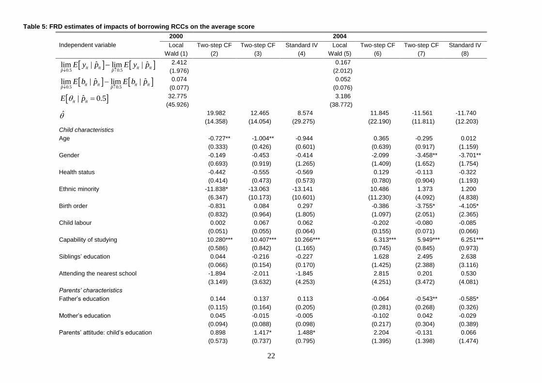
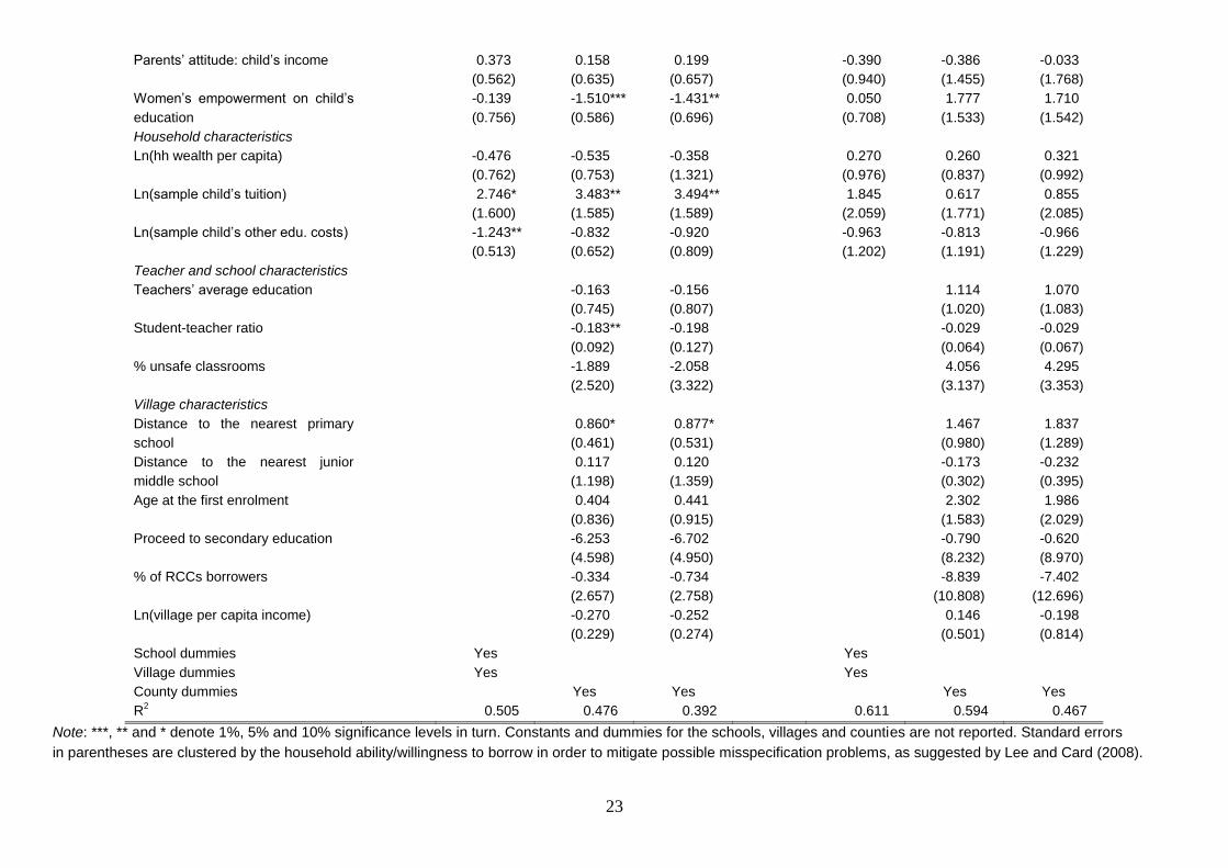
Table 5: FRD estimates of impacts of borrowing RCCs on the average score

Independent variable

2000 2004

Local

Wald (1)

Two-step CF

(2)

Two-step CF

(3)

Standard IV

(4)

Local

Wald (5)

Two-step CF

(6)

Two-step CF

(7)

Standard IV

(8)

ˆ ˆ0.5 0.5

ˆ ˆlim | lim |it it it itp p

E y p E y p

2.412

(1.976)

0.167

(2.012)

ˆ ˆ0.5 0.5

ˆ ˆlim | lim |it it it itp p

E b p E b p

0.074

(0.077)

0.052

(0.076)

ˆ| 0.5it itE p 32.775

(45.926)

3.186

(38.772)

19.982

(14.358)

12.465

(14.054)

8.574

(29.275)

11.845

(22.190)

-11.561

(11.811)

-11.740

(12.203)

Child characteristics

Age -0.727**

(0.333)

-1.004**

(0.426)

-0.944

(0.601)

0.365

(0.639)

-0.295

(0.917)

0.012

(1.159)

Gender -0.149

(0.693)

-0.453

(0.919)

-0.414

(1.265)

-2.099

(1.409)

-3.458**

(1.652)

-3.701**

(1.754)

Health status -0.442

(0.414)

-0.555

(0.473)

-0.569

(0.573)

0.129

(0.780)

-0.113

(0.904)

-0.322

(1.193)

Ethnic minority -11.838*

(6.347)

-13.063

(10.173)

-13.141

(10.601)

10.486

(11.230)

1.373

(4.092)

1.200

(4.838)

Birth order -0.831

(0.832)

0.084

(0.964)

0.297

(1.805)

-0.386

(1.097)

-3.755*

(2.051)

-4.105*

(2.365)

Child labour 0.002

(0.051)

0.067

(0.055)

0.062

(0.064)

-0.202

(0.155)

-0.080

(0.071)

-0.085

(0.066)

Capability of studying 10.280***

(0.586)

10.407***

(0.842)

10.266***

(1.165)

6.313***

(0.745)

5.949***

(0.845)

6.251***

(0.973)

Siblings’ education 0.044

(0.066)

-0.216

(0.154)

-0.227

(0.170)

1.628

(1.425)

2.495

(2.388)

2.638

(3.116)

Attending the nearest school -1.894

(3.149)

-2.011

(3.632)

-1.845

(4.253)

2.815

(4.251)

0.201

(3.472)

0.530

(4.081)

Parents’ characteristics

Father’s education 0.144

(0.115)

0.137

(0.164)

0.113

(0.205)

-0.064

(0.281)

-0.543**

(0.268)

-0.585*

(0.326)

Mother’s education 0.045

(0.094)

-0.015

(0.088)

-0.005

(0.098)

-0.102

(0.217)

0.042

(0.304)

-0.029

(0.389)

Parents’ attitude: child’s education 0.898

(0.573)

1.417*

(0.737)

1.488*

(0.795)

2.204

(1.395)

-0.131

(1.398)

0.066

(1.474)

23

Parents’ attitude: child’s income 0.373

(0.562)

0.158

(0.635)

0.199

(0.657)

-0.390

(0.940)

-0.386

(1.455)

-0.033

(1.768)

Women’s empowerment on child’s

education

-0.139

(0.756)

-1.510***

(0.586)

-1.431**

(0.696)

0.050

(0.708)

1.777

(1.533)

1.710

(1.542)

Household characteristics

Ln(hh wealth per capita) -0.476

(0.762)

-0.535

(0.753)

-0.358

(1.321)

0.270

(0.976)

0.260

(0.837)

0.321

(0.992)

Ln(sample child’s tuition) 2.746*

(1.600)

3.483**

(1.585)

3.494**

(1.589)

1.845

(2.059)

0.617

(1.771)

0.855

(2.085)

Ln(sample child’s other edu. costs) -1.243**

(0.513)

-0.832

(0.652)

-0.920

(0.809)

-0.963

(1.202)

-0.813

(1.191)

-0.966

(1.229)

Teacher and school characteristics

Teachers’ average education -0.163

(0.745)

-0.156

(0.807)

1.114

(1.020)

1.070

(1.083)

Student-teacher ratio -0.183**

(0.092)

-0.198

(0.127)

-0.029

(0.064)

-0.029

(0.067)

% unsafe classrooms -1.889

(2.520)

-2.058

(3.322)

4.056

(3.137)

4.295

(3.353)

Village characteristics

Distance to the nearest primary

school

0.860*

(0.461)

0.877*

(0.531)

1.467

(0.980)

1.837

(1.289)

Distance to the nearest junior

middle school

0.117

(1.198)

0.120

(1.359)

-0.173

(0.302)

-0.232

(0.395)

Age at the first enrolment 0.404

(0.836)

0.441

(0.915)

2.302

(1.583)

1.986

(2.029)

Proceed to secondary education -6.253

(4.598)

-6.702

(4.950)

-0.790

(8.232)

-0.620

(8.970)

% of RCCs borrowers -0.334

(2.657)

-0.734

(2.758)

-8.839

(10.808)

-7.402

(12.696)

Ln(village per capita income) -0.270

(0.229)

-0.252

(0.274)

0.146

(0.501)

-0.198

(0.814)

School dummies Yes Yes

Village dummies Yes Yes

County dummies Yes Yes Yes Yes

R2

0.505 0.476 0.392 0.611 0.594 0.467

Note: ***, ** and * denote 1%, 5% and 10% significance levels in turn. Constants and dummies for the schools, villages and counties are not reported. Standard errors

in parentheses are clustered by the household ability/willingness to borrow in order to mitigate possible misspecification problems, as suggested by Lee and Card (2008).

24

Figure 3: Relationship between actual and the predicted probability of borrowing

actual mean fraction

LOWESS smooth0.1

0.3

0.5

0.7

0.9

Actu

al m

ea

n fra

ctio

n o

f b

orr

ow

ing

0 10.2 0.4 0.6 0.80.5Household ability/willingness to borrow

(a) 2000

actual mean fractionLOWESS smooth

0.0

0.2

0.5

0.7

0.9

1

Actu

al m

ea

n fra

ctio

n o

f b

orr

ow

ing

0 10.2 0.4 0.6 0.80.5Household ability/willingness to borrow

(b) 2004

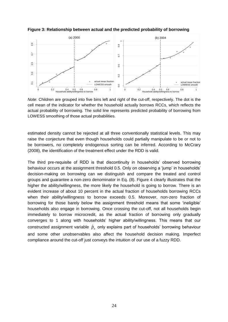
Note: Children are grouped into five bins left and right of the cut-off, respectively. The dot is the

cell mean of the indicator for whether the household actually borrows RCCs, which reflects the

actual probability of borrowing. The solid line represents predicted probability of borrowing from

LOWESS smoothing of those actual probabilities.

estimated density cannot be rejected at all three conventionally statistical levels. This may

raise the conjecture that even though households could partially manipulate to be or not to

be borrowers, no completely endogenous sorting can be inferred. According to McCrary

(2008), the identification of the treatment effect under the RDD is valid.

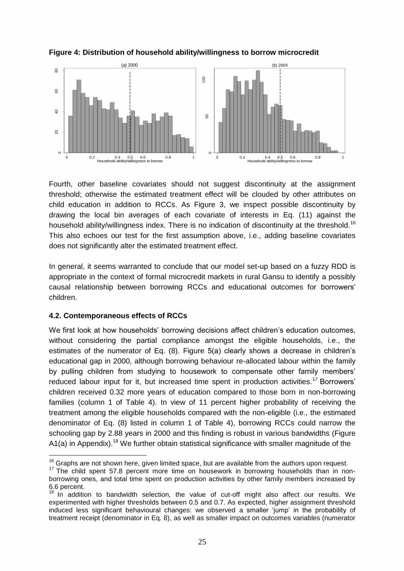
The third pre-requisite of RDD is that discontinuity in households’ observed borrowing

behaviour occurs at the assignment threshold 0.5. Only on observing a ‘jump’ in households’

decision-making on borrowing can we distinguish and compare the treated and control

groups and guarantee a non-zero denominator in Eq. (8). Figure 4 clearly illustrates that the

higher the ability/willingness, the more likely the household is going to borrow. There is an

evident increase of about 10 percent in the actual fraction of households borrowing RCCs

when their ability/willingness to borrow exceeds 0.5. Moreover, non-zero fraction of

borrowing for those barely below the assignment threshold means that some ‘ineligible’

households also engage in borrowing. Once crossing the cut-off, not all households begin

immediately to borrow microcredit, as the actual fraction of borrowing only gradually

converges to 1 along with households’ higher ability/willingness. This means that our

constructed assignment variable ˆitp only explains part of households’ borrowing behaviour

and some other unobservables also affect the household decision making. Imperfect

compliance around the cut-off just conveys the intuition of our use of a fuzzy RDD.

25

Figure 4: Distribution of household ability/willingness to borrow microcredit 0

20

40

60

80

Fre

qu

en

cy

0 10.2 0.4 0.6 0.80.5Household ability/willingness to borrow

(a) 2000

05

01

00

Fre

qu

en

cy

0 10.2 0.4 0.6 0.80.5Household ability/willingness to borrow

(b) 2004

Fourth, other baseline covariates should not suggest discontinuity at the assignment

threshold; otherwise the estimated treatment effect will be clouded by other attributes on

child education in addition to RCCs. As Figure 3, we inspect possible discontinuity by

drawing the local bin averages of each covariate of interests in Eq. (11) against the

household ability/willingness index. There is no indication of discontinuity at the threshold.16

This also echoes our test for the first assumption above, i.e., adding baseline covariates

does not significantly alter the estimated treatment effect.

In general, it seems warranted to conclude that our model set-up based on a fuzzy RDD is

appropriate in the context of formal microcredit markets in rural Gansu to identify a possibly

causal relationship between borrowing RCCs and educational outcomes for borrowers’

children.

4.2. Contemporaneous effects of RCCs

We first look at how households’ borrowing decisions affect children’s education outcomes,

without considering the partial compliance amongst the eligible households, i.e., the

estimates of the numerator of Eq. (8). Figure 5(a) clearly shows a decrease in children’s

educational gap in 2000, although borrowing behaviour re-allocated labour within the family

by pulling children from studying to housework to compensate other family members’

reduced labour input for it, but increased time spent in production activities.17 Borrowers’

children received 0.32 more years of education compared to those born in non-borrowing

families (column 1 of Table 4). In view of 11 percent higher probability of receiving the

treatment among the eligible households compared with the non-eligible (i.e., the estimated

denominator of Eq. (8) listed in column 1 of Table 4), borrowing RCCs could narrow the

schooling gap by 2.88 years in 2000 and this finding is robust in various bandwidths (Figure

A1(a) in Appendix).18 We further obtain statistical significance with smaller magnitude of the

16

Graphs are not shown here, given limited space, but are available from the authors upon request. 17

The child spent 57.8 percent more time on housework in borrowing households than in non-borrowing ones, and total time spent on production activities by other family members increased by 6.6 percent. 18

In addition to bandwidth selection, the value of cut-off might also affect our results. We experimented with higher thresholds between 0.5 and 0.7. As expected, higher assignment threshold induced less significant behavioural changes: we observed a smaller ‘jump’ in the probability of treatment receipt (denominator in Eq. 8), as well as smaller impact on outcomes variables (numerator

26

Figure 5: Schooling gap as a function of household ability/willingness index 1

.21

.41

.61

.82

2.2

Sch

oo

lin

g g

ap

0 10.50.2 0.4 0.6 0.8Household ability/willingness to borrow

(a) 2000

bandwidth=0.276

cell mean estimated schooling gap 95% CI

bandwidth=0.224

.51

1.5

22

.53

Sch

oo

lin

g g

ap

0 10.40.2 0.6 0.80.5Household ability/willingness to borrow

(b) 2004

cell mean estimated schooling gap 95% CI Note: Households are grouped into five bins left and right of the cut-off, respectively. The triangle

measures the average child education for those falling in the same bin. The solid line is the

kernel-weighted linear regression of the cell averages.

treatment effects of 2.56-2.85 years under the semi-parametric specification (columns 2-3 of

Table 4). We can see similar positive effects on schooling in 2004 (as illustrated in Figure

5(b)), while with larger magnitude of 0.34 (column 5 of Table 4). After considering the partial

compliance of 10 percent of eligible households, this leads to 3.28 years smaller schooling

gap, which is also robust across different bandwidths (Figure A1(b)). It appears that in the

circumstances of soaring educational costs, RCCs could assist households more in limiting

the child schooling gap. Nevertheless, all estimates in 2004 become statistically insignificant,

whichever the model specification is. Since unaffordable fees as a reason for drop-out fell by

16.6 percent between 2000 and 2004 (see Section 2), one can surmise that financial

concerns were no longer the biggest obstacle to education in 2004 compared to 2000.

Although educational costs rose quickly, many parents would still like to support their

children’s schooling, and 83.8 percent of parents expected their children to go to university in

the future. However, as shown by Figure 2 in Section 2, in 2004, children’s dislike of their

schools took over from unaffordable costs and emerged as the most frequently reported

reason for not attending schools (50.5 percent).

Regarding academic performance, Figure 6(a) reveals an increase in average scores, with

the magnitude of 2.41 points (column 1 of Table 5) in case of perfect compliance. The partial

compliance leads to 8.57-32.78 points in different model specifications (columns 1-4 of Table

5), however, the estimates are statistically insignificant and highly sensitive to the selection

of bandwidth (Figure A2(a)). Evidence in 2004 is mixed. Figure 6(b) suggests

in Eq. 8). As a result, the estimated impact of RCCs on schooling gap and scores reduced substantially under higher values of threshold. For example, if using 0.7 as the cut-off, the estimate of 2.88 years dropped to 0.1.

27

Figure 6: Scores as a function of household ability/willingness index

bandwidth=0.362

60

65

70

75

80

Ave

rag

e s

co

res

0 10.2 0.4 0.6 0.8Household ability/willingness to borrow

(a) 2000

cell mean estimated scores 95% CI

bandwidth=0.259

70

75

80

85

90

Ave

rag

e s

co

res

0 10.2 0.4 0.6 0.8Household ability/willingness to borrow

(b) 2004

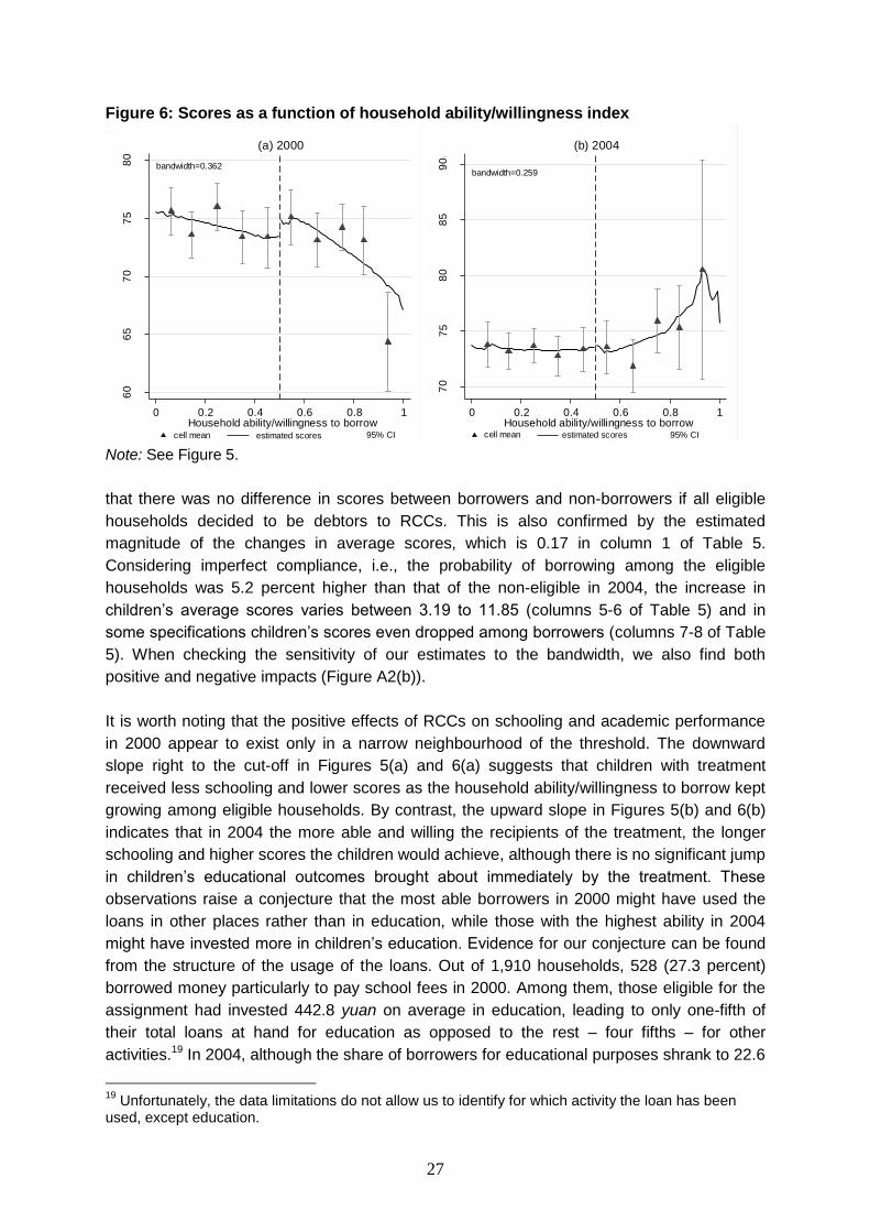
cell mean estimated scores 95% CI Note: See Figure 5.

that there was no difference in scores between borrowers and non-borrowers if all eligible

households decided to be debtors to RCCs. This is also confirmed by the estimated

magnitude of the changes in average scores, which is 0.17 in column 1 of Table 5.

Considering imperfect compliance, i.e., the probability of borrowing among the eligible

households was 5.2 percent higher than that of the non-eligible in 2004, the increase in

children’s average scores varies between 3.19 to 11.85 (columns 5-6 of Table 5) and in

some specifications children’s scores even dropped among borrowers (columns 7-8 of Table

5). When checking the sensitivity of our estimates to the bandwidth, we also find both

positive and negative impacts (Figure A2(b)).

It is worth noting that the positive effects of RCCs on schooling and academic performance

in 2000 appear to exist only in a narrow neighbourhood of the threshold. The downward

slope right to the cut-off in Figures 5(a) and 6(a) suggests that children with treatment

received less schooling and lower scores as the household ability/willingness to borrow kept

growing among eligible households. By contrast, the upward slope in Figures 5(b) and 6(b)

indicates that in 2004 the more able and willing the recipients of the treatment, the longer

schooling and higher scores the children would achieve, although there is no significant jump

in children’s educational outcomes brought about immediately by the treatment. These

observations raise a conjecture that the most able borrowers in 2000 might have used the

loans in other places rather than in education, while those with the highest ability in 2004

might have invested more in children’s education. Evidence for our conjecture can be found

from the structure of the usage of the loans. Out of 1,910 households, 528 (27.3 percent)

borrowed money particularly to pay school fees in 2000. Among them, those eligible for the

assignment had invested 442.8 yuan on average in education, leading to only one-fifth of

their total loans at hand for education as opposed to the rest – four fifths – for other

activities.19 In 2004, although the share of borrowers for educational purposes shrank to 22.6

19

Unfortunately, the data limitations do not allow us to identify for which activity the loan has been used, except education.

28

percent, the mean educational loans among educational borrowers with higher ability than

0.5 was nearly quadrupled to 1,652.3 yuan, possibly in response to the increased school

costs, as shown in Tables 1-2.20 The average share of educational borrowing in their total

loans rose up to 41.9 percent.

The above analysis suggests that formal microcredit is not automatically a magic bullet to

tackle the problems of child education, but needs to be monitored and guided. Imai et al.

(2010) and Imai and Azam (2012) also find that the impact on different welfare indicators

hinges on the different usage of microloans in the Indian and Bangladesh contexts,

respectively.

Of other explanatory variables, older age and illness of the sample child would make

children more likely to drop out. Within the family, competition for limited educational

resources matters for both schooling gap and academic performance. Children with later

birth order were less educated in 2000 (columns 2-3 of Table 4) and performed worse in

2004 (columns 7-8 of Table 5) than their elder siblings. Attending the nearest schools could

help reduce the schooling gap and this effect could be stronger in 2004 (columns 7-8 of

Table 4) than in 2000 (columns 2-3 of Table 4). As in 2004 most of sample children were at

the age of secondary education, this implies that attending the nearest schools could

facilitate more secondary education compared to primary education. Fathers’ education was

positively correlated with child schooling (columns 3 and 6 of Table 4), as found by Yi et al.

(2012), and this still holds, even after controlling for parents’ attitudes towards education

through variables of their expectations on the child’s highest educational achievement and

the siblings’ educational levels of the sample child; however, this did not necessarily improve

children’s academic performance (columns 7-8 of Table 5). As predicted, and as the study of

Zhao and Glewwe (2010) shows, parents’ higher expectation on children’s educational

attainment could keep children staying longer in schools and encourage them to achieve

higher scores. Nevertheless, these effects became statistically insignificant in 2004.

We find that women’s empowerment in terms of the position in decision-making on children’s

education only reduced marginally the schooling gap in 200021 (column 2 of Table 4) and

was even negatively correlated with children’s academic achievements (columns 3-4 of

Table 5).22 By re-estimating columns 2-4 of Table 5 with the interaction between mothers’

20

The monetary values in this and previous sentences are in real terms in 2004 prices according to the authors’ calculations. Price deflators are the rural CPI in Gansu province, which come from the China Data Centre at the University of Michigan. 21

One might be concerned with the identification of the impact of women’s empowerment on children’s educational outcomes, given positive correlation between access to microcredit and women’s power within the family found in many developing countries (Duflo, 2011). However, this might not cause serious bias in interpretation in our context, for two reasons. First, formal credits in rural China are in general not gender-targeted, but aimed at expanding credit access to rural households. Second, Li et al. (2011c) find that there exists a loan threshold of 30,000 yuan (equivalent to 24,324 yuan in 2004 prices) beyond which women’s power in decision-making begins to rise. In our panel, only 29 and 61 households (1.5 percent and 3.2 percent) in 2000 and 2004 respectively had more formal loans than this threshold. 22

We also re-estimated columns 2-4 and 6-8 by adding two other indicators of women’s empowerment, the power in managing family finances and planting crops, while we did not find statistical significance for them.

29

education and empowerment as an additional regressor, this latter may be a result of

mothers’ low educational levels, as indicated by the positive estimated coefficient (0.101):

being empowered to the same extent, less-educated women were less capable of helping

their children’s studies compared with those who were more educated. Moreover, as

summarised by Duflo (2011), women’s stronger position in decision-making within the family

is often related to improvement in child health and the family’s’ nutrients, health and housing,

while at the expense of child education. She points out that the welfare consequences of

empowering women depends on which objective is more important for women should they

be given more power. The negative effect of women’s empowerment on children’s academic

performance may be explained by the phenomenon that mothers with full control over

children’s education are more inclined to ask children to earn wage income than those

having zero influence on educational decision-making.23

Higher tuition fees and other unspecified educational costs were associated with smaller

schooling gap and better performance in 2000 only. Brown and Park (2002) derive similar

results. They attribute this to the fact that schools with better educational quality usually have

higher charges for students. As excpected, better educational quality proxied by teachers’

higher educational levels could narrow the children’s schooling gap in both 2000 and 2004,

and the magnitude in 2004 (-1.137) was more than four times as big as that in 2000 (-0.24 to

-0.25). This reflects parents’ increased consideration of educational quality when deciding

whether to send their children to schools. Nevertheless, the quality of schools’ physical

resources did not exhibit significant impact on children’s academic performance, which

alternatively is strongly affected by child capability for studying with the marginal effects

varying from five to 10 points.

Among various common factors shared by the villagers, later first enrolment could aggravate

children’s schooling gap, while pro-education culture represented by a higher share of

graduates from primary schools continuing to enter junior high schools substantially reduced

the schooling gap in 2004. The distance between the village and schools did not significantly

affect child schooling, but living in villages located further from primary schools slightly

increased children’s average scores in 2000 (columns 3-4 of Table 5). This might be

because the ‘key schools’ having more educational resources and better quality become

increasingly scattered in rural areas, as the government began to merge and reduce the

quantity of village schools in 2000, in the hope of enhancing each individual school’s quality.

Attending such ‘key schools’ would possibly mean higher academic achievement at the

expense of longer distance.

4.3. Dynamic effects of RCCs

Households’ ability/willingness to borrow RCCs evolves over time according to their

observed characteristics and the unobservables. Consequently, a previous borrower (non-

borrower) may become a non-borrower (borrower) and/or households may retain previous

decisions. In the presence of multiple treatments, the causal impact of RCCs derived from

our static analysis in Section 4.2 is a mixed outcome of households’ dynamic treatment

23

8.6 percent of mothers with full control over educational decision-making reported that they often asked their children to earn wage income, as opposed to 5.5 percent of those with zero control.

30

status. This sub-section proceeds to distinguish between short- and long-run impacts of

microcredit by drawing upon the dynamic FRD in Section 3.2.

Table 6 presents the estimation results. The general finding on explanatory variables in the

static RDD is also confirmed in the dynamic analysis, although a few lose or gain statistical

significance.24 For example, gender difference turned out to emerge in schooling gap, with

girls lacking behind, but disappeared in average scores. Some attributes lose their

explanatory power in Table 6 compared to Tables 4-5, such as child health, whether

attending the nearest school, parents’ attitudes towards the child’s educational

achievements, share of unsafe classrooms and the village progression rate to junior high

schools. In comparison, some became statistically significant, like two other indicators for

school quality.

The negative 1 in all columns, albeit statistically insignificant, implies that in general those

who had borrowed in 2000 would be 2.1-5.2 percent less likely to enter the second bids in

2004. The contemporaneous ITT effects of microcredit, 0ˆITT , become insignificant compared

to those in Tables 4-5, while borrowing of microcredit appears to improve longer-term

education for clients’ children. 1ˆITT

in columns 1-2 of Table 6 suggests that children of

clients in 2000 would enjoy 3.3-3.6 months less educational gap and 4.9-7.2 higher average

scores in 2004 compared to their counterparts in the non-client families, leaving the 2000

clients to make subsequent decisions on borrowing as they wish.

Prior to discussing the TOT estimates, we first examine the nature of our data on the

dynamics of treatment receipt, in order to better understand how households build or lose

their ability/willingness to borrow over time and this induced changes in treatment status. We

compare past borrowing behaviour in 2000 for sub-samples lying within ±5 percent, ±3

percent and ±1 percent of the cut-off in 2004. The 2000 recipiency rate of households just

above the cut-off in each of the three sub-groups is 57.8 percent, 85.3 percent and 75

24

An exemption is child labour. In the dynamic analysis (Column 1 of Table 6), one more hour of child labour per week would enlarge the schooling gap by 6.5 days within a year. However, the static analysis (columns 2-3 of Table 4) suggests the opposite: more child labour tended to narrow the schooling gap in 2000. Using data from rural Bangladesh, Islam and Choe (2013) attribute this to the fact that borrowing households use more child labour than non-borrowers. As borrowing microcredit helps to reduce the schooling gap, child labour thus might negatively correlate to the schooling gap. However, this seems counterintuitive – if borrowing is associated with use of child labour, then RCCs will have an adverse effect on attendance, leading to possibly poor performance. But we do not observe statistical significant relationship between borrowing RCCs and child average scores in the static analysis (Table 5).

31

Table 6 Dynamic treatment effects of borrowing RCCs

Independent variable Schooling gap Average scores

(1) (2) (3) (4) (5) (6)

A. ITT

0ˆITT

0.046

(0.050)

0.078

(0.064)

0.074

(0.061)

6.267***

(2.297)

-1.591

(1.399)

-1.440

(1.366)

1ˆITT -0.278***

(0.107)

-0.299*

(0.182)

-0.288

(0.184)

2.639

(2.079)

4.915*

(2.741)

7.160**

(2.833)

Child characteristics

Age 0.287***

(0.073)

0.131***

(0.024)

0.147***

(0.025)

-1.113

(1.401)

0.339

(0.463)

0.484

(0.498)

Gender -0.112

(0.124)

-0.092*

(0.050)

-0.069

(0.049)

-1.514

(3.095)

0.411

(1.073)

0.081

(1.065)

Health status 0.082

(0.078)

-0.008

(0.028)

-0.027

(0.028)

0.509

(1.621)

1.135*

(0.593)

1.284**

(0.625)

Ethnic minority -0.139

(0.277)

0.386

(0.483)

0.394

(0.462)

-13.138***

(5.446)

-0.913

(4.764)

1.868

(4.148)

Birth order 0.062

(0.167)

0.099**

(0.049)

0.084*

(0.049)

3.103

(2.660)

-1.152

(1.138)

-1.680

(1.164)

Child labour 0.018**

(0.007)

-0.003

(0.003)

-0.002

(0.003)

0.104

(0.151)

-0.051

(0.086)

-0.025

(0.089)

Capability of studying -0.002

(0.066)

-0.056*

(0.031)

-0.048

(0.031)

5.138**

(2.083)

4.110***

(0.824)

4.324***

(0.825)

Siblings’ education -0.453***

(0.164)

-0.015***

(0.005)

-0.013***

(0.005)

-1.189

(4.098)

-0.013

(0.113)

0.093

(0.114)

Attending the nearest school 0.317

(0.318)

-0.143

(0.119)

-0.121

(0.126)

-8.830

(14.143)

2.931

(4.051)

5.308

(3.801)

Parents’ characteristics

Father’s education -0.049** -0.018* -0.019** -0.261 0.107 -0.010

32

(0.023) (0.009) (0.005) (0.432) (0.177) (0.174)

Mother’s education 0.017

(0.024)

-0.003

(0.005)

0.001

(0.005)

0.547

(0.567)

0.150

(0.115)

0.183

(0.112)

Parents’ attitude: child’s edu. -0.035

(0.131)

-0.064

(0.045)

-0.061

(0.045)

-4.210

(4.056)

1.544*

(0.865)

1.312

(0.860)

Parents’ attitude: child’s inc. -0.072

(0.104)

0.029

(0.042)

0.028

(0.041)

-1.250

(2.734)

0.450

(0.855)

0.225

(0.820)

Women’s empowerment on child’s edu. 0.049

(0.109)

0.036

(0.030)

0.040

(0.031)

4.351***

(1.652)

0.795

(0.786)

0.426

(0.746)

Household characteristics

Ln(hh wealth per capita) 0.222

(0.174)

-0.022

(0.074)

-0.036

(0.074)

4.302

(4.470)

1.680

(1.496)

1.889

(1.584)

Ln(sample child’s tuition) -0.134

(0.125)

-0.098*

(0.051)

-0.134**

(0.055)

5.238*

(2.848)

2.748***

(1.021)

2.568**

(1.018)

Ln(sample child’s other edu. costs) -0.151**

(0.067)

-0.091***

(0.028)

-0.096***

(0.029)

1.739

(1.611)

0.203

(0.524)

0.172

(0.574)

Teacher and school characteristics

Teachers’ average edu. -0.034

(0.030)

-0.027

(0.034)

0.487

(0.623)

0.737

(0.702)

Student-teacher ratio -0.001

(0.003)

-0.002

(0.005)

0.039

(0.088)

-0.082

(0.103)

% unsafe classrooms 0.328***

(0.126)

0.309**

(0.150)

4.538***

(1.747)

2.901

(2.005)

Village characteristics

Distance to the nearest primary school 0.026

(0.018)

-0.013

(0.028)

0.479

(0.449)

0.227

(0.524)

Distance to the nearest junior middle school 0.051

(0.050)

-0.004

(0.062)

0.311

(0.873)

2.231**

(0.989)

Age at the first enrolment 0.062* 0.048 2.526*** 1.035

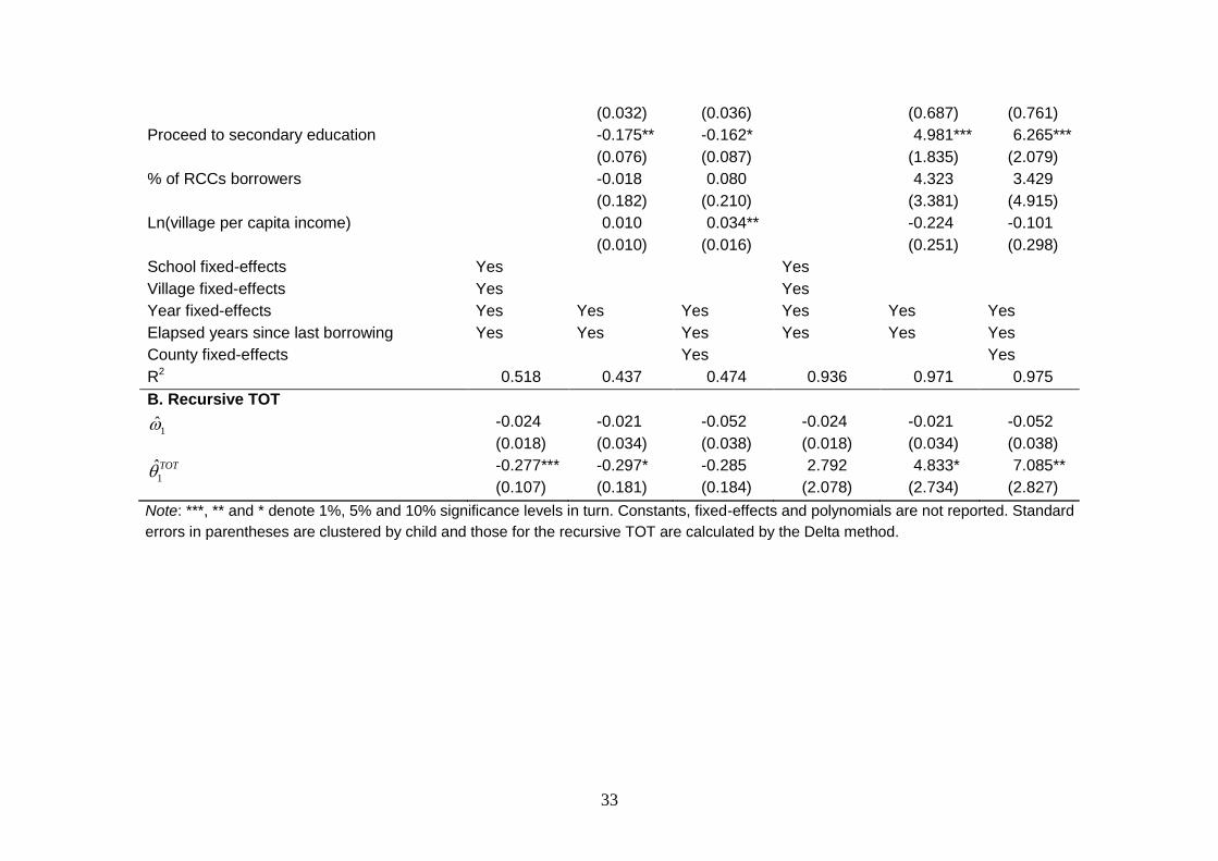
33

(0.032) (0.036) (0.687) (0.761)

Proceed to secondary education -0.175**

(0.076)

-0.162*

(0.087)

4.981***

(1.835)

6.265***

(2.079)

% of RCCs borrowers -0.018

(0.182)

0.080

(0.210)

4.323

(3.381)

3.429

(4.915)

Ln(village per capita income) 0.010

(0.010)

0.034**

(0.016)

-0.224

(0.251)

-0.101

(0.298)

School fixed-effects Yes Yes

Village fixed-effects Yes Yes

Year fixed-effects Yes Yes Yes Yes Yes Yes

Elapsed years since last borrowing Yes Yes Yes Yes Yes Yes

County fixed-effects Yes Yes

R2 0.518 0.437 0.474 0.936 0.971 0.975

B. Recursive TOT

1 -0.024

(0.018)

-0.021

(0.034)

-0.052

(0.038)

-0.024

(0.018)

-0.021

(0.034)

-0.052

(0.038)

1ˆTOT -0.277***

(0.107)

-0.297*

(0.181)

-0.285

(0.184)

2.792

(2.078)

4.833*

(2.734)

7.085**

(2.827)

Note: ***, ** and * denote 1%, 5% and 10% significance levels in turn. Constants, fixed-effects and polynomials are not reported. Standard

errors in parentheses are clustered by child and those for the recursive TOT are calculated by the Delta method.

34

percent, respectively, and exceeds that of those just below by -31.2, 3.2 and 8.3 percentage

points in turn. Similarly, we restrict samples to those within ±5 percent, ±3 percent and ±1

percent of the cut-off in 2000. The 2004 recipiency rate of households just above the cut-off

in each of the three sub-groups is 29.6 percent, 29.4 percent and 44.4 percent, respectively,

and exceeds that of those just below the cut-off by 6.6, 12.7 and 44.4 percentage points in

turn. These observations bear out two implications. First, 0ˆITT is an average outcome of the

cumulative effect of repeated borrowing and newly gaining RCCs status, while 1ˆITT

measures the consequence of both retaining debtors and those playing a ‘one-shot game’ by

exiting RCCs after 2000. This fleshes out our model set-up for ITT in Eq. (13). Second, the

cumulative impact of borrowing may explain more proportion of the ITT effects than new

entry or exit. Overall, the hybrid nature of the variation in the household treatment status

makes disentangling TOT from ITT effects not only important but also necessary to let our

estimation results better inform policy.

Based on the estimates of 0ˆITT and 1

ˆITT , we disentangle the long-term impact of a single

bid, 1ˆTOT , by exogenously authorising the borrowing of microcredit in 2000, but prohibiting

subsequent borrowing behaviour thereafter. Significantly negative 1ˆTOT in columns 1- 2 and

positive estimates in columns 5- 6 means that families’ borrowing behaviour in 2000 alone

was sufficient to narrow their children’s schooling gap by 3.3-3.6 months and to improve

children’s average scores by 4.8-7 points. Moreover, broadly similar magnitude of 1ˆTOT and

1ˆITT echoes the above exploratory analysis that protracted effects of microcredit dominate

the immediate impact of borrowing behaviour in benefiting child education.

5. Conclusion

This paper provides empirical evidence on the welfare effectiveness of microcredit

programmes in the context of an under-developed province of China, Gansu. It assesses the

causal impact of borrowing formal microcredit on children’s educational outcomes in a quasi-

experimental environment. We further distinguish between the immediate effects of

microcredit for borrowers’ welfare and longer-term consequences of borrowing behaviour.

Borrowing microcredit can bring about immediate consequences to narrowing child

schooling gap in 2000 by a magnitude of nearly three years. This positive treatment effect

becomes statistically insignificant over time, although RCCs appear to play a greater role in

improving schooling (with 0.4 more years in 2004) when households are faced with

escalating educational costs. There is no indication on improved academic performance for

borrowers. On identifying causal relationship running from formal microcredit to schooling

gap, pushing the lever of microcredit upwards can improve children’s schooling, which in

turn is likely to help Chinese rural households break the vicious circle between insufficient

education and poverty and establish a virtuous circle by removing educational exclusion.

We indeed find indication of such a positive role of formal microcredit in the longer term.

When incorporating the dynamics in treatment assignment, previous borrowing behaviour

35

takes over the role of current involvement. Irrespective of whether we prohibit households

from subsequent bids, the initial borrowers’ children appear to enjoy a modest reduction in

schooling gap by one semester (three to four months) and an appreciable increase in

average scores by five to seven points. While formal financial institutions need to guide the

usage of microcredit, especially for the most able/willing households, in order to channel the

loans to educational purposes for their children, policy addressing rising educational costs

for poor rural households for its own sake should be emphasised. Microfinance would

function better to improve welfare for its clients had education policy been designed

concurrently. Moreover, considering that most clients of RCCs are relatively rich households

(Li et al., 2011a), formal microcredit would contribute to child education more effectively if

the targeting problem for the poor could be alleviated.

36

References

Armendáriz de Aghion, B. and Morduch, J. (2005). The Economics of Microfinance.

Cambridge, MA: The MIT Press.

Banerjee, A., Duflo, E., Glennerster, R. and Kinnan, C. (2009). ‘The miracle of microfinance?

Evidence from a randomized evaluation’. Institute for Financial Management and Research

Working Paper Series, No.31.

Brandt, L., Park, A. and Wang, S. (2003). ‘Are China’s financial reforms leaving the poor

behind?’ In Huang, Y., Saich, A. and Steinfeld, E. (eds.), Financial Sector Reform in China.

Cambridge, MA: Harvard East Asian Press.

Brown, P. H. and Park, A. (2002). ‘Education and poverty in rural China’. Economics of

Education Review 21, 523-541.

Cellini, S. R., Ferreira, F. and Rothstein, J. (2010). ‘The value of school facility investments:

Evidence from a dynamic regression discontinuity design’. Quarterly Journal of Economics

125, 215-261.

Coleman, B. (1999). ‘The impact of group lending in northeast Thailand’. Journal of

Development Economics 60, 105-141.

Doan, T., Gibson, J. and Holmes, M. (2011). ‘Impacts of household credit on education and

healthcare spending by the poor in peri-urban areas in Vietnam’. Department of Economics

Working Paper Series 06/11, University of Waikato.

Dong, F., Lu, J. and Featherstone, A. M. (2010). ‘Effects of credit constraints on productivity

and rural household income in China’. Center for Agricultural and Rural Development

Working Paper, No. 516, Iowa State University.

Duflo, E. (2011). ‘Women’s empowerment and economic development’. NBER Working

Paper, No. 17702.

Glewwe, P. W., Hanushek, E. A., Humpage, S. D. and Ravina, R. (2011). ‘School resources

and educational outcomes in developing countries: A review of the literature from 1990 to

2010’. NBER Working Paper, No. 17554.

Gustafsson, B. and Li, S. (2004). ‘Expenditures on education and health care and poverty in

rural China’. China Economic Review 15, 292-301.

Hahn, J., Todd, P. E. and Van der Klaauw, W. (2001). ‘Identification and estimation of

treatment effect with a regression-discontinuity design’. Econometrica 69, 201-209.

37

Hannum, E. and Kong, P. (2007). ‘Educational resources and impediments in rural Gansu,

China’. The World Bank Working Paper Series No. 40251. Human Development Sector Unit

East Asia and the Pacific Region.

Hazarika, G. and Sarangi, S. (2008). ‘Household access to microcredit and child labor in

rural Malawi’. World Development 36, 843-859.

Hermes, N. and Lensink, R. (2011). ‘Microfinance: Its impact, outreach, and sustainability’.

World Development 39, 875-881.

Imai, K. S., Arun, T. and Annim, S. K. (2010). ‘Microfinance and household poverty

reduction: New evidence from India’. World Development 38, 1760-1774.

Imai, K. S. and Azam, M. S. (2012). ‘Does microfinance reduce poverty in Bangladesh? New

evidence from household panel data’. Journal of Development Studies 48, 633-653.

Imbens, G. W. and Kalyanaraman, K. (2009). ‘Optimal bandwidth choice for the regression

discontinuity estimator’. NBER Working Paper, No. 14726.

Imbens, G. W. and Lemieux, T. (2008). ‘Regression discontinuity designs: A guide to

practice’. Journal of Econometrics 142, 615-635.

Islam, A. (2011). ‘Medium- and long-term participation in microcredit: An evaluation using

new panel dataset from Bangladesh’. American Journal of Agricultural Economics 93, 847-

866.

Islam, A. and Choe, C. (2013). ‘Child labor and schooling responses to access to microcredit

in rural Bangladesh’. Economic Inquiry 51, 46-61.

Islam, A. and Maitra, P. (2012). ‘Health shocks and consumption smoothing in rural

households: Does microcredit have a role to play?’ Journal of Development Economics 97,

232-243.

Khandker, S. R. (2005). ‘Microfinance and poverty: Evidence using panel data from

Bangladesh’. World Bank Economic Review 19, 263-286.

Knight, J., Li, S. and Deng, Q. (2009). ‘Education and the poverty trap in rural China: Setting

the trap’. Oxford Development Studies 37, 311-332.

Knight, J., Li, S. and Deng, Q. (2010). ‘Education and the poverty trap in rural China: Closing

the trap’. Oxford Development Studies 38, 1-24.

Knight, J. Sicular, T. and Yue, X. (2011). ‘Education inequality in China: The

intergenerational dimension’. CIBC Working Paper Series, No. 2011-13, University of

Western Ontario.

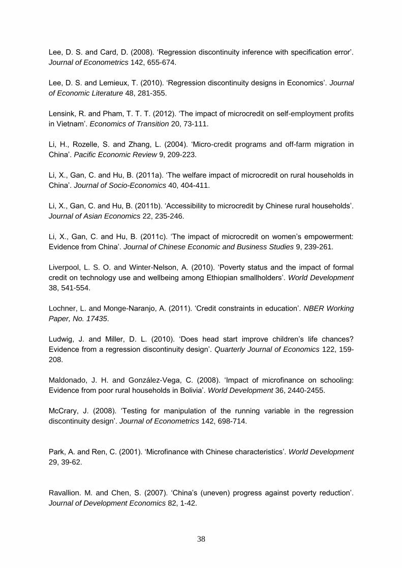
38

Lee, D. S. and Card, D. (2008). ‘Regression discontinuity inference with specification error’.

Journal of Econometrics 142, 655-674.

Lee, D. S. and Lemieux, T. (2010). ‘Regression discontinuity designs in Economics’. Journal

of Economic Literature 48, 281-355.

Lensink, R. and Pham, T. T. T. (2012). ‘The impact of microcredit on self-employment profits

in Vietnam’. Economics of Transition 20, 73-111.

Li, H., Rozelle, S. and Zhang, L. (2004). ‘Micro-credit programs and off-farm migration in

China’. Pacific Economic Review 9, 209-223.

Li, X., Gan, C. and Hu, B. (2011a). ‘The welfare impact of microcredit on rural households in

China’. Journal of Socio-Economics 40, 404-411.

Li, X., Gan, C. and Hu, B. (2011b). ‘Accessibility to microcredit by Chinese rural households’.

Journal of Asian Economics 22, 235-246.

Li, X., Gan, C. and Hu, B. (2011c). ‘The impact of microcredit on women’s empowerment:

Evidence from China’. Journal of Chinese Economic and Business Studies 9, 239-261.

Liverpool, L. S. O. and Winter-Nelson, A. (2010). ‘Poverty status and the impact of formal

credit on technology use and wellbeing among Ethiopian smallholders’. World Development

38, 541-554.

Lochner, L. and Monge-Naranjo, A. (2011). ‘Credit constraints in education’. NBER Working

Paper, No. 17435.

Ludwig, J. and Miller, D. L. (2010). ‘Does head start improve children’s life chances?

Evidence from a regression discontinuity design’. Quarterly Journal of Economics 122, 159-

208.

Maldonado, J. H. and González-Vega, C. (2008). ‘Impact of microfinance on schooling:

Evidence from poor rural households in Bolivia’. World Development 36, 2440-2455.

McCrary, J. (2008). ‘Testing for manipulation of the running variable in the regression

discontinuity design’. Journal of Econometrics 142, 698-714.

Park, A. and Ren, C. (2001). ‘Microfinance with Chinese characteristics’. World Development

29, 39-62.

Ravallion. M. and Chen, S. (2007). ‘China’s (uneven) progress against poverty reduction’.

Journal of Development Economics 82, 1-42.

39

Rui, L. and Xi, Z. (2010). ‘Econometric analysis of credit constraints of Chinese rural

households and welfare loss’. Applied Economics 42, 1615-1625.

Smith, J. and Todd, P. (2005). ‘Does matching overcome Lalonde’s critique of

nonexperimental estimators?’ Journal of Econometrics 125, 305-353.

Sun, A. and Yao, Y. (2010). ‘Health shocks and children’s school attainments in rural China’.

Economics of Education Review 29, 375-382.

Turvey, C. G. and Kong, R. (2010). ‘Informal lending amongst friends and relatives: Can

microcredit compete in rural China?’ China Economic Review 21, 544-556.

Van der Klaauw, W. (2008). ‘Breaking the link between poverty and low student

achievement: An evaluation of Title I’. Journal of Econometrics 142, 731-756.

Weiss, J. and Montgomery, H. (2005). ‘Great expectations: Microfinance and poverty

reduction in Asia and Latin America’. Oxford Development Studies 33, 391-416.

Yi, H., Zhang, L., Luo, R., Shi, Y., Mo, D., Chen, X., Brinton, C. and Rozelle, S. (2012).

‘Dropping out: Why are students leaving junior high in China’s poor rural areas?’

International Journal of Educational Development 32, 555-563.

Zhang, X., Xu, Z., Shen, M. and Cheng, E. (2010). ‘Rural finance in poverty-stricken areas in

the People’s Republic of China: Balancing government and market’. Asian Development

Bank, Philippines.

Zhao, M. and Glewwe, P. (2010). ‘What determines basic school attainment in developing

countries? Evidence from rural China’. Economics of Education Review 29, 451-460.

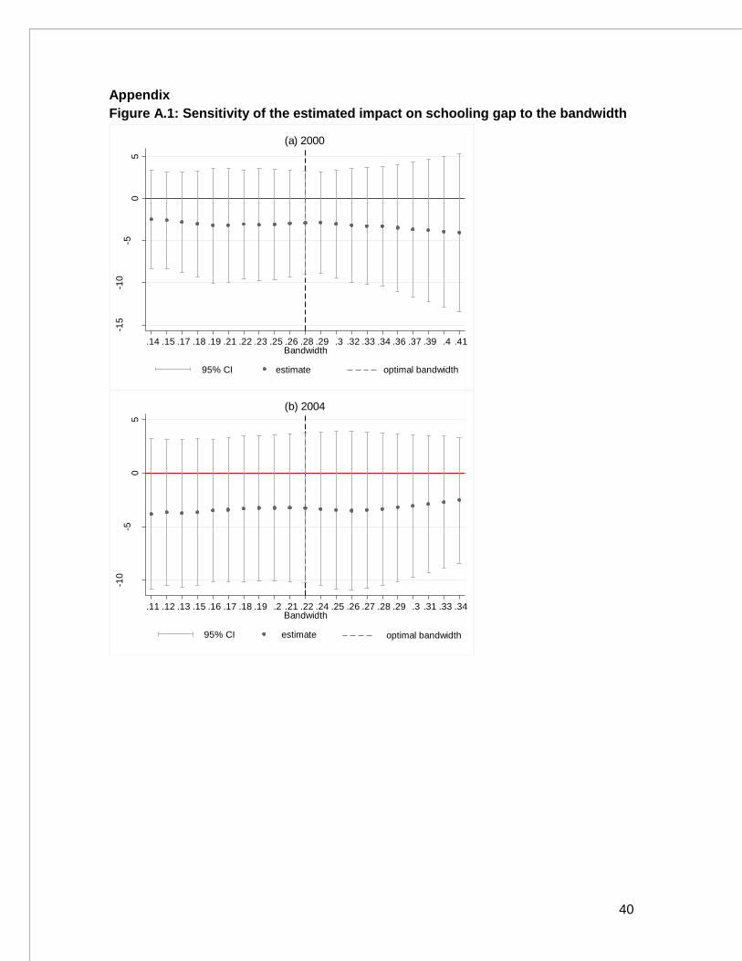
40

Appendix

Figure A.1: Sensitivity of the estimated impact on schooling gap to the bandwidth -1

5-1

0-5

05

Estim

ate

d e

ffe

ct

.28 .14 .15 .17 .18 .19 .21 .22 .23 .25 .26 .29 .3 .32 .33 .34 .36 .37 .39 .4 .41Bandwidth

95% CI estimate

(a) 2000

optimal bandwidth

-10

-50

5

Estim

ate

d e

ffe

ct

.22 .11 .12 .13 .15 .16 .17 .18 .19 .2 .21 .24 .25 .26 .27 .28 .29 .3 .31 .33 .34Bandwidth

95% CI estimate

(b) 2004

optimal bandwidth

41

Figure A.2: Sensitivity of the estimated impact on average scores to the bandwidth -2

00

-10

0

0

10

02

00

30

0

Estim

ate

d e

ffe

ct

.36 .18 .2 .22 .24 .25 .27 .29 .31 .33 .34 .38 .4 .42 .43 .45 .47 .49 .51 .52 .54Bandwidth

95% CI estimate

(a) 2000

optimal bandwidth

-15

0-1

00

-50

05

01

00

Estim

ate

d e

ffe

ct

.26 .13 .14 .15 .17 .18 .19 .2 .22 .23 .24 .27 .28 .29 .31 .32 .33 .34 .36 .37 .38Bandwidth

95% CI estimate

(b) 2004

optimal bandwidth

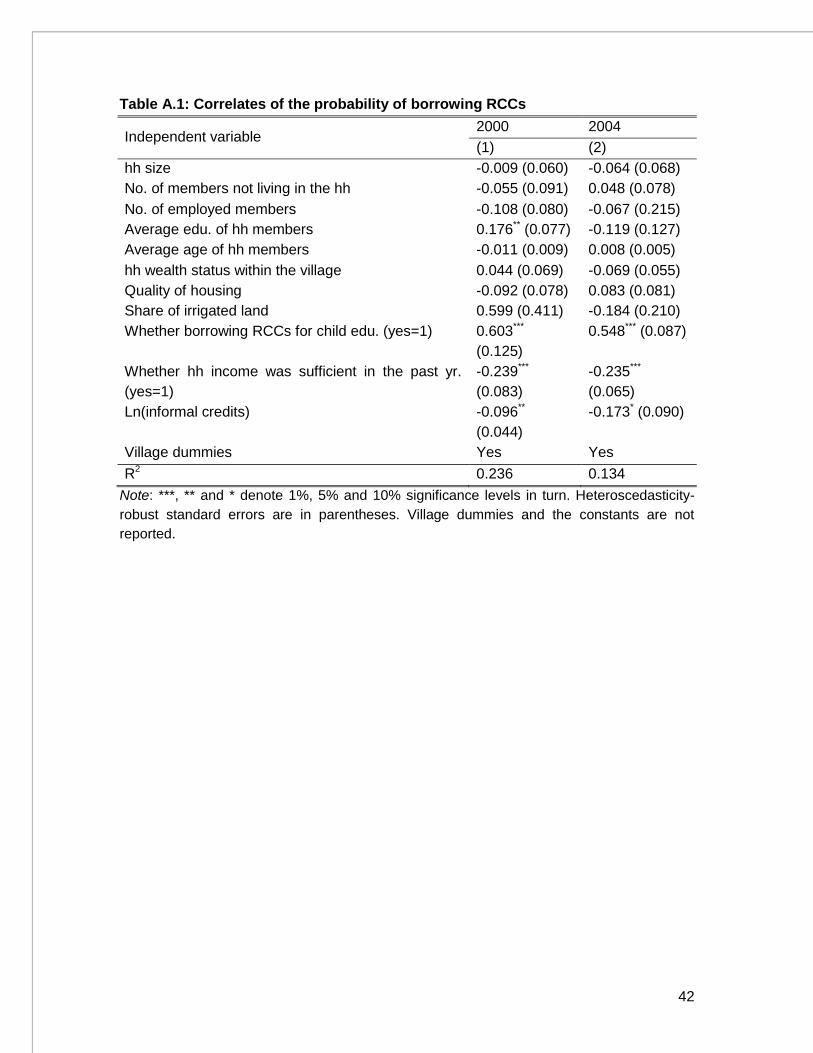
42

Table A.1: Correlates of the probability of borrowing RCCs

Independent variable 2000 2004

(1) (2)

hh size -0.009 (0.060) -0.064 (0.068)

No. of members not living in the hh -0.055 (0.091) 0.048 (0.078)

No. of employed members -0.108 (0.080) -0.067 (0.215)

Average edu. of hh members 0.176** (0.077) -0.119 (0.127)

Average age of hh members -0.011 (0.009) 0.008 (0.005)

hh wealth status within the village 0.044 (0.069) -0.069 (0.055)

Quality of housing -0.092 (0.078) 0.083 (0.081)

Share of irrigated land 0.599 (0.411) -0.184 (0.210)

Whether borrowing RCCs for child edu. (yes=1) 0.603***

(0.125)

0.548*** (0.087)

Whether hh income was sufficient in the past yr.

(yes=1)

-0.239***

(0.083)

-0.235***

(0.065)

Ln(informal credits) -0.096**

(0.044)

-0.173* (0.090)

Village dummies Yes Yes

R2 0.236 0.134

Note: ***, ** and * denote 1%, 5% and 10% significance levels in turn. Heteroscedasticity-

robust standard errors are in parentheses. Village dummies and the constants are not

reported.

Executive Director Professor David Hulme Research Directors Professor Armando Barrientos Professor Rorden Wilkinson Contact: Brooks World Poverty Institute The University of Manchester Arthur Lewis Building Oxford Road Manchester M13 9PL United Kingdom Email: [email protected] www.manchester.ac.uk/bwpi

The Brooks World Poverty Institute (BWPI) creates and

shares knowledge to help end global poverty.

BWPI is multidisciplinary, researching poverty in both

the rich and poor worlds.

Our aim is to better understand why people are poor,

what keeps them trapped in poverty and how they can

be helped – drawing upon the very best international

practice in research and policy making.

The Brooks World Poverty Institute is chaired by Nobel

Laureate, Professor Joseph E. Stiglitz.

www.manchester.ac.uk/bwpi