The Impact of Financial Crises and IT Revolution on Income ... · financial crises and IT revolution have generated larger income multiplier effect on Higher IT- intensive Manufacturing

For presentation at WIOD Conference (2012) Groningen (The Netherlands), April 24-26, 2012

The Impact of Financial Crises and IT Revolution on Income Distribution in Korea:

Evidence from Social Accounting Matrices

Hak K. Pyo1, Keun Hee Rhee** and Gong Lee***

Abstract

In recent years, Korea had experienced two financial crises in 1997-1998 and 2007-2008 respectively and the IT revolution during the interval between the two financial crises. We have constructed Social Accounting Matrix (SAM) in 2000 and 2009 for Korea by combining Input-output tables used in WIOD project in Korea with data from 10-decile Urban Household Income Survey. We analyze gross income effect and income redistribution effect of financial crises and IT revolution by adopting a SAM framework following Pyatt and Round (2004) and Saari, Dietzenbacher and Los (2010). Both financial crises and IT revolution have generated larger income multiplier effect on Higher IT-intensive Manufacturing sector but have affected negatively on income redistribution of lower income groups.

1 Director, Center for National Competitiveness and Faculty of Economics, Seoul National University, Seoul 151-746, Korea. Tel: +82-2-880-6395. Fax: +82-2-886-4231. E-mail: [email protected]. Corresponding author. ** Senior Researcher, Korea Productivity Center, E-mail:[email protected] *** Ph.D. Candidate, Department of Economics, Seoul National University, Seoul 151-746, Korea. Tel: +82-10-9586-2020, Fax: +82-2-886-4231, E-mail: [email protected]

1. INTRODUCTION Social Accounting Matrix (SAM) provides a useful framework to analyze the composition of national income and product and the process of income distribution. Even though SAM is a static analytical tool, we can examine the dynamic aspects of national income composition and its distribution by comparing two SAM over a time interval. We have shown in a recent report (Pyo, Kim and Lee (2011)) using SAM with the household micro cell by age group that exogenous injections of income to government mostly benefit the relative income of the pensioners, the age group over 60. The empirical result is consistent with that of Llop and Manresa (2004) who have found that exogenous injections of income to government mostly benefit the relative income of inactive households, which are mainly those of pensioners and have argued that such empirical evidence is important for policy making if the policies are aimed at modifying the distribution of income among economic agents. The purpose of the present paper is to analyze the impacts of IT revolution and two financial crises on the determination of national income and changes in the level of income of endogenous sectors through multiplier analysis and the structure of income distribution by constructing micro cell of household sector. As analyzed in Pyo (2000), the growth rate of real GDP which had averaged 7.1 percent during the pre-crisis period of 1993-1997 declined sharply recording – 6.9 percent in year 1998 when the so-called twin crises had hit the Korean economy. The financial crisis of 1997-1998 was called twin crises because there were both domestic banking crisis and foreign exchange crisis. As documented in Pyo (2004a) and Otsu and Pyo (2009), the macroeconomic adjustment during the post-crisis period was a successful one largely due to remarkable export performance helped by Won depreciation. During the period of 1998-2007, the export performance led by IT-intensive products has helped the economy to make a sustainable growth. When the global financial crisis occurred in 2007-2008, the recovery pattern of the Korean economy has been quite similar to the recovery pattern after the 1997-1998 crises. Korean Won was depreciated against not only US dollar but also Yen, Euro and Yuan and strong export performance in IT-intensive manufactures followed. We have attempted to analyze the impact of large scale depreciations immediately after two financial crises and export drive of IT-intensive products during the two post-crisis periods by multiplier and redistribution analysis based on SAM. For the purpose, we have constructed SAM for two discrete years of 2000 and 2009 in which we have treated Capital Accounts, External Accounts and Government Accounts as exogenous sectors and four-category production sectors as endogenous sectors:(1) Higher IT-intensive Manufacturing (2) Lower IT- intensive Manufacturing with Agriculture and Mining (3) Higher IT-intensive Services and (4) Lower IT-intensive Services following Ha and Pyo (2004) and Pyo and Ha (2007). We have also added a micro-SAM by decomposing the household sector to 10-decile units of income distribution by using KLIPS (Korea Labor Income Panel Study) dataset (1998-2008). There are major findings of the present study. The first finding is that the impact of both IT technology and two drastic depreciations have generated significant multiplier effects and redistributed income effects on Higher IT-intensity endogenous production sectors. The second finding is that the lowest income group (Unit 1) was the largest beneficiary group in terms of multiplier contribution and the highest income group (Unit 10) was the largest beneficiary group in terms of redistributed income effect. The last finding is consistent with the empirical finding by Llop and Manresa (2004) that injections of income to activities mostly benefit the relative income of the richest active households and the finding by Noh and Nam (2006).

In Section 2, we outline a SAM model of multiplier effects and redistribution effects. Section 3 presents empirical results after constructing SAM for the Korean economy of 2000 and 2009. The last section concludes the paper.

2. THE MULTIPLIER EFFECT AND RELATIVE INCOME DISTRIBUTION Following Roland-Holst and Sancho (1992) Llop and Manresa (2004) and Saari, Dietzenbacher and Los (2010), we can specify the multiplier analysis by dividing the accounts of a SAM into two separate sectors: endogenous and exogenous accounts as shown in Table 1. If we consider m endogenous sectors and z exogenous sectors, a SAM can be written as follows:

1

where Aij are partitioned sub-matrices that contain the expenditure share coefficients calculated by dividing the transactions in the SAM by the corresponding sum column. The multiplier analysis assumes that the expenditure coefficients are constant, so sub-matrices Aij assumed to be invariant over time. Income from endogenous accounts (Ym) can be obtained as follows from the top first row equations:

2

where I is the identity matrix, M = (I – Amm)-1 is a multiplier matrix and x = AmzYz is a vector of exogenous variables. The multiplier matrix M shows the overall effects of a unitary increase in the

exogenous components on the endogenous accounts. Therefore, the element ijm of M quantifies the

changes in the income of the sector I ( mdY ), i.e. gross income effect as a consequence of a unitary and

exogenous injection received by the sector j( mdY ).

From expression (2), the analysis of multipliers corresponding to endogenous sectors illustrates the changes in the absolute levels of income. Roland-Holst and Sancho (1992) presented an overall context for distributive incidence based on the SAM model. To identify the changes in the relative incomes2 of every endogenous sector, expression (2) can be normalized as follows:3

3 where e is a unitary row vector. From (3), the changes in the relative income of the endogenous

2 By relative income we mean relative to total income of all the endogenous accounts. 3 See Roland-Holst and Sancho (1992).

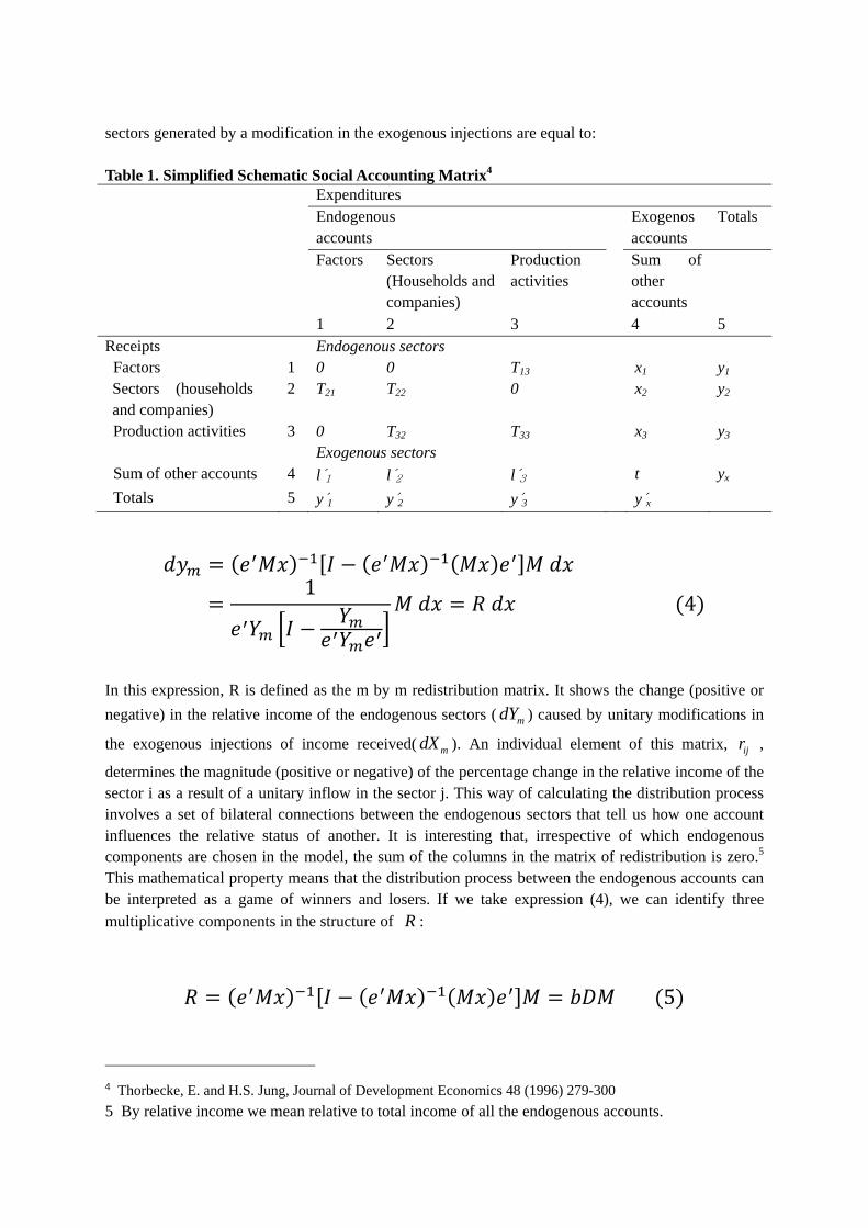
sectors generated by a modification in the exogenous injections are equal to: Table 1. Simplified Schematic Social Accounting Matrix4 Expenditures

Endogenous accounts

Exogenos accounts

Totals

Factors Sectors (Households and companies)

Production activities

Sum of other accounts

1 2 3 4 5 Receipts Endogenous sectors

Factors 1 0 0 T13 x1 y1 Sectors (households and companies)

2 T21 T22 0 x2 y2

Production activities 3 0 T32 T33 x3 y3 Exogenous sectors

Sum of other accounts 4 l′1 l′2 l′3 t yx

Totals 5 y′1 y′2 y′3 y′x

1

4

In this expression, R is defined as the m by m redistribution matrix. It shows the change (positive or

negative) in the relative income of the endogenous sectors ( mdY ) caused by unitary modifications in

the exogenous injections of income received( mdX ). An individual element of this matrix, ijr ,

determines the magnitude (positive or negative) of the percentage change in the relative income of the sector i as a result of a unitary inflow in the sector j. This way of calculating the distribution process involves a set of bilateral connections between the endogenous sectors that tell us how one account influences the relative status of another. It is interesting that, irrespective of which endogenous components are chosen in the model, the sum of the columns in the matrix of redistribution is zero.5 This mathematical property means that the distribution process between the endogenous accounts can be interpreted as a game of winners and losers. If we take expression (4), we can identify three multiplicative components in the structure of R :

5 4 Thorbecke, E. and H.S. Jung, Journal of Development Economics 48 (1996) 279-300 5 By relative income we mean relative to total income of all the endogenous accounts.

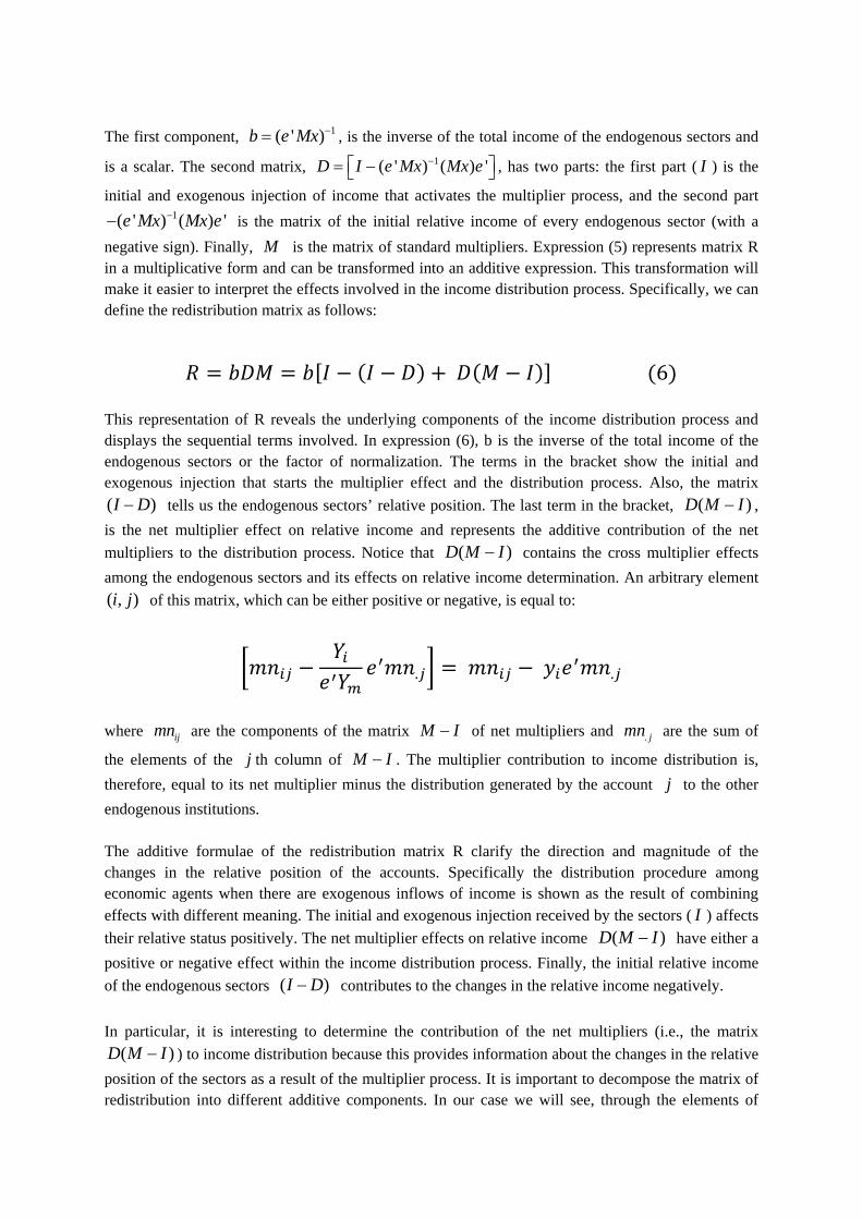
The first component, 1( ' )b e Mx , is the inverse of the total income of the endogenous sectors and

is a scalar. The second matrix, 1( ' ) ( ) 'D I e Mx Mx e , has two parts: the first part ( I ) is the

initial and exogenous injection of income that activates the multiplier process, and the second part 1( ' ) ( ) 'e Mx Mx e is the matrix of the initial relative income of every endogenous sector (with a

negative sign). Finally, M is the matrix of standard multipliers. Expression (5) represents matrix R in a multiplicative form and can be transformed into an additive expression. This transformation will make it easier to interpret the effects involved in the income distribution process. Specifically, we can define the redistribution matrix as follows:

6

This representation of R reveals the underlying components of the income distribution process and displays the sequential terms involved. In expression (6), b is the inverse of the total income of the endogenous sectors or the factor of normalization. The terms in the bracket show the initial and exogenous injection that starts the multiplier effect and the distribution process. Also, the matrix

( )I D tells us the endogenous sectors’ relative position. The last term in the bracket, ( )D M I ,

is the net multiplier effect on relative income and represents the additive contribution of the net

multipliers to the distribution process. Notice that ( )D M I contains the cross multiplier effects

among the endogenous sectors and its effects on relative income determination. An arbitrary element

( , )i j of this matrix, which can be either positive or negative, is equal to:

. .

where ijmn are the components of the matrix M I of net multipliers and . jmn are the sum of

the elements of the j th column of M I . The multiplier contribution to income distribution is,

therefore, equal to its net multiplier minus the distribution generated by the account j to the other

endogenous institutions. The additive formulae of the redistribution matrix R clarify the direction and magnitude of the changes in the relative position of the accounts. Specifically the distribution procedure among economic agents when there are exogenous inflows of income is shown as the result of combining effects with different meaning. The initial and exogenous injection received by the sectors ( I ) affects

their relative status positively. The net multiplier effects on relative income ( )D M I have either a

positive or negative effect within the income distribution process. Finally, the initial relative income

of the endogenous sectors ( )I D contributes to the changes in the relative income negatively.

In particular, it is interesting to determine the contribution of the net multipliers (i.e., the matrix

( )D M I ) to income distribution because this provides information about the changes in the relative

position of the sectors as a result of the multiplier process. It is important to decompose the matrix of redistribution into different additive components. In our case we will see, through the elements of

matrix ( )D M I , a poor multiplier capacity for modifying the relative income of the endogenous

accounts.

3. Multiplier Effects and Income Redistribution Effects in Korea (2000 and 2009)

(1) Financial Crises and IT Revolution: An Overview

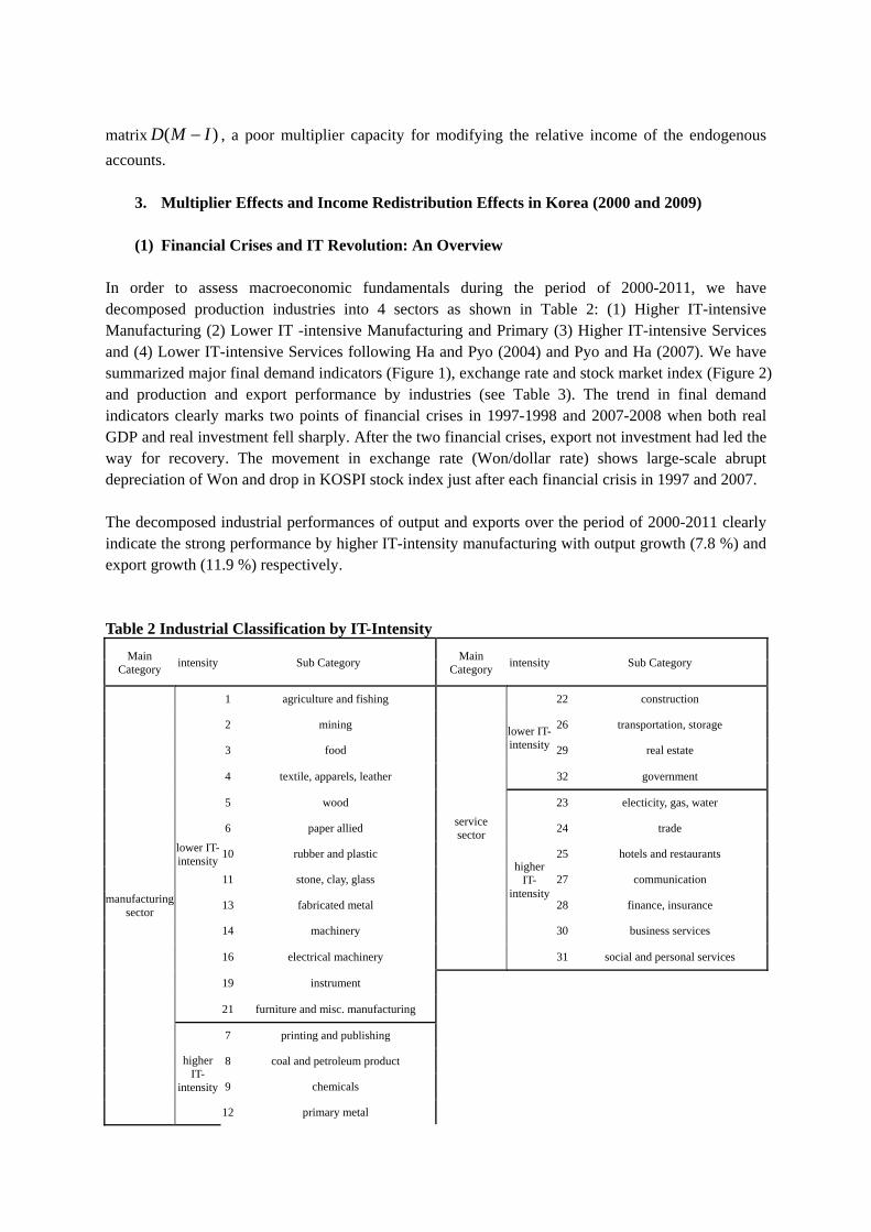
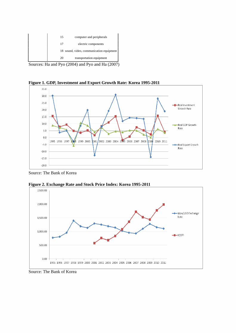
In order to assess macroeconomic fundamentals during the period of 2000-2011, we have decomposed production industries into 4 sectors as shown in Table 2: (1) Higher IT-intensive Manufacturing (2) Lower IT -intensive Manufacturing and Primary (3) Higher IT-intensive Services and (4) Lower IT-intensive Services following Ha and Pyo (2004) and Pyo and Ha (2007). We have summarized major final demand indicators (Figure 1), exchange rate and stock market index (Figure 2) and production and export performance by industries (see Table 3). The trend in final demand indicators clearly marks two points of financial crises in 1997-1998 and 2007-2008 when both real GDP and real investment fell sharply. After the two financial crises, export not investment had led the way for recovery. The movement in exchange rate (Won/dollar rate) shows large-scale abrupt depreciation of Won and drop in KOSPI stock index just after each financial crisis in 1997 and 2007. The decomposed industrial performances of output and exports over the period of 2000-2011 clearly indicate the strong performance by higher IT-intensity manufacturing with output growth (7.8 %) and export growth (11.9 %) respectively. Table 2 Industrial Classification by IT-Intensity

Main Category

intensity Sub Category Main

Category intensity Sub Category

manufacturing sector

lower IT- intensity

1 agriculture and fishing

service sector

lower IT-intensity

22 construction

2 mining 26 transportation, storage

3 food 29 real estate

4 textile, apparels, leather 32 government

5 wood

higher IT-

intensity

23 electicity, gas, water

6 paper allied 24 trade

10 rubber and plastic 25 hotels and restaurants

11 stone, clay, glass 27 communication

13 fabricated metal 28 finance, insurance

14 machinery 30 business services

16 electrical machinery 31 social and personal services

19 instrument

21 furniture and misc. manufacturing

higher IT-

intensity

7 printing and publishing

8 coal and petroleum product

9 chemicals

12 primary metal

15 computer and peripherals

17 electric components

18 sound, video, communication equipment

20 transportation equipment

Sources: Ha and Pyo (2004) and Pyo and Ha (2007)

Figure 1. GDP, Investment and Export Growth Rate: Korea 1995-2011

Source: The Bank of Korea Figure 2. Exchange Rate and Stock Price Index: Korea 1995-2011

Source: The Bank of Korea

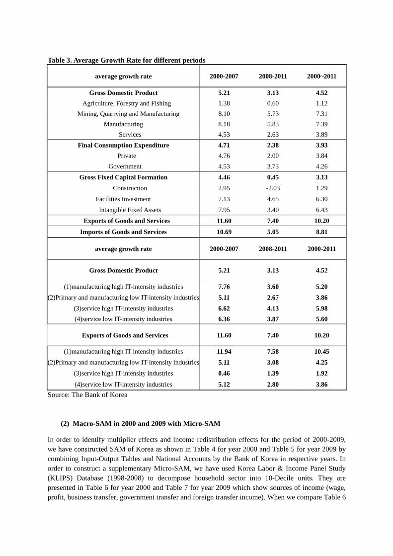
Table 3. Average Growth Rate for different periods

average growth rate 2000-2007 2008-2011 2000~2011

Gross Domestic Product 5.21 3.13 4.52

Agriculture, Forestry and Fishing 1.38 0.60 1.12

Mining, Quarrying and Manufacturing 8.10 5.73 7.31

Manufacturing 8.18 5.83 7.39

Services 4.53 2.63 3.89

Final Consumption Expenditure 4.71 2.38 3.93

Private 4.76 2.00 3.84

Government 4.53 3.73 4.26

Gross Fixed Capital Formation 4.46 0.45 3.13

Construction 2.95 -2.03 1.29

Facilities Investment 7.13 4.65 6.30

Intangible Fixed Assets 7.95 3.40 6.43

Exports of Goods and Services 11.60 7.40 10.20

Imports of Goods and Services 10.69 5.05 8.81

average growth rate 2000-2007 2008-2011 2000-2011

Gross Domestic Product 5.21 3.13 4.52

(1)manufacturing high IT-intensity industries 7.76 3.60 5.20

(2)Primary and manufacturing low IT-intensity industries 5.11 2.67 3.86

(3)service high IT-intensity industries 6.62 4.13 5.98

(4)service low IT-intensity industries 6.36 3.87 5.60

Exports of Goods and Services 11.60 7.40 10.20

(1)manufacturing high IT-intensity industries 11.94 7.58 10.45

(2)Primary and manufacturing low IT-intensity industries 5.11 3.08 4.25

(3)service high IT-intensity industries 0.46 1.39 1.92

(4)service low IT-intensity industries 5.12 2.80 3.86

Source: The Bank of Korea

(2) Macro-SAM in 2000 and 2009 with Micro-SAM In order to identify multiplier effects and income redistribution effects for the period of 2000-2009, we have constructed SAM of Korea as shown in Table 4 for year 2000 and Table 5 for year 2009 by combining Input-Output Tables and National Accounts by the Bank of Korea in respective years. In order to construct a supplementary Micro-SAM, we have used Korea Labor & Income Panel Study (KLIPS) Database (1998-2008) to decompose household sector into 10-Decile units. They are presented in Table 6 for year 2000 and Table 7 for year 2009 which show sources of income (wage, profit, business transfer, government transfer and foreign transfer income). When we compare Table 6

with Table 7, the income distribution of profit has been markedly skewed in favor of higher income deciles. For example, 40.5 percent of the profit income was distributed to the highest income decile (Unit of 10) in 2000 but 52.7 percent in 2009. On the other hand, the business transfer income moved to the opposite direction; the highest income decile received 73.9 percent in 2000 but only 45.4 percent in 2009. In general, the distribution structure of gross income by 10 deciles changed in favor of lower income groups. The ratio of upper 20 % income to lower 20 % income was 17.1 in 2000 and 12.1 in 2009 respectively. The wage income of the lower income deciles (Unit of 1 and 2) was only 3.1 percent in 2000 but improved to be 3.7 percent in 2009. It was mainly due to the welfare policies for the lower income groups by President Kim (1998-2002) and President Roh administration (2003-2007). On the household expenditure side, we have used 2001 KLIPS data for Micro-SAM (2000) and 2008 KLIPS data for Micro-SAM (2009) as shown in Table 8 and 9 respectively. In general, the distribution structure of gross expenditure by 10 deciles changed in favor of lower income groups too. The ratio of upper 20 % expenditure to lower 20 % expenditure was 4.5 in 2000 and 3.6 in 2009 respectively. The gross expenditure of the lower income deciles (Unit of 1 and 2) was only 8.3 percent in 2000 but improved to be 10.1 percent in 2009. Because of differences in survey items between 2001 KLIPS data and 2008 KLIPS data, we had to use the same proportions of income and expenditure in both 2000 and 2009.

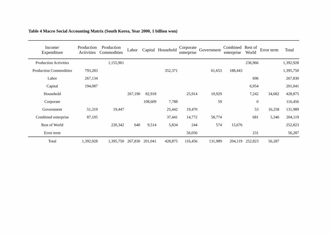
Table 4 Macro Social Accounting Matrix (South Korea, Year 2000, 1 billion won)

Income/ Expenditure

Production Activities

Production Commodities

Labor Capital HouseholdCorporateenterprise

GovernmentCombinedenterprise

Rest of World

Error term Total

Production Activities 1,155,961 236,966 1,392,928

Production Commodities 793,283 352,371 61,653 188,443 1,395,750

Labor 267,134 696 267,830

Capital 194,087 6,954 201,041

Household 267,190 82,918 25,914 10,929 7,242 34,682 428,875

Corporate 108,609 7,788 59 0 116,456

Government 51,319 19,447 25,442 19,470 53 16,258 131,989

Combined enterprise 87,105 37,441 14,772 58,774 681 5,346 204,119

Rest of World 220,342 640 9,514 5,834 244 574 15,676 252,823

Error term 56,056 231 56,287

Total 1,392,928 1,395,750 267,830 201,041 428,875 116,456 131,989 204,119 252,823 56,287

Table 5 Macro Social Accounting Matrix (South Korea, Year 2009, 1 billion won)

Income/ Expenditure



Labor Capital HouseholdCorporateenterprise

GovernmentCombinedenterprise

Rest of World

Error term Total

Production Activities 2,240,903 534,074 2,774,977

Production Commodities 1,727,071 575,970 170,325 279,285 2,752,651

Labor 493,686 872 494,558

Capital 310,604 20,129 330,733

Household 493,035 108,529 42,761 40,567 15,899 -8,776 692,015

Corporate 207,473 14,696 19 222,187

Government 101,522 17,131 59,479 35,824 195 47,143 261,295

Combined enterprise 142,094 27,771 104,550 48,447 -449 -87,144 235,269

Rest of World 494,617 1,523 14,731 14,098 684 1,938 -44,016 483,577

Error term 38,368 -87,144 -48,776

Total 2,774,977 2,752,651 494,558 330,733 692,015 222,187 261,295 235,269 483,577 -48,776

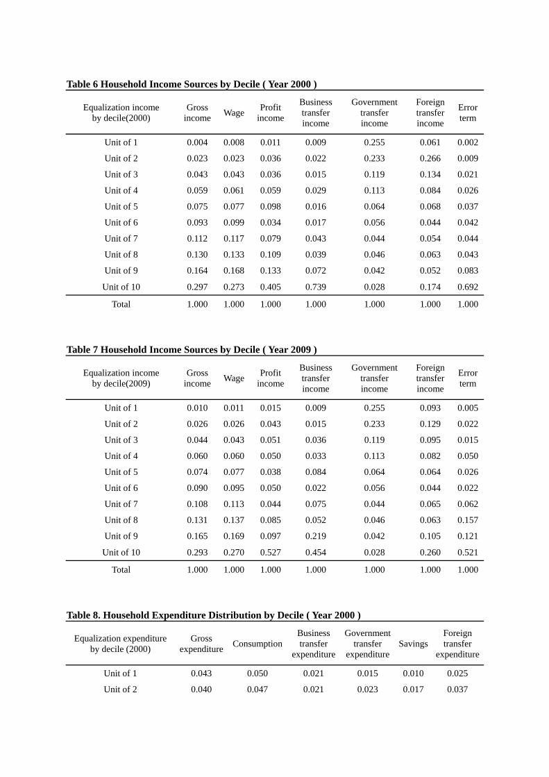
Table 6 Household Income Sources by Decile ( Year 2000 )

Equalization income by decile(2000)

Gross income

Wage Profit

income

Businesstransfer income

Government transfer income

Foreign transfer income

Errorterm

Unit of 1 0.004 0.008 0.011 0.009 0.255 0.061 0.002

Unit of 2 0.023 0.023 0.036 0.022 0.233 0.266 0.009

Unit of 3 0.043 0.043 0.036 0.015 0.119 0.134 0.021

Unit of 4 0.059 0.061 0.059 0.029 0.113 0.084 0.026

Unit of 5 0.075 0.077 0.098 0.016 0.064 0.068 0.037

Unit of 6 0.093 0.099 0.034 0.017 0.056 0.044 0.042

Unit of 7 0.112 0.117 0.079 0.043 0.044 0.054 0.044

Unit of 8 0.130 0.133 0.109 0.039 0.046 0.063 0.043

Unit of 9 0.164 0.168 0.133 0.072 0.042 0.052 0.083

Unit of 10 0.297 0.273 0.405 0.739 0.028 0.174 0.692

Total 1.000 1.000 1.000 1.000 1.000 1.000 1.000

Table 7 Household Income Sources by Decile ( Year 2009 )

Equalization income by decile(2009)

Gross income

Wage Profit

income

Businesstransfer income

Government transfer income

Foreign transfer income

Errorterm

Unit of 1 0.010 0.011 0.015 0.009 0.255 0.093 0.005

Unit of 2 0.026 0.026 0.043 0.015 0.233 0.129 0.022

Unit of 3 0.044 0.043 0.051 0.036 0.119 0.095 0.015

Unit of 4 0.060 0.060 0.050 0.033 0.113 0.082 0.050

Unit of 5 0.074 0.077 0.038 0.084 0.064 0.064 0.026

Unit of 6 0.090 0.095 0.050 0.022 0.056 0.044 0.022

Unit of 7 0.108 0.113 0.044 0.075 0.044 0.065 0.062

Unit of 8 0.131 0.137 0.085 0.052 0.046 0.063 0.157

Unit of 9 0.165 0.169 0.097 0.219 0.042 0.105 0.121

Unit of 10 0.293 0.270 0.527 0.454 0.028 0.260 0.521

Total 1.000 1.000 1.000 1.000 1.000 1.000 1.000

Table 8. Household Expenditure Distribution by Decile ( Year 2000 )

Equalization expenditure by decile (2000)

Gross expenditure

Consumption Business transfer

expenditure

Government transfer

expenditure Savings

Foreign transfer

expenditure

Unit of 1 0.043 0.050 0.021 0.015 0.010 0.025

Unit of 2 0.040 0.047 0.021 0.023 0.017 0.037

Unit of 3 0.057 0.064 0.043 0.044 0.031 0.056

Unit of 4 0.072 0.079 0.058 0.063 0.036 0.076

Unit of 5 0.084 0.089 0.082 0.083 0.056 0.087

Unit of 6 0.098 0.101 0.101 0.100 0.084 0.096

Unit of 7 0.112 0.112 0.131 0.119 0.091 0.112

Unit of 8 0.122 0.126 0.130 0.145 0.110 0.135

Unit of 9 0.151 0.140 0.157 0.170 0.188 0.151

Unit of 10 0.221 0.192 0.258 0.238 0.379 0.224

Total 1.000 1.000 1.000 1.000 1.000 1.000

Table 9. Household Expenditure Distribution by Decile (Year 2009 )

Equalization expenditure by decile (2009)

Gross expenditure

Consumption Business transfer

expenditure

Government transfer

expenditure Savings

Foreign transfer

expenditure

Unit of 1 0.053 0.038 0.008 0.015 0.002 0.025

Unit of 2 0.048 0.049 0.015 0.023 0.009 0.037

Unit of 3 0.055 0.064 0.031 0.044 0.025 0.056

Unit of 4 0.069 0.078 0.049 0.063 0.040 0.076

Unit of 5 0.080 0.089 0.070 0.083 0.059 0.087

Unit of 6 0.095 0.099 0.097 0.100 0.097 0.096

Unit of 7 0.112 0.118 0.115 0.119 0.120 0.112

Unit of 8 0.126 0.130 0.151 0.145 0.115 0.135

Unit of 9 0.145 0.143 0.182 0.170 0.189 0.151

Unit of 10 0.217 0.193 0.282 0.238 0.343 0.224

Total 1.000 1.000 1.000 1.000 1.000 1.0

(3)Multiplier Effects In both Table 10 and Table 11, we have shown multiplier income effects on four sectors of industries, (1) Manufacturing with low IT-intensity, (2)Manufacturing with high IT-intensity, (3)Service with low IT-intensity and (4)Service with high IT-intensity. The row average of each table represents average sensitivity of the sector when expenditure is injected from each of four sectors. In both Table 9 and 10, the multiplier effect is highest with the Sector (2) and lowest with the Sector (3). By comparing two tables, we can see that each sector’s income multiplier sums in all four sectors have become larger in 2009 than in 2000. The sector (3) Service with low IT-intensity had the lowest average sensitivity, 0.433 and 0.411 respectively. Therefore, we can conclude that sector (3) Service with low-IT intensity has both the lowest average sensitivity and the lowest income multiplier effect, which is a typical nature of the non-tradable service sector.

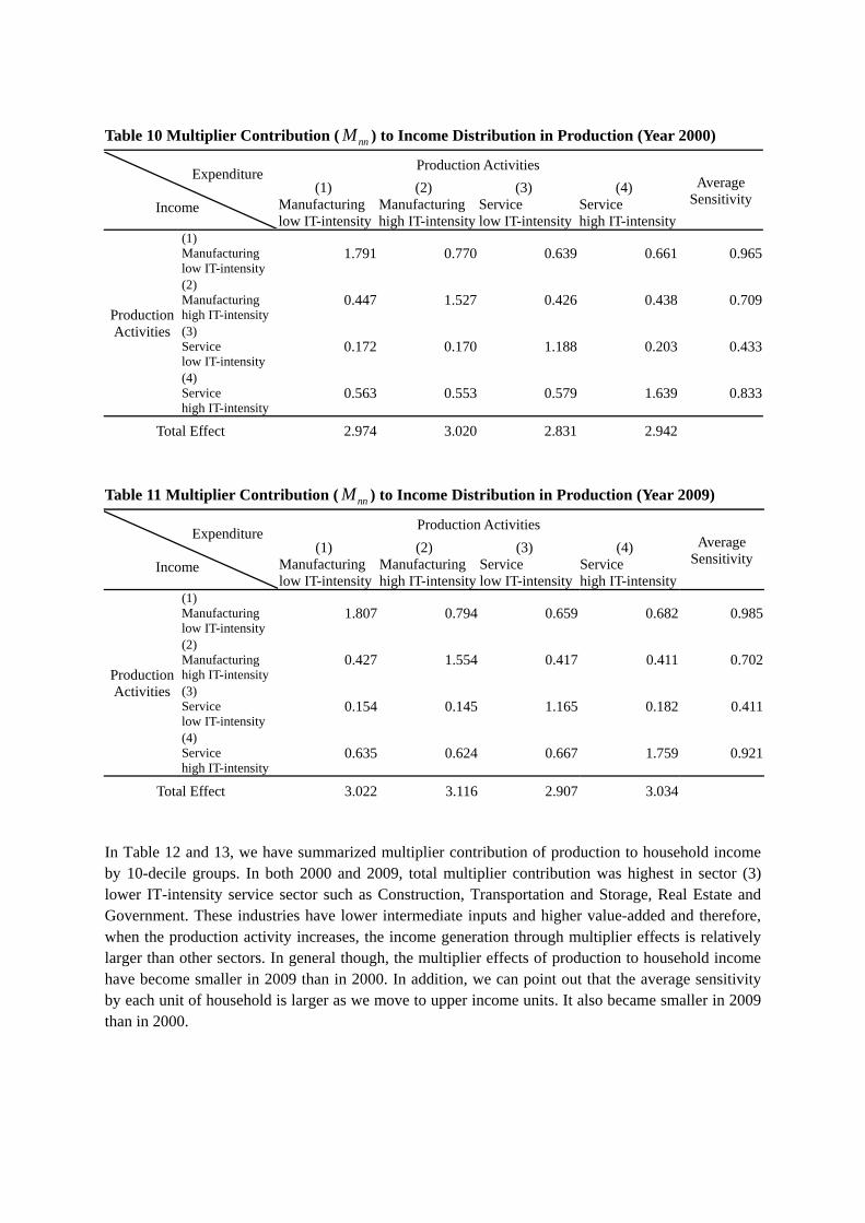
Table 10 Multiplier Contribution ( nnM ) to Income Distribution in Production (Year 2000)

Expenditure

Income

Production Activities Average

Sensitivity (1)

Manufacturinglow IT-intensity

(2) Manufacturinghigh IT-intensity

(3) Service low IT-intensity

(4) Service high IT-intensity


(1) Manufacturing low IT-intensity

1.791 0.770 0.639 0.661 0.965

(2) Manufacturing high IT-intensity

0.447 1.527 0.426 0.438 0.709


0.172 0.170 1.188 0.203 0.433


0.563 0.553 0.579 1.639 0.833

Total Effect 2.974 3.020 2.831 2.942

Table 11 Multiplier Contribution ( nnM ) to Income Distribution in Production (Year 2009)

Expenditure

Income


Sensitivity (1)







1.807 0.794 0.659 0.682 0.985


0.427 1.554 0.417 0.411 0.702


0.154 0.145 1.165 0.182 0.411


0.635 0.624 0.667 1.759 0.921

Total Effect 3.022 3.116 2.907 3.034

In Table 12 and 13, we have summarized multiplier contribution of production to household income by 10-decile groups. In both 2000 and 2009, total multiplier contribution was highest in sector (3) lower IT-intensity service sector such as Construction, Transportation and Storage, Real Estate and Government. These industries have lower intermediate inputs and higher value-added and therefore, when the production activity increases, the income generation through multiplier effects is relatively larger than other sectors. In general though, the multiplier effects of production to household income have become smaller in 2009 than in 2000. In addition, we can point out that the average sensitivity by each unit of household is larger as we move to upper income units. It also became smaller in 2009 than in 2000.

Table 12 Multiplier Contribution ( nnM ) of Production to Household Income (Year 2000)

Expenditure

Income


Sensitivity(1)

Manufacturing low IT-intensity




Equalization household by decile

Unit 1 0.006 0.005 0.007 0.007 0.006

Unit 2 0.017 0.015 0.021 0.020 0.018

Unit 3 0.026 0.024 0.033 0.032 0.029

Unit 4 0.039 0.036 0.049 0.048 0.043

Unit 5 0.051 0.047 0.065 0.063 0.056

Unit 6 0.050 0.047 0.067 0.063 0.057

Unit 7 0.067 0.062 0.087 0.083 0.075

Unit 8 0.078 0.073 0.102 0.098 0.088

Unit 9 0.100 0.093 0.130 0.125 0.112

Unit 10 0.224 0.206 0.275 0.271 0.244

Total Effect 0.657 0.607 0.835 0.810

Table 13 Multiplier Contribution ( nnM ) of Production to Household Income (Year 2009)

Expenditure

Income


Sensitivity(1)

Manufacturing low IT-intensity





Unit 1 0.007 0.006 0.009 0.009 0.008

Unit 2 0.016 0.015 0.021 0.021 0.018

Unit 3 0.025 0.023 0.034 0.032 0.028

Unit 4 0.031 0.029 0.043 0.041 0.036

Unit 5 0.039 0.036 0.054 0.051 0.045

Unit 6 0.045 0.042 0.064 0.060 0.053

Unit 7 0.054 0.050 0.077 0.071 0.063

Unit 8 0.067 0.062 0.094 0.088 0.078

Unit 9 0.089 0.082 0.123 0.116 0.102

Unit 10 0.186 0.170 0.244 0.238 0.210

Total Effect 0.559 0.515 0.763 0.727

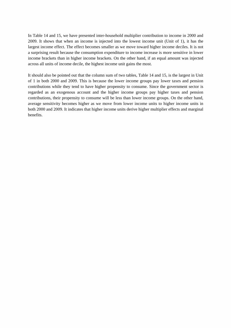
In Table 14 and 15, we have presented inter-household multiplier contribution to income in 2000 and 2009. It shows that when an income is injected into the lowest income unit (Unit of 1), it has the largest income effect. The effect becomes smaller as we move toward higher income deciles. It is not a surprising result because the consumption expenditure to income increase is more sensitive in lower income brackets than in higher income brackets. On the other hand, if an equal amount was injected across all units of income decile, the highest income unit gains the most. It should also be pointed out that the column sum of two tables, Table 14 and 15, is the largest in Unit of 1 in both 2000 and 2009. This is because the lower income groups pay lower taxes and pension contributions while they tend to have higher propensity to consume. Since the government sector is regarded as an exogenous account and the higher income groups pay higher taxes and pension contributions, their propensity to consume will be less than lower income groups. On the other hand, average sensitivity becomes higher as we move from lower income units to higher income units in both 2000 and 2009. It indicates that higher income units derive higher multiplier effects and marginal benefits.

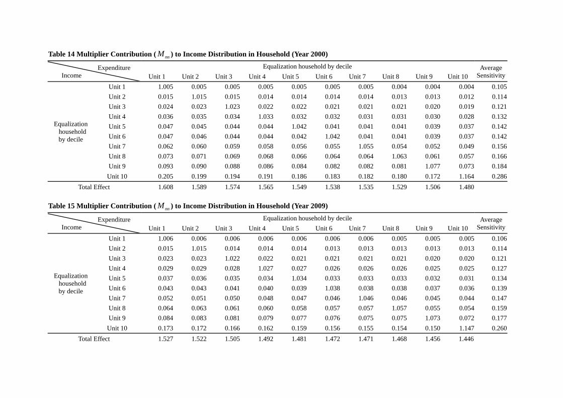
Table 14 Multiplier Contribution ( nnM ) to Income Distribution in Household (Year 2000)

Expenditure Income

Equalization household by decile Average Sensitivity Unit 1 Unit 2 Unit 3 Unit 4 Unit 5 Unit 6 Unit 7 Unit 8 Unit 9 Unit 10


Unit 1 1.005 0.005 0.005 0.005 0.005 0.005 0.005 0.004 0.004 0.004 0.105

Unit 2 0.015 1.015 0.015 0.014 0.014 0.014 0.014 0.013 0.013 0.012 0.114

Unit 3 0.024 0.023 1.023 0.022 0.022 0.021 0.021 0.021 0.020 0.019 0.121

Unit 4 0.036 0.035 0.034 1.033 0.032 0.032 0.031 0.031 0.030 0.028 0.132

Unit 5 0.047 0.045 0.044 0.044 1.042 0.041 0.041 0.041 0.039 0.037 0.142

Unit 6 0.047 0.046 0.044 0.044 0.042 1.042 0.041 0.041 0.039 0.037 0.142

Unit 7 0.062 0.060 0.059 0.058 0.056 0.055 1.055 0.054 0.052 0.049 0.156

Unit 8 0.073 0.071 0.069 0.068 0.066 0.064 0.064 1.063 0.061 0.057 0.166

Unit 9 0.093 0.090 0.088 0.086 0.084 0.082 0.082 0.081 1.077 0.073 0.184

Unit 10 0.205 0.199 0.194 0.191 0.186 0.183 0.182 0.180 0.172 1.164 0.286

Total Effect 1.608 1.589 1.574 1.565 1.549 1.538 1.535 1.529 1.506 1.480 Table 15 Multiplier Contribution ( nnM ) to Income Distribution in Household (Year 2009)

Expenditure Income



Unit 1 1.006 0.006 0.006 0.006 0.006 0.006 0.006 0.005 0.005 0.005 0.106

Unit 2 0.015 1.015 0.014 0.014 0.014 0.013 0.013 0.013 0.013 0.013 0.114

Unit 3 0.023 0.023 1.022 0.022 0.021 0.021 0.021 0.021 0.020 0.020 0.121

Unit 4 0.029 0.029 0.028 1.027 0.027 0.026 0.026 0.026 0.025 0.025 0.127

Unit 5 0.037 0.036 0.035 0.034 1.034 0.033 0.033 0.033 0.032 0.031 0.134

Unit 6 0.043 0.043 0.041 0.040 0.039 1.038 0.038 0.038 0.037 0.036 0.139

Unit 7 0.052 0.051 0.050 0.048 0.047 0.046 1.046 0.046 0.045 0.044 0.147

Unit 8 0.064 0.063 0.061 0.060 0.058 0.057 0.057 1.057 0.055 0.054 0.159

Unit 9 0.084 0.083 0.081 0.079 0.077 0.076 0.075 0.075 1.073 0.072 0.177

Unit 10 0.173 0.172 0.166 0.162 0.159 0.156 0.155 0.154 0.150 1.147 0.260

Total Effect 1.527 1.522 1.505 1.492 1.481 1.472 1.471 1.468 1.456 1.446

(4) Redistribution Effects When there is income generated by one account, the income generated is distributed not equally to each sector and it becomes a zero-sum game. We can analyze how income generated by each production sector gets redistributed across different income units of household. For example, we can identify the induced production activities of four endogenous sectors by increased final demand in three exogenous accounts. Then we can trace how the income generated in endogenous sectors gets redistributed among household income units. Table 16 and 17 is the matrix of such redistributed income which sums up to zero. The result is different from multiplier effects. When income is generated from the entire production sectors, the Higher IT-intensity Manufacturing sector has the lowest income redistribution effect. In particular, the sector’s redistribution effect became negative (-1.019) while all other three sectors have had positive redistribution effects. On the other hand, when income is injected to production activity, the lower IT-intensity Service sector has the lowest column sum like the sector’s multiplier effects and it became lower in 2009 than in 2000.

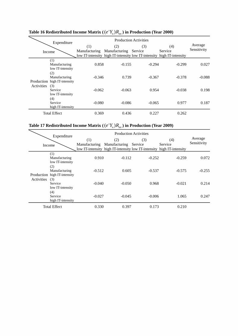
Table 16 Redistributed Income Matrix ( ( ' )n nne Y R ) in Production (Year 2000)

Expenditure

Income


Sensitivity (1)







0.858 -0.155 -0.294 -0.299 0.027


-0.346 0.739 -0.367 -0.378 -0.088


-0.062 -0.063 0.954 -0.038 0.198


-0.080 -0.086 -0.065 0.977 0.187

Total Effect 0.369 0.436 0.227 0.262

Table 17 Redistributed Income Matrix ( ( ' )n nne Y R ) in Production (Year 2009)

Expenditure

Income


Sensitivity (1)







0.910 -0.112 -0.252 -0.259 0.072


-0.512 0.605 -0.537 -0.575 -0.255


-0.040 -0.050 0.968 -0.021 0.214


-0.027 -0.045 -0.006 1.065 0.247

Total Effect 0.330 0.397 0.173 0.210

Table 18 and 19 are the results of redistributed income effects of production activity in four sectors on household income by ten income units. In both 2000 and 2009, the lower IT-intensity Service sector has generated the largest total income redistribution effect (0.034 and 0.081). In terms of average sensitivity, the highest income group, Unit 10, has had the largest negative sensitivity (-0.040) in 2000 but it became the only positive sensitivity (0.002) in 2009.

Table 18 Redistributed Income Effect ( ( ' )n nne Y R ) of Production on Household Income (Year

2000)

Expenditure

Income


Sensitivity (1)






Unit 1 -0.006 -0.007 -0.005 -0.006 -0.006

Unit 2 -0.010 -0.011 -0.006 -0.007 -0.008

Unit 3 -0.008 -0.009 0.000 -0.002 -0.005

Unit 4 -0.008 -0.010 0.003 0.000 -0.004

Unit 5 -0.008 -0.012 0.006 0.002 -0.003

Unit 6 -0.010 -0.013 0.007 0.002 -0.003

Unit 7 -0.010 -0.015 0.010 0.004 -0.003

Unit 8 -0.011 -0.016 0.012 0.006 -0.002

Unit 9 -0.015 -0.021 0.015 0.006 -0.004

Unit 10 -0.059 -0.075 -0.008 -0.020 -0.040

Total Effect -0.145 -0.189 0.034 -0.015

Table 19 Redistributed Income Effect ( ( ' )n nne Y R ) of Production on Household Income (Year

2009)

Expenditure

Income


Sensitivity (1)






Unit 1 -0.012 -0.013 -0.010 -0.011 -0.011

Unit 2 -0.013 -0.014 -0.008 -0.009 -0.011

Unit 3 -0.009 -0.011 0.000 -0.003 -0.006

Unit 4 -0.009 -0.012 0.002 -0.002 -0.005

Unit 5 -0.009 -0.012 0.006 0.001 -0.003

Unit 6 -0.009 -0.013 0.009 0.003 -0.003

Unit 7 -0.010 -0.015 0.011 0.004 -0.002

Unit 8 -0.011 -0.016 0.015 0.007 -0.001

Unit 9 -0.014 -0.021 0.019 0.009 -0.002

Unit 10 -0.018 -0.036 0.037 0.024 0.002

Total Effect -0.113 -0.163 0.081 0.022

Lastly we examine the redistribution effect of household income injected on household income redistributed among different income units. Table 20 and 21 are redistributed household income among different income units in 2000 and 2009 respectively. In general the total effects are positive across all income units. But within each unit, the redistribution effect is positive only to itself and negative in all other sectors. In other words, the redistributed income matrix of households has positive diagonal elements but all negative off-diagonal elements. The total redistribution effect is the largest in the highest income unit and became smaller as we move lower income units in both 2000 and 2009. The total effect was larger in 2009 than in 2000 across all units. On the other hand average sensitivity moved in the opposite direction becoming lower as we move from lower income units to higher ones. It implies when income is injected to household account, the higher income units derive higher redistribution effects. On the other hand, the redistribution effect becomes more sensitive with lower income groups because their income level are at lower level and therefore, they are affected marginally more. It is noted that average sensitivity of Unit 10 was negative (-0.002) in 2000 but it became positive (0.049) in 2009 which implies after the global financial crisis of 2007-2008, the highest income unit (Unit 10) has become net gainers than net losers in redistribution of household income.

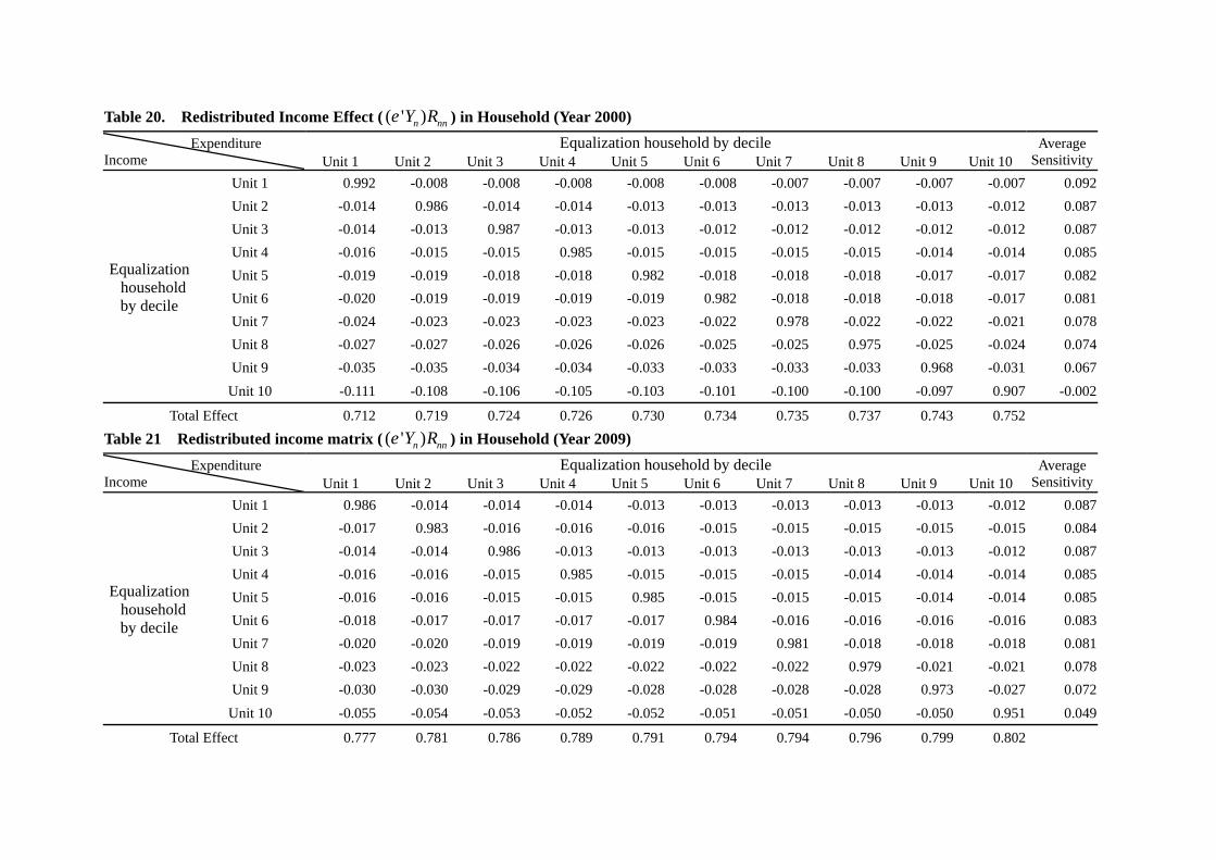
Table 20. Redistributed Income Effect ( ( ' )n nne Y R ) in Household (Year 2000)

Expenditure Income


Equalization householdby decile

Unit 1 0.992 -0.008 -0.008 -0.008 -0.008 -0.008 -0.007 -0.007 -0.007 -0.007 0.092

Unit 2 -0.014 0.986 -0.014 -0.014 -0.013 -0.013 -0.013 -0.013 -0.013 -0.012 0.087

Unit 3 -0.014 -0.013 0.987 -0.013 -0.013 -0.012 -0.012 -0.012 -0.012 -0.012 0.087

Unit 4 -0.016 -0.015 -0.015 0.985 -0.015 -0.015 -0.015 -0.015 -0.014 -0.014 0.085

Unit 5 -0.019 -0.019 -0.018 -0.018 0.982 -0.018 -0.018 -0.018 -0.017 -0.017 0.082

Unit 6 -0.020 -0.019 -0.019 -0.019 -0.019 0.982 -0.018 -0.018 -0.018 -0.017 0.081

Unit 7 -0.024 -0.023 -0.023 -0.023 -0.023 -0.022 0.978 -0.022 -0.022 -0.021 0.078

Unit 8 -0.027 -0.027 -0.026 -0.026 -0.026 -0.025 -0.025 0.975 -0.025 -0.024 0.074

Unit 9 -0.035 -0.035 -0.034 -0.034 -0.033 -0.033 -0.033 -0.033 0.968 -0.031 0.067

Unit 10 -0.111 -0.108 -0.106 -0.105 -0.103 -0.101 -0.100 -0.100 -0.097 0.907 -0.002

Total Effect 0.712 0.719 0.724 0.726 0.730 0.734 0.735 0.737 0.743 0.752

Table 21 Redistributed income matrix ( ( ' )n nne Y R ) in Household (Year 2009)

Expenditure Income


Equalization householdby decile

Unit 1 0.986 -0.014 -0.014 -0.014 -0.013 -0.013 -0.013 -0.013 -0.013 -0.012 0.087

Unit 2 -0.017 0.983 -0.016 -0.016 -0.016 -0.015 -0.015 -0.015 -0.015 -0.015 0.084

Unit 3 -0.014 -0.014 0.986 -0.013 -0.013 -0.013 -0.013 -0.013 -0.013 -0.012 0.087

Unit 4 -0.016 -0.016 -0.015 0.985 -0.015 -0.015 -0.015 -0.014 -0.014 -0.014 0.085

Unit 5 -0.016 -0.016 -0.015 -0.015 0.985 -0.015 -0.015 -0.015 -0.014 -0.014 0.085

Unit 6 -0.018 -0.017 -0.017 -0.017 -0.017 0.984 -0.016 -0.016 -0.016 -0.016 0.083

Unit 7 -0.020 -0.020 -0.019 -0.019 -0.019 -0.019 0.981 -0.018 -0.018 -0.018 0.081

Unit 8 -0.023 -0.023 -0.022 -0.022 -0.022 -0.022 -0.022 0.979 -0.021 -0.021 0.078

Unit 9 -0.030 -0.030 -0.029 -0.029 -0.028 -0.028 -0.028 -0.028 0.973 -0.027 0.072

Unit 10 -0.055 -0.054 -0.053 -0.052 -0.052 -0.051 -0.051 -0.050 -0.050 0.951 0.049

Total Effect 0.777 0.781 0.786 0.789 0.791 0.794 0.794 0.796 0.799 0.802

4. CONCLUSION

In the present paper, we have examined the impact of two financial crises and IT revolution on multiplier effects and redistribution effects of both production sectors and household income units in Korea for the period of 2000-2011. We have decomposed the entire production activities into four sectors by the ranking of It-intensity. As a consequence of depreciation in the post-crisis periods, there was a strong export performance in higher IT-intensity Manufacturing Sector. This has generated a strong exogenous impact on four endogenous sectors of production. It also has generated income redistribution effects among different sectors of production and across different income units. In general, the distribution structure of gross income by 10 deciles changed in favor of lower income groups. The ratio of upper 20 % income to lower 20 % income was 17.1 in 2000 and 12.1 in 2009 respectively. The wage income of the lower income deciles (Unit of 1 and 2) was only 3.1 percent in 2000 but improved to be 3.7 percent in 2009. It was mainly due to the welfare policies for the lower income groups by President Kim (1998-2002) and President Roh administration (2003-2007). In analysis of multiplier effects, we have found that the sector (3) Service with low IT-intensity had the lowest average sensitivity, 0.433 and 0.411 respectively. Therefore, we can conclude that sector (3) Service with low-IT intensity has both the lowest average sensitivity and the lowest income multiplier effect, which is a typical nature of the non-tradable service sector. On the other hand, the multiplier effects of production to household income have become smaller in 2009 than in 2000. In addition, we can point out that the average sensitivity by each unit of household is larger as we move to upper income units. It also became smaller in 2009 than in 2000. In analysis of redistribution effects, the lower IT-intensity Service sector has generated the largest total income redistribution effect (0.034 and 0.081) in both 2000 and 2009,. In terms of average sensitivity, the highest income group, Unit 10, has had the largest negative sensitivity (-0.040) in 2000 but it became the only positive sensitivity (0.002) in 2009. In general the total redistribution effects are positive across all income units. But within each unit, the redistribution effect is positive only to itself and negative in all other sectors. In other words, the redistributed income matrix of households has positive diagonal elements but all negative off-diagonal elements. The total redistribution effect is the largest in the highest income unit and became smaller as we move lower income units in both 2000 and 2009. The total effect was larger in 2009 than in 2000 across all units. On the other hand average sensitivity moved in the opposite direction becoming lower as we move from lower income units to higher ones. It implies when income is injected to household account, the higher income units derive higher redistribution effects. These finding provide evidence increasing globalization of production activities in Korea and IT-intensity deepening has generated more redistribution effect in favor of higher income units. However the overall indicator of income disparity has not been worsened between 2000 and 2009 after two financial crises. When we measure it as the ratio of upper 20 percent income divided by lower 20 % income, the income disparity has been narrowed.

References

Dadush, U., Dasgupta, D. & Uzan, M. (2000), Private Capital Flows in the Age of Globalization: the Aftermath

of the Asian Crisis", Edward Elgar, Cheltenham

Defourny, J. & Thorbecke, E (1984), "Structural path analysis and multiplier decomposition within a social

accounting matrix framework", Economic Journal Vol. 94, No. 373(March, 1984) pp.111-36.

Ha, B.C. & Pyo, H.K. (2004), "The Measurement of IT Contribution by Decomposed Dynamic Input-Output

Tables in Korea (1980-2002)", Seoul Journal of Economics 17, pp.511-546.

Keuning, S. & Thorbecke, E (1992), "The social accounting matrix and adjustment Policies: the impact of

budget retrenchment on income distribution", Chapter 3 of E.Thorbecke (Ed.), Adjustment and Equity in

Indonesia Paris, OECD.

Otsu, K. & Pyo, H.K. (2009), "A Comparative Estimation of Financial Frictions in Japan and Korea", Seoul

Journal of Economics Vol.22 no.1, pp.95-121 : Institute of Economics Research, Seoul National University

Pyatt, G.(2003) "An Alternative Approach to Poverty Analysis", Economic Systems Research, Vol. 15,

No.4(June) pp.113-133.

Pyatt,G., & Round, J.I.(1979), "Accounting and fixed price multipliers in a social accounting matrix framework",

Economic Journal Vol.89, pp.850-873.

Pyatt,G., & Round, J.I.(2003), "Multiplier analysis and the design of social accounting matrices" University of

Warwick.

Pyatt,G., & Round, J.I.(2006), "Multiplier Effects and The Reduction of Poverty", In Alain Janvry & Ravi

Kanbur (Ed.), Economic Studies in Inequality, Social Exclusion and Well-Being (pp.233-259). Springer

US.

Pyo, H.K. (2004), "Interdependency in East Asia and the Post-Crisis Macroeconomic Adjustment in Korea",

Seoul Journal of Economics Vol.17 No.1, pp117-152

Pyo, H.K. & Ha, B.C. (2007), "A Test of Separability and Random Effects in Production Function with

Decomposed IT capital", Hitotsubashi Journal of Economics 48, pp.67-81

Pyo, H.K., Kim, D.K. & Lee, G (2012),“An Analysis of Effects on National Pension Service through Socio-

Economic Changes by Using Social Account Matrix”, National Pension System Working Report 2012-02.

Roh, Y.H. & Nam, S.H.(2006), "Redistributed Income Effect of Korean Economy with Social Accounting

Matrix", The Bank of Korea(2006)

Roland-Holst, D. W. & Sancho, F. (1992), "Relative Income Determination In The United States: A Social

Accounting Perspective", Review of Income and Wealth Vol.38, pp311–327.

Round, J.I.(2003), "Social Accounting Matrices and SAM=based Multiplier Analysis", Chapter 14 in F

Bourguignon, and L A Pereira da Silva (editors) Techniques and Tools for Evaluating the Poverty Impact of

Economic Policies, World Bank and Oxford University Press.

Saari, M.Y., Dietzenbacher, E. & Los, B. (2010), "Modeling Impact of Higher Energy Prices on Income

Distribution with Substitutions in Production and Household Sectors," U.Groningen.

Stone, R. (1985), "The disaggregation of the household sector in the national accounts", Chapter 8 of Pyatt, G.

and J.I. Round (Ed.) Social Accounting Matrices: A Basis for Planning Washington, D.C., the World Bank

Thorbecke E.& Jung H.S.(1996), "A multiplier decomposition method to analyze poverty alleviation", Journal

of Development Economics, 48 (2) , pp. 279-300.

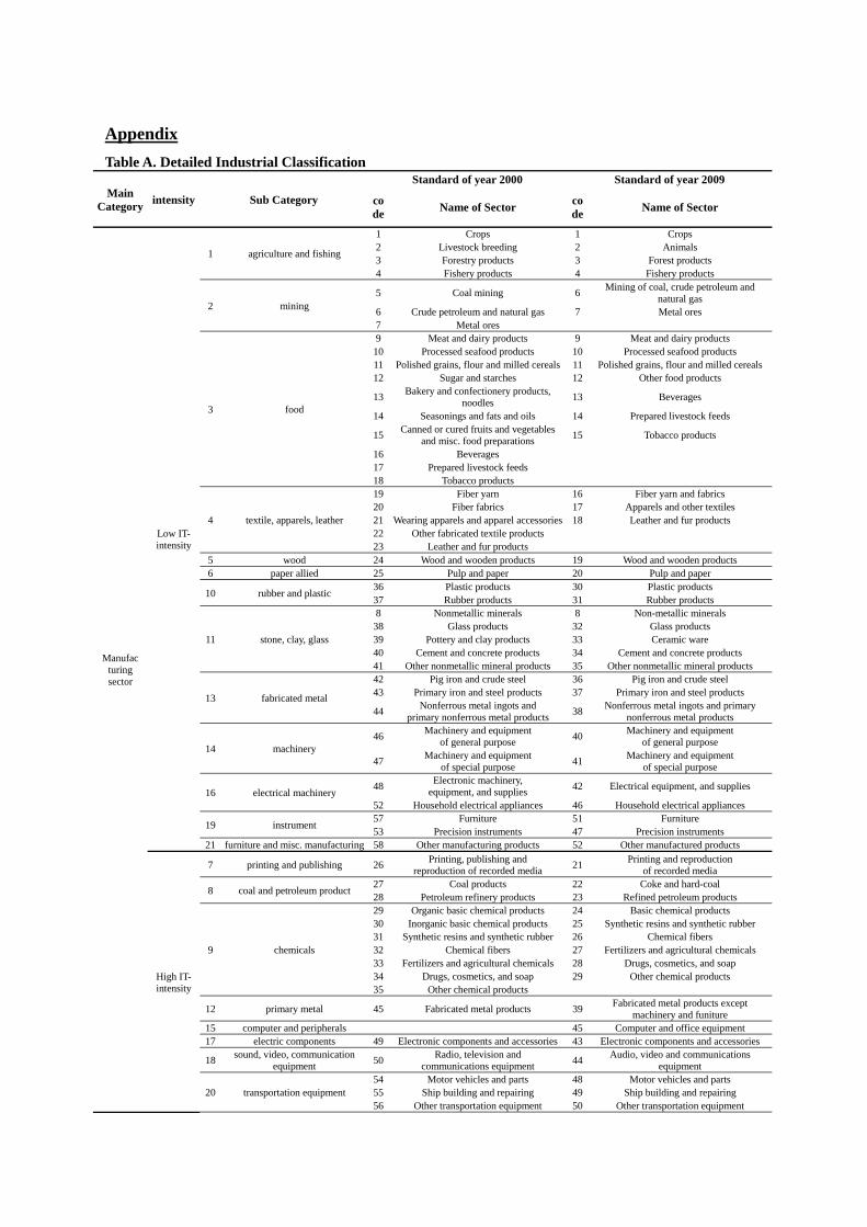
Appendix

Table A. Detailed Industrial Classification

Main Category

intensity Sub Category

Standard of year 2000 Standard of year 2009

code

Name of Sector code

Name of Sector

Manufac turing sector

Low IT- intensity

1 agriculture and fishing

1 Crops 1 Crops 2 Livestock breeding 2 Animals 3 Forestry products 3 Forest products 4 Fishery products 4 Fishery products

2 mining 5 Coal mining 6

Mining of coal, crude petroleum and natural gas

6 Crude petroleum and natural gas 7 Metal ores 7 Metal ores

3 food

9 Meat and dairy products 9 Meat and dairy products 10 Processed seafood products 10 Processed seafood products 11 Polished grains, flour and milled cereals 11 Polished grains, flour and milled cereals 12 Sugar and starches 12 Other food products

13 Bakery and confectionery products,

noodles 13 Beverages

14 Seasonings and fats and oils 14 Prepared livestock feeds

15 Canned or cured fruits and vegetables

and misc. food preparations 15 Tobacco products

16 Beverages 17 Prepared livestock feeds 18 Tobacco products

4 textile, apparels, leather

19 Fiber yarn 16 Fiber yarn and fabrics 20 Fiber fabrics 17 Apparels and other textiles 21 Wearing apparels and apparel accessories 18 Leather and fur products 22 Other fabricated textile products 23 Leather and fur products

5 wood 24 Wood and wooden products 19 Wood and wooden products 6 paper allied 25 Pulp and paper 20 Pulp and paper

10 rubber and plastic 36 Plastic products 30 Plastic products 37 Rubber products 31 Rubber products

11 stone, clay, glass

8 Nonmetallic minerals 8 Non-metallic minerals 38 Glass products 32 Glass products 39 Pottery and clay products 33 Ceramic ware 40 Cement and concrete products 34 Cement and concrete products 41 Other nonmetallic mineral products 35 Other nonmetallic mineral products

13 fabricated metal

42 Pig iron and crude steel 36 Pig iron and crude steel 43 Primary iron and steel products 37 Primary iron and steel products

44 Nonferrous metal ingots and

primary nonferrous metal products 38

Nonferrous metal ingots and primary nonferrous metal products

14 machinery 46

Machinery and equipment of general purpose

40 Machinery and equipment

of general purpose

47 Machinery and equipment

of special purpose 41

Machinery and equipment of special purpose

16 electrical machinery 48

Electronic machinery, equipment, and supplies

42 Electrical equipment, and supplies

52 Household electrical appliances 46 Household electrical appliances

19 instrument 57 Furniture 51 Furniture 53 Precision instruments 47 Precision instruments

21 furniture and misc. manufacturing 58 Other manufacturing products 52 Other manufactured products

High IT- intensity

7 printing and publishing 26 Printing, publishing and

reproduction of recorded media 21

Printing and reproduction of recorded media

8 coal and petroleum product 27 Coal products 22 Coke and hard-coal 28 Petroleum refinery products 23 Refined petroleum products

9 chemicals

29 Organic basic chemical products 24 Basic chemical products 30 Inorganic basic chemical products 25 Synthetic resins and synthetic rubber 31 Synthetic resins and synthetic rubber 26 Chemical fibers 32 Chemical fibers 27 Fertilizers and agricultural chemicals 33 Fertilizers and agricultural chemicals 28 Drugs, cosmetics, and soap 34 Drugs, cosmetics, and soap 29 Other chemical products 35 Other chemical products

12 primary metal 45 Fabricated metal products 39 Fabricated metal products except

machinery and funiture 15 computer and peripherals 45 Computer and office equipment 17 electric components 49 Electronic components and accessories 43 Electronic components and accessories

18 sound, video, communication

equipment 50

Radio, television and communications equipment

44 Audio, video and communications

equipment

20 transportation equipment 54 Motor vehicles and parts 48 Motor vehicles and parts 55 Ship building and repairing 49 Ship building and repairing 56 Other transportation equipment 50 Other transportation equipment

service sector

Low IT- intensity

22 construction 61 Building construction and repair 55 Building construction and repair 62 Civil Engineering 56 Civil engineering

26 transportation, storage

65 Transportation and warehousing 59 Land transport 60 Water and air transport

61 Strorage and support activities

for transportation 29 real estate 68 Real estate agencies and rental 65 Real estate

32 gonerment

70 Public administration and defense 69 Public administration and defense 71 Educational and research services 70 Education

72 Medical and health services,

and social security 71 Medical and health services

72 Social work activities 73 Sanitary services

High IT- intensity

23 electicity, gas, water 59 Electric services 53 Electric utilities 60 Gas and water supply 54 Gas and water supply

24 trade 63 Wholesale and retail trade 57 Wholesale and retail trade

25 hotels and restaurants 64 Eating and drinking places, and hotels and other lodging places

58 Accommodation and food services

27 communication 66 Communications and broadcasting 62 Communications services 28 finance, insurance 67 Finance and insurance 64 Finance and insurance

30 business services

51 Computer and office equipment 5 Agriculture, forestry and fishing related services

69 Business services 66 Research and development 75 Office supplies 67 Business services

68 Other business services

31 social and personal services

73 Culture and recreational services 63 Broadcasting 74 Other services 74 Publishing and cultural services 76 Business consumption expenditure 75 Amusement and sports activities 77 Nonclassifiable activities 76 Social organizations

77 Other services 78 Dummy sectors

Table B-1 Micro Social Accounting Matrix 25 25 (South Korea, Year 2000, 1 billion won)

Income/Expenditure

Production Activities Production Commodities

Labor Capital

Equalization household by decile Corporateenterprise

Govern-ment

Combinedcapital ccounts

Rest of World

Error term

Total Manufac- low-

intensity

Manufac- high-

intensity

Service low-

intensity

Servicehigh-

intensity

Manufac-low-

intensity

Manufac-high-

intensity

Servicelow-

intensity

Servicehigh-

intensity

Unit 1

Unit 2

Unit 3

Unit 4

Unit 5

Unit 6

Unit 7

Unit 8

Unit 9

Unit 10


Manufac-turinglow-

intensity

0 0 0 0 222493 113301 47934 49834 0 0 0 0 0 0 0 0 0 0 0 0 0 0 0 65562 0 499123

Manufac-turinghigh-

intensity

0 0 0 0 54841 162688 49454 40096 0 0 0 0 0 0 0 0 0 0 0 0 0 0 0 117212 0 424290

Servicelow-

intensity0 0 0 0 12686 12369 39668 38136 0 0 0 0 0 0 0 0 0 0 0 0 0 0 0 22509 0 125368

Servicehigh-

intensity0 0 0 0 57226 44552 69166 141519 0 0 0 0 0 0 0 0 0 0 0 0 0 0 0 31683 0 344146


Manufac-turinglow-

intensity

152686 77753 32895 34199 0 0 0 0 0 0 3475 3151 4226 5618 6505 7147 8132 9142 10309 13813 0 0 39018 0 0 408070

Manufac-turinghigh-

intensity

37635 111645 33938 27516 0 0 0 0 0 0 1141 1107 1530 1951 2344 2597 3029 3437 3778 4605 0 0 27600 0 0 263853

Servicelow-

intensity8706 8488 27222 26171 0 0 0 0 0 0 7254 6235 8168 9097 10106 11200 12244 12987 14316 20519 0 60733 96298 0 0 339745

Servicehigh-

intensity39271 30574 47466 97118 0 0 0 0 0 0 5656 6068 8800 11017 12446 14485 16225 18851 20869 28789 0 920 25527 0 0 384082

Labor 42137 28923 105275 90798 0 0 0 0 0 0 0 0 0 0 0 0 0 0 0 0 0 0 0 696 0 267830 Capital 45912 26791 56889 64495 0 0 0 0 0 0 0 0 0 0 0 0 0 0 0 0 0 0 0 6954 0 201041


Unit 1 0 0 0 0 0 0 0 0 2016 885 0 0 0 0 0 0 0 0 0 0 232 2785 0 444 86 6447 Unit 2 0 0 0 0 0 0 0 0 6014 2947 0 0 0 0 0 0 0 0 0 0 565 2549 0 1927 314 14316 Unit 3 0 0 0 0 0 0 0 0 11538 2989 0 0 0 0 0 0 0 0 0 0 379 1304 0 968 742 17919 Unit 4 0 0 0 0 0 0 0 0 16294 4926 0 0 0 0 0 0 0 0 0 0 763 1230 0 605 885 24702 Unit 5 0 0 0 0 0 0 0 0 20588 8092 0 0 0 0 0 0 0 0 0 0 412 699 0 495 1285 31570 Unit 6 0 0 0 0 0 0 0 0 26329 2843 0 0 0 0 0 0 0 0 0 0 441 610 0 322 1456 32000 Unit 7 0 0 0 0 0 0 0 0 31132 6551 0 0 0 0 0 0 0 0 0 0 1102 477 0 390 1541 41193 Unit 8 0 0 0 0 0 0 0 0 35425 9071 0 0 0 0 0 0 0 0 0 0 1006 507 0 455 1484 47947 Unit 9 0 0 0 0 0 0 0 0 44911 11018 0 0 0 0 0 0 0 0 0 0 1853 458 0 379 2883 61502 Unit 10 0 0 0 0 0 0 0 0 72945 33596 0 0 0 0 0 0 0 0 0 0 19163 310 0 1258 24006 151278

Corporate enterprise 0 0 0 0 0 0 0 0 0 108609 160 160 334 453 641 787 1017 1010 1219 2006 0 59 0 0 0 116456 Government 8542 15407 13528 13842 13038 4945 0 1464 0 0 375 582 1107 1614 2120 2533 3040 3677 4334 6060 19470 0 0 53 16258 131989

Combined capital acounts

15973 15787 31730 23614 0 0 0 0 0 0 361 627 1145 1333 2102 3137 3404 4110 7027 14195 14772 58774 0 681 5346 204119

Rest of World 0 0 0 0 110816 70456 11959 27111 640 9514 148 219 327 441 508 560 656 789 879 1308 244 574 15676 0 0 252824 Error term 0 0 0 0 0 0 0 0 0 0 0 0 0 0 0 0 0 0 0 0 56056 0 0 231 0 56287

Total 350862 315370 348944 377753 471100 408310 218181 298159 267830 201041 18570 18149 25638 31524 36772 42447 47747 54003 62730 91296 116456 131989 204119 252823 56287

Table B-2. Micro Social Accounting Matrix 25 25 (South Korea, Year 2009, 1 billion won)

Income/Expenditure

Production Activities Production Commodities

Labor Capital

Equalization household by decile Corporateenterprise

Govern-ment

Combinedcapital ccounts

Rest of World

Error term

Total Manufac- low-

intensity

Manufac- high-

intensity

Service low-

intensity

Servicehigh-

intensity

Manufac-low-

intensity

Manufac-high-

intensity

Servicelow-

intensity

Servicehigh-

intensity

Unit 1

Unit 2

Unit 3

Unit 4

Unit 5

Unit 6

Unit 7

Unit 8

Unit 9Unit 10


Manufac-turinglow-

intensity

0 0 0 0 391612 233180 89550 98605 0 0 0 0 0 0 0 0 0 0 0 0 0 0 0 111589 0 924536

Manufac-turinghigh-

intensity

0 0 0 0 85714 394709 95447 51181 0 0 0 0 0 0 0 0 0 0 0 0 0 0 0 341354 0 968405

Servicelow-

intensity0 0 0 0 26465 14171 62408 59491 0 0 0 0 0 0 0 0 0 0 0 0 0 0 0 37068 0 199604

Servicehigh-

intensity0 0 0 0 102228 96651 134432 305058 0 0 0 0 0 0 0 0 0 0 0 0 0 0 0 44064 0 682432


Manufac-turinglow-

intensity

301816 179713 69017 75995 0 0 0 0 0 0 4318 5358 6828 9127 10613 11454 13912 15405 17256 22684 0 0 39552 0 0 783047

Manufac-turinghigh-

intensity

66060 304203 73562 39445 0 0 0 0 0 0 1418 1883 2471 3169 3824 4162 5182 5792 6325 7563 0 0 25876 0 0 550935

Servicelow-

intensity20397 10922 48098 45850 0 0 0 0 0 0 9013 10602 13196 14778 16488 17949 20945 21883 23964 33697 0 164711 187884 0 0 660379

Servicehigh-

intensity78788 74489 103607 235109 0 0 0 0 0 0 7028 10317 14217 17898 20306 23214 27755 31764 34934 47278 0 5614 25973 0 0 758291

Labor 68540 54397 205422 165326 0 0 0 0 0 0 0 0 0 0 0 0 0 0 0 0 0 0 0 872 0 494558 Capital 62726 43763 89624 114490 0 0 0 0 0 0 0 0 0 0 0 0 0 0 0 0 0 0 0 20129 0 330733


Unit 1 0 0 0 0 0 0 0 0 5251 1634 0 0 0 0 0 0 0 0 0 0 374 10338 0 1479 -45 19031 Unit 2 0 0 0 0 0 0 0 0 12711 4669 0 0 0 0 0 0 0 0 0 0 635 9461 0 2056 -190 29342 Unit 3 0 0 0 0 0 0 0 0 21233 5502 0 0 0 0 0 0 0 0 0 0 1551 4840 0 1518 -128 34515 Unit 4 0 0 0 0 0 0 0 0 29411 5462 0 0 0 0 0 0 0 0 0 0 1420 4566 0 1301 -442 41717 Unit 5 0 0 0 0 0 0 0 0 37727 4110 0 0 0 0 0 0 0 0 0 0 3605 2594 0 1014 -227 48823 Unit 6 0 0 0 0 0 0 0 0 46961 5405 0 0 0 0 0 0 0 0 0 0 934 2265 0 701 -194 56072 Unit 7 0 0 0 0 0 0 0 0 55857 4758 0 0 0 0 0 0 0 0 0 0 3213 1772 0 1033 -541 66091 Unit 8 0 0 0 0 0 0 0 0 67339 9240 0 0 0 0 0 0 0 0 0 0 2223 1881 0 1009 -1380 80313 Unit 9 0 0 0 0 0 0 0 0 83218 10567 0 0 0 0 0 0 0 0 0 0 9378 1699 0 1662 -1058 105466 Unit 10 0 0 0 0 0 0 0 0 133327 57181 0 0 0 0 0 0 0 0 0 0 19428 1151 0 4127 -4570 210645

Corporate enterprise 0 0 0 0 0 0 0 0 0 207473 122 217 462 720 1032 1419 1684 2221 2676 4143 0 19 0 0 0 222187 Government 18743 27661 27109 28010 11853 5267 0 11 0 0 877 1360 2588 3772 4957 5922 7106 8597 10133 14168 35824 0 0 195 47143 261295

Combined capital acounts

22104 25603 56598 37789 0 0 0 0 0 0 68 242 697 1114 1636 2692 3341 3205 5248 9528 104550 48447 0 -449 -87144 235269

Rest of World 0 0 0 0 239066 181907 24410 49234 1523 14731 357 528 790 1067 1228 1353 1585 1907 2123 3160 684 1938 -44016 0 0 483577 Error term 0 0 0 0 0 0 0 0 0 0 0 0 0 0 0 0 0 0 0 0 38368 0 0 -87144 0 -48776

Total 639174 720750 673039 742013 856939 925885 406248 563579 494558 330733 23202 30508 41249 51645 60084 68166 81509 90774 102658 142221 222187 261295 235269 483577 -48776

The Impact of Financial Crises and IT Revolution on Income ... · financial crises and IT revolution have generated larger income multiplier effect on Higher IT- intensive Manufacturing

Documents