The-impact-of-beneficial-ownership-transparency-on-illicit ...

THE IMPACT OF BENEFICIALOWNERSHIP TRANSPARENCY ON ILLICIT PURCHASES OFU.S. PROPERTY

Matthew CollinFlorian HollenbachDavid Szakonyi

FEBRUARY 2022

ANTI-CORRUPTION DATA COLLECTIVE WORKING PAPER #1

The impact of beneficial ownership transparencyon illicit purchases of US property*

Matthew Collin†

& Florian M. Hollenbach‡

& David Szakonyi§

First Draft: August, 2021This Draft: February 21, 2022

Abstract

High value real estate is a popular destination for corrupt and criminal assets, in partcaused by limited oversight and lack of transparency in real estate transactions. In response tothese concerns, the US Treasury began implementing a series of Geographic Targeting Orders(GTOs) in 2016, forcing corporate buyers making all-cash purchases in targeted counties toreport the company’s ultimate beneficial owner. To estimate the causal effect of beneficialownership transparency on these types of purchases, we combine data on millions of realestate transactions over the period 2014-2019 with a staggered difference-in-differences design.Our analysis suggests the absence of an aggregate effect of the GTOs on corporate all-cashpurchases in targeted counties, as well as little evidence of attempts to evade the program. Wecontend that the lack of overt enforcement and validation of the ownership information failedto create a sufficient deterrent effect to drive out participation in the sector by illicit actors.

*Authors listed in alphabetical order. Equal authorship is implied. We thank Andrew Baker, Josh Kirschenbaumn,Lakshmi Kumar, Jakob Miethe, Bob Rijkers, Justin Sandefur, and participants at the 2022 Empirical Research on AMLand Financial Crime Conference as well as the World Bank Symposium on Data Analytics for Anticorruption inPublic Administration. Data provided by Zillow through the Zillow Transaction and Assessment Dataset (ZTRAX).More information on accessing the data can be found at http://www.zillow.com/ztrax. The results and opinionsare those of the author(s) and do not reflect the position of Zillow Group. Data was also generously provided byOpenCorporates, the largest open database of companies in the world whose public benefit mission is to increasetransparency of the corporate world. More information can be found at http://www.opencorporates.com. The paperalso benefited from key support from the Anti-Corruption Data Collective (http://www.acdatacollective.org). Allremaining errors are our own.

†World Bank, Brookings Institution Email: [email protected]. URL: https://sites.google.com/view/mattcollin/home

‡Associate Professor, Department of International Economics, Government and Business, Copenhagen BusinessSchool, Porcelænshaven 24A, 2000 Frederiksberg, Denmark. Email: [email protected]. URL: fhollenbach.org

§Assistant Professor, Department of Political Science, George Washington University, Monroe 416, 2115 G St. NW,Suite 440, Washington, DC 20052. Email: [email protected]. URL: http://www.davidszakonyi.com/

1 Introduction

Much of the scholarship on eradicating corruption in developing countries centers around fixing

domestic institutions and the incentive structures that enable the abuse of public office for pri-

vate gain (Olken and Pande, 2012; Ferraz and Finan, 2011). Yet a slew of recent investigations,

such as the Panama Papers, the FinCEN files, and the most recent Pandora Papers, highlight

the role that political and financial institutions in richer countries play in facilitating corrupt,

criminal, and kleptocratic activity abroad.1 The ability of bad actors to stash their illicit earn-

ings abroad incentivizes the underlying criminal activity, deprives origin countries of important

sources of revenue (Reuter, 2012; Gray et al., 2014), and produces a range of deleterious effects

in the recipient markets (Badarinza and Ramadorai, 2018; De Simone, 2015).

Real estate markets in rich countries, in particular, are considered to be a popular target

for money laundering (FATF, 2007). Real estate assets offer many attractive features for money

launderers, including the ability to store large amounts of cash without a clear mechanism to

determine the actual market value of the asset. Moreover, in many markets real estate companies

and their agents are not covered by the same anti-money laundering (AML) provisions that

govern banks, leading to less scrutiny of the source of their clients’ wealth. While it is difficult

to determine precisely how much illicit money makes its way into foreign property markets, the

amounts observed in prosecuted money laundering cases (a significant underestimate) suggest it

is sizable. A recent study noted that $2.3 billion were laundered through US real estate between

2015 and 2020 (GFI, 2021).

Lax oversight of the real estate sector is compounded by the fact that a majority of jurisdic-

tions impose weak reporting requirements on legal entities. Rather than owning a property in

one’s name, buyers of real estate can shield their identity using shell companies - firms that do

not engage in any substantive economic activity. In recent years, shell companies have been a

key conduit for corrupt politicians from countries such as the DRC, Malaysia and Ukraine to buy

luxury real estate in the US and other advanced economies (Gabriel, 2018; White, 2020). For ex-

ample, an analysis of London properties connected to owners under investigation for corruption

1"The Panama Papers: The largest investigation in journalism history exposes a shadow financial system that ben-efits the world’s most rich and powerful.," International Consortium of Investigative Journalists, October 2020, https://www.icij.org/investigations/pandora-papers/. "The FinCen Files," International Consortium of InvestigativeJournalists, September 2020, www.icij.org/investigations/fincen-files. "The Pandora Papers: The largest in-vestigation in journalism history exposes a shadow financial system that benefits the world’s most rich and power-ful." International Consortium of Investigative Journalists, October 2021, https://www.icij.org/investigations/pandora-papers/.

1

revealed that over 75% of the properties were purchased using a company based in an offshore

jurisdiction with high levels of financial secrecy (De Simone, 2015).2 In the hope of reducing

the ability for corrupt and criminal actors to hide behind shell companies when engaging in

economic activity, policymakers have begun introducing laws to require transparency around

“beneficial ownership,” requiring companies to disclosure who ultimately owns, benefits from,

or controls them.

In this paper we analyze an institutional change – beneficial ownership reporting – designed

to curb illicit financial flows into high-value real estate markets in the US. In January 2016, Fin-

CEN, a bureau within the US Department of Treasury tasked with combating money laundering,

announced the implementation of Geographic Targeting Orders (GTOs) in two counties: Miami-

Dade and Manhattan. These orders required title insurance companies to collect information

on the beneficial owners of any legal entities purchasing real estate using only cash (‘corporate

all-cash purchases’) whenever the sales price exceeded a threshold defined at the county level.

Though the information on beneficial owners was only made available to law enforcement au-

thorities (and not the general public), the strengthened transparency was designed to increase

the probability that someone purchasing real estate with laundered money would be detected.

From 2016-2018, the GTOs were extended to an additional twenty counties, with the monetary

thresholds also being lowered to expand the breadth of property transactions covered by the

policy.

In this study we estimate the causal effect of the GTO introduction on real estate transactions,

under the assumption that an increased probability of detection should result in a deterrence

effect, reducing the number of corporate all-cash purchases in the targeted markets. To do this,

we make use of Zillow’s Transaction and Assessment Dataset (ZTrax), which covers nearly all

residential real estate transactions in the United States over the past decade. We then exploit the

staggered roll-out of the GTO policies in certain counties and above certain price thresholds to

investigate whether the increased transparency leads market participants to adjust their behavior

following either the announcement or implementation of a GTO in a given county.

In our main analysis, we estimate the effect of GTO policies using a staggered difference-in-

differences design. Given the multiple treatment periods and large differences in group sizes, we

use the doubly robust estimator introduced by Callaway and Sant’Anna (2021b). Across a number

2Only 1.3% of properties in London are owned by companies based in offshore jurisdictions of this nature, sug-gesting that the preponderance of these firms in corruption cases is not an artefact of the nature of the UK propertymarket.

2

of different model specifications, we find no evidence of a sustained effect of the GTO policy on

the number of, the total price volume, or the share of corporate all-cash purchases in targeted

counties. We also see little difference in the patterns of corporate all-cash purchases versus a

‘placebo’ outcome that should not be affected by the policy: real estate purchases by individuals

using mortgages. In addition to the staggered difference-in-differences design, we also estimate

augmented synthetic control models as proposed by Ben-Michael, Feller, and Rothstein (2021).

Again, we find no systematic evidence that GTO policies affected the number or total value of

corporate all-cash purchases.

We then test whether, on the margin, the GTO program led potential buyers to either target

properties just below the reporting threshold or otherwise manipulate the price so that purchases

would not be reported. When considering the distribution of purchase prices in GTO-affected

counties following the introduction of the policy, we find no evidence of bunching just below

the reporting threshold. This stands in stark contrast to bunching in purchase prices observed in

response to real estate transaction taxes in New York as reported in Kopczuk and Munroe (2015),

a finding we replicate with the ZTrax data.

Finding no evidence of an average affect on corporate all-cash purchases, we dig in further

to test whether the GTOs had a differential effect on all-cash purchases by legal entities ’most

likely’ to be used for these illicit transactions. Merging in business registry data from OpenCor-

porates,3 we show that the GTOs did not lead to an overall decline in purchases by companies

registered by mass formation agents, all-cash purchases by companies registered in so-called

secrecy jurisdictions (Delaware, Nevada, and Wyoming), or by newly incorporated companies.

We also do not find any evidence that buyers in GTO-covered counties attempted to evade the

rules by substituting into other purchasing strategies such as using trusts (which were not cov-

ered by transparency requirement) or mortgages from foreign or bad banks. Across our different

estimations, we do find some suggestive evidence that the initial GTO in Miami and Manhattan

may have affected behavior in those real estate markets. Therefore, in the last section, we dig

deeper to investigate whether this first GTO in March 2016 produced any substantial results by

zooming in on the geographic areas ’most likely’ to have been attractive to money launderers:

Manhattan and Miami. At both the county and zip-code levels, we do not find evidence that the

GTOs differentially affected corporate all-cash purchases compared to other types of real estate

transactions not covered by the GTOs.

3https://opencorporates.com/

3

Taken together, our analysis suggests the absence of an aggregate effect of the GTOs on

corporate all-cash purchases in the targeted counties. Our findings differ sharply from those

presented by Hundtofte and Rantala (2018). Using the same underlying data but a shorter time

period, Hundtofte and Rantala (2018, 1) conclude that “all-cash purchases by corporations fall by

approximately 70%”. As we show in our paper, this finding is likely due to an oversight in the

identification of corporate buyer types. Once corrected, there is little evidence in the data that

the GTOs had any aggregate effect on real estate market behavior.

In the penultimate section, we discuss two possible explanations for the limited effectiveness

of the policy. The small scale explanation holds that even if the GTOs were implemented and

enforced, the amount of money laundered into high-value properties is too small to be picked up

by aggregate analysis. Although precisely defining the scale of illegal transactions prior to the

GTOs is near impossible, we argue that recent journalistic investigations as well as an internal

FinCEN evaluation demonstrate that significant amounts of suspicious money continue to flow

into GTO-covered counties. Instead, the qualitative evidence better supports an incomplete imple-

mentation explanation. Title companies may have only partially complied with the regulations,

while there has been little to no visible enforcement of the GTO orders. No properties have been

seized nor criminal investigations publicly linked to the data gathered from the GTOs. So long

as FinCEN’s capacity to ensure compliance with and visibly enforce the GTOs remains limited,

money launderers will continue to find the US real estate market attractive.

In this paper, we make several contributions to the empirical literature on anti-corruption

efforts and transparency. We are undertaking one of the first studies of an intervention specifi-

cally designed to counter illicit flows in property markets. Despite the fact that both regulators

and civil society have raised significant concerns about the abuse of this industry, few efforts

have been made to empirically evaluate the impact of policies intended to drive out illicit money

(Transparency International, 2017). In addition to Hundtofte and Rantala (2018), one of the few

studies that examines how policy can affect the laundering of wealth through property markets is

Agarwal, Chia, and Sing (2020). The authors find that in Singapore, cross-border cash limits and

enhanced real estate agent regulations lead to a reduction in the price of properties purchased

by persons linked to offshore shell companies.

More generally, this paper contributes to a nascent literature on the impact of AML policies

on various sectors of the economy. To date, most work in this area has focused on the impact

AML regimes have had both on and through the banking sector (Slutzky, Villamizar-Villegas,

4

and Williams, 2020; Agca, Slutzky, and Zeume, 2021) or the aggregate impact of international

AML watch-lists (Morse, 2019).

Our work also adds to a growing literature on how policies aimed at revealing ultimate

beneficial ownership can drive illicit wealth out of markets. This includes research on the large,

negative impact that tax transparency initiatives have on various forms of offshore wealth (Casi,

Spengel, and Stage, 2020; Menkhoff and Miethe, 2019; Beer, Coelho, and Leduc, 2019; O’Reilly,

Ramirez, and Stemmer, 2019) and a number of studies showing that removing the presumption

of anonymity can force those who previously evaded detection to come clean (Bethmann and

Kvasnicka, 2016; Londoño-Vélez and Ávila-Mahecha, 2021).

Finally, we build upon an existing literature that examines the drivers and impacts of foreign

demand for property. For example, Badarinza and Ramadorai (2018) find that fluctuations in

economic and political risk abroad leads to changes in real estate prices in London and New

York. Similarly, Gorback and Keys (2020) find that the introduction of foreign-buyer taxes by

other countries induced an increase in Chinese housing investment in the US and a subsequent

increase in housing prices. Other studies have found that foreign buyers typically buy at a

premium and are drivers of faster house price growth (Sá, 2016; Cvijanovic and Spaenjers, 2020).

2 Context

2.1 Motivation

The US is considered by many to be a popular destination for illicit finance. In an analysis

of grand corruption cases comprising $56 billion, a World Bank study found that corporations

and bank accounts were more likely to be established in the US than any other jurisdiction

(de Willebois et al., 2011). This is partly driven by the attractiveness of investing in the US

economy (Forbes, 2010), but also the perception that despite the US’s role in enforcing AML

standards around the world, its own banks and corporate service providers’ compliance with

those standards is lacking (Findley, Nielson, and Sharman, 2014).

Up until 2021, setting up a US-based shell company was relatively simple, allowing individ-

uals to easily conduct business with a significant degree of anonymity. Registering a company in

the US is not only inexpensive and quick, but there have been no requirements that the beneficial,

or true, owners of the corporation be reported to authorities at the time of registration. In some

states, this corporate registration process requires less information from an individual than what

is needed to obtain a library card (Global Financial Integrity, 2019). People from around the

5

world can hire a corporation service provider to set up a US-based shell company and then use

nominee officers, directors, and stockholders to shield the names of true beneficiaries from pub-

lic record (Network, 2006).4 Law enforcement officials often complain about their investigations

going cold when shell companies appear in the money trail.5

Real estate markets appear to be an attractive target for money launders, especially in the US,

given the corporate secrecy conferred. Data on the predominance of real estate in money launder-

ing cases is somewhat scarce, but according to a survey of legal professionals around the world

by the Financial Action Task Force (FATF), an international standard-setter for AML policies,

real estate makes up approximately 30% of criminal assets confiscated in around 20 countries

(FATF, 2013a). Investigative journalists have highlighted a large number of potentially-corrupt

individuals investing in US property, ranging from the CEO of Equatorial Guinea’s state-owned

oil company to the individuals behind the Malaysian 1MDB scandal (Martini, 2017; Massoko, Or-

phanides, and Jones, 2021). Other criminal organizations such as drug cartels, the Italian mafia,

and groups propagating Ponzi schemes have been caught moving money into US real estate

using anonymous shell companies (GW, 2020; Wieder, Dasgupta, and Wang, 2021).

The attractiveness of real estate markets to illicit finance is in part due to factors inherent

to the sector. The purchase of a high value property provides a ‘one and done’ method of

laundering a large amount of money, either to store it in a steadily appreciating asset or to resell

again, thus generating proceeds which are subsequently viewed as clean. This is compounded

by the fact that in countries such as the US, many of the non-financial parties involved in the real

estate market, such as brokers and lawyers, are not subject to AML regulation and are thus not

required to give the buyers nor the sellers of property much in the way of scrutiny (FATF, 2007;

Martini, 2017).

Although real estate professionals are not required by law to conduct due diligence on their

clients, financial institutions are. Consequently, illicit property purchases are more likely to be

spotted if they involve banks or similar institutions. Under the Bank Secrecy Act (BSA), financial

institutions must monitor their transactions and report any suspicious activity to FinCEN in the

form of Suspicious Activity Reports (SARs), exposing buyers that rely on external financing to

4The passage of the Corporate Transparency Act (2021) should undo this anonymity through the creation of acentralized database of the beneficial owners of all companies registered in the US. How and when this new law willbe implemented is still under deliberation at the time of writing.

5Barlyn, Suzanne. “Special Report: How Delaware kept America safe for corporate secrecy“.Reuters, August 24, 2016. https://www.reuters.com/article/us-usa-delaware-bullock-specialreport/special-report-how-delaware-kept-america-safe-for-corporate-secrecy-idUSKCN10Z1OH

6

Figure 1: Cash purchases by companies become more common in the luxury property market

Notes: Figure shows local polynomial estimate of the probability a purchase is both (i) made by a corporation and(ii) is made without a mortgage, for residential purchases over $50k and below $250m. Estimates made over everysingle purchase captured by the ZTrax database between 2010 and 2015 for the for 21 counties ultimately targeted bythe GTO program (approximately 8 million observations). 95% confidence intervals shown.

more scrutiny. Since 2012, FinCEN has applied these requirements not only to ordinary banks

but also to non-bank mortgage companies and brokers. Thus, even for purchases made using

anonymous shell companies, because of due diligence requirements, any lender must still gather

information on the beneficial owner(s) of the shell company.

Prior to the GTO program, the use of a shell company could still grant the buyer a reasonable

degree of anonymity if the purchase was made ‘in cash,’ as none of the parties in the transac-

tion would be subject to FinCEN’s reporting requirements. This loophole led to concerns that

corporate all-cash purchases have become an attractive means of investing in US property while

maintaining anonymity. While it is impossible to know the share of corporate cash purchases

that are illicit, the practice is particularly prevalent with regards to luxury properties. A recent

investigation by the New York Times found that almost half of the properties priced at $5 million

and above were bought using shell companies (Story, 2015). Our own estimates using Zillow’s

data confirms a similar pattern: as illustrated in Figure 1, corporate all-cash buyers seem to dom-

inate both the very low and and the very high end of the property market, with around 40% of

all purchases over $100 million in GTO countries involving these types of buyers.

7

2.2 The Geographic Targeting Order program

As a response to concerns that corporate cash transactions afford buyers a high degree of secrecy,

FinCEN developed its Geographic Targeting Order (GTO) program. On January 13th, 2016,

FinCEN announced its first two GTOs for Miami and Manhattan, which were set to come into

effect on March 1st of that year and last for 180 days. The order applied to all transactions in

which a legal entity purchased a residential property, without external financing, in either cash

currency or using a check. Only properties purchased above a set price ($1 million for Miami

and $3 million for Manhattan) were covered.

Importantly, the GTOs created a reporting requirement for title insurance companies, which

applied to any title insurance company involved with a reportable transaction. The companies

were required to collect identifying information on the person representing the legal entity in the

transaction as well as information on any and all beneficial owners (those with more than 25%

control over the legal entity). FinCEN reportedly chose title insurance companies because nearly

every buyer purchases title insurance (GAO, 2020).

The initial order was set to expire after 180 days, but after four months, FinCEN announced

a second GTO which covered a further 12 counties. To date, FinCEN has renewed its GTO

program eight times, eventually expanding the reach of the program to counties in California,

Texas, Hawaii, Nevada, Washington, Massachusetts, and Illinois. Over the first two and a half

years of the program, FinCEN applied different price thresholds for its reporting requirements,

but eventually reduced the threshold to $300,000 for all targeted counties. Figure 2 displays the

timing of when each county was introduced to the GTO program as well as the price threshold

that was applied.

In addition to expanding the geographic and price coverage of the GTOs, FinCEN slowly

expanded the set of monetary instruments that would be covered. As mentioned above, the first

GTO covered cashier’s, certified, and traveler’s checks as well as cash currency. In August 2016,

the scope was expanded to personal and business checks, then to all wire transfers in September

2018, and finally to virtual currencies in November 2018. While FinCEN has not updated the

scope of the GTOs in any manner since November 2018, it has continued to renew the program

every six months.

To date, FinCEN has issued eight public GTOs. However, reports from both title insurance

companies and the Miami Herald indicate that FinCEN also issued a confidential GTO directly

8

to title insurers in April 2018, to be implemented in the subsequent month, that lowered the

reporting threshold to $300,000 (Hall and Nehamas, 2018) and expanded the range of the GTO

to “five more metropolitan areas” (Bethencourt, 2018). If these reports are correct, then the terms

of FinCEN’s publicly-released GTO from November 2018 were actually introduced six months

earlier. In our analysis of the impact of the GTOs, we test whether this confidential GTO had a

separate impact from the publicly-released GTOs.

Despite only covering twenty-two counties in total,6 the GTO program targeted both a signif-

icant share of the US population and its overall housing market. In 2015, the counties covered

by the program represented about 20% of the country’s population, about 27% of the national

volume of real estate sales and more than 40% of all corporate all-cash purchases. They also

represent a sizable share of potentially-illicit behavior. GTO counties were the origin of roughly

29% of all suspicious activity reports filed by banks to FinCEN in 2015. Half of the GTO counties

are also designated by FinCEN as “High Intensity Financial Crime Areas” (HIFCAs), a special

designation for areas where authorities estimate that money laundering and financial crime is

extensive. Out of the fifty-seven money laundering cases which involved the purchase of real

estate detailed in a recent report, nearly 60% involved properties in GTO counties (GFI, 2021).

While there have occasionally been calls to expand the GTO program to other counties or to

expand its scope to other types of transactions such as commercial property, beyond Hundtofte

and Rantala (2018) there has been little analysis of the impact of the program. When interviewed

by the Government Accountability Office (GAO), FinCEN reported that - as of mid 2019 - 37%

of transactions reported through the GTO program involved a person who was also subject to

a suspicious activity report (SAR), a report that banks file with FinCEN when they suspect a

transaction may be facilitating money laundering (GAO, 2020). However, because it is unknown

what percentage of SARs actually reflect an illicit transaction,7 this overlap may just reflect the

tendency for banks to file SARs on similar types of transactions (large cash transfers involving

corporate buyers), rather than any underlying criminality.

6As of 2016, there were 3,007 counties in the United States.7Recent research suggests that banks in the US may file SARs ‘defensively,’ to avoid being punished for failing to

report an illicit transaction, leading to a low signal-to-noise ratio (Unger and Van Waarden, 2009).

9

Figure 2: Public revisions to the Real Estate Geographic Targeting Orders (GTO), 2016–2020

Note: Figure shows the timing of public GTO announcements (dotted vertical line) by FinCEN and their implemen-tation (solid vertical line) for each of the twenty-two counties ultimately included in the program. Not shown isthe confidential GTO announced in April 2018 and implemented in May 2018, which ran until the next public GTOannouncement in November 2018. Sources: FinCEN GTO announcements and GAO (2020)

10

3 Data and empirical framework

Our primary goal in this analysis is to identify whether the introduction of the GTO program led

to a decline in the types of transactions it was targeting: corporate all-cash purchases made at

prices at or higher than the thresholds set by FinCEN. Because the policy was publicly announced

and implemented, we would expect the initial GTOs to have created a significant deterrence

effect. Those who would have used shell companies to buy property should substitute away into

other types of behavior, for fear of detection by the authorities. Declines in economic activity

have been observed following the introduction of similar information sharing regimes, ranging

from beneficial ownership in partnership formation (GW, 2013) to offshore deposits (O’Reilly,

Ramirez, and Stemmer, 2019).

In the rest of this section, we discuss the data we use to identify these transactions in the US

property market as well as the econometric approach we take to estimate the impact of the GTOs

on these types of transactions.

3.1 ZTrax residential property data

Our primary data source on real estate transactions is Zillow’s Transaction and Assessment

Dataset (ZTrax) (ZTRAX, 2021). Zillow aggregates data from public records at the county level

using a variety of different private data providers (which are indicated in the data).8 The ZTrax

data includes separately-collected information on both deed transfers (ZTrans) and property as-

sessments (ZAsmt), which are linked by unique identifiers.

To create our sample, we start with universe of all deed transfers included in the ZTrans data

for the period 2014-2019. We keep only direct sales, removing other types of deed transfers,

such as foreclosures, second mortgages, or transfers between family members. Since GTOs do

not apply to commercial properties, we then restrict our data to only include sales of residential

properties.9 This initial data set includes over 39 million real estate transactions over ten years.

8Each row has an indicator for the provider that entered the data, but Zillow does not provide a dictionary to de-cipher the actual companies. Below we describe both how using the different data providers affects the measurementof several key variables and how we account for resulting differences.

9For more details on the creation of our sample, see Section A.1 in the Appendix. ZTrax is primarily a datasetof residential property transactions, preventing us from analyzing commercial properties as placebo or substitutionoutcomes.

11

3.2 Identifying and coding corporate buyers, all-cash purchases, and the use of title

companies

GTOs only target real estate transactions where the buyer includes legal entities (such as corpo-

rations, partnerships, or LLCs, but excluding trusts) and that are “all-cash” (financed without

the use of a loan). To investigate the effect of the GTO implementation, we first need to correctly

identify whether a buyer in a transaction is an individual, corporate entity, or trust.

We use a string-matching procedure to identify whether legal entities were used to purchase

properties.10 In brief, we first build a list of common ‘noise words’ that are used by Secretary of

State offices at the US state level to identify different types of corporations, trusts, government

agencies, and religious organizations.11 We use these keywords to code the type of buyer for

all buyer names listed on the deed transfer documents associated with a transaction.12 For the

period we consider, according to our coding, corporations were the buyers in 5.05 million (13%)

out of the total 39 million transactions recorded in the ZTrax single-property residential data set.

Trusts were involved as buyers in 1.3 million transactions, or 3.3% of the total.13

Next, we identify transactions that are all-cash. Zillow has its own field which indicates

whether a mortgage was attached to the deed transfer. However, starting in 2018, it appears that

some of Zillow’s data providers began entering mortgages in a separate record in the ZTrax data

set. We code a transaction as being a mortgage transaction if (i) Zillow lists it as including a

positive or non-missing loan amount or (ii) ZTrax indicates that a mortgage was issued for the

same property on the same date as the purchase in question.14 If neither a mortgage nor a loan

amount is listed, we code the transaction as being all-cash. Using this new measure, we estimate

that 17.2 million (44.1%) transactions were purchased using only cash.15

10For details on the string-matching procedure, see Section A.3 in the Appendix.11See the keyword dictionary in Appendix Table A.2. In most states, these departments are responsible for register-

ing business.12Specifically, we code a transaction as having a corporate buyer if any of the BuyerNonIndividualName fields for a

transaction contain one of the relevant corporate keywords, and zero otherwise.13Zillow identifies buyers using the BuyerNonIndividualName or BuyerIndividualFullName for non-natural and natural

persons, respectively. We code all buyers that are named in the BuyerIndividualFullName field as Individual Buyers.14As a robustness check, we also consider an alternative measure, where we check whether a mortgage was issued

in the seven days before or after the transaction took place. Our results do not change substantively with this morestringent coding of all-cash transactions.

15This estimate is a bit higher than several other analyses by leading real estate firms. In 2014, RealtyTrac calculatedthat 43% of all home purchases in the US were completed using only cash, while Redfin found that 30% of homesbought in the first four months of 2021 used all cash. However, neither firm disclosed the source of its data northe methodology used. For example, it is unclear if these numbers include inter-family transfers and other types oftransactions that we include in our calculations. When we include only arms length transactions, 50.4% of transactionsin our dataset are made using only cash. Without a federal registry of real estate transactions, we cannot validate ourZTrax analysis against these approaches.

12

3.3 Data availability and selection of counties

Unfortunately, ZTrax does not always contain comprehensive data for all transactions in all US

counties. In the US, county governments are responsible for collecting data on property sales

and assessments. Because of differences across state and local laws, data on transactions or sales

prices are not consistently available to the public and consequently the data brokers used by

Zillow to source the ZTrax dataset. For example, some counties do not publicly release data on

sales prices, mortgages, and/or the use of title companies.16 This means that some counties have

better coverage (e.g. more transactions with non-missing sales prices) than others. We thus trim

our sample to remove counties that do not have a minimum level of data coverage - keeping

those that have sufficient data on sales transactions and prices.

For a county to remain in the sample we use for our main analysis, we require that it meet

the following three conditions. First, the county must have transaction data available for every

year of our analysis period of 2015-2019. Second, sales price should not be missing for more than

25% of a county’s transactions in any given year. Finally, mortgage data should not be missing

for no more than 10% of that county’s transactions.17

Lastly, to ensure our control counties are more comparable to the counties targeted by GTOs,

we only include counties with at least 2, 500 recorded sales with sales prices per year.18 These

thresholds are based off of Figure A.6 in the Online Appendix, which shows density plots for the

same four indicators across all 451 counties (2, 255 county-years: 451× 5). The red-shaded curves

are for Non-GTO Counties (the vast majority of the observations), and the blue-shaded curves

are for GTO Counties (96 observations).

Table 1 shows summary statistics across the three different samples: (1) the full data set and

(2) our data set according to the thresholds applied above.19 As an additional robustness check,

we also use samples that only include counties with no minimum sales or 5, 000 sales recorded

in each and every year from 2015-2019. This removes smaller counties that are less comparable

16Our approach here differs from Hundtofte and Rantala (2018), who make decisions on including data on thestate level. However because real estate data are collected by county governments, significant within-state variationin missingness exists.

17The main results do not change when we require mortgage data to not be missing for no more than 25% of acounty’s transactions.

18We do not restrict our sample based on title company data availability. As discussed below, for some robustnesschecks, we vary our restriction on the minimum number of sales, ranging from setting no minimum or increasing theminimum number of yearly recorded sales with price information to 5, 000.

19Hundtofte and Rantala (2018) also restrict their sample based on the availability of BuyerDescriptionStndCode datain order to identify corporations and trusts. Instead, we use the variable BuyerNonIndividualName to classify buyers,which is available for all transactions in all states.

13

Table 1: Summary Statistics across Samples

Full Dataset Our Sample GTO Non-GTONum. States 51 33 8 33Num. Counties 2,777 289 17 272SumsNum. Purchases 39,013,825 22,154,345 3,966,609 18,187,736Volume (bil. $) 7,911.83 6,015.26 1,708.86 4,306.4All-Cash Volume (bil. $) 3,042.93 2,202.1 700.1 1,502Num. Corporate All-Cash Purchases 4,164,234 2,576,658 538,069 2,038,589Corporate All-Cash Transaction Volume (bil. $) 549.78 438.57 182.9 255.67Num. Individual Mortgage Purchases 18,376,732 10,848,964 1,780,023 9,068,941Individual Mortgage Transaction Volume (bil. $) 4,650.18 3,629.46 913.33 2,716.13Means (county-month)Num. Purchases 195.1 1,064.7 3,240.7 928.7Volume (bil. $) 0.04 0.29 1.4 0.22Num. Corporate All-Cash Purchases 20.8 123.8 439.6 104.1Corporate All-Cash Volume (bil. $) 0 0.02 0.15 0.01Num. Individual Mortgage Purchases 91.9 521.4 1,454.3 463.1Individual Mortgage Volume (bil. $) 0.02 0.17 0.75 0.14Note: This table gives summary statistics for the samples we analyze in the paper. The left panel distinguishesbetween the full ZTrax data (‘Full Dataset’) and the sample we use after applying the missingness thresholds (’OurSample’). The right panel divides our sample into transactions occurring in counties covered by the GTOs and thosethat were not. Data are for the years 2015-2019 inclusive, and a county assumes GTO status if it was ever treatedduring the period. All volume figures are in billion USD.

to the large, urban counties which were subject to GTOs.

3.4 Empirical Framework

Our main dependent variable of interest is the number of all-cash corporate purchases in county i at

time t. Using shell corporations with anonymous beneficial ownership is one way to hide the true

owner behind property purchases. The explicit goal of the GTOs was to make such anonymous

purchases more difficult. If the GTOs had the intended effect, we should, therefore, observe

a decrease in corporate all-cash purchases in counties subject to GTO policies. This should be

especially true for high priced properties (properties transactions above $3 million were subject

to the GTO requirements in all GTO counties).

Conversely, the GTOs should not lead to changes in the behavior of individual real estate

buyers (real persons) using mortgage financing, as these are self-identifying persons already

subject to AML due diligence procedures. We, therefore, create a second outcome as a placebo:

number of individual mortgage purchases. Given the design of the GTO policy, we should see

no changes in individual mortgage purchases associated with the GTO announcements. There

are a number of months (or quarters) where the outcome measures are zero (periods in which

there were no sales). Therefore, both of our main outcome measures are transformed using the

inverse hyperbolic sign (IHS) function. In addition to the number of sales, we also calculate the

14

total price volume in each category as an alternative outcome. If high value properties are more

likely to be represented in illicit purchases, GTO induced changes in price volume may be easier

to detect. Lastly, we also estimate our main models with a dependent variable measuring the

percentage of total price volume that comes from corporate all-cash purchases.

To estimate the effect of GTOs on county-level real estate markets, we estimate difference-

in-differences models as our primary specification. We use the GTO announcement date as a

respective county’s treatment date. The canonical approach when treatment is staggered has

been to estimate a two-way fixed effects specification, of the following form:

Sit = βTit + γXit + µi + αt + ηit (1)

where Sit are the IHS transformed total number sales (or in some specifications, the price

volume) within a category (e.g. corporate all-cash) in county i at time t (either month or quarter).

The vector Xit is a set of time varying characteristics, µi are county fixed effects and αt are period

fixed effects.

There are two chief limitations to this approach. The first is that the announcements and

implementation of GTOs are both staggered: there are several distinct periods in which counties

are exposed to the policy. A recent, but growing literature on difference-in-differences designs

has shown that both two-way fixed effects estimates and event-study designs exhibit a num-

ber of problems when the treatment is staggered and treatment effects are heterogeneous (Sun

and Abraham, 2020; Goodman-Bacon, 2021; Callaway and Sant’Anna, 2021b; Baker, Larcker, and

Wang, 2021). To account for these concerns, we primarily adopt the doubly robust estimation

method introduced by Callaway and Sant’Anna (2021b) and implemented in the did package

in R (Callaway and Sant’Anna, 2021a). One advantage of the Callaway and Sant’Anna (2021b)

method (henceforth CSA) is that it allows for the inclusion of covariates and “covariate-specific

trends across groups” (Callaway and Sant’Anna, 2021b).

The CSA approach assumes that treatment is irreversible, which holds in our case, given that

once a county was under a GTO order, these were never removed, only widened. Our main data

set includes 18 counties that at some point become subject to the geographic targeting order. As

noted above, the GTOs were implemented in different counties (and for different price brackets)

at three distinct time points: March 2016, August 2016, and November 2018.

As with the standard difference-in-differences design, the most fundamental assumption re-

15

quired for unbiased estimation is parallel trends, in our case extended to multiple treatment

groups. In the CSA estimation the specific parallel trends assumption depends on what com-

parison group is most appropriate: whether units treated at later time points (not-yet-treated)

would be appropriate comparison units for those treated in earlier time periods.20 In our case,

we believe that the not-yet-treated counties are likely the real estate markets most similar to early

treated counties and are thus our best comparison group. Our main results, therefore, focus on

the not-yet-treated group as the comparison.21

One problem for the parallel trends assumption in our case is how extraordinary the real

estate markets are in counties that received GTO orders. For example, it is unlikely that the

number or volume of real estate transactions (particularly corporate all-cash transactions) in

Manhattan follow a similar trend to that of Dickinson, Iowa. In fact, for a number of counties,

there is no trend to observe in corporate all-cash purchases, as it stays at zero throughout the

whole study period. For our preferred specifications, we therefore include two pre-treatment

covariates: county GDP in 2015 (log transformed) and the county-wide median sales price for

2015 (log transformed). In addition, we also show the results for a number of different samples

and covariate combinations.

3.5 Different approaches to county and price bracket aggregation

For our primary analysis, we ask whether GTOs led to a decline in either the number or total

dollar volume of corporate all-cash purchases in targeted counties. Because a treated unit in

this analysis is a county, and treatment is an absorbing state, counties are considered treated

whenever they are first subject to a GTO. This allows us to identify the initial impact of GTOs on

the corporate cash segment of the entire market.

There are a couple of limitations to this approach. The first is that, as shown in Figure

2, different counties faced different price thresholds. For example, the first GTO applied to

transactions above $1 million in Miami and transactions above $3 million in Manhattan. This

affected around 7% of corporate, cash sales and 38% of corporate cash dollar volume in Miami,

but 38% and 78% of the number and dollar volume of corporate cash transactions in Manhattan.

Thus a county-wide analysis may obscure the full impact of the program because it includes

20See the discussion in Callaway and Sant’Anna (2021b, 5-6) regarding assumptions 4 & 5: “Assumption 4 statesthat, conditional on covariates, the average outcomes for the group first treated in period g and for the “never-treated”group would have followed parallel paths in the absence of treatment. Assumption 5 imposes conditional paralleltrends between group g and groups that are “not-yet-treated” by time t + δ”

21Our results are largely unchanged if we rely on the less restrictive assumption and only use the never-treated unitsin the comparison group.

16

transactions that were not being targeted, and does so differentially across counties.

The second limitation is the fact that the same counties faced different price thresholds over

time. For example, in November 2018, the threshold was lowered to include transactions above

$300,000 for all affected counties. Thus some markets may have been treated multiple times: when

they were first subject to a GTO and then again when they faced a reduction in the threshold. In

our county-level analysis, we will miss out on this second effect.

As stated above, for our main analysis, we aggregate our data to the county-month, ignoring

any price thresholds, to estimate the aggregate impact on corporate cash purchases. Here the

treatment indicator is coded 1 after the first GTO announcement for a given county. Then, to

better identify the impact of GTOs on transactions that fall within the price range being targeted,

we take two additional approaches to focus on transactions that are more likely to have been

affected by the GTOs.

Alternative approach #1: aggregating within specific price ranges

Our first alternative approach is to aggregate sales into different ‘price brackets’ or bins re-

flecting all transactions for a range of prices. We first do this using $500,000 bins or ‘price

brackets’, from [$0 to $500,000), [$500,000 to $1 million) and so on. We code all transactions

above $5 million into one bin. This allows us to analyze the data above different sales price

cut-offs and establish comparisons in purchase patterns of similar properties before and after the

GTOs were introduced. In addition to using $500,000 price brackets, we also estimate results

using sales price brackets of widths that correspond closely to the GTO policy thresholds but are

of different sizes: 1. ($0 to $0.3mil); 2.[$0.3mil to $0.5mil); 3. [$0.5mil to $1mil); 4. [$1mil to

$1.5mil); 5. [$1.5mil to $2mil); 6. [$2mil to $3mil); 7. ≥$3mil.

For both these approaches, the unit of analysis is a county-bracket (e.g., purchases between

$500,000 and $1 million in Broward County). A county-bracket is considered treated whenever a

GTO is announced (or comes into effect) for that specific bracket. The implicit assumption behind

these estimations is that untreated price brackets in treated counties (for example, transactions

between $500k and $1 million in Miami-Dade) are valid controls for brackets that are currently

treated. This means that there should be not spillovers between brackets: that deterrence effects

do not push people who would have bought a $1.4 million dollar property in Miami-Dade into

buying two $700,000 properties instead. In practice, through our other estimation strategies we

17

do not find any evidence of this kind of behavior, and, if it did exist, it would bias our results to-

wards finding a negative impact. This approach also assumes that there are no “chilling effects,”

that those buying property below the GTO threshold in targeted counties are not dissuaded

from continuing to do so. However, we would expect general chilling effects to manifest in our

primary analysis, and we find little evidence of this.

There are significant trade-offs when it comes to aggregating the data into different sales

price brackets. One problem with the county-bracket aggregation is that the counties differ

substantially on the number of transactions that take place across the different price-brackets,

thus introducing implicit differential weights. This is particularly problematic for total volumes

based on summing purchase prices, which naturally are much larger in higher brackets. To best

account for these difficulties, we estimate our main models on several different data sets and

aggregation levels. We primarily focus on the county-month analysis.

Alternative approach #2: trimming out low value transactions

Additionally, we will also present results for the number of purchases from regression models

where we drop all transactions below different price thresholds before aggregating corporate-

cash purchases for every month within a county. We try this two different ways: first dropping

all transactions at each subsequent $500k threshold (e.g. dropping all of those below, $500k, $1m,

$1.5m) and also following the specific thresholds set by the various GTOs ($300k, $1m, and so

on). By trimming out low-value transactions, we compare high value transactions across counties

that are treated by GTOs to counties that are not treated by GTOs.

3.6 Final data aggregation and treatment dates

To aggregate transactions by month or quarter, we follow Zillow’s guidelines,22 and use a trans-

action’s document date (or if missing, recording date) to code the month or quarter in which the

transaction took place. We then collapse the transaction-level data to either the county-month

level, or the county-month-price bracket level for the period 2015-2019. Prior to collapsing, we

trim out extreme price values.23

22See: https://www.zillow.com/research/ztrax/ztrax-faqs/.23Close inspection reveals that some sales price values are highly likely to be entered incorrectly. Prior to our final

aggregation, we therefore code the sales price as missing for transactions where the recorded price is zero or if thesales price is outside the county specific 0.25th or 99.75th percentile in sales prices. We do not drop these transactionswith missing sales prices from the data entirely, but instead run additional robustness checks including them in thesample as transactions without sales price.

18

As noted above, we focus on two main outcomes for our main analysis: either the count or

the dollar total (the ‘price volume’) of all purchases at the county-month (or county-month-price

bracket) level. In addition, we estimate models with the share of the count or the dollar total (the

‘price volume’) of all purchases at the county-month (or county-month-price bracket) level. We

calculate the outcomes separately for both corporate all-cash purchases (which were targeted by

the GTOs) and purchases by individuals using mortgages, which we use as a placebo check. In

addition, we estimate some of our main models with the percentage of total price volume that is

due to corporate all-cash purchases as the dependent variable.

As Figure 2 shows, we observe three primary GTO announcements in our sample over the

time period analyzed: January 2016, July 2016, and November 2018.24 In general, the GTOs (or

announced changes) go into effect within less than a month of the announcement. Only the first

GTO exhibits a two months lag between announcement (January 13, 2016) and when the policy

goes into effect (March 1, 2016).

For our main analysis we use the date of the announcement as the relevant treatment date. We

believe using the announcement date to code treatment is preferable to using the implementation

date for theoretical and methodological reasons. First, we might expect a behavior change in

anticipation to the policy. In particular, given the uncertainty with respect to closing dates in

real estate, it is likely that behavior changes immediately in response to the announcement.

Second, using event study graphs will allow us to detect potential immediate effects to the policy

announcement, as well as potential effects that only occur after the policy comes into effect.

We, therefore, see the announcement date as the more conservative choice in terms of treatment

timing.

4 Results

4.1 Impact of the GTOs on corporate all-cash purchases

Figure 3 shows the results from our primary model specification estimated at the county-month

model for the main outcome of interest (corporate all-cash purchases - blue) and the placebo (indi-

vidual mortgage purchases - red). The top plot, Figure 3(a), shows the average treatment effect on

the treated (ATT) for each of the three public GTO announcement dates and averaged across all

24In addition, Honolulu is subject to the GTO starting in August 2017. Due to data missingness, however, we donot include Honolulu in our sample. Also, as indicated above, a confidential GTO was implemented in May of 2018,which we check for robustness.

19

groups.25 Given that we would expect an immediate response to the introduction of the GTOs,

we limit the calculation of the ATT to 12 months post-treatment. The aggregate ATT across all

three GTOs for corporate all-cash purchases is −0.04. The effect is not statistically different from

zero, with the 95% confidence interval ranging from −0.20 to 0.11. We do observe some hetero-

geneity in the estimated treatment effect across the different GTO groups. We find a negative

and significant effect of the first GTO, which covered Miami-Dade and Manhattan counties. It

is important to note, however, that the estimated effect is only based on two observations and

should be interpreted with caution. For our placebo outcome, the number of individual mort-

gage purchases, the average ATT is −0.06, with the 95% confidence interval ranging from −0.27

to 0.15. Surprisingly, the estimated ATT for the first GTO is substantially more negative for the

placebo outcome but with a very large confidence interval (and insignificant). Table B.4 shows

the full results that are the basis for Figure 3 for both number of sales (columns 1 and 3) but also

total price volume (columns 2 and 4).

Figure 3(b) shows the dynamic event-study estimates, the “average effect of participating in

the treatment over the first e’ periods of exposure to the treatment” (Callaway and Sant’Anna,

2021b, 12). Again, we show effects calculated for 12 months pre- and post-treatment. The dy-

namic event study coefficients show no clear effect of the GTO policies on the number of cor-

porate all-cash purchases in the following twelve months. As shown in Figure 3(b), some of

the event time estimates prior to the GTO announcements are above and below zero, we do not

observe systematic pre-treatment effects and nothing that indicates clear pre-trends. In Figure

B.7 in the Appendix, we present the dynamic event time ATTs for the maximum pre-treatment

exposure with all three GTO groups used for estimation.

We then turn to our alternate methods of aggregating the data, comparing the county-level

analysis above to one where we aggregate (and assign treatment) to specific price brackets. In

Figure 4(a) we show the average group ATT for the number of corporate all-cash purchases and

individual mortgage purchases for the model above (county-month, no brackets) and the same

models estimated on the $500k or GTO-threshold county-price bracket-month data. Table B.5

in the Appendix shows the full results for the estimations based on price-bracket aggregations.

As described above, these alternative approaches focus on the impact of the GTOs on purchases

within the specific price brackets that were targeted by the policy.

As one can see, the group specific effects vary across the different aggregations. For both

25Denoted ΘOSel in Callaway and Sant’Anna (2021b)

20

Figure 3: Overall impact of public GTO announcements on number of corporate-cash pur-chases (CSA estimation)

(a) Average and group-specific ATT estimates

18 treated counties 2 treated counties 11 treated counties 5 treated counties

-1.0

-0.5

0.0

Average Jan 2016 July 2016 Nov 2018GTO Announcement

ATT

Dependent Variable Corp. All-Cash PurchasesInd. Mortgage Purchases

(b) Event-study estimates

-1.0

-0.5

0.0

0.5

-10 -5 0 5 10Months until GTO is announced

ATT

Dependent Variable Corp. All-Cash PurchasesInd. Mortgage Purchases

Notes: Figure 3(a) shows estimates of the average treatment effect on the treated (ATT) for the GTO announce-ment, aggregating all the group-specific effects together (average) and group-specific ATT estimates for theJanuary 2016, July 2016 and November 2018 announcements, respectively. The outcome of interest is the inversehyperbolic sine of the number of monthly corporate cash purchases (blue) and individual mortgage purchases(red). All estimates calculated using Callaway and Sant’Anna’s (2021b) doubly robust estimation method. 95%confidence intervals shown. Sample includes 18 GTO counties. Group ATTs are calculated based on 12 pre- andpost-treatment months. Figure 3(b) shows the event time estimates for both dependent variables, averaging overall three GTO announcements.

21

models estimated on data aggregated at the price-bracket, the overall group ATT is actually

estimated to be positive, though both are statistically insignificant. The estimate based on the

$500k brackets are slightly larger compared to the GTO threshold brackets. There is no evidence

in either of these models, however, that the GTO announcements led to a significant decrease in

corporate all-cash purchases.

We then turn to our second alternative approach: estimating the effect of the GTOs at the

county level, but restricting our aggregation to purchases at different price levels. Figure 4(b)

shows the average group ATT for models estimated on data aggregated at different minimum

sales prices. Each point and line shows the average group ATT and 95% confidence interval for

a given sample. The leftmost estimate is based on the full sample, including all transactions,

even those with missing sales prices. For the next estimate we drop transactions with missing

sales prices. Moving to the right, we then subset further, only including transactions with sales

prices of $500k and above, then increasing the threshold for inclusion by $500k for each model.

Overall, there is once again no clear evidence that the GTOs led to a significant decrease in

corporate all-cash purchases. While the overall average ATT is negative for some thresholds, all

95% confidence intervals cover zero. In addition, if the GTOs were effective in reducing money

laundering in luxury real estate, we might expect to observe a stronger effect in higher valued

properties. As one can easily see in Figure 4(b), however, we do not observe any clear pattern

in the estimated effect size. In fact, the estimated effect is positive, i.e., opposite the expected

direction, for the highest valued transactions. Figure B.8 in the Appendix shows the same overall

group average ATTs but for the data subsets by the different GTO thresholds. The results are

quite similar.

Figure 5 shows the results from models estimated on the county-month data when we use

the percent of total price volume for each purchase category as the dependent variable. These

models test whether the percentage of total price volume that was due to corporate all-cash

purchases (blue) or individual mortgage purchases (red) changed as a result of the GTO policies.

Once again, there is no evidence of any effect on corporate all-cash purchases. In fact, the point

estimates of the average and group specific ATTs are quite close to zero (except for the last

GTO, where the group ATT is positive). Table B.6 in the Appendix shows the full results for the

percentage of total sales and total price volume.

Figure 6 shows the average group specific ATT and its 95% confidence interval for a number

of different specifications in models with the IHS-transformed number of corporate all-cash pur-

22

Figure 4: Overall impact of public GTO announcements on the number of corporate all-cashpurchases across different estimation strategies (CSA estimations)

(a) County-level treatment versus county-price bracket level treatment

-0.2

-0.1

0.0

0.1

No Price Brackets GTO Price Brackets 500k Price BracketsAggregation

ATT

(b) County-level aggregation versus county-level aggregation keeping onlyhigh-value transactions at different thresholds.

-0.4

-0.2

0.0

0.2

all w. Price > 500k > 1m > 1.5m > 2m > 2.5m > 3m > 3.5m > 4m > 4.5m > 5mIncluded Transactions

ATT

Notes: Figure 4(a) shows estimates of the average treatment effect on the treated (ATT) across the three GTOannouncements for the models estimated on data with different aggregation levels. The leftmost estimate isthe average group ATT and its 95% confidence interval for the without price brackets. Next are the estimatesbased on the model with GTO threshold price brackets and the $500,000 price brackets. None of the resultsprovide evidence that the GTOs had significant effects on corporate all cash purchases. Figure 4(b) shows theaverage group ATT and its 95% confidence interval for the non-bracket aggregation when we vary the sample byincreasing a minimum sales price above which transactions are included in the aggregation. While the overallaverage ATT is negaitve for some of the thresholds, it is never statistically significant from zero and we do notsee a clear pattern in the estimated effects. Once again, we find no clear evidence of a negative effect of theGTOs. All estimates calculated using Callaway & Sant’Ana’s (2021b) doubly robust estimation method. 95%confidence intervals shown. Sample includes 18 GTO counties. Group ATTs are calculated based on 12 pre- andpost-treatment months.

23

Figure 5: Overall impact of public GTO announcements on corporate all-cash & individualmortgage purchase price volume as percent of total price volume (CSA estimations)

-5

0

5

10

Average Jan 2016 July 2016 Nov 2018GTO Announcement

ATT

Corp. All-Cash Price Volume as % of Total Price VolumeInd. Mortgage Price Volume as % of Total Price Volume

Notes: Figure 3(a) shows estimates of the average treatment effect on the treated (ATT) for the GTO announce-ment, aggregating all the group-specific effects together (average) and group-specific ATT estimates for theJanuary 2016, July 2016 and November 2018 announcements, respectively. The outcome here is the percenageof total price volume that is due to corporate cash purchases (blue) and individual mortgage purchases (red).All estimates calculated using Callaway and Sant’Anna’s (2021b) doubly robust estimation method. 95% con-fidence intervals shown. Sample includes 18 GTO counties. Group ATTs are calculated based on 12 pre- andpost-treatment months.

24

chases as the dependent variable. We vary the model specifications across a number of parameter

combinations. Specifically, we estimate the doubly robust CSA method on different combinations

of several sets of pre-treatment covariates, quarterly or monthly data, different inclusion thresh-

olds for minimum county sales, as well as the county-month data with all transactions, only

transactions above $1 million, the GTO price bracket, and the $500,000 price bracket data. Points

are ordered based on the average group ATT estimate and shown in red if the 95% confidence

interval does not include zero. The median average group ATT is −0.056, similar to our main

estimate above, shown as the blue dashed horizontal line. While the estimated ATTs vary, they

do so in a clear manner and most are quite similar. Only four out of the 144 estimates are sta-

tistically significant. All four estimates that are significant are from models without a minimum

number of sales threshold and two include no covariates, i.e., these are the specifications we a

priori believe are least appropriate.

As Table B.8 shows, if we use the date that the GTOs went into effect as treatment date,

there is even less indication of an effect. In particular, the group specific ATT for the first GTO

is almost halved and all other GTO specific estimates are positive. Similarly, when we include

sales with missing price data in the sample, the overall average group ATT is even closer to zero,

again providing no indication of an aggregate effect (Table B.13 in the Appendix). Table B.7 in

the Appendix shows the results for our main model without sales price brackets but aggregated

at quarterly time intervals. Overall the results are quite similar; we do not find strong evidence

of a substantial effect of the GTO policies. In Table B.9 in the Appendix, we present the results

from our main models when using only the never-treated counties as comparison groups in the

CSA models. Again, the results are quite similar to those presented above.26

Furthermore, as noted above, there is some reporting that the last GTO announcement was

secretly made in April 2018 and only publicly announced in November. As a robustness check,

we therefore estimate our main models with the treatment re-coded such that the last GTO

is announced in April instead of November. The results are presented in Table B.10 in the

Appendix. There is no evidence that the secret announcement masked the impact of the GTO in

our main models.

Figures B.10 and B.11 show the overall group average ATT for the number of purchases and

price volume models when we exclude one treated county at a time. Similarly, Figures B.12 and

26In addition, as we show in the Appendix, the results are robust to a more liberal matching of mortgages totransaction data (Table B.11) and when we use a 25% threshold for minimum share of transactions involving mortgagesin non-GTO counties (Table B.12)

25

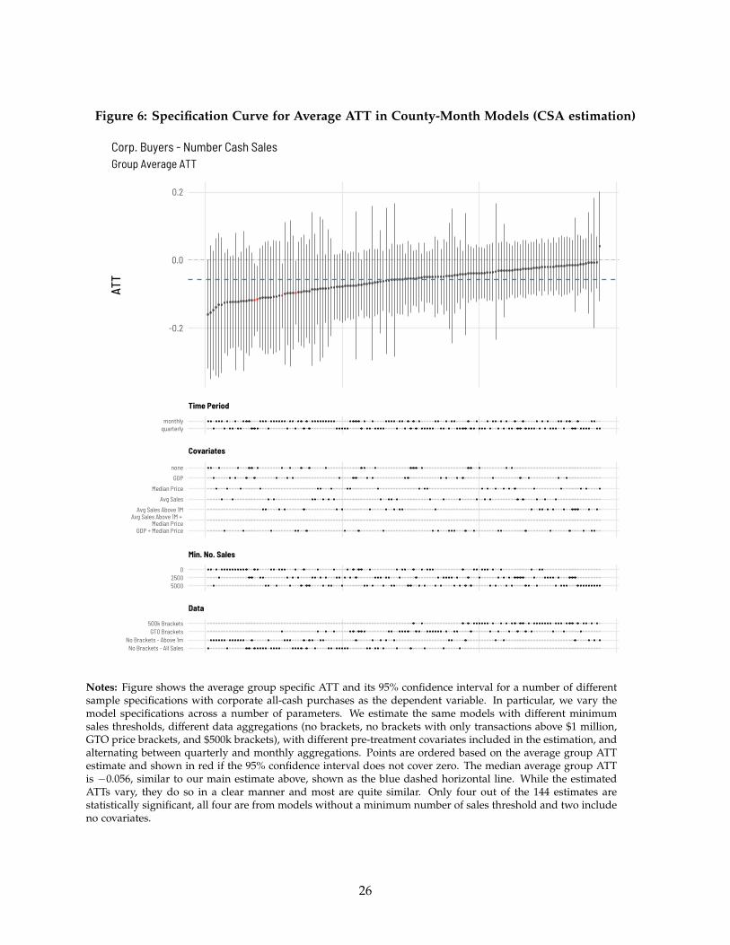
Figure 6: Specification Curve for Average ATT in County-Month Models (CSA estimation)

-0.2

0.0

0.2

ATT

quarterlymonthly

Time Period

GDP + Median Price

Avg Sales Above 1M + Median Price

Avg Sales Above 1M

Avg Sales

Median Price

GDP

none

Covariates

50002500

0

Min. No. Sales

No Brackets - All SalesNo Brackets - Above 1m

GTO Brackets500k Brackets

Data

Group Average ATT Corp. Buyers - Number Cash Sales

Notes: Figure shows the average group specific ATT and its 95% confidence interval for a number of differentsample specifications with corporate all-cash purchases as the dependent variable. In particular, we vary themodel specifications across a number of parameters. We estimate the same models with different minimumsales thresholds, different data aggregations (no brackets, no brackets with only transactions above $1 million,GTO price brackets, and $500k brackets), with different pre-treatment covariates included in the estimation, andalternating between quarterly and monthly aggregations. Points are ordered based on the average group ATTestimate and shown in red if the 95% confidence interval does not cover zero. The median average group ATTis −0.056, similar to our main estimate above, shown as the blue dashed horizontal line. While the estimatedATTs vary, they do so in a clear manner and most are quite similar. Only four out of the 144 estimates arestatistically significant, all four are from models without a minimum number of sales threshold and two includeno covariates.

26

B.13 show the group average ATT when each of the three treatment groups are being excluded

from the model. As one can easily see, the point estimate and confidence interval around the

estimate changes little when specific counties or whole treatment groups are excluded. Lastly,

Figure B.9 in the Appendix shows the dynamic event study estimates for our main outcomes

of interest as estimated by the augmented synthetic control method introduced by Ben-Michael,

Feller, and Rothstein (2021). Again, there is no clear evidence of a strong overall effect of the

GTO on corporate all-cash purchases.

4.2 The impact of GTOs on corporate cash transactions more likely to be illicit

One limitation of our main analysis is the noisiness of the data, driven by heterogeneity in cor-

porate cash transactions both across counties and across time. This leaves the possibility that

our inability to pin down precise effects is driven in part because changes in a small number

of illicit transactions are being obscured by large fluctuations in perfectly legal corporate crash

transactions. In this section we attempt to focus on transactions that are more likely to have in-

volved illicit money, under the assumption that these will be more responsive to the introduction

of GTO reporting requirements.27

We first consider purchases made by companies that are more likely to be anonymous shell

corporations: those that do not engage in any sort of economic activity aside from facilitating

transactions and buying and holding assets. To better identify transactions that involve shell

companies (and are thus more likely to have involved illicit money), we consider purchases by

companies with the following characteristics:

1. Created using formation agents, which are corporate service providers that specialize in

setting up shell companies and have been associated with criminal and corruption cases in

the past (Goodrich, Cowdock, and Simeone, 2019).

2. Companies incorporated shortly prior to the real estate transaction taking place, under the

assumption that the company was only created to facilitate the transaction or hold the real

estate.

3. Companies formed in US states that, due to local legislation, have allowed for anonymous

27Foreign individuals as well as legal entities registered in offshore tax havens have been anecdotally linked tosuspicious transactions in a number of markets across the United States. However, 99.5% of companies in the ZTraxdataset report US addresses when completing real estate transactions, with no other information available about theirforeign ties or ownership in state business registries. Therefore, we are unable to identify foreign-owned or operatedcompanies buying residential properties, and instead rely on the proxies described below.

27

ownership in the past and are associated with illicit finance.28

To create corporation types, we merge the universe of corporate buyers in the ZTRAX data

with the universe of firms in the Open Corporates data set.29 We apply the same standardizing

algorithm to the legal entity names from both the ZTrax and the OpenCorporates, and then

perform exact string matching based on name and state.30 This process was able to assign

OpenCorporates unique identifiers to 12.7 million of the 17.8 million legal entities appearing

as buyers in the Ztrax dataset from 2010-2019. We then create the four types of corporations

mentioned above by coding fields from the OpenCorporates data. This requires that we assume

that the match rate between the ZTrax data and OpenCorporates is orthogonal to the introduction

of the GTOs, which we believe is quite reasonable.

Companies were coded as using formation agents if that agent had registered at least 1,000

companies in the OpenCorporates dataset. We compared company incorporation dates to the

real estate transaction dates to code whether the company was formed just prior to the property

purchase. Specifically, we code companies as ’newly’ incorporated if they are registered fewer

than 183 days (six months) prior to the transaction date. Finally, we use data on the state of regis-

tration to determine whether a company was located in a secrecy jurisdiction.Next, we aggregate

all-cash purchases and total all-cash purchase price volume for each of the four company types

at the county-month level.

Figure 7 shows the average group ATT and GTO specific ATTs and 95% confidence intervals

for the number of purchases in each category. Tables B.14 and B.15 in the Appendix show the full

results for the number of purchases and price volume, respectively. There is no clear or consistent

evidence that GTO policies changed all-cash real estate transactions involving corporations regis-

tered using formation agents. In fact, the overall estimate is positive. The average group ATT for

corporate all-cash transactions by newly incorporated corporations or those from secretive states

is negative but both small and insignificant. However, we find a large, significant effect for the

first GTO: an approximately 30% decline in purchases using newly-incorporated companies and

28We define these states as Delaware, Nevada, and Wyoming. These three states were identified by both FinancialAction Task force and FinCEN as being prone to abuse, due to their lax position towards anonymous shell companies(Network, 2006; FATF, 2013b). A former special agent for the US Treasury also singled the three states out in 2013as being “nearly synonymous with underground financing” (Cassara, 2013). With the passing of the 2021 CorporateTransparency Act, all anonymous ownership of domestic companies will (in theory) be eliminated.

29OpenCorporates aggregates data from the business registries of 49 US states (plus the District of Company) intoa unified standard. Illinois does not make its business registry accessible public. https://opencorporates.com/registers

30At the state level, legal entities register with unique names.

28

Figure 7: Overall impact of public GTO announcements on more ‘suspicious’ purchases (CSAestimation)

18 treated counties 2 treated counties 11 treated counties 5 treated counties

-0.5

0.0

0.5

1.0

Average Jan 2016 July 2016 Nov 2018GTO Announcement

ATT

Dependent Variable Corp. All-Cash Purchases Formation Agents

Corp. All-Cash Purchases Newly Incorp.

Corp. All-Cash Purchases Secret State

Notes: Figure shows estimates of the average treatment effect on the treated (ATT) for the GTO announcement,aggregating all the group-specific effects together (average) and group-specific ATT estimates for the January2016, July 2016 and November 2018 announcements, respectively. The outcome of interest are the inversehyperbolic sine of the number of transactions we identify as particularly suspicious. The is no evidence of asignificant overall decline in these types of transactions, though the estimates for the first GTO suggest thatcorporate all-cash purchases by newly registered companies or those registered in secretive states may havedeclined. Though note that these estimates are only based on two observations (Miami & Manhattan) andare similar for placebo outcomes. All estimates calculated using Callaway & Sant’Ana’s (2021b) doubly robustestimation method. 95% confidence intervals shown. Sample includes 18 GTO counties. Group ATTs arecalculated based on 12 pre- and post-treatment months.

a roughly 50% reduction in those involving US states with high degrees of corporate secrecy.

Overall, given that all-cash transactions from these types of corporations are the most likely

cases for detecting any effect of GTOs, we interpret these results again as cautious evidence that

the GTOs are unlikely to have had large aggregate impacts on illicit monetary flows into real

estate. Again, however, there is some evidence that the first GTO may have made an impact,

though it is important to keep in mind that the group only includes two treated counties (Miami-

Dade and Manhattan). In addition, we find similar estimates for the first GTO for placebo

outcomes that should be unaffected by the policy: total sales and individual mortgage purchases.

We will investigate these two counties in more detail in Section 4.4.

29

4.3 Evasion of GTO reporting through substitution into other forms of purchases or

lower price brackets

4.3.1 Evasion through other types of entities or by avoiding the use of title companies

In our main specifications we have not found a clear or consistent effect of GTO policies on all-

cash corporate purchases. An additional observable implication of an impact of the GTOs might

be buyers adjusting their behavior in order to avoid being subject to the GTOs. For example,

anonymous buyers might stop using corporations to hide their identities or shift away from all-

cash purchases. Similarly, since the policies apply at specific price thresholds, purchase prices

might be adjusted. In this section, we investigate these possible substitution effects. First, we

test whether GTOs led to an increase in all-cash purchases by buyers using trusts instead of

corporations, as trusts were not covered by any of the GTOs. Second, one possibility of avoiding

the reporting of transactions to FINCEN is using mortgages instead of all-cash purchases.

Even though banks are required to conduct due diligence checks in their customers, buyers

may target those banks with the weakest levels of compliance, relying on short-term mortgages

with the main goal of avoiding all-cash declaration. We, therefore, estimate whether corporate

buyers moved to using mortgages from banks with a higher risk of compliance failure or foreign

banks. We define banks with a higher risk of compliance failure (bad banks, for short) as those

that have been subject to an enforcement action by a US financial regulator since the year 2000.

We describe in Section B.4 in the Appendix how we construct this list.

Figure 8 and Table B.16 in the Appendix show average group ATTs and GTO announcement

specific ATTs for the total number of purchases (IHS) for all-cash purchases by trusts, corporate

purchases with mortgages from bad banks, and lastly corporate purchases with mortgages from

foreign banks. We do not see any evidence of a positive effect of the GTOs on any of the potential

substitutes. The effects estimated are negative. Contrary to expectations, we find a negative and

significant overall group ATT on corporate purchases using mortgages from foreign banks. We

also find a negative effect of the first GTO on all-cash trust purchases, though recall this is only

based on two counties (Miami-Dade and Manhattan).

Table B.17 shows the results from the same models with purchase price volume (IHS) as

the dependent variables. As the table shows, there is some evidence that total price volume

of purchases using bad banks increased. Once again, we only find a negative significant overall

group ATT for corporate purchases with mortgages from foreign banks. As with number of

30

Figure 8: Overall impact of public GTO announcements on potential substitutes (CSA esti-mation)

18 treated counties 2 treated counties 11 treated counties 5 treated counties

-1.5

-1.0

-0.5

0.0

0.5

Average Jan 2016 July 2016 Nov 2018GTO Announcement

ATT

Dependent VariableCorp. Mortgage Purchases Bad BanksCorp. Mortgage Purchases Foreign Banks

Trust All-Cash Purchases

Notes: Figure shows estimates of the average treatment effect on the treated (ATT) for the GTO announcement,aggregating all the group-specific effects together (average) and group-specific ATT estimates for the January2016, July 2016 and November 2018 announcements, respectively. The outcome of interest are the inverse hyper-bolic sine of the number of transactions we identify as potential substitutions to corporate all cash purchases.If the GTO policies had the expected effects, we would expect an increase in purchases of these substitutioncategories, i.e., positive effect estimates. We do not find any positive ATTs, in fact we observe a negative andsignificant average group ATT for corporate purchases using mortgages from foreign banks. We also find a neg-ative effect of the first GTO on all-cash purchases using trusts. All other ATT estimates are quite close to zeroand the 95% intervals for the all of the ATTs cover zero. All estimates calculated using Callaway & Sant’Ana’s(2021b) doubly robust estimation method. 95% confidence intervals shown. Sample includes 18 GTO counties.Group ATTs are calculated based on 12 pre- and post-treatment months.

purchases, this indicates that purchases using mortgages from foreign banks actually decreased

in response to the GTO, opposite to what one would expect. All other 95% confidence intervals

for the average group ATT and GTO announcement specific ATTs include zero.

The GTO policies require title insurance companies to report all-cash transactions with legal

entity buyers to FinCEN. One potential strategy to avoid reporting under the GTO would be to

bypass title companies. Although nearly all institutional lenders mandate individual borrowers

take out title insurance policies to protect against financial losses, title insurance for all-cash

buyers is voluntary. To identify whether GTO implementation led to changes in the use of title

companies or attorneys, we measure whether title companies (or alternatives) were used in a

given transaction. To do so, we code a binary indicator if the ZTrax variable TitleCompanyName

31

Figure 9: Title company coverage for six counties affected by Geographic Targeting Orders

Notes: Figure shows the percentage of property sales where title companies were used in six counties that weresubject to GTOs in July 2016 and November 2018 (dotted lines show the months of announcement). The dotted lines(both with near 100% title company usage) track individual mortgage purchases above (red) and below (blue) $1million. The solid lines track corporate all-cash purchases above and below the same thresholds

was missing or had a value of "None Available", Zillow’s indicator for the use of title insurance.

Unfortunately, full data on title companies is missing for most counties in the ZTrax dataset;

we observe this through the substantial number of transactions where institutional lenders pro-

vide mortgages but no title company is reported (as is mandated). Therefore, we can only exam-

ine changes in the use of title companies in six counties covered by the GTOs: Los Angeles, San

Diego, San Francisco, San Mateo, Santa Clara, and Clark County. This small sample size prevents

the estimation of our preferred difference-in-differences models; instead we plot the raw data in

Figure 9 to look for potential breaks around the introduction of GTO policies. In none of the six

counties do we see a drop in the use of title companies following the GTOs, either for corporate

all-cash purchases above or below $1 million thresholds. Although the lack of data for the entire

group of affected counties prevents us from definitely stating that corporate buyers evaded the

GTOs by refusing to engage title companies, what we can observe from available data suggests

little such evasive behavior.

4.3.2 Testing for evasion into lower price brackets by examining bunching behavior

As we have described above, Geographic Targeting Orders do not only increase the probability

that a purchase funded through illicit means will be detected, but they also create a price thresh-

32

old over which that probability increases discontinuously. If a company purchases a luxury

apartment in Miami in mid-2017 for $1,000,001, in cash with title insurance, then the insurance

company will be required to report beneficial ownership information to FinCEN. But if that same

purchase is made for $999,999 then no report is made.

If GTOs create a credible threat of detection, those still wishing to purchase in affected mar-

kets may instead opt to purchase a property just below the reporting cutoff. This could both

create excess demand for properties that are close in price to the cutoff, but also create incentives

for buyers to negotiate a lower official purchase price, by either conceding on other dimensions

(e.g. the timing of the purchase) or by making unrecorded side payments to the seller.

There is an extensive literature that examines “bunching” behavior in respond to discontinu-

ous changes in payoffs. Particularly relevant to this study are a number of papers showing that

notches - discontinuous changes in transaction taxes- lead to bunching below the relevant cutoff

(Kopczuk and Munroe, 2015; Slemrod, Weber, and Shan, 2017; Best and Kleven, 2018).

For example, Kopczuk and Munroe (2015) find that the “mansion tax,” a 1% transaction tax

levied on all residential property sales valued at $1m or more in New York State and New Jersey,

leads to substantial bunching of the reported price, with an excess number of properties being

sold just below the threshold, as well as a missing mass of fewer properties being sold just above

it. Even though Kopczuk and Munroe (2015) examine transactions taking place between 2003-

2011, we find the effect of the mansion tax is still evident today in the ZTrax data covering New

York City (See Figure 10).

Do GTOs induce those who want to make a purchase through a corporation in cash to bunch

around the GTO threshold? To investigate this, we calculate the share of corporate cash purchases

at each $25k price point (e.g. a purchase at $330,000 would be coded as $325,000). We then graph

the share of purchases in each bin for each GTO threshold separately, for counties where a given

GTO threshold was active, only on the dates when it was active.

We graph these results in Figure 11. For comparison, we also show the density for all corpo-

rate cash purchases on dates prior to the date the GTO came into effect. If bunching behavior

was prevalent, it would manifest as excess mass to the left of the threshold, and missing mass

to the right of threshold, particularly relative to purchases prior to the GTO coming into effect.

Across all five thresholds we see no strong evidence of any bunching.

While this does not rule out the substitution of lower-value properties for higher value prop-

erties, it does suggest that, on the margin, buyers looking to avoid the scrutiny generated by

33

Figure 10: The impact of the mansion tax on price bunching in NYC purchases

Note: Figure shows the log of all recorded purchases in ZTrax in New York City between 2010-2020, aggregatedat every $25k interval. The black line shows the counterfactual density from a regression of the following form:Log(sales)p = βBp + ∑1075k

b=975k Db + ep, where the number of sales is regressed linearly on the binned price, withindicator variables for the bins that excess bunching and missing mass is observed. The counterfactual density is thenestimated using the estimate of β, thus excluding the influence of the bunched/lower density bins.

GTOs are not doing so by manipulating the purchase price in the area around the threshold.

4.4 Digging into potential hotspots: Miami-Dade and Manhattan

While there is no strong aggregate evidence that there was a decline in corporate cash purchases

in GTO-affected counties, Figure 3 does suggest there may have been a modest decline at the

time of the first GTO announcement in Miami and Manhattan - with the former being the county

driving most of the observed negative effect. Similarly, Figure 7 suggests there may also have

been a decline in purchases made through newly-incorporated shell companies incorporated in

US states with a high degree of secrecy.

To explore this possibility descriptively, we present purchase volumes for the first two GTO

countries, Miami-Dade and Manhattan, in Figure 12. Each figure shows the total dollar volume

of all corporate cash purchases above the GTO threshold (in red) versus below the threshold

(in blue). We also graph individual mortgages purchases above and below the threshold (using

34

Figure 11: (Non)evidence of bunching of corporate-cash purchases around the GTO thresholds

(a) $3m (b) $2m

(c) $1.5m (d) $1m

(e) $300k

Notes: Each subfigure shows the density of corporate-cash purchases around the GTO reporting threshold for every$25k price bin, for all for all counties affected by that GTO threshold both for (in red) the entire period following theintroduction of the GTO (until the end of 2019) and (in black) the entire period from 2010 until the GTO came intoeffect. For both of these, all transactions outside the observed window are dropped (to account for long term shifts inthe overall density) The counties used in each figure are as follows: $3m (Manhattan), $2m (Los Angeles, San Diego,San Francisco, San Mateo, Santa Clara), $1.5m (Brooklyn, Queens, Bronx, Staten Island), $1m (Miami-Dade, Broward,Palm Beach), $300k (All GTO counties). For the $300k threshold, we have dropped the period where the ‘secret’ GTOwas in effect (May 21,2018 until November 17, 2018). For Manhattan and Miami, the GTO threshold was defined as allpurchases "in excess" of the threshold. For these we assign all purchases at the threshold to the bin immediately below.

35

lighter versions of both colors), our placebo outcome of choice since mortgages were not subject

to any additional scrutiny under the GTO program.

In Miami-Dade, corporate cash and individual mortgage volumes roughly track each other

(in their respective price brackets) until the announcement and the implementation of the first

GTO in January and March, 2016, respectively. Corporate cash volumes decline substantially in

the months following the announcement of the first GTO, a decline that is not observed in any of

the comparison groups. This suggest that there may have been a small, albeit temporary, decline

in Miami around the announcement of the first GTO.

To investigate this further, we use a synthetic control approach to estimating the impact of

the first GTO on Miami-Dade and Manhattan separately: using the total number of all corporate-

cash purchases above $1 million in the former case and all corporate cash above $3 million in the

latter case. The relative uniqueness of these two counties in the luxury property market creates a

challenge for the standard synthetic control approach: because both counties are at the top of the

national distribution of corporate cash purchases, there is no combination of non-GTO ‘control’

counties will create a well-match synthetic Miami or Manhattan.

To overcome this, we do two things. First, we define the outcome variable as being the

number of corporate cash purchases relative to the last pre-treatment period (December 2015).

For example, in the Miami-Dade estimation, if a county has 50 corporate cash purchases above

$1m in December 2015 and 100 in January, 2016, the outcome is 2. We thus drop all counties

that have zero purchases above the threshold in December 2015. To minimize the number of

control counties lost due to this method, we calculate all of our outcomes at the quarterly level.

Second, to account for an imperfect fit, we use the bias-correction methods of the augmented

synthetic control approach detailed in Ben-Michael, Feller, and Rothstein (2021) (more detail on

this approach is provided in Appendix Section C). Finally, for each estimation we only keep the

treatment county (Manhattan or Miami-Dade, respectively) and all non-GTO counties, so as to

not use control counties that subsequently become treated.

The main results are shown in Figure 13. While we observe declines in corporate all-cash pur-

chases in both counties following the announcement of the first GTO, the decline only happens

immediately in Miami-Dade. Even though there is a noticeable decline in purchases above $1m

relative to synthetic Miami, we observe similar declines in individual mortgages purchases, and

in all purchases, respectively. We see a similar long term pattern in Manhattan. Our conclusion

from these results is that the negative effect observed for this group (Miami-Dade and Manhat-

36

Figure 12: The number of property purchases in Miami-Dade and Manhattan, relative to theintroduction of the first Geographic Targeting Order, compared to two adjacent counties

(a) Florida

(b) New York City

Notes: Figure shows the number of property purchases in the two counties that were subject to a GTO in March, 2016(lines show the months of announcement and implementation) relative to two adjacent counties that were subject to aGTO later, in August 2016.

tan) in our main analysis is likely driven by idiosyncratic shocks that hit these property markets

around the same time as the GTO came into effect, rather than an impact of the GTOs on the

types of transactions that were being targeted.

37

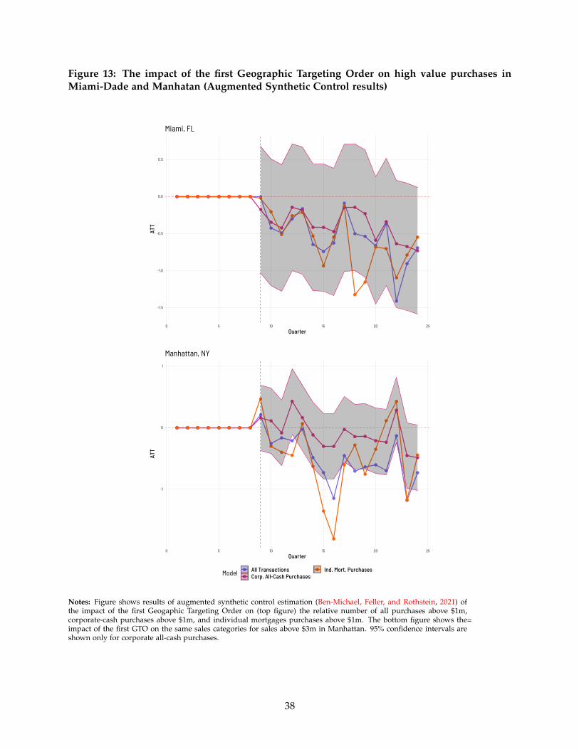
Figure 13: The impact of the first Geographic Targeting Order on high value purchases inMiami-Dade and Manhatan (Augmented Synthetic Control results)

-1.5

-1.0

-0.5

0.0

0.5

0 5 10 15 20 25

Quarter

ATT

Miami, FL

-1

0

1

0 5 10 15 20 25

Quarter

ATT

Model All TransactionsCorp. All-Cash Purchases

Ind. Mort. Purchases

Manhattan, NY

Notes: Figure shows results of augmented synthetic control estimation (Ben-Michael, Feller, and Rothstein, 2021) ofthe impact of the first Geogaphic Targeting Order on (top figure) the relative number of all purchases above $1m,corporate-cash purchases above $1m, and individual mortgages purchases above $1m. The bottom figure shows theimpact of the first GTO on the same sales categories for sales above $3m in Manhattan. 95% confidence intervals areshown only for corporate all-cash purchases.

=

38

Additional evidence for this interpretation comes from estimating the augmented synthetic

control models on the percentage of total price volume that is due to corporate all-cash pur-

chases. Again we estimate these models at the quarterly level but based on all sales with price

information. All non-GTO counties are potential comparison units. The results in Figure 14 are

even more striking. When looking at the percentage of price volume from all-cash corporate

purchases, there is no evidence of any effect of the GTOs in Manhattan, NY and Miami-Dade,

FL.

4.5 Did GTOs lead to a general chilling effect on illicit transactions?

Absent strong evidence that the GTOs led to a stark change in opaque transactions in the real

estate market, we consider the possibility that GTOs led to a general decline in illicit transactions

in affected counties. This might be the case because there was a small decline in illicit property

transactions that our previous analysis was unable to identify or because the GTOs led those

wanting to launder money to avoid targeting counties for fear of additional scrutiny by law

enforcement.

To study this, we turn to data on suspicious activity reports (SARs), the reports filed by

banks when they detect a transaction or activity by one of their customers that they deem is

worth reporting to FinCEN. There are no broad criteria as to what constitutes suspicious activity:

banks are left to their own devices to determine what might qualify. For example, a customer

who appears to be deliberately avoid automatic cash deposit reporting requirements by making

multiple deposits below the threshold might lead a bank employee to file a SAR.

On their own, SARs are not necessarily a good proxy or underlying levels of money launder-

ing. This is because the incentives that banks face to file SARS have changed over time. Because

filing a SAR allows banks to essentially ‘pass the buck’ on to law enforcement to follow up on

suspicious activity, there are significant incentives to over-file, what is often referred to as “defen-

sive filing” (Unger and Van Waarden, 2009). Thus an increase in SARs from one year to the next

could reflect a change in underlying criminal activity or just a change in the pressure financial

institutions face from regulators to report. However, because the GTO program did not affect

banks directly (by targeting only title companies and dealing only with property transactions),

we would not have expected banks to change their behavior in response to it. If the GTO program

led to a decrease in illicit money moving in and around targeted counties, we would expect the

39

Figure 14: The impact of the first Geographic Targeting Order on corporate all-cash volume aspercentage of total price volume in Miami-Dade and Manhatan (Augmented Synthetic Controlresults)

-20

0

20

0 5 10 15 20 25Quarter

ATT

Miami, FL

-10

0

10

20

0 5 10 15 20 25Quarter

ATT

Manhattan, NY

Notes: Figure shows the ATT estimate and 95% confidence based on the augmented synthetic control estimation (Ben-Michael, Feller, and Rothstein, 2021) of the impact of the first Geogaphic Targeting Order on the percentage of totalprice volume from all-cash corporate purchases in Miami (top) and Manhattan (bottom).

=

40

number of SARs filed by banks transacting with those counties to decline.31

We use data taken directly from FinCEN’s public portal, which detailed the number of

monthly SARs filed by each US county for the period 2014-2021. According to FinCEN, banks in-

dicate in a SAR where the suspicious activity took place.32 So while SARs should reflect changes

in the flow of illicit money moving in and out of a given county, it would not comprehen-

sively capture all flows connected to a given county. For example, if a buyer in Horry County,

South Carolina purchases a property in Miami-Dade from a seller who owns a bank account

in Shawnee County, Kansas, the location of the reported suspicious activity may be coded as

Horry or Shawnee, rather than Miami-Dade. Thus SARs will be a partial geographic measure of

suspicious activity, but not a perfect one.

We then estimate our main model, in which a county is considered treated when a GTO is

first announced. We also estimate an alternative model in which we use the ‘secret’ GTO date

in place of the third GTO. Finally, we estimate a third model in which counties covered by the

first two GTOs are not considered treated until the GTOs were amended to cover wire transfers.

This is to investigate whether this potential loophole, once closed down, led to a decline in wire-

transfers related to illicit property purchases and thus a decline in the number of transfers being

flagged through suspicious activity reports.

Table 2 and Figure 15 display the main results from this exercise. Across none of the three

specifications is there a significant impact of the introduction of the GTOs (or their revision) on

the number of SARS being filed at the county level. The largest estimated effects are for the

revision of the GTOs to include wire transfers, which led to an estimated increase in SARs of

around 2%. However, this effect is not significant at standard levels of inference. As can be seen

in Table 2, none of the group-specific estimates are significant, though some are positive. The

group specific ATT for the secret GTO is most substantial, suggesting a 6% increase in SARS

being filed.

Taken together, the introduction of the GTO program does not appear to have had a per-

ceptible impact on illicit activity in the targeted counties, as measured by suspicious activity

reports.

31However, at the same time, if the GTO program led buyers trying to launder illicit cash to rely more on theexisting banking system, then the introduction of the GTO program could lead to an increase in SARs).

32In instances where this field was empty, the location of the SAR may revert to the location of the relevant bankbranch or corporate office.

41

Table 2: Impact of GTO announcement on SARS – Quarterly Aggregation

Public GTOs Public & Secret GTOs Extension to Wire Transfers

(1) (2) (3)

Average −0.028 −0.020 0.019[−0.073, 0.018] [−0.072, 0.033] [−0.038, 0.077]

Quarter 1, 2016 −0.012 −0.012[−0.112, 0.089] [−0.103, 0.080]

Quarter 3, 2016 −0.067 −0.067[−0.149, 0.014] [−0.139, 0.004]

Quarter 3, 2017 0.011[−0.067, 0.089]

Quarter 2, 2018 0.063[−0.023, 0.150]

Quarter 4, 2018 0.037 0.037[−0.016, 0.091] [−0.016, 0.091]

No. Obs. 230 230 230

Note:Models estimated using the did package in R. Unit of analysis is the county-quarter.Control group: not-yet-treated. Sample includes 18 GTO counties. Included pre-treatment covariates are: County level GDP in 2015 (ln) and median sales price 2015(ln). Outcome is the inverse hyperbolic sign of the number of SARS filed at the countylevel in a given quarter. Public GTOs uses the three main public GTOs as the relevanttreatment dates. Public & Secret uses the date of the announcement of the secret GTOas the relavant treatment date for the third treatent group. Extension to Wire Transfersuses August 2017 as the relevant treatment date for the first two groups (as this isthe moment when the GTOs were expanded to cover wire transfers in these counties)and uses November 2018 as the relevant date for the final group. Standard errorsclustered at the GTO group-county level. Group ATTs calculated based on 6 pre- andpost-treatment quarters

42

Figure 15: Event study estimates of the impact of GTOs on Suspicious Activity Reports (SARs)filed by banks

-0.2

-0.1

0.0

0.1

0.2

0.3

-5 0 5Quarters until GTO is announced

ATT

Public & Secret GTOsPublic GTOs

Wire Transfer Expansion

Notes: estimates are (dynamic ATT) estimates of the impact of public GTO announcements on the inverse hyperbolicsign of the number of suspicious activity reports (SAR)s filed per 100,000 people at the county level to FinCEN between2014 and the end of 2019 (only shown for the window of 6 quarters leading to or following the announcement of aGTO). Event time is in months relative to the announcement date. All estimates calculated using Callaway & Sant’Ana’s(2021b) doubly robust estimation method with the median 2015 price and GDP-per capita included as controls (resultscorrespond to columns (1), (2) and (3) of Table 2. 95% confidence intervals shown.

4.6 Aggregate property market effects of the program

One often-cited concern over the use of local property by foreigners to launder money is that

this behavior has the potential to drive up local property prices (De Simone, 2015). While there

is evidence that other drivers of foreign investment in real estate (such as economic uncertainty

or restrictions on foreign ownership in other markets) have an impact on local house prices

(Badarinza and Ramadorai, 2018; Gorback and Keys, 2020) there has been little evidence that the

flow of dirty money has the same impact.

In theory, if the GTOs had led to a significant decline in investment in the markets being

targeted, we would expect this to manifest in a decline in property prices. To test this, we

repeat our main analysis using Zillow’s Home Value Index (ZHVI) as an outcome. Zillow’s

43

ZHVI is described as a seasonally-adjusted dollar value of the ‘typical’ home in a market. The

index derived from averages of Zillow’s Zestimate, the main estimate of a property’s value from

Zillow’s valuation model. Zillow publishes monthly data on the ZHVI separately for properties

in the ‘top tier’ (those priced at and above the 66th percentile for a given market), the ‘middle

tier’ (those priced between the 33rd and 66th percentile) and the ‘bottom’ tier, which is everything

below the 33rd percentile. Across most of our markets, we would expect the first two and third

GTOs to negatively affect primarily the top and mid-tiers respectively, but not the bottom tier of

the market.

Figure 16 shows the event study estimates when we use the same model in our main analysis,

but use the three tiers of the ZHVI as our outcome. We present the full results in Table B.18 in

the Appendix. While there is a short term decline in the ZHVI following the announcement of a

new GTO in targeted markets, the negative point estimates are small (less than 1%), insignificant

and transitory, lasting fewer than a few months. Furthermore, these small, insignificant declines

are observed across all three tiers, indicating that the shift in the ZHVI observed at this time is

not likely to be driven by the GTOs and themselves. The overall group-ATT for the three tiers

is estimated at -0.003, -0.002, and -0.002) respectively, indicating that there is effectively no long

term impacts of the GTOs on house prices.

While this is yet another clue that the GTOs are not likely to have led to a sizable shift in

investment in investment in these markets, it is also an indication that these policies have not

led to any substantive market impacts. Given that the reporting requirements of the GTOs may

ultimately raise transaction costs in these markets (via the extra costs borne by title companies),

it is reassuring that these costs do not appear to have manifested in changes in property values.

To the extent that the GTO program still has value as an information-gathering exercise for law

enforcement, the costs associated with it appear to be minimal.

5 Discussion

Overall the analysis has revealed that the GTOs had a small and statistically insignificant effect

on corporate all-cash purchases in the targeted counties. This null effect does not appear to

vary based on when, in which counties, or at what sales price threshold the orders were imple-

mented. We also do not see substitution into other types of purchases not covered by the GTOs,

for example, legal entities taking out loans from "bad" or foreign banks or trusts being used in-

stead of other types of legal entities. Similarly, the GTOs did not drive down all-cash purchases

44

Figure 16: Event study estimates of the impact of public GTO announcements on Zillow’sHome Value Index (ZHVI) at the county level

-0.02

-0.01

0.00

0.01

0.02

-5 0 5Month until GTO is announced

ATT

Lower Tier (0 - 33th pct)Middle Tier (33th-66th pct)

Top Tier (66th-100th pct)

Notes: estimates are (dynamic ATT) estimates of the impact of public GTO announcements on the log of the ZillowHome Value Index from between the beginning of 2014 to the end of 2019 (only shown for the window of two yearsleading to or following the announcement of a GTO). Event time is in months relative to the announcement date Allestimates calculated using Callaway & Sant’Ana’s (2021b) doubly robust estimation method with the median 2015 priceand GDP-per capita included as controls 95% confidence intervals. shown.

by some of the corporations most associated with this type of money laundering in the United

States: LLCs registered in so-called secrecy jurisdictions or by corporate service providers. Fi-

nally, whereas other regulatory interventions (such as mansion taxes) generated bunching just

under declared thresholds, we do not observe similar patterns with regards to the thresholds

used by FinCEN. Taken together, we find little evidence that the GTOs reduced the amount of

money being invested into the US real estate market through the corporate all-cash route.

5.1 Lack of illicit transactions or incomplete implementation?

We see two possible explanations for why the reform did not produce the intended, observable

results. On one hand, the GTO laws could have been properly implemented and enforced, but

the scale of money laundering into the luxury real estate market in the US might be substantially

smaller than expected. By definition, money laundering is a very difficult problem to identify

45

and measure. What we do know about the practice in the United States comes from anecdotal

journalistic investigations and criminal prosecutions rather than comprehensive forensic analysis.

It is possible that only a small fraction of corporate all-cash purchases actually involve suspicious,

wealthy individuals who would not want to reveal their identity to federal authorities. The GTOs

may have deterred such buyers from entering the targeted countries, but their number was not

so large that their exit from the market would affect aggregate statistics about corporate all-cash

purchases. We term this the small scale explanation.

On the other hand, we might hypothesize that the volume of money being laundered through

the US luxury real estate market is substantial, but GTOs did not effectively deter bad actors from

continuing to exploit the sector. We term this the incomplete implementation explanation, in that the

implementation of the GTOs by FinCEN may have been insufficient to change corporate buyer

behavior. Incomplete implementation can arise along three dimensions: compliance, verification,

and enforcement.33 First, corporate all-cash buyers may have refused to faithfully comply with

the regulation, either by submitting false (or even failing to submit) beneficial ownership infor-

mation as required. Such non-compliance deprived officials of actionable intelligence to pursue

money launderers and undermined the efficacy of the GTOs.

Next, even if corporate all-cash buyers complied and submitted reports on their beneficial

owners, law enforcement authorities may have failed to verify the information. Beneficial owner-

ship reporting is a relatively recent form of transparency requirement. As countries worldwide

begin to implement similar directives, journalists and academics have consistently uncovered fail-

ures by governments such as the United Kingdom and Luxembourg in ensuring the quality and

accuracy of data submitted to officials (GW, 2013; Martini and Szakonyi, 2021). Corporate buyers

may have realized that there were no mechanisms or penalties for submitting false information

and continued their money laundering activity as before. Finally, law enforcement officials must

both be able to identify and then hold money launderers accountable through criminal prose-

cution. Acquiring accurate information on beneficial owners aids in the former, but does not

necessarily ensure that investigations will be conducted, arrests made, and suspicious assets

seized.

Although testing between the two explanations is complicated by confidentiality surrounding

33Section 4.3 demonstrated that bad actors were not exploiting a fourth dimension, loopholes in the regulation, forexample, by using trusts or taking out mortgages from shoddy lenders in order to avoid the transparency requirementsof the GTOs.

46

official FinCEN data,34 the preponderance of publicly available evidence suggests the lack of

measurable effect of the GTOs is best explained by incomplete implementation. First, compliance

with the GTO orders may be incomplete. Official figures given by FinCEN (as of August 15,

2019) cite 23,659 beneficial ownership reports submitted by title companies pursuant to the GTOs

(GAO, 2020). Using the Ztrax dataset, we calculate that there were no fewer than 26,415 corporate

all-cash transactions occurring in GTO-covered counties during the same period, i.e. those that

had sales prices above the price threshold in place at the time of the transaction. Because Texas is

a non-disclosure state, ZTrax is missing data on covered transactions in Bexar, Dallas and Tarrant

Counties. Therefore, we estimate that at best, GTO reports were submitted in no more than 89%

of applicable cases; taking into consideration the missingness in Texas, the true number is likely

to be significantly lower.

In 2020, the Government Accountability Office (GAO) likewise identified significant short-

comings in FinCEN’s oversight of title companies, and in particular the lack of examination of

the dozens of firms submitting GTO reports (GAO, 2020). FinCEN did evaluate compliance by a

single title company, but only three years after the first directive was implemented in 2016. The

other 28 companies did not undergo such scrutiny nor were the results of that evaluation publicly

related. As written, the GTOs do not provide a clear mechanism for verifying that corporations

are accurately reporting their beneficial owners. In conversations with this paper’s authors,

FinCEN officials did not elaborate on how the GTO beneficial ownership data was handled or

analyzed, though perhaps because they were hesitant to share sensitive information about the

tactics used. Worryingly, the GTO orders are also vague about the civil and criminal liability that

these title companies face for not fully complying (McPherson, 2017).

Perhaps the biggest weakness in implementation relates to enforcement. FinCEN officials

reported to the GAO in 2020 that "the GTO reports, in some cases, helped identify potential

suspects of interest for further investigation and led to law enforcement referrals" (GAO, 2020,

13). Indeed, six enforcement agencies and two interagency task forces shared that GTO reports

had been used in their investigations. Yet as of 2020, government officials were not aware of

any cases where real assets were seized or forfeited based on the information contained in GTO

reports. In fact, it took more than two years after the first GTO was issued in 2016 for FinCEN

to systematically contact different law enforcement officials to share information (GAO, 2020).

34In March 2020, the authors submitted to FinCEN detailed questions and requests for data concerning the imple-mentation of the GTO program, but as the time of the writing, no response has been received.

47

Independently we were also unable to find any criminal cases involving real properties where

GTO reports were specifically cited in court documents or media reports. Without publicized

asset seizures and forfeitures, it remains unclear whether bad actors believed the GTO program

carried real punishments and thus would have changed their purchasing behavior.

The limited data shared by FinCEN about the GTO program also suggests that the scale

of money laundering through US real estate has been and continues to be substantial, thereby

helping excluding the "small scale" explanation. Of the 23,659 GTO reports submitted from 2016-

2019, 8,652 (37%) involved an individual who had been mentioned previously in a suspicious

activity report (SAR), which financial institutions file with the US Department of Treatment when

transactions of more than $10,000 are suspected of a connection to money laundering or other

criminal activity. Although a SAR in and of itself is not proof of criminal activity, the mere fact

that over a third of all GTO-covered (i.e. luxury) transactions involved such individuals after

the program was implemented suggests that scale of suspicious activity in the sector is large.

Likewise, the FBI indicated that "nearly 7 percent of the GTO reports identified individuals or

entities connected to FBI’s ongoing cases since the issuance of GTO in 2016" (italics added) (GAO,

2020).35 Although the number of counties targeted by the GTOs was both small and selective,

based on these official statistics, the volume of suspicious money flowing into the US real estate

market was large enough to be detected using our empirical approach and the fine-grained ZTrax

data.

6 Conclusions

Our analysis shows that across all targeted counties, the GTO orders had no aggregate effect

on the number or volume of all-cash corporate transactions. Using a variety of estimation tech-

niques, we see little evidence that would-be money launderers have been effectively deterred by

the policy as to decrease their purchase of high-end properties in the United States. We do not

observe a body of supporting evidence across a number of dimensions that corporate buying

behavior changed due to this policy. In all likelihood, the lack of visible enforcement of the GTO

orders, as signalled by criminal investigations and seizures of properties linked to criminal actor,

best explains the limited effectiveness of the policy.

35More recent reports by non-governmental investigators paint a similar picture of ongoing money laundering inthe sector. For example, Global Financial Integrity found 56 known criminal cases involving money laundering in USreal estate publicly reported from 2015-2021 that collectively were valued at least $2.3 billion (GFI, 2021). Over 80% ofthese cases used a corporate structure to hide the true owner, and 40% involved properties located in a GTO-coveredcounty.

48

-

49

References

Abadie, Alberto, Alexis Diamond, and Jens Hainmueller. 2010. “Synthetic control methods

for comparative case studies: Estimating the effect of California’s tobacco control program.”

Journal of the American statistical Association 105 (490): 493–505.

Abadie, Alberto, Alexis Diamond, and Jens Hainmueller. 2015. “Comparative politics and the

synthetic control method.” American Journal of Political Science 59 (2): 495–510.

Agarwal, Sumit, Liu Ee Chia, and Tien Foo Sing. 2020. “Straw Purchase or Safe Haven? The

Hidden Perils of Illicit Wealth in Property Markets.” The Hidden Perils of Illicit Wealth in

Property Markets (September 8, 2020) .

Agca, Senay, Pablo Slutzky, and Stefan Zeume. 2021. “Anti-money laundering enforcement,

banks, and the real economy.” Available at SSRN 3555123 .

Badarinza, Cristian, and Tarun Ramadorai. 2018. “Home away from home? Foreign demand and

London house prices.” Journal of Financial Economics 130 (3): 532–555.

Baker, Andrew, David F Larcker, and Charles CY Wang. 2021. “How Much Should We Trust

Staggered Difference-In-Differences Estimates?” Available at SSRN 3794018 .

Beer, Sebastian, Maria Delgado Coelho, and Sebastien Leduc. 2019. Hidden Treasure: The Impact

of Automatic Exchange of Information on Cross-Border Tax Evasion. Technical report Interna-

tional Monetary Fund.

Ben-Michael, Eli, Avi Feller, and Jesse Rothstein. 2021. “The Augmented Synthetic Control

Method.” Journal of the American Statistical Association 116 (536): 1789–1803.

URL: https://doi.org/10.1080/01621459.2021.1929245

Best, Michael Carlos, and Henrik Jacobsen Kleven. 2018. “Housing market responses to transac-

tion taxes: Evidence from notches and stimulus in the UK.” The Review of Economic Studies

85 (1): 157–193.

Bethencourt, Daniel. 2018. “Latest GTO Covers Less-Expensive Real Estate, More US Metropoli-

tan Areas.” ACAMS Money Laundering.com .

URL: https: // www. moneylaundering. com/ news/ latest-gto-covers-less-expensive-real-estate-more-us-metropolitan-areas/

50

Bethmann, Dirk, and Michael Kvasnicka. 2016. “International tax evasion, state purchases of

confidential bank data and voluntary disclosures.” Working Paper Series .

Callaway, Brantly, and Pedro H.C. Sant’Anna. 2021a. “did: Difference in Differences.”. R package

version 2.1.1.

URL: https://bcallaway11.github.io/did/

Callaway, Brantly, and Pedro H.C. Sant’Anna. 2021b. “Difference-in-differences with multiple

time periods.” Journal of Econometrics .

URL: https://doi.org/10.1016/j.jeconom.2020.12.001

Casi, Elisa, Christoph Spengel, and Barbara MB Stage. 2020. “Cross-border tax evasion after the

common reporting standard: Game over?” Journal of Public Economics 190: 104240.

Cassara, John. 2013. “Delaware, Den of Thieves?” The New York Times .

URL: https: // www. nytimes. com/ 2013/ 11/ 02/ opinion/ delaware-den-of-thieves. html

Cvijanovic, Dragana, and Christophe Spaenjers. 2020. ““We’ll Always Have Paris”: Out-of-

Country Buyers in the Housing Market.” Management Science .

De Simone, Matteo. 2015. Corruption on your doorstep: How corrupt capital is used to buy

property in the UK. Transparency International UK.

de Willebois, Emile van der Does, JC Sharman, Robert Harrison, Ji Won Park, and Emily Halter.

2011. The puppet masters: How the corrupt use legal structures to hide stolen assets and what

to do about it. World Bank Publications.

FATF. 2007. Money Laundering and Terrorist Financing Through the Real Estate Sector. Technical

report Financial Action Task Force.

URL: https: // www. fatf-gafi. org/ documents/ documents/ moneylaunderingandterroristfinancingthroughtherealestatesector.

html

FATF. 2013a. Money Laundering and Terrorist Financing Vulnerabilities of Legal Professionals.

Technical report Financial Action Task Force.

URL: https: // www. fatf-gafi. org/ documents/ documents/ mltf-vulnerabilities-legal-professionals.

html

51

FATF. 2013b. Third Mutual Evaluation Report on Anti-Money Laundering and Combating the

Finance of Terrorism. Technical report Financial Action Task Force.

URL: https: // www. fatf-gafi. org/ media/ fatf/ documents/ reports/ mer/ ME% 20US%

20full. pdf

Ferraz, Claudio, and Frederico Finan. 2011. “Electoral accountability and corruption: Evidence

from the audits of local governments.” American Economic Review 101 (4): 1274–1311.

Findley, Michael G, Daniel L Nielson, and Jason Campbell Sharman. 2014. Global shell games:

Experiments in transnational relations, crime, and terrorism. Number 128 Cambridge Univer-

sity Press.

Forbes, Kristin J. 2010. “Why do Foreigners Invest in the United States?” Journal of International

Economics 80 (1): 3–21.

Gabriel, Cynthia. 2018. “The rise of kleptocracy: Malaysia’s missing billions.” Journal of

Democracy 29 (1): 69–75.

GAO. 2020. Anti-Money Laundering: FinCEN Should Enhance Procedures for Implementing

and Evaluating Geographic Targeting Orders. Technical Report GAO-20-546 US Government

Accountability Office July 14: .

GFI. 2021. Acres of Money Laundering: Why U.S. Real Estate is a Kleptocrat’s Dream. Technical

report Global Financial Integrity.

Global Financial Integrity. 2019. “The Library Card Project: The Ease of Forming Anony-

mous Companies in the United States (March 2019); online https://www. gfintegrity. org/wp-

content/uploads/2019/03.” GFI-Library-Project_2019. pdf .

Goodman-Bacon, Andrew. 2021. “Difference-in-differences with variation in treatment timing.”

Journal of Econometrics .

Goodrich, Steve, Ben Cowdock, and Gabriele Simeone. 2019. At your service: Investigating how

UK businesses and institutions help corrupt individuals and regimes launder their money and

reputations. Transparency International UK.

Gorback, Caitlin S, and Benjamin J Keys. 2020. Global Capital and Local Assets: House Prices,

Quantities, and Elasticities. Technical report National Bureau of Economic Research.

52

Gray, Larissa, Kjetil Hansen, Pranvera Recica-Kirkbride, and Linnea Mills. 2014. Few and Far:

the hard facts on stolen asset recovery. The World Bank.

GW. 2013. The Companies We Keep: What the UK’s Open Data Register Actually Tells Us About

Company Ownership. Technical report Global Witness.

URL: https: // www. globalwitness. org/ en/ campaigns/ corruption-and-money-laundering/

anonymous-company-owners/ companies-we-keep/

GW. 2020. On The House: How Anonymous Companies Are Used to Launder Money In U.S.

Real Estate. Technical report Global Witness).

URL: https: // www. globalwitness. org/ documents/ 19961/ Briefing-On_ The_ House. pdf

Hall, Kevin, and Nicholas Nehamas. 2018. “Crackdown on dirty money shook Miami real estate.

Now, Rubio wants to take it national.” Miami Herald .

URL: https: // www. miamiherald. com/ news/ politics-government/ article215762120.

html

Hundtofte, Sean, and Ville Rantala. 2018. “Anonymous Capital Flows and US Housing Markets.”

University of Miami Business School Research Paper (18-3).

Kopczuk, Wojciech, and David Munroe. 2015. “Mansion tax: The effect of transfer taxes on the

residential real estate market.” American economic Journal: economic policy 7 (2): 214–57.

Londoño-Vélez, Juliana, and Javier Ávila-Mahecha. 2021. “Enforcing Wealth Taxes in the De-

veloping World: Quasi-Experimental Evidence from Colombia.” American Economic Review:

Insights .

Martini, Maíra. 2017. Doors Wide Open: Corruption and Real Estate in Four Key Markets.

Transparency International.

Martini, Maira, and David Szakonyi. 2021. In the Dark: Who is Behind Luxembourg’s 4.5

Trillion-euro Investment Fund Industry? Technical report Transparency International and

Anti-Corruption Data Collective.

URL: https: // images. transparencycdn. org/ images/ 2021_ Report_ Luxembourg_

investment_ funds_ industry. pdf

53

Massoko, Delfin Mocache, Stelios Orphanides, and Peter Jones. 2021. “Petroleum Profits and

Expensive Estates: Equatorial Guinea Oil Chief’s Wealth Revealed.” OCCRP .

URL: https: // www. occrp. org/ en/ investigations/ petroleum-profits-and-expensive-estates-equatorial-guinea-oil-chiefs-wealth-revealed

McPherson, Gary. 2017. “Floating on Sea of Funny Money: An Analysis of Money Laundering

through Miami Real Estate and the Federal Government’s Attempt to Stop It.” U. Miami Bus.

L. Rev. 26: 159.

Menkhoff, Lukas, and Jakob Miethe. 2019. “Tax evasion in new disguise? Examining tax havens’

international bank deposits.” Journal of Public Economics 176: 53–78.

Morse, Julia C. 2019. “Blacklists, market enforcement, and the global regime to combat terrorist

financing.” International Organization 73 (3): 511–545.

Network, Financial Crimes Enforcement. 2006. The Role of Domestic Shell Companies in

Financial Crime and Money Laundering: Limited Liability Companies. Technical report

Department of the Treasury (United States).

URL: https: // www. fincen. gov/ sites/ default/ files/ shared/ LLCAssessment_ FINAL.

pdf

Olken, Benjamin A, and Rohini Pande. 2012. “Corruption in developing countries.” Annual

Review of Economics 4 (1): 479–509.

O’Reilly, Pierce, Kevin Parra Ramirez, and Michael A Stemmer. 2019. “Exchange of information

and bank deposits in international financial centres.”.

Reuter, Peter. 2012. Draining development?: controlling flows of illicit funds from developing

countries. World Bank Publications.

Sá, Filipa. 2016. “The effect of foreign investors on local housing markets: Evidence from the

UK.”.

Slemrod, Joel, Caroline Weber, and Hui Shan. 2017. “The behavioral response to housing transfer

taxes: Evidence from a notched change in DC policy.” Journal of Urban Economics 100: 137–

153.

Slutzky, Pablo, Mauricio Villamizar-Villegas, and Tomas Williams. 2020. “Drug Money and Bank

54

Lending: The Unintended Consequences of Anti-Money Laundering Policies.” Available at

SSRN 3280294 .

Story, Louise. 2015. “U.S. Will Track Secret Buyers of Luxury Real Estate.” The New York Times .

URL: https: // www. nytimes. com/ 2016/ 01/ 14/ us/ us-will-track-secret-buyers-of-luxury-real-estate.

html

Sun, Liyang, and Sarah Abraham. 2020. “Estimating dynamic treatment effects in event studies

with heterogeneous treatment effects.” Journal of Econometrics .

Transparency International. 2017. Faulty Towers: Understanding the Impact of Overseas

Corruption on the London Property Market. Transparency International UK.

Unger, Brigitte, and Frans Van Waarden. 2009. “How to dodge drowning in data? Rule-and risk-

based anti money laundering policies compared.” Review of Law & Economics 5 (2): 953–985.

White, Natasha. 2020. The Cycle of Kleptocracy: a Congolese State Affair Part III. Global Witness.

Wieder, Ben, Shirsho Dasgupta, and Karen Wang. 2021. “Men tied to Italian mob money-

laundering case still able to snap up South Florida properties.”.

ZTRAX. 2021. Zillow Transaction and Assessor Dataset. Technical report Zillow.

URL: www. zillow. com/ ztrax

55

Appendix

A Data cleaning

A.1 Data Set Creation

To create our sample, we start with all 39 million deed transfers from the period of 2014-2019. We

code each transaction’s date based on ZTrax’s DocumentDate variable, or if missing, the Record-

ingDate variable. We next reduce this resulting transaction-level data to only include arms-length

transactions. Specifically, we only include transactions where the transfer code provided by ZTrax

(dataclassstndcode) takes values indicating Deed Transfer (D) and Deed with Concurrent Mortgage

(H) (identified as values "U" and "J" for Hawaii).36

We use two codes provided by ZTrax to drop non-residential property transactions. ZTrax

uses exact address matching to link property sales to the official county assessment record of

the property. First, we code residential properties as those with the prefixed "RR" in a land use

code that is included in the ZTrax data set (AssessmentLandUseStndCode).37 Next, we identify

additional residential properties based on the PropertyUseStndCode variable. Lastly, we link the

historical assessment data (the ZAmst data set) to our transaction data. We then change any

property transactions to residential if any PropertyLandUseStndCode in the property’s assessment

history indicates that the property is residential. In total, 2% of sales were missing both property

use codes. We drop transactions that are missing all three property use codes or that can not be

linked to the ZAsmt assessment data set (i.e. Ztrax’s ImportParcelId is missing).

A.2 Issues with Hundtofte and Rantala (2018)’s coding of legal entities

We argue that coding decisions made by Hundtofte and Rantala (2018) (hereafter H-R) mistak-

enly led to the exclusion of a significant portion of purchases by both corporations and trusts. In

their coding scheme, H-R use a two-letter field from the raw ZTrax data called DescriptionCode

that classifies transaction parties (buyers, sellers and borrowers) into common categories. The

ZTrax documentation provides a dictionary of the 97 possible values that DescriptionCode can

take (such as Company, Individual, Government, Trust, and so on). H-R identify corporate buy-

36This step removes foreclosures, second mortgages, and easements from the data set. We also remove all transfersbetween family members, as indicated by Zillow’s IntraFamilyTransferFlag variable.

37This includes the following categories: Residential General, Single Family Residential, Rural Residence, MobileHome, Townhouse, Cluster Home, Condominium, Cooperative, Row House, Planned Unit Development, ResidentialCommon Area, Timeshare, Seasonal, Cabin, Vacation Residence, Bungalow, Zero Lot Line, Manufactured, Modular,Prefabricated Homes, Patio Home, Residential Parking Garage, Miscellaneous Improvement, Garden Home, Lando-minium, Inferred Single Family Residential.

1

ers when the DescriptionCode for the buyer is “CO” and trusts when the DescriptionCode is “TR”.

Using this coding scheme, we were able to replicate Figure 1 of H-R, as shown here in Figure A.1

here.

Figure A.1: Replication of Figure 1, Hundtofte and Rantala (2018)

Note: this Figure plots the total volume of purchases conducted by Corporate All-Cash Buyers (dotted line) and AllOther Buyers in the 17 states (plus DC) included in H-R’s analysis sample. The left y-axis maps onto the CorporateAll-Cash Buyers, while the right y-axis maps onto All Other Buyers. The vertical gray lines indicate the announcement(dashed) and implementation (solid) of first set of GTOs implemented in the spring and summer 2016 in 14 counties.This Figure is a replication of Figure 1, Hundtofte and Rantala (2018).

We argue there are serious methodological issues with relying exclusively on these two De-

scriptionCodes to classify the purchases of interest. First, by our calculations, DescriptionCode is

blank for roughly 7% of buyers and 24% sellers of the 32.6 million transactions over the period of

2015-2019. Rather than try to assign DescriptionCodes where they are missing for buyers (for ex-

ample using string matching techniques to code based on names), H-R adopt a listwise-deletion

approach and remove all transactions where the DescriptionCode is blank.

However, the missingness in DescriptionCode is not random. First, almost all of the missing-

2

ness relates to buyers that are not natural persons. We find that DescriptionCode is missing for

46% of buyers that are corporations,38 and for 18% that are identified as trusts, while less than

1% for those that are natural persons. Excluding buyers from the analysis because their code is

missing leads to severe underestimation of purchases by legal entities.

Second, the missingness in DescriptionCode increases significantly beginning in 2016. Figure

A.2 plots the percentage of buyers and sellers, respectively, for whom DescriptionCode is miss-

ing. The light gray vertical lines indicate when a set of Geographic Targeting Orders is either

announced (dashed) or implemented (solid). From mid-2016 to 2020, the percentage of buyers

with missing DescriptionCode increases to and stabilizes at roughly 12%, while that for sellers

increases consistently to over 70% by 2020. Because these DescriptionCodes are missing predom-

inantly for corporations and trusts, removing the transactions from the analysis could create

the false impression that the GTOs implemented during this period are driving down corporate

transactions.

The trends in Figure A.2 could suggest that buyers were somehow strategically leaving blank

their DescriptionCode in order to avoid having to comply with the GTOs. We argue, however, that

the missingness is not a product of such evasion. First, DescriptionCode appears to be assigned

to transaction parties during the creation of the ZTrax dataset, with no evidence suggesting it

is an ‘official’ field filled out during the deed transfer. The ZTrax documentation does not give

an explanation of how DescriptionCodes are assigned to transaction parties, but does suggest that

string-matching on party name was used to create the ‘CO’ code. We were unable to get further

clarification from Zillow about how the codes were created.

Second, even if parties to the transaction intentionally left these codes blank, there is no reason

to believe that their absence would somehow mask their status as corporations and absolve them

from the beneficial ownership transparency requirements. As Table A.3 shows below, the names

of the legal entities that have missing codes clearly include indicators of corporate registration

(LLC, Corporation, etc.). The GTO regulations make no reference to only applying based on

how this somewhat arbitrary field was filled out. There is also substantial missingness in the

DescriptionCode assigned to sellers, who have nothing to gain by leaving this field blank. The

GTOs only required beneficial ownership transparency from the buyer in the transaction. If the

missingness was indeed the result of strategic action, we should see greater missingness among

buyers.

38See Appendix Section A.3 for the technique used to identify corporations.

3

Figure A.2: Missing Description Codes for Buyers and Sellers Over Time

Note: this Figure plots the percentage of transactions per month that are missing DescriptionCode for the involvedbuyers (solid line) and sellers (dashed line). The vertical gray lines indicate the announcement (dashed) and imple-mentation (solid) of the GTOs from 2016-2018.

We also examine the correlates of this missingness empirically. Table A.1 shows results at the

transaction-level where the outcome is whether the buyer (Columns 1-3) or seller (Columns 4-6)

had a missing DescriptionCode. We might expect corporate all-cash purchases to be more likely to

be missing a DescriptionCode. The classification of whether a transaction party was a corporation

or trust uses the ‘string-coding’ method described in the main text, and again in more detail in

Appendix Section A.3. The models confirm that transactions involving corporations and trusts

are more likely to have their DescriptionCode missing. These point estimates are by far the largest.

However, transactions involving all-cash corporate buyers (Column 3) are less likely to be missing

their DescriptionCode. The price paid for the property also is not related to this missingness,

suggesting that wealthier buyers are not declining to fill out this code to hide certain purchases.

Taken together, we interpret the missingness in the DescriptionCode field as not the product of

4

Table A.1: Correlates of Missingness in Description Codes

Buyer Code Missing Seller Code Missing(1) (2) (3) (4) (5) (6)

Buyer was Corporation 0.445∗∗∗ 0.445∗∗∗ 0.508∗∗∗ -0.0009 -0.0007 0.012∗∗∗

(0.012) (0.012) (0.015) (0.002) (0.002) (0.003)Buyer was Trust 0.143∗∗∗ 0.143∗∗∗ 0.140∗∗∗ 0.005∗∗∗ 0.005∗∗∗ 0.004∗∗∗

(0.006) (0.006) (0.006) (0.002) (0.002) (0.002)Seller was Corporation 0.009∗∗∗ 0.010∗∗∗ 0.009∗∗∗ 0.463∗∗∗ 0.463∗∗∗ 0.463∗∗∗

(0.001) (0.001) (0.001) (0.011) (0.011) (0.011)Seller was Trust 0.011∗∗∗ 0.011∗∗∗ 0.010∗∗∗ 0.146∗∗∗ 0.146∗∗∗ 0.146∗∗∗

(0.0008) (0.0008) (0.0008) (0.007) (0.007) (0.007)All-Cash Purchase 0.004∗∗∗ 0.005∗∗∗ 0.013∗∗∗ -0.013∗∗∗ -0.012∗∗∗ -0.011∗∗∗

(0.001) (0.001) (0.002) (0.001) (0.001) (0.001)Title Company Used 0.007∗∗∗ 0.007∗∗∗ 0.007∗∗∗ 0.011∗∗∗ 0.011∗∗∗ 0.011∗∗∗

(0.002) (0.002) (0.002) (0.002) (0.002) (0.002)Attorney Used -0.054∗∗∗ -0.054∗∗∗ -0.054∗∗∗ -0.110∗∗∗ -0.111∗∗∗ -0.111∗∗∗

(0.005) (0.006) (0.005) (0.021) (0.022) (0.022)Sales Price Present 0.002 0.001 0.0008 0.0002 -0.0003 -0.0004

(0.004) (0.004) (0.004) (0.006) (0.006) (0.006)Year: 2016 0.078∗∗∗ 0.140∗∗∗

(0.004) (0.005)Year: 2017 0.099∗∗∗ 0.175∗∗∗

(0.005) (0.006)Year: 2018 0.100∗∗∗ 0.162∗∗∗

(0.005) (0.007)Year: 2019 0.107∗∗∗ 0.172∗∗∗

(0.005) (0.007)Sales Bracket: 0.5−1m -0.007 -0.007 -0.005 -0.002 -0.002 -0.001

(0.005) (0.005) (0.005) (0.006) (0.006) (0.006)Sales Bracket: 0−0.3m -0.010∗∗ -0.009∗∗ -0.008∗ -0.015∗∗ -0.015∗∗ -0.014∗∗

(0.004) (0.004) (0.004) (0.006) (0.006) (0.006)Sales Bracket: 0.3−0.5 million -0.010∗∗ -0.010∗∗ -0.008∗ -0.004 -0.005 -0.004

(0.004) (0.004) (0.004) (0.006) (0.006) (0.006)Sales Bracket: Above $3 million -0.016 -0.016 -0.018 -0.016 -0.016 -0.017

(0.018) (0.018) (0.018) (0.021) (0.021) (0.021)Sales Bracket: 1−1.5m million -0.002 -0.003 -0.001 0.0005 0.0003 0.0005

(0.004) (0.004) (0.004) (0.004) (0.004) (0.004)Sales Bracket: 1.5−2m -0.0007 -0.0008 -0.0002 -0.0009 -0.001 -0.0010

(0.003) (0.003) (0.003) (0.003) (0.003) (0.003)Buyer was Corporation × All-Cash Purchase -0.082∗∗∗ -0.016∗∗∗

(0.008) (0.003)

R2 0.40852 0.41063 0.41252 0.66191 0.66441 0.66444Observations 32,642,210 32,642,210 32,642,210 32,642,210 32,642,210 32,642,210

County fixed effects X X X X X XData Vendor fixed effects X X X X X XMonth fixed effects X X X X

Note: This table examines the correlates of missingness in the DescriptionCodes for buyers (Columns 1-3) and sell-ers (Columns 4-6) in all transactions from 2015-2019. Corporations and trusts are coded using the string-matchingprocedure described in Appendix Section A.3. Standard errors are clustered at the county level.

willful evasion, but rather a mistake in data entry common to most counties across the country

from 2015-2019. Figure A.3 shows this missingness in buyer DescriptionCode is present throughout

the country during the period. However, because the missingness largely coincides with the

imposition of the GTO regulations, it must be properly accounted for in order to accurately

5

the aggregate effect of the orders. Figure A.4 extends H-R Figure 1 (replicated in Figure A.1

above) beyond year 2017 where they ended their analysis. Zooming out in this way indicates

that by the end of 2019, Corporate All-Cash Purchases returned to their pre-2016 levels, nearly

precisely mapping the missingness in Buyer DescriptionCodes for this period. Since the GTOs were

in effect for this entire period, we argue this reversal in the trend is because of measurement

issues rather than the effects of the GTOs. In all, the listwise-deletion approach adopted by

H-R introduces significant measurement error; instead, we propose the string-based approach

described in further detail in Appendix Section A.3.

Figure A.3: Missing Buyer Description Codes Across Counties

Note: this Figure plots the percentage of buyers that have a missing DescriptionCode in each US county from 2015-2019.The left y-axis maps onto the Corporate All-Cash Buyers, while the right y-axis maps onto All Other Buyers. Lightgrey columns indicate more or less full coverage of DescriptionCode, with the darker shades of green indicating moremissingness (dark grey counties have no transactions data in ZTrax over these years).

Finally, separate from the missingness issue, H-R arguably miss the majority of trust buyers

6

Figure A.4: Extension of H-R Figure 1 to Longer Time Period of 2015-2019

Note: this Figure extends H-R Figure 1 (replicated in Figure A.1) to the years 2017-2020. The left y-axis maps ontothe Corporate All-Cash Buyers, while the right y-axis maps onto All Other Buyers. The vertical gray lines indicate theannouncement (dashed) and implementation (solid) of the GTOs from 2016-2018.

by using only the “TR” DescriptionCode to identify trusts. The ZTrax data documentation lists ten

other categories that are also explicitly defined as trusts: Family Irrevocable Trust (“FI”), Family

Living Trust (“FL”), Family Revocable Trust (“FR”), Family Trust (“FT”), Irrevocable Living Trust

(“IL”), Irrevocable Trust (“IT”), Living Trust (“LV”), Revocable Living Trust (“RL”), Revocable

Trust (“RT”), and Survivor’s Trust (“SU”). The adjectives affixed to each category simply provide

greater detail about the legal nature of the trust. This oversight affects the analysis of substitution

effects potentially caused by the GTOs.39

39This issue also affected the exclusive use of “CO" for corporations, since there are several other DescriptionCodesdescribing companies, such as Doing Business As (“DB”) or Formerly Known As (“FK”).

7

A.3 Appendix: A String-based Approach for Coding Corporations and Trusts

Because of the missingness in DescriptionCode and the opacity around how the non-missing values

were created, we adopt a string-based approach for classifying corporate and trust buyers.40 We

code corporations, trusts, and other types of organizations based on the name field of the legal

entity used to purchase the real estate property. This method allows us to more accurately and

transparently identify buyers of all types, as well as focus on the activity of corporate entities,

rather than financial institutions, affected by the GTOs. For ease of explanation below, we refer

the method used by H-R that relies on DescriptionCode as the ‘H-R Code‘ and to our string method

as ‘String Code‘.41

We begin by creating a dictionary of ‘ending noise words’ used by several US states to identify

corporations in their Uniform Commercial Code.42 We then supplemented this list with common

noise words for other categories of interest based on the frequency they appeared in the cate-

gories of specific DescriptionCodes identified by Zillow. The list of noise words for the five main

buyer categories of interest is shown in Table A.2.43 We then use exact partial string matching

to assign a single ‘String Code‘ to each transaction buyer based on the name of the legal entity

included in the transaction record.44 That is, we only match strings for buyers that Zillow has

identified as non-natural persons, and code all buyers where that field is is blank as individual

(person) buyers.

Table A.3 illustrates how this new ‘String Code’ differs from the H-R approach using a sample

of 20 buyers from the dataset. The column NonIndividualName gives the buyer name as it

appears in the ZTrax data, and the column DescriptionCode shows the value that appears in the

Zrax data. The column ‘H-R Code’ shows how H-R built their sample off the data in these

columns: if the DescriptionCode equalled “CO” or “TR”, it entered their analysis sample as either

a corporation or a trust. Otherwise, it was excluded. The column ‘String Code’ shows the

40The ZTrax data documentation only partially describes how the “CO” code was assigned, noting it included, butwas not limited to “Corporation”, “Corp", “LLC", “Inc", and “Co". We presume this meant string-matching was used,but this could not be independently confirmed. Moreover, no list of matched terms was provided for the other 96values in the DescriptionCode dictionary.

41H-R write in footnote 19 that searching for ‘LLC‘ in the string of the buyer name returned similar results to usingthe DescriptionCode of “CO” to classify corporation buyers. We took this to mean they only were looking at the validityof the DescriptionCode indicator, and did not use other string matching procedures to address the missingness issue.

42Colorado (https://www.sos.state.co.us/pubs/UCC/FAQs/noiseWords.html) and Delaware(https://corpfiles.delaware.gov/uccnoisewords.pdf) post their guides online.

43Note we break out financial institutions from corporations since banks are not covered by the GTOs.44In the roughly 0.8% of instances where multiple ‘String Codes‘ could be assigned to single buyer, we used the

following rough ordering: CO>TR>GV>BK>RG.

8

Table A.2: Noise Words Dictionary

String Code Description Noise Words

GV Government MORTGAGE CORPORATION; NATIONAL MORTGAGEASSOCIATION; FHLMC; FNMA; DEPARTMENT; COUNTY;STATE OF; FINANCE AGENCY; FANNIE MAE;COMMISSION; THE SECRETARY OF; DISTRICT COUNCIL;NEIGHBORHOOD HOUSING; VETERANS; HUD; THEUNITED STATES OF AMERICA; VILLAGE OF; AUTHOR;DISTRICT; TOWN OF; CITY; SECRETARY; UNIVERSITY;SCHOOL

CO Corporation ASSN; ASSOC; BUSINESS TRUST; CHARTERED; CHTD;CO-OP; COMPANY; COOPERATIVE; CORP; CORPORATION;CU; FCU; MORTGAGE; FUND; ENTERPRISES; INVESTORS;CAPITAL; CONSTRUCTION; MANAGEMENT; APARTMENT;CONDOMINIUM; RESIDENTIAL; FINANCIAL; BUILDERS;VENTURES; ACQUISITION; EQUITY; COMMERCIAL;COMPANIES; PORTFOLIO; GRP; GENERAL PARTNERSHIP;GMBH; GP; INC; INCORPORATED; JOINT STOCKCOMPANY; JOINT VENTURE; JSC; JV; LIABILITY COMPANY;LIMITED; LIMITED COMPANY; LIMITED LIABILITYCOMPANY; LIMITED LIABILITY LIMITED; LIMITEDLIABILITY PARTNERSHIP; LIMITED PARTNERSHIP; LLC;ASSOCIATION; LLLP; LLP; LP; LTD; LTD CO; PARTNERSHIP;PC; PLC; PLLC; RLLP; SSB; HOLDING; L L C; INVESTMENT;PROPERTIES; PROPERTY; SAVING; PARTNERS; LOAN;HOMES; DEVELOPMENT; GROUP; REAL; REALTY;RELOCATION; TITLE; LC; COMP; ASSET; DEVELOPME;FOUNDATION; L P; INSTITUTE; CENTER; INVESTOR;BUSINESS

BK Bank CREDIT UNION; FEDERAL CREDIT UNION; BANK;FEDERAL SAVINGS BANK; SAVINGS ASSOCIATION; FSB

TR Trust TRUST; TRSTEES; FAMILY TRU; TRSTEE; LIV; TRS; REM; TRTITL HOLDRS; FAMILY TRUS; LIVING; REVOC; IRREVOC;JTRS; REVOCABLE; RRERF; REV; QUALIFIED; ESTATE;PERSONAL; SEPARATE; JOINT; FAMILY; IRA

RG Religious CHURCH; CATHOLIC; PARISH; CHABAD; SYNAGOGUE;MISSION; MOSQUE

9

results of applying our new string-based matching for classifying buyers as corporations (“CO”)

or trusts (“TR”) based on the keywords. We see that this procedure correctly picks up both

corporate and trust buyers that were originally missing Description Codes and those that might

have been classified using related codes but were missed in H-R.

From 2015-2019, the ‘String Code’ approach calculates that of 32.6 million transactions in the

ZTrax datasets, 13.9% had corporate buyers (roughly 4.5 million transactinos). That is nearly

double the amount captured by the ‘H-R Code‘ approach, which saw 8% of transactions having

corporate buyers, or 2.6 million transactions. Critically, the corporate transactions uncovered

by the ‘String Code’ approach return a much different, smoother over-time pattern of sales vol-

ume. Figure A.5 directly compares the volume of corporate all-cash purchases using the two

approaches, illustrating again how the ‘String Code‘ approach delivers a more accurate account-

ing of the full spectrum of buyers during this period.

10

Tabl

eA

.3:D

iffe

renc

ein

Cod

ing

App

roac

hes

Enti

tyN

ame

Ztr

axD

escr

ipti

onC

ode

H-R

Cod

eSt

ring

Cod

e

860

CO

UR

TLA

ND

AV

ELL

CC

OC

OC

OA

CH

RIS

TIA

NC

ON

STR

UC

TIO

NC

OM

PAN

Y#1

LLC

RG

mis

sing

CO

BETT

ERC

ALL

HO

MES

LLC

mis

sing

mis

sing

CO

CA

RR

ING

TON

MTG

SVC

SLL

CC

OC

OC

OC

OLD

WEL

LBA

NK

ERM

OR

TGA

GE

DB

mis

sing

CO

GA

IBLE

FAM

ILY

PRO

PER

TIES

,LLC

CO

CO

CO

HO

LMG

REN

WA

YIN

VES

TMEN

TSLL

Cm

issi

ngm

issi

ngC

OJE

AN

AD

AW

NM

OD

DEN

REV

OC

ABL

ELI

VIN

GTR

UST

RL

mis

sing

TRK

ALA

RA

LLC

CO

CO

CO

MA

RR

IOTT

OW

NER

SHIP

RES

OR

TSIN

Cm

issi

ngm

issi

ngC

O

MA

SIFA

MIL

YR

EVLI

VTR

UST

RL

mis

sing

TRM

AST

ERA

DJU

STA

BLE

RA

TEM

OR

TGA

GE

TRU

STC

OC

OC

OM

NH

SUB

LLC

mis

sing

mis

sing

CO

ON

EWES

TBA

NK

FSB

BFm

issi

ngBK

REV

OC

ABL

ELI

VIN

GTR

UST

LVm

issi

ngTR

SUM

MIT

FUN

DIN

GIN

CBF

mis

sing

CO

THE

BAN

KO

FN

EWY

OR

KFK

mis

sing

BKTH

EVA

UG

HN

FAM

ILY

TRU

STFT

mis

sing

TRV

ESU

VIU

STR

UST

TEm

issi

ngTR

ZIE

GLE

RC

UST

OM

HO

MES

INC

CO

CO

CO

11

Figure A.5: Comparing the ‘H-R Code‘ and ‘String Code‘ Corporate All-Cash Purchases

Note: this Figure plots the volume of Corporate All-Cash purchases over time using the ‘String Code‘ approach(solid line) and the ‘H-R Code‘ approach (dashed line). The left y-axis maps onto the Corporate All-Cash Buyers,while the right y-axis maps onto All Other Buyers. The vertical gray lines indicate the announcement (dashed) andimplementation (solid) of the GTOs from 2016-2018.

12

A.4 Appendix: Assessing missingness

Figure A.6: Data Missingness at County-Year Level: GTO versus Non-GTO Covered Counties

0.0

0.2

0.4

8 9 10 11 12

log(No. Sales)

Den

sity

Non−GTO County GTO County

Panel A: No. Sales

Pro

pose

d th

resh

old

0

2

4

6

0.00 0.25 0.50 0.75 1.00

Price Availability (%)

Den

sity

Non−GTO County GTO County

Panel B: Sales Price Availability

Pro

pose

d th

resh

old

0

1

2

3

0.00 0.25 0.50 0.75 1.00

Mortgage Availability (%)

Den

sity

Non−GTO County GTO County

Panel C: Mortgage Availability

0

1

2

3

4

0.00 0.25 0.50 0.75 1.00

Title Company Availability (%)

Den

sity

Non−GTO County GTO County

Panel D: Title Company Availability

Note: Figure shows the distribution of outcomes at the county-year level in order to assess data coverage in GTO-covered counties (blue) and non-GTO-covered counties (red). A county is covered by a GTO if the policy appliedat any point from 2015-2019. Panel A plots a density curve of the logged number of sales, while Panels B-D plotthe density of a missing indicator for whether data on mortgages, sales price, or title company usage was availableat the county-year level. The red dotted lines indicate the thresholds we apply in the primary analysis to paredown the full data into a set of counties with comparably full data coverage on key outcomes.

13

B Appendix: Robustness checks

Figure B.7: Event-study estimates – maximum pre-treatment exposure

-0.4

-0.2

0.0

0.2

0.4

-20 -10 0 10Months until GTO is announced

ATT

Note: Figure shows the event time estimates for the IHS transformed number of corporate all-cash purchases for themaximum pre-treatment exposure with all three GTO announcements used for estimation.

Figure B.8: County-level aggregation versus county-level aggregation keeping only high-valuetransactions at different thresholds.

-0.4

-0.2

0.0

0.2

all w. Price > 300k >500k > 1m > 1.5m > 2m > 3mIncluded Transactions

ATT

Note: Figure shows the average group ATT and its 95% confidence interval for the non-bracket aggregation when wevary the sample by increasing a minimum sales price above which transactions are included in the aggregation, hereusing the GTO thresholds. Again, there is no clear evidence of a negative effect of the GTOs.

14

Figure B.9: Event-study estimates – Augmented Synthetic Control Method

-0.5

0.0

0.5

-10 -5 0 5 10Months until GTO is announced

ATT

Dependent Variable Corp. All-Cash SalesInd. Mortgage Sales

Note: Figure shows the event time estimates for the IHS transformed number of corporate all-cash purchases andindividual mortgage purchases estimated using the augmented synthetic control method for staggered treatments(Ben-Michael, Feller, and Rothstein, 2021).

Table B.4: Main Results Corporate & Individual Purchases No Price Bracket

Corporate All-Cash Individual Mortgages

No. Sales Price Vol. No. Sales Price Vol.

(1) (2) (3) (4)

Average −0.044 0.007 −0.058 0.015[−0.202, 0.114] [−0.170, 0.184] [−0.266, 0.151] [−0.160, 0.190]

January 2016 −0.165 −0.168 −0.436 −0.194[−0.245, −0.084] [−0.363, 0.027] [−0.998, 0.127] [−0.397, 0.010]

July 2016 −0.069 −0.016 0.120 0.165[−0.342, 0.205] [−0.296, 0.263] [−0.011, 0.251] [0.016, 0.314]

November 2018 0.048 0.119 −0.227 −0.171[−0.238, 0.335] [−0.296, 0.535] [−0.794, 0.340] [−0.693, 0.352]

No. Obs. 251 251 251 251

Note:Models estimated using the did package in R. Unit of analysis is the county-month,including all transactions. Counties are coded as treated after the first GTO for anyprice threshold is announced. Standard errors are clustered at the county level. Con-trol group: not-yet-treated. Sample includes 18 GTO counties. Included pre-treatmentcovariates are: County level GDP in 2015 (ln) and median sales price 2015 (ln). GroupATTs calculated based on 12 pre- and post-treatment months.

15

Table B.5: Main Results Corporate & Individual Purchases Bracket Models

Corporate All-Cash Individual Mortgages

500k GTO Threshold 500k GTO Threshold

(1) (2) (3) (4)

Average 0.054 0.027 0.227 0.413[−0.046, 0.154] [−0.086, 0.139] [−0.220, 0.675] [−0.198, 1.024]

January 2016 −0.158 −0.445 0.076 0.072[−0.562, 0.245] [−0.848, −0.043] [−0.265, 0.416] [−0.258, 0.401]

July 2016 0.058 −0.007 0.093 0.086[−0.066, 0.182] [−0.200, 0.186] [−0.037, 0.223] [−0.076, 0.248]

November 2018 0.088 0.110 0.381 0.669[−0.093, 0.269] [−0.069, 0.288] [−0.600, 1.361] [−0.483, 1.821]

No. Obs. 3012 1757 3012 1757

Note:Models estimated using the did package in R. Unit of analysis is the county-pricebracket-month, including all transactions. Standard errors are clustered at the county-gto threshold level. Control group: not-yet-treated. Sample includes 18 GTO counties.Included pre-treatment covariates are: County level GDP in 2015 (ln) and median salesprice 2015 (ln). Group ATTs calculated based on 12 pre- and post-treatment months.

Table B.6: Percent Corporate & Individual Purchases .

Corporate All-Cash Individual Mortgages

Pct. No. Sales Pct. Price Vol. Pct. No. Sales Pct. Price Vol.

(1) (2) (3) (4)

Average −0.102 0.156 2.320 3.325[−0.836, 0.633] [−0.799, 1.110] [−1.358, 5.998] [0.122, 6.527]

January 2016 0.213 −0.328 −2.717 2.203[−2.768, 3.193] [−5.245, 4.589] [−14.848, 9.413] [−3.487, 7.893]

July 2016 −0.623 −0.274 3.416 3.557[−1.633, 0.387] [−1.537, 0.989] [0.747, 6.086] [0.339, 6.774]

November 2018 0.710 1.123 2.361 3.356[−0.467, 1.887] [−0.336, 2.581] [−8.083, 12.805] [−6.370, 13.082]

No. Obs. 251 251 251 251

Note:Models estimated using the did package in R. Unit of analysis is the county-month,including all transactions. Counties are coded as treated after the first GTO for anyprice threshold is announced. Standard errors are clustered at the county level. Con-trol group: not-yet-treated. Sample includes 18 GTO counties. Included pre-treatmentcovariates are: County level GDP in 2015 (ln) and median sales price 2015 (ln). GroupATTs calculated based on 12 pre- and post-treatment months.

16

Table B.7: Main Results Corporate & Individual Sales – Quarterly Aggregation No Price Brack-ets

No. Sales Price Vol. No. Sales Price Vol.

Corporate All-Cash Individual Mortgages

(1) (2) (3) (4)

Average −0.065 −0.025 −0.164 −0.129[−0.161, 0.030] [−0.129, 0.079] [−0.421, 0.094] [−0.407, 0.150]

Quarter 1, 2016 −0.130 −0.121 −0.313 −0.101[−0.296, 0.035] [−0.453, 0.212] [−0.699, 0.074] [−0.167, −0.036]

Quarter 3, 2016 −0.030 0.016 0.085 0.113[−0.199, 0.139] [−0.139, 0.170] [−0.004, 0.174] [−0.003, 0.229]

Quarter 4, 2018 −0.102 −0.061 −0.551 −0.575[−0.229, 0.024] [−0.256, 0.135] [−1.331, 0.229] [−1.488, 0.337]

No. Obs. 251 251 251 251

Note:Models estimated using the did package in R. Unit of analysis is the county-quarter,including transactions with sales price. Standard errors are clustered at the countylevel. Control group: not-yet-treated. Sample includes 18 GTO counties. Includedpre-treatment covariates are: County level GDP in 2015 (ln) and median sales price2015 (ln). Group ATTs calculated based on 4 pre- and post-treatment quarters

Table B.8: Corporate & Individual Purchases Policy Start

Corporate All-Cash Individual Mortgages

No. Sales Price Vol. No. Sales Price Vol.

(1) (2) (3) (4)

Average 0.063 0.074 0.004 0.027[−0.069, 0.196] [−0.125, 0.273] [−0.207, 0.214] [−0.177, 0.231]

March 2016 −0.089 −0.067 −0.155 −0.316[−0.376, 0.197] [−0.229, 0.096] [−0.235, −0.076] [−0.478, −0.154]

August 2016 0.106 0.080 0.167 0.213[−0.011, 0.223] [−0.103, 0.264] [−0.048, 0.382] [−0.006, 0.431]

November 2018 0.048 0.119 −0.227 −0.171[−0.238, 0.335] [−0.294, 0.533] [−0.830, 0.376] [−0.714, 0.373]

No. Obs. 251 251 251 251

Note:Models estimated using the did package in R. Unit of analysis is the county-month,including all transactions. Counties are coded as treated after the first GTO for anyprice threshold goes in effect. Standard errors are clustered at the county level. Con-trol group: not-yet-treated. Sample includes 18 GTO counties. Included pre-treatmentcovariates are: County level GDP in 2015 (ln) and median sales price 2015 (ln). GroupATTs calculated based on 12 pre- and post-treatment months.

17

Table B.9: Corporate & Individual Purchases Never-Treated Comp.

Corporate All-Cash Individual Mortgages

No. Sales Price Vol. No. Sales Price Vol.

(1) (2) (3) (4)

Average −0.062 −0.003 −0.058 0.015[−0.222, 0.098] [−0.184, 0.177] [−0.266, 0.151] [−0.162, 0.192]

January 2016 −0.199 −0.157 −0.436 −0.194[−0.283, −0.116] [−0.398, 0.083] [−0.998, 0.127] [−0.385, −0.002]

July 2016 −0.093 −0.038 0.120 0.165[−0.373, 0.186] [−0.323, 0.247] [−0.011, 0.251] [0.020, 0.310]

November 2018 0.048 0.119 −0.227 −0.171[−0.238, 0.335] [−0.294, 0.533] [−0.794, 0.340] [−0.698, 0.357]

No. Obs. 251 251 251 251

Note:Models estimated using the did package in R. Unit of analysis is the county-month,including all transactions. Counties are coded as treated after the first GTO for anyprice threshold is announced. Standard errors are clustered at the county level. Con-trol group: never-treated. Sample includes 18 GTO counties. Included pre-treatmentcovariates are: County level GDP in 2015 (ln) and median sales price 2015 (ln). GroupATTs calculated based on 12 pre- and post-treatment months.

Table B.10: Corporate & Individual Purchases Secret Announcement

Corporate All-Cash Individual Mortgages

No. Sales Price Vol. No. Sales Price Vol.

(1) (2) (3) (4)

Average −0.072 −0.070 0.269 0.311[−0.251, 0.107] [−0.297, 0.157] [−0.330, 0.868] [−0.255, 0.877]

January 2016 −0.165 −0.168 −0.436 −0.194[−0.245, −0.084] [−0.358, 0.022] [−0.998, 0.127] [−0.385, −0.002]

July 2016 −0.069 −0.016 0.120 0.165[−0.342, 0.205] [−0.299, 0.266] [−0.011, 0.251] [0.020, 0.310]

April 2018 −0.042 −0.127 0.820 0.777[−0.407, 0.323] [−0.689, 0.434] [−1.024, 2.664] [−1.033, 2.587]

No. Obs. 251 251 251 251

Note:Models estimated using the did package in R. Unit of analysis is the county-month,including all transactions. Counties are coded as treated after the first GTO for anyprice threshold is announced. Standard errors are clustered at the county level.Control group: not-yet-treated. Sample includes 18 GTO counties. Included pre-treatment covariates are: County level GDP in 2015 (ln) and median sales price 2015(ln). Group ATTs calculated based on 12 pre- and post-treatment months.

18

Table B.11: Corporate & Individual Purchases Wider Mortgage Window No Price Bracket

Corporate All-Cash Individual Mortgages

No. Sales Price Vol. No. Sales Price Vol.

(1) (2) (3) (4)

Average −0.040 0.013 −0.042 0.035[−0.194, 0.113] [−0.155, 0.181] [−0.181, 0.097] [−0.077, 0.147]

March 2016 −0.171 −0.185 −0.409 −0.192[−0.253, −0.089] [−0.379, 0.008] [−0.926, 0.107] [−0.375, −0.009]

August 2016 −0.057 0.007 0.120 0.165[−0.333, 0.220] [−0.272, 0.286] [−0.007, 0.247] [0.023, 0.307]

November 2018 0.041 0.104 −0.187 −0.108[−0.193, 0.275] [−0.256, 0.464] [−0.432, 0.058] [−0.322, 0.106]

No. Obs. 251 251 251 251

Note:Models estimated using the did package in R. Unit of analysis is the county-month,including all transactions. Counties are coded as treated after the first GTO for anyprice threshold is announced. Standard errors are clustered at the county level. Con-trol group: not-yet-treated. Sample includes 18 GTO counties. Included pre-treatmentcovariates are: County level GDP in 2015 (ln) and median sales price 2015 (ln). GroupATTs calculated based on 12 pre- and post-treatment months.

19

Table B.12: Corporate & Individual Purchases Minimum Mortgage Threshhold No PriceBracket

Corporate All-Cash Individual Mortgages

No. Sales Price Vol. No. Sales Price Vol.

(1) (2) (3) (4)

Average −0.073 0.000 0.079 0.150[−0.222, 0.076] [−0.163, 0.163] [−0.057, 0.215] [0.056, 0.244]

January 2016 −0.183 −0.171 −0.420 −0.175[−0.231, −0.135] [−0.333, −0.009] [−0.827, −0.014] [−0.354, 0.003]

July 2016 −0.031 0.057 0.150 0.210[−0.299, 0.237] [−0.213, 0.328] [−0.159, 0.458] [0.057, 0.364]

November 2018 −0.104 −0.035 0.152 0.172[−0.325, 0.118] [−0.374, 0.304] [−0.184, 0.488] [0.036, 0.307]

No. Obs. 191 191 191 191

Note:Models estimated using the did package in R. Unit of analysis is the county-month, in-cluding all transactions. Counties are coded as treated after the first GTO for any pricethreshold is announced. Standard errors are clustered at the county level. Control group:not-yet-treated. Sample includes 18 GTO counties, but control group only includes coun-ties with at least 25% of sales using a mortgage. Included pre-treatment covariates are:County level GDP in 2015 (ln) and median sales price 2015 (ln). Group ATTs calculatedbased on 12 pre- and post-treatment months.

20

Table B.13: Corporate & Individual Purchases Including Sales w. Missing Price

Corporate All-Cash Individual Mortgages

No. Sales Price Vol. No. Sales Price Vol.

(1) (2) (3) (4)

Average 0.004 0.007 −0.034 0.015[−0.106, 0.114] [−0.166, 0.180] [−0.222, 0.154] [−0.162, 0.192]

January 2016 −0.053 −0.168 −0.423 −0.194[−0.126, 0.020] [−0.371, 0.035] [−1.825, 0.979] [−0.391, 0.003]

July 2016 −0.014 −0.016 0.120 0.165[−0.190, 0.162] [−0.301, 0.268] [−0.200, 0.440] [0.020, 0.309]

November 2018 0.059 0.119 −0.156 −0.171[−0.186, 0.303] [−0.297, 0.535] [−1.444, 1.131] [−0.687, 0.346]

No. Obs. 251 251 251 251

Note:Models estimated using the did package in R. Unit of analysis is the county-month,including all transactions. Counties are coded as treated after the first GTO for anyprice threshold goes in effect. Standard errors are clustered at the county level.Control group: not-yet-treated. Sample includes 18 GTO counties. Included pre-treatment covariates are: County level GDP in 2015 (ln) and median sales price 2015(ln). Group ATTs calculated based on 12 pre- and post-treatment months.

21

Figure B.10: No Corporate Cash Purchases - Average Group ATT – Dropping Individual GTOCounties

-0.3

-0.2

-0.1

0.0

0.1

0.2

12011 12086 12099 17031 25017 25025 32003 36005 36047 36061 36081 36085 53033 6037 6073 6075 NoneDropped GTO County

ATT

Dependent Variable Corp. All Cash PurchasesInd. Mortgage Purchases

Note: Figure shows the overall average group ATT for corporate all cash purchases (blue) and individual mortgagepurchases (red) as the dependent variables when dropping individual GTO counties. The overall ATTs are quite stableacross the different samples.

Figure B.11: Price Volume Corporate Cash Purchases - Average Group ATT – Dropping Indi-vidual GTO Counties

-0.2

-0.1

0.0

0.1

0.2

12011 12086 12099 17031 25017 25025 32003 36005 36047 36061 36081 36085 53033 6037 6073 6075 NoneDropped GTO County

ATT

Dependent Variable Corp. All Cash Sales Price VolumeInd. Mortgage Sales Price Volume

Note: Figure shows the overall average group ATT for corporate all cash purchases price volume (blue) and individualmortgage purchases price volume (red) as the dependent variables when dropping individual GTO counties. Theoverall ATTs are quite stable across the different samples.

22

Figure B.12: No Corporate Cash purchases - Average Group ATT – Dropping TreatmentGroups

-0.75

-0.50

-0.25

0.00

0.25

None Jan 2016 July 2016 Nov 2018Dropped GTO Group

ATT

Dependent Variable Corp. All Cash PurchasesInd. Mortgage Purchases

Note: Figure shows the overall average group ATT for corporate all cash purchases (blue) and individual mortgagepurchases (red) as the dependent variables when dropping specific treatment groups (GTO announcements).

Figure B.13: Price Volume Corporate Cash purchases - Average Group ATT – Dropping Treat-ment Groups

-0.4

-0.2

0.0

0.2

None Jan 2016 July 2016 Nov 2018Dropped GTO Group

ATT

Dependent Variable Corp. All Cash Sales Price VolumeInd. Mortgage Sales Price Volume

Note: Figure shows the overall average group ATT for corporate all cash price volume (blue) and individual mortgageprice volume (red) as the dependent variables when dropping specific treatment groups (GTO announcements).

23

B.1 Appendix: Declines in transactions more likely to be illicit

Table B.14: Suspicious Patterns – No. Purchases

All-Cash Corporate Purchases

Formation Agents Newly Incorp. Secretive State

(1) (2) (3)

Average 0.378 −0.070 0.023

[0.119, 0.638] [−0.345, 0.206] [−0.251, 0.297]

January 2016 0.083 −0.342 −0.556

[−0.155, 0.320] [−0.579, −0.105] [−0.687, −0.425]

July 2016 0.553 −0.046 0.205

[0.153, 0.953] [−0.479, 0.388] [−0.173, 0.583]

November 2018 0.183 −0.004 −0.074

[−0.164, 0.529] [−0.542, 0.534] [−0.553, 0.406]

No. Obs. 251 251 251

Note:

Models estimated using the did package in R. Unit of analysis is the

county-month, including all transactions. Counties are coded as treated

after the first GTO for any price threshold is announced. Standard errors

are clustered at the county level. Control group: not-yet-treated. Sample

includes 18 GTO counties. Included pre-treatment covariates are: County

level GDP in 2015 (ln) and median sales price 2015 (ln). Group ATTs

calculated based on 12 pre- and post-treatment months.

24

Table B.15: Suspicious Patterns – Total Price Volume

All-Cash Corporate Price Volume

Formation Agents Newly Incorp. Secretive State

(1) (2) (3)

Average 1.562 0.146 0.866[0.269, 2.854] [−0.326, 0.617] [−1.184, 2.917]

January 2016 0.490 0.210 0.025[−0.651, 1.631] [−0.257, 0.676] [−0.454, 0.505]

July 2016 2.708 0.291 0.491[0.623, 4.793] [−0.409, 0.990] [−2.430, 3.413]

November 2018 −0.073 −0.140 1.878[−1.168, 1.021] [−1.518, 1.238] [−3.118, 6.874]

No. Obs. 251 251 251

Note:Models estimated using the did package in R. Unit of analysis isthe county-month, including all transactions. Counties are coded astreated after the first GTO for any price threshold is announced. Stan-dard errors are clustered at the county level. Control group: not-yet-treated. Sample includes 18 GTO counties. Included pre-treatmentcovariates are: County level GDP in 2015 (ln) and median sales price2015 (ln). Group ATTs calculated based on 12 pre- and post-treatmentmonths.

25

B.2 Appendix: Substitution into other forms of purchases

Table B.16: Substitution Patterns – No. Purchases

Trust Purchases Corp. Purchases Corp. Purchases

All-Cash Mortgage Bad Bank Mortgage Foreign Bank

(1) (2) (4)

Average −0.199 0.049 −0.330

[−0.453, 0.055] [−0.213, 0.312] [−0.571, −0.090]

January 2016 −0.309 −0.135 −1.024

[−0.421, −0.196] [−0.639, 0.370] [−1.410, −0.638]

July 2016 −0.146 0.144 −0.288

[−0.595, 0.304] [−0.276, 0.564] [−0.683, 0.108]

November 2018 −0.251 −0.047 −0.129

[−0.496, −0.006] [−0.431, 0.337] [−0.539, 0.281]

No. Obs. 251 251 251

Note:

Models estimated using the did package in R. Unit of analysis is the county-month,

including all transactions. Counties are coded as treated after the first GTO for any

price threshold is announced. Standard errors are clustered at the county level.

Control group: not-yet-treated. Sample includes 18 GTO counties. Included pre-

treatment covariates are: County level GDP in 2015 (ln) and median sales price

2015 (ln). Group ATTs calculated based on 12 pre- and post-treatment months.

26

Table B.17: Substitution Patterns – Total Price Volume

Trust Purchases Corp. Purchases Corp. Purchases

All-Cash Mortgage Bad Bank Mortgage Foreign Bank

(1) (2) (4)

Average −0.761 1.041 −2.753[−1.792, 0.270] [0.237, 1.844] [−5.718, 0.211]

January 2016 −0.111 −0.314 −4.191[−0.626, 0.405] [−0.996, 0.368] [−7.548, −0.835]

July 2016 −0.307 0.681 −2.948[−2.174, 1.560] [−0.281, 1.643] [−7.692, 1.796]

November 2018 −1.838 2.230 −1.828[−4.064, 0.388] [−0.632, 5.091] [−8.689, 5.033]

No. Obs. 251 251 251

Note:Models estimated using the did package in R. Unit of analysis is the county-month, including all transactions. Counties are coded as treated after the firstGTO for any price threshold is announced. Standard errors are clustered at thecounty level. Control group: not-yet-treated. Sample includes 18 GTO counties.Included pre-treatment covariates are: County level GDP in 2015 (ln) and mediansales price 2015 (ln). Group ATTs calculated based on 12 pre- and post-treatmentmonths.

27

Table B.18: Impact of GTO announcement on Price Index

Lower Tier (0 - 33th pct) Middle Tier Lower Tier

Lower Tier (66th - 100th pct) (33th - 66th pct) (0 - 33th pct)

(1) (2) (3)

Average −0.003 −0.002 −0.002[−0.014, 0.008] [−0.012, 0.009] [−0.012, 0.008]

January 2016 −0.015 −0.009 −0.011[−0.083, 0.054] [−0.032, 0.013] [−0.033, 0.011]

July 2016 0.004 0.004 0.003[−0.013, 0.020] [−0.008, 0.016] [−0.009, 0.014]

November 2018 −0.009 −0.009 −0.008[−0.026, 0.007] [−0.022, 0.005] [−0.021, 0.006]

No. Obs. 249 249 249

Note:Models estimated using the did package in R. Unit of analysis is the county-quarter. Control group: not-yet-treated. Sample includes 18 GTO counties. In-cluded pre-treatment covariates are: County level GDP in 2015 (ln) and mediansales price 2015 (ln). Outcome is the log of the Zillow Home Value Index. Stan-dard errors clustered at the GTO group-county level. Group ATTs calculatedbased on 6 pre- and post-treatment quarters

’

B.3 Appendix: Aggregate Market Effects

28

B.4 Appendix: identifying banks more likely to facilitate illicit transactions

We consider three different, potentially-overlapping categories of financial institutions that more

likely to have compliance deficiencies and thus be a target for individuals attempting to purchase

property without a great deal of scrutiny:

1. Banks with a history: smaller financial institutions that have a history of compliance fail-

ings, as proxied by those that have been subject to enforcement actions by US financial

regulators.

2. Foreign banks: small, foreign-owned bank branches.

3. Small players: lenders that make up a very small percentage of the total mortgage market.

In this section, we describe how we identify each of these three groups, how we identify

‘small’ banks, and how we match this information to the Zillow data on mortgage providers.

B.4.1 Identifying banks with a history of enforcement actions

To identify banks that have had systematic compliance failings, we turn to data on enforcement

actions by federal agencies spanning the 2001-2020 period.45 We use enforcement action lists

produced by the following regulators:

• Federal Deposit Insurance Corporation (FDIC)

• Federal Reserve

• The Financial Crimes Enforcement Network (FINCEN)

• The National Credit Union Association (NCUA)

• The Office of the Comptroller of Currency (OCC)

• The Office of Thrift Supervision (OTS)

Most of these regulator publish lists of prior enforcement actions which are machine-readable

and can be linked through unique institution-specific identifiers. We focus on enforcement ac-

tions that are levied directly against financial institutions (as opposed to individuals working in

45Specifically, we focus on enforcement actions taken following the introduction of the Patriot Act in 2001, afterwhich the US government drastically increased its scrutiny of and enforcement over financial institutions.

29

Table B.19: Sources of enforcement action data

Regulator SectorEnforcementActions Used

Number ofentities sanctioned

FDICDepository Institutions,including state charteredbanks not part of the Fed System

Civil Money Penalties;Cease and Desist Orders;Termination of Insurance;Prohibition/Removal Orders

2,585

Federal ReserveState and National Banksthat are members of theFederal Reserve System

Civil Money Penalties;Cease and Desist Orders;Order to Terminate Activities;Consent Orders;Written Agreements

1,415

FINCEN All financial institutions All available 55

NCUA Credit Unions All available 341

OCCNational banks andfederal savings associations

Civil Money Penalties;Cease and Desist Orders;Prohibition Orders

697

OTS* Federal savings associations

Civil Money Penalties;Cease and Desist Orders;Removal/Prohibition Orders;Supervisory Agreements

435

Notes: *The Office for Thrift Supervision (OTS) was the relevant regulator for Federal savings associations until July2011, after which the responsibility moved to the Office of the Comptroller of Currency (OCC).

financial institutions). Most regulators do not specify whether an enforcement action is specif-

ically for money-laundering related compliance failings46 When possible we omit enforcement

actions which are clearly linked to capital requirements. The source of our data, which sectors

each regulator covers and the enforcement actions we drew on are presented in Table B.19.

B.4.2 Identifying foreign-owned banks

To identify foreign-owned bank, we use the Federal Reserve’s list of U.S. Banking Offices of

Foreign Entities, keeping all offices active between 2010-2020 (a total of 570).

B.4.3 Creating a master list of banks and merging with ZTrax data

We assemble our master list of financial institutions from three sources: (i) the FDIC’s database

of 27,624 FDIC-insured institutions and their 86,148 branches, (ii) the Federal Reserve list of 570

foreign-owned banks described above and (iii) a list of 5,205 credit unions identified from a

database maintained by the National Information Center.

46This is often specified in the text of the enforcement action, but not in the published metadata.

30

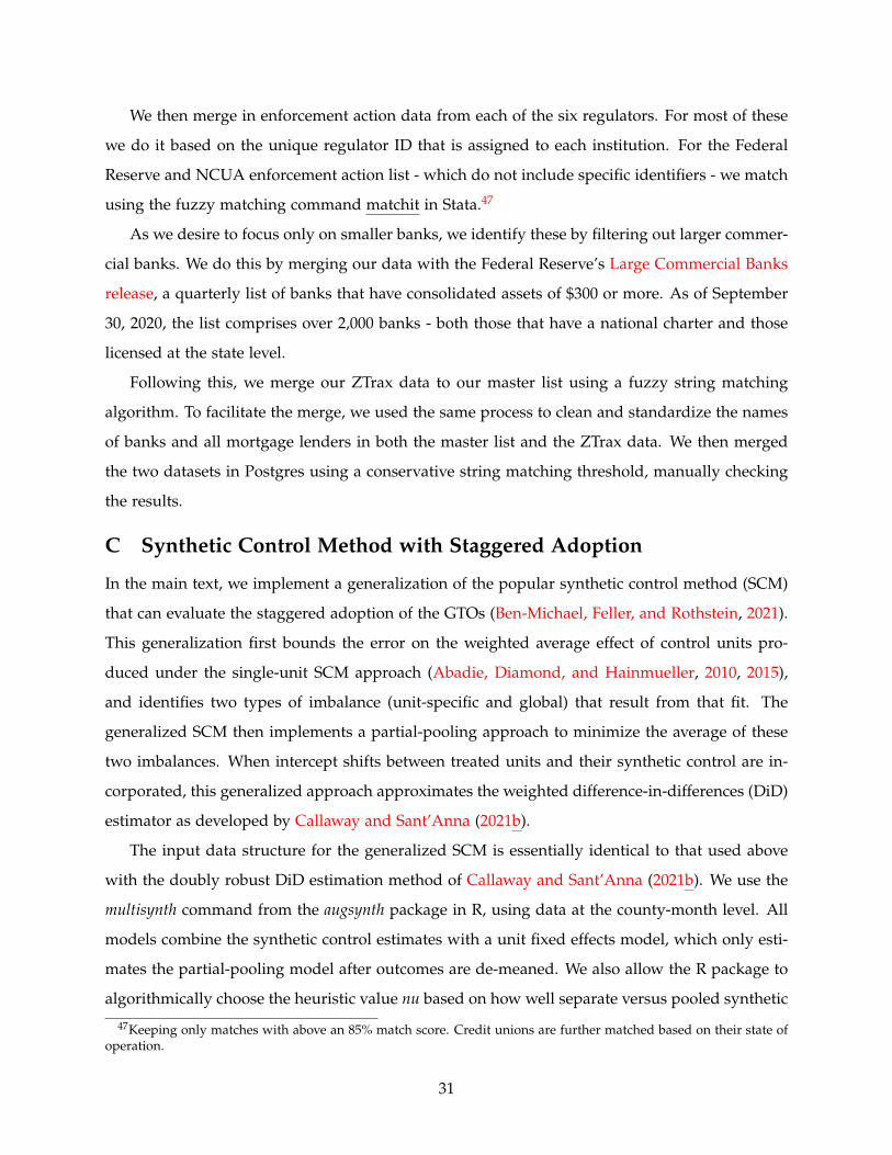
We then merge in enforcement action data from each of the six regulators. For most of these

we do it based on the unique regulator ID that is assigned to each institution. For the Federal

Reserve and NCUA enforcement action list - which do not include specific identifiers - we match

using the fuzzy matching command matchit in Stata.47

As we desire to focus only on smaller banks, we identify these by filtering out larger commer-

cial banks. We do this by merging our data with the Federal Reserve’s Large Commercial Banks

release, a quarterly list of banks that have consolidated assets of $300 or more. As of September

30, 2020, the list comprises over 2,000 banks - both those that have a national charter and those

licensed at the state level.

Following this, we merge our ZTrax data to our master list using a fuzzy string matching

algorithm. To facilitate the merge, we used the same process to clean and standardize the names

of banks and all mortgage lenders in both the master list and the ZTrax data. We then merged

the two datasets in Postgres using a conservative string matching threshold, manually checking

the results.

C Synthetic Control Method with Staggered Adoption

In the main text, we implement a generalization of the popular synthetic control method (SCM)

that can evaluate the staggered adoption of the GTOs (Ben-Michael, Feller, and Rothstein, 2021).

This generalization first bounds the error on the weighted average effect of control units pro-

duced under the single-unit SCM approach (Abadie, Diamond, and Hainmueller, 2010, 2015),

and identifies two types of imbalance (unit-specific and global) that result from that fit. The

generalized SCM then implements a partial-pooling approach to minimize the average of these

two imbalances. When intercept shifts between treated units and their synthetic control are in-

corporated, this generalized approach approximates the weighted difference-in-differences (DiD)

estimator as developed by Callaway and Sant’Anna (2021b).

The input data structure for the generalized SCM is essentially identical to that used above

with the doubly robust DiD estimation method of Callaway and Sant’Anna (2021b). We use the

multisynth command from the augsynth package in R, using data at the county-month level. All

models combine the synthetic control estimates with a unit fixed effects model, which only esti-

mates the partial-pooling model after outcomes are de-meaned. We also allow the R package to

algorithmically choose the heuristic value nu based on how well separate versus pooled synthetic

47Keeping only matches with above an 85% match score. Credit unions are further matched based on their state ofoperation.

31

controls balance the overall average.

32