The Impact of Aircraft Dropsonde and Satellite Wind Data ...pu/mypaper/Pu_WAF_Revise_Apr07.pdfThe Impact of Aircraft Dropsonde and Satellite Wind Data on Numerical Simulations of Two

The Impact of Aircraft Dropsonde and Satellite Wind Data on Numerical

Simulations of Two Landfalling Tropical Storms During Tropical

Cloud Systems and Processes Experiment

ZHAOXIA PU *, XUANLI LI

Department of Meteorology, University of Utah, Salt Lake City, Utah

CHRISTOPHER S. VELDEN

Cooperative Institute for Meteorological Satellite Studies, University of Wisconsin—Madison,

Madison, Wisconsin

SIM D. ABERSON

NOAA Hurricane Research Division, Miami, FL

W. TIMOTHY LIU

Jet Propulsion Laboratory, California Institute of Technology, Pasadena, California

Weather and Forecasting

Accepted on June 26, 2007

--------------

*Corresponding author address: Dr. Zhaoxia Pu, Department of Meteorology, University of

Utah, 135 S 1460 E, Rm.819, Salt Lake City, UT 84112

E-mail: [email protected]

1

Abstract

Dropwindsonde, GOES-11 rapid-scan atmospheric motion vectors and NASA

QuikSCAT near-surface wind data collected during NASA Tropical Cloud Systems and

Processes (TCSP) field experiment in July 2005 were assimilated into an advanced research

version of the Weather Research and Forecasting (WRF) model using its three-dimensional

variational (3DVAR) data assimilation system. The impact of the mesoscale data assimilation on

WRF numerical simulation of tropical storms Cindy and Gert (2005) near landfall are examined.

Sensitivity of the forecasts to the assimilation of each single data type is investigated.

Specifically, different 3DVAR data assimilation strategies with different analysis update cycles

and resolutions are compared in order to identify the better methodology to assimilate the data

from research aircraft and satellite for tropical cyclone study.

It is shown that: 1) Assimilation of dropwindsonde and satellite wind data into the

WRF model improves the forecasts of the two tropical storms up to the landfall time. The

QuikSCAT wind information is very important for improving the storm track forecast, whereas

the dropwindsonde and GOES-11 wind data are also necessary for improved forecasts of

intensity and precipitation. 2) Data assimilation also improves the quantitative precipitation

forecasts (QPF) near landfall of the tropical storms. 3) A 1-h rapid-update analysis cycle at high

resolution (9 km) provides more accurate tropical cyclone forecasts than a regular 6-h analysis

cycle at coarse (27 km) resolution. The high resolution rapid-updated 3DVAR analysis cycle

might be a practical way to assimilate the data collected from tropical cyclone field experiments.

2

1. Introduction

As witnessed in recent years, the social, ecological and economic impacts of tropical

cyclones can be devastating. Strong wind, heavy rain, and storm surge associated with tropical

cyclones may cause flooding, soil erosion, and landslides, even far away from the landfall

location, resulting in numerous human casualties and enormous property damage. Accurate

forecasts of tropical cyclones and their associated precipitation have been listed as a high-priority

research area by the U.S. Weather Research Program (e.g., Elsberry and Marks et al. 1999).

Tropical cyclones originate over the ocean, where conventional meteorological

observations tend to be sparse in daily routine basis. Due to lack of the data, deficiencies in

model initial condition can lead to inaccurate forecast of tropical cyclone forecasts. Our

knowledge on physics processes that control tropical cyclone evolution is also limited. Thus,

forecast of tropical cyclone track and intensity remains a challenging problem for numerical

weather prediction. Owing to the improvement of large-scale forecast models and data

assimilation techniques, and the use of satellite and aircraft reconnaissance observations, tropical

cyclone track forecasts have improved significantly during the last two decades. (Official error

trends are documented online at www.nhc.noaa.gov/verification). For instance, NOAA synoptic

surveillance missions are very useful in improving individual tropical cyclone track forecasts

(Franklin and DeMaria 1992; Franklin et al. 1993; Burpee et al. 1996; Aberson 2002 and 2003;

Aberson and Etherton 2006). Satellite-derived observations have also improved tropical cyclone

analyses and forecasts (e.g., Velden et al. 1992; Velden et al. 1998; Pu et al. 2002; Pu and Tao

2004; Zhu et al. 2002; Hou et al. 2004, Chen 2007). However, relatively little progress has been

made in hurricane intensity forecasts (Houze et al. 2006). In addition, only a little attention

3

(Rogers et al. 2003) has been given to improving tropical cyclone quantitative precipitation

forecasts (QPF).

In order to better understand tropical cyclone structure and intensity change, field

experiments, such as the annual National Oceanic and Atmospheric Administration (NOAA)

Hurricane Field Program (Aberson et al. 2006), the National Aeronautics and Space

Administration (NASA) Convective and Moisture Experiments (Kakar et al. 2006) and the

Hurricane Rainband and Intensity Change Experiment in 2005 (Houze et al. 2006), have been

conducted to collect data during intensive observing periods. During July 2005, NASA, in

collaboration with NOAA, executed the Tropical Cloud Systems and Process (TCSP) field

experiment (Halverson et al. 2007) based in Costa Rica. The goal was to improve the

understanding of tropical cyclogenesis and intensity change. During TCSP, in-situ

dropwindsondes from NOAA P-3 and many types of special remotely-sensed datasets were

collected along with regular satellite and aircraft reconnaissance and surveillance data [such as

dropwindsonde data from NOAA Gulfstream-IV (G-IV), P-3s, and the Air Force C-130

aircraft]. With routinely-available satellite data, such as those from the NOAA Geostationary

Operational Environmental Satellite (GOES), NASA Quick Scatterometer (QuikSCAT), and the

Tropical Rainfall Measuring Mission (TRMM) satellite, TCSP not only offered an opportunity to

study tropical cyclone development in detail, but also to study the impact of remotely sensed and

in-situ data on mesoscale forecasts of tropical cyclones.

The goal of the study is to assess the potential for improving high-resolution numerical

forecasts of tropical cyclone. Specifically, according to Pu and Braun (2001) and Wu et al.

(2006), who used tropical cyclone bogus vortices, wind information is important for tropical

cyclone initialization and prediction. Therefore, the main focus of this study is to incorporate

4

satellite-derived wind information with in situ dropwindsonde data into a mesoscale model with

the aim of producing the best possible analyses and forecasts. In particular, the impact of

dropwindsonde data, GOES-11 rapid-scan Atmospheric Motion Vectors (AMVs), and

QuikSCAT near-surface wind observations gathered during TCSP on mesoscale model forecasts

of tropical cyclones is demonstrated. Two tropical cyclones that occurred during TCSP, Cindy

and Gert, near their respective landfalls, are chosen for the study. The impact of the data on

forecasts of track, intensity and quantitative precipitation forecasts (QPF) through improved

strategies for mesoscale data assimilation is explored.

The Advanced Research WRF (ARW – hereafter WRF) model and its three-dimensional

variational data assimilation (3DVAR) system are used. A brief description of the two tropical

cyclones is given in Section 2. The data sources for the experiments are summarized in Section

3. The WRF and its 3DVAR system and the design of the data assimilation experiments are

introduced in Section 4. The sensitivity to the assimilation of each data type and all data to the

forecast of Tropical Storm Gert is examined in Section 5. The impact of the data assimilation on

the forecast of Tropical Storm Cindy is discussed in Section 6. Summary and conclusions are

presented in Section 7.

2. Overview of tropical storms Cindy and Gert (2005)

The 2005 Atlantic hurricane season (Beven et al. 2007) is notable for the most named

storms in a single season (28). Five storms, including three hurricanes (Cindy, Dennis, and

Emily), were active in July during the TCSP field campaign. Cindy and Gert were chosen for

study because TCSP aircraft data were collected during their approach toward landfall in the U.S

and Mexico, respectively.

5

According to the reports from Tropical Prediction Center (http://www.nhc.noaa.gov),

Cindy formed from a vigorous tropical wave and developed into a tropical depression in the

northwestern Caribbean Sea on July 3. It reached tropical storm strength after exiting the

Yucatán Peninsula on July 5. The storm then headed to the north across the Gulf of Mexico and

made landfall as a hurricane near Grand Isle, Louisiana, late on July 6 and again as a tropical

storm near Ansley, Mississippi, a few hours later. The storm weakened over Mississippi and

Alabama before evolving into an extratropical cyclone over the Carolinas on July 7. Heavy

rainfall and flooding were the main threat from Cindy, with one death attributed to the storm.

Gert originated from a tropical wave that emerged off of the west coast of Africa on July

10. It moved west-northwest over the Atlantic to the Lesser Antilles by July 18. The southern

part of the wave continued westward over the central and western Caribbean Sea and formed a

low pressure area to the east of Chetumal, Mexico, on July 22. The low moved west-

northwestward and organized into a tropical depression at 1800 UTC 23 July 2005 in the Bay of

Campeche. It developed into Tropical Storm Gert at 0600 UTC 24 July 2005, then continued to

strengthen and made landfall to the north of Cabo Rojo, Mexico at 0000 UTC 25 July 2005 with

maximum sustained winds of 40 knots (20 m s-1) and a minimum central pressure of 1005 hPa. It

then moved over central Mexico before dissipating on July 25. Gert struck in roughly the same

area as Hurricane Emily a few days earlier and brought heavy rainfall there, causing flooding and

landslides due to the saturated land.

3. Special observations collected during TCSP

TCSP was an earth science research program sponsored by the NASA Science Mission

Directorate. The field experiment was based out of the Juan Santamaría International Airport in

6

San José, Costa Rica, and carried out during July 1 - 28, 2005. Scientists from NASA, NOAA,

and the academic community were involved. During TCSP, a NOAA P-3 aircraft, directed by the

Hurricane Research Division and Aircraft Operations Center, flew 18 coordinated missions with

the NASA research aircraft, primarily to investigate developing tropical disturbances. With the

availability of routine information from NASA Earth Observing System satellites such as

QuikSCAT, TRMM, and Aqua, as well as special GOES-11 rapid-scan observations made

available by NOAA/NESDIS, and operational NOAA G-IV aircraft surveillance data and U. S.

Air Force C-130 reconnaissance data, TCSP provided a unique opportunity to incorporate high-

resolution aircraft and satellite data in mesoscale numerical prediction studies of tropical

cyclones.

QuikSCAT SeaWinds Level-2B wind vectors derived from Wentz and Smith (1999) at

approximately 25km resolution only over oceanic regions are used. A sample of the QuikSCAT

wind vector fields available for the Cindy case at 1200UTC 5 July 2005 is shown in Fig.1.

During part of the TCSP period, GOES-11 was activated by NOAA National

Environmental Satellite, Data, and Information Service (NESDIS) to operate in rapid-scan mode,

providing imagery at 5-min intervals over the Caribbean Sea, the East Pacific Ocean, and

adjacent regions. From these data, the Cooperative Institute for Meteorological Satellite Studies

(CIMSS) at the University of Wisconsin employed automated cloud tracking algorithms (Velden

et al. 1997) to produce high-density and high-quality AMVs over the domain (Velden et al.

2005). Figure 2 shows a sample of the GOES-11 AMV coverage at 0000UTC 24 July 2005 near

Tropical Storm Cindy. The data availability in different pressure ranges is marked in different

panels; most of the GOES-11 AMVs are located between 100 hPa to 250 hPa.

7

All available in-situ dropsonde observations during TCSP mission, including NOAA P-3

and operational NOAA G-IV aircraft surveillance data and U. S. Air Force C-130 reconnaissance

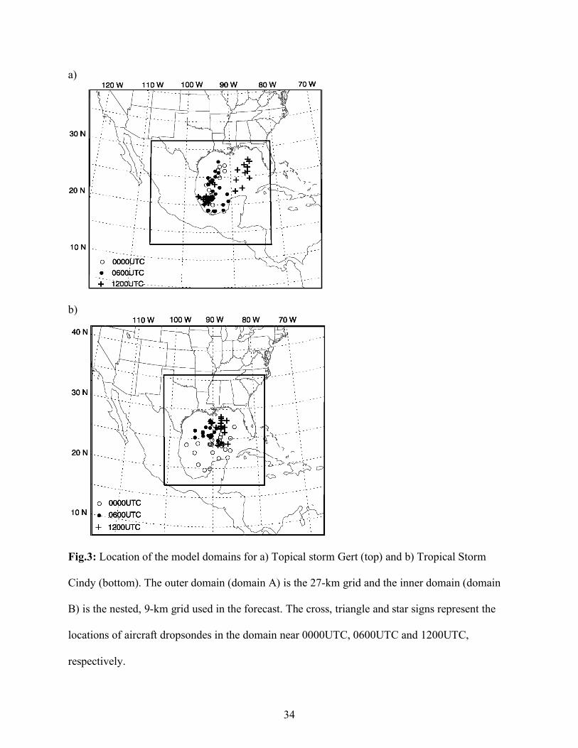
data, are used in this study. The locations of these data are shown in Fig. 3.

4. Description of the model, data assimilation system, and experimental design

a. WRF model and its 3DVAR system

WRF is a recently developed, next-generation, mesoscale numerical weather prediction

system featuring multiple dynamic cores designed to serve both operational forecast and research

needs. It is based on an Eulerian solver for the fully compressible nonhydrostatic equations, cast

in flux conservation form, using a mass (hydrostatic pressure) vertical coordinate. The solver

uses a third-order Runge-Kutta time integration scheme coupled with a split-explicit second-

order time integration scheme for the acoustic and gravity-wave modes. Fifth-order upwind-

biased advection operations are used in the fully conservative flux divergence integration;

second- to sixth-order schemes are run-time selectable. WRF has multiple physical options for

cumulus, microphysics, planetary boundary layer and radiation physical processes. Details of

the model are provided in Skamarock et al. 2005.

Along with WRF, a three-dimensional variational data assimilation (3DVAR) system was

developed based on MM5 3DVAR system (Barker et al. 2004a and b). Details of 3DVAR

method are referred to Barker (2004a), Kalnay (2003), and Lorenc(1986).

For the experiments in this study, model physics options include the Betts-Miller-Janjic

cumulus parameterization (Betts and Miller 1986), Ferrier microphysics scheme, Yonsei

University (YSU) planetary boundary layer parameterization (Skamarock et al. 2005; Hong and

Pan 1996), and the Rapid Radiative Transfer Model (RRTM; Mlawer et al. 1997) longwave and

8

Dudhia shortwave atmospheric radiation (Dudhia 1989) schemes. A two-way interactive, two-

level nested grid technique is employed to achieve the multi-scale forecast. The outer domain

resolution has 27-km grid spacing and the inner domain resolution is 9-km. The model vertical

structure is comprised of 31 σ levels with the top of the model set at 50 hPa, where

!

" = (ph # pht ) /(phs # pht ) while ph is the hydrostatic component of the pressure, and phs and pht

refer to values of the pressure along the surface and top boundaries, respectively. The σ levels

are placed close together in the low-levels (below 500hPa) and are relatively coarsely spaced

above. The model domains are shown in Fig. 3, and Table 1 gives the dimensions, grid spacing,

and time step for each domain.

For the 3DVAR experiments, the background error covariance matrix B was estimated

using the so-called “NMC” method (Parrish and Derber 1992; Wu et al. 2002; Barker 2004). The

observational error covariance matrices OQuikscat, OGoes were treated as diagonal matrices with

statistically determined variances of 25 m2s-2 and 40 m2s-2, respectively. Routine quality control

was conducted before the data assimilation.

b. Experimental design

The data from National Centers for Environmental Prediction (NCEP) global final

analysis (FNL) on a 1.0 x 1.0 degree grid were used to provide boundary conditions for

numerical simulations. Instead of directly using NCEP FNL analysis for the first guess in the

3DVAR experiments, a WRF simulation, initialized by the WRF standard initialization process

package using the NCEP FNL analysis, was first integrated 6-h to provide a first guess field for

3DVAR data assimilation. The control forecast (CNTL) continued the simulation without the

additional data assimilated.

9

In order to test the impact of model resolution on data assimilation, the data assimilation

experiments are conducted for the two domains separately. However, all the forecasts are run

using both domains. For the experiments with data assimilation performed on the outer domain,

the initial condition for the 9-km grid spacing domain is derived from the 27-km spacing using a

monotonic interpolation scheme based upon Smolarkiewicz and Grell (1992). All figures present

results from the 9-km grid spacing domain.

As we would like to investigate the impact of the aircraft and satellite data on the forecast

of the two tropical cyclones near landfall, the cycling 3DVAR experiments are conducted with

three consecutive 6-h data assimilation windows from 0000 UTC 5 July to 1200 UTC 5 July for

Cindy and from 0000 UTC 24 July to 1200 UTC 24 July for Gert, during the periods of intensive

observations. Forecasts are then run through 24 h for Gert and 36 h for Cindy to forecast the

landfall of the storms. Air Force and NOAA G-IV dropwindsonde data are available near

0000UTC, 0600 UTC and 1200 UTC 5 July 2005 for Cindy, whereas QuikSCAT surface wind

data are available only near 1200 UTC 5 July 2005 (no GOES-11 rapid-scan AMVs are

available). For Gert, Air Force and NOAA P-3 dropwindsonde, GOES-11 AMV and QuikSCAT

surface winds, are all available at or near 0000UTC and 1200 UTC on July 24, whereas only the

dropwindsonde and AMV data are available near 0600 UTC on July 24 (Table 2).

5. Data assimilation and forecasts for Tropical Storm Gert

a. The impact of different observation types on initial analyses

Since dropwindsonde data, QuikSCAT winds and GOES rapid-scan AMVs are all

available during Gert, a series of model runs are conducted to examine the impact of each

individual data type on the initial analyses and subsequent forecasts. A set of data assimilation

10

experiments is performed on the model outer-domain (27-km resolution) although all forecasts

are from 9-km grid. The CTRL and experiments with data assimilation are compared. The

detailed experimental design is listed in Table 2.

To get an idea of the impact from each data type on initial analysis and also to show how

other data affect the assimilation of the individual data type when all three types data are

assimilated, the statistics of initial conditions fit to each type of the observations are compared in

different experiments.

1) QUIKSCAT NEAR-SURFACE WINDS

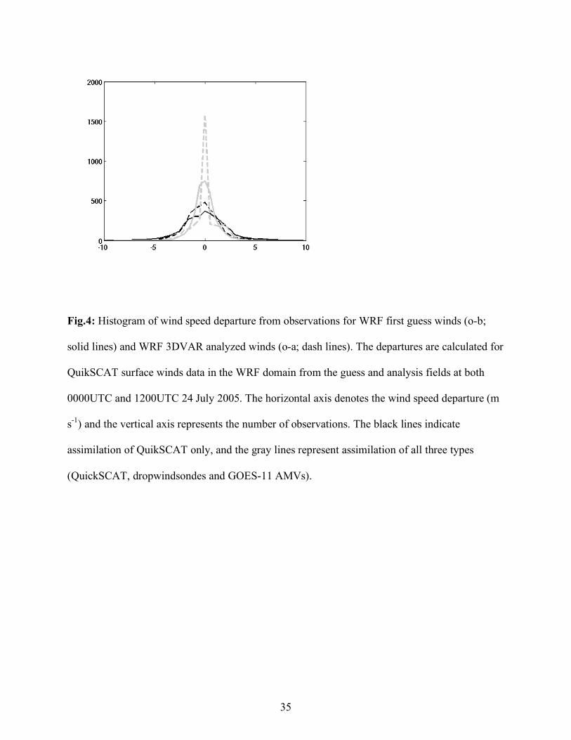
A total of 3117 QuikSCAT vector wind observations were assimilated at 0000UTC and

1200UTC 24 July 2005. The wind speed differences between observations and the first guess (o-

b) and the differences between the observations and the analysis (o-a) indicate that the difference

range is reduced from [-10.3, 14.4] m s-1 in o-b to [-5.4,7.5] m s-1 in o-a (Fig.4, black curves).

Specifically, there are about 363 observations in which the differences fall in the +/-0.25 m/s

range in o-b, whereas that number rose to nearly 749 after the data assimilation. The root-mean

square (RMS) fit is reduced from 3.0 m s-1 in o-b to 1.4 m s-1 in o-a. Overall, the data

assimilation produced analyses that fit the QuikSCAT observations well.

2) GOES-11 RAPID-SCAN AMVS

A total of 5216 AMVs were assimilated at 0000UTC, 0600UTC, and 1200UTC 24 July,

2005. The difference between the analysis and the observations (o-a), shown in Fig.5 (black

curves) with a difference range of [-4.7, 6.3] m s-1, is reduced significantly compared with the

difference between the first-guess and the observations (o-b) with a difference range of [-

11

12.6,16.4]m s-1. There are about 385 observations with the differences fall in the +/-0.25 m s-1 in

o-b, whereas that number rose to nearly 964 after data assimilation.

3) DROPWINDSONDE DATA

More than 50 dropwindsonde profiles (Fig. 3) with thousands of individual records of

wind vector, temperature, moisture and height at different pressure levels, were assimilated at

0000 UTC, 0600 UTC, and 1200UTC 24 July 2005. The black curves in Fig. 6 compare the

RMS of the first guess fit and analysis fit to the observations for 0000 UTC, 0600 UTC and 1200

UTC. The analysis with dropwindsonde data assimilated fits the observations more closely when

compared to the first guess.

4) ALL DATA

A final experiment includes the assimilation of all three data types (GOES, QuikSCAT

and dropwindsonde data). When all three data types are assimilated during the 12-h data

assimilation period, the analysis generally fits each type of the data better than the case when

only one type of observations is assimilated (gray curves in Figs 4, 5 and 6). Specifically, the

numbers of observations with the differences that fall in the +/-0.25 m s-1 range in o-a are

increased to 1582 for QuikSCAT observations (Fig.4) and 2109 for GOES-11 wind observations

(Fig.5), respectively. The RMS of the analysis fit to the dropwindsonde observations are also

significantly improved in most of the cases (Fig.6). Overall, the results indicate that assimilation

of all three data types together improves the fit of initial analysis to each and every type of the

data.

b. Forecast impact and sensitivity to observation type

12

1) STORM TRACK

Figure 7 shows the tracks produced by different experiments during the period between

0000UTC 24 July 2005 and 1800UTC 25 July 2005. Note that the forecasts shown in Fig.7 (also

Figs. 8, 9, 13, 17,18, 21) include the first 12-h analysis period. The track errors from each

experiment are shown in Figure 8. The storm track has been improved in all forecasts with data

assimilation. When all data are assimilated into the model (ALL-27), the forecast landfall

location and time are superior to that produced by the CTRL (Fig. 7) and yields the largest

improvement (~50%) for most forecast times (Figs. 7 and 8). The CTRL storm made landfall

almost 3 h earlier than observed about 75 km southwest of the verifying location. With

assimilation of all data (ALL-27), the landfall time error is about one-half hour, and the forecast

landfall location is about 40 km from the actual location (Fig.7). In regards to individual data

type assimilation, the QuikSCAT data show the most significant impact on the forecast track

(Fig. 8).

2) INTENSITY

Figure 9 compares storm intensity forecasts in terms of both minimum sea level pressure

and maximum surface wind speed. Similar to the track forecasts, the best forecasts are produced

by assimilating all three data types into the model. With assimilation of QuikSCAT data only,

the model reproduces a better maximum near surface wind forecast but slightly worse minimum

central sea level pressure than the CTRL. Assimilation of GOES wind and dropwindsonde data

both result in positive impact on the minimum sea level pressure and maximum surface wind

speed forecasts. The dropwindsonde data appear more beneficial to the minimum central sea

13

level pressure forecasts, whereas the GOES wind data produce more positive impact on the

maximum surface wind speed forecasts.

3) PRECIPITATION

Figure 10 shows the precipitation forecasts from the different experiments, compared

with the estimated rainfall rate derived from the TRMM Microwave Imager (TMI) and Infrared

(IR) data at 1435 UTC 24 July 2005. The observed precipitation distribution (Fig. 10a; Courtesy

of Naval Research Laboratory) includes two major rainbands on the east and north sides of the

tropical storm over the ocean, and a precipitation maximum in the southeast quadrant of the

storm near the coast of Mexico. The CTRL produces a fairly realistic precipitation structure to

the north of the storm (Fig. 10b), but misses the major maximum to the southeast. With the

assimilation of QuikSCAT data only, the model reproduces somewhat realistic rainband structure

to the north of the storm, but misses the major rainbands on the east side (Fig. 10c). The major

rainfall maximum near the coast is also missed. The forecast with GOES-11 wind data

assimilation is similar to the Quikscat and generates reasonable rainband structure on the north

side of the storm, but also misses the maximum precipitation center near the coast line (Fig.

10d). The dropwindsonde data assimilation forecasts capture the rainfall feature near the coast

line of Mexico well. Strong rainbands on the east and north sides are also reproduced, although

some details are still missing (Fig. 10e). The most successful results of the maximum rainfall

feature to the southeast of the storm are obtained with all three data types assimilated into the

model (Fig. 10f).

The differences in precipitation structures from forecasts with the various data types

assimilated may be attributed to the data impact on the overall convergent/divergent flow of the

14

vortex and vertical wind shear in the storm environment. Figure 11 shows the averaged

divergence profiles over the storm area (a circled region with radius of 250 km from the storm

center) at 1200 UTC 24 July 2005, the end of data assimilation period. It indicates that all data

assimilation experiments result in increases of low-level convergence and upper-level divergence

(except GOES doesn't increase low-level convergence) associated with the storm, although the

detailed impact from each data type tends to be different. Specifically, compared with the

CTRL, assimilation of the QuikSCAT and GOES wind data increases the integrated low-mid

level convergence, extending it upwards to about the 400mb level. The dropwindsonde data

causes a significant increase in both low level convergence and upper level divergence. With all

three data types assimilated into the model, the low level convergence and upper level

divergence both are moderately increased.

Figure 12 shows hodographs of the environmental flow between 850 to 200 hPa in a box

with 250km on a side centered on the storm at 1200 UTC 24 July 2005. Significant differences in

vertical wind shear are found in different experiments. Assimilation of GOES wind data caused

the largest change in vertical wind shear. Specifically, the shear is southwesterly in all cases

except GOES. In addition, magnitudes of the vertical wind shear are also different in different

experiments. Rogers et al. (2003) indicated that the vertical wind shear could govern azimuthal

variation of rainfall. In addition, it has been well accepted that the environmental wind shear in

low to middle troposphere is one of the key factors that influence the motion and intensity of

tropical cyclones (e.g., Zhang and Kieu 2006; Frank and Ritchie 1999). Therefore, the changes

in the environmental wind shears from different experiments explain at least partially why

assimilation of additional data into the model resulted in the significant impact on the track,

intensity and precipitation structures of Gert.

15

c) Regular 6-h data assimilation cycle versus 1-h rapid updated cycle (RUC)

In all the above experiments, the analyses were generated from regular 6-h data

assimilation cycles. However, for most of the special non-conventional observations, the exact

observing time is scattered within the cut-off window. Therefore, there is good reason to

assimilate the data with 3DVAR in a rapid update cycle (RUC) with a short cut-off window.

Thus, a set of experiments using a 1-h RUC data assimilation instead of a 6-h data assimilation

cycle was performed. All three types of the data were assimilated every hour (i.e., 1-h analysis

cycle) with a cut-off window of [-0.5hr, 0.5hr] during the first 12-h forecast period. Figure 13

compares the variation of the storm intensity in terms of both minimum sea level pressure and

maximum surface wind speed, showing slight impact on the intensity forecast from the RUC.

This small impact in the intensity forecast is mainly attributed to the weak storm intensity and

relatively small intensity errors in the CTRL for Gert, and partly also due to the fact that the

intensity of Gert barely changed during this period. However, when comparing the track errors

generated from the RUC analysis with those from the regular analysis (Figs. 7 and 8), the

differences are quite significant, indicating obvious benefit to the track forecast from the RUC

analyses.

d) Data assimilation at fine resolution (9-km grid-spacing) and its impact on forecasts

So far, all data assimilation experiments described have been conducted on the 27-km

resolution domain, although forecasts were performed on the nested domains with 9-km grid

spacing. In order to test the sensitivity of forecasts to the data assimilation at fine resolution, the

RUC data assimilation was performed using the model inner domain (9-km grid spacing). All

the observations that reside within the inner domain, were assimilated.

16

Compared with RUC-27, forecasts from the RUC analysis at 9-km (RUC-9) show

additional improvement in track (Figs.7 and 8) and intensity (Fig. 13) at most forecast times. The

impact on precipitation structure is also quite significant. Figure 14 shows the forecast

precipitation structure from RUC-9 at 1430 UTC 24 July 2005. Compared with Fig. 10a, Fig. 14

shows almost all of the main observed features of precipitation are nearly in the right location.

Better forecasts from RUC-9 could be attributed to the improved analysis after the data

assimilation. Figure 15 compares the streamline and vector wind fields at 850 hPa and 700hpa

from RUC-9 analysis and the CTRL at 0000 UTC 24 July 2005. It shows that the RUC-9

analysis produced a strong convergent circulation with tropical storm features at both pressure

levels, whereas the CTRL missed the strong convergent circulation associated with Gert.

6. Tropical Storm Cindy forecasts

Using a regular 6-h data assimilation cycle at 27-km grid-spacing domain (ALL-27),

dropwindsonde data from the Air Force and the G-IV were assimilated into the model at 0000

UTC, 0600 UTC and 1200 UTC 5 July 2005 for Cindy, whereas the QuikSCAT wind data were

assimilated into the model at 1200 UTC 5 July 2005 only. GOES-11 AMV were not available for

this case. In addition, in order to further test the benefit of 1-h RUC for tropical cyclone studies,

a 1-h RUC data assimilation cycle was performed during the same analysis period on the 9-km

domain (RUC-9) for Cindy. Forecasts were compared with the CTRL.

Figure 16 shows the initial conditions at 0000 UTC 5 July 2005 for Cindy before and

after data assimilation in ALL-27 and illustrates that the depiction of the tropical storm has been

improved after the assimilation. A closed center of low pressure was reproduced and the

magnitude of the minimum pressure is closer to that reported from the observations. Note that

17

the storm center was tracked by an algorithm described in Marchok (2002) for the initial

conditions before data assimilation, in which the closed circulation was not clearly shown.

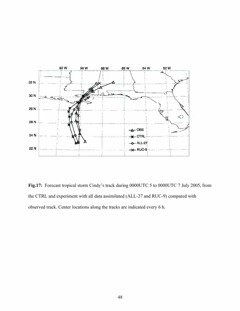
Figure 17 shows that the track forecast was significantly improved by assimilation of the

data. The track error was reduced by up to 50% in experiment ALL-27 and by more than 70% in

experiment RUC-9, indicating that the storm and environmental conditions are better represented

by those experiments. The landfall time and location are well captured by the forecast with data

assimilation. In the CTRL, the storm made landfall at 1200 UTC 6 July 2005, about 6-hour

behind the actual landfall time. With data assimilation, the model forecast was able to capture a

landfall time that is much closer to the observed landfall time. In addition, with the benefit of

data assimilation, the forecast storm track is approaching the observed track when compared with

the CTRL, in which the storm moved too slowly after the landfall. However, in both cases (with

and without data assimilation), the track error tends to be large after the storm made landfall.

This may be caused by the lack of high-resolution land surface information in the model.

Figure 18 illustrates the time variation of storm intensity in terms of minimum sea level

pressure and maximum surface wind speed. The intensity of the storm is indeed improved with

assimilation of the added datasets. Compared with experiment ALL-27, RUC-9 produces a

better intensity forecast for Cindy.

Figure 19 compares the 48-h accumulated precipitation along the storm track with

corresponding rainfall estimation from TMI, SSM/I, IR rainfall observational products (NASA

TRMM real-time rainfall products; Huffman et al. 2003). The model produces unrealistically

huge amounts of rainfall after landfall in the CTRL (Fig 19b). This accumulated heavy rainfall

mainly reflects the slower movement of the storm in the CTRL. The large precipitation

accumulation before the storm made landfall was missed. In contrast, with the added data

18

assimilated, the model was able to more realistically reproduce the features of observed rainfall

accumulation both before and after the storm made landfall (Fig. 19c).

In order to further provide support that the data assimilation improves the quantitative

precipitation forecast (QPF) in forecast, a comparison is illustrated by histograms of the

probability density function (PDF) for 48-h accumulated rainfall (Fig. 20). The PDF usually

represents the rainfall probability distribution in different magnitude ranges. The figure shows

that rainfall is generally overestimated in the low rainfall and underestimated in the high rainfall

in the CTRL experiment. However, with data assimilation, the spectrum of rainfall becomes

closer to the observed. Specifically, RUC-9 produces a better forecast compared with ALL-27.

7. Summary and conclusions

The impact of dropwindsonde observations, QuikSCAT near-surface vector winds and

GOES-11 rapid-scan atmospheric motion vectors on WRF forecasts of two landfalling tropical

cyclones (Cindy and Gert in 2005) during NASA TCSP experiment is evaluated in this study. It

is shown that there is a clear benefit to assimilate all three types of the data from dropwindsonde

and satellite result in positive impacts on track, intensity and precipitation forecasts for both

Cindy and Gert. The forecast landfall time and location are also improved. The in situ and

satellite data collected during the TCSP field program are a useful data source for studying

tropical cyclones.

In addition, new findings from this study using the WRF mesoscale model and data

assimilation system include: 1) assimilation of QuikSCAT wind data mainly contribute to the

improvement in the track forecasts as the impact of QuikSCAT surface vector winds extended

well above the surface (Fig.12 a & b), whereas the GOES AMV and dropwindsonde data are

19

necessary for improving the forecasts of the intensity and precipitation. 2) Compared with a

regular 6-h analysis cycle at coarser resolution (27-km), a 1-h rapid update analysis cycle at high

resolution (9-km) shows additional promise for improving forecasts of tropical cyclones. 3) Data

assimilation helps the model to produce more realistic QPF near the landfalls for both Cindy and

Gert.

Furthermore, compared with the results from assimilation of any single data type,

assimilation of all three data types together improves the fit of the initial analysis to each and

every type of the data (Fig.4-6). The improved analysis and forecasts from assimilation of all

three types of data implies that the information provide from different types of the data may be

complementary to each other. The differences in precipitation structures from forecasts with

assimilation of various data types can be attributed to the data impact on the overall

convergent/divergent flow of the vortex and vertical wind shear in the storm environment (Figs.

10-12).

Overall, data assimilation results from this study are quite positive. As 3DVAR is usually

computationally efficient, this suggests that a high-resolution rapidly updated 3DVAR analysis

might be a practical way to assimilate the data collected from tropical cyclone field experiments.

The WRF four-dimensional variational (4DVAR) data assimilation system is currently under

development (Huang et al. 2006), so there is still an open question as to whether the rapidly

updated data assimilation results will be compatible with the those from a 4DVAR data

assimilation, even though 4DVAR is generally computationally expensive. Therefore, more

questions can be addressed in detail in the future work. In addition, since the two cases studied

in this paper were weak tropical storms and their intensity changes during the whole period of

20

the studies were relatively small, general conclusions must await future studies.

.

21

Acknowledgments:

The authors would like to acknowledge the WRF model and 3DVAR working group for

their efforts to develop the community WRF model systems. The authors would also like to

acknowledge NOAA/NESDIS for providing the GOES-11 rapid scan data, and to Howard

Berger and Dave Stettner at CIMSS for processing and providing the GOES-11 winds.

This study was supported by the NASA TCSP program through partial support to the first

three authors. The first two authors are very grateful to Dr. Edward Zipser for his support and

encouragement during this study. Two anonymous reviewers and Prof. Da-Lin Zhang from

University of Maryland are also greatly appreciated for their valuable comments on the

manuscript.

The computer time for this study was provided by the Center for High Performance

Computing (CHPC) at the University of Utah.

22

REFERENCES

Aberson, S. D., and J. L. Franklin, 1999: Impact on hurricane track and intensity forecasts of GPS

dropwindsonde observations from the first-season flights of the NOAA Gulfstream-IV jet

aircraft. Bull. Amer. Meteor. Soc., 80, 421–427.

Aberson, S. D., 2002: Two years of operational hurricane synoptic surveillance. Wea.

Forecasting, 17, 1101–1110.

Aberson, S. D., and C. R. Sampson, 2003: On the predictability of tropical cyclone tracks in the

Northwest Pacific Basin. Mon. Wea. Rev., 131, 1491–1497.

Aberson, S. D., and B. J. Etherton. 2006: Targeting and data assimilation studies during

Hurricane Humberto (2001). J. Atmos. Sci., 63, 175–186.

Barker, D. M., W. Huang, Y. R. Guo, and Q. N. Xiao., 2004a: A three-dimensional (3DVAR) data

assimilation system for use with MM5: implementation and initial results. Mon. Wea. Rev.,

132, 897-914.

Barker, D. M., M.-S. Lee, Y.-R. Guo, W. Huang, Q.-N. Xiao, and R. Rizvi 2004b: WRF

Variational data assimilation development at NCAR. June 22-25, 2004. WRF/MM5

Users’ Workshop, Boulder, CO.

Betts, A. K., 1986: A new convective adjustment scheme. Part I: Observational and theoretical

basis. Q. J. Roy. Meteor. Soc., 112, 677-691.

Beven, J. L. II, L. A. AVila, E. S. Blake, D. P. Brown, J. L. Franklin, R. D. Knabb, R. J. Pasch,

J. R. Rhome, and S. R. Stewart, 2007: The Atlantic hurricane season of 2005. Mon.

Wea. Rev., in review.

Burpee, R. W., S. D. Aberson, J. L. Franklin, S. L. Lord, and R. E. Tuleya, 1996: The impact of

Omega dropwindsondes on operational hurricane track forecast models. Bull. Amer. Meteor.

Soc., 77, 925–933.

23

Chen, S.-H., 2007: The impact of assimilating SSM/I and QuikSCAT satellite winds on

Hurricane Isodore simulation. Mon. Wea. Rev., 135, 549-566.

Dudhia, J. 1989: Numerical study of convection observed during the winter monsoon experiment

using a mesoscale two-dimensional model. J. Atmos. Sci., 46, 3077-3107.

Elsberry, R. L., and F. D. Marks, 1999: The hurricane landfall workshop summary. Bull. Amer.

Meteor. Soc., 80, 683-685.

Frank, W. M. and E. A. Ritchie, 1999: Effects of environmental flow upon tropical cyclone

structure. Mon. Wea. Rev., 127, 2044–2061. Franklin, J. L., and M. DeMaria, 1992: The Impact of Omega Dropwindsonde Observations on

Barotropic Hurricane Track Forecasts. Mon. Wea. Rev., 120, 381–391.

Franklin, J. L., S. J. Lord, S. E. Feuer, and F. D. Marks, 1993: The kinematic structure of hurricane

Gloria (1985) determined from nested analyses of dropwindsonde and Doppler radar data.

Mon. Wea. Rev., 121, 2433–2451.

Goerss, J., C.S. Velden and J. Hawkins, 1998: The impact of multispectral GOES-8 wind information

on Atlantic tropical cyclone track forecasts in 1995. Part 2: NOGAPS forecasts. Mon. Wea.

Rev., 126, 1219-1227.

Halverson, J. B., M. Black, S. Braun, D. Cecil, M. Goodman, A. Heymsfield, G. Heymsfield,

R. Hood, T. Krishnamurti, G. McFarquhar, M. J. Mahoney, J. Molinari, R. Rogers, J. Turk,

C. Velden, D.-L. Zhang, E. Zipser, R. Kakar: 2007: NASA's Tropical Cloud Systems and

Processes Experiment: Investigating Tropical Cyclogenesis and Hurricane Intensity

Change. Bull. Amer. Meteor. Soc., (in press)

Hong, S.-Y., and H.-L. Pan, 1996: Nonlocal boundary layer vertical diffusion in a medium-range

forecast model, Mon. Wea. Rev., 124, 2322-2339

Hou, A. Y., S. Q. Zhang, and O. Reale, 2004: Variational ontinuous Assimilation of TMI and SSM/I

24

Rain Rates: Impact on GEOS-3 Hurricane Analyses and Forecasts. Mon. Weat. Rev., 132,

2094–2109.

Houze, R. A., S. S. Chen, W.-C. Lee, E. F. Rogers, J. A. Moore, G. J. Stossmeister, M. M. Bell, J.

Cetrone, W. Zhao, and R. Brodzik: The hurricane rainband and intensity change experiment.

Bull. Amer. Meteor. Soc., 87, 1503-1521.

Huang, X.-Y.,Q. Xiao, W. Huang, D. Barker, J. Michalakes, J. Bray, Z. Ma, Y. Guo, H.-C. Lin, and

Y.-H. Kuo, 2006: Preliminary results of WRF 4D-Var. 7th Annual WRF Users’

workshop, June 19-22, 2006, Boulder, CO

Huffman, G. J., and D. T. Bolvin, 2003: TRMM real-time multi-satellite precipitation

Analysis data set documentation. [Available on web site:

ftp://aeolus.nasacom.nasa.gov/pub/merged/3B4XRT_README]

Kakar, R., M. Goodman, R. Hood, and A. Guillory: 2006, Overview of Convection and Moisture

Experiment (CAMEX). J. Atmos. Sci., 63, 5-18

Kalnay, E., 2003: Atmospheric Modeling, Data Assimilation and Predictability, Cambridge

University Press, 340pp.

Lorenc, A. C., 1986: Analysis methods for numerical weather prediction. Q. J. R. Meteorol. Soc.,

112, 1177-1194.

Marchock, T. P., 2002: How the NCEP tropical cyclone tracker works. 25th Conference on

hurricane and tropical meteorology, San Diego, CA, April 29 – May 3, 2002.

Mlawer, E. J., S. J. Taubman, P. D. Brown, M. J. Iacono, and S. A. Clough, 1997: Radiative

transfer for inhomogeneous atmosphere: RRTM, a validated correlated-k model for the

long-wave. J. Geophy. Res., 102(D14),16663-16682.

25

Parrish, D. F., and J. C. Derber, 1992: The National Meteorological Center’s spectral statistical

-interpolation analysis system. Mon. Wea. Rev., 120, 1747-1763

Pu, Z., W.-K. Tao, S. Braun, J. Simpson, Y. Jia, J. Halverson, A. Hou, and W. Olson, 2002: The

impact of TRMM data on mesoscale numerical simulation of supertyphoon Paka. Mon. Wea.

Rev., 130, 2248-2258.

Pu, Z.-X., S. Braun, 2001: Evaluation of bogus vortex techniques with four-dimensional variational

data assimilation. Mon. Wea. Rev., 129, 2023-2039.

Rogers, R., S. Chen, J. Tenerelli and H. Willoughby, 2003: A numerical study of the impact of

vertical shear on the distribution of rainfall in Hurricane Bonnie (1998). Mon. Wea. Rev.,

131, 1577–1599.

Skamarock, W. C., J. B. Klemp, J. Dudhia, D. O. Gill, D. M. Barker, W. Wang and J. G. Powers,

2005: A Description of the Advanced Research WRF Version 2. NCAR Technical Note,

NCAR/TN-468+STR.[available at NCAR, Boulder, CO 80300]

Smolarkiewicz, P. K., and G. A. Grell, 1992: A class of monotone interpolation scheme. J. Comput.

Phys., 101, 431-440

Soden, B. J., C. S. Velden, and R. E. Tuleya, 2001: The impact of satellite winds on experimental

GFDL hurricane model forecasts. Mon. Wea. Rev., 129, 835–852.

Tomassini, M., D. LeMeur, and R. W. Saunders, 1998: Near-surface satellite wind observations of

hurricanes and their impact on ECMWF model analyses and forecasts. Mon. Wea. Rev., 126,

1274–1286.

Tuleya, R. E., and S. J. Lord, 1997: The impact of dropwindsonde data on GFDL hurricane model

forecasts using global analyses. Wea. Forecasting, 12, 307–323.

Velden, C. S., C. M. Hayden, W. P. Menzel, J. L. Franklin, and J. S. Lynch, 1992: The impact of

satellite-derived winds on numerical hurricane track forecasting. Wea. Forecasting, 7,

107–118.

26

Velden, C. S., C.M. Hayden, S. Nieman, W.P. Menzel, S. Wanzong and J. Goerss, 1997: Upper

-tropospheric winds derived from geostationary satellite water vapor observations. Bull.

Amer. Meteor. Soc., 78, 173-195.

Velden, C. S., T.L. Olander and S. Wanzong, 1998: The impact of multispectral GOES-8 wind

information on Atlantic tropical cyclone track forecasts in 1995. Part 1: Dataset

methodology, description and case analysis. Mon. Wea. Rev., 126, 1202-1218.

Velden, C. S., J. Daniels, D. Stettner, D. Santek, J. Key, J. Dunion, K. Holmlund, G. Dengel,

W. Bresky, and P. Menzel, 2005: Recent Innovations in Deriving Tropospheric Winds from

Meteorological Satellites. Bull. Amer. Meteor. Soc., 86, 205-223.

Wentz, F. J., and D. K. Smith, 1999: A model function for the ocean normalized radar cross section

at 14 GHz derived from NSCAT observations. J. Geophy. Res., 104, 11499-11514.

Wu, C.-C., K.-H. Chou, Y. Wang and Y.-H. Kuo, 2006: Tropical cyclone initialization and

prediction based on four-dimensional variational data assimilation. J. Atmos. Sci., 63,

2383–2395

Wu, W.-S., R. J. Purser, and D. F. Parrish, 2002: Three-dimensional variational analysis

with spatially inhomogeneous covariances. Mon. Wea. Rev., 130, 2905-2916.

Zhu, T., D.-L. Zhang, and F. Weng. 2002: Impact of the Advanced Microwave Sounding Unit

measurements on hurricane prediction. Mon. Wea. Rev., 130, 2416–2432.

Zhang, D.-L., and Kieu, C. Q., 2006: Potential vorticity diagnosis of a simulated hurricane. Part

II: Quasi-balanced contributions to forced secondary circulations. J. Atmos. Sci., 63,

2898–2914.

27

Table and Table Captions

Table 1. The dimension, grid space, and time step for each domain

---------------------------------------------------------------------------------------------------------- Case Domain Horizontal Grid Dimension Grid Space Time Step ---------------------------------------------------------------------------------------------------------- Cindy A 196x156 27 km 120s B 262x235 9 km 40s Gert A 190x150 27 km 120s B 298x235 9 km 40s ----------------------------------------------------------------------------------------------------------

28

Table 2. Experimental design for Gert

-------------------------------------------------------------------------------------------------------------------- Experiment Type of observations Time of data assimilated Domain of assimilated (on July 24, 2006) data assimilation --------------------------------------------------------------------------------------------------------------------- CTRL n/a n/a n/a DROP dropwindsonde 0000UTC, 0600 UTC, 1200UTC A QS QuikSCAT wind 0000UTC, 1200UTC A GOES GOES-11 wind 0000UTC, 0600UTC, 1200UTC A ALL-27 dropwindsonde 0000UTC, 0600UTC, 1200UTC A QuikSCAT wind 0000UTC, 1200UTC GOES-11 wind 0000UTC, 0600UTC, 1200UTC RUC-27 Same as All-27 1hr analysis cycle during A 0000--1200 UTC RUC-9 Same as All-27 Same as All-27 B --------------------------------------------------------------------------------------------------------------------

29

Figure Captions List Fig.1: QuikSCAT surface vector wind data at 1200UTC 5 July 2005.

Fig.2: The coverage of GOES-11 rapid-scan atmospheric motion vector wind data at 0000 UTC

24 July, 2005. The colors indicate the wind data in different pressure level ranges. The

triangle denotes the center of Tropical Storm Gert.

Fig.3: Location of the model domains for a) Topical storm Gert and b) Tropical Storm Cindy.

The outer domain is the 27-km grid and the inner domain is the nested, 9-km grid used in

the forecast. The cross, triangle and star signs represent the dropwindsonde locations in

the domain around 0000UTC, 0600UTC and 1200UTC, respectively.

Fig.4: Histogram of wind speed departure from observations for WRF first guess winds (o-b;

solid lines) and WRF 3DVAR analyzed winds (o-a; dash lines). The departures are

calculated for QuikSCAT surface winds data in the WRF domain from the guess and

analysis fields at both 0000UTC and 1200UTC 24 July 2005. The horizontal axis denotes

the wind speed departure (m s-1) and the vertical axis represents the number of

observations. The black lines indicate the results from assimilation of QuikSCAT only,

and the gray lines represent the results from assimilation of all three types (QuickSCAT,

dropwindsondes and GOES-11 AMVs).

Fig.5: Same as Fig.4, but the departures are for GOES-11 wind data in the WRF domain

at 0000UTC, 0600UTC and 1200UTC 24 July 2005.

Fig.6: Root-mean-square fit of temperature (K), dew point temperature (K), wind speed (m s-1)

and direction (degrees) against the dropwindsonde data for the analysis field at

0000UTC, 0600UTC, and 1200UTC 24 July 2005. Dashed line is for the data

assimilation experiment DROP and the solid line for the CTRL (first guess). The black

30

lines indicate the assimilation of dropwindsonde data only and the gray color lines

represent the assimilation of all three types (QuickSCAT, dropwindsondes and GOES-11

AMVs).

Fig.7: Forecast tropical storm Gert’s track during 0000UTC 24 to 1200UTC 25 July 2005, from

the CTRL and experiments, a) ALL-27, b) RUC-27 and c) RUC-9. The forecast tracks

are compared with the observed track. Center locations along the tracks are indicated

every 6 h. All forecasts shown in this paper are from the domain B (9-km grid spacing

resolution).

Fig. 8. Time series (at 6-h interval) of forecast track errors (km), which are defined as

the distances between the forecast storm centers and the observed positions, for all

forecasts during 0000UTC 24 to 1200UTC 25 July 2005.

Fig.9: Time series (at 6-h intervals) of (a) minimum sea level pressure (hPa) and (b) maximum

winds (m s-1) at the surface (10-m) during 0000UTC 24 to 1200UTC 25 July 2005.

Fig.10: Hourly rainfall rate (a) derived from IR and TMI satellite at 1435 UTC 24 July 2005 and

forecasted from experiment (b) CTRL, (c) QS, (d) GOES, (e) DROP and (f) ALL-27,

valid at 1430 UTC 24 July 2005.

Fig.11: Averaged divergence profiles over the area with radius of 250 km around storm center at

1200UTC 24 July 2005. The vertical axis denotes tropospheric pressure levels. The

horizontal axis represents the magnitudes of the divergence (10-5 m s-2).

Fig.12 The hodograph of environmental winds between 850 and 200 hPa in vicinity of vortex

(m s-1) at 1200 UTC 24 July 2005. a) CTRL, b) QS, c) GOES, d) DROP, e) ALL-27.

Fig.13. Same as Fig.9, except for different experiments.

Fig.14. Same as Fig.10, except for experiment RUC-9.

31

Fig.15: The analysis of streamline and wind vector at 850 hPa (left panels) and 700 hPa (right

panels) from RUC-9 (top), compared with first guess fields from CTRL (bottom), for

Gert at 0000UTC 24 July 2005.

Fig.16: The sea level pressure and vector wind at 0.5 km at 0000UTC 5 July 2005 for Tropical

Storm Cindy. a) CTRL; b) ALL-27.

Fig.17: Fig.17: forecast tropical storm Cindy’s track during 0000UTC 5 to 0000UTC 7 July

2005, from the CTRL and experiment with all data assimilated (ALL-27 and RUC-9)

compared with observed track. Center locations along the tracks are indicated every 6 h.

Fig.18: Time series (at 6-h intervals) of (a) minimum sea level pressure (hPa) and (b) maximum

winds (m s-1) at the surface (10-m ) during 0000UTC 5 to 0000UTC 7 July 2005.

Fig.19: Forecast 48-h accumulated rainfall amount (mm) during 0000UTC 5 July to 0000UTC 7

July 2005, compared with the corresponded rainfalls from TRMM real-time products

merged from multi satellites along the storm track during the tropical storm Cindy. (a)

TRMM real-time rainfall products merged from multi-satellite observations, (b) CTRL,

and (c) ALL-27.

Fig.20: Histograms of probability density functions (PDF) of 48-h accumulated rainfall amount

for Experiment RUC-9, ALL-27 and CTRL, compared with PDF of 48-h accumulated

rainfall amount from TRMM real-time rainfall products merged from multi-satellite

observations.

32

Fig.1: The QuikSCAT surface vector wind data at 1200UTC 5 July 2005.

33

Fig.2: The coverage of GOES-11 rapid-scan atmospheric motion vector wind data within the

model outer domain at 0000 UTC 24 July, 2005. Each panel indicates the wind data in different

pressure level ranges: a) 137-250hPa; b) 250-500hPa; and c) 700-925hPa. The triangle indicates

the center of Tropical Storm Gert.

a b

c

34

a)

b)

Fig.3: Location of the model domains for a) Topical storm Gert (top) and b) Tropical Storm

Cindy (bottom). The outer domain (domain A) is the 27-km grid and the inner domain (domain

B) is the nested, 9-km grid used in the forecast. The cross, triangle and star signs represent the

locations of aircraft dropsondes in the domain near 0000UTC, 0600UTC and 1200UTC,

respectively.

35

Fig.4: Histogram of wind speed departure from observations for WRF first guess winds (o-b;

solid lines) and WRF 3DVAR analyzed winds (o-a; dash lines). The departures are calculated for

QuikSCAT surface winds data in the WRF domain from the guess and analysis fields at both

0000UTC and 1200UTC 24 July 2005. The horizontal axis denotes the wind speed departure (m

s-1) and the vertical axis represents the number of observations. The black lines indicate

assimilation of QuikSCAT only, and the gray lines represent assimilation of all three types

(QuickSCAT, dropwindsondes and GOES-11 AMVs).

36

Fig.5: Same as Fig.4, but the departures are for GOES-11 wind data in the WRF domain at

0000UTC, 0600UTC and 1200UTC 24 July 2005.

37

Fig.6: Root-mean-square fit of temperature (K), dew point temperature (K), wind speed (m s-1)

and direction (degrees) against the dropwindsonde data for the analysis fields at 0000UTC,

0600UTC, and 1200UTC 24 July 2005. Dashed line is for the data assimilation experiment

DROP and the solid line for the CTRL (first guess). The black lines indicate the assimilation of

dropwindsonde data only and the gray lines represent the assimilation of all three types

(QuickSCAT, dropwindsondes and GOES-11 AMVs).

38

Fig.7: Forecast tropical storm Gert’s track during 0000UTC 24 to 1200UTC 25 July 2005, from

the CTRL and experiments, a) ALL-27, b) RUC-27 and c) RUC-9. The forecast tracks are

compared with the observed track. Center locations along the tracks are indicated every 6 h. All

forecasts shown in this paper are from the domain B (9-km grid spacing resolution).

39

Fig. 8. Time series (at 6-h interval) of forecast track errors (km), which are defined as

the distances between the forecast storm centers and the observed positions, for all

experiments during 0000UTC 24 to 1200UTC 25 July 2005.

40

a)

b)

Fig.9: Time series (at 6-h intervals) of (a) minimum sea level pressure (hPa) and (b) maximum

winds (m s-1) at the surface (10-m) during 0000UTC 24 to 1200UTC 25 July 2005.

41

a) b)

c) d)

e) f)

Fig.10: Hourly rainfall rate (a) derived from IR and TMI satellite at 1435 UTC 24 July 2005 and

simulated from experiment (b) CTRL, (c) QS, (d) GOES, (e) DROP and (f) ALL-27 valid at

1430 UTC 24 July 2005.

42

Fig.11: Averaged divergence profiles over the area with radius of 250km around the center of

the tropical storm Gert at 1200 UTC 24 July 2005. The vertical axis denotes the atmospheric

pressure levels. The horizontal axis represents the magnitudes of the divergence (10-5 m s-2).

43

a) b)

c) d) e)

Fig.12 The hodograph of environmental winds between 850 and 200 hPa in vicinity of vortex

(m s-1) at 1200 UTC 24 July 2005. a) CTRL, b) QS, c) GOES, d) DROP, e) ALL-27.

44

a)

b)

Fig.13. Same as Fig.9, except for different experiments.

45

Fig.14. Same as Fig.10, except for experiment RUC-9.

46

a) b)

c) d)

Fig.15: The analysis of streamline and wind vector at 850 hPa (left panels) and 700 hPa (right

panels) from RUC-9 (top), compared with first guess fields from CTRL (bottom), for Gert at

0000UTC 24 July 2005.

47

a)

b)

Fig.16: The sea level pressure and vector wind at 0.5km at 0000UTC 5 July 2005 for Tropical

Storm Cindy. a) CTRL; b) ALL-27.

48

Fig.17: Forecast tropical storm Cindy’s track during 0000UTC 5 to 0000UTC 7 July 2005, from

the CTRL and experiment with all data assimilated (ALL-27 and RUC-9) compared with

observed track. Center locations along the tracks are indicated every 6 h.

49

a)

b)

Fig.18: Time series (at 6-h intervals) of (a) minimum sea level pressure (hPa) and (b) maximum

winds (m s-1) at the surface (10-m) during 0000UTC 5 to 0000UTC 7 July 2005.

50

a)

b) c)

Fig.19: Forecast 48-h accumulated rainfall amount (mm) during 0000UTC 5 July to 0000UTC 7

July 2005, compared with the corresponded rainfalls from TRMM real-time products merged

from multi satellites along the storm track during the tropical storm Cindy. (a) TRMM real-time

rainfall products merged from multi-satellite observations, (b) CTRL, and (c) ALL-27.

51

Fig.20: Histograms of probability density functions (PDF) of 48-h accumulated rainfall amount

for Experiment RUC-9, ALL-27 and CTRL, compared with PDF of 48-h accumulated rainfall

amount from TRMM real-time rainfall products merged from multi-satellite observations.