The HYCOM (HYbrid Coordinate Ocean Model) data assimilative system

Form ApprovedREPORT DOCUMENTATION PAGE OMB No. 0704-0188

The public reporting burden for this collection of information is estimated to average 1 hour per response, including the time for reviewing instructions, searching existing data sources,gathering and maintaining the data needed, and completing and reviewing the collection of information. Send comments regarding this burden estimate or any other aspect of this collection ofinformation, including suggestions for reducing the burden, to the Department of Defense, Executive Services and Communications Directorate (0704-0188). Respondents should be awarethat notwithstanding any other provision of law, no person shall be subject to any penalty for failing to comply with a collection of information if it does not display a currently valid OMBcontrol number.PLEASE DO NOT RETURN YOUR FORM TO THE ABOVE ORGANIZATION.

1. REPORT DATE (DD-MM-YYYY) 2. REPORT TYPE 3. DATES COVERED (From - To)01-06-2007 Journal Article

4. TITLE AND SUBTITLE 5a. CONTRACT NUMBER

The HYCOM (HYbrid Coordinate Ocean Model) Data Assimilative System

5b. GRANT NUMBER

5c. PROGRAM ELEMENT NUMBER

PE0602435N

6. AUTHORIS) 6d. PROJECT NUMBER

Eric P. Chassignet, Harley E. Hurlburt, Ole Martin Smedstad, George R.Halliwell, Patrick J. Hogan, Alan J. Wallcraft, Remy Baraille, Rainer Bleck

5.. TASK NUMBER

5f. WORK UNIT NUMBER

73-7840-04-5

7. PERFORMING ORGANIZATION NAME(S) AND ADDRESS(ES) 8. PERFORMING ORGANIZATION

Naval Research Laboratory REPORT NUMBER

Oceanography Division NRL/JA/7304-05-5098Stennis Space Center, MS 39529-5004

9. SPONSORING/MONITORING AGENCY NAME(S) AND ADDRESS(ES) 10. SPONSOR/MONITOR'S ACRONYM(S)

Office of Naval Research ONR800 N. Quincy St.Arlington, VA 22217-5660 11. SPONSOR/MONITOR'S REPORT

NUMBER(S)

12. DISTRIBUTION/AVAILABILITY STATEMENT

Approved for public release, distribution is unlimited.

13. SUPPLEMENTARY NOTES

14. ABSTRACTThis article provides an overview of the effort centered on the HYbrid Coordinate Ocean Model (HYCOM) to develop an eddy-resolving, real-timeglobal and basin-scale ocean hindcast, nowcast, and prediction system in the context of the Global Ocean Data Assimilation Experiment (GODAE).The main characteristics of HYCOM are first presented, followed by a description and assessment of the present near real-time Atlantic forecasting

system. RegionaVcoastal applications are also discussed since an important attribute of the data assimilative HYCOM simulations is the capability to

provide boundary conditions to regional and coastal models. The final section describes the steps taken toward the establishment of the fully global

eddy-resolving HYCOM data assimilative system and discusses some of the difficulties associated with advanced data assimilation given the size of

the problem.

15. SUBJECT TERMS

ocean prediction; data assimilation; HYCOM; ocean modeling; GODAE; boundary conditions

16. SECURITY CLASSIFICATION OF: 17. LIMITATION OF 18. NUMBER 19a. NAME OF RESPONSIBLE PERSON

a. REPORT b. ABSTRACT c. THIS PAGE ABSTRACT OF Harley E. HurlburtPAGES

Unclassified Unclassified Unclassified UL 24 19b. TELEPHONE NUMBER (Include area code)228-688-4626

Standard Form 298 (Rev. 8/98)Prescribed by ANSI Sid, Z39.18

Available online at www.sciencedirect.com-- W JOURNAL OF

"-' ScienceDirect M A R I N ESYSTEMS

ELSEVIER Journal of Marine Systems 65 (2007) 60- 83www.elsevier.comllocate/jmarsys

The HYCOM (HYbrid Coordinate Ocean Model)data assimilative system

Eric P. Chassignet a,*, Harley E. Hurlburt b Ole Martin Smedstad C George R. Halliwell a

Patrick J. Hogan b, Alan J. Wallcraft b Remy Baraille d, Rainer Bleck e

SRSMAS/MPO, University of Miami, Miami, FL, USAb Naval Research Laboratory, Stennis Space Center, MS, USA

'Planning Systems Inc., Stennis Space Center. MS, USAd SHOM/CMO, Toulouse. France

€ Los Alamos National Laboratory, Los Alamos, NM. USA

Received 1 October 2004; accepted 2 September 2005Available online 1 November 2006

Abstract

This article provides an overview of the effort centered on the HYbrid Coordinate Ocean Model (HYCOM) to develop an eddy-resolving, real-time global and basin-scale ocean hindcast, nowcast, and prediction system in the context of the Global Ocean DataAssimilation Experiment (GODAE). The main characteristics of HYCOM are first presented, followed by a description andassessment of the present near real-time Atlantic forecasting system. Regional/coastal applications are also discussed since animportant attribute of the data assimilative HYCOM simulations is the capability to provide boundary conditions to regional andcoastal models. The final section describes the steps taken toward the establishment of the fully global eddy-resolving HYCOMdata assimilative system and discusses some of the difficulties associated with advanced data assimilation given the size of theproblem.© 2006 Elsevier B.V. All rights reserved.

Keywords: Ocean prediction; Data assimilation; HYCOM; Ocean modeling; GODAE; Boundary conditions

1. Introduction Model (HYCOM). The plan is to transition these systemsfor operational use by the U.S. Navy at the Naval

A broad partnership of institutions' is presently Oceanographic Office (NAVOCEANO), Stennis Spacecollaborating in developing and demonstrating the Center, MS, and the Fleet Numerical Meteorology andperformance and application of eddy-resolving, real- Oceanography Center (FNMOC), Monterey, CA; andtime global and basin-scale ocean hindcast, nowcast, and by NOAA at the National Centers for Environmentalprediction systems using the HYbrid Coordinate Ocean Prediction (NCEP), Washington, D.C. The partnership is

also the eddy-resolving global ocean data assimilative* Corresponding author. system development effort that is sponsored by the U.S.

E-mail address: [email protected] (E.P. Chassignet). component of the Global Ocean Data Assimilation'U. of Miami, NRL, Los Alamos, NOAA/NCEP, NOAA/AOML, Experiment (GODAE). GODAE is a coordinated inter-

NOAA/PMEL, PSI, FNMOC, NAVOCEANO, SHOM, LEGI, OPeN-DAP, U. of North Carolina, Rutgers, U. of South Florida, Fugro- national effort envisioning "a global system ofobserva-GEOS, ROFFS, Orbimage, Shell, ExxonMobil. tions, communications, modeling, and assimilation that

0924-7963/$ - see front matter © 2006 Elsevier B.V. All rights reserved.doi: 10. 1016/j.jmarsys.2005.09.016

E.P Chassignet et al. / Journal of Marine Systems 65 (2007) 60-83 61

will deliver regular, comprehensive information on the of representation and parameterization are often directlystate of the oceans, in a way that will promote and linked to the vertical coordinate choice (Griffies et al.,engender wide utility and availability of this resource for 2000). Currently, there are three main vertical coordi-maximum benefit to the community". Three of the nates in use, none of which provides universal utility.GODAE specific objectives are to apply state-of-the-art Hence, many developers have been motivated to pursuemodels and assimilation methods to produce short-range research into hybrid approaches. Isopycnal (densityopen ocean forecasts, boundary conditions to extend tracking) layers are best in the deep stratified ocean,predictability of coastal and regional subsystems, and z-levels (constant fixed depths) are best used toinitial conditions for climate forecast models (GODAE provide high vertical resolution near the surface with-Strategic Plan, International GODAE Steering Team, in the mixed layer, and a-levels are often the best2000). HYCOM development is the result of collabora- choice in shallow coastal regions. HYCOM combinestive efforts among the University of Miami, the Naval all three approaches and the optimal distribution isResearch Laboratory (NRL), and the Los Alamos chosen at every time step. The model makes a dy-National Laboratory (LANL), as part of the multi- namically smooth transition between the coordinateinstitutional HYCOM Consortium for Data Assimilative types via the continuity equation using the hybridOcean Modeling funded by the National Ocean vertical coordinate generator.Partnership Program (NOPP) in 1999 to develop and The layout of the paper is as follows. First, in Section 2,evaluate a data assimilative hybrid isopycnal-sigma- an overview of the HYCOM characteristics is presentedpressure (generalized) coordinate ocean model (Bleck, with model performance illustrated using non-data2002; Chassignet et al., 2003; Halliwell, 2004). assimilative basin-scale and regional nested simulations.

Numerical modeling studies over the past several The near real-time North Atlantic Ocean data assimilativedecades have demonstrated advances in both model system in then introduced in Section 3 and its hindcastarchitecture and the availability of computational re- capabilities evaluated. In Section 4, issues associated withsources for the scientific community. Perhaps the most regional/coastal applications are introduced and discussed.noticeable aspect of this progression has been the Future development plans are presented in Section 5.evolution from simulations on coarse-resolution hori-zontal/vertical grids outlining basins of simplified geo- 2. The ocean modelmetry and bathymetry and forced by idealized stresses,to fine-resolution simulations incorporating realistic HYCOM is designed to provide a significant im-coastal definition and bottom topography, forced provement over existing operational OGCMs, since itby observational data on relatively short time scales overcomes design limitations of present systems as well(Hurlburt and Hogan, 2000; Smith et al., 2000; as limitations in vertical discretization. The ultimate goalChassignet and Garraffo, 2001). Traditional Ocean is a more streamlined system with improved perfor-General Circulation Models (OGCMs) use a single co- mance and an extended range of applicability (e.g., theordinate type to represent the vertical, but recent model present U.S. NAVY systems are seriously limited incomparison exercises performed in Europe (DYnamics shallow water and in handling the transition from deep toof North Atlantic MOdels-DYNAMO) (Willebrand shallow water). The generalized coordinate (hybrid)et al., 2001) and in the U.S. (Data Assimilation and ocean model HYCOM used in this study retains manyModel Evaluation Experiment-DAMtE) (Chassignet of the characteristics of its predecessor, the isopycnicet al., 2000) have shown that no single vertical coor- coordinate model MICOM (Miami Isopycnic Coordi-dinate-depth, density, or terrain-following a-levels-can nate Model) (Bleck et al., 1992; Bleck and Chassignet,by itself be optimal everywhere in the ocean. These and 1994), while allowing coordinate surfaces to locallyearlier comparison studies (Chassignet et al., 1996; deviate from isopycnals wherever the latter may fold,Roberts et al., 1996; Marsh et al., 1996) have shown that outcrop, or generally provide inadequate vertical reso-the models considered are able to simulate the large-scale lution in portions of the model domain. Hybrid coor-characteristics of the oceanic circulation reasonably well, dinates can mean different things to different people: itbut that the interior water mass distribution and asso- can be a linear combination of two or more conventionalciated thermohaline circulation are strongly influenced coordinates (Song and Haidvogel, 1994; Ezer andby localized processes that are not represented equally by Mellor, 2004; Barron et al., in press) or truly generalized,each model's vertical discretization. The choice of the i.e. aims to mimic different types of coordinates invertical coordinate system is one of the most important different parts of a model (Bleck, 2002; Burchard andaspects of an ocean model's design and practical issues Beckers, 2004; Adcroft and Hallberg, 2006; Song and

62 E.P Chassignet et al. / Journal of Marine Systems 65 (2007) 60-83

Hou, 2006). HYCOM uses the same equations as follow their reference isopycnals in adjacent areasMICOM, except that they have been modified to account (Bleck, 2002). The default configuration in HYCOMfor nonzero horizontal density gradient within all layers, is one that is isopycnal in the open stratified ocean, butnot just the top layer as in MICOM. HYCOM remains a makes a dynamically smooth transition to a coordinatesLagrangian layer model in the sense that the MICOM in shallow coastal regions and to fixed pressure-levelsolution procedure is unmodified, except that remapping coordinates (hereafter referred to as p) in the surfaceof the vertical coordinate is performed via a hybrid mixed layer and/or unstratified seas (Fig. 1). In doing so,coordinate generator at the end of each baroclinic time the model combines the advantages of the differentstep (Bleck, 2002; Halliwell, 2004). HYCOM is thus coordinate types in optimally simulating coastal andclassified as a Lagrangian Vertical Direction (LVD) open-ocean circulation features. It is left to the user tomodel where the continuity (thickness tendency) equa- define the coordinate separation constraints that controltion is solved prognostically throughout the domain, regional transitions among the three coordinate choiceswith the Arbitrary Lagrangian-Eulerian (ALE) technique as described in the appendix.used to remap the vertical coordinate and maintain dif- After the model equations are solved, the hybridferent coordinate types within the domain (Adcroft and coordinate generator then relocates vertical interfaces toHallberg, 2006). This differs from Eulerian Vertical restore isopycnic conditions in the ocean interior to theDirection (EVD) models with fixed z- and a-coordinates greatest extent possible while enforcing the minimumthat use the continuity equation to diagnose vertical thickness requirements specified by (1) in the appendix. Ifvelocity, a layer is less dense than its isopycnic reference density,

The freedom to adjust the vertical spacing of the the generator attempts to move the bottom interfacecoordinate surfaces in HYCOM simplifies the numerical downward so that the flux of denser water across thisimplementation of several physical processes (mixed layer interface increases density. If the layer is denser than itsdetrainment, convective adjustment, sea ice modeling, ...) isopycnic reference density, the generator attempts towithout robbing the model of the basic and numerically move the upper interface upward to decrease density. Inefficient resolution of the vertical that is characteristic of both cases, the generator first calculates the verticalisopycnic models throughout most of the ocean's volume distance over which the interface must be relocated so that(see Section 2.1 for details). The capability of assigning volume-weighted density of the original plus new water inadditional coordinate surfaces to the oceanic mixed layer the layer equals the reference density. The minimumin HYCOM allows the option of implementing sophisti- permitted thickness of each layer at each model grid pointcated vertical mixing turbulence closure schemes. The is then calculated using (1) in the appendix. The finallatest release of HYCOM has five primary vertical mixing minimum thickness is then calculated using a "cushion"algorithms, of which three are vertical diffusion models function (Bleck, 2002) that produces a smooth transitionand two are slab models (see Section 2.2 for details). The from the isopycnic to thep and a domains. The minimumchoice of the vertical mixing parameterization is also of thickness constraint is not enforced at the bottom in theimportance in areas of strong entrainment, such as open ocean, permitting the model layers to collapse tooverflows (see Section 2.3 for details). zero thickness there, as in MICOM. Repeated execution

of this algorithm at every time step maintains layer density2.1. Hybrid coordinate generator and its transition to very close to its reference value as long as a minimumcoastal regions thickness does not have to be maintained and diabatic

processes are weak. To insure that a permanent p-The implementation of the generalized vertical co- coordinate domain exists near the surface year round at

ordinate in HYCOM follows the theoretical foundation all model grid points, the reference densities of theset forth in Bleck and Boudra (1981) and Bleck and uppermost layers are assigned values smaller than anyBenjamin (1993): i.e., each coordinate surface is density values found in the model domain.assigned a reference isopycnal. The model continually Fig. 1 'illustrates the transition that occurs betweenp/achecks whether or not grid points lie on their reference and isopycnic (p) coordinates in the fall and spring in theisopycnals and, if not, attempts to move them vertically upper 400 m and over the shelf in the East China andtoward the reference position. However, the grid points Yellow Seas. In the fall, the water column is stratified andare not allowed to migrate when this would lead to can be largely represented with isopycnals; in the spring,excessive crowding of coordinate surfaces. Thus, the water column is homogenized over the shelf and isvertical grid points can be geometrically constrained to represented by a mixture of p and a coordinates. Aremain at a fixed depth while being allowed to join and particular advantage of isopycnic coordinates is illustrated

E.R Chassignet et al. / Journal of Marine Systems 65 (2007) 60-83 63

40 100

10500I sopycnals over shelf region 20D

20 Snapshot on 14 OctoberI:__30_ _ 0

Sna40to 12Apr0

350

24N 2 iN 28N 30N 52N 34N 58N 38N

2D 15010 Pressure-levels and sigma-levels

b sover the shelf and in mixed layer 250

-4 Snp hton 12 Apl 0

24N 26N 28Ný . 0N .... i4N 3 38N

Fig. 1. Upper 400 m north-south velocity cross-section along 124.5'E in a 1/25° East China and Yellow Seas HYCOM embedded in a 1/6' NorthPacific configuration forced with climatological monthly winds: (a) in the fall, the water column is stratified over the shelf and can be represented withisopycnals (p9); (b) in the spring, the water column is homogenized over the shelf and the vertical coordinate becomes a mixture of pressure (p) levels

and terrain-following (a) levels. The isopycnic layers are numbered over the shelf, the higher the number, the denser the layer.

by the density front formed by the Kuroshio above the Maintaining hybrid vertical coordinates can be thoughtpeak of the sharp (lip) topography at the shelfbreak in of as upwind finite volume advection. The original gridFig. 1a. Since the lip topography is only a few grid points generator (Bleck, 2002) used the simplest possiblewide, this topography and the associated front is best scheme of this type, the 1st order donor-cell upwindrepresented in isopycnic coordinates. In other applications scheme. A major advantage of this scheme is that movingin the coastal ocean, it may be more desirable to provide a layer interface does not affect the layer profile in thehigh resolution from surface to bottom to adequately down-wind (detraining) layer, which greatly simplifiesresolve the vertical structure of water properties and of the remapping to isopycnal layers. However, the scheme isbottom boundary layer. Since vertical coordinate choices diffusive when layers are remapped (there is no diffusionfor open ocean HYCOM runs typically maximize the when layer interfaces remain at their original location).fraction of the water column that is isopycnic, it is often Isopycnal layers require minimal remapping in responsenecessary to add more layers in the vertical to coastal to weak interior diapycnal diffusivity, but fixed coordinateHYCOM simulations nested within larger-scale HYCOM layers often require significant remapping, especially inruns. The nested West Florida Shelf simulations analyzed regions with significant upwelling or downwelling.by Halliwell (in preparation) use this technique, which is Therefore, to minimize diffusion associated with theillustrated in the cross-sections in Fig. 2. The original remapping, the grid generator now uses the piecewisevertical discretization is compared to two others with six linear method with a monotonized central-differencelayers added at the top: one with p coordinates and the (MC) limiter (van Leer, 1997) for layers that are in fixedother with ar coordinates over the shelf. This illustrates the coordinates while still using donor-cell upwind for layersflexibility with which vertical coordinates can be chosen that are non-fixed (and hence tending to isopycnalusing the minimum layer thickness algorithm in the coordinates). The piecewise linear method replaces theappendix. Halliwell (in preparation) documents the "constant within each layer" profile of donor-cell with aadvantages of using high-resolution a coordinates linear profile that equals the layer average at the center ofcompared to the other two choices shown in Fig. 2. the layer. The slope must be limited to maintain

64 E.R Chassignet et al. / Journal of Marine Systems 65 (2007) 60-83

26.

26.526.2&.

255O

100

Original vertical

discretizatton 150

24.26

26 5026.2&. 6 additional layers

&s. at the top 10025.

2&: z coordinates over

25.0

2o. the shelf 1S24.

24

An b6 additional layerset at the top 100

A sigma coordinates2. Mover the shelf24 150

Fig. 2. Cross-sections of layer density and model interfaces across the West Florida Shelf iCustrating the capability to add new layers at the top for anested coastal simulation and the capability to specify different coordinate types over hhe shelf. The 1/25d West Florida Shelf subdomain covers the

Gulf of Mexico east o of ntof 23N and is embedded in a 1/25v Intra-Americas Sea, itself nested within a climatologically-forced 1/12

Atlantic basin HYCOM simulation (Halliwell, in preparation).

monotonicity; there are many possible limiters but the MC which gove n vertical mixing throughout the waterlimiter is one of the more widely used (Leveque, 2002). column, are the K-Profile Parametewization of Large

et al. (1994) (KPP), the level 2.5 turbulence closure of

2.2. Mixed layer options Mellor and Yamada (1982) (MY), and the GoddardInstitute for Space Studies (GISS) level 2 turbulence

As noted earlier, the capability of assigning addi- closure of Canuto et al. (2001, 2002). The other two aretional coordinate surfaces to the HYCOM mixed layer the quasi-bulk dynamical instability submodel of Priceallows the option of implementing sophisticated vertical et al. (1986) (PWP) and the bulk Kraus and Turnermixing turbulence closure schemes (see Halliwell, 2004 (1967) submodel (KT). Since these latter two mixedfor a review). The full set of vertical mixing options layer models do not provide mixing from surface tocontained in the latest version of HYCOM (http:// bottom, HYCOM contains two diapycnal mixinghycom.rsmas.miami.edu) includes five primary vertical models, one explicit and one implicit, to provide thismixing submodels, of which three are "continuous" mixing in the interior ocean. All mixing schemes withinvertical diffusion models and two are predominantly or HYCOM are kept up to date. The MY model is thetotally bulk models. The three vertical diffusion models, version implemented in the Princeton Ocean Model


(POM), specifically POM98. The latest recommended nearshore regions. Since isopycnic bottom layers arecoefficients are implemented in KPP, and we have an usually much thicker that the bottom boundary layerongoing collaboration with NASA/GISS to implement (BBL) in the deep ocean, use of the BBL parameterizationthe latest changes in their model. Future plans include is optional and usually invoked in coastal oceanimplementing and testing new mixing models, such as simulations where a coordinates provide good surfacethe generic length scale equation turbulence closure of to bottom resolution (Halliwell, in preparation). WhenUmlauf and Burchard (2003). invoked, BBL mixing is only implemented at grid points

The following procedure is used to implement the where at least one vertical coordinate exists within thethree vertical diffusion submodels (KPP, GISS, and diagnosed bottom boundary layer thickness above theMY). Velocity components are interpolated to the p bottom. Since isopycnic coordinates migrate to resolvegrid points from their native u and v points. The one- the density front on top of dense overflows, tests aredimensional submodels are then run at each p point to underway to determine if the KPP BBL parameterizationcalculate profiles of viscosity coefficients along with T improves the representation of these flows (Section 2.3).and S diffusion coefficients on model interfaces. The The three vertical diffusion mixing submodels areone-dimensional vertical diffusion equation is then capable of resolving both geostrophic shear and ageos-solved at each p point to mix T, S, and tracer variables, trophic wind-driven shear in the upper ocean, which waswhich involves the formulation and solution of a tri- not possible with the bulk mixed layer of MICOM.diagonal matrix system using the algorithm provided Halliwell (2004) demonstrated this by forcing HYCOMwith the KPP submodel (Large et al., 1994, 1997). To with slowly varying monthly climatological forcing in amix momentum components, viscosity profiles stored 30-layer Atlantic Ocean simulation designed so thaton interfaces at p grid points are horizontally interpo- several layers were available to resolve the surface Ekmanlated to interfaces at u and v grid points; then the vertical layer. The expected Ekman spiral is verified at two modeldiffusion equation is solved on both sets of points. These grid points: CRBN in the Caribbean Sea and NAC in thethree mixing models all diagnose mixed layer thickness North Atlantic Current (Fig. 3), with the former repre-using the method of Kara et al. (2000, 2003), which is senting the Trade Wind belt and the latter representing theimplemented as follows: the user first specifies a Westerly Wind belt. Vector velocity relative to velocity atminimum temperature jump for estimating mixed layer the Ekman layer base (Fig. 3) resemble Ekman spirals,thickness, which is converted to an equivalent density indicating that although geostrophic velocity shear isjump using the equation of state. The mixed layer base is present in all of the velocity profiles, it is too small to maskthen assumed to reside at the depth where density differs the Ekman spiral structure. Differences among the spiralfrom layer 1 density by the value of this jump. Moving structures are associated with different viscosity profilesdown from layer 1, the first model layer where the calculated by the mixing models (not shown). The centraldensity exceeds layer I density by more than the value depths of the reference layers can be used as a proxy forof this jump is identified. Given the central depth and Ekman layer thickness for comparison among the casesdensity of this layer along with the central depth and plotted in Fig. 3, the theoretical Ekman layer thicknessdensity of the layer above, linear interpolation is used to being an e-folding scale. At point CRBN, the MY Ekman

estimate the thickness. layer is thicker than the KPP and GISS Ekman layersThe original KPP submodel did not contain a bottom (67 m versus 41 m reference layer depth) because the MY

boundary layer parameterization, but one was added by model produces larger viscosity coefficients. The NACHalliwell (in preparation) to perform coastal simulations Ekman layers are equally thick (78 m reference layerover the West Florida Shelf. It is essentially the same depth) for all mixing models and thicker than all of theparameterization used for the surface layer, but turned CRBN Ekman layers. Although the increasing Coriolis"upside-down". The procedure implemented in HYCOM parameter acts to reduce Ekman layer thickness towardessentially follows the procedure implemented in the higher latitudes, the larger viscosity present at point NACRegional Ocean Model System (ROMS) (Durski et al., more than compensates for this influence.2004) with the exception that radiative fluxes are nonzero To illustrate the performance of two vertical mixingat the bottom wherever significant radiation can penetrate choices in continental shelf simulations, zonal sections ofto that depth. In this situation, the radiation reaching the temperature and vertical viscosity coefficient across thebottom is assumed to heat the bottom layer of the model West Florida Shelf at 27.550 N are presented for twoand also provide a destabilizing buoyancy flux that HYCOM experiments: one using KPP mixing that in-generates turbulence in the bottom boundary layer. This cludes the new bottom boundary layer parameterizationbottom buoyancy flux is significant only in very shallow and one using MY mixing (Fig. 4). Sections are shown for


KPP CRBN Val. Relative to Layer 9 KPP NAC Vel. Relative to Layer 1390 1 0 2130

2 .0 130-0 240 .3

270 270GISS CRBN Vel. Relative to Layer 9 GM8S NAC Vol. Relative to Layer 13

12 9-: 0 /01 0 6

240 300 240 300

270 270

Fig. 3. Winter (mid-February) velocity vectors (m/s) at two model grid points: CRBN (left) and NAC (right) for coarse resolution North Atlantic

HYCOM simulations (Halliwell, 2004) using KPP (top), GISS (middle) and MY (bottom) mixing. Vetors are shown for model layers located abovea reference layer given in the label for each panel and chosen by inspection to reside at the base of the Ekman layer. The reference layer velocity hasbeen subtracted

from all vectors in each panel.March 22, 2002 when there was a strong upwelling event Stronger nearbottom stratification in the MY case isin the presence of moderate stratification. The magnitude associated with the weaker turbulence. Offshore, strongerand distribution of vertical viscosity coefficients is turbulence is produced in the surface boundary layer bybroadly similar between the KPP and MY cases, with MY compared to KPP. This conclusion that the KPP anddistinct sur face and bottom boundary layers present over MY produce qualitatively similar, but quantitativelythe middle and outer shelf. Quantitative differences exist, different turbulence patterns has also been reached inwith weaker turbulence in the bottom boundary layer idealized shelf simulations using POM (Wijesekera et al.,present in the MY case compared to the KPP case. 2003) and ROMS (Durski et al., 2004).


t poaturezonal , sec. 27.33a Vow 9.2(Mwar22) 1.1 viscosity ze c.2?.S~n yew .22(srw22)(01IH)

21"2D 20 20

2094D 0 40

2068 0 so

to 10 100

Si

Fi.4sTmtpnrature (left nd stcal?~ vsoiye coe2f(ici22t (ri.gt) inascioico scth Ws~t FloriaIs. 21Shvelf f .22 Mwo simlatons2oeuingKP

miin wihtenwbto2budr0ae aamtrzto tp 20n sngM iig bto)

20 3

20~W 200

too. 10 02.

to 100¶00

Fig. 4. Temperature (left) and vertical viscosity coefficient (right) in a section across the West Florida Shelf from two simulations: one using KPPmixing with the new bottom boundary layer parameterization (top) and one using MY mixing (bottom).

2.3. Overflows to the density front atop a gravity current and do notrequire a deviation from the underlying model framework

A proper representation of overflow waters has always to capture the structure of the gravity current (Hallberg,been challenging for OGCMs. The primary reason for this 2000). In isopycnic coordinates, there is no numericallydifficulty is that most current model configurations utilize induced diapycnal mixing and it is necessary to explicitlyhorizontal resolutions that cannot explicitly resolve the parameterize the amount of mixing occurring duringcomplex geometry associated with most overflows. A entrainment. For example, Fig. 5 shows the colder fresherfurther challenge in the modeling of overflows is that water forming over the shelf in the Nordic Seas. It spillsdifferent model formulations have different levels of over the Denmark Strait entraining more saline Irmingersuccess in representing them (Griffies et al., 2000). Of Sea water in a 1/12' North Atlantic HYCOM. The defaultparticular importance is the model's vertical discretization parameterization used for the ocean interior in that(DYNAMO; Willebrand et al., 2001). On one hand, simulation is based on the original KPP without BBLterrain-following (ai) coordinates provide the ability to parameterization. Comparison to high-order non-hydro-concentrate resolution near the bottom boundaries, and static spectral element simulations and to the laboratoryhence can resolve overflow processes quite well (Jung- experiment of Turner (1986) however shows that theclaus and Mellor, 2000), provided that the vertical and interior KPP parameterization (primarily shear instabilityhorizontal resolution is sufficiently fine. However, the mixing tuned for the ocean interior) underestimates thepressure-gradient errors associated with ai coordinates amount of mixing that is needed for entrainment, butbecome large when the topography is steep. Without an that the KPP bottom boundary layer parameters can beexplicit representation of the BBL, z- (or p-) coordinate calibrated to agree with the high-order simulationsmodels tend to exhibit unphysically strong entrainment as (Chang et al., 2005), although it is not known if a uniquegravity currents descend, unless both the vertical reso- calibration can be found. This is illustrated in Fig. 6 whichlution is fine enough to resolve the BBL thickness (of shows the Mediterranean outflow representation in a 1/order tens of meters) and the horizontal resolution can 120 regional configuration of HYCOM using the originalresolve the BBL thickness divided by the slope (of order KPP parameterization and one modified to increasekilometers) (Winton et al., 1998); resolutions much higher mixing in high isopycnal slope regions (courtesy of X.than currently computationally affordable. Isopycnic Xu). With the modified parameterization, the Mediterra-coordinate models (or hybrid coordinate models that are nean outflow finds a neutral depth comparable to thatessentially isopycnic at depth such as HYCOM), on the observed (which is too deep with the original KPP). Moreother hand, have vertical resolution that naturally migrates work, however, is needed to fully develop a physically-

68 EP Chassignet et al. / Journal of Marine Systems 65 (2007) 60-83

12

109 10008

71500

654 200032 25001

06ON 62N 64N6N

35.335.2S 500

35.235.15

1000

35. 150034.95

34.9 200034.8534,8

250034.7534.7

60N 62N 64N 66N

Fig. 5. Example of entrainment in the Denmark Straits overflow along 3 l°W in a climatologically-forced 1/120 North Atlantic HYCOM: colderfresher water forms over the shelf in the Nordic Seas and spills over the Denmark Strait and entrains more saline Irminger Sea water (top panel:temperature; bottom panel: salinity).

based parameterization that can be used in all regions of characterize the horizontal variability, they providehigh vertical shear. valuable information about the vertical stratification.

Even together, these data sets are insufficient to deter-3. The prototype Atlantic Ocean data assimilative mine the state of the ocean completely, so it is necessarysystem to exploit prior knowledge in the form of statistics

determined from past observations as well as our un-While HYCOM is a highly sophisticated model, derstanding of ocean dynamics. By combining all of

including a large suite of physical processes and incor- these observations through data assimilation into anporating numerical techniques that are optimal for ocean model it is possible to produce a dynamicallydynamically different regions of the ocean, data assi- consistent depiction of the ocean. It is important that themilation is still essential for ocean prediction (a) because ocean model component of the forecast system has skillmany ocean phenomena are due to flow instabilities and in hindcasting and predicting the ocean features ofthus are not a deterministic response to atmospheric interest. Then the model can act as an efficient dy-forcing, (b) because of errors in the atmospheric forcing, namical interpolator of the observations. The 1/160 nearand (c) because of ocean model imperfections, including global Navy Layered Ocean Model (NLOM) is anlimitations in resolution. One large body of data is example of how an ocean model can be a successfulobtained remotely from instruments aboard satellites, dynamical interpolator of surface information in theThey provide substantial information about the ocean's assimilation of satellite altimetry observations (Smed-space-time variability at the surface, but they are stad et al., 2003). Shriver et al. (2006-this issue) showinsufficient by themselves for specifying the subsurface that the 1/32° version of NLOM is an even better dy-variability. Another significant body of data is in the namical interpolator.form of vertical profiles from XBTs, CTDs, and pro- Performance of HYCOM in the North and Equatorialfiling floats (e.g., ARGO). While these are too sparse to Atlantic has been documented by Chassignet et al.

E.P. Chassignet et al. /Journal of Marine Systems 65 (2007) 60-83 69

37.36.836.6 100036.4

36.2 2000

36.3S.8

3S.6 3000

35.4

35.2 3 5 . 400 0

34.8

34.6 SO0012W 11W lOW 9W 8W 7W 6W 5W 4W

37.

36.8

36.6 1000

36.436.2

36. 2000

35.83S.6 300035.4

35.2

35. 4000

34.8

34.6 500012W 11W lOW 9W 8W 7W 6W 5W 4W

37.36.8

36.6 100036.4

36.2 2000

36. 000

35.83S.6 300035.4

3S.2

34.8

34.6 5000

12W 11W loW 9w 8w 7W 6W 5W 4W

Fig. 6. Mediterranean overflow at 36-N in a 1/120 regional configuration (which includes most of the Gulf of Cadiz, part of the Eastern NorthAtlantic, and a small part of the Mediterranean Sea): left panels, original KPP; middle panels climatology; right panels, modified KPP. Top panels,temperature; bottom panels, salinity (courtesy of X. Xu).

(2003) within the framework of the Community treated as closed, but are outfitted with 3' buffer zonesModeling Experiment (CME). The near real-time 1/120 in which temperature, salinity, and pressure are linearly('-7 km mid-latitude resolution) HYCOM Atlantic relaxed toward their seasonally varying climatologicalOcean data assimilative system (http://hycom.rsmas. values. Three-hourly wind and daily thermal forcingmiami.edu/ocean-prediction.html) spans from 28°S to (interpolated to 3 h) are presently provided by the70°N, including the Mediterranean Sea and has been FNMOC Navy Operational Global Atmospheric Predic-running since July 2002. The vertical resolution consists tion System (NOGAPS), available from NAVOCEANOof 26 hybrid layers, with the top layer typically at its and the U.S. GODAE data server in Monterey. Theminimum thickness of 3 m (i.e., in fixed coordinate mode HYCOM data assimilative system uses surface windto provide near surface values). In coastal waters, there stress, air temperature, and specific humidity (from deware up to 15 a-levels and the coastline is at the 10 m point temperature and sea level pressure) in addition toisobath. The northern and southern boundaries are shortwave and longwave radiation. Surface heat flux is


1/12 HYCOM SSH nowcag .1 2000413

VI12 IYCOM SSH norcAst 9.1 20060413

40PN

22•N

-211 0 ZU---T 0 g

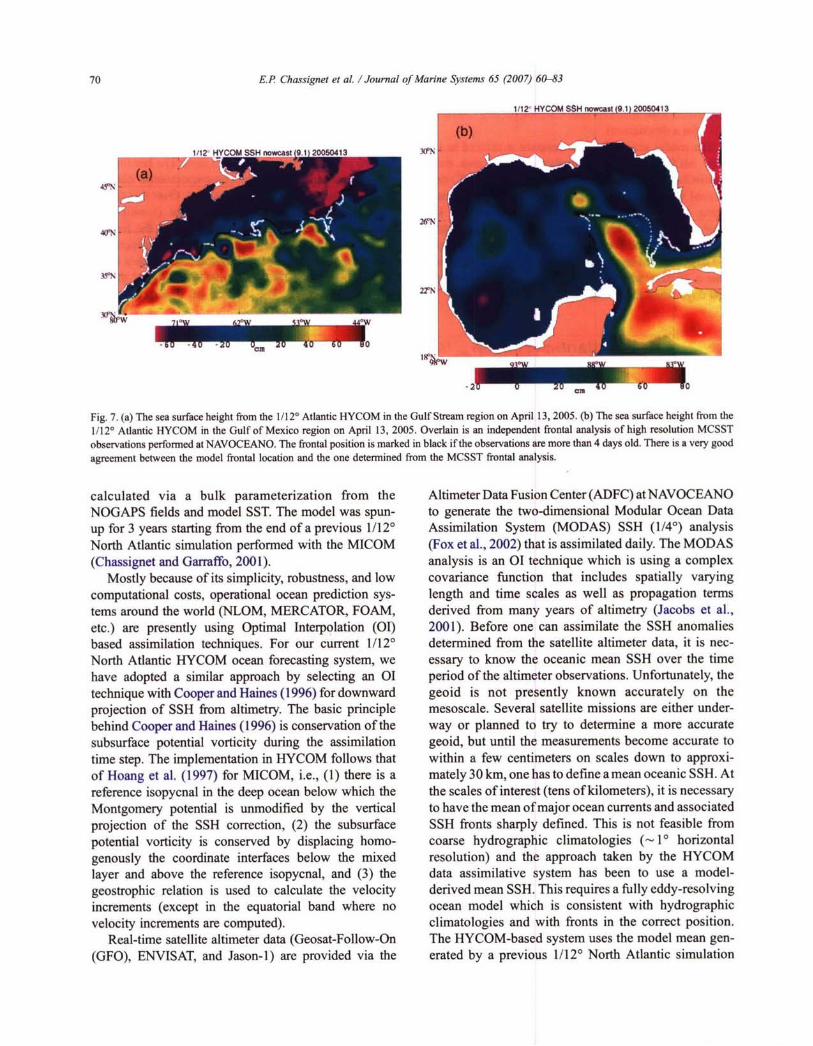
Fig. 7. (a) The sea surface height from the 1/120 Atlantic HYCOM in the Gulf Stream region on April 13, 2005. (b) The sea surface height from the

1/120 Atlantic HYCOM in the Gulf of Mexico region on April 13, 2005. Overlain is an independent frontal analysis of high resolution MCSST

observations performed at NAVOCEANO. The frontal position is marked in black if the observations are more than 4 days old. There is a very good

agreement between the model frontal location and the one determined from the MCSST frontal analysis.

calculated via a bulk parameterization from the Altimeter Data Fusion Center (ADFC) at NAVOCEANONOGAPS fields and model SST. The model was spun- to generate the two-dimensional Modular Ocean Dataup for 3 years starting from the end of a previous 1/12' Assimilation System (MODAS) SSH (1/40) analysisNorth Atlantic simulation performed with the MICOM (Fox et aL, 2002) that is assimilated daily. The MODAS(Chassignet and Garraffo, 2001). analysis is an 01 technique which is using a complex

Mostly because of its simplicity, robustness, and low covariance function that includes spatially varyingcomputational costs, operational ocean prediction sys- length and time scales as well as propagation termstems around the world (NLOM, MERCATOR, FOAM, derived from many years of altimetry (Jacobs et al.,etc.) are presently using Optimal Interpolation (01) 2001). Before one can assimilate the SSH anomaliesbased assimilation techniques. For our current 1/120 determined from the satellite altimeter data, it is nec-North Atlantic HYCOM ocean forecasting system, we essary to know the oceanic mean SSH over the timehave adopted a similar approach by selecting an 01 period of the altimeter observations. Unfortunately, thetechnique with Cooper and Haines (1996) for downward geoid is not presently known accurately on theprojection of SSH from altimetry. The basic principle mesoscale. Several satellite missions are either under-behind Cooper and Haines (1996) is conservation of the way or planned to try to determine a more accuratesubsurface potential vorticity during the assimilation geoid, but until the measurements become accurate totime step. The implementation in HYCOM follows that within a few centimeters on scales down to approxi-of Hoang et al. (1997) for MICOM, i.e., (1) there is a mately 30 km, one has to define a mean oceanic SSH. Atreference isopycnal in the deep ocean below which the the scales of interest (tens of kilometers), it is necessaryMontgomery potential is unmodified by the vertical to have the mean of major ocean currents and associatedprojection of the SSH correction, (2) the subsurface SSH fronts sharply defined. This is not feasible frompotential vorticity is conserved by displacing homo- coarse hydrographic climatologies (- 1 horizontalgenously the coordinate interfaces below the mixed resolution) and the approach taken by the HYCOMlayer and above the reference isopycnal, and (3) the data assimilative system has been to use a model-geostrophic relation is used to calculate the velocity derived mean SSH. This requires a fully eddy-resolvingincrements (except in the equatorial band where no ocean model which is consistent with hydrographicvelocity increments are computed). climatologies and with fronts in the correct position.

Real-time satellite altimeter data (Geosat-Follow-On The HYCOM-based system uses the model mean gen-(GFO), ENVISAT, and Jason-I) are provided via the erated by a previous 1/120 North Atlantic simulation


performed with MICOM (see Chassignet and Garraffo, The system runs once a week every Wednesday and2001 for a discussion). consists of a 10-day hindcast and a 14-day forecast. The

The model sea surface temperature is relaxed to the atmospheric forcing for the 14-day forecasts graduallydaily MODAS 1/80 SST analysis which uses daily reverts toward climatology after 5 days. The last forecastMulti-Channel Sea Surface Temperature (MCSST) data record is weighted with the contemporaneous climato-derived from the 5-channel Advanced Very High Reso- logical values over a 10 day time span. Over that time, alution Radiometers (AVHRR)-globally at 8.8 km linearly decreasing (increasing) weight (1-weight) isresolution and at 2 km in selected regions. The e-fold- used for the forecast (climatology). During the forecasting relaxation time is a function of the mixed layer depth period, the SST is relaxed toward climatologically-(30 days x mixed layer depth/20 m) so that the relaxation corrected persistence of the nowcast SST with a relax-time is 30 days when the mixed layer depth is 20 m and ation time scale of 1/4 the forecast length (i.e., 1 day for300 days when the mixed layer depth is 200 m. a 4-day forecast). The impact of these choices is

31'N 31*N

29PN 29N

27"9N

25*N 25*N

2rN 23*N

21*N 21*N

W'N •w* I 96-w 94"w 9r w-w tNw sew m-w .*w

9i'w 96W 94*W 9?W W0W U'W 86*W 84*W RVMW 9' 6W9' ? 0WS. 6 4

311N 31*N

29N

2r'N 2rN

25*N 25*N

23"N 23*N

21*N 21'N

19N 919NI9w 96*w 94"w 9w W0W *W 586W 64*W • 2"W 9w 96•W 94"W 9 WW W0'W 85W 86*W ,•4W VW

-2.5 -2 -1.5 -1 -0.5 0

Fig. 8. The sea surface height (contour interval of 10 cm) in the Gulf of Mexico from four different real-time or near real-time systems overlain on theSeaWiFS chlorophyll concentrations on August 8, 2003. Red/yellow colors indicate areas with high concentration, while the darker blue colorrepresents areas with low concentrations. With most of a previously detached ring reattached, the Loop Current is elongated and extends quite far tothe west and to the north. Both HYCOM 1/12' and the global NLOM 1/32' do a good job at capturing the full northwestward extent of the LoopCurrent. There are some small differences in the representation of the recaptured Loop Current ring; the ring in HYCOM 1/120 is still showing closedSSH contours with a signature slightly farther north. Both HYCOM 1/120 and NLOM 1/320 fail to correctly place the eastward frontal position of theLoop Current, which is well delineated by high chlorophyll in the observations. In the global NLOM 1/16', the ring did not remain attached andmoved westward of 90*W. The Loop Current position is however reasonably well represented east of 88*W. In the 1/24* Navy Coastal Ocean Model(NCOM) configured for the Intra-Americas Sea (lAS), the Loop Current is in generally the right location, except that it does not penetrate far enoughnorthward and the recaptured ring is too far south by half a degree.


discussed by Smedstad et al. (2003) and Shriver et al. different ocean data assimilative systems, including tests(2006-this issue). and evaluation of the inter-comparison process. The

Atlantic was chosen because of the developmental status3.1. Evaluation of the required components of an ocean forecasting

system: already well instrumented, large number ofAt the present time, evaluation of the model outputs available models, high user interest. The comparison

relies on systematic verification of key parameters and exercise took place within the framework of MERSEAcomputation of statistical indexes by reference to both (Marine EnviRonment and Security for the Europeanclimatological and real-time data, and, in a delayed Area) funded by the European Union and consisted ofmode, to quality controlled observations. The accuracy comparing similar diagnostics and fields from corres-of data assimilative model products is theoretically a ponding realizations of several systems (MERCATOR,non-decreasing function of the amount of data that is FOAM, MFS, TOPAZ, and HYCOM) (Crosnier and Leassimilated. A degradation caused by assimilation gen- Provost, 2006-this issue). In the remainder of this section,erally indicates inaccurate assumptions in the assimila- we provide evaluation examples for the HYCOMtion scheme. While models can be forced to agree with Atlantic forecasting system that differ from the onesobservations (e.g., by replacing equivalent model fields discussed by Crosnier and Le Provost (2006-this issue).with data), improvements with respect to independent Examples of assessments of the models' ability toobservations are not trivial. An assessment of model represent observed flow features can be seen in Figs. 7a, bimprovement (or lack of degradation) with respect to and 8. These tests qualitatively evaluate model analysesunassimilated, independent measurements is therefore against alternate, unassimilated observations of flowan effective means of assessing the performance of an features in regions of interest. Fig. 7a and b show theassimilation system. Variances of these model-data dif- model SSH hindcast on April 13, 2005 for the Gulfferences serve as common measures of the estimation Stream region and the Gulf of Mexico region. Overlainaccuracy. For the evaluation of flow accuracy and water on the SSH is an independent frontal analysis of SSTmass characteristics, we follow the guidelines put data. Close examination of the figures on this date andforward by the international GODAE metrics group others (see HYCOM web site for movies) shows overall a(Le Provost et al., 2002) as well as the validation tests very good agreement between the model frontal struc-commonly used at the operational centers before official tures and the independent SST observations. Compar-transition to operational use. isons of surface height and temperature with ocean color

Furthermore, within GODAE, the Atlantic Ocean has imagery can also at times provide clear and dramaticbeen chosen as a pilot project for an inter-comparison of qualitative model assessment (Chassignet et al., 2006).

Sea Surface Temperature at: 28.51 ln084.51w See Surface Temperature at: 29nO79w

3-(a) M-oa~ (b)

30 MS. 0.71( 30 f

28 28

26

S~ !26e24

22 224 24

20-2

18 - BUOY - BUOY- HYCOM nowoast (9.1) 2- - HYCOM nowcast (9.1)

16 - MODAS - MODAS08/07 10/07 11/15 02/23 06/02 09/10 12/19 03/29

11/15 02/23 06/02 9/10 12/19 03/29 From 01-Jun-2003 to 13-Apr-2005From 01-Jun-2003 to 13-Apr-2005

Fig. 9. Comparison between buoy observations of SST (blue), the 1/12' North Atlantic data assimilative system (red), and MODAS (black) at

(a) 28.5 1N, 84.51 °W and (b) 29°N, 79°W.


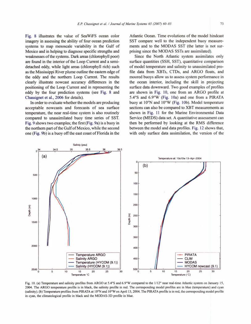
Fig. 8 illustrates the value of SeaWiFS ocean color Atlantic Ocean. Time evolutions of the model hindcastimagery in assessing the ability of four ocean prediction SST compare well to the independent buoy measure-systems to map mesoscale variability in the Gulf of ments and to the MODAS SST (the latter is not sur-Mexico and in helping to diagnose specific strengths and prising since the MODAS SSTs are assimilated).weaknesses of the systems. Dark areas (chlorophyll poor) Since the North Atlantic system assimilates onlyare found in the interior of the Loop Current and a semi- surface quantities (SSH, SST), quantitative comparisondetached eddy, while light areas (chlorophyll rich) such of model temperature and salinity to unassimilated pro-as the Mississippi River plume outline the eastern edge of file data from XBTs, CTDs, and ARGO floats, andthe eddy and the northern Loop Current. The results moored buoys allow us to assess system performance inclearly illustrate nowcast accuracy differences in the the ocean interior, including the skill in projectingpositioning of the Loop Current and in representing the surface data downward. Two good examples of profileseddy by the four prediction systems (see Fig. 8 and are shown in Fig. 10, one from an ARGO profile atChassignet et al., 2006 for details). 5.40S and 6.9°W (Fig. 10a) and one from a PIRATA

In order to evaluate whether the models are producing buoy at 100N and 10°W (Fig. 10b). Model temperatureacceptable nowcasts and forecasts of sea surface sections can also be compared to XBT measurements astemperature, the near real-time system is also routinely shown in Fig. 11 for the Marine Environmental Datacompared to unassimilated buoy time series of SST. Service (MEDS) data set. A quantitative assessment canFig. 9 shows two examples; the first (Fig. 9a) is a buoy in then be performed by looking at the RMS differencethe northern part of the Gulf of Mexico, while the second between the model and data profiles. Fig. 12 shows that,one (Fig. 9b) is a buoy off the east coast of Florida in the with only surface data assimilation, the version of the

Salmiy (Pau)

3 34.5 35 35.5 36 36.50

(a) Temperature at: lOe IOw 1 3-Apr-2004

50

500

100

150

1000

200

1500 0

13000

350-

2000400

- Temperature ARGO -. PIRATA- Salinity ARGO 450 - CLIM- Temperature (HYCOM (9.1)) - MODAS- Salin HYCOM 9.1)- HYCOM nowcast 9.1

2500 1 11 w0 5 10 15 20 25 30 0 5 10 15 20 25 30

Temperature "C Temperature (*C)

Fig. 10. (a) Temperature and salinity profiles from ARGO at 5.4°S and 6.9*W compared to the 1/120 near real-time Atlantic system on January 15,2004. The ARGO temperature profile is in black, the salinity profile in red. The corresponding model profiles are in blue (temperature) and cyan(salinity). (b) Temperature profiles from PIRATA at 10N and I 0°Won April 13, 2004. The PIRATA profile is in red, the corresponding model profilein cyan, the climatological profile in black and the MODAS-3D profile in blue.


T(z) 2003.12 Line A : 1/120 HYCOM Nowcast (9.1) T(z) 2003.12 Une A: MEDS(2003.12.01-200L 12.07) 12600212.O1-200U 12.07)

0 0so 32 5032

150 20

as aIsO26 26

200 20

250 20

o 35

14 150 1450 12 50 12

5O 10 550 1600 8 600650 56 650700 4 700 4750 2 750 2600 0 6000

0 5 10 Is 25 30 0 5 0 2 25 30Latitude Latitude

T(z) 2003.12 LUne B 1/12 0 HYCOM Nowcast (9.1) T(z) 200.1 2 Line 8 MEDS(2003 1202-2003.12.1) (200312.02-2002.tZ15)

32 3250 50

400~3 16•00 1

10 3055

29 26150 26 6200 0025022 2230022 302

3 0 30 0

450 4 4W1450012 502

560 to 55 0ISOO 6 0

6500 65

700 M4702750 2800 0 So0

-5 0 5 10 15 2D25 3035 40 45 .5 0 5 10 152 25 3035 40 45Latitude Latitude

SON SON

I ! I I I I I I I I I I

4, - -•I- -4-- ... . . 4- - -- -4-4ON -+- ON

I I -TI I I I

I I II I / O1I I ,

--N - ----I---

4 -I t 3014

ION L. ION

II !

I I I I I I10$ -4 - -4-I- 105

20S M0SOW 70W 60W SOW 40W 30W 20W 10W 00 BOW 7OW 60W SOW 40W 30W 20W 1OW 00

Fig. 11. (a) Temperature section along line A from the 1/12' near real-time Atlantic system, (b) corresponding section from the MEDS data,

(c) temperature section along line B from the 1/12' near real-time Atlantic system, (d) corresponding section from the MEDS data.

Atlantic HYCOM prediction system presented here has SST analyses assimilated by HYCOM, indicating

overall a greater nowcast RMS error than climatology or superior performance for a data-based method of down-MODAS-3D. MODAS-3D (Fox et al., 2002) uses the ward projection than the Cooper and Haines (1996)statistics of the historical hydrographic database to technique used in HYCOM, at least in this application.downward project the same MODAS SSH anomaly and This is also indicative of the drift in T and S that

E.P Chassignet et at / Journal of Marine Systems 65 (2007) 60-83 75

o Models vs MEDS 2093.09-2004.08 Models vs PIRATA 2003.09-2004.08

I(1 .. . . . . . 100

200 200

300 300

400 400-

500- E50D

8600- 600

700- Hean._NumET =12643 70DStats for 0-1000mNodl Mean RMSD Mean_NumBT - 2331CLIN 1.08 Stats for 1-500mGDUI3 1.08 Nodal Nfi -mD

90o HYCOM 1.57 900 CLIN 0.82LEVIT94 1.18 .HYCOM 1.48MODAS 0.94 MODAS 0.87

ooMSD Tempera ure [eC] FoMSD Tempera uro '1 0

Fig. 12. (a) Statistics for September 2003 through August 2004 between the 1/12° HYCOM system and available Marine Environmental Data Service(MEDS) profile observations. The RMS difference between the MEDS data and different climatologies, MODAS climatology (CLIM), MODASsynthetics (MODAS), Levitus et al. (1994), and the Generalized Digital Environmental Model (GDEM3) is also shown. (b) Statistics for September2003 through August 2004 between the 1/120 HYCOM system and available PIRATA profile observations. The RMS between the PIRATA data andthe MODAS climatology (CLIM) and MODAS synthetics (MODAS) is also shown.

occurred during the spin-up (Crosnier and Le Provost, nowcast/forecast partners as boundary conditions, and2006-this issue). Model velocity cross-sections can be increases the usability of HYCOM results by "applica-evaluated through qualitative and quantitative compar- tion providers".isons of biases when data are available. Two examplesof mean velocity comparisons are provided: one in 4. Boundary conditions for regional modelsFig. 13 for a cross-equatorial section at 35°W and one inFig. 14 for a section across the Yucatan channel. When An important attribute of the data assimilative HYCOMobservations are available, transport time series provide simulations is the capability to provide boundary condi-an excellent measure of the model's ability to represent tions to regional and coastal models. The chosendaily to seasonal variability (see example shown in horizontal and vertical resolution for the forecastingFig. 15 for the Florida Straits). system marginally resolves the coastal ocean (7 km at

mid-latitudes, with up to 15 terrain-following (a)3.2. Model outputs coordinates over the shelf), but is an excellent starting

point for even higher resolution coastal ocean predictionThe near real-time North Atlantic basin model systems. To increase the predictability of coastal regimes,

outputs are made available to the community at large several partners within the HYCOM consortium arewithin 24 h via the Miami Live Access Server (LAS) therefore developing and evaluating boundary conditions(http://hycom.rsmas.miami.edu/las). Specifically, the for coastal prediction models based on the HYCOM dataLAS supports model-data and model-model compar- assimilative system outputs. The inner nested models mayisons; provides HYCOM subsets to coastal or regional or may not be HYCOM, so the coupling of the global and

76 E.P. Chassignet et al. / Journal of Marine Systems 65 (2007) 60-83

NBC SEC EUC SECEU l.SC-6.OSv -7.0sv 8.6sv -2.0Sv

400

1000

1500

40 4A U2000

42.0

3500O

4000

46.6~4500

5000

58 4S 38 28 1S Eq IN 2N 3N 4N SN 58 4S 38 2S 18 Eq IN 2N 3N 4N 5N

Fig. 13. (a) Vertical section of the mean velocity across the Equator at 35°W from 5PS to 5°N from the 1/12* Atlantic system over the time period of

September 2003 through August 2004. (b) Observations of transports across the Equator at 35°W (Schott et al., 2003).

coastal models needs to be able to handle unlike vertical entire time interval of the nested model simulation at agrids. Coupling HYCOM to HYCOM is now routine via time interval specified by the user, typically once per day

one-way nesting. Outer model fields are interpolated to in our evaluations to date, and stored in HYCOM archivethe horizontal mesh of the nested model throughout the format Layers can be added to these archive files to

0-- -15

400 • I

1001

200

90.

s800 all

0 1000

1200

401400

4 05

.00 1800

87W 86W 85W M-1.

8640 85.50 8S.00Longitude

Fig. 14. (a) Vertical section of the mean velocity across the Yucatan Channel from the 1/120 Atlantic system over the time period of September 2003through August 2004. (b) Observations of velocities from Abascal et al. (2003).


HYCOM ATLWO.OS-9.1-nowoa,: Florila Strmt at 2es.n p yLaw l-36 Ma%:S31.17 En:20.701Max: 37.138t:2M existing HYCOM nesting capability to allow accurate

- oues 1.1a passage of a coastally trapped wave generated by Hurri-

46 cane Juliette (Zamudio et al., 2002). In Zamudio et al.(submitted for publication), nesting parameters such asupdating frequency, e-folding time, and buffer zone widthwere varied and the results were compared to coastal tidegauge stations. Coupling HYCOM to other models, suchas the Navy Coastal Ocean Model (NCOM) has alreadybeen demonstrated, while coupling of HYCOM to

30- Iunstructured grid/finite element models is in progress.In the remainder of this section, results from a 20-layer

1/25° horizontal resolution Gulf of Mexico HYCOMconfiguration nested within a non-assimilative 1999-2000 North Atlantic HYCOM are presented and dis-

wi4F/0 11/1n'& 0212M am02 W1,00o n 1204 MW cussed. The model domain used in the 1/250 nested GulfFin - to lS-Apr-2001 of Mexico HYCOM, including the location of the open

Fig. 15. The transport in the Florida Current at 27°N from the 1/120 boundary conditions, is shown in Fig. 16. Most flowAtlantic near real-time system is in black. Observed transport enters the domain on the southern and southeastern boun-variations in the Florida Current are being monitored by measuring daries and exits through the Florida Strait. Currently thethe cross-stream voltages using an undersea cable between Florida and nesting of HYCOM to HYCOM is one-way (informationthe Bahamas. Daily transport data are available from March 1982 toOctober 1998, and from March 2000 onward (Baringer and Larsen, is only passed from the outer grid to the inner grid) and2001). Observations from the cable data are shown in red. "off-line", meaning that the nested model does not run

concurrently with the outer model. An advantage of thisincrease the vertical resolution of the nested model and approach is that the nested region does not need to beinsure that there is sufficient vertical resolution to resolve known in advance, but a disadvantage is that the updatingthe bottom boundary layer. The nested model is initialized frequency of the boundary information is limited by howfrom the first archive file and the entire set of archives often outer grid model output is archived. In this nestedprovides boundary conditions during the nested run, in- Gulf of Mexico example, the method of characteristicssuring consistency between initial and boundary condi- (Browning and Kreiss, 1982, 1986) is used for the baro-tions. This procedure has proven to be very robust. Nested tropic open boundary condition on velocity and pressure.Gulf of California simulations (Zamudio et al., submitted At the open boundaries, 20 grid point-wide "buffer" (orfor publication) were used to investigate the ability of the boundary relaxation) zones with e-folding times of 0.1 to

ON 3ON

on00

£0.•

$000 21rN

3500

3000 24N

2600

2000 22'N

1600

98"W W'-W 04"W 92W oWW 8W MW 841W 82'W 8o'W 76'W

Fig. 16. Bathymetry used in the 1/251 nested Gulf of Mexico simulation. The yellow lines indicate the locations of the open boundaries that areupdated from a 1/120 Atlantic HYCOM simulation.


10 days (outer to inner grid) are used to relax the baro- size, speed, population, and vertical structure. Fig. 17clinic mode temperature, salinity, pressure and velocity depicts the sea surface height (top panel) and sea surfacecomponents once per baroclinic time step towards a non- salinity (bottom panel) on June 13, 2000 (although this isassimilative interannually forced 1/120 Atlantic HYCOM a non-assimilative simulation and so the ocean state is notsolution that is linearly interpolated in time. Although the representative of the Gulf of Mexico on that day). At thisbuffer zone is located on the fine grid mesh, the bottom time, the Loop Current Extension reaches almost 28*Ntopography and aforementioned variables are constrained and there is a relatively strong cyclone on its eastern flankto the coarse outer grid solution and thus should be con- at about 25*N. This cyclonic eddy plays a role in the Loopsidered part of the boundary condition, not part of the fine Current shedding an anticyclonic ring the followinginner grid solution. Concurrent 6-hourly NOGAPS was month (not shown). Several of the cyclonic eddies travelused for surface forcing in both the nested Gulf of Mexico along the Florida Keys and then exit the Gulf of Mexicomodel and the interannually forced 1/120 Atlantic through the Florida Straits. The surface salinity shows anHYCOM simulation. area of relatively fresh water just north of the Yucatan

Compared to similar 1/120 simulations, the 1/250 Peninsula (88'W, 22MN). This is an area of prolificsimulation shows that the higher resolution results in more upwelling during June, and it may be associated with therealistic cyclonic eddies that often are associated with the southward Yucatan Undercurrent (Merino, 1997; OchoaLoop Current and Loop Current eddies in terms of eddy et al., 2001), although Cochrane (1968, 1969) suggested

28N

26°N

24°N

22IN

20 N

SOW SO •W 941W 921W SOW 6S'W SOeW 64WV'W 6•0W TtVW

30iN

2WN

26'N

24°N

22IN

20*N

WW•' 9 "W 94r' SW 90'W U' ft4•W 84W• 92' f0OW 70'W

Fig. 17. Sea surface height (top panel) and salinity (bottom panel) on June 13, 2000 from the nested 1/25' simulation.


that bottom friction of the strong Yucatan Current against system with data assimilation to be transitioned tothe slope on the eastern edge of the Yucatan Shelf caused the U.S. Naval Oceanographic Office at 1/120the upwelling instead, equatorial (~-7 km mid-latitude) resolution in 2007

An example of the vertical structure of the anticyclonic and 1/250 resolution by 2011. The present near real-Loop Current and associated cyclonic eddies on June 1, time system as described in this paper is a first step2000 is shown in Fig. 18. At this time the Loop Current towards the fully global 1/120 HYCOM data assimi-extends to about 28°N and has cyclones on both the lative system. Development of the global system iswestern and eastern flanks. A zonal cross-section of the presently taking place and includes model develop-south to north (v) component of velocity and the salinity ment, data assimilation, and ice model embedment.are also shown in Fig. 18. The eddy on the eastern flank is The model configuration is fully global with the Lospropagating along the continental slope but in this case the Alamos CICE ice model embedded and will run atcore of the eddy does not propagate onto the shelf. The three resolutions: - 60 kin, - 20 km and - 7 km atsalinity depicts a subsurface salinity maximum in the mid-latitudes. The size of the problem makes it verycenter of the anticyclone, consistent with observations. In difficult to use sophisticated assimilation techniquesall of the nested Gulf of Mexico simulations, realistic flow since some of these methods can increase the cost ofthrough the southern boundary (about 40 south of the running the model by a factor of 100. The strategyYucatan Channel) from the 1/120 Atlantic HYCOM is adopted by the consortium is to start with a simple datacritical for realistic Loop Current Eddy shedding in the assimilation approach such as the Cooper-HainesGulf of Mexico. In particular, the flow through the technique described in Section 4, and then graduallyYucatan Channel needs to be surface intensified on the increase its complexity. Several of these morewestern side of the channel and have a mean volume sophisticated data assimilation techniques are alreadytransport of about 28 Sverdrups (Sv). Although recent in place and are in the process of being evaluated.measurements (Sheinbaum et al., 2002) suggest the value These techniques are, ordered by degree of sophisti-may be lower than this, 28 Sv is consistent with the more cation, the NRL Coupled Ocean Data Assimilationextensively observed transport through the Florida Straits (NCODA), the Singular Evolutive Extended Kalmanat 27'N (Baringer and Larsen, 2001; Johns et al., 2002). (SEEK) filter, the Reduced Order Information Filter

(ROIF), the Reduced Order Adaptive Filter (ROAF)5. Outlook (including adjoint), the Ensemble Kalman Filter

(EnKF), and the 4D-VAR Representer method. ThisThe long term goal of the HYCOM consortium is does not mean that all these techniques will be used

an eddy-resolving, fully global ocean prediction operationally: the NCODA and SEEK techniques are

10 4W

U Y~fffIIIV

40W•SW

MIAM

oWW WW 8STW 36'W "W Wm am "W emMW41

Fig. 18. Northeast Gulf of Mexico zoom-in of sea surface height (color), surface currents (vectors) and bottom topography (black line contours)(left panel) and cross-sections of v-component of velocity (top right) and salinity (bottom right) from the nested 1/25* simulation on June 1, 2000.


presently being considered as the next generation data It mostly differs from the system described in Section 4 inassimilation to be used in the near real-time system. two ways: (a) different horizontal grid and (b) NCEP-The remaining techniques, because of their cost, are based wind and thermal forcing. By taking advantage ofbeing evaluated mostly within specific limited areas of the general orthogonal curvilinear grid in HYCOM, thehigh interest or coastal HYCOM configurations. NOAA/NCEP group is using a configuration which, for

The NCODA is an oceanographic version of the the same number of grid points as in the regular Mercatormultivariate optimum interpolation (MVOI) technique projection used in the present system, has finer resolutionwidely used in operational atmospheric forecasting in the western and northern portions of the basin andsystems. A description of the MVOI technique can be on shelves (3-7 kin) in order to provide higher reso-found in Daley (1991). The ocean analysis variables in lution along the U.S. coast than toward the east andNCODA are temperature, salinity, geopotential (dy- southeast (7-13 km).namic height), and velocity. The horizontal correlationsare multivariate in geopotential and velocity, thereby Acknowledgmentspermitting adjustments to the mass field to be correlatedwith adjustments to the flow field. NCODA assimilates This work was sponsored by the National Oceanall available operational sources of ocean observations. Partnership Program (NOPP), the Office of NavalThis includes along track satellite altimeter observa- Research (ONR), and the Operational Effects Programstions, MCSST and in situ observations of SST and SSS, (OEP) Program Office, PMW 150 through the followingsubsurface temperature and salinity profiles from BT's projects: NOPP HYCOM Consortium for Data Assim-and profiling floats, and sea ice concentration. ilative Ocean Modeling, NOPP U.S. GODAE: Global

Both the SEEK filter (Pham et al., 1998) and ROIF Ocean Prediction with the HYbrid Coordinate Ocean(Chin et al., 1999) are sequential in nature, implying that Model (HYCOM), 6.1 Global Remote Littoral Forcingonly past observations can influence the current estimate via Deep Water Pathways (ONR), 6.2 Coastal Oceanof the ocean state and are especially well suited for large Nesting Studies (ONR), 6.4 Large Scale Ocean Models,dimensional problems. The ROIF assumes a tangent 6.4 Ocean Data Assimilation, and 6.4 Small Scalelinear approximation to the system dynamics, while the Oceanography (all the 6.4 projects sponsored by PMW-SEEK filter can use the non-linear model to propagate 150). Many thanks to Jan Dastugue for her help inthe error statistics forward in time (Ballabrera-Poy et al., redrafting some of the figures.2001). For both schemes, the analysis step is multivariatein nature, i.e., all model state variables are modified in a Appendix A. Controlling minimum layer thicknessconsistent manner after the analysis step. In the SEEK in the hybrid coordinate generatorfilter, the dominant eigenvectors describing the modelvariability can be used to specify the initial background The HYCOM vertical grid is controlled by referenceerror covariance matrix in decomposed form. This leads isopycnals and the minimum thickness permitted forto fully three-dimensional, multivariate dynamically each layer k-consistent corrections (see Parent et al., submitted forpublication for an application of the SEEK filter to the 6k max[62kminlk(5 6,)] (1 ) k >-5kN,) (1)North Atlantic configuration of Section 4). The ROIF where 61k (k >N.,)method factors the covariance functions into horizontaland vertical components and represents the correction 6lk = min(b, 61ak-I)) (l<k<-Ni) (2)field implicitly, using techniques transplanted from sta-, int (k >Ni)P (tistical mechanics (Gaussian Markov Random Field).The implicit technique tends to allow a highly efficient 6 = min(c5r", 621Ck-1), (3)way to represent smaller scale dynamic modes. The

reduced order aspect of ROWF refers to the fact that the 6, =D/N5, D is water depth, and Ns is the number of layersinformation matrix is approximated as a banded matrix, below the surface permitted to transition to a coordinatesThis allows more realistic tails for the correlation func- in shallow water. To estimate 61k and &,, the minimumtions than similarly approximating the error covariance thicknesses of layer 1 (61 and 621), the largest permittedmatrix. minimum thicknesses (61 and 6by), and the expansion/

Finally, another Atlantic configuration is under de- contraction factors (a1 and a2) must be specified. Thevelopment to form the backbone of the NOAA/NCEP/ expansion/contraction factors are often chosen to beMMAB North Atlantic Ocean Forecast System (NAOFS). greater than 1 to provide the highest resolution near the


surface. In this case, the minimum thicknesses will increase Bleck, R., Rooth, C., Hu, D., Smith, L.T., 1992. Salinity-driven thermo-

with depth until the largest permitted values are reached, cline transients in a wind- and thermohaline-forced isopycniccoordinate model of the North Atlantic. J. Phys. Oceanogr. 22,

and then remain constant with depth. It is also necessary 1486-1505.to identify the uppermost model layer that is isopycnic Browning, G.L., Kreiss, H.-O., 1982. Initialization of the shallow

(N,) and to specify an interior minimum thickness (6int). water equations with open boundaries by the bounded derivative

Thickness 61k governs the open ocean transition between P method. Tellus 34, 334-351.

and isopycnic coordinates by maintaining the minimum Browning, G.L., Kreiss, H.-O., 1986. Scaling and computation ofsmooth atmospheric motions. Tellus 38A, 295-313.

thickness of the nearsurface P-coordinate layers. In the Burchard, H., Beckers, J.-M., 2004. Non-uniform adaptive vertical

isopycnic coordinate layers beneath the P domain, mini- grids in one-dimensional numerical ocean models. Ocean Model.

mum thicknesses are specified by bint, which is typically 6, 51-81.

much smaller than the minimum thicknesses above so that Canuto, VM., Howard, A., Cheng, Y., Dubovikov, MS., 2001. Ocean

sharp pycnoclines can form in the isopycnic interior. For turbulence. Part 1. One-point closure model-momentum and heatvertical diffusivities. J. Phys. Oceanogr. 31, 1413-1426.

Canuto, VM., Howard, A., Cheng, Y., Dubovikov, M.S., 2002. Ocean

IfNs is chosen to be zero, then 6 k= 6 1k everywhere and turbulence. Part I. Vertical diffusivities of momentum, heat, salt,

the coastal transition to a' coordinates is not implemented. mass, and passive scalars. J. Phys. Oceanogr. 32, 240-264.

IfN, is nonzero, then the coastal transition is implemented Chang, Y., Xu, X., Ozg6kmen, T.M., Chassignet, E.P., Peters, H., Fisher,

in model layers 1 < k < N_. In these layers, the transition to P.F., 2005. Comparison of gravity current mixing parameterizationsand calibration using a high-resolution 3D nonhydrostatic spectral

or coordinates begins where the water depth becomes element model. Ocean Model. 10, 342-368.

sufficiently shallow to make 6s<6 1k. Where the water Chassignet, E.P., Garraffo, Z.D., 2001. Viscosity parameterization and

depth is shallow enough to make 6s<&-j, a transition back the Gulf Stream separation. In: Muller, P., Henderson, D. (Eds.),to level coordinates occurs to prevent layers from be- "From Stirring to Mixing in a Stratified Ocean". Proceedings 'Aha

coming too thin. Parameter N, is updated during model Huliko'a Hawaiian Winter Workshop. U. Hawaii. January 15-19,runs. The thickness of layer 1 is always restored to a 2001, pp. 37-41

Chassignet, E.P., Smith, L.T., Bleck, R., Bryan, F.O., 1996. A model

constant thickness 61 as given by (1). comparison: numerical simulations of the North and Equatorial

Atlantic Ocean circulation in depth and isopycnic coordinates.

J. Phys. Oceanogr. 26, 1849-1867.References Chassignet, E.P., Arango, H., Dietrich, D., Ezer, T., Ghil, M., Haidvogel,

D.B., Ma, C.-C., Mehra, A., Paiva, A.M., Sirkes, Z., 2000. DAMEE-Abascal, A.J., Sheinbaum, J., Candela, J., Ochoa, J., Badan, A., 2003. NAB: the base experiments. Dyn. Atmos. Ocean. 32, 155-184.

Analysis of flow variability in the Yucatan Channel. J. Geophys. Chassignet, E.P., Smith, L.T., Halliwell, G.R., Bleck, R., 2003. NorthRes. 108. doi: 10.1029/2003JC001922. Atlantic simulations with the HYbrid Coordinate Ocean Model

Adcroft, A., Hallberg, R., 2006. On methods for solving the oceanic (HYCOM): impact of the vertical coordinate choice, referenceequations of motion in generalized vertical coordinates. Ocean density, and thermobaricity. J. Phys. Oceanogr. 33, 2504-2526.Model. 11, 224-233. Chassignet, E.P., Hurlburt, H.E., Smedstad, O.M., Barron, C.N., Ko,

Ballabrera-Poy, J., Brasseur, P., Verron, J., 2001. Dynamical evolution D.S., Rhodes, R.C., Shriver, J.F., WallcrafL A.J., Arnone, R.A.,of the error statistics with the SEEK filter to assimilate altimetric 2006. Assessment of ocean prediction systems in the Gulf ofdata in eddy-resolving ocean models. Q. J. R. Meteorol. Soc. 127, Mexico using ocean color. In: Sturges, W., Lugo-Fernadez, A.233-253. (Eds.), New Developments in the Circulation of the Gulf of

Baringer, M.O., Larsen, J.C., 2001. Sixteen years of Florida Current Mexico. AGU Monograph Series, vol. 161. American Geophysicaltransport at 27'N. Geophys. Res. Lett. 28, 3179-3182. Union, Washington, D.C., pp. 87-100.

Barron, C.N., Martin, P.J., Kara, A.B., Rhodes, R1C., Smedstad, L.F., Chin, T.M., Mariano, A.J., Chassignet, E.P., 1999. Spatial regressionin press. Description and application of the Global Navy Coastal with Markov random fields for Kalman filter approximation in least-Ocean Model (NCOM), with examination of vertical coordinate squares solution of oceanic data assimilation problems. J. Geophys.system choices. Ocean Modelling. Res. 104, 7991-8014.

Block, R., 2002. An oceanic general circulation model framed in Cochrane, J.D., 1968. Currents and waters of the eastern Gulf of Mexicohybrid isopycnic-cartesian coordinates. Ocean Model. 4, 55-88. and western Caribbean, of the western tropical Atlantic Ocean, and of

Bleck, R., Benjamin, S., 1993. Regional weather prediction with a the eastern tropical Pacific Ocean. Dep. Oceanogr. Meteorl., Texasmodel combining terrain-following and isentropic coordinates. A&M Univ., Ref. 68-8T, pp. 19-28 (unpubl. rep.).Part I. Model description. Mon. Weather Rev. 121, 1770-1785. Cochrane, J.D., 1969. Water and circulation on the Campeche Bank in

Bleck, R., Boudra, D., 1981. Initial testing of a numerical ocean cir- May. Bull. Jpn. Soc. Fish. Oceanogr. Spec. 123-128 (Prof. Uda'sculation model using a hybrid (quasi-isopycnic) vertical coordinate. Commemorative Papers).J. Phys. Oceanogr. 11, 755-770. Cooper, M., Haines, K., 1996. Altimetric assimilation with water

Block, IL, Chassignet, E.P., 1994. Simulating the oceanic circulation with property conservation. J. Geophys. Res. 101, 1059-1078.isopycnic coordinate models. In: Majundar, S.K., Mill, E.W., Forbes, Crosnier, L., Le Provost, C., 2006-this issue. Inter-comparing fiveG.S., Schmalz, RIE., Pariah, A.A. (Eds.), The Oceans: Physical- forecast operational systems in the North Atlantic and Mediterra-Chemical Dynamics and Human Impact The Pennsylvania Academy nean basins: The MERSEA-strandl Methodology. J. Mar. Sys.

of Science, pp. 17-39. doi: 10.1016/j.jmarsys.2005.01.003.


Daley, R., 1991. Atmospheric Data Analysis. Cambridge University Leveque, R.J., 2002. Finite Volume Methods for Hyperbolic Problems.Press, Cambridge. 457 pp. Cambridge University Press. 578 pp.

Durski, S.M., Glenn, S.M., Haidvogel, D.B., 2004. Vertical mixing Levitus, S., Burgett, R., Boyer, T.P., 1994. World Ocean Atlas 1994,

schemes in the coastal ocean: comparison of the level 2.5 Mellor- Volume 3: Salinity. NOAA Atlas NESDIS 3. U.S. Govt. PrintingYamada scheme with an enhanced version of the K profile Office, Washington, DC. 99 pp.

parameterization. J. Geophys. Res. 109 (C01015). doi:10.1029/ Marsh, R., Roberts, M.J., Wood, R.A., New, A.L., 1996. An inter-2002JC001702. comparison of a Bryan-Cox type ocean model and an isopycnic

Ezer, T., Mellor, G.L., 2004. A generalized coordinate ocean model and ocean model. Part II. The subtropical gyre and heat balances.a comparison of the bottom boundary layer dynamics in terrain- J. Phys. Oceanogr. 26, 1528-1551.

following and in z-level grids. Ocean Model. 3-4, 379-403. Mellor, G.L., Yamada, T., 1982. Development of a turbulence closureFox, D.N., Teague, W.J., Barron, C.N., Carnes, M.R., Lee, C.M., 2002. model for geophysical fluid problems. Geophys. Space Phys. 20,

The Modular Ocean Data Analysis System (MODAS). J. Atmos. 851-875.

Ocean. Technol. 19, 240-252. Merino, M., 1997. Upwelling on the Yucatan Shelf: hydrographic

Griffies, S.M., B6ning, C., Bryan, F.O., Chassignet, E.P., Gerdes, R., evidence. J. Mar. Syst. 13, 101-121.Hasumi, H., Hirst, A., Treguier, A.-M., Webb, D., 2000. Develop- Ochoa, J., Sheinbaum, H., Badan, A., Candela, J., Wilson, D., 2001.ments in ocean climate modelling. Ocean Model. 2, 123-192. Geostrophy via potential vorticity inversion in the Yucatan

Hallberg, R., 2000. Time integration of diapycnal diffusion and Channel. J. Mar. Res. 59, 725-747.

Richardson number dependent mixing in isopycnal coordinate Parent, L., Brankart, J.M., Smedstad, O.M., Wallcrat A., Townsend, T,ocean models. Mon. Weather Rev. 128, 1402-1419. Hurlburt, H.E., Jacobs, G., Chassignet, E.P., Brasseur, P., submitted

Halliwell, G., 2004. Evaluation of vertical coordinate and vertical for publication. A data-assimilative hindcast experiment with the

mixing algorithms in the HYbrid Coordinate Ocean Model 1/120 Atlantic HYCOM: towards a reduced Kalman filter approach.

(HYCOM). Ocean Model. 7, 285-322. Pham, D.T., Verron, J., Roubaud, M.C., 1998. Singular evolutive

Halliwell Jr., G. R., in preparation. Sensitivity of HYCOM West extended Kalman Filter with EOF initialization for data assimila-Florida Shelf simulations to vertical coordinate and vertical mixing tion in oceanography. J. Mar. Syst. 16 (3-4), 323-340.

choices. Price, J.F., Weller, R.A., Pinkel, R., 1986. Diurnal cycling: observa-Hoang, S., Baraille, R., Tallagrand, 0., Carton, X., De Mey, P., 1997. tions and models of the upper ocean response to diurnal heating,

Adaptive filtering: application to satellite data assimilation in cooling and wind mixing. J. Geophys. Res. 91, 8411-8427.

oceanography. Dyn. Atmos. Ocean. 27, 257-281. Roberts, M.J., Marsh, R., New, A.L., Wood, R.A., 1996. An inter-Hurlburt, H.E., Hogan, P.J., 2000. Impact of 1/8' to 1/640 resolution on comparison of a Bryan-Cox type ocean model and an isopycnic

Gulf Stream model-data comparisons in basin-scale subtropical ocean model. Part 1. The subpolar gyre and high-latitude processes.Atlantic Ocean models. Dyn. Atmos. Ocean. 32, 283-329. J. Phys. Oceanogr. 26, 1495-1527.

International GODAE Steering Team, 2000. Global Ocean Data Schott, F.A., Dengler, M., Brandt, P., Affler, K., Fischer, J., Bourles, B.,Assimilation Experiment Strategic Plan. GODAE Report #6. 26 Gouriou, Y., Molinari, R.L., Rhein, M., 2003. The zonal currents

pp. [Available from the GODAE International Project Office, c/o and transports at 35OW in the tropical Atlantic. Geophys. Res. Lett.Bureau of Meteorology, Melbourne, Australia]. 30 (7), 1349. doi:10.1029/2002GL016849.

Jacobs, G.A., Barron, C.N., Rhodes, R.C., 2001. Mesoscale char- Sheinbaum, J., Candela, J., Badan, A., Ochoa, J., 2002. Flow structure

acteristics. J. Geophys. Res. 1006 (19), 19,581-19,595. and transport in the Yucatan Channel. Geophys. Res. Lett. 29 (3).

Johns, W.E., Townsend, T.L., Fratantoni, D.M., Wilson, W.D., 2002. doi:10.1029/2001GL0139990.On the Atlantic inflow into the Caribbean Sea. Deep Sea Res. 49 Shriver, J.F., Hurlburt, H.E., Smedstad, O.M., Wallcrafl, A.J., Rhodes,(2), 211-243. R.C., 2006-this issue. 1/320 real-time global ocean prediction and

Jungclaus, J.H., Mellor, G.L., 2000. A three dimensional model study value-added over 1/160 resolution. J. Mar. Syst. doi:10.1016/j.of the Mediterranean outflow. J. Mar. Syst. 24, 41-66. jmarsys.2005.11.021.

Kara, A.B., Rochford, P.A., Hurlburt, H.E., 2000. An optimal definition Smedstad, O.M., Hurlburt, H.E., Metzger, E.J., Rhodes, R.C., Shriver, J.F.,

for ocean mixed layer depth. J. Geophys. Res. 105, 16,803-16,821. Wallcraf, A.J., Kara, A.B., 2003. An operational eddy-resolving 1/160Kara, A.B., Rochford, P.A., Hurlburt, H.E., 2003. Mixed layer depth global ocean nowcast/forecast system. J. Mar. Syst. 40-41, 341-361.

variability over the global ocean. J. Geophys. Res. 108. doi:10.1029/ Smith, R.D., Maltrud, M.E., Bryan, F.O., Hecht, M.W., 2000.

2000C000736. Numerical simulations of the North Atlantic Ocean at 1/100.

Kraus, E.B., Turner, J.S., 1967. A one-dimensional model of the J. Phys. Oceanogr 30, 1532-1561.seasonal thermocline: I1. The general theory and its consequences. Song, Y., Haidvogel, D.B., 1994. A semi-implicit ocean circulationTellus 19, 98-106. model using topography-following coordinate. J. Comput. Phys.

Large, W.G., McWilliams, J.C., Doney, S.C., 1994. Oceanic vertical 115, 228-244.mixing: a review and a model with a nonlocal boundary layer Song, YT., Hou, T.Y., 2006. Parametric vertical coordinate formula-

parameterization. Rev. Geophys. 32, 363-403. tion for multiscale, Boussinesq, and non-Boussinesq oceanLarge, W.G., Danabasoglu, G., Doney, S.C., McWilliams, J.C., 1997. modeling. Ocean Model. 11, 298-332.

Sensitivity to surface forcing and boundary layer mixing in a Turner, J.S., 1986. Turbulent entrainment: the development of the

global ocean model: annual-mean climatology. J. Phys. Oceanogr. entrainment assumption, and its application to geophysical flows.27, 2418-2447. J. Fluid Mech. 173, 431-471.

Le Provost, C., Bell, M., Chassignet, E.P., Cummings, J., Fukomori, I., Umlauf, L., Burchard, H., 2003. A generic length-scale equation for

Hurlburt, H., Kamachi, M., 2002. Assessment and testing of the geophysical turbulence models. J. Mar. Res. 61, 235-265.GODAE products. "En route to GODAE". Symposium on the van Leer, B., 1997. Towards the ultimate conservative difference

Global Ocean Data Assimilation Experiment, Biarritz, France, scheme IV: a new approach to numerical numerical convection.June 13-15, 2002. J. Comput. Phys. 23, 276-299.


Wijesekera, H.W., Allen, J.S., Newberger, P.A., 2003. Modeling study of Zamudio, L., Hurlburt, H.E., Metzger, E.J., Smedstad, O.M., 2002. Onturblent mixing over the continental shelf: comparison of turbulent the evolution of coastally trapped waves generated by Hurricane

closure schemes. J. Geophys. Res. 108 (C3), 3103. doi:10.1029/ Juliette along the Mexican West Coast. Geophys. Res. Lett. 292001JC001234. (23), 2141. doi: 10. 1029/2002GL014769.

Willebrand, J., Bamier, B., B6ning, C., Dieterich, C., Killworth, P.D., Zamudio, L., Hogan, P.J. Metzger, E.J., submitted for publication.Le Provost, C., Jia, Y., Molines, J.-M., New, A.L., 2001. Circu- Nesting the Gulf of California in Pacific HYCOM, J. Geophys.lation characteristics in three eddy-permitting models of the North Res.Atlantic. Prog. Oceanogr. 48, 123-161.

Winton, M., Hallberg, R., Gnanadesikan, A., 1998. Simulation ofdensity-driven frictional downslope flow in Z-coordinate models.J. Phys. Oceanogr. 28, 2163-2174.

The HYCOM (HYbrid Coordinate Ocean Model) data assimilative system

Documents