The heterogeneous effects of government spending, by Axelle Ferriere (European University Institute)

The Heterogeneous Effects of GovernmentSpending: It’s All About Taxes.

Axelle Ferriere1 Gaston Navarro2

1European University Institute

2Federal Reserve Board

March 2017

These views are those of the authors and not necessarily those of the Board of Governors or the Federal Reserve System.

Motivation

Question:

How expansionary is government spending?

I Evidence: output increases, consumption does not decrease.(Barro & Redlick, 2011), (Blanchard & Perotti, 2002), (Ramey, 2016) More

I Puzzle: “Standard” models predict:

o A moderate output expansion, and a consumption decrease.(Hall, 2009)

o A contraction if distortionary taxes are used.(Baxter & King, 1993), (Uhlig, 2010) More

Previous work: Nominal rigidities + Non-Ricardian agents.

Motivation

Question:







Motivation

Question:







What we do

This paper:

Revisit this question, taking into account tax distribution.

I Macro evidence:

o Positive spending multipliers only in periods of higher progressivity

- Tax progressivity in the U.S. [1913-2012]

- Large changes associated with spending shocks

I Model:

o Larger multipliers when spending financed with more progressive taxes

- Heterogeneous households & indivisible labor

- Elasticities decline with income

I Micro evidence

I A quantitative evaluation of the mechanism

What we do

This paper:


I Macro evidence:




I Model:




I Micro evidence


What we do

This paper:


I Macro evidence:




I Model:




I Micro evidence


What we do

This paper:


I Macro evidence:




I Model:




I Micro evidence


What we do

This paper:


I Macro evidence:




I Model:




I Micro evidence


What we do

This paper:


I Macro evidence:




I Model:




I Micro evidence


What we do

This paper:


I Macro evidence:




I Model:




I Micro evidence


Macro evidence

Government spending measures

1920 1930 1940 1950 1960 1970 1980 1990 2000

0

0.002

0.004

0.006

0.008

0.01

Government Spending

Quarter1920 1930 1940 1950 1960 1970 1980 1990 2000

-50

0

50

100

News on Defense Spending

Notes: News variable is normalized by last quarter GDP. Source Ramey & Zubairy (2015). Vertical lines correspondto major military events.

A tax progressivity measure

Assume a non-linear income tax: τ(y) = 1− λy−γ(Heathcote, Storesletten & Violante, 2013), (Feenberg, Ferriere & Navarro, 2016)

More

I Tax progressivity is captured by More

o If = 0: flat tax rate τ(y) = 1− λo If > 0: progressive tax τ ′(y) > 0

o If = 1: full redistribution [1− τ(y)]y = λ ∀y

I Compute γ for 1913-2012 as More

γ =AMTR − ATR

1− ATR

AMTR = average marginal tax rate, ATR = average tax rate

I Robustness using NBER TAXSIM data.



More

I Tax progressivity is captured by γ More

o If γ = 0: flat tax rate τ(y) = 1− λo If γ > 0: progressive tax τ ′(y) > 0

o If γ = 1: full redistribution [1− τ(y)]y = λ ∀y


γ =AMTR − ATR

1− ATR





More





γ =AMTR − ATR

1− ATR





More





γ =AMTR − ATR

1− ATR



A century of U.S. tax progressivity

Notes: Tax progressivity corresponds to one minus tax-rate elasticity with respect to income. Authors’ computations.

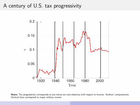
A century of U.S. tax progressivity

Notes: Tax progressivity corresponds to one minus tax-rate elasticity with respect to income. Authors’ computations.Vertical lines correspond to major military events.

State dependent multipliers: local projection

The linear case: Jorda (2005)

o For a vector xt+h =[Yt+h−Yt−1

Yt−1, Gt+h−Gt−1

Yt−1

]xt+h = αh + AhZt−1 + βhg

∗t + trend + εt+h

- Shock g∗t

- Control Zt : lags of GDP, total spending and g∗t

o Cumulative multiplier at horizon h

mh =

h∑j=0

βYj

/

h∑j=0

βGj


The linear case: Jorda (2005)



Yt−1

]xt+h = αh + AhZt−1 + βhg

∗t + trend + εt+h

- Shock g∗t

- Control Zt : lags of GDP, total spending and g∗t

o Cumulative multiplier at horizon h

mh =

h∑j=0

βYj

/

h∑j=0

βGj


The state-dependent case: Ramey and Zubairy (2016)



Yt−1

]xt+h = I (st = P)

{αh,P + Ah,PZt−1 + βh,Pg

∗t

}+ I (st = R)

{αh,R + Ah,RZt−1 + βh,Rg

∗t

}+ trend + εt+h

o Progressive state (st = P) if γ is higher on average for the next 3 years.

More

+ Cumulative multiplier mh,P ,mh,R

o An Instrumental Variable estimation:

More More

+ Ramey and Blanchard Perotti shocks





Yt−1

]xt+h = I (st = P)


∗t

}+ I (st = R)


∗t

}+ trend + εt+h


More+ Cumulative multiplier mh,P ,mh,R


More More+ Ramey and Blanchard Perotti shocks





Yt−1

]xt+h = I (st = P)


∗t

}+ I (st = R)


∗t

}+ trend + εt+h


More+ Cumulative multiplier mh,P ,mh,R


More More+ Ramey and Blanchard Perotti shocks

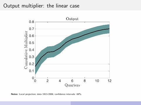
Output multiplier: the linear case

Notes: Local projection; data 1913-2006; confidence intervals: 68%.

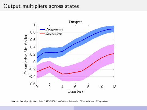
Output multipliers across states

Notes: Local projection; data 1913-2006; confidence intervals: 68%; window: 12 quarters.

Model

A Bewley economy with indivisible labor

Description of the steady-state:

+ A continuum of households:

- Bond economy with borrowing constraint.

- Indivisible labor choice.

- Idiosyncratic labor productivity shock.

More

+ A representative firm

+ Government:

- A constant level of government expenditures G .

- Financed by constant taxes and debt.

Households

The value function of an agent with productivity x and assets a is:

V (a, x) = maxc,a′,h∈{0,h̄}

{log c − D

h1+Φ

1 + Φ+ βEx′ [V (a′, x ′) |x ]

}subject to

c + a′ ≤ wxh + (1 + r)a− τk ra− τ (wxh) , a′ ≥ a

Productivity follows an AR(1) process: log(x it+1) = ρx log(x it ) + σxεit+1.

Tax progressivity will be captured by the shape of τ(·).

Firm and government

Government:

I Constant government expenditures G

I Government’s budget:

G + (1 + r)B = B +

∫{τk ra + τ (wxh)} dµ(a, x)

Firms:

+ Cobb-Douglas production function: Y = LαK 1−α

+ Firm’s static problem:

Π = maxK ,L

{LαK 1−α − wL− (r + δ)K

}Equilibrium definition Calibration Distribution of Wealth and Employment

Firm and government

Government:

I Constant government expenditures G

I Government’s budget:

G + (1 + r)B = B +

∫{τk ra + τ (wxh)} dµ(a, x)

Firms:

+ Cobb-Douglas production function: Y = LαK 1−α

+ Firm’s static problem:

Π = maxK ,L

{LαK 1−α − wL− (r + δ)K

}Equilibrium definition Calibration Distribution of Wealth and Employment

Government spending shocks

Experiment:

+ At t = 0, an unexpected shock:

- G increases by 1% and returns to steady state.

+ Financed with:

- Constant B and τ k

- A path for progressivity {γt}:

γt − γ = η(Gt − G )

- Adjust {λt} to satisfy its budget constraint:

Gt+rtB = τk rtKt+

∫ (1− λt(wtxht(a, x))−γt

)wtxht(a, x)dµt(a, x)

Government spending shocks

Experiment:

+ At t = 0, an unexpected shock:

- G increases by 1% and returns to steady state.

+ Financed with:

- Constant B and τ k

- A path for progressivity {γt}:

γt − γ = η(Gt − G )

- Adjust {λt} to satisfy its budget constraint:

Gt+rtB = τk rtKt+

∫ (1− λt(wtxht(a, x))−γt

)wtxht(a, x)dµt(a, x)

Effects of spending depend on tax progressivity

0 10 20 30 40

%

0

0.2

0.4

0.6

0.8

1

Government Spending

0 10 20 30 40

0.085

0.09

0.095

0.1

0.105

0.11

0.115

Progressivity Measure γ

0 10 20 30 40

0.14

0.145

0.15

0.155

0.16

Tax Level 1− λ


0 10 20 30 40

%

0

0.2

0.4

0.6

0.8

1

Government Spending

0 10 20 30 40

0.085

0.09

0.095

0.1

0.105

0.11

0.115


0 10 20 30 40

0.14

0.145

0.15

0.155

0.16

Tax Level 1− λ

0 5 10 15 20 25 30 35 40

%

-0.2

-0.15

-0.1

-0.05

0

Output

0 5 10 15 20 25 30 35 40

-0.06

-0.05

-0.04

-0.03

-0.02

-0.01

0

Consumption


0 10 20 30 40

%

0

0.2

0.4

0.6

0.8

1

Government Spending

0 10 20 30 40

0.085

0.09

0.095

0.1

0.105

0.11

0.115


0 10 20 30 40

0.14

0.145

0.15

0.155

0.16

Tax Level 1− λ

= Progressivity

⇑ Progressivity


0 10 20 30 40

%

0

0.2

0.4

0.6

0.8

1

Government Spending

0 10 20 30 40

0.085

0.09

0.095

0.1

0.105

0.11

0.115


0 10 20 30 40

0.14

0.145

0.15

0.155

0.16

Tax Level 1− λ

= Progressivity

⇑ Progressivity

0 5 10 15 20 25 30 35 40

%

-0.2

-0.1

0

0.1

0.2

Output

0 5 10 15 20 25 30 35 40

-0.1

-0.05

0

0.05

0.1

Consumption


0 10 20 30 40

%

0

0.2

0.4

0.6

0.8

1

Government Spending

0 10 20 30 40

0.085

0.09

0.095

0.1

0.105

0.11

0.115


0 10 20 30 40

0.14

0.145

0.15

0.155

0.16

Tax Level 1− λ

= Progressivity

⇑ Progressivity

⇓ Progressivity


0 10 20 30 40

%

0

0.2

0.4

0.6

0.8

1

Government Spending

0 10 20 30 40

0.085

0.09

0.095

0.1

0.105

0.11

0.115


0 10 20 30 40

0.14

0.145

0.15

0.155

0.16

Tax Level 1− λ

= Progressivity

⇑ Progressivity

⇓ Progressivity

0 5 10 15 20 25 30 35 40

%

-0.6

-0.4

-0.2

0

0.2

Output

0 5 10 15 20 25 30 35 40

-0.2

-0.15

-0.1

-0.05

0

0.05

0.1

Consumption

Heterogeneous changes in tax rates...

0 10 20 30 40

%

15

15.5

16

16.5

Labor Tax - Total Average

0 10 20 30 40

7

7.5

8

8.5

9

1st Quintile

0 10 20 30 40

14.5

15

15.5

16

2nd Quintile

Quarter0 10 20 30 40

%

17

17.5

18

18.5

3rd Quintile

Quarter0 10 20 30 40

19

19.5

20

20.5

4th Quintile

Quarter0 10 20 30 40

22

22.5

23

23.55th Quintile

... result in heterogenous responses More

0 10 20 30 40

0

0.2

0.4

0.6

0.8

1

%

Government Spending

0 10 20 30 40-0.2

0

0.2

0.4

0.6

0.81st Quintile

hours

consumption

0 10 20 30 40-0.2

0

0.2

0.4

0.6

0.82nd Quintile

0 10 20 30 40

Quarters

-0.2

0

0.2

0.4

0.6

0.8

%

3rd Quintile

0 10 20 30 40

Quarters

-0.2

0

0.2

0.4

0.6

0.84th Quintile

0 10 20 30 40

Quarters

-0.2

0

0.2

0.4

0.6

0.85th Quintile

Intratemporal and intertemporal tax allocation More

How important is debt financing?

Exercise:

+ Same path for {Gt} and {γt} as before.

+ A fraction financed with debt, implies a different path for {λt}.

+ Uhlig (2010): Bt+1 − Bss = (1− ϕ)(ωt − ωss),

WVWXXXXWWwhere ωt = Gt + rtBt − τ k rtAt .

I ϕ = 1: no additional debtI ϕ = 0.05: ≈ 95% of additional spending financed with debt

Intratemporal and intertemporal tax allocation

Micro evidence


State-dependent local projection method:



Yt−1

]xt+h = I (st = P)


∗t

}+ I (st = R)


∗t

}+ trend + εt+h

o Cross-sectional data: TAXSIM

- Pre-tax income of all taxpayers

- 1962-2008; Interpolated (Chow-Lin)

Heterogenous responses across households

Notes: Local projection; data 1962-2006; confidence intervals: 68%; window: 12 quarters.

Solving the puzzle?(preliminary)

Quantitative investigation of the mechanism

+ Data: Typical path for {Gt} and {γt} after a spending shock

- News shock (Ramey), 1960-2006

Quantitative investigation: enough to change signs

Conclusion

+ Tax progressivity is crucial to spending multipliers.

I Heterogeneous responses across households

I Generate changes in signs of multipliers

+ Policy implications: use taxes, not spending More

Conclusion

+ Tax progressivity is crucial to spending multipliers.

I Heterogeneous responses across households

I Generate changes in signs of multipliers

+ Policy implications: use taxes, not spending More

Appendix

Evidence: Output and Consumption Multipliers Return

Output ConsumptionBlanchard and Perotti 0.90 0.5

(0.30) (0.21)

Gali, Lopez-Salido and Valles 0.41 0.1(0.16) (0.10)

Barro and Redlick 0.45 0.005(0.07) (0.09)

Mountford and Uhlig 0.65 0.001(0.39) (0.0003)

Ramey 0.30 0.02(0.10) (0.001)

Note: output/consumption multiplier refers to the increase in output/consumption after a unit increase ingovernment spending.

Why a Puzzle? Return Return

I Assume U(C ,H) = C 1−σ

1−σ − H1+ϕ

1+ϕ and competitive labor markets.

I Then (in logs)

log(1− τt↑) +

mpht

↓

= σct

⇓⇓

+ ϕht

↑

+ Indivisible labor of agents heterogeneous in productivity

+ Distribution of taxes

log(1− ↑↓τ it ) + mpht↓ ≶ σc it + ϕhit↑

+ Progressivity shapes the effects of government spending.



1−σ − H1+ϕ


I Then (in logs)

log(1− τt↑) +

mpht ↓ = σct⇓

⇓

+ ϕht ↑







1−σ − H1+ϕ


I Then (in logs)

log(1− τt↑) + mpht ↓ = σct⇓⇓+ ϕht ↑







1−σ − H1+ϕ


I Then (in logs)




log(1− ↑↓τ it ) +

mpht↓ ≶ σc it + ϕhit↑




1−σ − H1+ϕ


I Then (in logs)








1−σ − H1+ϕ


I Then (in logs)






A Progressive Taxation Scheme Return

A non-linear labor income tax τ(y) ≡ 1− λy−γ

0 5 10 15 20 25 30−0.1

0

0.1

0.2

0.3

0.4

0.5

0.6

Income

Tax

rat

e

1−λ = 0.12, γ = 0.1



0 5 10 15 20 25 30−0.1

0

0.1

0.2

0.3

0.4

0.5

0.6

Income

Tax

rat

e

1−λ = 0.12, γ = 0.11−λ = 0.12, γ = 0.2



0 5 10 15 20 25 30−0.1

0

0.1

0.2

0.3

0.4

0.5

0.6

Income

Tax

rat

e

1−λ = 0.12, γ = 0.11−λ = 0.3, γ = 0.1

Heathcote Storesletten Violante (2016) Return

Measurement of τUS

• PSID 2000-06, age of head of hh 25-60, N = 12, 943

• Pre gov. income: income minus deductions (medical expenses,state taxes, mortgage interest and charitable contributions)

• Post-gov income: ... minus taxes (TAXSIM) plus transfers

8.5 9 9.5 10 10.5 11 11.5 12 12.5 13

8.5

9

9.5

10

10.5

11

11.5

12

12.5

13

Log of Pre−government Income

Log

of D

ispo

sabl

e In

com

e

τUS = 0.161

Pre-government Income ×1050 1 2 3 4 5

Tax

Rate

s

-0.3

-0.2

-0.1

0

0.1

0.2

0.3

0.4

0.5

Marginal Tax RateAverage Tax Rate

Heathcote-Storesletten-Violante, ”Optimal Tax Progressivity”

Tax progressivity estimate Return

I Tax function given by τ(y) = 1− λy−γ

I Total tax T (y) = τ(y)y and marginal tax T ′(y).

I Simple algebra

γ =T ′(y)− τ(y)

1− τ(y)

I AMTR =∫T ′(y) from Barro & Redlick (2011) and Mertens (2015)

I ATR =∫τ(y) our computations using IRS data and Piketty & Saez

(2003)’s income measure.




I Simple algebra

γ =T ′(y)− τ(y)

1− τ(y)







I Simple algebra

γ =T ′(y)− τ(y)

1− τ(y)




Tax progressivity estimate - Robustness Return

Notes: TAXSIM measure is the elasticity of the tax function for fixed income distribution.

State dependent multipliers: local projection Return

o Progressive state (st = P) if

1

Na

Na−1∑j=0

γt+j >1

Nb

Nb∑j=1

γt−j , Na = 12, Nb = 8.


h∑j=0

∆yt+j = I (st = P)

αP,h + AP,HZt−1 + mP,h

h∑j=0

∆gt+j

+ I (st = R)

αR,h + AR,HZt−1 + mR,h

h∑j=0

∆gt+j

+ trend + εt+h

where ∆xt+j = (xt+h − xt−1)/Yt−1.


o Progressive state (st = P) if

1

Na

Na−1∑j=0

γt+j >1

Nb

Nb∑j=1

γt−j , Na = 12, Nb = 8.


h∑j=0

∆yt+j = I (st = P)

αP,h + AP,HZt−1 + mP,h

h∑j=0

∆gt+j

+ I (st = R)

αR,h + AR,HZt−1 + mR,h

h∑j=0

∆gt+j

+ trend + εt+h

where ∆xt+j = (xt+h − xt−1)/Yt−1.


Notes: Spending shocks (Ramey) interacted with state St = P, R.

Equilibrium: definition Return

A stationary recursive competitive equilibrium is given by

+ Households’ value functions {V } and policies {c, a′, h}. Firm’s policies {L,K}.

+ Government’s policies {G , τ,B}+ A measure µ

such that given prices {r ,w}I Households and the firm solve their respective problems.

I Government runs a balanced budget.

I Markets clear

o Capital market clears: K + B =∫B a′(a, x)dµ(a, x)

o Labor market clears: L =∫B xh(a, x)dµ(a, x)

o Goods market clears: Y =∫B c(a, x)dµ(a, x) + δK + G

I Measure µ is stationary

µ(a′, x ′) =

∫I{a′(a, x) = a′}πx (x ′|x)dµ(a, x)

Calibration Return

+ Taxes:

- Flat capital tax rate: τk = 35% (Chen, et al., 2009)

- Progressive labor tax: γ = 0.1 (Heathcote, et al. 2013)

+ Structural parameters:

α = 0.64 Φ = 2.5 δ = 0.025 h̄ = 1/3 a = −2(ρx , σx) = (0.989, 0.287)

+ We calibrate (β,G ,D,B) s.t., in steady-state:

r = 0.01, G/Y = 0.15, E = 0.6, D/Y = 2.4

Distribution of Wealth and Employment

Calibration Return

+ Taxes:

- Flat capital tax rate: τk = 35% (Chen, et al., 2009)

- Progressive labor tax: γ = 0.1 (Heathcote, et al. 2013)

+ Structural parameters:

α = 0.64 Φ = 2.5 δ = 0.025 h̄ = 1/3 a = −2(ρx , σx) = (0.989, 0.287)

+ We calibrate (β,G ,D,B) s.t., in steady-state:

r = 0.01, G/Y = 0.15, E = 0.6, D/Y = 2.4

Distribution of Wealth and Employment

Househoulds Distribution Return

Quintiles 1st 2nd 3rd 4th 5th

Share of Wealth- PSID Data −0.00 0.02 0.07 0.15 0.77- Model −0.01 0.04 0.12 0.25 0.61

Participation Rate- PSID Data 0.65 0.75 0.69 0.60 0.57- Model 0.83 0.63 0.57 0.52 0.45

The PSID statistics reflect the family wealth and earnings in the 1984 survey. Thestatistics of ”primary households’ are those for household heads whose education was12 years and whose age is between 35 and 55.

Hours and consumption: households distribution Return

Notes: Income is defined as y(a, x) = wxh(a, x) + (1 + r)a − τ(wxh, ar).

Hours and consumption: households distribution Return

Notes: Income is defined as y(a, x) = wxh(a, x) + (1 + r)a − τ(wxh, ar).

Timing of the change in progressivity Return

How important is the timing of the increase in tax progressivity?

Exercise:

+ Same path for {Gt}.+ {γt} does not react on impact, increases slowly until quarter 5.

+ Debt: Φ = .05

Timing of the change in progressivity Return

0 10 20 30 400

0.2

0.4

0.6

0.8

1

%

Government Spending

0 10 20 30 400.1

0.102

0.104

0.106

0.108

0.11Progressivity Measure γ

0 10 20 30 400.142

0.143

0.144

0.145

0.146

0.147

0.148

0.149Tax Level 1− λ

0 10 20 30 40-0.05

0

0.05

0.1

0.15

0.2

0.25

%

Output

0 10 20 30 40-0.02

-0.01

0

0.01

0.02

0.03

0.04

0.05

0.06

Consumption

0 10 20 30 40-0.05

0

0.05

0.1

0.15

0.2

0.25Government Debt

Use taxes, not spending Return

What is the effect of a temporary increase in progressivity?

Exercise:

+ Same path for {γt} as before.

+ No increase in spending.

+ No debt.

Use taxes, not spending Return

0 10 20 30 40

%

0

0.2

0.4

0.6

0.8

1Government Spending

Increased Spending

Fixed Spending

0 10 20 30 400.095

0.1

0.105

0.11

0.115Progressivity Measure γ

0 10 20 30 400.14

0.142

0.144

0.146

0.148

0.15Tax Level 1− λ

0 5 10 15 20 25 30 35 40

%

-0.05

0

0.05

0.1

0.15

0.2

0.25Output

0 5 10 15 20 25 30 35 40-0.05

0

0.05

0.1

0.15Consumption

The heterogeneous effects of government spending, by Axelle Ferriere (European University Institute)

Economy & Finance