PEBS Long-term Performance of Engineered Barrier Systems PEBS The HE-E Experiment: Lay-out, Interpretation and THM Modelling Combining D2.2-11: Final Report on the HE-E Experiment and D3.2-2: Modelling and Interpretation of the HE-E Experiment of the PEBS Project Author(s): Gaus I., Garitte B., Senger R., Gens A., Vasconcelos R., Garcia-Sineriz J.-L., Trick T., Wieczorek K., Czaikowski O., Schuster K., Mayor J.C., Velasco M., Kuhlmann U., Villar M.V. Date of issue of this report: May 2014 Start date of project: 01/03/10 Duration : 48 Months Project co-funded by the European Commission under the Seventh Euratom Framework Programme for Nuclear Research &Training Activities (2007-2011)

Welcome message from author
This document is posted to help you gain knowledge. Please leave a comment to let me know what you think about it! Share it to your friends and learn new things together.
Transcript
PEBS
Long-term Performance of Engineered Barrier Systems PEBS
The HE-E Experiment: Lay-out, Interpretation and THM Modelling
Combining
D2.2-11: Final Report on the HE-E Experiment and
D3.2-2: Modelling and Interpretation of the HE-E Experiment of the PEBS Project
Author(s):
Gaus I., Garitte B., Senger R., Gens A., Vasconcelos R., Garcia-Sineriz J.-L.,
Trick T., Wieczorek K., Czaikowski O., Schuster K., Mayor J.C., Velasco M., Kuhlmann U., Villar M.V.
Date of issue of this report: May 2014
Start date of project: 01/03/10 Duration : 48 Months
Project co-funded by the European Commission under the Seventh Euratom Framework Programme for Nuclear Research &Training Activities (2007-2011)

ArbeitsberichtNAB 14-53
Nationale Genossenschaftfür die Lagerung
radioaktiver Abfälle
Hardstrasse 73CH-5430 Wettingen
Telefon 056-437 11 11
www.nagra.ch
May 2014
I. Gaus, B. Garitte, R. Senger, A. Gens, R. Vasconcelos, J.-L. Garcia-Sineriz, T. Trick,
K. Wieczorek, O. Czaikowski, K. Schuster, J. C. Mayor, M. Velasco, U. Kuhlmann,
M. V. Villar.
The HE-E Experiment: Lay-out, Interpretation and THM Modelling

ArbeitsberichtNAB 14-53
Nationale Genossenschaftfür die Lagerung
radioaktiver Abfälle
Hardstrasse 73CH-5430 Wettingen
Telefon 056-437 11 11
www.nagra.ch
KEYWORDS
FMT, Mont Terri, HE-E experiment, heating experiment, THM interpretative computations
May 2014
I. Gaus, B. Garitte, R. Senger, A. Gens, R. Vasconcelos, J.-L. Garcia-Sineriz, T. Trick,
K. Wieczorek, O. Czaikowski, K. Schuster, J. C. Mayor, M. Velasco, U. Kuhlmann,
M. V. Villar.
The HE-E Experiment: Lay-out, Interpretation and THM Modelling

Nagra Working Reports concern work in progress that may have had limited review. They are
intended to provide rapid dissemination of information. The viewpoints presented and
conclusions reached are those of the author(s) and do not necessarily represent those of
Nagra.
"Copyright © 2014 by Nagra, Wettingen (Switzerland) / All rights reserved.
All parts of this work are protected by copyright. Any utilisation outwith the remit of the
copyright law is unlawful and liable to prosecution. This applies in particular to translations,
storage and processing in electronic systems and programs, microfilms, reproductions, etc."
I Nagra NAB 14-53
Table of Contents
Table of Contents ......................................................................................................................... I
List of Tables ...................................................................................................................... III
List of Figures ...................................................................................................................... IV
1 Introduction and Objectives ........................................................................ 1 1.1 Context of the Experiment ............................................................................. 1 1.2 Objectives of the Experiment ......................................................................... 1 1.3 Reporting Related to the HE-E Experiment ................................................... 3
2 HE-E: As-built .............................................................................................. 5 2.1 Introduction .................................................................................................... 5 2.2 Initial Conditions in the Tunnel Prior to the Installation of the HE-E
Experiment ..................................................................................................... 6 2.3 Materials ......................................................................................................... 7 2.3.1 Bentonite Blocks ............................................................................................ 7 2.3.2 Sand/Bentonite Mixture ................................................................................. 8 2.3.3 Granular Bentonite Material ........................................................................... 9 2.3.4 Plugs and Plug Materials ................................................................................ 9 2.4 Instrumentation Concept .............................................................................. 10 2.4.1 Direct Monitoring ......................................................................................... 10 2.4.2 Indirect Monitoring ...................................................................................... 11 2.4.3 Temperature and Humidity Sensors in the EBS and the EBS/Host
Rock Interface .............................................................................................. 12 2.4.3.1 Types and Locations ..................................................................................... 12
2.4.3.2 Nomenclature of the Sensors in the Engineered Barrier .............................. 13
2.4.4 Monitoring in the Opalinus Clay Host Rock Close to the Micro Tunnel ........................................................................................................... 13
2.4.4.1 Location of the Sensors in the Cross Sections through the Micro Tunnel ........................................................................................................... 15
2.4.5 Sensors Installed at a Larger Distance from the Micro Tunnel .................... 20 2.4.5.1 Boreholes Installed as Part of the VE Experiment ....................................... 20
2.4.5.2 Boreholes Installed as Part of the HE-E Experiment ................................... 21
2.4.6 Heater Control and Heater Surface Instrumentation .................................... 22
3 Observations: Overview of the Collected Data ........................................ 27 3.1 Temperature Measurements ......................................................................... 27 3.1.1 Heaters .......................................................................................................... 27 3.1.2 EBS ............................................................................................................... 28 3.1.3 Opalinus Clay ............................................................................................... 36 3.2 Relative Humidity Measurements ................................................................ 38
Nagra NAB 14-53 II
3.2.1 EBS ............................................................................................................... 38 3.2.2 Opalinus Clay ............................................................................................... 46 3.3 Pore Water Pressure Measurements ............................................................. 47 3.3.1 Close to the Micro Tunnel ............................................................................ 47 3.3.2 Distant from the Micro Tunnel ..................................................................... 49 3.4 Geophysical campaigns ................................................................................ 50 3.4.1 Objectives and Motivation ........................................................................... 50 3.4.2 Layout of Experiment and Data Overview ................................................... 51 3.4.3 Seismic Parameters and Data ....................................................................... 52 3.4.4 Results and Preliminary Interpretation ......................................................... 53
4 Material Parameters .................................................................................. 57 4.1 Bentonite Materials ...................................................................................... 57 4.2 Opalinus Clay ............................................................................................... 61
5 Column Tests on HE-E Materials ............................................................. 64 5.1 Setup of the Column Tests ........................................................................... 64 5.2 Monitoring Results of the Column Tests...................................................... 65 5.2.1 Heating Phase ............................................................................................... 65 5.2.2 Hydration Phase ........................................................................................... 65 5.3 Modelling and Interpretation of the THM Cells by CIMNE ........................ 67 5.3.1 Modelling Features ....................................................................................... 67 5.3.2 Modelling Results......................................................................................... 74 5.3.2.1 Cell B ............................................................................................................ 75
5.3.2.2 Cell SB ......................................................................................................... 78
6 Modelling Results and Interpretation of the HE-E ................................. 83 6.1 TH Computations by Intera .......................................................................... 83 6.1.1 Code Description .......................................................................................... 83 6.1.2 Model Geometry and Boundary Conditions ................................................. 84 6.1.3 Initial Conditions .......................................................................................... 85 6.1.4 Validation Test ............................................................................................. 86 6.1.5 Model Input Parameter ................................................................................. 88 6.1.6 Heat Input ..................................................................................................... 88 6.1.7 Simulations: Reference Case R0 .................................................................. 88 6.1.8 Simulations: Case R1 ................................................................................... 93 6.1.9 Simulations: Case R2 ................................................................................... 95 6.1.10 Simulations: Case R3 ................................................................................... 96 6.1.11 Conclusions of the TOUGH2 Modelling of the HE-E Experiment .............. 97 6.2 THM Computations by GRS ........................................................................ 98 6.2.1 Model description and parameters................................................................ 98 6.2.2 Calculation results for the sand-bentonite section ...................................... 100 6.2.3 Bentonite Pellet Section ............................................................................. 105
III Nagra NAB 14-53
6.2.4 Conclusion .................................................................................................. 105 6.3 THM Computations by CIMNE ................................................................. 105 6.3.1 THM Formulation ...................................................................................... 105 6.3.2 Modelling Features ..................................................................................... 106 6.3.2.1 Conceptual Models ..................................................................................... 106
6.3.2.2 Model Parameters ....................................................................................... 109
6.3.3 Modelling Results....................................................................................... 110 6.3.3.1 Temperature Evolution ............................................................................... 110
6.3.3.2 Evolution of Hydraulic Variables (Degree of Saturation, Relative Humidity and Liquid Pressure) .................................................................. 121
6.3.4 Conclusions ................................................................................................ 129
7 Conclusions and Lessons Learnt ............................................................. 131 7.1 Conclusions Related to the Thermal Field (Observations and
Modelling) .................................................................................................. 132 7.2 Conclusions Related to the Hydraulic Field (Observations and
Modelling) .................................................................................................. 132 7.2.1 Relative Humidity in the Unsaturated Parts of the Experiment ................. 132 7.2.2 Saturated Zones under Suction ................................................................... 133 7.2.3 Pore Water Pressure in the Saturated Part .................................................. 133 7.3 General Conclusions from the Observations Covering June
2011 - December 2013 ............................................................................... 133 7.4 General Conclusions from the Modelling Conducted within the PEBS
Project ......................................................................................................... 135
8 References ................................................................................................. 137
Appendix A: Coordinates of all Sensors ....................................................................... A-1
Appendix B: Description of the Parameters used by Intera ....................................... B-1
Appendix C: Description of the Parameters used by GRS .......................................... C-1
Appendix D: Description of the Formulation used by CIMNE .................................. D-1
List of Tables
Tab. 1: Sensors installed in the cross-sections through the microtunnel .................. 14
Tab. 2: Properties for the different bentonite buffer materials ................................. 59
Tab. 3: Properties for the Opalinus clay ................................................................... 62
Tab. 4: Physical properties for water in pores .......................................................... 70
Nagra NAB 14-53 IV
Tab. 5: Physical properties for the bentonite columns and the insulation materials ....................................................................................................... 70
Tab. 6: Thermal parameters for the bentonite materials and the isolation materials ....................................................................................................... 71
Tab. 7: Hydraulic parameters for the bentonite materials and the insulation materials ....................................................................................................... 71
Tab. 8: Mechanical parameters for the bentonite columns (BBM parameters) ........ 72
Tab. 9: Elastic parameters for the insulation materials ............................................. 74
Tab. 10: Summary of the models used by the different teams.................................... 83
List of Figures
Fig. 1: Modelling framework developed for the HE-E experiment within the PEBS project .................................................................................................. 2
Fig. 2: Location of the HE-E experiment in the microtunnel (μtunnel) in the Mont Terri URL (Switzerland) ....................................................................... 5
Fig. 3: Schematic layout of the HE-E experiment showing the section in the back of the tunnel filled with bentonite pellets and the section in the front of the tunnel filled with sand/bentonite ................................................. 6
Fig. 4: 3D image of the test section before the emplacement of the HE-E experiment ...................................................................................................... 6
Fig. 5: Dimensions of bentonite blocks used for the HE-E experiment .................... 7
Fig. 6: Instrumentation concept for the HE-E experiment consisting of four monitoring zones: 1) heater surface 2) engineered barrier system, 3) Opalinus Clay <2 m from the HE-E microtunnel, 4) Opalinus Clay >2 m from the HE-E microtunnel ...................................................................... 11
Fig. 7: Technical drawing of the HS-Sensor arms and location of the sensors on the arms, in the bentonite blocks and at the interface between the engineered barrier and the OPA host rock ................................................... 12
Fig. 8: Clarification of the sensor nomenclature in the engineered barrier .............. 13
Fig. 9: Location of the instrumentation cross sections in the Opalinus clay and their position with respect to the HE-E experiment ............................... 14
Fig. 10: Sensor types and locations in Section SA1 (distances indicated are with respect to the microtunnel wall) ........................................................... 15
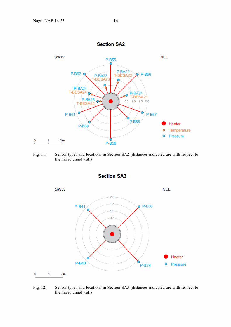
Fig. 11: Sensor types and locations in Section SA2 (distances indicated are with respect to the microtunnel wall) ........................................................... 16
Fig. 12: Sensor types and locations in Section SA3 (distances indicated are with respect to the microtunnel wall) ........................................................... 16
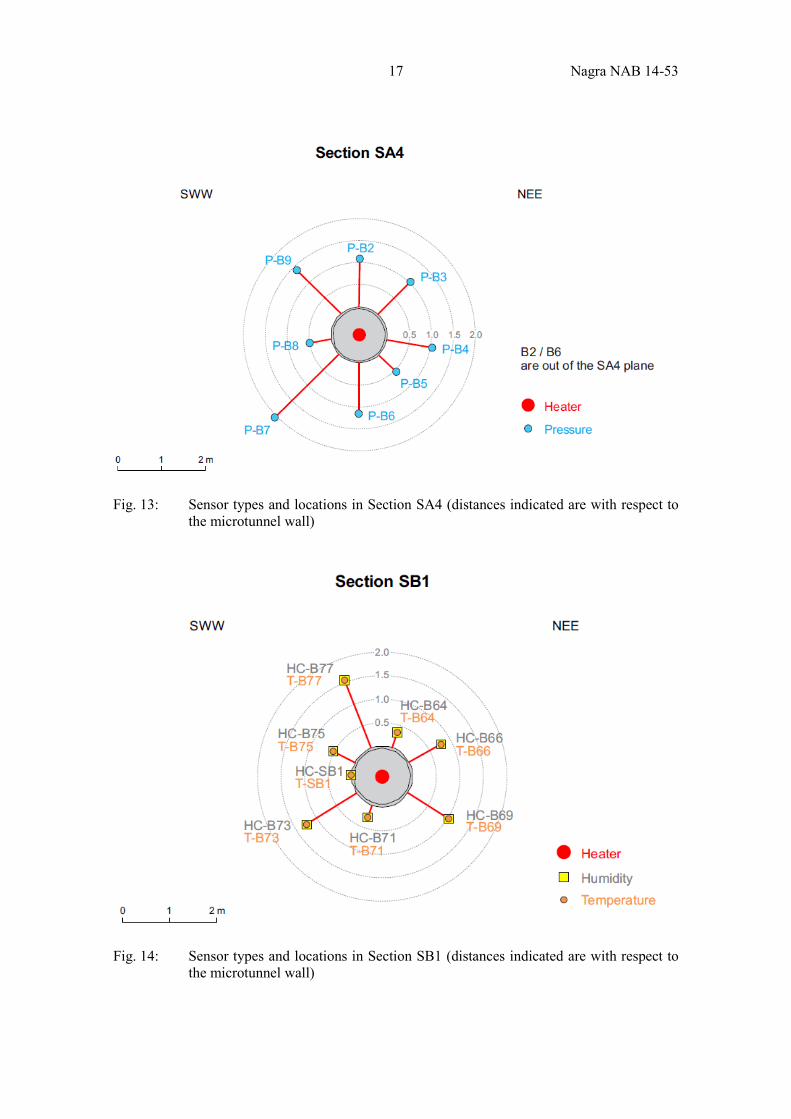
Fig. 13: Sensor types and locations in Section SA4 (distances indicated are with respect to the microtunnel wall) ........................................................... 17
V Nagra NAB 14-53
Fig. 14: Sensor types and locations in Section SB1 (distances indicated are with respect to the microtunnel wall) ........................................................... 17
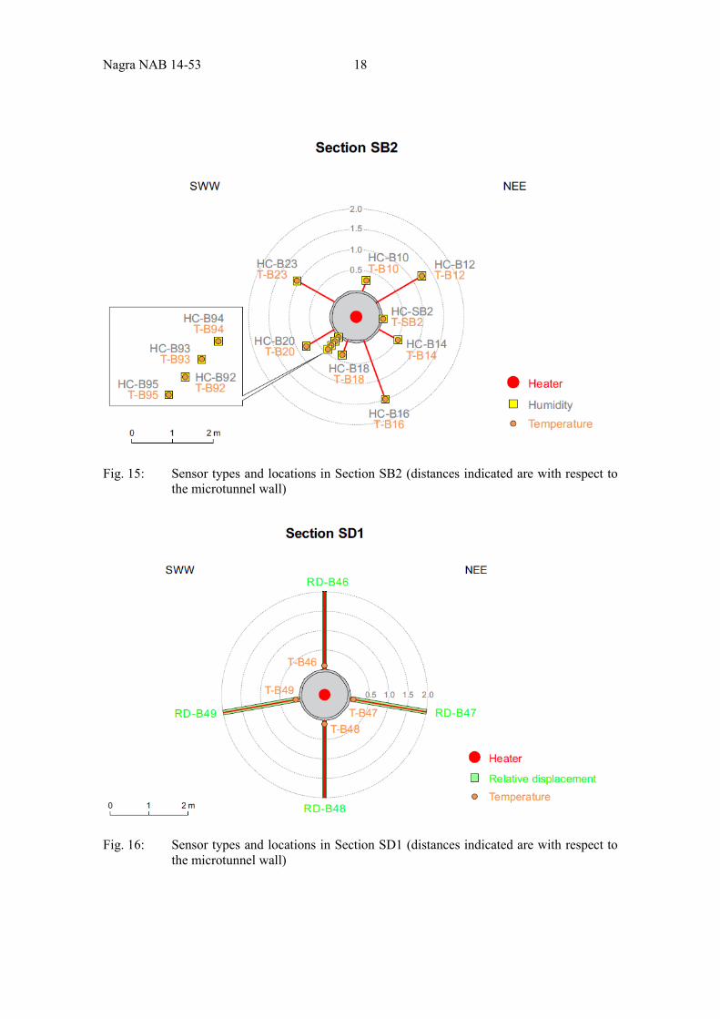
Fig. 15: Sensor types and locations in Section SB2 (distances indicated are with respect to the microtunnel wall) ........................................................... 18
Fig. 16: Sensor types and locations in Section SD1 (distances indicated are with respect to the microtunnel wall) ........................................................... 18
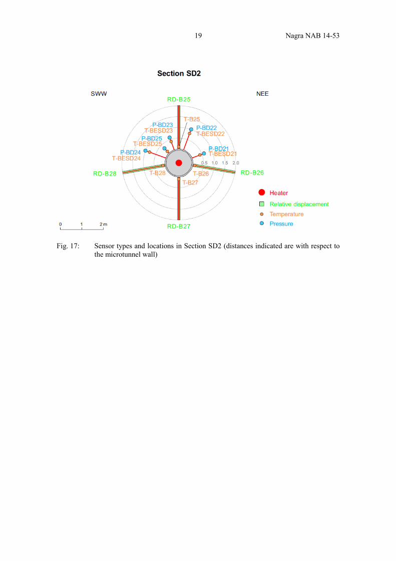
Fig. 17: Sensor types and locations in Section SD2 (distances indicated are with respect to the microtunnel wall) ........................................................... 19
Fig. 18: Location of borehole BVE-1 and distances of the pore pressure sensors to the microtunnel ............................................................................ 20
Fig. 19: Location of borehole BVE-91 and distances of the pore pressure sensors to the microtunnel ............................................................................ 20
Fig. 20: Plan view showing the locations of the boreholes BVE-1, BVE-91, BHE-E1, and BHE-E2 .................................................................................. 21
Fig. 21: Location of boreholes BHE-E1 and BHE-E2 and distances of the test intervals to the microtunnel .......................................................................... 21
Fig. 22: Layout of electrical heaters for HE-E experiment ........................................ 22
Fig. 23: Heating power evolution in Heater SB (left view) and Heater B (right view) ............................................................................................................. 23
Fig. 24: Evolution of maximal and minimal temperatures at the heater S/B surface (left view). Zoom on the 150 first days (right view) ........................ 23
Fig. 25: Evolution of maximal and minimal temperatures at the heater B surface (left view). Zoom on the 150 first days (right view) ........................ 23
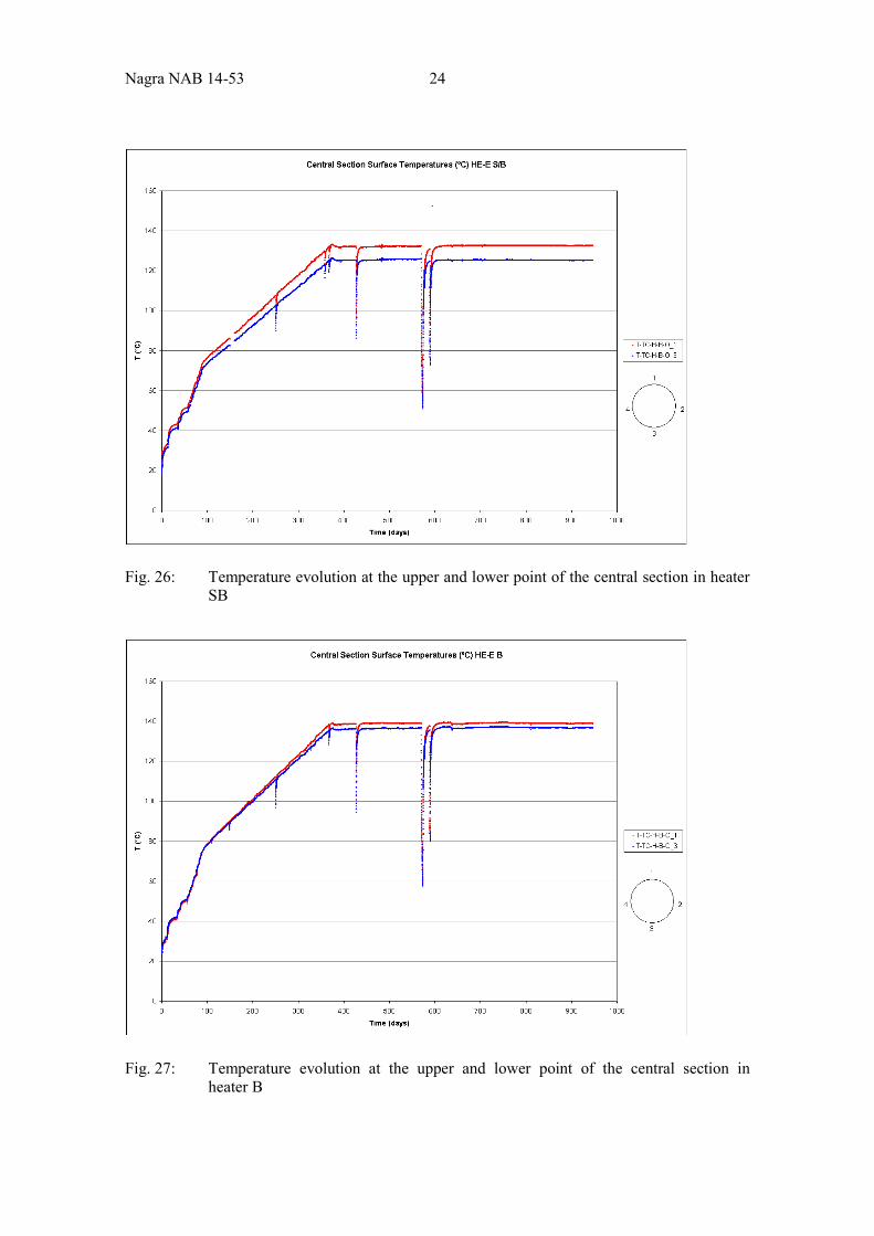
Fig. 26: Temperature evolution at the upper and lower point of the central section in heater SB ...................................................................................... 24
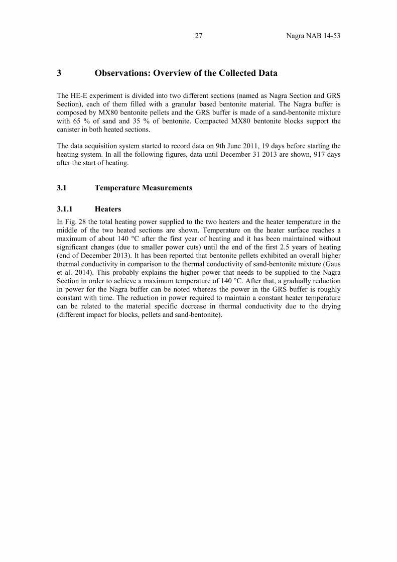
Fig. 27: Temperature evolution at the upper and lower point of the central section in heater B ........................................................................................ 24
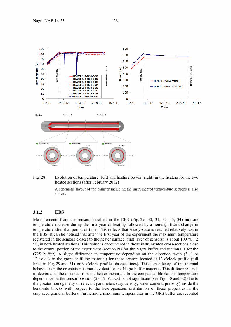
Fig. 28: Evolution of temperature (left) and heating power (right) in the heaters for the two heated sections (after February 2012) ........................................ 28
Fig. 29: Evolution of temperature in the Nagra Section for the three sensor carriers inside the granular backfilling (bentonite pellets) ........................... 30
Fig. 30: Evolution of temperature in the Nagra Section for the three sensor carriers inside the compacted blocks ............................................................ 31
Fig. 31: Evolution of temperature in the GRS Section for the three sensor carriers inside the granular backfilling (sand-bentonite mixture) ................ 32
Fig. 32: Evolution of temperature in the GRS Section for the three sensor carriers inside the compacted blocks ............................................................ 33
Fig. 33: Evolution of temperature in the middle of the Nagra Section (full lines) and in the middle of the GRS Section (dashed lines) at three main directions: 12 o'clock (up), 3 o'clock (centre) and 9 o'clock (down) .......................................................................................................... 34
Nagra NAB 14-53 VI
Fig. 34: Evolution of temperature in the middle of the Nagra Section (full lines) and in the middle of the GRS Section (dotted lines) in the "first" layer (up) and the "second" layer of sensors (down) inside the compacted blocks ......................................................................................... 35
Fig. 35: Evolution of temperature in the Opalinus Clay in the vicinity of the GRS Section for the instrumented cross sections: SB1 (up), SA2 (centre) and SD1 (down) .............................................................................. 37
Fig. 36: Evolution of temperature in the Opalinus Clay in the vicinity of the Nagra Section for the instrumented cross sections: SD2 (up) and SB2 (down) .......................................................................................................... 38
Fig. 37: Evolution of relative humidity in the Nagra Section for the three sensor carriers inside the granular backfilling (bentonite pellets) ................ 40
Fig. 38: Evolution of relative humidity in the Nagra Section for the three instrumented sections inside the compacted bentonite blocks ..................... 41
Fig. 39: Evolution of relative humidity in the GRS Section for the three sensor carriers inside the granular backfilling (sand-bentonite mixture) ................ 42
Fig. 40: Evolution of relative humidity in the GRS Section for the three instrumented sections inside the compacted bentonite blocks ..................... 43
Fig. 41: Evolution of relative humidity in the middle of the Nagra Section (full lines) and in the middle of the GRS Section (dashed lines) at three main directions: 12 o'clock (up), 3 o'clock (centre) and 9 o'clock (down) .......................................................................................................... 44
Fig. 42: Evolution of relative humidity in the middle of the Nagra Section (full lines) and in the middle of the GRS Section (dotted lines) in the upper instrumented layer (up) and the lower layer of sensors (down) inside the blocks ...................................................................................................... 45
Fig. 43: Evolution of relative humidity in the Opalinus Clay for the instrumented cross sections: SB1(in the vicinity of the GRS Section; UP) and SB2 (in the vicinity of the Nagra Section; DOWN) ....................... 46
Fig. 44: Evolution of pore water pressure in the Opalinus Clay in the vicinity of the GRS Section for the instrumented cross sections: SA1 (up) and SA2 (down) .................................................................................................. 47
Fig. 45: Evolution of pore water pressure in the Opalinus Clay in the middle of the HE-E Experiment Section (SA3) ............................................................ 48
Fig. 46: Evolution of pore water pressure in the Opalinus Clay in the vicinity of the Nagra Section for the instrumented cross sections: SD2 (up) and SA4 (down) .................................................................................................. 48
Fig. 47: Evolution of pore water pressure in the Opalinus Clay in the far field for the sensors in borehole BVE-1 (up) and BVE-91 (down) ...................... 49
Fig. 48: Evolution of pore water pressure in the Opalinus Clay in the far field for the sensors in borehole BHE-E1 (left) and BHE-E2 (right) ................... 50
Fig. 49: Layout of seismic array using 3 boreholes with 15 piezoelectric transducers, 5 emitters (A-E) and 10 receivers (R01-R10) .......................... 51
VII Nagra NAB 14-53
Fig. 50: Seismic section (E01 → R10) shows the strong variability of first arrival phases ................................................................................................ 52
Fig. 51: Simplified illustration of vp variation depending on anomalies encountered along the travel path. Left: Seismic wave field represented by a seismic ray path propagating through different anomalies in OPA. Right: Resultant normalised vp graphs for two extreme cases, all voids filled either with gas or with fluids ........................ 53
Fig. 52: Derived normalised P-wave velocities for three orientations of travel paths in the OPA and travelpaths through the sand-bentomite .................... 54
Fig. 53: Thermal Conductivity as a function of saturation ........................................ 58
Fig. 54: Water retention data ..................................................................................... 59
Fig. 55: Capillary pressure measurements (water retention curves) by stepwise desaturation and re-saturation in a desiccator (UPC: Romero and Gomez 2013; EPFL: Ferrari and Laloui 2012) ............................................. 63
Fig. 56: Experimental setup for the infiltration tests ................................................. 64
Fig. 57: Evolution of RH in cell S/B (left) and B (right) during the heating phase (sensor 1 placed at 40 cm from the bottom, sensor 2 at 22 cm and sensor 3 at 10 cm) .................................................................................. 65
Fig. 58: Evolution of RH and water intake in cell S/B (left) and B (right) during the hydration phase ........................................................................... 66
Fig. 59: Modelled domain of the column tests before (left) and after (right) the reinforcement in the external isolating material ........................................... 67
Fig. 60: Thermal load at the heating element and stages of the heating-hydration test for the Cell B (left) and for the Cell SB (right). Time "zero" corresponds to the start of heating ..................................................... 69
Fig. 61: (a) Thermal conductivity dependence on the degree of saturation for the bentonite materials. Dashed lines delimitate the range of values used in the numerical calculations and (b) water retention curves for the pellets (blue line) and the sand-bentonite mixture (red line). Symbols represent experimental results ....................................................... 69
Fig. 62: Schematic layout of the bentonite cell showing the position of the three temperature/relative humidity sensors ................................................. 74
Fig. 63: Temperature evolution (left) and relative humidity evolution (right) at the sensor positions during the heating and hydration of the Cell B ............ 76
Fig. 64: Temperature (left) and relative humidity (right) versus distance to the heater in the centre of the Cell B at different times ...................................... 76
Fig. 65: Temperature (left) and relative humidity (right) radial profiles at several distances to the heater (from the top to the bottom: 5.0 cm, 10 cm, 22 cm and 40 cm) inside the Cell B .................................................. 77
Fig. 66: Model predictions for the evolution of the degree of saturation (left) and some radial profiles of saturation (right) in the centre of the Cell B ..... 78
Fig. 67: Temperature evolution (left) and relative humidity evolution (right) at the sensor positions during the heating and hydration of the Cell SB .......... 79
Nagra NAB 14-53 VIII
Fig. 68: Temperature (left) and relative humidity (right) versus distance to the heater in the centre of the Cell SB at different times.................................... 80
Fig. 69: Temperature (left) and relative humidity (right) radial profiles at several distances to the heater (from the top to the bottom: 5.0 cm, 10 cm, 22 cm and 40 cm) inside the Cell SB ............................................... 81
Fig. 70: Model predictions for the evolution of the degree of saturation (left) and some radial profiles of saturation (right) in the centre of the Cell SB ................................................................................................................. 82
Fig. 71: Relative humidity evolution at the sensors during the heating-hydration experiment in the Cell SB for the three different mixture intrinsic permeabilities: 10-19 m2(the Base Case, results in dotted lines), 10-17 m2 (dashed lines) and 10-16m2 (full lines) .................................. 82
Fig. 72: 3D model geometry of the HE-E experiment with the detailed representation of the different materials in the micro-tunnel ....................... 84
Fig. 73: Ventilation period for 10 years: (a) simulated pressures with time (dashed lines) taking into account TM effects (solid line), (b) measured pressures in BE-91 at the corresponding locations, (c) simulated pressure distribution after 10 yrs .................................................. 86
Fig. 74: Comparison of computed temperature profiles of the analytical solution for a 1D radially-symmetric mesh (top) and for the 2D nested radial-rectangular mesh (showing the profile line for the computed temperature profile) ...................................................................................... 87
Fig. 75: Heat production for the two heaters and interpolated rates used as input into the model. ..................................................................................... 88
Fig. 76: Reference Case: Simulated temperature histories of (a) heaters1,2, (b) bentonite pellet (N2), and sand/bentonite section (G2) ................................ 89
Fig. 77: Reference Case: Computed relative humidities: left - bentonite pellet (N2); right - sand/bentonite section (G2) ..................................................... 90
Fig. 78: Reference Case: simulated gas saturation and liquid fluxes (left), computed relative humidities and diffusive vapour flux (right) after (a) 350d and (b) after 830d for bentonite pellets (N2) and (c) after 830d for sand/bentonite section (G2) .................................................................... 91
Fig. 79: Reference case: simulated temperature histories for nearfield OPA: top - bentonite pellet (N2); bottom - sand/bentonite section (G2) ............... 92
Fig. 80: Reference case: simulated pressyre histories for farfield OPA: left - BHE-1: sand/bentonite (G2); right - BHE-2 bentonite pellets (N2) ............. 93
Fig. 81: Case 1: simulated temperature histories of (a) heaters1,2, (b) bentonite pellet (N2), and sand/bentonite section (G2) ................................................ 94
Fig. 82: Simulation case R1: computed relative humidities: left - bentonite pellet (N2); right - sand/bentonite section (G2)............................................ 94
Fig. 83: Simulation case R2: simulated pressure histories for farfield OPA: left - BHE-1: sand/bentonite (G2); right - BHE-2 bentonite pellets (N2) .......... 95
IX Nagra NAB 14-53
Fig. 84: Simulation case R2: simulated distribution of pressures (left) and temperatures (right) at the start of heating (top) and after 950 days (bottom) ........................................................................................................ 96
Fig. 85: Simulation case R3: simulated pressyre histories for farfield OPA: left - BHE-1: sand/bentonite (G2); right - BHE-2 bentonite pellets (N2). ......... 97
Fig. 86: Plane strain model with boundary conditions for the HE-E simulation ....... 99
Fig. 87: Boundary conditions at the contours of the microtunnel (VE-MT) and the Gallery 98 (Ga98) ................................................................................... 99
Fig. 88: Temperature curve used as boundary condition for the simulation, with measured heater surface temperatures for comparison ...................... 100
Fig. 89: Temperature evolution at the measuring points in the heater midplane in the granular sand-bentonite buffer (lines = calculation, open squares = temperature measurement) - reference model ......................................... 100
Fig. 90: Temperature evolution at the measuring points in the heater midplane in the bentonite blocks (lines = calculation, open squares = temperature measurement) - reference model ............................................ 101
Fig. 91: Evolution of relative humidity at the measuring points in the heater midplane in the granular sand-bentonite buffer (lines = calculation, open squares = temperature measurement) - reference model ................... 101
Fig. 92: Evolution of relative humidity at the measuring points in the heater midplane in the bentonite blocks (lines = calculation, open squares = temperature measurement) - reference model ............................................ 102
Fig. 93: Temperature evolution in the heater midplane in the granular sand-bentonite buffer (lines = calculation, open squares = temperature measurement) - van Genuchten approximation of the retention curve (curves from Fig. 89 in grey) ...................................................................... 102
Fig. 94: Evolution of relative humidity in the heater midplane in the granular sand-bentonite buffer (lines = calculation, open squares = temperature measurement) - van Genuchten approximation of the retention curve (curves from Fig. 91 in grey) ...................................................................... 103
Fig. 95: Pore pressure evolution in the rock at the measuring points of the multipacker system BHE-E1 (lines = calculation, open squares = pressure measurements) - reference model ................................................ 104
Fig. 96: Pore pressure evolution in the rock at the measuring points of the multipacker system BHE-E1 (lines = calculation, open squares = pressure measurements) - TH simulation without mechanical coupling .... 104
Fig. 97: Modelled domain (left) and detailed view of the EBS (right) for the axisymmetric model ................................................................................... 107
Fig. 98: Heating power applied throughout the first year of the experiment ........... 108
Fig. 99: Modelled domain, detailed view of the microtunnel and the Gallery 98 (up) and detailed view of the EBS inside the microtunnel (down) ............ 109
Fig. 100: Measured (symbols) and computed (lines) temperature evolution in the middle of (a) the bentonite pellets section (Nagra-N2) and (b) the granular sand-bentonite section (GRS-G2) ................................................ 111
Nagra NAB 14-53 X
Fig. 101: Measured (symbols) and computed (lines) temperature evolution in the Opalinus Clay (in the surroundings of Nagra section) at section known as "SB2" .......................................................................................... 111
Fig. 102: Measured (symbols) and computed (lines) temperature evolution in the host clay (in the surroundings of GRS section) at the section "SB1" (up) and the section "SA2" (down) ................................................. 112
Fig. 103: Measured (symbols) and computed (lines) temperature versus distance to the microtunnel centre in the middle of the Nagra section (left) and the GRS section (right). Red dashed line shows the model prediction after 5 years of heating ............................................................................... 112
Fig. 104: Measured (symbols) and computed (lines) temperature at 10cm from the heater surface inside the Nagra section (left) and the GRS section (right) at different times (until 2.5 years of heating) .................................. 113
Fig. 105: Measured (symbols) and computed (lines) temperature at 45cm from the heater surface inside the Nagra section (left) and the GRS section (right) at different times ............................................................................. 113
Fig. 106: Thermal conductivity (calculated) versus distance to the microtunnel centre in the middle of the Nagra section (left) and the GRS section (right) at different times. Red dashed line shows the model prediction after 5 years of heating ............................................................................... 113
Fig. 107: Applied/estimated power in the two sections of the HE-E experiment. Symbols represent the measured data while lines indicate the modelling results ........................................................................................ 114
Fig. 108: Measured and calculated temperature versus distance to the microtunnel centre for a (a) 12 o'clock profile, (b) 3 o'clock profile and (c) 9 o'clock profile .............................................................................. 115
Fig. 109: Spatial distribution of temperature around the heater 180 days after the start of heating and temperature values for points at (a) 25 cm, (b) 40 cm, (c) 75 cm and (d) 140 cm from the centre of the microtunnel ............. 116
Fig. 110: Temperature distribution along two vertical (12 and 6 o'clock) and two horizontal (3 and 9 o'clock) profiles 180 days after the start of heating. A maximum temperature of 36 °C is predicted in the bottom of the microtunnel at that time .............................................................................. 117
Fig. 111: Spatial distribution of temperature around the heater 1 year after the start of heating and temperature values for points at (a) 25 cm, (b) 40 cm, (c) 75 cm and (d) 140 cm from the centre of the microtunnel ............. 118
Fig. 112: Temperature distribution along two vertical (12 and 6 o'clock) and two horizontal (3 and 9 o'clock) profiles 1 year (366 days) after the start of heating. A maximum temperature around 47.5 °C is predicted in the bottom of the microtunnel at that time ....................................................... 119
Fig. 113: Spatial distribution of temperature around the heater about 2 years after the start of heating and temperature values for points at (a) 25 cm, (b) 40 cm, (c) 75 cm and (d) 140 cm from the centre of the microtunnel ................................................................................................. 120
XI Nagra NAB 14-53
Fig. 114: Temperature distribution along two vertical (12 and 6 o'clock) and two horizontal (3 and 9 o'clock) profiles about 2 years after the start of heating. A maximum temperature of 52 °C is predicted in the bottom of the microtunnel at that time.................................................................... 121
Fig. 115: Modelling results of degree of saturation evolution time at different distances from the heater surface in the middle of the Nagra section (left) and the GRS section (right) ............................................................... 122
Fig. 116: Degree of saturation (modelling results) versus distance to the microtunnel centre in the middle of the Nagra section (left) and the GRS section (right) at different times ........................................................ 122
Fig. 117: Measured (symbols) and compued (lines) relative humidity evolution in the middle of (a) the bentonite pellets section (Nagra-N2) and (b) the sand-bentonite section (GRS-G2) ......................................................... 123
Fig. 118: Measured (symbols) and computed (lines) relative humidity versus distance to the microtunnel centre in the middle of the Nagra section (left) and the GRS section (right). Red dashed line shows the model prediction after 5 years of heating .............................................................. 124
Fig. 119: Measured (symbols) and computed (lines) relative humidity at 10cm from the heater surface inside the Nagra section (left) and the GRS section (right) at different times (until 2.5 years of heating experiment start) ............................................................................................................ 124
Fig. 120: Measured (symbols) and computed (lines) relative humidity at 45cm from the heater surface inside the Nagra section (left) and the GRS section (right) at different times ................................................................. 124
Fig. 121: Permeability (modelling results) versus distance to the microtunnel centre in the middle of the Nagra section (left) and the GRS section (right) at different times ............................................................................. 125
Fig. 122: Measured (symbols) and computed (lines) (a) pore water pressure evolution and (b) pore water pressure increments in the Opalinus Clay for BVE-91 sensors (representing the far field of the HE-E experiment) ................................................................................................. 126
Fig. 123: Measured (symbols) and computed (lines) liquid pressure evolution versus distance to the microtunnel in the surroundings of the Nagra section(left) and the GRS section (right) at different times........................ 126
Fig. 124: Measured (symbols) and computed (lines) liquid pressure increments versus distance to the microtunnel in the surroundings of the Nagra section (left) and the GRS section (right) at different times....................... 127
Fig. 125: Initial pore pressure state (for the HE-E experiment) in the vicinity of the MT immediately before the buffer emplacement ................................. 127
Fig. 126: Measured (symbols) and computed (lines) (a) pore water pressure evolution and (b) pore water pressure increments in the Opalinus Clay for BVE-91 sensors .................................................................................... 128
Fig. 127: Model predictions of temperature at the location of BVE-91 sensors ....... 128

1 Nagra NAB 14-53
1 Introduction and Objectives
1.1 Context of the Experiment The evolution of the engineered barrier system (EBS) of geological repositories for radioactive waste has been the subject of many national and international research programmes during the last decade. The emphasis of the research activities was on the elaboration of a detailed understanding of the complex THM-C processes, which are expected to evolve in the early post closure period in the near field. From the perspective of radiological long-term safety, an in-depth understanding of these coupled processes is of great significance, because the evolution of the EBS during the early post-closure phase may have a non-negligible impact on the radiological safety functions at the time when the canisters breach. Unexpected process interactions during the saturation phase (heat pulse, gas generation, non-uniform water uptake from the host rock) could impair the homogeneity of the safety-relevant parameters in the EBS (e.g. swelling pressure, hydraulic conductivity, diffusivity).
In previous EU-supported research programmes such as FEBEX, ESDRED and NFPRO, remarkable advances have been made to broaden the scientific understanding of THM-C coupled processes in the near field around the waste canisters. The experimental data bases were extended on the laboratory and field scale and numerical simulation tools were developed. Less successful, however, was the attempt to use this in-depth process understanding for constraining the conceptual and parametric uncertainties in the context of long-term safety assessment. It was recognised that Performance Assessment (PA)-related uncertainties could not be reduced significantly with the newly developed THM-C codes due to a lack of confidence in their predictive capabilities on time scales which are relevant for PA.
The 7th Framework PEBS project (Long Term Performance of Engineered Barrier Systems) is addressing this issue. Specifically, the HE-E experiment, as part of PEBS, is expected to provide a good quality experimental TH and THM database for the model validation process and will thus allow evaluating the key thermo-hydro-mechanical processes and parameters taking place during the early evolution of the EBS.
1.2 Objectives of the Experiment The HE-E experiment is a 1:2 scale heating experiment considering natural re-saturation of the EBS at a maximum heater surface temperature of 140 °C. The experiment is planned initially to run until 2014, but will most likely be extended beyond that date. The experiment is located in the Mont Terri URL (Switzerland) in a 50 m long microtunnel of 1.3 m diameter in Opalinus Clay. The test section of the microtunnel has a length of 10 meter and has been characterised in detail during the Ventilation Experiment which took place in the same test section (Mayor et al. 2007). The heating started in June 2011, whereby the maximum temperature was reached in June 2012. Since then, the temperature is being held constant.
The aims of the HE-E experiment are elucidating the early non-isothermal re-saturation period and its impact on the thermo-hydro-mechanical behaviour, namely:
1. to provide the experimental data base required for the calibration and validation of existing THM models of the early re-saturation phase
2. to upscale thermal conductivity of the partially saturated EBS from laboratory to field scale (pure bentonite and bentonite-sand mixtures)
Nagra NAB 14-53 2
The experiment (Gaus (Ed.) (2011), Teodori & Gaus (Ed.) (2011)) consists of two indepen-dently heated sections of 4 meters length each, whereby the heaters are placed in a steel liner supported by MX80 bentonite blocks (dry density 1.8 g/cm3, water content 11 %). The two sections are fully symmetric apart from the granular filling material. While section one is filled with a 65/35 granular sand/bentonite mixture, section two is filled with pure MX80 bentonite pellets. This allows comparing the thermo-hydraulic behaviour of the two EBS materials under almost identical conditions. The MX80 materials (blocks and pellets) are similar to those materials considered for the repository EBS in Switzerland. The sand/bentonite mixture is under consideration as an alternative EBS material in Germany.
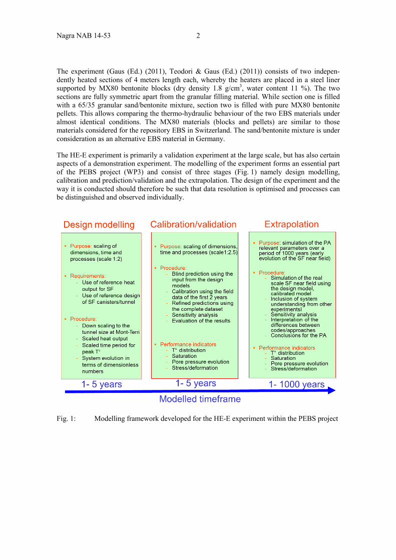
The HE-E experiment is primarily a validation experiment at the large scale, but has also certain aspects of a demonstration experiment. The modelling of the experiment forms an essential part of the PEBS project (WP3) and consist of three stages (Fig. 1) namely design modelling, calibration and prediction/validation and the extrapolation. The design of the experiment and the way it is conducted should therefore be such that data resolution is optimised and processes can be distinguished and observed individually.
Fig. 1: Modelling framework developed for the HE-E experiment within the PEBS project
3 Nagra NAB 14-53
1.3 Reporting Related to the HE-E Experiment The detailed design of the HE-E experiment is described in Gaus (Ed.) (2001) (PEBS deliverable D2.2-2). This report describes in detail the objectives, concept, design basis and the different elements and also provides a summary of the scoping calculations which supported the design. In Teodori & Gaus (Ed.) (2001) (PEBS deliverable D2.2-3) the as-built description of the experiment is given including the characteristics of the components and the sequence of construction. The scoping calculations are described in detail in Czaikowski et al. (2012) (PEBS deliverable D3.2-1. A summary of the experiment after 15 months of operation is given in Gaus et al. (2014).
This report covers PEBS deliverable 2.2-11 and PEBS deliverable 3.2-2. It describes the main features of the HE-E experiment, referring to the supporting reports where needed, the column tests characterizing the HE-E materials and their interpretation, the observations after approximately 30 months of operation, the modelling activities completed by the various partners, and the lessons learned from the experiment.

5 Nagra NAB 14-53
2 HE-E: As-built
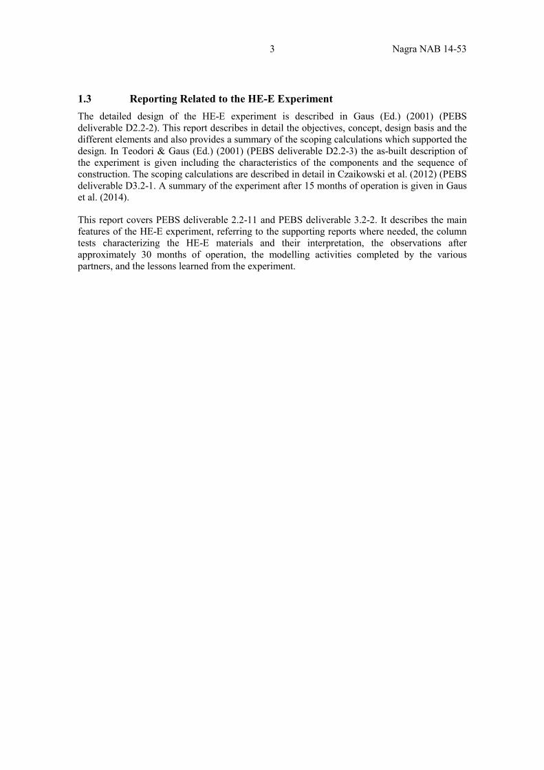
2.1 Introduction The HE-E experiment is constructed in the former VE test section, located in the raised-bored (RB) micro tunnel of the Mont Terri Rock Laboratory (Fig. 2) excavated in 1999 in the shaly facies of the Opalinus Clay, using the horizontal raise-boring technique. The detailed geological mapping of the test-section is described in Teodori & Gaus (Ed.) (2011).
Fig. 2: Location of the HE-E experiment in the microtunnel (μtunnel) in the Mont Terri URL (Switzerland)
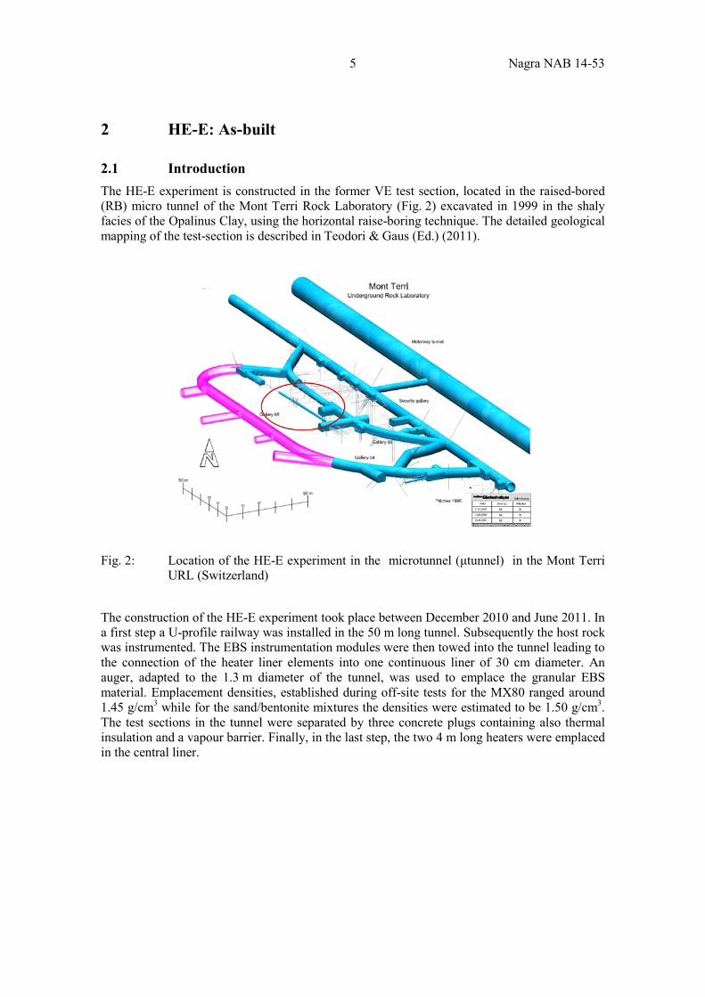
The construction of the HE-E experiment took place between December 2010 and June 2011. In a first step a U-profile railway was installed in the 50 m long tunnel. Subsequently the host rock was instrumented. The EBS instrumentation modules were then towed into the tunnel leading to the connection of the heater liner elements into one continuous liner of 30 cm diameter. An auger, adapted to the 1.3 m diameter of the tunnel, was used to emplace the granular EBS material. Emplacement densities, established during off-site tests for the MX80 ranged around 1.45 g/cm3 while for the sand/bentonite mixtures the densities were estimated to be 1.50 g/cm3. The test sections in the tunnel were separated by three concrete plugs containing also thermal insulation and a vapour barrier. Finally, in the last step, the two 4 m long heaters were emplaced in the central liner.
Nagra NAB 14-53 6
Fig. 3: Schematic layout of the HE-E experiment showing the section in the back of the tunnel filled with bentonite pellets and the section in the front of the tunnel filled with sand/bentonite
This chapter provides only an overview of the characteristics of the HE-E experiment. A detailed description can be found in the design report (Gaus (Ed.) 2011) and the as-built report (Teodori & Gaus (Ed.) 2011).
2.2 Initial Conditions in the Tunnel Prior to the Installation of the HE-E Experiment
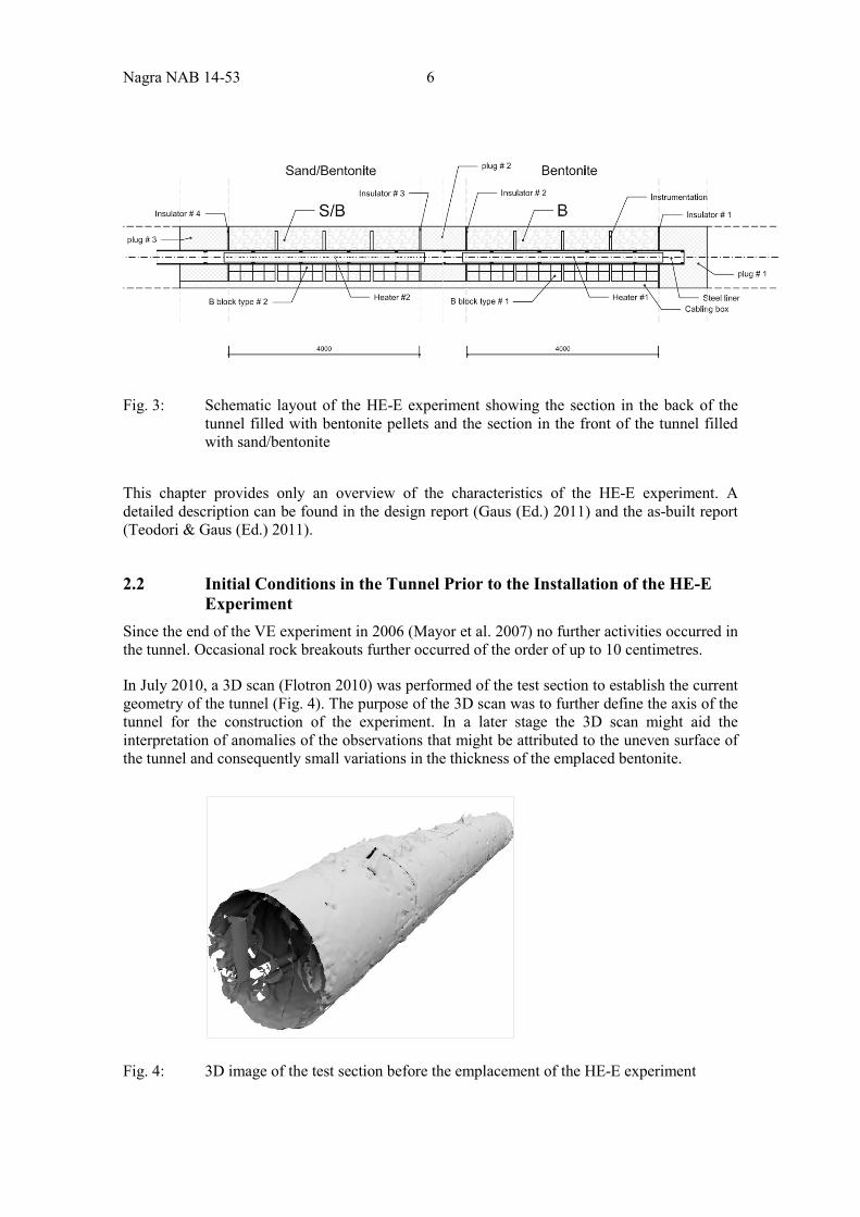
Since the end of the VE experiment in 2006 (Mayor et al. 2007) no further activities occurred in the tunnel. Occasional rock breakouts further occurred of the order of up to 10 centimetres.
In July 2010, a 3D scan (Flotron 2010) was performed of the test section to establish the current geometry of the tunnel (Fig. 4). The purpose of the 3D scan was to further define the axis of the tunnel for the construction of the experiment. In a later stage the 3D scan might aid the interpretation of anomalies of the observations that might be attributed to the uneven surface of the tunnel and consequently small variations in the thickness of the emplaced bentonite.
Fig. 4: 3D image of the test section before the emplacement of the HE-E experiment
7 Nagra NAB 14-53
The measurements in the tunnel during Mont Terri Phase 15 from July 2009 until June 2010 are described in Rösli (2010). The pressure measurements in the 4 test sections generally give atmospheric pressures or pressures above atmosphere between 100 and 300 kPa. 6 pressure sensors showing atmospheric pressures showed no changes in their measurements during Phase 15. A small pressure increase was observed for all the other sensors and one sensor showed a pronounced pressure increase by 138 kPa during Phase 15.
During the same period, the rock displacement sensors showed decreasing measurements (in the order of 1 mm maximum) meaning that the distance between the anchor at the deepest part of the borehole and the measuring head increased.
The relative humidity sensors generally gave values above 99 % or showed an increasing trend in the measurements (HC-B92, HC-B94, HC-B95). The relative humidity measured with the psychrometer type relative humidity sensors was variable without a pronounced trend in the measurements.
The volumetric water content measured by 6 short recess TDRs was stable or continuously increasing and the final measurements are at or slightly above the values measured in May 2003, where near full saturation conditions were assumed. The volumetric water content measured by the 4 long recess TDRs remained stable slightly below the values measured in May 2003.
One can conclude that the measurements until end of June 2010 indicate mostly nearly saturated or saturated conditions with stable or increasing pressures and increasing distances recorded by the extensometers reflecting the continuous re-saturation and swelling of the Opalinus Clay.
2.3 Materials
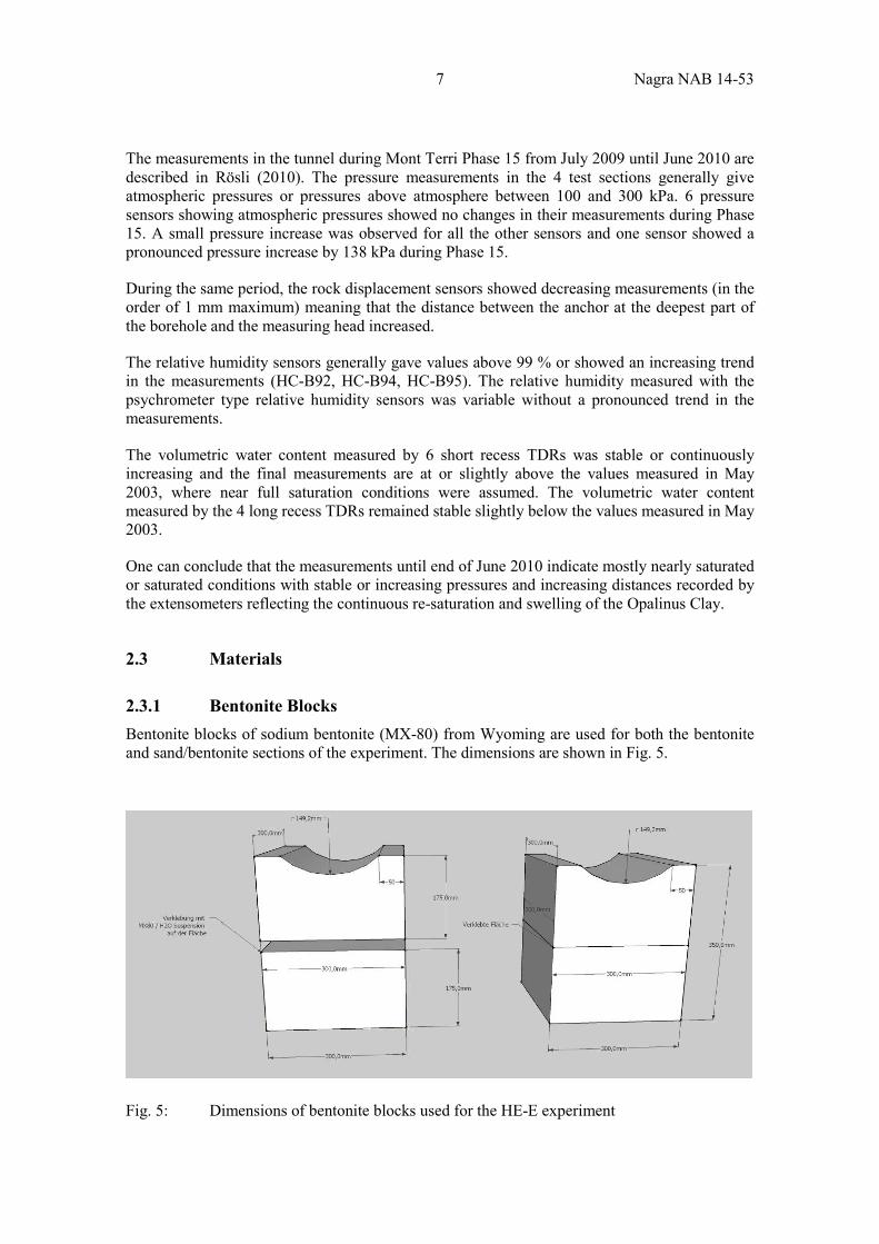
2.3.1 Bentonite Blocks Bentonite blocks of sodium bentonite (MX-80) from Wyoming are used for both the bentonite and sand/bentonite sections of the experiment. The dimensions are shown in Fig. 5.
Fig. 5: Dimensions of bentonite blocks used for the HE-E experiment
Nagra NAB 14-53 8
Fabrication was done by Alpha Ceramics (Aachen, Germany). Blocks are produced by a uniaxial press at 6kN/cm2. Blocks were "glued" together by moistening a little the upper surface of the lower block and the lower surface of the upper block.
The laboratory tests gave the following averaged results:
Water content: 10.34 %
Bulk density: 1,993 kg/m³
Dry density: 1,806 kg/m³
Porosity: 33.1 %
At the moment of emplacement, three fragments of broken bentonite blocks were tested indicating an averaged water content of 15.7 % and the averaged bulk density 1.874g/cm3. Although the pieces show increased water content, these are seen as extreme values as these refer to pieces chipped of in the microtunnel and thus not representative for the entire blocks.
2.3.2 Sand/Bentonite Mixture One section of the HE-E was backfilled using a sand/bentonite mixture of 65 % of sand and 35 % of bentonite as buffer material. The sand/bentonite mixture was provided by MPC, Limay/France. The components are 65 % of quartz sand with a grain spectrum of 0.5 - 1.8 mm and 35 % of sodium bentonite GELCLAY WH2 (granular material of the same composition as MX-80) of the same grain spectrum which was obtained by crushing and sieving from the qualified raw material. Water content is 13 % for the bentonite and 0.05 % for the sand, giving a total water content of the mixture in the range of 4 %.
The laboratory tests gave the following averaged results:
Water content: 4.1 %
Bulk density: 1,440 kg/m³
Dry density: 1,383 kg/m³
Porosity: 46.7 %
The density at emplacement based on separate measurements was determined to be around 1,480 kg/m³ (manual handling), while the large samples prepared with the emplacement auger range at 1,500 kg/m³. An estimation of the emplacement density of the buffer material was also made by calculation from the total emplaced material and the micro tunnel net volume to be filled. The total emplaced mass was 6,043 kg. This corresponds to a low density of only 1264 kg/m³. Therefore it has to be kept in mind that the density of the sand/bentonite mixture in the micro tunnel may be lower than expected, or that there are unfilled volumes not accounted for. For the calculations, however, a density of 1,500 kg/m³ should be used, since this is the value measured on the large samples prepared using the actual emplacement technique. The actually measured values definitely exhibit less uncertainty than the figure derived by the calculation.
9 Nagra NAB 14-53
2.3.3 Granular Bentonite Material The granular bentonite is the same as the one used for the ESDRED project, mixture type E (sodium bentonite MX-80 from Wyoming). The material is described in detail in the Plötze & Weber (2007 - NAB 07-24) and main properties are as follows:
Water content: 5.4 %
Bulk density: 1,595 kg/m³
Dry density: 1,513 kg/m³
A total of 6,665 kg granular bentonite was emplaced in the bentonite section with a mini-auger. The on-site measured water content was 5.91 %. The 3D laser scan of the RB micro tunnel (Flotron 2010) permitted to compute the tunnel volume of the bentonite section (5.43 m3) from which has been subtracted the volume occupied by the liner, blocks, cable channel, floor concreting, 150 kg rock fall and instrumentation. The effective volume occupied by the granular bentonite is therefore 4.318 m3. The bulk density averaged on the total volume occupied by the granular bentonite is 1.543 kg/m3; the dry bulk density 1.457 kg/m3. These values correspond to detailed in situ measurements performed during off-site tests (described in detail in Teodori & Gaus (Ed.) 2011).
2.3.4 Plugs and Plug Materials The plugs consist of the following elements (for a detailed description see Teodori et al. 2011):
Plug #1 (thickness 960 mm): Back end wall (cement bricks and mortar), vapour barrier (aluminium foil), thermal isolation (Rockwool), scaffolding wall for block (cement bricks and mortar), block (concrete), front scaffolding wall for block (cement bricks and mortar).
Plug #2 (thickness 550 mm): Back end wall for containment of bentonite material (cement bricks and mortar), vapour barrier (aluminium foil), thermal isolation (Rockwool), vapour barrier (aluminium foil), front wall (cement bricks and mortar)
Plug #3 (thickness 1,090 mm): Back end wall for containment of sand/bentonite material (cement bricks and mortar); thermal isolation (Rockwool); vapour barrier (aluminium foil); dying end scaffolding wall for block (cement bricks and mortar); block (concrete); front scaffolding wall for block (cement bricks and mortar)
Nagra NAB 14-53 10
2.4 Instrumentation Concept
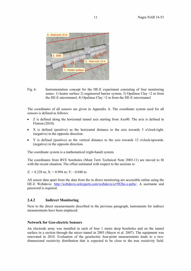
2.4.1 Direct Monitoring The instrumentation concept is targeting four zones (Fig. 6):
1. the heater surface where the temperature is measured
2. the EBS itself and the interface with the Opalinus Clay with very dense measurements of temperature and relative humidity
3. the Opalinus Clay close to the microtunnel which was under the influence of the ventilation before and during construction where temperature, humidity, hydraulic pressure and displacement are monitored
4. the Opalinus Clay at several meters from the microtunnel where hydrostatic conditions were less disturbed by the activities in the microtunnel and where hydraulic pressures are monitored.
The EBS and the host rock/OPA interface are instrumented with temperature and humidity sensors. Taking into account the temperature and the fact that only natural saturation is taking place, it is not expected that any saturation and/or swelling pressures will develop within the course of the experiment (see Gaus (Ed.) 2011). As the characterisation of the thermal behaviour in the EBS is one of the main objectives of the experiment, a very dense configuration of sensors was installed.
The Opalinus Clay close to the micro tunnel is instrumented with piezometers, humidity sensors (psychrometers), temperature sensors and extensometers. It is expected that saturation/de-saturation processes can be observed in this zone after the start of the experiment. The bulk of these sensors have been inherited from the VE-experiment (Mayor et al. 2007) and the cables were extended for the HE-E experiment. Additional piezometers and temperature sensors have been installed in certain sections.
At larger distance from the micro tunnel (through boreholes drilled from Gallery 98), piezometers are installed. Hydraulic overpressures, resulting from the thermal impact, might be produced as suggested by model calculations. With these boreholes and the pore pressure sensors installed therein the observations are expected allowing the evaluation of these overpressures. Two extra boreholes have been drilled as part of the construction of the HE-E experiment; two boreholes previously drilled were already instrumented during the VE experiment.
11 Nagra NAB 14-53
Fig. 6: Instrumentation concept for the HE-E experiment consisting of four monitoring zones: 1) heater surface 2) engineered barrier system, 3) Opalinus Clay <2 m from the HE-E microtunnel, 4) Opalinus Clay >2 m from the HE-E microtunnel
The coordinates of all sensors are given in Appendix A. The coordinate system used for all sensors is defined as follows:
• Z is defined along the horizontal tunnel axis starting from Axe00. The axis is defined in Flotron (2010).
• X is defined (positive) as the horizontal distance to the axis towards 3 o'clock/right. (negative) in the opposite direction.
• Y is defined (positive) as the vertical distance to the axis towards 12 o'clock/upwards. (negative) in the opposite direction.
The coordinate system is a mathematical (right-hand) system.
The coordinates from BVE boreholes (Mont Terri Technical Note 2003-11) are moved to fit with the recent situation. The offset estimated with respect to the sections is:
Z: + 0.228 m; X: + 0.994 m; Y: - 0.040 m
All sensor data apart from the data from the in direct monitoring are accessible online using the HE-E Webdavis: http://webdavis.solexperts.com/webdavis/a1982he-e-pebs/. A username and password is required.
2.4.2 Indirect Monitoring Next to the direct measurements described in the previous paragraph, instruments for indirect measurements have been emplaced:
Network for Geo-electric Sensors An electrode array was installed in each of four 1 metre deep boreholes and on the tunnel surface in a section through the micro tunnel in 2003 (Mayor et al. 2007). The equipment was renovated in 2010. Evaluation of the geoelectric four-point measurements leads to a two-dimensional resistivity distribution that is expected to be close to the true resistivity field.
Nagra NAB 14-53 12
Through calibration based on laboratory tests information on the water saturation can be obtained. The geo-electric sensor data were not analysed within the PEBS project.
Seismic Array A seismic array consisting of five piezoelectric transducers which serve as emitters and ten transducers which serve as receivers were installed in three 1 metre deep boreholes in a section of the micro tunnel. The seismic transmission experiment aims at characterising changes in the Opalinus Clay and EBS properties caused by the heating.
2.4.3 Temperature and Humidity Sensors in the EBS and the EBS/Host Rock Interface
The temperature and the relative air humidity are the key monitoring parameters for the EBS and the interface.
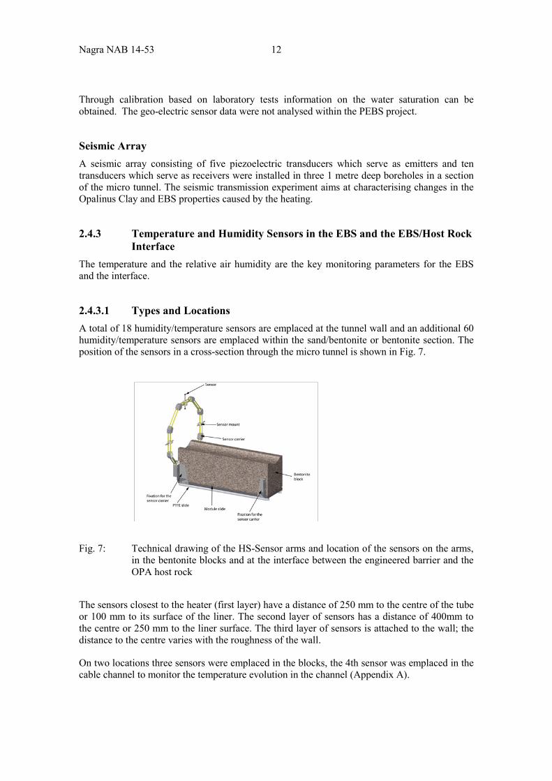
2.4.3.1 Types and Locations A total of 18 humidity/temperature sensors are emplaced at the tunnel wall and an additional 60 humidity/temperature sensors are emplaced within the sand/bentonite or bentonite section. The position of the sensors in a cross-section through the micro tunnel is shown in Fig. 7.
Fig. 7: Technical drawing of the HS-Sensor arms and location of the sensors on the arms, in the bentonite blocks and at the interface between the engineered barrier and the OPA host rock
The sensors closest to the heater (first layer) have a distance of 250 mm to the centre of the tube or 100 mm to its surface of the liner. The second layer of sensors has a distance of 400mm to the centre or 250 mm to the liner surface. The third layer of sensors is attached to the wall; the distance to the centre varies with the roughness of the wall.
On two locations three sensors were emplaced in the blocks, the 4th sensor was emplaced in the cable channel to monitor the temperature evolution in the channel (Appendix A).
13 Nagra NAB 14-53
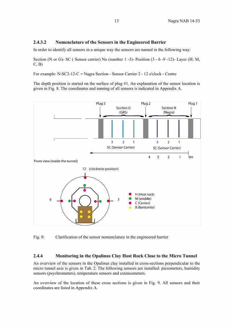
2.4.3.2 Nomenclature of the Sensors in the Engineered Barrier In order to identify all sensors in a unique way the sensors are named in the following way:
Section (N or G)- SC ( Sensor carrier) No (number 1 -3)- Position (3 - 6 -9 -12)- Layer (H; M, C, B)
For example: N-SC2-12-C = Nagra Section - Sensor Carrier 2 - 12 o'clock - Centre
The depth position is started on the surface of plug #1. An explanation of the sensor location is given in Fig. 8. The coordinates and naming of all sensors is indicated in Appendix A.
Fig. 8: Clarification of the sensor nomenclature in the engineered barrier
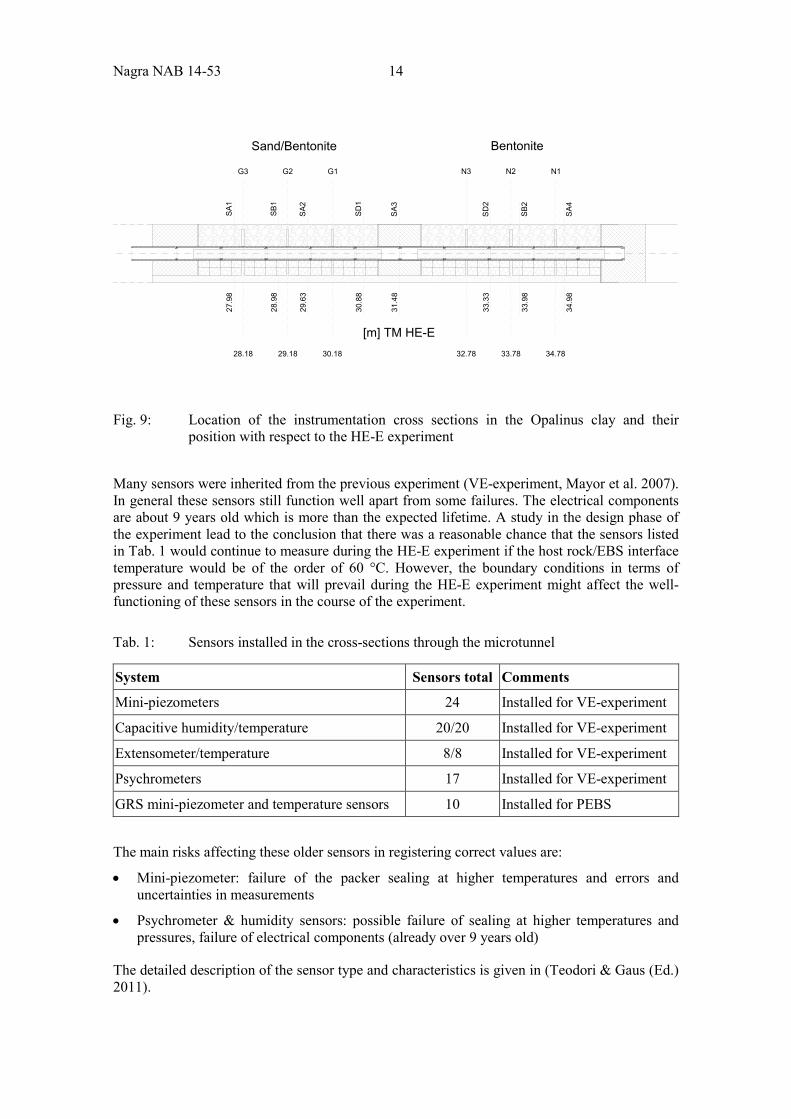
2.4.4 Monitoring in the Opalinus Clay Host Rock Close to the Micro Tunnel An overview of the sensors in the Opalinus clay installed in cross-sections perpendicular to the micro tunnel axis is given in Tab. 2. The following sensors are installed: piezometers, humidity sensors (psychrometers), temperature sensors and extensometers.
An overview of the location of these cross sections is given in Fig. 9. All sensors and their coordinates are listed in Appendix A.
Nagra NAB 14-53 14
Fig. 9: Location of the instrumentation cross sections in the Opalinus clay and their position with respect to the HE-E experiment
Many sensors were inherited from the previous experiment (VE-experiment, Mayor et al. 2007). In general these sensors still function well apart from some failures. The electrical components are about 9 years old which is more than the expected lifetime. A study in the design phase of the experiment lead to the conclusion that there was a reasonable chance that the sensors listed in Tab. 1 would continue to measure during the HE-E experiment if the host rock/EBS interface temperature would be of the order of 60 °C. However, the boundary conditions in terms of pressure and temperature that will prevail during the HE-E experiment might affect the well-functioning of these sensors in the course of the experiment.
Tab. 1: Sensors installed in the cross-sections through the microtunnel
System Sensors total Comments
Mini-piezometers 24 Installed for VE-experiment
Capacitive humidity/temperature 20/20 Installed for VE-experiment
Extensometer/temperature 8/8 Installed for VE-experiment
Psychrometers 17 Installed for VE-experiment
GRS mini-piezometer and temperature sensors 10 Installed for PEBS The main risks affecting these older sensors in registering correct values are:
• Mini-piezometer: failure of the packer sealing at higher temperatures and errors and uncertainties in measurements
• Psychrometer & humidity sensors: possible failure of sealing at higher temperatures and pressures, failure of electrical components (already over 9 years old)
The detailed description of the sensor type and characteristics is given in (Teodori & Gaus (Ed.) 2011).
Sand/Bentonite Bentonite
N1N2N3G1G2G3
32.78 33.78 34.7830.1829.1828.18
[m] TM HE-E
SA
127
.98
SB
128
.98
SA
229
.63
SD
130
.88
SA
331
.48
SD
233
.33
SB
233
.98
SA
434
.98
15 Nagra NAB 14-53
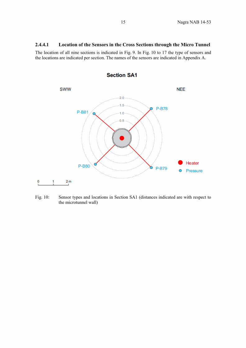
2.4.4.1 Location of the Sensors in the Cross Sections through the Micro Tunnel The location of all nine sections is indicated in Fig. 9. In Fig. 10 to 17 the type of sensors and the locations are indicated per section. The names of the sensors are indicated in Appendix A.
Fig. 10: Sensor types and locations in Section SA1 (distances indicated are with respect to the microtunnel wall)
Nagra NAB 14-53 16
Fig. 11: Sensor types and locations in Section SA2 (distances indicated are with respect to the microtunnel wall)
Fig. 12: Sensor types and locations in Section SA3 (distances indicated are with respect to the microtunnel wall)
17 Nagra NAB 14-53
Fig. 13: Sensor types and locations in Section SA4 (distances indicated are with respect to the microtunnel wall)
Fig. 14: Sensor types and locations in Section SB1 (distances indicated are with respect to the microtunnel wall)
Nagra NAB 14-53 18
Fig. 15: Sensor types and locations in Section SB2 (distances indicated are with respect to the microtunnel wall)
Fig. 16: Sensor types and locations in Section SD1 (distances indicated are with respect to the microtunnel wall)
19 Nagra NAB 14-53
Fig. 17: Sensor types and locations in Section SD2 (distances indicated are with respect to the microtunnel wall)
Nagra NAB 14-53 20
2.4.5 Sensors Installed at a Larger Distance from the Micro Tunnel
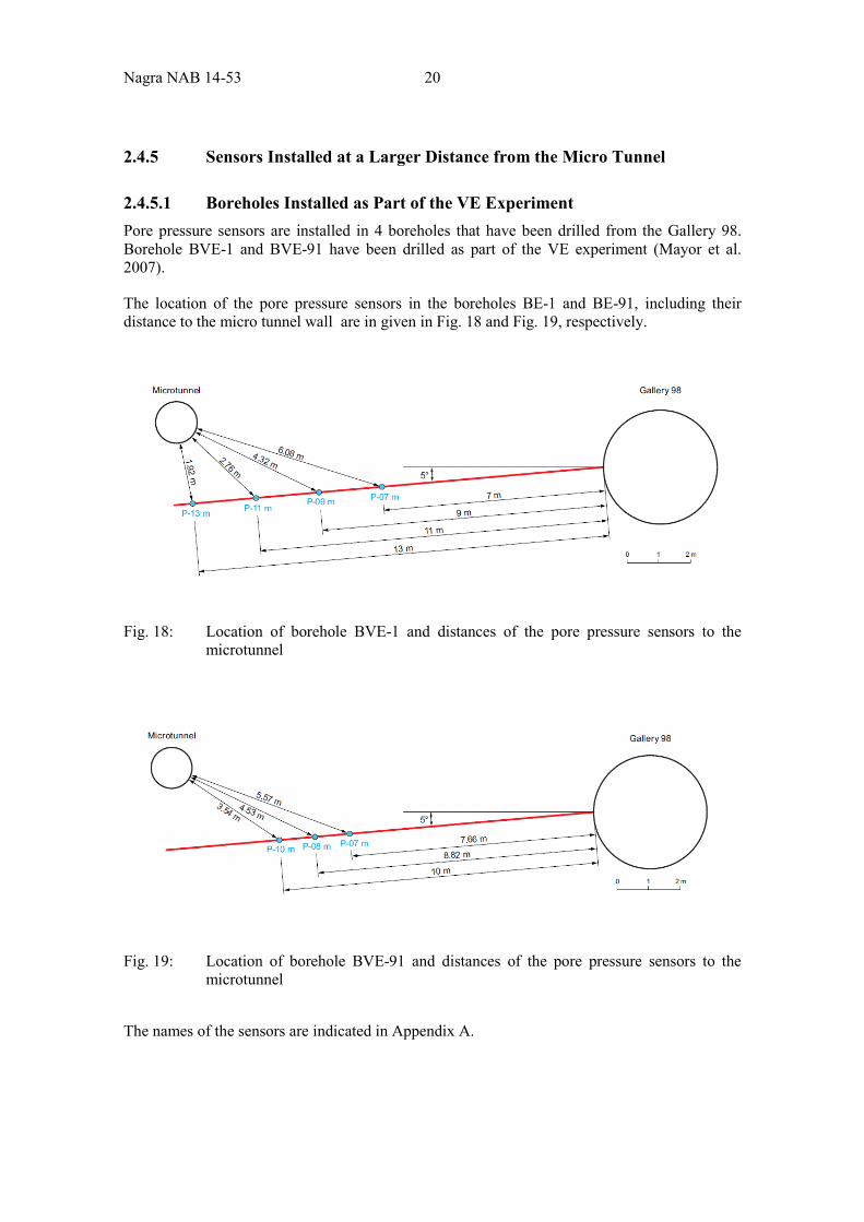
2.4.5.1 Boreholes Installed as Part of the VE Experiment Pore pressure sensors are installed in 4 boreholes that have been drilled from the Gallery 98. Borehole BVE-1 and BVE-91 have been drilled as part of the VE experiment (Mayor et al. 2007).
The location of the pore pressure sensors in the boreholes BE-1 and BE-91, including their distance to the micro tunnel wall are in given in Fig. 18 and Fig. 19, respectively.
Fig. 18: Location of borehole BVE-1 and distances of the pore pressure sensors to the microtunnel
Fig. 19: Location of borehole BVE-91 and distances of the pore pressure sensors to the microtunnel
The names of the sensors are indicated in Appendix A.
21 Nagra NAB 14-53
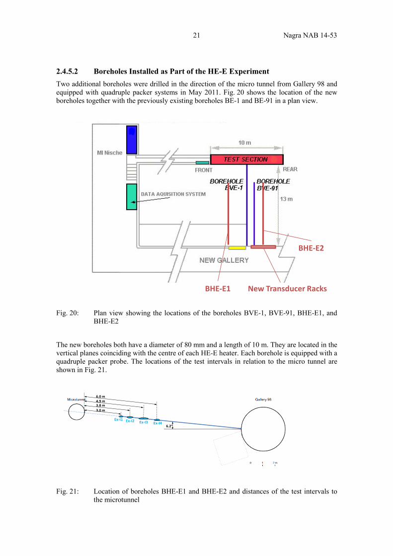
2.4.5.2 Boreholes Installed as Part of the HE-E Experiment Two additional boreholes were drilled in the direction of the micro tunnel from Gallery 98 and equipped with quadruple packer systems in May 2011. Fig. 20 shows the location of the new boreholes together with the previously existing boreholes BE-1 and BE-91 in a plan view.
Fig. 20: Plan view showing the locations of the boreholes BVE-1, BVE-91, BHE-E1, and BHE-E2
The new boreholes both have a diameter of 80 mm and a length of 10 m. They are located in the vertical planes coinciding with the centre of each HE-E heater. Each borehole is equipped with a quadruple packer probe. The locations of the test intervals in relation to the micro tunnel are shown in Fig. 21.
Fig. 21: Location of boreholes BHE-E1 and BHE-E2 and distances of the test intervals to the microtunnel
BHE-E1
BHE-E2
New Transducer Racks
6.2°Ex-I4
3.0 m3.8 m4.9 m6.0 m
Ex-I1 Ex-I2 Ex-I3
Nagra NAB 14-53 22
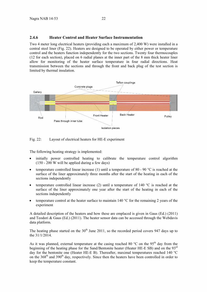
2.4.6 Heater Control and Heater Surface Instrumentation Two 4 meter long electrical heaters (providing each a maximum of 2,400 W) were installed in a central steel liner (Fig. 22). Heaters are designed to be operated by either power or temperature control and the heaters function independently for the two sections. Twenty four thermocouples (12 for each section), placed on 6 radial planes at the inner part of the 8 mm thick heater liner allow for monitoring of the heater surface temperature in four radial directions. Heat transmission between the sections and through the front and back plug of the test section is limited by thermal insulation.
Fig. 22: Layout of electrical heaters for HE-E experiment The following heating strategy is implemented:
• initially power controlled heating to calibrate the temperature control algorithm (150 - 200 W will be applied during a few days)
• temperature controlled linear increase (1) until a temperature of 80 - 90 °C is reached at the surface of the liner approximately three months after the start of the heating in each of the sections independently
• temperature controlled linear increase (2) until a temperature of 140 °C is reached at the surface of the liner approximately one year after the start of the heating in each of the sections independently
• temperature control at the heater surface to maintain 140 °C for the remaining 2 years of the experiment
A detailed description of the heaters and how these are emplaced is given in Gaus (Ed.) (2011) and Teodori & Gaus (Ed.) (2011). The heater sensor data can be accessed through the Webdavis data platform.
The heating phase started on the 30th June 2011, so the recorded period covers 947 days up to the 31/1/2014.
As it was planned, external temperature at the casing reached 80 °C on the 95th day from the beginning of the heating phase for the Sand/Bentonite heater (Heater HE-E SB) and on the 93rd
day for the bentonite one (Heater HE-E B). Thereafter, maximal temperatures reached 140 °C on the 368th and 390th day, respectively. Since then the heaters have been controlled in order to keep the temperature constant.
23 Nagra NAB 14-53
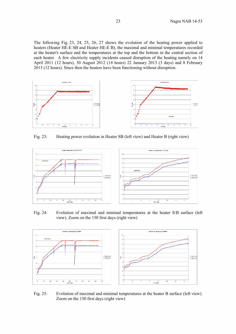
The following Fig. 23, 24, 25, 26, 27 shows the evolution of the heating power applied to heaters (Heater HE-E SB and Heater HE-E B), the maximal and minimal temperatures recorded at the heater's surface and the temperatures at the top and the bottom in the central section of each heater. A few electricity supply incidents caused disruption of the heating namely on 14 April 2011 (12 hours), 30 August 2012 (14 hours) 22 January 2013 (3 days) and 8 February 2013 (12 hours). Since then the heaters have been functioning without disruption.
Fig. 23: Heating power evolution in Heater SB (left view) and Heater B (right view)
Fig. 24: Evolution of maximal and minimal temperatures at the heater S/B surface (left view). Zoom on the 150 first days (right view)
Fig. 25: Evolution of maximal and minimal temperatures at the heater B surface (left view). Zoom on the 150 first days (right view)
Nagra NAB 14-53 24
Fig. 26: Temperature evolution at the upper and lower point of the central section in heater SB
Fig. 27: Temperature evolution at the upper and lower point of the central section in heater B

25 Nagra NAB 14-53
Except for the initial incidents related with a few power short cuts at the mains (sudden drops of the temperatures at the graphs) that were properly solved by modifying the components of the electrical connection to Mont Terri power network, the power and temperature control function as planned.

27 Nagra NAB 14-53
3 Observations: Overview of the Collected Data The HE-E experiment is divided into two different sections (named as Nagra Section and GRS Section), each of them filled with a granular based bentonite material. The Nagra buffer is composed by MX80 bentonite pellets and the GRS buffer is made of a sand-bentonite mixture with 65 % of sand and 35 % of bentonite. Compacted MX80 bentonite blocks support the canister in both heated sections.
The data acquisition system started to record data on 9th June 2011, 19 days before starting the heating system. In all the following figures, data until December 31 2013 are shown, 917 days after the start of heating.
3.1 Temperature Measurements
3.1.1 Heaters In Fig. 28 the total heating power supplied to the two heaters and the heater temperature in the middle of the two heated sections are shown. Temperature on the heater surface reaches a maximum of about 140 °C after the first year of heating and it has been maintained without significant changes (due to smaller power cuts) until the end of the first 2.5 years of heating (end of December 2013). It has been reported that bentonite pellets exhibited an overall higher thermal conductivity in comparison to the thermal conductivity of sand-bentonite mixture (Gaus et al. 2014). This probably explains the higher power that needs to be supplied to the Nagra Section in order to achieve a maximum temperature of 140 °C. After that, a gradually reduction in power for the Nagra buffer can be noted whereas the power in the GRS buffer is roughly constant with time. The reduction in power required to maintain a constant heater temperature can be related to the material specific decrease in thermal conductivity due to the drying (different impact for blocks, pellets and sand-bentonite).
Nagra NAB 14-53 28
Fig. 28: Evolution of temperature (left) and heating power (right) in the heaters for the two heated sections (after February 2012) A schematic layout of the canister including the instrumented temperature sections is also shown.
3.1.2 EBS Measurements from the sensors installed in the EBS (Fig. 29, 30, 31, 32, 33, 34) indicate temperature increase during the first year of heating followed by a non-significant change in temperature after that period of time. This reflects that steady-state is reached relatively fast in the EBS. It can be noticed that after the first year of the experiment the maximum temperature registered in the sensors closest to the heater surface (first layer of sensors) is about 100 °C ±2 °C, in both heated sections. This value is encountered in those instrumented cross-sections close to the central portion of the experiment (section N3 for the Nagra buffer and section G1 for the GRS buffer). A slight difference in temperature depending on the direction taken (3, 9 or 12 o'clock in the granular filling material) for those sensors located at 12 o'clock profile (full lines in Fig. 29 and 31) or 9 o'clock profile (dashed lines). This dependency of the thermal behaviour on the orientation is more evident for the Nagra buffer material. This difference tends to decrease as the distance from the heater increases. In the compacted blocks this temperature dependence on the sensor position (5 or 7 o'clock) is not significant (see Fig. 30 and 32) due to the greater homogeneity of relevant parameters (dry density, water content, porosity) inside the bentonite blocks with respect to the heterogeneous distribution of these properties in the emplaced granular buffers. Furthermore maximum temperatures in the GRS buffer are recorded
29 Nagra NAB 14-53
inside the compacted blocks for the upper temperature sensors (identified as T-XX-5Bt or T-XX-7Bt where XX stands for the instrumented section G1, G2 or G3) despite the fact that the sand-bentonite mixture has a higher thermal resistance to heat conduction compared to the bentonite blocks at low saturation conditions (Wieczorek et al. 2011). Temperature in the second layer of sensors inside the blocks (identified as T-XX-5Bl and T-XX-7Bl where XX means the instrumented section name) was found to vary between 79 °C and 82 °C for the Nagra buffer (Fig. 30) while for the GRS buffer it ranged from 79 °C to 87 °C (Fig. 32) at the end of December 2013. In addition, temperature evolution in the cable channel was also monitored and a value close to 52 °C was found for the T-N1-R sensor (see Fig. 30) and a temperature around 43 °C was measured for the T-G3-R sensor (see Fig. 32).Close to the buffer-rock interface, temperature is around 45 ± 2 °C after 2.5 years of experiment (end of December 2013) and it keeps increasing at a slower rate.
Nagra NAB 14-53 30
Fig. 29: Evolution of temperature in the Nagra Section for the three sensor carriers inside the granular backfilling (bentonite pellets) Data from the sensors at 12 o'clock (full lines), at 3 o'clock (dotted lines) and 9 o'clock (dashed lines) are plotted into three different colours: blue (first layer of sensors), red (second layer of sensors) and green (sensors at the buffer-rock interface).
31 Nagra NAB 14-53
Fig. 30: Evolution of temperature in the Nagra Section for the three sensor carriers inside the compacted blocks
Nagra NAB 14-53 32
Fig. 31: Evolution of temperature in the GRS Section for the three sensor carriers inside the granular backfilling (sand-bentonite mixture) Data from the sensors at 12 o'clock (full lines), at 3 o'clock (dotted lines) and 9 o'clock (dashed lines) are plotted into three different colours: blue (first layer of sensors), red (second layer of sensors) and green (sensors at the buffer-rock interface).
33 Nagra NAB 14-53
Fig. 32: Evolution of temperature in the GRS Section for the three sensor carriers inside the
compacted blocks
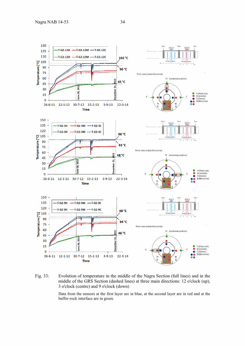
Nagra NAB 14-53 34
Fig. 33: Evolution of temperature in the middle of the Nagra Section (full lines) and in the middle of the GRS Section (dashed lines) at three main directions: 12 o'clock (up), 3 o'clock (centre) and 9 o'clock (down) Data from the sensors at the first layer are in blue, at the second layer are in red and at the buffer-rock interface are in green.
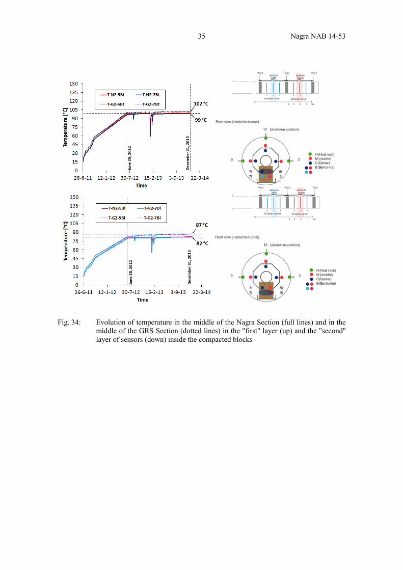
35 Nagra NAB 14-53
Fig. 34: Evolution of temperature in the middle of the Nagra Section (full lines) and in the middle of the GRS Section (dotted lines) in the "first" layer (up) and the "second" layer of sensors (down) inside the compacted blocks
Nagra NAB 14-53 36
3.1.3 Opalinus Clay In Fig. 35 and 36 the evolution of temperature in Opalinus Clay for some instrumented sections in the vicinity of the GRS buffer (Fig. 35) and in the surroundings of the Nagra buffer (Fig. 36) are presented. It is interesting to note a maximum increment of 27 - 28 °C for those sensors close to the rock-buffer interface and about 10 °C for sensors at 1.5 m from the tunnel wall (T-B16, T-B77) since the start of heating. Most of this temperature increase occurs during the first year of heating. Some temperature sensors have registered unreliable measurements (T-B48 and T-B49 in Fig. 36; T-B25 in Fig. 36).
Temperature data taken in the middle of each heated section after the first year of heating (when the temperature in each heater is kept constant and around 140 °C for both sections of the experiment) shows that the sensors around Nagra buffer reach a higher temperature compared to the ones in the GRS section (see Fig. 34). This probably reflects the reported higher thermal conductivity for the MX80 pellets (Gaus et al. 2014) with respect to the sand-bentonite mixture implying a need to provide more heating power to the heater into Nagra Section in order to maintain the thermal condition on the heater surface after that time.
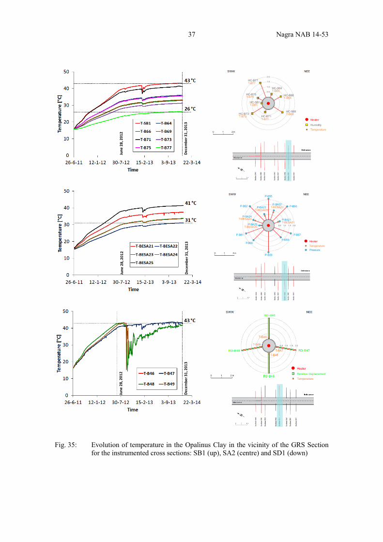
37 Nagra NAB 14-53
Fig. 35: Evolution of temperature in the Opalinus Clay in the vicinity of the GRS Section for the instrumented cross sections: SB1 (up), SA2 (centre) and SD1 (down)
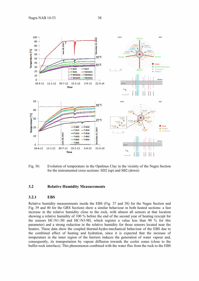
Nagra NAB 14-53 38
Fig. 36: Evolution of temperature in the Opalinus Clay in the vicinity of the Nagra Section for the instrumented cross sections: SD2 (up) and SB2 (down)
3.2 Relative Humidity Measurements
3.2.1 EBS Relative humidity measurements inside the EBS (Fig. 37 and 38) for the Nagra Section and Fig. 39 and 40 for the GRS Section) show a similar behaviour in both heated sections: a fast increase in the relative humidity close to the rock, with almost all sensors at that location showing a relative humidity of 100 % before the end of the second year of heating (except for the sensors HC-N1-3H and HC-N3-9H, which register a value less than 90 % for this parameter) and a strong reduction in the relative humidity for those sensors located near the heaters. These data show the coupled thermal-hydro-mechanical behaviour of the EBS due to the combined effect of heating and hydration, since it is expected that the increase of temperature in the inner region of the barriers induces the generation of water vapour and, consequently, its transportation by vapour diffusion towards the cooler zones (close to the buffer-rock interface). This phenomenon combined with the water flux from the rock to the EBS
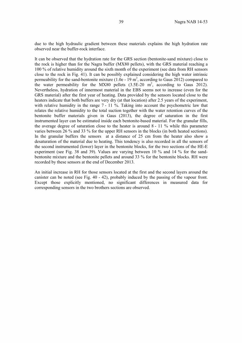
39 Nagra NAB 14-53
due to the high hydraulic gradient between these materials explains the high hydration rate observed near the buffer-rock interface.
It can be observed that the hydration rate for the GRS section (bentonite-sand mixture) close to the rock is higher than for the Nagra buffer (MX80 pellets), with the GRS material reaching a 100 % of relative humidity around the sixth month of the experiment (see data from RH sensors close to the rock in Fig. 41). It can be possibly explained considering the high water intrinsic permeability for the sand-bentonite mixture (1.0e - 19 m2, according to Gaus 2012) compared to the water permeability for the MX80 pellets (3.5E-20 m2, according to Gaus 2012). Nevertheless, hydration of innermost material in the EBS seems not to increase (even for the GRS material) after the first year of heating. Data provided by the sensors located close to the heaters indicate that both buffers are very dry (at that location) after 2.5 years of the experiment, with relative humidity in the range 7 - 11 %. Taking into account the psychometric law that relates the relative humidity to the total suction together with the water retention curves of the bentonite buffer materials given in Gaus (2013), the degree of saturation in the first instrumented layer can be estimated inside each bentonite-based material. For the granular fills, the average degree of saturation close to the heater is around 8 - 11 % while this parameter varies between 26 % and 33 % for the upper RH sensors in the blocks (in both heated sections). In the granular buffers the sensors at a distance of 25 cm from the heater also show a desaturation of the material due to heating. This tendency is also recorded in all the sensors of the second instrumented (lower) layer in the bentonite blocks, for the two sections of the HE-E experiment (see Fig. 38 and 39). Values are varying between 10 % and 14 % for the sand-bentonite mixture and the bentonite pellets and around 33 % for the bentonite blocks. RH were recorded by these sensors at the end of December 2013.
An initial increase in RH for those sensors located at the first and the second layers around the canister can be noted (see Fig. 40 - 42), probably induced by the passing of the vapour front. Except those explicitly mentioned, no significant differences in measured data for corresponding sensors in the two brothers sections are observed.
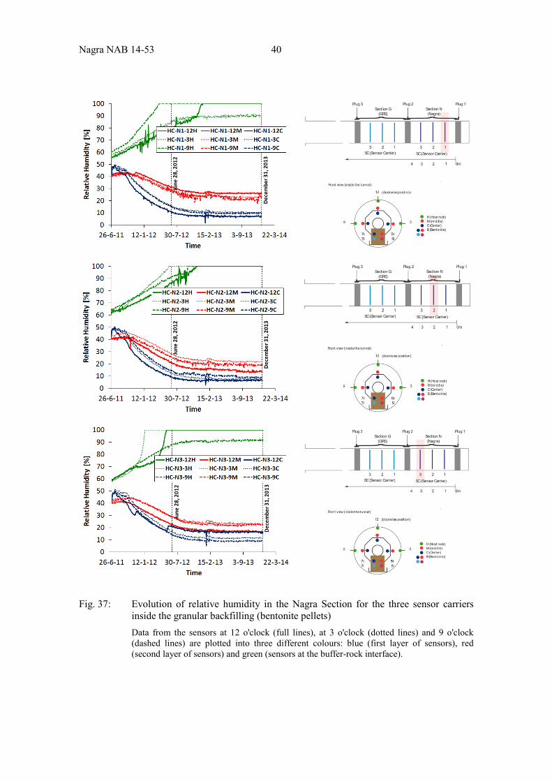
Nagra NAB 14-53 40
Fig. 37: Evolution of relative humidity in the Nagra Section for the three sensor carriers inside the granular backfilling (bentonite pellets) Data from the sensors at 12 o'clock (full lines), at 3 o'clock (dotted lines) and 9 o'clock (dashed lines) are plotted into three different colours: blue (first layer of sensors), red (second layer of sensors) and green (sensors at the buffer-rock interface).
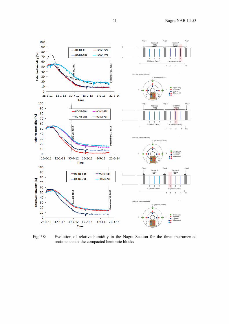
41 Nagra NAB 14-53
Fig. 38: Evolution of relative humidity in the Nagra Section for the three instrumented sections inside the compacted bentonite blocks
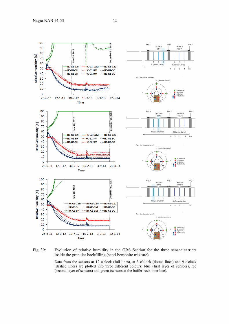
Nagra NAB 14-53 42
Fig. 39: Evolution of relative humidity in the GRS Section for the three sensor carriers inside the granular backfilling (sand-bentonite mixture) Data from the sensors at 12 o'clock (full lines), at 3 o'clock (dotted lines) and 9 o'clock (dashed lines) are plotted into three different colours: blue (first layer of sensors), red (second layer of sensors) and green (sensors at the buffer-rock interface).
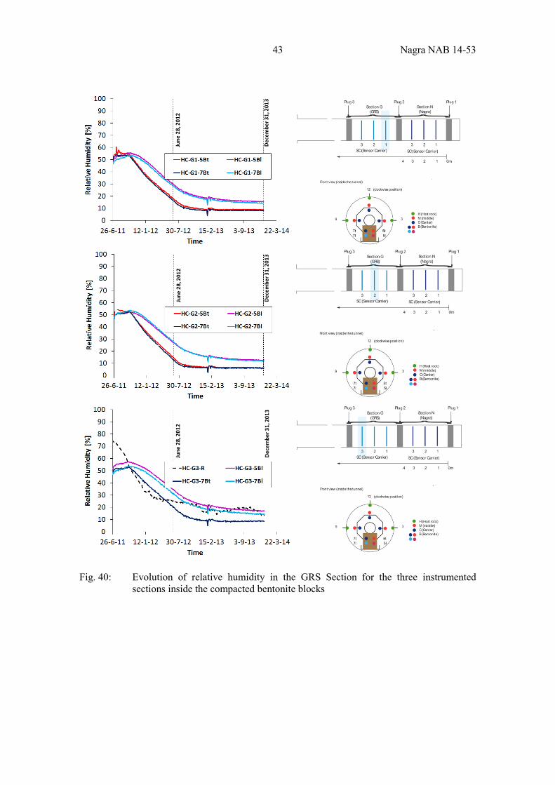
43 Nagra NAB 14-53
Fig. 40: Evolution of relative humidity in the GRS Section for the three instrumented sections inside the compacted bentonite blocks
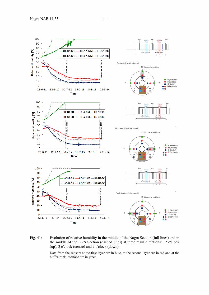
Nagra NAB 14-53 44
Fig. 41: Evolution of relative humidity in the middle of the Nagra Section (full lines) and in the middle of the GRS Section (dashed lines) at three main directions: 12 o'clock (up), 3 o'clock (centre) and 9 o'clock (down) Data from the sensors at the first layer are in blue, at the second layer are in red and at the buffer-rock interface are in green.
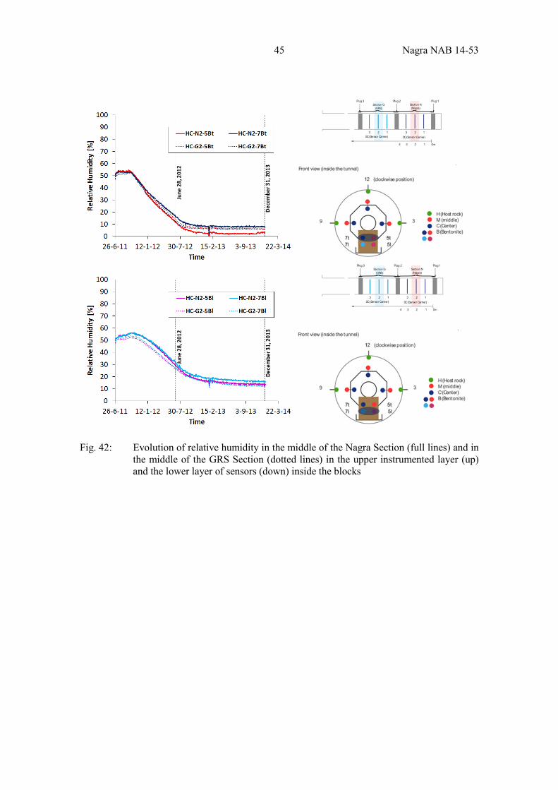
45 Nagra NAB 14-53
Fig. 42: Evolution of relative humidity in the middle of the Nagra Section (full lines) and in the middle of the GRS Section (dotted lines) in the upper instrumented layer (up) and the lower layer of sensors (down) inside the blocks
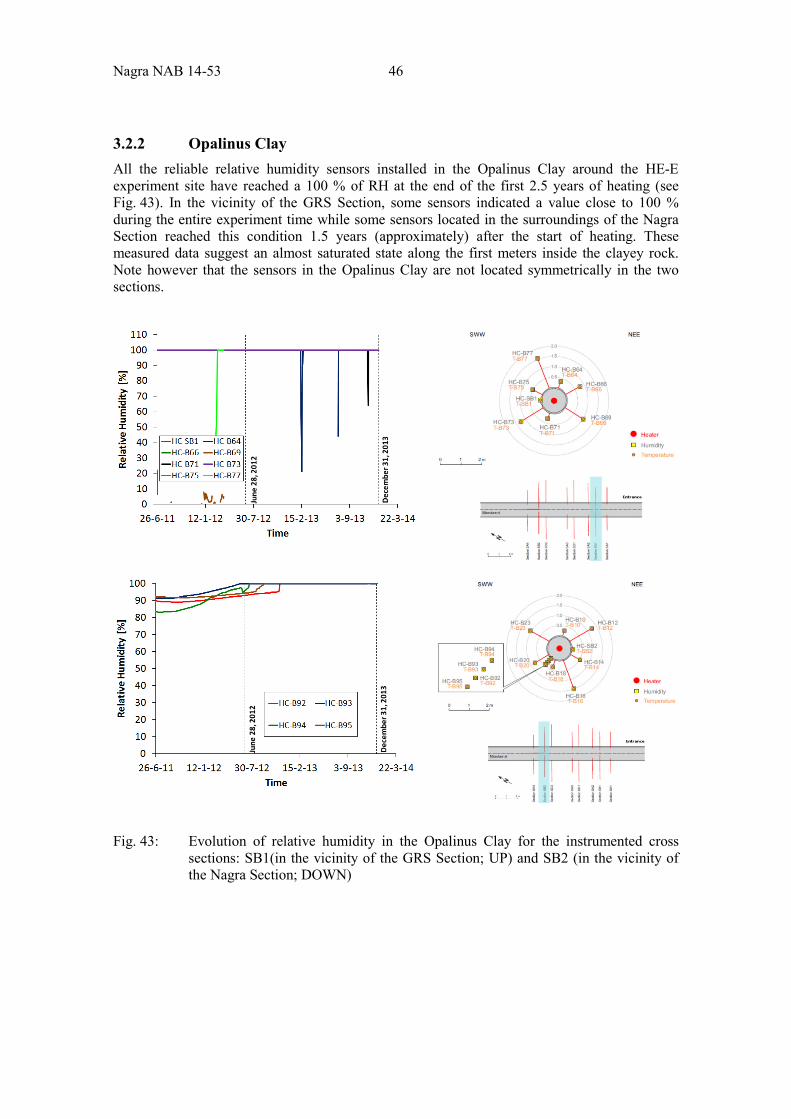
Nagra NAB 14-53 46
3.2.2 Opalinus Clay All the reliable relative humidity sensors installed in the Opalinus Clay around the HE-E experiment site have reached a 100 % of RH at the end of the first 2.5 years of heating (see Fig. 43). In the vicinity of the GRS Section, some sensors indicated a value close to 100 % during the entire experiment time while some sensors located in the surroundings of the Nagra Section reached this condition 1.5 years (approximately) after the start of heating. These measured data suggest an almost saturated state along the first meters inside the clayey rock. Note however that the sensors in the Opalinus Clay are not located symmetrically in the two sections.
Fig. 43: Evolution of relative humidity in the Opalinus Clay for the instrumented cross sections: SB1(in the vicinity of the GRS Section; UP) and SB2 (in the vicinity of the Nagra Section; DOWN)
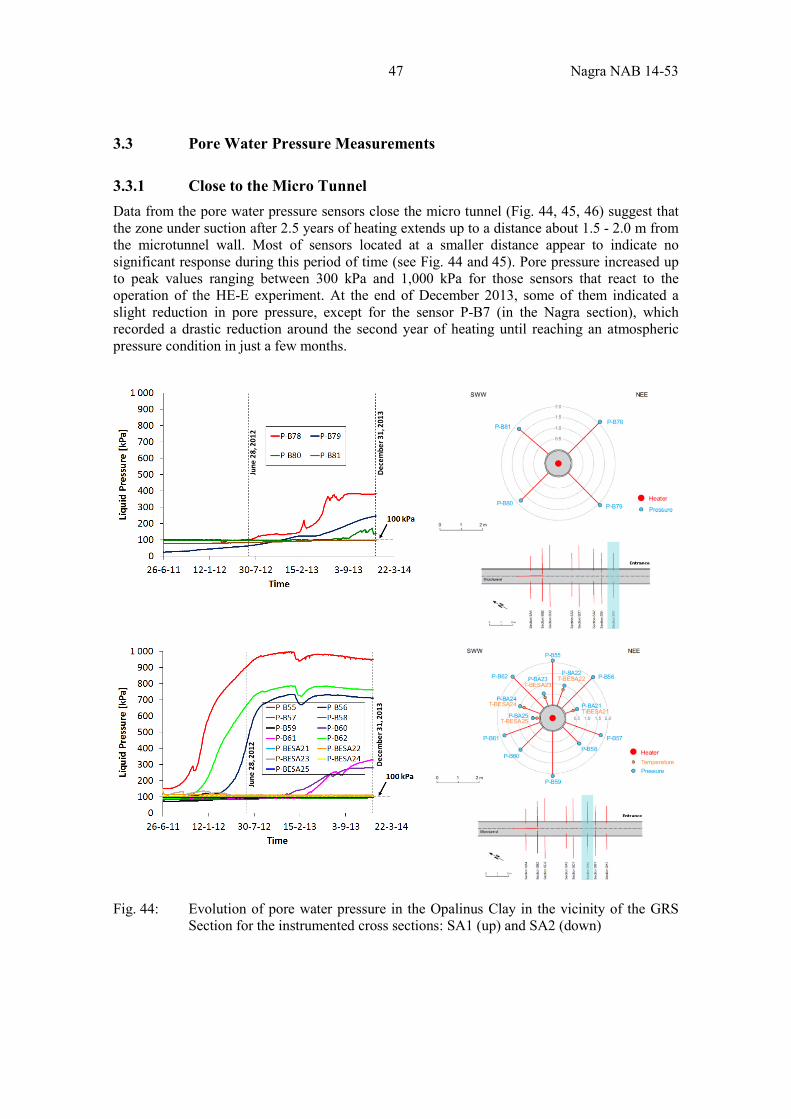
47 Nagra NAB 14-53
3.3 Pore Water Pressure Measurements
3.3.1 Close to the Micro Tunnel Data from the pore water pressure sensors close the micro tunnel (Fig. 44, 45, 46) suggest that the zone under suction after 2.5 years of heating extends up to a distance about 1.5 - 2.0 m from the microtunnel wall. Most of sensors located at a smaller distance appear to indicate no significant response during this period of time (see Fig. 44 and 45). Pore pressure increased up to peak values ranging between 300 kPa and 1,000 kPa for those sensors that react to the operation of the HE-E experiment. At the end of December 2013, some of them indicated a slight reduction in pore pressure, except for the sensor P-B7 (in the Nagra section), which recorded a drastic reduction around the second year of heating until reaching an atmospheric pressure condition in just a few months.
Fig. 44: Evolution of pore water pressure in the Opalinus Clay in the vicinity of the GRS Section for the instrumented cross sections: SA1 (up) and SA2 (down)
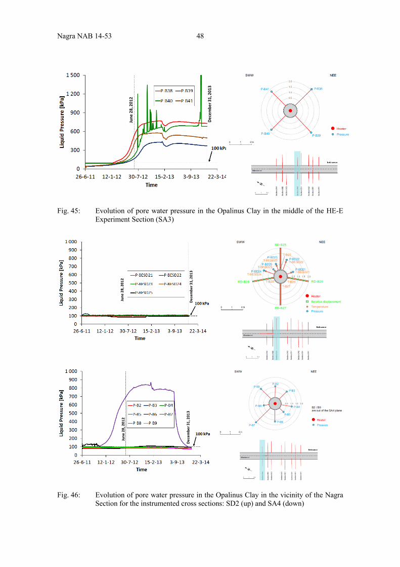
Nagra NAB 14-53 48
Fig. 45: Evolution of pore water pressure in the Opalinus Clay in the middle of the HE-E Experiment Section (SA3)
Fig. 46: Evolution of pore water pressure in the Opalinus Clay in the vicinity of the Nagra Section for the instrumented cross sections: SD2 (up) and SA4 (down)
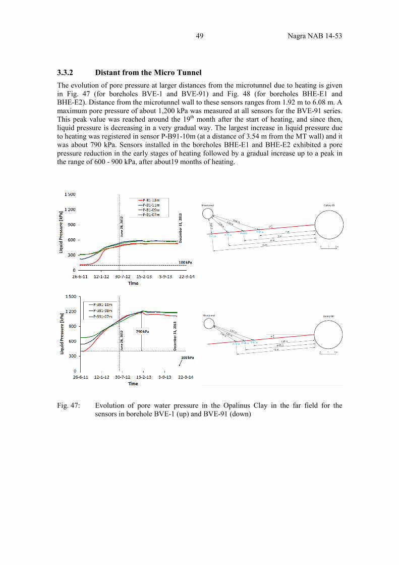
49 Nagra NAB 14-53
3.3.2 Distant from the Micro Tunnel The evolution of pore pressure at larger distances from the microtunnel due to heating is given in Fig. 47 (for boreholes BVE-1 and BVE-91) and Fig. 48 (for boreholes BHE-E1 and BHE-E2). Distance from the microtunnel wall to these sensors ranges from 1.92 m to 6.08 m. A maximum pore pressure of about 1,200 kPa was measured at all sensors for the BVE-91 series. This peak value was reached around the 19th month after the start of heating, and since then, liquid pressure is decreasing in a very gradual way. The largest increase in liquid pressure due to heating was registered in sensor P-B91-10m (at a distance of 3.54 m from the MT wall) and it was about 790 kPa. Sensors installed in the boreholes BHE-E1 and BHE-E2 exhibited a pore pressure reduction in the early stages of heating followed by a gradual increase up to a peak in the range of 600 - 900 kPa, after about19 months of heating.
Fig. 47: Evolution of pore water pressure in the Opalinus Clay in the far field for the sensors in borehole BVE-1 (up) and BVE-91 (down)
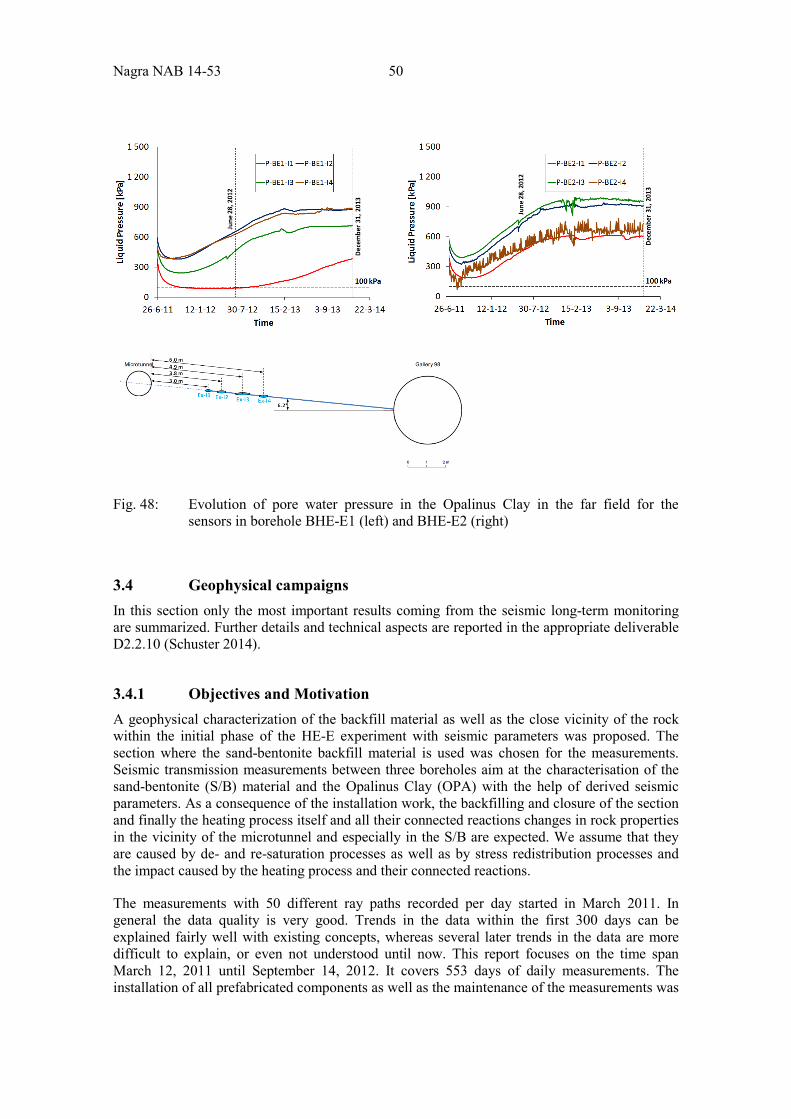
Nagra NAB 14-53 50
Fig. 48: Evolution of pore water pressure in the Opalinus Clay in the far field for the sensors in borehole BHE-E1 (left) and BHE-E2 (right)
3.4 Geophysical campaigns In this section only the most important results coming from the seismic long-term monitoring are summarized. Further details and technical aspects are reported in the appropriate deliverable D2.2.10 (Schuster 2014).
3.4.1 Objectives and Motivation A geophysical characterization of the backfill material as well as the close vicinity of the rock within the initial phase of the HE-E experiment with seismic parameters was proposed. The section where the sand-bentonite backfill material is used was chosen for the measurements. Seismic transmission measurements between three boreholes aim at the characterisation of the sand-bentonite (S/B) material and the Opalinus Clay (OPA) with the help of derived seismic parameters. As a consequence of the installation work, the backfilling and closure of the section and finally the heating process itself and all their connected reactions changes in rock properties in the vicinity of the microtunnel and especially in the S/B are expected. We assume that they are caused by de- and re-saturation processes as well as by stress redistribution processes and the impact caused by the heating process and their connected reactions.
The measurements with 50 different ray paths recorded per day started in March 2011. In general the data quality is very good. Trends in the data within the first 300 days can be explained fairly well with existing concepts, whereas several later trends in the data are more difficult to explain, or even not understood until now. This report focuses on the time span March 12, 2011 until September 14, 2012. It covers 553 days of daily measurements. The installation of all prefabricated components as well as the maintenance of the measurements was
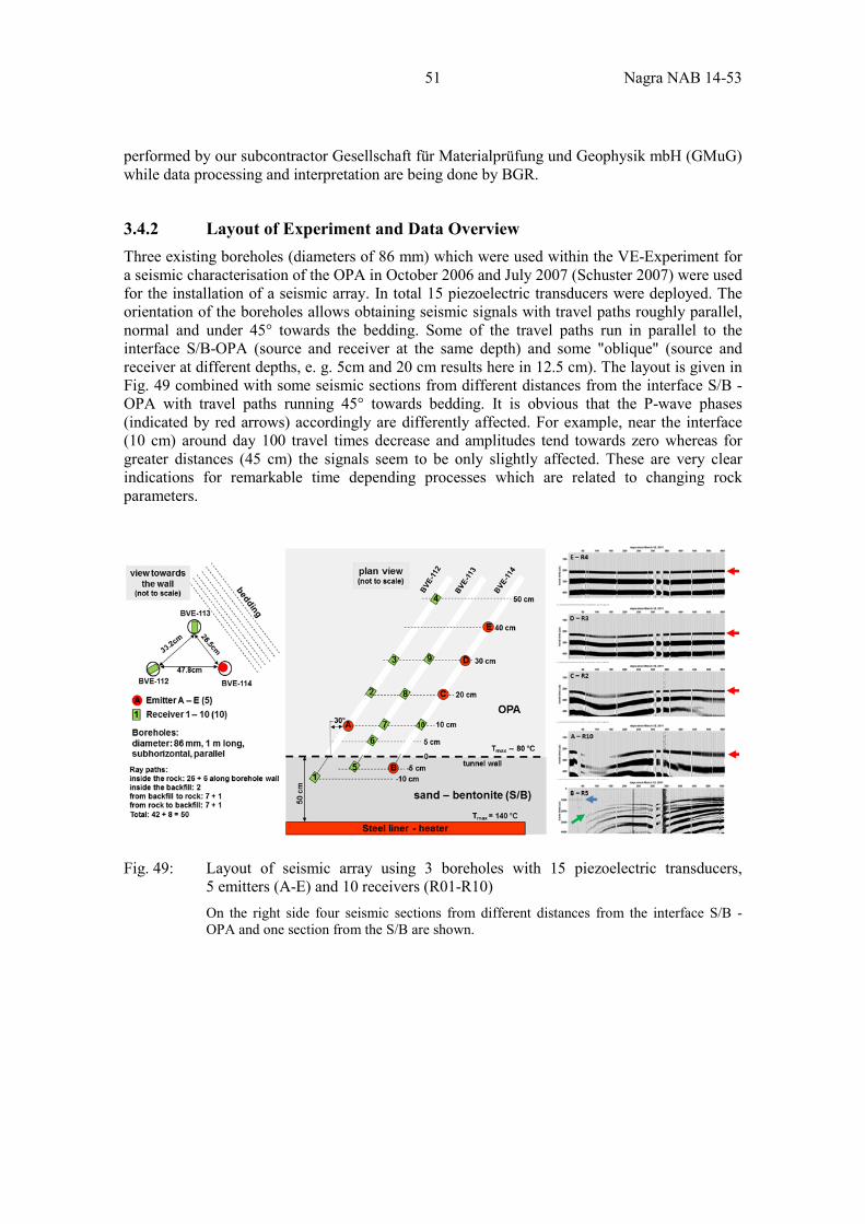
51 Nagra NAB 14-53
performed by our subcontractor Gesellschaft für Materialprüfung und Geophysik mbH (GMuG) while data processing and interpretation are being done by BGR.
3.4.2 Layout of Experiment and Data Overview Three existing boreholes (diameters of 86 mm) which were used within the VE-Experiment for a seismic characterisation of the OPA in October 2006 and July 2007 (Schuster 2007) were used for the installation of a seismic array. In total 15 piezoelectric transducers were deployed. The orientation of the boreholes allows obtaining seismic signals with travel paths roughly parallel, normal and under 45° towards the bedding. Some of the travel paths run in parallel to the interface S/B-OPA (source and receiver at the same depth) and some "oblique" (source and receiver at different depths, e. g. 5cm and 20 cm results here in 12.5 cm). The layout is given in Fig. 49 combined with some seismic sections from different distances from the interface S/B - OPA with travel paths running 45° towards bedding. It is obvious that the P-wave phases (indicated by red arrows) accordingly are differently affected. For example, near the interface (10 cm) around day 100 travel times decrease and amplitudes tend towards zero whereas for greater distances (45 cm) the signals seem to be only slightly affected. These are very clear indications for remarkable time depending processes which are related to changing rock parameters.
Fig. 49: Layout of seismic array using 3 boreholes with 15 piezoelectric transducers, 5 emitters (A-E) and 10 receivers (R01-R10) On the right side four seismic sections from different distances from the interface S/B - OPA and one section from the S/B are shown.
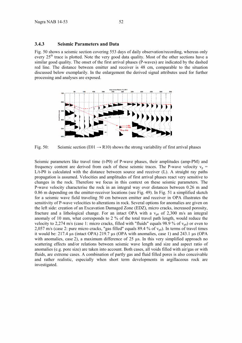
Nagra NAB 14-53 52
3.4.3 Seismic Parameters and Data Fig. 50 shows a seismic section covering 553 days of daily observation/recording, whereas only every 25th trace is plotted. Note the very good data quality. Most of the other sections have a similar good quality. The onset of the first arrival phases (P-waves) are indicated by the dashed red line. The distance between emitter and receiver is 48 cm, comparable to the situation discussed below exemplarily. In the enlargement the derived signal attributes used for further processing and analyses are exposed.
Fig. 50: Seismic section (E01 → R10) shows the strong variability of first arrival phases Seismic parameters like travel time (t-P0) of P-wave phases, their amplitudes (amp-PM) and frequency content are derived from each of these seismic traces. The P-wave velocity vp = L/t-P0 is calculated with the distance between source and receiver (L). A straight ray paths propagation is assumed. Velocities and amplitudes of first arrival phases react very sensitive to changes in the rock. Therefore we focus in this context on these seismic parameters. The P-wave velocity characterise the rock in an integral way over distances between 0.26 m and 0.86 m depending on the emitter-receiver locations (see Fig. 49). In Fig. 51 a simplified sketch for a seismic wave field traveling 50 cm between emitter and receiver in OPA illustrates the sensitivity of P-wave velocities to alterations in rock. Several options for anomalies are given on the left side: creation of an Excavation Damaged Zone (EDZ), micro cracks, increased porosity, fracture and a lithological change. For an intact OPA with a vp0 of 2,300 m/s an integral anomaly of 10 mm, what corresponds to 2 % of the total travel path length, would reduce the velocity to 2,274 m/s (case 1: micro cracks, filled with "fluids" equals 98.9 % of vp0) or even to 2,057 m/s (case 2: pure micro cracks, "gas filled" equals 89.4 % of vp0). In terms of travel times it would be: 217.4 µs (intact OPA) 219.7 µs (OPA with anomalies, case 1) and 243.1 µs (OPA with anomalies, case 2), a maximum difference of 25 µs. In this very simplified approach no scattering effects and/or relations between seismic wave length and size and aspect ratio of anomalies (e.g. pore size) are taken into account. Both cases, all voids filled with air/gas or with fluids, are extreme cases. A combination of partly gas and fluid filled pores is also conceivable and rather realistic, especially when short term developments in argillaceous rock are investigated.
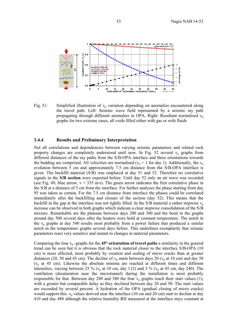
53 Nagra NAB 14-53
Fig. 51: Simplified illustration of vp variation depending on anomalies encountered along the travel path. Left: Seismic wave field represented by a seismic ray path propagating through different anomalies in OPA. Right: Resultant normalised vp graphs for two extreme cases, all voids filled either with gas or with fluids
3.4.4 Results and Preliminary Interpretation Not all correlations and dependencies between varying seismic parameters and related rock property changes are completely understood until now. In Fig. 52 several vp graphs from different distances of the ray paths from the S/B-OPA interface and three orientations towards the bedding are comprised. All velocities are normalised (vp = 1 for day 1). Additionally, the vp evolution between 5 cm and approximately 7.5 cm distance from the S/B-OPA interface is given. The backfill material (S/B) was emplaced at day 51 and 52. Therefore no correlative signals in the S/B section were expected before. Until day 52 only an air wave was recorded (see Fig. 49, blue arrow, v = 335 m/s). The green arrow indicates the first correlative phase in the S/B at a distance of 5 cm from the interface. For further analyses the phase starting from day 95 was taken as certain. For the 7.5 cm distance from interface the phases could be correlated immediately after the backfilling and closure of the section (day 52). This means that the backfill in the gap at the interface was not tightly filled. In the S/B material a rather stepwise vp increase can be observed in both graphs which indicate a clear stepwise consolidation of the S/B mixture. Remarkable are the plateaus between days 200 and 300 and the bend in the graphs around day 500 several days after the heaters were hold at constant temperature. The notch in the vp graphs at day 540 results most probably from a power failure that produced a similar notch in the temperature graphs several days before. This underlines exemplarily that seismic parameters react very sensitive and instant to changes in material parameters.
Comparing the four vp -graphs for the 45° orientation of travel paths a similarity in the general trend can be seen but it is obvious that the rock material closer to the interface S/B-OPA (10 cm) is more affected, most probably by creation and sealing of micro cracks than at greater distances (20, 30 and 45 cm). The decline of vp starts between days 20 (vp at 10 cm) and day 50 (vp at 45 cm). Likewise the absolute minima are reached at different times and different intensities, varying between 25 % (vp at 10 cm, day 112) and 3 % (vp at 45 cm, day 240). The ventilation (desaturation near the microtunnel) during the installation is most probably responsible for that. Between day 280 and 380 the four vp graphs reach their start values (1), with a greater but comparable delay as they declined between day 20 and 50. The start values are exceeded by several percent. A hydration of the OPA (gradual closing of micro cracks) would support this. vp values derived near the interface (10 cm and 20 cm) start to decline at day 410 and day 480 although the relative humidity RH measured at the interface stays constant at
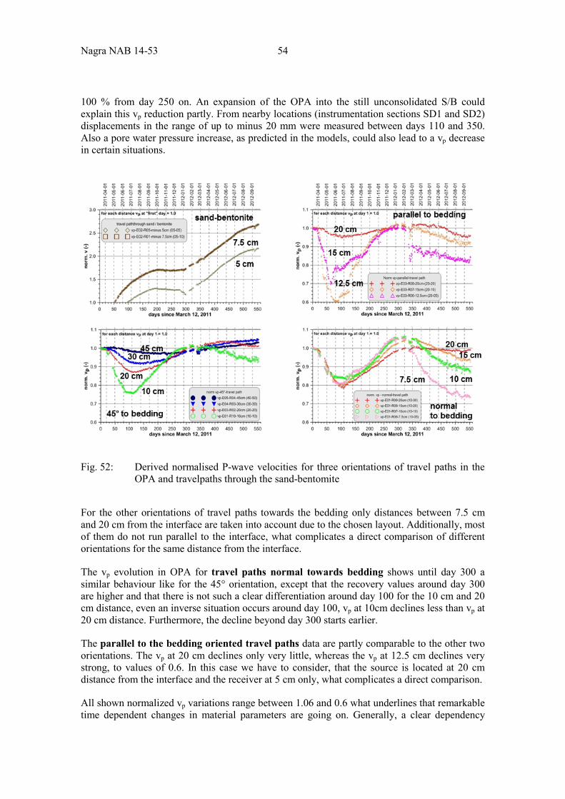
Nagra NAB 14-53 54
100 % from day 250 on. An expansion of the OPA into the still unconsolidated S/B could explain this vp reduction partly. From nearby locations (instrumentation sections SD1 and SD2) displacements in the range of up to minus 20 mm were measured between days 110 and 350. Also a pore water pressure increase, as predicted in the models, could also lead to a vp decrease in certain situations.
Fig. 52: Derived normalised P-wave velocities for three orientations of travel paths in the OPA and travelpaths through the sand-bentomite
For the other orientations of travel paths towards the bedding only distances between 7.5 cm and 20 cm from the interface are taken into account due to the chosen layout. Additionally, most of them do not run parallel to the interface, what complicates a direct comparison of different orientations for the same distance from the interface.
The vp evolution in OPA for travel paths normal towards bedding shows until day 300 a similar behaviour like for the 45° orientation, except that the recovery values around day 300 are higher and that there is not such a clear differentiation around day 100 for the 10 cm and 20 cm distance, even an inverse situation occurs around day 100, vp at 10cm declines less than vp at 20 cm distance. Furthermore, the decline beyond day 300 starts earlier.
The parallel to the bedding oriented travel paths data are partly comparable to the other two orientations. The vp at 20 cm declines only very little, whereas the vp at 12.5 cm declines very strong, to values of 0.6. In this case we have to consider, that the source is located at 20 cm distance from the interface and the receiver at 5 cm only, what complicates a direct comparison.
All shown normalized vp variations range between 1.06 and 0.6 what underlines that remarkable time dependent changes in material parameters are going on. Generally, a clear dependency

55 Nagra NAB 14-53
between the intensity of seismic parameter changes and the distance from the interface S/B-OPA can be seen in all results. For shorter distances the variations are more pronounced than for greater distances. Furthermore, it is worth mentioning that several tens of days after the vp in the S/B starts to rise (day 300), the vp for the short distances in the OPA start to decline. It seems that a "pulse" is entering the rock, and at later stages coming from the rock, but with a distinctive dependency from the orientation to the bedding (anisotropy of OPA). Which driving forces (thermal impact, vapour pressure, degree of saturation) generate this "pulse" and what process interactions define its origin needs further attention. It is shown however that seismic monitoring is a useful tool for the characterisation of continuously ongoing changes of rock properties.

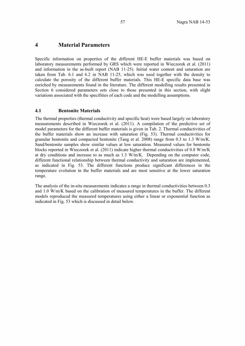
57 Nagra NAB 14-53
4 Material Parameters Specific information on properties of the different HE-E buffer materials was based on laboratory measurements performed by GRS which were reported in Wieczorek et al. (2011) and information in the as-built report (NAB 11-25). Initial water content and saturation are taken from Tab. 6.1 and 6.2 in NAB 11-25, which was used together with the density to calculate the porosity of the different buffer materials. This HE-E specific data base was enriched by measurements found in the literature. The different modelling results presented in Section 6 considered parameters sets close to those presented in this section, with slight variations associated with the specifities of each code and the modelling assumptions.
4.1 Bentonite Materials The thermal properties (thermal conductivity and specific heat) were based largely on laboratory measurements described in Wieczorek et al. (2011). A compilation of the predictive set of model parameters for the different buffer materials is given in Tab. 2. Thermal conductivities of the buffer materials show an increase with saturation (Fig. 53). Thermal conductivities for granular bentonite and compacted bentonite (Tang et al. 2008) range from 0.3 to 1.3 W/m/K. Sand/bentonite samples show similar values at low saturation. Measured values for bentonite blocks reported in Wieczorek et al. (2011) indicate higher thermal conductivities of 0.8 W/m/K at dry conditions and increase to as much as 1.3 W/m/K. Depending on the computer code, different functional relationship between thermal conductivity and saturation are implemented, as indicated in Fig. 53. The different functions produce significant differences in the temperature evolution in the buffer materials and are most sensitive at the lower saturation range.
The analysis of the in-situ measurements indicates a range in thermal conductivities between 0.3 and 1.0 W/m/K based on the calibration of measured temperatures in the buffer. The different models reproduced the measured temperatures using either a linear or exponential function as indicated in Fig. 53 which is discussed in detail below.
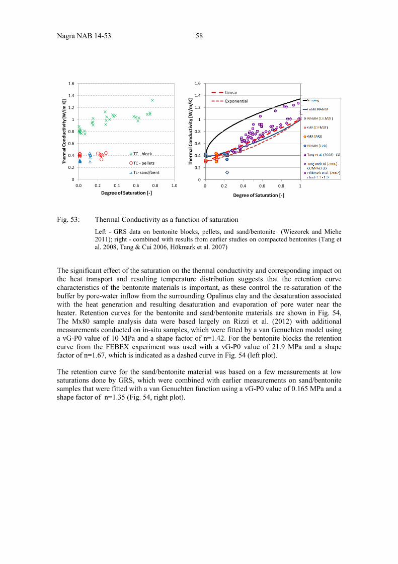
Nagra NAB 14-53 58
Fig. 53: Thermal Conductivity as a function of saturation Left - GRS data on bentonite blocks, pellets, and sand/bentonite (Wiezorek and Miehe 2011); right - combined with results from earlier studies on compacted bentonites (Tang et al. 2008, Tang & Cui 2006, Hökmark et al. 2007)
The significant effect of the saturation on the thermal conductivity and corresponding impact on the heat transport and resulting temperature distribution suggests that the retention curve characteristics of the bentonite materials is important, as these control the re-saturation of the buffer by pore-water inflow from the surrounding Opalinus clay and the desaturation associated with the heat generation and resulting desaturation and evaporation of pore water near the heater. Retention curves for the bentonite and sand/bentonite materials are shown in Fig. 54, The Mx80 sample analysis data were based largely on Rizzi et al. (2012) with additional measurements conducted on in-situ samples, which were fitted by a van Genuchten model using a vG-P0 value of 10 MPa and a shape factor of n=1.42. For the bentonite blocks the retention curve from the FEBEX experiment was used with a vG-P0 value of 21.9 MPa and a shape factor of n=1.67, which is indicated as a dashed curve in Fig. 54 (left plot).
The retention curve for the sand/bentonite material was based on a few measurements at low saturations done by GRS, which were combined with earlier measurements on sand/bentonite samples that were fitted with a van Genuchten function using a vG-P0 value of 0.165 MPa and a shape factor of n=1.35 (Fig. 54, right plot).
0
0.2
0.4
0.6
0.8
1
1.2
1.4
1.6
0 0.2 0.4 0.6 0.8 1Th
erm
al C
ondu
ctiv
ity [W
/m/K
]Degree of Saturation [-]
Linear
Exponential
0
0.2
0.4
0.6
0.8
1
1.2
1.4
1.6
0.0 0.2 0.4 0.6 0.8 1.0
Ther
mal
Con
duct
ivity
[W/(
m K
)]
Degree of Saturation [-]
TC - block
TC - pellets
Tc- sand/bent
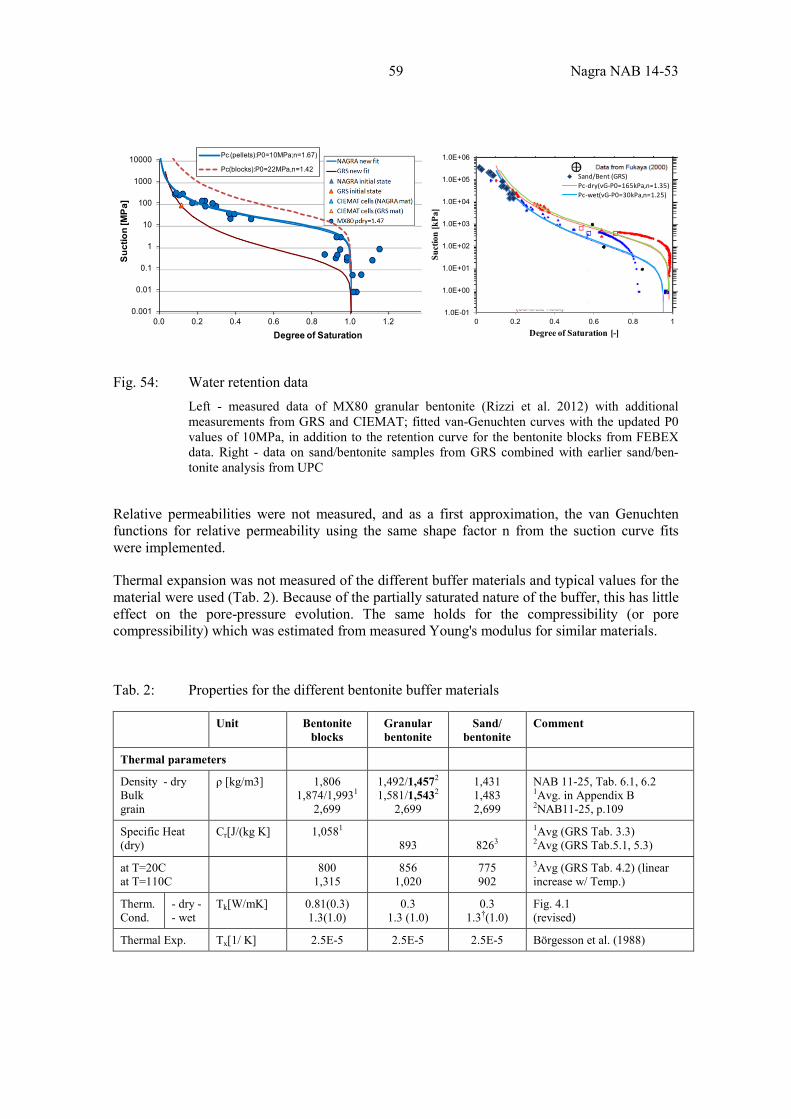
59 Nagra NAB 14-53
Fig. 54: Water retention data Left - measured data of MX80 granular bentonite (Rizzi et al. 2012) with additional measurements from GRS and CIEMAT; fitted van-Genuchten curves with the updated P0 values of 10MPa, in addition to the retention curve for the bentonite blocks from FEBEX data. Right - data on sand/bentonite samples from GRS combined with earlier sand/ben-tonite analysis from UPC
Relative permeabilities were not measured, and as a first approximation, the van Genuchten functions for relative permeability using the same shape factor n from the suction curve fits were implemented.
Thermal expansion was not measured of the different buffer materials and typical values for the material were used (Tab. 2). Because of the partially saturated nature of the buffer, this has little effect on the pore-pressure evolution. The same holds for the compressibility (or pore compressibility) which was estimated from measured Young's modulus for similar materials.
Tab. 2: Properties for the different bentonite buffer materials
Unit Bentonite blocks
Granular bentonite
Sand/ bentonite
Comment
Thermal parameters
Density - dry Bulk grain
ρ [kg/m3] 1,806 1,874/1,9931
2,699
1,492/1,4572
1,581/1,5432
2,699
1,431 1,483 2,699
NAB 11-25, Tab. 6.1, 6.2 1Avg. in Appendix B 2NAB11-25, p.109
Specific Heat (dry)
Cr[J/(kg K] 1,0581
893
8263
1Avg (GRS Tab. 3.3) 2Avg (GRS Tab.5.1, 5.3)
at T=20C at T=110C
800 1,315
856 1,020
775 902
3Avg (GRS Tab. 4.2) (linear increase w/ Temp.)
Therm. Cond.
- dry - - wet
Tk[W/mK] 0.81(0.3) 1.3(1.0)
0.3 1.3 (1.0)
0.3 1.3†(1.0)
Fig. 4.1 (revised)
Thermal Exp. Tx[1/ K] 2.5E-5 2.5E-5 2.5E-5 Börgesson et al. (1988)
0.001
0.01
0.1
1
10
100
1000
10000
0.0 0.2 0.4 0.6 0.8 1.0 1.2
Suc
tion
[MP
a]
Degree of Saturation
Pc (pellets):P0=10MPa;n=1.67)
Pc(blocks):P0=22MPa,n=1.42
1.0E-01
1.0E+00
1.0E+01
1.0E+02
1.0E+03
1.0E+04
1.0E+05
1.0E+06
0 0.2 0.4 0.6 0.8 1
Suct
ion
[kPa
]
Degree of Saturation [-]
Sand/Bent (GRS)Pc-dry(vG-P0=165kPa,n=1.35)Pc-wet(vG-P0=30kPa,n=1.25)
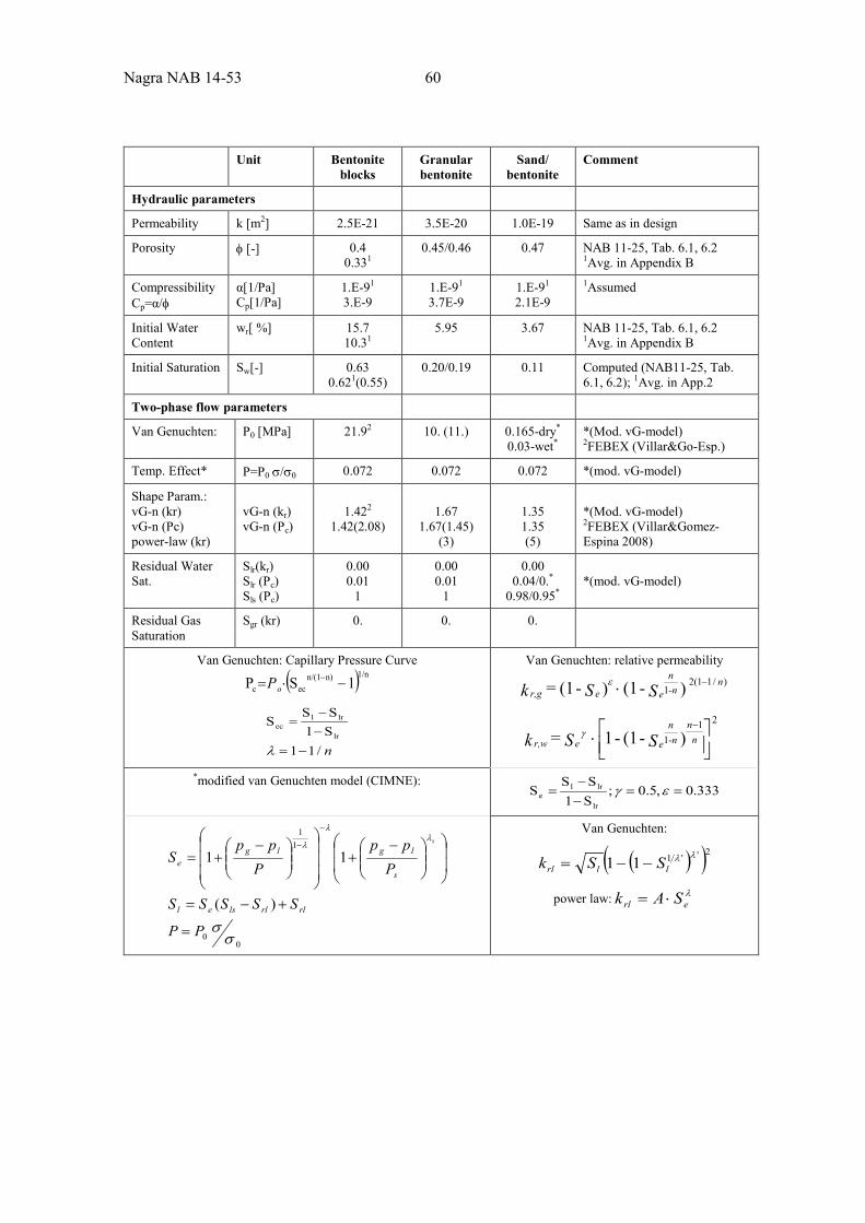
Nagra NAB 14-53 60
Unit Bentonite blocks
Granular bentonite
Sand/ bentonite
Comment
Hydraulic parameters
Permeability k [m2] 2.5E-21 3.5E-20 1.0E-19 Same as in design
Porosity φ [-] 0.4 0.331
0.45/0.46 0.47 NAB 11-25, Tab. 6.1, 6.2 1Avg. in Appendix B
Compressibility Cp=α/φ
α[1/Pa] Cp[1/Pa]
1.E-91
3.E-9 1.E-91 3.7E-9
1.E-91
2.1E-9 1Assumed
Initial Water Content
wr[ %] 15.7 10.31
5.95
3.67
NAB 11-25, Tab. 6.1, 6.2 1Avg. in Appendix B
Initial Saturation Sw[-] 0.63 0.621(0.55)
0.20/0.19
0.11
Computed (NAB11-25, Tab. 6.1, 6.2); 1Avg. in App.2
Two-phase flow parameters
Van Genuchten: P0 [MPa] 21.92
10. (11.)
0.165-dry* 0.03-wet*
*(Mod. vG-model) 2FEBEX (Villar&Go-Esp.)
Temp. Effect* P=P0 σ/σ0 0.072 0.072 0.072 *(mod. vG-model)
Shape Param.: vG-n (kr) vG-n (Pc) power-law (kr)
vG-n (kr) vG-n (Pc)
1.422
1.42(2.08)
1.67
1.67(1.45) (3)
1.35 1.35 (5)
*(Mod. vG-model) 2FEBEX (Villar&Gomez-Espina 2008)
Residual Water Sat.
Slr(kr) Slr (Pc) Sls (Pc)
0.00 0.01
1
0.00 0.01
1
0.00 0.04/0.*
0.98/0.95*
*(mod. vG-model)
Residual Gas Saturation
Sgr (kr) 0. 0. 0.
Van Genuchten: Capillary Pressure Curve
( )1/nn)n/(1ecc 1SP −⋅= −
oP
n/11S1SS
Slr
lrlec
−=−−
=
λ
Van Genuchten: relative permeability
*modified van Genuchten model (CIMNE):
333.0,5.0;S1SS
Slr
lrle ==
−−
= εγ
00
11
)(
11
σσ
λλ
λ
PP
SSSSS
Ppp
Ppp
S
rlrllsel
s
lglge
s
=
+−=
−+
−+=
−
−
Van Genuchten:
( )( )2''111 λλllrl SSk −−=
power law: λerl SAk ⋅=
)-(1 )-(1 = )/112( 1
ne -n
n
er,g SSk −⋅ε
)-(1-1 = 21
1
⋅
−n
n
e -nn
er,w SSk γ
61 Nagra NAB 14-53
4.2 Opalinus Clay The parameters for Opalinus clay differentiate between intact Opalinus Clay and an excavation disturbed zone (EDZ).
The potential EDZ was found important for establishing the initial saturation and pressure conditions in the vicinity of the micro-tunnel. For the temperature evolution as a function of distance from the micro-tunnel, the thermal conductivity and specific heat (thermal diffusivity) are the main parameters. Thermal expansion of the pore water and rock together with the hydraulic and two-phase properties (effective permeability and compressibility) control the pore-pressure development in Opalinus clay. The parameters are summarized in Tab. 3. The parameter values for thermal expansion were taken from previous laboratory analysis associated with the TIDOMAZ project (Zhang and Rothfuchs 2007). Furthermore, the range in thermal conductivity associated with the anisotropy for calibrated thermal conductivities parallel and perpendicular to bedding is given, derived from results of the HE-D experiment (Wileveau and Rothfuchts (2007, TN 2006-01). The reported range was also attributed to facies variations with the silty clay facies having higher thermal conductivity.
The updated two-phase parameters for the Opalinus Clay were based on laboratory analyses of Opalinus clay samples from Mt. Terri performed by UPC (Romero et al. 2012) and by EPFL (Ferrari et al. 2012). The fitted curve with the same van Genuchten parameters as before, which reproduced the updated data reasonably will, except at high saturation which suggests a more gradual, near linear decrease in suction (Fig. 55).
The important parameters affecting the pressure buildup in the Opalinus clay are the thermal expansion of the grains and rock mass compared to the expansion of the pore water. The simulations produced significant differences in the magnitude of pressure buildup by the different modelling teams, primarily related to the thermal expansion. The compressibility (or pore compressibility) was similar, only the treatment of the expansion of the rock grain and rock framework. The TOUGH2 model only considers the pore expansivity (rock framework) whereas the fully coupled geomechanical model considered both the expansivity of the grains as well as the rock framework.
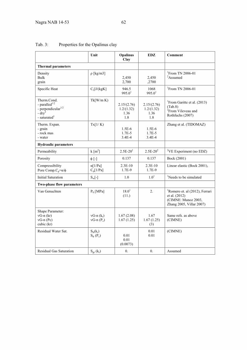
Nagra NAB 14-53 62
Tab. 3: Properties for the Opalinus clay
Unit Opalinus Clay
EDZ Comment
Thermal parameters
Density Bulk grain
ρ [kg/m3] 2,450
2,700
2,450
,2700
1From TN 2006-01 2Assumed
Specific Heat Cr[J/(kgK] 946.5 995.01
1068 995.01
1From TN 2006-01
Therm.Cond. - paralled1/2
- perpendicular1/2 - dry2
- saturated1
Tk[W/m K) 2.15/(2.76) 1.2/(1.32)
1.36 1.8
2.15/(2.76) 1.2/(1.32)
1.36 1.8
1From Garitte et al. (2013) (Tab.8) 2From Vileveau and Rothfuchs (2007)
Therm. Expan. - grain - rock mas - water
Tx[1/ K) 1.5E-6 1.7E-5 3.4E-4
1.5E-6 1.7E-5 3.4E-4
Zhang et al. (TIDOMAZ)
Hydraulic parameters
Permeability k [m2] 2.5E-201 2.5E-202 2VE Experiment (no EDZ)
Porosity φ [-] 0.137 0.137 Bock (2001)
Compressibility Pore Comp.Cp=α/φ
α[1/Pa] Cp[1/Pa]
2.3E-10 1.7E-9
2.3E-10 1.7E-9
Linear elastic (Bock 2001),
Initial Saturation Sw[-] 1.0 1.01 1Needs to be simulated
Two-phase flow parameters
Van Genuchten P0 [MPa] 18.01
(11.) 2. 1Romero et. al (2012), Ferrari
et al. (2012) (CIMNE: Munoz 2003, Zhang 2005, Villar 2007)
Shape Parameter: vG-n (kr) vG-n (Pc) cubic (kr)
vG-n (kr) vG-n (Pc)
1.67 (2.08) 1.67 (1.25)
1.67
1.67 (1.25) (3)
Same refs. as above (CIMNE)
Residual Water Sat. Slr(kr) Slr (Pc)
0.01 0.01
(0.0073)
0.01 0.01
(CIMNE)
Residual Gas Saturation Sgr (kr) 0. 0. Assumed
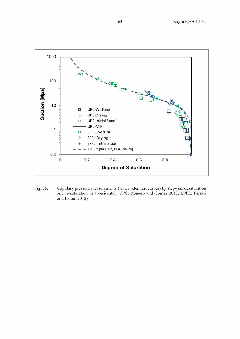
63 Nagra NAB 14-53
Fig. 55: Capillary pressure measurements (water retention curves) by stepwise desaturation and re-saturation in a desiccator (UPC: Romero and Gomez 2013; EPFL: Ferrari and Laloui 2012)
0.1
1
10
100
1000
0 0.2 0.4 0.6 0.8 1
Suct
ion
[Mpa
]
Degree of Saturation
UPC-WettingUPC-DryingUPC-Initial StateUPC-MIPEPFL-WettingEPFL-DryingEPFL-Initial State'Pc-Fit (n=1.67, P0=18MPa)
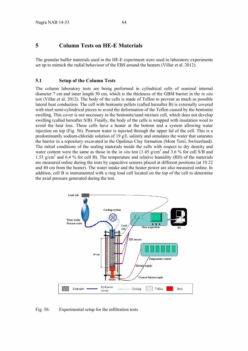
Nagra NAB 14-53 64
5 Column Tests on HE-E Materials The granular buffer materials used in the HE-E experiment were used in laboratory experiments set up to mimick the radial behaviour of the EBS around the heaters (Villar et al. 2012).
5.1 Setup of the Column Tests The column laboratory tests are being performed in cylindrical cells of nominal internal diameter 7 cm and inner length 50 cm, which is the thickness of the GBM barrier in the in situ test (Villar et al. 2012). The body of the cells is made of Teflon to prevent as much as possible lateral heat conduction. The cell with bentonite pellets (called hereafter B) is externally covered with steel semi-cylindrical pieces to avoid the deformation of the Teflon caused by the bentonite swelling. This cover is not necessary in the bentonite/sand mixture cell, which does not develop swelling (called hereafter S/B). Finally, the body of the cells is wrapped with insulation wool to avoid the heat loss. These cells have a heater at the bottom and a system allowing water injection on top (Fig. 56). Pearson water is injected through the upper lid of the cell. This is a predominantly sodium-chloride solution of 19 g/L salinity and simulates the water that saturates the barrier in a repository excavated in the Opalinus Clay formation (Mont Terri, Switzerland). The initial conditions of the sealing materials inside the cells with respect to dry density and water content were the same as those in the in situ test (1.45 g/cm3 and 3.6 % for cell S/B and 1.53 g/cm3 and 6.4 % for cell B). The temperature and relative humidity (RH) of the materials are measured online during the tests by capacitive sensors placed at different positions (at 10 22 and 40 cm from the heater). The water intake and the heater power are also measured online. In addition, cell B is instrumented with a ring load cell located on the top of the cell to determine the axial pressure generated during the test.
Fig. 56: Experimental setup for the infiltration tests
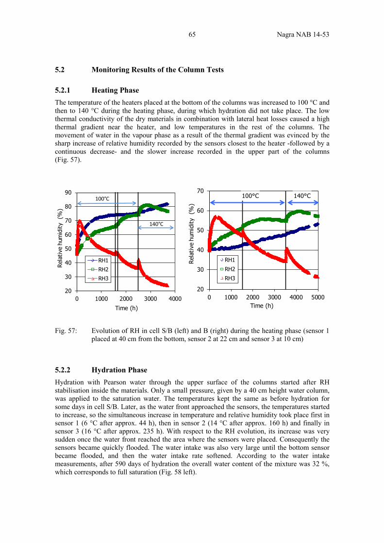
65 Nagra NAB 14-53
5.2 Monitoring Results of the Column Tests
5.2.1 Heating Phase The temperature of the heaters placed at the bottom of the columns was increased to 100 °C and then to 140 °C during the heating phase, during which hydration did not take place. The low thermal conductivity of the dry materials in combination with lateral heat losses caused a high thermal gradient near the heater, and low temperatures in the rest of the columns. The movement of water in the vapour phase as a result of the thermal gradient was evinced by the sharp increase of relative humidity recorded by the sensors closest to the heater -followed by a continuous decrease- and the slower increase recorded in the upper part of the columns (Fig. 57).
Fig. 57: Evolution of RH in cell S/B (left) and B (right) during the heating phase (sensor 1 placed at 40 cm from the bottom, sensor 2 at 22 cm and sensor 3 at 10 cm)
5.2.2 Hydration Phase Hydration with Pearson water through the upper surface of the columns started after RH stabilisation inside the materials. Only a small pressure, given by a 40 cm height water column, was applied to the saturation water. The temperatures kept the same as before hydration for some days in cell S/B. Later, as the water front approached the sensors, the temperatures started to increase, so the simultaneous increase in temperature and relative humidity took place first in sensor 1 (6 °C after approx. 44 h), then in sensor 2 (14 °C after approx. 160 h) and finally in sensor 3 (16 °C after approx. 235 h). With respect to the RH evolution, its increase was very sudden once the water front reached the area where the sensors were placed. Consequently the sensors became quickly flooded. The water intake was also very large until the bottom sensor became flooded, and then the water intake rate softened. According to the water intake measurements, after 590 days of hydration the overall water content of the mixture was 32 %, which corresponds to full saturation (Fig. 58 left).
20
30
40
50
60
70
80
90
0 1000 2000 3000 4000
Rela
tive
hum
idity
(%
)
Time (h)
RH1
RH2
RH3
100°C
140°C
20
30
40
50
60
70
0 1000 2000 3000 4000 5000
Rela
tive
hum
idity
(%
)
Time (h)
RH1
RH2
RH3
100°C 140°C
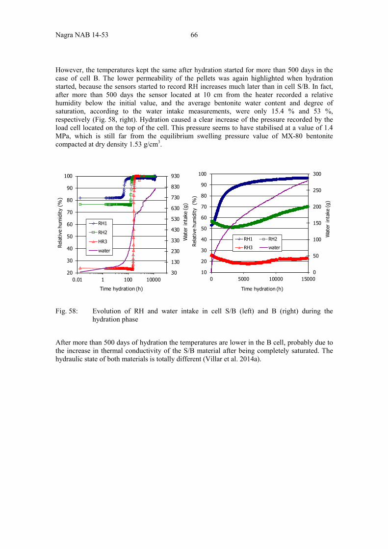
Nagra NAB 14-53 66
However, the temperatures kept the same after hydration started for more than 500 days in the case of cell B. The lower permeability of the pellets was again highlighted when hydration started, because the sensors started to record RH increases much later than in cell S/B. In fact, after more than 500 days the sensor located at 10 cm from the heater recorded a relative humidity below the initial value, and the average bentonite water content and degree of saturation, according to the water intake measurements, were only 15.4 % and 53 %, respectively (Fig. 58, right). Hydration caused a clear increase of the pressure recorded by the load cell located on the top of the cell. This pressure seems to have stabilised at a value of 1.4 MPa, which is still far from the equilibrium swelling pressure value of MX-80 bentonite compacted at dry density 1.53 g/cm3.
Fig. 58: Evolution of RH and water intake in cell S/B (left) and B (right) during the hydration phase
After more than 500 days of hydration the temperatures are lower in the B cell, probably due to the increase in thermal conductivity of the S/B material after being completely saturated. The hydraulic state of both materials is totally different (Villar et al. 2014a).
30
130
230
330
430
530
630
730
830
930
20
30
40
50
60
70
80
90
100
0.01 1 100 10000
Wat
er in
take
(g)
Rela
tive
hum
idity
(%
)
Time hydration (h)
RH1
RH2
HR3
water
0
50
100
150
200
250
300
10
20
30
40
50
60
70
80
90
100
0 5000 10000 15000
Wat
er in
take
(g)
Rela
tive
hum
idity
(%
)
Time hydration (h)
RH1 RH2
RH3 water
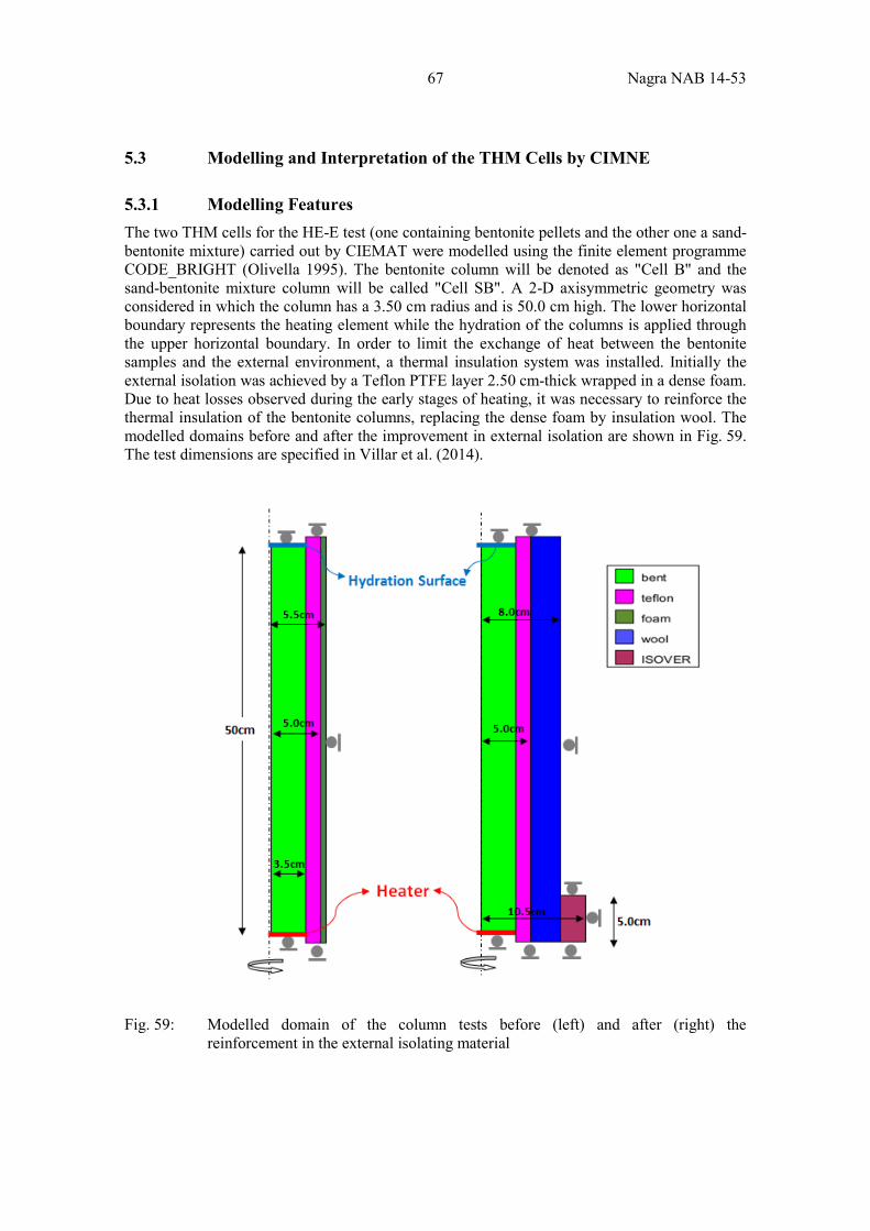
67 Nagra NAB 14-53
5.3 Modelling and Interpretation of the THM Cells by CIMNE
5.3.1 Modelling Features The two THM cells for the HE-E test (one containing bentonite pellets and the other one a sand-bentonite mixture) carried out by CIEMAT were modelled using the finite element programme CODE_BRIGHT (Olivella 1995). The bentonite column will be denoted as "Cell B" and the sand-bentonite mixture column will be called "Cell SB". A 2-D axisymmetric geometry was considered in which the column has a 3.50 cm radius and is 50.0 cm high. The lower horizontal boundary represents the heating element while the hydration of the columns is applied through the upper horizontal boundary. In order to limit the exchange of heat between the bentonite samples and the external environment, a thermal insulation system was installed. Initially the external isolation was achieved by a Teflon PTFE layer 2.50 cm-thick wrapped in a dense foam. Due to heat losses observed during the early stages of heating, it was necessary to reinforce the thermal insulation of the bentonite columns, replacing the dense foam by insulation wool. The modelled domains before and after the improvement in external isolation are shown in Fig. 59. The test dimensions are specified in Villar et al. (2014).
Fig. 59: Modelled domain of the column tests before (left) and after (right) the reinforcement in the external isolating material
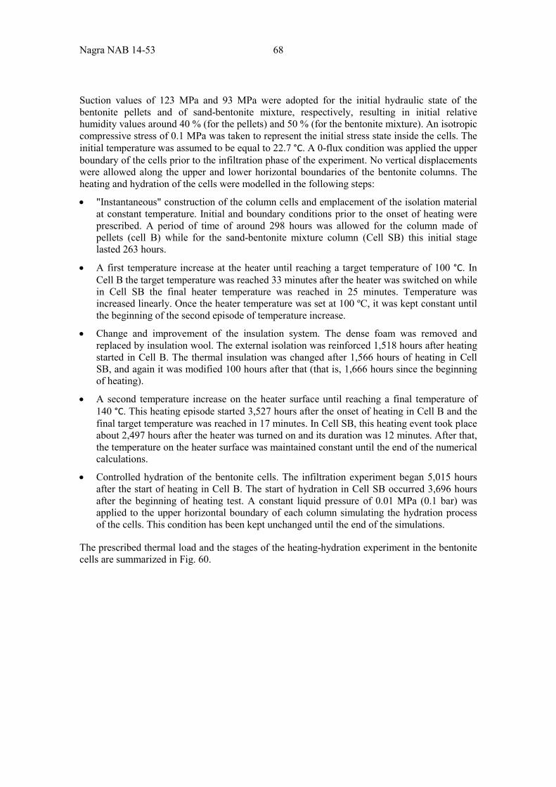
Nagra NAB 14-53 68
Suction values of 123 MPa and 93 MPa were adopted for the initial hydraulic state of the bentonite pellets and of sand-bentonite mixture, respectively, resulting in initial relative humidity values around 40 % (for the pellets) and 50 % (for the bentonite mixture). An isotropic compressive stress of 0.1 MPa was taken to represent the initial stress state inside the cells. The initial temperature was assumed to be equal to 22.7 °C. A 0-flux condition was applied the upper boundary of the cells prior to the infiltration phase of the experiment. No vertical displacements were allowed along the upper and lower horizontal boundaries of the bentonite columns. The heating and hydration of the cells were modelled in the following steps:
• "Instantaneous" construction of the column cells and emplacement of the isolation material at constant temperature. Initial and boundary conditions prior to the onset of heating were prescribed. A period of time of around 298 hours was allowed for the column made of pellets (cell B) while for the sand-bentonite mixture column (Cell SB) this initial stage lasted 263 hours.
• A first temperature increase at the heater until reaching a target temperature of 100 °C. In Cell B the target temperature was reached 33 minutes after the heater was switched on while in Cell SB the final heater temperature was reached in 25 minutes. Temperature was increased linearly. Once the heater temperature was set at 100 ºC, it was kept constant until the beginning of the second episode of temperature increase.
• Change and improvement of the insulation system. The dense foam was removed and replaced by insulation wool. The external isolation was reinforced 1,518 hours after heating started in Cell B. The thermal insulation was changed after 1,566 hours of heating in Cell SB, and again it was modified 100 hours after that (that is, 1,666 hours since the beginning of heating).
• A second temperature increase on the heater surface until reaching a final temperature of 140 °C. This heating episode started 3,527 hours after the onset of heating in Cell B and the final target temperature was reached in 17 minutes. In Cell SB, this heating event took place about 2,497 hours after the heater was turned on and its duration was 12 minutes. After that, the temperature on the heater surface was maintained constant until the end of the numerical calculations.
• Controlled hydration of the bentonite cells. The infiltration experiment began 5,015 hours after the start of heating in Cell B. The start of hydration in Cell SB occurred 3,696 hours after the beginning of heating test. A constant liquid pressure of 0.01 MPa (0.1 bar) was applied to the upper horizontal boundary of each column simulating the hydration process of the cells. This condition has been kept unchanged until the end of the simulations.
The prescribed thermal load and the stages of the heating-hydration experiment in the bentonite cells are summarized in Fig. 60.
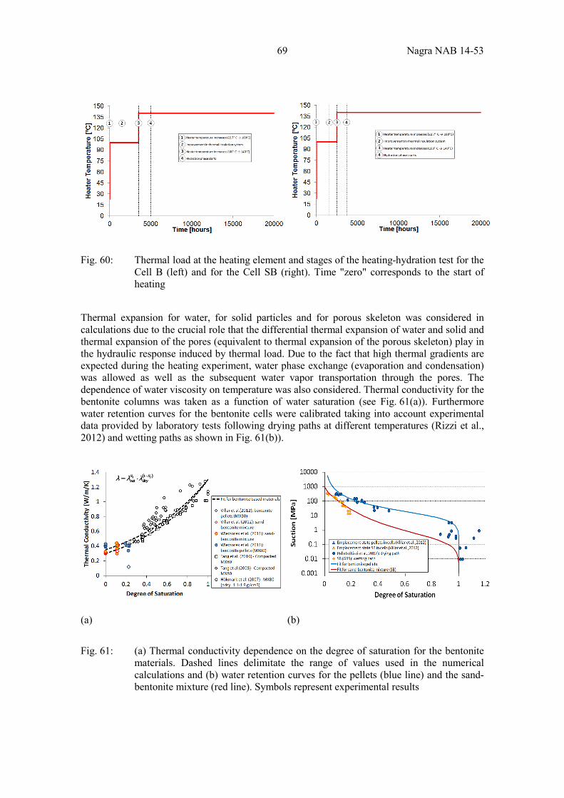
69 Nagra NAB 14-53
Fig. 60: Thermal load at the heating element and stages of the heating-hydration test for the Cell B (left) and for the Cell SB (right). Time "zero" corresponds to the start of heating
Thermal expansion for water, for solid particles and for porous skeleton was considered in calculations due to the crucial role that the differential thermal expansion of water and solid and thermal expansion of the pores (equivalent to thermal expansion of the porous skeleton) play in the hydraulic response induced by thermal load. Due to the fact that high thermal gradients are expected during the heating experiment, water phase exchange (evaporation and condensation) was allowed as well as the subsequent water vapor transportation through the pores. The dependence of water viscosity on temperature was also considered. Thermal conductivity for the bentonite columns was taken as a function of water saturation (see Fig. 61(a)). Furthermore water retention curves for the bentonite cells were calibrated taking into account experimental data provided by laboratory tests following drying paths at different temperatures (Rizzi et al., 2012) and wetting paths as shown in Fig. 61(b)).
(a) (b)
Fig. 61: (a) Thermal conductivity dependence on the degree of saturation for the bentonite materials. Dashed lines delimitate the range of values used in the numerical calculations and (b) water retention curves for the pellets (blue line) and the sand-bentonite mixture (red line). Symbols represent experimental results
Nagra NAB 14-53 70
Mechanical behavior of the external isolating materials was described by means of elastic models while the mechanical response of bentonite based materials was governed by a thermo-elastoplastic approach for unsaturated soils proposed by Alonso et al. (1990) commonly known as the Barcelona Basic Model (BBM). Mechanical parameters adopted for the bentonite columns were taken from data reported in the FEBEX final report (2000) and experimental information from Hoffman et al. (2007) due to lack of more specific data. Material properties for the bentonite columns were based on the updated HE-E modellers dataset (Gaus, 2013) and the thermal properties for the insulation system were taken from technical tables and notes found in literature. Parameters used in the numerical simulations are summarized in Tab. 4 to 9.
Tab. 4: Physical properties for water in pores
Water densitya
Reference density, ρl0 [kg.m-3] 1002.6
Water compressibility, β [MPa-1] 4.50e-04
Volumetric thermal expansion coefficient (at 40 ºC), α [ ºC-1]
-3.40e-04
Water viscosityb
Pre-exponential parameter, A [MPa.s] 2.10e-12
Exponential parameter, B [K] 1,808.5
a Input parameters for the dependence of water density on temperature: ( ) ( )[ ]TpppT lllll αβρρ +−= 00 exp,
b Input parameters for the dependence of water viscosity on temperature:
( )
+=
TBATl 15.273
expµ
Tab. 5: Physical properties for the bentonite columns and the insulation materials
Physical properties Bentonite pellets
Sand-bentonite mixture
Teflon PTFE
Dense foam Wool
Solid grain density [kg/m3]
2,700 2,700 2,200 2,200 2,200
Solid phase specific heat [J/kg.K]
893 826 1,300 1,400 1,200
Porosity 0.444 0.463 0.05 0.50 0.50
Linear thermal expansion for solid grain [K-1]
2.50e-05 2.50e-05 1.25e-04 5.00e-05 5.00e-05
Linear thermal expansion for the medium [K-1]
2.50e-05 2.50e-05 1.25e-04 5.00e-05 5.00e-05
71 Nagra NAB 14-53
Tab. 6: Thermal parameters for the bentonite materials and the isolation materials
Thermal properties Bentonite pelletsa
Sand-bentonite mixturea
Teflon PTFE
Dense foam Wool
Dry Thermal Conduct., λdry [W/m/K]
0.35 0.35 0.25 0.04 0.04
Saturated Thermal Conduct., λsat [W/m/K]
1.30 1.30 0.25 0.04 0.04
a Dependence of thermal conductivity (λ) on degree of saturation (Sl) through: ( )ll Sdry
Ssat
−⋅= 1λλλ
Tab. 7: Hydraulic parameters for the bentonite materials and the insulation materials
Hydraulic parameters
Bentonite pellets
Sand-bentonite mixture
Teflon PTFE
Dense foam Wool
Retention curvea
P0 [MPa] 10.0 0.20 100 100 100
σ0 [N/m] 7.20e-02 7.20e-02 7.20e-02 7.20e-02 7.20e-02
Shape Parameter, λ'' 0.38 0.24 0.40 0.40 0.40
Pressure related to the suction at full dry state, Pd [MPa]
1.0e27 5.0e03 1.0e27 1.0e27 1.0e27
Shape Parameter, λd 0 15 0 0 0
Residual/maximum water saturation
0.00 - 1.00 0.00 - 1.00 0 0 0
Water permeability
Intrinsec Permeab. [m2]
3.50e-20 1.00e-19* 1.00e-25 1.00e-20 1.00e-20
Shape Parameter, A 1.00b 1.00b - - -
Shape Parameter, λ' 10.0b 9.00b 0.52c 0.52c 0.52c
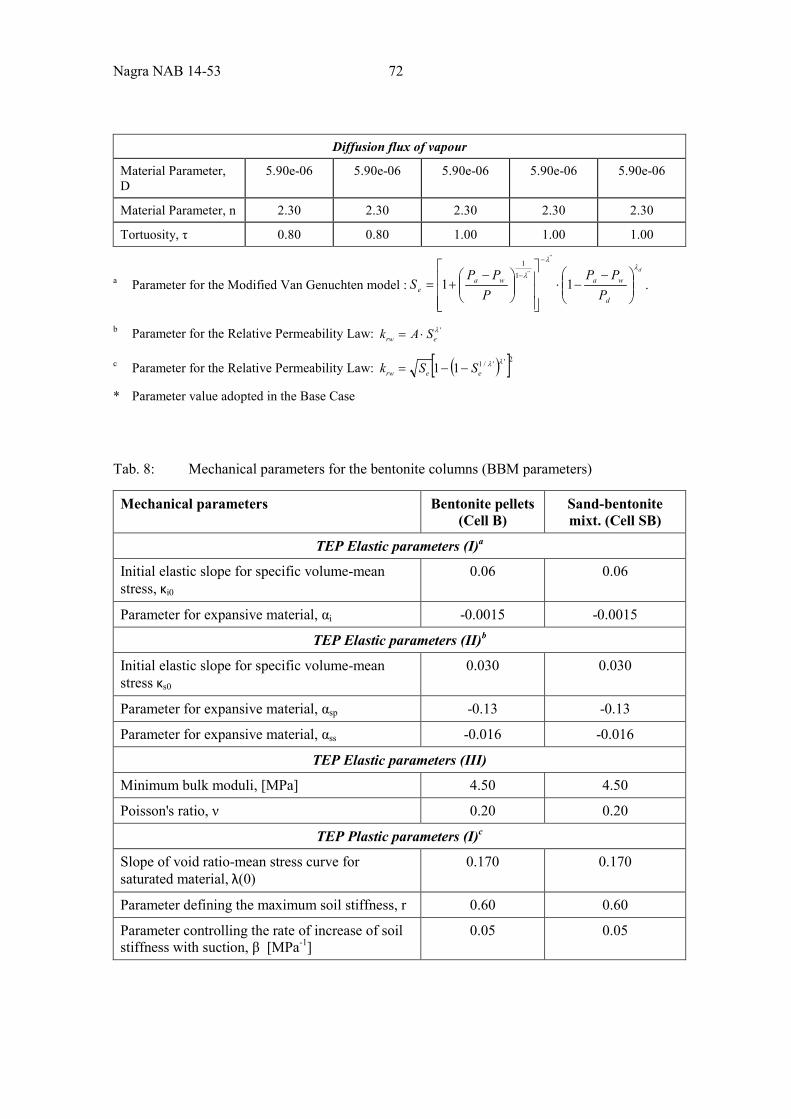
Nagra NAB 14-53 72
Diffusion flux of vapour
Material Parameter, D
5.90e-06 5.90e-06 5.90e-06 5.90e-06 5.90e-06
Material Parameter, n 2.30 2.30 2.30 2.30 2.30
Tortuosity, τ 0.80 0.80 1.00 1.00 1.00
a Parameter for the Modified Van Genuchten model :d
d
wawae P
PPP
PPS
λλ
λ
−−⋅
−+=
−
−11
''
''11
.
b Parameter for the Relative Permeability Law: 'λerw SAk ⋅=
c Parameter for the Relative Permeability Law: ( )[ ]2''/111 λλeerw SSk −−=
* Parameter value adopted in the Base Case
Tab. 8: Mechanical parameters for the bentonite columns (BBM parameters)
Mechanical parameters Bentonite pellets (Cell B)
Sand-bentonite mixt. (Cell SB)
TEP Elastic parameters (I)a
Initial elastic slope for specific volume-mean stress, κi0
0.06 0.06
Parameter for expansive material, αi -0.0015 -0.0015
TEP Elastic parameters (II)b
Initial elastic slope for specific volume-mean stress κs0
0.030 0.030
Parameter for expansive material, αsp -0.13 -0.13
Parameter for expansive material, αss -0.016 -0.016
TEP Elastic parameters (III)
Minimum bulk moduli, [MPa] 4.50 4.50
Poisson's ratio, ν 0.20 0.20
TEP Plastic parameters (I)c
Slope of void ratio-mean stress curve for saturated material, λ(0)
0.170 0.170
Parameter defining the maximum soil stiffness, r 0.60 0.60
Parameter controlling the rate of increase of soil stiffness with suction, β [MPa-1]
0.05 0.05
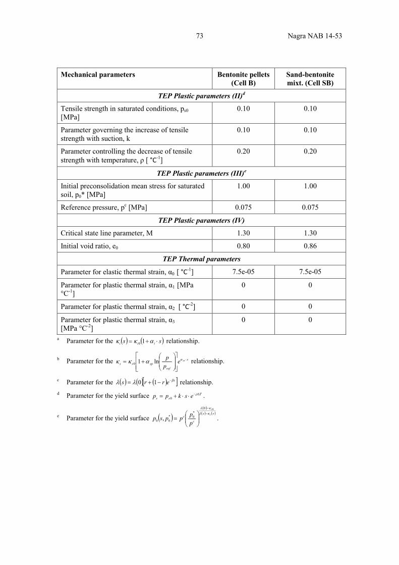
73 Nagra NAB 14-53
Mechanical parameters Bentonite pellets (Cell B)
Sand-bentonite mixt. (Cell SB)
TEP Plastic parameters (II)d
Tensile strength in saturated conditions, ps0 [MPa]
0.10 0.10
Parameter governing the increase of tensile strength with suction, k
0.10 0.10
Parameter controlling the decrease of tensile strength with temperature, ρ [ °C-1]
0.20 0.20
TEP Plastic parameters (III)e
Initial preconsolidation mean stress for saturated soil, p0* [MPa]
1.00 1.00
Reference pressure, pc [MPa] 0.075 0.075
TEP Plastic parameters (IV)
Critical state line parameter, M 1.30 1.30
Initial void ratio, e0 0.80 0.86
TEP Thermal parameters
Parameter for elastic thermal strain, α0 [ °C-1] 7.5e-05 7.5e-05
Parameter for plastic thermal strain, α1 [MPa °C-1]
0 0
Parameter for plastic thermal strain, α2 [ °C-2] 0 0
Parameter for plastic thermal strain, α3 [MPa °C-2]
0 0
a Parameter for the ( ) ( )ss iii ⋅+= ακκ 10 relationship.
b Parameter for the s
refspss
ssepp ⋅
+= αακκ ln10 relationship.
c Parameter for the ( ) ( ) ( )[ ]serrs βλλ −−+= 10 relationship. d Parameter for the yield surface T
ss eskpp ∆−⋅⋅+= ρ0 .
e Parameter for the yield surface ( )( )( ) ( )ss
cc i
i
ppppsp
κλκλ
−
−
=
00*0*
00 , .
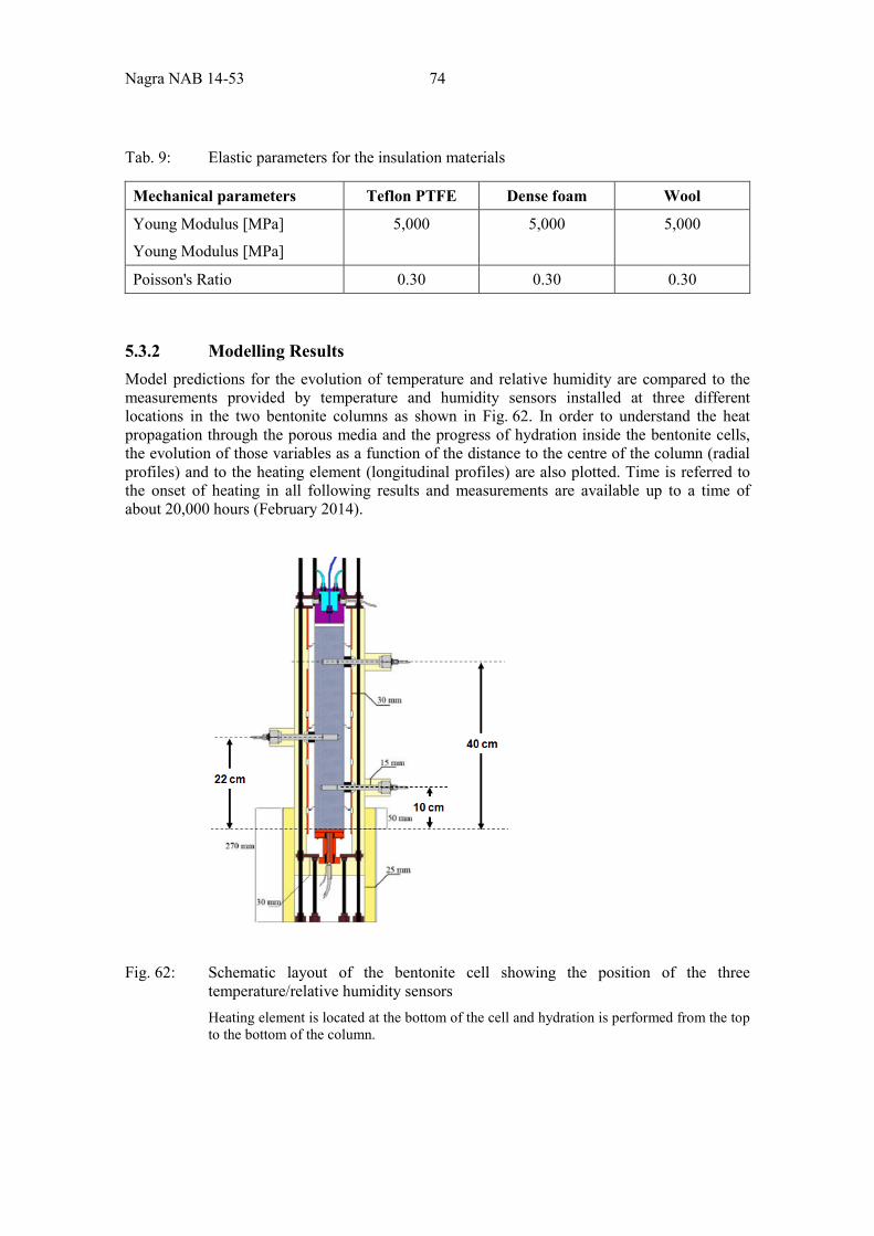
Nagra NAB 14-53 74
Tab. 9: Elastic parameters for the insulation materials
Mechanical parameters Teflon PTFE Dense foam Wool
Young Modulus [MPa]
Young Modulus [MPa]
5,000 5,000 5,000
Poisson's Ratio 0.30 0.30 0.30
5.3.2 Modelling Results Model predictions for the evolution of temperature and relative humidity are compared to the measurements provided by temperature and humidity sensors installed at three different locations in the two bentonite columns as shown in Fig. 62. In order to understand the heat propagation through the porous media and the progress of hydration inside the bentonite cells, the evolution of those variables as a function of the distance to the centre of the column (radial profiles) and to the heating element (longitudinal profiles) are also plotted. Time is referred to the onset of heating in all following results and measurements are available up to a time of about 20,000 hours (February 2014).
Fig. 62: Schematic layout of the bentonite cell showing the position of the three temperature/relative humidity sensors Heating element is located at the bottom of the cell and hydration is performed from the top to the bottom of the column.
75 Nagra NAB 14-53
5.3.2.1 Cell B Temperature and relative humidity evolution inside the Cell B at sensor locations are plotted in Fig. 63 in which the main stages of heating and hydration experiment are also shown. Longitudinal profiles of temperature and humidity through the centre of the bentonite column at different times since the start of heating are depicted in Fig. 64. The evolution of measured thermo-hydraulic variables along some radial profiles of the pellet column at several times is given in Fig. 65. The evolution of the degree of saturation in the centre of the Cell B predicted by the calculations is shown in Fehler! Verweisquelle konnte nicht gefunden werden.. Good agreement is achieved between computed and measured variables especially for the relative humidity sensors and for the temperature sensor closer to the heater. This fact demonstrates the ability of the numerical code used for modelling the whole heating-hydration experiment in a satisfying and realistic manner.
The two temperature increase episodes at the heater and the subsequent temperature evolution due to heat transmission into the Cell B are reproduced quite well by the numerical simulations. However, some discrepancies between measured and numerical results are observed at the sensor T3 (at 10 cm from the heater) immediately after the first increase of heater temperature. Discrepancies in temperature are also found in all sensors after the second episode of temperature increment at the heating element. These differences tend to be more significant as the distance to the heating face increases. The reinforcement of the insulation system 1,518 hours after the start of heating contributes to a further increment in temperature as a result of the reduction of heat losses from the cell experiment to the lab environment. Consequences of the improvement in external isolation are recorded by the three temperature sensors and are also captured by the numerical calculations (see Fig. 63, 64, 65). These heating episodes induce an initial increase in humidity for the RH sensor closer to the heater (sensor RH3). The thermal load applied by the heating element brings about water vapour generation at the bottom part of the pellet column. Condensation takes place close to the top of the bentonite cell where the water vapour (coming from the hot zones by diffusion mechanism) condensates. Vapour condensation leads to an increment of humidity (and consequently, an increase in degree of saturation) at the relatively "colder" zones inside the cell as indicated in the RH measurements and the model predictions for the two sensors farther from the heater (Fig. 63). In contrast, after the first RH increase, degree of saturation decreases near the heater during the heating experiment as recorded by the sensor RH3.
The hydration phase of Cell B starts around 5,015 hours after the beginning of heating experiment. The pellet column hydration is performed at a constant heater temperature of 140 ºC. As the water content inside the cell increases (from the top towards the bottom of the sample), an additional temperature increase is recorded at the sensors. This is a consequence of the coupling between thermal and hydraulic phenomena that take place at this stage of the experiment (Villar et al. 2014). Nevertheless, temperature at the sensor positions obtained by the simulations keeps almost steady during the hydration phase. At the end of the modelling period (20000 hours since the beginning of the heating-hydration test) the zone in the Cell B with degree of saturation values above 95 % extends up to 13 cm from the top of the sample (Fig. 66).
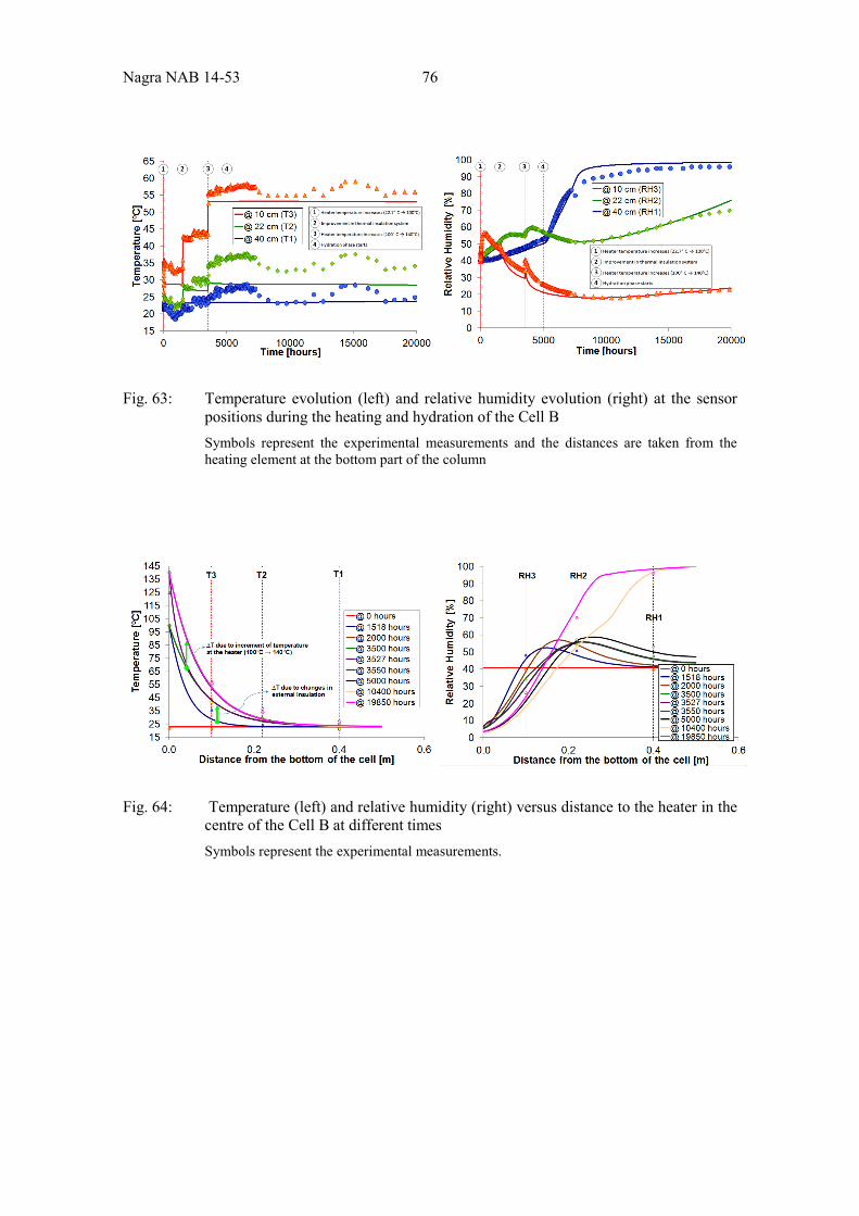
Nagra NAB 14-53 76
Fig. 63: Temperature evolution (left) and relative humidity evolution (right) at the sensor positions during the heating and hydration of the Cell B Symbols represent the experimental measurements and the distances are taken from the heating element at the bottom part of the column
Fig. 64: Temperature (left) and relative humidity (right) versus distance to the heater in the centre of the Cell B at different times Symbols represent the experimental measurements.
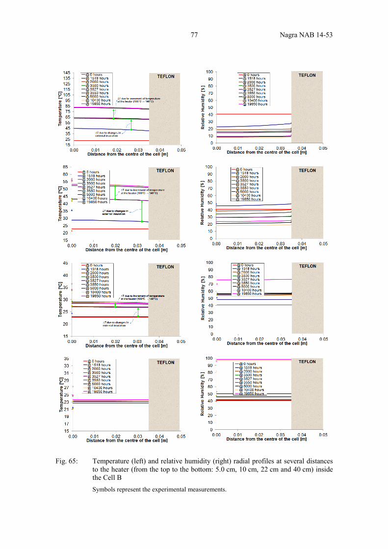
77 Nagra NAB 14-53
Fig. 65: Temperature (left) and relative humidity (right) radial profiles at several distances to the heater (from the top to the bottom: 5.0 cm, 10 cm, 22 cm and 40 cm) inside the Cell B Symbols represent the experimental measurements.
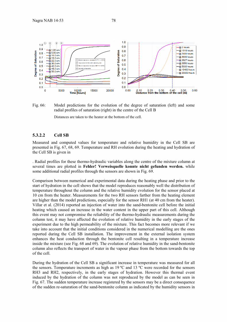
Nagra NAB 14-53 78
Fig. 66: Model predictions for the evolution of the degree of saturation (left) and some radial profiles of saturation (right) in the centre of the Cell B Distances are taken to the heater at the bottom of the cell.
5.3.2.2 Cell SB Measured and computed values for temperature and relative humidity in the Cell SB are presented in Fig. 67, 68, 69. Temperature and RH evolution during the heating and hydration of the Cell SB is given in
. Radial profiles for these thermo-hydraulic variables along the centre of the mixture column at several times are plotted in Fehler! Verweisquelle konnte nicht gefunden werden. while some additional radial profiles through the sensors are shown in Fig. 69.
Comparison between numerical and experimental data during the heating phase and prior to the start of hydration in the cell shows that the model reproduces reasonably well the distribution of temperature throughout the column and the relative humidity evolution for the sensor placed at 10 cm from the heater. Measurements for the two RH sensors farther from the heating element are higher than the model predictions, especially for the sensor RH1 (at 40 cm from the heater). Villar et al. (2014) reported an injection of water into the sand-bentonite cell before the initial heating which caused an increase in the water content in the upper part of this cell. Although this event may not compromise the reliability of the thermo-hydraulic measurements during the column test, it may have affected the evolution of relative humidity in the early stages of the experiment due to the high permeability of the mixture. This fact becomes more relevant if we take into account that the initial conditions considered in the numerical modelling are the ones reported during the Cell SB installation. The improvement in the external isolation system enhances the heat conduction through the bentonite cell resulting in a temperature increase inside the mixture (see Fig. 68 and 69). The evolution of relative humidity in the sand-bentonite column also reflects the transport of water in the vapour phase from the bottom towards the top of the cell.
During the hydration of the Cell SB a significant increase in temperature was measured for all the sensors. Temperature increments as high as 19 ºC and 13 ºC were recorded for the sensors RH3 and RH2, respectively, in the early stages of hydration. However this thermal event induced by the hydration of the column was not reproduced by the model as can be seen in Fig. 67. The sudden temperature increase registered by the sensors may be a direct consequence of the sudden re-saturation of the sand-bentonite column as indicated by the humidity sensors in
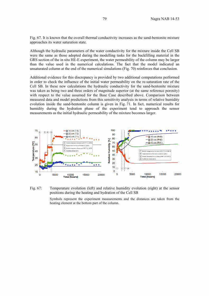
79 Nagra NAB 14-53
Fig. 67. It is known that the overall thermal conductivity increases as the sand-bentonite mixture approaches its water saturation state.
Although the hydraulic parameters of the water conductivity for the mixture inside the Cell SB were the same as those adopted during the modelling tasks for the backfilling material in the GRS section of the in situ HE-E experiment, the water permeability of the column may be larger than the value used in the numerical calculations. The fact that the model indicated an unsaturated column at the end of the numerical simulations (Fig. 70) reinforces that conclusion.
Additional evidence for this discrepancy is provided by two additional computations performed in order to check the influence of the initial water permeability on the re-saturation rate of the Cell SB. In these new calculations the hydraulic conductivity for the sand-bentonite mixture was taken as being two and three orders of magnitude superior (at the same reference porosity) with respect to the value assumed for the Base Case described above. Comparison between measured data and model predictions from this sensitivity analysis in terms of relative humidity evolution inside the sand-bentonite column is given in Fig. 71. In fact, numerical results for humidity during the hydration phase of the experiment tend to approach the sensor measurements as the initial hydraulic permeability of the mixture becomes larger.
Fig. 67: Temperature evolution (left) and relative humidity evolution (right) at the sensor positions during the heating and hydration of the Cell SB Symbols represent the experiment measurements and the distances are taken from the heating element at the bottom part of the column.
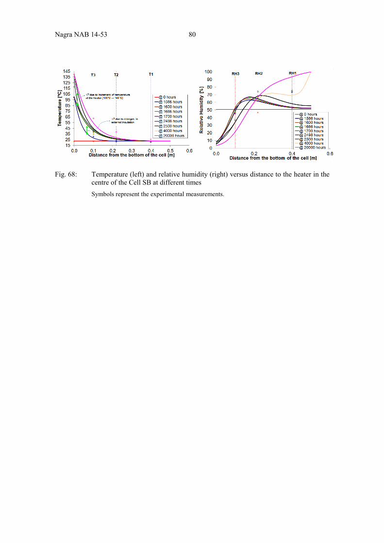
Nagra NAB 14-53 80
Fig. 68: Temperature (left) and relative humidity (right) versus distance to the heater in the centre of the Cell SB at different times Symbols represent the experimental measurements.
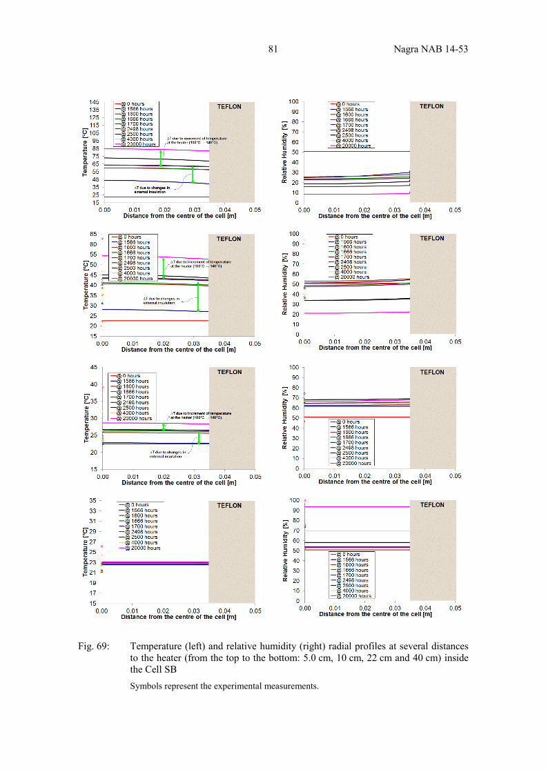
81 Nagra NAB 14-53
Fig. 69: Temperature (left) and relative humidity (right) radial profiles at several distances to the heater (from the top to the bottom: 5.0 cm, 10 cm, 22 cm and 40 cm) inside the Cell SB Symbols represent the experimental measurements.
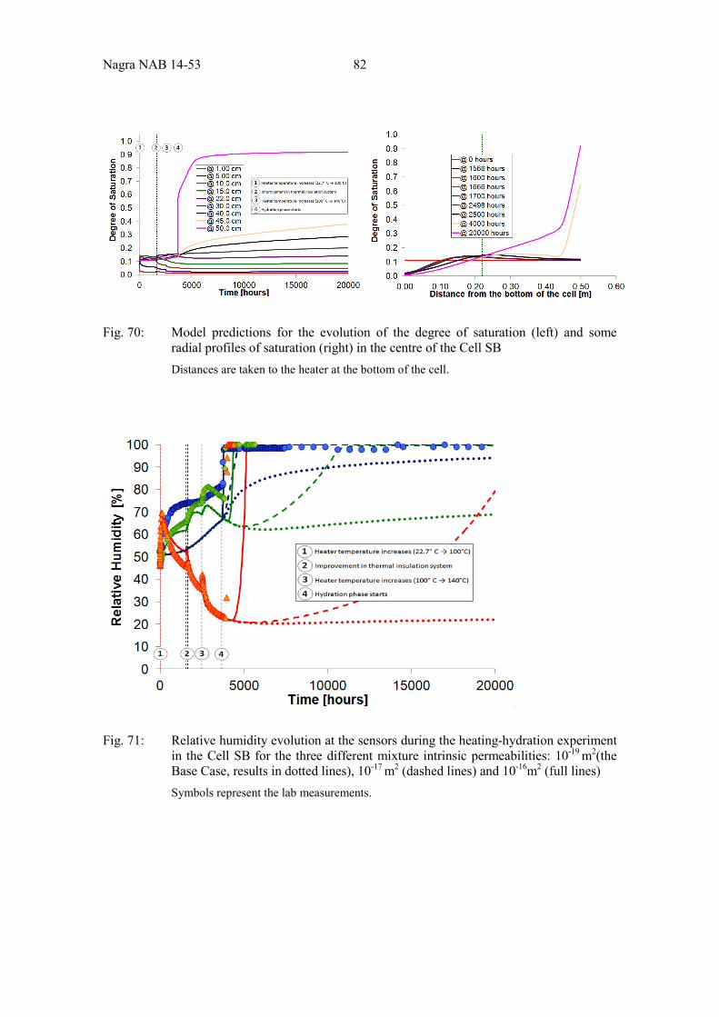
Nagra NAB 14-53 82
Fig. 70: Model predictions for the evolution of the degree of saturation (left) and some radial profiles of saturation (right) in the centre of the Cell SB Distances are taken to the heater at the bottom of the cell.
Fig. 71: Relative humidity evolution at the sensors during the heating-hydration experiment in the Cell SB for the three different mixture intrinsic permeabilities: 10-19 m2(the Base Case, results in dotted lines), 10-17 m2 (dashed lines) and 10-16m2 (full lines) Symbols represent the lab measurements.
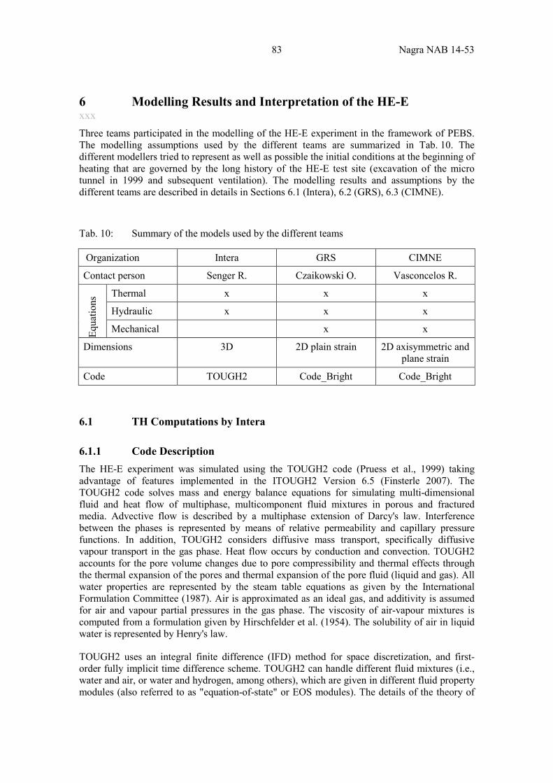
83 Nagra NAB 14-53
6 Modelling Results and Interpretation of the HE-E xxx Three teams participated in the modelling of the HE-E experiment in the framework of PEBS. The modelling assumptions used by the different teams are summarized in Tab. 10. The different modellers tried to represent as well as possible the initial conditions at the beginning of heating that are governed by the long history of the HE-E test site (excavation of the micro tunnel in 1999 and subsequent ventilation). The modelling results and assumptions by the different teams are described in details in Sections 6.1 (Intera), 6.2 (GRS), 6.3 (CIMNE).
Tab. 10: Summary of the models used by the different teams
Organization Intera GRS CIMNE
Contact person Senger R. Czaikowski O. Vasconcelos R.
Equa
tions
Thermal x x x
Hydraulic x x x
Mechanical x x
Dimensions 3D 2D plain strain 2D axisymmetric and plane strain
Code TOUGH2 Code_Bright Code_Bright
6.1 TH Computations by Intera
6.1.1 Code Description The HE-E experiment was simulated using the TOUGH2 code (Pruess et al., 1999) taking advantage of features implemented in the ITOUGH2 Version 6.5 (Finsterle 2007). The TOUGH2 code solves mass and energy balance equations for simulating multi-dimensional fluid and heat flow of multiphase, multicomponent fluid mixtures in porous and fractured media. Advective flow is described by a multiphase extension of Darcy's law. Interference between the phases is represented by means of relative permeability and capillary pressure functions. In addition, TOUGH2 considers diffusive mass transport, specifically diffusive vapour transport in the gas phase. Heat flow occurs by conduction and convection. TOUGH2 accounts for the pore volume changes due to pore compressibility and thermal effects through the thermal expansion of the pores and thermal expansion of the pore fluid (liquid and gas). All water properties are represented by the steam table equations as given by the International Formulation Committee (1987). Air is approximated as an ideal gas, and additivity is assumed for air and vapour partial pressures in the gas phase. The viscosity of air-vapour mixtures is computed from a formulation given by Hirschfelder et al. (1954). The solubility of air in liquid water is represented by Henry's law.
TOUGH2 uses an integral finite difference (IFD) method for space discretization, and first-order fully implicit time difference scheme. TOUGH2 can handle different fluid mixtures (i.e., water and air, or water and hydrogen, among others), which are given in different fluid property modules (also referred to as "equation-of-state" or EOS modules). The details of the theory of
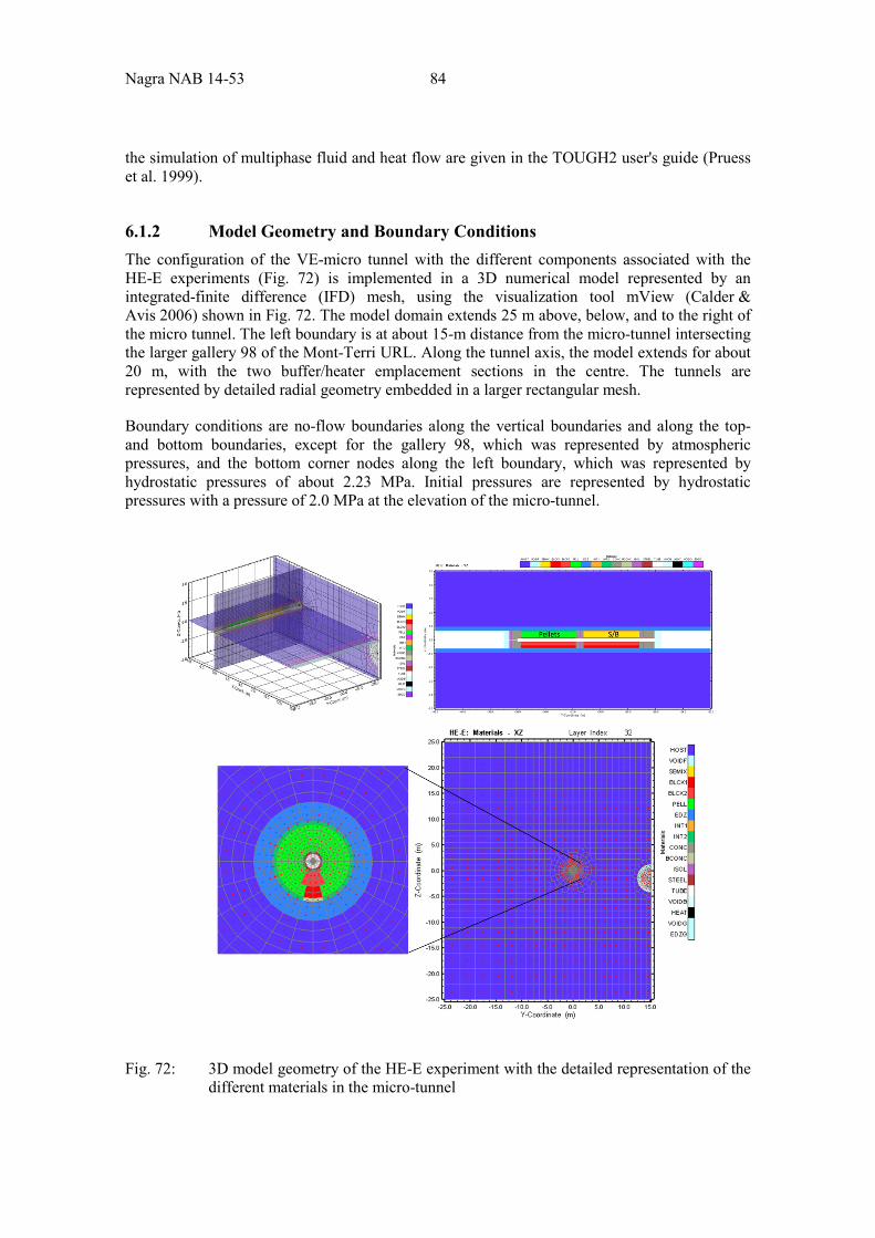
Nagra NAB 14-53 84
the simulation of multiphase fluid and heat flow are given in the TOUGH2 user's guide (Pruess et al. 1999).
6.1.2 Model Geometry and Boundary Conditions The configuration of the VE-micro tunnel with the different components associated with the HE-E experiments (Fig. 72) is implemented in a 3D numerical model represented by an integrated-finite difference (IFD) mesh, using the visualization tool mView (Calder & Avis 2006) shown in Fig. 72. The model domain extends 25 m above, below, and to the right of the micro tunnel. The left boundary is at about 15-m distance from the micro-tunnel intersecting the larger gallery 98 of the Mont-Terri URL. Along the tunnel axis, the model extends for about 20 m, with the two buffer/heater emplacement sections in the centre. The tunnels are represented by detailed radial geometry embedded in a larger rectangular mesh.
Boundary conditions are no-flow boundaries along the vertical boundaries and along the top- and bottom boundaries, except for the gallery 98, which was represented by atmospheric pressures, and the bottom corner nodes along the left boundary, which was represented by hydrostatic pressures of about 2.23 MPa. Initial pressures are represented by hydrostatic pressures with a pressure of 2.0 MPa at the elevation of the micro-tunnel.
Fig. 72: 3D model geometry of the HE-E experiment with the detailed representation of the different materials in the micro-tunnel
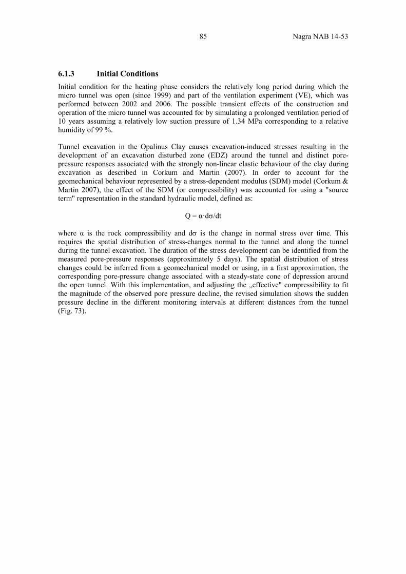
85 Nagra NAB 14-53
6.1.3 Initial Conditions Initial condition for the heating phase considers the relatively long period during which the micro tunnel was open (since 1999) and part of the ventilation experiment (VE), which was performed between 2002 and 2006. The possible transient effects of the construction and operation of the micro tunnel was accounted for by simulating a prolonged ventilation period of 10 years assuming a relatively low suction pressure of 1.34 MPa corresponding to a relative humidity of 99 %.
Tunnel excavation in the Opalinus Clay causes excavation-induced stresses resulting in the development of an excavation disturbed zone (EDZ) around the tunnel and distinct pore-pressure responses associated with the strongly non-linear elastic behaviour of the clay during excavation as described in Corkum and Martin (2007). In order to account for the geomechanical behaviour represented by a stress-dependent modulus (SDM) model (Corkum & Martin 2007), the effect of the SDM (or compressibility) was accounted for using a "source term" representation in the standard hydraulic model, defined as:
Q = α·dσ/dt
where α is the rock compressibility and dσ is the change in normal stress over time. This requires the spatial distribution of stress-changes normal to the tunnel and along the tunnel during the tunnel excavation. The duration of the stress development can be identified from the measured pore-pressure responses (approximately 5 days). The spatial distribution of stress changes could be inferred from a geomechanical model or using, in a first approximation, the corresponding pore-pressure change associated with a steady-state cone of depression around the open tunnel. With this implementation, and adjusting the „effective" compressibility to fit the magnitude of the observed pore pressure decline, the revised simulation shows the sudden pressure decline in the different monitoring intervals at different distances from the tunnel (Fig. 73).
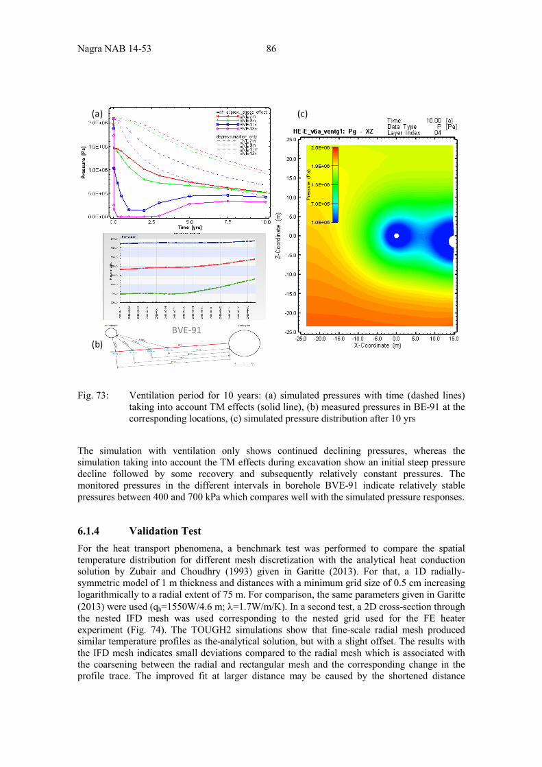
Nagra NAB 14-53 86
Fig. 73: Ventilation period for 10 years: (a) simulated pressures with time (dashed lines) taking into account TM effects (solid line), (b) measured pressures in BE-91 at the corresponding locations, (c) simulated pressure distribution after 10 yrs
The simulation with ventilation only shows continued declining pressures, whereas the simulation taking into account the TM effects during excavation show an initial steep pressure decline followed by some recovery and subsequently relatively constant pressures. The monitored pressures in the different intervals in borehole BVE-91 indicate relatively stable pressures between 400 and 700 kPa which compares well with the simulated pressure responses.
6.1.4 Validation Test For the heat transport phenomena, a benchmark test was performed to compare the spatial temperature distribution for different mesh discretization with the analytical heat conduction solution by Zubair and Choudhry (1993) given in Garitte (2013). For that, a 1D radially-symmetric model of 1 m thickness and distances with a minimum grid size of 0.5 cm increasing logarithmically to a radial extent of 75 m. For comparison, the same parameters given in Garitte (2013) were used (qh=1550W/4.6 m; λ=1.7W/m/K). In a second test, a 2D cross-section through the nested IFD mesh was used corresponding to the nested grid used for the FE heater experiment (Fig. 74). The TOUGH2 simulations show that fine-scale radial mesh produced similar temperature profiles as the-analytical solution, but with a slight offset. The results with the IFD mesh indicates small deviations compared to the radial mesh which is associated with the coarsening between the radial and rectangular mesh and the corresponding change in the profile trace. The improved fit at larger distance may be caused by the shortened distance
BVE-91
(a)
(b)
(c)
87 Nagra NAB 14-53
compared to the radial mesh and the no-flow outer boundary causing slightly higher temperatures (i.e., after 10 years the boundary effects becomes more dominant.
Fig. 74: Comparison of computed temperature profiles of the analytical solution for a 1D radially-symmetric mesh (top) and for the 2D nested radial-rectangular mesh (showing the profile line for the computed temperature profile)
0.0
20.0
40.0
60.0
80.0
100.0
120.0
140.0
0.0 1.0 2.0 3.0 4.0 5.0 6.0 7.0 8.0 9.0 10.0
dT [d
egC]
Distance [m]
dT (3D radial-rectangular mesh)
Analytical (Zubair)
0.0
20.0
40.0
60.0
80.0
100.0
120.0
140.0
0.0 1.0 2.0 3.0 4.0 5.0 6.0 7.0 8.0 9.0 10.0
dT [d
egC]
Distance [m]
dT (1D radial mesh)
Analytica (Zubair)l
After 10 yrs
After 5 yrs
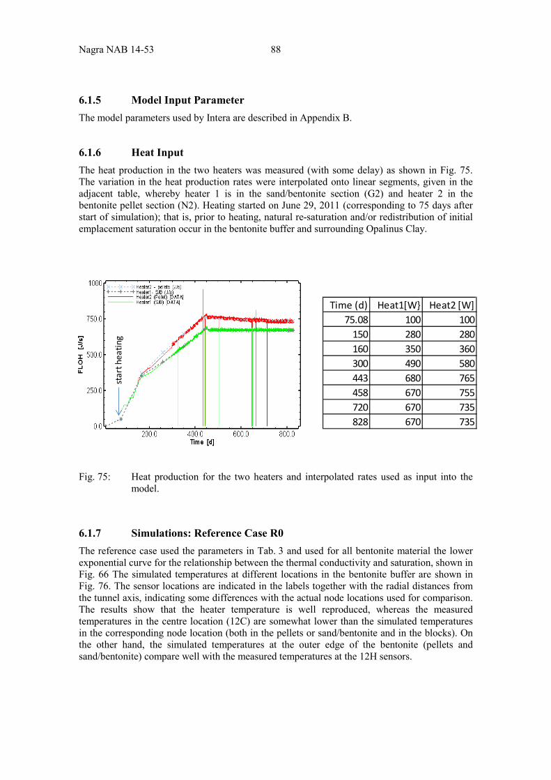
Nagra NAB 14-53 88
6.1.5 Model Input Parameter The model parameters used by Intera are described in Appendix B.
6.1.6 Heat Input The heat production in the two heaters was measured (with some delay) as shown in Fig. 75. The variation in the heat production rates were interpolated onto linear segments, given in the adjacent table, whereby heater 1 is in the sand/bentonite section (G2) and heater 2 in the bentonite pellet section (N2). Heating started on June 29, 2011 (corresponding to 75 days after start of simulation); that is, prior to heating, natural re-saturation and/or redistribution of initial emplacement saturation occur in the bentonite buffer and surrounding Opalinus Clay.
Fig. 75: Heat production for the two heaters and interpolated rates used as input into the model.
6.1.7 Simulations: Reference Case R0 The reference case used the parameters in Tab. 3 and used for all bentonite material the lower exponential curve for the relationship between the thermal conductivity and saturation, shown in Fig. 66 The simulated temperatures at different locations in the bentonite buffer are shown in Fig. 76. The sensor locations are indicated in the labels together with the radial distances from the tunnel axis, indicating some differences with the actual node locations used for comparison. The results show that the heater temperature is well reproduced, whereas the measured temperatures in the centre location (12C) are somewhat lower than the simulated temperatures in the corresponding node location (both in the pellets or sand/bentonite and in the blocks). On the other hand, the simulated temperatures at the outer edge of the bentonite (pellets and sand/bentonite) compare well with the measured temperatures at the 12H sensors.
Time (d) Heat1[W} Heat2 [W]75.08 100 100
150 280 280160 350 360300 490 580443 680 765458 670 755720 670 735828 670 735
star
t hea
ting
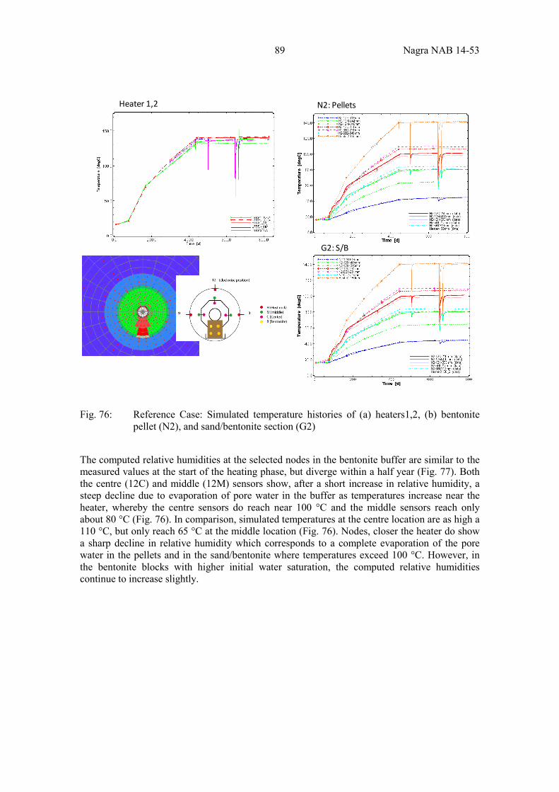
89 Nagra NAB 14-53
Fig. 76: Reference Case: Simulated temperature histories of (a) heaters1,2, (b) bentonite pellet (N2), and sand/bentonite section (G2)
The computed relative humidities at the selected nodes in the bentonite buffer are similar to the measured values at the start of the heating phase, but diverge within a half year (Fig. 77). Both the centre (12C) and middle (12M) sensors show, after a short increase in relative humidity, a steep decline due to evaporation of pore water in the buffer as temperatures increase near the heater, whereby the centre sensors do reach near 100 °C and the middle sensors reach only about 80 °C (Fig. 76). In comparison, simulated temperatures at the centre location are as high a 110 °C, but only reach 65 °C at the middle location (Fig. 76). Nodes, closer the heater do show a sharp decline in relative humidity which corresponds to a complete evaporation of the pore water in the pellets and in the sand/bentonite where temperatures exceed 100 °C. However, in the bentonite blocks with higher initial water saturation, the computed relative humidities continue to increase slightly.
Heater 1,2
G2: S/B
N2: Pellets
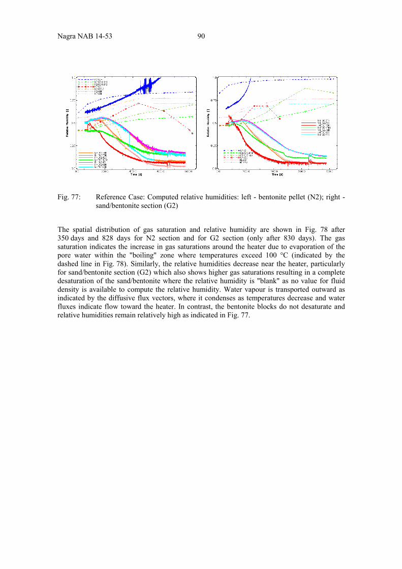
Nagra NAB 14-53 90
Fig. 77: Reference Case: Computed relative humidities: left - bentonite pellet (N2); right - sand/bentonite section (G2)
The spatial distribution of gas saturation and relative humidity are shown in Fig. 78 after 350 days and 828 days for N2 section and for G2 section (only after 830 days). The gas saturation indicates the increase in gas saturations around the heater due to evaporation of the pore water within the "boiling" zone where temperatures exceed 100 °C (indicated by the dashed line in Fig. 78). Similarly, the relative humidities decrease near the heater, particularly for sand/bentonite section (G2) which also shows higher gas saturations resulting in a complete desaturation of the sand/bentonite where the relative humidity is "blank" as no value for fluid density is available to compute the relative humidity. Water vapour is transported outward as indicated by the diffusive flux vectors, where it condenses as temperatures decrease and water fluxes indicate flow toward the heater. In contrast, the bentonite blocks do not desaturate and relative humidities remain relatively high as indicated in Fig. 77.
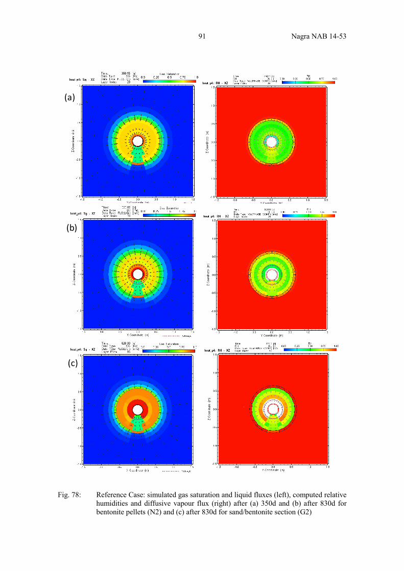
91 Nagra NAB 14-53
Fig. 78: Reference Case: simulated gas saturation and liquid fluxes (left), computed relative humidities and diffusive vapour flux (right) after (a) 350d and (b) after 830d for bentonite pellets (N2) and (c) after 830d for sand/bentonite section (G2)
(a)
(b)
(c)
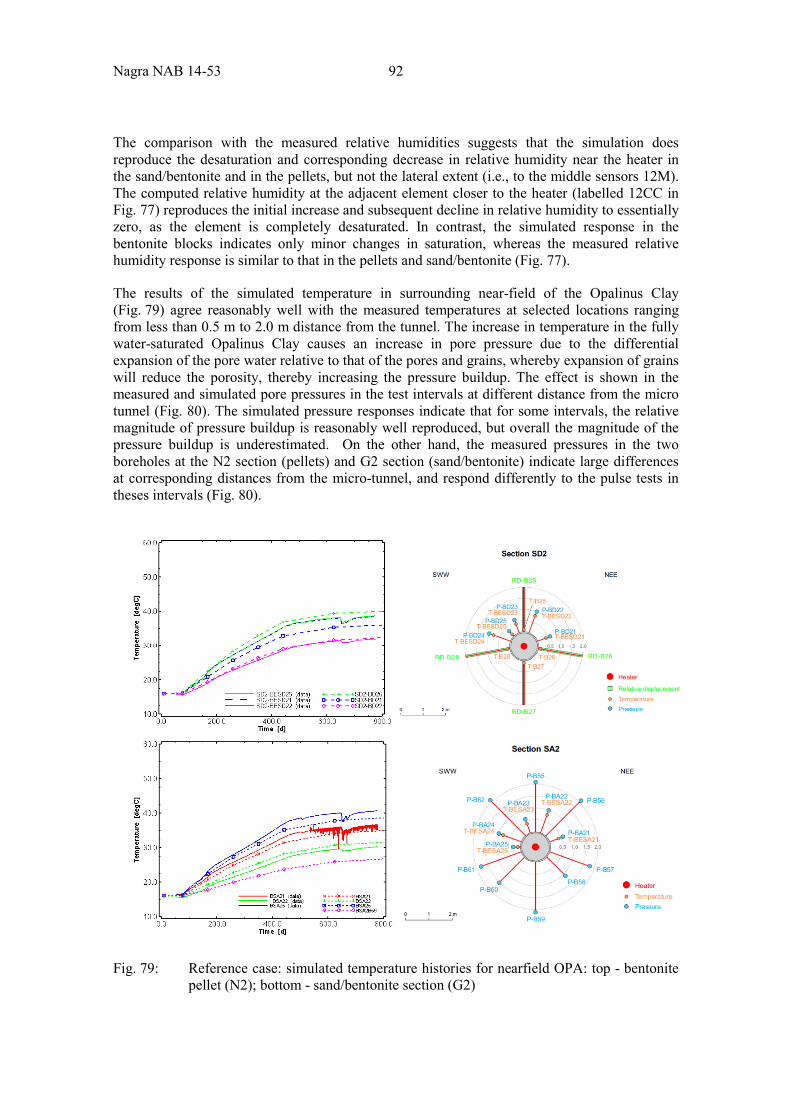
Nagra NAB 14-53 92
The comparison with the measured relative humidities suggests that the simulation does reproduce the desaturation and corresponding decrease in relative humidity near the heater in the sand/bentonite and in the pellets, but not the lateral extent (i.e., to the middle sensors 12M). The computed relative humidity at the adjacent element closer to the heater (labelled 12CC in Fig. 77) reproduces the initial increase and subsequent decline in relative humidity to essentially zero, as the element is completely desaturated. In contrast, the simulated response in the bentonite blocks indicates only minor changes in saturation, whereas the measured relative humidity response is similar to that in the pellets and sand/bentonite (Fig. 77).
The results of the simulated temperature in surrounding near-field of the Opalinus Clay (Fig. 79) agree reasonably well with the measured temperatures at selected locations ranging from less than 0.5 m to 2.0 m distance from the tunnel. The increase in temperature in the fully water-saturated Opalinus Clay causes an increase in pore pressure due to the differential expansion of the pore water relative to that of the pores and grains, whereby expansion of grains will reduce the porosity, thereby increasing the pressure buildup. The effect is shown in the measured and simulated pore pressures in the test intervals at different distance from the micro tunnel (Fig. 80). The simulated pressure responses indicate that for some intervals, the relative magnitude of pressure buildup is reasonably well reproduced, but overall the magnitude of the pressure buildup is underestimated. On the other hand, the measured pressures in the two boreholes at the N2 section (pellets) and G2 section (sand/bentonite) indicate large differences at corresponding distances from the micro-tunnel, and respond differently to the pulse tests in theses intervals (Fig. 80).
Fig. 79: Reference case: simulated temperature histories for nearfield OPA: top - bentonite pellet (N2); bottom - sand/bentonite section (G2)
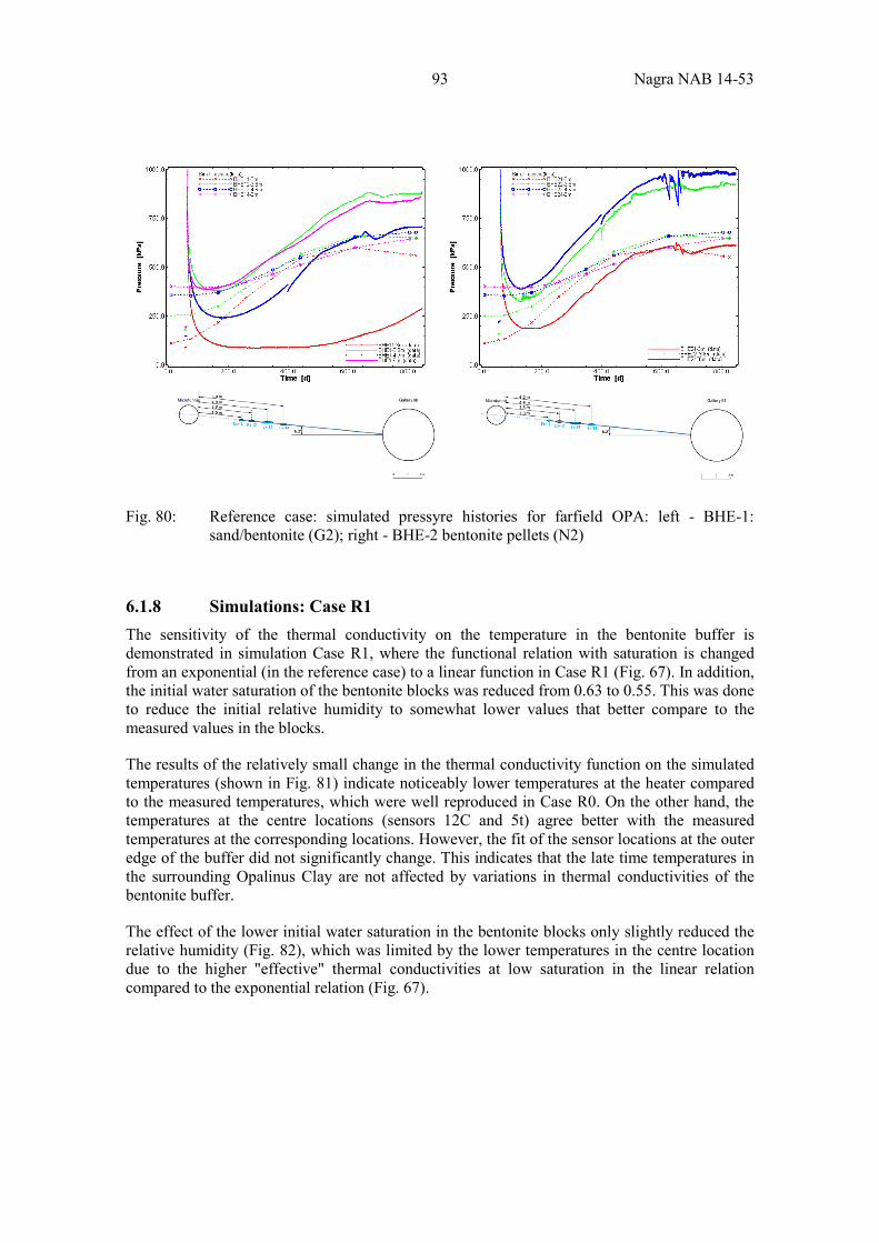
93 Nagra NAB 14-53
Fig. 80: Reference case: simulated pressyre histories for farfield OPA: left - BHE-1: sand/bentonite (G2); right - BHE-2 bentonite pellets (N2)
6.1.8 Simulations: Case R1 The sensitivity of the thermal conductivity on the temperature in the bentonite buffer is demonstrated in simulation Case R1, where the functional relation with saturation is changed from an exponential (in the reference case) to a linear function in Case R1 (Fig. 67). In addition, the initial water saturation of the bentonite blocks was reduced from 0.63 to 0.55. This was done to reduce the initial relative humidity to somewhat lower values that better compare to the measured values in the blocks.
The results of the relatively small change in the thermal conductivity function on the simulated temperatures (shown in Fig. 81) indicate noticeably lower temperatures at the heater compared to the measured temperatures, which were well reproduced in Case R0. On the other hand, the temperatures at the centre locations (sensors 12C and 5t) agree better with the measured temperatures at the corresponding locations. However, the fit of the sensor locations at the outer edge of the buffer did not significantly change. This indicates that the late time temperatures in the surrounding Opalinus Clay are not affected by variations in thermal conductivities of the bentonite buffer.
The effect of the lower initial water saturation in the bentonite blocks only slightly reduced the relative humidity (Fig. 82), which was limited by the lower temperatures in the centre location due to the higher "effective" thermal conductivities at low saturation in the linear relation compared to the exponential relation (Fig. 67).
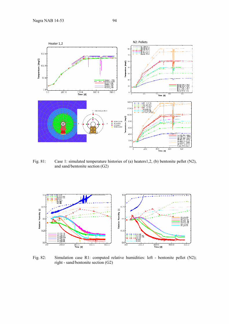
Nagra NAB 14-53 94
Fig. 81: Case 1: simulated temperature histories of (a) heaters1,2, (b) bentonite pellet (N2), and sand/bentonite section (G2)
Fig. 82: Simulation case R1: computed relative humidities: left - bentonite pellet (N2); right - sand/bentonite section (G2)
Heater 1,2 N2: Pellets
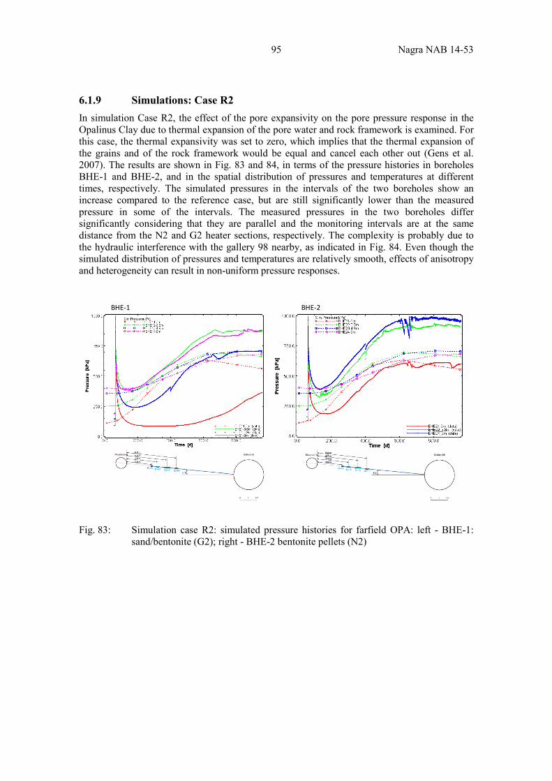
95 Nagra NAB 14-53
6.1.9 Simulations: Case R2 In simulation Case R2, the effect of the pore expansivity on the pore pressure response in the Opalinus Clay due to thermal expansion of the pore water and rock framework is examined. For this case, the thermal expansivity was set to zero, which implies that the thermal expansion of the grains and of the rock framework would be equal and cancel each other out (Gens et al. 2007). The results are shown in Fig. 83 and 84, in terms of the pressure histories in boreholes BHE-1 and BHE-2, and in the spatial distribution of pressures and temperatures at different times, respectively. The simulated pressures in the intervals of the two boreholes show an increase compared to the reference case, but are still significantly lower than the measured pressure in some of the intervals. The measured pressures in the two boreholes differ significantly considering that they are parallel and the monitoring intervals are at the same distance from the N2 and G2 heater sections, respectively. The complexity is probably due to the hydraulic interference with the gallery 98 nearby, as indicated in Fig. 84. Even though the simulated distribution of pressures and temperatures are relatively smooth, effects of anisotropy and heterogeneity can result in non-uniform pressure responses.
Fig. 83: Simulation case R2: simulated pressure histories for farfield OPA: left - BHE-1: sand/bentonite (G2); right - BHE-2 bentonite pellets (N2)
BHE-1 BHE-2
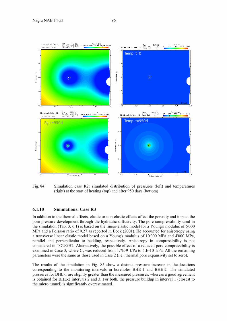
Nagra NAB 14-53 96
Fig. 84: Simulation case R2: simulated distribution of pressures (left) and temperatures (right) at the start of heating (top) and after 950 days (bottom)
6.1.10 Simulations: Case R3 In addition to the thermal effects, elastic or non-elastic effects affect the porosity and impact the pore pressure development through the hydraulic diffusivity. The pore compressibility used in the simulation (Tab. 3, 6.1) is based on the linear-elastic model for a Young's modulus of 6'000 MPa and a Poisson ratio of 0.27 as reported in Bock (2001). He accounted for anisotropy using a transverse linear elastic model based on a Young's modulus of 10'000 MPa and 4'000 MPa, parallel and perpendicular to bedding, respectively. Anisotropy in compressibility is not considered in TOUGH2. Alternatively, the possible effect of a reduced pore compressibility is examined in Case 3, where Cp was reduced from 1.7E-9 1/Pa to 5.E-10 1/Pa. All the remaining parameters were the same as those used in Case 2 (i.e., thermal pore expansivity set to zero).
The results of the simulation in Fig. 85 show a distinct pressure increase in the locations corresponding to the monitoring intervals in boreholes BHE-1 and BHE-2. The simulated pressures for BHE-1 are slightly greater than the measured pressures, whereas a good agreement is obtained for BHE-2 intervals 2 and 3. For both, the pressure buildup in interval 1 (closest to the micro tunnel) is significantly overestimated.
Temp: t=0
Temp: t=950dPg: t=950d
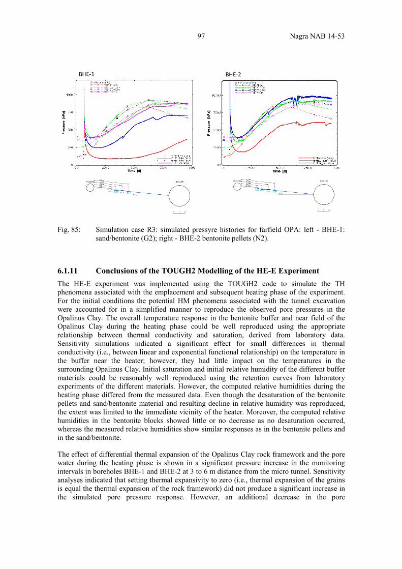
97 Nagra NAB 14-53
Fig. 85: Simulation case R3: simulated pressyre histories for farfield OPA: left - BHE-1: sand/bentonite (G2); right - BHE-2 bentonite pellets (N2).
6.1.11 Conclusions of the TOUGH2 Modelling of the HE-E Experiment The HE-E experiment was implemented using the TOUGH2 code to simulate the TH phenomena associated with the emplacement and subsequent heating phase of the experiment. For the initial conditions the potential HM phenomena associated with the tunnel excavation were accounted for in a simplified manner to reproduce the observed pore pressures in the Opalinus Clay. The overall temperature response in the bentonite buffer and near field of the Opalinus Clay during the heating phase could be well reproduced using the appropriate relationship between thermal conductivity and saturation, derived from laboratory data. Sensitivity simulations indicated a significant effect for small differences in thermal conductivity (i.e., between linear and exponential functional relationship) on the temperature in the buffer near the heater; however, they had little impact on the temperatures in the surrounding Opalinus Clay. Initial saturation and initial relative humidity of the different buffer materials could be reasonably well reproduced using the retention curves from laboratory experiments of the different materials. However, the computed relative humidities during the heating phase differed from the measured data. Even though the desaturation of the bentonite pellets and sand/bentonite material and resulting decline in relative humidity was reproduced, the extent was limited to the immediate vicinity of the heater. Moreover, the computed relative humidities in the bentonite blocks showed little or no decrease as no desaturation occurred, whereas the measured relative humidities show similar responses as in the bentonite pellets and in the sand/bentonite.
The effect of differential thermal expansion of the Opalinus Clay rock framework and the pore water during the heating phase is shown in a significant pressure increase in the monitoring intervals in boreholes BHE-1 and BHE-2 at 3 to 6 m distance from the micro tunnel. Sensitivity analyses indicated that setting thermal expansivity to zero (i.e., thermal expansion of the grains is equal the thermal expansion of the rock framework) did not produce a significant increase in the simulated pore pressure response. However, an additional decrease in the pore
BHE-1 BHE-2
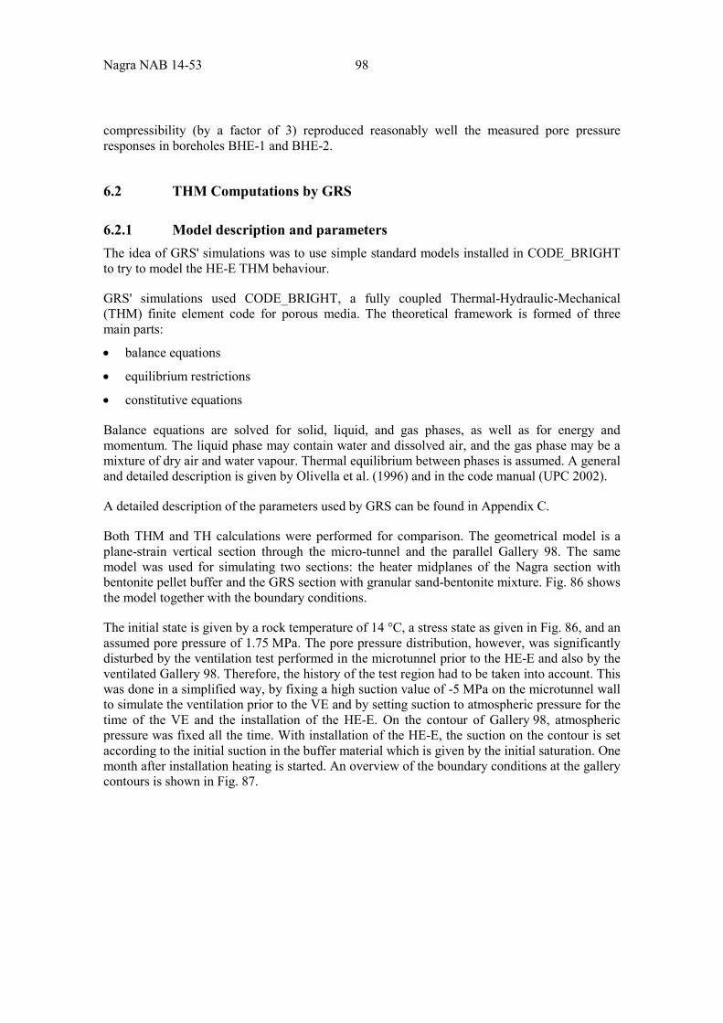
Nagra NAB 14-53 98
compressibility (by a factor of 3) reproduced reasonably well the measured pore pressure responses in boreholes BHE-1 and BHE-2.
6.2 THM Computations by GRS
6.2.1 Model description and parameters The idea of GRS' simulations was to use simple standard models installed in CODE_BRIGHT to try to model the HE-E THM behaviour.
GRS' simulations used CODE_BRIGHT, a fully coupled Thermal-Hydraulic-Mechanical (THM) finite element code for porous media. The theoretical framework is formed of three main parts:
• balance equations
• equilibrium restrictions
• constitutive equations
Balance equations are solved for solid, liquid, and gas phases, as well as for energy and momentum. The liquid phase may contain water and dissolved air, and the gas phase may be a mixture of dry air and water vapour. Thermal equilibrium between phases is assumed. A general and detailed description is given by Olivella et al. (1996) and in the code manual (UPC 2002).
A detailed description of the parameters used by GRS can be found in Appendix C.
Both THM and TH calculations were performed for comparison. The geometrical model is a plane-strain vertical section through the micro-tunnel and the parallel Gallery 98. The same model was used for simulating two sections: the heater midplanes of the Nagra section with bentonite pellet buffer and the GRS section with granular sand-bentonite mixture. Fig. 86 shows the model together with the boundary conditions.
The initial state is given by a rock temperature of 14 °C, a stress state as given in Fig. 86, and an assumed pore pressure of 1.75 MPa. The pore pressure distribution, however, was significantly disturbed by the ventilation test performed in the microtunnel prior to the HE-E and also by the ventilated Gallery 98. Therefore, the history of the test region had to be taken into account. This was done in a simplified way, by fixing a high suction value of -5 MPa on the microtunnel wall to simulate the ventilation prior to the VE and by setting suction to atmospheric pressure for the time of the VE and the installation of the HE-E. On the contour of Gallery 98, atmospheric pressure was fixed all the time. With installation of the HE-E, the suction on the contour is set according to the initial suction in the buffer material which is given by the initial saturation. One month after installation heating is started. An overview of the boundary conditions at the gallery contours is shown in Fig. 87.
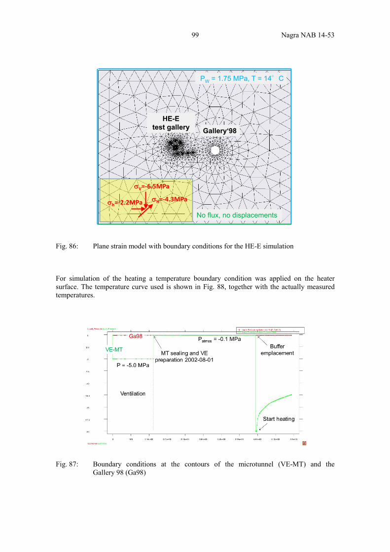
99 Nagra NAB 14-53
Fig. 86: Plane strain model with boundary conditions for the HE-E simulation For simulation of the heating a temperature boundary condition was applied on the heater surface. The temperature curve used is shown in Fig. 88, together with the actually measured temperatures.
Fig. 87: Boundary conditions at the contours of the microtunnel (VE-MT) and the Gallery 98 (Ga98)
No flux, no displacements
PW = 1.75 MPa, T = 14°C
HE-E test gallery Gallery‘98
σV=-6.5MPa
σH=-4.3MPaσh=-2.2MPa
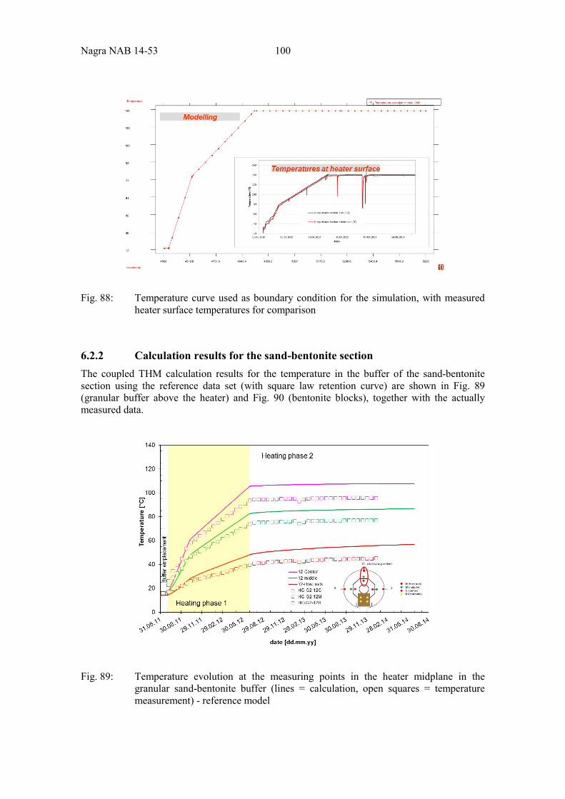
Nagra NAB 14-53 100
Fig. 88: Temperature curve used as boundary condition for the simulation, with measured heater surface temperatures for comparison
6.2.2 Calculation results for the sand-bentonite section The coupled THM calculation results for the temperature in the buffer of the sand-bentonite section using the reference data set (with square law retention curve) are shown in Fig. 89 (granular buffer above the heater) and Fig. 90 (bentonite blocks), together with the actually measured data.
Fig. 89: Temperature evolution at the measuring points in the heater midplane in the granular sand-bentonite buffer (lines = calculation, open squares = temperature measurement) - reference model
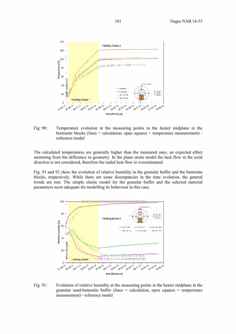
101 Nagra NAB 14-53
Fig. 90: Temperature evolution at the measuring points in the heater midplane in the bentonite blocks (lines = calculation, open squares = temperature measurement) - reference model
The calculated temperatures are generally higher than the measured ones, an expected effect stemming from the difference in geometry. In the plane strain model the heat flow in the axial direction is not considered, therefore the radial heat flow is overestimated.
Fig. 91 and 92 show the evolution of relative humidity in the granular buffer and the bentonite blocks, respectively. While there are some discrepancies in the time evolution, the general trends are met. The simple elastic model for the granular buffer and the selected material parameters seem adequate for modelling its behaviour in this case.
Fig. 91: Evolution of relative humidity at the measuring points in the heater midplane in the granular sand-bentonite buffer (lines = calculation, open squares = temperature measurement) - reference model
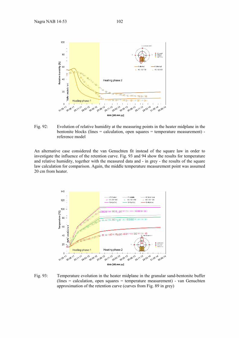
Nagra NAB 14-53 102
Fig. 92: Evolution of relative humidity at the measuring points in the heater midplane in the bentonite blocks (lines = calculation, open squares = temperature measurement) - reference model
An alternative case considered the van Genuchten fit instead of the square law in order to investigate the influence of the retention curve. Fig. 93 and 94 show the results for temperature and relative humidity, together with the measured data and - in grey - the results of the square law calculation for comparison. Again, the middle temperature measurement point was assumed 20 cm from heater.
Fig. 93: Temperature evolution in the heater midplane in the granular sand-bentonite buffer (lines = calculation, open squares = temperature measurement) - van Genuchten approximation of the retention curve (curves from Fig. 89 in grey)
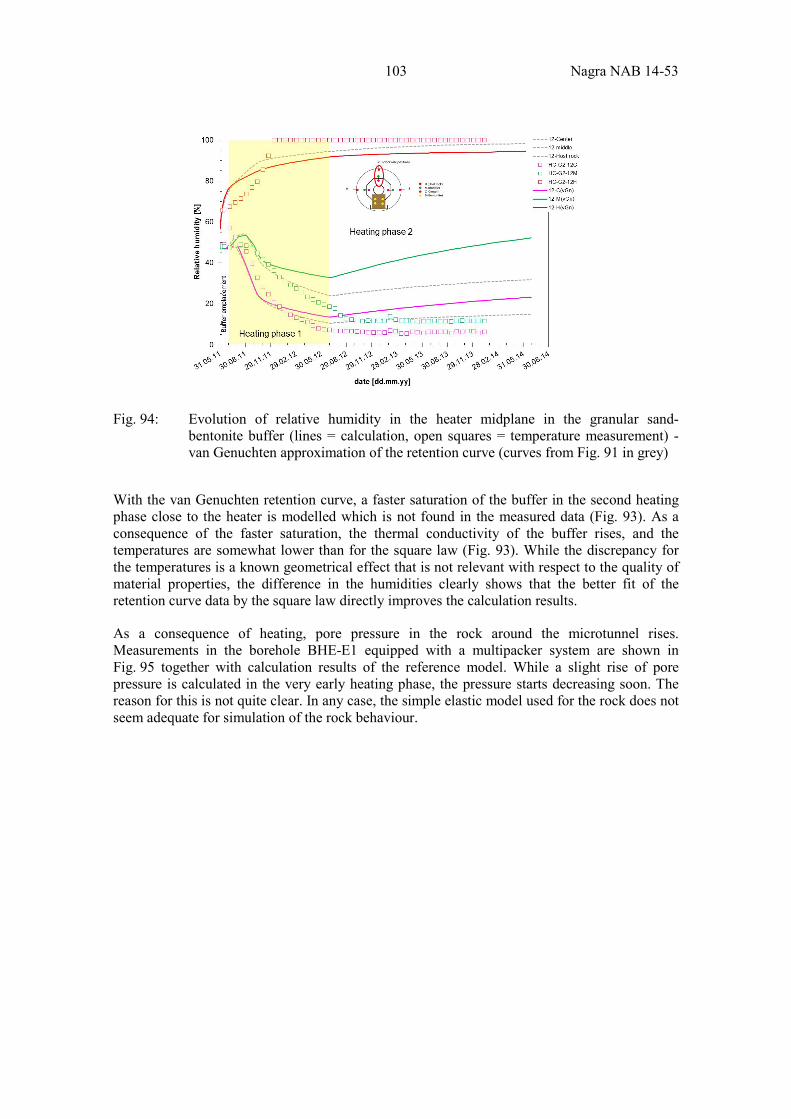
103 Nagra NAB 14-53
Fig. 94: Evolution of relative humidity in the heater midplane in the granular sand-bentonite buffer (lines = calculation, open squares = temperature measurement) - van Genuchten approximation of the retention curve (curves from Fig. 91 in grey)
With the van Genuchten retention curve, a faster saturation of the buffer in the second heating phase close to the heater is modelled which is not found in the measured data (Fig. 93). As a consequence of the faster saturation, the thermal conductivity of the buffer rises, and the temperatures are somewhat lower than for the square law (Fig. 93). While the discrepancy for the temperatures is a known geometrical effect that is not relevant with respect to the quality of material properties, the difference in the humidities clearly shows that the better fit of the retention curve data by the square law directly improves the calculation results.
As a consequence of heating, pore pressure in the rock around the microtunnel rises. Measurements in the borehole BHE-E1 equipped with a multipacker system are shown in Fig. 95 together with calculation results of the reference model. While a slight rise of pore pressure is calculated in the very early heating phase, the pressure starts decreasing soon. The reason for this is not quite clear. In any case, the simple elastic model used for the rock does not seem adequate for simulation of the rock behaviour.
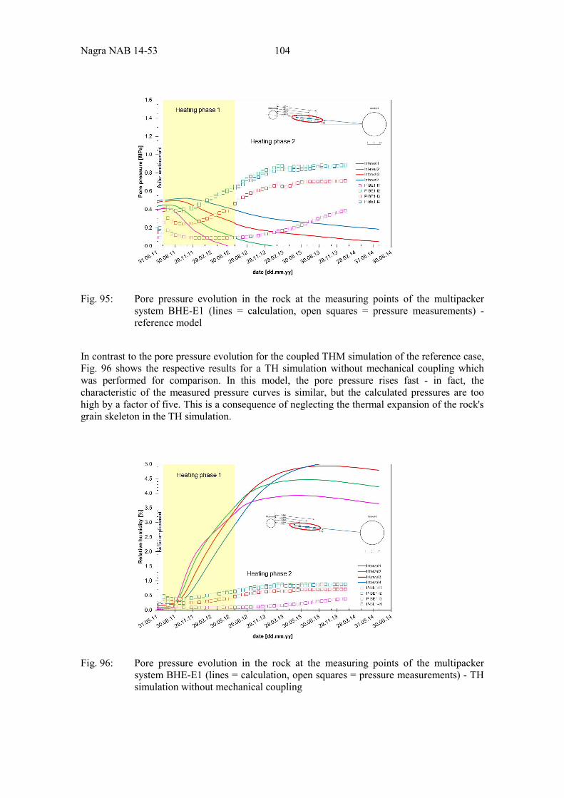
Nagra NAB 14-53 104
Fig. 95: Pore pressure evolution in the rock at the measuring points of the multipacker system BHE-E1 (lines = calculation, open squares = pressure measurements) - reference model
In contrast to the pore pressure evolution for the coupled THM simulation of the reference case, Fig. 96 shows the respective results for a TH simulation without mechanical coupling which was performed for comparison. In this model, the pore pressure rises fast - in fact, the characteristic of the measured pressure curves is similar, but the calculated pressures are too high by a factor of five. This is a consequence of neglecting the thermal expansion of the rock's grain skeleton in the TH simulation.
Fig. 96: Pore pressure evolution in the rock at the measuring points of the multipacker system BHE-E1 (lines = calculation, open squares = pressure measurements) - TH simulation without mechanical coupling
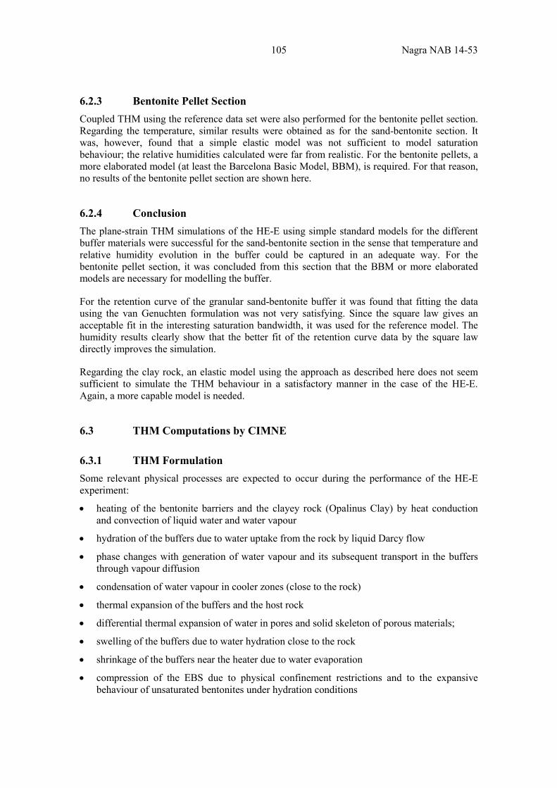
105 Nagra NAB 14-53
6.2.3 Bentonite Pellet Section Coupled THM using the reference data set were also performed for the bentonite pellet section. Regarding the temperature, similar results were obtained as for the sand-bentonite section. It was, however, found that a simple elastic model was not sufficient to model saturation behaviour; the relative humidities calculated were far from realistic. For the bentonite pellets, a more elaborated model (at least the Barcelona Basic Model, BBM), is required. For that reason, no results of the bentonite pellet section are shown here.
6.2.4 Conclusion The plane-strain THM simulations of the HE-E using simple standard models for the different buffer materials were successful for the sand-bentonite section in the sense that temperature and relative humidity evolution in the buffer could be captured in an adequate way. For the bentonite pellet section, it was concluded from this section that the BBM or more elaborated models are necessary for modelling the buffer.
For the retention curve of the granular sand-bentonite buffer it was found that fitting the data using the van Genuchten formulation was not very satisfying. Since the square law gives an acceptable fit in the interesting saturation bandwidth, it was used for the reference model. The humidity results clearly show that the better fit of the retention curve data by the square law directly improves the simulation.
Regarding the clay rock, an elastic model using the approach as described here does not seem sufficient to simulate the THM behaviour in a satisfactory manner in the case of the HE-E. Again, a more capable model is needed.
6.3 THM Computations by CIMNE
6.3.1 THM Formulation Some relevant physical processes are expected to occur during the performance of the HE-E experiment:
• heating of the bentonite barriers and the clayey rock (Opalinus Clay) by heat conduction and convection of liquid water and water vapour
• hydration of the buffers due to water uptake from the rock by liquid Darcy flow
• phase changes with generation of water vapour and its subsequent transport in the buffers through vapour diffusion
• condensation of water vapour in cooler zones (close to the rock)
• thermal expansion of the buffers and the host rock
• differential thermal expansion of water in pores and solid skeleton of porous materials;
• swelling of the buffers due to water hydration close to the rock
• shrinkage of the buffers near the heater due to water evaporation
• compression of the EBS due to physical confinement restrictions and to the expansive behaviour of unsaturated bentonites under hydration conditions
Nagra NAB 14-53 106
The basic formulation for solving these thermo-hydro-mechanical (THM) phenomena that take place in an engineered barrier during the lifetime of a radioactive waste repository considers the porous medium as multiphase and multispecies system (Olivella et al., 1994). The soil is a three-phase system composed by solid (s), liquid (l) and gas (g) in which the liquid phase contains the species "water" (in liquid form) while the gas phase includes the species "air" and "water" in vapour form.
A detailed description of the model used by CIMNE can be found in Appendix D.
6.3.2 Modelling Features
6.3.2.1 Conceptual Models Two conceptual models were set up.
An axisymmetric mesh (the microtunnel axis as the axisymmetry line) was chosen to represent the modelled domain. This geometry has a width of 40 m and is 30 m long and all the dimensions used are in agreement with the indications given in Gaus (2012). The vertical symmetry plane between the two heaters (upper boundary in Fig. 97) was used and the upper left corner of the mesh acts as a symmetry entity which implies a virtual second heater. Therefore only one heater and half of the middle concrete plug are represented. Consequently, the comparison between measurements provided by the in situ instrumentation and numerical results from the calculations using this conceptual model must take into account which buffer material is placed in the heated section (bentonite pellets or granular sand-bentonite mixture).
The heated section (EBS section) has a length of 4.0 m and the distance from the heater surface to the microtunnel wall is about 0.5 m. For numerical considerations, the insulator was modelled as a gap rather than as a material. Null fluxes are imposed on the upper, the lower and left boundaries. A liquid pressure value of 1.75 MPa and a prescribed temperature close to 16 °C are applied on the right boundary and represent the boundary conditions in the far field. The external mechanical boundary conditions are 0-displacement on the upper and the lower boundaries and a compressive stress state of 4.5 MPa on the right side. A 0-stress condition is applied on the left boundary in order to simulate the excavation process of the microtunnel. A value of 1.75 MPa was taken for representing the initial pore water pressure in the host rock. Furthermore the initial stress state in the rock was assumed to be isotropic with an average value of 4.5 MPa. Before the excavation of the microtunnel, the rock mass is considered to be saturated. The initial temperature in the Opalinus Clay was set as 15.75 °C. The modelled geometry and a detailed view of the heater and the bentonite barrier are given in (Fig. 97).
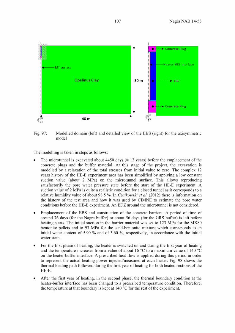
107 Nagra NAB 14-53
Fig. 97: Modelled domain (left) and detailed view of the EBS (right) for the axisymmetric model
The modelling is taken in steps as follows:
• The microtunnel is excavated about 4450 days (≈ 12 years) before the emplacement of the concrete plugs and the buffer material. At this stage of the project, the excavation is modelled by a relaxation of the total stresses from initial value to zero. The complex 12 years history of the HE-E experiment area has been simplified by applying a low constant suction value (about 2 MPa) on the microtunnel surface. This allows reproducing satisfactorily the pore water pressure state before the start of the HE-E experiment. A suction value of 2 MPa is quite a realistic condition for a closed tunnel as it corresponds to a relative humidity value of about 98.5 %. In Czaikowski et al. (2012) there is information on the history of the test area and how it was used by CIMNE to estimate the pore water conditions before the HE-E experiment. An EDZ around the microtunnel is not considered.
• Emplacement of the EBS and construction of the concrete barriers. A period of time of around 76 days (for the Nagra buffer) or about 56 days (for the GRS buffer) is left before heating starts. The initial suction in the barrier material was set to 123 MPa for the MX80 bentonite pellets and to 93 MPa for the sand-bentonite mixture which corresponds to an initial water content of 5.90 % and of 3.60 %, respectively, in accordance with the initial water state.
• For the first phase of heating, the heater is switched on and during the first year of heating and the temperature increases from a value of about 16 °C to a maximum value of 140 °C on the heater-buffer interface. A prescribed heat flow is applied during this period in order to represent the actual heating power injected/measured at each heater. Fig. 98 shows the thermal loading path followed during the first year of heating for both heated sections of the HE-E.
• After the first year of heating, in the second phase, the thermal boundary condition at the heater-buffer interface has been changed to a prescribed temperature condition. Therefore, the temperature at that boundary is kept at 140 °C for the rest of the experiment.
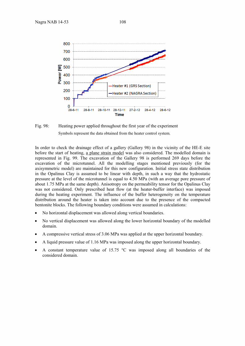
Nagra NAB 14-53 108
Fig. 98: Heating power applied throughout the first year of the experiment Symbols represent the data obtained from the heater control system.
In order to check the drainage effect of a gallery (Gallery 98) in the vicinity of the HE-E site before the start of heating, a plane strain model was also considered. The modelled domain is represented in Fig. 99. The excavation of the Gallery 98 is performed 269 days before the excavation of the microtunnel. All the modelling stages mentioned previously (for the axisymmetric model) are maintained for this new configuration. Initial stress state distribution in the Opalinus Clay is assumed to be linear with depth, in such a way that the hydrostatic pressure at the level of the microtunnel is equal to 4.50 MPa (with an average pore pressure of about 1.75 MPa at the same depth). Anisotropy on the permeability tensor for the Opalinus Clay was not considered. Only prescribed heat flow (at the heater-buffer interface) was imposed during the heating experiment. The influence of the buffer heterogeneity on the temperature distribution around the heater is taken into account due to the presence of the compacted bentonite blocks. The following boundary conditions were assumed in calculations:
• No horizontal displacement was allowed along vertical boundaries.
• No vertical displacement was allowed along the lower horizontal boundary of the modelled domain.
• A compressive vertical stress of 3.06 MPa was applied at the upper horizontal boundary.
• A liquid pressure value of 1.16 MPa was imposed along the upper horizontal boundary.
• A constant temperature value of 15.75 °C was imposed along all boundaries of the considered domain.
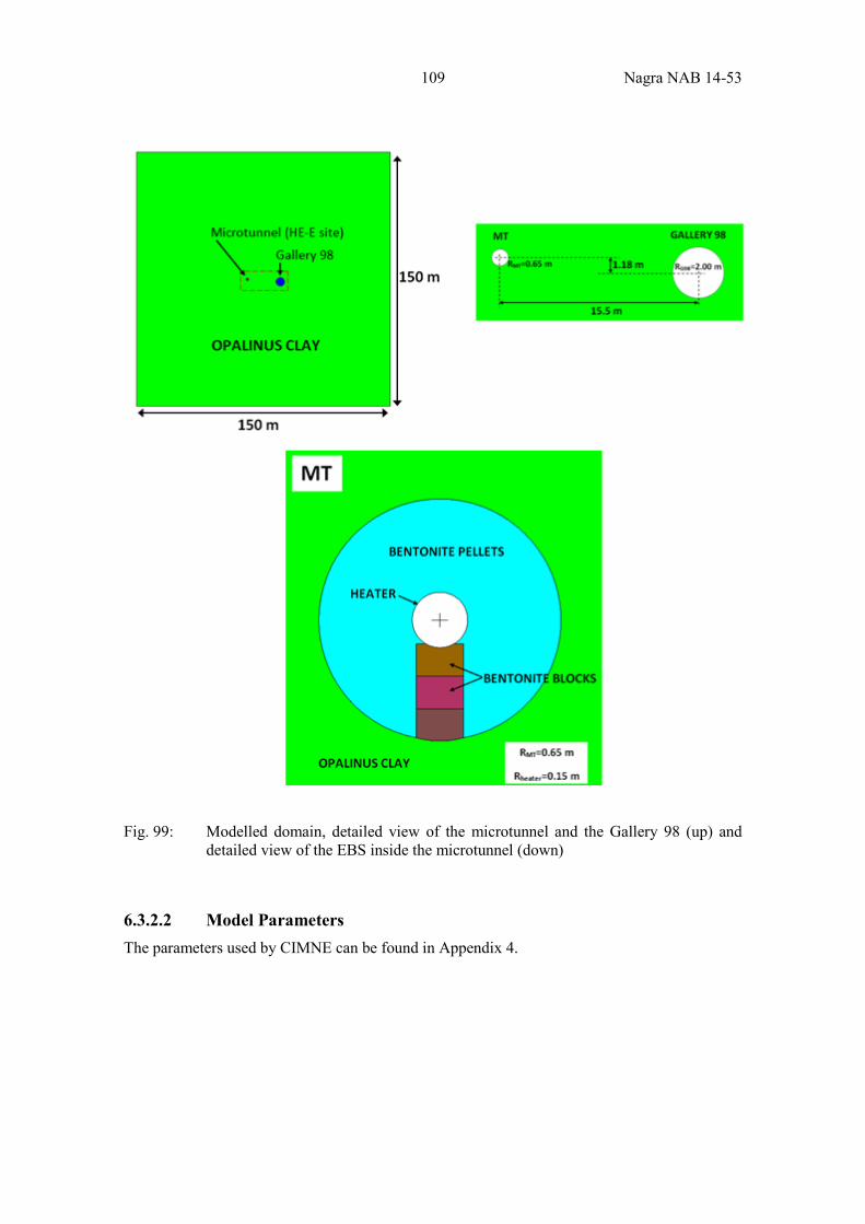
109 Nagra NAB 14-53
Fig. 99: Modelled domain, detailed view of the microtunnel and the Gallery 98 (up) and detailed view of the EBS inside the microtunnel (down)
6.3.2.2 Model Parameters The parameters used by CIMNE can be found in Appendix 4.
Nagra NAB 14-53 110
6.3.3 Modelling Results In the following, the evolution of computed and observed temperatures and hydraulic variables are presented. Time is referenced to the beginning of heating experiment (on June 28 2011) and measurements are included up to 917 days after that (end of December 2013). In all time evolution figures, vertical lines indicate the times at which radial profiles (representing variable distribution as a function of the distance to the microtunnel axis) are plotted.
6.3.3.1 Temperature Evolution Fig. 100 to 102 shows the temperature evolution in the buffer and in the first few meters into the host rock whereas in Fig. 103 the distribution of temperature in the middle of each heated section as a function of the distance to the microtunnel centre is depicted. In Fig. 104 and 105 some longitudinal profiles of temperature inside the EBS at different distances from the heater are shown. Line y=0 represents the upper boundary of the modelled geometry that is a symmetry plane for the axisymmetric conceptual model. The simulation with axial symmetry gives good temperature predictions indicating the model is able to capture the evolution of temperature during the experiment.
Concerning the numerical outcomes, the most remarkable feature to be remarked is the high thermal gradient inside the buffer due to heating. After the first year of the experiment the temperature reaches about 140 °C close to the heater-buffer interface and a value around 40 °C near the buffer-rock interface (see Fig. 100 and 103). In fact, 18 months after the end of the first heating phase (day nº 914 of the experiment) only the innermost 5 - 10 cm of the bentonite buffer exceeds a temperature of 100 °C (see Fig. 103 and 104). In the near field of the experiment, most of the temperature increase occurs during the temperature build-up at heater-bentonite interface. In this zone, temperature keeps increasing at a lower rate to a maximum value of about 47 °C (for the Nagra section) at the end of the fifth year of heating (model prediction) as seen in Fig. 101 to 103. At that time (day 1,825 of the experiment) the rock volume with a temperature increase larger than 15º is estimated to reach a maximum distance between 2.00 m (for the GRS buffer) and 2.30 m (for the Nagra buffer) from the tunnel axis.
Radial profiles of global thermal conductivity for both EBS materials (numerical results) are depicted in Fig. 105. The very low thermal conductivity for the bentonite barrier close to its dry state explains the high temperature gradient observed inside the buffers in the early post-closure phase of the experiment. Furthermore, the difference in thermal conductivities of the buffers (thermal conductivity for the bentonite-sand mixture is lower than the bentonite pellets one) also explains why the power required for applying/maintaining a similar temperature in both heaters is lower in the GRS section as shown in Fig. 107. Consequently temperature in the vicinity of the experiment is slightly higher around the Nagra section.
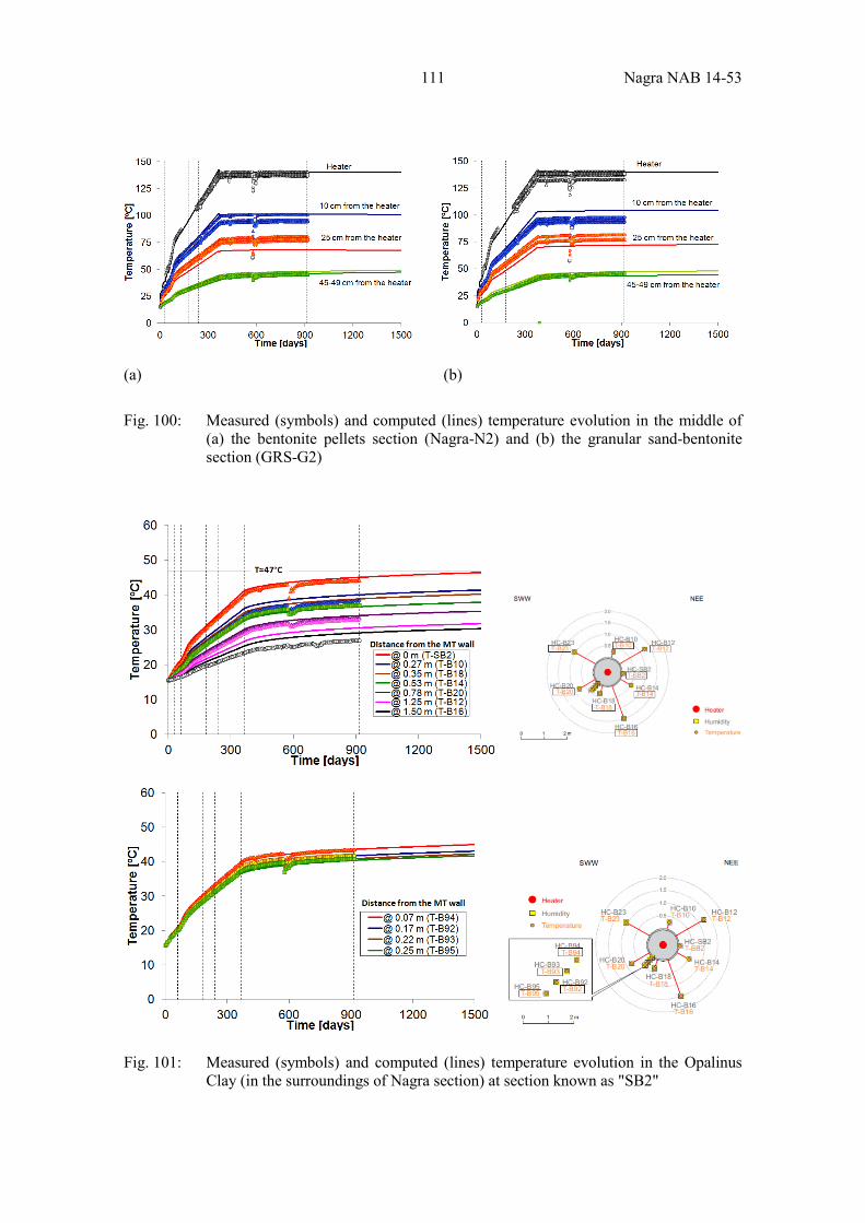
111 Nagra NAB 14-53
(a) (b)
Fig. 100: Measured (symbols) and computed (lines) temperature evolution in the middle of (a) the bentonite pellets section (Nagra-N2) and (b) the granular sand-bentonite section (GRS-G2)
Fig. 101: Measured (symbols) and computed (lines) temperature evolution in the Opalinus Clay (in the surroundings of Nagra section) at section known as "SB2"
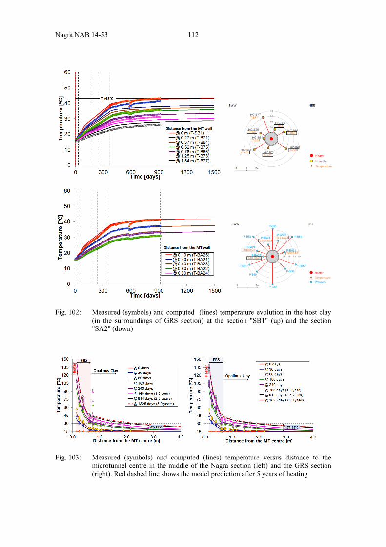
Nagra NAB 14-53 112
Fig. 102: Measured (symbols) and computed (lines) temperature evolution in the host clay (in the surroundings of GRS section) at the section "SB1" (up) and the section "SA2" (down)
Fig. 103: Measured (symbols) and computed (lines) temperature versus distance to the microtunnel centre in the middle of the Nagra section (left) and the GRS section (right). Red dashed line shows the model prediction after 5 years of heating
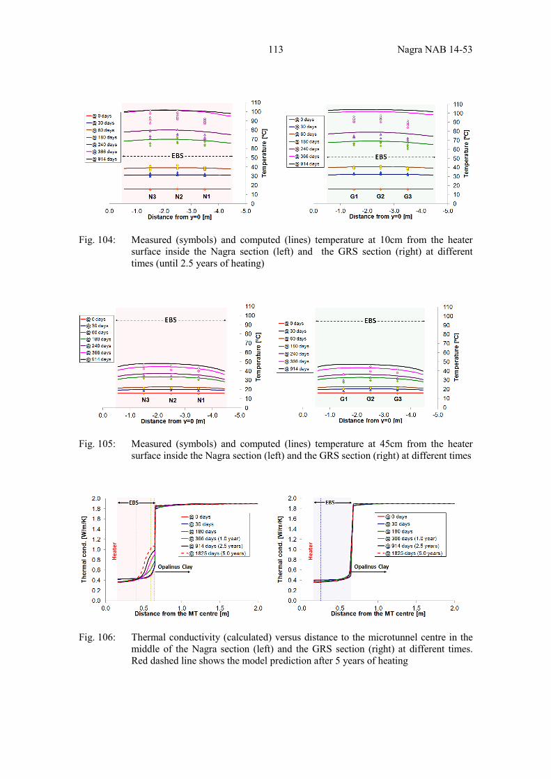
113 Nagra NAB 14-53
Fig. 104: Measured (symbols) and computed (lines) temperature at 10cm from the heater surface inside the Nagra section (left) and the GRS section (right) at different times (until 2.5 years of heating)
Fig. 105: Measured (symbols) and computed (lines) temperature at 45cm from the heater surface inside the Nagra section (left) and the GRS section (right) at different times
Fig. 106: Thermal conductivity (calculated) versus distance to the microtunnel centre in the middle of the Nagra section (left) and the GRS section (right) at different times. Red dashed line shows the model prediction after 5 years of heating
Nagra NAB 14-53 114
Fig. 107: Applied/estimated power in the two sections of the HE-E experiment. Symbols represent the measured data while lines indicate the modelling results
One limitation of the axisymmetric model is the inability to simulate the compacted blocks on which the heating system rests. The presence of these blocks is taken into account using the plane strain model. Numerical outcomes for this conceptual model are shown from Fig. 108 to 114. Good agreement between experimental data and modelling prediction is obtained along three radial profiles taken in the central section of the Nagra buffer as seen in Fig. 108. Spatial distribution of temperature around the heater at several times is given in Fig. 109 (day nº 180 of heating), Fig. 111 (1 year after the start of heating) and Fig. 113 (second year of heating). The shapes of isothermal contours indicate the higher thermal conductivity of the bentonite blocks. In fact, the model predicts a lower value of temperature for points inside the buffer and located at the same distance from the heater. In contrast, temperature in the rock mass tends to be slightly higher in the bottom portion of the microtunnel. This fact can be clearly noted in Fig. 110, 112 and 114 in which two vertical (12 and 6 o'clock) and two horizontal (3 and 9 o'clock) profiles of temperature are depicted at different times (days 180, 366 and 720 of heating, respectively).
115 Nagra NAB 14-53
(a)
(b)
(c)
Fig. 108: Measured and calculated temperature versus distance to the microtunnel centre for a (a) 12 o'clock profile, (b) 3 o'clock profile and (c) 9 o'clock profile
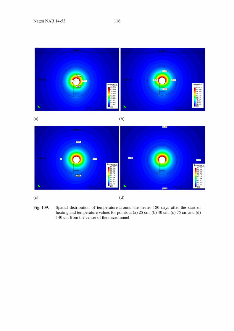
Nagra NAB 14-53 116
(a) (b)
(c) (d)
Fig. 109: Spatial distribution of temperature around the heater 180 days after the start of heating and temperature values for points at (a) 25 cm, (b) 40 cm, (c) 75 cm and (d) 140 cm from the centre of the microtunnel
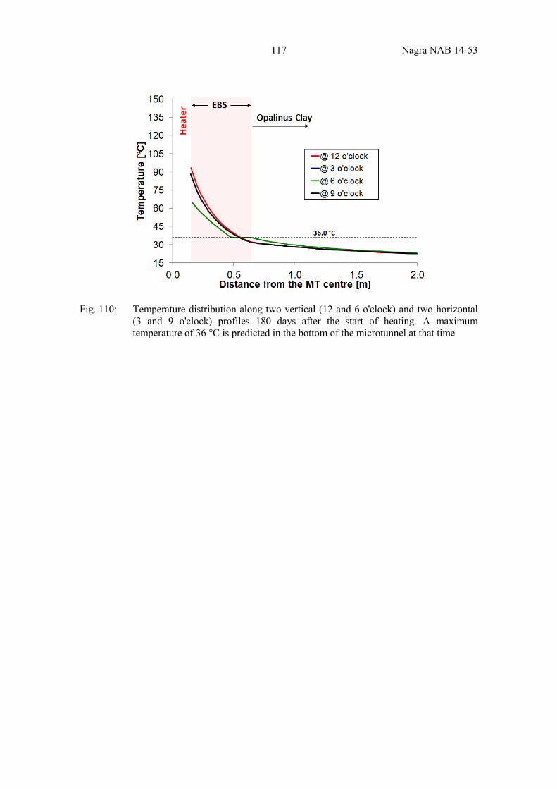
117 Nagra NAB 14-53
Fig. 110: Temperature distribution along two vertical (12 and 6 o'clock) and two horizontal (3 and 9 o'clock) profiles 180 days after the start of heating. A maximum temperature of 36 °C is predicted in the bottom of the microtunnel at that time
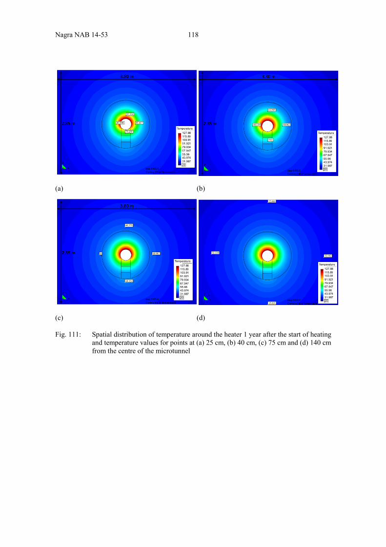
Nagra NAB 14-53 118
(a) (b)
(c) (d)
Fig. 111: Spatial distribution of temperature around the heater 1 year after the start of heating and temperature values for points at (a) 25 cm, (b) 40 cm, (c) 75 cm and (d) 140 cm from the centre of the microtunnel
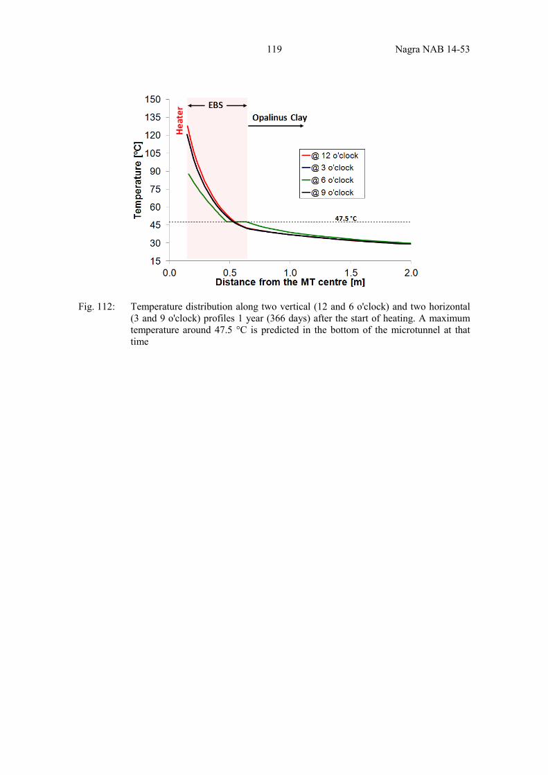
119 Nagra NAB 14-53
Fig. 112: Temperature distribution along two vertical (12 and 6 o'clock) and two horizontal (3 and 9 o'clock) profiles 1 year (366 days) after the start of heating. A maximum temperature around 47.5 °C is predicted in the bottom of the microtunnel at that time
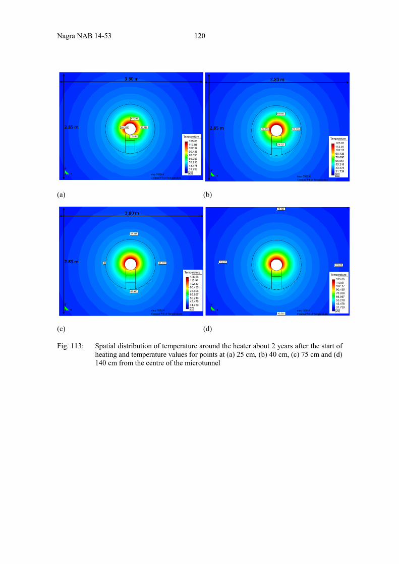
Nagra NAB 14-53 120
(a) (b)
(c) (d)
Fig. 113: Spatial distribution of temperature around the heater about 2 years after the start of heating and temperature values for points at (a) 25 cm, (b) 40 cm, (c) 75 cm and (d) 140 cm from the centre of the microtunnel
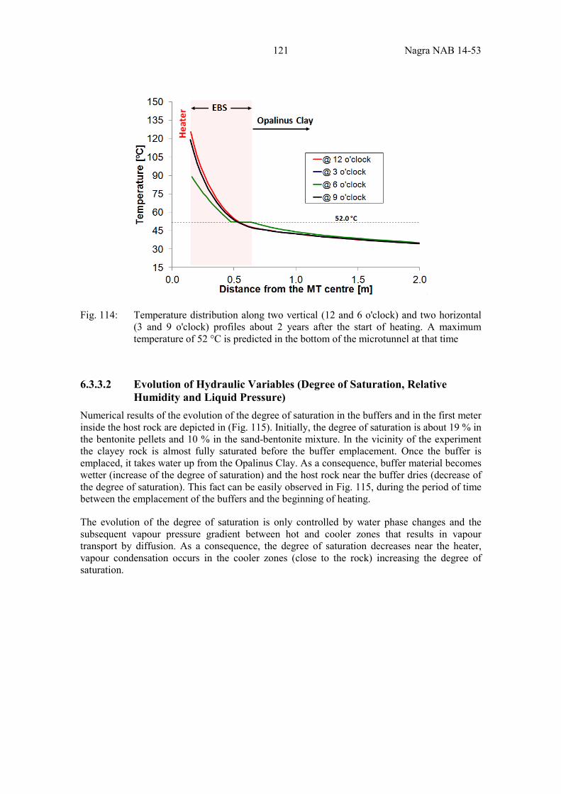
121 Nagra NAB 14-53
Fig. 114: Temperature distribution along two vertical (12 and 6 o'clock) and two horizontal (3 and 9 o'clock) profiles about 2 years after the start of heating. A maximum temperature of 52 °C is predicted in the bottom of the microtunnel at that time
6.3.3.2 Evolution of Hydraulic Variables (Degree of Saturation, Relative Humidity and Liquid Pressure)
Numerical results of the evolution of the degree of saturation in the buffers and in the first meter inside the host rock are depicted in (Fig. 115). Initially, the degree of saturation is about 19 % in the bentonite pellets and 10 % in the sand-bentonite mixture. In the vicinity of the experiment the clayey rock is almost fully saturated before the buffer emplacement. Once the buffer is emplaced, it takes water up from the Opalinus Clay. As a consequence, buffer material becomes wetter (increase of the degree of saturation) and the host rock near the buffer dries (decrease of the degree of saturation). This fact can be easily observed in Fig. 115, during the period of time between the emplacement of the buffers and the beginning of heating.
The evolution of the degree of saturation is only controlled by water phase changes and the subsequent vapour pressure gradient between hot and cooler zones that results in vapour transport by diffusion. As a consequence, the degree of saturation decreases near the heater, vapour condensation occurs in the cooler zones (close to the rock) increasing the degree of saturation.
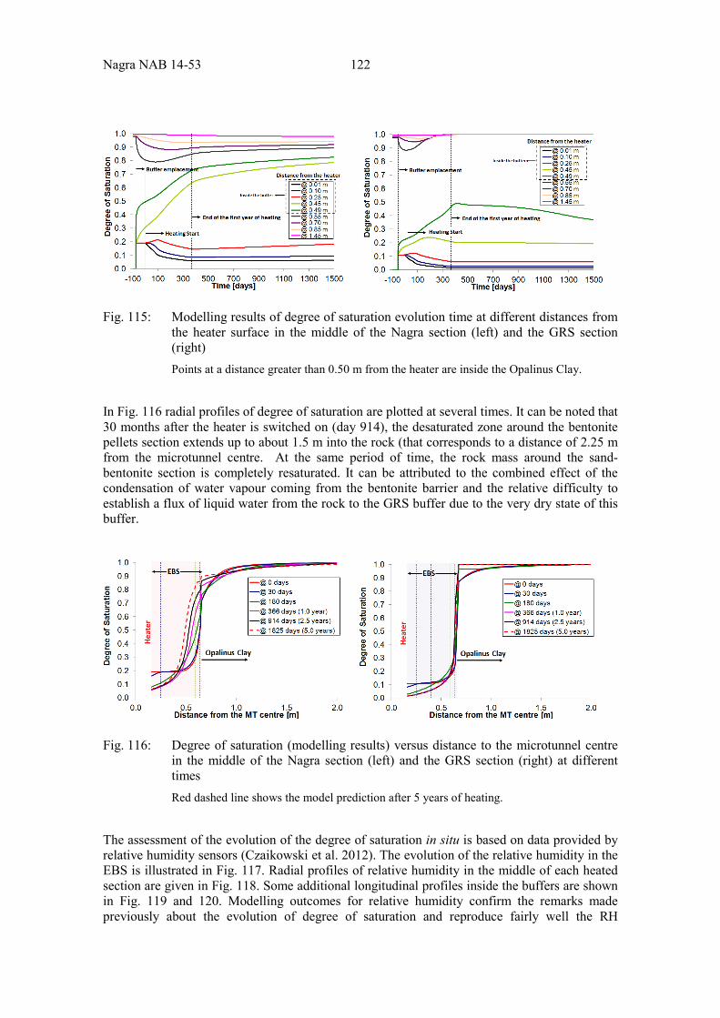
Nagra NAB 14-53 122
Fig. 115: Modelling results of degree of saturation evolution time at different distances from the heater surface in the middle of the Nagra section (left) and the GRS section (right) Points at a distance greater than 0.50 m from the heater are inside the Opalinus Clay.
In Fig. 116 radial profiles of degree of saturation are plotted at several times. It can be noted that 30 months after the heater is switched on (day 914), the desaturated zone around the bentonite pellets section extends up to about 1.5 m into the rock (that corresponds to a distance of 2.25 m from the microtunnel centre. At the same period of time, the rock mass around the sand-bentonite section is completely resaturated. It can be attributed to the combined effect of the condensation of water vapour coming from the bentonite barrier and the relative difficulty to establish a flux of liquid water from the rock to the GRS buffer due to the very dry state of this buffer.
Fig. 116: Degree of saturation (modelling results) versus distance to the microtunnel centre in the middle of the Nagra section (left) and the GRS section (right) at different times Red dashed line shows the model prediction after 5 years of heating.
The assessment of the evolution of the degree of saturation in situ is based on data provided by relative humidity sensors (Czaikowski et al. 2012). The evolution of the relative humidity in the EBS is illustrated in Fig. 117. Radial profiles of relative humidity in the middle of each heated section are given in Fig. 118. Some additional longitudinal profiles inside the buffers are shown in Fig. 119 and 120. Modelling outcomes for relative humidity confirm the remarks made previously about the evolution of degree of saturation and reproduce fairly well the RH
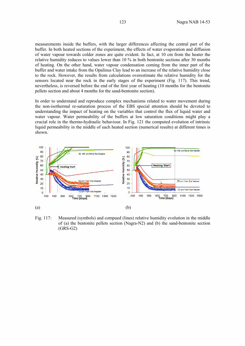
123 Nagra NAB 14-53
measurements inside the buffers, with the larger differences affecting the central part of the buffer. In both heated sections of the experiment, the effects of water evaporation and diffusion of water vapour towards colder zones are quite evident. In fact, at 10 cm from the heater the relative humidity reduces to values lower than 10 % in both bentonite sections after 30 months of heating. On the other hand, water vapour condensation coming from the inner part of the buffer and water intake from the Opalinus Clay lead to an increase of the relative humidity close to the rock. However, the results from calculations overestimate the relative humidity for the sensors located near the rock in the early stages of the experiment (Fig. 117). This trend, nevertheless, is reversed before the end of the first year of heating (10 months for the bentonite pellets section and about 4 months for the sand-bentonite section).
In order to understand and reproduce complex mechanisms related to water movement during the non-isothermal re-saturation process of the EBS special attention should be devoted to understanding the impact of heating on the variables that control the flux of liquid water and water vapour. Water permeability of the buffers at low saturation conditions might play a crucial role in the thermo-hydraulic behaviour. In Fig. 121 the computed evolution of intrinsic liquid permeability in the middle of each heated section (numerical results) at different times is shown.
(a) (b)
Fig. 117: Measured (symbols) and compued (lines) relative humidity evolution in the middle of (a) the bentonite pellets section (Nagra-N2) and (b) the sand-bentonite section (GRS-G2)
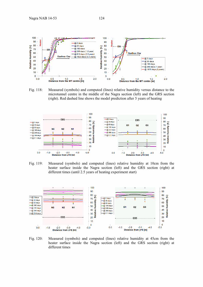
Nagra NAB 14-53 124
Fig. 118: Measured (symbols) and computed (lines) relative humidity versus distance to the microtunnel centre in the middle of the Nagra section (left) and the GRS section (right). Red dashed line shows the model prediction after 5 years of heating
Fig. 119: Measured (symbols) and computed (lines) relative humidity at 10cm from the heater surface inside the Nagra section (left) and the GRS section (right) at different times (until 2.5 years of heating experiment start)
Fig. 120: Measured (symbols) and computed (lines) relative humidity at 45cm from the heater surface inside the Nagra section (left) and the GRS section (right) at different times
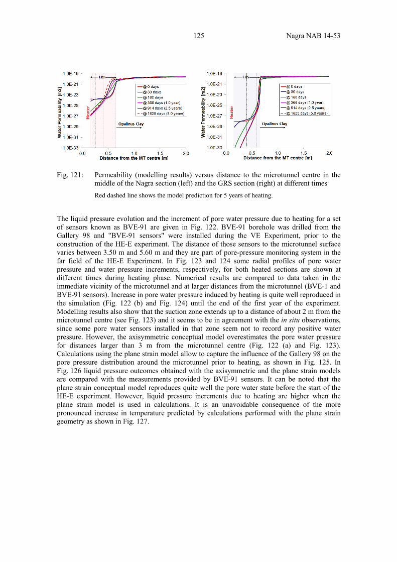
125 Nagra NAB 14-53
Fig. 121: Permeability (modelling results) versus distance to the microtunnel centre in the middle of the Nagra section (left) and the GRS section (right) at different times Red dashed line shows the model prediction for 5 years of heating.
The liquid pressure evolution and the increment of pore water pressure due to heating for a set of sensors known as BVE-91 are given in Fig. 122. BVE-91 borehole was drilled from the Gallery 98 and "BVE-91 sensors" were installed during the VE Experiment, prior to the construction of the HE-E experiment. The distance of those sensors to the microtunnel surface varies between 3.50 m and 5.60 m and they are part of pore-pressure monitoring system in the far field of the HE-E Experiment. In Fig. 123 and 124 some radial profiles of pore water pressure and water pressure increments, respectively, for both heated sections are shown at different times during heating phase. Numerical results are compared to data taken in the immediate vicinity of the microtunnel and at larger distances from the microtunnel (BVE-1 and BVE-91 sensors). Increase in pore water pressure induced by heating is quite well reproduced in the simulation (Fig. 122 (b) and Fig. 124) until the end of the first year of the experiment. Modelling results also show that the suction zone extends up to a distance of about 2 m from the microtunnel centre (see Fig. 123) and it seems to be in agreement with the in situ observations, since some pore water sensors installed in that zone seem not to record any positive water pressure. However, the axisymmetric conceptual model overestimates the pore water pressure for distances larger than 3 m from the microtunnel centre (Fig. 122 (a) and Fig. 123). Calculations using the plane strain model allow to capture the influence of the Gallery 98 on the pore pressure distribution around the microtunnel prior to heating, as shown in Fig. 125. In Fig. 126 liquid pressure outcomes obtained with the axisymmetric and the plane strain models are compared with the measurements provided by BVE-91 sensors. It can be noted that the plane strain conceptual model reproduces quite well the pore water state before the start of the HE-E experiment. However, liquid pressure increments due to heating are higher when the plane strain model is used in calculations. It is an unavoidable consequence of the more pronounced increase in temperature predicted by calculations performed with the plane strain geometry as shown in Fig. 127.
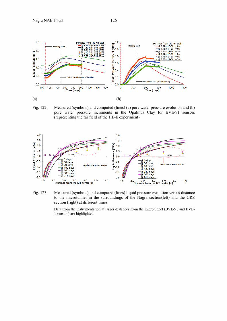
Nagra NAB 14-53 126
(a) (b)
Fig. 122: Measured (symbols) and computed (lines) (a) pore water pressure evolution and (b) pore water pressure increments in the Opalinus Clay for BVE-91 sensors (representing the far field of the HE-E experiment)
Fig. 123: Measured (symbols) and computed (lines) liquid pressure evolution versus distance to the microtunnel in the surroundings of the Nagra section(left) and the GRS section (right) at different times Data from the instrumentation at larger distances from the microtunnel (BVE-91 and BVE-1 sensors) are highlighted.
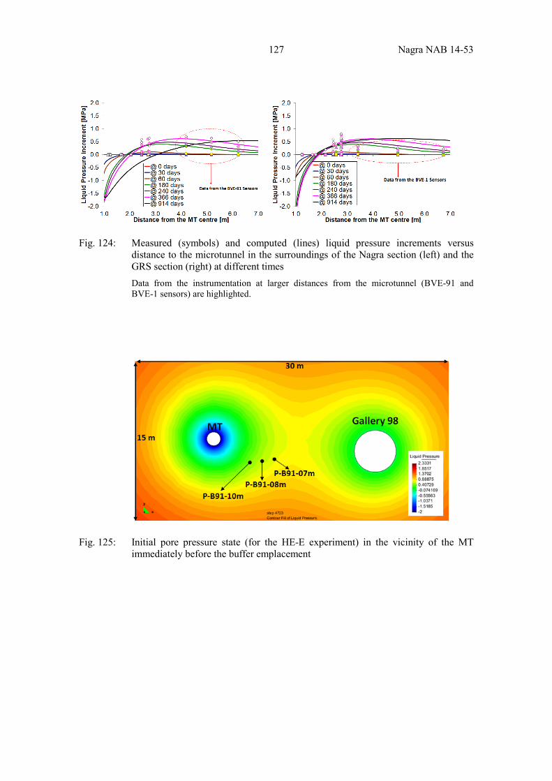
127 Nagra NAB 14-53
Fig. 124: Measured (symbols) and computed (lines) liquid pressure increments versus distance to the microtunnel in the surroundings of the Nagra section (left) and the GRS section (right) at different times Data from the instrumentation at larger distances from the microtunnel (BVE-91 and BVE-1 sensors) are highlighted.
Fig. 125: Initial pore pressure state (for the HE-E experiment) in the vicinity of the MT immediately before the buffer emplacement
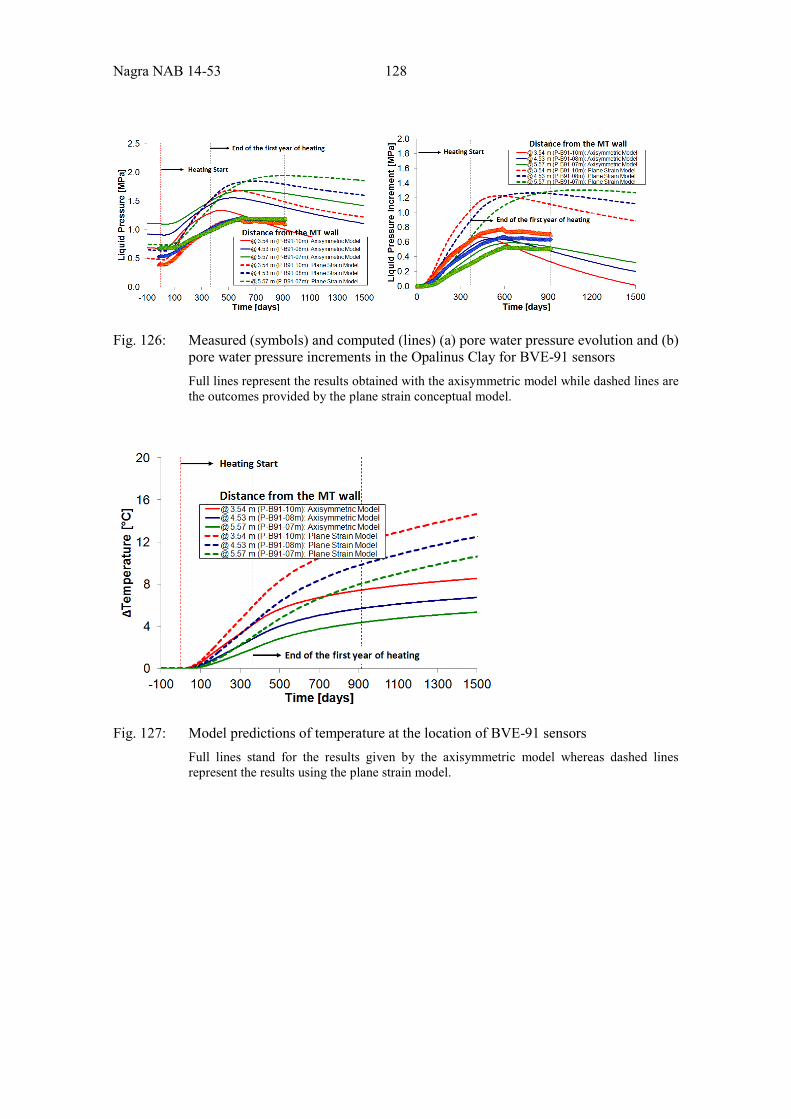
Nagra NAB 14-53 128
Fig. 126: Measured (symbols) and computed (lines) (a) pore water pressure evolution and (b) pore water pressure increments in the Opalinus Clay for BVE-91 sensors Full lines represent the results obtained with the axisymmetric model while dashed lines are the outcomes provided by the plane strain conceptual model.
Fig. 127: Model predictions of temperature at the location of BVE-91 sensors Full lines stand for the results given by the axisymmetric model whereas dashed lines represent the results using the plane strain model.
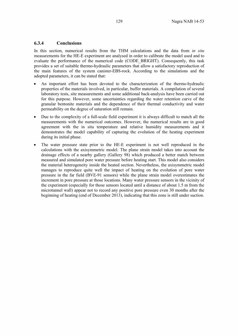
129 Nagra NAB 14-53
6.3.4 Conclusions In this section, numerical results from the THM calculations and the data from in situ measurements for the HE-E experiment are analysed in order to calibrate the model used and to evaluate the performance of the numerical code (CODE_BRIGHT). Consequently, this task provides a set of suitable thermo-hydraulic parameters that allow a satisfactory reproduction of the main features of the system canister-EBS-rock. According to the simulations and the adopted parameters, it can be stated that:
• An important effort has been devoted to the characterization of the thermo-hydraulic properties of the materials involved, in particular, buffer materials. A compilation of several laboratory tests, site measurements and some additional back-analysis have been carried out for this purpose. However, some uncertainties regarding the water retention curve of the granular bentonite materials and the dependence of their thermal conductivity and water permeability on the degree of saturation still remain.
• Due to the complexity of a full-scale field experiment it is always difficult to match all the measurements with the numerical outcomes. However, the numerical results are in good agreement with the in situ temperature and relative humidity measurements and it demonstrates the model capability of capturing the evolution of the heating experiment during its initial phase.
• The water pressure state prior to the HE-E experiment is not well reproduced in the calculations with the axisymmetric model. The plane strain model takes into account the drainage effects of a nearby gallery (Gallery 98) which produced a better match between measured and simulated pore water pressure before heating start. This model also considers the material heterogeneity inside the heated section. Nevertheless, the axisymmetric model manages to reproduce quite well the impact of heating on the evolution of pore water pressure in the far field (BVE-91 sensors) while the plane strain model overestimates the increment in pore pressure at those locations. Many water pressure sensors in the vicinity of the experiment (especially for those sensors located until a distance of about 1.5 m from the microtunnel wall) appear not to record any positive pore pressure even 30 months after the beginning of heating (end of December 2013), indicating that this zone is still under suction.

131 Nagra NAB 14-53
7 Conclusions and Lessons Learnt The HE-E experiment at the Mont Terri URL was one of the key elements of the PEBS project and was designed, constructed and operated successfully within the project timeframe. At the end of the PEBS project, the HE-E experiment continued as a Mont Terri partner project and its extension is decided upon on an annual basis by the partners (BGR, GRS, Enresa and Nagra).
This report describes:
1. The lay-out of the HE-E experiment providing the information that is needed to interpret the monitoring data and the modelling. The detail is described in the detailed design report (Gaus (ed.) 2011; PEBS deliverable D2.2-2)) and the as-built report (Teodori and Gaus (ed). 2011; PEBS deliverable D2.2-3). This is described in Section 1.
2. The collected data of the HE-E heating experiment in Mont Terri (Opalinus Clay) from heating start (June 2011) until the status at the end of PEBS (December 2013). This is based on the annual modelling reports (PEBS deliverables D2.2-8 (1 2, 3)) and the internet based data platform (WEBdavis). This is described in Sections 2, 3 and 5. This also includes the column tests on the HE-E EBS materials (PEBS Deliverable D2.2-7.3).
3. The modelling aided analysis of these data and associated optimal parameter set for the buffer materials and Opalinus Clay. This is described in Sections 4 and 6. The design and predictive modelling of the HE-E test describing earlier versions of the models referred to herein was summarized in Czaikowski et al. (2012; PEBS deliverable D3.2-1)
This report thus covers the final contribution on the HE-E experimental set-up (PEBS Deliverable D2.2-11) and the final contribution on the modelling and interpretation (PEBS Deliverable D3.2-2).
This report highlights the very consistent data set obtained for a challenging large number of sensors (78 relative humidity sensors and 80 temperature sensors in the EBS and 20 relative humidity, 30 pore water pressure and over 20 temperature sensors in Opalinus Clay). The high quality dataset allowed validating TH(M) models while the use of the models gave further insights into the material behaviour. On many occasions quantitative reproduction of the measured variables was achieved and all major observed patterns were qualitatively explained.
Considering the high density of the instrumentation characterising this experiment, the combination of a consistent dataset with the explanatory insights provided by the various models marks an achievement both from an experimental and modelling viewpoint.
In Section 7.1 general remarks regarding the thermal field and the hydraulic field are made from a combination of the observations and the modelling. In Section 7.2 the main conclusions from a pure observational point of view are given, while in Section 7.3 major general conclusion regarding the modelling are formulated.
Nagra NAB 14-53 132
7.1 Conclusions Related to the Thermal Field (Observations and Modelling)
The following items are put forward:
• The experimental methodology proved able to detect small temperature variations as a function of the sensor localization. Both the sensor reading and the localization of the sensors were precise enough to show e.g. longitudinal gradients along the heater length or around the heater
• The redundancy of the sensors as part of the experimental set-up illustrated the homogeneity of the thermal field and consistency of the sensor readings.
• Some sensors (in Opalinus Clay) are in place for more than 10 years now, but still show a consistent response, despite not being designed to be part of a heater experiment initially.
• The temperature response of the two buffer materials was reproduced well by the models, including second order processes such as the influence of the hydraulic behaviour of the buffer material on the thermal response
• The temperature behaviour of the buffer showed that the steady-state in the buffer is reached relatively fast. This observation was confirmed by the modelling results.
• The fact that the steady state in the buffer is reached relatively rapidly implies that all power emitted by the heater is transferred to the rock and hence the thermal response of the host rock is relatively independent of the buffer characteristics
• A precise reproduction of the thermal conductivity as a function of the saturation state (not only fully dry and wet values) was shown to be required in order to achieve an accurate reproduction of the thermal field. This relationship is suspected to be strongly dependent on the dry density and structural arrangement of the buffer particles. A thorough experimental characterization should thus be performed for each type of buffer material. This experimental characterization should be independent from the modelling calibration of the in-situ test to be able to attribute certain deviations to upscaling.
• The different models provided quite consistent modelling results regarding the thermal field.
• The influence of model assumptions (like 3D vs axisymmetric or plane strain) was significant and needs to be considered in detail when assessing the model results or calibrating the models (especially in case it is intended to extrapolate the model results).
7.2 Conclusions Related to the Hydraulic Field (Observations and Modelling)
7.2.1 Relative Humidity in the Unsaturated Parts of the Experiment The large number of relative humidity sensors allowed defining the unsaturated zone quite precisely. As expected, the major part of the buffer is unsaturated during the early phase represented by the HE-E experiment. Nevertheless, measurement of the relative humidity is only an indirect measurement of the saturation state of the buffer. According to those sensors, only a very small part of the rock is unsaturated. The pattern of measured relative humidity was reproduced satisfactorily. The quantitative match was good for some models. The following items are put forward:
133 Nagra NAB 14-53
• The experimental methodology is mature and the redundancy of the sensors as part of the experimental set-up showed very a homogenous pattern in relative humidities and consistent sensor readings
• Some sensors (in Opalinus Clay) are in place for more than 10 years now and show a consistent response, despite not being designed as part of a heater experiment initially. Most of the relative humidity sensors in the OPA show maximum readings
• The dryed zone around the heater, the advance of vapour diffusion front and the condensation of vapour in colder zones is reproduced by all models. A correct reproduction of the temperature field is necessary to reproduce the relative humidity behaviour
• The relative humidity response is highly dependent on the retention curve used. The calibration of the retention curve should ideally be done on the basis of independent laboratory measurements for the different backfilling materials. Furthermore, water perme-ability of the buffers at low saturation conditions might play a crucial role in the thermo-hydraulic behaviour. Also the role of vapour movement might not be fully understood.
• Despite the relative humidities in the blocks being initially very different from those in the granular materials, after approximately 1 year these become very similar at equal distances from the heater and seem entirely determined by the prevailing temperatures.
7.2.2 Saturated Zones under Suction The response of this zone is not characterized by any sensor. Only its extension can be derived from the relative humidity sensors indicating 100 % and pore water pressure measurements showing atmospheric pressure.
7.2.3 Pore Water Pressure in the Saturated Part The piezometers installed in the relatively far field showed the expected pore water pressure increase. The order of magnitude of this increase (order of 1 MPa) was matched satisfactorily by some models; nevertheless the modelled increase was shown to be very much dependent:
• On the selected conceptual model (plane strain computations that do not account for longitudinal flows overestimate this increase)
• On the selected constitutive law: a correct reproduction of the different constituents, in the line of poro-elastic frameworks, seems to be necessary for a correct understanding of this process
7.3 General Conclusions from the Observations Covering June 2011 - December 2013
The observed temperature increases in EBS and Opalinus Clay are in line with those predicted by the design calculations (slight variations are attributed to differences in model setup and conceptualization).
The EBS is characterized by a very strong temperature gradient owing to its low thermal conductivity of its very dry state especially in the inner part of the buffer. At the OPA interface a temperature of below 50 °C is registered. The heat pulse causes a further drying of the inner part of the buffer, whereby the initial water content is further reduced, below the water content at emplacement for both the granular material and the blocks. A complex development of the
Nagra NAB 14-53 134
humidity profiles takes place which is strongly determined by the different water contents and densities of the materials at installation, high sensitivity to changing two-phase flow parameters and the impact of vapour diffusion in a changing porous matrix. The vapour is driven out, in a most likely radial pattern and part of the increase in relative humidity at the interface between the EBS and the host rock can be attributed to condensation of vapour. The highest temperatures (>100 °C) are thus prevailing in an EBS with a very low water content (below <20 %RH).
The natural water inflow from the Opalinus Clay is occurring slowly. Although pores become saturated fairly rapidly (more so in the sand/bentonite than in the bentonite), after 32 months only at distances in the Opalinus Clay >1 m from the tunnel wall a hydraulic pressure is registered. The hydraulic pressure front is progressing toward the EBS, but how long this will take and when an equilibrium state will be reached if keeping the 140 °C constant cannot be determined from the current dataset. This can only be assessed using modelling.
The measured temperatures and relative humidities in the blocks and the granular materials are dominated by the distance of the measurement point to the heater and not by the differences in material properties although conditions at emplacement where somewhat different. This rapid homogenisation can also (partly) be explained by vapour movement and is observed for the first time in the HE-E, as this is the first large scale, high temperature experiment with different materials.
As predicted by the models, a hydraulic pressure increase, associated with the differential thermal expansion of the Opalinus Clay and the porewater, is observed in the saturated Opalinus Clay at a larger distance from the tunnel. The porewater pressure increase, which started developing shortly after switching on the heaters, developed further after the heater temperature was held stable at 140 °C and was maximal at about 3 m from the tunnel wall where an overpressure of 1 MPa developed, slowly flattening off a couple of months after the heater temperature stabilised. These overpressures were within the expected range, although it cannot be fully excluded that the overpressures are influenced by the presence of the tunnels nearby acting as a constant pressure boundary at 1 bar.
Based on the seismic transmission measurements, a variation of the derived P-wave velocity evolution was observed with pronounced dependencies on the orientation of the travel paths to the bedding (anisotropy) and their distances from the S/B-OPA interface. A sequence of decreasing and increasing P-wave velocities points to the creation and sealing of invisible microcracks within the first 50 cm from the S/B-OPA interface, most probably caused by desaturation, the thermal pulse and the saturation and porewater pressures changes. Seismic methods have been shown to be a very sensitive tool for the continuous characterization of changes in rock properties although no clear link between the seismic parameters and the physical phenomena could be established.
135 Nagra NAB 14-53
7.4 General Conclusions from the Modelling Conducted within the PEBS Project
The temperatures in the buffer materials and in the OPA nearfield (<2 m) are reasonably well reproduced with the various model approaches. Modelled temperatures are highly sensitive to the relationship between thermal conductivity and water saturation especially for low water saturation. Detailed characterisation of this aspect of the materials at hand is recommended.
There is reasonable agreement between models and measured TH parameters in early re-saturation. The most advanced THM models are capable of reproducing the dry-out zone which is developing over almost half the radial thickness of the bentonite. This is less the case for the TH models.
An important effort has been devoted to the characterization of the thermo-hydraulic properties of the materials involved, in particular, buffer materials. A compilation of several laboratory tests, site measurements and some additional back-analysis have been carried out for this purpose. However, some uncertainties regarding the water retention curve of the granular bentonite materials and the dependence of their thermal conductivity and water permeability on the degree of saturation still remain. The correlation between the parameters complicates the calibration process.
Models that differentiate in their setup between the initial state of the granular materials and the blocks (and their properties) are capable of capturing the evolution of these materials at the start of the experiment. However, the homogenisation in temperatures and relative humidities across the material boundaries that develop after a certain time (approximately 1 year) cannot be reproduced in detail as the model results are determined by the initial material parameters.
The built-up of hydraulic pressures in the OPA is slow and the area close to the tunnel surface is still in suction. It will require some years of monitoring to adequately test the models for re-saturation.
The size and the trend of the hydraulic overpressures can be reasonably well reproduced with various models. To obtain satisfactory results the hydraulic conditions in the OPA at a larger scale prior to the experiment initiation need to be established, which is not trivial in a URL as its presence causes an important disturbance of the hydraulic field compared to a natural (hydrostatic) regime.
Although, due to the complexity of a full-scale field experiment it is always difficult to match all the measurements with the numerical outcomes, the numerical results are in good agreement with the measurements and it demonstrates the model capability of capturing the evolution of the heating experiment during its initial phase.
The overall conclusion is that the tested TH(M) models have been shown to perform adequately for modelling this high temperature URL experiment, the performance of the barriers is well reproduced and the confidence in longer term calculations, beyond the experimental timescale, is reinforced.

137 Nagra NAB 14-53
8 References
Alonso, E.E., Gens, A. & Josa, A. (1990): A constitutive model for partially saturated soils. Géotechnique 40, Nº 3, 405 - 430
Börgesson, L., Hökmark, H. & Karnland, O., 1988: Rheological properties of sodium smectite clay, SKB TR-88-30, SKB, Stockholm, Sweden
Bock, H. (2001): RA Experiment. Rock Mechanics analyses and synthesis: Data Report on Rock Mechanics. Technical Report 2000-02. Mont Terri Project
Bock, H. (2002): RA Experiment: Rock mechanics analyses and synthesis: Conceptual model of the Opalinus Clay. Mont Terri Project Technical Report TR 2001-03 St-Ursanne, Switzerland
Czaikowski, O., Garitte, B., Gaus, I., Gens, A., Kuhlmann, U. & Wieczorek, K. (2012): Design and predictive modeling of the HE-E experiment. PEBS Deliverable D3.2-1. NAB 12-003. Nagra, Wettingen
Calder, N. & Avis, J. (2006): View User Manual, Version 4.0 2006. Intera Engineering, Ottawa, Canada
Corkum, A.G., and Martin, C.D. (2007), Modelling a mine-by test at the Mont Terri rock laboratory, Switzerland. International Journal of Rock Mechanics & Mining Sciences, 44, .846 - 859.
CODE_BRIGHT User's Manual (2009) UPC Geomechanical Group
ENRESA (2000): FEBEX Project. Full scale engineered barriers experiment for a deep geological repository for high level radioactive waste in crystalline host rock. Final Report. Madrid, Spain
Fernandez, A.M. (2011): Determination of the Specific Heat Capacity of materials used as confinement barrier at El Cabril, Report CIEMAT/DMA/2G208/3/11
Ferrari, A.& Laloui, L. (2012): Advances in the testing of the hydro-mechanical behaviour of shales. In L. Laloui and A. Ferrari editors. Multiphysical Testing of Soils and Shales, pages 57 - 68, Springer
Ferrari, A., Witteveen, P. & Laloui, L. (2012): Material properties and geomechanical tests on BHG-D1 cores: Mont Terri HG-D Experiment, Phase 15: Mont Terri HG-D Experiment, Phase 15. Mont Terri Technical Report TN 2010-52
Finsterle, S. (2007): ITOUGH2 User's Guide, Lawrence Berkeley National Laboratory, LBNL-40040, updated print
Floria, E., Sanz, F.J. & García-Siñeriz, J.L. (2002) Drying test: evaporation rate from core samples of "Opalinus Clay" under controlled environmental conditions. Deliverable D6, FIKW-CT2001-00126
Nagra NAB 14-53 138
Flotron, HE-E Experiment: 3D Scanning of microtunnel VE with Tachymeter, TECHNICAL NOTE 2011-12, October 2010
Garitte, B. (2013): FMT-FE Experiment: Updated scoping computations, Nagra Internal Report NIB 13-01, Nagra, Wettingen
Garitte, B., Gens, A., Vaunat, J., Armand, G. (2012): Thermal Conductivity of Argillaceous Rocks; Determination Methodology Using In Situ Heating Tests. Tests in Rock Mechanics and Rock Engineering. DOI 10.1007/s00603-012-0335-x
Gaus I. (Ed.) (2011): Long term Performance of Engineered Barrier Systems (PEBS) : Mont Terri HE-E experiment: detailed design. Nagra-Arbeitsbericht NAB 11-01. Nagra, Wettingen 2011
Gaus, I. (2012): HE-E Experiment: Modellers as-built dataset for the predictive modeling. Version 2. February 2012
Gaus, I. (2013): HE-E Experiment: Modellers as-built dataset for the model calibration. Version 3. April 2013
Gaus, I., Wieczorek, K., Schuster, K., Garitte, B., Senger, R., Vasconcelos, R. & Mayor, J.-C. (2014): EBS behaviour immediately after repository closure in a clay host rock: HE-E experiment(Mont Terri URL).- Geological Society Special Publication - Issue from the Clay Conference. 5th international meeting "Clays in Natural and Engineered Barriers for Radioactive WasteConfinement" 22th - 25th October 2012, Montpellier, 19. In press
Gens, A. (2000): HE Experiment: complementary rock laboratory tests. Technical Note 2000-47. Mont Terri Project
Gens, A., Garitte, B., Wileveau & Y. (2007): In situ behaviour of a stiff layered clay subject to thermal loading: observations and interpretation. Geotechnique 57: 207 - 228
Hirschfelder, J.O., Curtiss, C.F. & Bird, R.B.: Molecular Theory of Gases and Liquids, John Wiley & Sons, New York, NY, 1954
Hoffman, C., Alonso, E.E. & Romero, E. (2007): Hydro-mechanical behaviour of bentonite pellet mixtures. Physics and Chemistry of the Earth, Nº 32, 832 - 849
Hökmark, H., Ledesma, A., Lassabatere, T., Fälth, B., Börgesson, L., Robinet, J.C., Sellali, N. & Sémété, P. (2007): Modelling heat and moisture transport in the ANDRA/SKB temperature buffer test. Physics and Chemistry of the Earth, Nº 32, 753 - 766
International Formulation Committee. A Formulation of the Thermodynamic Properties of Ordinary Water Substance, IFC Secretariat, Düsseldorf, Germany, 1967
Mayor, J. C., García-Siñeriz, J. L., Velasco, M., Gómez- Hernández, J., Lloret, A., Matray, J.-M., Coste, F., Giraud, A., Rothfuchs, T., Marshall, P., Roesli, U. & Mayer, G. (2007): Ventilation Experiment in Opalinus Clay for the disposal of radioactive waste in underground repositories. - In: Bossart, P. & Nussbaum, C. (Eds.): Mont Terri Project - Heater Experiment, Engineered Barrier Emplacement and Ventilation Experiment (p.182 - 240). - Rep. Swiss Geol. Surv. 1
139 Nagra NAB 14-53
Muñoz, J.J., Lloret, A. & Alonso, E. (2003): Laboratory Report: Characterization of hydraulic properties under saturated and non saturated conditions. Project Deliverable 4 EC contract FIKW-CT2001-00126
Nagra 2008: Effects of post-disposal gas generation in a repository for low- and intermediate-level waste sited in the Opalinus Clay of Northern Switzerland, Nagra Technical Report, NTB 08-07
Olivella, S., Carrera, J., Gens, A. & Alonso, E.E. (1994): Non-isothermal multiphase flow of brine and gas through saline media. Transport in Porous Media, Nº 15, 271 - 293
Olivella, S. (1995): Nonisothermal multiphase flow of brine and gas through saline media. Doctoral Thesis, Technical University of Catalonia (UPC), Barcelona, Spain
Olivella, S. & Alonso, E.E. (2008): Gas flow through clay barriers, Geotechnique, v.58, no.3, p. 157 - 176.
Pruess, K., Oldenburg, K. & Moridis, G. (1999): TOUGH2 - User's Guide, Version 2.0., Lawrence Berkeley National Laboratory Report LBL-43134, Berkeley, CA, USA
Rizzi, M., Seiphoori, A., Ferrari, A., Ceresetti, D. & Laloui, L. (2012): Analysis of the behaviour of granular MX-80 bentonite in THM processes., Nagra-Aktennotiz AN 12-102
Rösli (2010): VE Experiment - Long Term Monitoring Data Report -Phase 15 -1 July 2009 - 30 June 2010. Technical Report TN 2010-12
Romero, E. & Gómez, R. (2013): Water and air permeability tests on deep core samples from Schlattingen SLA-1 borehole. Nagra-Arbeitsbericht NAB 13-51. Nagra, Wettingen, Switzerland
Schuster, K. (2007): High resolution seismic investigations within the VE-Experiment, Mont Terri Technical Report TR 07-06, Swisstopo, Wabern, Switzerland
Schuster, K. (2014): Seismic long-term monitoring of EBS evolution. PEBS Deliverable D2.2-10
Tang, A.M. & Cui, Y.J. (2006): Use of saturated saline solutions in determining the water retention curve of compacted bentonite at different temperatures. Proceedings of the 4th International Conference on Unsaturated Soils (UNSAT'2006), Carefree, Arizona, USA. April 2 - 6, 2006. Vol. 2, pp. 1439 - 1450
Tang, A.M., Cui, Y.J. & Le, T.T. (2008): A study on the thermal conductivity of compacted bentonites. Applied Clay Science, 41: 181 - 189
Tang, A.M. & Cui, Y.J. (2010): Effects of mineralogy on thermo-hydro-mechanical parameters of MX80 bentonite. Journal of Rock Mechanics and Geotechnical Engineering, Nº 2, 91 - 96
Teodori, S.-P. & Gaus, I. (2011): Long Term performance of Engineered Barrier Systems (PEBS), Mont Terri HE-E Experiment: as-built report, Nagra-Arbeitsbericht, NAB 11-25
Nagra NAB 14-53 140
Van Genuchten, M.Th.A. (1980): Closed-Form Equation for Predicting the Hydraulic Conductivity of Unsaturated Soils, Soil Sci. Soc. , Vol. 44, pp. 892 - 898
Villar, M.V. (2007): Retention curves determined on samples taken before the second drying phase. Technical Report M2144/5/07
Villar, M.V. & Gómez-Espina, R. (2008): Effect of temperature on the wáter retention capacity of FEBEX and MX-80 bentonites. In: Doll D G, Augarde C E, Gallipoli D, et al Ed. Unsaturated Soils: Advances in Geo-engineering, Proceedings of the First European Conference on Unsaturated Soils, E-UNSAT. London: CRC Press/A. A. Balkema, Taylor and Francis Group 2008: 257 - 262
Villar, M.V., Martín, P.L., Gómez-Espina, R., Romero, F.J. & Barcala, J.M. (2012): Long-term THM tests reports: THM cells for the HE-E experiment: setup and first results. PEBS Deliverable 2.2-7.1. CIEMAT Technical Report CIEMAT/DMA/2G210/03/2012. Madrid 27 pp
Villar, M.V., Martín, P.L., Romero, F.J., Gutiérrez, V. & Barcala, J.M. (2014a): Sealing Materials used in the HE-E experiment: Thermo-hydro-mechanical Characterisation. International Conference on the Performance of Engineered Barriers: Backfill, Plugs & Seals. Hannover, 6 - 7 February 2014
Villar, M.V., Martín, P.L. & Romero, F.J. (2014b): Long-term THM tests reports. THM cells for the HE-E test: update of results until February 2014. PEBS Deliverable D2.2-7.3. Madrid, Spain
Wileveau, Y. & Rothfuchs, T. (2007): THM behaviour of host rock(HE-D) Experiment: Study of Thermal effects on Opalinus Clay, Mont Terri Technical Report 2006-01
Wieczorek, K., Miehe, R. & Garitte, B. (2011): Measurement of thermal parameters of the HE-E buffer materials. PEBS Deliverable D2.2-5
Zhang, C. L. & Rothfuchs, T. (2005): Report on instrument layout and pre-testing of large lab VE-tests. Deliverable 4.3.11
Zhang, C-L. & Rothfuchs, T. (2007): Laboratory Experiments on the THM Behaviour of Clay Rocks, TIMODAZ, Report D.2
Zubair, S.M. & Chaudhry, M.A. (1993): Some analytical solutions of time-dependent, continuously operating heat sources. Wärme- und Stoffübertragung 28 217 223 (1993) © Springer-Verlag
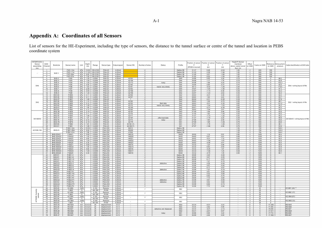
A-1 Nagra NAB 14-53
Appendix A: Coordinates of all Sensors
List of sensors for the HE-Experiment, including the type of sensors, the distance to the tunnel surface or centre of the tunnel and location in PEBS coordinate system
INTERFACE/
Sensor assembling
box
DAS -
Channel
Borehole
Sensor name
Unit
Depth
[m]
Range
Sensor type
Output signal
Sensor SN
Number of wires
Status
Profile
Position of sensor Z
[PEBS m tunnel]
Position of sensor X
[m]
Position of sensor Y
[m]
Height P-Sensor membran
above casted tunnel floor (m)
Offset
on GMII
Factor on GMII
Reference
on GMII
Atmos-pheric
pressure
Cable identification at DAS side
-
1 BVE-1
P-B1-13m kPa 13.00 100-2100 PAA-23 4-20mA 2 Gallery 98 31.37 0.28 -2.04 1.50 -1 500 100 2 P-B1-11m kPa 11.00 100-2100 PAA-23 4-20mA 2 Gallery 98 31.32 2.28 -1.86 1.50 -1 500 100 3 P-B1-09m kPa 9.00 100-2100 PAA-23 4-20mA 2 Gallery 98 31.26 4.27 -1.68 1.25 -1 500 100 4 P-B1-07m kPa 7.00 100-2100 PAA-23 4-20mA 2 Gallery 98 31.20 6.22 -1.50 1.25 -1 500 100
SA4
5 BVE-2 P-B2 kPa 1.55 0-2000 PAA-23 4-20mA 42183 2 SA4 33.88 0.00 2.30 0.70 -1 500 0 88.2
SA4 + wiring layout of Me
6 BVE-3 P-B3 kPa 1.04 0-2000 PAA-23 4-20mA 42194 2 SA4 34.98 1.17 1.76 0.70 -1 500 0 92.8 7 BVE-4 P-B4 kPa 1.05 0-2000 PAA-23 4-20mA 42172 2 noisy SA4 34.98 1.68 0.25 0.70 -1 500 0 102.2 8 BVE-5 P-B5 kPa 0.55 0-2000 PAA-23 4-20mA 42180 2 SA4 34.98 0.85 -0.31 0.70 -1 500 0 92.6 9 BVE-6 P-B6 kPa 1.63 0-2000 PAA-23 4-20mA 42181 2 reacts very slowly SA4 36.13 -0.02 -1.26 0.35 -1 500 0 119.0
10 BVE-7 P-B7 kPa 2.06 0-2000 PAA-23 4-20mA 42182 2 SA4 34.97 -1.94 -1.36 0.35 -1 500 0 97.3 11 BVE-8 P-B8 kPa 0.50 0-2000 PAA-23 4-20mA 42188 2 SA4 34.97 -1.15 0.36 0.35 -1 500 0 92.2 12 BVE-9 P-B9 kPa 1.40 0-2000 PAA-23 4-20mA 42196 2 SA4 34.97 -1.43 2.02 0.35 -1 500 0 92.4
SA2
13 BVE-55 P-B55 kPa 2.11 0-2000 PAA-23 4-20mA 42169 2 SA2 29.63 -0.01 3.39 0.30 -1 500 0 94.3
SA2 + wiring layout of Me
14 BVE-56 P-B56 kPa 2.11 0-2000 PAA-23 4-20mA 42167 2 SA2 29.64 1.94 2.44 0.30 -1 500 0 93.7 15 BVE-57 P-B57 kPa 1.80 0-2000 PAA-23 4-20mA ? 2 SA2 29.64 2.31 -0.36 0.30 -1 500 0 97.9 16 BVE-58 P-B58 kPa 1.12 0-2000 PAA-23 4-20mA 42184 2 SA2 29.63 1.28 -0.75 0.30 -1 500 0 98.1 17 BVE-59 P-B59 kPa 2.12 0-2000 PAA-23 4-20mA 42193 2 Bad data SA2 29.63 -0.01 -2.30 0.65 -1 500 0 101.2 18 BVE-60 P-B60 kPa 1.50 0-2000 PAA-23 4-20mA 42170 2 reacts very slowly SA2 29.62 -1.54 -1.03 0.65 -1 500 0 95.3 19 BVE-61 P-B61 kPa 1.80 0-2000 PAA-23 4-20mA 42185 2 SA2 29.61 -2.31 -0.36 0.65 -1 500 0 95.3 20 BVE-62 P-B62 kPa 2.13 0-2000 PAA-23 4-20mA 42195 2 SA2 29.62 -1.94 2.47 0.65 -1 500 0 93.5
SA1&SA3
21 BVE-38 P-B38 kPa 2.10 0-2000 PAA-23 4-20mA 42191 2 SA3 31.49 1.94 2.46 0.35 -1 500 0 93.5 SA1&SA3 + wiring layout of Me
22 BVE-39 P-B39 kPa 2.11 0-2000 PAA-23 4-20mA 42176 2 SA3 31.49 1.92 -1.49 0.35 -1 500 0 93.5 23 BVE-40 P-B40 kPa 1.80 0-2000 PAA-23 4-20mA 42177 2 SA3 31.47 -1.73 -1.24 0.35 -1 500 0 95.2 24 BVE-41 P-B41 kPa 1.81 0-2000 PAA-23 4-20mA 42187 2 often bad data SA3 31.47 -1.74 2.25 0.35 -1 500 0 98.8 25 BVE-78 P-B78 kPa 2.10 0-2000 PAA-23 4-20mA 42173 2 noisy SA1 27.99 1.95 2.39 0.70 -1 500 0 93.6 26 BVE-79 P-B79 kPa 2.10 0-2000 PAA-23 4-20mA 42175 2 SA1 27.99 1.95 -1.49 0.70 -1 500 0 84.6 27 BVE-80 P-B80 kPa 1.81 0-2000 PAA-23 4-20mA 42192 (?) 2 SA1 27.97 -1.76 -1.28 0.70 -1 500 0 96.1 28 BVE-81 P-B81 kPa 1.80 0-2000 PAA-23 4-20mA 42189 (?) 2 SA1 27.97 -1.86 2.06 0.70 -1 500 0 93.6
421038.182
29 BVE-91
P-B91-10m kPa 10.00 0-3000 PAA-33X 4-20mA 65014 2 Gallery 98 1.05 -1 750 0 108.3 30 P-B91-08m kPa 8.82 0-3000 PAA-33X 4-20mA 65269 2 Gallery 98 1.05 -1 750 0 100.2 31 P-B91-07m kPa 7.66 0-3000 PAA-33X 4-20mA 47458 2 Gallery 98 1.05 -1 750 0 109.4 32 BHE-ESA21 P-BA21 kPa 0.60 0-5000 PAA-23X 4-20mA 146519 2 SA20 29.62 1.14 0.91 0.80 -1 1250 0 92.4 33 BHE-ESA22 P-BA22 kPa 1.00 0-5000 PAA-23X 4-20mA 146520 2 SA20 29.62 0.57 2.01 0.80 -1 1250 0 92.0 34 BHE-ESA23 P-BA23 kPa 0.60 0-5000 PAA-23X 4-20mA 146521 2 SA20 29.62 -0.51 1.72 0.50 -1 1250 0 92.0 35 BHE-ESA24 P-BA24 kPa 1.00 0-5000 PAA-23X 4-20mA 146522 2 SA20 29.62 -1.58 1.03 0.50 -1 1250 0 92.0 36 BHE-ESA25 P-BA25 kPa 0.30 0-5000 PAA-23X 4-20mA 146523 2 SA20 29.62 -0.98 0.47 0.50 -1 1250 0 92.0 37 BHE-ESD21 P-BD21 kPa 0.60 0-5000 PAA-23X 4-20mA 146514 2 SD20 33.32 1.24 0.96 0.80 -1 1250 0 92.9 38 BHE-ESD22 P-BD22 kPa 1.00 0-5000 PAA-23X 4-20mA 146515 2 SD20 33.32 0.62 2.05 0.80 -1 1250 0 92.9 39 BHE-ESD23 P-BD23 kPa 0.60 0-5000 PAA-23X 4-20mA 146516 2 SD20 33.32 -0.45 1.81 0.50 -1 1250 0 92.5 40 BHE-ESD24 P-BD24 kPa 1.00 0-5000 PAA-23X 4-20mA 146517 2 SD20 33.32 -1.56 1.20 0.50 -1 1250 0 92.0 41 BHE-ESD25 P-BD25 kPa 0.30 0-5000 PAA-23X 4-20mA 146518 2 SD20 33.32 -0.70 1.35 0.50 -1 1250 0 90.1 42 BHE-E1 P-BE1-I1 kPa 0-5000 PAA-23X 4-20mA 2 Gallery 98 28.98 4.26 -0.46 -1 1250 0 43 BHE-E1 P-BE1-I2 kPa 0-5000 PAA-23X 4-20mA 2 Gallery 98 28.98 5.07 -0.55 -1 1250 0 44 BHE-E1 P-BE1-I3 kPa 0-5000 PAA-23X 4-20mA 2 Gallery 98 28.98 6.17 -0.67 -1 1250 0 45 BHE-E1 P-BE1-I4 kPa 0-5000 PAA-23X 4-20mA 2 Gallery 98 28.98 7.27 -0.79 -1 1250 0 46 BHE-E2 P-BE2-I1 kPa 0-5000 PAA-23X 4-20mA 2 defective Gallery 98 33.98 4.26 -0.46 -1 1250 0 47 BHE-E2 P-BE2-I2 kPa 0-5000 PAA-23X 4-20mA 2 Gallery 98 33.98 5.07 -0.55 -1 1250 0 48 BHE-E2 P-BE2-I3 kPa 0-5000 PAA-23X 4-20mA 2 Gallery 98 33.98 6.17 -0.67 -1 1250 0 49 BHE-E2 P-BE2-I4 kPa 0-5000 PAA-23X 4-20mA 2 defective Gallery 98 33.98 7.27 -0.79 -1 1250 0 50 BHE-E1 P-BE1-P1 kPa 0-5000 PAA-23X 4-20mA 2 Gallery 98 28.98 4.61 -0.50 -1 1250 0 51 BHE-E1 P-BE1-P2 kPa 0-5000 PAA-23X 4-20mA 2 Gallery 98 28.98 5.52 -0.60 -1 1250 0 52 BHE-E1 P-BE1-P3 kPa 0-5000 PAA-23X 4-20mA 2 Gallery 98 28.98 6.82 -0.74 -1 1250 0 53 BHE-E1 P-BE1-P4 kPa 0-5000 PAA-23X 4-20mA 2 Gallery 98 28.98 7.73 -0.84 -1 1250 0 54 BHE-E2 P-BE2-P1 kPa 0-5000 PAA-23X 4-20mA 2 defective Gallery 98 33.98 4.61 -0.50 -1 1250 0 55 BHE-E2 P-BE2-P2 kPa 0-5000 PAA-23X 4-20mA 2 defective Gallery 98 33.98 5.52 -0.60 -1 1250 0 56 BHE-E2 P-BE2-P3 kPa 0-5000 PAA-23X 4-20mA 2 Gallery 98 33.98 6.82 -0.74 -1 1250 0 57 BHE-E2 P-BE2-P4 kPa 0-5000 PAA-23X 4-20mA 2 Gallery 98 33.98 7.73 -0.84 -1 1250 0
AIT
EM
IN H
umid
ity
cabi
net
65 BVE-95 HC-B95 %RH 0-100 Rotronic 4-20mA - 7 SB2 - -1 25 0 - HC-B91 (22) ** 66 BVE-95 T-B95 °C -40-180 Pt100 4-20mA - -1 25 0 - 67 BVE-92 HC-B92 %RH 0-100 Rotronic 4-20mA - 7 SB2 - -1 25 0 - HC-B92 (17) 68 BVE-92 T-B92 °C -40-180 Pt100 4-20mA - -1 25 0 - 69 BVE-94 HC-B94 %RH 0-100 Rotronic 4-20mA - 7 SB2 - -1 25 0 - HC-B94 (07) 70 BVE-94 T-B94 °C -40-180 Pt100 4-20mA - -1 25 0 - 71 BVE-93 HC-B93 %RH 0-100 Rotronic 4-20mA - 7 SB2 - -1 25 0 - HC-B93 (12) 72 BVE-93 T-B93 °C -40-180 Pt100 4-20mA - -1 25 0 - 73 BVE-25 RD-B25 mm 0.0-2.0 25 displacement 0-5 V - 3 SD2 33.33 -0.01 3.23 - 0 5 -17.490 - RD-B25
74 BVE-26 RD-B26 mm 0.0-2.0 25 displacement 0-5 V - 3 SD2 33.34 2.62 0.08 - 0 5 -17.394 - RD-B26
75 BVE-27 RD-B27 mm 0.0-2.0 25 displacement 0-5 V - 3 defective and displaced SD2 33.33 -0.01 -2.13 - 0 5 -19.405 - RD-B27
76 BVE-28 RD-B28 mm 0.0-2.0 25 displacement 0-5 V - 3 SD2 33.31 -2.61 0.07 - 0 5 -17.911 - RD-B28
77 BVE-46 RD-B46 mm 0.0-2.0 25 displacement 0-5 V - 3 noisy SD1 30.88 0.00 3.22 - 0 5 -17.710 - RD-B46
78 BVE-47 RD-B47 mm 0.0-2.0 25 displacement 0-5 V - 3 SD1 30.89 2.62 0.04 - 0 5 -17.362 - RD-B47
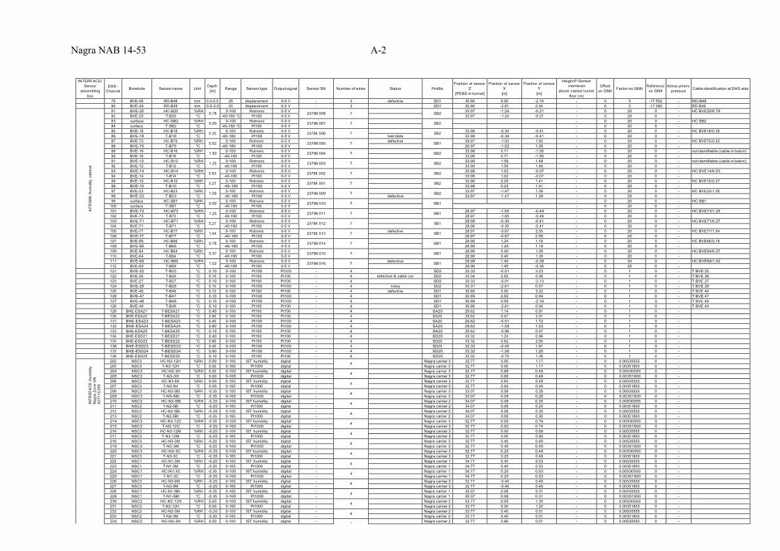
Nagra NAB 14-53 A-2
INTERFACE/ Sensor
assembling box
DAS -
Channel
Borehole
Sensor name
Unit
Depth
[m]
Range
Sensor type
Output signal
Sensor SN
Number of wires
Status
Profile
Position of sensor Z
[PEBS m tunnel]
Position of sensor X
[m]
Position of sensor Y
[m]
Height P-Sensor membran
above casted tunnel floor (m)
Offset
on GMII
Factor on GMII
Reference
on GMII
Atmos-pheric
pressure
Cable identification at DAS side
79 BVE-48 RD-B48 mm 0.0-2.0 25 displacement 0-5 V - 3 defective SD1 30.88 0.00 -2.16 - 0 5 -17.592 - RD-B48
80 BVE-49 RD-B49 mm 0.0-2.0 25 displacement 0-5 V - 3 SD1 30.86 -2.61 0.04 - 0 5 -17.580 - RD-B49
A
ITE
MIN
Hum
idity
cab
inet
81 BVE-20 HC-B20 %RH 0.78 0-100 Rotronic 0-5 V 23786 008 7 SB2 33.97 -1.24 -0.21 - 0 20 0 - HC BVE20/0.78 82 BVE-20 T-B20 °C -40-180 °C Pt100 0-5 V 33.97 -1.24 -0.21 - 0 20 0 - 83 surface HC-SB2 %RH 0.00 0-100 Rotronic 0-5 V 23786 007 7 SB2 - 0 20 0 - HC SB2 84 surface T-SB2 °C -40-180 °C Pt100 0-5 V - 0 20 0 - 85 BVE-18 HC-B18 %RH 0.35 0-100 Rotronic 0-5 V 23786 006 7 SB2 33.98 -0.34 -0.41 - 0 20 0 - HC BVE18/0.35 86 BVE-18 T-B18 °C -40-180
Pt100 0-5 V bad data 33.98 -0.34 -0.41 - 0 20 0 - 87 BVE-75 HC-B75 %RH 0.52 0-100 Rotronic 0-5 V 23786 005 7 defective SB1 28.97 -1.02 1.05 - 0 20 0 - HC BVE75/0.52
88 BVE-75 T-B75 °C -40-180
Pt100 0-5 V 28.97 -1.02 1.05 - 0 20 0 - 89 BVE-16 HC-B16 %RH 1.50 0-100 Rotronic 0-5 V 23786 004 7 SB2 33.98 0.71 -1.50 - 0 20 0 - not identifiable (cable in beton) 90 BVE-16 T-B16 °C -40-180 Pt100 0-5 V 33.98 0.71 -1.50 - 0 20 0 - 91 BVE-12 HC-B12 %RH 1.25 0-100 Rotronic 0-5 V 23786 003 7 SB2 33.99 1.59 1.48 - 0 20 0 - not identifiable (cable in beton) 92 BVE-12 T-B12 °C -40-180 Pt100 0-5 V 33.99 1.59 1.48 - 0 20 0 - 93 BVE-14 HC-B14 %RH 0.53 0-100 Rotronic 0-5 V 23786 002 7 SB2 33.98 1.02 -0.07 - 0 20 0 - HC BVE14/0.53 94 BVE-14 T-B14 °C -40-180 Pt100 0-5 V 33.98 1.02 -0.07 - 0 20 0 - 95 BVE-10 HC-B10 %RH 0.27 0-100 Rotronic 0-5 V 23786 001 7 SB2 33.98 0.25 1.41 - 0 20 0 - HC BVE10/0.27 96 BVE-10 T-B10 °C -40-180 Pt100 0-5 V 33.98 0.25 1.41 - 0 20 0 - 97 BVE-23 HC-B23 %RH 1.05 0-100 Rotronic 0-5 V 23786 009 7 SB2 33.97 -1.47 1.39 - 0 20 0 - HC BVE23/1.05 98 BVE-23 T-B23 °C -40-180 Pt100 0-5 V defective 33.97 -1.47 1.39 - 0 20 0 - 99 surface HC-SB1 %RH 0.00 0-100 Rotronic 0-5 V 23786 010 7 SB1 - 0 20 0 - HC SB1
100 surface T-SB1 °C -40-180 Pt100 0-5 V - 0 20 0 - 101 BVE-73 HC-B73 %RH 1.25 0-100 Rotronic 0-5 V 23786 011 7 SB1 28.97 -1.65 -0.49 - 0 20 0 - HC BVE73/1.25 102 BVE-73 T-B73 °C -40-180 Pt100 0-5 V 28.97 -1.65 -0.49 - 0 20 0 - 103 BVE-71 HC-B71 %RH 0.27 0-100 Rotronic 0-5 V 23786 012 7 SB1 28.98 -0.30 -0.41 - 0 20 0 - HC BVE71/0.27 104 BVE-71 T-B71 °C -40-180 Pt100 0-5 V 28.98 -0.30 -0.41 - 0 20 0 - 105 BVE-77 HC-B77 %RH 1.54 0-100 Rotronic 0-5 V 23786 013 7 defective SB1 28.97 -0.67 2.55 - 0 20 0 - HC BVE77/1.54 106 BVE-77 T-B77 °C -40-180 Pt100 0-5 V 28.97 -0.67 2.55 - 0 20 0 - 107 BVE-66 HC-B66 %RH 0.78 0-100 Rotronic 0-5 V 23786 014 7 SB1 28.98 1.24 1.18 - 0 20 0 - HC BVE66/0.78 108 BVE-66 T-B66 °C -40-180 Pt100 0-5 V 28.98 1.24 1.18 - 0 20 0 - 109 BVE-64 HC-B64 %RH 0.37 0-100 Rotronic 0-5 V 23786 015 7 SB1 28.98 0.40 1.39 - 0 20 0 - HC BVE64/0.37 110 BVE-64 T-B64 °C -40-180 Pt100 0-5 V 28.98 0.40 1.39 - 0 20 0 - 111 BVE-69 HC-B69 %RH 1.02 0-100 Rotronic 0-5 V 23786 016 7 defective SB1 28.98 1.45 -0.38 - 0 20 0 - HC BVE69/1.02 112 BVE-69 T-B69 °C -40-180 Pt100 0-5 V 28.98 1.45 -0.38 - 0 20 0 - 121 BVE-25 T-B25 °C 0.10 0-100 Pt100 Pt100 - 4 SD2 33.33 -0.01 3.23 - 0 1 0 - T BVE 25
122 BVE-26 T-B26 °C 0.10 0-100 Pt100 Pt100 - 4 defective & cable cut SD2 33.34 2.62 0.08 - 0 1 0 - T BVE 26
123 BVE-27 T-B27 °C 0.10 0-100 Pt100 Pt100 - 4 SD2 33.33 -0.01 -2.13 - 0 1 0 - T BVE 27
124 BVE-28 T-B28 °C 0.10 0-100 Pt100 Pt100 - 4 noisy SD2 33.31 -2.61 0.07 - 0 1 0 - T BVE 28
125 BVE-46 T-B46 °C 0.10 0-100 Pt100 Pt100 - 4 defective SD1 30.88 0.00 3.22 - 0 1 0 - T BVE 46
126 BVE-47 T-B47 °C 0.10 0-100 Pt100 Pt100 - 4 SD1 30.89 2.62 0.04 - 0 1 0 - T BVE 47
127 BVE-48 T-B48 °C 0.10 0-100 Pt100 Pt100 - 4 SD1 30.88 0.00 -2.16 - 0 1 0 - T BVE 48
128 BVE-49 T-B49 °C 0.10 0-100 Pt100 Pt100 - 4 SD1 30.86 -2.61 0.04 - 0 1 0 - T BVE 49
129 BHE-ESA21 T-BESA21 °C 0.40 0-100 Pt100 Pt100 - 4 SA20 29.62 1.14 0.91 - 0 1 0 - 130 BHE-ESA22 T-BESA22 °C 0.80 0-100 Pt100 Pt100 - 4 SA20 29.62 0.57 2.01 - 0 1 0 - 131 BHE-ESA23 T-BESA23 °C 0.40 0-100 Pt100 Pt100 - 4 SA20 29.62 -0.51 1.72 - 0 1 0 - 132 BHE-ESA24 T-BESA24 °C 0.80 0-100 Pt100 Pt100 - 4 SA20 29.62 -1.58 1.03 - 0 1 0 - 133 BHE-ESA25 T-BESA25 °C 0.10 0-100 Pt100 Pt100 - 4 SA20 29.62 -0.98 0.47 - 0 1 0 - 134 BHE-ESD21 T-BESD21 °C 0.40 0-100 Pt100 Pt100 - 4 SD20 33.32 1.24 0.96 - 0 1 0 - 135 BHE-ESD22 T-BESD22 °C 0.80 0-100 Pt100 Pt100 - 4 SD20 33.32 0.62 2.05 - 0 1 0 - 136 BHE-ESD23 T-BESD23 °C 0.40 0-100 Pt100 Pt100 - 4 SD20 33.32 -0.45 1.81 - 0 1 0 - 137 BHE-ESD24 T-BESD24 °C 0.80 0-100 Pt100 Pt100 - 4 SD20 33.32 -1.56 1.20 - 0 1 0 - 138 BHE-ESD25 T-BESD25 °C 0.10 0-100 Pt100 Pt100 - 4 SD20 33.32 -0.70 1.35 - 0 1 0 -
IN
TER
FAC
E H
umid
ity
Nag
ra Z
one
SN
42
1119
.255
202 NSC3 HC-N3-12H %RH 0.00 0-100 IST humidity digital - 4 Nagra carrier 3 32.77 0.00 1.17 - 0 0.00530555 0 - 203 NSC3 T-N3-12H °C 0.00 0-165 Pt1000 digital - Nagra carrier 3 32.77 0.00 1.17 - 0 0.00351800 0 - 204 NSC3 HC-N3-3H %RH 0.00 0-100 IST humidity digital - 4 Nagra carrier 3 32.77 0.66 0.49 - 0 0.00530555 0 - 205 NSC3 T-N3-3H °C 0.00 0-165 Pt1000 digital - Nagra carrier 3 32.77 0.66 0.49 - 0 0.00351800 0 - 206 NSC3 HC-N3-9H %RH 0.00 0-100 IST humidity digital - 4 Nagra carrier 3 32.77 0.64 0.49 - 0 0.00530555 0 - 207 NSC3 T-N3-9H °C 0.00 0-165 Pt1000 digital - Nagra carrier 3 32.77 0.64 0.49 - 0 0.00351800 0 - 208 NSC3 HC-N3-5Bt %RH -0.35 0-100 IST humidity digital - 4 Nagra carrier 3 33.07 0.08 0.28 - 0 0.00530555 0 - 209 NSC3 T-N3-5Bt °C -0.35 0-165 Pt1000 digital - Nagra carrier 3 33.07 0.08 0.28 - 0 0.00351800 0 - 210 NSC2 HC-N2-5Bl %RH -0.20 0-100 IST humidity digital - 4 Nagra carrier 2 34.07 0.08 0.20 - 0 0.00530555 0 - 211 NSC2 T-N2-5Bl °C -0.20 0-165 Pt1000 digital - Nagra carrier 2 34.07 0.08 0.20 - 0 0.00351800 0 - 212 NSC2 HC-N2-5Bt %RH -0.35 0-100 IST humidity digital - 4 Nagra carrier 2 34.07 0.08 0.30 - 0 0.00530555 0 - 213 NSC2 T-N2-5Bt °C -0.35 0-165 Pt1000 digital - Nagra carrier 2 34.07 0.08 0.30 - 0 0.00351800 0 - 214 NSC3 HC-N3-12C %RH -0.35 0-100 IST humidity digital - 4 Nagra carrier 3 32.77 0.00 0.74 - 0 0.00530555 0 - 215 NSC3 T-N3-12C °C -0.35 0-165 Pt1000 digital - Nagra carrier 3 32.77 0.00 0.74 - 0 0.00351800 0 - 216 NSC3 HC-N3-12M %RH -0.20 0-100 IST humidity digital - 4 Nagra carrier 3 32.77 0.00 0.89 - 0 0.00530555 0 - 217 NSC3 T-N3-12M °C -0.20 0-165 Pt1000 digital - Nagra carrier 3 32.77 0.00 0.89 - 0 0.00351800 0 - 218 NSC3 HC-N3-3M %RH -0.20 0-100 IST humidity digital - 4 Nagra carrier 3 32.77 0.40 0.49 - 0 0.00530555 0 - 219 NSC3 T-N3-3M °C -0.20 0-165 Pt1000 digital - Nagra carrier 3 32.77 0.40 0.49 - 0 0.00351800 0 - 220 NSC3 HC-N3-3C %RH -0.35 0-100 IST humidity digital - 4 Nagra carrier 3 32.77 0.25 0.49 - 0 0.00530555 0 - 221 NSC3 T-N3-3C °C -0.35 0-165 Pt1000 digital - Nagra carrier 3 32.77 0.25 0.49 - 0 0.00351800 0 - 222 NSC1 HC-N1-3M %RH -0.20 0-100 IST humidity digital - 4 Nagra carrier 1 34.77 0.40 0.53 - 0 0.00530555 0 - 223 NSC1 T-N1-3M °C -0.20 0-165 Pt1000 digital - Nagra carrier 1 34.77 0.40 0.53 - 0 0.00351800 0 - 224 NSC1 HC-N1-3C %RH -0.35 0-100 IST humidity digital - 4 Nagra carrier 1 34.77 0.25 0.53 - 0 0.00530555 0 - 225 NSC1 T-N1-3C °C -0.35 0-165 Pt1000 digital - Nagra carrier 1 34.77 0.25 0.53 - 0 0.00351800 0 - 226 NSC3 HC-N3-9M %RH -0.20 0-100 IST humidity digital - 4 Nagra carrier 3 32.77 -0.40 0.49 - 0 0.00530555 0 - 227 NSC3 T-N3-9M °C -0.20 0-165 Pt1000 digital - Nagra carrier 3 32.77 -0.40 0.49 - 0 0.00351800 0 - 228 NSC1 HC-N1-5Bt %RH -0.35 0-100 IST humidity digital - 4 Nagra carrier 1 35.07 0.08 0.31 - 0 0.00530555 0 - 229 NSC1 T-N1-5Bt °C -0.35 0-165 Pt1000 digital - Nagra carrier 1 35.07 0.08 0.31 - 0 0.00351800 0 - 230 NSC2 HC-N2-12H %RH 0.00 0-100 IST humidity digital - 4 Nagra carrier 2 33.77 0.00 1.20 - 0 0.00530555 0 - 231 NSC2 T-N2-12H °C 0.00 0-165 Pt1000 digital - Nagra carrier 2 33.77 0.00 1.20 - 0 0.00351800 0 - 232 NSC2 HC-N2-3M %RH -0.20 0-100 IST humidity digital - 4 Nagra carrier 2 33.77 0.40 0.51 - 0 0.00530555 0 - 233 NSC2 T-N2-3M °C -0.20 0-165 Pt1000 digital - Nagra carrier 2 33.77 0.40 0.51 - 0 0.00351800 0 - 234 NSC2 HC-N2-3H %RH 0.00 0-100 IST humidity digital - 4 Nagra carrier 2 33.77 0.66 0.51 - 0 0.00530555 0 -
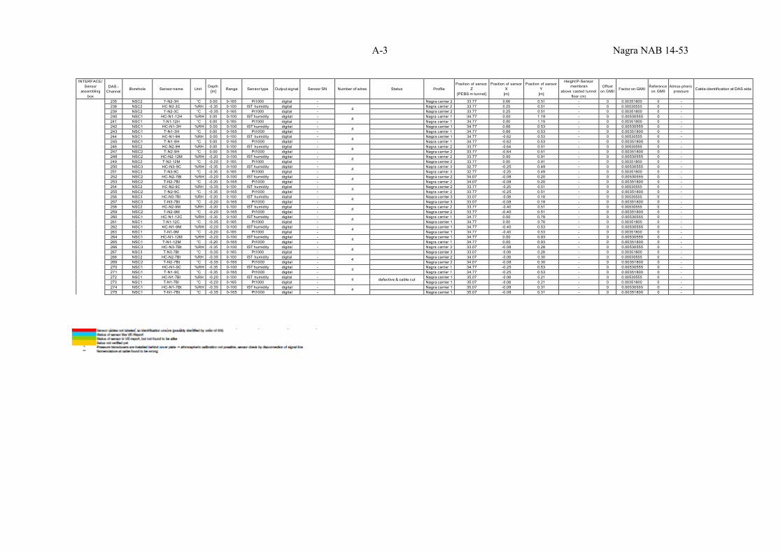
A-3 Nagra NAB 14-53
INTERFACE/ Sensor
assembling box
DAS -
Channel
Borehole
Sensor name
Unit
Depth
[m]
Range
Sensor type
Output signal
Sensor SN
Number of wires
Status
Profile
Position of sensor Z
[PEBS m tunnel]
Position of sensor X
[m]
Position of sensor Y
[m]
Height P-Sensor membran
above casted tunnel floor (m)
Offset
on GMII
Factor on GMII
Reference
on GMII
Atmos-pheric
pressure
Cable identification at DAS side
235 NSC2 T-N2-3H °C 0.00 0-165 Pt1000 digital - Nagra carrier 2 33.77 0.66 0.51 - 0 0.00351800 0 - 238 NSC2 HC-N2-3C %RH -0.35 0-100 IST humidity digital - 4 Nagra carrier 2 33.77 0.25 0.51 - 0 0.00530555 0 - 239 NSC2 T-N2-3C °C -0.35 0-165 Pt1000 digital - Nagra carrier 2 33.77 0.25 0.51 - 0 0.00351800 0 - 240 NSC1 HC-N1-12H %RH 0.00 0-100 IST humidity digital - 4 Nagra carrier 1 34.77 0.00 1.19 - 0 0.00530555 0 - 241 NSC1 T-N1-12H °C 0.00 0-165 Pt1000 digital - Nagra carrier 1 34.77 0.00 1.19 - 0 0.00351800 0 - 242 NSC1 HC-N1-3H %RH 0.00 0-100 IST humidity digital - 4 Nagra carrier 1 34.77 0.66 0.53 - 0 0.00530555 0 - 243 NSC1 T-N1-3H °C 0.00 0-165 Pt1000 digital - Nagra carrier 1 34.77 0.66 0.53 - 0 0.00351800 0 - 244 NSC1 HC-N1-9H %RH 0.00 0-100 IST humidity digital - 4 Nagra carrier 1 34.77 -0.62 0.53 - 0 0.00530555 0 - 245 NSC1 T-N1-9H °C 0.00 0-165 Pt1000 digital - Nagra carrier 1 34.77 -0.62 0.53 - 0 0.00351800 0 - 246 NSC2 HC-N2-9H %RH 0.00 0-100 IST humidity digital - 4 Nagra carrier 2 33.77 -0.64 0.51 - 0 0.00530555 0 - 247 NSC2 T-N2-9H °C 0.00 0-165 Pt1000 digital - Nagra carrier 2 33.77 -0.64 0.51 - 0 0.00351800 0 - 248 NSC2 HC-N2-12M %RH -0.20 0-100 IST humidity digital - 4 Nagra carrier 2 33.77 0.00 0.91 - 0 0.00530555 0 - 249 NSC2 T-N2-12M °C -0.20 0-165 Pt1000 digital - Nagra carrier 2 33.77 0.00 0.91 - 0 0.00351800 0 - 250 NSC3 HC-N3-9C %RH -0.35 0-100 IST humidity digital - 4 Nagra carrier 3 32.77 -0.25 0.49 - 0 0.00530555 0 - 251 NSC3 T-N3-9C °C -0.35 0-165 Pt1000 digital - Nagra carrier 3 32.77 -0.25 0.49 - 0 0.00351800 0 - 252 NSC2 HC-N2-7Bl %RH -0.20 0-100 IST humidity digital - 4 Nagra carrier 2 34.07 -0.08 0.20 - 0 0.00530555 0 - 253 NSC2 T-N2-7Bl °C -0.20 0-165 Pt1000 digital - Nagra carrier 2 34.07 -0.08 0.20 - 0 0.00351800 0 - 254 NSC2 HC-N2-9C %RH -0.35 0-100 IST humidity digital - 4 Nagra carrier 2 33.77 -0.25 0.51 - 0 0.00530555 0 - 255 NSC2 T-N2-9C °C -0.35 0-165 Pt1000 digital - Nagra carrier 2 33.77 -0.25 0.51 - 0 0.00351800 0 - 256 NSC3 HC-N3-7Bl %RH -0.20 0-100 IST humidity digital - 4 Nagra carrier 3 33.07 -0.08 0.18 - 0 0.00530555 0 - 257 NSC3 T-N3-7Bl °C -0.20 0-165 Pt1000 digital - Nagra carrier 3 33.07 -0.08 0.18 - 0 0.00351800 0 - 258 NSC2 HC-N2-9M %RH -0.20 0-100 IST humidity digital - 4 Nagra carrier 2 33.77 -0.40 0.51 - 0 0.00530555 0 - 259 NSC2 T-N2-9M °C -0.20 0-165 Pt1000 digital - Nagra carrier 2 33.77 -0.40 0.51 - 0 0.00351800 0 - 260 NSC1 HC-N1-12C %RH -0.35 0-100 IST humidity digital - 4 Nagra carrier 1 34.77 0.00 0.78 - 0 0.00530555 0 - 261 NSC1 T-N1-12C °C -0.35 0-165 Pt1000 digital - Nagra carrier 1 34.77 0.00 0.78 - 0 0.00351800 0 - 262 NSC1 HC-N1-9M %RH -0.20 0-100 IST humidity digital - 4 Nagra carrier 1 34.77 -0.40 0.53 - 0 0.00530555 0 - 263 NSC1 T-N1-9M °C -0.20 0-165 Pt1000 digital - Nagra carrier 1 34.77 -0.40 0.53 - 0 0.00351800 0 - 264 NSC1 HC-N1-12M %RH -0.20 0-100 IST humidity digital - 4 Nagra carrier 1 34.77 0.00 0.93 - 0 0.00530555 0 - 265 NSC1 T-N1-12M °C -0.20 0-165 Pt1000 digital - Nagra carrier 1 34.77 0.00 0.93 - 0 0.00351800 0 - 266 NSC3 HC-N3-7Bt %RH -0.35 0-100 IST humidity digital - 4 Nagra carrier 3 33.07 -0.08 0.28 - 0 0.00530555 0 - 267 NSC3 T-N3-7Bt °C -0.35 0-165 Pt1000 digital - Nagra carrier 3 33.07 -0.08 0.28 - 0 0.00351800 0 - 268 NSC2 HC-N2-7Bt %RH -0.35 0-100 IST humidity digital - 4 Nagra carrier 2 34.07 -0.08 0.30 - 0 0.00530555 0 - 269 NSC2 T-N2-7Bt °C -0.35 0-165 Pt1000 digital - Nagra carrier 2 34.07 -0.08 0.30 - 0 0.00351800 0 - 270 NSC1 HC-N1-9C %RH -0.35 0-100 IST humidity digital - 4 Nagra carrier 1 34.77 -0.25 0.53 - 0 0.00530555 0 - 271 NSC1 T-N1-9C °C -0.35 0-165 Pt1000 digital - Nagra carrier 1 34.77 -0.25 0.53 - 0 0.00351800 0 - 272 NSC1 HC-N1-7Bl %RH -0.20 0-100 IST humidity digital - 4 defective & cable cut Nagra carrier 1 35.07 -0.08 0.21 - 0 0.00530555 0 - 273 NSC1 T-N1-7Bl °C -0.20 0-165 Pt1000 digital - Nagra carrier 1 35.07 -0.08 0.21 - 0 0.00351800 0 - 274 NSC1 HC-N1-7Bt %RH -0.35 0-100 IST humidity digital - 4 Nagra carrier 1 35.07 -0.08 0.31 - 0 0.00530555 0 - 275 NSC1 T-N1-7Bt °C -0.35 0-165 Pt1000 digital - Nagra carrier 1 35.07 -0.08 0.31 - 0 0.00351800 0 -

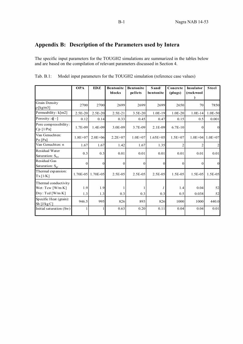
B-1 Nagra NAB 14-53
Appendix B: Description of the Parameters used by Intera The specific input parameters for the TOUGH2 simulations are summarized in the tables below and are based on the compilation of relevant parameters discussed in Section 4.
Tab. B.1: Model input parameters for the TOUGH2 simulation (reference case values)
OPA EDZ Bentonite blocks
Bentonite pellets
Sand/ bentonite
Concrete (plugs)
Insulator (rockwool
)
Steel
Grain Density ρ[kg/m3]
2700 2700 2699 2699 2699 2650 70 7850
Permeability: k[m2] 2.5E-20 2.5E-20 2.5E-21 3.5E-20 1.0E-19 1.0E-20 1.0E-14 1.0E-50Porosity: φ[−] 0.12 0.14 0.33 0.45 0.47 0.15 0.5 0.001Pore compressibility: Cp [1/Pa] 1.7E-09 1.4E-09 3.0E-09 3.7E-09 2.1E-09 6.7E-10 0 0
Van Genuchten: Po [Pa]
1.8E+07 2.0E+06 2.2E+07 1.0E+07 1.65E+05 1.5E+07 1.0E+04 1.0E+07
Van Genuchten: n 1.67 1.67 1.42 1.67 1.35 2 2 2Residual Water Saturation: Swr
0.3 0.3 0.01 0.01 0.01 0.01 0.01 0.01
Residual Gas Saturation: Sgr
0 0 0 0 0 0 0 0
Thermal expansion: Tx [1/K] 1.70E-05 1.70E-05 2.5E-05 2.5E-05 2.5E-05 1.5E-05 1.5E-05 1.5E-05
Thermal conductivity Wet: Tcw [W/m K] 1.9 1.9 1 1 1 1.4 0.04 52Dry: Tcd [W/m K] 1.3 1.3 0.3 0.3 0.3 0.5 0.038 52Specific Heat (grain): Sh [J/kg C]
946.5 995 826 893 826 1000 1000 440.0
Initial saturation (Sw) 1 1 0.63 0.20 0.11 0.04 0.04 0.01

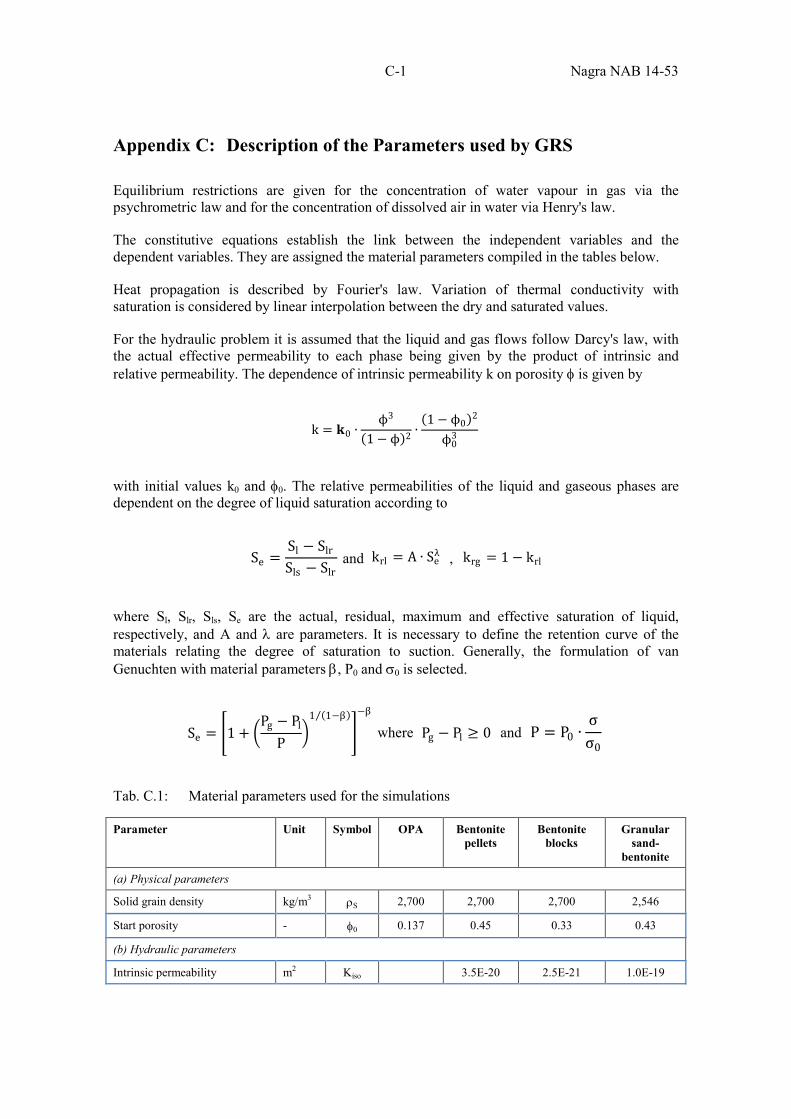
C-1 Nagra NAB 14-53
Appendix C: Description of the Parameters used by GRS Equilibrium restrictions are given for the concentration of water vapour in gas via the psychrometric law and for the concentration of dissolved air in water via Henry's law.
The constitutive equations establish the link between the independent variables and the dependent variables. They are assigned the material parameters compiled in the tables below.
Heat propagation is described by Fourier's law. Variation of thermal conductivity with saturation is considered by linear interpolation between the dry and saturated values.
For the hydraulic problem it is assumed that the liquid and gas flows follow Darcy's law, with the actual effective permeability to each phase being given by the product of intrinsic and relative permeability. The dependence of intrinsic permeability k on porosity φ is given by
with initial values k0 and φ0. The relative permeabilities of the liquid and gaseous phases are dependent on the degree of liquid saturation according to
and ,
where Sl, Slr, Sls, Se are the actual, residual, maximum and effective saturation of liquid, respectively, and A and λ are parameters. It is necessary to define the retention curve of the materials relating the degree of saturation to suction. Generally, the formulation of van Genuchten with material parameters β, P0 and σ0 is selected.
where and
Tab. C.1: Material parameters used for the simulations
Parameter Unit Symbol OPA Bentonite pellets
Bentonite blocks
Granular sand-
bentonite
(a) Physical parameters
Solid grain density kg/m3 ρS 2,700 2,700 2,700 2,546
Start porosity - φ0 0.137 0.45 0.33 0.43
(b) Hydraulic parameters
Intrinsic permeability m2 Kiso 3.5E-20 2.5E-21 1.0E-19
k = 𝐤𝐤0 ∙ϕ3
(1 − ϕ)2 ∙(1 − ϕ0)2
ϕ03
Se =Sl − Slr
Sls − Slr krl = A ∙ Se
λ krg = 1 − krl
Se = �1 + �Pg − Pl
P�
1 (1−β)⁄
�−β
Pg − Pl ≥ 0 P = P0 ∙σσ0
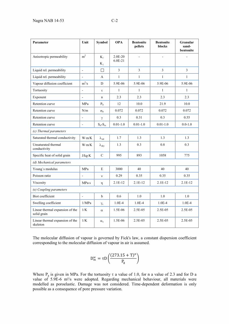
Nagra NAB 14-53 C-2
Parameter Unit Symbol OPA Bentonite pellets
Bentonite blocks
Granular sand-
bentonite
Anisotropic permeability m2 K//
K⊥
2.0E-20 6.0E-21
- - -
Liquid rel. permeability - 3 3 3 3
Liquid rel. permeability - A 1 1 1 1
Vapour diffusion coefficient m2/s D 5.9E-06 5.9E-06 5.9E-06 5.9E-06
Tortuosity - τ 1 1 1 1
Exponent - n 2.3 2.3 2.3 2.3
Retention curve MPa P0 12 10.0 21.9 10.0
Retention curve N/m σ0 0.072 0.072 0.072 0.072
Retention curve - γ 0.3 0.31 0.3 0.55
Retention curve - Srl-Srs 0.01-1.0 0.01-1.0 0.01-1.0 0.0-1.0
(c) Thermal parameters
Saturated thermal conductivity W⋅m/K λsat 1.7 1.3 1.3 1.3
Unsaturated thermal conductivity
W⋅m/K λdry 1.3 0.3 0.8 0.3
Specific heat of solid grain J/kg⋅K C 995 893 1058 775
(d) Mechanical parameters
Young`s modulus MPa E 3000 40 40 40
Poisson ratio - ν 0.29 0.35 0.35 0.35
Viscosity MPa⋅s η 2.1E-12 2.1E-12 2.1E-12 2.1E-12
(e) Coupling parameters
Biot coefficient - b 0.6 1.0 1.0 1.0
Swelling coefficient 1/MPa γs 1.0E-4 1.0E-4 1.0E-4 1.0E-4
Linear thermal expansion of the solid grain
1/K α 1.5E-06 2.5E-05 2.5E-05 2.5E-05
Linear thermal expansion of the skeleton
1/K αs 1.5E-06 2.5E-05 2.5E-05 2.5E-05
The molecular diffusion of vapour is governed by Fick's law, a constant dispersion coefficient corresponding to the molecular diffusion of vapour in air is assumed.
Where Pg is given in MPa. For the tortuosity τ a value of 1.0, for n a value of 2.3 and for D a value of 5.9E-6 m²/s were adopted. Regarding mechanical behaviour, all materials were modelled as poroelastic. Damage was not considered. Time-dependent deformation is only possible as a consequence of pore pressure variation.
Dmw = τD�
(273.15 + T)n
Pg�
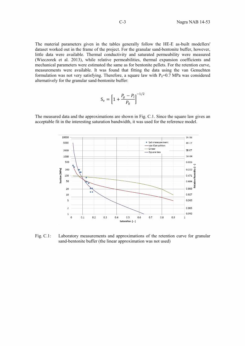
C-3 Nagra NAB 14-53
The material parameters given in the tables generally follow the HE-E as-built modellers' dataset worked out in the frame of the project. For the granular sand-bentonite buffer, however, little data were available. Thermal conductivity and saturated permeability were measured (Wieczorek et al. 2013), while relative permeabilities, thermal expansion coefficients and mechanical parameters were estimated the same as for bentonite pellets. For the retention curve, measurements were available. It was found that fitting the data using the van Genuchten formulation was not very satisfying. Therefore, a square law with P0=0.7 MPa was considered alternatively for the granular sand-bentonite buffer:
The measured data and the approximations are shown in Fig. C.1. Since the square law gives an acceptable fit in the interesting saturation bandwidth, it was used for the reference model.
Fig. C.1: Laboratory measurements and approximations of the retention curve for granular sand-bentonite buffer (the linear approximation was not used)
Se = �1 +𝑃𝑃𝑔𝑔 − 𝑃𝑃𝑙𝑙𝑃𝑃0
�−1/2

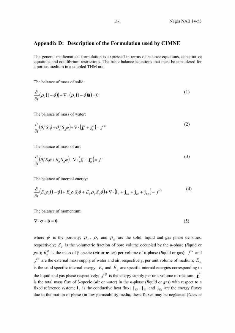
D-1 Nagra NAB 14-53
Appendix D: Description of the Formulation used by CIMNE The general mathematical formulation is expressed in terms of balance equations, constitutive equations and equilibrium restrictions. The basic balance equations that must be considered for a porous medium in a coupled THM are:
The balance of mass of solid:
( )( ) ( )( ) 011 =−⋅∇+−∂∂ uφρφρ sst
(1)
The balance of mass of water:
( ) ( ) wwg
wlg
wgl
wl fSS
t=+⋅∇++
∂∂ jjφθφθ
(2)
The balance of mass of air:
( ) ( ) aag
alg
agl
al fSS
t=+⋅∇++
∂∂ jjφθφθ
(3)
The balance of internal energy:
( )( ) ( ) QEgElEscggglllss fSESEE
t=+++⋅∇+++−
∂∂ jjjiφρφρφρ 1
(4)
The balance of momentum:
0bσ =+⋅∇ (5)
where φ is the porosity; sρ , lρ and gρ are the solid, liquid and gas phase densities,
respectively; αS is the volumetric fraction of pore volume occupied by the α-phase (liquid or
gas); βαθ is the mass of β-specie (air or water) per volume of α-phase (liquid or gas); wf and
af are the external mass supply of water and air, respectively, per unit volume of medium; sE
is the solid specific internal energy, lE and gE are specific internal energies corresponding to
the liquid and gas phase respectively; Qf is the energy supply per unit volume of medium; βαj
is the total mass flux of β-specie (air or water) in the α-phase (liquid or gas) with respect to a fixed reference system; ci is the conductive heat flux; Esj , Elj and Egj are the energy fluxes due to the motion of phase (in low permeability media, these fluxes may be neglected (Gens et
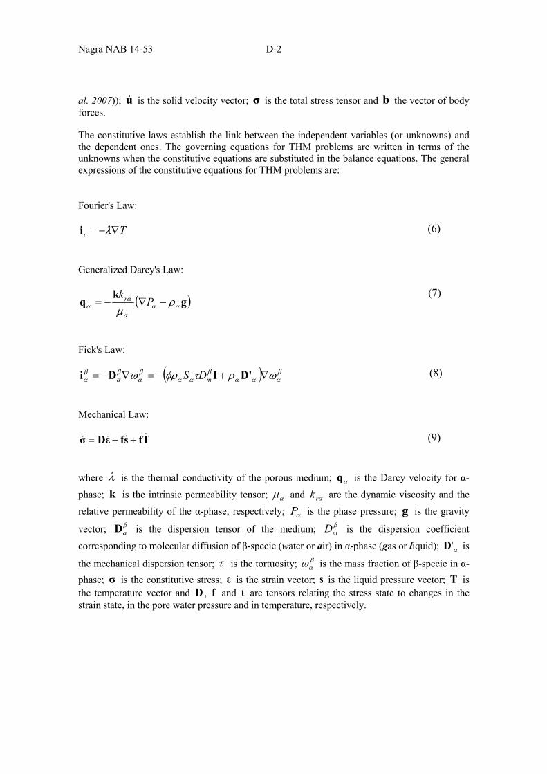
Nagra NAB 14-53 D-2
al. 2007)); u is the solid velocity vector; σ is the total stress tensor and b the vector of body forces.
The constitutive laws establish the link between the independent variables (or unknowns) and the dependent ones. The governing equations for THM problems are written in terms of the unknowns when the constitutive equations are substituted in the balance equations. The general expressions of the constitutive equations for THM problems are:
Fourier's Law:
Tc ∇−= λi (6)
Generalized Darcy's Law:
( )gk
q ααα
αα ρ
µ−∇−= P
kr (7)
Fick's Law:
( ) βααα
βαα
βα
βα
βα ωρτφρω ∇+−=∇−= D'IDi mDS (8)
Mechanical Law:
TtsfεDσ ++= (9)
where λ is the thermal conductivity of the porous medium; αq is the Darcy velocity for α-
phase; k is the intrinsic permeability tensor; αµ and αrk are the dynamic viscosity and the
relative permeability of the α-phase, respectively; αP is the phase pressure; g is the gravity
vector; βαD is the dispersion tensor of the medium; β
mD is the dispersion coefficient
corresponding to molecular diffusion of β-specie (water or air) in α-phase (gas or liquid); α'D is
the mechanical dispersion tensor; τ is the tortuosity; βαω is the mass fraction of β-specie in α-
phase; σ is the constitutive stress; ε is the strain vector; s is the liquid pressure vector; T is the temperature vector and D , f and t are tensors relating the stress state to changes in the strain state, in the pore water pressure and in temperature, respectively.
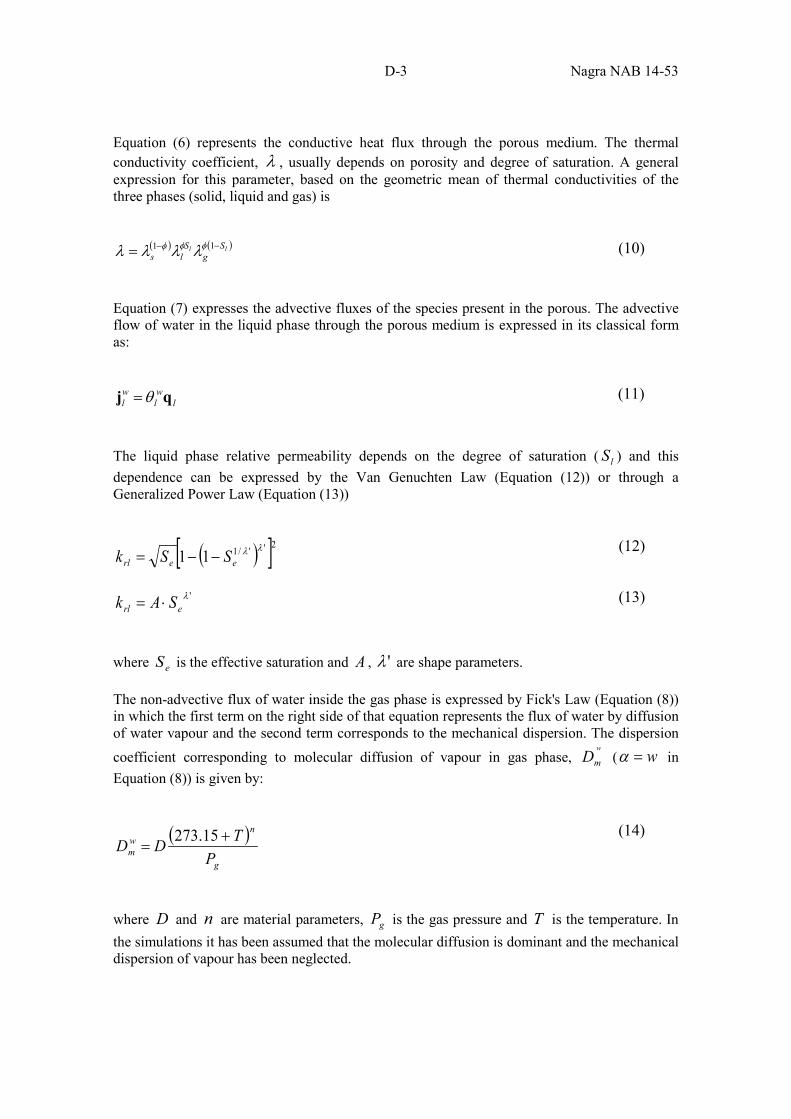
D-3 Nagra NAB 14-53
Equation (6) represents the conductive heat flux through the porous medium. The thermal conductivity coefficient, λ , usually depends on porosity and degree of saturation. A general expression for this parameter, based on the geometric mean of thermal conductivities of the three phases (solid, liquid and gas) is
( ) ( )ll S
gS
ls−−= 11 φφφ λλλλ (10)
Equation (7) expresses the advective fluxes of the species present in the porous. The advective flow of water in the liquid phase through the porous medium is expressed in its classical form as:
lwl
wl qj θ= (11)
The liquid phase relative permeability depends on the degree of saturation ( lS ) and this dependence can be expressed by the Van Genuchten Law (Equation (12)) or through a Generalized Power Law (Equation (13))
( )[ ]2''/111 λλeerl SSk −−=
(12)
'λerl SAk ⋅= (13)
where eS is the effective saturation and A , 'λ are shape parameters.
The non-advective flux of water inside the gas phase is expressed by Fick's Law (Equation (8)) in which the first term on the right side of that equation represents the flux of water by diffusion of water vapour and the second term corresponds to the mechanical dispersion. The dispersion coefficient corresponding to molecular diffusion of vapour in gas phase,
w
mD ( w=α in Equation (8)) is given by:
( )g
nwm P
TDD +=
15.273
(14)
where D and n are material parameters, gP is the gas pressure and T is the temperature. In the simulations it has been assumed that the molecular diffusion is dominant and the mechanical dispersion of vapour has been neglected.
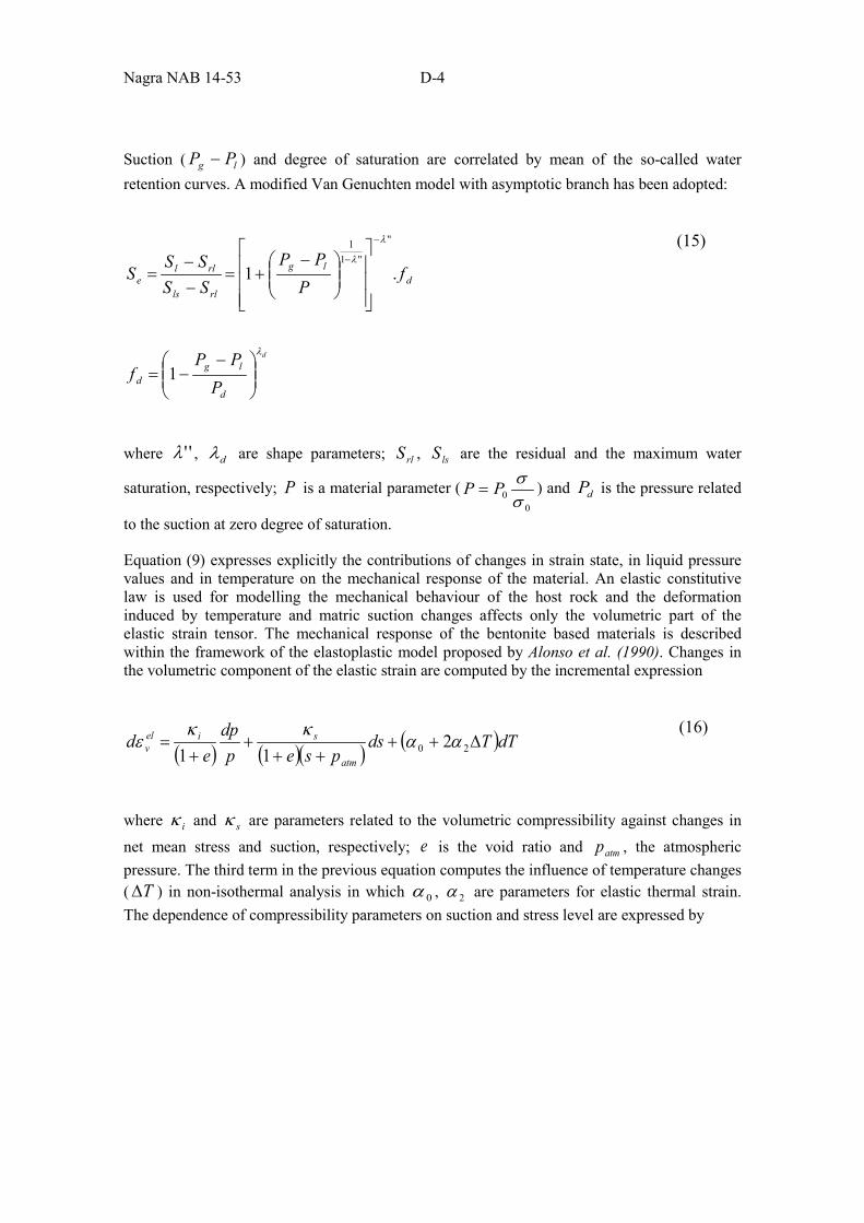
Nagra NAB 14-53 D-4
Suction ( lg PP − ) and degree of saturation are correlated by mean of the so-called water retention curves. A modified Van Genuchten model with asymptotic branch has been adopted:
d
d
lgd
dlg
rlls
rlle
PPP
f
fP
PPSSSS
S
λ
λ
λ
−−=
−+=
−−
=
−
−
1
.1
''
''11
(15)
where ''λ , dλ are shape parameters; rlS , lsS are the residual and the maximum water
saturation, respectively; P is a material parameter (0
0 σσPP = ) and dP is the pressure related
to the suction at zero degree of saturation.
Equation (9) expresses explicitly the contributions of changes in strain state, in liquid pressure values and in temperature on the mechanical response of the material. An elastic constitutive law is used for modelling the mechanical behaviour of the host rock and the deformation induced by temperature and matric suction changes affects only the volumetric part of the elastic strain tensor. The mechanical response of the bentonite based materials is described within the framework of the elastoplastic model proposed by Alonso et al. (1990). Changes in the volumetric component of the elastic strain are computed by the incremental expression
( ) ( )( ) ( )dTTdspsep
dpe
datm
sielv ∆++
+++
+= 20 2
11αα
κκε
(16)
where iκ and sκ are parameters related to the volumetric compressibility against changes in
net mean stress and suction, respectively; e is the void ratio and atmp , the atmospheric pressure. The third term in the previous equation computes the influence of temperature changes ( T∆ ) in non-isothermal analysis in which 0α , 2α are parameters for elastic thermal strain. The dependence of compressibility parameters on suction and stress level are expressed by
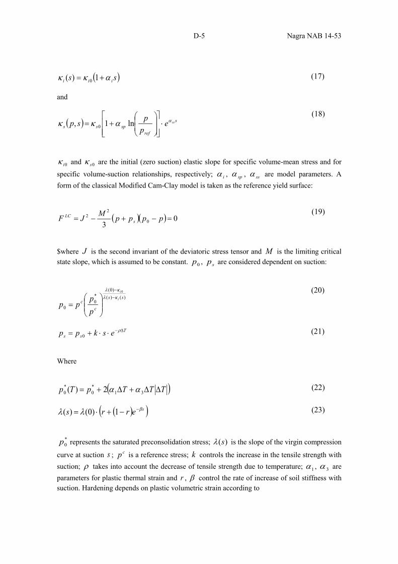
D-5 Nagra NAB 14-53
( )ss iii ακκ += 1)( 0 (17)
and
( ) s
refspss
sseppsp αακκ ⋅
+= ln1, 0
(18)
0iκ and 0sκ are the initial (zero suction) elastic slope for specific volume-mean stress and for
specific volume-suction relationships, respectively; iα , spα , ssα are model parameters. A form of the classical Modified Cam-Clay model is taken as the reference yield surface:
( )( ) 03 0
22 =−+−= ppppMJF s
LC (19)
$where J is the second invariant of the deviatoric stress tensor and M is the limiting critical state slope, which is assumed to be constant. 0p , sp are considered dependent on suction:
)()()0(
*0
0
0
ss
cc i
i
pp
ppκλκλ
−−
=
(20)
Tss eskpp ∆−⋅⋅+= ρ0 (21)
Where
( )TTTpTp ∆∆+∆+= 31*0
*0 2)( αα (22)
( )( )serrs βλλ −−+⋅= 1)0()( (23)
*0p represents the saturated preconsolidation stress; )(sλ is the slope of the virgin compression
curve at suction s ; cp is a reference stress; k controls the increase in the tensile strength with suction; ρ takes into account the decrease of tensile strength due to temperature; 1α , 3α are parameters for plastic thermal strain and r , β control the rate of increase of soil stiffness with suction. Hardening depends on plastic volumetric strain according to
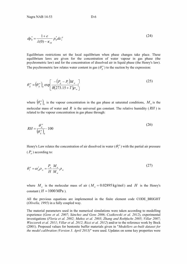
Nagra NAB 14-53 D-6
pv
i
dpedp εκλ
*0
0
*0 )0(
1−+
= (24)
Equilibrium restrictions set the local equilibrium when phase changes take place. These equilibrium laws are given for the concentration of water vapour in gas phase (the psychrometric law) and for the concentration of dissolved air in liquid phase (the Henry's law). The psychrometric law relates water content in gas ( w
gθ ) to the suction by the expression:
( ) ( )( )
+
−−=
w
wlgwg
wg TR
MPPρ
θθ15.273
exp0
(25)
where ( )0
wgθ is the vapour concentration in the gas phase at saturated conditions, wM is the
molecular mass of water and R is the universal gas constant. The relative humidity ( RH ) is related to the vapour concentration in gas phase through:
( ) 1000
⋅= wg
wgRH
θθ
(26)
Henry's Law relates the concentration of air dissolved in water ( alθ ) with the partial air pressure
( aP ) according to:
ww
aaw
la
al M
MHP
ρρωθ == (27)
where aM is the molecular mass of air ( kg/mol 02895.0=aM ) and H is the Henry's constant ( MPa 1000=H ).
All the previous equations are implemented in the finite element code CODE_BRIGHT (Olivella, 1995) in a fully coupled way.
The material parameters used in the numerical simulations were taken according to modelling experience (Gens et al. 2007; Sánchez and Gens 2006; Czaikowski et al. 2012), experimental investigations (Floria et al. 2002; Muñoz et al. 2003; Zhang and Rothfuchs 2005; Villar 2007; Wieczorek et al. 2011; Villar et al. 2012; Rizzi et al. 2012) and/or to the reference work by Bock (2001). Proposed values for bentonite buffer materials given in "Modellers as-built dataset for the model calibration (Version 3. April 2013)" were used. Updates on some key properties were
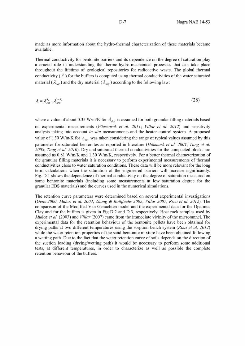
D-7 Nagra NAB 14-53
made as more information about the hydro-thermal characterization of these materials became available.
Thermal conductivity for bentonite barriers and its dependence on the degree of saturation play a crucial role in understanding the thermo-hydro-mechanical processes that can take place throughout the lifetime of geological repositories for radioactive waste. The global thermal conductivity (λ ) for the buffers is computed using thermal conductivities of the water saturated material ( satλ ) and the dry material ( dryλ ) according to the following law:
ww S
drySsat
−⋅= 1λλλ (28)
where a value of about 0.35 W/m/K for dryλ is assumed for both granular filling materials based on experimental measurements (Wieczorek et al. 2011; Villar et al. 2012) and sensitivity analysis taking into account in situ measurements and the heater control system. A proposed value of 1.30 W/m/K for satλ was taken considering the range of typical values assumed by this parameter for saturated bentonites as reported in literature (Hökmark et al. 2007; Tang et al. 2008; Tang et al. 2010). Dry and saturated thermal conductivities for the compacted blocks are assumed as 0.81 W/m/K and 1.30 W/m/K, respectively. For a better thermal characterization of the granular filling materials it is necessary to perform experimental measurements of thermal conductivities close to water saturation conditions. These data will be more relevant for the long term calculations when the saturation of the engineered barriers will increase significantly. Fig. D.1 shows the dependence of thermal conductivity on the degree of saturation measured on some bentonite materials (including some measurements at low saturation degree for the granular EBS materials) and the curves used in the numerical simulations.
The retention curve parameters were determined based on several experimental investigations (Gens 2000; Muñoz et al. 2003; Zhang & Rothfuchs 2005; Villar 2007; Rizzi et al. 2012). The comparison of the Modified Van Genuchten model and the experimental data for the Opalinus Clay and for the buffers is given in Fig D.2 and D.3, respectively. Host rock samples used by Muñoz et al. (2003) and Villar (2007) came from the immediate vicinity of the microtunnel. The experimental data for the retention behaviour of the bentonite pellets have been obtained for drying paths at two different temperatures using the sorption bench system (Rizzi et al. 2012) while the water retention properties of the sand-bentonite mixture have been obtained following a wetting path. Due to the fact that the water retention curve of soils depends on the direction of the suction loading (drying/wetting path) it would be necessary to perform some additional tests, at different temperatures, in order to characterize as well as possible the complete retention behaviour of the buffers.
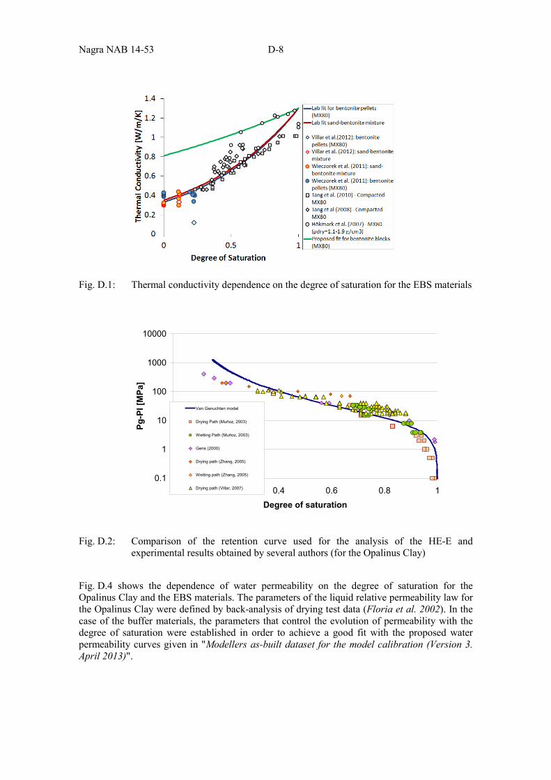
Nagra NAB 14-53 D-8
Fig. D.1: Thermal conductivity dependence on the degree of saturation for the EBS materials
Fig. D.2: Comparison of the retention curve used for the analysis of the HE-E and experimental results obtained by several authors (for the Opalinus Clay)
Fig. D.4 shows the dependence of water permeability on the degree of saturation for the Opalinus Clay and the EBS materials. The parameters of the liquid relative permeability law for the Opalinus Clay were defined by back-analysis of drying test data (Floria et al. 2002). In the case of the buffer materials, the parameters that control the evolution of permeability with the degree of saturation were established in order to achieve a good fit with the proposed water permeability curves given in "Modellers as-built dataset for the model calibration (Version 3. April 2013)".
0.1
1
10
100
1000
10000
0 0.2 0.4 0.6 0.8 1Degree of saturation
Pg-P
l [M
Pa]
Van Genuchten model
Drying Path (Muñoz, 2003)
Wetting Path (Muñoz, 2003)
Gens (2000)
Drying path (Zhang, 2005)
Wetting path (Zhang, 2005)
Drying path (Villar, 2007)
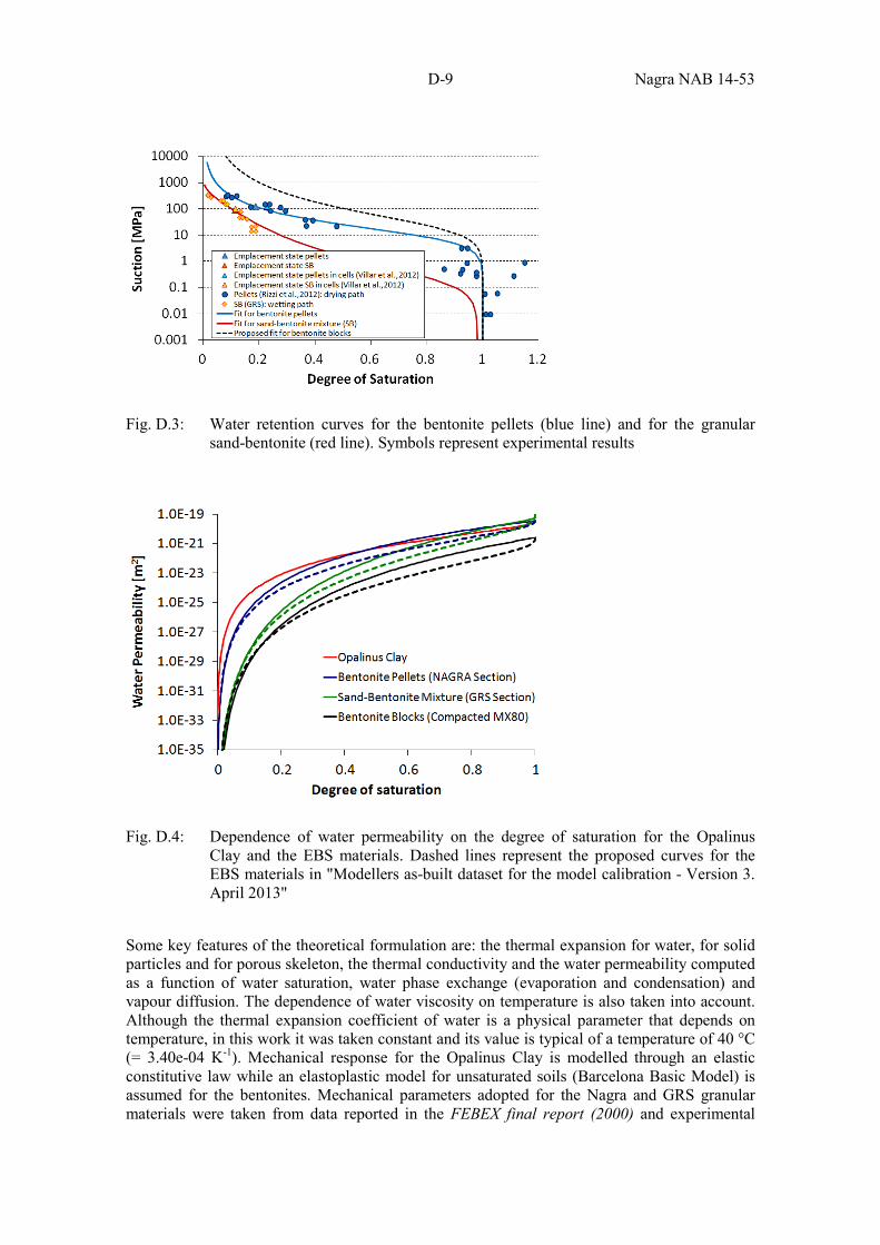
D-9 Nagra NAB 14-53
Fig. D.3: Water retention curves for the bentonite pellets (blue line) and for the granular sand-bentonite (red line). Symbols represent experimental results
Fig. D.4: Dependence of water permeability on the degree of saturation for the Opalinus Clay and the EBS materials. Dashed lines represent the proposed curves for the EBS materials in "Modellers as-built dataset for the model calibration - Version 3. April 2013"
Some key features of the theoretical formulation are: the thermal expansion for water, for solid particles and for porous skeleton, the thermal conductivity and the water permeability computed as a function of water saturation, water phase exchange (evaporation and condensation) and vapour diffusion. The dependence of water viscosity on temperature is also taken into account. Although the thermal expansion coefficient of water is a physical parameter that depends on temperature, in this work it was taken constant and its value is typical of a temperature of 40 °C (= 3.40e-04 K-1). Mechanical response for the Opalinus Clay is modelled through an elastic constitutive law while an elastoplastic model for unsaturated soils (Barcelona Basic Model) is assumed for the bentonites. Mechanical parameters adopted for the Nagra and GRS granular materials were taken from data reported in the FEBEX final report (2000) and experimental
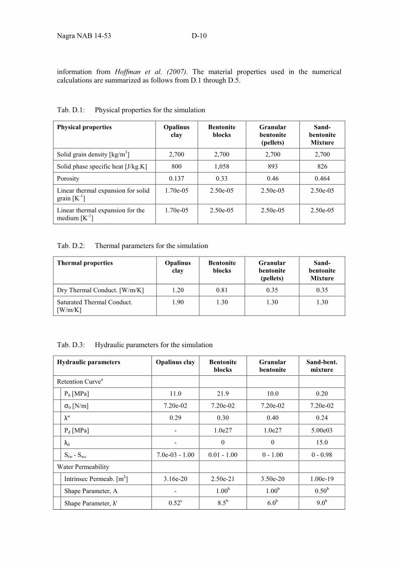
Nagra NAB 14-53 D-10
information from Hoffman et al. (2007). The material properties used in the numerical calculations are summarized as follows from D.1 through D.5.
Tab. D.1: Physical properties for the simulation
Physical properties Opalinus clay
Bentonite blocks
Granular bentonite (pellets)
Sand-bentonite Mixture
Solid grain density [kg/m3] 2,700 2,700 2,700 2,700
Solid phase specific heat [J/kg.K] 800 1,058 893 826
Porosity 0.137 0.33 0.46 0.464
Linear thermal expansion for solid grain [K-1]
1.70e-05 2.50e-05 2.50e-05 2.50e-05
Linear thermal expansion for the medium [K-1]
1.70e-05 2.50e-05 2.50e-05 2.50e-05
Tab. D.2: Thermal parameters for the simulation
Thermal properties Opalinus clay
Bentonite blocks
Granular bentonite (pellets)
Sand-bentonite Mixture
Dry Thermal Conduct. [W/m/K] 1.20 0.81 0.35 0.35
Saturated Thermal Conduct. [W/m/K]
1.90 1.30 1.30 1.30
Tab. D.3: Hydraulic parameters for the simulation
Hydraulic parameters Opalinus clay Bentonite blocks
Granular bentonite
Sand-bent. mixture
Retention Curvea
P0 [MPa] 11.0 21.9 10.0 0.20
σ0 [N/m] 7.20e-02 7.20e-02 7.20e-02 7.20e-02
λ'' 0.29 0.30 0.40 0.24
Pd [MPa] - 1.0e27 1.0e27 5.00e03
λd - 0 0 15.0
Srw - Sws 7.0e-03 - 1.00 0.01 - 1.00 0 - 1.00 0 - 0.98
Water Permeability
Intrinsec Permeab. [m2] 3.16e-20 2.50e-21 3.50e-20 1.00e-19
Shape Parameter, A - 1.00b 1.00b 0.50b
Shape Parameter, λ' 0.52c 8.5b 6.0b 9.0b
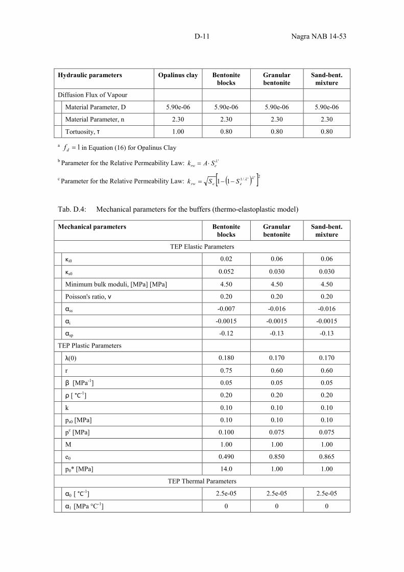
D-11 Nagra NAB 14-53
Hydraulic parameters Opalinus clay Bentonite blocks
Granular bentonite
Sand-bent. mixture
Diffusion Flux of Vapour
Material Parameter, D 5.90e-06 5.90e-06 5.90e-06 5.90e-06
Material Parameter, n 2.30 2.30 2.30 2.30
Tortuosity, τ 1.00 0.80 0.80 0.80
a 1=df in Equation (16) for Opalinus Clay
b Parameter for the Relative Permeability Law: 'λerw SAk ⋅=
c Parameter for the Relative Permeability Law: ( )[ ]2''/111λλ
eerw SSk −−=
Tab. D.4: Mechanical parameters for the buffers (thermo-elastoplastic model)
Mechanical parameters Bentonite blocks
Granular bentonite
Sand-bent. mixture
TEP Elastic Parameters
κi0 0.02 0.06 0.06
κs0 0.052 0.030 0.030
Minimum bulk moduli, [MPa] [MPa] 4.50 4.50 4.50
Poisson's ratio, ν 0.20 0.20 0.20
αss -0.007 -0.016 -0.016
αi -0.0015 -0.0015 -0.0015
αsp -0.12 -0.13 -0.13
TEP Plastic Parameters
λ(0) 0.180 0.170 0.170
r 0.75 0.60 0.60
β [MPa-1] 0.05 0.05 0.05
ρ [ °C-1] 0.20 0.20 0.20
k 0.10 0.10 0.10
ps0 [MPa] 0.10 0.10 0.10
pc [MPa] 0.100 0.075 0.075
M 1.00 1.00 1.00
e0 0.490 0.850 0.865
p0* [MPa] 14.0 1.00 1.00
TEP Thermal Parameters
α0 [ °C-1] 2.5e-05 2.5e-05 2.5e-05
α1 [MPa °C-1] 0 0 0

Nagra NAB 14-53 D-12
Mechanical parameters Bentonite blocks
Granular bentonite
Sand-bent. mixture
α2 [ °C-2] 0 0 0
α3 [MPa °C-2] 0 0 0
Tab. D.5: Mechanical parameters for Opalinus Clay (elastic constitutive law)
Young Modulus [MPa] Poisson's Ratio
Opalinus Clay 4.00e03 0.24
Related Documents