Welcome message from author
This document is posted to help you gain knowledge. Please leave a comment to let me know what you think about it! Share it to your friends and learn new things together.
Transcript


THE HANDBOOK OF STRUCTUREDFINANCE
ARNAUD DE SERVIGNYNORBERT JOBST
McGraw-HillNew York Chicago San Francisco Lisbon LondonMadrid Mexico City Milan New Delhi San JuanSeoul Singapore Sydney Toronto

Copyright © 2007 by The McGraw-Hill Companies. All rights reserved. Manufactured in the UnitedStates of America. Except as permitted under the United States Copyright Act of 1976, no part of thispublication may be reproduced or distributed in any form or by any means, or stored in a database orretrieval system, without the prior written permission of the publisher.
0-07-150884-8
The material in this eBook also appears in the print version of this title: 0-07-146864-1.
All trademarks are trademarks of their respective owners. Rather than put a trademark symbol afterevery occurrence of a trademarked name, we use names in an editorial fashion only, and to the benefit of the trademark owner, with no intention of infringement of the trademark. Where such designations appear in this book, they have been printed with initial caps.
McGraw-Hill eBooks are available at special quantity discounts to use as premiums and sales promotions, or for use in corporate training programs. For more information, please contact GeorgeHoare, Special Sales, at [email protected] or (212) 904-4069.
TERMS OF USE
This is a copyrighted work and The McGraw-Hill Companies, Inc. (“McGraw-Hill”) and its licensorsreserve all rights in and to the work. Use of this work is subject to these terms. Except as permittedunder the Copyright Act of 1976 and the right to store and retrieve one copy of the work, you may notdecompile, disassemble, reverse engineer, reproduce, modify, create derivative works based upon,transmit, distribute, disseminate, sell, publish or sublicense the work or any part of it withoutMcGraw-Hill’s prior consent. You may use the work for your own noncommercial and personal use;any other use of the work is strictly prohibited. Your right to use the work may be terminated if youfail to comply with these terms.
THE WORK IS PROVIDED “AS IS.” McGRAW-HILL AND ITS LICENSORS MAKE NO GUARANTEES OR WARRANTIES AS TO THE ACCURACY, ADEQUACY OR COMPLETE-NESS OF OR RESULTS TO BE OBTAINED FROM USING THE WORK, INCLUDING ANYINFORMATION THAT CAN BE ACCESSED THROUGH THE WORK VIA HYPERLINK OROTHERWISE, AND EXPRESSLY DISCLAIM ANY WARRANTY, EXPRESS OR IMPLIED,INCLUDING BUT NOT LIMITED TO IMPLIED WARRANTIES OF MERCHANTABILITY ORFITNESS FOR A PARTICULAR PURPOSE. McGraw-Hill and its licensors do not warrant or guarantee that the functions contained in the work will meet your requirements or that its operationwill be uninterrupted or error free. Neither McGraw-Hill nor its licensors shall be liable to you or any-one else for any inaccuracy, error or omission, regardless of cause, in the work or for any damagesresulting therefrom. McGraw-Hill has no responsibility for the content of any information accessedthrough the work. Under no circumstances shall McGraw-Hill and/or its licensors be liable for anyindirect, incidental, special, punitive, consequential or similar damages that result from the use of orinability to use the work, even if any of them has been advised of the possibility of such damages. This limitation of liability shall apply to any claim or cause whatsoever whether such claim or cause arises in contract, tort or otherwise.
DOI: 10.1036/0071468641

We hope you enjoy thisMcGraw-Hill eBook! If
you’d like more information about this book,its author, or related books and websites,please click here.
Professional
Want to learn more?

C O N T E N T S
INTRODUCTION vChapter 1
Overview of the Structured Credit Markets by Alexander Batchvarov 1
Chapter 2
Univariate Risk Assessment by Arnaud de Servigny and Sven Sandow 29
Chapter 3
Univariate Credit Risk Pricing by Arnaud de Servigny and Philippe Henrotte 91
Chapter 4
Modeling Credit Dependency by Arnaud de Servigny 137
Chapter 5
Rating Migration and Assset Correlation by Astrid Van Landschoot and Norbert Jobst 217
Chapter 6
CDO Pricing by Arnaud de Servigny 239
Chapter 7
An Introduction to the CDO Risk Management by Norbert Jobst 295
Chapter 8
A Practical Guide to CDO Trading Risk Management by Andrea Petrelli, Jun Zhang, Norbert Jobst, and Vivek Kapoor 339
Chapter 9
Cash and Synthetic CDOs by Olivier Renault 373
iii
For more information about this title, click here

Chapter 10
The CDO Methodologies Developed by Standard and Poor’s 397
Chapter 11
Recent and Not So Recent Developments in Synthetic CDOs by Norbert Jobst 465
Chapter 12
Residential Mortgage-Backed Securities by Varqa Khadem andFrancis Parisi 543
Chapter 13
Covered Bonds by Arnaud de Servigny and Aymeric Chauve 593
Chapter 14
An Overview of Structured Investment Vehicles and OtherSpecial Purpose Companies by Cristina Polizu 621
Chapter 15
Securitizations in Basel II by William Perraudin 675
Chapter 16
Secritization in the Context of Basel II by Arnaud de Servigny 697
BIOGRAPHIES 759INDEX 765
iv CONTENTS

I N T R O D U C T I O N
The Handbook of Structured Finance presents many modern quantitativetechniques used by investment banks, investors, and rating agenciesactive in the structured finance markets. In recent years, we have observedan exponential growth in market activity, knowledge, and quantitativetechniques developed in industry and academia, such that the writing ofa comprehensive book is becoming increasingly difficult. Rather than try-ing to cover all topics on our own, we have taken advantage from theexpert wisdom of market participants and academic scholars and tried toprovide a solid coverage of a wide range of structured finance topics, butchoices had to be made.
The clear objective of this book is to blend three types of experiencesin a single text. We always aim to consider the topics from an academicstandpoint, as well as from a professional angle, while not forgetting theperspective of a rating agency.
The review in this book goes beyond a simple list of tools and meth-ods. In particular, the various contributors try to provide a robust frame-work regarding the monitoring of structured finance risk and pricing. Inorder to do so, we analyze the most widely used methodologies in thestructured finance community and point out their relative strengths andweaknesses whenever appropriate. The contributors also offer insightfrom their experience of practical implementation of these techniqueswithin the relevant financial institutions.
Another feature of this book is that it surveys significant amounts ofempirical research. Chapters dealing with correlation, for example, areillustrated with recent statistics that allow the reader to have a bettergrasp of the topic and to understand the practical implementation chal-lenges.
Although the book focuses on collateral debt obligations (CDOs), itprovides extensive insight related to other vehicles and techniquesemployed for residential mortgage-backed securities, Credit card securi-tization, Covered Bonds, and structured investment vehicles.
v
Copyright © 2007 by The McGraw-Hill Companies. Click here for terms of use.

STRUCTURE OF THE BOOK
The book is divided into 16 chapters. We start with the building blocksthat are necessary to price and measure risk on portfolio structures. Thisinvolves pricing techniques for single-name credit instruments (univari-ate pricing), and estimation/modeling techniques for default probabili-ties and loss given default (univariate risk) of such products. We thenfocus on dependence, and more specifically on correlation in generalterms, applied to correlation among corporates as well as across struc-tured tranches. Once this toolbox is available, we can move to the CDOspace, the second part of this book. We investigate the techniques relatedto CDO pricing, CDO strategy, CDO hedging, the CDO risk assessmentemployed by Standard & Poor’s, and we end up with an overview ofrecent developments in the CDO space. A third building block is based ona review of the methods used in the RMBS sector, for Covered Bonds, forOperating Companies, and finally we focus on Basel II both from a theo-retical as well as from a case study perspective.
ACKNOWLEDGMENTS
As editors, we would like to thank all the contributors to this book:Alexander Batchvarov, Sven Sandow, Philippe Henrotte, Astrid VanLandschoot, Olivier Renault, Vivek Kapoor, Varqa Khadem, FrancisParisi, Cristina Polizu, Aymeric Chauve, and William Perraudin.
Our gratitude also goes to those who have helped us in carefullyreading this book and providing valuable comments. We would like tothank in particular Jean-David Fermanian, Pieter Klaassen, Andre Lucas,Jean-Paul Laurent, Joao Garcia, Olivier Renault, Benoit Metayer, andSriram Rajan.
Arnaud de Servigny
Norbert Jobst
vi INTRODUCTION

C H A P T E R 1
Overview of the StructuredCredit Markets: Trendsand New Developments
Alexander Batchvarov
1
OVERVIEW OF STRUCTURED FINANCEMARKETS AND TRENDS
The easiest way to highlight the development of the structured finance mar-ket is to quantify its new issuance volume. That volume has been steadilyclimbing all over the world, with U.S. leading, followed closely by Europe,and Japan and Australia a distant third and fourth. The rest of the world isnow awakening to the opportunities offered by structured credit productsto both issuers and investors and gearing up for a strong future growth. Inthat respect, it is worth mentioning Mexico, which is leading the way inLatin America; South Korea and Republic of China lead in continental Asiaand Turkey in for the Middle East and Eastern Europe. It is only a matter oftime before Central and Eastern Europe and China and India spring intoaction, and the Middle East launches its own version of securitization.
The data shown in Tables 1.1 to 1.4 are based on publicly availableinformation about deals executed on each market. We believe such datato seriously understate the size of the respective markets due to severalfactors:
♦ the availability of private placement markets in many countries,data for which are not widely available;
♦ the execution of numerous transactions executed for a specificclient, known as bespoke or custom-tailored deals, especially in
Copyright © 2007 by The McGraw-Hill Companies. Click here for terms of use.

the area of synthetic collateralized debt obligations (CDOs) andsynthetic risk transfers;
♦ the exclusion from the count of many transactions based onsynthetic indices, such as iTraxx and CDX, ABX, etc., wherebystructured products are created using tranches from those indices.
That being said, the publicly visible size of the markets and their growthrates are sufficient to attract investors, issuers, and regulators. The struc-tured finance market growth also stands out against the background ofdeclining bond issuance volumes by corporates and the rising issuancevolumes of covered bonds, which in turn are increasingly becoming more“structured” in nature.
The markets of United States, Australia, and Europe can be viewedas international markets, i.e., providing supply to both domestic and for-eign investors on a regular basis and in significant amounts, whereasthe other securitization markets remain predominantly domestic in theirfocus. The international or domestic nature of a given market is not onlyrelated to where the securities are sold and who the investors are, but alsoto the level of disclosure, availability of information and, subsequently, thelevel of quantification (as opposed to qualification) of the risks involved,in particular structured finance securities and underlying pools. If wewere to rank the markets by the level of disclosure of information aboutthe structured finance securities and their related asset pools, we shouldconsider the U.S. market as the leader by far in terms of breadth, depth, andquality of the information provided—being the oldest structured financemarket helps, but it is not the only reason: investor sophistication, type ofinstruments used (those subject to high convexity risk, for example), big-ger share of lower credit quality securitization pools, higher trading inten-sity with related desire to find and explore pricing inefficiencies, etc. areall contributing factors.
Other structured finance markets, however, are making strides in thatdirection as well. Some of the reasons are associated with the type of instru-ments used: say, convexity-heavy-Japanese mortgages, refinancing-drivenUK subprime, default- and correlation-dependent collateralized debtobligations (CDO) structures, etc. The existence of repeat issuers with largeissuance programs and pools of information also helps. However, outsidethe United States, another major change is quietly driving toward morequantitative work: the need to quantify risks in structured finance bonds ismoving from the esoteric (for many) area of back-office risk management tofront-office investment decision making based on economic and regulatory
2 CHAPTER 12 CHAPTER 1

3
T A B L E 1 . 1
U.S. Structured Product New Issuance Volume, 2000–2005
Auto CrCards HEL MH Equip StLoans Other Other ABS CDO CMBS
2000 64.72 50.45 55.73 9.13 9.56 12.42 16.90 38.89 68.45 48.9
2001 68.96 58.47 71.79 6.27 7.40 9.94 24.14 41.48 58.49 74.3
2002 93.08 70.04 148.14 4.30 6.54 20.18 12.41 39.14 59.23 67.3
2003 85.49 66.55 214.99 0.44 10.09 39.96 16.67 66.71 65.90 88
2004 77.02 50.36 320.11 0.50 5.92 44.99 6.73 57.64 106.06 103.221
2005 102.44 67.51 493.20 na 7.93 70.36 14.93 93.23 171.62 178.443
Abbreviations: na = not available; ABS = asset backed securitizations; CMBS = commercial mortgage backed securitizations; CDO = collateral debt obligations;Auto = automobile loan securitizations; CrCards = credit card securitizations; HEL = Home Equity Loans; MH = Manufactured Housing securitizations;Equip = Equipement / Utility recievables backed Securitizations; StLoans = Student Loans Securitizations.Source: Merrill Lynch.
capital considerations, under the new regulatory guidelines of BIS2 (Basel 2Banking Regulation) and Solvency2 (Regulation of Insurance Companies).Parallel with that, the increase in trading of structured finance securitiesbeyond the United States, now in Europe, and in other markets over time,requires better pricing and, hence, more sophisticated pricing models.
Besides transparency and quantification, it is worth taking a look atsome key recent developments in the U.S. and European structured finance
4 CHAPTER 1
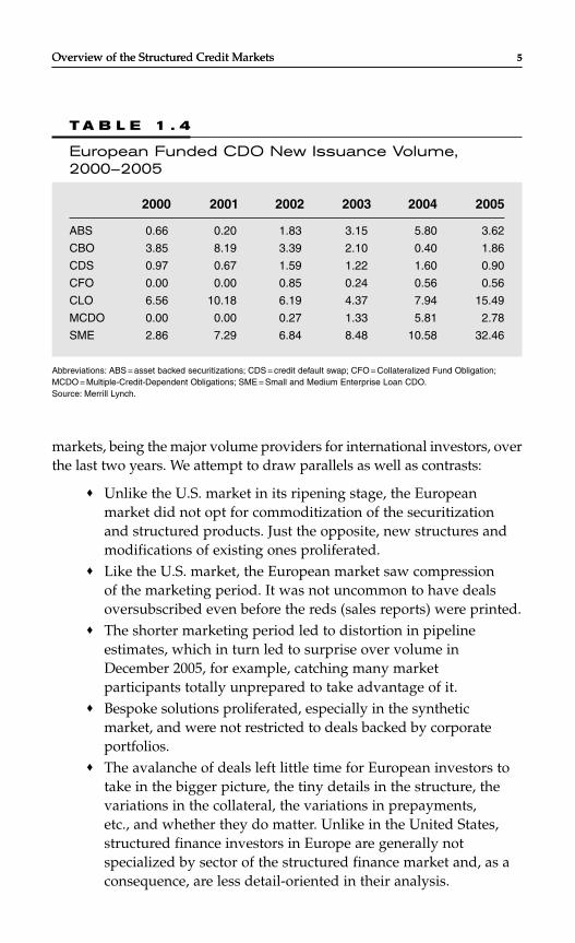
T A B L E 1 . 3
European Funded Structured Product New Issuance Volume, 2000–2005
2000 2001 2002 2003 2004 2005
ABS 16.195 28.325 30.652 36.929 47.821 53.517
CDO 14.900 26.528 20.966 20.892 32.690 57.657
CMBS 9.455 22.882 20.904 10.139 14.736 45.750
CORP 6.430 14.641 13.536 18.299 17.989 9.416
RMBS 42.186 54.001 69.463 110.653 125.933 159.748
Total 89.166 146.377 155.521 196.912 239.168 326.088
Abbreviations: ABS = asset backed securitizations; CDO = collateral debt obligations; CMBS = commercial mortgagebacked securitizations; CORP = Corporate Securitization; RMBS = Residential Mortgage Backed Securitization.Source: Merrill Lynch.
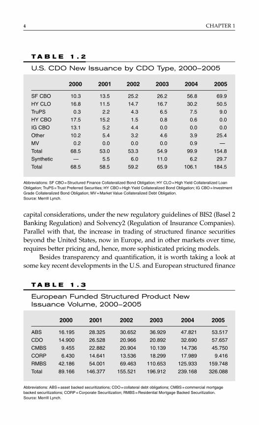
T A B L E 1 . 2
U.S. CDO New Issuance by CDO Type, 2000–2005
2000 2001 2002 2003 2004 2005
SF CBO 10.3 13.5 25.2 26.2 56.8 69.9
HY CLO 16.8 11.5 14.7 16.7 30.2 50.5
TruPS 0.3 2.2 4.3 6.5 7.5 9.0
HY CBO 17.5 15.2 1.5 0.8 0.6 0.0
IG CBO 13.1 5.2 4.4 0.0 0.0 0.0
Other 10.2 5.4 3.2 4.6 3.9 25.4
MV 0.2 0.0 0.0 0.0 0.9 —
Total 68.5 53.0 53.3 54.9 99.9 154.8
Synthetic — 5.5 6.0 11.0 6.2 29.7
Total 68.5 58.5 59.2 65.9 106.1 184.5
Abbreviations: SF CBO = Structured Finance Collateralized Bond Obligation; HY CLO = High Yield Collateralized LoanObligation; TruPS = Trust Preferred Securities; HY CBO = High Yield Collateralized Bond Obligation; IG CBO = InvestmentGrade Collateralized Bond Obligation; MV = Market Value Collateralized Debt Obligation.Source: Merrill Lynch.
Overview of the Structured Credit Markets 5
markets, being the major volume providers for international investors, overthe last two years. We attempt to draw parallels as well as contrasts:
♦ Unlike the U.S. market in its ripening stage, the Europeanmarket did not opt for commoditization of the securitizationand structured products. Just the opposite, new structures andmodifications of existing ones proliferated.
♦ Like the U.S. market, the European market saw compressionof the marketing period. It was not uncommon to have dealsoversubscribed even before the reds (sales reports) were printed.
♦ The shorter marketing period led to distortion in pipelineestimates, which in turn led to surprise over volume inDecember 2005, for example, catching many marketparticipants totally unprepared to take advantage of it.
♦ Bespoke solutions proliferated, especially in the syntheticmarket, and were not restricted to deals backed by corporateportfolios.
♦ The avalanche of deals left little time for European investors totake in the bigger picture, the tiny details in the structure, thevariations in the collateral, the variations in prepayments,etc., and whether they do matter. Unlike in the United States,structured finance investors in Europe are generally notspecialized by sector of the structured finance market and, as aconsequence, are less detail-oriented in their analysis.
Overview of the Structured Credit Markets 5
T A B L E 1 . 4
European Funded CDO New Issuance Volume,2000–2005
2000 2001 2002 2003 2004 2005
ABS 0.66 0.20 1.83 3.15 5.80 3.62
CBO 3.85 8.19 3.39 2.10 0.40 1.86
CDS 0.97 0.67 1.59 1.22 1.60 0.90
CFO 0.00 0.00 0.85 0.24 0.56 0.56
CLO 6.56 10.18 6.19 4.37 7.94 15.49
MCDO 0.00 0.00 0.27 1.33 5.81 2.78
SME 2.86 7.29 6.84 8.48 10.58 32.46
Abbreviations: ABS = asset backed securitizations; CDS = credit default swap; CFO = Collateralized Fund Obligation;MCDO = Multiple-Credit-Dependent Obligations; SME = Small and Medium Enterprise Loan CDO.Source: Merrill Lynch.

♦ The collateral quality softened, sometimes visibly—in commercialreal estate securitizations and in leveraged loans, for example;sometimes less so—in the residential mortgage deals, wherereportedly prime mortgage pools contained products, which willnot be viewed as prime in countries, where the differentiation isclearer, e.g., the UK. In contrast, in the United States, the subprimesector, usually associated with home equity loans of lower FICO(Fair Isaac & Co. Credit) score, experienced massive growth. Thedifferentiation between prime and subprime pools, especially inthe mortgage and consumer finance area, is clearly defined in theUnited States, and is further helped by the use of quantitativemeasurements of consumer credit quality, such as FICO scoring.
♦ European deal reporting and information disclosure is improv-ing, although slowly. While the necessary information for resi-dential mortgage pools is getting through in larger quantities,such information remains fairly sporadic for, say, commercialreal estate transactions. The understanding of loan prepaymentfactors in either market remains largely in embryo.
While the above list of developments and trends is by no means exhaus-tive, it is consistent with the developments we expect in the comingyears. Our positive views on the structured credit market are also sup-ported by:
♦ The persistence of relatively weak supply of corporate paperand covered bonds. Structured products exceeded both corpo-rate bond and covered bond supply for a second year in a row,which is expected to be the case in the future.
♦ Structured product spreads that remain attractive compared tosimilarly rated corporate and covered bonds. The predomi-nantly triple-A supply (about 85 percent of new issuance on thestructured product market) is offering a significant yield pick-upover sovereign, covered bond and bank paper. We do not attrib-ute this pick-up in its entirety to a liquidity premium (except forbespoke structures, of course). The liquidity component is amore appropriate explanation for the yield differential betweenstructured product, on the one hand, and the corporate bonds,on the other, at below-triple-A levels.
♦ The ability of structurers to offer bespoke deals addressing spe-cific investor demands or concerns. That alone explains the large
6 CHAPTER 1

private volume in synthetic execution. The requirement for pub-lic rating for regulatory capital purposes may make some of thisvolume more visible in the future. We note the increasing flexi-bility and ingenuity applied by structurers in an effort to meetspecific client’s requirements and needs. Further customizationof the market may lead to a less volatile and less tradablemarket at least for larger segments.
♦ The large range of structured product offerings dealing withrepackaging of exposures. Many of these, which are otherwiseunavailable to numerous investors, remain an attractive pointfor them; e.g., the investors can take direct exposure to con-sumer risk or real estate risk and leveraged or managed expo-sure to familiar and less familiar corporates.
♦ The “safe harbour” argument, which is as old as the structuredcredit market itself. There is a modification of this argument,though: investors in Europe are now becoming more concernedabout mark-to-market of their bond holdings, and structuredproducts, at least historically, have offered lower spread volatil-ity, maybe due to their lower liquidity, given that their ratingvolatility was low. While the argument about lower event-risksensitivity of structured products remains valid, many structuredproducts have assumed more leverage, which by itself makesthem more susceptible to volatility in the future. However, bytheir nature, structured products, in general, should remain moreresilient to event-idiosyncratic risk, which is one of the mainconcerns of corporate bond investors. While individual eventsmay have little impact on specific structured finance products,we note the delayed effect of accumulating credit risks in lateryears. We emphasize this point: credit deterioration has acumulative negative effect in the predominantly static collateralpools backing the majority of structured bonds.
♦ The development of synthetic asset backed securitizations (ABS)exposures, be it on individual names [the European credit defaultswap (CDS) on ABS or U.S. PAYGO versions] or on a pool basis—through synthetic ABS pools or via the synthetic ABS index ABXin the United States—has dramatically changed the structuredfinance market. These innovations allow the ABS market to speedup execution, provide the exposures that the cash market cannotoffer, and supply a mechanism to express a negative view on the
Overview of the Structured Credit Markets 7

market, to hedge or speculate. The importance of these develop-ments cannot be overestimated. In this regard, the United States isleading Europe and the rest of the world, as has often been thecase in the structured finance market.
Having said all these nice things about the structured product market, letus be more critical and highlight some of its shortcomings. Many of ourconcerns have been voiced before, but they may take a new light now thatthe market, by wide consensus, has reached the peak of the current cycleand has nowhere to go but sideways and eventually descend. The start-ing point of that descent may be triggered by several weaknesses:
♦ Overall, deals are more leveraged: be it because of underlyingconsumer indebtedness, companies’ financial ratios, or the dealstructures. That should lead to bigger swings under unfavorableand/or unexpected market developments.
♦ Investors are stretched in their ability to absorb new deals, mon-itor old ones, and keep an eye on new developments. Thegrowth of the market in complexity and volume has yet to bereflected in increasing investor specialization across asset sectorsand products. Corporate analysts often know everything abouta couple or so industries and the main companies within thoseindustries; hence the need for several corporate analysts to man-age a larger corporate bond portfolio. Structured credit analystsand portfolio managers, however, are expected to cope withnumerous sectors, structures, and deals simply because they fallinto the simplistic misnomer “structured.”
♦ There is a serious need for more quantitative power dedicated tostructured products. That power can be fully used only if thereis more information about the structured product collateral.That power, though, is powerless in the face of unquantifiablequantities—say, the likelihood of prepayment of a given loan ina commercial real estate portfolio or the impact of a manager ina CDO under adverse market conditions. Under such circum-stances, the good old reliance on “gut feeling” seems to be theone and only last resort for the investor.
♦ Lack of tiering to reflect differences in structure, pool composi-tion, information availability, and servicer or manager capabili-ties. The deplored lack of tiering is an enduring feature of theEuropean market and will properly change, we think, only under
8 CHAPTER 1

market distress. We hope some signs of change are already in theair, say in commercial mortgage backed securitizations (CMBS)or CDO land, although with recent tight CMBS spreads pricinghas looked haphazard, particularly for the more junior tranches.
♦ Regulatory uncertainty or uncertainty about the impact ofregulations such as BIS2 and the respective national imple-mentation guidelines, The accounting Standard IAS39,Solvency2, and the potential for a not-quite-level playing fieldthey may be creating across countries and markets. One concernwe have is that regulators’ ambiguity about synthetics in somecountries is hurting not only the market development, but alsothe regulated entities themselves, as they are precluded fromusing this market to their benefit.
THE NOT-SO-HOMOGENEOUS CDO SECTOR
One of the major market developments in recent years is the emergenceof the CDO sector as a major market sector, with the capacity to influencedevelopments in other seemingly independent market sectors. The CDOsector is not homogeneous and consists of many different subsectors andniches. Referring to the developments in any one CDO sector, and gener-alizing and applying the conclusions to all the others is wrong and grosslymisleading. It can increase market volatility, deter investors from makingreasonable investment decisions and, in the extreme, create a liquidity cri-sis in a specific market sector or on the entire market, if the panic spreadswide enough.
While this is fairly obvious, it is not fully appreciated by manymarket participants. Hence, there is a need to broadly differentiate amongthe several main categories of CDOs that are dominant on the markettoday, and highlight their interaction with the rest of the market.
Arbitrage Cash CDOs
The arbitrage cash CDO sector includes a number of CDO types, widelydifferentiated by the type of exposure used to rampup the CDO collateralpool. Among them are:
♦ cash CDOs comprising high grade and/or mezzanine ABS♦ cash CLO of leveraged loans and/or middle market loans
Overview of the Structured Credit Markets 9

♦ cash CDOs of insurance and bank trust preferred securities♦ CDO of emerging markets exposures, both sovereign and
corporate.
Each of these subsectors follows the credit and technical dynamics of itsrespective market. A CDO backed by a portfolio of such instruments iseffectively a vehicle for creating tranched risk profile and leverage on thatportfolio.
In the past, there were large subsectors of cash CDOs backed by highyield (HY) and high grade (HG) bonds, and their fortunes rose and sankwith the movements in the HY or HG bonds backing them and, not least,with the strategy, behavior, and luck of the CDO managers running thoseportfolios.
We note that in a cash CDO, the asset and liability sides of theCDO are established at launch and may change little during the life of thetransaction:
♦ The liability side (i.e., the capital structure of the CDO) is deter-mined at deal’s launch and changes only with the amortizationof the senior tranches or the write-down of the equity and juniortranches in case of default and losses in the pools.
♦ The asset side (i.e., the pool of investments) is also determinedat launch and may experience little change during the life of thedeal. In the currently dominant types of cash CDOs (listedearlier), trading occurs to a very limited degree, if at all. In mostdeals, trading by the manager is restricted to credit impairmenttrade (due to expected or real deterioration of a given name)and credit improvement trade (upon certain spread tightening,but under condition that traded credit must be replaced bysimilar or better credit quality name).
♦ The asset–liability gap (i.e., the funding gap) determines thelevel of return that a CDO equity investor can expect (depend-ing on the level of defaults in the investment pool) and is a keyconsideration in the placement of equity and overall economicviability of a cash CDO.
Hence, a cash arbitrage CDO is a structure mostly set at the beginningof the transaction and is meant to be maintained as stable as possiblethroughout its life, with the ultimate purpose of repaying debt investorsand providing adequate return to equity investors over its scheduledlife.
10 CHAPTER 1

The initial and on-going pricing of the cash CDO tranches is market-based (rather than model-based). It takes into account where other simi-lar transactions price on the primary and secondary market and, in caseof significant defaults or downgrades in the pool, considers the value ofthe pool and how it relates to the outstanding CDO debt obligations thatthe pool is backing.
From this it follows that a cash CDO once launched has little on-going impact on the market, with its asset and liability side meant to berelatively stable. Looking at it the other way around: ongoing marketchanges may have little impact on the cash CDO, except for defaults andthe mark-to-market of the CDO debt and equity tranches.
Hence, defaults are the issue of main consideration for arbitragecash CDOs, as their occurrence or not, the degree thereof, and the subse-quent crystallized loss will determine the yield on the debt tranches andreturn on the equity tranches of these transactions.
Synthetic CDOs
Synthetic CDOs are diverse in nature and include a number of instru-ments, which are not directly comparable in terms of investment charac-teristics and market impact. These include:
♦ Synthetic structured finance (or ABS) CDOs—an emergingsector, in which CDS on ABS in Europe and PAYGO SFCDS inthe United States are used to build an ABS portfolio quickly andefficiently. Such a portfolio would be more difficult to executein 100 percent cash due to allocation and sector and vintagelimitations on the cash-structured finance market today. Suchsynthetic deals may be fully/partially funded or may be singletranche deals. The latter require hedging for the unfundedsenior and junior (to the funded portion) tranches; hedgingusually takes place through a combination of cash purchaseand selling protection on the respective cash bonds and isusually adjusted downwards as the referenced exposuresamortize or experience losses.
♦ Balance sheet synthetic CDOs/CLOs—associated with creditrisk transfer of a bank bond or loan portfolio—their share oftoday’s market is miniscule and their behavior is more akin tocash CDOs discussed earlier (relatively constant structure andprimarily default-driven investment performance).
Overview of the Structured Credit Markets 11

♦ Other synthetic CDO products, such as those based on constantmaturity CDS, principle protected tranches of CDOs, etc.,whose behavior is further modified by their specific structuralfeatures and will differ from that of other synthetic CDOsubtypes.
♦ Bespoke synthetic CDOs—single tranche CDOs on corporatenames, referenced through CDS.
♦ Standardized tranches of CDS indices—iTraxx in Europe andCDX in the United States.
The last two sectors tend to be also lumped together under the “correla-tion trades” moniker. The latter, because correlation is a derived variablefrom a pricing/trading model and a function of spread movements. Theformer, because to be priced, the implied correlation input is referencedfrom the standardized tranche market. These two sectors can be viewedas model-driven from the perspective of pricing and trading (exploringtrading opportunities), but there are differences:
♦ The structure of a bespoke single-tranche CDO is set at itslaunch, but there is a need for the intermediary to hedge expo-sures senior and junior to the investor’s tranche, creating an on-going interaction with and impact on the market. The need torebalance the delta hedges creates the need to trade certain CDSand thus influences the supply and demand for these credits inthe market. The larger the size of the single-tranche market, thelarger the impact such secondary delta-rebalancing trades mayhave on it: large and more single-tranche deals suggest largerand more referenced portfolios, whose senior and juniortranches must be hedged and the hedges rebalanced. However,the single-tranche investor may be relatively sheltered in hisinvestment from such movements, as long as defaults do notcross certain threshold or he is in some way protected againsttrading/hedging losses.
♦ The standardized index tranches are used by investors toexpress a view (take a position) on spread direction and correla-tion, and as their view changes or the market developments donot justify such view (positioning), a need to trade arises. It maytake place in order to adjust the position or to reverse it (to closea position altogether). That creates secondary market activity
12 CHAPTER 1

and, almost inevitably, market volatility. The standardizedtranches market is also used to hedge positions or execute cer-tain strategies. A desire to unwind the hedges or the positionswhen not needed or the market moves against them mayfurther exacerbate market volatility.
From this it follows that correlation trades can have a strong on-goingimpact on the market either through the need to rebalance the hedges orto take a position and subsequently unwind it. The opposite is also true:ongoing market changes, such as spread movements, and the perceptionin correlation changes can have an impact on standardized index tranchepricing and associated positions. Hence, ongoing spread movements,actual downgrades/defaults, and the related perception of correlation arethe main factors to consider in synthetic standardized tranche trades and inhedging single-tranche CDOs. From the perspective of the single-trancheCDO investor, though, the main concern is the level of default in thereference pool.
Different Investors “Own” Different CDO Sectors
The review of the CDO market so far indicates some fairly fundamentaldifferences among the broadly defined cash arbitrage and synthetic CDOsectors. Such differences can be further illustrated by looking at the moti-vation and identity of the investors in the different sectors:
♦ “Real” money accounts tend to focus on cash CDOs and tend tobe buy-and-hold investors when buying synthetic and bespokesynthetic CDOs. In that space, different parts of the capitalstructure of a CDO attract a different type of investor—thatspreads the slices of risk to the broadest possible range ofmarket participants.
♦ “Leveraged” money accounts (hedge funds) drive most ofthe activities on the standardized tranche market, althoughsome real money accounts have become more active in recentmonths. The activities in that space are associated withtaking a view on correlation and how spread changes in themarket could trigger repricing of the different tranches of thesynthetic indices. To some degree, this sector can be viewed as
Overview of the Structured Credit Markets 13
“speculative,” although using it for the purposes of hedging isnot uncommon.
Although this division is general and there are some investors who crossthe line in both directions, it is certainly not imprecise.
The mark-to-market aspect affects the different investor types in a dif-ferent way and is common to all fixed income instruments. We note thatcash CDO “held to maturity” are not subject to mark-to-market, whereasall synthetic CDOs regardless of their classification are subject to mark-to-market. MTM issues are of a particular concern to European fixed incomeinvestors this year, as a result of the introduction of IAS39.
While the fall-out from the recent hedge fund standardized tranchesinvestment strategy gone wrong could be wider spreads and high mark-to-market losses, there is no evidence in the market to suggest that the differentcash and synthetic tranche CDOs have widened more than similarly ratedother fixed income investments.
Liquidity and the “Unexpected” MTM Problem
A key market consideration is the liquidity of structured finance instru-ments and the associated mark-to-market volatility. The latter is a rela-tively recent concern associated with the introduction of mark-to-marketaccounting.
Table 1.5 demonstrates the spread movements for a variety of Euro-pean structured products. Given the limited time frame of this analysis, aswell as the limited time frame of a relatively mature European market, wesuggest that readers do not focus on the nominal values, but rather on therelative magnitude across asset classes and sectors. If we assume that theperiod given in Table 1.5 embraces the tightest spreads seen on the mar-ket in recent years, it is natural to ask the question as to how much thespreads can widen. While we expect spread widening to be cyclical (trend-line), we foresee the actual spread movements to be shaped by technicaland fundamental factors along the way (zigzagging along the trend line).From that perspective, it is important for investors to understand theexpected behavior of the different sectors and subsectors of the Europeanstructured finance market, their reaction to technical and fundamentalfactors, and their interaction with each other.
When considering their portfolio strategies, investors can conceptual-ize the market and their portfolios in different ways. On that basis, they canre-examine their tolerance to mark-to-market and credit risk in a market
14 CHAPTER 1
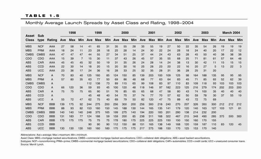
T A B L E 1 . 5
Monthly Average Launch Spreads by Asset Class and Rating, 1998–2004
Asset Sub1998 1999 2000 2001 2002 2003 March 2004
Class type Rating Ave Max Min Ave Max Min Ave Max Min Ave Max Min Ave Max Min Ave Max Min Ave Max Min
MBS NCF AAA 27 58 14 41 65 31 35 55 28 35 55 19 27 50 22 35 54 26 19 19 19MBS PRM AAA 18 24 11 23 28 18 25 28 14 24 30 22 24 28 18 24 40 20 17 22 12CMBS CMBS AAA 47 47 47 44 55 27 34 51 25 37 44 24 43 63 28 45 50 40 38 38 38CDO CDO AAA 15 39 7 15 30 11 37 43 26 45 57 35 55 68 25 71 81 61 57 64 48ABS CAR AAA 45 45 45 32 50 19 31 35 26 24 28 14 24 38 13 30 42 11 15 15 15ABS CCD AAA 22 30 14 18 20 15 20 30 16 25 28 23 20 22 16 20 27 5 13 22 3ABS UCC AAA 23 36 17 24 36 16 28 33 25 32 35 28 31 36 28 25 31 20
MBS NCF A 70 83 40 125 160 85 124 150 85 139 203 100 109 125 98 164 188 135 95 95 95MBS PRM A 57 80 35 63 77 50 69 86 48 68 77 63 64 83 45 71 85 65 52 62 39CMBS CMBS A 112 138 73 89 115 65 99 108 83 97 110 83 109 118 93 103 103 103CDO CDO A 66 120 36 59 93 45 100 120 48 118 146 97 182 223 125 216 279 174 202 203 200ABS CAR A 75 75 75 65 90 51 76 85 65 65 68 47 58 80 43 74 100 35 40 40 40ABS CCD A 45 48 40 54 75 37 74 77 70 57 62 50 59 78 30 37 55 19ABS UCC A 55 72 47 62 75 40 69 79 50 82 120 47 75 88 43 72 75 69
MBS NCF BBB 139 175 92 244 275 200 256 300 200 256 300 218 240 270 207 326 350 300 212 212 212MBS PRM BBB 88 93 82 153 160 150 145 188 130 144 165 135 141 179 120 140 163 127 103 121 81CMBS CMBS BBB 140 140 140 248 375 165 199 275 140 194 220 183 201 280 138 214 232 200CDO CDO BBB 131 183 77 124 188 59 159 200 85 238 311 168 322 467 215 348 490 285 375 500 300ABS CAR BBB 175 175 175 75 75 75 178 180 175 225 225 225 150 150 150 160 170 155ABS CCD BBB 90 90 90 112 150 88 151 165 138 149 168 120 159 187 110 83 120 45ABS UCC BBB 130 130 130 160 160 160 175 175 175 217 275 188 150 170 125 153 170 140
Abbreviations: Ave = average; Max = maximum; Min = minimum.Asset Class: MBS = mortgage backed securitizations; CMBS = commercial mortgage backed securitizations; CDO = collateral debt obligations; ABS = asset backed securitizations.Subtypes: NCF = nonconforming; PRM = prime; CMBS = commercial mortgage backed securitizations; CDO = collateral debt obligations; CAR = automobiles; CCD = credit cards; UCC = unsecured consumer loans.Source: Merrill Lynch.

downturn. Then, they can model how their current (at the peak of the mar-ket) portfolio will react to different levels of market downturn and deter-mine what is the acceptable credit and marked-to-market loss they can bear.
Furthermore, investors can anticipate the evolution of their portfo-lio between today and some future point [factoring WAL (WeightedAverage Loss) scheduled and unscheduled amortization, expected losses,etc.], when they expect the market downturn and see how such a portfo-lio will react to such downturn. Finally, investors must consider whatsteps to take now and in the near future to bring their current portfolioto that which is sensitive to credit and MTM losses and is consistent withtheir own (institutional or personal) tolerance.
CRITERIA FOR STRUCTURED FINANCEDEALS AND PORTFOLIOS
Review and Risk Tolerance
The analysis of structured finance products and portfolios is a complexundertaking. We highlight a number of criteria in no particular order:
GranularityGranular deals with strong credit quality are less susceptible to event riskof single-name exposures than nongranular deals. Historical evidence sug-gests that more granular, high quality ABS have experienced little spreadvolatility compared with low quality granular deals and nongranular deals.These observations are true across ABS capital structures. They also holdfor high grade mortgage backed securitizations (MBS) and CMBS as anexample of highly granular and less granular deals, as well as for primeRMBS and subprime RMBS as an example of deals with similar granularitybut different credit quality. While correct, this outcome may be influencedby the fact that granular deals in general are associated with consumerexposures and nongranular deals—with corporate exposures.
Types of Credit ExposureConsumer ABS in Europe tends to demonstrate less spread volatility thancorporate exposure ABS (in the form of CDOs and CMBS). That may bealso associated with the granularity of the portfolios as mentioned earlier.In general, though, consumer pools’ tranches tend to reflect tranching ofthe systemic risk, associated with a large securitization pool and reflectthe state of the economy of the respective country.
16 CHAPTER 1

In addition, consumer portfolios are exposed more to systemic risk,say widespread economic deterioration, than to event risk (collapse of asingle company or an industrial sector). We caution, however, that today,in most countries, the consumer is over-indebted, i.e., the consumer sec-tor is stretched or even over-stretched, which was not the case during thelast corporate credit cyclical downturn. (The two countries, which in thepast downturns have had relatively high consumer indebtedness—United States and UK, are even more indebted today, with the consumerdebt stretching beyond residential mortgage debt.) Consumer lendingand spending softened the blow during the last downturn—this buffermay not be as readily available in a future downturn. Hence, the economyas a whole and the consumer pools, in particular, may suffer more thanprevious downturns in history.
Senior versus Junior TranchesIt is a fact that senior tranches have more cushion against credit deterio-ration than junior tranches. The former seems to hold true for differentasset classes, even ones of similar granularity. An interesting way to lookat the credit cushion is to compare the level of credit enhancement foreach tranche to the level of five-year cumulative losses of a given assetclass. The challenge arises, when such cumulative loss numbers are notrobust, statistically speaking.
As mentioned earlier, senior tranches tend to experience less spreadvolatility than junior tranches of the same asset class. Their bid-offerspread is much lower than the one for junior tranches. Almost always se-nior tranches are more liquid than junior tranches of the same deal. Itis not uncommon for market participants to often use secondary trade-based pricing for marking-to-market their senior tranche positions andestimated pricing (on the basis of primary market or dealer talk) for mez-zanine positions. In the case of the latter, there is the risk that one-off trademay lead to serious repricing and mark-to-market volatility.
Sensitivity to Third Parties (Originator,Servicer, Counterparty)While structured finance bonds are set up in such a way as to minimizeor eliminate the role of the asset originator and its potential bankruptcy,some linkages (in terms of credit or portfolio performance) remain—theymay be with the originator or servicer, a third-party servicer and/or hedgecounterparty. These linkages may have both direct and indirect effect onthe bond pricing on the secondary market, and understanding the potential
Overview of the Structured Credit Markets 17

for problems from that corner is crucial in defending against mark-to-market losses, defaults or downgrades.
In addition, idiosyncratic aspects of underwriting and servicingshould be taken into account in determining future pool performance—this is particularly true for subprime and commercial real estate sectors.Nonbank, nonrated servicers are of particular concern when anticipatingthe performance of the securitized pools and the headline risk of therespective bonds.
High versus Low Leverage PositionsIn a low spread, low default market environment, leverage is a necessaryway of achieving yield. In the course of the last couple years, investorshad to take leverage to achieve their yield targets. The discussion aboutwhat leverage is in structured finance, how to estimate it, etc. is a neverending one, and we do not intend to reproduce it here. What is clear,though, is that leverage can enhance returns in good times and magnifylosses in bad times. Hence, there is a need to review the amount of lever-age, how it is achieved, and the extent to which it can be detrimental tothe portfolio performance in a market downturn. Investors need to dif-ferentiate between de-levering structures (say, an MBS) and those that aremeant to remain fully levered for life (say, a CDO Squared).
Pool versus Single-Name ExposuresWhile this may seem as a repetition of the granularity argument, it is notnecessarily so. Single-name exposure may have many different connota-tions: it could be in the repetition of a given corporate name in numerousportfolios, or in the presence of the same servicer in multiple deals, or,alternatively, in the high dependence of a given transaction on the cashflows generated by a given entity. The need to estimate the accumulationof multiple exposures to a single name under different transactions isobvious, but the estimate is not that simple to make in practice. We sug-gest going beyond the issue of overlap, as know from CDO land, and con-sidering all forms of exposure or potential exposure to a given namepresent in the structured finance portfolio.
Anticipated Impact of BIS2We believe that BIS2 considerations should be an inextricable part of theEuropean investment strategy over the next several years. BIS2 riskweights favor all senior securitization exposures and do not favor allsubinvestment grade securitization exposures. Investors should factor the
18 CHAPTER 1

lower and higher capital requirements post January 1, 2007, when deter-mining the adequate price for a securitization bonds, scheduled to matureafter 2006. We also note the granularity adjustment differentiation forsenior tranches of securitization exposures.
Other Country-Specific ConsiderationsSuch considerations, e.g., may include:
♦ The changes in pension regulations and eventual new RealEstate Investment Trust (REITS) legislation in the UK shouldhave a positive impact on commercial real estate pricing. Thatmay make CMBS rarer, on one hand, and improve the propertyvalues for existing deals, on the other. In the short-term, this isoffset by the growth in real estate conduits.
♦ The introduction of covered bonds in more countries shouldreduce the supply of MBS and make them more attractive.
♦ The reduction of budget support for SMEs in Spain shouldreduce their supply, change their geographic diversity, or con-vert them into stand-alone structures with higher subordinationlevels (more supply of non-triple-A paper).
We certainly do not intend an exhaustive list here, but suggest thatinvestors consider these changes and how they could affect future supplyand pricing in specific structured finance sectors.
ModelingStructured finance securities are complex credit structures, which can per-form differently under similar economic and market scenarios. All themore, when addressing the need to fully understand the variations intheir performance, modeling comes handy. In that regard, availability ofmodels and people able to use them properly becomes a key factor inbetter understanding the future performance of structured finance dealsand related portfolios. The preceding discussion indicates that the simplyrerunning historical scenarios are not enough for investors to fully under-stand the risk (credit, MTM, duration) of their holdings. One needs notonly modellers, but also credit-savvy ones at that.
Increase Asset-Based Liquidity of the PortfolioIn a market downturn scenario the need for liquidity in a portfolio is mostacutely felt, especially one with margin calls or with a potential for moneywithdrawals at a short notice. In that regard, we suggest that investors
Overview of the Structured Credit Markets 19

use the rating agencies guidelines for liquidity eligibility and haircuts fordifferent asset classes of structured finance securities, in determining theasset-based liquidity of structured investment vehicles. Regulatory guide-lines for repo eligibility and haircuts can also be useful, although the listof such securities is limited to primarily senior tranches of ABS backed bygranular pools.
Distinguishing Between Cyclical SectorsDistinguish between cyclical (CLOs, office CMBS, subprime consumer, etc.)and cycle-neutral sectors (retail CMBS, high quality consumer pools, etc.).Corporate ABS seems to be more affected by the event risk of down cyclesthan prime consumer ABS. Alternatively, high quality consumer-relatedABS seems to be more cycle-neutral than low-credit-quality consumer-poolABS. We refer here to the cyclical nature of the exposures comprising thepool of the respective structured financing. A CDO, e.g., being a derivativeof the underlying corporate high-yield or high-grade sector will performaccording to the cycles of that sector—the deal performance, however, willbe modified by the actions of the CDO managers. Similarly, the perfor-mance of a subprime mortgage pool will be dependent on the performanceof the economy and the housing market (hence, its cyclical nature), butmodified by the actions of the respective servicer.
Senior Mezzanine-Equity PositionsThat the credit risk and mark-to-market risk of the different tranches ofstructured financings are different is a given. What is more important isthat such differences persist across the tranches of different asset classes,so the equity position of a CDO of senior ABS will have different suscep-tibility to the earlier risks than, say, the equity position of a CDO of high-yield loans, not to mention the mezzanine of prime mortgage master trustMBS compared to the mezzanine of a residential real estate mezzanineCDO, or the senior tranche of stand-alone amortizing Dutch prime MBSin comparison with senior tranche of a mixed lease Italian ABS.
BIS2 AND OTHER REGULATIONS—LONGER-TERM IMPACT ON THESTRUCTURED FINANCE MARKETS
As we noted on several occasions so far, BIS2 is expected to have a majoreffect on the structured finance market in all its aspects: supply, demand,
20 CHAPTER 1
spreads, and mark-to-market volatility. We explored some of the mark-to-market aspects earlier, and we turn our attention now to some ofthe more fundamental changes we anticipate BIS2 implementation willprompt. Here, we take into account only the consequences from the newcapital treatment, as if securitization’s only function were to achieve cap-ital relief for the securitizing bank and as if banks invested only on thebasis of regulatory capital considerations. We note that the number ofbanks expected to adopt the IRB (Internal Rating Based) approach is highin Europe, making this approach dominant in determining risk capitaland the BIS2 impact in securitization.
From the Perspective of the Originating Bank
Again, if the only reason for securitization were capital relief, then theexpected changes in capital requirements for different types of exposureson the banks’ balance sheet should give a good understanding of whichassets could conducive to securitization and which not. The chart aboveis based on QIS3 data and broadly indicates that banks will have reducedincentive to securitize consumer assets, and increased incentive to securi-tize special lending exposures, sovereign and to some degree other banks.That is because BIS2 leads to significant reduction in risk weights for retailexposures, particularly mortgages, and an increase in risk weights forspecialized lending and sovereigns, particularly high volatility real estate.In more specific terms:
♦ There will be a seriously reduced capital relief benefit fromsecuritizing mortgage portfolios and somewhat reduced benefitfor retail and retail SME portfolios.
♦ The incentive should shift toward the securitization of higher-risk weighted assets such as lower investment and subinvest-ment grade corporate exposures, commercial real estate, special-ized lending, etc.
♦ Securitization of mortgage and retail portfolios should be drivenmore by nonregulated companies, as well as by the funding con-siderations of banks.
These conclusions, however, should be further detailed on the basis of thecredit quality of the underlying exposures, subject to securitization. Thechart below compares the capital requirements for different types of retailexposures under both standardized and the IRB approaches.
Overview of the Structured Credit Markets 21
In all cases, the bank should consider the capital requirementbefore securitization and after securitization (in the form of capital forretained portion of securitization exposure). To simplify, it will dependon whether the capital before securitization is higher, equal, or less thanthe equity piece of the securitization transactions, which is usually thepiece retained by the bank originator. In that regard, the supervisor’sand bank’s own estimates for loss given default, EAD (Exposure atDefault), and M (Maturity) play a key role in determining the benefits ofsecuritization for a Foundation IRB bank.
In that respect, we note the wide range of corporate exposures listedunder the IRB approach and the potential difficulty for banks to getsupervisory approval to use their own inputs for capital calculation. Thatmay lead the banks to use the prescribed risk weightings for specializedlending, as indicated in the discussion of IRB, and thus have regulatorycapital incentives to securitize such exposures.
Banks who continue to dominate the issuance volume of structuredproducts may modify their issuance patterns, as a result of incorporatingregulatory capital treatment of the underlying exposures in the econom-ics equation of securitization. Securitization of mortgages may be prima-rily done for funding purposes, given limited regulatory capital benefit forit, whereas securitization of commercial real estate, unsecured consumerloans, and project finance may be driven by regulatory capital relief con-siderations in the first place. Alternatively, banks using the standardizedapproach may still have a regulatory capital benefit from securitization,while that benefit will be largely unavailable for banks applying the IRBapproach. All this could lead to a change in supply levels, types of prod-ucts securitized, and servicer considerations.
To achieve better realignment of regulatory and economic capital,banks may be tempted to issue also double-Bs and single-Bs, and evensell first loss positions. That raises questions about the rating agencies’methodologies for rating below investment grade pieces and howreliable they are as well as about the breadth of investor base for suchexposures.
From the Perspective of the Investing Bank
An investing bank naturally takes into account the cost of regulatory cap-ital among other things when determining its investment interest in a
22 CHAPTER 1
securitization position. Again from the perspective of regulatory capitalconsiderations alone, a bank investor should:
♦ Buy riskier sovereign, bank and corporate exposures (say, ratedsingle B and below) rather than less risky securitizationexposures (say, rated double-B).
♦ Avoid subinvestment grade securitization tranches regardless oftheir actual risk, unless of course the pricing of such tranches issufficient to compensate the bank for both the risk of the trancheand the increased cost of capital. The placement of subordinatedtranches may become more dependent on the appetite ofnonregulated investors. In fact, the question of placement ofnoninvestment grade tranches of securitizations will becomea key factor in determining the viability of many futuresecuritization transactions.
♦ Standardized approach requires more capital for investmentgrade tranches (except for BBB−) and less capital for lower-ratedtranches, which should lead to different investment incentivesfor standardized and IRB bank investors and lead them tomodify their investment allocations.
♦ IRB banks are even less likely than standardized banks to investin subordinated noninvestment grade securitization tranches,and even more likely than standardized banks to seek mostsenior investment grade tranches.
♦ The gap between senior secured corporate and securitizationexposure risk weightings for noninvestment grade exposurewidens even further. This creates even bigger disincentives forIRB banks to invest in subordinated securitization exposuresand make them choose instead high-yield corporate exposures.
♦ The risk weightings for covered bonds and RMBS are converging,thus reducing or eliminating the regulatory capital advantage ofcovered bonds, characterizing the current investment decisions.
Given the reduced risk weights for senior tranches under BIS2, banks areexpected to realize certain savings from holding such securitization posi-tions. Given that banks are the dominant investors in securitization inEurope, it is highly likely that such savings are passed on to the market inthe form of spread tightening. Those savings, which can be viewed as apotential range of spread tightening for securitization exposures. We note
Overview of the Structured Credit Markets 23
the “dis-saving” BB exposures or increase in regulatory capital require-ment for bank investors, which we already stated, should lead them toshun away from such exposures.
To clarify further, a standardized bank investing in AAA RMBSsecuritization tranche will use risk weight of 50 percent under BIS1 (Basel1 regulation) and 20 percent under BIS2. That will translate into 40 bpssavings on average cost of capital. Those savings can be passed on to themarket in the form of spread tightening, although that will not be a one-for-one transfer. The same bank needs to increase the risk weight for a BBsecuritization exposure from 100 percent under BIS1 to 350 percent underBIS2. The increase in its regulatory capital is 125 bps, which in turn shouldsee respective widening of the BB spreads of such exposure, to compen-sate the bank for the increased regulatory capital. Similar analysis canbe performed for the RBA approach to securitization to be applied by theIRB banks under BIS2. The respective capital savings or “gains” areslightly larger in comparison to the standardized approach.
Demand–Supply Dynamics
From the perspective of the demand–supply dynamics of the securitiza-tion market, our conclusions can be further expanded:
♦ Nonregulated companies may increase their share in consumerasset securitization, while banks could increase their share in thesecuritization of commercial real estate and other corporateassets. In addition, there will be differentiation of the incentivesto securitize by asset class or at all across banks depending onthe approach to regulatory capital they adopt.
♦ Spreads on subinvestment grade securitization tranches shouldwiden, and on senior tranches should tighten, compared to pres-ent levels, although it is difficult to anticipate the changes in theoverall cost of securitization, as the earlier movements may ormay not be netted out.
♦ The spread movements of securitization tranches in comparisonto similarly rated corporate exposures is somewhat less certain,although we would expect noninvestment grade securitizationtranches to widen more than similarly rated corporate exposures.
♦ We expect ratings to continue to play a major role in the securiti-zation market, probably more so than in the corporate market.
24 CHAPTER 1

In that respect, further improvement in rating approachesand models for securitization tranching will likely become amatter of urgency, given the significant differentiation of riskweights by tranche’s credit rating.
♦ The new BIS2 guidelines will probably slow down thesecuritization market, as we know it today, but simultaneouslycreate new distortions that new structuring techniques will aimto address. Hence, while this may be the end of securitization,as we know it, it may be the beginning of a new stage ofsecuritization and structured market development.
♦ Given that banks and related conduits account for two-thirdsroughly of securitization paper placed on the market, it isconceivable that lower-risk weights should translate into lower-target spreads for such holdings. The potential forsignificantly lower-risk weights for senior tranches may befuelling demand for them in expectation for spread tightening,as those weights are introduced (or less spread widening iftheir introduction coincides with a softening market):
° Entities, which benefit from such spread tightening as itoccurs, but do not have the permanent benefit of regulatorycapital reduction, may be induced to sell once the tighteningis over, i.e., once the risk weight effect is fully priced in.
° Entities, which benefit from the permanent reduction of regu-latory capital will be exposed to different regulatory capitaland, subsequently, potentially higher spread volatility as theirsecuritization holdings are upgraded or, God forbid, aredowngraded.
° In both cases, the aforementioned result may be more tradingand more volatility.
° Downgrades may lead to higher than before spread move-ments, especially on the border points, where one tranchemoves from one type of investors to another; particularlygiven the fact that at least, at present, the breadth and depthof the investor base rapidly declines from senior to juniortranches.
♦ Banks may be more sensitive to downgrades in the future, asthey will have to tolerate both MTM losses and regulatory capi-tal increase. As a result, they may be more likely to sell upon adowngrade.
Overview of the Structured Credit Markets 25
♦ More pronounced differentiation of investor base by tranchewill eventually subject the pricing and dynamics of each trancheto the developments in its respective specialized investor base,which in turn may suggest more opportunities to arbitrage thecapital structure of structured products (akin to correlation arbi-trage of the different layers of standardized tranches of iTraxx).
♦ Given the lack of clarity about regulatory capital treatment ofmany structured products (say, combo notes, CPPI, securitiza-tion of a single commercial real estate loan, etc.), the conse-quences of a treatment away from market expectation orpractices may be dramatic: no demand and oversell are two thatcome to mind.
REGULATORY CHANGES PARALLEL TO BIS2
Two other regulatory changes are already putting their stamp on thestructured finance market. One is the change in accounting practices, theother is the introduction of regulatory capital requirements for insurancecompanies and pension funds, loosely tailored after BIS1 (rather thanBIS2). The accounting changes strike at the heart of securitization prac-tices, affecting off-balance sheet treatment of securitization, accountingfor securitization exposures, etc. Given the uncertainty about the final res-olution of numerous points here below we highlight only one of them—the accounting for synthetic securitizations. Solvency2, on the other hand,is an exercise similar to the introduction of BIS1 years ago and couldchange the way insurance companies and pension funds go about doingtheir business in the future.
IAS/Accountancy
While IAS may seem more straightforward, its consequences remainunder scrutiny. The main issue of ambiguity there is related to syntheticsecuritizations, in general, and synthetic CDOs, in particular. The ques-tion has taken on a magnitude worthy almost of Hamlet: to invest or notto invest? The requirement for bifurcation of synthetic CDOs has intro-duced unnecessary complexity.
In some cases, auditors have taken the Draconian approach ofstopping certain institutions from investing in the product altogether.Not to mention that different auditors have adopted different views and
26 CHAPTER 1

interpretations of the issue. This suggests replacement of economic sensewith auditor’s inclination. The American FASB has left some hope thatbifurcation issue may find a quiet end for the benefit of all parties con-cerned. If that is to be the solution, the interest in single tranche synthet-ics and their secondary and tertiary derivatives will likely be rejuvenated.
Solvency2
As for Solvency2 (the insurance companies and pension funds equivalentto BIS2), it may be too early to discuss yet—it is not coming into forcebefore 2009, but it suffices to point to two potential developments: moredemand from insurance companies and pension funds for structuredproducts and more insurance companies becoming originators of securi-tization in their own right.
Overview of the Structured Credit Markets 27

This page intentionally left blank
C H A P T E R 2
Univariate RiskAssessment*
Arnaud de Servigny and Sven Sandow
29
INTRODUCTION
In this chapter, we discuss the credit risk that is associated with a singledebt instrument and various methods to assess this risk. The credit riskassociated with a defaultable debt instrument can be decomposed into twocomponents: default risk and recovery risk. The former captures the uncer-tainty related to a possible default while the latter reflects the uncertaintyrelated to recovery in the case of default. We shall discuss both types of riskin this chapter while keeping the focus on single credits; the risk associatedwith portfolios of defaultable instruments is discussed in Chapters 4 to 10.
Default risk can be analyzed from various perspectives. One of theseperspectives is provided by the rating approach, in which default risk isquantified by means of a credit rating. These credit ratings are assignedby rating agencies, such as Standard & Poor’s (S&P), Moody’s, and Fitch,and the ratings assigned by these agencies are widely used as default riskindicators by market participants. We shall review the rating approach inthe next section.
Another widely used approach to quantifying credit risk is theapplication of statistical techniques. In this approach, one uses historicaldata and analyzes them by means of methods from classical statistics or
*This chapter contains material from de Servigny and Renault (2004).
Copyright © 2007 by The McGraw-Hill Companies. Click here for terms of use.
machine learning. The result of such an analysis can be a credit score or aprobability of default (PD) for an obligor. The thus estimated PDs canrefer to a fixed period of time, typically one year, or they can provide acomplete term structure for the possible default event. These statisticalapproaches are the topic of Section 2.
From a fundamental perspective, one can view default as the exer-cise of an option by the shareholders of a firm. Therefore, one can, at leastin principle, derive PDs based on the Black–Scholes option pricing frame-work. This leads to the so-called structural or Merton models, which areanalyzed in the section “The Merton Approach.”
Yet another perspective on default risk is provided by spreads oftraded bonds and credit default swaps. These spreads contain informa-tion about the market’s view on default risk. Although these spreadsdepend on other factors as well, they can be used for the extraction ofdefault risk information. We shall discuss these in the section “Spreads.”
Recovery risk is not as well understood as default risk. However,recovery risk has received a lot of attention in recent years; this is in partdriven by the Basel II requirements. A number of models have been devel-oped, which will be reviewed in the section “Recovery Risk.” In the finalsection, we will discuss the combined effect of recovery and default risk.In particular, we shall focus on the effect of common factors underlyingthe two types of risk.
Some of the models and results reviewed in this chapter are dis-cussed more rigorously and in more detail in various textbooks on creditrisk such as the ones by Bielicki and Rutkowski (2002), Duffie andSingleton (2003), Schönbucher (2003), de Servigny and Renault (2004), andLando (2004). A more detailed review of models for recovery risk is pro-vided by Altman et al. (2005). Other results are not included in thesebooks; we shall give references for those below.
Many of the modeling approaches that we discuss in this chapter, aswell as many other approaches that practitioners use for quantifying creditrisk, rely on standard statistical methods as well as on methods fromthe field of machine learning. For a more detailed discussion of statisticalmethods, we refer the reader to statistics textbooks, e.g., to the ones byDavidson and MacKinnon (1993), Gelman et al. (1995), or Greene (2000).Good overviews of machine learning approaches are provided by Hastieet al. (2003), Jebara (2004), Mitchell (1997), and Witten and Frank (2005). Wewould also like to refer the reader to the textbooks by Andersen et al. (1993),Hougaard (2000), and Klein and Moeschberger (2003) on survival analysis,which underlies most of the commonly used default term-structure models.
30 CHAPTER 2
THE RATING APPROACH
What is a Rating?
A credit rating represents the agency’s opinion about the creditworthinessof an obligor, with respect to a particular debt security or other financialobligation (issue-specific credit ratings). It also applies to an issuer’s generalcreditworthiness (issuer credit ratings). There are generally two types ofassessment corresponding to different financial instruments: long-termand short-term ones. One should stress that ratings from various agenciesdo not convey the same information. S&P perceives its ratings primarilyas an opinion on the likelihood of default of an issuer,* while Moody’sratings tend to reflect the agency’s opinion on the expected loss (probabilityof default times loss severity) on a facility.
Long-term issue-specific credit ratings and issuer ratings aredivided into several categories, e.g., from “AAA” to “D” for S&P. Short-term issue-specific ratings can use a different scale (e.g., from “A-1” to“D”). Figure 2.1 reports Moody’s and S&P rating scales. Although thesegrades are not directly comparable as recalled earlier, it is common to putthem in parallel. The rated universe is broken down into two very broadcategories: investment grade (IG) and noninvestment grade (NIG) orspeculative issuers. IG firms are relatively stable issuers with moderatedefault risk while bonds issued in the NIG category, often called “junkbonds,” are much more likely to default.
The credit quality of firms is best for Aaa/AAA ratings and deterio-rates as ratings go down the alphabet. The coarse grid AAA, AA, A, . . .CCC can be supplemented with plusses and minuses in order to providea finer indication of risk.
The Rating ProcessA rating agency supplies a rating only if there is adequate informationavailable to provide a credible credit opinion. This opinion relies on vari-ous analyses† based on a defined analytical framework. The criteriaaccording to which any assessment is provided are very strictly definedand constitute the intangible assets of rating agencies, accumulated overyears of experience. Any change in criteria is typically discussed at aworldwide level.
Univariate Risk Assessment 31
*A notching-down may be applied to junior debt, given relatively worse recovery prospects.Notching up is also possible.†Quantitative, qualitative, and legal.

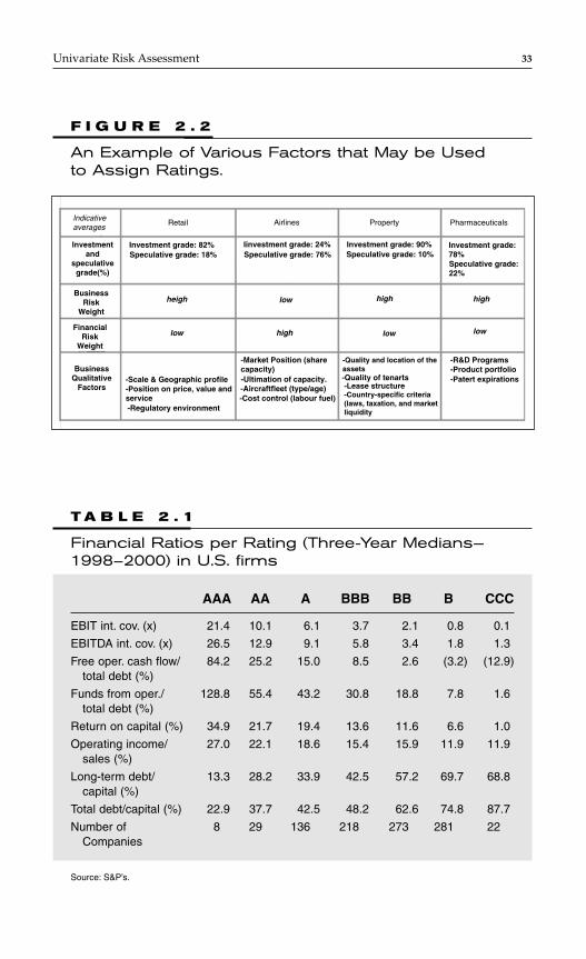
For industrial companies, the analysis is commonly split betweenbusiness reviews (firm competitiveness, quality of the management andof its policies, business fundamentals, regulatory actions, markets, opera-tions, cost control, etc.) and quantitative analyses (financial ratios, etc.).The impact of these factors depends highly on the industry.
Figure 2.2* is an illustration of how various factors may impact dif-ferently on various industries. It also reports various business factors thatimpact the ratings in different sectors.
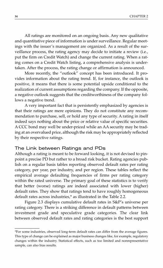
Following meetings with the management of the firm asking for arating, the rating agency reviews qualitative as well as quantitative fac-tors and compares the company’s performance to its peers (see the ratiomedians per rating in Table 2.1). Following this review, a rating commit-tee meeting is convened. The committee discusses the lead analyst’s rec-ommendation before voting on it.
The issuer is subsequently notified of the rating and the major con-siderations supporting it. A rating can be appealed prior to its publicationif meaningful new or additional information is to be presented by theissuer. But there is no guarantee that a revision will be granted. When arating is assigned, it is disseminated to the public through the newsmedia.
32 CHAPTER 2
A A
B B
Moody’sDescription
Investment grade
Speculative grade
S&P
Aaa
Aa
Baa
AAA
AA
BBB
Maximum safety
Worst credit quality
Ba BB
Caa CCC
F I G U R E 2 . 1
Moody’s and S&P’s Rating Scales.
*This figure is for illustrative purposes and may not reflect the actual weights and factorsused by one agency or another.
Univariate Risk Assessment 33
F I G U R E 2 . 2
An Example of Various Factors that May be Used to Assign Ratings.
Indicativeaverages
Retail Airlines Property Pharmaceuticals
Investmentand
speculativegrade(%)
BusinessRisk
Weight
FinancialRisk
Weight
BusinessQualitative
Factors
Investment grade: 82%Speculative grade: 18%
heigh
low
-Scale & Geographic profile-Position on price, value andservice-Regulatory environment
Iinvestment grade: 24%Speculative grade: 76%
low
high
-Market Position (sharecapacity)-Ultimation of capacity.-Aircraftfleet (type/age)-Cost control (labour fuel)
-Quality and location of theassets-Quality of tenarts-Lease structure-Country-specific criteria(laws, taxation, and marketliquidity
low
high
Investment grade: 90%Speculative grade: 10%
Investment grade:78%Speculative grade:22%
high
low
-R&D Programs-Product portfolio-Patert expirations
T A B L E 2 . 1
Financial Ratios per Rating (Three-Year Medians—1998–2000) in U.S. firms
AAA AA A BBB BB B CCC
EBIT int. cov. (x) 21.4 10.1 6.1 3.7 2.1 0.8 0.1
EBITDA int. cov. (x) 26.5 12.9 9.1 5.8 3.4 1.8 1.3
Free oper. cash flow/ 84.2 25.2 15.0 8.5 2.6 (3.2) (12.9)total debt (%)
Funds from oper./ 128.8 55.4 43.2 30.8 18.8 7.8 1.6total debt (%)
Return on capital (%) 34.9 21.7 19.4 13.6 11.6 6.6 1.0
Operating income/ 27.0 22.1 18.6 15.4 15.9 11.9 11.9sales (%)
Long-term debt/ 13.3 28.2 33.9 42.5 57.2 69.7 68.8capital (%)
Total debt/capital (%) 22.9 37.7 42.5 48.2 62.6 74.8 87.7
Number of 8 29 136 218 273 281 22Companies
Source: S&P’s.
All ratings are monitored on an ongoing basis. Any new qualitativeand quantitative piece of information is under surveillance. Regular meet-ings with the issuer’s management are organized. As a result of the sur-veillance process, the rating agency may decide to initiate a review (i.e.,put the firm on Credit Watch) and change the current rating. When a rat-ing comes on a Credit Watch listing, a comprehensive analysis is under-taken. After the process, the rating change or affirmation is announced.
More recently, the “outlook” concept has been introduced. It pro-vides information about the rating trend. If, for instance, the outlook ispositive, it means that there is some potential upside conditional to therealization of current assumptions regarding the company. If the opposite,a negative outlook suggests that the creditworthiness of the company fol-lows a negative trend.
A very important fact that is persistently emphasized by agencies isthat their ratings are mere opinions. They do not constitute any recom-mendation to purchase, sell, or hold any type of security. A rating in itselfindeed says nothing about the price or relative value of specific securities.A CCC bond may well be under-priced while an AA security may be trad-ing at an overvalued price, although the risk may be appropriately reflectedby their respective ratings.
The Link between Ratings and PDsAlthough a rating is meant to be forward looking, it is not devised to pin-point a precise PD but rather to a broad risk bucket. Rating agencies pub-lish on a regular basis tables reporting observed default rates per ratingcategory, per year, per industry, and per region. These tables reflect theempirical average defaulting frequencies of firms per rating categorywithin the rated universe. The primary goal of these statistics is to verifythat better (worse) ratings are indeed associated with lower (higher)default rates. They show that ratings tend to have roughly homogeneousdefault rates across industries,* as illustrated in the Table 2.2.
Figure 2.3 displays cumulative default rates in S&P’s universe perrating category. There is a striking difference in default patterns betweeninvestment grade and speculative grade categories. The clear linkbetween observed default rates and rating categories is the best support
34 CHAPTER 2
*For some industries, observed long-term default rates can differ from the average figures.This type of change can be explained as major business changes like, for example, regulatorychanges within the industry. Statistical effects, such as too limited and nonrepresentativesample, can also bias results.
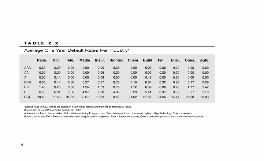
T A B L E 2 . 2
Average One Year Default Rates Per Industry*
Trans. Util. Tele. Media Insur. Hightec Chem Build Fin. Ener. Cons. Auto.
AAA 0.00 0.00 0.00 0.00 0.00 0.00 0.00 0.00 0.00 0.00 0.00 0.00
AA 0.00 0.00 0.00 0.00 0.06 0.00 0.00 0.00 0.00 0.00 0.00 0.00
A 0.00 0.11 0.00 0.00 0.09 0.00 0.00 0.42 0.00 0.20 0.00 0.00
BBB 0.00 0.14 0.00 0.27 0.67 0.73 0.19 0.64 0.32 0.22 0.17 0.29
BB 1.46 0.25 0.00 1.24 1.59 0.75 1.12 0.89 0.86 0.98 1.77 1.47
B 6.50 6.31 5.86 4.97 2.38 4.35 5.29 5.41 8.97 9.57 6.77 5.19
CCC 19.40 71.43 35.85 29.27 10.53 9.52 21.62 21.88 24.66 14.44 26.00 33.33
*Default rates for CCC bonds are based on a very small sample and may not be statistically robust.Source: S&P’s CreditPro, over the period 1981–2001.Abbreviations: Trans. = transportation; Util. = utilities excluding Energy comps.; Tele. = telecoms; Insur. = insurance; Hightec = High Technology; Chem = chemistry;Build = construction; Fin. = Financial companies excluding insurance companies; Ener. = Energy companies; Cons. = consumer products; Auto. = automotive companies..
35
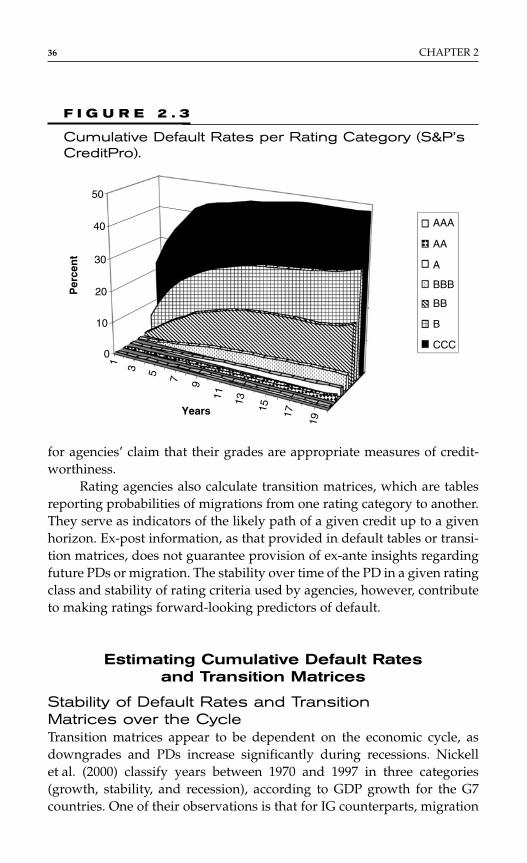
for agencies’ claim that their grades are appropriate measures of credit-worthiness.
Rating agencies also calculate transition matrices, which are tablesreporting probabilities of migrations from one rating category to another.They serve as indicators of the likely path of a given credit up to a givenhorizon. Ex-post information, as that provided in default tables or transi-tion matrices, does not guarantee provision of ex-ante insights regardingfuture PDs or migration. The stability over time of the PD in a given ratingclass and stability of rating criteria used by agencies, however, contributeto making ratings forward-looking predictors of default.
Estimating Cumulative Default Rates and Transition Matrices
Stability of Default Rates and Transition Matrices over the CycleTransition matrices appear to be dependent on the economic cycle, asdowngrades and PDs increase significantly during recessions. Nickellet al. (2000) classify years between 1970 and 1997 in three categories(growth, stability, and recession), according to GDP growth for the G7countries. One of their observations is that for IG counterparts, migration
36 CHAPTER 2
F I G U R E 2 . 3
Cumulative Default Rates per Rating Category (S&P’sCreditPro).
50
40
30
20
10
0
1
3 5 7 9
11 13
15 17
19
Years
Per
cen
t
AAA
AA
A
BBB
BB
B
CCC
volatility is much lower during growth periods than during recessions.Their conclusion is that transition matrices unconditional on the economiccycle cannot be considered as Markovian.*
In another study based on S&P’s data, Bangia et al. (2002) observe thatthe more the time horizon of an independent transition matrix increases, theless monotonic† the matrix becomes. Regarding its Markovian property, theauthors tend to be less affirmative than Nickell et al. (2000), that is, theirtests show that the Markovian hypothesis is not strongly rejected. Theauthors however acknowledge that one can observe path dependency intransition probabilities. For example, a past history of downgrades has animpact on future migrations. Such path dependency is significant as futurePDs can increase up to five times for recently downgraded companies.
The authors then focus on the impact of economic cycles on transi-tion matrices. They select two types of periods (expansion, recession)according to NBER indicators. The main difference between the two matri-ces corresponds mainly to a higher frequency of downgrades duringrecession periods. Splitting transition matrices in two periods is helpful,i.e., out of diagonal terms are much more stable. Their conclusion is thatchoosing two transition matrices conditional to the economic cycle givesmuch better results, in terms of Markovian stability, than considering onlyone matrix unconditional on the economic cycle.
In order to further investigate the impact of cycles on transitionmatrices and credit VaR, Bangia et al. (2002) use a version of CreditMetricson a portfolio of 148 bonds. They show that during recession periods, thenecessary economic capital increases substantially compared to growthperiods (by 30 percent for a 99 percent confidence level of credit VaR or 25percent for a 99.9 percent confidence level). Note that the authors ignorethe increase in correlation during recessions.
Estimating Default and Rating Transition Probabilities via Cohort AnalysisA common approach for rated companies is to derive historic averagedefault or rating transition probabilities by observing the performance ofgroups of companies—frequently called cohorts—with identical credit
Univariate Risk Assessment 37
*A Markov chain is defined by the fact that information known at time t − 1, used in thechain, is sufficient to determine the probabilities at time t. In other words, it is not necessarythe complete path till t − 1 in order to obtain the probabilities at time t.†Monotonicity rule: probabilities are decreasing when the distance to the diagonal of thematrix increases. This property is characteristic from the trajectory concept: migrations occurthrough regular downgrade or upgrade rather than through a big shift.
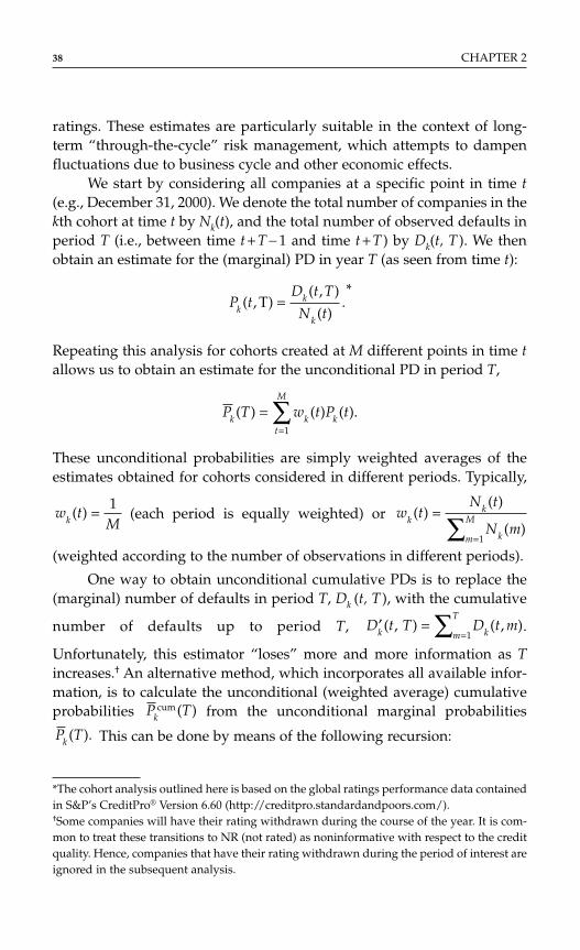
ratings. These estimates are particularly suitable in the context of long-term “through-the-cycle” risk management, which attempts to dampenfluctuations due to business cycle and other economic effects.
We start by considering all companies at a specific point in time t(e.g., December 31, 2000). We denote the total number of companies in thekth cohort at time t by Nk(t), and the total number of observed defaults inperiod T (i.e., between time t + T − 1 and time t + T ) by Dk(t, T). We thenobtain an estimate for the (marginal) PD in year T (as seen from time t):
*
Repeating this analysis for cohorts created at M different points in time tallows us to obtain an estimate for the unconditional PD in period T,
These unconditional probabilities are simply weighted averages of theestimates obtained for cohorts considered in different periods. Typically,
(each period is equally weighted) or
(weighted according to the number of observations in different periods).
One way to obtain unconditional cumulative PDs is to replace the(marginal) number of defaults in period T, Dk (t, T ), with the cumulative
number of defaults up to period T, .
Unfortunately, this estimator “loses” more and more information as Tincreases.† An alternative method, which incorporates all available infor-mation, is to calculate the unconditional (weighted average) cumulativeprobabilities from the unconditional marginal probabilities
This can be done by means of the following recursion:P Tk ( ).
P Tkcum ( )
′ ==∑D t T D t mk km
T( , ) ( , )
1
w tN t
N mk
k
km
M( )( )
( )=
=∑ 1
w tMk ( ) = 1
P T w t P tk k kt
M
( ) ( ) ( ).==∑
1
P tD t T
N tkk
k
( , )( , )
( ).T =
38 CHAPTER 2
*The cohort analysis outlined here is based on the global ratings performance data containedin S&P’s CreditPro® Version 6.60 (http://creditpro.standardandpoors.com/).†Some companies will have their rating withdrawn during the course of the year. It is com-mon to treat these transitions to NR (not rated) as noninformative with respect to the creditquality. Hence, companies that have their rating withdrawn during the period of interest areignored in the subsequent analysis.
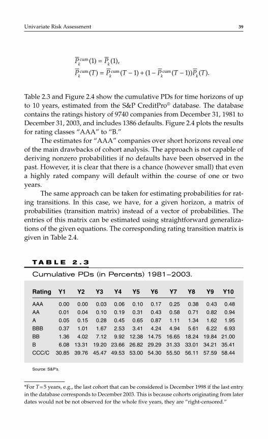
Table 2.3 and Figure 2.4 show the cumulative PDs for time horizons of upto 10 years, estimated from the S&P CreditPro® database. The databasecontains the ratings history of 9740 companies from December 31, 1981 toDecember 31, 2003, and includes 1386 defaults. Figure 2.4 plots the resultsfor rating classes “AAA” to “B.”
The estimates for “AAA” companies over short horizons reveal oneof the main drawbacks of cohort analysis. The approach is not capable ofderiving nonzero probabilities if no defaults have been observed in thepast. However, it is clear that there is a chance (however small) that evena highly rated company will default within the course of one or twoyears.
The same approach can be taken for estimating probabilities for rat-ing transitions. In this case, we have, for a given horizon, a matrix ofprobabilities (transition matrix) instead of a vector of probabilities. Theentries of this matrix can be estimated using straightforward generaliza-tions of the given equations. The corresponding rating transition matrix isgiven in Table 2.4.
P P
P T P T P T P Tk k
k k k k
cum
cum cum cum
( ) ( ),
( ) ( ) ( ( )) ( ).
1 1
1 1 1
=
= − + − −
Univariate Risk Assessment 39
*For T = 5 years, e.g., the last cohort that can be considered is December 1998 if the last entryin the database corresponds to December 2003. This is because cohorts originating from laterdates would not be not observed for the whole five years, they are “right-censored.”
T A B L E 2 . 3
Cumulative PDs (in Percents) 1981–2003.
Rating Y1 Y2 Y3 Y4 Y5 Y6 Y7 Y8 Y9 Y10
AAA 0.00 0.00 0.03 0.06 0.10 0.17 0.25 0.38 0.43 0.48
AA 0.01 0.04 0.10 0.19 0.31 0.43 0.58 0.71 0.82 0.94
A 0.05 0.15 0.28 0.45 0.65 0.87 1.11 1.34 1.62 1.95
BBB 0.37 1.01 1.67 2.53 3.41 4.24 4.94 5.61 6.22 6.93
BB 1.36 4.02 7.12 9.92 12.38 14.75 16.65 18.24 19.84 21.00
B 6.08 13.31 19.20 23.66 26.82 29.29 31.33 33.01 34.21 35.41
CCC/C 30.85 39.76 45.47 49.53 53.00 54.30 55.50 56.11 57.59 58.44
Source: S&P’s.
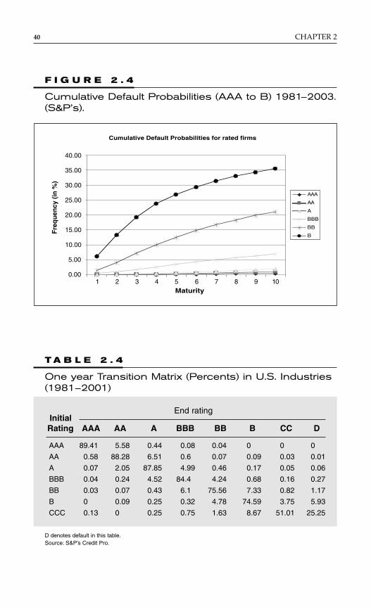
40 CHAPTER 2
F I G U R E 2 . 4
Cumulative Default Probabilities (AAA to B) 1981–2003.(S&P’s).
Cumulative Default Probabilities for rated firms
0.00
5.00
10.00
15.00
20.00
25.00
30.00
35.00
40.00
1 2 3 4 5 6 7 8 9 10Maturity
Fre
qu
ency
(in
%)
AAA
AA
A
BBB
BB
B
T A B L E 2 . 4
One year Transition Matrix (Percents) in U.S. Industries(1981–2001)
InitialEnd rating
Rating AAA AA A BBB BB B CC D
AAA 89.41 5.58 0.44 0.08 0.04 0 0 0
AA 0.58 88.28 6.51 0.6 0.07 0.09 0.03 0.01
A 0.07 2.05 87.85 4.99 0.46 0.17 0.05 0.06
BBB 0.04 0.24 4.52 84.4 4.24 0.68 0.16 0.27
BB 0.03 0.07 0.43 6.1 75.56 7.33 0.82 1.17
B 0 0.09 0.25 0.32 4.78 74.59 3.75 5.93
CCC 0.13 0 0.25 0.75 1.63 8.67 51.01 25.25
D denotes default in this table.Source: S&P’s Credit Pro.
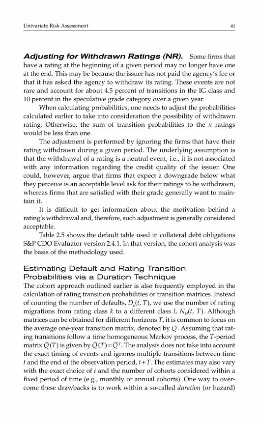
Adjusting for Withdrawn Ratings (NR). Some firms thathave a rating at the beginning of a given period may no longer have oneat the end. This may be because the issuer has not paid the agency’s fee orthat it has asked the agency to withdraw its rating. These events are notrare and account for about 4.5 percent of transitions in the IG class and10 percent in the speculative grade category over a given year.
When calculating probabilities, one needs to adjust the probabilitiescalculated earlier to take into consideration the possibility of withdrawnrating. Otherwise, the sum of transition probabilities to the n ratingswould be less than one.
The adjustment is performed by ignoring the firms that have theirrating withdrawn during a given period. The underlying assumption isthat the withdrawal of a rating is a neutral event, i.e., it is not associatedwith any information regarding the credit quality of the issuer. Onecould, however, argue that firms that expect a downgrade below whatthey perceive is an acceptable level ask for their ratings to be withdrawn,whereas firms that are satisfied with their grade generally want to main-tain it.
It is difficult to get information about the motivation behind arating’s withdrawal and, therefore, such adjustment is generally consideredacceptable.
Table 2.5 shows the default table used in collateral debt obligationsS&P CDO Evaluator version 2.4.1. In that version, the cohort analysis wasthe basis of the methodology used.
Estimating Default and Rating Transition Probabilities via a Duration TechniqueThe cohort approach outlined earlier is also frequently employed in thecalculation of rating transition probabilities or transition matrices. Insteadof counting the number of defaults, Dk(t, T ), we use the number of ratingmigrations from rating class k to a different class l, Nkl(t, T ). Althoughmatrices can be obtained for different horizons T, it is common to focus onthe average one-year transition matrix, denoted by Q– . Assuming that rat-ing transitions follow a time homogeneous Markov process, the T-periodmatrix Q– (T) is given by Q– (T) = Q– T. The analysis does not take into accountthe exact timing of events and ignores multiple transitions between timet and the end of the observation period, t + T. The estimates may also varywith the exact choice of t and the number of cohorts considered within afixed period of time (e.g., monthly or annual cohorts). One way to over-come these drawbacks is to work within a so-called duration (or hazard)
Univariate Risk Assessment 41
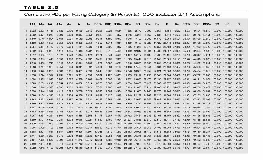
T A B L E 2 . 5
Cumulative PDs per Rating Category (in Percents)—CDO Evaluator 2.41 Assumptions
AAA AA+ AA AA− A+ A A− BBB+ BBB BBB− BB+ BB BB− B+ B B− CCC+ CCC CCC− CC SD D
1 0.023 0.023 0.111 0.136 0.136 0.136 0.145 0.225 0.225 0.544 1.666 2.772 2.792 3.667 8.594 9.563 14.693 19.824 46.549 100.000 100.000 100.000
2 0.062 0.071 0.242 0.290 0.303 0.317 0.358 0.532 0.638 1.357 3.316 5.265 5.667 7.535 14.514 16.626 23.401 30.176 53.451 100.000 100.000 100.000
3 0.119 0.143 0.394 0.464 0.501 0.542 0.632 0.911 1.182 2.317 4.916 7.498 8.380 11.078 18.594 21.564 28.696 35.829 57.219 100.000 100.000 100.000
4 0.193 0.239 0.565 0.659 0.728 0.808 0.959 1.352 1.814 3.344 6.439 9.489 10.826 14.122 21.446 24.962 32.024 39.086 59.390 100.000 100.000 100.000
5 0.284 0.357 0.757 0.875 0.984 1.111 1.330 1.841 2.500 4.387 7.866 11.255 12.973 16.655 23.488 27.316 34.200 41.083 60.722 100.000 100.000 100.000
6 0.392 0.497 0.968 1.113 1.265 1.448 1.737 2.368 3.215 5.415 9.189 12.817 14.834 18.735 24.997 28.985 35.690 42.394 61.596 100.000 100.000 100.000
7 0.517 0.656 1.198 1.372 1.570 1.814 2.173 2.921 3.941 6.410 10.407 14.197 16.436 20.438 26.151 30.208 36.762 43.317 62.211 100.000 100.000 100.000
8 0.658 0.835 1.445 1.650 1.896 2.204 2.632 3.492 4.667 7.360 11.525 15.419 17.816 21.840 27.065 31.141 37.576 44.010 62.673 100.000 100.000 100.000
9 0.815 1.033 1.710 1.946 2.242 2.614 3.108 4.074 5.383 8.261 12.548 16.503 19.008 23.004 27.816 31.883 38.222 44.562 63.041 100.000 100.000 100.000
10 0.988 1.247 1.990 2.259 2.604 3.041 3.597 4.661 6.084 9.112 13.486 17.470 20.044 23.984 28.453 32.497 38.760 45.023 63.349 100.000 100.000 100.000
11 1.176 1.478 2.285 2.588 2.981 3.481 4.096 5.248 6.766 9.914 14.346 18.338 20.952 24.821 29.008 33.023 39.223 45.424 63.616 100.000 100.000 100.000
12 1.378 1.724 2.594 2.931 3.371 3.931 4.599 5.831 7.428 10.671 15.139 19.122 21.755 25.548 29.504 33.488 39.635 45.782 63.855 100.000 100.000 100.000
13 1.594 1.985 2.916 3.287 3.772 4.389 5.106 6.409 8.068 11.384 15.872 19.835 22.473 26.190 29.957 33.910 40.011 46.111 64.074 100.000 100.000 100.000
14 1.823 2.259 3.249 3.654 4.183 4.852 5.614 6.979 8.687 12.058 16.554 20.489 23.122 26.765 30.377 34.300 40.359 46.418 64.278 100.000 100.000 100.000
15 2.066 2.546 3.593 4.032 4.601 5.319 6.120 7.539 9.286 12.697 17.189 21.093 23.714 27.288 30.771 34.667 40.687 46.708 64.472 100.000 100.000 100.000
16 2.320 2.844 3.947 4.418 5.025 5.789 6.624 8.090 9.864 13.304 17.786 21.655 24.260 27.770 31.146 35.015 41.000 46.986 64.657 100.000 100.000 100.000
17 2.586 3.154 4.310 4.812 5.454 6.259 7.125 8.629 10.425 13.882 18.349 22.182 24.768 28.220 31.506 35.349 41.301 47.253 64.835 100.000 100.000 100.000
18 2.863 3.473 4.681 5.213 5.887 6.728 7.621 9.159 10.967 14.435 18.882 22.680 25.245 28.643 31.854 35.673 41.593 47.513 65.009 100.000 100.000 100.000
19 3.150 3.802 5.058 5.619 6.323 7.197 8.112 9.677 11.493 14.965 19.390 23.152 25.696 29.045 32.191 35.987 41.877 47.766 65.178 100.000 100.000 100.000
20 3.447 4.140 5.442 6.030 6.761 7.663 8.598 10.185 12.005 15.474 19.875 23.603 26.126 29.430 32.520 36.294 42.154 48.014 65.343 100.000 100.000 100.000
21 3.753 4.485 5.831 6.444 7.200 8.127 9.078 10.683 12.502 15.966 20.342 24.036 26.538 29.801 32.843 36.595 42.427 48.258 65.505 100.000 100.000 100.000
22 4.067 4.838 6.224 6.861 7.639 8.588 9.552 11.171 12.987 16.442 20.792 24.454 26.935 30.161 33.159 36.892 42.695 48.498 65.665 100.000 100.000 100.000
23 4.389 5.197 6.622 7.281 8.078 9.046 10.021 11.650 13.460 16.904 21.227 24.858 27.319 30.510 33.471 37.183 42.959 48.735 65.823 100.000 100.000 100.000
24 4.719 5.562 7.023 7.702 8.517 9.500 10.483 12.120 13.923 17.353 21.650 25.251 27.692 30.852 33.779 37.472 43.220 48.969 65.979 100.000 100.000 100.000
25 5.056 5.932 7.426 8.124 8.954 9.950 10.940 12.582 14.376 17.791 22.062 25.634 28.056 31.186 34.083 37.756 43.479 49.201 66.134 100.000 100.000 100.000
26 5.398 6.307 7.831 8.547 9.389 10.396 11.391 13.036 14.819 18.219 22.463 26.008 28.412 31.515 34.383 38.039 43.734 49.430 66.287 100.000 100.000 100.000
27 5.747 6.686 8.239 8.970 9.823 10.838 11.836 13.482 15.255 18.638 22.856 26.375 28.761 31.838 34.681 38.318 43.988 49.658 66.438 100.000 100.000 100.000
28 6.101 7.068 8.647 9.392 10.254 11.276 12.276 13.921 15.683 19.048 23.242 26.735 29.104 32.157 34.976 38.595 44.239 49.883 66.589 100.000 100.000 100.000
29 6.459 7.454 9.056 9.813 10.684 11.710 12.711 14.354 16.104 19.452 23.620 27.089 29.442 32.472 35.268 38.870 44.489 50.107 66.738 100.000 100.000 100.000
30 6.822 7.842 9.465 10.234 11.110 12.140 13.140 14.780 16.518 19.848 23.992 27.437 29.775 32.783 35.559 39.143 44.737 50.330 66.887 100.000 100.000 100.000
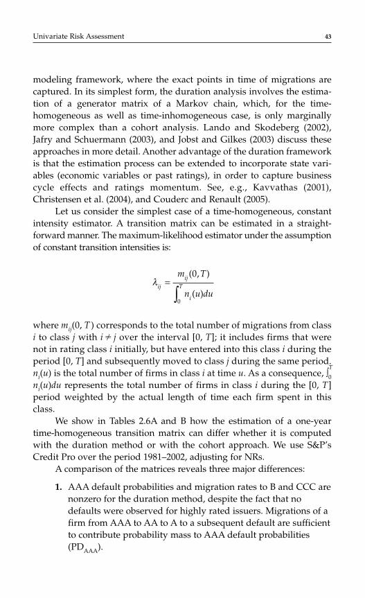
modeling framework, where the exact points in time of migrations arecaptured. In its simplest form, the duration analysis involves the estima-tion of a generator matrix of a Markov chain, which, for the time-homogeneous as well as time-inhomogeneous case, is only marginallymore complex than a cohort analysis. Lando and Skodeberg (2002),Jafry and Schuermann (2003), and Jobst and Gilkes (2003) discuss theseapproaches in more detail. Another advantage of the duration frameworkis that the estimation process can be extended to incorporate state vari-ables (economic variables or past ratings), in order to capture businesscycle effects and ratings momentum. See, e.g., Kavvathas (2001),Christensen et al. (2004), and Couderc and Renault (2005).
Let us consider the simplest case of a time-homogeneous, constantintensity estimator. A transition matrix can be estimated in a straight-forward manner. The maximum-likelihood estimator under the assumptionof constant transition intensities is:
where mij(0, T ) corresponds to the total number of migrations from classi to class j with i j over the interval [0, T]; it includes firms that werenot in rating class i initially, but have entered into this class i during theperiod [0, T] and subsequently moved to class j during the same period.ni(u) is the total number of firms in class i at time u. As a consequence, ∫
T
0ni(u)du represents the total number of firms in class i during the [0, T]period weighted by the actual length of time each firm spent in thisclass.
We show in Tables 2.6A and B how the estimation of a one-yeartime-homogeneous transition matrix can differ whether it is computedwith the duration method or with the cohort approach. We use S&P’sCredit Pro over the period 1981–2002, adjusting for NRs.
A comparison of the matrices reveals three major differences:
1. AAA default probabilities and migration rates to B and CCC arenonzero for the duration method, despite the fact that nodefaults were observed for highly rated issuers. Migrations of afirm from AAA to AA to A to a subsequent default are sufficientto contribute probability mass to AAA default probabilities(PDAAA).
λijij
i
T
m T
n u du=
∫( , )
( )
0
0
Univariate Risk Assessment 43
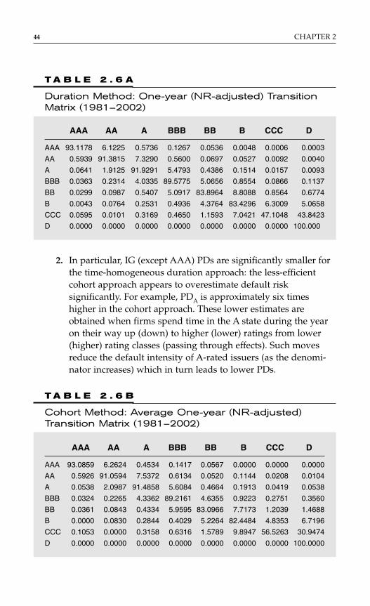
2. In particular, IG (except AAA) PDs are significantly smaller forthe time-homogeneous duration approach: the less-efficientcohort approach appears to overestimate default risksignificantly. For example, PDA is approximately six timeshigher in the cohort approach. These lower estimates areobtained when firms spend time in the A state during the yearon their way up (down) to higher (lower) ratings from lower(higher) rating classes (passing through effects). Such movesreduce the default intensity of A-rated issuers (as the denomi-nator increases) which in turn leads to lower PDs.
44 CHAPTER 2
T A B L E 2 . 6 A
Duration Method: One-year (NR-adjusted) TransitionMatrix (1981–2002)
AAA AA A BBB BB B CCC D
AAA 93.1178 6.1225 0.5736 0.1267 0.0536 0.0048 0.0006 0.0003
AA 0.5939 91.3815 7.3290 0.5600 0.0697 0.0527 0.0092 0.0040
A 0.0641 1.9125 91.9291 5.4793 0.4386 0.1514 0.0157 0.0093
BBB 0.0363 0.2314 4.0335 89.5775 5.0656 0.8554 0.0866 0.1137
BB 0.0299 0.0987 0.5407 5.0917 83.8964 8.8088 0.8564 0.6774
B 0.0043 0.0764 0.2531 0.4936 4.3764 83.4296 6.3009 5.0658
CCC 0.0595 0.0101 0.3169 0.4650 1.1593 7.0421 47.1048 43.8423
D 0.0000 0.0000 0.0000 0.0000 0.0000 0.0000 0.0000 100.000
T A B L E 2 . 6 B
Cohort Method: Average One-year (NR-adjusted)Transition Matrix (1981–2002)
AAA AA A BBB BB B CCC D
AAA 93.0859 6.2624 0.4534 0.1417 0.0567 0.0000 0.0000 0.0000
AA 0.5926 91.0594 7.5372 0.6134 0.0520 0.1144 0.0208 0.0104
A 0.0538 2.0987 91.4858 5.6084 0.4664 0.1913 0.0419 0.0538
BBB 0.0324 0.2265 4.3362 89.2161 4.6355 0.9223 0.2751 0.3560
BB 0.0361 0.0843 0.4334 5.9595 83.0966 7.7173 1.2039 1.4688
B 0.0000 0.0830 0.2844 0.4029 5.2264 82.4484 4.8353 6.7196
CCC 0.1053 0.0000 0.3158 0.6316 1.5789 9.8947 56.5263 30.9474
D 0.0000 0.0000 0.0000 0.0000 0.0000 0.0000 0.0000 100.0000
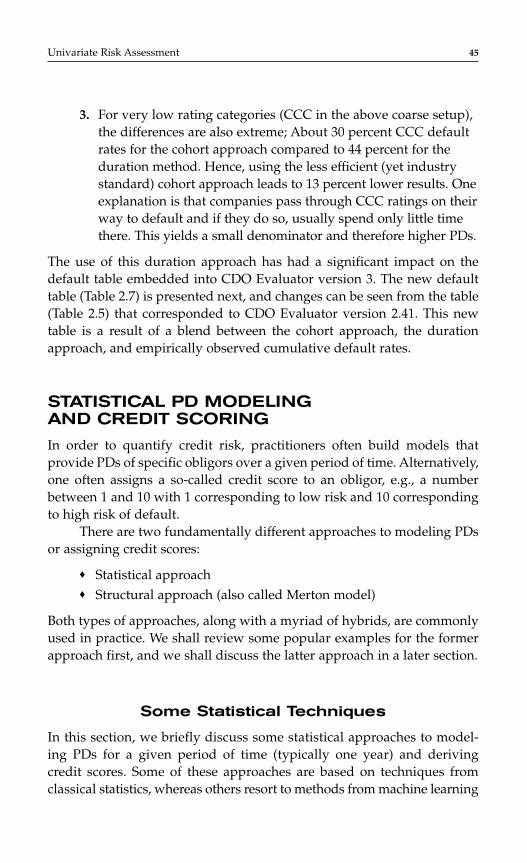
3. For very low rating categories (CCC in the above coarse setup),the differences are also extreme; About 30 percent CCC defaultrates for the cohort approach compared to 44 percent for theduration method. Hence, using the less efficient (yet industrystandard) cohort approach leads to 13 percent lower results. Oneexplanation is that companies pass through CCC ratings on theirway to default and if they do so, usually spend only little timethere. This yields a small denominator and therefore higher PDs.
The use of this duration approach has had a significant impact on thedefault table embedded into CDO Evaluator version 3. The new defaulttable (Table 2.7) is presented next, and changes can be seen from the table(Table 2.5) that corresponded to CDO Evaluator version 2.41. This newtable is a result of a blend between the cohort approach, the durationapproach, and empirically observed cumulative default rates.
STATISTICAL PD MODELING AND CREDIT SCORING
In order to quantify credit risk, practitioners often build models thatprovide PDs of specific obligors over a given period of time. Alternatively,one often assigns a so-called credit score to an obligor, e.g., a numberbetween 1 and 10 with 1 corresponding to low risk and 10 correspondingto high risk of default.
There are two fundamentally different approaches to modeling PDsor assigning credit scores:
♦ Statistical approach♦ Structural approach (also called Merton model)
Both types of approaches, along with a myriad of hybrids, are commonlyused in practice. We shall review some popular examples for the formerapproach first, and we shall discuss the latter approach in a later section.
Some Statistical Techniques
In this section, we briefly discuss some statistical approaches to model-ing PDs for a given period of time (typically one year) and derivingcredit scores. Some of these approaches are based on techniques fromclassical statistics, whereas others resort to methods from machine learning
Univariate Risk Assessment 45
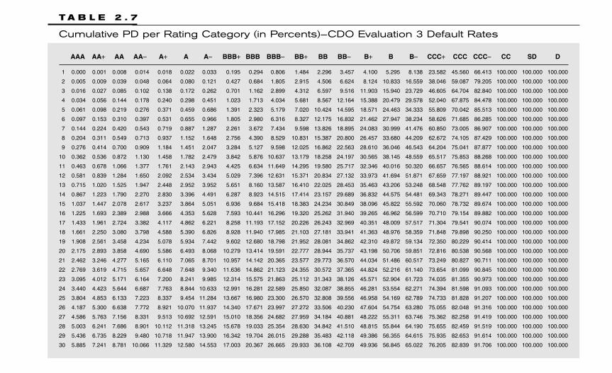
T A B L E 2 . 7
Cumulative PD per Rating Category (in Percents)—CDO Evaluation 3 Default Rates
AAA AA+ AA AA− A+ A A− BBB+ BBB BBB− BB+ BB BB− B+ B B− CCC+ CCC CCC− CC SD D
1 0.000 0.001 0.008 0.014 0.018 0.022 0.033 0.195 0.294 0.806 1.484 2.296 3.457 4.100 5.295 8.138 23.582 45.560 66.413 100.000 100.000 100.000
2 0.005 0.009 0.039 0.048 0.064 0.080 0.121 0.427 0.684 1.805 2.915 4.506 6.624 8.124 10.833 16.559 38.046 59.087 79.205 100.000 100.000 100.000
3 0.016 0.027 0.085 0.102 0.138 0.172 0.262 0.701 1.162 2.899 4.312 6.597 9.516 11.903 15.940 23.729 46.605 64.704 82.840 100.000 100.000 100.000
4 0.034 0.056 0.144 0.178 0.240 0.298 0.451 1.023 1.713 4.034 5.681 8.567 12.164 15.388 20.479 29.578 52.040 67.875 84.478 100.000 100.000 100.000
5 0.061 0.098 0.219 0.276 0.371 0.459 0.686 1.391 2.323 5.179 7.020 10.424 14.595 18.571 24.463 34.333 55.809 70.042 85.513 100.000 100.000 100.000
6 0.097 0.153 0.310 0.397 0.531 0.655 0.966 1.805 2.980 6.316 8.327 12.175 16.832 21.462 27.947 38.234 58.626 71.685 86.285 100.000 100.000 100.000
7 0.144 0.224 0.420 0.543 0.719 0.887 1.287 2.261 3.672 7.434 9.598 13.826 18.895 24.083 30.999 41.476 60.850 73.005 86.907 100.000 100.000 100.000
8 0.204 0.311 0.549 0.713 0.937 1.152 1.648 2.756 4.390 8.529 10.831 15.387 20.800 26.457 33.680 44.209 62.672 74.105 87.429 100.000 100.000 100.000
9 0.276 0.414 0.700 0.909 1.184 1.451 2.047 3.284 5.127 9.598 12.025 16.862 22.563 28.610 36.046 46.543 64.204 75.041 87.877 100.000 100.000 100.000
10 0.362 0.536 0.872 1.130 1.458 1.782 2.479 3.842 5.876 10.637 13.179 18.258 24.197 30.565 38.145 48.559 65.517 75.853 88.268 100.000 100.000 100.000
11 0.463 0.678 1.066 1.377 1.761 2.143 2.943 4.425 6.634 11.649 14.295 19.580 25.717 32.346 40.016 50.320 66.657 76.565 88.614 100.000 100.000 100.000
12 0.581 0.839 1.284 1.650 2.092 2.534 3.434 5.029 7.396 12.631 15.371 20.834 27.132 33.973 41.694 51.871 67.659 77.197 88.921 100.000 100.000 100.000
13 0.715 1.020 1.525 1.947 2.448 2.952 3.952 5.651 8.160 13.587 16.410 22.025 28.453 35.463 43.206 53.248 68.548 77.762 89.197 100.000 100.000 100.000
14 0.867 1.223 1.790 2.270 2.830 3.396 4.491 6.287 8.923 14.515 17.414 23.157 29.689 36.832 44.575 54.481 69.343 78.271 89.447 100.000 100.000 100.000
15 1.037 1.447 2.078 2.617 3.237 3.864 5.051 6.936 9.684 15.418 18.383 24.234 30.849 38.096 45.822 55.592 70.060 78.732 89.674 100.000 100.000 100.000
16 1.225 1.693 2.389 2.988 3.666 4.353 5.628 7.593 10.441 16.296 19.320 25.262 31.940 39.265 46.962 56.599 70.710 79.154 89.882 100.000 100.000 100.000
17 1.433 1.961 2.724 3.382 4.117 4.862 6.221 8.258 11.193 17.152 20.226 26.243 32.969 40.351 48.009 57.517 71.304 79.541 90.074 100.000 100.000 100.000
18 1.661 2.250 3.080 3.798 4.588 5.390 6.826 8.928 11.940 17.985 21.103 27.181 33.941 41.363 48.976 58.359 71.848 79.898 90.250 100.000 100.000 100.000
19 1.908 2.561 3.458 4.234 5.078 5.934 7.442 9.602 12.680 18.798 21.952 28.081 34.862 42.310 49.872 59.134 72.350 80.229 90.414 100.000 100.000 100.000
20 2.175 2.893 3.858 4.690 5.586 6.493 8.068 10.279 13.414 19.591 22.777 28.944 35.737 43.198 50.706 59.851 72.816 80.538 90.568 100.000 100.000 100.000
21 2.462 3.246 4.277 5.165 6.110 7.065 8.701 10.957 14.142 20.365 23.577 29.773 36.570 44.034 51.486 60.517 73.249 80.827 90.711 100.000 100.000 100.000
22 2.769 3.619 4.715 5.657 6.648 7.648 9.340 11.636 14.862 21.123 24.355 30.572 37.365 44.824 52.216 61.140 73.654 81.099 90.845 100.000 100.000 100.000
23 3.095 4.012 5.171 6.164 7.200 8.241 9.985 12.314 15.575 21.863 25.112 31.343 38.126 45.571 52.904 61.723 74.035 81.355 90.973 100.000 100.000 100.000
24 3.440 4.423 5.644 6.687 7.763 8.844 10.633 12.991 16.281 22.589 25.850 32.087 38.855 46.281 53.554 62.271 74.394 81.598 91.093 100.000 100.000 100.000
25 3.804 4.853 6.133 7.223 8.337 9.454 11.284 13.667 16.980 23.300 26.570 32.808 39.556 46.958 54.169 62.789 74.733 81.828 91.207 100.000 100.000 100.000
26 4.187 5.300 6.638 7.772 8.921 10.070 11.937 14.340 17.671 23.997 27.272 33.506 40.230 47.604 54.754 63.280 75.055 82.048 91.316 100.000 100.000 100.000
27 4.586 5.763 7.156 8.331 9.513 10.692 12.591 15.010 18.356 24.682 27.959 34.184 40.881 48.222 55.311 63.746 75.362 82.258 91.419 100.000 100.000 100.000
28 5.003 6.241 7.686 8.901 10.112 11.318 13.245 15.678 19.033 25.354 28.630 34.842 41.510 48.815 55.844 64.190 75.655 82.459 91.519 100.000 100.000 100.000
29 5.436 6.735 8.229 9.480 10.718 11.947 13.900 16.342 19.704 26.015 29.288 35.483 42.118 49.386 56.355 64.615 75.935 82.653 91.614 100.000 100.000 100.000
30 5.885 7.241 8.781 10.066 11.329 12.580 14.553 17.003 20.367 26.665 29.933 36.108 42.709 49.936 56.845 65.022 76.205 82.839 91.706 100.000 100.000 100.000

(also called statistical learning). They share the common idea that the PDof an obligor is learned from the data with no or little input of knowledgeabout the mechanisms that lead firms to default.
In statistical learning, one often makes a distinction between super-vised and unsupervised classification. These two approaches differ withrespect to the data from which we learn. In the first case, so-called labeledtraining data are available, i.e., observations that provide a default indi-cator or a credit score along with the potential risk factors. In other words,a supervised algorithm learns from historical observations of firms forwhich we know the class labels (default indicator or credit score).Unsupervised learning algorithms, on the other hand, rely on so-calledunlabeled data, i.e., observations for which the class labels are unknown.While this type of learning can be used for the assignment of credit scores,it is not commonly used for modeling PDs; we will not discuss unsuper-vised learning in this chapter.
Some approaches that can be used for modeling PDs or derivingcredit scores are*:
1. Logistic regression and probit2. Maximum-likelihood estimation3. Bayesian estimation (e.g., naïve Bayes classifier)4. Minimum-relative-entropy models5. Fisher linear-discriminant analysis6. k-Nearest neighbor classifiers7. Classification trees8. Support vector machines9. Neural networks
10. Genetic algorithms
Some of the methods in this list are closely related to each other, and themethods in the list are not exclusive. For example, logistic regression canbe viewed as a special case of methods 2, 3, or 4, and maximum-likelihoodestimation can be interpreted in the Bayesian framework. However, allof these methods are interesting in their own right and are applied bypractitioners.
The first four of these methods provide conditional probabilities forthe classes (default or nondefault for PD modeling and the score for credit
Univariate Risk Assessment 47
* See, e.g., Mitchell (1997), Hastie et al. (2003), Jebara (2004), or Witten and Frank (2005).
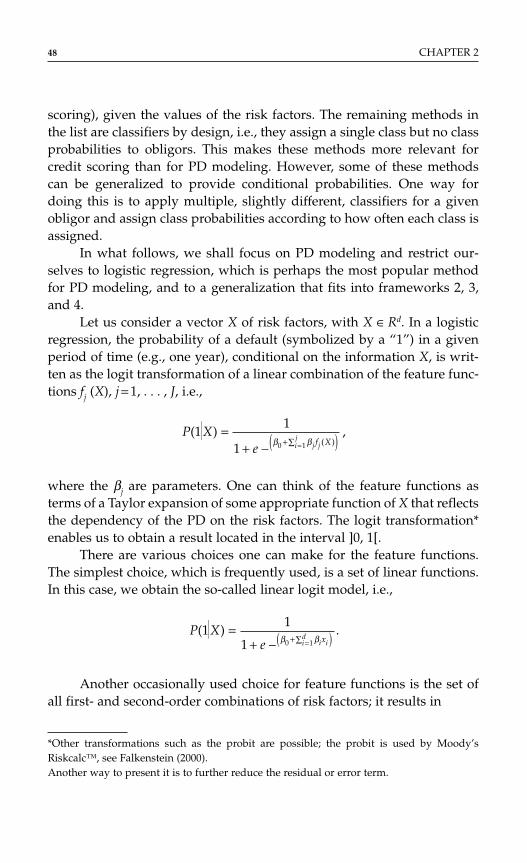
scoring), given the values of the risk factors. The remaining methods inthe list are classifiers by design, i.e., they assign a single class but no classprobabilities to obligors. This makes these methods more relevant forcredit scoring than for PD modeling. However, some of these methodscan be generalized to provide conditional probabilities. One way fordoing this is to apply multiple, slightly different, classifiers for a givenobligor and assign class probabilities according to how often each class isassigned.
In what follows, we shall focus on PD modeling and restrict our-selves to logistic regression, which is perhaps the most popular methodfor PD modeling, and to a generalization that fits into frameworks 2, 3,and 4.
Let us consider a vector X of risk factors, with X ∈ Rd. In a logisticregression, the probability of a default (symbolized by a “1”) in a givenperiod of time (e.g., one year), conditional on the information X, is writ-ten as the logit transformation of a linear combination of the feature func-tions fj (X), j = 1, . . . , J, i.e.,
where the βj are parameters. One can think of the feature functions asterms of a Taylor expansion of some appropriate function of X that reflectsthe dependency of the PD on the risk factors. The logit transformation*enables us to obtain a result located in the interval ]0, 1[.
There are various choices one can make for the feature functions.The simplest choice, which is frequently used, is a set of linear functions.In this case, we obtain the so-called linear logit model, i.e.,
Another occasionally used choice for feature functions is the set ofall first- and second-order combinations of risk factors; it results in
P Xe i ii
d x( ) .1
1
1 0 1 =
+ − +∑( )=β β
P Xe j ji
j f X( ) ,
( )1
1
1 0 1
=+ − +∑( )=β β
48 CHAPTER 2
*Other transformations such as the probit are possible; the probit is used by Moody’sRiskcalc™, see Falkenstein (2000).Another way to present it is to further reduce the residual or error term.
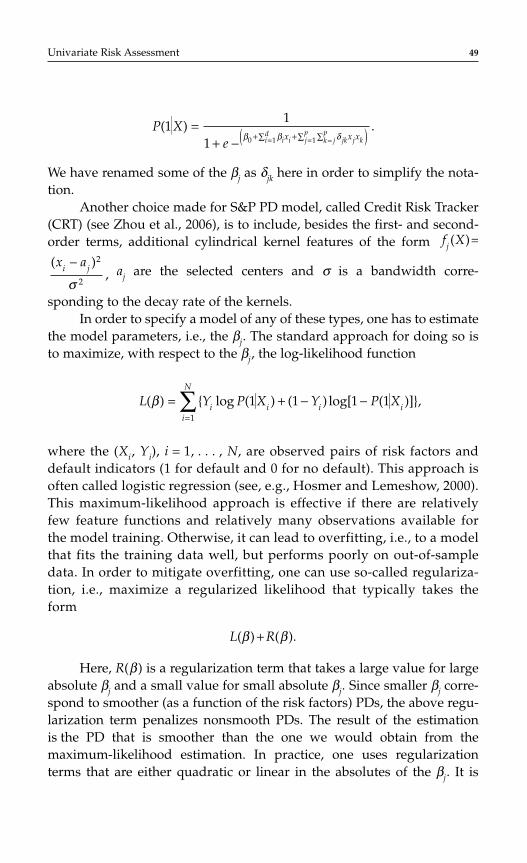
We have renamed some of the βj as δjk here in order to simplify the nota-tion.
Another choice made for S&P PD model, called Credit Risk Tracker(CRT) (see Zhou et al., 2006), is to include, besides the first- and second-order terms, additional cylindrical kernel features of the form
aj are the selected centers and σ is a bandwidth corre-
sponding to the decay rate of the kernels.In order to specify a model of any of these types, one has to estimate
the model parameters, i.e., the βj. The standard approach for doing so isto maximize, with respect to the βj, the log-likelihood function
where the (Xi, Yi), i = 1, . . . , N, are observed pairs of risk factors anddefault indicators (1 for default and 0 for no default). This approach isoften called logistic regression (see, e.g., Hosmer and Lemeshow, 2000).This maximum-likelihood approach is effective if there are relativelyfew feature functions and relatively many observations available forthe model training. Otherwise, it can lead to overfitting, i.e., to a modelthat fits the training data well, but performs poorly on out-of-sampledata. In order to mitigate overfitting, one can use so-called regulariza-tion, i.e., maximize a regularized likelihood that typically takes theform
L(β ) + R(β ).
Here, R(β ) is a regularization term that takes a large value for largeabsolute βj and a small value for small absolute βj. Since smaller βj corre-spond to smoother (as a function of the risk factors) PDs, the above regu-larization term penalizes nonsmooth PDs. The result of the estimationis the PD that is smoother than the one we would obtain from themaximum-likelihood estimation. In practice, one uses regularizationterms that are either quadratic or linear in the absolutes of the βj. It is
L Y P X Y P Xii
N
i i i( ) log ( ) ( ) log[ ( )],β = + − −=∑
1
1 1 1 1
( ),
x ai j− 2
2σ
f Xj ( ) =
P Xe i i jk j kk j
pjp
id x x x
( ) .11
1 0 11
=+ − + + ∑∑∑( )===β β δ
Univariate Risk Assessment 49
interesting to observe that regularization linear in the absolutes of the βjleads to automatic feature selection.*
The above statistical methods are usually characterized as (pos-sibly regularized) maximum-likelihood estimations of exponentialprobabilities. They can also be shown to be equivalent to minimum-relative-entropy methods (see, e.g., Jebara, 2004). Moreover, the result-ing probabilities turn out to be robust from the perspective of anexpected utility maximizing investor (see Friedman and Sandow,2003b).
Performance Analysis for PD Models
There are a variety of measures that are commonly used to quantify theperformance of PD models. Many, such as the Gini curve or cumulativeaccuracy curve (CAP) and receiver operator characteristic (ROC), whichwe shall discuss next, analyze how a PD model ranks individual obligors.Other performance measures, such as the likelihood, which we shall alsodiscuss next, do not explicitly focus on ranks but rather depend on the PDvalues that are assigned to obligors.
The Gini/CAP and ROC Approaches†
A commonly used measure of classification performance is the Gini curveor CAP. This curve assesses the consistency of the predictions of a scoringmodel (in terms of the ranking of firms by order of default probability) tothe ranking of observed defaults. Firms are first sorted in descendingorder of default probability as produced by the scoring model (horizontalaxis of Figure 2.5). The vertical axis displays the fraction of firms that haveactually defaulted.
A perfect model would have assigned the D highest PDs to the Dfirms that have actually defaulted out of a sample of N. The perfectmodel would therefore be a straight line from the point (0, 0) to the point(D/N,1), and then a horizontal line from (D/N, 1) to (1, 1). Conversely,an uninformative model would assign randomly the PDs to high riskand low risk firms. The resulting CAP curve is the diagonal from (0, 0)to (1, 1).
50 CHAPTER 2
*See Hastie et al. (2003) for the general idea of regularization, and Zhou et al. (2006) for anapplication in the PD context.†A more formal presentation of the Gini is in Appendix 1. For a more detailed discussion ofROC, see, e.g., Hosmer and Lemeshow (2000).
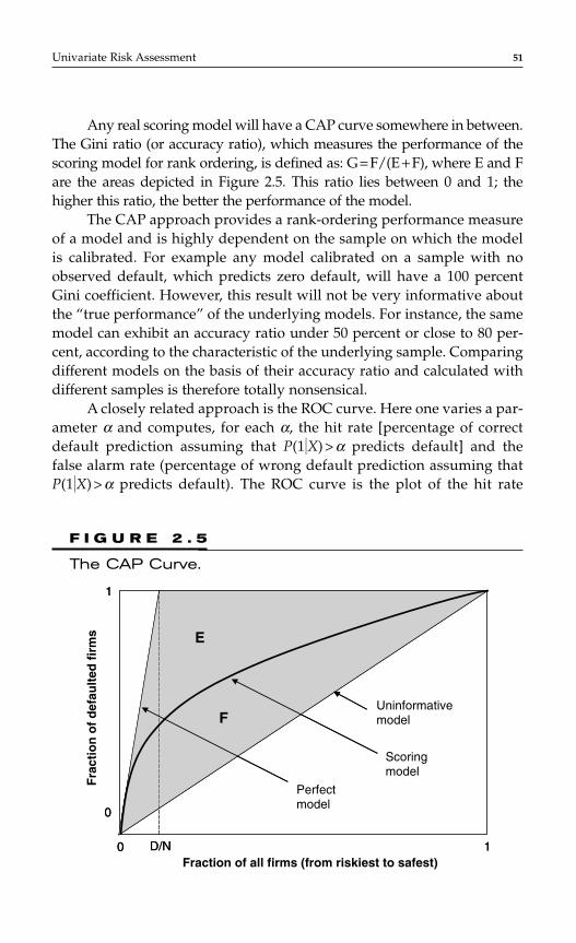
Any real scoring model will have a CAP curve somewhere in between.The Gini ratio (or accuracy ratio), which measures the performance of thescoring model for rank ordering, is defined as: G = F/(E + F), where E and Fare the areas depicted in Figure 2.5. This ratio lies between 0 and 1; thehigher this ratio, the better the performance of the model.
The CAP approach provides a rank-ordering performance measureof a model and is highly dependent on the sample on which the modelis calibrated. For example any model calibrated on a sample with noobserved default, which predicts zero default, will have a 100 percentGini coefficient. However, this result will not be very informative aboutthe “true performance” of the underlying models. For instance, the samemodel can exhibit an accuracy ratio under 50 percent or close to 80 per-cent, according to the characteristic of the underlying sample. Comparingdifferent models on the basis of their accuracy ratio and calculated withdifferent samples is therefore totally nonsensical.
A closely related approach is the ROC curve. Here one varies a par-ameter α and computes, for each α, the hit rate [percentage of correctdefault prediction assuming that P(1X) > α predicts default] and thefalse alarm rate (percentage of wrong default prediction assuming thatP(1X) > α predicts default). The ROC curve is the plot of the hit rate
Univariate Risk Assessment 51
F I G U R E 2 . 5
The CAP Curve.
E
F
D/N0
0
1
1
E
F
D/N0
0
1
1Fraction of all firms (from riskiest to safest)
Fra
ctio
n o
f d
efau
lted
fir
ms
Uninformativemodel
Scoringmodel
Perfectmodel
against the false alarm rate. There exists a simple relationship betweenthe area, ROC, under the ROC curve and the Gini coefficient, Gini,which is
Gini = 2(ROC − 0.5).
In order to give an idea of what ranges to expect for Gini or ROC, wequote Hosmer and Lemeshow (2000):
♦ If ROC = 0.5: this suggests no discrimination (i.e., we might aswell flip a coin).
♦ If 0.7 < ROC < 0.8: this is considered as an acceptable discrimina-tion.
♦ If 0.8 < ROC < 0.9: this is considered as an excellent discrimina-tion.
♦ If ROC > 0.9: this is considered as an outstanding discrimination.♦ In practice, it is extremely unusual to observe areas under the
ROC curve greater than 0.9.
All of the model performance measures focus exclusively on how a modelranks the PDs of a set of obligors. They provide very valuable informationand often work well in practice. However, they neglect the absolute lev-els of the PDs. That is, if, e.g., all PDs for a given set of obligors are mul-tiplied by 10 (or any other monotone transformation is applied), the aboveperformance measures do not change their values. So it seems advisableto supplement these measures, e.g., with the likelihood.
Log-likelihood RatioAmong statisticians, the perhaps most popular performance measure forprobabilistic models is the likelihood. We have discussed it in the previ-ous section as a tool to estimate model parameters. For the purpose ofmeasuring the relative performance of two PD models, one often uses thefollowing log-likelihood ratio (the logarithm of the ratio of the two modellikelihoods):
where the (Xi, Yi), i = 1, . . . , N, are observed pairs of risk factors anddefault indicators (1 for default and 0 for survival) on a test dataset (asopposed to the model training dataset) here.
L P P YP X
P XY
P X
P Xii
ii
i
ii
N
( , ) log( )
( )( ) log
( )
( ),1 2
1
2
1
21
1
11
1 1
1 1= + −
−−
=∑
52 CHAPTER 2
The above log-likelihood ratio has a number of interpretations:
♦ It measures the relative probabilities the two models assign tothe observed data (by construction).
♦ It is the natural performance measure from the standpoint ofBayesian statistics (see, e.g., Jaynes, 2003).
♦ It is the performance measure that generates an optimal (in thesense of the Neyman–Pearson Lemma) decision surface formodel selection (see, e.g., Cover and Thomas, 1991).
♦ It is the difference in expected utility between a particularrational investor who believes the first model and such aninvestor who believes the second model, in a complete marketwith probabilities corresponding to the empirical ones of the testdataset (see Friedman and Sandow, 2003a).
Modeling the Term Structure of PDs
So far, we have discussed PDs for a fixed period of time. For many prac-tical applications in Structured Finance, one needs to quantify the termstructure of PDs, i.e., one needs to know the probability of default for aseries of time intervals in the future. For example, in order to understandthe credit risk associated with a typical CDO tranche, one has to be ableto model the quantity and the timing of cashflows originated by thecollateral, which requires a model for the term structure of PDs.
The most natural framework for modeling PD term structures is theso-called hazard rate framework. Perhaps, the easiest way to introducehazard rates is to start with a set of consecutive discrete time intervals t1,t2, . . . , tN that start at the current time. The discrete-time hazard-rate of agiven obligor is then defined as
h(ti , x, z(ti)) = Prob(default in ti|no default before ti , X = x, Z(ti) = z(ti)),
where X is a set of risk factors at time zero (e.g., balance sheet informationabout an obligor) and Z(ti) is a set of risk factors at time ti (e.g., the stateof the economy). There are various choices one can make for the risk fac-tors X and Z; in particular, one can omit variables of the Z-type or vari-ables of the X-type.
Knowing the hazard rates of a given obligor, one can compute theprobability of survival till the end of ti as
S t x z h t x z ti j jj
i
( , , ) [ ( , , ( ))]= −=
∏ 11
Univariate Risk Assessment 53
and the probability of default at time ti as
S(ti − 1, x, z) h(ti, x, z(ti)).
Unfortunately, the survival probability, S(ti), depends on the Z(tj) forall times upto ti. which are unknown at the observation time. There areessentially two ways to deal with this issue: one can either build a modelthat does not include any Z-type factors, or one can build a time seriesmodel for those factors and average over their joint distribution.* Bothapproaches are viable and are used in practice.
Many models work with a continuous-time hazard rate λ(t, x, z(t)),which can be defined by letting the time-interval length, ∆t, approachzero, i.e., as
The survival probability is then
For both type of models, discrete or continuous, the hazard rateshave to be estimated from data. This is typically done by assuming a para-metric form and estimating the parameters by means of the (possibleregularized) maximum-likelihood method.† One can also make use ofnonparametric techniques, such as the Nelson–Aalen estimator (see, e.g.,Klein and Moeschberger, 2003). However, these nonparametric tech-niques are not appropriate for directly deriving the conditional (on Xand/or Z) hazard rates; one can use them in our context only for model-ing the time dependence after separating out the time-dependence fromthe risk-factor dependence.‡
S t x z x z dt
( , , ) exp ( , , ( ) ) .= −
∫ λ τ τ τ
0
λ( , , ( )) lim( , , ))
.t x z th t x z t
tt
i i=→∆ ∆0
(
54 CHAPTER 2
*Including, modeling, and averaging out Z-type factors (e.g., macroeconomic variables) thatare common to all obligors in a portfolio provides a way to model default dependencies.Even if the individual hazard rates are independent given a realization of the Z-paths, afteraveraging out the Z-type variables, defaults become dependent.†In a somewhat different approach, one can model the hazard rates as an affine stochasticprocesses of the type commonly used for interest rates (see, e.g., Lando, 2004).‡The latter approach is usually taken to estimate the Cox proportional hazard model (seeCox, 1972, or Klein and Moeschberger, 2003).

An example for a model that contains only credit factors of X-type isthe model by Shumway (2001). In this model, a discrete hazard rate of theform
is estimated, where θ1 and θ2 are parameters, and g is a function of time,which reflects the firm’s age.
A model that includes Z-type variables, but no X-type variables, isthe one from Duffie et al. (2005). Here, the Z-type variables describemacroeconomic as well as firm-specific information; e.g., each firm’s dis-tance to default (see the next section) and trailing one-year stock return areZ-type variables in the model. The model is formulated in the continuous-time setting.
Another, slightly different, approach is taken by Friedman et al.(2006), who incorporate firm-specific information in terms of X-type andmacroeconomic information in terms of Z-type variables.
THE MERTON APPROACH
In their original option pricing paper, Black and Scholes (1973) suggestedthat their methodology could be used to price corporate securities.Merton (1974) was the first to use their intuition and to apply it to corpo-rate debt pricing. Many academic extensions have been proposed andsome commercial products use the same basic structure.
The Merton Model
The Merton (1974) model is the first example of an application of contin-gent claims analysis to corporate security pricing. Using simplifyingassumptions about the firm value dynamics and the capital structure ofthe firm, the author is able to give pricing formulas for corporate bondsand equities in the familiar Black and Scholes (1973) paradigm.
In the Merton model, a firm with value V is assumed to be financedthrough equity (with value S) and pure discount bonds with value P andmaturity T. The principal of the debt is K. The value of the firm is the sumof the values of its securities: Vt = St + Pt. In the Merton model, it is assumedthat bondholders cannot force the firm into bankruptcy before the maturity
h t xg t xi
i
( , )exp( ( ) )
=+ + ′
11 1 2θ θ
Univariate Risk Assessment 55
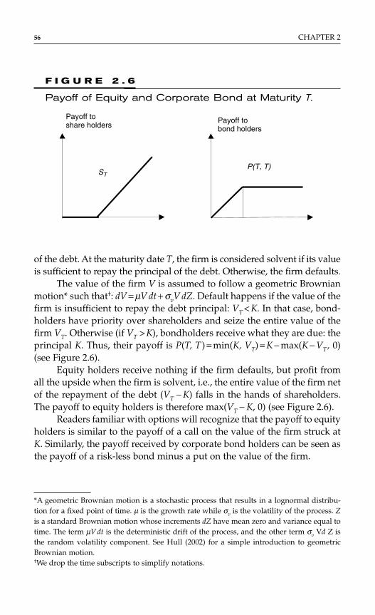
of the debt. At the maturity date T, the firm is considered solvent if its valueis sufficient to repay the principal of the debt. Otherwise, the firm defaults.
The value of the firm V is assumed to follow a geometric Brownianmotion* such that†: dV = µV dt + σvV dZ. Default happens if the value of thefirm is insufficient to repay the debt principal: VT < K. In that case, bond-holders have priority over shareholders and seize the entire value of thefirm VT. Otherwise (if VT > K), bondholders receive what they are due: theprincipal K. Thus, their payoff is P(T, T) = min(K, VT) = K − max(K − VT, 0)(see Figure 2.6).
Equity holders receive nothing if the firm defaults, but profit fromall the upside when the firm is solvent, i.e., the entire value of the firm netof the repayment of the debt (VT − K) falls in the hands of shareholders.The payoff to equity holders is therefore max(VT − K, 0) (see Figure 2.6).
Readers familiar with options will recognize that the payoff to equityholders is similar to the payoff of a call on the value of the firm struck atK. Similarly, the payoff received by corporate bond holders can be seen asthe payoff of a risk-less bond minus a put on the value of the firm.
56 CHAPTER 2
*A geometric Brownian motion is a stochastic process that results in a lognormal distribu-tion for a fixed point of time. µ is the growth rate while σv is the volatility of the process. Zis a standard Brownian motion whose increments dZ have mean zero and variance equal totime. The term µV dt is the deterministic drift of the process, and the other term σv Vd Z isthe random volatility component. See Hull (2002) for a simple introduction to geometricBrownian motion.†We drop the time subscripts to simplify notations.
K
ST
Payoff toshare holders
Payoff tobond holders
P(T, T)
F I G U R E 2 . 6
Payoff of Equity and Corporate Bond at Maturity T.

Merton (1974) makes the same assumptions as Black and Scholes(1973), and the call and the put can be priced using Black–Scholes optionprices. For example, the call (equity) is immediately obtained as:
with and N(·) denoting the cumulative normal distribution and r the risk-less interest rate.
The Merton model provides a lot of insight into the relationshipbetween the fundamental value of a firm and of its securities. The origi-nal model, however, relies on very strong assumptions:
♦ The capital structure is simplistic: equity + one issue of zero-coupon debt.
♦ The value of the firm is assumed to be perfectly observable.♦ The value of the firm follows a lognormal diffusion process.
With this type of process, a sudden surprise (a jump), leading toan unexpected default, cannot be captured. Default has to bereached gradually, “not with a bang but with a whisper,” asDuffie and Lando (2001) put it.
♦ Default can only occur at debt maturity.♦ Risk-less interest rates are constant through time and maturity.♦ The model does not allow for debt renegotiation between equity
and debt holders.♦ There is no liquidity adjustment.
These stringent assumptions may explain why the simple version ofthe Merton model struggles to cope with the empirical spreads observed onthe market. Van Deventer and Imai (2002) test empirically the hypothesis ofinverse comovement of stock prices and of credit spread prices, as predictedby the Merton model. Their sample comprises First Interstate Bancorp two-year credit spread data and associated stock price. The authors find thatonly 42 percent of changes in credit spread and equity prices are consistentwith the directions (increases or decreases) predicted by the Merton model.
Practical difficulties also contribute to hamper the empirical rele-vance of the Merton model:
♦ The value of the firm is difficult to pin down, because themarked-to-market value of debt is often unknown. In addition,all that relates to goodwill or to out-of-the-balance-sheetelements is difficult to measure accurately.
k V K r T t T tt V V= + − − −(ln( / ) ( )( ))/( )12
2σ σ
S V N k T t Ke N kt t Vr T t= + − − − −( ) ( ),( )σ
Univariate Risk Assessment 57

♦ The estimation of assets volatility is difficult due to the lowfrequency of observations.
A vast literature has contributed to extend the original Mertonmodel and lift some of its most unrealistic assumptions. To cite a few, wecan mention:
♦ Early bankruptcy (default barrier) and liquidation costs havebeen introduced by Black and Cox (1976)
♦ Coupon bonds, e.g., Geske (1977)♦ Stochastic interest rates, e.g., Nielsen et al. (1993) and Shimko
et al. (1993)♦ More realistic capital structures (senior and junior debt), e.g.,
Black and Cox (1976)♦ Stochastic processes including jumps in the value of the firm,
e.g., Zhou (1997)♦ Strategic bargaining between shareholders and debtholders, e.g.,
Anderson and Sundaresan (1996)♦ The effect of incomplete accounting information is analyzed in
Duffie and Lando (2001)♦ Uncertain default barrier, e.g., Duffie and Lando (2001)♦ Endogenous default boundaries, e.g., Leland (1994) and Leland
and Toft (1996).
Moody’s KMV Credit Monitor® Modeland Related Approaches
Although the primary focus of Merton (1974) was on debt pricing, thefirm-value based approach has been scarcely applied for that purpose inpractice. Its main success has been in default prediction.
Moody’s KMV Credit Monitor® (see Crosbie and Bohn, 2003) appliesthe structural approach to extract probabilities of default at a given hori-zon from equity prices. Equity prices are available for a large number ofcorporates. If the capital structure of these firms is known, then it is pos-sible to extract market-implied probabilities of default from their equityprice. The probability of default is called expected default frequency(EDF) by Moody’s KMV.
There are two key difficulties in implementing the Merton-typeapproach to firms with realistic capital structure. The original Mertonmodel only applies to firms financed by equity, and one issue of zero-
58 CHAPTER 2
coupon debt is: how should one calculate the strike price of the call(equity) and put (default component of the debt) when there are multi-ple issues of debt? The estimation of the firm value process is also diffi-cult: how to estimate the drift and volatility of the asset value processwhen this value is unobservable? Moody’s KMV uses a “rule of thumb”to calculate the strike price of the default put and a “proprietary method-ology” to calculate the volatility.
Moody’s KMV assumes that the capital structure of an issuer is con-stituted of long-term debt (i.e., with maturity longer than the chosen hori-zon) denoted by LT and short-term debt (maturing before the chosenhorizon) denoted by ST. The strike price default point is then calculatedas a combination of short- and long-term debt: “We have found that thedefault point, the asset value at which the firm will default, generally liessomewhere between total liabilities and current, or short term liabilities”(see Crosbie and Bohn, 2003). The practical rule for choosing the defaultvalue, K, is
K = ST + 0.5 LT.
This rule of thumb is purely empirical and does not rest on any solidtheoretical foundation. Therefore, there is no guarantee that the same ruleshould apply to all countries/jurisdictions and all industries. In addition,no empirical study has been shown to provide information about the con-fidence level associated with this default point.*
In the Merton model, the PD† is
is the so-called distance to default, and we have used the following notation:
N(·) = the cumulative Gaussian distributionVt = the value of the firm at tX = the default threshold
σV = the asset volatility of the firmµ = the expected return on assets
where (ln( ) ln( ) ( / )( ))/( )DD = − + − − −V K T t T tt V Vµ σ σ2 2
PD DDt N= −( ),
Univariate Risk Assessment 59
*Recent articles and papers focus on the stochastic behavior of this default threshold. Seee.g., Hull and White (2000) and Avellaneda and Zhu (2001).†This is the probability under the historical measure. The risk neutral probability is N(−K) = 1 − N(K), as described in the equity pricing formula.

Example: Consider a firm with a market cap of $3 billion, an equityvolatility of 40 percent, ST liabilities of $7 billion and LT of $6 billion. ThusX = 7 + 0.5 × 6 = $10 billion. Assume, further, that we have solved forA0 = $12.511 billion and σ = 9.6 percent. Finally µ = 5 percent, the firm doesnot pay dividends, and the credit horizon is one year. Then (log(Vt/K) + (µ −σV
2 /2))/σV = 3. And the “Merton” probability of default at a one-year hori-zon is N(−3) = 0.13 percent.
In order to use the Merton framework for practical ends, one needsto estimate the current asset value and the asset volatility from marketdata.* Moody’s KMV does this by using the Black–Scholes option pricingframework, viewing equity as an option on the asset value. In this picturewe have the following two equations:
where St is the equity value, σS its volatility, and C is the function thatassigns the Black–Scholes value to a call option. The equity value is usu-ally known (at least for publicly traded firms), and the equity volatilitycan be either estimated from historical data or implied from option pricesif those are available. Knowing St and σS, one can solve the above equa-tions for Vt and σV, which completes the calibration of the Merton model.
An alternative approach to the estimation of Vt and σV is the itera-tive scheme of Vassalou and Xing (2004). According to this scheme, a timeseries of asset values is computed from a times series of equity values bymeans of the Black–Scholes formula for call options, and σV is subse-quently estimated from this time series.
Moody’s KMV approximates the DD as
.
The EDF is then computed as
EDFt = Ξ(−DD)
(see Crosbie and Bohn, 2003). Here, we denote by Ξ(·) the function map-ping the DD to EDFs. Unlike Merton, Moody’s KMV does not rely on the
DD =−V K
Vt
V tσ
σ σ σ σs t V Vt
tt t VC V
V
SS C V t K r= ′ =( , ) , and ( , , , , ),
60 CHAPTER 2
*The PD actually depends, through the distance to default, on the asset value drift as well.However, this dependence is often neglected in practical approaches (see the approximativeformula for the DD given herewith).
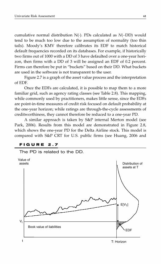
cumulative normal distribution N(·). PDs calculated as N(−DD) wouldtend to be much too low due to the assumption of normality (too thintails). Moody’s KMV therefore calibrates its EDF to match historicaldefault frequencies recorded on its databases. For example, if historicallytwo firms out of 1000 with a DD of 3 have defaulted over a one-year hori-zon, then firms with a DD of 3 will be assigned an EDF of 0.2 percent.Firms can therefore be put in “buckets” based on their DD. What bucketsare used in the software is not transparent to the user.
Figure 2.7 is a graph of the asset value process and the interpretationof EDF.
Once the EDFs are calculated, it is possible to map them to a morefamiliar grid, such as agency rating classes (see Table 2.8). This mapping,while commonly used by practitioners, makes little sense, since the EDFsare point-in-time measures of credit risk focused on default probability atthe one-year horizon; while ratings are through-the-cycle assessments ofcreditworthiness, they cannot therefore be reduced to a one-year PD.
A similar approach is taken by S&P internal Merton model (seePark, 2006). Results from this model are demonstrated in Figure 2.8,which shows the one-year PD for the Delta Airline stock. This model iscompared with S&P CRT for U.S. public firms (see Huang, 2006 and
Univariate Risk Assessment 61
F I G U R E 2 . 7
The PD is related to the DD.
Value ofassets Distribution of
assets at T
EDF
Vt
t
E[VT]
T: Horizon
Book value of liabilities
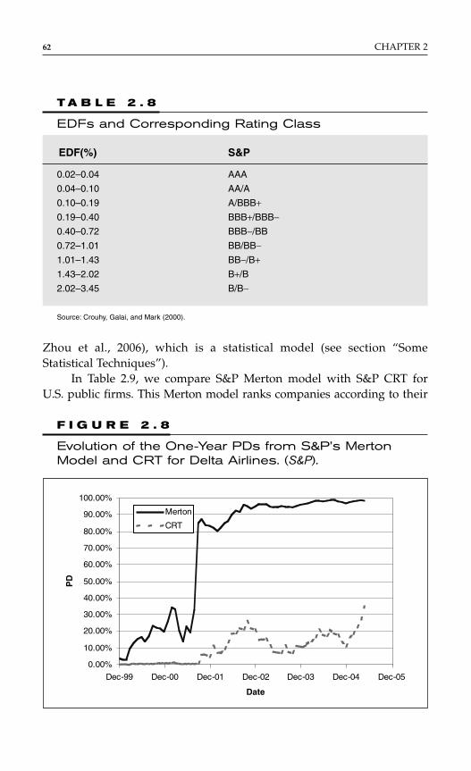
62 CHAPTER 2
T A B L E 2 . 8
EDFs and Corresponding Rating Class
EDF(%) S&P
0.02–0.04 AAA
0.04–0.10 AA/A
0.10–0.19 A/BBB+0.19–0.40 BBB+/BBB−0.40–0.72 BBB−/BB
0.72–1.01 BB/BB−1.01–1.43 BB−/B+1.43–2.02 B+/B
2.02–3.45 B/B−
Source: Crouhy, Galai, and Mark (2000).
0.00%
10.00%
20.00%
30.00%
40.00%
50.00%
60.00%
70.00%
80.00%
90.00%
100.00%
Dec-99 Dec-00 Dec-01 Dec-02 Dec-03 Dec-04 Dec-05
Date
PD
Merton
CRT
F I G U R E 2 . 8
Evolution of the One-Year PDs from S&P’s MertonModel and CRT for Delta Airlines. (S&P).
Zhou et al., 2006), which is a statistical model (see section “SomeStatistical Techniques”).
In Table 2.9, we compare S&P Merton model with S&P CRT forU.S. public firms. This Merton model ranks companies according to their

Univariate Risk Assessment 63
distance to default, which is sufficient to compute ROC without any map-ping on a real-world PD. CRT uses the distance to default from theMerton model as one of its input variables. The results shown in the tableare very interesting. One can see that both models perform much betteron the largest 2000 firms than on the set of all public firms. One can alsosee that the Merton model rank-orders firms surprisingly well. In partic-ular, for large firms, the ROC difference between the statistical model andthe Merton model is only 3 percent; i.e., a large part of the explanatorypower of the statistical model can be derived from the DD. Furthermore,the table seems to suggest that the Merton model is somewhat tunedtoward large firms.
Uses and Abuses of Equity-Based Models for Default Prediction
Equity-based models can be useful as early warning systems for individ-ual firms. Crosbie (1997) and Delianedis and Geske (1999) study the earlywarning power of structural models and show that these models can giveearly information about ratings migration and defaults.
There has undoubtedly been many examples of successes wherestructural models have been able to capture early warning signals fromthe equity markets. These examples, such as the WorldCom case, areheavily publicized by vendors of equity-based systems. What the vendorsdo not mention is that there are also many examples of false starts: a gen-eral fall in the equity markets will tend to be reflected in increases inall EDFs and many “downgrades” in internal ratings based on them,
Univariate Risk Assessment 63
T A B L E 2 . 9
ROCs for S&P’s Merton Model (see Park, 2006) andS&P’s CRT for U.S. Public Firms. ROCs wereComputed for all Public U.S. Firms and for the Subsetof the Largest 2000 Firms. In All Cases, a Five-FoldCross-Validation was Applied.
CRT Merton model
ROC on all public U.S. firms 0.87 0.80
ROC on largest 2000 public U.S. firms 0.95 0.92
Source: S&P (see Zhou et al. 2006).
although the credit quality of some firms may be unaffected. False startscan be costly, as they often induce banks to sell the position in a tempo-rary downturn at an unfavorable price.
Conversely, in a period of booming equity markets such as 1999,these models will tend to assign very low PDs to almost all firms. In short,equity-based models are prone to overreaction due to market bubbles.
Toward a Term Structure of Merton PDs: Use of Merton Model Results as an
Input into CDO Models
In order to obtain a default term structure, one has to generalize theMerton model. One such generalization was proposed by Black and Cox(1976), who assume that default can occur at any time before the maturityof a particular bond, whenever the asset value hits a given barrier. Thisidea can be motivated if there are bond safety covenenants or in the con-text of a continuous stream of payments to be made by the obligor.
The basic idea of the Black–Cox model is that, as in the Mertonmodel, the firm’s value undergoes a geometric Brownian motion, i.e.,
dV = µV dt + σVV dZ.
Default occurs when V hits, for the first time, the barrier C, whichundergoes the dynamics
Ct = C0 exp(γ t).
Computing the term structure of PDs in this setting amounts to solv-ing a well-understood first passage time problem. This makes theBlack–Cox model very attractive. Moreover, it is theoretically possible togeneralize this model to a multivariate setting (see Zhou, 2001).
The default term structure one obtains from a Black–Cox model isnot necessarily realistic. Although one can try to calibrate the parametersC0 and γ to a term structure obtained from a statistical hazard rate model,the calibration is rarely very good, since there are only two parametersavailable. To avoid this problem, one can generalize the dynamics of thedefault barrier. One such generalization has been proposed by Hull andWhite (2001), who assume a very flexible dynamics that can be calibratedto an arbitrary term structure. This type of model, however, can hardly beviewed as a structural model anymore.
64 CHAPTER 2
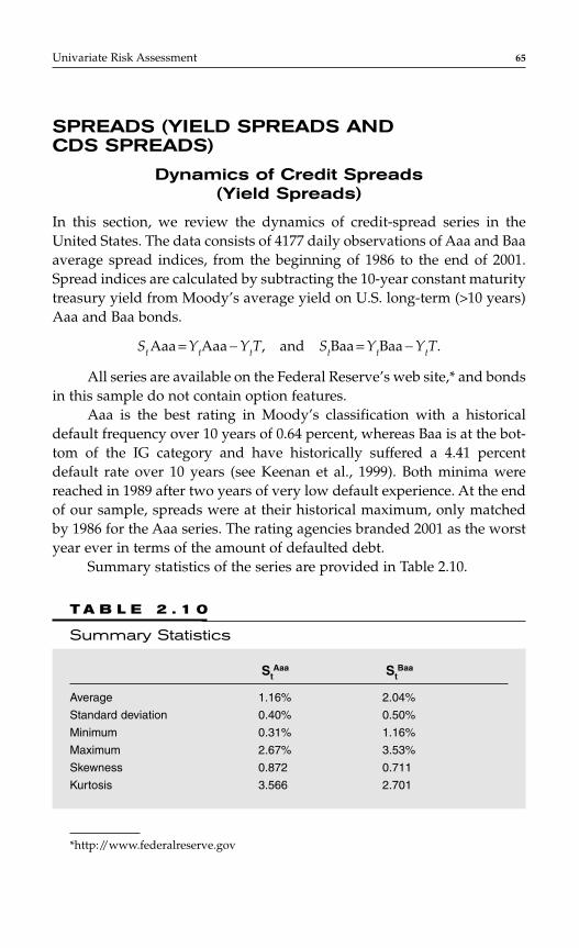
SPREADS (YIELD SPREADS ANDCDS SPREADS)
Dynamics of Credit Spreads (Yield Spreads)
In this section, we review the dynamics of credit-spread series in theUnited States. The data consists of 4177 daily observations of Aaa and Baaaverage spread indices, from the beginning of 1986 to the end of 2001.Spread indices are calculated by subtracting the 10-year constant maturitytreasury yield from Moody’s average yield on U.S. long-term (>10 years)Aaa and Baa bonds.
StAaa = YtAaa − YtT, and StBaa = YtBaa − YtT.
All series are available on the Federal Reserve’s web site,* and bondsin this sample do not contain option features.
Aaa is the best rating in Moody’s classification with a historicaldefault frequency over 10 years of 0.64 percent, whereas Baa is at the bot-tom of the IG category and have historically suffered a 4.41 percentdefault rate over 10 years (see Keenan et al., 1999). Both minima werereached in 1989 after two years of very low default experience. At the endof our sample, spreads were at their historical maximum, only matchedby 1986 for the Aaa series. The rating agencies branded 2001 as the worstyear ever in terms of the amount of defaulted debt.
Summary statistics of the series are provided in Table 2.10.
Univariate Risk Assessment 65
*http://www.federalreserve.gov
T A B L E 2 . 1 0
Summary Statistics
StAaa St
Baa
Average 1.16% 2.04%
Standard deviation 0.40% 0.50%
Minimum 0.31% 1.16%
Maximum 2.67% 3.53%
Skewness 0.872 0.711
Kurtosis 3.566 2.701
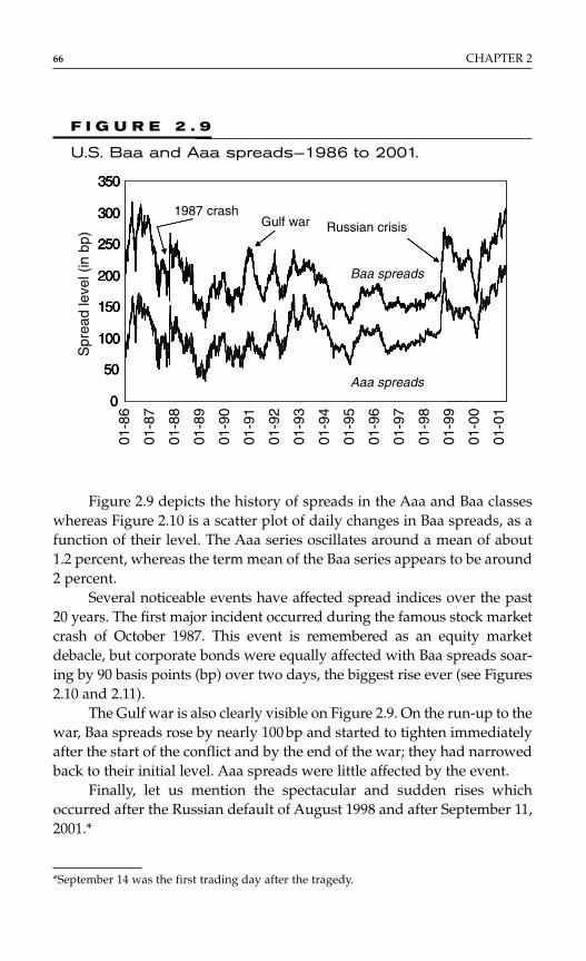
Figure 2.9 depicts the history of spreads in the Aaa and Baa classeswhereas Figure 2.10 is a scatter plot of daily changes in Baa spreads, as afunction of their level. The Aaa series oscillates around a mean of about1.2 percent, whereas the term mean of the Baa series appears to be around2 percent.
Several noticeable events have affected spread indices over the past20 years. The first major incident occurred during the famous stock marketcrash of October 1987. This event is remembered as an equity marketdebacle, but corporate bonds were equally affected with Baa spreads soar-ing by 90 basis points (bp) over two days, the biggest rise ever (see Figures2.10 and 2.11).
The Gulf war is also clearly visible on Figure 2.9. On the run-up to thewar, Baa spreads rose by nearly 100 bp and started to tighten immediatelyafter the start of the conflict and by the end of the war; they had narrowedback to their initial level. Aaa spreads were little affected by the event.
Finally, let us mention the spectacular and sudden rises whichoccurred after the Russian default of August 1998 and after September 11,2001.*
66 CHAPTER 2
*September 14 was the first trading day after the tragedy.
0
50
100
150
200
250
300
350
0
50
100
150
200
250
300
350
0
50
100
150
200
250
300
350
Russian crisisGulf war1987 crash
Spr
ead
leve
l (in
bp)
Aaa spreads
Baa spreads
01-8
6
01-8
7
01-8
8
01-8
9
01-9
0
01-9
1
01-9
2
01-9
3
01-9
4
01-9
5
01-9
6
01-9
7
01-9
8
01-9
9
01-0
0
01-0
1
F I G U R E 2 . 9
U.S. Baa and Aaa spreads—1986 to 2001.
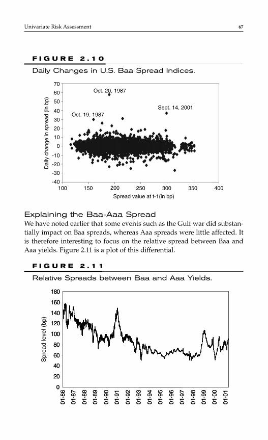
Univariate Risk Assessment 67
Oct. 20, 1987
Sept. 14, 2001Oct. 19, 1987
Spread value at t-1(in bp)
70
60
50
40
30
20
10
0
-10
-20
-30
-40100 150 200 250 300 350 400
Dai
ly c
hang
e in
spr
ead
(in b
p)
F I G U R E 2 . 1 0
Daily Changes in U.S. Baa Spread Indices.
0
20
40
60
80
100
120
140
160
180
01-8
6
01-8
7
01-8
8
01-8
9
01-9
0
01-9
1
01-9
2
01-9
3
01-9
4
01-9
5
01-9
6
01-9
7
01-9
8
01-9
9
01-0
0
01-0
1
0
20
40
60
80
100
120
140
160
180
01-8
6
01-8
7
01-8
8
01-8
9
01-9
0
01-9
1
01-9
2
01-9
3
01-9
4
01-9
5
01-9
6
01-9
7
01-9
8
01-9
9
01-0
0
01-0
1
Spr
ead
leve
l (bp
)
F I G U R E 2 . 1 1
Relative Spreads between Baa and Aaa Yields.
Explaining the Baa-Aaa SpreadWe have noted earlier that some events such as the Gulf war did substan-tially impact on Baa spreads, whereas Aaa spreads were little affected. Itis therefore interesting to focus on the relative spread between Baa andAaa yields. Figure 2.11 is a plot of this differential.

One can observe a clear downward trend between 86 and 98 onlyinterrupted by the Gulf war. This contraction in relative spreads was duemainly to the improvement in liquidity of the market for lower-rated bonds.
We can observe three spikes in the relative spread (Baa–Aaa): 1991,1998, and 2001. These are all linked to increases in market volatility, andthe peaks can be explained in the light of a structural model of credit risk.
Recall that in a Merton (1974)-type model, a risky bond can be seenas a risk-less bond minus a put on the value of the firm. The put’s exerciseprice is linked to the leverage of the issuing firm (in the simple case, wherethe firm’s debt is only constituted of one issue of zero-coupon bond, thestrike price of the put is the principal of the debt). Obviously the values ofBaa firms are closer to their “strike price” (higher risk) than those of Aaafirms. Therefore, Baa firms have higher vega than Aaa issuers.* As a result,as volatility increases, Baa spreads increase more than Aaa spreads.
Determinants of Yield Spreads
Spreads should at least reflect the probability of default and the recoveryrate. In a careful analysis of the components of corporate spreads in thecontext of a structural model, Delianedis and Geske (2001) report thatonly 5 percent of AAA spreads and 22 percent of BBB spreads can beattributed to default risk. We now turn in greater details to the possiblecomponents of an explanatory model for spreads.
RecoveryThe expected recovery rate for a bond of given seniority in a given industryaffects credit spreads and is therefore a natural candidate for inclusion ina spread model. Recoveries will be discussed in the forthcoming section.We shall see there that they tend to fluctuate with the economic cycle. So,ideally, a measure of expected recovery conditional on the state of theeconomy would be a more appropriate choice.
Probability of DefaultSpreads should also reflect PD. The most readily available measure ofcreditworthiness for large corporates is undoubtedly ratings, and they are
68 CHAPTER 2
*The vega (or kappa) of an option is the sensitivity of the option price to changes in thevolatility of the underlying. The vega is higher for options near the money, i.e., when theprice of the underlying is close to the exercise price of the option (see, e.g., Hull, 2002).
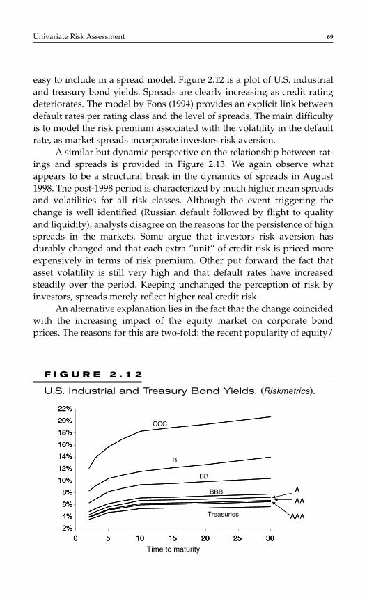
easy to include in a spread model. Figure 2.12 is a plot of U.S. industrialand treasury bond yields. Spreads are clearly increasing as credit ratingdeteriorates. The model by Fons (1994) provides an explicit link betweendefault rates per rating class and the level of spreads. The main difficultyis to model the risk premium associated with the volatility in the defaultrate, as market spreads incorporate investors risk aversion.
A similar but dynamic perspective on the relationship between rat-ings and spreads is provided in Figure 2.13. We again observe whatappears to be a structural break in the dynamics of spreads in August1998. The post-1998 period is characterized by much higher mean spreadsand volatilities for all risk classes. Although the event triggering thechange is well identified (Russian default followed by flight to qualityand liquidity), analysts disagree on the reasons for the persistence of highspreads in the markets. Some argue that investors risk aversion hasdurably changed and that each extra “unit” of credit risk is priced moreexpensively in terms of risk premium. Other put forward the fact thatasset volatility is still very high and that default rates have increasedsteadily over the period. Keeping unchanged the perception of risk byinvestors, spreads merely reflect higher real credit risk.
An alternative explanation lies in the fact that the change coincidedwith the increasing impact of the equity market on corporate bondprices. The reasons for this are two-fold: the recent popularity of equity/
Univariate Risk Assessment 69
F I G U R E 2 . 1 2
U.S. Industrial and Treasury Bond Yields. (Riskmetrics).
2%
4%
6%
8%
10%
12%
14%
16%
18%
20%
22%
0 5 10 15 20 25 30
BB
A
AA
AAA
2%
4%
6%
8%
10%
12%
14%
16%
18%
20%
22%
0 5 10 15 20 25 302%
4%
6%
8%
10%
12%
14%
16%
18%
20%
22%
0 5 10 15 20 25 30
CCC
B
BBB A
AA
AAA
Time to maturity
Treasuries
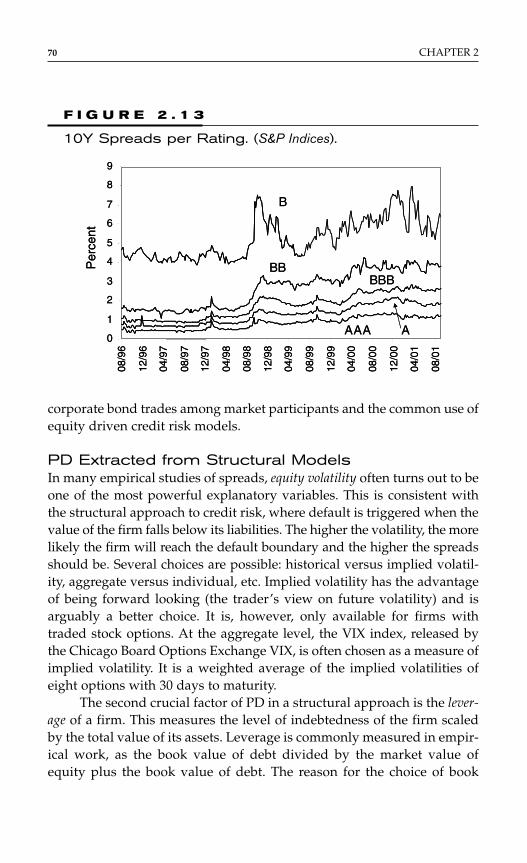
corporate bond trades among market participants and the common use ofequity driven credit risk models.
PD Extracted from Structural ModelsIn many empirical studies of spreads, equity volatility often turns out to beone of the most powerful explanatory variables. This is consistent withthe structural approach to credit risk, where default is triggered when thevalue of the firm falls below its liabilities. The higher the volatility, the morelikely the firm will reach the default boundary and the higher the spreadsshould be. Several choices are possible: historical versus implied volatil-ity, aggregate versus individual, etc. Implied volatility has the advantageof being forward looking (the trader’s view on future volatility) and isarguably a better choice. It is, however, only available for firms withtraded stock options. At the aggregate level, the VIX index, released bythe Chicago Board Options Exchange VIX, is often chosen as a measure ofimplied volatility. It is a weighted average of the implied volatilities ofeight options with 30 days to maturity.
The second crucial factor of PD in a structural approach is the lever-age of a firm. This measures the level of indebtedness of the firm scaledby the total value of its assets. Leverage is commonly measured in empir-ical work, as the book value of debt divided by the market value ofequity plus the book value of debt. The reason for the choice of book
70 CHAPTER 2
F I G U R E 2 . 1 3
10Y Spreads per Rating. (S&P Indices).
0
1
2
3
4
5
6
7
8
9
08/9
6
12/9
6
04/9
7
08/9
7
12/9
7
04/9
8
08/9
8
12/9
8
04/9
9
08/9
9
12/9
9
04/0
0
08/0
0
12/0
0
04/0
1
08/0
1
Per
cent
B
BBBBB
AAA A0
1
2
3
4
5
6
7
8
9
08/9
6
12/9
6
04/9
7
08/9
7
12/9
7
04/9
8
08/9
8
12/9
8
04/9
9
08/9
9
12/9
9
04/0
0
08/0
0
12/0
0
04/0
1
08/0
1
Per
cent
B
BBBBB
AAA A
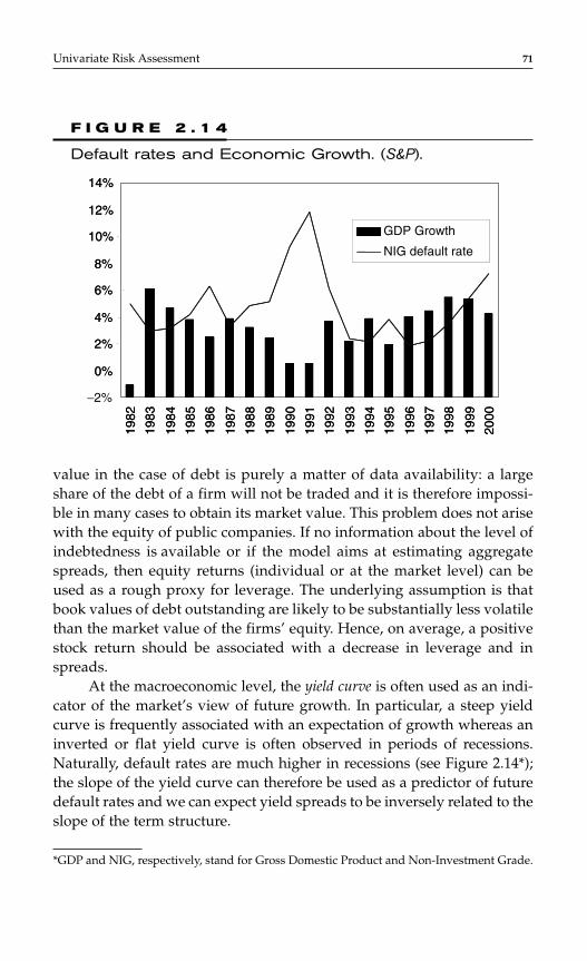
value in the case of debt is purely a matter of data availability: a largeshare of the debt of a firm will not be traded and it is therefore impossi-ble in many cases to obtain its market value. This problem does not arisewith the equity of public companies. If no information about the level ofindebtedness is available or if the model aims at estimating aggregatespreads, then equity returns (individual or at the market level) can beused as a rough proxy for leverage. The underlying assumption is thatbook values of debt outstanding are likely to be substantially less volatilethan the market value of the firms’ equity. Hence, on average, a positivestock return should be associated with a decrease in leverage and inspreads.
At the macroeconomic level, the yield curve is often used as an indi-cator of the market’s view of future growth. In particular, a steep yieldcurve is frequently associated with an expectation of growth whereas aninverted or flat yield curve is often observed in periods of recessions.Naturally, default rates are much higher in recessions (see Figure 2.14*);the slope of the yield curve can therefore be used as a predictor of futuredefault rates and we can expect yield spreads to be inversely related to theslope of the term structure.
Univariate Risk Assessment 71
F I G U R E 2 . 1 4
Default rates and Economic Growth. (S&P).
0%
2%
4%
6%
8%
10%
12%
14%
1982
1983
1984
1985
1986
1987
1988
1989
1990
1991
1992
1993
1994
1995
1996
1997
1998
1999
2000
GDP Growth
NIG default rate
−2%
0%
2%
4%
6%
8%
10%
12%
14%
1982
1983
1984
1985
1986
1987
1988
1989
1990
1991
1992
1993
1994
1995
1996
1997
1998
1999
2000
GDP Growth
NIG default rate
*GDP and NIG, respectively, stand for Gross Domestic Product and Non-Investment Grade.
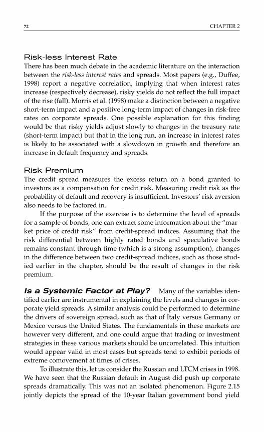
Risk-less Interest RateThere has been much debate in the academic literature on the interactionbetween the risk-less interest rates and spreads. Most papers (e.g., Duffee,1998) report a negative correlation, implying that when interest ratesincrease (respectively decrease), risky yields do not reflect the full impactof the rise (fall). Morris et al. (1998) make a distinction between a negativeshort-term impact and a positive long-term impact of changes in risk-freerates on corporate spreads. One possible explanation for this findingwould be that risky yields adjust slowly to changes in the treasury rate(short-term impact) but that in the long run, an increase in interest ratesis likely to be associated with a slowdown in growth and therefore anincrease in default frequency and spreads.
Risk PremiumThe credit spread measures the excess return on a bond granted toinvestors as a compensation for credit risk. Measuring credit risk as theprobability of default and recovery is insufficient. Investors’ risk aversionalso needs to be factored in.
If the purpose of the exercise is to determine the level of spreadsfor a sample of bonds, one can extract some information about the “mar-ket price of credit risk” from credit-spread indices. Assuming that therisk differential between highly rated bonds and speculative bondsremains constant through time (which is a strong assumption), changesin the difference between two credit-spread indices, such as those stud-ied earlier in the chapter, should be the result of changes in the riskpremium.
Is a Systemic Factor at Play? Many of the variables iden-tified earlier are instrumental in explaining the levels and changes in cor-porate yield spreads. A similar analysis could be performed to determinethe drivers of sovereign spread, such as that of Italy versus Germany orMexico versus the United States. The fundamentals in these markets arehowever very different, and one could argue that trading or investmentstrategies in these various markets should be uncorrelated. This intuitionwould appear valid in most cases but spreads tend to exhibit periods ofextreme comovement at times of crises.
To illustrate this, let us consider the Russian and LTCM crises in 1998.We have seen that the Russian default in August did push up corporatespreads dramatically. This was not an isolated phenomenon. Figure 2.15jointly depicts the spread of the 10-year Italian government bond yield
72 CHAPTER 2
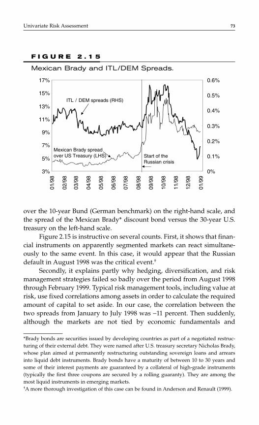
over the 10-year Bund (German benchmark) on the right-hand scale, andthe spread of the Mexican Brady* discount bond versus the 30-year U.S.treasury on the left-hand scale.
Figure 2.15 is instructive on several counts. First, it shows that finan-cial instruments on apparently segmented markets can react simultane-ously to the same event. In this case, it would appear that the Russiandefault in August 1998 was the critical event.†
Secondly, it explains partly why hedging, diversification, and riskmanagement strategies failed so badly over the period from August 1998through February 1999. Typical risk management tools, including value atrisk, use fixed correlations among assets in order to calculate the requiredamount of capital to set aside. In our case, the correlation between thetwo spreads from January to July 1998 was −11 percent. Then suddenly,although the markets are not tied by economic fundamentals and
Univariate Risk Assessment 73
*Brady bonds are securities issued by developing countries as part of a negotiated restruc-turing of their external debt. They were named after U.S. treasury secretary Nicholas Brady,whose plan aimed at permanently restructuring outstanding sovereign loans and arrearsinto liquid debt instruments. Brady bonds have a maturity of between 10 to 30 years andsome of their interest payments are guaranteed by a collateral of high-grade instruments(typically the first three coupons are secured by a rolling guaranty). They are among themost liquid instruments in emerging markets.†A more thorough investigation of this case can be found in Anderson and Renault (1999).
3%
5%
7%
9%
11%
13%
15%
17%
01/9
8
02/9
8
03/9
8
04/9
8
05/9
8
06/9
8
07/9
8
08/9
8
09/9
8
10/9
8
11/9
8
12/9
8
01/9
9
0%
0.1%
0.2%
0.3%
0.4%
0.5%
0.6%
Start of theRussian crisis
ITL / DEM spreads (RHS)
Mexican Brady spreadover US Treasury (LHS)
F I G U R E 2 . 1 5
Mexican Brady and ITL/DEM Spreads.

although the crisis occurred in a third market apparently unrelated, cor-relations all turned positive and very significantly so. In this example, thecorrelation over the rest of 1998 increased to 62 percent.
Some may argue that the Russian default may just have increaseddefault risk globally or that market participants expected spill-over effectsin all bond markets. Another explanation lies in the flight-to-liquidity andflight-to-safety observed over that period: investors massively turned tothe most liquid and safest products, which were U.S. treasuries andGerman bunds. Many products bearing credit risk did not seem to findany buyer at any price in the immediate aftermath of the crisis.
From a risk management perspective, it is sensible to consider that aglobal factor (possibly investors’ risk aversion) impacts across all bondmarkets and may lead to substantial losses in periods of turmoil.
LiquidityFinally, and perhaps most importantly, yield spreads reflect the relativeliquidity of corporate and treasury securities. Liquidity is one of themain explanations for the existence of corporate yield spreads. This hasbeen recognized early (see, e.g., Fisher, 1959) and can be justified by thefact that government bonds are typically very actively traded largeissues, whereas the corporate bond market is an over-the-counter mar-ket whose volumes and trade frequencies are much smaller. Investorsrequire some compensation (in terms of added yield) for holding lessliquid securities.
In the case of IG bonds, where credit risk is not as important as in thespeculative class, liquidity is arguably the main factor in spreads. Liquidityis, however, a very nebulous concept and there does not exist any clear-cutdefinition for it. It can encompass the rapid availability of funds for a cor-porate to finance unexpected outflows or it can mean the marketability ofthe debt on the secondary market. We will focus on the latter definition.More specifically, we perceive liquidity as the ability to close out a positionquickly on the market without substantially affecting the price. Liquiditycan therefore be seen as an option to unwind a position.
Longstaff (1995) follows this approach and provides upper boundson the liquidity discounts on securities with trading restrictions. If a secu-rity cannot be bought or sold for say seven days, it will trade at a discountcompared to an identical security for which trading is available continu-ously. This discount represents the opportunity cost of not being able totrade during the restricted period. It should therefore be bounded by the
74 CHAPTER 2
value of selling* the position at the best (highest) price during therestricted period. The value of liquidity is thus capped by the price of alookback put option.
Little research has been performed on the liquidity of nontreasurybonds. Kempf and Uhrig (1997) propose a direct modeling of liquidityspreads—the share of yield spreads attributable to the liquidity differen-tial between government and corporate bonds. They assume that liquid-ity spreads follow a mean reverting process and estimate it on Germangovernment bond data. Longstaff (1994) considers the liquidity of munic-ipal and other credit risky bonds in Japan. Ericsson and Renault (2001)model the behaviour of a bondholder who may be forced to sell his posi-tion due to and external shock (immediate need for cash). Liquidityspreads arise because a forced sale may coincide with a lack of demand inthe market (liquidity crisis). Their theoretical model based on a Merton(1974) default risk framework generates downward sloping term struc-ture of liquidity spreads as those reported in Kempf and Uhrig (1997) andalso in Longstaff (1994). They also find that liquidity spreads should beincreasing in credit risk: if liquidity is the option to liquidate a position,then this option is more valuable in presence of credit risk, as the inabil-ity to unwind a position for a long period may lead the bondholder to beforced to keep a bond entering default and to face bankruptcy costs. On asample of over 500 U.S. corporate bonds, they find support for the nega-tive slope of the term structure of liquidity premiums and for the positivecorrelation between credit risk and liquidity spreads.
On the empirical side, the liquidity of equity markets (and to a lesserextent also of treasury bond markets) has been extensively studied empir-ically, but very little has yet been done to measure liquidity premiums indefault risky securities. Several variables can be used to proxy for liquid-ity. The natural candidates are the number of trades and the volume oftrading on the market. The OTC nature of the corporate bond marketmakes this data difficult to obtain. As second best, the issue amount out-standing can also serve as proxy for liquidity. The underlying implicitassumption is that larger issues are traded more actively than smallerones.
A stylized fact about bonds is that they are more liquid immediatelyafter issuance and rapidly lose their marketability as a larger share of theissues becomes locked into portfolios (see, e.g., Chapter 10 in Fabozzi and
Univariate Risk Assessment 75
*We assume the investor has a long position in the security.
Fabozzi, 1995). The age of an issue could therefore stand for liquidity inan explanatory model for yield spreads. In the same spirit, the on-the-run/off-the-run spread (the difference between the yields of seasoned andnewly issued bonds with same residual time to maturity) is frequentlyused as an indicator of liquidity. During the Russian crisis of 1998, whichwas associated with a substantial liquidity crunch, the U.S. long bond(30-year benchmark) was trading at a 35 basis point premium versus thesecond longest bond with just a few months less to maturity, while thehistorical differential was only 7 to 8 basis points (Poole, 1998).
TaxesIn order to conclude this nonexhaustive list of factors influencing spreads,we can mention taxes. In some jurisdictions (such as the United States), cor-porate and treasury bonds do not receive the same tax treatment (see Eltonet al., 2001). For example, in the United States, treasury securities are exemptfrom some taxes while corporate bonds are not. Investors will of coursedemand a higher return on instruments on which they are taxed more.
We have reported that many factors impact on yield spreads andthat spreads cannot be seen as purely due to credit. We will now focusmore specifically on the ability of structural models to explain the dynam-ics and level of spreads.
CDS Rates
Another market quantity that provides default risk information is theCDS rate. Here, CDS stands for credit default swap. The credit defaultswap is the most commonly used credit derivative. In its most basic form,it works as follows: Party A, the so-called protection buyer, pays anannual or semi-annual premium to party B, the so-called protection seller.These payments end either after a given period of time (the maturity ofthe CDS) or at default of the reference entity. In the case of such a default,the protection seller compensated the protection buyer for the lossincurred due to the default. The CDS rate, also called credit-swap spreadsor CDS premiums, is the premium paid by the protection buyer. Figure 2.16illustrates the cashflows in a credit default swap.
It follows from a no-arbitrage argument that, under some idealizedassumptions, the CDS rates are the same as the corresponding bondspreads (off LIBOR) for the same obligor, and are therefore determined bysome of the same factors, such as default probability, risk premium, and
76 CHAPTER 2
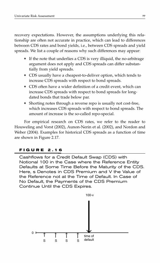
recovery expectations. However, the assumptions underlying this rela-tionship are often not accurate in practice, which can lead to differencesbetween CDS rates and bond yields, i.e., between CDS spreads and yieldspreads. We list a couple of reasons why such differences may appear:
♦ If the note that underlies a CDS is very illiquid, the no-arbitrageargument does not apply and CDS spreads can differ substan-tially from yield spreads.
♦ CDS usually have a cheapest-to-deliver option, which tends toincrease CDS spreads with respect to bond spreads.
♦ CDS often have a wider definition of a credit event, which canincrease CDS spreads with respect to bond spreads for long-dated bonds that trade below par.
♦ Shorting notes through a reverse repo is usually not cost-free,which increases CDS spreads with respect to bond spreads. Theamount of increase is the so-called repo-special.
For empirical research on CDS rates, we refer to the reader toHouweling and Vorst (2002), Aunon-Nerin et al. (2002), and Nordon andWeber (2004). Examples for historical CDS spreads as a function of timeare shown in Figure 2.17.
Univariate Risk Assessment 77
F I G U R E 2 . 1 6
Cashflows for a Credit Default Swap (CDS) withNotional 100 in the Case where the Reference EntityDefaults at Some Time Before the Maturity of the CDS.Here, s Denotes in CDS Premium and V the Value ofthe Reference not at the Time of Default. In Case ofNo Default, the Payments of the CDS PremiumContinue Until the CDS Expires.
100-v
time ofdefaultS S S S
0
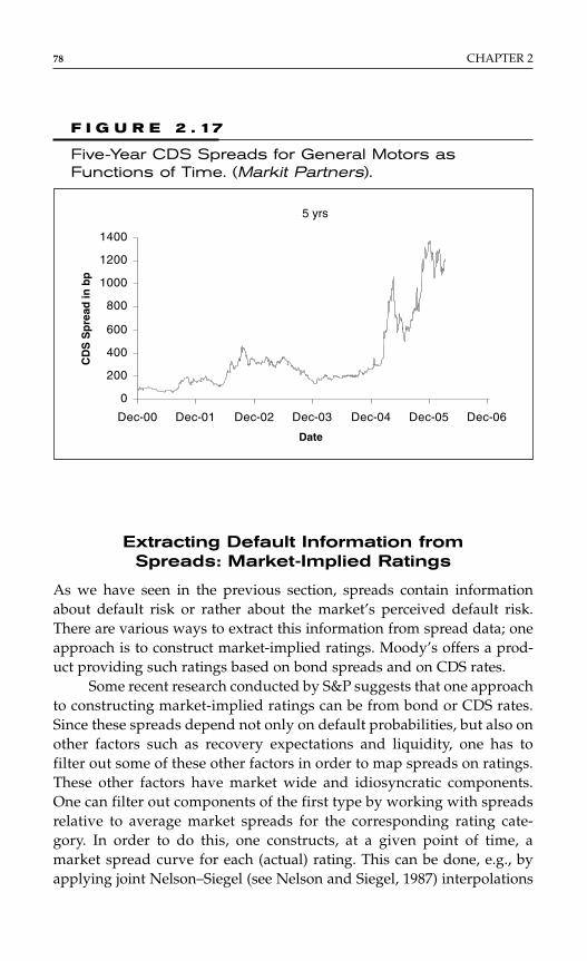
Extracting Default Information from Spreads: Market-Implied Ratings
As we have seen in the previous section, spreads contain informationabout default risk or rather about the market’s perceived default risk.There are various ways to extract this information from spread data; oneapproach is to construct market-implied ratings. Moody’s offers a prod-uct providing such ratings based on bond spreads and on CDS rates.
Some recent research conducted by S&P suggests that one approachto constructing market-implied ratings can be from bond or CDS rates.Since these spreads depend not only on default probabilities, but also onother factors such as recovery expectations and liquidity, one has tofilter out some of these other factors in order to map spreads on ratings.These other factors have market wide and idiosyncratic components.One can filter out components of the first type by working with spreadsrelative to average market spreads for the corresponding rating cate-gory. In order to do this, one constructs, at a given point of time, amarket spread curve for each (actual) rating. This can be done, e.g., byapplying joint Nelson–Siegel (see Nelson and Siegel, 1987) interpolations
78 CHAPTER 2
F I G U R E 2 . 17
Five-Year CDS Spreads for General Motors as Functions of Time. (Markit Partners).
5 yrs
0
200
400
600
800
1000
1200
1400
Dec-00 Dec-01 Dec-02 Dec-03 Dec-04 Dec-05 Dec-06
CD
S S
pre
ad in
bp
Date
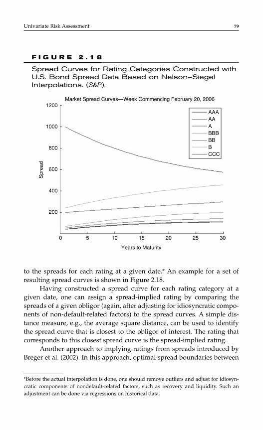
to the spreads for each rating at a given date.* An example for a set ofresulting spread curves is shown in Figure 2.18.
Having constructed a spread curve for each rating category at agiven date, one can assign a spread-implied rating by comparing thespreads of a given obligor (again, after adjusting for idiosyncratic compo-nents of non-default-related factors) to the spread curves. A simple dis-tance measure, e.g., the average square distance, can be used to identifythe spread curve that is closest to the obligor of interest. The rating thatcorresponds to this closest spread curve is the spread-implied rating.
Another approach to implying ratings from spreads introduced byBreger et al. (2002). In this approach, optimal spread boundaries between
Univariate Risk Assessment 79
F I G U R E 2 . 1 8
Spread Curves for Rating Categories Constructed withU.S. Bond Spread Data Based on Nelson–SiegelInterpolations. (S&P ).
00 5 10 15
Years to Maturity
20 25 30
1200
1000
800
600
400
200
Spr
ead
Market Spread Curves—Week Commencing February 20, 2006
AAAAAABBBBBBCCC
*Before the actual interpolation is done, one should remove outliers and adjust for idiosyn-cratic components of nondefault-related factors, such as recovery and liquidity. Such anadjustment can be done via regressions on historical data.
the rating categories are determined by means of a penalty function; theseboundaries are subsequently used to imply ratings. Kou and Varotto(2004) use this approach to predict rating migrations.
RECOVERY RISK
In the previous sections, we have reviewed various approaches to assessdefault risk. However, the credit risk that an investor is exposed to con-sists of default risk and recovery risk. The latter, which reflects the uncer-tainty associated with the recovery from defaulted debt, is the topic of thissection. To date, much less research effort has been made toward model-ing recovery risk than toward understanding default risk. Consequently,the literature on this topic is fairly small in volume; the perhaps earliestworks on recoveries were published by Altman and Kishore (1996) andAsarnow and Edwards (1995). A fairly comprehensive overview is pro-vided by Altman et al. (2005).
The quantity that characterizes recovery risk is recovery givendefault (RGD) or equivalently loss given default (LGD). RGD is usuallydefined as the ratio of the recovery value from a defaulted debt instru-ment and the invested par amount, and LGD = 1 − RGD. There are variousways to define the recovery value; some people define it as the tradedvalue of the defaulted security immediately after default, others define itas the payout to the debt holder at the time of emergence from bank-ruptcy (often called ultimate recovery). Which one of the recovery defini-tion is the appropriate one, depends on the purpose of the analysis. Forexample, an investor (e.g., a mutual bond fund) who always sells debtsecurities immediately after they have defaulted should be interested inthe first type of recovery value; whereas an investor (e.g., a bank thatworks out defaulted loans) who holds on to defaulted debt till emergenceshould care about the second type of recovery.
A prominent feature of RGD is its high uncertainty given the infor-mation a typical investor can obtain at a time before default. For exam-ple, an investor in bonds of large U.S. firms who has access to theobligor’s balance sheet and is aware of the economic environment, butdoes not have any more detailed information about the debt, is only ableto predict RGD with an uncertainty in the range of 30 to 40 percent,as measured by the standard deviation of a forecasting model (seeFriedman and Sandow, 2005). For this reason, given relevant factors it isdesirable to model the uncertainty associated with recovery and not justits expected value.
80 CHAPTER 2
The perhaps most commonly used approach to modeling RGD is thebeta-distribution. Here one assumes that RGD has the following condi-tional probability density function (pdf ):*
where rmax is the largest and rmin the smallest possible value of RGD,† Bdenotes the beta function, and α and β are parameterized functions of therisk factors x. The D in this equation indicates that we condition all PDshaving happened. Often one assumes the α and β are linear in the risk fac-tors x. It is then straightforward to estimate the model parameters via themaximum-likelihood method.
An RGD model that relies on this beta-distribution is Moody’sKMV’s LossCalc™ (see Gupton and Stein, 2002).‡ This model, which pre-dicts trading price recoveries of U.S. corporations, is commercially avail-able. It was trained on data from Moody’s recovery database.
Another commercially available RGD model is S&P’s LossStats™Model (see Friedman and Sandow, 2005). This model predicts ultimaterecoveries and trading prices at arbitrary times after default for large U.S.corporations; it was built using data from S&P LossStats™ Database.§ It isbased on a methodology that is related to the one S&P’s for PD modeling(see section “Some Statistical Techniques”). Specifically, for trading pricesit is assumed that
p r D xZ x
x r x r x r( , )( )
exp ( ) ( ) ( ) = + +1 2 3α β γ
p r D xB x x
r r
r
r r
r
x x
( , )( ( ), ( ))
,min
max
( )
min
max
( )
=−
−
−
− −1
11 1
α β
β α
Univariate Risk Assessment 81
*This conditional probability density function is interpreted as follows: for an obligor withrisk factors x, the probability of recovering a value in the infinitesimal interval (r, r + dr) isp(r|D, x)dr.†One might think that rmax = 1, which corresponds to complete recovery. However, at least forultimate recoveries of large U.S. firms, one can actually recover more than the invested paramount. This happens, e.g., if the investor recovers equity that has increased in value dur-ing the bankruptcy proceedings. The smallest possible recovery value, rmin , is zero, unlesswe include workout costs. In the latter case, rmin can be negative.‡ In LossCalc™, the parameters of the distribution are not estimated via the maximum-likelihood method, but rather by means of a linear regression after a transformation of thedistribution into a normal distribution.§ See, e.g., Bos et al., 2002, for more details.
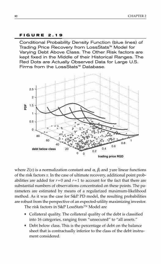
where Z(x) is a normalization constant and α, β, and γ are linear functionsof the risk factors x. In the case of ultimate recovery, additional point prob-abilities are added for r = 0 and r = 1 to account for the fact that there aresubstantial numbers of observations concentrated on these points. The pa-rameters are estimated by means of a regularized maximum-likelihoodmethod. As it was the case for S&P PD model, the resulting probabilitiesare robust from the perspective of an expected-utility maximizing investor.
The risk factors in S&P LossStats™ Model are
♦ Collateral quality. The collateral quality of the debt is classifiedinto 16 categories, ranging from “unsecured” to “all assets.”
♦ Debt below class. This is the percentage of debt on the balancesheet that is contractually inferior to the class of the debt instru-ment considered.
82 CHAPTER 2
F I G U R E 2 . 1 9
Conditional Probability Density Function (blue lines) ofTrading Price Recovery from LossStats™ Model forVarying Debt Above Class. The Other Risk factors arekept fixed in the Middle of their Historical Ranges. TheRed Dots are Actually Observed Data for Large U.S.Firms from the LossStats™ Database.
2.5
2
1.5
1
0.5
0
PD
F
00.2
0.40.6
0.81
trading price RGD
debt below class
80
6040
200
♦ Debt above class. This is the percentage of debt on the balancesheet that is contractually superior to the class of the debtinstrument considered.
♦ Regional default rate. This is the percentage of S&P-rated U.S.-bonds that defaulted within the 12 months prior to default.
♦ Industry factor. This is the ratio of the percentage of S&P-ratedbonds in the industry of interest that defaulted within the12 months prior to default to the above regional default rate.
The risk factors in Moody’s KMV’s LossCalc™ are not the same, but cap-ture similar characteristics of the balance sheet and the economy.
A typical model output is shown in Figure 2.19. The figure demon-strates how the probability density depends on one of the risk factors. Italso shows that the probability density is fairly flat, i.e., is associated witha high uncertainty.
The models mentioned here approach recoveries from a statisticalpoint of view: a probability density is learned from data without anyassumptions about the underlying process, which leads to default. Analternative approach is taken by Chew and Kerr (2005), who approachrecovery modeling from a fundamental perspective.
COMBINING PD AND RECOVERY MODELS
Investors in credit-risky debt are usually interested in the expected lossor the loss distribution of a given debt instrument. The latter one can beused, in its turn, as an input into a portfolio model for the computationof portfolio VaR, economic capital, or other risk characteristics of acredit portfolio. The loss distribution of a single credit can be computedby combining a PD model and a recovery model. Let us consider a debtinstrument with risk factors x (this denotes the vector of all risk factorsthat affect either LGD or PD), and denote the PD by P(Dx) and the prob-ability density for LGD (which is 1 − RGD) by p(lD, x), where l denotesa loss value and D denotes the default event. The loss distribution isthen
p(l x) = (1 − P(D x))δ(l) + P(D x)p(l D, x),
where δ is Dirac’s delta function. This equation implies that
E[L x] = P(D x)E[L D, x],
Univariate Risk Assessment 83
that is, that, for a debt instrument with known risk factors x, the expectedloss is equal to the PD times the expected LGD. This formula is widelyused by practitioners.
In many practical applications, however, the risk factors should beviewed as having a probability distribution, p(x), rather than being givenby a single value. Possible reasons for this are the following:
♦ The economic environment at the default time is uncertain.♦ We are interested in a portfolio instead of in a single loan. The
components of the portfolio are typically not identical withrespect to their risk factor values.
In this case, the loss distribution is
p(l) = ∫p(x)p(lx)dx = ∫p(x)[(1 − P(Dx))δ (l) + P(Dx)p(lD, x)]dx,
and the expected loss is
E[L] = ∫p(x)E[Lx]dx = ∫p(x)P(Dx)E[LD, x]dx.
These expressions involve integrals over products. Therefore, ifthere are any risk factors that PD and LGD share,* one cannot simply cal-culate the loss distribution or the expected loss based on the formulae forgiven credit factors after averaging PD and LGD separately over x. Thisfact, which received some attention in the recent literature (see, e.g., Frye,2003 or Altman et al., 2006), has important practical consequences. It hasbeen shown that there are indeed joint risk factors, such as the economy-wide default rate, which typically drive PDs and LGDs in the same direc-tion. Numerical experiments have shown (see Altman et al., 2006) thatthis leads to an expected loss; a VAR that is higher than the expected losswould be in the absence of such joint risk factors. These experiments arein line with what one would expect from the previous equation for p(l); ifthose x-values with a higher PD have a greater probability for largerlosses than those x-values with a lower PD, then p(l) is more concentratedon higher loss values than it would be otherwise. In other words, in thecase of common factors that drive PD and LGD in the same direction, ifsituations turn bad with regard to PDs they also turn bad with regard toLGDs, and the investor gets hit twice.
84 CHAPTER 2
*Risk factors that affect either the PD or LGD only can be averaged out separately, and there-fore do not affect the argument which follows.
CONCLUSION
In this chapter, we have reviewed some popular approaches to modelingPDs and RGD. Most practitioners analyze PDs from one of the followingperspectives:
1. Ratings2. Statistical modeling3. Structural (Merton-type) models4. Spreads
Interestingly enough, in the pricing world (risk-neutral), the dominanttechnique relies on spread, but we have seen that under the historicalmeasure, it is very difficult to extract a probability of default from spread.This explains why the first three methods have been so dominant.
Going forward, we believe that the two dominant approaches thatare going to be used are rating-based models and statistical models, i.e.,approaches 1 and 2. We do not exclude structural models, but think thatthe refinements they go through these days increasingly bring them closerto statistical models. These two approaches usually provide different infor-mation. The first one, which is based to a large extent on expert judgement,gives a smoothed view over a longer horizon (through the cycle), whereasapproach 2, which is usually used to derive a one-year PD from quantita-tive factors, gives a more precise but more volatile view of the term struc-ture of the creditworthiness of an obligor. One can, however, use approach2 to estimate long-term PDs, in which case its output resembles a rating-derived PD more closely.
RGD is rather difficult to predict. For this reason, it seems advisableto model its conditional probability distribution given a set of credit fac-tors. Perhaps the most popular approach to doing so is to estimate a beta-distribution. More general families of distributions (e.g., exponentialdensities with point probabilities), however, can improve the perfor-mance of an RGD model substantially. An important feature, which anyRGD model should reflect, is the empirical observation that RGD and PDshare some credit factors, a fact which tends to increase the risk of highportfolio losses.
Univariate Risk Assessment 85

APPENDIX 1
Definition of the Gini Coefficient
Given a sample of n ordered individuals with xi the size of individual i, inthis specific case ordered by the PD with respect to the percentage ofdefault events, and x1 < x2 < · · · < xn, the sample Lorenz curve is the poly-gon joining the points (h/n, Lh, Ln), where h = 0, 1, 2, . . . , n, L0 = 0 and
If all the individuals are the same size, the Lorenz curve is a
straight diagonal line, called the line of equality. The Lorentz curve can be
expressed as where F(x) is a c.d.f. and µ is the mean size
of xi.If there is any equality in size, the Lorenz curve falls below or above
the line of equality.The total amount of inequality can be summarized by the Gini coef-
ficient, which is the ratio between the area enclosed by the line of equal-ity and the Lorenz curve, and the total triangular area under the line ofequality. The Gini coefficient G is a summary statistic of the Lorenz curveand a measure of inequality in a population. The Gini coefficient is mosteasily calculated from unordered size data as the “relative mean differ-ence,” i.e., the mean of the difference between every possible pair ofindividuals, divided by µ:
Alternatively, if the data is ordered by increasing size of individuals, inthis specific case ordered by PD with respect to the percentage of defaultevents, G is given by:
The Gini coefficient ranges from a minimum value of zero, when allindividuals are equal, to a theoretical maximum of one, in an infinitepopulation in which every individual except one has a size of zero. In
Gi n x
nii
n
=− −
=∑ ( )2 11
2µ
Gx x
n
i jj
n
i
n
=−
== ∑∑ | |11
22 µ
L yxF xy
( )( )
,=∫ 0
µ
L xh i
h
i==Σ
1.
86 CHAPTER 2
general, in the Credit universe, Gini coefficients are positioned in the 50to 85 percent interval.
REFERENCESAltman, E., B. Brady, A. Resti, and A. Sironi (2006), “The link between default and
recovery rates: theory, empirical evidence and implications,” Journal ofBusiness, forthcoming, also: Working Paper Series #S-03-4, NYU Stern.
Altman, E., and V. Kishore (1996), “Almost everything you wanted to knowabout recoveries on defaulted bonds,” Financial Analyst Journal, November/December, 57.
Altman, E., A. Resti, and A. Sironi (2005), Recovery Risk: The Next Challenge inCredit Risk Management, Risk Books.
Andersen, P. K., Ø. Borgan, R. D. Gill, and N. Keiding (1993), Statistical ModelsBased on Counting Processes, Springer.
Anderson, R., and O. Renault (1999), “Systemic factors in international bondmarkets,” IRES Quarterly Review, December, 75–91.
Anderson, R., and S. Sundaresan (1996), “Design and valuation of debt con-tracts,” Review of Financial Studies, 9, 37–68.
Asarnow, E., and D. Edwards (1995), “Measuring loss on defaulted bank loans: a24-year study,” Journal of Commercial Lending, 77, 11.
Aunon-Nerin, D., D. Cossin, T. Hricko, and Z. Huang (2002), “Exploring for thedeterminants of credit risk in credit default swap transaction data: Isfixed-income markets’ information sufficient to evaluate credit risk?”FAME Research Paper No. 65, http://papers.ssrn.com/sol3/papers.cfm?abstract_id=375563
Avellaneda, M., and J. Zhu (2001), “Modeling the distance-to-default process of afirm,” WP Courant Institute of Mathematical Sciences.
Bangia, A., F. Diebold, A. Kronimus, C. Schagen, and T. Schuermann (2002),“Rating migration and the business cycle, with application to credit port-folio stress testing,” Journal of Banking and Finance, 26, 445–474.
Bielicki, T. R., and M. Rutkowski (2002), Credit Risk: Modeling, Valuation andHedging, Springer.
Black, F., and J. Cox (1976), “Valuing corporate securities: Some effects of bondindenture provisions,” Journal of Finance, 31, 351–367.
Black, F., and M. Scholes (1973), “The pricing of options and corporate liabilities,”Journal of Political Economy, 81, 637–659.
Bos, R., K. Kelhoffer, and D. Keisman (2002), “Ultimate recovery in an era ofrecord defaults,” Standard & Poor’s CreditWeek, August 7, 23.
Breger, L., L. Goldberg, and O. Cheyette (2002), “Market implied ratings,” Horizon,The Barra Newsletter, Autumn.
Chew, W. H., and S. S. Kerr (2005), “Recovery ratings: A fundamental approachto estimating recovery risk”, in E. Altman, A. Resti, and A. Sironi (eds.),Recovery Risk: The Next Challenge in Credit Risk Management, Risk Books.
Univariate Risk Assessment 87
Christensen, J., E. Hansen, and D. Lando (2004), “Confidence sets for continuous-time rating transition probabilities,” working paper, Copenhagen BusinessSchool and University of Copenhagen.
Couderc, F., and O. Renault (2005), “Times-to-default: life cycle, global andIndustry cycle impacts,” WPFame.
Cover, T., and J. Thomas (1991), Elements of Information Theory, Wiley.Cox, D. R. (1972), “Regression Models and Life-Time Tables (with discussion),”
J. R. Statist. Soc. B, 34, 187–220.Crosbie, P., and J. Bohn (2003), “Modeling default risk,” Moody’s KMV white paper,
http://www.moodyskmv.com/research/files/wp/ModelingDefaultRisk.pdfCrosbie, P. J. (1997), “Modeling default risk,” KMV, June.Davidson, R., and J. G. MacKinnon (1993), Estimations and Inference in
Econometrics, Oxford University Press.de Servigny, A., and O. Renault (2004), Measuring and Managing Credit Risk,
McGraw Hill.Delianedis, G., and R. Geske (1999), “Credit risk and risk neutral default proba-
bilities: Information about default migrations and defaults,” WP UCLA,May.
Duffee, G. (1998), “The relation between treasury yields and corporate bond yieldspreads,” Journal of Finance, 53, 2225–2242.
Duffie, D., and D. Lando (2001), “Term structure of credit spreads with incom-plete accounting information,” Econometrica, 69, 633–664.
Duffie, D., L. Saita, and K. Wang (2005), “Multi-period corperate default predic-tion with stochastic covariates,” CIRJE-F-373, http://www.e.u-tokyo.ac.jp/cirje/research/03research02dp.html
Duffie, D., and K. J. Singleton (2003), Credit Risk, Princeton University Press.Elton, E., M. Gruber, D. Agrawal, and C. Mann (2001), “Explaining the rate
spread on corporate bonds,” Journal of Finance, 56, 247–277.Ericsson, J. and O. Renault (2001), “Liquidity and credit risk,” working paper,
London School of Economics.Fabozzi, F., and T. Fabozzi (1995), The Handbook of Fixed Income Securities, Irwin.Falkenstein, E. (2000), “Riskcalc™ for private companies: Moody’s default
model,” Moody’s Investor Service, May.Fisher, L. (1959), “Determinants of the risk premiums on corporate bonds,”
Journal of Political Economy, 67, 217–237.Fons, J. (1994), “Using default rates to model the term structure of credit risk,”
Financial Analysts Journal, 25–32.Friedman, C., J. Huang, S. Sandow, and X. Zhou (2006), “An approach to model-
ing multi-period default probabilities,” working paper, InternationalConference on Financial Engineering at the University of Florida inGainesville, March 22–24.
Friedman, C., and S. Sandow (2003a), “Model performance measures forexpected utility maximizing investors,” International Journal of Applied andTheoretical Finance, 5(4), 335–401.
Friedman, C., and S. Sandow (2003b), “Learning probabilistic models: anexpected utility maximization approach,” Journal of Machine LearningResearch, 4, 257–291.
88 CHAPTER 2

Friedman, C., and S. Sandow (2005), “Estimating conditional probability distri-butions of recovery rates: A utility-based approach,” in E. Altman, A. Resti,and A. Sironi (eds.), Recovery Risk: The Next Challenge in Credit RiskManagement, Risk Books.
Frye, J. (2003), “A false sense of security,” Risk, August, 63.Gelman, A., J. B. Carlin, H. S. Stern, and D. B. Rubin (1995), Bayesian Data
Analysis, Chapman & Hall/CRC.Geske, R. (1977), “The valuation of corporate liabilities as compound options,”
Journal of Financial and Quantitative Analysis, 12, 541–552.Greene, W. (2000), Econometric Analysis, Prentice Hall.Gupton, G., and R. Stein (2002), “LossCalc™: Model for predicting loss given
default (LGD),” Moody’s Investors Service.Hastie, T., R. Tibshirani, and J. H. Friedman (2003), The Elements of Statistical
Learning, Springer.Hosmer, D., and S. Lemeshow (2000), Applied Logistic Regression, 2nd ed., Wiley.Hougaard, P. (2000), Analysis of Multivariate Survival Data, Springer.Houweling, P., and A.C.F. Vorst (2002), “An empirical comparison of default
swap pricing models,” Research Paper ERS; ERS-2002-23-F&A, ErasmusResearch Institute of Management (ERIM), RSM Erasmus University,http://ideas.repec.org/e/pho1.html
Huang, J. (2006), personal communication.Hull, J. (2002), Options, Futures and Other Derivatives, 5th ed., Prentice Hall.Hull, J., and A. White (2000), “Valuing credit default swaps I: No counterparty
default risk,” Journal of Derivatives, 8(1), 29–40.Hull, J., and A. White (2001), “Valuing credit default swaps II: modelling default
correlations,” Journal of Derivatives, 8(3), 12–22.Jafry, Y., and T. Schuermann (2003), “Measurement and estimation of credit
migration matrices,” working paper, Federal Reserve Board of New York.Jaynes, E. T. (2003), Probability Theory. The Logic of Science, Cambridge University
Press.Jebara, T. (2004), Machine Learning: Discriminative and Generative, Kluwer.Jobst, N., and K. Gilkes (2003), “Investigation transtition matrices: Empirical
insights and methodologies,” working paper, Standard & Poor’s, StructuredFinance Europe.
Journal of Commercial Lending, 77, 11.Kavvathas, D. (2001), “Estimating credit rating transition probabilities for corporate
bonds,” working paper, Department of Economics, University of Chicago.Keenan, S., I. Shtogrin, and J. Sobehart (1999), “Historical default rates of corporate
bond issuers, 1920–1998,” Special Comment, Moody’s Investors Service.Kempf, A., and M. Uhrig (1997), “Liquidity and its impact on bond prices,” work-
ing paper, Universität Mannheim.Kim, J. (2006), personal communication.Klein, J. P., and M. L. Moeschberger (2003), Survival Analysis, Springer.Kou, J., and S. Varotto (2004), “Predicting agency rating migration with spread
implied ratings,” working paper, http://ccfr.org.cn/cicf2005/paper/20050201065013.PDF
Lando, D. (2004), Credit Risk Modeling, Princeton University Press.
Univariate Risk Assessment 89

Lando, D., and T. Skodeberg (2002), “Analysing rating transitions and ratingdrift with continuous observations,” Journal of Banking and Finance, 26,423–444.
Leland, H. E. (1994), “Corporate debt value, bond covenenants, and optimalcapital structure,” Journal of Finance 49, 157–196.
Leland, H. E., and K. Toft (1996), “Optimal capital structure, endogenous bank-ruptcy, and the term structure of credit spreads,” Journal of Finance, 51,987–1019.
Longstaff, F. (1994), “An analysis of non-JGB term structures,” Report for CreditSuisse First Boston.
Longstaff, F. (1995), “How much can marketability affect security values,” Journalof Finance, 50, 1767–1774.
Merton R. (1974), “On the pricing of corporate debt: the risk structure of interestrates,” Journal of Finance, 29, 449–470.
Mitchell, T. M. (1997), Machine Learning, McGraw-Hill.Morris, C., R. Neal, and D. Rolph (1998), “Credit spreads and interest rates: A coin-
tegration approach,” working paper, Federal Reserve Bank of Kansas City.Nelson, C., and A. Siegel (1987), “Parsimonious modelling of yield curves,”
Journal of Business, 60, 473–489.Nickell, P., W. Perraudin, and S. Varotto (2000), “Stability of rating transitions,”
Journal of Banking and Finance, 24, 203–228.Nielsen, L. T., J. Saa-Requejo, and P. Santa-Clara (1993), “Default risk and interest
rate risk: the term structure of default spreads,” WP Insead.Nordon, L., and M. Weber (2004), “The comovement of credit default swap, bond
and stock markets: an empirical analysis,” CFS Working Paper No.2004/20, http://www.ifk-cfs.de/papers/04_20.pdf
Poole, W. (1998), “Whither the U.S. Credit Markets?,” Presidential Speech,Federal Reserve of St Louis.
Schönbucher, P. (2003), Credit Derivative Pricing Models, Wiley.Shimko, D., H. Tejima, and D. Van Deventer (1993), “The pricing of risky debt
when interest rates are stochastic,” Journal of Fixed Income, September,58–66,
Shumway, T. (2001), “Forecasting bankruptcy more accurately,” Journal ofBusiness, 74, 101–124.
Vassalou, M., and Y. Xing (2004), “Default risk in equity returns,” The Journal ofFinance, 59, 831–868.
Witten, H., and E. Frank (2005), Data Mining, Elsevier.Zhou, C. (1997), “Jump-diffusion approach to modeling credit risk and valuing
defaultable securities,” WP Federal Reserve Board, Washington,Zhou, C. (2001), “An analysis of default correlations and multiple defaults,”
Review of Financial Studies, 14, No. 2, 555–576.Zhou, X., J. Huang, C. Friedman, R. Cangemi, and S. Sandow (2006), “Private
firm default probabilities via statistical learning theory and utility maxi-mization,” Journal of Credit Risk, forthcoming.
90 CHAPTER 2

C H A P T E R 3
Univariate CreditRisk Pricing
Arnaud de Servigny and Philippe Henrotte
91
INTRODUCTION
Univariate pricing is a key component to the pricing of structured creditvehicles. Several books like Bielecki and Rutkowski (2002) (BR) provide adetailed review of up to date modeling techniques.* In this chapter, we ratherfocus on giving an overview of the various possible pricing alternatives. Westart with reduced-form models that have become the market standard. Wethen detail recent customizations in structural modeling, and we ultimatelyoffer an example of a more advanced hybrid-modeling framework.
To date, credit is still very much an incomplete market. In addition,it is usually difficult to use a simple diffusion setup to model its dynamic,as default risk is usually perceived as an unexpected event, i.e., a jump.An incomplete market and the presence of jumps make the credit space adifficult market, where it is not always easy to derive prices from the costof related replicating (hedging) strategies/portfolios.
Due to these characteristics, market participants have been tryinghard to make the most of two alternatives:
*These authors spend some time on the definition of the appropriate reference filtration,more generally of the appropriate probability space and the uniqueness of martingale mea-sures. We revert interested readers to them.
Copyright © 2007 by The McGraw-Hill Companies. Click here for terms of use.

92 CHAPTER 3
♦ Use the dynamics derived from the rating information in orderto take advantage of the (more or less perfect) Markov chainproperties of credit events.
♦ Use the information available in equity markets (stock and optionprices) to improve the accuracy of the pricing of credit instru-ments. Interestingly, the structural approach has been rejuvenatedmainly for this purpose. Unfortunately, its contribution in termsof calibration is generally poor and the incremental information itconsiders is limited, as these models mainly focus on the price ofstocks and very little on equity option information.
We believe that further developments are required in this area. In thischapter, we therefore provide a discussion of joint calibration of variousrisks/underlyings, such as ratings and credit spreads, or debt and equityinstruments.
REDUCED-FORM MODELS*
In structural models of credit risk, the default event is explicitlyrelated to the value of the issuing firm. One of the difficulties with thisapproach lies in the estimation of the parameters of the asset value pro-cess and in the definition of the default boundary. For complex capitalstructures or securities with nonstandard payoffs such as credit deriva-tives, firm value-based models tend to be cumbersome to deal with.Reduced-form models aim at simplifying the pricing of these instru-ments by ignoring what the default mechanism is. In this approach,default is unpredictable and driven by a jump process: when no jumpoccurs, the firm remains solvent, but as soon as there is a jump, defaultis triggered.
In this section, we first review the usual processes used in the pric-ing literature to describe default, namely hazard rate processes. Once theirmain properties have been recalled, we give pricing formulae for default-risky bonds and explain some key results derived using the reduced-formapproach.
In a second step, we build on continuous time transition matrices tocover rating-based pricing models for bonds and credit derivatives, beforefocusing on spread calibration.
92 CHAPTER 3
*Also called intensity-based models.
At last, we focus on what tends to become a market standard: thecombination of spread processes with migrations.
Pricing Based on Hazard Rate Models
The main approach to spread modeling (see Lando, 1998; Duffie andSingleton, 1999) consists of describing the default event as the unpre-dictable outcome of a jump process. Default occurs when a Poisson pro-cess with intensity λt jumps for the first time. λt dt is the instantaneousprobability of default. Under some assumptions, Duffie and Singleton(1999) establish that default risky bonds can be priced in the usual mar-tingale framework* used for pricing treasury bonds. Hence the price of acredit risky zero-coupon bond is:
where As = rs + λs Ls and Q denotes the risk neutral probability measure(see Appendix 1 for further details).
Ls is the loss given default (LGD) and the second term thereforetakes the interpretation of an expected loss (probability of default timesloss given default). λs Ls can also be seen as an instantaneous spread, theextra return above the risk-less rate. This approach is very versatile as itallows to price bonds and also credit-risky securities as discounted expec-tation under Q but with modified discount rate.
Standard Poisson ProcessLet Nt be a standard Poisson process. It is initialized at time 0 (N0 = 0) andincreases by one unit at random times T1, T2, T3, . . . . Durations betweensjump times Ti −Ti −1 are exponentially distributed.
The traditional way to approach Poisson processes is to consider dis-crete time intervals and to take the limit to continuous time. Consider aprocess whose probability of jumping over a small time period ∆t isproportional to time:
P[Nt + ∆t − Nt= 1] = λ∆t and† P[Nt + ∆t − Nt = 0] ≈ 1 − λ∆t.
The constant λ is called the intensity or hazard rate of the Poisson process.
P t T E etQ A dsst
T
( , ) ,=
−∫
Univariate Credit Risk Pricing 93
*See Appendix 1 for a brief introduction to this concept.†For ∆t sufficiently small, the probability of multiple jumps is negligible.

Breaking down the time interval [t, s] into n subintervals of length ∆tand letting n → ∞ and ∆t → dt, we obtain the probability of the processnot jumping:
P[Ns − Nt = 0] = exp(−λ(s − t)),
and the probability of observing exactly m jumps is:
(0)
Finally, the intensity is such that: E[dN] = λ dt. These properties character-ize a Poisson process with intensity λ.
Inhomogeneous Poisson ProcessAn inhomogeneous Poisson process is built in a similar way as the stan-dard Poisson process and shares most of its properties. The difference isthat the intensity is no longer a constant but a deterministic function oftime λ(t). Jump probabilities are slightly modified accordingly:
(1)
and
(2)
Cox ProcessCox processes or “doubly stochastic” Poisson processes go one step fur-ther and let the intensity itself to be random. Therefore, not only the timeof jump is stochastic (as in all Poisson processes) but so is the conditionalprobability of observing a jump over a given time interval. Equations (1)and (2) remain valid but in expectation, that is,
(3)
and
(4)
where λu is a positive-valued stochastic process.
P N N m Em
du dus t ut
s m
ut
s[ ]
!exp− = =
−
∫ ∫1 λ λ
P N N E dus t ut
s[ ] exp− = = −
∫0 λ
P N N mm
u du u dus t t
s m
t
s[ ]
!( ) exp ( ) .− =
−
∫ ∫1 λ λ
P N N u dus t t
s[ ] exp ( )− = = −
∫0 λ
P N N mm
s t s ts tm m[ ]
!( ) exp( ( )).− = = − − −1 λ λ
94 CHAPTER 3
Default-Only Reduced-Form Models
We now study the pricing of defaultable bonds in a hazard-rate setting byassuming that the default process is a Poisson process with intensity λ.The case of Cox processes is studied afterwards. We further assume thatmultiple defaults are possible and that each default incurs a fractional lossof a constant percentage L of the principal (RMV).* This means that in caseof default, the bond is exchanged for a security with identical maturityand lower face value.
In this section, we do not derive the equations of the pricing modelsfor all the recovery options. For the RT and RFV cases, we revert the read-ers to Jobst and Schönbucher (2002).
Let P(t, T) be the price at time t of a defaultable zero-coupon bondwith maturity T.
Using Ito’s lemma, we derive the dynamics of the risky bond price:
(5)
The first three terms in Equation (5) correspond to the dependence of thebond price on calendar time and on the risk-less interest rate. The lastterm translates the fact that when there is a jump (dN = 1), the price dropsby a fraction L.
Under the risk-neutral measure† Q, we must have EQ[dP] = rP dt andthus, assuming that the risk-less rate follows a stochastic process dr = µrdt + σr dwr , with a drift term µr and a volatility σr , under Q, we obtain:
‡ (6)
Comparing this partial differential equation with that satisfied by adefault free bond B(t, T ):
(7)012
22
2= ∂
∂+ ∂
∂+ ∂
∂−B
tBr
Br
rBr rµ σ ,
012
22
2= ∂
∂+ ∂
∂+ ∂
∂− +P
tPr
Pr
r L Pr rµ σ λ( ) .
dPPt
dtPr
drP
rdr LP dN= ∂
∂+ ∂
∂+ ∂
∂−1
2
2
22( ) .
Univariate Credit Risk Pricing 95
*So far, we have not considered the case of uncertain recovery. Various options have beenstudied like (1) the recovery of treasury (RT), where a predefined fraction of the value of acomparable default-free bond is provided in the event of default, (2) the fractional recoveryof face value immediately upon default (recovery of face value—RVF), (3) the fractionalrecovery of predefault value of the defaultable bond (recovery of market value—RMV), (4)the stochastic recovery, etc. We revert the readers to BR for further details.†See Appendix 1. ‡Given that EQ[dN] = λ dt and EQ[dr] = µr dt.
96 CHAPTER 3
one can easily see that the only difference is in the last term and that if onecan solve Equation (7) for B(t, T), the solution for the risky bond is imme-diately obtained as P(t, T ) = B(t, T )e−Lλ(T − t). The spread is therefore Lλ,which is the risk-neutral expected loss.
Of course, this example is simplistic in many ways. The probabilityof default over an interval of given length is assumed to be constant as theintensity of the process is constant. In addition, default risk and interestrates are also not correlated.
We can consider a more the versatile specification of a stochastichazard rate with intensity λt , such that under the risk-neutral measure:*
dr = µr dt + σr dW1,
dλ = µλ dt + σλ dW2,
The instantaneous correlation between the two Brownian motions W1 andW2 is ρ.
The derivation of the credit-risky zero-coupon bond follows closelythat described earlier in the case of a Poisson intensity. We start by apply-ing Ito’s lemma to the dynamics of the bond price:
(8)
We then impose the no arbitrage condition: EQ[dP] = rP dt which leads tothe partial differential equation:
(9)
The solution of this equation of course depends on the specification of theinterest rate and intensity processes, but again one can observe that thespread is likely to be related to Lλ.
Rather than setting up the dynamics of the credit-risky zero couponbond through the stochastic differential equation (SDE) defined in
01
222
2
22
2
2
2
=∂∂
+∂∂
+∂∂
+∂∂
+∂∂
+∂∂ ∂
− +
P
t
P
r
P P
r
P P
rr L P
r r rµ
λµ σ σ
λρσ σ
λλ
λ λ λ( ) .
dPPt
dtPr
drP
d
Pr
P Pr
dt LPdNr r
= ∂∂
+ ∂∂
+ ∂∂
+ ∂∂
+ ∂∂
+ ∂∂ ∂
−
λλ
σ σλ
ρσ σλλ λ
12
222
22
2
2
2.
*We drop the time subscripts in rt and λt to simplify notations.
Equation (9), it is possible to derive the solution using martingale meth-ods. This is the approach chosen by Duffie and Singleton (1999).
From the FTAP* we know that the risk-less and risky bond pricesmust satisfy
(10)
and
(11)
respectively.Equation (10) corresponds to the discounted expected value of the
$1 risk-free zero-coupon bond, given the paths of rs. Equation (11) expressesthe fact that the payoff at maturity is no longer always $1 as in the caseof the risk-less security, but is reduced by a percentage L each time theprocess has jumped over the period [0, T]. NT is the total number of jumpsbefore maturity and the payoff is therefore (1 − L)NT ≤ 1.
Using the properties of Cox processes, one can simplify equation(11)† to obtain
(12)
which corresponds to the discounted expected value of a defaultable bond,conditional on the paths of rs and λs. This formulation is extremely useful,as it signifies that one can use the familiar Treasury bond pricing tools toprice defaultable bonds as well. One just has to substitute the risk-adjusteddiscount rate At ≡ rt + Lλt for the risk-less rate and all the usual formulasremain valid. Similar formulas can be derived for defaultable securities withmore general payoffs by decomposing them into combinations/functionsof defaultable zero-coupon bonds with different characteristics.
Obviously, the main practical challenge remains the appropriate cal-ibration of the hazard rate process. Up to now, we have focused on a par-ticular credit event: default. The next section focuses on multiple credit
P t T E r L ds
E A ds
tQ
s st
T
tQ
st
T
( , ) exp
exp
= − +( )
≡ −
∫
∫
λ
P t T E L r dstQ N
st
TT( , ) ( ) exp ,= − × −
∫1
B t T E r dstQ
st
T( , ) exp ,= × −
∫1
Univariate Credit Risk Pricing 97
*FTAP: first fundamental theorem of asset pricing, see Appendix 1.†See Schönbucher (2000) for details of the steps.

98 CHAPTER 3
events in an elegant setup based on the existence of multiple discreteintensity regimes related to rating migrations.
Defaultable HJM/Market Models
As in the interest rate universe, the natural next step is to move from thecalibration of a unique hazard rate specification to the modeling of itsentire term structure.
The Heath, Jarrow, and Morton (1992) (HJM) framework is thereforeextended in order to model the dynamics of the defaultable forward rates:
♦ Schönbucher (2000) shows that under certain arbitrage freeconditions, this model is applicable to the “zero recovery”situation and a multiple default setup that is (under certainassumptions) equivalent to the RMV assumption.
♦ Duffie and Singleton (1999) obtain similar results in the case offractional recovery (RMV).
♦ Duffie and Singleton (1998) show that in the case of RT, it is stillpossible to refer to the HJM setup, provided that the usual con-ditions get customized.
These results are important from a methodological perspective. A practi-cal limitation has, however, been so far the lack of data to calibrate suchterm structures appropriately.
Rating-Based Models
The idea behind this class of models is to use the creditworthiness of theissuer as a key state variable on which to calibrate the risk-neutral haz-ard rate.
The seminal article in this rating-based class is Jarrow, Lando andTurnbull (1997) (JLT). We review their continuous time pricing approachand discuss extensions that have lifted some of the original assumptionsof the JLT model.
Key Assumptions and Basic StructureThe model by JLT considers a progressive drift in credit quality towarddefault and no longer a single jump to bankruptcy, as in many intensity-based models. Recovery rates are assumed to be constant and default isan absorbing state.
JLT assume the availability of risk-less and risky zero-coupon bondsfor all maturities and the existence of a martingale measure Q equivalentto the historical measure P. In the sequel we work directly under Q.
The authors assume that the transition process under the historicalmeasure is a time homogeneous Markov chain with K nondefault states (1being the best rating and K the worst) and one absorbing default state(K + 1).The risk-neutral transition matrix over a given horizon h is
(13)
where for example qh1,2 denotes the risk-neutral probability to migrate
from rating 1 to rating 2 over the time period h.Transition matrices for all horizons h can be obtained from the gen-
erator* matrix Λ:
(14)
via the relationship Q(h) = exp(hΛ). Over an infinitesimal period dt, Q(dt) =I + Λ dt, where I is the (K + 1) × (K + 1) identity matrix.
Pricing Zero-Coupon BondsLet B(t, T) be the price of a risk-less zero-coupon bond paying $1 at matu-rity T, with t ≤ T. It is such that:
Pi(t, T) is the value at time t of a defaultable zero-coupon bond with rat-ing i due to pay $1 at T. In case of default (assumed to be absorbing inthe JLT model), the recovery rate is constant and equal to δ < 1. The default
B t T E r dstQ
st
T( , ) exp ,= −
∫
Λ =
⋅ ⋅ ⋅
+
λ λλ λ
λ
1 12
21 2
1
0 0 0
,,M O K K
Q h
q q q
q q q
h h hK
hK
hK
hK K
( ) ,
, , ,
, , ,=
⋅ ⋅ ⋅⋅ ⋅ ⋅ ⋅ ⋅ ⋅ ⋅ ⋅ ⋅
⋅ ⋅ ⋅⋅ ⋅ ⋅
+
+
1 1 1 2 1 1
1 2 1
0 0 1
Univariate Credit Risk Pricing 99
*Loosely speaking the matrix of intensities.
100 CHAPTER 3
process is assumed to be independent from the interest rate process andthe time of default is denoted as τ. Finally, let G(t) = 1, . . . , K be the ratingof the obligor at time t.
The price of the risky bond therefore is:
(15)
Given that the default process is independent from interest rates we cansplit the expectations into two components:
(16)
where qT − ti,K + 1 = EQ
t [1(τ ≤ T)|G(t) = i] is the probability of default before matu-rity T for an i-rated bond.
From Equations (10) and (16), one can observe that the term struc-ture of spreads is fully determined by the changes in probability of defaultas T changes. We return to spreads a little later.
Pricing other Credit-Risky InstrumentsThe main comparative advantage of a rating-based model does notreside in the pricing of zero-coupon bonds for which the only relevantinformation is whether or not default will occur before maturity. JLT-type models are particularly convenient for the pricing of securitieswhose payoffs depend on the rating of the issuer. Some credit derivativesare written on the rating of specific firms, e.g., derivatives compensatingfor downgrades.* More commonly, step-up bonds whose coupon is afunction of the rating of the issuer can also be priced using rating-basedmodels.
We will consider a simple example of an European style credit deriv-ative based on the terminal rating G(T) of a company. We assume that itsinitial rating is G(t) = i and that the derivative pays nothing in default. Thepayoff of the derivative is Φ(G(T)) and its values are known conditionalon the realization of a terminal rating G(T).
P t T E r ds E G t i
B t T E G t i
B t T q
itQ
st
T
tQ
T T
tQ
T
T ti K
( , ) exp ( )
( , ) ( ) ( )
( , ) ( ) ,
( ) ( )
( )
,
= −
+ =[ ]
= − − =[ ]= − −( )
∫ ≤ >
≤
−+
δ
δ
δ
τ τ
τ
1 1
1 1 1
1 1 1
P t T E r ds G t iitQ
st
T
T T( , ) exp ( ) ( ) .( ) ( )= −
+ =
∫ ≤ >δ τ τ1 1
*See Moraux and Navatte (2001) for pricing formulas for this type of options.
From the FTAP, the price of the derivative is:
(17)
Given that the rating process is independent from the interest rate, we canwrite:
(18)
Deriving Spreads in the JLT Model
Let be the risk-less forward rate agreed at date t for
borrowing and lending over an instantaneous period of time at time T. Itis such that: f(t, t) = rt.
The risky forward rate for rating class i is:
Hence,
(19)
The credit spread in rating class i for maturity T is defined as f i(t, T) − f(t, T).From Equation (19), one can indeed observe that spread variations reflectchanges in the probability of default and changes in the steepness of thecurve relating the probability of default to time T.
In order to obtain the risky short rate, one takes the limit as T → tand f(t, T) → rt:
rit = rt + 1τ > T(1 − δ )λiK + 1,
which immediately yields the spot instantaneous spread as rit − rt.
f t T f t T
q
Tq
it
T ti K
T ti K
( , ) ( , )( )
( ).
,
,= +
−∂
∂− −
>
−+
−+
11
1 1
1
1τ
δ
δ
f t TP t TT
B t T q
Ti
iT ti K
( , )log ( , ) log( ( , )( ( ) ))
.,
= −∂
∂=
−∂ − −
∂−
+1 1 1δ
f t TB t TT
( , )log ( , )
= −∂
∂
C t T E r ds E G T G t i
B t T q j
itQ
st
T
tQ
T ti j
j
K
( , ) exp ( ( )) ( )
( , ) ( ).,
= −
=[ ]
=
∫
∑ −=
Φ
Φ
1
C t T E r ds G T G t iitQ
st
T( , ) exp ( ( )) ( ) .= −
=
∫ Φ
Univariate Credit Risk Pricing 101
102 CHAPTER 3
Calculating Risk-Neutral Transition Matrices fromEmpirical Ones*For pricing purposes, one requires “risk-neutral” probabilities. A risk neu-tral transition matrix can be extracted from the historical matrix and a setof corporate bond prices.
where all q probabilities take the same interpretation as the empiricaltransition matrix that follows, but are under the risk-neutral measure.
Time Nonhomogeneous Markov Chain In the original JLT paper,the authors impose the following specification for the risk premiumadjustment, allowing to compute risk-neutral probabilities from histori-cal ones:
(20)
Note that the risk premium adjustments πi(t) are deterministic and do notdepend on the terminal rating but only on the initial one. This assumptionenables JLT to obtain a nonhomogenous Markov chain for the transitionprocess under the risk-neutral measure.
The calculation of risk-neutral matrices on real data can be per-formed as follows. Assuming that the recovery in default is a fraction δ ofa treasury bond with same maturity, the price of a risky zero-coupon bondat time t with maturity T is
Pi(t, T) = B(t, T) × (1 − qi,K + 1(1 − δ )).
q t tt p
t pi j
i ji j i
i j
ii i
,,
( , )( )
( )( )for ,for .
+ =− −
≠=
11 1π
π ,
P h
p p p
p p p
h h hK
hK
hK
hK K
( )
, , ,
, , ,=
⋅ ⋅ ⋅⋅ ⋅ ⋅ ⋅ ⋅ ⋅ ⋅ ⋅ ⋅
⋅ ⋅ ⋅⋅ ⋅ ⋅
+
+
1 1 1 2 1 1
1 2 1
0 0 1
Q h
q q q
q q q
h h hK
hK
hK
hK K
( ) ,
, , ,
, , ,=
⋅ ⋅ ⋅⋅ ⋅ ⋅ ⋅ ⋅ ⋅ ⋅ ⋅ ⋅
⋅ ⋅ ⋅⋅ ⋅ ⋅
+
+
1 1 1 2 1 1
1 2 1
0 0 1
*Some parts of the section come from de Servigny and Renault (2004).
Thus, we have
and thus the one-year risk premium is
The JLT specification is easy to implement but often leads to numericalproblems because of the very low probability of default of investmentgrade bonds at short horizons. In order to preclude arbitrage, the risk-neutral probabilities must indeed be non-negative. This constrains therisk premium adjustments to be in the interval:
From this we notice that the historical probability of an AAA bond default-ing over a one-year horizon is zero. Therefore, the risk-neutral probabilityof the same event is also zero.* This would however imply that the spreadson short dated AAA bond should be zero. (Why have a spread on defaultrisk-less bonds?) To tackle this numerical problem, JLT assume that thehistorical one-year probability of default for an AAA bond is actually 1basis point. The risk premium for the AAA row adjustment is thereforebounded above. This bound is, as we will see in the next equation, fre-quently violated on actual data.
Kijima and Komoribayashi (1998) propose another risk premiumadjustment that guarantees the positivity of the risk-neutral probabilitiesin practical implementations.
(21)
where li(t) are deterministic functions of time. Thanks to this adjustment,“negative prices” can be avoided.
Time-Homogeneous Markov Chain Unlike the precedent authors,Lamb, Peretyatkin, and Perraudin (2005) propose to compute a time-
π ij i
i j ii j
ii i
t l t j K
q t tl t p
l t pi K
i K
( ) ( ) for ,
( , )( )
( )( )for ,for .
,,
,
= ≠ +
+ =− −
≠ += +
1
11 1
11
01
1< ≤
−π i i i
tp
i( ) , for all .,
πδi
i
i Kt
B t t P t tB t t q
( )( , ) ( , )( , )( )
.,
= + − ++ − +
1 11 1 1
qB t T P t T
B t Ti K
i, ( , ) ( , )
( , )( ),+ = −
−1
1 δ
Univariate Credit Risk Pricing 103
*Recall that two equivalent probability measures share the same null sets.
104 CHAPTER 3
homogeneous Markovian risk-adjusted transition matrix. They rely onbond spreads, thanks to the term structure of spreads per rating category.
exp(−Si(t)) = (δqiK + 1(t) + (1 − qi
K + 1(t)).
where t corresponds to integer-year maturities.In order to obtain the matrix, they minimize*
(22)
knowing that qK + 1i (t) is a function of the q j
i (⋅).A minor weakness of this approach is that it does not ensure that
spreads are matching market prices for all maturities.
Some Extentions of JLT
Das and Tufano (1996) The specificity of the model by Das andTufano (1996) is to allow for stochastic recovery rates correlated to therisk-less interest rate. A wider variety of spreads can be generated due tothis flexibility. In particular, features of the model include the following:
♦ Credit spreads can change although ratings are unchanged. Inthe JLT model, a given rating class is associated with a uniqueterm structure of spreads, and all bonds with same maturity andrating are identical.
♦ Spreads are correlated with interest rates.♦ Spreads are “firm specific” and not only “rating class specific.”♦ The pricing of credit derivatives is facilitated.
While the JLT model assumed that recovery in default was paid atthe maturity of the claim,† Das and Tufano (1996) assume that recovery isa random fraction of par paid at the default time τ.
Arvanitis et al. (1999): Arvanitis et al. (1999) extend the JLT model byconsidering nonconstant transition matrices. Their model is “pseudo
Min ( ) ( ( ) ( ( ))( )q t
i iK
iK
i
K
t
n
ij
S t q t q t− + −[ ]+ +
==∑∑ δ 1 1
2
11
1
*Attaching penalties if entries in the transition matrix become negative in the course of theminimization.†Or identically that recovery occurs at the time of default but is a fraction δ of a T-maturityrisk-less bond.
nonMarkovian” in the sense that past ratings changes impact on futuretransition probabilities. This conditioning enables the authors to replicatemuch more closely the observed term structure of spreads.
In particular, their class of models allows for correlations betweendefault probabilities and interest rate changes and for correlation ofspreads across credit classes and spread differences within a given ratingclass for bonds that have been upgraded or downgraded.
Calibration of Spread Processes
Market practice is often to model spreads directly, which eliminates theneed to make assumptions on recovery.
Spread modelingLongstaff and Schwartz (1995) present a simple parametric specificationand provide first empirical results on real market data. The main stylizedfact incorporated in their model is the mean reverting behavior ofspreads: the logarithm of the spread is assumed to follow an Ornstein-Uhlenbeck process under the risk-neutral measure Q:
dst = κ (θ − st)dt + σ dWt, (23)
where the log of the spread is st. The parameters are constant, with long-term mean θ, and volatility σ and a speed of mean reversion κ.
Mean reversion is an important feature in credit spreads and hasbeen found in Longstaff and Schwartz (1995) and Prigent, Renault, andScaillet (2001) (PRS). Interestingly the speed of mean reversion is not thesame for Baa and Aaa spreads, for example. PRS provide a detailed para-metric and nonparametric analysis of credit spread indices and find thathigher rated spreads tend to revert much faster to their long-term meanthan lower rated spreads. A similar finding is reported on a different sam-ple by Longstaff and Schwartz (1995).
Another property of spreads is that their volatility tends to beincreasing in level. This was not captured by the earlier model. To tacklethis, Das and Tufano (1996) suggest an alternative specification, similar tothe Cox–Ingersoll–Ross (1985) specification for interest rates:
dst = κ (θ − st)dt + σ √st–
dWt.* (24)
Univariate Credit Risk Pricing 105
*Their specification is actually in discrete time. This stochastic differential equation is the“equivalent” specification in continuous time.

106 CHAPTER 3
Of course, various other stochastic processes can be considered. Forexample, a generalization of Equation (1) is given by
dx = (a + bx)dt + σxγ dW
where the mean reverting level is given by θ = −(a/b) and the mean rever-sion speed is given by β = −b, and γ is a scalar. PRS apply the model to creditspread data. Depending on the parameter γ (which measures the level ofnonlinearity between the level and volatility), several commonly knownmodels can be derived. For example, γ = 0 leads to the Vasicek (1977) process,while γ = 1/2 results in the Cox, Ingersoll, and Ross (1985) (CIR) process.
PRS also discuss a Jump-diffusion dynamics and support their claimby empirical evidence. They therefore extend the model of Longstaff andSchwartz (1995b) in a different direction and incorporate binomial jumps:*
dst = κ (θ − st)dt + σ dWt + dNt, (25)
where Nt is a compound Poisson process whose jumps take either thevalue +a or −a (given that the specification is in logarithm, they are per-centage jumps).
Jumps are found to be significant in different rating series (Aaa andBaa), and a likelihood ratio test of the jump process versus its diffusioncounterpart strongly rejects the assumption of no jumps at the 5 percentlevel. Note that the size of percentage jumps in Baa spreads is about halfthat of jumps in Aaa spreads. In absolute terms, however, average jumpsin both series are approximately the same size, because the level of Aaaspreads is about half that of Baa spreads.
Calibration of Spreads Modeled as Jump-Diffusion ProcessesThe model specification we retain here corresponds to Equation (25)
Specification The discretization of Equation (25) leads to:
(26)
The compound Poisson process specification means that the time-arrivalof the jumps follows a Poisson process and that the size of the jumps
s s s dt t N I N ut t t t t+ − = − + +1 0 1κ θ σ ν( ) . ( , ) . ( , )
*Models estimated by PRS are under the historical measure and cannot be directly comparedto the risk-neutral process mentioned earlier.

follows a normal distribution with parameters u and v. Practically, It isequal to 1 when there is a jump at time t and 0 otherwise. u is drawnfrom a standard uniform distribution and a jump takes place if u < 1 −exp(−λ dt).
MLE Calibration The common approach is to maximize the log-likelihood function. In order to build this function, we want to define theprobability of obtaining a level of spread st, given a level of spread st − 1 inprevious observation. We know from Ball and Torous (1983) that p(dst)will follow a normal distribution weighted by the probability of a jump(K = P(x = 1) ≈1 − exp(−λt))
with the density of normally distributed spread changes being written as:
Eno_jump = κ (θ − s)dt and Ejump = κ (θ − s)dt + u being the expectation of thespread process
Vno_jump = σ 2dt and Vjump = σ 2 dt + v2.
The Log-likelihood function to be maximized is then:
(27)
The tractability of the approach has been previously demonstrated, andthe more data is available, the more the MLE estimators are close to the“true” parameters (i.e., there is a high confidence level).
More Advanced Calibration
A relatively recent trend in spread calibration has been to calibrate spreadmovements as the combination of a jump-diffusion process and a correlated
Max( ) with log( ( )), , , ,
L L p s su
t tt
T
κ θ ν λ= − −
=∑ 1
1
p dsV
ds E
Vtt( ) exp
( )=
− −
12 2
2
π
p ds p s s KV
ds E
V
KV
ds E
V
t t tt
t
( ) ( ) exp( )
( ) exp( )
jump
jump
jump
no_jump
no_jump
no_jump
= − =− −
+ −− −
−1
2
2
12 2
11
2 2
π
π
Univariate Credit Risk Pricing 107

108 CHAPTER 3
migration process. This type of process can be seen as an advanced versionof the CreditMetrics setup where instead of relying on deterministicspreads, we would add pure spread uncertainty. Such a framework hasbeen considered in Kiesel et al. (2001) and Jobst and Zenios (2005), wherethe relative contribution of spread, (interest rate) and transition/defaultrisk is explored for various bond portfolios.
The calibration of the two processes does not represent a seriousissue as long as they are considered as independent from each other. Thechallenge becomes obvious when dealing with dependence betweenthese two processes and when suggesting cocalibration. This topic seemsto be open for research, See for example, Bielecki et al. (2005) who try totackle the problem formally.
STRUCTURAL MODELS
Structural models have received some renewed consideration recently, asmarket participants investigate more thoroughly hybrid products as wellas debt equity arbitrage, e.g., through credit default swap and equitydefault swap carry trades. In addition as the equity market is more com-plete than the credit market, credit pricing, and hedging solutions basedon equity products receives ongoing market interest.*
The Merton Model
The Merton (1974) model is the first example of an application of contin-gent claims analysis to corporate security pricing. Using simplifyingassumptions about the firm value dynamics and the capital structure ofthe firm, the author is able to give pricing formulae for corporate bondsand equities in the familiar Black and Scholes (1973) paradigm.
In the Merton model a firm with value V is assumed to be financedthrough equity (with value S) and pure discount bonds (with value P) andmaturity T. The principal of the debt is K, and the value of the firm isgiven by the sum of the values of its securities: Vt = St + Pt. In the Mertonmodel, it is assumed that bondholders cannot force the firm into bank-ruptcy before the maturity of the debt. At the maturity date T, the firm is
*Such models allow in particular to provide a “fair value” spread estimation on loans relatedto listed companies.
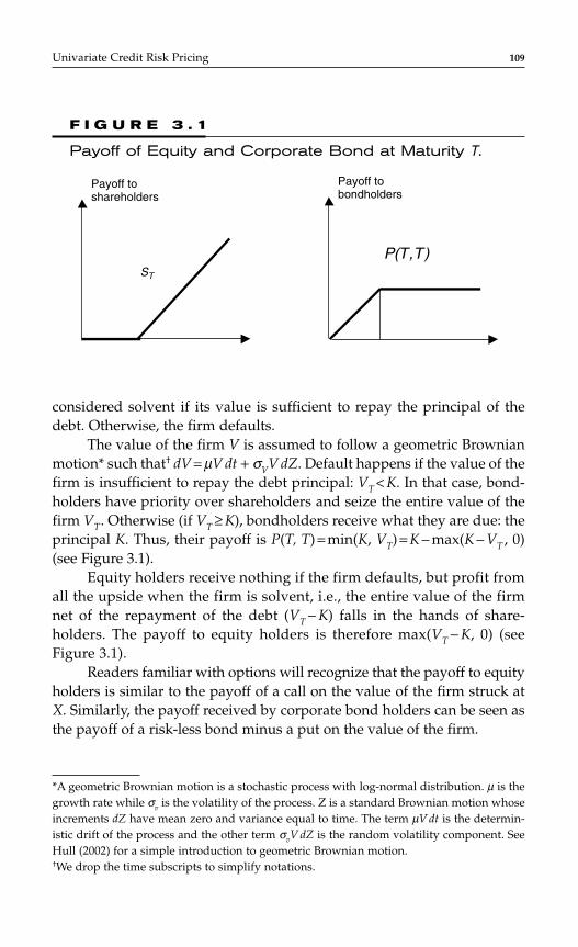
considered solvent if its value is sufficient to repay the principal of thedebt. Otherwise, the firm defaults.
The value of the firm V is assumed to follow a geometric Brownianmotion* such that† dV = µV dt + σVV dZ. Default happens if the value of thefirm is insufficient to repay the debt principal: VT < K. In that case, bond-holders have priority over shareholders and seize the entire value of thefirm VT. Otherwise (if VT ≥ K), bondholders receive what they are due: theprincipal K. Thus, their payoff is P(T, T) = min(K, VT) = K − max(K − VT , 0)(see Figure 3.1).
Equity holders receive nothing if the firm defaults, but profit fromall the upside when the firm is solvent, i.e., the entire value of the firmnet of the repayment of the debt (VT − K) falls in the hands of share-holders. The payoff to equity holders is therefore max(VT − K, 0) (seeFigure 3.1).
Readers familiar with options will recognize that the payoff to equityholders is similar to the payoff of a call on the value of the firm struck atX. Similarly, the payoff received by corporate bond holders can be seen asthe payoff of a risk-less bond minus a put on the value of the firm.
Univariate Credit Risk Pricing 109
),( TTP
Payoff toshareholders
ST
Payoff tobondholders
F I G U R E 3 . 1
Payoff of Equity and Corporate Bond at Maturity T.
*A geometric Brownian motion is a stochastic process with log-normal distribution. µ is thegrowth rate while σv is the volatility of the process. Z is a standard Brownian motion whoseincrements dZ have mean zero and variance equal to time. The term µV dt is the determin-istic drift of the process and the other term σvV dZ is the random volatility component. SeeHull (2002) for a simple introduction to geometric Brownian motion.†We drop the time subscripts to simplify notations.
110 CHAPTER 3
Merton (1974) makes the same assumptions as Black and Scholes(1973), and the call and the put can be priced using option prices derivedin Black–Scholes.
For example, the call (equity) is immediately obtained as:
(28)
with and N(⋅) denoting thecumulative normal distribution and r the constant risk-less interest rate.
From Risk-Neutral Probabilities to Spreads
The firm value approach suffers from several theoretical shortcomingslike the fact that the evolution of the value of the firm usually follows adiffusion process that does not allow for unexpected default.
What is more important from the point of view of practitioners isto evaluate whether a structural model can help them to derive pricesfor credit instruments such as defaultable debt or credit default swaps(CDSs). A particular area of focus is short-term credit spreads, as in thetraditional structural setup the probability of a firm to default in theshort term is zero, leading to zero initial credit spreads. We review var-ious approaches and assess whether they can provide realistic results.
The Capital Asset Pricing Model (CAPM) ApproachIn Chapter 2, we have mainly focused on historical probabilities of default,i.e., probabilities estimated on historical data. However, for pricing pur-poses (for the calculation of spreads), one needs to estimate risk-neutralprobabilities. Here, we show a customary way to obtain spreads from his-torical probabilities: a similar calculation is used by the firm MKMV(Moody’s KMV) and many banks (see, e.g., McNulty and Levin, 2000).
Recall that the cumulative default probability (historical probability)for a firm i (HPi
t) is defined as the probability of default at the horizon tunder the historical measure P. In the MKMV (model, this corresponds totheir expected default frequency.
We now introduce the risk-neutral probability, RNPit, which is the
equivalent probability under the risk-neutral measure Q (see Appendix 1).Under Q, all assets drift at the risk-free rate and therefore one should sub-stitute r for µi in the dynamics of the value of the firm.*
k V X r T t T tt V V= + − − −(ln( / ) ( )( )) / ( )12
2σ σ
S V N k T t Ke N kt tr T t= + − − − −( ) ( ),( )σ ν
*That is, we have dAt = rAt dt + σAt dWt under Q and dAt = µAt dt + σAt dW*t under P.
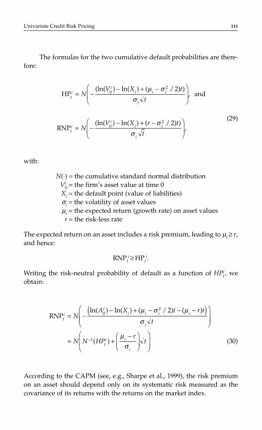
The formulas for the two cumulative default probabilities are there-fore:
(29)
with:
N(⋅) = the cumulative standard normal distributionVi
0 = the firm’s asset value at time 0Xi = the default point (value of liabilities)σi = the volatility of asset valuesµi = the expected return (growth rate) on asset valuesr = the risk-less rate
The expected return on an asset includes a risk premium, leading to µi ≥ r,and hence:
RNPti ≥ HPt
i.
Writing the risk-neutral probability of default as a function of HPit , we
obtain:
(30)
According to the CAPM (see, e.g., Sharpe et al., 1999), the risk premiumon an asset should depend only on its systematic risk measured as thecovariance of its returns with the returns on the market index.
RNPln( ) ln( ) ( / ) ( )
( )
ti
ii i i i
i
ti i
i
NA X t r t
t
N N HPr
t
= −− + − − −( )
= +−
−
02
1
2µ σ µ
σ
µσ
HP(ln( ) ln( ) ( / ) )
, and
RNP(ln( ) ln( ) ( / ) )
,
ti
ii i i
i
ti
ii i
i
NV X t
t
NV X r t
t
= −− + −
= −− + −
02
02
2
2
µ σσ
σσ
Univariate Credit Risk Pricing 111
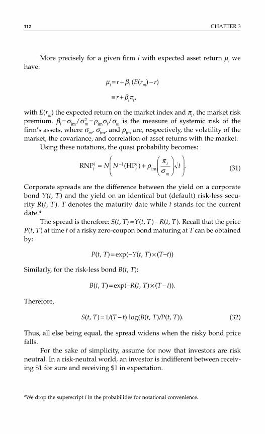
112 CHAPTER 3
More precisely for a given firm i with expected asset return µi wehave:
µi = r + βi (E(rm) − r)
≡ r + βiπt,
with E(rm) the expected return on the market index and πt, the market riskpremium. βi = σim/σ 2
m = ρimσi/σm is the measure of systemic risk of thefirm’s assets, where σm, σim, and ρim are, respectively, the volatility of themarket, the covariance, and correlation of asset returns with the market.
Using these notations, the quasi probability becomes:
(31)
Corporate spreads are the difference between the yield on a corporatebond Y(t, T ) and the yield on an identical but (default) risk-less secu-rity R(t, T ). T denotes the maturity date while t stands for the currentdate.*
The spread is therefore: S(t, T) = Y(t, T ) − R(t, T ). Recall that the priceP(t, T ) at time t of a risky zero-coupon bond maturing at T can be obtainedby:
P(t, T) = exp(−Y(t, T) × (T−t))
Similarly, for the risk-less bond B(t, T):
B(t, T) = exp(−R(t, T) × (T − t)).
Therefore,
S(t, T) = 1/(T − t) log(B(t, T)/P(t, T)). (32)
Thus, all else being equal, the spread widens when the risky bond pricefalls.
For the sake of simplicity, assume for now that investors are riskneutral. In a risk-neutral world, an investor is indifferent between receiv-ing $1 for sure and receiving $1 in expectation.
RNP (HP ) .imti
ti t
m
N N t= +
−1 ρ
πσ
*We drop the superscript i in the probabilities for notational convenience.
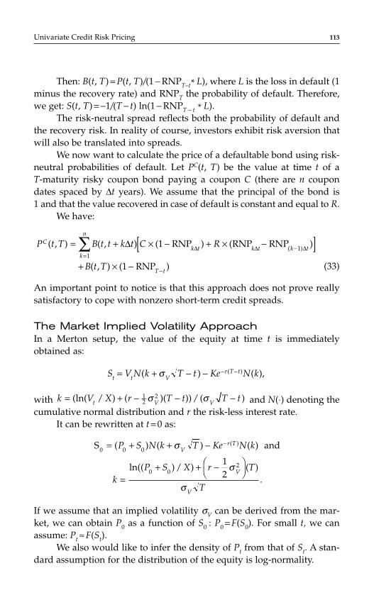
Then: B(t, T) = P(t, T)/(1 − RNPT−t* L), where L is the loss in default (1minus the recovery rate) and RNPT the probability of default. Therefore,we get: S(t, T) = −1/(T − t) ln(1 − RNPT − t * L).
The risk-neutral spread reflects both the probability of default andthe recovery risk. In reality of course, investors exhibit risk aversion thatwill also be translated into spreads.
We now want to calculate the price of a defaultable bond using risk-neutral probabilities of default. Let PC(t, T) be the value at time t of aT-maturity risky coupon bond paying a coupon C (there are n coupondates spaced by ∆t years). We assume that the principal of the bond is1 and that the value recovered in case of default is constant and equal to R.
We have:
(33)
An important point to notice is that this approach does not prove reallysatisfactory to cope with nonzero short-term credit spreads.
The Market Implied Volatility ApproachIn a Merton setup, the value of the equity at time t is immediatelyobtained as:
with and N(⋅) denoting thecumulative normal distribution and r the risk-less interest rate.
It can be rewritten at t = 0 as:
If we assume that an implied volatility σV can be derived from the mar-ket, we can obtain P0 as a function of S0 : P0 = F(S0). For small t, we canassume: Pt ≈ F(St).
We also would like to infer the density of Pt from that of St. A stan-dard assumption for the distribution of the equity is log-normality.
S0 = + + −
=+ + −
−( ) ( ) ( ) and
ln(( ) / ) ( ).
( )P S N k T Ke N k
kP S X r T
T
Vr T
V
V
0 0
0 021
2
σ
σ
σ
k V X r T t T tt V V= + − − −(ln( / ) ( )( )) / ( )12
2σ σ
S V N k T t Ke N kt t Vr T t= + − − − −( ) ( ),( )σ
P t T B t t k t C R
B t T
Ck t k t k t
k
n
T t
( , ) ( , ) ( RNP ) (RNP RNP )
( , ) ( RNP )
( )= + × − + × −[ ]+ × −
−=
−
∑ ∆ ∆ ∆ ∆1
1
11
Univariate Credit Risk Pricing 113
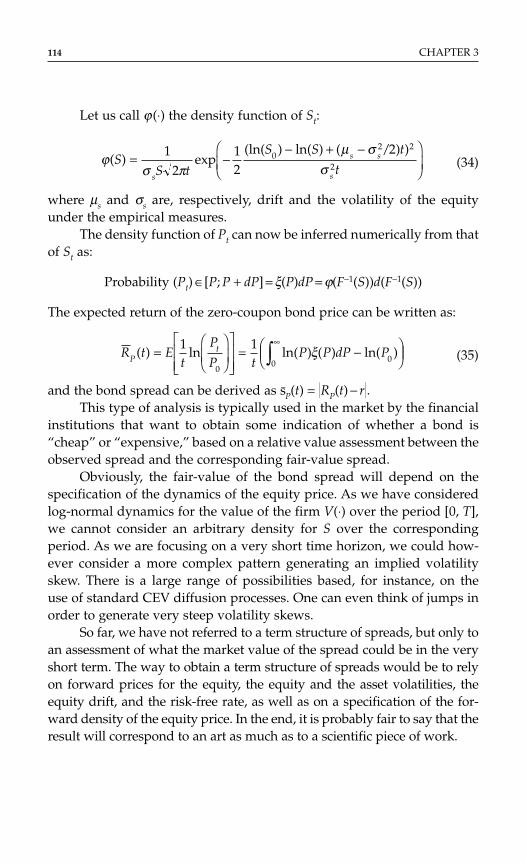
114 CHAPTER 3
Let us call ϕ (⋅) the density function of St:
(34)
where µs and σs are, respectively, drift and the volatility of the equityunder the empirical measures.
The density function of Pt can now be inferred numerically from thatof St as:
Probability (Pt) ∈[P; P + dP] = ξ(P)dP = ϕ(F−1(S))d(F−1(S))
The expected return of the zero-coupon bond price can be written as:
(35)
and the bond spread can be derived as s–P(t) = RP(t) − r.This type of analysis is typically used in the market by the financial
institutions that want to obtain some indication of whether a bond is“cheap” or “expensive,” based on a relative value assessment between theobserved spread and the corresponding fair-value spread.
Obviously, the fair-value of the bond spread will depend on thespecification of the dynamics of the equity price. As we have consideredlog-normal dynamics for the value of the firm V(⋅) over the period [0, T],we cannot consider an arbitrary density for S over the correspondingperiod. As we are focusing on a very short time horizon, we could how-ever consider a more complex pattern generating an implied volatilityskew. There is a large range of possibilities based, for instance, on theuse of standard CEV diffusion processes. One can even think of jumps inorder to generate very steep volatility skews.
So far, we have not referred to a term structure of spreads, but only toan assessment of what the market value of the spread could be in the veryshort term. The way to obtain a term structure of spreads would be to relyon forward prices for the equity, the equity and the asset volatilities, theequity drift, and the risk-free rate, as well as on a specification of the for-ward density of the equity price. In the end, it is probably fair to say that theresult will correspond to an art as much as to a scientific piece of work.
R t Et
P
P tP P dP PP
t( ) ln ln( ) ( ) ln( )=
= −
∞
∫1 1
000
ξ
ϕσ π
µ σσ
( ) exp(ln( ) ln( ) ( / ) )
SS t
S S t
ts
s s
s
= −− + −
1
212
202 2
2
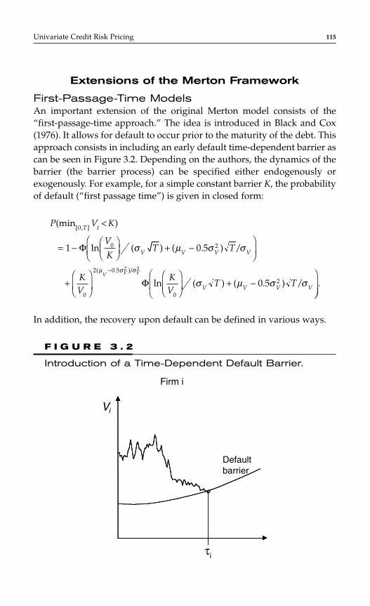
Extensions of the Merton Framework
First-Passage-Time ModelsAn important extension of the original Merton model consists of the“first-passage-time approach.” The idea is introduced in Black and Cox(1976). It allows for default to occur prior to the maturity of the debt. Thisapproach consists in including an early default time-dependent barrier ascan be seen in Figure 3.2. Depending on the authors, the dynamics of thebarrier (the barrier process) can be specified either endogenously orexogenously. For example, for a simple constant barrier K, the probabilityof default (“first passage time”) is given in closed form:
In addition, the recovery upon default can be defined in various ways.
P V K
V
KT T
KV
KV
T T
T t
V V V V
V V V V
V V V
(min )
ln ( ) ( . ) /
ln ( ) ( . ) /
[ , ]
( . )/
0
0 2
0
2 0 5
0
2
1 0 5
0 5
2 2
<
= −
+ −
+
+ −
−
Φ
Φ
σ µ σ σ
σ µ σ σµ σ σ
.
Univariate Credit Risk Pricing 115
τi
Vi
Defaultbarrier
Firm i
F I G U R E 3 . 2
Introduction of a Time-Dependent Default Barrier.
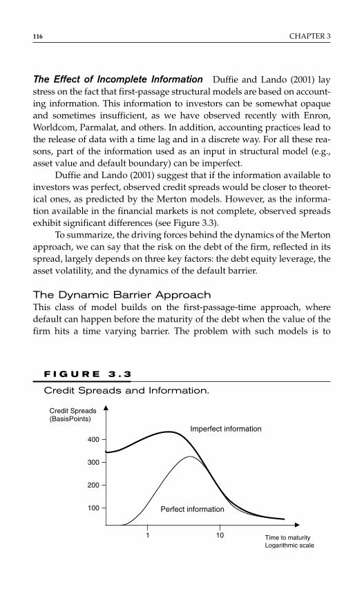
The Effect of Incomplete Information Duffie and Lando (2001) laystress on the fact that first-passage structural models are based on account-ing information. This information to investors can be somewhat opaqueand sometimes insufficient, as we have observed recently with Enron,Worldcom, Parmalat, and others. In addition, accounting practices lead tothe release of data with a time lag and in a discrete way. For all these rea-sons, part of the information used as an input in structural model (e.g.,asset value and default boundary) can be imperfect.
Duffie and Lando (2001) suggest that if the information available toinvestors was perfect, observed credit spreads would be closer to theoret-ical ones, as predicted by the Merton models. However, as the informa-tion available in the financial markets is not complete, observed spreadsexhibit significant differences (see Figure 3.3).
To summarize, the driving forces behind the dynamics of the Mertonapproach, we can say that the risk on the debt of the firm, reflected in itsspread, largely depends on three key factors: the debt equity leverage, theasset volatility, and the dynamics of the default barrier.
The Dynamic Barrier ApproachThis class of model builds on the first-passage-time approach, wheredefault can happen before the maturity of the debt when the value of thefirm hits a time varying barrier. The problem with such models is to
116 CHAPTER 3
400
300
200
100
Imperfect information
Credit Spreads(BasisPoints)
1 10 Time to maturityLogarithmic scale
Perfect information
F I G U R E 3 . 3
Credit Spreads and Information.
define a specification for the time-dependent barrier that allows fortractable pricing solutions.
The CreditGrades Approach Finger et al. (2002) propose a fair valuespread estimator (CreditGrades) more refined than the MKMV one. Inorder to allow for non-zero spreads at the beginning of the life of a CDS, themodel assumes a stochastic barrier driven by a log-normally distributedstochastic recovery rate.
Assuming zero drift, the authors show that it is then possible toderive the risk-neutral probability of default of the obligor in a simple way:
with Xˆ i being the mean value of the new barrier depending on the meanrecovery value and vari a time-dependent element derived from the vari-ance term of the Brownian component of the geometric Brownian motioncharacterizing the asset value of the firm, complemented with the varianceof the recovery. As a result, initially as time is zero or close to zero, the variterm differs from zero and the risk-neutral probability remains strictly pos-itive. This in turn justifies the existence of a nonzero initial spread.
The spread can be derived as in the previous paragraph. The authorsdescribe a closed form solution in the case of a continuously compoundedspread.
This model has become a market standard in particular because ofits tractability. It however relies on an ad hoc hypothesis on recovery thatis difficult to validate empirically and that positions the model at theboundary of structural models.
The Safety Barrier Approach Brigo and Tarenghi (2005) suggest toconsider a “safety barrier” that is defined as the product of the barrier atthe maturity of the debt and a discount factor derived from an adjusteddrift extracted from the geometric Brownian motion corresponding to theasset return of the firm. The risk-neutral drift is adjusted in the sense thatit includes a parameter β whose main role is to vary the steepness of thesafety barrier by reinforcing the effect of the volatility. Based on this choice,they derive analytically the risk-neutral survival probability of the firm. By
RNPln( ) ln( ˆ )
varvar /
ˆ
ln( ) ln( ˆ )
varvar /
ti
ii
ii
i
i
ii
ii
NV X
V
XN
V X
=−( )
−
− −−( )
−
0
0 0
2
2
Univariate Credit Risk Pricing 117
118 CHAPTER 3
assuming a deterministic risk-free rate and an equivalence between theequity and the firm value volatilities, they can ultimately infer in astraightforward manner the price of a CDS at time 0.
To start with, the authors assume a diffusion process for the dynam-ics of the value of the firm under the risk-neutral measure, with time-dependent risk-free rate, payout ratio, and asset volatility.
The expression of the “safety barrier” H (t) is related to the default thresh-old H
(36)
τ is the first time when V hits H
τ = inf t ≥ 0: Vt ≤ H(t).
The survival probability is given in a closed form way:
(37)
Under deterministic interest rates, the value at time 0 of a CDS betweentimes Ta and Tb corresponding to two payment date of the installments,with a fixed running amount per period R and fixed LGD can easily beinferred as:
with P(0, t) the zero-coupon bond at time 0 for maturity t.As can be seen, the pricing of the CDS will depend on the definition
of V0/H, the asset volatility that is approximated by the equity volatilityand the barrier curvature parameter β.
CDS ( , , LGD) ( , ) ( )
LGD ( , ) ( )
,T Ti a
b
i i i
T
T
a b
a
b
R R P T Q T
P t dQ t
0 0
0
1
= − ≥
− >
= +∑
∫
α τ
τ
Q T
V
Hds
ds
HV
HV
ds
ds
s
T
s
T
s
T
s
T
ln ln
τβ σ
σ
β σ
σ
β
> =+
−
+
∫∫
∫
∫Φ Φ
0 2
0
2
0
0
2
0
2
0
2
0
ˆ ( ) exp ( )H t H q r dss ss
t= − − + +
∫ 1 22
2
0β
σ
dV
Vr q dt dWt
tt t t t= − +( ) σ

The authors calibrate* their model with V0/H = 2 and β = 0.5. Withthis calibration, they show that they are able to provide a calibration of theCDS on Vodafone with results quite close to those derived from an inten-sity model.
This paper looks quite promising in the sense that it leads totractable results while providing some intuition in terms of rational eco-nomic interpretation.
The Structural Approach Blended with a Jump-Diffusion Process to Model the Evolution of the FirmThe pioneer article related to jump-diffusion structural models is Zhou(2001).
We can write the evolution of the value of the firm as the sum of adiffusion process and a compound Poisson jump process Z. c is theproduct of the arrival intensity of the Poisson process by the mean jumpsize.
(38)
Zhou (2001) is able to derive a closed form expression of the risk-neutralprobability of default.
There are some technical difficulties to calibrate such a model:
♦ Asset returns are not observable♦ A proxy is to rely on equity return or on an index return, but
this calibration needs to be transformed from the real to the risk-neutral probability measure and as the market is not complete,there is no unique solution to the problem.
Huang and Huang (2003) go through the process of calibrating ajump-diffusion process in a structural framework. Their finding is thateven when introducing a jump term, pure credit risk cannot account forthe observed level of credit spread. The only way to reach such level
dV
Vr c dt dW dZt
tt t= − − + +( )γ σ
Univariate Credit Risk Pricing 119
*Brigo and Tarenghi (2005) suggest to link the ratio of the initial value of the firm to the bar-rier to expected recovery. I.e., we have dAt = rAt dt + σAt dWt under Q and dAt = µAt + σAtdWt*under P.

would be by forcing parameters into the model that lack empiricalsupport.
Hybrid Models: A Discussion Around the Equity-to-Credit ParadigmIn this section, we discuss new approaches to the pricing of credit instru-ment based on the cocalibration with equity products. This is summarizedas the “equity-to-credit paradigm” that attempts to grasp the complexityof the full spectrum of securities issued by or related to a single name in aconsistent framework. It results from the need to price consistently equityproducts such as options, credit instruments such as bonds and CDSs, andhybrid securities such as convertible bonds. The intuitive idea is simple.The prices of out-of-the-money put must say something about the proba-bility of default of the issuer, and reciprocally the credit standing revealedby the term structure of CDS spreads should impact the implied volatilitysmile. The joint calibration of different classes of assets related to a singlename is often viewed as a complex and distant challenge. We argue insteadthat a large set of available market data provides a great opportunityto extract precise information on a single name. This nice feature of singlename modeling is in sharp contrast with multiname problems such asCDO pricing, where there is less hope of finding enough instruments to cal-ibrate precisely a correlation structure for hundreds of names. As a result,multiname pricing is limited to educated guesses and statistical inferencefrom past data. The calibration of single name models has the luxury to relyon a large set of forward looking derivative prices. The challenge is to pro-pose models that are capable of handling this rich source of information.We review why both standard structural models and simple reduced-formmodels fail and propose a new class of regime-based models, versatileenough to handle most situations in a numerically tractable way.
Structural Models
As we have seen earlier, structural models attempt to explain the pricedynamics of the instruments related to a single name, the so-called equity-to-credit universe, by making use of the available information on the capitalstructure of the firm. Default is triggered when the assets of the company fallbelow some critical threshold. The value of the company’s assets is the onlystate variable, and the price of every security is derived from its process andits relation to the critical threshold. From their introduction by Merton in1974, these models have been continuously refined but have kept the same
120 CHAPTER 3

philosophy. The most advanced refinements introduce complex jointdynamics for the value of the assets and the critical default threshold. Jumpsfor instance, either in the asset value or in the threshold itself, make it pos-sible for a firm to fall into default at every instant. This is a much-needed fea-ture as otherwise default would always be predictable and short-term CDSspread should consequently be close to zero, a clear empirical contradiction.
The main problem with structural models is their inability to repro-duce the observed prices of the equity-to-credit instruments. By tweakingthe volatility parameter of the asset value process, for instance, it is possi-ble to account for the observed term structure of CDS spreads. Such cali-bration exercise is however limited to a single asset class. The tweakedmodel will, in general, fail to reproduce the observed term structure of at-the-money implied volatilities, let alone the entire smile across strikes andmaturities or the prices of critical exotic derivatives such as barrier or for-ward starting options.
It is important to understand why the shortcoming of the struc-tural model is not marginal. Its inability to calibrate the equity-to-credituniverse is fundamental and cannot be dealt with by a few adjustmentson the underlying process. The reason is rather obvious: corporate life isa complex process that cannot be summarized in a one-dimensional pro-cess. A trader with equity and credit exposures knows intuitively thatthe stock price is not the only variable which affects his P&L (Profit andLoss). At the minimum, he is equally concerned with the volatility andthe evolution of the spread. These risk dimensions, although clearly cor-related with the stock price, cannot be reduced to a one-dimensionalproblem. The critical weakness of structural models is to assume that thevalue of every security linked to an issuer is a function of the assets ofthe company alone. The empirical reality presents a much more complexpicture.
Simple scatter plots of CDS spread or implied volatility against stockprice show the gap that often exists between the structural theory and theempirical evidence. Figures 3.4 and 3.5 show, respectively, the five-yearCDS spread and the one-year ATM implied volatility as a function of spotfor the firm Accor from April 2003 to December 2005. Structural theorypredicts that both the spread and the implied volatility should be decreas-ing functions of the spot price.
Not only is it clear that in many situations the price dynamics ofequity-to-credit securities cannot be reduced to a one-dimensional manifold,but in some critical cases the structural models fail to grasp the sign of thecorrelations. Structural models view the equity as a call written on the assetsof the company whose value decreases with the value of the assets. As the
Univariate Credit Risk Pricing 121
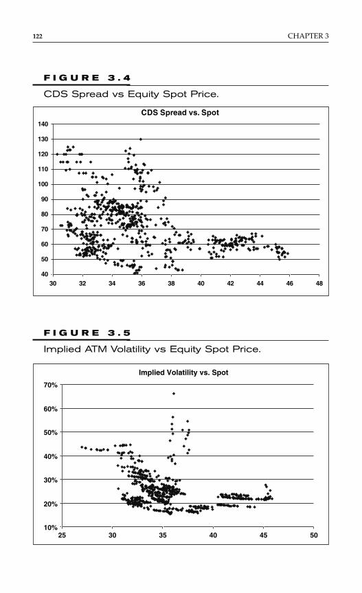
122 CHAPTER 3
CDS Spread vs. Spot
40
50
60
70
80
90
100
110
120
130
140
30 32 34 36 38 40 42 44 46 48
F I G U R E 3 . 4
CDS Spread vs Equity Spot Price.
10%
20%
30%
40%
50%
60%
70%
25 30 35 40 45 50
Implied Volatility vs. Spot
F I G U R E 3 . 5
Implied ATM Volatility vs Equity Spot Price.
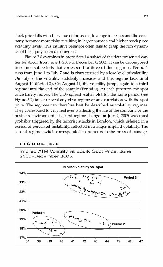
Univariate Credit Risk Pricing 123
stock price falls with the value of the assets, leverage increases and the com-pany becomes more risky resulting in larger spreads and higher stock pricevolatility levels. This intuitive behavior often fails to grasp the rich dynam-ics of the equity-to-credit universe.
Figure 3.6 examines in more detail a subset of the data presented ear-lier for Accor, from June 1, 2005 to December 8, 2005. It can be decomposedinto three subperiods that correspond to three distinct regimes. Period 1runs from June 1 to July 7 and is characterized by a low level of volatility.On July 8, the volatility suddenly increases and this regime lasts untilAugust 10 (Period 2). On August 11, the volatility jumps again to a thirdregime until the end of the sample (Period 3). At each juncture, the spotprice barely moves. The CDS spread scatter plot for the same period (seeFigure 3.7) fails to reveal any clear regime or any correlation with the spotprice. The regimes can therefore best be described as volatility regimes.They correspond to very real events affecting the life of the company or thebusiness environment. The first regime change on July 7, 2005 was mostprobably triggered by the terrorist attacks in London, which ushered in aperiod of perceived instability, reflected in a larger implied volatility. Thesecond regime switch corresponded to rumours in the press of manage-
24%
23%
22%
21%
20%
19%
18%
17%37 38 39 40 41 42 43 44 45 46 47
Period 1
Period 3
Period 2
Implied Volatility vs. Spot
F I G U R E 3 . 6
Implied ATM Volatility vs Equity Spot Price: June2005–December 2005.
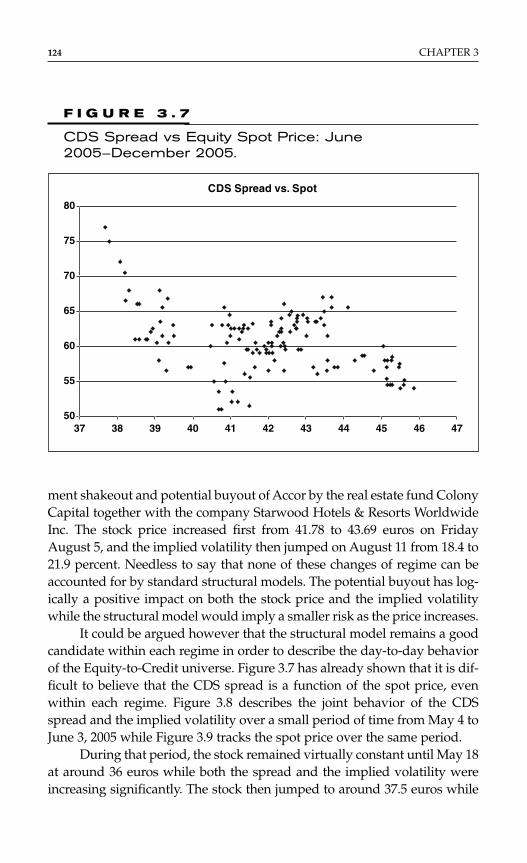
124 CHAPTER 3
ment shakeout and potential buyout of Accor by the real estate fund ColonyCapital together with the company Starwood Hotels & Resorts WorldwideInc. The stock price increased first from 41.78 to 43.69 euros on FridayAugust 5, and the implied volatility then jumped on August 11 from 18.4 to21.9 percent. Needless to say that none of these changes of regime can beaccounted for by standard structural models. The potential buyout has log-ically a positive impact on both the stock price and the implied volatilitywhile the structural model would imply a smaller risk as the price increases.
It could be argued however that the structural model remains a goodcandidate within each regime in order to describe the day-to-day behaviorof the Equity-to-Credit universe. Figure 3.7 has already shown that it is dif-ficult to believe that the CDS spread is a function of the spot price, evenwithin each regime. Figure 3.8 describes the joint behavior of the CDSspread and the implied volatility over a small period of time from May 4 toJune 3, 2005 while Figure 3.9 tracks the spot price over the same period.
During that period, the stock remained virtually constant until May 18at around 36 euros while both the spread and the implied volatility wereincreasing significantly. The stock then jumped to around 37.5 euros while
CDS Spread vs. Spot
80
75
70
65
60
55
5037 38 39 40 41 42 43 44 45 46 47
F I G U R E 3 . 7
CDS Spread vs Equity Spot Price: June2005–December 2005.
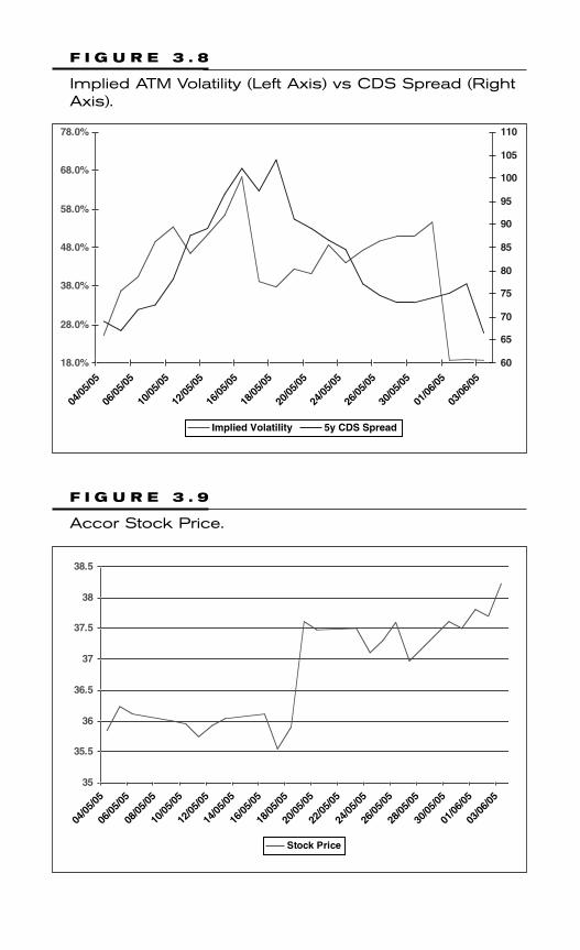
F I G U R E 3 . 8
Implied ATM Volatility (Left Axis) vs CDS Spread (RightAxis).
18.0%
28.0%
38.0%
48.0%
58.0%
68.0%
78.0%
04/05
/05
06/05
/05
10/05
/05
12/05
/05
16/05
/05
18/05
/05
20/05
/05
24/05
/05
26/05
/05
30/05
/05
01/06
/05
03/06
/05
60
65
70
75
80
85
90
95
100
105
110
Implied Volatility 5y CDS Spread
35
35.5
36
36.5
37
37.5
38
38.5
04/05
/05
06/05
/05
08/05
/05
10/05
/05
12/05
/05
14/05
/05
16/05
/05
18/05
/05
20/05
/05
22/05
/05
24/05
/05
26/05
/05
28/05
/05
30/05
/05
01/06
/05
03/06
/05
Stock Price
F I G U R E 3 . 9
Accor Stock Price.

both the spread and the implied volatility went back to their original values.Traders who would have hedged their credits or volatility position on Accorin the first two weeks of May 2005 with the underlying alone according toa structural model would have been widely off the mark.
Reduced-form Equity to Credit Models
A reduced-form model is sometimes seen as an attempt to alleviate themost striking shortcoming of the structural model: the fact that the defaultevent itself is triggered by the stock price. In its standard formulation, a typ-ical reduced-form model often keeps the stock price as the only explanatoryvariable for the entire equity-to-credit universe but for one event, which isthe time of default. Default is seen as an exogenous and unexplained eventthat may occur anytime according to a Poisson process. The intensity of thisprocess, just like the instantaneous volatility of the stock price, may itself bea function of time and spot. The state space is therefore expanded from thestock price alone (as in structural models) to the stock price and the defaultevent in the reduced-form model. The stock price S follows a stochastic dif-ferential equation under the risk-neutral probability:
dSt / St = (rt + λ(St, t)) dt + σ (St, t) dWt − dNt
where rt is the short-term risk-free rate at time t and Nt is a Poisson processwith instantaneous intensity λ(St, t), which triggers default. We assume herefor simplicity that the stock price jumps to zero upon default. Notice that thedrift is adjusted to make sure that the stock price follows a discounted mar-tingale in the risk-neutral probability measure, as required by the absence ofarbitrage opportunity. Any derivative instrument should also earn the risk-free rate on average under the risk-neutral measure and from this we derivethe value V of any derivative security:
E[dV]/dt = rtV = ∂V/∂t + (rt + λ(St, t))S∂V/∂S + 12σ 2S2∂ 2V/∂S2 + λ(St, t)∆V
The term ∆V describes the jump in value on the derivative caused by ajump to default of the underlying. Contrary to structural models, reduced-form models do not impose any a priori structure on the local defaultintensity and volatility parameters. In practice, one seeks to calibrate thesefunctions to market data such as vanilla options and CDS.
The structural model setup fails to grasp the rich behavior of theequity-to-credit universe, because the spot price alone is too crudely a statevariable. Adding the default event to the state space is certainly welcome but
126 CHAPTER 3

is unlikely to be sufficient. Standard reduced-form models are still unable tograsp regime changes, except in the most extreme case of default. As a result,even if they manage to reproduce a smile of vanilla options and a term struc-ture of CDS at a given time, they will not properly account for the richdynamics of these objects. This in turn implies that they will produce wronghedges and that they will fail to correctly price exotic instruments.
Regime-Switching Models
The models that we have reviewed so far share the same drawback. Theyrely on a state space that is too restrictive to correctly handle the complexsituations that are common in the corporate life of a firm. Expanding thestate space from the stock price alone in the structural model to an addi-tional default state variable in the standard reduced-form model goes inthe right direction but is still too limited. Our choice of additional dimen-sions for the state space will be guided by two complementary sources,asset pricing theory on the one hand and corporate finance on the otherhand.
From advanced asset pricing theory, we know that robust pricingand hedging of equity and credit derivatives require complex models forthe stock price process with jumps, stochastic volatility with possiblyjumps on the volatility, and finally a stochastic credit dimension with a richcorrelation structure between these risk factors. This means that we needto keep track of at least two or more processes, in addition to the stockprice and the default status: a process for the instantaneous volatility andanother one for the instantaneous default intensity. A full-fledged three ormore dimensional state variable is however extremely cumbersome towork with and such complex models have so far been confined to aca-demic studies. Their calibration time is often too important to be of anyvalue for practitioners, which explains the popularity of simpler modelswhere the state space is essentially limited to the stock price. We face a dis-turbing contradiction. Asset pricing theory requires a rich state space whilenumerical tractability demands a limited number of risk dimensions.
Discrete regimes offer a nice way to solve this contradiction. We con-sider here a small number of abstract regimes: in practice, two areoften enough and three is plenty. In each regime, the stock price follows ageometric jump-diffusion process with constant parameters. Each regimeis defined by a distinct volatility, a distinct hazard rate, and distinct stockprice jumps. The switch between regimes is driven by a Markov chain incontinuous time. Default can be seen as an additional regime from which
Univariate Credit Risk Pricing 127

128 CHAPTER 3
the firm does not recover. Formally, the state space is described by thestock price and an additional discrete variable that tracks the regime anddefault status. Finally, the much needed correlation between stock price,volatility, and default risk is obtained by allowing stock price jumps ofvarious sizes when changes of regime occur. The proposed state space isboth coarse enough to remain numerically tractable and rich enough tocapture the risk dimensions called for by advanced pricing theory. It iscrucial to remark that, contrary to the stock price or the default status, thevolatility and the hazard rate are abstract variables, which are not directlyobserved. An elementary Markov chain is the simplest framework wherethese variables are stochastic with potentially rich correlation patterns.
One drawback of any regime-switching model is the absence of anyclosed form solution, which means that a calibration exercise must relyon fast numerical procedures. Luckily, the regime-switching model lendsitself to fast numerical analysis through the use of coupled partial differ-ential equations. We need to solve one backward one-dimensional gridper regime, which means that the pricing of an option with three regimesis only three times as costly as in the case of a standard jump diffusion, afar cry from the time needed to solve a full three-dimensional grid. Ineach regime i, the underlying price follows a jump-diffusion process inthe risk-neutral probability with Brownian volatility σi and some jumps ofpercentage size yij and intensity λij:
dSt / St = (rt − ∑j λijyij) dt + σi dWt + ∑j yij dNijt
We distinguish three kinds of jumps: simple price jumps within eachregime, a jump to default with a regime-dependent intensity or hazardrate, and jumps that occur together with a regime switch. The value Vi ofa derivative in regime i is a solution to a one-dimensional evolution equa-tion which results from the fact that in the absence of arbitrage every secu-rity must earn the risk-free rate in the risk-neutral probability:
The last term ∆Vij measures the jump on the value of the instrumentimplied by the corresponding jump of the underlying. For the jump todefault, we need to input here the residual value of the instrument afterdefault. In the case of a switch between regimes, ∆Vij involves the value
E dV dt r V V r Y S V S S V S
V
i t i i t j ij ij i i i
j ij ij
[ ]/ / ) / /= = ∂ ∂ − ∑ ∂ ∂ + ∂ ∂
+ ∑
t + ( λ σ
λ
12
2 2 2 2
∆
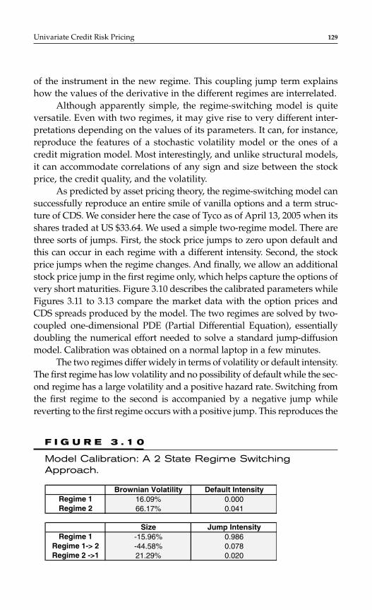
of the instrument in the new regime. This coupling jump term explainshow the values of the derivative in the different regimes are interrelated.
Although apparently simple, the regime-switching model is quiteversatile. Even with two regimes, it may give rise to very different inter-pretations depending on the values of its parameters. It can, for instance,reproduce the features of a stochastic volatility model or the ones of acredit migration model. Most interestingly, and unlike structural models,it can accommodate correlations of any sign and size between the stockprice, the credit quality, and the volatility.
As predicted by asset pricing theory, the regime-switching model cansuccessfully reproduce an entire smile of vanilla options and a term struc-ture of CDS. We consider here the case of Tyco as of April 13, 2005 when itsshares traded at US $33.64. We used a simple two-regime model. There arethree sorts of jumps. First, the stock price jumps to zero upon default andthis can occur in each regime with a different intensity. Second, the stockprice jumps when the regime changes. And finally, we allow an additionalstock price jump in the first regime only, which helps capture the options ofvery short maturities. Figure 3.10 describes the calibrated parameters whileFigures 3.11 to 3.13 compare the market data with the option prices andCDS spreads produced by the model. The two regimes are solved by two-coupled one-dimensional PDE (Partial Differential Equation), essentiallydoubling the numerical effort needed to solve a standard jump-diffusionmodel. Calibration was obtained on a normal laptop in a few minutes.
The two regimes differ widely in terms of volatility or default intensity.The first regime has low volatility and no possibility of default while the sec-ond regime has a large volatility and a positive hazard rate. Switching fromthe first regime to the second is accompanied by a negative jump whilereverting to the first regime occurs with a positive jump. This reproduces the
Univariate Credit Risk Pricing 129
Brownian Volatility Default IntensityRegime 1 16.09% 0.000Regime 2 66.17% 0.041
Size Jump IntensityRegime 1 -15.96% 0.986
Regime 1-> 2 -44.58% 0.078Regime 2 ->1 21.29% 0.020
F I G U R E 3 . 1 0
Model Calibration: A 2 State Regime SwitchingApproach.
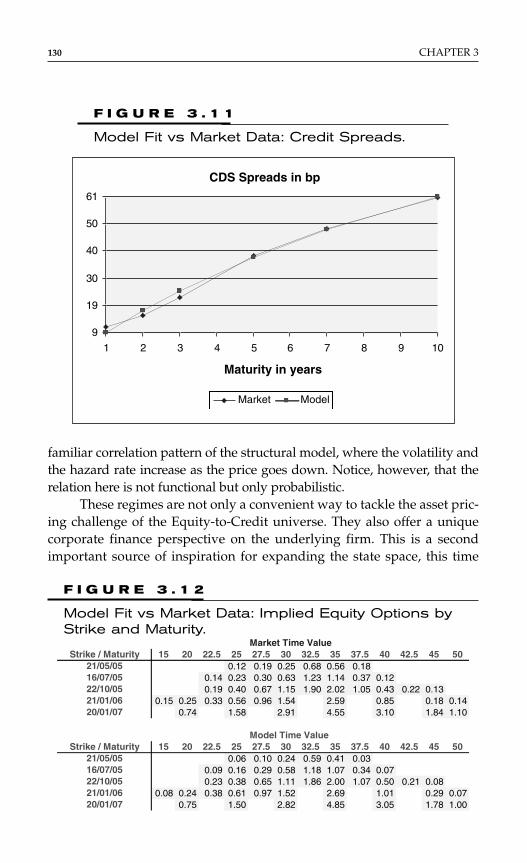
familiar correlation pattern of the structural model, where the volatility andthe hazard rate increase as the price goes down. Notice, however, that therelation here is not functional but only probabilistic.
These regimes are not only a convenient way to tackle the asset pric-ing challenge of the Equity-to-Credit universe. They also offer a uniquecorporate finance perspective on the underlying firm. This is a secondimportant source of inspiration for expanding the state space, this time
130 CHAPTER 3
CDS Spreads in bp
9
19
30
40
50
61
1 2 3 4 5 6 7 8 9 10
Maturity in years
Market Model
F I G U R E 3 . 1 1
Model Fit vs Market Data: Credit Spreads.
Market Time ValueStrike / Maturity 15 20 22.5 25 27.5 30 32.5 35 37.5 40 42.5 45 50
21/05/05 0.12 0.19 0.25 0.68 0.56 0.1816/07/05 0.14 0.23 0.30 0.63 1.23 1.14 0.37 0.1222/10/05 0.19 0.40 0.67 1.15 1.90 2.02 1.05 0.43 0.22 0.1321/01/06 0.15 0.25 0.33 0.56 0.96 1.54 2.59 0.85 0.18 0.1420/01/07 0.74 1.58 2.91 4.55 3.10 1.84 1.10
Model Time ValueStrike / Maturity 15 20 22.5 25 27.5 30 32.5 35 37.5 40 42.5 45 50
21/05/05 0.06 0.10 0.24 0.59 0.41 0.0316/07/05 0.09 0.16 0.29 0.58 1.18 1.07 0.34 0.0722/10/05 0.23 0.38 0.65 1.11 1.86 2.00 1.07 0.50 0.21 0.0821/01/06 0.08 0.24 0.38 0.61 0.97 1.52 2.69 1.01 0.29 0.0720/01/07 0.75 1.50 2.82 4.85 3.05 1.78 1.00
F I G U R E 3 . 1 2
Model Fit vs Market Data: Implied Equity Options byStrike and Maturity.
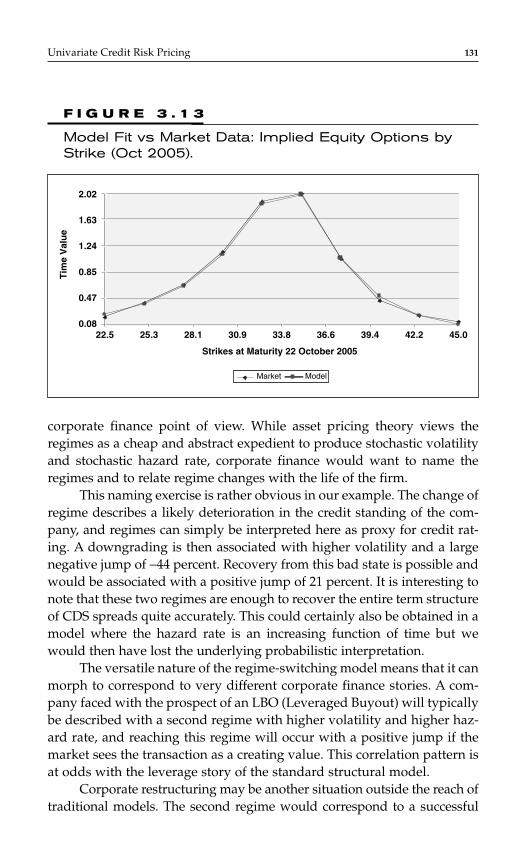
corporate finance point of view. While asset pricing theory views theregimes as a cheap and abstract expedient to produce stochastic volatilityand stochastic hazard rate, corporate finance would want to name theregimes and to relate regime changes with the life of the firm.
This naming exercise is rather obvious in our example. The change ofregime describes a likely deterioration in the credit standing of the com-pany, and regimes can simply be interpreted here as proxy for credit rat-ing. A downgrading is then associated with higher volatility and a largenegative jump of −44 percent. Recovery from this bad state is possible andwould be associated with a positive jump of 21 percent. It is interesting tonote that these two regimes are enough to recover the entire term structureof CDS spreads quite accurately. This could certainly also be obtained in amodel where the hazard rate is an increasing function of time but wewould then have lost the underlying probabilistic interpretation.
The versatile nature of the regime-switching model means that it canmorph to correspond to very different corporate finance stories. A com-pany faced with the prospect of an LBO (Leveraged Buyout) will typicallybe described with a second regime with higher volatility and higher haz-ard rate, and reaching this regime will occur with a positive jump if themarket sees the transaction as a creating value. This correlation pattern isat odds with the leverage story of the standard structural model.
Corporate restructuring may be another situation outside the reach oftraditional models. The second regime would correspond to a successful
Univariate Credit Risk Pricing 131
0.08
0.47
0.85
1.24
1.63
2.02
22.5 25.3 28.1 30.9 33.8 36.6 39.4 42.2 45.0
Strikes at Maturity 22 October 2005
Tim
e V
alu
e
Market Model
F I G U R E 3 . 1 3
Model Fit vs Market Data: Implied Equity Options byStrike (Oct 2005).

132 CHAPTER 3
restructuring of the balance sheet of the company. It would typically beassociated with a smaller hazard rate and a smaller volatility. The stockprice direction is unclear since it depends on the outcome of the negotiationbetween the various stakeholders.
Larger hazard rate should not automatically be associated withhigher volatility. A company that is the target of an acquisition could seeits shares swapped and the acquiring company may be less risky in termsof default, but more risky in terms of share price volatility. This wouldtypically be associated with a positive jump for the target company, butthis is certainly not a rule and no scenario should be a priori rejected.
In conclusion, the regime-switching model proposes an elegantanswer to three apparently contradictory requests:
♦ Asset pricing theory needs a model complex enough to graspthe securities of the equity-to-credit universe
♦ Traders want quick numerical solutions♦ Finally, corporate finance seeks to capture the significant events
of the life of the company.
No doubt that in addition to its flexibility, this type model will gen-erate heated debates between the derivatives experts and the capitalstructure specialists.
APPENDIX 1
Fundamental Theorems of Asset Pricing (FTAP) and Risk Neutral Measure
In many occasions in this book, we encounter the concept of risk-neutralmeasure and of pricing by discounted expectation. We will now summa-rize briefly the key results in this area. A more detailed and rigorous expo-sition can be found, for example, in Duffie (1996).
Intuitively, the price of a security should be related to its possiblepayoffs, to the likelihood of such payoffs, and to discount factors reflect-ing both the time value of money and investors risk aversion.
Standard pricing models such as the Dividend Discount Models usethis approach to determine the value of stocks. For derivatives, or securitieswith complex payoffs in general, there are two fundamental difficultieswith this approach:
1. To determine the actual probability of a given payoff2. To calculate the appropriate discount factor.
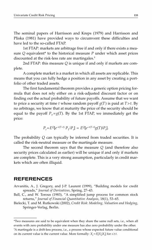
The seminal papers of Harrisson and Kreps (1979) and Harrisson andPliska (1981) have provided ways to circumvent these difficulties andhave led to the so-called FTAP.
1st FTAP: markets are arbitrage free if and only if there exists a mea-sure Q equivalent* to the historical measure P under which asset pricesdiscounted at the risk-less rate are martingales.†
2nd FTAP: this measure Q is unique if and only if markets are com-plete.
A complete market is a market in which all assets are replicable. Thismeans that you can fully hedge a position in any asset by creating a port-folio of other traded assets.
The first fundamental theorem provides a generic option pricing for-mula that does not rely either on a risk-adjusted discount factor or onfinding out the actual probability of future payoffs. Assume that we wantto price a security at time t whose random payoff g(T ) is paid at T > t. Byno arbitrage, we know that at maturity the price of the security should beequal to the payoff PT = g(T). By the 1st FTAP, we immediately get theprice:
Pt = EQ[e−r(T−t) PT|Pt] = EQ[e−r(T−t)g(T)|Pt].
The probability Q can typically be inferred from traded securities. It iscalled the risk-neutral measure or the martingale measure.
The second theorem says that the measure Q (and therefore alsosecurity prices calculated as earlier) will be unique if and only if marketsare complete. This is a very strong assumption, particularly in credit mar-kets which are often illiquid.
REFERENCESArvanitis, A., J. Gregory, and J-P. Laurent (1999), “Building models for credit
spreads,” Journal of Derivatives, Spring, 27–43.Ball, C., and W. Torous (1983), “A simplified jump process for common stock
returns,” Journal of Financial Quantitative Analysis, 18(1), 53–65.Bielecki, T. and M. Rutkowski (2002), Credit Risk: Modeling, Valuation and Hedging,
Springer-Verlag, Berlin.
Univariate Credit Risk Pricing 133
*Two measures are said to be equivalent when they share the same null sets, i.e., when allevents with zero probability under one measure has also zero probability under the other.†A martingale is a drift-less process, i.e., a process whose expected future value conditionalon its current value is the current value. More formally: Xt = E[Xs|Xt] for s ≥ t.

Black, F., and J. Cox, Valuing Corporate Securities (1976), “Some effects of bondindenture provisions,” Journal of Finance, 31, 351–367.
Black, F., and M. Scholes (1973), “The pricing of options and corporate liabilities,”Journal of Political Economy, 81, 637–659,
Brigo, D., and M. Tarenghi (2005), “Credit default swap calibration and equity swapvaluation under counterparty risk with a tractable structural model,” inProceedings of the FEA 2004 Conference at MIT, Cambridge, Massachusetts,November 8–10, and in Proceedings of the Counterparty Credit Risk 2005C.R.E.D.I.T. conference, Venice, September 22–23, 2005, Vol. 1.
Cox, J., J. Ingersoll, and S. Ross (1985), “A theory of the term structure of interestrates,” Econometrica, 53, 385–407.
Das, S., and P. Tufano (1996), “Pricing credit sensitive debt when interest rates,credit ratings and credit spreads are stochastic”, Journal of FinancialEngineering, 5, 161–198.
Duffie D. (1996), 201cDynamic Asset Pricing Theory201d, Princeton UniversityPress.
Duffie D., and Lando D. (2001), “Term structures of credit spreads with incom-plete accounting information,” Econometrica, 69, 633–664.
Duffie, D., and K. Singleton (1998), “Defaultable term structure models with frac-tional recovery at par,” working paper, Graduate School of Business,Stanford University.
Duffie, D., and K. Singleton (1999), “Modeling term structures of defaultablebonds,” Review of Financial Studies, 12, 687–720.
Finger, C., V. Finkelstein, G. Pan, J-P. Lardy, and T. Ta, (2002), CreditGrades™
Technical Document, RiskMetrics Publication.Harrison J. and D. Kreps (1979), 201cMartingale and arbitrage in multiperiod
securities markets201d, Journal of Economic Theory, 20, 348–408.Harrison J. and S. Pliska (1981), 201cMartingales and stochastic integrals in the
theory of continuous trading201d, Stochastic Processes and theirApplications, 11, 215–260.
Heath, D., R. Jarrow, and A. Morton, (1992), “Bond Pricing and the term structureof interest rates: a new methodology for contingent claims valuation,”Econometrica, 60, 77–105.
Huang, J. and M. Huang (2003), “How much of the corporate-treasury yieldspread is due to credit risk?” working paper, Penn State University.
Hull J. (2002), Options, Futures and Other Derivatives, 5th edition, PrenticeHall.
Jarrow, R., D. Lando, and S. Turnbull (1997), “A Markov model for the term struc-ture of credit risk spreads,” Review of Financial Studies, 10, 481–523.
Jobst, N., and P. J. Schönbucher (2002) “Current developments in reduced-formmodels of default risk,” working paper, Department of MathematicalSciences, Brunel University.
Jobst, N., and S. A. Zenios (2005), “On the simulation of interest rate and creditrisk sensitive securities,” European Journal of Operational Research, 161,298–324.
Kiesel, R., Perraudin, W., and Taylor, A. (2001), “The structure of credit risk: spreadvolatility and ratings transitions,” technical report, Bank of England.
134 CHAPTER 3
Kijima, Masaaki and Katsuya Komoribayashi, “A Markov chain model for valu-ing credit risk derivatives”, Journal of Derivatives, Vol. 6, Kyoto University,(Fall 1998) pp. 97–108.
Lamb R., Peretyatkin V. and Perraudin W. (2005), 201c Hedging and asset alloca-tion for structured products201d, Working Paper Imperial College.
Lando, D. (1998), “On Cox processes and credit risky securities,” Review ofDerivatives Research, 2, 99–120.
Longstaff, F., and E. Schwartz (1995) “Valuing credit derivatives,” Journal of FixedIncome, 5, 6–12.
McNulty, C., and R. Levin (2000), “Modeling credit migration,” Risk ManagementResearch Report, J.P. Morgan.
Merton, R. (1974), “On the pricing of corporate debt: The risk structure of inter-est rates,” Journal of Finance, 29, 449–470.
Moraux, F., and P. Navatte (2001), “Pricing credit derivatives in credit classesframeworks,” in Geman, Madan, Pliska, and Vorst (eds.), MathematicalFinance—Bachelier Congress 2000 Selected Papers, Springer, 339–352.
Prigent, J-L., O. Renault, and O. Scaillet (2001), “An empirical investigation intocredit spread indices,” Journal of Risk, 3, 27–55.
Sharpe W., G. Alexander and J. Bailey (1999), Investments, Prentice-Hall.Schönbucher, P. J., (2000), “A Libor market model with default risk”, working
paper, Department of Statistics, University of Bonn.Valuation of Basket Credit Derivatives in the Credit Migrations Environment by
Tomasz R. Bielecki of the Illinois Institute of Technology, St9c28ane Cr9c25yof the Universit9824'0276ry Val d’Essonne, Monique Jeanblanc of theUniversit9824'0276ry Val d’Essonne, and Alexander McNeil of the Universityof New South Wales and Warsaw University of Technology, March 30, 2005.
Zhou, C., (2001), “The term structure of credit spreads with jump risk,” Journal ofBanking and Finance, 25, 2015–2040.
Univariate Credit Risk Pricing 135

This page intentionally left blank
137
C H A P T E R 4
Modeling Credit Dependency
Arnaud de Servigny
137
INTRODUCTION
In this chapter,* we introduce multivariate effects, i.e., interactions betweencredit instruments or obligors.
The analysis of credit risk in a portfolio requires measures of depend-ency across assets. Individual spreads in the pricing world, probabilities ofdefault (PDs) and loss-given-default in the risk universe, management world,are important but insufficient to determine the price/risk of multiname prod-ucts and their entire distribution of losses. Because the diversification effectsare related to dependency, neither the price of a portfolio can be defined asa linear combination of the price of its underlying components, nor its lossdistribution can be the sum of the distributions of individual losses.
The most common measure of dependency is linear correlation.Figure 4.1 illustrates the impact of correlation on portfolio losses.† Whendefault correlation is zero, the probability of extreme events in the portfolio(large number of defaults or zero default) is low. However, when correlation
*Some elements of this chapter have been extracted from “Measuring and Managing CreditRisk” by Arnaud de Servigny and Olivier Renault, Mc Graw Hill, 2004.†Correlation here refers to factor correlation. This graph was created by using a factor modelof credit risk and assuming that there are 100 bonds in the portfolio and that the probabilityof default of all bonds is 5 percent. Maturity is one year.
Copyright © 2007 by The McGraw-Hill Companies. Click here for terms of use.
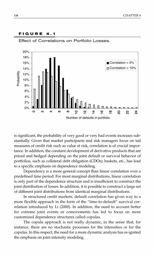
is significant, the probability of very good or very bad events increases sub-stantially. Given that market participants and risk managers focus on tailmeasures of credit risk such as value at risk, correlation is of crucial impor-tance. In addition, the constant development of derivative products that arepriced and hedged depending on the joint default or survival behavior ofportfolios, such as collateral debt obligation (CDOs), baskets, etc., has leadto a specific emphasis on dependence modeling.
Dependency is a more general concept than linear correlation over apredefined time period. For most marginal distributions, linear correlationis only part of the dependence structure and is insufficient to construct thejoint distribution of losses. In addition, it is possible to construct a large setof different joint distributions from identical marginal distributions.
In structured credit markets, default correlation has given way to amore flexible approach in the form of the “time-to-default” survival cor-relation introduced by Li (2000). In addition, the need to account betterfor extreme joint events or comovements has led to focus on morecustomized dependence structures called copulas.
The copula approach is not really dynamic, in the sense that, forinstance, there are no stochastic processes for the intensities or for thecopulas. In this respect, the need for a more dynamic analysis has re-ignitedthe emphasis on joint intensity modeling.
138 CHAPTER 4
0 2 4 6 8 10 12 14 16 18 20 22 24
0%
2%
4%
6%
8%
10%
12%
14%
16%
18%
20%
0 2 4 6 8 10 12 14 16 18 20 22 24
Correlation = 0%
Correlation = 10%
Number of defaults in portfolio
Pro
babi
lity
F I G U R E 4 . 1
Effect of Correlations on Portfolio Losses.
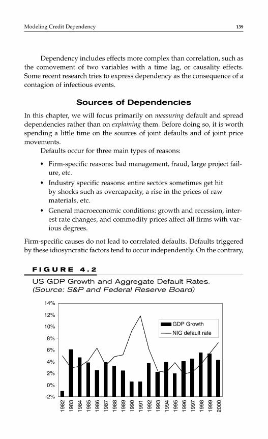
Dependency includes effects more complex than correlation, such asthe comovement of two variables with a time lag, or causality effects.Some recent research tries to express dependency as the consequence of acontagion of infectious events.
Sources of Dependencies
In this chapter, we will focus primarily on measuring default and spreaddependencies rather than on explaining them. Before doing so, it is worthspending a little time on the sources of joint defaults and of joint pricemovements.
Defaults occur for three main types of reasons:
♦ Firm-specific reasons: bad management, fraud, large project fail-ure, etc.
♦ Industry specific reasons: entire sectors sometimes get hitby shocks such as overcapacity, a rise in the prices of rawmaterials, etc.
♦ General macroeconomic conditions: growth and recession, inter-est rate changes, and commodity prices affect all firms with var-ious degrees.
Firm-specific causes do not lead to correlated defaults. Defaults triggeredby these idiosyncratic factors tend to occur independently. On the contrary,
Modeling Credit Dependency 139
1983
1984
1985
1986
1987
1988
1989
1990
1991
1992
1993
1994
1995
1996
1997
1998
1999
2000
-2%
0%
2%
4%
6%
8%
10%
12%
14%
1982
GDP Growth
NIG default rate
F I G U R E 4 . 2
US GDP Growth and Aggregate Default Rates.(Source: S&P and Federal Reserve Board)
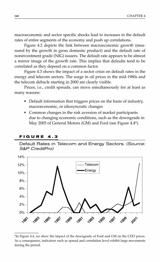
140 CHAPTER 4
1981
1983
1985
1987
1989
1991
1993
1995
1997
1999
2001
0%
2%
4%
6%
8%
10%
12%
14%
1981
1983
1985
1987
1989
1991
1993
1995
1997
1999
2001
Telecom
Energy
F I G U R E 4 . 3
Default Rates in Telecom and Energy Sectors. (Source:S&P CreditPro)
macroeconomic and sector specific shocks lead to increases in the defaultrates of entire segments of the economy and push up correlations.
Figure 4.2 depicts the link between macroeconomic growth (mea-sured by the growth in gross domestic product) and the default rate ofnoninvestment grade (NIG) issuers. The default rate appears to be almosta mirror image of the growth rate. This implies that defaults tend to becorrelated as they depend on a common factor.
Figure 4.3 shows the impact of a sector crisis on default rates in theenergy and telecom sectors. The surge in oil prices in the mid-1980s andthe telecom debacle starting in 2000 are clearly visible.
Prices, i.e., credit spreads, can move simultaneously for at least asmany reasons:
♦ Default information that triggers prices on the basis of industry,macroeconomic, or idiosyncratic changes
♦ Common changes in the risk aversion of market participantsdue to changing economic conditions, such as the downgrade inMay 2005 of General Motors (GM) and Ford (see Figure 4.4*).
*In Figure 4.4, we show the impact of the downgrade of Ford and GM on the CDO prices.As a consequence, indicators such as spread and correlation level exhibit large movementsduring the period.
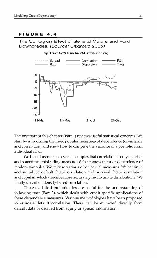
Modeling Credit Dependency 141
The first part of this chapter (Part 1) reviews useful statistical concepts. Westart by introducing the most popular measures of dependence (covarianceand correlation) and show how to compute the variance of a portfolio fromindividual risks.
We then illustrate on several examples that correlation is only a partialand sometimes misleading measure of the comovement or dependence ofrandom variables. We review various other partial measures. We continueand introduce default factor correlation and survival factor correlationand copulas, which describe more accurately multivariate distributions. Wefinally describe intensity-based correlation.
These statistical preliminaries are useful for the understanding offollowing part (Part 2), which deals with credit-specific applications ofthese dependence measures. Various methodologies have been proposedto estimate default correlation. These can be extracted directly fromdefault data or derived from equity or spread information.
-25
-20
-15
-10
-5
0
5
21-Mar 21-May 21-Jul 20-Sep
SpreadDispersion TimeRateCorrelation
5y iTraxx 0-3% tranche P&L attribution (%)
P&L
F I G U R E 4 . 4
The Contagion Effect of General Motors and FordDowngrades. (Source: Citigroup 2005)
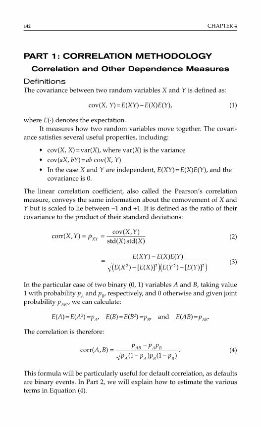
PART 1: CORRELATION METHODOLOGY
Correlation and Other Dependence Measures
DefinitionsThe covariance between two random variables X and Y is defined as:
cov(X, Y) = E(XY) − E(X)E(Y), (1)
where E(⋅) denotes the expectation.It measures how two random variables move together. The covari-
ance satisfies several useful properties, including:
♦ cov(X, X) = var(X), where var(X) is the variance♦ cov(aX, bY) = ab cov(X, Y)♦ In the case X and Y are independent, E(XY) = E(X)E(Y), and the
covariance is 0.
The linear correlation coefficient, also called the Pearson’s correlationmeasure, conveys the same information about the comovement of X andY but is scaled to lie between −1 and +1. It is defined as the ratio of theircovariance to the product of their standard deviations:
(2)
(3)
In the particular case of two binary (0, 1) variables A and B, taking value1 with probability pA and pB, respectively, and 0 otherwise and given jointprobability pAB., we can calculate:
E(A) = E(A2) = pA, E(B) = E(B2) = pB, and E(AB) = pAB.
The correlation is therefore:
(4)
This formula will be particularly useful for default correlation, as defaultsare binary events. In Part 2, we will explain how to estimate the variousterms in Equation (4).
corr( , )( ) ( )
.A Bp p p
p p p pAB A B
A A B B
=−
− −1 1
= −
−( ) −( )E XY E X E Y
E X E X E Y E Y
( ) ( ) ( )
( ) [ ( )] ( ) [ ( )]2 2 2 2
corr( , )cov( , )
std( )std( )X Y
X YX XXY= =ρ
142 CHAPTER 4

Calculating Diversification Effect in a Portfolio
Two Asset Case Let us first consider a simple case of a portfolio withtwo assets X and Y with proportions w and 1 − w, respectively. Their vari-ance and covariance are σX
2, σY2, and σXY.
The variance of the portfolio is given by
σP2 = w2σX
2 + (1 − w)2 σY2 + 2w(1 − w)σXY. (5)
The minimum variance of the portfolio can be obtained by differentiatingEquation (5) and setting the derivative equal to 0:
(6)
The optimal allocation w* is the solution to Equation (6):
(7)
We thus find the optimal allocation in both assets that minimizes the totalvariance of the portfolio. We can immediately see that the optimal alloca-tion depends on the correlation between the two assets and that theresulting variance is also affected by the correlation. Figures 4.5 and 4.6illustrate how the optimal allocation and resulting minimum portfoliovariance change as a function of correlation. In this example, σX = 0.25 andσY = 0.15.
In Figure 4.5, we can see that the allocation of the portfolio betweenX and Y is highly nonlinear in the correlation. If the two assets are highlypositively correlated, it becomes optimal to sell short the asset with high-est variance (X in our example), hence W* is negative. If the correlation is“perfect” between X and Y, that is, if ρ = 1 or ρ = −1, it is possible to createa risk-less portfolio (Figure 4.6). Otherwise, the optimal allocation w* willlead to a low but positive variance.
Figure 4.7 shows the impact of correlation on the joint density of X andY, assuming that they are standard-normally distributed. It is a snapshot ofthe bell-shaped density seen in this figure. In the case where the correlationis zero (left-hand side), the joint density looks like concentric circles. Whennonzero correlation is introduced (positive in this example), the shapebecomes elliptical: it shows that high (low) values of X tend to be associatedwith high (low) values of Y. Thus there is more probability in the top-right
w Y XY X Y
X Y XY X Y
* .=−
+ −σ ρ σ σ
σ σ ρ σ σ
2
2 2 2
∂∂
= = − + + −σ
σ σ σ σPX Y Y XYw
w w w2
2 20 2 2 2 2 1 2( )
Modeling Credit Dependency 143
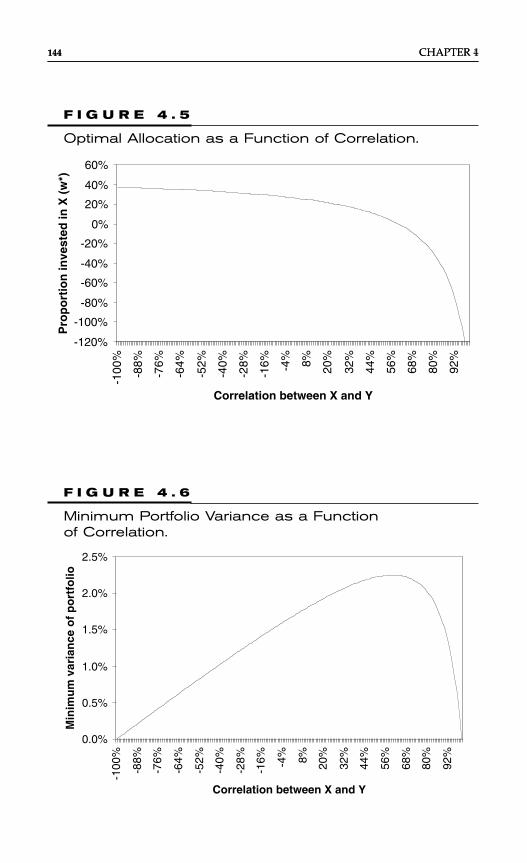
144 CHAPTER 4144 CHAPTER 1
-120%
-100%
-80%
-60%
-40%
-20%
0%
20%
40%
60%
-100
%
-88%
-76%
-64%
-52%
-40%
-28%
-16% -4
% 8% 20%
32%
44%
56%
68%
80%
92%
Correlation between X and Y
Pro
po
rtio
n in
vest
ed in
X (
w*)
F I G U R E 4 . 5
Optimal Allocation as a Function of Correlation.
0.0%
0.5%
1.0%
1.5%
2.0%
2.5%
-100
%
-88%
-76%
-64%
-52%
-40%
-28%
-16% -4
% 8% 20%
32%
44%
56%
68%
80%
92%
Min
imu
m v
aria
nce
of
po
rtfo
lio
Correlation between X and Y
F I G U R E 4 . 6
Minimum Portfolio Variance as a Functionof Correlation.
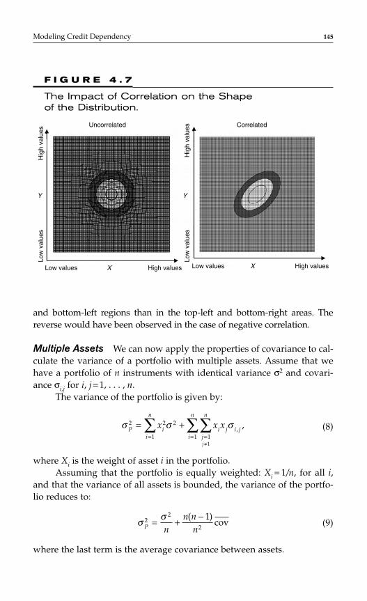
Modeling Credit Dependency 145H
igh
valu
esLo
w v
alue
s
Low values High values Low values High values
Hig
h va
lues
Low
val
ues
Uncorrelated Correlated
Y
XX
Y
F I G U R E 4 . 7
The Impact of Correlation on the Shape of the Distribution.
and bottom-left regions than in the top-left and bottom-right areas. Thereverse would have been observed in the case of negative correlation.
Multiple Assets We can now apply the properties of covariance to cal-culate the variance of a portfolio with multiple assets. Assume that wehave a portfolio of n instruments with identical variance σ2 and covari-ance σi,j for i, j = 1, . . . , n.
The variance of the portfolio is given by:
(8)
where Xi is the weight of asset i in the portfolio.Assuming that the portfolio is equally weighted: Xi = 1/n, for all i,
and that the variance of all assets is bounded, the variance of the portfo-lio reduces to:
(9)
where the last term is the average covariance between assets.
σ σP n
n nn
22
2
1= + −( )cov
σ σ σP ii
n
i j i jj
n
i
n
x x x
j
2 2
1
2
111
= += ==∑ ∑∑
≠
, ,
When the portfolio becomes more and more diversified, i.e., whenn → ∞, we have σP
2 → cov___
. The variance of the portfolio converges to theaverage covariance between assets. The variance term becomes negligiblecompared to the joint variation.
For a portfolio of stocks, diversification benefits are obtained fairlyquickly: for a correlation of 30 percent between all stocks and a volatilityof 30 percent, one is within 10 percent of the minimum covariance with naround 20. For a pure default model (i.e., when we ignore spread andtransition risk and assume 0 recovery) the number of assets necessary toreach the same level of diversification is much larger. For example, if theprobability of default and the pair-wise correlations for all obligors are 2percent, one needs around 450 counterparts to reach a variance that iswithin 10 percent of its asymptotic minimum.
Deficiencies of CorrelationAs mentioned earlier, correlation is by far the most used measure ofdependence in financial markets, and it is common to talk about correla-tion as a generic term for comovement. We will use it a lot in Section 3 ofthis chapter and in the following chapter on CDO pricing. In this section,we want to review some properties of the linear correlation that makeit insufficient as a measure of dependence in general, and misleading insome cases. This is best explained through examples.*
♦ Using Equation (2), we see immediately that correlation is notdefined if one of the variances is infinite. This is not a very fre-quent occurrence in credit risk models, but some market riskmodels exhibit this property in some cases.Example: see the large financial literature on α-stable modelssince Mandelbrot (1963), where the finiteness of the variancedepends on the value of the α parameter.
♦ When specifying a model, one cannot choose correlation arbi-trarily over [−1; 1] as a degree of freedom. Depending on thechoice of distribution, the correlation may be bounded in anarrower range , with .Example: if we have two normal random variable x and y, bothwith mean 0 and with standard deviation 1 and σ, respectively.Then X = exp(x) and Y = exp(y) are lognormally distributed.However, not all correlations between X and Y are attainable.
− < < <1 1ρ ρρ ρ;[ ]
146 CHAPTER 4
*Embrecht et al. (1999a,b) give a very clear analysis of the limitations of correlations.
One can show that their correlation is restricted to lie between:
See Embrecht et al. (1999a) for a proof.
♦ Two perfectly functionally dependent random variables canhave zero correlation.Example: Consider a normally distributed random variable Xwith mean 0 and define Y = X2. Although changes in X com-pletely determine changes in Y, they have zero correlation. Thisclearly shows that while independence implies zero correlation,the reverse is not true!
♦ Linear correlation is not invariant under monotonic transforma-tions.Example: (X, Y) and (exp(X), exp(Y)) do not have the samecorrelation.
♦ Many bivariate distributions share the same marginal distribu-tions and the same correlation but are not identical.Example: See section on copulas.
All these considerations should make clear that correlation is a partial andinsufficient measure of dependence in the general case. It only measureslinear dependence. This does not mean that correlation is useless. For theclass of elliptical distributions, correlation is sufficient to combine themarginals into the bivariate distribution. For example, given two normalmarginal distributions for X and Y and a correlation coefficient ρ, one canbuild a joint normal distribution for (X, Y).
Loosely speaking, this class of distribution is called elliptical becausewhen we project the multivariate density on a plane, we find ellipticalshapes (see Figure 4.6). The normal and the t-distribution, among others,are part of this class.
Even for other nonelliptical distributions, covariances (and thereforecorrelations) are second moments that need to be calibrated. While they areinsufficient to incorporate all dependence, they should not be neglectedwhen empirically fitting a distribution.
Other Dependence Measures: Rank CorrelationsMany other measures have been proposed to tackle the problems of lin-ear correlations mentioned earlier. We only mention two here, but thereare countless examples:
ρ ρσ
σ
σ
σ= −
− −= −
− −
−e
(e )(e )and
e
(e )(e ).
1
1 1
1
1 12 2
Modeling Credit Dependency 147
Spearman’s Rho This is simply the linear correlation but applied to theranks of the variables rather than on the variables themselves.
Kendall’s Tau Assume we have n observations for each of two randomvariables, i.e., (Xi, Yi), i = 1, . . . , n.
We start by counting the number of pairs of bivariate observationswhose components are concordant, i.e., pairs for which the two elementsare either both larger or both lower than the elements of another pair. Callthat number Nc.
Then Kendall’s Tau is calculated as:
τK = (Nc − ND)(Nc + ND),
where ND is the number of discordant (nonconcordant) pairs.Kendall’s Tau shares some properties with the linear correlation:
τK ∈ [−1, 1] and τK(X, Y) = 0 for X, Y independent. However, it has somedistinguishing features that make it more appropriate than the linearcorrelation in some cases. If X and Y are comonotonic,* then τK(X, Y) = 1;whereas if they are counter-monotonic, τK(X, Y) = −1. τK is also invariantunder strictly monotonic transformations. To return to our earlier exam-ple, τK(X, Y) = τK(exp(X), exp(Y)).
An interesting feature of Kendall’s tau is that it gives the opportu-nity to analyze comovement in a dynamic way (see Figure 4.8).
In the case of the normal distribution,† the linear and rank correla-tions can be linked analytically:
(10)
These dependence measures have nice properties but tend to be less usedby finance practitioners. Again, they are insufficient to obtain the entirebivariate distribution from the marginals. We are now going to focus on avery important class of models that accounts for correlation: factor models.
Factor Models of Credit RiskThis approach underlies portfolio models based on a structural approachof the firm. It is used in commercial portfolio credit risk models such asthose offered to the market by Risk Metrics, MKMV, and Standard &
τπ
ρK ( , ) arcsin( ( , )).X Y X Y= 2
148 CHAPTER 4
*X and Y are comonotonic if we can write Y = G(X) with G(⋅) an increasing function. They arecountermonotonic if G(⋅) is a decreasing function.†More generally, this result holds for elliptical distributions.
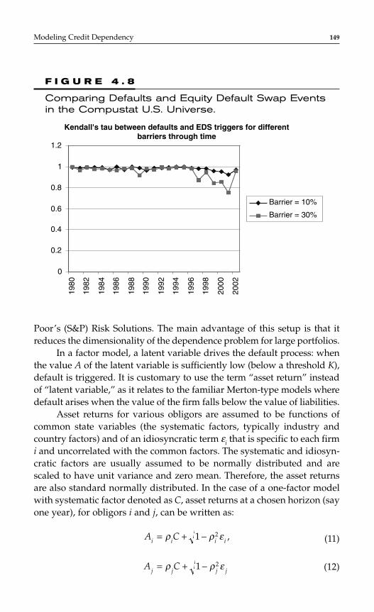
Poor’s (S&P) Risk Solutions. The main advantage of this setup is that itreduces the dimensionality of the dependence problem for large portfolios.
In a factor model, a latent variable drives the default process: whenthe value A of the latent variable is sufficiently low (below a threshold K),default is triggered. It is customary to use the term “asset return” insteadof “latent variable,” as it relates to the familiar Merton-type models wheredefault arises when the value of the firm falls below the value of liabilities.
Asset returns for various obligors are assumed to be functions ofcommon state variables (the systematic factors, typically industry andcountry factors) and of an idiosyncratic term εi that is specific to each firmi and uncorrelated with the common factors. The systematic and idiosyn-cratic factors are usually assumed to be normally distributed and arescaled to have unit variance and zero mean. Therefore, the asset returnsare also standard normally distributed. In the case of a one-factor modelwith systematic factor denoted as C, asset returns at a chosen horizon (sayone year), for obligors i and j, can be written as:
(11)
(12)A Cj j j j= + −ρ ρ ε1 2
A Ci i i i= + −ρ ρ ε1 2 ,
Modeling Credit Dependency 149
0
0.2
0.4
0.6
0.8
1
1.2
Kendall's tau between defaults and EDS triggers for differentbarriers through time
1980
1982
1984
1986
1988
1990
1992
1994
1996
1998
2000
2002
Barrier = 10%
Barrier = 30%
F I G U R E 4 . 8
Comparing Defaults and Equity Default Swap Eventsin the Compustat U.S. Universe.
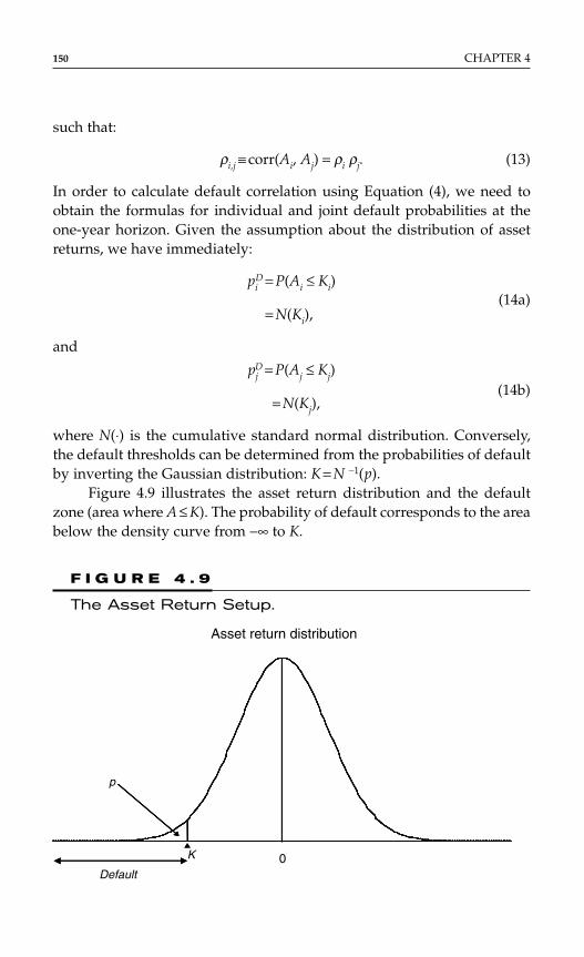
such that:
ρi,j ≡ corr(Ai, Aj) = ρi ρj. (13)
In order to calculate default correlation using Equation (4), we need toobtain the formulas for individual and joint default probabilities at theone-year horizon. Given the assumption about the distribution of assetreturns, we have immediately:
piD = P(Ai ≤ Ki)
= N(Ki),(14a)
and
pjD = P(Aj ≤ Kj)
= N(Kj),(14b)
where N(⋅) is the cumulative standard normal distribution. Conversely,the default thresholds can be determined from the probabilities of defaultby inverting the Gaussian distribution: K = N −1(p).
Figure 4.9 illustrates the asset return distribution and the defaultzone (area where A ≤ K). The probability of default corresponds to the areabelow the density curve from −∞ to K.
150 CHAPTER 4
K
p
0
Asset return distribution
Default
F I G U R E 4 . 9
The Asset Return Setup.
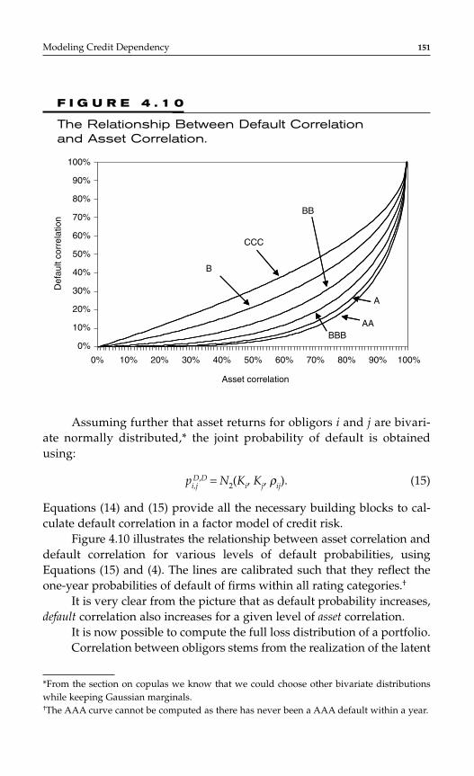
Assuming further that asset returns for obligors i and j are bivari-ate normally distributed,* the joint probability of default is obtainedusing:
pi,jD,D = N2(Ki, Kj, ρij). (15)
Equations (14) and (15) provide all the necessary building blocks to cal-culate default correlation in a factor model of credit risk.
Figure 4.10 illustrates the relationship between asset correlation anddefault correlation for various levels of default probabilities, usingEquations (15) and (4). The lines are calibrated such that they reflect theone-year probabilities of default of firms within all rating categories.†
It is very clear from the picture that as default probability increases,default correlation also increases for a given level of asset correlation.
It is now possible to compute the full loss distribution of a portfolio.Correlation between obligors stems from the realization of the latent
Modeling Credit Dependency 151
*From the section on copulas we know that we could choose other bivariate distributionswhile keeping Gaussian marginals.†The AAA curve cannot be computed as there has never been a AAA default within a year.
100%
90%
80%
70%
60%
50%
40%
30%
20%
10%
0%
100%90%80%70%60%50%40%30%20%10%0%
Asset correlation
BB
BBB
CCC
AA
B
A
Def
ault
corr
elat
ion
F I G U R E 4 . 1 0
The Relationship Between Default Correlationand Asset Correlation.
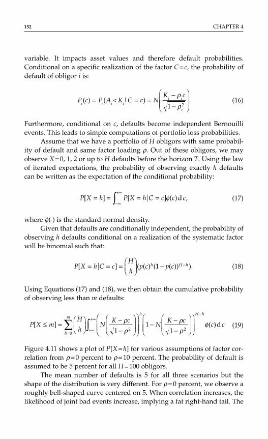
variable. It impacts asset values and therefore default probabilities.Conditional on a specific realization of the factor C = c, the probability ofdefault of obligor i is:
(16)
Furthermore, conditional on c, defaults become independent Bernouillievents. This leads to simple computations of portfolio loss probabilities.
Assume that we have a portfolio of H obligors with same probabil-ity of default and same factor loading ρ. Out of these obligors, we mayobserve X = 0, 1, 2 or up to H defaults before the horizon T. Using the lawof iterated expectations, the probability of observing exactly h defaultscan be written as the expectation of the conditional probability:
(17)
where φ(⋅) is the standard normal density.Given that defaults are conditionally independent, the probability of
observing h defaults conditional on a realization of the systematic factorwill be binomial such that:
(18)
Using Equations (17) and (18), we then obtain the cumulative probabilityof observing less than m defaults:
(19)
Figure 4.11 shows a plot of P[X = h] for various assumptions of factor cor-relation from ρ = 0 percent to ρ = 10 percent. The probability of default isassumed to be 5 percent for all H = 100 obligors.
The mean number of defaults is 5 for all three scenarios but theshape of the distribution is very different. For ρ = 0 percent, we observe aroughly bell-shaped curve centered on 5. When correlation increases, thelikelihood of joint bad events increase, implying a fat right-hand tail. The
P X mH
hN
K cN
K cc c
h
mh H h
[ ] ( )d≤ =
−−
− −
−
=−∞
+∞−
∑ ∫0
2 211
1
ρρ
ρρ
φ
P X h C cH
hp c p ch H h[ ] ( ( ) ( ( )) ).= = =
− − 1
P X h P X h C c c c[ ] [ ] ( )d ,= = = =−∞
+∞
∫ φ
P c P A K C c NK c
i i i ii i
i
( ) ( | ) .= < = =−
−
ρ
ρ1 2
152 CHAPTER 4
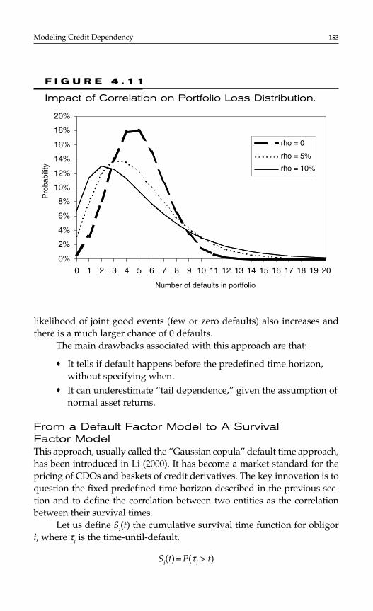
likelihood of joint good events (few or zero defaults) also increases andthere is a much larger chance of 0 defaults.
The main drawbacks associated with this approach are that:
♦ It tells if default happens before the predefined time horizon,without specifying when.
♦ It can underestimate “tail dependence,” given the assumption ofnormal asset returns.
From a Default Factor Model to A Survival Factor ModelThis approach, usually called the “Gaussian copula” default time approach,has been introduced in Li (2000). It has become a market standard for thepricing of CDOs and baskets of credit derivatives. The key innovation is toquestion the fixed predefined time horizon described in the previous sec-tion and to define the correlation between two entities as the correlationbetween their survival times.
Let us define Si(t) the cumulative survival time function for obligori, where τi is the time-until-default.
Si(t) = P(τi > t)
Modeling Credit Dependency 153
0 1 2 3 4 5 6 7 8 9 10 11 12 13 14 15 16 17 18 19 20
Pro
babi
lity
0%
2%
4%
6%
8%
10%
12%
14%
16%
18%
20%
Number of defaults in portfolio
rho = 0
rho = 5%
rho = 10%
F I G U R E 4 . 1 1
Impact of Correlation on Portfolio Loss Distribution.
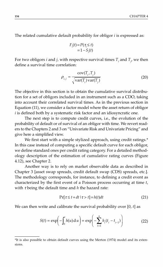
The related cumulative default probability for obligor i is expressed as:
Fi(t) = P(τi ≤ t)= 1 − Si(t)
For two obligors i and j, with respective survival times Ti and Tj, we thendefine a survival time correlation:
(20)
The objective in this section is to obtain the cumulative survival distribu-tion for a set of obligors included in an instrument such as a CDO, takinginto account their correlated survival times. As in the previous section inEquation (11), we consider a factor model where the asset return of obligori is defined both by a systematic risk factor and an idiosyncratic one.
The next step is to compute credit curves, i.e., the evolution of theprobability of default or of survival of an obligor with time. We revert read-ers to the Chapters 2 and 3 on “Univariate Risk and Univariate Pricing” andgive here a simplified view.
We first start with a simple stylized approach, using credit ratings.*In this case instead of computing a specific default curve for each obligor,we define standard ones per credit rating category. For a detailed method-ology description of the estimation of cumulative rating curves (Figure4.12), see Chapter 2.
Another way is to rely on market observable data as described inChapter 3 [asset swap spreads, credit default swap (CDS) spreads, etc.].The methodology corresponds, for instance, to defining a credit event ascharacterized by the first event of a Poisson process occurring at time t,with τ being the default time and h the hazard rate:
Pr[τ ≤ t + dt|τ > t] = h(t)dt (21)
We can then write and calibrate the survival probability over [0, t] as
(22)S t h u u h t tt
i i it
n
( ) exp ( )d exp ( )= −
= − −
∫ ∑ −
=0 1
1
ρi ji j
i j
T T
T T,
cov( , )
var( )var( )=
154 CHAPTER 4
*It is also possible to obtain default curves using the Merton (1974) model and its exten-sions.
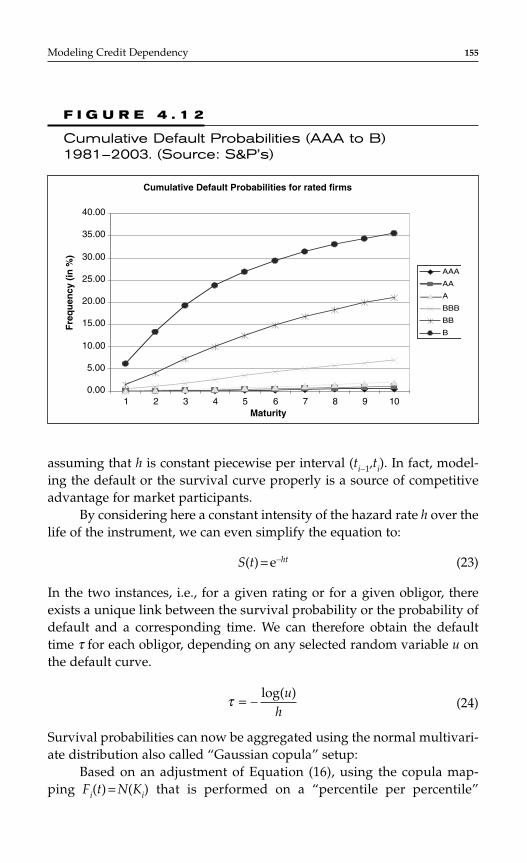
assuming that h is constant piecewise per interval (ti−1,ti). In fact, model-ing the default or the survival curve properly is a source of competitiveadvantage for market participants.
By considering here a constant intensity of the hazard rate h over thelife of the instrument, we can even simplify the equation to:
S(t) = e−ht (23)
In the two instances, i.e., for a given rating or for a given obligor, thereexists a unique link between the survival probability or the probability ofdefault and a corresponding time. We can therefore obtain the defaulttime τ for each obligor, depending on any selected random variable u onthe default curve.
(24)
Survival probabilities can now be aggregated using the normal multivari-ate distribution also called “Gaussian copula” setup:
Based on an adjustment of Equation (16), using the copula map-ping Fi(t) = N(Ki) that is performed on a “percentile per percentile”
τ = −log( )u
h
Modeling Credit Dependency 155
Cumulative Default Probabilities for rated firms
0.00
5.00
10.00
15.00
20.00
25.00
30.00
35.00
40.00
1 2 3 4 5 6 7 8 9 10
Fre
qu
ency
(in
%)
AAA
AA
A
BBB
BB
B
Maturity
F I G U R E 4 . 1 2
Cumulative Default Probabilities (AAA to B)1981–2003. (Source: S&P’s)

basis,* any marginal conditional probability of survival ui = (S(τi|C) =P(t < τi|C) can be written as:
(25)
Because of conditional independence, the joint conditional survival prob-ability can be written as:
(26)
The joint unconditional survival probability can ultimately be expressedas:
(27)
The empirical mechanism to generate correlated survival default timesfrom Excel is articulated here and summarized in Figure 4.13. We considera portfolio of i obligors. Let us first consider A an i x j matrix of i uncor-related uniform random variables of size j.
♦ Step 1: Draw i random variables from a uniform [0, 1] distribu-tion to obtain A.
♦ Step 2: Invert the cumulative standard normal distribution func-tion to obtain a new matrix B of i uncorrelated random variablesfrom N(0, 1).
♦ Step 3: Impose the correlation structure by multiplying matrixB by the Cholesky decomposition of the covariance matrix.The new matrix C contains i correlated random variables fromN(0, 1).
♦ Step 4: Use the cumulative standard normal distribution toobtain the new matrix of uniform random variables.
♦ Step 5: From the default/survival curve, infer for each obligor ithe series of j conditional survival times.
S t t S t t c cn n
c( , , ) ( , , )
ed
/
1 1
22
2K K=
−∞
+∞ −
∫ π
S t t C S t Cn i ii
n
( , , ) ( )11
K ==
∏
P t C NC N F t
ii i
i
( )( ( ))
< =−
−
−
τρ
ρ
1
21
156 CHAPTER 4
*This means that the closer the realization of the latent variable Ai is from the default thresh-old Ki, the sooner the default is going to occur.
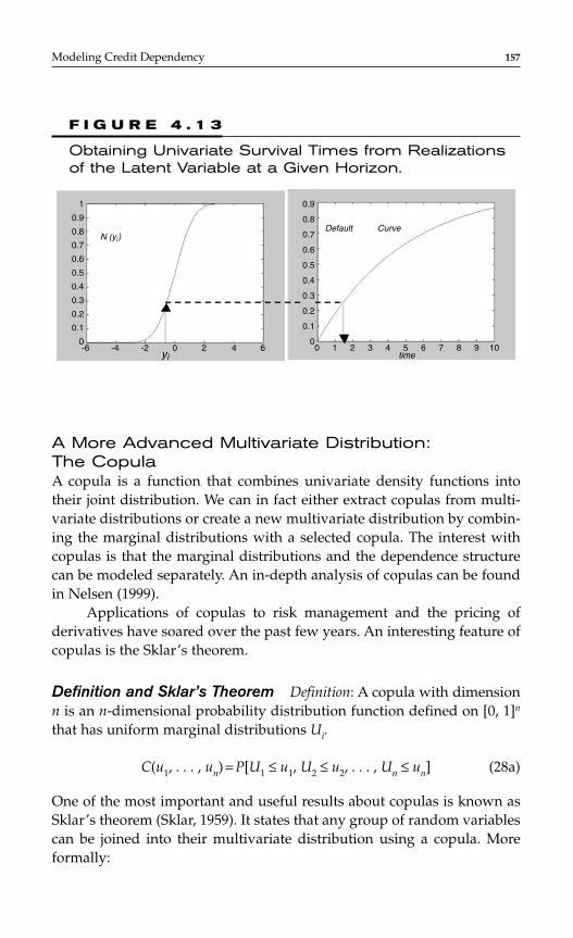
A More Advanced Multivariate Distribution: The CopulaA copula is a function that combines univariate density functions intotheir joint distribution. We can in fact either extract copulas from multi-variate distributions or create a new multivariate distribution by combin-ing the marginal distributions with a selected copula. The interest withcopulas is that the marginal distributions and the dependence structurecan be modeled separately. An in-depth analysis of copulas can be foundin Nelsen (1999).
Applications of copulas to risk management and the pricing ofderivatives have soared over the past few years. An interesting feature ofcopulas is the Sklar’s theorem.
Definition and Sklar’s Theorem Definition: A copula with dimensionn is an n-dimensional probability distribution function defined on [0, 1]n
that has uniform marginal distributions Ui.
C(u1, . . . , un) = P[U1 ≤ u1, U2 ≤ u2, . . . , Un ≤ un] (28a)
One of the most important and useful results about copulas is known asSklar’s theorem (Sklar, 1959). It states that any group of random variablescan be joined into their multivariate distribution using a copula. Moreformally:
Modeling Credit Dependency 157
0.1
0.2
0.3
0.4
0.5
0.6
0.7
0.8
0.9
1
0.1
0.2
0.3
0.4
0.5
0.6
0.7
0.8
0.9
-6 0 1 2 3 4 5 6 7 8 9 10-4 -2 0 2 4 600
N (yi)
yi time
Default Curve
F I G U R E 4 . 1 3
Obtaining Univariate Survival Times from Realizationsof the Latent Variable at a Given Horizon.
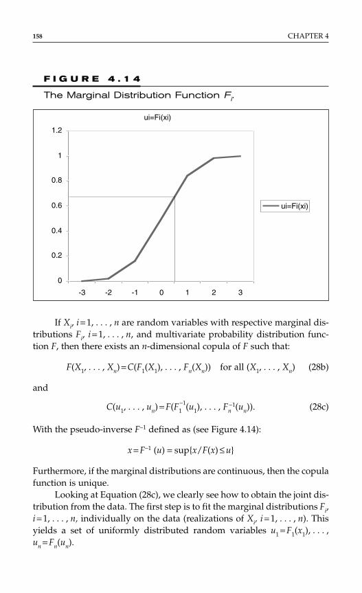
If Xi, i = 1, . . . , n are random variables with respective marginal dis-tributions Fi, i = 1, . . . , n, and multivariate probability distribution func-tion F, then there exists an n-dimensional copula of F such that:
F(X1, . . . , Xn) = C(F1(X1), . . . , Fn(Xn)) for all (X1, . . . , Xn) (28b)
and
C(u1, . . . , un) = F(F1−1(u1), . . . , Fn
−1(un)). (28c)
With the pseudo-inverse F−1 defined as (see Figure 4.14):
x = F−1 (u) = supx/F(x) ≤ u
Furthermore, if the marginal distributions are continuous, then the copulafunction is unique.
Looking at Equation (28c), we clearly see how to obtain the joint dis-tribution from the data. The first step is to fit the marginal distributions Fi,i = 1, . . . , n, individually on the data (realizations of Xi, i = 1, . . . , n). Thisyields a set of uniformly distributed random variables u1 = F1(x1), . . . ,un = Fn(un).
158 CHAPTER 4
0
0.2
0.4
0.6
0.8
1
1.2
-3 -2 -1 0 1 2 3
ui=Fi(xi)
ui=Fi(xi)
F I G U R E 4 . 1 4
The Marginal Distribution Function Fi.
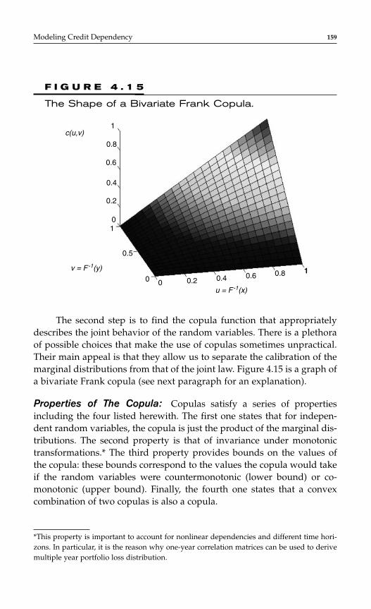
The second step is to find the copula function that appropriatelydescribes the joint behavior of the random variables. There is a plethoraof possible choices that make the use of copulas sometimes unpractical.Their main appeal is that they allow us to separate the calibration of themarginal distributions from that of the joint law. Figure 4.15 is a graph ofa bivariate Frank copula (see next paragraph for an explanation).
Properties of The Copula: Copulas satisfy a series of propertiesincluding the four listed herewith. The first one states that for indepen-dent random variables, the copula is just the product of the marginal dis-tributions. The second property is that of invariance under monotonictransformations.* The third property provides bounds on the values ofthe copula: these bounds correspond to the values the copula would takeif the random variables were countermonotonic (lower bound) or co-monotonic (upper bound). Finally, the fourth one states that a convexcombination of two copulas is also a copula.
Modeling Credit Dependency 159
*This property is important to account for nonlinear dependencies and different time hori-zons. In particular, it is the reason why one-year correlation matrices can be used to derivemultiple year portfolio loss distribution.
c(u,v)
v = F-1(y)
u = F-1(x)
1
0.8
0.6
0.4
0.2
01
0.5
0 0 0.2 0.4 0.6 0.8 1
F I G U R E 4 . 1 5
The Shape of a Bivariate Frank Copula.
Using similar notations as earlier where X and Y denote randomvariables and u and v stand for the uniformly distributed margins of thecopula, we have:
1. If X and Y are independent, then C(u, v) = uv.2. Copulas are invariant under increasing and continuous trans-
formations of marginals.3. For any copula C, we have max(u + v − 1, 0) ≤ C(u, v) ≤ min(u, v).4. If C1 and C2 are copulas, then C = α C1 + (1 − α )C2 for 0 <α < 1 is
also a copula.
Survival Copulas As we have seen in the previous section, the CDOworld focuses on joint survival times.
We can define Si(t) the cumulative survival time function for obligori, where τi is the time until default.
St(t) = P(τi > t)
The related cumulative default probability for obligor i is expressed as:
Ft(t) = P(τi ≤ t)
= 1 − Si(t)
Let us now consider two obligors i and j. We call C as the copula that linksτi and τj. The joint survival function can be written as S (ti, tj) = P(τi, > ti, τj > tj)and S(ti, tj) = C
∼ (Si(ti),Sj(tj)) = Si(ti) + Sj(tj) − 1 + C(1 − Si(ti), 1 − Sj(tj)), where C
∼is
called the survival copula of τi and τj.We now briefly review three important classes of copulas which are
most frequently used in risk management applications: Elliptical (Gaussianand Student-t) copulas, Archimedean copulas, and Marshall-Olkin copulas.
Important Classes of Copulas There exists a wide variety of possiblecopulas. Many but not all are listed in Nelsen (1999). In what follows, weintroduce briefly elliptical, Archimedean, and Marshall-Olkin copulas.Among elliptical copulas, Gaussian copulas are now commonly used togenerate dependent random vectors in applications requiring Monte-Carlo simulations (see Bouyé et al., 1999, or Wang, 2000). TheArchimedean family is convenient as it is parsimonious and has a simpleadditive structure. Applications of Archimedean copulas to risk manage-ment can be found in Das and Geng (2002) or Schönburcher (2002), amongmany others. The Marshall-Olkin copula has recently be used in the CDOworld as an alternative way to compensate for the weaknesses of theGaussian copula.
160 CHAPTER 4
Elliptical Copulas: Gaussian and t-CopulasThe Gaussian Copula As recalled earlier, copulas are multivariatedistribution functions. Obviously, the Gaussian copula will be amultivariate Gaussian (normal) distribution.
Using the notations of Equation (28b), we can write C∑Gau, the n-
dimensional Gaussian copula with covariance matrix ∑*:
C∑Gau (u1, . . . , un) = N∑
n (N−1(u1), . . . , N−1(un)), (29)
with N∑n and N−1 denoting, respectively, the n-dimensional cumulative
Gaussian distribution with covariance matrix, ∑ and the inverse of thecumulative univariate standard normal distribution.
In the bivariate case, assuming that the correlation between the tworandom variables is ρ, Equation (29) boils down to:
(30)
The t-Copula The t-copula (bivariate t-distribution) with ν degreesof freedom is obtained in a similar way. Using evident notations, wehave:
Ctρ,ν (u, v) = tρ,
2ν (tν
−1(u),tν−1(v)), (31)
The bivariate t-copula can be defined as an independent mixture of a
multivariate normal distribution N∑2 and of scalar random ,
variable where W follows a chi-squared distribution with ν degrees of
freedom, with and . Its usage for credit
modeling purposes has been suggested by different authors such as Freyet al. (2001). t-Copulas generate “tail dependence,” i.e., more extremeevents than the Gaussian copulas.
Σ = σ ijρ σ σ σij ij ii jj= / *
SW
= ν
C u N N u N
g gh hg h
NN u
ρ ρ
ν
ν ν
π ρρ
ρ
Gau
( )( )
( , ) ( ( ), ( ))
( )exp
( )d d
=
=−
−− +
−
− −
−∞−∞
−−
∫∫
2 1 1
2
2 2
2
12 1
22 1
11
Modeling Credit Dependency 161
*Also the correlation matrix in this case.

More recently, Hull and White (2004) have referred to double t cop-ulas for the pricing of CDOs. In this case, the marginal probability distri-butions are not derived from a latent variable following a Student-tdistribution but following a convolution of two Student-t distributions.This convolution is not a Student-t distribution itself and the copula is nota Student-t copula either.
Archimedean Copulas The family of Archimedean copulas is the classof multivariate distributions on [0,1]n that can be written as
CArch (u1, . . . , un) = G−1(G(u1) + · · · + G(un)), (32)
where G is a suitable continuous monotonic function from [0, 1] to + sat-isfying G(1) = 0. G(⋅) is called the generator of the copula.
Three examples of Archimedean copulas used in the finance litera-ture are the Gumbel, the Frank, and the Clayton copulas, for which weprovide the functional form now. They can easily be built by specifyingtheir generator (see Marshall and Olkin, 1988, or Nelsen, 1999).
♦ Example 1: The Gumbel copula (multivariate exponential)The generator for the Gumbel copula is:
GG(t) = (−ln t)θ (33)
with inverse: and θ ≥ 1.Therefore using Equation (29), the copula function in the bivari-ate case is:
(34)
♦ Example 2: The Frank copula
The generator is:
(35)
with inverse and θ ≠ 0.
The bivariate copula function is therefore:
(36)C uF
u vθ
θ θ
θν
θ( , ) ln
(e )(e )(e )
.= − + − −−
− −
−
11
1 11
G sFs[ ]( ) ln[ e ( e )],− = − − −1 1
1 1θ
θ
G tF
t( ) ln
ee
,= − −−
−
−
θ
θ
11
C u v u vGθ θ θ θ( , ) exp ( ln ) ( ln ) .= − − + −[ ]
1
G s sG[ ] /( ) exp( )− = −1 1 θ
162 CHAPTER 4
♦ Example 3: The Clayton copula
The generator is:
(37)
with inverse: and θ ≥ 0.The bivariate copula function is therefore:
CCθ (u, v) = max([u−θ + v−θ − 1]−1/θ, 0). (38)
Calculating a Joint Cumulative Probability Using anArchimedean Copula Assume we want to calculate the jointcumulative probability of two random variables X and Y P(X < x, Y < y).Both X and Y are standard-normally distributed. We are interested inlooking at the joint probability depending on the choice of copula and onthe parameter θ.
The first step is to calculate the margins of the copula distribution:v = P(Y< y) = N(y) and u = P(X< x) = N(x). For our numerical example, weassume x = −0.1 and y = 0.3. Hence u = 0.460 and v = 0.618.
The joint cumulative probability is then obtained by plugging thesevalues into the chosen copula function [Equations (34), (36), and (38)].Figure 4.16 illustrates how the joint probabilities change as a function of θfor the three Archimedean copulas presented earlier. The graph showsthat different choices of copulas and theta parameters lead to very differ-ent results in terms of joint probability.
The Marshall-Olkin Copula This type of copula has been promotedrecently by several authors such as Elouerkhaoui (2003a,b) and Giesecke(2003). It can be useful to describe intensity-based models for correlateddefaults in which unpredictable default arrival times are jointly exponen-tially distributed.
The bivariate survival copula is expressed as:
(39)
where θ1 and θ2 are the controls for the degree of dependence between thedefault times of firms 1 and 2, respectively.
C u v uv u vMO, ( , ) min( , )θ θ θ θ1 2 1 2= − −
G s sC[ ] /( ) ( ) ,− −= +1 11 θ θ
G t tC ( ) ( ),= −−11
θθ
Modeling Credit Dependency 163
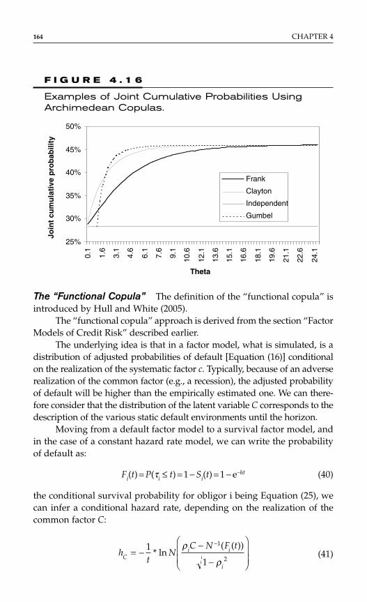
The “Functional Copula” The definition of the “functional copula” isintroduced by Hull and White (2005).
The “functional copula” approach is derived from the section “FactorModels of Credit Risk” described earlier.
The underlying idea is that in a factor model, what is simulated, is adistribution of adjusted probabilities of default [Equation (16)] conditionalon the realization of the systematic factor c. Typically, because of an adverserealization of the common factor (e.g., a recession), the adjusted probabilityof default will be higher than the empirically estimated one. We can there-fore consider that the distribution of the latent variable C corresponds to thedescription of the various static default environments until the horizon.
Moving from a default factor model to a survival factor model, andin the case of a constant hazard rate model, we can write the probabilityof default as:
Fi(t) = P(τi ≤ t) = 1 − Si(t) = 1 − e–ht (40)
the conditional survival probability for obligor i being Equation (25), wecan infer a conditional hazard rate, depending on the realization of thecommon factor C:
(41)ht
NC N F t
Ci i
i
= −−
−
−1
1
1
2* ln
( ( ))ρ
ρ
164 CHAPTER 4
25%
30%
35%
40%
45%
50%
0.1
1.6
3.1
4.6
6.1
7.6
9.1
10.6
12.1
13.6
15.1
16.6
18.1
19.6
21.1
22.6
24.1
Join
t cu
mu
lati
ve p
rob
abili
ty
Frank
Clayton
Independent
Gumbel
Theta
F I G U R E 4 . 1 6
Examples of Joint Cumulative Probabilities UsingArchimedean Copulas.
The distribution of C, leads to a distribution of static pseudo-hazard rateshC. These conditional hazard rates represent the range of possible expectedhazard rates, depending on different realizations of the macroeconomicenvironment. Such conditional average hazard rates during the life of theinstrument are not, however, currently observable.
Hull and White (2005) suggest that there is no reason to assume anormal distribution for the common factor C and the idiosyncratic term εi.Equation (41) can therefore be written in a more general way as:
(42)
where Hi is the cumulative probability distribution of εi and Gi thecumulative probability distribution of the latent variable Ai. In addition,of course, the conditional hazard rates can be considered as time-dependent.
The idea of the authors is in fact not to specify the parametric formfor any variable, but to extract from empirical CDO pricing observationsthe empirical distribution of conditional hazard rates.
The empirical distribution can be inferred from a three-step process:
♦ Step 1: Assume a series of possible default rates at the horizon ofthe instrument and extract the corresponding pseudo-hazardrates.
♦ Step 2: Compute the cash inflows and outflows of the variousmarket instruments (CDO tranches) for each pseudo-hazard rateextracted from step 1.
♦ Step 3: Write the unconditional expected value of the instru-ments as a linear combination of weighted step 2 conditionalexpected values. Estimate the weights by considering that theunconditional expected values of each instrument should bezero.
There is no single set of values, given the fact that there are usually morepossible default rates than credit instruments, but results are stable whena regularization term is added in the optimization problem to maximizethe smoothness of the distribution of conditional hazard rates.
Thanks to this approach, the fit with the observation is almost per-fect at the time the distribution of pseudo-hazard rates is computed. Thisdistribution is time-dependent and reflects the changes in the marketexpectation related to this multiple regime-switching pattern.
ht
HC G F t
C ii i i
i
= −−
−
−1
1
1
2* ln
( ( ))ρ
ρ
Modeling Credit Dependency 165
Copulas and Other Dependence Measures Recall that we introducedearlier Spearman’s Rho and Kendall’s Tau as two alternatives to linear cor-relation. We mentioned that they could be expressed in terms of the copula.The formulas linking these dependence measures to the copula are:
♦ Spearman’s rho:
ρS = 12 ∫1
0 ∫1
0 (C(u, ν) − uν) du dν (43)
♦ Kendall’s tau:
τK = 4 ∫1
0 ∫1
0 C(u, ν)dC(u, ν)−1 (44)
Thus, once the copula is defined analytically, one can immediately calcu-late rank correlations from it. Copulas also incorporate tail dependence.Intuitively, tail dependence will exist when there is a significant probabil-ity of joint extreme events. Lower (upper) tail dependence captures jointnegative (positive) outliers.
If we consider two random variables X1 and X2 with respective mar-ginal distributions F1 and F2, the coefficients of lower (LTD) and upper taildependence (UTD) are*:
(45)
and(46)
Figure 4.17 illustrates the asymptotic dependence of variables in theupper tail, using t-copulas. The tail dependence coefficient shown in theFigure 4.17 corresponds to UTD. As can be observed, Gaussian copulasexhibit no tail dependence.
Statistical Techniques Used to Select andCalibrate CopulasIn this section, we mainly focus on two sensitive issues related to the useof copulas: how to select the most appropriate copula and how to cali-brate any selected copula.
In summary, copula estimation is still in its infancy, and so far therehas not been any real way to define and estimate the “optimal parametric
LTD lim Pr ( ) ( )= < < →− −
zX F z X F z
0 2 21
1 11
UTD lim Pr ( ) ( )= > > →− −
zX F z X F z
1 2 21
1 11
166 CHAPTER 4
*The UTD and the LTD depend only on the copula and not on the margins.
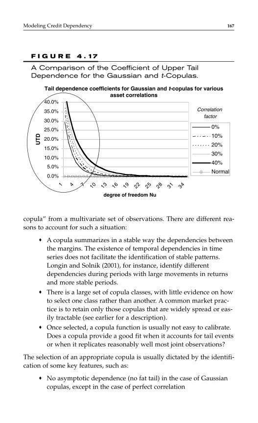
copula” from a multivariate set of observations. There are different rea-sons to account for such a situation:
♦ A copula summarizes in a stable way the dependencies betweenthe margins. The existence of temporal dependencies in timeseries does not facilitate the identification of stable patterns.Longin and Solnik (2001), for instance, identify differentdependencies during periods with large movements in returnsand more stable periods.
♦ There is a large set of copula classes, with little evidence on howto select one class rather than another. A common market prac-tice is to retain only those copulas that are widely spread or eas-ily tractable (see earlier for a description).
♦ Once selected, a copula function is usually not easy to calibrate.Does a copula provide a good fit when it accounts for tail eventsor when it replicates reasonably well most joint observations?
The selection of an appropriate copula is usually dictated by the identifi-cation of some key features, such as:
♦ No asymptotic dependence (no fat tail) in the case of Gaussiancopulas, except in the case of perfect correlation
Modeling Credit Dependency 167
0.0%
5.0%
10.0%
15.0%
20.0%
25.0%
30.0%
35.0%
40.0%
1 4 7 10 13 16 19 22 25 28 31 34
UT
D
0%
10%
20%
30%
40%
Normal
Correlationfactor
degree of freedom Nu
Tail dependence coefficients for Gaussian and t-copulas for variousasset correlations
F I G U R E 4 . 17
A Comparison of the Coefficient of Upper TailDependence for the Gaussian and t-Copulas.

♦ Symmetric asymptotic dependence both for t-copulas and Frankcopulas
♦ Higher dependence in bear conditions when using Clayton cop-ulas
♦ Higher dependence in bull conditions with Gumbel copulas
Based on the selection of a class of copulas, we review how to calibrateand to measure subsequently the goodness-of-fit.
In terms of calibration, there is a first choice between parametric andnonparametric estimations.
We are presenting here the three most common parametricapproaches: Full Maximum Likelihood (FML, a one-step parametricapproach), Inference Functions for Margins (IFM, a two-step paramet-ric approach) and Conditional Maximum Likelihood (CML, a two-stepsemiparametric approach). Fermanian and Scaillet (2004) show that therecan be pitfalls attached to these different estimation techniques, either dueto a misspecification of the margins or to a loss of efficiency when the mar-gins do not require explicit specification.
We then introduce nonparametric estimation, based on the calcula-tion of the “Empirical copula” defined in Deheuvels (1979).
Mapping the empirical copula to a well-known parametric onebecomes a problem of goodness-of-fit in a multivariate environment.Classical statistical tests, such as the Kolmogorov-Smirnov, the Chi-square,or the Anderson-Darling tests, usually cannot be used in a straightforwardmanner.
There are mainly two types of approaches that are usually consid-ered to obtain the best fit:
♦ An approach based on a visual comparison, as suggested byGenest and Rivest (1993).
♦ The selection of the copula that minimizes the distance with theempirical copula. Obviously, results will depend on the choiceof such a distance. Scaillet (2000), Fermanian (2003), and Chenet al. (2004), among others, suggest the use of Kernels to smooththe empirical copula before fitting in order to obtain an explicitlimiting law for the test statistic.
Full Maximum Likelihood Also Called Exact Maximum LikelihoodIn this approach, the parameters of the copula and of the marginal distri-butions are estimated simultaneously. It is worth noting that both the
168 CHAPTER 4
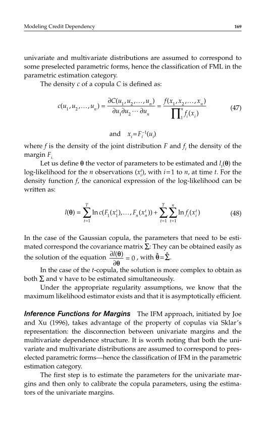
univariate and multivariate distributions are assumed to correspond tosome preselected parametric forms, hence the classification of FML in theparametric estimation category.
The density c of a copula C is defined as:
(47)
and xi = Fi−1(ui)
where f is the density of the joint distribution F and fi the density of themargin Fi.
Let us define θ the vector of parameters to be estimated and lt(θ) thelog-likelihood for the n observations (xi
t), with i = 1 to n, at time t. For thedensity function f, the canonical expression of the log-likelihood can bewritten as:
(48)
In the case of the Gaussian copula, the parameters that need to be esti-mated correspond the covariance matrix ∑: They can be obtained easily as
the solution of the equation , with θ= ∑.
In the case of the t-copula, the solution is more complex to obtain asboth ∑ and ν have to be estimated simultaneously.
Under the appropriate regularity assumptions, we know that themaximum likelihood estimator exists and that it is asymptotically efficient.
Inference Functions for Margins The IFM approach, initiated by Joeand Xu (1996), takes advantage of the property of copulas via Sklar’srepresentation: the disconnection between univariate margins and themultivariate dependence structure. It is worth noting that both the uni-variate and multivariate distributions are assumed to correspond to pres-elected parametric forms—hence the classification of IFM in the parametricestimation category.
The first step is to estimate the parameters for the univariate mar-gins and then only to calibrate the copula parameters, using the estima-tors of the univariate margins.
∂∂
=l( )θθ
0
l c F x F x f xtn n
ti i
t
t
n
t
T
t
T
( ) ln ( ( ), , ( )) ln ( )θ = +===∑∑∑ 1 1
111
K
c u u uC u u u
u u u
f x x x
f xn
n
n
n
i i
n( , , , )( , , , ) ( , , , )
( )1 2
1 2
1 2
1 2
1
KK
L
K=
∂∂ ∂ ∂
=∏
Modeling Credit Dependency 169

Let us call θ= (θ1, . . . , θn, α), with θi the parameters related to themarginal distributions and α the vector of the copula parameters. The log-likelihood expression [Equation (48)] can be written as:
(49)
The two-step maximization process follows:
(50)
and subsequently
(51)
It is worth mentioning that the IFM estimation is computationally easierto obtain than the FML/exact maximum likelihood one.
Conditional Maximum Likelihood or Canonical Maximum LikelihoodWith this approach presented inter alia in Mashal and Zeevi (2002), there isno parametric assumption related to the distribution of the margins.
The dataset of n sequences of observations X = (X1t, . . . , Xn
t)Tt =1 is
transformed into discrete variates û = (û1t, . . . , µt
n)Tt=1 through empirical
distribution functions Fi (⋅) defined as:
(52)
This transformation is referred to as the “empirical marginal transfor-mation.” See Figure 4.18 for an example corresponding to two quarterlytime series of default rates over 20 years corresponding to two groups ofindustry. Data has been retrieved from CreditPro.
In a second step, the copula parameters, corresponding to the para-metric family that has been selected, can be estimated in a straightforwardway as:
(53)ˆ arg max ln ( ˆ , , ˆ , )α α=−∑
αc u ut
nt
t
T
11
K
ˆ , and ˆ ( ˆ ( ))
FT T
u F Xi X Xt
T
i i i tT
it
i
ττ
= =
≤=
=∑11
11
ˆ arg max ln [ ( , ˆ ), , ( , ˆ ), ]α α==∑
αθ θc F x F xt
n nt
nt
T
1 1 11
K
ˆ arg max ln ( , )θ θθ
i i it
it
T
i
f x==∑
1
l c F x F x f xtn n
tn
t
T
i it
it
n
t
T
( ) ln ( ( , ), , ( , ), ) ln ( , )θ α= += ==∑ ∑∑1 1 1
1 11
θ θ θK
170 CHAPTER 4
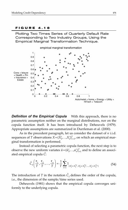
Definition of the Empirical Copula With this approach, there is noparametric assumption neither on the marginal distributions, nor on thecopula function itself. It has been introduced by Deheuvels (1979).Appropriate assumptions are summarized in Durrleman et al. (2000).
As in the precedent paragraph, let us consider the dataset of n i.i.d.sequences of T observations X = (X1
t,…,Xnt)T
t =1, on which an empirical mar-ginal transformation is performed.
Instead of selecting a parametric copula function, the next step is toobserve the new uniform variates û = (û1
t,…,utn)T
t=1 and to define an associ-ated empirical copula C:
(54)
The introduction of T in the notation CT defines the order of the copula,i.e., the dimension of the sample/time series used.
Deheuvels (1981) shows that the empirical copula converges uni-formly to the underlying copula.
ˆ , , , , ,...,
CT T T TT
n
X X X X X Xt
T
t tnt
nn
τ τ ττ τ τ
1 2
1
11
1 11
2 22
K
=≤ ≤ ≤
=∑
Modeling Credit Dependency 171
empirical marginal transformation
0 0.2 0.4 0.6 0.8 10
0.1
0.2
0.3
0.4
0.5
0.6
0.7
0.8
0.9
1
Cons + leisure+ Health + Fin+ Insurance +
Estate
Auto/metal + home + Energy + Utility +HiTech + Telecom
F I G U R E 4 . 1 8
Plotting Two Times Series of Quarterly Default RateCorresponding to Two Industry Groups, Using theEmpirical Marginal Transformation Technique.
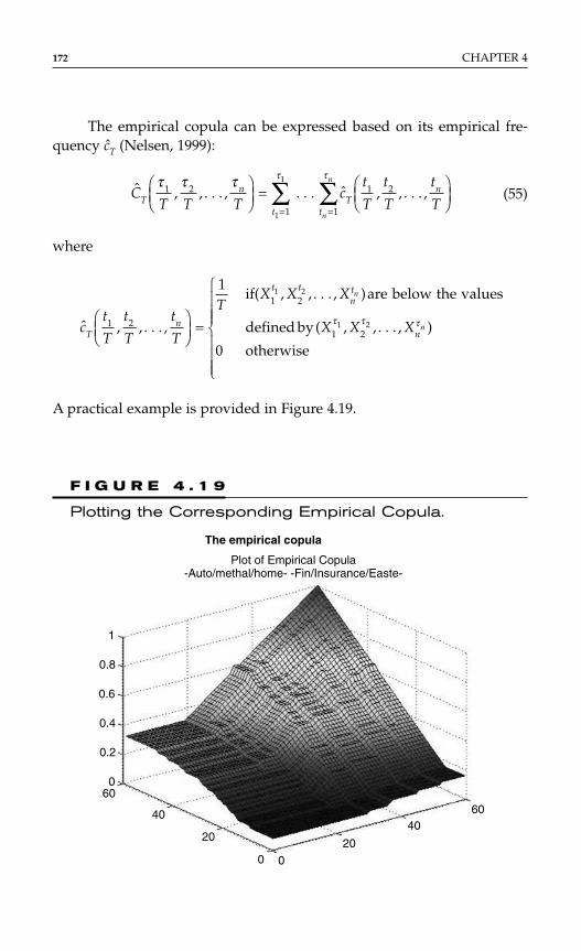
The empirical copula can be expressed based on its empirical fre-quency cT (Nelsen, 1999):
(55)
where
A practical example is provided in Figure 4.19.
ˆ , , ,
if( , , , )are below the values
defined by( , , , )
otherwise
ct
T
t
T
t
T
TX X X
X X XTn
t tnt
n
n
n1 2
1 2
1 2
1 1 2
1 2. . .
. . .
. . .
=
τ τ τ
0
ˆ , , , ˆ , , ,CT T T
ct
T
t
T
t
TTn
Ttt
n
n
nτ τ τ ττ1 2
11
1 2
1
1
. . . . . . . . .
=
==
∑∑
172 CHAPTER 4
The empirical copula
Plot of Empirical Copula-Auto/methal/home- -Fin/Insurance/Easte-
1
0.8
0.6
0.4
0.2
060
40
20
0 0
20
4060
F I G U R E 4 . 1 9
Plotting the Corresponding Empirical Copula.
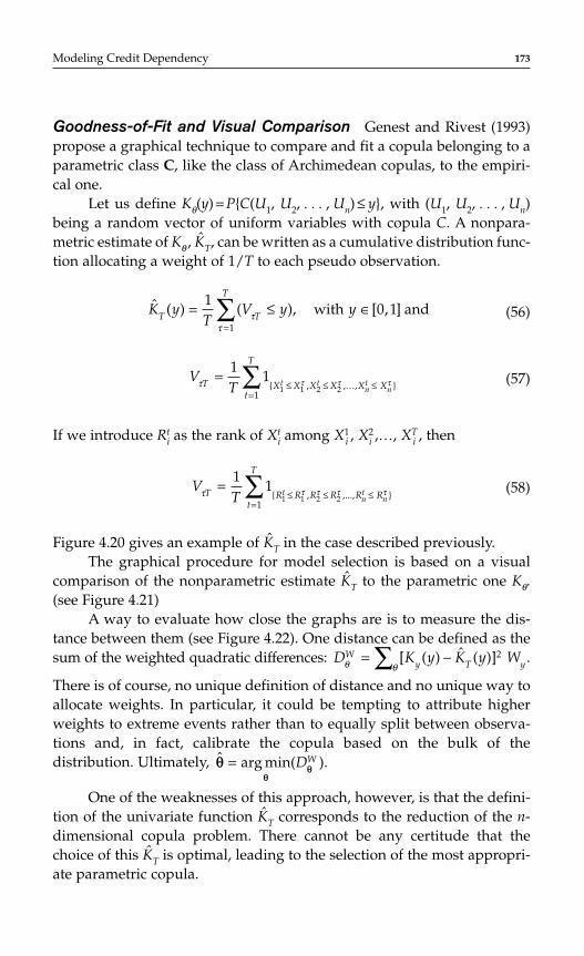
Goodness-of-Fit and Visual Comparison Genest and Rivest (1993)propose a graphical technique to compare and fit a copula belonging to aparametric class C, like the class of Archimedean copulas, to the empiri-cal one.
Let us define Kθ(y) = PC(U1, U2, . . . , Un) ≤ y, with (U1, U2, . . . , Un)being a random vector of uniform variables with copula C. A nonpara-metric estimate of Kθ , KT, can be written as a cumulative distribution func-tion allocating a weight of 1/T to each pseudo observation.
(56)
(57)
If we introduce Rti as the rank of Xt
i among X1i , X2
i ,…, XTi , then
(58)
Figure 4.20 gives an example of KT in the case described previously.The graphical procedure for model selection is based on a visual
comparison of the nonparametric estimate KT to the parametric one Kθ.(see Figure 4.21)
A way to evaluate how close the graphs are is to measure the dis-tance between them (see Figure 4.22). One distance can be defined as thesum of the weighted quadratic differences: .
There is of course, no unique definition of distance and no unique way toallocate weights. In particular, it could be tempting to attribute higherweights to extreme events rather than to equally split between observa-tions and, in fact, calibrate the copula based on the bulk of thedistribution. Ultimately,
One of the weaknesses of this approach, however, is that the defini-tion of the univariate function KT corresponds to the reduction of the n-dimensional copula problem. There cannot be any certitude that thechoice of this KT is optimal, leading to the selection of the most appropri-ate parametric copula.
ˆ arg min( ).θθ
θ= DW
D K y K y WWy T yθ θ
= −∑ [ ( ) ˆ ( )]2
VTT R R R R R R
t
T
tnt
nτ τ τ τ τ=
≤ ≤ ≤=∑1
11 1 2 2
1 , ,...,
VTT X X X X X X
t
T
t tnt
nτ τ τ τ=
≤ ≤ ≤=∑1
11 1 2 2
1 , , , K
ˆ ( ) ( ), with [ , ] andK yT
V y yT T
T
= ≤ ∈=
∑10 1
1τ
τ
Modeling Credit Dependency 173
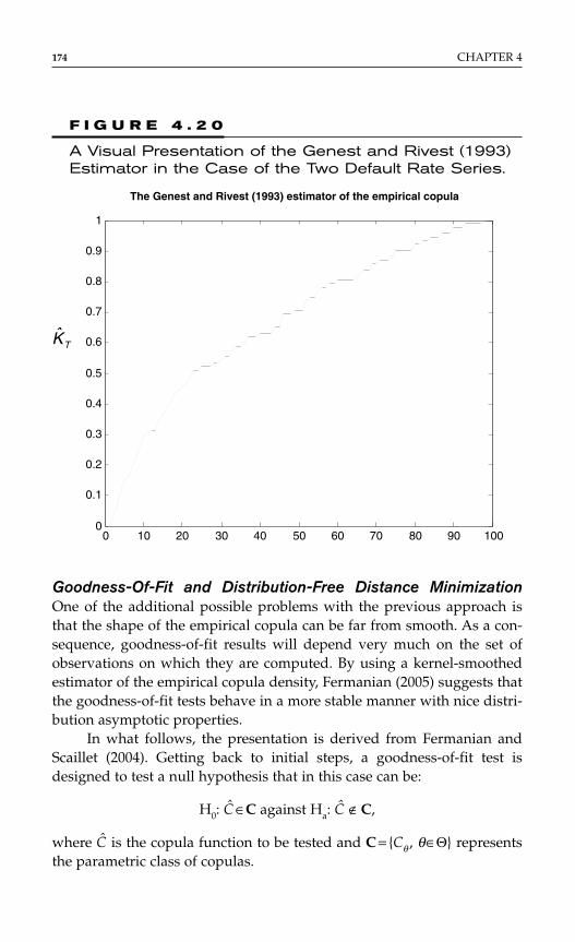
174 CHAPTER 4
0 10 20 30 40 50 60 70 80 90 1000
0.1
0.2
0.3
0.4
0.5
0.6
0.7
0.8
0.9
1
TK
The Genest and Rivest (1993) estimator of the empirical copula
F I G U R E 4 . 2 0
A Visual Presentation of the Genest and Rivest (1993)Estimator in the Case of the Two Default Rate Series.
Goodness-Of-Fit and Distribution-Free Distance MinimizationOne of the additional possible problems with the previous approach isthat the shape of the empirical copula can be far from smooth. As a con-sequence, goodness-of-fit results will depend very much on the set ofobservations on which they are computed. By using a kernel-smoothedestimator of the empirical copula density, Fermanian (2005) suggests thatthe goodness-of-fit tests behave in a more stable manner with nice distri-bution asymptotic properties.
In what follows, the presentation is derived from Fermanian andScaillet (2004). Getting back to initial steps, a goodness-of-fit test isdesigned to test a null hypothesis that in this case can be:
H0: C ∈C against Ha: C ∉ C,
where C is the copula function to be tested and C = Cθ , θ∈Θ representsthe parametric class of copulas.
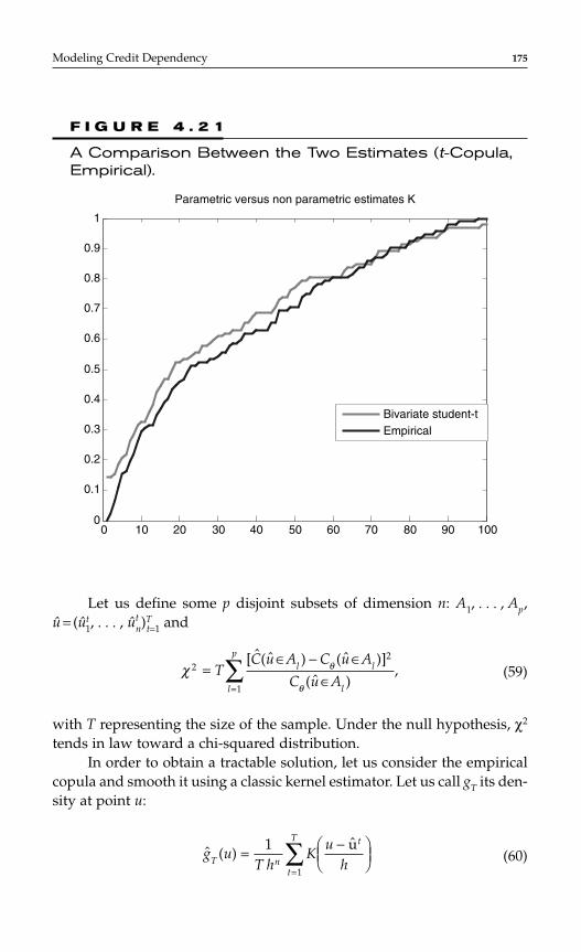
Let us define some p disjoint subsets of dimension n: A1, . . . , Ap,û = (ût
1, . . . , ûtn)T
t=1 and
(59)
with T representing the size of the sample. Under the null hypothesis, χ2
tends in law toward a chi-squared distribution.In order to obtain a tractable solution, let us consider the empirical
copula and smooth it using a classic kernel estimator. Let us call gT its den-sity at point u:
(60)ˆ ( )ˆ
g uT h
Ku
hT n
t
t
T
= −
=∑1
1
u
χ θ
θ
22
1
=∈ − ∈
∈=∑T
C u A C u A
C u Al l
ll
p [ ˆ( ˆ ) ( ˆ )]
( ˆ ),
Modeling Credit Dependency 175
0 10 20 30 40 50 60 70 80 90 1000
0.1
0.2
0.3
0.4
0.5
0.6
0.7
0.8
0.9
1
Bivariate student-tEmpirical
Parametric versus non parametric estimates K
F I G U R E 4 . 2 1
A Comparison Between the Two Estimates (t-Copula,Empirical).
where K(⋅) is an n-dimensional kernel, with h(T) being the bandwidth andvector ut = (û1
t,…, utn) being defined on the basis of the empirical marginal
transformation Equation (52).
As usual, ∫K(⋅) = 1 and .
Based on the definition of this kernel, we can now revert to the χ2-test that can be written as:
(61)
where gθ(⋅) corresponds to the parametric copula density, θ to the esti-mated parameter vector, and the p vectors to some arbitrary choicedefined by where the tester wants to assess the quality of the fit.
Discussing the Estimation of Copulas for Time Series Copula esti-mation has been presented so far under the assumption of an environment
( ˆ )ul lp=1
χ θ
θ
22
2
1
=∫
−
=∑T h
K
g g
g
nT
l l
ll
p [ ˆ ( ˆ ) ( ˆ )]
( ˆ )ˆ
ˆ
u u
u
lim ( )T h T→∞ = 0
176 CHAPTER 4
0 10 20 30 40 50 60 70 80 90 1000
0.002
0.004
0.006
0.008
0.01
0.012
0.014
0.016
0.018
0.02
F I G U R E 4 . 2 2
Distance (Quadratic Difference) Between Parametricand Nonparametric Estimates of K. Case of the TwoDefault Rate Data Series Described Earlier.
of i.i.d. observable samples or time series. When dealing with partiallyautocorrelated time series displaying varying heteroscedasticity, we needto revisit the previous copula estimation techniques and to assess theirrobustness. This point is of particular importance, for instance, in the syn-thetic CDO world where samples typically correspond to spread prices.
Some initial transformation of the data at the univariate level may beneeded in order to be able to rely on the i.i.d. assumption. Some tech-niques are available. Serial autocorrelation, nonstationarity, heteroscedas-ticity of the time series can be filtered through GARCH and ARMAprocesses.
Based on this transformation, we can focus on the residuals, as it ismuch more likely to be i.i.d. Parametric copulas can then be typically fit-ted on these residuals.
We revert readers to Scaillet and Fermanian (2003), Fermanian et al.(2004), Doukhan et al. (2005), and Chen and Fan (2006) on this topic ofestimation of copulas on time series and of time-dependent copulas.
Correlation as a Result of Joint Intensity ModelingIn May 2005, the downgrade of Ford and GM by S&P lead to a widen-ing of the spreads of almost all the components of the CDS indices. In aCredit Metrics setup, we could imagine that a shock on the automotivesector would lead to some rating actions on other corporate firms in thesame industry and to a lesser extent on other firms in different sectors.In this case, no other significant rating change has occurred as a conse-quence. Thereby, the Credit Metrics approach proved unable to accountfor the changes in the prices of CDO tranches. The period was surpris-ing in the sense that two investors holding exactly the same tranche ofa CDO in their portfolio (assuming it did not include Ford and GM)could have completely different views about the quality of their asset,whether they would consider it from a market-to-market or from atraditional pure default risk perspective. The general trend, over therecent period, has been to take into account both default dependencyand market price risk.
As Schönbucher and Schubert (2001) point out, the joint risk-neutralsurvival function of two obligors A and B will depend dramatically on adefault event on any of them. Typically, the default probability of B willincrease as soon as obligor A defaults. If we focus on the period boundedby the time just before default and the time of obligor A’s default, we willobserve a jump in the default intensity of B. Any substantial jump like thedowngrade to a NIG level of some obligors can have the same effect as a
Modeling Credit Dependency 177
default and entail price contagion for other obligors, which could not be eas-ily explained by Gaussian copulas. The GM and Ford examples stand as agood illustration of the phenomenon.
All these classes of joint-intensity models start by focusing heavilyon the estimation of the price or the creditworthiness (hazard rate) of eachobligor considered separately. These approaches do not preclude then theuse of copulas but tend to encourage the selection of a multivariate modelbased on some explicit rationale. One of the main reasons why theseapproaches have not been widely used by practitioners so far is probablybecause the estimation problems that arise are generally more complexthan with the traditional Gaussian copula setup. There seems, however,to be growing interest for these types of models as they can representobserved prices quite accurately.
In this context, it is important to refer to intensity-based modelswhen dealing with dependence. In order to summarize the evolution inthis field, we can identify four parallel classes of joint intensity models:
♦ The most traditional class initially corresponded to the introduc-tion of some correlation in the dynamics of the default intensityof obligors. This approach had been widely used in the contextof interest rates and FX modeling and has then been introducedin credit. These initial models are usually considered to underes-timate observed correlation. Duffie (1998) and Duffie andSingleton (1999) have suggested that higher default dependen-cies could be obtained by increasing the likelihood of jointdefault events. In their model, when an obligor defaults, anenhancement in the intensity of the jump of the other obligors isobserved. Obviously, with a large sample, calibration of intensi-ties can be a problem. Since then, other models presenting jump-intensity correlation have been developed, allowing foridiosyncratic as well as systematic jumps, like Giesecke (2003)and dealing with calibration thanks to an exponential copulaframework.
♦ Another area of investigation has been in the direction offrailty models. These models are used in other fields like biol-ogy and medicine. In such a setup, individuals within differentgroups can be affected by common frailties. In credit, thistranslates into an extra stress factor due to unobserved riskfactors (see Yashin and Iachine, 1995). In this case, a particular
178 CHAPTER 4
Modeling Credit Dependency 179
specification of the intensity for a Gamma frailty model can beexpressed as:
λt(t, X, Z) = (Z0 + Zt)λ0(t)exp(β'Xt) (62)
With Z0 an unobservable gamma random variable common toall obligors (the shared frailty component), Zi an unobservablegamma random variable that is specific to obligor i, and the restof the specifications corresponding to a classic proportional haz-ard rate model*; i.e., a combination of a simple time-dependenthazard rate function and of a multifactor model of additionalexplanatory variables. Fermanian and Sbai (2005) show that thisclass of models can provide realistic levels of dependence.
♦ Another class corresponds to default infection models. The orig-inal papers in this area are Davis and Lo (1999a,b, 2000) andJarrow and Yu (2001). In this approach the default of an obligorwill impact the default intensities of other obligors through ajump. Let us consider n obligors. The default intensity of obligori at time t can be written as:
(63)
Calibration of this class of models may not prove straightforward.♦ The last class we will mention here is the threshold copula
approach presented by Schönbucher and Schubert (2001). Adetailed description of the model is provided in Appendix A. It focuses particularly on the dynamic specification of the survivalprobabilities and hazard rates. The concept is that any default in aportfolio will create a threshold effect through a modified specifi-cation of the survival copula, due to additional informationgained over time on the default status of the obligors in the port-folio. This threshold information can also be seen as modifyingthe individual pseudo-intensities over time. Though the equationsin the model look complex, the intuition remains simple. Themajor constraint resides with its implementation, as it seems to betractable mainly with Archimedean copulas.
λ α β τi i ij tj
n
t t tj
( ) ( ) ( ) ( )= + ≤=
∑ 11
*Also called Cox regression model.

Discussion on the Evolution of Dependency Modeling
This section completes our introduction to correlation, copulas, and otherdependence measures. Looking backwards, we can see that dependencemeasurement has considerably gained inaccuracy but also in complexityin a short time span. From the initial linear correlation approach, thecredit world has quickly moved toward static factor models at the end ofthe 1990s, with the Credit Metrics setup. The subsequent leap has beenfrom default correlation toward survival correlation with Li (2000). It hasenabled us to adopt a more flexible view of correlation, taking into con-sideration the timing of default. With an almost simultaneous access tovarious forms of copulas, market participants have also been able toaccount for dependence in a more refined way. Surprisingly, many practi-tioners have however not fully adopted these innovative solutions so farfor several reasons. The most reasonable cause accounting for it is that theselection of an appropriate copula is not a fully objective process and itscalibration is not immediate. A second one corresponds to the very prac-tical fact that no common language, other than the Gaussian copula, hasemerged among practitioners so far. A point to mention at this stage isthat there seems to be an increasing view on credit markets that the cop-ula approach has shown some limitations and that there may not exist anyperfect solution or “the Perfect Copula” as Hull and White (2005) put it.Such limitations are to be related, among other things, to the incompletetreatment by copulas of dynamic aspects. The next frontier for depend-ence models would indeed be to account not only for the default dynam-ics but also for the price dynamics, following, for instance, credit eventor credit contagion. Possible paths for the future could be to introduceregime-switching patterns associated with copulas in order to accountbetter for temporal dependencies or to focus on the joint modeling ofintensity-based models, and on finding, among other issues, new solu-tions to the inherent dimensionality problem related to this approach.
PART 2: EMPIRICAL RESULTS ON CORRELATION
Calculating Empirical Asset Implied Correlations
In order to compute the loss distribution of a portfolio, a traditionalapproach has been to assume that the general correlation process is driven
180 CHAPTER 4
by latent variables that partially drive the movement to default or thetime to default of the corporate obligors in that portfolio. Such modelsbelong to the category of factor models described in the section “FactorModels of Credit Risk” of the previous part. This class of models ulti-mately relies on an interpretation within the structural Merton frame-work. In this context, default correlation is derived indirectly from assetcorrelation, as the comovement of the asset value of different obligors, toa default threshold.
The usual approach in CDO pricing and risk management is to con-sider equity or credit spread correlation as proxies for asset correlation. Inwhat follows, we focus on extracting asset correlation from empiricaldefault observations. This will enable us later on to understand properlythe arbitrage between ratings and prices of structures.
We describe three ways to estimate implied asset correlation. Thefirst way in called the joint default probability approach (JPD). The sec-ond corresponds to a maximum likelihood approach (MLE). The thirdone is based on a Bayesian inference technique generalized linear mixedmodel (GLMM).
The Joint Default Probability ApproachIn Equation (4) of the previous part, we have derived the correlationformula for two binary events A and B. These two events can be jointdefaults or joint downgrades, for example. Consider two firms originallyrated i and j, respectively, and let D denotes the default category. The mar-ginal probabilities of default are Pi
D and PjD, while Pi,j
D,D denotes the jointprobability of the two firms defaulting over a chosen horizon. Equation(4) can thus be rewritten as:
(64)
Obtaining individual probabilities of default per rating class is straight-forward. These statistics can be read off transition matrices. The onlyunknown term that has to be estimated in Equation (64) is the jointprobability.
Estimating the Joint Probability Consider the joint migration of twoobligors from the same class i (say, a BB rating) to default D. The defaultcorrelation formula is given by Equation (64) with j = i, and we want toestimate pi, i
D,D.
ρi jD D i j
D DiD
jD
iD
iD
jD
jD
p p p
p p p p,, ,
,
( ) ( )=
−
− −1 1
Modeling Credit Dependency 181
Assume that at the beginning of a year t, we have Nti firms rated i.
From a given set with Nti elements, one can create (Ni
t (Nit − 1))/2 different
pairs. Denoting by Tti,D the number of bonds migrating from this group to
default D, one can create (Tti,D (Tt
i,D − 1))/2 defaulting pairs. Taking the ratioof the number of pairs that defaulted to the number of pairs that could havedefaulted, one obtains a natural estimator of the joint probability.Considering that we have n years of data and not only one, the estimator is:
(65)
where w are weights representing the relative importance of a given year.Among possible choices for the weighting schemes, one can find:
(66a)
(66b)
(66c)
Equation (65) is the formula used by Lucas (1995) and Bahar and Nagpal(2001) to calculate the joint probability of default. Similar formulae can bederived for transitions to and from different classes. Both papers rely onEquation (66c) as weighting system.
Although intuitive, the estimator in Equation (65) has the drawbackthat it can generate spurious negative correlation when defaults are rare.Taking a specific year, we can indeed check that when there is only onedefault, T(T − 1) = 0. This leads to a zero probability of joint default. However,the probability of an individual default is 1/N. Therefore, Equation (64)immediately generates a negative correlation as the joint probability is 0 andthe product of marginal probabilities is (1/N)2.
de Servigny and Renault (2002) therefore propose to replace theEquation (2) with:
(67)p wT
Ni iD D
it i D
t
it
t
n
,, ,( )
( ).=
=∑
2
21
wN N
N Nit i
tit
is
is
s
n=−
−=
∑( )
( )
.1
11
wN
Nit i
t
is
s
n=
=∑
1
, or
wni
t = 1,
p wT T
N Ni iD D
it i D
ti Dt
it
it
t
n
,, , ,( )
( ),=
−−=
∑1
11
182 CHAPTER 4
This estimator of joint probability follows the same intuition of compar-ing pairs of defaulting firms to the total number of pairs of firms. The dif-ference lies in the assumption of drawing pairs with replacement. deServigny and Renault (2002) use the weights in Equation (66b). On a sim-ulation experiment, they show that formula (65) has better finite sampleproperties than (65), that is, for small samples (small N) using Equation (67)provides an estimate that is on average closer to the true correlation thanusing Equation (65).
Empirical Default Correlation Using the S&P’s CreditPro 6.20 data-base that contains about 10,000 firms and 22 years of data (from 1981 to2002), we can apply formulas (4) and (1) to compute empirical default cor-relations. Results are shown in Table 4.1.
The highest correlations can be observed on the diagonal, i.e., withinthe same industry. Most industry correlations are in the range of 1 to 3 per-cent. Real estate and, above all, Telecoms stand out as exhibiting particu-larly high correlations. Out-of-diagonal correlations tend to be fairly low.
Table 4.2 illustrates pairwise default correlations per class of rating.*From these results we can see that default correlation tends to increase sub-stantially as the rating deteriorates. This is in line with results from variousstudies of structural models and intensity-based models of credit risk.
We will return to this issue later on when we investigate default cor-relation in the context of intensity models of credit risk.
From Default Correlation to Asset-Implied Correlation The estimatedjoint default probabilities can be used to back out the latent variable corre-lation ∑= [ρij] within the factor model setup described in the previous part.
Let us consider two companies (or two industries) i and j. Their jointdefault probability Pij is given by
Pij = Φ(Zi, Zj, ρij), (68)
where Zi and Zj correspond to the default thresholds for each of thesecompanies (or the average default threshold for each industrial sector).
The asset correlation between the two companies (or between thetwo sectors) can be derived by solving:
ρij = Φ−1 (Pij, Zi, Zj) (69)
Modeling Credit Dependency 183
*One-year default correlation involving AAA issuers cannot be calculated, as there has neverbeen any AAA-rated company defaulting within a year.
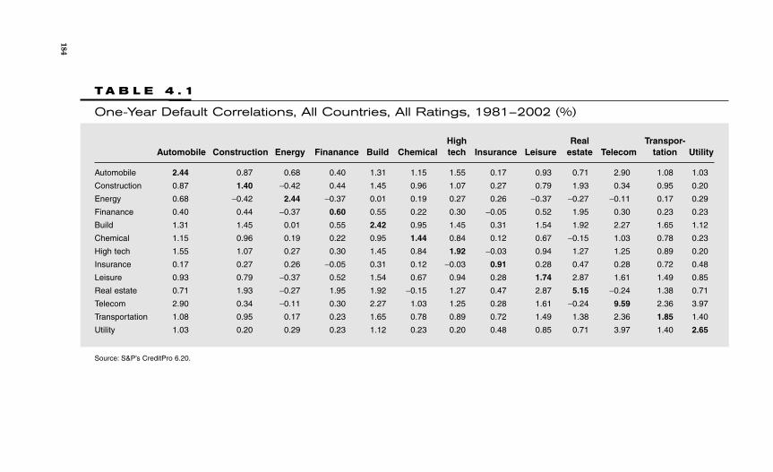
T A B L E 4 . 1
One-Year Default Correlations, All Countries, All Ratings, 1981–2002 (%)
High Real Transpor-Automobile Construction Energy Finanance Build Chemical tech Insurance Leisure estate Telecom tation Utility
Automobile 2.44 0.87 0.68 0.40 1.31 1.15 1.55 0.17 0.93 0.71 2.90 1.08 1.03
Construction 0.87 1.40 −0.42 0.44 1.45 0.96 1.07 0.27 0.79 1.93 0.34 0.95 0.20
Energy 0.68 −0.42 2.44 −0.37 0.01 0.19 0.27 0.26 −0.37 −0.27 −0.11 0.17 0.29
Finanance 0.40 0.44 −0.37 0.60 0.55 0.22 0.30 −0.05 0.52 1.95 0.30 0.23 0.23
Build 1.31 1.45 0.01 0.55 2.42 0.95 1.45 0.31 1.54 1.92 2.27 1.65 1.12
Chemical 1.15 0.96 0.19 0.22 0.95 1.44 0.84 0.12 0.67 −0.15 1.03 0.78 0.23
High tech 1.55 1.07 0.27 0.30 1.45 0.84 1.92 −0.03 0.94 1.27 1.25 0.89 0.20
Insurance 0.17 0.27 0.26 −0.05 0.31 0.12 −0.03 0.91 0.28 0.47 0.28 0.72 0.48
Leisure 0.93 0.79 −0.37 0.52 1.54 0.67 0.94 0.28 1.74 2.87 1.61 1.49 0.85
Real estate 0.71 1.93 −0.27 1.95 1.92 −0.15 1.27 0.47 2.87 5.15 −0.24 1.38 0.71
Telecom 2.90 0.34 −0.11 0.30 2.27 1.03 1.25 0.28 1.61 −0.24 9.59 2.36 3.97
Transportation 1.08 0.95 0.17 0.23 1.65 0.78 0.89 0.72 1.49 1.38 2.36 1.85 1.40
Utility 1.03 0.20 0.29 0.23 1.12 0.23 0.20 0.48 0.85 0.71 3.97 1.40 2.65
Source: S&P’s CreditPro 6.20.
184
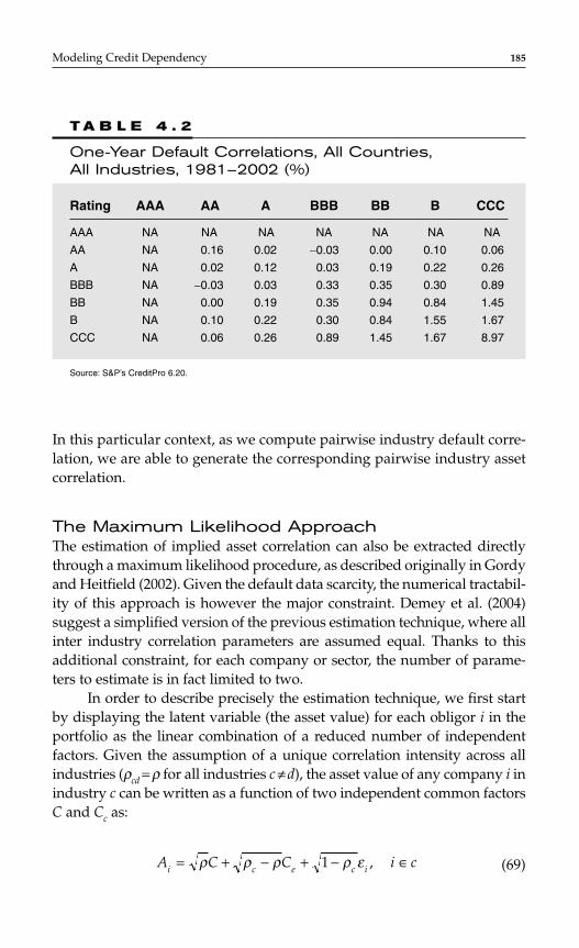
In this particular context, as we compute pairwise industry default corre-lation, we are able to generate the corresponding pairwise industry assetcorrelation.
The Maximum Likelihood ApproachThe estimation of implied asset correlation can also be extracted directlythrough a maximum likelihood procedure, as described originally in Gordyand Heitfield (2002). Given the default data scarcity, the numerical tractabil-ity of this approach is however the major constraint. Demey et al. (2004)suggest a simplified version of the previous estimation technique, where allinter industry correlation parameters are assumed equal. Thanks to thisadditional constraint, for each company or sector, the number of parame-ters to estimate is in fact limited to two.
In order to describe precisely the estimation technique, we first startby displaying the latent variable (the asset value) for each obligor i in theportfolio as the linear combination of a reduced number of independentfactors. Given the assumption of a unique correlation intensity across allindustries (ρcd = ρ for all industries c ≠ d), the asset value of any company i inindustry c can be written as a function of two independent common factorsC and Cc as:
(69)A C C i ci c e c i= + − + − ∈ρ ρ ρ ρ ε1 ,
Modeling Credit Dependency 185
T A B L E 4 . 2
One-Year Default Correlations, All Countries, All Industries, 1981–2002 (%)
Rating AAA AA A BBB BB B CCC
AAA NA NA NA NA NA NA NA
AA NA 0.16 0.02 −0.03 0.00 0.10 0.06
A NA 0.02 0.12 0.03 0.19 0.22 0.26
BBB NA −0.03 0.03 0.33 0.35 0.30 0.89
BB NA 0.00 0.19 0.35 0.94 0.84 1.45
B NA 0.10 0.22 0.30 0.84 1.55 1.67
CCC NA 0.06 0.26 0.89 1.45 1.67 8.97
Source: S&P’s CreditPro 6.20.

C can be considered as a factor common to the whole economy, whereasCc is a more industry specific common factor and εi is the idiosyncraticterm corresponding to obligor j.
The resulting asset correlation matrix can be written as:
Assuming that the idiosyncratic factor εi is Gaussian, and that Zc corre-sponds to the average, time invariant, default threshold of all companiesin industry c, we can write the probability of default within industry c,conditional on the realization ( f, fc) of factors (F, Fc) as:
(70)
where Φ is the normal c.d.f.Conditional on the realization of the factors, the number of defaults
in a given industrial sector c has a binomial distribution, with parametersNc, the number of firms in class c at time t, and Dc the default number inthe same class.
(71)
Due to the property of conditional independence, we can write theunconditional log-likelihood as:
(72)
Demey et al. (2004) investigate the potential stability and bias problems inseveral bootstrap experiments. They obtain reasonably good perfor-mances, as the mean of the bootstrap distribution converges quickly to thetrue correlation for class samples as small as 50.
l f f f ft c c cRc
C
( ) log Bin ( , )d ( ) d ( )θ =
∫∏∫
=
Φ Φ1
Bin ( , ) ( , ) ( ( , ))c cc
cc c
Dc c
N Df fN
DP f f P f fc c c=
− −1
P f fZ f f
c cc c c
c
( , ) =− − −
−
Φ
ρ ρ ρ
ρ1
ΣMLE =
ρ ρ ρρ ρ
ρρ ρ ρ
1
2
L
O
M O M
O
L C
186 CHAPTER 4
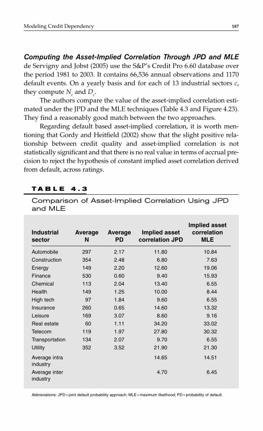
Computing the Asset-Implied Correlation Through JPD and MLEde Servigny and Jobst (2005) use the S&P’s Credit Pro 6.60 database overthe period 1981 to 2003. It contains 66,536 annual observations and 1170default events. On a yearly basis and for each of 13 industrial sectors c,they compute Nc and Dc.
The authors compare the value of the asset-implied correlation esti-mated under the JPD and the MLE techniques (Table 4.3 and Figure 4.23).They find a reasonably good match between the two approaches.
Regarding default based asset-implied correlation, it is worth men-tioning that Gordy and Heitfield (2002) show that the slight positive rela-tionship between credit quality and asset-implied correlation is notstatistically significant and that there is no real value in terms of accrual pre-cision to reject the hypothesis of constant implied asset correlation derivedfrom default, across ratings.
Modeling Credit Dependency 187
T A B L E 4 . 3
Comparison of Asset-Implied Correlation Using JPDand MLE
Implied asset Industrial Average Average Implied asset correlationsector N PD correlation JPD MLE
Automobile 297 2.17 11.80 10.84
Construction 354 2.48 6.80 7.63
Energy 149 2.20 12.60 19.06
Finance 530 0.60 9.40 15.93
Chemical 113 2.04 13.40 6.55
Health 149 1.25 10.00 8.44
High tech 97 1.84 9.60 6.55
Insurance 260 0.65 14.60 13.32
Leisure 169 3.07 8.60 9.16
Real estate 60 1.11 34.20 33.02
Telecom 119 1.97 27.80 30.32
Transportation 134 2.07 9.70 6.55
Utility 352 3.52 21.90 21.30
Average intra 14.65 14.51industry
Average inter 4.70 6.45industry
Abbreviations: JPD = joint default probability approach; MLE = maximum likelihood; PD = probability of default.
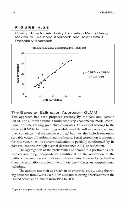
The Bayesian Estimation Approach—GLMMThis approach has been proposed recently by Mc Neil and Wendin(2005). The authors assume a multi time-step econometric model condi-tional on time varying predictive covariates. This model belongs to theclass of GLMMs. In this setup, probabilities of default rely on some usualfixed covariates that are used in scoring,* but they also include one unob-servable vector of random dynamic factors. Serial correlation is assumedfor this vector, i.e., its current realization is partially conditioned by itspast realizations through a serial dependence AR(1) specification.
The aggregation of the probabilities of default in a portfolio is per-formed assuming independence conditional on the realization of thepaths of the common vector of random covariates. In order to resolve thisdynamic estimation problem, the authors use a Bayesian computationaltechnique.
The authors test their approach in an empirical study, using the rat-ing database from S&P’s Credit Pro 6.60 and selecting observations in theUnited States and Canada from 1981 to 2000.
188 CHAPTER 4
Comparison asset correlation JPD—MLE plot
y = 0.9974x - 0.0954
R2 = 0.8321
0
10
20
30
ML
E c
orr
elat
ion
40
0 10 20 30 40JPD correlation
F I G U R E 4 . 2 3
Quality of the Intra-Industry Estimation Match UsingMaximum Likelihood Approach and Joint DefaultProbability Approach.
*Typically company specific or macroeconomic covariates.

For an obligor i, at time t, the probability of default conditional onthe realization of this systematic, unobserved, risk factor Fi is therefore:
P(Yti = 1/Ft) = logit(µt
i+ βXt + γ it Ft)
where Xt corresponds to a vector of explainable common macroeconomiceffects,* µi
t to the intercept,† and β it and γ i
t to related weights. The AR(1)process for the vector of latent systematic unobserved Gaussian randomrisk factors Fi can be written as: Ft = αFt-1 + φεt.
At the portfolio level, the usual assumption of conditional indepen-dence leads to the calculation of the loss distribution in a straightforwardmanner.
In a first analysis, the authors assume that there is no fixed commonvariable Xt, but only one random unobservable variable Ft. Using theBayesian technique, they observe that the hypothesis of an independentsimulation of the factor at each step, i.e., α = 0, is strongly rejected empir-ically. The estimation of α gives a mean value of around 0.65 with a stan-dard deviation representing around 25 percent of the mean. In addition,the expected value of the implied asset correlation can be estimated.Practically it comes to 7.6 percent.
In a second step, the authors incorporate a fixed macroeconomic vari-able Xt corresponding to the Chicago Fed National Activity Index, pub-lished on a monthly basis. They also consider six broad industrial sectors:
♦ Aerospace, automotive, capital goods, and metal♦ Consumer and service sector♦ Leisure time and media♦ Utility♦ Health care and chemicals♦ High tech, computers, office equipment, and Telecom
They show that the mean realization of the common random factor isdepending very clearly on the economic cycle, as can be seen on Figure 4.24.
Results show that both the introduction of industrial sectors and ofa macroeconomic factor reinforces the quality of the estimation. With thisspecification, average inter-industry asset-implied correlation comes to 6percent and intra-industry correlation to 10.5 percent. These results are inline in terms of magnitude with the results provided by the previous MLE
Modeling Credit Dependency 189
*Let us think of the typical credit factors used in credit scoring models.†Possibly derived from company specific factors and a true intercept.

and JPD estimators, especially given the fact that we are now talkingabout a less granular industry specification. We also note that asset corre-lation follows a cycle-dependent pattern.
Are Equity Correlations Good Proxies for Asset Correlations?We have just seen that the formula for pairwise default correlation is quitesimple but relies on asset correlation, which is not directly observable. It hasbecome market practice to use equity correlation as a proxy for asset corre-lation. The underlying assumption is that equity returns should reflect thevalue of the underlying firms and, therefore, that two firms with highly cor-related asset values should also have high equity correlations.
To test the validity of this assumption, de Servigny and Renault (2002)have gathered a sample of over 1100 firms for which they had at least fiveyears of data on the ratings, equity prices, and industry classification. Theythen computed average equity correlations across and within industries.
These scaled equity correlations were inserted in Equation (68) toobtain a series of default correlations extracted from equity prices. Theythen proceeded to compare default correlations calculated in this way todefault correlations calculated empirically using Equation (69).
Figure 4.25A summarizes their findings. Equity-driven default corre-lations and empirical correlations appear to be only weakly related or, inother words, equity correlations provide at best a noisy indicator of defaultcorrelations. This casts some doubt on the robustness of the market standard
190 CHAPTER 4
E(Ft)
01/01/1981 01/01/1987 01/01/1993 01/01/1999
-1.0
0.0
0.5
βi Xtt
F I G U R E 4 . 2 4
A Clear Correlation of the Common Factor with theEconomic Cycle. (McNeil and Wendin, 2005)
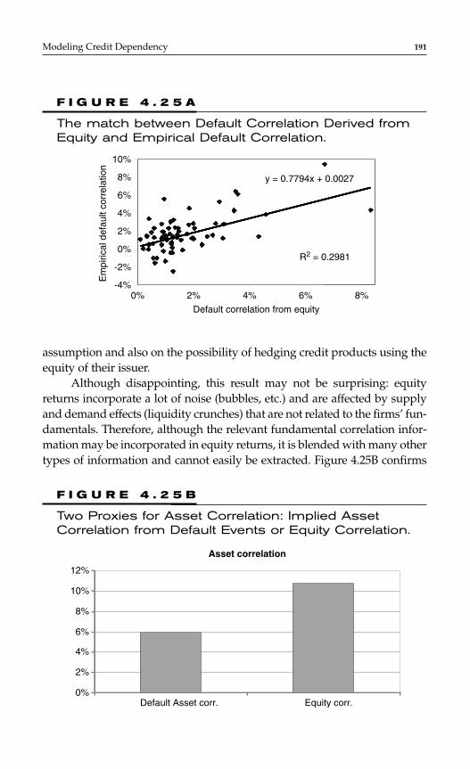
Modeling Credit Dependency 191
y = 0.7794x + 0.0027
R2 = 0.2981
0%
Em
piric
al d
efau
lt co
rrel
atio
n
-4%
-2%
0%
2%
4%
6%
8%
10%
2% 4% 6% 8%
Default correlation from equity
F I G U R E 4 . 2 5 A
The match between Default Correlation Derived fromEquity and Empirical Default Correlation.
assumption and also on the possibility of hedging credit products using theequity of their issuer.
Although disappointing, this result may not be surprising: equityreturns incorporate a lot of noise (bubbles, etc.) and are affected by supplyand demand effects (liquidity crunches) that are not related to the firms’ fun-damentals. Therefore, although the relevant fundamental correlation infor-mation may be incorporated in equity returns, it is blended with many othertypes of information and cannot easily be extracted. Figure 4.25B confirms
0%
2%
4%
6%
8%
10%
12%
Default Asset corr. Equity corr.
Asset correlation
F I G U R E 4 . 2 5 B
Two Proxies for Asset Correlation: Implied AssetCorrelation from Default Events or Equity Correlation.
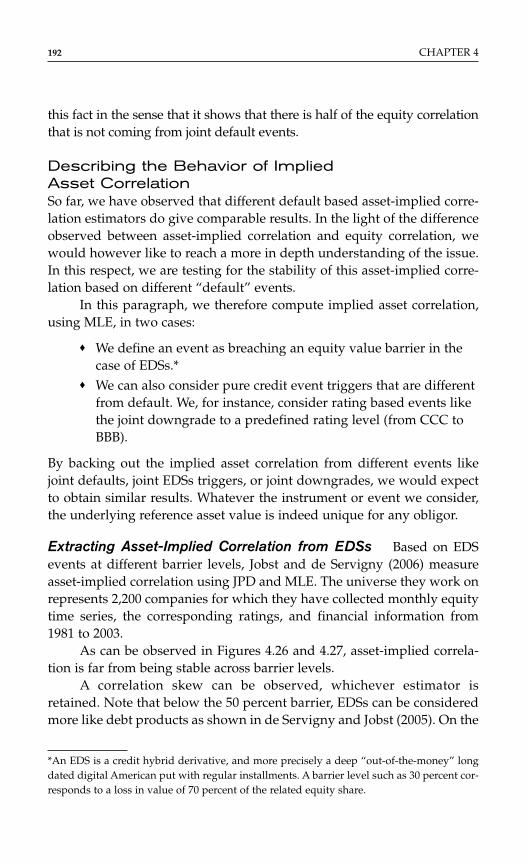
this fact in the sense that it shows that there is half of the equity correlationthat is not coming from joint default events.
Describing the Behavior of Implied Asset CorrelationSo far, we have observed that different default based asset-implied corre-lation estimators do give comparable results. In the light of the differenceobserved between asset-implied correlation and equity correlation, wewould however like to reach a more in depth understanding of the issue.In this respect, we are testing for the stability of this asset-implied corre-lation based on different “default” events.
In this paragraph, we therefore compute implied asset correlation,using MLE, in two cases:
♦ We define an event as breaching an equity value barrier in thecase of EDSs.*
♦ We can also consider pure credit event triggers that are differentfrom default. We, for instance, consider rating based events likethe joint downgrade to a predefined rating level (from CCC toBBB).
By backing out the implied asset correlation from different events likejoint defaults, joint EDSs triggers, or joint downgrades, we would expectto obtain similar results. Whatever the instrument or event we consider,the underlying reference asset value is indeed unique for any obligor.
Extracting Asset-Implied Correlation from EDSs Based on EDSevents at different barrier levels, Jobst and de Servigny (2006) measureasset-implied correlation using JPD and MLE. The universe they work onrepresents 2,200 companies for which they have collected monthly equitytime series, the corresponding ratings, and financial information from1981 to 2003.
As can be observed in Figures 4.26 and 4.27, asset-implied correla-tion is far from being stable across barrier levels.
A correlation skew can be observed, whichever estimator isretained. Note that below the 50 percent barrier, EDSs can be consideredmore like debt products as shown in de Servigny and Jobst (2005). On the
192 CHAPTER 4
*An EDS is a credit hybrid derivative, and more precisely a deep “out-of-the-money” longdated digital American put with regular installments. A barrier level such as 30 percent cor-responds to a loss in value of 70 percent of the related equity share.
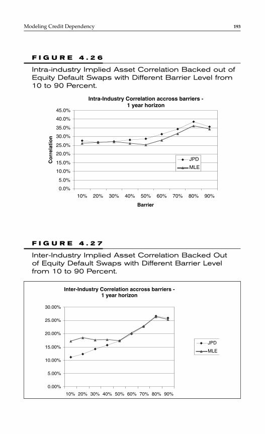
Modeling Credit Dependency 193
Intra-Industry Correlation accross barriers - 1 year horizon
0.0%
5.0%
10.0%
15.0%
20.0%
25.0%
30.0%
35.0%
40.0%
45.0%
10% 20% 30% 40% 50% 60% 70% 80% 90%
Barrier
Co
rrel
atio
n
JPD
MLE
F I G U R E 4 . 2 6
Intra-industry Implied Asset Correlation Backed out ofEquity Default Swaps with Different Barrier Level from10 to 90 Percent.
Inter-Industry Correlation accross barriers - 1 year horizon
0.00%
5.00%
10.00%
15.00%
20.00%
25.00%
30.00%
10% 20% 30% 40% 50% 60% 70% 80% 90%
JPD
MLE
F I G U R E 4 . 2 7
Inter-Industry Implied Asset Correlation Backed Outof Equity Default Swaps with Different Barrier Levelfrom 10 to 90 Percent.
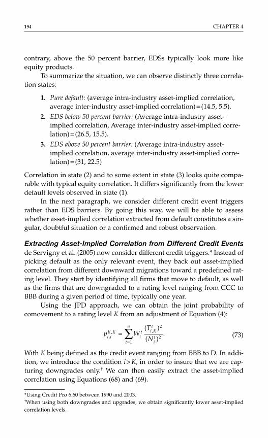
contrary, above the 50 percent barrier, EDSs typically look more likeequity products.
To summarize the situation, we can observe distinctly three correla-tion states:
1. Pure default: (average intra-industry asset-implied correlation,average inter-industry asset-implied correlation) = (14.5, 5.5).
2. EDS below 50 percent barrier: (Average intra-industry asset-implied correlation, Average inter-industry asset-implied corre-lation) = (26.5, 15.5).
3. EDS above 50 percent barrier: (Average intra-industry asset-implied correlation, average inter-industry asset-implied corre-lation) = (31, 22.5)
Correlation in state (2) and to some extent in state (3) looks quite compa-rable with typical equity correlation. It differs significantly from the lowerdefault levels observed in state (1).
In the next paragraph, we consider different credit event triggersrather than EDS barriers. By going this way, we will be able to assesswhether asset-implied correlation extracted from default constitutes a sin-gular, doubtful situation or a confirmed and robust observation.
Extracting Asset-Implied Correlation from Different Credit Eventsde Servigny et al. (2005) now consider different credit triggers.* Instead ofpicking default as the only relevant event, they back out asset-impliedcorrelation from different downward migrations toward a predefined rat-ing level. They start by identifying all firms that move to default, as wellas the firms that are downgraded to a rating level ranging from CCC toBBB during a given period of time, typically one year.
Using the JPD approach, we can obtain the joint probability ofcomovement to a rating level K from an adjustment of Equation (4):
(73)
With K being defined as the credit event ranging from BBB to D. In addi-tion, we introduce the condition i > K, in order to insure that we are cap-turing downgrades only.† We can then easily extract the asset-impliedcorrelation using Equations (68) and (69).
p WT
Ni iK K
it i K
t
it
t
n
,, ,( )
( ).=
=∑
2
21
194 CHAPTER 4
*Using Credit Pro 6.60 between 1990 and 2003.†When using both downgrades and upgrades, we obtain significantly lower asset-impliedcorrelation levels.
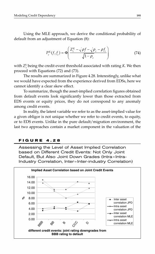
Using the MLE approach, we derive the conditional probability ofdefault from an adjustment of Equation (8):
(74)
with Zkc being the credit event threshold associated with rating K. We then
proceed with Equations (72) and (73).The results are summarized in Figure 4.28. Interestingly, unlike what
we would have expected from the experience derived from EDSs, here wecannot identify a clear skew effect.
To summarize, though the asset-implied correlation figures obtainedfrom default events look significantly lower than those extracted fromEDS events or equity prices, they do not correspond to any anomalyamong credit events.
In reality, the latent variable we refer to as the asset-implied value fora given obligor is not unique whether we refer to credit events, to equity,or to EDS events. Unlike in the pure default/migration environment, thelast two approaches contain a market component in the valuation of the
P f fZ f f
cK
ccK
c c
c
( , ) =− − −
−
Φ
ρ ρ ρ
ρ1
Modeling Credit Dependency 195
Implied Asset Correlation based on Joint Credit Events
0.00
2.00
4.00
6.00
8.00
10.00
12.00
14.00
16.00
BBB BB B
CCC D
different credit events: joint rating downgrades fromBBB rating to default
% Inter assetcorrelation JPDIntra assetcorrelation JPDInter assetcorrelation MLEIntra assetcorrelation MLE
F I G U R E 4 . 2 8
Assessing the Level of Asset Implied Correlationbased on Different Credit Events: Not Only JointDefault, But Also Joint Down Grades (Intra= Intra-Industry Correlation, Inter= Inter-industry Correlation)
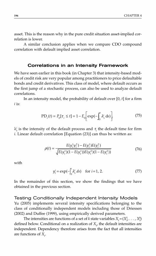
asset. This is the reason why in the pure credit situation asset-implied cor-relation is lower.
A similar conclusion applies when we compare CDO compoundcorrelation with default implied asset correlation.
Correlations in an Intensity Framework
We have seen earlier in this book (in Chapter 3) that intensity-based mod-els of credit risk are very popular among practitioners to price defaultablebonds and credit derivatives. This class of model, where default occurs asthe first jump of a stochastic process, can also be used to analyze defaultcorrelations.
In an intensity model, the probability of default over [0, t] for a firmi is:
(75)
λis is the intensity of the default process and τi the default time for firm
i. Linear default correlation [Equation (23)] can thus be written as:
(76)
with
yit = exp(−∫0
tλt
s ds) for i = 1, 2. (77)
In the remainder of this section, we show the findings that we haveobtained in the previous section.
Testing Conditionally Independent Intensity ModelsYu (2005) implements several intensity specifications belonging to theclass of conditionally independent models including those of Driessen(2002) and Duffee (1999), using empirically derived parameters.
The intensities are functions of a set of k state variables Xt = (X1t, . . . , Xk
t)defined below. Conditional on a realization of Xt, the default intensities areindependent. Dependency therefore arises from the fact that all intensitiesare functions of Xt.
ρ( )( ) ( ) ( )
( )( ( )) ( )( ( ))t
E y y E y E y
E y E y E y E yt t t t
t t t t
=−
− −
1 2 1 2
1 1 2 21 1
PD ( ) [ ] exp( d ) .i i si
tt P t E s= ≤ = − −
∫0 0 0
1τ λ
196 CHAPTER 4
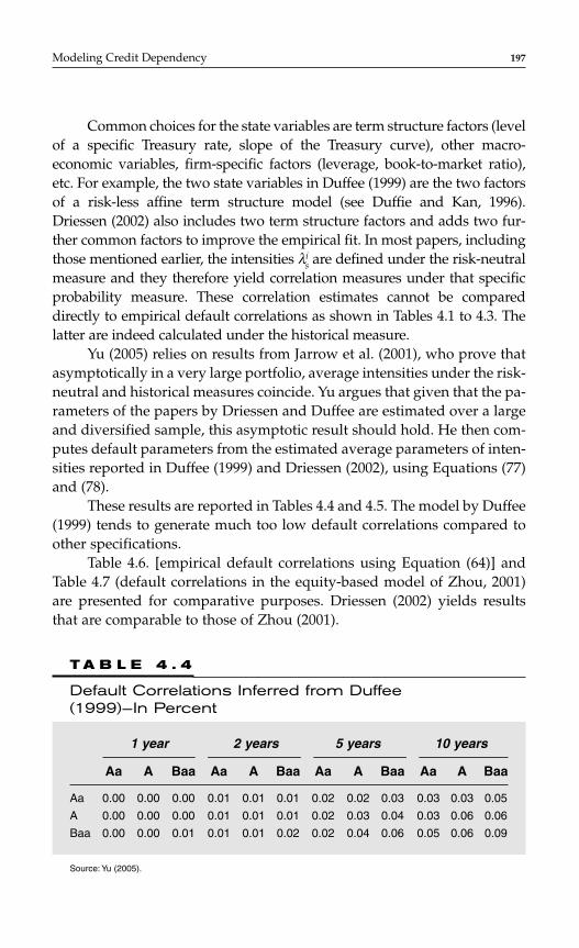
Common choices for the state variables are term structure factors (levelof a specific Treasury rate, slope of the Treasury curve), other macro-economic variables, firm-specific factors (leverage, book-to-market ratio),etc. For example, the two state variables in Duffee (1999) are the two factorsof a risk-less affine term structure model (see Duffie and Kan, 1996).Driessen (2002) also includes two term structure factors and adds two fur-ther common factors to improve the empirical fit. In most papers, includingthose mentioned earlier, the intensities λi
s are defined under the risk-neutralmeasure and they therefore yield correlation measures under that specificprobability measure. These correlation estimates cannot be compareddirectly to empirical default correlations as shown in Tables 4.1 to 4.3. Thelatter are indeed calculated under the historical measure.
Yu (2005) relies on results from Jarrow et al. (2001), who prove thatasymptotically in a very large portfolio, average intensities under the risk-neutral and historical measures coincide. Yu argues that given that the pa-rameters of the papers by Driessen and Duffee are estimated over a largeand diversified sample, this asymptotic result should hold. He then com-putes default parameters from the estimated average parameters of inten-sities reported in Duffee (1999) and Driessen (2002), using Equations (77)and (78).
These results are reported in Tables 4.4 and 4.5. The model by Duffee(1999) tends to generate much too low default correlations compared toother specifications.
Table 4.6. [empirical default correlations using Equation (64)] andTable 4.7 (default correlations in the equity-based model of Zhou, 2001)are presented for comparative purposes. Driessen (2002) yields resultsthat are comparable to those of Zhou (2001).
Modeling Credit Dependency 197
T A B L E 4 . 4
Default Correlations Inferred from Duffee (1999)—In Percent
1 year 2 years 5 years 10 years
Aa A Baa Aa A Baa Aa A Baa Aa A Baa
Aa 0.00 0.00 0.00 0.01 0.01 0.01 0.02 0.02 0.03 0.03 0.03 0.05
A 0.00 0.00 0.00 0.01 0.01 0.01 0.02 0.03 0.04 0.03 0.06 0.06
Baa 0.00 0.00 0.01 0.01 0.01 0.02 0.02 0.04 0.06 0.05 0.06 0.09
Source: Yu (2005).
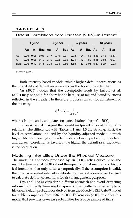
Both intensity-based models exhibit higher default correlations asthe probability of default increases and as the horizon is extended.
Yu (2005) notices that the asymptotic result by Jarrow et al.(2001) may not hold for short bonds because of tax and liquidity effectsreflected in the spreads. He therefore proposes an ad hoc adjustment ofthe intensity:
where t is time and a and b are constants obtained from Yu (2002).Tables 4.9 and 4.10 report the liquidity-adjusted tables of default cor-
relations. The differences with Tables 4.4 and 4.5 are striking. First, thelevel of correlations induced by the liquidity-adjusted models is muchhigher. More surprisingly, the relationship between probability of defaultand default correlation is inverted: the higher the default risk, the loweris the correlation.
Modeling Intensities Under the Physical MeasureThe modeling approach proposed by Yu (2005) relies critically on theresult by Jarrow et al. (2001) about the equality of risk-neutral and histor-ical intensities that only holds asymptotically. If the assumption is valid,then the risk-neutral intensity calibrated on market spreads can be usedto calculate default correlations for risk management purposes.
Das et al. (2006) consider a different approach and avoid extractinginformation directly from market spreads. They gather a large sample ofhistorical default probabilities derived from the Moody’s RiskCalc™ modelfor public companies from 1987 to 2000. Falkenstein (2000) describes thismodel that provides one-year probabilities for a large sample of firms.
λ λt t
ab t
adj ,= −+
198 CHAPTER 4
T A B L E 4 . 5
Default Correlations from Driessen (2002)—In Percent
1 year 2 years 5 years 10 years
Aa A Baa Aa A Baa Aa A Baa Aa A Baa
Aa 0.04 0.05 0.08 0.17 0.19 0.31 0.93 1.04 1.68 3.16 3.48 5.67
A 0.05 0.06 0.10 0.19 0.32 0.35 1.04 1.17 1.89 3.48 3.85 6.27
Baa 0.08 0.10 0.15 0.31 0.35 0.56 1.68 1.89 3.05 5.67 6.27 10.23
Source: Yu (2005).
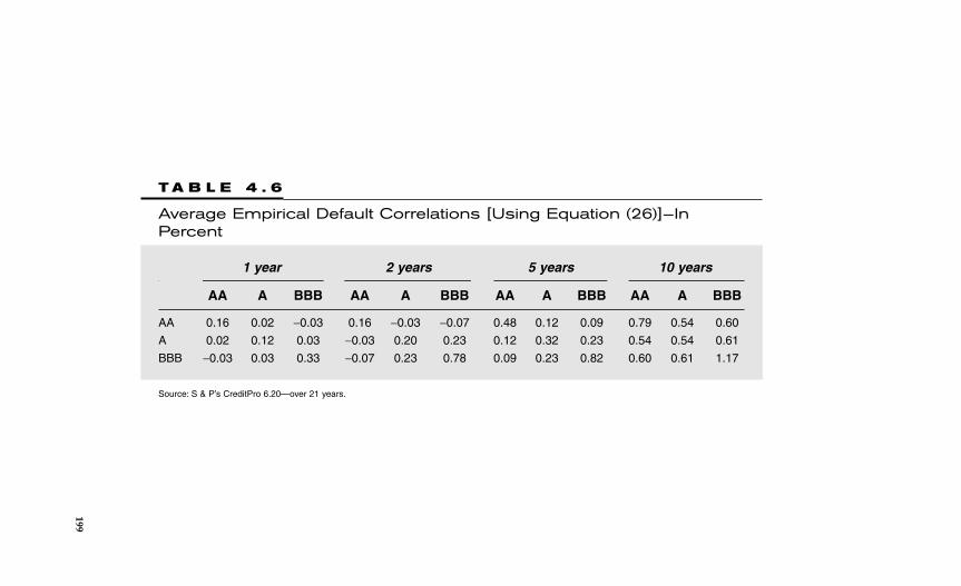
T A B L E 4 . 6
Average Empirical Default Correlations [Using Equation (26)]—In Percent
1 year 2 years 5 years 10 years
AA A BBB AA A BBB AA A BBB AA A BBB
AA 0.16 0.02 −0.03 0.16 −0.03 −0.07 0.48 0.12 0.09 0.79 0.54 0.60
A 0.02 0.12 0.03 −0.03 0.20 0.23 0.12 0.32 0.23 0.54 0.54 0.61
BBB −0.03 0.03 0.33 −0.07 0.23 0.78 0.09 0.23 0.82 0.60 0.61 1.17
Source: S & P’s CreditPro 6.20—over 21 years.
199
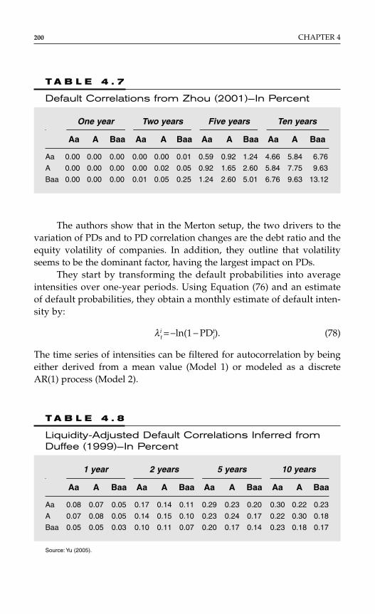
200 CHAPTER 4
T A B L E 4 . 7
Default Correlations from Zhou (2001)—In Percent
One year Two years Five years Ten years
Aa A Baa Aa A Baa Aa A Baa Aa A Baa
Aa 0.00 0.00 0.00 0.00 0.00 0.01 0.59 0.92 1.24 4.66 5.84 6.76
A 0.00 0.00 0.00 0.00 0.02 0.05 0.92 1.65 2.60 5.84 7.75 9.63
Baa 0.00 0.00 0.00 0.01 0.05 0.25 1.24 2.60 5.01 6.76 9.63 13.12
T A B L E 4 . 8
Liquidity-Adjusted Default Correlations Inferred fromDuffee (1999)—In Percent
1 year 2 years 5 years 10 years
Aa A Baa Aa A Baa Aa A Baa Aa A Baa
Aa 0.08 0.07 0.05 0.17 0.14 0.11 0.29 0.23 0.20 0.30 0.22 0.23
A 0.07 0.08 0.05 0.14 0.15 0.10 0.23 0.24 0.17 0.22 0.30 0.18
Baa 0.05 0.05 0.03 0.10 0.11 0.07 0.20 0.17 0.14 0.23 0.18 0.17
Source: Yu (2005).
The authors show that in the Merton setup, the two drivers to thevariation of PDs and to PD correlation changes are the debt ratio and theequity volatility of companies. In addition, they outline that volatilityseems to be the dominant factor, having the largest impact on PDs.
They start by transforming the default probabilities into averageintensities over one-year periods. Using Equation (76) and an estimateof default probabilities, they obtain a monthly estimate of default inten-sity by:
λit = −ln(1 − PDt
i). (78)
The time series of intensities can be filtered for autocorrelation by beingeither derived from a mean value (Model 1) or modeled as a discreteAR(1) process (Model 2).
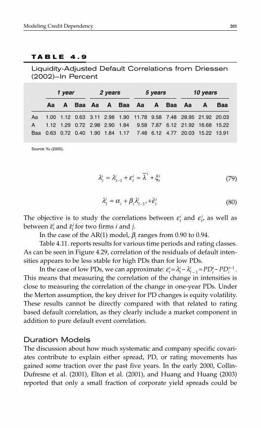
(79)
(80)
The objective is to study the correlations between ε it and ε j
t, as well asbetween ε~i
t and ε~ jt for two firms i and j.
In the case of the AR(1) model, βi ranges from 0.90 to 0.94.Table 4.11. reports results for various time periods and rating classes.
As can be seen in Figure 4.29, correlation of the residuals of default inten-sities appears to be less stable for high PDs than for low PDs.
In the case of low PDs, we can approximate: εit = λi
t − λit − 1 ≈ PDt
i − PDit−1 .
This means that measuring the correlation of the change in intensities isclose to measuring the correlation of the change in one-year PDs. Underthe Merton assumption, the key driver for PD changes is equity volatility.These results cannot be directly compared with that related to ratingbased default correlation, as they clearly include a market component inaddition to pure default event correlation.
Duration ModelsThe discussion about how much systematic and company specific covari-ates contribute to explain either spread, PD, or rating movements hasgained some traction over the past five years. In the early 2000, Collin-Dufresne et al. (2001), Elton et al. (2001), and Huang and Huang (2003)reported that only a small fraction of corporate yield spreads could be
λ α β λ εti
i i ti
ti= + +−1 , ˜
λ λ ε λ ξti
ti
ti i
ti= + = +−1
Modeling Credit Dependency 201
T A B L E 4 . 9
Liquidity-Adjusted Default Correlations from Driessen(2002)—In Percent
1 year 2 years 5 years 10 years
Aa A Baa Aa A Baa Aa A Baa Aa A Baa
Aa 1.00 1.12 0.63 3.11 2.98 1.90 11.78 9.58 7.48 28.95 21.92 20.03
A 1.12 1.29 0.72 2.98 2.90 1.84 9.58 7.87 6.12 21.92 16.68 15.22
Baa 0.63 0.72 0.40 1.90 1.84 1.17 7.48 6.12 4.77 20.03 15.22 13.91
Source: Yu (2005).
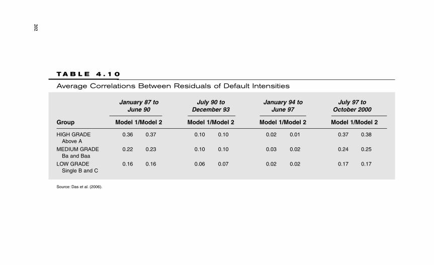
T A B L E 4 . 1 0
Average Correlations Between Residuals of Default Intensities
January 87 to July 90 to January 94 to July 97 to June 90 December 93 June 97 October 2000
Group Model 1/Model 2 Model 1/Model 2 Model 1/Model 2 Model 1/Model 2
HIGH GRADE 0.36 0.37 0.10 0.10 0.02 0.01 0.37 0.38Above A
MEDIUM GRADE 0.22 0.23 0.10 0.10 0.03 0.02 0.24 0.25Ba and Baa
LOW GRADE 0.16 0.16 0.06 0.07 0.02 0.02 0.17 0.17Single B and C
Source: Das et al. (2006).
202

explained by default information.* Based on these findings, systematicrisk components, such as common factors, liquidity effects, and riskaversion, can be considered as very important drivers to account forspread changes. From an opposite perspective a legitimate question canbe: how much company specific are default intensities under the empir-ical measure?
In the research community, the first step has been to move from adiscontinuous rating based approach to a time continuous intensity one.In the wake of Lando and Skodeberg (2002), Jafry and Schuermann (2003),Jobst and Gilkes (2003), and several authors like Couderc and Renault(2005) or Duffie et al. (2005), the model default intensity as a parametricor semiparametric factor model derived from the Cox proportional haz-ard methodology (Cox, 1972 and 1975)† as follows:
λi(t) = λ0(t) exp (β’Xi(t)),
where Xi(t) corresponds to the vector of covariates.In Table 4.11, we draw a comparison between the categories of fac-
tors that have been tested, in order to explain default intensity changes.Interestingly, at a rating category level, Couderc and Renault (2005) showthat contemporaneous financial market factors as well as past financial,
Modeling Credit Dependency 203
Delta Default intensity correlation (Das et al. 2005)
00.050.1
0.150.2
0.250.3
0.350.4
Jan 87 toJun 90
Jul 90 toDec 93
Jan 94 toJun 97
Jul 97 toOct 2000
corr
el. (
%)
HIGH GRADE
MEDIUM GRADE
LOW GRADE
F I G U R E 4 . 2 9
The evolution of Correlation of Delta Default Intensitiesthrough Time using Model 1.
*Less than 25 percent Collin-Dufresne et al. (2001) and Elton et al. (2001).†The former estimates the default intensity at a company level, the latter per rating category.
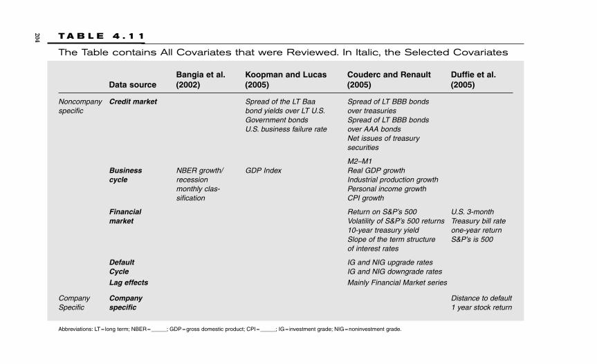
T A B L E 4 . 1 1
The Table contains All Covariates that were Reviewed. In Italic, the Selected Covariates
Bangia et al. Koopman and Lucas Couderc and Renault Duffie et al.Data source (2002) (2005) (2005) (2005)
Noncompany Credit market Spread of the LT Baa Spread of LT BBB bonds specific bond yields over LT U.S. over treasuries
Government bonds Spread of LT BBB bondsU.S. business failure rate over AAA bonds
Net issues of treasury securities
M2–M1Business NBER growth/ GDP Index Real GDP growthcycle recession Industrial production growth
monthly clas- Personal income growthsification CPI growth
Financial Return on S&P’s 500 U.S. 3-month market Volatility of S&P’s 500 returns Treasury bill rate
10-year treasury yield one-year return Slope of the term structure S&P’s is 500of interest rates
Default IG and NIG upgrade ratesCycle IG and NIG downgrade rates
Lag effects Mainly Financial Market series
Company Company Distance to defaultSpecific specific 1 year stock return
Abbreviations: LT = long term; NBER = _____; GDP = gross domestic product; CPI = _____; IG = investment grade; NIG = noninvestment grade.
204
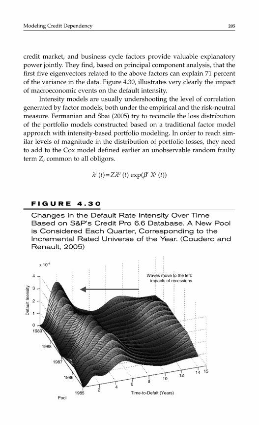
credit market, and business cycle factors provide valuable explanatorypower jointly. They find, based on principal component analysis, that thefirst five eigenvectors related to the above factors can explain 71 percentof the variance in the data. Figure 4.30, illustrates very clearly the impactof macroeconomic events on the default intensity.
Intensity models are usually undershooting the level of correlationgenerated by factor models, both under the empirical and the risk-neutralmeasure. Fermanian and Sbai (2005) try to reconcile the loss distributionof the portfolio models constructed based on a traditional factor modelapproach with intensity-based portfolio modeling. In order to reach sim-ilar levels of magnitude in the distribution of portfolio losses, they needto add to the Cox model defined earlier an unobservable random frailtyterm Z, common to all obligors.
λi (t) = Zλ0 (t) exp(β’ Xi (t))
Modeling Credit Dependency 205
x 10-4
Waves move to the left:impacts of recessions
Def
ault
Inen
sity
Time-to-Defalt (Years)
4
3
2
1
01989
1988
1987
1986
19852
46
810
1214 15
Pool
F I G U R E 4 . 3 0
Changes in the Default Rate Intensity Over TimeBased on S&P’s Credit Pro 6.6 Database. A New Poolis Considered Each Quarter, Corresponding to theIncremental Rated Universe of the Year. (Couderc andRenault, 2005)
The calibration of this frailty term (typically a gamma distributed variable)enables us to obtain even more skewed loss distributions and thereby toavoid the underestimation problem that factor models usually face, due tothe assumption of a Gaussian distribution of the common factors.*
Das et al. (2006) tend to provide some rationale for the use of a frailtyterm. They look at the same problem from a different perspective and esti-mate a default intensity model for each of the 2770 firms in their sample,according to the specification detailed in Duffie et al. (2005). Because someof the covariates in the estimation are common to all obligors, they ini-tially assume that it is possible to aggregate losses in the portfolio condi-tional on the realization of these factors. Based on the different tests theyperform, they find that their model fails to fully match the tail of the trueloss distribution of the portfolio. This could be because their intensitymodel is not capturing all the relevant common macrofactors at play.They focus on one extra covariate in particular: “the growth rate of theindustrial production.” It could also well be that more fundamentally, theassumption of conditional independence does not hold due to contagion(i.e., the presence of an unobservable variable common to all firms). As weknow, contagion cannot be accounted for in a proper manner under theconditional independence assumption.
Implications for CDOs
Identifying How Sensitive CDO Tranches are toEmpirical CorrelationIn order to investigate the impact of correlation on CDO tranches, we con-sider the simple case of a well-diversified portfolio of 100 BB (or BBB)bonds with a nominal exposure of 1$ each. During growth periods weconsider that the average default rate at a five-year horizon Q corre-sponds to Pgr
BB, and during recession periods the average default ratejumps to Pre
BB. In terms of correlation, we assume a one-factor model com-mon to all obligors. Based on empirical work, we consider that the aver-age asset-implied correlation ρ in a portfolio is in the range of ρgr duringgrowth periods and moves up to ρre during recessions.
We focus on four scenarios:
♦ A growth scenario where the default rate and the correlationlevels are, respectively, Pgr
BB and ρgr
206 CHAPTER 4
*The point is to calibrate the frailty term properly.
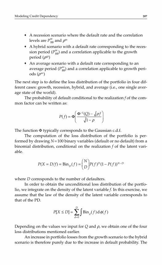
♦ A recession scenario where the default rate and the correlationlevels are Pre
BB and ρre
♦ A hybrid scenario with a default rate corresponding to the reces-sion period (Pre
BB) and a correlation applicable to the growthperiod (ρgr)
♦ An average scenario with a default rate corresponding to anaverage period (Pav
BB) and a correlation applicable to growth peri-ods (ρav)
The next step is to define the loss distribution of the portfolio in four dif-ferent cases: growth, recession, hybrid, and average (i.e., one single aver-age state of the world).
The probability of default conditional to the realization f of the com-mon factor can be written as:
The function Φ typically corresponds to the Gaussian c.d.f.The computation of the loss distribution of the portfolio is per-
formed by drawing N = 100 binary variables (default or no default) from abinomial distribution, conditional on the realization f of the latent vari-able.
where D corresponds to the number of defaulters.In order to obtain the unconditional loss distribution of the portfo-
lio, we integrate on the density of the latent variable f. In this exercise, weassume that the law of the density of the latent variable corresponds tothat of the PD.
Depending on the values we input for Q and ρ, we obtain one of the fourloss distributions mentioned earlier.
An increase in portfolio losses from the growth scenario to the hybridscenario is therefore purely due to the increase in default probability. The
P X D f fdd
D
[ ] Bin ( )d ( )≤ = ∫∑=
φ0
P X D f fN
DP f P fD
D N D( / ) Bin ( ) ( ) ( ( ))= = =
− −1
P fQ f
( )( )
=−
−
−Φ
Φ 1
1
ρρ
Modeling Credit Dependency 207
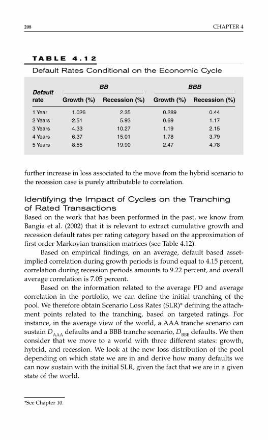
further increase in loss associated to the move from the hybrid scenario tothe recession case is purely attributable to correlation.
Identifying the Impact of Cycles on the Tranchingof Rated TransactionsBased on the work that has been performed in the past, we know fromBangia et al. (2002) that it is relevant to extract cumulative growth andrecession default rates per rating category based on the approximation offirst order Markovian transition matrices (see Table 4.12).
Based on empirical findings, on an average, default based asset-implied correlation during growth periods is found equal to 4.15 percent,correlation during recession periods amounts to 9.22 percent, and overallaverage correlation is 7.05 percent.
Based on the information related to the average PD and averagecorrelation in the portfolio, we can define the initial tranching of thepool. We therefore obtain Scenario Loss Rates (SLR)* defining the attach-ment points related to the tranching, based on targeted ratings. Forinstance, in the average view of the world, a AAA tranche scenario cansustain DAAA defaults and a BBB tranche scenario, DBBB defaults. We thenconsider that we move to a world with three different states: growth,hybrid, and recession. We look at the new loss distribution of the pooldepending on which state we are in and derive how many defaults wecan now sustain with the initial SLR, given the fact that we are in a givenstate of the world.
208 CHAPTER 4
T A B L E 4 . 1 2
Default Rates Conditional on the Economic Cycle
DefaultBB BBB
rate Growth (%) Recession (%) Growth (%) Recession (%)
1 Year 1.026 2.35 0.289 0.44
2 Years 2.51 5.93 0.69 1.17
3 Years 4.33 10.27 1.19 2.15
4 Years 6.37 15.01 1.78 3.79
5 Years 8.55 19.90 2.47 4.78
*See Chapter 10.
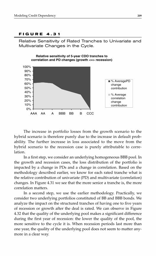
The increase in portfolio losses from the growth scenario to thehybrid scenario is therefore purely due to the increase in default prob-ability. The further increase in loss associated to the move from thehybrid scenario to the recession case is purely attributable to corre-lation.
In a first step, we consider an underlying homogeneous BBB pool. Inthe growth and recession cases, the loss distribution of the portfolio isimpacted by a change in PDs and a change in correlation. Based on themethodology described earlier, we know for each rated tranche what isthe relative contribution of univariate (PD) and multivariate (correlation)changes. In Figure 4.31 we see that the more senior a tranche is, the morecorrelation matters.
In a second step, we use the earlier methodology. Practically, weconsider two underlying portfolios constituted of BB and BBB bonds. Weanalyze the impact on the structured tranches of having one to five yearsof recession or growth after the deal is rated. We can observe in Figure4.32 that the quality of the underlying pool makes a significant differenceduring the first year of recession: the lower the quality of the pool, themore sensitive to the cycle it is. When recession periods last more thanone year, the quality of the underlying pool does not seem to matter any-more in a clear way.
Modeling Credit Dependency 209
Relative sensitivity of 5-year CDO tranches tocorrelation and PD changes (growth <=> recession)
0%10%20%30%40%50%60%70%80%90%
100%
AAA AA A BBB BB B CCC
% AveragePDchangecontribution
% Averagecorrelationchangecontribution
F I G U R E 4 . 3 1
Relative Sensitivity of Rated Tranches to Univariate andMultivariate Changes in the Cycle.
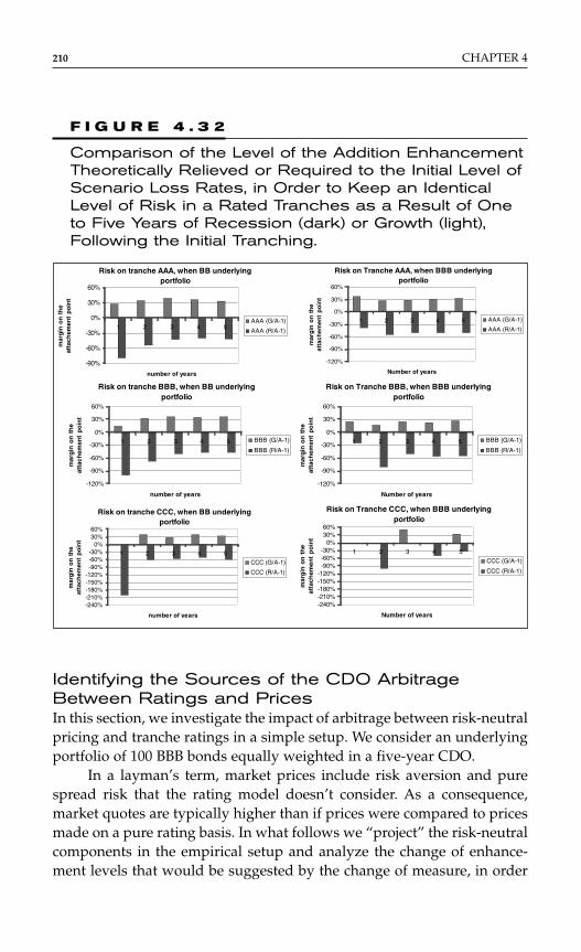
Identifying the Sources of the CDO ArbitrageBetween Ratings and PricesIn this section, we investigate the impact of arbitrage between risk-neutralpricing and tranche ratings in a simple setup. We consider an underlyingportfolio of 100 BBB bonds equally weighted in a five-year CDO.
In a layman’s term, market prices include risk aversion and purespread risk that the rating model doesn’t consider. As a consequence,market quotes are typically higher than if prices were compared to pricesmade on a pure rating basis. In what follows we “project” the risk-neutralcomponents in the empirical setup and analyze the change of enhance-ment levels that would be suggested by the change of measure, in order
210 CHAPTER 4
Risk on tranche AAA, when BB underlyingportfolio
-90%
-60%
-30%
0%
30%
60%
1 2 3 4 5
number of years
mar
gin
on
th
e at
tach
emen
t p
oin
t
AAA (G/A-1)
AAA (R/A-1)
Risk on Tranche AAA, when BBB underlyingportfolio
-120%
-90%
-60%
-30%
0%
30%
60%
1 2 3 4 5
Number of years
mar
gin
on
th
e at
tach
emen
t p
oin
tAAA (G/A-1)
AAA (R/A-1)
Risk on tranche BBB, when BB underlyingportfolio
-120%
-90%
-60%
-30%
0%
30%
60%
1 2 3 4 5
number of years
mar
gin
on
th
e at
tach
emen
t p
oin
t
BBB (G/A-1)
BBB (R/A-1)
Risk on Tranche BBB, when BBB underlyingportfolio
-120%
-90%
-60%
-30%
0%
30%
60%
1 2 3 4 5
Number of years
mar
gin
on
th
e at
tach
emen
t p
oin
t
BBB (G/A-1)
BBB (R/A-1)
Risk on tranche CCC, when BB underlyingportfolio
-240%-210%-180%-150%-120%-90%-60%-30%
0%30%60%
1 2 3 4 5
number of years
mar
gin
on
th
e at
tach
emen
t p
oin
t
CCC (G/A-1)
CCC (R/A-1)
Risk on Tranche CCC, when BBB underlyingportfolio
-240%-210%-180%-150%-120%-90%-60%-30%
0%30%60%
1 2 3 4 5
Number of years
mar
gin
on
th
e at
tach
emen
t p
oin
t
CCC (G/A-1)
CCC (R/A-1)
F I G U R E 4 . 3 2
Comparison of the Level of the Addition EnhancementTheoretically Relieved or Required to the Initial Level ofScenario Loss Rates, in Order to Keep an IdenticalLevel of Risk in a Rated Tranches as a Result of Oneto Five Years of Recession (dark) or Growth (light),Following the Initial Tranching.
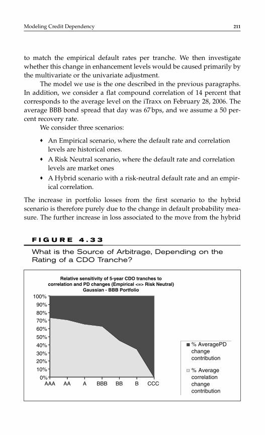
to match the empirical default rates per tranche. We then investigatewhether this change in enhancement levels would be caused primarily bythe multivariate or the univariate adjustment.
The model we use is the one described in the previous paragraphs.In addition, we consider a flat compound correlation of 14 percent thatcorresponds to the average level on the iTraxx on February 28, 2006. Theaverage BBB bond spread that day was 67 bps, and we assume a 50 per-cent recovery rate.
We consider three scenarios:
♦ An Empirical scenario, where the default rate and correlationlevels are historical ones.
♦ A Risk Neutral scenario, where the default rate and correlationlevels are market ones
♦ A Hybrid scenario with a risk-neutral default rate and an empir-ical correlation.
The increase in portfolio losses from the first scenario to the hybridscenario is therefore purely due to the change in default probability mea-sure. The further increase in loss associated to the move from the hybrid
Modeling Credit Dependency 211
Relative sensitivity of 5-year CDO tranches to correlation and PD changes (Empirical <=> Risk Neutral)
Gaussian - BBB Portfolio
0%
10%
20%
30%
40%
50%
60%
70%
80%
90%
100%
AAA AA A BBB BB B CCC
% AveragePDchangecontribution
% Averagecorrelationchangecontribution
F I G U R E 4 . 3 3
What is the Source of Arbitrage, Depending on theRating of a CDO Tranche?
scenario to the risk-neutral case is purely attributable to a change in mea-sure for correlation.
As can be seen in Figure 4.33, for investment grade tranches, it is thechange from an average 7 percent correlation level to an average 14 per-cent, which explains the majority of the arbitrage. On the opposite, in thecase of subinvestment grade tranches, it is the change, at a name level,from the empirical measure to the risk-neutral one, which explains themajority of the arbitrage.
When we run a similar exercise with a subinvestment grade under-lying pool, we observe an increased contribution of the univariate com-ponent (change from the empirical to the risk-neutral measure) withrespect to that of the change in correlation.
Of course, some precaution is required with all these results, as theydo not factor in the correlation skew observed in the market.
CONCLUSION
Dependency is a vast and complex topic. A lot of progress has been madeas the size of this chapter shows. There are still many problems to besolved in this field. An important area of investigation is undoubtedlyaround the dynamic dimension of comovements. Copulas have shownsome limit in this respect.
REFERENCESBahar, R., and K. Nagpal (2001), “Measuring default correlation,” Risk, March,
129–132.Bangia, A., F. X. Diebold, A. Kronimus, C. Schagen, and T. Schuermann (2002),
“Ratings migration and the business cycle, with application to credit port-folio stress testing,” Journal of Banking and Finance, Elsevier, 26(2–3), 445–474,March.
Bouyé, E., V. Durrelman, A. Nikeghbali, G. Riboulet, and T. Roncalli (2000),“Copulas for finance: A reading guide and some applications,” workingpaper, Credit Lyonnais.
Chen, X., and y. Fan (2006), “A model selection test for bivariate failure-timedata,” working paper NYU.
Chen, X., Y. Fan, and A. Patton (2004), “Simple tests for models of dependencebetween multiple financial time series, with applications to U.S. equityreturns and exchange rates,” working paper, LSE.
Collin-Dufresne, P., R. S. Goldstein, and S. J. Martin (2001), “The Determinants ofCredit Spreads,” The Journal of Finance, LVI (6), December.
212 CHAPTER 4
Couderc, F., and O. Renault (2005), “Times to default: life cycle, global and indus-try cycle impacts,” working paper, Fame.
Cox, D. R. (1972), “Regression models and life tables (with discussion),” J. Roy.Statist. Soc B., 34, 187–220.
Cox, D. R. (1975), “Partial likelihood.” Biometrika, 62, 269–276.Das, S., D. Duffie, N. Kapadia, and L. Saita, (2006), “Common failings: How cor-
porate defaults are correlated,” Graduate School of Business, StanfordUniversity, forthcoming in The Journal of Finance.
Das, S., L. Freed, G. Geng, and N. Kapadia (2002), “Correlated default risk,”working paper, Santa Clara University.
Das, S., and G. Geng (2002), “Measuring the processes of correlated default,”working paper, Santa Clara University.
Davis, M., and V. Lo (1999a), “Infectious defaults,” working paper, Tokyo-Mitsubishi Bank.
Davis, M., and V. Lo (1999b), “Modelling default correlation in bond portfolios,”working paper, Tokyo-Mitsubishi Bank.
Davis, M., and V. Lo (2000), “Infectious default,” working paper, ImperialCollege.
de Servigny, A., R. Garcia-Moral, N. Jobst, and A. Van Lanschoot (2005), InternalDocument. Standard & Poor’s.
de Servigny, A., and N. Jobst (2005), “An empirical analysis of equity defaultswaps I: univariate insights,” Risk, December, 84–89.
de Servigny, A., and O. Renault (2002), “Default correlations: empirical evi-dence,” working paper, Standard & Poor’s.
Deheuvels, P. (1979), “La fonction de dependance empirique et ses proprietes.”Acad. Roy. Belg., Bull.C1 Sci. 5ieme ser., 65, 274–292.
Deheuvels, P. (1981), “A nonparametric test for independence.” Pub. Inst. Stat.Univ. Paris., 26 (2), 29–50.
Demey, P., J.-F. Jouanin, and C. Roget (2004), “Maximum likelihood estimate ofdefault correlations.” Risk, November, 104–108.
Doukhan, P., J-D. Fermanian, and G. Lang (2005), “Copulas of a vector-valuedstationary weakly dependent process,” Stat. Inf. Stoc. Pro.
Driessen, J. (2002), “Is default event risk priced in corporate bonds?” workingpaper, University of Amsterdam.
Duffee, G. (1999), “Estimating the price of default risk,” Review of FinancialStudies, 12, 197–226.
Duffie, D. (1998), Defaultable Term Structure Models with Fractional Recovery of Par,Graduate School of Business, Stanford University,
Duffie, D., A. Berndt, R. Douglas, M. Ferguson, and D, Schranz (2005), “Measur-ing default-risk premia from default swap rates and EDFs,” working paper,Graduate School of Business, Stanford University,
Duffie, D., and R. Kan (1996), “A yield-factor model of interest rates,” MathematicalFinance, 6, 379–406.
Duffie, D., L. Saita, and K. Wang (2005), “Multi-period corporate default predic-tion with stochastic covariates” working paper.
Duffie, D., and K. Singleton (1999), “Modeling Term Structures of DefaultableBonds” (with Ken Singleton), Review of Financial Studies, 12, 687–720.
Modeling Credit Dependency 213
Durrleman, V., A. Nikeghbali, and T. Roncalli (2000), “Which copula is the rightone?” working paper, GRO Credit Lyonnais.
Elouerkhaoui, Y. (2003a), “Credit risk: correlation with a difference”, workingpaper, UBS Warburg.
Elouerkhaoui, Y. (2003b), “Credit derivatives: basket asymptotics,” workingpaper, UBS Warburg.
Elton, E., M. Gruber, D. Agrawal, and C. Mann (2001), “Explaining the ratespread on corporate bonds,” Journal of Finance, 56, 247–277.
Embrecht, P., A. McNeil, and D. Strautmann (1999a), “Correlation and dependen-cy in risk management: Properties and pitfalls,” working paper, Universityof Zurich.
Embrecht, P., A. McNeil, and D. Strautmann (1999b), “Correlations: Pitfalls andalternatives,” working paper, ETH Zurich.
Falkenstein, E. (2000), “RiskCalc™ for private companies: Moody’s defaultmodel,” Report, Moody’s Investors Service.
Fermanian, J. D. (2005), “Goodness of fit tests for copulas,” Journal of MultivariateAnalysis, 95, 119–152.
Fermanian, J. D., D. Radulovic, and M. Wegkamp (2004), “Weak convergence ofempirical copula processes,” Bernoulli, 10(5), 847–860.
Fermanian, J-D., and M. Sbai (2005), “A comparative analysis of dependence lev-els in intensity-based and Merton-style credit risk models,” working paperavailable on www.defaultrisk.com.
Fermanian, J. D., and O. Scaillet (2004), “Some statistical pitfalls in copula mod-eling for financial applications,” FAME Research Paper Series rp108,International Center for Financial Asset Management and Engineering.
Frey, R., A. J. McNeil, and M. Nyfeler (2001), “Copulas and credit models,” Risk,14(10), 111–114.
Genest, C., and L-P. Rivest (1993), “Statistical inference procedures for bivariateArchimedean copulas,” J. Amer. Statist. Assoc., 88, 1034–1043.
Giesecke, K. (2003), “A simple exponential model for dependent defaults,” Journalof Fixed Income, December, 74–83.
Gordy, M., and E. Heitfield (2002), “Estimating default correlations from short pan-els of credit rating performance data,” working paper, Federal Reserve Board.
Harrison (1985), Brownian Motion and Stochastic Flow Systems, Wiley, New York.Huang, J.Z., and M. Huang (2003), “How much of corporate-treasury
yield spread is due to credit risk?: A new calibration approach,” workingpaper.
Hull, J., and A. White (2004), “Valuation of a CDO and an nth to default CDSwithout Monte Carlo simulation,” Journal of Derivatives, 2, 8–23.
Hull, J., and A. White (2005), “The perfect copula,” working paper, J. L. RotmanSchool of Management, University of Toronto.
Jafry, Y., and T. Schuermann (2003), “Measurement and estimation of creditmigration matrices,” working paper, Federal Reserve Board of New York.
Jarrow, R., D. Lando and F. Yu (2001), “Default risk and diversification: Theoryand applications,” working paper, UC Irvine.
Jarrow, R., and F. Yu (2001), “Counterparty risk and the pricing of defaultablesecurities,” Journal of Finance, 56, 1765–1800.
214 CHAPTER 4
Jobst, N., and A. de Servigny (2006), “An empirical analysis of equity defaultswaps II: multivariate insights,” Risk, January, 97–103.
Jobst, N., and K. Gilkes (2003), “Investigation transtition matrices: empiricalinsights and methodologies,” working paper, Standard & Poor’s,Structured Finance Europe.
Joe, H. and J. J. Xu (1996), “The estimation method of inference functions for mar-gins for multivariate models,” working paper, Department of Statistics,University of British Columbia.
Koopman, Siem Jan, and André Lucas (2005), “Business and default cycles forcredit risk,” Journal of Applied Econometrics, 20, 311–323.
Lando, D., and T. Skodeberg (2002), “Analysing rating transitions and rating driftwith continuous observations,” Journal of Banking and Finance, 26, 423–444.
Li, D. (2000), “On default correlation: a copula function approach,” Journal ofFixed Income, 9, 43–54.
Longin, F., and B. Solnik (2001), Extreme correlation of international equity mar-kets,” Journal of Finance, 56, 649–676
Lucas, D. (1995), “Default correlation and credit analysis,” Journal of Fixed Income,March, 76–87.
Mandelbrot, B. (1963), “The variation of certain speculative prices,” Journal ofBusiness, 36, 394–419.
Marshall, A., and I. Olkin (1988), “Families of multivariate distributions,” Journalof the American Statistical Association, 83, 834–841.
McNeil, A. J., and Wendin, J. (2005): “Bayesian inference for generalized linearmixed models of portfolio credit risk,” working paper, ETH.
Nelsen, R. (1999), An Introduction to Copulas, Springer-Verlag.Scaillet, O. (2000), “Nonparametric estimation of copulas for time series,” work-
ing paper, Departement des Sciences Economiques, Universite Catholiquede Louvain, Belgium.
Scaillet, O., and J.D. Fermanian (2003). “Nonparametric estimation of copulas fortimes series,” Journal of Risk, 5, 25–54
Schönbucher, P. (2002), “Taken to the limit: Simple and not-so-simple loan lossdistributions,” working paper, Bonn University.
Schönbucher, P. J. and D. Schubert (2001), “Copula-dependent default risk in inten-sity models,” working paper, Department of Statistics, Bonn University.
Sklar, A. (1959), “Fonctions de répartition à n dimensions et leurs marges,”Publication de l’Institut Statistique Universitaire de Paris, 8, 229–231.
Wang, S. (2000), “Aggregation of correlated risk portfolios: models and algo-rithm,” working paper, Casualty Actuarial Society.
Yashin, A. I., and I. A. Iachine (1995), “Genetic analysis of durations: Correlatedfrailty model applied to survival of danish twins,” Genetic Epidemiology, 12,529–538.
Yu, F. (2002), “Modeling expected returns on defaultable bonds,” Journal of FixedIncome, 12, 69–81.
Yu, F. (2005), “Default correlation in reduced-form models,” Journal of InvestmentManagement, 3(4), 33–42.
Zhou, C. (2001), “An analysis of default correlation and multiple defaults,”Review of Financial Studies, 14, 555–576.
Modeling Credit Dependency 215

This page intentionally left blank
C H A P T E R 5
Rating Migration andAsset Correlation:Structured versusCorporate Portfolios*
Astrid Van Landschoot and Norbert Jobst
217
INTRODUCTION
This chapter investigates the differences in rating migration behavior ofstructured finance (SF) tranches and corporates and analyzes asset cor-relation within and between these groups. Although the market size ofSF products such as asset-backed securities (ABS), collateralized debtobligations (CDO), residential-mortgage backed securities (RMBS), etc.has grown enormously over the past decade, only little is known abouttheir behavior in terms of rating migration, especially default, com-pared to corporates. Credit risk portfolio models generally rely onthe estimation of rating migration and/or default probabilities andasset correlation between exposures.† The latter significantly affects theportfolio loss distribution and in particular the tails of the distribu-tion. Therefore, the accuracy of these parameter estimates is of vitalimportance.
*We would like to thank Arnaud de Servigny, Kai Gilkes, and André Lucas for very helpfulcomments and suggestions.†The loss distribution also requires information on the recovery rate. However, the latter isnot the focus of this chapter.
Copyright © 2007 by The McGraw-Hill Companies. Click here for terms of use.

We use Standard & Poor’s rating migration data to perform theanalysis. Rating transition matrices are estimated using the cohort method,which corresponds to the industry standard, and the time-homogeneousduration method. For SF tranches, we focus on portfolios based on ratingsand/or collateral types, whereas for corporates, we focus on portfoliosbased on ratings and/or industry classification. We then estimate assetcorrelation within and between portfolios using two methods. The firstmethod derives implied asset correlation from joint default probabilitiesusing historical transition data. [see, e.g., Bahar and Nagpal (2001) and deServigny and Renault (2002)]. The second method uses a two-factor creditrisk model to estimate asset correlation applying a maximum likelihoodapproach similar to Gordy and Heitfield (2002) and Demey et al. (2004).
DATA DESCRIPTION
We use Standard & Poor’s rating performance data for SF and corporatetranches and the Standard & Poor’s CreditPro dataset for corporates. Thesample covers the period December 1989–December 2005. Since the SFmarket is much less mature than the corporate bond market. The reasonfor using this period is simply the availability of data. The SF (corporate)dataset consists of 71,646 tranches from 26,256 deals (11,436 corporateissuers, respectively) with at least one long-term Standard & Poor’s rat-ing during the sample period. Both datasets include U.S.-denominatedas well as non-U.S.-denominated assets and only cover the assets with along-term Standard & Poor’s rating. For the SF tranches, similarly ratedcredit classes in the same deal are collapsed into a single tranche.*
As shown in Panels A and B of Table 5.1, the majority of SF tranches(83 percent) and corporates (69 percent) are issued in North America, espe-cially in the United States. For corporates, the regional distribution of thefinancial sector is somewhat different from the other sectors. On average, 33percent of the financials have their main office in Europe, which is high rel-ative to the corporate average of 14 percent. For SF tranches, the regionaldistribution of CDOs is somewhat different from ABS, CMBS, and RMBS.An important percentage (39 percent) of CDOs is issued in Europe. Makinga distinction between different types of CDOs, namely cash flow (CF)or synthetic (Synt), shows that the majority of U.S. CDOs are CF deals,whereas the majority of European CDOs are synthetic deals (see Panel B of
218 CHAPTER 5
*Notice that corporate issuer ratings are based on senior bond ratings.
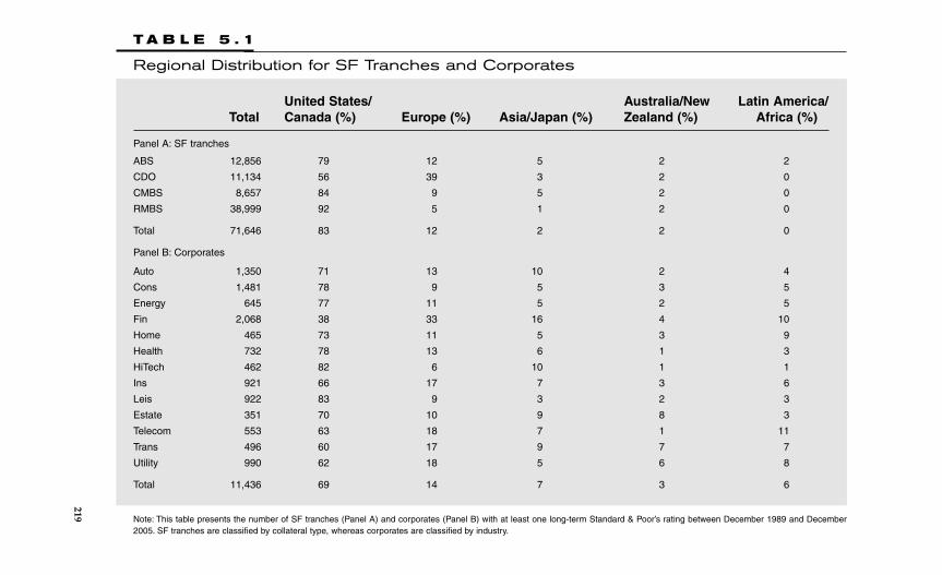
T A B L E 5 . 1
Regional Distribution for SF Tranches and Corporates
United States/ Australia/New Latin America/Total Canada (%) Europe (%) Asia/Japan (%) Zealand (%) Africa (%)
Panel A: SF tranches
ABS 12,856 79 12 5 2 2
CDO 11,134 56 39 3 2 0
CMBS 8,657 84 9 5 2 0
RMBS 38,999 92 5 1 2 0
Total 71,646 83 12 2 2 0
Panel B: Corporates
Auto 1,350 71 13 10 2 4
Cons 1,481 78 9 5 3 5
Energy 645 77 11 5 2 5
Fin 2,068 38 33 16 4 10
Home 465 73 11 5 3 9
Health 732 78 13 6 1 3
HiTech 462 82 6 10 1 1
Ins 921 66 17 7 3 6
Leis 922 83 9 3 2 3
Estate 351 70 10 9 8 3
Telecom 553 63 18 7 1 11
Trans 496 60 17 9 7 7
Utility 990 62 18 5 6 8
Total 11,436 69 14 7 3 6
Note: This table presents the number of SF tranches (Panel A) and corporates (Panel B) with at least one long-term Standard & Poor’s rating between December 1989 and December2005. SF tranches are classified by collateral type, whereas corporates are classified by industry.
219

Figure 5.1). Panel A of Figure 5.1 shows the most common types of ABSincluded in the sample: auto loans or lease (18 percent), credit cards (20 per-cent), synthetic ABS (15 percent), student loans (10 percent), equipment(6 percent), and manufactured housing (MH) (5 percent). Even though theMH sector is relatively small compared to other sectors, it can significantlyaffect the results be discussing.
Making a distinction between different rating categories showsthat the majority of SF tranches rated by Standard & Poor’s betweenDecember 1989 and December 2005 are high quality, often AAA. Overthe last decade, the number of rated SF tranches has grown enormously.To get an indication of the growth rate, we split the sample in two sub-periods 1990–1997 and 1998–2005 (see Table 2). From the results, it isclear that the total number of observations between December 1997 andDecember 2005 is significantly higher than the number of observationsbetween December 1989 and December 1997. For corporates, the mostimportant rating categories in terms of number of observations are Aand BBB. While the number of corporates has grown as shown in Table5.2, the growth rate is much smaller relative to SF tranches.
220 CHAPTER 5
Synt15% StudLoans
10%
Equipment6%
CF Rest 1%
Synt US10%
Synt Europe31%
Synt Rest3%
Other9%
CF US38%
CF Europe8%
Man Housing5%
Other26%
Coards20%
Auto18%
F I G U R E 5 . 1
Different Types of ABS and CDOs (Sample period:December 1989–December 2005)
Note: Panel A and B give an overview of the different types of ABS and CDOs, respectively. The percentages are cal-
culated as the total number observations for a specific subgroup of ABS and CDOs between December
1989–December 2005 divided by the total number of ABS and CDOs, respectively, between December
1989–December 2005. In Panel B, CF stands for cash-flow CDOs, whereas Synt stands for synthetic CDOs.
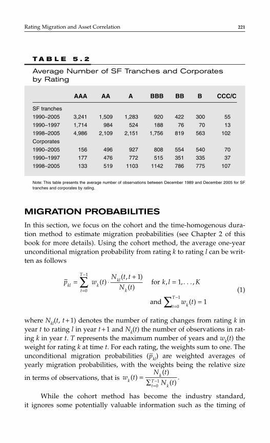
Rating Migration and Asset Correlation 221
T A B L E 5 . 2
Average Number of SF Tranches and Corporates by Rating
AAA AA A BBB BB B CCC/C
SF tranches
1990–2005 3,241 1,509 1,283 920 422 300 55
1990–1997 1,714 984 524 188 76 70 13
1998–2005 4,986 2,109 2,151 1,756 819 563 102
Corporates
1990–2005 156 496 927 808 554 540 70
1990–1997 177 476 772 515 351 335 37
1998–2005 133 519 1103 1142 786 775 107
Note: This table presents the average number of observations between December 1989 and December 2005 for SFtranches and corporates by rating.
MIGRATION PROBABILITIES
In this section, we focus on the cohort and the time-homogenous dura-tion method to estimate migration probabilities (see Chapter 2 of thisbook for more details). Using the cohort method, the average one-yearunconditional migration probability from rating k to rating l can be writ-ten as follows
(1)
where Nkl(t, t + 1) denotes the number of rating changes from rating k inyear t to rating l in year t + 1 and Nk(t) the number of observations in rat-ing k in year t. T represents the maximum number of years and wk(t) theweight for rating k at time t. For each rating, the weights sum to one. Theunconditional migration probabilities (p–kl) are weighted averages ofyearly migration probabilities, with the weights being the relative size
in terms of observations, that is
While the cohort method has become the industry standard,it ignores some potentially valuable information such as the timing of
w tN t
N tkk
tT
k
( )( )
( ).=
∑ =−01
p w tN t t
N tk l K
w t
klt
T
kkl
k
kt
T
= ⋅+
=
=
=
−
=
−
∑∑
0
1
0
1
11
1
( )( , )
( )for , , ,
and ( )
. . .
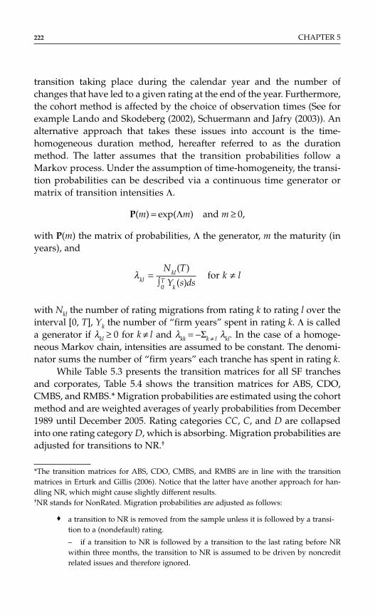
transition taking place during the calendar year and the number ofchanges that have led to a given rating at the end of the year. Furthermore,the cohort method is affected by the choice of observation times (See forexample Lando and Skodeberg (2002), Schuermann and Jafry (2003)). Analternative approach that takes these issues into account is the time-homogeneous duration method, hereafter referred to as the durationmethod. The latter assumes that the transition probabilities follow aMarkov process. Under the assumption of time-homogeneity, the transi-tion probabilities can be described via a continuous time generator ormatrix of transition intensities Λ.
P(m) = exp(Λm) and m ≥ 0,
with P(m) the matrix of probabilities, Λ the generator, m the maturity (inyears), and
with Nkl the number of rating migrations from rating k to rating l over theinterval [0, T], Yk the number of “firm years” spent in rating k. Λ is calleda generator if λkl ≥ 0 for k ≠ l and λkk = −Σk ≠ l λkl. In the case of a homoge-neous Markov chain, intensities are assumed to be constant. The denomi-nator sums the number of “firm years” each tranche has spent in rating k.
While Table 5.3 presents the transition matrices for all SF tranchesand corporates, Table 5.4 shows the transition matrices for ABS, CDO,CMBS, and RMBS.* Migration probabilities are estimated using the cohortmethod and are weighted averages of yearly probabilities from December1989 until December 2005. Rating categories CC, C, and D are collapsedinto one rating category D, which is absorbing. Migration probabilities areadjusted for transitions to NR.†
λklkl
Tk
N T
Y s dsk l=
∫≠
( )
( )for
0
222 CHAPTER 5
*The transition matrices for ABS, CDO, CMBS, and RMBS are in line with the transitionmatrices in Erturk and Gillis (2006). Notice that the latter have another approach for han-dling NR, which might cause slightly different results.†NR stands for NonRated. Migration probabilities are adjusted as follows:
♦ a transition to NR is removed from the sample unless it is followed by a transi-tion to a (nondefault) rating.
– if a transition to NR is followed by a transition to the last rating before NRwithin three months, the transition to NR is assumed to be driven by noncreditrelated issues and therefore ignored.
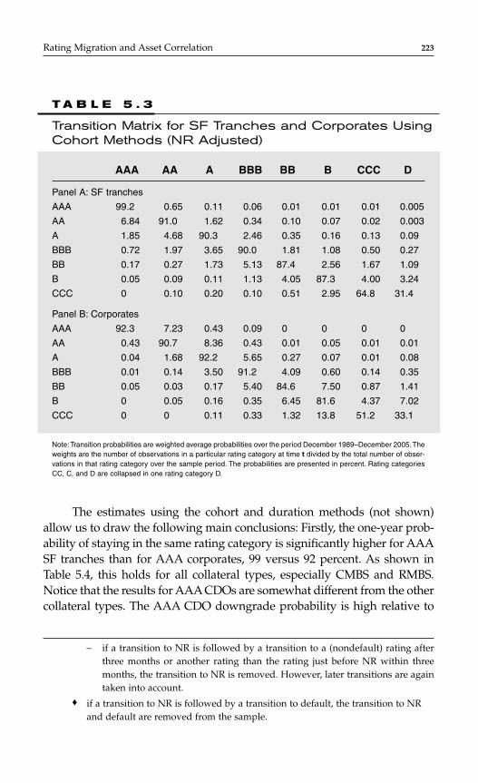
The estimates using the cohort and duration methods (not shown)allow us to draw the following main conclusions: Firstly, the one-year prob-ability of staying in the same rating category is significantly higher for AAASF tranches than for AAA corporates, 99 versus 92 percent. As shown inTable 5.4, this holds for all collateral types, especially CMBS and RMBS.Notice that the results for AAA CDOs are somewhat different from the othercollateral types. The AAA CDO downgrade probability is high relative to
Rating Migration and Asset Correlation 223
T A B L E 5 . 3
Transition Matrix for SF Tranches and Corporates UsingCohort Methods (NR Adjusted)
AAA AA A BBB BB B CCC D
Panel A: SF tranches
AAA 99.2 0.65 0.11 0.06 0.01 0.01 0.01 0.005
AA 6.84 91.0 1.62 0.34 0.10 0.07 0.02 0.003
A 1.85 4.68 90.3 2.46 0.35 0.16 0.13 0.09
BBB 0.72 1.97 3.65 90.0 1.81 1.08 0.50 0.27
BB 0.17 0.27 1.73 5.13 87.4 2.56 1.67 1.09
B 0.05 0.09 0.11 1.13 4.05 87.3 4.00 3.24
CCC 0 0.10 0.20 0.10 0.51 2.95 64.8 31.4
Panel B: Corporates
AAA 92.3 7.23 0.43 0.09 0 0 0 0
AA 0.43 90.7 8.36 0.43 0.01 0.05 0.01 0.01
A 0.04 1.68 92.2 5.65 0.27 0.07 0.01 0.08
BBB 0.01 0.14 3.50 91.2 4.09 0.60 0.14 0.35
BB 0.05 0.03 0.17 5.40 84.6 7.50 0.87 1.41
B 0 0.05 0.16 0.35 6.45 81.6 4.37 7.02
CCC 0 0 0.11 0.33 1.32 13.8 51.2 33.1
Note:Transition probabilities are weighted average probabilities over the period December 1989–December 2005.Theweights are the number of observations in a particular rating category at time t divided by the total number of obser-vations in that rating category over the sample period. The probabilities are presented in percent. Rating categoriesCC, C, and D are collapsed in one rating category D.
– if a transition to NR is followed by a transition to a (nondefault) rating afterthree months or another rating than the rating just before NR within threemonths, the transition to NR is removed. However, later transitions are againtaken into account.
♦ if a transition to NR is followed by a transition to default, the transition to NRand default are removed from the sample.
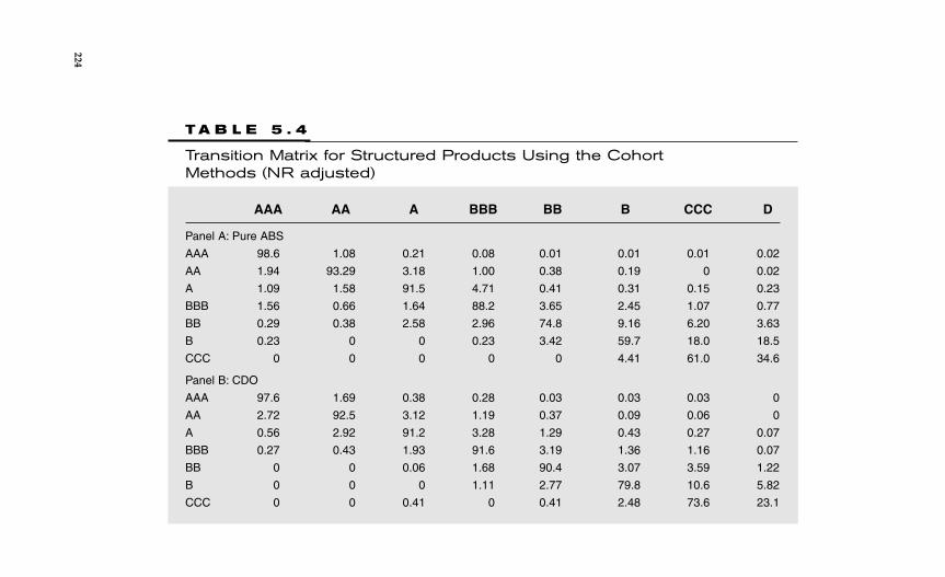
T A B L E 5 . 4
Transition Matrix for Structured Products Using the Cohort Methods (NR adjusted)
AAA AA A BBB BB B CCC D
Panel A: Pure ABS
AAA 98.6 1.08 0.21 0.08 0.01 0.01 0.01 0.02
AA 1.94 93.29 3.18 1.00 0.38 0.19 0 0.02
A 1.09 1.58 91.5 4.71 0.41 0.31 0.15 0.23
BBB 1.56 0.66 1.64 88.2 3.65 2.45 1.07 0.77
BB 0.29 0.38 2.58 2.96 74.8 9.16 6.20 3.63
B 0.23 0 0 0.23 3.42 59.7 18.0 18.5
CCC 0 0 0 0 0 4.41 61.0 34.6
Panel B: CDO
AAA 97.6 1.69 0.38 0.28 0.03 0.03 0.03 0
AA 2.72 92.5 3.12 1.19 0.37 0.09 0.06 0
A 0.56 2.92 91.2 3.28 1.29 0.43 0.27 0.07
BBB 0.27 0.43 1.93 91.6 3.19 1.36 1.16 0.07
BB 0 0 0.06 1.68 90.4 3.07 3.59 1.22
B 0 0 0 1.11 2.77 79.8 10.6 5.82
CCC 0 0 0.41 0 0.41 2.48 73.6 23.1
224
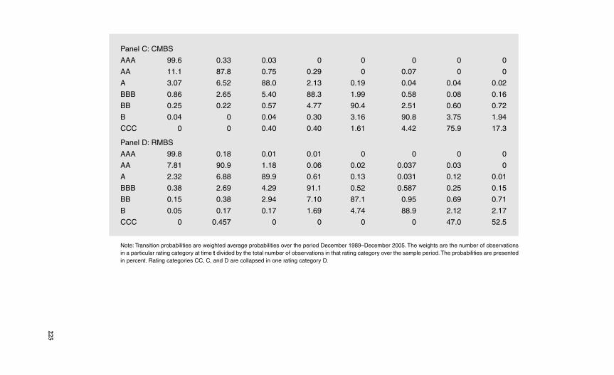
Panel C: CMBS
AAA 99.6 0.33 0.03 0 0 0 0 0
AA 11.1 87.8 0.75 0.29 0 0.07 0 0
A 3.07 6.52 88.0 2.13 0.19 0.04 0.04 0.02
BBB 0.86 2.65 5.40 88.3 1.99 0.58 0.08 0.16
BB 0.25 0.22 0.57 4.77 90.4 2.51 0.60 0.72
B 0.04 0 0.04 0.30 3.16 90.8 3.75 1.94
CCC 0 0 0.40 0.40 1.61 4.42 75.9 17.3
Panel D: RMBS
AAA 99.8 0.18 0.01 0.01 0 0 0 0
AA 7.81 90.9 1.18 0.06 0.02 0.037 0.03 0
A 2.32 6.88 89.9 0.61 0.13 0.031 0.12 0.01
BBB 0.38 2.69 4.29 91.1 0.52 0.587 0.25 0.15
BB 0.15 0.38 2.94 7.10 87.1 0.95 0.69 0.71
B 0.05 0.17 0.17 1.69 4.74 88.9 2.12 2.17
CCC 0 0.457 0 0 0 0 47.0 52.5
Note: Transition probabilities are weighted average probabilities over the period December 1989–December 2005. The weights are the number of observationsin a particular rating category at time t divided by the total number of observations in that rating category over the sample period. The probabilities are presentedin percent. Rating categories CC, C, and D are collapsed in one rating category D.
225

226 CHAPTER 5
CMBS, RMBS, and even ABS. This might be due to the relatively short rat-ing history for CDOs and a higher downgrade probability at the end of oursample. Furthermore, the fact that there is a high degree of portfolio overlapbetween synthetic CDOs might cause higher downgrade probabilities (see,for example, South, 2005). For rating categories below AAA, the diagonalprobabilities are very similar for SF tranches and corporates. Similarly toSchuermann and Jafry (2003), we estimate a mobility index (MI) or metric,which is the average of the singular values of the mobility matrix. The higherprobability of staying in AAA for SF tranches is also reflected in a lower MIfor SF tranches than corporates, 0.17 versus 0.12.
Secondly, the off-diagonal downgrade probabilities are significantlyhigher for corporates than for SF tranches. This holds for all rating cate-gories, except for B and CCC. Thirdly, the upgrade probability for invest-ment grade SF tranches, especially AA and A, is significantly higher thanfor corporates. As shown in Table 5.4, this is mainly driven by the results forCMBS and RMBS. Over the last few years, the MBS market could have ben-efited from a strong mortgage credit environment, including rapid industrywide prepayments, generally rising home prices and low interest rates.
Finally, the results using the cohort method seem to indicate thatthe default probabilities are higher for corporates than for SF tranches.However, using the duration method, the differences are much less pro-nounced and no clear conclusion can be drawn. Regarding the differencebetween the cohort and the duration methods, we find that default prob-abilities for high quality ratings (AAA and AA) are higher using the dura-tion method, whereas for the below A rating assets, the probabilities arehigher using the cohort method.
In Panels A and B of Figure 5.2, we present the distribution ofnotch-level rating migrations for SF tranches and corporates. For eachproduct, we analyze the rating at the end of each year and compare itto the rating at the end of the previous year. The maximum notch-leveldowngrade is −19 (from AAA to D) and the maximum notch-levelupgrade is 18 (from CCC–to AAA). The distributions are adjusted formigrations to NR (see footnote * on page 222). The following conclu-sions can be drawn from Figure 5.2: Firstly, for SF tranches, the numberof rating migrations is clearly dominated by upgrades (64 percent),whereas for corporates, it is dominated by downgrades (63 percent).*
*This is even more pronounced when we focus on investment grade rating migrations (notshown).
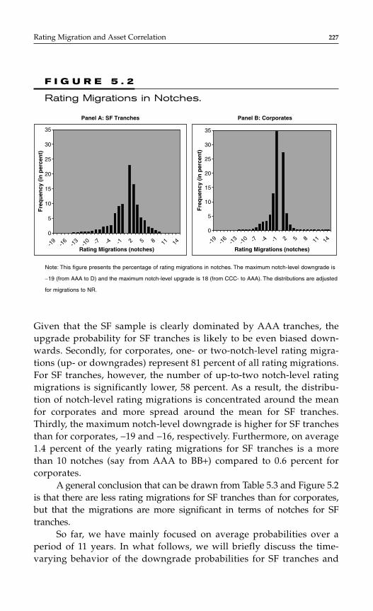
Given that the SF sample is clearly dominated by AAA tranches, theupgrade probability for SF tranches is likely to be even biased down-wards. Secondly, for corporates, one- or two-notch-level rating migra-tions (up- or downgrades) represent 81 percent of all rating migrations.For SF tranches, however, the number of up-to-two notch-level ratingmigrations is significantly lower, 58 percent. As a result, the distribu-tion of notch-level rating migrations is concentrated around the meanfor corporates and more spread around the mean for SF tranches.Thirdly, the maximum notch-level downgrade is higher for SF tranchesthan for corporates, −19 and −16, respectively. Furthermore, on average1.4 percent of the yearly rating migrations for SF tranches is a morethan 10 notches (say from AAA to BB+) compared to 0.6 percent forcorporates.
A general conclusion that can be drawn from Table 5.3 and Figure 5.2is that there are less rating migrations for SF tranches than for corporates,but that the migrations are more significant in terms of notches for SFtranches.
So far, we have mainly focused on average probabilities over aperiod of 11 years. In what follows, we will briefly discuss the time-varying behavior of the downgrade probabilities for SF tranches and
Rating Migration and Asset Correlation 227
35
30
Fre
qu
ency
(in
per
cen
t)
Rating Migrations (notches)
25
20
15
10
5
0
-19
-16
-13
-10 -7 -4 -1 2 5 8 11 14
35
30
Fre
qu
ency
(in
per
cen
t)
Panel A: SF Tranches Panel B: Corporates
Rating Migrations (notches)
25
20
15
10
5
0
-19
-16
-13
-10 -7 -4 -1 2 5 8 11 14
F I G U R E 5 . 2
Rating Migrations in Notches.
Note: This figure presents the percentage of rating migrations in notches. The maximum notch-level downgrade is
−19 (from AAA to D) and the maximum notch-level upgrade is 18 (from CCC- to AAA). The distributions are adjusted
for migrations to NR.
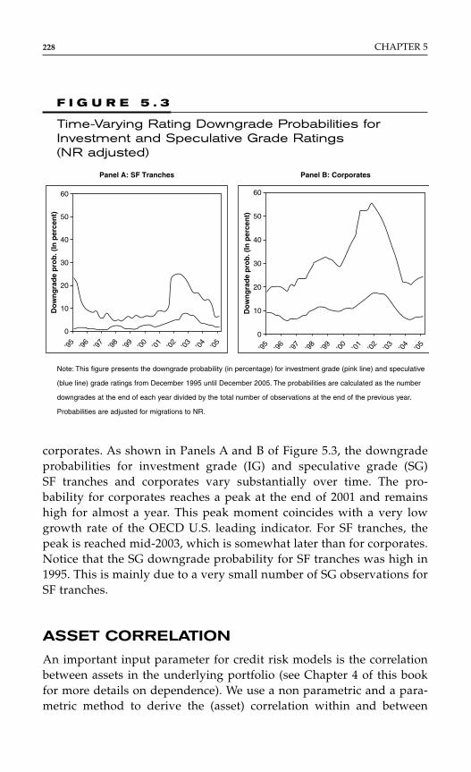
corporates. As shown in Panels A and B of Figure 5.3, the downgradeprobabilities for investment grade (IG) and speculative grade (SG)SF tranches and corporates vary substantially over time. The pro-bability for corporates reaches a peak at the end of 2001 and remainshigh for almost a year. This peak moment coincides with a very lowgrowth rate of the OECD U.S. leading indicator. For SF tranches, thepeak is reached mid-2003, which is somewhat later than for corporates.Notice that the SG downgrade probability for SF tranches was high in1995. This is mainly due to a very small number of SG observations forSF tranches.
ASSET CORRELATION
An important input parameter for credit risk models is the correlationbetween assets in the underlying portfolio (see Chapter 4 of this bookfor more details on dependence). We use a non parametric and a para-metric method to derive the (asset) correlation within and between
228 CHAPTER 5
60
50
40
30
Do
wn
gra
de
pro
b. (
In p
erce
nt)
Panel A: SF Tranches Panel B: Corporates
Do
wn
gra
de
pro
b. (
In p
erce
nt)
20
10
0
60
50
40
30
20
10
0
’95
’96
’97
’98
’99
’00
’01
’02
’03
’04
’05
’95
’96
’97
’98
’99
’00
’01
’02
’03
’04
’05
F I G U R E 5 . 3
Time-Varying Rating Downgrade Probabilities forInvestment and Speculative Grade Ratings (NR adjusted)
Note: This figure presents the downgrade probability (in percentage) for investment grade (pink line) and speculative
(blue line) grade ratings from December 1995 until December 2005. The probabilities are calculated as the number
downgrades at the end of each year divided by the total number of observations at the end of the previous year.
Probabilities are adjusted for migrations to NR.
portfolios of assets from time series of default probabilities.*,† The non-parametric method, which will hereafter be referred to as the joint defaultprobabilities (JDP) approach, estimates JDP using historical transitiondata. Implied asset correlation is derived from JDP (see, for example,Bahar and Nagpal, 2001 and de Servigny and Renault, 2002). In the para-metric approach, asset correlation is derived from a credit risk model. Assuggested by Gordy and Heitfield (2002) and similar to Frey and McNeil(2003), Demey et al. (2004), Tasche (2005), Jobst and de Servigny (2006),and others, we use a two-factor model. The latter assumes that correlationbetween firm asset values is driven by two systematic risk factors, whichcould be thought of as an economic and a sector-specific factor. In theremainder of this chapter, we will create portfolios of assets based on sec-tor classification, which implicitly assumes that sectors can be seen ashomogeneous risk classes that are driven by similar factors.
Joint Default Probabilities (JDP) Approach
Based on the number of transitions to the default state D for sector i andj (MD
i and MDi , respectively) and the total number of assets in sector i
and j (Ni and Ni, respectively), the average JDP can be estimated asfollows
(2)
with T the maximum number of years and w(t) the weight at time t.To analyze the impact of the strong growth of the SF market, weestimate equally-weighted (that is, w(t) = 1/T) and size-weighted (that is,w(t) = √Ni(t)Nj(t)/∑t=0
T-1 √Ni(t)Nj(t)) average JDP.Implied asset correlation, which is the correlation needed in a typi-
cal credit risk model to recover or match the joint default events that have
p w tt t t t
N t tDi j
t
T
i, ( )
( , ) ( , )
( ) ( )=
+ +
=
−
∑0
1 1 1M M
NDi
Dj
j
Rating Migration and Asset Correlation 229
*In this chapter, we focus on asset correlation derived from rating migrations to default.Alternatively, we could use credit spread data or equity data to obtain asset correlation. SeeSchönbucher (2003) (p. 297) for a detailed discussion of the advantages and disadvantagesof the three approaches.†See Van Landschoot (2006) for a detailed analysis of asset correlation estimates derivedfrom default probabilities and rating transitions (including default) for SF tranches and cor-porates and a discussion of confidence intervals for correlation estimates based on a simu-lation analysis.
been observed, is derived from JDP. We start from a structural credit riskmodel, initiated by Merton (1974), and assume that default occurs whenthe firm’s asset value falls below a threshold ZD. The threshold is cali-brated such that the default probability corresponds to the observed prob-ability
piD = Φ(Zi
D)
with ZDi = Φ−1(pD
i ) and Φ the standard Gaussian cumulative distributionfunction (CDF).
The joint default probability for sector i and j is given by
p–Di,j = Φ2(Z
iD, Zj
D, ρij) (3)
with Φ2 the bivariate standard Gaussian CDF. The implied asset correlation,ρij, can be derived by solving Equation (3). Estimating asset correlationbetween I sectors results in the following estimator of the correlation matrix
(4)
with the elements being the intra (within sectors) and inter (between sec-tors) asset correlation. In what follows, we will only present the intra assetcorrelation (diagonals) and the average inter asset correlation (average ofoff-diagonal elements). The correlation structure ΣJDP is the result ofI(I − 1)/2 pairwise estimations.
Two-Factor Model
In a two-factor model, the asset value Vi is driven by two common, stan-dard normally distributed factors Y and Yi and an idiosyncratic standardnormal noise component εn
(5)
Y can be seen as a common (or economywide) factor that affects all assetsat the same time and Yi as a sector-specific factor. The asset values are cor-related with correlation coefficients ρ and ρi. Default occurs when the
V Ynt
i i i n= + − + − ≤ρ ρ ρ ρ εY n N1 for
ˆ
ˆ ˆ ˆˆ ˆ ˆ
ˆ ˆ ˆ
, ,
, ,
, ,
∑ =
JDP
ρ ρ ρρ ρ ρ
ρ ρ ρ
1 1 2 1
2 1 2 2
1 2
K
K
M M M M
K
I
I
I I I
230 CHAPTER 5
asset value hits a threshold. An interesting feature of this model is thatdefault events are independent conditional on the two common factors.The conditional default probability of sector i can be written as follows
with ZDi = φ−1 (p–D
i ) the default threshold for sector i, p–Di the average (uncon-
ditional) default probability for sector i, and Φ the standard GaussianCDF. This two-factor model implies the following correlation structure
with ρ the inter asset correlation (or the correlation between I sectors) andρi the intra asset correlation (or the correlation within the ith sector). Thistwo-factor model approach differs from the JDP approach in that thecorrelation structure is the result of one joint estimation. Default information for all sectors is considered at the same time. Similar toDemey et al. (2004), we apply the asymptotic maximum likelihood(ML) method to estimate the factor loadings and thus asset correlation.
Empirical Results: SF Tranches versus Corporates
In this section, we present the asset correlation estimates for different sec-tors defined by collateral type for SF and industries for corporates. Weapply the JDP and the two-factor model approach. For each approach, weestimate asset correlation based on equally and size weighted defaultprobabilities. We use time series of 3-monthly default probabilities for dif-ferent sectors from December 1994 until December 2005.* In this chapter,we do not analyze the impact of country and/or regional differences.
( ˆ )MLE∑
ˆ
ˆ ˆ ˆˆ ˆ ˆ
ˆ ˆ ˆ
∑ =
MLE
ρ ρ ρρ ρ ρ
ρ ρ ρ
1
2
K
K
M M M M
K I
p y yZ y
Di
iDi
i
i
( , ) =− − −
−
Φ
ρ ρ ρ
ρ
yi
1
Rating Migration and Asset Correlation 231
*The reason for using a shorter sample period for asset correlation than for the transitionmatrices is because of a lack of default observations before December 1994.
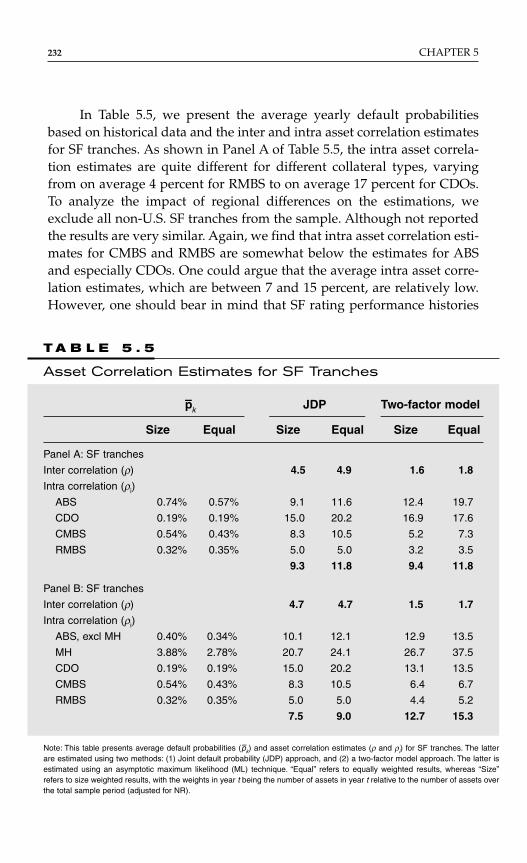
In Table 5.5, we present the average yearly default probabilitiesbased on historical data and the inter and intra asset correlation estimatesfor SF tranches. As shown in Panel A of Table 5.5, the intra asset correla-tion estimates are quite different for different collateral types, varyingfrom on average 4 percent for RMBS to on average 17 percent for CDOs.To analyze the impact of regional differences on the estimations, weexclude all non-U.S. SF tranches from the sample. Although not reportedthe results are very similar. Again, we find that intra asset correlation esti-mates for CMBS and RMBS are somewhat below the estimates for ABSand especially CDOs. One could argue that the average intra asset corre-lation estimates, which are between 7 and 15 percent, are relatively low.However, one should bear in mind that SF rating performance histories
232 CHAPTER 5
T A B L E 5 . 5
Asset Correlation Estimates for SF Tranches
p–k JDP Two-factor model
Size Equal Size Equal Size Equal
Panel A: SF tranches
Inter correlation (ρ) 4.5 4.9 1.6 1.8
Intra correlation (ρi)
ABS 0.74% 0.57% 9.1 11.6 12.4 19.7
CDO 0.19% 0.19% 15.0 20.2 16.9 17.6
CMBS 0.54% 0.43% 8.3 10.5 5.2 7.3
RMBS 0.32% 0.35% 5.0 5.0 3.2 3.5
9.3 11.8 9.4 11.8
Panel B: SF tranches
Inter correlation (ρ) 4.7 4.7 1.5 1.7
Intra correlation (ρi)
ABS, excl MH 0.40% 0.34% 10.1 12.1 12.9 13.5
MH 3.88% 2.78% 20.7 24.1 26.7 37.5
CDO 0.19% 0.19% 15.0 20.2 13.1 13.5
CMBS 0.54% 0.43% 8.3 10.5 6.4 6.7
RMBS 0.32% 0.35% 5.0 5.0 4.4 5.2
7.5 9.0 12.7 15.3
Note: This table presents average default probabilities (p–k) and asset correlation estimates (ρ and ρi) for SF tranches. The latterare estimated using two methods: (1) Joint default probability (JDP) approach, and (2) a two-factor model approach. The latter isestimated using an asymptotic maximum likelihood (ML) technique. “Equal” refers to equally weighted results, whereas “Size”refers to size weighted results, with the weights in year t being the number of assets in year t relative to the number of assets overthe total sample period (adjusted for NR).
are very short and only include one recession period.* As a result, theeffect of (severe) several recession periods on rating transitions anddefault behavior has not been tested. Asset correlation is likely to be lowerduring economic growth periods.
The inter asset correlation estimates are always below 5 percent.However, they are significantly higher using the JDP approach than thetwo-factor model. An analysis of one-by-one inter asset correlation esti-mates using the JDP approach [see ρi,i in Equation (4)] shows that this ismainly driven by the inter asset correlation estimates with CDOs.Excluding CDOs from the sample (not shown) results in average interasset correlation estimates just below 2 percent, which is very similar tothe results based on a two-factor model. This shows that ABS, CMBS, andRMBS are very different and react differently to changes in a common fac-tor, which could be seen as the business cycle.
Comparing equally- and size-weighted results indicates that theestimates for ABS and CDOs are most affected by the enormous growthin the SF market. However, when we split the ABS sector into two sepa-rate sectors, namely MH and ABS excluding MH, we find that the intraasset correlation estimates for ABS are much less affected by the method-ology (see Panel B of Table 5.5). At the same time, it shows that the MH-sector is different from other ABS subsectors. In general, MH seems to bea risky sector in a sense that the behavior of MH tranches is substantiallyaffected by sector-specific events, which results in a high intra asset cor-relation estimate. The average default probabilities are also substantiallyhigher for MH than for other sectors. This is mainly due to an increasingtrend in the delinquency rate for MH loans and the level of losses for MHpools over the last decade. As a result, the majority of MH issuers wereaffected by high levels of cumulative repossessions and losses.
In Table 5.6, we present the average annual default probabilities andasset correlation estimates for corporates. Similarly to the results for SFtranches, we find that intra asset correlation estimates differ substantiallybetween sectors. However, average intra asset correlation estimates for SFtranches and corporates have more or less the same order of magnitude.This is somewhat surprising given the substantial differences betweenthese markets. Comparing the default probabilities for SF tranches and cor-porates shows that the average default probability for ABS (excluding MH),CDO, CMBS, and RMBS are significantly below the average for corporates.
Rating Migration and Asset Correlation 233
*A recession period is defined according to the NBER definition of a recession.
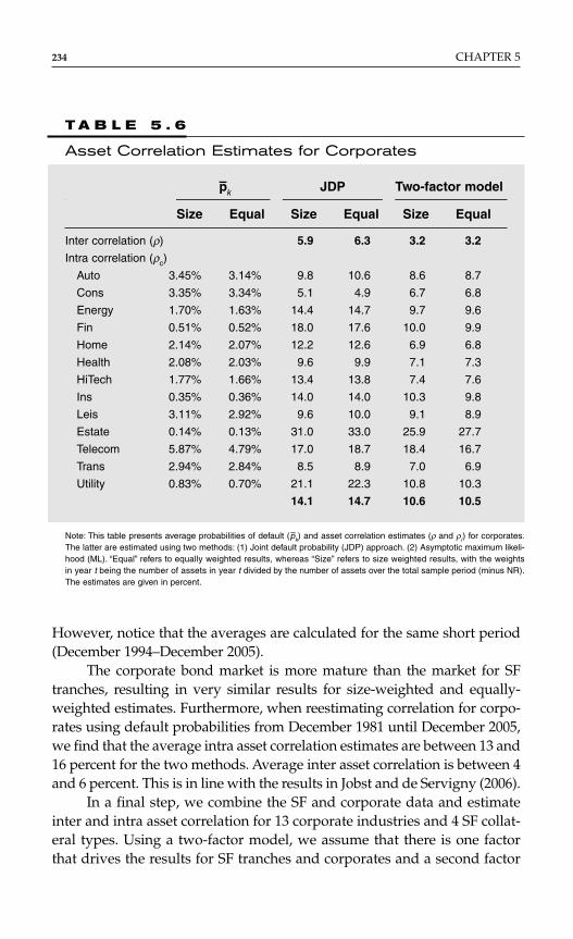
234 CHAPTER 5
However, notice that the averages are calculated for the same short period(December 1994–December 2005).
The corporate bond market is more mature than the market for SFtranches, resulting in very similar results for size-weighted and equally-weighted estimates. Furthermore, when reestimating correlation for corpo-rates using default probabilities from December 1981 until December 2005,we find that the average intra asset correlation estimates are between 13 and16 percent for the two methods. Average inter asset correlation is between 4and 6 percent. This is in line with the results in Jobst and de Servigny (2006).
In a final step, we combine the SF and corporate data and estimateinter and intra asset correlation for 13 corporate industries and 4 SF collat-eral types. Using a two-factor model, we assume that there is one factorthat drives the results for SF tranches and corporates and a second factor
T A B L E 5 . 6
Asset Correlation Estimates for Corporates
p–k JDP Two-factor model
Size Equal Size Equal Size Equal
Inter correlation (ρ) 5.9 6.3 3.2 3.2
Intra correlation (ρc)
Auto 3.45% 3.14% 9.8 10.6 8.6 8.7
Cons 3.35% 3.34% 5.1 4.9 6.7 6.8
Energy 1.70% 1.63% 14.4 14.7 9.7 9.6
Fin 0.51% 0.52% 18.0 17.6 10.0 9.9
Home 2.14% 2.07% 12.2 12.6 6.9 6.8
Health 2.08% 2.03% 9.6 9.9 7.1 7.3
HiTech 1.77% 1.66% 13.4 13.8 7.4 7.6
Ins 0.35% 0.36% 14.0 14.0 10.3 9.8
Leis 3.11% 2.92% 9.6 10.0 9.1 8.9
Estate 0.14% 0.13% 31.0 33.0 25.9 27.7
Telecom 5.87% 4.79% 17.0 18.7 18.4 16.7
Trans 2.94% 2.84% 8.5 8.9 7.0 6.9
Utility 0.83% 0.70% 21.1 22.3 10.8 10.3
14.1 14.7 10.6 10.5
Note: This table presents average probabilities of default (p–k) and asset correlation estimates (ρ and ρi) for corporates.The latter are estimated using two methods: (1) Joint default probability (JDP) approach. (2) Asymptotic maximum likeli-hood (ML). “Equal” refers to equally weighted results, whereas “Size” refers to size weighted results, with the weightsin year t being the number of assets in year t divided by the number of assets over the total sample period (minus NR).The estimates are given in percent.
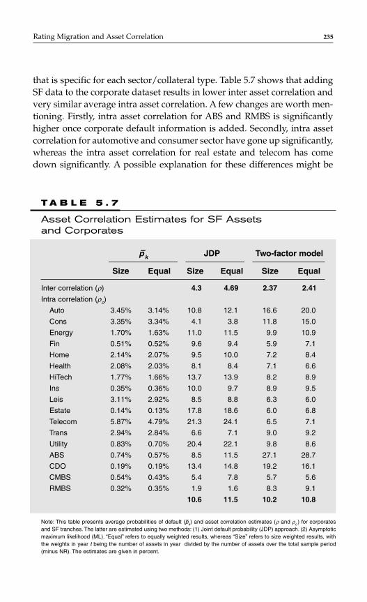
that is specific for each sector/collateral type. Table 5.7 shows that addingSF data to the corporate dataset results in lower inter asset correlation andvery similar average intra asset correlation. A few changes are worth men-tioning. Firstly, intra asset correlation for ABS and RMBS is significantlyhigher once corporate default information is added. Secondly, intra assetcorrelation for automotive and consumer sector have gone up significantly,whereas the intra asset correlation for real estate and telecom has comedown significantly. A possible explanation for these differences might be
Rating Migration and Asset Correlation 235
T A B L E 5 . 7
Asset Correlation Estimates for SF Assetsand Corporates
p–k JDP Two-factor model
Size Equal Size Equal Size Equal
Inter correlation (ρ) 4.3 4.69 2.37 2.41
Intra correlation (ρc)
Auto 3.45% 3.14% 10.8 12.1 16.6 20.0
Cons 3.35% 3.34% 4.1 3.8 11.8 15.0
Energy 1.70% 1.63% 11.0 11.5 9.9 10.9
Fin 0.51% 0.52% 9.6 9.4 5.9 7.1
Home 2.14% 2.07% 9.5 10.0 7.2 8.4
Health 2.08% 2.03% 8.1 8.4 7.1 6.6
HiTech 1.77% 1.66% 13.7 13.9 8.2 8.9
Ins 0.35% 0.36% 10.0 9.7 8.9 9.5
Leis 3.11% 2.92% 8.5 8.8 6.3 6.0
Estate 0.14% 0.13% 17.8 18.6 6.0 6.8
Telecom 5.87% 4.79% 21.3 24.1 6.5 7.1
Trans 2.94% 2.84% 6.6 7.1 9.0 9.2
Utility 0.83% 0.70% 20.4 22.1 9.8 8.6
ABS 0.74% 0.57% 8.5 11.5 27.1 28.7
CDO 0.19% 0.19% 13.4 14.8 19.2 16.1
CMBS 0.54% 0.43% 5.4 7.8 5.7 5.6
RMBS 0.32% 0.35% 1.9 1.6 8.3 9.1
10.6 11.5 10.2 10.8
Note: This table presents average probabilities of default (p–k) and asset correlation estimates (ρ and ρc) for corporatesand SF tranches. The latter are estimated using two methods: (1) Joint default probability (JDP) approach. (2) Asymptoticmaximum likelihood (ML). “Equal” refers to equally weighted results, whereas “Size” refers to size weighted results, withthe weights in year t being the number of assets in year divided by the number of assets over the total sample period(minus NR). The estimates are given in percent.

236 CHAPTER 5
T A B L E 5 . 8
Abbreviations for Corporate Sectors
Corporate Sectors Abbreviations
Aerospace/automotive/capital goods/metal Auto
Consumer/service sector Cons
Energy and natural resources Energy
Financial Institutions Fin
Forest and building products/homebuilders Home
Health care/chemicals Health
High technology/computers/office equipment HiTech
Insurance Ins
Leisure time/media Leis
Real estate Estate
Telecommunications Telecom
Transportation Trans
Utility Utility
For an overview of the different corporate industries, see Table 5.8.
that SF tranches and corporates are very different, in which case the sectorand collateral specific factor partially captures the corporate common riskfor corporate sector and the SF common risk for SF tranches. A possiblesolution, which has not been explored in this chapter, would be to usemulti-factor extensions.
CONCLUSIONS
In this chapter, we investigate and compare transition probabilities and assetcorrelation estimates for SF tranches and corporates. We use Standard &Poor’s rating transition data from December 1989 until December 2005 toperform the analysis. Rating transition probabilities are estimated using thecohort method, which is the industry standard, and the time-homogeneousduration method. Asset correlation within and between sectors of SFtranches and corporates are estimated using two methods. The first method,referred to as the joint default probability approach, derives implied assetcorrelation from joint default probabilities using historical transition data.The second method uses a two-factor credit risk model to estimate asset cor-relation. The latter is estimated using a asymptotic maximum likelihood.The following main conclusions can be drawn from the empirical analysis:
♦ Over the past decade, AAA SF tranches show much higher rat-ing stability than AAA corporates.
♦ For SF tranches, the number of rating migrations is clearlydominated by upgrades (64 percent), whereas for corporates,it is dominated by downgrades (63 percent). This is evenmore pronounced when we focus on investment grade ratingmigrations.
♦ One and two notch downgrades and upgrades represent a muchhigher percentage of the total number of migrations for corpo-rates (81 percent) than for SF tranches (58 percent). This meansthat the distribution of notch-level rating migrations is concen-trated around the mean, whereas for SF tranches, the distribu-tion is more spread around the mean.
♦ The distribution of notch-level rating migrations is also fattertailed for SF tranches than for corporates. On average, 1.4 per-cent of the yearly rating migrations for SF tranches is more than10 notches (say from AAA to BB+) compared to 0.6 percent forcorporates.
♦ Even though the SF and corporate markets are very different, theaverage intra asset correlation estimates within and betweengroups of SF tranches and corporates are comparable. Individualintra asset correlation estimates, however, can differ substantially.
♦ The results seem to indicate that asset correlation within portfo-lios of CDOs and manufactured housing (MH) is higher than forother collateral types such as RMBS and CMBS.
REFERENCESBahar, R., and K. Nagpal (2001), “Measuring default correlation,” Risk, 14(3),
129–132.de Servigny, A., and O. Renault (2002), Default correlation: Empirical evidence.
Standard & Poor’s working paper.Demey, P., J-F. Jouanin, C. Roget, and T. Roncalli (2004), “Maximum likelihood
estimate of default correlations,” Risk, 104–114.Erturk, E., and T. G. Gillis (2006), Rating transitions 2005: Global structured secu-
rities exhibit solid credit behavior. Standard & Poor’s Report.Frey, R., and A. J. McNeil (2003), “Dependent defaults in models of portfolio
credit risk.” Journal of Risk, 6(1), 59–92.Gordy, M., and E. Heitfield (2002), Estimating default correlations from short
panels of credit rating performance data, Federal Reserve Board ofGoverners, mimeo.
Rating Migration and Asset Correlation 237

Jobst, N., and de A. Servigny (2006), “An empirical analysis of equity defaultswaps: Multivariate insights,” Risk, 97–103.
Lando, D., and T. M. Skodeberg (2002), “Analyzing rating transitions and ratingdrift with continuous observations,” Journal of Banking and Finance, 26,423–444.
Merton, R. C. (1974), “On the pricing of corporate debt: The risk structure ofinterest rates,” Journal of Finance, 29(2), 449–470.
Schönbucher, P. J. (2003), Credit Derivatives Pricing Models: Models, Pricing andImplementation. John Wiley & Sons Ltd.
Schuermann, T. and Y. Jafry (2003), Measurement and estimation of credit migra-tion matrices. Wharton Financial Institutions Center.
South, A. (2005), CDO spotlight: Overlap between reference portfolios sets syn-thetic CDOs apar Standard & Poor’s Commentary.
Tasche, D. (2005), “Risk contributions in an asymptotic multi-factor framework,”working paper, Deutsche Bundesbank.
Van Landschoot, A. (2006), “Dependent credit migrations: Structured versus cor-porate portfolios,” working paper, Standard & Poor’s.
238 CHAPTER 5
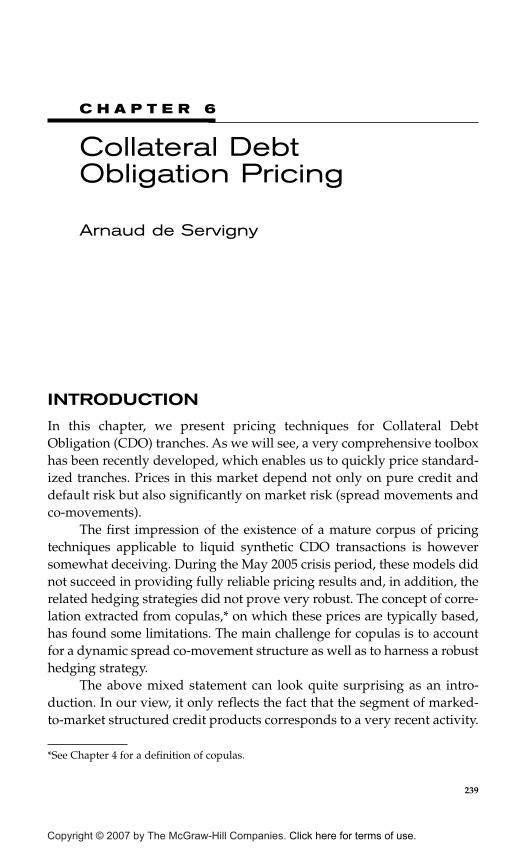
C H A P T E R 6
Collateral Debt Obligation Pricing
Arnaud de Servigny
239
INTRODUCTION
In this chapter, we present pricing techniques for Collateral DebtObligation (CDO) tranches. As we will see, a very comprehensive toolboxhas been recently developed, which enables us to quickly price standard-ized tranches. Prices in this market depend not only on pure credit anddefault risk but also significantly on market risk (spread movements andco-movements).
The first impression of the existence of a mature corpus of pricingtechniques applicable to liquid synthetic CDO transactions is howeversomewhat deceiving. During the May 2005 crisis period, these models didnot succeed in providing fully reliable pricing results and, in addition, therelated hedging strategies did not prove very robust. The concept of corre-lation extracted from copulas,* on which these prices are typically based,has found some limitations. The main challenge for copulas is to accountfor a dynamic spread co-movement structure as well as to harness a robusthedging strategy.
The above mixed statement can look quite surprising as an intro-duction. In our view, it only reflects the fact that the segment of marked-to-market structured credit products corresponds to a very recent activity.
*See Chapter 4 for a definition of copulas.
Copyright © 2007 by The McGraw-Hill Companies. Click here for terms of use.

The tools that have been developed so far are not perfect, but certainlyfacilitate the expansion of that market. In equity and fixed income pricing,it is agreed that the market standard Black and Scholes (1973) approachhas a rather weak performance, everybody still uses it as the market stan-dard. In a similar way, we have recently seen that copulas are not fullyaccurate in the fast growing credit space, but almost everybody keeps onusing the paradigm for the sake of consolidating a common language.
In parallel to this liquid and traded market, there exists an importantbut less liquid bespoke synthetic market. The appropriate word used todescribe these instruments is single tranche CDO (STCDO). The challengehere is to harness a pricing technique to an illiquid market.
In what follows, we focus at first on the synthetic CDO market, withsome particular emphasis on “correlation trading” related to indices. Wethen discuss briefly the pricing techniques used for the more bespokesynthetic tranches.
The second type of instruments we will focus on in this chapter arecash CDOs. Pricing such instruments is not straightforward, especiallywhen, on the asset side, there is no market price for the loans in the under-lying pool. On the liability side, we need to be aware that the waterfallstructure of cashflows has an effect on the value of tranches.
TYPOLOGIES OF CDOS
It is customary to classify CDOs depending on their function. In this case,usually consider CDOs are in balance sheets and arbitrage deals. The for-mer type of transactions is typically used by financial institutions in orderto rebalance their portfolio, whereas the latter focuses on the excessspread generated in the securitized pools because of diversification (seeChapter 10 for further details).
In the current analysis we focus on a different perspective, i.e.,pricing techniques. As a consequence, it is more relevant to concentrateprimarily on the way CDO instruments are structured. What reallymatters in order to differentiate CDO prices is the nature and the sourceof repayment of the collateral pool. We distinguish here between the twomain categories of CDOs: synthetic and cashflow CDOs.
♦ Synthetic CDOs: These are based on a portfolio of Credit DefaultSwaps (CDSs) and constitute an alternative to the actual transferof assets to the SPV, see Figure 6.1. These structures benefit from
240 CHAPTER 6
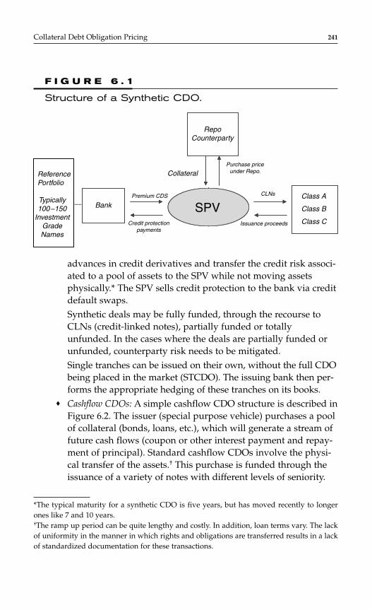
advances in credit derivatives and transfer the credit risk associ-ated to a pool of assets to the SPV while not moving assetsphysically.* The SPV sells credit protection to the bank via creditdefault swaps.Synthetic deals may be fully funded, through the recourse toCLNs (credit-linked notes), partially funded or totallyunfunded. In the cases where the deals are partially funded orunfunded, counterparty risk needs to be mitigated.Single tranches can be issued on their own, without the full CDObeing placed in the market (STCDO). The issuing bank then per-forms the appropriate hedging of these tranches on its books.
♦ Cashflow CDOs: A simple cashflow CDO structure is described inFigure 6.2. The issuer (special purpose vehicle) purchases a poolof collateral (bonds, loans, etc.), which will generate a stream offuture cash flows (coupon or other interest payment and repay-ment of principal). Standard cashflow CDOs involve the physi-cal transfer of the assets.† This purchase is funded through theissuance of a variety of notes with different levels of seniority.
Collateral Debt Obligation Pricing 241
*The typical maturity for a synthetic CDO is five years, but has moved recently to longerones like 7 and 10 years.†The ramp up period can be quite lengthy and costly. In addition, loan terms vary. The lackof uniformity in the manner in which rights and obligations are transferred results in a lackof standardized documentation for these transactions.
SPVSPVClass A
Class B
Class CIssuance proceeds
CLNs
Bank
RepoCounterparty
Purchase priceunder Repo.Collateral
Credit protectionpayments
Premium CDS
ReferencePortfolio
F I G U R E 6 . 1
Structure of a Synthetic CDO.
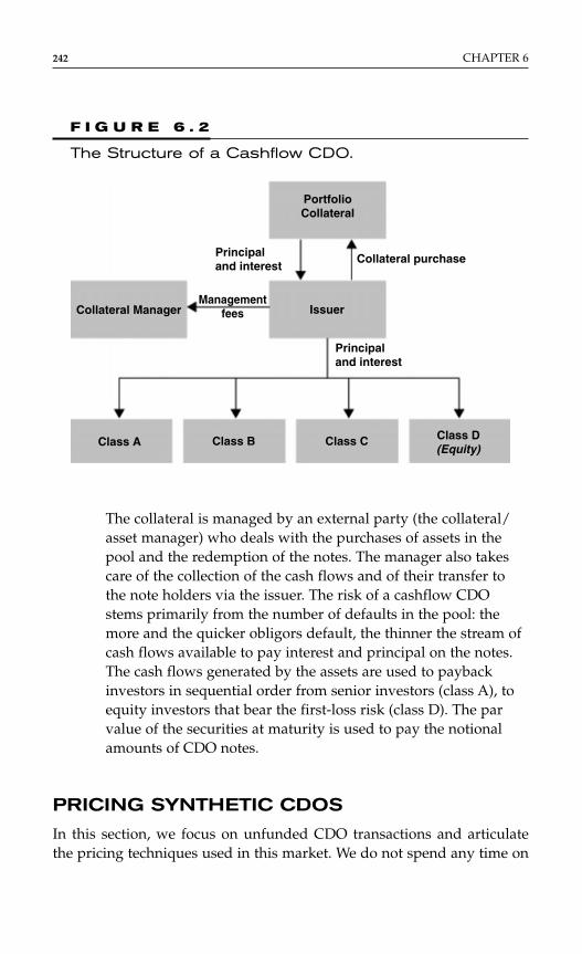
The collateral is managed by an external party (the collateral/asset manager) who deals with the purchases of assets in thepool and the redemption of the notes. The manager also takescare of the collection of the cash flows and of their transfer tothe note holders via the issuer. The risk of a cashflow CDOstems primarily from the number of defaults in the pool: themore and the quicker obligors default, the thinner the stream ofcash flows available to pay interest and principal on the notes.The cash flows generated by the assets are used to paybackinvestors in sequential order from senior investors (class A), toequity investors that bear the first-loss risk (class D). The parvalue of the securities at maturity is used to pay the notionalamounts of CDO notes.
PRICING SYNTHETIC CDOS
In this section, we focus on unfunded CDO transactions and articulatethe pricing techniques used in this market. We do not spend any time on
242 CHAPTER 6
PortfolioCollateral
Collateral purchase
Collateral Manager
Principaland interest
Managementfees Issuer
Principaland interest
Class A Class B Class C Class D(Equity)
F I G U R E 6 . 2
The Structure of a Cashflow CDO.
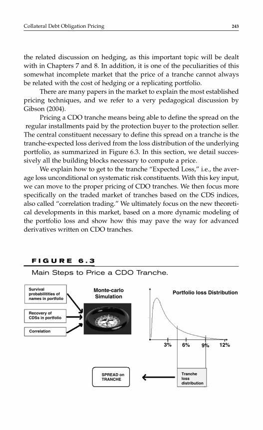
the related discussion on hedging, as this important topic will be dealtwith in Chapters 7 and 8. In addition, it is one of the peculiarities of thissomewhat incomplete market that the price of a tranche cannot alwaysbe related with the cost of hedging or a replicating portfolio.
There are many papers in the market to explain the most establishedpricing techniques, and we refer to a very pedagogical discussion byGibson (2004).
Pricing a CDO tranche means being able to define the spread on theregular installments paid by the protection buyer to the protection seller.
The central constituent necessary to define this spread on a tranche is thetranche-expected loss derived from the loss distribution of the underlyingportfolio, as summarized in Figure 6.3. In this section, we detail succes-sively all the building blocks necessary to compute a price.
We explain how to get to the tranche “Expected Loss,” i.e., the aver-age loss unconditional on systematic risk constituents. With this key input,we can move to the proper pricing of CDO tranches. We then focus morespecifically on the traded market of tranches based on the CDS indices,also called “correlation trading.” We ultimately focus on the new theoreti-cal developments in this market, based on a more dynamic modeling ofthe portfolio loss and show how this may pave the way for advancedderivatives written on CDO tranches.
Collateral Debt Obligation Pricing 243
Survivalprobabilitities ofnames in portfolio
Recovery of CDSs in portfolio
Correlation
SPREAD onTRANCHE
Tranchelossdistribution
Monte-carloSimulation
Portfolio loss Distribution
3% 6% 9% 12%
F I G U R E 6 . 3
Main Steps to Price a CDO Tranche.
Generating the Loss Distribution of the Portfolio
In the previous chapters, we have discussed in great detail how to esti-mate univariate survival probabilities (Chapters 2 and 3) as well as recov-ery rates (Chapter 3) and correlation (Chapter 4). Based on these threeconstituents, we can generate the loss distribution of the portfolio at adefined horizon. The loss distribution in the CDO portfolio is a key inputto obtain the tranche loss distribution and, subsequently, the expected lossper tranche.
More generally, what we would like to generate is the continuum ofloss distributions in the portfolio at any point in time until the maturity ofthe CDO. In order to reach this point, Li (2000) and Gregory and Laurent(2003) have really been instrumental to orientate the market approachtowards the concepts of a default survival approach, copulas and condi-tional independence.
Basically, in order to obtain the portfolio loss distribution at any hori-zon, we need to know the survival probability of each obligor in the pool atthe corresponding time (step 1), as well as the nature of the dependence ofthese probabilities on systematic risk factors (step 2). On the basis of theseconstituents, we can identify the joint survival probability in the portfolioconditional on the systematic risk factors (step 3). By blending it with recov-ery at default and simulating the behavior of the systemic risk factors, wewill be in a position to extract the portfolio loss distribution at the varioushorizons (step 4) and the related term structure of expected losses pertranche.
Step 1: Let us define τ1, . . . , τn the default times of the n obligors inthe CDO portfolio.For each obligor i, a risk-neutral survival probability functionS(ti) = Q(τi > ti) is defined and extracted from spreads as a resultfrom/credit curves.* It does not assume any dependence betweenobligors.Step 2: The joint probability cannot be computed directly. We needto introduce a dependence structure. This joint survival probabilityfunction is therefore written as a (survival) copula
S(t1, . . . , tn) = Q(τ1 > t1, . . . , τn > tn)
244 CHAPTER 6
*See Chapter 3 for a description of different methodologies.
In order to avoid dimensionality issues, dependence across oblig-ors is typically modeled through a vector of latent factors V that iscommon to all obligors. The usual approach in the CDO world isto consider a single latent factor for ease of computation, but thereis no theoretical restriction on the number.Step 3: This step consists of expressing the joint survival probabilityconditional on the realization of the latent factor.Let us denote the survival probability for obligor i, at time t, condi-tional on the factor V as:
qVi (t) = Q(τi > t|V). (1)
Based on the property of conditional independence, we can writethe conditional joint survival probability in a simple way as:
(2)
Step 4: The unconditional joint survival probability distribution canthen be obtained by integrating the conditional joint survival prob-ability on the density of the common latent factor. In addition, byassuming a constant recovery level such as 40 percent, we obtainthe portfolio loss distribution.
From this “recipe,” it is clear that the key building block necessaryto obtain the portfolio loss distribution, apart from the distribution of thelatent factor V, is the conditional survival probability for each obligor[Equation (1)].*
We review different approaches based on copulas that have beenused in the market.
Possible Candidates for Conditional Survival ProbabilityGregory and Laurent (2003) and Burtschell et al. (2005) provide a taxon-omy of possible candidates for conditional probabilities based on thechoice of different copulas. Each of the options presented in this sectionare derived from the assumption of a deterministic asset correlation
S t t V q tn iV
ii
n
( , , | ) ( )11
. . . ==
∏
Collateral Debt Obligation Pricing 245
*Or the univariate conditional risk neutral default probability for each obligor pVi(t) = 1 − qV
i(t).

structure. The selection of any one of them is usually driven by how wellit can fit empirical evidence.*
We start with the Gaussian copula that corresponds by far to themarket standard.
Gaussian Copula The most established setup is the one factorGaussian copula. That has been presented in the previous chapter on cor-relation. It can be interpreted as the asset value of the firm i being drivenby a latent common factor and an independent idiosyncratic factor, bothnormally distributed:
(3)
If we define the cumulative default probability pi(t) = Q(τi ≤ t), ρi the factorloading corresponding to asset i and Φ, the normal c.d.f., the conditionaldefault probability can be written as (Vasicek, 1987):
(4)
Student-t Copula The Student-t copula is a natural extension ofthe Gaussian copula suggested by several authors, such as O’Kane andSchloegl (2001) and Frey and McNeil (2003). It is supposed to account forfat tails better than the Gaussian copula, but the drawback is its symme-try, leading to a high probability of zero losses, too.
The asset value of the firm i follows a Student-t distribution. It is,however, driven by a latent common factor and an independent idiosyn-cratic factor, both normally distributed:
where W is an inverse Gamma distribution with parameter equal to (ν/2),independent from the Gaussian factors.
The conditional default probability becomes:
A W Vi i i i= + −( ),ρ ρ ξ1 2
p t
p t ViV i i
i
( )( ( ))
=−
−
−
ΦΦ 1
21
ρ
ρ
A Vi i i i= + −ρ ρ ξ1 2
246 CHAPTER 6
*As a caveat though, we have seen in the previous chapter on correlation that a determinis-tic approach to correlation, whatever the circumstances, may not correspond to a fullyappropriate representation of the reality.
(5)
Double-t Copula This approach has been suggested in Hull andWhite (2004) in order to partially decouple the size and shape of the upperand lower tail of the loss distribution.
The asset value of the firm i does not follow a Student-t distribution,but is a convolution of a latent common factor and an independent idio-syncratic factor, both Student-t distributed, with respectively ν and ν–
degrees of freedom:
(6)
In this situation, the conditional default probability can be expressed as:
(7)
where Hi(Ai) = pi(t) corresponds to the distribution function of Ai that hasto be computed numerically as it is not a Student-t.
Normal Inverse Gaussian (NIG) Copulas There aretwo rationales for using NIG Gaussian distributions:
♦ Fat tails: the fact that asset returns tend to exhibit more asym-metric, as well as fatter, tails than a Gaussian distribution sup-ports the use of a NIG distribution.
♦ Tractability reasons: the point that a convolution of NIG distri-butions is a NIG distribution facilitates the computation of thepricing of tranches.
In Kalemanova et al. (2005), the asset value of the firm i is driven by alatent common factor and an independent idiosyncratic factor, both NIGdistributed:
A Vi i i i= + −ρ ρ ξ1 2
p t tH p t V
iV
V
i i i
i
( ) *( ( ))
=−
−−
−
−ν
ν
ρν
νρ2
2
1
1
2
A Vi i i i=
−
+−
−ν
νρ
νν
ρ ξ2 2
11 2 1 2
2/ /
,
p t
W t p t ViV W i i
i
,/
( )( ( ))
=−
−
− −
Φ1 2 1
21ν ρ
ρ
Collateral Debt Obligation Pricing 247

If we define the NIG c.d.f. as:
With s, α, and β the parameters of the NIG. The first one is related to cor-relation, whereas the next two are related to the mean and the variance.
Kalemanova et al. (2005) show that the conditional probability ofdefault can be written as:
(8)
Archimedean Copulas Archimedean copulas have been pro-posed in particular by Schönbucher and Schubert (2001) in the context ofcontagion models.
In the case of the Clayton copula, the conditional default probabilitycan be expressed as:
pVi (t) = exp(V(1 − pi(t)
−θ)), (9)
where θ is the parameter of the copula.
Marshall-Olkin Copula Multivariate exponential spread mod-eling associated with the Marshall-Olkin copula is also called a “Poissonshock” model. It allows for simultaneous defaults and fat tails, as thedefault intensity for each obligor is split between a systematic and an idio-syncratic component. Several authors like Duffie and Singleton (1998),Lindskog and McNeil (2003), Elouerkhaoui (2003a,b), and Giesecke (2003)have suggested its use. Practical calibration can be challenging, as manyparameters need to be calibrated. Figure 6.4 shows how this copula givessignificant modeling flexibility.
In order to obtain a one factor representation of this approach, let usconsider one latent common variable V and n obligor specific randomvariables V
–i, all independent and exponentially distributed with respec-
tive parameters α and 1 − α and α ∈ [0, 1].* For each obligor i, we can
p t F
F p t V
iV
i i
ii
i
i( )
( ( ))
NIG
NIG
=
−
−
−
−
1
11
22 1ρρ
ρ
ρ
ρ
F x F x s s s ssNIG( ) NIG( ) ; , , ,= −−
α β
αβα β
α2 2
248 CHAPTER 6
*α should be seen as describing the intensity of co-movement to default, α = 1, meaning totalcomonotonicity.
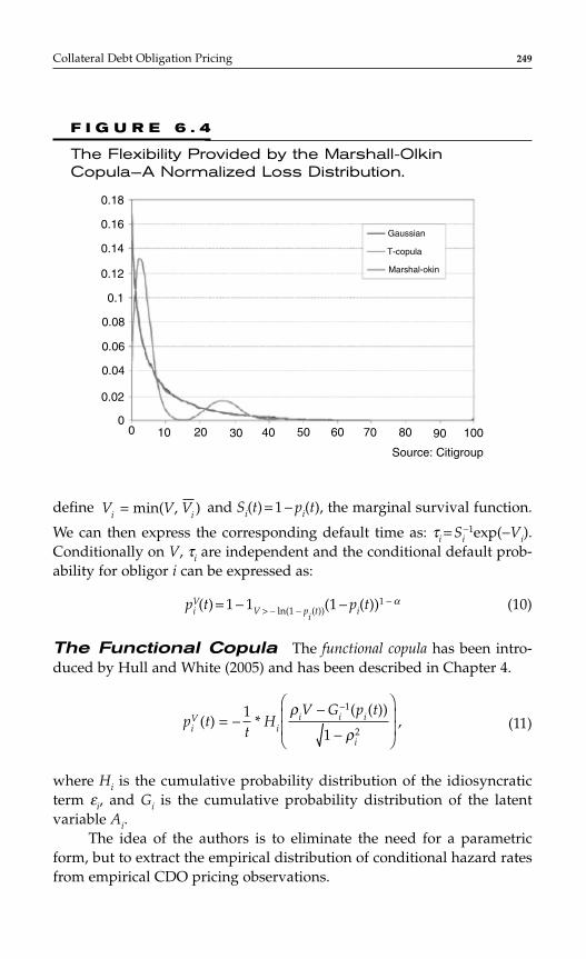
define and Si(t) = 1 − pi(t), the marginal survival function.
We can then express the corresponding default time as: τi = Si−1exp(−Vi).
Conditionally on V, τi are independent and the conditional default prob-ability for obligor i can be expressed as:
pVi (t) = 1 − 1V > − ln(1 − p
i(t))(1 − pi(t))
1 − α (10)
The Functional Copula The functional copula has been intro-duced by Hull and White (2005) and has been described in Chapter 4.
(11)
where Hi is the cumulative probability distribution of the idiosyncraticterm εi, and Gi is the cumulative probability distribution of the latentvariable Ai.
The idea of the authors is to eliminate the need for a parametricform, but to extract the empirical distribution of conditional hazard ratesfrom empirical CDO pricing observations.
p t
tH
V G p tiV
ii i i
i
( ) *( ( ))
,= −−
−
−1
1
1
2
ρ
ρ
V V Vi i= min( , )
Collateral Debt Obligation Pricing 249
0.18
0.16
0.14
0.12
0.1
0.08
0.06
0.04
0.02
00 10 20 30 40 50 60 70 80 90 100
Source: Citigroup
Gaussian
T-copula
Marshal-okin
F I G U R E 6 . 4
The Flexibility Provided by the Marshall-Olkin Copula—A Normalized Loss Distribution.

To date, the market standard remains the Gaussian copula.However, this Gaussian set-up does not prove very effective in pricingtranches. As an illustration of this problem, market participants havenoted that a strong correlation skew is empirically observed based onmarket prices. This skew cannot be matched in a simple way with theGaussian copula. As a result, finding a more accurate model has becomethe new frontier. In addition to the alternative copulae described previ-ously, market practitioners have also tried to provide some extensions ofthe Gaussian copula in order to better match observed prices.
Possible Extensions of the Gaussian Copula:Relaxing Deterministic AssumptionsGaussian copulas have such a footprint in the CDO market that it wouldbe nice to be able to keep this framework while gaining accuracy in thevaluation of tranches. Two related extensions have been suggested. Theyconsist of either modifying the dependence structure of the asset valuedepending on different states of the world,* or considering that LossGiven Default is correlated to the realization of the common systematicfactor.
Random Factor Loadings The idea is that it is possible toapproximate the apparently non-Gaussian behavior of an asset value as aconvolution of Gaussian distributions.
In the correlation Chapter 4, it was noted that under the empiricalmeasure there was evidence supporting a two-regime-switching approachdepending on growth and recession periods in the economy. Andersenand Sidenius (2005) head towards this direction with “random factor load-ings.” Practically in their simplest setup, factor loadings depend on therealization of the common factor with respect to a barrier that can be seenas describing the state of the economy.
Burtschell et al. (2005) present the approach in a generic way underthe wording of “stochastic correlation.” Like in the simple Gaussian case,the asset value of the firm i is still driven by a latent common factor andan independent idiosyncratic factor, both normally distributed, but thereare two possible states that come to play. In this respect, Bi is the Bernouillidistributed weight associated with the case where the factor-loadingcorresponding to company i is ρi, and a weight (1 − Bi) corresponds to acorrelation of ρ–i. As a result, the asset value of the firm can be written as:
250 CHAPTER 6
*Also, sometimes referred to as “local correlation.”

Let us define the probability bi = Q(Bi = 1), the conditional default proba-bility can be written as:
(12)
Random Recovery The principle here is to have not only theasset value to be dependent on a vector of common factors, but also tohave the recovery rate dependent on the same factors.
Ri = C(µi + biVi + εi), (13)
where C is a function on [0, 1], such as a beta distribution function.Increasing the dependency of the recovery on the common factors
generates a fatter tail and therefore can account for some of the correlationskew observed for senior tranches. However, Andersen (2005) notes thatwhen realistically calibrated, random recovery does not seem to be suffi-cient to explain the equity and the super senior correlation skews.
Assuming Homogeneity in the PortfolioIn an active market, traders require fast models and simple ways to com-municate. Speed of computation and communication are often obtainedat the expense of accuracy. Will a stylized model be sufficiently rich androbust to price and hedge transactions? This question represents a keychallenge for the industry to date.
In addition to the assumption of the single factor copula framework,we mention below some other simplifications that are sometimes consid-ered by market participants. Simplification can be obtained by assumingobligor homogeneity in the CDO portfolio. This leads to two simplifications:
♦ Factor loadings (i.e., the weight on the common factor, ρi) areindependent from the obligors in the CDO portfolio. Thismeans that we move from multiple, obligor dependent, factorloadings to a single one for the pool, ρ.
♦ Obligors can be considered as reasonably close in terms ofcreditworthiness and prices and as a result an average spread orprobability of default is supposed to characterize the portfolioof obligors well. Practically, in all previous formulas, this
p t bp t V
bp t V
iV
ii i
ii
i i
i
( )( ( ))
( )( ( )
=−
−
+ −
−
−
− −
ΦΦ
ΦΦ1
2
1
211
1
ρ
ρ
ρ
ρ
A B B V B Bi i i i i i i i i i= + − + − + −( ( ) ) ( ( ) )ρ ρ ρ ρ ξ1 1 1 2
Collateral Debt Obligation Pricing 251
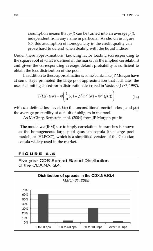
assumption means that pi(t) can be turned into an average p(t),independent from any name in particular. As shown in Figure6.5, this assumption of homogeneity in the credit quality canprove hard to defend when dealing with the liquid indices.
Under these approximations, knowing factor loading (corresponding tothe square root of what is defined in the market as the implied correlation)and given the corresponding average default probability is sufficient toobtain the loss distribution of the pool.
In addition to these approximations, some banks like JP Morgan haveat some stage promoted the large pool approximation that facilitates theuse of a limiting closed-form distribution described in Vasicek (1987, 1997).
(14)
with α a defined loss level, L(t) the unconditional portfolio loss, and p(t)the average probability of default of obligors in the pool.
As McGinty, Bernstein et al. (2004) from JP Morgan put it:
“The model we (JPM) use to imply correlations in tranches is knownas the homogeneous large pool gaussian copula (the ‘large poolmodel’, or ‘HLPGC’), which is a simplified version of the Gaussiancopula widely used in the market.
P L t p t( ( ) ) ( ( ) ( ( ))≤ = − −
− −α
ρρ αΦ Φ Φ
11 2 1 1
252 CHAPTER 6
Distribution of spreads in the CDX.NA.IG.4March 31, 2005
0%
10%
20%
30%
40%
50%
60%
70%
0 to 20 bps 20 to 50 bps 50 to 100 bps over 100 bps
F I G U R E 6 . 5
Five-year CDS Spread-Based Distribution of the CDX.NA.IG.4.
. . . The model is based on three major assumptions. First, defaultof a reference entity is triggered when its asset value falls belowa barrier. Second, asset value of the portfolio is driven by a common,standard normally distributed factor M, which is often referred to asthe ‘Market,’ and can be taken to imply the state of the overall busi-ness cycle. Finally, the portfolio consists of a very large number ofcredits of uniform size, which effectively cancels the effect of a sin-gle name’s performance on tranche loss and is why the portfolio canbe considered homogenous.
We believe that the fundamental benefits of the large pool modelare transparency and replicability—we can provide our specificimplementation of the model. The model also has the advantagethat it requires few inputs–only the average level of market spreadsand average recovery rate (which we define as 40%), rather thanindividual spreads for all of the credits in the portfolio, whichwould be impossible for a user to reproduce at any instant. Thedownside of course, is that the model does not consider singlename blow-ups correctly. This manifests itself in two main ways:one, the model cannot differentiate between a single name widen-ing by 10,000 bp and 100 names widening by 100 bp, and two, thereis a discontinuity as credit spreads widen towards default. Themodel is unlikely to produce spreads consistent with marketobservations in these scenarios. . . .”
Such an approximation facilitates immensely the calculation of correla-tion and ultimately of prices. However, it can be very misleading whenapplied to a portfolio characterized by a low number of names and/ordifferent profiles in terms of creditworthiness.
This fully granular model assumes full diversification of the idio-syncratic risk, but empirical evidence shows that full diversification ina credit portfolio is typically obtained with a minimum of 400–500obligors. Indices like CDX, I-Traxx only contain up to 125 names. It canbe therefore quite risky to apply the large pool model to index basedcorrelation trading.
Pre-May 2005, Finger (2005) reported that the JP Morgan model hadperformed well for investment grade index tranches. This set-up is, how-ever, no longer used by market participants, and other ways to reducecomputational time are investigated next.
Collateral Debt Obligation Pricing 253

Getting to the Loss Distribution of the Portfolio:Monte-Carlo and Semi-analytical Techniques
Option 1: The Full Monte-Carlo Calculation* TheMonte-Carlo approach is based on the random draw of realizations of thecommon systematic factor and for each realization, a portfolio loss canbe computed as the sum of individual losses. The unconditional portfolioloss corresponds to the integration of the conditional losses on the distri-bution of the common factor.
This “brute force” approach is usually not selected by market par-ticipants, as it is time consuming.† Some techniques, often based on vari-ance reduction, can help to speed-up the computation time.
Option 2: The Recursive Approach This approach hasbeen suggested almost simultaneously by Andersen et al. (2003) and byHull and White (2003). The principle is integration over a discretelyapproximated portfolio loss distribution.
In a portfolio of j names, the probability of observing exactly hdefaults (with h ≤ j) by time t, conditional on the realization of the commonfactor V can be written as pV
i (h, t). Furthermore, pVj –1(t) is the condi-
tional default probability of name j–1:
pVj +1(h, t) = pV
j (h, t)(1 – pVj+1(t)) + pV
j (h – 1, t)pVj+1(t)
where, of course,
pVj+1(0, t) = pV
j (0, t)(1 − pVj+1(t))
pVj+1( j + 1, t) = pV
j ( j, t) pVj+1(t)
Based on the above recursion, we can obtain the unconditional probabil-ity of observing h defaults in a portfolio of n names by time t by integrat-ing over the common factor with distribution function f(V):
(15)p h t p h t f V Vn nV( , ) ( , ) ( )d=
−∞
∞∫
254 CHAPTER 6
*See Rott and Fries (2005) regarding the use of variance reduction techniques.†It is particularly cumbersome for CDO squared.

Option 3: Using Fourier Transform Techniques*We consider the total accumulated loss of the reference pool at time t, andδ is the recovery fraction at default on each name. The default time forobligor j is τj. Once the nominal on each name j, Nj, is defined, we canwrite the accumulated loss at time t, by calling theindicator function: 1τi ≤ t = Xj.
The Fourier transform of the accumulated loss function can beexpressed as:
ϕL(t)(u) = E[exp(−iuL(t)] = E[E(exp(−iuL(t)|V)],
where V is the common systematic factor.We can then introduce the expression of the Fourier transform of the
loss
(16)
The Fourier transform of the conditional loss is more tractable, due tothe possibility to permute the expectation under conditional indepen-dence. Based on the Bernoulli distribution of the indicator function Xj,we obtain:
In turn, this can be written as
ϕ ϕ δ
VL t j
VjV
Nj
n
u q t p t uj
( ) ( )( ) [ ( ) ( ) ( )],= + −=
∏ 11
ϕ δ δ
δ
VL t
iuN X V
j
niuN X V
j
n
jV
jV iu N
j
n
u E E
q t p t e
j j j j
j
( )( ) | ( ) |
( )
( ) [ ]
[ ( ) ( )( )]
=
=
= +
− −
=
− −
=
− −
=
∏ ∏
∏
e e1
1
1
1
1
1
ϕ δ δ δ
δ
L tiu N X N X N X
iuN X
j
n
u E
E
n n
j j
( )– ( ( ) ( ) ( ) )
– ( )
( ) [e ]
e
=
=
− + − + + −
−
=∏
1 1 2 21 1 1
1
1
L
L t N Xjn
j j( ) ( ) ,= ∑ −=1 1 δ
Collateral Debt Obligation Pricing 255
*We revert readers to the presentation on Fourier Transform techniques, by Debuysscherand Szego (2003). There are other possible convolution techniques, such as Laplace trans-forms and Moment Generating functions.

where ϕV(1−δ )(Nj u) is derived from the Fourier transform of the Loss Given
Default on asset j.The unconditional Fourier transform is then obtained numerically
by integrating on the distribution of the common systematic factor:
(17)
In a final step, the unconditional loss can be computed using the inverseFourier transform by practically applying standard Fast Fourier trans-form algorithms.
Option 4: Proxy Integration Proxy integration, presented inShelton (2004), has gained traction in the market because of its simplicity.
The central limit theorem states that the sum of independentrandom variables with finite variance and arbitrary probabilitydistribution converges to a normal distribution as the number of vari-ables increases.
Shelton’s approach is based on the idea that the convergence to anormal distribution might take place sufficiently quickly to allow for theapproximation.
In the case of CDO pricing, we cannot consider the survival proba-bility variables for each obligor to be independent, as obligor losses aretypically correlated. We have seen though that conditional on a vector oflatent risk factors, the portfolio loss distribution can be expressed as theweighted sum of conditionally independent random variables.
Let us consider again the total accumulated loss of the reference poolat time t, with δ the recovery fraction at default on each name. The defaulttime for obligor j is τj. Once the nominal on each name j, Nj, is defined, we
can write the accumulated loss at time horizon t,by calling the indicator function: 1τ j ≤ t = Xj.
We then consider various realizations of the common systematiclatent factor V. Under the assumption of conditional independence, wecan now easily compute the conditional loss distribution in the portfo-lio based on Equation (2). According to the Proxy integration approach,we assume that conditional on each realization of V, the joint distribu-tion of losses in the portfolio converges to a normal distribution asshown in Figure 6.6. For each realization of the systematic factor, wecan compute the mean and the variance of the approximated normaldistribution.
L t N Xjn
j j( ) ( ) ,= ∑ −=1 1 δ
ϕ ϕ δL t j
VjV
jj
n
u q t p t N u f V dV( ) ( )( ) [ ( ) ( ) ( )] ( )= +−∞
∞
−=
∫ ∏ 11
256 CHAPTER 6
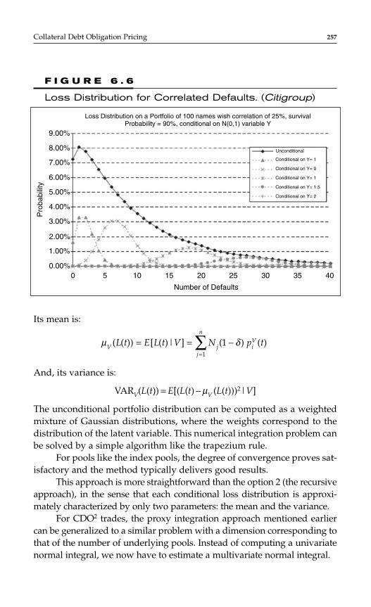
Its mean is:
And, its variance is:
VARV(L(t)) = E[(L(t) − µV (L(t)))2|V]
The unconditional portfolio distribution can be computed as a weightedmixture of Gaussian distributions, where the weights correspond to thedistribution of the latent variable. This numerical integration problem canbe solved by a simple algorithm like the trapezium rule.
For pools like the index pools, the degree of convergence proves sat-isfactory and the method typically delivers good results.
This approach is more straightforward than the option 2 (the recursiveapproach), in the sense that each conditional loss distribution is approxi-mately characterized by only two parameters: the mean and the variance.
For CDO2 trades, the proxy integration approach mentioned earliercan be generalized to a similar problem with a dimension corresponding tothat of the number of underlying pools. Instead of computing a univariatenormal integral, we now have to estimate a multivariate normal integral.
µ δV j i
V
j
n
L t E L t V N p t( ( )) [ ( )| ] ( ) ( )= = −=∑ 1
1
Collateral Debt Obligation Pricing 257
Loss Distribution on a Portfolio of 100 names wish correlation of 25%, survivalProbability = 90%, conditional on N(0,1) variable Y
9.00%
8.00%
7.00%
6.00%
5.00%
4.00%
3.00%
2.00%
1.00%
0.00%
Pro
babi
lity
Number of Defaults
Unconditional
Conditional on Y= 1
Conditional on Y= 0
Conditional on Y= 1
Conditional on Y= 1.5
Conditional on Y= 2
0 5 10 15 20 25 30 35 40
F I G U R E 6 . 6
Loss Distribution for Correlated Defaults. (Citigroup)
Pricing a CDO Tranche Once the UnconditionalPortfolio Loss Distribution is Obtained
A synthetic CDO tranche can be valued like any other swap contract.There are two parties involved: the issuer who typically is the protec-tion buyer and the investor, the protection seller. The investor receivesfrom the issuer a regular “fee” or “premium.” When default impactsthe tranche, the investor has to pay a “contingent” amount, correspon-ding to the “contingent” or “default” leg. For the investor holding atranche, there is a need to be compensated appropriately for bearingpotential losses (the expected losses). The higher the seniority, thelower the fees.
Let us introduce the following notations:In the CDO we consider, there are n different names with i = 1, . . . , n.
A default time τt is associated to each name i.We can now define the counting process of the
number of defaults at time t, T the maturity of the CDO, and δ the stan-dard recovery fraction at default on each name. When conditioned on thecommon factor, these Bernouilli variables become independent and theconditional loss distribution at time t can be obtained easily. As a result,once the nominal on each name i, Ni, is defined, we can write theaccumulated unconditional losses at time t, also called expected loss, as
where V corresponds to the common sys-
tematic factor. Its practical computation has been described previously.
Computing the Value of the “Contingent Leg”*We initially start with a three-tranche CDO with equity, mezzanine, andsenior pieces, but nothing precludes us to consider more tranches in theremainder of this section. The subordination priority rule means thatlosses will be allocated first to the equity piece, then to the mezzanine,and the remainder to the senior tranche. The equity tranche correspondsto [A0 = 0, A1 = A], the mezzanine to [A, A2 = B], and the senior to
where Aj are agreed upon thresholds. Accumulated
losses will therefore be successively absorbed by each of the tranches.The next step is to measure explicitly overtime the unconditional
average accumulated loss in each of the tranches [Aj, Aj +1].
[ , ],B A Nin
i3 1= ∑ =
EL t E N Vin
i ti( ) [ ( ) ],= ∑ −= ≤1 1 1δ τ
N t in
ti( ) ,= ∑ = ≤1 1τ
258 CHAPTER 6
*Also called “protection leg” or “loss leg.”
ELj(t) = E(max[min((L(t) − Aj), (Aj +1 − Aj)), 0]) (18)
The discounted payout corresponding to contingent losses intranche j during the life of the CDO can be written as:
(19)
where D(k) is the discount factor term. We consider here the time series ofthe premium payment dates k = 1, . . . , K.
More rigorously, this contingent leg can be written as an integral andcan be integrated by parts:
(20)
where f(t) = −(1/D(t))(dD(t)/dt) is the spot forward rate.
Computing the Value of the “Fee Leg”*The expected present value of the fee leg on each tranche corresponds tothe payment of regular installments at a predefined spread Sj appliedto the principal exposure of the tranche outstanding at the date of pay-ment of the premium.
(21)
The initial mark-to-market value of the tranche is Cj(0) − Fj(0). In thecase that the CDO tranche is unfunded and fairly priced, this initialmarked-to-market value is 0.
The value of the spread can be deducted in a straightforward way as:
(22)sC
A A EL k D kj
j
j j jk
K=− −+=∑
( )
[( ) ( )] ( )
0
11
F s A A EL k D kj j j j jk
K
( ) [( ) ( )] ( )0 11
= − −+=
∑
C D T EL T EL t D t
D T EL T EL t D t f t t
j j j
T
j j
T
( ) ( ) ( ) ( ) d ( )
( ) ( ) ( ) ( ) ( ) d
00
0
= +
= +
∫∫
C t D k EL k EL kj j jk
K
( ) ( )[ ( ) ( )]= = + −=
∑0 11
Collateral Debt Obligation Pricing 259
*Also called “premium leg.” For ease of presentation, we assume here that tranches arepriced using spreads only, with no upfront payment.
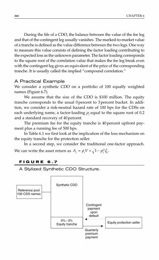
During the life of a CDO, the balance between the value of the fee legand that of the contingent leg usually vanishes. The marked-to-market valueof a tranche is defined as the value difference between the two legs. One wayto measure this value consists of defining the factor loading contributing tothe expected loss as the unknown parameter. The factor loading correspondsto the square root of the correlation value that makes the fee leg break evenwith the contingent leg gives an equivalent of the price of the correspondingtranche. It is usually called the implied “compound correlation.”
A Practical ExampleWe consider a synthetic CDO on a portfolio of 100 equally weightednames (Figure 6.7).
We assume that the size of the CDO is $100 million. The equitytranche corresponds to the usual 0 percent to 3 percent bucket. In addi-tion, we consider a risk-neutral hazard rate of 100 bps for the CDSs oneach underlying name, a factor-loading ρi equal to the square root of 0.2and a standard recovery of 40 percent.
The premium fee for the equity tranche is 40 percent upfront pay-ment plus a running fee of 500 bps.
In Table 6.1 we first look at the implication of the loss mechanism onthe equity tranche for the protection seller.
In a second step, we consider the traditional one-factor approach.
We can write the asset return as A Vi i i i= + −ρ ρ ξ1 2 .
260 CHAPTER 6
Synthetic CDO
0%−3%Equity tranche
Reference pool100 CDS names
Quarterlypremiumpayment
Contingentpayment
upondefault
Equity protection seller
F I G U R E 6 . 7
A Stylized Synthetic CDO Structure.
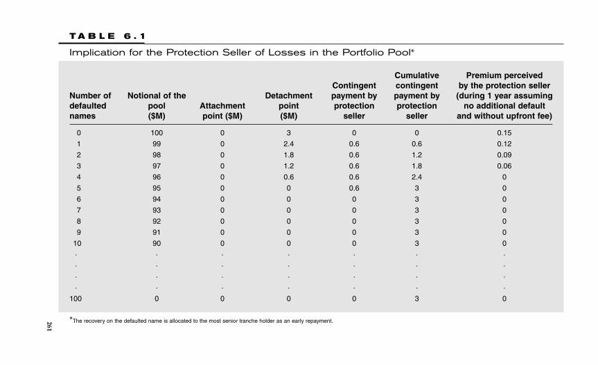
T A B L E 6 . 1
Implication for the Protection Seller of Losses in the Portfolio Pool*
Cumulative Premium perceivedContingent contingent by the protection seller
Number of Notional of the Detachment payment by payment by (during 1 year assumingdefaulted pool Attachment point protection protection no additional default names ($M) point ($M) ($M) seller seller and without upfront fee)
0 100 0 3 0 0 0.15
1 99 0 2.4 0.6 0.6 0.12
2 98 0 1.8 0.6 1.2 0.09
3 97 0 1.2 0.6 1.8 0.06
4 96 0 0.6 0.6 2.4 0
5 95 0 0 0.6 3 0
6 94 0 0 0 3 0
7 93 0 0 0 3 0
8 92 0 0 0 3 0
9 91 0 0 0 3 0
10 90 0 0 0 3 0
· · · · · · ·
· · · · · · ·
· · · · · · ·
· · · · · · ·
100 0 0 0 0 3 0
*The recovery on the defaulted name is allocated to the most senior tranche holder as an early repayment.261
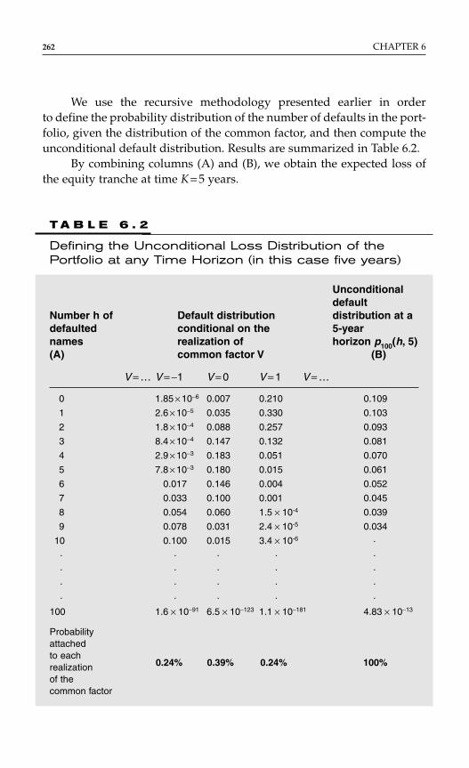
We use the recursive methodology presented earlier in orderto define the probability distribution of the number of defaults in the port-folio, given the distribution of the common factor, and then compute theunconditional default distribution. Results are summarized in Table 6.2.
By combining columns (A) and (B), we obtain the expected loss ofthe equity tranche at time K = 5 years.
262 CHAPTER 6
T A B L E 6 . 2
Defining the Unconditional Loss Distribution of thePortfolio at any Time Horizon (in this case five years)
Unconditionaldefault
Number h of Default distribution distribution at a defaulted conditional on the 5-year names realization of horizon p100(h, 5)(A) common factor V (B)
V = … V = −1 V = 0 V = 1 V = …
0 1.85 × 10⁻⁶ 0.007 0.210 0.109
1 2.6 × 10⁻⁵ 0.035 0.330 0.103
2 1.8 × 10⁻⁴ 0.088 0.257 0.093
3 8.4 × 10⁻⁴ 0.147 0.132 0.081
4 2.9 × 10⁻³ 0.183 0.051 0.070
5 7.8 × 10⁻³ 0.180 0.015 0.061
6 0.017 0.146 0.004 0.052
7 0.033 0.100 0.001 0.045
8 0.054 0.060 1.5 × 10⁻⁴ 0.039
9 0.078 0.031 2.4 × 10⁻⁵ 0.034
10 0.100 0.015 3.4 × 10⁻⁶ ·
· · · · ·
· · · · ·
· · · · ·
· · · · ·
100 1.6 × 10−91 6.5 × 10−123 1.1 × 10−181 4.83 × 10⁻¹³
Probabilityattachedto each realizationof the common factor
0.24% 0.39% 0.24% 100%
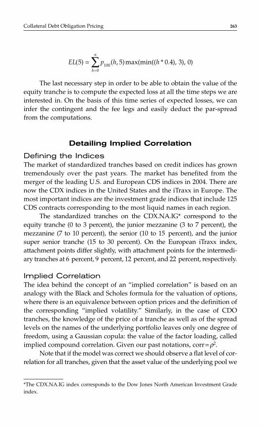
The last necessary step in order to be able to obtain the value of theequity tranche is to compute the expected loss at all the time steps we areinterested in. On the basis of this time series of expected losses, we caninfer the contingent and the fee legs and easily deduct the par-spreadfrom the computations.
Detailing Implied Correlation
Defining the IndicesThe market of standardized tranches based on credit indices has growntremendously over the past years. The market has benefited from themerger of the leading U.S. and European CDS indices in 2004. There arenow the CDX indices in the United States and the iTraxx in Europe. Themost important indices are the investment grade indices that include 125CDS contracts corresponding to the most liquid names in each region.
The standardized tranches on the CDX.NA.IG* correspond to theequity tranche (0 to 3 percent), the junior mezzanine (3 to 7 percent), themezzanine (7 to 10 percent), the senior (10 to 15 percent), and the juniorsuper senior tranche (15 to 30 percent). On the European iTraxx index,attachment points differ slightly, with attachment points for the intermedi-ary tranches at 6 percent, 9 percent, 12 percent, and 22 percent, respectively.
Implied CorrelationThe idea behind the concept of an “implied correlation” is based on ananalogy with the Black and Scholes formula for the valuation of options,where there is an equivalence between option prices and the definition ofthe corresponding “implied volatility.” Similarly, in the case of CDOtranches, the knowledge of the price of a tranche as well as of the spreadlevels on the names of the underlying portfolio leaves only one degree offreedom, using a Gaussian copula: the value of the factor loading, calledimplied compound correlation. Given our past notations, corr = ρ2.
Note that if the model was correct we should observe a flat level of cor-relation for all tranches, given that the asset value of the underlying pool we
EL p h hh
n
( ) ( , 5)max(min(( * . ), ), )5 0 4 3 01000
==
∑
Collateral Debt Obligation Pricing 263
*The CDX.NA.IG index corresponds to the Dow Jones North American Investment Gradeindex.
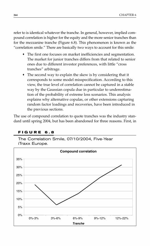
refer to is identical whatever the tranche. In general, however, implied com-pound correlation is higher for the equity and the more senior tranches thanfor the mezzanine tranche (Figure 6.8). This phenomenon is known as the“correlation smile.” There are basically two ways to account for this smile:
♦ The first one focuses on market inefficiencies and segmentation.The market for junior tranches differs from that related to seniorones due to different investor preferences, with little “crosstranches” arbitrage.
♦ The second way to explain the skew is by considering that itcorresponds to some model misspecification. According to thisview, the true level of correlation cannot be captured in a stableway by the Gaussian copula due in particular to underestima-tion of the probability of extreme loss scenarios. This analysisexplains why alternative copulas, or other extensions capturingrandom factor loadings and recoveries, have been introduced inthe previous sections.
The use of compound correlation to quote tranches was the industry stan-dard until spring 2004, but has been abandoned for three reasons. First, in
264 CHAPTER 6
Compound correlation
0%
5%
10%
15%
20%
25%
30%
35%
0%-3% 3%-6% 6%-9% 9%-12% 12%-22%
Tranche
F I G U R E 6 . 8
The Correlation Smile, 07/10/2004, Five-Year iTraxx Europe.
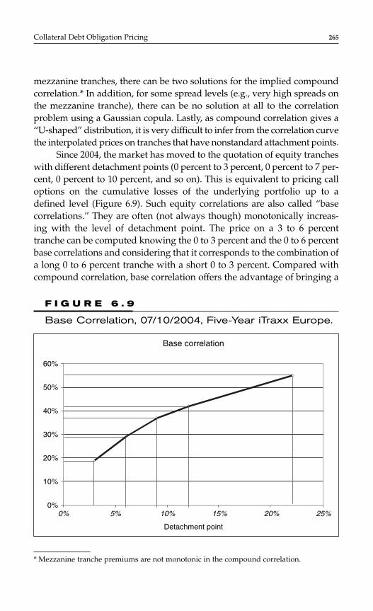
mezzanine tranches, there can be two solutions for the implied compoundcorrelation.* In addition, for some spread levels (e.g., very high spreads onthe mezzanine tranche), there can be no solution at all to the correlationproblem using a Gaussian copula. Lastly, as compound correlation gives a“U-shaped” distribution, it is very difficult to infer from the correlation curvethe interpolated prices on tranches that have nonstandard attachment points.
Since 2004, the market has moved to the quotation of equity trancheswith different detachment points (0 percent to 3 percent, 0 percent to 7 per-cent, 0 percent to 10 percent, and so on). This is equivalent to pricing calloptions on the cumulative losses of the underlying portfolio up to adefined level (Figure 6.9). Such equity correlations are also called “basecorrelations.” They are often (not always though) monotonically increas-ing with the level of detachment point. The price on a 3 to 6 percenttranche can be computed knowing the 0 to 3 percent and the 0 to 6 percentbase correlations and considering that it corresponds to the combination ofa long 0 to 6 percent tranche with a short 0 to 3 percent. Compared withcompound correlation, base correlation offers the advantage of bringing a
Collateral Debt Obligation Pricing 265
* Mezzanine tranche premiums are not monotonic in the compound correlation.
Base correlation
0%
10%
20%
30%
40%
50%
60%
5% 10% 15% 20% 25%0%
Detachment point
F I G U R E 6 . 9
Base Correlation, 07/10/2004, Five-Year iTraxx Europe.
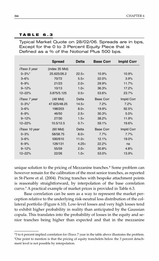
unique solution to the pricing of Mezzanine tranches.* Some problem canhowever remain for the calibration of the most senior tranches, as reportedin St-Pierre et al. (2004). Pricing tranches with bespoke attachment pointsis reasonably straightforward, by interpolation of the base correlationcurve.† A practical example of market prices is provided in Table 6.3.
Base correlation can be seen as a way to represent the market per-ception relative to the underlying risk-neutral loss distribution of the col-lateral portfolio (Figure 6.10). Low-level losses and very high losses tendto exhibit higher probability in reality than anticipated by the Gaussiancopula. This translates into the probability of losses in the equity and se-nior tranches being higher than expected and that in the mezzanine
266 CHAPTER 6
T A B L E 6 . 3
Typical Market Quote on 28/02/06. Spreads are in bps,Except for the 0 to 3 Percent Equity Piece that isDefined as a % of the Notional Plus 500 bps.
Spread Delta Base Corr Impld Corr
iTraxx 5 year (index 35 Mid)
0–3%* 25.625/26.2 22.5× 10.9% 10.9%
3–6% 70/72 5.5× 22.0% 3.9%
6–9% 21/23 2.0× 29.9% 11.7%
9–12% 10/13 1.0× 36.3% 17.2%
12–22% 3.875/5.125 0.5× 53.6% 23.7%
iTraxx 7 year (48 Mid) Delta Base Corr Impld Corr
0–3%* 47.625/48.25 14.5× 7.2% 7.2%
3–6% 198/203 8.0× 19.9% 92.5%
6–9% 46/50 2.5× 30.3% 5.0%
9–12% 27/30 1.5× 38.2% 11.9%
12–22% 10.5/12.5 0.7× 59.1% 19.6%
iTraxx 10 year (60 Mid) Delta Base Corr Impld Corr
0–3% 58/58.75 8.0× 7.7% 7.7%
3–6% 590/610 11.0× 12.1% 19.0%
6–9% 126/131 4.25× 22.2% na
9–12% 55/59 2.0× 30.8% 4.8%
12–22% 22/26 1.0× 53.0% 13.9%
*3 to 6 percent implied correlation for iTraxx 7 year in the table above illustrates the problem.†One point to mention is that the pricing of equity tranchelets below the 3 percent detach-ment level is not possible by interpolation.
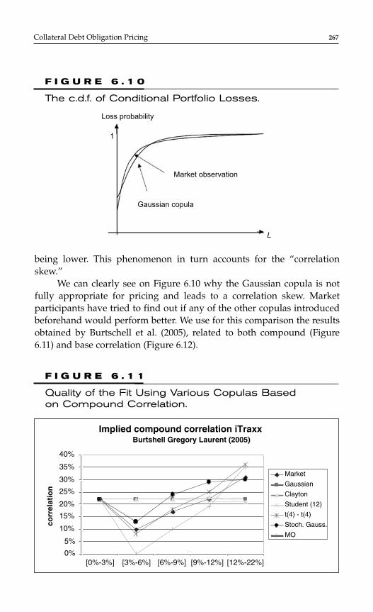
being lower. This phenomenon in turn accounts for the “correlationskew.”
We can clearly see on Figure 6.10 why the Gaussian copula is notfully appropriate for pricing and leads to a correlation skew. Marketparticipants have tried to find out if any of the other copulas introducedbeforehand would perform better. We use for this comparison the resultsobtained by Burtschell et al. (2005), related to both compound (Figure6.11) and base correlation (Figure 6.12).
Collateral Debt Obligation Pricing 267
Loss probability
1
Market observation
Gaussian copula
L
F I G U R E 6 . 1 0
The c.d.f. of Conditional Portfolio Losses.
Implied compound correlation iTraxxBurtshell Gregory Laurent (2005)
0%
5%
10%
15%
20%
25%
30%
35%
40%
[0%-3%] [3%-6%] [6%-9%] [9%-12%] [12%-22%]
corr
elat
ion
Market
Gaussian
Clayton
Student (12)
t(4) - t(4)
Stoch. Gauss.
MO
F I G U R E 6 . 1 1
Quality of the Fit Using Various Copulas Basedon Compound Correlation.
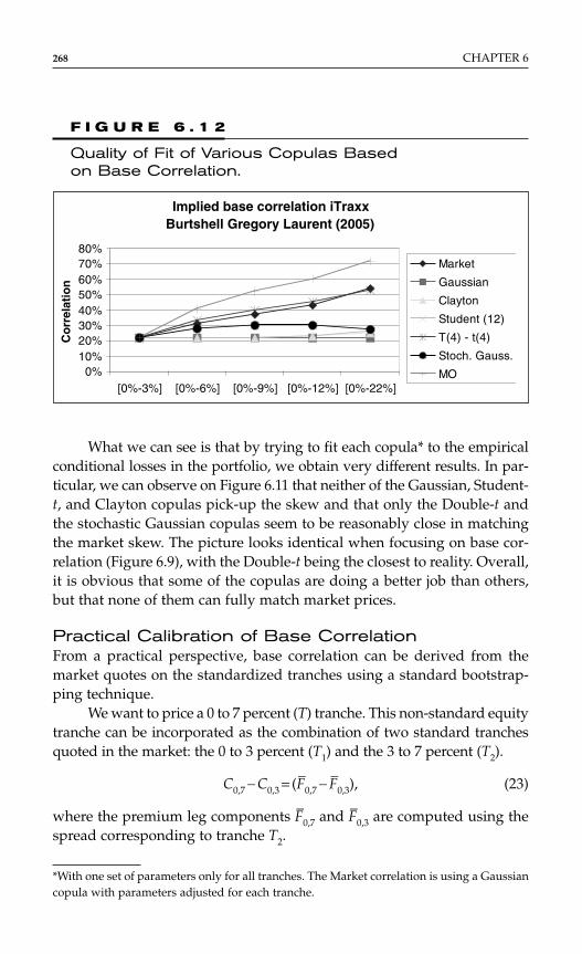
What we can see is that by trying to fit each copula* to the empiricalconditional losses in the portfolio, we obtain very different results. In par-ticular, we can observe on Figure 6.11 that neither of the Gaussian, Student-t, and Clayton copulas pick-up the skew and that only the Double-t andthe stochastic Gaussian copulas seem to be reasonably close in matchingthe market skew. The picture looks identical when focusing on base cor-relation (Figure 6.9), with the Double-t being the closest to reality. Overall,it is obvious that some of the copulas are doing a better job than others,but that none of them can fully match market prices.
Practical Calibration of Base CorrelationFrom a practical perspective, base correlation can be derived from themarket quotes on the standardized tranches using a standard bootstrap-ping technique.
We want to price a 0 to 7 percent (T) tranche. This non-standard equitytranche can be incorporated as the combination of two standard tranchesquoted in the market: the 0 to 3 percent (T1) and the 3 to 7 percent (T2).
C0,7 − C0,3 = (F–0,7 − F–0,3), (23)
where the premium leg components F–0,7 and F–0,3 are computed using thespread corresponding to tranche T2.
268 CHAPTER 6
Implied base correlation iTraxxBurtshell Gregory Laurent (2005)
0%10%20%30%40%50%60%70%80%
[0%-3%] [0%-6%] [0%-9%] [0%-12%] [0%-22%]
Co
rrel
atio
n
Market
Gaussian
Clayton
Student (12)
T(4) - t(4)
Stoch. Gauss.
MO
F I G U R E 6 . 1 2
Quality of Fit of Various Copulas Based on Base Correlation.
*With one set of parameters only for all tranches. The Market correlation is using a Gaussiancopula with parameters adjusted for each tranche.

Let us decompose the process in three steps:
Step 1: We price T1 and T2 using the premium/fee (S2) correspon-ding to T2. We in fact only have to price T1, given the fact that theprice of T2 given s2 is zero. The price we compute for T1 uses s2 asthe premium but the T1 base correlation. It will always be positive,given the fact that the more senior the tranche, the lower the price.We can price tranche T1 using s2 = s3,7
(24)
(25)
PT1= C0,3 − F–0,3
Step 2: All what we need is to price T, given the knowledge of T1computed in step 1. A rescaling operation has to take place atthis stage, given the respective notional width of the two tranchesT1 and T2:
PT = PT1[(A3 − A0)/(A7 − A0)] (26)
Step 3: Once the value of tranche T is computed, the 0 to 7 percentbase correlation can be inferred using the Gaussian copulaapproach.
ρ0, 7 = Arg(PT = C0, 7 − F–0, 7) (27)
With
Pain et al. (2005) suggest that the estimation of base correla-tions can be further refined by the use of quotes at different
C D k EL k EL k
F s A A EL k D k
k
K
k
K
0 71
0 7 0 7
0 7 3 71
7 0 0 7
0 7 0 7
0 7
1, , ,
, , ,
( )[ ( ) ( )]
[( ) ( )] ( )
, ,
,
= + −
= − −
=
=
∑
∑
ρ ρ
ρ
F s A A EL k D k
k
K
0 3 3 7 3 0 0 31
0 3
, , ,[( ) ( )] ( ),= − −=
∑ ρ
C D k EL k EL k
k
K
0 3 0 3 0 31
0 3 0 31, , ,( )[ ( ) ( )], ,= + −=
∑ ρ ρ
Collateral Debt Obligation Pricing 269

horizons, typically 5, 7, and 10 years, hence moving from asingle correlation term over the pricing period towards a termstructure of correlations.
Massaging the Correlation Skew: Towards a Term Structure of Base CorrelationsMany people have pointed out that the Gaussian copula model is not adynamic model in the sense that spreads and correlation levels do notevolve through time. In addition it can be observed in the market that cor-relation is maturity dependent. This explains the attempt to build a more-time-dependent term structure of correlation. The principle of this morerefined calibration is that the pricing of CDO tranches at different hori-zons gives some information about the dynamics of the expected loss overtime, i.e., about the timing of defaults.
So far we have considered a unique premium payment date K, usu-ally based on quarterly instalment over 5, 7, or 10 years and we havederived a unique base correlation over the life of the instrument. What wecan do is to compute the term structure of base correlation over 10 years asa three-step process. We consider that from years zero to five we can relyon the price of the five-year tranche, from years five to seven we rely onthe zero to five base correlation and on the price of the seven-year tranche,from years 7 to 10 we rely on the zero to five base correlation, on the fiveto seven adjusted base correlation, and on the price of the 10-year tranche.
Step 1: computing the five-year base correlationWe can rewrite the base correlation formula for a five-year tranche:
ρ50, 7 = Arg(PT = C5
0, 7 − F–50, 7) (28)
With
Step 2: computing the base correlation between years five andseven
C D k EL k EL k
F s A A EL k D k
k
K
k
K
0 75
10 7
0 70 7
0 7
0 75
3 75
17 0 0 7
0 7
55 5
55
1, ,,
,,
, , ,,
( )[ ( ) ( )]
[( ) ( )] ( )
= + −
= − −
=
=
∑
∑
ρ ρ
ρ
270 CHAPTER 6

ρ5/70, 7 = Arg(PT = C7
0, 7 − F–70, 7) (29)
With
A more refined way to compute the base correlation between yearfive and year seven suggested by Pain et al. (2005) is to consider an interpolation, for instance, linear, for all the intermediary timesteps.Step 3: computing the base correlation between years 7 and 10.
The process is following the approach outlined in step 2.
Discussion on Implied CorrelationThe CDO business had initially emerged as an illiquid activity helping inparticular financial institutions to hedge their portfolio from a perspectiveof credit and default risk.
Little attention was paid at the time to the evolution of the price of aCDO tranche with respect to the movement of the credit spreads in theunderlying pool. Factor models, whether they translate into a Gaussiancopula or any more refined approach, provided results in terms of correla-tion or price without really integrating the dynamics of spread move-ments. The Gaussian copula model with the large portfolio approximationshould be seen as the most extreme case of poor integration of the sensi-tivity to the dynamics of spreads.
With active trading on secondary markets, the focus has now changeddramatically towards an integration of market risk. Banks and investors are
C D k EL k EL k
D k EL k EL k
F s A A EL
k
K
k K
K
k
K
0 77
0 71
0 7
10 7 0 7
0 77
3 77
7 01
0 755
0 75
5
70 75 7
0 75 7
5
1
1
, , ,
, ,
, ,
( )[ ( ) [ ( )]
( )[ ( ) ( )]
[( )
, ,
,/
,/
= + −
+ + −
= − −
=
= +
=
∑
∑
∑
ρ ρ
ρ ρ
00 7
71
0 0 7
0 75
5
70 75 7
,
,
,
,/
( )] ( )
[( ) ( )] ( )
ρ
ρ
k D k
A A EL k D kk K
K
+ − −
= +∑
Collateral Debt Obligation Pricing 271

increasingly exposed to market risk in a way that is difficult to hedge. Theyare left with the traditional hedging techniques based on what is commonlycalled the “greeks,”* with the losses it may lead to when market shocks surge(see Chapter 8) translating into P&L damaging spread widening and conta-gion. Due to this problem, implied correlation, unlike implied equity volatil-ity, looks like a poor instrument to work with. It offers limited security withexisting instruments and is not the relevant parameter in order to price morecomplex instruments, such as options on tranches, or forward-starting CDOsthat depend on the dynamics of the loss distributions of the CDO pool.
Currently, we observe a shift in the market, with banks keepingcorrelation as a pricing tool mainly for spot transactions and possiblygradually moving to a more robust framework for both, hedging andnew CDO-related instruments. In this respect, two interesting theoreti-cal papers have emerged in the second half of 2005: Sidenius et al.(2005) and Schönbucher (2005) suggesting the adoption of the wholeloss distribution of the CDO portfolio and its dynamics as the underly-ing process to price CDO-based instruments. In what follows, wedescribe the methodology related to this change of paradigm anddiscuss related implications.
Dynamic Portfolio Loss Modeling
The idea behind this approach is to model the dynamics of portfolio lossesdirectly and ensure an initial calibration to tranche prices for differentseniorities and maturities (i.e., a calibration to a curve of tranche spreads).This is different to the Gaussian copula approach that focuses on correlateddefault times on a name-by-name basis and is not able to integrate the evo-lution of the univariate and multivariate parameters to future time underchanging market conditions. Essentially, this is a result the static creditspread curve and constant correlation setup that is usually assumed. Here,we focus on a more macroscopic approach by specifying the dynamics ofportfolio losses directly, motivated by the need to value advanced (hybrid)derivatives written on CDO tranches (e.g., options on tranches).
The SPA (Sidenius, Piterbarg, and Andersen) ModelThe idea of Sidenius et al. (2005) is to consider the portfolio loss distribu-tion corresponding to the underlying pool as the relevant variable. This
272 CHAPTER 6
*Typically, “delta hedging,” see Chapter 7 for a detailed introduction.
variable is considered in a dynamic way. The authors use a classical mod-eling technique that consists of splitting the modeling effort in two steps:the first one corresponding to the modeling of a diffusion process for the“smooth” portfolio loss probabilities (or forward rates), whereas the sec-ond focuses on the actual loss process consistent with, or conditional on,the loss probability or forward process.
In the first step, the authors define the variable they want to modelas a diffusion. For any given level of loss considered in the portfolio ini-tially, they consider the term structure of forward portfolio losses, in ananalogy with the Heath, Jarrow, and Morton (HJM) approach for interestrates. The dynamics of the initial portfolio loss distribution can be inferredfrom the aggregation of the dynamics of the probability of portfolio losses*considered for any initial level of portfolio loss. The level of loss isassumed to remain stable over time in each forward process. From a tech-nical perspective, as this first layer of modeling does not include any infor-mation about the dynamics of losses in the portfolio, they say that it isrelated to the “background filtration.”
In a second step, the authors focus more precisely on the dynamics ofdefaults in the pool, thanks to a second layer of modeling based on properinformation on default (i.e., under the loss filtration). The typical model con-sidered is a one-step Markov chain. Transition probabilities are definedexclusively from the knowledge of the background forward loss rate at thattime. Forward loss rates can in fact be seen as a way to describe the state ofthe market. In other words, the dynamics of losses in the portfolio at anytime t will only depend on the situation in the market at that time, hence theview that we now have a much more dynamic set-up to assess CDO prices.
Portfolio Loss Probabilities and Forward DynamicsIn step 1, let us define first the loss probability
px(t, T ) = P(τx > T Mt) = P[l(T) ≤ x Mt],
where l(t) denotes the (nondecreasing) loss fraction at time t, and P is amartingale that corresponds to the risk-neutral measure with respect to thebackground filtration Mt, x [0, 1] is a possible loss level in the portfolioand τx the corresponding stopping time. T corresponds to the horizon.
We can think of this stopping time as the first jump of a Cox processwith intensity λx(t), and we can write the loss probability as:
Collateral Debt Obligation Pricing 273
*Or from the forward loss rates defined from the probability of portfolio losses.
By defining the compounded forward rates as:
(30)
we can express the loss probability as:
with fx (t, t) = λx (t) (31)Given the fact that px (., T) is a martingale, and that we consider a
diffusion process, we can write the process of the portfolio loss as:
dpx(t, T )/px(t, T ) = Σx(t, T ) dWx(t), (32)
where Σx(t, T) denotes a general stochastic process (in t) indexed by x, andT, and Wx(t) is a Brownian Motion for each loss level x.
SPA outline a number of conditions a general loss process has to sat-isfy. For example, the probability of losses should be decreasing in matu-rity, and increasing in loss fraction, i.e., P[l(T) ≤ x] ≤ P[l(T) ≤ y], for all x ≤ y.Essentially, this means that the probability of portfolio losses being lowerthan x has to be lower than the probability of losses being lower than y, andis denoted as “spatial order preservation” condition. Instead of workingwith portfolio loss probabilities, the first condition can be easily satisfiedin terms of the forward loss rates, i.e., fx (t, T) ≥ 0. These forward loss ratesfx (t, T) can naturally be derived from Equation (32) using the Ito’s lemma.
Given this framework, SPA derive conditions for the dynamics ofthe processes to satisfy the necessary conditions (e.g., spatial ordering)under a dynamic loss probability, or instantaneous forward rate (HJM), orforward Libor (BGM) modeling framework. The advantage of the fullmodeling of a forward curve for each loss level (as in the HJM or BGMsetup) is that it is very flexible and able to capture the full loss curvedynamics, whereas the “short-rate” loss probability modeling is lessflexible but needs to propagate fewer variables.
p t T f u u u f t u ux x
t
xt
T( , ) exp ( , )d exp ( , )d= −
−
∫ ∫0
f t TT p t T
p t Txx
x
( , )( / ) ( , )
( , ),= −
∂ ∂
p t T E s s M s s
E s s M
x x
T
t x
t
xt
T
t
( , ) exp ( )d | exp ( )d
exp ( )d |
= −
= −
× −
∫ ∫
∫
λ λ
λ
0 0
274 CHAPTER 6
Practically, this still means that in a portfolio of say 125 names likean index and assuming, homogenous recoveries across all names, wewould need to calibrate up to 125 such diffusion processes for the lossprobabilities in order to characterize all the realizations of x and be able toobtain the dynamics of the entire loss distribution. If idiosyncratic recov-eries are assumed, the state space of x would further increase, which fur-ther increases the number of processes (and their interaction) to beconsidered. The only way to get there is to restrict the volatility processΣx(t, T) to be a deterministic function of time t and of loss probabilitiespx(t, s), s ≥ t. The SPA provide several examples of such functions, someof which are computationally challenging, while more tractable ones maylead to a violation of some of the conditions discussed beforehand.
Portfolio Loss Process Assuming that the dynamics of theloss probabilities is properly specified under the background filtrationMt, we can move to the second step, i.e., the calibration of the loss pro-cess under a broader filtration Lt, called the loss filtration.
We can now consider the intensity of the jump from the loss level xito the loss level xi + l, conditional on the background filtration Mt as:
Kxi(t, T) dT = P[l(T + dT) = xi + l l(T) = xi, Mt]
or
(33)
The main contribution here is that SPA have constructed a one-stepMarkov chain (“one-step” as it is assumed that losses can take values ona finite grid (0 = x0 < x1 < … < xN) and that loses can actually shift only byone step), i.e., a discrete one-step loss process on xi
Ni = 0 that is consistent
with the loss probability process (32).While the previous derivation is useful when a homogeneous port-
folio (i.e., same recoveries) is considered, for idiosyncratic or stochasticrecoveries, the state space needs to be extended to a much thin discretisa-tion or to a continuous setup x∈[0, 1], respectively.
In a more general setup using Markov processes, we can define ajump survival function: mz, x(t, T ):
mz, x(t, T)dT = P[l(T + dT) > x|l(T) = z, Mt]
K t TT p t T
p t T p t Tx
x
x xi
i
i i
( , )( / ) ( , )
( , ) ( , )=
−∂ ∂
−+1
Collateral Debt Obligation Pricing 275
and write, assuming that l(t) is a nondecreasing pure-jump conditionalMarkov process on [0, 1]:
(34)
It remains to define the actual dynamics of the loss process, giventhe knowledge of px(t, T). This corresponds to the estimation of the jumpsurvival process mz, x (t, T) itself.
In order to be able to estimate the latter process with sparse data, theonly way is to specify more precisely a corresponding parametric func-tion, and SPA motivate functions of the form mz, x (t, T) = θ(T, x − z) ⋅ νx(t, T).Note that for θ(T, y) = 1y ∈[0, 1/N], a single one-step Markov chain is recov-ered. Then, even a more general setup where θ(⋅) is given externally, νx(t, T)can be estimated from Equation (32).
Tranche Valuation Assuming that the loss process is properlycalibrated, we can reconsider the Equations (19) and (21) driving the priceof any tranche j and write it for any starting time anterior to the firstcoupon date as:
Note that EL(k|Lt) satisfies the following form EL(k|Lt) =E[ f(l(k))|Mt, l(t)], and it can be shown that this expectation can be decom-posed into a linear combination of conditional loss probabilities:
py, x(t, k) = P[l(k) ≤ x Mt, l(t) = y] (35)
In other words, px (t, T) provides an average default loss probability,and py, x (t, T), is the loss probability conditional on a particular loss levely at time t.* It can be obtained by solving the following forwardKolmogorov equations in T and in x, with proper initial conditions (seeSPA).
C t D t k EL k L EL k L
F t s A A EL k L D t k
j jk
K
t j t
j j jk
K
j j t
( ) ( , )[ (( )| ) (( )| )]
( ) [( ) (( )| )] ( , )
= + −
= − −
=
+=
∑
∑1
11
1
∂∂
= − ∂∂∫T
p t T m t Tz
p t T zx z x
x
z( , ) ( ( , ) ( , )) d,0
276 CHAPTER 6
*Note that py, x (t, T ) is not observable from the background filtration.
(36)
This model is undoubtedly conceptually very attractive. In termsof tractability and practical implementation, it requires simplifyingassumptions related to the volatility of the loss probability process. Italso requires assumptions on the loss process through a tight character-ization of the Markov chain (or Markov process). In order to be able toapply it for practical pricing purposes, three to four calibrations need tobe undertaken with little data:
1. calibration of the loss probability processes (or?);2. calibration of the compound forward rates;3. calibration of the jump survival functions; and4. calibration of the conditional loss probability processes.
The number of calibration steps involved requires a good understandingof the model behaviour, stability of parameterization and estimation, andthe development of hedging strategies in order to mitigage the possibilityof model risk and over fitting. If these issues can be addressed successfully,and if more market data becomes available, the model is capable of pric-ing options on tranches, forward starting tranches, and tranches withdynamic (loss dependent) attachment points, consistently.
Schönbucher’s ModelSchönbucher’s model does not differ very much from the SPA model. Itdoes not go through a two-step model but models the loss distribution viatime-inhomogeneous Markov chains.
Schönbucher calls P(t, T) the transition probability matrix with adimension corresponding to the number N of obligors in the underlyingpool. P(t, T) can be retrieved from a Kolmogorov equation with appropri-ate initial conditions:
with A(T) being a generator function constituted of N · (N + 1)/2 elementsanm(T).
As with the previous model, the dynamic calibration of the genera-tor function corresponds to the key challenge. Restrictions are required to
dd
( , ) ( , ) ( ),t
P t T P t T A T= ⋅
∂∂
= − ∂∂∫T
p t T m t Tz
p t T zx y z x
x
z y, , ,( , ) ( ( , ) ( , ))d0
Collateral Debt Obligation Pricing 277
be able to come with some tractable results. In our view, the SPA modelmight give more accurate results as it leads to a better understanding of theunderlying processes and consequently perhaps to more realism regardingthe simplifying assumptions required to be able to calibrate the model.
Pricing Based on a Dynamic Modeling of theUnderlying Obligors
Given the tractability problems we think the dynamic loss distributionmodelling approach might encounter, we believe it is important to men-tion alternative dynamic set-ups.
The most noticeable alternative is to simulate directly the dynamicsof each exposure in the CDO pool. Duffie and Garleanu (2001) suggestedto analyze the risk and valuation of CDOs in an intensity model wherethe issuers’ hazard rates are assumed to follow correlated jump diffusionprocesses.
More recent approaches focus on less cumbersome solutions.Instead of describing the survival probability for a given obligor i over[0, t] as Si(t) = exp(−∫t
0 λi(u)du) and of thinking independently of correla-tion, di Graziano and Rogers (2005)* or Joshi and Stacey (2005) suggestto describe the survival probability as Si(t) = exp(−∫t
0 λi( f(u))du). For theformer authors, the intensity is a deterministic function of a time con-tinuous market chain common to all obligors, for the latter f(u) is aGamma process common to all obligors. In the two instances, the ideais to represent the dynamic time as a stochastic variable depending onmarket situations such as the state of the economy. With these spec-ifications, correlation across the survival times of the obligors in thepool is coming naturally from the dependency on the state of thechain or from the calibration of the Gamma process and is not tobe “forced” thanks to the use of a copula or by the calibration of avariance–covariance matrix.
In principle, the calibration of such processes looks reasonablytractable due to the recourse to conditional independence. Speed of com-putational calculation is most likely to be an issue as pointed out in therelevant papers.
278 CHAPTER 6
*These authors suggest to add some jump terms too.
Pricing Bespoke CDO Tranches
Throughout this section, we consider two different types of “bespoke”tranches: first, bespoke tranches on traded indices and bespoke tranchesbased on a bespoke pool.
In the first case, we are typically talking about an investor who isconsidering, for example, a 5 to 8 percent five-year tranche on, say theiTraxx, for which there is no market price. Market practice is to use thelevels of correlation at the bespoke attachment points from the interpo-lated base correlation curve to derive the price of the tranche. Recent prac-tice has been to compute “centi-tranches” (1 percent tranchelets) as abuilding block to the pricing of bespoke tranches.
In the second case, the approach is cruder in the sense that bankstend to use internal recipes in order to get a sense of what the appropriatelevel of “market correlation” should be for the bespoke transaction, givencorrelation trends in the related index-based market.
Prince (2006) provides a review of three different valuation method-ologies used in the industry and suggests to use a blend of them:
♦ Net asset value: The first one is the liquidation value (NAV). Inthis method, the first step is to measure the net market value ofa CDO as the market value of the asset pool plus the value ofthe hedges minus all the liabilities. When the net market value isdivided by the notional amount of the Equity, we have the liqui-dation value of the equity.
♦ Cashflow analysis: This approach is more forward looking, as it isbased on the dynamics of the CDO collateral over time. It is infact very close to what is presented in the following section ofthis chapter when dealing with cash CDOs.
♦ Comparables: This approach typically involves deriving pricesfrom liquid tranches on indices.
PRICING CASH CDOS
In a cash CDO, loans and bonds in the asset pool are usually not tradedactively. Price indications are therefore mainly related to ratings or toprobabilities of default extracted from, e.g., a Merton type model. Theywill incorporate default risk, migration risk, and a component related tosome average risk premium per rating category. However, these fair value
Collateral Debt Obligation Pricing 279

prices cannot integrate idiosyncratic spread movements, as there is nomarket reference on which to rely.
In order to price a cash CDO, three constituents are necessary: a risk-neutral transition matrix, a risk-neutral asset correlation structure, andthe knowledge of the waterfall structure. With these ingredients, it helpsto have a multi-period rating-based portfolio model in order to be able tocapture the dynamics of the waterfall structure that is conditioned by theperformance of the asset pool, on the liability side.
Once these elements are defined, we detail various ways to obtainthe fair value prices of the CDO tranches.
The numerical methodology presented next consists of simulatingrealizations of the value of the collateral pool and calculating the price of theCDO tranches by a technique similar to least square Monte-Carlo approachproposed by Longstaff and Schwartz (2001). The algorithm starts by calcu-lating the payoff of each tranche at the maturity of the CDO and rolls back-wards until the issuance of the notes by estimating the payoff of each trancheconditional on the performance of the pool of assets at each time step.
On the Asset Side
From Historical to Risk-Neutral Transition Matrices*For pricing purposes, one requires “risk-neutral” probabilities. A risk-neutral transition matrix can be extracted from the historical matrix and aset of corporate bond prices.
All q probabilities take the same interpretation as the empirical transitionmatrix below, but are under the risk-neutral measure.
P( )
, , ,
, , ,h
p p p
p p p
h h hK
hK
hK
hK K
=
+
+
1 1 1 2 1 1
1 2 1
0 0 1
K
M M M
K
K
Q( ) ,
, , ,
, , ,h
q q q
q q q
h h hK
hK
hK
hK K
=
+
+
1 1 1 2 1 1
1 2 1
0 0 1
K
M M M
K
K
280 CHAPTER 6
*Some parts of the section are taken from de Servigny and Renault (2004).
Time Nonhomogeneous Markov Chain In the origi-nal Jarrow-Lando-Turnbull (1997) (JLT) paper, the authors impose the fol-lowing specification for the risk premium adjustment, allowing to computerisk-neutral probabilities from historical ones:
(37)
Note that the risk premium adjustments πi(t) are deterministic and do notdepend on the terminal rating but only on the initial one. This assumptionenables JLT to obtain a nonhomogenous Markov chain for the transitionprocess under the risk-neutral measure.
The calculation of risk-neutral matrices on real data can be per-formed as described below. Assuming that the recovery in default is afraction δ of a treasury bond with same maturity, the price of a risky zerocoupon bond at time t with maturity T is
Pi(t, T) = B(t, T) × (1 − qi,K + 1(1 − δ )).
Thus, we have
and thus the one-year risk premium is
(38)
The JLT specification is easy to implement, but often leads to numericalproblems because of the very low probability of default of investmentgrade bonds at short horizons. In order to preclude arbitrage, the risk-neutral probabilities must indeed be non-negative. This constrains therisk premium adjustments to be in the interval:
As noticed above, the historical probability of an AAA bond defaultingover a one-year horizon is zero. Therefore, the risk-neutral probability of
01
1< ≤
−π i i i
tp
i( ) , for all .,
πδi
i
i Kt
B t t P t tB t t q
( )( , ) ( , )( , )( )
.,
=+ − ++ − +
1 11 1 1
qB t T P t T
B t Ti K
i, ( , ) ( , )
( , )( ),+ =
−−
1
1 δ
q t tt p i j
t p i ji j i
i j
ii i
,,
,( , )
( ) for ,
( )( ) for .+ =
≠
− − =
1
1 1
π
π
Collateral Debt Obligation Pricing 281
the same event is also zero.* This would however imply that the spreadson short-dated AAA bond should be zero (why have a spread on defaultrisk-less bonds?). To tackle this numerical problem, JLT assume that thehistorical one-year probability of default for an AAA bond is actually 1basis point. The risk premium for the AAA row adjustment is thereforebounded above. This bound is, as will be shown later, frequently violatedon actual data.
Kijima and Komoribayashi (1998) propose another risk premiumadjustment that guarantees the positivity of the risk-neutral probabilitiesin practical implementations.
πij(t) = li(t) for j ≠ K + 1
(39)
where li(t) are deterministic functions of time. Thanks to this adjustment,“negative prices” can be avoided.
Time-Homogeneous Markov Chain Unlike the prece-dent authors, Lamb et al. (2005) propose to compute a time-homogeneousMarkovian risk-adjusted transition matrix. They rely on bond spreads,thanks to the term structure of spreads per rating category.
exp(−Si(t)) = (δ ⋅qK + 1i (t)) + (1 − qK + 1
i (t)). (40)
where t corresponds to integer-year maturities.In order to obtain the matrix, they minimize†
(41)
Knowing that qK + 1i (t) is a function of the qj
i (⋅)A minor weakness of this approach is that it does not ensure that
spreads are matching market prices for all maturities.
Min [ ( ) ( ( )) ( ( ))]( )q t
ii
K
t
n
iK
iK
ij
S t q t q t==
+ +∑∑ − ⋅ + −11
1 1 21δ
q t tl t p i K
l t p i Ki j i
i j
ii i
,,
,( , )
( ) for ,
( )( ) for .+ =
≠ +
− − = +
1
1
1 1 1
282 CHAPTER 6
*Recall that two equivalent probability measures share the same null sets.†Attaching penalties if entries in the transition matrix become negative in the course of theminimization.
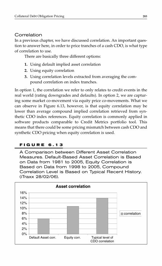
CorrelationIn a previous chapter, we have discussed correlation. An important ques-tion to answer here, in order to price tranches of a cash CDO, is what typeof correlation to use.
There are basically three different options:
1. Using default implied asset correlation2. Using equity correlation3. Using correlation levels extracted from averaging the com-
pound correlation on index tranches.
In option 1, the correlation we refer to only relates to credit events in thereal world (rating downgrades and defaults). In option 2, we are captur-ing some market co-movement via equity price co-movements. What wecan observe in Figure 6.13, however, is that equity correlation may belower than average compound implied correlation retrieved from syn-thetic CDO index references. Equity correlation is commonly applied insoftware products comparable to Credit Metrics portfolio tool. Thismeans that there could be some pricing mismatch between cash CDO andsynthetic CDO pricing when equity correlation is used.
Collateral Debt Obligation Pricing 283
Asset correlation
0%2%4%6%8%
10%12%14%16%
Default Asset corr. Equity corr. Typical level ofCDO correlation
correlation
F I G U R E 6 . 1 3
A Comparison between Different Asset CorrelationMeasures. Default-Based Asset Correlation is Basedon Data from 1981 to 2005, Equity Correlation isBased on Data from 1998 to 2005, CompoundCorrelation Level is Based on Typical Recent History.(iTraxx 28/02/06).
A related point to mention is that CPM* teams in commercial bankstend to rely primarily on models based on equity correlation, while thereference in the CDO market† may be closer to compound correlation lev-els. As a consequence, offloading exposures from the balance sheet ofbanks may turn out to be a costly exercise if the market grants less bene-fit to diversification than banks expect. The interest of obtaining a rating,from the perspective of a bank, is to counterbalance this mismatch withinvestors. Rating agencies, by using models that rely on default-basedasset correlation, typically grant a higher benefit of diversification tooffloaded tranches compared to the underlying assets staying on the port-folio of the bank. This situation, while it gives confidence to investorswith respect to the risk/return of their structured investment, creates suf-ficient excess spread to facilitate disintermediation.
In what follows, we show how, in a portfolio model, correlationimpacts the migration process. As we are considering a ratings-basedmodel, the primary purpose of the simulation engine is precisely to gen-erate migration events with the appropriate correlation structure.
Figure 6.14 illustrates the impact of asset correlations on the jointmigration of obligors, assuming that there are two nondefault states(investment grade IG and noninvestment grade NIG) and an absorbingdefault state D.
The experiment uses a one-factor model. Similar results would beobtained in the multifactor setup. The tables are bivariate transition matri-ces for various levels of asset correlation under the assumption of joint nor-mality of assets returns and using aggregate probabilities of transitionextracted from CreditPro®.‡ In order to reduce the size of the tables, wehave assumed that the pair IG/NIG is identical from a portfolio point ofview to the pair NIG/IG. Thus, each bivariate matrix is 6 × 6 instead of 9 × 9.
Taking, e.g., the case of two noninvestment grade obligors (rowNIG/NIG) one can observe that, as the correlation increases, the jointdefault probability (as well as the joint probability of upgrades) increasessignificantly.
Multivariate transition probabilities cannot be computed for portfo-lios with reasonable numbers of lines. In a standard rating system witheight categories, a portfolio with N counterparts would imply an 8N × 8N
transition matrix that soon becomes intractable.
284 CHAPTER 6
*Credit Portfolio Management.†For instance, when investors try to assess the fair value of their investment on the basis ofcorrelation trading-based prices.‡A database from Standard & Poor’s Risk Solutions.
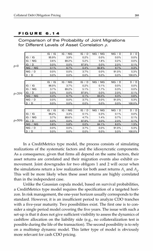
In a CreditMetrics type model, the process consists of simulatingrealizations of the systematic factors and the idiosyncratic components.As a consequence, given that firms all depend on the same factors, theirasset returns are correlated and their migration events also exhibit co-movement. Joint downgrades for two obligors 1 and 2 will occur whenthe simulations return a low realization for both asset returns A1 and A2.This will be more likely when these asset returns are highly correlatedthan in the independent case.
Unlike the Gaussian copula model, based on survival probabilities,a CreditMetrics type model requires the specification of a targeted hori-zon. In risk management, the one-year horizon usually corresponds to thestandard. However, it is an insufficient period to analyze CDO trancheswith a five-year maturity. Two possibilities exist. The first one is to con-sider a single period model covering the five years. The issue with such aset-up is that it does not give sufficient visibility to assess the dynamics ofcashflow allocation on the liability side (e.g., no collateralization test ispossible during the life of the transaction). The second possibility is to relyon a multistep dynamic model. This latter type of model is obviouslymore relevant for cash CDO pricing.
Collateral Debt Obligation Pricing 285
95.9% 3.9% 0.2% 0.0% 0.0% 0.0%
0.0%
0.0%0.0%0.0%
0.0%
IG / IG IG / NIG NIG / NIG NIG / DIG / D
3.6% 89.2% 5.2% 1.8% 0.2%
0.0% 0.0% 97.9% 0.0% 2.0% 0.1%
96.2% 3.3% 0.1% 0.3% 0.1%
0.1%
0.0% 0.0% 97.9% 0.0% 2.0% 0.1%
0.3%0.1% 6.7% 0.4% 82.8% 9.7%
5.3%0.0% 0.0% 3.7% 0.0% 91.0%
5.3%0.0% 0.0% 3.7% 0.0% 91.0%
5.3%0.0% 0.0% 3.7% 0.0% 91.0%
100.0%0.0% 0.0% 0.0% 0.0% 0.0%
100.0%0.0% 0.0% 0.0% 0.0% 0.0%
D / D
IG / IG IG / NIG NIG / NIG NIG / DIG / D D / D
IG / IGIG / NIG
NIG / NIG
NIG / D
IG / D
D / D
IG / IGIG / NIG
NIG / NIG
NIG / D
IG / D
D / D
IG / IG IG / NIG NIG / NIG NIG / DIG / D D / DIG / IGIG / NIG
NIG / NIG
NIG / D
IG / D
D / D
96.0% 3.7% 0.2%
0.0% 0.0% 97.9% 0.0% 2.0% 0.1%
0.0%
0.8% 5.8% 0.0% 84.1% 8.0% 1.3%
0.0% 0.0% 0.0% 0.0% 100.0%
3.7% 89.2% 5.1% 1.7% 0.3%
0.3% 6.7% 0.1% 83.0% 9.3% 0.6%
3.7% 89.6% 4.7% 1.4% 0.7% 0.1%
ρ=0
ρ=20%
ρ=50%
F I G U R E 6 . 1 4
Comparison of the Probability of Joint Migrationsfor Different Levels of Asset Correlation ρ.
However, one aspect related to multiple time-step models needs tobe highlighted. A multi-period model with independence between theperiods and a correlation level of ρ at each period will undershoot the cor-responding single period model with a similar correlation level ρ. The dif-ference can be explained intuitively, as in the case of a single periodmodel, some autocorrelation prevails, whereas in a multi-period model,the assumption of independence between periods, there is essentially cor-responds to no autocorrelation.
Computing the Price of Each Line in the PortfolioDepending on its RatingIn the previous paragraph, we have intuitively described how aCreditMetrics type model simulates all the ratings up to the horizon of inter-est t for any of the obligors in the portfolio.* The next step is to calculate theprofits or losses arising from these risk-neutral migrations including defaults.
For “surviving” obligors, the value of the assets at time t is calcu-lated using the risk free rate as observed at the time of calculation.
Let us consider a defaultable fixed rate bond with j∈1, . . . , Ncoupons c beyond the horizon t and with principal P. Its rating at the sim-ulation horizon is i, its price Vi(t), the spread level defined in Equation(40) from the risk neutral transition matrices is Si( j), and the forward riskfree interest rate corresponding to the period [t; t + j] is rt, t + j .
(42)
The Monte Carlo simulation of the common and the idiosyncratic factorsto which the latent variable (the asset value) of each exposure in the port-folio is tied enables us to draw many realizations of rating paths for eachobligor at each future sub-period before the horizon. It ultimately allowsus to price each of the exposures based on Equation (42).
On the Liability Side
A Brief Description of the Waterfall StructureIn this section, we describe briefly how the cashflows generated on the assetside are distributed on the liability side, thereby influencing the pricing of
V t r j S j P r N S Nij
N
t t j i t t N i( ) exp[ ( ( ))] exp[ ( ( ))], ,= − + + ⋅ − +=
+ +∑1
286 CHAPTER 6
*For a more refined description, see Chapter 4.
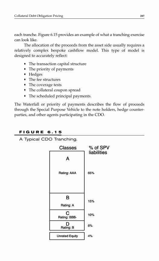
each tranche. Figure 6.15 provides an example of what a tranching exercisecan look like.
The allocation of the proceeds from the asset side usually requires arelatively complex bespoke cashflow model. This type of model isdesigned to accurately reflect:
♦ The transaction capital structure♦ The priority of payments♦ Hedges♦ The fee structures♦ The coverage tests♦ The collateral coupon spread♦ The scheduled principal payments.
The Waterfall or priority of payments describes the flow of proceedsthrough the Special Purpose Vehicle to the note holders, hedge counter-parties, and other agents participating in the CDO.
Collateral Debt Obligation Pricing 287
Classes % of SPVliabilities
A
Unrated Equity
D
C
B
Rating: B
Rating: BBB-
Rating: A
Rating: AAA
4%
6%
10%
15%
65%
Classes % of SPVliabilities
A
Unrated Equity
D
C
B
Rating: B
Rating: BBB-
Rating: A
Rating: AAA
4%
6%
10%
15%
65%
F I G U R E 6 . 1 5
A Typical CDO Tranching.

♦ Money flows into the CDO as asset interest proceeds and principalamortizations and hedge receipts.
♦ Money flows out of the CDO as fees, expenses, hedge paymentsand interests, and principal payments to the rated notes andpreferred shares.
Coverage tests are ratios calculated in a CDO structure that alter the dis-tribution priority of collateral proceeds by delevering the notes when therequired ratio level is breached. There are two main tests:
♦ The over collateralization (OC) test. It is a ratio that tests theability of the collateral balance (net of defaults and recoveries) tosupport the current liability balance (including deferred intereston the notes).
♦ The interest coverage (IC) test. It is a ratio that tests the ability ofthe collateral interest proceeds to support the current liabilityinterest payouts (i.e., tests excess spread).
The dynamics of the waterfall structure is described in Figure 6.16 in ageneric manner.
Impact on the Pricing of CDO TranchesThe payoff of a structured exposure depends in a complex way on thecashflows generated by the exposures on the asset side as well as on theway these cashflows are allocated to the tranches on the liability side,given the waterfall structure of the deal.
In practice, there are as many pricing models as there are differentstructures. Due to the Monte-Carlo approach, computational times areusually substantial.
Lamb et al. (2005) suggest an interesting shortcut consisting of theestimation of a pricing function by applying scoring techniques. More pre-cisely, they show that it is possible to fit a regression-type function for eachtranche that will give a price at the maturity of the CDO as a function ofthe realization of the vector of latent variables corresponding to the oblig-ors in the CDO pool. As a result, any price of a tranche before maturity ofthe pool is easily obtainable by proper discounting. In terms of speed ofcalculation, the pricing functions for each deal typically require less than10,000 Monte Carlo replications to provide accurate results. The tests per-formed by Lamb et al. (2005) show that this class of model performs wellin terms of first moments, Value at Risk and Expected Shortfall. In terms ofhedging, this model provides interesting and accurate strategies.
288 CHAPTER 6
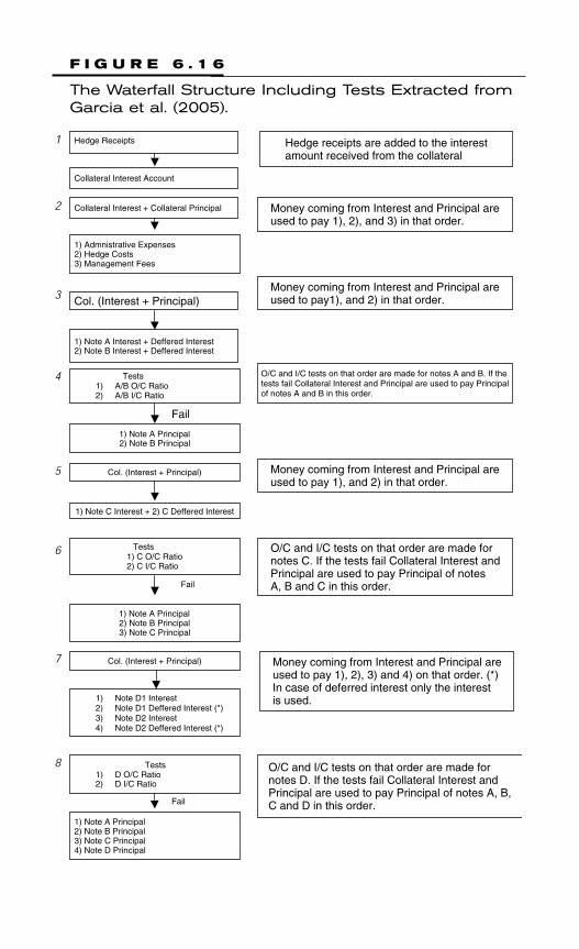
Hedge Receipts
Collateral Interest Account
1
Col. (Interest + Principal)
1) Note A Interest + Deffered Interest2) Note B Interest + Deffered Interest
3
Tests1) A/B O/C Ratio2) A/B I/C Ratio
1) Note A Principal2) Note B Principal
Fail
4
Col. (Interest + Principal)
1) Note C Interest + 2) C Deffered Interest
5
Tests1) C O/C Ratio2) C I/C Ratio
1) Note A Principal2) Note B Principal3) Note C Principal
Fail
6
Col. (Interest + Principal)
1) Note D1 Interest2) Note D1 Deffered Interest (*)3) Note D2 Interest4) Note D2 Deffered Interest (*)
7
Tests1) D O/C Ratio2) D I/C Ratio
1) Note A Principal2) Note B Principal3) Note C Principal4) Note D Principal
Fail
8
1) Admnistrative Expenses2) Hedge Costs3) Management Fees
Hedge receipts are added to the interestamount received from the collateral
Money coming from Interest and Principal areused to pay1), and 2) in that order.
O/C and I/C tests on that order are made for notes A and B. If thetests fail Collateral Interest and Principal are used to pay Principalof notes A and B in this order.
Money coming from Interest and Principal areused to pay 1), and 2) in that order.
O/C and I/C tests on that order are made fornotes C. If the tests fail Collateral Interest andPrincipal are used to pay Principal of notesA, B and C in this order.
Money coming from Interest and Principal areused to pay 1), 2), 3) and 4) on that order. (*)In case of deferred interest only the interestis used.
O/C and I/C tests on that order are made fornotes D. If the tests fail Collateral Interest andPrincipal are used to pay Principal of notes A, B,C and D in this order.
Money coming from Interest and Principal areused to pay 1), 2), and 3) in that order.
2 Collateral Interest + Collateral Principal
F I G U R E 6 . 1 6
The Waterfall Structure Including Tests Extracted fromGarcia et al. (2005).

CONCLUSION
In this chapter, we have tried to provide some insight into the most promi-nent pricing techniques used in the synthetic and cash CDO markets. It isvery difficult to offer a full coverage given the amount of academic as wellas applied research that is continuously generated in this area.
The driving force in the efforts that we have reported is focused ongenerating accurate results while using data in a parsimonious way. We cansee that the most recent techniques tend to be less parsimonious though.One question we might ask ourselves is: what is the appropriate minimumlevel of information (factors, and parameters) that is required to match mar-ket prices? In this respect, Longstaff and Rajan (2006) suggest that singlefactor models are too simplistic to price CDO tranches accurately. Theyadvocate that the ideal number of common factors to consider should be 2in order to allow for firm specific, industry, and economy-wide events to be
290 CHAPTER 6
Col. Principal
1) Note A Principal2) Note B Principal3) Note C Principal4) Note D Principal
After reinvestment period Money coming fromPrincipal is used to redeem (pay principal) thenotes from 1) to 4) in that order.
9b
Col Interest
1) Note E Interest2) Note E Interest Deferred
Money coming from Interest and Principal areused to pay 1), 2) on that order.
10
Excess Interest
Note E Interest
Excess interest is given to the Equity holders.11
Col. Principal
Note E Principal
Money coming from principal is paid to the equity holders.12
Col. Principal
Reinvest in new collateral
Before the end of the reinvestment periodmoney coming from Principal is used toreinvest in new collateral followingcertain guidelines.
9a
F I G U R E 6 . 1 6 ( C o n t i n u e d )
explained. On the basis of this specification, they are able to identify threeloss regimes on the CDX index. These regimes correspond to 0.4 percent, 6percent, and 35 percent loss levels and take place respectively every 1.2,41.5, and 763 years on average. The first firm-specific regime typically dom-inates 65 percent of the time, the second industry-specific regime is at play27 percent of the time and the third regime, corresponding to catastrophicrisk, accounts for the remaining 8 percent. The authors may not have a suf-ficiently large data sample yet to be too assertive on these results, with onlytwo years of daily observations of the CDX index. There is, however, cer-tainly an interesting aspect to these first statistical results.
REFERENCESAndersen, L. (2005), “Base correlation, Models and Musings,” in PPT presenta-
tion ICBI Credit Derivative Conference, Paris.Andersen, L., and J. Sidenius (2005), “Extensions to the Gaussian copula:
Random recovery and random factor loadings,” Journal of Credit Risk, 1(1).Andersen, L., J. Sidenius, and S. Basu (2003), “All your Hedges in One Basket,”
Risk, November, 67–72.Black, F., and M. Scholes (1973), “The pricing of options and corporate liabilities,”
Journal of Political Economy, 81, 637–654.Burtschell, X., J. Gregory, and J. P. Laurent (2005), “A comparative analysis of
CDO pricing models,” working paper.Debuysscher, A., and M. Szego (2005), “Fourier Transform Techniques applied to
Structured Finance,” PPT presentation Moody’s.de Servigny, A., and O. Renault (2004) “Measuring and Managing Credit Risk,”
McGraw Hill book.di Graziano, G., and L. C. G. Rogers (2005), “A new approach to the modelling
and pricing of correlation credit derivatives,” working paper StatisticalLaboratory, University of Cambridge.
Duffie, D., and K. J. Singleton (1998), “Modeling the term structures of default-able bonds,” Review of Financial Studies, 12, 687–720.
Duffie, D., and N. Gârleanu (2001), “Risk and the valuation of collateralized debtObligations,” Financial Analysts Journal, 57, 41–59.
Elouerkhaoui, Y. (2003a), “Credit risk: Correlation with a difference,” workingpaper, UBS Warburg.
Elouerkhaoui, Y. (2003b), “Credit Derivatives: Basket asymptotics,” workingpaper, UBS Warburg.
Finger, C. C. (2005), “Issues in the pricing of synthetic CDOs,” Journal of CreditRisk, 1(1).
Frey, R., and A. McNeil (2003). “Dependent defaults in models of portfolio creditrisk,” Journal of Risk, 6(1), 59–92.
Garcia, J., T. Dewyspelaere, R. Langendries, L. Leonard, and T. Van Gestel (2005),“On rating cash flow CDO’s using BET technique,” Dexia working paper.
Collateral Debt Obligation Pricing 291

Gibson, M. (2004), “Understanding the risk of synthetic CDOs,” working paperFED.
Giesecke, K. (2003), “A simple exponential model for dependent defaults,”Journal of Fixed Income, December, 74–83.
Gregory, J., and J.-P. Laurent (2003), “I Will Survive,” Risk, June, 103–107.Hull, J., and A. White (2003), “Valuation of a CDO and an nth to default CDS
without Monte Carlo simulation,” working paper J. L. Rotman School ofManagement, University of Toronto.
Hull, J., and A. White (2004), “Valuation of a CDO and an nth to default CDSwithout Monte Carlo simulation,” Journal of Derivatives, 2, 8–23.
Hull, J., and A. White (2005), “The perfect copula,” working paper J. L. RotmanSchool of Management, University of Toronto.
Jarrow, R. A., D. Lando, and S. M. Turnbull (1997), “A Markov model for the termstructure of credit risk spreads,” The Review of Financial Studies, 10, n. 2,481–523.
Joshi, M., and A. Stacey (2005), “Intensity gamma: a new approach to pricing.portfolio credit derivatives,” working paper.
Kalemanova, A., B. Schmid, and R. Werner (2005), “The normal inverse Gaussiandistribution for synthetic CDO,” working paper.
Kijima, M., and K. Komoribayashi (1998), “A Markov Chain Model for ValuingCredit Risk Derivatives,” Journal of Derivatives, Fall, 97–108.
Lamb, R., V. Peretyatkin, and W. Perraudin (2005), “Hedging and asset allocationfor structured products,” working paper Imperial College.
Li, D. (2000), “On default correlation: a Copula approach,” Journal of Fixed Income,9, 43–54.
Lindskog, F., and A. McNeil (2003), “Common poisson shock models: Applicationsto insurance and credit risk modelling,” ASTIN Bulletin, 33(2), 209–238.
Longstaff, F., and A. Rajan (2006), “An empirical analysis of the pricing of collat-eralized debt obligations,” working paper.
Longstaff, F., and E. Schwartz (2001), “Valuing American options by simulation:a simple least-squares approach,” Review of Financial Studies, 14(1), 113–147.
McGinty, L., E. Bernstein, R. Ahluwalia, and M. Watts (2004), “Introducing BaseCorrelations,” JP Morgan.
O’Kane, D., and L. Schloegl (2001), “Modeling Credit: Theory and Practice,”Lehman Brothers International.
Pain, A., O. Renault, and D. Shelton (2005), “Base correlation, The term structuredimension,” Fixed Income Strategy and Analysis paper Citigroup, 09-12-05.
Prince, J. (2006), “A general review of CDO valuation methods,” Global StructuredCredit Strayegy paper Citigroup, 15-02-06.
Rott, M. G., and C. P. Fries (2005), “Fast and robust Monte Carlo CDO sensitivi-ties,” working paper.
Schönbucher, P., and D. Schubert (2001), “Copula dependent default risk inintensity models,” working paper, Bonn University.
Schönbucher, P. J. (2005), “Portfolio losses and the term structure od loss transi-tion rates: a new methodology for the pricing of portfolio credit deriva-tives,” Working Paper.
292 CHAPTER 6

Shelton, D. (2004), “Back to Normal,” Global Structured Credit Research, 20-08-04.Sidenius, J., V. Piterbarg, and L. Andersen (2005), “A new framework for dynamic
portfolio loss modelling,” Working Paper.St Pierre, M., E. Rousseau, J. Zavattero, and O. van Eyseren (2004), “Valuing and
hedging synthetic CDO tranches using base correlations”—Bear StearnsCredit Derivatives.
Vasicek (1987), “Probability of loss on loan portfolio,” working paper, KMVCorporation.
Vasicek, O.A. (1997), “An equilibrium characterization of the term structure,” Journalof Financial Economics, 5, 1997–288.
Collateral Debt Obligation Pricing 293

This page intentionally left blank
C H A P T E R 7
An Introduction to theRisk Management ofCollateral Debt Obligations
Norbert Jobst
295
INTRODUCTION
In recent years, the market for collateral debt obligations (CDOs) and,in particular, the development of the synthetic CDO market and corre-lation trading has resulted in significant developments in valuation andrisk management for such products. The market has been dominated bydevelopments around the static Gaussian copula model, the introduc-tion of base correlation as an alternative to the compound correlation,and extensions to better capture the observed correlation smile/skew,only recently more dynamic models that incorporate credit spreads—orother major modeling parameters—have been introduced by practition-ers and academics (see Chapter 6). All valuation approaches are based onrisk-neutral pricing principles and little focus has been given toreplication-based arguments that would also lead to developments forpractical hedging and risk management. Currently, risk managementoften focuses on static risk measures that address the likelihood ofa CDO investor receiving full notional and actual interest in a timelymanner (ratings perspective), or on mark-to-market (MtM) sensitivitiesand “the greeks” frequently employed by correlation investors andtraders.
This chapter focuses on a MtM-based risk assessment. A brief andconcise overview of static risk measures frequently employed by rating
Copyright © 2007 by The McGraw-Hill Companies. Click here for terms of use.
agencies or “buy-and-hold” investors is given in the next section. Thischapter is complemented by Chapter 8, where many of the theoreticalconcepts introduced here are put into practice. Hence, whereas thefocus in this chapter is on introducing “the greeks” conceptually andproviding guidelines for practical implementation, the next chapterprovides a critical discussion based on a number of popular syntheticCDO trading strategies. As with the chapter on valuation, many deri-vations evolve around the Gaussian copula model, and we provideimplementation details on simulation-based and semianalyticaltechniques.
RISK MEASUREMENT I: A CREDIT RISK AND RATINGS PERSPECTIVE
Rating agencies (RAs), such as Standard & Poor’s, Moody’s, Fitch, orDRBS, are typically interested in the risk a CDO investor is facing, andbase their opinions partly on model-based statistics. For example, Moody’srating is a so-called “expected loss” rating and, as a result, the expectedloss on a CDO tranche is assessed and benchmarked to various rating-specific targets. Standard & Poor’s, on the other hand, applies a “probabil-ity of default” (PD) or “first dollar of loss” rating and estimates thelikelihood of an investor facing any loss at all.
Underlying such approaches is an assessment, in one form oranother, of the (likelihood of ) losses a CDO tranche investor may faceover the life of the transaction. Traditionally, the definition of losses isrestricted to a buy-and-hold perspective and hence to losses from defaultevents only, but recently, RAs moved towards an assessment of the preva-lent MtM risk (see Chapter 11 for a brief discussion). For now, we focuson potential losses from defaults that may occur until maturity T of atransaction.
More specifically, we consider a portfolio of N different names/oblig-ors (i = 1, . . . , N) referenced by a CDO, and default times τi associated witheach name. If τi is less than the maturity T of the CDO transaction, the lossLi is determined as Li = Ni × (1 − δi), where Ni and δi are the exposure-at-default and recovery,* respectively for the ith asset. We can therefore writethe portfolio loss up to time T, L(T), as
296 CHAPTER 7
*The recovery can either be assumed to be constant, or drawn from a distribution.
An Introduction to the Risk Management of CDOs 297
(1)
where is the default indicator for the ith asset.*
In practice, the distribution of portfolio losses can be determinedwith high accuracy, and various approaches capturing dependence in dif-ferent ways have been discussed in Chapters 4 and 6.
Most rating agencies employ simulation-based approaches that gen-erate correlated default times τi in which case the distribution of portfoliolosses [Equation (1)] can be readily determined. Standard & Poor’s simula-tion model, the CDO Evaluator, is outlined in Chapter 10 in further detail.
CDO Risk Measures and Rating Assignment
From now onwards, we assume that a model computing the loss distri-bution, FL(T)(l) = P(L(T) ≤ l), and/or default times τi is available, and weintroduce a few popular risk measures employed by “buy-and-hold”investors or RAs.
Tranche Default ProbabilityGiven a CDO tranche Tj with attachment point Aj and detachment point Dj(i.e., a tranche thickness equal to Dj − Aj), the tranche default probability (PD)is the probability that portfolio losses at maturity T exceed Aj. This is given by
(2)
where E[] denotes the expectation. This measure forms the basis for assign-ing a rating to a synthetic CDO tranche for a PD-based rating, as providedfor example by Standard & Poor’s (see Chapters 10 and 11 for further details).
Expected Tranche LossRather than focusing only on whether or not a single tranche (ST)CDO investor is facing a loss, we should also focus on the size of thelosses. The cumulative loss on tranche Tj at time T, , is given by
Then, the expected
tranche loss is given by
L T L T A D ATj A L T D j j L T D
j
j j j( ) ( ( ) ) ( ) . ( ) ( ) = − + −≤ ≤ ≥1 1
L TTj ( )
PD F A P L T A ETL T j j L T A
j
j= − = > = >1 1( ) ( ) ( ) ( ( ) ) [ ],
1τ i T≤
L T Ni i Ti
i( ) ( ) ,= × − ×
≤ ∑ 1 1δτ
*The default indicator equals 1 if the expression within parentheses is true, and 0 if it is false.
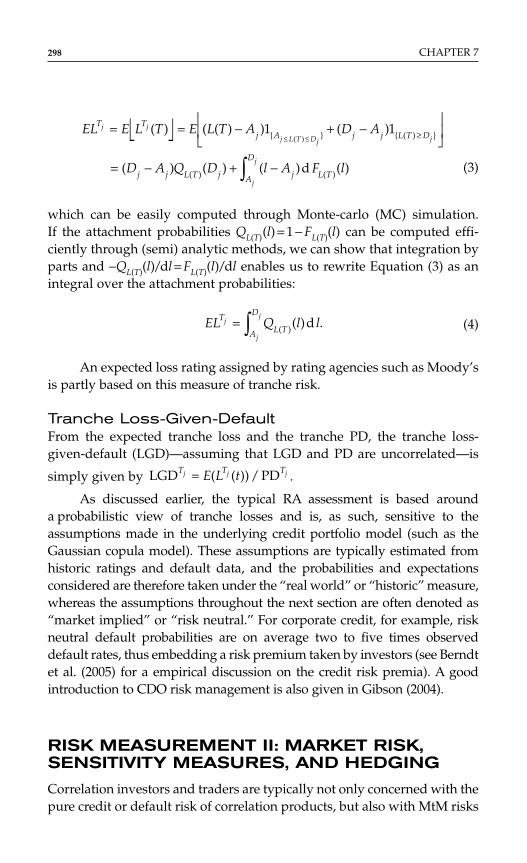
(3)
which can be easily computed through Monte-carlo (MC) simulation.If the attachment probabilities QL(T)(l) = 1 − FL(T)(l) can be computed effi-ciently through (semi) analytic methods, we can show that integration byparts and −QL(T)(l)/dl = FL(T)(l)/dl enables us to rewrite Equation (3) as anintegral over the attachment probabilities:
(4)
An expected loss rating assigned by rating agencies such as Moody’sis partly based on this measure of tranche risk.
Tranche Loss-Given-DefaultFrom the expected tranche loss and the tranche PD, the tranche loss-given-default (LGD)—assuming that LGD and PD are uncorrelated—is
simply given by .
As discussed earlier, the typical RA assessment is based arounda probabilistic view of tranche losses and is, as such, sensitive to theassumptions made in the underlying credit portfolio model (such as theGaussian copula model). These assumptions are typically estimated fromhistoric ratings and default data, and the probabilities and expectationsconsidered are therefore taken under the “real world” or “historic” measure,whereas the assumptions throughout the next section are often denoted as“market implied” or “risk neutral.” For corporate credit, for example, riskneutral default probabilities are on average two to five times observeddefault rates, thus embedding a risk premium taken by investors (see Berndtet al. (2005) for a empirical discussion on the credit risk premia). A goodintroduction to CDO risk management is also given in Gibson (2004).
RISK MEASUREMENT II: MARKET RISK,SENSITIVITY MEASURES, AND HEDGING
Correlation investors and traders are typically not only concerned with thepure credit or default risk of correlation products, but also with MtM risks
LGD ( ( )) / PDT T Tj j jE L t=
EL Q l lTL TA
Dj
j
j= ∫ ( )( )d .
EL E L T E L T A D A
D A Q D l A F l
T Tj A j j L T D
j j L T j j L TA
D
j j
j L T Dj j
j
j
= = − + −
= − + −
≤ ≤ ≥
∫
( ) ( ( ) ) ( )
( ) ( ) ( )d ( )
( )
( ) ( )
( )1 1
298 CHAPTER 7
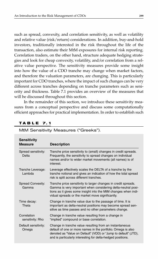
such as spread, convexity, and correlation sensitivity, as well as volatilityand relative value (risk/return) considerations. In addition, buy-and-holdinvestors, traditionally interested in the risk throughout the life of thetransaction, also estimate their MtM exposures for internal risk reporting.Correlation traders, on the other hand, structure adequate hedging strate-gies and look for cheap convexity, volatility, and/or correlation from a rel-ative value perspective. The sensitivity measures provide some insightinto how the value of a CDO tranche may change when market factors,and therefore the valuation parameters, are changing. This is particularlyimportant for CDO tranches, where the impact of such changes can be verydifferent across tranches depending on tranche parameters such as seni-ority and thickness. Table 7.1 provides an overview of the measures thatwill be discussed throughout this section.
In the remainder of this section, we introduce these sensitivity mea-sures from a conceptual perspective and discuss some computationallyefficient approaches for practical implementation. In order to establish such
An Introduction to the Risk Management of CDOs 299
T A B L E 7. 1
MtM Sensitivity Measures (“Greeks”).
SensitivityMeasure Description
Spread sensitivity: Tranche price sensitivity to (small) changes in credit spreads.Delta Frequently, the sensitivity to spread changes on individual
names and/or to wider market movements (all names) is ofinterest.
Tranche Leverage: Leverage effectively scales the DELTA of a tranche by the Lambda tranche notional and gives an indication of how the total spread
risk is split across different tranches.
Spread Convexity: Tranche price sensitivity to larger changes in credit spreads.Gamma Gamma is very important when considering delta-neutral posi-
tions as it gives some insight into the MtM changes when indi-vidual spreads or the market move significantly.
Time decay: Change in tranche value due to the passage of time. It is Theta important as delta-neutral positions may become spread sen-
sitive as time passes and no other parameters change.
Correlation Change in tranche value resulting from a change in sensitivity: Rho “implied” compound or base correlation.
Default sensitivity: Change in tranche value resulting from an instantaneous Omega default of one or more names in the portfolio. Omega is also
denoted as “Value on Default” (VOD) or “Jump to default” (JTD),and is particularly interesting for delta-hedged positions.

sensitivities, a consistent valuation framework, as outlined in Chapter 6 onpricing, needs to be in place.
First Order Spread Sensitivity: Delta
In practice, the spread risk of a CDO tranche is managed by buying andselling single name CDS protection as an offsetting hedge. This, of course,is not addressing all risks inherent in ST CDOs and provides only a partialhedge (a spread hedge), compared to entering an offsetting but identicaltrade. Such an offsetting trade, however, is rarely possible due to thebespoke nature of many ST CDOs. With the recent growth in standardizedindex tranches—ST CDOs referencing the CDX indices in the United Statesand/or the ITraxx ones in Europe—such offsetting hedges are possible.Depending on how similar a bespoke tranche portfolio is to the composi-tion of a CDS index, liquid tranches on that index can provide a goodapproximate hedge. In practice, instead of single name CDS, liquid indicescan be used directly (in unlevered form) to manage spread sensitivity. Wedenote the sensitivity to single name spread movements by individual ormicrospread sensitivity (CS01), while the sensitivity to a broad move in theportfolio spread will be denoted by market or macrosensitivity (Credit01).*
Defining Single Name/Individual DeltaA widening in credit spreads (keeping everything else equal) leads to anincrease in expected portfolio loss and, correspondingly, to the expectedloss of all tranches. Hence, ST positions are subject to MtM movements ascredit spreads in the underlying portfolio change. To hedge a long (short)position in a tranche requires buying (selling) protection on each of theunderlying names according to the delta. We therefore define the delta of a credit j in the underlying portfolio as the amount of protection thedealer sells (buys) on that name to hedge the MtM risk of a short (long)tranche position, denoted by Tj, due to credit spread change of name i. Inpractice, such a change in spreads will lead to MtM gains or losses on the
tranche position as well as on the single name CDS or hedge
portfolio (∆MtMi). Hence, holding amount of CDS on name i will leadto the same profit and loss (P&L) impact as holding the CDO tranche, ifthe credit spread of name i changes slightly. Formally,
∆ ∆ ∆i
T
i i
Tj jx x⋅ =MtM ( ) MtM ( ),r r
∆ i
Tj
( MtM )∆ i
Tj
∆ i
Tj
300 CHAPTER 7
*“01” in CS01 and Credit01 stands for a small, 1 bp shift in credit spreads.
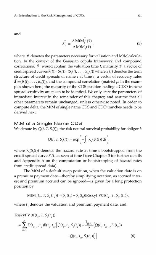
and
(5)
where denotes the parameters necessary for valuation and MtM calcula-tion. In the context of the Gaussian copula framework and compoundcorrelations, would contain the valuation time t, maturity T, a vector ofcredit spread curves S
→(t):= S
→(t):= (S1(t), . . . , SN(t)) where Si(t) denotes the term
structure of credit spreads of name i at time t, a vector of recovery ratesδ→:= (δ1(t), . . . , δN(t)), and the compound correlation (matrix) ρ. In the exam-ples shown here, the maturity of the CDS position heding a CDO tranchespread sensitivity are taken to be identical. We only state the parameters ofimmediate interest in the remainder of this chapter, and assume that allother parameters remain unchanged, unless otherwise noted. In order tocompute delta, the MtM of single name CDS and CDO tranches needs to bederived next.
MtM of a Single Name CDSWe denote by Q(t, T, Si(t)), the risk neutral survival probability for obligor i:
where λs(Si(t)) denotes the hazard rate at time s bootstrapped from thecredit spread curve Si(t) as seen at time t (see Chapter 3 for further detailsand Appendix A on the computation or bootstrapping of hazard ratesfrom credit spread data).
The MtM of a default swap position, when the valuation date is ona premium payment date—thereby simplifying notation, as accrued inter-est and premium accrued can be ignored—is given for a long protectionposition by
MtMi(tν , T, Si (tν )) = (Si (tν ) − Si (t0))RiskyPV01(tν , T, Si, (tν )),
where tν denotes the valuation and premium payment date, and
RiskyPV 01( , , ( ))
( , ) ( , ) ( , , ( )) ( , , ( ))
( , , ( )) ( )
– –
t T S t
D t t B t t Q t t S t Q t t S t
Q t t S t
i
n n n n in
N
n i
n i
ν ν
ν ν ν ν ν
ν ν
= [ + (− )]
=∑ 1
11
1
2
6
PA
Q t T S t S t si s it
T( , , ( )) exp ( ( ))d ,= −
∫ λ
rx
rx
∆∆∆i
T i
T
i
jj x
x=
MtM ( )
MtM ( ),
r
r
An Introduction to the Risk Management of CDOs 301
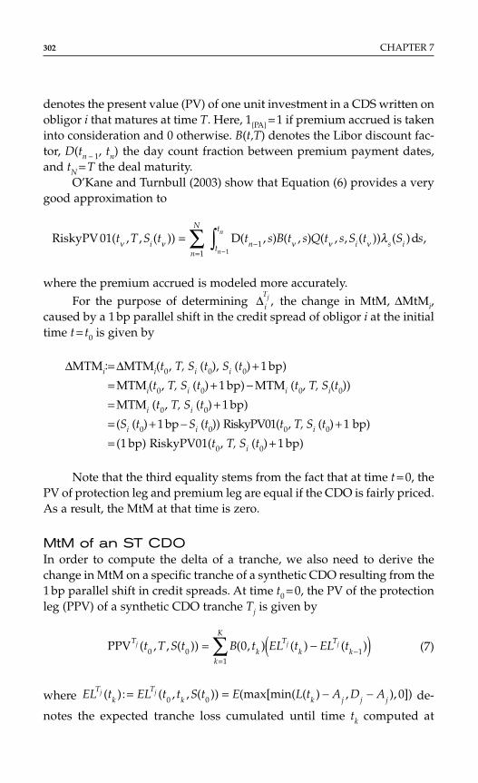
denotes the present value (PV) of one unit investment in a CDS written onobligor i that matures at time T. Here, 1PA = 1 if premium accrued is takeninto consideration and 0 otherwise. B(t,T) denotes the Libor discount fac-tor, D(tn − 1, tn) the day count fraction between premium payment dates,and tN = T the deal maturity.
O’Kane and Turnbull (2003) show that Equation (6) provides a verygood approximation to
where the premium accrued is modeled more accurately.For the purpose of determining the change in MtM, ∆MtMi,
caused by a 1 bp parallel shift in the credit spread of obligor i at the initialtime t = t0 is given by
∆MTMi:= ∆MTMi(t0, T, Si (t0), Si (t0) + 1 bp)
= MTMi(t0, T, Si (t0) + 1 bp) − MTMi (t0, T, Si(t0))
= MTMi (t0, T, Si (t0) + 1 bp)
= (Si (t0) + 1 bp − Si (t0)) RiskyPV01(t0, T, Si (t0) + 1 bp)
= (1 bp) RiskyPV01(t0, T, Si (t0) + 1 bp)
Note that the third equality stems from the fact that at time t = 0, thePV of protection leg and premium leg are equal if the CDO is fairly priced.As a result, the MtM at that time is zero.
MtM of an ST CDOIn order to compute the delta of a tranche, we also need to derive thechange in MtM on a specific tranche of a synthetic CDO resulting from the1 bp parallel shift in credit spreads. At time t0 = 0, the PV of the protectionleg (PPV) of a synthetic CDO tranche Tj is given by
(7)
where de-
notes the expected tranche loss cumulated until time tk computed at
EL t EL t t S t E L t A D ATk
Tk k j j j
j j( ): ( , , ( )) (max[min( ( ) , ), ])= = − −0 0 0
PPV ( , , )) ( , ) ( ) ( )Tk
Tk
Tk
k
Kj j jt T S t B t EL t EL t0 1
1
0( 0 = −( )−=
∑
∆ i
Tj ,
RiskyPV 01( , , ( )) ( , ) ( , ) ( , , ( )) ( )d ,t T S t t s B t s Q t s S t S si t
t
n i s in
N
n
n
ν ν ν ν ν λ=−
∫∑ −=
D1
11
302 CHAPTER 7
time t0 by employing the spread information (curve) available at thattime (S(t0)). Here, S(t0) denotes the vector of credit spreads (curves) forall names in the underlying portfolio. As before, the expected trancheloss can be computed from an adequate model, such as the Gaussiancopula, and through various numerical techniques such as MC simula-tion, Fast Fourier Transform Methods, recursive schemes, or the proxyintegration method. An overview of these approaches is provided inChapter 6.
Given an estimate of expected tranche losses through time, we canalso compute the PV of the fee or premium leg, that is,
(8)
We also define the Tranche PV01 as the PV of 1 bp (unit) invested intranche j as:
Then, at time t = 0, the MtM for tranche j is defined as the difference inthe fee and PPVs, which, assuming a fairly priced tranche, is zero at
inception of a trade
S(t0)) = 0. The fair tranche spread, is therefore given by
At a later date, say a premium payment date tν (to keep the notationsimple), the MtM is given by
S t T S tt T S t
t T S tT
T
Tj
j
j( , , ( ))
PPV ( , , ( ))
TrPV ( , , ( )).0 0
0 0
0 001=
S t T S tTj ( , , ( )),0 0
(MtM ( , , ( )) FPV ( , , ( )) PPV ( , ,T T Tj j jt T S t t T S t t T0 0 0 0 0= −
TrPV ( , , ( )): CS ( , , ( )):
( , ) ( , ) ( , , ( )) .
01 01
0
0 0 0 0
11
0 0
T
k k kk
K
j jT
j
j
t T S t t T S t
B t D t t D A EL t T S t
=
= × − −( )−=
∑
FPV t T S t S t T S t B t D t t
D A EL t
T Tk k k
k
K
j jT
k
j j
j
( , , ( )) ( , , ( )) ( , ) ( , )
( ) .
0 0 0 0 11
0= [× − −( )
−=
∑
An Introduction to the Risk Management of CDOs 303
which is unequal to zero as time passes, and spreads and other pricing pa-rameters may have changed. Hence, with
we obtain
For the purpose of calculating the change in tranche MtM for a1 bp parallel shift in the credit spread term structure of name i is given by
where Si01(t) := (S1(t), . . . , Si − 1(t), Si(t) + 1 bp, Si + 1(t), . . . , SN(t)) denotes thevector of credit spreads and where the term structure of name i is shifteduniformly by 1 bp while all other term structures remain unchanged.
The approach just outlined is frequently denoted as “brute force” or“bumping,” and is fairly flexible and independent of the actual valuationmodel employed. In order to compute the change in MtM, the expectedtranche loss needs to be derived at different points in time efficiently.While simulation is in principle feasible, more efficient approaches arepreferable, especially as calculations need to be repeated for each under-lying name. Although there are generally no explicit analytical expressionsfor tranche deltas available, practitioners and academics have developedvarious approaches for determining tranche sensitivities more efficientlyand accurately. These approaches are often developed for a specificpricing model or numerical implementation of such models and employthe exact definition rather than the approx-imate relationship
∂ ∂MtM ( , , ( ))/ ( )Ti
j t T S t S t0 0 0
∆ ∆MtM : MtM ( , , ( ), ( ))
MtM ( , , ( )) MtM ( , , ( ))
MtM ( , , ( ))
( ( , , ( )) ( , , ( )))TrPV (
i
T
i
T i
T i T
T i
T T i
j j
j j
j
j j
t T S t S t
t T S t t T S t
t T S t
S t T S t S t T S t t
=
= −
=
= −
0 001
0
001
0 0 0
001
0
0 0 001
0 01 0001
0, , ( ))T S ti
∆ i
Tj ,
MtM ( , , ( )) ( , , ( )) ( , , ( )) TrPV ( , , ( )).T T Tj j jt T S t S t T S t S t T S t t T S tν ν ν ν ν ν= −( )0 0 01
S t T S tt T S t
t T S tT
Tj
Tj
j( , , ( ))
PPV ( , , ( ))
TrPV ( , , ( ))ν νν ν
ν ν
=01
MtM ( , , ( )) ( , , ( ))TrPV ( , , ( ))
PPV ( , , ( )),
T T
T
j j
j
t T S t S t T S t t T S t
t T S t
ν ν ν ν
ν ν
=
−0 0 01
304 CHAPTER 7

Closed form or semi-closed-form solutions for the partial integral are fre-quently developed.
Appendix B outlines a semi-analytic computation of the sensitivityof the tranche value to small changes in PDs (spreads) within the com-monly used recursive scheme of Andersen et al. (2003) as outlined in“Option 2: The recursive approach” of Chapter 6.
Appendix C reviews the LH+ model of Greenberg et al. (2004) wherespread hedges are computed in closed form. The model is based on thelarge homogeneous portfolio (LHP) approximation with one additionalasset, for which sensitivities are computed.
Additional insights into efficient and accurate computation of CDOand basket sensitivities, within a simulation framework can be found inJoshi and Kainth (2003), Rott and Fries (2005), and Glasserman and Li(2003). We provide some insight in appendix D on MC deltas, and alsorefer to Brasch (2004) who revisits analytic and semianalytic methodsfocusing on sensitivities for CDO and CDO^2 structures.
Practical Hedging and Delta SensitivityBy definition, delta hedging immunizes the tranche against smallchanges in credit spreads. For larger spread movements, a significantamount of spread risk (spread convexity) prevails, resulting in a need todynamically rebalance the hedges throughout the life of the transaction.Such a process may incur a significant amount of transaction costs,depending on the frequency of rebalancing actions and current bid–askspreads. Furthermore, liquidity in some of the underlying names may bepoor due to the bespoke nature of underlying assets in synthetic STCDOs. Nevertheless, tranche deltas provide significant insight into thebehavior of CDOs and are a major risk management tool. If the behaviorof deltas is well understood, it is possible to design trading strategieswith desired spread sensitivities over time. Similarly, strategies can beconstructed with an initial delta-mismatch that become delta neutralwhen spreads move in line with one’s expectations. We will thereforereview the sensitivity of tranche deltas to various parameters that impactCDO performance.
∂∂
≈
= −
MtM ( , , ( ))
( )( bp) MtM
MtM ( , , ( )) MtM ( , , ( )).
T
ii
T
T i T
jj
j j
t T S t
S t
t T S t t T S t
0 0
0
001
0 0 0
1 ∆
An Introduction to the Risk Management of CDOs 305
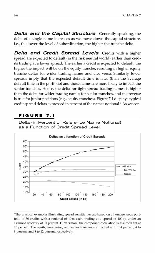
Delta and the Capital Structure Generally speaking, thedelta of a single name increases as we move down the capital structure,i.e., the lower the level of subordination, the higher the tranche delta.
Delta and Credit Spread Levels Credits with a higherspread are expected to default (in the risk neutral world) earlier than cred-its trading at a lower spread. The earlier a credit is expected to default, thehigher the impact will be on the equity tranche, resulting in higher equitytranche deltas for wider trading names and vice versa. Similarly, lowerspreads imply that the expected default time is later (than the averagedefault time in the portfolio) and those names are more likely to impact thesenior tranches. Hence, the delta for tight spread trading names is higherthan the delta for wider trading names for senior tranches, and the reverseis true for junior positions (e.g., equity tranches). Figure 7.1 displays typicalcredit spread deltas expressed in percent of the names notional.* As we con-
306 CHAPTER 7
*The practical examples illustrating spread sensitivities are based on a homogeneous port-folio of 50 credits with a notional of 10 m each, trading at a spread of 100 bp under anassumed recovery of 38 percent. Furthermore, the compound correlation is assumed flat at25 percent. The equity, mezzanine, and senior tranches are trached at 0 to 4 percent, 4 to8 percent, and 8 to 12 percent, respectively.
Deltas as a function of Credit Spreads
10%
15%
20%
25%
30%
35%
40%
45%
50%
55%
60%
20 40 60 80 100 120 140 160 180 200
Credit Spread (in bp)
Del
ta
Equity
Mezzanine
Senior
F I G U R E 7. 1
Delta (in Percent of Reference Name Notional) as a Function of Credit Spread Level.

sider a homogenous pool (same spreads, recoveries, and correlations), thedelta is the same for each name. Figure 7.1 reveals that mezzanine tranchesappear to have less directionality with respect to credit spread levels.
Deltas of individual credits will rise in time for the equity tranche ifthe spread on that name widens (assuming little change in average port-folio spread) as a result of an earlier expected default time for that name.For senior tranches, however, deltas will reduce as spreads widen on asingle credit only, as this credit is expected to default earlier, impactingthe equity tranche more than the senior exposures.
Of course, in practice, credit spreads on more than one name maywiden, and one wants to consider how single name deltas change whenall (or some) credits in the portfolio widen. A cumulative widening of allnames in the portfolio leads to an increase in the chance of a high numberof defaults and reduces the probability of a small number of defaults.Hence, the spread sensitivity of the value of an equity tranche reduceswhile the spread sensitivity of a senior tranche increases, leading to anincrease in each individual senior tranche delta and a decrease in eachindividual equity tranche delta. The reverse holds when all spreadsare tightening. A cumulative spread move also underlies the definitionof Credit01, and is frequently used to estimate hedge ratios when liquidtranches are hedged with CDS indices, as further discussed in the section“Delta hedging with a CDS index: Credit01 sensitivity.”
Delta as a Function of Time Assuming there are no lossesin the underlying portfolio, deltas will change due to the passage of time.The delta of the equity tranche will increase to 100 percent as time to matu-rity decreases. Mezzanine and senior tranches at the same time becomeless risky compared to the equity tranche, resulting in a decrease in theirdelta towards zero at maturity (see Figure 7.2 for a illustrative example).
Delta and Correlation The MtM or fair spread on a CDO tranchewithin the usual Gaussian copula valuation framework depends on thecurrent (observable) term structure of credit spreads on each of the under-lying names, the maturity of the transaction, a recovery assumption for eachname, and the correlation assumption (see Appendices B, C, and D for dif-ferent numerical implementation techniques and Chapter 6 on pricing).Assuming that the first two sets of parameters are observable, (or can be atleast implied from the single name CDS market) and a fixed maturity, theonly variable left unspecified is the correlation applied in the pricing model.Then, given quoted tranche prices, one can compute the corresponding
An Introduction to the Risk Management of CDOs 307
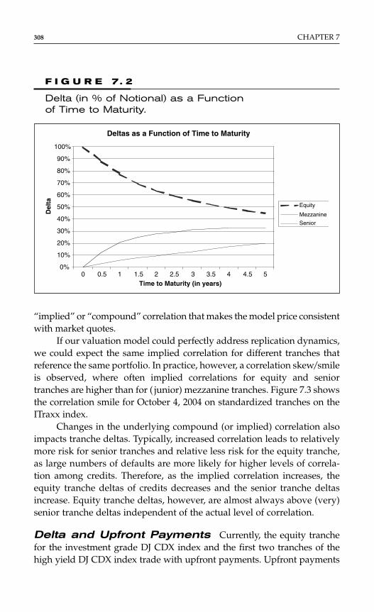
“implied” or “compound” correlation that makes the model price consistentwith market quotes.
If our valuation model could perfectly address replication dynamics,we could expect the same implied correlation for different tranches thatreference the same portfolio. In practice, however, a correlation skew/smileis observed, where often implied correlations for equity and seniortranches are higher than for ( junior) mezzanine tranches. Figure 7.3 showsthe correlation smile for October 4, 2004 on standardized tranches on theITraxx index.
Changes in the underlying compound (or implied) correlation alsoimpacts tranche deltas. Typically, increased correlation leads to relativelymore risk for senior tranches and relative less risk for the equity tranche,as large numbers of defaults are more likely for higher levels of correla-tion among credits. Therefore, as the implied correlation increases, theequity tranche deltas of credits decreases and the senior tranche deltasincrease. Equity tranche deltas, however, are almost always above (very)senior tranche deltas independent of the actual level of correlation.
Delta and Upfront Payments Currently, the equity tranchefor the investment grade DJ CDX index and the first two tranches of thehigh yield DJ CDX index trade with upfront payments. Upfront payments
308 CHAPTER 7
F I G U R E 7. 2
Delta (in % of Notional) as a Function of Time to Maturity.
Deltas as a Function of Time to Maturity
0%
10%
20%
30%
40%
50%
60%
70%
80%
90%
100%
0 0.5 1 1.5 2 2.5 3 3.5 4 4.5 5Time to Maturity (in years)
Del
ta Equity
Mezzanine
Senior
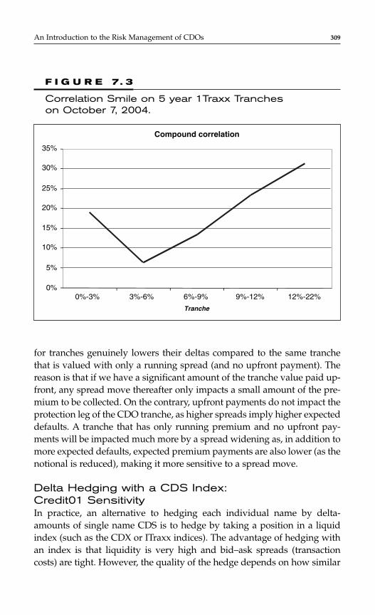
for tranches genuinely lowers their deltas compared to the same tranchethat is valued with only a running spread (and no upfront payment). Thereason is that if we have a significant amount of the tranche value paid up-front, any spread move thereafter only impacts a small amount of the pre-mium to be collected. On the contrary, upfront payments do not impact theprotection leg of the CDO tranche, as higher spreads imply higher expecteddefaults. A tranche that has only running premium and no upfront pay-ments will be impacted much more by a spread widening as, in addition tomore expected defaults, expected premium payments are also lower (as thenotional is reduced), making it more sensitive to a spread move.
Delta Hedging with a CDS Index: Credit01 SensitivityIn practice, an alternative to hedging each individual name by delta-amounts of single name CDS is to hedge by taking a position in a liquidindex (such as the CDX or ITraxx indices). The advantage of hedging withan index is that liquidity is very high and bid–ask spreads (transactioncosts) are tight. However, the quality of the hedge depends on how similar
An Introduction to the Risk Management of CDOs 309
F I G U R E 7. 3
Correlation Smile on 5 year 1Traxx Tranches on October 7, 2004.
Compound correlation
0%
5%
10%
15%
20%
25%
30%
35%
0%-3% 3%-6% 6%-9% 9%-12% 12%-22%
Tranche
the portfolio referenced by the CDO tranche is to the computation of theindex. Formally, we define the Credit01 as the change in MtM (dollar value)for a 1 bp parallel shift in credit spreads on all names in the portfolio. It cantherefore be seen as a cumulative or aggregate (market) spread sensitivitymeasure:
where S01(t0) : = (S1(t) + 1 bp, . . . , Si − 1(t) + 1 bp, Si(t) + 1 bp, Si + 1(t) + 1 bp, . . . ,SN(t) + 1 bp).
can therefore be used to estimate a hedge ratio when astandardized CDO tranche (e.g., ITraxx tranche) is hedged with theunderlying CDS index (e.g., ITraxx), that is,
where · ∆MtMI corresponds to the change in MtM on the CDS indexfor a 1 bp spread widening on each of the underlying names (and henceon the overall index).*
Unlike individual spread sensitivity CS01, Credit01 increases for se-nior tranches as all spreads widen in parallel, whereas Credit01 of theequity tranche decreases if all spreads widen in a parallel move. This resultsfrom the fact that a widening in all spreads increases the risk of higher num-bers of defaults shifting the risk from the equity to senior tranches.
Note, however, that an index hedge in practice provides only anapproximate (or average) delta hedge when the underlying names in theportfolio are very dispersed, whereas it provides a perfect spread hedge ifall names trade at the same spread. As a result, for an equity tranche in theindex, a tighter name would be overhedged as the relative risk to the equitytranche of a low spread name is lower than that of a name with a (higher)average spread. Similarly, wider trading names would be underhedged asthe deltas of the equity tranche are lower if the credits trade at a lower(average) level. The reverse behavior holds for hedging a senior tranche.
rx
∆∆
TT
I
jj
=⋅
Credit ( )MtM ( )
01r
rx
x
Credit 01Tj
Credit : MtM ( , , ( ), ( ))
( , , ( )) ( , , ( )) TrPV ( , , ( ))
01
01
0 001
0
0 0 001
0 001
0
T T
T T T
j j
j j j
t T S t S t
S t T S t S t T S t t T S t
=
= −( )∆
310 CHAPTER 7
*In practice, an alternative way is to sum over all individual single name deltas and enter aCDS index position according to the resulting notional. The reason why there is hardly a dif-ference in bumping all spreads at once or summing over all hedges when one spread isbumped at the time is that convexity is less of an issue for a small (typically 1 bp) spread move.

Tranche Leverage: Lambda
The leverage, or lambda, of a tranche is closely linked to tranche deltasand provides useful information as it effectively scales the delta by thetranche notional. Formally, we define leverage, or lambda, as
where denotes the tranche notional and Ni the notional ofname i in the underlying portfolio.
Practically, leverage gives an indication of how the total risk is dis-tributed between different tranches. Hence, the higher the leverage, thehigher the spread risk in relation to the tranche notional. For example, con-sider a 7 to 10 percent tranche of a $1 billion underlying portfolio with anotional of $30 million. Assume an (average) hedge ratio of per-cent for this senior tranche resulting in a total notional of $150 million forthe hedge portfolio. The lambda, or leverage, for this tranche is therefore 5.
A super senior position (for example, 10 to 100 percent) usuallyresults in a higher delta portfolio, but also a significantly lower leverage.Of course, given the leverage or lambda we can compute an average deltafor an index tranche (as discussed in the previous section). Given theleverage and tranche size, the size of the underlying hedge portfolio canbe computed and the index can be bought accordingly.
Credit Spread Convexity: Gamma
While first order spread sensitivity is a very important measure of risk, thesensitivity of credit product spread changes beyond 1 bp also needs to beconsidered. This is especially true when hedging instruments have differentleverage, i.e. hedging a tranche with an index, or an equity tranche with amezzanine or senior tranche. Spread convexity of credit products usuallyrefers to the MtM behavior as a function of the underlying level of creditspreads. Spread convexity, or gamma, of various tranches can be very dif-ferent, and particularly large compared to the convexity of single name CDSor CDS indices. A detailed understanding is therefore required, particularlywhen we want to implement various relative value or credit strategies.
As with first order sensitivity, we can differentiate between macro-and microspread convexity, and it is particularly important to understand
∆Tj = 15
N D ATj j
j = −
Lambda(delta– hedge portfolio)
,TT
i
T
in
N
T
Tin
N
Tj
j
j
j
j
j
N
N
N
N
N
N= = ≈= =∑ ∑∆ ∆
1 1
An Introduction to the Risk Management of CDOs 311
the behavior of (delta-hedged) tranche products when individual spreadsare moving (microconvexity), or when the overall market/portfoliospread is moving (macroconvexity).
Macroconvexity: GammaMore formally, we define the macro spread convexity, gamma, as the addi-tional MtM change on a tranche over that obtained by multiplying theCredit01 of that tranche by the parallel spread move for all of the underly-ing single name CDSs. Put another way, it is the difference between the lin-ear approximation and the actual movement in market value. For example,assuming a 100 bp spread widening, gamma is given by:
(9)
where S100(t): = (S1(t) + 100 bp, . . . , SN(t) + 100 bp).In practice, a relative spread shift factor is frequently introduced and
gamma is calculated by bumping the underlying spreads uniformly byvarying amounts (for example, in the range of 50 to 150 percent depend-ing on the actual level of spreads). We therefore require efficient algo-rithms once again, as it requires a recalculation for various spread levelsin a brute-force computation.*
Microconvexity: iGammaSingle name, or idiosyncratic convexity, iGamma, is defined as the con-vexity resulting from a single CDS spread moving independently ofthe others, i.e., one spread moves while the other names remainunchanged:
(10)
where Si100(t): = (S1(t), . . . , S1i − 1(t), Si(t) + 100 bp, Si + 1(t), . . . , SN(t)).
iGamma : MtM ( , , ( ), ( )) MtM ( , , ( ), ( ))
MtM ( , , ( ), ( )) RiskyPV ( , , ( ))
100 0 0100
0 0 001
0
0 0100
0 001
0
100
100 01
T
i
T ii
T i
i
T ii
T i
j j j
j j
t T t S t t T t t
t T t S t t T t
S S S
S S
= −
= −
∆ ∆
∆ ∆
Gamma : MtM ( , , ( ), ( ))
Credit ( , , ( ), ( ))100 0 0
1000
0 001
0100 01
T T
T
j j
j
t T S t S t
t T S t S t
=
−
∆
312 CHAPTER 7
*While some of the efficient calculations of spread sensitivities outlined in the Appendix canbe extended to higher order sensitivities, we are focusing on the most generic implementa-tion through “brute-force” or “bumping” in the remainder of this chapter.

Convexity of Delta-Hedged TranchesIn practice, one is mostly concerned with the convexity of delta-neutraltranches, or portfolios of tranches, index, and single name positions whenspecific trading strategies are being developed. While a more elaboratediscussion of specific strategies follows in the next chapter, we exploreimportant convexity issues for simple delta-hedged equity and seniortranche positions next.
Similarly to the definitions in Equations (9) and (10), the convexity ofa single name CDS can be defined as the difference between the RiskyPV100and 100 times the RiskyPV01. For relatively simple credit exposures, multi-plying the spread shift by the RiskyPV01 provides a good approximation ofthe true MtM impact, and while some level of convexity is present, the signof the MtM impact is the same for various levels of spread widening. Wewill show that such consistency is not guaranteed for CDO tranches, high-lighting the need to compute such higher order spread sensitivities. We willillustrate that the convexity of tranches can be very different to the convex-ity of single name CDS (and across tranches), which therefore expose delta-hedged or neutral portfolios to spread convexity. This not surprising, as thedelta itself is a function of spread level and changes when spreads move.Again, in practice, the easiest way to observe convexity is to plot the P&L ofa delta-hedged transaction. In particular, the change in tranche MtM, thechange in hedge portfolio MtM, and the net P&L for a uniform and parallelshift in all (or a single) credit spreads provide some valuable insight into thelikely MtM behavior of delta-neutral strategies.
Macroconvexity In order to understand spread convexity andthe resulting MtM of delta-hedged positions, we consider a delta-hedgedequity tranche (long correlation) and a delta-hedged senior tranche (shortcorrelation) when all spreads move together (macroconvexity/gamma)next.*
Delta-Neutral Long Equity Tranche Selling protection on an equitytranche and buying delta-amounts of single name CDS results in anincrease in expected tranche loss and a shift of the risk away from the
An Introduction to the Risk Management of CDOs 313
*A (delta-neutral) equity tranche is often denoted as a long correlation position as anincrease in implied correlation leads to a decrease in tranche value. Similarly, a (delta-hedged) senior tranche is a short correlation as an increase in compound correlation impliesan increase in tranche value.

equity tranche to mezzanine and senior tranches when all credit spreadswiden. Essentially, this means that we are overhedged, as discussed in theprevious section on first order sensitivity. Therefore, the MtM change onthe delta portfolio is greater than the MtM on the equity tranche. Since theMtM on the hedge portfolio is positive, the net MtM, or P&L, is positive.Table 7.2 summarizes the behavior for both spread widening andtightening scenario, and Figure 7.4 shows a typical plot for such a longcorrelation trade.
314 CHAPTER 7
F I G U R E 7. 4
Gamma for a Long Correlation Equity Tranche.
Gamma: Delta neutral long equity tranche as a function of parallel shift inall spreads
-6000000
-4000000
-2000000
0
2000000
4000000
6000000
8000000
-50% -40% -30% -20% -10% 0% 10% 20% 30% 40% 50%
Spread Shift Factor
Ch
ang
e in
MtM
(in
do
llars
) Equity Tranche MtM
Delta-MtM
Net MtM (P&L)
T A B L E 7. 2
Delta-Neutral Portfolio MtM (Long Equity Tranche) for a Change in ALL Spreads
All Spreads Widen All Spreads Tighten
Equity Tranche (protection sold) −MtM +MtM
Delta notional of CDS +MtM −MtM(protection bought)
Effective Hedge Overhedged Underhedged
Net MtM (net P&L) +MtM +MtM

From an investor’s perspective, in order to maintain a delta-neutralposition, single name CDS contracts need to be sold at higher spreads,thus locking in a profit. However, if spreads are significantly tighter, theequity tranche becomes relatively more risky, implying higher deltas, i.e.,the portfolio is underhedged. Put another way, the change in equitytranche position MtM is higher than the change in the current hedge port-folio, which implies again a positive net position.
Delta-Neutral Long Senior Tranche For an investor who is shortcorrelation by selling protection on a senior tranche and buyingunderlying CDS, the net MtM behaves the opposite. If all portfolio spreadsare widening, the risk shifts towards the senior tranche, which implies thatsenior tranche deltas need to increase: the tranche is underhedged. Withthe MtM of the tranche decreasing (the tranche is worth more, but we soldprotection) and the delta MtM increasing, further CDS contracts need to bebought at a higher spread. This means a net loss to the portfolio. Thereverse holds for the tightening scenario and is further illustrated in Table7.3 and Figure 7.5.
Microconvexity Perhaps counter-intuitive, the iGamma or micro-convexity of a tranche is generally the opposite to macroconvexity. Forexample, a spread widening on a single CDS implies, for the long equitytranche, a positive MtM on the hedge portfolio and a negative MtM on theequity tranche. The equity delta for that name increases as, relative to theother credits, this name becomes more risky. Hence, the MtM of the hedgeportfolio increases as all other spreads remain unchanged, leading to an
An Introduction to the Risk Management of CDOs 315
T A B L E 7. 3
Delta-Neutral Portfolio MtM (Long Senior Tranche) for a Change in ALL Spreads
All Spreads Widen All Spreads Tighten
Senior Tranche (protection sold) −MtM +MtM
Delta notional of CDS +MtM −MtM(protection bought)
Effective Hedge Underhedged Overhedged
Net MtM (net P&L) −MtM −MtM
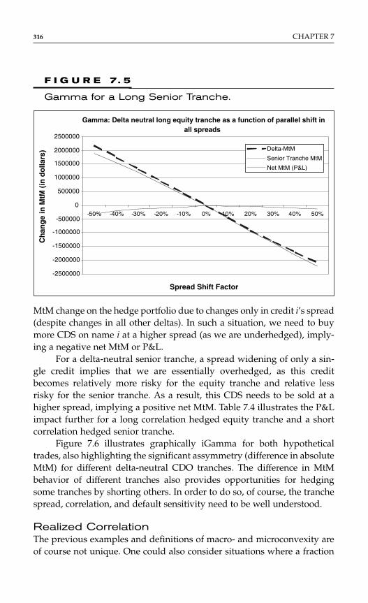
MtM change on the hedge portfolio due to changes only in credit i’s spread(despite changes in all other deltas). In such a situation, we need to buymore CDS on name i at a higher spread (as we are underhedged), imply-ing a negative net MtM or P&L.
For a delta-neutral senior tranche, a spread widening of only a sin-gle credit implies that we are essentially overhedged, as this creditbecomes relatively more risky for the equity tranche and relative lessrisky for the senior tranche. As a result, this CDS needs to be sold at ahigher spread, implying a positive net MtM. Table 7.4 illustrates the P&Limpact further for a long correlation hedged equity tranche and a shortcorrelation hedged senior tranche.
Figure 7.6 illustrates graphically iGamma for both hypotheticaltrades, also highlighting the significant assymmetry (difference in absoluteMtM) for different delta-neutral CDO tranches. The difference in MtMbehavior of different tranches also provides opportunities for hedgingsome tranches by shorting others. In order to do so, of course, the tranchespread, correlation, and default sensitivity need to be well understood.
Realized CorrelationThe previous examples and definitions of macro- and microconvexity areof course not unique. One could also consider situations where a fraction
316 CHAPTER 7
F I G U R E 7. 5
Gamma for a Long Senior Tranche.
-2500000
-2000000
-1500000
-1000000
-500000
0
500000
1000000
1500000
2000000
2500000
-50% -40% -30% -20% -10% 0% 10% 20% 30% 40% 50%
Ch
ang
e in
MtM
(in
do
llars
) Delta-MtM
Senior Tranche MtM
Net MtM (P&L)
Spread Shift Factor
Gamma: Delta neutral long equity tranche as a function of parallel shift inall spreads
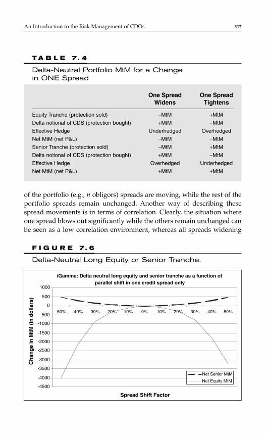
An Introduction to the Risk Management of CDOs 317
T A B L E 7. 4
Delta-Neutral Portfolio MtM for a Change in ONE Spread
One Spread One SpreadWidens Tightens
Equity Tranche (protection sold) −MtM +MtM
Delta notional of CDS (protection bought) +MtM −MtM
Effective Hedge Underhedged Overhedged
Net MtM (net P&L) −MtM −MtM
Senior Tranche (protection sold) −MtM +MtM
Delta notional of CDS (protection bought) +MtM −MtM
Effective Hedge Overhedged Underhedged
Net MtM (net P&L) +MtM +MtM
F I G U R E 7. 6
Delta-Neutral Long Equity or Senior Tranche.
iGamma: Delta neutral long equity and senior tranche as a function ofparallel shift in one credit spread only
-4500
-4000
-3500
-3000
-2500
-2000
-1500
-1000
-500
0
500
1000
-50% -40% -30% -20% -10% 0% 10% 20% 30% 40% 50%
Ch
ang
e in
MtM
(in
do
llars
)
Net Senior MtM
Net Equity MtM
Spread Shift Factor
of the portfolio (e.g., n obligors) spreads are moving, while the rest of theportfolio spreads remain unchanged. Another way of describing thesespread movements is in terms of correlation. Clearly, the situation whereone spread blows out significantly while the others remain unchanged canbe seen as a low correlation environment, whereas all spreads widening
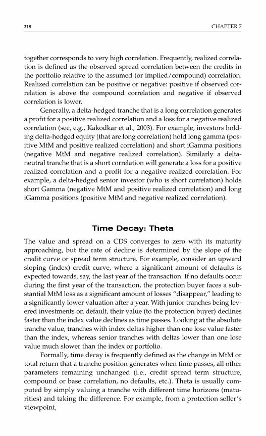
together corresponds to very high correlation. Frequently, realized correla-tion is defined as the observed spread correlation between the credits inthe portfolio relative to the assumed (or implied/compound) correlation.Realized correlation can be positive or negative: positive if observed cor-relation is above the compound correlation and negative if observedcorrelation is lower.
Generally, a delta-hedged tranche that is a long correlation generatesa profit for a positive realized correlation and a loss for a negative realizedcorrelation (see, e.g., Kakodkar et al., 2003). For example, investors hold-ing delta-hedged equity (that are long correlation) hold long gamma (pos-itive MtM and positive realized correlation) and short iGamma positions(negative MtM and negative realized correlation). Similarly a delta-neutral tranche that is a short correlation will generate a loss for a positiverealized correlation and a profit for a negative realized correlation. Forexample, a delta-hedged senior investor (who is short correlation) holdsshort Gamma (negative MtM and positive realized correlation) and longiGamma positions (positive MtM and negative realized correlation).
Time Decay: Theta
The value and spread on a CDS converges to zero with its maturityapproaching, but the rate of decline is determined by the slope of thecredit curve or spread term structure. For example, consider an upwardsloping (index) credit curve, where a significant amount of defaults isexpected towards, say, the last year of the transaction. If no defaults occurduring the first year of the transaction, the protection buyer faces a sub-stantial MtM loss as a significant amount of losses “disappear,” leading toa significantly lower valuation after a year. With junior tranches being lev-ered investments on default, their value (to the protection buyer) declinesfaster than the index value declines as time passes. Looking at the absolutetranche value, tranches with index deltas higher than one lose value fasterthan the index, whereas senior tranches with deltas lower than one losevalue much slower than the index or portfolio.
Formally, time decay is frequently defined as the change in MtM ortotal return that a tranche position generates when time passes, all otherparameters remaining unchanged (i.e., credit spread term structure,compound or base correlation, no defaults, etc.). Theta is usually com-puted by simply valuing a tranche with different time horizons (matu-rities) and taking the difference. For example, from a protection seller’sviewpoint,
318 CHAPTER 7
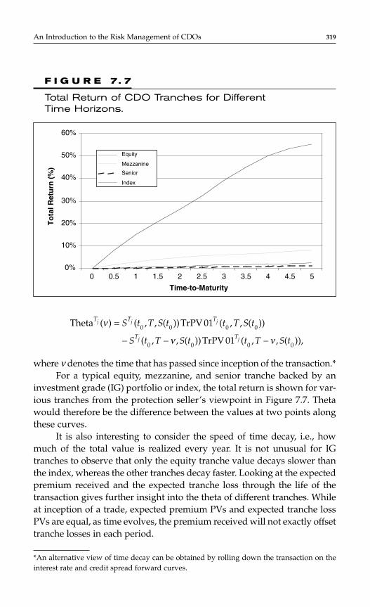
where ν denotes the time that has passed since inception of the transaction.*For a typical equity, mezzanine, and senior tranche backed by an
investment grade (IG) portfolio or index, the total return is shown for var-ious tranches from the protection seller’s viewpoint in Figure 7.7. Thetawould therefore be the difference between the values at two points alongthese curves.
It is also interesting to consider the speed of time decay, i.e., howmuch of the total value is realized every year. It is not unusual for IGtranches to observe that only the equity tranche value decays slower thanthe index, whereas the other tranches decay faster. Looking at the expectedpremium received and the expected tranche loss through the life of thetransaction gives further insight into the theta of different tranches. Whileat inception of a trade, expected premium PVs and expected tranche lossPVs are equal, as time evolves, the premium received will not exactly offsettranche losses in each period.
Theta ( ) ( , , ( ))TrPV ( , , ( ))
( , , ( ))TrPV ( , , ( )),
T T T
T T
j j j
j j
S t T S t t T S t
S t T S t t T S t
ν
ν ν
=
− − −0 0 0 0
0 0 0 0
01
01
An Introduction to the Risk Management of CDOs 319
*An alternative view of time decay can be obtained by rolling down the transaction on theinterest rate and credit spread forward curves.
F I G U R E 7. 7
Total Return of CDO Tranches for Different Time Horizons.
0%
10%
20%
30%
40%
50%
60%
0 0.5 1 1.5 2 2.5 3 3.5 4 4.5 5
To
tal R
etu
rn (
%)
Equity
Mezzanine
Senior
Index
Time-to-Maturity
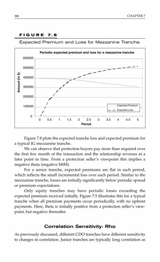
Figure 7.8 plots the expected tranche loss and expected premium fora typical IG mezzanine tranche.
We can observe that protection buyers pay more than required overthe first few month of the transaction and the relationship reverses at alater point in time. From a protection seller’s viewpoint this implies anegative theta (negative MtM).
For a senior tranche, expected premiums are flat in each period,which reflects the small incremental loss over each period. Similar to themezzanine tranche, losses are initially significantly below periodic spreador premium expectations.
Only equity tranches may have periodic losses exceeding theexpected premium received initially. Figure 7.9 illustrates this for a typicaltranche when all premium payments occur periodically, with no upfrontpayments. Here, theta is initially positive from a protection seller’s view-point, but negative thereafter.
Correlation Sensitivity: Rho
As previously discussed, different CDO tranches have different sensitivityto changes in correlation. Junior tranches are typically long correlation as
320 CHAPTER 7
F I G U R E 7. 8
Expected Premium and Loss for Mezzanine Tranche.
Periodic expected premium and loss for a mezzanine tranche
0
100000
200000
300000
400000
500000
600000
0 0.5 1 1.5 2 2.5 3 3.5 4 4.5 5Period
Expected Premium
Expected Loss
Am
ou
nt
(in
$)
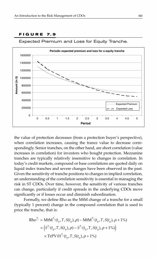
the value of protection decreases (from a protection buyer’s perspective),when correlation increases, causing the trance value to decrease corre-spondingly. Senior tranches, on the other hand, are short correlation (valueincreases in correlation) for investors who bought protection. Mezzaninetranches are typically relatively insensitive to changes in correlation. Intoday’s credit markets, compound or base correlations are quoted daily onliquid index tranches and severe changes have been observed in the past.Given the sensitivity of tranche positions to changes in implied correlation,an understanding of the correlation sensitivity is essential in managing therisk in ST CDOs. Over time, however, the sensitivity of various tranchescan change, particularly if credit spreads in the underlying CDOs movesignificantly or if losses occur and diminish subordination.
Formally, we define Rho as the MtM change of a tranche for a small(typically 1 percent) change in the compound correlation that is used toprice the tranche, that is:
Rho MtM ( , , ( ), ) MtM ( , , ( ), %)
( , , ( ), ) ( , , ( ), %)
TrPV ( , , ( ), %)
T T T
T T
T
j j j
j j
j
t T S t t T S t
S t T S t S t T S t
t T S t
= − +
= − +( )× +
0 0 0 0
0 0 0 0
0 0
1
1
01 1
ρ ρ
ρ ρ
ρ
An Introduction to the Risk Management of CDOs 321
Periodic expected premium and loss for a equity tranche
0
200000
400000
600000
800000
1000000
1200000
1400000
1600000
0 0.5 1 1.5 2 2.5 3 3.5 4 4.5 5
Period
Am
ou
nt
(in
$)
Expected Premium
Expected Loss
F I G U R E 7. 9
Expected Premium and Loss for Equity Tranche.

In practice, Rho is once again computed by bumping the correlationparameters and tranche revaluation.
In general, long equity or short senior tranches have positive Rho(long correlation positions), while long senior or short equity postitionshave negative Rho (short correlation positions). For example, Figure 7.10plots Rho as a percentage of the tranche size for a typical (and risky) CDOportfolio with a fixed tranche size of 1 percent and varying attachmentpoints (or levels of subordination).
The figure reveals that Rho tends to zero for very high levels of sub-ordination (senior positions) but there is also a correlation neutral pointbetween the senior and equity tranches. It is therefore possible to con-struct a correlation neutral mezzanine tranche around this point. Forexample, in a tight spread environment, junior mezzanine tranches tendto be correlation neutral. Indeed, we can try to construct tranches (e.g.,two mezzanine tranches, one at each side of the correlation neutral point)such that the portfolio of tranches is correlation neutral, particularly asthe change in expected tranche loss due to a correlation move from ρ tocan be derived as an integral over changes in the attachment probabilities:
.∆ ∆EL T Q l l Q l l Q l lTL TA
D
L TA
D
L TA
Dj
j
j
j
j
j
j( ) ( )d ( )d ( )d( ), ( ), ( ), ,= − =∫ ∫ ∫ρ ρ ρ ρ
ρ
322 CHAPTER 7
RHO as a function of subordination (fixed tranche size of 1%)
-0.005
0
0.005
0.01
0.015
0.02
0.025
0% 1% 3% 5% 8% 10%
13%
15%
18%
20%
23%
25%
28%
30%
33%
35%
38%
40%
43%
45%
Subordination
Rh
o (
% o
f tr
anch
e si
ze)
RHO
F I G U R E 7. 1 0
Correlation Sensitivity as a Function of Subordination.
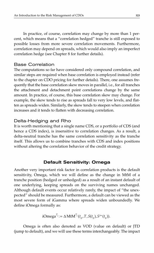
In practice, of course, correlation may change by more than 1 per-cent, which means that a “correlation hedged” tranche is still exposed topossible losses from more severe correlation movements. Furthermore,correlation may depend on spreads, which would also imply an imperfectcorrelation hedge (see Chapter 8 for further details).
Base CorrelationThe computations so far have considered only compound correlation, andsimilar steps are required when base correlation is employed instead (referto the chapter on CDO pricing for further details). There, one assumes fre-quently that the base correlation skew moves in parallel, i.e., for all tranchesthe attachment and detachment point correlations change by the sameamount. In practice, of course, this base correlation skew may change. Forexample, the skew tends to rise as spreads fall to very low levels, and flat-ten as spreads widen. Similarly, the skew tends to steepen when correlationincreases and it tends to flatten with decreasing correlation.
Delta-Hedging and RhoIt is worth mentioning that a single name CDS, or a portfolio of CDS (andhence a CDS index), is insensitive to correlation changes. As a result, adelta-neutral tranche has the same correlation sensitivity as the trancheitself. This allows us to combine tranches with CDS and index positionswithout altering the correlation behavior of the credit strategy.
Default Sensitivity: Omega
Another very important risk factor in correlation products is the defaultsensitivity, Omega, which we will define as the change in MtM of atranche position (hedged or unhedged) as a result of an instant default ofone underlying, keeping spreads on the surviving names unchanged.Although default events occur relatively rarely, the impact of “the unex-pected” should be measured. Furthermore, a default can be viewed as themost severe form of iGamma where spreads widen unboundedly. Wedefine iOmega formally as:
Omega is often also denoted as VOD (value on default) or JTD(jump to default), and we will use these terms interchangeably. The impact
iOmega : MtM ( , , ( ), ( )).T T ij j t T S t S t= ∞∆ 0 0 0
An Introduction to the Risk Management of CDOs 323

of an instantaneous default is genuinely high for unhedged tranches,whereas the level of risk for hedged strategies depends on the trancheseniority and thickness. The impact of a sudden default on the perfor-mance of credit strategies is important, particularly when comparingdifferent strategies with similar expected returns (or carries) at the out-set. This section only provides some conceptual discussion, and a moredetailed insight into the performance/relative value of popular tradingstrategies is given in Chapter 8.
Multiple Defaults (Omega)In practice, it is not only interesting to consider the MtM change as a resultof a single default, but also as resulting from multiple defaults. We definethe default sensitivity, when the n-widest trading names are defaulting, as
.* The n names with the highest credit spreads are chosen as theseare the most likely defaulters, but many different combinations of n default-ers could be chosen. In reality, of course, a probabilistic view can beimposed and a distribution of Omega, and tranche P&L more generally, canbe derived for different trading strategies (see Chapter 8).
iOmega and Omega for Hedged and UnhedgedTranche PositionsFigures 7.11 and 7.12 show iOmega (VOD) and Omega (RVOD), respec-tively, for a delta hedged equity and senior tranche. It is apparent that thedefault sensitivity is significantly reduced for the delta-neutral strategyup to a point where the sign of the sensitivity even reverses.
We can observe the maximum loss for six defaults in the case ofequity tranche and five defaults for the delta-neutral equity strategy.Furthermore, Omega reduces for more than five defaults again andbecomes neutral around the breakeven scenario of eight defaults. Beyondthat, Omega is positive. It is also worth pointing out that due to upfrontpayments (typical for equity tranches), losses amount to less than the totaltranche notional (<100 percent).
The (delta neutral) senior position reveals quite a different behavior.The Omega of the delta-hedged position is significantly higher for thehedge position for the first few defaults, compared to the senior tranche.The hedged senior positions Omega is positive for the first 11 defaults,and becomes negative thereafter.
OmeganTj
324 CHAPTER 7
*In Chapter 8, this measure will be denoted as Running VOD (RVOD).
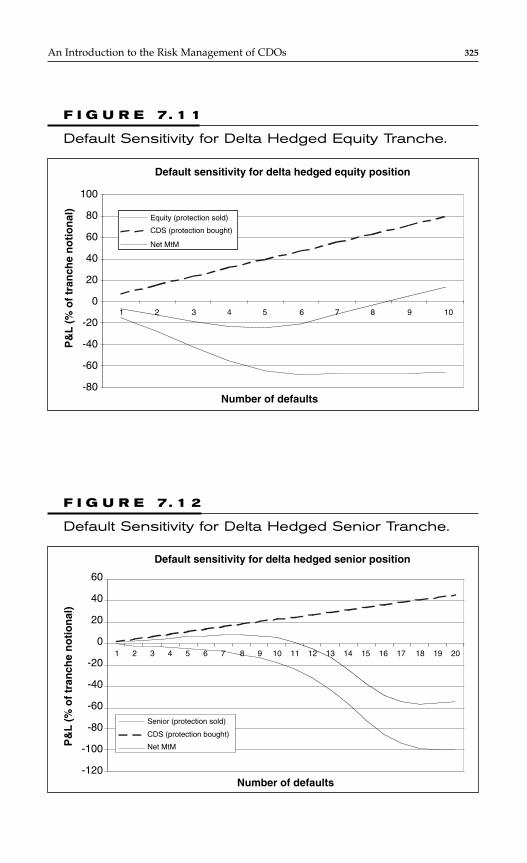
An Introduction to the Risk Management of CDOs 325
Default sensitivity for delta hedged equity position
-80
-60
-40
-20
0
20
40
60
80
100
1 2 3 4 5 6 7 8 9 10
Number of defaults
P&
L (
% o
f tr
anch
e n
oti
on
al)
Equity (protection sold)
CDS (protection bought)
Net MtM
Default sensitivity for delta hedged senior position
-120
-100
-80
-60
-40
-20
0
20
40
60
1 2 3 4 5 6 7 8 9 10 11 12 13 14 15 16 17 18 19 20
Number of defaults
P&
L (
% o
f tr
anch
e n
oti
on
al)
Senior (protection sold)
CDS (protection bought)
Net MtM
F I G U R E 7. 1 1
Default Sensitivity for Delta Hedged Equity Tranche.
F I G U R E 7. 1 2
Default Sensitivity for Delta Hedged Senior Tranche.

By focusing once again on just a single default, i.e., iOmega, we cansay that a long correlation delta hedged tranche has a negative MtM as aresult of default, is short iGamma, and also short iOmega. A short correla-tion delta-hedged tranche (e.g., delta-neutral senior tranche) has positiveMtM after a single default, positive MtM is long iGamma and long iOmega.
(i)Omega and Spread WideningIn practice, it is also interesting to consider situations where spreads onthe surviving names widen as a result of one or more defaults. For a deltahedged equity tranche that is long correlation, a widening of spreads onthe surviving names implies that the realized correlation increases. Thishas a positive MtM impact and would therefore reduce the level of defaultsensitivity (iOmega). Similarly, a short correlation position suffers anMtM loss if all spreads widen and hence, the positive iOmega reduces.
Omega behaves in a similar way, e.g., a delta hedged equitytranche’s default sensitivity reduces if all surviving spreads in the portfo-lio would widen.
Of course, this last example highlights the possibility of interactionbetween various (pricing) variables or risk factors and, as a result, high-lights the need for more advanced sensitivities. For example, time decayin the “Time decay-Theta” section is simply computed as the difference inMtM when we reduce maturity while keeping all the other parametersunchanged. Essentially, we ignore the impact of the new, shorter maturityon other inputs, most notably correlation. If the correlation skew is differ-ent for different maturities, the MtM calculation for a one-year time decayof a five-year tranche should use the four-year base correlation. Similarly,if we calculate spread sensitivity (convexity) and bump spreads up sig-nificantly, we should use the correlation assumption applied for a morejunior tranche. Essentially, these are all higher order effects that can bequite significant and would need to be addressed in more advanced sen-sitivity calculations. We address such issues in Chapter 8 by motivating amore flexible (and computationally demanding) MC framework for CDOrisk management.
SUMMARY AND CONCLUSIONS
This chapter forms the first part of our discussion on CDO risk manage-ment. After a very brief introduction of risk measures important to buy-and-hold investors and rating agencies, we focus on popular MtM
326 CHAPTER 7

sensitivity measures. We start with first order spread sensitivity and deltahedging, by capturing the conceptual paradigm as well as practical imple-mentation. Delta hedging gained widespread acceptance in credit mar-kets, partially because many (fixed-income) risk management systemswere initially designed for single name exposures such as corporatebonds or single name CDSs. For such products, delta hedging has provenadequate and at first sight it seems plausible to introduce synthetic CDOsinto such a risk management framework through their delta-exposures.However, the nonlinearity inherent in tranched products necessitates acloser look into the likely MtM sensitivity to additional risk factors. Weintroduce micro- and macrospread convexity, and show that the sign ofthe MtM impact changes when the overall market is moving instead ofone individual spread. Similarly, the concepts of correlation and instanta-neous default sensitivity are introduced, highlighting—once again—thatsynthetic tranche positions, even when delta-hedged, exhibit significantMtM risk.
Furthermore, spread, correlation, and default risk between varioustranches on the same reference portfolio can vary substantially, providingopportunities to create hedging strategies that immunize against some (orall) of the risks prevailing. For example, equity tranches exhibit substan-tial default risk as well as spread risk, whereas the default risk of seniortranches is much smaller when some spread risk still prevails. A delta-neural combination of equity and senior tranches (has positive carry and)compensates investors for taking default risk without having spreadexposure (at least to first order). The resulting hedge is cheaper than buy-ing protection on all single names; however, residual higher order spreadand correlation risk exist (in addition to the default risk). For example, thestraddle outlined above has significant correlation risk, as changes in cor-relation have an impact on both the long equity and the short seniorexposure.
In the next chapter, the practical aspects of many of these conceptsare put into practice by analyzing several popular CDO strategies. Byinvestigating the performance of real trades, we shed some further lightonto the inadequacy of pure delta-hedging for synthetic tranche products.In addition, we are take a detailed look at risk/return characteristics ofsuch trades.
An Introduction to the Risk Management of CDOs 327
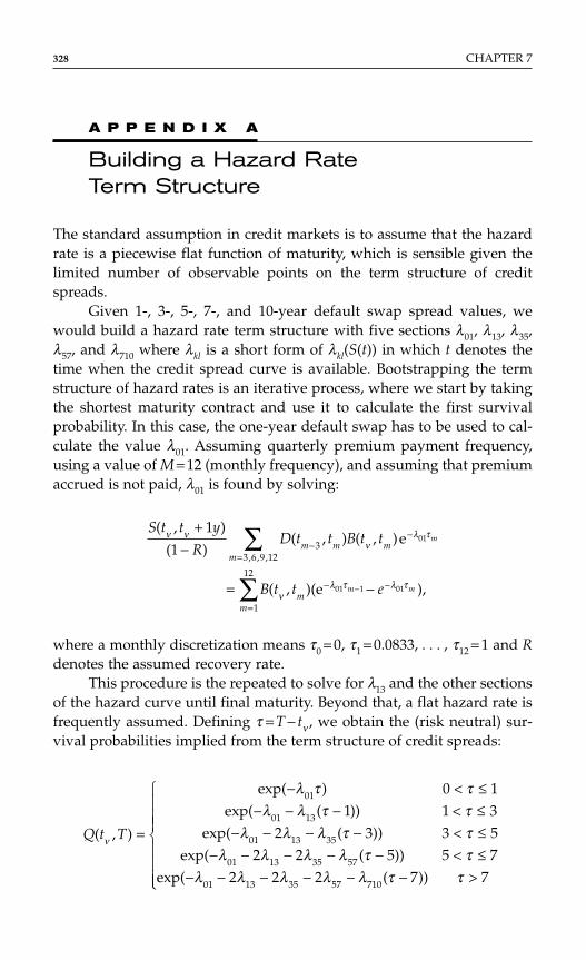
A P P E N D I X A
Building a Hazard Rate Term Structure
The standard assumption in credit markets is to assume that the hazardrate is a piecewise flat function of maturity, which is sensible given thelimited number of observable points on the term structure of creditspreads.
Given 1-, 3-, 5-, 7-, and 10-year default swap spread values, wewould build a hazard rate term structure with five sections λ01, λ13, λ35,λ57, and λ710 where λkl is a short form of λkl(S(t)) in which t denotes thetime when the credit spread curve is available. Bootstrapping the termstructure of hazard rates is an iterative process, where we start by takingthe shortest maturity contract and use it to calculate the first survivalprobability. In this case, the one-year default swap has to be used to cal-culate the value λ01. Assuming quarterly premium payment frequency,using a value of M = 12 (monthly frequency), and assuming that premiumaccrued is not paid, λ01 is found by solving:
where a monthly discretization means τ0 = 0, τ1 = 0.0833, . . . , τ12 = 1 and Rdenotes the assumed recovery rate.
This procedure is the repeated to solve for λ13 and the other sectionsof the hazard curve until final maturity. Beyond that, a flat hazard rate isfrequently assumed. Defining τ = T − tν , we obtain the (risk neutral) sur-vival probabilities implied from the term structure of credit spreads:
Q t T( , )
exp( )exp( ( ))
exp( ( ))exp( ( ))
exp( ( ))
ν
λ τ τλ λ τ τ
λ λ λ τ τλ λ λ λ τ τ
λ λ λ λ λ τ τ
=
− < ≤− − − < ≤
− − − − < ≤− − − − − < ≤
− − − − − − >
01
01 13
01 13 35
01 13 35 57
01 13 35 57 710
0 11 1 3
2 3 3 52 2 5 5 7
2 2 2 7 7
S t t y
RD t t B t t
B t t e
m m mm
mm
m
m m
( , )
( )( , ) ( , )e
( , )(e ),
, , ,
ν νν
λ τ
νλ τ λ τ
+−
= −
−−
=
− −
=
∑
∑ −
1
1 33 6 9 12
1
12
01
01 1 01
328 CHAPTER 7
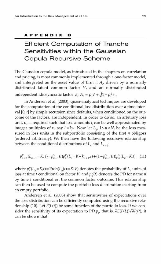
A P P E N D I X B
Efficient Computation of TrancheSensitivities within the GaussianCopula Recursive Scheme
The Gaussian copula model, as introduced in the chapters on correlationand pricing, is most commonly implemented through a one-factor model,and interpreted as the asset value of firm i, Ai, driven by a normallydistributed latent common factor V, and an normally distributed
independent idiosyncratic factor
In Andersen et al. (2003), quasi-analytical techniques are developedfor the computation of the conditional loss distribution over a time inter-val [0, t] by simple recursion since defaults, when conditioned on the out-come of the factors, are independent. In order to do so, an arbitrary lossunit, u, is required such that loss amounts li can be well approximated byinteger multiples of u, say li = kiu. Now let Ln, 1 ≤ n < N, be the loss mea-sured in loss units in the subportfolio consisting of the first n obligors(ordered arbitrarily). We then have the following recursive relationshipbetween the conditional distributions of Ln and Ln + 1:
pn + 1V (Ln + 1 = K, t) = pn + 1
V (t)pnV (Ln = K − kn + 1,t) + (1 − pn + 1
V (t))pnV (Ln = K,t) (11)
where pnV(Ln = K,t) = Prob(Ln(t) = K|V) denotes the probability of Ln units of
loss at time t conditional on factor V, and pnV(t) denotes the PD for name n
by time t conditional on the common factor outcome. This relationshipcan then be used to compute the portfolio loss distribution starting froman empty portfolio.
Andersen et al. (2003) show that sensitivities of expectations overthe loss distribution can be efficiently computed using the recursive rela-tionship (10). Let F(L(t)) be some function of the portfolio loss. If we con-sider the sensitivity of its expectation to PD pi, that is, ∂E(F(L))/∂Pi(t), itcan be shown that
ε ρ ρ εi i i i iA V: .= + −1 2
An Introduction to the Risk Management of CDOs 329

(12)
where Φ denotes the cumulative Gaussian distribution function andci(t) := Φ−1(pi) denotes the default threshold of asset i.
The first two factors of the integrand can be easily computed ana-lytically, and the last factor can be derived from the recursive relationship:
Here, LN − 1i is the loss of the portfolio with the ith obligor removed
and can be obtained from the recursive relationship very efficiently.Within the context of the computation of spread sensitivities for CDO
tranches, we are interested in the computation of
Hence, E(F(L(t))) = MtMTj(t0 ,t,S(t0)) = FPVTj(t0,t,S(t0)) − PPVTj(t0,t,S(t0),where the fee PV and protection PV are functions of the expectedtranche loss , and are given byEquations (7) and (8). As a result, the sensitivity of the MtM with respectto changes in the underlying PD, ofname i requires the calculation of sensitivities of form Equation (12),that is:
∂∂
=
× − −∂
∂
−=
∑FPV ( , , ( ))
( )( , , ( )) ( , ) ( , )
EL ( )
( ), and
T
i
Tk k k
k
K
j j
Tk
i
jj
j
t T S t
p TS t T S t B t D t t
D At
p T
0 00 0 1
1
0
∂∂
=∂
∂−
∂∂
MtM ( , , ( ))
( )
FPV ( , , ( ))
( )
PPV ( , , ( ))
( ), with
T
i
T
i
T
i
j j jt T S t
p T
t T S t
p T
t T S t
p T0 0 0 0 0 0
( MtM ( , , ( )) / ( ))( bp)∂ ∂Ti
j t T S t p T0 0 1
EL t E L t A D ATj j j
j ( ) (max[min( ( ) , ), ])= − − 0
∂S ti ( ))( bp).0 1
( MtM ( , , ( ))/∂ Tj t T S t0 0
∂ ( )∂
=∂ =
∂
= = − − =[ ]∑∑ − − − −
E F L Vp t
F Kp L K t
p t
F K p L K k t p L K t
iV
K
NV
N
iV
KNV
Ni
i NV
Ni
i
( )|( )
( )( , )
( )
( ) ( , ) ( , ) .1 1 1 1
∂ ( )∂
=∂ ( )
∂
=∂ ( )
∂
=
∂ (
∫
∫−
E F Lp t
E F L Vp t
V
p t
p tE F L V
p tV
p t
c t
p t
c tE F L V
i i
iV
i iV
iV
i
i
i
( )( )
( )|( )
d ( )
d ( )
d ( )( )|
( )d ( )
d ( )
d ( )
d ( )
d ( )( )|
Φ
Φ
1))
∂∫ p tV
iV ( )
d ( )Φ
330 CHAPTER 7
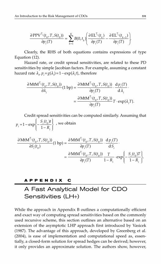
Clearly, the RHS of both equations contains expressions of typeEquation (12).
Hazard rate, or credit spread sensitivities, are related to these PDsensitivities by simple Jacobian factors. For example, assuming a constanthazard rate λi, pi = g(λi) = 1 − expλit, therefore
Credit spread sensitivities can be computed similarly. Assuming that
, we obtain
A P P E N D I X C
A Fast Analytical Model for CDO Sensitivities (LH+)
While the approach in Appendix B outlines a computationally efficientand exact way of computing spread sensitivities based on the commonlyused recursive scheme, this section outlines an alternative based on anextension of the asymptotic LHP approach first introduced by Vasicek(1987). The advantage of this approach, developed by Greenberg et al.(2004), is ease of implementation and computational speed as, essen-tially, a closed-form solution for spread hedges can be derived; however,it only provides an approximate solution. The authors show, however,
∂∂
=∂
∂⋅ ⋅
=∂
∂ −⋅ −
−
MtM ( , , ( ))
( )( bp)
MtM ( , , ( ))
( )
d ( )
d
MtM ( , , ( ))
( )exp
( ).
T
i
T
i
i
i
T
i i
i
i
j j
j
t T S t
S t
t T S t
p T
p T
S
t T S t
p TT
R
S t T
R
0 0
0
0 0
0 0 0
1
1 1
pS t t
Rii
i
≈ − −−
1
10exp
( )
∂∂
=∂
∂⋅ ⋅
=∂
∂⋅
MtM ( , , ( ))( bp)
MtM ( , , ( ))
( )
d ( )
d
MtM ( , , ( ))
( )exp .
T
i
T
i
i
i
T
ii
j j
j
t T S t t T S t
p T
p T
t T S t
p TT T
0 0 0 0
0 0
1λ λ
λ
∂∂
=∂
∂−
∂∂
−
=∑PPV ( , , ( ))
( )( , )
EL ( )
( )
EL ( )
( ).
T
ik
Tk
i
Tk
ik
Kj j jt T S t
p TB t
t
p T
t
p T0 0 1
1
0
An Introduction to the Risk Management of CDOs 331
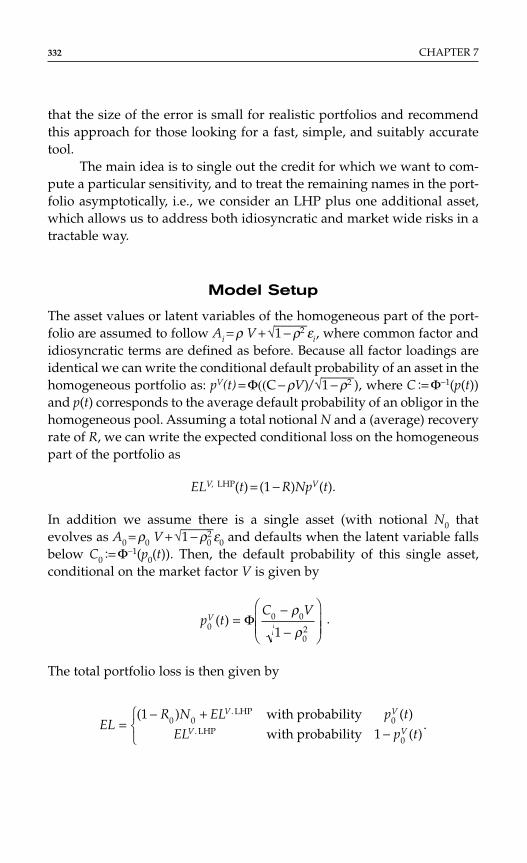
that the size of the error is small for realistic portfolios and recommendthis approach for those looking for a fast, simple, and suitably accuratetool.
The main idea is to single out the credit for which we want to com-pute a particular sensitivity, and to treat the remaining names in the port-folio asymptotically, i.e., we consider an LHP plus one additional asset,which allows us to address both idiosyncratic and market wide risks in atractable way.
Model Setup
The asset values or latent variables of the homogeneous part of the port-folio are assumed to follow Ai = ρ V + √1 − ρ2–––––εi, where common factor andidiosyncratic terms are defined as before. Because all factor loadings areidentical we can write the conditional default probability of an asset in thehomogeneous portfolio as: pV(t) = Φ((C − ρV)/ √1 − ρ2–––––), where C := Φ−1(p(t))and p(t) corresponds to the average default probability of an obligor in thehomogeneous pool. Assuming a total notional N and a (average) recoveryrate of R, we can write the expected conditional loss on the homogeneouspart of the portfolio as
ELV, LHP(t) = (1 − R)NpV(t).
In addition we assume there is a single asset (with notional N0 thatevolves as A0 = ρ0 V + √1 − ρ0
2–––––ε0 and defaults when the latent variable fallsbelow C0 := Φ−1(p0(t)). Then, the default probability of this single asset,conditional on the market factor V is given by
.
The total portfolio loss is then given by
ELR N EL p t
EL p t
V V
V V=− +
−
( ) with probability ( )with probability ( )
.. LHP
. LHP
11
0 0 0
0
p tC V
V0
0 0
021
( ) =−
−
Φ
ρ
ρ
332 CHAPTER 7

PORTFOLIO LOSS DISTIRBUTION
Greenberg et al. (2004) show that the conditional loss distribution,pV (L(t) ≥ K) = Prob(L(t) ≥ K V) ,
is given by pV (L(t) ≥ K) = 1V ≤ X + p0V(t) 1X < V ≤ Y, where
and
Integrating over the common factor V enables us to derive the uncondi-tional loss distribution in terms of the bivariate normal distributionp(L(t) ≥ K) = Φ(X) + Φ2(C0, Y; ρ0) − Φ2(C0, X; ρ0), which can be very easily andaccurately evaluated numerically and is essentially a closed-form approach.
TRANCHE LOSSES
Rewriting the tranche loss LTj(t) = max[min(L(t) = Aj ,Dj − Aj), 0] = [L(t) −A]+ −[L(t) − D]+, is, beneficial as it can be shown that the expectation E[L(t) − K]+
can also be computed very efficiently within the current model setup:
where denotes the covariance matrix used in the
evaluation of the trivariate normal distribution that can also be evaluatedvery efficiently, see, e.g., Genz (2002).
CREDIT SPREAD SENSITIVITY
Calculation of credit spread sensitivities
∂∂
=∂
∂−
∂∂
MtM ( , , ( ))
( )
FPV ( , , ( ))
( )
PPV ( , , ( ))
( )
T
i
T
i
T
i
j j jt T S t
S t
t T S t
S t
t T S t
S t0 0
0
0 0
0
0 0
0
Σ =
1
1
1
0 0
0
0
ρρ ρ
ρρ ρ
ρ ρ
E L t K K C X X R N K C Y
R N C X C C Y C C X
([ ( ) ] ) ( , ; ) ( ) ( ) ( , ; )
( ) ( , ; ) ( , , ; ) ( , , ; )
− = −( ) + − −( )+ −( ) + −[ ]
+ Φ Φ Φ
Φ Φ Φ2 0 0 0 0 2 0 0
2 3 0 3 0
1
1
ρ ρ
ρ Σ Σ
Y K CK R N
R N( )
( )
( ).= − −
− −−
−1
11
12 1 0 0
ρρ Φ
X K CKR N
( )( )
= − −−
−1
11
2 1
ρρ Φ
An Introduction to the Risk Management of CDOs 333

requires the efficient computation of , as
.
Greenberg et al. (2004) show that can be computed veryefficiently as
∂∂
=−−
−
−
+ − −−
−
+ −−
−
EL tS t
Tp
RA
X A C
R N AY A C
R NC C Y
T
ij
j
jj
j ( )( )
( )
[( ) ]( )
( )( )
,(
0
0
0
0 0
02
0 00 0
02
20 0
02
1
1 1
11
11
Φ
Φ
Φ
ρ
ρ
ρ
ρ
ρρ
ρρ
AA C
C C X A C
DX D C
R N DY D
j
j
jj
jj
);
( ),
( );
( )( )
( )
−
−
−−
−
−
−
−−
−
− − −[ ]
ρ
ρρ
ρρ
ρρ
ρ
ρρ
ρ
ρ
0 0
02
20 0
02
0 0
02
0 0
02 0 0
1
1 1
11
Φ
Φ Φ−−
−
− −−
−
−
−
−−
−
−
−
ρ
ρ
ρρ
ρρ
ρ
ρρ
ρρ
ρρ
ρ
ρρ
0 0
02
20 0
02
0 0
02
20 0
02
0 0
02
1
11 1
1 1
C
R NC C Y D C
C C X D C
j
j
( )( )
,( )
;
( ),
( );
Φ
Φ
∂∂EL tS t
T
i
j ( )( )0
∂∂
=∂∂
−∂
∂
−
=∑PPV ( , , ( ))
( )( , )
( )
( )
( )
( )
T
ik
Tk
i
Tk
ik
Kj j jt T S t
S tB t
EL t
S t
EL t
S t0 0
0 0
1
01
0
∂∂
=
× − −∂∂
−=
∑FPV ( , , ( ))
( )( , , ( )) ( , ) ( , )
( )
( )and
T
i
Tk k k
k
K
j j
Tk
i
jj
j
t T S t
S tS t T S t B t D t t
D AEL t
S t
0 0
00 0 1
1
0
0
∂∂EL t
S t
Tk
i
j ( )
( )0
334 CHAPTER 7
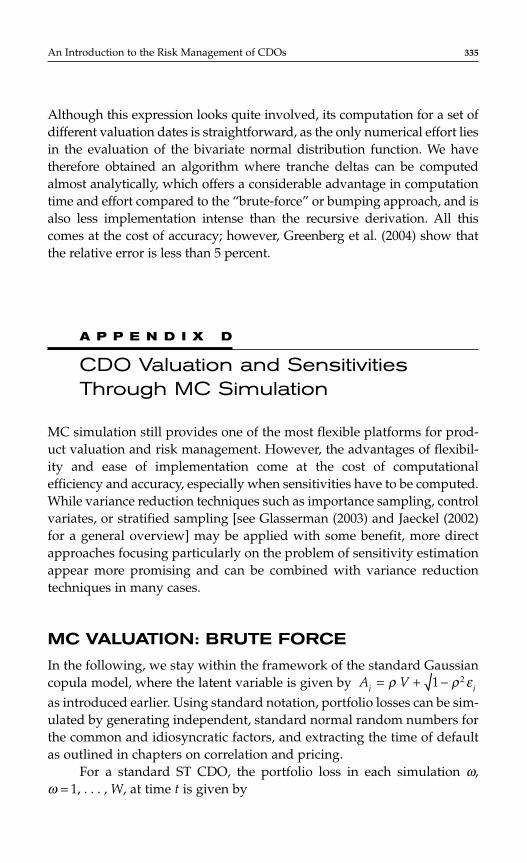
Although this expression looks quite involved, its computation for a set ofdifferent valuation dates is straightforward, as the only numerical effort liesin the evaluation of the bivariate normal distribution function. We havetherefore obtained an algorithm where tranche deltas can be computedalmost analytically, which offers a considerable advantage in computationtime and effort compared to the “brute-force” or bumping approach, and isalso less implementation intense than the recursive derivation. All thiscomes at the cost of accuracy; however, Greenberg et al. (2004) show thatthe relative error is less than 5 percent.
A P P E N D I X D
CDO Valuation and SensitivitiesThrough MC Simulation
MC simulation still provides one of the most flexible platforms for prod-uct valuation and risk management. However, the advantages of flexibil-ity and ease of implementation come at the cost of computationalefficiency and accuracy, especially when sensitivities have to be computed.While variance reduction techniques such as importance sampling, controlvariates, or stratified sampling [see Glasserman (2003) and Jaeckel (2002)for a general overview] may be applied with some benefit, more directapproaches focusing particularly on the problem of sensitivity estimationappear more promising and can be combined with variance reductiontechniques in many cases.
MC VALUATION: BRUTE FORCE
In the following, we stay within the framework of the standard Gaussiancopula model, where the latent variable is given by as introduced earlier. Using standard notation, portfolio losses can be sim-ulated by generating independent, standard normal random numbers forthe common and idiosyncratic factors, and extracting the time of defaultas outlined in chapters on correlation and pricing.
For a standard ST CDO, the portfolio loss in each simulation ω,ω = 1, . . . , W, at time t is given by
A Vi i= + −ρ ρ ε1 2
An Introduction to the Risk Management of CDOs 335
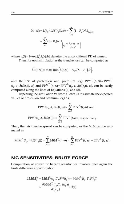
where pi(t) = 1− exp[∫t0λi(s)ds] denotes the unconditional PD of name i.
Then, for each simulation ω the tranche loss can be computed as
and the PV of protection and premium leg, PP (t, ω) = PP(t0, t, λ(S(t0)), ω) and FP (t, ω) = FP (t0, t, λ(S(t0)), ω), can be easilycomputed along the lines of Equations (7) and (8).
Repeating the simulation W times allows us to estimate the expectedvalues of protection and premium legs as
and
respectively.
Then, the fair tranche spread can be computed, or the MtM can be esti-mated as
MC SENSITIVITIES: BRUTE FORCE
Computation of spread or hazard sensitivities involves once again thefinite difference approximation
∆ MtM MtM ( , , ( )) MtM ( , , ( ))
MtM ( , , ( ))
( )( )
i
T T i T
T
i
j j j
j
t T S t t T S t
t T S t
S tbp
= −
≈∂
∂
001
0 0 0
0 0
0
1
MtM ( , , ( ( ))) MtM ( , ) FPV ( , ) PPV ( , ).T TW
TW
Tj j j jt t S t t t t0 01 1
λ ω ω ωω ω
= = −= =
∑ ∑
FPV ( , , ( ( ))) FPV ( , ),T TW
j jt t S t t0 01
λ ωω
==
∑
PPV ( , , ( ( ))) PPV ( , )T TW
j jt t S t t0 01
λ ωω
==
∑
VTjVTj
VTjVTj
L t L t A D ATj j j
j ( , ) max min ( , ) , , ,ω ω= − −( )
0
L t L t t S t R N
R N
i i ti
N
i i p t Vi
N
i
ii
( , ): ( , ( ( )), ) ( )
( )
,
( ( ))
ω λ ω τ
ερ
ρ
= = −
= −
≤=
≤−
−
=
∑
∑ −
0 01
11
1 1
1 11
2
Φ
336 CHAPTER 7

within the MC framework. The brute force computation of sensitivitiesproceeds by bumping of the spread curve and re-evalution; i.e.,
Of course, the problem with this MC simulation is that the sensitivity ismainly determined by just a few MC paths. Shifting the spread curve ofname i by 1 bp will increase this PD slightly, and hence decrease the defaulttime. The sensitivity is therefore mainly determined by the few paths thatresult in additional defaults, and only when this additional default resultsin an additional payout of the default leg of the CDO. In general, it is obvi-ous that such a solution is highly unstable, and approaches focusing moredirectly on MC sensitivities need to be considered.
MC Sensitivities: Likelihood Ratio Method
One such approach that greatly enhances computation and accuracy is thelikelihood ratio method. Rott and Fries (2005) show that we can approxi-mate the derivative by
where LRi denotes the likelihood ratio for the change of measure from theoriginal to the shifted default intensities for the underlying credit i. If wedenote by τi and the random default times corresponding to the inten-sities λi(Si) and λi(Si + 1 bp), respectively, and by di(t) = λit(Si + 1 bp) − λit(Si),the difference in intensities at time t, it can be shown that within each MCsimulation, this likelihood ratio is given by
Here, τi(ω) denotes the simulated default time in iteration ω, and φ denotesthe density of the standard normal distribution function, while Φ denotesthe cumulative distribution functions of the standard normal distribution.
LR ( )[ ( ( ( )) ]/
[ ( ( ( )) ]/
( ( ( ))
( ( ( ))
( ( ))
( ( ))
i
i i
i i
i i
i i
i
i i
P V
P V
P
P
e w
w
ωφ τ τ ω ρ ρ
φ τ τ ω ρ ρ
φ τ τ ω
φ τ τ ω
τλ τ
=≤ − −( )( )≤ − −( )( )
≤( )≤( )
× +
−
−
−
−
Φ
Φ
Φ
Φ
1 2
1 2
1
1
1
1
1
−
∫exp ( )d .
( )d s si
wi
0
τ
τ i
∂∂
≈ −[ ]=
∑MtM ( , , ( ))
( )( ) MtM ( , , ( ( )), )(LR ( ) ) ,
T
i
Ti
Wjj
t T S t
tbp
Wt T S t0 0
00 0
1
11
1λ
λ ω ωω
∆ MtM MtM ( , , ( ( )), ) MtM ( , , ( ( )), ) .i
TW
T i Tj j j
Wt T S t t T S t= −[ ]
=∑1
10
010 0 0
ω
λ ω λ ω
An Introduction to the Risk Management of CDOs 337

From this expression, it is apparent that only the default times τi(ω)are simulated from the original spread or hazard curve, and each simula-tion path contributes to the computation of the hazard sensitivity. Thismethod depends purely on the density of the default times and not on thepayoff as such; hence, once implemented for ST CDOs, it also works forall other credit products where a valuation code is available. Furtherdetails on the likelihood ratio method within the Gaussian copula frame-work can be found in Rott and Fries (2005) and Joshi and Kainth (2003).
An alternative to the previous method is the pathwise method, whichis often the most efficient, but the payoff of each product must be differen-tiated analytically, which makes it more difficult to implement. We refer thereader to Joshi and Kainth (2003) and Glasserman (2003) for further details.
REFERENCESAndersen, L., J. Sidenius, and S. Basu (2003), “All your Hedges in One Basket,”
Risk, November, 67–72.Berndt, A., R. Douglas, D. Duffie, M. Ferguson, and D. Schranz (2005),
“Measuring Default Risk Premia from Default Swap Rates and EDFs,”working paper, Tepper School of Business, Carnegie Mellon University.
Brasch, H-J. (2004), “A note on efficient pricing and risk calculation of credit bas-ket products,” working paper.
Genz. (2002), “Numerical Computation of Rectangular Bivariate and TrivariateNormal and t Probabilities,” Department of Mathematics, WashingtonState University.
Gibson, M. (2004), “Understanding the risk of synthetic CDOs,” working paper.Glasserman, P. (2003), Monte Carlo Methods in Financial Engineering, Springer.Glasserman, P., and J. Li (2003), “Importance sampling for portfolio credit risk,”
working paper.Greenberg, A., D. O’Kane, and L. Schloegl (2004), “LH+: A fast analytical model
for CDO hedging and risk management,” Quantitative Credit ResearchQuarterly, Lehman Brothers, Q2.
Jaeckel, P. (2002), Monte Carlo Methods in Finance, Wiley Interscience.Joshi, M., and D. Kainth (2003), “Rapid and accurate development of prices and
greeks for nth to default credit swaps in the Li model,” working paper.Kakodkar, A., B. Martin, and S. Galiani (2003), “Correlation trading,” Fixed-
Income Stategy, Merrill Lynch.O’Kane, D., and S. Turnbull (2003), “Valuation of Credit Default Swaps,”
Quantitative Credit Research Quarterly, Lehman Brothers, Q1/Q2.Rott, M. G., and C. P. Fries (2005), “Fast and Robust Monte Carlo CDO sensitivi-
ties,” working paper.Vasicek, O. (1987), “Probability of loss on loan portfolio,” working paper,
Moody’s KMV.
338 CHAPTER 7
C H A P T E R 8
A Practical Guide to CDOTrading Risk Management
Andrea Petrelli, Jun Zhang, Norbert Jobst, and Vivek Kapoor
339
INTRODUCTION AND MOTIVATION
The collateral debt obligations (CDO) modeling framework with staticspread term structures and employing copula functions (see Chapters4 and 6 for further details) is taking hold in the accounting of syn-thetic CDO trading profit and loss (P&L). This has been spurred bytranches on standardized credit indexes (e.g., CDX.NA.IG, CDX.NA.HY,ITRAXX Eur, etc.) that have provided a calibration target for pricingmodels. There are ongoing discussions on different ways of fitting pricesacross the capital structure (e.g., “compound correlation,” versus “basecorrelation”) as discussed in Chapter 6. Less understood are hedgingstrategies and their cost and effectiveness, and the basic risk-rewardprofiles of popular CDO trading strategies and the associated capital-ization needs for banks. The two main reasons for this state of affairsare:
1. The popular emphasis and practical techniques for pricing CDOtranches have not addressed replication and hedging errors(accounting for spread diffusion, spread jumps, and jumps todefault with uncertain recovery) and therefore have not resultedin a commensurate maturing of the hedging and risk manage-ment paradigm.
Copyright © 2007 by The McGraw-Hill Companies. Click here for terms of use.

2. Risk aggregation regimes that are based merely on marginaland linear spread sensitivities are rendered ineffective andmisleading due to the nonlinearity created by tranching (i.e.,payoff is non linear in reference asset performance). Theselinear risk aggregation regimes are deeply entrenched in riskmanagement circles that have not effectively participated in therevolution of structured credit products.
The practical task of assessing risk and developing a hedging strategyinvolves delineating probabilistic descriptions of the variables that theprevalent pricing models depend upon, and assessing a probabilisticdescription of the P&L associated with the trading strategy. While Chapter7 focused on the conceptual framework and practical computation ofpopular risk measures, this Chapter is focused on assessing credit relatedrisks and P&L performance. It can, therefore, be seen as part two of ourdiscussion of CDO risk management.
The risks in one elementary long-only credit trade (sell protection ona credit index) and three popular synthetic CDO strategies are comparedthroughout this chapter. We will illustrate how marginal spread anddefault sensitivities are insufficient for the CDO trading strategieson account of the nonlinearities created by tranching credit exposures,despite providing a good description of the elementary credit strategy(sell protection on pool of names). In addition, we will compare the carryat inception with the downsides of popular CDO trades and provide acomparison of the carry and value on default (VOD) probabilitydistributions for different CDO strategies.
After analyzing the risk characteristics of static portfolios in terms ofdefault, spread, and correlation as introduced in Chapter 7, we providean exposition of dynamic hedging and risk management. Specifically, weexplore the equity trade (sell equity protection and buy index protection)and show how the trading P&L evolves and can be attributed to differentmarket variables. We therefore go beyond the static risk measurespreviously described.
OVERVIEW OF SOME POPULAR TRADING STRATEGIES
Throughout this chapter, we will investigate a number of popular CDOtrading strategies by using the tools introduced in Chapter 7, and by
340 CHAPTER 8

providing a probabilistic P&L exposition. The trading strategies consid-ered are outlined next:
Elementary Portfolio
Selling protection on an index of credit default swap (CDS) is an exampleof an elementary credit portfolio. For example, the credit index,CDX.NA.IG, consisting of 125 North American credits, will be used toprovide sample calculations. The risk-profile for the CDO trades will becompared with risks incurred in simply selling protection on the index.
CDO Portfolios
Quotes on tranches referencing credit indices and market participants’estimates of associated deltas (CS01 or Credit01 hedges)* are widely avail-able on at least a daily frequency. These trades are sometimes based ondelta-exchanges, which are ostensibly CS01 “hedges” for the tranches,which can, in certain strategies, be the long credit risk driver. We focus onthree CDO trades based on such an indexed product:
I. Positive Carry Equity Tranche TradeSell protection on the 0 to 3 percent tranche referencing the CDX.NA.IGindex and hedge CS01 exposure by buying protection on the index.
II. Positive Carry Straddle TradeSell protection on 0 to 3 percent of the CDX.NA.IG index and hedge CS01exposure by buying protection on the 7 to 10 percent tranche.
III. Positive Carry Senior Mezzanine Tranche TradeBuy protection on the 7 to 10 percent tranche of the CDX.NA.IG index andhedge CS01 exposure by selling protection on the index.
In these CDO strategies, at execution, the premium received as a resultof selling credit protection exceeds the premium paid to immunize small
A Practical Guide to CDO Trading Risk Management 341
*CS01 and Credit01 terminology was introduced in Chapter 7 to denote single name andbroad market sensitivity, respectively. Throughout this chapter, we will mostly use CS01notation, for both, single name and market spread sensitivity. Unless otherwise stated, weare mostly concerned with hedging strategies that employ a credit index.
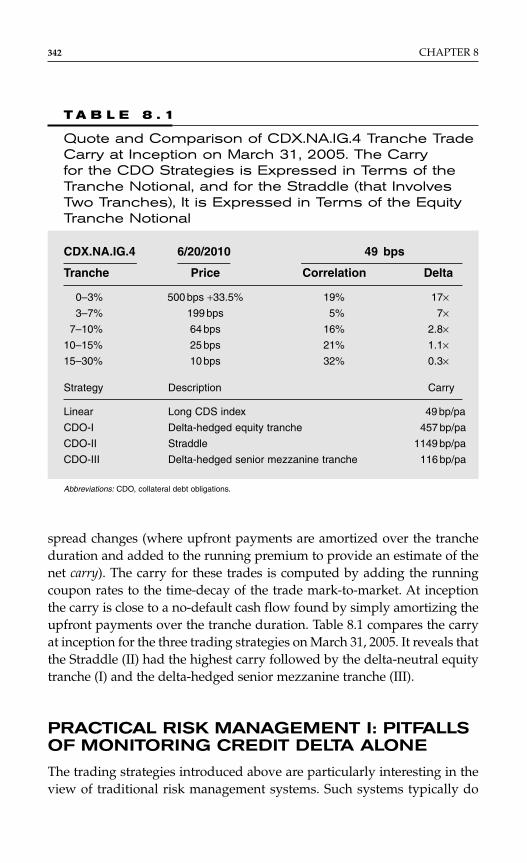
spread changes (where upfront payments are amortized over the trancheduration and added to the running premium to provide an estimate of thenet carry). The carry for these trades is computed by adding the runningcoupon rates to the time-decay of the trade mark-to-market. At inceptionthe carry is close to a no-default cash flow found by simply amortizing theupfront payments over the tranche duration. Table 8.1 compares the carryat inception for the three trading strategies on March 31, 2005. It reveals thatthe Straddle (II) had the highest carry followed by the delta-neutral equitytranche (I) and the delta-hedged senior mezzanine tranche (III).
PRACTICAL RISK MANAGEMENT I: PITFALLSOF MONITORING CREDIT DELTA ALONE
The trading strategies introduced above are particularly interesting in theview of traditional risk management systems. Such systems typically do
342 CHAPTER 8
T A B L E 8 . 1
Quote and Comparison of CDX.NA.IG.4 Tranche TradeCarry at Inception on March 31, 2005. The Carryfor the CDO Strategies is Expressed in Terms of theTranche Notional, and for the Straddle (that InvolvesTwo Tranches), It is Expressed in Terms of the EquityTranche Notional
CDX.NA.IG.4 6/20/2010 49 bps
Tranche Price Correlation Delta
0–3% 500 bps +33.5% 19% 17×3–7% 199 bps 5% 7×
7–10% 64 bps 16% 2.8×10⁻¹⁵% 25 bps 21% 1.1×15–30% 10 bps 32% 0.3×
Strategy Description Carry
Linear Long CDS index 49 bp/pa
CDO-I Delta-hedged equity tranche 457 bp/pa
CDO-II Straddle 1149 bp/pa
CDO-III Delta-hedged senior mezzanine tranche 116 bp/pa
Abbreviations: CDO, collateral debt obligations.
not address structured credit capital structures and the ensuing credit non-linearity. These risk systems were built for aggregating risks from vanillacredit products, such as corporate bonds or single name CDS, and aredesigned to monitor delta exposures (“bond equivalent market values” ascustomary in big bond shops, or delta-notional, respectively). These riskmanagement systems typically monitor CS01: i.e., the change in mark-to-market (mtm) due to an issuer spread widening by 1 bps. Even for a singleCDS, this is a simplification because the duration over which premiumsare expected to be paid depends on the issuer risk-neutral default probabil-ity and then non linearly on the issuer spreads. As a consequence, the P&Limpact of spreads changing by more than 1 bps doesn’t have to be theproduct of CS01 and the spread move (in bps). Indeed, if an issuer, onwhich a trading book has sold default protection, was to suddenly approachdefault (say by an unbounded spread rise), the loss is bounded above bythe notional amount (minus recovery and adjusting for mtm). Such non-linearity is endemic to credit instruments and it renders the results ofsensitivity based risk management systems as approximations of the truerisks. However for vanilla credit, such approximations are not pernicious.A book that is a net CDS protection purchaser will have its losses underspread tightening understated in a CS01 based system. A book that is a netCDS protection seller will have its losses under extreme moves somewhatexaggerated in a CS01 based system. In either situation, the sign of themtm move incurred due to the extreme spread widening or tightening iscaptured by the spot CS01 of a vanilla credit book.
In the presence of such risk management regimes, the chosen CDOstrategies can be particularly popular as they essentially provide positivecash flows (carry) with no delta exposure (widely regulated and moni-tored risk). In addition, if risk capital requirements are explicitly drivenby, or proportional to, delta exposures, as they have been traditionallyand continue to be, trading desks can essentially book positive-carrywithout having to set aside anticipatory risk capital.
Unless risk management systems and risk capital models capturecredit spread-default convexity (single name and marketwide), and corre-lation risk measures, the risk–return characteristics of CDO trading strate-gies illustrated here can be quite different compared to risk managementrendition based on the equivalent “delta-portfolio.” We show here how the“delta-portfolio” can miss both the risks and the opportunities in CDOtrading. In the next section, we shed some light on the sensitivities intro-duced in Chapter 7 for the three CDO strategies, before providing a fullP&L (back-testing) case study thereafter.
A Practical Guide to CDO Trading Risk Management 343

Credit Spread Sensitivity
As previously discussed, a CS01 based risk management framework canprovide a good approximation for vanilla credits, while the nonlinearityintroduced through tranching creates non monotonic mtm changes forspread changes (e.g., market moves versus single-name, idiosyncraticmoves). Here, we put the machinery developed in Chapter 7 into practiceand examine model CDO trades. At inception, there is little or no “CS01risk,” yet if spreads were to blowout on any issuer name, the trade incursa mtm loss. Figures 8.1 to 8.3 show the mtm impact when spreads on mul-tiple names are widening-tightening for the three trading strategies,respectively. For each figure, the bottom panel provides a “zoom-in” forspread shifts from −20 to 40 bps.
We can clearly see that the mtm impact of spread widening on mul-tiple names is certainly not the same as the sum of mtm impacts whenindividual names widen, and that the impact is amplified for larger spreadchanges. In fact, the simultaneous widening of spreads on many namescould result in an mtm gain for the strategies shown here. This is referredto as having “positive index gamma.” The positive index gamma can be ofa local nature (e.g., if all names widen by 100 bps the mtm impact is posi-tive), and the event of the spreads of all names increasing unboundedlycould still be a loss event as shown in Figure 8.3 for the delta-neutral se-nior mezzanine tranche. It is also interesting to note that all trades appearto incur a positive mtm impact when spreads blow out enormously onsomewhere between 5 and 10 names. However, while a further wideningon even more names leads to larger and larger gains for the first two strate-gies, Figure 8.3 reveals that large “blowouts” may reduce the mtm gainagain or even cause losses if the number of blowouts is too large.
While some of these spread shock scenarios are quite unlikely, it isinteresting to note that when considering more realistic market changes(e.g., a large number of assets moving by moderate amounts, or thespreads of a few names widening modestly, as shown in the lower panelsof Figures 8.1 to 8.3), the mtm sensitivity of the CDO trades is an increas-ing function of the initial trade carry (Table 8.1). The highest carry trade,the straddle (II), has the highest spread sensitivity, while the lowest carrytrade, the senior mezzanine trade (III), has the lowest, when consideringa spread shock scenarios in the range of −20 to +50 basis points. For thestraddle, this is caused by the higher convexity causing larger losses (inthe event of the spread of a handful of names widening) on both sides ofthe trade (i.e., long equity and short senior tranche).
344 CHAPTER 8
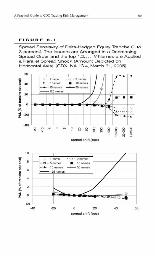
A Practical Guide to CDO Trading Risk Management 345
(40)
(20)
0
20
40
60
-20
-10 -5 0 5 10 20 50 100
300
1,00
0
10,0
00
20,0
00
Def
ault
1 name 2 names5 names 10 names
15 names 50 names125 names
P&
L (%
of t
ranc
he n
otio
nal)
(2)
0
2
4
6
8
10
-40 -20 0 20 40 60
spread shift (bps)
spread shift (bps)
1 name 2 names
5 names 10 names15 names 50 names
125 names
P&
L (%
of t
ranc
he n
otio
nal)
F I G U R E 8 . 1
Spread Sensitivity of Delta-Hedged Equity Tranche (0 to3 percent). The Issuers are Arranged in a DecreasingSpread Order and the top 1,2, . . . , N Names are Applieda Parallel Spread Shock (Amount Depicted onHorizontal Axis). (CDX. NA. IG.4, March 31, 2005)
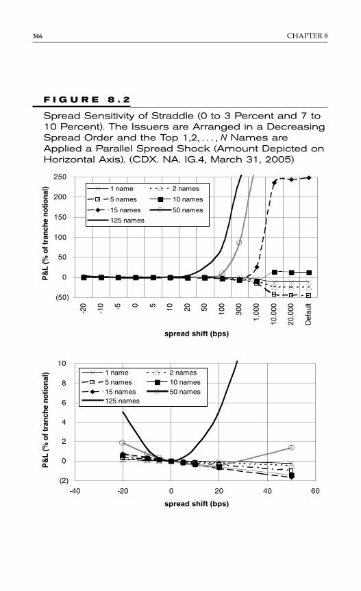
346 CHAPTER 8
(50)
0
50
100
150
200
250
-20
-10 -5 0 5 10 20 50 100
300
1,00
0
10,0
00
20,0
00
Def
ault
1 name 2 names
5 names 10 names
15 names 50 names
125 names
P&
L (%
of t
ranc
he n
otio
nal)
(2)
0
2
4
6
8
10
-40 -20 0 20 40 60
1 name 2 names5 names 10 names15 names 50 names125 names
P&
L (%
of t
ranc
he n
otio
nal)
spread shift (bps)
spread shift (bps)
F I G U R E 8 . 2
Spread Sensitivity of Straddle (0 to 3 Percent and 7 to10 Percent). The Issuers are Arranged in a DecreasingSpread Order and the Top 1,2, . . . , N Names areApplied a Parallel Spread Shock (Amount Depicted onHorizontal Axis). (CDX. NA. IG.4, March 31, 2005)
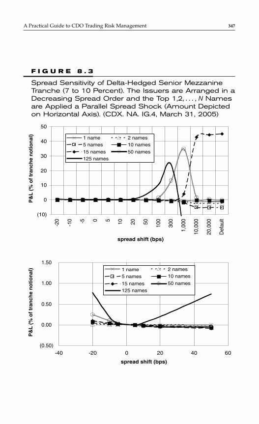
A Practical Guide to CDO Trading Risk Management 347
(10)
0
10
20
30
40
50
-20
-10 -5 0 5 10 20 50 100
300
1,00
0
10,0
00
20,0
00
Def
ault
1 name 2 names5 names 10 names
15 names 50 names125 names
P&
L (
% o
f tr
anch
e n
oti
on
al)
(0.50)
0.00
0.50
1.00
1.50
-40 -20 0 20 40 60
P&
L (
% o
f tr
anch
e n
oti
on
al)
spread shift (bps)
spread shift (bps)
1 name5 names
15 names125 names
2 names10 names
50 names
F I G U R E 8 . 3
Spread Sensitivity of Delta-Hedged Senior MezzanineTranche (7 to 10 Percent). The Issuers are Arranged in aDecreasing Spread Order and the Top 1,2, . . . , N Namesare Applied a Parallel Spread Shock (Amount Depictedon Horizontal Axis). (CDX. NA. IG.4, March 31, 2005)

Hence, the carry may be seen as compensation for the idiosyncraticand systematic spread risk inherent in the corresponding CDO strategies.These examples highlight how a marginal CS01 based risk managementframework does not effectively capture risks prevailing in popular CDOstrategies. The spread sensitivity computations show that the popularCDO strategies are susceptible to idiosyncratic spread move risks, andany effort to “bucket” spread moves by ratings or sectors and potentiallyperturb many issuers simultaneously in the same direction is a poor wayto assess CDO trading “market risks.” The market risk of these CDOstrategies can be controlled by the propensity of spreads to not movetogether and, therefore, the broad-brush coherent moves based on eithersector or ratings are misleading.
In practice, when interested in synthetic CDO trading Value at Risk(VaR), both CS01 based VaR and/or VaR based on broad market movesare troublesome. While a CS01 based “VaR” can be completely uninfor-mative for synthetic CDOs (by not addressing convexity and correlationrisk), a “VaR” based on broad index moves can be even more misleading,because the positive carry strategies encounter losses under spread twistsand not necessarily under coherent parallel shocks that are more amenableto traditional “market-risk” scenarios.
As a result, while there can be index or sector factor drivers for spreadmoves, a name specific spread time series (modeled or historically sam-pled) is a prerequisite for articulating a hedging strategy and for assessinga synthetic CDO trading VaR. Hence, good risk management requires a rea-sonable (probabilistic) description of possible future outcomes including a“real world” description of the credit spread environment.
The actual hedging, of course, still employs liquid indices because ofease–efficiency of execution. Periodic single name hedging can be under-taken as an overlay on top of the index hedging if one desires to maintaina small CS01 exposure per name. As the index is equally weighted, andthe hedge ratios per name (found by bumping individual spreads one ata time) are not identical, employing the index as a CS01 hedge results inslight residual negative and positive CS01 exposures to individualnames.*
348 CHAPTER 8
*Note that whether one bumps all the names 1 bps simultaneously and finds the overallindex hedge ratio (in terms of notional), or one bumps individual names to assess individ-ual hedge ratios and hedges using the index with a notional that equals the sum of the indi-vidual hedge notionals, one arrives at the same point (because convexity does not manifeststrongly at 1 bps).

Correlation Sensitivity
For illustration purposes all of the sensitivities shown above did not involveany changes to the implied correlation of the tranches. The tranche impliedcorrelation reflects how the market views interact with model assumptions,which are: (1) static spread term structure; (2) normal copula; (3) fixed recov-ery; (4) deterministic asset-correlation structure. Indeed, there is no way toseparate the effect of all of these assumptions once they have been throwninto the kitchen sink of implied correlation. Correlation is not the only uncer-tain variable in portfolio credit derivative pricing. Recovery uncertainty andrecovery-default correlation are long outstanding features that do not findsystematic treatment even in single name CDS pricing practice, to date.
The need for different implied correlation values to be used in pric-ing different tranches across the capital structure is referred to as the cor-relation skew. The correlation skew can be at least qualitatively explainedwith even a small set of the kitchen sink ingredients.
In the standard pricing model with static spreads, the asset correla-tion input controls the correlation between the times to default of differ-ent issuers. The value of buying protection on a tranche is a nonlinearfunction of the input correlation as shown in Figure 8.4. Therefore if onehypothesizes a correlation uncertainty band and assesses the expectationof the tranche value under uncertain correlation, one gets a price that ispossibly quite different from what one gets by simply inputting the aver-age correlation (Jensen’s inequality). As value of default protection in dif-ferent tranches have different degrees of dependence on the correlationinput parameter, the implied correlation that produces the same price, asfound under a correlation uncertainty band, is tranche-dependent. Theserudimentary correlation convexity arguments are sufficient to explain thecorrelation skew qualitatively. Of course, asset and default correlation arenot deterministically knowable parameters. Under significant correlationconvexity, it is inconceivable for the market to price different tranches ofthe same structure at the same implied correlation.
As correlation is a pricing variable, CDO trades are exposed to themarket risk of that pricing parameter changing. Interestingly, just like forspread-convexity for small to medium spread movements the correlationsensitivity is also an increasing function of the initial trade carry (seeFigure 8.4 for the three CDO trades analyzed here). The highest carrytrade, the straddle, has the highest correlation sensitivity (moving boththe equity and senior mezzanine tranche correlation simultaneously inthe same direction which is not guaranteed to occur). The equity tranche
A Practical Guide to CDO Trading Risk Management 349
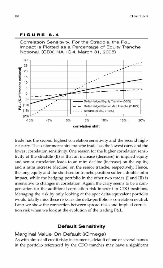
trade has the second highest correlation sensitivity and the second high-est carry. The senior mezzanine tranche trade has the lowest carry and thelowest correlation sensitivity. One reason for the higher correlation sensi-tivity of the straddle (II) is that an increase (decrease) in implied equityand senior correlation leads to an mtm decline (increase) on the equity,and a mtm increase (decline) on the senior tranche, respectively. Hence,the long equity and the short senior tranche position suffer a double mtmimpact, while the hedging portfolio in the other two trades (I and III) isinsensitive to changes in correlation. Again, the carry seems to be a com-pensation for the additional correlation risk inherent in CDO positions.Managing the risk by only looking at the spot delta-equivalent portfoliowould totally miss these risks, as the delta-portfolio is correlation neutral.Later we show the connection between spread risks and implied correla-tion risk when we look at the evolution of the trading P&L.
Default Sensitivity
Marginal Value On Default (iOmega)As with almost all credit risky instruments, default of one or several namesin the portfolio referenced by the CDO tranches may have a significant
350 CHAPTER 8
(20)
(15)
(10)
(5)
0
5
10
15
20
25
30
-10% -5% 0% 5% 10% 15% 20%
correlation shift
Delta Hedged Equity Tranche (0-3%)
Delta Hedged Senior Mez Tranche (7-10%)
Straddle (0-3%, 7-10%)
P&
L (%
of t
ranc
he n
otio
nal)
F I G U R E 8 . 4
Correlation Sensitivity. For the Straddle, the P&LImpact is Plotted as a Percentage of Equity TrancheNotional. (CDX. NA. IG.4, March 31, 2005)
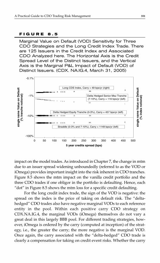
impact on the model trades. As introduced in Chapter 7, the change in mtmdue to an issuer spread widening unboundedly (referred to as the VOD oriOmega) provides important insight into the risk inherent in CDO tranches.Figure 8.5 shows the mtm impact on the vanilla credit portfolio and thethree CDO trades if one obligor in the portfolio is defaulting. Hence, each“dot” in Figure 8.5 shows the mtm loss for a specific credit defaulting.
For the long credit index trade, the sign of the VOD is negative: thespread on the index is the price of taking on default risk. The “delta-hedged” CDO trades also have negative marginal VODs to each referenceentity in the pool. Within each positive carry CDO strategy onCDX.NA.IG.4, the marginal VODs (iOmega) themselves do not vary agreat deal in this largely BBB pool. For different trading strategies, how-ever, iOmega is ordered by the carry (computed at inception) of the strat-egy, i.e., the greater the carry; the more negative is the marginal VOD.Once again, the carry associated with the “delta-hedged” CDO trade isclearly a compensation for taking on credit event risks. Whether the carry
A Practical Guide to CDO Trading Risk Management 351
0 50 100 150 200 250 300 350 400 450 500
5 year credits spread (bps)
sin
gle
nam
e V
alu
e o
n D
efau
lt(%
tra
nch
e n
oti
on
al)
sin
gle
nam
e V
alu
e o
n D
efau
lt(%
ind
ex n
oti
on
al)
Long CDS Index, Carry = 49 bps/yr (right)
Delta Hedged Senior Mez Tranche(7-10%), Carry = 116 bps/yr (left)
Delta Hedged Equity Tranche (0-3%), Carry = 457 bps/yr (left)
Straddle (0-3% and 7-10%), Carry = 1149 bps/yr (left)
-0.1%
-1%
-10%
-100%
F I G U R E 8 . 5
Marginal Value on Default (VOD) Sensitivity for ThreeCDO Strategies and the Long Credit Index Trade. Thereare 125 Issuers in the Credit Index and AssociatedCDO Analyzed here. The Horizontal Axis is the CreditSpread Level of the Distinct Issuers, and the VerticalAxis is the Marginal P&L Impact of Default (VOD) ofDistinct Issuers. (CDX. NA.IG.4, March 31, 2005)
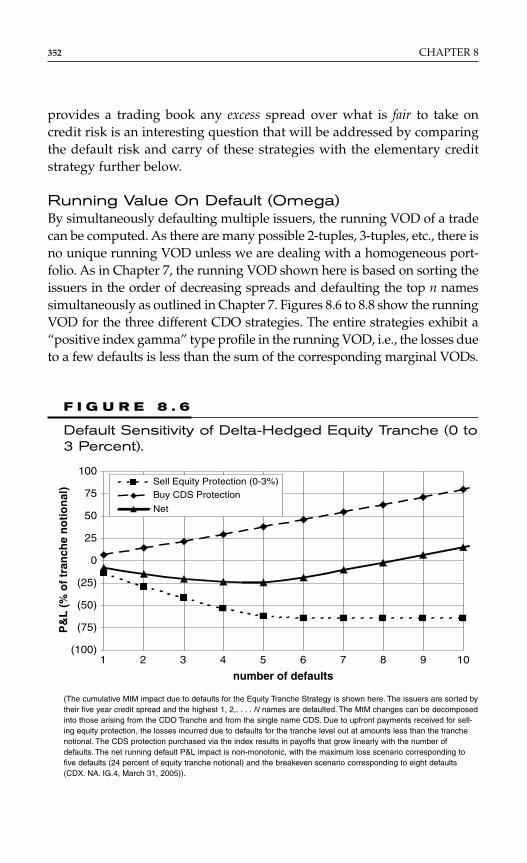
provides a trading book any excess spread over what is fair to take oncredit risk is an interesting question that will be addressed by comparingthe default risk and carry of these strategies with the elementary creditstrategy further below.
Running Value On Default (Omega)By simultaneously defaulting multiple issuers, the running VOD of a tradecan be computed. As there are many possible 2-tuples, 3-tuples, etc., there isno unique running VOD unless we are dealing with a homogeneous port-folio. As in Chapter 7, the running VOD shown here is based on sorting theissuers in the order of decreasing spreads and defaulting the top n namessimultaneously as outlined in Chapter 7. Figures 8.6 to 8.8 show the runningVOD for the three different CDO strategies. The entire strategies exhibit a“positive index gamma” type profile in the running VOD, i.e., the losses dueto a few defaults is less than the sum of the corresponding marginal VODs.
352 CHAPTER 8
(100)
(75)
(50)
(25)
0
25
50
75
100
1 2 3 4 5 6 7 8 9 10
number of defaults
Sell Equity Protection (0-3%)Buy CDS Protection
Net
P&
L (
% o
f tr
anch
e n
oti
on
al)
F I G U R E 8 . 6
Default Sensitivity of Delta-Hedged Equity Tranche (0 to3 Percent).
(The cumulative MtM impact due to defaults for the Equity Tranche Strategy is shown here. The issuers are sorted bytheir five year credit spread and the highest 1, 2,. . . . N names are defaulted. The MtM changes can be decomposedinto those arising from the CDO Tranche and from the single name CDS. Due to upfront payments received for sell-ing equity protection, the losses incurred due to defaults for the tranche level out at amounts less than the tranchenotional. The CDS protection purchased via the index results in payoffs that grow linearly with the number ofdefaults. The net running default P&L impact is non-monotonic, with the maximum loss scenario corresponding tofive defaults (24 percent of equity tranche notional) and the breakeven scenario corresponding to eight defaults(CDX. NA. IG.4, March 31, 2005)).
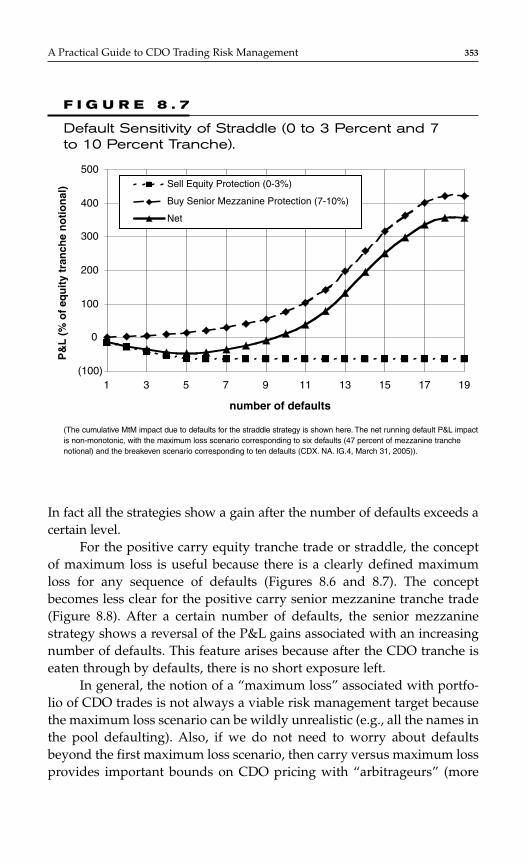
A Practical Guide to CDO Trading Risk Management 353
In fact all the strategies show a gain after the number of defaults exceeds acertain level.
For the positive carry equity tranche trade or straddle, the conceptof maximum loss is useful because there is a clearly defined maximumloss for any sequence of defaults (Figures 8.6 and 8.7). The conceptbecomes less clear for the positive carry senior mezzanine tranche trade(Figure 8.8). After a certain number of defaults, the senior mezzaninestrategy shows a reversal of the P&L gains associated with an increasingnumber of defaults. This feature arises because after the CDO tranche iseaten through by defaults, there is no short exposure left.
In general, the notion of a “maximum loss” associated with portfo-lio of CDO trades is not always a viable risk management target becausethe maximum loss scenario can be wildly unrealistic (e.g., all the names inthe pool defaulting). Also, if we do not need to worry about defaultsbeyond the first maximum loss scenario, then carry versus maximum lossprovides important bounds on CDO pricing with “arbitrageurs” (more
(100)
0
100
200
300
400
500
1 3 5 7 9 11 13 15 17 19
number of defaults
Sell Equity Protection (0-3%)
Buy Senior Mezzanine Protection (7-10%)
Net
P&
L (
% o
f eq
uit
y tr
anch
e n
oti
on
al)
F I G U R E 8 . 7
Default Sensitivity of Straddle (0 to 3 Percent and 7to 10 Percent Tranche).
(The cumulative MtM impact due to defaults for the straddle strategy is shown here. The net running default P&L impactis non-monotonic, with the maximum loss scenario corresponding to six defaults (47 percent of mezzanine tranchenotional) and the breakeven scenario corresponding to ten defaults (CDX. NA. IG.4, March 31, 2005)).
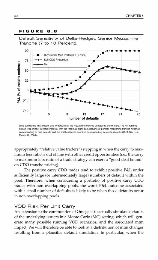
appropriately “relative value traders”) stepping in when the carry to max-imum loss ratio is out of line with other credit opportunities (i.e., the carryto maximum loss ratio of a trade strategy can exert a “good-deal bound”on CDO tranche pricing).
The positive carry CDO trades tend to exhibit positive P&L undersufficiently large (or intermediately large) numbers of default within thepool. Therefore, when considering a portfolio of positive carry CDOtrades with non overlapping pools, the worst P&L outcome associatedwith a small number of defaults is likely to be when those defaults occurin non overlapping pools.
VOD Risk Per Unit CarryAn extension to the computation of Omega is to actually simulate defaultsof the underlying issuers in a Monte-Carlo (MC) setting, which will gen-erate many possible running VOD scenarios, and the associated mtmimpact. We will therefore be able to look at a distribution of mtm changesresulting from a plausible default simulation. In particular, when the
354 CHAPTER 8
(50)
(25)
0
25
50
75
100
1 5 9 13 17 21 25
Buy Senior Mez Protection (7-10%)
Sell CDS Protection
Net
P&
L (
% o
f tr
anch
e n
oti
on
al)
number of defaults
F I G U R E 8 . 8
Default Sensitivity of Delta-Hedged Senior MezzanineTranche (7 to 10 Percent).
(The cumulative MtM impact due to defaults for the mezzanine tranche strategy is shown here. The net runningdefault P&L impact is nonmonotonic, with the first maximum loss scenario (9 percent mezzanine tranche notional)corresponding to nine defaults and the first breakeven scenario corresponding to eleven defaults (CDX. NA. IG.4,March 31, 2005)).
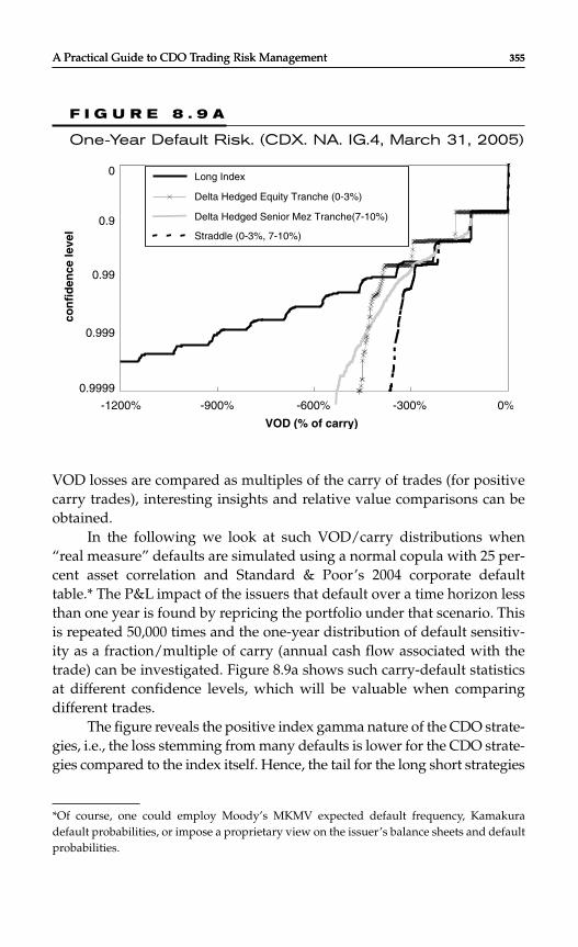
VOD losses are compared as multiples of the carry of trades (for positivecarry trades), interesting insights and relative value comparisons can beobtained.
In the following we look at such VOD/carry distributions when“real measure” defaults are simulated using a normal copula with 25 per-cent asset correlation and Standard & Poor’s 2004 corporate defaulttable.* The P&L impact of the issuers that default over a time horizon lessthan one year is found by repricing the portfolio under that scenario. Thisis repeated 50,000 times and the one-year distribution of default sensitiv-ity as a fraction/multiple of carry (annual cash flow associated with thetrade) can be investigated. Figure 8.9a shows such carry-default statisticsat different confidence levels, which will be valuable when comparingdifferent trades.
The figure reveals the positive index gamma nature of the CDO strate-gies, i.e., the loss stemming from many defaults is lower for the CDO strate-gies compared to the index itself. Hence, the tail for the long short strategies
A Practical Guide to CDO Trading Risk Management 355A Practical Guide to CDO Trading Risk Management 355
*Of course, one could employ Moody’s MKMV expected default frequency, Kamakuradefault probabilities, or impose a proprietary view on the issuer’s balance sheets and defaultprobabilities.
-1200% -900% -600% -300% 0%
VOD (% of carry)
Long Index
Delta Hedged Equity Tranche (0-3%)
Delta Hedged Senior Mez Tranche(7-10%)
Straddle (0-3%, 7-10%)
0
0.9
0.99
0.999
0.9999
con
fid
ence
leve
l
F I G U R E 8 . 9 A
One-Year Default Risk. (CDX. NA. IG.4, March 31, 2005)
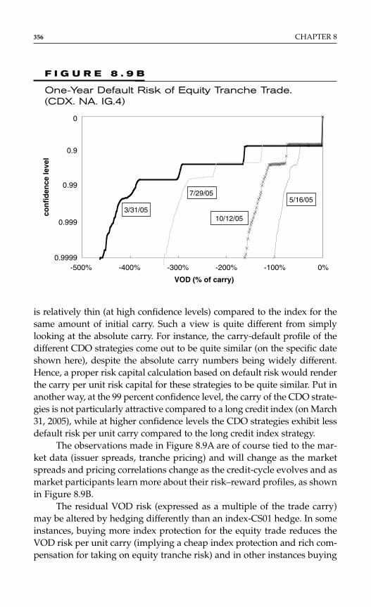
is relatively thin (at high confidence levels) compared to the index for thesame amount of initial carry. Such a view is quite different from simplylooking at the absolute carry. For instance, the carry-default profile of thedifferent CDO strategies come out to be quite similar (on the specific dateshown here), despite the absolute carry numbers being widely different.Hence, a proper risk capital calculation based on default risk would renderthe carry per unit risk capital for these strategies to be quite similar. Put inanother way, at the 99 percent confidence level, the carry of the CDO strate-gies is not particularly attractive compared to a long credit index (on March31, 2005), while at higher confidence levels the CDO strategies exhibit lessdefault risk per unit carry compared to the long credit index strategy.
The observations made in Figure 8.9A are of course tied to the mar-ket data (issuer spreads, tranche pricing) and will change as the marketspreads and pricing correlations change as the credit-cycle evolves and asmarket participants learn more about their risk–reward profiles, as shownin Figure 8.9B.
The residual VOD risk (expressed as a multiple of the trade carry)may be altered by hedging differently than an index-CS01 hedge. In someinstances, buying more index protection for the equity trade reduces theVOD risk per unit carry (implying a cheap index protection and rich com-pensation for taking on equity tranche risk) and in other instances buying
356 CHAPTER 8
-500% -400% -300% -200% -100% 0%
VOD (% of carry)
3/31/055/16/05
7/29/05
10/12/05
con
fid
ence
leve
l
0
0.9
0.99
0.999
0.9999
F I G U R E 8 . 9 B
One-Year Default Risk of Equity Tranche Trade.(CDX. NA. IG.4)
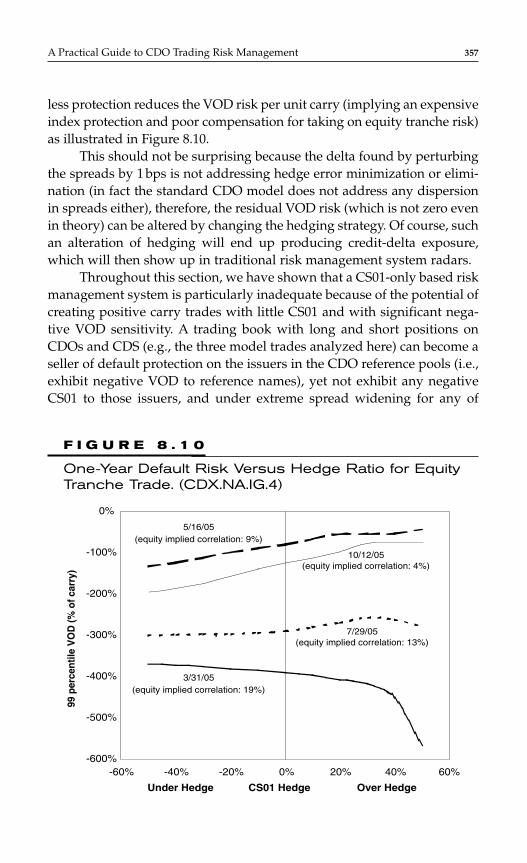
A Practical Guide to CDO Trading Risk Management 357
-600%
-500%
-400%
-300%
-200%
-100%
0%
-60% -40% -20% 0% 20% 40% 60%
Under Hedge CS01 Hedge Over Hedge
99 p
erce
ntile
VO
D (%
of c
arry
)
5/16/05(equity implied correlation: 9%)
10/12/05(equity implied correlation: 4%)
7/29/05(equity implied correlation: 13%)
3/31/05(equity implied correlation: 19%)
F I G U R E 8 . 1 0
One-Year Default Risk Versus Hedge Ratio for EquityTranche Trade. (CDX.NA.IG.4)
less protection reduces the VOD risk per unit carry (implying an expensiveindex protection and poor compensation for taking on equity tranche risk)as illustrated in Figure 8.10.
This should not be surprising because the delta found by perturbingthe spreads by 1 bps is not addressing hedge error minimization or elimi-nation (in fact the standard CDO model does not address any dispersionin spreads either), therefore, the residual VOD risk (which is not zero evenin theory) can be altered by changing the hedging strategy. Of course, suchan alteration of hedging will end up producing credit-delta exposure,which will then show up in traditional risk management system radars.
Throughout this section, we have shown that a CS01-only based riskmanagement system is particularly inadequate because of the potential ofcreating positive carry trades with little CS01 and with significant nega-tive VOD sensitivity. A trading book with long and short positions onCDOs and CDS (e.g., the three model trades analyzed here) can become aseller of default protection on the issuers in the CDO reference pools (i.e.,exhibit negative VOD to reference names), yet not exhibit any negativeCS01 to those issuers, and under extreme spread widening for any of
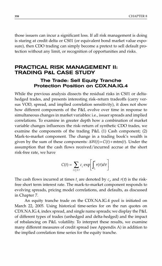
those issuers can incur a significant loss. If all risk management is doingis staring at credit delta or CS01 (or equivalent bond market value expo-sure), then CDO trading can simply become a pretext to sell default pro-tection without any limit, or recognition of opportunities and risks.
PRACTICAL RISK MANAGEMENT II: TRADING P&L CASE STUDY
The Trade: Sell Equity Tranche Protection Position on CDX.NA.IG.4
While the previous analysis dissects the residual risks in CS01 or delta-hedged trades, and presents interesting risk–return tradeoffs (carry ver-sus VOD, spread, and implied correlation sensitivity), it does not showhow different components of the P&L evolve over time in response tosimultaneous changes in market variables: i.e., issuer spreads and impliedcorrelations. To examine in greater depth how a combination of marketvariable changes influences the risk–return of synthetic CDO trades, weexamine the components of the trading P&L (1) Cash component; (2)Mark-to-market component. The change in a trading book’s wealth isgiven by the sum of these components: ∆W(t) = C(t) + mtm(t). Under theassumption that the cash flows received/incurred accrue at the shortrisk-free rate, we have
The cash flows incurred at times ti are denoted by ci, and r(τ) is the risk-free short term interest rate. The mark-to-market component responds toevolving spreads, pricing model correlations, and defaults, as discussedin Chapter 7.
An equity tranche trade on the CDX.NA.IG.4 pool is initiated onMarch 22, 2005. Using historical time-series for on the run quotes onCDX.NA.IG.4, index spread, and single name spreads; we display the P&Lof different types of trades (unhedged and delta-hedged) and the impactof rebalancing on P&L volatility. To interpret these results, we examinemany different measures of credit spread (see Appendix A) in addition tothe implied correlation time series for the equity tranche.
C t c r di t
t
i t t ii
( ) exp ( );
=
∫∑
≤
τ τ
358 CHAPTER 8
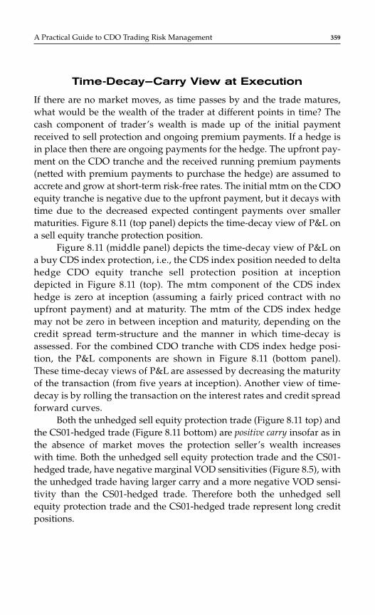
Time-Decay—Carry View at Execution
If there are no market moves, as time passes by and the trade matures,what would be the wealth of the trader at different points in time? Thecash component of trader’s wealth is made up of the initial paymentreceived to sell protection and ongoing premium payments. If a hedge isin place then there are ongoing payments for the hedge. The upfront pay-ment on the CDO tranche and the received running premium payments(netted with premium payments to purchase the hedge) are assumed toaccrete and grow at short-term risk-free rates. The initial mtm on the CDOequity tranche is negative due to the upfront payment, but it decays withtime due to the decreased expected contingent payments over smallermaturities. Figure 8.11 (top panel) depicts the time-decay view of P&L ona sell equity tranche protection position.
Figure 8.11 (middle panel) depicts the time-decay view of P&L ona buy CDS index protection, i.e., the CDS index position needed to deltahedge CDO equity tranche sell protection position at inceptiondepicted in Figure 8.11 (top). The mtm component of the CDS indexhedge is zero at inception (assuming a fairly priced contract with noupfront payment) and at maturity. The mtm of the CDS index hedgemay not be zero in between inception and maturity, depending on thecredit spread term-structure and the manner in which time-decay isassessed. For the combined CDO tranche with CDS index hedge posi-tion, the P&L components are shown in Figure 8.11 (bottom panel).These time-decay views of P&L are assessed by decreasing the maturityof the transaction (from five years at inception). Another view of time-decay is by rolling the transaction on the interest rates and credit spreadforward curves.
Both the unhedged sell equity protection trade (Figure 8.11 top) andthe CS01-hedged trade (Figure 8.11 bottom) are positive carry insofar as inthe absence of market moves the protection seller’s wealth increaseswith time. Both the unhedged sell equity protection trade and the CS01-hedged trade, have negative marginal VOD sensitivities (Figure 8.5), withthe unhedged trade having larger carry and a more negative VOD sensi-tivity than the CS01-hedged trade. Therefore both the unhedged sellequity protection trade and the CS01-hedged trade represent long creditpositions.
A Practical Guide to CDO Trading Risk Management 359
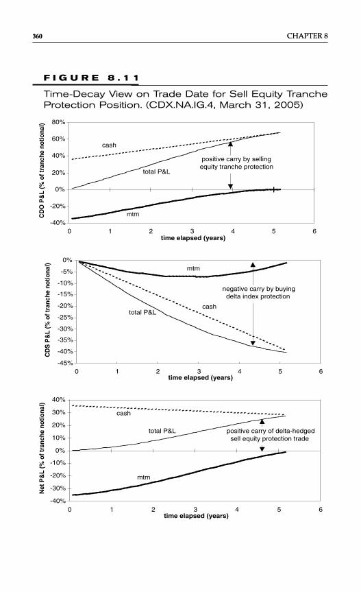
360 CHAPTER 8360 CHAPTER 8
-40%
-20%
0%
20%
40%
60%
80%
0 1 2 3 4 5 6time elapsed (years)
CD
O P
&L
(% o
f tra
nche
not
iona
l)
cash
total P&L
mtm
positive carry by sellingequity tranche protection
-45%
-40%
-35%
-30%
-25%
-20%
-15%
-10%
-5%
0%
0 1 2 3 4 5 6time elapsed (years)
CD
S P
&L
(% o
f tra
nche
not
iona
l)
cashtotal P&L
mtm
negative carry by buyingdelta index protection
-40%
-30%
-20%
-10%
0%
10%
20%
30%
40%
0 1 2 3 4 5 6time elapsed (years)
Net
P&
L (%
of t
ranc
he n
otio
nal)
total P&L
cash
mtm
positive carry of delta-hedgedsell equity protection trade
F I G U R E 8 . 1 1
Time-Decay View on Trade Date for Sell Equity TrancheProtection Position. (CDX.NA.IG.4, March 31, 2005)

P&L Components With Market Moves: Back Testing Insights
We look at the P&L performance taking into account what actually hap-pened in the market between March and December 2005 next. We dissectagain the cash and mtm components in this exercise. In the long-only (sellequity tranche protection) trade or the statically delta-hedged trade, thecash component is not influenced by movements in credit spreads (Figure8.12 top panel). A sell equity protection position results in receiving anupfront payment and ongoing running premium payments that havebeen accrued continuously here. Delta hedging of the equity trancheresults in the running net premium to be negative (i.e., negative cash out-flow) on top of the positive upfront payment. For the static hedge, the pre-mium payments are also insensitive to spread moves after conducting theinitial trade, while rebalancing introduces some spread sensitivity.
The mtm of the trade is influenced by movements in credit spreadsand implied correlation, on top of time-decay (Figure 8.12 mid). Theunhedged sell equity tranche protection position is an outright longcredit-delta exposure and is also long correlation and therefore suffers adeep blow when spreads widen on the average and the equity trancheimplied correlation falls. A short credit hedging position of course damp-ens the mtm fluctuations (and reduces the cash component of the P&L).The total P&L (cash plus mtm) is displayed in Figure 8.12 bottom panel.
Of course, as deltas change with changes in market variables, differ-ent hedging frequencies will impact the P&L differently. It turns out that astatic hedge, i.e., a CS01 hedge using the index at inception, ends up per-forming not too different from a daily CS01-hedged trade employing theindex to hedge. The less frequently hedged trade that involves delta hedg-ing every two weeks or two months happens to perform better than thedaily or statically hedged trade (Figure 8.12 bottom panel). In the following,we provide an interpretation of the P&L moves based on market variablesattempting to gain further insight into the drivers of P&L performance.
Interpretation: Role of Index Spread, SpreadDispersion, & Implied Correlation
Figure 8.12 revealed that a sharp P&L drawdown event for the sell equitytranche trade (initiated in March 2005 on CDX.NA.IG.4) occurred in May2005. Figure 8.13 shows that this was associated with a widening of theindex average spread (top panel), a widening of the index cross-sectional
A Practical Guide to CDO Trading Risk Management 361A Practical Guide to CDO Trading Risk Management 361
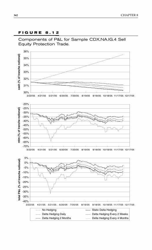
362 CHAPTER 8
36%
35%
34%
33%
32%
31%
30%3/22/05 4/21/05 5/21/05 6/20/05 7/20/05 8/19/05 9/18/05 10/18/05 11/17/05 12/17/05
cash
(%
of
tran
che
no
tio
nal
)
-20%
-25%
-30%
-35%
-40%
-45%
-50%
-55%
-60%
-65%
-70%3/22/05 4/21/05 5/21/05 6/20/05 7/20/05 8/19/05 9/18/05 10/18/05 11/17/05 12/17/05
mtm
(%
of
tran
che
no
tio
nal
)
-40%
-35%
-30%
-25%
-20%
-15%
-10%
-5%
0%
5%
3/22/05 4/21/05 5/21/05 6/20/05 7/20/05 8/19/05 9/18/05 10/18/05 11/17/05 12/17/05
No Hedging Static Delta Hedging
Delta Hedging Daily Delta Hedging Every 2 Weeks
Delta Hedging 2 Months Delta Hedging Every 4 Months
tota
l P&
L (
% o
f tr
anch
e n
oti
on
al)
F I G U R E 8 . 1 2
Components of P&L for Sample CDX.NA.IG.4 SellEquity Protection Trade.
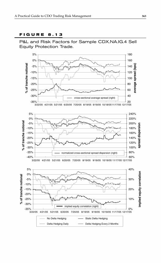
A Practical Guide to CDO Trading Risk Management 363
-35%
-30%
-25%
-20%
-15%
-10%
-5%
0%
5%
3/22/05 4/21/05 5/21/05 6/20/05 7/20/05 8/19/05 9/18/05 10/18/0511/17/05 12/17/05
3/22/05 4/21/05 5/21/05 6/20/05 7/20/05 8/19/05 9/18/05 10/18/05 11/17/05 12/17/05
3/22/05 4/21/05 5/21/05 6/20/05 7/20/05 8/19/05 9/18/05 10/18/05 11/17/05 12/17/05
20
40
60
80
100
120
140
160
180
cross-sectional average spread (right)
aver
age
spre
ad (b
ps)
% o
f tra
nche
not
iona
l
-40%
-35%
-30%
-25%
-20%
-15%
-10%
-5%
0%
5%
60%
80%
100%
120%
140%
160%
180%
200%
220%
240%
normalized cross-sectional spread dispersion (right)
spre
ad d
ispe
rsio
n
% o
f tra
nche
not
iona
l
-35%
-30%
-25%
-20%
-15%
-10%
-5%
0%
5%
0%
10%
20%
30%
40%
No Delta Hedging Static Delta Hedging
Delta Hedging Daily Delta Hedging Every 2 Months
impl
ied
equi
ty c
orre
latio
n
% o
f tra
nche
not
iona
l
implied equity correlation (right)
F I G U R E 8 . 1 3
P&L and Risk Factors for Sample CDX.NA.IG.4 SellEquity Protection Trade.

dispersion of spreads (middle panel), and a sudden drop in the impliedcorrelation for the equity tranche (bottom panel). Both index spreadwidening and increase in dispersion had built up over April, and then inMay there was a sharp drop in implied correlation.
Even the delta-hedged equity tranche trade experienced a signifi-cant P&L drawdown (10 to 15 percent of equity tranche notional) despitebeing CS01 hedged using the index, although delta hedging significantlyreduces the negative P&L relative to naked long equity risk position (39to 35 percent of equity tranche notional). This is because of the increasein cross-sectional spread dispersion in the index and the concomitantdecrease in the equity tranche implied correlation. Index average spreadwidening, increase of cross-sectional dispersion, and drop of implied cor-relation tended to occur together (Figures 8.14 and 8.15).
The scatter plot of the equity implied correlation versus spread dis-persion (Figure 8.15) suggests that the market developed a new realizationof the vulnerability of the sell equity protection trade to pool idiosyn-crasies in May 2005.
The response of the implied correlation pricing parameter to mar-ket spread moves can be interpreted as follows. As the index spreadwidens, those market players who have a leveraged long exposure to theindex via an unhedged equity tranche protection sell position and thosewho have a heightened exposure to idiosyncratic spread moves via CS01hedged sell equity tranche protection positions incur losses. In responseto these losses they either try to close out their position by taking anopposing position, or demand greater compensation for taking on therisk. The increased demand for buying equity tranche protection and thehigher asking price for selling equity tranche protection both manifest asa downward move in the equity tranche implied correlation parameter.
This empirical feature of spread dispersion being associated withindex widening and equity implied correlation decreasing underlines theinadequacy of employing CS01 as the primary risk-monitoring tool forsynthetic CDO trades. A delta-hedged trade will not exhibit any CS01 andnot prepare anyone for losses that will occur when the index spreadwidens: These losses are inflicted by idiosyncratic spread-movements andthe associated decrease in equity implied correlation which can be inter-preted as an increase in risk-aversion to idiosyncratic credit impairments.If a CDO tranche is thought to simply be a collection of single name creditinstruments (albeit with the correct individual CS01) one is not preparedfor the downside risks associated with idiosyncratic spread flare-outs andimplied correlation movements.
364 CHAPTER 8364 CHAPTER 8
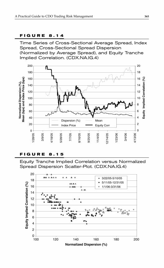
A Practical Guide to CDO Trading Risk Management 365
0
20
40
60
80
100
120
140
160
180
200
1/28
/05
3/9/
05
4/18
/05
5/28
/05
7/7/
05
8/16
/05
9/25
/05
11/4
/05
12/1
4/05
1/23
/06
3/4/
06
4/13
/06
0
2
4
6
8
10
12
14
16
18
20
Dispersion (%) Mean
Index Price Equity Corr
No
rmal
ized
Dis
per
sio
n (
%),
M
ean
(b
ps)
an
d In
dex
Pri
ce (
bp
s)
Eq
uit
y Im
plie
d C
orr
elat
ion
(%
)
F I G U R E 8 . 1 4
Time Series of Cross-Sectional Average Spread, IndexSpread, Cross-Sectional Spread Dispersion(Normalized by Average Spread), and Equity TrancheImplied Correlation. (CDX.NA.IG.4)
0
2
4
6
8
10
12
14
16
18
20
100 120 140 160 180 200
Normalized Dispersion (%)
Eq
uit
y Im
plie
d C
orr
elat
ion
(%
)
3/22/05-5/10/05
5/11/05-12/31/05
1/1/06-3/31/06
F I G U R E 8 . 1 5
Equity Tranche Implied Correlation versus NormalizedSpread Dispersion Scatter-Plot. (CDX.NA.IG.4)

366 CHAPTER 8
Tales of poor P&L attribution from credit-delta risk factors and ele-ments of surprise and fear associated with P&L marking and risk-assessment abound the broker-dealer and hedge fund communitytransacting in synthetic CDOs. The experiences in 2005 have crystallizedthe fallacy of measuring synthetic CDO risk by systems that were builtprimarily for single name instruments and have also highlighted theimportance of assessing P&L risk scenarios under a comprehensive set ofspread moves, with single name granularity, and correlation move sce-narios, in addition to the Monte-Carlo default risk described in previoussections.
Realized Correlation of Spread Moves and Hedging Frequency
A measure of the tendency of spreads to move together is expressed bythe “realized correlation,” which for a pair of names is the correlation ofchanges in spreads over different intervals. This measure is defined inAppendix A. To calculate the correlation between the changes of spreadsfor a pair of obligors from a time series requires a time window, which istaken to be the CDX.NA.IG.4 life (from March 22 onwards). This creates apair-wise realized correlation matrix of spread change over different timeintervals, and the average of those correlations (off-diagonal elements) isshown in Figure 8.16.
Spreads show a tendency to have more coherent moves over longertime-intervals (e.g., two months) compared to shorter time-intervals(daily). For example, the daily time-interval spread changes have an aver-age correlation of about 16% whereas the correlation of spread changesover two weeks rises to 35 percent, and at two months it becomes ~ 40 per-cent. Beyond time-intervals of two months the realized correlationappears to fall (although that inference is relatively less reliable consider-ing the time averaging window to infer correlations is approximately ninemonths long).
The relationship of realized correlation with time-interval helps tointerpret the performance of the hedging strategy, where hedging everytwo weeks ends up with a more favorable P&L outcome relative todaily delta hedging, and hedging every two months ends up even bet-ter (Figure 8.12). This is a demonstration of monetization of positiveindex spread gamma when spreads move coherently over the hedging
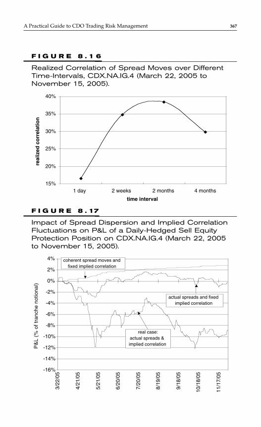
A Practical Guide to CDO Trading Risk Management 367
15%
20%
25%
30%
35%
40%
1 day 2 weeks 2 months 4 months
time interval
real
ized
co
rrel
atio
n
F I G U R E 8 . 1 6
Realized Correlation of Spread Moves over DifferentTime-Intervals, CDX.NA.IG.4 (March 22, 2005 toNovember 15, 2005).
-16%
-14%
-12%
-10%
-8%
-6%
-4%
-2%
0%
2%
4%
3/22
/05
4/21
/05
5/21
/05
6/20
/05
7/20
/05
8/19
/05
9/18
/05
10/1
8/05
11/1
7/05
P&
L (%
of t
ranc
he n
otio
nal)
coherent spread moves andfixed implied correlation
actual spreads and fixedimplied correlation
real case:actual spreads &implied correlation
F I G U R E 8 . 17
Impact of Spread Dispersion and Implied CorrelationFluctuations on P&L of a Daily-Hedged Sell EquityProtection Position on CDX.NA.IG.4 (March 22, 2005to November 15, 2005).
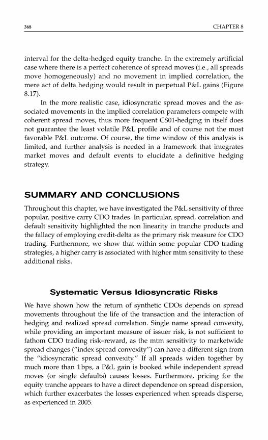
interval for the delta-hedged equity tranche. In the extremely artificialcase where there is a perfect coherence of spread moves (i.e., all spreadsmove homogeneously) and no movement in implied correlation, themere act of delta hedging would result in perpetual P&L gains (Figure8.17).
In the more realistic case, idiosyncratic spread moves and the as-sociated movements in the implied correlation parameters compete withcoherent spread moves, thus more frequent CS01-hedging in itself doesnot guarantee the least volatile P&L profile and of course not the mostfavorable P&L outcome. Of course, the time window of this analysis islimited, and further analysis is needed in a framework that integratesmarket moves and default events to elucidate a definitive hedgingstrategy.
SUMMARY AND CONCLUSIONS
Throughout this chapter, we have investigated the P&L sensitivity of threepopular, positive carry CDO trades. In particular, spread, correlation anddefault sensitivity highlighted the non linearity in tranche products andthe fallacy of employing credit-delta as the primary risk measure for CDOtrading. Furthermore, we show that within some popular CDO tradingstrategies, a higher carry is associated with higher mtm sensitivity to theseadditional risks.
Systematic Versus Idiosyncratic Risks
We have shown how the return of synthetic CDOs depends on spreadmovements throughout the life of the transaction and the interaction ofhedging and realized spread correlation. Single name spread convexity,while providing an important measure of issuer risk, is not sufficient tofathom CDO trading risk–reward, as the mtm sensitivity to marketwidespread changes (“index spread convexity”) can have a different sign fromthe “idiosyncratic spread convexity.” If all spreads widen together bymuch more than 1 bps, a P&L gain is booked while independent spreadmoves (or single defaults) causes losses. Furthermore, pricing for theequity tranche appears to have a direct dependence on spread dispersion,which further exacerbates the losses experienced when spreads disperse,as experienced in 2005.
368 CHAPTER 8
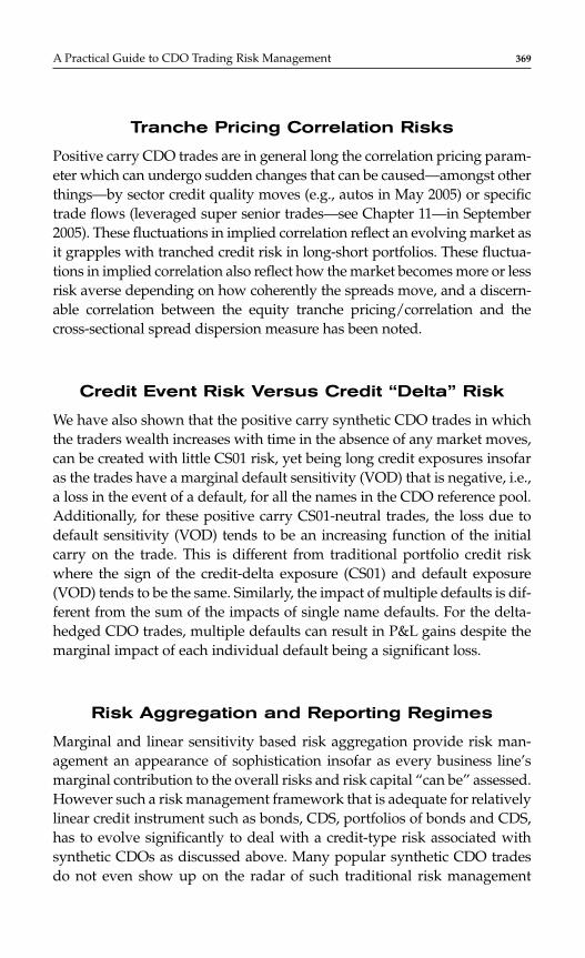
Tranche Pricing Correlation Risks
Positive carry CDO trades are in general long the correlation pricing param-eter which can undergo sudden changes that can be caused—amongst otherthings—by sector credit quality moves (e.g., autos in May 2005) or specifictrade flows (leveraged super senior trades—see Chapter 11—in September2005). These fluctuations in implied correlation reflect an evolving market asit grapples with tranched credit risk in long-short portfolios. These fluctua-tions in implied correlation also reflect how the market becomes more or lessrisk averse depending on how coherently the spreads move, and a discern-able correlation between the equity tranche pricing/correlation and thecross-sectional spread dispersion measure has been noted.
Credit Event Risk Versus Credit “Delta” Risk
We have also shown that the positive carry synthetic CDO trades in whichthe traders wealth increases with time in the absence of any market moves,can be created with little CS01 risk, yet being long credit exposures insofaras the trades have a marginal default sensitivity (VOD) that is negative, i.e.,a loss in the event of a default, for all the names in the CDO reference pool.Additionally, for these positive carry CS01-neutral trades, the loss due todefault sensitivity (VOD) tends to be an increasing function of the initialcarry on the trade. This is different from traditional portfolio credit riskwhere the sign of the credit-delta exposure (CS01) and default exposure(VOD) tends to be the same. Similarly, the impact of multiple defaults is dif-ferent from the sum of the impacts of single name defaults. For the delta-hedged CDO trades, multiple defaults can result in P&L gains despite themarginal impact of each individual default being a significant loss.
Risk Aggregation and Reporting Regimes
Marginal and linear sensitivity based risk aggregation provide risk man-agement an appearance of sophistication insofar as every business line’smarginal contribution to the overall risks and risk capital “can be” assessed.However such a risk management framework that is adequate for relativelylinear credit instrument such as bonds, CDS, portfolios of bonds and CDS,has to evolve significantly to deal with a credit-type risk associated withsynthetic CDOs as discussed above. Many popular synthetic CDO tradesdo not even show up on the radar of such traditional risk management
A Practical Guide to CDO Trading Risk Management 369
schemes that are largely driven by credit-delta exposures—which providesthe lowest common denominator of exposures than “can be aggregated.”Risk reports will have to first stop equating credit-delta risk exposures withcredit event risk exposures because CDO trades may not exhibit any credit-delta risk at inception (based on 1 bps spread moves) and yet be long all thecredits underlying the CDO pool from a credit event perspective (i.e., neg-ative VOD). The risk-systems challenge is to replace the highly convenientmarginal and linear sensitivity based approaches, with the trade strategycognizant approach that requires: (1) resolving single name credit descrip-tion without any bucketing (or artificial separation of “index” and “specific”risks); and (2) a revaluation of the CDO positions under historical and/orsimulated scenarios (including spread jumps and defaults) that explicitlydescribe the CDO reference pool at a constituent level and capture realisticspread dispersion, spread jumps, defaults, recovery, and correlation moves.Then, hedging strategies can be constructed that address all prevalent risksby minimizing P&L hedging-errors rather than only addressing spot spreaddelta sensitivity.
Models that explicitly capture the joint credit spread and defaultdynamics and directly address hedging costs provide a competitiveadvantage over the practice of just fitting static spread copula models toobserved prices (without addressing replication-hedging challenges andcosts) while accounting for synthetic CDO P&L. As the hedging and riskmanagement strategy evolves, the correlation markets will “learn” toco-exist with the volatility markets (e.g., single name and index CDSswaptions) and the differences in index and single name implied volatil-ities should provide some constraint on the implied correlation markets.As these two markets start to transmit to each other, the credit modelingparadigm will be further pushed towards directly addressing hedgingcosts and hedging-errors while accounting for coherent and idiosyncraticspread moves and credit events, as an essential precursor to assessingfair-value rather than as an after thought.
370 CHAPTER 8
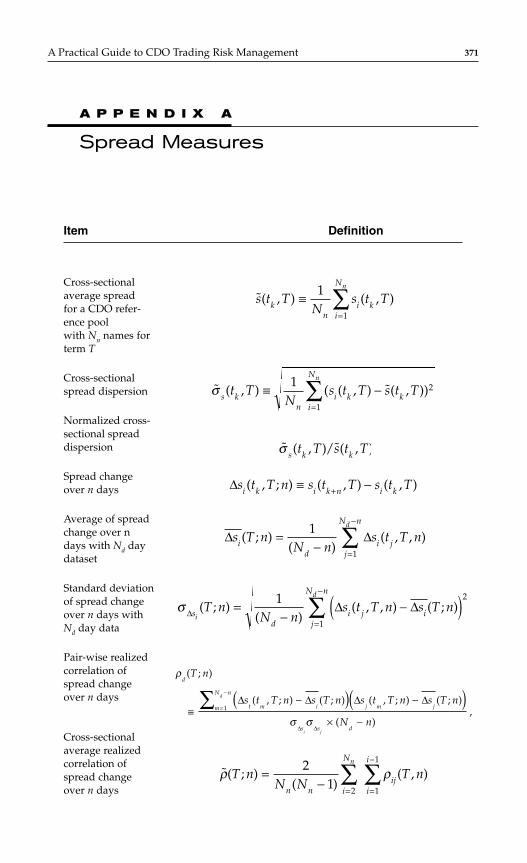
A Practical Guide to CDO Trading Risk Management 371
A P P E N D I X A
Spread Measures
Cross-sectionalaverage spread for a CDO refer-ence pool with Nn names for term T
Cross-sectional spread dispersion
Normalized cross-sectional spread dispersion
Spread change over n days
Average of spreadchange over n days with Nd daydataset
Standard deviation of spread change over n days with Nd day data
Pair-wise realizedcorrelation of spread changeover n days
Cross-sectionalaverage realized correlation ofspread change over n days
Item Definition
˜ ( ; )( )
( , )ρ ρT nN N
T nn n
iji
i
i
Nn
=− =
−
=∑∑2
11
1
2
ρ
σ σ
d
t m i j m jm
N n
s s d
T n
s t T n s T n s t T n s T n
N n
d
i j
( ; )
( , ; ) ( ; ) ( , ; ) ( ; )
( ),≡
− −
× −
( )( )=
−∑ ∆ ∆ ∆ ∆
∆ ∆
1
σ ∆ ∆ ∆sd
i j ij
N n
i
d
T nN n
s t T n s T n( ; )( )
( , , ) ( ; )=−
−( )=
−
∑1 2
1
∆ ∆s T nN n
s t T nid
ij
N n
j
d
( ; )( )
( , , )=− =
−
∑1
1
∆s t T n s t T s t Ti k i k n i k( , ; ) ( , ) ( , )≡ −+
˜ ( , )/˜( , )σ s k kt T s t T
˜ ( , ) ( ( , ) ˜( , ))σ s kn
i k ki
N
t TN
s t T s t Tn
≡ −=∑1 2
1
˜( , ) ( , )s t TN
s t Tkn
i ki
Nn
≡=∑1
1

Disclaimer: The authors make no representation as to the accuracy orcompleteness of the information provided. The views expressed here arethose of the authors, and do not necessarily represent those of theiremployers.
372 CHAPTER 8372 CHAPTER 8

C H A P T E R 9
Cash and SyntheticCollateral DebtObligations: Motivationsand Investment Strategies
Olivier Renault
373
In this chapter, we discuss the key motivations for investment in the struc-tured credit’s most popular product to date—collateral debt obligations(CDOs). We tackle this vast area by breaking it down into the two mainstructured credit markets: cash CDOs and synthetic CDOs. Althoughthese two markets are broadly defined as CDOs, they are very different interms of structure, underlying assets, and investor focus. Accordingly, wewill deal with the motivations for both of these markets separately. First,we will discuss cash CDOs that are natural extension of asset-backed secu-rity (ABS) technology to more lumpy assets. Then, we will address syn-thetic CDOs that apply credit derivative technology to portfolios. Bothmarkets share some of the same motivations for issuance, which we willdiscuss in the next section.
THE MOTIVATIONS OF A CDO ISSUER
The two main motivation for issuing CDOs are the need to free up capitalor optimize return on capital, and rating arbitrage, i.e., the possibility tofund assets more cheaply in securitized format than by holding them onbalance sheet.
Copyright © 2007 by The McGraw-Hill Companies. Click here for terms of use.
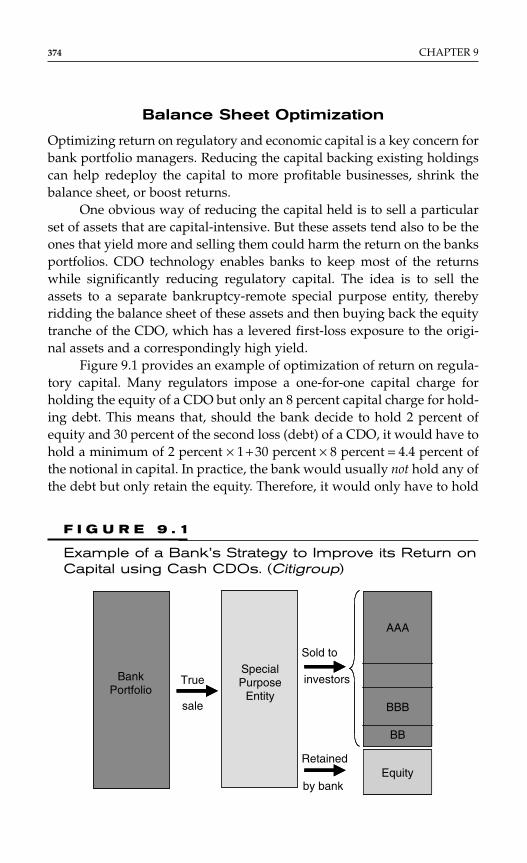
Balance Sheet Optimization
Optimizing return on regulatory and economic capital is a key concern forbank portfolio managers. Reducing the capital backing existing holdingscan help redeploy the capital to more profitable businesses, shrink thebalance sheet, or boost returns.
One obvious way of reducing the capital held is to sell a particularset of assets that are capital-intensive. But these assets tend also to be theones that yield more and selling them could harm the return on the banksportfolios. CDO technology enables banks to keep most of the returnswhile significantly reducing regulatory capital. The idea is to sell theassets to a separate bankruptcy-remote special purpose entity, therebyridding the balance sheet of these assets and then buying back the equitytranche of the CDO, which has a levered first-loss exposure to the origi-nal assets and a correspondingly high yield.
Figure 9.1 provides an example of optimization of return on regula-tory capital. Many regulators impose a one-for-one capital charge forholding the equity of a CDO but only an 8 percent capital charge for hold-ing debt. This means that, should the bank decide to hold 2 percent ofequity and 30 percent of the second loss (debt) of a CDO, it would have tohold a minimum of 2 percent × 1 + 30 percent × 8 percent = 4.4 percent ofthe notional in capital. In practice, the bank would usually not hold any ofthe debt but only retain the equity. Therefore, it would only have to hold
374 CHAPTER 9
F I G U R E 9 . 1
Example of a Bank’s Strategy to Improve its Return onCapital using Cash CDOs. (Citigroup)
AA
Equity
BankPortfolio
SpecialPurpose
Entity
BB
BBB
AAA
Retained
by bank
Sold to
investorsTrue
sale
2 percent capital in our example. This contrasts with 8 percent capital tobe held against the loans on the balance sheet. Thus, even with a first-losspiece requiring a one-for-one holding of capital, this strategy still typicallycan improve the return on the capital held against it. In our example, thecapital drops by a factor of four, whereas the return may drop by only onehalf. Furthermore, the operation can drastically reduce the amount ofassets on the balance sheet, and therefore help the bank extend new loans.The Balance sheet management was the original motivation behind cashCDOs, but balance sheet CDOs went out of fashion. They made a significantcomeback in 2005.
By 2001, as the credit derivative market developed, banks were ableto hedge credit exposure synthetically through the use of credit defaultswaps (CDSs) and, later, portfolio CDSs. The advantage of synthetic se-curitization is that the original assets are still owned by the bank, butbecause some of the credit risk is hedged, a reduction of capital can beachieved.
The rationale of the trade is the same as for cash CDO, but it doesnot involve a true sale of assets. The bank buys protection on the secondloss piece of its loan book and retains the first loss. Because assetsremain on the balance sheet, a full deduction of capital cannot beachieved but the hedged portion would typically benefit from a reduc-tion of capital from 8 percent to 1.6 percent. The much lower costsinvolved in synthetic reduction of risk compared to a true sale partly off-set the lower reduction in capital. The added benefit of synthetic balancesheet CDOs is that the risk transfer can occur without the original bor-rower’s knowledge that the bank has hedged the credit risk. Thisenables banks to maintain or even increase relationships with borrowerswhile keeping the bank’s risk exposures to individual borrowers undercontrol (Figure 9.2).
Spread/Rating Arbitrage
Arbitrage CDOs, whether cash or synthetic, are motivated mainly by themismatch between the return on assets (spread on loans or CDSs) andthe cost of liabilities (spread on CDO notes). Because spreads on bothsides are partly driven by ratings, it is often possible to tranche up aportfolio where the weighted average spread on rated liabilities is sig-nificantly lower than the spread generated by the assets. This enables togenerate excess spread for equity holders who are often the arrangers ofthe transaction. The main difference between a balance sheet CDO and
Cash and Synthetic CDOs 375
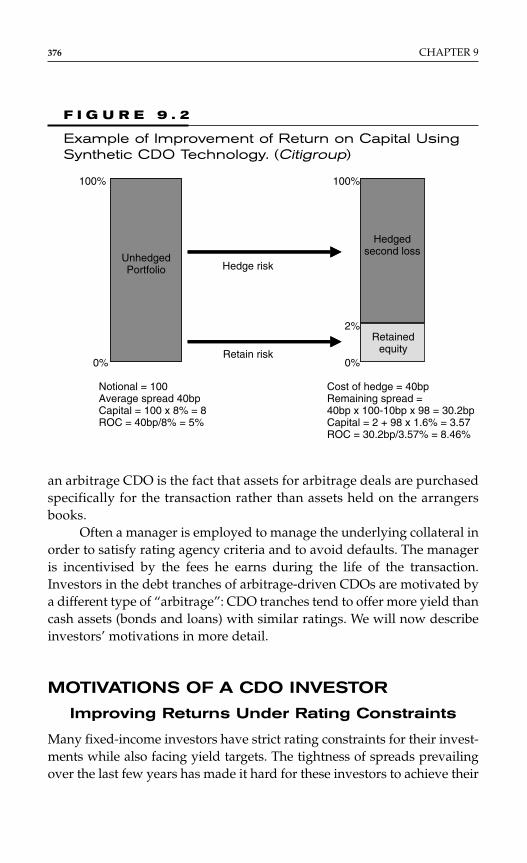
an arbitrage CDO is the fact that assets for arbitrage deals are purchasedspecifically for the transaction rather than assets held on the arrangersbooks.
Often a manager is employed to manage the underlying collateral inorder to satisfy rating agency criteria and to avoid defaults. The manageris incentivised by the fees he earns during the life of the transaction.Investors in the debt tranches of arbitrage-driven CDOs are motivated bya different type of “arbitrage”: CDO tranches tend to offer more yield thancash assets (bonds and loans) with similar ratings. We will now describeinvestors’ motivations in more detail.
MOTIVATIONS OF A CDO INVESTOR
Improving Returns Under Rating Constraints
Many fixed-income investors have strict rating constraints for their invest-ments while also facing yield targets. The tightness of spreads prevailingover the last few years has made it hard for these investors to achieve their
376 CHAPTER 9
F I G U R E 9 . 2
Example of Improvement of Return on Capital UsingSynthetic CDO Technology. (Citigroup)
Hedgedsecond loss
Retainedequity
UnhedgedPortfolio
Retain risk
Hedge risk
Notional = 100Average spread 40bpCapital = 100 x 8% = 8ROC = 40bp/8% = 5%
Cost of hedge = 40bpRemaining spread =40bp x 100-10bp x 98 = 30.2bpCapital = 2 + 98 x 1.6% = 3.57ROC = 30.2bp/3.57% = 8.46%
100% 100%
2%
0% 0%
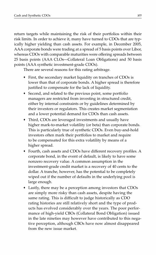
return targets while maintaining the risk of their portfolios within theirrisk limits. In order to achieve it, many have turned to CDOs that are typ-ically higher yielding than cash assets. For example, in December 2005,AAA corporate bonds were trading at a spread of 5 basis points over Libor,whereas CDOs with comparable maturities were offering spreads between25 basis points (AAA CLOs—Collateral Loan Obligations) and 50 basispoints (AAA synthetic investment-grade CDOs).
There are several reasons for this rating arbitrage.
♦ First, the secondary market liquidity on tranches of CDOs islower than that of corporate bonds. A higher spread is thereforejustified to compensate for the lack of liquidity.
♦ Second, and related to the previous point, some portfoliomanagers are restricted from investing in structured credit,either by internal constraints or by guidelines determined bytheir investors or regulators. This creates market segmentationand a lower potential demand for CDOs than cash assets.
♦ Third, CDOs are leveraged investments and usually have higher mark-to-market volatility (or beta) than corporate bonds.This is particularly true of synthetic CDOs. Even buy-and-holdinvestors often mark their portfolios to market and requireto be compensated for this extra volatility by means of ahigher spread.
♦ Fourth, cash assets and CDOs have different recovery profiles. Acorporate bond, in the event of default, is likely to have somenonzero recovery value. A common assumption in theinvestment-grade credit market is a recovery of 40 cents to thedollar. A tranche, however, has the potential to be completelywiped out if the number of defaults in the underlying pool islarge enough.
♦ Lastly, there may be a perception among investors that CDOsare simply more risky than cash assets, despite having thesame rating. This is difficult to judge historically as CDOrating histories are still relatively short and the type of prod-ucts has evolved considerably over the years. The poor perfor-mance of high-yield CBOs (Collateral Bond Obligation) issuedin the late nineties may however have contributed to this nega-tive perception, although CBOs have now almost disappearedfrom the new issue market.
Cash and Synthetic CDOs 377
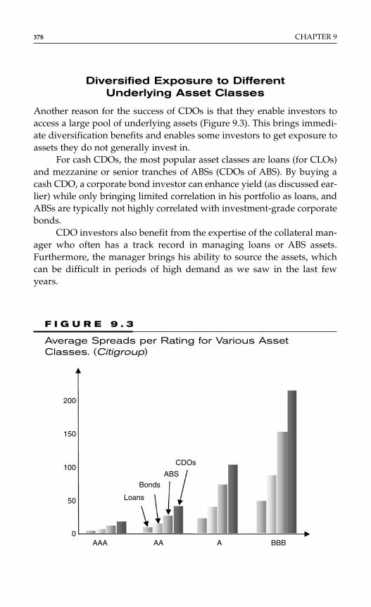
Diversified Exposure to Different Underlying Asset Classes
Another reason for the success of CDOs is that they enable investors toaccess a large pool of underlying assets (Figure 9.3). This brings immedi-ate diversification benefits and enables some investors to get exposure toassets they do not generally invest in.
For cash CDOs, the most popular asset classes are loans (for CLOs)and mezzanine or senior tranches of ABSs (CDOs of ABS). By buying acash CDO, a corporate bond investor can enhance yield (as discussed ear-lier) while only bringing limited correlation in his portfolio as loans, andABSs are typically not highly correlated with investment-grade corporatebonds.
CDO investors also benefit from the expertise of the collateral man-ager who often has a track record in managing loans or ABS assets.Furthermore, the manager brings his ability to source the assets, whichcan be difficult in periods of high demand as we saw in the last fewyears.
378 CHAPTER 9
F I G U R E 9 . 3
Average Spreads per Rating for Various AssetClasses. (Citigroup)
200
150
100
50
0AAA AA A BBB
Loans
BondsABS
CDOs

Tailored Risk and Return Profiles
CDOs are often said to have tailored risk return profiles. The “tailoring”can be performed in at least four ways: choice of underlying assets, choiceof leverage, choice of rating, and choice of maturity.
One of the main advantages of CDOs is that they let investors dis-connect their choice of risk from their choice of asset class. In a traditionalbond portfolio, investors who are restricted to hold investment-gradepaper will be forced to invest in well-rated bonds even if they believe thevalue is in noninvestment-grade issues. With CDOs, the same investorcan access noninvestment-grade collateral while securing a high-graderating for his investment.
Conversely, investors looking for high return may still want to haveexposure to AAA ABS for diversification or value purposes. This can beachieved by buying an equity piece of a CDO of ABS.
SYNTHETIC CDOS
Synthetic CDOs are one of the key products in the structured credit world.They are portfolios of CDS that are tranched and sold on to investorsbased on their risk/reward preferences. Figure 9.4 illustrates the basic
Cash and Synthetic CDOs 379
F I G U R E 9 . 4
Simple Synthetic CDO Structure and AAA TrancheLoss Mechanics. (Citigroup)
……
Sample Tranche Credit Portfolio Loss Mechanics
Credit defaultswaps on adiverse portfolio...
...are pooledtogether ina portfolio...
...and tranched tocreate a capitalstructure
Supter SeniorSwap
(15-100%) Excess
AAA Investor
Subordination
Excess
AAA Investor
Subordination
CumulativeLoss AmountLoss Amount 1N/R (0-3%)
BBB(3-7%)
AAA(7-10%)
Junior SS(10-15%)
Credit events in the ReferencePortfolio erode subordination, andeventually incur losses on theinvested tranche
ReferencePortfolio
Credit 1
Credit 2
Credit 3
Credit 4
Credit N
setup of a standard synthetic CDO and how losses accrue up the capitalstructure, starting with the erosion of the most junior tranche (equity) andprogressively affecting mezzanine and more senior tranches.
Over the last several years, synthetic CDOs have evolved throughdifferent stages, from full capital structure deals to single tranches. Today,they are firmly established as a credit investment and hedging tool. In thefollowing sections, we will discuss the motivation behind synthetic CDOsand their main differences with cash products. We will also address whothe participants to that market are and what are the main investmentstrategies followed by hedge funds and real money investors in the syntheticCDO market.
COMPARISON TO CASH CDOS
Synthetic and cash CDOs have many similarities as they offer leveragedexposures to a diversified basket of credits. Synthetic CDOs referenceCDSs which are standardized bilateral contracts, whereas cash CDOs aremore akin to a miniature bank, financing real assets, and distributing cashflows. Some of the main differences between the two types of products arelisted below:
♦ Separation of credit risk from other types of risk. Synthetic structuresare not exposed to interest rates, prepayments, and other typesof risk that are common in cash CDOs. In particular, they allowinvestors to disconnect their choice of interest rate duration tothat of credit duration.
♦ Sourcing collateral: asset diversity and speed of ramp-up. Using syn-thetic credit risk transfer technology, originators are not lim-ited by the ability to physically source the collateral assets.Synthetic CDOs can be structured very fast as they do not requirea ramp-up period. On the other hand, the need of dealers tohedge single-tranches restricts the universe of names that can beincluded in synthetic deals. These are normally only credits thatare traded in the single-name CDS market.
♦ Single-tranche versus full-capital structure deals. Unlike cash CDOswhere the entire capital structure is sold, synthetic CDOs areusually structured as single-tranche deals where only the risk ofa limited part of the capital structure is sold to investors. Dealershold the residuals risks (spreads, defaults, correlation, etc.) that
380 CHAPTER 9

are aggregated and hedged in their correlation book. Full-capitalstructure synthetic CDOs are rare but attractive for dealers asthey prevent imbalances in their correlation books.
♦ Simplified CDO structures. Standard synthetic CDOs are muchsimpler than cash CDOs as they only involve the distribution ofdefault losses. Cash CDOs rely on complex cash flow waterfallsand various technical features such as interest coverage andovercollateralization tests, prepayments, etc. The simplicity ofsynthetics have enabled structurers and investors to use simplemodels for pricing and risk management with only a limitednumber of inputs (CDS spreads, correlations, and tranchingdetails). Proper modeling of cash CDOs require a detailedknowledge of the underlying pool of assets and of the cash flowdistribution rules.
♦ Customization and easy execution. The simplicity of syntheticCDOs allows them to be customized in terms of size and attach-ment points for each individual tranche. Investors can selecttheir reference portfolios and choose the credit exposure thatbest fits into their investment strategy.
♦ Static versus managed structures. Index-linked tranches are staticin their nature, but bespoke tranches can be managed. In privatetransactions, investors can play the role of the manager if thestructure includes credit substitution rights, and publicly placedsynthetic deals usually include an external manager.
♦ Liquid and transparent market for standard index-linked tranches.Index-linked tranches are some of the most liquid products inthe credit space. With the growth of CDS indices referencingnew asset classes and the increasing number of liquid tenors, weexpect that the index-linked tranche market will continue toexpand. Derivatives referencing index-linked tranches are alsolikely to be introduced in coming years. No such benchmarkexists for cash CDOs.
♦ Shorting the credit risk in a leveraged form. Unlike for cash CDOsthat are primarily buy-and-hold investments, investors can takelong or short positions in synthetic tranches. Synthetic CDOmarkets provide a variety of different directional and hedginginvestment opportunities. Short buckets can also be included inbespoke synthetic CDOs to mitigate the effect of a credit marketselloff.
Cash and Synthetic CDOs 381

MOTIVATION BEHIND SYNTHETIC CDO INVESTORS
Synthetic CDOs gained their popularity from the variety of advantagesthey offer over cash CDOs or other related credit investments. These differ-ences will be discussed in greater details next, but the advantages of syn-thetics are primarily their ease of structuring, their ability to separatefunding (interest rate component) and risk transfer (credit risk component),and the ability they offer to investors to express views on the market.
Liquidity of Index Tranches and Flexibility of Bespokes
One of the most important motivations behind the use of synthetic struc-tures is the flexibility and customization that can be achieved by thesingle-tranche technology. Instead of structuring a full-capital structureCDO, synthetic CDOs are issued in single-tranche form, where each trans-action is a transfer of the credit risk between the seller and the buyerof protection on a specific part of the capital structure (e.g., from 3 to 7percent on Figure 9.4). In that way, investors can target their specificrisk/return profiles, and originators combine and manage outstandingpositions in aggregated portfolios (“correlation books”).
The synthetic CDO market is separated into flow tranche products,such as index-linked tranches that are primarily used as relative valueand hedging tools, and bespoke (customized) tranches, which are privateor publicly placed synthetic CDOs with a structure that is designed to fitinvestor needs. Liquidity and transparency in CDX/iTraxx index-linkedtranches shaped the correlation market in the variety of ways. Creditinvestors can take on long or short leveraged positions, look for relativevalue trades, or express directional view strategies. On the other side,dealers are using index-linked tranches to hedge their positions in thebespoke products. In the recent past, we have experienced a significantimprovement in liquidity of index-linked tranche across the term structure.
More Growth to Come
The development of synthetic indexes outside the corporate creditdomain, in particular in ABS, should contribute to future expansion. The
382 CHAPTER 9

bespoke tranche market has also been developing at a rapid pace. Buy-and-hold investors, who focus on senior bespoke tranches, use theseproducts not just as a leveraged investment, but also to achieve diversifi-cation of their positions. Leveraged accounts can find attractive investmentopportunities in the junior and equity tranches of customized portfolios,as dealers are usually left with the overhang of bespoke equity positionsfrom the process of placing customized senior tranches to traditionalinvestors. In the past, credit hedge funds have been the natural buyers ofthe equity residual. As index-linked synthetic tranches become even moreliquid and transparent, the key advantage of bespoke products is in cus-tomization: investors can select the credits in the reference pool and alsocustomize the size and attachment point of the tranche.
Some Drawbacks as Well
Synthetic CDOs also have some drawbacks compared to cash products.The accounting treatment of derivatives and their perceived mark-to-market volatility can be major obstacles for certain types of investors. Assynthetic tranches are marked-to-market and largely held by leveragedaccounts, the tranche market can go through strong technical periodsleading to significant repricings, as witnessed in May 2005. The relativeyouth of the synthetic CDO market compared to the seasoned cash CDOmarket may also be of concern to some investors. In particular, they mayquestion the ability of single-tranche products to withstand a credit mar-ket downturn and a pick-up in default rates. CDS are bilateral contractsand not “real assets,” and there is an element of legal risk wheneverdefaults occur in synthetic CDO pools.
SYNTHETIC CDOS: WHO BUYS WHAT AND WHY?
As mentioned previously, one of the main attractions of CDOs (cash orsynthetic) is that they enable to split the choice of the credit risk of theactual investment (the tranche) from that of the underlying assets. Forexample, an investor may want to buy AAA paper but based on BB col-lateral. This property of CDOs makes them accessible to a very large sec-tion of the investment community, from risk averse pension funds to yieldhungry hedge funds (Figure 9.5).
Cash and Synthetic CDOs 383
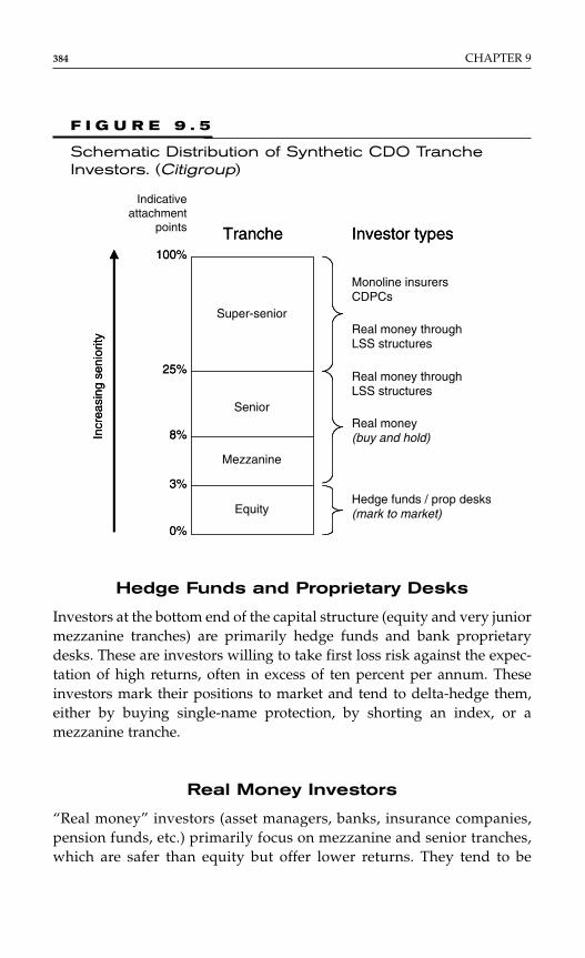
Hedge Funds and Proprietary Desks
Investors at the bottom end of the capital structure (equity and very juniormezzanine tranches) are primarily hedge funds and bank proprietarydesks. These are investors willing to take first loss risk against the expec-tation of high returns, often in excess of ten percent per annum. Theseinvestors mark their positions to market and tend to delta-hedge them,either by buying single-name protection, by shorting an index, or amezzanine tranche.
Real Money Investors
“Real money” investors (asset managers, banks, insurance companies,pension funds, etc.) primarily focus on mezzanine and senior tranches,which are safer than equity but offer lower returns. They tend to be
384 CHAPTER 9
F I G U R E 9 . 5
Schematic Distribution of Synthetic CDO TrancheInvestors. (Citigroup)
Tranche
Incr
easi
ng s
enio
rity
0%
25%
3%
8%
100%
Investor typesTranche
Incr
easi
ng s
enio
rity
Indicativeattachment
points
0%
25%
3%
8%
100%
Investor types
Hedge funds / prop desks(mark to market)
Real money(buy and hold)
Real money throughLSS structures
Real money throughLSS structures
Monoline insurersCDPCs
Super-senior
Senior
Mezzanine
Equity

buy-and-hold and often rating-sensitive investors who are attracted bythe higher spread offered by synthetic CDOs compared to cash productswith identical ratings.
Dealers and Other Market Participants
One of the key differences between cash and synthetic CDOs is that syn-thetics most often are not full-capital structure deals but single-trancheCDOs. This means that structurers do not sell all the risk of the underlyingportfolio of CDS, but only a portion, e.g., the 3 to 9 percent tranche. Strongdemand for mezzanine tranches risk from real money investors can leaddealers holding significant positions. Figure 9.6 illustrates schematically theresidual position of a dealer after selling a mezzanine tranche to an investorin two extreme scenarios. In the first scenario, the dealer sells the mezza-nine tranche risk to the investor and does not hedge its position, resultingin a net short mezzanine position. In the second scenario, the mezzanine ishedged with the full underlying portfolio of CDS, resulting in long equityand super senior positions. These positions (long equity, long super senior,and short mezzanine) are typical of the dealer community.
Dealers therefore hold significant positions in their correlationbooks and are not mere arrangers of deals, as is often the case for cashCDOs. Equity risk is either retained by dealers or passed on to hedgefunds. Super senior tranches can also be retained by the bank or soldto monoline insurers (wrappers) or to Credit Derivative Product
Cash and Synthetic CDOs 385
F I G U R E 9 . 6
Dealer’s Residual Position After Selling MezzanineTranche Risk. (Citigroup)
Dealter’s Residual Position without CDS Dealter’s Residual Position with CDSProdection sold
by dealerProdection sold
by dealerProdection sold
by investorsProdection sold
by investorsDealter’s residualshort risk position
Dealter’s residuallong risk position
Tranching Tranching
Super-senior Super-senior
MezzanineMezzanineMezzanineMezzanine
CDSportfolio
Equity Equity

Companies (CDPCs). The risk on these tranches can also be transferred toreal money investors in leveraged super senior (LSS) structures. LSS con-sists of recourse leverage notes referencing the super senior tranche, andlevered several times to enhance return. They are usually designed to havea low probability of recourse ( justifying a AAA rating) but their leveragemakes them quite sensitive to mark-to-market fluctuations, hence theirbetter suitability for buy-and-hold investors. We will return to LSS in thesection on double leverage.
SYNTHETIC CDO STRATEGIES
Investment strategies in synthetic CDOs are as diverse as investors intranches. Broadly speaking, we can split strategies into leverage trades,relative value trades, and directional trades. Tranches can also be used forhedging portfolios.
Taking Leverage
The tranching of CDS portfolios distributes the risk into the varioustranches and introduces leverage. Recall that the delta of a tranche is thesensitivity of that tranche’s spread to a one basis point change in theunderlying portfolio. By definition, the delta of the portfolio itself (whichcan be seen as the 0 to 100 percent tranche) is equal to one. Junior trancheshave deltas significantly higher than one and very senior tranches havedeltas below one. The former are thus levered in spread terms and the lat-ter de-levered. Tranching concentrates most of spread and default risksinto the equity and junior mezzanine pieces but, although both sources ofrisk are higher at the bottom of the capital structure, the split betweendefault risk and spread risk is very different to that of senior tranches.Thanks to their high degree of subordination, senior tranches bear verylittle default risk but they still suffer from some spread risk. In proportion,equity has more default risk than spread risk and vice versa for the senior.At this stage, it is useful to distinguish between idiosyncratic (single name)spread risk and market-wide spread risk. What we refer to as spread risk,unless clearly mentioned otherwise, is the widening of the entire marketor underlying portfolio, not that of a single credit or group of credits.Equity tranches are more sensitive to high spread names, whereas seniortranches tend to react more to low spread names widening. They have dif-ferent single-name deltas.
386 CHAPTER 9

Figure 9.7 (right panel) illustrates a tranche combination that relieson these differences in default and spread risks. Assuming that the equitytranche has a delta 20 times higher than that of the senior, one can build adelta-neutral position by buying one unit of equity tranche and selling 20units of the senior. The resulting position has positive carry to compensateinvestors for default risk but does not have spread exposure (ignoringconvexity). This “bull-bear” trade (long default risk but spread-hedged)was popular with hedge funds but is very sensitive to changes in correla-tions. In particular, falls in correlations hurt the trade both on its long legand on its short leg.
In summary, tranching distributes spread and default risks unequallyacross tranches. Investors can choose what type of risk they want to takeand their degree of exposure by taking more or less senior tranches. Thespreads paid on the tranches are compensation for both sources of risk.Through tranche combinations risk can be separated into a spread and adefault component. Care should be taken not to consider that delta-neutral strategies are immune from all spread risk. Delta-hedging protectsfrom small moves in the average spread of the portfolio, but not fromlarge swings. Tranches exhibit convexity (second order spread sensitivi-ties) that can be significant. Delta-hedging also relies on all spreads mov-ing by an equal amount. We mentioned earlier that tranches havedifferent micro-deltas. An uneven spread widening (with some nameswidening more than others) will not be perfectly hedge by traditionaldelta-hedging.
Cash and Synthetic CDOs 387
F I G U R E 9 . 7
Indicative Risks and Returns of Tranches and Bull-Bear Combination. (Citigroup)
Hypothetical Risks and Returns Long Equity / Short Senior Combination
Senior= 40 bp
Mezzanine= 150 bp
Equity= 1200 bp
Default risk Spread risk
Risk 1 m Equity
20 mSenior
Bull-bear
=
Spreadrisk
Defaultrisk

Relative Value Trades
Arguably the main motivation for real money investors for investing intranches is their search of relative value. Value is present at two levels insynthetic CDOs. First, market segmentation, the lower liquidity of bespokesynthetic tranches compared to cash instruments and their higher mark-to-market sensitivity make them trade cheaper (offering higher spread)than cash products with identical ratings. Rating-sensitive investors, whoare able to hold their positions to maturity and can withstand mark-to-market fluctuations, can thus find tranches attractive on a risk/rewardbasis. Second, as mentioned earlier, tranches enable investors to targetunderlying assets that they consider offer good relative value, irrespectiveof their ratings. They can thus extract the value of these underlying assetsin levered form and benefit from the additional value brought by syntheticstructures.
Directional and “Undirectional” Trades
Both the leverage and the relative value arguments apply equally to cashand synthetic CDOs. A peculiarity of synthetics is that they enableinvestors to go long or short risk, hence putting on directional trades. Wehave described long investment strategies earlier, including outright longpositions or delta-hedged trades. Investors expecting spreads to widencan take short positions on mezzanine or senior tranches. These shouldbenefit from a spread selloff, and the carry-to-delta ratio is often favorableto tranches compared to untranched portfolios. Investors who are bearishon default risk can buy equity risk protection, although the cost of thishedge is likely to be prohibitively high.
There are countless possible combinations of tranches offering dif-ferent spread and default risk sensitivities. These enable savvy investorsto express views on the direction of spreads and of default risk, possiblyin different directions (e.g., bullish on default and bearish on spreads).This is not possible with cash products (bonds, cash CDOs, or even CDS)with which investors must either be long default and spread risk or, if atall possible, short both risks. Other trades do not take views on the direc-tion of the market but rather on the behaviour of a subset of the market(sector, group of credits, etc.). For example, a dispersion trade consists ofbuying a senior tranche and delta-hedging the position by selling a morejunior tranche on the same portfolio. If all spreads move by an equal smallamount, the trade should be unaffected (but it suffers from negative
388 CHAPTER 9
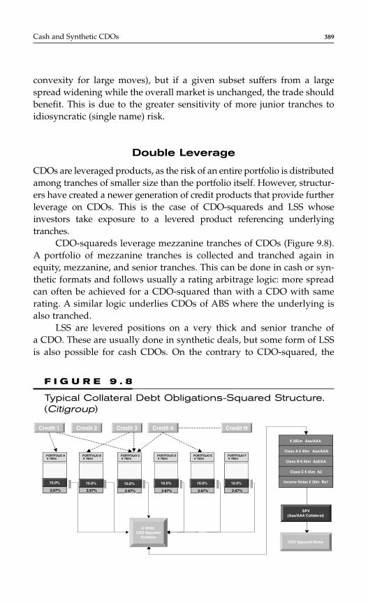
convexity for large moves), but if a given subset suffers from a largespread widening while the overall market is unchanged, the trade shouldbenefit. This is due to the greater sensitivity of more junior tranches toidiosyncratic (single name) risk.
Double Leverage
CDOs are leveraged products, as the risk of an entire portfolio is distributedamong tranches of smaller size than the portfolio itself. However, structur-ers have created a newer generation of credit products that provide furtherleverage on CDOs. This is the case of CDO-squareds and LSS whoseinvestors take exposure to a levered product referencing underlyingtranches.
CDO-squareds leverage mezzanine tranches of CDOs (Figure 9.8).A portfolio of mezzanine tranches is collected and tranched again inequity, mezzanine, and senior tranches. This can be done in cash or syn-thetic formats and follows usually a rating arbitrage logic: more spreadcan often be achieved for a CDO-squared than with a CDO with samerating. A similar logic underlies CDOs of ABS where the underlying isalso tranched.
LSS are levered positions on a very thick and senior tranche ofa CDO. These are usually done in synthetic deals, but some form of LSSis also possible for cash CDOs. On the contrary to CDO-squared, the
Cash and Synthetic CDOs 389
F I G U R E 9 . 8
Typical Collateral Debt Obligations-Squared Structure.(Citigroup)
PORTFOLIO AEUR 750 m
10.00%
PORTFOLIO BEUR 750 m
1.00%
2.00%10.00%
2.667%
PORTFOLIO C! 750m
10.00%
2.667%
PORTFOLIO D! 750m
10.00%
2.667%
PORTFOLIO E! 750m
10.00%
2.667%
PORTFOLIO E! 750m
10.00%
2.667%
CitigroupEntity
PORTFOLIO A! 750m
10.00%
PORTFOLIO A750m
10.00%10.00%
PORTFOLIO B! 750m
1.00%
2.00%10.00%
2.667%
PORTFOLIO B750m
1.00%10.00%
2.667%
10.00%
2.667%
PORTFOLIO C! 750m
10.00%
2.667%
PORTFOLIO C750m
10.00%
2.667%
10.00%
2.667%
PORTFOLIO D! 750m
10.00%
2.667%
PORTFOLIO D750m
10.00%
2.667%
10.00%
2.667%
PORTFOLIO E! 750m
10.00%
2.667%
PORTFOLIO E750m
10.00%
2.667%
10.00%
2.667%
PORTFOLIO E! 750m
10.00%
2.667%
PORTFOLIO F750m
10.00%
2.667%
10.00%
2.667%2.667%2.667%2.667%2.667%2.67% 2.667%2.667%2.667%2.667%2.67% 2.667%2.667%2.667%2.667%2.67% 2.667%2.667%2.667%2.667%2.67% 2.667%2.667%2.667%2.667%2.67% 2.667%2.667%2.667%2.667%2.67%
SEALS Finance SA
Sp -1Senior CLN’s
SEALS Finance SA
Spinnaker 2003-1Senior CLN’s
SPV(Aaa/AAA Collateral)
Spinnaker
CLN’s
285m Aaa/AAA
Class A 45m Aaa/AAA
Class B 45m Aa2/AA
Class C 45m A2
Income Notes 30m Ba1
CDO Squared Notes
450mCDO-Squared
Portfolio
Credit 1
10.0% 10.0% 10.0% 10.0% 10.0% 10.0%
SPV(Aaa/AAA Collateral)
Credit 2 Credit 4 Credit NCredit 3

technology underlying LSS does not rely on further tranching but simplyon the principle of recourse leverage. An investor can, e.g., take an expo-sure to a a500 million piece of the super senior tranche of a CDO (say, the10 to 70 percent tranche), through a a50 million note. The leverage is 10times (500/50) and the spread on the LSS is 10 times that on the unlev-ered super senior tranche. However, the contract is designed in such away that if there are defaults in the portfolio or if spreads widen sub-stantially, the protection buyer can ask the protection seller eitherto unwind the deal or post further collateral, on top of the initial a50million.
Tranches as Hedging Vehicles
Although the vast majority of single tranche CDOs are issued to satisfycustomer needs to take risk and receive premium, they are also used bysome investors as hedging devices. Returning to Figure 9.7 (left panel),the advantage of hedging a portfolio with senior mezzanine tranchesbecomes apparent. Investors who are comfortable with the default risk ontheir portfolio can hedge their spread risk (delta-hedging) by buying pro-tection on a mezzanine or senior tranche of a synthetic CDO, referencingthe same or similar names. This hedge will offer little protection againstdefault risk but should be significantly cheaper than single-name CDSprotection or even index protection. Protection buyers thus only pay forthe risk they want to hedge: spread risk in this example. The leverage ofCDO tranches will often require hedgers to buy protection on a smallertranche notional than that of the hedged portfolio, unless they use a verysenior tranche (with delta lower than one).
As discussed at the beginning of this chapter, bank loan managersand insurance companies can also use tranche hedges to optimize theirreturn on regulatory capital. Under the current banking regulations,which do not link regulatory capital based on the riskiness of exposures(e.g., all corporate loans and bonds have an 8 percent risk charge irre-spective of maturity and default probability), the incentive has been forbanks to buy protection on low risk and low yield exposures. These arecheaper to hedge and offer the same capital relief as more risky exposures.However, the new regulatory framework (Basel II) is about to change this(see the last section of this chapter).
390 CHAPTER 9
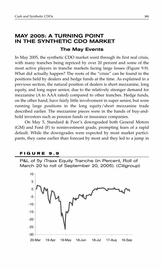
MAY 2005: A TURNING POINT IN THE SYNTHETIC CDO MARKET
The May Events
In May 2005, the synthetic CDO market went through its first real crisis,with many tranches being repriced by over 20 percent and some of themost active players in tranche markets facing large losses (Figure 9.9).What did actually happen? The roots of the “crisis” can be found in thepositions held by dealers and hedge funds at the time. As explained in aprevious section, the natural position of dealers is short mezzanine, longequity, and long super senior, due to the relatively stronger demand formezzanine (A to AAA rated) compared to other tranches. Hedge funds,on the other hand, have fairly little involvement in super senior, but wererunning large positions in the long equity/short mezzanine tradedescribed earlier. The mezzanine pieces were in the hands of buy-and-hold investors such as pension funds or insurance companies.
On May 5, Standard & Poor’s downgraded both General Motors(GM) and Ford (F) to noninvestment grade, prompting fears of a rapiddefault. While the downgrades were expected by most market partici-pants, they came earlier than forecast by most and they led to a jump in
Cash and Synthetic CDOs 391
F I G U R E 9 . 9
P&L of 5y iTraxx Equity Tranche (in Percent, Roll ofMarch 20 to roll of September 20, 2005). (Citigroup)
-30
-25
-20
-15
-10
-5
0
5
10
20-Mar 19-Apr 19-May 18-Jun 18-Jul 17-Aug 16-Sep
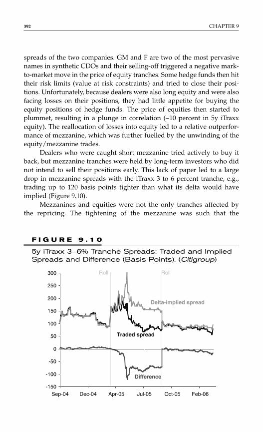
spreads of the two companies. GM and F are two of the most pervasivenames in synthetic CDOs and their selling-off triggered a negative mark-to-market move in the price of equity tranches. Some hedge funds then hittheir risk limits (value at risk constraints) and tried to close their posi-tions. Unfortunately, because dealers were also long equity and were alsofacing losses on their positions, they had little appetite for buying theequity positions of hedge funds. The price of equities then started toplummet, resulting in a plunge in correlation (−10 percent in 5y iTraxxequity). The reallocation of losses into equity led to a relative outperfor-mance of mezzanine, which was further fuelled by the unwinding of theequity/mezzanine trades.
Dealers who were caught short mezzanine tried actively to buy itback, but mezzanine tranches were held by long-term investors who didnot intend to sell their positions early. This lack of paper led to a largedrop in mezzanine spreads with the iTraxx 3 to 6 percent tranche, e.g.,trading up to 120 basis points tighter than what its delta would haveimplied (Figure 9.10).
Mezzanines and equities were not the only tranches affected bythe repricing. The tightening of the mezzanine was such that the
392 CHAPTER 9
F I G U R E 9 . 1 0
5y iTraxx 3–6% Tranche Spreads: Traded and ImpliedSpreads and Difference (Basis Points). (Citigroup)
-150
-100
-50
0
50
100
150
200
250
300
Sep-04 Dec-04 Apr-05 Jul-05 Oct-05 Feb-06
Roll Roll
Delta-implied spread
Traded spread
Difference
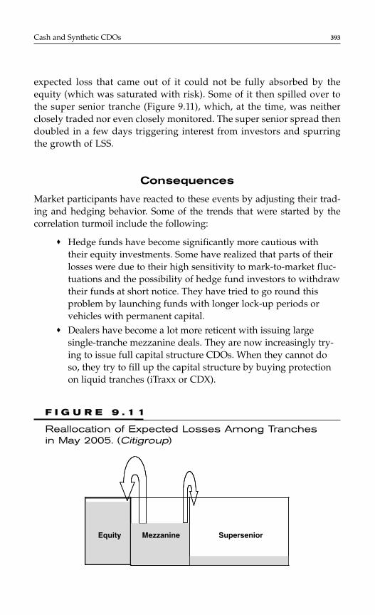
Cash and Synthetic CDOs 393
F I G U R E 9 . 1 1
Reallocation of Expected Losses Among Tranchesin May 2005. (Citigroup)
Equity Mezzanine Supersenior
expected loss that came out of it could not be fully absorbed by theequity (which was saturated with risk). Some of it then spilled over tothe super senior tranche (Figure 9.11), which, at the time, was neitherclosely traded nor even closely monitored. The super senior spread thendoubled in a few days triggering interest from investors and spurringthe growth of LSS.
Consequences
Market participants have reacted to these events by adjusting their trad-ing and hedging behavior. Some of the trends that were started by thecorrelation turmoil include the following:
♦ Hedge funds have become significantly more cautious withtheir equity investments. Some have realized that parts of theirlosses were due to their high sensitivity to mark-to-market fluc-tuations and the possibility of hedge fund investors to withdrawtheir funds at short notice. They have tried to go round thisproblem by launching funds with longer lock-up periods orvehicles with permanent capital.
♦ Dealers have become a lot more reticent with issuing largesingle-tranche mezzanine deals. They are now increasingly try-ing to issue full capital structure CDOs. When they cannot doso, they try to fill up the capital structure by buying protectionon liquid tranches (iTraxx or CDX).

♦ Given the high demand for mezzanine, the main difficulty facingdealers since the May repricing is the placement of equitytranches, as placing the super senior is now straightforward withLSS. Equity tranches are more difficult to sell, as some of their nat-ural holders (hedge funds and dealers) have shied away fromthem. Structurers have therefore developed new equity-linkedproducts to broaden the investor base of equity. Buy-and-holdinvestors are particularly sought after, as they could bring morestability to the market and are less prone to overreaction linked tomark-to-market fluctuations. Rated equity and principal-protectedstructures such as simple combination securities, step-downcoupon notes are CPPI (Constant Proportional Portfolio Insurance)referencing equity tranches, have now become mainstream.
♦ While the May events have led to financial innovation such asLSS and the equity-linked structures mentioned earlier, theyhave also led to the quasi-disappearance of CDO-squared, whichwere one of the most popular trades of 2004 and early 2005. Thetightness of mezzanine spreads has made the rating arbitrage ofCDO-squared less compelling, and dealers have become morewary of correlation risk inherent to those structures.
♦ Finally, buy-and-hold investors have moved their preferredmaturity to seven year from five year because of the tightnessof mezzanine spreads. Seven year is now the most commonmaturity for synthetic CDOs.
BASEL II—CHANGING THE RULES OF CDOISSUANCE AND INVESTMENT
We have shown in this chapter how important banks are in the CDO mar-ket, both from an issuance perspective (balance sheet CDOs, synthetichedging) and also as investors. Until now, no global set of regulationis available for banks with respect to CDOs and other securitizations. Thecurrent international regulatory framework (Basel I) does not cover CDOs,and each jurisdiction has its own local regulations.
However, this is about to change with the implementation of BaselII rules, from January 2007.*
394 CHAPTER 9
*Banks opting for the standardized approach of Basel II will switch to the new rules inJanuary 2007. Banks opting for the internal ratings-based approach have until January 2008.
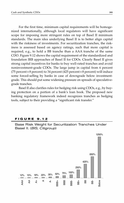
For the first time, minimum capital requirements will be homoge-nized internationally, although local regulators will have significantscope for imposing more stringent rules on top of Basel II minimumstandards. The main idea underlying Basel II is to better align capitalwith the riskiness of investments. For securitization tranches, the risk-iness is assessed based on agency ratings, such that more capital isrequired, e.g., to hold a BB tranche than a AAA tranche of the sameCDO. Figure 9.12 shows the capital requirement of the standardized andfoundation IRB approaches of Basel II for CDOs. Clearly Basel II givesstrong capital incentives for banks to buy well-rated tranches and avoidnoninvestment-grade CDOs. The large jump in capital from 6 percent(75 percent × 8 percent) to 34 percent (425 percent × 8 percent) will inducesome forced-selling by banks in case of downgrade below investment-grade. This should put some widening pressure on spreads of speculative-grade tranches.
Basel II also clarifies rules for hedging risk using CDOs, e.g., by buy-ing protection on a portion of a bank’s loan book. The proposed newbanking regulatory framework indeed recognizes tranches as hedgingtools, subject to their providing a “significant risk transfer.”
Cash and Synthetic CDOs 395
F I G U R E 9 . 1 2
Base Risk Weight for Securitization Tranches UnderBasel II. (BIS, Citigroup)
12% 15% 18% 20% 35% 50% 75% 100%
250%
425%
650%
1250%
AA
A
AA A+ A A-
BB
B+
BB
B
BB
B-
BB
+
BB
BB
-
Bel
ow

When buying protection on a tranche, the bank can replace the riskweight of the hedged portion of its portfolio with the risk weight of itshedge counterparty (another bank or an insurance company), asdescribed at the begining of this chapter. We expect a lot of activity to takeplace in the junior mezzanine portion of the capital structure, as it iscurrently the most efficient in terms of improvement of return on capital.
396 CHAPTER 9

C H A P T E R 1 0
The Collateral DebtObligation MethodologiesDeveloped by Standardand Poor’s
397
This chapter consists of two parts. Part 1 describes the modeling of thecredit behavior of the assets employed in Standard & Poor’s Tool: “CDOEvaluator.” Part 2 describes the modeling of the liabilities, i.e., the modelingof the cashflows of Cash CDOs. Both parts are retrieved from S&P criteria.
PART 1 DESCRIPTION OF S&PPORTFOLIO MODEL: CDO EVALUATORVERSION 3* FOR SYNTHETICSECURITIZATION
Standard & Poor’s Ratings Service’s CDO Evaluator is a portfolio creditrisk model for analysis of CDO transactions. This document describes thetheory, assumptions, and computational methods used by CDO Evaluatorversion 3.0 to simulate the portfolio loss distribution, which allows deter-mination of the various portfolio risk measures we use in the CDO ratingprocess. The application of the CDO Evaluator to different types of CDOtransactions is also discussed.
* Extracted from the S&P criteria publication CDO Evaluator Version 3.0: Technical Documentby Kai Gilkes, Norbert Jobst, and Bob Watson dated 19-12-05.
Copyright © 2007 by The McGraw-Hill Companies. Click here for terms of use.

398 CHAPTER 10
INTRODUCTION
CDO Market Developments
The collateral debt obligations (CDOs) are financial instruments that trans-fer the risk associated with a portfolio of assets to one or more investors.The first CDOs were issued as funded (cash) investments by a special pur-pose entity (SPE), collateralized by portfolios of bonds and loans. Over thepast decade, the unfunded (synthetic) CDO market has grown rapidly,especially in Europe. Instead of purchasing a debt instrument of a givenentity, the SPE enters into a credit default swap (CDS) that references theentity. This use of credit derivatives technology has greatly simplified theexecution of CDO transactions, and has led to a market dominated by so-called “single-tranche” CDOs, bilateral contracts between a buyer andseller of default protection on a portfolio of entities. These can either takethe form of a portfolio CDS between two counterparties or a credit-linkednote (CLN).
While the rise of the synthetic CDO market has led to a simplifica-tion of the debt issuance, the composition of the asset portfolio hasbecome more complex. In addition to corporate bonds and loans, CDOportfolios now routinely include sovereign bonds, loans to small- or mid-sized enterprises (SMEs), asset-backed securities (ABS), and other CDOs.More recently, equity default swaps (EDSs) and commodity options havealso been included. The CDO risk transfer mechanism has also increasedin complexity. In addition to referencing a single portfolio, a CDO trans-action can also reference a number of bespoke CDO tranches, each ofwhich in turn references a single portfolio. This leveraging creates aninvestment that is more isolated from small numbers of credit eventswithin the underlying portfolio, but is also more likely to suffer largelosses once its credit protection is eroded. The so-called “CDO-squared”transactions dominated synthetic CDO issuance in 2004 and in early 2005,partly due to the tightening of CDS spreads.*
In recent years, the synthetic CDO market has witnessed the prolif-eration of many innovative structures, including CDOs with short CDSpositions, forward starting CDOs, nth-to-default baskets, leveraged supersenior structures, and constant proportion portfolio insurance (CPPI)structures. These innovations typically arise from a variety of different
*These transactions often include a large proportion of ABS in addition to bespoke CDOs,and are therefore often referred to as “CDO of ABS” transactions.

incentives expressed by market participants: from the search by investorsfor yield in a tight spread environment to the need for investment diver-sification, from the quest for arbitrage to structures that can be used toexpress a view on either the credit cycle or idiosyncratic credit risk.
Portfolio Credit Risk Models
Models for CDO risk analysis are generally based on the estimation oftransition/default probabilities and recoveries, and the linkage of thesethrough a dependency model, which specifies the joint transition/defaultbehavior. This allows simulation of the full loss distribution at maturity ofa portfolio of assets. This loss distribution can then be used to determinea number of useful measures of portfolio risk.
Many portfolio credit risk models fall into the category of “struc-tural” models, which assume that the default behavior of a firm can bedetermined from knowledge of the firm’s assets and liabilities. These arebased largely on a model originally proposed by Merton (1974), in whichthe asset value of a firm is assumed to follow a Geometric BrownianMotion characterized by the asset volatility. Default of the firm occurswhen the asset value falls below a certain threshold.* Within this frame-work, the default correlation between pairs of firms will depend both onthe correlation of asset value and the default threshold for each firm. Foran excellent review of structural models, see de Servigny and Renault(2004).
In common with many other structural models, CDO Evaluatorassumes that the transition/default probabilities, recoveries, and assetvalue correlations of all assets in the portfolio are exogenous variables,driven either by firm-specific (i.e., idiosyncratic) or systematic effects.†
However, rather than using market data to estimate these parameters foreach firm, we estimate these parameters from historical data.
For example, in the case of rated firms, we make use of our globalCreditPro® database‡ of rating transitions and defaults over the period
CDO Methodologies Developed by S&P 399
*In the Merton framework, this threshold is related to the value of the liabilities of the firm,and hence more highly leveraged firms will generally possess higher probabilities of default,assuming similar asset volatilities.†Other models focus instead on the instantaneous default probability (also known as the“hazard rate” or “default intensity”), which is itself treated as a stochastic process.‡For details, visit www.standardandpoors.com, run a search using “CreditPro,” and scrolldown to Products & Services.

400 CHAPTER 10
1981–2003. This method assumes that the rating on a firm is a good proxyfor the likelihood of the firm defaulting over a given horizon, when thisfirm is part of a portfolio.*
Technical Document Outline
The remainder of this part is divided into five sections. In the section “TheCDO evaluator model,” the underlying mathematical model for CDOEvaluator version 3.0 is outlined, along with the assumptions required bythe model for computation of the portfolio loss distribution. The sections“Transition and default probabilities,” “Recoveries,” and “Correlation” out-line the data and methods used to estimate these assumptions, which arethe main inputs required by CDO Evaluator. The section “CDO risk analy-sis” describes the different CDO risk measures computed by CDO Evaluatorand the application of CDO Evaluator to the risk assessment of various CDOtransactions in the marketplace. Many of the detailed assumptions withinCDO Evaluator are contained within the Appendices.
While this document addresses all of the technical aspects of theCDO Evaluator model and assumptions, it does not necessarily covereach and every aspect in full, as the purpose of this document is to pro-vide a complete picture of CDO Evaluator to a wide range of market par-ticipants. Those readers interested in drilling down to a deeper technicalor theoretical level should consult the references provided within thedocument.
THE CDO EVALUATOR MODEL
The main purpose of the CDO Evaluator model is the computation of theloss distribution of a portfolio of N assets. This is carried out by first sim-ulating the default time of each asset. If the default occurs before the matu-rity of the CDO transaction, an asset-specific recovery is also computed. Ifthe exposure to each asset at the time of default is known, then the com-plete distribution of portfolio losses can be computed.
In addition to modeling the individual (or univariate) default andrecovery of each asset in the portfolio, the dependency between defaults of
*It is important that this method is used only for portfolios, not single firms. Given that rat-ings are ordinal measures of creditworthiness, a single rating cannot be uniquely linked to adefault probability.
CDO Methodologies Developed by S&P 401
different assets must also be modeled. The standard dependency modelin the marketplace is the Gaussian copula model, originally proposed byLi (2000). In this approach, a term structure of survival probabilities Si(t)is assumed for the ith asset. These survival probabilities can be obtainedfrom the cumulative default probabilities for each asset, which we referto as the credit curves. Dependency is then introduced via the Gaussiancopula function C(u1 , . . . , uN) = ΦΣ(y1 , . . . , yN), where Σ denotes the cor-relation matrix, Φ the univariate standard normal cumulative distribu-tion function, and ΦΣ the multivariate standard normal distributionfunction with correlation matrix Σ. The copula function therefore linkstogether the standard normal variables y1 to create a multivariate distri-bution of uniform random variables u1. The standard normal variables yiare often referred to as latent variables (analogous to asset values in theMerton model).
Correlated default times can therefore be simulated in the followingorder.
♦ Simulate a vector of N standard normal random variables yi foreach asset;*
♦ Impose a given correlation matrix Σ on the above vector.†
♦ Calculate ui = Φ(yi); and♦ Calculate a default time τi = S−1(ui) for each asset. An example is
shown in Figure 10.1 for a “BBB” rated asset.‡
If τi is less than the maturity T of the CDO transaction, the loss Li is deter-mined as Li = Ei × (1 − δi), where Ei and δi are the exposure-at-default andrecovery,§ respectively, for the ith asset. We can therefore write the portfo-lio loss up to time t, L(t), as:
where is the default indicator for the ith asset.||1 τ i t≤
L t Ei i ti
i( ) ( ) ,= × − ×
≤ ∑ 1 1δτ
*Standard normal random numbers are computed using the well-known Mersenne Twisteralgorithm. For details, see Matsumoto and Nishimura (1998).†This is performed using Cholesky factorisation. See, e.g., Glasserman (2004), pp. 72–73.‡S−1 is used to denote the quasi-inverse of the survival function.§The recovery can either be assumed to be constant, or drawn from a distribution.||The default indicator equals 1 if the expression within parentheses is true, and 0 if it isfalse.
402 CHAPTER 10
Simulation ProcedureThere are two aspects of the simulation procedure worth discussingin more detail in order to understand the impact of different ratings,maturities, and correlation assumptions on the portfolio loss distri-bution.
Individual Asset Default BehaviorWhen assets are uncorrelated, the default time for each asset i is sim-ply obtained by comparing a uniform random variable ui with thecredit curve for the asset, as shown in Figure 10.1 for a “BBB” ratedasset. If the default time occurs before the asset maturity, a default isrecorded. For example, if the “BBB” rated asset in Figure 10.1 has amaturity of seven years, a default is recorded halfway through yearfive. For the same rating, it is clear that high values of ui will resultin lower default times, whereas low values will result in higherdefault times. Also, for the same value of ui, it is clear that higherratings will experience higher default times.
Joint Default BehaviorWhen assets are correlated, the uniform random numbers for theseassets are first correlated to the required level, as described above.For any pair of correlated assets, this produces values of ui that tendto move together, i.e., are “clustered” around high or low values. Asa result, the default times of the two assets will also move together,leading to more cases in which the assets survive or default togetherbefore their maturity.
Using the above Monte Carlo simulation procedure, the distribu-tion of portfolio losses can be determined to a high level of accuracy bygenerating a sufficient number of default times to achieve satisfactoryconvergence, which depends on the shape of the credit curves and thedegree of asset correlation. For example, highly rated assets will rarelygenerate low default times, requiring a larger number of simulation tri-als to generate a significant number of default events before maturity. Formost portfolios, 500,000 simulation trials are sufficient to obtain satisfac-tory convergence.
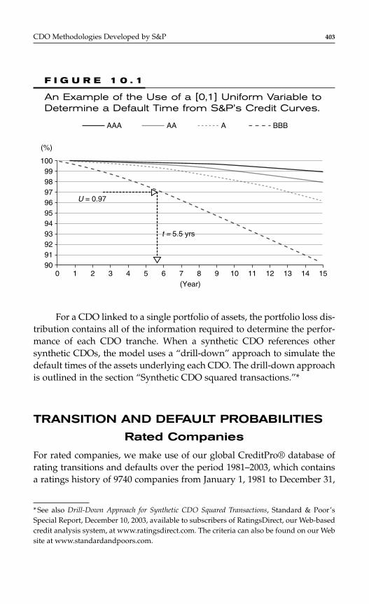
For a CDO linked to a single portfolio of assets, the portfolio loss dis-tribution contains all of the information required to determine the perfor-mance of each CDO tranche. When a synthetic CDO references othersynthetic CDOs, the model uses a “drill-down” approach to simulate thedefault times of the assets underlying each CDO. The drill-down approachis outlined in the section “Synthetic CDO squared transactions.”*
TRANSITION AND DEFAULT PROBABILITIES
Rated Companies
For rated companies, we make use of our global CreditPro® database ofrating transitions and defaults over the period 1981–2003, which containsa ratings history of 9740 companies from January 1, 1981 to December 31,
CDO Methodologies Developed by S&P 403
10099989796959493929190
0 1 2 3 4 5 6 7 8 9 10 11 12 13 14 15(Year)
(%)
t = 5.5 yrs
U = 0.97
AAA BBBAA A
F I G U R E 1 0 . 1
An Example of the Use of a [0,1] Uniform Variable toDetermine a Default Time from S&P’s Credit Curves.
* See also Drill-Down Approach for Synthetic CDO Squared Transactions, Standard & Poor’sSpecial Report, December 10, 2003, available to subscribers of RatingsDirect, our Web-basedcredit analysis system, at www.ratingsdirect.com. The criteria can also be found on our Website at www.standardandpoors.com.
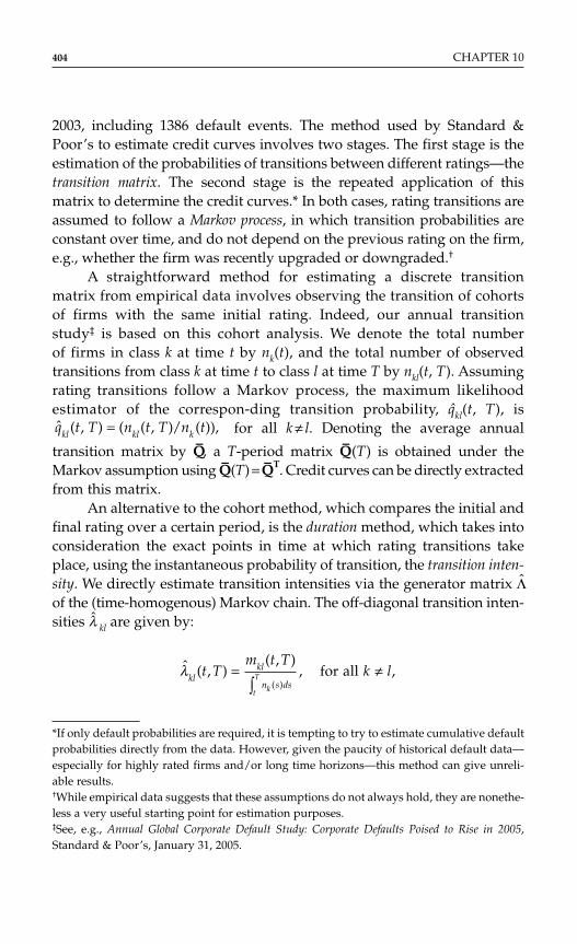
404 CHAPTER 10
2003, including 1386 default events. The method used by Standard &Poor’s to estimate credit curves involves two stages. The first stage is theestimation of the probabilities of transitions between different ratings—thetransition matrix. The second stage is the repeated application of thismatrix to determine the credit curves.* In both cases, rating transitions areassumed to follow a Markov process, in which transition probabilities areconstant over time, and do not depend on the previous rating on the firm,e.g., whether the firm was recently upgraded or downgraded.†
A straightforward method for estimating a discrete transitionmatrix from empirical data involves observing the transition of cohortsof firms with the same initial rating. Indeed, our annual transitionstudy‡ is based on this cohort analysis. We denote the total numberof firms in class k at time t by nk(t), and the total number of observedtransitions from class k at time t to class l at time T by nkl(t, T). Assumingrating transitions follow a Markov process, the maximum likelihoodestimator of the correspon-ding transition probability, qkl(t, T), is
for all k ≠ l. Denoting the average annual
transition matrix by Q–, a T-period matrix Q– (T) is obtained under theMarkov assumption using Q– (T) = Q– T. Credit curves can be directly extractedfrom this matrix.
An alternative to the cohort method, which compares the initial andfinal rating over a certain period, is the duration method, which takes intoconsideration the exact points in time at which rating transitions takeplace, using the instantaneous probability of transition, the transition inten-sity. We directly estimate transition intensities via the generator matrix Λof the (time-homogenous) Markov chain. The off-diagonal transition inten-sities λ kl are given by:
ˆ ( , )( , )
, for all ,( )
λklkl
n s dst T
m t Tk l
kt
T= ≠∫
ˆ ( , ) ( ( , )/ ( )),q t T n t T n tkl kl k=
*If only default probabilities are required, it is tempting to try to estimate cumulative defaultprobabilities directly from the data. However, given the paucity of historical default data—especially for highly rated firms and/or long time horizons—this method can give unreli-able results.†While empirical data suggests that these assumptions do not always hold, they are nonethe-less a very useful starting point for estimation purposes.‡See, e.g., Annual Global Corporate Default Study: Corporate Defaults Poised to Rise in 2005,Standard & Poor’s, January 31, 2005.
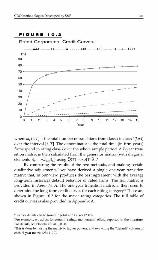
CDO Methodologies Developed by S&P 405
where mkl(t, T) is the total number of transitions from class k to class l (k ≠ l)over the interval [t, T]. The denominator is the total time (in firm-years)firms spend in rating class k over the whole sample period. A T-year tran-sition matrix is then calculated from the generator matrix (with diagonalelements ) using Q– (T) = expT ⋅ Λ~.*
By comparing the results of the two methods, and making certainqualitative adjustments,† we have derived a single one-year transitionmatrix that, in our view, produces the best agreement with the averagelong-term historical default behavior of rated firms. The full matrix isprovided in Appendix A. The one-year transition matrix is then used todetermine the long-term credit curves for each rating category.‡ These areshown in Figure 10.2 for the major rating categories. The full table ofcredit curves is also provided in Appendix A.
λ λll k l kl= − ≠Σ
*Further details can be found in Jobst and Gilkes (2003).†For example, we adjust for certain “ratings momentum” effects reported in the literature.For details, see Fledelius et al. (2004).‡This is done by raising the matrix to higher powers, and extracting the “default” column ofeach N-year matrix (N = 1–30).
90
AAA AA A BBB BB B CCC
(%)
80
70
60
50
40
30
20
0 1 2 3 4 5 6 7 8 9 10
Year
11 12 13 14 15
10
0
F I G U R E 1 0 . 2
Rated Corporates—Credit Curves.

406 CHAPTER 10
Asset-Backed Securities
Given that structured finance securities themselves are often included inCDO portfolios, their transition and default behavior also needs to be esti-mated. On average, these securities have exhibited considerable ratingsstability over the past two decades, and as a result there have been veryfew cases of default.* Given the relative paucity of default data, we haveso far adopted a conservative treatment of these securities by using cor-porate default rates as proxies for their long-term default behavior.
In CDO Evaluator version 3.0, ABS default rates are determinedusing a transition matrix that is based on the average historical ABS tran-sition matrix, with certain qualitative adjustments. These adjustmentsresult in long-term ABS default rates that are approximately 55 and 75percent of the corresponding default rates for rated firms at investment-grade and non-investment-grade, respectively (for maturities betweenfive and seven years). The ABS credit curves are provided in Appendix A.Note that ABS maturities are capped at seven years for modeling pur-poses, as we consider that the probability of default of an ABS asset—conditional upon survival for seven years—is negligible.
Sovereign Securities
Given that transition and default data for sovereign debt securities are rel-atively sparse in comparison with rated firms, the credit curves used forrated firms are currently used as conservative proxies for sovereigndefault behavior.
Small- to Mid-sized Enterprises
The wealth of financial information obtained by Standard & Poor’s RiskSolutions Group on SMEs has been used to create advanced “credit scor-ing” models for SME default prediction. For example, in Europe, thecredit risk tracker (CRT) product can be used to obtain one-year defaultprobability forecasts for more than 1 million SMEs across France,Germany, Italy, Spain, and the U.K. These models have also been used toanalyze the historical volatility of default probabilities, in order to create
*See, e.g., Global Structured Securities Rating Performance: 1978–2004, Standard & Poor’s,March 24, 2005.
“rating estimates” that combine one-year default probabilities and annu-alized default volatilities.* By analyzing the transition behavior across dif-ferent rating categories, we have created a one-year SME transition matrixand used it to create credit curves for SMEs. The credit curves are pro-vided in Appendix A. Note that while the rating identifiers are written inthe same way as those for traditional Standard & Poor’s ratings, they arenot obtained through the normal rating analysis conducted by our ana-lysts. It is therefore not possible to make direct comparisons between thecredit curves for SMEs and those for other rated entities.
Equity Default Swaps
An EDS is similar to a CDS, in that a protection seller agrees to pay the pro-tection buyer if the contract is triggered. However, as opposed to a creditevent, an EDS is linked to the drop of the equity price of the reference entitybelow a certain barrier, typically 30 percent of the initial price. As a result ofextensive analysis of historical equity price data from our Compustat® data-base, capturing approximately 12,000 companies trading in the UnitedStates or Canada between 1962 and 2003, we have developed new criteriafor estimating the probability of an EDS contract triggering over a giventime horizon. Using scoring techniques similar to those described in the pre-vious section, we have identified five variables that are very informative:
♦ The credit rating;♦ The historical equity volatility;♦ The market capitalization;♦ The historical equity return; and♦ The general level of the equity market measured by the current
value of the S&P500 compared with the highest value of the pre-vious 10 years.
The resulting EDS scoring models are used to derive a risk score betweenone and five for each EDS. These scores can then be mapped to an EDSdefault curve, i.e., the cumulative probability of the EDS contract breach-ing its price barrier.† Further technical details can be found in de Servignyand Jobst (2005). An overview of our criteria for CDOs containing EDS
CDO Methodologies Developed by S&P 407
*For example, in the case of two SMEs with low one-year default probabilities but very dif-ferent volatilities, the one with the lower volatility is likely to be assigned a higher rating.†We can provide these scoring models upon request.

can be found in a forthcoming criteria article, and Appendix A containsfurther details of the EDS default curves.
RECOVERIES
In general, the level of recovery achieved following a default is uncertain,or stochastic. For a debt instrument, such as a bond or loan, recoverydepends on a number of factors, for instance, the seniority of the instru-ment and the economic environment in which the default occurred.However, in the context of synthetic CDOs, recovery can be determinedin different ways, including the specification of a fixed level that does notdepend on these factors.
In order to properly model the different types of recovery mecha-nisms included in CDOs, CDO Evaluator treats recoveries in two ways:fixed and variable. This section outlines the two different methods, both interms of the rationale for using each method, and the underlying dataused to estimate recoveries in each case.
Fixed Recoveries
Although recoveries are usually uncertain, there are two main reasonsfor using fixed recovery assumptions. First, recovery can in certain trans-actions be set at a fixed percentage of the amount at risk, e.g., 50 per-cent.* Secondly, historical data is not always sufficient to allow precisedetermination of the degree of variability in recoveries. For this reason,a fixed recovery that incorporates some degree of conservatism can bethe best compromise. As this clearly involves some level of qualitativejudgment, these assumptions are normally determined through acommittee process.
Variable Recoveries
In some cases, sufficient historical data exists to allow the degree of vari-ability in recoveries to be explicitly modeled. For example, our LossStats®
database† contains recovery information for more than 500 non-financial
408 CHAPTER 10
*This is the recovery level typically used for EDSs.†For details, visit www.standardandpoors.com, run a search using “LossStats,” and scrolldown to Products & Services.

public and private U.S. companies that have defaulted since 1988. It con-tains information on more than 2,000 defaulted bank loans and high-yieldbonds, and other debt instruments. This extensive data has allowed us tocreate recovery distributions for certain types of assets, based on the betadistribution, a well-known two-parameter distribution. Specification ofthe mean and standard deviation of the beta distribution is sufficient forCDO Evaluator version 3.0 to simulate the full range of potential recover-ies for each type of asset. These assumptions are provided in Appendix B.
CORRELATION
In addition to specifying the univariate default probabilities and recoveryassumptions for each asset in the portfolio, the correlation between pairsof assets must also be specified. As explained in the section “The CDOevaluator model,” this is assumed to be the asset value correlation betweeneach pair of assets, which is not directly observable in the market. In prin-ciple, there are several ways to estimate asset value correlation:
♦ Regression analysis of equity returns within a factor model;♦ Using equity return correlations as proxies for asset value corre-
lation;♦ Using credit spread correlations as proxies for asset value corre-
lation;♦ Inferring asset value correlations from rating migrations; and♦ Estimating asset value correlations from empirical default obser-
vations.
We have chosen to use empirical default observations to estimate the cor-relation assumptions within CDO Evaluator, as this estimation method islikely to be less prone to the “noise” within equity return data, and thelimited time period of credit spread data. In addition, unlike rating migra-tions, it can be used consistently for a wide range of different rated andnon-rated assets, such as corporates, ABS, SMEs, and EDS. In order todetermine correlation assumptions for rated firms and EDSs, we haveundertaken an extensive analysis of historical data, making use of theCreditPro® and Compustat® databases mentioned earlier. For SMEs, theCRT database mentioned earlier has been used.
We consider several statistical techniques which ensures a gooddegree of stability, ranging from maximum likelihood methods and factormodels, to simple methods based on empirical joint default events. While
CDO Methodologies Developed by S&P 409
a detailed overview of these techniques for corporate defaults and EDScan be found in Jobst and de Servigny (2006), the latter approach—frequently referred to as joint default probability (JDP) method—is out-lined next, given the significance of correlation estimates for CDO riskanalysis.
The JDP method involves two stages. The first is the estimation ofthe JDP Pij(t) between pairs of companies, either in the same industry ordifferent industries. If pairs of companies are drawn (with replacement)from the database, an estimate of the JDP within an industry is given by:
and between industries by:
In these expressions, Dct, Dd
t and Nct, Nd
t are the number of defaultedcompanies and total number of companies in industries c and d, respec-tively, observed over a time period t. The empirical default correlation ρ cd
can easily be obtained from the standard correlation equation:
In this formula, P–k denotes the average default probability of com-panies in industry k.
The second stage of the JDP method is the calculation of the impliedasset correlation from the JDPs. This is done using the Gaussian copulamodel described in the section “The CDO evaluator model” by calculat-ing the asset correlation required to recover the empirically observedJDPs. For two companies, the JDP Pij is given within the model byPij = Φ(Zi, Zj, ρij), where Zi = Φ−1(Pi) and Zj = Φ−1(Pj) are “z-scores” indicat-ing the default threshold for each company. This means that the impliedasset correlation ρij can be determined by solving ρij = Φ−1(Zi, Zj, Pij).* In allcases, correlations were estimated within and between different industrysectors. The average intra-industry and inter-industry correlations across
ρ cdcd c d
c c d d
P P P
P P P P= −
− −( ) ( ).
1 1
P tD D
N Nijcd t
ctd
tc
td
( ) .=
P tD
Nijc t
c
tc
( )( )
( ),=
2
2
410 CHAPTER 10
*For further details, see Jobst and de Servigny (2006).
the entire datasets were then used to create the assumptions used in CDOEvaluator. These assumptions are contained in Appendix C.
CDO RISK ANALYSIS
This section describes how CDO Evaluator can be applied to differentCDO transactions, in order to analyze the risk exposure of each CDOtranche. First, we discuss the different risk measures that can be com-puted for each CDO transaction, and then go on to show how the modelis used in the risk analysis and rating of different CDO transactions. Theemphasis here is on synthetic CDO transactions, as these can be com-pletely analyzed by CDO Evaluator, whereas cash CDO transactionsrequire some additional steps, such as modeling the impact of interest rateand currency risk on the interest payments made to each CDO tranche.
Scenario Loss Rate
The primary risk measure used in our analysis of CDO transactions is thescenario loss rate (SLR), which is a quantile of the portfolio loss distribu-tion consistent with a given rating and maturity.* For example, if the rat-ing quantile corresponding to a certain rating and maturity is 0.5 percent,the required percentile of the loss distribution will be 99.5 percent. It isimportant to note that the rating quantiles have been developed specifi-cally for CDO tranches and are not identical to the corporate credit curvesas in previous versions of CDO Evaluator. This is mainly due to the factthat both the corporate credit curves and CDO rating quantiles werehighly “idealized” in previous versions, due to a lack of historical data. Asdescribed earlier, the corporate credit curves are now based on a moreextensive analysis of historical corporate transition and default data, andhave therefore been de-linked from the CDO rating quantiles.
Given that there is much less historical performance data for CDOsthan the underlying corporates, the CDO rating quantiles have not beendetermined purely from historical data. In this case, we have used a num-ber of quantitative and qualitative considerations, including the avoid-ance of potential instability in high investment-grade SLRs when verylow CDO quantiles are imposed, and the observation that high degrees of
CDO Methodologies Developed by S&P 411
*The mean and standard deviation of the loss distribution are also computed by the CDOEvaluator.
leverage in CDO tranches tend to result in higher average rating volatil-ity than investment-grade corporates. As a result, the CDO rating quan-tiles are higher than the corporate credit curves at investment-graderating levels, and converge to the corporate credit curves at low,speculative-grade rating levels. The CDO rating quantiles are provided inAppendix A.
For a synthetic CDO, the SLR is equivalent to the attachment point (orcredit enhancement) required for a tranche with the relevant rating andmaturity. For cash CDOs, the credit enhancement is determined througha cash flow modeling exercise, in which the default times of the asset port-folio are combined with interest rates and currency exchange rates (ifrequired) to determine the overall credit performance of each rated CDOtranche.
Rated Overcollateralization
Once a CDO transaction has been structured, it is possible to determinethe extent to which available credit enhancement exceeds the requiredlevel. This can be done either for a cash or synthetic tranche. In the lattercase, the SROC (synthetic rated overcollateralization) is given simply by:
In the case of cash CDO tranches, the value of any excess spreadmust also be included, which requires the additional modeling of thetransaction cash flows.
Synthetic CDO Tranche Risk Measures
The SLR is a portfolio risk measure. There are also several useful CDOtranche risk measures, such as the tranche default probability, expectedloss, and the loss-given-default.* For a synthetic CDO tranche, these canall be computed by “overlaying” the tranche on the portfolio loss distri-bution, as shown schematically in Figure 10.3. Here, the tranche has anattachment point equal to 4 percent of the total notional amount of the
SROCPortfolioNotional SLR
PortfolioNotional CreditEnhancement=
−−
412 CHAPTER 10
*Clearly these measures also exist for cash CDO tranches. However, their determinationrequires the additional step of modelling time-dependent cash flows.
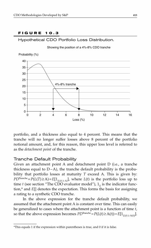
portfolio, and a thickness also equal to 4 percent. This means that thetranche will no longer suffer losses above 8 percent of the portfolionotional amount, and, for this reason, this upper loss level is referred toas the detachment point of the tranche.
Tranche Default ProbabilityGiven an attachment point A and detachment point D (i.e., a tranchethickness equal to D −A), the tranche default probability is the proba-bility that portfolio losses at maturity T exceed A. This is given by:PDTranche = P(L(T) ≥ A) = E[1L(t) ≥ A], where L(t) is the portfolio loss up totime t (see section “The CDO evaluator model”), 1 is the indicator func-tion,* and E[] denotes the expectation. This forms the basis for assigninga rating to a synthetic CDO tranche.
In the above expression for the tranche default probability, weassumed that the attachment point A is constant over time. This can easilybe generalized to cases where the attachment point is a function of time t,so that the above expression becomes PDTranche = P(L(t) ≥ A(t)) = E[1L(t) ≥ A(t)].
CDO Methodologies Developed by S&P 413
40
35
30
25
20
15
10
0 2 4 6 8 10 12 14 16
5
0
Loss (%)
4%-8% tranche
Probability (%)
Showing the position of a 4%-8% CDO tranche
F I G U R E 1 0 . 3
Hypothetical CDO Portfolio Loss Distribution.
*This equals 1 if the expression within parentheses is true, and 0 if it is false.
In this case, we evaluate the loss distribution at all points in time at whichthe attachment point changes. As an example, consider a hypotheticalseven-year synthetic CDO transaction. If the attachment point is initially setat 3 percent of the portfolio notional balance, but then increases to 5 percentafter three years and remains at this level until maturity, we need to evalu-ate the loss distribution at years three and seven. The cumulative defaultprobability of the tranche is therefore the probability that losses exceed3 percent by year three, plus the probability that losses exceed 5 percent byyear seven, conditional upon losses not exceeding 3 percent by year three.
Finally, the time dependency of the attachment point can even bemade conditional upon certain levels of loss being reached within theportfolio. For example, it is possible to model transactions in which theattachment point “resets” according to the cumulative loss experiencedby the portfolio by a certain date. This dynamic behavior is easily mod-eled by keeping track of the portfolio loss paths during simulation.
Expected Tranche LossThe cumulative loss on the tranche at time t, M(t), is given by: M(t) = (L(t) −A)1A ≤ L(t) ≤ D + (D − A)1L(t) ≥ D. The expected tranche loss is therefore givenby E[M(t)] = E (L(t) − A)1A ≤ L(t) ≤ D + (D − A)1L(t) ≥ D.
Tranche Loss-Given-DefaultThe tranche loss-given-default is given simply by:
Other Tranche Risk Measures
The tranche leverage and hedge ratio
are also useful in quantifying implied
tranche performance.
Synthetic CDO-Squared Transactions
Synthetic CDO-squared transactions have now become an established fea-ture of the global CDO marketplace. Rather than referencing secondary
HRLeverage
TrancheNotionalTranche
Tranche
=
Leverage( ( ))
Tranche =
E(M(t))E L t
LGD( ( ))
.TrancheTranche
= E M tPD
414 CHAPTER 10
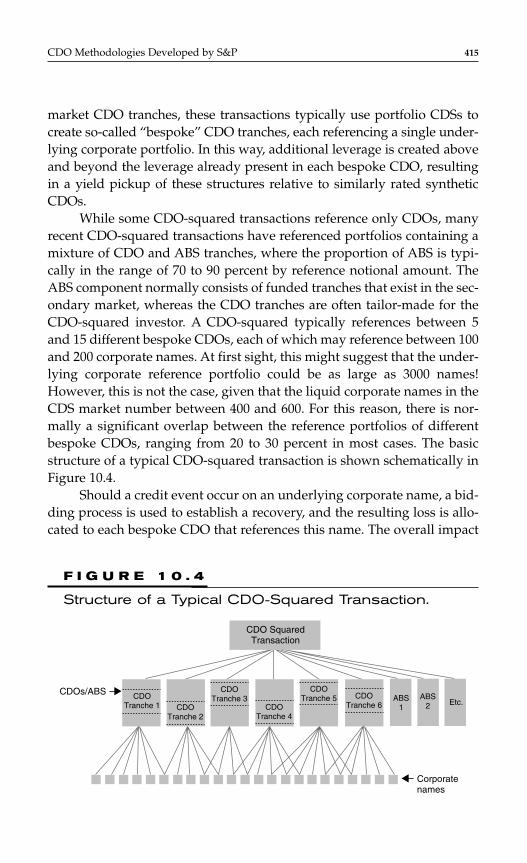
market CDO tranches, these transactions typically use portfolio CDSs tocreate so-called “bespoke” CDO tranches, each referencing a single under-lying corporate portfolio. In this way, additional leverage is created aboveand beyond the leverage already present in each bespoke CDO, resultingin a yield pickup of these structures relative to similarly rated syntheticCDOs.
While some CDO-squared transactions reference only CDOs, manyrecent CDO-squared transactions have referenced portfolios containing amixture of CDO and ABS tranches, where the proportion of ABS is typi-cally in the range of 70 to 90 percent by reference notional amount. TheABS component normally consists of funded tranches that exist in the sec-ondary market, whereas the CDO tranches are often tailor-made for theCDO-squared investor. A CDO-squared typically references between 5and 15 different bespoke CDOs, each of which may reference between 100and 200 corporate names. At first sight, this might suggest that the under-lying corporate reference portfolio could be as large as 3000 names!However, this is not the case, given that the liquid corporate names in theCDS market number between 400 and 600. For this reason, there is nor-mally a significant overlap between the reference portfolios of differentbespoke CDOs, ranging from 20 to 30 percent in most cases. The basicstructure of a typical CDO-squared transaction is shown schematically inFigure 10.4.
Should a credit event occur on an underlying corporate name, a bid-ding process is used to establish a recovery, and the resulting loss is allo-cated to each bespoke CDO that references this name. The overall impact
CDO Methodologies Developed by S&P 415
CDOTranche 1 CDO
Tranche 2
CDOTranche 3
CDOTranche 5 CDO
Tranche 6ABS
2 Etc.ABS1
CDO SquaredTransaction
CDOTranche 4
CDOs/ABS
Corporatenames
F I G U R E 1 0 . 4
Structure of a Typical CDO-Squared Transaction.

of the credit event will therefore clearly depend on the overlap amongthe underlying CDO tranches. When the loss allocated to a bespoke CDOexceeds the attachment point of the CDO tranche, the loss is passedthrough to the CDO-squared transaction. Bespoke CDOs therefore act as“loss filters” between the underlying corporate assets and the CDO-squared. This is very different to the ABS tranches, where a credit event ingeneral triggers a bidding process, the ABS tranche is removed from theCDO-squared reference portfolio, and the resulting loss is allocated to theCDO-squared transaction.
While each bespoke CDO tranche can be analyzed using the approachdescribed earlier, CDO-squared transactions require additional modeling,such as the ability to “drill down” to the corporate names underlying eachCDO tranche included within the CDO-squared portfolio. In this way,losses are modeled “from bottom to top,” flowing through each bespokeCDO before being allocated to the CDO-squared tranche. This allows theoverlap between pairs of bespoke CDO tranches to be explicitly modeled, inaddition to their individual default and loss-given-default characteristics.*
Cross-Subordination
One of the innovations in the CDO-squared market has been the intro-duction of so-called “cross-subordination.” This mechanism allows dif-ferent bespoke CDOs to share the total subordination provided by allbespoke CDOs. For example, eight CDOs with attachment points andthicknesses of i10 million would create a total cross-subordination of i80million. During the life of the transaction, if any CDO experiences lossesgreater than i10 million, these losses are not passed through to the CDO-squared until the total aggregate losses exceed i80 million. In this way, theCDO-squared investor is protected from the risk of a small number ofCDOs experiencing losses, but is exposed to the risk that a large numberof CDOs experience losses.†
This is easily modeled within CDO Evaluator by “tracking” thelosses experienced by each bespoke CDO in each simulation step, and
416 CHAPTER 10
* See Drill-Down Approach for Synthetic CDO Squared Transactions, Standard & Poor’s SpecialReport, December 10, 2003.†Another way of stating this is that cross-subordination reduces the idiosyncratic risk spe-cific to each CDO, but increases the systematic risk common to all CDOs.
only passing through the aggregate loss if it exceeds the total availablesubordination. This can also be extended to cases in which the subordi-nation is only “partially” cross-subordinated (e.g., the CDO-squaredtransaction is insulated from only 75 percent of the total aggregate subor-dination of the bespoke CDOs).
Consider a hypothetical CDO-squared with the following character-istics:
♦ The CDO-squared references a portfolio containing eightbespoke CDO tranches and 50 “AAA” rated ABS tranches, withan average asset correlation of 10 percent.
♦ Each bespoke CDO tranche references a portfolio of approxi-mately 100 “A” rated names with 5 percent average asset corre-lation, equal reference notional amounts of euro;10 million, andassumed recoveries of 35 percent.
♦ Each bespoke CDO tranche has an attachment point of i40 mil-lion (consistent with a CDO rating at the “A” rating level) anda detachment point of i0 million, i.e., a tranche thickness of i10 million.
♦ The average overlap between pairs of bespoke CDOs is 33percent.
♦ Each ABS tranche has a reference notional amount of i10million and an assumed recovery of 90 percent.
♦ The CDO-squared has a maturity of five years.
The CDO-squared portfolio therefore has a total reference notionalamount of i580 million. Of this amount, the ABS portion makes up 86 per-cent, and the bespoke CDOs 14 percent.
Figure 10.5 shows the loss distribution of the CDO-squared portfo-lio. In one case, the CDOs are assumed to contribute losses to the CDO-squared without cross-subordination, as described earlier. In the othercase, all eight bespoke CDOs are assumed to be cross-subordinated, asdescribed above. In both cases, the probability of zero or small losses isvery high, while there is a “tail” of higher losses. However, in the case ofthe cross-subordinated transaction, the probability of zero/small lossesincreases significantly, with a corresponding decrease in the probability oflarger losses. This means that a senior CDO-squared tranche with a rela-tively high attachment point has a lower probability of default in the caseof cross-subordination, as the total area of the distribution above 6 percent
CDO Methodologies Developed by S&P 417
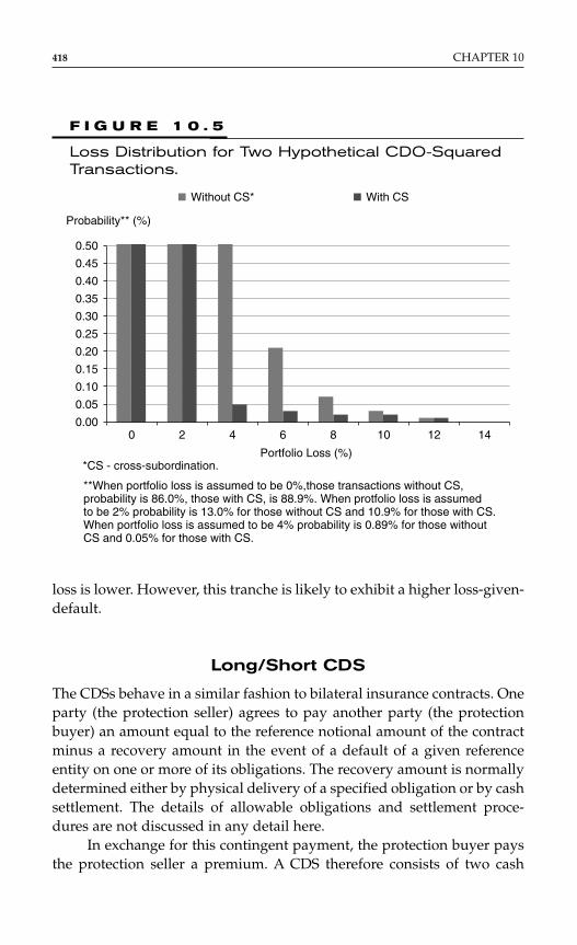
loss is lower. However, this tranche is likely to exhibit a higher loss-given-default.
Long/Short CDS
The CDSs behave in a similar fashion to bilateral insurance contracts. Oneparty (the protection seller) agrees to pay another party (the protectionbuyer) an amount equal to the reference notional amount of the contractminus a recovery amount in the event of a default of a given referenceentity on one or more of its obligations. The recovery amount is normallydetermined either by physical delivery of a specified obligation or by cashsettlement. The details of allowable obligations and settlement proce-dures are not discussed in any detail here.
In exchange for this contingent payment, the protection buyer paysthe protection seller a premium. A CDS therefore consists of two cash
418 CHAPTER 10
0.50
0.45
0.40
0.35
0.30
0.25
0.20
0.15
0.10
0.05
0.000 2 4 6 8 10 12 14
Portfolio Loss (%)
Probability** (%)
Without CS* With CS
*CS - cross-subordination.
**When portfolio loss is assumed to be 0%,those transactions without CS, probability is 86.0%, those with CS, is 88.9%. When protfolio loss is assumedto be 2% probability is 13.0% for those without CS and 10.9% for those with CS.When portfolio loss is assumed to be 4% probability is 0.89% for those withoutCS and 0.05% for those with CS.
F I G U R E 1 0 . 5
Loss Distribution for Two Hypothetical CDO-SquaredTransactions.
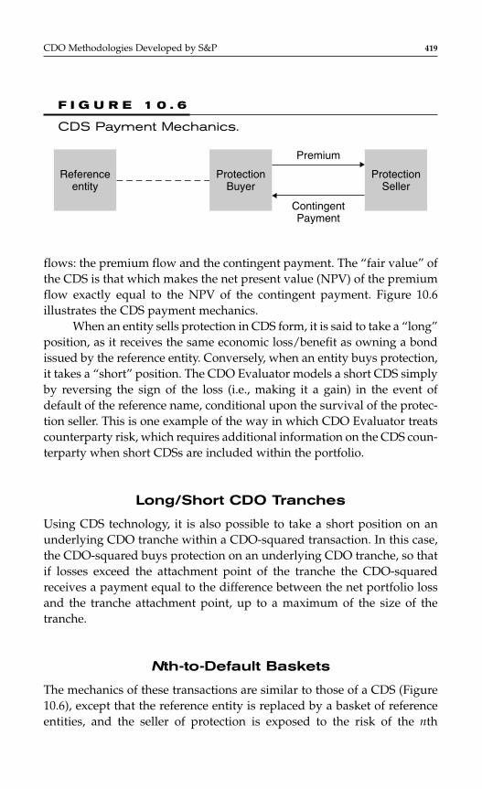
flows: the premium flow and the contingent payment. The “fair value” ofthe CDS is that which makes the net present value (NPV) of the premiumflow exactly equal to the NPV of the contingent payment. Figure 10.6illustrates the CDS payment mechanics.
When an entity sells protection in CDS form, it is said to take a “long”position, as it receives the same economic loss/benefit as owning a bondissued by the reference entity. Conversely, when an entity buys protection,it takes a “short” position. The CDO Evaluator models a short CDS simplyby reversing the sign of the loss (i.e., making it a gain) in the event ofdefault of the reference name, conditional upon the survival of the protec-tion seller. This is one example of the way in which CDO Evaluator treatscounterparty risk, which requires additional information on the CDS coun-terparty when short CDSs are included within the portfolio.
Long/Short CDO Tranches
Using CDS technology, it is also possible to take a short position on anunderlying CDO tranche within a CDO-squared transaction. In this case,the CDO-squared buys protection on an underlying CDO tranche, so thatif losses exceed the attachment point of the tranche the CDO-squaredreceives a payment equal to the difference between the net portfolio lossand the tranche attachment point, up to a maximum of the size of thetranche.
Nth-to-Default Baskets
The mechanics of these transactions are similar to those of a CDS (Figure10.6), except that the reference entity is replaced by a basket of referenceentities, and the seller of protection is exposed to the risk of the nth
CDO Methodologies Developed by S&P 419
Referenceentity
ProtectionBuyer
ProtectionSeller
ContingentPayment
Premium
F I G U R E 1 0 . 6
CDS Payment Mechanics.

default within the basket. An nth-to-default basket can be treated as a spe-cial case of a synthetic CDO containing a small number of equal expo-sures (typically three to five). As described earlier, the tranche defaultprobability is the probability that portfolio losses at maturity T exceed theattachment point A. For an nth-to-default basket with a fixed recovery δ,the attachment point is clearly equal to (n − 1)δ.
420 CHAPTER 10
A P P E N D I X A
Transition Matrices and Credit Curvesfor CDO Evaluator Assets
Rated Firms—One-Year Transition Matrix

CDO Methodologies Developed by S&P 421
Rated Firms—Credit Curves

422 CHAPTER 10
ABS—Credit Curves
SMEs—Credit Curves

EDSs

424 CHAPTER 10
CDOs Tranches—Credit Curves and Rating Quanties
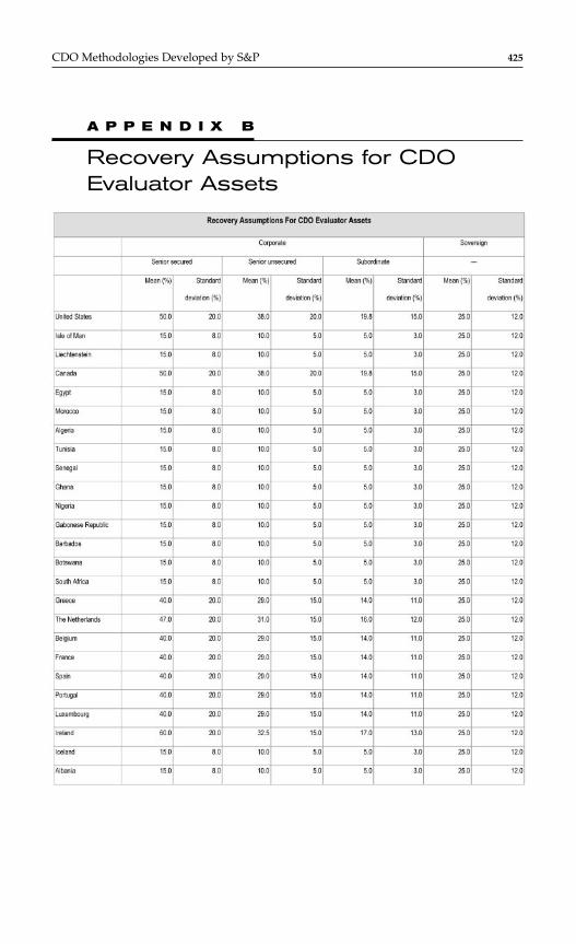
CDO Methodologies Developed by S&P 425
A P P E N D I X B
Recovery Assumptions for CDOEvaluator Assets
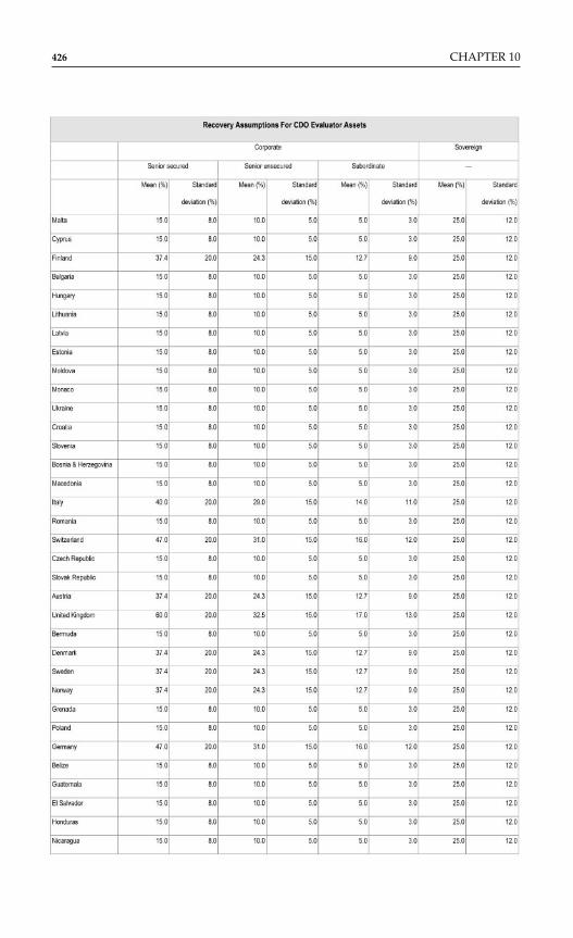
426 CHAPTER 10
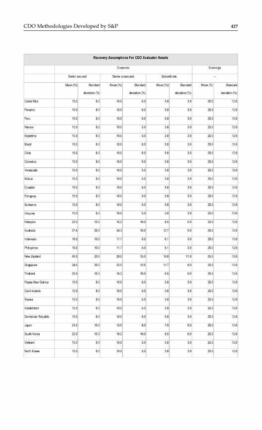
CDO Methodologies Developed by S&P 427
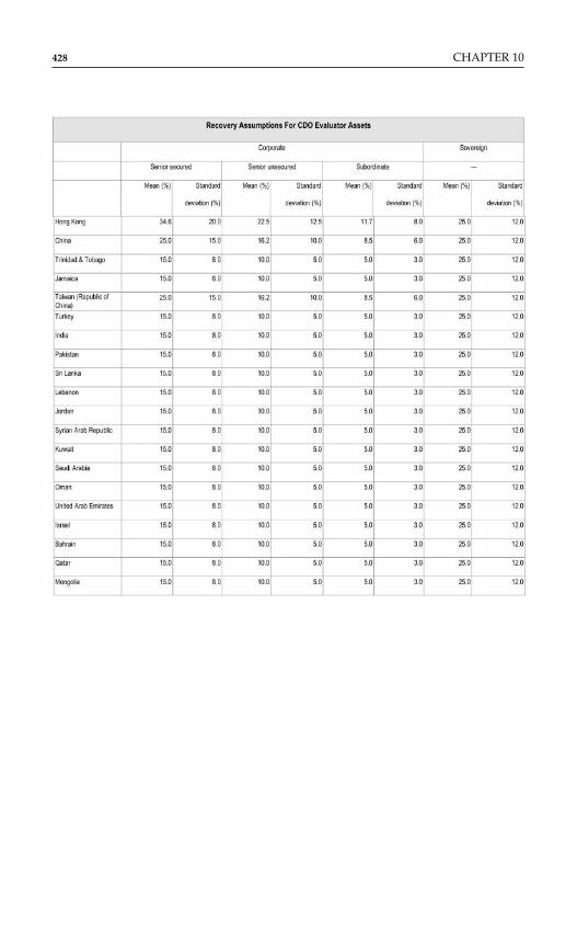
428 CHAPTER 10
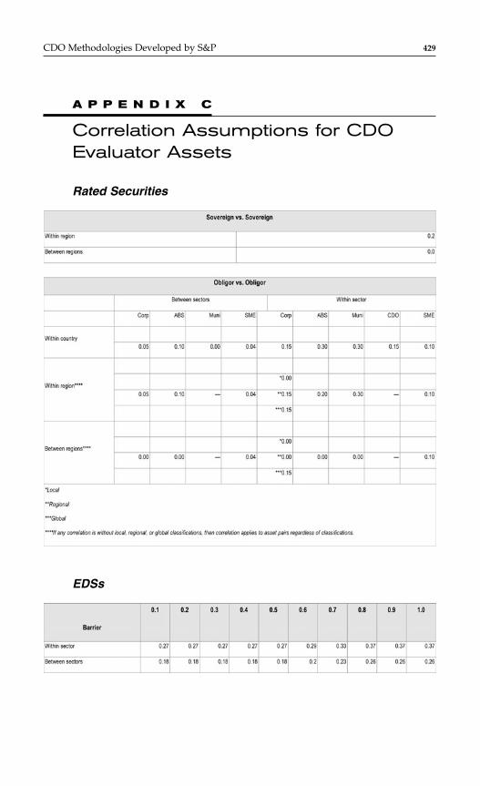
CDO Methodologies Developed by S&P 429
A P P E N D I X C
Correlation Assumptions for CDOEvaluator Assets
Rated Securities
EDSs
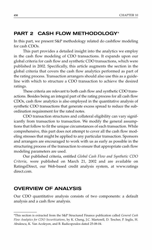
430 CHAPTER 10
PART 2 CASH FLOW METHODOLOGY*
In this part, we present S&P methodology related do cashflow modelingfor cash CDOs.
This part provides a detailed insight into the analytics we employin the cash flow modeling of CDO transactions. It expands upon ourglobal criteria for cash flow and synthetic CDO transactions, which werepublished in 2002. Specifically, this article augments the section in theglobal criteria that covers the cash flow analytics performed as part ofthe rating process. Transaction arrangers should also use this as a guide-line with which to structure a CDO transaction to achieve the desiredratings.
These criteria are relevant to both cash flow and synthetic CDO trans-actions. Besides being an integral part of the rating process for all cash flowCDOs, cash flow analytics is also employed in the quantitative analysis ofsynthetic CDO transactions that generate excess spread to reduce the sub-ordination requirement for the rated notes.
CDO transaction structures and collateral eligibility can vary signif-icantly from transaction to transaction. We modify the general assump-tions that follow to fit the unique circumstances of each transaction. Whilecomprehensive, this part does not attempt to cover all the cash flow mod-eling stresses that might be applied to any particular transaction. Sponsorsand arrangers are encouraged to work with us as early as possible in thestructuring process of the transaction to ensure that appropriate cash flowmodeling parameters are used.
Our published criteria, entitled Global Cash Flow and Synthetic CDOCriteria, were published on March 21, 2002 and are available onRatingsDirect, our Web-based credit analysis system, at www.ratingsdirect.com.
OVERVIEW OF ANALYSIS
Our CDO quantitative analysis consists of two components: a defaultanalysis and a cash flow analysis.
*This section is extracted from the S&P Structured Finance publication called General CashFlow Analytics for CDO Securitizations, by K. Cheng, J.C. Martorell, D. Tescher, P. Inglis, H.Abulescu, K. Van Acoleyen, and B. Radicopoulos dated 25-08-04.

CDO Methodologies Developed by S&P 431
Default Analysis
The default analysis uses CDO Evaluator to determine the default rateexpected on a defined portfolio at each rating level. This default rate isreferred to as the scenario default rate (SDR).
The CDO Evaluator uses “Monte Carlo” statistical methodology toevaluate the credit quality of a portfolio. The basic information requiredof each asset is the issuer ID, the par amount, the maturity date, the indus-try group, and the corporate issuer credit rating or ABS rating. These assetattributes are superimposed upon the model parameters—sector correla-tion coefficients, the table of default probabilities for assets, and the tableof default probabilities for CDO classes—to determine a probability dis-tribution of potential default rates for the portfolio in the aggregate. Theset of SDRs at each rating level is then derived from this distribution.
Our published criteria, Global Cash Flow and Synthetic CDO Criteria,give a detailed description of CDO Evaluator and how we estimate SDRs.
Cash Flow Analysis
The second component of the CDO quantitative analysis, the cash flowanalysis, evaluates the availability of funds for full payment of interestand principal in accordance with the terms of each rated class of notes.For transactions with multiple classes, the cash flow analysis is run foreach class to assess whether the level of credit support provided is con-sistent with the rating sought on each class. Cash flow modeling is alsoused to size liquidity and other reserves.
The analysis is transaction-specific and takes into account the struc-tural elements of a transaction, including:
♦ The principal and interest priority of payment;♦ Overcollateralization and interest coverage tests;♦ Reinvestment of proceeds;♦ Early amortization, fast pay, or redemption events;♦ Excess spread accumulation; and♦ Reserve levels.
In assessing a CDO class’s ability to meet the desired ratings level, theflow of proceeds from the assets to cover the payments due on the liabil-ities is subjected to a series of stress scenarios. The severity of these stress

432 CHAPTER 10
scenarios depends on the desired rating as well as transaction-specific fac-tors like the quality of the portfolio and the liability payment sequence.The result of this analysis is a series of breakeven default rates (BDRs),one for each stress scenario.
Each BDR is the default rate the portfolio can withstand and still beable to generate adequate cash flow to meet contractual payments ofinterest and principal on the CDO class when subjected to the particularstress scenario. The lowest of these BDRs is compared with the SDR gen-erated by CDO Evaluator for the portfolio at the desired rating level.
Achieving the Desired Rating
The desired rating is achieved when the BDR, i.e., the level of defaultsthe portfolio can withstand at the rating level, is the same or higher thanthe SDR, i.e., the level of defaults expected for the portfolio at that ratinglevel. The excess of the BDR above the SDR is commonly referred to asthe “cushion.” It reflects the ability of the portfolio to withstand the com-bination of additional defaults beyond the SDR and still pay out thenotes.
Approach to Cash Flow Modeling
This article details our analytical guidelines for the cash flow analysis ofCDO transactions. Central to these guidelines are the stress elements thatform the scenarios used to test the ability of the cash flow generated by theassets to cover payment obligations on the CDO liabilities. Many of theseelements, such as the timing and pattern of defaults, timing and extent ofrecovery, and interest-rate movements, are difficult to model because theyare historically variable.
To tackle this problem, we have established a set of basic defaultpaths for each variable. We pay particular attention to the nature of theassets eligible for inclusion in the portfolio and the jurisdictions fromwhich they are issued. Where appropriate, adjustments are made to thecash flow modeling stresses to account for asset-specific characteristicsand legal requirements.
Accurate cash flow modeling of the transaction, as dictated in thegoverning legal documentation, is crucial to our analysis. Proper repre-sentation of the characteristics of the asset pool in all material aspects isalso critical.
THE MEANING OF THE RATING
The combination of default patterns and timing sequences, interest-ratepaths, and various additional stresses applied in the cash flow modelinglead to a multitude of scenarios, each of which has a separate BDR. Toachieve the desired rating on a specific class of notes, we compare thelowest of these BDRs for the class with the corresponding SDR generatedby CDO Evaluator.
For “AAA” to “A” rated CDO classes, we generally rate to the timelypayment of interest and ultimate payment of principal by the legal finalmaturity date. The cash flow model at these ratings levels should demon-strate that interest and principal are paid when due and there is no defer-ral of interest payments.
At the “A−” rating level, our cash flow model allows for the defer-ral of interest for no more than three consecutive years. After the interestdeferral period, interest payments should resume as scheduled.
At the “BBB+” rating level and lower, we allow for the deferral ofinterest until the legal final maturity date. However, all current and pastinterest, along with interest on interest, due must be paid by that date.
If the interest cannot be paid within the required time frame for thedesired rating, it is still possible for the notes to achieve the rating but thelegal name of the notes must specify “deferred interest.” This is also toavoid any confusion among the investors.
In all cases, interest incurred on all accrued and unpaid interestshould also be incorporated into the cash flow model. The applicable inter-est rate is typically the same as that on the subject notes.
DEFAULTS
Although CDO Evaluator estimates the magnitude of defaults expected inthe portfolio at each rating level, a lack of empirical loss curves leaves thepattern or timing of these defaults unclear. This problem is addressed inour cash flow models by testing the sensitivity of the transaction to a vari-ety of default patterns. Four standard default patterns—which are eachshifted in accordance with the expected life of the transaction—and a fewother default patterns designed to stress certain cash flow behavior, formthe core of our established default stresses.
Details of these patterns and timings follow. These core defaultstresses are conceived to address the risks inherent in most of thesequential pay senior/subordinated structures common to the CDO
CDO Methodologies Developed by S&P 433
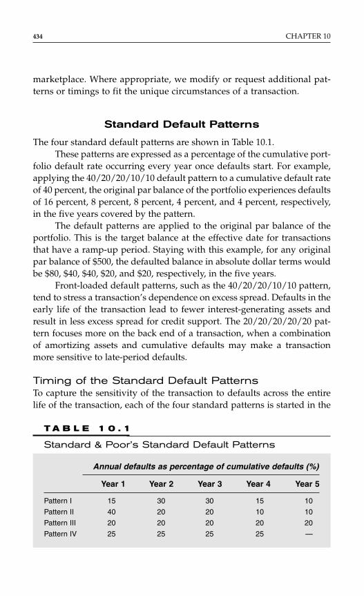
434 CHAPTER 10
marketplace. Where appropriate, we modify or request additional pat-terns or timings to fit the unique circumstances of a transaction.
Standard Default Patterns
The four standard default patterns are shown in Table 10.1.These patterns are expressed as a percentage of the cumulative port-
folio default rate occurring every year once defaults start. For example,applying the 40/20/20/10/10 default pattern to a cumulative default rateof 40 percent, the original par balance of the portfolio experiences defaultsof 16 percent, 8 percent, 8 percent, 4 percent, and 4 percent, respectively,in the five years covered by the pattern.
The default patterns are applied to the original par balance of theportfolio. This is the target balance at the effective date for transactionsthat have a ramp-up period. Staying with this example, for any originalpar balance of $500, the defaulted balance in absolute dollar terms wouldbe $80, $40, $40, $20, and $20, respectively, in the five years.
Front-loaded default patterns, such as the 40/20/20/10/10 pattern,tend to stress a transaction’s dependence on excess spread. Defaults in theearly life of the transaction lead to fewer interest-generating assets andresult in less excess spread for credit support. The 20/20/20/20/20 pat-tern focuses more on the back end of a transaction, when a combinationof amortizing assets and cumulative defaults may make a transactionmore sensitive to late-period defaults.
Timing of the Standard Default PatternsTo capture the sensitivity of the transaction to defaults across the entirelife of the transaction, each of the four standard patterns is started in the
T A B L E 1 0 . 1
Standard & Poor’s Standard Default Patterns
Annual defaults as percentage of cumulative defaults (%)
Year 1 Year 2 Year 3 Year 4 Year 5
Pattern I 15 30 30 15 10
Pattern II 40 20 20 10 10
Pattern III 20 20 20 20 20
Pattern IV 25 25 25 25 —

first year, then started in the second year, and so on. The start times of thepatterns are pushed back to the point where the final default in the pat-tern occurs in the same year that the balance of the portfolio are expectedto mature. That is, the starting points continue to be shifted as long as ade-quate assets remain in the portfolio. This is dictated by the length of thereinvestment period and the weighted-average expected life (WAL) of thecollateral. The maximum WAL at the end of the reinvestment period isgenerally the appropriate measure for the WAL because it reflects thetenor of the portfolio when it becomes static.
If the collateral manager is allowed to buy assets during the amortiza-tion period, the trading constraints are assessed to gauge the need for addi-tional timing shifts beyond those dictated by the maximum WAL covenant.Some transactions have a maximum WAL covenant at the effective date thatdoes not reduce during the reinvestment period. For these transactions, wegenerally use the effective date WAL covenant as the WAL at the end of thereinvestment period to determine the appropriate timing shifts.
As an example, take a transaction with a five-year reinvestmentperiod, a maximum WAL covenant of four years at the end of the rein-vestment period, and trading activities permitted only during the rein-vestment period. Because the balance of the portfolio does not matureuntil the end of year nine (four years after the end of the reinvestmentperiod), the start of the default patterns can be pushed back to year five,which spreads defaults across years five through nine. The constraints inthis example dictate the use of the standard default patterns beginning inyears one through five.
If the WAL covenant is two years at the end of the reinvestmentperiod, rather than four years as in the previous example, there would notbe adequate assets remaining after year seven. We would run the defaultpatterns from years one through three so that the last default would occurin year seven.
Modifying the Timing Based on Liability RatingsThe stress elements must reflect the difference between each rating cate-gory. Different default timing stresses are applied in the cash flow model-ing according to which rating is sought on the notes. Although each of thefour standard default patterns is run beginning in year one, we delay thestart of these patterns by a longer period to capture the effect of laterdefaults at the higher liability ratings.
For example, the reinvestment period and WAL covenant of a transac-tion might dictate stressing the transaction with default patterns beginning
CDO Methodologies Developed by S&P 435
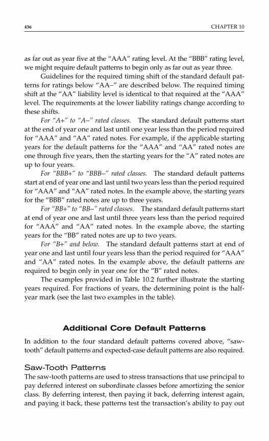
as far out as year five at the “AAA” rating level. At the “BBB” rating level,we might require default patterns to begin only as far out as year three.
Guidelines for the required timing shift of the standard default pat-terns for ratings below “AA−” are described below. The required timingshift at the “AA” liability level is identical to that required at the “AAA”level. The requirements at the lower liability ratings change according tothese shifts.
For “A+” to “A−” rated classes. The standard default patterns startat the end of year one and last until one year less than the period requiredfor “AAA” and “AA” rated notes. For example, if the applicable startingyears for the default patterns for the “AAA” and “AA” rated notes areone through five years, then the starting years for the “A” rated notes areup to four years.
For “BBB+” to “BBB−” rated classes. The standard default patternsstart at end of year one and last until two years less than the period requiredfor “AAA” and “AA” rated notes. In the example above, the starting yearsfor the “BBB” rated notes are up to three years.
For “BB+” to “BB−” rated classes. The standard default patterns startat end of year one and last until three years less than the period requiredfor “AAA” and “AA” rated notes. In the example above, the startingyears for the “BB” rated notes are up to two years.
For “B+” and below. The standard default patterns start at end ofyear one and last until four years less than the period required for “AAA”and “AA” rated notes. In the example above, the default patterns arerequired to begin only in year one for the “B” rated notes.
The examples provided in Table 10.2 further illustrate the startingyears required. For fractions of years, the determining point is the half-year mark (see the last two examples in the table).
Additional Core Default Patterns
In addition to the four standard default patterns covered above, “saw-tooth” default patterns and expected-case default patterns are also required.
Saw-Tooth PatternsThe saw-tooth patterns are used to stress transactions that use principal topay deferred interest on subordinate classes before amortizing the seniorclass. By deferring interest, then paying it back, deferring interest again,and paying it back, these patterns test the transaction’s ability to pay out
436 CHAPTER 10
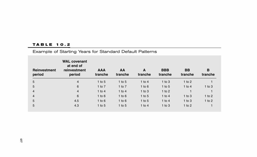
T A B L E 1 0 . 2
Example of Starting Years for Standard Default Patterns
WAL covenantat end of
Reinvestment reinvestment AAA AA A BBB BB Bperiod period tranche tranche tranche tranche tranche tranche
5 4 1 to 5 1 to 5 1 to 4 1 to 3 1 to 2 1
5 6 1 to 7 1 to 7 1 to 6 1 to 5 1 to 4 1 to 3
4 4 1 to 4 1 to 4 1 to 3 1 to 2 1 1
4 6 1 to 6 1 to 6 1 to 5 1 to 4 1 to 3 1 to 2
5 4.5 1 to 6 1 to 6 1 to 5 1 to 4 1 to 3 1 to 2
5 4.3 1 to 5 1 to 5 1 to 4 1 to 3 1 to 2 1
437
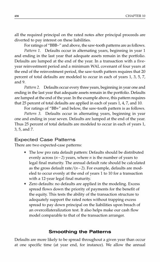
all the required principal on the rated notes after principal proceeds arediverted to pay interest on these liabilities.
For ratings of “BBB−” and above, the saw-tooth patterns are as follows.Pattern 1. Defaults occur in alternating years, beginning in year 1
and ending in the last year that adequate assets remain in the portfolio.Defaults are lumped at the end of the year. In a transaction with a five-year reinvestment period and a minimum WAL covenant of four years atthe end of the reinvestment period, the saw-tooth pattern requires that 20percent of total defaults are modeled to occur in each of years 1, 3, 5, 7,and 9.
Pattern 2. Defaults occur every three years, beginning in year one andending in the last year that adequate assets remain in the portfolio. Defaultsare lumped at the end of the year. In the example above, this pattern requiresthat 25 percent of total defaults are applied in each of years 1, 4, 7, and 10.
For ratings of “BB+” and below, the saw-tooth pattern is as follows.Pattern 3. Defaults occur in alternating years, beginning in year
one and ending in year seven. Defaults are lumped at the end of the year.Thus 25 percent of total defaults are modeled to occur in each of years 1,3, 5, and 7.
Expected Case PatternsThere are two expected-case patterns:
♦ The low pro rata default pattern: Defaults should be distributedevenly across (n − 2) years, where n is the number of years tolegal final maturity. The annual default rate should be calculatedas the gross default rate/(n − 2). For example, defaults are mod-eled to occur evenly at the end of years 1 to 10 for a transactionwith a 12-year legal final maturity.
♦ Zero defaults: no defaults are applied in the modeling. Excessspread flows down the priority of payments for the benefit ofthe equity. This tests the ability of the transaction structure toadequately support the rated notes without trapping excessspread to pay down principal on the liabilities upon breach ofan overcollateralization test. It also helps make our cash flowmodel comparable to that of the transaction arranger.
Smoothing the Patterns
Defaults are more likely to be spread throughout a given year than occurat one specific time (at year end, for instance). We allow the annual
438 CHAPTER 10
defaults on the standard default patterns to be modeled to occur as fre-quently as quarterly for transactions where at least 80 percent of the assetspay not less frequently than quarterly, after taking into account any basisswaps. In this manner, annual defaults are spread evenly across the fourquarters with defaults occurring on the last day of each quarter. Giventhat transactions typically have a 5 to 10 percent allowance for less fre-quent pay assets, most quarterly pay transactions would qualify for thesmoothing of annual defaults. The transaction arranger also has the optionof modeling defaults less frequently. Regardless, in all cases, assets matur-ing in any period remain subject to defaults in that period.
The entire default amount in the first year, however, should be mod-eled to occur on the last day of the year. This reflects our opinion that, inmost instances, some time lapses before defaults occur on a recentlyassembled portfolio. An exception to this is when the targeted portfolioconsists of an abnormally high concentration of low credit quality assets.In these cases, we may request that the model begin defaults earlierduring the first year.
Defaults clearly affect the interest received from the defaultedassets—interest is earned only on the performing pool balance. Duringthe liability payment period when the asset is assumed to default, creditis given for the interest earned only if the asset pays interest more fre-quently than the liabilities. For example, in a transaction paying semi-annually, an asset that receives quarterly interest payments is modeled toreceive interest for the first, but not the second, quarter of the defaultperiod. In contrast, an asset that receives semi-annual interest paymentsis not given credit for interest in the modeling for that default period.
We assume a lag period from the time the asset defaults to the timerecoveries are realized on defaulted assets and the money is available forreinvestment in substitute collateral. During this period (which is addressedin the section “Recoveries”), no interest is received on the defaulted assets.Following the lag period, recovery proceeds are modeled to occur on thelast day of the payment period that recovery is realized. Redeployment ofthe proceeds in interest income-generating assets does not occur until thefirst day of the subsequent period.
Adjustments to Default Patterns and Timing
The default patterns and timings that form the core of our default stressesare designed to address the risks common in many of the traditionalsequential pay senior/subordinated CDO transaction structures.
CDO Methodologies Developed by S&P 439
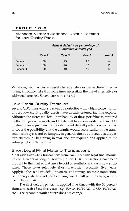
440 CHAPTER 10
Variations, such as certain asset characteristics or transactional mecha-nisms, introduce risks that sometimes necessitate the use of alternative oradditional stresses. Several are now covered.
Low Credit Quality PortfoliosSeveral CDO transactions backed by portfolios with a high concentrationof very low credit quality assets have already entered the marketplace.Although the increased default probability of these portfolios is capturedby the ratings on the assets and the default tables embedded within CDOEvaluator, an adjustment to the established default patterns is warrantedto cover the possibility that the defaults would occur earlier in the trans-action’s life cycle, and be lumpier. In general, three additional default pat-tern stresses, all beginning in year one, are required and applied to theentire portfolio (Table 10.3).
Short Legal Final Maturity TransactionsMost cash flow CDO transactions issue liabilities with legal final maturi-ties of 10 years or longer. However, a few CDO transactions have beenbrought to the market that are a hybrid of synthetic and cash flow struc-tures. These have relatively short maturities, typically five years.Applying the standard default patterns and timings on these transactionsis inappropriate. Instead, the following two default patterns are generallyused (Table 10.4).
The first default pattern is applied five times with the 50 percentshifted to each of the five years (e.g., 50/10/10/10/20, 10/50/10/10/20,etc.). The second default pattern does not change.
T A B L E 1 0 . 3
Standard & Poor’s Additional Default Patterns for Low Quality Pools
Annual defaults as percentage of cumulative defaults (%)
Year 1 Year 2 Year 3 Year 4
Pattern I 50 25 25 —
Pattern II 60 20 10 10
Pattern III 70 10 10 10
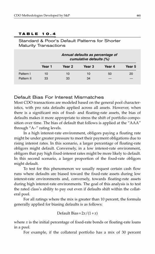
CDO Methodologies Developed by S&P 441
Default Bias For Interest MismatchesMost CDO transactions are modeled based on the general pool character-istics, with pro rata defaults applied across all assets. However, whenthere is a significant mix of fixed- and floating-rate assets, the bias ofdefaults makes it more appropriate to stress the shift of portfolio compo-sition over time. The bias of default that follows is applied at the “AAA”through “A−” rating levels.
In a high interest-rate environment, obligors paying a floating ratemight be under greater pressure to meet their payment obligations due torising interest rates. In this scenario, a larger percentage of floating-rateobligors might default. Conversely, in a low interest-rate environment,obligors that pay high fixed-interest rates might be more likely to default.In this second scenario, a larger proportion of the fixed-rate obligorsmight default.
To test for this phenomenon we usually request certain cash flowruns where defaults are biased toward the fixed-rate assets during lowinterest-rate environments and, conversely, towards floating-rate assetsduring high interest-rate environments. The goal of this analysis is to testthe rated class’s ability to pay out even if defaults shift within the collat-eral pool.
For all ratings where the mix is greater than 10 percent, the formulagenerally applied for biasing defaults is as follows:
Default Bias = 2x/(1 + x)
where x is the initial percentage of fixed-rate bonds or floating-rate loansin a pool.
For example, if the collateral portfolio has a mix of 30 percent
T A B L E 1 0 . 4
Standard & Poor’s Default Patterns for Shorter Maturity Transactions
Annual defaults as percentage of cumulative defaults (%)
Year 1 Year 2 Year 3 Year 4 Year 5
Pattern I 10 10 10 50 20
Pattern II 33 33 34 — —
fixed-rate assets and 70 percent floating-rate assets, the applicable fixed-rate default bias would be:
Fixed-Rate Default Bias = 2(0.3)/(1 + 0.3) = 0.46
In this case, the cash flow model would be adjusted to default 46percent of the fixed-rate assets and 54 percent of the floating-rate assets,instead of the actual 30 percent/70 percent split. This fixed-rate defaultbias is generally applied only to the dominant run in the Index Downinterest-rate stresses.
In the same example, the applicable floating-rate default biaswould be:
Floating-Rate Default Bias = 2(0.7)/(1 + 0.7) = 0.82.
In this case, the cash flow model would default 18 percent of thefixed-rate assets and 82 percent of the floating-rate assets. This floating-rate default bias is generally applied only to the dominant run in theIndex Up interest-rate stresses.
RECOVERIES
Loss severity and recovery timing assumptions are another intrinsic partof CDO transaction analyses. These aim to estimate the loss on an assetupon default and when the recovery is realized.
Recovery Rates
Recoveries specify the amount of money realized on a defaulted obliga-tion after it has defaulted. Factors such as the breadth and depth of thesecondary market profoundly influence recovery rates realized. Thesefactors differ across markets, so recovery rates must be assigned by assettype and domicile.
Within each asset type, additional influences affect recovery rates. Inthe case of corporate obligations, recoveries are not dependent on the rat-ing on the obligor or on the notes in the transaction. Instead, they dependon the type, seniority, domicile, and security of the obligation. The recoveryrates that are ultimately realized are further influenced by the actions of thecollateral manager. Thus, two collateral managers, following differentworkout strategies, may realize significantly different recoveries for the
442 CHAPTER 10

same assets under identical market environments. We use an establishedrange of recovery rates for each classification of corporate asset and assigntransaction-specific recovery rates within these ranges based on a review ofthe collateral manager.
The recovery rates applied for assets governed by one jurisdictionare not necessarily appropriate for other jurisdictions. The recoveryranges also differ across governing domicile. The Global Cash Flow andSynthetic CDO Criteria book shows the various recovery ranges for corpo-rate bonds and loans issued under U.S. and European jurisdictions, andrecovery assumptions for defaulted emerging market assets. These recov-ery assumptions are generally lower and reflect the relative lack of liq-uidity in the secondary market for emerging market obligations.
In contrast to corporate obligations, the ratings on structured financesecurities—as a reflection of position in the capital structure—influencerecovery prospects, as does the seniority of an asset. The recovery ratesassigned are also tiered across economic conditions, using the rating on theCDO notes as the proxy for those conditions. The resultant recovery matri-ces for structured finance securities under U.S. and European jurisdictionsare shown in the Global Cash Flow and Synthetic CDO Criteria book.
It is critical to note that the recovery ranges and tables are applica-ble to many, but not all, assets that fall within the collateral classificationsidentified in those tables. Recoveries may be adjusted based on character-istics or mechanisms particular to any asset. Assets not covered by theexisting recovery tables (e.g., project finance bonds, operating companyobligations, and distressed-debt CDOs) are assigned recoveries on a case-by-case basis.
Although recoveries are assigned to each asset, we use the minimumweighted-average recovery rate covenant (as defined by the transaction’sportfolio eligibility criteria) in cash flow modeling for CDO transactionsthat allow for reinvestment of proceeds.
The CDO transactions that prohibit reinvestment of proceeds andare fully ramped up on the closing date have no need to incorporate min-imum weighted-average recovery rate tests. In these transactions, theactual weighted-average recovery rate at closing is generally used in thecash flow modeling. However, a “bar-belled” portfolio might necessitatethe use of a recovery rate lower than the weighted-average or a bias ofdefaults toward the lower recovery assets.
In all instances, recovery rates are applied to the par balance of theasset without accounting for any deferred and capitalized portion of paroutstanding.
CDO Methodologies Developed by S&P 443

Recovery Timing
Recovery timing specifies the time it takes to achieve recoveries once anobligation defaults. Time to recovery is influenced by the type of asset, theform of the obligation, the actions of the collateral manager, the liquidityof the market, the governing legal jurisdiction, and the requirements ofthe transaction with regard to forced sale or settlement. In most cases, twogeneral assumptions are made for the timing of recoveries on defaultedassets, as follows:
♦ Recoveries on defaulted sovereign, corporate, and structuredfinance securities are assumed to occur one year after defaultthrough secondary market liquidation.
♦ Recoveries on defaulted loans are assumed to occur over athree-year workout period, with one-half of the recoveryreceived at the end of the second year and the remaining half atthe end of the third year.
The above assumptions are consistent across many jurisdictions. A longerrecovery horizon is assumed on defaulted loans because loan markets arenot generally as liquid as bond markets. These recovery horizons are con-sistent with the holding periods that we consider sufficient to allow the man-ager to maximize recoveries on defaulted securities. The recovery levels inour recovery rate ranges and tables are reflective of this holding period.
When modeling recoveries, the model should show recoveries real-ized at the end of the appropriate period. In this manner, recovery pro-ceeds are not available for reinvestment and, therefore, no interest incomeis earned on these proceeds during this period. Earning of interest beginsin the subsequent period.
INTEREST RATE STRESSES
The CDO transactions often have a fixed-to-floating interest-rate mis-match between the assets and the liabilities. To mitigate this risk, transac-tions are commonly structured with interest-rate hedges. In the absence ofa balanced guaranteed hedge, mismatches between the notional of thehedge and the liabilities might develop as the magnitude or bias ofdefaults between fixed- and floating-rate assets diverge from projectedlevels. Testing of the transaction under several distinct interest-rate pathsis performed to gauge the effectiveness of the hedge structure in a varietyof interest-rate environments.
444 CHAPTER 10

CDO Methodologies Developed by S&P 445
Stresses
In general, transactions are stressed under the index scenarios listed inTable 10.5. In addition, the “At Swap” and “At Cap” rates are typicallyrun to test the transaction’s ability to perform without depending on thehedges for additional credit support.
The interest rate curves for each transaction are adjusted to matchthe length of the transaction and the index used. They may also vary byrating level. We provide to the arranger the curves applicable to the trans-action early in the rating process. General details of our interest-rateassumptions are provided in the Global Cash Flow and Synthetic CDOCriteria book.
Adjustments to Interest Rate Sensitivity Analysis
These interest rate paths or the manner in which they are applied aresometimes adjusted to address peculiarities of a transaction. Additionaladjustments to other aspects of the cash flow modeling are sometimesalso necessary to address interest rate related risks. Several are nowcovered.
Fixed-Rate/Floating-Rate Asset MixTransactions that allow for reinvestment of proceeds typically containinvestment guidelines that allow for a range of asset mix between fixed-and floating-rate collateral. When the mix is heavily concentrated towardone or the other of these possibilities (either at least 95 percent fixed or 95percent floating), the transaction can be modeled in one of two ways atthe discretion of the transaction arranger:
T A B L E 1 0 . 5
Standard & Poor’s Interest Rate Paths
Index Up
Index Down
Index Down/Up
Current Index Forward Curve
At Swap
At Cap
♦ Model either as 100 percent fixed or floating; or♦ Model at a maximum percentage of fixed or floating.
For transactions that allow for greater flexibility between the mix of fixed-and floating-rate assets, disparities in the minimum weighted-averagecoupon and spread covenants could lead to pronounced differences in thecash flow performance along the fixed/floating-rate asset mix continuum.In these circumstances, the mix of fixed/floating-rate assets must be mod-eled at the maximum and minimum levels to capture the extremes in thespectrum of possibilities.
When a transaction is stressed to the maximum allowance forfloating-rate assets, it often leads to a high concentration of loans. Sincehigher recoveries are generally extended to loans relative to bonds, it ispossible that the weighted-average recovery for the portfolio in this sce-nario could be higher than the minimum weighted-average recovery ratecovenant typically used in the cash flow modeling exercise. We take thisinto consideration when stressing the transaction for the fixed/floating-rate asset mix.
Loan Basis RiskThe floating-rate liabilities of CDO transactions and the floating-rateassets in the portfolio typically use the same repricing index. Often, theindex is LIBOR or EURIBOR. Occasionally, there is a mismatch betweenthese indices due to the payment frequencies. The ability of the assets toadequately cover the interest due on the liabilities is strained when themovement of the indices between any two points in time is different.
The additional stress required to capture this risk depends on themagnitude of the difference between the two indices’ movements. In gen-eral, we apply a five basis point haircut to the weighted-average spreadabove the index when the mismatch is greater than 5 percent and the gapin rate movements between the pair of indices has historically exhibitedsignificant variability.
Multiple Liability IndicesThe presence of floating-rate liabilities tied to more than one index raisesquestions regarding the appropriate interest-rate stresses. In this situation,we apply the interest-rate curves commensurate with the dominant index.For example, if 60 percent of floating-rate liabilities are based on EURIBORand 40 percent are based on LIBOR, then the EURIBOR interest-rate stressscenarios generated by our LIBOR/EURIBOR curve dynamic model prevail.
446 CHAPTER 10
PORTFOLIO CONSIDERATIONS
Factors such as the composition of a portfolio or specific asset character-istics introduce risks that might necessitate the use of additional or alter-native stresses. Several are now covered.
Prepayment Sensitivities
Most structured finance products are collateralized by loans or mortgagesthat include provisions, allowing the borrower to make unscheduled pay-ments without a penalty. These prepayments affect the timing and mag-nitude of the cash flow available to cover the liabilities on the structuredfinance securities. In turn, this affects the cumulative excess spread gen-erated by the securities. Since excess spread is often used to cover losses,prepayments affect the ability of the transaction to support losses andmust be considered in the cash flow modeling.
To capture the effect of these prepayment provisions, we impose pre-payment stress scenarios on those assets that exhibit elastic prepaymentsensitivities to interest-rate movement, including RMBS and home equityline of credit (HELOC) securities. We should be consulted to help identifythese asset types. The prepayment stresses are applied to those CDO trans-actions in which these assets make up more than 5 percent of the portfolioin aggregate par balance. When the permitted concentration exceeds thisthreshold, the entire bucket is stressed to test the impact of prepayments.
The three scenarios typically modeled include:
♦ The market (base) prepayment speed;♦ An accelerated prepayment speed of 150 percent of the market
prepayment speed; and♦ A decelerated prepayment speed of 50 percent of the market
prepayment speed.
For new issuance, the market prepayment speed is the expected prepay-ment speed of the transaction. For seasoned issuance, it is the average ofactual market prepayment speeds during the previous six months.
When applying the accelerated and decelerated prepayment speedstresses, consideration is given to the relationship between prepaymentbehavior of the asset and interest-rate movements in determining theappropriate accompanying interest-rate stresses. For example, prepaymentof fixed-rate mortgages is apt to pick up when interest rates are decliningand likely to slow down when they are increasing. Thus, the accelerated
CDO Methodologies Developed by S&P 447

prepayment speed stress would be applied in conjunction with the interest-rate index down stress, and the decelerated prepayment speed stress wouldbe applied in conjunction with the interest-rate index up stress. Regardless,we should be consulted to determine the appropriate prepaymentspeed/interest-rate stress pairings based on the mix of these assets.
When the mix of prepayment-sensitive assets cuts across nationalmarkets subject to different prepayment behavior (e.g., U.K. vs. ItalianRMBS), we should be consulted for guidance on the appropriate base pre-payment speed to apply. In general, this is the prepayment speed prevail-ing in the market where most of the assets are expected to be purchased.
Foreign Currency Risk
Some CDO transactions, particularly those issued out of Europe, allow fora bucket of assets denominated in a currency different from that of thenotes issued. The currency mismatch introduced is best hedged with abalance-guaranteed foreign exchange swap, but the cost of entering intothese swaps is often prohibitive. The most common way to address thisrisk is to use a natural hedge or asset-specific foreign exchange swapsbased on set notional balances. In both of these cases, the foreign exchangerisk is not fully hedged throughout the life of the transaction, thus neces-sitating additional cash flow stresses to capture the foreign exchange risk.
A natural foreign exchange hedge exists when both the assets andliabilities denominated in each currency make up the same proportion ofa given pool. For instance, the collateral pool may have 70 percent euro-denominated and 30 percent U.S. dollar-denominated assets matched to70 percent euro-denominated and 30 percent U.S. dollar-denominatedliabilities, thereby creating a natural hedge. However, this natural hedgeoften does not immunize the CDO against foreign exchange risk. Thishedge remains perfectly balanced so long as defaults to the assets occurpro rata across the currency denominations. If defaults do not occur inproportion (the more likely scenario), the resultant imbalance wouldthrow the natural hedge askew. The balance of the natural hedge couldalso be upset by prepayments on the assets or diversion of principal pro-ceeds to pay down liabilities in a sequential pay structure triggered by thebreach of a coverage test.
The effectiveness of a natural hedge is also dependent upon its posi-tion in the capital structure. Segregating the most senior class of notesacross the currencies is more effective than segregating a more junior class.
448 CHAPTER 10

The other common strategy for addressing foreign exchange risk isto use asset-specific foreign exchange swaps. The issuer of the securitiesenters into a foreign exchange swap, often for a set notional balance or aschedule of notional balances. This hedging strategy is likewise suscepti-ble to hedging imbalances due to the bias of defaults or prepayments onthe asset balance.
In the absence of a strategy that adequately addresses foreignexchange risk over the life of the transaction, we typically employ a two-part analysis to test for the potential effect of this risk. First, the cash flowis subjected to additional stresses that bias defaults toward each of thecurrency denominations. The magnitude of the bias is dictated by factorsthat include the position of the natural hedge in the capital structure, theproportion of assets denominated in each currency, and the disparity ofthe credit risk profiles between each currency-denominated sub-portfolio.Currency devaluation factors, calculated using a currency devaluationmodel, are then applied to the resultant hedge imbalance to size the extentof the currency mismatch.
The presence of different indices (e.g., LIBOR and EURIBOR) in trans-actions with multiple currencies might also necessitate additional analysis tocapture the mismatch of indices. The empirical relative movement of theindices and the magnitude of the mismatch determine this need.
We should be consulted for the default bias, currency devaluationstresses, and index mismatch stresses applicable to each particular trans-action.
In addition to hedging the periodic payments, the foreign exchangestrategy should remain in place to cover the recoveries realized on defaultedsecurities. Automatic termination of the foreign exchange swap upondefault of an asset exposes the recoveries to foreign exchange risk. Wetypically adjust the recovery rate assigned when the swap is required toterminate before the base recovery delay assumptions. The magnitude ofthis adjustment is determined according to factors such as the lengthof time the defaulted asset is exposed to foreign exchange risk and theparticular currencies involved.
Foreign exchange risk also arises when an asset is sold, but the asset-specific foreign exchange swap is not automatically retired or, conversely,the foreign exchange swap terminates before the asset matures. In the firstinstance, the collateral manager is likely to include the economic effect ofthe swap in making its sell decision and, in the latter, the manager mightsell the unhedged asset to eliminate foreign exchange concerns. In both
CDO Methodologies Developed by S&P 449

cases, noncredit-based considerations are factored into the decision pro-cess and we consider adjusting the recovery rate assigned.
Coupon on Assets
We base our cash flow analysis on a portfolio that generates interestincome at the minimum coupon/spread dictated by the collateral pooleligibility criteria. This assumes that market conditions prevent the col-lateral manager from purchasing collateral at spreads or coupons higherthan the minimum weighted-average spread or coupon.
However, if the portfolio is fully ramped up at closing and tradingis allowed, credit is afforded to the actual weighted-average coupon/spread of the pool at the start of the transaction. The pool coupon/spreadmigrates down to the minimum levels over two years on a straight-linebasis. The form of this migration is dictated by the frequency of paymentson the liabilities. For example, take a transaction that covenants to a min-imum weighted-average coupon of 6 percent but has an actual weighted-average coupon of 8 percent, and pays out on its liabilities quarterly. Theappropriate cash flow modeling allows interest to be earned at an 8percent coupon between closing and the first payment period, with thecoupon reduced by 25 bps each subsequent payment period until it reaches6 percent after the eighth payment period.
It is important to note that the cash flow should be modeled at thecoupon and not the stated yield rate.
Interest Income on Eligible Investments
Proceeds received from assets in the form of scheduled principal andinterest payments and recovery proceeds are held in eligible investmentsbefore being reinvested in substitute collateral or being used to pay lia-bilities on a payment date.
In the cash flow model, the analysis should assume that scheduledprincipal and interest proceeds are held in eligible investments for one-halfof the payment period of the collection before it is reinvested in substitutecollateral. Also, in the analysis, recoveries should be assumed to occur at theend of a payment period. Therefore, interest is not earned on recovery pro-ceeds held as eligible investments during the period in which it is recovered.
Interest earned on the regular payments received from the eligibleinvestments is modeled at the index referenced minus 100 bps.
450 CHAPTER 10

Payment Timing Mismatch
It is common for transactions to include a bucket for assets that pay lessfrequently than the payment terms of the liabilities. In many instances, thetransaction uses an interest reserve mechanism or enters into a basis swapto address this mismatch. In the absence of an adequate mitigant, themodeling should reflect the mismatches in payment timing, as they actu-ally occur, to allow for accurate testing of cash flows. There should be no“smoothing” of asset payments to match liability payments.
Pay in Kind (PIK) Assets
When more than 5 percent of the assets in a portfolio by par balance havethe ability to pay in kind, we apply a PIK stress test to ensure that the liq-uidity facility can cover interest shortfalls from the assets. The PIK stressapplied is determined after taking into account the transaction structureand targeted portfolio profile. We typically ask that this is done only forthe most severe stress case to verify if it can pass; BDRs may be set with-out this stress.
It is important to note that some transactions treat assets that pay inkind for a defined time period as defaulted assets. The defaulted balanceof the PIK assets should be marked as the original par principal balance,not its principal plus accrued interest balance.
Long-Dated Corporate Assets
The inclusion of corporate assets that mature on a date beyond the legalfinal maturity date of the liabilities requires the CDO transaction to sellthese assets before this date. This exposes the transaction to the noncredit-related risk of loss of par and is particularly troublesome for corporatebonds and other types of instruments that return all or substantially all ofthe par balance at the asset’s legal final maturity date.
We address this concern by limiting the concentration of assets inthe long-dated bucket to 5 percent. When the allowance for this bucketexceeds 5 percent, the par credit for each long-dated asset is reduced byapplying a present value of 10 percent per year to each principal paymentdue on the asset beyond the legal final maturity date of the transaction.This adjustment reflects a potential par loss incurred for the forced sale ofthe asset under less than ideal market conditions.
CDO Methodologies Developed by S&P 451

Note that this approach applies only to corporate assets. Long-datedstructured finance assets raise different issues that are beyond the scopeof this chapter.
Corporate Mezzanine Loans
Corporate mezzanine loans are common to many European leveragedloan CDO transactions. These loans have a junior secured position andtypically have two components to their interest payments: a current-paycoupon and a PIK coupon. The latter coupon is structured in the loan doc-uments to pay in kind from day 1 and accrues to principal; in effect, itbehaves like a zero coupon bond.
Although a mezzanine loan typically has a 10-year tenor, it is quitelikely that it will be refinanced within two to three years. The ability of aCDO manager to reinvest in new mezzanine loans depends upon thelength of the reinvestment period, the ability of the manager to reinvestunscheduled principal proceeds after the end of the reinvestment period,and any maturity restriction imposed on each new loan. Given the currentlack of a secondary market for European mezzanine loans, it is unlikelythat a manager will be able to maintain its desired/covenanted mezza-nine loan balance throughout the transaction.
We give credit to the accrued portion of the PIK coupon componentin the cash flow modeling, subject to the following conditions:
♦ Credit for the accrual of PIK coupon is typically allowed for thereinvestment period plus an additional 2.5 years. The amount ofcredit would have to be reduced if the maturity of the CDOnotes or the WAL test of the assets would prevent reinvestmentof mezzanine loans during the reinvestment period. Conversely,if the CDO transaction is structured with a long note maturityand unscheduled proceeds can be reinvested after the reinvest-ment period, then we consider extending the credit given to thePIK coupon.
♦ For the purpose of the coverage tests, credit is extended to theaccrued PIK interest in the overcollateralization test so long asthe accrued interest is treated as principal proceeds; credit is notgiven in the interest coverage test because it is not interest thatis received in cash during the payment periods.
♦ The asset eligibility guidelines for the transaction should includecovenants for a minimum mezzanine loan bucket and a mini-
452 CHAPTER 10

mum PIK interest-rate for the mezzanine loans. This is neededto size aggregate credit to extend to the accrued PIK interest.
♦ For purposes of default and recovery, the defaulted balance iscalculated as the product of the default probability and the parbalance inclusive of the accrued PIK interest. The recovery bal-ance is calculated as the product of the recovery rate and thebase par. Accrued PIK balance is excluded.
The recovery range for corporate loans is used in the assignment of recov-ery rates to mezzanine loans.
Amortizing Assets
The CDO portfolios often include assets that pay back principal accord-ing to an amortization schedule rather than as a single bullet payment atmaturity. Difficulty in modeling this amortization arises when the fullportfolio has not been identified and “dummy” assets are used or whenthe portfolio is actively managed. We scrutinize the reasonable nature ofthe assumptions used. As a guideline, the amortization schedule shouldgenerally coincide with the minimum WAL covenant of the transaction.
OTHER STRUCTURAL CONSIDERATIONS
Transactional mechanisms and features also vary across transactions,often necessitating the use of alternative or additional cash flow stressesto properly address the risks specific to the transaction. Some of the morecommon mechanisms and features are discussed as follows.
Forced Sale of Defaulted Assets
Although we do not require the forced sale of defaulted assets within adefined period, and often discourage it, this feature is included in sometransactions. When the terms of the transaction require the sale of defaultedassets more quickly than we would ideally assume, the manager’s ability tomaximize recoveries is potentially inhibited. In these cases, we generallyapply a haircut to the recovery rate assigned to the transaction. The magni-tude of the haircut is generally the present value at 10 percent per yearbased on the differential between the transaction’s required sale time limitand the idealized recovery timing that we use.
CDO Methodologies Developed by S&P 453
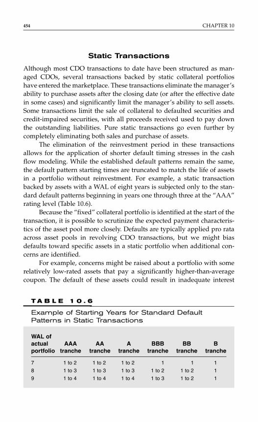
Static Transactions
Although most CDO transactions to date have been structured as man-aged CDOs, several transactions backed by static collateral portfolioshave entered the marketplace. These transactions eliminate the manager’sability to purchase assets after the closing date (or after the effective datein some cases) and significantly limit the manager’s ability to sell assets.Some transactions limit the sale of collateral to defaulted securities andcredit-impaired securities, with all proceeds received used to pay downthe outstanding liabilities. Pure static transactions go even further bycompletely eliminating both sales and purchase of assets.
The elimination of the reinvestment period in these transactionsallows for the application of shorter default timing stresses in the cashflow modeling. While the established default patterns remain the same,the default pattern starting times are truncated to match the life of assetsin a portfolio without reinvestment. For example, a static transactionbacked by assets with a WAL of eight years is subjected only to the stan-dard default patterns beginning in years one through three at the “AAA”rating level (Table 10.6).
Because the “fixed” collateral portfolio is identified at the start of thetransaction, it is possible to scrutinize the expected payment characteris-tics of the asset pool more closely. Defaults are typically applied pro rataacross asset pools in revolving CDO transactions, but we might biasdefaults toward specific assets in a static portfolio when additional con-cerns are identified.
For example, concerns might be raised about a portfolio with somerelatively low-rated assets that pay a significantly higher-than-averagecoupon. The default of these assets could result in inadequate interest
454 CHAPTER 10
T A B L E 1 0 . 6
Example of Starting Years for Standard DefaultPatterns in Static Transactions
WAL of actual AAA AA A BBB BB Bportfolio tranche tranche tranche tranche tranche tranche
7 1 to 2 1 to 2 1 to 2 1 1 1
8 1 to 3 1 to 3 1 to 3 1 to 2 1 to 2 1
9 1 to 4 1 to 4 1 to 4 1 to 3 1 to 2 1

cash flow from the remaining assets. This scenario is not tested by thestandard application of pro rata defaults. In this situation, bias of defaultstoward these assets could be warranted.
Senior Collateral Manager Fees
Senior collateral manager fees should be at market levels to provide ade-quate incentive for a replacement manager to take over the transaction,should the need arise. In general, these fees are modeled at the higher ofthe contractual fee and the minimum fees listed in Table 10.7 to ensurethat the transaction can support such fees.
Factors such as other forms of compensation to the collateral man-ager, the responsibilities of the manager, and the size of the transaction areconsidered when determining the appropriate senior fee. For instance, acontractual senior fee of 10 bps could be sufficient when the notional bal-ance of the portfolio of a corporate CLO transaction is $1 billion. Lowerfees might also be adequate in static transactions where the activities ofthe collateral manager are limited.
Equity
One challenge confronted in the cash flow analysis for rating equity orcombination notes that include equity as an asset is the sizing of unknownand uncapped administrative expenses senior in the priority of payments.For the purposes of cash flow modeling, we assume that these additionalexpenses are equal to the capped expenses located near the top part of thepriority of payments (Table 10.8).
In addition, the cash flows are also stressed with the three additionaldefault patterns employed for low credit quality portfolios. These pat-terns are applied to the equity analysis even if the credit quality of theportfolio is not necessarily low.
CDO Methodologies Developed by S&P 455
T A B L E 1 0 . 7
Annual Senior Collateral Manager Fees
Corporate CBO/CLO 15 bps
ABS CDO 15 bps
CSOs (collateralized swap obligations) 10 bps
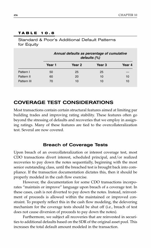
456 CHAPTER 10
T A B L E 1 0 . 8
Standard & Poor’s Additional Default Patterns for Equity
Annual defaults as percentage of cumulative defaults (%)
Year 1 Year 2 Year 3 Year 4
Pattern I 50 25 25 —
Pattern II 60 20 10 10
Pattern III 70 10 10 10
COVERAGE TEST CONSIDERATIONS
Most transactions contain certain structural features aimed at limiting parbuilding trades and improving rating stability. These features often gobeyond the stressing of defaults and recoveries that we employ in assign-ing ratings. Many of these features are tied to the overcollateralizationtest. Several are now covered.
Breach of Coverage Tests
Upon breach of an overcollateralization or interest coverage test, mostCDO transactions divert interest, scheduled principal, and/or realizedrecoveries to pay down the notes sequentially, beginning with the mostsenior outstanding class, until the breached test is brought back into com-pliance. If the transaction documentation dictates this, then it should beproperly modeled in the cash flow exercise.
However, the documentation for some CDO transactions incorpo-rates “maintain or improve” language upon breach of a coverage test. Inthese cases, cash is not diverted to pay down the notes. Instead, reinvest-ment of proceeds is allowed within the maintained or improved con-straint. To properly reflect this in the cash flow modeling, the deleveringmechanism for the coverage tests should be shut off (i.e., breach of testdoes not cause diversion of proceeds to pay down the notes).
Furthermore, we subject all recoveries that are reinvested in securi-ties to additional defaults based on the SDR of the original asset pool. Thisincreases the total default amount modeled in the transaction.
Haircut for Low-Rated Collateral
While a certain concentration of “CCC” rated assets is not necessarily bad,especially if factored into the original class sizing of the transaction,“CCC” rated assets have a tendency to be downgraded more quickly.Most transactions include a value haircut to “CCC” rated assets to capturethis increased proclivity to default in the overcollateralization test. Thiscauses it to breach earlier as the “CCC” asset concentration increases,allowing for faster paydown of the rated debt. We generally look for theovercollateralization test haircut when the percentage of assets in the poolwith a rating of “CCC” or less exceeds the original amount by 5 percent.Any amount over the original amount plus the 5 percent threshold is thencarried at either 70 percent of its par value or at the market value of theasset in the numerator of the test. The collateral manager before the clos-ing date of the transaction makes the choice between treatment at 70 per-cent of par or market value. When the market value treatment is chosen,the rating analyst should be consulted to determine the proper marketvalue treatment.
Overcollateralization Reinvestment Test
In addition to the “CCC” haircut in the overcollateralization tests, manytransactions also include a reinvestment overcollateralization test with a“CCC” haircut. This latter test is lower in the priority of payments, and, ifbreached, requires the manager to start reinvesting all or part of the excessinterest proceeds. The overcollateralization reinvestment threshold is typ-ically set higher than the minimum class overcollateralization threshold,thus allowing for reinvestment of interest proceeds before any deleveringovercollateralization trigger is breached.
As the portfolio starts losing par from credit-impaired sales, the rein-vestment trigger would be breached before the class overcollateralizationtrigger is breached. This would allow the transaction to start purchasingnew collateral to improve the overcollateralization reinvestment test. Thistest works best for transactions that incur slow, gradual declines in collat-eral values. If the transaction experiences large asset defaults in a shortperiod, the delevering overcollateralization test would likely be trippedsimultaneously. Even under these circumstances, the overcollateralizationreinvestment test is likely to bring some benefits, as it should force addi-tional reinvestments, once the delevering overcollateralization test isbrought back into compliance.
CDO Methodologies Developed by S&P 457
Current-Pay Collateral
A “current-pay” security is defined as an obligation that continues topay interest or principal payments even though the obligor hasdefaulted on other obligations. In general, the collateral manager cannotpurchase current-pay assets into the transaction, because these assetsare credit-impaired obligations that they are typically prohibited frompurchasing.
However, if the transaction holds an asset that then becomes acurrent-pay obligation, the collateral value is reduced to reflect the higherrating volatility. We use a market value test for this, giving full par valueif the security trades at 80 percent or better, and the assigned recovery ifit trades below. This haircut also reduces the numerator of the overcollat-eralization test, causing faster paydown of the rated debt.
Value of Defaulted Securities
Other than the current-pay securities valuation, all defaulted securitiesshould be carried at the lower of their assigned recovery rate or currentmarket value for the purpose of the overcollateralization test. In certaininstances, however, we may assign instrument-specific recoveries. Equitysecurities received as part of a workout can be held in the CDO transac-tion, but are given no value.
REQUIREMENTS FOR RUNNING THE CASHFLOW MODEL
In order to ensure timely completion of the cash flow analysis, we ask thatthe arranger provide:
♦ A summary of all assumptions used in the cash flow modeling;♦ A summary of the cash flow model results showing BDRs. We
request the BDRs for all classes (rated and unrated) be provided;♦ Detailed printouts of at least the two most stressful cash flow
model runs for each rating level;♦ A working, Excel-based cash flow model;♦ A reliance letter from an accountant for each substantially differ-
ent transaction structure or model; and
458 CHAPTER 10
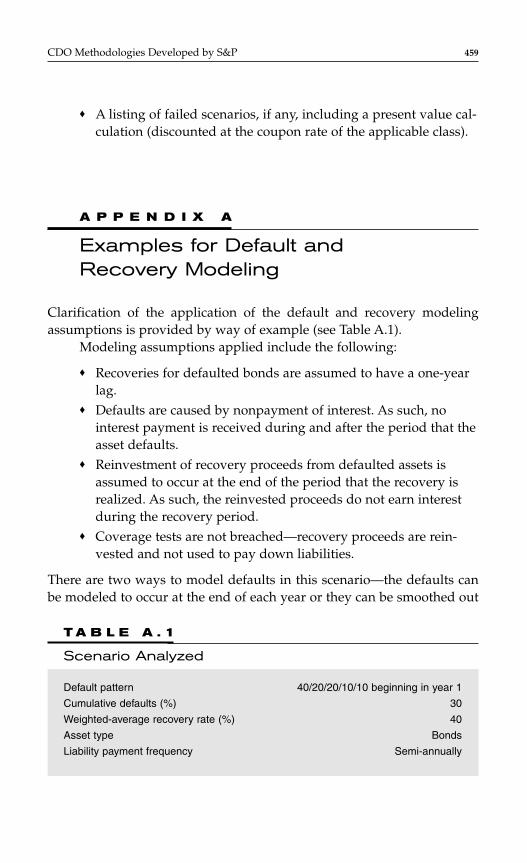
♦ A listing of failed scenarios, if any, including a present value cal-culation (discounted at the coupon rate of the applicable class).
A P P E N D I X A
Examples for Default and Recovery Modeling
Clarification of the application of the default and recovery modelingassumptions is provided by way of example (see Table A.1).
Modeling assumptions applied include the following:
♦ Recoveries for defaulted bonds are assumed to have a one-yearlag.
♦ Defaults are caused by nonpayment of interest. As such, nointerest payment is received during and after the period that theasset defaults.
♦ Reinvestment of recovery proceeds from defaulted assets isassumed to occur at the end of the period that the recovery isrealized. As such, the reinvested proceeds do not earn interestduring the recovery period.
♦ Coverage tests are not breached—recovery proceeds are rein-vested and not used to pay down liabilities.
There are two ways to model defaults in this scenario—the defaults canbe modeled to occur at the end of each year or they can be smoothed out
CDO Methodologies Developed by S&P 459
T A B L E A . 1
Scenario Analyzed
Default pattern 40/20/20/10/10 beginning in year 1
Cumulative defaults (%) 30
Weighted-average recovery rate (%) 40
Asset type Bonds
Liability payment frequency Semi-annually

460 CHAPTER 10
semi-annually. During the first year, defaults are usually modeled tooccur at the end of the year. An initial portfolio with a high concentrationof low-rated assets is one exception where defaults might be modeled tobegin earlier.
First Method
All defaults occur at the end of the year (Table A.2).
Key Observations for First MethodDefaults are lumped together at the end of each year. For assets payingsemi-annually, the defaulting assets earn interest during the first paymentperiod, but not the second period, of the year. Thus, for the 6 percent ofthe portfolio that defaults (20 × 30 percent) in year 2, these assets receivecredit for interest payments in period 3 but none beginning in period 4.Assets paying annually, however, would not earn interest in either ofthese periods.
Recovery of defaulted bonds occurs after a one-year lag. Again tak-ing the 6 percent of the portfolio that defaults in year 2 (at end of period4) and applying a 40 percent recovery rate to the defaulted balance, recov-eries equating to 2.4 percent of the portfolio balance (40 × 20 × 30 percent)is realized at the end of period 6. If these recoveries occur during the rein-vestment period, the recovery proceeds are reinvested and begin to earninterest starting in period 7.
Second Method
Annual defaults are separated into two semi-annual periods, startingafter the first year. During first year, all defaults occur at the end of theyear (Table A.3).
Key Observations for Second MethodBeginning with the second year, defaults are smoothed semi-annually.Thus, for the 6 percent of the portfolio that defaults (20 × 30 percent) inyear 2, 3 percent occurs in period 3 and the remaining 3 percent occurs inperiod 4. For assets paying semi-annually, those defaulting in period 3 donot earn interest in that period; those defaulting in period 4 earn interestin period 3, but not in period 4. Assets paying annually do not receiveinterest in either of these periods.
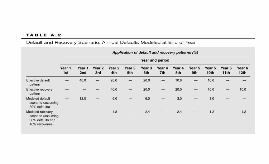
T A B L E A . 2
Default and Recovery Scenario: Annual Defaults Modeled at End of Year
Application of default and recovery patterns (%)
Year and period
Year 1 Year 1 Year 2 Year 2 Year 3 Year 3 Year 4 Year 4 Year 5 Year 5 Year 6 Year 61st 2nd 3rd 4th 5th 6th 7th 8th 9th 10th 11th 12th
Effective default — 40.0 — 20.0 — 20.0 — 10.0 — 10.0 — —pattern
Effective recovery — — — 40.0 — 20.0 — 20.0 — 10.0 — 10.0pattern
Modeled default — 12.0 — 6.0 — 6.0 — 3.0 — 3.0 — —scenario (assuming 30% defaults)
Modeled recovery — — — 4.8 — 2.4 — 2.4 — 1.2 — 1.2scenario (assuming 30% defaults and 40% recoveries)
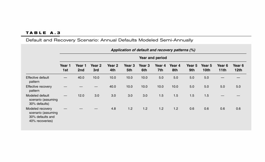
T A B L E A . 3
Default and Recovery Scenario: Annual Defaults Modeled Semi-Annually
Application of default and recovery patterns (%)
Year and period
Year 1 Year 1 Year 2 Year 2 Year 3 Year 3 Year 4 Year 4 Year 5 Year 5 Year 6 Year 61st 2nd 3rd 4th 5th 6th 7th 8th 9th 10th 11th 12th
Effective default — 40.0 10.0 10.0 10.0 10.0 5.0 5.0 5.0 5.0 — —pattern
Effective recovery — — — 40.0 10.0 10.0 10.0 10.0 5.0 5.0 5.0 5.0pattern
Modeled default — 12.0 3.0 3.0 3.0 3.0 1.5 1.5 1.5 1.5 — —scenario (assuming 30% defaults)
Modeled recovery — — — 4.8 1.2 1.2 1.2 1.2 0.6 0.6 0.6 0.6scenario (assuming 30% defaults and 40% recoveries)

Recovery of defaulted bonds occurs after a one-year lag. Recoverieson the 3 percent balance defaulting in period 3 are realized at the end ofperiod 5 and begin to earn interest in period 6 (if the reinvestment periodhas not lapsed).
R E F E R E N C E S
de Servigny, A., and O. Renault (2004), Measuring and Managing Credit Risk,McGraw-Hill.
de Servigny, A., and N. Jobst (2005), “An empirical analysis of equity defaultswaps I: Univariate insights,” Risk, December.
Fledelius, P., D. Lando, and J. P. Nielsen (2004), “Non-parametric analysis of rat-ing transition and default data,” working paper, Copenhagen BusinessSchool.
Glasserman, P. (2004), Monte Carlo Methods In Financial Engineering, Springer-Verlag.
Jobst, N., and A. de Servigny (2006), “An empirical analysis of equity defaultswaps II: Multivariate insights,” RISK, January.
Jobst, N., and K. Gilkes (2003), “Investigating transition matrices: Empiricalinsights and methodologies,” working paper, Standard & Poor’s.
Li, D. (2000), “On default correlation: A copula function approach,” Journal ofFixed Income, 9, 43–54.
Matsumoto, M. and Nishimura, T. (1998). Mersenne twister: A 623-dimensionallyequidistributed uniform pseudo-random number generator, ACMTransactions on Modelling and Computer Simulation, 8(1), 3–30.
Merton, R. (1974), “On the pricing of corporate debt: The risk structure of inter-est rates,” Journal of Finance, 29, 449–470.
CDO Methodologies Developed by S&P 463

This page intentionally left blank
C H A P T E R 1 1
Recent and Not SoRecent Developmentsin Synthetic CollateralDebt Obligations
Norbert Jobst
465
INTRODUCTION
Collateralized debt obligations (CDOs) are designed to transfer the riskinherent in a portfolio of (credit) risky assets to one or more investors.Although the first CDOs were “cash”-funded and backed by portfolios ofbonds and loans, in recent years the unfunded “synthetic” CDO markethas grown enormously. Instead of purchasing a debt instrument of agiven entity, the special purpose vehicle (SPV) enters into a credit defaultswap (CDS) that references the entity. This use of credit derivatives led toa European market dominated by “single-tranche” (ST) CDOs, bilateralcontracts between a buyer and seller of default protection on a portfolioof entities. The U.S. market is currently evolving toward a blend of cashand synthetic transactions in a more gradual way.
Since 2004, the pace of innovation in structured credit markets, andparticularly in synthetic CDOs, has increased significantly. The rise toprominence of ST synthetic CDOs stems from ease of execution, providingthe flexibility of expressing various views on (credit) markets, and enablingthe separation of funding and risk (see Chapter 9). In recent years, investordemands for higher yielding products in a extremely tight spread environ-ment, combined with (various) market events, have led to financial inno-vations addressing higher structural complexity and nontraditional(noncredit) risks. Throughout this chapter, we provide an overview of a
Copyright © 2007 by The McGraw-Hill Companies. Click here for terms of use.

466 CHAPTER 11
number of these developments mainly from a rating agency perspectivewhere the risk assessment usually involves an estimate of the expected lossto the investor, or an estimate of the likelihood of principal and interestbeing paid in a timely manner.* The genesis of these innovations, as almostany in the synthetic CDO market, comes from a mixture of different driversfrom the market participants: from investors’ search for new yield in a tightspread environment to the need to investment diversification, and fromarbitrage exploitation to structures that can be used to express a view on thesystemic credit cycle as well as idiosyncratic credit risk.
We start in the following section by discussing various extensions orvariants of ST CDOs where the main risks (from a rating agency perspec-tive) are still default events and subsequent losses. We will discuss CDOsquared transactions that were very popular in 2004/2005 with demanddrying up after the downgrade of Ford and General Motors (GM) in May2005. Forward-starting transactions, long/short structures, and ST CDOswith time varying attachment points are further examples that will bebriefly introduced. In addition to these “add-ons” to traditional syntheticCDOs, investors frequently seek to try and take advantage from develop-ments in noncredit markets.
In section “Beyond Credit Risk: Hybrid Structured Products,” wefocus on the most significant developments in alternative asset classesthat find their way into so-called hybrid transactions. We also focus onequity risk via so-called equity default swaps (EDSs) and commodity riskin its subsections.
In section “Structural Innovations: Introducing MtM Risk,” we focuson some of the latest developments caused by changes in the market partic-ipants’ trading and hedging behavior, following the May 2005 events. Thesenew structures aim at placing equity and/or super senior risk to “hedge”the high demand of mezzanine tranches and go beyond a pure default riskassessment of the underlying pool of assets by taking into account the riskof mark-to-market (MtM) changes. We start by discussing leveraged supersenior (LSS) transaction in the first subsection, a product that is very popu-lar since 2005. In the second subsection, a very recent development, the so-called credit constant propostional portfolio insurance (CPPI) transaction,which addresses guaranteed principal and interest payments and involvesautomatic portfolio rebalancing depending on portfolio performance,
*The focus lies therefore on a discussion (and modeling overview) of the main risk factors,rather than on valuation and relative-value considerations. References on the latter will beprovided when available and adequate.
followed by a brief discussion of the latest innovation in rated structuredcredit markets: Constant Proportion Debt Obligation (CPDO). The last sec-tion summarized current trends and future modelling challenges.
VARIANTS OF ST CDOs
ST CDOs: A Ratings Perspective
Before moving to the evolution on ST synthetic CDOs, we start by review-ing typical risk assessments conducted in a similar way by most ratingagencies (RAs) on the standard, vanilla ST CDO product. RAs, such asStandard & Poor’s, Moody’s, Fitch, or DBRS, are typically interested in therisk a CDO investor is facing throughout the life of the transaction and basetheir opinions partly on model-based statistics. For example, Moody’s rat-ing is a so-called “expected loss” rating and, as a result, the expected losson a CDO tranche is estimated and benchmarked to various rating specifictargets. Standard & Poor’s, on the other hand, applies a “probability ofdefault” rating and estimates the probability of the investor to face a “firstdollar of loss” using its CDO Evaluator (see Chapter 10 for further details).
RAs, to date, mostly employ simulation methodologies in order toestimate the relevant risk measures. For example, Standard & Poor’smodels the dependency between defaults of different assets through theGaussian copula approach, as introduced in the Chapters 4 and 6. For thismodel, correlated default times can be easily simulated by
1. Generating N standard multivariate normal random variables yiadmitting a correlation matrix Σ,
2. Calculating ui = Φ(yi), and3. Calculating a default time τi = S−1(ui) for each asset.*
If τi is less than the maturity T of the CDO transaction, the loss Li is deter-mined as Li = Ni × (1 − δi), where Ni and δ i are the exposure-at-default andrecovery,† respectively, for the ith asset. We can therefore write the portfo-lio loss up to time t, L(t), as
L t Ni i ti
i( ) ( ) ,= × − ×
≤ ∑ 1 1δτ
Recent and Not So Recent Developments in Synthetic CDOs 467
*S−1 is used to denote the quasi-inverse of the survival function.†The recovery can either be assumed to be constant or drawn from a distribution.
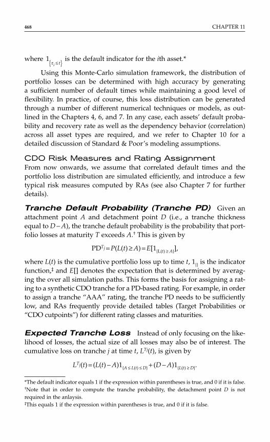
where is the default indicator for the ith asset.*
Using this Monte-Carlo simulation framework, the distribution ofportfolio losses can be determined with high accuracy by generatinga sufficient number of default times while maintaining a good level offlexibility. In practice, of course, this loss distribution can be generatedthrough a number of different numerical techniques or models, as out-lined in the Chapters 4, 6, and 7. In any case, each assets’ default proba-bility and recovery rate as well as the dependency behavior (correlation)across all asset types are required, and we refer to Chapter 10 for adetailed discussion of Standard & Poor’s modeling assumptions.
CDO Risk Measures and Rating AssignmentFrom now onwards, we assume that correlated default times and theportfolio loss distribution are simulated efficiently, and introduce a fewtypical risk measures computed by RAs (see also Chapter 7 for furtherdetails).
Tranche Default Probability (Tranche PD) Given anattachment point A and detachment point D (i.e., a tranche thicknessequal to D − A), the tranche default probability is the probability that port-folio losses at maturity T exceeds A.† This is given by
PDTj = P(L(t) ≥ A) = E[1L(t) ≥ A],
where L(t) is the cumulative portfolio loss up to time t, 1 is the indicatorfunction,‡ and E[] denotes the expectation that is determined by averag-ing the over all simulation paths. This forms the basis for assigning a rat-ing to a synthetic CDO tranche for a PD-based rating. For example, in orderto assign a tranche “AAA” rating, the tranche PD needs to be sufficientlylow, and RAs frequently provide detailed tables (Target Probabilities or“CDO cutpoints”) for different rating classes and maturities.
Expected Tranche Loss Instead of only focusing on the like-lihood of losses, the actual size of all losses may also be of interest. Thecumulative loss on tranche j at time t, LTj(t), is given by
LTj(t) = (L(t) − A)1A ≤ L(t) ≤ D + (D − A)1L(t) ≥ D.
1τ i t≤
468 CHAPTER 11
*The default indicator equals 1 if the expression within parentheses is true, and 0 if it is false.†Note that in order to compute the tranche probability, the detachment point D is notrequired in the anlaysis.‡This equals 1 if the expression within parentheses is true, and 0 if it is false.

The expected tranche loss is therefore given by
E[LTj (t)] = E[(L(t) − A)1A ≤ L(t) ≤ D + (D − A)1L(t) ≥ D],
which is computed easily by simulation. An expected loss rating assignedby RAs, such as Moody’s, is partly based on this measure of tranche risk.
Tranche Loss-Given-Default From the expected trancheloss and the tranche PD, the tranche loss-given-default is simply given
by under the assumption of independencebetween tranche PD and LGD.
With ST CDOs and several risk measures introduced earlier, we willnow start to discuss evolutions of standard tranche products and assess therisks prevalent within the framework presented earlier. Unless otherwisestated, all numerical examples are based on Standard & Poor’s modelingassumptions, as outlined in Chapter 10.
CDO Squared Transactions: Extending Leverage
Synthetic CDO squared transactions have become an established featureof the global CDO marketplace in 2004/2005. Since May 2005, however,demand has reduced significantly, as a result of MtM losses caused bymany market participants following the downgrade of Ford and GM byStandard & Poor’s (see Chapters 8 and 9 for further details). CDO squaredtransactions typically reference other “bespoke” CDO tranches, each ref-erencing a single underlying corporate portfolio. In this way, additionalleverage is created, resulting in a yield pick-up of these structures relativeto similarly rated synthetic CDOs. This leveraging creates an investmentthat is less sensitive to small numbers of credit events within the under-lying portfolio, but is also more likely to suffer large losses once its creditprotection is eroded. Within the framework of the risk measures pre-sented earlier, this implies very small tranche PDs but high tranche LGDs,hence, keeping expected tranche losses balanced. While some CDOsquared transactions reference only CDOs, others have referenced portfo-lios containing a mixture of CDO and asset-backed securities (ABS)tranches, where the proportion of ABS is typically in the range of 70 to90 percent by reference notional amount. The basic structure of a typicalCDO squared transaction is shown schematically in Figure 11.1.
LGD [ ( )] /PDjT T TE L tj j= ( )
Recent and Not So Recent Developments in Synthetic CDOs 469
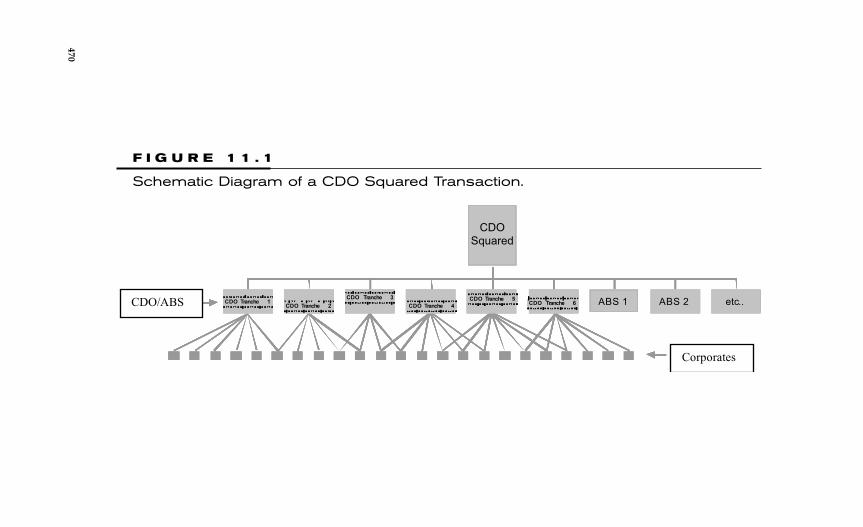
F I G U R E 1 1 . 1
Schematic Diagram of a CDO Squared Transaction.
ABS 1 ABS 2 etc..CDO Tranche 1CDO Tranche 2
CDO Tranche 3
CDO Tranche 4
CDO Tranche 5CDO Tranche 6 ABS 1 ABS 2 etc..CDO Tranche 1
CDO Tranche 2
CDO Tranche 3
CDO Tranche 4
CDO Tranche 5CDO Tranche 6
CDO
Squared
ABS 1 ABS 2 etc..CDO Tranche 1CDO Tranche 2
CDO Tranche 3
CDO Tranche 4
CDO Tranche 5CDO Tranche 6 ABS 1 ABS 2 etc..CDO Tranche 1CDO Tranche 1
CDO Tranche 2CDO Tranche 2
CDO Tranche 3CDO Tranche 3
CDO Tranche 4CDO Tranche 4
CDO Tranche 5CDO Tranche 5CDO Tranche 6CDO Tranche 6CDO/ABS
Corporates
470
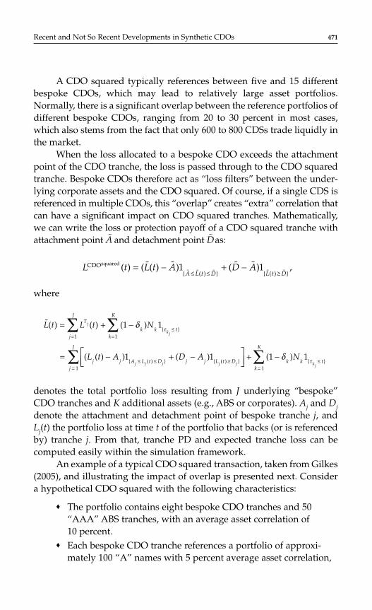
A CDO squared typically references between five and 15 differentbespoke CDOs, which may lead to relatively large asset portfolios.Normally, there is a significant overlap between the reference portfolios ofdifferent bespoke CDOs, ranging from 20 to 30 percent in most cases,which also stems from the fact that only 600 to 800 CDSs trade liquidly inthe market.
When the loss allocated to a bespoke CDO exceeds the attachmentpoint of the CDO tranche, the loss is passed through to the CDO squaredtranche. Bespoke CDOs therefore act as “loss filters” between the under-lying corporate assets and the CDO squared. Of course, if a single CDS isreferenced in multiple CDOs, this “overlap” creates “extra” correlation thatcan have a significant impact on CDO squared tranches. Mathematically,we can write the loss or protection payoff of a CDO squared tranche withattachment point A
~and detachment point D
~as:
where
denotes the total portfolio loss resulting from J underlying “bespoke”CDO tranches and K additional assets (e.g., ABS or corporates). Aj and Djdenote the attachment and detachment point of bespoke tranche j, andLj(t) the portfolio loss at time t of the portfolio that backs (or is referencedby) tranche j. From that, tranche PD and expected tranche loss can becomputed easily within the simulation framework.
An example of a typical CDO squared transaction, taken from Gilkes(2005), and illustrating the impact of overlap is presented next. Considera hypothetical CDO squared with the following characteristics:
♦ The portfolio contains eight bespoke CDO tranches and 50“AAA” ABS tranches, with an average asset correlation of10 percent.
♦ Each bespoke CDO tranche references a portfolio of approxi-mately 100 “A” names with 5 percent average asset correlation,
˜( ) ( ) ( )
( ( ) ) ( ) ( )
( ) ( )
L t L t N
L t A D A N
T
k k tk
K
j
J
j j A L t D j j L t Dj
J
k k tk
K
j
k j
j j j j j k j
= + −
= − + − + −
≤==
≤ ≤ ≥=
≤=
∑∑
∑ ∑
1 1
1 1 1 1
11
1 1
δ
δ
τ
τ
L t L t A D AA L t D L t D
CDO ˜ ˜ ( ) ˜ ˜ ( ) ˜
( ) ( ˜( ) ˜ ) ( ˜ ˜ ) ,squared = − + −≤ ≤ ≥
1 1
Recent and Not So Recent Developments in Synthetic CDOs 471
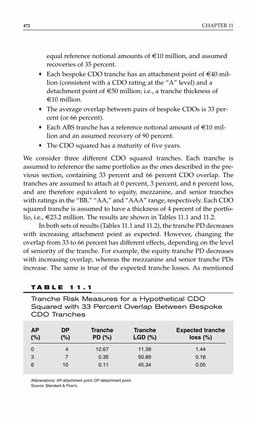
equal reference notional amounts of m10 million, and assumedrecoveries of 35 percent.
♦ Each bespoke CDO tranche has an attachment point of m40 mil-lion (consistent with a CDO rating at the “A” level) and adetachment point of m50 million; i.e., a tranche thickness ofm10 million.
♦ The average overlap between pairs of bespoke CDOs is 33 per-cent (or 66 percent).
♦ Each ABS tranche has a reference notional amount of m10 mil-lion and an assumed recovery of 90 percent.
♦ The CDO squared has a maturity of five years.
We consider three different CDO squared tranches. Each tranche isassumed to reference the same portfolios as the ones described in the pre-vious section, containing 33 percent and 66 percent CDO overlap. Thetranches are assumed to attach at 0 percent, 3 percent, and 6 percent loss,and are therefore equivalent to equity, mezzanine, and senior trancheswith ratings in the “BB,” “AA,” and “AAA” range, respectively. Each CDOsquared tranche is assumed to have a thickness of 4 percent of the portfo-lio, i.e., m23.2 million. The results are shown in Tables 11.1 and 11.2.
In both sets of results (Tables 11.1 and 11.2), the tranche PD decreaseswith increasing attachment point as expected. However, changing theoverlap from 33 to 66 percent has different effects, depending on the levelof seniority of the tranche. For example, the equity tranche PD decreaseswith increasing overlap, whereas the mezzanine and senior tranche PDsincrease. The same is true of the expected tranche losses. As mentioned
472 CHAPTER 11
T A B L E 1 1 . 1
Tranche Risk Measures for a Hypothetical CDOSquared with 33 Percent Overlap Between BespokeCDO Tranches
AP DP Tranche Tranche Expected tranche (%) (%) PD (%) LGD (%) loss (%)
0 4 12.67 11.39 1.44
3 7 0.35 50.89 0.18
6 10 0.11 45.34 0.05
Abbreviations: AP-attachment point; DP-detachment point.Source: Standard & Poor’s.
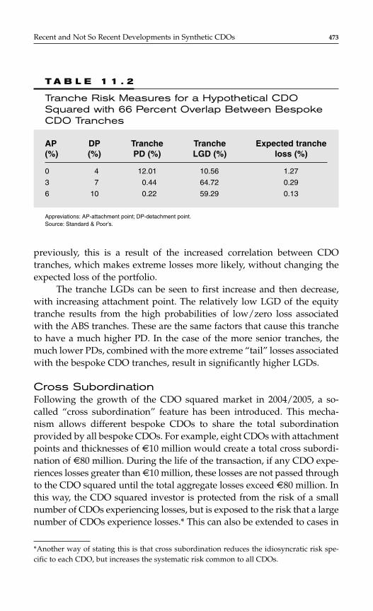
previously, this is a result of the increased correlation between CDOtranches, which makes extreme losses more likely, without changing theexpected loss of the portfolio.
The tranche LGDs can be seen to first increase and then decrease,with increasing attachment point. The relatively low LGD of the equitytranche results from the high probabilities of low/zero loss associatedwith the ABS tranches. These are the same factors that cause this trancheto have a much higher PD. In the case of the more senior tranches, themuch lower PDs, combined with the more extreme “tail” losses associatedwith the bespoke CDO tranches, result in significantly higher LGDs.
Cross SubordinationFollowing the growth of the CDO squared market in 2004/2005, a so-called “cross subordination” feature has been introduced. This mecha-nism allows different bespoke CDOs to share the total subordinationprovided by all bespoke CDOs. For example, eight CDOs with attachmentpoints and thicknesses of m10 million would create a total cross subordi-nation of m80 million. During the life of the transaction, if any CDO expe-riences losses greater than m10 million, these losses are not passed throughto the CDO squared until the total aggregate losses exceed m80 million. Inthis way, the CDO squared investor is protected from the risk of a smallnumber of CDOs experiencing losses, but is exposed to the risk that a largenumber of CDOs experience losses.* This can also be extended to cases in
Recent and Not So Recent Developments in Synthetic CDOs 473
T A B L E 1 1 . 2
Tranche Risk Measures for a Hypothetical CDOSquared with 66 Percent Overlap Between BespokeCDO Tranches
AP DP Tranche Tranche Expected tranche (%) (%) PD (%) LGD (%) loss (%)
0 4 12.01 10.56 1.27
3 7 0.44 64.72 0.29
6 10 0.22 59.29 0.13
Appreviations: AP-attachment point; DP-detachment point.Source: Standard & Poor’s.
*Another way of stating this is that cross subordination reduces the idiosyncratic risk spe-cific to each CDO, but increases the systematic risk common to all CDOs.
which the subordination is only “partially” cross-subordinated (e.g., theCDO squared tranche is only insulated from 75 percent of the total aggre-gate subordination of the bespoke CDOs).
The payoff of such a cross subordination feature (assuming onlybespoke CDO tranches and no other assets in the underlying pool ofassets) can be represented as follows.
where
where denotes the total amount of cross subordination available
and With credit spreads at some of their tightest levels in
recent years and the respective vanishing of “rating arbitrage” and araised awareness of correlation/overlap risk of CDO squared transac-tions, demand has dried up subsequently. Further details can be found inGilkes (2005), and a discussion of CDO squared valuation and risk man-agement is given in Metayer (2005).
Forward Starting CDOs
Also in 2005, ST CDOs evolved to incorporate so-called forward startingfeatures, i.e., the risk horizon of the CDO only starts after time ν. Lossesdue to defaults prior to ν are not accounted for in the payoff and portfo-lio loss calculation:
This feature allows investors to express their specific, short-term defaultviews into the CDO product, or take advantage of favourable divergencesbetween the credit curve perceived by RAs (under the real measure) andthat of the market (implied, risk-neutral measure).
Of course, such a forward starting feature essentially impacts alltranches along the capital structures as the overall default rate reduces,
L t Ni i ti
i( ) ( ) .= × − ×
≤ ≤ ∑ 1 1δν τ
D DjJ
j= =Σ 1 .
A AjJ
j= =Σ 1
˜ ( ) ( ) ,CS
( ) ( ) L t L t A D AT
j
J
A L t D L t D
jTj
j
J Tjj
J= −
+ −( )
= ≤ ≤ ≥∑
= =∑ ∑1
1 11 1
L t L t A D AA L t D L t D
CS CS CS ˜ ˜ ( ) ˜
CS CS ˜ ( ) ˜
( ) ( ˜ ( ) ˜ )1 ( ˜ ˜ )1 ,CS CS CS CS CS
= − + −≤ ≤ ≥
474 CHAPTER 11
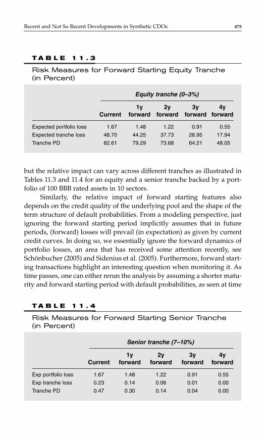
but the relative impact can vary across different tranches as illustrated inTables 11.3 and 11.4 for an equity and a senior tranche backed by a port-folio of 100 BBB rated assets in 10 sectors.
Similarly, the relative impact of forward starting features alsodepends on the credit quality of the underlying pool and the shape of theterm structure of default probabilities. From a modeling perspective, justignoring the forward starting period implicitly assumes that in futureperiods, (forward) losses will prevail (in expectation) as given by currentcredit curves. In doing so, we essentially ignore the forward dynamics ofportfolio losses, an area that has received some attention recently, seeSchönbucher (2005) and Sidenius et al. (2005). Furthermore, forward start-ing transactions highlight an interesting question when monitoring it. Astime passes, one can either rerun the analysis by assuming a shorter matu-rity and forward starting period with default probabilities, as seen at time
Recent and Not So Recent Developments in Synthetic CDOs 475
T A B L E 1 1 . 3
Risk Measures for Forward Starting Equity Tranche(in Percent)
Equity tranche (0–3%)
1y 2y 3y 4y Current forward forward forward forward
Expected portfolio loss 1.67 1.48 1.22 0.91 0.55
Expected tranche loss 48.70 44.25 37.73 28.95 17.94
Tranche PD 82.61 79.29 73.68 64.21 48.05
T A B L E 1 1 . 4
Risk Measures for Forward Starting Senior Tranche(in Percent)
Senior tranche (7–10%)
1y 2y 3y 4y Current forward forward forward forward
Exp portfolio loss 1.67 1.48 1.22 0.91 0.55
Exp tranche loss 0.23 0.14 0.06 0.01 0.00
Tranche PD 0.47 0.30 0.14 0.04 0.00
0 on the credit curve. That means, for future time s, we assume defaultprobabilities Pi(0, T − s), where T denotes the time maturity, and ignoredefaults in the simulation between 0 and ν − s. Alternatively, we can rollthe transaction down the credit curve by assuming forward starting prob-abilities, i.e., use Pi(s, T) ≈ Pi(0, T) − Pi(0, s). Each approach has got draw-backs if static credit curves are assumed, and a detailed forward lossmodeling is avoided. For example, in the former approach, we wouldessentially assume that noninvestment grade (NIG) companies havealways the same default risk over the next year, despite the common opin-ion that credit risk is declining if an NIG firm stays in a specific rating fora significant period of time. The latter approach, on the other hand, isclearly based on the assumption that the forward expectation will prevail,and carries the problem that we would need to monitor the duration acompany is/was in a given rating category prior to the risk assessment,unless a Markov assumption can be empirically justified.* Hence, thisapproach would be heavily dependent on the Markov property that haspreviously been questioned in empirical studies (see, e.g., Lando andSkodeberg, 2002).
Long/Short Structures
In a CDS, the protection seller agrees to pay the protection buyer the ref-erence notional amount of the contract minus a recovery amount, in theevent of default of a given reference entity. In exchange for this contingentpayment, the protection buyer pays the protection seller a premium. Whenan entity sells protection in CDS form, it is said to take a “long” position,whereas buying protection corresponds to entering a “short” position. Forloss computations, we can simply change the sign of the loss (i.e., makingit a gain) in the event of default of the reference name, conditional uponthe survival of the protection seller.†
The impact of shorting assets in the underlying portfolio depends,amongst other factors, on the credit quality of the long positions, thecredit quality of the short positions, and the target rating that one wantsto achieve (i.e., the level of subordination). We illustrate this on the fol-lowing examples. First, we consider a portfolio of 100 long “A” rated
476 CHAPTER 11
*Here we assume a typical RA approach, where default probabilities are directly linked tothe rating of a company.†Hence, there is some additional counterparty risk, which requires additional information onthe CDS counterparty when short CDS are included within the portfolio.

assets in 10 sectors. We then gradually add buckets of short positions,from 10 percent of the long notional amount up to 200 percent of the longnotional amount. We consider “A” and “B” quality assets for the shortbuckets. Figure 11.2 shows the impact of adding short positions on thecredit enhancement (CE) required, in order to achieve a “AAA” and“BBB” rating from Standard & Poor’s. The left exhibit shows the absoluteCE, whereas the right exhibit shows the relative CE as a fraction of thelong only “A” rated portfolio notional (put another way, the right panelshows the CE with shorts scaled by the CE needed without shorts).
The grey line shows the CE required to achieve an “AAA” ratingwhen different amounts of “A” shorts are added, whereas the greylineshows the same statistic when “B” shorts are added instead. The dottedand dashed line shows the same statistic for a target “BBB” rating. Whatis apparent is that the required CE reduces with the introduction of a shortbucket and, as expected, that this reduction depends highly on the creditquality of the short portfolio. When “B” quality short positions are added,we see a stark decline in required subordination, resulting from signifi-cantly higher PDs of NIG assets compared to investment grade, (IG) ones.
Figure 11.3 repeats this exercise, but now for a long portfolio of “BB”quality, and we consider shorting “BB” and “B” quality assets this time.
Although the observations of Figure 11.2 also hold for this experi-ment, we can further observe that the relative decline in CE when shortsof the same credit quality as longs are introduced is higher for low creditquality portfolios.
In addition to shorting single-name exposures, short positions canalso be taken in synthetic CDO tranches. Going long and short tranchesallows one to execute directional trades where a (speculative) view is taken
Recent and Not So Recent Developments in Synthetic CDOs 477
F I G U R E 1 1 . 2
Impact of Short Positions on “A” Quality Portfolio.
100 "A" longs ("A"/ "B" Shorts)
0%
1%
2%
3%
4%
5%
6%
0%
20%
40%
60%
80%
100%
0 10% 20% 30% 100% 150% 200%% shorts
0 10% 20% 30% 100% 150% 200%% shorts
Su
bo
rdin
atio
n (
CE
) AAA (A shorts)
BBB (A shorts)
AAA (B shorts)
BBB (B shorts)
100 "A" longs ("A"/ "B" Shorts): % of 0-Shorts
CE
as
% o
f n
o s
ho
rts
AAA (A shorts)
BBB (A shorts)
AAA (B shorts)
BBB (B shorts)
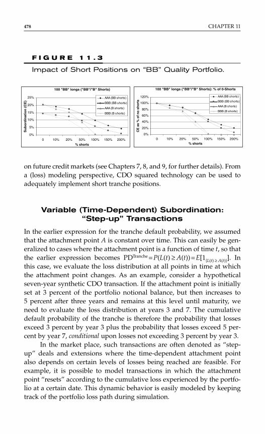
on future credit markets (see Chapters 7, 8, and 9, for further details). Froma (loss) modeling perspective, CDO squared technology can be used toadequately implement short tranche positions.
Variable (Time-Dependent) Subordination: “Step-up” Transactions
In the earlier expression for the tranche default probability, we assumedthat the attachment point A is constant over time. This can easily be gen-eralized to cases where the attachment point is a function of time t, so thatthe earlier expression becomes PDTranche = P(L(t) ≥ A(t)) = E[1L(t) ≥ A(t)]. Inthis case, we evaluate the loss distribution at all points in time at whichthe attachment point changes. As an example, consider a hypotheticalseven-year synthetic CDO transaction. If the attachment point is initiallyset at 3 percent of the portfolio notional balance, but then increases to5 percent after three years and remains at this level until maturity, weneed to evaluate the loss distribution at years 3 and 7. The cumulativedefault probability of the tranche is therefore the probability that lossesexceed 3 percent by year 3 plus the probability that losses exceed 5 per-cent by year 7, conditional upon losses not exceeding 3 percent by year 3.
In the market place, such transactions are often denoted as “step-up” deals and extensions where the time-dependent attachment pointalso depends on certain levels of losses being reached are feasible. Forexample, it is possible to model transactions in which the attachmentpoint “resets” according to the cumulative loss experienced by the portfo-lio at a certain date. This dynamic behavior is easily modeled by keepingtrack of the portfolio loss path during simulation.
478 CHAPTER 11
F I G U R E 1 1 . 3
Impact of Short Positions on “BB” Quality Portfolio.
100 "BB" longs ("BB"/"B" Shorts)
0%
5%
10%
15%
20%
25%
0 10% 20% 50% 100% 150% 200%
% shorts
Su
bo
rdin
atio
n (
CE
)
AAA (BB shorts)
BBB (BB shorts)
AAA (B shorts)
BBB (B shorts)
100 "BB" longs ("BB"/"B" Shorts): % of 0-Shorts
0%
20%
40%
60%
80%
100%
120%
0 10% 20% 50% 100% 150% 200%% shorts
CE
as
% o
f no
shor
ts
AAA (BB shorts)
BBB (BB shorts)
AAA (B shorts)
BBB (B shorts)
BEYOND CREDIT RISK: HYBRIDSTRUCTURED PRODUCTS
In recent years, structured credit products, and in particular syntheticCDOs, evolved toward referencing a variety of asset types. Routinely, STCDOs reference corporate CDSs, ABS tranches, other CDOs, or loansgiven to small and medium enterprises. When included in a CDO, com-mon to all these assets is the risk of default or credit risk of the underly-ing reference obligation. More recently, several noncredit derivatives havebeen introduced to the synthetic CDO market in a search for higher yield-ing instruments in a very tight credit environment.
In 2004, an upsurge in interest in so-called EDSs took place. EDSs arelong-dated, deep out-of-the-money equity puts that are similar to CDS, inwhich a contingency payment takes place if the equity price of a specificentity breaches a low barrier (typically 30 percent). The reason for thesedevelopments was the search for higher yield in a tight spread environ-ment, but also a general trend towards the convergence of credit andequity markets. Frequently, CDOs of EDS (or CEOs) reference both, CDSand EDSs. In the next section, we review a number of developments onEDS, as well as CDOs of EDS.
At the same time, dealers started to consider the introduction ofdeep out-of-the-money (European) commodity options into ST CDOs.The interest in this product has also increased toward the end of 2005, asa result of steadily rising commodity markets. Again, the incorporation ofcredit and commodity (and potentially equity) risk within an ST CDOcomes with a number of modeling challenges. Dependence issues, e.g.,the link between large oil corporations and oil prices, need to be carefullyaddressed. The section “CDOs: Commodity Transactions” reviews somerecent developments by Standard & Poor’s in modeling collateralizedcommodity obligations.
In addition to these developments, some general interest onmultiasset-class products has been noted. Such transactions aim to trans-fer various other risks such as interest rate or FX risk, in addition to com-modity, equity, and credit risk, via synthetic CDO technology.
When dealing with the problem of modeling ST CDOs backed byvarious (noncredit) asset types, one has the choice of staying within (andextending) the common framework used for ST CDOs or to develop anew methodology. Throughout this chapter, we focus on developmentswithin the usual copula framework, offering a brief discussion of alterna-tives in the last section. For now, when looking at alternative asset types
Recent and Not So Recent Developments in Synthetic CDOs 479

and risks, we focus on univariate and multivariate aspects separately,focusing on the Gaussian copula framework discussed in the “Variants ofST CDOs” section previously and in various other chapters.
Equity Default Swaps
Over the last two years, there has been some interest in CDOs referencingportfolios of EDS. These contracts trigger a payment when the underlyingequity price falls below a predetermined level. This price decline is oftenreferred to as an “equity event” (or interchangeably as “equity default,”or “EDS default”) analogous to a credit event within a CDS contract. Asthe trigger price is set closer to zero, these contracts can be expectedto become more “credit-like,” and EDS/CDS spreads should start toconverge.
In a CDO that references a pool of equities under an EDS contract,the same basic roles exist as for a typical CDO referencing CDSs. Theseller is paid a premium in exchange for a principal commitment whenlosses exceed the threshold amount. In this case, however, losses aredefined as the notional amount of equities whose prices fall to the triggerlevel, minus a predetermined recovery rate. Although any combination oftrigger level and recovery rate could be considered, EDS contracts are typ-ically structured in the market with a trigger level set at 30 percent and afixed recovery rate of 50 percent. For some investors, the risk–return char-acteristics of portfolios of these deep “out-of-the-money,” long-dated dig-itals offer relative value, especially given the recent tightening of CDSspreads.
Introducing EDSs into ST CDOs within the current copula frame-work requires an assessment of the (univariate) likelihood of equity priceson individual names to breach the barrier (hit the strike), as well as anassessment of joint equity behavior, and potentially the link between creditand equity. All analysis conducted herewith are based on Standard andPoor’s CreditPro® ratings and default database linked to Standard &Poor’s Compustat® (North America) data. CreditPro contains the ratingshistory of approximately 9740 companies from December 31, 1981 toDecember 31, 2003 and includes 1170 default events. The Compustat data-base contains approximately 56,500 corporations trading in the UnitedStates or Canada between 1962 and 2003, of which, up to 12,240 equitytime series or over 128,000 yearly observations are analyzed herewith.
480 CHAPTER 11

Equity Events: Empirical Insights and Univariate ModelingIn the following, we review three different types of analysis. First, a purecohort analysis, second, a direct modeling of equity prices via stochasticprocesses; and lastly, a statistical credit scoring approach.
Equity Default Events: Cohort Results Jobst and Gilkes(2004) present a cohort analysis (see Chapter 2 for further details) that iscommonly used to derive historic average default or rating transitionprobabilities. We start by considering all companies at a specific point intime t (e.g., December 31, 2000). We denote the total number of companiesin the kth cohort at time t by Nk(t), and the total number of observed events(e.g., default or equity price decline) in period T (i.e., between time t + T − 1and time t + T) by Dk(t, T). We then obtain an estimate for the (marginal)probability of default in year T (as seen from time t):*
Repeating this analysis for cohorts created at M different points intime t allows us to obtain an estimate for the unconditional probability ofdefault in period T,
These unconditional probabilities are simply weighted averages ofthe estimates obtained for cohorts considered in different periods. Typically,
wk(t) = 1/M (each period is equally weighted) or
(weighted according to the number of observations in different periods).
Unconditional (weighted average) cumulative probabilities capturing defaults over T periods can be calculated from the uncondi-tional marginal probabilities P–k(T):
P Tkcum ( )
w t N t N mk k mM
k( ) ( )/ ( )= =Σ 1
P T w t P t Tk k kt
M
( ) ( ) ( , ).==∑
1
P t TD t T
N tkk
k
( , )( , )
( ).=
Recent and Not So Recent Developments in Synthetic CDOs 481
*Some companies will have their rating withdrawn during the course of the year. It is com-mon to treat these transitions to NR (not rated) as noninformative with respect to the creditquality. Hence, companies that have their rating withdrawn during the period of interest areignored in the subsequent analysis.
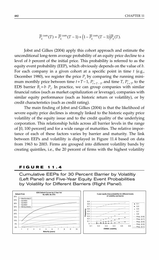
Jobst and Gilkes (2004) apply this cohort approach and estimate theunconditional long-term average probability of an equity price decline to alevel of b percent of the initial price. This probability is referred to as theequity event probability (EEP), which obviously depends on the value of b.For each company in a given cohort at a specific point in time t (e.g.,December 1980), we register the price Pt by comparing the running mini-mum monthly price between time t + T − 1, P−
t + T − 1, and time T, P−t + T, to the
EDS barrier Bt = b ⋅ Pt. In practice, we can group companies with similarfinancial ratios (such as market capitalization or leverage), companies withsimilar equity performance (such as historic return or volatility), or bycredit characteristics (such as credit rating).
The main finding of Jobst and Gilkes (2004) is that the likelihood ofsevere equity price declines is strongly linked to the historic equity pricevolatility of the equity issue and to the credit quality of the underlyingcorporation. This relationship holds across all barrier levels in the rangeof [0, 100 percent] and for a wide range of maturities. The relative impor-tance of each of these factors varies by barrier and maturity. The linkbetween EEPs and volatility is displayed in Figure 11.4 based on datafrom 1963 to 2003. Firms are grouped into different volatility bands bycreating quintiles, i.e., the 20 percent of firms with the highest volatility
P T P T P T P Tk k k kcum cum cum( ) ( ) ( ) ( ).= − + − −( )1 1 1
482 CHAPTER 11
F I G U R E 1 1 . 4
Cumulative EEPs for 30 Percent Barrier by Volatiltiy(Left Panel) and Five-Year Equity Event Probabilitiesby Volatility for Different Barriers (Right Panel).
EDS Default Curves by 5 Year VolNo ADR, No OTC
0%
5%
10%
15%
20%
25%
30%
35%
40%
45%
1 2 3 4 5 6 7 8 9 10
Maturity (years)
Default Prob
MaxQuntile(1)Quntile2Quntile3Quntile4MinQuntile(5)
5 year equity drop probability for different levelsof volatility and barrier
0
0.1
0.2
0.3
0.4
0.5
0.6
0.7
0.8
0.9
0.1 0.2 0.3 0.4 0.5 0.6
EWMA volatility
Freq
uenc
y
0.1
0.3
0.5
0.7
0.9
Poly. (0.9)
Poly. (0.7)
Poly. (0.5)
Poly. (0.3)
Poly. (0.1)

are grouped into Quintile 1, whereas the 20 percent of firms with the low-est volatility result in Quintile 5.
Occasionally, an equity price decline of 70 percent is denotedas “credit-like” or “default-like” event, which motivates the use of credit-related variables in empirical studies. We consider therefore a subset ofrated firms over the period 1981 to 2003 and create cohorts by rating class.The cumulative equity drop probabilities are shown in Figure 11.5.
Although the cohort approach provides a first indication of EDS risk-iness when the factors/groups are known, a more systematic approach ispresented further next.
Direct Modeling of Equity Price Dynamics An alter-native to a statistical counting approach is to apply stochastic modelsfor equity prices. There are several models for equity prices that can beused in the analysis of EDS. Usually, research on equity returns orequity risk measurement focuses on horizons much shorter (typically afew days) than the standard five-year EDS maturity (e.g., a few days).Hence, it is necessary to gain insight into the performance of theseapproaches for extended horizons, an area that has received very littleattention by (academic) researchers so far. An exception* is Kaufmannand Patie (2004) who discuss quantile risk measures estimated fromlognormal (LN) models, generalized autoregressive conditional
Recent and Not So Recent Developments in Synthetic CDOs 483
F I G U R E 1 1 . 5
Equity Event Probabilities by Rating Category (LeftPanel) and “A” Rated Firms by Volatility (Right Panel).
EDS Curves by Rating (1980-2003)45%
40%
35%
30%
25%
20%
15%
10%
5%
0%1 2 3 4 5 6 7 8 9 10
Maturity (years)
Default Prob
AAAAAABBBBB
EDS trigger probability (30% barrier) for A rated firms
14%
12%
10%
8%
6%
4%
2%
0%1 2 3 4 5 6 7 8 9 10
Horizon (in years)
Fre
qu
en
cy
Group 1 (36% vol)Group 2 (28% vol)Group 3 (21% vol)
*In addition, Christoffersen et al. (1998) and Morillo and Pohlman (2002) discuss long-termrisk management.
heteroscedastic (GARCH) models, and heavy-tailed distributions for a one-year horizon. Bayliffe and Pauling (2003) also study long-termequity returns, focusing on the issue of mean reversion in equity mar-kets, and compare several models, including mean-reverting (MR),index MR, and regime-switching models.
Jobst and Gilkes (2004) also present some insights into practicalapplication and performance of two of the most common models—the LNand GARCH(1,1) models.
Lognormal Model with Constant Drift The standard LNmodel with constant volatility is given by dPt = µEPtdt + σEPt dWt, where µEand σE are constants denoting the drift and volatility. The great advantageof this model is its analytical tractability, which can lead to closed-formresults for EEPs:
where B = b ⋅ P0 denotes the EDS barrier.In principle, the model parameters can easily be estimated from his-
toric equity returns. Because the data generating process frequently doesnot follow Geometric Brownian Motion (GBM), a straightforward applica-tion of the model to real life data may need to overcome several difficulties.
Jobst and Gilkes (2004) conduct a back-testing experiment within theEDS framework on a very large number of companies over the period1967 to 2003. A LN model with constant drift is calibrated to five yearsof historic data for each company in our database. The companies aregrouped into volatility quintiles in the usual way, and we calculate theaverage EEP for a 30 percent barrier over maturities of 1 to 10 years byaveraging the relevant probabilities derived for each company. The result-ing weighted average EEPs derived by the model are compared to the his-toric average EEPs from the cohort analysis in Figure 11.6.
The outcome of this analysis is quite encouraging, in that themodel estimates (dashed lines) are quite close to the unconditional
P P BP B
P
P B
T tE
E
E
E E
E
T
T
BT
TE E
(min )ln( / )
ln( / )
[ , ]
( . )/
( . )
( . ),
00
2
0
2 0 5
0
10 5
0 522
2
< = −
+−
+
+
−
−
Φ
Φ
σµ σ
σ
σ
µ σσ
µ σ σ
484 CHAPTER 11
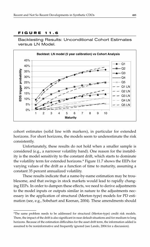
cohort estimates (solid line with markers), in particular for extendedhorizons. For short horizons, the models seem to underestimate the riskconsistently.
Unfortunately, these results do not hold when a smaller sample isconsidered (e.g., a narrower volatility band). One reason for the instabil-ity is the model sensitivity to the constant drift, which starts to dominatethe volatility term for extended horizons.* Figure 11.7 shows the EEPs forvarying values of the drift as a function of time to maturity, assuming aconstant 35 percent annualized volatility.
These results indicate that a name-by-name estimation may be trou-blesome, and that swings in stock markets would lead to rapidly chang-ing EEPs. In order to dampen these effects, we need to derive adjustmentsto the model inputs or outputs similar in nature to the adjustments nec-essary in the application of structural (Merton-type) models for PD esti-mation (see, e.g., Sobehart and Keenan, 2004). These amendments should
Recent and Not So Recent Developments in Synthetic CDOs 485
Backtest: LN model (5 year calibration) vs Cohort Analysis
45%
40%
35%
30%
25%
20%
15%
10%
5%
0%1 2 3 4 5 6 7 8 9 10
Maturity
ED
S t
rig
ger
pro
bab
ility
Q1
Q2
Q3
Q4
Q5
Q1 LN
Q2 LN
Q3 LN
Q4 LN
Q5 LN
F I G U R E 1 1 . 6
Backtesting Results: Unconditional Cohort Estimatesversus LN Model.
*The same problem needs to be addressed for structural (Merton-type) credit risk models.There, the impact of the drift is also significant in near default situations and for medium to longhorizons. Because of the estimation difficulties for the asset drift term, the information added isassumed to be noninformative and frequently ignored (see Lando, 2004 for a discussion).

result in a better agreement between model performance and empiricalevidence.
GARCH(1,1) Model with Constant Drift A simpleextension of the LN model is based on the observation that volatility infinancial markets is usually not constant. Indeed, clustering of volatilitycan be frequently observed, where tranquil periods of low returnsare interspersed with volatile periods of high returns. Technically, this isknown as autoregressive conditional heteroscedasticity (ARCH), andgeneralized ARCH (GARCH) models—first developed by Bollerslev(1986)—attempt to capture this behavior. In a simple GARCH(1,1) modelwith constant drift, the return of an equity is given by rt = µ + εt, whereεt ∼ Φ(0, σt). The conditional variance σt is modeled as σ2
t = ω + αε2t − 1 + βσ 2
t − 1,and the model calibration is usually performed within a maximum like-lihood framework.
The calibration of the GARCH parameters turns out to be quite sen-sitive to the chosen time series, in particular when a long time series(advisable for long-term risk management) are considered. Starica (2003)provides a very useful discussion on GARCH parameter estimation andstability for large amounts of historic data.
Nevertheless, the more realistic specification of the volatilitydynamics makes GARCH models suitable for EDS modeling. Compared
486 CHAPTER 11
Equity event probabilities for different drift assumtions
50%45%40%35%30%25%20%15%10%5%0%
1 2 3 4 5 6 7 8 9 10
Maturity
Fre
qu
ency
r = 0%
r = 5%
r = 10%
r = 15%
r = 20%
F I G U R E 1 1 . 7
EEPs for Different Drift Assumptions.
to LN models, EEPs tend to be higher for short horizons (the first fewyears) while the estimates converge for longer horizons. As a result, someof the underestimation of the models compared to empirical evidenceshown in Figure 11.6 would be reduced, and a further improvement maybe achieved by introducing non-normal residuals. Equity time-series datausually exhibits fatter tails that the normal distribution is able to capture,and other distributions are employed to capture these tail events moreadequately, see, e.g., McNeil and Frey (2000). The most common exten-sions of the GARCH(1,1) model involve non-normal residuals, higherorder GARCH models, and extended GARCH models that focus on asym-metry in observed equity returns (see, Alexander, 2001 for an overview).The insights of Kaufmann and Patie (2004) on the choice of data frequencyfor estimation and on the adequacy of the “square-root-of time” scalingrules are also very relevant within our context of EDS modeling. Furtherdetails on the application of GARCH models for EDS ratings purposes canbe found in Standard & Poor’s (2004), and Fitch (2004).
A Statistical Credit Scoring Approach Although the firstcohort results illustrate the importance of ratings and volatility whenassessing the performance of EDSs, several other variables could be inform-ative, too. de Servigny and Jobst (2005) adapt commonly used credit scor-ing models for EDS. There, up to 23 variables—ranging from marketvariables (such as the S&P 500 volatility) and equity performance variables(e.g., equity specific mean return, volatility, or higher moments), to firm-specific accounting information (e.g., debt-to-equity ratio)—are consideredin the scoring exercise.
In the credit world, this is one of the most widespread techniques toassess the risk on a large population, for which discrete information isavailable. Among the various scoring techniques, logistical regressions(logit models) correspond to a standard approach. These scoring tech-niques deliver point-in-time information in the sense that they enable usto assess default or event risk at a targeted and explicitly defined horizon.The results they provide are usually less informative before or beyondthis horizon.
Overview of Methodology de Servigny and Jobst (2005) useadvanced logit techniques described in Cangemi et al. (2003). Let us con-sider a vector X of risk factors, with X ∈Rd. The probability of a default orof an equity event (symbolized by a “1”), conditional on the informationX, can be written as the logit transformation of a feature function, F(X),
Recent and Not So Recent Developments in Synthetic CDOs 487

maximizing the combined predictive power of the factors. The logit trans-formation* enables us to obtain a result located in the interval ]0,1[:
The specification of F(X) can be simple, corresponding to the first orderof the Taylor expansion of the “true,” unobservable, underlying featurefunction. In this case, we have a linear logit model. The specification can bemore refined, including the quadratic terms too, leading to a quadratic logit.In order to better account for higher power terms† without having to esti-mate too many weights, we can include some additional cylindrical kernelfeatures of the form
where εiθ are weights, aθ the selected centers, and σ a bandwidth term cor-responding to the decay rate of the kernel.
Practically, the models we run can be described as follows:
♦ A linear logit model
♦ A quadratic logit model
♦ A Full logit model, i.e., a combination of linear + quadratic +Kernel features
By using different logit specifications, we reduce model risk and can bet-ter analyze the real predictive power of the data. The calibration of the
Px x xi ii
pjk j kk
pjp( | )
exp( ( ))1
11 1 11
X =+ − + ∑ + ∑∑= ==β δ γ
Pxii
pi
( | )exp( ( ))
11
1 1
X =+ − + ∑ =β δ
fx a
k ii
n
i
p
( )( )
,X =−
==∑∑ ε
σθθ
θ
2
211
PF
( | )e
.( )
11
1X =
+ − X
488 CHAPTER 11
*Other transformations are possible such as the Probit one.†Another way to present it is to further reduce the residual or error term.
P
i iip
jk j k iin
ip
kp
jpx x x
x a( | )
exp( )
11
1 1
2
21111
X =
+ − + ∑ + +−
∑∑∑∑
= ====β δ γ ε
σθθ
θ
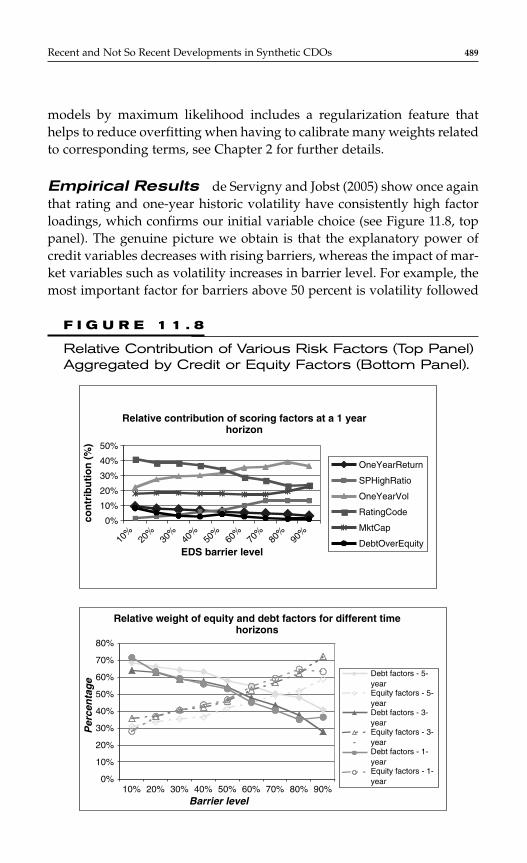
models by maximum likelihood includes a regularization feature thathelps to reduce overfitting when having to calibrate many weights relatedto corresponding terms, see Chapter 2 for further details.
Empirical Results de Servigny and Jobst (2005) show once againthat rating and one-year historic volatility have consistently high factorloadings, which confirms our initial variable choice (see Figure 11.8, toppanel). The genuine picture we obtain is that the explanatory power ofcredit variables decreases with rising barriers, whereas the impact of mar-ket variables such as volatility increases in barrier level. For example, themost important factor for barriers above 50 percent is volatility followed
Recent and Not So Recent Developments in Synthetic CDOs 489
F I G U R E 1 1 . 8
Relative Contribution of Various Risk Factors (Top Panel)Aggregated by Credit or Equity Factors (Bottom Panel).
Relative contribution of scoring factors at a 1 yearhorizon
10%
20%
30%
40%
50%
60%
70%
80%
90%
EDS barrier level
con
trib
uti
on
(%
)
OneYearReturn
SPHighRatio
OneYearVol
RatingCode
MktCap
DebtOverEquity
10%
0%
20%
30%
40%
50%
Relative weight of equity and debt factors for different timehorizons
10%
0%
20%
30%
40%
50%
60%
70%
80%
10% 20% 30% 40% 50% 60% 70% 80% 90%Barrier level
Per
cen
tag
e
Debt factors - 5-yearEquity factors - 5-yearDebt factors - 3-yearEquity factors - 3-yearDebt factors - 1-yearEquity factors - 1-year
by credit rating, whereas for barriers below 50 percent the rank orderingis reversed. For extended horizons, however, the explanatory power ofcredit variables still appears most significant (Figure 11.8, bottom panel).
After identifying important factors using simple linear logit models,de Servigny and Jobst (2005) apply the advanced credit scoring models inorder to improve the already encouraging performance of the scoringmethodology. Using models estimated for 10 percent, 30 percent, and50 percent barriers and 1-, 3-, and 5-year maturities, a filtering system isdeveloped that allows us to classify EDSs into risk categories I to V.
The performance of this risk classification is reported through rankordering statistics—so-called Gini coefficients (see Appendix A)—inTable 11.5. Basically, Gini coefficients give an indication whether or notthe risky EDSs predicted by the model are indeed the ones that triggerEDS events. The same statistic is frequently applied for PD models, whereGini coefficients vary between 50 percent and 90 percent, depending ondataset and application. As can be seen from Table 11.5, the performanceof the proposed EDS classification is very encouraging, supporting thechoice of models and classification. For further details, we refer to deServigny and Jobst (2005).
Although the section presented several ways of measuring the like-lihood of equity events, many interesting valuation issues are addressedin Medova and Smith (2004) and Albanese and Chen (2005).
Dependent Events: Multivariate Aspects of EDS ModelingThe interpretation of the Gaussian copula model within the structural—Merton—framework indicates that all securities are functions of the firmsasset value process. Therefore, all securities will move comonotonicallywith that process suggesting the adequacy of using equity or credit spread
490 CHAPTER 11
T A B L E 1 1 . 5
Rank Ordering of Categories—Performance Measurement (in Percent)
EDScategories 10% barrier 30% barrier 50% barrier
Horizon 1 year 3 years 5 years 1 year 3 years 5 years 1 year 3 years 5 years
Gini 91.97 83.98 80.88 82.79 75.34 69.86 73.47 63.08 57.53coefficient
data for calibration. The advantage of correlations from equity prices isclearly data availability and the ability to estimate issuer specific comove-ments. Although this is true for corporate assets, the generalization to otherstructured finance assets that are frequently contained in CDOs [such asresidential-mortgage backed securities (RMBS), ABS, etc.] and the exposureof equity prices to trends and market movements independent of the creditquality changes produce at best very noisy estimates (de Servigny andRenault, 2003). Similarly, credit spreads are likely to be influenced by mar-ket trends or liquidity issues. Unlike equity- and spread-based correlations,an approach that directly employs actual (observed) default events reducesthe possibility of spurious correlation caused by unrelated external factors.Because event-based correlations usually require large samples spanning atleast 20 years of data, they are frequently seen as long-term estimates thatshould dampen the fluctuations due to business cycle and economic effects.Jobst and de Servigny (2006) focus on empirical event-based correlations,where both default and equity events are considered (within the same ana-lytic framework). They employ, once again, methods developed in thecredit risk arena to EDSs. Stability of estimation is addressed by consider-ing three different correlation estimators, all of which can produce esti-mates for industry- (or more generally risk-class-) specific correlations thatwould need to be used within the Gaussian copula model to reproduceaverage historic joint default/equity default behavior. First, joint (pairwise)event probabilities are estimated and transformed into empirical event andimplied asset correlations, following the approach of de Servigny andRenault (2003). In order to mitigate bias due to (unknown) properties of cer-tain estimators, we also consider the Binomial maximum likelihood esti-mator (MLE) and Asymptotic MLE of Demey et al. (2004) based on a factormodeling approach and conditional independence. While the first estima-tor is capable of producing correlations between all industry combinations,the second estimator produces industry specific correlations only within acertain industry. Correlations between two industries are constant and,hence, independent of the specific industries.
Constraint Factor Structure in MLE ApproachHaving a very large number of firms to cope with in practice, it is usualto assume that we have identified a (lower) number of factors and rewritethe latent random variables/asset values (V1, . . . , VN) as a linear functionof the factors:
V F F i ci c c c i= + − + − ∈ρ ρ ρ ρ ε1
Recent and Not So Recent Developments in Synthetic CDOs 491
The resulting restricted correlation dynamics (with constant andindentical correlation between different groups),
implies efficient numerical optimization of the MLE compared to theunconstrained model, as default probabilities conditional on the commonfactors can be computed in closed form. Then, the distribution ofdefaults/events follows a binomial distribution with known parameters,and the MLE is determined by integrating over the common factor (seeDemey et al., 2004 or Jobst and de Servigny, 2006).
EDS Correlations: Empirical InsightsThe Standard 30 Percent Barrier Table 11.6 shows industry specificcorrelation estimates obtained form the EDS database for a 30 percentbarrier. Column AvgN contains the average number of firms in eachyear in each industry; DefCorr and ImpAssCorr contain the empiricalEDS event and implied asset correlation according to the de Servignyand Renault (2003) approach; and AsyMLE and BinMLE contains theAsymptotic MLE and Binomial MLE results of Jobst and de Servigny(2006). The last row contains the (average) correlation between twoindustries, and the average intra-industry correlation is reported in therow above.
This table (Table 11.6) reveals several interesting insights. First, theEDS correlations for 30 percent barriers appear to be significantly higherthan the default correlations. The average intra- and inter-industry corre-lations are approximately 27 percent and 15 to 17 percent, respectively,which compares to 14 to 18 percent and 5 to 6 percent for (credit) defaultdata (see Jobst and de Servigny, 2006 for results on credit defaults).
EDS Correlations for Different Barriers In the follow-ing, we calculate intra- and inter-industry correlations based on all threeestimators for barriers of 10 percent (corresponding to a 90 percent drop)to 90 percent (corresponding to a 10 percent drop). Figures 11.9A and11.9B plot the corresponding intra-industry and inter-industry correla-tions for different barriers, respectively.
=
∑ρ ρ ρρ ρ
ρρ ρ ρ
1
2
L
O M
M O O
L I
MLE
Ind
492 CHAPTER 11
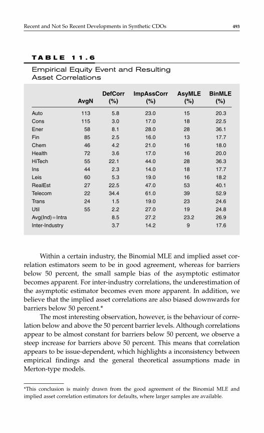
Within a certain industry, the Binomial MLE and implied asset cor-relation estimators seem to be in good agreement, whereas for barriersbelow 50 percent, the small sample bias of the asymptotic estimatorbecomes apparent. For inter-industry correlations, the underestimation ofthe asymptotic estimator becomes even more apparent. In addition, webelieve that the implied asset correlations are also biased downwards forbarriers below 50 percent.*
The most interesting observation, however, is the behaviour of corre-lation below and above the 50 percent barrier levels. Although correlationsappear to be almost constant for barriers below 50 percent, we observe asteep increase for barriers above 50 percent. This means that correlationappears to be issue-dependent, which highlights a inconsistency betweenempirical findings and the general theoretical assumptions made inMerton-type models.
Recent and Not So Recent Developments in Synthetic CDOs 493
*This conclusion is mainly drawn from the good agreement of the Binomial MLE andimplied asset correlation estimators for defaults, where larger samples are available.
T A B L E 1 1 . 6
Empirical Equity Event and ResultingAsset Correlations
DefCorr ImpAssCorr AsyMLE BinMLEAvgN (%) (%) (%) (%)
Auto 113 5.8 23.0 15 20.3
Cons 115 3.0 17.0 18 22.5
Ener 58 8.1 28.0 28 36.1
Fin 85 2.5 16.0 13 17.7
Chem 46 4.2 21.0 16 18.0
Health 72 3.6 17.0 16 20.0
HiTech 55 22.1 44.0 28 36.3
Ins 44 2.3 14.0 18 17.7
Leis 60 5.3 19.0 16 18.2
RealEst 27 22.5 47.0 53 40.1
Telecom 22 34.4 61.0 39 52.9
Trans 24 1.5 19.0 23 24.6
Util 55 2.2 27.0 19 24.8
Avg(Ind) = Intra 8.5 27.2 23.2 26.9
Inter-Industry 3.7 14.2 9 17.6
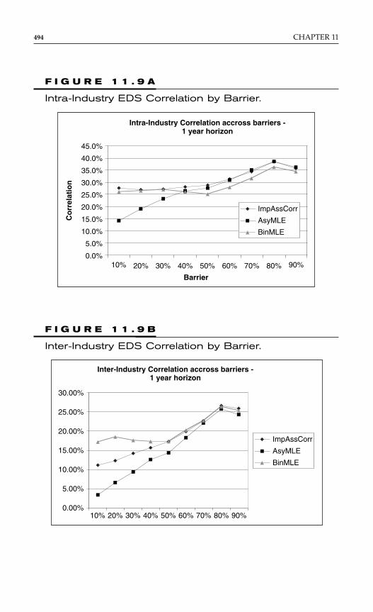
494 CHAPTER 11
Inter-Industry Correlation accross barriers -1 year horizon
30.00%
25.00%
20.00%
15.00%
10.00%
5.00%
0.00%20%10% 30% 40% 50% 60% 70% 80% 90%
ImpAssCorr
AsyMLE
BinMLE
F I G U R E 1 1 . 9 B
Inter-Industry EDS Correlation by Barrier.
Intra-Industry Correlation accross barriers -1 year horizon
45.0%
30.0%
35.0%
40.0%
25.0%
20.0%
15.0%
10.0%
5.0%
0.0%
Barrier
Co
rrel
atio
n
20%10% 30% 40% 50% 60% 70% 80% 90%
ImpAssCorr
AsyMLE
BinMLE
F I G U R E 1 1 . 9 A
Intra-Industry EDS Correlation by Barrier.
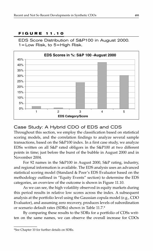
Recent and Not So Recent Developments in Synthetic CDOs 495
Case Study: A Hybrid CDO of EDS and CDSThroughout this section, we employ the classification based on statisticalscoring models, and the correlation findings to analyze several sampletransactions, based on the S&P100 index. In a first case study, we analyzeEDSs written on all S&P rated obligors in the S&P100 at two differentpoints in time; just before the burst of the bubble in August 2000 and inNovember 2004.
For 92 names in the S&P100 in August 2000, S&P rating, industry,and regional information is available. The EDS analysis uses an advancedstatistical scoring model (Standard & Poor’s EDS Evaluator based on themethodology outlined in “Equity Events” section) to determine the EDScategories, an overview of the outcome is shown in Figure 11.10.
As we can see, the high volatility observed in equity markets duringthis period results in relative low scores across the index. A subsequentanalysis at the portfolio level using the Gaussian copula model (e.g., CDOEvaluator), and assuming zero recovery, produces levels of subordinationor scenario default rates (SDRs) shown in Table 11.7.*
By comparing these results to the SDRs for a portfolio of CDSs writ-ten on the same names, we can observe the overall increase for CDOs
*See Chapter 10 for further details on SDRs.
EDS Scores in %: S&P 100 -August 200045%
40%
35%
30%
25%
20%
15%
10%
5%
0%1 2 3 4 5
EDS Category/Score
F I G U R E 1 1 . 1 0
EDS Score Distribution of S&P100 in August 2000.1= Low Risk, to 5=High Risk.
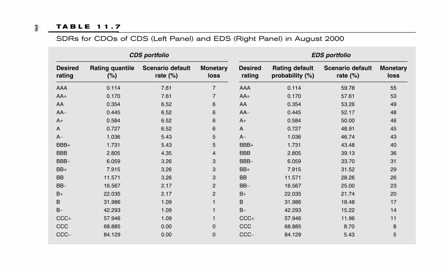
T A B L E 1 1 . 7
SDRs for CDOs of CDS (Left Panel) and EDS (Right Panel) in August 2000
CDS portfolio EDS portfolio
Desired Rating quantile Scenario default Monetary Desired Rating default Scenario default Monetaryrating (%) rate (%) loss rating probability (%) rate (%) loss
AAA 0.114 7.61 7 AAA 0.114 59.78 55
AA+ 0.170 7.61 7 AA+ 0.170 57.61 53
AA 0.354 6.52 6 AA 0.354 53.26 49
AA− 0.445 6.52 6 AA− 0.445 52.17 48
A+ 0.584 6.52 6 A+ 0.584 50.00 46
A 0.727 6.52 6 A 0.727 48.91 45
A− 1.036 5.43 5 A− 1.036 46.74 43
BBB+ 1.731 5.43 5 BBB+ 1.731 43.48 40
BBB 2.805 4.35 4 BBB 2.805 39.13 36
BBB− 6.059 3.26 3 BBB− 6.059 33.70 31
BB+ 7.915 3.26 3 BB+ 7.915 31.52 29
BB 11.571 3.26 3 BB 11.571 28.26 26
BB− 16.567 2.17 2 BB− 16.567 25.00 23
B+ 22.035 2.17 2 B+ 22.035 21.74 20
B 31.986 1.09 1 B 31.986 18.48 17
B− 42.293 1.09 1 B− 42.293 15.22 14
CCC+ 57.946 1.09 1 CCC+ 57.946 11.96 11
CCC 68.885 0.00 0 CCC 68.885 8.70 8
CCC− 84.129 0.00 0 CCC− 84.129 5.43 5
496
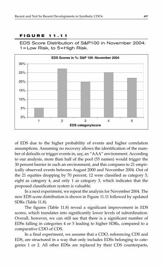
of EDS due to the higher probability of events and higher correlationassumptions. Assuming no recovery allows the identification of the num-ber of defaults or trigger events in, say, an “AAA” environment. Accordingto our analysis, more than half of the pool (55 names) would trigger the30 percent barrier in such an environment, and this compares to 21 empir-ically observed events between August 2000 and November 2004. Out ofthe 21 equities dropping by 70 percent, 12 were classified as category 5,eight as category 4, and only 1 as category 3, which indicates that theproposed classification system is valuable.
In a next experiment, we repeat the analysis for November 2004. Thenew EDS score distribution is shown in Figure 11.11 followed by updatedSDRs (Table 11.8).
The figures (Table 11.8) reveal a significant improvement in EDSscores, which translates into significantly lower levels of subordination.Overall, however, we can still see that there is a significant number ofEDSs falling in categories 4 or 5 leading to higher SDRs, compared to acomparative CDO of CDS.
In a final experiment, we assume that a CDO, referencing CDS andEDS, are structured in a way that only includes EDSs belonging to cate-gories 1 or 2. All other EDSs are replaced by their CDS counterparts,
Recent and Not So Recent Developments in Synthetic CDOs 497
EDS Scores in %: S&P 100 -November 2004
0%
5%
10%
15%
20%
25%
30%
1 2 3 4 5EDS category/score
F I G U R E 1 1 . 1 1
EDS Score Distribution of S&P100 in November 2004.1= Low Risk, to 5=High Risk.
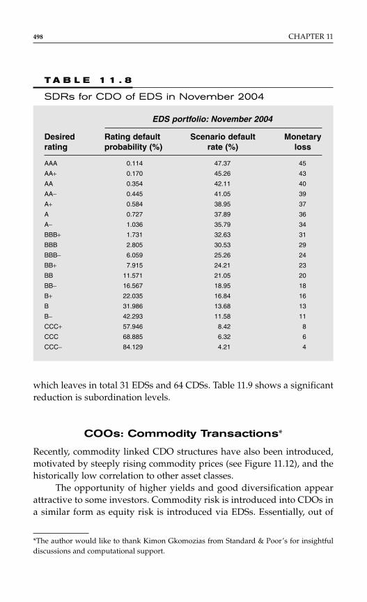
which leaves in total 31 EDSs and 64 CDSs. Table 11.9 shows a significantreduction is subordination levels.
COOs: Commodity Transactions*
Recently, commodity linked CDO structures have also been introduced,motivated by steeply rising commodity prices (see Figure 11.12), and thehistorically low correlation to other asset classes.
The opportunity of higher yields and good diversification appearattractive to some investors. Commodity risk is introduced into CDOs ina similar form as equity risk is introduced via EDSs. Essentially, out of
498 CHAPTER 11
*The author would like to thank Kimon Gkomozias from Standard & Poor’s for insightfuldiscussions and computational support.
T A B L E 1 1 . 8
SDRs for CDO of EDS in November 2004
EDS portfolio: November 2004
Desired Rating default Scenario default Monetary rating probability (%) rate (%) loss
AAA 0.114 47.37 45
AA+ 0.170 45.26 43
AA 0.354 42.11 40
AA− 0.445 41.05 39
A+ 0.584 38.95 37
A 0.727 37.89 36
A− 1.036 35.79 34
BBB+ 1.731 32.63 31
BBB 2.805 30.53 29
BBB− 6.059 25.26 24
BB+ 7.915 24.21 23
BB 11.571 21.05 20
BB− 16.567 18.95 18
B+ 22.035 16.84 16
B 31.986 13.68 13
B− 42.293 11.58 11
CCC+ 57.946 8.42 8
CCC 68.885 6.32 6
CCC− 84.129 4.21 4
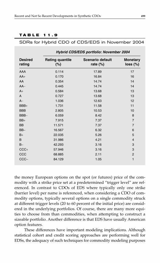
the money European options on the spot (or futures) price of the com-modity with a strike price set at a predetermined “trigger level” are ref-erenced. In contrast to CDOs of EDS where typically only one strike(barrier level) per name is referenced, when considering a CDO of com-modity options, typically several options on a single commodity struckat different trigger levels (20 to 60 percent of the initial price) are consid-ered in the underlying portfolios. Of course, there are many more equi-ties to choose from than commodities, when attempting to construct asizeable portfolio. Another difference is that EDS have usually Americanoption features.
These differences have important modeling implications. Althoughstatistical cohort and credit scoring approaches are performing well forEDSs, the adequacy of such techniques for commodity modeling purposes
Recent and Not So Recent Developments in Synthetic CDOs 499
T A B L E 1 1 . 9
SDRs for Hybrid CDO of CDS/EDS in November 2004
Hybrid CDS/EDS portfolio: November 2004
Desired Rating quantile Scenario default Monetary rating (%) rate (%) loss (%)
AAA 0.114 17.89 17
AA+ 0.170 16.84 16
AA 0.354 14.74 14
AA− 0.445 14.74 14
A+ 0.584 13.68 13
A 0.727 13.68 13
A− 1.036 12.63 12
BBB+ 1.731 11.58 11
BBB 2.805 10.53 10
BBB− 6.059 8.42 8
BB+ 7.915 7.37 7
BB 11.571 7.37 7
BB− 16.567 6.32 6
B+ 22.035 5.26 5
B 31.986 4.21 4
B− 42.293 3.16 3
CCC+ 57.946 3.16 3
CCC 68.885 2.11 2
CCC− 84.129 1.05 1
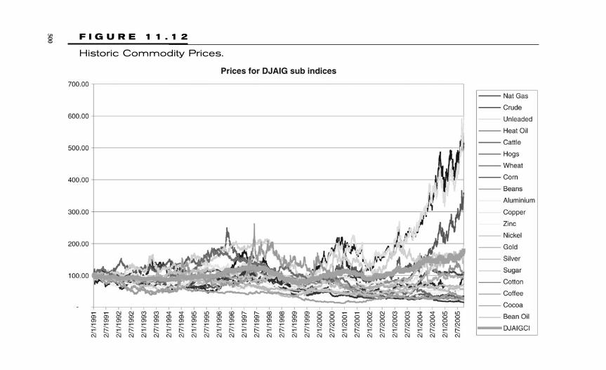
F I G U R E 1 1 . 1 2
Historic Commodity Prices.
500

is questionable. The number of commodities considered, and the numberof commodities with similar characteristics in general, is typically not large(usually, between 10 and 15 different commodities are referenced in aCDO). As a result, one needs to assess whether or not commodities couldbe grouped into meaningful categories (e.g., energy, metals, etc.) and/or ifa sufficient number of commodities is available in order to conduct ananalysis based on discrete events (e.g., historic strike hits). Similarly, for acorrelation or dependence analysis, the number of commodity events issignificantly smaller compared to thousands of events observed for a largenumber of equities, resulting in difficulties when attempting to apply esti-mation techniques based on discrete events as outlined in “Equity DefaultSwaps” section.
Modeling Individual Commodity PricesFrequently, the commodity price dynamics are modeled through stochas-tic models (processes), see, e.g., Eydeland and Wolyniec (2003) or Geman(2005). For example, we recently considered the modeling of commodityspot prices using an arithmetic MR process based on the logarithm ofprices. The model is discussed in detail in Schwartz (1997) and Geman(2005) and has the following form:
Here, the spot price, S, mean reverts to the long-term level of eξ at aspeed β. Introducing the new variable x = ln(S), leads to
dx = β(θ − x)dt + σdW (1)
where θ = ξ − (σ 2/2β) and the long-term spot price is given by S–=exp(θ + (σ 2/2β)).
The solution to the stochastic process in Equation (1) is given by:
and the discrete form solution
x x Zi it t t t t t
ii i i i i i
+− −( ) − −( ) − −( )= + −( ) + −
+ + +1
21 1 111
21e e e ,β β βθ σ
β
x t x s e W ut s t s t u
u s
t( ) = ( ) + −( ) + ( )− −( ) − −( ) − −( )
=∫e e d ,β β βθ σ1
dln d d .
SS
S t W= −( ) +β ξ σ
Recent and Not So Recent Developments in Synthetic CDOs 501

502 CHAPTER 11
is very useful for simulation purposes when Zi’s are sampled from thestandard normal distribution.
Of course, various other stochastic processes can be considered. Forexample, a generalization of Equation (1) is given by
dx = (a + bx)dt + σxγ dW (2)
where the MR level is given by θ = −(a/b) and the MR speed is given byβ = − b, and γ is a scalar. Prigent et al. (2001) apply the model to creditspread data. Depending on the parameter γ (which measures the level ofnonlinearity between the level and volatility), several commonly knownmodels can be derived. For example, γ = 0 leads to the Vasicek (1977) pro-cess, whereas γ = 1
2 results in the Cox, Ingersoll, and Ross (1985) (CIR) pro-cess. Prigent et al. (2001) also discuss a specific jump-diffusion model, andthe adequacy of introducing jump terms for modeling commodity pricesneeds to be investigated further.
Empirical Results and Model Calibration Before esti-mating a parametric model for various commodities, it is useful to applynonparametric techniques to gain some insight into the possible specifi-cation of the drift and diffusion terms. Appendix B outlines first-orderapproximations for the drift µ and diffusion term σ, where the stochasticprocess follows a general diffusion of type
dSt = µ(St)dt + σ (St)dWt.
Figures 11.13 and 11.14 display the drift term as a function of prices, forsilver and crude oil, respectively, estimated on daily data from 1991 to 2004.
It is apparent from both figures that the drift is not constant in thelevel of the price of the relevant commodity, especially when commodityprices are high. This gives a strong indication of an MR behavior, andtherefore helps in the choice of a appropriate parametric model.
Similarly, the diffusion term can be estimated as outlined inAppendix B. For silver and crude oil, we obtain the following Figures11.15 and 11.16, respectively.
For both commodities, the diffusion is almost linear in the pricelevel; i.e., when prices are low, volatility is low, and when prices are high,volatility is high. Given these findings on drift and volatility, the choice ofprocess presented earlier seems reasonable, at least for these commodi-ties. For further results, we refer to Standard and Poor’s (2006).

Recent and Not So Recent Developments in Synthetic CDOs 503
50 100 150 200 250 300-0.3
-0.25
-0.2
-0.15
-0.1
-0.05
0
0.05
1.0
Price
Drif
t
Crude Oil
F I G U R E 1 1 . 1 4
Drift as a Function of Price for Crude Oil.
Appendix C outlines the parametric estimation of stochastic process[Equation (2)], and we present some of the estimation results on a set offive commodities next.
The results of an unconstrained estimation are shown in Table 11.10,while we constrain the model to the Brennan and Schwartz (1980) model(γ = 1) in Table 11.11.
0
Price
Drif
t
Silver
50 60 70 80 90 120110100-0.35
-0.25
-0.3
-0.2
-0.15
-0.1
-0.05
0.05
0.1
F I G U R E 1 1 . 1 3
Drift as a Function of Price for Silver.
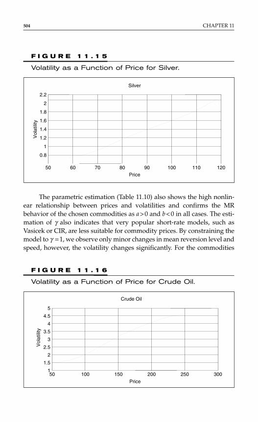
The parametric estimation (Table 11.10) also shows the high nonlin-ear relationship between prices and volatilities and confirms the MRbehavior of the chosen commodities as a > 0 and b < 0 in all cases. The esti-mation of γ also indicates that very popular short-rate models, such asVasicek or CIR, are less suitable for commodity prices. By constraining themodel to γ = 1, we observe only minor changes in mean reversion level andspeed, however, the volatility changes significantly. For the commodities
504 CHAPTER 11
Price
Vol
atili
ty
Silver
50 60 70 80 90 120110100
0.8
1
1.2
1.4
1.6
1.8
2
2.2
Price
Vol
atili
ty
Crude Oil
50 100 150 200 250 3001
1.5
2
2.5
3
3.5
4
4.5
5
F I G U R E 1 1 . 1 5
Volatility as a Function of Price for Silver.
F I G U R E 1 1 . 1 6
Volatility as a Function of Price for Crude Oil.
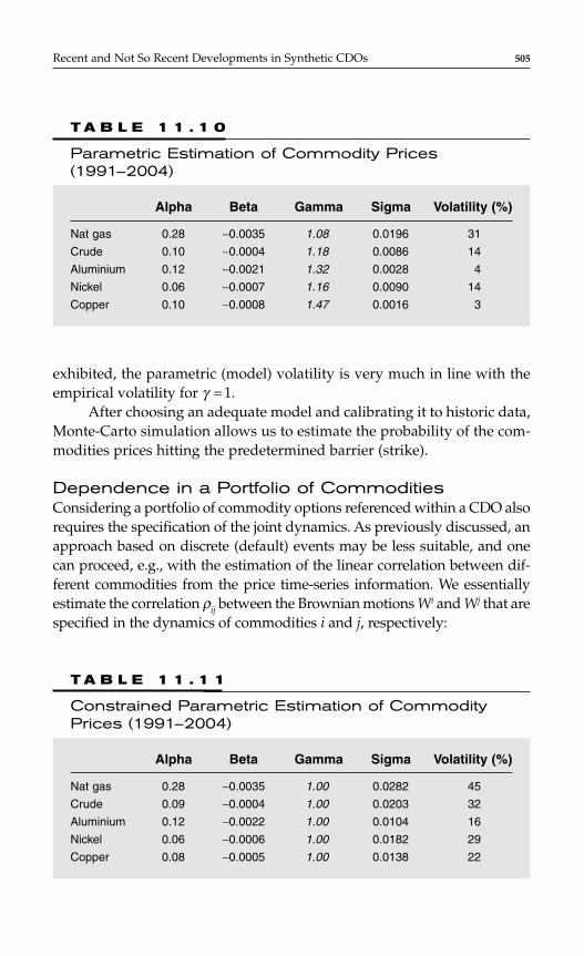
exhibited, the parametric (model) volatility is very much in line with theempirical volatility for γ = 1.
After choosing an adequate model and calibrating it to historic data,Monte-Carto simulation allows us to estimate the probability of the com-modities prices hitting the predetermined barrier (strike).
Dependence in a Portfolio of CommoditiesConsidering a portfolio of commodity options referenced within a CDO alsorequires the specification of the joint dynamics. As previously discussed, anapproach based on discrete (default) events may be less suitable, and onecan proceed, e.g., with the estimation of the linear correlation between dif-ferent commodities from the price time-series information. We essentiallyestimate the correlation ρij between the Brownian motions Wi and Wj that arespecified in the dynamics of commodities i and j, respectively:
Recent and Not So Recent Developments in Synthetic CDOs 505
T A B L E 1 1 . 1 1
Constrained Parametric Estimation of CommodityPrices (1991–2004)
Alpha Beta Gamma Sigma Volatility (%)
Nat gas 0.28 −0.0035 1.00 0.0282 45
Crude 0.09 −0.0004 1.00 0.0203 32
Aluminium 0.12 −0.0022 1.00 0.0104 16
Nickel 0.06 −0.0006 1.00 0.0182 29
Copper 0.08 −0.0005 1.00 0.0138 22
T A B L E 1 1 . 1 0
Parametric Estimation of Commodity Prices(1991–2004)
Alpha Beta Gamma Sigma Volatility (%)
Nat gas 0.28 −0.0035 1.08 0.0196 31
Crude 0.10 −0.0004 1.18 0.0086 14
Aluminium 0.12 −0.0021 1.32 0.0028 4
Nickel 0.06 −0.0007 1.16 0.0090 14
Copper 0.10 −0.0008 1.47 0.0016 3
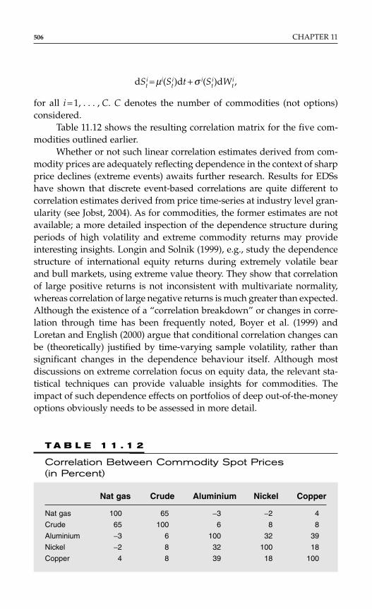
dSti = µi(St
i)dt + σ i(Sti)dWt
i,
for all i = 1, . . . , C. C denotes the number of commodities (not options)considered.
Table 11.12 shows the resulting correlation matrix for the five com-modities outlined earlier.
Whether or not such linear correlation estimates derived from com-modity prices are adequately reflecting dependence in the context of sharpprice declines (extreme events) awaits further research. Results for EDSshave shown that discrete event-based correlations are quite different tocorrelation estimates derived from price time-series at industry level gran-ularity (see Jobst, 2004). As for commodities, the former estimates are notavailable; a more detailed inspection of the dependence structure duringperiods of high volatility and extreme commodity returns may provideinteresting insights. Longin and Solnik (1999), e.g., study the dependencestructure of international equity returns during extremely volatile bearand bull markets, using extreme value theory. They show that correlationof large positive returns is not inconsistent with multivariate normality,whereas correlation of large negative returns is much greater than expected.Although the existence of a “correlation breakdown” or changes in corre-lation through time has been frequently noted, Boyer et al. (1999) andLoretan and English (2000) argue that conditional correlation changes canbe (theoretically) justified by time-varying sample volatility, rather thansignificant changes in the dependence behaviour itself. Although mostdiscussions on extreme correlation focus on equity data, the relevant sta-tistical techniques can provide valuable insights for commodities. Theimpact of such dependence effects on portfolios of deep out-of-the-moneyoptions obviously needs to be assessed in more detail.
506 CHAPTER 11
T A B L E 1 1 . 1 2
Correlation Between Commodity Spot Prices (in Percent)
Nat gas Crude Aluminium Nickel Copper
Nat gas 100 65 −3 −2 4
Crude 65 100 6 8 8
Aluminium −3 6 100 32 39
Nickel −2 8 32 100 18
Copper 4 8 39 18 100

Given some indication of the dynamics of individual commodities,and the correlation across commodities, a portfolio can be simulated andthe number of times the price breaches the barrier can be estimated. For agiven tranche referencing commodity options, tranche PD and expectedloss can then be easily estimated. For further details, outlining Standard& Poor’s approach to employ the standard copula model for commodityportfolios, see Standard & Poor’s (2006).
Of course, the models and developments outlined earlier can also beextended to portfolios of out-of-the-money interest rate and FX products,introducing new challenges for single-asset level, as well as dependence,modeling.
STRUCTURAL INNOVATIONS: INTRODUCINGMtM RISK*
In May 2005, the synthetic CDO market experienced difficult times follow-ing the downgrade of Ford and GM by Standard & Poor’s. The largedemand for mezzanine tranches in recent years left dealers exposed to largeshort mezzanine positions that were hit hard during May 2005 (seeChapters 8 and 9 for further details). As a result of this experience, dealersare now trying to place full capital structure CDOs or employ (approximate)index hedges to reduce the prevalent risk. In order to place super seniorrisk, LSS transactions, one of the most successful products of 2005, havebeen introduced. We will discuss such transactions in the next section, high-lighting the MtM component new to rated CDO tranches. Toward the endof 2005, and in early 2006, CPPI entered the structured credit market in anattempt to reduce MtM risk by guaranteeing principal while offering poten-tial upside to investors. We will provide a brief overview of credit CPPI, aswell as CPDOs-the latest innovation in the structured credit market.
Leverage Super Senior Transactions
LSS structures are relatively new products offered in the synthetic CDOmarket.† Their development in 2005 has resulted from a desire by protection
Recent and Not So Recent Developments in Synthetic CDOs 507
*The author would like to thank Sriram Rajan, Derek Ding, Benoit Metayer, Lapo Guadagnuolo,and Cian Chandler from Standard & Poor’s for many interesting discussions and numericalsupport.†LSS could be cash funded, too, in which case a detailed modeling of excess spreads andIC/OC tests would be required.
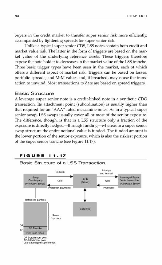
buyers in the credit market to transfer super senior risk more efficiently,accompanied by tightening spreads for super senior risk.
Unlike a typical super senior CDS, LSS notes contain both credit andmarket value risk. The latter in the form of triggers are based on the mar-ket value of the underlying reference assets. These triggers thereforeexpose the note holder to decreases in the market value of the LSS tranche.Three basic trigger types have been seen in the market, each of whichoffers a different aspect of market risk. Triggers can be based on losses,portfolio spreads, and MtM values and, if breached, may cause the trans-action to unwind. Most transactions to date are based on spread triggers.
Basic StructureA leverage super senior note is a credit-linked note in a synthetic CDOtransaction. Its attachment point (subordination) is usually higher thanthat required for an “AAA” rated mezzanine notes. As in a typical supersenior swap, LSS swaps usually cover all or most of the senior exposure.The difference, though, is that in a LSS structure only a fraction of theexposure is directly hedged—through funding—whereas in a super seniorswap structure the entire notional value is funded. The funded amount isthe lower portion of the senior exposure, which is also the riskiest portionof the super senior tranche (see Figure 11.17).
508 CHAPTER 11
LSS-Leveraged super senior.AP-Attachment pointDP-Detachment point
DP
APLSS Tranche
First Loss Piece
SeniorExposure
Reference portfolio
Protection payments
CDS
Premium
SwapCounterparty
(Protection Buyer)
SPE(Issuer)
Collateral
Principaland interest
Note
Proceeds
Leveraged SuperSenior Noteholder(Protection Seller)
F I G U R E 1 1 . 17
Basic Structure of a LSS Transaction.

Hedging the entire super senior portion of the reference portfolioby funding only a fraction of it creates a “leverage,” which is a distin-guishing feature of this product. The number of times that the seniorexposure is leveraged is equal to the senior exposure divided by thefunded notional. Initially, most transactions had tenors of between fiveand seven years and were leveraged between 10 and 15 times, withportfolios typically referencing between 100 and 200 corporate and finan-cial entities. More recently, LSS transactions reference ABS, including port-folios of RMBS and commercial mortgage backed securitization tranches.
Perspective of Protection Buyers and Sellers In aLSS structure, the protection seller earns the risk premium associated withselling protection on the entire senior exposure when the protection itprovides is limited to only the principal amount that is funded, which isjust a fraction of the entire exposure. For example, take a senior exposure(10 to 100 percent) of a portfolio with a notional equal to m100 million thatpays 5 bp. If the funded portion of the resultant m90 million exposure ism6 million, the tranche is 15 times leveraged earning a spread of 75 bpsper year on the funded notional.
The protection buyer on the other hand does not only protect oneselffrom the credit risk, but also from market value risk in the structure in formof MtM losses in excess of the principal amount funded by the protectionseller. The combination of these risks justifies the return that the sellerearns. From a protection buyer’s point of view, the unwind event and thesubsequent MtM payment means that it is effectively hedging the full se-nior portion of the portfolio even though only a fraction of the exposure hasbeen funded. On a trigger being breached and the transaction terminating,the buyer has the MtM amount that it needs to purchase protection on therest of the structure.
From a protection buyer’s perspective, the most attractive structurewould be the MtM trigger on the tranche value, because this would pro-vide it with exact protection on the tranche (i.e., perfect hedge). However,the subjectivity associated with valuing bespoke tranches makes this lessattractive to the protection seller. Both, the loss and spread triggers are“only” proxies for the market value of the tranche, and we will mostlyfocus on the spread trigger for the remainder of this chapter.
LSS with Spread TriggersThe rationale behind the spread trigger is that the market value of the LSStranche is heavily dependent on the spread level of the portfolio. While
Recent and Not So Recent Developments in Synthetic CDOs 509

the market value of the issued tranche is dependent on more than just theunderlying asset values, spread triggers that provide a good (conserva-tive) proxy to MtM movements can be constructed. This is normally doneby the arranging bank that employs typical tranche pricing methodolo-gies with conservative valuation assumptions to determine various aver-age portfolio spreads that would cause specific MtM losses.
These trigger spreads are given in the transaction documents in theform of a trigger matrix, an example of which is shown in the extract inTable 11.13. This matrix tells us the level that the average portfolio spreadwould have to widen to for a trigger event to be caused. For example, pre-suming a closing date of December 20, 2004, if the transaction is threemonths into its life and 1 percent portfolio losses have occurred, spreadswould need to widen to 262 bps to breach the spread trigger.
Modeling LSS Notes with Spread TriggersRAs, such as Standard & Poor’s, Moody’s, and Fitch have developedmethodologies to assess the risk in LSS transactions, see, e.g., Standard &Poor’s (2005). We will provide a brief overview of the approach developedby Standard & Poor’s, and provide a discussion of possible extensions. Themethodology used in rating LSS transactions with a spread triggerinvolves an evaluation of both the credit risk on the reference portfolio andthe risk that a spread trigger is breached.
Standard & Poor’s LSS Model The matrix in Table 11.13shows that we need to address two (inter-linked) risks in our analysis:
510 CHAPTER 11
T A B L E 1 1 . 1 3
Example of a Typical Spread Trigger Matrix asof December 20, 2004 (in bp)
Time to maturity (years)
Losses (%) 5.00 4.92 4.83 4.75 4.67
0.0 267 271 275 279 283
0.5 258 262 267 271 275
1.0 250 254 258 262 266
1.5 247 251 254 258 262
2.0 238 242 246 250 253
2.5 232 236 240 244 248
3.0 226 230 234 237 241

Recent and Not So Recent Developments in Synthetic CDOs 511
first, the default risk of the LSS note due to portfolio defaults, and second,the risk of spread widening to a level that would cause an unwind event.We address these risks by modeling the evolution of portfolio losses untilmaturity, and combining these loss scenarios with an assessment ofwhether portfolio spreads are likely to widen sufficiently to breach thematurity- and loss-dependent barrier.
Portfolio loss paths are determined from the default time simulationas outlined in “ST CDOs: A Ratings Perspective” section. For each simu-lation, after determining the percentage losses along each path, the barrieris calculated from the trigger matrix at fixed time-steps (usually onemonth) until maturity. End-of-month cumulative losses are used to deter-mine the barrier for the beginning-of-month to end-of-month period, orlinear interpolation is applied occasionally.
Modeling the Average Portfolio Spread Standard &Poor’s models the average portfolio spread directly by focusing on sys-tematic spread risk and considers idiosyncratic spread risk of secondaryimportance. As for commodities, there is a vast number of models to beconsidered, and the techniques outlined in Appendices B and C can beapplied to gain some insight into drift and diffusion restrictions.
Prigent et al. (2001), e.g., show that both “AAA” and “BBB” corpo-rate bond yield spreads show MR behavior. However, only the “BBB”volatility appears to scale linearly with the level of spreads while it oscil-lates around a constant mean for “AAA” data. S&P has chosen to estimatethe diffusion model outlined in Appendix C and restricted the diffusionscalar γ ≤ 1 for daily time series data on IG (“AAA,” “AA,” “A,” and“BBB”) option adjusted spreads (OAS) over the period 1997 to 2004.The resulting parameters shown in Table 11.14 confirm the MR behaviorfor all ratings (as a > 0 and b < 0 in each case).*
The diffusion estimates also confirm Prigent et al. (2001), indicating thatthe relationship between the spreads and volatility is stronger for lower rat-ings and weaker for higher ones. This indicated that a Brennan and Schwartzmodel (γ = 1) may be adequate for “AA” and “BBB” spreads, and a CIR orVasicek process may be more suitable for “A” and “AAA” spreads, respec-tively. Of course, one can always estimate the same model for all IG spreads.For example, for γ = 1, we obtain the parameters shown in Table 11.15.
The results reveal a very systematic behaviour of IG credit spreads.Volatility appears to be decreasing in ratings, long-term MR levelsincreasing, and the MR speed also increases with decreasing ratings.
*Thanks to Astrid van Landschoot for empirical support.
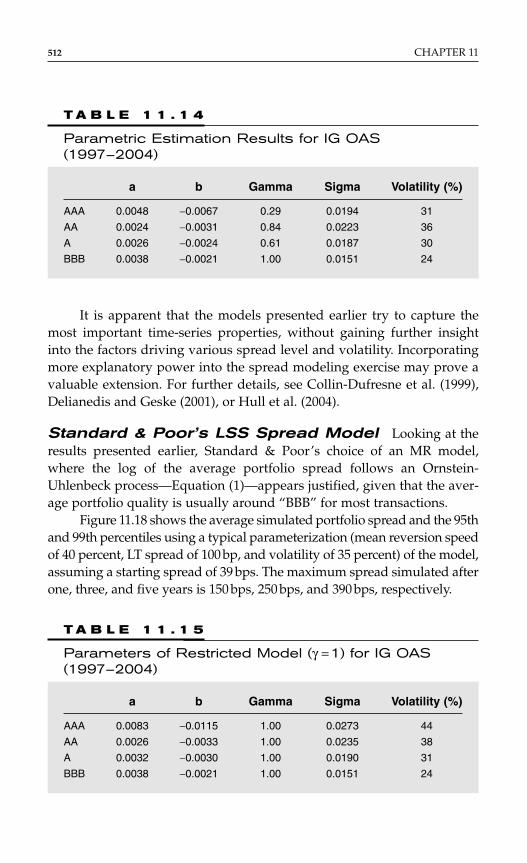
512 CHAPTER 11
It is apparent that the models presented earlier try to capture themost important time-series properties, without gaining further insightinto the factors driving various spread level and volatility. Incorporatingmore explanatory power into the spread modeling exercise may prove avaluable extension. For further details, see Collin-Dufresne et al. (1999),Delianedis and Geske (2001), or Hull et al. (2004).
Standard & Poor’s LSS Spread Model Looking at theresults presented earlier, Standard & Poor’s choice of an MR model,where the log of the average portfolio spread follows an Ornstein-Uhlenbeck process—Equation (1)—appears justified, given that the aver-age portfolio quality is usually around “BBB” for most transactions.
Figure 11.18 shows the average simulated portfolio spread and the 95thand 99th percentiles using a typical parameterization (mean reversion speedof 40 percent, LT spread of 100 bp, and volatility of 35 percent) of the model,assuming a starting spread of 39 bps. The maximum spread simulated afterone, three, and five years is 150 bps, 250 bps, and 390 bps, respectively.
T A B L E 1 1 . 1 4
Parametric Estimation Results for IG OAS(1997–2004)
a b Gamma Sigma Volatility (%)
AAA 0.0048 −0.0067 0.29 0.0194 31
AA 0.0024 −0.0031 0.84 0.0223 36
A 0.0026 −0.0024 0.61 0.0187 30
BBB 0.0038 −0.0021 1.00 0.0151 24
T A B L E 1 1 . 1 5
Parameters of Restricted Model (γ =1) for IG OAS(1997–2004)
a b Gamma Sigma Volatility (%)
AAA 0.0083 −0.0115 1.00 0.0273 44
AA 0.0026 −0.0033 1.00 0.0235 38
A 0.0032 −0.0030 1.00 0.0190 31
BBB 0.0038 −0.0021 1.00 0.0151 24
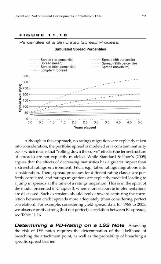
Although in this approach, no ratings migrations are explicitly takeninto consideration, the portfolio spread is modeled on a constant maturitybasis which means that “rolling down the curve” effects (the term-structureof spreads) are not explicitly modeled. While Standard & Poor’s (2005)argues that the effects of decreasing maturities has a greater impact thana stressful ratings environment, Fitch, e.g., takes ratings migrations intoconsideration. There, spread processes for different rating classes are per-fectly correlated, and ratings migrations are explicitly modeled leading toa jump in spreads at the time of a ratings migration. This is in the spirit ofthe model presented in Chapter 3, where more elaborate implementationsare discussed. Such extensions should evolve toward capturing the corre-lation between credit spreads more adequately (than considering perfectcorrelation). For example, considering yield spread data for 1988 to 2005,we observe pretty strong (but not perfect) correlation between IG spreads,see Table 11.16.
Determining a PD-Rating on a LSS Note Assessingthe risk of LSS notes requires the determination of the likelihood ofbreaching the attachment point, as well as the probability of breaching aspecific spread barrier.
Recent and Not So Recent Developments in Synthetic CDOs 513
350
300
250
200
150
100
50
0.0 0.5 1.0 1.5 2.0 2.5 3.0 3.5 4.0 4.5 5.00
Sp
read
leve
l (b
ps)
Spread (1st percentile)
Simulated Spread Percentiles
Spread (5th percentile)Spread (95th percentile)Spread (maximum)
Spread (mean)Spread (99th percentile)Long-term Spread
Years elapsed
F I G U R E 1 1 . 1 8
Percentiles of a Simulated Spread Process.
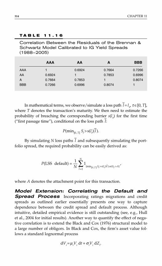
In mathematical terms, we observe/simulate a loss path ~l = lτ, τ ∈[0, T],
where T denotes the transaction’s maturity. We then need to estimate theprobability of breaching the corresponding barrier s(lτ) for the first time(“first passage time”), conditional on the loss path
~l:
P(min[0, T] St > s(lt)~l ).
By simulating N loss paths ~l and subsequently simulating the port-
folio spread, the required probability can be easily derived as:
where A denotes the attachment point for this transaction.
Model Extension: Correlating the Default andSpread Process Incorporating ratings migrations and creditspreads as outlined earlier essentially presents one way to capturedependence between the credit spread and default process. Althoughintuitive, detailed empirical evidence is still outstanding (see, e.g., Hullet al., 2004 for initial results). Another way to quantify the effect of nega-tive correlation is to extend the Black and Cox (1976) structural model toa large number of obligors. In Black and Cox, the firm’s asset value fol-lows a standard lognormal process
dVi = µiVi dt + σiVi dZi.
PN T t t TS s l l l A
l
N
(LSS default) ,min ( )| or
˜ [ , ] =
11
01
> >=
∑
514 CHAPTER 11
T A B L E 1 1 . 1 6
Correlation Between the Residuals of the Brennan &Schwartz Model Calibrated to IG Yield Spreads(1988–2005)
AAA AA A BBB
AAA 1 0.6924 0.7664 0.7266
AA 0.6924 1 0.7853 0.6996
A 0.7664 0.7853 1 0.8074
BBB 0.7266 0.6996 0.8074 1

Hence, Vi(t) = Vi(0) exp((µi − 0.5σ i2)t + σiZi(t)), and default occurs when
the firm value, V, hits the default barrier Hi for the first time (first passagetime). The parameters of this stochastic process and/or the default barrierH can be calibrated to a given term structure of default probabilities (orhazard rates), see Hull et al. (2005) for further details.
When a portfolio of entities is considered, a factor model correlatingthe Wiener terms, such as
where F can be interpreted as a global factor and Fc can be interpreted asan industry or risk-class factor, can be applied. The actual correlationstructure corresponds to a correlation of ρc between two entities in thesame industry or risk-class c, and ρ between two firms in different indus-tries or risk-classes. In practice, of course, any other (multi) factor modelcan be applied.
Defaults in this framework are determined by simulating the factorsand idiosyncratic random terms through time, calculating the correspon-ding asset values Vi(t), and comparing it to the default barriers Hi(t).
The advantage of this structural factor model for LSS is that the fac-tors driving the firms value can be correlated to the Brownian motion,driving the average portfolio spread process. This can be either done bysetting up the Brownian motion W(t) driving the spread process as a func-tion of F(t) and Fc(t), or by simply imposing a linear correlation betweenthe Wiener terms and simulating the factors and spread term from a mul-tivariate normal distribution. Although the estimation and calibration ofsuch a correlated default and spread model needs to be conducted care-fully and the assumption of linear dependence is rather restrictive, theimpact of simulating correlated asset values (default processes) and creditspreads can be assessed.
Table 11.17 shows the impact of increasing negative correlationbetween portfolio spreads and asset values by assuming some level ofcorrelation between the average portfolio spread process and the globaland industry specific factors, driving the firm’s asset values (and there-fore defaults).
In Table 11.17, we determine factor weights that are consistent withan assumption of 30 percent correlation between two obligors in thesame industry, and 0 percent between obligors in different industries.The first row shows the results if we assume, in addition, a 30 percent
d ( ) d ( ) d ( ) ( ) ,Z t F t F t t i ci c c c i= + − + − ∈ρ ρ ρ ρ ε 1
Recent and Not So Recent Developments in Synthetic CDOs 515
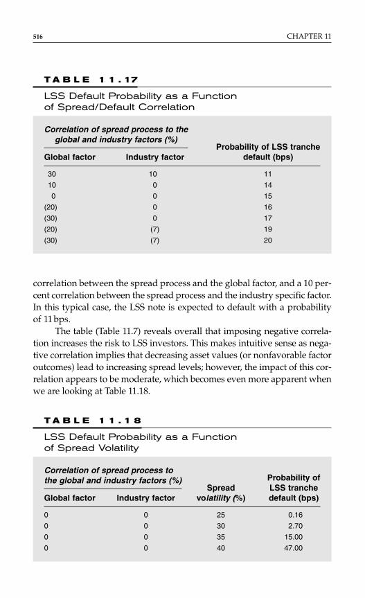
correlation between the spread process and the global factor, and a 10 per-cent correlation between the spread process and the industry specific factor.In this typical case, the LSS note is expected to default with a probabilityof 11 bps.
The table (Table 11.7) reveals overall that imposing negative correla-tion increases the risk to LSS investors. This makes intuitive sense as nega-tive correlation implies that decreasing asset values (or nonfavorable factoroutcomes) lead to increasing spread levels; however, the impact of this cor-relation appears to be moderate, which becomes even more apparent whenwe are looking at Table 11.18.
516 CHAPTER 11
T A B L E 1 1 . 17
LSS Default Probability as a Functionof Spread/Default Correlation
Correlation of spread process to theglobal and industry factors (%)
Global factor Industry factor
30 10 11
10 0 14
0 0 15
(20) 0 16
(30) 0 17
(20) (7) 19
(30) (7) 20
Probability of LSS tranchedefault (bps)
T A B L E 1 1 . 1 8
LSS Default Probability as a Functionof Spread Volatility
Correlation of spread process to
SpreadProbability ofthe global and industry factors (%)
volatility (%)LSS tranche
Global factor Industry factor default (bps)
0 0 25 0.16
0 0 30 2.70
0 0 35 15.00
0 0 40 47.00
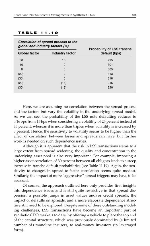
Here, we are assuming no correlation between the spread processand the factors but vary the volatility in the underlying spread model.As we can see, the probability of the LSS note defaulting reduces to0.16 bps from 15 bps when considering a volatility of 25 percent instead of35 percent, whereas it is more than triples when volatility is increased by5 percent. Hence, the sensitivity to volatility seems to be higher than theeffect of correlation between losses and spreads can have, but furtherwork is needed on such dependence issues.
Although it is apparent that the risk in LSS transactions stems to alarge extent from spread widening, the quality and concentration in theunderlying asset pool is also very important. For example, imposing ahigher asset correlation of 30 percent between all obligors leads to a steepincrease in tranche default probabilities (see Table 11.19). Again, the sen-sitivity to changes in spread-to-factor correlation seems quite modest.Similarly, the impact of more “aggressive” spread triggers may have to beassessed.
Of course, the approach outlined here only provides first insightsinto dependence issues and is still quite restrictive in that spread dis-persion, a possible jumps in asset values and/or credit spreads, theimpact of defaults on spreads, and a more elaborate dependence struc-ture still need to be explored. Despite some of these outstanding model-ing challenges, LSS transactions have become an important part ofsynthetic CDO markets to date, by offering a vehicle to place the top endof the capital structure, which was previously dominated by (a limitednumber of ) monoline insurers, to real-money investors (in leveragedform).
Recent and Not So Recent Developments in Synthetic CDOs 517
T A B L E 1 1 . 1 9
Correlation of spread process to the
Probability of LSS trancheglobal and industry factors (%)
default (bps)Global factor Industry factor
30 10 295
10 0 301
0 0 305
(20) 0 313
(30) 0 318
(20) (15) 316
(30) (15) 320
Credit Constant Proportional Portfolio Insurance*
Following the development of the CDO squared market in 2004, LSS in2005, the early part of 2006 was driven by a large interest in so-called creditCPPI. CPPI is a rules-based portfolio management framework where theportfolio allocation changes dynamically between a risky subportfolio anda risk-free subportfolio. The aim of this rebalancing exercise is to maximizereturn while guaranteeing (partial) principal protection. This is in starkcontrast to typical ST CDOs where a fixed upside (premium) is counteredby unlimited downside and a turn away from aggressive structures thatfocus on maximizing yield toward more defensive structures. CPPI is notnew to capital markets; the concept of CPPI goes back to Black and Jones(1986), who consider this Portfolio Insurance mechanism in the context ofequities. Perold (1986) and Perold and Sharpe (1988) apply the concept tofixed income instruments (see also Black and Rouhani, 1989; Roumanet al., 1989). Similarly to LSS, the rise in prominence of CPPI stems partiallyfrom the events of May 2005. Although higher leverage was achieved atthe cost of significantly higher correlation sensitivity (e.g., CDO squaredtransactions) before May 2005, most CPPI transactions to date introduceleverage (or higher sensitivity) to an overall credit portfolio (or index), andhence, eliminates the direct exposure to (base) correlation risk.
A Typical Credit CPPI StructureThe basic idea of CPPI is that at any time, the investors principal invest-ment can be repaid at maturity. In order to do so, the portfolio value P(t)needs to be maintained above a minimum value, denoted as the floor orcost of guarantee F(t, T). Hence, the floor if invested at the current risk-freerate will allow repayment of the guaranteed principal. More formally, thefollowing condition needs to be satisfied for all t ≥ T: P(t) ≥ F(t, T),
where denotes the present value of the final
principal at time T, P–
T, discounted at the current risk-free rate r.The difference between the portfolio value (the sum of the initial
investment plus the MtM of the risky exposure) and the floor is usuallydenoted as the reserve or cushion, C(t). This cushion is invested in riskyassets, which within the framework of credit CPPI usually comprises ofsingle-name CDS or CDS indices. Usually, at this part of the structure,
F t T P E r s sT t
T( , ) exp ( )d= −
∫
518 CHAPTER 11
*Thanks to Benoit Metayer and Sriram Rajan for their contribution to this topic.
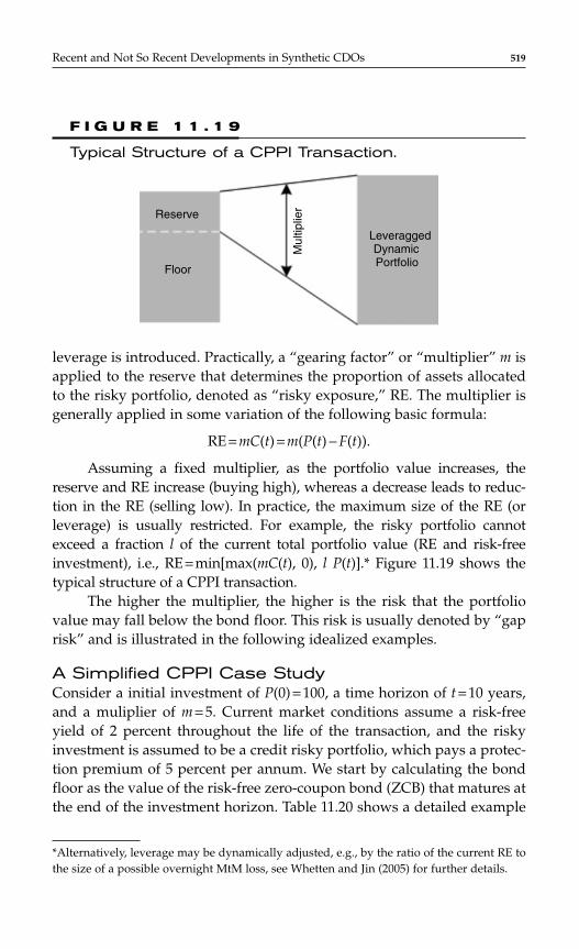
leverage is introduced. Practically, a “gearing factor” or “multiplier” m isapplied to the reserve that determines the proportion of assets allocatedto the risky portfolio, denoted as “risky exposure,” RE. The multiplier isgenerally applied in some variation of the following basic formula:
RE = mC(t) = m(P(t) − F(t)).
Assuming a fixed multiplier, as the portfolio value increases, thereserve and RE increase (buying high), whereas a decrease leads to reduc-tion in the RE (selling low). In practice, the maximum size of the RE (orleverage) is usually restricted. For example, the risky portfolio cannotexceed a fraction l of the current total portfolio value (RE and risk-freeinvestment), i.e., RE = min[max(mC(t), 0), l P(t)].* Figure 11.19 shows thetypical structure of a CPPI transaction.
The higher the multiplier, the higher is the risk that the portfoliovalue may fall below the bond floor. This risk is usually denoted by “gaprisk” and is illustrated in the following idealized examples.
A Simplified CPPI Case StudyConsider a initial investment of P(0) = 100, a time horizon of t = 10 years,and a muliplier of m = 5. Current market conditions assume a risk-freeyield of 2 percent throughout the life of the transaction, and the riskyinvestment is assumed to be a credit risky portfolio, which pays a protec-tion premium of 5 percent per annum. We start by calculating the bondfloor as the value of the risk-free zero-coupon bond (ZCB) that matures atthe end of the investment horizon. Table 11.20 shows a detailed example
Recent and Not So Recent Developments in Synthetic CDOs 519
*Alternatively, leverage may be dynamically adjusted, e.g., by the ratio of the current RE tothe size of a possible overnight MtM loss, see Whetten and Jin (2005) for further details.
Floor
Reserve
LeveraggedDynamicPortfolio
Mul
tiplie
r
F I G U R E 1 1 . 1 9
Typical Structure of a CPPI Transaction.

T A B L E 1 1 . 2 0
A Typical Dynamic CPPI Example
Losses Risky Total Purchase/Bond from portfolio portfolio Maximum sale of Risk-free
Time floor Defaults value value Reserve RE credit risk asset
0 81.87 — — 100.00 18.13 90.63 90.63 9.37
1 83.53 0.00 95.17 106.62 23.10 106.62 11.46 0.00
2 85.21 20% 90.63 92.44 7.23 36.14 −54.49 56.31
3 86.94 0.00 37.94 96.13 9.20 45.99 8.04 50.15
4 88.69 0.00 48.29 100.40 11.71 58.55 10.26 41.85
5 90.48 0.00 61.47 105.40 14.91 74.56 13.08 30.84
6 92.31 0.00 78.29 111.31 18.99 94.97 16.68 16.34
7 94.18 0.00 99.72 118.38 24.20 118.38 18.66 0.00
8 96.08 0.00 124.29 126.78 30.70 126.78 2.49 0.00
9 98.02 0.00 133.12 135.78 37.76 135.78 2.66 0.00
10 100.00 0.00 142.57 145.42 45.42 145.42 2.85 0.00
520
of the CPPI dynamics, when RE is restricted to the current portfolio value(l = 1), and the spreads received from the risky portfolio are reinvested.*
In this illustrative example, we also assume that the portfolio value isreadjusted by (annual) spread payments and losses from defaults, only,rather than by “true” MtM changes of the portfolio value. Changes inspreads (and other relevant pricing variables) typically causes MtM gainsand losses that need to be addressed. Despite this simplification, the generalmechanics illustrated here is still reflective of CPPI. This means that a port-folio rebalancing takes place when the MtM value of the portfolio changessignificantly as a result of changes in credit spreads and/or dependencebehaviour, in addition to credit events/defaults.
At trade initiation, the bond floor is 81.87 resulting in a reserve of 18.13and an RE of 5 times that value (90.63). Hence, 9.37 is invested in the risk-free portfolio,† whereas 90.63 is invested in the risky portfolio. After oneyear, the ZCB value increased, leading to an increased bond floor. Since therisky portfolio earned 5 percent spread, the total portfolio value increased to106.62 [= (90.63 + 9.37) * (1 + 0.05 + 0.02)]. This results in a higher reserve of23.1 and a subsequent purchase of 11.46 of the risky portfolio and a reducedrisk-free investment. Repeating these calculations until maturity reveals thatthe overall portfolio value far exceeds the bond floor at any point in time,despite 20 percent losses in the risky portfolio in year 2. These losses lead toa significant reduction in the risky investment and a shift towards the risk-free portfolio, as shown in the Table 11.20.‡ It is also worth noting that theoverall RE in this example is restricted to be at most the total portfolio value.In the example, this constraint is hit in year 2 and from year 7 onwards.
Sensitivity to Defaults and Default TimingTable 11.21 shows the performance of the CPPI transaction introduced ear-lier for various loss scenarios. In loss scenario 1, 30 percent and 20 percentlosses are assumed in the risky portfolio in years 5 and 8, respectively.
Recent and Not So Recent Developments in Synthetic CDOs 521
*Alternatively, spreads could be passed to investors, which would lead to very differenttransaction dynamics and performance (Internal rate of return IRR).†Note that in real transactions, specific investment rules may require a minimum holding inthe risk-free investment to further ensure market volatility. For example, in “static hedge”CPPI structures, a portion of the initial investment is allocated to a risk-free asset thataccrues to return full-rated principal at maturity.‡As indicated earlier, investment guidelines in real-world transactions would result in port-folio rebalancing subject to MtM changes. These MtM changes are often less severe thanindicated here in the case of default. Hence, the situation where the portfolio compositionchanges as a result of defaults, only, as outlined in this case study, is highly illustrative andshould not be misinterpreted.
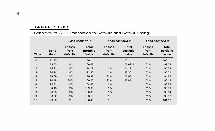
T A B L E 1 1 . 2 1
Sensitivity of CPPI Transaction to Defaults and Default Timing
Loss scenario 1 Loss scenario 2 Loss scenario 3
Losses Total Losses Total Losses TotalBond from portfolio from portfolio from portfolio
Time floor defaults Value defaults value defaults value
0 81.87 100 100 100
1 83.53 0 106.62 0 106.6224 10% 97.38
2 85.21 0% 114.19 0% 114.19 10% 95.79
3 86.94 0% 122.30 0% 122.30 10% 95.01
4 88.69 0% 130.98 20% 106.03 10% 94.85
5 90.48 30% 100.20 30% 86.04 10% 95.18
6 92.31 0% 104.68 0% 10% 95.88
7 94.18 0% 109.93 0% 10% 96.89
8 96.08 20% 100.08 0% 10% 98.14
9 98.02 0% 103.10 0 10% 99.57
10 100.00 0 106.46 0 10% 101.17
522
Despite these losses, the CPPI investor receives full principal at maturity,which essentially means that the return generated in the initial years wassufficient to repay full principal. In loss scenario 2, the same amount ofdefault occurs (in percent terms), however, losses occur in two successiveyears and in reverse order. We can observe that in year 5, the overall port-folio value falls below the bond floor—the “gap risk” scenario occurred.This highlights that the timing and clustering, and therefore correlation, ofdefaults can impact CPPI transactions significantly.
In loss scenario 3, 10 percent losses are observed in every year of thetransaction. Although this results in absolute losses higher than in the pre-vious two scenarios, the full principal investment can still be repaid. Thisresults from the fact that the RE is steadily reduced and shifted toward therisk-free investment. In doing so, the total amount in the risky portfoliois not very high after a few years running, leading to a lower impact ofdefaults/losses.
Sensitivity to Gearing/LeverageChanging the constant multiplier has a significant impact on the perfor-mance of the dynamic CPPI transaction, as shown in Table 11.22. Loss sce-narios 2 is considered once again illustrating that a leverage of m = 3 leadsto a full repayment of principal, compared to m = 4 and m = 5, respectively.
We also consider loss scenario 3 with significantly higher leverage ofm = 15. The higher RE due to higher gearing leads to large year on yearlosses, resulting in a gapping out of the transaction in year 7. Althoughthe sign of the impact of leverage depends on may factors, these simpleexamples show that CPPI transactions are very sensitive to the multiplier.
Sensitivity to Interest Rates and Credit SpreadsApart from losses and leverage, two other factors—interest rates andcredit spreads—are very important for Credit CPPI.* Assuming a multi-plier of m = 4 and loss scenario 2, Table 11.23 reveals the impact of increas-ing interest rates systematically until a maximum of 6 percent over thefirst four years of the transactions life. Higher interest rates imply a lowercost of guarantee, but also higher returns from the risk-free investment.Although for a constant 2 percent interest rate environment the transac-tion “gapped out” (Table 11.21) under loss scenario 2, the full principalcan now be repaid at any point in time.
The table (Table 11.23) also reveals that a tightening in credit spreadshas a massive impact on the transaction, leading to the portfolio value
Recent and Not So Recent Developments in Synthetic CDOs 523
*Note that in a real transaction, spread risk also enters the MtM calculations.
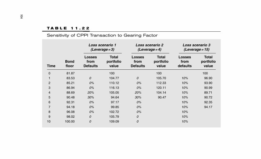
T A B L E 1 1 . 2 2
Sensitivity of CPPI Transaction to Gearing Factor
Loss scenario 1 Loss scenario 2 Loss scenario 3(Leverage = 3) (Leverage = 4) (Leverage = 15)
Losses Total Losses Total Losses TotalBond from portfolio from portfolio from portfolio
Time floor Defaults value Defaults value defaults value
0 81.87 100 100 100
1 83.53 0 104.77 0 105.70 10% 96.90
2 85.21 0% 110.12 0% 112.33 10% 93.90
3 86.94 0% 116.13 0% 120.11 10% 90.99
4 88.69 20% 105.05 20% 104.14 10% 89.71
5 90.48 30% 94.64 30% 90.47 10% 90.72
6 92.31 0% 97.17 0% 10% 92.35
7 94.18 0% 99.85 0% 10% 94.17
8 96.08 0% 102.72 0% 10%
9 98.02 0 105.79 0 10%
10 100.00 0 109.09 0 10%
524
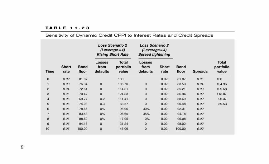
T A B L E 1 1 . 2 3
Sensitivity of Dynamic Credit CPPI to Interest Rates and Credit Spreads
Loss Scenario 2 Loss Scenario 2(Leverage =4) (Leverage =4)
Rising Short Rate Spread tightening
Losses Total Losses Total Short Bond from portfolio from Short Bond portfolio
Time rate floor defaults value defaults rate floor Spreads value
0 0.02 81.87 100 0.02 81.87 0.05 100
1 0.03 76.34 0 105.70 0 0.02 83.53 0.04 104.96
2 0.04 72.61 0 114.31 0 0.02 85.21 0.03 109.68
3 0.05 70.47 0 124.83 0 0.02 86.94 0.02 113.87
4 0.06 69.77 0.2 111.41 0 0.02 88.69 0.02 96.37
5 0.06 74.08 0.3 88.57 0 0.02 90.48 0.02 89.53
6 0.06 78.66 0% 96.96 30% 0.02 92.31 0.02
7 0.06 83.53 0% 106.65 35% 0.02 94.18 0.02
8 0.06 88.69 0% 117.95 0% 0.02 96.08 0.02
9 0.06 94.18 0 131.24 0 0.02 98.02 0.02
10 0.06 100.00 0 146.06 0 0.02 100.00 0.02
525
falling significantly below the bond floor in year 5. In this example, thespread income from the risky investment reduced from 5 percent perannum initially to 2 percent in year 3 and stays at 2 percent until maturity.
Overall, these illustrative examples reveal the sensitivity of CPPItransactions to various risk factors, which are summarized herewith.
Risks in CPPI Transactions
♦ Structural factors such as investment guidelines and rebalanc-ing rules (e.g., maximum RE restrictions).
♦ Leverage introduced via a multiplier. In practice, upper orlower limits on leverage, or dynamic multipliers that react tomarket conditions are feasible.
♦ Credit risk in form of the likelihood and timing of defaultsand/or the erosion in credit quality.
♦ Market risk in form of MtM changes on the risky portfolio andmarket value triggers that may drive the asset allocation andlimit the ability to “ride out” temporary swings in prices. Forsimple credit indices, MtM is mostly a result of changes incredit spreads, and the term structure of credit spreads moregenerally.
♦ Interest rate risk in form of sensitivity of the risk-free invest-ment return and the change in bond floor.
Expected PerformanceThe nature of dynamically shifting the portfolio between the risky andrisk-free investment depending on the performance of the credit riskyportfolio, aims toward achieving a stable MtM profile, whereas guarantee-ing principal investment and taking advantage of potential upside. Whenthe credit market performs well, the pure credit portfolio can be expectedto outperform the CPPI strategy, as the latter is only partially exposed tohigh yield. However, the impact of a sudden downturn in credit marketson the CPPI trade is somewhat reduced. When the credit portfolio per-forms badly (high losses and wide spreads), the CPPI strategy shifts expo-sure toward risk-free assets and, hence, significantly reduces downsiderisk for CPPI.
More generally, CPPI strategies are known to perform poorly whenmarkets are very volatile. Under high volatility, gains and losses mayquickly follow each other, resulting in exactly the “wrong” rebalancingactions guided by the CPPI trading rules. For further details, see Whetten
526 CHAPTER 11
and Jin (2005). As previously mentioned, CPPI has been an integral partof hedge fund activities for equity and fixed-income markets. Althoughcredit CPPI introduces some new idiosyncracies (e.g., sudden severe MtMlosses due to defaults), the CPPI framework can be applied to portfoliosof complex credit exposures (e.g., portfolios of ST CDOs) or alternativeasset classes (hybrids). Particularly, if credit CPPI could be referencing(synthetic) CDO equity tranches, and efficient framework for transfer-ring CDO equity risk and, hence, another efficient hedging tool could bedeveloped.
Modeling CPPI TransactionsAssessing the risk in credit CPPI transactions requires a comprehensivemodeling of the risk factors outlined earlier. Such models are required bytraders and risk managers for assessing the gap risk and for forming rel-ative value views. RAs are getting involved in providing an assessmentof a minimum coupon (or minimum IRR) that can be guaranteed with adesired (rating specific) certainty, in addition to a typical gap risk analy-sis. In order to compute such statistics, one needs to develop a probabilis-tic description of all underlying risk factors and address their interactionor joint behaviour adequately.
Although we are not describing a detailed approach to CPPIs due tothe bespoke nature of transactions (and rules) and the high level of com-plexity it becomes apparent that many of the modeling approaches andchallenges discussed throughout this chapter apply to credit CPPI.
Of course, the complexity of assessing MtM changes on a portfolioof (credit) exposures depends highly on the nature of the underlying port-folio. For a relatively homogeneous portfolio of CDS, a straightforwardmodel for portfolio losses and spreads may be sufficient to gain someinteresting insights, whereas high spread dispersion or low quality creditsmay require a more refined approach to modeling the interaction betweenspread and default risk. Similarly, when CDO tranches are also consid-ered in reference portfolio, the quantitative complexity increases signifi-cantly as the sensitivity to base or compound correlation changes alsoneeds to be assessed (see Chapter 7 for further details) in MtM computa-tions. At the same time, there is scope for credit CPPI to move toward“hybrid CPPI,” where equity, real estate, FX, or commodity risk may alsobe repackaged. For such problems, the approaches outlined in “BeyondCredit Risk: Hybrid Structured Products” section may provide someguidelines, however, the integration of all risks in a common modelingplatform presents a big challenge.
Recent and Not So Recent Developments in Synthetic CDOs 527
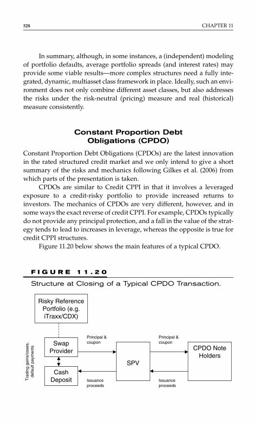
In summary, although, in some instances, a (independent) modelingof portfolio defaults, average portfolio spreads (and interest rates) mayprovide some viable results—more complex structures need a fully inte-grated, dynamic, multiasset class framework in place. Ideally, such an envi-ronment does not only combine different asset classes, but also addressesthe risks under the risk-neutral (pricing) measure and real (historical)measure consistently.
Constant Proportion Debt Obligations (CPDO)
Constant Proportion Debt Obligations (CPDOs) are the latest innovationin the rated structured credit market and we only intend to give a shortsummary of the risks and mechanics following Gilkes et al. (2006) fromwhich parts of the presentation is taken.
CPDOs are similar to Credit CPPI in that it involves a leveragedexposure to a credit-risky portfolio to provide increased returns toinvestors. The mechanics of CPDOs are very different, however, and insome ways the exact reverse of credit CPPI. For example, CPDOs typicallydo not provide any principal protection, and a fall in the value of the strat-egy tends to lead to increases in leverage, whereas the opposite is true forcredit CPPI structures.
Figure 11.20 below shows the main features of a typical CPDO.
528 CHAPTER 11
CPDO NoteHolders
SPV
CashDeposit
Risky ReferencePortfolio (e.g.iTraxx/CDX)
SwapProvider
Issuanceproceeds
Principal &coupon
Issuanceproceeds
Principal &coupon
Tra
ding
gai
ns/o
sses
,de
faul
t pay
men
ts
F I G U R E 1 1 . 2 0
Structure at Closing of a Typical CPDO Transaction.
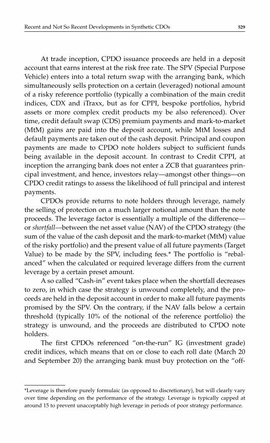
At trade inception, CPDO issuance proceeds are held in a depositaccount that earns interest at the risk free rate. The SPV (Special PurposeVehicle) enters into a total return swap with the arranging bank, whichsimultaneously sells protection on a certain (leveraged) notional amountof a risky reference portfolio (typically a combination of the main creditindices, CDX and iTraxx, but as for CPPI, bespoke portfolios, hybridassets or more complex credit products my be also referenced). Overtime, credit default swap (CDS) premium payments and mark-to-market(MtM) gains are paid into the deposit account, while MtM losses anddefault payments are taken out of the cash deposit. Principal and couponpayments are made to CPDO note holders subject to sufficient fundsbeing available in the deposit account. In contrast to Credit CPPI, atinception the arranging bank does not enter a ZCB that guarantees prin-cipal investment, and hence, investors relay—amongst other things—onCPDO credit ratings to assess the likelihood of full principal and interestpayments.
CPDOs provide returns to note holders through leverage, namelythe selling of protection on a much larger notional amount than the noteproceeds. The leverage factor is essentially a multiple of the difference—or shortfall—between the net asset value (NAV) of the CPDO strategy (thesum of the value of the cash deposit and the mark-to-market (MtM) valueof the risky portfolio) and the present value of all future payments (TargetValue) to be made by the SPV, including fees.* The portfolio is “rebal-anced” when the calculated or required leverage differs from the currentleverage by a certain preset amount.
A so called “Cash-in” event takes place when the shortfall decreasesto zero, in which case the strategy is unwound completely, and the pro-ceeds are held in the deposit account in order to make all future paymentspromised by the SPV. On the contrary, if the NAV falls below a certainthreshold (typically 10% of the notional of the reference portfolio) thestrategy is unwound, and the proceeds are distributed to CPDO noteholders.
The first CPDOs referenced “on-the-run” IG (investment grade)credit indices, which means that on or close to each roll date (March 20and September 20) the arranging bank must buy protection on the “off-
Recent and Not So Recent Developments in Synthetic CDOs 529
*Leverage is therefore purely formulaic (as opposed to discretionary), but will clearly varyover time depending on the performance of the strategy. Leverage is typically capped ataround 15 to prevent unacceptably high leverage in periods of poor strategy performance.
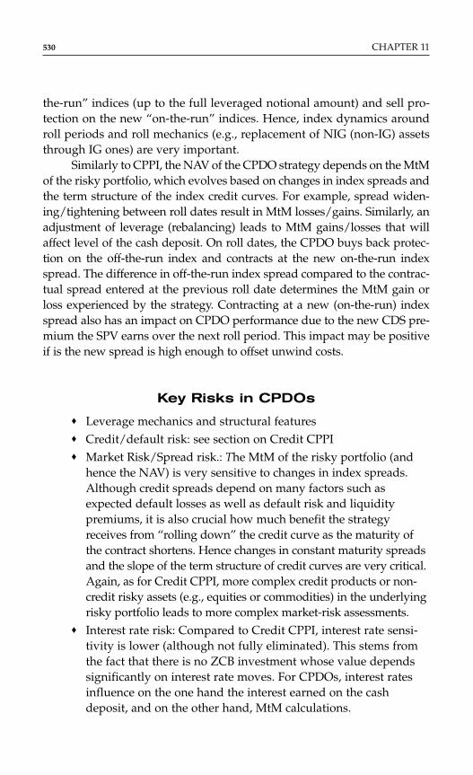
the-run” indices (up to the full leveraged notional amount) and sell pro-tection on the new “on-the-run” indices. Hence, index dynamics aroundroll periods and roll mechanics (e.g., replacement of NIG (non-IG) assetsthrough IG ones) are very important.
Similarly to CPPI, the NAV of the CPDO strategy depends on the MtMof the risky portfolio, which evolves based on changes in index spreads andthe term structure of the index credit curves. For example, spread widen-ing/tightening between roll dates result in MtM losses/gains. Similarly, anadjustment of leverage (rebalancing) leads to MtM gains/losses that willaffect level of the cash deposit. On roll dates, the CPDO buys back protec-tion on the off-the-run index and contracts at the new on-the-run indexspread. The difference in off-the-run index spread compared to the contrac-tual spread entered at the previous roll date determines the MtM gain orloss experienced by the strategy. Contracting at a new (on-the-run) indexspread also has an impact on CPDO performance due to the new CDS pre-mium the SPV earns over the next roll period. This impact may be positiveif is the new spread is high enough to offset unwind costs.
Key Risks in CPDOs
♦ Leverage mechanics and structural features♦ Credit/default risk: see section on Credit CPPI♦ Market Risk/Spread risk.: The MtM of the risky portfolio (and
hence the NAV) is very sensitive to changes in index spreads.Although credit spreads depend on many factors such asexpected default losses as well as default risk and liquiditypremiums, it is also crucial how much benefit the strategyreceives from “rolling down” the credit curve as the maturity ofthe contract shortens. Hence changes in constant maturity spreadsand the slope of the term structure of credit curves are very critical.Again, as for Credit CPPI, more complex credit products or non-credit risky assets (e.g., equities or commodities) in the underlyingrisky portfolio leads to more complex market-risk assessments.
♦ Interest rate risk: Compared to Credit CPPI, interest rate sensi-tivity is lower (although not fully eliminated). This stems fromthe fact that there is no ZCB investment whose value dependssignificantly on interest rate moves. For CPDOs, interest ratesinfluence on the one hand the interest earned on the cashdeposit, and on the other hand, MtM calculations.
530 CHAPTER 11
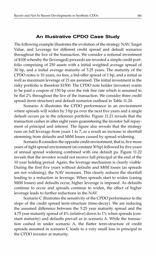
An Illustrative CPDO Case Study
The following example illustrates the evolution of the strategy NAV, TargetValue, and Leverage for different credit spread and default scenariosthroughout the live of the transaction. We consider a notional investmentof $100 whereby the (leveraged) proceeds are invested a simple credit port-folio comprising of 250 assets with a initial weighted average spread of30 bp, and a initial average maturity of 5.25 years. The maturity of theCPDO notes is 10 years, no fees, a bid-offer spread of 1 bp, and a initial aswell as maximum leverage of 15 are assumed. The initial investment in therisky portfolio is therefore $1500. The CPDO note holder (investor) wantsto be paid a coupon of 150 bp over the risk free rate which is assumed tobe flat 2% throughout the live of the transaction. We consider three creditspread (term structure) and default scenarios outlined in Table 11.24.
Scenario A illustrates the CPDO performance in an environmentwhere spreads will widen by 3 bp pa over the next five years and a singledefault occurs pa in the reference portfolio. Figure 11.21 reveals that thetransaction cashes in after eight years guaranteeing the investor full repay-ment of principal and interest. The figure also reveals that the strategyruns on full leverage from years 1 to 7, as a result an increase in shortfallstemming from defaults and MtM losses caused by spread widening.
Scenario B considers the opposite credit environment, that is, five moreyears of tight spread environment (at constant 30 bp) followed by five yearsof annual spread widening combined with one default pa. Figure 11.22reveals that the investor would not receive full principal at the end of the10 year holding period. Again, the leverage mechanism is clearly visible.During the first five years without defaults and MtM losses (as spreadsare not widening), the NAV increases. This clearly reduces the shortfallleading to a reduction in leverage. When spreads start to widen (casingMtM losses) and defaults occur, higher leverage is imposed. As defaultscontinue to occur and spreads continue to widen, the effect of higherleverage leads to further reductions in the NAV.
Scenario C illustrates the sensitivity of the CPDO performance to theslope of the credit spread term-structure (time-decay). We are reducingthe assumed difference between the 5.25 year maturity spread and the4.75 year maturity spread of 4% (relative) down to 1% when spreads (con-stant maturity) and defaults prevail as in scenario A. While the transac-tion cashed in under scenario A, the flatter term-structure of creditspreads assumed in scenario C leads to a very small loss in principal tothe CPDO investor at maturity.
Recent and Not So Recent Developments in Synthetic CDOs 531
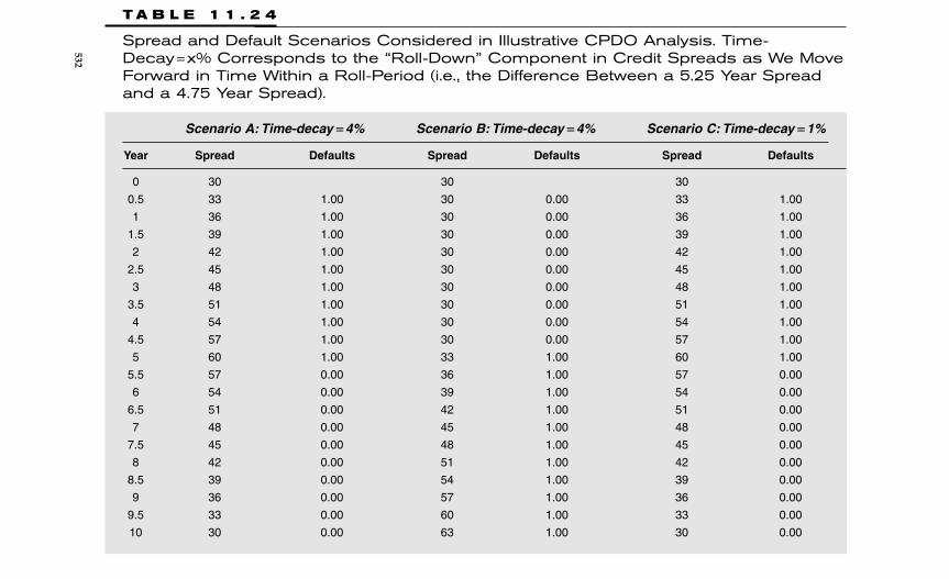
T A B L E 1 1 . 2 4
Spread and Default Scenarios Considered in Illustrative CPDO Analysis. Time-Decay=x% Corresponds to the “Roll-Down” Component in Credit Spreads as We MoveForward in Time Within a Roll-Period (i.e., the Difference Between a 5.25 Year Spreadand a 4.75 Year Spread).
Scenario A: Time-decay =4% Scenario B: Time-decay =4% Scenario C: Time-decay =1%
Year Spread Defaults Spread Defaults Spread Defaults
0 30 30 30
0.5 33 1.00 30 0.00 33 1.00
1 36 1.00 30 0.00 36 1.00
1.5 39 1.00 30 0.00 39 1.00
2 42 1.00 30 0.00 42 1.00
2.5 45 1.00 30 0.00 45 1.00
3 48 1.00 30 0.00 48 1.00
3.5 51 1.00 30 0.00 51 1.00
4 54 1.00 30 0.00 54 1.00
4.5 57 1.00 30 0.00 57 1.00
5 60 1.00 33 1.00 60 1.00
5.5 57 0.00 36 1.00 57 0.00
6 54 0.00 39 1.00 54 0.00
6.5 51 0.00 42 1.00 51 0.00
7 48 0.00 45 1.00 48 0.00
7.5 45 0.00 48 1.00 45 0.00
8 42 0.00 51 1.00 42 0.00
8.5 39 0.00 54 1.00 39 0.00
9 36 0.00 57 1.00 36 0.00
9.5 33 0.00 60 1.00 33 0.00
10 30 0.00 63 1.00 30 0.00
532
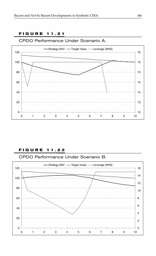
Recent and Not So Recent Developments in Synthetic CDOs 533
0
20
40
60
80
100
120
0 2 4 6 8 1013
13
14
14
15
15
16Strategy NAV Target Value Leverage (RHS)
97531
F I G U R E 1 1 . 2 1
CPDO Performance Under Scenario A.
0
20
40
60
80
100
120
0 2 4 6 8 100
2
4
6
8
10
12
14
16Strategy NAV Target Value Leverage (RHS)
97531
F I G U R E 1 1 . 2 2
CPDO Performance Under Scenario B.
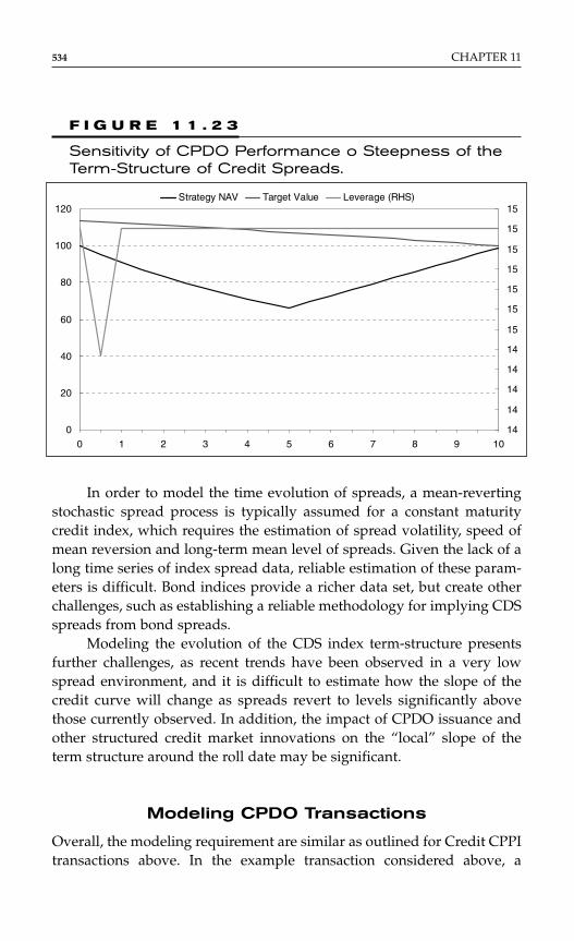
In order to model the time evolution of spreads, a mean-revertingstochastic spread process is typically assumed for a constant maturitycredit index, which requires the estimation of spread volatility, speed ofmean reversion and long-term mean level of spreads. Given the lack of along time series of index spread data, reliable estimation of these param-eters is difficult. Bond indices provide a richer data set, but create otherchallenges, such as establishing a reliable methodology for implying CDSspreads from bond spreads.
Modeling the evolution of the CDS index term-structure presentsfurther challenges, as recent trends have been observed in a very lowspread environment, and it is difficult to estimate how the slope of thecredit curve will change as spreads revert to levels significantly abovethose currently observed. In addition, the impact of CPDO issuance andother structured credit market innovations on the “local” slope of theterm structure around the roll date may be significant.
Modeling CPDO Transactions
Overall, the modeling requirement are similar as outlined for Credit CPPItransactions above. In the example transaction considered above, a
534 CHAPTER 11
0
20
40
60
80
100
120
0 2 4 6 8 1014
14
14
14
14
15
15
15
15
15
15
15Strategy NAV Target Value Leverage (RHS)
97531
F I G U R E 1 1 . 2 3
Sensitivity of CPDO Performance o Steepness of theTerm-Structure of Credit Spreads.
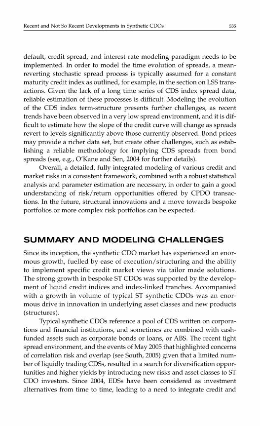
default, credit spread, and interest rate modeling paradigm needs to beimplemented. In order to model the time evolution of spreads, a mean-reverting stochastic spread process is typically assumed for a constantmaturity credit index as outlined, for example, in the section on LSS trans-actions. Given the lack of a long time series of CDS index spread data,reliable estimation of these processes is difficult. Modeling the evolutionof the CDS index term-structure presents further challenges, as recenttrends have been observed in a very low spread environment, and it is dif-ficult to estimate how the slope of the credit curve will change as spreadsrevert to levels significantly above those currently observed. Bond pricesmay provide a richer data set, but create other challenges, such as estab-lishing a reliable methodology for implying CDS spreads from bondspreads (see, e.g., O’Kane and Sen, 2004 for further details).
Overall, a detailed, fully integrated modeling of various credit andmarket risks in a consistent framework, combined with a robust statisticalanalysis and parameter estimation are necessary, in order to gain a goodunderstanding of risk/return opportunities offered by CPDO transac-tions. In the future, structural innovations and a move towards bespokeportfolios or more complex risk portfolios can be expected.
SUMMARY AND MODELING CHALLENGES
Since its inception, the synthetic CDO market has experienced an enor-mous growth, fuelled by ease of execution/structuring and the abilityto implement specific credit market views via tailor made solutions.The strong growth in bespoke ST CDOs was supported by the develop-ment of liquid credit indices and index-linked tranches. Accompaniedwith a growth in volume of typical ST synthetic CDOs was an enor-mous drive in innovation in underlying asset classes and new products(structures).
Typical synthetic CDOs reference a pool of CDS written on corpora-tions and financial institutions, and sometimes are combined with cash-funded assets such as corporate bonds or loans, or ABS. The recent tightspread environment, and the events of May 2005 that highlighted concernsof correlation risk and overlap (see South, 2005) given that a limited num-ber of liquidly trading CDSs, resulted in a search for diversification oppor-tunities and higher yields by introducing new risks and asset classes to STCDO investors. Since 2004, EDSs have been considered as investmentalternatives from time to time, leading to a need to integrate credit and
Recent and Not So Recent Developments in Synthetic CDOs 535

equity risk in a consistent yet practical manner. More recently, ST CDOshave been suggested as vehicles to transfer commodity risk requiring yetanother need to adequately model and integrate such products. In general,we expect these developments towards hybrid transactions to continueand, linked with further growth in noncorporate synthestic indices (e.g.,ABSX), expect further growth in synthetic CDO markets.
Events like May 2005 have lead to changes in market participantstrading behaviour, and fuelled the desire and need to place whole capitalstructure CDOs, as well as the need to develop structures aiming to reduceMtM volatility, too. LSS transactions allowed to sell super senior risk toreal-money investors in leveraged form where in addition to credit risk,MtM risk is explicitly taken into consideration. While 2005 was the year ofLSS, 2006 and 2007 are expected to be interesting due to further develop-ments of credit CPPI and CPDO transactions. Such defensive trades arebased on dynamic asset allocation to protect principal investment yet pro-viding potential for substantial upside. We expect these developments tocontinue to evolve toward more complex credit and hybrid portfolios andtoward their application as new, innovative structures for efficient risktransfer.
Hand in hand with these developments is the need for quantitativemodels that are capable of capturing univariate risks and dependenceaspects inherent in such structures. Although the standard copula frame-work has the advantage of separating the marginal risk factors from port-folio aspects, further research on viable alternatives is required. Forexample, the recently renewed interest in structural—Merton type—models for consistent pricing of single-name credit and equity products(see Chapter 3) could lead to extensions where portfolios of equities, debtinstruments and, hence, credit spread sensitive and default sensitive prod-ucts are consistently integrated. Alternatively, practical development ofstochastic intensity/hazard models appears to provide room for furtherresearch and application toward multiple asset classes. Both of thesedevelopments require further research, bearing in mind that consistencyto current methodologies is frequently required.
In summary, we believe that developments in synthetic CDOs pro-vide exciting opportunities for the convergence of various financial risksand markets, as well as further opportunities for innovative risk transfer.This is accompanied by a number of quantitative challenges and shouldprovide room for further growth in coming years.
536 CHAPTER 11
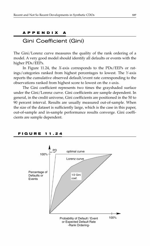
A P P E N D I X A
Gini Coefficient (Gini)
The Gini/Lorenz curve measures the quality of the rank ordering of amodel. A very good model should identify all defaults or events with thehigher PDs/EEPs.
In Figure 11.24, the X-axis corresponds to the PDs/EEPs or rat-ings/categories ranked from highest percentages to lowest. The Y-axisreports the cumulative observed default/event rate corresponding to theobservations ranked from highest score to lowest on the x-axis.
The Gini coefficient represents two times the grayshaded surfaceunder the Gini/Lorenz curve. Gini coefficients are sample dependent. Ingeneral, in the credit universe, Gini coefficients are positioned in the 50 to90 percent interval. Results are usually measured out-of-sample. Whenthe size of the dataset is sufficiently large, which is the case in this paper,out-of-sample and in-sample performance results converge. Gini coeffi-cients are sample dependent.
Recent and Not So Recent Developments in Synthetic CDOs 537
Probability of Default / Eventor Expected Default Rate
-Rank Ordering-
100%
100%optimal curve
Lorenz curve
PD
Percentage ofDefaults orEvents
1/2 Ginicoef.
F I G U R E 1 1 . 2 4

A P P E N D I X B
Nonparametric Estimation
Before estimating a parametric model for a general diffusion process oftype dSt = µ (St)dt + σ (St)dWt, it is useful to apply nonparametric tech-niques to gain some insight into the possible specification of the drift µand diffusion term σ. Here, S could denote the price of a specific com-modity, the level of interest rates, or the level of credit spreads. Stanton(1997) proposes first- and higher-order approximations to the drift anddiffusion term, and the first-order approximations are outlined next.
DENSITY ESTIMATION
The first step is to estimate the density of the data generating process,through a Gaussian kernel estimator. That is,
where φ denotes the standard normal density, n is the number of obser-vations, and the window or band width is given by h = cσ∼n−1/5, where c isa constant and σ∼ the empirical standard deviation from the data. The levelof smoothness of the density depends significantly on the choice of c.Prigent et al. (2001) and Stanton (1997) propose a value close to 3.
DRIFT AND VOLATILITY/DIFFUSION ESTIMATION
The drift term at a level of x can be estimated to first order, using
and the corresponding first-order approximation for the diffusion isgiven by
˜ ( )( )
,µφ
φx
S Sx S
hx S
h
t tt
t
n
tt
n=
−−
−
+=
−
=
−
∑∑
11
1
1
1
f xnh
x S
ht
t
n
( ) ,=−
=
∑1
1
φ
538 CHAPTER 11
For higher-order estimators, we refer the reader to Stanton (1997).
A P P E N D I X C
Parametric Estimation by Chan et al.(1992)
Chan et al. (1992) propose to estimate the discrete time version of equa-tion (2) that is given by:
St+1−St = a + bSt + σ St γεt+1,
where εt + 1 are assumed to be i.i.d. normal variables. The Markovian prop-erty of the process and the assumption of normality enable the derivationof the log-likelihood function that can be maximized thereafter:
As an assymptotically unbiased estimator with minimum variance, MLEis often preferred to alternative approaches such as method of moments,see Broze, Scaillet, and Zakoian (1995) for a discussion.
REFERENCESAlbanese, C., and O. Chen (2005), “Pricing equity default swaps,” Risk, June.Alexander, C. (2001), Market Models: A Guide to Financial Data Analysis, John Wiley
& Sons.Bayliffe, D., and B. Pauling (2003), “Long term equity returns,” working paper,
Tower Perrin.Black, F., and R. Jones (1986), “Simplifying portfolio insurance,” Journal of
Portfolio Management.
L n SS a b S
St
t
nt t
tt
n
= − −
−
− − +
−
=
−
−=∑ ∑ln( ) ln
( ).2
11
1
1
11
2
πσσ
γ
γ
˜ ( )[ ˜ ( )]
.
/
σµ φ
φx
S S xx S
hx S
h
t tt
t
n
tt
n=
− −−
−
+=
−
=
−
∑∑1
21
1
1
1
1 2
Recent and Not So Recent Developments in Synthetic CDOs 539

Black, F., and R. Rouhani (1989), “Constant proportion portfolio insurance andthe synthetic put option: a comparison,” in F. J. Fabozzi (ed.), InstitutionalInvestor Focus on Investment Management, Cambridge, Massachusetts:Ballinger, 695–708.
Boyer, B., M. S. Gibson, and M. Loretan (1999), “Pitfalls in tests for changes in cor-relation,” International Finance discussion papers, Number 597, Board ofGovernors of the Federal Reserve System.
Cangemi, B., A. de Servigny, and C. Friedman (2003), “Standard & Poor’s creditrisk tracker for private firms, technical document,” working paper,Standard & Poor’s, Risk Solutions.
Christoffersen, P. F., F. X. Diebold, and T. Schuermann (1998), “Horizon problemsand extreme events in financial risk management,” working paper pre-pared for the Federal Reserve Bank of New York Economic Policy Review.
Collin-Dufresne, Goldstein, and Martin (1999), “The determinants of creditspread changes,” working paper, Carnegie Mellon University.
Cox, J., J. Ingersoll, and S. Ross (1985), “A theory of the term structure of interestrates,” Econometrica, 53, 385–407.
de Servigny, A., and N. Jobst (2005), “An empirical analysis of equity defaultswaps (I): Univariate insights,” Risk, December.
de Servigny, A., and O. Renault (2003), “Correlations evidence,” Risk, 90–94.Delianedis, G., and R. Geske (2001), “The components of corporate credit
spreads,” Technical Report, The Andersen School, UCLA.Demey, P., J.-F. Jouanin, and C. Roget (2004), “Maximum likelihood estimate of
default correlations,” Risk, November, 104–108.Eydeland and Wolyniec (2003), “Energy and Power Risk Management.”Fitch (2004), “Equity Default Swaps in CDOs,” Fitch Ratings, www.fitchratings.com.Geman (2005), “Commodities and commodity derivatives.”Gilkes, K. (2005), “Modelling credit risk in synthetic CDO squared transactions,”
in Securitisation of Derivatives and Alternative Asset Classes, Kluwer LawInternational.
Gilkes, K., Jobst, N., Wong, J., and Xuan, Y. (2006) “Constant Proportion DebtObligations—The DBRS Perspective”, DBRS CDO Newsletter.
Hull, J., M. Predescu, and A. White (2004), “The relationship between credit defaultswap spreads, bond yields, and credit rating announcements,” workingpaper, University of Toronto.
Hull, J., M. Predescu, and A. White (2005), “The valuation of correlation-dependent credit derivatives using a structural model,” working paper,University of Toronto.
Jobst, N. (2004), “CDS/EDS correlation: Empirical insights,” unpublished inter-nal document, Standard & Poor’s.
Jobst, N., and A. de Servigny (2006), “An empirical analysis of equity defaultswaps (II): Multivariate insights,” Risk, January.
Jobst, N., and K. Gilkes (2004), “Risk analysis of CDS/EDS correlation products,”in [A. Batchvarov (ed.),] Hybrid Products: Instruments, Applications andModelling.
Kaufmann, R., and P. Patie (2004), “Strategic long-term financial risks: Single riskfactors,” working paper, ETH Zürich.
540 CHAPTER 11

Lando, D. (2004), “Credit risk modelling: Theory and applications,” in PrincetonSeries in Finance, Princeton University Press.
Longin, F., and B. Solnik (1999), “Correlation structure of international equity mar-kets during extremely volatile periods,” working paper, Department ofFinance, ESSEC Graduate Business School.
Loretan, M., and W. B. English (2000), “Evaluating correlation breakdowns duringperiods of market volatility,” International Finance discussion papers,Number 658, Board of Governors of the Federal Reserve System.
McNeil, A. J., and R. Frey (2000), “Estimation of tail-related risk measures for het-eroscedastic financial time series: an extreme value approach,” workingpaper, Department of Mathematics, ETH Zürich.
Medova, E., and R. G. Smith (2004), “Pricing equity default swaps using structuralcredit models,” working paper, University of Cambridge.
Metayer, B. (2005), “CDO^2, correlation, overlap and subordination: Implicationfor pricing and risk management,” working paper, Swiss Banking Institute,University of Zurich.
Morillo, D., and L. Pohlman (2002), “Large scale multivariate GARCH risk mod-elling for long-horizon international equity portfolios,” working paper,Panagora Asset. Management.
Perold, A. F. (1986), Constant portfolio insurance,” Harvard Business School,Unpublished manuscript.
Perold, A. F., and W. F. Sharpe (1988), “Dynamic strategies for asset allocation,”Financial Analysts Journal, 44, 16–27.
Prigent, Renault, and Scaillet (2001), “An empirical investigation into creditspread indices,” Journal of Risk, 3, Spring.
Roman, E., R. Kopprash, and E. Hakanoglu (1989), “Constant proportion portfolio insurance for fixed-income investment,” Journal of PortfolioManagement.
Schönbucher, P. J. (2005), “Portfolio losses and term structure of loss transitionrates: A new methodology for pricing of portfolio credit derivatives,”Working paper.
Schwartz (1997), “The stochastic behaviour of commodity prices: Implication forvaluation and hedging,” Journal of Finance, 52.
Sidenius, J., V. Peterbarg, and L. Andersen (2005), “A new framework for dynamicportfolio loss modeling,” working paper.
Sobehart, J. R., and S. C. Keenan (2004), “Hybrid probability of default models—A practical approach to modeling default risk,” Citigroup, The QuantitativeCredit Analyst, Issue 3, 5–29.
South, A. (2005), “CDO spotlight: Overlap between reference portfolios sets syn-thetic CDOs,” Standard & Poor’s Commentary.
Starica, C. (2003), “Is GARCH(1,1) as good a model as the Nobel prize accoladeswould imply?”, working paper, Department of Mathematical Statistics,Chalmers University of Technology, Gothenburg.
Standard & Poor’s (2004), “Global methodology for portfolios of credit and equitydefault swaps,” Standard & Poor’s, Criteria.
Standard & Poor’s, (2005), “CDO spotlight: Approach to rating leveraged supersenior CDO notes,” Standard & Poor’s Criteria.
Recent and Not So Recent Developments in Synthetic CDOs 541

Standard & Poor’s (2006), “Collateralized Commodity Obligations (CCO): CDOEmodelling methodology overview,” Internal Document, Structured FinanceRatings.
O’Kane, D. and S. Sen, (2004) “Credit spreads explained”, Lehman Brothers,Quantitative credit research quarterly, March 2004.
Vasicek, O. (1977), “An equilibrium characterization of the term structure,”Journal of Financial Economics, 5, 177–188.
542 CHAPTER 11

543
C H A P T E R 1 2
Residential Mortgage-Backed Securities
Varqa Khadem and Francis Parisi
INTRODUCTION
In this chapter, we start with a detailed presentation of the approach, fol-lowed by a rating agency. This approach looks simple, but is important tounderstand the more recent developments in the residential mortgage-backed securities (RMBS) sector. In a second stage, we focus on the moreadvanced modeling techniques that have emerged among the most activemarket participants.
From an historical perspective, the structured finance market beganwith the issuance of the first mortgage-backed security in the U.S. by theGovernment National Mortgage Association (Ginnie Mae) in 1968. Soonafter, the Federal Home Loan Mortgage Corporation (Freddie Mac) intro-duced its mortgage participation certificates in 1970, and, by 1977, theFederal National Mortgage Association (Fannie Mae) was in the game.Loans eligible for sale to one of these agencies must satisfy specific crite-ria; such loans are conforming mortgages. Loans not eligible for sale to theagencies, or nonconforming mortgages, needed another way to the capitalmarkets. Around that time, Standard & Poor’s rated the first U.S. privateissue mortgage-backed bond. This was the beginning of one of the fastestgrowing and most innovative sectors of the global capital markets. Today,Standard & Poor’s rates transactions are backed by a wide variety ofassets, including residential and commercial mortgages, credit cards, auto
Copyright © 2007 by The McGraw-Hill Companies. Click here for terms of use.
544 CHAPTER 12
loans, and small business loans, to name a few. While historically theRMBS sector has dominated with respect to overall issuance volume, thecollateral debt obligation (CDO) market currently is the fastest growingsector.
Standard & Poor’s global criteria for rating structured finance trans-actions have their basis in the U.S. criteria developed for RMBS in themid-1970s. The U.S. RMBS criteria also served as the starting point fordeveloping criteria for other asset classes. All structured finance securitiesare either cash flow or synthetic securitizations. Simply put, in a cash flowstructured finance transaction, an issuer conveys ownership of the assetsto a special-purpose entity (SPE), which then issues the rated debt. Principaland interest related to those assets are conveyed along with the risks. Insynthetic securities, only the risk is transferred. Standard & Poor’s roleis to evaluate the risk, assess the likelihood of repayment according to theterms of the transaction, and assign a rating to reflect the level of risk.Within this structural framework it is apparent that structured financesecurities are generally the same so as the market evolved into other assetsand then other regions of the world, this common ground was the start-ing point. The legal aspect of these transactions is also a key componentand the criteria evolved to accommodate the local laws.
The U.S. RMBS sector has evolved quite a bit from those early daysfrom the typical nonconforming prime mortgage pool to over a dozen dif-ferent types of underlying assets. One of the fastest growing RMBS sec-tors is the sub-prime market. Sub-prime RMBS represent about a third toa half of the volume of Standard & Poor’s-rated RMBS, and prime is about20 percent. The remaining securities include home-equity, Alt-A, hi-LTV,scratch-n-dent, and net interest margin securities (NIMs). Interestingly,the European RMBS market has grown rapidly over the recent years andrepresents a non-negligeable proportion of the U.S. structured financemarket.
Lastly, the banking industry has considerably developed the model-ing techniques applicable to the RMBS sector and more generally to theasset-backed securities (ABS) sector. Talking about mortgage risk withoutdescribing the modeling of the broad prepayment and credit risks ofunderlying assets backing structured finance bonds is not possible anymore. Cash flow statistical modeling is another area of focus for marketparticipants.
The remainder of this chapter is as follows. In Part 1, we describeStandard & Poor’s analytical methods for rating U.S. RMBS. Part 2 presentsthe analytical approach for European RMBS. Finally, Part 3 provides an
overview of the quantitative methods used in structured finance with a par-ticular focus on European transactions.
PART 1: ANALYTICAL TECHNIQUES TO RATE RMBS TRANCHES IN THE UNITED STATES
The rating process for RMBS begins when a banker or issuer contactsStandard & Poor’s to discuss a proposal. This beginning phase usuallytakes place through a conference call or brief meeting, where an overviewof the transaction is presented. The purpose of this discussion is to iden-tify any unusual or complicated structural, credit, or legal issues that mayneed to be ironed out before a formal rating process can begin. If no suchcomplication exists, the rating process proceeds according to an agreed-upon time schedule.
When the issuer decides to proceed, a complete analysis of the trans-action begins. Rating analysts meet on-site with management of the orig-inator or seller of the receivables. This exercise enables analysts to expandtheir understanding of the issuer’s strategic and operational objectives. Italso provides a more defined level of familiarity with underwriting poli-cies, contractual breach procedures, and operational controls. In addition,a detailed discussion of the characteristics of the originator’s collateral,the repayment pattern of the obligors, and the performance history of theassets, as well as an examination of prior transactions, is typically under-taken. These discussions are often complemented by walk-through toursof the originator and servicer. It is important to note that the review doesnot include an audit. Instead, the rating is based on the representations ofthe various parties to the transaction, including the issuer and its counsel,the investment banker and its counsel, and the issuer’s accountants.
Overview: Collateral, Legal, and Structural Analysis
As with any structured finance rating, the analysis focuses primarily on thecredit, structural, and legal characteristics of the transaction. The legal cri-teria for U.S. structured finance ratings were developed in the mid-1970sfor RMBS and served as a launching point for criteria development in otherasset classes and in other countries. The fundamental tenet of these criteriais to isolate the assets from the credit risk of the seller or originator.
Residential Mortgage-Backed Securities 545
The collateral analysis involves an in-depth review of historical assetperformance. Analysts collect and examine years of data on the perfor-mance variables that affect transaction credit risk. In the United States,credit risk in RMBS pools is sized using Standard & Poor’s LEVELS™,a loan-level model that evaluates the foreclosure frequency (FF) (riskof default) and loss severity (LS) (loss given default) for each loan inthe pool. LEVELS is used internally by Standard & Poor’s analysts andlicensed externally to mortgage originators, issuers, and investors. In theUnited Kingdom, analysts use a similar model that is not yet commer-cially available.
The structural review involves an examination of the disclosure andcontractually binding documents for the transaction. The criteria covermany aspects of the structure, from the method of conveyance of mort-gage loans to the trust, to the method of security payment and termina-tion. The analysis also considers the payment allocation and what is beingpromised to security holders.
After a rating is assigned, it is monitored and maintained by Standard& Poor’s surveillance analysts. The purpose of surveillance is to ensurethat the rating continues to reflect the performance and structure of thetransaction, as it was analyzed at transaction closing. Performance infor-mation is disclosed in a report prepared monthly by the servicer of thetransaction. Before a transaction’s closing date, analysts review the dataitemized in the servicing report to ensure that all necessary information isincluded.
Credit Analysis
Quantifying the amount of loss that a mortgage pool will experience in alleconomic scenarios is the key to modeling credit risk for ratings. Toachieve this, analysts use varying stress assumptions to gauge mortgagepool performance in all types of economic environments. The basis for thestress scenario applied to each rating category can be found in the histor-ical loss experience of the mortgage market. Based on studies of historicaldata, Standard & Poor’s developed the criteria embedded in LEVELS.
The great depression of the 1930s provided what many consider themost catastrophic environment for mortgages in the United States in thiscentury. While no one expects a repeat of a 1930s depression, it is an excel-lent case study of how unemployment and falling property values canimpact mortgage losses. Loss data on individual loans vary from one toanother, depending on the characteristics of the mortgages. A combination
546 CHAPTER 12
Residential Mortgage-Backed Securities 547
of historical evidence along with strong analytical judgment is used indetermining loss criteria. The individual risk characteristics usually havean affect on one of the two factors that determine the overall risk of loss ona loan, although some characteristics affect both factors. These factors are:
♦ FF, which is the probability that a loan will default; and♦ LS, which is the amount of loss that will be realized on a
defaulted loan.
Foreclosure FrequencyStandard & Poor’s LEVELS™ model determines the risk associated with amortgage loan or a portfolio of mortgage loans. LEVELS uses standardmortgage and credit file data to compute credit enhancement require-ments for residential mortgage loans based on the rating criteria. Theseindividual loan analyses are then aggregated to provide credit enhance-ment levels needed to assign the appropriate ratings to a portfolio ofmortgage loans. The FF reflects the borrower’s ability and willingness torepay the mortgage according to the terms of the loan.
In 1996, the use of credit scores became commonplace in the residen-tial mortgage industry. Used for many years in unsecured consumer lend-ing, the credit score assesses the default risk based on a borrower’s credithistory. A credit score is a numerical summary of the relative likelihoodthat an individual will pay back a loan. As an index, the score reflects therelative risk of serious delinquency, foreclosure, or bankruptcy associatedwith a borrower. Although widely used in the U.S. consumer credit mar-ket, credit scores are still emerging in Europe. Based on research done,Standard & Poor’s found that the use of consumer credit scores enhancesthe ratings process. Therefore, when loan level information regarding themortgage loans is sent in for analysis, the consumer credit score should beincluded. Credit scores, in addition to other loan characteristics, are usedto derive loan-level FF. The base FF assumptions for each rating categoryare affected by loan characteristics such as:
♦ Borrower credit quality (credit score)♦ Loan-to-value (LTV) ratio♦ Property type♦ Loan purpose♦ Occupancy status♦ Mortgage seasoning♦ Pool size
♦ Loan size♦ Loan maturity♦ Loan documentation♦ Adjustable-rate mortgages (ARMs)♦ Balloon mortgages♦ Lien status.
The default and loss models embedded in LEVELS were estimated basedon these variables. From these models, we can estimate the effect each vari-able has on the likelihood of borrower default, and the LS on a defaultedloan. For example, LTVs historically have proven to be key predictors ofthe likelihood of foreclosure. The LTV of a loan is defined as the mortgageloan balance divided by the lower of the home’s purchase price or appraisedvalue, expressed as a percentage. The higher the LTV ratio, the greater therisk of mortgage foreclosure, and the greater the expected loss after fore-closure; thus, these loans require more loss coverage than lower LTV loans.
Similarly, the type of property pledged to secure a mortgage loanalso affects the borrower’s likelihood of default. A loan secured by asingle-family home generally has a lower risk of default than say a three-to-four family home. In the latter, the mortgagor most likely will rely onrental income to meet monthly obligations. This same phenomenon isobserved with mortgages on non-owner-occupied homes. Here too, themortgagor is relying on rental income in the case of an investment prop-erty. And, a homeowner is more likely to forfeit a second home or aninvestment property than their primary residence.
With the extremely low interest rates observed since 2001, the U.S.RMBS market witnesses record breaking origination volume. Borrowersrefinancing their homes fueled a large portion of that volume. The purposeof any mortgage loan impacts the risk of default. A “purchase mortgage”is the term used to describe the typical mortgage transaction where abuyer is funding a portion of the acquisition price for a new home. The col-lateral value pledged to the lender is strongly supported by both the pur-chase price and an appraisal. In a rate/term refinancing, the mortgagorreplaces an existing loan with a new, shorter maturity or lower interest rateloan, thereby decreasing the term or lowering the monthly payments.Cash-out refinance loans have a higher risk profile because of the difficultyin measuring actual market value without a sales price. LEVELS adjuststhe expected loss on a cash-out loan to reflect this added risk.
Generally, default risk is diminished as a loan seasons. Thus, for sea-soned pools, Standard & Poor’s will make adjustments to the default and
548 CHAPTER 12
loss assumptions, reducing the credit enhancement needed for a similarbut unseasoned pool of loans. The rationale is that as loans season and theborrower makes payments, the outstanding loan balance is amortizing;thus reducing the principal at risk. Additionally, in the past decade, homeprices in the United States have grown at a steady rate, in some areas atdouble-digit rates, further reducing the exposure relative to the home’svalue. While we cannot guaranty house price appreciation, loan amorti-zation is a sure bet (except, of course, in some ARMs where the balancenegatively amortizes). Also dependent on the idea of building equityreduces risk is the relationship between mortgage term and default risk.By their very nature, mortgages with 15-year terms are less risky thancomparable 30-year mortgages. The “shorter term” means that the 15-year mortgage amortizes faster, allowing for a quicker build-up of owner-equity. Industry data show that 15-year mortgages default less frequentlythan 30-year mortgages, as this equity build-up increases the borrower’sincentive to keep the loan current.
As in any statistical sample, the number of loans in a pool is impor-tant in determining risk. The reason for this is that LEVELS was devel-oped based on data on millions of loans, and the criteria represent law oflarge numbers properties. Any given pool under review for a rating is asubset of this larger universe. Based on research, Standard & Poor’s foundthat pools with at least 250 loans are of sufficient size to ensure diversityand the accuracy of loss assumptions. Pools with fewer than 250 loans areratable and an adjustment is made in pool credit quality analysis. Theanalysis focused on the observed variability in the default rate for thou-sands of samples of loans drawn randomly from a larger population. Thedistribution of the sampled default rates was compared and were notfound to have a statistically significant difference until the sample sizesfell below 250. Estimating the coefficient of variation for each sample sizeand fitting a robust (M-estimate) regression, Standard & Poor’s derived arelationship of the form
where n is the number of loans in the pool.Another factor relating to concentration of risk is loan size. Higher
balance loans are considered higher risk. In an economic downturn,“jumbo loans” are more likely to suffer greater market value decline(MVD) as a result of a limited market for the underlying properties. This
f nn
( )ˆ
log( ),∝ β
Residential Mortgage-Backed Securities 549
would increase the LS on the mortgage. LEVELS default equation reflectsthis risk and adjusts accordingly. An important point to note in develop-ing criteria for loan size is that in the United States, mortgage purchaseentities Fannie Mae and Freddie Mac publish annually their guidelinesfor conforming loan balances to reflect the change in home prices acrossthe country. What would have been a jumbo loan five years ago is mostlikely conforming today.
Besides establishing loan balance criteria, the agencies have stan-dards for loan documentation requirements. In its research, Standard &Poor’s found that reduced loan documentation may introduce additionalrisk, and an assessment must be made whether total credit risk hasincreased. Many accelerated underwriting programs aim to offset poten-tially higher credit risk by increasing the required size of the mortgagor’sdown payment. Intuitively, there is a point at which a certain level of riskis offset by an increased down payment. Therefore, a loan having a lowLTV with limited documentation may have the same loss coveragerequirement as a higher LTV loan with full documentation.
In analyzing ARM credit risk, the rating analysis focuses on the fol-lowing additional factors to determine the level of credit enhancementneeded for the various ratings: the frequency of interest rate changes; theamount of the potential rate increase per period; the interest rate life-cap,or the amount of rate increase over the life of the mortgage; the amount ofnegative amortization, if any; and the volatility of the underlying interestrate index. Similar in risk is the balloon mortgage. A balloon mortgage isa loan with principal payments that do not fully amortize the loan balanceby the stated maturity. One common form of balloon mortgage offered inthe U.S. residential market is a fixed-rate loan with level principal andinterest payments calculated on the basis of a 30-year amortization sched-ule. After a specified term (usually 5, 7, 10, or 15 years), the remainingunpaid principal balance is due in one large payment. In light of thisadded credit risk, Standard & Poor’s looks for higher levels of lossprotection for rated transactions involving balloons.
Loss SeverityStandard & Poor’s has LS assumptions for residential mortgages based onstudies of historical data. The LS is made up of several components. Upona mortgage foreclosure, the lender often takes title to the property and re-sells the property at auction to recover the loan amount. Quite often, prop-erties sold after foreclosure sell for less than the loan balance outstanding.For rating purposes, Standard & Poor’s assumes larger losses on sale,
550 CHAPTER 12
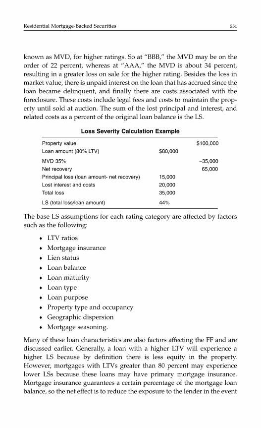
known as MVD, for higher ratings. So at “BBB,” the MVD may be on theorder of 22 percent, whereas at “AAA,” the MVD is about 34 percent,resulting in a greater loss on sale for the higher rating. Besides the loss inmarket value, there is unpaid interest on the loan that has accrued since theloan became delinquent, and finally there are costs associated with theforeclosure. These costs include legal fees and costs to maintain the prop-erty until sold at auction. The sum of the lost principal and interest, andrelated costs as a percent of the original loan balance is the LS.
Loss Severity Calculation Example
Property value $100,000
Loan amount (80% LTV) $80,000
MVD 35% −35,000
Net recovery 65,000
Principal loss (loan amount- net recovery) 15,000
Lost interest and costs 20,000
Total loss 35,000
LS (total loss/loan amount) 44%
The base LS assumptions for each rating category are affected by factorssuch as the following:
♦ LTV ratios♦ Mortgage insurance♦ Lien status♦ Loan balance♦ Loan maturity♦ Loan type♦ Loan purpose♦ Property type and occupancy♦ Geographic dispersion♦ Mortgage seasoning.
Many of these loan characteristics are also factors affecting the FF and arediscussed earlier. Generally, a loan with a higher LTV will experience ahigher LS because by definition there is less equity in the property.However, mortgages with LTVs greater than 80 percent may experiencelower LSs because these loans may have primary mortgage insurance.Mortgage insurance guarantees a certain percentage of the mortgage loanbalance, so the net effect is to reduce the exposure to the lender in the event
Residential Mortgage-Backed Securities 551
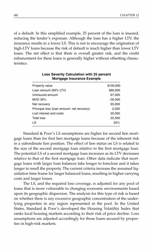
of a default. In this simplified example, 25 percent of the loan is insured,reducing the lender’s exposure. Although the loan has a higher LTV, theinsurance results in a lower LS. This is not to encourage the origination ofhigh-LTV loans because the risk of default is much higher than lower LTVloans. The net effect is that there is overall greater risk, and the creditenhancement for these loans is generally higher without offsetting charac-teristics.
Loss Severity Calculation with 25 percent Mortgage Insurance Example
Property value $100,000
Loan amount (90% LTV) $90,000
Uninsured amount 67,500
MVD 35% −35,000
Net recovery 65,000
Principal loss (loan amount- net recovery) 2,500
Lost interest and costs 20,000
Total loss 22,500
LS 25%
Standard & Poor’s LS assumptions are higher for second lien mort-gage loans than for first lien mortgage loans because of the inherent riskin a subordinate lien position. The effect of lien status on LS is related tothe size of the second mortgage loan relative to the first mortgage loan.The potential LS of a second mortgage loan increases as its LTV decreasesrelative to that of the first mortgage loan. Other data indicate that mort-gage loans with larger loan balances take longer to foreclose and it takeslonger to resell the property. The current criteria increase the assumed liq-uidation time frame for larger balanced loans, resulting in higher carryingcosts and larger losses.
The LS, and the required loss coverage, is adjusted for any pool ofloans that is more vulnerable to changing economic environments basedupon its geographic dispersion. The analysis for this type of risk is basedon whether there is any excessive geographic concentration of the under-lying properties in any region represented in the pool. In the UnitedStates, Standard & Poor’s developed the Housing Volatility Index thatranks local housing markets according to their risk of price decline. Lossassumptions are adjusted accordingly for those loans secured by proper-ties in high-risk markets.
552 CHAPTER 12

Structural Considerations for RMBS
There are different structural forms that RMBS issuers can use. They can besenior/subordinated structures where the lower rated or unrated tranchesprovide the credit support for the more highly rated tranches, and theycan be senior/subordinated/over-collateralized structures where part ofthe credit support is in the form of over-collateralization usually derivedfrom the value of excess interest, or the spread between the underlyingmortgage coupons and the coupon on the rated securities.
The issuer’s decision as to which type of credit enhancement struc-ture to use takes into consideration many factors but is primarily investordriven, based upon which structure yields the best economic value. Thecredit analysis for these structures is the same, regardless of type. Mostimportantly, it is the use of the shifting interest structure that allows creditsupport to grow over time, at least until the transaction is through themajority of Standard & Poor’s assumed default curve. This occurs throughcriteria that mandate that the majority of principal cash flow be allocatedto the most senior classes, or by requiring that the over-collateralizationtarget be pegged to the initial pool balance during the early stages of atransaction’s life.
Only after determining that the mortgage pool is performing wellwill credit support be allowed to step down. The delinquency and losslevels experienced by the mortgage pool is critical to the determinationof how much credit support will be needed over the life of the deal.Adequate credit support or loss coverage will enable all rated classes toreceive their promised monthly interest payment and to ultimatelyreceive back their entire principal amount. Accordingly, if the pool is per-forming well (relative to the initial expectation of delinquency, loss, andthe level of credit support), the release or stepping down of credit supportis permitted.
Senior/Subordinate StructuresA senior/subordinate structure for RMBS is characterized by the sub-ordination of junior certificates that serve as credit support for the moresenior certificates. Generally, in U.S. RMBS, all interest shortfalls andprincipal losses are allocated to the most junior bond first, resulting in awrite-down of its principal balance. In contrast, in the United Kingdom,market bonds are not written down, as losses are experienced on theassets. Instead, principal losses experienced on the mortgage pool are
Residential Mortgage-Backed Securities 553

recorded in a principal deficiency ledger (PDL), which tracks the extentto which the liabilities’ principal balance exceeds that of the assets’ prin-cipal balance. At each rating level, Standard & Poor’s requires that prin-cipal deficiencies do not exceed the existing subordination. For example,in a transaction with £100 million “AAA” senior notes, £9 million “A”subordinate notes, and £1 million unrated notes, the principal deficiencyat any point in time should not exceed £10 million in the “AAA” cashflow runs and £1 million in the “A” cash flow runs. If there is insufficientincome to fund the principal deficiency, however, Standard & Poor’s con-siders the risk to a transaction to be low if the principal deficiency isremedied within a short period of time using excess spread. In contrastto a structure that uses excess interest, in this structure, the subordinatebonds solely provide credit support. The result is larger subordinatebonds than would have been needed, if excess interest was also used tocover losses.
Allocation of Cash Flow Most RMBS are structured as pass-through transactions. All principal and interest (including liquidation andinsurance proceeds, seller repurchase and substitution proceeds, serviceradvances, and other unscheduled collections) generated by the underlyingmortgage pool are allocated in a priority order to bondholders. Interest isgenerally paid to all outstanding bonds, beginning with the most senior,and then in priority order to the remaining junior bonds. After all classeshave received in full their promised interest payment, principal will beallocated based upon the terms of the governing documents. According tothe rating criteria, since the subordinate bonds provide the only sourceof credit support in this type of structure, their receipt of principal mustbe delayed until a majority of borrower defaults have occurred. Amongstthe senior classes, principal will be allocated sequentially or pro rata, basedupon the average life preferences of investors.
When a loss is realized on a defaulted loan, issuers have two optionsin allocating cash flow. The most senior bonds can be promised the full,unpaid principal balance of the defaulted loan, or more simply the pro-ceeds generated from the loan’s final disposition.
If the full, unpaid principal balance of the defaulted loan is paid tosenior classes, all rated classes must receive interest before any paymentsof principal are made. This is necessary because the payment to seniorclasses of more cash flow than the defaulted loan generates will resultin the temporary shortfall of interest to subordinate bondholders. Thisviolates Standard & Poor’s timely receipt of interest criteria.
554 CHAPTER 12
There is the possibility that the credit composition of a mortgagepool will diminish over time, as the level of defaults increases. This canoccur as a result of stronger borrowers refinancing out of the pool, as timegoes on. This shift in pool makeup is commonly known as “adverse selec-tion.” Accordingly, the rating criteria require that all principal collectionsbe paid first to the most senior class, lowering its percentage interest inthe pool and, therefore, increasing the percentage interest representedby the subordinate classes. The resulting “shifting interest” increases thelevel of credit protection to the most senior bondholders over time.
Typically, the senior bondholders will receive all principal paymentsfor at least three years and until the level of credit support has increasedto two times its initial level. After that time, and provided that additionalperformance-based tests are met, holders of the subordinate bonds mayreceive a portion of principal collections.
Allocation of Losses In the case of the senior/subordinatestructure, the right of the junior class certificate-holders to receive a shareof the cash flow are subordinated to the rights of the senior certificate-holders. In addition, losses cause the certificate balance of lower-ratedcertificates to be written down (in the United States) prior to the moresenior bonds. Whenever the mortgage pool suffers a loss that threatensthe amount due to the senior certificate-holders, cash flow that wouldotherwise be due to the subordinated certificate-holders must bediverted to cover the shortfall. Therefore, all interest shortfalls and prin-cipal loss will be allocated to the most junior class outstanding. Serviceradvances that must ultimately be backed by a highly rated party, usuallythe trustee, generally cover shortfalls that result from delinquencies.
Stepping Down of Loss Protection As stated earlier, allrated transactions must preserve credit support until the mortgage poolhas experienced a majority of its defaults and the remaining borrowershave proven their ability to perform well, as judged by delinquency andloss tests. However, after that point, the decline of credit enhancementover time has traditionally been a feature of Standard & Poor’s-ratedmortgage-backed securities. This stepping down of credit enhancementis contingent upon collateral performance, measured by loss and delin-quency numbers as well as the time elapsed since securitization.
In the senior/subordinate structure, the stepping down of loss pro-tection occurs when principal is allocated to the subordinate bonds.Historical data show that the majority of all defaults occur in the first five
Residential Mortgage-Backed Securities 555
years after mortgage loan origination. Accordingly, to protect againstsevere losses during this stressful time period, a five-year lockout periodapplies. During this time period, no reduction in credit enhancement isexpected. This lockout is also intended to protect certificate holders againstdeterioration in the collateral pool’s credit profile due to adverse selection.Once the determination has been made that principal may be allocated tothe subordinate bonds, principal may be allocated to each subordinatebond that has maintained at least two times its original credit support as apercentage of the current outstanding pool balance. Delinquency and losstests should also continue to be met.
Principal may also be paid to the senior and mezzanine classes pro-rata. To attain pro rata allocation between the senior and the mezzanineclasses before the end of the standard lockout period, the mezzanine classmust be oversized to compensate for the early receipt of principal.
Excess Interest Valuation and Cash Flow AnalysisThe senior/subordinate with over-collateralization structure is a hybridstructure that combines the use of excess interest to cover losses and cre-ate over-collateralization. The capital structure for these securities andbased on the value of excess interest determined through cash flow analy-sis. Excess interest is the difference between the net mortgage rates paidby the borrowers in the underlying mortgage pool and the interest ratepaid to bondholders. Cash flow analysis is necessary to determine howmuch excess interest will be available to cover losses over the life of thetransaction. The analysis must consider the following variables:
♦ Mortgage interest rates♦ Weighted average coupon (WAC) deterioration♦ Fees♦ Rate and timing of default and prepayment speeds♦ Length of time for loss realization♦ Bond pass-through rates♦ Structural features such as the prioritization of principal cash flow.
An analysis of cash flows is done to determine the amount of over-collateralization and the size of the subordinate bonds necessary at eachrating category. Cash flows should demonstrate that each rated classreceives timely interest and ultimate repayment of principal. Default andLS projections are made at each rating category, regardless of structure ortype of credit support.
556 CHAPTER 12
For cash flow allocation, interest is generally paid to all seniorclasses of certificates concurrently based upon their pro rata percentageinterest in the mortgage pool. Interest is then allocated sequentially, in pri-ority order, to the subordinate bonds. Excess interest is then used to covercurrent losses, paid to the most senior bonds to build towards the over-collateralization target, and lastly will be “released” from the deal throughpayments to a residual certificate holder. The targeted level of over-collateralization is usually set as a percentage of the original pool balance.Principal is then allocated sequentially, pro rata, or in some combinationamong the senior classes, in order to accommodate investor’s varyingaverage-life requirements. Remaining principal is then paid sequentially,in priority order, to the subordinate bonds.
In this hybrid structure, the credit enhancement to each rated class isprovided first by the monthly-generated excess interest, second throughthe decrease in any over-collateralization, and third will be allocated to thesubordinate bonds. After all excess interest and over-collateralization hasbeen depleted, subordinate bonds, on a priority basis, are shorted interestor written down for principal loss.
Defaults play a major role in the amount of excess interest availablein a given transaction. The frequency of defaults and the timing of thosedefaults will influence the amount of excess interest that may be on handto cover potential losses. If the cash flows show that payment of currentinterest can be maintained and the losses adequately absorbed while ulti-mately paying the rated class, the transaction will meet the stress test. Inaddition, the balance of the loan at the time of default is calculated byassuming that only scheduled principal payments have occurred on theloan, and that no prepayments on that loan have taken place.
Typically, a 12-month lag is assumed from the time a loan defaultsuntil the loan is liquidated for U.S. RMBS; the assumption is 18 monthsfor the U.K. market. In other words, 12 (or 18) months after the defaultoccurs, a percentage of the balance (equal to the LS at the rating levelbeing analyzed) will be lost, and the remainder of the balance will berecovered as net proceeds.
The availability of excess interest is also impacted by whether or notadvances are being made on delinquent and defaulted loans. Typically,transactions require the servicer to make advances on delinquent anddefaulted loans until such time the loan is liquidated. However, the servicerdoes not have to make an advance on a specific loan if it determines thatthe amount advanced will not be recoverable from liquidation proceeds.If advances are required, then the excess interest from these loans may be
Residential Mortgage-Backed Securities 557
available to offset potential losses. Transactions without an advancingmechanism will not have any interest flowing into the transaction fromdelinquent or defaulted loans. Therefore, this is assumed in the cash flowanalysis. In this case, an added stress is placed on the cash flows. Becauseno advancing is occurring, analysts will assume in the cash flow modelingthat a certain percentage of loans are delinquent at any point in time, inaddition to the amount of loans in default at that time. Six months prior toeach bullet default, beginning with the default balance in month 12, a likepercentage of loans will be delinquent in interest as is in default. Recoveryof this delinquent interest occurs six months later; that is, the first delin-quent period begins in month 6 with recovery in month 12. This delin-quency stress continues for all bullets throughout the default curve.
The prepayment rate significantly impacts the amount of excessinterest that is available in a transaction. The greater the amount of loansprepaying, the less excess interest will be available. The prepayment ratethat is assumed is based on the historical experience of the industry or thespecific issuer. The pricing speed may be used as a proxy for this speedand is typically reported as a constant prepayment rate (CPR). This indi-cates the “all in” speed at which loans are removed from the pool. That is,the speed at which loans voluntarily prepay combined with the rate atwhich defaults occur.
However, Standard & Poor’s uses this pricing speed to indicate vol-untary prepayments only. The rating analysis assumes that poorer creditquality borrowers will not be able to prepay, and that therefore onlyincludes voluntary prepayments. Default assumptions are layered overthe prepayment assumptions. In this regard, it is believed that voluntaryprepayments are inversely related to the economic scenario as we go upthe rating scale to a more stressful economic scenario. However, becausedefaults increase at a greater pace as the more severe economic downturnoccurs, the overall speed at which loans are removed from the pool willincrease.
It should be again noted that Standard & Poor’s will analyze thespeed at which the deal is priced versus the issuer’s historical experience,and if it is determined that the pricing speed does not adequately reflectthe actual prepayment history for the issuer and the collateral type, theprepayment assumptions will be adjusted accordingly.
Mortgage prepayment history has shown that the WAC of a pool,and therefore the available excess spread, decreases over time in mort-gage pools. That is, loans having higher interest rates and greater marginsare more likely to prepay if the borrower’s credit improves, and more
558 CHAPTER 12
likely to default if it does not. Therefore, the ratings analysis stresses thecash flows in order to reflect this situation.
When a transaction contains mortgage loans with an interest rateindex that is different from that of the certificates, basis risk occurs. Thechanging spread between the two rates may cause shortfalls in the cashflow needed to pay the bonds. To address this issue, Standard & Poor’suses its stressed interest rate scenarios in the cash flow modeling. Severalyears ago, Standard & Poor’s revised its interest modeling approach forU.S. RMBS. The research began with the estimation of a Cox-Ingersoll-Ross (CIR) model for the one-month LIBOR. The estimated CIR modelwas used in the simulation of hundreds of thousands of interest ratepaths. Simulations were repeated for various ranges of starting rates, upto 2.25 percent, 2.25 to 2.75 percent, 2.75 to 3.25 percent, and so on up to20 percent. For each starting range, the simulation results were selectedbased on a point-wise quantile, that is, from the month one results the val-ues corresponding to specific quantiles were chosen, from the month tworesults, from the month three results, and so on. These points were “con-nected” to create the base curves. Additionally, to reflect the naturalmovement of rates up and down, a sinusoidal component was added. Toensure consistency, all other indices were modeled against the one-monthLIBOR.
Each month the RMBS vectors for about a dozen indices and all rat-ing categories are published. These vectors are used in the U.S. RMBScash flow model, SPIRE. In the United Kingdom, the interest rate scenar-ios are more straightforward and perhaps more stressful. LIBOR isassumed to increase at 2 percent per month until a ceiling of 18 percent(12 percent for EURIBOR) is reached. The rate is assumed to remain at theceiling for the life of the transaction. For falling rate environments, ratesare assumed to fall 2 percent per month until a 2 percent floor is reached,where rates remain for life.
Legal Issues in RMBS
Banks or other financial institutions, insurance companies, or nonbankingcorporations transfer residential mortgage loans into a securitizationstructure. Some of the legal issues raised by these transactions differdepending on whether the entity transferring the loans is a nonbankingcorporation that is eligible to become a debtor under the U.S. BankruptcyCode, a bank, other financial institution. Also relevant is whether the
Residential Mortgage-Backed Securities 559
entity is an insurance company that is not eligible to become a debtorunder the Bankruptcy Code, or an entity subject to the Bankruptcy Code(such as a municipality or public-purpose entity), but which is deemed byStandard & Poor’s to be bankruptcy-remote in that the bankruptcy or dis-solution of such entity for reasons unrelated to the transaction structure isdeemed unlikely to occur (a “special-purpose entity transferor”). Unlessotherwise indicated, an entity either selling, contributing, depositing, orpledging assets for purposes of securitization, including the originator ofthe assets and any intermediary entity participating at any level in a struc-ture transaction as a transferor of assets, is referred to as a transferor.
Structured financings are rated based primarily on the creditworthi-ness of isolated assets or asset pools, whether sold, contributed, orpledged into a securitization structure, without regard to the creditwor-thiness of the seller, contributor, or borrower. The structured financingseeks to insulate transactions from entities that are either unrated and forwhom Standard & Poor’s is unable to quantify the likelihood of a poten-tial bankruptcy, or that are rated investment grade but wish a higher rat-ing for the transaction. Standard & Poor’s worst-case scenario assumesthe bankruptcy of each transaction participant deemed not to bebankruptcy-remote or that is rated lower than the transaction. Standard &Poor’s resolves most legal concerns by analyzing the legal documents,and where appropriate, receiving opinions of counsel that address insol-vency, as well as security interest and other issues. Understanding theimplications of the assumptions and its criteria enables an issuer to antic-ipate and resolve most legal concerns early in the rating process.
Special-Purpose Entities Standard & Poor’s legal criteria forsecuritization transactions are designed to ensure that the entity owningthe assets required to make payments on the rated securities is bankruptcyremote, that is, is unlikely to be subject to voluntary or involuntary insol-vency proceedings. In this regard, both the incentives of this entity, knownas an SPE, or its equity holders to resort to voluntary insolvency proceed-ings and the incentives for other creditors of the SPE to resort to involun-tary proceedings are considered. The analysis also examines whetherthird-party creditors of the SPE’s parent would have an incentive to reachthe assets of the SPE (e.g., if the SPE is a trust, whether creditors of thebeneficial holder would have an incentive to cause the dissolution of thetrust to reach the assets of the trust). In this regard, Standard & Poor’s hasdeveloped “SPE criteria,” which an entity should satisfy to be deemedbankruptcy remote.
560 CHAPTER 12

Trustee, Servicer, and Eligible Accounts The indenturetrustee/custodian in a structured transaction is primarily responsible forreceiving payments from servicers, guarantors, and other third parties andremitting these receipts to investors in the rated securities in accordancewith the terms of the indenture, in addition to its monitoring, custodial, andadministrative functions. In a structured transaction, the servicer agrees toservice and administer assets in accordance with its customary practicesand guidelines and has full power and authority to make payments to andwithdrawals from deposit accounts that are governed by the documents.
The servicer’s fee should cover its servicing and collection expensesand be in line with industry norms for securities of similar quality. If thefee is considered below industry averages, an increase may be built intothe transaction. The increase might be needed to entice a substitute ser-vicer to step in and service the portfolio. If the servicing fee is calculatedbased on a certain dollar amount per contract, the fee will increase as apercentage of assets due to amortization of the pool. This is an importantconsideration when assessing available excess spread to cover losses andfund any reserve account.
The filing of a bankruptcy petition would place a stay on all fundsheld in a servicer’s own accounts. As a result, funds held to make pay-ments on the rated securities would be delayed. In addition, funds com-mingled with those of the servicer would be unavailable to the structuredtransaction. As a general matter, Standard & Poor’s addresses this com-mingling risk by looking both to the rating of the servicer and the amountof funds likely to be held in a servicer account at any given time.
A structured financing provides for different accounts to be estab-lished at closing to serve as collection accounts in which revenues gener-ated by the securitized assets are deposited and to establish reservesfunds. Often, the accounts in which the reserves are held contain signifi-cant sums held over a substantial period of time. Standard & Poor’s hascriteria regarding these accounts. The criteria are intended to immunizeand isolate a transaction’s payments, cash proceeds, and distributionsfrom the insolvency of each entity that is a party to the transaction. Aninsolvency of the servicer (sub or master), trustee, or other party to thetransaction should not cause a delay or loss to the investor’s scheduledpayments on the rated securities. As a general matter, Standard & Poor’srelies on credit, structural, and legal criteria to ensure that a structuredtransaction’s cash flows are protected at every link in the cash flow chain.
Unless collections on assets are concentrated at certain times of themonth, for a period of up to two-business days after receipt, any servicer,
Residential Mortgage-Backed Securities 561

whether or not rated, may keep collections on the assets in any account ofthe servicer’s choice, commingled with other money of the servicer or ofany other entity. Before the end of the two-business day period, the collec-tions on the assets should be deposited into an eligible deposit account. As ageneral matter, all servicers, including unrated servicers, may keep/com-mingle collections for up to two business days, based on Standard &Poor’s credit assumption, made in connection with all structured transac-tions, that two days’ worth of collections on assets will be lost.
If, however, collections on the assets are concentrated at certaintimes within a month (e.g., the first, 15th, or 30th of a month), a servicerrated below “A-1” should not be able to keep/commingle collectionson the assets even for the two-business day period, as described above.Rather, to prevent a potentially significant loss on assets, Standard &Poor’s generally requires that, in transactions involving concentrated col-lections in which the servicer is rated below “A-1,” either additional creditsupport be provided to cover commingling risk or obligors be instructedto make payments to lockbox accounts, which, in turn, are swept daily toan eligible deposit account. The servicer, unless rated the same as the rat-ing sought on the structured transaction, should be prevented fromaccessing either the lockbox or sweep accounts. If a servicer is rated below“A-1” or is unrated, or if an “A-1” rated servicer’s obligation to remit col-lections is not unconditional, the servicer should deposit all collectionsinto an eligible deposit account within two business days of receipt. Allother accounts maintained by the master servicer, special servicer, ortrustee in a structured transaction (e.g., reserve accounts) should qualifyas eligible deposit accounts.
PART 2: ANALYTICAL TECHNIQUES TO RATE RMBS TRANCHES IN EUROPE
In this part, we review the main modeling features used by Standard &Poor’s to come with rated tranches on the European market.
Portfolio Credit Analysis
The credit analysis performed by Standard & Poor’s estimates the expectedprincipal loss (EL) that a mortgage portfolio might exhibit under differenteconomic scenarios. At the primary rating level, loan level data is almostinvariably available to complete this analysis. The loan level data includes
562 CHAPTER 12
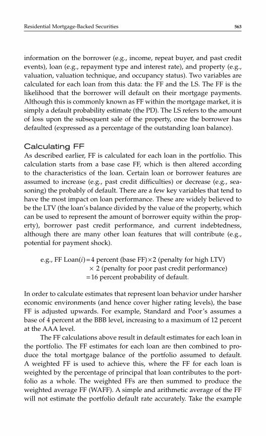
information on the borrower (e.g., income, repeat buyer, and past creditevents), loan (e.g., repayment type and interest rate), and property (e.g.,valuation, valuation technique, and occupancy status). Two variables arecalculated for each loan from this data: the FF and the LS. The FF is thelikelihood that the borrower will default on their mortgage payments.Although this is commonly known as FF within the mortgage market, it issimply a default probability estimate (the PD). The LS refers to the amountof loss upon the subsequent sale of the property, once the borrower hasdefaulted (expressed as a percentage of the outstanding loan balance).
Calculating FFAs described earlier, FF is calculated for each loan in the portfolio. Thiscalculation starts from a base case FF, which is then altered accordingto the characteristics of the loan. Certain loan or borrower features areassumed to increase (e.g., past credit difficulties) or decrease (e.g., sea-soning) the probably of default. There are a few key variables that tend tohave the most impact on loan performance. These are widely believed tobe the LTV (the loan’s balance divided by the value of the property, whichcan be used to represent the amount of borrower equity within the prop-erty), borrower past credit performance, and current indebtedness,although there are many other loan features that will contribute (e.g.,potential for payment shock).
e.g., FF Loan(i) = 4 percent (base FF) × 2 (penalty for high LTV)× 2 (penalty for poor past credit performance)
= 16 percent probability of default.
In order to calculate estimates that represent loan behavior under harshereconomic environments (and hence cover higher rating levels), the baseFF is adjusted upwards. For example, Standard and Poor’s assumes abase of 4 percent at the BBB level, increasing to a maximum of 12 percentat the AAA level.
The FF calculations above result in default estimates for each loan inthe portfolio. The FF estimates for each loan are then combined to pro-duce the total mortgage balance of the portfolio assumed to default.A weighted FF is used to achieve this, where the FF for each loan isweighted by the percentage of principal that loan contributes to the port-folio as a whole. The weighted FFs are then summed to produce theweighted average FF (WAFF). A simple and arithmetic average of the FFwill not estimate the portfolio default rate accurately. Take the example
Residential Mortgage-Backed Securities 563
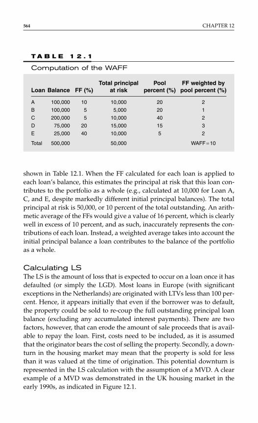
564 CHAPTER 12
shown in Table 12.1. When the FF calculated for each loan is applied toeach loan’s balance, this estimates the principal at risk that this loan con-tributes to the portfolio as a whole (e.g., calculated at 10,000 for Loan A,C, and E, despite markedly different initial principal balances). The totalprincipal at risk is 50,000, or 10 percent of the total outstanding. An arith-metic average of the FFs would give a value of 16 percent, which is clearlywell in excess of 10 percent, and as such, inaccurately represents the con-tributions of each loan. Instead, a weighted average takes into account theinitial principal balance a loan contributes to the balance of the portfolioas a whole.
Calculating LSThe LS is the amount of loss that is expected to occur on a loan once it hasdefaulted (or simply the LGD). Most loans in Europe (with significantexceptions in the Netherlands) are originated with LTVs less than 100 per-cent. Hence, it appears initially that even if the borrower was to default,the property could be sold to re-coup the full outstanding principal loanbalance (excluding any accumulated interest payments). There are twofactors, however, that can erode the amount of sale proceeds that is avail-able to repay the loan. First, costs need to be included, as it is assumedthat the originator bears the cost of selling the property. Secondly, a down-turn in the housing market may mean that the property is sold for lessthan it was valued at the time of origination. This potential downturn isrepresented in the LS calculation with the assumption of a MVD. A clearexample of a MVD was demonstrated in the UK housing market in theearly 1990s, as indicated in Figure 12.1.
T A B L E 1 2 . 1
Computation of the WAFF
Total principal Pool FF weighted by Loan Balance FF (%) at risk percent (%) pool percent (%)
A 100,000 10 10,000 20 2
B 100,000 5 5,000 20 1
C 200,000 5 10,000 40 2
D 75,000 20 15,000 15 3
E 25,000 40 10,000 5 2
Total 500,000 50,000 WAFF = 10
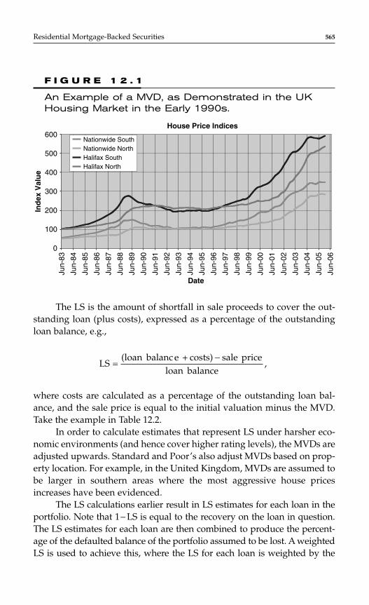
Residential Mortgage-Backed Securities 565
The LS is the amount of shortfall in sale proceeds to cover the out-standing loan (plus costs), expressed as a percentage of the outstandingloan balance, e.g.,
where costs are calculated as a percentage of the outstanding loan bal-ance, and the sale price is equal to the initial valuation minus the MVD.Take the example in Table 12.2.
In order to calculate estimates that represent LS under harsher eco-nomic environments (and hence cover higher rating levels), the MVDs areadjusted upwards. Standard and Poor’s also adjust MVDs based on prop-erty location. For example, in the United Kingdom, MVDs are assumed tobe larger in southern areas where the most aggressive house pricesincreases have been evidenced.
The LS calculations earlier result in LS estimates for each loan in theportfolio. Note that 1− LS is equal to the recovery on the loan in question.The LS estimates for each loan are then combined to produce the percent-age of the defaulted balance of the portfolio assumed to be lost. A weightedLS is used to achieve this, where the LS for each loan is weighted by the
LS(loan balanc e costs) sale price
loan balance,=
−+
F I G U R E 1 2 . 1
An Example of a MVD, as Demonstrated in the UKHousing Market in the Early 1990s.
House Price Indices
0
100
200
300
400
500
600
Jun-
83
Jun-
84
Jun-
85
Jun-
86
Jun-
87
Jun-
88
Jun-
89
Jun-
90
Jun-
91
Jun-
92
Jun-
93
Jun-
94
Jun-
95
Jun-
96
Jun-
97
Jun-
98
Jun-
99
Jun-
00
Jun-
01
Jun-
02
Jun-
03
Jun-
04
Jun-
05
Jun-
06
Date
Ind
ex V
alu
e
Nationwide SouthNationwide NorthHalifax SouthHalifax North
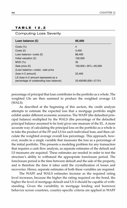
566 CHAPTER 12
percentage of principal that loan contributes to the portfolio as a whole. Theweighted LSs are then summed to produce the weighted average LS(WALS).
As described at the beginning of this section, the credit analysisattempts to estimate the expected loss that a mortgage portfolio mightexhibit under different economic scenarios. The WAFF (the defaulted prin-cipal balance) multiplied by the WALS (the percentage of the defaultedprincipal balance assumed to be lost) gives one measure of the EL. A moreaccurate way of calculating the principal loss on the portfolio as a whole isto take the product of the FF and LS for each individual loan, and then cal-culate the weighted average overall loss percentage. This approach, how-ever, results in a single variable that measures the loss as a percentage ofthe initial portfolio. This presents a modeling problem for any transactionthat requires a cash flow analysis, as separate estimates of the default andLS measures are required. These estimates are needed in order to test thestructure’s ability to withstand the appropriate foreclosure period. Theforeclosure period is the time between default and the sale of the property,and is therefore the time it takes until the crystallization of losses andrecoveries. Hence, separate estimates of both these variables are required.
The WAFF and WALS estimates increase as the required ratinglevel increases, because the higher the rating required on the bond, thehigher the level of mortgage default and LS it should be capable of with-standing. Given the variability in mortgage lending and borrowerbehavior across countries, country-specific criteria are applied in WAFF
T A B L E 1 2 . 2
Computing Loss Severity
Loan balance (£) 85,000
Costs (%) 4
Costs (£) 3,400
Loan balance + costs (£) 88,400
Initial valuation (£) 100,000
MVD (%) 35
Sale price (£) 100,000 × 35% = 65,000
(Loan balance + costs) − sale price
(loss in £ amount) 23,400
LS (loss in £ amount expressed as a percentage of outstanding loan balance) 23,400/85,000 = 27.5%
Residential Mortgage-Backed Securities 567
and WALS assessments. As a consequence, the assumed percentage ofdefaults and subsequent losses can differ substantially across jurisdic-tions. It is worth mentioning that WAFF/WALS are measures that workonly for large pools, as for smaller pools, idiosyncrasies may not vanish.
Cashflow Analysis
Many RMBS transactions are cash flow based, where the revenue streamgenerated by the mortgages is used to service rated note obligations. A keyfeature of the primary rating process for these types of transactions is toassess the adequacy of the cash flow from the mortgage loans to satisfythe terms of the rated debt. Economic stress scenarios are applied to thecash flows, and then the rated note interest payments and principalrepayments are assessed for their adequacy in a given rating scenario.Standard and Poor’s ensures under any given stress scenario, principalpayments will be made in full and interest payments on a timely basis.
A typical RMBS cash flow transaction consists of a number of ratednotes that differ in seniority with respect to interest and principal paymentsfrom the underlying mortgage portfolio, in so-called senior/subordinatedstructures. There is usually a first-loss fund provided by the originator ofthe assets underneath the rated notes, often called the reserve fund. Thisis used to cover both interest shortfalls and principal losses arising in thetransaction. A liquidity facility might also be incorporated, which is usedto bridge timing mismatches that can occur between the asset cash flowsand the required liability payments. The transaction might also includespecific structural features designed to minimize the issuer’s exposure toexternal economic factors (e.g., interest rate hedges).
There are many variants to the generalized case described above.Structures tend to vary depending on the underlying collateral (e.g.,prime RMBS transactions tend to differ structurally from nonconformingRMBS transactions), and across different countries (e.g., UK prime RMBStransactions differ structurally from Spanish or Italian prime RMBS trans-actions). This is generally for practical reasons. For example, UK primemortgage originators tend to have very large portfolios, and have used“master trust” type structures primarily as a tool to reduce the costs ofmultiple securitizations over time. In contrast, Spanish and Italian trans-actions typically swap the entire asset cash flows to receive principal plusa fixed spread, primarily because the underlying mortgage loans tend tohave quite variable interest rates, reset dates, and fixed periods.
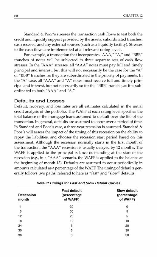
Standard & Poor’s stresses the transaction cash flows to test both thecredit and liquidity support provided by the assets, subordinated tranches,cash reserve, and any external sources (such as a liquidity facility). Stressesto the cash flows are implemented at all relevant rating levels.
For example, a transaction that incorporates “AAA,” “A,” and “BBB”tranches of notes will be subjected to three separate sets of cash flowstresses. In the “AAA” stresses, all “AAA” notes must pay full and timelyprincipal and interest, but this will not necessarily be the case for the “A”or “BBB” tranches, as they are subordinated in the priority of payments. Inthe “A” case, all “AAA” and “A” notes must receive full and timely prin-cipal and interest, but not necessarily so for the “BBB” tranche, as it is sub-ordinated to both “AAA” and “A.”
Defaults and LossesDefault, recovery, and loss rates are all estimates calculated in the initialcredit analysis of the portfolio. The WAFF at each rating level specifies thetotal balance of the mortgage loans assumed to default over the life of thetransaction. In general, defaults are assumed to occur over a period of time.In Standard and Poor’s case, a three-year recession is assumed. Standard &Poor’s will assess the impact of the timing of this recession on the ability torepay the liabilities, and chooses the recession start period based on thisassessment. Although the recession normally starts in the first month ofthe transaction, the “AAA” recession is usually delayed by 12 months. TheWAFF is applied to the principal balance outstanding at the start of therecession (e.g., in a “AAA” scenario, the WAFF is applied to the balance atthe beginning of month 13). Defaults are assumed to occur periodically inamounts calculated as a percentage of the WAFF. The timing of defaults gen-erally follows two paths, referred to here as “fast” and “slow” defaults.
Default Timings for Fast and Slow Default Curves
Fast default Slow default Recession (percentage (percentage month of WAFF) of WAFF)
1 30 0
6 30 5
12 20 5
18 10 10
24 5 20
30 5 30
36 0 30
568 CHAPTER 12

Standard & Poor’s assumes that the recovery of proceeds from theforeclosure and sale of repossessed properties occurs 18 months after apayment default in UK transactions (i.e., if a default occurs in month one,then recovery proceeds are received in month 19). The value of recoverieswill be equal to the defaulted amount less the WALS. The time taken torepossess and sell a property can vary widely across the European coun-tries, primarily because the legal procedures required before a lender canrepossess and sell a property differ across jurisdictions (see Table 12.3).Standard & Poor’s will therefore adjust the foreclosure period for eachcountry to account for this.
Note that the WALS used in a cash flow model will always be basedon principal loss, including costs. Standard & Poor’s assumes no recoveryof any interest accrued on the mortgage loans during the foreclosureperiod. In addition, after the WAFF is applied to the balance of the mort-gages, the asset balance is likely to be lower than that on the liabilities(a notable exception is when a transaction relies on over-collateralization).The interest reduction created by the defaulted mortgages during the fore-closure period will need to be covered by other structural mechanisms inthe transaction (e.g., excess spread).
Residential Mortgage-Backed Securities 569
T A B L E 1 2 . 3
Foreclosure Periods in Different European Jurisdictions
Foreclosure period (time from default Country to recovery in months)
Belgium 18
France 36
Germany 24
Greece 72
Ireland 18
Italy 60 (on average, but can be vary depending on location of property)
The Netherlands 18
Portugal 36
Spain 30
Sweden 18
Switzerland 18
United Kingdom 18
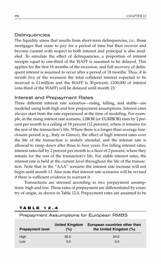
DelinquenciesThe liquidity stress that results from short-term delinquencies, i.e., thosemortgages that cease to pay for a period of time but then recover andbecome current with respect to both interest and principal is also mod-eled. To simulate the effect of delinquencies, a proportion of interestreceipts equal to one-third of the WAFF is assumed to be delayed. Thisapplies for the first 18 months of the recession, and full recovery of delin-quent interest is assumed to occur after a period of 18 months. Thus, if inmonth five of the recession the total collateral interest expected to bereceived is £1 million and the WAFF is 30 percent, £100,000 of interest(one-third of the WAFF) will be delayed until month 23.
Interest and Prepayment RatesThree different interest rate scenarios—rising, falling, and stable—aremodeled using both high and low prepayment assumptions. Interest ratesalways start from the rate experienced at the time of modeling. For exam-ple, in the rising interest rate scenario, LIBOR (or EURIBOR) rises by 2 per-cent per month to a ceiling of 18 percent (12 percent), where it remains forthe rest of the transaction’s life. Where there is a longer-than-average fore-closure period (e.g., Italy or Greece), the effect of high interest rates overthe life of the transaction is unduly stressful, and the interest rate isallowed to ramp down after three to four years. For falling interest rates,interest rates fall by 2 percent per month to a floor of 2 percent, where theyremain for the rest of the transaction’s life. For stable interest rates, theinterest rate is held at the current level throughout the life of the transac-tion. Note that in the “AAA” scenario the interest rate increase will notbegin until month 13. Also note that interest rate scenarios will be revisedif there is sufficient evidence to warrant it.
Transactions are stressed according to two prepayment assump-tions: high and low. These rates of prepayment are differentiated by coun-try of origin, as shown in Table 12.4. Prepayment rates are assumed to be
570 CHAPTER 12
T A B L E 1 2 . 4
Prepayment Assumptions for European RMBS
United Kingdom European countries other than Prepayment level (%) the United Kingdom (%)
High 30.0 24.0
Low 0.5 0.5
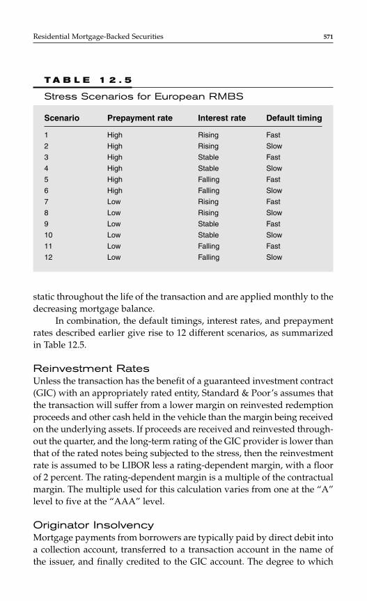
Residential Mortgage-Backed Securities 571
static throughout the life of the transaction and are applied monthly to thedecreasing mortgage balance.
In combination, the default timings, interest rates, and prepaymentrates described earlier give rise to 12 different scenarios, as summarizedin Table 12.5.
Reinvestment RatesUnless the transaction has the benefit of a guaranteed investment contract(GIC) with an appropriately rated entity, Standard & Poor’s assumes thatthe transaction will suffer from a lower margin on reinvested redemptionproceeds and other cash held in the vehicle than the margin being receivedon the underlying assets. If proceeds are received and reinvested through-out the quarter, and the long-term rating of the GIC provider is lower thanthat of the rated notes being subjected to the stress, then the reinvestmentrate is assumed to be LIBOR less a rating-dependent margin, with a floorof 2 percent. The rating-dependent margin is a multiple of the contractualmargin. The multiple used for this calculation varies from one at the “A”level to five at the “AAA” level.
Originator InsolvencyMortgage payments from borrowers are typically paid by direct debit intoa collection account, transferred to a transaction account in the name ofthe issuer, and finally credited to the GIC account. The degree to which
T A B L E 1 2 . 5
Stress Scenarios for European RMBS
Scenario Prepayment rate Interest rate Default timing
1 High Rising Fast
2 High Rising Slow
3 High Stable Fast
4 High Stable Slow
5 High Falling Fast
6 High Falling Slow
7 Low Rising Fast
8 Low Rising Slow
9 Low Stable Fast
10 Low Stable Slow
11 Low Falling Fast
12 Low Falling Slow

insolvency of the originator will affect the cash flow from the assets there-fore depends on the collection account characteristics. The amount at riskdepends on the timing of payments from borrowers and the frequencywith which these funds are transferred to the transaction account. If allborrowers pay on the same day of the month, then even with daily sweep-ing of the collection account, up to one month’s cash flow from the assetsis potentially at risk.
The collection account is often not in the name of the issuer, as mostoriginators do not want to ask borrowers to change their direct debitinstructions as a result of securitization. Under English law, if the issuerhas been granted the benefit of a properly executed declaration of trustover the collection account, then insolvency of the originator should notresult in a loss of funds, but should only involve a simple delay. This riskwill need to be modeled appropriately for each transaction, but normallyresults in a delay of one month’s cash flow for three months over an inter-est payment date. In other European countries, insolvency of the origina-tor is more likely to result in a loss of funds, the amount of which dependson the frequency of the transfer of money from the collection to the trans-action account. This amount is generally modeled as a loss of interest andprincipal in the first month of the recession.
ExpensesAll the issuer’s foreseeable expenses should be modeled (e.g., mortgageadministration fees, trustee fees, standby servicer fees, cash/bond admin-istration fees, etc.). These expenses should also include any tax liability theissuer may have. These fees are either a fixed amount per annum, or aresized as a percentage of the outstanding mortgage loans (or a combinationof both). Standard & Poor’s normally requires a schedule of these expensesto be provided. In addition to foreseeable expenses, the model shouldcontain amounts sized for contingent expenses, such as the need for thetrustee to register legal title to the mortgages in the event of insolvency ofthe originator. This amount can vary from £150,000 to £300,000, depend-ing on the size of the transaction, and can be modeled either as a separatecontingency reserve or as a haircut to the reserve fund.
Principal DeficienciesIn general, bonds are not written down, as losses are experienced on theassets. Instead, principal losses experienced on the mortgage pool arerecorded in a PDL, which tracks the extent to which the principal balanceof liabilities exceeds that of the assets. At each rating level, Standard &
572 CHAPTER 12
Poor’s requires that principal deficiencies do not exceed the existing sub-ordination. For example, in a transaction with £100 million “AAA” seniornotes, £9 million “A” junior notes, and a £1 million reserve fund, the prin-cipal deficiency at any point in time should not exceed £10 million in the“AAA” runs and £1 million in the “A” runs. If there is insufficient incometo fund the principal deficiency, however, Standard & Poor’s considersthe risk to a transaction to be low if the principal deficiency is remediedwithin a short period of time using excess spread.
Basis RiskBasis risk occurs when the value of the interest rate index used to deter-mine the interest payments received from the assets differs from that ofthe liabilities. This can occur when assets and liabilities are linked to dif-ferent indices (e.g., mortgages are linked to three-month Libor, liabilitiesto three-month Euribor), or both are linked to the same index, but it is seton a different date (mortgage interest rate set on 1st of the month and lia-bility interest rate on the 20th). Here, there is the risk that the index for theassets falls below that of the liabilities, such that asset interest paymentsare insufficient to make the required payments to the liabilities. In situa-tions where this risk is not hedged, Standard & Poor’s typically assessesthe historical performance of the indices in question, and calculates thedifference over a certain time horizon (e.g., 20 days in the above example)that has been experienced historically. The average difference between theindices is then calculated, assuming that in periods where the index forthe mortgages has been higher than that of the liabilities, the differencebetween the two is assumed to be zero. This average is then subtractedevery month from the asset margin. In addition, two spikes in the liabil-ity interest rate index are also modeled. The height of each spike is deter-mined as the maximum difference between the two indices and occurs atthe beginning of the first two years of the transaction.
PART 3: A REVIEW OF THE GENERIC QUANTITATIVE TECHNIQUES USED BY MARKET PARTICIPANTS FOR ASSET BACK SECURITIES IN EUROPE
The ABS or structured finance constitutes one of the fastest growing andmost innovative sectors of the European bond market. Banks, specialistfinance companies, credit card companies, governments, mortgage
Residential Mortgage-Backed Securities 573
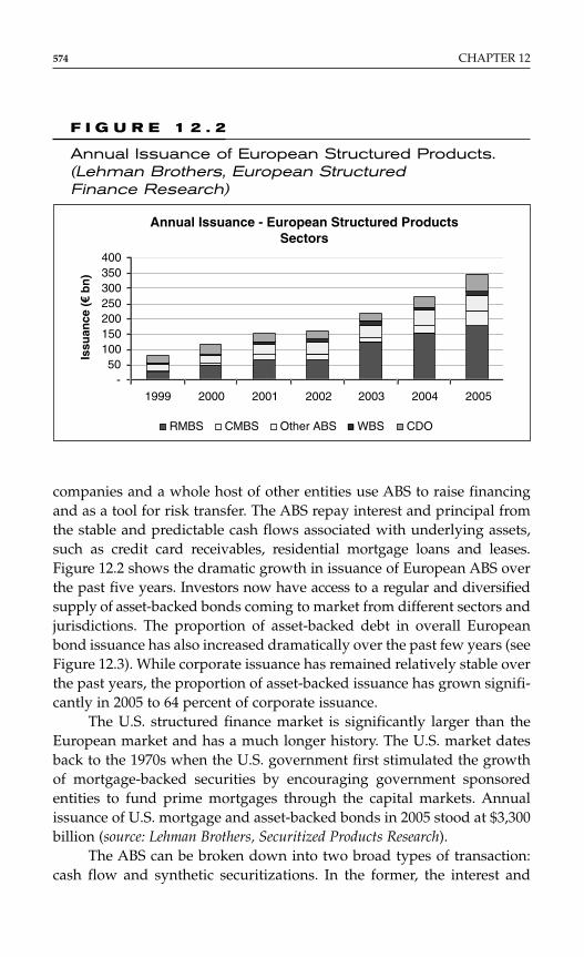
companies and a whole host of other entities use ABS to raise financingand as a tool for risk transfer. The ABS repay interest and principal fromthe stable and predictable cash flows associated with underlying assets,such as credit card receivables, residential mortgage loans and leases.Figure 12.2 shows the dramatic growth in issuance of European ABS overthe past five years. Investors now have access to a regular and diversifiedsupply of asset-backed bonds coming to market from different sectors andjurisdictions. The proportion of asset-backed debt in overall Europeanbond issuance has also increased dramatically over the past few years (seeFigure 12.3). While corporate issuance has remained relatively stable overthe past years, the proportion of asset-backed issuance has grown signifi-cantly in 2005 to 64 percent of corporate issuance.
The U.S. structured finance market is significantly larger than theEuropean market and has a much longer history. The U.S. market datesback to the 1970s when the U.S. government first stimulated the growthof mortgage-backed securities by encouraging government sponsoredentities to fund prime mortgages through the capital markets. Annualissuance of U.S. mortgage and asset-backed bonds in 2005 stood at $3,300billion (source: Lehman Brothers, Securitized Products Research).
The ABS can be broken down into two broad types of transaction:cash flow and synthetic securitizations. In the former, the interest and
574 CHAPTER 12
F I G U R E 1 2 . 2
Annual Issuance of European Structured Products.(Lehman Brothers, European StructuredFinance Research)
Annual Issuance - European Structured Products Sectors
-50
100150200250300350400
1999 2000 2001 2002 2003 2004 2005
RMBS CMBS Other ABS WBS CDO
Issu
ance
(
bn
)
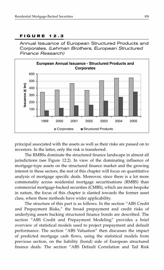
principal associated with the assets as well as their risks are passed on toinvestors. In the latter, only the risk is transferred.
The RMBSs dominate the structured finance landscape in almost alljurisdictions (see Figure 12.2). In view of the dominating influence ofmortgage-type assets on the structured finance market and the growinginterest in these sectors, the rest of this chapter will focus on quantitativeanalysis of mortgage specific deals. Moreover, since there is a lot morecommonality across residential mortgage securitisations (RMBS) thancommercial mortgage-backed securities (CMBS), which are more bespokein nature, the focus of this chapter is slanted towards the former assetclass, where these methods have wider applicability.
The structure of this part is as follows. In the section “ABS Creditand Prepayment Risks,” the broad prepayment and credit risks ofunderlying assets backing structured finance bonds are described. Thesection “ABS Credit and Prepayment Modeling” provides a briefoverview of statistical models used to project prepayment and defaultperformance. The section “ABS Valuation” then discusses the impactof predicted mortgage cash flows, using the statistical models fromprevious section, on the liability (bond) side of European structuredfinance deals. The section “ABS Default Correlation and Tail Risk
Residential Mortgage-Backed Securities 575
F I G U R E 1 2 . 3
Annual Issuance of European Structured Products andCorporates. (Lehman Brothers, European StructuredFinance Research)
European Annual Issuance - Structured Products andCorporates
-
100
200
300
400
500
600
1999 2000 2001 2002 2003 2004 2005
Corporates Structured Products
Issu
ance
(
bn
)

Scenarios” presents a methodology for assessing tail credit risk in ABSand the valuation impact this has on ABS bonds. The last section is the“Conclusion.”
ABS Credit and Prepayment Risks
The fundamental value of ABS is intimately related to the interest andprincipal cash-flows due on the bonds and the likelihood and timing ofthose being made in part or full. There are a number of key risks impact-ing the likelihood of these payments being made: defaults, delinquencies,losses, and prepayments. The former three of these constitute the creditrisk in a collateral pool, whereas the last relates intimately to investmentrisk. The first three risks interact with each other to reduce the totalamount of principal and interest available to bondholders. Note holdersare also subject to prepayment risk, as they may receive their proceedsmore quickly than originally anticipated, forcing them to re-invest thenotional amount at sub-optimal levels. This is a problem when the secu-rity they are holding is priced at a premium to par, which has been a fairlycommon scenario in the European ABS market over the past few years.Conversely, for securities priced at a discount to par, early redemption isbeneficial and allows bondholders to find a more efficient vehicle forinvesting their proceeds.
Figure 12.4 presents a fairly generic overview of the pricing of ABS.Statistical models provide projections of prepayments, and credit risk onthe asset side of the transaction. These models often take loan level vari-ables, such as a mortgage’s LTV ratio, loan size or term and may com-bine this with macro-economic information, on, e.g., interest rates.These projections are then used to adjust contractual mortgage cashflows and these are passed through a bespoke cash flow model, whichspecifies the order and priority of all these payments. By applying a sto-chastic interest rate model over all months and running many interestrate scenarios, a value for the ABS may be generated as an expectationover the interest rates. Alternatively, a value may be desired that leadsto an option-adjusted spread (OAS) to account for the stochastic natureof rates. This approach clearly has the advantage of factoring in thevolatility of interest rates.
The current practice in the European ABS market falls some way shortof the description above, as historical performance data is quite limited.Since the availability and quantity of such data is intimately linked with the
576 CHAPTER 12
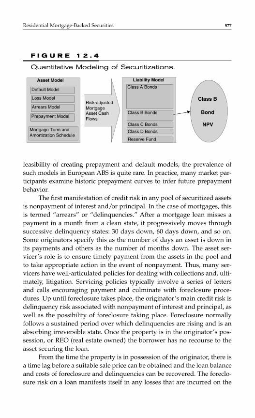
feasibility of creating prepayment and default models, the prevalence ofsuch models in European ABS is quite rare. In practice, many market par-ticipants examine historic prepayment curves to infer future prepaymentbehavior.
The first manifestation of credit risk in any pool of securitized assetsis nonpayment of interest and/or principal. In the case of mortgages, thisis termed “arrears” or “delinquencies.” After a mortgage loan misses apayment in a month from a clean state, it progressively moves throughsuccessive delinquency states: 30 days down, 60 days down, and so on.Some originators specify this as the number of days an asset is down inits payments and others as the number of months down. The asset ser-vicer’s role is to ensure timely payment from the assets in the pool andto take appropriate action in the event of nonpayment. Thus, many ser-vicers have well-articulated policies for dealing with collections and, ulti-mately, litigation. Servicing policies typically involve a series of lettersand calls encouraging payment and culminate with foreclosure proce-dures. Up until foreclosure takes place, the originator’s main credit risk isdelinquency risk associated with nonpayment of interest and principal, aswell as the possibility of foreclosure taking place. Foreclosure normallyfollows a sustained period over which delinquencies are rising and is anabsorbing irreversible state. Once the property is in the originator’s pos-session, or REO (real estate owned) the borrower has no recourse to theasset securing the loan.
From the time the property is in possession of the originator, there isa time lag before a suitable sale price can be obtained and the loan balanceand costs of foreclosure and delinquencies can be recovered. The foreclo-sure risk on a loan manifests itself in any losses that are incurred on the
Residential Mortgage-Backed Securities 577
F I G U R E 1 2 . 4
Quantitative Modeling of Securitizations.
Asset Model Liability Model
Default Model
Loss Model
Arrears Model
Prepayment Model
Class A Bonds
Class B Bonds
Class C Bonds
Class D Bonds
Risk-adjustedMortgageAsset CashFlows
Mortgage Term andAmortization Schedule
Reserve Fund
Class B
Bond
NPV
578 CHAPTER 12
loan. Typically, the priority of payments to different claimants is specifiedaccording to a schedule. Fees (administrative and legal for foreclosure)are normally senior, followed by arrears interest payments. The mostjunior payment tends to be the principal balance outstanding on the loan.Depending on the priority of claims, mortgage originators can lose a sub-stantial part of the principal balance outstanding at the time of propertysale. This situation is exacerbated if the loan itself is a second or third lien,in which case all cash received is first used to pay off claims on the moresenior mortgage loans.
When asset originators generate new loans for securitization, a keyrisk they bear is that obligors may decide to prepay the obligation earlierto take advantage of more attractive rates or other opportunities in themarket. Since assets are priced at a premium to par by originators, inorder to maintain the profitability of their business franchise, prepay-ments tend to limit the interest payments available to them and hence thevalue of the asset. Effectively, the originator of the asset must re-invest theloan amount lent to the obligor in the event of a prepayment at possiblyless attractive rates.
ABS Credit and Prepayment Modeling
Normally, prepayments are expressed as a conditional prepayment rate(conditional on a loan’s nonprepayment and nondefault up to a certainpoint in time) or CPR. This measure is calculated over a specific time hori-zon and is expressed as an annualized measure. If the asset balance in anasset-backed transaction is expressed at two successive points in time, t,and t + d as B(t) and B(t + d), with scheduled principal payments on theassets of S(t, t + d) over the period and unscheduled principal payments ofU(t, t + d), the prepayment rate may then be expressed as:
where d is the number of days in the time increment.The default rate can be calculated in a similar way as the proportion
of balance going into repossession over a given time period. The constantdefault rate (CDR) is an annualized default rate. Denoting DF(t, t + d) asthe actual total balance of loans in the asset pool going into foreclosureover the time period, we have:
CPR( , )
( ) ( )
( / )
= − −−
1 1365
U td
t + dB t S t, t + d
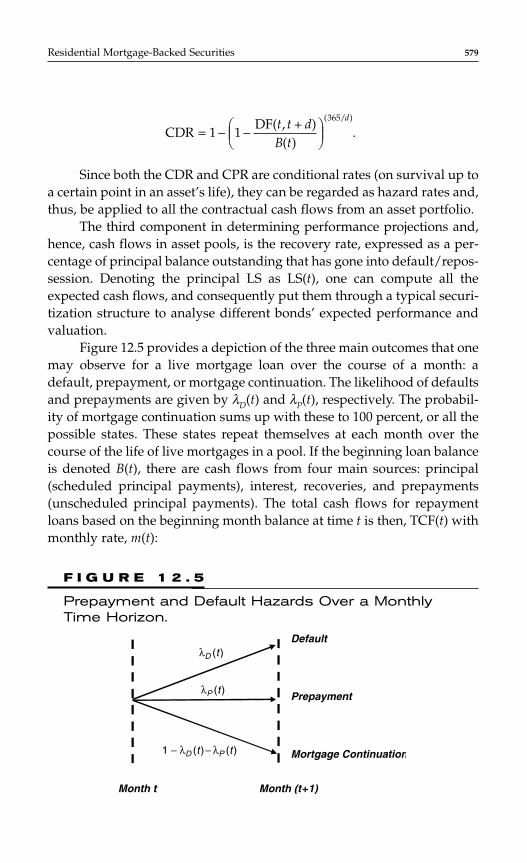
Since both the CDR and CPR are conditional rates (on survival up toa certain point in an asset’s life), they can be regarded as hazard rates and,thus, be applied to all the contractual cash flows from an asset portfolio.
The third component in determining performance projections and,hence, cash flows in asset pools, is the recovery rate, expressed as a per-centage of principal balance outstanding that has gone into default/repos-session. Denoting the principal LS as LS(t), one can compute all theexpected cash flows, and consequently put them through a typical securi-tization structure to analyse different bonds’ expected performance andvaluation.
Figure 12.5 provides a depiction of the three main outcomes that onemay observe for a live mortgage loan over the course of a month: adefault, prepayment, or mortgage continuation. The likelihood of defaultsand prepayments are given by λD(t) and λP(t), respectively. The probabil-ity of mortgage continuation sums up with these to 100 percent, or all thepossible states. These states repeat themselves at each month over thecourse of the life of live mortgages in a pool. If the beginning loan balanceis denoted B(t), there are cash flows from four main sources: principal(scheduled principal payments), interest, recoveries, and prepayments(unscheduled principal payments). The total cash flows for repaymentloans based on the beginning month balance at time t is then, TCF(t) withmonthly rate, m(t):
CDRDF( , )
( ).
( / )
= − −
1 1365
tB t
dt + d
Residential Mortgage-Backed Securities 579
Default
Prepayment
Mortgage Continuation
Month t Month (t+1)
1 − λD (t )− λP (t )
λD (t )
λP (t )
F I G U R E 1 2 . 5
Prepayment and Default Hazards Over a MonthlyTime Horizon.
TCF(t) = ICF(t) + PCF(t) + RCF(t) + PP(t)
where
RCF(t) = λD(t − ∆)(1 − LS(t − ∆))B(t − ∆),
PP(t) = λP(t)B(t),
where ∆ is the lag (in number of months) between the time properties arerepossessed and sold. ICF(t) is the interest cash flow, PCF(t) is the sched-uled principal cash flows, RCF(t) is the recovery cash flow associated withdefaulted mortgages, and PP(t) is the unscheduled principal cash flowfrom full prepayments. The hazard rates are applied to all of the cashflows in the equations above in a multiplicative way. Thus, the expectedunscheduled principal payment in month, t, is equal to the beginningmonthly mortgage balance, B(t), multiplied by the hazard of prepaymentstaking place in that month. To determine the cash flows in the next month(t + 1), one must determine the next month’s expected beginning asset bal-ance as the previous month’s expected balance minus the expected pre-payments in the period, principal cash flow, and default balance:
E[B(t + 1)] = B(t) − PP(t) − PCF(t) − λD(t)B(t)
In this successive way, future expected cash flows can be generatedfor all future months. The cash flows arising from the asset pool are thendependent on the deterministic and fixed nature of contractual mortgageloan characteristics (e.g., fixed rate period, interest-only or repayment,and prepayment penalties and rates), as well as the stochastic nature ofactual prepayments, defaults and losses, denoted by the hazards λD(t) andλP(t) and LS(t). These stochastic rates lend themselves well to economet-ric modeling.
Given a large enough performance data set, prepayments can be mod-eled as the conditional hazard of prepayment given survival at a particular
PCF( ) ( ) ( )( ) ( )
( )
( ) ( ) ,t t tB t m t
m t
B t m tD P T t= − −( )−
+
−
−1
11
1
λ λ
ICF( ) ( ) ( ) ( )t = 1 t B t m t ,−( )λD
580 CHAPTER 12
month in time following origination. In markets where full prepayments faroutweigh partial prepayments (e.g., the UK nonconforming mortgagemarket), this can be modeled as a binary event.
Suppose that the probability of full prepayment for loan i ∈1, . . . , N,conditional on survival up till month, t − 1, is denoted by λPi(t), in month tafter completion, and that this is modeled using the logistic function:
The likelihood function for a single loan can be computed as:
where T is the last possible monthly observation. It is fairly straightfor-ward to extend this to all loans in a sample to determine the log-likelihoodfunction of the data set. Such a model can easily be estimated using a sta-tistical package such as SAS or S-Plus. The academic literature on sucheconometric models is vast, largely in the context of U.S. mortgages [see,e.g., Deng et al. (2000) among others as well as references therein]. Lesseffort has been devoted to econometric modeling of defaults and prepay-ments of European mortgages. The most statistically significant variablesin such models vary by European ABS market.
The covariates themselves fall into a number of broad categories:
♦ Seasoning variables: In most prepayment models, mortgagorsare less inclined to prepay in the first few months than later inthe life of the mortgage loan. There may be other dependenciesover time and these may relate to structural features of the loan.
♦ Obligor-specific: This includes whether the borrower is single/married/widowed as well as the mortgagor’s past paymentbehavior. Bespoke credit scores may also play an important rolein predicting prepayments.
♦ Loan-specific: This can include the LTV ratio, which effectivelydetermines the loan’s leverage, as well as the term and the
L
t
V t Vi
Pit
t T
Pi Pit
V( )
( ( )), no prepayment .
( ) ( ) , prepayment in month .
β
λ
λ λ
=
−
−( )
=
=
=
−
∏
∏
1
1
1
1
1
λ
β βPi
j jij
Jt
x
( )
exp
=
+ − +
=
∑1
1 01
Residential Mortgage-Backed Securities 581
582 CHAPTER 12
presence of any prepayment penalties. These latter features areoften found to play a profound role in determining prepaymentsbecause of the economic incentives that may exist. The loanpurpose may often play a significant role in predicting prepay-ments, whether the loan is used to finance an investment prop-erty or for a mortgagor to be the owner-occupier. The rate on theloan also plays an important role in determining rate incentivesfor prepaying.
♦ Macroeconomic variables: This includes house prices, unemploy-ment rates, inflation rates, and, crucially, market interest rates.The dependence on these rates varies significantly by jurisdic-tion. For fixed rate mortgages, the rate incentive is important inpredicting prepayment behavior. If rates rally following origina-tion of a fixed rate mortgage loan, borrowers have a higherpropensity to prepay, all things equal. Conversely, in a sell-off,mortgagors are less incentivized to re-finance their mortgage.
The first three categories are usually fixed for the life of the mortgageloan, or vary in some deterministic way (e.g., loan term or remaining bal-ance). The last category of variables, however, evolve in a stochastic man-ner and lend themselves well to this type of modeling. Alternatively, bymaking specific assumptions on each of these variables, the resultant cashexpected flows can be computed under that particular scenario. There isa vast literature on pricing LIBOR market models (see, e.g., Brace et al.,1997) and by running many simulations with such an interest rate model,prepayments on a pool of mortgages can be generated for many possiblestates of the world.
The covariates themselves may assume quite complex functionalforms, such as polynomial functions or nonparametric kernel functions.Another popular approach is the use of cubic splines, which produce asmooth dependence of prepayments on the underlying covariate, whilecapturing the nuances of this dependence. As in all other univariate mod-eling, the danger of over-fitting is always a concern and these more com-plex functional forms must be tempered with an awareness of thispotential problem.
As in the case of prepayments, one can create loan level models ofdefaults, provided there is sufficient performance data, including a suffi-cient number of defaults. If there are insufficient defaults in a mortgagedata set, one may have to resort to using a more conservative default def-inition and adjust the model for loss severities to account for the higher

default rate. One possibility, e.g., is to model the probability of a loanbeing 90 or 180 days or more down at a particular month after origina-tion. This definition of default fits well with the regulatory framework inmost countries, as the Basel II Accord specifies this default definition. Theproblem with this definition, however, is that 90 or 180 days past due maynot technically or historically be a fully absorbing irreversible state. Thus,the modeling of loss severities will need to take this into account by beingconditioned on loans being 90 days down. This will introduce a largecohort of cured mortgage loans, which have zero loss. Analysis of mort-gage transition matrices is indispensable in informing such modelingdecisions. Low transition probabilities from high delinquency states tolower delinquency states suggest that using a more conservative defaultdefinition is less likely to be problematic. In other words, credit curing isnot very common and so 90 days past due is generally a robust measureof default.
As in the case of prepayment modeling, statistical models of defaultmay depend on macroeconomic variables, such as house prices and rates.By simulating these variables through separate stochastic models, creditrisk volatility can be introduced and evaluated in the context of portfoliosof mortgage loans.
The above paragraphs have discussed modeling mortgage prepay-ments and defaults as competing hazards. In other words, there are onlytwo events that can lead to mortgage termination with the former beingthe decision of the borrower, and the latter the decision of the originator.Another broad modeling approach for mortgage is to model the full tran-sition behavior of mortgages through finer arrears states. This involvesmodeling the probabilities of transitions one typically sees in a monthlymortgage transition matrix. The disadvantage with this approach, how-ever, is that estimation can be tricky if the performance data is limited andthe implementation is more cumbersome. With 300 months for a 25-yearmortgage loan one would have to calculate 300 transitions per mortgageloan to generate cash flows, as described earlier. Fortunately, mortgagearrears transition matrices are more sparse than other matrices, such ascredit rating transition matrices, as barring prepayments and defaults; themaximum downward migration in any monthly period can only be 30days of more arrears.
Figure 12.6 shows a typical mortgage transition matrix. In this matrix,each row corresponds to the initial state of a mortgage loan. These statesinclude: clean, 30 days past due, 60 days past due, 90 days past due, . . . ,default, prepayment. The columns correspond to the final mortgage state
Residential Mortgage-Backed Securities 583
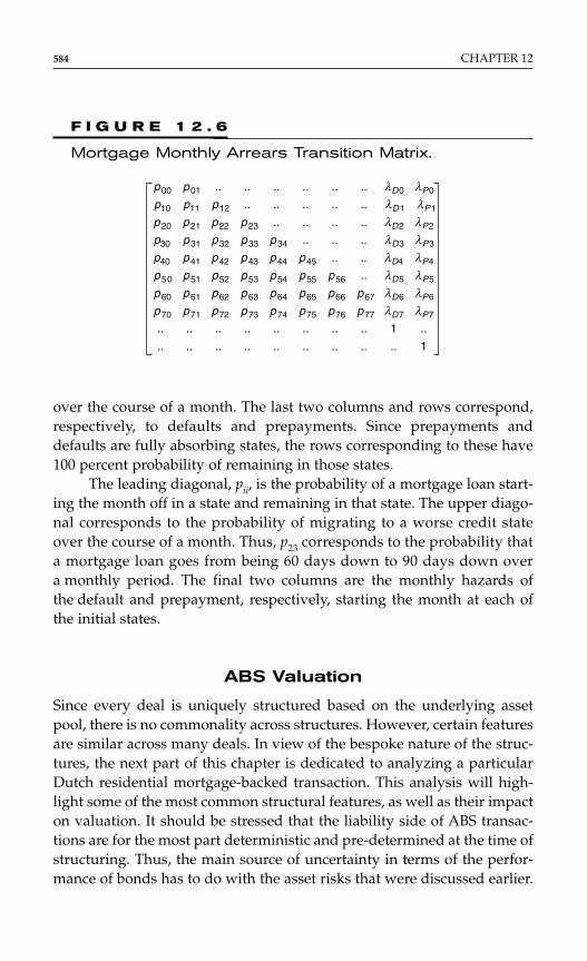
584 CHAPTER 12
over the course of a month. The last two columns and rows correspond,respectively, to defaults and prepayments. Since prepayments anddefaults are fully absorbing states, the rows corresponding to these have100 percent probability of remaining in those states.
The leading diagonal, pii, is the probability of a mortgage loan start-ing the month off in a state and remaining in that state. The upper diago-nal corresponds to the probability of migrating to a worse credit stateover the course of a month. Thus, p23 corresponds to the probability thata mortgage loan goes from being 60 days down to 90 days down overa monthly period. The final two columns are the monthly hazards ofthe default and prepayment, respectively, starting the month at each ofthe initial states.
ABS Valuation
Since every deal is uniquely structured based on the underlying assetpool, there is no commonality across structures. However, certain featuresare similar across many deals. In view of the bespoke nature of the struc-tures, the next part of this chapter is dedicated to analyzing a particularDutch residential mortgage-backed transaction. This analysis will high-light some of the most common structural features, as well as their impacton valuation. It should be stressed that the liability side of ABS transac-tions are for the most part deterministic and pre-determined at the time ofstructuring. Thus, the main source of uncertainty in terms of the perfor-mance of bonds has to do with the asset risks that were discussed earlier.
1..................
..1................
..
....
......
........
..........
............
P7D7
P6D6
P5D5
P4D4
P3D3
P2D2
P1D1
P0D0
p77p76p75p74p73p72p71p70
p67p66p65p64p63p62p61p60
p56p55p54p53p52p51p50
p45p44p43p42p41p40
p34p33p32p31p30
p23p22p21p20
p12p11p10
p01p00
λλλλλλλλλλλλλλλλ
F I G U R E 1 2 . 6
Mortgage Monthly Arrears Transition Matrix.

The BS structures usually have a combination of the followingsources of credit enhancement:
♦ Senior/subordinate bonds: credit enhancement is provided bymore junior tranches in the transaction by structurally forcingthem to take earlier losses from the asset pool.
♦ Over-collateralization: the notional amount of assets may belarger than the notional of bonds issued. In stressed loss scenar-ios, there are more assets which can be drawn upon to repayinterest and principal.
♦ Monoline wraps: large monoline insurers may guarantee theinterest and principal payments of senior tranches in transac-tions, thereby giving extra strength to the deal.
♦ Excess spread: this is the remaining interest after all trancheshave been paid off and losses incurred and provides the firstline of defense in most transactions.
♦ Reserve funds: these typically correspond to a percentage ofthe total deal size of the transaction. They may be funded infull at origination, or be built-up through excess spread overthe life of the transaction. In many cases, this fund amortizesover time.
Many European residential mortgage securitizations have a sequentialprincipal structure which reverts to a pro-rata structure. In this arrange-ment, all principal from the asset side is first used to pay down the prin-cipal on the most senior tranche. When a certain pro-rata trigger is met(e.g., the remaining bond balance on the most senior note reaches a frac-tion of the original amount), the entire deal reverts to a pro-rata pay downof the notes. Principal is paid down on a pro-rata basis across all notes.Interest is first used to pay the AAA class and then the AA class, and soon. If there is a shortfall in any note, the shortfall is registered in thatclass’s PDL. This then becomes senior in the waterfall and is paid off bysuccessive interest payments.
The Bloomberg screen shot (source: Bloomberg L. P.) in Figure 12.7 setsout the transaction structure of the Dutch MBS X transaction (deal pricedon March 27, 2003), which has quite a few features discussed earlier. Thedeal included five tranches: a AAA bond (the A class), a longer-life AAbond (the B class), a A bond (the C class), a BBB bond (the D class), and,finally, a BB bond (the E class). The transaction first pays down principalon the A class up to a pro-rata trigger.
Residential Mortgage-Backed Securities 585
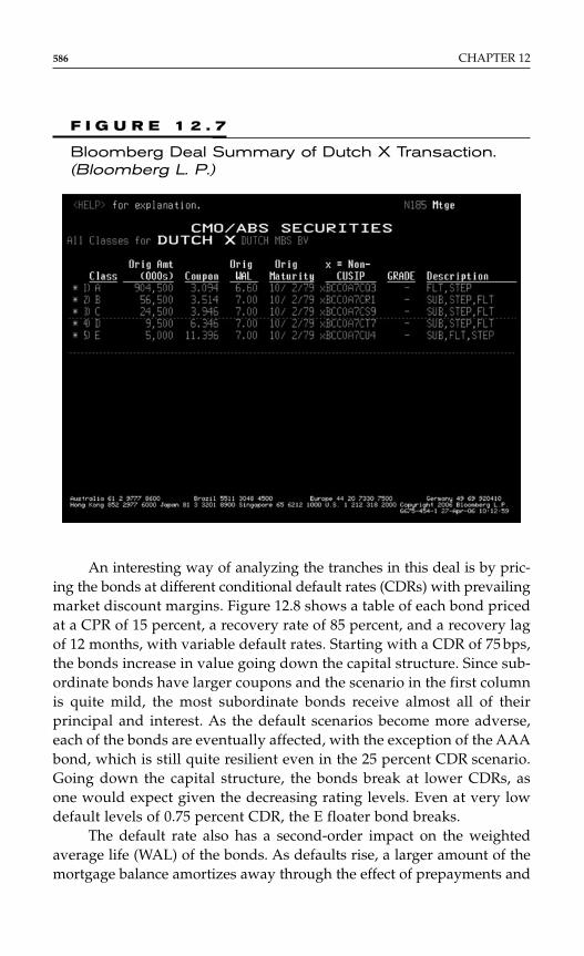
586 CHAPTER 12
An interesting way of analyzing the tranches in this deal is by pric-ing the bonds at different conditional default rates (CDRs) with prevailingmarket discount margins. Figure 12.8 shows a table of each bond pricedat a CPR of 15 percent, a recovery rate of 85 percent, and a recovery lagof 12 months, with variable default rates. Starting with a CDR of 75 bps,the bonds increase in value going down the capital structure. Since sub-ordinate bonds have larger coupons and the scenario in the first columnis quite mild, the most subordinate bonds receive almost all of theirprincipal and interest. As the default scenarios become more adverse,each of the bonds are eventually affected, with the exception of the AAAbond, which is still quite resilient even in the 25 percent CDR scenario.Going down the capital structure, the bonds break at lower CDRs, asone would expect given the decreasing rating levels. Even at very lowdefault levels of 0.75 percent CDR, the E floater bond breaks.
The default rate also has a second-order impact on the weightedaverage life (WAL) of the bonds. As defaults rise, a larger amount of themortgage balance amortizes away through the effect of prepayments and
F I G U R E 1 2 . 7
Bloomberg Deal Summary of Dutch X Transaction.(Bloomberg L. P.)
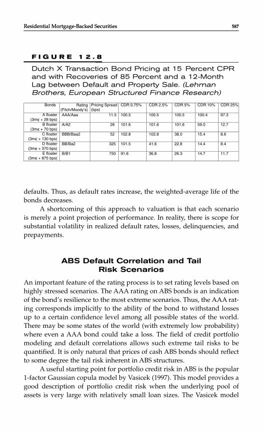
defaults. Thus, as default rates increase, the weighted-average life of thebonds decreases.
A shortcoming of this approach to valuation is that each scenariois merely a point projection of performance. In reality, there is scope forsubstantial volatility in realized default rates, losses, delinquencies, andprepayments.
ABS Default Correlation and Tail Risk Scenarios
An important feature of the rating process is to set rating levels based onhighly stressed scenarios. The AAA rating on ABS bonds is an indicationof the bond’s resilience to the most extreme scenarios. Thus, the AAA rat-ing corresponds implicitly to the ability of the bond to withstand lossesup to a certain confidence level among all possible states of the world.There may be some states of the world (with extremely low probability)where even a AAA bond could take a loss. The field of credit portfoliomodeling and default correlations allows such extreme tail risks to bequantified. It is only natural that prices of cash ABS bonds should reflectto some degree the tail risk inherent in ABS structures.
A useful starting point for portfolio credit risk in ABS is the popular1-factor Gaussian copula model by Vasicek (1997). This model provides agood description of portfolio credit risk when the underlying pool ofassets is very large with relatively small loan sizes. The Vasicek model
Residential Mortgage-Backed Securities 587Residential Mortgage-Backed Securities 587
Bonds Rating(Fitch/Moody’s)
Pricing Spread(bps)
CDR 0.75% CDR 2.5% CDR 5% CDR 10% CDR 25%
A floater AAA/Aaa 11.5 100.5 100.5 100.5 100.4 97.3
B floater A/A2 26 101.6 101.6 101.6 59.0 12.7
C floater BBB/Baa2 52 102.8 102.8 38.0 15.4 8.6
D floater BB/Ba2 325 101.5 41.6 22.8 14.4 8.4
E floater B/B1 750 91.6 36.8 26.3 14.7 11.7
(3m + 28 bps)
(3m + 70 bps)
(3m + 130 bps)
(3m + 370 bps)
(3m + 875 bps)
F I G U R E 1 2 . 8
Dutch X Transaction Bond Pricing at 15 Percent CPRand with Recoveries of 85 Percent and a 12-MonthLag between Default and Property Sale. (LehmanBrothers, European Structured Finance Research)
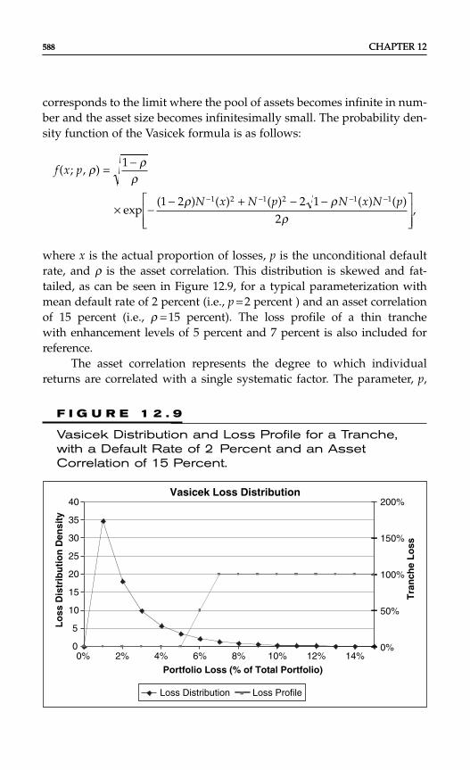
corresponds to the limit where the pool of assets becomes infinite in num-ber and the asset size becomes infinitesimally small. The probability den-sity function of the Vasicek formula is as follows:
where x is the actual proportion of losses, p is the unconditional defaultrate, and ρ is the asset correlation. This distribution is skewed and fat-tailed, as can be seen in Figure 12.9, for a typical parameterization withmean default rate of 2 percent (i.e., p = 2 percent ) and an asset correlationof 15 percent (i.e., ρ = 15 percent). The loss profile of a thin tranchewith enhancement levels of 5 percent and 7 percent is also included forreference.
The asset correlation represents the degree to which individualreturns are correlated with a single systematic factor. The parameter, p,
f x p
N x N p N x N p
( ; , )
exp( ) ( ) ( ) ( ) ( )
,
ρ ρρ
ρ ρρ
= −
× −− + − −
− − − −
1
1 2 2 12
1 2 1 2 1 1
588 CHAPTER 12588 CHAPTER 12
Vasicek Loss Distribution
0
5
10
15
20
25
30
35
40
0% 2% 4% 6% 8% 10% 12% 14%
Portfolio Loss (% of Total Portfolio)
Lo
ss D
istr
ibu
tio
n D
ensi
ty
0%
50%
100%
150%
200%
Tra
nch
e L
oss
Loss Distribution Loss Profile
F I G U R E 1 2 . 9
Vasicek Distribution and Loss Profile for a Tranche,with a Default Rate of 2 Percent and an AssetCorrelation of 15 Percent.

effectively sets the mean for the distribution of defaults, whereas the assetcorrelation sets the amount of volatility in the distribution.
The density distribution above leads to a closed-form solution forthe cumulative distribution function:
And, this may be inverted to give actual losses for different quantilelevels:
where x is the proportion of portfolio losses and α is the quantile level. If,e.g., α is set to 99.9 percent, then the portfolio losses are equal to theamount in this formula, with the twin parameters set to typical levels.
The Vasicek model can be used in the context of European mortgagesecuritizations to identify the likelihood of certain stressed scenarios. Bysetting the mean of the distribution of the Vasicek distribution to theexpected loss from an econometric model and by making some assump-tions about asset correlations, one can obtain stressed default rates basedon an objective opinion about the state of the world.
One way of determining such stressed scenarios for defaults andlosses is as follows. Suppose one is interested in looking at the 90 percentquantile level of worst possible credit risk scenarios. One can then takethe mean projected CDR and LS from an econometric model for these tworisks and take their product. This yields a projected curve of annualizedexpected losses (even though this does not take into account the effect oflags between default and property sale, where the loss is finally bookedin the transaction):
EL(t) = CDR(t) × LS(t)
One can then compute the upper quantile annualized loss at eachpoint in time using the Vasicek formula above. This then leads to the fol-lowing formula for the adjusted expected loss:
EL ( )EL( )
2
1 1
1t N
N t N= ( ) + ( )
−
− −ρ αρ
x NN p N
=+
−
− −1 1
1
( ) ( )ρ αρ
F x p NN x N p
( ; , )( ) ( )
ρρ
ρ=
− −
− −1 1 1
Residential Mortgage-Backed Securities 589Residential Mortgage-Backed Securities 589
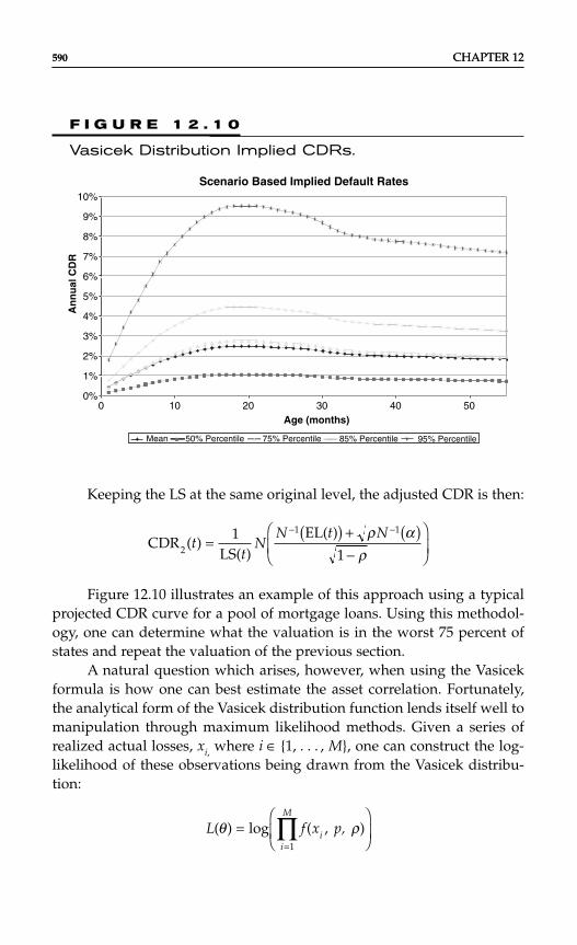
Keeping the LS at the same original level, the adjusted CDR is then:
Figure 12.10 illustrates an example of this approach using a typicalprojected CDR curve for a pool of mortgage loans. Using this methodol-ogy, one can determine what the valuation is in the worst 75 percent ofstates and repeat the valuation of the previous section.
A natural question which arises, however, when using the Vasicekformula is how one can best estimate the asset correlation. Fortunately,the analytical form of the Vasicek distribution function lends itself well tomanipulation through maximum likelihood methods. Given a series ofrealized actual losses, xi, where i ∈ 1, . . . , M, one can construct the log-likelihood of these observations being drawn from the Vasicek distribu-tion:
L f xii
M
( ) log ( , )θ ρ=
=∏ p,
1
CDR ( )LS( )
EL( )2
1 111
tt
NN t N
= ( ) + ( )−
− −ρ αρ
590 CHAPTER 12590 CHAPTER 12
Scenario Based Implied Default Rates
0%
1%
2%
3%
4%
5%
6%
7%
8%
9%
10%
0 10 20 30 40 50Age (months)
An
nu
al C
DR
Mean 50% Percentile 75% Percentile 85% Percentile 95% Percentile
F I G U R E 1 2 . 1 0
Vasicek Distribution Implied CDRs.
It can be shown that this log-likelihood function leads to the followingmaximum likelihood estimators for the mean default rate, p, and assetcorrelation, ρ, (see Khadem and Hofstetter, 2006 for details):
An attractive feature of these estimators is the fact that they are avail-able in closed-form and rely only on actual default data. Other approachesof estimating asset correlations based on actual loss data include Gordyand Heitfield (2000). The estimation involves estimating the asset correla-tion in the Vasicek model before the distribution is taken to the asymptoticlimit. This estimation necessitates maximizing the likelihood of a fairlycomplex function.
The first expression above allows the specification of bespoke assetcorrelations based on historical performance, and this can easily bemanipulated to obtain default correlations:
where the estimators are as included in the previous formulae.Given a sufficient amount of data from individual quarterly asset-
backed investor reports or other loan data, one may be able to deriveestimates of the asset correlation from the formula above. This, then, givesan indication of the tail risk in that particular asset class.
Conclusion
This brief part has presented a broad approach used for modeling cashABS transactions. Some attention has been devoted to considering creditvolatility and default correlations in ABS. Credit portfolio modeling-
ˆ( ˆ), ( ˆ), ˆ ˆ
ˆ( ˆ),ρ
ρD
N N p p p
p p=
( ) −−
− −2
1 1 2
1
N
ˆˆ
( ) .p NM
N xii
M=
−
−
=∑1 11
ρ
ˆ( / ) ( ) ( / ) ( )
( / ) ( ) ( / ) ( ),ρ =
−
−
+
− −==
−=
−=
∑∑∑ ∑
1 1
1 1 1
1 2 11
2
1
11
2 11
2
M N x M N x
M N x M N x
i ii
M
i
M
i
M
i ii
M
Residential Mortgage-Backed Securities 591Residential Mortgage-Backed Securities 591

techniques are relatively less developed in ABS than in structured credit,and this represents an interesting area of future research in ABS modeling.
REFERENCESBrace, A., D. Gaterek, and M. Musiela (1997), “The market model of interest rate
dynamics,” Mathematical Finance.Deng, Y., J. M. Quigley, and R. Van Order (2000), “Mortgage terminations, het-
erogeneity and the exercise of mortgage options,” Econometrica.Dietsch, M., and J. Petey (2002), “The credit risk in SME loans portfolios: model-
ling issues, pricing and capital requirements,” Journal of Banking andFinance.
Gordy, M., and E. Heitfield (2000), “Estimating factor loadings when ratings per-formance data are scarce,” working paper, Federal Reserve Board.
Khadem, V., and E. Hofstetter (2006), “A credit risk methodology for retail andSME portfolios,” working paper.
Vasicek, O. A. (1997), “Loan loss distribution,” working paper, KMV.
592 CHAPTER 12592 CHAPTER 12

C H A P T E R 1 3
Covered Bonds*
Arnaud de Servigny and Aymeric Chauve
593
INTRODUCTION
The concept of covered bonds has existed for about 200 years. This instru-ment was initiated by Frederick the Great of Prussia (Germany), with thecreation of “Pfandbriefe.” The underlying idea was to help project financ-ing. Typically, a bank issuing pfandbriefe bonds would be able to collater-alize the bonds with some underlying assets already on its balance sheet.
In simple terms, a covered bond is a financial product whose creditorsare benefiting from a pledge. This pledge usually corresponds to mortgageor public sector loans that are on the balance sheet of the issuing bank.
This product has remained a pure German instrument until recently,with mostly German investors purchasing local pfandbriefe issuance.Due to the globalization of the Western European economies as well as tothe rising appetite of non-German investors for this kind of very securedproduct, other countries have enacted laws to replicate the concept, amongwhich the French with “Obligations Foncières” or the Spanish with“Cédulas.” New jurisdictions continue to expand the universe of coveredbonds, with legal and regulatory frameworks being amended to facilitatethis development.
*We would like to thank Karlo Fuchs and Jean-Baptiste Michau for their support andcontribution.
Copyright © 2007 by The McGraw-Hill Companies. Click here for terms of use.
Apart from Germany, the fastest growing markets at the moment arethe United Kingdom, with its Structured covered bonds, the Netherlandsand, more recently, Italy. In the Nordic countries, regulation has evenwidened the scope of the product. Covered Bonds may, for instance, becollateralized by shipping loans.
PRODUCT CONSIDERATIONS
Structural Aspects
Let us clarify first the distinction between Pfandbriefe-like Covered Bondsand Structured Covered Bonds:
♦ Pfandbriefe-like Covered Bonds are bonds backed by mortgage orpublic sector assets in a well-defined regulatory environment.Practically, the local Financial Code/Act clearly sets the rulesapplicable to the product.
♦ Structured Covered Bonds are issued in jurisdictions where thereis no specifically adjusted regulatory framework. The robustnessunderlying this more recent type of product, such as the bondsissued in the United Kingdom, relies on a pure contractual basisand on legal opinions related to the case of insolvency of theissuing bank.
In both cases, the principle is that, upon insolvency of the issuing bank, atrustee (or administrator) would be appointed to service the registeredcover pool* and that such a pool would be segregated from the otherassets on the balance sheet of the bankrupt bank. One key point to notehere is that all covered bonds issued by a bank benefit from the sameregistered cover pool and are ranked pari passu.
Structured Covered Bonds can typically be compared to on-balancesheet replenishing residential mortgage backed securities (RMBS) andreference a portfolio of mortgage assets.
Pfandbriefe-like covered bonds can be split into two main segments:“mortgage-backed” Covered Bonds, which represent about 1/3 of theglobal market, and “public-sector backed” Covered Bonds, which repre-sent the remaining and historically correspond to a large proportion of theGerman market (Offentliche Pfandbriefe). However, some jurisdictions
594 CHAPTER 13
*The portfolio of mortgage and/or public loans that are granted as collateral to the coveredbonds holders.
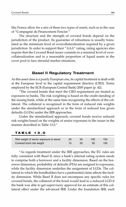
like France allow for a mix of these two types of assets, such as in the caseof “Compagnie de Financement Foncier.”
The structure and the strength of covered bonds depend on thejurisdiction of the product. Its guarantee of robustness is usually trans-lated as the minimum level of overcollateralization required by a givenjurisdiction. In order to support their “AAA” rating, rating agencies alsorequire that the Covered Bond issuer commits to a minimal level of over-collateralization and to a reasonable proportion of liquid assets in thecover pool to face stressful market situations.
Basel II Regulatory Treatment
As this asset class is a purely European one, its capital treatment is dealt withat the European level in the capital requirement directive (CRD). Termsemployed by the ECB (European Central Bank) 2005 paper (p. 42).
“The covered bonds that meet the CRD requirement are treated asexposures to banks. The risk weighting is based on the credit standing ofthe issuing bank, while at the same time recognizing the effects of the col-lateral. The collateral is recognized in the form of reduced risk weightsunder the standardized approach or in the form of reduced loss givendefaults (LGDs) under the IRB approaches.
Under the standardized approach, covered bonds receive reducedrisk weights based on the weights of senior exposures to the issuer in themanner described in Table 13.0.”
T A B L E 1 3 . 0
Risk weight of senior exposure to issuer 20 50 100 150
Covered bond risk weight 10 20 50 100
“As regards treatment under the IRB approaches, the EU rules arefully consistent with Basel II, since a bank’s internal rating system needsto comprise both a borrower and a facility dimension. Based on the bor-rower dimension, probability of defaults (PDs) are assigned to exposures,while the facility dimension underlies the assignment of LGDs. The col-lateral to which the bondholders have a preferential claim affects the facil-ity dimension. While Basel II does not encompass any specific rules forcovered bonds, the collateral of the bond would lead to a reduced LGD ifthe bank was able to get supervisory approval for an estimate of this col-lateral effect under the advanced IRB. Under the foundation IRB, such
Covered Bonds 595
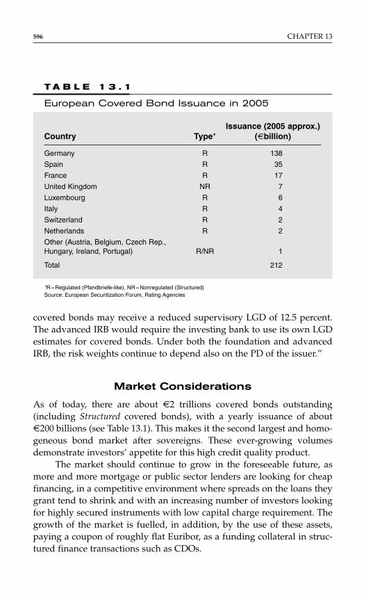
covered bonds may receive a reduced supervisory LGD of 12.5 percent.The advanced IRB would require the investing bank to use its own LGDestimates for covered bonds. Under both the foundation and advancedIRB, the risk weights continue to depend also on the PD of the issuer.”
Market Considerations
As of today, there are about m2 trillions covered bonds outstanding(including Structured covered bonds), with a yearly issuance of aboutm200 billions (see Table 13.1). This makes it the second largest and homo-geneous bond market after sovereigns. These ever-growing volumesdemonstrate investors’ appetite for this high credit quality product.
The market should continue to grow in the foreseeable future, asmore and more mortgage or public sector lenders are looking for cheapfinancing, in a competitive environment where spreads on the loans theygrant tend to shrink and with an increasing number of investors lookingfor highly secured instruments with low capital charge requirement. Thegrowth of the market is fuelled, in addition, by the use of these assets,paying a coupon of roughly flat Euribor, as a funding collateral in struc-tured finance transactions such as CDOs.
596 CHAPTER 13
T A B L E 1 3 . 1
European Covered Bond Issuance in 2005
Issuance (2005 approx.) Country Type* (mbillion)
Germany R 138
Spain R 35
France R 17
United Kingdom NR 7
Luxembourg R 6
Italy R 4
Switzerland R 2
Netherlands R 2
Other (Austria, Belgium, Czech Rep.,Hungary, Ireland, Portugal) R/NR 1
Total 212
*R = Regulated (Pfandbriefe-like), NR = Nonregulated (Structured)Source: European Securitization Forum, Rating Agencies

Almost all European countries have now set up a covered bond reg-ulation, with the noticeable exception of the United Kingdom. The latestcountry to have adopted such a regulatory framework is Italy with state-owned Cassa di Depositi e Prestiti having set up a m20 billion program inMarch 2005.
Market MomentumThe current market trend is around Jumbo issuances, i.e., issuances with a sizetypically exceeding m1 billion, and where the issuing bank and the arrangercommit to market making in order to ensure liquidity. This corresponds to achange as until a recent past most of the issuances where small private deals.
Spanish issuers are the most active in this area of public, high-volume,issues tapping a wide range of investors. According to the European secu-ritization forum, Spain has been overwhelming Germany recently, withabout m55 billion new Jumbo issuances, compared to a mere m50 billion forGermany.
The size and liquidity of the covered bond market is now such thatsome investment banks like J.P. Morgan-Chase have started offeringPfandriefe CDSs.
As already mentioned, the CDO market directly benefits from thegrowth of the covered bond market, with the increasing use of the prod-uct as a funding collateral to guaranty the payment of contingent claimsarising from defaults in the underlying CDO portfolio.
MODELING RISK IN COVERED BONDS*
In this section, we review the quantitative methodology that underpinsthe rating process at Standard & Poor’s (S&P).
As already mentioned, a covered bond is a debt instrument typicallyissued by a bank and overcollateralized by sound assets such as residentialmortgage loans or loans to the public sector. If the issuing bank is publiclycommitted to maintaining the overcollateralization levels commensuratewith target rating specific stress scenarios, S&P is usually able to assign arating to the transaction. This rating can be significantly higher than, anddelinked from the counterparty issuer credit rating, further enhancing theappeal of the market.†
Covered Bonds 597
*This part is derived from an S&P technical document produced by the authors.†For more information see “Expanding European covered bond universe Puts Spotlight onkey analytics,” July 16, 2004, available on S&P website.

S&P has used proprietary models to analyze the quality of pools ofassets and the adequacy of cash flow structures for several years. Theimproved transparency, which the products such as CDO Evaluator andCDS Accelerator have provided to participants in the CDO market, hasled S&P to offer the issuer a product Covered Bond Monitor (CBM)—acore analytical tool used in the analysis of covered bonds.
Currently, CBM is used to perform the quantitative analysis of cov-ered bond programs in Germany, Denmark, France, Ireland, andLuxembourg. It will also be used for upcoming Scandinavian coveredbonds.
The quantitative piece of the analysis of a covered bond can bebroadly split into two parts:
♦ A credit quality analysis performed by S&P analysts, whichresults in the determination of the default and recoveryassumptions applicable to the pool of the assets of the coveredbond transaction.
♦ An analysis of the strength of the structure under these defaultand recovery assumptions as well as under interest and foreignexchange rate stresses. This analysis leads to the assessment ofwhether the covered bond is strong enough to withstand thesestresses, and may obtain the target rating.
This technical section deals with the latter part of the analysis and pro-vides interested parties with further information on the advanced detailsof CBM. CBM aims to offer maximum transparency to the market. It con-sists of three parts. Firstly, an explanation of how the model simulatesinterest and foreign exchange rates. Secondly, details of how the defaultrisk on the asset side is factored in. Finally, the quantitative ratingeligibility test itself.
Interest Rate and Foreign Exchange Rate Simulation
Covered bonds are typically issued by banks whose main activity is mort-gage lending or public sector financing. In contrast to securitization trans-actions like RMBS, covered bonds programs are “on-balance sheet”instruments, collateralized by mortgages and/or public sector assets. Basedon its experience, S&P has observed that despite the regulatory and legalframeworks in place, covered bonds can be exposed to significant liquidity,
598 CHAPTER 13
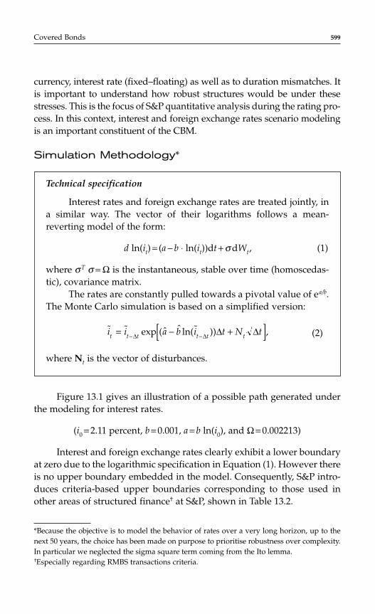
currency, interest rate (fixed–floating) as well as to duration mismatches. Itis important to understand how robust structures would be under thesestresses. This is the focus of S&P quantitative analysis during the rating pro-cess. In this context, interest and foreign exchange rates scenario modelingis an important constituent of the CBM.
Simulation Methodology*
Covered Bonds 599
Technical specification
Interest rates and foreign exchange rates are treated jointly, ina similar way. The vector of their logarithms follows a mean-reverting model of the form:
d ln(it) = (a − b ⋅ ln(it))dt + σ dWt, (1)
where σT σ = Ω is the instantaneous, stable over time (homoscedas-tic), covariance matrix.
The rates are constantly pulled towards a pivotal value of ea/b.The Monte Carlo simulation is based on a simplified version:
(2)
where Nt is the vector of disturbances.
˜ ˜ exp ( ˆ ˆ ln(˜ )) ,i i a b i t N tt t t t t t= − +[ ]− −∆ ∆ ∆ ∆
Figure 13.1 gives an illustration of a possible path generated underthe modeling for interest rates.
(i0 = 2.11 percent, b = 0.001, a = b ln(i0), and Ω = 0.002213)
Interest and foreign exchange rates clearly exhibit a lower boundaryat zero due to the logarithmic specification in Equation (1). However thereis no upper boundary embedded in the model. Consequently, S&P intro-duces criteria-based upper boundaries corresponding to those used inother areas of structured finance† at S&P, shown in Table 13.2.
*Because the objective is to model the behavior of rates over a very long horizon, up to thenext 50 years, the choice has been made on purpose to prioritise robustness over complexity.In particular we neglected the sigma square term coming from the Ito lemma.†Especially regarding RMBS transactions criteria.
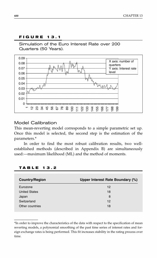
Model CalibrationThis mean-reverting model corresponds to a simple parametric set up.Once this model is selected, the second step is the estimation of theparameters.*
In order to find the most robust calibration results, two well-established methods (described in Appendix B) are simultaneouslyused:—maximum likelihood (ML) and the method of moments.
600 CHAPTER 13
F I G U R E 1 3 . 1
Simulation of the Euro Interest Rate over 200Quarters (50 Years).
X axis: number ofquartersY axis: Interest ratelevel
1 12 23 34 45 56 67 78 89 100
111
122
133
144
155
166
177
188
199
0.09
0.08
0.07
0.06
0.05
0.04
0.03
0.02
0.01
0
*In order to improve the characteristics of the data with respect to the specification of meanreverting models, a polynomial smoothing of the past time series of interest rates and for-eign exchange rates is being performed. This fit increases stability in the rating process overtime.
T A B L E 1 3 . 2
Country/Region Upper Interest Rate Boundary (%)
Eurozone 12
United States 18
Japan 8
Switzerland 12
Other countries 18
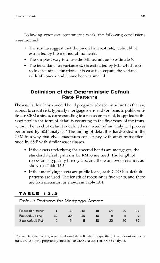
Following extensive econometric work, the following conclusionswere reached:
♦ The results suggest that the pivotal interest rate, i−, should be
estimated by the method of moments.♦ The simplest way is to use the ML technique to estimate b.♦ The instantaneous variance (Ω) is estimated by ML, which pro-
vides accurate estimations. It is easy to compute the variancewith ML once i
−and b have been estimated.
Definition of the Deterministic Default Rate Patterns
The asset side of any covered bond program is based on securities that aresubject to credit risk; typically mortgage loans and/or loans to public enti-ties. In CBM a stress, corresponding to a recession period, is applied to theasset pool in the form of defaults occurring in the first years of the trans-action. The level of default is defined as a result of an analytical processperformed by S&P analysts.* The timing of default is hard-coded in theCBM in a way that gives maximum consistency with other transactionsrated by S&P with similar asset classes.
♦ If the assets underlying the covered bonds are mortgages, thestandard default patterns for RMBS are used. The length ofrecession is typically three years, and there are two scenarios, asshown in Table 13.3.
♦ If the underlying assets are public loans, cash CDO-like defaultpatterns are used. The length of recession is five years, and thereare four scenarios, as shown in Table 13.4.
Covered Bonds 601
*For any targeted rating, a required asset default rate d is specified; it is determined usingStandard & Poor’s proprietary models like CDO evaluator or RMBS analyzer.
T A B L E 1 3 . 3
Default Patterns for Mortgage Assets
Recession month 1 6 12 18 24 30 36
Fast default (%) 30 30 20 10 5 5 0
Slow default (%) 0 5 5 10 20 30 30
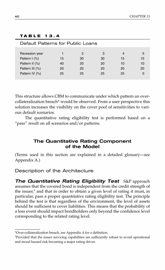
This structure allows CBM to communicate under which pattern an over-collateralization breach* would be observed. From a user perspective thissolution increases the visibility on the cover pool of sensitivities to vari-ous default scenarios.
The quantitative rating eligibility test is performed based on a“pass” result on all scenarios and/or patterns.
The Quantitative Rating Component of the Model
(Terms used in this section are explained in a detailed glossary—seeAppendix A.)
Description of the Architecture
The Quantitative Rating Eligibility Test S&P approachassumes that the covered bond is independent from the credit strength ofthe issuer,† and that in order to obtain a given level of rating it must, inparticular, pass a proper quantitative rating eligibility test. The principlebehind the test is that regardless of the environment, the level of assetsshould be sufficient to cover liabilities. This means that the probability ofa loss event should impact bondholders only beyond the confidence levelcorresponding to the related rating level.
602 CHAPTER 13
T A B L E 1 3 . 4
Default Patterns for Public Loans
Recession year 1 2 3 4 5
Pattern I (%) 15 30 30 15 10
Pattern II (%) 40 20 20 10 10
Pattern III (%) 20 20 20 20 20
Pattern IV (%) 25 25 25 25 0
*Over-collateralization breach, see Appendix A for a definition.†Provided that the issuer servicing capabilities are sufficiently robust to avoid operationaland moral hazard risk becoming a major rating driver.
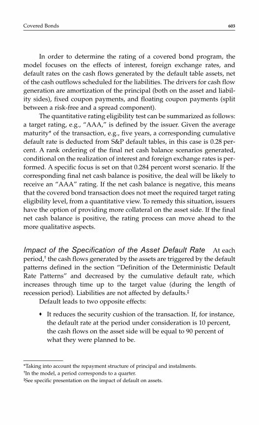
In order to determine the rating of a covered bond program, themodel focuses on the effects of interest, foreign exchange rates, anddefault rates on the cash flows generated by the default table assets, netof the cash outflows scheduled for the liabilities. The drivers for cash flowgeneration are amortization of the principal (both on the asset and liabil-ity sides), fixed coupon payments, and floating coupon payments (splitbetween a risk-free and a spread component).
The quantitative rating eligibility test can be summarized as follows:a target rating, e.g., “AAA,” is defined by the issuer. Given the averagematurity* of the transaction, e.g., five years, a corresponding cumulativedefault rate is deducted from S&P default tables, in this case is 0.28 per-cent. A rank ordering of the final net cash balance scenarios generated,conditional on the realization of interest and foreign exchange rates is per-formed. A specific focus is set on that 0.284 percent worst scenario. If thecorresponding final net cash balance is positive, the deal will be likely toreceive an “AAA” rating. If the net cash balance is negative, this meansthat the covered bond transaction does not meet the required target ratingeligibility level, from a quantitative view. To remedy this situation, issuershave the option of providing more collateral on the asset side. If the finalnet cash balance is positive, the rating process can move ahead to themore qualitative aspects.
Impact of the Specification of the Asset Default Rate At eachperiod,† the cash flows generated by the assets are triggered by the defaultpatterns defined in the section “Definition of the Deterministic DefaultRate Patterns” and decreased by the cumulative default rate, whichincreases through time up to the target value (during the length ofrecession period). Liabilities are not affected by defaults.‡
Default leads to two opposite effects:
♦ It reduces the security cushion of the transaction. If, for instance,the default rate at the period under consideration is 10 percent,the cash flows on the asset side will be equal to 90 percent ofwhat they were planned to be.
Covered Bonds 603
*Taking into account the repayment structure of principal and instalments.†In the model, a period corresponds to a quarter.‡See specific presentation on the impact of default on assets.
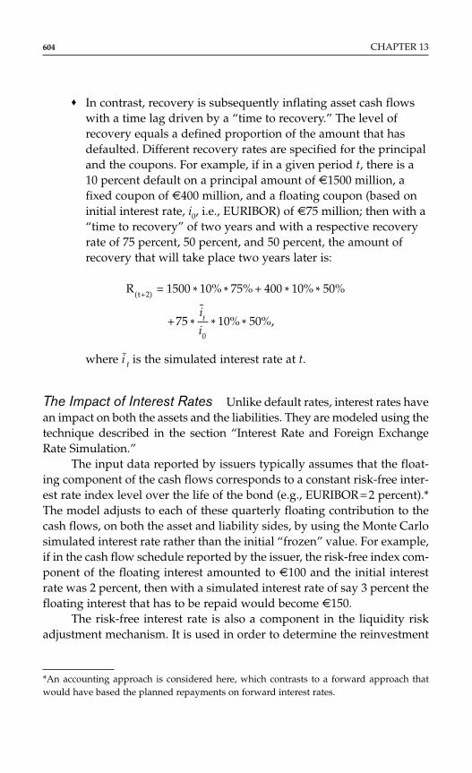
♦ In contrast, recovery is subsequently inflating asset cash flowswith a time lag driven by a “time to recovery.” The level ofrecovery equals a defined proportion of the amount that hasdefaulted. Different recovery rates are specified for the principaland the coupons. For example, if in a given period t, there is a10 percent default on a principal amount of m1500 million, afixed coupon of m400 million, and a floating coupon (based oninitial interest rate, i0, i.e., EURIBOR) of m75 million; then with a“time to recovery” of two years and with a respective recoveryrate of 75 percent, 50 percent, and 50 percent, the amount ofrecovery that will take place two years later is:
where i~
t is the simulated interest rate at t.
The Impact of Interest Rates Unlike default rates, interest rates havean impact on both the assets and the liabilities. They are modeled using thetechnique described in the section “Interest Rate and Foreign ExchangeRate Simulation.”
The input data reported by issuers typically assumes that the float-ing component of the cash flows corresponds to a constant risk-free inter-est rate index level over the life of the bond (e.g., EURIBOR = 2 percent).*The model adjusts to each of these quarterly floating contribution to thecash flows, on both the asset and liability sides, by using the Monte Carlosimulated interest rate rather than the initial “frozen” value. For example,if in the cash flow schedule reported by the issuer, the risk-free index com-ponent of the floating interest amounted to m100 and the initial interestrate was 2 percent, then with a simulated interest rate of say 3 percent thefloating interest that has to be repaid would become m150.
The risk-free interest rate is also a component in the liquidity riskadjustment mechanism. It is used in order to determine the reinvestment
R = * * + * *
+ * * *
t+( 2)
0
1500 10% 75% 400 10% 50%
75˜
10% 50%,i
it
604 CHAPTER 13
*An accounting approach is considered here, which contrasts to a forward approach thatwould have based the planned repayments on forward interest rates.
rate of the cash balance. In the model, there is a reinvestment margin overthe simulated risk-free interest rate if the cash balance is positive and aborrowing margin if it is negative. The margins embedded in the modelare −50 bps and 100 bps, respectively.
The Impact of Foreign Exchange Rates Foreign exchange ratesare simulated in a similar way, and in conjunction with interest rates.They are only used to convert the cash balances into the pool’s workingcurrency, typically euros. When there are periodic non-euro deposits,then cash balances are transformed into euros at the end of eachquarterly period, using the simulated foreign exchange rate for thatperiod.
The Quantitative Rating Eligibility Test Once all thesimulated cash flows generated by assets and liabilities have been com-puted, the model generates the final net cash balance corresponding toeach realization of the foreign exchange/risk-free interest rates. If it isnegative, the covered bond is considered to be in default. In order to getto this final net cash balance, the model computes for each simulation theevolution over time of the cumulative cash balance. It then counts the pro-portion of iterations that end up with a negative final cash balance. If thisproportion is smaller than the default rate tolerated for the targeted ratinglevel, then the covered bond passes the quantitative rating eligibility test.In the example given in Figure 13.2, the final cash balance at the requiredpercentile is positive, therefore the covered bond passes the test. Clearly,the percentile is lower for higher ratings and accordingly, the tolerance inthe number of failing runs is lower.
Additional Features
Treatment of Recoveries
♦ Mortgage assets
As soon as a default occurs, recovery impacts the entire value ofthe mortgage loan (on the asset side) that was affected by thedefault.
To illustrate this point, let At, Pt, and ct denote the out-standing asset, the principal repayment and the cumulative
Covered Bonds 605
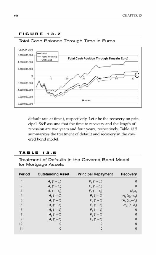
default rate at time t, respectively. Let r be the recovery on prin-cipal. S&P assume that the time to recovery and the length ofrecession are two years and four years, respectively. Table 13.5summarizes the treatment of default and recovery in the cov-ered bond model.
606 CHAPTER 13
F I G U R E 1 3 . 2
Total Cash Balance Through Time in Euros.
0 10 20 30 40 50 60
Quarter
6,000,000,000
4,000,000,000
2,000,000,000
0
−2,000,000,000
−4,000,000,000
−8,000,000,000
Cash, in Euro
Mean
Rating Percentile
Unstressed Total Cash Position Through Time (in Euro)
−6,000,000,000
T A B L E 1 3 . 5
Treatment of Defaults in the Covered Bond Model for Mortgage Assets
Period Outstanding Asset Principal Repayment Recovery
1 A1 (1 − c1) P1 (1 − c1) 0
2 A2 (1 − c2) P2 (1 − c2) 0
3 A3 (1 − c3) P3 (1 − c3) rA1c1
4 A4 (1 − c–) P4 (1 − c–) rA2 (c2 − c1)
5 A5 (1 − c–) P5 (1 − c–) rA3 (c3 − c2)
6 A6 (1 − c–) P6 (1 − c–) rA4 (c–− c3)
7 A7 (1 − c–) P7 (1 − c–) 0
8 A8 (1 − c–) P8 (1 − c–) 0
9 A9 (1 − c–) P9 (1 − c–) 0
10 0 0 0
11 0 0 0

♦ Public sector assets
Public sector issuers often rely on some support from othergovernment levels and ultimately on the tax base in the con-cerned country. S&P therefore considers that a default wouldnot usually result in an ultimate loss of principal, but that pay-ments, including arrears, would be resumed after a certainperiod of time. For public sector issuers S&P assumes thatrecovery rates would be close to 100 percent, although interestrate conditions may be renegotiated after default. An exampleis shown in Table 13.6, with a two-year time to recovery and afour-year recession.
As a result, S&P focus on the redemption cash flows,rather than on outstanding assets and liabilities for mortgagepools. However, the net effect for both is largely similar. In ear-lier periods of the remaining life of the pool, cash inflows arelower than planned, owing to payment delays occurring. Lateron, most of these amounts are recovered so that in particular forpublic sector assets simulated cash inflows could even be higherthan planned.
Covered Bonds 607
T A B L E 1 3 . 6
Treatment of Defaults in the Covered Bond Modelfor Public Sector Assets
Outstanding Principal Current Period Asset Repayment Recovery
1 A1 (1 − c1) P1 (1 − c1) 0
2 A2 (1 − c2) P2 (1 − c2) 0
3 A3 (1 − c3) P3 (1 − c3) rP1c1
4 A4 (1 − c–) P4 (1 − c–) rP2c2
5 A5 (1 − c–) P5 (1 − c–) rP3c3
6 A6 (1 − c–) P6 (1 − c–) rP4c–
7 A7 (1 − c–) P7 (1 − c–) rP5c–
8 A8 (1 − c–) P8 (1 − c–) rP6c–
9 A9 (1 − c–) P9 (1 − c–) rP7c–
10 0 0 rP8c–
11 0 0 rP9c–
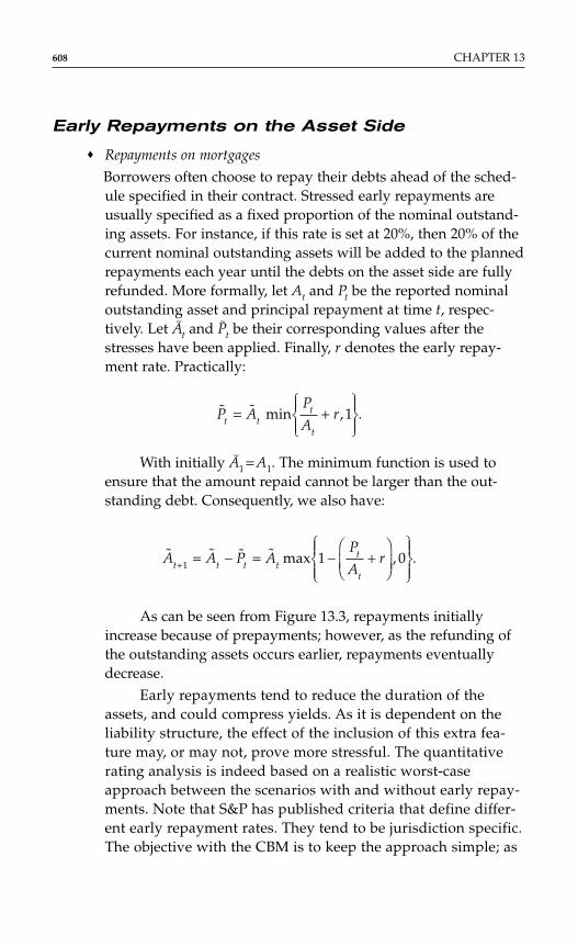
Early Repayments on the Asset Side
♦ Repayments on mortgages
Borrowers often choose to repay their debts ahead of the sched-ule specified in their contract. Stressed early repayments areusually specified as a fixed proportion of the nominal outstand-ing assets. For instance, if this rate is set at 20%, then 20% of thecurrent nominal outstanding assets will be added to the plannedrepayments each year until the debts on the asset side are fullyrefunded. More formally, let At and Pt be the reported nominaloutstanding asset and principal repayment at time t, respec-tively. Let A
~t and P
~t be their corresponding values after the
stresses have been applied. Finally, r denotes the early repay-ment rate. Practically:
With initially A~
1 = A1. The minimum function is used toensure that the amount repaid cannot be larger than the out-standing debt. Consequently, we also have:
As can be seen from Figure 13.3, repayments initiallyincrease because of prepayments; however, as the refunding ofthe outstanding assets occurs earlier, repayments eventuallydecrease.
Early repayments tend to reduce the duration of theassets, and could compress yields. As it is dependent on theliability structure, the effect of the inclusion of this extra fea-ture may, or may not, prove more stressful. The quantitativerating analysis is indeed based on a realistic worst-caseapproach between the scenarios with and without early repay-ments. Note that S&P has published criteria that define differ-ent early repayment rates. They tend to be jurisdiction specific.The objective with the CBM is to keep the approach simple; as
˜ ˜ ˜ ˜ max , .A A P AP
Art t t t
t
t+ = − = − +
1 1 0
˜ ˜ min , .P AP
Art t
t
t
= +
1
608 CHAPTER 13
a consequence, the value retained in the model corresponds toa weighted-average of the appropriate prepayment rates.
♦ Prepayments on public finance
Public finance assets are typically not exposed to prepaymentrisk; so early repayment is usually not factored into the analysis.
Servicing Fees The liquidity stress included in the model implic-itly assumes that the parent bank can go out of business and that the rat-ing is performed on an extinguishing cash flow profile. It is thereforereasonable to include servicing fees that represents the management costof the structure issuing the covered bonds. These fees typically correspondto a fixed proportion of the nominal outstanding assets that should be sub-tracted each period from the cash balance. If s denotes the servicing fee peryear expressed as a percentage, and At the outstanding assets at time t,then the servicing fee that has to be paid at quarter t equals (s/4)* At.
MacroSwaps Issuers often buy swaps to hedge interest rate andcurrency risk, e.g., by converting a flow of fixed interests into floatinginterests. In the case of macroswaps, i.e., where the notional of the swapsis expected to follow, albeit imperfectly, the dynamics of the asset, two
Covered Bonds 609
F I G U R E 1 3 . 3
Principal Repayment of Assets.
Contractual With Early Repayments
1 5 9 13 17 21 25 29 33 37 41 45 49 53 57
Quarters
7000
6000
4000
5000
3000
2000
1000
0
M
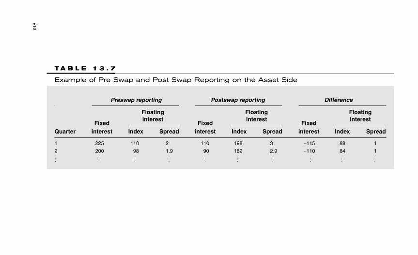
T A B L E 1 3 . 7
Example of Pre Swap and Post Swap Reporting on the Asset Side
Preswap reporting Postswap reporting Difference
Fixed
Floating
Fixed
Floating
Fixed
Floating
interest
interest
interest
interest
interest
interest
Quarter Index Spread Index Spread Index Spread
1 225 110 2 110 198 3 −115 88 1
2 200 98 1.9 90 182 2.9 −110 84 1
610
… ………………………
types of risks can arise:
♦ On the positive side, the swaps modify and usually reduce theexposure of the bank to interest rate risk; and
♦ On the negative side, because of defaults on the asset side, thenotional of the swap will turn out to only match the underlyingexposure approximately and will accordingly put the coveredbond transaction at risk.
The input data received by S&P from covered bond issuers does not typ-ically include the detail of the swap contracts in which the issuers areinvolved with respect to their covered bond programs. Issuers generallyprovide a pre swap ALM (Asset Liability Management) report (before theeffect of swaps is included) and a postswap ALM report (after the effectof swaps is included). Assuming these swaps are in compliance with S&Pcriteria, the difference between the two reports gives the net series ofexposures that has been swapped, including fees. This series is sensitiveto interest rate fluctuations, however, it is not sensitive to the occurrenceof defaults, as swap contracts are not subject to the realization of eventsaffecting the covered bond asset pool. The easiest way to model the effectof these macroswaps is therefore to add the difference between thepostswap and the pre swap reports to the existing liabilities.
Table 13.7 gives an example of pre swap and postswap reports onthe asset side. In the first quarter, the bank has swapped m115 of fixedinterests into m89 of floating interests [split between m88 risk-free (index)and m1 spread]. As can be seen in the table, the net effect of the swap caneasily be identified by observing the difference between the two reports.*Obviously, the value of the risk-free floating component, and therefore thecost of the swap, will be affected by interest rate changes. This explainswhy each column should be treated separately.
After the realization, i~
i, of the simulated interest rate has beenapplied to the risk-free rate component, the impact of the swap can becomputed.
For example, in quarter 1, this cost is:
− + +115 88 11
0
˜.
i
i
Covered Bonds 611
*It should be emphasized that the reported flow corresponding to the risk-free componentof the floating interest is based on the initial interest rate i0.

Similarly in quarter 2, the cost of the swap is:
This cost should be added to the preswap net cash flow of the cor-responding period. Denoting Kt the cash balance and cft the net cash flow(preswap) at time t, we have for quarter 1:
An easy way to take the cost of swaps into account is to add it (seeTable 13.7, column 3) to the preswap liabilities. The reason why the costof macroswaps is included to the preswap liabilities rather than to theassets, is a practical one. It is to ring-fence it from the occurrence ofdefaults. By including it in liabilities, it will be affected by interest ratechanges, but not by the default rate patterns.
Communication of ResultsCBM focuses on the value and sign of the final cash balance based on theassets and liabilities after the different stresses have been applied in orderto help S&P analysts be able to assign a rating.
In order to improve transparency and communication, Standard andPoor’s is careful to articulate results according to the terminology used bycovered bond issuers.
Issuers typically target an “AAA” rating for their covered bond pro-grams. They are usually interested to know what collateral margin isneeded to secure this rating or to know the quantity of extra assets theyneed to add or remove as collateral during the life of the transaction inorder to maintain the initial rating level (see definition of the break-evenportfolio in Appendix A).
Issuers also communicate on their unstressed schedule of assets andliabilities. S&P therefore provides relevant reporting in this respect.Market participants typically focus on two key parameters, one regardingtheir level of current overcollateralization and another one regarding theduration gap between assets and liabilities.
♦ Overcollateralization: Issuers are increasingly communicatingwith the market and the rating agencies in terms of collateralsurpluses defined as overcollateralization. Communication can
K i K cfi
i1 1 0 11
0
1 115 88 1= + + + − + +
( ˜ )
˜.
− + +110 84 12
0
˜.
i
i
612 CHAPTER 13

either be provided in terms of a nominal overcollateralization orin terms of a net present value (NPV) overcollateralization (seeglossary in Appendix A for the definition of terms).
♦ Duration: Duration is an important communication element asthere is increasing focus from customers and regulators on theduration gap.
Identifying the Break-even Portfolio with anOvercollateralization Focus From a S&P perspective a crit-ical point is to evaluate how far, from a quantitative point of view, thestructure is from the break-even portfolio corresponding to the ratinglevel in consideration. Given the initial reporting provided by the bank,there are two simple ways of getting to (and communicating on) thebreak-even portfolio. One can either initially add or subtract cash, or alter-natively, increase or decrease proportionally the amount of assets ownedby the bank.
♦ Initial cash
There are several ways of communicating the break-even pool.First the model gives the initial amount of cash that could bewithdrawn (or that needs to be added) such that the rating isjust secured. Let Kt, it, and cft be the cash balance, the interestrate (risk-free interest rate plus bid/ask margins*) and the netcash flow (flow of assets minus flow of liabilities) at time t,respectively.We have:
Kt = (1 + it)Kt − 1 + cft
As the interest rate it comprises borrowing and reinvest-ment margins that depend on the sign of Kt − 1, it requires somecalculation effort to obtain the initial amount of cash that couldbe withdrawn from the final cash balance, KT .
♦ Proportional increase or decrease of assets
The other way to communicate on the break-even pool is to givethe proportion by which the nominal outstanding assets and the
Covered Bonds 613
*Under Standard & Poor’s criteria, it = i~
t + 1% ⋅ IKt − 1 < 0 − 0.5% ⋅ IKt − 1 ≥ 0 where i~
t is thesimulated risk-free interest rate and I is an indicator. Recall that the indicator is such that
I if is True
if is False .A
A
A=
1
0

cash flow they generate can be reduced (or increased), so that thefinal cash balance at the quantile level corresponding to the ratingtarget is zero. However, it is not possible to compute the exactvalue of this proportion without resorting to an iterative process.
Adjustment of the Portfolio with a Duration FocusCBM tries to help communication with market participants in a way thatenables covered bond issuers to adjust their portfolio within the con-straints of their commitments and such that they obtain the desired rat-ing. This section explains how CBM adjusts the portfolio, with a focus onthe duration gap, while also maintaining the targeted rating.
Throughout the proposed procedure it is assumed that the durationof assets does not change. In order to change the duration gap, the CBMuser can only change the duration of liabilities by adding or repurchasingcovered bonds with a given bullet maturity τ. The interest rate, it, paid onthese bonds is reported by the user. As illustrated in the calculation below,this allows us to determine the quantity of covered bonds, Cτ , that needsto be issued in order to reach the desired duration for liabilities. Let Bt bethe cash flow generated by the newly issued bonds, then:
If lt denote the flow of liabilities and Γ the targeted duration for lia-bilities, then Cτ must be found such that:
This gives:
C
tl
i
ti
i i
t
ss
tt
T
t
t
ss
t
ss
τ τ
ττ
=
−+
−+
+ −
+
=
=
=
= =
∏∑
∑∏ ∏
( )( )
( )ˆ
( ) ( )
.
Γ
Γ Γ
1
1 1
1
1
1
1 1
t B l i
B l i
t t ss
t
t
T
t t ss
t
t
T
⋅ + +
+ +
===
==
∏∑∏∑
( ) ( )
( ) ( ).
1
1
11
11
Γ
B
i C t
i C C t
tt
t
=
<
+ =>
ˆ ,
ˆ ,
,
.
τ
τ τ τ
τ
ττ0
614 CHAPTER 13
Once these new bullet single maturity covered bonds have beenissued, we can apply the described procedure to discover the quantity ofassets, or how much initial cash needs to be added in order to obtain abreak-even portfolio.
CONCLUSION
This model has been designed to be as simple as possible in order to pro-vide strong visibility to investors and issuers. It is in addition meant to berobust in the sense that it allows for seriously stressed conditions and thatits conclusions do not rely on the support of the issuing bank. It is ulti-mately as consistent as possible with the other rating tools developed byS&P. Note that the quantitative analysis performed with CBM is only partof the rating process for S&P. Potential users shall be aware that S&Preserve the right to assign the suggested rating or not, based, among otherthings, on qualitative and legal analysis.
A P P E N D I X A
Glossary of Terms
DEFINITIONS
Break-Even Pool
A pool that just passes the quantitative rating eligibility test, i.e., a poolwith final cash balance of zero.
Cash Balance
The cash balance at time t represents the total amount of cash available tothe bank at time t. (Note it is a stock rather than a flow.)
Cash Flow
The (net) cash flow at time t is the difference between the cash generatedby assets and by liabilities over the tth period.
Covered Bonds 615

Duration
The duration of assets and liabilities is the discounted weighted averagetime at which their respective cash flows occur. Let ct
Tt = 1 denote a cash
flow series, then its duration is defined as:
where it is the interest used for discounting, typically the forward rate.
Duration Gap
The duration gap between assets and liabilities is one of the key parame-ters on which banks focus; it gives information on the mismatch in thetiming of cash flows. Market practice in the covered bond area is to com-pute the duration gap as the difference between the duration of the assetsand that of the liabilities is,
Duration gap = duration of assets − duration of liabilities
where at and lt denote the asset and liability flows at time t. It is clearfrom the equation that the duration of assets is computed indepen-dently from duration of liabilities. It can also be noted that the durationgap is different from the duration of the net cash flow as usuallyexpressed:
Duration of assets − duration of liabilities ≠ duration of (assets −liabilities).
Final Cash Balance
The cash balance observed at the last period, after the different stresses(defaults, interest rates, . . . ) have been applied. The pool under con-sideration passes the rating test if and only if the final cash balance ispositive.
t a i
a i
t l i
l i
t ss
t
t
T
t ss
t
t
T
t ss
t
t
T
t ss
t
t
T
⋅ +
+
−⋅ +
+
==
==
==
==
∏∑∏∑
∏∑∏∑
( )
( )
( )
( ),
1
1
1
1
11
11
11
11
Duration( )
( )=
⋅ +
+
==
==
∏∑∏∑
t c i
c i
t ss
t
t
T
t ss
t
t
T
1
1
11
11
616 CHAPTER 13

Net Present Value
The NPV of a cash flow ctTt = 1 is given by:*
The interest rate, it, used for discounting in the computation of theNPVO/C is given by the prevailing market yield curve, considered as theforward value of three-month interest rates (e.g., Euribor).
Nominal Overcollateralization
Amount by which the outstanding assets initially exceed the outstandingliabilities. If A1 and L1 denote the initial nominal outstanding assets andliabilities, then:
NPV Overcollateralization
Amount by which the initial net present value of assets (i.e., the sum of alldiscounted flows starting from the first period) exceeds that of the liabil-ities. If NPVA and NPVL denote the initial net present value of thoseflows, then:
Overcollateralization
Overcollateralization, amount by which assets exceed liabilities. The twomost important measures of overcollateralization are the nominal over-collateralization and the NPV overcollateralization.
NPVO/CNPVA NPVL
NPVL.= −
Nominal O/C .=−A L
L1 1
1
NPV( )
.=+
== ∏∑ c
it
ss
tt
T
11
1
Covered Bonds 617
*The net present value is sometimes computed as:
∑T
t=1ct/(1 + it)
t.
However, the formula reported in the text is more accurate.

Main Relations
Cash Balance and Cash FlowsLet Kt, it, and cft be respectively the cash balance, the interest rate, and thenet cash flow (flow of assets minus flow of liabilities) at time t. We have:
Kt = (1 + it)Kt − 1 + cft. (1)
Note: if several currencies are involved, the net cash flows generatedin foreign currencies should be converted into euros and added to thedomestic cash flows.
Discounted Final Cash Balance and Net PresentValue of the Cash FlowsBy iterating Equation 1, we obtain:
In the special case where it is the forward interest rate, then we have:
There is therefore a link between the final cash balance and theNPVO/C (expressed in euros rather than as a percentage).
NPV Overcollateralization and NominalOvercollateralizationIt turns out that the two measures of O/C are closely related. Let At’ andAt” denote the nominal outstanding fixed and floating assets at time t,respectively; similarly for Lt’ and Lt”. Let it be the forward risk-free interestrate used for discounting and used as index in the computation of thefloating interest that has to be paid. Let i
−A, t be the fixed interest rate cor-
responding to received coupons on fixed assets;* similarly i−
L,t corresponds
K
i i iT
T( )( ) ( )NPVA NPVL
1 1 11 2+ + += −
L
K
i i iK
cf
i
cf
i i
cf
i i i
T
T
T
T
( )( ) ( ) ( )( )
( )( ) ( ).
1 1 1 1 1 1
1 1 1
1 20
1
1
2
1 2
1 2
+ + += +
++
+ +
+ ⋅ ⋅ ⋅ ++ + ⋅ ⋅ ⋅ +
L
618 CHAPTER 13
*The fixed interest rate is time dependent because the aggregate asset is made of differentassets having different maturities and paying different fixed interest rates.

to coupons due on fixed liabilities. Finally, SA, t and SL, t denote the spread com-ponent in currency units (e.g., in euros) of the floating interest of assets andliabilities, respectively. We have:
and it could be checked that:
It can easily be seen that the difference between the nominal O/Cand the NPV_O/C is entirely due to the difference between the effectivefixed or floating interest rates and the risk-free interest rate.
A P P E N D I X B
MAXIMUM LIKELIHOOD
The simplified discretized version of the model can also be written as:
(3)
The discretized model (3) turns out to be a linear regression model.As ML and Ordinary Least Squares give the same estimates for a and b,we can use this latter technique that is much simple to implement.
METHOD OF MOMENTS
Starting from the discretized version of the model, for a given interest, wehave:
ln(it) = a + (1 − b)ln(it − 1) + εt
ln( ) ln( ) ( ln( )) .i i a b i t R tt t t i t t− = − ⋅ +− −∆ ∆ ∆ ∆σ
NPVO/C
( ) ( )
( )
( )
( )
, , , ,
, ,1
1 1 1
1
1
11
1
1
=
′ + ′′ − ′ − ′′ +− ′ + − − ′ +
+
′ + ′′ +− ′ +
+
=
=
=
∏∑
∏
A A L Li i A S i i L S
i
L Li i L S
i
A k k k A t L k k k L t
ll
kk
T
L k k k L t
l
kk
T
∑∑.
Nominal O/C ,11 1 1 1
1 1
=′ + ′′− ′ − ′′
′ + ′′A A L L
L L
Covered Bonds 619

where εt ~ normal (0, Ω). This is a standard AR(1) process, and we cancompute the first two terms of its autocorrelation function:
We also have:
This leaves us with three equations in three unknowns, thus:
REFERENCESStandard and Poor’s Research:“Research: Expanding European Covered Bond Universe Puts Spotlight on Key
Analytics” (published on July 16, 2004).“FI Criteria: Approach to Rating European Covered Bonds Refined” (published on
March 29, 2004).“FI Criteria: Rating Pfandbriefe—The Analytical Perspective” (published on April 8,
2004).“Research: Revised Analytical Approach to Residential Mortgages in Hypotheken-
Pfandbrief Collateral Pools” (published on April 19, 2002).“Research: Criteria for Rating German Residential Mortgage-Backed Securities” (pub-
lished on Aug. 31, 2001).“Research: New Mortgage Pfandbriefe Criteria” (published on April 8, 1999).Frank Dierick, Fatima Pires, Martin Scheicher and Kai Gereon Spitzer “The new
basel capital Framework and its implementation in the European Union” ECBOccasional Paper Series NO. 42 / DECEMBER 2005
ˆ Cov(ln( ), ln( ))
Var(ln( ))
ˆ [Var(ln( ))] [Cov(ln( ), ln( ))]
Var(ln( ))
ˆ ˆ (ln( )).
bi i
i
i i i
i
a bE i
t t
t
t t t
t
t
= −
=−
=
−
−
1 1
21
2
Ω
E iabt(ln( )) .=
Var(ln( )) ( )Cov(ln( ), ln( ))
Cov(ln( ), ln( )) Var(ln( )).
i b i i
i i b it t t
t t t
= − +=
−
−
1 1
1
Ω
620 CHAPTER 13

C H A P T E R 1 4
An Overview of StructuredInvestment Vehicles andOther Special PurposeCompanies
Cristina Polizu
621
In the recent years, new structures have been developed. Special purposecompanies or quasi-operating vehicles are designed to be operating inprimarily one type of business: interest rate and FX derivatives or creditderivatives or repo markets or as a traditional asset manager. They arebankruptcy remote entities, nonconsolidated with any other financialinstitution with which they may interact. They are managed using rigor-ous tests for capital adequacy, collateral and liquidity adequacy and donot rely on third party capital injection. They own and hold their capitalrequired by the adequacy tests in eligible investments. In this chapter, themost frequent quasi-operating companies will be presented with a moredetailed focus on structured investment vehicles (SIVs). The quantitativetechniques that build the capital and liquidity adequacy of the companyare presented and examples of models are illustrated without trying to beprescriptive in any way.
STRUCTURED INVESTMENT VEHICLES
Definition of What an SIV is
SIVs have been operating in the U.S. and European debt markets for morethan a decade. They are designed to be limited-purpose companies that takearbitrage opportunities by purchasing mostly highly rated medium- and
Copyright © 2007 by The McGraw-Hill Companies. Click here for terms of use.
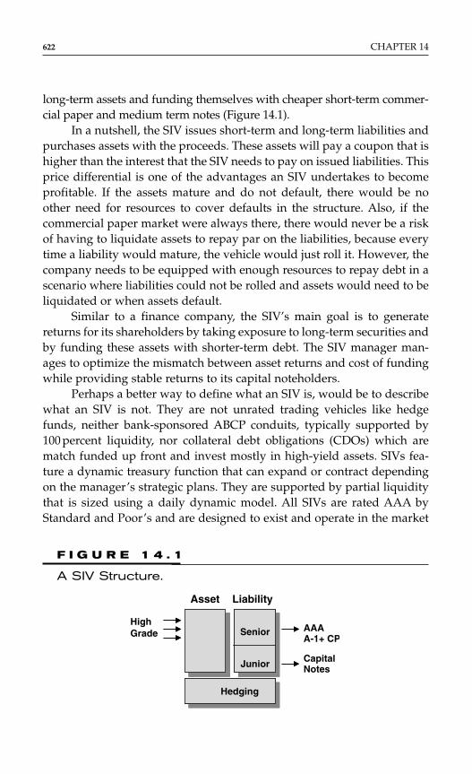
622 CHAPTER 14
long-term assets and funding themselves with cheaper short-term commer-cial paper and medium term notes (Figure 14.1).
In a nutshell, the SIV issues short-term and long-term liabilities andpurchases assets with the proceeds. These assets will pay a coupon that ishigher than the interest that the SIV needs to pay on issued liabilities. Thisprice differential is one of the advantages an SIV undertakes to becomeprofitable. If the assets mature and do not default, there would be noother need for resources to cover defaults in the structure. Also, if thecommercial paper market were always there, there would never be a riskof having to liquidate assets to repay par on the liabilities, because everytime a liability would mature, the vehicle would just roll it. However, thecompany needs to be equipped with enough resources to repay debt in ascenario where liabilities could not be rolled and assets would need to beliquidated or when assets default.
Similar to a finance company, the SIV’s main goal is to generatereturns for its shareholders by taking exposure to long-term securities andby funding these assets with shorter-term debt. The SIV manager man-ages to optimize the mismatch between asset returns and cost of fundingwhile providing stable returns to its capital noteholders.
Perhaps a better way to define what an SIV is, would be to describewhat an SIV is not. They are not unrated trading vehicles like hedgefunds, neither bank-sponsored ABCP conduits, typically supported by100 percent liquidity, nor collateral debt obligations (CDOs) which arematch funded up front and invest mostly in high-yield assets. SIVs fea-ture a dynamic treasury function that can expand or contract dependingon the manager’s strategic plans. They are supported by partial liquiditythat is sized using a daily dynamic model. All SIVs are rated AAA byStandard and Poor’s and are designed to exist and operate in the market
F I G U R E 1 4 . 1
A SIV Structure.
CapitalNotes
Hedging
Junior
Senior
Asset
AAAA-1+ CP
HighGrade
Liability

as AAA corporations. They can be funding vehicles, swap counterparties,and repo counterparties in other structured finance transactions.
SIVs and CDOsThe SIVs are not purely credit arbitrage vehicles. This is partially truebecause their portfolio may exhibit defaults, which constitute a loss to theportfolio in the same way a CDO does. However, having a high-gradeportfolio, mainly AA, the default rate is small. Their role is more on man-aging the mismatch between assets and liabilities and the consequences ofa liquidity shortfall. A CDO’s main focus is credit risk, as BB portfolio ispurchased with AAA debt that is usually longer in tenor than the assetportfolio.
Assets in SIVs and CDOs SIVs purchase usually AAA to Arange assets, have limited BBB exposure. There is a subinvestment bucketallowed to pick up the downgrade of an investment-grade security.
Some SIVS have synthetic credit derivative exposure. The assets arediversified per type, geography, tenor, and size and all rated by the ratingagencies in a proportion of 95 percent.
In a CDO, the range of assets is wider. It can go from high-grade tohigh-yield bonds and loans. CDOs can take cash or synthetic exposure. Asfor SIVs, approved sets of concentration guidelines are applied. For both,concentrated pools or assets are further penalized in the model for quan-tifying appropriate capital adequacy.
Liabilities in SIVs and CDOs In an SIV, there is no maturitymatching. The gap between assets and liabilities is about three to fouryears. More than 50 percent of the debt is CP (U.S. and EURO). Capitalstructure is evolving, depending on market conditions. Typically, in anSIV, we see two tranches. Senior liabilities are rated AAA and issued inseveral classes. Capital notes are the mezz piece and are usually onetranche. In the past couple of years, SIVs have seeked a rating (private orpublic) on their capital notes. Sometimes, the capital notes are tranched ina rated piece and an unrated first loss position. SIVs roll their debt andissue new debt as they deem appropriate. They could use alternativefunding instruments like repurchase agreements and credit-linked notes.
CDOs are more focused on maturity matching than SIVs. Capitalstructure is multitranched from AAA to BB and usually CDOs have anunrated first loss position. The tenor, rating, and size are determined onday one. The intention is to keep the capital structure fixed during the life
An Overview of Structured Investment Vehicles 623

of a CDO. Management is allowed on the asset side within certain param-eters. The rating on the debt has to remain unaltered during the activemanagement of the portfolio.
It is important to understand that because an SIV carries a corporaterating of AAA, it has to satisfy all its obligation with AAA certainty. In aCDO, given the multiple layers of subordination, some liabilities of theCDO (e.g., swap termination payments) could be subordinated in thewaterfall and not addressed in the model.
Liquidity in SIVs and CDOs Management of liquidity is oneof the most challenging elements in the SIVs. Due to a considerable gapbetween assets and liabilities, the SIV needs to rely on external/internalliquidity in the form of bank lines, breakable deposits, committed repos,put options, and liquid assets. It is monitored through specially designedtests, commonly known as net cumulative outflow (NCO), that monitorthe peak liquidity need over the coming year. It is run daily and quanti-fies what amount of resources has to be in liquid assets. In a CDO, liq-uidity is managed through internal reserve accounts. Because they do notrun a refinancing risk, outside liquidity is not necessary. Cash flow mis-matches are mitigated by cash diversion if certain tests do not pass. Sometranches could also have their interest deferrable.
SIVs and CP ConduitsA CP conduit is primarily driven by off-balance sheet regulatory capitalrelief. An SIV is motivated by profit for its shareholders. The number ofCP conduits to date exceeds the number of SIVs.
Assets in SIVs and CP Conduits Both invest in assetbacked and corporates. While an SIV has to have all of its assets rated, aCP conduit can have unrated illiquid assets like trade receivables. CP con-duits are not subject to the diversification criteria that an SIV is. For exam-ple, there can be CP conduits 100 percent concentrated in one asset class.
Liabilities in SIVs and CP Conduits CP conduit accessesthe commercial paper market primarily. The SIVs have access to bothshort- and long-term funding. In an SIV, there is a floor on the weightedaverage life of the liabilities of three-months. This is to mitigate a forcedone-day sale, should the commercial paper market be disrupted. In a CPconduit, there is no such limit. The liabilities can be 100 percent one day or
624 CHAPTER 14

very short term. This is mitigated by the credit and liquidity enhancementprograms in a CP conduit, which are most onerous than those of an SIV.
Liquidity in SIVs and CP Conduits Due to the range ofliabilities, through the NCO test, an SIV does not have to keep 100 percentliquidity as a CP conduit does. The model in the SIV quantifies what theone-year liquidity need is and reserves bank lines for that amount, whichis lower than 100 percent (could range from 25 to 40 percent).
SIVs and Hedge FundsThe hedge funds attempt to make profit on their bets on market direc-tionality for interest rates, currency, and stocks. An SIV is designed to nottake such bets. For example, when a fixed rate asset is purchased, themanager attaches a swap, which converts the fixed rate asset into afloater. The asset stays in such an asset swap package till its maturity ortill the counterparty defaults, case in which it has to be immediatelyreplaced. In an SIV, the profit is made from prudent management of thecredit spread of the assets versus liabilities.
It is true that both operate at a leverage to increase profits. But,whereas all the positions of SIVs have to be reported to rating agenciesand are subject to stringent compliance tests, a hedge fund does notrequire full transparency on its positions.
Due to their high-rating and high-management standards, the SIVscan access the commercial paper and medium term notes market forfunding purposes, whereas the hedge funds do not.
SIVs are closer to be labeled as buy and hold vehicles with statichedges, whereas hedge funds have active trading and rely on dynamichedging of their risk.
What Does the Rating of AAA for an SIV Mean?
If a series of trigger events occur that impact the normal operations of theSIV, a wind down event will start and the manager or a third party (i.e.,security trustee) will step in and liquidate gradually the portfolio. No debtwill be further rolled or issued, and the cash obtained from liquidating theportfolio will be used to repay the senior liabilities. Capital will be used tomake up the shortfalls on the asset liquidation. Practically, in a finite time,the SIV will cease to exist. The SIVs wind down when their resources are
An Overview of Structured Investment Vehicles 625
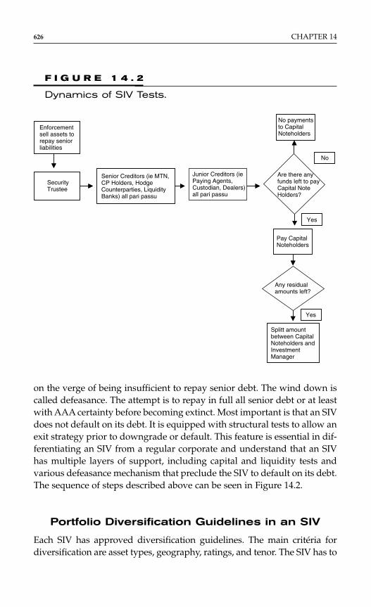
626 CHAPTER 14
on the verge of being insufficient to repay senior debt. The wind down iscalled defeasance. The attempt is to repay in full all senior debt or at leastwith AAA certainty before becoming extinct. Most important is that an SIVdoes not default on its debt. It is equipped with structural tests to allow anexit strategy prior to downgrade or default. This feature is essential in dif-ferentiating an SIV from a regular corporate and understand that an SIVhas multiple layers of support, including capital and liquidity tests andvarious defeasance mechanism that preclude the SIV to default on its debt.The sequence of steps described above can be seen in Figure 14.2.
Portfolio Diversification Guidelines in an SIV
Each SIV has approved diversification guidelines. The main critéria fordiversification are asset types, geography, ratings, and tenor. The SIV has to
F I G U R E 1 4 . 2
Dynamics of SIV Tests.
Enforcementsell assets torepay seniorliabilities
SecurityTrustee
Senior Creditors (ie MTN,CP Holders, HodgeCounterparties, LiquidityBanks) all pari passu
Junior Creditors (iePaying Agents,Custodian, Dealers)all pari passu
No paymentsto CapitalNoteholders
Are there anyfunds left to payCapital NoteHolders?
Pay CapitalNoteholders
Any residualamounts left?
Splitt amountbetween CapitalNoteholders andInvestmentManager
Yes
Yes
No

comply with these guidelines. Beside the model that quantifies losses, thediversification requirements are an important feature for the creditenhancement of the SIV. Breach of the guidelines has to be cured either byselling collateral or by capital charging the excess dollar for dollar. Forexample, in February 2001, when Hollywood Funding was downgradedfrom AAA to CCC− (default status), Asset Backed Capital Ltd. (ABC)owned approximately $100 million of these notes at the time of downgrade.The asset became ineligible for the SIV and, at that time, ABC had five daysto cure. ABC sold massively liquid assets to reduce its leverage and returnedinto compliance. The rating was reaffirmed by all rating agencies.
Sponsorship, Managers, and Investors
An SIV sponsor is usually a major commercial bank, asset manager, insur-ance company, or a combination of thereof. It plays an important role, asinvestors differentiate SIVs by their perception of the sponsor. The spon-sor usually is setting up the SIV, may or may not provide liquidity sup-port, may or may not invest its own money in a portion of the capitalstructure (capital notes).
The asset manager is responsible for daily management of creditand liquidity. Their management style reflects in the asset composition ofthe portfolio. Some are focused on asset-backed security (ABS) assets,some invest more in bank subdebt, some focus more on certain ratingcategories.
As for the range of investors, it varies depending on the portion ofthe capital structure that they are targeting. Commercial paper is attrac-tive to money market funds, banks, and conduits. Banks and corporatesare buyers of medium term notes. Banks, insurance companies, as well asprivate individuals may invest in rated or unrated capital notes.
Table 14.1 presents a snapshot of the market as of December 2005(as shown by an S&P’s update: SIV Outlook Report/Assets Top $200Million in SIV Market; Continued Growth Expected in 2006—January2006).
In Figure 14.3, outstanding senior debt is displayed as ofDecember 2005. The asset classes in SIV portfolios cover mostly floatingrate USD bullet or soft-bullet ABS and bank debt. However, they areable and some do invest in nonbank corporates and sovereign paper.Assets held by the SIV sector exceeded $200 billion at the end of 2005,and stand at almost $204 billion, a rise of almost 40 percent over theprevious year.
An Overview of Structured Investment Vehicles 627
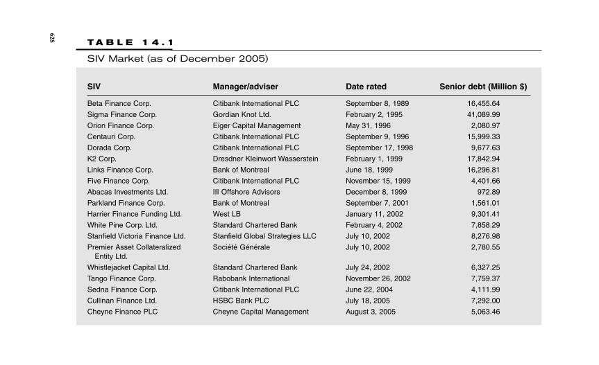
T A B L E 1 4 . 1
SIV Market (as of December 2005)
SIV Manager/adviser Date rated Senior debt (Million $)
Beta Finance Corp. Citibank International PLC September 8, 1989 16,455.64
Sigma Finance Corp. Gordian Knot Ltd. February 2, 1995 41,089.99
Orion Finance Corp. Eiger Capital Management May 31, 1996 2,080.97
Centauri Corp. Citibank International PLC September 9, 1996 15,999.33
Dorada Corp. Citibank International PLC September 17, 1998 9,677.63
K2 Corp. Dresdner Kleinwort Wasserstein February 1, 1999 17,842.94
Links Finance Corp. Bank of Montreal June 18, 1999 16,296.81
Five Finance Corp. Citibank International PLC November 15, 1999 4,401.66
Abacas Investments Ltd. III Offshore Advisors December 8, 1999 972.89
Parkland Finance Corp. Bank of Montreal September 7, 2001 1,561.01
Harrier Finance Funding Ltd. West LB January 11, 2002 9,301.41
White Pine Corp. Ltd. Standard Chartered Bank February 4, 2002 7,858.29
Stanfield Victoria Finance Ltd. Stanfield Global Strategies LLC July 10, 2002 8,276.98
Premier Asset Collateralized Société Générale July 10, 2002 2,780.55Entity Ltd.
Whistlejacket Capital Ltd. Standard Chartered Bank July 24, 2002 6,327.25
Tango Finance Corp. Rabobank International November 26, 2002 7,759.37
Sedna Finance Corp. Citibank International PLC June 22, 2004 4,111.99
Cullinan Finance Ltd. HSBC Bank PLC July 18, 2005 7,292.00
Cheyne Finance PLC Cheyne Capital Management August 3, 2005 5,063.46
628
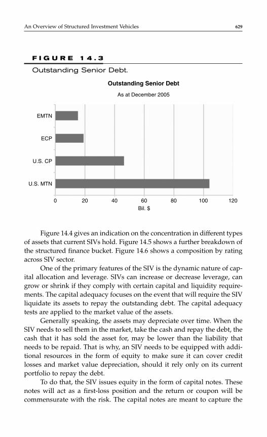
An Overview of Structured Investment Vehicles 629
F I G U R E 1 4 . 3
Outstanding Senior Debt.
EMTN
ECP
0 20 40 60 80 100 120Bil. $
Outstanding Senior Debt
As at December 2005
U.S. CP
U.S. MTN
Figure 14.4 gives an indication on the concentration in different typesof assets that current SIVs hold. Figure 14.5 shows a further breakdown ofthe structured finance bucket. Figure 14.6 shows a composition by ratingacross SIV sector.
One of the primary features of the SIV is the dynamic nature of cap-ital allocation and leverage. SIVs can increase or decrease leverage, cangrow or shrink if they comply with certain capital and liquidity require-ments. The capital adequacy focuses on the event that will require the SIVliquidate its assets to repay the outstanding debt. The capital adequacytests are applied to the market value of the assets.
Generally speaking, the assets may depreciate over time. When theSIV needs to sell them in the market, take the cash and repay the debt, thecash that it has sold the asset for, may be lower than the liability thatneeds to be repaid. That is why, an SIV needs to be equipped with addi-tional resources in the form of equity to make sure it can cover creditlosses and market value depreciation, should it rely only on its currentportfolio to repay the debt.
To do that, the SIV issues equity in the form of capital notes. Thesenotes will act as a first-loss position and the return or coupon will becommensurate with the risk. The capital notes are meant to capture the
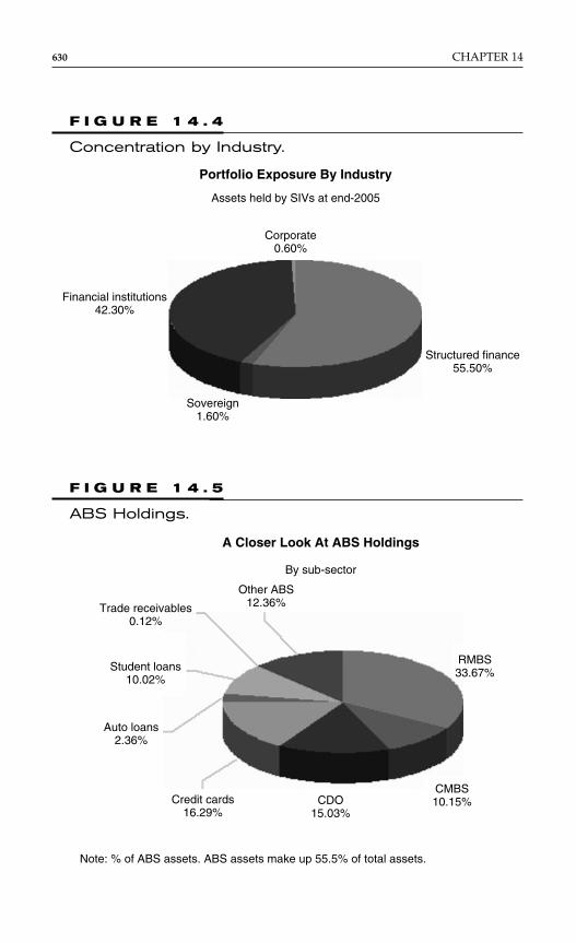
630 CHAPTER 14
F I G U R E 1 4 . 5
ABS Holdings.
Trade receivables0.12%
Other ABS12.36%
RMBS33.67%
CMBS10.15%CDO
15.03%Credit cards
16.29%
Auto loans2.36%
Student loans10.02%
Note: % of ABS assets. ABS assets make up 55.5% of total assets.
By sub-sector
A Closer Look At ABS Holdings
F I G U R E 1 4 . 4
Concentration by Industry.
Corporate0.60%
Sovereign1.60%
Structured finance55.50%
Financial institutions42.30%
Portfolio Exposure By Industry
Assets held by SIVs at end-2005
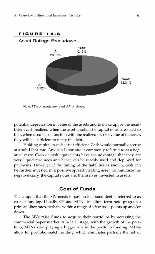
An Overview of Structured Investment Vehicles 631
potential depreciation in value of the assets and to make up for the insuf-ficient cash realized when the asset is sold. The capital notes are sized sothat, when used in conjunction with the realized market value of the asset,they will be sufficient to repay the debt.
Holding capital in cash is not efficient. Cash would normally accrueat a sub-Libor rate. Any sub-Libor rate is commonly referred to as a neg-ative carry. Cash or cash equivalents have the advantage that they arevery liquid resources and hence can be readily used and deployed forpayments. However, if the timing of the liabilities is known, cash canbe further invested in a positive spread yielding asset. To minimize thenegative carry, the capital notes are, themselves, invested in assets.
Cost of Funds
The coupon that the SIV needs to pay on its issued debt is referred to ascost of funding. Usually, CP and MTNs (medium-term note programs)price at Libor rates, perhaps within a range of a few basis points up and/ordown.
The SIVs raise funds to acquire their portfolios by accessing thecommercial paper market. At a later stage, with the growth of the port-folio, MTNs start playing a bigger role in the portfolio funding. MTNsallow for portfolio match funding, which eliminates partially the risk of
F I G U R E 1 4 . 6
Asset Ratings Breakdown.
'BBB'0.13%'A'
20.81%
'AA'16.72%
'AAA'62.34%
Note: 79% of assets are rated 'AA' or above.

632 CHAPTER 14632 CHAPTER 14
liquidation, leaving only the default risk in. However, MTNs are moreexpensive than short-term debt.
Any disruption in the normal mode of an SIV would be immediatelyreflected in the cost of funds for its rolled commercial paper. Cost of fundsfor capital notes includes a stated coupon (25 to 50 above Libor) that is, ornot, rated as well as profit or performance coupon. Profit depends on theexcess spread of the SIV and ultimately on the excess capital that an SIVhas. Capital notes are rated in most cases BBB.
In a CDO, the AAA tranche prices somewhere in the range of Libor+25 and +45. The short tenor of the debt in an SIV (typically senior MTNare 18 to 24 months) is reflected in the spread above Libor which islower than the CDO AAA spread. Same comparison can be made toEuropean covered bonds where the stated maturity is typically 20 to 30years.
The BBB CDO tranche prices in the range of Libor +200 to +350 witha five-year average of approximately 250 above Libor. The floatingRMBS/CMBS pay a coupon which on average over last five years is Libor+190. Spread raged within 170 to 230. SIVs may pay similar coupon oreven higher to their capital noteholders but most of the spread is profitand their stated coupon is much lower.
Leverage
In its simplest definition, leverage is the ratio between senior debt andequity. Other equivalent definitions involve net asset value. Irrespective ofthe capital model outcome, SIVs have to comply with leverage constraints.Typically, SIV leverage is within the range of 12 to 14. At 18 or 19 leveragelevel, they enter restricted operations, and, at a leverage of 20, they need towind down.
Quantitative analysis on an SIV focuses mainly on capital adequacy,market neutrality, and adequate liquidity.
Capital Adequacy
Example 1SIV XYZ issues $100 million one-year note at Libor + 10 bps. It buys
a five-year asset of 10 million MTM. The asset pays Libor +30 bps, so thespread differential is 20 bps.

If at the end of one year the SIV cannot roll the liability (e.g., marketdisruption), it needs to sell the asset (which has four more years to matu-rity). The SIV will sell it and may get only 9.8 million.
It means that the SIV is 0.2 million short of its debt obligation, so itshould have raised 0.2 million in equity. See a simplified example of aSIVs balance sheet:
Sample SIV Balance SheetAssets Liabilities
$10 million $ 9.8 million
Capital
$ 0.2 million
$10 million $10 million
This example leads naturally to the kind of questions we need toanswer in sizing the capital adequacy of such an entity: how much resourcesshould the SIV have so that if the SIV is short on assets due to defaults ormarket value deterioration, it can still pay in full its debt holders?
In sizing the capital adequacy of an SIV, a series of assumptions arebeing made: the SIV winds down today with current portfolio, the debt isno longer rolled, and there are no further reinvestments. The analysis isan analysis of a static portfolio that winds down and repays liabilities asthey come due.
The winddown timeline is presented subsequently:Time step 0, day of trigger event or starting day for the simulation
♦ Input in the model the current portfolio of assets with type, rat-ings, notional, market price, and domicile.
♦ Input debt information with tenor, size, and coupon frequency.
Time step 1
♦ Evolve the ratings of assets, derivative counterparties, and mar-ket price of the assets.
♦ Inflows are asset coupons, par on the maturing assets, recoveryon defaulted assets, hedging counterparty-related inflows.
♦ Outflows are senior expenses and fees, any derivative-relatedoutflows, coupon or principal which are due in that time step.
♦ Sell assets, if needed, to repay liabilities.
An Overview of Structured Investment Vehicles 633

Time step 2 onward
♦ Repeat time step 1 till all liabilities are paid back. If there is ashortfall in assets and they are insufficient to repay the debt, theSIV has inadequate AAA capital.
In evolving the portfolio through its winddown period, key risk factors are:
♦ Credit migration including defaults♦ Recovery♦ Asset spreads♦ Interest rates and♦ Foreign exchange rates.
The market price of the portfolio changes as a consequence of a change inthe rating of the asset but also as a consequence of the fluctuation in thespread.
Some vehicles take the asset-by-asset approach and capital chargeeach asset for its potential loss in value due to credit and market envi-ronment. In these companies, when debt is issued and proceeds areused to buy an asset, depending on its rating and tenor, a capital chargeis attached to it. The daily capital adequacy test will check whethercurrent market value of the assets adjusted for the capital chargesare enough to cover par on the liabilities. These SIVs are referred to as“matrix” SIVs.
Other vehicles take a portfolio simulation approach where creditand market risk variables are stochastically modeled and integratedwith a cash flow model in which the waterfall of payments is input. Thismeans that market paths and credit paths are simulated for each assetin the portfolio. The asset cash flows and their market value are thenused to pay the liabilities as they become due. If assets are insuffi-cient to pay liabilities, losses will occur. These SIVs are referred to asmodeled SIVs.
Final output is a distribution of losses. The latter can be a distributionof the first dollar of loss on the liabilities. Or, it can be an expected lossmetric on each of the vehicle’s liabilities. Both are relevant in sizing appro-priate resources in the vehicle. Figure 14.7 shows a hypothetical loss dis-tribution.
Figure 14.7 is helpful in sizing the capital requirement in a first dol-lar of loss framework as well as to quantify other loss metrics.
634 CHAPTER 14
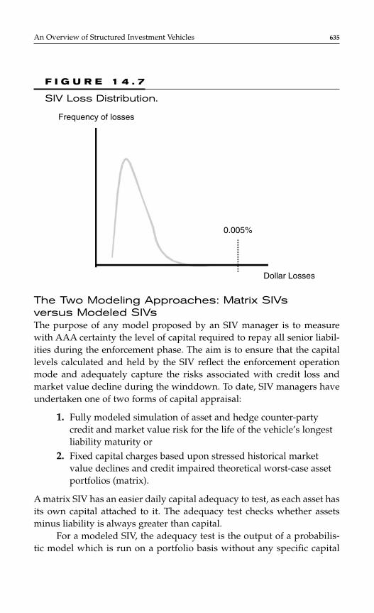
The Two Modeling Approaches: Matrix SIVs versus Modeled SIVsThe purpose of any model proposed by an SIV manager is to measurewith AAA certainty the level of capital required to repay all senior liabil-ities during the enforcement phase. The aim is to ensure that the capitallevels calculated and held by the SIV reflect the enforcement operationmode and adequately capture the risks associated with credit loss andmarket value decline during the winddown. To date, SIV managers haveundertaken one of two forms of capital appraisal:
1. Fully modeled simulation of asset and hedge counter-partycredit and market value risk for the life of the vehicle’s longestliability maturity or
2. Fixed capital charges based upon stressed historical marketvalue declines and credit impaired theoretical worst-case assetportfolios (matrix).
A matrix SIV has an easier daily capital adequacy to test, as each asset hasits own capital attached to it. The adequacy test checks whether assetsminus liability is always greater than capital.
For a modeled SIV, the adequacy test is the output of a probabilis-tic model which is run on a portfolio basis without any specific capital
An Overview of Structured Investment Vehicles 635
F I G U R E 1 4 . 7
SIV Loss Distribution.
Frequency of losses
0.005%
Dollar Losses
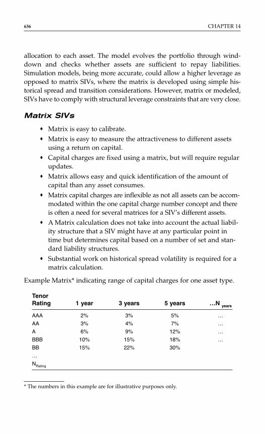
allocation to each asset. The model evolves the portfolio through wind-down and checks whether assets are sufficient to repay liabilities.Simulation models, being more accurate, could allow a higher leverage asopposed to matrix SIVs, where the matrix is developed using simple his-torical spread and transition considerations. However, matrix or modeled,SIVs have to comply with structural leverage constraints that are very close.
Matrix SIVs
♦ Matrix is easy to calibrate.♦ Matrix is easy to measure the attractiveness to different assets
using a return on capital.♦ Capital charges are fixed using a matrix, but will require regular
updates.♦ Matrix allows easy and quick identification of the amount of
capital than any asset consumes.♦ Matrix capital charges are inflexible as not all assets can be accom-
modated within the one capital charge number concept and thereis often a need for several matrices for a SIV’s different assets.
♦ A Matrix calculation does not take into account the actual liabil-ity structure that a SIV might have at any particular point intime but determines capital based on a number of set and stan-dard liability structures.
♦ Substantial work on historical spread volatility is required for amatrix calculation.
Example Matrix* indicating range of capital charges for one asset type.
TenorRating 1 year 3 years 5 years …N years
AAA 2% 3% 5% …
AA 3% 4% 7% …
A 6% 9% 12% …
BBB 10% 15% 18% …
BB 15% 22% 30%
…
NRating
636 CHAPTER 14
* The numbers in this example are for illustrative purposes only.
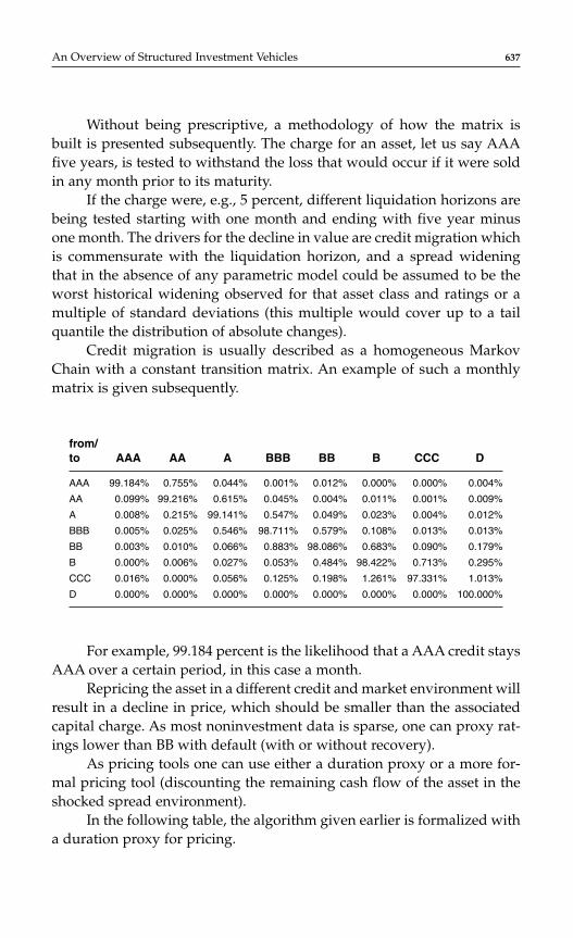
An Overview of Structured Investment Vehicles 637
Without being prescriptive, a methodology of how the matrix isbuilt is presented subsequently. The charge for an asset, let us say AAAfive years, is tested to withstand the loss that would occur if it were soldin any month prior to its maturity.
If the charge were, e.g., 5 percent, different liquidation horizons arebeing tested starting with one month and ending with five year minusone month. The drivers for the decline in value are credit migration whichis commensurate with the liquidation horizon, and a spread wideningthat in the absence of any parametric model could be assumed to be theworst historical widening observed for that asset class and ratings or amultiple of standard deviations (this multiple would cover up to a tailquantile the distribution of absolute changes).
Credit migration is usually described as a homogeneous MarkovChain with a constant transition matrix. An example of such a monthlymatrix is given subsequently.
from/to AAA AA A BBB BB B CCC D
AAA 99.184% 0.755% 0.044% 0.001% 0.012% 0.000% 0.000% 0.004%
AA 0.099% 99.216% 0.615% 0.045% 0.004% 0.011% 0.001% 0.009%
A 0.008% 0.215% 99.141% 0.547% 0.049% 0.023% 0.004% 0.012%
BBB 0.005% 0.025% 0.546% 98.711% 0.579% 0.108% 0.013% 0.013%
BB 0.003% 0.010% 0.066% 0.883% 98.086% 0.683% 0.090% 0.179%
B 0.000% 0.006% 0.027% 0.053% 0.484% 98.422% 0.713% 0.295%
CCC 0.016% 0.000% 0.056% 0.125% 0.198% 1.261% 97.331% 1.013%
D 0.000% 0.000% 0.000% 0.000% 0.000% 0.000% 0.000% 100.000%
For example, 99.184 percent is the likelihood that a AAA credit staysAAA over a certain period, in this case a month.
Repricing the asset in a different credit and market environment willresult in a decline in price, which should be smaller than the associatedcapital charge. As most noninvestment data is sparse, one can proxy rat-ings lower than BB with default (with or without recovery).
As pricing tools one can use either a duration proxy or a more for-mal pricing tool (discounting the remaining cash flow of the asset in theshocked spread environment).
In the following table, the algorithm given earlier is formalized witha duration proxy for pricing.
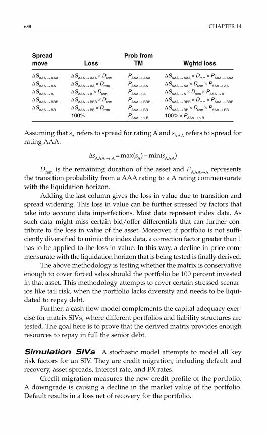
638 CHAPTER 14
Spread Prob from move Loss TM Wghtd loss
∆SAAA → AAA ∆SAAA → AAA × Drem PAAA → AAA ∆SAAA → AAA × Drem × PAAA → AAA
∆SAAA → AA ∆SAAA → AA × Drem PAAA → AA ∆SAAA → AA × Drem × PAAA → AA
∆SAAA → A ∆SAAA → A × Drem PAAA → A ∆SAAA → A × Drem × PAAA → A
∆SAAA → BBB ∆SAAA → BBB × Drem PAAA → BBB ∆SAAA → BBB × Drem × PAAA → BBB
∆SAAA → BB ∆SAAA → BB × Drem PAAA → BB ∆SAAA → BB × Drem × PAAA → BB
100% PAAA → ≤ B 100% × PAAA → ≤ B
Assuming that sA refers to spread for rating A and sAAA refers to spread forrating AAA:
∆sAAA → A = max(sA) − min(sAAA)
Drem is the remaining duration of the asset and PAAA→A representsthe transition probability from a AAA rating to a A rating commensuratewith the liquidation horizon.
Adding the last column gives the loss in value due to transition andspread widening. This loss in value can be further stressed by factors thattake into account data imperfections. Most data represent index data. Assuch data might miss certain bid/offer differentials that can further con-tribute to the loss in value of the asset. Moreover, if portfolio is not suffi-ciently diversified to mimic the index data, a correction factor greater than 1has to be applied to the loss in value. In this way, a decline in price com-mensurate with the liquidation horizon that is being tested is finally derived.
The above methodology is testing whether the matrix is conservativeenough to cover forced sales should the portfolio be 100 percent investedin that asset. This methodology attempts to cover certain stressed scenar-ios like tail risk, when the portfolio lacks diversity and needs to be liqui-dated to repay debt.
Further, a cash flow model complements the capital adequacy exer-cise for matrix SIVs, where different portfolios and liability structures aretested. The goal here is to prove that the derived matrix provides enoughresources to repay in full the senior debt.
Simulation SIVs A stochastic model attempts to model all keyrisk factors for an SIV. They are credit migration, including default andrecovery, asset spreads, interest rate, and FX rates.
Credit migration measures the new credit profile of the portfolio.A downgrade is causing a decline in the market value of the portfolio.Default results in a loss net of recovery for the portfolio.
Asset spreads indicate the evolution in the market price of the port-folio. Both are essential in evaluating the value of the assets that need to bedeployed to repay liabilities and hence in measuring any shortfall thatmight occur. A decline in price can occur because of a downgrade in con-junction with spread widening. Interest rates and FX rates project the markto market of the derivative contracts. A default of a derivative counter-party could mean a loss for the vehicle and replacement comes at a cost.
Correlation is a key component in the model for each of the aboverisk factors. There is correlation for pairwise transition. Transition, as wellas default correlation, captures joint movements in credit. It helps simu-late clusters of default or transition. In projecting spreads, the correlationbetween intra-and inter-asset classes has to be incorporated. And, finally,there is correlation among interest rates and FX rates. When projectingmarket rates, correlation between different interest rate curves andforeign exchange curves has to be incorporated.
Calibration of the above-mentioned risk factors is a historical cali-bration as opposed to risk-neutral. Stability of capital requirement is oneof the key components in the risk management of an SIV. Major swings inparameters generated by implied parameters that could cause volatility inthe capital requirements are not reflective for the buy and hold businessin which an SIV is. Without being prescriptive, examples of such modelsare being presented subsequently.
A Correlated transitionsThere are a few approaches for modeling correlated transition. Below,three of them are presented:
A1 HistoricalThe most direct way to estimate joint rating change likelihoods is to exam-ine credit ratings time series across many firms, which are synchronized intime with each other. This method has the advantage that it does not makeassumptions as to the underlying process, the joint distribution shape, buthas the limitation that it needs extensive data in a pairwise format perregion, country, and industry. A factor model can be fit to this data set,hence correlated transition could be modeled using a series of standardnormal variates, which will translate via Merton approach into ratings.
A2 Corporate bond pricesA second way to estimate credit correlations using historical data is toexamine price histories of corporate bonds. It is intuitive to link bond
An Overview of Structured Investment Vehicles 639

640 CHAPTER 14
prices with changes in credit quality, so a robust history for bond pricesmay allow estimations of correlated transitions. This approach requiresadequate data on bond prices and a model that links bond prices to creditevents on a pairwise basis. The main drawback here is historical data.There are a couple of models that attempt to use bond spreads for model-ing credit migration.
A3 Asset correlationThere is a third way to model joint transition using as underlying assetcorrelation.A3.1. Asset correlation could be derived from observable firm specificequity returns. This model uses the Merton approach for default simula-tion, extended to transition. A firm defaults if its asset values go below lia-bilities. This approach may be extended to derive certain real numberthresholds that are linked to a certain rating of the firm. Crossing a thresh-old is equated to transiting from a rating to another. So a joint migrationin the assets’ value will be translated in a joint move in credit.
This method has the drawback of overlooking the differences betweenequity and asset correlations. However, one could make the argument thatit is more accurate than using a fixed correlation, is based on more datawhich is daily available, and is sensitive to countries and industries. Equityvariations address market movements as well as credit migration, which isour sole interest in this exercise. In Credit Metrics, Chapter 8, this approachis described in great detail. The reader is referred to Credit Metrics (1997) fora detailed analysis on correlation.
Essentially, a correlation matrix is built that captures joint move-ments for asset values. Then, each time step (e.g., each month) a multi-normal draw with this correlation matrix is performed and its numericoutcome is used to determine the new credit ratings.
The correlation matrix is derived using the obligor’s participation toa country and industry and uses as underlying equity returns.
Looking at equity for a obligor’s transition is a well-accepted frame-work in the Merton/MKMV approach and is one of the few availableproxies for defining and simulating performance. What gives comfort isthat data for this method is observable, is available daily. Datametrics is aweb based product that gives access to such correlation information. Thedata covers a wide range of countries and industries in those countries.Currently, there is a lot of research done to strip out of the equity returnsthe credit information and use that to find asset correlation because theaim is to find credit migration and not market movements.

A3.2. The above model can be used with constant historical assetcorrelations as well. These correlation levels can be derived from the jointtransition information. The problem that needs to be solved is the following.Assume for simplicity two states: default and nondefault. Assuming sameMerton framework for the asset’s value, the question is to find the asset cor-relation that best matches the theoretical variance of the number of defaultswith the observed variance of the number of defaults. The number ofunknowns is defined by the number of pairwise correlations one is lookingfor. Asset correlation can be pairwise constant for an industry and the samefor all industries. A second asset correlation can be searched for interindus-try. The problem can be further refined to incorporate countries and regions.Extension of the problem to incorporate transition can be easily done, usingsame Merton assumption for transitions, namely that credit worthinessunderlying ratings transition could be modeled with a normal variate.
Finally, a simple example of correlated transition simulation withtwo obligors is given for illustration purposes only.
First, one needs to use a transition matrix to determine the probabil-ity of moving to each rating. These probabilities are further used to setthresholds in a normal distribution. Each threshold is corresponding to apossible rating outcome. Then draw a set of correlated normal deviatesequal in number to the number of obligors in the portfolio. Finally, usethese numbers, combined with the thresholds, to determine the forwardcredit rating of each obligor.
A convenient way to think about the thresholds is in terms ofFigure 14.8. Underlying ratings transition, there exists a “credit perfor-mance” random variable that is normally distributed. Change in letter rat-ing is merely a reflection of the realization of “credit performance.” Acredit A is migrating with different probabilities to the other ratings andhas the highest likelihood to stay A.
A bell-shaped curve representing the asset value as a standard nor-mal density function is sliced in such a way that the areas underneathequate the transition probabilities to other ratings.
Note that the probabilities of moving to AAA, CCC, and D are toosmall to be seen in the figure. In the bell-shaped figure, the area beneaththe curve is divided into smaller areas, each of which is in a one-to-onecorrespondence with a certain credit worthiness of the asset. The readercan see that the middle area below the curve corresponds to the highprobability of the obligor staying in its current state.
To use an example, consider two obligors, A and B, and suppose thatobligor A is an A-rated entity, whereas obligor B is an B-rated entity.
An Overview of Structured Investment Vehicles 641
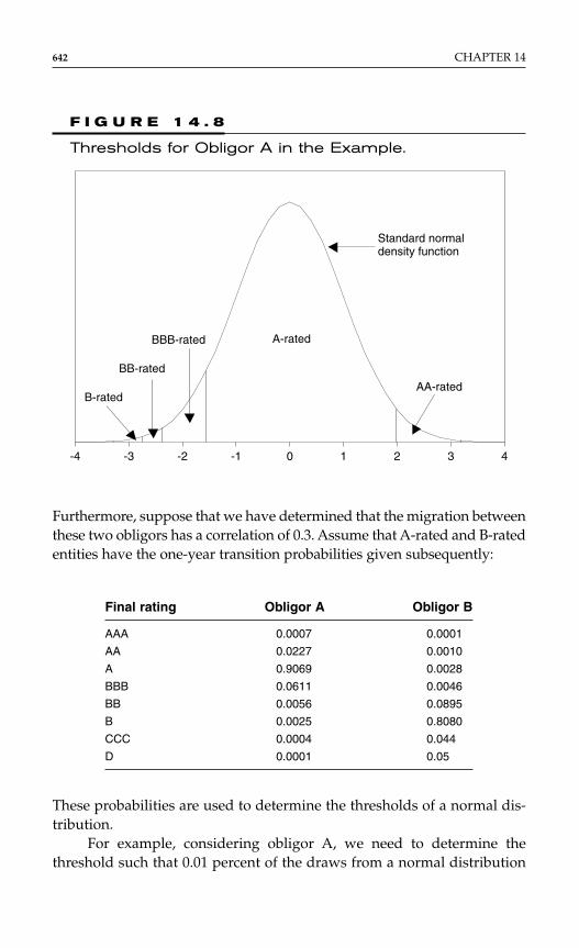
642 CHAPTER 14
Furthermore, suppose that we have determined that the migration betweenthese two obligors has a correlation of 0.3. Assume that A-rated and B-ratedentities have the one-year transition probabilities given subsequently:
Final rating Obligor A Obligor B
AAA 0.0007 0.0001
AA 0.0227 0.0010
A 0.9069 0.0028
BBB 0.0611 0.0046
BB 0.0056 0.0895
B 0.0025 0.8080
CCC 0.0004 0.044
D 0.0001 0.05
These probabilities are used to determine the thresholds of a normal dis-tribution.
For example, considering obligor A, we need to determine thethreshold such that 0.01 percent of the draws from a normal distribution
F I G U R E 1 4 . 8
Thresholds for Obligor A in the Example.
-4 -3 -2 -1 0 1 2 3 4
A-ratedBBB-rated
BB-rated
B-rated
Standard normal density function
AA-rated
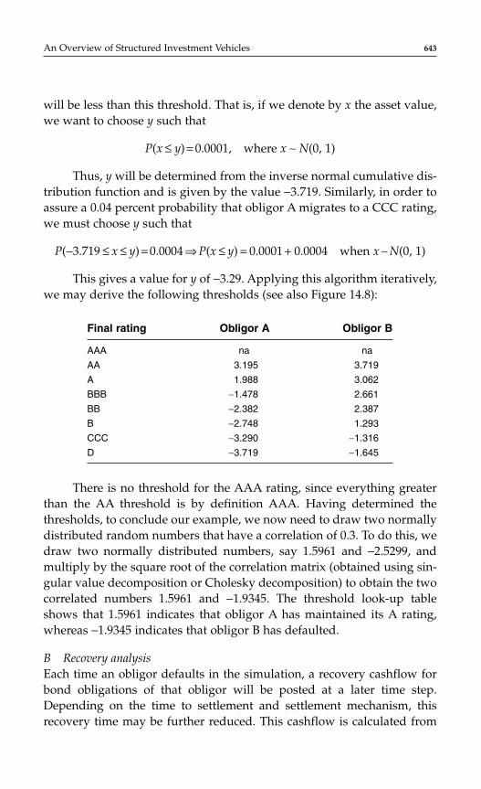
will be less than this threshold. That is, if we denote by x the asset value,we want to choose y such that
P(x ≤ y) = 0.0001, where x ∼ N(0, 1)
Thus, y will be determined from the inverse normal cumulative dis-tribution function and is given by the value −3.719. Similarly, in order toassure a 0.04 percent probability that obligor A migrates to a CCC rating,we must choose y such that
P(−3.719 ≤ x ≤ y) = 0.0004 ⇒ P(x ≤ y) = 0.0001 + 0.0004 when x ∼ N(0, 1)
This gives a value for y of −3.29. Applying this algorithm iteratively,we may derive the following thresholds (see also Figure 14.8):
Final rating Obligor A Obligor B
AAA na na
AA 3.195 3.719
A 1.988 3.062
BBB −1.478 2.661
BB −2.382 2.387
B −2.748 1.293
CCC −3.290 −1.316
D −3.719 −1.645
There is no threshold for the AAA rating, since everything greaterthan the AA threshold is by definition AAA. Having determined thethresholds, to conclude our example, we now need to draw two normallydistributed random numbers that have a correlation of 0.3. To do this, wedraw two normally distributed numbers, say 1.5961 and −2.5299, andmultiply by the square root of the correlation matrix (obtained using sin-gular value decomposition or Cholesky decomposition) to obtain the twocorrelated numbers 1.5961 and −1.9345. The threshold look-up tableshows that 1.5961 indicates that obligor A has maintained its A rating,whereas −1.9345 indicates that obligor B has defaulted.
B Recovery analysisEach time an obligor defaults in the simulation, a recovery cashflow forbond obligations of that obligor will be posted at a later time step.Depending on the time to settlement and settlement mechanism, thisrecovery time may be further reduced. This cashflow is calculated from
An Overview of Structured Investment Vehicles 643

the total exposure to that obligor (taking into account investments andderivative exposure and the appropriate netting rules) as follows:
Recovery amount = Obligor exposure × Recovery %
B1 Beta distributionA Beta distribution is now commonly accepted method for modeling therecovery percentage that has now been adopted for use in a variety ofmodeling applications.
The constant pdf (the flat line) shows that the standard uniform dis-tribution is a special case of the beta distribution.
This distribution has the following attractive properties for the pur-pose of modeling recoveries (see Figure 14.9):
1. Bell curve distribution2. Bounded at 0 percent and 100 percent3. Ability to derive distribution parameters to fit mean and stan-
dard deviation4. Can be sampled relatively quickly within a simulation
The probability density function for a Beta distribution with parameters aand b is shown as follows:
for x ∈ [0, 1] else fa, b(x) = 0,
where the gamma function is defined as Γ( ) e da xa
x
x= −=
∞−∫ 1
0x.
f xa ba b
x xa ba b
, ( )( )( ) ( )
( )= + −− −ΓΓ Γ
1 11
644 CHAPTER 14
F I G U R E 1 4 . 9
Range of Shapes Obtainable from a Beta Distribution.
0 0.2 0.4 0.6 0.8 10
0.5
1
1.5
2
2.5
a − b − 0.75 a − b − 4
a − b − 1
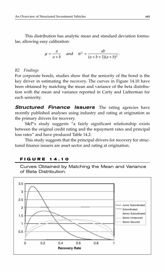
This distribution has analytic mean and standard deviation formu-lae, allowing easy calibration:
B2 FindingsFor corporate bonds, studies show that the seniority of the bond is thekey driver in estimating the recovery. The curves in Figure 14.10 havebeen obtained by matching the mean and variance of the beta distribu-tion with the mean and variance reported in Carty and Lieberman foreach seniority.
Structured Finance Issuers The rating agencies haverecently published analyses using industry and rating at origination asthe primary drivers for recovery.
S&P’s study suggests “a fairly significant relationship existsbetween the original credit rating and the repayment rates and principalloss rates” and have produced Table 14.2:
This study suggests that the principal drivers for recovery for struc-tured finance issuers are asset sector and rating at origination.
µ σ=+
=+ + +
aa b
aba b a b
and( )( )
.221
An Overview of Structured Investment Vehicles 645
F I G U R E 1 4 . 1 0
Curves Obtained by Matching the Mean and Varianceof Beta Distribution.
0
0.5
1
1.5
2
2.5
3
3.5
0.2 0.4
Recovery Rate
0.6 0.8 1
Junior Subordinated
Subordinated
Senior Subordinated
Senior Unsecured
Senior Secured
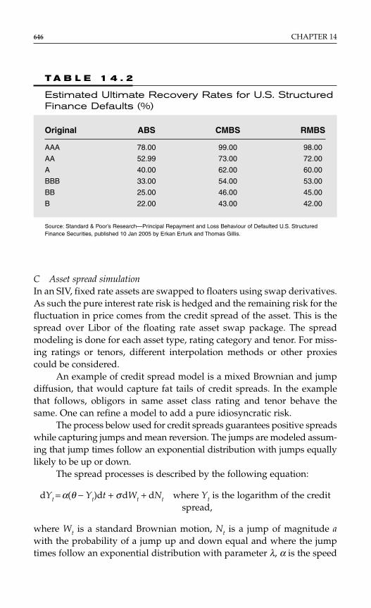
C Asset spread simulationIn an SIV, fixed rate assets are swapped to floaters using swap derivatives.As such the pure interest rate risk is hedged and the remaining risk for thefluctuation in price comes from the credit spread of the asset. This is thespread over Libor of the floating rate asset swap package. The spreadmodeling is done for each asset type, rating category and tenor. For miss-ing ratings or tenors, different interpolation methods or other proxiescould be considered.
An example of credit spread model is a mixed Brownian and jumpdiffusion, that would capture fat tails of credit spreads. In the examplethat follows, obligors in same asset class rating and tenor behave thesame. One can refine a model to add a pure idiosyncratic risk.
The process below used for credit spreads guarantees positive spreadswhile capturing jumps and mean reversion. The jumps are modeled assum-ing that jump times follow an exponential distribution with jumps equallylikely to be up or down.
The spread processes is described by the following equation:
dYt = α(θ − Yt)dt + σdWt + dNt where Yt is the logarithm of the creditspread,
where Wt is a standard Brownian motion, Nt is a jump of magnitude awith the probability of a jump up and down equal and where the jumptimes follow an exponential distribution with parameter λ, α is the speed
646 CHAPTER 14
T A B L E 1 4 . 2
Estimated Ultimate Recovery Rates for U.S. StructuredFinance Defaults (%)
Original ABS CMBS RMBS
AAA 78.00 99.00 98.00
AA 52.99 73.00 72.00
A 40.00 62.00 60.00
BBB 33.00 54.00 53.00
BB 25.00 46.00 45.00
B 22.00 43.00 42.00
Source: Standard & Poor’s Research—Principal Repayment and Loss Behaviour of Defaulted U.S. StructuredFinance Securities, published 10 Jan 2005 by Erkan Erturk and Thomas Gillis.
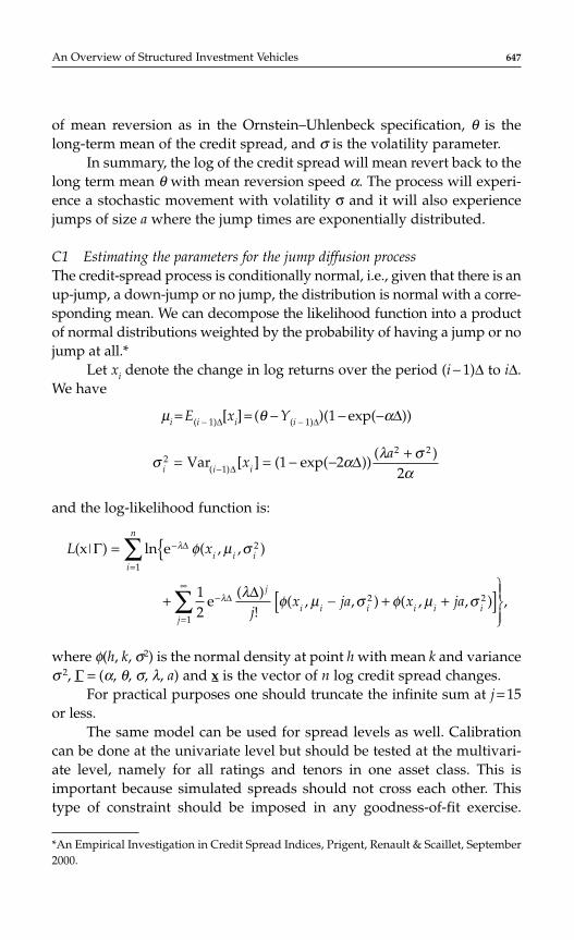
An Overview of Structured Investment Vehicles 647
of mean reversion as in the Ornstein–Uhlenbeck specification, θ is thelong-term mean of the credit spread, and σ is the volatility parameter.
In summary, the log of the credit spread will mean revert back to thelong term mean θ with mean reversion speed α. The process will experi-ence a stochastic movement with volatility σ and it will also experiencejumps of size a where the jump times are exponentially distributed.
C1 Estimating the parameters for the jump diffusion processThe credit-spread process is conditionally normal, i.e., given that there is anup-jump, a down-jump or no jump, the distribution is normal with a corre-sponding mean. We can decompose the likelihood function into a productof normal distributions weighted by the probability of having a jump or nojump at all.*
Let xi denote the change in log returns over the period (i − 1)∆ to i∆.We have
µi = E(i − 1)∆[xi] = (θ − Y(i − 1)∆)(1 − exp(−α∆))
and the log-likelihood function is:
where φ(h, k, σ2) is the normal density at point h with mean k and varianceσ 2, Γ = (α, θ, σ, λ, a) and x is the vector of n log credit spread changes.
For practical purposes one should truncate the infinite sum at j = 15or less.
The same model can be used for spread levels as well. Calibrationcan be done at the univariate level but should be tested at the multivari-ate level, namely for all ratings and tenors in one asset class. This isimportant because simulated spreads should not cross each other. Thistype of constraint should be imposed in any goodness-of-fit exercise.
L x
jx ja x ja
i
n
i i i
j
ji i i i i i
(x ) ln e ( , , )
e( )
!( , , ) ( , , ) ,
Γ
∆
∆
∆
=
+ − + +[ ]
=
−
−
=
∞
∑
∑1
2
1
2 212
λ
λ
φ µ σ
λ φ µ σ φ µ σ
σ λ σi i ix
a2 = = − − +−Var [ ] ( exp( ))
( )( )1
2 21 2
2∆ ∆αα
*An Empirical Investigation in Credit Spread Indices, Prigent, Renault & Scaillet, September2000.
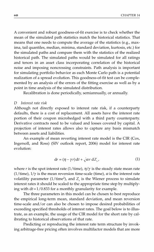
A convenient and robust goodness-of-fit exercise is to check whether themean of the simulated path statistics match the historical statistics. Thatmeans that one needs to compute the average of the statistics (e.g., max-ima, tail quantiles, median, minima, standard deviation, kurtosis, etc.) forthe simulated paths and compare them with the statistics of the realizedhistorical path. The simulated paths would be simulated for all ratingsand tenors in an asset class incorporating correlation of the historicalnoise and imposing noncrossing constraints. Path analysis is importantfor simulating portfolio behavior as each Monte Carlo path is a potentialrealization of a spread evolution. This goodness-of-fit test can be comple-mented by an analysis of the errors of the fitting exercise as well as by apoint in time analysis of the simulated distribution.
Recalibration is done periodically, semiannually, or annually.
D Interest rate riskAlthough not directly exposed to interest rate risk, if a counterpartydefaults, there is a cost of replacement. All assets have the interest rateportion of their coupon microhedged with a third party counterparty.Derivative contracts need to be valued and losses covered by capital. Aprojection of interest rates allows also to capture any basis mismatchbetween assets and liabilities.
An example of mean reverting interest rate model is the CIR (Cox,Ingersoll, and Ross) (SIV outlook report, 2006) model for interest rateevolution:
(1)
where r is the spot interest rate (1/time), η/γ is the steady state mean rate(1/time), 1/γ is the mean reversion time-scale (time), α is the interest ratevolatility parameter (1/time2), and Zr is the Wiener process to simulateinterest rates it should be scaled to the appropriate time step by multiply-ing with dt = 1/0.833 for a monthly granularity for example.
The three parameters in this model can be chosen to best reproducethe empirical long-term mean, standard deviation, and mean reversiontime-scale and/or can also be chosen to impose desired probabilities ofexceeding specified thresholds of interest rates. The goal below is to illus-trate, as an example, the usage of the CIR model for the short rate by cal-ibrating to historical observations of that rate.
Predicting or reproducing the interest rate term structure by invok-ing arbitrage-free pricing often involves multifactor models that are more
d ( )d d ,r r t r Zr= − +η γ α
648 CHAPTER 14
An Overview of Structured Investment Vehicles 649
complex that the single factor CIR model used here. Interest rates areassumed uncorrelated to credit spreads. See Appendix A for the calibra-tion of the CIR model.
E FX ratesFX Evolution may be required by the need of valuing assets in a differentcurrency or cross currency swaps for defaulting counterparties.
Evolution of an exchange rate could be modeled using a lognormalprocess as in:
de(t) = e(t)(rD(t) − rF(t))dt + e(t)σ(t)dw(t),
where rD(t) is the domestic short rate process, rF(t) is the foreign short rateprocess, and σ (t) is the volatility parameter determined from historicaltime series.
SIV Tests
Market RiskOne important feature of the SIVs is that they are market risk neutral.They are not taking position on where interest rates or FX might move. Asopposed to most hedge funds, they are not betting on market directional-ity. The SIV microhedges its positions on an asset-by-asset basis. If thehedge provider defaults, the SIV manager has to find a replacement forthe hedging counterparty. When an asset is sold, it is sold as a packagewith its associated hedge, such that the SIV does not enter into open IR orFX positions.
Each asset is hedged to floating rate USD exposure using interestrate or cross currency swaps. That is why, often, SIVs are referred to ascredit arbitrage vehicles.
The hedging counterparties are introducing additional credit risk.As such, they are treated as any other asset and capital is allocated againstsuch counterparties.
An SIV is equipped with IR and FX sensitivity test to provide theverification of its necessary representation of market neutrality. Thesetests basically measure the change in NAV due to a sudden IR shock ofeach point of the yield curve or of the entire yield curve. Tolerance limitsare set for each structure. These tolerance limits usually allow for a resid-ual basis mismatch. An uncured breach of an IR/FX sensitivity test trig-gers wind down for the SIV.

In the following figure, the reader can see a simplified example onhow a SIV manages its IR/FX exposure by putting on hedges for bothassets and liabilities to convert both into floating USD.
To monitor their exposure to interest rates and FX rates, SIV man-agers use a simple deterministic test. The test helps identify the absenceof a hedge or a significant mismatch between assets and liabilities. Theyare based on shocking current interest rate curve and revaluing assets andliabilities in the new environment. If there is perfect hedging, there is nosensitivity to the yield curve movement. The change on the asset side iscounterbalanced by the change on the liability side. A few such tests arepresented subsequently. The tolerance level is positive indicating thatthere is room for a residual mismatch. Breach of this tolerance level sendsthe vehicle in a cure period. If the test is not cured within five businessdays, the vehicle goes into irreversible winddown.
Parallel Yield Curve ShiftAll the inflows are discounted with the respective zero coupon LIBORyield curve for each currency. This test involves a parallel shift in yieldcurve for each currency by increasing and decreasing every point on thecurve by one basis point (see Figure 14.11). The aggregate impact on thepresent value (PV) of the SIV net asset value of all currencies must not bemore than a low tolerance, for example, 0.20 bps.
650 CHAPTER 14
StructuredInvestmentVehicle
GBP 10 mil 4-year fixed rate MTN at 7%
Issued debtEuro 10mil 6-year floating rated Euro RMB Sat Euribor+50
Swap paying 4 year floating $ receiving4y fixed GBP at 7%
Swaps 6 y floating Euro into floating Libor $
bought
swap swap
Bought 4 y $ USD forward vs GBP
Bought 6 y SUSD forward vs Euro
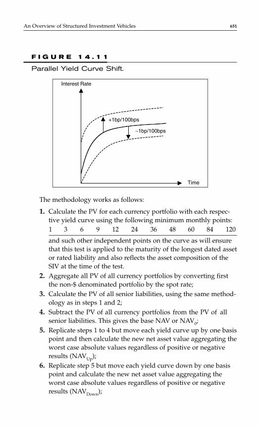
The methodology works as follows:
1. Calculate the PV for each currency portfolio with each respec-tive yield curve using the following minimum monthly points:1 3 6 9 12 24 36 48 60 84 120
and such other independent points on the curve as will ensurethat this test is applied to the maturity of the longest dated assetor rated liability and also reflects the asset composition of theSIV at the time of the test.
2. Aggregate all PV of all currency portfolios by converting firstthe non-$ denominated portfolio by the spot rate;
3. Calculate the PV of all senior liabilities, using the same method-ology as in steps 1 and 2;
4. Subtract the PV of all currency portfolios from the PV of allsenior liabilities. This gives the base NAV or NAV0;
5. Replicate steps 1 to 4 but move each yield curve up by one basispoint and then calculate the new net asset value aggregating theworst case absolute values regardless of positive or negativeresults (NAVUp);
6. Replicate step 5 but move each yield curve down by one basispoint and calculate the new net asset value aggregating theworst case absolute values regardless of positive or negativeresults (NAVDown);
An Overview of Structured Investment Vehicles 651
F I G U R E 1 4 . 1 1
Parallel Yield Curve Shift.
Interest Rate
Time
−1bp/100bps
+1bp/100bps

7. Compare the results of NAV0 minus NAVUp, and NAV0 minusNAVDown. The highest absolute value of these two calculationsis called NAV1.
ExampleAssume that an SIV has two bonds, one denominated in US$, and anotherin Euro and the $/m spot rate = 0.90. Also assume that outstanding seniorliabilities are $180.
The US asset pays: $LIBOR + 50 basis points has a three-year matu-rity and a PV of $100.
The Euro asset pays: three-month EURIBOR + 30 basis points alsomatures in year 3 and has a m PV value of 100. PV of asset = $90.
PV of the portfolio is therefore = $190.Senior liabilities pay three-month LIBOR + 20 basis points and con-
sist of a principal bullet in year 2 with a PV = $180.Net asset value0 (NAV0) = $190 − $180 = $10.The parallel shift calculations are followed, resulting in NAV1 = $9.999.Thus, the test will be passed if (NAV0 − NAV1)/NAV0 < 0.2 bps.In our example, ($10 − $9.999)/$10 = 0.01% or 0.1 basis point, there-
fore the test is passed.The test is then repeated assuming a 100 bps parallel shift.
Point-by-Point Yield Curve ShiftThis test involves an instantaneous one basis point shift (up and down) ofthe zero coupon LIBOR yield curves for each currency at each specifiedpoint along the respective curve. The manager will, therefore, be runningNAV tests as described before assuming a yield curve shift of +1 bps at theone-month point only for all yield curves. It will then rerun the tests usinga −1 bps shift at the one-month point only. The test will be repeated assess-ing the same shifts at the three-month point only, etc. The largest NAVchange result from all of these runs is compared to NAV0 in the same wayas the parallel shift test (Figure 14.12).
This test assumes that yield curve do not necessary move in a paral-lel fashion. The test particularly stresses cash flows that might be concen-trated in a specific part of the curve.
Spot Foreign ExchangeThis test involves individually changing the value of each currency rela-tive to the U.S. dollar by 1 percent (up and down). The aggregate impactfor all eligible currencies may not result in more than a preset level of
652 CHAPTER 14

tolerance, for example, 2.0 bps movement (up or down) of the SIV netasset value. Again, the new net asset value is calculated by aggregatingthe worst-case absolute values regardless of the positive or negativeresult.
Liquidity RiskLiquidity risk in an SIV arises in two ways:
1. Rollover of current outstanding debt or2. Sale of assets to meet senior liabilities.
Because the assets mature in four years on average but the liabilities falldue between one month and 18 months, cash from maturing assets can-not be relied upon to pay liabilities. The SIV relies on refinancing exist-ing debt and repaying outstanding debt with new issued debt. Whenmarket conditions are not favorable to roll current debt, the SIV faces aliquidity problem. Not being able to roll debt can cause the winddown ofthe SIV if it needs to liquidate the portfolio to repay the debt. So liquid-ity management is a very important task for the manager and that is whyin addition to the capital adequacy model, an SIV is equipped with spe-cial models to cover for liquidity shortages for limited periods of time.
The liquidity model is a tool to provide information about the vehi-cle’s internal liquidity relative to its liability. This is very important in thecontext of funding longer term assets with the issuance of commercialpaper. The liquidity model usually looks at daily inflow and outflow in
An Overview of Structured Investment Vehicles 653
F I G U R E 1 4 . 1 2
Point-by-Point Yield Curve Shift.
Month
Time
Interest Rate
−1/100 bps
+1/100 bps

654 CHAPTER 14
rolling five business days intervals to determine the peak cumulative poten-tial cash need over one year. The requirements for liquidity are covered bycredit lines, or by assets that are deemed to be “liquid,” meaning readilyavailable for sale at a price close to their current market price.
Daily cash inflows and outflows from the vehicle drive the liquidityrequirement. Unlike other areas of structured finance, 100 percent liquidityfacilities are not required as the SIV is subject to many stringent tests andconstraints and benefit can be given to the liquidity of the assets that it holds.
The SIV has to have an appropriate mix of liquidity lines and inter-nal liquidity to be able to repay some level of its short maturing liabilitieswhen they fall due. This risk takes on great importance in an SIV becausemost vehicles fund the purchase of longer-term assets with the issuanceof commercial paper that may be rolling every few days. Medium-termnotes can also be issued and as these are not normally maturity-matchedto specific assets liquidity risk arises here as well.
Given the dynamic feature of the SIV, it is appropriate to measurethe liquidity levels in the SIV on a dynamic basis referred to as the NCOtests. Some SIV managers may actually refer to this test as the MCO (max-imum cumulative outflow). This test measures on a deterministic basisthe projected one-year net payments for the vehicle. In this way, the man-ager can reserve liquid resources to cover his short-term need and avoidselling longer-dated assets for these payments which would then makehim exposed to market risk unnecessarily.
NCO TestsNCO tests are normally calculated for each rolling 1, 5, 10, and 15 busi-ness day period commencing on the next day of calculation through andincluding the day which is one year from the day of such calculation (i.e.,the vehicle needs to determine on a daily basis its 1, 5, 10, and 15 day peakNCO requirements over the next year). SIV managers may decide to haveother NCO tests beside these standards depending on the specifics of theindividual vehicle.
The NCO tests are produced by subtracting daily Outflows (i.e.,interest and principal on senior and junior debt, all admin and operatingexpenses, and all net payments on derivatives contracts) from dailyInflows (i.e., all interest and principal received from the SIV’s assets) andcumulating the results of these individual calculations over the relevantperiod. The SIV will need to ensure that the cumulative peak amount fromthe NCO tests is covered by eligible liquidity. Eligible liquidity is providedthrough a mixture of bank liquidity lines and liquid assets held by the SIV.

The table that follows shows an example of the NCO5 test for thenext six business days. The same “rolling first day” method will be usedin calculating the 10-day and 15-day periods.
Such calculation must be done for all NCOs up to one year, i.e.,approximately 240 business days.
NCO5 NCO5 NCO5 NCO5 NCO5 NCO5 NCO5Time I O I − O T T + 1 T + 2 T + 3 T + 4 T + 5 T + 6
T
T + 1 5 25 −20 −20
T + 2 4 20 −16 −36 −16
T + 3 2 0 2 −34 −14 2
T + 4 3 4 −1 −35 −15 1 −1
T + 5 4 3 1 −34 −14 −2 0 1
T + 6 2 2 0 −14 2 0 1 0
T + 7 4 3 1 3 1 2 1 1
For example, for each five-day period, there will be five differentcumulative values, except for the last 4, 3, 2, and 1 five business days ofthe year. The NCO will be the largest of the five different values, calcu-lated as follows:
Day 1 cumulative sum = Daily NCO for day 1Day 2 cumulative sum = Sum of daily NCOs for days 1 and 2Day 3 cumulative sum = Sum of daily NCOs for days 1, 2 and 3Day 4 cumulative sum = Sum of daily NCOs for days 1, 2, 3 and 4Day 5 cumulative sum = Sum of daily NCOs for days 1, 2, 3, 4 and 5
In the previous example, the largest five business days NCO is −36,which is the two-day cumulative sum of the daily NCO for days T + 1, andT + 2. In this example if the NCO5 test was run for the rest of the year (i.e.,out to T + 364) and no higher NCO5 amount was encountered, then thevehicle will need to have eligible liquidity at least equivalent to $36 millions.The vehicle will run the other NCO tests (e.g., NCO1, NCO10, and NCO15)and if any produces a higher NCO requirement than the NCO5 peak dis-cussed, that higher amount will become the eligible liquidity requirement.
Eligible liquidity can be provided through a mixture of externalliquidity facilities from A-1+ rated banks and highly liquid assets heldby the SIV. The expectation is that the SIV will cover the peak NCO5Eligible liquidity requirement with external liquidity lines only (on thebasis that a five-day liquidity period for even highly liquidity assets is
An Overview of Structured Investment Vehicles 655

656 CHAPTER 14
not an appropriate assumption at AAA). So, in the above example, if saythe NCO1 test resulted in a peak of $30, the NCO 10 test resulted in a peakof $80 and the NCO15 test resulted in a requirement of $60, the actual liq-uidity amount held by the vehicle, based on the calculations on that day,would be $80 with $36 provided by bank liquidity lines (i.e., the peakNCO5 requirement) and the remaining $44 coming from liquid assets.
Recent Developments in SIV Land
Most recent SIVs have increased their exposure to non-USD assets andnon-USD capital by creating ring fenced subportfolios in non-USD cur-rencies. SIVs have expressed interest in alternative types of funding, viacredit linked notes or repurchase agreements. In the past few years, SIVshave attempted to rate their capital notes. This is driven by risk manage-ment motivations, in an effort to quantify all exposures for internal pur-poses or for the benefit of the purchasers of the note. To date more than11 billion of capital notes has been privately or publicly rated not higherthan A. To rate the capital notes A or BBB, one needs to show that the like-lihood of losing a first dollar on the capital notes is A or BBB remote. Oncethe vehicle enters winddown, capital will be used to repay the debt, andhence capital notes will suffer a loss. So, the focus of the analysis is toquantify the likelihood of the vehicle to not enter irreversible winddown.If one makes the assumption that the manager is diligent enough to notforce the vehicle into winddown, the only drivers remain to be a massiverating deterioration and a spread widening that would consume all theexcess capital and hit the capital adequacy test. So basically, the excesscapital will have to cover all the bad credit cycles as well as market spreadwidening. The excess capital would cover for defaults and any loss inmarket value of the portfolio. Once it is used, and the minimum level ofcapital attained, the vehicle is very likely to fall short of the AAA ade-quacy test and go into winddown, when most likely the capital noteswould suffer a positive loss.
Older and newer SIVs have expressed interest in entering othertypes of markets like credit derivative markets, where they act as protec-tion sellers.
It is also worth mentioning that other types of operating companieshave borrowed from SIV technology to a greater or lesser degree (mostlyto manage market and liquidity risk), like repurchase agreement vehiclesas well as credit derivative companies.

OTHER TYPES OF QUASI-OPERATING COMPANIES
In addition to the SIVs, other operating companies have been designed toserve a special purpose. Derivative product companies are intermediariesbetween financial institutions (known as their parent or sponsor) andtheir third party counterparties. Derivative product companies (DPCs)intermediate swaps between the sponsor and third parties underapproved ISDA master agreement. Enhanced subsidiaries differ fromother derivative-product subsidiaries, as their credit ratings do not rely ontheir parent’s guarantee. A DPC may engage in over-the-counter interestrate, currency and equity swaps, and options as well as certain exchange-traded futures and options depending on its individual structure. A DPCis capitalized at a level appropriate for the scope of its business activitiesand desired rating. DPCs have been set up in most cases to overcomecredit sensitivity in the derivative product markets. There are two typesof DPCs: continuation or termination structures. The continuation struc-tures are designed to honor their contracts to full maturity even when awinddown event occurs, whereas the termination structures are designedto honor their contracts to full maturity, or should certain events occur, toterminate and cash settle all their contracts prior to their final maturity.The chart presented subsequently illustrates a DPCs role as an intermedi-ary with offsetting trades.
The DPCs have AAA rating and are often projected as the AAA faceof the sponsor. They are market risk neutral by mirroring their trades withthird parties with the parent or sponsor. They are exposed to credit risk ofthird parties. As with the SIVs, the structure is equipped with exit strate-gies and resources that ensure that even in a winddown scenario, thevehicle meets with AAA certainty its derivative obligations.
The market for derivative product companies started in early 1990.Every bank that wanted to be eligible as an AAA counterparty in deriva-tive contracts, sponsored its own derivative product company. Currentlythere are 15 active DPCs.
♦ Bank of America Financial Products, Inc.♦ Bear Stearns Financial Products, Inc.♦ BT CreditPlus (closed)
Sponsor(e.g.“A”) DPC CTPY
An Overview of Structured Investment Vehicles 657
658 CHAPTER 14
♦ Credit Lyonnais Derivative Program♦ GS Financial Products International L.P. (closing)♦ Lehman Brothers Derivative Products, Inc.♦ Lehman Brothers Financial Products, Inc.♦ Merrill Lynch Derivatives Products AG♦ Morgan Stanley Derivative Products, Inc.♦ Nomura Derivative Products Inc.♦ Paribas Derives Guarantis♦ Sakura Prime (closed)♦ Salomon Swapco, Inc.♦ SMBC Derivative Products, Ltd♦ JP Morgan Enhanced ISDA Program
Once a trigger event occurs, the DPC freezes its operations and activemanagement. The termination DPCs accelerate all their contracts and exitthe market in a short termination window, typically 15 days. Hence, thetermination payments that the counterparties owe to the DPC will bepassed through to the parent to close out the mirror contracts. If the coun-terparties default, capital will be used for those payments.
If the DPC owes money to the counterparty, the parent is deliveringthat termination payment to the DPC from the mirror trade, in which par-ent owes money to the DPC. That amount is quantified and held as col-lateral posted by the parent on behalf of the DPC.
Practically, two models are being developed for a DPC: a creditmodel in which capital is quantified to cover for third party defaults, aVaR type of model in which the amount that the parent owes to the DPCon all its trades is quantified over a 15-day horizon.
Quantitative techniques in sizing capital adequacy for a DPC rely ona market rate generator in which new market environment is projected forthe lifetime of the portfolio. This means that interest rates in each currencyand foreign exchange rates are projected in a correlated fashion up to thelongest tenor of the swap book.
The forward rates require models for the entire yield curve. Thefinancial literature provides a wide range of models from one to multiplefactor models.
Principal component analysis (PCA) involves a mathematical proce-dure that transforms a number of (possibly) correlated variables into a(smaller) number of uncorrelated variables called principal components. Thefirst principal component accounts for as much of the variability in the data
658 CHAPTER 14

as possible, and each succeeding component accounts for as much of theremaining variability as possible.
The mathematical technique used in PCA is called eigen analysis: itsolves for the eigenvalues and eigenvectors of a square symmetric matrix,the covariance matrix of key points on the yield curve. The eigenvectorassociated with the largest eigenvalue has the same direction as the firstprincipal component. The eigenvector associated with the second largesteigenvalue determines the direction of the second principal component.The sum of the eigenvalues equals the trace of the square matrix and themaximum number of eigenvectors equals the number of rows (or columns)of this matrix.
In most cases, two or three PCAs are enough to explain more than90 percent of the variance covariance matrix.
Once the market environment is simulated, valuation moduleswill be used to project the mark-to-market of each swap contract. Bycombining market paths with credit paths (in which the credit worthi-ness of the counterparty is simulated), one can see where capital isbeing deployed to cover for losses. The potential losses correspondingto each market path can be obtained by combining the results of defaultsimulations and the counterparty exposures. A consideration of lossesacross all market paths permits the construction of a distribution ofpotential credit losses. The necessary credit enhancement to protectagainst losses at a given level of confidence may be obtained. This riskmodel can also quantify the potential change in the portfolio’s valueover a period of time.
A DPC with a continuation structure generally receives collateralfrom the parent to cover its exposure to the parent resulting from theback-to-back trades. This collateral amount, after appropriate discountfactors are applied, is equivalent to the net mark-to-market value of theDPC’s portfolio of contracts with its parent. Upon the occurrence of cer-tain events, however, the management of the DPC’s portfolio will bepassed on to a contingent manager.
In the short period prior to the transfer of portfolio management tothe contingent manager, the value of the DPC’s contracts with its parentcould rise. Using the capabilities of the risk model, the potential increasein the DPC’s credit exposure to the parent may be quantified.
In a termination structure, the value of the DPC’s portfolio can changeover the period beginning with the last regular valuation date and endingat the early termination valuation date upon occurrence of a terminationtrigger event. Again, the potential change in the portfolio’s value may
An Overview of Structured Investment Vehicles 659
be determined at the desired level of confidence by using the same riskmodel.
The DPC’s liquidity needs also require evaluation. The DPC must beable to meet its obligations on a timely basis. These include its payables toits counterparties under its derivative contracts, and to its parent result-ing from the back-to-back transactions and, in certain cases, obligation tomeet margin calls on the exchange-traded futures contracts used ashedges. The risk model may be used in determining the liquidity needs ofthe DPC by using simulated market evolution and evaluating the currentportfolio of derivative contracts and the likely portfolio of offsettinghedges. Using the model, a distribution of daily portfolio positions can besimulated, thus establishing, at an appropriate level of confidence, thepotential liquidity need of the DPC on a daily basis and over a specifictime horizon.
CREDIT DERIVATIVE PRODUCT COMPANIES
Since credit default swaps made their debut in 1991, their marketplace hasgrown exponentially. This has created a new asset type for derivativeproduct companies, called credit derivative product companies (CDPCs).
Generally, a CDPC is a special-purpose entity that sells credit pro-tection under credit default swaps or certain approved forms of insurancepolicies. Sometimes, they can also buy credit protection. A CDPC is orga-nized to invest in credit risk exposure in certain segments of the marketsthrough the use of credit derivatives or insurance policies.
The following chart illustrates the typical structure of a CDPC thatsells credit protection under a credit default swap.
The AAA counterparty rating assigned to a CDPC ensures that allobligations of the company are met with AAA certainty, should a triggerevent occur and send the vehicle into winddown.
The CDPCs rated to date are listed:
1- Primus AAA ICR—focused on single name primarilyNotional approximately $13 billionLaunch: 20012- Athilon AAA ICR—focused on tranche business primarilysenior and super senior tranchesNotional approximately $10 billionLaunch: 2005
660 CHAPTER 14
3- Theta AAA operating program—focused on single nameprimarilyNotional approximately $2 billionLaunch: 2005
CDPCs and CDOs
The two structures are indeed in the same type of business: selling pro-tection on a portfolio of reference entities. These reference entities can besingle name corporates, single name ABS, baskets of names or structuredcredit, namely indices or CDO tranches. The tranches can be anywhere inthe capital structure of the CDO ranging from the first loss position tosuper senior.
CDPCs are evergreen vehicles, whereas CDOs have a finite life. Inaddition, the risk model of a CDPC has to account for all obligations ofthe CDPC including termination payments on credit default swap con-tracts. In a CDO, such obligations are subordinated in the waterfall andthe risk model does not address the likelihood of such obligations to bepaid.
When a credit default swap counterparty defaults, a terminationpayment may need to be calculated. The termination payment is thepotential future mark-to-market of the credit derivative contract. This ter-mination payment on the swap contract is the expected risky discountedvalue of the remaining cash flows of the swap. The key variables in com-puting the forward value of the swap are the then-current rating of theentity of which protection is sold or bought and the potential future creditswap premium. For each counterparty, the termination payments on theunderlying contracts are computed and aggregated at the counterpartylevel if netting is applicable. For each out-of-the-money position witheach counterparty, capital is reserved. The termination payments on swapcontracts of a CDPC are AAA obligations pari passu with payments oncredit events and other AAA obligations.
The future rating of single names can be explicitly modeled using amultiperiod transition matrix, or a distribution of ratings could be inferredfrom the timing of defaults of the underlying obligors (in case a time todefault model was chosen). Given the current liquidity in the market of cer-tain tenors on the credit default swap curve, it is likely that a model for afull-term structure for the credit default swap premium would be hard tocalibrate. As a simple method of implementing proxy, a flat-term structure
An Overview of Structured Investment Vehicles 661
may be assumed at the most liquid point on the curve (e.g., five years). Thatpoint could be projected forward using a model that takes into considera-tion serial correlation, fat tails, and correlation across different industriesand ratings. Further, the simulated premium is used to derive the risky dis-count factors, which, when applied to the remaining premium payment,would compute the fair market value at the then-current time step. Thecredit derivative market is expected to become more liquid, and, in thefuture, term structure models for the entire credit default swap curve areexpected to be developed. This would allow further enhancements of thevaluation modules currently used by the market.
The fair market value of a credit default swap on a structured creditdepends on the behavior of the underlying portfolio of reference entities.As opposed to a single name, where the default is a binary event, a struc-tured credit is approached based on expected loss of the tranche. Forexample, for a first-loss position, losses due to defaults have a directimpact on the size of the tranche. For a mezzanine tranche, defaults willimpact the position in the capital structure of that tranche and, poten-tially, the size of the tranche. At each time step, the distribution of lossesto the tranche can be calculated based on aggregating losses in theunderlying portfolio. Then, the incremental expected losses in eachperiod can be derived and discounted to size the net PV of aggregate losson the tranche. Pricing of the tranche is affected by the defaults in theunderlying pool and by the movement of rating/credit spreads of thenondefaulting entities. Correlation among the credits in the portfolio isanother key input in the pricing module of a tranche. Reader is referredto recent research papers on correlation term structure and impact ontranche pricing.
CDPCs and SIVs
As with an SIV, the CDPC has a dedicated management team that decidesto increase or decrease leverage as they see appropriate. Although the twohave different businesses and, perhaps, motivations, in the recent yearsthe two have borrowed from each other important structural features. Assuch, we have seen SIVs trying to enter the credit derivative market andsell and buy protection. So their risk model had to be adjusted for defaultof the underlying and swap termination payments.
Also CDPCs, which traditionally held their capital in highly rated
662 CHAPTER 14

investments expressed interest in investing and holding higher yieldingassets. If the eligible investments include riskier assets, like corporatesand/or ABS, their market value and credit risk needs to be explicitlyincorporated by modeling their key risk factors: asset spreads and creditmigration. In this way, the model can size appropriately the impact ofthe investments on the cash flows of the company. It can address, in anaccurately and timely fashion, the cash inflows for the coupons and theliquidation risk for the assets that need to be sold to meet the timely“AAA” obligations of the company. The potential future credit ratingof the asset that needs to be liquidated, as well as its market value, ismodeled.
Hybrid vehicles have attracted the interest of the market and we seethis interest growing.
There are currently special purpose companies that combine struc-tural features of a CDPC with SIVs (e.g., Theta) and vice versa.
The CDO technology and tiered capital structures start to attractinterest for a more efficient funding strategy. We expect the three types pre-sented earlier to overlap and to lead to the creation of new innovativestructures.
REPO COMPANIES
Repo companies are AAA vehicles that engage in repurchase agreements.They provide financing to institutional investors through reverse repur-chase transactions and total return swaps. To achieve that, these vehiclesfinance themselves through repurchase agreements or commercial paperand medium term notes.
A repurchase agreement (or repo) is an agreement between two par-ties whereby one party sells the other a security at a specified price with acommitment to buy the security back at a later date for another specifiedprice. Most repos are overnight transactions, with the sale taking placeone day and being reversed the next day. Long-term repos—called termrepos—can extend for a month or more. Usually, repos are for a fixedperiod of time, but open-ended deals are also possible. Reverse repo is aterm used to describe the opposite side of a repo transaction. The partywho sells and later repurchases a security is said to perform a repo.The other party—who purchases and later resells the security—is said toperform a reverse repo.
An Overview of Structured Investment Vehicles 663
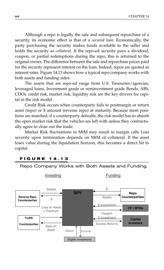
Although a repo is legally the sale and subsequent repurchase of asecurity, its economic effect is that of a secured loan. Economically, theparty purchasing the security makes funds available to the seller andholds the security as collateral. If the repo-ed security pays a dividend,coupon, or partial redemptions during the repo, this is returned to theoriginal owner. The difference between the sale and repurchase prices paidfor the security represent interest on the loan. Indeed, repos are quoted asinterest rates. Figure 14.13 shows how a typical repo company works withboth assets and funding sides.
The assets that are repo-ed range from U.S. Treasuries/agencies,leveraged loans, Investment grade or noninvestment grade Bonds, ABS,CDOs. credit risk, market risk, liquidity risk are the key drivers for capi-tal in the risk model.
Credit Risk occurs when counterparty fails to postmargin or returnasset (repo) or $ amount (reverse repo) at maturity. Because most posi-tions are matched, if a counterparty defaults, the risk model has to absorbthe open market risk that the vehicles are left with unless they contractu-ally agree to close out the trade.
Market Risk fluctuations in MtM may result in margin calls Lossseverity upon termination depends on MtM of collateral. If the assetloses value during the liquidation horizon, this becomes a direct hit tocapital.
664 CHAPTER 14
SPV RepoCounterparties
CP / MTNs
CapitalInvestors
Funding
Reverse RepoCounterparties
TroRS
Counterparties
Assets
$
Eligible Investments
Assets
$
Investing
Loss on Asset+ Premium
Gain onAsset Return $ Funds
Excess Returns
$ Investment
$ Investment
Coupon
F I G U R E 1 4 . 1 3
Repo Company Works with Both Assets and Funding.

An Overview of Structured Investment Vehicles 665
Liquidity Risk
SPV may be required to post additional margin/return excess margin.That is why a spread model is needed to accurately evolve through timethe market value of the assets.
In a repo, SPV would post more assets or return cash to counterpartyif MtM of original assets falls below maintenance margin.
In a reverse repo, SPV would return assets or send additional cashto counterparty if MtM of asset rises above maintenance margin.
All three risks can be modeled according to the terms of the repo con-tracts. One could use modules similar with the ones presented as examplesgiven earlier.
LIQUIDITY FACILITIES
Another type of special purpose company is a vehicle that is set up toprovide multilateral and bilateral commitment facilities extended to cor-porate borrowers. It is a limited purpose company that seeks to provideback-up liquidity to its corporate clients.
A structural diagram, like the one presented subsequently, shows theSPV has to raise capital from its capital investors to cover for the potentialpeak drawdown over the life of the commitments. Funding for such vehi-cles rely on the fact that not all borrowers draw up to to their limit in thesame time.
The corporate borrowers usually have a two-year or a five-year com-mitment line with the SPV. They can borrow any amount up to their com-mitment size and have the obligation to repay it within the tenor of thefacility. A borrower that cannot pay back the amount borrowed is deemedto have defaulted on its obligation. The SPV has to have resources to coverless than the total notional of the commitments, as not all borrowers willdraw in the same time. The quantitative exercise here is to size an amount
SPV
Capital investors
Corporate
borrower
that covers the borrowers who will default and not pay back and, moreimportant, cover the potential maximum drawdown amount over the life-time of these commitments.
The key risk factors for such an exercise are frequency of drawdown,magnitude of drawdown, and persistence of drawdowns. They are dif-ferent per rating and certain industries. Credit worthiness is modeledusing the technologies presented before, applying a rating transitionapproach. The other factors are modeled from data collected on them.Each of the factors is a source of randomness and noise in the simulation.By combining credit paths with paths for drawdowns and persistence, astochastic model is built.
Typically, this Monte Carlo exercise results in a percentage less than100 percent (the size of the commitments extended), in capital require-ment. As mentioned earlier, tranching using CDO technology can providea more efficient source of funding for the operating company.
A P P E N D I X A
CIR Model Calibration
The steady state probability and cumulative density functions
fr(r)dr ≡ Probr < r ≤ r + dr; Fr(r) ≡ Probr ≤ r (2)
of the interest rates following the CIR process is given by
(3)
(4)
(5)
A way to infer the three parameters of the CIR model is by calculat-ing statistical moments of quantities involving the interest rates and fitting
κ ηα
κ κκ κ= = =− −∞
− −∞
∫ ∫2 1
0
1; ( ) e d ( , ) e d .Γ Γx x z x xx x
z
;
F rr
r ( )( , / )
( ),= −1
ΓΓ
κ κγ ηκ
f rr r
r ( )( / ) exp[ / ]
( ),=
−−2 21γ α γ ακ
κ κ
Γ
666 CHAPTER 14

the parameters to best reproduce the moments. The steady state first sta-tistical moment of the interest rate is given by
(6)
The steady state second statistical moment is given by
(7)
It follows directly from Equation (1) that the second statisticalmoment of the interest rate change ∆r over small time intervals ∆t isgiven by
(8)
Substituting Equation (6) in (8) gives
(9)
Equations (6), (7), and (9) along with empirical inferences of rr, σr2,
and provide a method for calibrating η, γ, and α. Hence,
(10)
(11)
and
(12)
Using historical time series from 1963–2003, closed form solutionsfor the three parameters were derived.
The empirical statistics are
r = 0.071483(1/yr); σr = 0.03379823(1/yr); = 0.000049099(1/yr2).∆r2
ασ
σ= − + +
21 1
12 2
2r
rrr
t∆
∆.
ησ
= − + +
r
rtr
1 112
2
∆∆
,
γσ
= − + +
1 1
12
2
∆∆
rtr
,
∆r2
∆ ∆ ∆r t r tr2 2 2 2= +γ σ α .
∆ ∆ ∆r r t r t2 2 2= − +( ) .η γ α
σ ηαγr
222
= .
r = ηγ
.
An Overview of Structured Investment Vehicles 667

The fitted parameters are
η = 0.018205493(1/yr2); γ = 0.25468 (1/yr);α = 0.00813991(1/yr2) 1/γ = 3.926 yr.
In Cox et al. (1985), it is shown that zero-coupon bond prices, withterm (T − t) and issued at time t, when the short rate is r(t), have the fol-lowing general form:
P(t, T) = A(t, T)e−B(t, T)r(t),
where
and
The continuously compounded rate for a zero-coupon bond is then;
The CIR model allows us to price any bond regardless of maturity,simply by modeling the short rate. For any given term, L = (T − t), both Aand B are constants and the earlier equation becomes
Hence, the long rate is a linear function of the short rate. In this way,a full discounting curve can be built for each currency and used to derivethe market value of the assets and the mark-to-market on derivativecontracts.
R tBr t
( , )( ) ln
. LA
L= −
R tP t
( , )ln ( , )
T T
T t=
− ( )−
k = +γ λ2 22 .
A tk
k k
k T t
k T t( , )
e( )(e )
,( )( )/
( )
( / )
T =+ − +
+ −
−
21 2
2 2γ γη γα
γ
B tk k
k T t
k T t( , )
2(e )( )(e )
,( )
( )T =
−
−
−+ − +
11 2γ
668 CHAPTER 14
A P P E N D I X B
Analyzing Capital Notes for a SIV
The rating on the capital notes of an SIV can be assigned either confiden-tially or publicly—the methodology does not differ—and addresses theSIV’s ability to make ultimately payment of the principal amount of thecapital notes, plus the minimum interest amount. These interest paymentscan be addressed in the rating definition as being timely or ultimately. Thiswill depend on whether the capital note (or junior) model is able to pro-duce results that suggest that the minimum coupon can be paid timely, orthe transaction documents specify that coupons can be deferred.
We assume that in defeasance, the capital note investors lose at leastone dollar of their investment, hence P(first dollar of loss conditionalupon defeasance) = 1.
However, capital note investors could suffer losses outside defea-sance as well, hence it may be the case that P(first dollar of loss condi-tional upon no defeasance) > 0.
Therefore, the rating analysis must address three main areas,namely:
♦ Analysis of defeasance events♦ Probability of defeasance and♦ Likelihood of first dollar of loss to capital note investors outside
defeasance.
For the capital notes, the evaluations that one would make in order toreach comfort to look only at a parametric model are more heavily basedon qualitative than quantitative assumptions. They relate to the man-ager’s ability to perform in the future and to avoid noncredit/noncapitalrelated winddown/defeasance events. However, the likelihood or remote-ness of triggering defeasance is not an assumption in the rating method-ology for the senior debt of a SIV, where defeasance is supposed to occuron day 1, regardless of what caused it.
In practice, the SIV manager requests a desired rating on the capitalnotes. The majority of managers have requested a rating in the “BBB”range.
It must be noted that the methodology that follows is neither spe-cific to any vehicle S&P currently rates, nor it is prescriptive to anyvehicle seeking a rating on the capital notes. Indeed, other issues could
An Overview of Structured Investment Vehicles 669
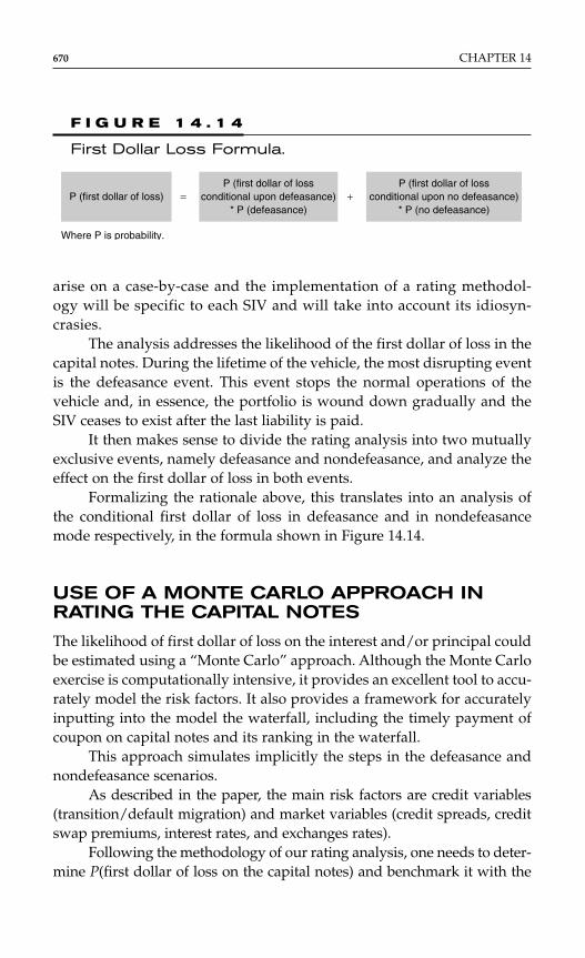
arise on a case-by-case and the implementation of a rating methodol-ogy will be specific to each SIV and will take into account its idiosyn-crasies.
The analysis addresses the likelihood of the first dollar of loss in thecapital notes. During the lifetime of the vehicle, the most disrupting eventis the defeasance event. This event stops the normal operations of thevehicle and, in essence, the portfolio is wound down gradually and theSIV ceases to exist after the last liability is paid.
It then makes sense to divide the rating analysis into two mutuallyexclusive events, namely defeasance and nondefeasance, and analyze theeffect on the first dollar of loss in both events.
Formalizing the rationale above, this translates into an analysis ofthe conditional first dollar of loss in defeasance and in nondefeasancemode respectively, in the formula shown in Figure 14.14.
USE OF A MONTE CARLO APPROACH INRATING THE CAPITAL NOTES
The likelihood of first dollar of loss on the interest and/or principal couldbe estimated using a “Monte Carlo” approach. Although the Monte Carloexercise is computationally intensive, it provides an excellent tool to accu-rately model the risk factors. It also provides a framework for accuratelyinputting into the model the waterfall, including the timely payment ofcoupon on capital notes and its ranking in the waterfall.
This approach simulates implicitly the steps in the defeasance andnondefeasance scenarios.
As described in the paper, the main risk factors are credit variables(transition/default migration) and market variables (credit spreads, creditswap premiums, interest rates, and exchanges rates).
Following the methodology of our rating analysis, one needs to deter-mine P(first dollar of loss on the capital notes) and benchmark it with the
670 CHAPTER 14
F I G U R E 1 4 . 1 4
First Dollar Loss Formula.
P (first dollar of loss)
Where P is probability.
P (first dollar of lossconditional upon defeasance)
* P (defeasance)
P (first dollar of lossconditional upon no defeasance)
* P (no defeasance)+=
default probability of a corporate bond with a similar rating and tenor. Thetenor may depend on certain structural features of the capital notes, typi-cally with expected maturities of seven to 10 years, although this expectedmaturity can be shorter if puts are exercised by capital note investors.
To do the exercise using a Monte Carlo tool, one needs to evolve theportfolio through time and analyze if timely payment of coupon and prin-cipal on the capital notes can be achieved. In each “time step,” one wouldstochastically evolve the credit and market variables and analyze the newprofile of the portfolio. This means that in each time step, the creditwor-thiness and market value of the portfolio are computed and then checkedwhether the portfolio meets the guidelines and passes the capital ade-quacy tests (in each time step, the simulated market value of the assetportfolio should be greater than par of all senior debt issued).
Therefore, in each time step, a random process would define thethen-current market and credit environment. Assets have a stochasticmarket value that reflects their new rating, new market spreads, and newtenor. Breaching portfolio guidelines (e.g., rating limits) should be curedto get back into compliance by selling assets or 100 percent capital charg-ing the assets.
In each time step, the waterfall is implemented starting with the“AAA” senior fees and expenses, then the senior debt, and finally incor-porating the minimum coupon on capital notes. The remaining fundscould be distributed as profit according to the guidelines (with or withouta cap). Thereafter, any remaining funds are cash trapped for the subse-quent time steps and reinvested at the original ratings and at spread lev-els simulated stochastically.
In evolving credit spread curves for reinvestment purposes, focus ison stressing the spread tightening as opposed to the same exercise forasset pricing purposes, where focus is on stressing the spread widening.Debt is rolled at a cost of funds that itself is a stochastic variable thatneeds to be simulated.
In each time step, as long as the adequacy tests (portfolio guidelines,capital, and capital gearing) are met, the model makes assumptions of sto-chastically reinvesting the cash amount from maturing assets or recover-ies, recontracting derivative contracts, and rolling debt (cost of funds mayvary as well).
If the capital test is breached during a time step and defeasance is trig-gered, the vehicle stops issuing debt and sells assets to repay liabilities. It isalmost certain that in the defeasance mode, capital would be deployed torepay senior debt. That path should be deemed a failed path for the purpose
An Overview of Structured Investment Vehicles 671

of rating the capital notes. Let us say there is a total of D paths that triggerdefeasance out of the total of N paths simulated. In this way, the Monte Carloexercise sized the probability of defeasance to be D/N.
The paths in which all the tests are met do not trigger defeasance.Those paths are re-run each time step until the maturity of the capitalnotes. The challenge is to see whether the minimum coupon and the fullnotional value of the notes can be paid.
Intuitively, this translates into having enough spread to make up forthe defaulted assets, which would be the main consumer of capital.
There may be paths in which, although defeasance is not triggered,there is not enough cash to repay in full the capital notes. These are alsoconsidered to be failed paths. Let us say there are E paths in which thenotes are not paid in full out of the total of N paths simulated. In this way,the Monte Carlo exercise sized the probability of first dollar of loss if nodefeasance occurs to be E/N.
The number of failed paths for the capital notes is therefore(D + E)/N, where
♦ D = Defeasance paths♦ E = Non-defeasance paths but notes not paid in full and♦ N = Total number of paths.
This has to be commensurate with a default probability of a corporatebond with the desired rating and tenor.
In a Monte Carlo stochastic model, if there is a similar model for thesenior notes, parameters are kept the same if they were already calibrated.The level of confidence lower than “AAA” is incorporated in the cut-offpoint or the tolerance for failed paths.
It is worth reminding readers that this methodology is not prescrip-tive; in fact, one could use this Monte Carlo tool to simulate defeasanceand see how much capital was deployed. There may be paths in whichnot all the capital is used (e.g., if assets recover in price) and the capitalnote investors may get a portion of their notes back.
THE NON-MONTE CARLO APPROACH
Given the formula for calculating the probability of the first dollar of loss(see chart 4), one needs to estimate only P(defeasance) and P(first dollarof loss given no defeasance). Besides the Monte Carlo approach, these twoprobabilities could be quantified with other methods.
672 CHAPTER 14
For example: P(defeasance) can be quantified by assuming that defea-sance occurs due to a drastic downgrade of asset ratings and spread widen-ing over a short horizon, say, one month or three months. Intuitively, thisdowngrade and spread widening would consume all excess capital andmake the “AAA” capital adequacy test trip and hence trigger defeasance.
Performing the earlier exercise amounts to quantifying the probabil-ity of a spread widening occurring over a short horizon and compound-ing it to the tenor of the capital notes (e.g., 10 years).
This requires a probabilistic model to be fitted to the spreads.Furthermore, the analysis has to reflect the composition of the portfolio,hence the asset mix. The spreads usually have “fat” tails and may varyfrom one asset type to another.
P(loss given no defeasance) can be quantified using a profit and lossapproach in which conservatively assessed incomes are counted againststressed defaults, senior fees and other expenses, senior debt, and theminimum coupon on the capital notes.
The methodologies given earlier are only examples of alternativeapproaches to a Monte Carlo approach. They could be adapted to eachSIV’s model or technology. For nonstochastic models, parameter stressesmay need to be lowered to reflect the increase in tolerance in the exerciseof rating the capital notes as opposed to senior debt. For portfolios thatare not ramped up, a variety of assumptions on initial asset spreads andcost of funds is tested.
In rating capital notes, to address rating volatility several portfoliosshould be tested, with low, medium, and high leverage or, respectively,with high, average, and low credit quality. Ultimately, the excess spread(beyond the “AAA” model) is the main contributor to the payment ofcoupon and principal on the capital notes. Refining the capital structureof the capital notes into a mezzanine and first-loss piece may help absorbthe losses and achieve a higher rating.
REFERENCESCarty, lea V. and Lieberman, D. (1996), “Corporate Bond defaults and Default
Rates 1938–1995,” Moody’s Investors Service, Global Credit Research.Cox, J.C., J.E. Ingersoll, and S.A. Ross (1985), “A Theory of the Term Structure of
Interest rates,” Econometrica, 53(2), March, 385–408.CreditMetrics (1997), Technical Document April.“Global Methodology For Rating Capital Notes In SIV Structures” (published on
February 11, 2005).Jolliffe, I.T. (1986), Principal Component Analysis, Springer-Verlag.
An Overview of Structured Investment Vehicles 673

Merrill Lynch (2005), Fixed Income Strategy, “SIVs are running strong,” January 28.Merrill Lynch (2005), International Structured product Monthly ( jan), “SIV capi-
tal Notes vs. CDO Mezzanine Notes and equity,” February 1.Hull, J. (2005), Options, Futures and other Derivative Securities.Prigent, Renault, and Scaillet (2000), An Empirical Investigation in Credit Spread
Indices.Rating Derivative product Companies S&P Structured Finance Criteria February
2000.Standard & Poor’s Research—Principal Repayment and Loss Behaviour of
Defaulted U.S. Structured Finance Securities, published 10 January 2005 byErkan Erturk and Thomas Gillis.
“Structured Investment Vehicle Criteria: New Developments” (published onSeptember 4, 2003).
“Structured Investment Vehicle Criteria” (published on March 13, 2002).SIV Outlook Report/Assets Top $200 Million in SIV Market; Continued Growth
Expected in 2006—January 2006.
674 CHAPTER 14
C H A P T E R 1 5
Securitizations in Basel II
William Perraudin*
675
INTRODUCTION
In this chapter we consider the rules governing regulatory capital forstructured products† in the new Basel II proposals.‡ We look at themotives that have influenced regulators in designing the rules, review thedifferent approaches banks will be required to follow, discuss the finan-cial engineering that underpins the main approaches, and consider thelikely effects of the new Basel II system on the structured product market.To ensure that the discussion is self contained, we briefly review somerelevant features of the market in this introduction.
Growth in structured products began in the 1980s with the emer-gence of the residential mortgaged-backed security (RMBS) market in theUnited States. In the 1990s, substantial asset-backed security (ABS) mar-kets emerged in auto loans and credit card receivables. Since the late 1990s,there has been major growth in different types of collateralized debt obli-gations (CDOs) in which the special purpose vehicle (SPV) pool is madeup of illiquid bonds or loans by banks to large corporate borrowers.
675
*The author thanks Patricia Jackson and Ralph Mountford of Ernst of Young for valuablediscussions and Robert Lamb for research assistance.†We use the terms “structured product” and “securitization” interchangeably.‡See Basel Committee on Banking Supervision (2005).
Copyright © 2007 by The McGraw-Hill Companies. Click here for terms of use.
Recently, the range of collateral types included in structured prod-uct pools has widened further, as issuers have created securitizationsbased on trade receivables of different kinds, equities, commercial prop-erty, utility receivables, and even energy derivatives. Issuers have realizedthat, in principle, any assets that represent claims to future cash flows canbe securitized.
As well as classic securitizations in which assets are transferred to anSPV, banks have made extensive use of structures in which off balancesheet conduits issue commercial paper and use the proceeds to purchaserevolving pools of assets. Such Asset-Backed Commercial Paper (ABCP)conduits are particularly important in the United States.
Also common are synthetic securitizations. In these, the SPV pro-vides a bank with credit protection on its loans [often, in the form of creditdefault swaps (CDS)]. At the same time, it issues notes to the market andinvests the proceeds in high credit standing bonds such as Treasuries. Thepremiums the SPV receives from the bank on the CDSs plus the couponson the Treasuries provide it with income it uses to pay coupons on thenotes. Such structures are often cheaper to create than traditional struc-tured products, since the legal complication of transferring ownership ofthe underlying assets is avoided.
The impact of structured products has been substantial for issuersand investors alike. Structured products have provided investors with abroader and more liquid range of debt instruments in which they caninvest, permitted issuers to manage better their balance sheets risks, andopened up new sources of funding for banks. As early as 1998, one esti-mate suggested that 40 percent of the nonmortgage loan books of the 10largest U.S. bank holding companies had been securitized.
THE REGULATORS’ OBJECTIVES
This section reviews the broad objectives regulators have had in framingthe Basel II rules for structured products. The treatment of securitizationsis a key part of Basel II. This is not just because of the sheer volume ofsecuritization exposures in bank portfolios, but also because banks havemade widespread use of securitization to circumvent regulatory capitalrequirements through the so-called capital arbitrage. Indeed, the preva-lence of such capital arbitrage has been one of the major reasons that reg-ulators have felt obliged to replace the simple rules of the 1988 BaselAccord with the more complex, risk-sensitive regulatory capital require-ments of Basel II.
676 CHAPTER 15
Examples of how securitizations may be used for capital arbitrageare provided by Jones (2000). Consider the following example. Suppose abank possesses a loan pool worth $100. The chance of losses exceeding $5might be negligibly small. In this case, the bank could create a securitiza-tion and retain a junior tranche with par value of $5. It thereby retains allcredit risk in the transaction.
The maximum capital charge that the regulatory authorities cancharge is 100 percent. Hence, the bank which would have had to hold cap-ital of $8 under Basel I if the exposures were held on balance sheet nowhas to hold no more than $5 in capital even though its risk position hasnot changed.
Under Basel I, even lower regulatory capital charges may be achievedif the pool exposures are actually originated by the SPV. In this case, thebank may provide the SPV with a credit enhancement like a subordinatedloan so that it effectively bears the credit risk associated with the pool ofassets. Under Basel I, the subordinated loan in this case just attracts an 8percent capital charge.
In the light of these examples, one may understand how importantit has been for bank regulators designing the Basel II system to come upwith rules likely to reduce the incentives banks face to engage in capitalarbitrage.
To achieve this, regulators have tried, first, to design regulatory cap-ital charges for loans that are aligned with the capital that banks wouldthemselves wish to hold. Second, they have aimed to create a system ofcapital charges that preserves on and off balance sheet neutrality, i.e., thecapital banks must hold should be the same whether they hold a pool ofloans on balance sheet or if they securitize it and retain all the tranches.Third, they have sought to ensure that the individual capital chargesattracted by the different tranches in a structure are consistent with therelative distribution of risks between the tranches.
The new system of capital charges will inevitably have an impact onthe securitization market. One of the major objectives of Basel II after allis to reduce the volume of transactions motivated by capital arbitrage con-siderations. Nevertheless, an important objective has been not to impedeactivity unreasonably in particular segments of the market, especiallywhere the transactions are clearly aimed at effecting genuine transfer ofrisk off the issuer’s balance sheet.
As we shall see, in certain key areas, regulators have felt obliged toinclude additional flexibility to prevent the new regulations having a prej-udicial effect upon market segments. In particular, the impact of Basel II
Securitizations in Basel II 677
on suppliers of liquidity and credit enhancement facilities in the ABCPmarket has been of great concern to the U.S. regulators because of theimportance of this market to U.S. companies.
Given these general objectives, regulators have provided a menu ofdifferent approaches that should permit banks to calculate capital for thevery diverse range of securitization exposures in their books in a risk-sensitive fashion.
The different approaches permitted in the menu is heavily influ-enced by the question of how much information one may expect banks tohave about the securitization exposure they hold. For example, as arms-length investors, a bank may hold substantial securitization exposuresabout which they have only hazy information. Typically, they will onlyhave a broad notion of the composition and credit quality of the underly-ing asset pool. On the other hand, if a bank has originated and continuesto manage the securitized assets, it will have very detailed informationabout the securitization.
An intermediate case occurs when a bank acts as the sponsor of acommercial paper programme. The sponsoring bank may supply creditenhancements and liquidity facilities to the programme that will then rep-resent exposures subject to the Basel II securitization framework. Theunderlying assets will in most cases have been bought in from other orig-inators, and so the sponsor will only have limited information aboutthem.
The two possible ways in which securitization capital chargesmight be calculated are either (1) to base charges on the ratings attributedto securitization tranches by external credit rating agencies, or (2) to basecharges on a formula supplied by supervisors into which the regulatedbank can substitute parameters describing features of the tranche inquestion.
A ratings-based approach is attractive for its simplicity and the factthat it recognizes the key role that rating agencies play in the securitizationmarket. Agencies are relied on heavily by investors evaluating the creditquality of securitization tranches after issue and strongly influenced bytheir assessments the form that many deals take at issuance. (In the run-upto an issue, issuers often effectively have to negotiate with the rating agen-cies on such features as the degree of credit enhancement a tranches mustenjoy if it is to obtain a particular target rating, for example.)
Also, the principle of basing capital charges on ratings has beenwidely applied in the Basel II rules for conventional credit exposures likebonds on ratings. (In some cases, the ratings employed are internal and in
678 CHAPTER 15
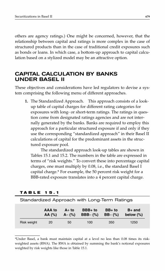
Securitizations in Basel II 679
others are agency ratings.) One might be concerned, however, that therelationship between capital and ratings is more complex in the case ofstructured products than in the case of traditional credit exposures suchas bonds or loans. In which case, a bottom-up approach to capital calcu-lation based on a stylized model may be an attractive option.
CAPITAL CALCULATION BY BANKS UNDER BASEL II
These objectives and considerations have led regulators to devise a sys-tem comprising the following menu of different approaches.
1. The Standardized Approach. This approach consists of a look-up table of capital charges for different rating categories forexposures with long- or short-term ratings. The ratings in ques-tion come from designated ratings agencies and are not inter-nally generated by the banks. Banks are required to employ thisapproach for a particular structured exposure if and only if theyuse the corresponding “standardized approach” in their Basel IIcalculations of capital for the predominant assets in the struc-tured exposure pool.
The standardized approach look-up tables are shown inTables 15.1 and 15.2. The numbers in the table are expressed interms of “risk weights.” To convert these into percentage capitalcharges, one must multiply by 0.08, i.e., the standard Basel Icapital charge.* For example, the 50 percent risk weight for aBBB-rated exposure translates into a 4 percent capital charge.
T A B L E 1 5 . 1
Standardized Approach with Long-Term Ratings
AAA to A+ to BBB+ to BB+ to B+ andAA (%) A− (%) BBB− (%) BB− (%) below (%)
Risk weight 20 50 100 350 1250
*Under Basel, a bank must maintain capital at a level no less than 0.08 times its risk-weighted assets (RWA). The RWA is obtained by summing the bank’s notional exposuresweighted by risk weights like those in Table 15.1.
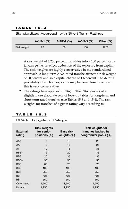
680 CHAPTER 15
A risk weight of 1,250 percent translates into a 100 percent capi-tal charge, i.e., in effect deduction of the exposure from capital.The risk weights are highly conservative in the standardizedapproach. A long-term AAA-rated tranche attracts a risk weightof 20 percent and so a capital charge of 1.6 percent. The defaultprobability of such an exposure may be very close to zero, sothis is very conservative.
2. The ratings base approach (RBA). The RBA consists of aslightly more elaborate pair of look-up tables for long-term andshort-term rated tranches (see Tables 15.3 and 15.4). The riskweights for tranches of a given rating vary according to:
T A B L E 1 5 . 3
RBA for Long-Term Ratings
Risk weights Risk weights forExternal for senior Base risk tranches backed byrating positions (%) weights (%) nongranular pools (%)
AAA 7 12 20
AA 8 15 25
A+ 10 18 35
BBB+ 12 20 35
BBB 20 35 35
BBB+ 35 50 50
BBB 60 75 75
BBB− 100 100 100
BB+ 250 250 250
BB 425 425 425
BB− 650 650 650
Other rated 1,250 1,250 1,250
Unrated 1,250 1,250 1,250
T A B L E 1 5 . 2
Standardized Approach with Short-Term Ratings
A-1/P-1 (%) A-2/P-2 (%) A-3/P-3 (%) Other (%)
Risk weight 20 50 100 1250
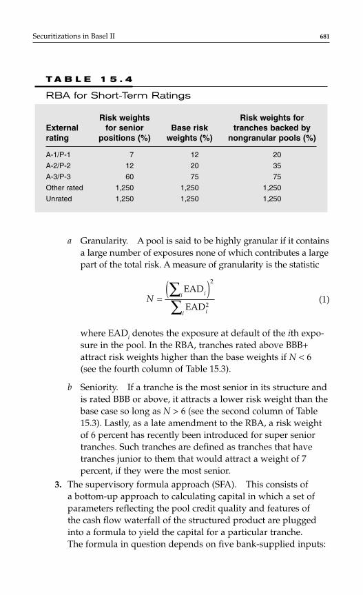
Securitizations in Basel II 681
a Granularity. A pool is said to be highly granular if it containsa large number of exposures none of which contributes a largepart of the total risk. A measure of granularity is the statistic
(1)
where EADi denotes the exposure at default of the ith expo-sure in the pool. In the RBA, tranches rated above BBB+attract risk weights higher than the base weights if N < 6(see the fourth column of Table 15.3).
b Seniority. If a tranche is the most senior in its structure andis rated BBB or above, it attracts a lower risk weight than thebase case so long as N > 6 (see the second column of Table15.3). Lastly, as a late amendment to the RBA, a risk weightof 6 percent has recently been introduced for super seniortranches. Such tranches are defined as tranches that havetranches junior to them that would attract a weight of 7 percent, if they were the most senior.
3. The supervisory formula approach (SFA). This consists ofa bottom-up approach to calculating capital in which a set ofparameters reflecting the pool credit quality and features ofthe cash flow waterfall of the structured product are plugged into a formula to yield the capital for a particular tranche.The formula in question depends on five bank-supplied inputs:
Nii
ii
=( )∑∑
EAD
EAD
2
2
T A B L E 1 5 . 4
RBA for Short-Term Ratings
Risk weights Risk weights forExternal for senior Base risk tranches backed byrating positions (%) weights (%) nongranular pools (%)
A-1/P-1 7 12 20
A-2/P-2 12 20 35
A-3/P-3 60 75 75
Other rated 1,250 1,250 1,250
Unrated 1,250 1,250 1,250
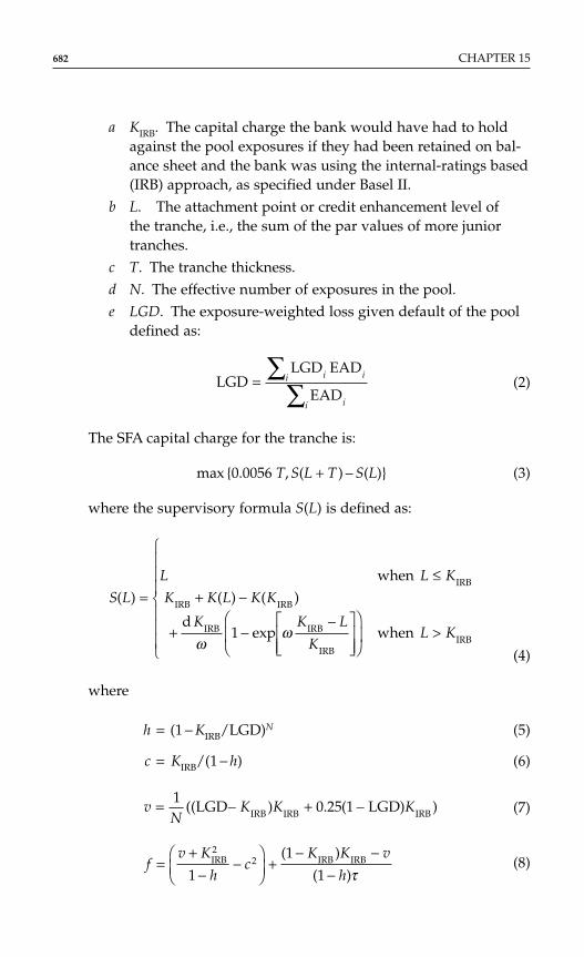
682 CHAPTER 15
a KIRB. The capital charge the bank would have had to holdagainst the pool exposures if they had been retained on bal-ance sheet and the bank was using the internal-ratings based(IRB) approach, as specified under Basel II.
b L. The attachment point or credit enhancement level of the tranche, i.e., the sum of the par values of more juniortranches.
c T. The tranche thickness.d N. The effective number of exposures in the pool.e LGD. The exposure-weighted loss given default of the pool
defined as:
(2)
The SFA capital charge for the tranche is:
max 0.0056 T, S(L + T ) − S(L) (3)
where the supervisory formula S(L) is defined as:
(4)
where
h = (1 − KIRB/LGD)N (5)
c = KIRB/(1 − h) (6)
(7)
(8)fv K
hc
K K v
h=
+−
−
+− −
−IRB IRB IRB( )
( )
22
1
1
1 τ
vN
K K K= − + −10 25 1((LGD ) . ( LGD) )IRB IRB IRB
S L
L L K
K K L K K
K K L
KL K
( ) when
( ) ( )
dexp when
IRB
IRB IRB
IRB IRB
IRBIRB
=≤
+ −
+ −−
>ω
ω1
LGDLGD EAD
EAD= ∑
∑i ii
ii
Securitizations in Basel II 683
(9)
a = gc (10)
b = g(1 − c) (11)
d = 1 − (1 − h)(1 − Beta(KIRB; a, b)) (12)
K(L) = (1 − h) ((1 − Beta(L ; a, b))L + Beta(L ; a + 1, b)c). (13)
Here, Beta(x; p, q) denotes the cumulative beta distributionevaluated at x and with parameters p and q. The parametersτ and ω are set at τ = 1000 and ω = 20. The underpinnings ofthis approach are explained at greater length next.
The practical use of these different approaches is best explained byreviewing the flow chart shown in Figure 15.1. This flow chart shows thesequence of questions that a bank must answer in deciding what capitalto hold against a given securitization exposure.
1. Is it a securitization? The definition of a securitization in theEU’s draft Capital Requirements Directive (Article 4, 36) is: “Atransaction or scheme, whereby the credit risk associated withan exposure or pool of exposures is tranched, having the fol-lowing characteristics: (1) payments in the transaction aredependent upon the performance of the exposure or pool ofexposures; (2) the subordination of tranches determines the dis-tribution of losses during the life of the transaction or scheme.”*
2. Supposing that the exposure is a securitization, the bank mustdecide whether it is held as part of the trading or the bankingbook. In the former case, the capital charge will be based on theusual trading book rules.
3. For the bank to apply the above securitization capital approaches,it must satisfy two sets of conditions: (1) risk transfer require-ments if the bank is an originator of the securitized assets, and (2) implicit support requirements if it is either an Originator
gc c
f= − −( )1
1
*This definition encompasses both traditional and synthetic securitizations and is simplerthan the definition in Basel Committee on Banking Supervision (2005).
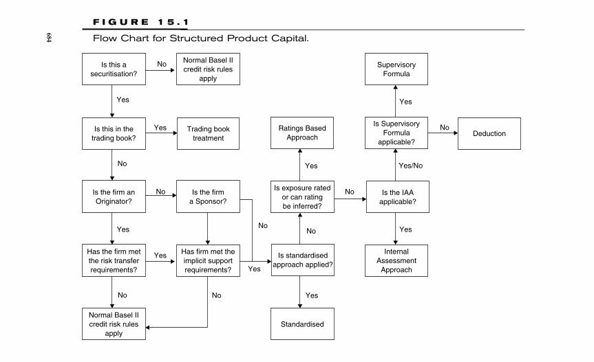
Is this asecuritisation?
Is this in thetrading book?
Is the firm anOriginator?
Has the firm metthe risk transferrequirements?
Has firm met theimplicit supportrequirements?
Is the firma Sponsor?
Trading booktreatment
Normal Basel IIcredit risk rules
apply
Ratings BasedApproach
Is exposure ratedor can ratingbe inferred?
Is standardisedapproach applied?
Standardised
InternalAssessment
Approach
Is the IAAapplicable?
Is SupervisoryFormula
applicable?
SupervisoryFormula
Deduction
Normal Basel IIcredit risk rules
apply
No
No
No
No No
NoNo
No
No
Yes
Yes
Yes
Yes
Yes
Yes
Yes
Yes
Yes/No
Yes
F I G U R E 1 5 . 1
Flow Chart for Structured Product Capital.
684
Securitizations in Basel II 685
or a Sponsor* of the securitization. If either of these sets of condi-tions is not satisfied, then the bank must calculate capital for thepool exposures as though they are held on balance sheet.
4. If it satisfies these conditions, the bank must use the standard-ized approach as described earlier if it uses the standardizedapproach for on balance sheet assets of the same type as thosethat predominantly make up the securitization pool.
5. If the bank uses the IRB approach for the assets that predomi-nantly comprise the pool, then it must employ either the RBA orthe SFA. If the exposure is rated by an external agency recog-nized by the bank’s national supervisor, the bank must employthe RBA. This is also true if the exposure is unrated, but thebank may infer a rating for the exposure by taking the rating ofa more junior tranche with an equal or longer maturity.
6. If an external rating is not directly available and cannot beinferred, then the bank must decide whether the internal assess-ment approach (IAA) is applicable. This approach applies onlyto eligible liquidity and credit enhancement exposures to ABCPfacilities. In effect, banks are able for this narrow set of expo-sures to calculate their own internal ratings. In so doing, theymust devise a rating process that broadly mimics the approachfollowed in rating exposures to similar deals by a recognizedrating agency.
7. If the IAA is applicable, the bank may choose to employ thisapproach or it may decide to use the SFA instead. If it imple-ments the IAA, the bank determines its capital charges from theRBA look-up tables based on the the IAA-generated ratings. Ingeneral, the bank must adopt a consistent principle in choosingwhether to use the SFA or the IAA/RBA.
8. If the IAA is not applicable or if the bank opts not to implementit, it must either use the SFA if that is feasible or otherwise
*An Originator is either of the following: An entity which, either itself or through relatedentities, directly or indirectly, was involved in the original agreement that created the obli-gations or potential obligations of the debtor or potential debtor giving rise to exposurebeing securitized; an entity which purchases a third partys exposures onto its balance sheetand then securitizes them. A Sponsor is a firm other than an Originator that establishes andmanages an asset-backed commercial paper programme or other securitization scheme thatpurchases exposures from third parties.

deduct the exposure from its capital, i.e., apply a 1250 percentrisk weight.
The sticking point for implementing the SFA in many cases is likely to bethe bank’s ability to calculate the inputs to the formula. These includemost notably KIRB, the capital that the bank would have to hold against thepool of assets backing the securitization if it held the pool on balancesheet. Basel II places rather tight restrictions on the information and datathat banks must possess if they are to calculate KIRB. A concession wasmade in the informational requirements for calculating KIRB for portfoliosof purchased receivables at quite a late stage in the Basel II process specif-ically because it was felt that otherwise many securitization exposures inbank portfolios that embodied relatively little risk would otherwise haveto be deducted, disrupting reasonable market activity in several areas.
The IAA requires a substantial investment in procedures and sys-tems by a bank. The idea is that banks will be able to rate tranches them-selves in one quite circumscribed area of the securitization market, ABCP,but it must adopt an approach that resembles an approach employed bya recognized rating agency. The bank’s procedures have to be auditedthoroughly and authorized by the regulators. Banks are allowed to choosewhich of the SFA or the IAA combined with RBA look-up tables they wishto employ for nonrated ABCP liquidity and credit enhancement facilities.But they must adopt a consistent policy of using one approach or theother and not hop and change between different deals.
The implicit support and risk transfer requirements are an impor-tant part of the rules. The former are intended to ensure that originatorsmaintain a clean break with their securitized assets. (Originators are ableto support their past securitizations but only if this support is formallyimplemented, as an exposure against which capital can be levied.) Therisk transfer requirements contain potential for some ambiguity.
THE FINANCIAL ENGINEERING OF THE RBA AND SFA
Regulators have been very keen to ensure that the Basel II rules willreduce banks’ incentives to engage in capital arbitrage. The only way toachieve this is to maintain a reasonable level of neutrality between the onand off balance sheet treatment of exposures and to make sure that capi-tal charges are similar in absolute level to what a bank would wish to holdas economic capital.
686 CHAPTER 15
Decisions about the levels of structured product capital chargesin Basel II was informed and influenced by financial engineering stud-ies performed by analysts at the Federal Reserve Board and the Bank ofEngland. This section provides a brief summary of these studies. Keycontributions are (1) Peretyatkin and Perraudin (2004) on the RBA and(2) Gordy and Jones (2003) and Gordy (2004) on the SFA.
On the RBA, devising a set of capital charges for structured productsbased on ratings can be viewed as a significant challenge. Indeed, at anearly stage in the Basel II process, some regulators disputed whether itcould be achieved at all. To understand the issues, one needs some back-ground about the capital treatment of other exposures like bonds andloans in Basel II.
The IRB charges for traditional, on balance sheet credit exposures inBasel II are based on measures of marginal Value at Risk (MVaR) for expo-sures with given probabilities of default over a one-year horizon. Thedefault probabilities may be mapped into ratings by associating with eachrating the historically observed one-year default probability. Hence, theapproach may be thought of as one of basing capital charges on ratings.(The standardized approach to on-balance-sheet credit exposures is explic-itly framed in terms of ratings rather than default probabilities in any case.)
A justification for linking capital to ratings is that analysis using sim-ple industry standard models suggests that when there is a single com-mon risk factor driving a portfolio of loans, the MVaRs for individualexposures within a large portfolio are a function of the default probabil-ity.* Other influences on the MVaR for a given exposure are the expectedLGD, the degree of correlation between the claim in question and the sin-gle common risk factor and the maturity of the claim. If regulators are pre-pared to specify reasonable correlation values for each different marketsegment, suitable capital curves may be deduced.†
Turning to capital charges for structured products, one may be con-cerned that the mapping from default probability/rating to capital will bemore complex, dependent, e.g., on tranche thickness, correlation of thefactor risk in the pool and the factor risk in the bank’s wider portfolio andthe maturities both of the pool and of the structure.
Securitizations in Basel II 687
*See Gordy (2003).†This has been the approach followed under Basel II, so there are a set of capital curves orfunctions for five different credit exposure asset classes (C%I loans, SME loans, revolvingretail exposures, and other retail and residential mortgages.) See Basel Committee onBanking Supervision (2005).
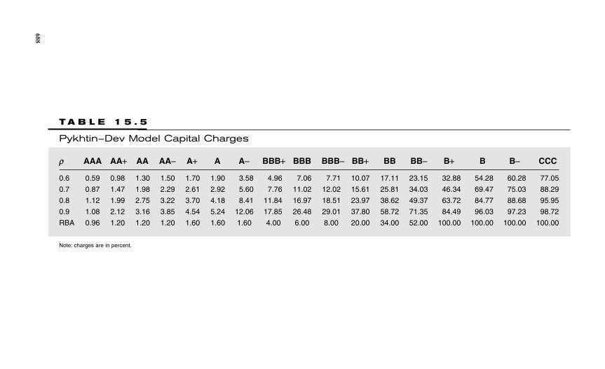
T A B L E 1 5 . 5
Pykhtin–Dev Model Capital Charges
ρ AAA AA+ AA AA− A+ A A− BBB+ BBB BBB− BB+ BB BB− B+ B B− CCC
0.6 0.59 0.98 1.30 1.50 1.70 1.90 3.58 4.96 7.06 7.71 10.07 17.11 23.15 32.88 54.28 60.28 77.05
0.7 0.87 1.47 1.98 2.29 2.61 2.92 5.60 7.76 11.02 12.02 15.61 25.81 34.03 46.34 69.47 75.03 88.29
0.8 1.12 1.99 2.75 3.22 3.70 4.18 8.41 11.84 16.97 18.51 23.97 38.62 49.37 63.72 84.77 88.68 95.95
0.9 1.08 2.12 3.16 3.85 4.54 5.24 12.06 17.85 26.48 29.01 37.80 58.72 71.35 84.49 96.03 97.23 98.72
RBA 0.96 1.20 1.20 1.20 1.60 1.60 1.60 4.00 6.00 8.00 20.00 34.00 52.00 100.00 100.00 100.00 100.00
Note: charges are in percent.
688
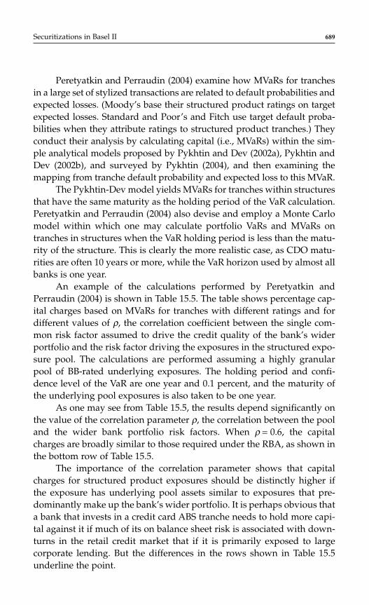
Securitizations in Basel II 689
Peretyatkin and Perraudin (2004) examine how MVaRs for tranchesin a large set of stylized transactions are related to default probabilities andexpected losses. (Moody’s base their structured product ratings on targetexpected losses. Standard and Poor’s and Fitch use target default proba-bilities when they attribute ratings to structured product tranches.) Theyconduct their analysis by calculating capital (i.e., MVaRs) within the sim-ple analytical models proposed by Pykhtin and Dev (2002a), Pykhtin andDev (2002b), and surveyed by Pykhtin (2004), and then examining themapping from tranche default probability and expected loss to this MVaR.
The Pykhtin-Dev model yields MVaRs for tranches within structuresthat have the same maturity as the holding period of the VaR calculation.Peretyatkin and Perraudin (2004) also devise and employ a Monte Carlomodel within which one may calculate portfolio VaRs and MVaRs ontranches in structures when the VaR holding period is less than the matu-rity of the structure. This is clearly the more realistic case, as CDO matu-rities are often 10 years or more, while the VaR horizon used by almost allbanks is one year.
An example of the calculations performed by Peretyatkin andPerraudin (2004) is shown in Table 15.5. The table shows percentage cap-ital charges based on MVaRs for tranches with different ratings and fordifferent values of ρ, the correlation coefficient between the single com-mon risk factor assumed to drive the credit quality of the bank’s widerportfolio and the risk factor driving the exposures in the structured expo-sure pool. The calculations are performed assuming a highly granularpool of BB-rated underlying exposures. The holding period and confi-dence level of the VaR are one year and 0.1 percent, and the maturity ofthe underlying pool exposures is also taken to be one year.
As one may see from Table 15.5, the results depend significantly onthe value of the correlation parameter ρ, the correlation between the pooland the wider bank portfolio risk factors. When ρ = 0.6, the capitalcharges are broadly similar to those required under the RBA, as shown inthe bottom row of Table 15.5.
The importance of the correlation parameter shows that capitalcharges for structured product exposures should be distinctly higher ifthe exposure has underlying pool assets similar to exposures that pre-dominantly make up the bank’s wider portfolio. It is perhaps obvious thata bank that invests in a credit card ABS tranche needs to hold more capi-tal against it if much of its on balance sheet risk is associated with down-turns in the retail credit market that if it is primarily exposed to largecorporate lending. But the differences in the rows shown in Table 15.5underline the point.
T A B L E 1 5 . 6
Monte Carlo-Based Capital Charges
AAA AA+ AA AA− A+ A A− BBB+ BBB BBB− BB+ BB BB− B+ B B− CCC
1 year 0.54 0.99 1.36 1.58 1.77 1.96 3.50 4.63 6.25 6.75 8.75 14.78 19.87 28.30 49.53 56.21 76.26
2 years 0.17 0.86 1.72 1.89 2.27 2.70 4.99 6.98 9.30 11.83 14.65 20.50 26.31 35.74 55.72 62.58 78.81
3 years 0.67 1.55 2.68 2.80 3.31 3.93 6.29 8.55 10.91 14.59 18.66 24.57 30.93 40.79 58.84 65.15 77.46
4 years 1.41 2.53 3.86 3.99 4.62 5.45 7.88 10.38 12.86 17.32 20.97 26.49 32.83 42.27 56.79 61.28 67.66
5 years 1.29 2.49 3.82 3.96 4.67 5.62 7.96 10.51 13.03 17.83 23.05 29.14 35.98 45.27 57.17 60.41 64.02
Note: Simulations assume a portfolio of 264 BB-rated exposures, 50 percent LGD, a correlation of 60 percent between single factors driving the pool and wider bank portfolio, and a correlation between indi-vidual exposure latent variables of 80 percent.Capital charges (MVaRs) are in percent.
690
Securitizations in Basel II 691
Peretyatkin and Perraudin conclude that some other aspects of thestructured product have only a second-order effect on the appropriatecapital charges. For example, the degree to which the underlying poolexposures are correlated with each other or are nongranular leads to rela-tively small changes in capital. The reason is that when the riskiness of thepool is increased, the rating agencies tend to downgrade the more seniortranches, so capital increases even without a direct rise in the capitalcharge for tranches with a given rating.
On the other hand, Peretyatkin and Perraudin find that maturityagain has a first-order effect on the capital charges for particular rating cat-egories. Using a novel Monte Carlo technique, they are able to calculateMVaRs and hence capital for structured products of different maturities.The results are shown in Table 15.6. The capital more than doubles whenone considers relatively senior tranches with the same rating, but a matu-rity of four years rather than one year.
As described above, the RBA in Basel II provides simple look-uptables for risk weights (and hence implicitly capital charges) by rating cat-egory. No distinction is made between tranches (1) backed by differentunderlying assets (e.g., credit cards versus large corporate loans), (2) ofdifferent maturities, or (3) backed by assets similar or dissimilar to expo-sures predominant in the bank’s wider portfolio. While there are reasonsfor believing that that (1) is not a serious drawback, as factors that affectthe riskiness of the securitization pool may have second-order effects oncapital, (2) and (3) may be more serious. These might have been dealt withthrough Pillar II requirements, but Basel II did not take that approach.
Lastly, one may be critical of the RBA on the grounds that agenciesassign ratings to securitization exposures taking into account complex setsof factors that they perceive to drive the risk of the transactions. These fac-tors include the probability that the issuer will be able to meet principaland interest payments, the structure of the cash flow waterfall, the typeof assets in the pool, other risks, such as market, legal and counter-partyrisks, and credit and liquidity enhancements of various sorts. The differentrating agencies also employ significantly different procedures in assigningratings. Expecting all of this to be satisfactorily summarized in a stylizedcalculation of expected losses on tranches as was performed in the param-eterization of the RBA is somewhat ambitious.
The counter-argument to the above criticism is that the differentrating agencies seem over time to be converging in the approaches theytake to rating structured products in that they are increasingly usingcomparable Monte Carlo methods to simulate pool performance andpayoffs to tranches. The RMA parameterization may be viewed as

employing a stylized version of these simulations for representativetransactions.
The financial engineering background to the SFA is set out in Gordyand Jones (2003) and Gordy (2004). To calculate a bottom-up formula forcapital on a structured product tranche, the most obvious approach mightbe to employ the single asymptotic risk factor model used elsewhere inBasel II as the basis for capital curves linking default probabilities to cap-ital for on balance sheet assets. This model is described in Gordy (2003).
The problem with this approach in the context of securitizationtranches is that when the pool is perfectly granular, the implied capitalcharges turn out to equal 100 percent for junior tranches. For thin tranches,at a certain level of protection,* the capital charge drops abruptly from 100to 0 percent. This implication of the model makes the model unappealingas a basis for capital calculations, as it implies that a bank might have aportfolio of mezzanine tranches against which it was not required to holdany capital but which would obviously be subject to credit risk.
Therefore, Gordy and Jones devised a model that effectively smoothsout the step function for capital charges. In principle, various differentapproaches could be followed, as the basic aim was just to incorporatesome smoothing of capital charges as the level of protection varies. TheGordy–Jones approach consists of assuming that the protection level for agiven tranche is uncertain. They argue that in practise, the complexity oftypical cash-flow waterfalls means that one cannot be sure of the exactlevel of protection enjoyed by a given tranche. Assuming a Wishart dis-tribution, they derive a formula.
Figure 15.2 shows the capital for marginally thin tranches implied bythe single asymptotic risk factor model plotted against protection as a stepfunction. (Note that the protection level at which the capital jumps to 0 per-cent equals KIRB, i.e., the capital that the bank would be obliged to holdagainst the asset pool if it retained it on balance sheet.) The Gordy–Jonessmoothing approach yields a reverse S-shaped curve. Their model containsa parameter ω that reflects the degree of uncertainty about the level of pro-tection. The figure shows capital plotted for different levels of ω. The BaselII supervisory formula is based on an ω value of 1000.
The SFA is not based solely on the supervisory formula just described,however, as it includes additional overrides that build in greater conser-vatism. In particular:
692 CHAPTER 15
*The protection of a tranche here denotes the sum of the par value of more junior tranchestranches. It is also sometimes called the attachment point of the tranche.
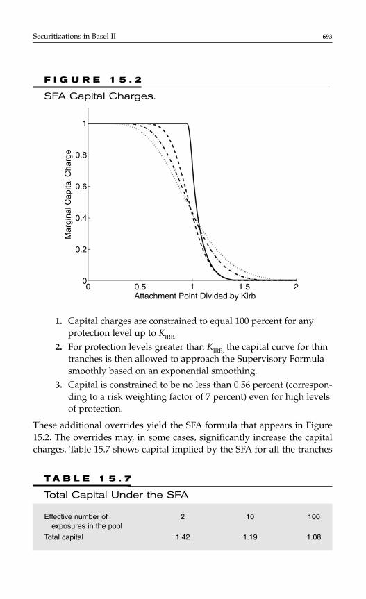
1. Capital charges are constrained to equal 100 percent for anyprotection level up to KIRB.
2. For protection levels greater than KIRB, the capital curve for thintranches is then allowed to approach the Supervisory Formulasmoothly based on an exponential smoothing.
3. Capital is constrained to be no less than 0.56 percent (correspon-ding to a risk weighting factor of 7 percent) even for high levelsof protection.
These additional overrides yield the SFA formula that appears in Figure15.2. The overrides may, in some cases, significantly increase the capitalcharges. Table 15.7 shows capital implied by the SFA for all the tranches
Securitizations in Basel II 693
T A B L E 1 5 . 7
Total Capital Under the SFA
Effective number of 2 10 100exposures in the pool
Total capital 1.42 1.19 1.08
0.5Attachment Point Divided by Kirb
1 1.5 2
0.2
0
0.4
Mar
gina
l Cap
ital C
harg
e
0.6
0.8
1
0
F I G U R E 1 5 . 2
SFA Capital Charges.
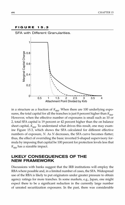
in a structure as a fraction of KIRB. When there are 100 underlying expo-sures, the total capital for all the tranches is just 8 percent higher than KIRB.However, when the effective number of exposures is small such as 10 or2, total SFA capital is 19 percent or 42 percent higher than the on balancesheet capital, KIRB. To understand what drives this result, one may exam-ine Figure 15.3, which shows the SFA calculated for different effectivenumbers of exposure, N. As N decreases, the SFA curve becomes flatter;thus, the effect of overriding the basic inverted S-shaped supervisory for-mula by imposing that capital be 100 percent for protection levels less thatKIRB has a sizeable impact.
LIKELY CONSEQUENCES OF THE NEW FRAMEWORK
Discussions with banks suggest that the IRB institutions will employ theRBA where possible and, in a limited number of cases, the SFA. Widespreaduse of the RBA is likely to put originators under greater pressure to obtainagency ratings for more tranches. In some markets, e.g., Japan, one mightexpect there to be a significant reduction in the currently large numberof unrated securitization exposures. In the past, there was considerable
694 CHAPTER 15
00
0.5Attachment Point Divided by Kirb
1 1.5 2 2.5 3 3.5 4
0.2
0.4
Mar
gina
l Cap
ital C
harg
e
0.6
0.8
1
F I G U R E 1 5 . 3
SFA with Different Granularities.
concern that large numbers of exposures would not fit into any of theapproaches permitted. The less restrictive informational requirements forcalculating KIRB with purchased receivables and the introduction of the IAAhas calmed these concerns.
Initially, many in the industry were anxious that the securitizationmarket would be impaired by the reduction in capital arbitrage-relateddeals that the Basel II regulations would bring. However, the scope forsecuritization is likely to be significantly increased when banks havedeveloped the systematic approaches to measuring and managing portfo-lio credit risk required by Basel. The nature of the market is likely to shift,therefore, with more transactions being motivated by genuine risk transferand funding considerations and fewer by regulatory capital arbitrage.
In any case, if regulatory capital on individual securitization expo-sures is high, capital arbitrage between the banking and trading booksmay provide a safety valve. The boundary between the trading and bank-ing books has been reconsidered by regulators, following the 2005 reviewof the trading book completed by the Basel Committee and the InternationalOrganization of Securities Commissions (IOSCO). Exposures can be classi-fied as trading book exposures if they “arise out of a financial instrumentor commodity” and “are held with trading intent or to hedge elements ofthe trading book.” An increasing number of securitization exposures aresufficiently actively traded to be eligible for such treatment.
The capital charges that securitization exposures attract in a tradingbook context will depend on the volatility and correlations of market-wide factors driving spread and on specific risk charges. Perraudin andVan Landschoot (2004) show that the volatility of ABS exposures may below, but that sudden and dramatic increases in risk may occur if shiftsoccur in the credit quality of particular market segments. To the extentthat internal risk models employ relatively short return and spreadchange data series, the possibility of regime shifts in volatility may not befully allowed for and capital may be too low.
Under the new rules, securitizations that would attract a 1250 percentrisk-weight under the securitization framework or would be deducted willface equivalent charges in the trading book. This will reduce the scope forcapital arbitrage between banking and trading books for equity tranches.However, it may remain for mezzanine tranches.
This chapter has focussed on the Pillar 1 part of Basel II, i.e., the rulesgoverning minimum regulatory capital requirements. But other parts ofBasel II will affect the securitization market. In particular, Pillar 3 coversrules on disclosure that banks will have to follow. For example, banks will
Securitizations in Basel II 695
have to reveal to the market qualitative information, such as the aims oftheir securitizations, the regulatory capital treatment adopted, and whichrating agencies they employ to rate their securitizations.
They will also have to supply quantitative information about thebank’s total outstanding volume of securitized exposures with a break-down by type, and by whether the securitizations are traditional or syn-thetic,* and with information on the volume of impaired assets that havebeen securitized. They will also have to publish information about theiraggregate holdings of securitization exposures. These substantial disclo-sures will reveal a lot about what directions are being taken in securitiza-tions by individual banks and the market as a whole.
REFERENCESBasel Committee on Banking Supervision (2005), Basel II: International
Convergence of Capital Measurement and Capital Standards: a RevisedFramework Bank for International Settlement: Basel, November.
Gordy, M. B. (2003), “A risk-factor model foundation for ratings-based bank cap-ital rules,” Journal of Financial Intermediation, 12, 199–232.
Gordy, M. B. (2004), “Model foundations for the supervisory formula approach,”in W. Perraudin (ed.), Structured Credit Products: Pricing, Rating, RiskManagement and Basel II, Risk Books: London, 307–328.
Gordy, M. B., and D. Jones (2003), “Random tranches,” Risk, 16(3), March, 78–81.Jones, D. (2000), “Emerging problems with the accord: Regulatory Capital arbi-
trage and related issues,” Journal of Banking and Finance, 24, 35–58.Peretyatkin, V., and W. Perraudin (2004), “Capital for structured products,” in W.
Perraudin (ed.), Structured Credit Products, Risk Books: London, 329–362.Perraudin, W., and A. Van Landschoot (2004), “How risky are structured expo-
sures compared with corporate bonds? in W. Perraudin (ed.), StructuredCredit Products, Risk Books: London, 283–303.
Pykhtin, M. (2004), “Asymptotic model of economic capital for securitization,” inW. Perraudin (ed.), Structured Credit Products, Risk Books: London, 215–244.
Pykhtin, M., and A. Dev (2002a), “Credit risk in asset securitizations: Analyticalmodel.” Risk, March, S26–S32.
Pykhtin, M., and A. Dev (2002b), “Credit risk in asset securitizations: The case ofCDOs,” Risk, May, S16–S20.
696 CHAPTER 15
*Where no exposures are retained, this information will have to be disclosed in the first yearonly.
C H A P T E R 1 6
Securitization in theContext of Basel II: Case Studies*
Arnaud de Servigny
697
INTRODUCTION
In this chapter, we review the impact of Basel II treatment of securitiza-tion on two asset classes: credit cards and residential-mortgage backedsecurities (RMBS). We focus in particular on the discrepancies betweenthe regulatory approach and S&P approach. One important point to recallis that S&P considers its models as one of the constituents leading to thetranching of a transaction. It is not the only one.
In the first part, we concentrate on credit cards and consider threetypes of transactions.
In the second part, we analyze four types of RMBS transactions.
PART 1: ANALYSIS OF THE IMPACT OF BASEL II ON THE CREDIT CARD ASSET CLASS†
The main finding in this part is related to the importance of excess spreadin the analysis of the credit card asset class. Basel II(*) option to ignore
*The author would like to thank Alain Carron, Bernard de Longevialle, Wai To Wong, andPrashant Dwivedi for contribution.†A definition of terms can be found in Appendix A.
Copyright © 2007 by The McGraw-Hill Companies. Click here for terms of use.
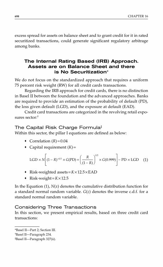
excess spread for assets on balance sheet and to grant credit for it in ratedsecuritized transactions, could generate significant regulatory arbitrageamong banks.
The Internal Rating Based (IRB) Approach.Assets are on Balance Sheet and there
is No Securitization*
We do not focus on the standardized approach that requires a uniform75 percent risk weight (RW) for all credit cards transactions.
Regarding the IRB approach for credit cards, there is no distinctionin Basel II between the foundation and the advanced approaches. Banksare required to provide an estimation of the probability of default (PD),the loss given default (LGD), and the exposure at default (EAD).
Credit card transactions are categorized in the revolving retail expo-sures sector:†
The Capital Risk Charge Formula‡
Within this sector, the pillar I equations are defined as below:
♦ Correlation (R) = 0.04♦ Capital requirement (K) =
(1)
♦ Risk-weighted assets = K × 12.5 × EAD♦ Risk-weight = K × 12.5
In the Equation (1), N(x) denotes the cumulative distribution function fora standard normal random variable. G(z) denotes the inverse c.d.f. for astandard normal random variable.
Considering Three TransactionsIn this section, we present empirical results, based on three credit cardtransactions:
LGD ( ) (PD)( )
( . ) PD LGD.
.
× − × +−
× − ×−
N R G
R
RG1
10 9990 5
0 5
698 CHAPTER 16
*Basel II—Part 2; Section III.†Basel II—Paragraph 234.‡Basel II—Paragraph 327(ii).
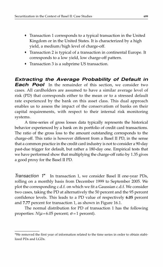
♦ Transaction 1 corresponds to a typical transaction in the UnitedKingdom or in the United States. It is characterized by a highyield, a medium/high level of charge-off.
♦ Transaction 2 is typical of a transaction in continental Europe. Itcorresponds to a low yield, low charge-off pattern.
♦ Transaction 3 is a subprime US transaction.
Extracting the Average Probability of Default inEach Pool In the remainder of this section, we consider twocases. All cardholders are assumed to have a similar average level ofrisk (PD) that corresponds either to the mean or to a stressed defaultrate experienced by the bank on this asset class. This dual approachenables us to assess the impact of the conservatism of banks on theircapital requirements, with respect to their internal risk monitoringsystems.
A time-series of gross losses data typically represents the historicalbehavior experienced by a bank on its portfolio of credit card transactions.The ratio of the gross loss to the amount outstanding corresponds to thecharge-off. This ratio is however different from a Basel II PD, in the sensethat a common practice in the credit card industry is not to consider a 90-daypast-due trigger for default, but rather a 180-day one. Empirical tests thatwe have performed show that multiplying the charge-off ratio by 1.35 givesa good proxy for the Basel II PD.
Transaction 1* In transaction 1, we consider Basel II one-year PDs,rolling on a monthly basis from December 1999 to September 2005. Weplot the corresponding c.d.f. on which we fit a Gaussian c.d.f. We considertwo cases, taking the PD at alternatively the 50 percent and the 95 percentconfidence levels. This leads to a PD value of respectively 6.05 percentand 7.77 percent for transaction 1, as shown in Figure 16.1.
The normal distribution for PD of transaction 1 has the followingproperties: N(µ = 6.05 percent; σ = 1 percent).
Securitization in the Context of Basel II: Case Studies 699
*We removed the first year of information related to the time series in order to obtain stabi-lized PDs and LGDs.
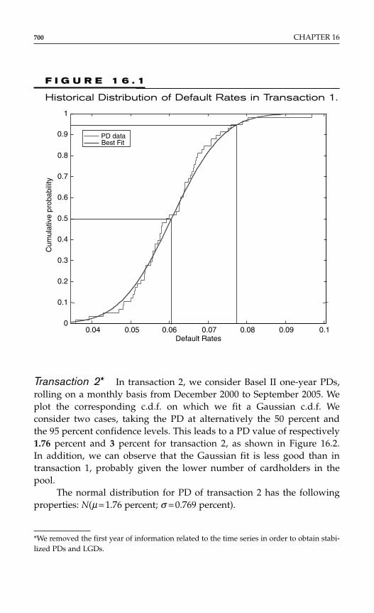
Transaction 2* In transaction 2, we consider Basel II one-year PDs,rolling on a monthly basis from December 2000 to September 2005. Weplot the corresponding c.d.f. on which we fit a Gaussian c.d.f. Weconsider two cases, taking the PD at alternatively the 50 percent andthe 95 percent confidence levels. This leads to a PD value of respectively1.76 percent and 3 percent for transaction 2, as shown in Figure 16.2.In addition, we can observe that the Gaussian fit is less good than intransaction 1, probably given the lower number of cardholders in thepool.
The normal distribution for PD of transaction 2 has the followingproperties: N(µ = 1.76 percent; σ = 0.769 percent).
700 CHAPTER 16
*We removed the first year of information related to the time series in order to obtain stabi-lized PDs and LGDs.
F I G U R E 1 6 . 1
Historical Distribution of Default Rates in Transaction 1.
0.04 0.05 0.06 0.07 0.08 0.09 0.10
0.1
0.2
0.3
0.4
0.5
0.6
0.7
0.8
0.9
1
Default Rates
Cum
ulat
ive
prob
abili
ty
PD dataBest Fit
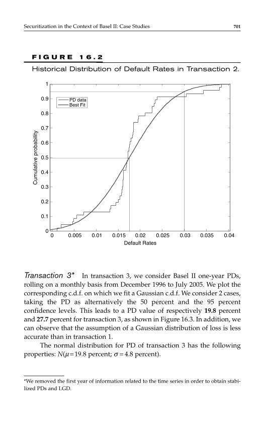
Transaction 3* In transaction 3, we consider Basel II one-year PDs,rolling on a monthly basis from December 1996 to July 2005. We plot thecorresponding c.d.f. on which we fit a Gaussian c.d.f. We consider 2 cases,taking the PD as alternatively the 50 percent and the 95 percentconfidence levels. This leads to a PD value of respectively 19.8 percentand 27.7 percent for transaction 3, as shown in Figure 16.3. In addition, wecan observe that the assumption of a Gaussian distribution of loss is lessaccurate than in transaction 1.
The normal distribution for PD of transaction 3 has the followingproperties: N(µ = 19.8 percent; σ = 4.8 percent).
Securitization in the Context of Basel II: Case Studies 701
F I G U R E 1 6 . 2
Historical Distribution of Default Rates in Transaction 2.
0 0.005 0.01 0.015 0.02 0.025 0.03 0.035 0.040
0.1
0.2
0.3
0.4
0.5
0.6
0.7
0.8
0.9
1
Default Rates
Cum
ulat
ive
prob
abili
ty
PD dataBest Fit
*We removed the first year of information related to the time series in order to obtain stabi-lized PDs and LGD.
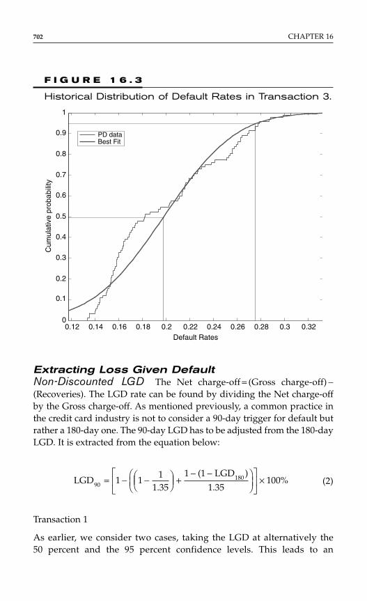
Extracting Loss Given DefaultNon-Discounted LGD The Net charge-off = (Gross charge-off) −(Recoveries). The LGD rate can be found by dividing the Net charge-offby the Gross charge-off. As mentioned previously, a common practice inthe credit card industry is not to consider a 90-day trigger for default butrather a 180-day one. The 90-day LGD has to be adjusted from the 180-dayLGD. It is extracted from the equation below:
(2)
Transaction 1
As earlier, we consider two cases, taking the LGD at alternatively the50 percent and the 95 percent confidence levels. This leads to an
LGD.
( LGD )
.%90
1801 11
1 35
1 1
1 35100= − −
+
− −
×
702 CHAPTER 16
F I G U R E 1 6 . 3
Historical Distribution of Default Rates in Transaction 3.
0.12 0.14 0.16 0.18 0.2 0.22 0.24 0.26 0.28 0.3 0.320
0.1
0.2
0.3
0.4
0.5
0.6
0.7
0.8
0.9
1
Default Rates
Cum
ulat
ive
prob
abili
ty
PD dataBest Fit
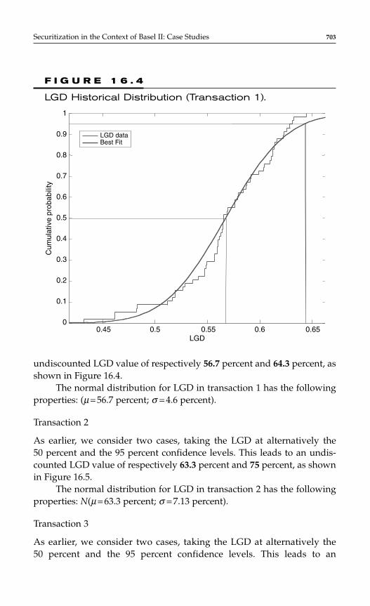
undiscounted LGD value of respectively 56.7 percent and 64.3 percent, asshown in Figure 16.4.
The normal distribution for LGD in transaction 1 has the followingproperties: (µ = 56.7 percent; σ = 4.6 percent).
Transaction 2
As earlier, we consider two cases, taking the LGD at alternatively the50 percent and the 95 percent confidence levels. This leads to an undis-counted LGD value of respectively 63.3 percent and 75 percent, as shownin Figure 16.5.
The normal distribution for LGD in transaction 2 has the followingproperties: N(µ = 63.3 percent; σ = 7.13 percent).
Transaction 3
As earlier, we consider two cases, taking the LGD at alternatively the50 percent and the 95 percent confidence levels. This leads to an
Securitization in the Context of Basel II: Case Studies 703
F I G U R E 1 6 . 4
LGD Historical Distribution (Transaction 1).
0.45 0.5 0.55 0.6 0.650
0.1
0.2
0.3
0.4
0.5
0.6
0.7
0.8
0.9
1
LGD
Cum
ulat
ive
prob
abili
ty
LGD dataBest Fit
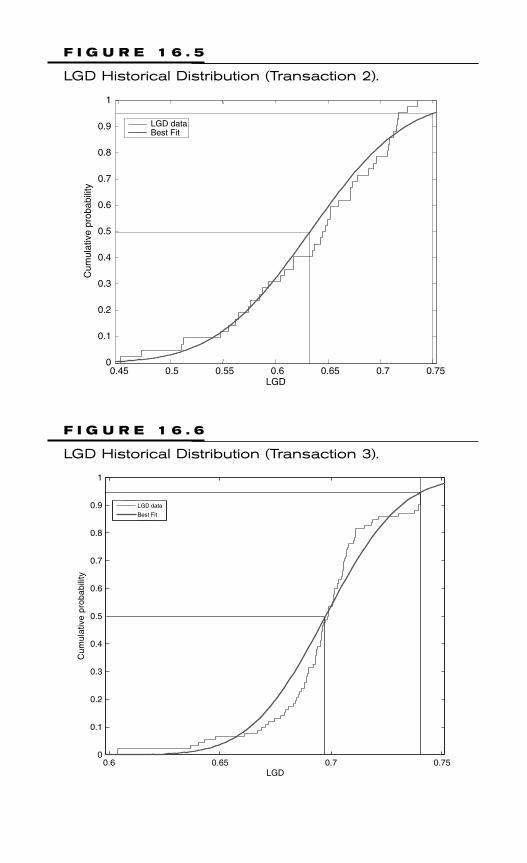
F I G U R E 1 6 . 5
LGD Historical Distribution (Transaction 2).
0.45 0.5 0.55 0.6 0.65 0.7 0.750
0.1
0.2
0.3
0.4
0.5
0.6
0.7
0.8
0.9
1
LGD
Cum
ulat
ive
prob
abili
ty
LGD dataBest Fit
F I G U R E 1 6 . 6
LGD Historical Distribution (Transaction 3).
0.6 0.65 0.7 0.750
0.1
0.2
0.3
0.4
0.5
0.6
0.7
0.8
0.9
1
LGD
Cum
ulat
ive
prob
abili
ty
LGD data
Best Fit
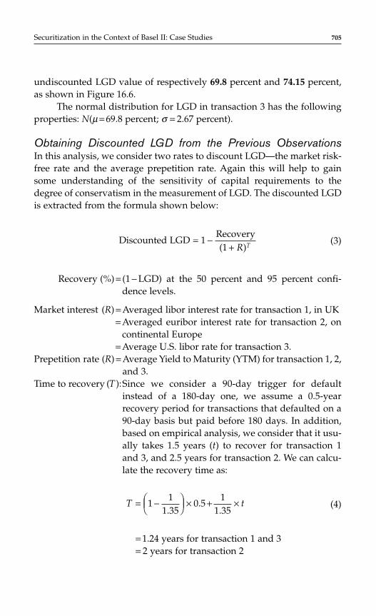
undiscounted LGD value of respectively 69.8 percent and 74.15 percent,as shown in Figure 16.6.
The normal distribution for LGD in transaction 3 has the followingproperties: N(µ = 69.8 percent; σ = 2.67 percent).
Obtaining Discounted LGD from the Previous ObservationsIn this analysis, we consider two rates to discount LGD—the market risk-free rate and the average prepetition rate. Again this will help to gainsome understanding of the sensitivity of capital requirements to thedegree of conservatism in the measurement of LGD. The discounted LGDis extracted from the formula shown below:
(3)
Recovery (%) = (1 − LGD) at the 50 percent and 95 percent confi-dence levels.
Market interest (R) = Averaged libor interest rate for transaction 1, in UK= Averaged euribor interest rate for transaction 2, on
continental Europe= Average U.S. libor rate for transaction 3.
Prepetition rate (R) = Average Yield to Maturity (YTM) for transaction 1, 2,and 3.
Time to recovery (T ):Since we consider a 90-day trigger for defaultinstead of a 180-day one, we assume a 0.5-yearrecovery period for transactions that defaulted on a90-day basis but paid before 180 days. In addition,based on empirical analysis, we consider that it usu-ally takes 1.5 years (t) to recover for transaction 1and 3, and 2.5 years for transaction 2. We can calcu-late the recovery time as:
(4)
= 1.24 years for transaction 1 and 3= 2 years for transaction 2
T t= −
× + ×1
11 35
0 51
1 35..
.
Discounted LGDRecovery( )
= −+
11 R T
Securitization in the Context of Basel II: Case Studies 705
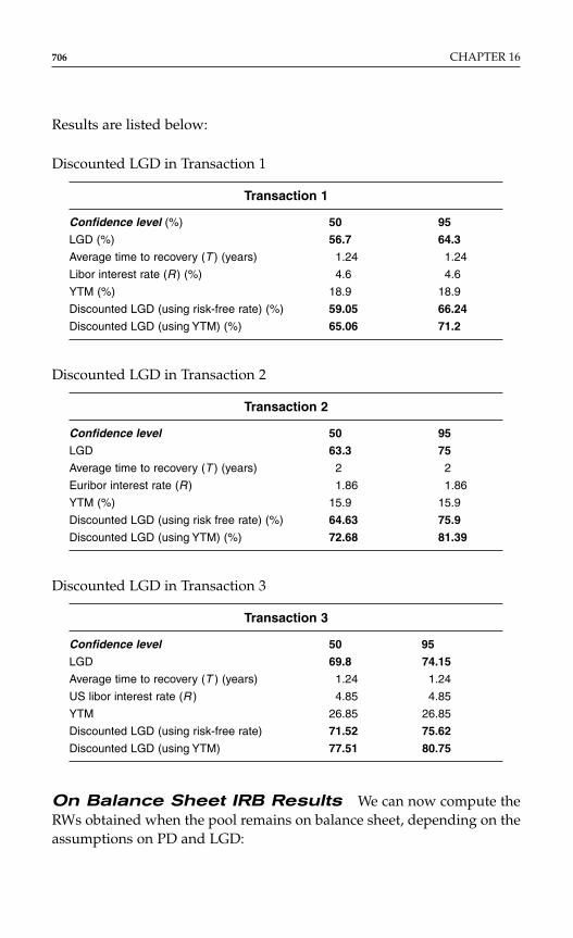
Results are listed below:
Discounted LGD in Transaction 1
Transaction 1
Confidence level (%) 50 95
LGD (%) 56.7 64.3
Average time to recovery (T ) (years) 1.24 1.24
Libor interest rate (R ) (%) 4.6 4.6
YTM (%) 18.9 18.9
Discounted LGD (using risk-free rate) (%) 59.05 66.24
Discounted LGD (using YTM) (%) 65.06 71.2
Discounted LGD in Transaction 2
Transaction 2
Confidence level 50 95
LGD 63.3 75
Average time to recovery (T ) (years) 2 2
Euribor interest rate (R ) 1.86 1.86
YTM (%) 15.9 15.9
Discounted LGD (using risk free rate) (%) 64.63 75.9
Discounted LGD (using YTM) (%) 72.68 81.39
Discounted LGD in Transaction 3
Transaction 3
Confidence level 50 95
LGD 69.8 74.15
Average time to recovery (T ) (years) 1.24 1.24
US libor interest rate (R ) 4.85 4.85
YTM 26.85 26.85
Discounted LGD (using risk-free rate) 71.52 75.62
Discounted LGD (using YTM) 77.51 80.75
On Balance Sheet IRB Results We can now compute theRWs obtained when the pool remains on balance sheet, depending on theassumptions on PD and LGD:
706 CHAPTER 16
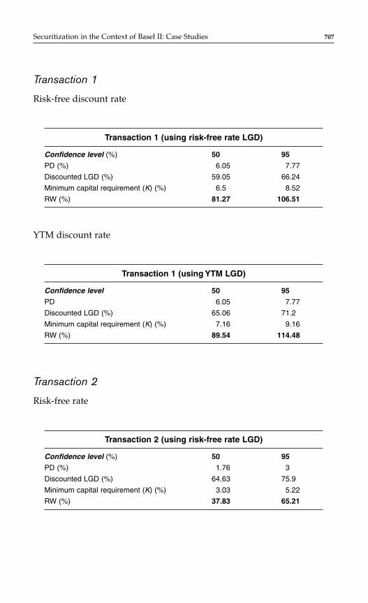
Transaction 1
Risk-free discount rate
Transaction 1 (using risk-free rate LGD)
Confidence level (%) 50 95
PD (%) 6.05 7.77
Discounted LGD (%) 59.05 66.24
Minimum capital requirement (K) (%) 6.5 8.52
RW (%) 81.27 106.51
YTM discount rate
Transaction 1 (using YTM LGD)
Confidence level 50 95
PD 6.05 7.77
Discounted LGD (%) 65.06 71.2
Minimum capital requirement (K) (%) 7.16 9.16
RW (%) 89.54 114.48
Transaction 2
Risk-free rate
Transaction 2 (using risk-free rate LGD)
Confidence level (%) 50 95
PD (%) 1.76 3
Discounted LGD (%) 64.63 75.9
Minimum capital requirement (K) (%) 3.03 5.22
RW (%) 37.83 65.21
Securitization in the Context of Basel II: Case Studies 707
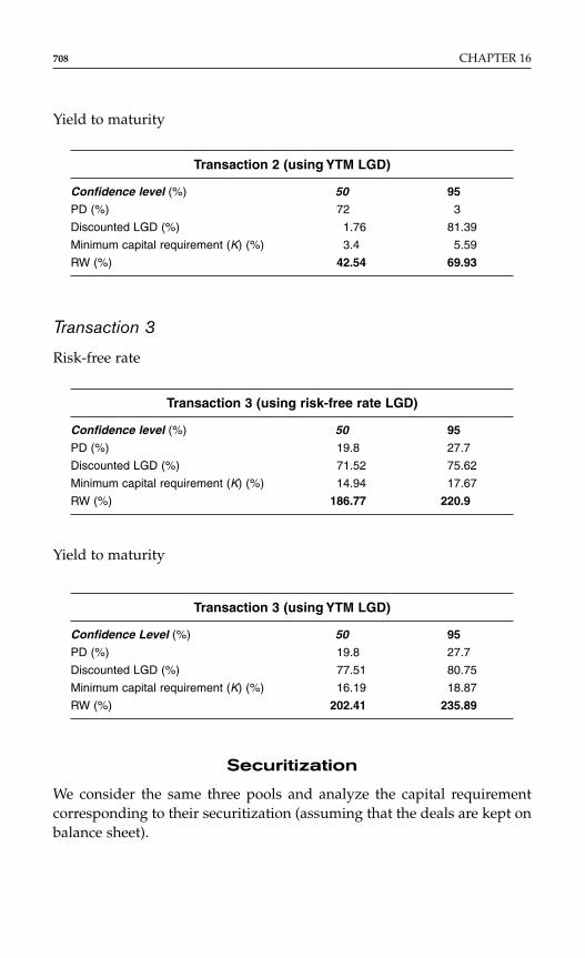
Yield to maturity
Transaction 2 (using YTM LGD)
Confidence level (%) 50 95
PD (%) 72 3
Discounted LGD (%) 1.76 81.39
Minimum capital requirement (K) (%) 3.4 5.59
RW (%) 42.54 69.93
Transaction 3
Risk-free rate
Transaction 3 (using risk-free rate LGD)
Confidence level (%) 50 95
PD (%) 19.8 27.7
Discounted LGD (%) 71.52 75.62
Minimum capital requirement (K) (%) 14.94 17.67
RW (%) 186.77 220.9
Yield to maturity
Transaction 3 (using YTM LGD)
Confidence Level (%) 50 95
PD (%) 19.8 27.7
Discounted LGD (%) 77.51 80.75
Minimum capital requirement (K) (%) 16.19 18.87
RW (%) 202.41 235.89
Securitization
We consider the same three pools and analyze the capital requirementcorresponding to their securitization (assuming that the deals are kept onbalance sheet).
708 CHAPTER 16
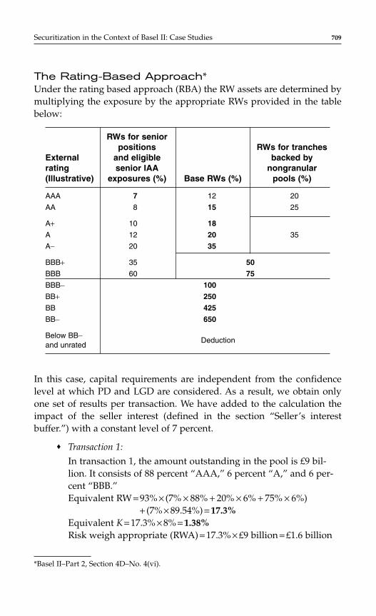
The Rating-Based Approach*Under the rating based approach (RBA) the RW assets are determined bymultiplying the exposure by the appropriate RWs provided in the tablebelow:
RWs for senior positions RWs for tranches
External and eligible backed by rating senior IAA nongranular(Illustrative) exposures (%) Base RWs (%) pools (%)
AAA 7 12 20
AA 8 15 25
A+ 10 18
A 12 20 35
A− 20 35
BBB+ 35 50
BBB 60 75
BBB− 100
BB+ 250
BB 425
BB− 650
Below BB−Deduction
and unrated
In this case, capital requirements are independent from the confidencelevel at which PD and LGD are considered. As a result, we obtain onlyone set of results per transaction. We have added to the calculation theimpact of the seller interest (defined in the section “Seller’s interestbuffer.”) with a constant level of 7 percent.
♦ Transaction 1:
In transaction 1, the amount outstanding in the pool is £9 bil-lion. It consists of 88 percent “AAA,” 6 percent “A,” and 6 per-cent “BBB.”Equivalent RW = 93% × (7% × 88% + 20% × 6% + 75% × 6%)
+ (7% × 89.54%) = 17.3%Equivalent K = 17.3% × 8% = 1.38%Risk weigh appropriate (RWA) = 17.3% × £9 billion = £1.6 billion
Securitization in the Context of Basel II: Case Studies 709
*Basel II–Part 2, Section 4D–No. 4(vi).
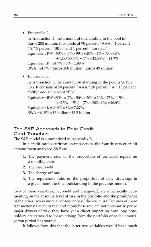
♦ Transaction 2:
In Transaction 2, the amount of outstanding in the pool isEuros 200 million. It consists of 90 percent “AAA,” 4 percent“A,” 5 percent “BBB,” and 1 percent “unrated.”Equivalent RW = 93% × (7% × 90% + 20% × 4% + 75% × 5%
+ 1250% × 1%) + (7% × 42.54%) = 24.7%Equivalent K = 24.7% × 8% = 1.98%RWA = 24.7% × Euros 200 million = Euros 49 million
♦ Transaction 3:
In Transaction 3, the amount outstanding in the pool is $6 bil-lion. It consists of 50 percent “AAA,” 20 percent “A,” 15 percent“BBB,” and 15 percent “BB.”Equivalent RW = 93% × (7% × 50% + 20% × 20% + 75% × 15%
+ 425% × 15%) + (7% × 202.41%) = 90.9%Equivalent K = 90.9% × 8% = 7.27%RWA = 90.9% × $6 billion = $5.5 billion
The S&P Approach to Rate Credit Card TranchesThe S&P model is summarized in Appendix B.
In a credit card securitization transaction, the four drivers of creditenhancement analyzed S&P are
1. The payment rate, or the proportion of principal repaid ona monthly basis
2. The asset yield3. The charge-off rate4. The repurchase rate, or the proportion of new drawings in
a given month to total outstanding in the previous month.
Two of these variables, i.e., yield and charge-off, are intrinsically com-menting on the absolute level of risk in the portfolio and the prominenceof the other two is more a consequence of the structural features of thesetransactions: Payment rate and repurchase rate are not necessarily per semajor drivers of risk, they have yet a direct impact on how long note-holders are exposed to losses arising from the portfolio once the amorti-zation period has started.
It follows from this that the latter two variables would have much
710 CHAPTER 16
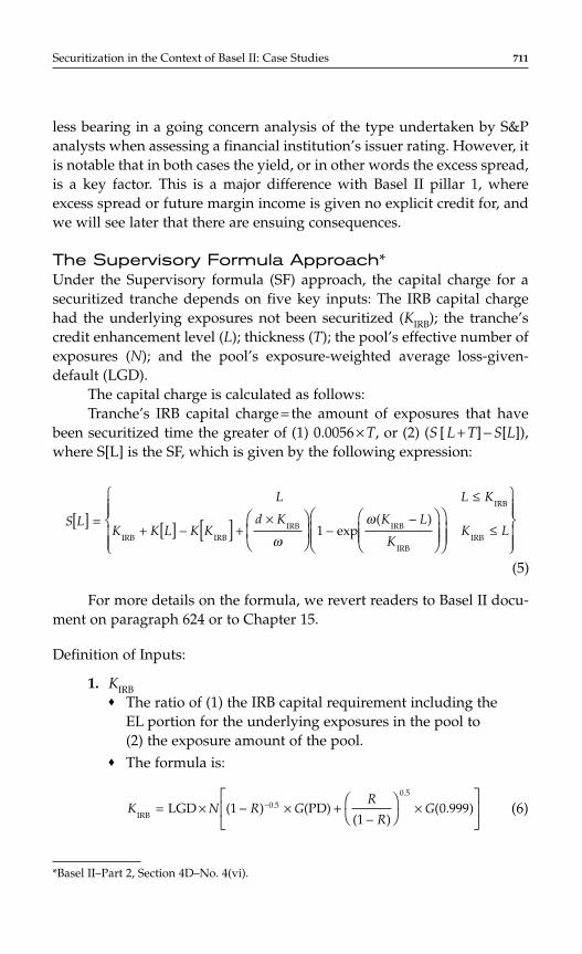
less bearing in a going concern analysis of the type undertaken by S&Panalysts when assessing a financial institution’s issuer rating. However, itis notable that in both cases the yield, or in other words the excess spread,is a key factor. This is a major difference with Basel II pillar 1, whereexcess spread or future margin income is given no explicit credit for, andwe will see later that there are ensuing consequences.
The Supervisory Formula Approach*Under the Supervisory formula (SF) approach, the capital charge for asecuritized tranche depends on five key inputs: The IRB capital chargehad the underlying exposures not been securitized (KIRB); the tranche’scredit enhancement level (L); thickness (T); the pool’s effective number ofexposures (N); and the pool’s exposure-weighted average loss-given-default (LGD).
The capital charge is calculated as follows:Tranche’s IRB capital charge = the amount of exposures that have
been securitized time the greater of (1) 0.0056 × T, or (2) (S [ L + T] − S[L]),where S[L] is the SF, which is given by the following expression:
For more details on the formula, we revert readers to Basel II docu-ment on paragraph 624 or to Chapter 15.
Definition of Inputs:
1. KIRB♦ The ratio of (1) the IRB capital requirement including the
EL portion for the underlying exposures in the pool to (2) the exposure amount of the pool.
♦ The formula is:
(6)K N R GR
RG
IRB.
.
LGD ( ) (PD)( )
( . )= × − × +−
×−
1
10 9990 5
0 5
S L
L L K
K K L K Kd K K L
KK L
[ ] [ ] [ ]
=
≤
+ − +×
−−
≤
IRB
IRB IRBIRB IRB
IRBIRB
exp( )
ω
ω1
Securitization in the Context of Basel II: Case Studies 711
*Basel II–Part 2, Section 4D–No. 4(vi).
(5)
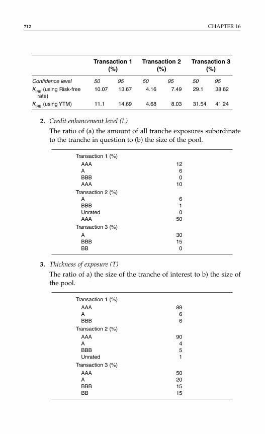
Transaction 1 Transaction 2 Transaction 3 (%) (%) (%)
Confidence level 50 95 50 95 50 95
KIRB (using Risk-free 10.07 13.67 4.16 7.49 29.1 38.62rate)
KIRB (using YTM) 11.1 14.69 4.68 8.03 31.54 41.24
2. Credit enhancement level (L)
The ratio of (a) the amount of all tranche exposures subordinateto the tranche in question to (b) the size of the pool.
Transaction 1 (%)
AAA 12A 6BBB 0AAA 10
Transaction 2 (%)A 6BBB 1Unrated 0AAA 50
Transaction 3 (%)
A 30BBB 15BB 0
3. Thickness of exposure (T)
The ratio of a) the size of the tranche of interest to b) the size ofthe pool.
Transaction 1 (%)
AAA 88A 6BBB 6
Transaction 2 (%)
AAA 90A 4BBB 5Unrated 1
Transaction 3 (%)
AAA 50A 20BBB 15BB 15
712 CHAPTER 16
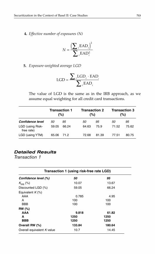
4. Effective number of exposures (N)
5. Exposure-weighted average LGD
The value of LGD is the same as in the IRB approach, as weassume equal weighting for all credit card transactions.
Transaction 1 Transaction 2 Transaction 3(%) (%) (%)
Confidence level 50 95 50 95 50 95
LGD (using Risk- 59.05 66.24 64.63 75.9 71.52 75.62free rate)
LGD (using YTM) 65.06 71.2 72.68 81.39 77.51 80.75
Detailed ResultsTransaction 1
Transaction 1 (using risk-free rate LGD)
Confidence level (%) 50 95
KIRB (%) 10.07 13.67
Discounted LGD (%) 59.05 66.24
Equivalent K (%)AAA 0.785 4.95A 100 100BBB 100 100
RW (%)AAA 9.818 61.82A 1250 1250BBB 1250 1250
Overall RW (%) 133.84 180.64
Overall equivalent K value 10.7 14.45
LGDLGD EAD
EAD=
⋅∑∑i i i
i i
Ni i
i i
=( )∑∑
EAD
EAD
2
2
Securitization in the Context of Basel II: Case Studies 713
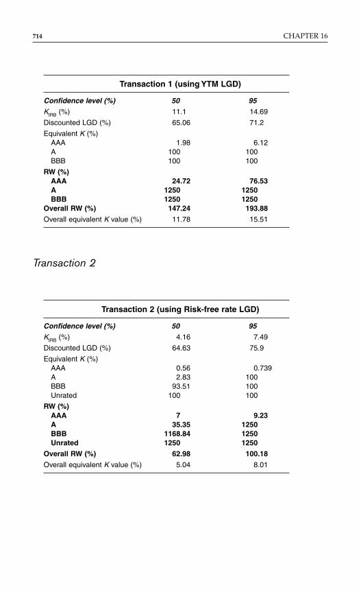
Transaction 1 (using YTM LGD)
Confidence level (%) 50 95
KIRB (%) 11.1 14.69
Discounted LGD (%) 65.06 71.2
Equivalent K (%)AAA 1.98 6.12A 100 100BBB 100 100
RW (%)AAA 24.72 76.53A 1250 1250BBB 1250 1250
Overall RW (%) 147.24 193.88
Overall equivalent K value (%) 11.78 15.51
Transaction 2
Transaction 2 (using Risk-free rate LGD)
Confidence level (%) 50 95
KIRB (%) 4.16 7.49
Discounted LGD (%) 64.63 75.9
Equivalent K (%)AAA 0.56 0.739A 2.83 100BBB 93.51 100Unrated 100 100
RW (%)AAA 7 9.23A 35.35 1250BBB 1168.84 1250Unrated 1250 1250
Overall RW (%) 62.98 100.18
Overall equivalent K value (%) 5.04 8.01
714 CHAPTER 16
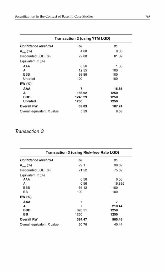
Transaction 2 (using YTM LGD)
Confidence level (%) 50 95
KIRB (%) 4.68 8.03
Discounted LGD (%) 72.68 81.39
Equivalent K (%)
AAA 0.56 1.35A 12.55 100BBB 99.86 100Unrated 100 100
RW (%)
AAA 7 16.85A 156.92 1250BBB 1248.29 1250Unrated 1250 1250
Overall RW 69.83 107.24
Overall equivalent K value 5.59 8.58
Transaction 3
Transaction 3 (using Risk-free Rate LGD)
Confidence level (%) 50 95
KIRB (%) 29.1 38.62
Discounted LGD (%) 71.52 75.62
Equivalent K (%)AAA 0.56 0.56A 0.56 16.835BBB 66.12 100BB 100 100
RW (%)
AAA 7 7A 7 210.44BBB 826.51 1250BB 1250 1250
Overall RW 384.47 505.45
Overall equivalent K value 30.76 40.44
Securitization in the Context of Basel II: Case Studies 715
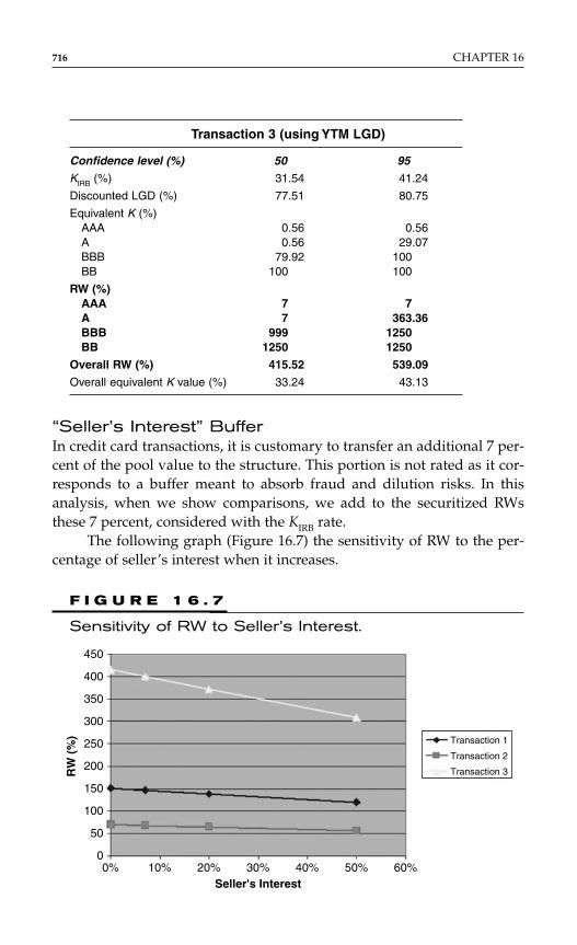
Transaction 3 (using YTM LGD)
Confidence level (%) 50 95
KIRB (%) 31.54 41.24
Discounted LGD (%) 77.51 80.75
Equivalent K (%)AAA 0.56 0.56A 0.56 29.07BBB 79.92 100BB 100 100
RW (%)AAA 7 7A 7 363.36BBB 999 1250BB 1250 1250
Overall RW (%) 415.52 539.09
Overall equivalent K value (%) 33.24 43.13
“Seller’s Interest” BufferIn credit card transactions, it is customary to transfer an additional 7 per-cent of the pool value to the structure. This portion is not rated as it cor-responds to a buffer meant to absorb fraud and dilution risks. In thisanalysis, when we show comparisons, we add to the securitized RWsthese 7 percent, considered with the KIRB rate.
The following graph (Figure 16.7) the sensitivity of RW to the per-centage of seller’s interest when it increases.
716 CHAPTER 16
F I G U R E 1 6 . 7
Sensitivity of RW to Seller’s Interest.
0%
450
400
350
300
250
200
150
100
50
010% 20% 30% 40% 50% 60%
Transaction 1
Transaction 2
Transaction 3
Seller's Interest
RW
(%
)
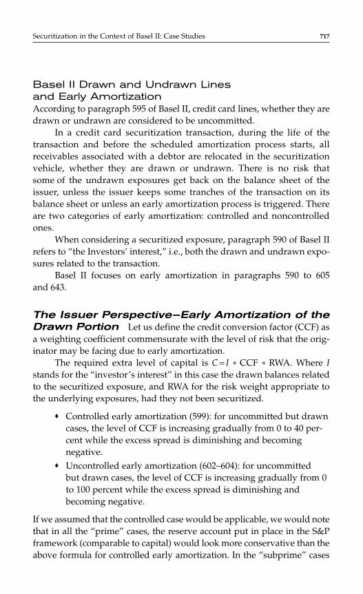
Securitization in the Context of Basel II: Case Studies 717
Basel II Drawn and Undrawn Lines and Early AmortizationAccording to paragraph 595 of Basel II, credit card lines, whether they aredrawn or undrawn are considered to be uncommitted.
In a credit card securitization transaction, during the life of thetransaction and before the scheduled amortization process starts, allreceivables associated with a debtor are relocated in the securitizationvehicle, whether they are drawn or undrawn. There is no risk thatsome of the undrawn exposures get back on the balance sheet of theissuer, unless the issuer keeps some tranches of the transaction on itsbalance sheet or unless an early amortization process is triggered. Thereare two categories of early amortization: controlled and noncontrolledones.
When considering a securitized exposure, paragraph 590 of Basel IIrefers to “the Investors’ interest,” i.e., both the drawn and undrawn expo-sures related to the transaction.
Basel II focuses on early amortization in paragraphs 590 to 605and 643.
The Issuer Perspective—Early Amortization of theDrawn Portion Let us define the credit conversion factor (CCF) asa weighting coefficient commensurate with the level of risk that the orig-inator may be facing due to early amortization.
The required extra level of capital is C = I * CCF * RWA. Where Istands for the “investor’s interest” in this case the drawn balances relatedto the securitized exposure, and RWA for the risk weight appropriate tothe underlying exposures, had they not been securitized.
♦ Controlled early amortization (599): for uncommitted but drawncases, the level of CCF is increasing gradually from 0 to 40 per-cent while the excess spread is diminishing and becomingnegative.
♦ Uncontrolled early amortization (602–604): for uncommitted but drawn cases, the level of CCF is increasing gradually from 0to 100 percent while the excess spread is diminishing andbecoming negative.
If we assumed that the controlled case would be applicable, we would notethat in all the “prime” cases, the reserve account put in place in the S&Pframework (comparable to capital) would look more conservative than theabove formula for controlled early amortization. In the “subprime” cases
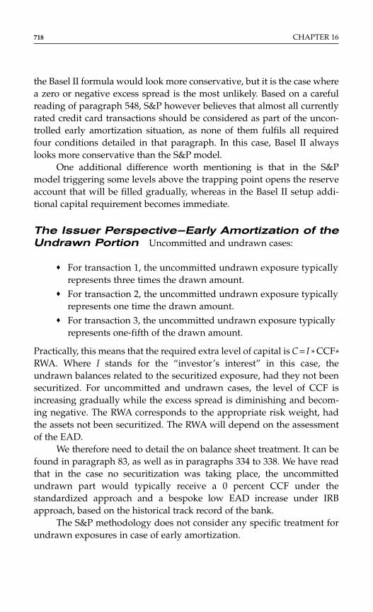
the Basel II formula would look more conservative, but it is the case wherea zero or negative excess spread is the most unlikely. Based on a carefulreading of paragraph 548, S&P however believes that almost all currentlyrated credit card transactions should be considered as part of the uncon-trolled early amortization situation, as none of them fulfils all requiredfour conditions detailed in that paragraph. In this case, Basel II alwayslooks more conservative than the S&P model.
One additional difference worth mentioning is that in the S&Pmodel triggering some levels above the trapping point opens the reserveaccount that will be filled gradually, whereas in the Basel II setup addi-tional capital requirement becomes immediate.
The Issuer Perspective—Early Amortization of theUndrawn Portion Uncommitted and undrawn cases:
♦ For transaction 1, the uncommitted undrawn exposure typicallyrepresents three times the drawn amount.
♦ For transaction 2, the uncommitted undrawn exposure typicallyrepresents one time the drawn amount.
♦ For transaction 3, the uncommitted undrawn exposure typicallyrepresents one-fifth of the drawn amount.
Practically, this means that the required extra level of capital is C = I * CCF*RWA. Where I stands for the “investor’s interest” in this case, theundrawn balances related to the securitized exposure, had they not beensecuritized. For uncommitted and undrawn cases, the level of CCF isincreasing gradually while the excess spread is diminishing and becom-ing negative. The RWA corresponds to the appropriate risk weight, hadthe assets not been securitized. The RWA will depend on the assessmentof the EAD.
We therefore need to detail the on balance sheet treatment. It can befound in paragraph 83, as well as in paragraphs 334 to 338. We have readthat in the case no securitization was taking place, the uncommittedundrawn part would typically receive a 0 percent CCF under thestandardized approach and a bespoke low EAD increase under IRBapproach, based on the historical track record of the bank.
The S&P methodology does not consider any specific treatment forundrawn exposures in case of early amortization.
718 CHAPTER 16
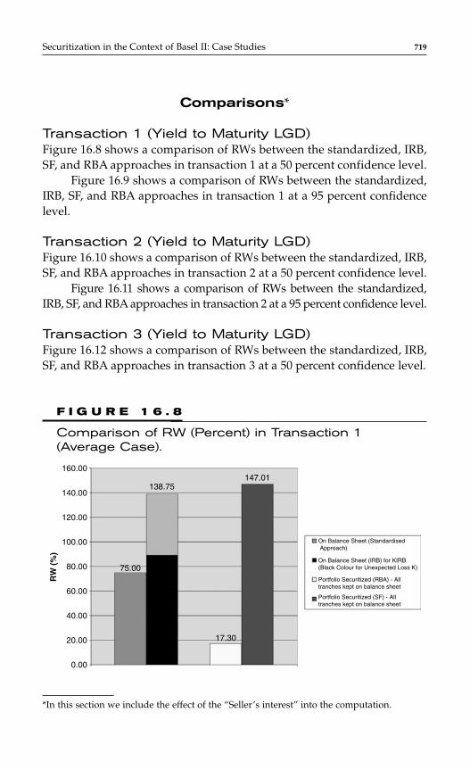
Comparisons*
Transaction 1 (Yield to Maturity LGD)Figure 16.8 shows a comparison of RWs between the standardized, IRB,SF, and RBA approaches in transaction 1 at a 50 percent confidence level.
Figure 16.9 shows a comparison of RWs between the standardized,IRB, SF, and RBA approaches in transaction 1 at a 95 percent confidencelevel.
Transaction 2 (Yield to Maturity LGD)Figure 16.10 shows a comparison of RWs between the standardized, IRB,SF, and RBA approaches in transaction 2 at a 50 percent confidence level.
Figure 16.11 shows a comparison of RWs between the standardized,IRB, SF, and RBA approaches in transaction 2 at a 95 percent confidence level.
Transaction 3 (Yield to Maturity LGD)Figure 16.12 shows a comparison of RWs between the standardized, IRB,SF, and RBA approaches in transaction 3 at a 50 percent confidence level.
Securitization in the Context of Basel II: Case Studies 719
F I G U R E 1 6 . 8
Comparison of RW (Percent) in Transaction 1 (Average Case).
160.00
140.00
120.00
100.00
80.00 75.00
138.75
17.30
147.01
60.00
40.00
20.00
0.00
On Balance Sheet (Standardised Approach)
On Balance Sheet (IRB) for KIRB (Black Colour for Unexpected Loss K)
Portfolio Securitized (RBA) - Alltranches kept on balance sheet
Portfolio Securitized (SF) - Alltranches kept on balance sheet
RW
(%
)
*In this section we include the effect of the “Seller’s interest” into the computation.
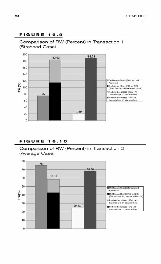
720 CHAPTER 16
F I G U R E 1 6 . 9
Comparison of RW (Percent) in Transaction 1(Stressed Case).
200
180
160
140
120
100
80
60
40
20
0
On Balance Sheet (StandardisedApproach)
Portfolio Securitized (RBA) - All tranches kept on balance sheet
RW
(%
)
75
183.63
19.04
188.33
Portfolio Securitized (SF) - All tranches kept on balance sheet
On Balance Sheet (IRB) for KIRB(Black Colour for Unexpected Loss K)
F I G U R E 1 6 . 1 0
Comparison of RW (Percent) in Transaction 2 (Average Case).
0
10
20
30
40
50
60
70
80
On Balance Sheet (Standardised Approach)
Portfolio Securitized (RBA) - Alltranches kept on balance sheet
RW
(%)
75
58.50
24.69
68.00
Portfolio Securitized (SF) - Alltranches kept on balance sheet
On Balance Sheet (IRB) for KIRB(Black Colour for Unexpected Loss K)
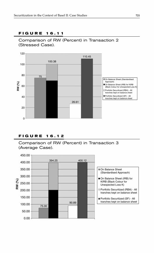
Securitization in the Context of Basel II: Case Studies 721
F I G U R E 1 6 . 1 1
Comparison of RW (Percent) in Transaction 2(Stressed Case).
RW
(%
)
0
20
40
60
110.45
26.61
100.38
7580
100
120
On Balance Sheet (Standardised Approach)
On Balance Sheet (IRB) for KIRB(Black Colour for Unexpected Loss K)
Portfolio Securitized (RBA) - Alltranches kept on balance sheet
Portfolio Securitized (SF) - Alltranches kept on balance sheet
F I G U R E 1 6 . 1 2
Comparison of RW (Percent) in Transaction 3 (Average Case).
394.25
90.89
On Balance Sheet(Standardised Approach)
On Balance Sheet (IRB) forKIRB (Black Colour forUnexpected Loss K)
Portfolio Securitized (RBA) - Alltranches kept on balance sheet
75.00
450.00
RW
(%
)
400.00400.12
350.00
300.00
250.00
200.00
150.00
100.00
50.00
0.00
Portfolio Securitized (SF) - Alltranches kept on balance sheet
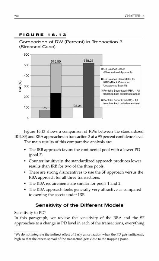
722 CHAPTER 16
F I G U R E 1 6 . 1 3
Comparison of RW (Percent) in Transaction 3(Stressed Case).
515.50
93.24
On Balance Sheet(Standardised Approach)
On Balance Sheet (IRB) forKIRB (Black Colour forUnexpected Loss K)
Portfolio Securitized (RBA) - Alltranches kept on balance sheet
Portfolio Securitized (SF) - Alltranches kept on balance sheet
75
500
600
RW
(%
)
400
518.25
300
200
100
0
*We do not integrate the indirect effect of Early amortization when the PD gets sufficientlyhigh so that the excess spread of the transaction gets close to the trapping point.
Figure 16.13 shows a comparison of RWs between the standardized,IRB, SF, and RBA approaches in transaction 3 at a 95 percent confidence level.
The main results of this comparative analysis are:
♦ The IRB approach favors the continental pool with a lower PD(pool 2).
♦ Counter intuitively, the standardized approach produces lowerresults than IRB for two of the three pools.
♦ There are strong disincentives to use the SF approach versus theRBA approach for all three transactions.
♦ The RBA requirements are similar for pools 1 and 2.♦ The RBA approach looks generally very attractive as compared
to owning the assets under IRB.
Sensitivity of the Different Models
Sensitivity to PD*In this paragraph, we review the sensitivity of the RBA and the SFapproaches to a change in PD level in each of the transactions, everything
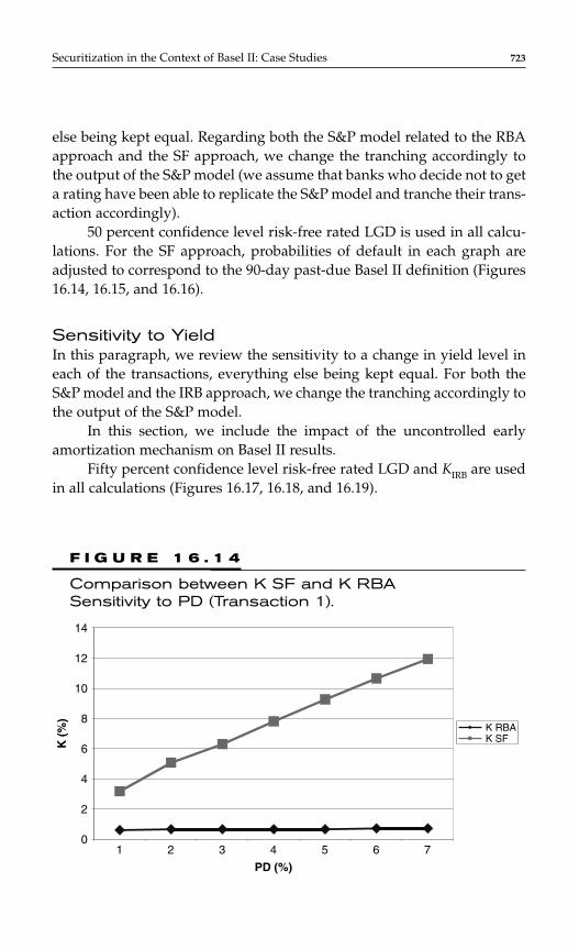
else being kept equal. Regarding both the S&P model related to the RBAapproach and the SF approach, we change the tranching accordingly tothe output of the S&P model (we assume that banks who decide not to geta rating have been able to replicate the S&P model and tranche their trans-action accordingly).
50 percent confidence level risk-free rated LGD is used in all calcu-lations. For the SF approach, probabilities of default in each graph areadjusted to correspond to the 90-day past-due Basel II definition (Figures16.14, 16.15, and 16.16).
Sensitivity to YieldIn this paragraph, we review the sensitivity to a change in yield level ineach of the transactions, everything else being kept equal. For both theS&P model and the IRB approach, we change the tranching accordingly tothe output of the S&P model.
In this section, we include the impact of the uncontrolled earlyamortization mechanism on Basel II results.
Fifty percent confidence level risk-free rated LGD and KIRB are usedin all calculations (Figures 16.17, 16.18, and 16.19).
Securitization in the Context of Basel II: Case Studies 723
F I G U R E 1 6 . 1 4
Comparison between K SF and K RBA Sensitivity to PD (Transaction 1).
14
0
2
4
6
8
10
12
1 2 3 4 5 6 7
PD (%)
K (
%)
K RBAK SF
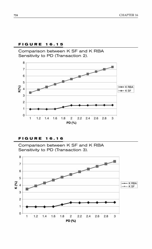
724 CHAPTER 16
F I G U R E 1 6 . 1 6
Comparison between K SF and K RBA Sensitivity to PD (Transaction 3).
0
1
2
3
4
5
6
7
8
1 1.2 1.4 1.6 1.8 2 2.2 2.4 2.6 2.8 3
PD (%)PD (%)
K (
%)
K RBAK SF
F I G U R E 1 6 . 1 5
Comparison between K SF and K RBA Sensitivity to PD (Transaction 2).
8
0
1
2
3
4
5
6
7
1 1.2 1.4 1.6 1.8 2 2.2 2.4 2.6 2.8 3
PD (%)
K(%
) K RBAK SF
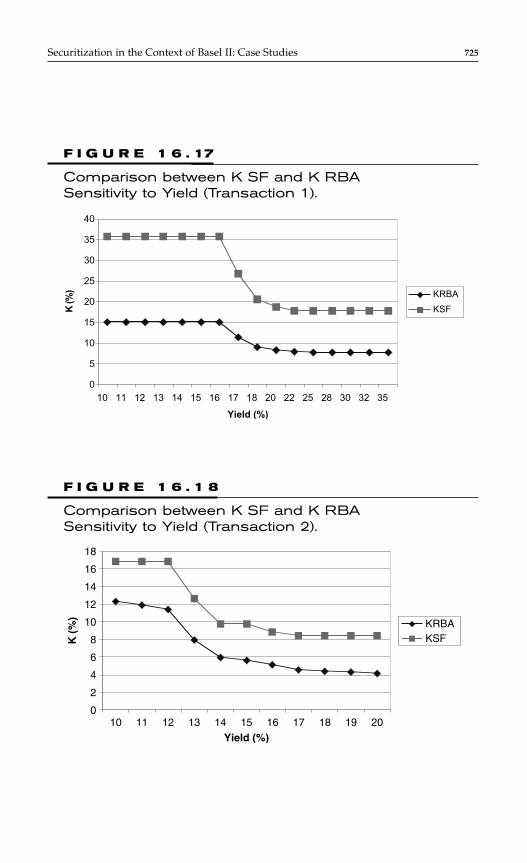
Securitization in the Context of Basel II: Case Studies 725
F I G U R E 1 6 . 17
Comparison between K SF and K RBA Sensitivity to Yield (Transaction 1).
0
5
10
15
20
25
30
35
40
10 11 12 13 14 15 16 17 18 20 22 25 28 30 32 35
Yield (%)
K (%
) KRBA
KSF
F I G U R E 1 6 . 1 8
Comparison between K SF and K RBA Sensitivity to Yield (Transaction 2).
0
2
4
6
8
10
12
14
16
18
10 11 12 13 14 15 16 17 18 19 20
Yield (%)
K (
%)
KRBAKSF
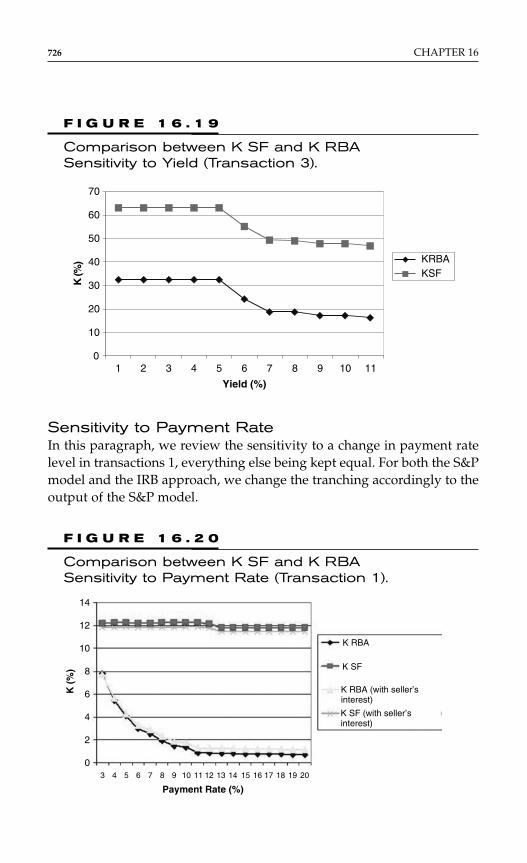
Sensitivity to Payment RateIn this paragraph, we review the sensitivity to a change in payment ratelevel in transactions 1, everything else being kept equal. For both the S&Pmodel and the IRB approach, we change the tranching accordingly to theoutput of the S&P model.
726 CHAPTER 16
F I G U R E 1 6 . 2 0
Comparison between K SF and K RBA Sensitivity to Payment Rate (Transaction 1).
F I G U R E 1 6 . 1 9
Comparison between K SF and K RBA Sensitivity to Yield (Transaction 3).
0
10
20
30
40
50
60
70
1 2 3 4 5 6 7 8 9 10 11
Yield (%)
K (%
) KRBAKSF
3 4 5 6 7 8 9 10 11 12 13 14 15 16 17 18 19 20
Payment Rate (%)
K (
%)
14
12
10
8
6
4
2
0
K RBA
K SF
K RBA (with seller’sinterest)
K SF (with seller’sinterest)
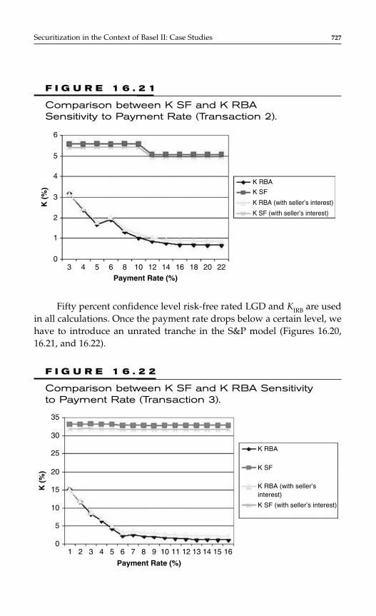
Securitization in the Context of Basel II: Case Studies 727
F I G U R E 1 6 . 2 1
Comparison between K SF and K RBA Sensitivity to Payment Rate (Transaction 2).
6
5
4
3
2
1
03 4 5 6 8 10 12 14 16 18 20 22
K (
%)
Payment Rate (%)
K RBA
K SF
K RBA (with seller’s interest)
K SF (with seller’s interest)
Fifty percent confidence level risk-free rated LGD and KIRB are usedin all calculations. Once the payment rate drops below a certain level, wehave to introduce an unrated tranche in the S&P model (Figures 16.20,16.21, and 16.22).
F I G U R E 1 6 . 2 2
Comparison between K SF and K RBA Sensitivity to Payment Rate (Transaction 3).
35
30
25
20
15
10
5
01 2 3 4 5 6 7 8 9 10 11 12 13 14 15 16
K (
%)
Payment Rate (%)
K RBA
K SF
K RBA (with seller’sinterest)
K SF (with seller’s interest)

Conclusion of Part 1
Securitization versus Keeping Assets on BalanceSheet: The Impact of Excess SpreadAs discussed in the introduction, the level of excess spread in a securiti-zation transaction has a direct effect on the capital structure. This is whyin the credit card field, it is not uncommon, even if counterintuitive at firstsight, for subprime portfolios to have a AAA tranche as large as or evenlarger than a prime pool. On the other hand, excess spread or future mar-gin income is not a factor in Basel II’s pillar 1. Pillar 1 is meant to measureunexpected loss only.
The credit card sector is probably the one where this discrepancy hasthe widest consequences, as reinforced by the fact the most junior notes ina capital structure for UK or US assets can often be rated BBB on the basisof the strength of the excess spread alone.
Securitization: Discussion on the Use of the Supervisory FormulaFrom the three examples we have considered above, it seems clear thatthe SF has been calibrated to dissuade regulated investors from keepingunrated securitization tranches on their balance sheet. Such capital treat-ment should represent an incentive for originators to have a systematicrecourse to more transparent external rating assessment on their securi-tization transactions. We can identify two elements that make the SFapproach way more conservative than the RBA approach:
♦ The size of the tranches below BBB seems to be most of the timemuch smaller than the KIRB level. As a result, some of the mezza-nine and even the senior tranches get penalized as if they werejunior (with a one for one capital treatment).
♦ The capital charge related to the most senior tranches in thepool are negatively impacted in the SF framework by thealmost exclusive focus on a typically high KIRB level and theabsence of credit granted to a high level of excess spread.
PART 2: ANALYSIS OF THE IMPACT OFBASEL II ON THE RMBS ASSET CLASS
The main finding in this part is that apart for subprime deals, regulatoryarbitrage will probably not be a key driver for securitization.
728 CHAPTER 16
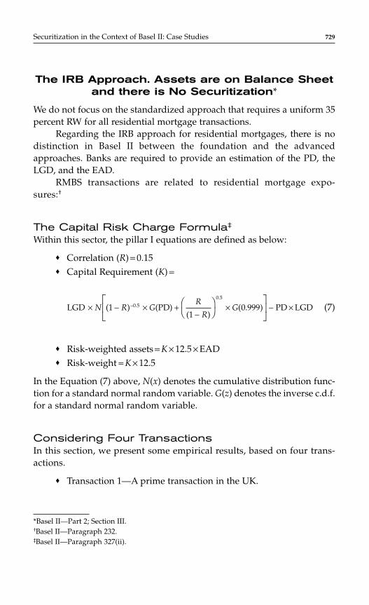
The IRB Approach. Assets are on Balance Sheetand there is No Securitization*
We do not focus on the standardized approach that requires a uniform 35percent RW for all residential mortgage transactions.
Regarding the IRB approach for residential mortgages, there is nodistinction in Basel II between the foundation and the advancedapproaches. Banks are required to provide an estimation of the PD, theLGD, and the EAD.
RMBS transactions are related to residential mortgage expo-sures:†
The Capital Risk Charge Formula‡
Within this sector, the pillar I equations are defined as below:
♦ Correlation (R) = 0.15♦ Capital Requirement (K) =
(7)
♦ Risk-weighted assets = K × 12.5 × EAD♦ Risk-weight = K × 12.5
In the Equation (7) above, N(x) denotes the cumulative distribution func-tion for a standard normal random variable. G(z) denotes the inverse c.d.f.for a standard normal random variable.
Considering Four TransactionsIn this section, we present some empirical results, based on four trans-actions.
♦ Transaction 1—A prime transaction in the UK.
LGD ( ) (PD)( )
( . ) PD LGD.
.
× − × +−
× − ×−
N R G
R
RG1
10 9990 5
0 5
Securitization in the Context of Basel II: Case Studies 729
*Basel II—Part 2; Section III.†Basel II—Paragraph 232.‡Basel II—Paragraph 327(ii).
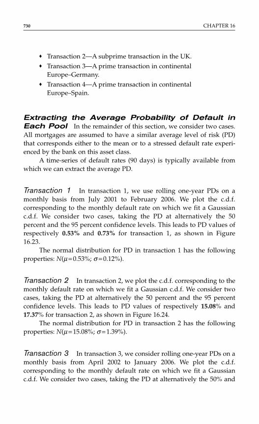
♦ Transaction 2—A subprime transaction in the UK.♦ Transaction 3—A prime transaction in continental
Europe–Germany.♦ Transaction 4—A prime transaction in continental
Europe–Spain.
Extracting the Average Probability of Default inEach Pool In the remainder of this section, we consider two cases.All mortgages are assumed to have a similar average level of risk (PD)that corresponds either to the mean or to a stressed default rate experi-enced by the bank on this asset class.
A time-series of default rates (90 days) is typically available fromwhich we can extract the average PD.
Transaction 1 In transaction 1, we use rolling one-year PDs on amonthly basis from July 2001 to February 2006. We plot the c.d.f.corresponding to the monthly default rate on which we fit a Gaussianc.d.f. We consider two cases, taking the PD at alternatively the 50percent and the 95 percent confidence levels. This leads to PD values ofrespectively 0.53% and 0.73% for transaction 1, as shown in Figure16.23.
The normal distribution for PD in transaction 1 has the followingproperties: N(µ = 0.53%; σ = 0.12%).
Transaction 2 In transaction 2, we plot the c.d.f. corresponding to themonthly default rate on which we fit a Gaussian c.d.f. We consider twocases, taking the PD at alternatively the 50 percent and the 95 percentconfidence levels. This leads to PD values of respectively 15.08% and17.37% for transaction 2, as shown in Figure 16.24.
The normal distribution for PD in transaction 2 has the followingproperties: N(µ = 15.08%; σ = 1.39%).
Transaction 3 In transaction 3, we consider rolling one-year PDs on amonthly basis from April 2002 to January 2006. We plot the c.d.f.corresponding to the monthly default rate on which we fit a Gaussianc.d.f. We consider two cases, taking the PD at alternatively the 50% and
730 CHAPTER 16
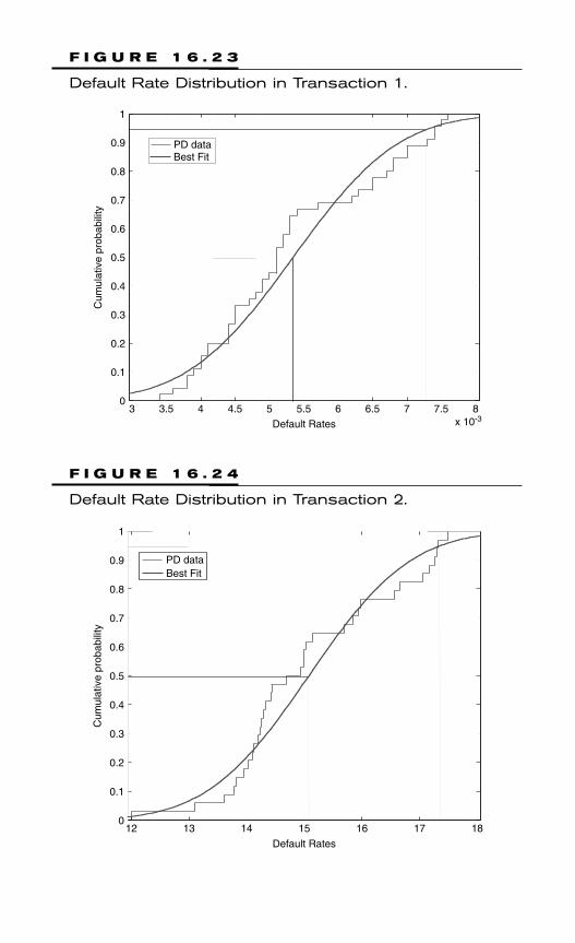
F I G U R E 1 6 . 2 3
Default Rate Distribution in Transaction 1.
3 3.5 4 4.5 5 5.5 6 6.5 7 7.5 8x 10⁻³
0
0.1
0.2
0.3
0.4
0.5
0.6
0.7
0.8
0.9
1
Default Rates
Cum
ulat
ive
prob
abili
ty
PD dataBest Fit
F I G U R E 1 6 . 2 4
Default Rate Distribution in Transaction 2.
12 13 14 15 16 17 180
0.1
0.2
0.3
0.4
0.5
0.6
0.7
0.8
0.9
1
Default Rates
Cum
ulat
ive
prob
abili
ty
PD dataBest Fit
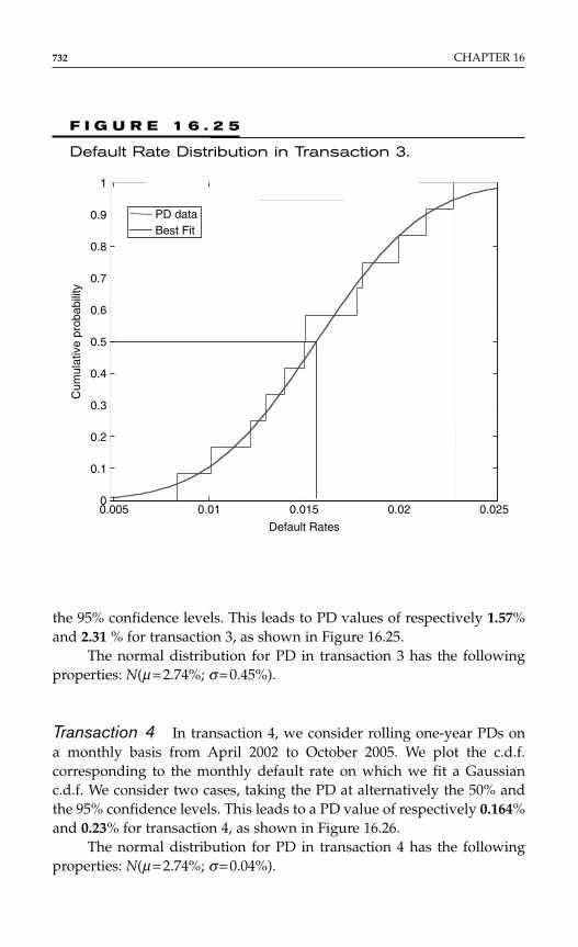
the 95% confidence levels. This leads to PD values of respectively 1.57%and 2.31 % for transaction 3, as shown in Figure 16.25.
The normal distribution for PD in transaction 3 has the followingproperties: N(µ = 2.74%; σ = 0.45%).
Transaction 4 In transaction 4, we consider rolling one-year PDs ona monthly basis from April 2002 to October 2005. We plot the c.d.f.corresponding to the monthly default rate on which we fit a Gaussianc.d.f. We consider two cases, taking the PD at alternatively the 50% andthe 95% confidence levels. This leads to a PD value of respectively 0.164%and 0.23% for transaction 4, as shown in Figure 16.26.
The normal distribution for PD in transaction 4 has the followingproperties: N(µ = 2.74%; σ = 0.04%).
732 CHAPTER 16
F I G U R E 1 6 . 2 5
Default Rate Distribution in Transaction 3.
0.005 0.01 0.015 0.02 0.0250
0.1
0.2
0.3
0.4
0.5
0.6
0.7
0.8
0.9
1
Default Rates
Cum
ulat
ive
prob
abili
ty
PD dataBest Fit
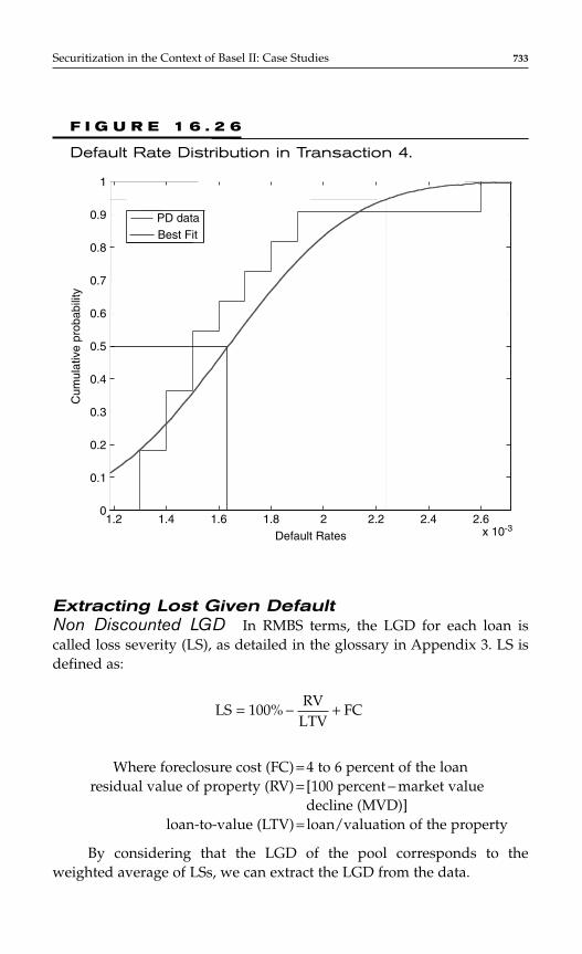
Extracting Lost Given DefaultNon Discounted LGD In RMBS terms, the LGD for each loan iscalled loss severity (LS), as detailed in the glossary in Appendix 3. LS isdefined as:
Where foreclosure cost (FC) = 4 to 6 percent of the loanresidual value of property (RV) = [100 percent − market value
decline (MVD)]loan-to-value (LTV) = loan/valuation of the property
By considering that the LGD of the pool corresponds to theweighted average of LSs, we can extract the LGD from the data.
LS %RV
LTVFC= − +100
Securitization in the Context of Basel II: Case Studies 733
F I G U R E 1 6 . 2 6
Default Rate Distribution in Transaction 4.
1.2 1.4 1.6 1.8 2 2.2 2.4 2.6x 10⁻³
0
0.1
0.2
0.3
0.4
0.5
0.6
0.7
0.8
0.9
1
Default Rates
Cum
ulat
ive
prob
abili
ty
PD dataBest Fit
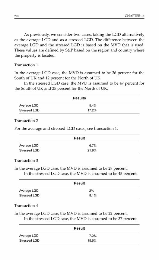
As previously, we consider two cases, taking the LGD alternativelyas the average LGD and as a stressed LGD. The difference between theaverage LGD and the stressed LGD is based on the MVD that is used.These values are defined by S&P based on the region and country wherethe property is located.
Transaction 1
In the average LGD case, the MVD is assumed to be 26 percent for theSouth of UK and 12 percent for the North of UK.
In the stressed LGD case, the MVD is assumed to be 47 percent forthe South of UK and 25 percent for the North of UK.
Results
Average LGD 5.4%
Stressed LGD 17.2%
Transaction 2
For the average and stressed LGD cases, see transaction 1.
Result
Average LGD 6.7%
Stressed LGD 21.8%
Transaction 3
In the average LGD case, the MVD is assumed to be 28 percent.In the stressed LGD case, the MVD is assumed to be 45 percent.
Result
Average LGD 2%
Stressed LGD 8.1%
Transaction 4
In the average LGD case, the MVD is assumed to be 22 percent.In the stressed LGD case, the MVD is assumed to be 37 percent.
Result
Average LGD 7.2%
Stressed LGD 15.6%
734 CHAPTER 16
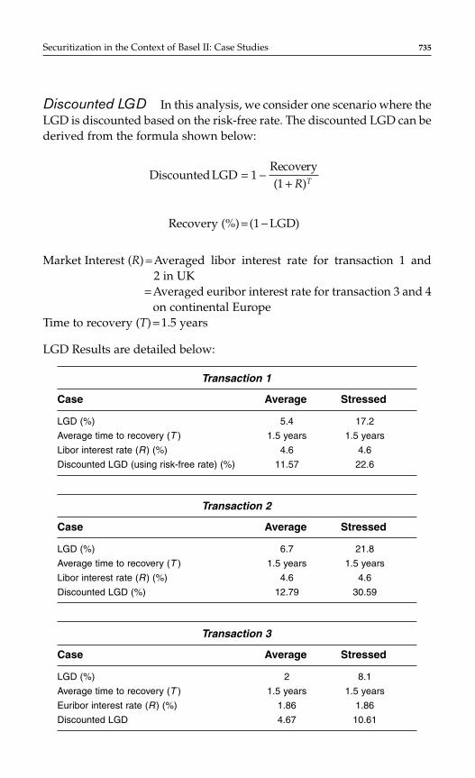
Discounted LGD In this analysis, we consider one scenario where theLGD is discounted based on the risk-free rate. The discounted LGD can bederived from the formula shown below:
Recovery (%) = (1 − LGD)
Market Interest (R) = Averaged libor interest rate for transaction 1 and 2 in UK
= Averaged euribor interest rate for transaction 3 and 4on continental Europe
Time to recovery (T) = 1.5 years
LGD Results are detailed below:
Transaction 1
Case Average Stressed
LGD (%) 5.4 17.2
Average time to recovery (T ) 1.5 years 1.5 years
Libor interest rate (R ) (%) 4.6 4.6
Discounted LGD (using risk-free rate) (%) 11.57 22.6
Transaction 2
Case Average Stressed
LGD (%) 6.7 21.8
Average time to recovery (T ) 1.5 years 1.5 years
Libor interest rate (R ) (%) 4.6 4.6
Discounted LGD (%) 12.79 30.59
Transaction 3
Case Average Stressed
LGD (%) 2 8.1
Average time to recovery (T ) 1.5 years 1.5 years
Euribor interest rate (R ) (%) 1.86 1.86
Discounted LGD 4.67 10.61
Discounted LGDRecov ry( )
= −+
11
eR T
Securitization in the Context of Basel II: Case Studies 735
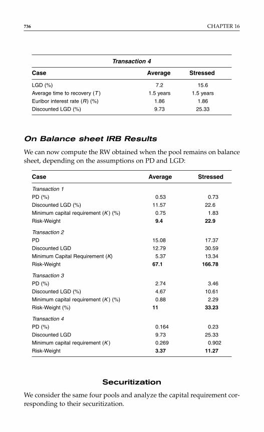
Transaction 4
Case Average Stressed
LGD (%) 7.2 15.6
Average time to recovery (T ) 1.5 years 1.5 years
Euribor interest rate (R ) (%) 1.86 1.86
Discounted LGD (%) 9.73 25.33
On Balance sheet IRB Results
We can now compute the RW obtained when the pool remains on balancesheet, depending on the assumptions on PD and LGD:
Case Average Stressed
Transaction 1
PD (%) 0.53 0.73
Discounted LGD (%) 11.57 22.6
Minimum capital requirement (K ) (%) 0.75 1.83
Risk-Weight 9.4 22.9
Transaction 2
PD 15.08 17.37
Discounted LGD 12.79 30.59
Minimum Capital Requirement (K) 5.37 13.34
Risk-Weight 67.1 166.78
Transaction 3
PD (%) 2.74 3.46
Discounted LGD (%) 4.67 10.61
Minimum capital requirement (K ) (%) 0.88 2.29
Risk-Weight (%) 11 33.23
Transaction 4
PD (%) 0.164 0.23
Discounted LGD 9.73 25.33
Minimum capital requirement (K ) 0.269 0.902
Risk-Weight 3.37 11.27
Securitization
We consider the same four pools and analyze the capital requirement cor-responding to their securitization.
736 CHAPTER 16
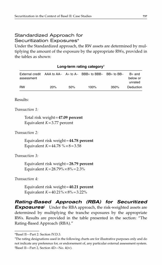
Standardized Approach for Securitization Exposures*Under the Standardized approach, the RW assets are determined by mul-tiplying the amount of the exposure by the appropriate RWs, provided inthe tables as shown:
Long-term rating category†
External credit AAA to AA− A+ to A− BBB+ to BBB− BB+ to BB− B+ andassessment below or
unrated
RW 20% 50% 100% 350% Deduction
Results:
Transaction 1:
Total risk weight = 47.09 percentEquivalent K = 3.77 percent
Transaction 2:
Equivalent risk weight = 44.78 percentEquivalent K = 44.78 % × 8 = 3.58
Transaction 3:
Equivalent risk weight = 28.79 percentEquivalent K = 28.79% × 8% = 2.3%
Transaction 4:
Equivalent risk weight = 40.21 percentEquivalent K = 40.21% × 8% = 3.22%
Rating-Based Approach (RBA) for Securitized Exposures‡ Under the RBA approach, the risk-weighted assets aredetermined by multiplying the tranche exposures by the appropriateRWs. Results are provided in the table presented in the section: “TheRating-Based Approach (RBA).”
Securitization in the Context of Basel II: Case Studies 737
*Basel II—Part 2: Section IV.D.3.†The rating designations used in the following charts are for illustrative purposes only and donot indicate any preference for, or endorsement of, any particular external assessment system.‡Basel II—Part 2, Section 4D—No. 4(iv).
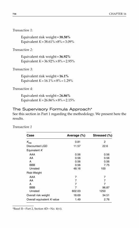
Transaction 1:
Equivalent risk weight = 38.58%Equivalent K = 38.61% ×8% = 3.09%
Transaction 2:
Equivalent risk weight = 36.92%Equivalent K = 36.92% × 8% = 2.95%
Transaction 3:
Equivalent risk weight = 16.1%Equivalent K = 16.1% × 8% = 1.29%
Transaction 4:
Equivalent risk weight = 26.86%Equivalent K = 26.86% × 8% = 2.15%
The Supervisory Formula Approach*See this section in Part 1 regarding the methodology. We present here theresults.
Transaction 1
Case Average (%) Stressed (%)
KIRB 0.81 2
Discounted LGD 11.57 22.6
Equivalent K
AAA 0.56 0.56AA 0.56 0.56A 0.56 0.56BBB 0.56 7.75Unrated 48.16 100
Risk-Weight
AAA 7 7AA 7 7A 7 7BBB 7 96.87Unrated 602.03 1250
Overall risk weight 18.69 34.51
Overall equivalent K value 1.49 2.76
738 CHAPTER 16
*Basel II—Part 2, Section 4D—No. 4(vi).
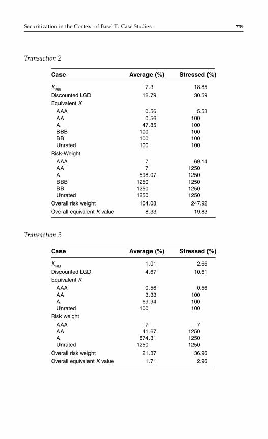
Transaction 2
Case Average (%) Stressed (%)
KIRB 7.3 18.85
Discounted LGD 12.79 30.59
Equivalent K
AAA 0.56 5.53AA 0.56 100A 47.85 100BBB 100 100BB 100 100Unrated 100 100
Risk-Weight
AAA 7 69.14AA 7 1250A 598.07 1250BBB 1250 1250BB 1250 1250Unrated 1250 1250
Overall risk weight 104.08 247.92
Overall equivalent K value 8.33 19.83
Transaction 3
Case Average (%) Stressed (%)
KIRB 1.01 2.66
Discounted LGD 4.67 10.61
Equivalent K
AAA 0.56 0.56AA 3.33 100A 69.94 100Unrated 100 100
Risk weight
AAA 7 7AA 41.67 1250A 874.31 1250Unrated 1250 1250
Overall risk weight 21.37 36.96
Overall equivalent K value 1.71 2.96
Securitization in the Context of Basel II: Case Studies 739
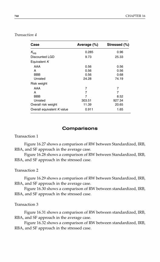
Transaction 4
Case Average (%) Stressed (%)
KIRB 0.285 0.96
Discounted LGD 9.73 25.33
Equivalent K
AAA 0.56 0.56A 0.56 0.56BBB 0.56 0.68Unrated 24.28 74.19
Risk weight
AAA 7 7A 7 7BBB 7 8.52Unrated 303.51 927.34
Overall risk weight 11.39 20.65
Overall equivalent K value 0.911 1.65
Comparisons
Transaction 1
Figure 16.27 shows a comparison of RW between Standardized, IRB,RBA, and SF approach in the average case.
Figure 16.28 shows a comparison of RW between Standardized, IRB,RBA, and SF approach in the stressed case.
Transaction 2
Figure 16.29 shows a comparison of RW between Standardized, IRB,RBA, and SF approach in the average case.
Figure 16.30 shows a comparison of RW between standardized, IRB,RBA, and SF approach in the stressed case.
Transaction 3
Figure 16.31 shows a comparison of RW between standardized, IRB,RBA, and SF approach in the average case.
Figure 16.32 shows a comparison of RW between standardized, IRB,RBA, and SF approach in the stressed case.
740 CHAPTER 16
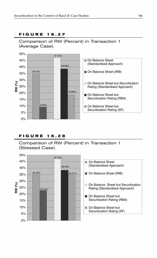
Securitization in the Context of Basel II: Case Studies 741
F I G U R E 1 6 . 2 7
Comparison of RW (Percent) in Transaction 1 (Average Case).
RW
(%
)
35.00%
9.40%
47.12%
38.58%
18.69%
0%
5%
10%
15%
20%
25%
30%
35%
40%
45%
50%
On Balance Sheet(Standardised Approach)
On Balance Sheet (IRB)
On Balance Sheet but SecuritizationRating (Standardised Approach)
On Balance Sheet butSecuritization Rating (RBA)
On Balance Sheet butSecuritization Rating (SF)
F I G U R E 1 6 . 2 8
Comparison of RW (Percent) in Transaction 1 (Stressed Case).
35.00%
22.90%
47.12%
38.58%
34.51%
0%
5%
10%
15%
20%
25%
30%
35%
40%
45%
50%
On Balance Sheet(Standardised Approach)
On Balance Sheet (IRB)
On Balance Sheet but Securitization Rating (Standardised Approach)
On Balance Sheet but Securitization Rating (RBA)
On Balance Sheet butSecuritization Rating (SF)
RW
(%
)
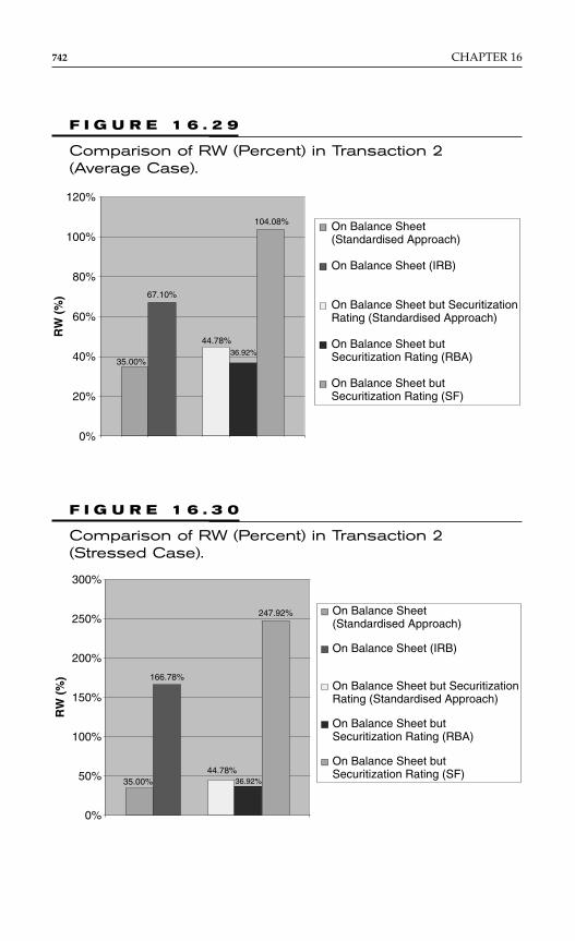
742 CHAPTER 16
F I G U R E 1 6 . 2 9
Comparison of RW (Percent) in Transaction 2 (Average Case).
F I G U R E 1 6 . 3 0
Comparison of RW (Percent) in Transaction 2(Stressed Case).
35.00%
67.10%
44.78%36.92%
104.08%
0%
20%
40%
60%
80%
100%
120%
On Balance Sheet (Standardised Approach)
On Balance Sheet (IRB)
On Balance Sheet but Securitization Rating (Standardised Approach)
On Balance Sheet but Securitization Rating (RBA)
On Balance Sheet but Securitization Rating (SF)
RW
(%
)
35.00%
166.78%
44.78%36.92%
247.92%
0%
50%
100%
150%
200%
250%
300%
On Balance Sheet (Standardised Approach)
On Balance Sheet (IRB)
On Balance Sheet but Securitization Rating (Standardised Approach)
On Balance Sheet but Securitization Rating (RBA)
On Balance Sheet but Securitization Rating (SF)
RW
(%
)
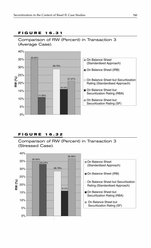
Securitization in the Context of Basel II: Case Studies 743
F I G U R E 1 6 . 3 1
Comparison of RW (Percent) in Transaction 3 (Average Case).
35.00%
11.00%
28.79%
16.10%
21.37%
0%
5%
10%
15%
20%
25%
30%
35%
40%
On Balance Sheet(Standardised Approach)
On Balance Sheet (IRB)
On Balance Sheet but SecuritizationRating (Standardised Approach)
On Balance Sheet but Securitization Rating (RBA)
On Balance Sheet but Securitization Rating (SF)
RW
(%
)
F I G U R E 1 6 . 3 2
Comparison of RW (Percent) in Transaction 3 (Stressed Case).
35.00%
33.23%
28.79%
16.10%
36.96%
0%
5%
10%
15%
20%
25%
30%
35%
40%
-
On Balance Sheet (Standardised Approach)
On Balance Sheet (IRB)
On Balance Sheet but SecuritizationRating (Standardised Approach)
On Balance Sheet but Securitization Rating (RBA)
On Balance Sheet butSecuritization Rating (SF)
RW
(%
)
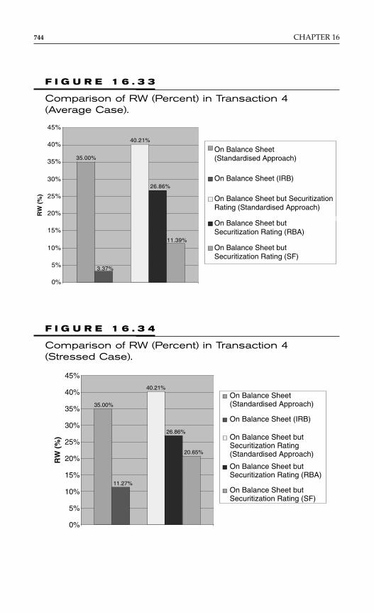
744 CHAPTER 16
F I G U R E 1 6 . 3 4
Comparison of RW (Percent) in Transaction 4 (Stressed Case).
RW
(%
)
35.00%
11.27%
40.21%
26.86%
20.65%
0%
5%
10%
15%
20%
25%
30%
35%
40%
45%
On Balance Sheet(Standardised Approach)
On Balance Sheet (IRB)
On Balance Sheet butSecuritization Rating(Standardised Approach)
On Balance Sheet butSecuritization Rating (RBA)
On Balance Sheet butSecuritization Rating (SF)
F I G U R E 1 6 . 3 3
Comparison of RW (Percent) in Transaction 4 (Average Case).
RW
(%
)
35.00%
3.37%
40.21%
26.86%
11.39%
0%
5%
10%
15%
20%
25%
30%
35%
40%
45%
On Balance Sheet (Standardised Approach)
On Balance Sheet (IRB)
On Balance Sheet but SecuritizationRating (Standardised Approach)
On Balance Sheet but Securitization Rating (RBA)
On Balance Sheet butSecuritization Rating (SF)

Transaction 4
Figure 16.33 shows a comparison of RW between standardized, IRB,RBA, and SF approach in the average case.
Figure 16.34 shows a comparison of RW between standardized, IRB,RBA, and SF approach in the stressed case.
Conclusion of Part 2
The first conclusion is that the type of arbitrage, we could observe sys-tematically, in the credit card asset class does not occur anymore for theRMBS sector. A point could however mitigate this statement slightly aswhen no securitization is taking place, the bank needs to provision anamount that should be reasonably close to the expected loss level (seeparagraphs 380 to 386).
Another point to mention is that the way banks will measure PDsand LGDs will very much impact the existence of an opportunity of arbi-trage linked to securitization transactions.
Lastly, securitization seems to make more sense for subprime poolsthan for prime ones.
Securitization in the Context of Basel II: Case Studies 745

Payment The credit card payment rate can be defined as:Rate Principal Repayment this month as a percentage
of outstanding receivables in the previous month.
Yield The yield represents the total revenue collected by the issuer, as a percentage of the outstanding.The numerator of the Yield consists of three items:♦ Finance charges, i.e., primarily interest paid♦ Fees (late fee and over-limit fee)♦ Interchange (It is the fee paid to originators by ♦ VISA or MasterCard for absorbing risk and fundingreceivables during grace periods) [S&P does not take interchange into account in its cash flow model.].
Gross losses Losses on the principal of receivables on the (charge off ) basis of a 180 days past due definition.
Default rate The default rate corresponds to the 90-day pastdue Basel II definition.
Gross Losses on the principal of receivables due in 180charge-off days divided by outstanding in corresponding (%) month, annualized.
Recovery Realization on receivables that are charged off.Recovery figures provided by originators are notdiscounted when received.
Tranching (initial The initial class size is the relative weight of class size) each tranche in a transaction.
Certificate rate The Certificate rate is the ratio of certificate(coupon rate) interest paid to investors divided by outstanding
invested amount annualized.
Beginning S&P assumes that the certificate rate is a coupon (beg. floating rate rather than a fixed rate. The cer-coup)/Max tificate rate is assumed to increase over time coupon rate from a beginning coupon rate. In floating-(max. coup) rate deals in which interest rate caps are pro-
vided, interest rates are increased to the level ofthe cap (max coupon rate). It is in ratio, since itis the coupon payment to the total notes out-standing.
Beginning loss The beginning loss corresponds to the initiallevel of loss assumed in the transaction understress. It is usually calculated as the maximumof 0 or yield—servicing charge—beg. coup—excess spread.
Step-up It is the rate of increase of the coupon rate. S&Passumes 1% step up. If the beginning couponrate is 10% and the max coupon rate is 15%, itwill go up from 10%, 11%, 12%, so on, and sofar till it reaches 15%.
Asset side Liability side
A P P E N D I X A
Definitions and General Terminology—Credit Cards
746
Copyright © 2007 by The McGraw-Hill Companies. Click here for terms of use.
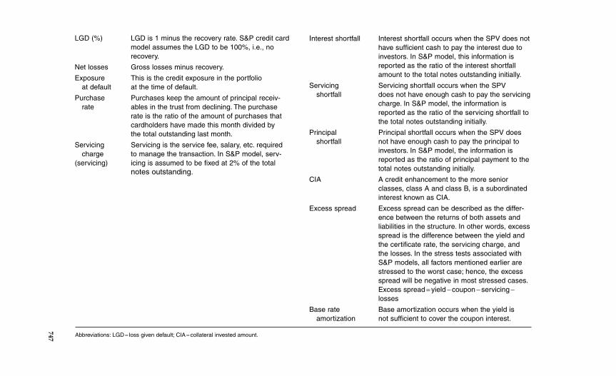
LGD (%) LGD is 1 minus the recovery rate. S&P credit cardmodel assumes the LGD to be 100%, i.e., norecovery.
Net losses Gross losses minus recovery.
Exposure This is the credit exposure in the portfolio at default at the time of default.
Purchase Purchases keep the amount of principal receiv- rate ables in the trust from declining. The purchase
rate is the ratio of the amount of purchases thatcardholders have made this month divided bythe total outstanding last month.
Servicing Servicing is the service fee, salary, etc. required charge to manage the transaction. In S&P model, serv-
(servicing) icing is assumed to be fixed at 2% of the total notes outstanding.
Interest shortfall Interest shortfall occurs when the SPV does nothave sufficient cash to pay the interest due toinvestors. In S&P model, this information isreported as the ratio of the interest shortfallamount to the total notes outstanding initially.
Servicing Servicing shortfall occurs when the SPV shortfall does not have enough cash to pay the servicing
charge. In S&P model, the information isreported as the ratio of the servicing shortfall tothe total notes outstanding initially.
Principal Principal shortfall occurs when the SPV doesshortfall not have enough cash to pay the principal to
investors. In S&P model, the information isreported as the ratio of principal payment to thetotal notes outstanding initially.
CIA A credit enhancement to the more seniorclasses, class A and class B, is a subordinatedinterest known as CIA.
Excess spread Excess spread can be described as the differ-ence between the returns of both assets andliabilities in the structure. In other words, excessspread is the difference between the yield andthe certificate rate, the servicing charge, andthe losses. In the stress tests associated withS&P models, all factors mentioned earlier arestressed to the worst case; hence, the excessspread will be negative in most stressed cases.Excess spread = yield − coupon − servicing −losses
Base rate Base amortization occurs when the yield is amortization not sufficient to cover the coupon interest.
Abbreviations: LGD = loss given default; CIA = collateral invested amount.
747
A P P E N D I X B
Credit Card Model, the S&PMethodology
After assessing the seller and servicer’s (SPV) operations and analyzingthe performance of the issuer’s (Originator) receivables, S&P runs cashflow scenarios that stress five key performance variables:
♦ Payment rate♦ Purchase rate♦ Losses♦ Portfolio yield♦ Certificate rate
If the average three months portfolio yield is insufficient to cover the cer-tificate interest and servicing fees averaged for the same period, a baserate amortization will occur. Different issuers will have different rules forthe amortization; In this model, S&P assumes that as an issuer enters inthe amortization, it will pay out the principal and the interest to the moresenior tranche holder first. For some other transactions, it may be payingback the principal to all investors first and then the payment of interest asper the waterfall.
TRAPPING POINT
All credit card structures incorporate a series of amortization events that,if triggered, cause principal collections allocated to investors to be passedthrough immediately and before the maturity date. Amortization eventsinclude insolvency of the originator of the receivables, breaches of repre-sentations or warranties, a servicer default, failure to add receivables asrequired, and asset performance-related events. Additionally, amortiza-tion happens if the three-month average excess spread falls below zero.
In a typical credit card structure, credit enhancement for the Class Aand Class B are fully funded at closing. For example, the Class A certifi-cate relies on the credit enhancement provided by the subordination ofClass B and Class C notes. In constant, the enhancement for the Class Cnotes is dynamic. Generally, if excess spread falls below specified levels,excess finance charge collections are trapped in a spread account for theCIA’s benefit.
748 CHAPTER 16
Copyright © 2007 by The McGraw-Hill Companies. Click here for terms of use.
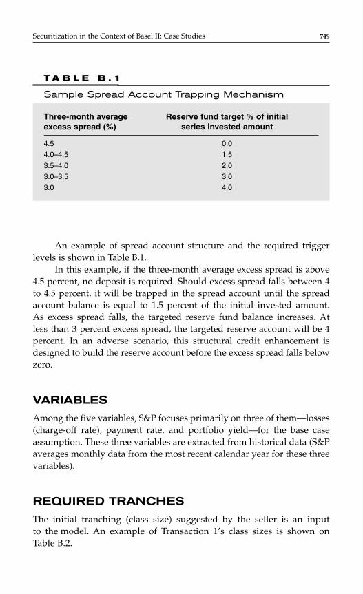
An example of spread account structure and the required triggerlevels is shown in Table B.1.
In this example, if the three-month average excess spread is above4.5 percent, no deposit is required. Should excess spread falls between 4to 4.5 percent, it will be trapped in the spread account until the spreadaccount balance is equal to 1.5 percent of the initial invested amount.As excess spread falls, the targeted reserve fund balance increases. Atless than 3 percent excess spread, the targeted reserve account will be 4percent. In an adverse scenario, this structural credit enhancement isdesigned to build the reserve account before the excess spread falls belowzero.
VARIABLES
Among the five variables, S&P focuses primarily on three of them—losses(charge-off rate), payment rate, and portfolio yield—for the base caseassumption. These three variables are extracted from historical data (S&Paverages monthly data from the most recent calendar year for these threevariables).
REQUIRED TRANCHES
The initial tranching (class size) suggested by the seller is an inputto the model. An example of Transaction 1’s class sizes is shown onTable B.2.
Securitization in the Context of Basel II: Case Studies 749
T A B L E B . 1
Sample Spread Account Trapping Mechanism
Three-month average Reserve fund target % of initial excess spread (%) series invested amount
4.5 0.0
4.0–4.5 1.5
3.5–4.0 2.0
3.0–3.5 3.0
3.0 4.0
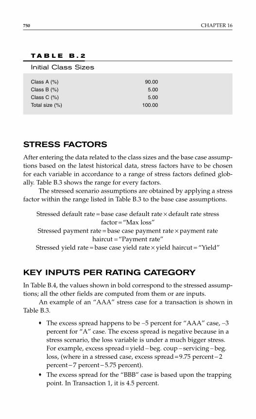
STRESS FACTORS
After entering the data related to the class sizes and the base case assump-tions based on the latest historical data, stress factors have to be chosenfor each variable in accordance to a range of stress factors defined glob-ally. Table B.3 shows the range for every factors.
The stressed scenario assumptions are obtained by applying a stressfactor within the range listed in Table B.3 to the base case assumptions.
Stressed default rate = base case default rate × default rate stress factor = “Max loss”
Stressed payment rate = base case payment rate × payment ratehaircut = “Payment rate”
Stressed yield rate = base case yield rate × yield haircut = “Yield”
KEY INPUTS PER RATING CATEGORY
In Table B.4, the values shown in bold correspond to the stressed assump-tions; all the other fields are computed from them or are inputs.
An example of an “AAA” stress case for a transaction is shown inTable B.3.
♦ The excess spread happens to be −5 percent for “AAA” case, −3percent for “A” case. The excess spread is negative because in astress scenario, the loss variable is under a much bigger stress.For example, excess spread = yield − beg. coup − servicing − beg.loss, (where in a stressed case, excess spread = 9.75 percent − 2percent − 7 percent − 5.75 percent).
♦ The excess spread for the “BBB” case is based upon the trappingpoint. In Transaction 1, it is 4.5 percent.
750 CHAPTER 16
T A B L E B . 2
Initial Class Sizes
Class A (%) 90.00
Class B (%) 5.00
Class C (%) 5.00
Total size (%) 100.00
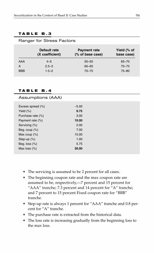
♦ The servicing is assumed to be 2 percent for all cases.♦ The beginning coupon rate and the max coupon rate are
assumed to be, respectively,—7 percent and 15 percent for“AAA” tranche; 7.3 percent and 14 percent for “A” tranche;and 7 percent to 15 percent Fixed coupon rate for “BBB”tranche.
♦ Step-up rate is always 1 percent for “AAA” tranche and 0.8 per-cent for “A” tranche.
♦ The purchase rate is extracted from the historical data.♦ The loss rate is increasing gradually from the beginning loss to
the max loss.
Securitization in the Context of Basel II: Case Studies 751
T A B L E B . 3
Ranger for Stress Factors
Default rate Payment rate Yield (% of (X coefficient) (% of base case) base case)
AAA 4–5 50–55 65–70
A 2.5–3 60–65 70–75
BBB 1.5–2 70–75 75–80
T A B L E B . 4
Assumptions (AAA)
Excess spread (%) −5.00
Yield (%) 9.75
Purchase rate (%) 3.00
Payment rate (%) 10.00
Servicing (%) 2.00
Beg. coup (%) 7.00
Max coup (%) 15.00
Step-up (%) 1.00
Beg. loss (%) 5.75
Max loss (%) 30.00
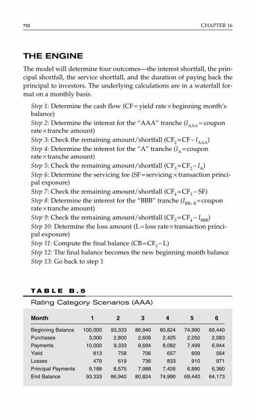
THE ENGINE
The model will determine four outcomes—the interest shortfall, the prin-cipal shortfall, the service shortfall, and the duration of paying back theprincipal to investors. The underlying calculations are in a waterfall for-mat on a monthly basis.
Step 1: Determine the cash flow (CF = yield rate × beginning month’sbalance)Step 2: Determine the interest for the “AAA” tranche (IAAA = couponrate × tranche amount)Step 3: Check the remaining amount/shortfall (CF2 = CF − IAAA)Step 4: Determine the interest for the “A” tranche (IA = couponrate × tranche amount)Step 5: Check the remaining amount/shortfall (CF3 = CF2 − IA)Step 6: Determine the servicing fee (SF = servicing × transaction princi-pal exposure)Step 7: Check the remaining amount/shortfall (CF4 = CF3 − SF)Step 8: Determine the interest for the “BBB” tranche (IBB> B = couponrate × tranche amount)Step 9: Check the remaining amount/shortfall (CF5 = CF4 − IBBB)Step 10: Determine the loss amount (L = loss rate × transaction princi-pal exposure)Step 11: Compute the final balance (CB = CF5 − L)Step 12: The final balance becomes the new beginning month balanceStep 13: Go back to step 1
752 CHAPTER 16
T A B L E B . 5
Rating Category Scenarios (AAA)
Month 1 2 3 4 5 6
Beginning Balance 100,000 93,333 86,940 80,824 74,990 69,440
Purchases 3,000 2,800 2,608 2,425 2,250 2,083
Payments 10,000 9,333 8,694 8,082 7,499 6,944
Yield 813 758 706 657 609 564
Losses 479 619 736 833 910 971
Principal Payments 9,188 8,575 7,988 7,426 6,890 6,380
End Balance 93,333 86,940 80,824 74,990 69,440 64,173
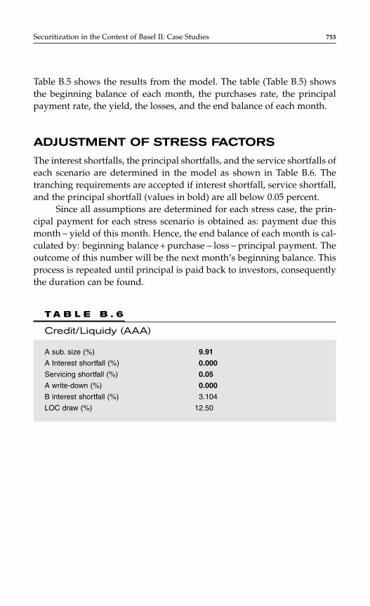
Table B.5 shows the results from the model. The table (Table B.5) showsthe beginning balance of each month, the purchases rate, the principalpayment rate, the yield, the losses, and the end balance of each month.
ADJUSTMENT OF STRESS FACTORS
The interest shortfalls, the principal shortfalls, and the service shortfalls ofeach scenario are determined in the model as shown in Table B.6. Thetranching requirements are accepted if interest shortfall, service shortfall,and the principal shortfall (values in bold) are all below 0.05 percent.
Since all assumptions are determined for each stress case, the prin-cipal payment for each stress scenario is obtained as: payment due thismonth − yield of this month. Hence, the end balance of each month is cal-culated by: beginning balance + purchase − loss − principal payment. Theoutcome of this number will be the next month’s beginning balance. Thisprocess is repeated until principal is paid back to investors, consequentlythe duration can be found.
Securitization in the Context of Basel II: Case Studies 753
T A B L E B . 6
Credit/Liquidy (AAA)
A sub. size (%) 9.91
A Interest shortfall (%) 0.000
Servicing shortfall (%) 0.05
A write-down (%) 0.000
B interest shortfall (%) 3.104
LOC draw (%) 12.50
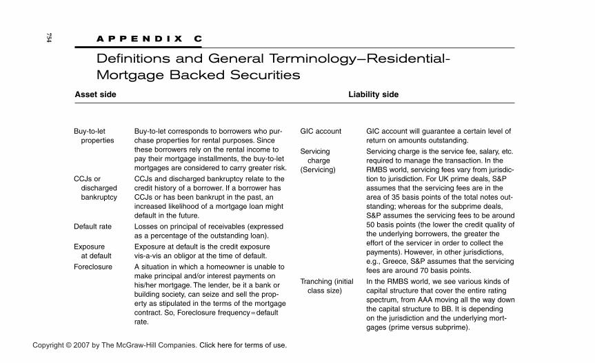
754
Buy-to-let Buy-to-let corresponds to borrowers who pur-properties chase properties for rental purposes. Since
these borrowers rely on the rental income topay their mortgage installments, the buy-to-letmortgages are considered to carry greater risk.
CCJs or CCJs and discharged bankruptcy relate to thedischarged credit history of a borrower. If a borrower hasbankruptcy CCJs or has been bankrupt in the past, an
increased likelihood of a mortgage loan might default in the future.
Default rate Losses on principal of receivables (expressedas a percentage of the outstanding loan).
Exposure Exposure at default is the credit exposure at default vis-a-vis an obligor at the time of default.
Foreclosure A situation in which a homeowner is unable tomake principal and/or interest payments onhis/her mortgage. The lender, be it a bank orbuilding society, can seize and sell the prop-erty as stipulated in the terms of the mortgagecontract. So, Foreclosure frequency = defaultrate.
GIC account GIC account will guarantee a certain level ofreturn on amounts outstanding.
Servicing Servicing charge is the service fee, salary, etc.charge required to manage the transaction. In the
(Servicing) RMBS world, servicing fees vary from jurisdic-tion to jurisdiction. For UK prime deals, S&Passumes that the servicing fees are in thearea of 35 basis points of the total notes out-standing; whereas for the subprime deals,S&P assumes the servicing fees to be around50 basis points (the lower the credit quality ofthe underlying borrowers, the greater theeffort of the servicer in order to collect thepayments). However, in other jurisdictions,e.g., Greece, S&P assumes that the servicingfees are around 70 basis points.
Tranching (initial In the RMBS world, we see various kinds of class size) capital structure that cover the entire rating
spectrum, from AAA moving all the way downthe capital structure to BB. It is depending on the jurisdiction and the underlying mort-gages (prime versus subprime).
Asset side Liability side
A P P E N D I X C
Definitions and General Terminology—Residential-Mortgage Backed Securities
Copyright © 2007 by The McGraw-Hill Companies. Click here for terms of use.
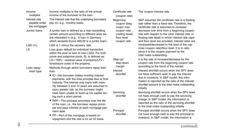
755
Income Income multiples is the ratio of the annualmultiples income of the borrower to the loan.
Interest rate The interest rate that the underlying borrowerspayable under pay on, e.g., monthly basis.the mortgages
Jumbo loans A jumbo loan is defined as a loan exceedingcertain amount according to different area weare interested in (e.g., A loan in Germanywhich exceeds Euros 400,00 is a jumbo loan).
LGD (%) LGD is 1 minus the recovery rate.
LS Loss given default for individual transactionwithin the pool (a loan to loan LGD). For bothprime and subprime pools, SL is defined as:LS = 100% − residual value of property/LTV +foreclosure costs of the property.
Loan repay- Methods through which borrowers repay theirment type loan.
♦ IO—the borrower makes monthly interestpayments, with the total principal due at finalmaturity. The interest only loans with matu-rity between 5 and 10 years are assumed tocarry greater risk, as the borrower mighthave been unable to build up his capital dur-ing such a short period.
♦ REP—The principal amortizes over the lifeof the loan; i.e., the borrower repays princi-pal and pays interest at each mortgage pay-ment date.
♦ PP—Part of the mortgage is based onrepayment and the rest is on an IO basis.
Certificate rate The coupon interest rate.
(coupon rate)
Beginning S&P assumes the certificate rate is a floatingcoupon (beg. rate rather than a fixed rate. Therefore, the coup)/ max certificate rate is assumed to increase/coupon rate decrease over time from a beginning coupon (ceiling level)/ rate with respect to the Libor interest rate. In floor level floating-rate deals in which interest rate caps coupon rate and floor level are provided, interest rates are
increased/decreased to the level of the cap (max coupon rate)/floor level. It is in ratio since it is the coupon payment to the total notes outstanding.
Step-up/ It is the rate of increase/decrease for the step-down coupon rate from the beginning coupon ratemargin according to the trend of the market.
Interest Interest shortfall occurs when the SPV does shortfall not have sufficient cash to pay the interest
due to investors. In S&P model, this infor-mation is reported as the ratio of the interest shortfall amount to the total notes outstandinginitially.
Servicing Servicing shortfall occurs when the SPV doesshortfall not have enough cash to pay the servicing
charge. In S&P model, the information isreported as the ratio of the servicing shortfallto the total notes outstanding initially.
Principal Principal shortfall occurs when the SPV does shortfall not have enough cash to pay the principal to
investors. In S&P model, the information is
(continued)
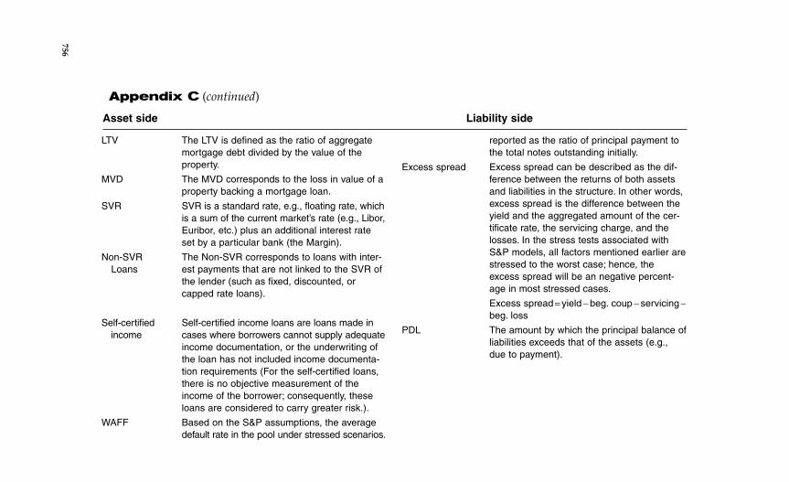
756
LTV The LTV is defined as the ratio of aggregatemortgage debt divided by the value of theproperty.
MVD The MVD corresponds to the loss in value of aproperty backing a mortgage loan.
SVR SVR is a standard rate, e.g., floating rate, whichis a sum of the current market’s rate (e.g., Libor,Euribor, etc.) plus an additional interest rateset by a particular bank (the Margin).
Non-SVR The Non-SVR corresponds to loans with inter-Loans est payments that are not linked to the SVR of
the lender (such as fixed, discounted, or capped rate loans).
Self-certified Self-certified income loans are loans made in income cases where borrowers cannot supply adequate
income documentation, or the underwriting of the loan has not included income documenta-tion requirements (For the self-certified loans, there is no objective measurement of the income of the borrower; consequently, these loans are considered to carry greater risk.).
WAFF Based on the S&P assumptions, the average default rate in the pool under stressed scenarios.
reported as the ratio of principal payment tothe total notes outstanding initially.
Excess spread Excess spread can be described as the dif-ference between the returns of both assetsand liabilities in the structure. In other words,excess spread is the difference between theyield and the aggregated amount of the cer-tificate rate, the servicing charge, and the losses. In the stress tests associated withS&P models, all factors mentioned earlier arestressed to the worst case; hence, theexcess spread will be an negative percent-age in most stressed cases.
Excess spread = yield − beg. coup − servicing −beg. loss
PDL The amount by which the principal balance ofliabilities exceeds that of the assets (e.g.,due to payment).
Asset side Liability side
Appendix C (continued)

757
Timing of The WAFF at each rating level specifies the defaults total balance of the mortgage loans assumed
to default over the life of the transaction. S&P assumes that these defaults occur over a three-year recession. S&P analyzes the impact of the timing of this recession on the ability to repay the liabilities, and defines the recession starting period specific to each rating level.Although the recession normally starts the first month of the transaction, the “AAA” recession is usually delayed by 12 months. The WAFF is applied to the principal balance outstanding at the start of the recession (e.g., in a “AAA”scenario the WAFF is applied to the balance atthe beginning of month 13).
WALS The loss severity in the entire pool understressed scenarios. WALS is 1 minus the recov-ery rate. Calculations are based on S&Passumptions.
Abbreviations: CCIs = county court judgment; LGD = loss given default; LS = loss severity; LTV = Loan-to-value ratio; IO = interest only; REP = repayment; PP = part by part; MVD = market valuedecline; SVR = standard variable rate; WAFF = weighted-average foreclosure frequency; WALS = weighted-average loss severity; GIC = Guaranteed investment contract; PDL = principalbalance of deficiency ledger.

This page intentionally left blank

B I O G R A P H I E S
759
Arnaud de Servigny is a Managing Director at Barclays Wealth. He isresponsible for Quantitative Analytics. Up until August 2006 he was aManaging Director at Standard & Poor’s. He was responsible forQuantitative Analytics in Credit Market Services. One of his dominantareas of focus was Structured Finance Quantitative Analytics. His initialposition within Standard & Poor’s was as the European head of quantita-tive analytics and products within S&P Risk Solutions. Prior to joiningStandard and Poor’s, Arnaud worked in the Group Risk ManagementDepartment of BNP-Paribas in France. He is a Visiting Professor ofFinance at Imperial College, London. He holds a Ph.D. in FinancialEconomics from the Sorbonne University, an MSc in Finance from a pro-gram associating Dauphine University and HEC Business School, and aCivil Engineering MSc from Ecole Nationale des Ponts & Chaussees.
Publications include many papers and articles as well as three books
♦ The Standard & Poor’s Guide to Measuring and Managing CreditRisk, McGraw Hill 2004, with Olivier Renault.
♦ Le Risque de Credit, Dunod Editions 2001—2003—2006, with IvanZelenko and Benoit Metayer.
♦ Economie Financiere, Dunod Editions 1999, with Ivan Zelenko.
Norbert Jobst joined DBRS in May 2006 as a SVP, Quantitative Analytics.Prior to that, and at the time of writing this book, he was a Director at
Copyright © 2007 by The McGraw-Hill Companies. Click here for terms of use.

Standard & Poor’s Structured Finance Ratings Division and Head ofMultivariate Quantitative Research within Standard & Poor’s Credit MarketServices. He has lead a team of quantitative analysts, focusing on modeldevelopment for synthetic CDOs, covering also research into portfolio(credit) risk analytics.
He holds a degree in Mathematics from Regensburg (FH), Germany,and a Ph.D. in Mathematical Sciences from Brunel University, U.K. Heconducted research into credit risk modeling and optimization underuncertainty, which was funded by Fidelity Investments.
Alexander Batchvarov, Ph.D., CFA, is a Managing Director at MerrillLynch in London. He has been Head of Merrill Lynch’s InternationalStructured Product Research group since 1998 when he relocated fromNew York to London. He and his team cover a range of structured prod-ucts originated in Europe and Asia categorized in four main categories:RMBS, consumer ABS, CMBS, and cash and synthetic CDOs.
Prior to Merrill Lynch, he worked at Moody’s Investors Service andat Citibank, both in New York City, and has covered the securitization andstructured finance markets in the United States, Latin America, Europe,and Asia. He and his team have been consistently ranked in the top threepositions in investors’ surveys carried out by Institutional Investors,EuroMoney, ISR in Europe, etc.
He has published extensively on numerous topics in structuredfinance. He co-authored and edited the Merrill Lynch Guide to InternationalMortgage Markets and MBS—the first extensive comparative study of themortgage markets in 12 European and Asian countries. He is the editor ofthe first publication on Hybrid Products by Risk Books. He has also con-tributed chapters to different books; among others, the different editionsof the Fabozzi’s The Handbook of Mortgage-Backed Securities and theHandbook of European Structured Financial Products.
He holds a Ph.D. in Economics from the Bulgarian Academy ofSciences and an MBA in Finance from the University of Alberta in Canada.
Sven Sandow has recently moved to a tier 1 international bank. Up untilrecently he headed the univariate quantitative research group withinStandard & Poor’s Credit Market services. His responsibilities includeddeveloping methods for modeling credit risk, as well as developing spe-cific models for various asset classes. He taught graduate level courses atNew York University’s Courant Institute of Mathematical Sciences and atPolytechnic University. He is a Fellow in Courant’s Mathematics in FinanceProgram. Prior to joining Standard & Poor’s in 2002, he held positions
760 Biographies

with Lord, Abbett & Co. and with TechHackers/Citibank, where heworked as a quantitative analyst. He worked as a researcher in statisticalphysics at Virginia Polytechnic University and the Weizmann Institute ofScience.
He received a Ph.D. in Physics and a M.Sc. in Physics from Martin-Luther Universität Halle-Wittenberg. He has published articles in physics,finance, statistics, and machine learning journals.
Philippe Henrotte is a Professor of Finance at HEC, a French businessschool, and Head of Financial Theory, at ITO 33, a software companyactive in quantitative finance.
He has earned his Ph.D. from Stanford University, and he graduatedfrom Ecole Polytechnique de Paris before that.
Astrid Van Landschoot is an Associate Director in the Structured FinanceQuantitative Group at Standard & Poor’s. She works in the analyticsteam, where she focuses primarily on quantitative credit risk modelingfor structured finance products, mainly CDOs. Prior to joining Standard& Poor’s in 2005, she worked in the Financial Stability Group (Researchand Analysis) of the National Bank of Belgium, where she also conductedresearch on credit risk modeling.
She holds a MSc in Economics and a Ph.D. in Finance from GhentUniversity, Belgium.
Vivek Kapoor recently joined UBS as an Executive Director. He is respon-sible for analyzing the risk-reward profile for structured credit tradingwithin UBS’s new alternative investment management business, DillonRead Capital Management. Prior to that, he was the risk-manager forCDO trading at Credit-Suisse, where he was responsible for analyzingand communicating the risk-return profile of individual trades and forthe CDO trading in aggregate and for developing a risk-assessment strat-egy to assess risk-capital on CDO trading. Prior to Credit-Suisse, Vivekworked for S&P, where he developed approaches for rating market andcredit risk sensitive structured products.
He holds a Ph.D. from MIT in the area of stochastic modeling ofgeophysical flows and dispersion.
Andrea Petrelli is a Vice President at Credit Suisse. He initially joined theHigh Energy Physics Division at Argonne National Laboratory, Argonne,Illinois, U.S.A., mainly working on heavy quarks interaction. In 2002, hemoved to Banca Intesa, Milan, Italy, where his work was mainly devoted
Biographies 761

to credit derivatives modeling. In 2004, he joined Credit Suisse in London,where he is responsible for CDO Trading Risk Management in Europe.His main interest is credit derivatives modeling, valuation and risk, andcorrelation trading.
He graduated at Pisa University, where he also obtained his Ph.D. inTheoretical Physics, developing his thesis on perturbative QCD at CERNTH Division.
Jun Zhang is the head of CDO Risk Management (U.S.) and Vice Presidentat Credit-Suisse. His main responsibility is to monitor the risks for bothsynthetic and cash CDO, such as spread, default, and correlation risks.Before joining Credit-Suisse, he was a Credit Risk Quantitative Analyst atToyko Mitsuibish Financial Group, where his main responsibility wasportfolio analysis of credit derivatives products. He has been a speaker attrading and risk management conferences.
He has BS in Engineering from ShangHai Jiao Tong University inChina, a MS in Mathematics in Finance from New York University, and aPh.D. in Engineering from the Johns Hopkins University.
Varqa Khadem is a Director working in the European Structured FinanceResearch Group at Lehman Brothers, covering ABS, CMBS, RMBS, andother esoteric securitised products. His focus has been on research andmodeling of prepayments, and defaults and losses in European residen-tial mortgages and RMBS. Prior to this, he worked at Standard and Poor’sRisk Solutions as a Quantitative Analyst working on the credit risk analy-sis of middle market/SME sectors in the United Kingdom, Germany,France, Italy, and Spain. He started his career in 2001 in the portfolio man-agement and group risk functions at Abbey National Treasury Services(now Abbey Financial Markets, part of Banco Santander) working princi-pally on economic capital and capital allocation across both the wholesalebank and the residential mortgage bank.
He holds a Ph.D. in Finance from Oxford University on the pricingof defaultable corporate and convertible bonds incorporating the effectsof strategic game theoretic behaviour. His undergraduate and mastersstudies were in Physics (Imperial College, University of London).
Francis Parisi is a Managing Director in the Quantitative Analytics groupat Standard & Poor’s. He joined Standard & Poor’s in 1985 as a rating offi-cer in the residential mortgage group. Since then, Frank has held variouspositions in structured finance, including training director, manager of the
762 Biographies

surveillance group, member of the research and criteria group, and ana-lytical manager in the residential mortgage group. Prior to joiningStandard & Poor’s, he worked at Chemical Bank in New York with respon-sibility for mortgage warehouse lending, secondary mortgage marketing,and issuing and servicing mortgage-backed securities.
He earned his BA in Philosophy, his MS in Statistics, and his Ph.D. inManagement of Engineering and Technology. His research interestsinclude extreme value theory, time series analysis, applied probability, andMarkov decision processes, with applications in finance and climatology.
Olivier Renault recently moved to CDO structuring within Citigroup. Heuse to be the Head of European Structured Credit Strategy for Citigroup,based in London. He is a regular speaker at professional and academicconferences and is the author of a book and many published articles oncredit risk. Prior to joining Citigroup, Olivier was responsible for portfoliomodeling projects at Standard & Poor’s Risk Solutions and was a lecturerin finance at the London School of Economics, where he taught derivativesand risk. He was also a consultant for several fund management andfinancial services companies.
He holds a Ph.D. in financial economics from the University ofLouvain (Belgium) and MSc from Warwick University (U.K.).
Cristina Polizu is a Director in the Quantitative Analytics group in S&P.Her responsibilities include model, structure, and criteria development forstructured finance primarily but also for corporate, financial institutionsand insurance departments within S&P. She runs the lead efforts for ratingquasi-operating companies and alternative assets in S&P.
She develops models that cover the financial risks of bankruptcyremote companies as well and of structured transactions that include eso-teric assets. Her focus of interest is portfolio credit and market risk mod-eling. Her research is geared to finding new modeling tools and new areasin which S&P can expand business. She joined S&P in 1995.
She holds a Ph.D. in Mathematics from Courant Institute ofMathematical Sciences. Her research focus was probability theory. Prior tothat, she was an assistant professor in mathematics in Romania.
Aymeric Chauve is a CDO structurer at SG CIB. Prior to this, he wasworking with Standard and Poor’s as an analyst in structured finance(CDO, RMBS, and Covered bonds). His activity included discussions onstructuring with arranging banks, publications, client meetings, etc.
Biographies 763

He holds an Engineering degree from Ecole centrale Paris, and apostgraduate degree in finance from Universite Paris Dauphine.
William Perraudin is Head of the Accounting, Finance and Macro-economics Department at Tanaka Business School and Director of the newMSc degrees in Risk Management and Financial Engineering.
His research interests include risk management, structured prod-ucts, the pricing of defaultable debt, portfolio credit risk modeling, andfinancial regulation.
For seven years, he worked part-time as Special Advisor to the Bankof England and was deeply involved in the financial engineering behindthe current Basel II proposals for bank capital. He has consulted withnumerous banks and public bodies.
He was formerly the Head of the Finance Group in Birkbeck College.He is an Associate Editor of Quantitative Finance, the Journal of Bankingand Finance and the Journal of Credit Risk.
764 Biographies

765
AAAA rating, meaning of, SIV and, 617–618ABS (asset backed securitizations) 7, 217
credit risks, 568–570covariates, 573–574default snap (CDS), 7modeling of, 570–576default correlations, 579–583prepayment risks, 568–570modeling of, 570–576quantitative analysis, European
methods, 565–583RMBS tranches and, 565–583tail risk scenario, 579–583transition and default probabilities
and, 406valuation, 576–579
Asset based liquidity, structured financemarkets criteria and, 19–20
Accounting practices, structured financemarkets and, 26–27
Amortization, Basel II credit card lines and,709–714
Amortizing assets, 453Arbitrage
cash, 9–11defaults, 11high grade (HG), 10high yield (HY), 10CDO implications and, 210–212
Archimedean copula, 162–163, 248Clayton, 162Frank, 162Gumbel, 162joint cumulative probability calculation,
163–166functional copula, 164–165Kendall’s tau, 166Marshall Olkin, 163Spearman’s rho, 166Arvanitis et al model, 104–105
Assetamortizing of, 453correlation 217–237
estimatescorporates and, 234structured finance tranches and, 233joint default probabilities (JPD)
approach, 230–231two-factor model, 231default rate, covered bonds and,
595–596forced sale of, 453implied correlationextraction, credit events and, 194–196default correlation and, 183–185mix, fixed and floating, 445–446pricing, fundamentals of, 132–133sidecash CDO pricing and, 280–286early repayments, 600–601spread simulation, 638–639
Asset-based liquidity, structured financemarkets criteria and, 19–20
Asset-based securities. See ABS.Asset-implied correlation calculation
JPD technique, 187–188MLE technique, 187–188
Attachment point, 412Average portfolio spread, model of LSS
spread triggers and, 510–513
BBalance sheet
CDO issuing and, 374–375synthetic CDO, 11
BanksBIS2 regulations impact on, 21–22capital calculationsBasel II and, 671–678ratings base approach (RBA),
672–673standardized approach, 671–672supervisory formula
approach (SFA), 673–675investment, 22–24
Barriers, equity default swaps and, 492–494
INDEX
Copyright © 2007 by The McGraw-Hill Companies. Click here for terms of use.

Base correlation, 323calibration, synthetic CDO
pricing and, 268–270Basel II
bank capital calculations, 671–678credit card asset classamortization, 709–714capital risk charge formula, 690–700impact of, 689–720IRB, 690probability of default, 691rating based approach, 701securitization, 700effects of, 686–688objectives of, 668–671RBA financial engineering, 678–686regulatory treatment, covered
bonds and, 587–588RMBS asset class, case studies, 720–737rules implementation, 394–396securitizations and, 667–688case studies, 689–749SFA financial engineering, 678–686
Bayesian estimation approach, GLMM, 188–190
BespokeCDO tranches pricing, 279flexibility, synthetic CDO investor
motivation and, 382synthetic CDO, 12correlation trades and, 12single tranche type, 12
Beta distribution, simulation SIV and, 636–637
BIS2 regulations, impact ondemand-supply dynamics, 24–26investment banks, 22–24originating banks, 21–22structured finance markets, 18–26
Bonds, covered, 585–612Break even portfolio
covered bonds and, 605–606overcollateralization, 605–606
Brute force, MC simulation and, 335–337Buffer, seller’s interest, 708
CCalibration, advanced, reduced form
models and, 107–108Canonical maximum likelihood. See condi-
tional maximum likelihood.
CAP. See Gini curve.Capital
adequacy, SIV and, 624–626asset pricing model (CAPM), 110–113notesMonte Carlo approach, 662–665non Monte Carlo approach, 664–665SIV and, 661–662requirementsinsurance companies, 27pension funds, 27structured finance markets and, 26–27risk charge formula, 690–700structure, delta sensitivity and, 306
CAPM. See capital asset pricing model.Cash
arbitrage, 9–11CDO, 373–396Investing in, 13pricing, 279–282asset side, 280–286risk-neutral transition matrices, 280–282liability side, 286–290tranches, 288waterfall structure, 286–289synthetic CDO, comparison of, 380–381
Cash flowallocation, RMBS senior/subordinate
structures and, 546–547analysisEuropean RMBS tranches and, 559–565RMBS and, 548–551S&P CDO evaluator version
3 and, 431–432CDO, 241–242methodology, S&P CDO evaluator
version 3 and, 430–463amortizing assets, 453cash flow analysis, 431–432corporate mezzanine loans, 452coupon on assets, 450coverage tests, 456–463default, 433–442analysis, 431assets, forced sale of, 453recovery modeling, 459–463equity, 455foreign currency risk, 448–450interest rate stresses, 444–446interest income, 450long dated corporate assets, 451–452
766 INDEX

pay in kind assets, 451payment timing mismatch, 451portfolio considerations, 447–453prepayment sensitivities, 447–448ratings, definition of, 433recoveries, 442–444senior collateral manager fees, 455standard default patterns, 434–436static transactions, 454–455
CDO (collateralized debt obligations)cash and synthetic, comparison
of, 380–381categories of, 9–16arbitrage cash, 9–11CDPC, comparison of, 653–654evaluator version 3, S&P methodologies
and, 397–429forward starting, 474–476implicationsarbitrage, 210–212empirical correlation, 206–212rated transaction tranching, cycle
impact on, 208–210tranches, 206–208investment, Basel II rules
implementation, 394–396investormotivations, 376–379diversification, 378rating constraints, 376–379tailored risk return profiles, 379types, 13–14cash investing, 13hedge funds, 13–14leveraged, 13–14issuance, Basel II rules
implementation, 394–396methodologies, Standard and Poor’s
(S&P), 397–463motivations for, 373–376balance sheet optimization, 374–375spread/rating arbitrage, 375–376new issuanceEurope, 5United States, 4pricing, 239–291ratings assignment, 297–298risk management, 295–338CDO sensitivities analytical model,
331–333credit spread sensitivity, 333–335
Gaussian copula recursive scheme,329–331
hazard rate term structure, 328–329mark to market (MtM), 295MC simulation, 335–338portfolio loss distribution, 333sensitivity measures, 299–326trading P & L case study, 358–368tranchedefault probability, 297loss given default, 298losses, 297–298, 333pricing correlation risks, 369risk measurement, 297–298sensitivities, 335–338analytical model, 331–333SIVassets in, 615comparison of, 615–616liabilities in, 615–616liquidity in, 616squared transactions, 414–416synthetic, 11–13, 379–380developments in, 465–531MtM and, 302–305trading risk management, 339–372credit deltacorrelation sensitivity, 349–350credit spread sensitivity, 344–348default sensitivity, 350–358monitoring of, 342–358spread measures, 371strategies, 340–342CDO portfolios, 341–342elementary portfolio, 341tranches, empirical correlation and,
206–208types, 240–242cashflow, 241–242mezzanine tranche, 14synthetic, 240–241valuation, 335–338
CDO. See collateralized debt obligations.CDPC
CDO, comparison of, 653–654SIV, comparison of, 654–655
CDS (credit default swap)CDO hybrids, case study, 494–498index, delta hedging and, credit
sensitivity, 309–310long position, 418–419
INDEX 767
CDS (Continued)short position, 418–419single name, 301–302spreads, 65–80
CDX, 12CIR model calibration, 658–661Clayton copula, 162CMBS. See commercial mortgage backed
securitizations.Cohort
analysiscredit rating transition probabilities and,
37–41, 44default rates and, 37–41methods, structured finance tranches
and, 223–224Collateral
coverage tests, 456–463breach of, 456current pay, 458debt obligations (CDO), 2, 217low rated, 457overcollateralization test, 456–458RMBS tranches and, 537–538senior manager fees, 455static transactions, 454–455
Commercial mortgage backed securitiza-tions (CMBS), 9
Commodity transactionspricing, 500–506drift, 501–504empirical results, 501–504model calibration, 501–504spot pricing, 505–506synthetic CDO and, 498–506individual prices, 500–506
Conditional maximum likelihood, 170–171Conditional survival probability
Archimedean copulas, 248functional copula, 249–250Gaussian copula, 246Marshall Olkin copula, 248normal inverse Gaussian (NIG) copulas,
247–248possible candidates for, 245–250student t copula, 246–247
Conforming mortgages, 535Constant drift
GARCH(1,1) and, 486–487lognormal model, 484–486
Constant proportional portfolio insurance(CPPI), credit, 517–527
Contingent leg value, 258–259Copula, 157–179
appropriate choice of, 166–177Archimedean, 248calibration of, 166–177classes of, 160–179elliptical, 161–163definition of, 157–159estimation, time series, 176–177functional, 164–165, 249–250Gaussian model, 246, 401extension of, 250–251Kendall’s tau, 166Marshall Olkin, 163, 247–248normal inverse Gaussian, 247–248properties of, 159–160recursive scheme, 329–331Sklar’s theorem, 157–159Spearman’s rho, 166statistical techniques, 166–177conditional maximum likelihood,
170–171empirical, 171–172full maximum likelihood, 168–169goodness of fit, 173–176inference functions for margins (IFM),
169–170visual comparison, 173–174student t, 246–247survival, 160
Corporateasset correlation estimates, 234mezzanine loans, 452structured finance tranches, comparison
of, 232–237Correlation
assumption matrices, 429deficiencies of, 146–147definitions, 142delta and, 307–308dependencyempirical results, 180–212measures and, 142–160diversification effect calculations,
143–146multiple assets, 145–146two asset case, 143–145empiricalasset implied, 180–196results, 180–212CDO implications, 206–212intensity based models, 196–206
768 INDEX

implied, 263–272joint default probability method (JDP),
410–411S&P CDO evaluator version 3 and,
409–411sensitivitydelta and, 349–350rho, 320–323base correlation, 323delta hedging, 323skew, synthetic CDO pricing and,
270–271smile, 264synthetic CDO pricing and, 283–286tradesbespoke synthetic CDO, 12standardized index tranches, 12–13synthetic CDO and, 12–13transition, simulation SIV and, 631–635
Cost of funds, SIV and, 623–624Counterparty, structured finance market
and, 17–18Coupon on assets, 450Covariates, ABS credit risks and, 573–574Coverage tests
breach of, 456collateral, 456–463value of defaulted securities, 458
Covered bonds, 585–612asset default rate, 595–596Basel II regulatory treatment, 587–588deterministic default rate patterns,
593–594foreign exchange rates, 597–607break even portfolio, 605–606communication of results, 604–605duration focus, 606–607early repayments, 600–601macroswaps, 601–604quantitative rating eligibility test, 597recovery treatment, 597–600servicing fees, 601glossary, 607interest rate’s impact on, 596–597marketconsiderations, 588–589momentum, 589maximum likelihood, 611method of moments, 611–612modeling risk of, 589–595foreign exchange rate simulation,
590–593
interest rate simulation, 590–593model calibration, 592–593quantitative rating component, 594–595Pfandbriefe-like, 586structural aspects, 586–589
Cox process, 94CP conduits, SIV
assets in, 616comparison of, 616–617liabilities in, 617liquidity in, 617
CPPI. See constant proportional portfolioinsurance.
Creditanalysis, rating of RMBS tranches and,
538–544foreclosure frequency, 539–542loss severity, 542–544Basel II and, amortization and, 709–714cardasset classBasel II impact on, 689–720Basel II IRB, 690Basel II RBA, 701–702Basel II securitization, 700probability of default, 691capital risk charge formula, 690–700LGD, discounted, 697–698non discounted, 694–697S&P rating model, 702–703seller’s interest buffer, 708supervisory formula approach, 703–708definitions used in, 738–739S&P model for, 740–745outcome, 744–745required tranches, 741stress factors, 742–743, 745trapping point, 740–741variables, 741tranches, S&P rating model of, 702–703constant proportional portfolio insurance
(CPPI), 517–527CPPI, 517–527case study of, 519–521defaults, 521gearing, 521–524interest rates sensitivity, 524leverage, 521–524modeling of, 526–527risks in, 524–527expected performance, 524–526spreads, 524
INDEX 769

Credit (Continued)structure of, 517–519curves, 401matrices, 420–424default snap, 7delta, risk in, 342–358derivative product companies. See CDPC.eventasset implied correlation extraction,
194–196risk vs delta risk, 369exposure, types, 16–17ratingapproach, credit risk assessment and,
31–45categories of, 31default rates, 36–45economic cycle transition matrices, 36–45factors to use in, 33industry default rates, 35investment grade, 31issue specific, 31issuer, 31Moody’s rating scales, 31–32noninvestment grade, 31outlook concept, 34PD, links between, 34, 36process of, 31–34S&P rating scales, 31–32scales, financial ratios, 33transition probabilitiescohort analysis and, 37–41, 44duration technique, 41, 43–45withdrawn, 41riskABS and, 568–570modeling of, 570–576assessment, 29–87probability of default (PD), 30rating and, 31–45factor modelscommercial availability of, 148–149dependency measures and, 148–153intensity based models, 196–206scoring, 45–55, 487spread convexitygamma, 311–313delta hedged tranches, 313realized correlation, 316–318macroconvexity, 313–315microconvexity, 315–316spread, 65–80
levels, delta and, 306–307sensitivity, 333–335delta and, 344–348
Credit01 sensitivity, delta hedging and,309–310
CreditGrades approach, 117Cross subordination, 416–418
squared transactions and, 473–474Cumulative default rates, 36–45Current pay collateral, 458Cycle-neutral sectors, 20Cyclical sectors
cycle-neutral sectors, 20structured finance markets criteria and,
20
DDas and Tufano model, 104Deal criteria, structured finance markets
and, 16–20Dealers, attraction to synthetic CDO,
385–386Default
analysis, S&P CDO evaluator version 3and, 431
arbitrage cash and, 11bias, 441–442cash flow methodology and, 433–442correlation, 410ABS and, 579–583asset implied correlation and, 183–185credit CPPI and, 521events, equity, 481–483factor model, dependency measures and,
153–157forced sale of assets, 453HJM/Market models, 98losses, European RMBS tranches and,
560–561only reduced form models, 95–98patternsadjustments to, 439–442low credit quality portfolios, 440short legal final maturity transactions,
440cash flow methodology and, 434–436default bias, 441–442expected case, 438saw tooth type, 436–437smoothing of, 438–439timing of, 434–435liability ratings effect on, 435–436
770 INDEX

types, 434probabilitiescredit card asset class and, 691duration technique and, 41, 43–45S&P CDO evaluator version 3 and,
403–408tranche risk measures and, 413–414rateasset, 595–596cohort analysis, 37–41cumulative 36–45PD, 39probability of, 40by industry, 35recovery modeling and, 459–463securities value, coverage tests and,
458sensitivitydelta and, 350–358iOmega, 350–352omega, 323–326, 352–353VOD risk per unit carry, 353–358spread process and, LSS spread triggers,
514–517time, 400
Deficiencies of correlations, 146–147Definitions
credit card terminology, 738–739RMBS and, 746–749
Delinquencies, European RMBS tranchesand, 562
Delta, 300–311correlation, 307–308creditcorrelation sensitivity, 349–350default sensitivity, 350–358monitoring of, 342–358spreadlevels, 306–307sensitivity and, 344–348function of time, 307hedged tranches, 313hedging, 305–309, 323capital structure, 306CDS index, 309–310credit01 sensitivity, 309 –310MtMsingle name CDS, 301–302synthetic CDO, 302–305neutral longequity tranche, 313–315senior tranche, 315
risk vs. credit event risk, 369single name/individual, 300–301upfront payments, 308–309
Demand and supply, BIS2 regulationsimpact on, 24–26
Density, nonparametric estimation and, 500Dependence
joint intensity modeling, 177–180modeling, evolution of, 180
Dependencycorrelation, empirical results, 180–212measures, 137–212copula, 157–179correlation, 142–160credit risk factor models, 148–153default factor model, 153–157Gaussian copula, 153–157rank correlations, 147–148sources of, 139–141survival factor model, 153–157
Derivative product companies (DPC), SIVand, 649–652
Deterministic default rate patterns, coveredbonds and, 593–594
Directional trades, 388–389Discounted LGD, 697–698, 727–728Distribution free distance minimization,
174–176Diversification
CDO investor motivations and, 378calculations, correlations and,
143–146multiple assets, 145–146two asset case, 143–145
Double leverage, synthetic CDO strategiesand, 389–390
DPC. See derivative product companies.Drift
commodity transaction pricing and,501–504
nonparametric estimation and, 500–501Duration
focus, covered bonds and, 606–607method, 404models, 201–206techniquecredit rating transition probabilities and,
41, 43–45default probabilities and, 41, 43–45
Dynamic barrier approach, 116–119CreditGrades, 117safety barrier, 117–119
INDEX 771
EEarly repayments
asset side, 600–601covered bonds and, 600–601
Economic cycle transition matrices, 36–45Markov chain, 37
EDF. See expected default frequency.EDS. See equity default swaps.Elementary portfolio, CDO trading risk
management and, 341Eligible accounts, RMBS legal issues and,
553–554Elliptical copula, 161–163
archimedean, 162–163Gaussian, 161t-copula, 161–162
Empiricalasset implied correlationsBayesian estimation approach, 188–190calculations of, 180–196joint default probability approach,
181–185correlationsequity correlations, 190–192implied asset correlation behaviour,
192–196maximum likelihood approach, 185–188copula, 171–172correlation, CDO tranches and, 206–208default correlations, joint default proba-
bility approach and, 183matrices, reduced form models and, 102results, correlation and, 180–212CDO implications, 206–212intensity based models, 196–206
Equitybased PD models, 63–64cash flow methodology and, 455correlations, as proxies, 190–192credit paradigm to, 120defaultevents, cohort results, 481–483swaps (EDS), 480–498barriers, 492–494CDO hybrids, case study, 494–498default events, 481–483definition of, 192implied asset correlation behavior,
extraction from 192–194multivariate aspects, 490–494MLE approach, 491price dynamics, modeling of, 483–484
price dynamicsempirical results, 489–490GARCH(1,1), modeling of, 486–487logit techniques, 487–488lognormal, modeling of, 484–486modeling of, 483–484statistical credit scoring, 487volatility, yield spread determinants
and, 70Europe
CDO new issuance and, 5structured finance market new issuances
and, 4European
ABS analysis, 565–583RMBS tranches, 554–565cashflow analysis, 559–565defaults and losses, 560–561delinquencies, 562expenses, 564interest rates, 562–563originator insolvency, 563–564prepayment rates, 562–563principle deficiencies, 564–565reinvestment rates, 563risk, 565portfolio credit analysis, 554–559LS calculations, 556–559
Exact maximum likelihood. See full maxi-mum likelihood.
Excess interest valuation, RMBS and,548–551
Expected case default patterns, 438Expected default frequency (EDF), 58Expenses, European RMBS tranches and,
564Exposure
pool type, 18single name, 18structured finance markets and, 18
FFee leg value, 259–260FF calculations
definition of, 555European RMBS tranches and, 555–556
Financialmarkets, structured, 1–27ratios, credit rating scales and, 33
First order spread sensitivity, delta, 300–311hedging, 309MtM
772 INDEX

single name CDS, 301–302synthetic CDO, 302–305single name/individual, 300–301
First passage time models, 115–116Fixed rate asset mix, 445–446Fixed recoveries, 408Floating rate asset mix, 445–446Foreclosure frequency, rating of RMBS
tranches and, 539–542Foreign currency risk, 448–450Foreign exchange rates, covered bonds and,
597–607break even portfolio, 605–606communication of results, 604–604duration focus, 606–607early repayments, 600–601macroswaps, 601–604servicing fees, 601treatment of recoveries, 597–600quantitative rating eligibility test, 597
Forward dynamics, SPA model and,273–275
Forward starting CDO, 474–476Fourier transform techniques, 255–256Frank copula, 162Full maximum likelihood, copula statistical
techniques and, 168–169Functional copula, 164–165, 249–250FX evolution, 641
GGamma, 311–313
delta hedged tranches, 313macroconvexity, 312microconvexity, 312realized correlation, 316–318
GARCH(1,1), constant drift, modeling of,486–487
Gaussian copula, 153–157, 161, 246extension of, 250–251randomfactor loadings, 250–251recovery, 251model, 401recursive scheme, 329–331
Gearing, credit CPPI and, 521–524Gini
coefficient, 529curve, 50–52coefficient definition, 86–87
GLMM, Bayesian estimation approach and,188–190
Global Cash Flow and Synthetic CDO Criteria,431, 443
Goodness of fitcopula statistical techniques and,
173–176distribution free distance minimization,
174–176Granularity, 16Gumbel copula, 162
HHair cut, low rated collateral and, 457Hazard rate
models, 93–94pricing, 93–94Cox process, 94inhomogeneous Poisson process, 94standard Poisson process, 93term structure, 328–329
Heath, Jarrow and Morton (HJM) frame-work, 98
Hedge funds, 13–14attraction to synthetic CDO, 384
Hedgingcapital structure, 306delta sensitivity and, 305–309risk management and, 298–300tranche positions, 324–326
Heath, Jarrow and Morton (HJM) frame-work, 98
HG. See high grade.High grade (HG) arbitrage cash, 10High yield (HY) arbitrage cash, 10HJM, Heath, Jarrow and Morton frame-
work, 98Homogeneity, synthetic CDO types and,
251–253HY. See high yield.
IIAA. See internal assessment approach.IFM. See inference function for margins.iGamma, 312Implied asset correlation behavior,
192–196credit events, asset implied correlation
extraction, 194–196duration models, 201–206EDS, extraction from, 192–194
Implied correlation, 263–272smile, 264
Independent intensity models, 196–198
INDEX 773

Index tranches liquidity, synthetic CDOinvestor motivation and, 382
Individual asset default behavior, 402Inference functions for margins (IFM),
169–170Inhomogeneous Poisson process, 94Insolvency, European RMBS tranches and,
563–564Insurance companies, capital requirements
and, 27Intensity based models of credit risk,
196–206Intensity based models. See hazard rate
models.Intensity models
independent 196–198physical measure, 198–201
Interestincome, cash flow methodology
and, 450mismatches, default bias and, 441–442ratecovered bonds and, 596–597credit CPPI and, 524European RMBS tranches and,
562–563sensitivity analysis, 445–446fixed rate asset mix, 445–446floating rate asset mix, 445–446liability indices, 446loan basis risk, 446simulation, covered bonds and,
590–593stressescash flow methodology and, 444–446sensitivity analysis, 445–446specifics of, 445
Internal assessment approach (IAA), 677Investment banks
BIS2 regulations impact on, 22–24grade credit rating, 31
iOmegadefault sensitivity and, 350–352tranche positions and, 324–326
IRB, credit card asset class and, 690Issue
specific credit rating, 31volumes, structured finance markets
and, 1–6United States, 3
Issuer credit rating, 31iTraxx, 12
JJarrow, Lando and Turnbull. See JLT.JLT (Jarrow, Lando and Turnbull), 98–99
model, 98–99extentions of, 104–105Arvanitis et al, 104–105Das and Tufano model, 104spreads, derived from, 101time homogeneous Markov chain,
102–104Joint cumulative probability calculation,
163–166functional copula, 164–165Kendall’s tau, 166Marshall Olkin copula, 163Spearman’s rho copula, 166
Joint default behavior, 402Joint default probability (JPD)
approach, 181–185, 230–231asset implied correlation, 183–185empirical default correlations, 183estimating of, 181–185method, 410–411default correlation, 410technique, 187–188
Joint intensity modeling, 177–180JPD. See joint default probability.Jump diffusion
processes, 106–107, 639–640MLE calibration, 107structural models, 119–120
Junior tranches, 17
KKendall’s Tau, 148
copula and, 166
LLambda, 311Latent variables, 401Legal issues, RMBS and, 551–554
eligible accounts, 553–554servicer accounts, 553–554special purpose entities, 552trustee accounts, 553–554
LeverageCDOs, 13–14credit CPPI and, 521–524cross subordination, 473–474double, 389–390positions, structured finance markets
and, 18
774 INDEX
SIV and, 624squared transactions and, 469–474super senior (LSS) transactions. See LSS.synthetic CDO strategies and, 386–387yield spreads determinants and, 70–71
LGD (loss given default)discounted, 697–698, 727–728lost severity (LS), 725non discounted, 694–697, 725–726RMBS asset class and 725–726tranche, 414
LGD, See loss given default.Liability
indices, 446ratings, default pattern timing and,
435–436side, cash CDO pricing and, 286–290
Likelihood ratio method, 337–338Liquidity
asset based, 19–20facilities, SIV and, 657–658risk, SIV test and, 645–646structure finance markets and, 14–16mark to market (MTM) accounting,
14–16yield spreads and, 74–76
Loan basis risk, 446Logit techniques, equity price dynamics
and, 487–488Log-likelihood ratio, 52–53Lognormal
constant drift, 484–486modeling of, 484–486
Long CDO tranche, 419Long CDS, 418–419Long dated corporate assets, 451–452Long/short structures, synthetic CDO and,
476–478Loss
allocation, RMBS senior/subordinatestructures and, 547
given default. See LGD.eg. See contingent leg value.protection, stepping down of, 547–548severity (LS), 725calculationsdefinition of, 555European RMBS tranches and,
556–559RMBS tranches rating and, 542–544
Low credit quality portfolios, default pat-terns and, 440
Low rated collateral, hair cut for, 457LS. See lost severity.LSS (leverage super senior)
spread triggersmodeling ofaverage portfolio spread, 510–513default and spread process, 514–517PD rating determination, 513S&P version, 510, 512–513transactions, 507–517basic structure, 507–509protection buyers, 508–509protection sellers, 508–509spread triggers, 509–510modeling of, 510–517
MMacroconvexity, 313–315
delta neutral longequity tranche, 313–315senior tranche, 315gamma and, 312
Macroswaps, covered bonds and, 601–604
Mark to market. See MtMMarket implied
ratings, spreads and, 78–80volatility approach, 113–115
Market risk, 298–300SIV tests and, 641–642
Markovchain, 37, 102–104timehomogeneous, 103–104, 282non homogeneous, 281–282process, 404
Marshall Olkin copula, 163, 248–249Matrix SIV, 627–641Maximum likelihood estimator.
See MLE.MBS. See mortgage backed securitizations.MC simulation
brute force, 335–337CDOsensitivities, 335–338valuation, 335–338likelihood ratio method, 337–338
Measuring risk, 296–298Merton
frameworkextensions of, 115–120first passage time models, 115–116
INDEX 775

Merton (Continued)incomplete information, 116model, 55–58, 108–110term structure, 64
Method of moments, 611–612Mezzanine
equity positions, 20loans, corporate, 452tranche types, 14
Microconvexity, 315–316iGamma, 312
MLE (maximum likelihood estimator)approach, 185–188asset-implied correlation calculation,
187–188equity default swaps and, 491calibration, 107covered bonds and, 611technique, 187–188
Modelingcalibration, commodity transaction pric-
ing and, 501–504SIV, 627–641structured finance markets criteria and,
19Monte Carlo approach
capital notes and, 662–665portfolio loss distribution and, 254
Moody’sKMV credit monitor, 58–63expected default frequency (EDF), 58rating scales, 31–32
Mortgageassets, treatment of recoveries and,
597–598backed securitizations (MBS), 16conforming, 535nonconforming, 535residential backed securities, 535–584
MtM (mark to market) 295, 506–526accounting, violatility of, 14–16riskcredit constant proportional portfolio
insurance (CPPI), 517–527leverage super senior (LSS) transactions,
507–517sensitivity measures, 299single name CDS, 301–302synthetic CDO, 302–305
Multiple assets, 145–146Multiple defaults, omega and, 324Multivariate aspects, MLE approach, 491
NNCO test, 646–648NIG. See normal inverse Gaussian
copulas.Non conforming mortgages, 535Non discounted LGD, 694–697, 725–726Non investment grade credit rating, 31Non parametric estimation
density, 500drift, 500–501parametric, 531volatility/diffusion, 530–531
Normal inverse Gaussian (NIG) copulas,247–248
nth to default baskets, 419–420
OOmega, 323–326
default sensitivity and, 352–353hedged tranche positions, 324–326iOmega, 324–326multiple defaults, 324unhedged tranche positions, 324–326
Originatorinsolvency, European RMBS tranches
and, 563–564structured finance market and, 17–18
Outlook concept, credit ratings and, 34Overcollateralization
break even portfolio and, 605–606reinvestment test, 457test, 456–458breach of coverage tests, 456
PParallel yield curve shift, SIV tests and,
642–644Parametric estimation, 531Pay in kind assets, 451Payments
timing mismatch, 451upfront, delta and, 308–309
PD (probability of default), 30credit rating, links between, 34, 36default rates, cumulative, 39modelingstatistical, 45–55term structures, 53–55types, 50–53Gini curve, 50–52log-likelihood ratio, 52–53per rating category, 42
776 INDEX

rating determination, LSS spread triggersand, 513
recovery model combination and, 83–84yield spread determinants and, 68–70
Pension funds, capital requirements and, 27Pfandbriefe-like covered bonds, 586Physical measure, intensity models and
198–201Point by point yield curve shift, SIV tests
and, 644Poisson
inhomogeneous process, 94process, standard, 93
Pool exposure, 18Portfolio
considerations, cash flow methodologyand, 447–453
credit analysis, European RMBS tranchesand, 554–559
FF calculations, 555–556LS calculations, 556–559criteria, structured finance markets and,
16–20diversification guidelines, SIV and,
618–619homogeneity, synthetic CDO types and,
251–253lossdistribution, 333conditional survival probability, possible
candidates for, 245–250Fourier transform techniques, 255–256Monte Carlo approach, 254proxy integration, 256–257recursive approach, 254synthetic CDO pricing and,
244–263modelingSchonbucher’s model, 277–278SPA model, 272–277synthetic CDO pricing and, 272–278probabilities, SPA model and, 273–275process, SPA model and, 275–276trading risk management, CDO and,
341–342Premium leg. See fee leg value.Prepayment
rates, European RMBS tranches and,562–563
risks, ABS and, 568–570risks, ABS and, modeling of, 570–576sensitivities, 447–448
Pricingcommodity transactions and, 500–506drift, 501–504empirical results, 501–504model calibration, 501–504Cox process, 94dynamics, equity, 483–484hazard rate models and, 93–94inhomogeneous Poisson,94spot, 505–506standard Poisson process, 93
Principle deficiencies, European RMBStranches and, 564–565
Probability of default. See PD.Proprietary desks, attraction to synthetic
CDO, 384Protection
buyers, LSS transactions and, 508–509sellers, LSS transactions and, 508–509
Protection leg. See contingent leg value.Proxy integration, 256–257Public sector assets, treatment of recoveries
and, 599
QQuantitative rating eligibility test, covered
bonds and, 597
RRandom
factor loadingsGaussian copula and, 250–251stochastic correlation 250recovery, Gaussian copula and, 251
Rank correlations, 147–148Kendall’s Tau, 148Spearman’s Rho, 148
Ratedcompanies, transition and default proba-
bilities, 403–406duration method, 404Markov process, 404transitionmatrix, 404method, 403–406patterns, deterministic default, 593–594transaction tranching, cycle impact on,
208–210Rating
approach, 31–45assignment, 468base approach. See RBA.
INDEX 777

Rating (Continued)based reduced form models, 98–105basic structure, 98–99models, JLT, 98–99key assumptions, 98–99component, covered bonds modeling
and, 594–595constraints, CDO investor motivation
and, 376–379definitions, cash flow methodology and,
433migration, 217–237probabilities of, 222–229structured finance (SF) tranches, 217RMBS tranches and, Europe and, 554–565techniques, RMBS tranches and, 537–554tranchedefault probability, 468loss, 468–469given default, 469
RBA (rating base approach)financial engineering, 678–686credit card asset class and, 701–702
Real money investors, attraction tosynthetic CDO, 384–385
Realized correlation, gamma and, 316–318Recovery
analysis, simulation SIV and, 635–636assumption matrices, 425–428fixed, 408given default (RGD), 80–83market value. See RMV.modeling, 459–463PD model combination and, 83–84rates, 442–443yield spread determinants and, 68risk, 80–83loss given default (LGD), 80recovery given default (RGD), 80S&P CDO evaluator version 3 and,
408–409timingcash flow methodology and, 442–444recovery rates, 442–443specifics of, 444variable, 408–409
Recursive approach, portfolio loss distribution and, 254
Reduced form modelscalibration, advanced, 107–108default only, 95defaultable HJM/Market, 98
effectiveness of, 126–127empirical matrices, 102hazard rate, 93–94other types, 100–101rating based, 98–105risk neutral transition matrices, 102spread processes calibration, 105–107structural, 108–132univariate pricing and, 92–108zero-coupon bonds, 99–100
Regime switching models, effectiveness of,127–132
Reinvestmentrates, European RMBS tranches and, 563test, overcollateralization and, 457
Repayment, early, 600–601Repo companies, SIV and, 655–657Residential mortgage backed securities. See
RMBS.RGD. See recovery given default.Rho
base correlation, 323correlation sensitivity and, 320–323delta hedging, 323
RiskABScredit and, 568–570modeling of, 570–576prepayment and, 568–570modeling of, 570–576aggregation, 369–370analysisCDS, 418–419cross subordination, 416–418nth to default baskets, 419–420rated overcollateralization, 412S&P CDO evaluator version 3 and,
411–420scenario loss rate, 411–412synthetic CDO squared transactions,
414–416trancheslong position, 419risk measures, 412–414short position, 419assessment, univariate, 29–87covered bonds and, 589–595modeling calibration, 592–593credit CPPI, 524–527expected performance, 524–526European RMBS tranches and, 565loan basis, 446
778 INDEX

managementaggregation, 369–370CDO, 295–338measurement, 297–298correlation sensitivity, rho, 320–323credit event vs delta, 369default sensitivity, omega, 323–326hedging, 298–300market risk, 298–300measurement of, 296–298sensitivity measures, 298–300measurementcredit spread convexity, gamma, 311–313synthetic CDO and, 468–469time delay, theta, 318–320tranche leverage, lambda, 311modeling, covered bonds and, interest
rate simulation, 590–593neutralmeasure, fundamentals of, 132–133probabilities, spreads, structural reduced
form models and, 110–114transition matricesreduced form models and, 102timehomogeneous Markov chain, 282nonhomogeneous Markov chain, 281–282premium, 72yield spreads and, systemic factors,
72–74return profiles, CDO investor motiva-
tions and, 379RMBS (residential mortgage backed securi-
ties), 217, 535–584asset classBasel II and, case studies, 720–737LGD, 725–726securitization, 728–730supervisory formula approach, 730–737cash flow analysis, 548–551definitions used in, 746–749excess interest valuation, 548–551legal issues, 551–554eligible accounts, 553–554servicer accounts, 553–554special purpose entities, 552trustee accounts, 553–554residential mortgage backed securities,
535–584senior/subordinate structures, 545–546cash flow allocation, 546–547loss allocation, 547
stepping down of loss protection,547–548
structural considerations, 545–548tranchesABS, 565–583default correlations, 579–583tail risk scenario, 579–583valuation, 576–579collateral, 537–538Europecashflow analysis, 559–565defaults and losses, 560–561delinquencies, 562expenses, 564interest rates, 562–563originator insolvency, 563–564prepayment rates, 562–563principle deficiencies, 564–565reinvestment rates, 563risk, 565portfolio credit analysis, 554–559FF calculations, 555–556LS calculations, 556–559rating of, 554–565legal, 537–538rating of, 537–554credit analysis, 538–544foreclosure frequency, 539–542loss severity, 542–544structural analysis, 537–538
RMV (recovery of market value), 95
SS&P (Standard & Poor’s)
CDO evaluator version 3, 397–429cash flow methodology, 430–463amortizing assets, 453cash flow analysis, 431–432corporate mezzanine loans, 452coupon on assets, 450coverage tests, 456–463default 433–442analysis, 431assets, forced sale of, 453recovery modeling and, 459–463definition of ratings, 433equity, 455foreign currency risk, 448–450interestincome, 450rate stresses, 444–446long dated corporate assets, 451–452
INDEX 779

S&P (Standard & Poor’s) (Continued)pay in kind assets, 451payment timing mismatch, 451portfolio considerations, 447–453prepayment sensitivities, 447–448recoveries, 442–444senior collateral manager fees, 455standard default patterns, 434–436static transactions, 454–455correlation, 409–411assumption matrices, 429joint default probability method (JDP),
410–411credit curve matrices, 420–424key points of, 400–403credit curves, 401default time, 400Gaussian copula model, 401individual asset default behavior, 402joint default behavior, 402latent variables, 401univariate default, 400recoveries, 408–409fixed, 408variable, 408–409recovery assumption matrices,
425–428risk analysis, 411–420CDS, 418–419cross subordination, 416–418nth to default baskets, 419–420rated overcollateralization, 412scenario loss rate, 411–412squared transactions, 414–416trancheslong position, 419risk measures, 412–414short position, 419transition and default probabilities,
403–408rated companies, 403–406transition matrices, 420–424credit card modeloutcome, 744–745required tranches, 741stress factors, 742–743, 745trapping point, 740–741variables, 741methodologies, 397–463model of LSS spread triggers, 510,
512–513rating
model, credit card tranches, 702–703scales, 31–32
Safety barrier approach, 117–119Saw tooth default patterns, 436–437Scenario loss rate, 411–412
attachment point, 412Schonbucher’s model, 277–278Securitization, 700
Basel II, 667–688treatment of, case studies 689–749RMBS asset class and, 728–730
Seller’s interest buffer, 708Senior collateral manager fees, 455Senior mezzanine equity positions, 20Senior tranches, 17Senior/subordinate structures, RMBS and,
545–546cash flow allocation, 546–547loss allocation, 547stepping down of loss protection,
547–548Sensitivity
analysis, interest rate, 445–446measures, 299–326first order spread, 300–311risk management and, 298–300
Serviceraccounts, RMBS legal issues and, 553–554structured finance market and, 17–18
Servicing fees, covered bonds and, 601SF. See structured finance.SFA. See supervisory formula approach.Short
CDO tranche, 419CDS, 418–419legal final maturity transactions, default
patterns and, 440structure, synthetic CDO and,
476–478Simulation SIV, 630–637
beta distribution, 636–637correlated transition, 631–635recovery analysis, 635–636
Single nameCDS, 301–302exposure, 18individual, delta and, 300–301tranche CDO, 12
SIV (structured investment vehicles)AAA rating, meaning of, 617–618capitaladequacy, 624–626
780 INDEX

notes, 661–662CDOassets in, 615comparison of, 615–616liabilities in, 615–616liquidity in, 616CDPC, comparison of, 654–655CIR model calibration, 658–661cost of funds, 623–624CP conduitsassets in, 616comparison of, 616–617liabilities in, 617liquidity in, 617credit derivative product companies
(CDPC), 652–653definition of, 613–615derivative product companies (DPC),
649–652developments in, 648hedge funds, comparison of, 617investor range, 619–623leverage, 624liquidity facilities, 657–658managers of, 619–623matrix vs modeled, 627–641structured finance issuers, 637–641modeling approaches, 627matrix SIVs, 627–641portfolio diversification guidelines,
618–619repo companies, 655–657simulation, 630–637sponsorship of, 619–623structured investment vehicles, 613–665tests, 641–648liquidity risk, 645–646market risk, 641–642NCO, 646–648parallel yield curve shift, 642–644point by point yield curve shift, 644spot foreign exchange, 644–645
Sklar’s theorem, 157–159Small to mid sized enterprises. See SMEs.SMEs (small to mid sized enterprises),
406–407Smoothing default patterns, 438–439Sovereign securities, 406SPA model, 272–277
forward dynamics, 273–275portfolio lossprobabilities, 273–275
process, 275–276tranche valuation, 276–277
Spearman’s Rho, 148copula and, 166
Special purpose entities, RMBS legal issuesand, 552
Spotforeign exchanges, SIV tests and,
644–645pricing, commodity transactions and,
505–506Spread
measures, 371modeling, spread processes calibration
and, 105–106processes calibration, 105–107jump-diffusion processes, 106–107spread modeling, 105–106triggers, LSS transactions and, 509–510modeling of, 510–517
Spread/rating arbitrage, CDO issuing and,375–376
SpreadsCDS, 65–80, 76–78credit CPPI and, 524default information from, 78–80JLT model derivation of, 101market implied ratings, 78–80risk neutral probabilities and, 110–114yield, 65–76
Squared transactionsextending leverage, 469–474cross subordination, 473–474synthetic CDO, 414–416
Standard and Poor’s. See S&P.Standard Poisson process, 93Standardized index tranches, correlation
trades and, 12–13CDX, 12iTraxx, 12
Static transactions, collateral and, 454–455
Statistical PD modeling, 45–55equity based, 63–64Merton model, 55–58Moody’s KMV credit monitor, 58–63types and techniques, 45–50
Step up transactions, 478Stepping down of loss protection,
RMBS senior/subordinate structuresand, 547–548
Stochastic correlation, 250
INDEX 781

Stress factors, S&P credit card model and,742–743, 745
Structuralanalysis, RMBS tranches and, 537–538reduced form models, 108–132capital asset pricing model (CAPM),
110–113dynamic barrier approach, 116–119equity to credit, 120hybrid models, 120jump-diffusion, 119–120market implied volatility approach,
113–115Mertonframework, extensions of, 115–120model, 108–110risk neutral probabilities, spreads,
110–114Structured covered bonds, 586Structured finance (SF)
issuersasset spread simulation, 638FX evolution, 641jump diffusion process, 639–640SIV and, 637–641marketsBIS2 regulations, impact on, 20–26CDO, 2, 11new issuance, United States, 4commercial mortgage backed securitiza-
tions (CMBS), 9criteria forasset based liquidity, 19–20BIS2 impact, 18–19counterparty, 17–18country specific considerations, 19credit exposure type, 16–17cyclical sectors, 20exposures, 18granularity, 16junior tranches, 17leverage postions, 18modeling, 19originator involvement, 17–18seniormezzanine equity positions, 20tranches, 17servicer, 17–18tructured finance markets, criteria for,
third party involvement, 17–18deal and portfolio criteria, 16–20developments and trends in, 4–5
expectations of, 6–8asset backed securitizations (ABS), 7issue volumes, 1–6United States, 3liquidity of, 14–16mark to market (MTM) accounting,
14–16new issuances, Europe, 4overview of, 1–27regulatory changes to, 26–27accounting practices, 26–27capital requirements, 26–27shortcomings of, 8–9productsasset-backed securities (ABS), 217collateralized debt obligations (CDO),
217residential mortgage backed securities
(RMBS), 217tranches, 217asset correlation estimates, 233corporates, comparison of, 232–236data description, 219–221regional distribution, 220quantity by rating, 221rating migration, probabilities of,
222–229transition matrix, cohort methods,
223–224investment vehicles. See SIV.modelseffectiveness of, 120–126reduced form model, effectiveness
of, 126–127regime-switching, 127–132
Student t copula, 246–247Supervisory formula approach, (SFA),
673–675, 703–708financial engineering, 678–686RMBS asset class and, 730–737
Supply and demand, BIS2 regulationsimpact on, 24–26
Survival copula, 160Survival factor model, dependency mea-
sures and, 153–157Synthetic CDO, 11–13, 240–241, 373–396,
attractions of, 383–386dealers, 385–386hedge funds, 384proprietary desks, 384real money investors, 384–385balance sheet type, 11
782 INDEX

bespoke synthetic type, 12cash CDO, comparison of, 380–381commodity transactions, 498–506individual prices, 500–506correlation trades, 12–13crisis of, 391–394developments in, 398–399, 465–531drawbacks of, 383equity default swaps, 480general modeling of, 399–400Gini coefficient, 529hybridscase study, 494–498products, 479investor motivation, 382–383bespokes flexibility, 382index tranches liquidity, 382MtM and, 302–305risk, 506–526nonparametric estimation, 530–531pricing of, 242–279base correlation, calibration, 268–270bespoke tranches, 279cash, 279–282correlation, 283–286skew, 270–271implied correlation, 263–272,portfolio lossdistribution, 244–263modeling, 272–278unconditional portfolio loss distribution,
258–263contingent leg value, 258–259fee leg value, 259–260illustration of, 260–263underlying obligors, modeling of, 278ratings of, 467–460assignment, 468forward starting CDOs, 474–476long/short structures, 476–478tranchedefault probability, 468loss, 468–469given default, 469variable subordination, 478risk measures, 468–469squared transactions, 414–416, 469–474standardized tranches, 12strategies, 386–390directional trades, 388–389double leverage, 389–390relative value trades, 388
taking leverage, 386–387tranches as hedging vehicles, 390unidirectional trades, 388–389structured finance type, 11typesportfolio homogeneity, 251–253portfolio loss distribution, 254–257variants in, 467–478
Systemic factors, yield spreads and, 72–74
TTail risk scenario, 579–583Taxes, yield spreads and, 76t-copula, 161–162Term structures
Merton model and, 64PD modeling and, 53–55
Theta, 318–320Time
delay, theta, 318–320delta and, 307homogeneous Markov chain, 103–104,
282nonhomogeneous Markov chain,
102–103, 281–282series, copula estimation and, 176–177
Timingdefault patterns and, 434–435liability ratings effect on, 435–436
Tranche, 12bespoke CDO, 279cash CDO pricing and, 288CDO, 206–208efault probability, 468CDO risk management and, 297deltahedged, 313neutral longequity, 313–315senior, 315hedging vehicles, 390junior, 17leverage, lambda, 311loss 333, 468–469CDO risk management and, 297–298given default, 469CDO risk management and, 298risk measures and, 414positions, 419iOmega and, 324–326omega and, 324–326
INDEX 783

Tranche (Continued)pricing correlation risks, 369rated transaction, 208–210risk measures, 412–414default probability, 413–414expected tranche loss, 414loss given default, 414other types, 414RMBS, 537–554S&P credit card model and, 741senior, 17structured finance (SF), 217valuation, SPA model and,
276–277Transition
default probabilities andasset backed securities, 406equity default swaps, 407–408rated companies, 403–406duration method, 404Markov process, 404transitionmatrix, 404method, 403–406SMEs (small to mid sized enterprises),
406–407sovereign securities, 406matrices, 420–424matrix, 404structured finance tranches and, cohort
methods, 223–224method, 403–406probabilities, S&P CDO evaluator
version 3 and, 403–408Trapping point, 740–741Treatment of recoveries
covered bonds and, 597–600mortgage assets, 597–598public sector assets, 599
Trustee accounts, RMBS legal issues and,553–554
Two asset case, 143–145Two- factor model, asset correlation and,
231
UUnconditional portfolio loss distribution
contingent leg value, 258–259fee leg value, 259–260illustration of, 260–263synthetic CDO pricing and, 258–263
Underlying obligors, synthetic CDO pric-ing based on, 278
Unhedged tranche positions, omega and,324–326
Unidirectional trades, 388–389United States
CDO new issuance and, 4structured finance market issue volumes
in, 3Univariate
default, 400pricing, 91–133reduced form models, 92–108risk assessment, 29–87credit scoring, 45–55PD and recovery models, 83–84recovery risk, 80–83spreads, 65–80statistical PD modeling, 45–55
VValue on default (VOD), 351Value trades, synthetic CDO strategies
and, 388Variable
recoveries, 408–409subordination, 478step up transactions, 478
Variables, S&P credit card model and, 741
Visual comparison, copula statistical techniques and, 173–174
VOD (value on default), 351risk per unit carry, 353–358
Volatility/diffusion estimation, nonparametric estimation and, 530–531
WWaterfall structure, cash CDO pricing and,
286–289Withdrawn credit ratings, 41
YYield
Baa vs Aaa rating, 67–68curve, yield spreads determinants
and, 71spreads, 65–76determinants of, 68–76equity volatility, 70
784 INDEX

leverage, 70–71PD, 68–70recovery rate, 68yield curve, 71dynamics of, 65–68Baa vs Aaa yields, 67–68
liquidity, 74–76risk premium, 72systemic factors, 72–74taxes, 76
ZZero-coupon bonds, 99–100
INDEX 785
Related Documents