The Gini Index in Algebraic Combinatorics and ...

University of Wisconsin Milwaukee University of Wisconsin Milwaukee

UWM Digital Commons UWM Digital Commons

Theses and Dissertations

May 2021

The Gini Index in Algebraic Combinatorics and Representation The Gini Index in Algebraic Combinatorics and Representation

Theory Theory

Grant Joseph Kopitzke University of Wisconsin-Milwaukee

Follow this and additional works at: https://dc.uwm.edu/etd

Part of the Mathematics Commons

Recommended Citation Recommended Citation Kopitzke, Grant Joseph, "The Gini Index in Algebraic Combinatorics and Representation Theory" (2021). Theses and Dissertations. 2680. https://dc.uwm.edu/etd/2680

This Dissertation is brought to you for free and open access by UWM Digital Commons. It has been accepted for inclusion in Theses and Dissertations by an authorized administrator of UWM Digital Commons. For more information, please contact [email protected].

THE GINI INDEX IN ALGEBRAIC COMBINATORICS AND

REPRESENTATION THEORY

by

Grant Kopitzke

A Dissertation Submitted in

Partial Fulfillment of the

Requirements for the Degree of

Doctor of Philosophy

in Mathematics

at

The University of Wisconsin-Milwaukee

May 2021

ABSTRACTTHE GINI INDEX IN ALGEBRAIC COMBINATORICS AND REPRESENTATION

THEORY

by

Grant Kopitzke

The University of Wisconsin-Milwaukee, 2021Under the Supervision of Dr. Jeb Willenbring

The Gini index is a number that attempts to measure how equitably a resource is

distributed throughout a population, and is commonly used in economics as a

measurement of inequality of wealth or income. The Gini index is often defined as the area

between the “Lorenz curve” of a distribution and the line of equality, normalized to be

between zero and one. In this fashion, we will define a Gini index on the set of integer

partitions and prove some combinatorial results related to it; culminating in the proof of an

identity for the expected value of the Gini index. These results comprise the principle

contributions of the author, some of which have been published in [Kop20] .

We will then discuss symmetric polynomials, and show that the Gini index can be

understood as the degrees of certain Kostka-foulkes polynomials. This identification yields

a generalization whereby we may define a Gini index on the irreducible representations of a

complex reflection group, or connected reductive linear algebraic group.

ii

For Amanda

iii

TABLE OF CONTENTS

1 Introduction 1

2 Preliminaries 3

2.1 Integer Partitions . . . . . . . . . . . . . . . . . . . . . . . . . . . . . . . . . 3

2.2 Irreducible representations of the symmetric group . . . . . . . . . . . . . . . 5

2.3 Linear algebraic groups . . . . . . . . . . . . . . . . . . . . . . . . . . . . . . 9

2.4 The Theorem of the Highest Weight . . . . . . . . . . . . . . . . . . . . . . . 11

2.5 The General Linear Group . . . . . . . . . . . . . . . . . . . . . . . . . . . . 14

3 The Gini Index 16

3.1 The “Standard” Gini Index . . . . . . . . . . . . . . . . . . . . . . . . . . . 16

3.2 The second elementary symmetric polynomial e2 . . . . . . . . . . . . . . . . 18

3.3 The Gini Index of an Integer Partition . . . . . . . . . . . . . . . . . . . . . 19

3.4 Antichains in the Dominance Order . . . . . . . . . . . . . . . . . . . . . . . 25

3.5 Expected Value of the Gini Index on Pn . . . . . . . . . . . . . . . . . . . . 32

3.6 Further Generalizations . . . . . . . . . . . . . . . . . . . . . . . . . . . . . . 37

4 Kostka-Foulkes Polynomials 40

4.1 Kostka Numbers . . . . . . . . . . . . . . . . . . . . . . . . . . . . . . . . . 40

4.2 Schur Polynomials . . . . . . . . . . . . . . . . . . . . . . . . . . . . . . . . 42

4.3 Hall-Littlewood Polynomials . . . . . . . . . . . . . . . . . . . . . . . . . . . 43

4.4 Kostka Foulkes Polynomials . . . . . . . . . . . . . . . . . . . . . . . . . . . 44

4.5 The Degree of Kλ,µ(t) . . . . . . . . . . . . . . . . . . . . . . . . . . . . . . 48

5 The Gini Index and Complex Reflection Groups 49

5.1 The Symmetric Group . . . . . . . . . . . . . . . . . . . . . . . . . . . . . . 49

iv

5.2 Examples for Sn . . . . . . . . . . . . . . . . . . . . . . . . . . . . . . . . . . 52

5.3 Invariants of Complex Reflection Groups . . . . . . . . . . . . . . . . . . . . 56

5.4 Graded Multiplicities and the Gini Index . . . . . . . . . . . . . . . . . . . . 58

5.5 The Gini Index of an Irreducible Representation of the Dihedral Group . . . 60

6 The Gini Index and Connected Reductive Linear Algebraic Groups 66

6.1 Harmonics of Connected Reductive Linear Algebraic Groups . . . . . . . . . 66

6.2 Graded Multiplicities and the Gini Index . . . . . . . . . . . . . . . . . . . . 69

6.3 The Gini index of an irreducible representation of GLn(C) . . . . . . . . . . 71

6.4 Examples for GLn(C) . . . . . . . . . . . . . . . . . . . . . . . . . . . . . . . 76

References 82

Curriculum Vitae 84

v

LIST OF FIGURES

3.1 Area between the line of equality and a typical Lorenz curve . . . . . . . . . 17

3.2 The line of equity (dashed) and the Lorenz curve of the partition (3,2,1) of 6

(solid). . . . . . . . . . . . . . . . . . . . . . . . . . . . . . . . . . . . . . . . 20

3.3 The line of equality (dashed), the Lorenz curve of the partition (4,2,0) of 6

(solid), and the area between them (shaded). . . . . . . . . . . . . . . . . . . 38

5.1 Standard tableaux of shapes λ ` 4 and their charge statistics. . . . . . . . . 55

6.1 The line of equality (dashed), the Lorenz curve of the partition (5,5,2,2,1) of

15 (solid), and the area between them (shaded). . . . . . . . . . . . . . . . . 75

6.2 The line of equality (dashed), the Lorenz curve of the partition (7,7,4,4,3) of

25 (solid), and the area between them (shaded). . . . . . . . . . . . . . . . . 75

6.3 Semi-standard Young tableaux with shape (4, 2) and weight (23), and their

corresponding charges. . . . . . . . . . . . . . . . . . . . . . . . . . . . . . . 77

6.4 Semi-standard Young tableaux with shape (5, 4, 3) and weight (34), and their

corresponding charges. . . . . . . . . . . . . . . . . . . . . . . . . . . . . . . 79

6.5 Semi-standard Young tableaux with shape (7, 6, 3) and weight (44), and their

corresponding charges. . . . . . . . . . . . . . . . . . . . . . . . . . . . . . . 81

vi

LIST OF TABLES

3.1 Expected value of g1 on Pn . . . . . . . . . . . . . . . . . . . . . . . . . . . . 36

5.1 1-dimensional characters of D2n when n is odd . . . . . . . . . . . . . . . . . 61

5.2 1-dimensional characters of D2n when n is even . . . . . . . . . . . . . . . . 61

5.3 Values of the Gini Index gD2n on an irreducible representation of D2n. . . . . 65

vii

ACKNOWLEDGMENTS

There are many people without whom this work would not have been possible. Chiefly

among them is my advisor, Dr. Jeb Willenbring. His advice, patience, insight, guidance, and

encouragement have surpassed anything I could have expected. I am extremely honored and

grateful to have worked with him. By the same token, I thank my dissertation committee

members; Professors Allen Bell, Kevin McLeod, Boris Okun, and Yi Ming Zou for their

instruction, readership and comments. Nearly all of the mathematics I know is due to the

hard work of these professors, and I am forever indebted to them.

Outside of UW Milwaukee, but within the realm of mathematics, I first wish to thank

Dr. Carrie Tirel of UW Oshkosh, Fox Cities; for giving me the opportunity to tutor in the

math lab, for convincing me to go on to graduate school, and for sparking within me a love

of teaching that has guided my career choices ever since. Also at UW Oshkosh, I would like

to thank Dr. David Penniston, my undergraduate thesis advisor, who pushed me harder and

further than I thought I could go at the time, and who taught me what it really means to

do mathematical research.

Lastly, I wish to thank my family. Even though they may not understand the contents

of this work, their support proved invaluable throughout the process. First and foremost, I

want to thank my wife Amanda Kopitzke. Throughout this process, the only person who has

been more patient with me than my advisor, was Amanda. Her constant love, support, and

reassurance have been truly overwhelming. Next my father and mother, Lynn and Barbara

Kopitzke, I thank for their generosity, confidence, and support. I thank my brother, Dr.

Ryan Ross for his advice and encouragement throughout the job hunting and interviewing

process. Finally I thank my sisters, Grace and Amy Lucas, and my brother Tyler Ross.

Research can be a lonely process, especially during a quarantine. Despite this, Grace, Amy,

and Tyler were always a text away to keep me company. For that I am very grateful.

viii

Many more people have touched my life along this journey — far too many to thank

individually by name. However, their presence, assistance, and guidance is acknowledged

and greatly appreciated.

ix

1 Introduction

There are two primary goals to this work. The first, addressed in Chapter 3, is to investigate

the combinatorial properties of the discrete Gini index, g, defined on the set, Pn, of partitions

of a positive integer n. We prove a convenient identity relating the Gini index, g, to the

second elementary symmetric polynomial e2. This identity provides us with a generating

function for the Gini index

∞∏n=1

1

1− q(n+12 )xn

− 1 =∞∑n=1

∑λ`n

q((n+12 )−g(λ))xn.

From here, we analyze two different properties of the Gini index: its dominance properties

(known as “Schur convexity”), and its expected value on the set Pn. We show that the

generating function for the Gini index provides us with easily computed lower bounds on the

length of the maximum antichain in the dominance lattice - which touches on a longstanding

open problem in the theory of integer partitions. Finally, in the end of Chapter 3 we prove

an identity by which one can easily calculate the expected value of the Gini index on the set

Pn.

The second goal of this work is to frame the discrete Gini index, g, within the structure of

representation theory. This function occurs naturally as the degrees of certain Kostka-Foulkes

polynomials Kλ,µ, which we discuss in Chapter 4. The first connections to representation

theory are seen in Chapter 5, where the Gini index appears as the degrees of the graded

multiplicities of irreducible representations of the symmetric group, Sn, inside the coinvariant

ring of Sn. We then extend the notion of the Gini index to one defined on the irreducible

representations of a complex reflection group.

The discrete Gini index g has a natural extension, gnk,n, discussed in Section 3.6, which is

directly related to the representation theory of the general linear group GLn(C). In Chapter

1

6 we show that this “extended” Gini index occurs as the degree of the graded multiplicity of

an irreducible rational representation of GLn(C) inside the harmonic polynomials of GLn(C).

As was done in Chapter 5, we extend this notion to define a Gini index on the irreducible

representations of a connected reductive linear algebraic group over C.

2

2 Preliminaries

Unless otherwise stated, throughout this dissertation the ground field will always be the

complex numbers, and vector spaces will always be assumed to be finite dimensional over

C. Furthermore, representations are always assumed to be linear, and finite dimensional. If

ρ : G −→ GL(V ) is a representation of a group G, we will usually suppress either the map

ρ or the vector space V .

2.1 Integer Partitions

A partition, λ, of a positive integer n (sometimes written as λ ` n) is a sequence (λ1, λ2, . . . , λ`)

of ` ≤ n decreasing non-negative integers such that∑`

i=1 λi = n. The λi (1 ≤ i ≤ `) are called

the “parts” of λ. To avoid repeating parts, it is sometimes useful to write a partition as

(λa11 , λa22 , . . . , λ

a`` ) to represent λi repeating ai times. In this case we have that

∑`i=1 aiλi = n,

and λi 6= λj for all i 6= j. This notation will be used in the proof of Proposition 14. In order

to make the length of λ (the number of parts) equal to n, one can “pad out” the partition

by adding n− ` zeros to the end.

Example 1. The partition (4, 3, 1, 1) of 9 is equivalent to (4, 3, 1, 1, 0, 0, 0, 0, 0). This identi-

fication will be used when defining the Lorenz curve of a partition.

A Young diagram is a finite collection of boxes arranged in left-justified rows, with a

weakly decreasing number of boxes in each row (see [Ful97]). Integer partitions are in one

to one correspondence with Young diagrams in the following way: if λ = (λ1, λ2, . . . , λ`) is a

partition of n, then the Young diagram of shape λ has λ1 boxes in its first row, λ2 boxes in

its second row, etc.

3

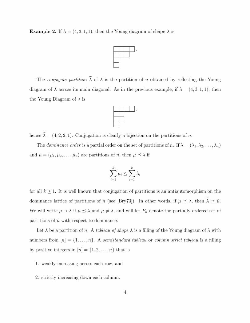
Example 2. If λ = (4, 3, 1, 1), then the Young diagram of shape λ is

.

The conjugate partition λ of λ is the partition of n obtained by reflecting the Young

diagram of λ across its main diagonal. As in the previous example, if λ = (4, 3, 1, 1), then

the Young Diagram of λ is

,

hence λ = (4, 2, 2, 1). Conjugation is clearly a bijection on the partitions of n.

The dominance order is a partial order on the set of partitions of n. If λ = (λ1, λ2, . . . , λn)

and µ = (µ1, µ2, . . . , µn) are partitions of n, then µ λ if

k∑i=1

µi ≤k∑i=1

λi

for all k ≥ 1. It is well known that conjugation of partitions is an antiautomorphism on the

dominance lattice of partitions of n (see [Bry73]). In other words, if µ λ, then λ µ.

We will write µ ≺ λ if µ λ and µ 6= λ, and will let Pn denote the partially ordered set of

partitions of n with respect to dominance.

Let λ be a partition of n. A tableau of shape λ is a filling of the Young diagram of λ with

numbers from [n] = 1, . . . , n. A semistandard tableau or column strict tableau is a filling

by positive integers in [n] = 1, 2, . . . , n that is

1. weakly increasing across each row, and

2. strictly increasing down each column.

4

For brevity, if λ is a partition of n, then we will often use λ to refer to the partition or the

Young diagram of shape λ interchangeably. A standard tableau of shape λ is a semistandard

tableau in which each number in [n] occurs exactly once.

Example 3. If λ = (3, 2, 1, 1) ` 7, then

1 2 22 337

is a semistandard tableau, whereas

1 2 53 467

is a standard tableau.

2.2 Irreducible representations of the symmetric group

If G is any finite group, then a finite dimensional representation of G over C is a group

homomorphism G −→ GL(V ), where V is a finite dimensional complex vector space, and

GL(V ) is the group of invertible linear transformations on V . The contents of chapter 5

deal with representations of finite complex reflection groups. The canonical example of such

a group is the symmetric group, Sn, of permutations of [n] = 1, . . . , n. In this section we

will cover the classification of irreducible representations of Sn over C.

The number of irreducible representations of Sn, like any finite group, is the number of

conjugacy classes. As the conjugacy classes of Sn are indexed by cycle types, their number

is P (n); the number of partitions of n. There is, in fact, a natural indexing of the irreducible

representations of Sn by these partitions via a construction called the Specht module of a

partition. Our construction of the Specht modules follows that in [Ful97].

5

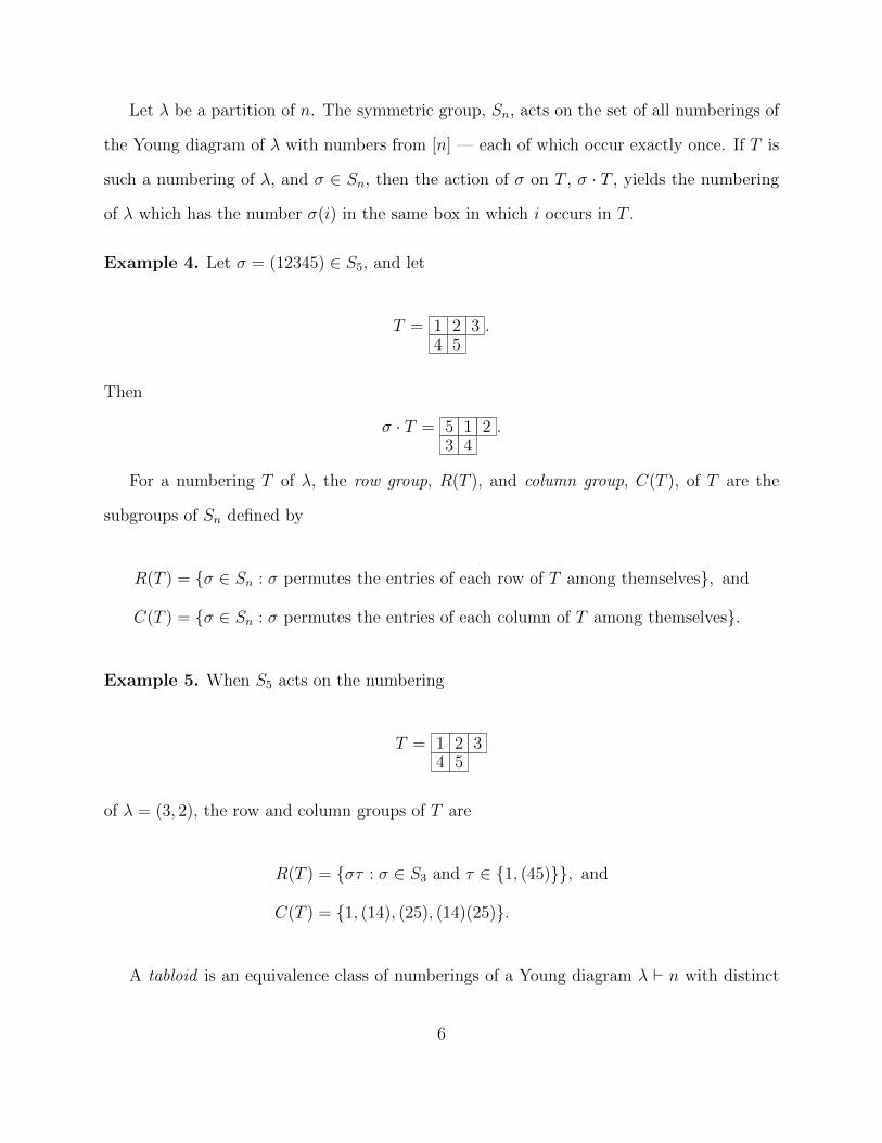
Let λ be a partition of n. The symmetric group, Sn, acts on the set of all numberings of

the Young diagram of λ with numbers from [n] — each of which occur exactly once. If T is

such a numbering of λ, and σ ∈ Sn, then the action of σ on T , σ · T , yields the numbering

of λ which has the number σ(i) in the same box in which i occurs in T .

Example 4. Let σ = (12345) ∈ S5, and let

T = 1 2 34 5

.

Then

σ · T = 5 1 23 4

.

For a numbering T of λ, the row group, R(T ), and column group, C(T ), of T are the

subgroups of Sn defined by

R(T ) = σ ∈ Sn : σ permutes the entries of each row of T among themselves, and

C(T ) = σ ∈ Sn : σ permutes the entries of each column of T among themselves.

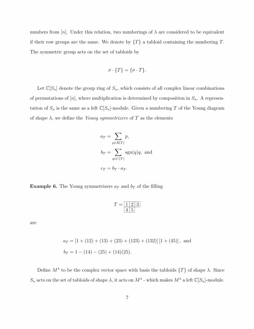
Example 5. When S5 acts on the numbering

T = 1 2 34 5

of λ = (3, 2), the row and column groups of T are

R(T ) = στ : σ ∈ S3 and τ ∈ 1, (45), and

C(T ) = 1, (14), (25), (14)(25).

A tabloid is an equivalence class of numberings of a Young diagram λ ` n with distinct

6

numbers from [n]. Under this relation, two numberings of λ are considered to be equivalent

if their row groups are the same. We denote by T a tabloid containing the numbering T .

The symmetric group acts on the set of tabloids by

σ · T = σ · T.

Let C[Sn] denote the group ring of Sn, which consists of all complex linear combinations

of permutations of [n], where multiplication is determined by composition in Sn. A represen-

tation of Sn is the same as a left C[Sn]-module. Given a numbering T of the Young diagram

of shape λ, we define the Young symmetrizers of T as the elements

aT =∑

p∈R(T )

p,

bT =∑

q∈C(T )

sgn(q)q, and

cT = bT · aT .

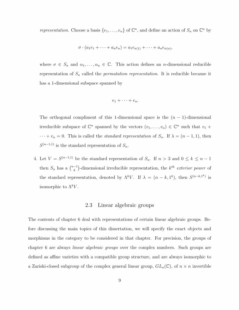
Example 6. The Young symmetrizers aT and bT of the filling

T = 1 2 34 5

are

aT = [1 + (12) + (13) + (23) + (123) + (132)] [1 + (45)] , and

bT = 1− (14)− (25) + (14)(25).

Define Mλ to be the complex vector space with basis the tabloids T of shape λ. Since

Sn acts on the set of tabloids of shape λ, it acts on Mλ - which makes Mλ a left C[Sn]-module.

7

For each numbering T of λ, there is a special element of Mλ defined by the formula

vT = bT · T.

We then define the Specht module Sλ to be the subspace of Mλ spanned by the elements vT

as T varies over all numberings of λ. The Specht module Sλ is then a C[Sn]-submodule of

Mλ. Putting this all together, we obtain the following theorem.

Theorem 7. Classification of Irreducible Representations of Sn ( [Ful97] )

For each partition λ of n, Sλ is an irreducible representation of Sn. Every irreducible repre-

sentation of Sn is isomorphic to exactly one Sλ.

Example 8. 1. For any n ∈ N, the symmetric group Sn has a one-dimensional represen-

tation called the trivial representation, defined by

σ · x = x,

for all σ ∈ Sn and x ∈ C. If λ = (n), then S(n) is the trivial representation of Sn.

2. If n ≥ 2, then Sn has a one-dimensional representation called the sign representation,

defined by

σ · x = sgn(σ)x,

for all σ ∈ Sn and x ∈ C. Here, the sign of σ is defined to be 1 if σ is a product of

an even number of transpositions, and is −1 otherwise. If λ = (1n), then S(1n) is the

alternating representation of Sn.

3. if n > 2, then Sn has a (n−1)-dimensional irreducible representation called the standard

8

representation. Choose a basis e1, . . . , en of Cn, and define an action of Sn on Cn by

σ · (a1e1 + · · ·+ anen) = a1eσ(1) + · · ·+ aneσ(n),

where σ ∈ Sn and α1, . . . , αn ∈ C. This action defines an n-dimensional reducible

representation of Sn called the permutation representation. It is reducible because it

has a 1-dimensional subspace spanned by

e1 + · · ·+ en.

The orthogonal compliment of this 1-dimensional space is the (n − 1)-dimensional

irreducible subspace of Cn spanned by the vectors (v1, . . . , vn) ∈ Cn such that v1 +

· · · + vn = 0. This is called the standard representation of Sn. If λ = (n − 1, 1), then

S(n−1,1) is the standard representation of Sn.

4. Let V = S(n−1,1) be the standard representation of Sn. If n > 3 and 0 ≤ k ≤ n − 1

then Sn has a(n−1k

)-dimensional irreducible representation, the kth exterior power of

the standard representation, denoted by ΛkV . If λ = (n − k, 1k), then S(n−k,1k) is

isomorphic to ΛkV .

2.3 Linear algebraic groups

The contents of chapter 6 deal with representations of certain linear algebraic groups. Be-

fore discussing the main topics of this dissertation, we will specify the exact objects and

morphisms in the category to be considered in that chapter. For precision, the groups of

chapter 6 are always linear algebraic groups over the complex numbers. Such groups are

defined as affine varieties with a compatible group structure, and are always isomorphic to

a Zariski-closed subgroup of the complex general linear group, GLn(C), of n × n invertible

9

complex matrices (for some n ∈ N). If G ⊆ GLn(C) is a algebraic group, then a rational

representation of G is a group homomorphism, G −→ GLm(C) for some m ∈ N, which is a

regular morphism in the category of affine varieties.

To each linear algebraic group G there is an associated Lie algebra g, which is defined as

the derivations (infinitesimal transformations) of the regular functions O[G] that commute

with left translations (see [GW09]). By O[G] we mean the algebra of regular (rational)

functions on G, which are defined as the restriction to G of the regular functions

O[GLn(C)] = C[x11, x12, . . . , xnn, det(x)−1]

on GLn(C), where x = [xij] ∈ GLn(C). The Lie algebra of a linear algebraic group has

a natural embedding into the n × n complex matrices Mn(C), and is equipped with a Lie

bracket

[ • , • ] : g× g −→ g,

which can be defined in terms of matrices as

[X, Y ] = XY − Y X,

for X, Y ∈ g. Henceforth we will always view a Lie algebra as being comprised of matrices.

Any element X ∈ g yields a linear transformation

adX(Y ) = [X, Y ],

which is called the adjoint representation of g. The representation theories of G and its Lie

algebra g are closely connected. In fact, a representation of G is irreducible if and only if its

differential is an irreducible representation of the Lie algebra g (c.f. [GW09] Theorem 2.2.7).

Hence g plays a significant role in the classification of the irreducible representations of G.

10

We will further restrict the linear algebraic groups under consideration to those that

are connected and reductive. A linear algebraic group G is connected if O[G] has no zero

divisors. G is reductive if every rational representation of G is completely reducible (hence

the name “reductive”). In other words, every rational representation of a reductive group

can be written as a sum of irreducible representations. The complete reducibility of rational

representations makes the study of reductive groups and the classification of their irreducible

representations particularly nice.

A toral subgroup T ⊆ G is a subgroup that is isomorphic to (C×)m, for some non-negative

integer m. A torus is maximal if it is not properly contained within any other torus. If the

group G is connected and reductive, then all maximal tori are conjugate and have the same

dimension (known as the rank of G). Furthermore, every element of G lies in a maximal

torus. In this case, the lie algebra ,h, of a maximual torus, T , is called a Cartan subalgebra

of g. Cartan subalgebras are maximal abelian subalgebras of g in which every element is

semisimple. Just as with maximal tori, all Cartan subalgebras are conjugate in g.

2.4 The Theorem of the Highest Weight

Let G be a connected reductive linear algebraic group of rank n, and fix a choice T ∼= (C×)n

of maximal torus in G. Let g and h be the Lie algebras of G and T , respectively. Let h∗

denote the algebraic dual space of h; that is, the set of all linear functionals h −→ C.

Since T is abelian, its irreducible representations are all 1-dimensional. Denote by X(T )

the group (under tensor products of representations) of all irreducible representations of T .

The group X(T ) is isomorphic to Zn. The weight lattice of G is the set

P (G) = dθ : θ ∈ X(T ) ⊆ h∗

of differentials of irreducible representations of T (i.e., the irreducible representations of h

11

corresponding to those of T ). The elements of P (G) are called weights of G. If α ∈ P (G) is

a weight of G, we define

gα = X ∈ g : [A,X] = α(A)X for all A ∈ h.

If α = 0, then g0 = h. If α is nonzero and gα is nonzero, then we call α a root of T on g, and

we call gα a root space. We call the set Φ ⊆ h∗ of roots the root system of g, with respect to

our choice T of maximal torus. The root system Φ spans h∗.

A subset

∆ = α1, . . . , αn ⊆ Φ

is a set of simple roots of g if every γ ∈ Φ can be written uniquely as

γ = n1α1 + · · ·+ · · ·+ nkαk,

with n1, . . . , nk integers all of the same sign. The simple roots ∆ form a basis for h∗, and

partition the root system Φ into two disjoint subsets

Φ = Φ+ ∪ Φ−,

where Φ+ consists of all roots for which the coefficients n1, . . . , nk are non-negative. We call

γ ∈ Φ+ a positive root relative to ∆.

For a root α ∈ Φ, we call an element hα ∈ [gα, gα] such that α(hα) = 2 a coroot of α.

The weight lattice of g is defined as

P (g) = λ ∈ h∗ : λ(hα) ∈ Z for all α ∈ Φ,

and the dominant integral weights of g (relative to the choice of simple roots ∆) are defined

12

as,

P++(g) = λ ∈ h∗ : λ(hα) ∈ Z≥0 for all α ∈ Φ.

Finally, the dominant weights of G are defined to be the weights of G that are also dominant

integral weights of the Lie algebra g:

P++(G) = P (G) ∩ P++(g).

There is a partial order defined on the set of weights of g (and thus on the dominant

weights of G). Let λ, µ ∈ h∗ be two dominant weights of g. Since Φ+ spans h∗, λ and µ can

be written as linear combinations of the positive roots. If λ − µ can be written as a linear

combination of the positive roots with non-negative real coefficients, then we say that λ is

higher than µ. This partial order then restricts to the dominant weights of G. Let V be a

(finite dimensional) irreducible representation of G. A weight λ of V is called the highest

weight of V if λ is higher than every other weight µ of V .

The irreducible representations of G are classified by a result known as the “theorem of

the highest weight”.

Theorem 9. Theorem of the Highest Weight If G is a connected reductive linear algebraic

group and T is a maximal torus in G, the following results hold

1. Every irreducible representation of G has a highest weight.

2. Two irreducible representations of G with the same highest weight are isomorphic.

3. The highest weight of each irreducible representation of G is dominant.

4. If λ is a dominant weight of G, there exists an irreducible representation of G with

highest weight λ.

13

2.5 The General Linear Group

Fix a positive integer n. The general linear group GLn(C) of complex n × n invertible

matrices is a connected reductive linear algebraic group. As a affine variety, it is defined as

the set of points (x, y) ∈ Cn2 × C satisfying the polynomial equation

y det(x) = 1.

The canonical choice of maximal torus in GLn(C) is the subgroup T of diagonal matrices.

The Lie algebra of GLn(C) is the set gln(C) = Mn(C) of all n × n complex matrices, and

the Lie algebra of T is the subalgebra

h = X ∈ gln(C) : X is diagonal.

Define εi ∈ h∗ such that

εi(A) = ai,

for any A = diag[a1, . . . , an] ∈ h. The root system of T is the set

Φ = εi − εj : 1 ≤ i 6= j ≤ n.

The standard choice for the set of simple roots is

∆ = εi − εi+1 : 1 ≤ i < n,

and the corresponding set of positive roots is

Φ+ = εi − εj : 1 ≤ i < j ≤ n.

14

The weight lattice P (GLn(C)) can then be written in terms of these weights as

P (GLn(C)) =n⊕k=1

Zεk.

The set of dominant integral weights of g is given by

P++(g) = k1ε1 + · · ·+ knεn : k1 ≥ k2 ≥ · · · ≥ kn and ki − ki+1 ∈ Z.

Hence the dominant weights of GLn(C) are

P++(GLn(C)) = P (GLn(C)) ∩ P++(g)

= k1ε1 + · · ·+ knεn : k1 ≥ k2 ≥ · · · ≥ kn and ki ∈ Z.

By the theorem of the highest weight, if V is an irreducible representation of GLn(C), then

V has a highest weight, and its highest weight is dominant. If λ ∈ P++(GLn(C)) is the

highest weight of V , then we write V = V λ and call V λ a “highest weight representation”

of λ.

For a more detailed look at the information provided in this chapter, we refer the reader

to [GW09].

15

3 The Gini Index

3.1 The “Standard” Gini Index

Much of this first section has appeared in the Journal of Integer Sequences in a paper by

the author (see [Kop20]).

In part one of his 1912 book “Variabilita e Mutabilita” (Variability and Mutability),

the statistician Corrado Gini formulated a number of different summary statistics; among

which was what is now known as the Gini index - a measure that attempts to quantify how

equitably a resource is distributed throughout a population. Referring to “the” Gini index

can be misleading, as no fewer than thirteen formulations of his famous index appeared

in the original publication [CV12]. Since then, many others have appeared in a variety of

different fields.

The Gini index is usually defined using a construction known as a Lorenz Curve. In

“Methods of Measuring the Concentration of Wealth”, Lorenz defined this curve in the

following fashion. Consider a population of people amongst whom is distributed some fixed

amount of wealth. Let L(x) be the percentage of total wealth possessed by the poorest x

percent of the population. The graph y = L(x) is the Lorenz curve of the population [Lor05].

It is clear from this definition that L(0) = 0 (I.E., none of the people have none of the

wealth), L(1) = 1 (all of the people have all of the wealth), and L is non-decreasing. Since

any population of people must have finite size n, the function L(x) as defined above would

appear to be a discrete function on the set kn

: k ∈ Z and 0 ≤ k ≤ n. However, in practice

L is often made continuous on the interval [0, 1] by linear interpolation [Far10].

If each person possesses the same amount of wealth, then the Lorenz curve for this

distribution is the line y = x, which we call the “line of equality”. The area between the

16

line of equality and the Lorenz curve of a wealth distribution provides a measurement of the

wealth inequality in that population.

Figure 3.1: Area between the line of equality and a typical Lorenz curve

The maximum possible area of 12

arises from the distribution in which one person controls

all of the wealth (L(1) = 1, and L(x) = 0 for all x 6= 1). The Gini index of a distribution

is then defined by calculating the area between the line of equality and Lorenz curve of the

distribution, and normalizing this area to be between zero and one:

G = 2

∫ 1

0

(x− L(x)

)dx.

In this paper we consider distributions of a discrete indivisible resource in a finite popu-

lation, where the amount of that resource is equal to the number of people in the population.

There is a natural one-to-one correspondence between the set of such distributions with n

people, and the set of partitions of n. We will then define the Gini index of a partition in a

similar fashion as above.

17

3.2 The second elementary symmetric polynomial e2

The second elementary symmetric polynomial, e2, in n variables, x1, x2, . . . xn, is defined

e2(x1, x2, . . . , xn) =∑

1≤i<j≤n

xixj.

Example 10. If λ = (4, 3, 1, 1) is a partition of 9, then

e2(λ) =(

4(3 + 1 + 1) + 3(1 + 1) + 1(1))

= 27.

We will make use of the following result.

Lemma 11. If λ = (λ1, λ2, . . . , λn) is a partition of a positive integer n, then

e2(λ) =

(n

2

)−

n∑i=1

(λi2

).

18

Proof. Let λ = (λ1, λ2, . . . , λn) be a partition of n. Note that∑n

i=1 λi = n. Then

e2(λ) =∑

1≤i<j≤n

λiλj

=

(n

2

)−

( ∑1≤i<j≤n

(− λiλj

)+

(n

2

))

=

(n

2

)− 1

2

( ∑1≤i<j≤n

(− 2λiλj

)+ n(n− 1)

)

=

(n

2

)− 1

2

( ∑1≤i<j≤n

(− 2λiλj

)+

(l∑

i=1

λi

)(l∑

j=1

λj − 1

))

=

(n

2

)− 1

2

( ∑1≤i<j≤n

(− 2λiλj

)+

l∑i=1

(λ2i − λi

)+

∑1≤i<j≤l

(2λiλj

))

=

(n

2

)− 1

2

(n∑i=1

λi(λi − 1)

)

=

(n

2

)−

(n∑i=1

(λi2

)).

3.3 The Gini Index of an Integer Partition

As previously stated, we restrict our study of the Gini index to finite populations where

the amount of a discrete indivisible resource is equal to the size of the population. In other

words, there is one of said resource available for each person. The distributions of n of such

a resource amongst n people is in one-to-one correspondence with the integer partitions of

n.

Example 12. If there are 4 dollars in a population of 4 people, then the partition (3, 1) of

4 would correspond to one person having 3 dollars, one person having 1 dollar, and the two

19

remaining people having nothing. Whereas the partitions (1, 1, 1, 1) and (4) correspond to

completely equitable and completely inequitable distributions, respectively.

Given a partition λ = (λ1, . . . , λn) of a positive integer n (padded with zeros on the

tail, if necessary), the Lorenz curve of λ, Lλ : [0, n] −→ [0, n], is defined as Lλ(0) = 0, and

Lλ(x) =∑n

i=n−k+1 λi, where 1 ≤ k ≤ n is the unique positive integer such that x ∈ (k−1, k].

In other words, for k from 1 to n, the Lorenz curve of λ on the interval (k− 1, k] is the sum

of the last k parts of λ, λn +λn−1 + · · ·+λn−k+1. Since total equality corresponds to the flat

partition (1n), using the above definition for the Lorenz curve of a partition, we find that

the line of equality is given by y = dxe.

Figure 3.2: The line of equity (dashed) and the Lorenz curve of the partition (3,2,1) of 6(solid).

The standard Gini index is calculated by finding the area between the line of equality

and the Lorenz curve, and normalizing. In a similar fashion we define the Gini index, g, of

20

a partition λ = (λ1, . . . , λn) of n by

g(λ) =

∫ n

0

(dxe − Lλ(x)) dx

=

(n+ 1

2

)−

n∑i=1

iλi

=

(n

2

)−

n∑i=1

(i− 1)λi.

The ordinary Gini index is normalized to be between zero and one. For a fixed value of n,

the function g attains its maximum value of(n2

)on the partition (n) of n. So the Gini index

of a partition λ of n can be normalized by dividing g(λ) by(n2

). As long as n, and g(λ) are

both known, the normalized Gini index of λ can always be calculated in this fashion. With

this in mind, we may disregard the normalization, and view g itself as the integer valued

“discrete” Gini index of a partition.

The sumsn∑i=1

(λi2

)and

n∑i=1

(i− 1)λi

have appeared in our formulas for e2 and g, respectively. It is known (cf. [GK86]) that these

two quantities are equal. This fact, in conjunction with Lemma 11 yield some interesting

results.

Proposition 13. If λ is an integer partition, then g(λ) = e2(λ), where λ is the conjugate

partition of λ.

In light of Lemma 11, this result follows from statements in [GK86]. These statements

are, however, given without proof, so we will now provide proofs of these facts.

Proof. Let λ = (λ1, λ2, . . . , λn) be a partition of a positive integer n, where λ1 ≥ λ2 ≥ . . . ≥ λn > 0

21

and∑n

i=1 λi = n. We can calculate g(λ) by filling the Young diagram of shape λ with num-

bers, where the entry in any box counts the number of boxes in that column that are strictly

above it. For example, for the partition (4, 3, 1, 1), we would have

0 0 0 01 1 123

.

Then the sums of the values in each row are

∑(Entries in row 1

)= 0λ1,∑(

Entries in row 2)

= 1λ2,∑(Entries in row 3

)= 2λ3,...∑(

Entries in row n)

= (n− 1)λn.

Summing all values in the Young diagram of λ yields∑n

i=1(i − 1)λi. By subtracting this

from(n2

)we have

(n

2

)−∑(

Entries in Young Diagram i)

=

(n

2

)−

n∑i=1

(i− 1)λi = g(λ).

We can calculate e2(λ) similarly by forming a Young diagram of shape λ where each each

box’s entry counts the number of boxes in the same row that are strictly to the left of its

own. Again using (4, 3, 1, 1) as an example, we would have

0 1 2 30 1 200

.

22

In general, the ith row of the diagram for λ will be of the form

0 1 . . . λi−2 λi−1,

so the sum of the boxes in the ith row will be(λi2

). Summing all of the entries in the

Young diagram of λ and subtracting this from(n2

)yields

(n

2

)−

n∑i=1

(Entries in row i

)=

(n

2

)−

n∑i=1

(λi2

)= e2(λ),

where the last equality is by Lemma 11. Since g(λ) is calculated by counting boxes in the

columns of the Young diagram of λ, and e2(λ) is calculated by counting boxes in the rows,

it follows that g(λ) = e2(λ).

Proposition 14. Let λ and µ be partitions of n. If µ ≺ λ then g(µ) < g(λ) and e2(λ) <

e2(µ).

The normalized Gini index on Rn, discussed in [MOA11], is equal to 2gn2 when restricted

to Pn. This function is known to be strictly Schur convex, so Proposition 14 can be partially

deduced from this fact. A complete proof of Proposition 14 that does not utilize these facts

is presented below.

Proof. Let λ = (λ1, λ2, . . . , λn) and µ = (µ1, µ2, . . . , µn) be partitions of n (padded with

zeros in their tails, if necessary). Suppose that λ covers µ, I.E. there is no partition ρ of n

such that µ ≺ ρ ≺ λ. Now λ covers µ if and only if

λi = µi + 1,

λk = µk − 1, and

λj = µj,

23

for all j 6= i or k, and either k = i+ 1 or µi = µk [Bry73]. In other words, λ covers µ if and

only if all but two of the rows (row i and k, with i < k) in the Young diagrams of λ and µ

are of the same length, and the diagram of λ can be obtained from that of µ by removing

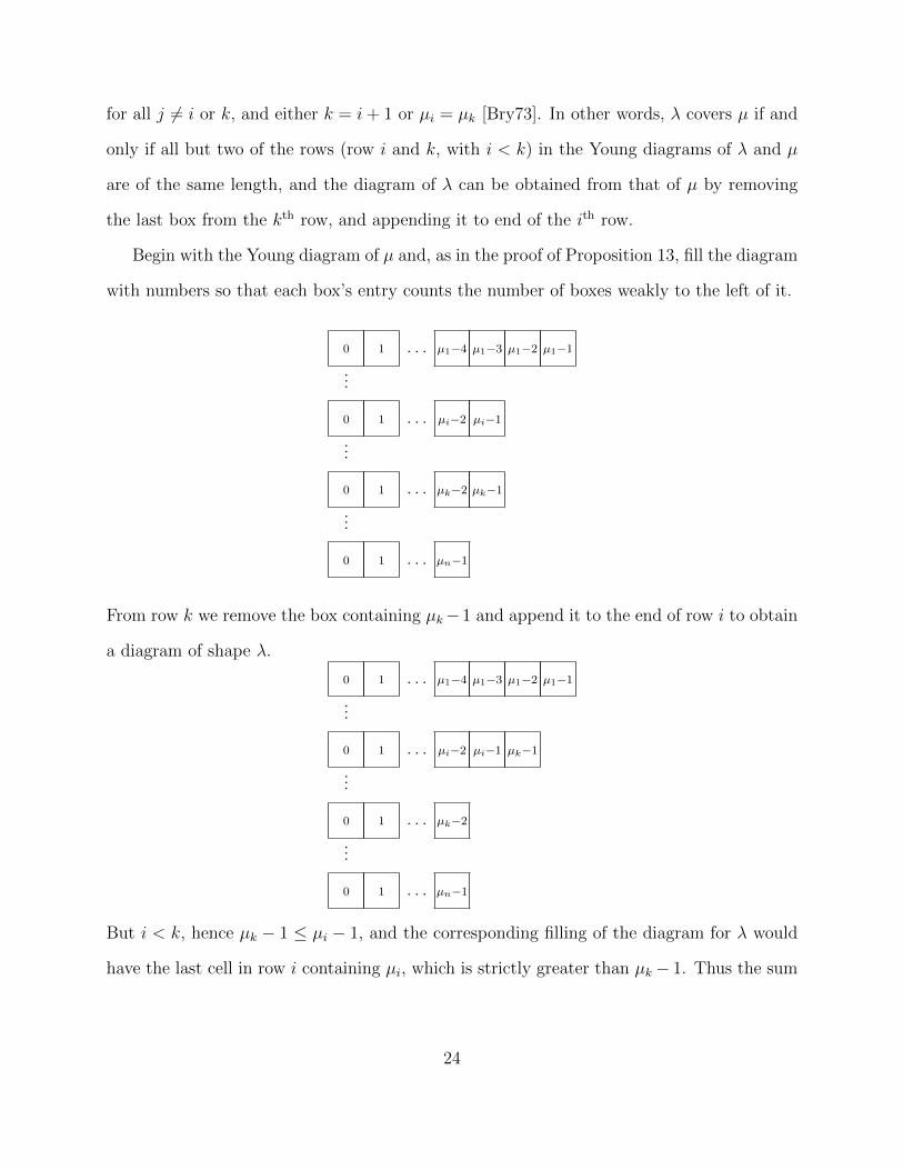
the last box from the kth row, and appending it to end of the ith row.

Begin with the Young diagram of µ and, as in the proof of Proposition 13, fill the diagram

with numbers so that each box’s entry counts the number of boxes weakly to the left of it.

0 1 . . . µ1−4 µ1−3 µ1−2 µ1−1

...

0 1 . . . µi−2 µi−1

...

0 1 . . . µk−2 µk−1

...

0 1 . . . µn−1

From row k we remove the box containing µk−1 and append it to the end of row i to obtain

a diagram of shape λ.

0 1 . . . µ1−4 µ1−3 µ1−2 µ1−1

...

0 1 . . . µi−2 µi−1 µk−1

...

0 1 . . . µk−2

...

0 1 . . . µn−1

But i < k, hence µk − 1 ≤ µi − 1, and the corresponding filling of the diagram for λ would

have the last cell in row i containing µi, which is strictly greater than µk − 1. Thus the sum

24

of all numbers in the diagram for λ is

n∑j=1j 6=i,k

(µj2

)+

(µi + 1

2

)+

(µk − 1

2

),

and the sum of all numbers in the diagram for µ is

n∑j=1

(µj2

).

By Lemma 11, we have

e2(µ)− e2(λ) =

(n

2

)−

n∑j=1

(µj2

)−(n2

)−

n∑j=1j 6=i,k

(µj2

)+

(µi + 1

2

)+

(µk − 1

2

)

=

(µi + 1

2

)+

(µk − 1

2

)−(µi2

)(µk2

)=

(µi)(µi + 1− µi + 1) + (µk − 1)(µk − 2− µk + 1)

2

=2µi + 1− µk

2

> 0.

So e2(µ) > e2(λ). Moreover µ ≺ λ if and only if λ ≺ µ. Hence µ covers λ, and by Proposition

13, g(µ) < g(λ). The general case follows by transitivity.

3.4 Antichains in the Dominance Order

The converse of Proposition 14 does not hold, in general, as seen in Example 15.

25

Example 15. Let λ = (5, 5) and µ = (6, 2, 2) be partitions of n = 10. Then

g(µ) = 39 < g(λ) = 40, and

e2(λ) = 25 < e2(µ) = 28,

but µ ⊀ λ.

The contrapositive of Propasition 14, however, provides us with an easily calculated lower

bound on the width of Pn.

Corollary 16. (Contrapositive to Prop. 14) Let λ 6= µ be partitions of n. If

g(µ) = g(λ),

e2(µ) = e2(λ),

g(µ) > g(λ) and e2(µ) > e2(λ), or

g(µ) < g(λ) and e2(µ) < e2(λ),

then λ and µ are incomparable.

In other words, we can find lower bounds on the size of the maximal level set of g on Pn.

As we will see shortly, these lower bounds can be calculated using the generating function

of Proposition 18.

It is often useful in Algebraic Combinatorics to record a discrete data set in the coefficients

or powers of a formal power series. We call these power series “generating functions” for the

data set. By “formal” we mean that the convergence of the series is immaterial. Any variables

appearing in the series are taken as indeterminates rather than numbers. Alternatively, one

may consider a formal power series as an ordinary power series that converges only at zero.

26

We define a generating function for the Gini index g(λ) of an integer partition λ by

G(q, x) =∞∑n=1

∑λ`n

q((n+12 )−g(λ))xn.

Perhaps the most widely known example of a generating function is that of the integer

partition function, P (n), which counts the number of partitions of the integer n.

Example 17. n = 5 has partitions

(1, 1, 1, 1, 1), (2, 1, 1, 1), (2, 2, 1), (3, 1, 1), (3, 2), (4, 1), and (5),

so P (5) = 7.

It is well known (see, for example, [AE04]) that P (n) has generating function

∞∏n=1

1

1− xn=∞∑n=0

P (n)xn,

Where P (0) is defined to be 1.

In light of our previous results, we obtain a similar equality for G(q, x).

Proposition 18.∞∏n=1

1

1− q(n+12 )xn

− 1 =∞∑n=1

∑λ`n

q((n+12 )−g(λ))xn

Proof. We will show that the power series about x = 0 of the product

∞∏n=1

1

1− q(n+12 )xn

− 1 (3.1)

has as its general coefficient ∑λ`n

q((n+12 )−g(λ)).

27

Considering each factor of the product as a geometric series, we have

∞∏n=1

1

1− q(n+12 )xn

=1(

1− q(22)x) · 1(

1− q(32)x2

) · 1(1− q(

42)x3

) · 1(1− q(

52)x4

) · · · ·=(

1 + q(22)x+ q2(

22)x2 + q3(

22)x3 + q4(

22)x4 + · · ·

)·(

1 + q(32)x2 + q2(

32)x4 + q3(

32)x6 + q4(

32)x8 + · · ·

)·(

1 + q(42)x3 + q2(

42)x6 + q3(

42)x9 + q4(

42)x12 + · · ·

)·(

1 + q(52)x4 + q2(

52)x8 + q3(

52)x12 + q4(

52)x16 + · · ·

)· · · · .

If we distribute and simplify, for example, the coefficient of x4, we see that it is

q4(22) + q2(

32) + q(

22)+(4

2) + q2(22)+(3

2) + q(52),

where each of the terms correspond to the partitions

(1, 1, 1, 1), (2, 2), (3, 1), (2, 1, 1), and (4),

respectively, by

(λ1, λ2, . . . , λl) 7→ q(∑li=1 (λi+1

2 )).

This is true, in general, for the coefficient of xn, for all positive integers n. To see this,

consider the coefficient on xn in the power series expansion of equation 3.1. If we set q = 1

in the product of equation 3.1, we obtain the generating function of P (n) (the number of

partitions of n). Hence there are P (n) different ways to obtain a power of xn. So the xn

28

term in equation 3.1 will be of the form

P (n)∑j=1

mj∏i=1

q(aj,i(λj,i+1

2 ))x(aj,iλj,i),

where aj,i, λj,i > 0, and∑mj

i=1 aj,iλj,i = n. Thus the coefficient on xn will be

P (n)∑j=1

q(∑mji=1 aj,i(

λj,i+1

2 )). (3.2)

Since each(λj,i+1

2

)in equation 3.2 comes from a different term of the product in equation 3.1,

we have that λj,i 6= λj,k whenever i 6= k. Therefore, by reordering, we may choose the power

aj,i(λj,i+1

2

)on q so that λj,i > λj,i+1 > 0, for 1 ≤ i < mj. It follows that (λ

aj,1j,1 , λ

aj,2j,2 , . . . , λ

aj,mjj,mj

)

is a partition of n, where λj,i is repeated aj,i times.

Again, using the generating function for P (n), the ways of writing xn as a product∏i x

(aj,iλj,i) (where aj,iλj,i > 0) is in bijection with the partitions of n. Since each of the

sums∑mj

i=1 aj,iλj,i = n have distinct summands for all 1 ≤ j ≤ P (n), it follows that the

sums∑mj

i=1 aj,i(λj,i+1

2

)are all distinct for different values of j. In other words, every partition

(λaj,1j,1 , . . . , λ

aj,mjj,mj

) of n appears as a power in equation 3.2. Hence equation 3.2 is equal to

∑λ`n

q(∑ni=1 (λi+1

2 )).

By Lemma 11, e2(λ) =(n+12

)−∑n

i=1

(λi+12

), thus

∑λ`n

q(∑ni=1 (λi+1

2 )) =∑λ`n

q(∑ni=1 (n+1

2 )−e2(λ)).

Finally, by Proposition 13, we have that the general coefficient on xn in the power series

29

expansion of equation 3.1 is ∑λ`n

q(∑ni=1 (n+1

2 )−g(λ)).

We can use G(q, x) to find lower bounds on the width of Pn by calculating the cardinalities

of the maximum level sets of g on Pn. In particular, the “size” of these level sets will be

the largest coefficient on the powers of q that form the coefficient of xn. Expanding G(q, x)

yields

∞∑n=1

∑λ`n

q((n+12 )−g(λ))xn = qx+ (q2 + q3)x2 + (q3 + q4 + q6)x3

+ (q4 + q5 + q6 + q7 + q10)x4

+ (q5 + q6 + q7 + q8 + q9 + q11 + q15)x5

+ (· · ·+ 2q9 + · · · )x6 + (· · ·+ 2q10 + · · · )x7

+ (· · ·+ 2q11 + · · · )x8 + (· · ·+ 3q15 + · · · )x9

+ · · · .

So the size of the maximal level sets of g are 1, 1, 1, 1, 1, 2, 2, 2, and 3, on P1 through P9,

respectively.

Let b(n) denote the size of the maximal level set of g on Pn (A337206 in [OFI21]).

Proposition 14 implies that b(n) ≤ a(n) for all positive integers n, where a(n) is the size of

the maximum antichain in Pn (A076269 in [OFI21]). There are known asymptotic bounds

on a(n). The best known bounds follow from Dilworth’s Theorem; since P (n) (the number

of partitions of n) is clearly an upper bound on a(n), we have that a(n) ≥ P (n)/(h(Pn) +

1), where h(Pn) is the length of a maximal chain in Pn. This argument was applied in

[Ear13] without proof, so we will sketch the proof and use the same reasoning to acquire

an asymptotic lower bound on the sequence b(n). Formulas for the sequence h(Pn) have

30

been known for some time, but the asymptotics were not fully understood until Greene and

Kleitman ( [GK86] ) proved that

h(Pn) ∼ (2n)3/2/3.

Combining this with the famous result of Hardy and Ramanujan ( [HR00] ),

P (n) ∼ eπ√

2n/3

4n√

3,

we see that

Ω

(eπ√

(2n/3)

n5/2

)≤ a(n) ≤ O

(eπ√

2n/3

n

).

We can similarly obtain a lower bound on b(n). Observe that g may take on values

between 0 and(n2

). As such, the level sets b(n) of g on Pn are bounded below by

P (n)(n2

) ≤ b(n).

Applying the same formulas as above, yields the following.

Proposition 19.

Ω

(eπ√

2n/3

n3

)≤ b(n),

for all n > 1.

While not as “sharp” as the bound obtained via Dilworth’s Theorem, Proposition 19

shows that the level sets of the Gini index provide a good lower bound on the size of the

maximum antichain in Pn.

31

3.5 Expected Value of the Gini Index on Pn

With the results from the previous section, a natural follow-up question would be, “What

is the expected value of the Gini index?” To formalize this question, we will view g as a

real-valued discrete random variable with sample space Pn. To each outcome m ∈[0,(n2

)],

we assign the probability

P(g = m) =|g−1(m)|P (n)

.

That is, the probability that g = m is the number of partitions λ ∈ Pn such that g(λ) = m,

divided by the number of partitions of n. For a fixed valued of n ∈ N, computing the

expected value of the Gini index is as simple as calculating the partitions of n (which, in

reality, is not at all simple).

Example 20. If n = 6, the partitions of n are

(1,1,1,1,1,1),

(2,1,1,1,1),

(2,2,1,1),

(2,2,2),

(3,1,1,1),

(3,2,1),

(3,3),

(4,1,1),

(4,2),

(5,1), and

(6).

32

Their function values under g are

g((16)) = 0,

g((2, 14)) = 5,

g((22, 12)) = 8,

g((23)) = 9,

g((3, 13)) = 9,

g((3, 2, 1)) = 11,

g((32)) = 12,

g((4, 12)) = 12,

g((4, 2)) = 13,

g((5, 1)) = 14, and

g((6)) = 15.

Let E(g, Pn) represent the expected value of g on Pn. By the above example, we have

that

E(g) =0

11+

5

11+

8

11+ 2

9

11+

11

11+ 2

12

11+

13

11+

14

11+

15

11=

108

11≈ 9.8.

If λ ` n, then g(λ) < n only when λ = (1n). Hence the expected value of the Gini index

on Pn tends to infinity as n approaches infinity. A natural followup question is, “What is

the expected value of the Gini index on Pn when normalized by its maximum value, and

what is its end behavior?” In our example of n = 6, the “normalized” expected value of g is

obtained by dividing by the maximum value of 15:

0

165+

5

165+

8

165+ 2

9

165+

11

165+ 2

12

165+

13

165+

14

165+

15

165=

36

55≈ 0.655.

33

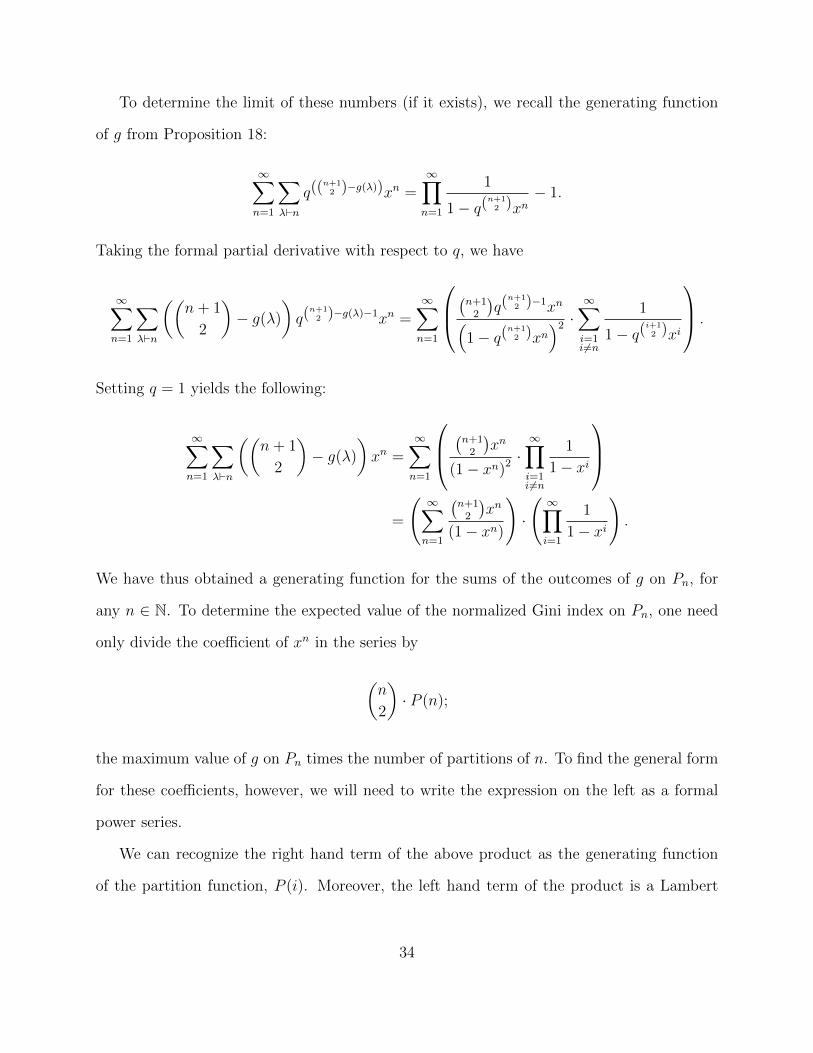
To determine the limit of these numbers (if it exists), we recall the generating function

of g from Proposition 18:

∞∑n=1

∑λ`n

q((n+12 )−g(λ))xn =

∞∏n=1

1

1− q(n+12 )xn

− 1.

Taking the formal partial derivative with respect to q, we have

∞∑n=1

∑λ`n

((n+ 1

2

)− g(λ)

)q(

n+12 )−g(λ)−1xn =

∞∑n=1

(n+12

)q(

n+12 )−1xn(

1− q(n+12 )xn

)2 · ∞∑i=1i 6=n

1

1− q(i+12 )xi

.

Setting q = 1 yields the following:

∞∑n=1

∑λ`n

((n+ 1

2

)− g(λ)

)xn =

∞∑n=1

(n+12

)xn

(1− xn)2·∞∏i=1i 6=n

1

1− xi

=

(∞∑n=1

(n+12

)xn

(1− xn)

)·

(∞∏i=1

1

1− xi

).

We have thus obtained a generating function for the sums of the outcomes of g on Pn, for

any n ∈ N. To determine the expected value of the normalized Gini index on Pn, one need

only divide the coefficient of xn in the series by

(n

2

)· P (n);

the maximum value of g on Pn times the number of partitions of n. To find the general form

for these coefficients, however, we will need to write the expression on the left as a formal

power series.

We can recognize the right hand term of the above product as the generating function

of the partition function, P (i). Moreover, the left hand term of the product is a Lambert

34

series, which formally sums to

∞∑n=1

(n+12

)xn

(1− xn)=∞∑n=1

∑d|n

(d+ 1

2

)xn.

Manipulating the sum on the right, we obtain

∞∑n=1

∑d|n

(d+ 1

2

)xn =

∞∑n=1

∑d|n

1

2(d2 + d)xn

=1

2

∞∑n=1

(σ1(n) + σ2(n))xn,

where

σx(n) =∑d|n

dx

is the so-called sum of divisors function, for x ∈ C.

Putting this all together yields

∞∑n=1

∑λ`n

((n+ 1

2

)− g(λ)

)xn =

(1

2

∞∑n=1

(σ1(n) + σ2(n))xn

)·

(∞∑i=0

P (i)xi

)

=1

2

∞∑n=1

n−1∑i=0

P (i)(σ1(n− i) + σ2(n− i))xn.

By distributing the xn on the left we can isolate the sum containing g(λ), obtaining

∞∑n=1

∑λ`n

g(λ)xn =∞∑n=1

P (n)

(n+ 1

2

)xn − 1

2

∞∑n=1

n−1∑i=0

P (i)(σ1(n− i) + σ2(n− i))xn

=∞∑n=1

1

2

(P (n)(n2 + n)−

n−1∑i=0

P (i)(σ1(n− i) + σ2(n− i))

)xn.

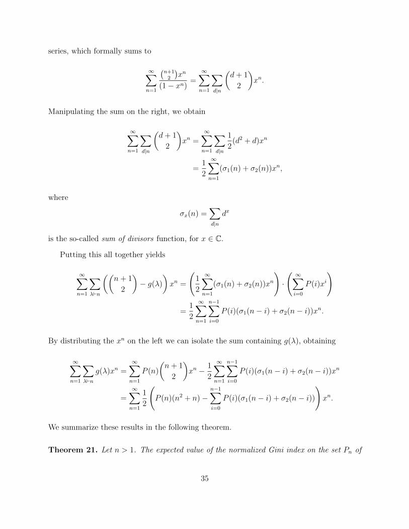
We summarize these results in the following theorem.

Theorem 21. Let n > 1. The expected value of the normalized Gini index on the set Pn of

35

partitions of n is

E(g, Pn) =∑λ`n

g(λ)(n2

)P (n)

=n+ 1

n− 1−

n−1∑i=0

P (i)(σ1(n− i) + σ2(n− i))P (n)(n2 − n)

,

where P (n) is the number of partitions of n.

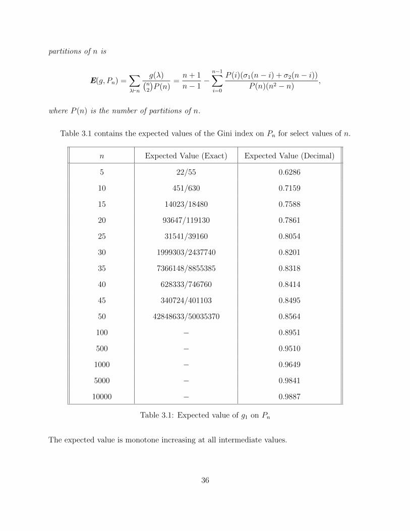
Table 3.1 contains the expected values of the Gini index on Pn for select values of n.

n Expected Value (Exact) Expected Value (Decimal)

5 22/55 0.6286

10 451/630 0.7159

15 14023/18480 0.7588

20 93647/119130 0.7861

25 31541/39160 0.8054

30 1999303/2437740 0.8201

35 7366148/8855385 0.8318

40 628333/746760 0.8414

45 340724/401103 0.8495

50 42848633/50035370 0.8564

100 − 0.8951

500 − 0.9510

1000 − 0.9649

5000 − 0.9841

10000 − 0.9887

Table 3.1: Expected value of g1 on Pn

The expected value is monotone increasing at all intermediate values.

36

One of the questions at the start of this section regarded the asymptotic behavior of the

expected value in Theorem 21. Based on the experimental data in the above table, we make

the conservative conjecture that

limn→∞

E(g, Pn) = 1.

3.6 Further Generalizations

So far we have been working with the Gini index g defined on the set Pn of partitions of

a positive integer n. This corresponds to the “real life” situation in which n dollars are

distributed amongst n people. we can broaden our notion of the Gini index of a partition

by considering distributions of the following nature.

Suppose we have 6 dollars distributed amongst three people, where one person gets 4

dollars, one gets 2, and the last gets 0. This distribution corresponds to the partition

λ = (4, 2, 0) of 6. The most equitable distribution would be that in which all three people

have the same amount; that is, the partition µ = (2, 2, 2). It is clear that such distributions

are in bijection with those partitions of 6 with at most 3 parts.

To find the Lorenz Curve of λ, we pad its tail with zeros until it has 6 parts

λ = (4, 2, 0, 0, 0, 0).

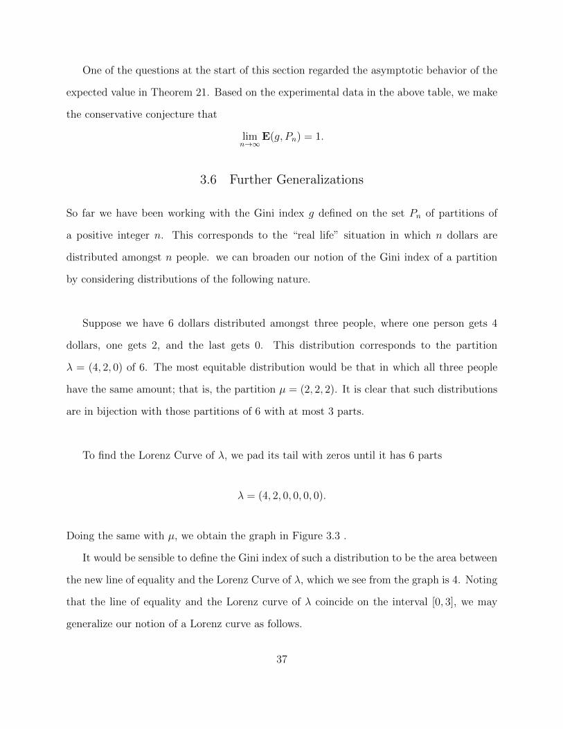
Doing the same with µ, we obtain the graph in Figure 3.3 .

It would be sensible to define the Gini index of such a distribution to be the area between

the new line of equality and the Lorenz Curve of λ, which we see from the graph is 4. Noting

that the line of equality and the Lorenz curve of λ coincide on the interval [0, 3], we may

generalize our notion of a Lorenz curve as follows.

37

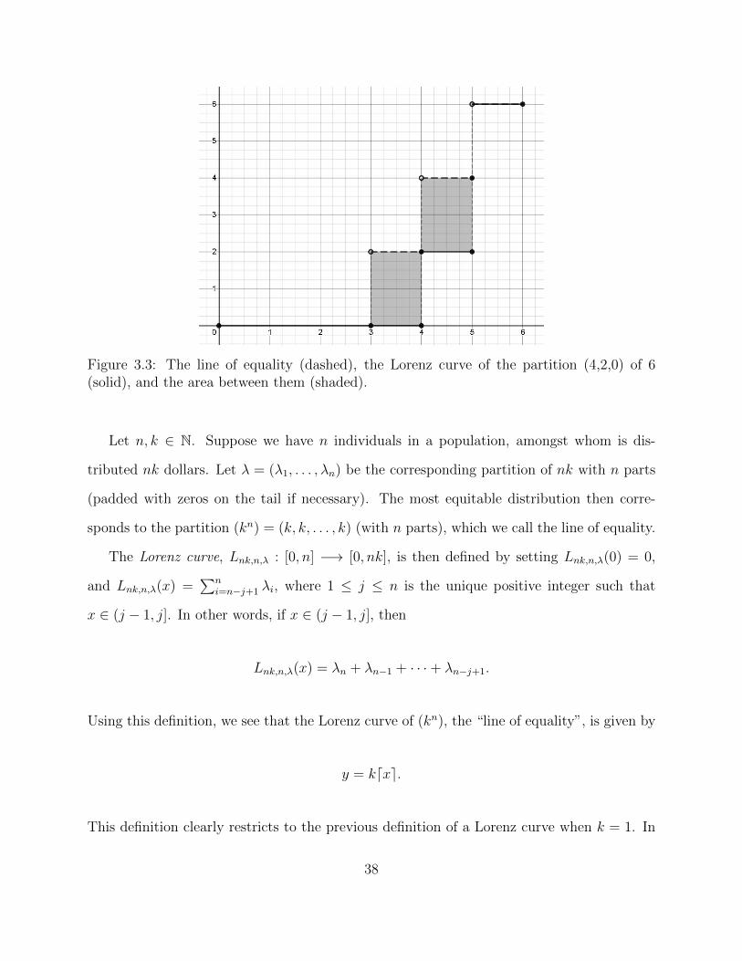
Figure 3.3: The line of equality (dashed), the Lorenz curve of the partition (4,2,0) of 6(solid), and the area between them (shaded).

Let n, k ∈ N. Suppose we have n individuals in a population, amongst whom is dis-

tributed nk dollars. Let λ = (λ1, . . . , λn) be the corresponding partition of nk with n parts

(padded with zeros on the tail if necessary). The most equitable distribution then corre-

sponds to the partition (kn) = (k, k, . . . , k) (with n parts), which we call the line of equality.

The Lorenz curve, Lnk,n,λ : [0, n] −→ [0, nk], is then defined by setting Lnk,n,λ(0) = 0,

and Lnk,n,λ(x) =∑n

i=n−j+1 λi, where 1 ≤ j ≤ n is the unique positive integer such that

x ∈ (j − 1, j]. In other words, if x ∈ (j − 1, j], then

Lnk,n,λ(x) = λn + λn−1 + · · ·+ λn−j+1.

Using this definition, we see that the Lorenz curve of (kn), the “line of equality”, is given by

y = kdxe.

This definition clearly restricts to the previous definition of a Lorenz curve when k = 1. In

38

this event, we will simplify our notation to Ln,n,λ = Lλ.

To generalize the notion of the Gini index, we note that the formulas from section 2.3

still hold in this setting. That is, the area under the Lorenz curve Lnk,n,λ is given by

n∑i=1

iλi.

The area between the line of equality and the Lorenz curve of λ is then

n∑i=1

in−n∑i=1

iλi =n∑i=1

(i− 1)k −n∑i=1

(i− 1)λi.

These sums occur frequently throughout this paper, so we will adopt the function notation

b(λ) =n∑i=1

(i− 1)λi.

As expected, we then define the Gini index of λ to be

gnk,n(λ) = b(kn)− b(λ).

If k = 1, then we obtain the previous definition of the Gini index, and simplify our notation

to gn,n(λ) = g(λ).

This generalization, gnk,n, of the Gini index is featured prominently in Chapter 6.

39

4 Kostka-Foulkes Polynomials

The Gini index, g of Chapter 3 is closely related to the representation theory of the symmetric

group, Sn. These connections are discussed at length in Chapter 5. The construction that

bridges the gap between the combinatorics we have seen thus far, and the representation

theory we will encounter later, is that of the so-called “Kostka-Foulkes” polynomials.

4.1 Kostka Numbers

Let λ be a partition of n. Recall that a semistandard tableau of shape λ is a filling of the

Young diagram of λ by positive integers in [n] that is

1. weakly increasing across each row, and

2. strictly increasing down each column.

To each tableaux, T , of shape λ ` n, there is an associated n-tuple of non-negative integers

µ = (µ1, . . . , µn) called the weight of T , where each µi records the number of times that i

appears as an entry in T . We will be especially interested in tableaux whose weights are

partitions.

Example 22. The tableau

1 2 22 334

of shape λ = (3, 2, 1, 1) has content (1, 3, 2, 1), and is a semistandard tableau. The tableau

1 2 53 467

40

has shape λ, and weight (17), and is a standard tableau.

As illustrated in the previous example, a semistandard tableau is standard if and only if

its weight is (1n).

A natural question to ask at this point would be, “what is the number of (semi) standard

tableaux of shape λ (and weight µ)? The answer when λ has weight (1n) is given by the

so-called hook length formula. Each box in a Young diagram λ determines a hook - which

consists of the boxes weakly below, and weakly to the right of that box. The hook length of

a box is the number of boxes in its hook.

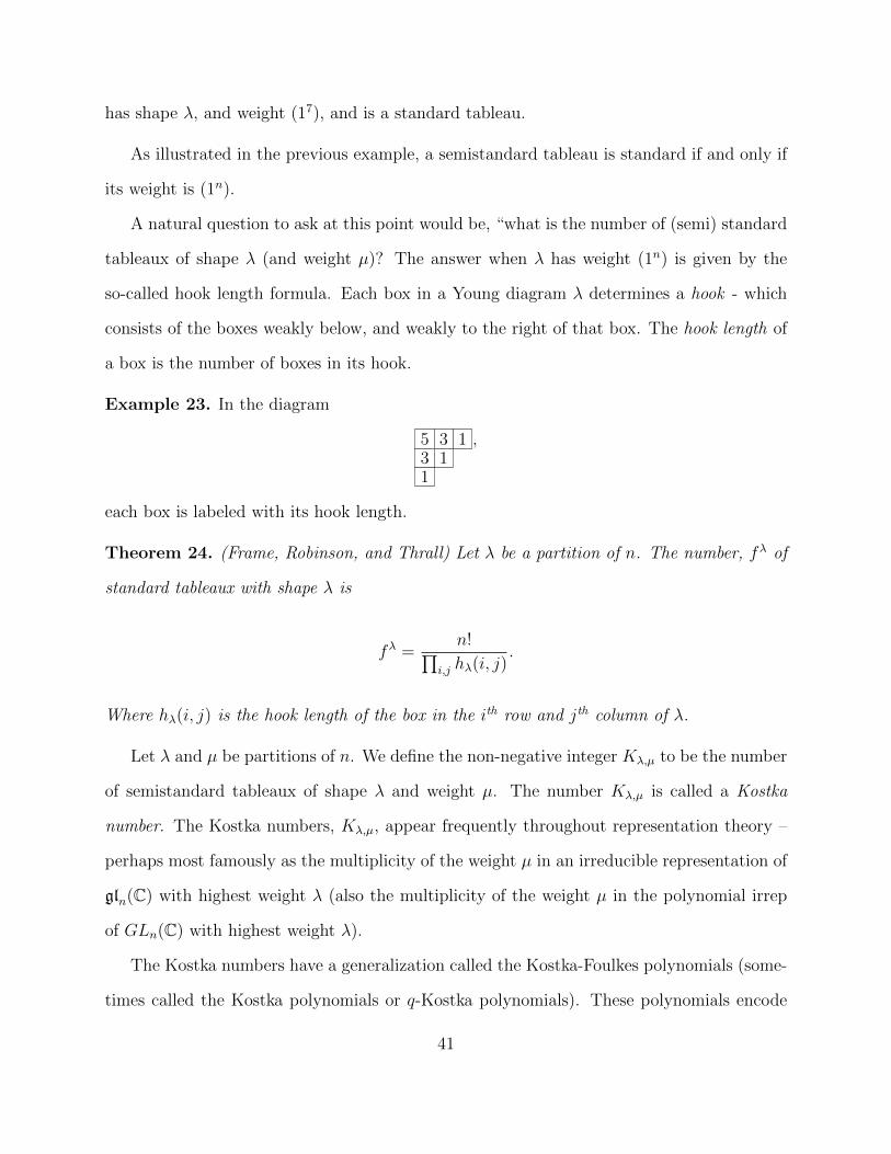
Example 23. In the diagram

5 3 13 11

,

each box is labeled with its hook length.

Theorem 24. (Frame, Robinson, and Thrall) Let λ be a partition of n. The number, fλ of

standard tableaux with shape λ is

fλ =n!∏

i,j hλ(i, j).

Where hλ(i, j) is the hook length of the box in the ith row and jth column of λ.

Let λ and µ be partitions of n. We define the non-negative integer Kλ,µ to be the number

of semistandard tableaux of shape λ and weight µ. The number Kλ,µ is called a Kostka

number. The Kostka numbers, Kλ,µ, appear frequently throughout representation theory –

perhaps most famously as the multiplicity of the weight µ in an irreducible representation of

gln(C) with highest weight λ (also the multiplicity of the weight µ in the polynomial irrep

of GLn(C) with highest weight λ).

The Kostka numbers have a generalization called the Kostka-Foulkes polynomials (some-

times called the Kostka polynomials or q-Kostka polynomials). These polynomials encode

41

information about the irreducible representations of the symmetric and general linear groups,

and relate the Gini index, as we know it, to representation theory. They are defined in terms

of the Schur polynomials, and Hall-Littlewood polynomials.

4.2 Schur Polynomials

Let λ be a partition of n with at most ` parts. The Schur polynomial, sλ(x1, . . . , x`), asso-

ciated to λ is defined as

sλ =∑T

xT ,

where the sum is over all semistandard tableaux T of shape λ using numbers from [`], and

the monomial xT is defined

xT =∏i=1

(xi)number of times i occurs in T .

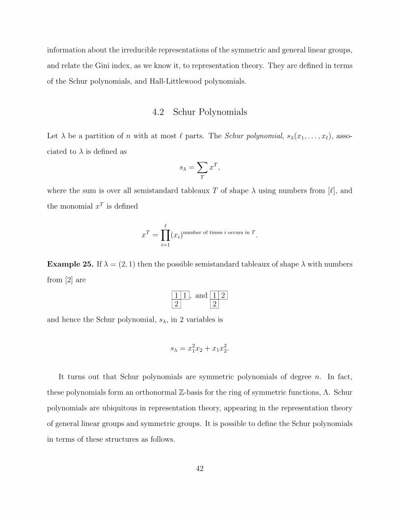
Example 25. If λ = (2, 1) then the possible semistandard tableaux of shape λ with numbers

from [2] are

1 12

, and 1 22

and hence the Schur polynomial, sλ, in 2 variables is

sλ = x21x2 + x1x22.

It turns out that Schur polynomials are symmetric polynomials of degree n. In fact,

these polynomials form an orthonormal Z-basis for the ring of symmetric functions, Λ. Schur

polynomials are ubiquitous in representation theory, appearing in the representation theory

of general linear groups and symmetric groups. It is possible to define the Schur polynomials

in terms of these structures as follows.

42

1. The Schur polynomials sλ, for λ ` n, are the images of the irreducible representations

of Sn under the Frobenius map.

2. The Schur polynomials sλ, for λ ` n, are the characters of the finite dimensional

irreducible (polynomial) representations of GLn(C).

For more on Schur functions, see [Ful97] chapters 7 and 8, or [Mac15] section 1.7.

4.3 Hall-Littlewood Polynomials

The Hall-Littlewood polynomials were originally defined to address a problem in group

theory. If G is a finite abelian p-group, then by the fundamental theory of finitely generated

abelian groups, G can be factored as

G =⊕i=1

Zpλi

where, without loss of generality, λ1 ≥ λ2 ≥ · · · ≥ λ` > 0. The partition λ = (λ1, . . . , λ`) is

called the type of G.

A family of symmetric polynomials called Hall polynomials (not to be confused with Hall-

Littlewood polynomials) arise from the following scenario. Given a finite abelian p-group G

of type λ, let Gλµ(1)...µ(k)

(p) denote the number of chains of subgroups

< 1 >= H0 / H1 / · · · / Hk = G

in G of type λ such that Hi/Hi+1 is of type µ(i), where the µ(i) are integer partitions for

1 ≤ i ≤ k ( [Mac15], [DLT94]). Hall formally introduced these numbers in [Hal57] and proved

several important results - among them was that Gλµ(1)···µ(`)(p) is a symmetric polynomial

in p. Moreover, the these polynomials can be used as the multiplication constants of a

commutative and associate algebra H called the Hall algebra. Littlewood found in [Lit61]

43

that the generators, uλ(p), of H (indexed by all partitions λ) are of the form

uλ(p) = pb(λ)Pλ(p−1),

where

b(λ) =∑i=1

(i− 1)λi,

` is the number of parts of λ, and the Pλ(q) are called the Hall-Littlewood polynomials. These

polynomials are defined by

Pλ(x1, . . . , xn; t) =

∏i≥0

m(i)∏j=1

1− ti

1− tj

∑σ∈Sn

σ

(xλ11 · · · xλnn

∏i<j

xi − txjxi − xj

),

where m(i) is the number of times that i occurs in λ. It turns out that the Hall-Littlewood

polynomials, like the Schur polynomials, are homogeneous symmetric functions of degree

|λ|, and form a Z-basis for Λ. They too, like the Schur polynomials, are ubiquitous in

representation theory, appearing in the character theory of finite linear groups, and projective

and modular representations of symmetric groups ( [DLT94] ).

4.4 Kostka Foulkes Polynomials

The monomial symmetric functions,

mλ =∑σ∈Sn

xσ(λ1)1 · · · xσ(λn)n ,

are yet another Z-basis for the ring of symmetric function, Λ. Moreover, since

Pλ(x1, . . . , xn; 0) = sλ(x1, . . . , xn),

44

and

Pλ(x1, . . . , xn; 1) = mλ(x1, . . . , xn),

we see that the Hall-Littlewood polynomials interpolate between the Schur polynomials and

the monomial symmetric functions. The entries of the transition matrix from mµ to sλ are

the Kostka numbers, Kλ,µ:

sλ =∑µ

Kλ,µmµ. (4.1)

The Kostka numbers can be generalized by substituting the Hall-Littlewood polynomials

into equation 4.1 as follows.

sλ =∑µ

Kλ,µ(t)Pµ(x1, . . . , xn; t)

Here, the Kλ,µ(t) are called the Kostka-Foulkes polynomials. It was conjectured by Foulkes

that the polynomials Kλ,µ(t) have non-negative integer coefficients. This was eventually

proven by Lascoux and Schutzenberger in [LS78] using the notion of the charge of a partition

– their result is now given.

Theorem 26. (Lascoux and Schutzenberger) Let λ and µ be partitions of an integer n.

1. Kλ,µ(t) =∑

T tc(T ), where the sum is over all semistandard tableaux T of shape λ and

weight µ.

2. If λ µ, then Kλ,µ(t) is monic of degree b(µ)− b(λ). If λ µ then Kλ,µ(t) = 0.

The function c in the theorem is a combinatorial statistic known as the charge of the

tableaux T . The charge statistic has a somewhat complicated definition, so we opt to explain

it through example.

Example 27. Let T be the tableaux of shape λ = (4, 2, 1) and weight µ = (3, 2, 1, 1) given

45

by

T = 1 1 1 22 43

.

First we form the reading word of T , which we denote by w(T ), by reading T from right to

left in consecutive rows, starting from the top.

w(T ) = 2111423

Next we find the standard subwords of T by finding the first 1 in w(T ), and underlining

it. Then we find the first 2 in w(T ) occurring to the right of the 1 that was underlined –

looping back to the beginning if necessary. Continuing in this fashion until one of each of

the numbers from 1 to `(µ) has been underlined (where `(µ) is the number of parts of µ).

w(T ) = 2111423

Removing the underlined numbers from w(T ) yields the first standard subword,

w1 = 1423.

To find the second standard subword, we perform the same procedure on the leftover num-

bers,

211,

which yields a second standard subword of

w2 = 21,

46

and a third standard subword of

w3 = 1.

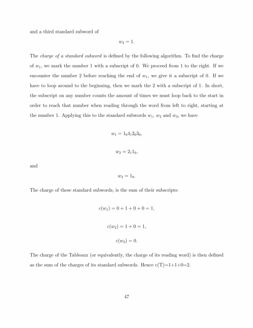
The charge of a standard subword is defined by the following algorithm. To find the charge

of w1, we mark the number 1 with a subscript of 0. We proceed from 1 to the right. If we

encounter the number 2 before reaching the end of w1, we give it a subscript of 0. If we

have to loop around to the beginning, then we mark the 2 with a subscript of 1. In short,

the subscript on any number counts the amount of times we must loop back to the start in

order to reach that number when reading through the word from left to right, starting at

the number 1. Applying this to the standard subwords w1, w2 and w3, we have

w1 = 10412030,

w2 = 2110,

and

w3 = 10.

The charge of these standard subwords, is the sum of their subscripts:

c(w1) = 0 + 1 + 0 + 0 = 1,

c(w2) = 1 + 0 = 1,

c(w3) = 0.

The charge of the Tableaux (or equivalently, the charge of its reading word) is then defined

as the sum of the charges of its standard subwords. Hence c(T)=1+1+0=2.

47

4.5 The Degree of Kλ,µ(t)

Let n, k ∈ N and let λ be a partition of nk into at most n parts. Recall that the Gini index

gnk,n of λ is given by

gnk,n(λ) = b((kn))− b(λ),

where b(λ) =∑n

i=1(i− 1)λi, and (kn) = (k, k, . . . , k) is the so-called “flat” partition.

Since λ (kn), for all partitions λ of nk with at most n parts, by the theorem of Lascoux

and Schutzenberger, we have

Corollary 28. The Kostka-Foulkes polynomial Kλ,(kn)(t) is monic of degree gnk,n(λ). More-

over

gnk,n(λ) = max c(T ) : T is a semistandard tableaux of shape λ and weight (kn) .

The Kostka-Foulkes polynomials encode information about the irreducible representa-

tions of the symmetric and general linear groups, and therefore Corollary 28 frames the Gini

index within the context of representation theory. We will elaborate on, and explore these

connections in the subsequent chapters.

48

5 The Gini Index and Complex Reflection Groups

Let n be a positive integer and λ a partition of n. For each Specht module Sλ (an irreducible

representation of Sn) there is a special polynomial called the “graded multiplicity” of Sλ in

the coinvariants, which encodes how the coinvariant ring of Sn decomposes with respect to

Sλ. It turns out that the Kostka-Foulkes polynomial Kλ,(1n) is the graded multiplicity of Sλ

in the coinvariants. We will see that the degrees of the graded multiplicity polynomials of

Sn are exactly the values of the Gini index g (= gn,n) on Pn.

The symmetric group is a member of a broader family of finite groups known as “complex

reflection groups”. Using graded multiplicity polynomials, we will extend the notion of the

Gini index to all other complex reflection groups, and provide formulas for the Gini index

for dihedral groups.

5.1 The Symmetric Group

Let n be a positive integer and V ∼= Cn be the defining representation of Sn, and fix a basis

x1, x2, . . . , xn for V . In other words, if x denotes the column vector (x1, x2, . . . , xn)t, then Sn

acts on V by

σx = (xσ(1), xσ(2), . . . , xσ(n))t,

where σ ∈ Sn. By C[V ] we mean the ring of polynomials C[V ] ∼= C[x1, x2, . . . , xn], obtained

by treating each basis vector as an indeterminant. If f ∈ C[V ], then we can define an action

of Sn on C[V ] by

(σf)(x) = f(σx).

This action turns C[V ] into an infinite dimensional representation of Sn. Since every poly-

nomial in C[V ] is a finite sum of homogeneous monomials, as a vector space, C[V ] admits

49

the gradation

C[V ] =⊕d≥0

C[V ]d,

where C[V ]d = f ∈ C[V ] : f is a homogeneous polynomial of degree d. Thus we say that

C[V ] is a graded representation of Sn. Note that each graded component is a finite dimen-

sional Sn-representation, with basis given by the collection of all monomials in x1, . . . , xn of

total degree d.

A polynomial f ∈ C[V ] is called symmetric if

σf = f

for all σ ∈ Sn. The collection of all symmetric polynomials in C[V ] forms a subring of C[V ]

called the ring of symmetric polynomials in n-variables, which we denote by Λn. That is,

Λn = f ∈ C[V ] : σf = f for all σ ∈ Sn.

The symmetric polynomials are generated (as a C-algebra) by the power sum symetric

polynomials p1, . . . , pn, where

pi = xi1 + xi2 + · · ·+ xin.

In other words,

Λn∼= C[p1, . . . , pn].

The ring of coinvariants of Sn is the quotient ring

C[V ]Sn = C[V ]/(p1, . . . , pn)

by the ideal generated by the symmetric polynomials with no constant term. The ring of

50

symmetric polynomials and the coinvariant ring are also graded representations of Sn, and

are similarly graded by homogeneous degree:

Λn =⊕d≥0

Λdn, and

C[V ]Sn =⊕d≥0

C[V ]dSn ,

where Λdn = Λn∩C[V ]d, and C[V ]dSn = C[V ]Sn ∩C[V ]d. The graded components of these rep-

resentations are finite dimensional representations of Sn, and therefore decompose into finite

direct sums of irreducible representations. What makes the coinvariant ring of particular

interest, is that it is a graded representation that is isomorphic to the regular representation

of Sn [Sta79]. This fact will be important when defining the Gini index of an irreducible

representation of Sn.

An interesting question one might ask at this point is, “how do the graded components

of the coinvariant ring decompose into sums of irreducible representations?” To address

this question, we recall that the irreducible representations of the symmetric group Sn are

indexed by the partitions of n, and unlike most other finite groups, there is a canonical way

to index them using Specht Modules (as seen in Chapter 2). Under this identification, the

partition (n) indexes the trivial representation and (1n) indexes the sign representation.

Let λ be a partition of n, and let Sλ be the corresponding irreducible representation

(Specht module) indexed by λ. Denote by [Sλ : C[V ]dSn ] the multiplicity of Sλ in the

homogeneous degree d coinvariants of Sn. The graded multiplicity polynomial of Sλ in the

coinvariant ring is defined by

pλ(t) =∑d≥0

[Sλ : C[V ]dSn ]td.

It has been known for some time (a result likely due to Frobenius) that the graded

51

multiplicities of the symmetric group are exactly the Kostka-Foulkes polynomials ( [DLT94]).

Theorem 29. Let λ be a partition of n indexing a irreducible representation Sλ of Sn (in

the usual way). Then

pλ(t) = Kλ,(1n)(t)

By applying Theorem 26, we obtain the following corollary which frames the “ordinary”

Gini index, g, within the context of the representation theory of the Symmetric group.

Corollary 30. Let λ be a partition of n indexing a irreducible representation Sλ of Sn. The

Gini index of Sλ, gSn(Sλ), is the degree of the graded multiplicity polynomial pλ(t) of Sλ.

Moreover, gSn(Sλ) = g(λ).

We see here that, for the symmetric group, the degree of the graded multiplicity poly-

nomial pλ yields the Gini index of the conjugate partition λ. We accommodate for this

by asserting that the Gini index of a irreducible representation Sλ of the Symmetric group

Sn is the degree of the graded multiplicity polynomial pλ. This adjustment is to force the

Gini index of the partition λ to equal that of the irreducible representation Sλ. Since their

irreducible representations do not have a canonical indexing, we will not encounter these

difficulties when defining the Gini index for other complex reflection groups.

At this point the relationship between the degree of the graded multiplicity polynomial

and the Gini index may appear a bit forced. In the next chapter, we will see that this trend

grows even stronger when we consider the graded multiplicities of irreducible representations

of linear algebraic groups.

5.2 Examples for Sn

Example 31. The Gini indices of S3 irreps.

52

The symmetric group S3 acts on C3 by permuting coordinates, and therefore acts on

C[x1, x2, x3]. The symmetric polynomials in 3 variables, Λ3, are generated by the power sum

polynomials:

Λ3 = C[x1 + x2 + x3, x21 + x22 + x23, x

31 + x32 + x33].

The partitions of n = 3 are

(1, 1, 1), (2, 1), and (3).

These correspond to the sign representation, standard representation, and trivial represen-

tation, respectively. The standard tableaux of shape λ, for all λ ` 3 are

Standard tableaux of (1, 1, 1) : T1 = 123

,

Standard tableaux of (2, 1) : T2 = 1 23

, T3 = 1 32

, and

Standard tableaux of (3) : T4 = 3 2 1 .

The charge statistics of these tableaux are 0, 2, 1, and 3, respectively. By Theorem 26, the

corresponding Kostka-Foulkes polynomials are

K(1,1,1),(13)(t) = 1,

K(2,1),(13)(t) = t2 + t, and

K(3),(13)(t) = t3.

53

By Corollary 30 we find that the Gini indices of the irreducible representations of S3 are

gS3(S(1,1,1)) = deg(p(3)(t)) = deg(K(13),(13)(t)) = 0,

gS3(S(2,1)) = deg(p(2,1)(t)) = deg(K(2,1),(13)(t)) = 2, and

gS3(S(3)) = deg(p(1,1,1)(t)) = deg(K(3),(13)(t)) = 3.

Comparing these values to the “ordinary” Gini indices of

g((1, 1, 1)) = 0,

g((2, 1)) = 2, and

g((3)) = 3,

we find, as desired, that they are equal.

Example 32. The Gini indices of S4 irreps. The partitions of n = 4 are

(1, 1, 1, 1), (2, 1, 1), (2, 2) (3, 1), and (4).

These label the irreducible representations of S4 as follows

S(1,1,1,1) = The sign representation,

S(2,1,1) = The standard representation,

S(2,2) = (No name),

S(3,1) = sign ⊗ standard, and

S(4) = The trivial representation.

The standard tableaux of shape λ (for all λ ` 4), and their corresponding charge statistics

54

are given in figure 5.1.

λ = (1, 1, 1, 1) : 1234

charge = 0

λ = (2, 1, 1) : 1 234

charge = 3, 1 324

charge = 2, 1 423

charge = 1

λ = (2, 2) : 1 23 4

charge = 4, 1 32 4

charge = 2

λ = (3, 1) : 1 2 34

charge = 5, 1 2 43

charge = 4, 1 3 42

charge = 3

λ = (4) : 1 2 3 4 charge = 6

Figure 5.1: Standard tableaux of shapes λ ` 4 and their charge statistics.

By Theorem 26, the corresponding Kostka-Foulkes polynomials are

K(14),(14)(t) = 1,

K(2,1,1),(14)(t) = t3 + t2 + t,

K(2,2),(14)(t) = t4 + t2,

K(3,1),(14)(t) = t5 + t4 + t3, and

K(4),(q4)(t) = t6.

55

By Corollary 30 we find that the Gini indices of the irreducible representations of S4 are

gS4(S(14)) = deg(p(4)(t)) = deg(K(14),(14)(t)) = 0

gS4(S(2,1,1)) = deg(p(3,1)(t)) = deg(K(2,1,1),(14)(t)) = 3

gS4(S(2,2)) = deg(p(2,2)(t)) = deg(K(2,2),(14)(t)) = 4

gS4(S(3,1)) = deg(p(2,1,1)(t)) = K(3,1),(14)(t) = 5, and

gS4(S(4)) = deg(p(14)(t)) = deg(K(4),(q4)(t)) = 6.

Comparing these values to the “ordinary” Gini indices of

g((1, 1, 1, 1)) = 0,

g((2, 1, 1)) = 3,

g((2, 2)) = 4,

g((3, 1)) = 5, and

g((4)) = 6.

we find, as desired, that they are equal.

5.3 Invariants of Complex Reflection Groups

One might wonder whether the structures in the Section 5.1 occur similarly for other finite

groups. This is not the true in general, as the results of Section 5.1 relied heavily on the

fact that every polynomial can be uniquely written as a finite sum of symmetric polynomials

multiplied by co-invariant polynomials. That is, there is an isomorphism

Λn ⊗ C[V ]Sn −→ C[x1, . . . , xn].

56

This behavior can be attributed to the fact that the ring of symmetric polynomials is a

finitely generated polynomial ring. Without this additional structure, the invariant ring

C[V ]G is quite difficult to understand. It was shown by Shephard and Todd in [ST54]

that the finite groups whose invariant ring has such a structure are precisely the so-called

“complex reflection groups”.

A linear transformation r ∈ GLn(C) is called a complex reflection if r has finite order

and r fixes a complex hyperplane (a co-dimension 1 subspace of Cn) pointwise. A complex

reflection group, G, is a finite subgroup of GLn(C) that is generated by complex reflections.

Let G be any finite group acting on a finite dimensional complex vector space V . Let

x1, x2, . . . , xn be a basis for V , and let x = (x1, . . . , xn)t be the column vector of basis

elements. Just as with the symmetric group, we can extend the action of G on V to an

action on C[V ] = C[x1, . . . , xn] by defining

(gf)(x) = f(gx),

for any g ∈ G and f ∈ C[V ]. Then C[V ] is an infinite dimensional graded representation of

G, and is graded by homogeneous degree. An element f ∈ C[V ] is called an invariant of G

(or a “G-invariant”) if

gf = f,

for all g ∈ G. The collection of all invariants of G is a ring, and is called the invariant ring

of G; for this we will use the notation

C[V ]G = f ∈ C[V ] : gf = f for all g ∈ G.

The aforementioned result due to Shephard and Todd, and later expanded by Chevalley

in [Che55], is now presented.

57

Theorem 33. (Shephard-Todd-Chevalley Theorem) Let V be a finite dimensional complex

vector space, and let G be a finite subgroup of GL(V ). The following are equivalent:

1. G is a complex reflection group.

2. There are ` algebraically independent non-constant homogeneous polynomials f1, f2, . . . , f` ∈

C[V ] such that

C[V ]G = C[f1, . . . , f`], and

|G| = deg(f1) · deg(f2) · · · · · deg(f`).

Shephard and Todd proved this result by deriving a full classification of such groups.

The complex reflection groups consist of 34 exceptional groups, and three infinite families;

the symmetric, cyclic, and “imprimitive” groups - the last of which contains the dihedral

groups, which we will examine in detail later in this chapter.

5.4 Graded Multiplicities and the Gini Index

Let V be a n-dimensional complex vector space with fixed basis x1, . . . , xn, G ⊆ GL(V ) a

complex reflection group, and C[V ]G = C[f1, . . . , f`] the invariant ring of G. The coinvariant

ring of G is quotient ring

C[V ]G = C[V ]/(f1, . . . , f`)

by the ideal generated by the invariant ring generators. As was the case with the sym-

metric group, the invariant ring and coinvariant ring of a complex reflection group G are

graded representations of G. Furthermore, the coinvariant ring is isomorphic to the regular

representation of G. Let

C[V ]G =⊕d≥0

C[V ]dG

58

be the gradation of the coinvariant ring of G by homogeneous degree d, where

C[V ]dG = f ∈ C[V ]G : f is homogeneous of degree d.

Let V λ be an irreducible representation of G indexed by an irreducible character λ of G.

Denote by [V λ : C[V ]dG] the multiplicity of V λ in the homogeneous degree d coinvariants of

G. The graded multiplicity polynomial of V λ is defined by

pλ(t) =∑d≥0

[V λ : C[V ]dG]td.

In [Sta79], Stanley proved that the graded multiplicity of a irreducible representation can be

calculated using Molien’s Theorem as follows.

Theorem 34. (Stanley) Let f1, . . . , f` be the generators of C[V ]G, where G ⊆ GL(V ) is a

complex reflection group, and set di = deg(fi). Let λ be an irreducible character of G, and

let V λ be the corresponding irreducible representation. The graded multiplicity of V λ is given

by

pλ(t) =1

|G|∏i=1

(1− tdi)∑T∈G

λ(T )

det(I − tT ).

We define the Gini index of an irreducible representation of a complex reflection group as

follows. If G is the symmetric group Sn, then the Gini index of a irreducible representation

Sλ (indexed by the partition λ ` n) is, as before, the degree of the graded multiplicity

polynomial of the “conjugate” representation:

gSn(Sλ) = deg(pλ(t)) = deg(Kλ,(1n)(t)).

If G is any other complex reflection group, we define the Gini index of an irreducible repre-

59

sentation V λ (indexed by an irreducible character λ) by

gG(V λ) = deg(pλ(t))

The conjugation performed when calculating the Gini index of a irreducible representation

of Sn is necessary, as (unlike most other finite groups) the irreducible representations of Sn

have an accepted standard indexing, and we want gSn to agree with the Gini index defined

on the index set Pn. No adjustments are necessary for other complex reflection groups, as

the indexing of their irreducible representations is not standardized.

Recall that the coinvariant ring C[V ]G of a complex reflection group G is isomorphic

to the regular representation of G; that is, the representation of G acting on itself by left

translations. The regular representation of a finite group G always decomposes as the direct

sum of irreducible representations

⊕λ∈G

(V λ)dim(V λ)

,

where each irreducible representation V λ of G occurs with multiplicity equal to its dimension.

in other words, every irreducible representation of G occurs in the decomposition of the

regular representation of G, and therefore occurs in the decomposition of the coinvariant

ring of G. Thus the Gini index gG is well defined.

5.5 The Gini Index of an Irreducible Representation of the Dihedral Group

Let n ≥ 3. The dihedral group D2n of order 2n is an example of a complex reflection group,

and belongs the infinite family of “imprimitive” complex reflection groups. We will describe

the irreducible characters of D2n and fix an indexing for these characters. We will then

apply Stanley’s theorem to determine formulas for the Gini index gD2n , based on our choice

60

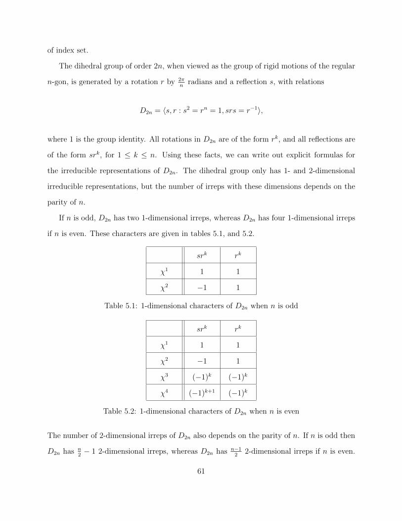
of index set.

The dihedral group of order 2n, when viewed as the group of rigid motions of the regular

n-gon, is generated by a rotation r by 2πn

radians and a reflection s, with relations

D2n = 〈s, r : s2 = rn = 1, srs = r−1〉,

where 1 is the group identity. All rotations in D2n are of the form rk, and all reflections are

of the form srk, for 1 ≤ k ≤ n. Using these facts, we can write out explicit formulas for

the irreducible representations of D2n. The dihedral group only has 1- and 2-dimensional

irreducible representations, but the number of irreps with these dimensions depends on the

parity of n.

If n is odd, D2n has two 1-dimensional irreps, whereas D2n has four 1-dimensional irreps

if n is even. These characters are given in tables 5.1, and 5.2.

srk rk

χ1 1 1

χ2 −1 1

Table 5.1: 1-dimensional characters of D2n when n is odd

srk rk

χ1 1 1

χ2 −1 1

χ3 (−1)k (−1)k

χ4 (−1)k+1 (−1)k

Table 5.2: 1-dimensional characters of D2n when n is even

The number of 2-dimensional irreps of D2n also depends on the parity of n. If n is odd then

D2n has n2− 1 2-dimensional irreps, whereas D2n has n−1

22-dimensional irreps if n is even.

61

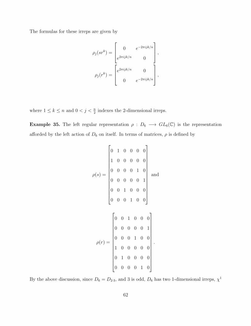
The formulas for these irreps are given by

ρj(srk) =

0 e−2πijk/n

e2πijk/n 0

,ρj(r

k) =

e2πijk/n 0

0 e−2πijk/n

,

where 1 ≤ k ≤ n and 0 < j < n2

indexes the 2-dimensional irreps.

Example 35. The left regular representation ρ : D6 −→ GL6(C) is the representation

afforded by the left action of D6 on itself. In terms of matrices, ρ is defined by

ρ(s) =

0 1 0 0 0 0

1 0 0 0 0 0

0 0 0 0 1 0

0 0 0 0 0 1

0 0 1 0 0 0

0 0 0 1 0 0

and

ρ(r) =

0 0 1 0 0 0

0 0 0 0 0 1

0 0 0 1 0 0

1 0 0 0 0 0

0 1 0 0 0 0

0 0 0 0 1 0

.

By the above discussion, since D6 = D2·3, and 3 is odd, D6 has two 1-dimensional irreps, χ1

62

and χ2, and one 2-dimensional irrep, ρ1. The left regular representation ρ is 6-dimensional,

and decomposes as

ρ = χ1 ⊕ χ2 ⊕ 2ρ1.

Each irreducible representation appears in the decomposition of ρ with multiplicity equal to

its dimension, which is true for the left regular representation of any finite group.

To determine formulas for the graded multiplicity polynomials of D2n, we represent D2n

as a subgroup of a general linear group GL2(C) via the (faithful) representation ρ1. Under

this identification we see that the reflections and rotations of D2n are respectively given by

the matrices

srk =

0 e−2πik/n

e2πik/n 0

and

rk =

e2πik/n 0

0 e−2πik/n

.The polynomials

f1(x1, x2) = x1x2 and

f2(x1, x2) = xn1 + xn2

are algebraically independent, and are also invariants of D2n. Moreover, since

deg(f1) · deg(f2) = 2n,

by the Shephard-Todd-Chevalley theorem, these polynomials generate the ring of invariants

of D2n. That is,

C[x1, x2]D2n = C[f1, f2].

We will now apply Stanley’s theorem to the dihedral group to acquire formulas for the

63

graded multiplicity polynomials, and in turn, the Gini index gD2n .

Let n ≥ 3. D2n has at least two 1-dimensional irreducible representations, χ1 and χ2.

Since these representations are 1-dimensional, they are the same as their characters, and we

may apply Stanley’s theorem directly to find their graded multiplicity polynomials:

pχ1(t) =(1− t2)(1− tn)

2n

∑T∈D2n

1

det(I − tT )

=(1− t2)(1− tn)

2n

n∑k=1

(1

(1− t2)+

1

(1− tωk)(1− tω−k)

)=

(1− tn)

2+

1

2n

n∑k=1

(1− t2)(1− tn)

(1− tωk)(1− tω−k)

=(1− tn)

2+

(1 + tn)

2

= 1,

where ω = e2πi/n. Similarly, we find that

pχ2(t) = tn,

and if n is even,

pχ3(t) = tn/2, and

pχ4(t) = tn/2.

To determine the graded multiplicity polynomials of the 2-dimensional irreps ρj, we first

calculate their characters χj:

χj(srk) = 0 and

χj(rk) = 2 cos(2πjk/n),

64

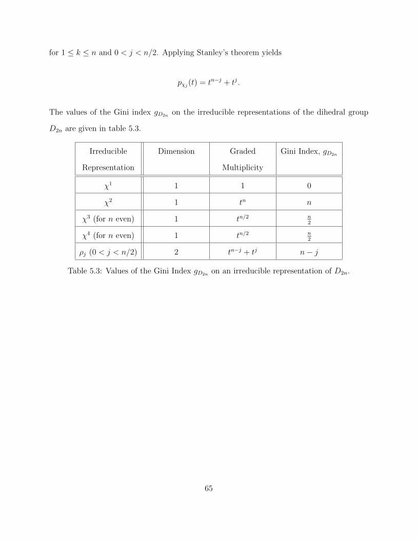
for 1 ≤ k ≤ n and 0 < j < n/2. Applying Stanley’s theorem yields

pχj(t) = tn−j + tj.

The values of the Gini index gD2n on the irreducible representations of the dihedral group

D2n are given in table 5.3.

Irreducible

Representation

Dimension Graded

Multiplicity

Gini Index, gD2n

χ1 1 1 0

χ2 1 tn n

χ3 (for n even) 1 tn/2 n2

χ4 (for n even) 1 tn/2 n2

ρj (0 < j < n/2) 2 tn−j + tj n− j

Table 5.3: Values of the Gini Index gD2n on an irreducible representation of D2n.

65

6 The Gini Index and Connected Reductive Linear Algebraic Groups

Let n and k be positive integers, and let α be a decreasing sequence of n integers. Such

sequences index the irreducible rational representations, V α, of GLn(C). As was the case

with complex reflection groups, GLn(C) has certain graded representations of invariants

and harmonics that exhibit special properties. To the representation V α we associate a

polynomial, pα, which is again called the “graded multiplicity” of V α in the harmonics. To

the sequence α there is also an associated pair of partitions λ and µ of nk, and it turns out

that the Kostka-Foulkes polynomial Kλ,µ is the graded multiplicity of V α in the harmonics.

We will see that the degrees of the graded multiplicity polynomials pα are exactly the values

of the Gini index gnk,n on Pnk.

The general linear group is the principle example of a connected reductive linear algebraic

group. Using graded multiplicities, we will extend the notion of the Gini index to all other

connected reductive linear algebraic groups.

6.1 Harmonics of Connected Reductive Linear Algebraic Groups

Let G be a connected reductive linear algebraic group over C. The general linear group

belongs to this family, as does any semisimple linear algebraic group. Let V be a n-

dimensional rational representation of G, and choose a basis x1, x2, . . . , xn for V . Let

C[V ] = C[x1, x2, . . . , xn] denote the algebra of polynomial functions on V . This algebra

is a infinite dimensional graded representation of G with gradation

C[V ] =⊕d≥0

C[V ]d,

where C[V ]d is the vector space of homogeneous degree d polynomials in C[V ]. Just as we

defined the invariant and coinvariant rings of a complex reflection group, we can define the

66

invariant and coinvariant rings of a linear algebraic group G. Let

C[V ]G = f ∈ C[V ] : gf = f for all g ∈ G

be the ring of G-invariant polynomials in C[V ]. The coinvariant ring of G is the quotient

C[V ]G = C[V ]/C[V ]G+,

of the full polynomial ring by the ideal C[V ]G+ of G-invariant polynomials without constant

term. When discussing the coinvariants of a linear algebraic group it is more common to

define them in terms of G-harmonic functions.

Let ∂i = ∂∂xi

and, for f ∈ C[V ], define

f(∂) = f(∂1, ∂2, . . . , ∂n).

The constant coefficient differential operators on C[V ] is the set

D(V ) = f(∂) : f ∈ C[V ].

Denote by D[V ]+ the set of differential operators without constant term, and by D[V ]G+ the

set of G-invariant differential operators with no constant term. The module of G-harmonic

polynomials defined as

H(V ) = f ∈ C[V ] : ∆f = 0 for all ∆ ∈ D(V )G+.

The G-harmonic functions, and G-coinvariants are isomorphic as graded representations of

67

G, and are graded by homogeneous degree:

H(V ) =⊕d≥0

Hd(V ),

where Hd(V ) = H(V ) ∩ C[V ]d. This fact is non-trivial, since it says that if a function is

harmonic, then so are its homogeneous components. In general, every polynomial function

can be expressed as a sum of G-invariant functions multiplied by G-harmonic functions. In

other words, there is a surjection

C[V ]G ⊗H(V ) −→ C[V ] −→ 0

obtained by linearly extending multiplication. This corresponds to the separation of vari-

ables that one does when studying the Laplace operator in two dimensions. The two tensor

components correspond to the decomposition into radial and spherical parts, respectively.

A guiding question in the study of G-harmonic functions was (and is), “When is the above

map an isomorphism?” That is, when is the sum of products of invariants and harmonics

unique? Equivalently, when is C[V ] a free module over C[V ]G? This question was partially

answered by Kostant in his pivotal 1963 paper Lie group representations on polynomials

rings (see [Kos63]).

Let g denote the Lie algebra of G, and let Ad : G −→ GL(g) denote the Adjoint

representation of G, defined by

(Adx)(A) = xAx−1,

for x ∈ G and A ∈ g. Among the many results in [Kos63], Kostant proved that C[g] is a free

module over C[g]G, for any connected reductive group G.

68

6.2 Graded Multiplicities and the Gini Index

Let G be a connected reductive linear algebraic group, and let g be the Lie algebra of G. Let

H(g) be the infinite-dimensional module of G-harmonic functions. The graded components

of H(g) are all finite dimensional, and since G is reductive, Hd(g) is completely reducible,

for each d ≥ 0. Given a dominant weight α ∈ P++(G) of G, what is the multiplicity,

[V α : Hd(g)] =?,

of V α in Hd(g), where V α is the irreducible rational representation of G with highest weight

α. A natural thing to do, as in Chapter 5, is consider the, indeed, polynomial defined by the

series

pα(t) =∑d≥0

[V α : Hd(g)]td,

which is called the graded multiplicity of V α in the G-harmonic functions. These polynomials

extract deep information in representation theory, but outside of Kostant’s setting, very little

is known about them. Hesselink showed in [Hes80] that if G is semisimple, then pα(t) can

be expressed as an alternating sum in terms of Kostant’s partition function. In particular,

if g is of Lie type A, then Hesselink’s alternating sum formula shows that pα(t) is equal to

a Kostka-Foulkes polynomial Kλ,µ(t), where λ and µ are integer partitions that depend (to

a certain extent) on α. This case is explored in the next section.

Kostant defined the generalized exponents of V α to be the exponents e1, e2, . . . , es of the

nonzero terms in the graded multiplicity,

pα(t) =∑d≥0

[V α : Hd(g)]td =s∑i=1

citei ,

of V α in the G-harmonic functions. Due to the connections between pα(t) and the Kostka-

69

Foulkes polynomials in Lie type A, we define the Gini index gG(V α) of an irreducible rational

representation of G as the maximum of the generalized exponents,

gG(V α) = maxe1, . . . , es,

or equivalently, as the degree of the graded multiplicity of V α in the G-harmonic functions,

gG(V α) = deg(pα(t)).

Unlike the case of complex reflection groups, not every irreducible rational representation of

G occurs in the decomposition of the harmonics. So that gG is well defined, we will adopt

the convention that the degree of the zero polynomial is −∞. Thus if V α is an irreducible

rational representation of G, and pα(t) = 0, the Gini index is

gG(V α) = −∞.

We will see in the following section that if G = GLn(C) and V α is an irreducible polyno-

mial representation of G, then the Gini index gGLn(C)(Vα) is given by the Gini index gnk,n(λ),

for a certain partition λ of nk.

70

6.3 The Gini index of an irreducible representation of GLn(C)

As seen in Chapter 2, the highest weights of the irreducible rational representations of

GLn(C) are canonically indexed by the set of n-tuples of non-increasing integers. Let α =

(α1, α2, . . . , αn) and β = (β1, β2, . . . , βn) be two dominant weights of GLn(C). The sum α+β

is defined as a sum of vectors

α + β = (α1 + β1, α2 + β2, . . . , αn + βn).

The dominant weights of GLn(C) are equipped with a equivalence relation, under which

equivalent weights yield isomorphic highest weight representations. Two dominant weights,

α and β, are equivalent if there is a positive integer k such that

α = β + (kn),

where (kn) = (k, k, . . . , k) is the so-called “flat” partition of nk containing n values of k.

Let α = (α1, α2, . . . , αn) be a non-zero dominant weight of GLn(C) such that

α1 + α2 + · · ·+ αn = 0.

As α is non-zero, the last term, αn, in α is always negative. Let k be an integer with

k ≥ −αn, and define

λ = α + (kn).

Then λ is a partition of nk with at most n parts. If k = −αn, then λn = 0 so λ is a partition

of nk with at most n− 1 parts. The weights λ and α are both dominant weights of GLn(C),

and are equivalent; hence the corresponding irreducible highest weight representations V λ

and V α are isomorphic.

71

Let α be a dominant weight of GLn(C). When does the irreducible representation V α

of GLn(C) of highest weight α appear in the graded decomposition of the harmonics of

GLn(C)? That is, when is the graded multiplicity polynomial pV α(t) nonzero? The answer,

due to Kostant, is that the only irreducible highest weight representations of GLn(C) with

positive multiplicity in H(g) are those with highest weights that sum to zero (c.f. [Kos63]).

Combining this fact with the details of the above discussion yields the following theorem

(originally shown in [DLT94]):

Theorem 36. Let V α be an irreducible representation of GLn(C) with highest weight α ∈ Zn

such that α1 ≥ · · · ≥ αn.

1. If α1 + . . .+ αn 6= 0, then pV α(t) = 0.

2. If α1 + . . .+ αn = 0, then

pV α(t) = Kλ,(kn)(t),

where k ≥ |αn|, and λ = α + (kn).

We then obtain the following corrolary, which characterizes the Gini index gGLn(C) on the

irreducible representations of GLn(C).

Corollary 37. Let V α be a irreducible representation of GLn(C) with highest weight α ∈ Zn

such that α1 ≥ · · · ≥ αn.

• If α1 + · · ·+ αn 6= 0, then

gGLn(C)(Vα) = −∞.

• If α1 + · · ·+ αn = 0, then

gGLn(C)(Vα) = deg(Kλ,(kn)(t)),

72

where k ≥ |αn| and λ = α + (kn).

By Theorem 26, we see that if α1 + · · ·+ αn = 0, then

gGLn(C)(Vα) = b((kn))− b(λ)

= gnk,n(λ).

In other words, if we disregard the irreducible representations whose highest weight α has

nonzero sum, the Gini index for GLn(C) is precisely the Gini index gnk,n defined on the set

of partitions of nk with at most n parts. Since the choice of k ≥ |αn| in theorem 37 was

immaterial, we obtain the following Corollary on the Gini index on partitions of nk with at

most n parts:

Corollary 38. Let n, and k be positive integers, and let λ be a partition of nk with at most

n parts. Let j ≥ k, and define

µ = λ− (kn) + (jn).

Then µ is a partition of nj with at most n parts, and

gnk,n(λ) = gnj,n(µ).

Example 39. To illustrate Corollary 38, suppose we have two populations of n = 5 people.

Amongst the first population is distributed nk = 15 dollars so that two people have 5 dollars

each, two have 2 dollars each, and one person has 1 dollar. That is, the first distribution

corresponds to the partition

λ = (5, 5, 2, 2, 1).

73

Amongst the second population suppose there is distributed nj = 25 dollars in a fashion

corresponding to the partition

µ = (7, 7, 4, 4, 3)

Then the Gini indices of these distributions are

g15,5(λ) = b((35))− b(λ) = 11, and

g25,5(µ) = b((55))− b(µ) = 11.

The reasons for this equality become obvious when we look at the graphs of the Lorenz

curves of λ and µ, which are given in figures 6.1 and 6.2, respectively.

The Lorenz curve of µ is simply that of λ translated up 2-units. But that translation

increases the amount of money in circulation, and results in the line of equality also being

translated up 2-units — leaving the Gini index invariant.

74

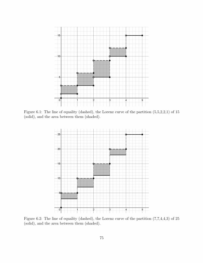
Figure 6.1: The line of equality (dashed), the Lorenz curve of the partition (5,5,2,2,1) of 15(solid), and the area between them (shaded).

Figure 6.2: The line of equality (dashed), the Lorenz curve of the partition (7,7,4,4,3) of 25(solid), and the area between them (shaded).

75

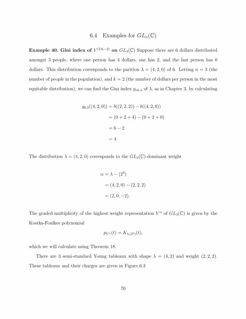
6.4 Examples for GLn(C)

Example 40. Gini index of V (2,0,−2) on GL3(C) Suppose there are 6 dollars distributed

amongst 3 people, where one person has 4 dollars, one has 2, and the last person has 0

dollars. This distribution corresponds to the parition λ = (4, 2, 0) of 6. Letting n = 3 (the

number of people in the population), and k = 2 (the number of dollars per person in the most

equitable distribution), we can find the Gini index gnk,n of λ, as in Chapter 3, by calculating

g6,3((4, 2, 0)) = b((2, 2, 2))− b((4, 2, 0))

= (0 + 2 + 4)− (0 + 2 + 0)

= 6− 2

= 4.

The distribution λ = (4, 2, 0) corresponds to the GL3(C)-dominant weight

α = λ− (23)

= (4, 2, 0)− (2, 2, 2)

= (2, 0,−2).

The graded multiplicity of the highest weight representation V α of GL3(C) is given by the

Kostka-Foulkes polynomial

pV α(t) = Kλ,(23)(t),

which we will calculate using Theorem 18.

There are 3 semi-standard Young tableaux with shape λ = (4, 2) and weight (2, 2, 2).

These tableaux and their charges are given in Figure 6.3

76

1 1 2 23 3

, charge = 4

1 1 3 32 2

, charge = 3

1 1 2 32 3

, charge = 2

Figure 6.3: Semi-standard Young tableaux with shape (4, 2) and weight (23), and theircorresponding charges.

Thus the Kostka-Foulkes polynomial (and graded multiplicity of V α) is

pV α(t) = Kλ,(23)(t) = t4 + t3 + t2.

Therefore, the Gini index of V α is

gGL3(C)(Vα) = deg(pV α(t)) = 4,

and we see that g6,3(λ) = gGL3(C)(Vα).

Example 41. Gini index of V (2,1,0,−3) on GL4(C). Suppose there are 4 people in a

population, amongst whom is distributed 12 dollars, where one person has 5 dollars, one

has 4, one has 3 dollars, and the last has 0. This distribution corresponds to the partition

λ = (5, 4, 3, 0) of 12. Letting n = 4 (the number of people in the population), and k = 3

(the number of dollars per person in the most equitable distribution), we can find the Gini

77

index gnk,n of λ, as in Chapter 3, by calculating

g12,4((5, 4, 3, 0)) = b((3, 3, 3, 3))− b((5, 4, 3, 0))

= (0 + 3 + 6 + 9)− (0 + 4 + 6 + 0)

= 18− 8

= 8.

The distribution λ = (4, 4, 3, 1) corresponds to the GL4(C)-dominant weight

α = λ− (34)

= (5, 4, 3, 0)− (3, 3, 3, 3)

= (2, 1, 0,−3).

The graded multiplicity of the highest weight representation V α is given by the Kostka-

Foulkes polynomial

pV α(t) = Kλ,(34)(t),

which we will calculate using Therem 26.

There are 8 semi-standard Young tableaux with shape λ = (5, 4, 3, 0) and weight (3, 3, 3, 3).

These tableaux and their charges are given in Figure 6.4, and show that the Kostka-Foulkes

polynomial (and graded multiplicity of V α) is

pV α(t) = Kλ,(34)(t) = t4 + 2t5 + 2t6 + 2t7 + t8.

78

1 1 1 2 32 3 3 34 4 4

, charge = 8 1 1 1 2 32 2 3 34 4 4

, charge = 7

1 1 1 2 32 2 3 43 4 4

, charge = 6 1 1 1 2 42 2 3 33 4 4

, charge = 6

1 1 1 2 22 3 3 43 4 4

, charge = 7 1 1 1 3 42 2 2 43 3 4

, charge = 4

1 1 1 2 42 2 3 43 3 4

, charge = 5 1 1 1 3 32 2 2 43 4 4

, charge = 5

Figure 6.4: Semi-standard Young tableaux with shape (5, 4, 3) and weight (34), and theircorresponding charges.

Therefore, the Gini index of V α is

gGL4(C)(Vα) = deg(pV α(t)) = 8,

and we see that g12,4(λ) = gGL4(C)(Vα).

Example 42. Gini index of V (3,2,−1,−4) on GL4(C) Suppose there are 4 people in a

population, amongst whom is distributed 16 dollars according to the partition λ = (7, 6, 3, 0).

Letting n = 4 (the number of people in the population), and k = 4 (the number of dollars

per person in the most equitable distribution), we can find the Gini index gnk,n of λ, as in

Chapter 3, by calculating,

g16,4((7, 6, 3, 0)) = b((4, 4, 4, 4))− b((7, 6, 3, 0))

= (0 + 4 + 8 + 12)− (0 + 6 + 6 + 0)

= 24− 12

= 12.

79

The distribution λ = (7, 6, 3, 0) corresponds to the GL4(C)-dominant weight

α = λ− (44)

= (7, 6, 3, 0)− (4, 4, 4, 4)

= (3, 2,−1,−4).

The graded multiplicity of the highest weight representation V α of GL4(C) is given by the

Kostka-Foulkes polynomial

pV α(t) = Kλ,(44)(t),

which we will calculate using Theorem 26.

There are 16 semi-standard Young tableaux with shape λ = (7, 6, 3) and weight (4, 4, 4, 4).

These tableaux and their charges are given in Figure 6.5, and show that the Kostka-Foulkes

polynomial (and graded multiplicity of V α) is

pV α(t) = Kλ,(44)(t) = t12 + 2t11 + 3t10 + 4t9 + 3t8 + 2t7 + t6.

Therefore, the Gini index of V α is

gGL4(C)(Vα) = deg(pV α(t)) = 12,

and we see that g16,4(λ) = gGL4(C)(Vα).

In each of these examples, we have computed the Gini index of a partition λ ` nk for

which λn = 0. Using Corollary 38, these Gini indices are equal to those of any µ = λ+ (jn),

for any j ∈ N. The Kostka-Foulkes polynomials Kλ,(kn)(t) and Kµ,(jn)(t) will be equal, but

the semi-standard Young tableaux of shape µ and weight (jn) are more difficult to work

80

1 1 1 1 2 3 42 2 2 4 4 43 3 3

, charge = 8 1 1 1 1 3 3 42 2 2 2 4 43 3 4

, charge = 6

1 1 1 1 2 2 42 2 3 3 4 43 3 4

, charge = 9 1 1 1 1 2 2 32 2 3 4 4 43 3 4

, charge = 10

1 1 1 1 2 3 32 2 2 4 4 43 3 4

, charge = 9 1 1 1 1 2 3 42 2 2 3 4 43 3 4

, charge = 7

1 1 1 1 3 3 32 2 2 2 4 43 4 4

, charge = 7 1 1 1 1 2 2 22 3 3 3 3 44 4 4

, charge = 12

1 1 1 1 2 3 42 2 2 3 3 43 4 4

, charge = 8 1 1 1 1 2 3 32 2 2 3 4 43 4 4

, charge = 8

1 1 1 1 2 2 22 3 3 3 4 43 4 4

, charge = 11 1 1 1 1 2 2 42 2 3 3 3 43 4 4

, charge = 10

1 1 1 1 2 2 32 2 3 3 4 43 4 4

, charge = 9 1 1 1 1 2 3 32 2 2 3 3 44 4 4

, charge = 9

1 1 1 1 2 2 42 2 3 3 3 34 4 4

, charge = 11 1 1 1 1 2 2 32 2 3 3 3 44 4 4

, charge = 10

Figure 6.5: Semi-standard Young tableaux with shape (7, 6, 3) and weight (44), and theircorresponding charges.

with than those of shape λ and weight (kn). In other words, we intentionally looked at the

simplest distributions, those for which λn = 0, in order to simplify our computations. The

results, however, would have been similar had we chosen more complicated examples.

81

References

Bibliography

[AE04] G. E. Andrews and K. Eriksson, Integer partitions, Cambridge University Press, Cambridge, 2004.

MR2122332

[MOA11] A. W. Marshall, I. Olkin, and B. C. Arnold, Inequalities: theory of majorization and its applications,

2nd ed., Springer Series in Statistics, Springer, New York, 2011. MR2759813

[Bry73] T. Brylawski, The lattice of integer partitions, Discrete Math. 6 (1973), 201–219, DOI

10.1016/0012-365X(73)90094-0. MR325405

[CV12] L. Ceriani and P. Verme, The origins of the Gini index: extracts from variabilita e mutabilita (1912)

by Corrado Gini, Journal of Economic Inequality 10 (2012), 421–443, DOI 10.1007/s10888-011-

9188-x.

[Che55] C. Chevalley, Invariants of finite groups generated by reflections, Amer. J. Math. 77 (1955), 778–

782, DOI 10.2307/2372597. MR72877

[DLT94] J. Desarmenien, B. Leclerc, and J. Y. Thibon, Hall-Littlewood functions and Kostka-Foulkes poly-

nomials in representation theory, Sem. Lothar. Combin. 32 (1994), Art. B32c, approx. 38 (English,

with English and French summaries). MR1399504

[Ear13] E. Early, Chain lengths in the dominance lattice, Discrete Math. 313 (2013), no. 20, 2168–2177,

DOI 10.1016/j.disc.2013.05.016. MR3084260

[Far10] F. A. Farris, The Gini index and measures of inequality, Amer. Math. Monthly 117 (2010), no. 10,

851–864, DOI 10.4169/000298910X523344. MR2759359

[Ful97] W. Fulton, Young tableaux, London Mathematical Society Student Texts, vol. 35, Cambridge

University Press, Cambridge, 1997. With applications to representation theory and geometry.

MR1464693

[GW09] Roe Goodman and Nolan R. Wallach, Symmetry, representations, and invariants, Graduate Texts

in Mathematics, vol. 255, Springer, Dordrecht, 2009. MR2522486

[GK86] C. Greene and D. J. Kleitman, Longest chains in the lattice of integer partitions ordered by

majorization, European J. Combin. 7 (1986), no. 1, 1–10, DOI 10.1016/S0195-6698(86)80013-0.

MR850140

[Hal57] P. Hall, The algebra of partitions, Proceedings of the 4th Canadian Mathematical Conference

(1957), 147–159.

82

[HR00] G. H. Hardy and S. Ramanujan, Asymptotic formulæin combinatory analysis [Proc. London Math.

Soc. (2) 17 (1918), 75–115], Collected papers of Srinivasa Ramanujan, AMS Chelsea Publ., Prov-

idence, RI, 2000, pp. 276–309. MR2280879

[Hes80] Wim H. Hesselink, Characters of the nullcone, Math. Ann. 252 (1980), no. 3, 179–182, DOI

10.1007/BF01420081. MR593631

[Kop20] G. Kopitzke, The Gini index of an integer partition, J. Integer Seq. 23 (2020), no. 9, Art. 20.9.7,

13. MR4167937

[Kos63] Bertram Kostant, Lie group representations on polynomial rings, Bull. Amer. Math. Soc. 69 (1963),

518–526, DOI 10.1090/S0002-9904-1963-10980-5. MR150240

[LS78] A. Lascoux and M. Schutzenberger, Sur une conjecture de H. O. Foulkes, C. R. Acad. Sci. Paris

Ser. A-B 286 (1978), no. 7, A323–A324 (French, with English summary). MR472993

[Lit61] D. E. Littlewood, On certain symmetric functions, Proc. London Math. Soc. (3) 11 (1961), 485–

498, DOI 10.1112/plms/s3-11.1.485. MR130308

[Lor05] M. O. Lorenz, Methods of measuring the concentration of wealth, Publications of the American

Statistical Association 9 (1905), no. 70, 209–219.

[Mac15] I. G. Macdonald, Symmetric functions and Hall polynomials, 2nd ed., Oxford Classic Texts in

the Physical Sciences, The Clarendon Press, Oxford University Press, New York, 2015. With

contribution by A. V. Zelevinsky and a foreword by Richard Stanley; Reprint of the 2008 paperback

edition [ MR1354144]. MR3443860

[OFI21] OEIS Foundation Inc. (2021).

[ST54] G. C. Shephard and J. A. Todd, Finite unitary reflection groups, Canad. J. Math. 6 (1954),

274–304, DOI 10.4153/cjm-1954-028-3. MR59914

[Sta83] R. P. Stanley, GL(n,C) for combinatorialists, Surveys in combinatorics (Southampton, 1983),

London Math. Soc. Lecture Note Ser., vol. 82, Cambridge Univ. Press, Cambridge, 1983, pp. 187–

199. MR721186

[Sta79] , Invariants of finite groups and their applications to combinatorics, Bull. Amer. Math.

Soc. (N.S.) 1 (1979), no. 3, 475–511, DOI 10.1090/S0273-0979-1979-14597-X. MR526968

83

Curriculum Vitae

Grant Kopitzke

EDUCATION

• University of Wisconsin, Milwaukee May 2021

Ph.D. in Mathematics

Dissertation Title: “The Gini Index in Algebraic Combinatorics and Representation

Theory”

Advisor: Dr. Jeb Willenbring

• University of Wisconsin, Milwaukee May 2019

M.S. in Mathematics

• University of Wisconsin, Oshkosh May 2017

B.S. in Mathematics

Thesis Title: “Congruences of the 11 and 13-Regular Partition Function”

• University of Wisconsin, Fox Valley May 2014

A.A.S. in Mathematics

TEACHING EXPERIENCE

University of Wisconsin, Milwaukee 2017–2021

Teaching Assistant – Had full responsibility for the preparation, instruction, and grading

of the following courses.

• Math 431 – Modern Algebra with Applications Fall 2020

Responsibility for course design, syllabus development, instruction and grading of

one section. Wrote all new course notes in book form – which will be revised and sub-

mitted for future publication. Course topics included groups, rings, fields, Boolean

84

algebras, Diffie-Helman key exchanges, RSA cryptosystems, El Gamal cryptosys-

tems, elliptic curve cryptography, cryptanalysis, and circuit simplification.

• Math 276 – Alg. Structures for Elementary Ed. Majors Spring 2020, 2021

Responsible for creation of all course materials, including syllabi, homework as-

signments, quizzes, and exams. Course topics included mathematical logic, sets,

functions, groups, rings, and elementary number theory.

• Math 105 – Intro to College Algebra Online Summer 2020

Responsible for creation of all course materials, including syllabi, online homework

system, quizzes, and exams. Course topics included quadratic equations, rational

expressions, exponential and logarithmic functions, and rational exponents.

• Math 231 – Calculus and Analytic Geometry 1 Summer 2019

Responsible for creation of all course materials, including syllabi, homework assign-

ments, quizzes, and exams. Course topics included limits, derivatives, graphing,

antiderivatives, integrals, and applications.

• Math 103 – Contemporary Applications of Mathematics Spring 2019

Responsible for instruction and grading of two sections. Course topics included

voting theory, fair division, apportionment, graph theory, financial mathematics,

and statistical inference.

• Math 211 – Survey in Calculus and Analytic Geometry Fall 2018

Responsible for instruction and grading of three discussion sections. Course topics

included coordinate systems, equations of curves, limits, differentiation, integration,

and applications.

• Math 105 – Intro to College Algebra Fall 2017, Spring 2018, Fall 2019

Responsible for instruction and grading of six sections over three semesters. Course

topics included quadratic equations, rational expressions, exponential and logarith-

85

mic functions, and rational exponents.

RESEARCH INTERESTS

• Algebraic Combinatorics

• Representation Theory

• Algebraic Groups

• Enumerative Combinatorics

• Number Theory

• Cryptology

• Mathematics Education

PUBLICATIONS AND PAPERS

• “The Gini Index in Alg. Combinatorics and Rep. Theory” 2021

Ph.D. Dissertation – University of Wisconsin, Milwaukee

• “The Gini Index of an Inter Partition” 2020

Journal of Integer Sequences

• “Self-Similarity of the 11-Regular Partition Function” 2017

Oshkosh Scholar (Undergraduate Paper)

RELATED EXPERIENCE

• University of Wisconsin, Milwaukee Spring 2021

Senior Project Advisor: Co-advised an undergraduate student’s senior thesis.

Topic: Applications of the Ax+B group in cryptography.

• University of Wisconsin, Milwaukee Spring 2021

Grader: Graded assignments for “Highschool Mathematics from an Advanced

Viewpoint.”

86

• University of Wisconsin, Milwaukee Spring 2021

Placement Test Monitor: Proctored online mathematics placement tests.

• University of Wisconsin, Milwaukee Fall 2020

Teaching Assistant for Mathematical Literacy for College Students: As-

sisted the primary instructor with grading, proctoring, etc..

• University of Wisconsin, Milwaukee Spring 2020

Calculus Testing Center Staff: Administered, proctored and graded proficiency

tests for Calculus I and II.

• University of Wisconsin, Oshkosh & Fox Valley 2013-2017

Mathematics Tutor: Tutored students in the walk-in math lab.

TALKS

• Binghampton Uni. Grad. Conference in Alg. and Top. Fall 2020

“the Gini Index and Representations of the Symmetric Group”

• Algebra Seminar (UW Milwaukee) Spring 2020, Fall 2020

– The Gini index of an Integer Partition (Spring 2020)

– Dominance Properties of the Gini Index (Spring 2020)

– Representation Theory of the Dihedral Group (Fall 2021)

– The Gini Index and Representations of the Symmetric Group (Fall 2021)

• MAA Wisconsin Sectional Meeting, UW Milwaukee April 2017

“Speial K: Congruences for the k-Regular Partition Function”

AWARDS, SCHOLARSHIPS AND GRANTS

• Academic Excellence and Service Award May 2014

An award for service and academic excellence in the mathematics department.

87

• Harvey C. McKenzie Mathematics Award May 2017

An award for senior mathematics majors recognizing outstanding academic perfor-

mance.

• Chancellor’s Award Fall 2017-Spring 2021

• Research Excellence Award Fall 2017, Fall 2019

An award in recognition of excellence in mathematical research.

• Ernst Schwandt Teaching Assistant Award May 2020

Ernst Schwandt Memorial Scholarship and Teaching Assistant Award in recognition

outstanding teaching performance.

• Mark Lawrence Teply Award May 2020

An award in recognition of outstanding research potential.

PROFESSIONAL DEVELOPMENT

• UW Milwaukee Teaching Seminar Spring 2021

• Active Learning for Equitable Instruction Summer 2020

Participated in system-wide professional development course.

MEMBERSHIPS

• American Mathematical Society

COMPUTING SKILLS

• Mathematical Software – Maple, Mathematica

• Programming Languages – VBA, Java, Latex

• Online Homework Systems – WeBWork, Aleks, Wiley Connect, Realizeit

• Course Management Systems – D2L, Canvas

88

• Other – Microsoft Excel, Power BI, Sharepoint, Dynamics

REFERENCES

• Dr. Boris Okun

University of Wisconsin, Milwaukee

e-mail: [email protected]

phone: (414) 251-7188

• Dr. Jeb Willenbring (Advisor)

University of Wisconsin, Milwaukee

e-mail: [email protected]

phone: (414) 229-5280

• Dr. Kevin McLeod

University of Wisconsin, Milwaukee

e-mail: [email protected]

phone: (414) 229-5269

Mailing Address for all references:

P. O. Box 413

Department of Mathematical Sciences

University of Wisconsin-Milwaukee

Milwaukee, WI 53201-0413

USA

89