The geometry of singular foci of planar linkages

The Geometry of Singular Foci of Planar

Linkages

Charles W. Wampler

General Motors Research Laboratories, Mail Code 480-106-359,30500 Mound Road, Warren, MI 48090-9055, USA

Abstract

The focal points of a curve traced by a planar linkage capture essential informationabout the curve. In a previous paper, we showed how to determine the singularfoci of planar linkages from an expression for the tracing curve derived by use ofthe Dixon determinant. This paper gives an alternative approach to finding thesingular foci, one that lends itself to simple geometric interpretations and does notrequire a derivation of the tracing curve equation. In many cases, singular foci can bedetermined from a simple graphical construction. The method is demonstrated forone inversion each of the Stephenson-3 six-bar and the Watt-1 six-bar. A by-productof the study is a technique for illustrating the non-real points on a tracing curve.Knowledge of the singular foci will be helpful in further study of path cognates.

Key words: Focal points, singular focus, Foci: singular, Linkages: planar, isotropiccoordinates

1 Introduction

The focal triangle of a planar four-bar is well-known in kinematics: two ver-tices are the fixed pivots of the four-bar and the third vertex is obtained bynoting that the focal triangle is similar to the coupler triangle of the linkage.These three points are the singular foci of the four-bar coupler curve. Theyplay a central role in the determination of path cognates, which are distinctmechanisms that produce the same curve. Roberts’ Theorem [11] proved thatevery four-bar curve is triply generated, and as shown by Cayley [3], the threeRoberts cognates obtain from choosing any two of the three singular foci as

Email address: [email protected] (Charles W. Wampler).

Preprint submitted to Elsevier Science 22 June 2004

the fixed pivots. The uniqueness of Roberts cognates is demonstrated in [12].(See also [2, pp. 339-341] and [6, pp. 150–155] for more on Roberts cognates.)

It is natural to wonder how these results might generalize to more complicatedplanar linkages. It is known, for example, that six-bar linkages have fullycircular tracing curves (often called coupler curves) of degree either 14, 16,or 18, depending on the type of six-bar [13]. This implies that they have either7, 8, or 9 singular foci. Is there a simple geometric relation that determinesthe singular foci of a six-bar, something analogous to the focal triangle of thefour-bar? How do the singular foci relate to path cognates for six-bars? Thispaper gives a method for answering the first question and partially addressesthe second. The method applies not just to six-bar linkages, but to any planarlinkage.

An algorithm for computing the singular foci of any planar linkage having allrotational joints, with extensibility to prismatic joints as well, is given in [17].That approach extracts the singular foci from an expression for the tracingcurve derived in [16] via the Dixon determinant. This method can be conve-niently automated to handle any linkage, but it does not give much insightinto the geometry of the foci. One can easily use a numerical implementationof that approach to observe, for example, that the fixed pivots of a mecha-nism are often singular foci. One can also write out the conditions (preferablywith use of computer algebra) to get symbolic expressions. The method of thecurrent paper yields a better understanding of the foci in terms of geometricdiagrams and often leads to simple symbolic expressions. The new geometricpicture also explains why some singular foci appear with multiplicity greaterthan one. The drawback of the geometric approach is that it is not easilyautomated, so that we use it on a case-by-case basis.

The paper proceeds as follows. First, in §2 we review how singular foci relateto the behavior of a planar curve at infinity. In particular, as shown in [17],it is convenient to formulate equations in isotropic coordinates and to use atwo-homogenization of the tracing curve. Before presenting the new method,we first discuss in §3 a technique for drawing a linkage in a “non-real” con-figuration, including drawing it as the tracing point reaches infinity. In §4, wedevelop the new method for finding singular foci and apply it to a Stephenson-3six-bar and a Watt-1 six-bar. We conclude with two brief sections: one dis-cusses how singular foci relate to the problem of finding all path cognates fora given linkage (§5), and one identifies a class of mechanisms, called “couplermechanisms,” for which the theory is especially easy to apply (§6).

2

2 Background

Generally speaking, the curves generated by planar linkages have special prop-erties not expected of a general algebraic curve of the same degree. A notableexample is the four-bar coupler curve, which is a sixth-degree curve. A generalsextic in the plane has 28 terms, while a four-bar with a coupler triangle hasonly nine link parameters. Clearly a four-bar coupler curve is not a generalsextic. Most of the difference is due to the fact that the curve is tricircu-lar, which means that in the usual Cartesian coordinates, the coupler-curveequation is of the form

a0(x2 + y2)3 +(a1x + a2y)(x2 + y2)2

+(a3x2 + a4xy + a5y

2)(x2 + y2) + f(x, y) = 0,(1)

where a0, . . . , a5 are constant coefficients and f(x, y) is a cubic in x, y. Thisequation has in total only 16 constants, which accounts for the bulk of thedifference. 1 It has also been shown that general six-bar curves are also fullycircular [13]: depending on the type of six-bar, they are degree 14, 16, or 18with circularity 7, 8, or 9. Thus, circularity is a fundamental property of curvesdrawn by planar linkages having rotational joints. In the next few paragraphs,we use the four-bar equation to illustrate concepts that generalize naturallyto any planar algebraic curve.

A circular curve passes through two special points at infinity, called theisotropic points, denoted I and J . As is readily seen from the sixth-degreeterms in Eq.(1), as x and y grow large, they must be in the ratio x/y = ±i,where i =

√−1. Or more precisely, we may homogenize Eq.(1) by substituting(x, y) = (X/W, Y/W ) and clearing denominators to get

a0(X2 +Y 2)3 + W (a1X + a2Y )(X2 + Y 2)2

+W 2(a3X2 + a4XY + a5Y

2)(X2 + Y 2) + W 3F (X,Y,W ) = 0,(2)

where F (X,Y, W ) is the homogenization of f(x, y). Using the bracket notation[X,Y,W ] to indicate that in homogeneous coordinates only the ratio of thecoordinates matter, we may write the points where the curve hits infinity,W = 0, as

I := [1,−i, 0] and J := [1, i, 0]. (3)

1 The full accounting is that the curve is also trinodal, meaning it has three doublepoints, and these nodes must lie on the focal circle [3].

3

The four-bar curve passes through each of I and J three times, each timealong a different tangent line. The singular foci of any circular curve are thepoints that are common to two such tangents [4]. This is important enoughthat we restate it as a formal definition.

Definition 1 A singular focal point 2 of an algebraic curve in the plane isthe intersection of a tangent at isotropic point I with a tangent at isotropicpoint J .

It is not immediately clear from this definition why singular foci are of particu-lar interest nor how we would determine them from the coupler-curve equation.This all becomes much easier to fathom if we change our expressions from theCartesian coordinates (x, y) to isotropic coordinates (p, p), where

(p, p) = (x + iy, x− iy).

This is, in effect, just a mapping of the Cartesian plane into the complex(Argand) plane, so that when x and y are real, p is just the correspondingcomplex vector, and p is its complex conjugate. Despite the greater familiarityof Cartesian coordinates, it can be argued that almost all derivations in planarkinematics are more easily developed in isotropic coordinates. Their use inkinematics has a long history, see for example [1,5,7,11]. More exposition inthe context of recent work can be found in [14–17].

Since x2 + y2 = pp, in isotropic coordinates Eq.(1) becomes

a0p3p3 + (b1p + b1p)p2p2 + (b2p

2 + b3pp + b2p2)pp + g(p, p) = 0, (4)

where g(p, p) is a cubic polynomial. Note that if the coefficients in the Carte-sian expression are real, then the coefficients on monomials pj pk and pkpj

are complex conjugates of each other, for example, b1 = (a1 − a2i)/2 andb1 = (a1 + a2i)/2. This complex conjugate relationship between coefficientsholds in general, not just for four-bars.

In isotropic coordinates we have the desirable situation that the circularity ofthe curve is completely determined by which monomials appear. The salientfeature of Eq.(4) is that although it is of sixth degree, variables p and ponly appear up to degree three; that is, it is a bicubic equation. Definingthe bidegree b as the highest power of p that appears, which is the same asthe highest power of p that appears, and letting d be the total degree of theequation, we say that the difference c = d− b is the circularity of the curve.

2 Bottema and Roth [2] note that singular foci are also sometimes called special,principal, or Laguerre foci.

4

The behavior at infinity of the curve is not altered by a linear change ofcoordinates. Homogenizing Eq.(4) via the substitution (p, p) = (P/W, P/W ),one obtains an expression analogous to Eq.(2) as

a0P3P 3 +W (b1P + b1P )P 2P 2

+W 2(b2P2 + b3PP + b2P

2)PP + W 3G1(P, P , W ) = 0,(5)

where G1 is the one-homogenization of g(p, p). The curve still hits infinity intwo triple points, which keep their labels I and J , as

I := [1, 0, 0] and J := [0, 1, 0]. (6)

The final step in simplifying the whole picture is to consider a two-homogenizationof the plane. We introduce a separate homogeneous coordinate for p and p bymaking the substitutions (p, p) = (P/V, P /V ) and clearing denominators. Nowthe four-bar coupler curve equation reads

a0P3P 3 +(b1PV + b1P V )P 2P 2

+(b2P2V 2 + b3PPV V + b2P

2V 2)PP + G2(P, P , V, V ) = 0,(7)

where G2 is the two-homogenization of g. As discussed in [17], this transfor-mation blows up isotropic points I and J into the lines at infinity V = 0and V = 0, respectively. (See also [8, ex.7.22] for a discussion of blowing upfrom the perspective of algebraic geometry.) This maneuver restructures thepicture at infinity, so that the former multiple intersections of the couplercurve with I and J are now separated into (generally) distinct points of in-tersection with these lines at infinity. More precisely, for each line throughI in the one-homogeneous formulation there is a corresponding point alongthe line V = 0 in the two-homogeneous formulation. A similar one-to-onecorrespondence holds for lines through J and points on V = 0.

The bottom line is that a complete picture of the behavior of the coupler curveat infinity is obtained by finding its intersections with the lines V = 0 andV = 0. But substituting V = 0 into the coupler curve equation means that allbut the terms of top degree in P drop out. Also, since [P, V ] are homogeneouscoordinates, we may set P = 1 when V = 0. The upshot is that we are left withjust a homogeneous cubic equation in P , V . This is just the homogenizationof the leading terms in p of the original equation. We get a similar result fromsetting V = 0, but now we are picking out the leading terms in p. Thesetwo leading polynomials have coefficients that are complex conjugates of eachother, so the solutions of one are just the complex conjugates of those of the

5

other. Hence, we just need to solve one of them to know how the curve hitsinfinity.

Since the solutions to these leading polynomials correspond to the tangentsof the coupler curve at the isotropic points, we have the following result con-cerning singular foci.

Theorem 1 [17]. Let F (P, V, P , V ) be the two homogenization of a polyno-mial f(p, p). The singular focal points of f(p, p) = 0 are the points (p, p) =(qJ , qI), where qJ is any root of F of the form ([qJ , 1], [1, 0]), and qI is anyroot of F of the form ([1, 0], [qI , 1]). These are just the roots of the leadingpolynomials of f(p, p).

Finally, we see why the singular foci are of interest. They tell us where thecurve reaches infinity and they depend only on the terms of highest degree.This is useful in the search for path cognates, because the two cognate mech-anisms must reach infinity in the same points, and hence they must have thesame singular foci. These points are easier to evaluate than general points ofthe curve, because they depend only on the leading terms. Another implica-tion is that if two curves have a common singular focus, it means they havepoints in common on each of the lines V = 0 and V = 0, and thus the numberof finite intersections is reduced by two.

A final remark is necessary to clarify what follows. A four-bar coupler curvehas three points on each of the lines V = 0 and V = 0, so by Thm. 1, there arenine singular foci. However, we have already noted that the three qI and threeqJ appear as complex conjugates of each other. Thus, the three pairs (qJ , qI)that match up the complex conjugates are “real” points. These are the onesthat form the focal triangle of the four-bar, and they completely encode allthe focal information. Since we are only interested in real curves, it is alwaysenough to only consider these real focal points, and so just finding the qI issufficient.

This paper is concerned with finding the singular foci of curves traced out byplanar linkages. For any planar linkage with all rotational joints, the singularfoci can be found by applying the Dixon determinant to get the tracing curveequations, as in [16], and then picking out the leading polynomials [17]. Inthis paper, we give a method that skips the first step and directly finds thesingular foci from the loop equations for a mechanism. This has the advantageof giving simpler expressions and also giving a simpler geometric interpretationof the singular foci. In fact, we can find many singular foci by drawing simplediagrams that depend on the shape of the links in the mechanism. But first,we must work out a method of drawing a linkage at a non-real configuration.

6

3 Drawing Non-Real Configurations

By Def.1, the singular foci are determined by how the tracing curve reachesthe isotropic points. These points are not on the real portion of the curve andthey are at infinity, so at first thought, it would not seem possible to drawthe linkage in such a position. This section will reveal a method for drawingnon-real points on the tracing curve, which will subsequently be used to showthe locations of the singular foci.

The tracing curve, C ∈ C2, may be regarded as the projection onto (p, p) ofthe motion curve, C ∈ C2N , in the variables (x, p) = (θ1, . . . , θN−1, p) andtheir conjugate variables (x, p) = (θ1, . . . , θN−1, p). The curve C shows thecoordinated motion of all the links along the motion, while C is just the motionof the tracing point. To draw the linkage at a point on C, we must know theplacement of all the links, which is the information in the corresponding pointof C.

Throughout the article, we denote complex conjugation with an asterix, thatis, c∗ is the complex conjugate of c.

As shown in [14] and used in [15–17], the curve C is given by n = N/2 primaryloop equations and n conjugate equations, written for k = 1, . . . , n as

ck0 +N−1∑

i=1

ckiθi + ckNp = 0, (8)

c∗k0 +N−1∑

i=1

c∗kiθi + c∗kN p = 0. (9)

In addition, the joint variables must satisfy the condition of unit magnituderotation, written

θiθi − 1 = 0, i = 1, . . . , N − 1. (10)

(Those unfamiliar with this formulation may understand it by examining theexamples in the next section.) For real points on the curve, θ∗i = θi, all i,which is synonymous with θi having unit magnitude. The non-real points onthe curve are those for which Eqs.(8–10) hold, but θ∗i 6= θi, for some i. Then,θi and θi are stretch-rotations, one of which magnifies link i and the otherreduces link i by a reciprocal factor.

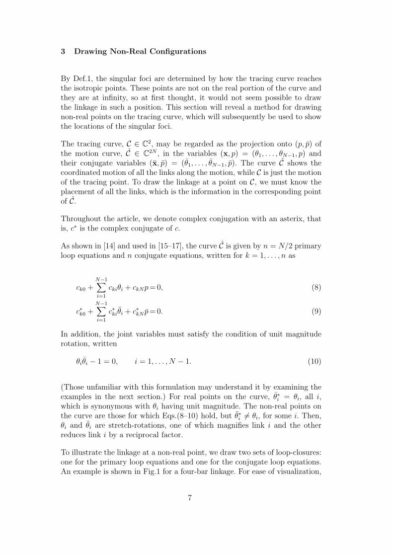
To illustrate the linkage at a non-real point, we draw two sets of loop-closures:one for the primary loop equations and one for the conjugate loop equations.An example is shown in Fig.1 for a four-bar linkage. For ease of visualization,

7

Real Non-Real

p = p∗

p∗

p

Fig. 1. Real and non-real points on a four-bar coupler curve.

it is helpful to draw the complex-conjugate of the conjugate loop equation,namely

ck0 +N−1∑

i=1

ckiθ∗i + ckN p∗ = 0. (11)

For real points, the primary and conjugate loops are identical, so they appearas one at the left in Fig.1. But for a non-real point, such as illustrated at theright in Fig.1, one sees that the although link i has the same rotation anglein both the primary loop and the conjugate loop, it is magnified in one anddemagnified in the other. Even so, the loop remains closed in both. For thenon-real point, we have taken θ1 at the same angle as the real diagram, butits magnitude is decreased from 1 to 0.7. As the magnitude of θ1 decreasesfurther, the coupler triangle for the primary loop will settle down onto thefixed pivots, while in the conjugate loop, the two binary links grow withoutbound, taking point p∗ to infinity. The next few paragraphs will make thisobservation precise.

4 Diagrams of Singular Foci

Now that we can draw the linkage in non-real configurations, it is possiblealso to draw it at a singular focus. The singular foci are the locations of thetracing point p when the conjugate tracing point p is at infinity. Generally,there is more than one such point.

It is best to begin by writing the equations that describe the singular foci.By Theorem 1, the singular foci of the tracing curve C are determined by itstwo-homogeneous roots at infinity. Thus, one may determine the singular fociof C as the projections of the roots at infinity of C. Let g(x, p, x, p) = 0 denotethe entire system of 2N − 1 equations in 2N variables given by Eqs.(8–10),and let G(X, P, V, X, P , V ) be the two-homogenization of g. Accordingly, wewish to find the solutions of the system

G(X, P, 1, X, 1, 0) = 0,

8

which when written out is

ck0 +N−1∑

i=1

ckiΘi + ckNP = 0, k = 1, . . . , n, (12)

N−1∑

i=1

c∗kiΘi + c∗kN = 0, k = 1, . . . , n, (13)

ΘiΘi = 0, i = 1, . . . , N − 1. (14)

This system of equations is simple to solve because Eqs.(12,13) are linear andEqs.(14) imply either Θi = 0 or Θi = 0 for all i. Finding all solutions is only amatter of cycling through the choices of Θi = 0 vs. Θi = 0. Generally, since theextra variable P appears in Eq.(12) where no corresponding variable appearsin Eq.(13), the solutions have n variables among (Θ1, . . . , ΘN−1) that are zeroand the complementary n− 1 variables among (Θ1, . . . , ΘN−1) are zero. Thissatisfies all of Eqs.(14) and leaves just enough variables to solve the linearsystems Eqs.(12,13). An exception to this rule occurs when the linear systemsare not both full rank; this is related to the appearance of extraneous factorsin the Dixon determinant, as we shall discuss below in a re-examination of theWatt-1 six-bar.

An appealing feature of this approach is that we may interpret the results assimple geometric diagrams. The solutions we seek use one half of the links,including the ground link, to close the primary loop equations, Eq.(12). Theremaining links close the conjugate loop equations, Eq.(13). Normally, thesetwo sets of equations are coupled together through the unit magnitude condi-tions, Eq.(10), but at infinity these conditions are replaced by Eq.(14), whichdecouples the two subsystems.

In the primary loop closure diagram for Eq.(12), the location of the tracingpoint is a singular focus. However, one must not neglect to check the existenceof a solution in the conjugate loop diagram. In that diagram, the ground linkis scaled to zero; that is, all ground pivots move to the origin. Meanwhile,P = 1; that is, the conjugate tracing point is placed off the origin one unit.

The diagrams for the singular foci are limiting cases of the finite tracing curveas the scale of some links shrink to zero in the primary loop diagram while theirreciprocals in the conjugate diagram grow infinitely large. We have alreadyobserved the beginning of this process for a four-bar in Fig.1. In the limit, theconjugate loop diagram may be understood as a picture of the linkage zoomedout infinitely, so that the finite links shrink to nothing at the origin and onlythe links that have been infinitely magnified appear.

Some partitions of the links between the two sets of loops may fail to have

9

a0 b0c0

a1

a2

b3

b2

a5

b4

a4

A0 B0

C0

A

BC

D

E

O

2

4

Fig. 2. Four-bar (point D) and Stephenson-3 six-bar (point E) path-generatinglinkages

solutions. On the primary side, this may happen for example when all Θi

are zero in a loop that includes the (nonzero) ground link. On the conjugateside, this happens when all Θi are zero on some path between ground and thetracing point.

The best way to understand these diagrams is to draw them for a few examples.We begin with the familiar four-bar linkage.

Example 1 Four-bar focal diagrams. Consider the four-bar linkage A0ADBB0,a sub-mechanism of the six-bar in Fig.2. The focal diagrams are shown inFig.3, with the diagrams for the primary loop closure at the left and the di-agrams for the conjugate loop shown on the right. Unlike in Fig.1, here theconjugate loop diagram is separated from the primary loop diagram so that itcan be rescaled to finite size. In the main focal diagram, we draw the groundlink and a stretch-rotation of one of the three moving links, scaling the othertwo to zero. The connectivity between links remains the same despite some ofthem having zero size. In case (a), Θ1 = Θ2 = 0, binary link 1 and the couplerlink 2 are scaled to zero, and the tracing point is at ground pivot A0. In case (b),Θ3 = Θ2 = 0, and the tracing point is at ground pivot B0. Finally, in case (c),Θ1 = Θ3 = 0, the coupler triangle is stretch-rotated to bridge the ground piv-ots, placing the third singular focal point at p = a0 + a2(b0 − a0)/(a2 − b2). Ineach case, the conjugate loop diagrams are satisfactory, once again confirmingthe classical result that there are three singular foci, and the focal triangle issimilar to the coupler triangle.

The singular foci of a Stephenson-3 mechanism are related to its four-bar sub-mechanism in a special way. One may see from the following example that asimilar relationship will hold for any linkage formed by adding a tracer dyad

10

(a)

b3Θ3

A0 B0

P

Θ1 = Θ2 = 0

a1Θ1 a2Θ2

b2Θ2

O P = 1

A

Θ3 = 0

(b)

a1Θ1

A0 B0

P

Θ2 = Θ3 = 0

b3Θ3 b2Θ2

a2Θ2

O P = 1

B

Θ1 = 0

(c)

a2Θ2 b2Θ2

A0 B0

P

Θ1 = Θ3 = 0

a1Θ1

b3Θ3

O P = 1

Θ2 = 0

Fig. 3. Focal diagrams for a four-bar: primary loop on left and conjugate loop onright for each.

to a simpler linkage.

Example 2 Stephenson-3 focal diagrams. Refer again to the Stephenson-3six-bar linkage shown in Fig.2. This linkage has nine singular foci as dia-grammed in Fig.4. This time, to save space, the conjugate loop diagrams areomitted. In the main focal diagram, we draw the ground link and a stretch-rotation of two of the five moving links, scaling the other three to zero. Thediagrams are arranged in columns, according to whether links 4 and 5 arescaled to zero. When Θ4 = 0 with Θ5 6= 0, the focal diagrams give singularfoci F1, F2, F3 that are just the singular foci of the four-bar, as in the previousexample, with link 5 closing the loop to ground pivot C0. When Θ4 6= 0 andΘ5 = 0, one obtains a new focal triangle that is a stretch-rotation about C0 ofthe four-bar focal triangle; the stretch-rotation factor is the ratio of two sidesof the tracer link 4. That is,

Fi+3 = c0 + (b4/a4)(c0 − Fi), i = 1, 2, 3. (15)

When both Θ4 = Θ5 = 0 and any one of the other three links is scaled tozero, the tracing point is at C0, indicating that this ground pivot is a triplesingular focus. The final case of Θ4 6= 0 and Θ5 6= 0 simultaneously is notpossible: it forces Θ1 = Θ2 = Θ3 = 0, and the four-bar loop cannot be closed.In summary, we have as singular foci the three singular foci of the base four-

11

Θ4 = 0, Θ5 6= 0 Θ4 6= 0, Θ5 = 0 Θ4 = Θ5 = 0

F3

2

F2

F1

F6

2

4

F5

4

F4

4

F9

F82

F72

Θ1 = Θ3 = 0

Θ2 = Θ3 = 0

Θ1 = Θ2 = 0

Θ1 = Θ3 = 0

Θ2 = Θ3 = 0

Θ1 = Θ2 = 0

Θ2 = 0

Θ1 = 0

Θ3 = 0

Fig. 4. Focal diagrams for a Stephenson-3 six-bar.

a0 b0

a1

a2

b2

a3

b3

a4

a5 b5

A0 B0

AB

C

D

E

P

O

2

3

5

Fig. 5. Watt-1 path-generating linkage

bar, three singular foci that are a stretch-rotation of the four-bar focal triangle,and a triple singular focus at pivot C0.

Significantly, the singular foci of the Stephenson-3 depend only on the groundpivots and the shape of links 2 and 4. The scale of the links does not matter.

As the final example, we examine the Watt-1 linkage drawn in Fig.5. Thisexample requires some extra analysis to deal with solution lines at infinity.This is related to the eigenvalue problem that arises when the method of [17]is applied to this mechanism.

12

Points Lines

F1

Θ1 = Θ2 = Θ5 = 0

3

F2

Θ1 = Θ3 = Θ5 = 0

2

F3

Θ1 = Θ3 = Θ4 = 0

2

5

Primary Conjugate

P

23

P = 15

Θ4 = Θ5 = 0 Θ1 = Θ2 = Θ3 = 0

Line 1

PP = 1

23

5

Θ2 = Θ3 = 0

Θ4 = Θ5 = 0Θ1 = 0

Line 2

Fig. 6. Solutions at infinity, (P = 1, V = 0), for a Watt-1 six-bar.

Example 3 Watt1 focal diagrams. Consider the Watt six-bar linkage shownin Fig.5. Denoting p = ~OP , the loop equations are

(a0 − b0) + a1θ1 + a2θ2 + a3θ3 = 0

b2θ2 + b3θ3 + a4θ4 + a5θ5 = 0

b0 − (a3 + b3)θ3 + b5θ5 − p = 0

(16)

This linkage is more difficult to analyze than the Stephenson-3 previously con-sidered. In the case of the Stephenson-3 linkage, the system of equations (12–14) had nine solution points, each giving a focal point. In the case of the Watt-1linkage, we find that the system has three solution points and two solution lines.These solutions are diagrammed in Fig.6. Expressions for the singular foci areas follows: F1 = a0+(a0−b0)b3/a3, F2 = b0 and F3 = b0+(a0−b0)b2b5/(a2a5).Note that singular focus F2 is at the ground pivot B0.

To understand the line solutions, it helps to write out Eqs.(12–14) explicitlyas they apply to this linkage:

(a0 − b0) + a1Θ1 + a2Θ2 + a3Θ3 = 0 (17)

b2Θ2 + b3Θ3 + a4Θ4 + a5Θ5 = 0 (18)

b0 − (a3 + b3)Θ3 + b5Θ5 − P = 0 (19)

a∗1Θ1 + a∗2Θ2 + a∗3Θ3 = 0 (20)

b∗2Θ2 + b∗3Θ3 + a∗4Θ4 + a∗5Θ5 = 0 (21)

13

(a3 + b3)∗Θ3 + b∗5Θ5 − 1 = 0 (22)

ΘiΘi = 0, i = 1, . . . , 5 (23)

Solution Line 1 in Fig.6 arises because the first conjugate loop equation, Eq.(20),is satisfied by Θ1 = Θ2 = Θ3 = 0, which allows all three conjugate loopequations, Eqs.(20–22), to be satisfied with only two conjugate variables, Θ4

and Θ5, being nonzero. Consequently, in the main loop equations, we haveΘ4 = Θ5 = 0, leaving four variables, {Θ1, Θ2, Θ3, P}, to close the threemain loop equations, Eqs.(17–19). The point P can be placed anywhere inthe plane and still there will be a solution for the remaining variables. How-ever, we are only interested in the points on Line 1 that are limits of the finitetracing curve as it approaches infinity. On the finite curve as it approachesΘ4 = Θ5 = V = 0, we have

(a0 − b0) + a1θ1 + a2θ2 + a3θ3 = 0

b2θ2 + b3θ3 = 0

b0 − (a3 + b3)θ3 − p = 0

(a0 − b0)∗ + a∗1θ

−11 + a∗2θ

−12 + a∗3θ

−13 = 0.

(24)

One may use the second of these to eliminate θ2 from the rest. Then, multiply-ing the last equation by θ1θ3 to clear away the negative exponents, one obtainsa quadratic equation. This gives two singular foci, shown in Fig.7. In the con-jugate loop diagrams on the right of this figure, links 4 and 5 are infinite inextent. If we zoom out infinitely far, the conjugate diagrams will look just likethe one shown in Fig.6 for Line 1.

Solution Line 2 arises in a complementary fashion to Line 1. This time, thesecond main loop equation, Eq.(18), is satisfied by Θ2 = Θ3 = Θ4 = Θ5 = 0,so that only link 1 is needed to bridge across the two ground pivots. Thisleaves four variables, {Θ2, Θ3, Θ4, Θ5}, to close only three loops in the conju-gate equations, Eqs.(20–22), thus giving a one-dimensional solution line. Notethat Eq.(19) gives P = b0, that is, the singular focus remains at the fixed pivotB0 along the whole solution line. However, just as for Line 1, we need to de-termine if Line 2 is approached by the finite portion of the tracing curve. Thegoverning equations in the approach to Θ1 = V = 0, P = 1 are

a∗2θ2 + a∗3θ3 = 0

b∗2θ2 + b∗3θ3 + a∗4θ4 + a∗5θ5 = 0

−(a3 + b3)∗θ3 + b∗5θ5 − p = 0

b2θ−12 + b3θ

−13 + a4θ

−14 + a5θ

−15 = 0

(25)

14

Primary Conjugate

F4

23

2

5

3

F5

2

32

3

5

Fig. 7. Focal points on solution Line 1 of Watt-1 six-bar.

Since these are all homogeneous, we may set θ2 = 1 to dehomogenize. Thenthe first equation determines θ3 = −(a2/a3)

∗. After substituting these into thefinal equation, we may clear negative exponents by multiplying by θ4θ5. We areleft with one quadratic equation and two linears, hence there are two solutions.Since the tracing point coincides with fixed pivot B0 for every configuration inLine 2 (see Fig.6), we get two more copies of B0, which along with focus F2

make B0 a triple singular focus.

In total, we have B0 as a triple singular focus along with four other singularfoci. This agrees with the results obtained in [17].

The final observation to make is that Lines 1 and 2 intersect at Θ2 = Θ3 =Θ4 = Θ5 = Θ1 = Θ2 = Θ3 = 0 with P = b0. This degenerate point at infinityis not approached by the finite portion of the tracing curve, so it does not countas a singular focus. However, it appears as the extraneous factor (p−b0)(p−b0)in the Dixon determinant when using the methods of [16,17].

5 Path Cognates

A detailed discussion of the use of the singular foci to determine path cognatesmust be postponed to a later paper. However, we can use the results shownabove for the Stephenson-3 six-bar to give a hint of how to proceed.

Two linkages which produce the same tracing curve must have the same sin-gular foci. The Stephenson-3 linkage is drawn in Fig.2, and its singular fociare diagrammed in Fig.4. We see that fixed pivot C0 is a triple singular focusand the only multiple focus. Thus, all path cognates must have this point as

15

the ground pivot for link 5. We have already noted that the focal trianglesF1F2F3 and F4F5F6 are similar. For a general Stephenson-3 linkage, no otherpartitioning of these six foci into two triangles will give similar triangles. Con-sequently, for any path cognate, one of these must be the focal triangle forthe four-bar sub-linkage formed by links 0,1,2,3, and the other is generated bystretch-rotation about C0 via link 4. We know that the same four-bar curve isgenerated by three cognates (Robert’s cognates), each having the same focaltriangle F1F2F3, so we immediately get three cognates for the six-bar fromthis. We can get another three cognates by reversing the roles of the two focaltriangles; that is, stretch-rotate the four-bars about C0 such that their focaltriangle is F4F5F6 instead of F1F2F3. These are the six path cognates foundby Roth [12].

The argument of the last paragraph shows that there are six possible assign-ments of the singular foci to the fixed pivots of the Stephenson-3 six-bar.Roth’s constructions give one path cognate for each of these: the reversal ofthe roles of the two focal triangles is accomplished via the construction of aHart pantograph, and reassignment of the fixed pivots within a focal triangleis done via Roberts cognates. To conclude that there are no other cognates,one must show that each assignment of the foci to the fixed pivots determinesa unique linkage. This will be done in a future report.

6 Coupler Mechanisms

A coupler mechanism consists of two one-degree-of-freedom path-generatingmechanisms that are connected by a coupler link, see [14]. This is a specialcase of the type of planar motion considered in [10]. When a tracing pointis placed on the coupler link, the singular foci of the tracing curve of thecoupler mechanism are easily derived from those of the two sub-linkages. Anexample is the Stephenson-3 linkage, where link 4 couples together a four-bar(links 0,1,2,3) with a two-bar (link 5 pinned to link 0). We have seen that thesingular foci of the six-bar are those of the four-bar (F1, F2, F3), the centerpoint of the circle generated by link 5 (C0), and three obtained by scaling andmoving the coupler link to bridge from one of F1, F2, F3 to C0.

It can be seen from the geometric constructions of §4 that the pattern ofthe Stephenson-3 linkage generalizes to any coupler mechanism: its singularfoci will be those of its two sub-linkages along with new ones constructed bybridging the coupler link from a singular focus of one sub-linkage to one of theother sub-linkage. If the sub-linkages have n1 and n2 singular foci, then thebridging gives n1n2 new singular foci, for a total of n1+n2+n1n2. Those comingdirectly from the sub-linkages may be multiple singular foci. The multiplicitiescan be counted by the same construction method, but we will not go into that

16

level of detail here.

The special case of “Stephenson-pattern” linkages, which result from sequen-tially adding any number of output dyads to an initial four-bar, are partic-ularly easy to analyze. Wunderlich [18] found that the coupler curve of then-loop Stephenson-pattern linkage is fully circular of degree 2 · 3n (see also [9,pp. 227–228]). It thus has 3n singular foci. Applying the results of this paper,one can generate all the singular foci recursively. The n-loop mechanism in-herits 3n−1 singular foci from the (n − 1) loop sub-mechanism it is built on,the ground pivot of the new output dyad is a singular focus of order 3n−1,and there are 3n−1 new singular foci obtained by stretch-rotation of the previ-ous foci about the new ground pivot. The stretch-rotation factor is the ratioof two of the sides of the coupler triangle, as we saw in the case of the theStephenson-3 linkage. The recursion can be started with the ”0-loop” linkage,which is a single link pinned to ground. The 0-loop “coupler curve” is just acircle, having degree 2, with a single singular focus at its center. Using the re-cursive approach just outlined, one can easily determine the 3 singular foci forthe 1-loop mechanism, which is just the four-bar linkage, then the 9 singularfoci of the 2-loop mechanism, which is the Stephenson-3 six-bar linkage, andso on.

7 Conclusion

This paper gives a method for finding the singular foci of planar linkages.Based on analysis of the solutions at infinity of the loop equations, it leads toa detailed geometric interpretation of the foci. A key step in this interpreta-tion is a technique for drawing linkages in non-real configurations. Althoughthe new approach to singular foci must be applied on a case-by-case basisfor each linkage type, it yields simple formulae for the singular foci. This isin contrast to the method of [17], which is easier to implement as a generalnumerical algorithm but does not readily yield simple formulae or geometricunderstanding. The new method is particularly apt for determining the sin-gular foci of a class of mechanisms called “coupler mechanisms,” including allof the Stephenson-pattern linkages.

The singular foci represent essential characteristics of the curve traced outby a planar linkage; in particular, they describe the behavior of the curve atinfinity. Two curves sharing one or more singular foci have a reduced numberof intersection points and two linkages can generate the same tracing curveonly if they have all singular foci in common. These facts can be useful in thedesign of path-generating linkages.

17

References

[1] R. Bricard, Leons de Cinematique: Tome II, Cinematique Appliquee, Gauthier-Villars, Paris, 1927.

[2] O. Bottema and B. Roth, Theoretical Kinematics, Dover Publications, NewYork, 1990.

[3] A. Cayley, “On three-bar motion,” Proc. London Math. Soc., Vol. VII, 1875-76,pp. 136-166.

[4] J.L. Coolidge, A Treatise on Algebraic Plane Curves, Dover, New York, 1959.

[5] G. Darboux, “De l’emploi des fonctions elliptiques dans la theorie duquadrilatere plan,” Bull. des Sciences Math. Astro., Tome III, 1879.

[6] E. Dijksman, Motion Geometry of Mechanisms, Cambridge University Press,Cambridge, 1976.

[7] A. Haarbleicher, “Application des coordonnees isotropes a l’etude de la courbedes trois barres,” J. de l’Ecole Polytechnique, II serie, v. 31, pp. 13–40, 1933.

[8] J. Harris, Algebraic Geometry: A First Course, Springer, New York, 1992.

[9] K.H. Hunt, Kinematic Geometry of Mechanisms, Clarendon Press, Oxford,1978.

[10] S. Roberts, “On the motion of a plane under certain conditions,” Proc. LondonMath. Soc., Vol. III, pp. 286–319, 1871.

[11] S. Roberts, “On three-bar motion in plane space,” Proc. London Math. Soc.,Vol. VII, pp. 14–23, 1875.

[12] B. Roth, “On the multiple generation of coupler curves,” Trans. ASME, SeriesB, J. Eng. Industry, v.87, n.2, pp.177–183, 1965.

[13] E.J.F. Primrose, F. Freudenstein and B. Roth, “Six-bar motion (Parts I–III),”Arch. Rational Mech. Anal., v.24, pp.22-77, 1967.

[14] C. Wampler, “Isotropic coordinates, circularity and Bezout numbers: Planarkinematics from a new perspective,” Proc. ASME DETC, Aug. 18–22, 1996,Irvine, CA, Paper 96-DETC/MECH-1210.

[15] C. Wampler, “Solving the kinematics of planar mechanisms,” ASME J. Mech.Des., v.121, n.3, pp.387–391, 1999.

[16] C. Wampler, “Solving the kinematics of planar mechanisms by Dixondeterminant and a complex-plane formulation,” ASME J. Mech. Design, v.123,n.3, pp.382–387, 2001.

[17] C. Wampler, “Singular Foci of Planar Linkages,” Mech. Mach. Theory (inpress).

[18] W. Wunderlich, “Hohere koppelkurven,” Ost. Ing. Arch., v.17, n.3, pp.162–165,1963.

18